Structured Polynomial Eigenproblems Related to

Time-Delay Systems

H. Fassbender, D. S. Mackey, N. Mackey and

C. Schroder

March 2009

MIMS EPrint: 2009.26

Manchester Institute for Mathematical Sciences

School of Mathematics

The University of Manchester

Reports available from: http://www.manchester.ac.uk/mims/eprints

And by contacting: The MIMS Secretary

School of Mathematics

The University of Manchester

Manchester, M13 9PL, UK

ISSN 1749-9097

STRUCTURED POLYNOMIAL EIGENPROBLEMSRELATED TO TIME-DELAY SYSTEMS

H. FASSBENDER∗, D. S. MACKEY† , N. MACKEY† , AND C. SCHRODER‡

Abstract. A new class of structured polynomial eigenproblems arising in the stability analysisof time-delay systems is identified and analyzed together with new types of closely related structuredpolynomials. Relationships between these polynomials are established via the Cayley transforma-tion. Their spectral symmetries are revealed, and structure-preserving linearizations constructed. Astructured Schur decomposition for the class of structured pencils associated with time-delay systemsis derived, and an algorithm for its computation that compares favorably with the QZ algorithm ispresented along with numerical experiments.

Key words. polynomial eigenvalue problem, palindromic matrix polynomial, quadratic eigen-value problem, even matrix polynomial, structure-preserving linearization, matrix pencil, structuredSchur form, real QZ algorithm, spectral symmetry, Cayley transformation, involution, time-delaysystems, delay-differential equations, stability analysis.

AMS subject classifications. 15A18, 15A21, 15A22, 34K06, 34K20, 47A56, 47A75, 65F15

1. Introduction. In this paper we discuss a new class of structured matrixpolynomial eigenproblems Q(λ)v = 0, where

Q(λ) =k∑

i=0

λiBi , Bi ∈ Cn×n , Bk 6= 0 ,

and Bi = PBk−iP , i = 0, . . . , k

(1.1)

for a real involutory matrix P (i.e. P 2 = I). Here B denotes the entrywise conjugationof the matrix B. With

Q(λ) :=

k∑

i=0

λiBi and revQ(λ) := λkQ

(1

λ

)=

k∑

i=0

λiBk−i , (1.2)

we see that Q(λ) in (1.1) satisfies

P · revQ(λ) · P = Q(λ). (1.3)

As shown in Section 2, the stability analysis of time-delay systems is one importantsource of eigenproblems as in (1.1). Throughout this paper we assume that all matrixpolynomials Q(λ) are regular, i.e. that det Q(λ)≡/ 0.

Matrix polynomials satisfying (1.3) are reminiscent of the various types of palin-dromic polynomials defined in [18]:

• palindromic: revQ(λ) = Q(λ),• anti-palindromic: revQ(λ) = −Q(λ),• ⋆ -palindromic: revQ⋆(λ) = Q(λ),

∗TU Braunschweig, Carl-Friedrich-Gauß-Fakultat, Institut Computational Mathematics, AG Nu-merik, 38023 Braunschweig, Germany, h.fassbender@tu-bs.de

†Department of Mathematics, Western Michigan University, Kalamazoo, MI 49008, USA,(steve.mackey@wmich.edu, nil.mackey@wmich.edu). Supported by National Science Foundationgrant DMS-0713799.

‡TU Berlin, Institut fur Mathematik, MA 4-5, 10623 Berlin, Germany,schroed@math.tu-berlin.de, Supported by Matheon, the DFG research center in Berlin.

1

• ⋆ -anti-palindromic: revQ⋆(λ) = −Q(λ),where ⋆ denotes transpose T in the real case and either T or conjugate transpose∗ in the complex case. These palindromic matrix polynomials have the propertythat reversing the order of the coefficient matrices, followed perhaps by taking theirtranspose or conjugate transpose, leads back to the original matrix polynomial (up tosign). Several other types of structured matrix polynomial are also defined in [18],

• even, odd: Q(−λ) = ±Q(λ),• ⋆-even, ⋆-odd: Q⋆(−λ) = ±Q(λ),

and shown there to be closely related to palindromic polynomials via the Cayleytransformation.

We will show that matrix polynomials satisfying (1.3) have properties parallel tothose of the palindromic polynomials discussed in [18]. Hence we refer to polynomialswith property (1.3) as P -conjugate-P -palindromic polynomials, or PCP polynomialsfor short. Analogous to the situation in [18], we examine four related types of PCP-likestructures,

• PCP: P · revQ(λ) · P = Q(λ),• anti-PCP: P · revQ(λ) · P = −Q(λ),• PCP-even: P ·Q(−λ) · P = Q(λ),• PCP-odd: P ·Q(−λ) · P = −Q(λ),

revealing their spectral symmetry properties, their relationships to each other via theCayley transformation, as well as their structured linearizations. Here we continuethe practice stemming from Lancaster [14] of developing theory for polynomials ofdegree k wherever possible in order to gain the most insight and understanding.

There are a number of ways in which palindromic matrix polynomials can bethought of as generalizations of symplectic matrices. For example, palindromic poly-nomials and symplectic matrices both have reciprocal pairing symmetry in theirspectra. In addition, the Cayley transformation relates palindromic polynomials toeven/odd matrix polynomials in the same way as it relates symplectic matrices toHamiltonian matrices, and even/odd matrix polynomials represent generalizations ofHamiltonian matrices. Further information on the relationship between symplecticmatrices and palindromic polynomials can be found in [23] and, in the context ofoptimal control problems, in [2].

The classical approach to investigate or numerically solve polynomial eigenvalueproblems is linearization. A kn × kn pencil L(λ) is said to be a linearization foran n × n polynomial Q(λ) of degree k if E(λ)L(λ)F (λ) = diag[Q(λ), I(k−1)n] forsome E(λ) and F (λ) with nonzero constant determinants. The companion forms [5]provide the standard examples of linearization for a matrix polynomial Q(λ). LetX1 = X2 = diag(Bk, In, . . . , In),

Y1 =

Bk−1 Bk−2 · · · B0

−In 0 · · · 0. . .

. . ....

0 −In 0

, and Y2 =

Bk−1 −In 0

Bk−2 0. . .

......

. . . −In

B0 0 · · · 0

. (1.4)

Then C1(λ) = λX1 + Y1 and C2(λ) = λX2 + Y2 are the first and second companionforms for Q(λ). These linearizations do not reflect any structure that might be presentin the matrix polynomial Q, so only standard numerical methods can be applied tosolve the eigenproblem Ci(λ)v = 0. In a finite precision environment this may producephysically meaningless results [24], e.g., loss of symmetries in the spectrum. Hence it

2

is useful to construct linearizations that reflect the structure of the given polynomial,and then to develop numerical methods for the resulting linear eigenvalue problemthat properly address these structures.

It is well known that for regular matrix polynomials, linearizations preserve al-gebraic and partial multiplicities of all finite eigenvalues [5]. In order to preserve themultiplicities of the eigenvalue ∞, one has to consider linearizations L(λ) which havethe additional property that revL(λ) is also a linearization for revQ(λ), see [4]. Suchlinearizations have been named strong linearizations in [15]. Both the first and thesecond companion form are strong linearizations for any regular matrix polynomial[4, Proposition 1.1].

Several recent papers have systematically addressed the tasks of broadening themenu of available linearizations, providing criteria to guide the choice of linearization,and identifying structure-preserving linearizations for various types of structured poly-nomial. In [19], two vector spaces of pencils generalizing the companion forms wereconstructed and many interesting properties were proved, including that almost allof these pencils are linearizations. The conditioning and backward error properties ofsome of these linearizations were analyzed in [7], [9], and [11], developing criteria forchoosing a linearization best suited for numerical computation. Linearizations withinthese vector spaces were identified in [18], [8], and [10] that respect palindromic andodd-even structure, symmetric and Hermitian structure, and definiteness structure,respectively.

In this paper we investigate the four types of PCP-structured matrix polynomial,analyzing their spectral symmetries in Section 3, the relationships between the variousPCP-structures via the Cayley transformation in Section 4, and then showing howto build structured linearizations for each type of PCP-structure in Section 5. Theexistence and computation of a structured Schur-type decomposition for PCP-pencilsis discussed in Section 6, and Section 7 concludes with numerical results for someexamples arising from physical applications. We first, though, discuss in more detaila key source of PCP-structured eigenproblems.

2. Time-delay systems. To motivate our consideration of matrix polynomialswith PCP-structure, we describe how the stability analysis of time-delay systems(also known as delay-differential equations, see e.g. [6, 21]) leads to eigenproblemswith this structure. A neutral linear time-delay system (TDS) with m constant delaysh1, . . . , hm ≥ 0 and h0 = 0 is given by

S =

{ ∑mk=0 Dkx(t− hk) =

∑mk=0 Akx(t− hk) , t ≥ 0

x(t) = ϕ(t) , t ∈ [−h, 0)(2.1)

with h = maxi{hi}, x : [−h,∞) → Rn, ϕ ∈ C1[−h, 0] , and Ak, Dk ∈ Rn×n fork = 0, . . . , m. An important special case of (2.1) is the class of retarded time-delaysystems, in which D0 = I and Dk = 0 for k = 1, . . . , m.

The stability of a TDS can be determined from its characteristic equation, i.e.,from the nontrivial solutions of the nonlinear eigenvalue problem

M(s)v = 0 , where M(s) = −sD(s) + A(s)

with D(s) =

m∑

k=0

Dke−hks and A(s) =

m∑

k=0

Ake−hks.(2.2)

As usual, s ∈ C is called an eigenvalue associated with the eigenvector v ∈ Cn, and theset of all eigenvalues σ(S) is called the spectrum of S. Having an eigenvalue in the right

3

half-plane implies that S is unstable; conversely, having σ(S) completely contained inthe left half-plane usually implies that S is stable, although some additional technicalassumptions are required. For further details see [13], [21].

A time-delay system S is called critical if σ(S) ∩ iR 6= ∅, i =√−1. The set

of all points (h1, h2, . . . , hm) in delay-parameter space for which S is critical formthe critical curves (m = 2) or critical surfaces (m > 2) of the TDS. Since a TDScan change stability when an eigenvalue pair crosses the imaginary axis, the criticalcurves/surfaces are important in the study of the delay-parameter space stabilitydomain. In most cases of practical interest, the boundary of the stability domain isjust a subset of the critical curves/surfaces [21, Section 1.2].

Thus the computation of critical sets, for which a number of approaches exist(see [13] for a list of references), is a key step in the stability analysis of time-delaysystems. Here we outline the new method for this computation developed in [13],leading ultimately to a quadratic eigenproblem with PCP-palindromic structure thatwill have to be solved repeatedly for many different parameter values.

To determine critical points in delay-parameter space, we need to compute purelyimaginary eigenvalues of M(s) in (2.2), i.e., to find s = iω with ω ∈ R such that

M(iω)v = 0 . (2.3)

As shown in [13], for any ω ∈ R and v ∈ Cn such that v∗v = 1 and v := D(iω)v 6= 0,

equation (2.3) is equivalent to the pair of conditions

L(vv∗, iω) = 0 and v ∗M(iω)v = 0 , (2.4)

where L is a Lyapunov-type operator

L(X, s) := M(s)XD(s)∗ + D(s)XM(s)∗

= A(s)XD(s)∗ + D(s)XA(s)∗ − 2D(s)XD(s)∗Re(s)(2.5)

for X ∈ Cn×n, s ∈ C. That (2.3) ⇒ (2.4) follows immediately from

L(vv∗, iω) = M(iω)vv∗D(iω)∗ + D(iω)vv∗M(iω)∗

= M(iω)v v ∗ + v(M(iω)v

)∗,

(2.6)

while the implication (2.4)⇒ (2.3) follows by pre-multiplying (2.6) with v ∗ and usingthe assumption v 6= 0.

Note that the assumption v = D(iω)v 6= 0 is not very restrictive, and can beregarded as a kind of genericity condition, since D(iω)v = 0 in (2.3) implies thatA(iω)v = 0 would have to simultaneously hold. In addition D(iω)v = 0 if and only ifthe difference equation

D0x(t) + D1x(t− h1) + . . . + Dmx(t− hm) = 0 (2.7)

has a purely imaginary eigenvalue, which happens only in very special situations.We now see how (2.4) can be used to systematically explore delay-parameter space

to find the critical set. From (2.5) we have

L(vv∗, iω) = A(iω)vv∗D(iω)∗ + D(iω)vv∗A(iω)∗

with D(iω) =

m∑

k=0

Dke−iωhk and A(iω) =

m∑

k=0

Ake−iωhk .(2.8)

4

Because of the periodicity in the exponential terms of D(iω) and A(iω), there isan ω-dependent periodicity in the critical set; if (h1, h2, . . . , hm) is a critical delaycorresponding to the solution iω, v of the equation L(vv∗, iω) = 0, then

(h1, h2, . . . , hm) + (2π/ω)(p1, p2, . . . , pm)

is also a critical delay for any (p1, p2, . . . , pm) ∈ Zm. Thus it suffices to consider onlythe angles ϕk := ωhk for k = 1, . . . , m where ϕk ∈ [−π, π]. These can be exploredby a line-search strategy: with ϕ0 := ωh0 = 0, for each fixed choice of ϕ1, . . . , ϕm−1

view z := e−iϕm as a variable and rewrite L(vv∗, iω) = 0 as an eigenproblem in termsof z and vv∗. Defining

AS :=

m−1∑

k=0

Ake−iϕk and DS :=

m−1∑

k=0

Dke−iϕk (2.9)

and using (2.8), we have

(Amz + AS

)vv∗(Dmz + DS

)∗+(Dmz + DS

)vv∗(Amz + AS

)∗= 0 . (2.10)

Expanding and vectorizing (2.10) yields

(zE + F + zG) vec(vv∗) = 0 , (2.11)

where

E = DS ⊗Am + AS ⊗Dm ,

F = Dm ⊗Am + DS ⊗AS + AS ⊗DS + Am ⊗Dm ,

G = Dm ⊗AS + Am ⊗DS ,

(2.12)

and ⊗ denotes the usual Kronecker product [12, Chapter 4.3]. Then multiplying(2.11) by z with |z| = 1 results in the quadratic eigenvalue problem

(z2E + zF + G)u = 0 . (2.13)

A solution (z, u) of (2.13) with |z| = 1 and u of the form vec(vv∗) completes thedetermination of (ϕ1, ϕ2, . . . , ϕm) = ω(h1, h2, . . . , hm), and hence of a critical delayup to a real scalar multiple ω. The scaling factor ω, and hence a pure imaginaryeigenvalue s = iω of (2.2), is determined by invoking the second condition in (2.4):

0 = iv ∗M(iω)v

= iv ∗(−iωD(iω) + A(iω)

)v

= ωv ∗D(iω)v + ıv ∗

A(iω)v

= ωv ∗v + iv ∗(Amz + AS

)v ,

and hence

ω = −iv ∗(Amz + AS

)v/(v ∗v

).

From (2.10) we can see that ω ∈ R. Define x :=(Amz + AS

)v, so that (2.10) says

xv ∗+vx ∗ = 0. Then v ∗(xv ∗+vx ∗)v = 0 ⇒ (v ∗v)(v ∗x+x ∗v) = 0 ⇒ v ∗x+x ∗v = 0,so v ∗x ∈ iR and hence ω ∈ R.

The preceding discussion can be summarized in the following theorem.

5

Theorem 2.1 ([13]). Assume that the difference equation (2.7) has no purelyimaginary eigenvalues. With ϕ0 = 0 and any given combination of angles ϕk ∈ [−π, π]for k = 1, . . . , m− 1, consider the quadratic eigenvalue problem

(z2E + zF + G)u = 0 (2.14)

where E, F, G ∈ Cn2×n2

are given by (2.12). Then for any solution of (2.14) with|z| = 1 and u of the form u = vec(vv∗) = v ⊗ v for some v ∈ Cn with v∗v = 1,critical delays for the TDS (2.1) can be constructed as follows. Let

v =(Dmz + DS

)v and ω = −iv ∗

(Amz + AS

)v/(v ∗v

). (2.15)

Then for any (p1, p2, . . . , pm) ∈ Zm,

(h1, h2, . . . , hm) =

(1

ω

)[(ϕ1, . . . , ϕm−1,−Arg z) + 2π(p1, p2, . . . , pm)

]

is a critical delay for (2.1).

It is now straightforward to see why the quadratic matrix polynomial

Q(z) = z2E + zF + G (2.16)

in (2.14) has PCP-structure. By [12, Cor 4.3.10] there exists an involutory, symmetric

permutation matrix P ∈ Rn2×n2

(i.e. P = P−1 = PT ) such that

B ⊗ C = P (C ⊗B)P (2.17)

for all B, C ∈ Cn×n. Thus we have in (2.16) that E = PGP and F = PFP , since

E = DS ⊗ Am + AS ⊗Dm

= P[Am ⊗DS

]P + P

[Dm ⊗AS

]P

= P[Am ⊗DS + Dm ⊗AS

]P = PGP .

The fact that F = PFP follows in a similar fashion. This implies

Q(z) = z2E + zF + G = P (z2G + zF + E)P = P · revQ(z) · P ,

that is, (2.16) is a matrix polynomial as in (1.1) and (1.3).Time-delay systems arise in a variety of applications [22], including electric cir-

cuits, population dynamics, and the control of chemical processes. Several realisticproblems are discussed in Section 7, and some numerical results are given.

3. Spectral symmetry. Suppose Q(λ) has property (1.3), and let λ 6= 0 be aneigenvalue of Q(λ) associated to the eigenvector v, that is Q(λ)v = 0. Then we have

0 = Q(λ)v = P · revQ(λ) · Pv ⇒ revQ(λ) · (Pv) = 0 ,

which from definition (1.2) of rev implies that

Q(1/λ) · (P v) = 0 .

6

Hence if λ is an eigenvalue with eigenvector v, then 1/λ is an eigenvalue with eigen-vector P v. Note that for any matrix polynomial Q, (1.2) implies that the nonzerofinite eigenvalues of revQ(λ) are the reciprocals of those of Q.

The following theorem extends this observation of reciprocal pairing for eigenval-ues of PCP-palindromic polynomials to include eigenvalues at∞, pairing of eigenvaluemultiplicities, as well as to an analogous eigenvalue pairing for PCP-even/odd poly-nomials. As in [18], we will employ the convention that Q(λ) has an eigenvalue at ∞with eigenvector x if revQ(λ) has the eigenvalue 0 with eigenvector x. The algebraic,geometric, and partial multiplicities of an eigenvalue at ∞ are defined to be the sameas the corresponding multiplicities of the zero eigenvalue of revQ(λ).

Theorem 3.1 (Spectral Symmetry). Let Q(λ) =∑k

i=0 λiBi, Bk 6= 0 be a regularmatrix polynomial and P a real involution.

(a) If Q(λ) = ±P revQ(λ) P , then the spectrum of Q(λ) has the pairing (λ, 1/λ).(b) If Q(λ) = ±P Q(−λ) P , then the spectrum of Q(λ) has the pairing (λ,−λ).

Moreover, the algebraic, geometric, and partial multiplicities of the eigenvalues in eachsuch pair are equal. (Here we allow λ = 0 and interpret 1/λ as the eigenvalue ∞.)

Proof. We first recall some well-known facts [5] about strict equivalence of pencilsand about the companion form C1(λ) of a matrix polynomial Q(λ):

1. Q(λ) and C1(λ) have the same eigenvalues (including ∞) with the samealgebraic, geometric, and partial multiplicities.

2. Any two strictly equivalent pencils have the same eigenvalues (including ∞)with the same algebraic, geometric, and partial multiplicities.

Because of these two facts it suffices to show that C1(λ) is strictly equivalent torevC1(λ) for part (a), and to C1(−λ) for part (b). The desired eigenvalue pairingsand equality of multiplicities then follow. See [3] for details.

The same eigenvalue pairings have also been previously observed in [18] for ∗-(anti)-palindromic and ∗-even/odd matrix polynomials; these results are summarizedin Table 3.1. Observe further that when the coefficient matrices of Q are all real, then

Table 3.1Spectral symmetries

Structure of Q(λ) eigenvalue pairing

(anti)-palindromic, T-(anti)-palindromic (λ, 1/λ)

∗-palindromic, ∗-anti-palindromic (λ, 1/λ)

(anti)-PCP (λ, 1/λ)

even, odd, T-even, T-odd (λ,−λ)

∗-even, ∗-odd (λ,−λ)

PCP-even, PCP-odd (λ,−λ)

for all the palindromic structures listed in Table 3.1 the eigenvalues occur not justin pairs but in quadruples (λ, λ, 1/λ, 1/λ). This property is sometimes referred to as“symplectic spectral symmetry”, since real symplectic matrices exhibit this behavior.In the context of the time-delay problem, though, the coefficient matrices E, F, G ofQ(z) in (2.16) are typically not all real unless there is only a single delay h1 in theproblem.

4. Relationships between structured polynomials. It is well known thatthe Cayley transformation and its generalizations to matrix pencils relates Hamilto-nian structure to symplectic structure for both matrices and pencils [16, 20]. By using

7

the extensions of the classical definition of this transformation to matrix polynomialsas given in [18], we develop analogous relationships between the structured matrixpolynomials considered here.

The Cayley transforms of a degree k matrix polynomial Q(λ) with pole at +1 or−1, respectively, are the matrix polynomials C+1(Q) and C−1(Q) defined by

C+1(Q)(µ) := (1− µ)kQ

(1 + µ

1− µ

)

and C−1(Q)(µ) := (µ + 1)kQ

(µ− 1

µ + 1

).

(4.1)

This choice of definition was motivated in [18] by the observation that the Mobiustransformations µ−1

µ+1 and 1+µ1−µ map reciprocal pairs (µ, 1

µ) to plus/minus pairs (λ,−λ),

as well as conjugate reciprocal pairs (µ, 1/µ) to conjugate plus/minus pairs (λ,−λ).When viewed as maps on the space of n × n matrix polynomials of degree k, theCayley transformations in (4.1) can be shown by direct calculation to be inverses ofeach other up to a scaling factor [18], that is,

C+1(C−1(Q)) = C−1(C+1(Q)) = 2k ·Q , where 1 ≤ k = deg Q .

The following theorem relates structure in Q(λ) to that of its Cayley transforms.Theorem 4.1 (Structure of Cayley transforms). Let Q(λ) be a matrix polynomial

of degree k and let P be a real involution.1. If Q(λ) is (anti-)PCP, then the Cayley transforms of Q are PCP-even or

PCP-odd. More precisely, if Q(λ) = ±P · revQ(λ) · P then

C+1(Q)(µ) = ±P · C+1(Q)(−µ) · P ,

C−1(Q)(µ) = ±(−1)kP · C−1(Q)(−µ) · P .

2. If Q(λ) has PCP-even/odd structure, then the Cayley transforms of Q are(anti-)PCP. Specifically, if Q(λ) = ±P ·Q(−λ) · P then

C+1(Q)(µ) = ±(−1)kP · rev(C+1(Q)(µ)) · P ,

C−1(Q)(µ) = ±P · rev(C−1(Q)(µ)) · P .

Direct algebraic calculations yield straightforward proofs [3] of the results in The-orem 4.1. Analogous relationships between palindromic and even/odd matrix poly-nomials have been observed in [18]. Table 4.1 summarizes all these results.

5. Structured linearizations. Following the strategy in [18], we will considerthe vector spaces L1(Q) and L2(Q) introduced in [17, 19],

L1(Q) :={L(λ) = λX + Y : L(λ) · (Λ⊗ In) = v ⊗Q(λ), v ∈ C

k}

, (5.1)

L2(Q) :={L(λ) = λX + Y : (ΛT ⊗ In) · L(λ) = wT ⊗Q(λ), w ∈ C

k}

, (5.2)

where Λ = [ λk−1 λk−2 · · · λ 1 ]T ,

as sources of structured linearizations for our structured polynomials. The vector vin (5.1) is called the right ansatz vector of L(λ) ∈ L1(Q), while w in (5.2) is called theleft ansatz vector of L(λ) ∈ L2(Q). We recall some of the key results known aboutthese spaces for the convenience of the reader.

8

Table 4.1Cayley transformations

C−1(Q)(µ) C+1(Q)(µ)Q(λ)

k even k odd k even k odd

palindromic even odd even⋆-palindromic ⋆-even ⋆-odd ⋆-even

anti-palindromic odd even odd⋆-anti-palindromic ⋆-odd ⋆-even ⋆-odd

PCP PCP-even PCP-odd PCP-evenanti-PCP PCP-odd PCP-even PCP-odd

even palindromic palindromic anti-palindromic⋆-even ⋆-palindromic ⋆-palindromic ⋆-anti-palindromic

odd anti-palindromic anti-palindromic palindromic⋆-odd ⋆-anti-palindromic ⋆-anti-palindromic ⋆-palindromic

PCP-even PCP PCP anti-PCPPCP-odd anti-PCP anti-PCP PCP

The pencil spaces Li(Q) are generalizations of the first and second companionforms (1.4); direct calculations show that Ci(λ) ∈ Li(Q), with ansatz vector e1 inboth cases. These spaces can be represented using the column-shifted sum and row-shifted sum defined as follows. Viewing X and Y as block k×k matrices, partitionedinto n × n blocks Xij , Yij , the column shifted sum X ⊞→ Y and the row shifted sumX ⊞↓ Y are defined to be

X ⊞→ Y :=

X11 · · · X1k 0...

......

Xk1 · · · Xkk 0

+

0 Y11 · · · Y1k...

......

0 Yk1 · · · Ykk

,

X ⊞↓ Y :=

X11 · · · X1k...

...Xk1 · · · Xkk

0 · · · 0

+

0 · · · 0Y11 · · · Y1k...

...Yk1 · · · Ykk

,

where the zero blocks are also n× n. An alternate characterization [19],

L1(Q) ={λX + Y : X ⊞→ Y = v ⊗ [ Bk Bk−1 · · · B0 ], v ∈ C

k}

, (5.3)

L2(Q) =

λX + Y : X ⊞↓ Y = wT ⊗

Bk...

B0

, w ∈ C

k

, (5.4)

now shows that like the companion forms, pencils L(λ) ∈ Li(Q) are easily con-structible from the data in Q(λ).

The spaces Li(Q) are fertile sources of linearizations: having nearly half thedimension of the full pencil space (they are both of dimension k(k− 1)n2 +k [19, Cor3.6]), almost all pencils in these spaces are strong linearizations when Q is regular [19,Thm 4.7]. Furthermore, eigenvectors of Q(λ) are easily recoverable from those of L(λ).For an eigenvalue λ of Q, the correspondence x ↔ Λ⊗ x is an isomorphism between

9

right eigenvectors x of Q(λ) and those of any linearization L(λ) ∈ L1(Q). Similarobservations hold for linearizations in L2(Q) and left eigenvectors [19, Thms 3.8 and3.14].

It is natural to consider pencils in

DL(Q) := L1(Q) ∩ L2(Q) ,

since for such pencils both right and left eigenvectors of Q are easily recovered. It isshown in [19, Thm 5.3] that the right and left ansatz vectors v and w must coincidefor pencils L(λ) ∈ DL(Q), and that every v ∈ Ck uniquely determines X and Y suchthat λX +Y is in DL(Q). Thus DL(Q) is a k-dimensional space of pencils, almost allof which are strong linearizations for Q [19, Thm 6.8].

Furthermore, all pencils in DL(Q) are block-symmetric [8]; in particular, the setof all block-symmetric pencils in L1(Q) is precisely DL(Q). Here a block k×k matrixA with n× n blocks Aij is said to be block-symmetric if AB = A, where AB denotesthe block transpose of A, that is, AB is the block k×k matrix with n×n blocks definedby (AB)ij := Aji. See [8] for more on symmetric linearizations of matrix polynomialsand their connection to DL(Q).

The existence of other types of structured linearization in L1(Q), in particularfor ⋆-(anti)-palindromic and ⋆-even/odd polynomials Q, has been established in [17]and [18] by showing how they may be constructed from DL(Q)-pencils. A secondmethod for building these structured pencils using the shifted sum was presentedin [17]. In the following subsections we develop analogous methods to constructPCP-structured linearizations in L1(Q), L2(Q) and DL(Q) for all the types of PCP-structured polynomials considered in this paper.

It is important to point out that linearizations other than the ones in L1(Q) andL2(Q) discussed here are also possible. Indeed, several other methods for constructingblock-symmetric linearizations of matrix polynomials have appeared previously in theliterature, see [8, Section 4] for more details.

5.1. Structured linearizations of (anti-)PCP polynomials. We now turnto the problem of finding structured linearizations for general (anti-)PCP polynomials,

that is, for Q(λ) =∑k

i=1 λiBi satisfying Bi = ±PBk−iP for some n×n real involutionP . Our search for these structured linearizations will take place in the spaces L1(Q),L2(Q), and DL(Q).

In this context a linearization L(λ) = λX + Y for Q will be considered structure-preserving if it satisfies

P · revL(λ) · P = ±L(λ) , equivalently Y = ±P ·X · P , (5.5)

for some kn × kn real involution P . It is not immediately obvious, though, whatwe should use for P . One might reasonably expect that an appropriate P wouldincorporate the original involution P in some way. An apparently natural choice,

Ik ⊗ P =

[P . . .

P

],

works only when the coefficient matrices Bi of Q are very specifically tied to oneanother; e.g., for k = 2, Q would be constrained by B1 = PB2P + B2 = B0 + B2,and a structured L(λ) ∈ L1(Q) would have to have right ansatz vector v = [ 1 1 ]T .

10

Things work out better if we use instead the involution

P := R⊗ P =

[P

. ..

P

]where R =

[1

. ..

1

]

k×k

. (5.6)

Note that P = R⊗ P is symmetric whenever P is, a property that will be importantin Section 6.

Fixing the involution P = R⊗ P for the rest of this section, we begin by observ-ing that if a pencil λX(1) + Y (1) is (anti-)PCP with respect to P , then from (5.5)

Y (1) = ±P X(1)

P is uniquely determined by X(1), so it suffices to specify all the

admissible X(1). Partitioning X(1) and Y (1) into n × n blocks X(1)ij and Y

(1)ij with

i, j = 1, . . . , k, we obtain from (5.5) and (5.6) that these blocks satisfy

Y(1)ij = ±PX

(1)

k−i+1,k−j+1P . (5.7)

For λX(1) + Y (1) to be a pencil in L1(Q), we know from (5.3) that

X(1)⊞→ Y (1) = v ⊗ [ Bk Bk−1 · · · B0 ] =: Z for some v ∈ C

k. (5.8)

It follows immediately from the definition of the column shifted sum ⊞→ that if Z ispartitioned conformably into n× n blocks Ziℓ with ℓ = 1, . . . , k + 1, then

Ziℓ = viBk−ℓ+1 =

X(1)i1 ℓ = 1 ,

X(1)iℓ + Y

(1)i,ℓ−1 1 < ℓ < k + 1 ,

Y(1)ik ℓ = k + 1 .

(5.9)

Invoking (5.7) with j = k, (5.9) with ℓ = 1 and ℓ = k + 1, together with the PCP-structure of Q yields

viB0 = Y(1)ik = ±PX

(1)

k−i+1,1P

= ±P(vk−i+1Bk

)P

= vk−i+1(±PBkP ) = vk−i+1B0 (5.10)

for all i. Hence vi = vk−i+1, equivalently Rv = v, is a necessary condition for theright ansatz vector v of any PCP-pencil in L1(Q).

The first block column of X(1) is completely determined by (5.9) with ℓ = 1,

X(1)i1 = viBk , (5.11)

while (5.9) for 2 ≤ ℓ = j ≤ k together with (5.7) provides a pairwise relation

X(1)ij = viBk−j+1 − Y

(1)i,j−1 = viBk−j+1 ∓ PX

(1)

k−i+1,k−j+2P (5.12)

among the remaining k(k − 1) blocks of X(1) in block columns 2 through k. Becausethe “centrosymmetric” pairing of indices in (5.12)

(i, j) ←→ (k − i + 1, k − j + 2) with j ≥ 2

has no fixed points, (5.12) is always a relation between distinct blocks of X(1). Oneblock in each of these centrosymmetric pairs can be chosen arbitrarily; then (5.12)

11

uniquely determines the rest of the blocks X(1)ij with j ≥ 2. Gathering (5.11) and

(5.12) together with the conditions on the blocks of Y (1) that follow from (5.7) givesus the following blockwise specification

X(1)ij =

{viBk j = 1

viBk−j+1 ∓ PX(1)

k−i+1,k−j+2P j > 1 ,(5.13)

Y(1)ij =

{viBk−j −X

(1)i,j+1 j < k

viB0 j = k .(5.14)

of an (anti-)PCP-pencil λX(1) + Y (1). These pencils can now all be shown to be inL1(Q) by a straightforward verification of property (5.8).

Thus we see that for any v ∈ Ck satisfying Rv = v, there always exist pencilsL(λ) ∈ L1(Q) with right ansatz vector v and (anti-)PCP structure. These pencilsare far from unique — the above analysis shows that for each admissible v thereare k(k− 1)n2/2 (complex) degrees of freedom available for constructing (anti-)PCP-pencils in L1(Q) with v as right ansatz vector. Indeed, the set of all PCP-pencils inL1(Q) can be shown to be a real subspace of L1(Q) of real dimension k + k(k− 1)n2.This is quite different from the palindromic structures considered in [19, Thm 3.5],where for each suitably restricted right ansatz vector there was shown to be a uniquestructured pencil in L1(Q).

A similar analysis can be used to develop formulas for the set of all (anti-)PCP-structured pencils λX(2) + Y (2) in L2(Q), using the row shifted sum characterization(5.4) as a starting point in place of (5.8). We find that the left ansatz vector w ofany (anti-)PCP-pencil in L2(Q) is restricted, just as it was for (anti-)PCP-pencils in

L1(Q), to ones satisfying Rw = w. Partitioning X(2) and Y (2) into n×n blocks X(2)ij

and Y(2)ij as before now forces the first block row of X(2) to be

X(2)1j = wjBk ,

while the remaining blocks of X(2) in block rows 2 through k must pairwise satisfythe relations

X(2)ij = wjBk−i+1 ∓ PX

(2)

k−i+2,k−j+1P for 2 ≤ i ≤ k , (5.15)

analogous to (5.13) for (anti-)PCP-pencils in L1(Q). Here the pairing of indices forblocks of X(2) is

(i, j) ←→ (k − i + 2, k − j + 1) for i ≥ 2 .

Once again we have a pairing with no fixed points, allowing one block in each blockpair to be chosen arbitrarily, while the other is then uniquely specified by (5.15).Thus we obtain the following blockwise specification for a general (anti-)PCP pencilin L2(Q),

X(2)ij =

{wjBk i = 1

wjBk−i+1 ∓ PX(2)

k−i+2,k−j+1P i > 1 ,(5.16)

Y(2)ij =

{wjBk−i −X

(2)i+1,j i < k

wjB0 i = k ,(5.17)

analogous to (5.13) and (5.14) for (anti-)PCP pencils in L1(Q).

12

An alternative way to generate (anti-)PCP pencils in L2(Q) is to use the blocktranspose linear isomorphism [8, Thm 2.2]

L1(Q) −→ L2(Q)

L(λ) 7−→ L(λ)B ,

between L1(Q) and L2(Q). For any (anti-)PCP pencil λX±P XP with the particular

involution P = R⊗ P we can show that(λX ± P XP

)B= λXB ±

(P XP

)B= λXB ± P X

BP .

Thus block transpose preserves (anti-)PCP structure, and hence restricts to an iso-morphism between the (real) subspaces of all (anti-)PCP pencils in L1(Q) and all(anti-)PCP pencils in L2(Q).

We now know how to generate lots of (anti-)PCP pencils in L1(Q) and in L2(Q) foreach admissible right or left ansatz vector. But what about DL(Q) = L1(Q)∩L2(Q)?Are there any (anti-)PCP pencils in this very desirable subspace of pencils? Thefollowing theorem answers this question in the affirmative, and also gives a uniquenessresult analogous to the ones for the palindromic structures considered in [19].

Theorem 5.1 (Existence/Uniqueness of PCP-Structured Pencils in DL(Q)).Suppose Q(λ) is an (anti-)PCP-polynomial with respect to the involution P . Letv ∈ Ck be any vector such that Rv = v, and let L(λ) be the unique pencil in DL(Q)with ansatz vector v. Then L(λ) is an (anti-)PCP-pencil with respect to the involution

P = R⊗ P .Proof. Our strategy is to show that the pencil L(λ) := ± P revL(λ)P (using +

when Q is PCP and − when Q is anti-PCP) is also in DL(Q), with the same ansatzvector v as L(λ). Then from the unique determination of DL(Q)-pencils by their

ansatz vectors, see [8, Thm 3.4] or [19, Thm 5.3], we can conclude that L(λ) ≡ L(λ),

and hence that L(λ) is (anti-)PCP with respect to P .We begin by showing that L(λ) ∈ L1(Q) with right ansatz vector v implies that

L(λ) ∈ L1(Q) with right ansatz vector v. From the defining identity (in the variableλ) for a pencil in L1(Q) we have

L(λ) · (Λ⊗ I) = v ⊗Q(λ) = v ⊗[±P revQ(λ)P

].

Taking rev of both sides of this identity, and using the fact that revΛ = RΛ, we get

revL(λ) · (RΛ⊗ I) = ±v ⊗[PQ(λ)P

].

Multiplying on the right by the involution 1⊗ P = P and simplifying yields

±revL(λ) · (RΛ⊗ P ) =(v ⊗

[PQ(λ)P

])(1⊗ P )

=⇒ ±revL(λ) · (R⊗ P )(Λ⊗ I) = v ⊗ PQ(λ) .

Now multiply on the left by R⊗ P , and use the hypothesis Rv = v to obtain

±(R⊗ P ) · revL(λ) · (R⊗ P )(Λ⊗ I) = Rv ⊗Q(λ)

=⇒[±P revL(λ) P

]· (Λ⊗ I) = v ⊗Q(λ) .

Finally conjugate both sides, and replace λ by λ in the resulting identity:[±P revL(λ) P

](Λ⊗ I) = v ⊗Q(λ) =⇒

[±P revL(λ) P

](Λ⊗ I) = v ⊗Q(λ) .

13

Thus L(λ) · (Λ⊗ I) = v ⊗Q(λ), and so L(λ) ∈ L1(Q) with right ansatz vector v.A similar computation starts from the defining identity

(ΛT ⊗ I) · L(λ) = vT ⊗Q(λ)

for a pencil L(λ) to be in L2(Q), and shows that whenever L(λ) ∈ L2(Q) has left ansatz

vector v, then L(λ) is also in L2(Q) with left ansatz vector v. Thus L(λ) ∈ DL(Q)

with ansatz vector v, hence L(λ) ≡ L(λ), and so L(λ) is a PCP-pencil with respect

to the involution P = R ⊗ P .

Now that we know there exists a unique structured pencil in DL(Q) for eachadmissible ansatz vector, how can we go about constructing it in a simple and effectivemanner? Perhaps the simplest answer is just to use either of the explicit formulasfor DL(Q) pencils given in [8] and [19, Thm 5.3]. An alternative is to adapt theprocedures used in [17] for constructing ⋆ -palindromic and ⋆ -even/odd pencils inDL(Q), as follows.

Given a vector v ∈ Ck such that Rv = v, our goal is to construct the pencil λX+Yin DL(Q) with ansatz vector v that is (anti-)PCP with respect to the involution

P = R ⊗ P . Recall that it suffices to determine X, since the (anti-)PCP structure

forces Y to be ±P XP . We now construct X one group of blocks at a time, alternatingbetween using the fact that X comes from a pencil in DL(Q) and hence is block-symmetric, and the fact that it comes from a pencil that is (anti-)PCP in L1(Q) andso satisfies the conditions in (5.13).

1. the first block column of X is determined by (5.13) to be Xi1 = viBk.2. the first block row of X is now forced to be X1j = vjBk by block-symmetry.3. (5.13) now determines the last block row of X from the first block row.4. the last block column of X is now determined by block-symmetry.5. (5.13) determines the second block column of X from the last block column.6. the second block row of X follows by block-symmetry.7. (5.13) determines the next-to-last block row of X from the second block row.8. the next-to-last block column of X is now determined by block-symmetry.9. and so on ...

The order of construction for the various groups of blocks in X follows the pattern

X =

1

3

2

45

7

6

8. . .

(5.18)

similar to that in [17, Section 7.3.2] for ⋆-even and ⋆-odd linearizations.The matrix X resulting from this construction is necessarily block-symmetric,

since all the blocks in the even-numbered panels 2, 4, 6, 8, . . . are determined by im-

posing the condition of block-symmetry. Since(P XP

)B= P X

BP = P XP , we see

that the pencil λX ± P XP as a whole is block-symmetric, and hence is in DL(Q).

Example 5.2 (Quadratic case). To illustrate this procedure we find all the struc-tured pencils in DL(Q) for the quadratic PCP-polynomial Q(λ) = λ2B2 + λB1 + B0,

14

where B1 = PB1P and B0 = PB2P . An admissible ansatz vector v ∈ C2 must sat-isfy Rv = v, i.e., must be of the form v = [ α, α ]T . The matrix X in the structuredDL(Q)-pencil λX + Y with ansatz vector v is then constructed in three steps:

first

[αB2 ∗αB2 ∗

], then

[αB2 αB2

αB2 ∗

], and finally

[αB2 αB2

αB2 αB1 − αPB2P

],

resulting in the structured pencil λX + PXP given by

λ

[αB2 αB2

αB2 αB1 − αPB2P

]+

[αB1 − αB2 αPB2P

αPB2P αPB2P

].

So far in this section we have shown how to construct many structured pencils inL1(Q), L2(Q), and DL(Q). But which, if any, of these pencils are actually lineariza-tions for the structured polynomial Q that we began with? It is known that whenQ(λ) is regular, then any regular pencil in L1(Q) or L2(Q) is a (strong) linearizationfor Q [19, Thm 4.3]. Although there is a systematic approach [19] for determiningthe regularity of a pencil L(λ) in L1(Q) or L2(Q), there is in general no connectionbetween its regularity and the right (or left) ansatz vector of L(λ). By contrast,for pencils in DL(Q) the Eigenvalue Exclusion Theorem [19, Thm 6.7] characterizesregularity directly in terms of the ansatz vector : L(λ) ∈ DL(Q) with ansatz vectorv = [vi] ∈ Ck is regular, and hence a (strong) linearization for Q(λ), if and only if noroot of the scalar v-polynomial p(x; v) := v1x

k−1 + v2xk−2 + . . . + vk−1x + vk is an

eigenvalue of Q(λ). Among the ansatz vectors v satisfying Rv = v, there will alwaysbe many choices such that the roots of the v-polynomial

p(x; v) = v1xk−1 + v2x

k−2 + . . . + v2x + v1

are disjoint from the eigenvalues of Q(λ), thus providing many structured pencils inDL(Q) that are indeed linearizations for Q(λ).

One might also wish to choose the ansatz vector v so that the desired eigenvaluesare optimally conditioned. Although the problem of determining the best conditionedlinearization in DL(Q) for an unstructured polynomial Q has been investigated in [9],up to now it is not clear how to do this for structured linearizations of structuredpolynomials Q.

Remark 1: Consider again the general quadratic PCP-polynomial Q as discussedin Example 5.2. In this case admissible ansatz vectors have the form v = [ α, α ]T withcorresponding v-polynomial p(x; v) = αx + α. So to obtain a linearization we needonly choose α ∈ C so that the number −α/α on the unit circle is not an eigenvalueof Q(λ). Clearly this can always be done. ⋄

Remark 2: In this section our structured linearizations have been of the sametype as the structured polynomial — we linearize a PCP-polynomial with a PCP-pencil, and an anti-PCP-polynomial with an anti-PCP-pencil. It should be noted,however, that “crossover” linearizations are also possible. Small modifications of theconstructions given in this section show that any PCP-polynomial can be linearizedby an anti-PCP-pencil, and any anti-PCP-polynomial by a PCP-pencil. The admissi-bility condition for the ansatz vectors of these crossover linearizations is now Rv = −vrather than Rv = v. From the point of view of numerical computation such crossoverlinearizations are just as useful, since spectral symmetries are still preserved. ⋄

15

Remark 3: It is not yet clear whether the choice of P = R⊗P as the involutionfor our structured linearizations is the only one possible, or if there might be otherchoices for P that work just as well. ⋄

5.2. Structured linearizations of PCP-even/odd polynomials. Next weconsider the linearization of PCP-even/odd polynomials by PCP-even/odd pencils

in L1(Q), L2(Q), and DL(Q). Recall that Q(λ) =∑k

i=1 λiBi is PCP-even/odd ifQ(λ) = ±PQ(−λ)P , equivalently if Bi = ±(−1)iPBiP , for some real involution P .

Thus a pencil L(λ) = λX + Y is PCP-even/odd if there is some involution P suchthat

X = ∓P X P and Y = ±P Y P . (5.19)

Now just as in Section 5.1, the first issue is to decide which P to use; certainly wewant P such that structured pencils which linearize Q(λ) can always be found. Thefirst two possibilities that spring to mind, Ik ⊗ P and Rk ⊗ P , turn out to work onlyfor structured Q having additional restrictions on its coefficient matrices. We will see,however, that choosing

P := Σk ⊗ P =

. . .−P

P−P

P

where Σk :=

(−1)k−1

(−1)k−2

. . .(−1)0

k×k

(5.20)

works for any PCP-even/odd Q(λ). Fixing P = Σk ⊗ P for the rest of this section,

and partitioning X and Y like P into n×n blocks Xij and Yij , we obtain from (5.19)that

Xij = ∓(−1)i+jPXijP and Yij = ±(−1)i+jPY ijP . (5.21)

Now we know from (5.3) that a pencil λX(1) + Y (1) is in L1(Q) exactly when

X(1)⊞→ Y (1) = v ⊗ [ Bk Bk−1 · · · B0 ] for some v ∈ C

k. (5.22)

Thus the blocks of such a pencil have to satisfy the conditions

X(1)ij =

{viBk j = 1

viBk−j+1 − Y(1)i,j−1 j > 1 ,

(5.23)

Y(1)ij =

{Y

(1)ij j < k

viB0 j = k ,(5.24)

for an arbitrary choice of the blocks Y(1)ij for 1 ≤ j ≤ k − 1 and v ∈ Ck. For

λX(1) + Y (1) to be a structured pencil in L1(Q), it remains to determine how thesearbitrary choices can be made so that all the relations in (5.21) hold.

To satisfy (5.21) for Y(1)ij with j = k, i.e. for Y

(1)ik = viB0, we must have

viB0 = ±(−1)i+kP(viB0

)P = (−1)i+kviB0 for all i . (5.25)

Hence the right ansatz vector v must satisfy vi = (−1)i+kvi, or equivalently Σkv = v.

Choosing the rest of the Y(1)ij for 1 ≤ j ≤ k − 1 in any way such that (5.21) holds

clearly yields Y (1) such that Y (1) = ±P Y(1)

P . The matrix X(1) is now completely

16

determined by (5.23), and a straightforward, albeit tedious, verification shows thatall the relations in (5.21) hold for this X(1). Thus we have obtained a completedescription of all the PCP-even/odd pencils in L1(Q).

Remark 4: It is interesting to note an unexpected consequence of this character-ization: when Q is PCP-even, a small variation of the first companion form lineariza-tion C1(λ) is structure-preserving! Letting Z denote the k × k cyclic permutation

Z =

0 1. . .

. . .0 1

1 0

,

we see that the block-row-permuted companion form (Z ⊗ I)C1(λ) is a PCP-evenpencil in L1(Q) with right ansatz vector v = ek. ⋄

A similar analysis, starting from the row shifted sum characterization (5.4) inplace of (5.22), yields the following description of all the PCP-even/odd pencilsλX(2) + Y (2) in L2(Q) with left ansatz vector w. The blocks of such a structuredpencil satisfy

X(2)ij =

{wjBk i = 1

wjBk−i+1 − Y(2)i−1,j i > 1 ,

(5.26)

Y(2)ij =

{Y

(2)ij i < k

wjB0 i = k ,(5.27)

where once again the left ansatz vector w is restricted to ones such that Σkw = w, and

the blocks Y(2)ij for 1 ≤ i ≤ k− 1 are chosen in any way satisfying (5.21). The matrix

X(2) is then determined by (5.26), and the resulting pencil λX(2) + Y (2) ∈ L2(Q) isguaranteed to be PCP-even/odd.

When we look in DL(Q) for pencils that are PCP-even/odd, we find a situationvery much like the one described in Theorem 5.1 for PCP-polynomials. The followingtheorem shows that PCP-even/odd pencils in DL(Q) are uniquely defined by anyadmissible ansatz vector v, i.e. by any v that satisfies Σkv = v.

Theorem 5.3 (Existence/Uniqueness of PCP-Even/Odd Pencils in DL(Q)).Suppose Q(λ) is a PCP-even/odd polynomial with respect to the involution P . Letv ∈ Ck be any vector such that Σkv = v, and let L(λ) be the unique pencil in DL(Q)with ansatz vector v. Then L(λ) is PCP-even/odd with respect to the involution

P = Σk ⊗ P .Proof. Defining the auxiliary pencil L(λ) := ± P L(−λ)P , computations parallel

to those in Theorem 5.1 (with just a few changes) demonstrate that L(λ) is in DL(Q)with the same ansatz vector as L(λ). The “ rev” operation is replaced by the sub-stitution λ → −λ, R is replaced by Σk, and the observation revΛ = RΛ is replacedby Λ(−λ) = ΣkΛ. Then the unique determination of DL(Q)-pencils by their ansatz

vectors implies that L(λ) ≡ L(λ), and hence that L(λ) is PCP-even/odd with respect

to P . Further details can be found in [3].To construct these structured pencils L(λ) ∈ DL(Q) we once again have two main

options — use the explicit formulas for general DL(Q)-pencils given in [8] and [19], oralternatively build them up blockwise using a shifted sum construction analogous tothe procedures used in [17, Section 7.3.2] for building ⋆-even and ⋆-odd linearizations.In this construction we alternate between using the fact that L(λ) = λX + Y is

17

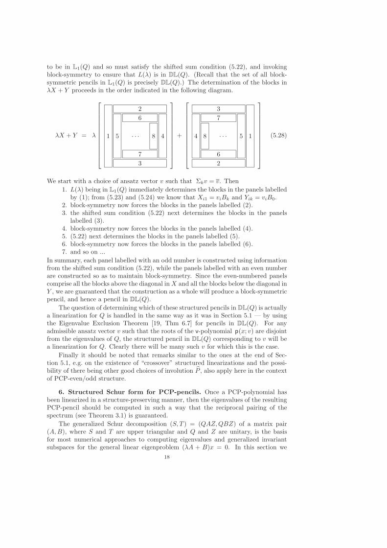
to be in L1(Q) and so must satisfy the shifted sum condition (5.22), and invokingblock-symmetry to ensure that L(λ) is in DL(Q). (Recall that the set of all block-symmetric pencils in L1(Q) is precisely DL(Q).) The determination of the blocks inλX + Y proceeds in the order indicated in the following diagram.

λX + Y = λ

1

3

2

45

7

6

8. . .

+

1

2

3

4 5

6

7

8 . . .

(5.28)

We start with a choice of ansatz vector v such that Σkv = v. Then

1. L(λ) being in L1(Q) immediately determines the blocks in the panels labelledby (1); from (5.23) and (5.24) we know that Xi1 = viBk and Yik = viB0.

2. block-symmetry now forces the blocks in the panels labelled (2).3. the shifted sum condition (5.22) next determines the blocks in the panels

labelled (3).4. block-symmetry now forces the blocks in the panels labelled (4).5. (5.22) next determines the blocks in the panels labelled (5).6. block-symmetry now forces the blocks in the panels labelled (6).7. and so on ...

In summary, each panel labelled with an odd number is constructed using informationfrom the shifted sum condition (5.22), while the panels labelled with an even numberare constructed so as to maintain block-symmetry. Since the even-numbered panelscomprise all the blocks above the diagonal in X and all the blocks below the diagonal inY , we are guaranteed that the construction as a whole will produce a block-symmetricpencil, and hence a pencil in DL(Q).

The question of determining which of these structured pencils in DL(Q) is actuallya linearization for Q is handled in the same way as it was in Section 5.1 — by usingthe Eigenvalue Exclusion Theorem [19, Thm 6.7] for pencils in DL(Q). For anyadmissible ansatz vector v such that the roots of the v-polynomial p(x; v) are disjointfrom the eigenvalues of Q, the structured pencil in DL(Q) corresponding to v will bea linearization for Q. Clearly there will be many such v for which this is the case.

Finally it should be noted that remarks similar to the ones at the end of Sec-tion 5.1, e.g. on the existence of “crossover” structured linearizations and the possi-bility of there being other good choices of involution P , also apply here in the contextof PCP-even/odd structure.

6. Structured Schur form for PCP-pencils. Once a PCP-polynomial hasbeen linearized in a structure-preserving manner, then the eigenvalues of the resultingPCP-pencil should be computed in such a way that the reciprocal pairing of thespectrum (see Theorem 3.1) is guaranteed.

The generalized Schur decomposition (S, T ) = (QAZ, QBZ) of a matrix pair(A, B), where S and T are upper triangular and Q and Z are unitary, is the basisfor most numerical approaches to computing eigenvalues and generalized invariantsubspaces for the general linear eigenproblem (λA + B)x = 0. In this section we

18

discuss the computation of a structured Schur-type decomposition for the linear PCP-eigenproblem

(λX + P XP )v = 0 , (6.1)

where X ∈ Cm×m and P ∈ R

m×m is an involution. We begin by assuming that Pis also symmetric; this is true for the involution in the quadratic PCP-eigenproblemarising from the stability analysis of time-delay systems discussed in Section 2, as wellas in the structured linearizations for such problems described in Section 5.1.

Since P is an involution its eigenvalues are in {±1}, so when P is symmetric itadmits a Schur decomposition of the form

P = WDWT , D =

[Ip

−Im−p

],

where W ∈ Rm×m is orthogonal. With

X = WT XW and v = WT v

we can then simplify (6.1) to the linear PCP-eigenproblem

(λX + DXD) v = 0 (6.2)

with involution D.Using a Cayley transform and scaling yields

12

(C+1

(λX + DXD

))(µ) v =: (µN + M) v = 0 (6.3)

where µ = λ−1λ+1 . By Theorem 4.1, the pencil µN + M is PCP-even with involution

D, hence N = −DND and M = DMD. These relations can also be directly verified

from the defining equations N := 12 (X−DXD), and M := 1

2 (X +DXD). Note alsothat Theorem 3.1 guarantees symmetry of the spectrum of µN + M with respect tothe imaginary axis. Partitioning N and M conformably with D we have

N =

[N11 N12

N21 N22

]=

[−N11 N12

N21 −N22

]= −DND ,

M =

[M11 M12

M21 M22

]=

[M11 −M12

−M21 M22

]= DMD .

Hence the blocks N12, N21, M11, and M22 are real while N11, N22, M12, and M21 arepurely imaginary.

Multiplying on both sides by D := diag(Ip , −iIm−p) yields the equivalent realpencil

D(µN + M)D

=

(µ

[iIm(X11) −iRe(X12)

−iRe(X21) −iIm(X22)

]+

[Re(X11) Im(X12)

Im(X21) −Re(X22)

])

=

((−iµ)

[−Im(X11) Re(X12)

Re(X21) Im(X22)

]+

[Re(X11) Im(X12)

Im(X21) −Re(X22)

])=: (νX1 + X2)

19

with X1, X2 real and ν = −iµ. Here Re(X) and Im(X) denote the real and imaginaryparts of X, respectively.

Now let (S, T ) = (QX1Z, QX2Z) be a real generalized Schur form for the real pair

(X1, X2); i.e., Q and Z are real orthogonal, T is real and upper triangular, and S isreal and quasi-upper triangular with 1×1 and 2×2 blocks. Any 1×1 block in this realSchur form corresponds to a real eigenvalue of νX1 +X2, hence to a purely imaginaryeigenvalue of µN + M , and thus to an eigenvalue of λX + PXP on the unit circle.Similarly, any 2 × 2 block corresponds to a complex conjugate pair of eigenvaluesfor νX1 + X2, which in turn corresponds to an eigenvalue pair (µ,−µ) for µN + M ,and thence to a reciprocal pair of eigenvalues (λ, 1/λ) for λX + P XP . Thus we seethat the block structure in the real Schur form of the real pencil νX1 + X2 preciselymirrors the reciprocal pairing structure in the spectrum of the original PCP-pencilλX + P XP .

We recover a structured Schur form for λX + P XP by re-assembling all thetransformations together to obtain

(QDWT

︸ ︷︷ ︸Q

)(λX + PXP )(WDZ︸ ︷︷ ︸Z

) = λ (T − iS)︸ ︷︷ ︸S

+ (T + iS)︸ ︷︷ ︸T

.

Since λS + T = λS + S this Schur form is again a PCP-pencil, but with respect tothe involution P = I. This derivation can be summarized in the following algorithm.

Algorithm 1 (Structured Schur form for PCP-pencils).

Input: X ∈ Cm×m and P ∈ R

m×m with P 2 = I and PT = P .Output: Unitary Q, Z ∈ Cm×m and block upper triangular S ∈ Cm×m such that

QXZ = S and QPXPZ = S; the diagonal blocks of S are only of size 1 × 1(corresponding to eigenvalues of magnitude 1) and 2 × 2 (corresponding to pairsof eigenvalues of the form (λ, 1/λ)).

1: P →WDWT with D = diag(Ip ,−Im−p) [ find real symmetric Schur form ]

2: X ←WT XW

3: X1 ←[−Im(X11) Re(X12)

Re(X21) Im(X22)

]where X11 ∈ Cp×p

4: X2 ←[

Re(X11) Im(X12)

Im(X21) −Re(X22)

]where X11 ∈ Cp×p

5: (X1, X2) → (QT SZT , QT T ZT ) [ compute real generalized Schur form ]

6: Q← Qdiag(Ip,−iIm−p)WT , Z ←Wdiag(Ip,−iIm−p)Z

7: S ← T − iS

This algorithm has several advantages over the standard QZ algorithm applieddirectly to λX+PXP . First, it is faster, since the main computational work is the realQZ rather than the complex QZ algorithm. Second, structure preservation guaranteesreciprocally paired eigenvalues; in particular, the presence of eigenvalues on the unitcircle can be robustly detected. It is interesting to note that an algorithm with theseproperties (computation of a structured Schur form with the resulting guaranteedspectral symmetry, and greater efficiency than the standard QZ algorithm) is not yetavailable for the T- or ∗-palindromic eigenvalue problem.

In many applications it is also necessary to compute eigenvectors for a PCP-polynomial, e.g., in the stability analysis of time-delay systems described in Section 2.

20

These can be found by starting with the eigenvalue problem (νS + T )x = 0 in realgeneralized Schur form, and computing eigenvectors x using standard methods. Itthen follows that

(1+iν1−iν S + T

)x =

(1+iν1−iν S + S

)x = 0, which in turn implies that(

1+iν1−iν X + PXP

)(Zx) = 0. In other words, v = Zx is an eigenvector of (6.1) corre-

sponding to the eigenvalue λ = 1+iν1−iν . If (6.1) was originally obtained as a structured

linearization in L1(Q) for a PCP-polynomial Q(λ), then (as described in Section 5)v must be of the form Λ ⊗ u for some eigenvector u of Q(λ) corresponding to theeigenvalue λ = 1+iν

1−iν . Thus eigenvectors u of Q(λ) are immediately recoverable fromthe eigenvectors v of (6.1).

Remark 5: Any real involution P that is not symmetric admits a Schur decom-position of the form

R = WT PW =

[Ip R12

−Im−p

].

Defining

K :=

[Ip

12R12

−Im−p

]

we have K−1RK = D = diag(Ip ,−Im−p), and so P = WDW−1 with W = WK.Thus if P is only mildly non-normal (i.e., ‖R12‖ is small), then there is a well-conditioned similarity transformation that brings P to the diagonal form D, andreplacing W by W and WT by W−1 in Algorithm 1 would still be a reasonable wayto compute the eigenvalues and eigenvectors of a PCP-pencil. Note, however, thatthe output matrices Q and Z will no longer be unitary. ⋄

Remark 6: Note that with some minor modifications, Algorithm 1 can also beused on an anti-PCP-pencil to compute a structured Schur form that is anti-PCP, ofthe form λS − S. ⋄

7. Applications and Numerical Results. As we saw earlier in Section 2,eigenvalue problems with PCP-structure arise in the stability analysis of neutral lin-ear time-delay systems. Such systems provide useful mathematical models in manyphysical application areas (see [13, 22] and the references therein); one example iscircuits with delay elements, such as transmission lines and partial element equivalentcircuits (PEEC’s). A realistic problem motivated by the small PEEC model in Fig.7.1 is given by

S =

{D1x(t− h) + x(t) = A0x(t) + A1x(t− h) , t ≥ 0

x(t) = ϕ(t) , t ∈ [−h, 0)(7.1)

where

A0 = 100 ·

−7 1 2

3 −9 01 2 −6

, A1 = 100 ·

1 0 −3−0.5 −0.5 −1−0.5 −1.5 0

,

D1 = − 1

72·

−1 5 2

4 0 3−2 4 1

, D0 = I, and

ϕ(t) =[sin(t), sin(2t), sin(3t)

]T.

21

I

1 2 3

Lp11Lp22

ic1ic2

ic3

i1 i2

I1 I2 I31

P11

1P22

1P33

1 2 3

(a) (b)

Fig. 7.1. (a) Metal strip with two Lp cells (three capacitive cells dashed) and (b) small PEECmodel for metal strip. Figures are redrawn from [1].

More details on this example can be found in [1].The quadratic eigenproblem (2.14) for this example is (z2E + zF + G)u = 0

with

E = (D0 ⊗A1) + (A0 ⊗D1), G = (D1 ⊗A0) + (A1 ⊗D0),

F = (D0 ⊗A0) + (A0 ⊗D0) + (D1 ⊗A1) + (A1 ⊗D1).

It is easy to verify that E = PGP and F = PFP hold for

P =

M11 M21 M31

M12 M22 M32

M13 M23 M33

,

where Mij denotes the 3 × 3 matrix with the entry 1 in position (i, j) and zeroeseverywhere else.

The standard companion forms for this quadratic eigenproblem are

C1(λ) = λ

[E

I

]+

[F G−I 0

]and C2(λ) = λ

[E

I

]+

[F −IG 0

].

A structured pencil in L1(Q) (as discussed in Section 5.1) is given by

λ

[v1E −X12

v1E v1F + PX12P

]+

[X12 + v1F v1PEP−PX12P v1PEP

], v1 ∈ C, (7.2)

where X12 is arbitrary, while a structured pencil in L2(Q) is given by

λ

[w1E w1EX21 w1F − PX21P

]+

[w1F −X21 PX21Pw1PEP w1PEP

], w1 ∈ C, (7.3)

where X21 is arbitrary. With w1 = v1 and X21 = v1E = −X12 the pencils (7.2) and(7.3) are the same, and give the unique structured pencil (up to choice of scalar v1)

λ

[v1E v1Ev1E v1F − v1PEP

]+

[v1F − v1E v1PEP

v1PEP v1PEP

](7.4)

that lies in the intersection DL(Q) = L1(Q) ∩ L2(Q). By the Eigenvalue ExclusionTheorem [19, Thm 6.7] the pencil (7.4) is a structured linearization if and only if−v1/v1 is not an eigenvalue of Q(λ).

22

Choosing v1 = 1 and applying Algorithm 1 we found that (7.4) has no eigenvalueson the unit circle, so the time-delay system S in (7.1) has no critical delays. Thesystem S is stable for h = 0, since all eigenvalues of the pencil L(α) = α(D0 + D1)−(A0 + A1) have negative real part. Continuity of the eigenvalues of S as a functionof the delay h then implies that S is stable for every choice of the delay h ≥ 0, aproperty known as delay-independent stability.

Our next example arises from the discretization of a partial delay-differentialequation (PDDE), taken from Example 3.22 in [13, Sections 2.4.1, 3.3, 3.5.2]. Itconsists of the retarded time-delay system

x(t) = A0x(t) + A1x(t− h1) + A2x(t− h2) (7.5)

where A0 ∈ Rn×n is tridiagonal and A1, A2 ∈ Rn×n are diagonal with

(A0)kj =

{−2(n + 1)2/π2 + a0 + b0 sin

(jπ/(n + 1)

)if k = j

(n + 1)2/π2 if |k − j | = 1 ,

(A1)jj = a1 + b1jπ

n + 1

(1− e−π

(1−j/(n+1)

)),

(A2)jj = a2 + b2jπ2

n + 1

(1− j/(n + 1)

).

Here aℓ, bℓ are real scalar parameters and n ∈ N is the number of uniformly spacedinterior grid points in the discretization of the PDDE. We used the values

a0 = 2, b0 = 0.3, a1 = −2, b1 = 0.2, a2 = −2, b2 = −0.3

(as in [13]) and considered various values for n. With ϕ1 = −π/2 (i.e. eiϕ1 = i) thequadratic PCP eigenvalue problem to solve is

(λ2E + λF + PEP ) v = 0 (7.6)

where

E = I ⊗A2 , F =(I ⊗ (A0 − iA1)

)+((A0 + iA1)⊗ I

),

and P is the n2 × n2 permutation that interchanges the order of Kronecker productsas in (2.17). Table 7.1 displays the results of our numerical experiments. Here ndenotes the dimension of the time-delay system (7.5), 2n2 the dimension of the PCP-pencil (7.4), and tpolyeig, tQZ, tPCP denote the execution times in seconds of the threetested methods:

1. solving the quadratic eigenvalue problem (7.6) using MATLAB’s polyeig

command, which applies the QZ algorithm to a (permuted) companion form,

Table 7.1

n 2n2 tpolyeig tQZ tPCP errpolyeig errQZ #polyeig #QZ #PCP

5 50 0.02 0.02 0.01 5.5e-15 3.7e-15 4 4 410 200 0.50 0.55 0.28 6.5e-14 1.2e-13 4 4 415 450 5.5 6.3 3.0 4.4e-13 2.6e-13 4 3 420 800 33 36 20 1.3e-12 4.8e-13 3 0 425 1250 131 137 72 3.1e-12 6.6e-13 3 0 430 1800 413 435 227 1.1e-11 7.5e-13 0 0 4

23

2. solving the generalized eigenproblem for the PCP-pencil (7.4) using MAT-LAB’s QZ algorithm, and

3. solving the eigenproblem for the PCP-pencil (7.4) using Algorithm 1.All computations were done in MATLAB 7.5 (R2007b) under OpenSUSE Linux 10.2(kernel 2.6.18, 64 bit) on a Core 2 Duo Processor E6850 3.0GHz with 4GB memory.The quantities errpolyeig and errQZ, defined by

err = maxλj

minλk

|λj − (1/λk) ||λj |

where λj , λk are (not necessarily distinct) eigenvalues of (7.6), measure the distance ofthe computed eigenvalues from being paired for the two unstructured methods. Notethat this measure is zero for Algorithm 1 by construction. The numbers #polyeig, #QZ,and #PCP denote the number of eigenvalues on the unit circle found by each method;for the unstructured methods this is the number of eigenvalues λ with

∣∣ |λ|−1∣∣ < 10−14,

while for Algorithm 1 this is the number of 1× 1 blocks in the structured Schur form.As can be seen from the table, our structured method is about twice as fast as

both unstructured methods. Note that the QZ algorithm applied to the PCP lineariza-tion (column tQZ) is slightly slower than the QZ algorithm applied to a companionform linearization (column tpolyeig). On the other hand, the eigenvalues computed bypolyeig are not as well paired as those computed by the QZ algorithm applied tothe PCP linearization. In the time-delay setting the only eigenvalues of interest arethose on the unit circle and in this respect the three methods perform very differently.All methods correctly find the number of eigenvalues of unit magnitude for n = 5, 10.For larger n the unstructured methods do not find all, and sometimes not any, of thedesired eigenvalues. In particular, for n = 30 only the structured method finds all 4eigenvalues on the unit circle whereas the unstructured methods find none.

As a third example, we tested PCP-pencils of the form λX + PXP where X israndomly generated by the Matlab command randn(n)+i*randn(n) and P is thematrix R as defined in (5.6). We found that for values of 50 < n < 2000 on this typeof problem our Algorithm 1 performs 2.5 to 3 times faster than the QZ algorithm.

8. Concluding Summary. Motivated by a quadratic eigenproblem arising inthe stability analysis of time-delay systems [13], we have identified a new type ofmatrix polynomial structure, termed PCP-structure, that is analogous to the palin-dromic structures investigated in [18]. The properties of these PCP-polynomials wereinvestigated, along with those of three closely related structures — anti-PCP, PCP-even and PCP-odd polynomials. Spectral symmetries were revealed, and relationshipsbetween these structures were established via the Cayley transformation.

Building on the work in [19], we have shown how to construct structure-preservinglinearizations for all these structured polynomials in the pencil spaces L1(Q), L2(Q),and DL(Q). In addition to preservation of eigenvalue symmetry, such linearizationsalso permit easy eigenvector recovery, which can be an important consideration inapplications. Structured Schur forms for PCP and anti-PCP pencils were derived,along with a new algorithm for their computation that compares favorably with theQZ algorithm. Using a structure-preserving linearization followed by the computationof a structured Schur form thus allows us to solve the new structured eigenproblemefficiently, reliably, and with guaranteed preservation of spectral symmetries.

Acknowledgment. The authors thank Elias Jarlebring for many enlighteningdiscussions about time-delay systems.

24

REFERENCES

[1] A. Bellen, N. Guglielmi, and A.E. Ruehli, Methods for linear systems of circuit delay-differential equations of neutral type, IEEE Trans. Circuits and Systems - I: FundamentalTheory and Applications, 46 (1999), pp. 212–216.

[2] R. Byers, D. S. Mackey, V. Mehrmann, and H. Xu, Symplectic, BVD, and palindromicapproaches to discrete-time control problems, MIMS EPrint 2008.35, Manchester Institutefor Mathematical Sciences, The University of Manchester, UK, Mar. 2008. To appear in the“Jubilee Collection of Papers dedicated to the 60th Anniversary of Mihail Konstantinov”(P. Petkov and N. Christov, eds.), Bulgarian Academy of Sciences, Sofia, 2008.

[3] H. Fassbender, D.S. Mackey, N. Mackey, and C. Schroder, Detailed version of “Struc-tured polynomial eigenproblems related to time-delay systems”, preprint, TU Braunschweig,Institut Computational Mathematics, 2008.

[4] I. Gohberg, M.A. Kaashoek, and P. Lancaster, General theory of regular matrix polyno-mials and band Toeplitz operators, Integr. Eq. Operator Theory, 11 (1988), pp. 776–882.

[5] I. Gohberg, P. Lancaster, and I. Rodman, Matrix Polynomials, Academic Press, New York,1982.

[6] J. K. Hale and S. M. Verduyn Lunel, Introduction to Functional-differential Equations,vol. 99 of Applied Mathematical Sciences, Springer-Verlag, New York, 1993.

[7] N.J. Higham, R-C. Li, and F. Tisseur, Backward error of polynomial eigenproblems solvedby linearization, SIAM J. Matrix Anal. Appl., 29 (2007), pp. 1218–1241.

[8] N.J. Higham, D.S. Mackey, N. Mackey, and F. Tisseur, Symmetric linearizations for matrixpolynomials, SIAM J. Matrix Anal. Appl., 29 (2006), pp. 143–159.

[9] N.J. Higham, D.S. Mackey, and F. Tisseur, The conditioning of linearizations of matrixpolynomials, SIAM J. Matrix Anal. Appl., 28 (2006), pp. 1005–1028.

[10] , Definite matrix polynomials and their linearization by definite pencils, MIMS EPrint2007.97, Manchester Institute for Mathematical Sciences, The University of Manchester,UK, 2008. To appear in SIAM J. Matrix Anal. Appl.

[11] N.J. Higham, D.S. Mackey, F. Tisseur, and S.D. Garvey, Scaling, sensitivity and stabilityin the numerical solution of quadratic eigenvalue problems, Int. J. of Numerical Methodsin Engineering, 73 (2008), pp. 344–360.

[12] R.A. Horn and C. R. Johnson, Topics in Matrix Analysis, Cambridge University Press,reprinted paperback version ed., 1995.

[13] E. Jarlebring, The Spectrum of Delay-Differential Equations: Numerical Methods, Stabilityand Perturbation, PhD thesis, TU Braunschweig, Institut Computational Mathematics,Carl-Friedrich-Gauß-Fakultat, 38023 Braunschweig, Germany, 2008.

[14] P. Lancaster, Lambda-Matrices and Vibrating Systems, Pergamon Press, Oxford, 1966.reprinted by Dover, New York, 2002.

[15] P. Lancaster and P. Psarrakos, A note on weak and strong linearizations of regular matrixpolynomials, MIMS EPrint 2006.72, Manchester Institute for Mathematical Sciences, TheUniversity of Manchester, UK, 2005.

[16] P. Lancaster and L. Rodman, The Algebraic Riccati Equation, Oxford University Press,Oxford, 1995.

[17] D.S. Mackey, Structured Linearizations for Matrix Polynomials, PhD thesis, The Universityof Manchester, U.K., 2006. Available as MIMS-EPrint 2006.68, Manchester Institute forMathematical Sciences, Manchester, England, 2006.

[18] D.S. Mackey, N. Mackey, C. Mehl, and V. Mehrmann, Structured polynomial eigenvalueproblems: Good vibrations from good linearizations, SIAM J. Matrix Anal. Appl., 28 (2006),pp. 1029–1051.

[19] , Vector spaces of linearizations for matrix polynomials, SIAM J. Matrix Anal. Appl., 28(2006), pp. 971–1004.

[20] V. Mehrmann, A step toward a unified treatment of continuous and discrete-time controlproblems, Linear Algebra Appl., 241-243 (1996), pp. 749–779.

[21] W. Michiels and S.-I. Niculescu, Stability and Stabilization of Time-Delay Systems: AnEigenvalue-Based Approach, vol. 12 of Advances in Design and Control, Society for Indus-trial and Applied Mathematics, Philadelphia, PA, 2007.

[22] S.-I. Niculescu, Delay Effects on Stability: A Robust Control Approach, Springer-Verlag,London, 2001.

[23] C. Schroder, Palindromic and Even Eigenvalue Problems - Analysis and Numerical Methods,PhD thesis, Technical University Berlin, Germany, 2008.

[24] F. Tisseur and K. Merbergen, A survey of the quadratic eigenvalue problem, SIAM Review,43 (2001), pp. 234–286.

25