arX

iv:0

909.

0272

v1 [

astr

o-ph

.CO

] 1

Sep

200

9

Structural Parameters of the M87 Globular Clusters1

Juan P. Madrid2, William E. Harris2, John P. Blakeslee 3, Matıas Gomez 4

Received ; accepted

submitted to ApJ

1Based on observations made with the NASA/ESA Hubble Space Telescope, obtained at

the Space Telescope Science Institute, which is operated by the Association of Universities

for Research in Astronomy, Inc., under NASA contract NAS 5-26555. These observations

are associated with program 10543.

2Department of Physics and Astronomy, McMaster University, Hamilton ON L8S 4M1,

Canada

3Herzberg Institute of Astrophysics, Victoria, BC V9E 2E7, Canada

4Departamento de Ciencias Fisicas, Facultad de Ingenieria, Universidad Andres Bello,

Concepcion, Chile

– 2 –

ABSTRACT

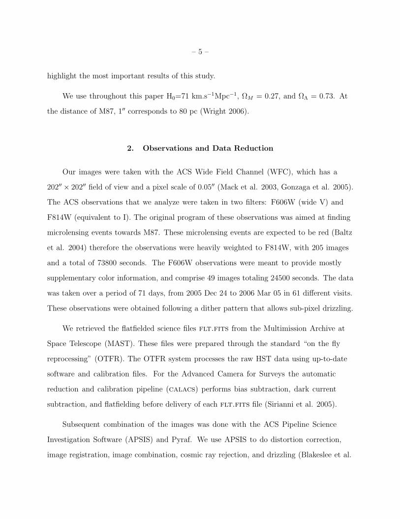
We derive structural parameters for ∼ 2000 globular clusters in the giant

Virgo elliptical M87 using extremely deep Hubble Space Telescope images in

F606W (V) and F814W (I) taken with the ACS/WFC. The cluster scale sizes

(half-light radii rh) and ellipticities are determined from PSF-convolved King-

model profile fitting. We find that the rh distribution closely resembles the inner

Milky Way clusters, peaking at rh ≃ 2.5 pc and with virtually no clusters more

compact than rh ≃ 1 pc. The metal-poor clusters have on average an rh 24%

larger than the metal-rich ones. The cluster scale size shows a gradual and

noticeable increase with galactocentric distance. Clusters are very slightly larger

in the bluer waveband V , a possible hint that we may be beginning to see the

effects of mass segregation within the clusters. We also derived a color magnitude

diagram for the M87 globular cluster system which show a striking bimodal

distribution.

Subject headings: galaxies: star clusters - galaxies: individual (M87) - galaxies:

elliptical and lenticular, cD - globular clusters: general

– 3 –

1. Introduction

Messier 87 (Virgo A, and NGC 4486) is the central dominant elliptical galaxy of the

Virgo Cluster located 16.7 Megaparsecs away from us (Blakeslee et al. 2009). M87 is

one of the most fascinating and best studied celestial objects and due to its relative close

distance it has been a prime target of observations that have provided precious clues for the

understanding of black hole physics, accretion disks, radio galaxies, and jets, among many

other fields.

M87 has also played a crucial role in the understanding of extragalactic globular

cluster systems (GCS). One of the most prominent characteristics of this galaxy is its

extremely large number of globular clusters. Recent ground-based observations found that

the M87 GCS has in total more than 14000 members (Tamura et al. 2006). M87 is also

the paradigmatic high specific frequency (SN) globular cluster system (McLaughlin et al.

1994, Harris 2009). The specific frequency represents the number of clusters per unit galaxy

luminosity (Harris & van den Bergh 1981) and for M87 SN=14, a value three times higher

than other Virgo giant ellipticals (McLaughlin et al. 1994, Peng et al. 2008). This large

sample of globular clusters (GC) constitutes a superb basis for carrying out many studies,

including now accurate measurements of their structural parameters.

The large number of globular clusters belonging to M87 was first noticed in 1955 (Baum

1955) but the study of their structural parameters, e. g. characteristic sizes, ellipticities,

luminosities, is enabled only by the superior resolution of the Hubble Space Telescope

(HST). A typical size expected for a globular cluster, namely reff ∼ 2 to 3 parsecs in radius,

corresponds to only about 0.035′′at the Virgo distance, or one pixel of the instruments

onboard HST (Larsen et al. 2001). Previous work of this type for the globular clusters

in the Virgo members was done by Jordan et al. (2005, 2009) with Advanced Camera for

Surveys (ACS) data but with much shorter-exposure data than we use here. Even earlier

– 4 –

work for M87 (Kundu at al. 1999) used the WFPC2 with its larger pixel scale and smaller

field of view, and is now superseded by the capabilities of the ACS.

In this study we use one of the deepest datasets in the HST archive to derive the

structural parameters for globular clusters in M87. A large, multi-orbit program imaging

the central region of the galaxy was carried out with the ACS and produced exceptionally

deep images of the inner region of M87 (GO 10543, PI: Baltz), a region heavily illuminated

by galaxy light and difficult to image to such detail with a telescope of lower resolution

or image quality. In this very deep dataset more than two thousand sources are globular

clusters, and their radial profiles are distinctly and obviously larger than the PSF of the

HST/ACS. We use the fact that these clusters are resolved to measure their structural

parameters with ishape, a software specially designed to derive these parameters for barely

resolved objects (Larsen 1999).

The morphology of individual globular clusters is characterized by a number of standard

parameters, perhaps most importantly the effective radius rh, the radius that contains

half the total luminosity of the cluster. The effective radius remains virtually constant

through up to ten relaxation times and thus plays an important role in the understanding

of evolutionary processes of globular clusters systems back nearly to the proto-cluster stage

(Spitzer & Thuan 1972, Aarseth & Heggie 1998, Gomez et al. 2006). The M87 clusters

are associated with the very dense environment of the Virgo Cluster core in a supergiant

elliptical and thus their structural parameters give us the chance to probe a very different

environment than the ones in the Milky Way.

This paper is structured as follows: §2 describes the observations and data reduction,

§3 describes the modeling of the PSF used to derived the structural parameters presented

in §4, in §5 we discuss the photometry and the color-magnitude diagram of the M87 GCS

while §6 does a comparison with another recent study using the same dataset, and in §7 we

– 5 –

highlight the most important results of this study.

We use throughout this paper H0=71 km.s−1Mpc−1, ΩM = 0.27, and ΩΛ = 0.73. At

the distance of M87, 1′′ corresponds to 80 pc (Wright 2006).

2. Observations and Data Reduction

Our images were taken with the ACS Wide Field Channel (WFC), which has a

202′′ × 202′′ field of view and a pixel scale of 0.05′′ (Mack et al. 2003, Gonzaga et al. 2005).

The ACS observations that we analyze were taken in two filters: F606W (wide V) and

F814W (equivalent to I). The original program of these observations was aimed at finding

microlensing events towards M87. These microlensing events are expected to be red (Baltz

et al. 2004) therefore the observations were heavily weighted to F814W, with 205 images

and a total of 73800 seconds. The F606W observations were meant to provide mostly

supplementary color information, and comprise 49 images totaling 24500 seconds. The data

was taken over a period of 71 days, from 2005 Dec 24 to 2006 Mar 05 in 61 different visits.

These observations were obtained following a dither pattern that allows sub-pixel drizzling.

We retrieved the flatfielded science files flt.fits from the Multimission Archive at

Space Telescope (MAST). These files were prepared through the standard “on the fly

reprocessing” (OTFR). The OTFR system processes the raw HST data using up-to-date

software and calibration files. For the Advanced Camera for Surveys the automatic

reduction and calibration pipeline (calacs) performs bias subtraction, dark current

subtraction, and flatfielding before delivery of each flt.fits file (Sirianni et al. 2005).

Subsequent combination of the images was done with the ACS Pipeline Science

Investigation Software (APSIS) and Pyraf. We use APSIS to do distortion correction,

image registration, image combination, cosmic ray rejection, and drizzling (Blakeslee et al.

– 6 –

2003). APSIS was developed by the ACS science team and proved to be more effective

than multidrizzle, the alternative software, at registering this large data set taken

during different epochs. Using Python, APSIS performs subpixel drizzling, and we chose

to construct the final science images with a pixel scale of 0.035′′/pixel. We use a gaussian

function as interpolation kernel and a pixel fraction (pixfrac) of 1.

As a test to the solidity of our results, all measurements described below were also

performed on an image with a narrower PSF. An image with a 10% narrower PSF was built

by using a smaller value for pixfrac (0.5 instead of 1.0) during the data reduction. The final

cluster sizes measured from these two different reductions were identical. Using a different

fitting code (kingphot), Peng et al. (2009) come to the same conclusion that we do here,

namely that the differences for the magnitudes and sizes are negligible between the two

reductions.

From the master combined F606W and F814W images we created a median subtracted

image to eliminate the galaxy light in order to facilitate the detection of the position of

globular clusters on our images. The pyraf task daofind did a fine job detecting globular

clusters and ignoring brightness fluctuations and background galaxies.

We performed a careful visual inspection of the frame to verify these detections. We

manually removed spurious sources along the edges of the different knots belonging to the

prominent M87 jet. Sharp gradients in brightness are often misinterpreted as sources by

daofind. We also removed spurious detections along the edges of the image. We detect a

total of 2010 objects on our images almost all of which are globular clusters. In Figure 1 we

show a section of the median subtracted image with our detections of cluster candidates.

Given the very large number of clusters in our sample a few field contaminants have a

negligible impact on our results (Larsen et al. 2001). We should note that we performed

all measurements presented below on the original image, the median subtracted image was

– 7 –

used only to locate the clusters. Systematics introduced by a routine such as median or

ellipse are difficult to evaluate and therefore difficult to correct even though they may be

small.

3. PSF modeling

An accurate PSF is crucial for our purpose of deriving precise structural parameters for

the GCs, given that we are working in a regime where the GC intrinsic sizes rh are similar

to the FWHM of the PSF itself. In principle, PSFs can be constructed through modeling

techniques such as TinyTim, but extensive discussions of this approach in recent papers

directed towards the same goal of measuring GC sizes in relatively nearby galaxies imaged

with ACS (Spitler et al 2006, Georgiev et al. 2008) show considerable difficulty matching

the models to empirical PSFs derived directly from stars on the images. Working from this

experience, we have adopted the approach of using purely empirical PSFs built from stars

on the master F814W and F606W images described above.

An immediate practical issue is to find candidate stars on these images: of the more

than 2000 detected objects on the field, roughly 98% are globular clusters belonging to M87

and these must all be weeded out. Fortunately, the true size of the stars is accurately known

beforehand: for properly co-added images, the HST image resolution is ≃ 0.095′′, and thus

we expect genuine stars to have FWHM ≃ 2.7 − 2.8 pixels at our final drizzled scale of

0.035′′/px. Equally important for our purposes, as will be seen below, there is almost no

overlap between the stars and the measured sizes of the GCs (that is, their intrinsic sizes

convolved with the PSF), with a clear gap between the true stars and the smallest GCs.

To pick out the stars, we used the SExtractor software (Bertin & Arnouts 1996) to

make preliminary measurements of the half-light radii and FWHMs of all 2000+ objects

– 8 –

on our detection list, including GCs, stars, and a few small background galaxies. These

scale sizes were plotted against the SE total aperture magnitude. On these diagnostic

graphs, the stars then show up as an easily identified, narrow (though thinly populated)

sequence clearly separated from the GCs and other objects. See, for example, Figure 2 of

Harris (2009) for the same approach. We selected the 30 brightest of these and inspected

them individually on the images, rejecting any with faint companions, nearby bad pixels,

or other anomalies; one bright star that was at or near saturation was also rejected. Our

final starlist has 17 stars distributed uniformly across the ACS field, from which the PSF

is then constructed. To minimize any later concerns about systematic differences between

the F606W and F814W images in the measured GC parameters, we used exactly the same

17 stars to derive the PSF separately in each filter. The final PSF profiles have FWHMs of

2.75 pixels (F606W) and 2.78 pixels (F814W).

We create the PSF for each filter by using the standard daophot routines within

pyraf. We perform photometry of the candidate stars with phot and then run pstselect

to select the stars to be used to build the PSF by the task psf. The output of psf is a

luminosity weighted PSF with a radius of 79 pixels. We ensured that all stars used to

calculate the PSF had similar luminosity and thus we avoid any strong bias in favor of

particularly bright stars. We use seepsf to subsample our PSF to the pixel size required

by ishape, i.e. ten times smaller than the image pixel size (Larsen 1999).

4. Structural Parameters

4.1. Effective Radius

We use the software ishape developed by Søren Larsen to calculate the effective radius,

ellipticity, and position angle θ for each individual cluster on our images (Larsen 1999).

– 9 –

ishape convolves an analytical model of the cluster profile, with the PSF and finds the

best fit to the data by performing iterative adjustments to the cluster profile FWHM. The

analytical model used to fit the clusters is chosen by the user from a predefined list e. g.

Gaussian, King, Sersic, see Larsen (1999). We use model King profiles (King, 1962) with a

concentration parameter of c=30, where c = rt

rc, the ratio of the tidal radius divided by the

core radius. This c-value accurately represents the average of real globular clusters (Harris

1996, Larsen 1999, Larsen et al. 2001). By contrast, Waters et al. (2009) used c=10, a

value near the minimum for real globular clusters rather than the mean.

The measurement of the effective radius carried out by ishape is robust and nearly

independent of the fitting function. We set a fitting radius of six pixels and we convert our

measurements of the cluster FWHM into the effective radius by following the prescription

of Larsen (1999). Namely, we convert the ishape internal radius for the FWHM, which is

model dependent, into a model independent quantity rh = 1.48 × FWHM , where 1.48 is

the respective value for c=30. We obtain thus the cluster size in pixels, we multiply by the

scale, and then obtain the cluster rh in arcseconds. All clusters considered in the following

analysis have an effective radius measured with a signal-to-noise ratio > 50. The ishape

Manual (Larsen 2008) has a tentative formula to take into account the effects of ellipticity

on determining the effective radius. Strictly, ishape measures the rh along the major

axis of the profile and in theory a small correction should be made to derive rh for a non

circular cluster (Larsen 2008). Given that most clusters of our sample are nearly circular

we quote the direct values of rh given by ishape without further corrections for the effects

of the ellipticity during the fitting process. Details on the sensitivity of our measurements

to cluster ellipticity and tests of the validity of our assumptions are given in Harris (2009).

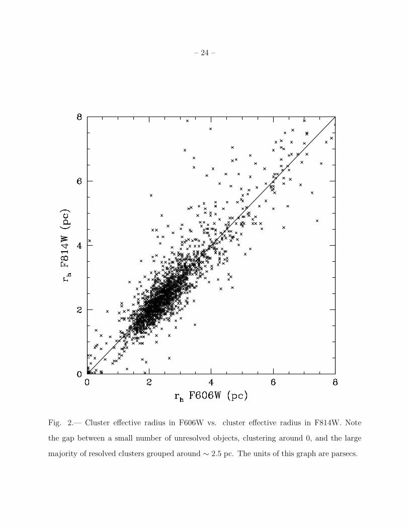
Results are shown in Figures 2 and 3.

An extensive set of tests and simulations to characterize the uncertainties associated

– 10 –

with ishape measurements is presented in Harris (2009). In this work it is clearly shown

that ishape derives accurate values for cluster effective radius, ellipticity and position

angle when S/N>50, which is the cut-off that we adopt in this study. The main sources of

error in the size measurements can be summarized in three components: the ishape fitting

procedure itself, the uncertainty in the true values of the concentration parameter c, and

the error associated with the size of the PSF. The random uncertainty per object taking

into account the three sources of uncertainty cited above is σrh= ±0.006′′ (Harris 2009) for

his BCG data sample. For comparison, the rms scatter around the 1:1 line in Figure 2 is

±0.004′′; this should give a reasonable estimate of our internal measurement uncertainty

since it is the direct comparison of two independent measurements of the same objects in

different filters. The equivalent uncertainty for rh is then ±0.3 pc.

The values for the linear effective radii that we derived are in good agreement with

the values of Milky Way globular clusters. The Milky Way has 142 clusters with known

effective radius, out of these 142 clusters 114 (80%) have an effective radius between 1 and

6 pc (Harris 1996). It can be seen in Figure 2 and the histograms in Figure 3 that most

M87 clusters also have an effective radius between 1 and 6 parsecs and peak at very much

the same radius (≃ 2.5 pc ) as the Milky Way.

It is intriguing that clusters belonging to two galaxies with different Hubble type have

the same size distribution. Forbes (2002) plotted side by side the size distribution of GCS

for five galaxies of completely different Hubble type: cD, gE, S0, Sa, Sbc. Strikingly, the size

distributions of the overall GCS, and of both sup-populations are very similar, indicating

that the physical processes determining the size of globular clusters and the size difference

between the two sub-populations are independent of galaxy type. Whitmore et al. (2007)

suggest a universal initial mass function for clusters followed by an evolution dominated by

internal dynamics. The host galaxy has only a secondary effect on cluster size.

– 11 –

We recover the well documented size difference between red (metal-rich) and blue

(metal-poor) clusters, i.e. blue clusters are 24% larger than red ones in the M87 GCS (a

result first noted by Kundu et al. 1998), as discussed further below.

We also find a hint of a size difference versus wavelength such that, the cluster size

measured in F606W is very slightly larger on average than in the F814W . For all clusters

we calculated the ratio rhF606WrhF814W

; the histogram of the values of this ratio is plotted in Figure

4. Of the 1896 clusters which are within our high confidence range 61% of them have

rhF606W ≥ rhF814W . The median ratio, near the peak of the histogram, is 1.02 ± 0.006

and the standard deviation is 0.24. We rejected objects at more than 3σ level as outliers.

We are well aware that the mean difference may have arisen from small residual systematics.

However we have attempted to minimize any such systematics as much as possible, and we

should note that the very small raw difference between the two PSF sizes noted above is

not large enough by itself to produce the difference we see, particularly for bigger clusters.

However, if the difference in mean rh between the two filters is physically real, we suggest

that we may be seeing the visible results of mass segregation. Dynamical evolution of the

population of stars within each cluster drives the less massive stars to larger radii and

the more massive ones inward toward the core, while maintaining a nearly constant rh.

Over time, a secondary observational effect is that the cluster effective radius will look

progressively smaller in redder bandpasses that systematically favor the light from the

massive red-giant and subgiant stars, compared with the bluer, lighter upper-main-sequence

stars that preferentially populate the outskirts. To gauge the expected size of the effect,

we have used the predicted rh values in the B, V, I bandpasses for model globular clusters

with an initial mass of 105M⊙ evolved through an advanced N-body code (Hurley 2009,

private communication; see also Hurley et al. 2008). After 10-12 Gy of dynamical evolution,

the model clusters have measured rh values that are 5% larger in V than in I. Both the

direction and size of the effect are very close to the mean offset that we see in the M87

– 12 –

system. We view our result as only suggestive, but it may point the way to a valuable new

test of our understanding of GC dynamical evolution. We will further investigate this effect

with more data that we are currently analyzing.

4.2. Ellipticity

ishape measures the ratio of minor/major axis and thus the ellipticity of each cluster.

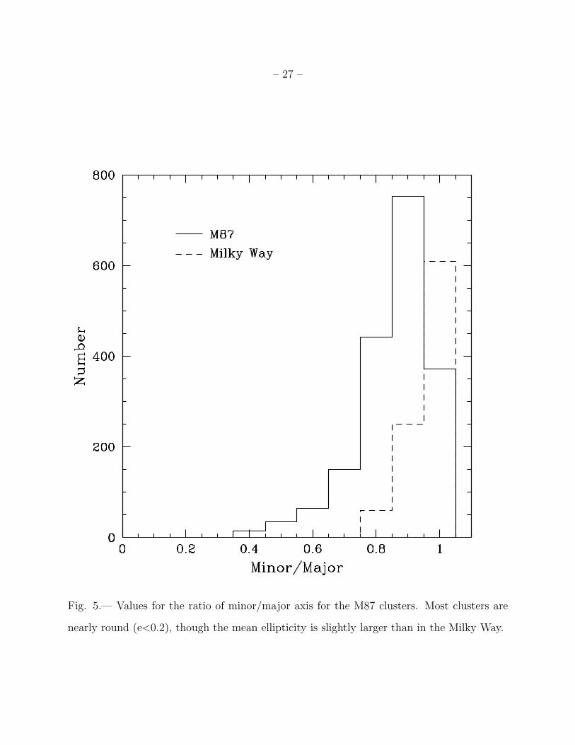
In Figure 5 we plot the values obtained with ishape for the ratio of minor/major axis for

1767 clusters of our dataset. Similarly to the Milky Way globular clusters (Harris 1996)

most M87 clusters are roughly spherical, i.e. for more than 55% of clusters in our sample

the ratio minor/major > 0.8. A normal two sample Kolmogorov-Smirnov test shows that

the M87 and Milky Way distributions are formally different at high statistical significance.

However, these two samples were measured in completely different ways: the Milky Way

clusters are orders of magnitude better resolved and thus their ellipticities are much better

determined and physically meaningful. Figure 5 shows that, roughly, M87 clusters have the

expected range of small ellipticity.

4.3. Effective radius as a function of galactocentric distance

Hodge (1960, 1962) measured the sizes of Large Magellanic Cloud globular clusters

using data taken with the ADH Baker-Schmidt telescope in South Africa. Despite the fact

that Hodge (1962) observed a projected distribution of the cluster population instead of

the real spatial distribution, he first recognized the correlation between cluster size and

galactocentric radius (Rgc), i. e. cluster size increases with increasing distance to the center

of the galaxy. Hodge (1962) postulated the tidal effects of the parent galaxy on the cluster

as the most probable explanation for this effect. Based on data for Milky Way globular

– 13 –

clusters, and therefore free of projection bias, van den Bergh et al. (1991) find a relation

between cluster effective radius and true 3D galactocentric distance of rh ∝√

Rgc. The

same dependence of cluster size and galactocentric distance has been well documented in

NGC5128 (Hesser et al. 1984, Gomez & Woodley 2007), NGC4594 (Spitler et al. 2006),

and in six other giant ellipticals (Harris 2009). For these galaxies the general trend is for rh

to increase roughly as rh ∼ R0.1−0.2gc where Rgc is the projected distance.

In Figure 6 we plot the effective radius rh versus projected galactocentric distance Rgc.

Our observations target the central regions of M87 where tidal forces exerted by the galaxy

are expected to have the strongest effect limiting the size of clusters (Hesser et al 1984). For

Rgc ≤ 5 kpc the mean cluster size is nearly constant, but then begins to increase gradually,

out to the limits of our data at Rgc = 11 kpc. Kundu et al. (1999) failed to observe this

trend given their smaller WFPC2 field size.

In order to demonstrate that the increase in effective radii of clusters with Rgc is real,

we performed a test with the stars on the field. We selected all the objects that ishape

returned as having FWHM=0, that is the ones that are by definition starlike. There were

42 such stars, we then measured with imexamine the FWHM of these point sources. These

stars can also be clearly seen in Figure 2, 3 & 6 as the sources around the zero value for

the effective radius, and are also apparent in Figure 3 as the first bin of the histogram

i.e. rh = 0. We find that the FWHM of these point sources is consistent with the value

of the PSF FWHM of 2.7 pixels, and more importantly does not show a dependence with

galactocentric radius (see Figure 7 top panel). We also plot in Figure 7 (bottom panel) the

residual of the PSF with unresolved sources across the detector that is, the “size” of each

star as returned by the ISHAPE fit. This additional test to the accuracy of the PSF shows

that the residuals are minor and do not show any specific trend across the detector.

– 14 –

5. Photometry

The photometry section of this paper is placed at the end to better reflect the steps we

followed in our analysis. Indeed, we calibrate our photometry after we obtain the effective

radius for our clusters as follows.

We determine the magnitudes on the output images of APSIS using the expression:

mV EGA = −2.5log(FLUX × CORRECTION) + 2.5log(EXPTIME) + ZP

where flux is the number of counts within a circular aperture of 5 pixels (0.175′′) in

radius. correction is the aperture correction factor that we apply and that we describe

below. exptime is the total exposure time for each image and ZP is the zeropoint in the

VEGAMAG system.

Our data was taken before the failure of the ACS Side 1 electronics and following

temperature change of the camera in 2006 June (Sirianni et al. 2006). Our photometric

zeropoints are obtained from the STScI website: ZPF606W = 26.420 and ZPF814W = 25.536.

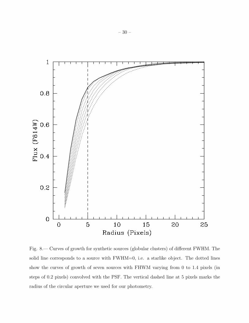
To calculate the aperture correction we used the procedure below. Using the ishape

tasks mkcmppsf and mksynth we create model images of synthetic globular clusters.

We make these synthetic clusters with different profiles of varying intrinsic FWHM, and

convolve them with the PSF. In order to recreate the sizes we obtained for the effective

radius, we built clusters with FWHM from 0 to 3 pixels by steps of 0.02 pixels. These

synthetic clusters have different curves of growth that we plot in Figure 8. With the curves

of growth for these synthetic point sources, of known FWHM, we can perform an accurate

aperture correction by measuring the offset in flux (or magnitude) for each cluster size to

a stellar PSF. Once we determine the offset to a stellar source we can apply the aperture

correction of Sirianni et al. 2005. Given that the Sirianni et al. (2005) tables do not give

– 15 –

an aperture correction for r=0.175′′ we use an interpolated value, i.e. 0.8205 for F606W

and 0.7985 for F814W. With the above method we obviate the objections of Kundu (2008)

related to the use of a fixed aperture to measure the flux of clusters with different sizes.

5.1. Color-Magnitude Diagram

We present our final color-magnitude diagram for the M87 globular clusters in Figure

9. We plot the F814W magnitudes in the y-axis since these are a better tracer of the

cluster stellar mass. The CMD in Figure 9 is consistent with previously published M87

CMDs, particularly with the CMD derived by Larsen et al. (2001) using WFPC2 data and

a similar pair of filters i.e. the F555W and the F814W.

The sharpness of the M87 bimodality is striking and is more clearly defined than in

previous work (e. g. Larsen et al. 2001, Peng et al. 2006) because of the much higher

S/N of this deep dataset. In the magnitude range F814W ≃ 22.0 − 22.5 we note a

”bridge” between the normal blue and red sequences, with many more clusters than usual

at intermediate colors. These do not seem to lie in any special location, nor to have scale

sizes different from other clusters. They may be genuinely intermediate-metallicity objects.

Given the age/metallicity degeneracy for old clusters they might also be metal-rich but

younger by a few Gigayears than the red sequence clusters. Further discussion is given in

Peng et al. (2009).

The CMD presented here differs from the CMD derived by Waters et al. (2009). One

of the most evident differences is the presence in the Waters et al. (2009) CMD of bright

(I < 22) clusters that are either very blue (V − I < 0.9) or very red (V − I > 1.3). The

equivalent areas of our CMD are completely devoid of clusters, suggesting that the random

errors in the magnitudes calculated from the curve-of-growth procedure are low. A detailed

– 16 –

study of the CMD for the M87 GCS is presented by Peng et al. (2009).

5.2. Effective radius versus magnitude

In Figure 10 where we plot magnitude versus effective radius for metal-poor and

metal-rich clusters, the boundary between red and blue clusters is set at F814W-F606W >

or < than 0.8. In this figure we can see how metal poor clusters have larger rh than their

metal rich counterparts. Red clusters have a median rh of 2.1 pc while for blue clusters

the median rh is 2.6 pc. Blue clusters are thus on average 24% larger than red clusters,

this offset is in excellent agreement with the findings of previous studies using large cluster

samples in other galaxies (e. g. Larsen et al. 2001, Spitler et al. 2006, Harris 2009). The rh

median value is not affected by the presence of clusters with rh ∼ 0 visible at the bottom

of the two graphs of Figure 10. This size difference between sub-populations was explained

by Jordan (2004) as the result of mass segregation and the dependence of main-sequence

lifetimes on metallicity. Another possibility is that this difference reflects conditions of

formation (Harris, 2009). We do not observe any clear trends of increasing (or decreasing)

rh with magnitude.

One clear fact evident in Figure 10 is the unfilled space between 0 and ∼1.5 pc in both

plots at all magnitudes except the faint end. This gap between the unresolved stars and

the smallest clusters is also visible in Figures 2, 3, and 6. It appears as most clusters have a

minimum effective radius. This gap in the rh distribution is also present in previous studies

of M87 (Kundu et al. 1999, Larsen et al. 2001). Of the Cen A and Milky Way clusters

none has been reported with an effective radius of less than 1pc (Gomez et al. 2006, Gomez

& Woodley 2007).

An explanation for the existence of this is gap is the fact that smaller clusters have

– 17 –

a smaller chance of survival. McLaughlin & Fall (2008) study the relation of the globular

cluster mass function and the cluster half-mass density (ρh). In their study these authors

normalize the disruption time of a globular cluster to the relaxation time and find that

the evaporation rate µev is proportional to ρ1/2

h . Using their relation between ρh and the

effective radius we can write µev ∝ r−3/2

h . This means that smaller clusters evaporate much

faster than bigger ones (Fall & Rees 1977, 1985). The evaporation rate determined by

McLaughlin & Fall (2008) only takes into account internal relaxation effects. The influence

of an external potential on the dissolution timescale is examined by Gieles & Baumgardt

(2008). These authors conclude that in the presence of a tidal field the dissolution time

scales with the number of stars in the cluster N and the angular frequency ω of the cluster

in the host galaxy: tdis = N0.65

ω.

6. Comparison with a recent study

A recent paper by Waters et al. (2009) analyzed the same dataset used here but aimed

at discussing the mass/metallicity relation in the GCS and its color bimodality. Waters

et al. (2009) do not make specific conclusions on structural parameters for the clusters

themselves. We note below several steps in our analysis of this dataset that differ from their

work.

A first important difference in our data reduction concerns the final combined

image that we use to measure the structural parameters. In this study the final image

is subsampled to a pixel scale of 0.035′′taking thus full advantage of the dithered raw

observations. Waters et al. (2009) keep the ACS camera native pixel size of 0.05′′. The PSF

is also computed in a different fashion: Waters et al. (2009) use the software of Anderson &

King (2006) while in this work we create a purely empirical PSF using a sequence of tasks

described in section 4.

– 18 –

The magnitudes and radii of ∼ 2000 clusters, each with different size cannot be

measured with either standard PSF-fitting or fixed aperture techniques. In order to derive

proper magnitudes both our work and Waters et al. (2009) compute flux corrections based

on the size of each object. In this study we calculate the magnitudes by scaling the flux

that we measure at a 5 pixel radius to large radius using the curve of growth of each object

appropriate to its particular effective radius. The details of this method are given in the

photometry section. Waters et al. (2009) instead use the magnitude difference between a

radius of 4 pixels and a radius of 2 pixels as the main parameter to estimate the cluster

size and their aperture correction. Lastly, our measurements of cluster size is done with

a different code, ishape, and using a fiducial King-model concentration rt/rc = 30 that

is more representative of the true mean for globular clusters than their adopted ratio of

rt/rc = 10 (see section 5 above).

When compared with Waters et al. (2009) some of our methods are obvious

improvements, such as obtaining an image with higher resolution, while other differences

are an independent approach to measure the same quantity, such as the use of an alternate

fitting profile code.

7. Conclusions

With extremely deep HST/ACS data in V and I, we have obtained precise measurements

of the scale radii rh for ∼ 2000 globular clusters in M87. To first order, their size distribution

closely resembles the Milky Way GCS. We find that the mean cluster size depends noticeably

on both metallicity and galactocentric distance. Metal rich clusters are 24% larger than the

metal-poor subpopulation. The mean rh, for all clusters, begins to increase with Rgc for

Rgc ≥ 6 kpc.

– 19 –

A new, but very tentative, finding of this work is that the effective radius of these old

globular clusters may depend on bandpass, appearing slightly larger at bluer wavelengths.

This effect is just on the margin of being statistically significant, but if it is physically real,

it may point to the effects of mass segregation within the clusters. Future studies from

other, perhaps more nearby, galaxies should be able to test this idea more strongly.

The measurement of structural parameters of globular clusters belonging to galaxies of

different Hubble type and located in different environments should reveal in the future any

existent correlation between galaxy type and cluster sizes (Gomez et al. 2006).

We are grateful to Jennifer Mack, and Marco Sirianni (STScI) for kindly answering

several queries related to the ACS. We thank Warren Hack (STScI) for helpful discussions

on Multidrizzle. We also thank Jarrod Hurley (Swinburne University, Australia) for

sharing with us evolved globular cluster models. This research has made use of the NASA

Astrophysics Data System Bibliographic services. STSDAS and PyRAF are products of the

Space Telescope Science Institute, which is operated by AURA for NASA.

Facilities: HST (ACS)

– 20 –

REFERENCES

Aarseth, S. J. & Heggie, D. C. 1998, MNRAS, 297, 794

Anderson, J., King I. R. 2006, ACS Instrument Science Report 2006-01, Baltimore, STScI

Baltz, E. A. et al. 2004, ApJ, 610, 691

Baum, W. A. 1955, PASP, 67, 328

Bertin, E., & Arnouts, S. 1996, A&AS, 117, 393

Blakeslee, J. P., Anderson, K. R., Meurer, G. R., Benıtez, N. & Magee, D. 2003, An

Automatic Image Reduction Pipeline for the Advanced Camera for Surveys, ADASS

XII, ASP Conference Series, Vol 295

Blakeslee, J. P. et al. 2009, ApJ, 694, 556

Fall, S. M.& Rees, M. J. 1977, MNRAS, 181, 37

Fall, S. M. & Rees, M. J. 1985, ApJ, 298, 18

Forbes, D. A., 2002, The Globular Cluster Systems in Ellipticals and Spirals, in Extragalactic

Star Clusters, IAU Symposium 207, ASP

Georgiev, I.Y., Goudfrooij, P., Puzia, T.H., & Hilker, M. 2008, AJ, 135, 1858

Gomez, M. et al. 2006, A&A, 447, 877

Gomez, M. & Woodley, K. A. 2007, ApJL, 670, L105

Gonzaga, S. et al. 2005, ACS Instrument Handbook, version 6.0, Baltimore, STScI

Harris, W. E. 1996, AJ, 112, 1487

Harris, W. E. 2009, ApJ, in press arXiv:0904.4208

– 21 –

Harris, W. E. & van den Bergh, S. 1981, AJ, 86, 1627

Hesser, J. E., Harris, H. C., van den Bergh, & Harris, G. L. H. 1984, ApJ, 276, 491

Hodge, P. W. 1960, ApJ, 131, 351

Hodge, P. W. 1962, PASP, 74, 248

Hurley, J.R. et al. 2008, AJ, 135, 2129

Jordan, A. 2004, ApJ, 613, L117

Larsen, S. S. 1999, A&AS, 139, 393

Larsen, S. S. 2008, An Ishape User’s Guide

Larsen, S. S., Brodie, J. P., Huchra, J. P., Forbes, D. A., & Grillmar, C. J. 2001, AJ, 121,

2974

Mack, J. et al. 2003, ACS Data Handbook, Version 2.0, Baltimore, STScI

McLaughlin, D. E., Harris, W. E., & Hanes, D. A. 1994, ApJ, 422, 486

McLaughlin, D. E. & Fall, S. M. 2008, ApJ, 679, 1272

King, I. R. 1966, AJ, 71, 64

Kundu, A., & Whitmore, B. C., 1998, AJ, 116, 2841

Kundu, A., Whitmore, B. C., Sparks, W. B., Macchetto, F. D., Zepf, S. E., & Ashman, K.

M. 1999, ApJ, 513, 733

Kundu, A. 2008, AJ, 136, 1013

Peng, E. W. et al. 2006, ApJ, 639, 95

– 22 –

Peng, E. W. et al. 2008, ApJ, 681, 197

Peng, E. W. et al. 2009, ApJ accepted, astro-ph: arxiv0907.2524

Sirianni, M. et al. 2005, PASP, 117, 1049

Sirianni, M., Gilliland, R., & Sembach, K. 2006 Technical Instrument Report ACS 2006-02,

Baltimore, STScI

Spitler, L.R., Larsen, S.S., Strader, J., Brodie, J.P., Forbes, D.A., & Beasley, M.A. 2006,

AJ, 132, 1593

Spitzer, L., & Thuan, T. X. 1972, ApJ, 175,31

van den Bergh, S., Morbey, C., & Pazder, J. 1991, ApJ, 375, 594

Waters, C. Z., Zepf, S. E., Lauer, T. R., & Baltz, E. A. 2009, ApJ, 693, 463

Whitmore, B. C., Chandar, R., & Fall, S. M. 2008, AJ, 133, 1067

Wright, E. L. 2006, PASP, 118, 1711

This manuscript was prepared with the AAS LATEX macros v5.2.

– 23 –

Fig. 1.— Median subtracted image of a portion of the ACS/WFC field of view of the inner

region of M87. Detected clusters are shown by circles, the prominent plasma jet emanating

from the super-massive black hole at the core of the galaxy is clearly visible. This image is

∼ 13 kpc across, north is up and east is left.

– 24 –

Fig. 2.— Cluster effective radius in F606W vs. cluster effective radius in F814W. Note

the gap between a small number of unresolved objects, clustering around 0, and the large

majority of resolved clusters grouped around ∼ 2.5 pc. The units of this graph are parsecs.

– 25 –

Fig. 3.— Histogram of effective radius in F606W and F814W. It can be seen on this figure

how the effective radius of most clusters lies between 1 and 6 pc. The histogram of the

effective radius for Milky Way clusters (×15) is overplotted for comparison.

– 26 –

Fig. 4.— Ratio of the effective radius of M87 clusters in F606W over F814W, the median of

this distribution is 1.02 with a standard deviation of 0.24.

– 27 –

Fig. 5.— Values for the ratio of minor/major axis for the M87 clusters. Most clusters are

nearly round (e<0.2), though the mean ellipticity is slightly larger than in the Milky Way.

– 28 –

Fig. 6.— Effective radius, in the F814W filter, versus galactocentric distance. Note the

small number of starlike objects scattered along the bottom of the graph, clearly separated

from the globular cluster population.

– 29 –

Fig. 7.— FWHM of sources with zero effective radius vs. galactocentric distance as measured

with imexamine, top panel. The bottom panel shows the residuals of the PSF and the stars

across the detector. We do not see any correlation of PSF size with position on the image.

– 30 –

Fig. 8.— Curves of growth for synthetic sources (globular clusters) of different FWHM. The

solid line corresponds to a source with FWHM=0, i.e. a starlike object. The dotted lines

show the curves of growth of seven sources with FHWM varying from 0 to 1.4 pixels (in

steps of 0.2 pixels) convolved with the PSF. The vertical dashed line at 5 pixels marks the

radius of the circular aperture we used for our photometry.

– 31 –

Fig. 9.— Color-magnitude diagram (top) and histogram of cluster colors (bottom) for the

M87 Globular Cluster System, the sharpness of the bimodality is striking. The dashed lines

correspond to a Gaussian fit to each subpopulation. The solid line is sum of these two

Gaussians.

– 32 –

Fig. 10.— Effective radius versus magnitude for the two, red and blue, sub-populations

of globular clusters. The dotted line represents the median value for the rh of each sub-

population.