arX

iv:a

stro

-ph/

9712

258v

1 1

8 D

ec 1

997

Old Stellar Populations. VI. Absorption-Line Spectra of Galaxy Nuclei and

Globular Clusters1

S. C. Trager2

UCO/Lick Observatory and Board of Studies in Astronomy and Astrophysics,

University of California, Santa Cruz

Santa Cruz, CA 95064

sctrager@ociw.edu

Guy Worthey3,4

Astronomy Department, University of Michigan

Ann Arbor, MI 48109-1090

worthey@astro.lsa.umich.edu

S. M. Faber

UCO/Lick Observatory and Board of Studies in Astronomy and Astrophysics,

University of California, Santa Cruz

Santa Cruz, CA 95064

faber@ucolick.org

David Burstein

Department of Physics and Astronomy,

Arizona State University

Tempe, AZ 58287-1504

burstein@samuri.la.asu.edu

J. Jesus Gonzalez

Instituto de Astronomıa—UNAM

Apdo Postal 70-264, Mexico D.F., Mexico

jesus@astroscu.unam.mx

ABSTRACT

We present absorption-line strengths on the Lick/IDS line-strength system of 381

galaxies and 38 globular clusters in the 4000–6400 A region. All galaxies were observed

1Lick Observatory Bulletin #1375

2Present address: Observatories of the Carnegie Institution of Washington, 813 Santa Barbara Street, Pasadena,

CA 91101

3Hubble Fellow

4Present address: Department of Physics and Astronomy, St. Ambrose University, Davenport, IA 52803-2829

– 2 –

at Lick Observatory between 1972 and 1984 with the Cassegrain Image Dissector

Scanner spectrograph, making this study one of the largest homogeneous collections

of galaxy spectral line data to date. We also present a catalogue of nuclear velocity

dispersions used to correct the absorption-line strengths onto the stellar Lick/IDS

system. Extensive discussion of both random and systematic errors of the Lick/IDS

system is provided. Indices are seen to fall into three families: α-element-like indices

(including CN, Mg, Na D, and TiO2) that correlate positively with velocity dispersion;

Fe-like indices (including Ca, the G band, TiO1, and all Fe indices) that correlate only

weakly with velocity dispersion and the α indices; and Hβ which anti-correlates with

both velocity dispersion and the α indices. C24668 seems to be intermediate between

the α and Fe groups. These groupings probably represent different element abundance

families with different nucleosynthesis histories.

Subject headings: galaxies: stellar content — globular clusters: stellar content

1. Introduction

This paper is the sixth in a series describing a two-decades long effort to comprehend the

stellar populations of early-type galaxies. Previous papers in this series have defined the Lick/IDS

absorption-line index system, presented observations of globular clusters and stars, and derived

absorption-line index fitting functions (Burstein et al. 1984; Faber et al. 1985; Burstein, Faber &

Gonzalez 1986; Gorgas et al. 1993). Worthey et al. (1994, hereafter Paper V) expanded the original

eleven-index system to 21 indices and presented the complete library of stellar data. Other papers

utilizing this database presented preliminary galaxy Mg2 strengths (Burstein et al. 1988; Faber

et al. 1989), galaxy velocity dispersions (Faber & Jackson 1976; Davies et al. 1987; Dalle Ore et

al. 1991), comparisons of morphological disturbances with absorption-line strengths (Schweizer et

al. 1990), and preliminary comparisons of galaxy absorption-line strengths with models (Worthey,

Faber & Gonzalez 1992; Worthey 1992, 1994; Faber et al. 1995; Worthey, Trager & Faber 1996;

Trager 1997).

The Lick/IDS system has also been used extensively by other authors. Galaxy and globular

cluster line strengths on this system have been published by, among others, Efstathiou & Gorgas

(1985); Couture & Hardy (1988); Thomsen & Baum (1989); Gorgas, Efstathiou & Aragon

Salamanca (1990); Bender & Surma (1992); Davidge (1992); Guzman et al. (1992); Gonzalez

(1993); Davies, Sadler & Peletier (1993); Carollo, Danziger & Buson (1993); de Souza, Barbuy &

dos Anjos (1993); Gregg (1994); Cardiel, Gorgas & Aragon-Salamanca (1995); Fisher, Franx &

Illingworth (1995, 1996); Bender, Zeigler & Bruzual (1996); Gorgas et al. (1997); Jørgensen (1997);

Vazdekis et al. (1997); Kuntschner & Davies (1997); and Mehlert et al. (1997). Much theoretical

and empirical calibration of the Lick/IDS absorption-line strengths of stars (particularly Mg2) has

also been pursued by, e.g., Gulati, Malagnini & Morossi (1991, 1993); Barbuy, Erdelyi-Mendes &

– 3 –

Milone (1992); Barbuy (1994); McQuitty et al. (1994); Borges et al. (1995); Chavez, Malagnini

& Morossi (1995); Tripicco & Bell (1995); and Casuso et al. (1996). The Lick/IDS indices of

the stellar populations of composite systems have been modelled by, e.g., Aragon, Gorgas &

Rego (1987); Couture & Hardy (1990); Buzzoni, Gariboldi, & Mantegazza (1992); Buzzoni,

Mantegazza & Gariboldi (1994); Matteucci (1994); Buzzoni (1995); Weiss, Peletier & Matteucci

(1995); Tantalo et al. (1996); Bressan, Chiosi & Tantalo (1996); Bruzual & Charlot (1996); de

Freitas Pacheco (1996); Vazdekis et al. (1996); Greggio (1997); and Moller, Fritze-von Alvenleben

& Fricke (1997). We also point out the ongoing efforts of Rose and colleagues to study old stellar

populations using high-resolution absorption-line strengths in the blue (Rose 1985a, 1985b, 1985c,

1994; Rose & Tripicco 1986; Rose, Stetson & Tripicco 1987; Bower et al. 1990; Caldwell et al.

1993, 1996; Rose et al. 1994; Leonardi & Rose 1996; Caldwell & Rose 1997), and those of Brodie,

Huchra and colleagues to study extragalactic globular cluster systems using a spectrophotometric

index system in the red (Brodie & Huchra 1990, 1991; Huchra, Kent & Brodie 1991; Perelmuter,

Brodie & Huchra 1995; Huchra et al. 1996).

The full IDS database contains absorption-line strengths of 381 galaxies, 38 globular clusters,

and 460 stars based on 7417 spectra observed in the 4000–6400 A region. Here, we present final

IDS index strengths for galaxies and globular clusters. All were observed at Lick Observatory

between 1972 and 1984 with the Cassegrain Image Dissector Scanner spectrograph, making this

study one of the largest homogeneous collections of galaxy spectral line data to date.

This paper begins by describing the method of measuring Lick/IDS absorption-line strengths

in Section 2. Section 3 presents a discussion of uncertainties in these measurements. As early-type

galaxies typically have significant internal motions, Section 4 derives the corrections needed to

bring the galaxies to a common zero-velocity-dispersion system and the additional uncertainties

incurred by this correction. Section 4 also presents the velocity dispersions themselves and a first

discussion of “families” of absorption-line indices according to each index’s behavior with velocity

dispersion. Section 5 illustrates remaining levels of suspected systematic errors and compares to

previously published values. Finally, Section 6 presents final mean corrected indices and their

associated errors for the entire sample.

This paper plus Paper V (for the stellar data) together contain the sum total of all

observations on the Lick/IDS system. Previously published data on galaxies and globular clusters

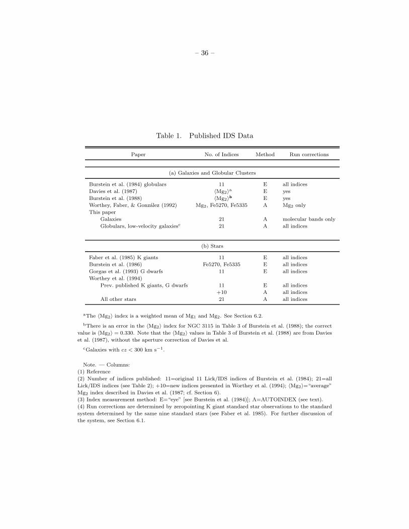
are superseded by the values given here. Table 1 presents published papers containing IDS data,

the index data presented in those papers, the index measurement method, and the run corrections

applied (terms are explained in Sections 2 and 5).

The complete tables in this paper and individual spectra for all Lick/IDS stellar, globular

cluster, and galaxy observations are available electronically from the Astrophysical Data Center

(http://adc.gsfc.nasa.gov/adc.html). The complete versions of the long tables (Tables 4, 7–10) are

also presented in the electronic Astrophysical Journal Supplements.

– 4 –

2. Absorption-Line Measurements

A general introduction to the Image Dissector Scanner (IDS) is given by Robinson & Wampler

(1972), and further relevant details are found in Faber & Jackson (1976), Burstein et al. (1984)

and Faber et al. (1985). A discussion of signal-to-noise and the noise power spectrum is presented

in Faber & Jackson (1976) and Dalle Ore et al. (1991).

Briefly, spectra were obtained between 1972 and 1984 using the red-sensitive IDS and

Cassegrain spectrograph on the 3m Shane Telescope at Lick Observatory. The spectra cover

roughly 4000–6400 A and have a resolution of about 9 A (about 30% higher at the ends of

the region) although this varied slightly from run to run. Most spectra of galaxy nuclei were

taken through a spectrograph entrance aperture of 1.′′4 by 4′′, with a second aperture for sky

subtraction located 21′′ or 35′′ away. Object and sky were chopped between these apertures in

such a way as to equalize the time spent in each. Long slit observations of galaxies (of width 1.′′4

and various lengths) and spatial scans of globular clusters and galaxies were also taken and have

equivalent resolution to the nuclear data. Larger-aperture observations of galaxies with wider slits

(typically off-nucleus observations or dwarf galaxies) were also taken and calibrated separately.

These wide-slit observations have lower spectral resolution. Helium, neon, mercury, and (in later

observations) cadmium lamps provided wavelength calibrations at the beginning and end of every

night. Global shifts and stretches of the wavelength scale of up to 3 A per observation could

occur due to instrument flexure and variable stray magnetic fields. Spectra were not fluxed, but

rather divided by a quartz-iodide tungsten lamp, the energy distribution of which was made

more constant with wavelength by “rocking” the dispersion grating in a reproducible, systematic

manner. Line-strength standard stars (detailed in Paper V) were observed nightly to insure a

calibration of the system. A sampling of low- to high-quality galaxy nuclei spectra are shown in

Figure 1. For display purposes, these spectra have been flattened by a fifth-order polynomial fit.

However, all measurements of line strengths were made on the original, unflattened spectra.

2.1. The Lick/IDS System

The Lick/IDS absorption-line index system is fully described in Paper V. We present a

summary here and point out changes to the system caused by measuring galaxies with significant

systemic velocities and velocity dispersions. Absorption-line strengths are measured in the

Lick/IDS system by “indices,” where a central “feature” bandpass is flanked to the blue and

red by “pseudocontinuum” bandpasses. The choice of bandpasses is dictated by three needs:

proximity to the feature, less absorption in the continuum regions than in the central bandpass,

and maximum insensitivity to velocity dispersion broadening. While the last point is unnecessary

when measuring stars, in the case of galaxies it is crucial, and it sets a minimum length for the

pseudocontinuum bandpasses. The sidebands are called “pseudocontinua” because the resolution

of the Lick/IDS system does not allow the measurement of “true” continua in late-type stars or in

– 5 –

most galaxies.

Table 2 presents the bandpasses of the 21 Lick/IDS absorption line indices and the features

measured by these indices. The wavelengths have been further refined since Paper V through

cross-correlation with more accurate CCD spectra taken by GW. Indices 1–8 have been corrected

by 1.25 A, and indices 17–21 have been corrected by 1.75 A. Uncertainties of 0.3 A are still present

in these bandpass definitions, but such shifts produce negligible changes in the measured indices.

Systemic velocities of the galaxies sometimes caused the reddest absorption features to fall outside

of the wavelength range of the observation, and the starting wavelength of the spectra also varied

somewhat. Occasionally other effects prevented the measurement of particular indices, including

bubbles in the immersion oil of the IDS, exceptionally strong galaxy emission, or poorly-subtracted

night sky lines (see Section 6 for a complete list). As a result, not all indices are measured for all

galaxies.

The Lick/IDS index system was nominally designed to include six different molecular bands

[CN4150, the G band (CH), MgH, MgH + Mg b, and two TiO bands] plus 14 different blends

of atomic absorption lines. The CN2 index, introduced in Paper V, is a variant of the original

CN1 index with a shorter blue sideband to avoid Hδ. Along with the higher-order Balmer lines

presented in Worthey & Ottaviani (1997), we believe we have extracted all of the useful absorption

features from the Lick/IDS stellar and galaxy spectra.

We note here the recent work of Tripicco & Bell (1995), who modelled the Lick/IDS system

using synthetic stellar spectra. They found that many of the Lick/IDS indices do not in fact

measure the abundances of the elements for which they were named. Column 6 of Table 2

describes their results, in order of the most significant contributing element. To retain conformity

with previously published studies we have chosen not to rename most of the Lick/IDS indices for

their primary contributor. However, following Worthey, Trager & Faber (1996), we have renamed

the Fe4668 index C24668.

2.2. Index measurements

Index measurements from the Lick/IDS galaxy spectra are problematic owing to unpredictable

wavelength shifts and stretches (of order 1–3 A) and also from the (sometimes unknown) systemic

radial velocities of the galaxies themselves. Indices were measured automatically using the program

AUTOINDEX written by J. J. Gonzalez and G. Worthey. This program begins by locating Na D

(centroid assumed at 5894 A) and the G band (centroid assumed at 4306 A) or, for a few galaxies

with very strong Balmer lines, Hγ (centroid assumed at 4340 A). It then removes any global

wavelength shift and stretch, including the effects of the systemic velocity. Local wavelength shifts

at each index are calculated by cross-correlating the galaxy spectrum with a template spectrum in

the region around each index. For galaxies, a K0 giant template is generally used, but occasionally

an F5 dwarf template is used for galaxies with very strong Balmer lines.

– 6 –

Once each index was centered, it is measured following the scheme outlined in Paper V.

The mean height in each of the two pseudocontinuum regions is determined on either side of the

feature bandpass, and a straight line was drawn through the midpoint of each one. The difference

in flux between this line and the observed spectrum within the feature bandpass determines the

index. For narrow features, the indices are expressed in Angstroms of equivalent width; for broad

molecular bands, in magnitudes. Specifically, the average pseudocontinuum flux level is

FP =

∫ λ2

λ1

Fλdλ/(λ2 − λ1), (1)

where λ1 and λ2 are the wavelength limits of the pseudocontinuum sideband. If FCλ represents the

straight line connecting the midpoints of the blue and red pseudocontinuum levels, an equivalent

width is then

EW =

∫ λ2

λ1

(

1 − FIλ

FCλ

)

dλ, (2)

where FIλ is the observed flux per unit wavelength and λ1 and λ2 are the wavelength limits of the

feature passband. Similarly, an index measured in magnitudes is

Mag = −2.5 log

[

(

1

λ2 − λ1

)∫ λ2

λ1

FIλ

FCλ

dλ

]

. (3)

As explained in Paper V, the above AUTOINDEX definitions differ slightly from those used

in Burstein et al. (1984) and Faber et al. (1985) for the original 11 IDS indices. In the original

scheme, the continuum was taken to be a horizontal line over the feature bandpass, at the level

FCλ taken at the midpoint of the bandpass. This flat rather than sloping continuum induces

small, systematic shifts in the feature strengths, as described in further detail in Section 5. For

now it is sufficient to note that slight additive corrections have been applied to the new indices to

preserve agreement with the older published data. These corrections are discussed in Section 5

and are always quite small.

Run corrections for the galaxies also differ from those described for stars in Paper V. Stars

always have nearly zero velocities, and their features occupy the same IDS channels on a given

run. It was therefore found to be advantageous to apply small additive corrections to all indices to

correct for small variations in continuum shape and/or resolution for that run. Galaxies however

occupy different channels due their varying radial velocities, making the stellar-derived continuum

shape corrections invalid. Hence, the following scheme was adopted, according to the velocity

offset of a galaxy from the stars: globular clusters and galaxies with cz ≤ 300 km s−1 (i.e., Local

Group galaxies) had stellar run corrections applied for all indices; galaxies with 300 < cz < 10 000

km s−1 had stellar run corrections applied only to the broad molecular indices measured in

magnitudes; and galaxies with cz ≥ 10 000 km s−1 had no run corrections applied.

– 7 –

3. Error Estimation

The errors of the IDS indices are due partly to photon statistics and partly to the fact that

the flat-field calibration of the IDS had limited accuracy. A thorough knowledge of the errors is

essential to the proper use of these data. The error estimates derived here will be used in later

papers to simulate the absorption-line data and test the significance of any conclusions.

The IDS was not a true photon-counting detector. This makes estimation of uncertainties

difficult, as the errors are not strictly photon counting statistics. We present in this section a

brief overview of the steps required to derive reasonable error estimates for galaxy Lick/IDS index

measurements. A complete discussion of the error estimates presented here may be found in

Trager (1997).

In the IDS, light from the spectrograph fell on a series of three image-tube photocathodes,

which amplified the signal by about 105. The amplified light fell on a phosphor screen, which

held the light long enough for an image dissector to scan and digitize the image before it faded

(Robinson & Wampler 1972). Each incident photon produced a burst of typically seven to ten

detected photons covering ∼ 9 A (7 channels) in the digitized scan. Uncertainties in the spectra

arise from three sources: (1) input photon shot noise, (2) the statistics of the amplification process,

and (3) flat-fielding errors. This last noise source is due to the movement of the spectrum of the

first photocathode, caused by instrument flexure, and movement of the amplified spectrum, caused

by stray magnetic fields affecting the magnetically-focused image-tubes and image dissector. As

a result, flat-field spectra taken at different telescope locations and position angles do not divide

perfectly but rather show low-level undulations a few channels wide.

The effect of these three noise sources on the power spectrum is discussed in Dalle Ore et al.

(1991), Paper V, and Trager (1997). At low frequencies the noise is dominated by flat-fielding

errors (at high counts) and photon shot-noise and the statistics of the IDS burst amplification

process (at low counts). At high frequencies the noise is dominated by flat-fielding errors (very

high counts) and photon statistics (low and moderate counts). The resultant power spectrum

changes shape with count level, as shown schematically by Trager (1997). In galaxy spectra,

photon statistics tend to be the overall dominant noise source, as opposed to the stellar spectra

(Paper V) and the highest-signal-to-noise galaxies (e.g., M31 and M32), in which flat-fielding

errors dominate.

The net result is that the high-frequency noise is a good measure of photon statistics except

at very high count levels, where flat-fielding errors begin to dominate. Paper V therefore defined

a “goodness parameter” that measures the noise power at high frequencies. For each spectrum, a

Fourier transform was taken of the 256 channels starting at 5519 A in the rest frame, a region

relatively free of spectral lines. The average power at high spatial frequencies was measured, then

divided by the power at zero frequency. The square root of this ratio is a measure of photon noise,

and its inverse is defined to be the goodness G.

– 8 –

G is defined such that, if all noise were photon statistics, G would be exactly proportional

to σ−1. The constant of proportionality is unknown a priori (it depends on the average number

of detected photons per burst, which is not well known) but can be determined empirically by

comparing to errors derived from multiply-observed data. At high count levels, G saturates

(bottoms out) due to the influence of flat-field errors, and the relation of G to σ−1 becomes

non-linear. This curvature can also be determined empirically from multiply-observed objects.

The empirical calibration proceeds as follows. Because G scales as σ−1 for poor data, it

should average quadratically for multiple observations, and thus we compute the goodness 〈G〉k of

a single, typical observation of galaxy k as

〈G〉2k =1

N

∑

G2i,k, (4)

where Gi,k is the goodness of each individual spectrum and N is the number of observations of

galaxy k. 〈G〉k would be the goodness of each single observation of galaxy k if all observations were

of equal quality. All galaxies with three or more observations had average goodnesses computed

by Equation 4. The same galaxies also had mean standard deviations computed for each of the 16

Lick/IDS indices between the G band and Na D (in the spectral range of virtually all galaxies).

The average total error σTOT,k of galaxy k averaged over these 16 indices is calculated as

σ2TOT,k =

1

16

19∑

j=4

(

σjk

σsj

)2

, (5)

where j is the IDS index number (Table 2), σjk is the standard deviation per observation of index

j for galaxy k, and σsj is the standard star error of index j (Table 2). Thus σTOT,k is the average

error in units of the standard star error for a typical single observation of galaxy k. It is an

external error determined from multiple, independent observations of the same object.

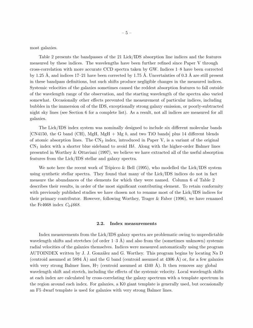
To determine a preliminary scaling of total error with goodness, individual total errors σTOT,k

were plotted against average goodnesses 〈G〉k (Figure 2). There is a reasonably tight relation

between the two with the expected trend. The slope is −1 in the low-signal limit, where photon

statistics dominate, and flattens out in the high-signal limit, where flat-fielding errors dominate.

The solid curve is a least squares fit to the equation σ2TOT,k = a〈G〉−2

k + b:

σ2TOT,k =

(

2561

〈G〉k

)2

+ (0.94)2. (6)

Equation 6 is assumed to hold for each individual observation, with 〈G〉k replaced by Gi,k.

Weighted mean indices for multiply-observed galaxy k are calculated as

〈Ijk〉 =

(

N∑

i=1

Iijk/σ2TOT,i,k

/

N∑

i=1

1/σ2TOT,i,k

)

, (7)

where i represents an individual observation, j represents a given index, and σTOT,i,k is now

derived from Gi,k using Equation 6.

– 9 –

Finally, the error of each mean index j is taken to be

σjk =1√N

σTOT,k × σsj, (8)

where N is the number of observations of galaxy k, σsj is the standard star error, and the mean

error of galaxy k for all indices, σTOT,k, is calculated from Equation 6, using 〈G〉k determined as

in Equation 4. This version of σjk is more accurate than the individual index standard deviations

because it uses the average error per spectrum, σTOT,k, made possible by knowing the ratios of

the errors between indices from the standard stars.

We then set out to check the quality of these preliminary error estimates. We were interested

in both the magnitude of the errors averaged over all indices and the ratio of the individual index

errors. To anticipate the results, we found that the mean magnitude of the galaxy errors was well

determined (to within 8%) but that certain individual error ratios needed adjustment.

The details of this step are given in Trager (1997) but a brief description follows. Independent

nuclear data from galaxies in the sample of Gonzalez (1993; hereafter G93) were compared against

individual observations of 37 IDS galaxies in common. The G93 spectra cover only the region

4780–5600 A, and so only the indices from Hβ through Fe5406 could be compared. A chi-squared

analysis was performed to determine the relative scaling of the Lick/IDS galaxy errors with respect

to G93. Gonzalez’s indices are so accurate (except for Mg1 and Mg2) that his errors contribute

negligibly, and the resultant χ2 values are a good test of the Lick/IDS errors alone. Though we

expect the errors in G93 to be negligible, we allowed for mean zeropoint and slope differences,

as Gonzalez could not calibrate his CCD system precisely onto the IDS system (see his Figure

4.4). The error rescalings determined from the G93 comparison were fairly small, about 0.92. The

exception was Fe5270, which required a large error rescaling (0.75; i.e., the preliminary IDS errors

from Equation 8 above were too large by 25% in this index).

A further check for wavelengths not covered by the G93 spectra was performed using pairs of

indices from the Lick/IDS sample itself. Indices were chosen that might be expected a priori to

track each other closely (i.e., to be multiples of one another) and have similar velocity dispersion

corrections. The best choices came from the Fe-peak family of indices (see Section 4.4, although

note that these indices do not all track Fe abundance—see Tripicco & Bell 1995 and Table 2). Two

groups were defined by their similar velocity dispersion corrections: Fe4383, Fe4531, and Fe5709

were compared against Fe5270; and Fe5782 and Ca4455 were compared against Fe5335. The errors

of Fe5270 and Fe5335 were first rescaled to match G93 as described above. Chi-squared analyses

were performed, and the resultant reduced-χ2 value was forced to equal unity by rescaling the

Lick/IDS errors of the dependent index. The error rescalings from these internal comparisons are

comparable to those derived from the G93 comparison, typically again about 0.92.

A final mean fractional error scaling was then computed from all scalings derived in these

tests. This mean scaling was again 0.92. Errors in the remaining 10 indices were rescaled by this

factor. We checked the final adopted index scalings by performing a final set of chi-squared tests

– 10 –

on various Fe-line pairs. The resulting reduced-χ2 values were consistent with our final scaling of

the errors to typically within a few percent (and never worse than 5%). From these various tests,

we believe that systematic errors in the final uncertainties are ∼< 5%.

The adjusted final errors for the raw indices of all galaxies and globular clusters are computed

as

σadjj = cjσj, (9)

where σj is the preliminary error of index j computed in Equation 8, and cj is the scaling of index

j relative to the standard star indices as determined in these tests. Adopted values of cj are shown

in Table 3.

4. Velocity Dispersion Corrections

The observed spectrum of a galaxy is the convolution of the integrated spectrum of its

stellar population by the instrumental broadening and the distribution of line-of-sight velocities

of the stars. The instrumental and velocity-dispersion broadenings broaden the spectral features,

causing the absorption-line indices to appear weaker than they intrinsically are. In this section,

we discuss the corrections required to remove the effects of velocity dispersion from the galaxy

index measurements and the additional uncertainties that arise from these corrections.

4.1. Velocity dispersion data

The adopted nuclear galaxy velocity dispersions, their fractional errors, and their sources

are presented in Table 4. The majority of the velocity dispersions was derived directly from the

IDS spectra themselves. The basic method was discussed in Dalle Ore et al. (1991), and the

data were presented in Davies et al. (1987, as tabulated by Faber et al. 1989) and Dalle Ore

et al. Other sources of nuclear dispersions include G93, the compilation of Faber et al. (1997),

and the compilation of Whitmore, McElroy & Tonry (1985), in order of preference. The velocity

dispersions of both Whitmore et al. and Faber et al. are derived from comprehensive literature

searches, but the data of G93 are excellent and uniform (and supersede all other measurements

when available). Two other sources noted in Table 4 (Bender, Paquet & Nieto 1991; Peterson

& Caldwell 1993) were used for dwarf galaxies. For a few galaxies, no velocity dispersions were

available, so educated guesses were made by eye or by comparing against similar galaxies with

known velocity dispersions These rough velocity dispersions are derived for the purpose of velocity

dispersion corrections only and should not be used for any other purpose. They are indicated in

Table 4 as Source 8.

– 11 –

For off-nuclear observations of galaxies (Table 10), velocity dispersions were calculated as

σr = σ0

(

r

1.′′4

)−0.06

, (10)

where r is the radius at which the aperture was placed and σ0 is the velocity dispersion given in

Table 4. The exponent is a mean for early-type galaxies as determined from Figure 6.10 of G93.

Finally, a few galaxy nuclei were observed by scanning a long slit of dimensions 1.′′4 × 16′′

across the nucleus to create a 16′′ × 16′′ aperture (denoted “scan” in Table 10). These were

observed to determine aperture corrections to velocity dispersion and Mg2 in Davies et al. (1987).

For these we have used the velocity dispersions as corrected by Equation 1 of Davies et al.

4.2. Corrections from broadened stellar spectra

To correct absorption-line strengths for the effects of velocity dispersion, a reference

velocity dispersion must be chosen. As we plan to compare the indices derived in this study to

stellar-population models based on our stellar observations (Paper V, Worthey 1994), the indices

are corrected to zero velocity dispersion. To achieve this goal, a variety of stellar spectra was

convolved with broadening functions of various widths. A selection of G dwarfs and the K giant

standard stars was convolved with Gaussians of widths ranging up to σ = 450 km s−1. Index

strengths were measured from each convolved spectrum and compared to the original strengths.

A third-order polynomial was then fit to the ratios (original/convolved) for all the stars in each

index versus velocity dispersion. Several observations of M32 were also included in the fits (M32

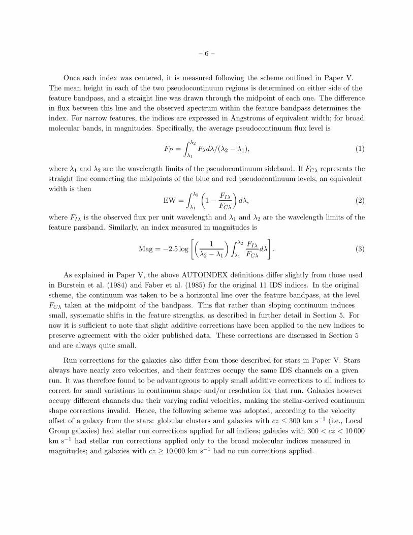
has a very small velocity dispersion compared to the resolution of the IDS system). Figure 3 shows

the results of these fits, and Table 5 presents the coefficients of the polynomials.

A velocity-dispersion corrected index is then

Icorrj,k = Cj(σv) × 〈Ij〉k, (11)

where 〈Ij〉k is the mean value of index j of galaxy k from Equation 7, and Cj(σv) is the

velocity-dispersion correction:

Cj(σv) =3∑

i=0

cijσiv, (12)

where cij are the coefficients of the correction polynomial for index j (Table 5), and σv is the

velocity dispersion.

Figure 3 shows that considerable scatter exists in certain velocity-dispersion corrections. As

noted by G93, a variation with spectral type is seen in several indices. Some of the scatter is

negligible, reflecting variations in indices that are intrinsically small (Mg1, TiO1, TiO2). Scatter

in CN1, CN2, and Hβ is real. However, CN is not heavily used, while the scatter in Hβ is inflated

due to the inclusion of a few very cool K giants with Hβ strengths weaker than typical galaxies.

– 12 –

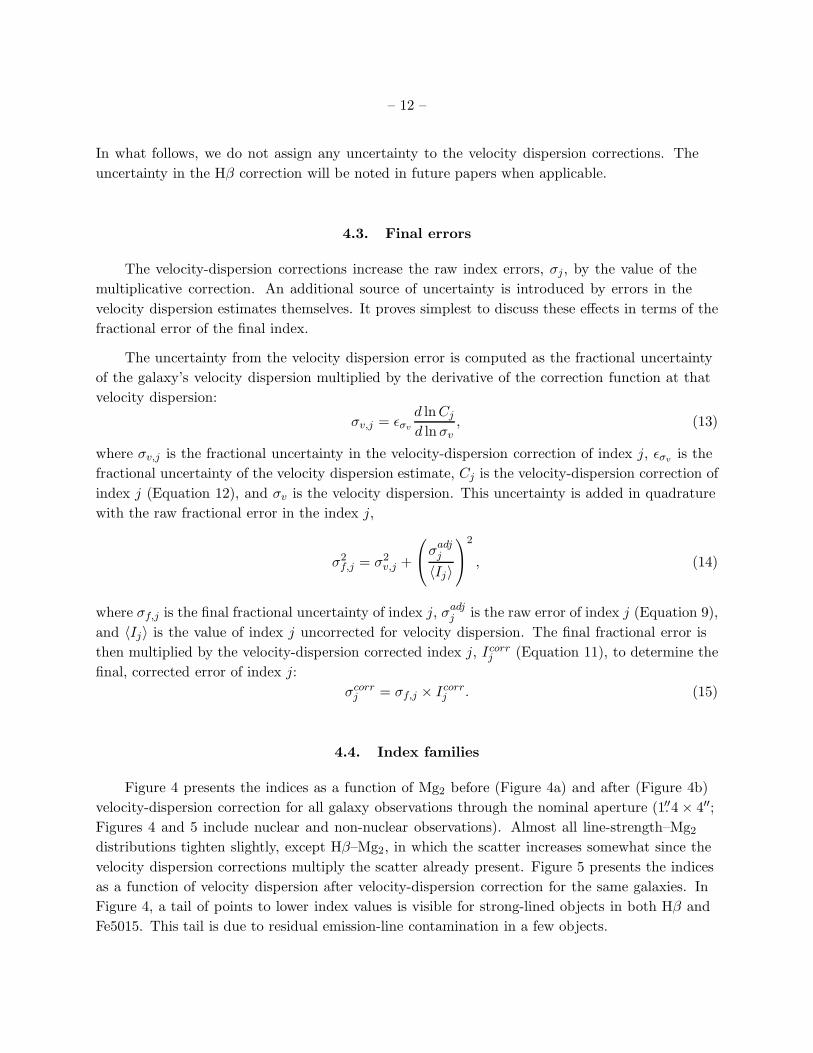
In what follows, we do not assign any uncertainty to the velocity dispersion corrections. The

uncertainty in the Hβ correction will be noted in future papers when applicable.

4.3. Final errors

The velocity-dispersion corrections increase the raw index errors, σj, by the value of the

multiplicative correction. An additional source of uncertainty is introduced by errors in the

velocity dispersion estimates themselves. It proves simplest to discuss these effects in terms of the

fractional error of the final index.

The uncertainty from the velocity dispersion error is computed as the fractional uncertainty

of the galaxy’s velocity dispersion multiplied by the derivative of the correction function at that

velocity dispersion:

σv,j = ǫσv

d ln Cj

d ln σv

, (13)

where σv,j is the fractional uncertainty in the velocity-dispersion correction of index j, ǫσvis the

fractional uncertainty of the velocity dispersion estimate, Cj is the velocity-dispersion correction of

index j (Equation 12), and σv is the velocity dispersion. This uncertainty is added in quadrature

with the raw fractional error in the index j,

σ2f,j = σ2

v,j +

σadjj

〈Ij〉

2

, (14)

where σf,j is the final fractional uncertainty of index j, σadjj is the raw error of index j (Equation 9),

and 〈Ij〉 is the value of index j uncorrected for velocity dispersion. The final fractional error is

then multiplied by the velocity-dispersion corrected index j, Icorrj (Equation 11), to determine the

final, corrected error of index j:

σcorrj = σf,j × Icorr

j . (15)

4.4. Index families

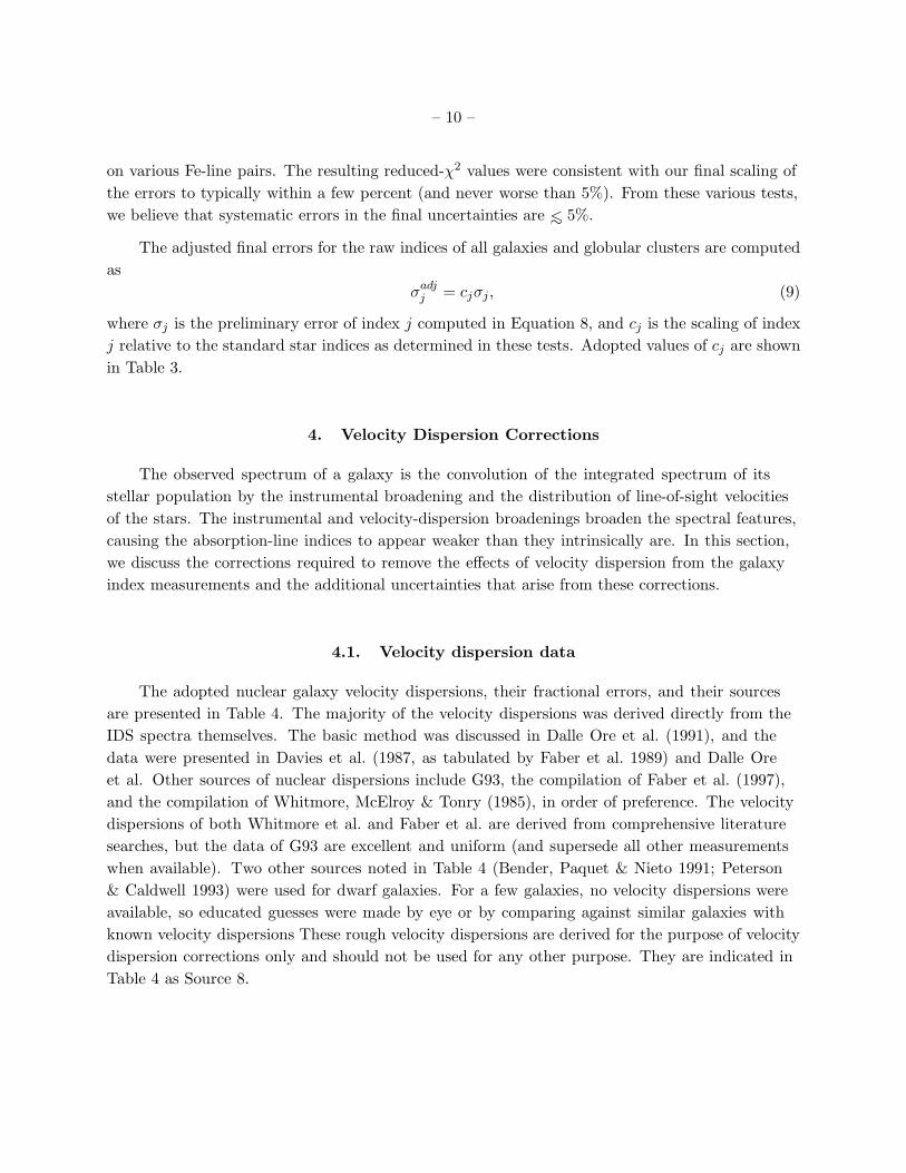
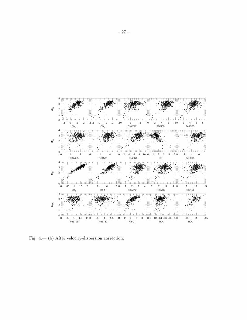
Figure 4 presents the indices as a function of Mg2 before (Figure 4a) and after (Figure 4b)

velocity-dispersion correction for all galaxy observations through the nominal aperture (1.′′4 × 4′′;

Figures 4 and 5 include nuclear and non-nuclear observations). Almost all line-strength–Mg2

distributions tighten slightly, except Hβ–Mg2, in which the scatter increases somewhat since the

velocity dispersion corrections multiply the scatter already present. Figure 5 presents the indices

as a function of velocity dispersion after velocity-dispersion correction for the same galaxies. In

Figure 4, a tail of points to lower index values is visible for strong-lined objects in both Hβ and

Fe5015. This tail is due to residual emission-line contamination in a few objects.

– 13 –

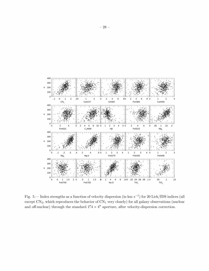
After correction, indices seem to fall into three general families: (1) α-element-like indices,

including both CN indices, all three Mg indices, Na D, and TiO2, characterized by relatively

narrow, positive correlations with both Mg2 and velocity dispersion; (2) Fe-like indices, including

both Ca indices, the G band, TiO1, and all Fe indices, with quite broad distributions that

are only weakly correlated with Mg2 and velocity dispersion; and (3) Hβ, which acts inversely

to the α-element indices, with a relatively narrow, negative correlation with Mg2 and velocity

dispersion. Similar correlations were seen in a restricted set of indices by Burstein et al. (1984),

Carollo et al. (1993) and Jørgensen (1997). C24668 seems to be intermediate to the α- and Fe-like

indices, with a relatively broad, but positive correlation with Mg2 and velocity dispersion. These

groupings probably represent element abundance families with different nucleosynthesis histories,

as discussed in Worthey (1996).

5. Remaining Systematic Errors

We now estimate the remaining systematic errors in the Lick/IDS data. Even small

systematic errors are a source of concern because indices change only slightly over time for old

stellar populations, so that small index differences can translate to significant age differences.

For example, a systematic error in the key Hβ index of only 0.05 A corresponds to a model age

difference of ∼ 1 Gyr at 15 Gyr (Worthey 1994).

There are two potential sources of inhomogeneities, and thus systematic errors, in the data.

One comes from the use of two measurement schemes, the original scheme described by Burstein

et al. (1984) (hereafter called “eye”) and the current scheme used here and for many stars in

Paper V (called “AUTOINDEX”). The second source of error comes from the presence of two

separate instrumental systems (for the first 11 indices only) — an earlier one (called “old”)

based on standardizing to mean data for K giant standards in Runs 3–24, and a second one

(called “new”) based on K giant standards from all runs. The original 11 indices published for K

giants (Faber et al. 1985) and G dwarfs (Gorgas et al. 1993) were measured with the eye method

and transformed to the old system, whereas the new stellar data in Paper V and the galaxy

and globular data measured here were measured with AUTOINDEX and transformed (at least

initially, see below) to the new system. We therefore consider (1) systematic differences in raw

measurements between the eye and AUTOINDEX schemes and (2) any zeropoint differences and

their uncertainty between the old and new standard systems. We stress that these issues exist

only for the 11 original indices; the 10 new indices added in Paper V have always been measured

using AUTOINDEX and standardized to the K giant data from all runs.

– 14 –

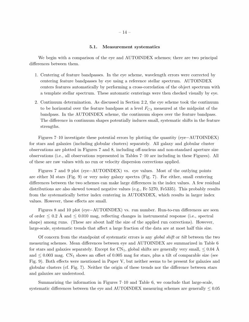
5.1. Measurement systematics

We begin with a comparison of the eye and AUTOINDEX schemes; there are two principal

differences between them.

1. Centering of feature bandpasses. In the eye scheme, wavelength errors were corrected by

centering feature bandpasses by eye using a reference stellar spectrum. AUTOINDEX

centers features automatically by performing a cross-correlation of the object spectrum with

a template stellar spectrum. These automatic centerings were then checked visually by eye.

2. Continuum determination. As discussed in Section 2.2, the eye scheme took the continuum

to be horizontal over the feature bandpass at a level FCλ measured at the midpoint of the

bandpass. In the AUTOINDEX scheme, the continuum slopes over the feature bandpass.

The difference in continuum shapes potentially induces small, systematic shifts in the feature

strengths.

Figures 7–10 investigate these potential errors by plotting the quantity (eye−AUTOINDEX)

for stars and galaxies (including globular clusters) separately. All galaxy and globular cluster

observations are plotted in Figures 7 and 8, including off-nucleus and non-standard aperture size

observations (i.e., all observations represented in Tables 7–10 are including in these Figures). All

of these are raw values with no run or velocity dispersion corrections applied.

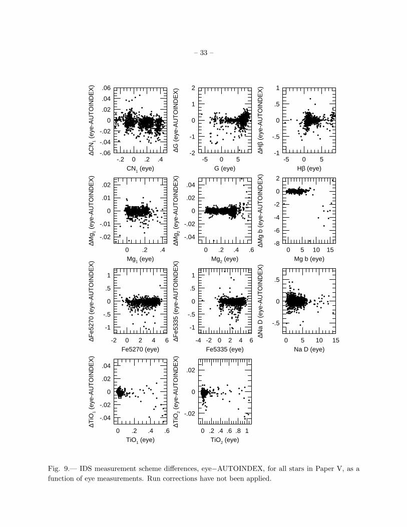
Figures 7 and 9 plot (eye−AUTOINDEX) vs. eye values. Most of the outlying points

are either M stars (Fig. 9) or very noisy galaxy spectra (Fig. 7). For either, small centering

differences between the two schemes can make large differences in the index values. A few residual

distributions are also skewed toward negative values (e.g., Fe 5270, Fe5335). This probably results

from the systematically better index centering in AUTOINDEX, which results in larger index

values. However, these effects are small.

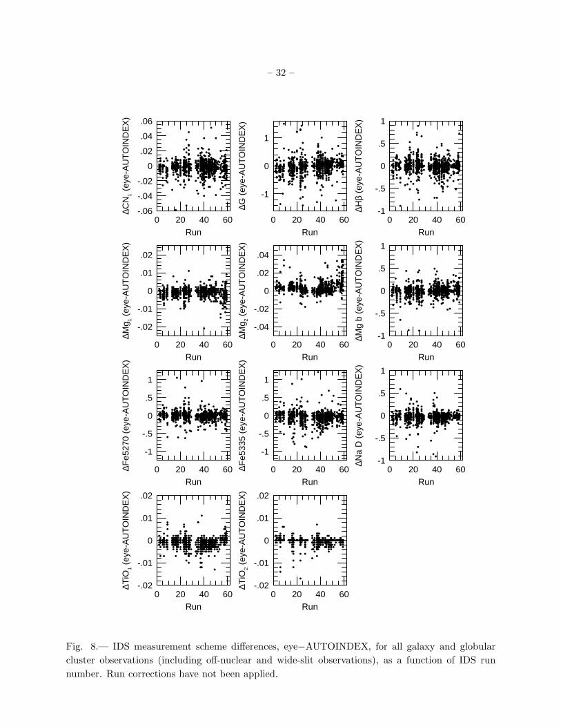
Figures 8 and 10 plot (eye−AUTOINDEX) vs. run number. Run-to-run differences are seen

of order ≤ 0.2 A and ≤ 0.010 mag, reflecting changes in instrumental response (i.e., spectral

shape) among runs. (These are about half the size of the applied run corrections). However,

large-scale, systematic trends that affect a large fraction of the data are at most half this size.

Of concern from the standpoint of systematic errors is any global shift or tilt between the two

measuring schemes. Mean differences between eye and AUTOINDEX are summarized in Table 6

for stars and galaxies separately. Except for CN1, global shifts are generally very small, ≤ 0.04 A

and ≤ 0.003 mag. CN1 shows an offset of 0.005 mag for stars, plus a tilt of comparable size (see

Fig. 9). Both effects were mentioned in Paper V, but neither seems to be present for galaxies and

globular clusters (cf. Fig. 7). Neither the origin of these trends nor the difference between stars

and galaxies are understood.

Summarizing the information in Figures 7–10 and Table 6, we conclude that large-scale,

systematic differences between the eye and AUTOINDEX measuring schemes are generally ≤ 0.05

– 15 –

A and ≤ 0.003 mag, with the exception of CN1, for which the differences are twice as large.

We turn now to differences between the “old” and “new” standard systems. Recall that the

standard system for the 11 original indices (here called the “old” system) was standardized to the

K giant standards in Runs 3 – 24, about one-third of the data. In hindsight, we see that these

early runs were atypical in some indices and that the standard system is therefore slightly “off”

with respect to the whole data. Rather than change zeropoints now, since many data have been

published and fitting-functions derived from them (Gorgas et al. 1993; Paper V), we compute

zeropoint corrections needed to transform AUTOINDEX plus its new system of run corrections

to the old, published system. The adopted corrections, based on the 9 K giant standard stars,

are given in the last column of Table 6; they are applied to all the galaxy and globular data in

this paper. For most indices, the corrections are quite small, a few hundredths of an A or a few

thousandths of a magnitude. The significant exception is the G-band, for which the offset is 0.21

A. A previous, similar analysis in Paper V yielded the corrections shown in the second-to-last

column. These shifts were used to correct the new stellar data in Paper V. The differences between

the two sets of corrections are again at most a few hundredths of an A or a few thousandths

of a magnitude. These are small to negligible in the context of old stellar-populations. The

differences between the Paper V and present corrections are a measure of the irreducible zeropoint

uncertainties inherent in the published Lick/IDS system.

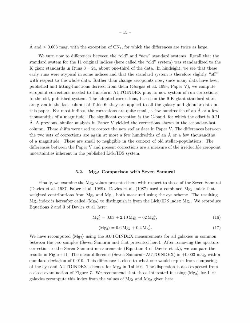
5.2. Mg2: Comparison with Seven Samurai

Finally, we examine the Mg2 values presented here with respect to those of the Seven Samurai

(Davies et al. 1987, Faber et al. 1989). Davies et al. (1987) used a combined Mg2 index that

weighted contributions from Mg2 and Mg1, both measured using the eye scheme. The resulting

Mg2 index is hereafter called 〈Mg2〉 to distinguish it from the Lick/IDS index Mg2. We reproduce

Equations 2 and 3 of Davies et al. here:

Mg′2 = 0.03 + 2.10Mg1 − 62Mg41 , (16)

〈Mg2〉 = 0.6Mg2 + 0.4Mg′2. (17)

We have recomputed 〈Mg2〉 using the AUTOINDEX measurements for all galaxies in common

between the two samples (Seven Samurai and that presented here). After removing the aperture

correction to the Seven Samurai measurements (Equation 4 of Davies et al.), we compare the

results in Figure 11. The mean difference (Seven Samurai−AUTOINDEX) is +0.003 mag, with a

standard deviation of 0.010. This difference is close to what one would expect from comparing

of the eye and AUTOINDEX schemes for Mg2 in Table 6. The dispersion is also expected from

a close examination of Figure 7. We recommend that those interested in using 〈Mg2〉 for Lick

galaxies recompute this index from the values of Mg1 and Mg2 given here.

– 16 –

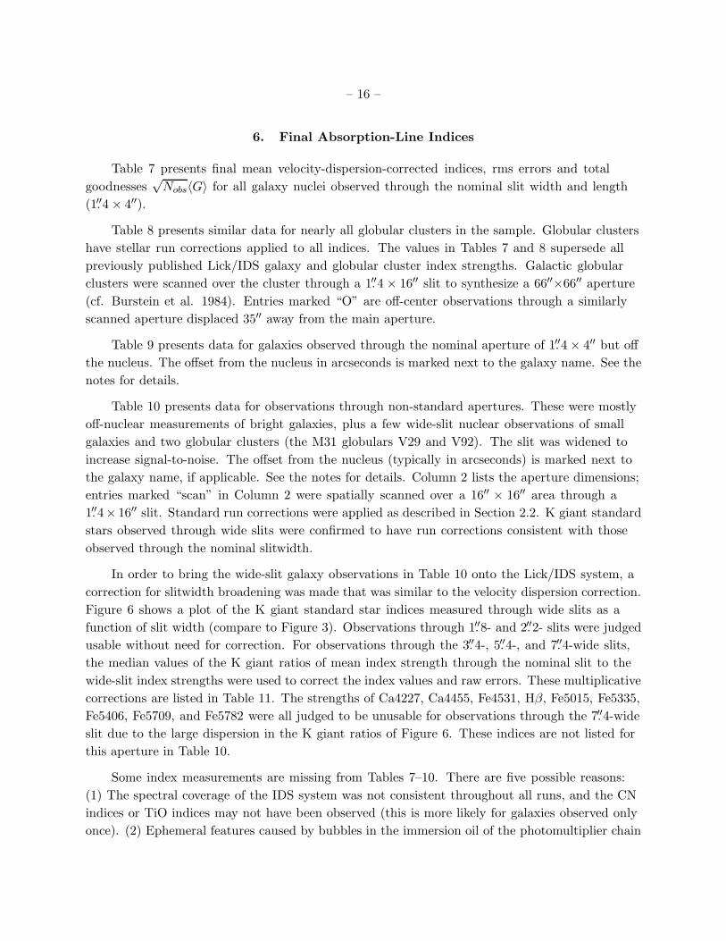
6. Final Absorption-Line Indices

Table 7 presents final mean velocity-dispersion-corrected indices, rms errors and total

goodnesses√

Nobs〈G〉 for all galaxy nuclei observed through the nominal slit width and length

(1.′′4 × 4′′).

Table 8 presents similar data for nearly all globular clusters in the sample. Globular clusters

have stellar run corrections applied to all indices. The values in Tables 7 and 8 supersede all

previously published Lick/IDS galaxy and globular cluster index strengths. Galactic globular

clusters were scanned over the cluster through a 1.′′4 × 16′′ slit to synthesize a 66′′×66′′ aperture

(cf. Burstein et al. 1984). Entries marked “O” are off-center observations through a similarly

scanned aperture displaced 35′′ away from the main aperture.

Table 9 presents data for galaxies observed through the nominal aperture of 1.′′4 × 4′′ but off

the nucleus. The offset from the nucleus in arcseconds is marked next to the galaxy name. See the

notes for details.

Table 10 presents data for observations through non-standard apertures. These were mostly

off-nuclear measurements of bright galaxies, plus a few wide-slit nuclear observations of small

galaxies and two globular clusters (the M31 globulars V29 and V92). The slit was widened to

increase signal-to-noise. The offset from the nucleus (typically in arcseconds) is marked next to

the galaxy name, if applicable. See the notes for details. Column 2 lists the aperture dimensions;

entries marked “scan” in Column 2 were spatially scanned over a 16′′ × 16′′ area through a

1.′′4× 16′′ slit. Standard run corrections were applied as described in Section 2.2. K giant standard

stars observed through wide slits were confirmed to have run corrections consistent with those

observed through the nominal slitwidth.

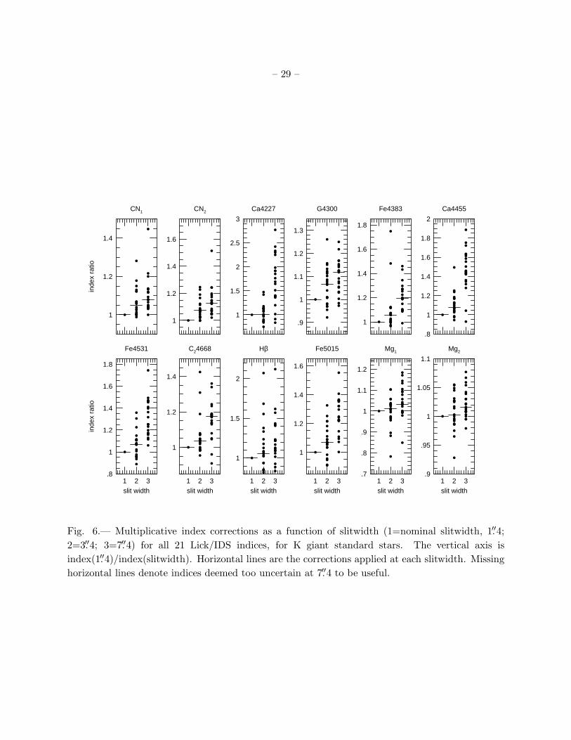
In order to bring the wide-slit galaxy observations in Table 10 onto the Lick/IDS system, a

correction for slitwidth broadening was made that was similar to the velocity dispersion correction.

Figure 6 shows a plot of the K giant standard star indices measured through wide slits as a

function of slit width (compare to Figure 3). Observations through 1.′′8- and 2.′′2- slits were judged

usable without need for correction. For observations through the 3.′′4-, 5.′′4-, and 7.′′4-wide slits,

the median values of the K giant ratios of mean index strength through the nominal slit to the

wide-slit index strengths were used to correct the index values and raw errors. These multiplicative

corrections are listed in Table 11. The strengths of Ca4227, Ca4455, Fe4531, Hβ, Fe5015, Fe5335,

Fe5406, Fe5709, and Fe5782 were all judged to be unusable for observations through the 7.′′4-wide

slit due to the large dispersion in the K giant ratios of Figure 6. These indices are not listed for

this aperture in Table 10.

Some index measurements are missing from Tables 7–10. There are five possible reasons:

(1) The spectral coverage of the IDS system was not consistent throughout all runs, and the CN

indices or TiO indices may not have been observed (this is more likely for galaxies observed only

once). (2) Ephemeral features caused by bubbles in the immersion oil of the photomultiplier chain

– 17 –

may have contaminated certain index measurements. (3) The systemic velocity of the galaxy may

have moved the reddest indices (TiO1 and TiO2) out of the spectral range of the IDS system.

(4) Intrinsic emission such as Hβ or [O III] λ5007 in the galaxy may have contaminated a central

bandpass or sideband. We have culled the most obvious examples of emission contamination, but

subtle contamination remains. Users of these data should be aware of this. (5) Poorly-subtracted

night-sky lines contaminated certain indices. Table 12 presents a list of indices possibly affected

by residual contamination from poor night-sky subtraction.

7. Summary

This paper presents the complete database of Lick/IDS absorption-line index strengths for

galaxies and globular clusters. This database supersedes all previously published Lick/IDS data

on these objects. The Lick/IDS galaxy data are among the largest collection of homogeneous

absorption-line strengths for stars and galaxies currently available.

We have reviewed the measurement of Lick/IDS indices from IDS spectra and characterized

the errors. The level of remaining systematic uncertainties is discussed. We also present for the

first time the correction of Lick/IDS absorption-line strengths for velocity dispersion. Such a

correction is a crucial step to compare Lick/IDS galaxy absorption-line strengths to models of

stellar populations based on the Lick/IDS stellar library (Worthey 1994).

In a subsequent paper, we will present an analysis of a subset of these data using stellar

population models in an attempt to derive stellar population ages, metallicities, and relative

element abundances of the nuclei of early-type galaxies.

The authors would like to thank their previous collaborators on this project, particularly

C. Dalle Ore; the directors, telescope operators, and staff of Mount Hamilton, Lick Observatory;

J. Wampler and L. Robinson for their development of the Image Dissector Scanner; and the

referee, J. Rose, for helpful comments. This work was supported by NSF grants AST 76-08258,

82-11551, 87-02899, and 95-29008 to SMF and AST 90-16930 to DB; by an ASU Faculty

Grant-in-Aid to DB; by the WFPC Investigation Definition Team contract NAS 5-1661; NASA

grant HF-1066.01-94A to GW from the Space Telescope Science Institute, which is operated by the

Association of Universities for Research in Astronomy, Inc., under NASA contract NAS5-26555;

and by a Flintridge Foundation Fellowship and by a Starr Fellowship to SCT.

– 18 –

REFERENCES

Abell, G. 1958, ApJS, 3, 211

Aragon, A., Gorgas, J., & Regos, M. 1987, A&A, 185, 97

Barbuy, B. 1994, ApJ, 430, 218

Barbuy, B., Erdelyi-Mendes, M., & Milone, A. 1992, A&AS, 93, 235

Bender, R., Paquet, A., & Nieto, J.-L. 1991, A&A, 246, 349

Bender, R. & Surma, P. 1992, A&A, 258, 250

Bender, R., Zeigler, B., & Bruzual, G. 1996, ApJ, 463, L51

Borges, A. C., Idiart, T. P., de Freitas Pacheco, J. P., & Thevenin, F. 1995, AJ, 110, 2408

Bower, R. G., Ellis, R. S., Rose, J. A., Sharples, R. M. 1990, AJ, 99, 530

Bressan, A., Chiosi, C., & Tantalo, R. 1996, A&A, 311, 361

Brodie, J. P. & Huchra, J. P. 1990, ApJ, 362, 503

Brodie, J. P. & Huchra, J. P. 1991, ApJ, 379, 157

Bruzual, G. & Charlot, S. 1996, GISSEL96

Burstein, D., Faber, S. M., Gaskell, C. M., & Krumm, N. 1984, ApJ, 287, 586

Burstein, D., Faber, S. M., & Gonzalez, J. J. 1986, AJ, 91, 1130

Burstein, D., Bertola, F., Buson, L. M., Faber, S. M., & Lauer, T. R. 1988, ApJ, 328, 440

Buzzoni, A. 1995, ApJS, 98, 69

Buzzoni, A., Gariboldi, G., & Mantegazza, L. 1992, AJ, 103, 1814

Buzzoni, A., Mantegazza, L., & Gariboldi, G. 1994, AJ, 107, 513

Caldwell, N., Rose, J. A., Sharples, R. M., Ellis, R. S., & Bower, R. G. 1993, AJ, 106, 473

Caldwell, N., Rose, J. A., Franx, M., & Leonardi, A. J. 1996, AJ, 111, 78

Caldwell, N. & Rose, J. A. 1997, AJ, 113, 492

Cardiel, N., Gorgas, J., & Aragon-Salamanca, A. 1995, MNRAS, 277, 502

Carollo, C. M., Danziger, I. J., & Buson, L. 1993, MNRAS, 265, 553

Casuso, E., Vazdekis, A., Peletier, R. F., & Beckman, J. E. 1996, ApJ, 458, 533

– 19 –

Chavez, M., Malagnini, M. L., & Morossi, C. 1995, ApJ, 440, 210

Chincarini, G. & Rood, H. J. 1971, ApJ, 168, 321

Couture, J. & Hardy, E. 1990, AJ, 99, 540

Couture, J. & Hardy, E. 1988, AJ, 96, 867

Dalle Ore, C., Faber, S. M., Gonzalez, J. J., Stoughton, R., & Burstein, D. 1991, ApJ, 366, 38

Davidge, T. J. 1992, AJ, 103, 1512

Davies, R. L., Burstein, D., Dressler, A., Faber, S. M., Lynden-Bell, D., Terlevich, R. J., &

Wegner, G. 1987, ApJS, 64, 581

Davies, R. L., Sadler, E. M., & Peletier, R. 1993, MNRAS, 262, 650

de Freitas Pacheco, J. A. 1996, MNRAS, 278, 841

de Souza, R. E., Barbuy, B., & dos Anjos, S. 1993, AJ, 105, 1737

Efstathiou, G. & Gorgas, J. 1985, MNRAS, 245, 37

Faber, S. M. & Jackson, R. E. 1976, ApJ, 204, 668

Faber, S. M., Friel, E. D., Burstein, D., & Gaskell, C. M. 1985, ApJS, 57, 711

Faber, S. M., Wegner, G., Burstein, D., Davies, R. L., Dressler, A., Lynden-Bell, D., & Terlevich,

R. J. 1989, ApJS, 69, 763

Faber, S. M., Trager, S. C., Gonzalez, J. J., & Worthey, G. 1995, in IAU Symposium 164, Stellar

Populations, ed. P. C. van der Kruit & G. Gilmore (Dordrecht: Kluwer), p. 249

Faber, S. M., et al. 1997, AJ, in press

Fisher, D., Franx, M., & Illingworth, G. 1995, ApJ, 448, 119

Fisher, D., Franx, M., & Illingworth, G. 1996, ApJ, 459, 110

Gonzalez, J. J. 1993, Ph. D. Thesis, University of California, Santa Cruz

Gorgas, J., Efstathiou, G., & Aragon Salamanca, A. 1990, MNRAS, 245, 217

Gorgas, J., Faber, S. M., Burstein, D., Gonzalez, J. J., Courteau, S., & Prosser, C. 1993, ApJS,

86, 153

Gorgas, J., Pedraz, S., Guzman, R., Cardiel, N., & Gonzalez, J. J. 1997, ApJ, 481, L19

Gregg, M. D. 1994, AJ, 108, 2164

– 20 –

Greggio, L. 1997, MNRAS, 285, 151

Gulati, R. K., Malagnini, M. L., & Morossi, C. 1991, A&A, 247, 447

Gulati, R. K., Malagnini, M. L., & Morossi, C. 1993, ApJ, 413, 166

Guzman, R., Lucey, J. R., Carter, D., & Terlevich, R. J. 1992, MNRAS, 257, 187

Huchra, J. P., Kent, S. M., & Brodie, J. P. 1991, ApJ, 370, 495

Huchra, J. P., Brodie, J. P., Caldwell, N., Christian, C., & Schommer, R. 1996, ApJS, 102, 29

Jørgensen, I. 1997, MNRAS, 288, 16

Kuntschner, H. & Davies, R. L. 1997, MNRAS, in press

Leonardi, A. J. & Rose, J. A. 1996, AJ, 111, 182

Matteucci, F. 1994, A&A, 288, 57

McQuitty, R. G., Jaffe, T. R., Friel, E. D., & Dalle Ore, C. M. 1994, AJ, 107, 359

Mehlert, D., Bender, R., Saglia, R., & Wegner, G. 1997, in “A New Vision of an Old Cluster:

Untangling Coma Berenices,” ed. F. Durret et al., in press

Moller, C. S., Fritze-von Alvenleben, U., & Fricke, K. J. 1997, A&A, 317, 676

Peterson, R. C. & Caldwell, N. 1993, AJ, 105, 1411

Robinson, L. B. & Wampler, E. J. 1972, PASP, 84, 161

Rose, J. A. 1985a, AJ, 90, 787

Rose, J. A. 1985b, AJ, 90, 803

Rose, J. A. 1985c, AJ, 90, 1927

Rose, J. A. & Tripicco, M. J. 1986, AJ, 92, 610

Rose, J. A., Stetson, P. B., & Tripicco, M. J. 1987, AJ, 94, 1202

Rose, J. A., Bower, R. G., Caldwell, N., Ellis, R. S., Sharples, R. M., & Teague, P. 1994, AJ, 108,

2054

Schweizer, S., Seitzer, P., Faber, S. M., Burstein, D., Dalle Ore, C. M., & Gonzalez, J. J. 1990,

ApJ, 364, L33

Tantalo, R., Chiosi, C., Bressan, A., & Fagotto, F. 1996, A&A, 311, 361

Thomsen, B. & Baum, W. A. 1989, ApJ, 347, 214

– 21 –

Trager, S. C. 1997, Ph. D. Thesis, University of California, Santa Cruz

Tripicco, M. & Bell, R. A. 1995, AJ, 110, 3035

Vazdekis, A., Casuso, E., Peletier, R. F., & Beckman, J. E. 1996, ApJS, 106, 307

Vazdekis, A., Peletier, R. F., Beckman, J. E., & Casuso, E. 1996, ApJS, 111, 203

Weiss, A., Peletier, R. F., & Matteucci, F. 1995, A&A, 296, 73

Whitmore, B. C., McElroy, D. B., Tonry, J. L. 1985, ApJS, 59, 1

Worthey, G. 1992, Ph. D. Thesis, University of California, Santa Cruz

Worthey, G. 1994, ApJS, 95, 107

Worthey, G. 1996, in From Stars to Galaxies: The Impact of Stellar Physics on Galaxy Evolution,

ed. C. Leitherer, U. Fritze-von Alvensleben, & J. Huchra, A. S. P. Conf. Ser., vol. 98 (San

Francisco: ASP), p. 467

Worthey, G., Faber, S. M., & Gonzalez, J. J. 1992, ApJ, 398, 69

Worthey, G., Faber, S. M., Gonzalez, J. J., & Burstein, D. 1994, ApJS, 94, 687 (Paper V)

Worthey, G., Trager, S. C., & Faber, S. M. 1996, in Fresh Views on Elliptical Galaxies, ed. A.

Buzzoni, A. Renzini, & A. Serrano, A. S. P. Conf. Ser., vol. 86 (San Francisco: ASP), p. 203

Worthey, G. & Ottaviani, D. L. 1997, ApJS, 111, 377

This preprint was prepared with the AAS LATEX macros v4.0.

– 22 –

NGC 6051 G=854

NGC 4486B G=1103

NGC 1700 G=1504

NGC 4551 G=2004

4500 5000 5500 6000

Fλ

(rel

ativ

e)

λ

NGC 3610 G=3000

NGC 4377 G=4077

M31 G=5190

M32 G=10106

4500 5000 5500 6000λ

Fig. 1.— A selection of IDS spectra covering a range of S/N. Spectra are labelled with their name

and goodness G (see Section 3).

– 23 –

2.6 2.8 3 3.2 3.4 3.6 3.8 4

0

.2

.4

.6

log <G>k

log

σ TO

T,k

NGC6205NGC6205-OFF

NGC6838

NGC6838-OFF

M31

M31-35ew

NGC221

NGC2300

NGC2634

NGC2693

NGC2768NGC2865

NGC2974

NGC3115

NGC3377

NGC3379

NGC3489

NGC3610NGC4374

NGC4387

NGC4406

NGC4459

NGC4464

NGC4467

NGC4472

NGC4478

NGC4552

NGC4636NGC4649

NGC4762NGC4860

NGC4874

NGC4889NGC5812NGC5813NGC5831

NGC584NGC5846

NGC6166

NGC687

NGC708

NGC720

NGC7626

Fig. 2.— Preliminary calibration of the independently determined error σTOT,k with goodness

〈G〉k. The size of the galaxy labels is proportional to the number of observations. The middle of

the label is the location of the point. The relation flattens at high 〈G〉k due to flat-fielding errors.

The solid line is a least-squares linear fit to the relation σ2TOT,k = a〈G〉−2

k + b (see Section 3).

– 24 –

.95

1

1.05

1.1

1.15

c j(σ)

CN1

.8

1

1.2

CN2

1

1.5

2

2.5

3

3.5

Ca4227

1

1.05

1.1

1.15

1.2

1.25

G4300

1

1.2

1.4

1.6

Fe4383

1

1.5

2

Ca4455

0 200 400

1

1.2

1.4

1.6

σ

c j(σ)

Fe4531

0 200 400

1

1.1

1.2

1.3

1.4

σ

C24668

0 200 400

.8

1

1.2

σ

Hβ

0 200 400

1

1.2

1.4

1.6

σ

Fe5015

0 200 400

1

1.05

1.1

1.15

1.2

σ

Mg1

0 200 400

1

1.02

1.04

1.06

σ

Mg2

Fig. 3.— Multiplicative index correction, Cj , as a function of velocity dispersion (in km s−1) for all

21 Lick/IDS indices. The corrections have been determined by measuring various stellar spectra

convolved to different broadenings. Symbols represent K giant standard stars (small dots), G dwarfs

(crosses), and M32 (multiple observations; open circles). The quantity shown is index(0)/index(σ).

– 25 –

1

1.2

1.4

c j(σ)

Mg b

1

1.2

1.4

Fe5270

1

1.5

2

Fe5335

1

1.5

2

Fe5406

1

1.2

1.4

1.6

1.8

Fe5709

1

1.5

2

2.5

3

Fe5782

0 200 400

1

1.1

1.2

1.3

σ

c j(σ)

Na D

0 200 400

.5

1

1.5

2

σ

TiO1

0 200 400

.95

1

1.05

1.1

1.15

σ

TiO2

K giantsG dwarfsM32

Fig. 3.— Continued.

– 26 –

-.1 0 .1 .2 .30

.1

.2

.3

.4

Mg 2

CN1 -.1 0 .1 .2 .3

CN2 0 1 2

Ca4227 0 2 4 6 8

G4300 0 2 4 6 8

Fe4383

0 1 2 30

.1

.2

.3

.4

Mg 2

Ca4455 0 2 4

Fe4531 0 2 4 6 8 10

C24668 0 1 2 3 4 5

Hβ 0 2 4 6

Fe5015

0 .05 .1 .15 .20

.1

.2

.3

.4

Mg 2

Mg1 2 4 6

Mg b 0 1 2 3 4

Fe5270 1 2 3 4

Fe5335 0 1 2 3

Fe5406

0 .5 1 1.5 20

.1

.2

.3

.4

Mg 2

Fe5709 0 .5 1 1.5 2

Fe5782 0 2 4 6 8 10

Na D 0 .02 .04 .06 .08 .1

TiO1 0 .05 .1 .15

TiO2

Fig. 4.— Index strengths as a function of Mg2 (in mag) for all 21 Lick/IDS indices for all galaxy

observations (nuclear and off-nuclear) through the standard 1.′′4× 4′′ aperture. (a) Before velocity-

dispersion correction.

– 27 –

-.1 0 .1 .2 .30

.1

.2

.3

.4

Mg 2

CN1 -.1 0 .1 .2 .3

CN2 0 1 2

Ca4227 0 2 4 6 8

G4300 0 2 4 6 8

Fe4383

0 1 2 30

.1

.2

.3

.4

Mg 2

Ca4455 0 2 4

Fe4531 0 2 4 6 8 10

C24668 0 1 2 3 4 5

Hβ 0 2 4 6

Fe5015

0 .05 .1 .15 .20

.1

.2

.3

.4

Mg 2

Mg1 2 4 6

Mg b 0 1 2 3 4

Fe5270 1 2 3 4

Fe5335 0 1 2 3

Fe5406

0 .5 1 1.5 20

.1

.2

.3

.4

Mg 2

Fe5709 0 .5 1 1.5 2

Fe5782 0 2 4 6 8 10

Na D 0 .02 .04 .06 .08 .1

TiO1 0 .05 .1 .15

TiO2

Fig. 4.— (b) After velocity-dispersion correction.

– 28 –

-.1 0 .1 .2 .30

100

200

300

400

σ

CN1 0 1 2

Ca4227 0 2 4 6 8

G4300 0 2 4 6 8

Fe4383 0 1 2 3

Ca4455

0 2 40

100

200

300

400

σ

Fe4531 0 2 4 6 8 10

C24668 0 1 2 3 4 5

Hβ 0 2 4 6

Fe5015 0 .05 .1 .15 .2

Mg1

0 .1 .2 .3 .40

100

200

300

400

σ

Mg2 2 4 6

Mg b 0 1 2 3 4

Fe5270 1 2 3 4

Fe5335 0 1 2 3

Fe5406

0 .5 1 1.5 20

100

200

300

400

σ

Fe5709 0 .5 1 1.5 2

Fe5782 0 2 4 6 8 10

Na D 0 .02 .04 .06 .08 .1

TiO1 0 .05 .1 .15

TiO2

Fig. 5.— Index strengths as a function of velocity dispersion (in km s−1) for 20 Lick/IDS indices (all

except CN2, which reproduces the behavior of CN1 very closely) for all galaxy observations (nuclear

and off-nuclear) through the standard 1.′′4 × 4′′ aperture, after velocity-dispersion correction.

– 29 –

1

1.2

1.4

inde

x ra

tio

CN1

1

1.2

1.4

1.6

CN2

1

1.5

2

2.5

3

Ca4227

.9

1

1.1

1.2

1.3

G4300

1

1.2

1.4

1.6

1.8

Fe4383

.8

1

1.2

1.4

1.6

1.8

2

Ca4455

1 2 3.8

1

1.2

1.4

1.6

1.8

slit width

inde

x ra

tio

Fe4531

1 2 3

1

1.2

1.4

slit width

C24668

1 2 3

1

1.5

2

slit width

Hβ

1 2 3

1

1.2

1.4

1.6

slit width

Fe5015

1 2 3.7

.8

.9

1

1.1

1.2

slit width

Mg1

1 2 3.9

.95

1

1.05

1.1

slit width

Mg2

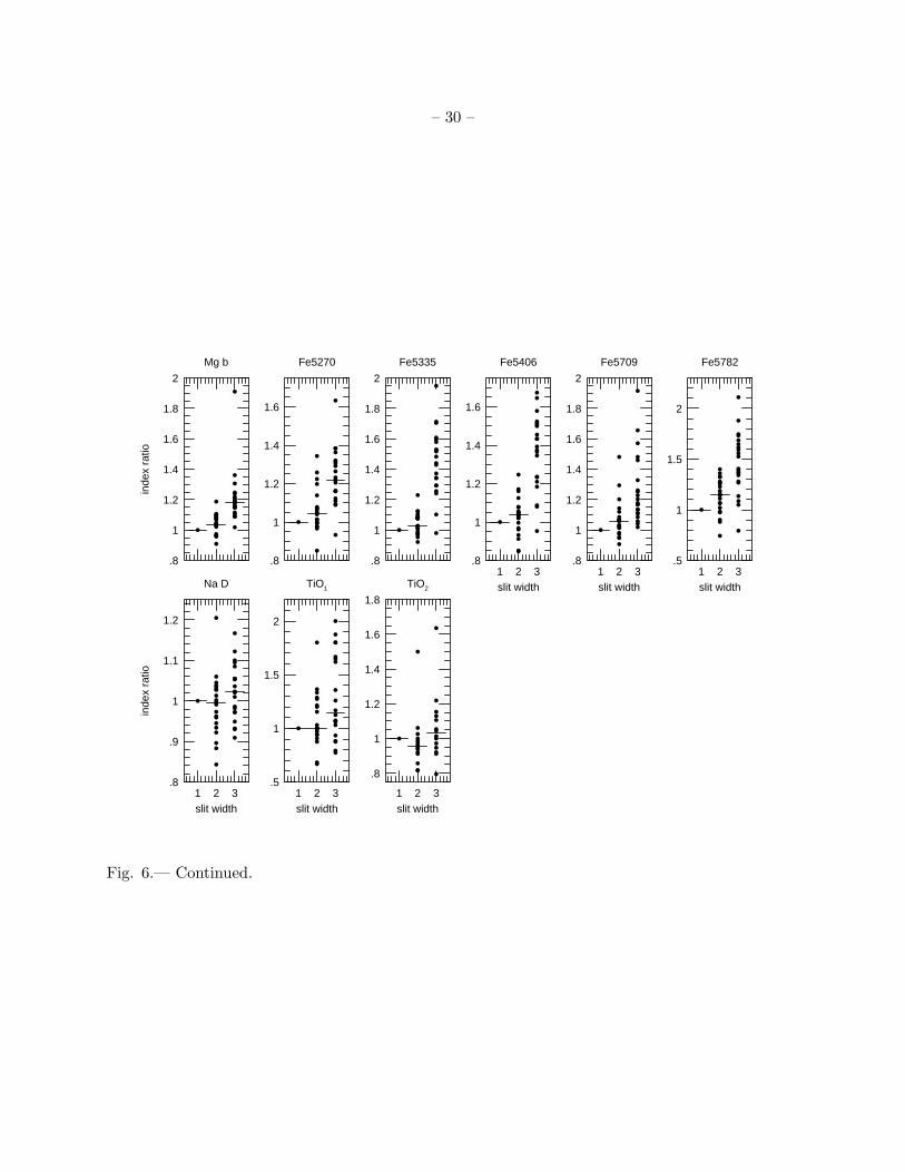
Fig. 6.— Multiplicative index corrections as a function of slitwidth (1=nominal slitwidth, 1.′′4;

2=3.′′4; 3=7.′′4) for all 21 Lick/IDS indices, for K giant standard stars. The vertical axis is

index(1.′′4)/index(slitwidth). Horizontal lines are the corrections applied at each slitwidth. Missing

horizontal lines denote indices deemed too uncertain at 7.′′4 to be useful.

– 30 –

.8

1

1.2

1.4

1.6

1.8

2

inde

x ra

tio

Mg b

.8

1

1.2

1.4

1.6

Fe5270

.8

1

1.2

1.4

1.6

1.8

2

Fe5335

1 2 3.8

1

1.2

1.4

1.6

slit width

Fe5406

1 2 3.8

1

1.2

1.4

1.6

1.8

2

slit width

Fe5709

1 2 3.5

1

1.5

2

slit width

Fe5782

1 2 3.8

.9

1

1.1

1.2

slit width

inde

x ra

tio

Na D

1 2 3.5

1

1.5

2

slit width

TiO1

1 2 3

.8

1

1.2

1.4

1.6

1.8

slit width

TiO2

Fig. 6.— Continued.

– 31 –

-.2 -.1 0 .1 .2 .3-.06

-.04

-.02

0

.02

.04

.06

CN1 (eye)

∆CN

1 (e

ye-A

UT

OIN

DE

X)

-2 0 2 4 6 8

-1

0

1

G (eye)∆G

(ey

e-A

UT

OIN

DE

X)

-2 0 2 4-1

-.5

0

.5

1

Hβ (eye)

∆Hβ

(eye

-AU

TO

IND

EX

)

0 .1 .2

-.02

-.01

0

.01

.02

Mg1 (eye)

∆Mg 1

(eye

-AU

TO

IND

EX

)

0 .1 .2 .3 .4

-.04

-.02

0

.02

.04

Mg2 (eye)

∆Mg 2

(eye

-AU

TO

IND

EX

)

0 2 4 6-1

-.5

0

.5

1

Mg b (eye)∆M

g b

(eye

-AU

TO

IND

EX

)

0 2 4

-1

-.5

0

.5

1

Fe5270 (eye)

∆Fe5

270

(eye

-AU

TO

IND

EX

)

-1 0 1 2 3 4

-1

-.5

0

.5

1

Fe5335 (eye)

∆Fe5

335

(eye

-AU

TO

IND

EX

)

-2 0 2 4 6 8 10-1

-.5

0

.5

1

Na D (eye)

∆Na

D (

eye-

AU

TO

IND

EX

)

-.05 0 .05 .1 .15-.02

-.01

0

.01

.02

TiO1 (eye)

∆TiO

1 (e

ye-A

UT

OIN

DE

X)

-.05 0 .05 .1 .15-.02

-.01

0

.01

.02

TiO2 (eye)

∆TiO

2 (e

ye-A

UT

OIN

DE

X)

Fig. 7.— IDS measurement scheme differences, eye−AUTOINDEX, for all galaxy and globular

cluster observations (including off-nuclear and wide-slit observations), as a function of eye

measurements. Run and velocity-dispersion corrections have not been applied.

– 32 –

0 20 40 60-.06

-.04

-.02

0

.02

.04

.06

Run

∆CN

1 (e

ye-A

UT

OIN

DE

X)

0 20 40 60

-1

0

1

Run∆G

(ey

e-A

UT

OIN

DE

X)

0 20 40 60-1

-.5

0

.5

1

Run

∆Hβ

(eye

-AU

TO

IND

EX

)

0 20 40 60

-.02

-.01

0

.01

.02

Run

∆Mg 1

(eye

-AU

TO

IND

EX

)

0 20 40 60

-.04

-.02

0

.02

.04

Run

∆Mg 2

(eye

-AU

TO

IND

EX

)

0 20 40 60-1

-.5

0

.5

1

Run∆M

g b

(eye

-AU

TO

IND

EX

)

0 20 40 60

-1

-.5

0

.5

1

Run

∆Fe5

270

(eye

-AU

TO

IND

EX

)

0 20 40 60

-1

-.5

0

.5

1

Run

∆Fe5

335

(eye

-AU

TO

IND

EX

)

0 20 40 60-1

-.5

0

.5

1

Run

∆Na

D (

eye-

AU

TO

IND

EX

)

0 20 40 60-.02

-.01

0

.01

.02

Run

∆TiO

1 (e

ye-A

UT

OIN

DE

X)

0 20 40 60-.02

-.01

0

.01

.02

Run

∆TiO

2 (e

ye-A

UT

OIN

DE

X)

Fig. 8.— IDS measurement scheme differences, eye−AUTOINDEX, for all galaxy and globular

cluster observations (including off-nuclear and wide-slit observations), as a function of IDS run

number. Run corrections have not been applied.

– 33 –

-.2 0 .2 .4-.06

-.04

-.02

0

.02

.04

.06

CN1 (eye)

∆CN

1 (e

ye-A

UT

OIN

DE

X)

-5 0 5-2

-1

0

1

2

G (eye)∆G

(ey

e-A

UT

OIN

DE

X)

-5 0 5-1

-.5

0

.5

1

Hβ (eye)

∆Hβ

(eye

-AU

TO

IND

EX

)

0 .2 .4

-.02

-.01

0

.01

.02

Mg1 (eye)

∆Mg 1

(eye

-AU

TO

IND

EX

)

0 .2 .4 .6

-.04

-.02

0

.02

.04

Mg2 (eye)

∆Mg 2

(eye

-AU

TO

IND

EX

)

0 5 10 15-8

-6

-4

-2

0

2

Mg b (eye)∆M

g b

(eye

-AU

TO

IND

EX

)

-2 0 2 4 6

-1

-.5

0

.5

1

Fe5270 (eye)

∆Fe5

270

(eye

-AU

TO

IND

EX

)

-4 -2 0 2 4 6

-1

-.5

0

.5

1

Fe5335 (eye)

∆Fe5

335

(eye

-AU

TO

IND

EX

)

0 5 10 15

-.5

0

.5

Na D (eye)

∆Na

D (

eye-

AU

TO

IND

EX

)

0 .2 .4 .6

-.04

-.02

0

.02

.04

TiO1 (eye)

∆TiO

1 (e

ye-A

UT

OIN

DE

X)

0 .2 .4 .6 .8 1

-.02

0

.02

TiO2 (eye)

∆TiO

2 (e

ye-A

UT

OIN

DE

X)

Fig. 9.— IDS measurement scheme differences, eye−AUTOINDEX, for all stars in Paper V, as a

function of eye measurements. Run corrections have not been applied.

– 34 –

0 20 40 60-.06

-.04

-.02

0

.02

.04

.06

Run

∆CN

1 (e

ye-A

UT

OIN

DE

X)

0 20 40 60-2

-1

0

1

2

Run∆G

(ey

e-A

UT

OIN

DE

X)

0 20 40 60-1

-.5

0

.5

1

Run

∆Hβ

(eye

-AU

TO

IND

EX

)

0 20 40 60

-.02

-.01

0

.01

.02

Run

∆Mg 1

(eye

-AU

TO

IND

EX

)

0 20 40 60

-.04

-.02

0

.02

.04

Run

∆Mg 2

(eye

-AU

TO

IND

EX

)

0 20 40 60-8

-6

-4

-2

0

2

Run∆M

g b

(eye

-AU

TO

IND

EX

)

0 20 40 60

-1

-.5

0

.5

1

Run

∆Fe5

270

(eye

-AU

TO

IND

EX

)

0 20 40 60

-1

-.5

0

.5

1

Run

∆Fe5

335

(eye

-AU

TO

IND

EX

)

0 20 40 60

-.5

0

.5

Run

∆Na

D (

eye-

AU

TO

IND

EX

)

0 20 40 60

-.04

-.02

0

.02

.04

Run

∆TiO

1 (e

ye-A

UT

OIN

DE

X)

0 20 40 60

-.02

0

.02

Run

∆TiO

2 (e

ye-A

UT

OIN

DE

X)

Fig. 10.— IDS measurement scheme differences, eye−AUTOINDEX, for all stars in Paper V, as a

function of IDS run number. Run corrections have not been applied.

– 35 –

<Mg2> (7 Samurai, no aperture corrections)

0 .1 .2 .3

0

.2

.4

<M

g 2> (

AU

TO

IND

EX

)

0 .1 .2 .3

-.04

-.02

0

.02

.04 ∆<

Mg

2 > (7 S

am-A

UT

OIN

DE

X)

Fig. 11.— Comparison of IDS and Seven Samurai measurements of 〈Mg2〉. Data for Seven Samurai

measurements are taken from Davies et al. (1987), without aperture corrections to Coma.

– 36 –

Table 1. Published IDS Data

Paper No. of Indices Method Run corrections

(a) Galaxies and Globular Clusters

Burstein et al. (1984) globulars 11 E all indices

Davies et al. (1987) 〈Mg2〉a E yes

Burstein et al. (1988) 〈Mg2〉ab E yes

Worthey, Faber, & Gonzalez (1992) Mg2, Fe5270, Fe5335 A Mg2 only

This paper

Galaxies 21 A molecular bands only

Globulars, low-velocity galaxiesc 21 A all indices

(b) Stars

Faber et al. (1985) K giants 11 E all indices

Burstein et al. (1986) Fe5270, Fe5335 E all indices

Gorgas et al. (1993) G dwarfs 11 E all indices

Worthey et al. (1994)

Prev. published K giants, G dwarfs 11 E all indices

+10 A all indices

All other stars 21 A all indices

aThe 〈Mg2〉 index is a weighted mean of Mg1 and Mg2. See Section 6.2.

bThere is an error in the 〈Mg2〉 index for NGC 3115 in Table 3 of Burstein et al. (1988); the correct

value is 〈Mg2〉 = 0.330. Note that the 〈Mg2〉 values in Table 3 of Burstein et al. (1988) are from Davies

et al. (1987), without the aperture correction of Davies et al.

cGalaxies with cz < 300 km s−1.

Note. — Columns:

(1) Reference

(2) Number of indices published: 11=original 11 Lick/IDS indices of Burstein et al. (1984); 21=all

Lick/IDS indices (see Table 2); +10=new indices presented in Worthey et al. (1994); 〈Mg2〉=“average”

Mg2 index described in Davies et al. (1987; cf. Section 6).

(3) Index measurement method: E=“eye” [see Burstein et al. (1984)]; A=AUTOINDEX (see text).

(4) Run corrections are determined by zeropointing K giant standard star observations to the standard

system determined by the same nine standard stars (see Faber et al. 1985). For further discussion of

the system, see Section 6.1.

– 37 –

Table 2. Index Definitions

j Name Index Bandpass Pseudocontinua Units Measuresa Errorb Notes

01 CN1 4142.125-4177.125 4080.125-4117.625 mag C,N,(O) 0.018 1,2

4244.125-4284.125

02 CN2 4142.125-4177.125 4083.875-4096.375 mag C,N,(O) 0.019 1,2

4244.125-4284.125

03 Ca4227 4222.250-4234.750 4211.000-4219.750 A Ca,(C) 0.25 1

4241.000-4251.000

04 G4300 4281.375-4316.375 4266.375-4282.625 A C,(O) 0.33 1

4318.875-4335.125

05 Fe4383 4369.125-4420.375 4359.125-4370.375 A Fe,C,(Mg) 0.46 1

4442.875-4455.375

06 Ca4455 4452.125-4474.625 4445.875-4454.625 A (Fe),(C),Cr 0.22 1

4477.125-4492.125

07 Fe4531 4514.250-4559.250 4504.250-4514.250 A Ti,(Si) 0.37 1

4560.500-4579.250

08 C24668 4634.000-4720.250 4611.500-4630.250 A C,(O),(Si) 0.57 1,3

4742.750-4756.500

09 Hβ 4847.875-4876.625 4827.875-4847.875 A Hβ,(Mg) 0.19

4876.625-4891.625

10 Fe5015 4977.750-5054.000 4946.500-4977.750 A (Mg),Ti,Fe 0.41

5054.000-5065.250

11 Mg1 5069.125-5134.125 4895.125-4957.625 mag C,Mg,(O),(Fe) 0.006 3

5301.125-5366.125

12 Mg2 5154.125-5196.625 4895.125-4957.625 mag Mg,C,(Fe),(O) 0.007

5301.125-5366.125

13 Mgb 5160.125-5192.625 5142.625-5161.375 A Mg,(C),(Cr) 0.20

5191.375-5206.375

14 Fe5270 5245.650-5285.650 5233.150-5248.150 A Fe,C,(Mg) 0.24

5285.650-5318.150

15 Fe5335 5312.125-5352.125 5304.625-5315.875 A Fe,(C),(Mg),Cr 0.22

5353.375-5363.375

16 Fe5406 5387.500-5415.000 5376.250-5387.500 A Fe 0.18

5415.000-5425.000

17 Fe5709 5696.625-5720.375 5672.875-5696.625 A (C),Fe 0.16 1

5722.875-5736.625

18 Fe5782 5776.625-5796.625 5765.375-5775.375 A Cr 0.19 1

5797.875-5811.625

19 Na D 5876.875-5909.375 5860.625-5875.625 A Na,C,(Mg) 0.21 1

5922.125-5948.125

20 TiO1 5936.625-5994.125 5816.625-5849.125 mag C 0.006 1,4

6038.625-6103.625

21 TiO2 6189.625-6272.125 6066.625-6141.625 mag C,V,Sc 0.005 1,4

6372.625-6415.125

aDominant species; species in parentheses control index in a negative sense (index weakens as

abundance grows). See Tripicco & Bell (1995) and Worthey (1996).

bStandard star error. See text.

Note. —

(1) Wavelength definition has been refined. See text.

(2) C, N are dominant as CN.

(3) C is dominant as C2.

(4) TiO appears at M0 and cooler.

– 38 –

Table 3. Lick/IDS Error Rescalingsa

G93 IDS-IDS Adopted

j Name rescaling rescaling rescaling

01 CN1 · · · · · · 0.92

02 CN2 · · · · · · 0.92

03 Ca4227 · · · · · · 0.92

04 G4300 · · · · · · 0.92

05 Fe4383 · · · 1.11 1.11

06 Ca4455 · · · 0.87 0.87

07 Fe4531 · · · 0.90 0.90

08 C24668 · · · · · · 0.92

09 Hβ 0.95 · · · 0.95

10 Fe5015 1.05 · · · 1.05

11 Mg1 · · · · · · 0.92

12 Mg2 · · · · · · 0.92

13 Mg b 0.94 · · · 0.94

14 Fe5270 0.75 · · · 0.75

15 Fe5335 0.95 · · · 0.95

16 Fe5406 0.88 · · · 0.88

17 Fe5709 · · · 0.94 0.94

18 Fe5782 · · · 0.81 0.81

19 Na D · · · · · · 0.92

20 TiO1 · · · · · · 0.92

21 TiO2 · · · · · · 0.92

aThese corrections adjust the assumed standard star

errors in Table 2 to produce the correct mean error

level relative to Gonzalez (1993; G93) and the right

balance among index errors internal to the IDS data

as described in Section 3.

– 39 –

Table 4. Velocity dispersions used to correct the raw indices

Name σ ǫσvSource

A 569A 226 14 3

IC 171 179 14 3

IC 179 214 14 3

IC 310 232 14 3

IC 783 100 50 8

IC 1131 104 20 5

IC 1696 169 14 3

IC 1907 238 14 3

IC 2955 188 14 3

IC 3303 100 50 8

IC 3470 120 23 4

IC 3652 100 50 8

IC 3653 240 14 3

IC 3672 100 50 8

IC 4051 223 14 3

NGC 80 296 14 3

NGC 83 254 14 3

NGC 128 198 12 5

NGC 185 23 22 6

NGC 194 208 14 3

NGC 205 14 7 7

NGC 221 77 3 1

NGC 224 183 1 1

NGC 227 268 14 3

NGC 315 310 1 1

NGC 379 245 14 3

NGC 380 277 14 3

NGC 382 153 14 3

NGC 383 265 14 3

NGC 385 180 14 3

NGC 386 61 14 3

NGC 392 261 14 3

NGC 404 55 14 3

NGC 410 321 14 3

– 40 –

Table 4—Continued

Name σ ǫσvSource

NGC 474 171 13 4

NGC 499 237 14 3

NGC 501 163 14 3

NGC 507 275 2 1

NGC 524 275 10 2

NGC 529 216 14 3

Note. — Columns:

(1) Galaxy name. See note, Table

6.

(2) Velocity dispersion, σ, in units

of km s−1.

(3) Fractional

uncertainty of velocity dispersion, in

percent. Taken from estimates in

individual sources except source 7,

whose uncertainties were estimated

to be 10%, and this paper (source

8), in which velocity dispersions

and uncertainties are based on eye

estimates on comparison to galaxies

with similar Mg2 using the Mg2–σ

relation.

(4) Sources of velocity dispersion.

1=Gonzalez (1993); 2=Faber et

al. (1997); 3=Faber et al. (1989);

4=Whitmore, McElroy & Tonry

(1985); 5=Dalle Ore et al. (1991);

6=Bender, Paquet & Nieto (1991);

7=Peterson & Caldwell (1993);

8=this paper (rough eye estimates;

see text).

– 41 –

Table 5. Velocity dispersion correction polynomial coefficients

j Name c0 c1 c2 c3

01 CN1 1.000e+00 3.333e−05 2.222e−07 −7.105e−15

02 CN2 1.000e+00 5.333e−05 5.333e−07 −2.963e−10

03 Ca4227 1.000e+00 1.378e−04 1.356e−06 9.432e−09

04 G4300 1.000e+00 7.222e−05 4.000e−07 3.457e−10

05 Fe4383 1.000e+00 5.553e−06 1.933e−06 −9.877e−10

06 Ca4455 1.000e+00 1.489e−04 2.467e−06 4.198e−09

07 Fe4531 1.000e+00 3.889e−05 2.578e−06 −1.136e−09

08 C24668 1.000e+00 −6.667e−06 1.244e−06 −2.963e−10

09 Hβ 1.000e+00 7.444e−05 2.667e−07 1.136e−09

10 Fe5015 1.000e+00 9.667e−05 2.578e−06 −1.926e−09

11 Mg1 1.000e+00 −2.223e−06 5.333e−07 −4.938e−10

12 Mg2 1.000e+00 3.444e−05 −4.445e−08 2.469e−10

13 Mg b 1.000e+00 −9.333e−05 2.800e−06 −1.481e−09

14 Fe5270 1.000e+00 4.000e−05 2.667e−06 −1.481e−09

15 Fe5335 1.000e+00 −5.667e−05 5.444e−06 2.963e−10

16 Fe5406 1.000e+00 −6.778e−05 4.956e−06 7.901e−10

17 Fe5709 1.000e+00 2.111e−04 6.222e−07 4.839e−09

18 Fe5782 1.000e+00 1.033e−04 2.867e−06 5.926e−09

19 Na D 1.000e+00 5.222e−05 2.000e−07 1.975e−09

20 TiO1 1.000e+00 −3.922e−04 3.178e−06 −3.753e−09

21 TiO2 1.000e+00 −8.889e−05 7.111e−07 −7.901e−10

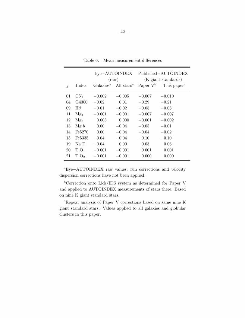
– 42 –

Table 6. Mean measurement differences

Eye−AUTOINDEX Published−AUTOINDEX

(raw) (K giant standards)

j Index Galaxiesa All starsa Paper Vb This paperc

01 CN1 −0.002 −0.005 −0.007 −0.010

04 G4300 −0.02 0.01 −0.29 −0.21

09 Hβ −0.01 −0.02 −0.05 −0.03

11 Mg1 −0.001 −0.001 −0.007 −0.007

12 Mg2 0.003 0.000 −0.001 −0.002

13 Mg b 0.00 −0.04 −0.05 −0.01

14 Fe5270 0.00 −0.04 −0.04 −0.02

15 Fe5335 −0.04 −0.04 −0.10 −0.10

19 Na D −0.04 0.00 0.03 0.06

20 TiO1 −0.001 −0.001 0.001 0.001

21 TiO2 −0.001 −0.001 0.000 0.000

aEye−AUTOINDEX raw values; run corrections and velocity

dispersion corrections have not been applied.

bCorrection onto Lick/IDS system as determined for Paper V

and applied to AUTOINDEX measurements of stars there. Based

on nine K giant standard stars.

cRepeat analysis of Paper V corrections based on same nine K

giant standard stars. Values applied to all galaxies and globular

clusters in this paper.

– 43 –

Table 11. Multiplicative corrections to bring wide slit observations onto 1.′′4 system

3.′′4 5.′′4 7.′′4

j Name correction correction correction

01 CN1 1.05 1.06 1.08

02 CN2 1.07 1.10 1.13

03 Ca4227 1.00 1.00 · · ·04 G4300 1.07 1.09 1.12

05 Fe4383 1.06 1.13 1.20

06 Ca4455 1.08 1.08 · · ·07 Fe4531 1.07 1.07 · · ·08 C24668 1.03 1.10 1.17

09 Hβ 1.06 1.06 · · ·10 Fe5015 1.07 1.07 · · ·11 Mg1 1.01 1.02 1.03

12 Mg2 1.00 1.01 1.02

13 Mg b 1.04 1.11 1.18

14 Fe5270 1.04 1.13 1.22

15 Fe5335 1.03 1.03 · · ·16 Fe5406 1.04 1.04 · · ·17 Fe5709 1.06 1.06 · · ·18 Fe5782 1.14 1.14 · · ·19 Na D 0.99 1.01 1.02

20 TiO1 1.00 1.07 1.15

21 TiO2 0.95 0.99 1.03

– 44 –

Table 12. Indices most affected by strong night-sky emission

Name Contaminants Location

G4300 Hg I λ4358 sideband, for some redshifts

Fe5406 Hg I λ5461 sideband, for some redshifts

Fe5709 Na I λλ5683,5688 sideband

Fe5782 Hg I λ5770 sideband

Hg I λ5791 central bandpass

arXiv:astro-ph/9712258v1 18 Dec 1997

TABLE 7

Fully corrected indices for galactic nuclei observed through the standard aperture

Name CN1 CN2 Ca42 G Fe43 Ca44 Fe45 C246 Hβ Fe50 Mg1 Mg2 Mg b Fe52 Fe53 Fe54 Fe57 Fe57 Na D TiO1 TiO2

G N σ σ σ σ σ σ σ σ σ σ σ σ σ σ σ σ σ σ σ σ σ

A569A 0.116 0.139 1.66 4.87 3.91 1.89 2.83 7.75 1.59 5.84 0.135 0.281 4.74 2.67 3.32 1.94 0.92 0.99 3.92 0.039 · · ·2325 2 0.019 0.024 0.37 0.40 0.72 0.32 0.49 0.73 0.24 0.66 0.007 0.009 0.31 0.28 0.41 0.28 0.22 0.26 0.28 0.008 · · ·

IC171 0.101 0.114 0.57 6.04 6.28 2.00 3.39 7.45 1.92 4.79 0.117 0.254 3.81 2.78 2.88 1.72 0.90 0.74 4.20 0.019 · · ·1339 1 0.032 0.039 0.54 0.65 1.15 0.47 0.77 1.16 0.39 1.00 0.012 0.014 0.44 0.42 0.53 0.39 0.35 0.38 0.44 0.013 · · ·

IC179 0.142 0.166 1.36 4.47 5.96 1.96 3.84 8.06 1.65 6.58 0.162 0.317 5.19 2.80 2.43 1.76 1.01 0.45 6.00 0.021 · · ·1826 1 0.026 0.031 0.46 0.52 0.94 0.40 0.64 0.94 0.31 0.84 0.009 0.011 0.38 0.35 0.46 0.34 0.29 0.32 0.36 0.010 · · ·

IC310 0.085 0.129 0.61 4.58 2.85 1.33 3.10 8.28 1.00 2.68 0.139 0.261 4.27 2.96 3.21 1.49 0.42 1.79 4.27 0.030 · · ·2266 2 0.019 0.024 0.37 0.41 0.73 0.32 0.51 0.75 0.24 0.64 0.007 0.009 0.31 0.29 0.42 0.28 0.22 0.29 0.28 0.008 · · ·

IC1696 0.102 0.150 1.79 6.13 6.24 1.92 3.75 8.03 1.52 4.33 0.138 0.287 4.55 3.58 3.01 1.75 0.94 1.06 4.70 0.050 · · ·2430 2 0.018 0.023 0.32 0.38 0.67 0.27 0.45 0.68 0.23 0.58 0.007 0.008 0.26 0.25 0.32 0.23 0.20 0.22 0.26 0.007 · · ·

IC1907 0.079 0.115 1.63 4.71 5.68 1.66 4.51 9.12 1.73 5.83 0.158 0.294 5.11 2.76 3.73 1.95 1.44 0.00 4.08 0.041 · · ·1550 1 0.028 0.035 0.55 0.59 1.08 0.46 0.74 1.08 0.36 0.96 0.011 0.013 0.44 0.40 0.59 0.40 0.34 0.30 0.41 0.011 · · ·

IC2955 0.073 0.109 1.55 6.64 5.72 1.64 3.72 8.05 1.62 4.78 0.126 0.286 4.14 2.60 1.90 1.96 0.81 0.96 4.18 0.030 · · ·2198 2 0.019 0.025 0.35 0.42 0.74 0.30 0.50 0.74 0.25 0.64 0.007 0.009 0.29 0.27 0.34 0.26 0.22 0.25 0.28 0.008 · · ·

IC4051 0.154 0.201 1.56 · · · 5.52 2.71 3.45 9.59 1.80 3.94 0.204 0.344 5.30 2.43 2.69 · · · 0.65 1.71 3.73 0.063 · · ·1136 1 0.038 0.045 0.68 · · · 1.36 0.59 0.92 1.37 0.45 1.18 0.014 0.016 0.54 0.50 0.66 · · · 0.41 0.49 0.51 0.015 · · ·

NGC80 0.119 0.138 1.53 5.52 4.33 1.66 5.07 8.38 2.18 6.73 0.163 0.339 5.40 3.94 · · · 2.11 0.87 1.13 5.18 0.040 · · ·1561 1 0.029 0.036 0.64 0.61 1.12 0.52 0.81 1.13 0.37 1.04 0.011 0.013 0.49 0.46 · · · 0.47 0.36 0.45 0.44 0.012 · · ·

NGC83 0.155 0.165 1.84 4.10 0.95 1.33 3.21 6.66 1.26 2.56 0.172 0.325 5.54 2.77 · · · 2.22 0.72 0.72 5.13 0.052 · · ·1487 1 0.031 0.036 0.60 0.60 1.11 0.49 0.77 1.12 0.37 0.97 0.011 0.013 0.47 0.42 · · · 0.44 0.35 0.41 0.43 0.012 · · ·

NGC128 0.149 0.195 0.96 4.32 6.48 1.94 2.39 8.54 1.06 4.01 0.109 0.278 4.41 3.21 2.78 1.99 0.88 0.44 4.87 0.034 · · ·2225 1 0.023 0.027 0.39 0.45 0.82 0.34 0.55 0.82 0.27 0.71 0.008 0.010 0.32 0.30 0.39 0.29 0.25 0.27 0.31 0.009 · · ·

NGC194 0.043 0.076 1.69 4.83 5.42 1.92 4.70 7.89 1.61 4.75 0.136 0.291 4.09 2.99 2.91 1.77 0.86 0.67 4.22 0.036 · · ·2836 2 0.015 0.021 0.32 0.35 0.63 0.27 0.44 0.63 0.21 0.56 0.006 0.007 0.26 0.24 0.33 0.23 0.19 0.21 0.24 0.007 · · ·

NGC205 -0.140 -0.067 0.45 0.38 1.66 0.89 1.47 1.32 4.20 · · · 0.018 0.080 0.77 1.96 1.44 1.13 0.68 0.40 2.17 0.029 0.0032807 1 0.023 0.023 0.30 0.26 0.67 0.25 0.44 0.69 0.23 · · · 0.005 0.008 0.25 0.23 0.26 0.20 0.20 0.21 0.27 0.008 0.007

NGC221 0.011 0.053 1.17 4.89 5.15 1.64 3.46 5.79 2.20 5.48 0.075 0.196 2.97 2.96 2.53 1.71 1.10 0.85 3.37 0.037 0.06119770 10 0.003 0.006 0.07 0.10 0.17 0.06 0.11 0.17 0.06 0.14 0.002 0.002 0.06 0.06 0.07 0.05 0.05 0.05 0.06 0.002 0.002

NGC224 0.164 0.216 1.64 4.99 6.22 1.98 4.15 7.92 1.72 6.17 0.150 0.331 4.89 3.33 3.04 2.12 1.07 1.15 6.60 0.053 0.09513341 12 0.005 0.006 0.09 0.11 0.19 0.08 0.12 0.19 0.06 0.18 0.002 0.002 0.07 0.07 0.09 0.06 0.06 0.06 0.07 0.002 0.002

NGC227 0.063 0.106 1.14 5.83 5.88 2.02 3.84 8.35 1.58 6.67 0.153 0.297 4.65 3.33 3.75 1.71 1.36 1.07 5.09 0.053 · · ·2884 2 0.016 0.021 0.35 0.37 0.68 0.33 0.47 0.67 0.22 0.65 0.006 0.007 0.31 0.28 0.47 0.28 0.22 0.26 0.27 0.007 · · ·

NGC315 0.126 0.172 1.21 4.69 4.10 2.10 3.75 8.92 0.87 0.44 0.131 0.285 4.81 3.27 2.81 2.54 1.37 1.60 5.05 0.032 · · ·1366 1 0.033 0.040 0.70 0.66 1.24 0.57 0.86 1.23 0.40 1.09 0.012 0.014 0.48 0.47 0.66 0.49 0.40 0.49 0.46 0.013 · · ·

NGC380 0.118 0.171 1.56 5.87 2.74 1.04 5.59 9.18 0.75 5.81 0.192 0.343 5.90 2.75 2.21 2.37 1.18 0.89 5.61 0.040 · · ·1561 1 0.029 0.035 0.60 0.61 1.09 0.49 0.79 1.11 0.35 1.00 0.011 0.013 0.49 0.42 0.58 0.46 0.35 0.42 0.43 0.012 · · ·

NOTE.—This table gives nuclear observations of galaxies through the standard slitsize 1.′′4 by 4.′′0.A 569 A: Member of galaxy cluster Abell 569. The wrong coordinates were given in Faber et al. (1989). The proper coordinates are 07h 04m 06.s6, +48◦ 43′ 34′′.IC 1907: Called CR 32 in Faber et al. (1989).

1

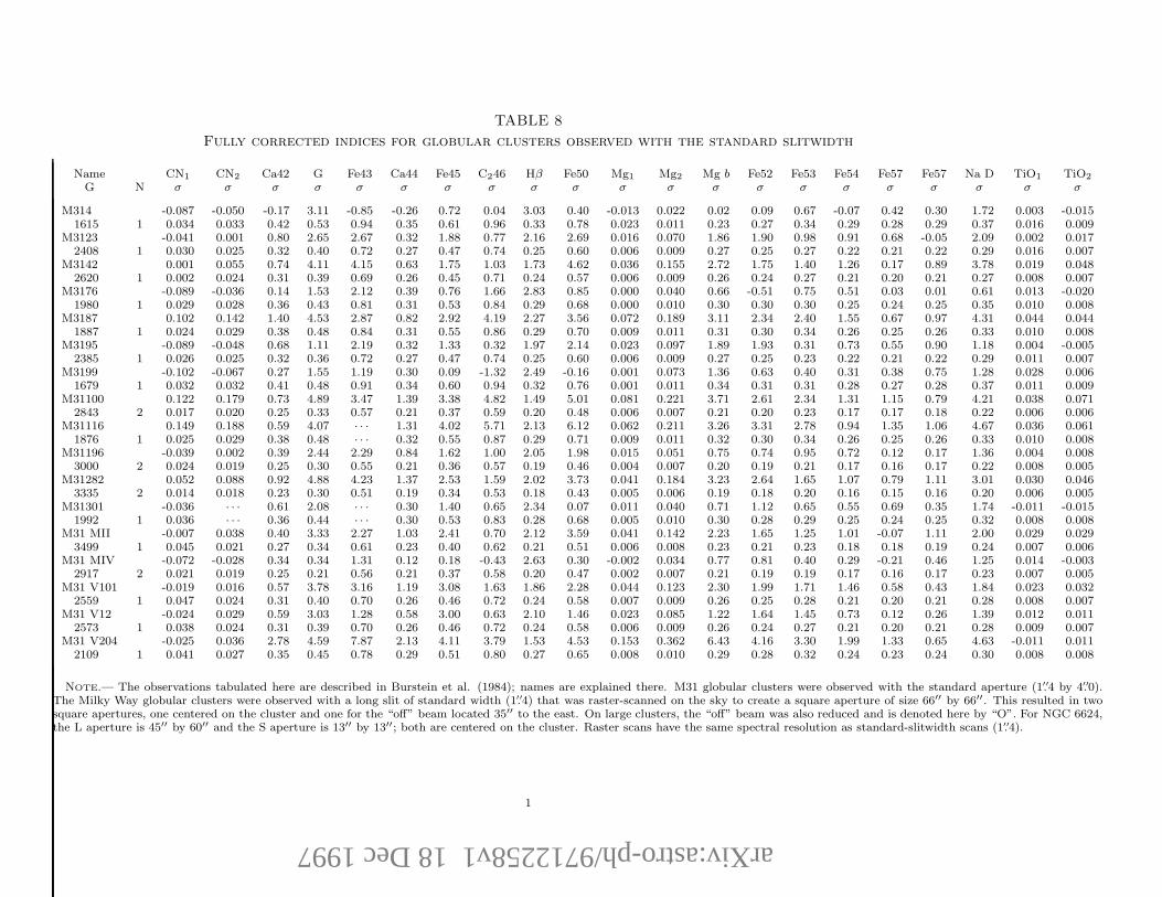
arXiv:astro-ph/9712258v1 18 Dec 1997

TABLE 8

Fully corrected indices for globular clusters observed with the standard slitwidth

Name CN1 CN2 Ca42 G Fe43 Ca44 Fe45 C246 Hβ Fe50 Mg1 Mg2 Mg b Fe52 Fe53 Fe54 Fe57 Fe57 Na D TiO1 TiO2

G N σ σ σ σ σ σ σ σ σ σ σ σ σ σ σ σ σ σ σ σ σ

M314 -0.087 -0.050 -0.17 3.11 -0.85 -0.26 0.72 0.04 3.03 0.40 -0.013 0.022 0.02 0.09 0.67 -0.07 0.42 0.30 1.72 0.003 -0.0151615 1 0.034 0.033 0.42 0.53 0.94 0.35 0.61 0.96 0.33 0.78 0.023 0.011 0.23 0.27 0.34 0.29 0.28 0.29 0.37 0.016 0.009

M3123 -0.041 0.001 0.80 2.65 2.67 0.32 1.88 0.77 2.16 2.69 0.016 0.070 1.86 1.90 0.98 0.91 0.68 -0.05 2.09 0.002 0.0172408 1 0.030 0.025 0.32 0.40 0.72 0.27 0.47 0.74 0.25 0.60 0.006 0.009 0.27 0.25 0.27 0.22 0.21 0.22 0.29 0.016 0.007

M3142 0.001 0.055 0.74 4.11 4.15 0.63 1.75 1.03 1.73 4.62 0.036 0.155 2.72 1.75 1.40 1.26 0.17 0.89 3.78 0.019 0.0482620 1 0.002 0.024 0.31 0.39 0.69 0.26 0.45 0.71 0.24 0.57 0.006 0.009 0.26 0.24 0.27 0.21 0.20 0.21 0.27 0.008 0.007

M3176 -0.089 -0.036 0.14 1.53 2.12 0.39 0.76 1.66 2.83 0.85 0.000 0.040 0.66 -0.51 0.75 0.51 0.03 0.01 0.61 0.013 -0.0201980 1 0.029 0.028 0.36 0.43 0.81 0.31 0.53 0.84 0.29 0.68 0.000 0.010 0.30 0.30 0.30 0.25 0.24 0.25 0.35 0.010 0.008

M3187 0.102 0.142 1.40 4.53 2.87 0.82 2.92 4.19 2.27 3.56 0.072 0.189 3.11 2.34 2.40 1.55 0.67 0.97 4.31 0.044 0.0441887 1 0.024 0.029 0.38 0.48 0.84 0.31 0.55 0.86 0.29 0.70 0.009 0.011 0.31 0.30 0.34 0.26 0.25 0.26 0.33 0.010 0.008

M3195 -0.089 -0.048 0.68 1.11 2.19 0.32 1.33 0.32 1.97 2.14 0.023 0.097 1.89 1.93 0.31 0.73 0.55 0.90 1.18 0.004 -0.0052385 1 0.026 0.025 0.32 0.36 0.72 0.27 0.47 0.74 0.25 0.60 0.006 0.009 0.27 0.25 0.23 0.22 0.21 0.22 0.29 0.011 0.007

M3199 -0.102 -0.067 0.27 1.55 1.19 0.30 0.09 -1.32 2.49 -0.16 0.001 0.073 1.36 0.63 0.40 0.31 0.38 0.75 1.28 0.028 0.0061679 1 0.032 0.032 0.41 0.48 0.91 0.34 0.60 0.94 0.32 0.76 0.001 0.011 0.34 0.31 0.31 0.28 0.27 0.28 0.37 0.011 0.009

M31100 0.122 0.179 0.73 4.89 3.47 1.39 3.38 4.82 1.49 5.01 0.081 0.221 3.71 2.61 2.34 1.31 1.15 0.79 4.21 0.038 0.0712843 2 0.017 0.020 0.25 0.33 0.57 0.21 0.37 0.59 0.20 0.48 0.006 0.007 0.21 0.20 0.23 0.17 0.17 0.18 0.22 0.006 0.006

M31116 0.149 0.188 0.59 4.07 · · · 1.31 4.02 5.71 2.13 6.12 0.062 0.211 3.26 3.31 2.78 0.94 1.35 1.06 4.67 0.036 0.0611876 1 0.025 0.029 0.38 0.48 · · · 0.32 0.55 0.87 0.29 0.71 0.009 0.011 0.32 0.30 0.34 0.26 0.25 0.26 0.33 0.010 0.008

M31196 -0.039 0.002 0.39 2.44 2.29 0.84 1.62 1.00 2.05 1.98 0.015 0.051 0.75 0.74 0.95 0.72 0.12 0.17 1.36 0.004 0.0083000 2 0.024 0.019 0.25 0.30 0.55 0.21 0.36 0.57 0.19 0.46 0.004 0.007 0.20 0.19 0.21 0.17 0.16 0.17 0.22 0.008 0.005

M31282 0.052 0.088 0.92 4.88 4.23 1.37 2.53 1.59 2.02 3.73 0.041 0.184 3.23 2.64 1.65 1.07 0.79 1.11 3.01 0.030 0.0463335 2 0.014 0.018 0.23 0.30 0.51 0.19 0.34 0.53 0.18 0.43 0.005 0.006 0.19 0.18 0.20 0.16 0.15 0.16 0.20 0.006 0.005

M31301 -0.036 · · · 0.61 2.08 · · · 0.30 1.40 0.65 2.34 0.07 0.011 0.040 0.71 1.12 0.65 0.55 0.69 0.35 1.74 -0.011 -0.0151992 1 0.036 · · · 0.36 0.44 · · · 0.30 0.53 0.83 0.28 0.68 0.005 0.010 0.30 0.28 0.29 0.25 0.24 0.25 0.32 0.008 0.008

M31 MII -0.007 0.038 0.40 3.33 2.27 1.03 2.41 0.70 2.12 3.59 0.041 0.142 2.23 1.65 1.25 1.01 -0.07 1.11 2.00 0.029 0.0293499 1 0.045 0.021 0.27 0.34 0.61 0.23 0.40 0.62 0.21 0.51 0.006 0.008 0.23 0.21 0.23 0.18 0.18 0.19 0.24 0.007 0.006

M31 MIV -0.072 -0.028 0.34 0.34 1.31 0.12 0.18 -0.43 2.63 0.30 -0.002 0.034 0.77 0.81 0.40 0.29 -0.21 0.46 1.25 0.014 -0.0032917 2 0.021 0.019 0.25 0.21 0.56 0.21 0.37 0.58 0.20 0.47 0.002 0.007 0.21 0.19 0.19 0.17 0.16 0.17 0.23 0.007 0.005

M31 V101 -0.019 0.016 0.57 3.78 3.16 1.19 3.08 1.63 1.86 2.28 0.044 0.123 2.30 1.99 1.71 1.46 0.58 0.43 1.84 0.023 0.0322559 1 0.047 0.024 0.31 0.40 0.70 0.26 0.46 0.72 0.24 0.58 0.007 0.009 0.26 0.25 0.28 0.21 0.20 0.21 0.28 0.008 0.007

M31 V12 -0.024 0.029 0.59 3.03 1.28 0.58 3.00 0.63 2.10 1.46 0.023 0.085 1.22 1.64 1.45 0.73 0.12 0.26 1.39 0.012 0.0112573 1 0.038 0.024 0.31 0.39 0.70 0.26 0.46 0.72 0.24 0.58 0.006 0.009 0.26 0.24 0.27 0.21 0.20 0.21 0.28 0.009 0.007

M31 V204 -0.025 0.036 2.78 4.59 7.87 2.13 4.11 3.79 1.53 4.53 0.153 0.362 6.43 4.16 3.30 1.99 1.33 0.65 4.63 -0.011 0.0112109 1 0.041 0.027 0.35 0.45 0.78 0.29 0.51 0.80 0.27 0.65 0.008 0.010 0.29 0.28 0.32 0.24 0.23 0.24 0.30 0.008 0.008

NOTE.— The observations tabulated here are described in Burstein et al. (1984); names are explained there. M31 globular clusters were observed with the standard aperture (1.′′4 by 4.′′0).The Milky Way globular clusters were observed with a long slit of standard width (1.′′4) that was raster-scanned on the sky to create a square aperture of size 66′′ by 66′′. This resulted in twosquare apertures, one centered on the cluster and one for the “off” beam located 35′′ to the east. On large clusters, the “off” beam was also reduced and is denoted here by “O”. For NGC 6624,the L aperture is 45′′ by 60′′ and the S aperture is 13′′ by 13′′; both are centered on the cluster. Raster scans have the same spectral resolution as standard-slitwidth scans (1.′′4).

1

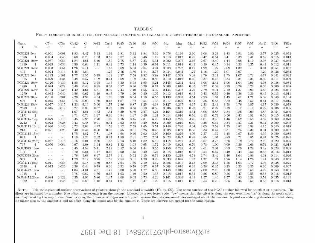
arXiv:astro-ph/9712258v1 18 Dec 1997

TABLE 9

Fully corrected indices for off-nuclear locations in galaxies observed through the standard aperture

Name CN1 CN2 Ca42 G Fe43 Ca44 Fe45 C246 Hβ Fe50 Mg1 Mg2 Mg b Fe52 Fe53 Fe54 Fe57 Fe57 Na D TiO1 TiO2

G N σ σ σ σ σ σ σ σ σ σ σ σ σ σ σ σ σ σ σ σ σ

NGC221 5ew -0.001 0.001 1.83 4.47 5.33 1.63 3.81 5.32 1.84 5.39 0.076 0.196 2.90 3.08 2.21 1.43 0.91 0.80 2.77 0.025 0.0521066 1 0.004 0.046 0.60 0.76 1.33 0.50 0.87 1.36 0.46 1.12 0.013 0.017 0.49 0.47 0.54 0.41 0.39 0.41 0.52 0.015 0.013

NGC221 10ew 0.037 0.054 1.84 4.81 5.40 1.59 2.75 5.67 2.33 5.31 0.092 0.207 3.16 2.67 2.40 1.44 0.98 1.10 2.95 0.037 0.0551319 1 0.028 0.039 0.50 0.64 1.11 0.42 0.73 1.14 0.39 0.94 0.011 0.014 0.41 0.39 0.45 0.34 0.33 0.35 0.44 0.012 0.011

NGC221 15ew 0.003 0.054 1.26 5.11 · · · 1.53 0.68 6.33 2.04 4.94 0.088 0.222 3.17 1.99 1.27 2.09 1.32 · · · 3.04 0.051 0.067405 1 0.024 0.114 1.48 1.89 · · · 1.25 2.16 3.36 1.14 2.77 0.034 0.042 1.22 1.16 1.29 1.01 0.97 · · · 1.29 0.036 0.032

NGC224 5ew 0.143 0.161 1.77 5.55 5.79 1.22 3.37 7.58 1.92 5.98 0.147 0.309 5.09 2.70 2.11 1.75 1.07 0.72 4.77 0.041 0.0921575 1 0.029 0.034 0.48 0.57 1.02 0.41 0.68 1.02 0.34 0.89 0.010 0.012 0.40 0.37 0.46 0.34 0.31 0.34 0.39 0.011 0.009

NGC224 10ew 0.126 0.139 1.85 5.17 3.55 1.47 3.30 6.58 1.95 5.21 0.145 0.292 4.41 3.08 2.44 1.96 1.04 0.91 4.98 0.038 0.0841986 1 0.024 0.029 0.40 0.48 0.85 0.34 0.57 0.86 0.29 0.74 0.009 0.010 0.33 0.32 0.39 0.29 0.26 0.28 0.33 0.009 0.008

NGC224 15ew 0.104 0.136 1.42 4.64 5.61 0.97 2.44 7.40 1.56 4.39 0.144 0.302 4.27 2.79 2.14 2.12 1.37 0.90 4.60 0.025 0.0811270 1 0.033 0.040 0.56 0.67 1.19 0.47 0.79 1.20 0.40 1.02 0.012 0.015 0.45 0.43 0.52 0.40 0.36 0.39 0.45 0.013 0.011

NGC224 20ew 0.108 0.207 2.20 4.94 4.34 1.90 3.90 6.64 1.19 6.55 0.139 0.308 4.54 2.93 1.61 1.49 0.61 1.21 5.38 0.049 0.104899 1 0.045 0.054 0.75 0.90 1.60 0.63 1.07 1.62 0.54 1.38 0.017 0.020 0.61 0.58 0.68 0.52 0.48 0.52 0.61 0.017 0.015

NGC224 35ew 0.077 0.115 1.33 5.16 5.00 1.77 2.86 6.87 1.25 4.63 0.127 0.267 4.17 2.33 2.44 1.58 0.76 0.87 4.17 0.039 0.0782689 4 0.015 0.019 0.27 0.32 0.57 0.23 0.38 0.58 0.19 0.50 0.006 0.007 0.23 0.21 0.27 0.19 0.17 0.19 0.22 0.006 0.005

NGC3115 5mj · · · · · · 1.07 4.81 4.53 1.51 3.39 8.30 2.27 4.24 0.164 0.310 4.34 3.08 2.83 2.34 0.86 0.90 4.85 0.054 0.0961171 1 · · · · · · 0.71 0.74 1.37 0.60 0.94 1.37 0.46 1.21 0.014 0.016 0.56 0.53 0.74 0.56 0.43 0.51 0.53 0.015 0.012

NGC3115 7mj 0.079 0.118 0.45 5.95 7.70 1.95 4.16 8.45 2.01 6.20 0.150 0.298 4.76 4.01 3.46 1.46 0.82 0.58 4.32 0.069 0.0702222 1 0.022 0.028 0.43 0.48 0.91 0.41 0.62 0.88 0.29 0.82 0.009 0.010 0.40 0.38 0.57 0.34 0.27 0.31 0.34 0.009 0.008

NGC3115 10mj 0.096 0.146 0.72 5.03 4.22 1.53 3.12 7.59 1.65 5.51 0.146 0.280 4.04 3.05 2.58 1.35 0.82 0.98 4.15 0.040 0.0782131 2 0.021 0.026 0.40 0.44 0.80 0.36 0.55 0.81 0.26 0.75 0.008 0.009 0.35 0.33 0.47 0.31 0.25 0.30 0.31 0.009 0.007

NGC3115 15mj · · · · · · 1.75 4.87 7.81 1.08 4.68 9.46 2.02 3.90 0.169 0.276 4.06 2.27 1.32 1.45 0.97 1.89 4.30 0.059 0.085643 1 · · · · · · 1.18 1.26 2.32 0.97 1.58 2.31 0.77 2.01 0.023 0.027 0.89 0.85 1.07 0.83 0.71 0.85 0.87 0.025 0.021

NGC3115 28mj 0.067 0.116 -0.16 6.01 2.80 1.58 2.73 8.10 1.82 6.42 0.118 0.247 4.26 3.67 3.75 0.78 -0.19 0.72 2.40 0.020 0.095767 1 0.050 0.064 0.97 1.08 1.94 0.82 1.32 1.95 0.65 1.72 0.019 0.023 0.76 0.73 1.00 0.69 0.59 0.69 0.74 0.021 0.018

NGC3379 10ew · · · · · · 0.45 4.52 5.11 2.19 3.12 6.66 1.44 3.55 0.156 0.295 4.07 2.61 2.04 0.93 0.79 1.29 3.42 0.028 0.0651011 1 · · · · · · 0.70 0.81 1.47 0.60 0.99 1.48 0.49 1.27 0.015 0.018 0.57 0.54 0.67 0.49 0.44 0.50 0.56 0.016 0.014

NGC3379 20ns · · · · · · 0.78 5.68 6.67 2.77 3.11 5.52 3.15 6.73 0.130 0.279 4.53 2.74 3.46 1.46 1.64 -0.86 4.38 0.014 0.026369 1 · · · · · · 1.79 2.12 3.78 1.52 2.54 3.81 1.29 3.26 0.038 0.046 1.43 1.37 1.71 1.26 1.14 1.26 1.44 0.043 0.035

NGC4111 8mj 0.011 0.056 0.80 5.18 4.89 0.88 2.94 7.36 2.19 4.62 0.086 0.207 3.13 2.69 3.33 1.58 1.04 0.77 4.96 0.038 0.0752248 1 0.013 0.026 0.36 0.44 0.78 0.30 0.52 0.79 0.27 0.67 0.008 0.010 0.29 0.28 0.35 0.25 0.23 0.25 0.30 0.009 0.007

NGC4472 10ew · · · · · · 1.04 4.81 4.51 1.72 3.00 5.20 1.77 6.86 0.148 0.316 4.81 2.00 2.78 1.30 0.67 0.53 4.22 0.053 0.0611045 1 · · · · · · 0.78 0.82 1.50 0.66 1.03 1.49 0.50 1.36 0.015 0.017 0.62 0.56 0.80 0.56 0.47 0.55 0.57 0.016 0.013

NGC4472 20ns 0.084 0.122 0.35 4.96 5.86 1.47 3.08 6.65 0.73 4.29 0.161 0.306 4.41 1.57 1.46 1.57 0.83 0.28 3.54 0.035 0.1011022 2 0.038 0.048 0.74 0.80 1.48 0.64 1.01 1.47 0.47 1.29 0.015 0.017 0.60 0.54 0.70 0.55 0.45 0.52 0.56 0.016 0.013

NOTE.— This table gives off-nuclear observations of galaxies through the standard slitwidth (1.′′4 by 4.′′0). The name consists of the NGC number followed by an offset or a position. Theoffsets are indicated by a number (the offset in arcseconds from the nucleus) followed by a two-letter code: “ew” means that the offset is along the east-west line; “ns” is along the north-southline; “mj” is along the major axis; “mn” is along the minor axis. Signs are not given because the data are sometimes averaged about the nucleus. A position code x, y denotes an offset alongthe major axis by the amount x and an offset along the minor axis by the amount y. These are likewise not signed for the same reason.

1

arXiv:astro-ph/9712258v1 18 Dec 1997

TABLE 10

Fully corrected indices for non-standard aperture observations of galaxies and M31 globular clusters

Name width CN1 CN2 Ca42 G Fe43 Ca44 Fe45 C246 Hβ Fe50 Mg1 Mg2 Mg b Fe52 Fe53 Fe54 Fe57 Fe57 Na D TiO1 TiO2

G N length σ σ σ σ σ σ σ σ σ σ σ σ σ σ σ σ σ σ σ σ σ

M31 V29 3.′′4 0.112 0.156 0.41 7.87 7.29 1.94 2.28 4.39 1.78 4.38 0.081 0.212 4.54 1.97 0.97 1.00 0.74 · · · 3.26 0.031 0.0681630 1 4′′ 0.027 0.033 0.42 0.54 0.93 0.35 0.61 0.96 0.32 0.78 0.010 0.012 0.35 0.33 0.35 0.28 0.27 · · · 0.37 0.011 0.009

M31 V92 2.′′2 -0.025 0.015 1.08 4.39 3.00 0.69 3.55 1.33 1.79 2.28 0.026 0.104 1.76 1.68 0.99 0.31 0.87 · · · 1.60 0.020 0.0112314 1 4′′ 0.039 0.026 0.33 0.42 0.74 0.28 0.48 0.76 0.26 0.62 0.006 0.009 0.28 0.26 0.28 0.23 0.22 · · · 0.30 0.009 0.007

IC783 3.′′4 -0.006 0.018 1.14 2.48 5.31 1.92 3.58 3.94 2.75 4.26 0.040 0.120 1.40 1.89 1.52 0.74 0.94 1.04 1.69 0.018 · · ·1018 1 4′′ 0.060 0.048 0.63 0.76 1.39 0.54 0.93 1.42 0.48 1.19 0.013 0.017 0.52 0.50 0.57 0.44 0.41 0.44 0.55 0.016 · · ·

IC1131 3.′′4 0.024 0.115 1.86 · · · 3.62 -0.03 3.13 3.76 3.07 2.76 0.079 0.211 2.02 3.61 1.89 · · · · · · 0.54 2.86 0.025 0.050735 1 6′′ 0.042 0.065 0.85 · · · 1.88 0.72 1.24 1.91 0.65 1.59 0.019 0.023 0.70 0.67 0.77 · · · · · · 0.59 0.73 0.021 0.018

IC3303 5.′′4 -0.120 -0.141 -0.81 0.02 1.83 0.27 0.78 1.65 3.06 1.01 0.021 0.080 0.96 1.17 -0.20 0.57 0.09 · · · 0.48 0.030 0.0331183 1 6′′ 0.042 0.042 0.56 0.07 1.23 0.47 0.81 1.25 0.43 1.04 0.010 0.015 0.45 0.43 1.07 0.38 0.36 · · · 0.54 0.014 0.012

IC3470 3.′′4 0.107 0.146 1.14 3.83 2.47 0.22 4.42 1.33 2.13 7.12 0.051 0.179 2.47 2.26 1.50 0.63 1.54 0.96 1.29 0.030 0.047986 1 4′′ 0.041 0.050 0.66 0.81 1.44 0.56 0.96 1.47 0.50 1.24 0.014 0.018 0.54 0.52 0.59 0.46 0.43 0.46 0.58 0.016 0.014

IC3652 5.′′4 -0.149 -0.140 1.14 4.12 1.59 1.97 4.21 2.59 2.48 2.75 0.071 0.137 2.17 4.61 3.96 1.41 1.19 · · · 0.69 0.019 0.049838 1 6′′ 0.056 0.057 0.76 0.94 1.66 0.64 1.10 1.70 0.58 1.41 0.017 0.021 0.62 0.61 0.73 0.52 0.50 · · · 0.70 0.019 0.016

IC3653 3.′′4 0.028 0.070 1.61 5.57 5.94 1.62 5.41 7.00 2.11 6.61 0.091 0.251 4.48 3.73 1.87 2.82 1.76 1.08 2.91 0.036 0.0511393 1 4′′ 0.025 0.038 0.60 0.64 1.17 0.50 0.81 1.16 0.39 1.04 0.011 0.013 0.46 0.45 0.56 0.46 0.37 0.42 0.44 0.013 0.011

IC3672 5.′′4 0.017 0.038 1.33 3.85 2.08 2.29 2.82 7.05 2.27 5.59 0.055 0.210 3.92 2.39 2.89 1.67 0.26 · · · 2.25 0.044 0.056898 1 6′′ 0.031 0.054 0.71 0.88 1.56 0.60 1.03 1.59 0.54 1.33 0.015 0.019 0.59 0.56 0.67 0.49 0.46 · · · 0.61 0.017 0.015

NGC128 35mj 3.′′4 0.163 0.179 -0.19 · · · 6.15 0.46 2.72 4.33 2.21 7.20 0.116 0.265 4.67 1.96 3.14 · · · · · · 1.45 5.08 0.046 · · ·835 1 16′′ 0.050 0.058 0.80 · · · 1.72 0.68 1.15 1.73 0.59 1.49 0.018 0.021 0.65 0.62 0.77 · · · · · · 0.57 0.66 0.019 · · ·

NGC185 3.′′4 -0.138 -0.102 -0.28 1.60 · · · 0.04 2.46 1.44 2.40 2.76 0.032 0.106 1.34 1.40 1.23 0.80 1.00 · · · 2.27 0.014 0.0081415 1 16′′ 0.036 0.036 0.47 0.55 · · · 0.39 0.68 1.07 0.36 0.87 0.010 0.013 0.39 0.36 0.40 0.32 0.31 · · · 0.41 0.012 0.010

NGC185 10ew 3.′′4 -0.132 -0.135 0.53 2.25 · · · 1.76 2.39 3.17 1.49 3.41 0.019 0.125 2.72 -0.14 1.10 0.73 1.23 · · · 3.11 0.014 0.059422 1 16′′ 0.108 0.109 1.40 1.72 · · · 1.18 2.05 3.22 1.09 2.62 0.026 0.040 1.17 1.31 1.20 0.95 0.92 · · · 1.23 0.037 0.031

NGC185 25ew 3.′′4 -0.170 -0.074 0.27 4.08 · · · -0.75 4.56 1.59 2.32 4.77 0.028 0.096 2.06 2.29 1.34 0.27 1.37 · · · 1.29 0.022 0.069557 1 16′′ 0.081 0.083 1.07 1.36 · · · 0.90 1.57 2.46 0.84 2.00 0.021 0.030 0.89 0.84 0.93 0.73 0.70 · · · 0.97 0.028 0.024

NGC185 35ew 3.′′4 -0.126 -0.097 0.42 3.22 · · · 1.54 2.61 4.78 3.38 1.02 0.057 0.096 1.45 1.01 2.33 -0.61 0.50 · · · 0.62 0.011 -0.005492 1 16′′ 0.093 0.094 1.21 1.52 · · · 1.01 1.77 2.77 0.95 2.26 0.027 0.034 1.00 0.94 1.08 0.82 0.79 · · · 1.15 0.033 0.026

NGC205 17mj 3.′′4 -0.155 -0.103 0.26 0.88 3.45 0.47 1.34 0.29 3.12 2.23 0.017 0.096 1.43 1.73 1.06 0.94 0.94 · · · 1.22 0.004 0.0221719 1 16′′ 0.030 0.031 0.40 0.43 0.90 0.34 0.59 0.92 0.31 0.75 0.007 0.011 0.33 0.32 0.34 0.27 0.26 · · · 0.36 0.013 0.009

NGC205 54mj 3.′′4 -0.080 -0.059 0.72 2.27 · · · 0.76 2.32 1.60 2.34 · · · 0.013 0.090 1.55 2.17 1.11 0.86 -0.06 · · · 1.03 0.001 0.0171521 1 16′′ 0.036 0.034 0.44 0.54 · · · 0.37 0.64 1.01 0.34 · · · 0.007 0.012 0.37 0.35 0.38 0.30 0.29 · · · 0.40 0.011 0.010

NGC221 25ns 1.′′4 -0.025 0.011 0.95 4.68 · · · 1.43 3.31 5.03 1.99 4.47 0.070 0.184 3.42 1.83 1.47 1.67 1.01 1.19 2.82 0.045 0.0581998 2 16′′ 0.039 0.026 0.33 0.42 · · · 0.28 0.49 0.76 0.26 0.62 0.007 0.009 0.28 0.26 0.29 0.23 0.22 0.23 0.29 0.008 0.007

NGC221 45ns 1.′′4 -0.023 0.011 1.00 4.31 5.80 1.24 2.92 6.50 2.18 3.99 0.073 0.178 3.26 2.64 1.69 1.51 1.24 1.07 2.82 0.067 0.0641724 2 16′′ 0.046 0.029 0.38 0.48 0.84 0.32 0.55 0.86 0.29 0.71 0.009 0.011 0.31 0.30 0.33 0.26 0.25 0.26 0.33 0.009 0.008

NOTE.— This table contains all observations of galaxies (plus two M31 globular clusters) made through non-standard apertures (raster scans of Milky Way globular clusters are given in Table 7).Slitwidth and length are given in the third column. “Scan” denotes a raster scan made with a 1.′′4 × 16′′ slit covering a square aperture 16′′ by 16′′ centered on the nucleus. These scans resemble thelarger raster scans of globulars in Table 7 and have the same spectral resolution as standard-slitwidth scans (1.′′4). They were taken to determine the aperture correction to nuclear σ (see Davies etal. 1987).The naming convention for off-nuclear locations in this table is the same as in Table 8. Special names are:M31 V29 and M31 V92: Two M31 globular clusters observed with a wide slit. See notes to Table 7 for further information.NGC 3379 61se: Aperture located 61′′ south-east of the nucleus.

1