Page 1

SC/63/SH3

Strategies to obtain a new abundance estimate for Antarctic blue whales: a feasibility study NATALIE KELLY1,2, MICHAEL C. DOUBLE2, DAVID PEEL1,2, MARK BRAVINGTON1,2AND NICK GALES2 1 CSIRO Mathematical and Information Sciences and Wealth from Oceans National Research Flagship, Castray Esplanade, Hobart, Tasmania, 7000, Australia 2 Australian Marine Mammal Centre, Australian Antarctic Division, DSEWPaC, Hobart, Australia

ABSTRACT

During the twentieth century some 330,000 Antarctic blue whales (Balaenoptera musculus intermedia) were killed by commercial whaling operations and were close to extinction when hunting was banned in 1964. Subsequent abundance estimates derived from IDCR/SOWER line transect surveys between 1981 and 1998 provide low precision abundance estimates and suggest that the population is increasing, but remains less than 5% of their pre-exploitation abundance. Following the cessation of SOWER surveys in 2010 there is currently no strategy or means to obtain further abundance estimates for Antarctic blue whales but renewed effort could be conducted as a part of the multi-national, circumpolar Southern Ocean Research Partnership (SORP).Here, based on relatively simple calculations, we assess possible strategies for obtaining a new abundance estimate against the effort required and the likely precision of the estimates. We assessed three strategies (line-transect, mark recapture (MR), and hotspot-based MR). We found that to detect positive population growth from a new IDCR/SOWER type survey in 2013/14 with a power of 0.8 requires relatively little effort (2 to 4 vessel-seasons) because the new estimate can have relatively low precision (due to the trend provided by previous abundance estimates). To deliver a more precise abundance estimate (CV of 0.25 or lower), then the effort required from an IDCR/SOWER-type line-transect survey is approximately 9 vessel-seasons. A MR strategy (with structured, dedicated IDCR/SOWER vessel behaviour) required much greater effort (approximately 40 vessel-seasons) to deliver an abundance estimate with a CV of 0.25. However, the effort required drops considerably if vessels targeted areas with higher sightings rates and stayed within 200km of the ice edge. For MR to be the most cost-effective (least effort) option sighting rates would need to be enhanced through the use of passive acoustics. KEYWORDS: SOWER, MARK-RECAPTURE, DISTANCE SAMPLING, PASSIVE ACOUSTICS, SORP

INTRODUCTION

The blue whale is an iconic species. Reaching over 30m in length it is the largest animal to have existed on Earth. Two subspecies occur in the Southern Hemisphere , the Antarctic (or true) blue whale (Balaenoptera musculus intermedia) and the pygmy blue whale (B. m. brevicauda). The pygmy blue whale tends to be smaller (max. 24m) and predominantly remains in lower attitudes throughout the year. During the austral summer Antarctic blue whales feed in the krill rich waters close to the Antarctic continent where, during the late 19th and 20th centuries some 330,000 Antarctic blue whales were killed, first by shore-based operations and then by the pelagic catcher and factory ships. Close to extinction, in 1964 the International Whaling Commission banned the hunting of blue whales although they were still caught by illegal Soviet whaling operations until 1973 (Branch et al., 2004). Our understanding of the impact of the whaling era on Antarctic blue whale population is predominantly based on two sources of information: catch data derived from the logbooks of whaling vessels and from circumpolar cetacean sightings surveys. Circumpolar sighting surveys were initiated in 1978 as the International Decade of Cetacean Research (IDCR) and later Southern Ocean Whale Ecosystem Research (SOWER) initiatives (Branch & Butterworth, 2001). The IDCR/SOWER surveys were largely funded by the Japanese Government but operated under the direction of the International Whaling Commission. The surveys usually involved two ships conducting line-transect surveys from the Antarctic ice-edge up to 60oS. These vessels conducted three circumpolar surveys (CPI, CPII and CPIII) that were completed in 2004, although further regional surveys went on until 2010. While the catch data can provide yearly catch distribution and magnitude as well as often detailed information on the animals caught (including size, sex, pregnancy status, stomach contents etc.), the data from sightings surveys can generate estimates of circumpolar abundance, trends and distribution. The low sighting rates of Antarctic blue whales from the IDCR/SOWER surveys generated abundance estimates with low precision which in turn hampered early efforts to assess population trend (see Table 1, Branch & Butterworth, 2001; Gerrodette, 1995 #5374). Later, Branch et al. (2004) estimated trend using catch and sightings data in a Bayesian

Page 2

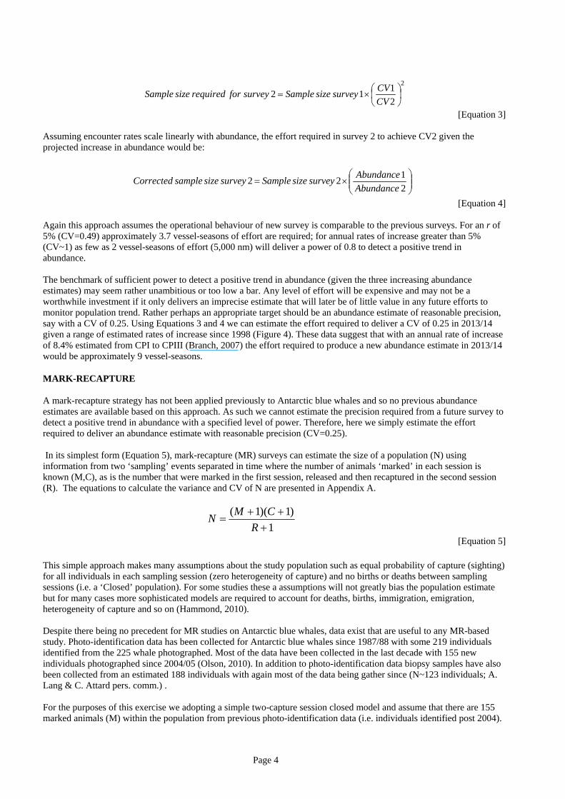
modelling framework which estimated that the circumpolar Antarctic blue whale population decreased from pre-exploitation abundance of 239 000 (95% Bayesian interval of 202 000 – 311 000) to a low of around 360 individuals (95% Bayesian interval of 150 – 840) in the early 1970s. This represents a population decline of greater than 99%. This study also determined that from the lowest abundance the population had increased at a mean rate of 7.3% per year (95% CI 1.4-11.6%) and the estimated abundance in 1996 was 1,700 individuals (CV = 0.51, 95% CI 860 - 2900). On completion of CPIII Branch (2007), using only the IDCR/SOWER sightings data and a maximum likelihood approach (Branch et al., 2004), estimated the rate of increase to be 8.2% per year (95% CI 1.6-14.8%) with point abundance estimates for the mid-year of each circumpolar survey to be 453 (CV = 0.4), 559 (CV = 0.47) and 2,280 (CV = 0.36) for 1981 (CPI), 1988 (CPII) and 1998 (CPIII) respectively (cf. Table 1). The associated sightings rate (number of pods per 1000 nm) reflected this increased abundance from 0.44 (CPI) to 0.67 (CPII) to 1.48 (CPIII). Branch (2007), noted that these circumpolar abundance estimates are likely to be underestimates of the true population size given individuals may have been north of 60°S during the summer months when the IDCR/SOWER surveys were conducted. After the completion of the CPIII survey in 2003/04 further SOWER sightings surveys have been conducted but not with the specific aim of generating a new circumpolar dataset; the surveys focused largely in IWC Management Areas IV and V. In 2009 the Japanese Government indicated the 2009/10 would be the last SOWER survey after 32 years of effort covering some 216,000 nm and 4,100 vessel days (International Whaling Commission, 2009). With the cessation of the SOWER surveys there are now no large scale, formal cetacean sightings surveys operating in Antarctic waters and there is no strategy to monitor the recovery or otherwise of Antarctic blue whales. The loss of such surveys is of great concern given the predicted climatic and ecological changes in the Antarctic sea ice ecosystem (Nicol et al., 2008) and the recent and very rapid expansion of the Antarctic krill fishery (e.g. Nicol et al., 2011; Trathan & Agnew, 2010). Clearly these processes and activities may impact on all cetacean species that predominantly feed within the Antarctic ecosystem but arguably Antarctic blue whales are most vulnerable given the magnitude of depletion and their slower rate of recovery compared to other baleen whales (Branch et al., 2004). In 2009 the Southern Ocean Research Partnership (SORP) program was initiated within the International Whaling Commission to promote collaborative cetacean research through coordination, cooperation and data sharing between research groups and national Antarctic programs (SORP, 2009). Several projects have now been initiated under the SORP banner including studies focussing on the acoustic monitoring of fin and blue whales, niche portioning among baleen whales and mixing of humpback whale populations in Antarctic waters (Childerhouse, 2010). Without SOWER it seems that SORP is now the only program that could deliver the high-investment, multinational initiative that would be required to deliver a new abundance estimate for Antarctic blue whales. Here, using broad assumptions and relatively simple calculations, we investigate potential strategies to obtain a new abundance estimate for Antarctic blue whales as part of a potential multinational SORP initiative. In considering feasibility, we explore the how effort (both in term of the total number of vessels required and the effort of each vessel within an austral summer season) affects the precision of abundance estimates (low CVs) and whether the levels of precision will allow trend in abundance to be estimated with a reasonable level of statistical power. These considerations are made in the context of projections of circumpolar abundance, as estimated by Branch (2007). The strategies assessed (line-transect, mark recapture, and hotspot-based mark recapture) were those with a well established theoretical basis and considered the most likely candidates to deliver a precise abundance estimates with the least effort (i.e. lowest financial cost).

FEASABILITY ASSESSMENT

In the study we simply assess feasibility in terms of the effort required to deliver a specified level of statistical power to detect a positive population trend (line-transect) or a specified level of precision for an abundance estimate (line-transect and mark-recapture). Effort is measured in vessel-seasons where in one vessel-season the ship is ‘on-effort’ for 2,500 nautical miles (as if it were on a SOWER survey). Final measures of effort are usually reported assuming an 8.2% annual rate of increase using the point estimated derived from the last abundance estimate (CPIII) and that the future survey would operate in the 2013/14 season. We have chosen this season because logistically it would be the first opportunity to initiate any structured, multinational survey effort of this scale. Although this implies a single season of effort we would not expect all the effort required to occur in a single year due to the difficulties in coordinating polar programs and the long and variable lead-in times for voyage planning. Effort might more reasonably be expected to be spread over a period of up to about three years (perhaps 2013/14 to 2015/16).

Page 3

LINE TRANSECT SIGHTINGS SURVEY

The most obvious, established strategy to obtain a new circumpolar abundance estimate for Antarctic blue whales is to repeat a visual line transect survey similar to the IDCR/SOWER surveys. During the CPI, CPII and CPIII surveys, two vessels travelled along transects within a given longitudinal block within a single season; moving to another longitudinal block the following season; total distances ‘on effort’ for each circumpolar survey are given in Table 1. In addition to estimating circumpolar abundance from the three CP surveys, Branch (2007) estimated the annual rate of change for Antarctic blue whales using an exponential growth model,

tt rNN )1(ˆ

0 ,

[Equation 1] where t is the number of years after the starting year; Nt is the projected population at time t; N0 is the estimated population at time 0 (i.e., at 1981, the first time point for which there is a circumpolar abundance estimate); r is the estimated annual rate of increase. Although the values of the parameters in this model can be estimated relatively simply Branch (2007) recognised that the geographical distribution of whales changes from year to year, generating what is known as ‘additional variance’ or ‘process error’. To account for this additional variance (assumed to be equal for all three CP abundance estimates) Branch (2007) derived a convenient negative log likelihood expression for generating maximum likelihood parameter estimates,

t addt

ttaddt

CVCV

NNCVCVL

)(2

)ˆln(lnlnln

22

222

,

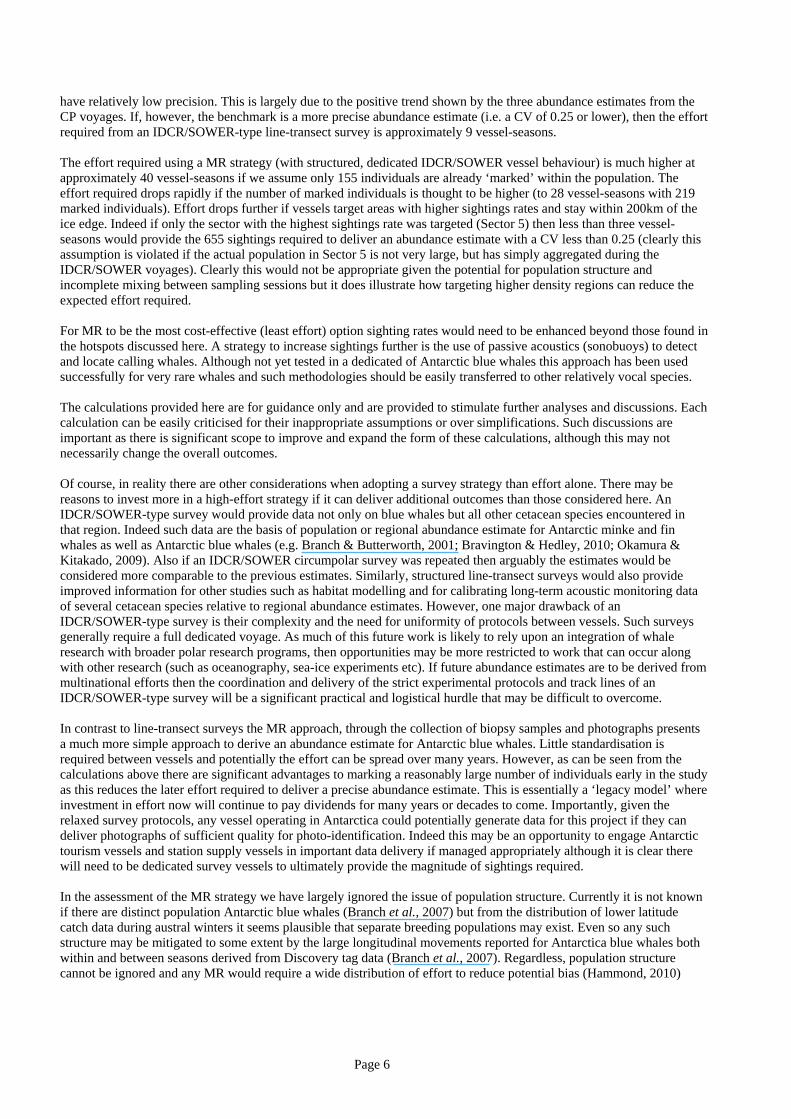
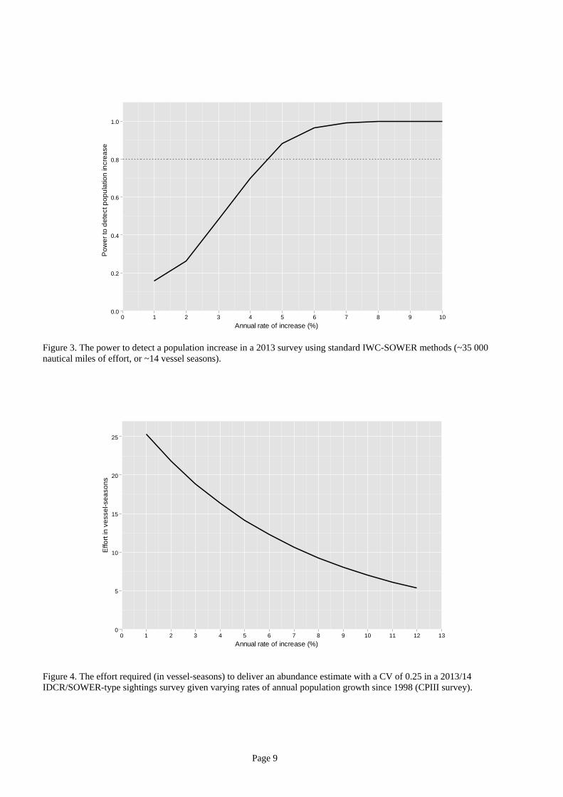
[Equation 2] where CVadd is the additional variance, and CVt is the variance of each survey. This maximum likelihood approach can be used to estimate the power to detect a positive rate of change in abundance of Antarctic blue whales given the three abundance estimates from the CP surveys and a new estimate from a future 2013/14 SOWER-type survey (of 35,000 nm effort or 14 vessel-seasons). A power of 0.8 is considered reasonable in experimental design (e.g. Thomas & Juanes, 1996) and is the benchmark used here. As abundance estimates are log-normally distributed, an algebraic method to calculate power would introduce bias (Zhou & Gao, 1997) therefore we used Monte Carlo simulation. First, abundance estimates for a future survey (in 2013/14) were generated for a range of annual rates of change (1 to 12%). Then the CV for the estimate was calculated based on the assumption that if the new survey has similar effort to past surveys then the only factor affecting the CV of a new survey is abundance itself; as such the CV will be a function of 1/sqrt(abundance) (Burnham et al., 1980; Gerrodette, 1987). Therefore using the CVs of previous abundance estimates we crudely estimated the CV of a future survey given the estimated abundance at the time of the survey (see Figure 2 for fitted non-linear function). Finally the simulated abundance estimates, along with their associated projected CVs, were then fed into the negative log likelihood expression (together with the abundance estimates and CVs from CPI-CPIII) to derive estimates of r. Out of the above maximum likelihood analysis, we can also derive a hessian matrix which allows the standard errors of the parameter estimates to be calculated. With each estimated r, and its standard error, we can then perform a simple Wald test to formally test whether r is significantly greater than zero (i.e., a one-sided test). Compared against a standard Normal distribution, the p-value of this test is returned. Over a large number of simulation runs (~ 5000), the proportion of p-values that are less than a nominated significance level (0.05 is a reasonable Type I error level) is an estimate of the power of the future survey. Figure 3 shows the relationship between power and the annual rate of increase; even if the rate of increase is as low as 4.5% there is still sufficient power (> 0.8 probability) to detect a positive population trend from a SOWER-type survey in 2013. It is important to note, however, that given that a positive rate of change has already been estimated in Antarctic blue whales using results of CPI-CPIII (Branch, 2007; Branch et al., 2004) it would take a very low future abundance estimate (i.e., negative from 1998 estimate), accompanied by a high CV to greatly decrease the probability of detecting a positive rate of change over the four abundance estimates. This process can also be used to estimate the maximum allowable CV that will still deliver a power of 0.8 for a set annual rate of population increase (r). Using this approach, if r is less that 4% then the precision required to deliver a power of 0.8 is not achievable regardless of effort. If r is 5% then the maximum allowable CV is 0.49; at rates of increase over 5% the maximum allowable CVs approach 1. These CVs were then used to estimate the effort required using Equation 3.

Page 4

2

2

112

CV

CVsurveysizeSamplesurveyforrequiredsizeSample

[Equation 3]

Assuming encounter rates scale linearly with abundance, the effort required in survey 2 to achieve CV2 given the projected increase in abundance would be:

2

122

Abundance

AbundancesurveysizeSamplesurveysizesampleCorrected

[Equation 4]

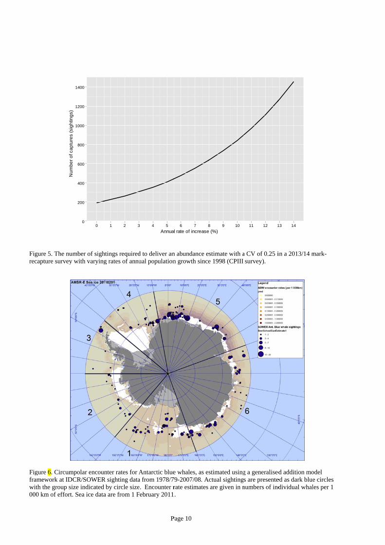
Again this approach assumes the operational behaviour of new survey is comparable to the previous surveys. For an r of 5% (CV=0.49) approximately 3.7 vessel-seasons of effort are required; for annual rates of increase greater than 5% (CV~1) as few as 2 vessel-seasons of effort (5,000 nm) will deliver a power of 0.8 to detect a positive trend in abundance. The benchmark of sufficient power to detect a positive trend in abundance (given the three increasing abundance estimates) may seem rather unambitious or too low a bar. Any level of effort will be expensive and may not be a worthwhile investment if it only delivers an imprecise estimate that will later be of little value in any future efforts to monitor population trend. Rather perhaps an appropriate target should be an abundance estimate of reasonable precision, say with a CV of 0.25. Using Equations 3 and 4 we can estimate the effort required to deliver a CV of 0.25 in 2013/14 given a range of estimated rates of increase since 1998 (Figure 4). These data suggest that with an annual rate of increase of 8.4% estimated from CPI to CPIII (Branch, 2007) the effort required to produce a new abundance estimate in 2013/14 would be approximately 9 vessel-seasons.

MARK-RECAPTURE

A mark-recapture strategy has not been applied previously to Antarctic blue whales and so no previous abundance estimates are available based on this approach. As such we cannot estimate the precision required from a future survey to detect a positive trend in abundance with a specified level of power. Therefore, here we simply estimate the effort required to deliver an abundance estimate with reasonable precision (CV=0.25). In its simplest form (Equation 5), mark-recapture (MR) surveys can estimate the size of a population (N) using information from two ‘sampling’ events separated in time where the number of animals ‘marked’ in each session is known (M,C), as is the number that were marked in the first session, released and then recaptured in the second session (R). The equations to calculate the variance and CV of N are presented in Appendix A.

1

)1)(1(

R

CMN

[Equation 5]

This simple approach makes many assumptions about the study population such as equal probability of capture (sighting) for all individuals in each sampling session (zero heterogeneity of capture) and no births or deaths between sampling sessions (i.e. a ‘Closed’ population). For some studies these a assumptions will not greatly bias the population estimate but for many cases more sophisticated models are required to account for deaths, births, immigration, emigration, heterogeneity of capture and so on (Hammond, 2010). Despite there being no precedent for MR studies on Antarctic blue whales, data exist that are useful to any MR-based study. Photo-identification data has been collected for Antarctic blue whales since 1987/88 with some 219 individuals identified from the 225 whale photographed. Most of the data have been collected in the last decade with 155 new individuals photographed since 2004/05 (Olson, 2010). In addition to photo-identification data biopsy samples have also been collected from an estimated 188 individuals with again most of the data being gather since (N~123 individuals; A. Lang & C. Attard pers. comm.) . For the purposes of this exercise we adopting a simple two-capture session closed model and assume that there are 155 marked animals (M) within the population from previous photo-identification data (i.e. individuals identified post 2004).

Page 5

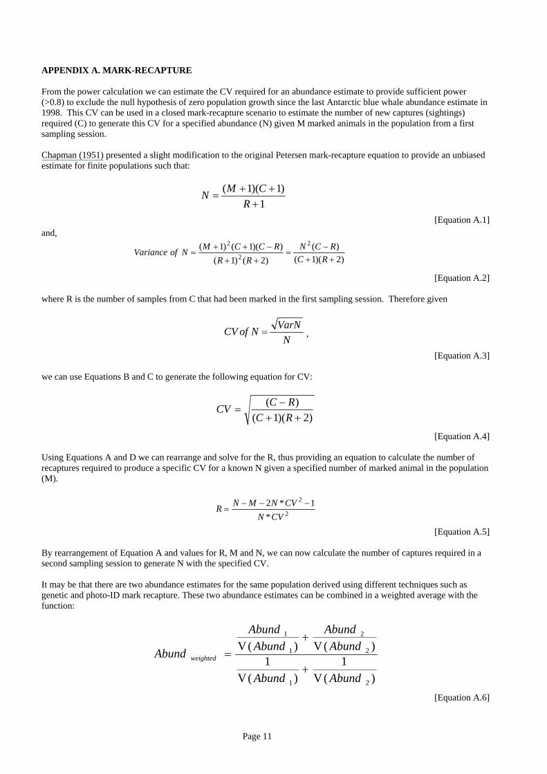
We adopt this model here for simplicity but to complete this assessment we intend to use a simulation-based approach which will allow us to explore the effect of using more complex open models and multi-year capture-recapture histories (cf. Cooch & White, 2010; Devineau et al., 2006) . If we are seeking a new abundance estimate with a CV of 0.25 and M is 155 then we can calculate R (the number of required recaptures) from Equation A.5 (Appendix A) for a given annual rate of increase (r) since 1998 (which provides N from Equation 1). Hence we can also calculate C, the number of captures/sightings required from the future survey by rearrangement of Equation 5. The relationship between the annual rate of increase and the number of recaptures required to provide a CV of 0.25 is presented in Figure 5. We find that 655 sightings (C) would be required in the second sampling session for an annual rate of increase of 8.2% since CPIII (Branch, 2007). Next we must estimate how much effort is required to sight 655 Antarctic blue whales. Here we assume all individuals sighted are also marked for the purpose of a MR analysis and that there is a linear relationship between overall sighting rates and circumpolar abundance. During the third IDCR/SOWER circumpolar survey, overall sighting rates were around 1.48 sightings of Antarctic blue whale schools per 1,000 nm of effort (Branch, 2007). Therefore, if the circumpolar abundance increased by 8.2% per year, the sighting rate in 2013 would be around 5 pods per 1000 nm of effort with an average of 1.48 individuals per pod (Branch et al., 2004). Therefore if the ships followed track lines similar to the IDCR/SOWER survey vessels (moving evenly and systematically around the Antarctic coast line up to 60°S) we estimate approximate 40 vessel-seasons of effort would be required to sight 655 blue whales. If we assumed M to be 219 (the number of individuals in the photo-identification catalogue) then the effort required drops to 28 vessel seasons. Although we have only focused on one method of individual identification (photo-identification) it is possible to combine population estimates derived from multiple sources (e.g. genetic and photo-ID mark-recapture programs ) in a weighted average estimate (See Appendix A).

SPATIAL MODELLING, PASSIVE ACCOUSTICS AND BLUE WHALE ‘HOTSPOTS’

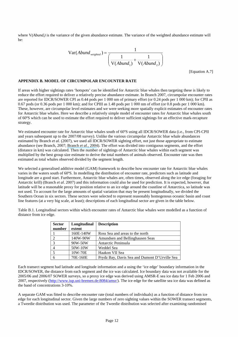
Although appropriate for the aims of the IDCR/SOWER cruises there is no requirement for random or systematic distribution of effort for robust MR methods. Therefore it may be possible to increase encounter rates by focussing effort in areas where blue whales are more frequently sighted (hotspots). Using IDCR/SOWER effort and sightings data (see Figure 6) we constructed a simple spatial model to estimate sighting rates in smaller regions within the overall IDCR/SOWER study area (Appendix B). From this model we can estimate the expected sighting rate for particular regions and relative to the ice edge. For example if the survey ship operated within 200km of the ice edge then the mean circumpolar sightings rate would be expected to 1 animal per 1000km of effort. However this value varies greatly between regions rising to 17 animals per 1000km in Sector 5 (Figure 6). Thus effort can be directed towards areas with greater sightings rates. If Sectors 1, 5 and 6 were targeted within 200km of the ice edge then 24 vessel-seasons would be required to provide the 655 sightings necessary to generate an abundance estimate with a CV of 0.25 (if r = 0.82 and M = 155). Again, if we assume M to be 219 then this drops to about 17 vessel seasons. Sightings rates within hotspots may be improved further using passive acoustics. Male (and possibly female) Antarctic blue whales are vocal while in their feeding grounds and their sounds travel long distances (McDonald et al., 2006; Sirovic et al., 2007; Sirovic et al., 2009; Stafford et al., 2004). These calls therefore provide a method to locate individuals and groups. Gedamke and Robinson (2010) acoustically detected Antarctic blue whales and deployed multiple sonobuoys to triangulate the position of the calling whale(s). While obtaining multiple acoustic detections their work was conducted during systematic line-transect sightings surveys and so they did have the opportunity to close on calling whales. Although not a proven for blue whales, acoustic detection and monitoring is an effective technique for very rare species such as North Pacific right whales (Clark et al., 2010; Wade et al., 2006). Thus pilot studies are required to assess the effectiveness of this approach for Antarctic blue whales and the degree to which encounter rates might be maximised. Even if we assume a relatively modest outcome that passive acoustics doubled encounter rates then, in addition to targeting areas of higher density, the effort required to achieve some 600 sightings would fall below 10 vessel-seasons.

DISCUSSION

This paper presents several strategies for delivering an updated abundance estimate for Antarctic blue whale. The strategies were assessed either by calculating the effort required (measured in vessel-seasons, assuming an ‘on-effort track length of 2,500 nm) to detect positive population growth in 2013/14 with a power of 0.8 or simply the effort required to produce an abundance estimate with a CV of 0.25 or lower. If the benchmark was simply a power of 0.8 to detect positive population growth then very little effort is required (2 to 4 vessel-seasons) because the new estimate can

Page 6

have relatively low precision. This is largely due to the positive trend shown by the three abundance estimates from the CP voyages. If, however, the benchmark is a more precise abundance estimate (i.e. a CV of 0.25 or lower), then the effort required from an IDCR/SOWER-type line-transect survey is approximately 9 vessel-seasons. The effort required using a MR strategy (with structured, dedicated IDCR/SOWER vessel behaviour) is much higher at approximately 40 vessel-seasons if we assume only 155 individuals are already ‘marked’ within the population. The effort required drops rapidly if the number of marked individuals is thought to be higher (to 28 vessel-seasons with 219 marked individuals). Effort drops further if vessels target areas with higher sightings rates and stay within 200km of the ice edge. Indeed if only the sector with the highest sightings rate was targeted (Sector 5) then less than three vessel-seasons would provide the 655 sightings required to deliver an abundance estimate with a CV less than 0.25 (clearly this assumption is violated if the actual population in Sector 5 is not very large, but has simply aggregated during the IDCR/SOWER voyages). Clearly this would not be appropriate given the potential for population structure and incomplete mixing between sampling sessions but it does illustrate how targeting higher density regions can reduce the expected effort required. For MR to be the most cost-effective (least effort) option sighting rates would need to be enhanced beyond those found in the hotspots discussed here. A strategy to increase sightings further is the use of passive acoustics (sonobuoys) to detect and locate calling whales. Although not yet tested in a dedicated of Antarctic blue whales this approach has been used successfully for very rare whales and such methodologies should be easily transferred to other relatively vocal species. The calculations provided here are for guidance only and are provided to stimulate further analyses and discussions. Each calculation can be easily criticised for their inappropriate assumptions or over simplifications. Such discussions are important as there is significant scope to improve and expand the form of these calculations, although this may not necessarily change the overall outcomes. Of course, in reality there are other considerations when adopting a survey strategy than effort alone. There may be reasons to invest more in a high-effort strategy if it can deliver additional outcomes than those considered here. An IDCR/SOWER-type survey would provide data not only on blue whales but all other cetacean species encountered in that region. Indeed such data are the basis of population or regional abundance estimate for Antarctic minke and fin whales as well as Antarctic blue whales (e.g. Branch & Butterworth, 2001; Bravington & Hedley, 2010; Okamura & Kitakado, 2009). Also if an IDCR/SOWER circumpolar survey was repeated then arguably the estimates would be considered more comparable to the previous estimates. Similarly, structured line-transect surveys would also provide improved information for other studies such as habitat modelling and for calibrating long-term acoustic monitoring data of several cetacean species relative to regional abundance estimates. However, one major drawback of an IDCR/SOWER-type survey is their complexity and the need for uniformity of protocols between vessels. Such surveys generally require a full dedicated voyage. As much of this future work is likely to rely upon an integration of whale research with broader polar research programs, then opportunities may be more restricted to work that can occur along with other research (such as oceanography, sea-ice experiments etc). If future abundance estimates are to be derived from multinational efforts then the coordination and delivery of the strict experimental protocols and track lines of an IDCR/SOWER-type survey will be a significant practical and logistical hurdle that may be difficult to overcome. In contrast to line-transect surveys the MR approach, through the collection of biopsy samples and photographs presents a much more simple approach to derive an abundance estimate for Antarctic blue whales. Little standardisation is required between vessels and potentially the effort can be spread over many years. However, as can be seen from the calculations above there are significant advantages to marking a reasonably large number of individuals early in the study as this reduces the later effort required to deliver a precise abundance estimate. This is essentially a ‘legacy model’ where investment in effort now will continue to pay dividends for many years or decades to come. Importantly, given the relaxed survey protocols, any vessel operating in Antarctica could potentially generate data for this project if they can deliver photographs of sufficient quality for photo-identification. Indeed this may be an opportunity to engage Antarctic tourism vessels and station supply vessels in important data delivery if managed appropriately although it is clear there will need to be dedicated survey vessels to ultimately provide the magnitude of sightings required. In the assessment of the MR strategy we have largely ignored the issue of population structure. Currently it is not known if there are distinct population Antarctic blue whales (Branch et al., 2007) but from the distribution of lower latitude catch data during austral winters it seems plausible that separate breeding populations may exist. Even so any such structure may be mitigated to some extent by the large longitudinal movements reported for Antarctica blue whales both within and between seasons derived from Discovery tag data (Branch et al., 2007). Regardless, population structure cannot be ignored and any MR would require a wide distribution of effort to reduce potential bias (Hammond, 2010)

Page 7

In the presentation of the hotspot strategy we introduced the possibility of using passive acoustic techniques to increase sightings rates. This has great potential and it is hoped that trials of this approach will be conducted in the 2011/12 season on an Australian vessel as part of the SORP collaboration. However, in a MR approach this is likely to generate individual heterogeneity in sighting probabilities in that it is thought only males call and it is probable some males will call more loudly, more often and for longer periods than others. Clearly this approach will have to be adopted with caution and with a clear vision of how the data will be analysed given the potential biases this technique is likely to introduce. In this paper we have not attempted to predict what effort can be delivered; that is, the number of vessels that could be provided by the international community for an endeavour such as this. Access to vessels for polar research is managed through a variety of mechanism in different countries with determinants including the excellence of the research, the relevance to national priorities and political aspects of regional and international engagement. It is obvious that any strategy, even one requiring less than ten vessel-seasons over several years, represents a significant investment in Antarctic research and will require considerable buy in from many Governments and their polar programs. Although ambitious, funding such an initiative is achievable if sufficient planning and collaboration occur. The SORP, which includes at least 12 nations with active polar programs, is an ideal mechanism for a project of this scale. A focused effort on understanding the current status and behaviour of the Antarctic blue whale builds well on the legacy of the multi-decadal ; IDCR/SOWER cruises which made a significant contribution to non-lethal whale research in the Southern Ocean (International Whaling Commission, 2009).

ACKNOWLEDGEMENTS

We thank Trevor Branch and attendees of the SORP Steering Committee meeting in Paris (April 2011) for valuable discussions and guidance during the development and preparation of this manuscript.

TABLES

Table 1. Estimates of Antarctic blue whale abundance, from (Branch 2007), for each IDCR/SOWER circumpolar survey; survey mid-year indicated in first column.

Year Abundance CV 95% CI Total survey effort (nm) Sighting rate (pods /1000 nm)

1981 (CPI) 453 0.4 (250, 1 200) 41 558 0.44 1988 (CPII) 559 0.47 (270, 1 700) 31 007 0.67 1998 (CPIII) 2 280 0.36 (860, 4 200) 35 411 1.48

Page 8

FIGURES

Figure 1. Estimated and projected abundance estimate for Antarctic blue whales. The black lines are population estimates for CPI, CPII and CPIII, respectively (as given in Branch (2007)); dotted black lines are the upper and lower 95% confidence intervals on those estimates, see Table 1 for values. The solid grey line represents projected abundance based on an estimated rate of increase of 8.2% per year from 1998 (Branch 2007) and the associated confidence interval (grey dotted lines).

Figure 2. The estimated CVs for a SOWER-type survey in 2013 as a function of abundance. The relationship is CV = 10.46*(1/sqrt(abundance)).

Year

Est

ima

ted

an

d p

roje

cte

d a

bu

nd

an

ce

0

5000

10000

15000

20000

25000

30000

35000

40000

1980 1985 1990 1995 2000 2005 2010 2015

Estimated and projected abundance

CV

(%

)

0.00

0.05

0.10

0.15

0.20

0.25

0.30

0.35

0.40

0.45

0.50

0.55

0 1000 2000 3000 4000 5000 6000 7000 8000

Page 9

Figure 3. The power to detect a population increase in a 2013 survey using standard IWC-SOWER methods (~35 000 nautical miles of effort, or ~14 vessel seasons).

Figure 4. The effort required (in vessel-seasons) to deliver an abundance estimate with a CV of 0.25 in a 2013/14 IDCR/SOWER-type sightings survey given varying rates of annual population growth since 1998 (CPIII survey).

Annual rate of increase (%)

Po

we

r to

de

tect

po

pu

latio

n in

cre

ase

0.0

0.2

0.4

0.6

0.8

1.0

0 1 2 3 4 5 6 7 8 9 10

Annual rate of increase (%)

Effo

rt in

ve

sse

l-se

aso

ns

0

5

10

15

20

25

0 1 2 3 4 5 6 7 8 9 10 11 12 13

Firec

Fifrawi00

gure 5. The nucapture survey

gure 6. Circumamework at IDith the group s00 km of effor

Nb

ft

(i

hti

)

umber of sighy with varying

mpolar encounDCR/SOWERsize indicated rt. Sea ice data

Nu

mb

er

of c

ap

ture

s (s

igh

ting

s)

0

200

400

600

800

1000

1200

1400

0

htings requiredg rates of annu

nter rates for AR sighting data

by circle sizea are from 1 F

1 2 3

P

d to deliver anual population

Antarctic bluea from 1978/7e. Encounter rFebruary 2011

Annua3 4 5

Page 10

n abundance en growth since

e whales, as es79-2007/08. Arate estimates .

l rate of increase6 7 8

stimate with ae 1998 (CPIII

stimated usingctual sightingare given in n

e (%)8 9 10

a CV of 0.25 isurvey).

g a generaliseds are presente

numbers of ind

11 12 1

in a 2013/14 m

d addition moed as dark bluedividual whal

13 14

mark-

odel e circles les per 1

Page 11

APPENDIX A. MARK-RECAPTURE

From the power calculation we can estimate the CV required for an abundance estimate to provide sufficient power (>0.8) to exclude the null hypothesis of zero population growth since the last Antarctic blue whale abundance estimate in 1998. This CV can be used in a closed mark-recapture scenario to estimate the number of new captures (sightings) required (C) to generate this CV for a specified abundance (N) given M marked animals in the population from a first sampling session. Chapman (1951) presented a slight modification to the original Petersen mark-recapture equation to provide an unbiased estimate for finite populations such that:

1

)1)(1(

R

CMN

[Equation A.1]

and,

)2)(1(

)(

)2()1(

))(1()1( 2

2

2

RC

RCN

RR

RCCMN of Variance

[Equation A.2]

where R is the number of samples from C that had been marked in the first sampling session. Therefore given

N

VarNNofCV ,

[Equation A.3] we can use Equations B and C to generate the following equation for CV:

)2)(1(

)(

RC

RCCV

[Equation A.4] Using Equations A and D we can rearrange and solve for the R, thus providing an equation to calculate the number of recaptures required to produce a specific CV for a known N given a specified number of marked animal in the population (M).

2

2

*

1*2

CVN

CVNMNR

[Equation A.5]

By rearrangement of Equation A and values for R, M and N, we can now calculate the number of captures required in a second sampling session to generate N with the specified CV. It may be that there are two abundance estimates for the same population derived using different techniques such as genetic and photo-ID mark recapture. These two abundance estimates can be combined in a weighted average with the function:

)(V

1

)(V

1)(V)(V

21

2

2

1

1

AbundAbund

Abund

Abund

Abund

Abund

Abund weighted

[Equation A.6]

Page 12

where V(Abundi) is the variance of the given abundance estimate. The variance of the weighted abundance estimate will be:

)(V1

)(V1

1)(Var

21 AbundAbund

Abundweighted

[Equation A.7]

APPENDIX B. MODEL OF CIRCUMPOLAR ENCOUNTER RATE

If areas with higher sightings rates ‘hotspots’ can be identified for Antarctic blue whales then targeting these is likely to reduce the effort required to deliver a relatively precise abundance estimate. In Branch 2007, circumpolar encounter rates are reported for IDCR/SOWER CPI as 0.44 pods per 1 000 nm of primary effort (or 0.24 pods per 1 000 km); for CPII as 0.67 pods (or 0.36 pods per 1 000 km); and for CPIII as 1.48 pods per 1 000 nm of effort (or 0.8 pods per 1 000 km). These, however, are circumpolar level estimates and we were seeking more spatially explicit estimates of encounter rates for Antarctic blue whales. Here we describe a relatively simple model of encounter rates for Antarctic blue whales south of 60ºS which can be used to estimate the effort required to deliver sufficient sightings for an effective mark-recapture strategy. We estimated encounter rate for Antarctic blue whales south of 60ºS using all IDCR/SOWER data (i.e., from CPI-CPII and years subsequent up to the 2007/08 survey). Unlike the various circumpolar Antarctic blue whale abundances estimated by Branch et al. (2007), we used all IDCR/SOWER sighting effort, not just those appropriate to estimate abundance (see Branch, 2007; Branch et al., 2004). The effort was divided into contiguous segments, and the effort (distance in km) was calculated. Then the number of sightings of Antarctic blue whales within each segment was multiplied by the best group size estimate to derive the total numbers of animals observed. Encounter rate was then estimated as total whales observed divided by the segment length. We selected a generalised additive model (GAM) framework to describe how encounter rate for Antarctic blue whales varies in the waters south of 60ºS. In modelling the distribution of encounter rate, predictors such as latitude and longitude are a good start. Furthermore, Antarctic blue whales are, often times, observed along the ice edge (foraging for Antarctic krill) (Branch et al. 2007) and this information could also be used for prediction. It is expected, however, that latitude will be a reasonable proxy for position relative to an ice edge around the coastline of Antarctica, so latitude was not used. To account for the large amounts of spatial variation that may be present longitudinally, we divided the Southern Ocean in six sectors. These sectors were selected to represent reasonably homogenous oceanic basin and coast line features (at a very big scale, at least); descriptions of each longitudinal sector are given in the table below. Table B.1. Longitudinal sectors within which encounter rates of Antarctic blue whales were modelled as a function of distance from ice edge.

Sector number

Longitudinal extent

Description

1 160E-140W Ross Sea and areas to the north 2 140W-90W Amundsen and Bellinghausen Seas 3 90W-50W Antarctic Peninsula 4 50W-10W Weddel Sea 5 10W-70E Haakon VII Sea 6 70E-160E Prydz Bay, Davis Sea and Dumont D’Urville Sea

Each transect segment had latitude and longitude information and a using the ‘ice edge’ boundary information in the IDCR/SOWER, the distance from each segment and the ice was calculated. Ice boundary data was not available for the 2005/06 and 2006/07 SOWER surveys, so a proxy ice edge was derived using AMSR-E sea ice data for 1 Feb 2006 and 2007, respectively (http://www.iup.uni-bremen.de:8084/amsr/). The ice edge for the satellite sea ice data was defined as the band of concentrations 3-10%. A separate GAM was fitted to describe encounter rate (total numbers of individuals) as a function of distance from ice edge for each longitudinal sector. Given the large numbers of zero sighting values within the SOWER transect segments, a Tweedie distribution was used. The parameter of the Tweedie distribution was selected after examining randomised

quto A reagrFetra

Ficorepmi

uantile residuamake the long

prediction griasonable date id point. To b

ebruary 2011; averse.

gure B.1. Shaoncentration) fpresent 95% Biddle left: 90ºW

als (results notgitudinal secto

id that coveredfrom which t

be considered aareas of sea i

apes of the funfor observed SBayesian confW-50ºW; mid

t shown). Theors contiguou

d the circumpto derive satella valid predicce concentrati

nctional formsSOWER encoufidence intervaddle right: 50º

P

segment lengus. These indiv

olar region uplite sea ice dattion grid poinion 0-3% are c

s for the smootunter rates (Cals. Upper lefW-10ºW; low

Page 13

gth was used avidual GAMs

p to 60S was pata to give ‘disnt, the point haconsidered are

thed covariateCPI-CPIII and ft: longitudina

wer left: 10ºW

as an offset terare shown in

produced. 1 Fstance to ice edad to be in waeas where a no

e ‘distance froyears subsequ

al sector 160ºE-70ºE; lower r

rm in the GAMFigure x.

ebruary 2011 dge’ informatter and not coon-ice strengt

om ice edge’ (uent to 2007/0E-140ºW; uppright: 70ºE-16

M. No attemp

was selected tion for each povered by >3%thened vessel

(defined as 3-108 survey). Daper right: 140º60ºE.

t was made

as a prediction % ice as of 1

might

10% sea ice ashed lines W-90ºW;

Page 14

REFERENCES

Branch, T.A. 2007. Abundance of Antarctic blue whales south of 60°S from three complete circumpolar sets of surveys. Journal of Cetacean Research

and Management, 9: 253–262. Branch, T.A. and Butterworth, D.S. 2001. Estimates of abundance south of 60°S for cetacean species sighted frequently on the 1978/79 to 1997/98

IWC/IDCR-SOWER sighting surveys. . Journal of Cetacean Research and Management Special Issue, 3: 251-270. Branch, T.A., Matsuoka, K. and Miyashita, T. 2004. Evidence for increase in Antarctic blue whales based on Bayesian modelling. Marine Mammal

Science, 20: 726-754. Branch, T.A., Stafford, K.M., Palacios, D.M., Allison, C., Bannister, J.L., Burton, C.L.K., Cabrera, E., Carlson, C.A., Galletti Vernazzani, B., Gill,

P.C., Hucke-Gaete, R., Jenner, K.C.S., Jenner, M.N.M., Matsuoka, K., Mikhalev, Y.A., Miyashita, T., Morrice, M.G., Nishiwaki, S., Sturrock, V.J., Tormosov, D., Anderson, R.C., Baker, A.N., Best, P.B., Borsa, P., Brownell Jr, R.L., Childerhouse, S., Findlay, K.P., Gerrodette, T., Ilangakoon, A.D., Joergensen, M., Kahn, B., Ljungblad, D.K., Maughan, B., McCauley, R.D., McKay, S., Norris, T.F. and Rankin, S. 2007. Past and present distribution, densities and movements of blue whales Balaenoptera musculus in the Southern Hemisphere and northern Indian Ocean. Mammal Review, 37: 116-175.

Bravington, M.V. and Hedley, S.L. 2010 Antarctic minke whale abundance from the SPLINTR model: some 'reference' dataset results and 'preferred' estimates from the second and third IDCR/SOWER surveys. Paper SC/62/IA12 presented the IWC Scientific Committee, 2010 (unpublished).

Burnham, K.P., Anderson, D.R. and Laake, J.L. 1980. Estimation of density from line transect sampling of biological populations. Wildlife Monographs, 72: 1-202.

Chapman, D.G. 1951. Some properties of the hypergeometric distribution with applications to zoological censuses. University of California Publications in Statistics, 1: 131-160.

Childerhouse, S. 2010 Project outlines for the Southern Ocean Research Partnership. Paper SC/62/O10 presented to the IWC Scientific Committee, 2010 (unpublished).

Clark, C.W., Brown, M.W. and Corkeron, P. 2010. Visual and acoustic surveys for North Atlantic right whales, Eubalaena glacialis, in Cape Cod Bay, Massachusetts, 2001-2005: Management implications. Marine Mammal Science, 26: 837-854.

Cooch, E. and White, G. 2010 Program MARK: a gentle introduction. Devineau, O., Choquet, R., Lebrton, J.-D., DEVINEAU, O., CHOQUET, R.M. and JEAN-DOMINIQUE LEBRETON 2006. Planning capture–

recapture studies: straightforward precision, bias, and power calculations. Wildlife Bulletin, 34: 1028-1035. Gedamke, J. and Robinson, S.M. 2010. Acoustic survey for marine mammal occurrence and distribution off East Antarctica (30-80 degrees E) in

January-February 2006. Deep-Sea Research Part II-Topical Studies in Oceanography 57(9-10 Special Issue, 57: 968-981. Gerrodette, T. 1987. A power analysis for detecting trends. Ecology, 68: 1364-1372. Hammond, P.S. 2010 Estimating the abundance of marine mammals. In: Marine Mammal Ecology and Conservation: A Handbook of Techniques eds.

Boyd I.L., Bowen D.W., Iverson S.J.). Oxford University Press. International Whaling Commission 2009 Report of the Scientific Committee Paper SC/61/Rep1, IWC Scientific Committee, 2009 (unpublished). McDonald, M.A., Mesnick, S.L. and Hildebrand, J.A. 2006. Biogeographic characterisation of blue whale song worldwide: using song to identify

populations. Journal of Cetacean Research and Management, 8: 55–65. Nicol, S., Foster, J. and Kawaguchi, S. 2011. The fishery for Antarctic krill – recent developments. Fish and Fisheries: 1-9. Nicol, S., Worby, A. and Leaper, R. 2008. Changes in the Antarctic sea ice ecosystem: potential effects on krill and baleen whales [Review]. Marine &

Freshwater Research, 59: 361-382. Okamura, H. and Kitakado, T. 2009 Abundance estimates and diagnostics of Antarctic minke whales from the historical IDCR/SOWER survey data

using the OK method. 58pp. Paper SC/61/IA6 presented to the IWC Scientific Committee, 2009 (unpublished). Olson, P.A. 2010 Status of blue whale photo-identification from IWC IDCR/SOWER cruises 1987/1988 to 2008-2009. Paper SC/62/SH29, presented

to the IWC Scientific Committee (unpublished). SC/62/SH29. Sirovic, A., Hildebrand, J.A. and Wiggins, S.M. 2007. Blue and fin whale call source levels and propagation range in the Southern Ocean. Journal of

the Acoustical Society of America, 122: 1208-1215. Sirovic, A., Hildebrand, J.A., Wiggins, S.M. and Thiele, D. 2009. Blue and fin whale acoustic presence around Antarctica during 2003 and 2004.

Marine Mammal Science, 25: 125-136. SORP 2009 Report of the planning workshop of the Southern Ocean Research Partnership (SORP), Sydney, Australia 23-26 March 2009. 63pp. Paper

SC/61/O16 presented to the IWC Scientific Committee, 2009 (unpublished). Stafford, K.M., Bohnenstiehl, D.R., Tolstoy, M., Chapp, E., Mellinger, D.K. and Moore, S.E. 2004. Antarctic-type blue whale calls recorded at low

latitudes in the Indian and eastern Pacific Oceans. Deep-Sea Research Part I-Oceanographic Research Papers, 51: 1337-1346. Thomas, L. and Juanes, F. 1996. The importance of statistical power analysis: an example from Animal Behaviour. Animal Behaviour, 52: 856–859. Trathan, P.N. and Agnew, D. 2010. Climate change and the Antarctic marine ecosystem: an essay on management implications. Antarctic Science, 22:

387-398. Wade, P., Heide-Jorgensen, M.P., Shelden, K., Barlow, J., Carretta, J., Durban, J., Leduc, R., Munger, L., Rankin, S., Sauter, A. and Stinchcomb, C.

2006. Acoustic detection and satellite-tracking leads to discovery of rare concentration of endangered North Pacific right whales. Biology Letters, 2: 417-419.

Zhou, X.-H. and Gao, S. 1997. Confidence intervals for the log-normal mean. Statistics in Medicine, 16: 783-790.