STL-based Analysis of TRAIL-induced Apoptosis Challenges the Notion of Type I/Type II Cell Line...

STL-based Analysis of TRAIL-induced ApoptosisChallenges the Notion of Type I/Type II Cell LineClassificationSzymon Stoma1., Alexandre Donze2.¤, Francois Bertaux1, Oded Maler2, Gregory Batt1*

1 INRIA Paris-Rocquencourt, Le Chesnay, France, 2 VERIMAG, CNRS and the University of Grenoble, Gieres, France

Abstract

Extrinsic apoptosis is a programmed cell death triggered by external ligands, such as the TNF-related apoptosis inducingligand (TRAIL). Depending on the cell line, the specific molecular mechanisms leading to cell death may significantly differ.Precise characterization of these differences is crucial for understanding and exploiting extrinsic apoptosis. Cells showdistinct behaviors on several aspects of apoptosis, including (i) the relative order of caspases activation, (ii) the necessity ofmitochondria outer membrane permeabilization (MOMP) for effector caspase activation, and (iii) the survival of cell linesoverexpressing Bcl2. These differences are attributed to the activation of one of two pathways, leading to classification ofcell lines into two groups: type I and type II. In this work we challenge this type I/type II cell line classification. We encodethe three aforementioned distinguishing behaviors in a formal language, called signal temporal logic (STL), and use it toextensively test the validity of a previously-proposed model of TRAIL-induced apoptosis with respect to experimentalobservations made on different cell lines. After having solved a few inconsistencies using STL-guided parameter search, weshow that these three criteria do not define consistent cell line classifications in type I or type II, and suggest mutants thatare predicted to exhibit ambivalent behaviors. In particular, this finding sheds light on the role of a feedback loop betweencaspases, and reconciliates two apparently-conflicting views regarding the importance of either upstream or downstreamprocesses for cell-type determination. More generally, our work suggests that these three distinguishing behaviors shouldbe merely considered as type I/II features rather than cell-type defining criteria. On the methodological side, this workillustrates the biological relevance of STL-diagrams, STL population data, and STL-guided parameter search implemented inthe tool Breach. Such tools are well-adapted to the ever-increasing availability of heterogeneous knowledge on complexsignal transduction pathways.

Citation: Stoma S, Donze A, Bertaux F, Maler O, Batt G (2013) STL-based Analysis of TRAIL-induced Apoptosis Challenges the Notion of Type I/Type II Cell LineClassification. PLoS Comput Biol 9(5): e1003056. doi:10.1371/journal.pcbi.1003056

Editor: Stanislav Shvartsman, Princeton University, United States of America

Received November 16, 2012; Accepted March 26, 2013; Published May 9, 2013

Copyright: � 2013 Stoma et al. This is an open-access article distributed under the terms of the Creative Commons Attribution License, which permitsunrestricted use, distribution, and reproduction in any medium, provided the original author and source are credited.

Funding: This work was supported by the research grant Syne2arti ANR-10-COSINUS-007 from the French National Research Agency. The funders had no role instudy design, data collection and analysis, decision to publish, or preparation of the manuscript.

Competing Interests: The authors have declared that no competing interests exist.

* E-mail: [email protected]

. These authors contributed equally to this work.

¤ Current address: EECS Department, University of California Berkeley, Berkeley, California, United States of America.

Introduction

Apoptosis, a major form of programmed cell death, plays a

crucial role in shaping organs during development and controls

homeostasis and tissue integrity throughout life [1,2]. Moreover

defective apoptosis is often involved in cancer development and

progression [3]. Apoptosis can be triggered by intrinsic or extrinsic

stimuli. Intrinsic apoptosis is triggered in case of cell damage (e.g.

stress, UV radiation) or cell malfunction (e.g. oncogene activation).

Extrinsic apoptosis is initiated by the presence of extracellular

death ligands, such as Fas ligand (FasL), Tumor Necrosis Factor

(TNF), or TRAIL [2]. Because the latter has a unique ability to

trigger apoptosis in various cancer cell lines without significant

toxicity toward normal cells, TRAIL-induced apoptosis has been

the focus of extensive studies [1].

The effects of TRAIL application can be significantly different

from one cell line to another [4–6]. The current understanding is

that cell death results from the activation of one of two parallel

pathways, leading to the classification of cell lines into two distinct

cell types. In type I cells, effector caspases are directly activated by

initiator caspases. Mitochondria outer membrane permeabiliza-

tion (MOMP) is not required to generate lethal levels of caspase

activity. In type II cells, the activation of initiator caspases triggers

MOMP that in turn triggers effector caspases activation. MOMP

is required for cell death. This necessity of mitochondrial pathway

activation to undergo apoptosis is often referred as type II phenotype,

in contrast to type I phenotype where MOMP is a side effect of

apoptosis.

Many models of apoptosis, based on different mathematical

formalisms, ranging from logical models to differential equation

systems, have been proposed so far [2,6–21]. To investigate the

molecular origins of the two above-mentioned distinct phenotypes,

Aldridge and colleagues developed a model describing key

biochemical steps in TRAIL-induced apoptosis: extrinsic apoptosis

reaction model (EARM1.4) [6]. EARM1.4 is an extension of a

model developed to capture cell-to-cell variability in apopotosis of

PLOS Computational Biology | www.ploscompbiol.org 1 May 2013 | Volume 9 | Issue 5 | e1003056

HeLa cells [15,16]. In [6], the authors tested the hypothesis that

the distinct cell behaviors can be explained solely by measured

differences in protein concentrations before stimulation among

different cell lines. Cell line models share the same set of ordinary

differential equations and kinetic parameters, but possess specific

protein contents at the initial state (i.e. before TRAIL application).

These differences in the initial concentrations of a dozen of key

apoptotic proteins are consistent with quantitative immunoblotting

measurements. Then the authors use an abstract criterion that

measures the influence of changes in initial protein concentrations

on the future states of the system (i.e. divergence of trajectories):

the direct finite-time Lyapunov exponent (DLE). They show that

this criterion defines a partition of the state space that preserves

known differences between phenotypes: type I and type II cells are

associated to distinct regions in the state space [6]. The DLE-

induced partition can be graphically represented as 2D slices of the

high dimensional state space called DLE diagrams [6,22]. As

shown in [6], DLE diagrams are intuitive tools to predict the effect

of mutations on cell type. However, the connection between the

abstract DLE notion and cell phenotypes remains elusive: why

type I and type II cells correspond to two different regions

separated by a third one having high DLE values? Understanding

this relationship is important to evaluate the general applicability

of the proposed approach. Moreover in [6], the authors also

probed the functioning of the apoptotic pathways in different cell

lines and for different mutants using three different experimental

methods: clonogenic assays, microscopy imaging and flow

cytometry measurements of immunostained cells. These experi-

ments probe subtly different aspects of the interplay of different

pathway components, and most notably on the role of MOMP in

the apoptotic response: death/survival following TRAIL stimula-

tion of derived cell lines overexpressing Bcl2 (Property 1),

synchronous/sequential activation of initiator and effector cas-

pases (Property 2), and effector caspase activation prior/posterior

to MOMP (Property 3). However, the authors do not test the

consistency of EARM predictions with the detailed experimental

information they provide.

In this work we address the two above-mentioned problems by

using a formal language, signal temporal logic (STL). STL was

originally developed for monitoring purposes to specify the

expected behavior of physical systems, including notably the order

of physical events as well as the temporal distance between them

[23]. Like other temporal logics and formal verification frame-

works [24–31], it has been applied to the analysis of biomolecular

networks [32,33]. In particular, because it allows expressing in a

rigorous manner transient behaviors of dynamical systems, one

can encode as STL properties various cellular responses observed

with different experimental methods and associated to type I/II

phenotypes. Because STL properties have a quantitative interpre-

tation, describing how robustly behaviors of the system satisfy or

violate the property, STL diagrams can be constructed analo-

gously to DLE diagrams. However, since STL diagrams are each

associated to a specific STL property their interpretations do not

suffer from ambiguities. Moreover, one can benefit from the

expressive power of the STL language to encode detailed

experimental information and thoroughly test the consistency of

EARM with the various observations (Figure 1).

We report three findings. Firstly, our results highlighted that the

three experimental methods proposed in [6] to investigate the

importance of MOMP for cell death from three different

perspectives, each suggesting a type I/II distinguishing criterion,

do not lead to consistent cell line classifications. For example the

DXIAP HCT116 cell line should be classified as type II based on

Properties 1 and 2, and as type I based on Property 3. This

challenges the well-posedness of the type I/II notion. Secondly,

using our systematic approach, we found several inconsistencies

between model predictions and actual observations. Taking again

advantage of the quantitative interpretation of STL properties, we

searched for valid parameters using a cost function that is minimal

when all properties are consistent with experimental data and

state-of-the-art global optimization tools. Inconsistencies have

been resolved simply by modifying a few parameters, thus showing

that there is no need for structural changes in the model. Thirdly,

our findings reconciliate the apparently contradictory views

expressed by Scaffidi and colleagues [5] and Aldridge and

colleagues [6] about the origins of type I and II phenotypes.

Indeed, Scaffidi, Barnhart and colleagues suggest that the initiator

caspase activation capabilities are the main determinants of the

type I/II phenotype of a cell line [5,34], whereas Eissing and

colleagues, Jost and colleagues, and Aldridge and colleagues

suggest that the latter is mainly controlled by the relative

abundance of downstream proteins, most notably XIAP and

caspase-3 [4,6,7]. Our results suggest that, unlike downstream

proteins, the modification of the concentration of upstream

proteins within physiological range has a negligible effect on

cellular responses. However, the critical effects of downstream

protein concentration changes are fed back to upstream processes

and are amplified via a positive feedback loop involving caspases 3,

6, and 8, leading to the activation of initiator caspases. Finally, the

comparison of the STL and DLE diagrams showed that the DLE

criterion essentially captures the notion of cell survival or cell

death, like Property 1. This lead us to better understand why the

fairly abstract DLE criterion induced biologically-relevant parti-

tions in the work of Aldridge and colleagues [6]. A last

contribution is that we extended the functionalities of the Breach

tool [33] so that phase diagrams can be automatically computed

given any differential equation model and STL property.

Therefore, the methodology presented here can be applied to

other complex biomolecular networks.

The first three sections of the Results part deal with the detailed

analysis of three different observed phenotypes associated with

Author Summary

Apoptosis, a major form of programmed cell death, plays acrucial role in shaping organs during development andcontrols homeostasis and tissue integrity throughout life.Defective apoptosis is often involved in cancer develop-ment and progression. Current understanding of externallytriggered apoptosis is that death results from theactivation of one out of two parallel signal transductionpathways. This leads to a classification of cell lines in twomain types: type I and II. In the context of chemotherapy,understanding the cell-line-specific molecular mechanismsof apoptosis is important since this could guide drugusage. Biologists investigate the details of signal transduc-tion pathways often at the single cell level and constructmodels to assess their current understanding. However, nosystematic approach is employed to check the consistencyof model predictions and experimental observations onvarious cell lines. Here we propose to use a formalspecification language to encode the observed propertiesand a systematic approach to test whether modelpredictions are consistent with expected properties. Suchproperty-guided model development and model revisionapproaches should guarantee an optimal use of the oftenheterogeneous experimental data.

STL-based Analysis of TRAIL-induced Apoptosis


type I/II behaviors, encoded in STL, and confronted with model

predictions. In the last two sections, we study whether the EARM

model can be reconciled with all the considered observations on all

cell lines and search for the origins of cell type differences.

Results

Property 1: Type II cells survive if Bcl2 is over-expressedSTL encoding. Bcl2 over-expression is the standard experi-

mental method for distinguishing type I and type II cells [5]. Type

I cells overexpressing the anti-apoptotic protein Bcl2 die in the

presence of death ligand but type II cells survive. The

sequestration of Bax by high levels of Bcl2 prevents the formation

of pores in the mitochondrial outer membrane (Figure 2).

Therefore clonogenic survival of an OE-Bcl2 derived cell line

reveals the need for MOMP to trigger cell death in type II cells.

Clonogenic survival data is available in [6] for three cell lines,

SKW6.4 (human B lymphoma cells), HCT116 (human colon

carcinoma cells), T47D (human breast carcinoma cells), and for

the DXIAP mutant of HCT116 cells [6,35,36]. Cells were exposed

to a 50 ng/ml TRAIL treatment for 6 hours.

Here, we encode in STL the observations made in clonogenic

assays on HCT116, SKW6, and T47D cells [6]. Effector caspases

cleave essential structural proteins and inhibitors of DNase,

leading eventually to cell death. PARP is a substrate of these

effector caspases and its cleavage is often regarded as a marker of

commitment to death by cells [15,16,37]. Therefore, we consider

here that a cell is alive if less than a half of the PARP proteins is

cleaved. In STL, this translates into: alive: = cPARP/PARPtotal,0.5.

Note that although the 50% threshold used here is somewhat

arbitrary, we found that our conclusions are robust with respect to

threshold changes in the range 10%–90% (see Figure S1). Then

cell survival is simply expressed in STL as the cell is always alive:

Property1: = always[0–6h](alive). Here, always is an STL keyword (see

Methods). Its scope is limited to the first 6 hours as in experiments.

STL phase diagrams. For each initial protein concentration,

one can predict the behavior of the system after TRAIL

stimulation and assess whether this behavior satisfies a given

STL property, or more precisely, estimate the value of the STL

property given the behavior (see Methods). One can then

graphically represent the value of the property in the state space

by so-called phase diagrams (see Methods). The placement of cell

lines in the phase diagram, based on their initial protein

concentrations, indicates whether the cell line satisfies the given

property (see Methods). Since it has been shown that the ratio of

XIAP to caspase-3 concentrations plays a key role for the

determination of the apoptotic type [6], we first constructed

diagrams associated with these two variables. The corresponding

STL phase diagram associated to Property 1 is represented in

Figure 3. The death/survival property is tested in derived cell lines

where Bcl2 is overexpressed (OE-Bcl2 cells; 10-fold increase of

Bcl2 initial concentrations). The presence of two distinct regions in

Figure 1. Property-based model analysis framework. Heterogeneous observations on the system are formalized as STL properties. Consistencybetween model and experimental observations is tested via STL diagrams and population data. Inconsistencies can be resolved via property-guidedmodel revision. In contrast to DLE, STL properties explicitly encode specific aspects of cell’s response, in our case, of the role of mitochondria in type I/II apoptosis. Bold boxes allows distinguishing our contribution with respect to the work of Aldridge and colleagues [6]. (Images reused withpermission from Nature Publishing Group).doi:10.1371/journal.pcbi.1003056.g001



the diagram, one where Property 1 is satisfied (positive values,

green) corresponding to cell survival, typical of type II cells, and

one where Property 1 is falsified (negative values, red) correspond-

ing to cell death, typical of type I cells, suggests that the model

correctly predicts the importance of the XIAP/caspase-3 ratio as a

key factor to determine cell survival following TRAIL treatment.

We then positioned cell lines in the diagram based on measured

mean and standard deviations of protein concentrations (see

Methods). In agreement with the observations (Figure 2B in [6])

and the known type of these cell lines, the STL diagram predicts

that OE-Bcl2 HCT116 cells do satisfy Property 1, but OE-Bcl2

SKW6.4 cells do not. OE-Bcl2 T47D cells are located close to

separatrix and most cells satisfy Property 1. This is only in partial

agreement with the fact that only half of T47D cells were found to

survive (Figure 7C in [6]). Interestingly, as noted by Aldridge and

colleagues, one can immediately see the consequences of

mutations [6]. For example, DXIAP cell lines are shifted to the

leftmost part of the diagram (regions with low XIAP concentra-

tions) and are thus predicted to violate Property 1. That is, all OE-

Bcl2/DXIAP mutants of the HCT116, SKW6.4, and T47D cell

lines are predicted to die in clonogenic experiments. This is again

in accordance with experimental observations for HCT116 cells

(Figure 2B in [6]). A detailed comparison of the Property 1

diagrams and the DLE diagrams used in [6] shows that the

successful classification of cells provided by DLE diagrams

implicitly relies on the snap-action, all-or-none aspect of apoptosis

(Figure S2). Using the approach we propose here, the property of

interest is explicitly stated and the interpretation of the resulting

diagrams is not ambiguous. Moreover, since STL is a property

specification language, this framework can be applied to analyze

other properties of the system, not necessarily relying on snap-

action responses.

STL population data. Using STL diagrams helps in

understanding how cell behavior depends on its initial protein

content and hence suggests why cell lines exhibit different

phenotypes. However, DLE and STL diagrams suffer from some

limitations. In both cases, only two initial protein concentrations

are modified (XIAP and caspase-3 in our examples). Therefore,

they fail to capture all the differences between cell lines. In more

precise terms, DLE and STL diagrams represent the value of the

DLE or of an STL property in a 2D slice of the high-dimensional

state space, and cell line distributions are projected onto the slice.

Therefore, even if they provide insight into the behavior of cells

that are affected by changes in initial protein concentrations, DLE

and STL diagrams must be interpreted with care. The information

is exact for the cell line used to construct the diagram, called the

Figure 2. Simplified view on TRAIL-dependent apoptotic pathway. The activation of the membrane receptor by TRAIL binding promotes theassembly of the death-inducing signaling complexes (DISC), which recruit and activate initiator (pro-) caspases, including notably caspase-8 (C8) [53].The recruitment of initiator caspases is modulated by FLIP. Once activated, initiator caspases cleave and activate effector caspases such as caspase-3(C3). This effect is reinforced by a feedback loop involving caspase-6 (C6). Effector caspases cleave essential structural proteins, inhibitors of DNase,and DNA repair proteins (PARP), eventually leading to cell death. The cellular effect of effector caspase activation is regulated by factors such as the X-linked inhibitor of apoptosis protein (XIAP), which blocks the proteolytic activity of caspase-3 by binding tightly to its active site [54] and promotes itsdegradation via ubiquitination [55]. In addition to the direct activation of effector caspases, initiator caspases also activate Bid and Bax [56]. If not keptin check by inhibitors, most notably Bcl2, activated Bax directly contributes to the formation of pores in the mitochondria outer membrane, leadingto MOMP [57]. Following MOMP, critical apoptosis regulators, such as Smac and cytochrome c (CyC), translocate into the cytoplasm. Smac binds toand inactivates XIAP, thus relieving the inhibition of effector caspases by XIAP [58]. Cytochrome c combines with Apaf-1 to form the apoptosome thatin turn activates the initiator caspase-9 that activates effector caspases.doi:10.1371/journal.pcbi.1003056.g002



reference cell line, but it is only approximate for other, projected

cell lines. To investigate how the diagrams change when reference

cell line change, we constructed the Property 1 diagrams with

respect to OE-Bcl2 HCT116, OE-Bcl2 SKW6.4, and OE-Bcl2

T47D cell lines (Figure S3A–C). Although the conclusions based

on Figure 3 are indeed valid for HCT116 and SKW6.4 cell lines

(OE-Bcl2 HCT116 cells survive, OE-Bcl2 SKW6.4 cells die), they

differ for T47D cells. When using a slice of the state space based

on OE-Bcl2 T47D cells, it appears that these cells are classified as

exhibiting mixed-type behaviors (Figure S3C), as experimentally

observed, instead of mostly type I as suggested by Figure 3. This

example illustrates that problems may arise when placing different

cell lines on the same phase diagram. To obtain a less

comprehensive but more accurate view of the value of STL

properties, we propose to use STL population data in combination

with phase diagrams. Population data are statistics describing the

STL property values associated to whole cell populations (see

Methods). For Property 1, these statistics are presented in Figure 4

(and Figure S4 for all cell lines). One can first check that indeed

the mean values, distributions and satisfaction rates of Property 1

are qualitatively consistent with the predictions we obtained from

the STL diagram in Figure 3 for the OE-Bcl2 HCT116, OE-Bcl2

SKW6.4, OE-Bcl2 T47D, and OE-Bcl2/DXIAP HCT116 cells.

Moreover, the satisfaction rates in Figure 4 can be directly

compared with the experimentally-measured survival rates in

clonogenic assays (Figure 2B and Figure 7C in [6]). Strikingly, our

data shows excellent quantitative agreement with observed cell

behaviors for all but the parental T47D cell line. Like in

clonogenic assays, we predict the survival of a large majority of

OE-Bcl2 HCT116 cells, half of the OE-Bcl2 T47D cells and a

minority of HCT116 cells, the death of all DXIAP HCT116 and

SKW6.4 cells and their OE-Bcl2 variants. The sole discrepancy

concern T47D cells that are predicted to be more resistant to

apoptosis than experimentally-observed.

Property 2: Activations of initiator and effector caspasesare sequential in Type II cells

STL encoding. In addition to survival of derived cell lines

overexpressing Bcl2, Scaffidi and colleagues observed another

important difference between type I and II cell lines: the dynamics

of the activations of initiator and effector caspases by cleavage

shows marked differences [5]. These are two critical events that

can be considered as markers of the beginning and of the end of

the apoptosis decision-making process. By using Western blots,

Scaffidi and colleagues showed that in type I cells the activation of

the effector caspase caspase-3 closely follows the activation of the

initiator caspase caspase-8: caspase activations are gradual and

near synchronous. In contrast, in type II cells the activation of

initiator caspases is not closely followed by the activation of

effector caspases [5]. Similar results have been obtained with a

cellular resolution using FACS analysis (Figure 5 in [6]). The

current understanding is that effector caspase activation is delayed

until MOMP happens. Hence, the observed sequential activation

is explained by a pre-MOMP delay in type II cells. Therefore this

synchronous versus sequential activation is not only a robustly

observed pattern but also relates to mechanistic interpretation of

cell death.

We will consider that initiator and effector caspases activations

are sequential if they are separated by more than one hour, in

accordance with the low-temporal resolution of available obser-

vations in [5,6]. So to express sequential activation, we say that ‘‘at

some time point, caspase-8 is active and for at least an hour,

caspase-3 remains inactive’’. Hence, we have the following STL

formula: Property2: = eventually(Casp8active and always[0–1h] not Casp3active).

We still have to set the threshold concentration for cleaved

caspases that corresponds to a detectable activity. Since it has

been shown that caspases are highly potent proteases (a few

hundred caspases can cleave millions of substrate proteins within

hours [38,39]), we set this threshold concentration to 1% of the

total caspase concentration: Casp8active: = Casp8*/Casp8total.1%,

and Casp3active: = Casp3*/Casp3total.1% where Casp8* and Casp3*

are the sum of the concentrations of all cleaved forms of

caspase-8 and caspase-3, with the exclusion of caspase-8 bound

to Bar and of caspase-3 bound to XIAP, respectively (the

influence of the threshold is discussed in Figure S1).

STL phase diagrams and population data. Having

formalized our property in STL, one can automatically construct

the corresponding diagram (Figure 5, left). On this diagram one

can clearly see two distinct, positive and negative, regions.

HCT116 and T47D cells lie in the positive region and hence

are predicted to satisfy Property 2, whereas SKW6.4 cells lie on

the separatrix, and hence are predicted to show a mixed

phenotype with respect to Property 2. Note that in the case of

SKW6.4 cells, it is important to consider the diagram computed

with respect to this cell line to have an accurate representation

(compare S3D and E). The diagram also predicts that DXIAP

mutants violate Property 2 (i.e. lie in the negative region). The

predicted phenotypes of HCT116 and of DXIAP HCT116 cells

are consistent with observations: whereas HCT116 cells show a

clear sequential activation of caspases, this behavior is lost in

DXIAP HCT116 cells [6]. Diagram shows that EARM1.4 is also

compatible with the hypothesis that high levels of XIAP control

caspase activation and substrate cleavage, and may promote

apoptosis resistance and sublethal caspase activation in vivo [13].

However, the predicted phenotype of SKW6.4 cells is in

contradiction with the observed one (Figure S3E and Figure 5

Figure 3. Property-1 phase diagram. Each point in the diagramrepresents a different initial concentration for XIAP and caspase-3proteins, and its color represents the value of Property 1 evaluated oncell simulated behavior starting in these initial conditions (p1: =always[0–6h](cPARP/PARPtotal,0.5)). Other protein concentrations corre-spond to nominal protein concentrations for HCT116 cells (Table 1).Green regions satisfy the property (positive values). Red regions do not(negative values). Cell lines can be positioned in this diagram, usingcrosses which center and size are determined by the mean andstandard deviation of measured protein concentrations (Methods and[6]).doi:10.1371/journal.pcbi.1003056.g003



Right). As expected from type I cells, SKW6.4 cells clearly show

synchronous activations of caspases and shoud therefore violate

Property 2. The analysis of the OE-Bcl2 mutants of the HCT116,

DXIAP HCT116, and SKW6.4 cell lines shows that consistent

results are obtained in these cases (Figure 5, right). One should

note that because caspase-3 is not activated in OE-Bcl2 HCT116

cells (they survive TRAIL treatment), Property 2 holds trivially in

these cells. To investigate whether EARM1.4 can account for the

observed phenotype of SKW6.4 cells, we slightly relaxed the

timing constraint between the caspases activation times and found

that by setting a slightly longer delay (e.g. 1h30 min), the mean

value of Property 2 for the SKW6.4 cell population becomes

negative as expected, and even more, that the percentage of cells

satisfying Property 2 decreases to zero with longer delays.

Therefore we conclude that the observed discrepancy results from

EARM 1.4 limitations to capture quantitatively the elapse of time

between events, rather than from severe modeling flaws.

Property 3: MOMP precedes caspase-3 activation in TypeII cells

STL encoding. In type I and type II cells, MOMP happens

during apoptosis with comparable kinetics [5]. This is in apparent

contradiction with the very different role of MOMP in the two

Figure 4. Property 1 population statistics. Plots indicate the satisfaction of Property 1 by the nominal cell (cross, top), the distribution of thevalues (middle), and the percentage of satisfaction (bottom) of Property 1 for populations of cells of different cell lines. For distributions, boxboundaries and red line indicate first and third quartiles, and median, respectively. When experimental data is available, circles in the top plotrepresent the expected values. The following abbreviations are used in this and further figures: H is HCT116, HX is DXIAP HCT116, HB is OE-Bcl2HCT116, HBX is OE-Bcl2/DXIAP HCT116, S is SKW6.4, SX is DXIAP SKW6.4, SB is OE-Bcl2 SKW6.4, SBX is OE-Bcl2/DXIAP SKW6.4, T is T47D, TX is DXIAPT47D, TB is OE-Bcl2 T47D and TBX is OE-Bcl2/DXIAP T47D.doi:10.1371/journal.pcbi.1003056.g004

Figure 5. Property-2 phase diagram and statistics. Left: Values of Property 2 evaluated on cell simulated behaviors and represented as afunction of the XIAP and caspase-3 initial concentrations (p2: = eventually(Casp8active and always[0–1h] not Casp3active)). Other protein concentrationscorrespond to nominal protein concentrations for HCT116 cells. As in Figure 3, cell lines are positioned in this diagram according to their proteininitial concentrations. Right: distributions of the values of Property 2 across populations of cells of different cell lines. Notations are identical to thoseused in Figure 4. Note the discrepancy between the predicted (cross) and expected (circle) values for Property 2 in SKW6.4 cells.doi:10.1371/journal.pcbi.1003056.g005



pathways, as revealed by Bcl2 overexpression experiments

(Property 1), and with the different kinetics of caspases activations

(Property 2). The current understanding is that in type I cells

MOMP is a consequence of effector caspases activation, whereas

in type II cells, MOMP is the cause of effector caspases activation

[5,34,40]. Under this assumption one should observe that in the

first case MOMP follows effector caspases activation, and in the

second case, that MOMP precedes effector caspases activation.

This question has been directly investigated by Aldridge and

colleagues by staining cells with anti-cytochrome c and anti-

cPARP antibodies [6]. The authors demonstrate that most of

HCT116 cells showing effector caspases activation also show

cytoplasmic cytochrome c localization indicating that MOMP has

happened. Stated differently, caspase-3 is not active until MOMP

happens. This is not always true for DXIAP HCT116 cells, or for

OE-Bcl2 DXIAP HCT116 cells: a significant proportion (respec-

tively 20% and 80% of the cells) shows effector caspase activation

in absence of cytoplasmic cytochrome c (Figure 3 in [6]). The same

experiment was made for T47D and OE-Bcl2 T47D cells,

showing that these cells behave like HCT116 cells: caspase-3 is

not active until MOMP happens (Figure 7 in [6]).

To test the consistency of EARM1.4 with these observations, we

express in STL the property, typical of type II behaviors, that cells

remain alive until MOMP happens. We simply write Proper-

ty3: = MOMP release alive. The release operator states that the second

property (alive) must hold until the first property holds for the first

time (MOMP). The occurrence of MOMP is detected by the

titration of Apaf-1 by the released cytochrome c to form the

apoptosome. We say that MOMP happened when more than 50%

of Apaf-1 is bound to cytochrome c: MOMP: = Apaffree/Apaftotal,0.5

(see Figure S1 for discussion of threshold).

STL phase diagrams and population data. We used

Breach to compute the STL diagram associated with Property 3

with respect to HCT116 cells, and the Property 3 population data

(Figure 6). One should note that like in the in vitro setup of [6], only

cells in which MOMP happened were taken into account: we

excluded surviving cells to compute statistics.

The diagram presented in Figure 6 is consistent with the

observation that HCT116 cells satisfy the property. However, it

suggests that the DXIAP mutant falsify the property, since

negative values are found in the region where XIAP concentra-

tion is null. This is in contradiction with the observation that

caspase-3 is active before MOMP happened in a majority (80%)

of these cells. In summary, DXIAP HCT116 cells present a type I

phenotype with respect to clonogenic survival and caspases

activation dynamics, and a type II phenotype with respect to the

need for MOMP for cell death, but the model classifies them as

type I cells for all properties. In fact, the fact that DXIAP

HCT116 cells have been observed to satisfy Property 3 but not

Property 2 imposes strong constraints on the kinetics of the

apoptosis process. In these cells, caspase-3 activation is preco-

cious, since it follows by less than one hour the activation of

caspase-8, implying that death (i.e. PARP cleavage) is rapid since

it follows shortly after caspase-3 activation. But then Property 3

implies that MOMP happened even before this time instant.

Given the efficient caspase-3 activation in EARM1.4, the model

fails to capture the need for MOMP in these cells. Lastly, one can

note that contradictions are also found with T47D, and OE-Bcl2

T47D cells (Figure 6, right).

Improving EARM 1.4: Property-guided parameter searchIn summary, we found that EARM1.4 satisfies the majority of

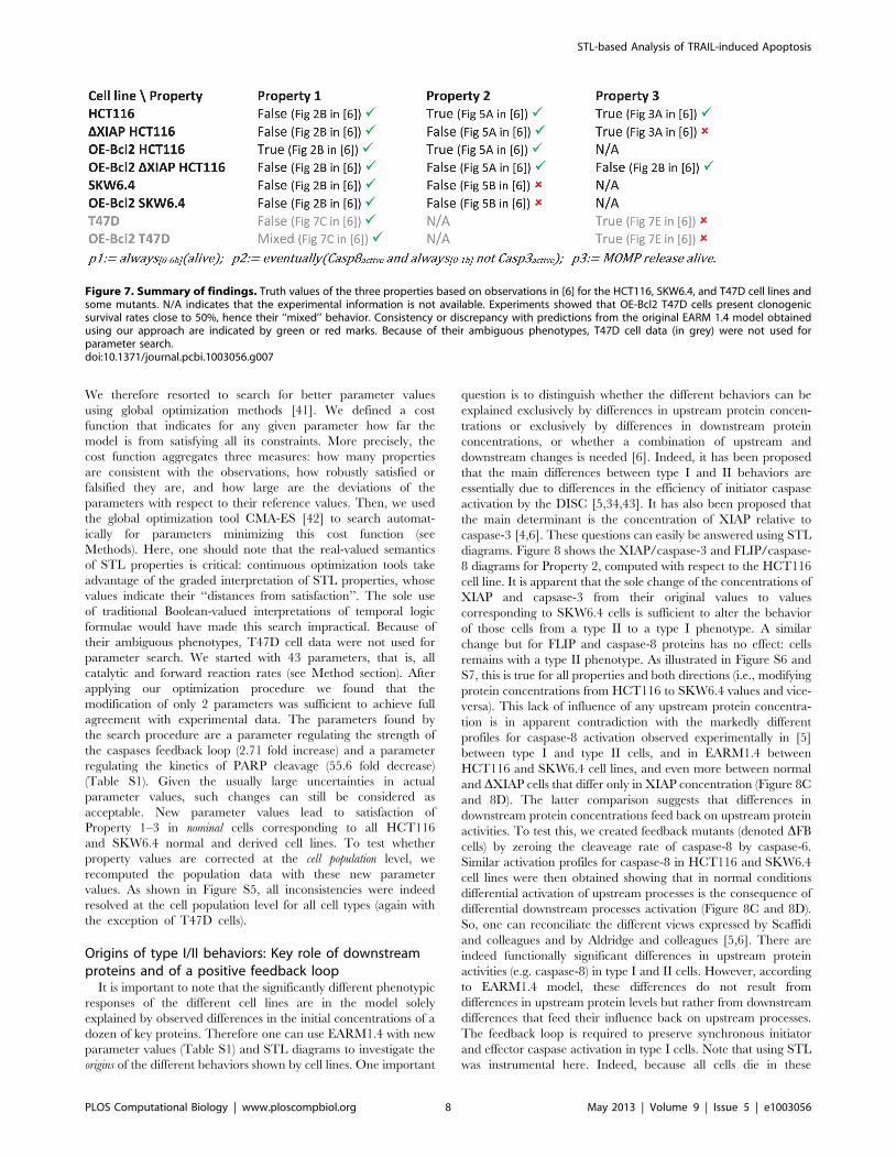
the observed behaviors encoded in STL (Figure 7). This is

commendable for a model of this size and complexity, given that

EARM1.4 has not been tuned with respect to these properties,

even if the model and the specific observations we used to state our

STL properties have been published in the same paper [6].

However, few discrepancies were identified. It is important to test

whether the proposed model is structurally not capable of

accounting for all the observed properties. If not, this would call

for significant model revision.

We first tried to resolve inconsistencies by minor adjustments

of the thresholds we used in formulae. However, property

satisfaction values proved robust to threshold changes (Figure S1).

Figure 6. Property-3 phase diagram and statistics. The value of Property 3 (p3: = MOMP release alive) is represented as a function of the XIAPand caspase-3 initial concentrations. Other protein concentrations correspond to nominal protein concentrations for HCT116 cells. As in Figure 3, celllines are positioned in this diagram according to their protein initial concentrations. Note that HCT116 cells depleted from all XIAP ([XIAP] = 0) arepredicted not to satisfy Property 3. This is in contradiction to experimental observations [6]. (Right) Distributions of the values of Property 3 acrosspopulations of cells of different cell lines. Notations are identical to those used in Figure 4. One can note that discrepancies between predicted meanvalues (crosses) and observed phenotypes (circles) exist for DXIAP HCT116, T47D and OE-Bcl2 T47D cells.doi:10.1371/journal.pcbi.1003056.g006



We therefore resorted to search for better parameter values

using global optimization methods [41]. We defined a cost

function that indicates for any given parameter how far the

model is from satisfying all its constraints. More precisely, the

cost function aggregates three measures: how many properties

are consistent with the observations, how robustly satisfied or

falsified they are, and how large are the deviations of the

parameters with respect to their reference values. Then, we used

the global optimization tool CMA-ES [42] to search automat-

ically for parameters minimizing this cost function (see

Methods). Here, one should note that the real-valued semantics

of STL properties is critical: continuous optimization tools take

advantage of the graded interpretation of STL properties, whose

values indicate their ‘‘distances from satisfaction’’. The sole use

of traditional Boolean-valued interpretations of temporal logic

formulae would have made this search impractical. Because of

their ambiguous phenotypes, T47D cell data were not used for

parameter search. We started with 43 parameters, that is, all

catalytic and forward reaction rates (see Method section). After

applying our optimization procedure we found that the

modification of only 2 parameters was sufficient to achieve full

agreement with experimental data. The parameters found by

the search procedure are a parameter regulating the strength of

the caspases feedback loop (2.71 fold increase) and a parameter

regulating the kinetics of PARP cleavage (55.6 fold decrease)

(Table S1). Given the usually large uncertainties in actual

parameter values, such changes can still be considered as

acceptable. New parameter values lead to satisfaction of

Property 1–3 in nominal cells corresponding to all HCT116

and SKW6.4 normal and derived cell lines. To test whether

property values are corrected at the cell population level, we

recomputed the population data with these new parameter

values. As shown in Figure S5, all inconsistencies were indeed

resolved at the cell population level for all cell types (again with

the exception of T47D cells).

Origins of type I/II behaviors: Key role of downstreamproteins and of a positive feedback loop

It is important to note that the significantly different phenotypic

responses of the different cell lines are in the model solely

explained by observed differences in the initial concentrations of a

dozen of key proteins. Therefore one can use EARM1.4 with new

parameter values (Table S1) and STL diagrams to investigate the

origins of the different behaviors shown by cell lines. One important

question is to distinguish whether the different behaviors can be

explained exclusively by differences in upstream protein concen-

trations or exclusively by differences in downstream protein

concentrations, or whether a combination of upstream and

downstream changes is needed [6]. Indeed, it has been proposed

that the main differences between type I and II behaviors are

essentially due to differences in the efficiency of initiator caspase

activation by the DISC [5,34,43]. It has also been proposed that

the main determinant is the concentration of XIAP relative to

caspase-3 [4,6]. These questions can easily be answered using STL

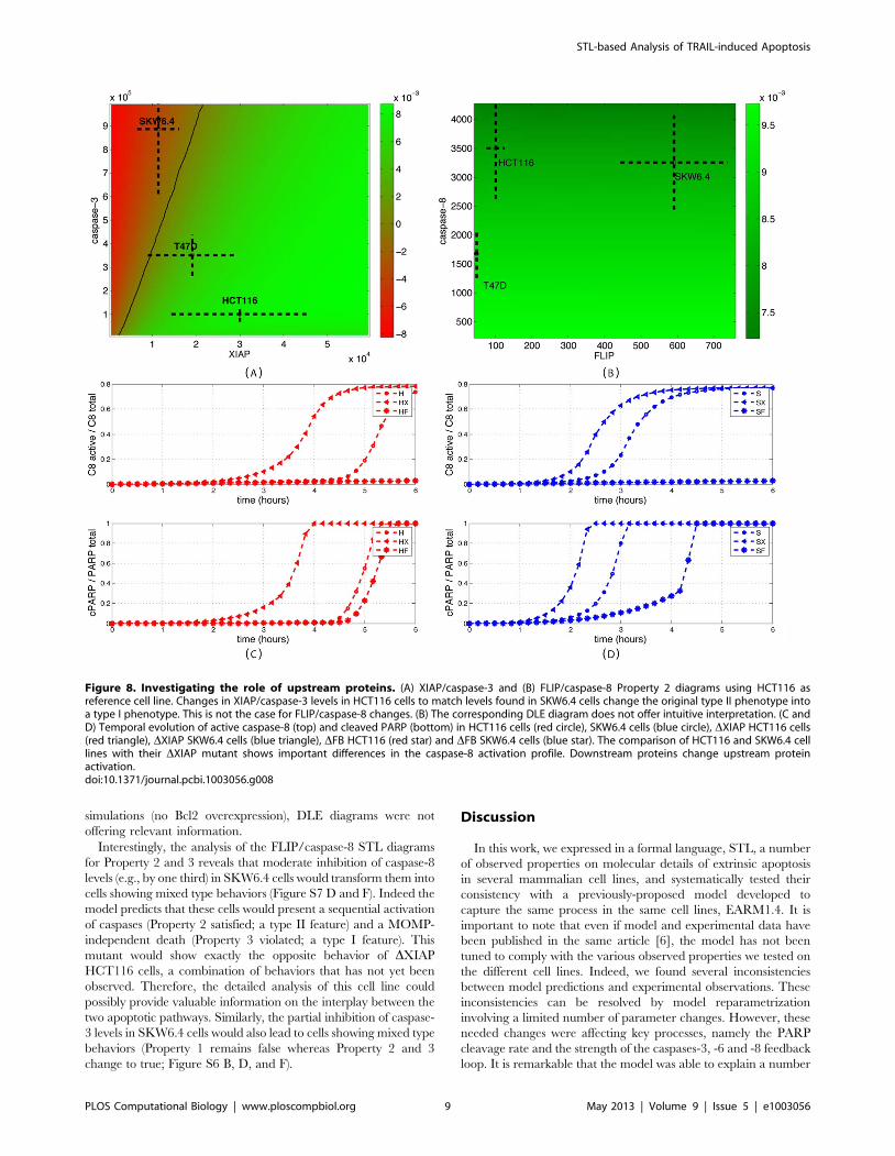
diagrams. Figure 8 shows the XIAP/caspase-3 and FLIP/caspase-

8 diagrams for Property 2, computed with respect to the HCT116

cell line. It is apparent that the sole change of the concentrations of

XIAP and capsase-3 from their original values to values

corresponding to SKW6.4 cells is sufficient to alter the behavior

of those cells from a type II to a type I phenotype. A similar

change but for FLIP and caspase-8 proteins has no effect: cells

remains with a type II phenotype. As illustrated in Figure S6 and

S7, this is true for all properties and both directions (i.e., modifying

protein concentrations from HCT116 to SKW6.4 values and vice-

versa). This lack of influence of any upstream protein concentra-

tion is in apparent contradiction with the markedly different

profiles for caspase-8 activation observed experimentally in [5]

between type I and type II cells, and in EARM1.4 between

HCT116 and SKW6.4 cell lines, and even more between normal

and DXIAP cells that differ only in XIAP concentration (Figure 8C

and 8D). The latter comparison suggests that differences in

downstream protein concentrations feed back on upstream protein

activities. To test this, we created feedback mutants (denoted DFB

cells) by zeroing the cleaveage rate of caspase-8 by caspase-6.

Similar activation profiles for caspase-8 in HCT116 and SKW6.4

cell lines were then obtained showing that in normal conditions

differential activation of upstream processes is the consequence of

differential downstream processes activation (Figure 8C and 8D).

So, one can reconciliate the different views expressed by Scaffidi

and colleagues and by Aldridge and colleagues [5,6]. There are

indeed functionally significant differences in upstream protein

activities (e.g. caspase-8) in type I and II cells. However, according

to EARM1.4 model, these differences do not result from

differences in upstream protein levels but rather from downstream

differences that feed their influence back on upstream processes.

The feedback loop is required to preserve synchronous initiator

and effector caspase activation in type I cells. Note that using STL

was instrumental here. Indeed, because all cells die in these

Figure 7. Summary of findings. Truth values of the three properties based on observations in [6] for the HCT116, SKW6.4, and T47D cell lines andsome mutants. N/A indicates that the experimental information is not available. Experiments showed that OE-Bcl2 T47D cells present clonogenicsurvival rates close to 50%, hence their ‘‘mixed’’ behavior. Consistency or discrepancy with predictions from the original EARM 1.4 model obtainedusing our approach are indicated by green or red marks. Because of their ambiguous phenotypes, T47D cell data (in grey) were not used forparameter search.doi:10.1371/journal.pcbi.1003056.g007



simulations (no Bcl2 overexpression), DLE diagrams were not

offering relevant information.

Interestingly, the analysis of the FLIP/caspase-8 STL diagrams

for Property 2 and 3 reveals that moderate inhibition of caspase-8

levels (e.g., by one third) in SKW6.4 cells would transform them into

cells showing mixed type behaviors (Figure S7 D and F). Indeed the

model predicts that these cells would present a sequential activation

of caspases (Property 2 satisfied; a type II feature) and a MOMP-

independent death (Property 3 violated; a type I feature). This

mutant would show exactly the opposite behavior of DXIAP

HCT116 cells, a combination of behaviors that has not yet been

observed. Therefore, the detailed analysis of this cell line could

possibly provide valuable information on the interplay between the

two apoptotic pathways. Similarly, the partial inhibition of caspase-

3 levels in SKW6.4 cells would also lead to cells showing mixed type

behaviors (Property 1 remains false whereas Property 2 and 3

change to true; Figure S6 B, D, and F).

Discussion

In this work, we expressed in a formal language, STL, a number

of observed properties on molecular details of extrinsic apoptosis

in several mammalian cell lines, and systematically tested their

consistency with a previously-proposed model developed to

capture the same process in the same cell lines, EARM1.4. It is

important to note that even if model and experimental data have

been published in the same article [6], the model has not been

tuned to comply with the various observed properties we tested on

the different cell lines. Indeed, we found several inconsistencies

between model predictions and experimental observations. These

inconsistencies can be resolved by model reparametrization

involving a limited number of parameter changes. However, these

needed changes were affecting key processes, namely the PARP

cleavage rate and the strength of the caspases-3, -6 and -8 feedback

loop. It is remarkable that the model was able to explain a number

Figure 8. Investigating the role of upstream proteins. (A) XIAP/caspase-3 and (B) FLIP/caspase-8 Property 2 diagrams using HCT116 asreference cell line. Changes in XIAP/caspase-3 levels in HCT116 cells to match levels found in SKW6.4 cells change the original type II phenotype intoa type I phenotype. This is not the case for FLIP/caspase-8 changes. (B) The corresponding DLE diagram does not offer intuitive interpretation. (C andD) Temporal evolution of active caspase-8 (top) and cleaved PARP (bottom) in HCT116 cells (red circle), SKW6.4 cells (blue circle), DXIAP HCT116 cells(red triangle), DXIAP SKW6.4 cells (blue triangle), DFB HCT116 (red star) and DFB SKW6.4 cells (blue star). The comparison of HCT116 and SKW6.4 celllines with their DXIAP mutant shows important differences in the caspase-8 activation profile. Downstream proteins change upstream proteinactivation.doi:10.1371/journal.pcbi.1003056.g008



of experiments probing different aspect of apoptosis made on

different cell lines and mutants, simply by taking into account

observed differences in protein concentrations but keeping the

same model structure and reaction rates for all cell lines. This

makes it a valuable tool to investigate the origins of the two different

cell responses. Unlike in in vivo experiments, the number of factors

that could explain these differences is limited in EARM1.4. Using

STL diagrams, we showed that observed differences in the

concentrations of upstream proteins in different cell lines could not

account for the observed cell type changes. This finding is

consistent with the observation based on in vivo and in silico works

that downstream proteins, most notably XIAP and caspase-3, play

a key role [6], but is in apparent contradiction with the

observation that upstream protein activities are markedly different

in type I and II cell lines [5]. Detailed analysis showed that the

effects of downstream protein concentration differences are in fact

fed back to upstream processes and amplified via the positive

feedback loop involving caspases 3, 6, and 8. This finding

reconciliates the views expressed by Scaffidi and colleagues and by

Aldridge and colleagues [5,6].

Based on experimental observations, we defined three proper-

ties associated with type II behaviors: (1) the cell survives if Bcl2 is

over-expressed, (2) the activations of initiator and effector caspases

are sequential, and (3) MOMP precedes caspase-3 activation.

They all assess the role of mitochondria for cell death and differ

only in subtle means. However, they are not always equivalent.

For example, DXIAP HCT116 cells satisfy Property 3 but not

Property 2, leading to interpretations like DXIAP HCT116 being

type I cells while exhibiting a type II phenotype. Based on our

work, there is no evidence that one property could be considered

as a defining criterion, excepted maybe for historical or practical

reasons (cell types were originally defined based on caspase

activation kinetics whereas Bcl2 overexpression is considered as

the standard method for cell type classification). This challenges

the consensual understanding that there exists (implicitly) well-

defined type I and type II phenotypes. It should be noted that here

we go beyond the notion of mixed cell type introduced by Aldridge

and colleagues for describing T47D cells. The authors implicitly

assume that cell types are well defined but that within a population

of cells a mixture of both phenotypes can be observed, coming

from cell-to-cell variability [16,44,45]. Here we propose that these

three properties are considered as type II features. Then the DXIAP

HCT116 cells would be more consistently qualified as possessing

some type I and some type II features. With the accumulation of

more detailed characterizations of apoptosis in more cell lines, it is

likely that the use of the loosely-defined notion of cell types will

otherwise become more and more problematic.

Like the DLE diagrams introduced by Aldridge and Haller [22],

STL diagrams are a convenient and intuitive way to represent the

influence of various factors on complex dynamical properties.

However, STL diagrams are superior on several counts. Firstly,

one can benefit from the expressive power of temporal logics to

express different observed properties of the dynamics of the cell

response. It allows us to test in which respect are the cell lines

different. Secondly, although the evaluation of STL properties and

of the DLE returns continuous values, the fact that STL values are

signed – positive values indicate satisfaction and negative values

indicate falsity – allows for a more direct interpretation of the

diagrams. Moreover, it allows defining statistics over populations

of cells. Thirdly, DLE generates well-defined partitions if in some

regions a small change in the initial state has a mild effect on the

future system’s state, thus generating low DLE values, and in other

regions, similar changes have drastic effects, thus generating high

DLE values. Although this is clearly the case in cell lines

overexpressing Bcl2 since some cells die, whereas others survive

(Figure 3), this is not generally true.

DLE and STL diagrams are particularly useful to have a rapid

view of the consequences of changing a few factors, initial

concentrations in our case. This feature allows us to foresee the

consequences of mutations (e.g. DXIAP mutants in XIAP/

caspase-3 diagrams), to investigate the (lack of) influence of given

factors (e.g. FLIP changes in FLIP/caspase-8 diagrams), and to

assess the influence of cell-to-cell heterogeneity by representing

graphically the means and standard values of populations in

diagrams. However, heterogeneity in diagrams is limited to two

dimensions. Moreover, since the cell lines differ in more than two

dimensions, only one cell line can be correctly mapped in the state

space slice of the diagram. Other cell lines are projected onto it,

making their interpretations subject to caution. To solve this issue,

we introduced population property values for describing the

behavior of cell populations. These values and their statistics,

notably means, standard deviations, and percentage of satisfaction,

offer a more accurate view than phase diagrams. Indeed, even if

we found that the rapid picture offered by STL diagrams are often

consistent with population property values, a few cases illustrated

the need to compute these statistics as well (e.g. T47D cells

manifesting in silico a clear mixed-type behavior with respect to

Property 1, that is not present in the phase diagram in Figure 3).

In addition to computing diagram and population statistics,

STL properties also enable model revision based on experimental

observations. Observed properties are encoded in STL and the

continuous semantics of STL is used to search for valid parameter

values. Traditional model revision methods based on curve fitting

could not be adapted here by lack of well-defined time series data.

The non-standard use of continuous semantics for temporal logic

formula interpretation is essential to allow for an effective search

[46–48]. Using global optimization methods, we found that the

few discrepancies we had identified in earlier steps can be resolved

by modifying only a restricted set of model parameters.

Remarkably, one of the two selected parameters is regulating the

strength of the caspases feedback loop, a process that is predicted

to play an important role in the genesis of type I or type II

behaviors.

The development of experimental methods to probe quantita-

tively subtle aspects of the dynamics of biological processes has

spurred the development of large and complex quantitative models

[49,50]. However the available experimental data is seldom in the

form of time series data directly usable by standard model

validation and model calibration techniques. Therefore tools

allowing for the exploration of model properties, the comparison

between predictions and observations and the revision of models

that are adapted to the available experimental data are

increasingly needed. Temporal logics offer a flexible means to

encode for a broad range of experimentally-observed properties.

Moreover they are also formal languages that allow automating

model analysis. Because it supports STL and uses by default

distributions for parameter and initial concentrations, Breach

naturally allows the exploration of properties of cell populations.

We expect that Breach will become a valuable tool for the

computational biologists to explore model properties, and more

importantly, to get tight connections between experimental data

and model predictions [51].

Methods

Modeling extrinsic apoptosis and cell line differencesWe used the model of extrinsic apoptosis proposed by

Aldridge and colleagues [6] named EARM1.4. This model is



an extension and adaptation of a previous model, EARM1.0,

proposed in [15]. EARM1.0 has been calibrated on HeLa cells

using live and fixed cell imaging, flow cytometry of caspases

substrates and biochemical analysis. EARM1.4 has been

adapted to HCT116, SKW6.4 and T47D cells, and has been

shown to capture their capacity to die or survive in OE-Bcl2

clonogenic experiments. It is a mass-action ODE model based

on nearly 70 reactions and involving 17 native proteins, 40

modified proteins or protein complexes, and TRAIL. For each

cell line, the model assumes different nominal initial protein

concentrations. Nominal concentrations refer here to concen-

trations found in a hypothetical mean cell within the cell

population. More precisely, out of the 17 native proteins, 12

have been quantified by immunoblotting and the relative

differences between cell lines have been used to set nominal

initial protein concentrations for HCT116, SKW6.4 and T47D

cells (see Table 1). Besides initial concentrations, the 3 models

are identical. DXIAP and OE-Bcl2 mutant cell lines are defined

with respect to their parent cell line. In DXIAP cells, the XIAP

concentration is set to 0. In OE-Bcl2 cells, the initial Bcl2

concentration is 10 times higher than in the parent cell line. For

cells with modified feedback (DFB cells) we set the cleavage rate

of caspase 8 by caspase 6, k7, to 0. To represent cell-to-cell

variability within cell lines, we assumed that protein concentra-

tions are log-normally distributed. The means of protein

concentrations were the nominal values. The coefficient of

variation were either measured, for caspase-3 and XIAP [6], or

assumed to be 25% as in [16]. The complete model together

with Breach is available in Supplementary Materials as

MATLAB files (S9). The names of the variables, constants

and reactions used in the model are the same as in [6].

STL semantics and property evaluationSTL is an intuitive yet formal language for specifying the

properties of continuous dynamical systems. It allows us to

express in a (pseudo-) natural language hypothesis on the

mechanistic functioning of the system taken from available

biological knowledge in a formal way so that model consistency

can be precisely and systematically tested. Given a model of the

system, expected properties are expressed using predicates

describing constraints on protein concentrations, like

cPARP,105, traditional logical operators, like and, or and implies,

and temporal operators, like eventually[a,b], always[a,b], and until[a,b].

Time intervals [a,b] limit the scope of temporal operators. These

operators can be combined to create properties of arbitrary

complexities. For example, always[0–6h] (XIAP.103 and

cPARP,105) is a valid STL formula. The formal syntax is given

in Table S2 (top). STL properties are then interpreted with

respect to so-called signals. In this context, signals are functions

from time to the reals representing the evolution of the different

concentrations in the system. Computationaly speaking, they

often come from (discrete) time-series data obtained by numerical

simulation of the ODE model. The semantics is defined such that

it captures a notion of distance from satisfaction. For example,

the interpretation at time t of the predicate XIAP.103 is simply

the value of XIAP(t) - 103. Trivially it is positive if XIAP.103, and

negative if XIAP,103. The interpretation of XIAP.103 and

cPARP,105 at time t is the minimum of the value of the two

operands at time t. Note that it is positive if and only if both

operands have positive values. Similarly, the interpretation of

always(XIAP.103) is the minimum of the value of XIAP.103 at

all future time instants. It is positive if XIAP is always greater than

103. The interpretation of STL formulas is also illustrated on

Figure 9. More generally, the continuous interpretation of STL

properties ensures that if the value of a property is positive (resp.

negative), then the property holds (resp. is violated) in a more

usual Boolean interpretation. Moreover, it captures a notion of

‘‘distance from satisfaction’’: a large positive value indicates a

robustly satisfied property, whereas a large negative value

indicates a property that is far from satisfaction. The semantics

is formally defined in Table S2 (bottom). Note that property

values are relative to the formula, in the sense that values

obtained for different STL formulas are not directly comparable

between each other.

Computation of property diagramsGiven an STL property, the associated STL phase diagram is a

representation of the value of the property as a function of the

system’s initial configuration. More precisely diagrams represent

property values in 2D slices of a high dimensional state space.

Each point in the diagram is associated to the value of the STL

formula evaluated on the system’s trajectory starting at this point.

Boundaries were set so as to enclose the variability observed

between cell lines. Diagrams are defined with respect to a

particular cell line: with the exception of the two variables of the

diagram, all other variables assume their nominal values for the

given cell line. Other cell lines are placed on the diagram based on

the initial concentrations of the selected proteins. Unless

mentioned otherwise, the HCT116 cell line is used as a reference.

In practice, a 50650 grid of linearly-spaced points is used for the

computation of each diagram. For each point on the grid, we

computed the cell behavior predicted by the model and then the

value of the STL property associated with this behavior (see

Program S1). The ranges for caspase-3, XIAP, caspase-8 and FLIP

are [0, 106], [0, 6*104], [1200, 4500] and [0, 800], respectively.

Similarly, DLE diagrams represent the direct finite-time Lyapunov

exponent for all points in (a 2D slice of) the state space. This value

captures the sensitivity to initial conditions: DLE(t,x0)~

log lmax((Lx(t)

Lx0)T (

Lx(t)

Lx0)), where lmax(M) denotes the maximum

eigenvalue of the matrix M and t is some future time instant (here 6

or 4 hours). Again, a 50650 grid of linearly-spaced points is used

for the computation of DLE diagrams.

Table 1. Initial concentrations of proteins in HCT116, SKW6.4,and T47D cells.

Protein\Cell line HCT116 SKW6.4 T47D

FLIP 100 (0.25) 591 (0.25) 48 (0.25)

caspase-8 3500 (0.25) 3255 (0.25) 1680 (0.25)

caspase-6 10000 (0.25) 6700 (0.25) 22500 (0.25)

caspase-3 100000 (0.32) 886000 (0.31) 351000 (0.25)

XIAP 30000 (0.52) 11400 (0.42) 19200 (0.53)

PARP 1000000 (0.25) 1120000 (0.25) 1040000 (0.25)

Bid 40000 (0.25) 74800 (0.25) 53600 (0.25)

Mcl1 1000 (0.25) 1250 (0.25) 4640 (0.25)

Bax 80000 (0.25) 786400 (0.25) 113600 (0.25)

Bcl2 20000 (0.25) 400000 (0.25) 104000 (0.25)

Smac 100000 (0.25) 177000 (0.25) 139000 (0.25)

Nominal values and coefficients of variations for initial protein concentrationsthat differ between cell lines (see [6] for concentrations of other proteins).Protein concentrations are assumed log-normally distributed across the cellpopulations.doi:10.1371/journal.pcbi.1003056.t001



Computation of STL population dataGiven an STL property, the STL population data correspond to

the evaluation of this property on all the simulated individual cell

behaviors among a population of cells of a given cell line. Based on

these property values, statistics are computed. For STL population

data, 5000 different initial conditions are obtained for each cell

line by sampling around its nominal initial conditions from

lognormal distributions. Mean values, value distributions and

percentages of satisfaction of the property (i.e. the percentage of

cells in the population satisfying a given property) are then

computed.

Parameter search procedureThe search procedure has two phases. In the first phase we

search for new parameters for EARM1.4 that lead to full

agreement with experimental data (Figure 7). In the second phase,

when a solution is found, we minimize the number of modified

parameters. We use a cost function composed of three different

components: continuous, Boolean, and parameter penalties. The

continuous penalties correspond to the (negation of) the contin-

uous values of STL properties, and the Boolean penalties

correspond to their Boolean value multiplied by a (negative)

constant. These costs decrease when more properties are

consistent with observations (Bpenalty), and when they are more

robustly consistent with observations (Cpenalty). In the continuous

component, weights are used to balance the importance of all

properties, given their typical range. The last component penalizes

parameter deviations from their original values (Ppenalty). The

overall cost is the weighted sum of these three components.

cost(p) :~a Ppenalty(p)zX

i[CellLines

X

p[Properties

(b Bpenalty(p,i,p)zc Cpenalty(p,i,p))

In the first phase, we selected 43 parameters (14 catalytic rates of

enzymatic reactions and 29 forward rates) out of approximately 80

parameters in EARM1.4. Parameter modifications were limited to

a 100-fold change. We set weights so that the Boolean, continuous,

and parameter penalties contributed to approximately 50%, 30%,

and 20% of the cost, respectively. After 10 hours of computations

(2.2 GHz processor, 8GB RAM), the search converged to a state

in which all expected properties were satisfied by the model (T47D

cells excluded).

In the second phase, we selected the parameters that changed

by more than 5 folds (there were 5 such parameters: kc9, kc25,

kc20, k7 and k24) and run the search again for each pair of these

parameters. The cost function was modified by setting the Cpenalty

parameter to 0, and the beta parameter such as the Boolean

penalty was responsible for approximately 90% of the cost. As a

result, parameter deviations were minimized while preserving the

agreement with the experimental data. We found that reparame-

trization of only one pair of parameters allowed for satisfaction of

all properties for all cell lines.

Breach toolAll the computations have been made using Breach [33,48].

This MATLAB/C++ toolbox allows for efficient numerical

simulation, for sensitivity computation, and for STL property

and DLE evaluation. In particular, DLEs can efficiently be

computed via forward sensitivity analysis [52]. Breach is partic-

ularly oriented towards the analysis of parametric systems, in the

sense that it offers efficient routines for global sensitivity analysis

and parameter search, and that the graphical user interface

facilitates the modification of parameters and initial conditions,

and the exploration of parameter spaces.

Supporting Information

Figure S1 Formula robustness. Number of matches between

predicted and observed satisfaction values for Properties 1–3 in all

HCT116 and SKW6.4 cell lines (Figure 7) as a function of the PARP-

related threshold, a, defining the alive property, of the Apaf-related

threshold, b, defining the MOMP occurrence and of the caspase-

related threshold, c, defining caspases activation when (A) a and bvary, and c is fixed, or (B) c varies, and a and b are fixed. Thresholds

a, b, and c are defined as follows: p1: = always[0–6h](cPARP/PARPtotal,a);

p2: = eventually(Casp8active and always[0–1h] not Casp3active); p3: = Apaffree/

Apaftotal,b release (cPARP/PARPtotal,a)), where Casp8active: = Casp8*/

Casp8total.c and Casp3active: = Casp3*/Casp3total.c. Full consistency

Figure 9. Evaluation of STL properties. Temporal evolution of the ratio cPARP/PARPtotal, of the value of the property alive: = cPARP/PARPtotal,0.5,and of Property 1: = always[0–6h]( cPARP/PARPtotal,0.5) for HCT116 and OE-Bcl2 HCT116 cells (left), and SKW6.4 and OE-Bcl2 SKW6.4 cells (right). Whenthe concentration of cleaved PARP increases, the value of the alive property gradually decreases from a positive value (‘‘true’’) to a negative value(‘‘false’’). Property 1 at time t evaluates to the minimal value of alive at all future times. So, Property 1 simply captures whether at all times alive holds.doi:10.1371/journal.pcbi.1003056.g009



with all experimental data corresponds to 16 matches (15 in Figure 7

and, additionally, p2(SKW6.4) = True). For original properties

(a=b= 50% and c= 1%), we found three mismatches (Figure 7).

This number is robust with respect to changes of the PARP-related

threshold, a, and of the Apaf-related threshold, b. It is also robust to

the caspase-related threshold, c, provided that this value remains low

enough (i.e. ,2%).

(TIF)

Figure S2 Comparison between DLE and Property 1STL diagrams. Diagrams representing the values of the DLE

computed at time T (A,C) and of the STL Property:= always[0-T]

(cPARP/PARPtotal,0.5) (B,D) for T = 6 h (A–B) and T = 4 h (C–D).

Strikingly, for the two time instants the separatrix is exactly at the

same position, revealing that DLE and Property 1 capture

precisely the same behavior: the existence of two different possible

outcomes: survival or death. However, in full generality the DLE

simply measures the influence of small changes in initial protein

concentrations on the future state of the system. In fact, this

similarity comes from the snap-action aspect of apoptotic cell death,

captured by the EARM model: cell death is immediately preceded

by a sudden activation of effector caspases (all-or-none behavior)

[15]. Small changes in initial protein concentrations will result in

dramatic differences in protein concentrations at the time of death

and therefore in high DLE values. One should also note that the

interpretation of low DLE values is ambiguous, since low values

are found in regions corresponding to type I (SKW6.4) and to type

II cell types (HCT116).

(TIF)

Figure S3 XIAP/capsase-3 STL diagrams for all prop-erties and using HCT116, SKW6.4 or T47D as referencecell line. Diagrams representing the values of the STL properties

p1 (A–C), p2 (D–F) and p3 (G–H) computed using HCT116

(A,D,G), SKW6.4 (B,E,H), or T47D (C,F,I) nominal protein

concentrations. Bcl2 is overexpressed in Property 1 diagrams. In

most cases, for a given property the satisfaction values associated

with each cell type is similar irrespectively of the reference cell line

used to construct the diagram. However, there are exceptions, like

in the case of T47D cell line behavior (H and I). So care must be

taken when interpreting STL diagrams. The same situation holds

with DLE diagrams (not shown).

(TIF)

Figure S4 STL property values across all cell lines forProperties 1–3 for the EARM1.4. For each property, plots

indicate the nominal cell value (top), the distribution (middle), and

the percentage of satisfaction (bottom) of the property values for

populations of cells of different cell lines. Notations are identical to

those used in Figure 4.

(TIF)

Figure S5 Population statistics for Property 1, 2 and 3,computed with new parameter values. (see Table S1) This

data should be compared with Figure 4, 5 (right), and 6 (right).

The new parameter values allow resolving the inconsistencies

found for SKW6.4, OEBcl2 SKW6.4 cells for Property 2, and for

DXIAP HCT116 cells for Property 3. T47D cells still do not satisfy

Property 3 as expected. Notations are identical to those used in

Figure 4.

(TIF)

Figure S6 XIAP/Capsase-3 STL diagrams computedwith new parameter values for all properties and usingHCT116 or SKW6.4 as reference cell lines. Diagrams

representing the values of the STL properties p1 (A–B), p2 (C–D)

and p3 (E–F), computed using HCT116 (A,C,E) or SKW6.4

(B,D,F) nominal protein concentrations.

(TIF)

Figure S7 FLIP/Capsase-8 STL diagrams computedwith new parameter values for all properties and usingHCT116 or SKW6.4 as reference cell lines. Diagrams

representing the values of the STL properties p1 (A–B), p2 (C–D)

and p3 (E–F), computed using HCT116 (A,C,E) or SKW6.4

(B,D,F) nominal protein concentrations.

(TIF)

Program S1 Computation of STL diagrams usingBreach [33]. The archive contains the freely-distributed Matlab

tool Breach, an implementation of EARM1.4 in Breach, initial

conditions for each of 12 cell lines used in this article, and example

scripts illustrating how to generate STL phase diagrams.

(ZIP)

Table S1 Valid parameters. List of minimal parameter set

leading to Property1–3 satisfaction for all but T47D cells, together

with their new and original values, and the corresponding fold

change.

(TIF)

Table S2 Syntax and semantics of STL [48]. The syntax of

STL formulas is defined inductively. Here, w, w1, w2 are STL

formulas, m(x) is an equality of type f (x(t))w0, with f a real-valued

function on the state x, and [a,b] is a time interval. The real-valued

semantics r(w,t) of an STL formula Q at time t is interpreted on a

real-valued signal x(t) defined on a time interval [0,Tf], where Tf is

typically the end time of a simulation. One additionally defines

w1 or w2 as not(not w1 and not w2), eventually a,b½ � w asTrue until a,b½ � w

and always a,b½ � w as not eventually a,b½ � not w.

(TIF)

Acknowledgments

We thank Denis Thieffry, Magdalena Stepien and Xavier Duportet for

their critical suggestions. We are grateful for reviewers’ comments which

significantly helped to improve our manuscript.

Author Contributions

Conceived and designed the experiments: SS AD FB GB. Performed the

experiments: SS AD GB. Analyzed the data: SS AD FB OM GB.

Contributed reagents/materials/analysis tools: SS AD. Wrote the paper:

SS GB.

References

1. Gonzalvez F, Ashkenazi A (2010) New insights into apoptosis signaling byApo2L/TRAIL. Oncogene 29: 4752–4765.

2. Spencer SL, Sorger PK (2011) Measuring and modeling apoptosis in single cells.

Cell 144: 926–939.

3. Kasibhatla S, Tseng B (2003) Why Target Apoptosis in Cancer Treatment?

Molecular Cancer Therapeutics 2: 573–580.

4. Jost PJ, Grabow S, Gray D, McKenzie MD, Nachbur U, et al. (2009) XIAP

discriminates between type I and type II FAS-induced apoptosis. Nature 460:

1035–1039.

5. Scaffidi C, Fulda S, Srinivasan A, Friesen C, Li F, et al. (1998) Two

CD95 (APO-1/Fas) signaling pathways. The EMBO Journal 17: 1675–

1687.

6. Aldridge BB, Gaudet S, Lauffenburger DA, Sorger PK (2011) Lyapunov

exponents and phase diagrams reveal multi-factorial control over TRAIL-

induced apoptosis. Molecular Systems Biology 7: 553.

7. Eissing T, Conzelmann H, Gilles ED, Allgower F, Bullinger E, et al. (2004)

Bistability analyses of a caspase activation model for receptor-induced apoptosis.

The Journal of Biological Chemistry 279: 36892–36897.



8. Hoffmann A, Levchenko A, Scott ML, Baltimore D (2002) The IkappaB-NF-

kappaB signaling module: temporal control and selective gene activation.Science 298: 1241–1245.

9. Bentele M, Lavrik I, Ulrich M, Stosser S, Heermann DW, et al. (2004)

Mathematical modeling reveals threshold mechanism in CD95-inducedapoptosis. The Journal of Cell Biology 166: 839–851.

10. Hua F, Cornejo MG, Cardone MH, Stokes CL, Lauffenburger DA (2005)

Effects of Bcl-2 levels on Fas signaling-induced caspase-3 activation: moleculargenetic tests of computational model predictions. Journal of Immunology 175:

985–995.

11. Bagci EZ, Vodovotz Y, Billiar TR, Ermentrout GB, Bahar I (2006) Bistability in

apoptosis: roles of Bax, Bcl-2, and mitochondrial permeability transition pores.

Biophysical Journal 90: 1546–1559.

12. Legewie S, Bluthgen N, Herzel H (2006) Mathematical modeling identifies

inhibitors of apoptosis as mediators of positive feedback and bistability. PLoSComputational Biology 2: e120.

13. Rehm M, Huber HJ, Dussmann H, Prehn JHM (2006) Systems analysis of

effector caspase activation and its control by X-linked inhibitor of apoptosisprotein. The EMBO Journal 25: 4338–4349.

14. Chen C, Cui J, Lu H, Wang R, Zhang S, et al. (2007) Modeling of the Role of a

Bax-Activation Switch in the Mitochondrial Apoptosis Decision. BiophysicalJournal 92: 4304–4315.

15. Albeck JG, Burke JM, Spencer SL, Lauffenburger DA, Sorger PK (2008)Modeling a snap-action, variable-delay switch controlling extrinsic cell death.

PLoS Biology 6: 2831–2852.

16. Spencer SL, Gaudet S, Albeck JG, Burke JM, Sorger PK (2009) Non-geneticorigins of cell-to-cell variability in TRAIL-induced apoptosis. Nature 459: 428–

432.

17. Fricker N, Beaudouin J, Richter P, Eils R, Krammer PH, et al. (2010) Model-based dissection of CD95 signaling dynamics reveals both a pro- and

antiapoptotic role of c-FLIPL. The Journal of Cell Biology 190: 377–389.

18. Mai Z, Liu H (2009) Boolean network-based analysis of the apoptosis network:

irreversible apoptosis and stable surviving. Journal of Theoretical Biology 259:

760–769.

19. Calzone L, Tournier L, Fourquet S, Thieffry D, Zhivotovsky B, et al. (2010)

Mathematical modelling of cell-fate decision in response to death receptor

engagement. PLoS Computational Biology 6: e1000702.

20. Saez-Rodriguez J, Alexopoulos LG, Zhang M, Morris MK, Lauffenburger DA,

et al. (2011) Comparing signaling networks between normal and transformedhepatocytes using discrete logical models. Cancer Research 71: 5400–5411.

21. Schlatter R, Schmich K, Avalos Vizcarra I, Scheurich P, Sauter T, et al. (2009)

ON/OFF and beyond–a boolean model of apoptosis. PLoS ComputationalBiology 5: e1000595.

22. Aldridge B, Haller G (2006) Direct Lyapunov exponent analysis enables

parametric study of transient signalling governing cell behaviour. SystemsBiology, IEE Proceedings 153: 425–432.

23. Maler O, Nickovic D (2004) Monitoring Temporal Properties of ContinuousSignals. Proceedings of the Formal Techniques, Modelling and Analysis in Real-

Time and Fault-Tolerant Systems Conference, FORMATS/FTRTFT 2004,

LNCS 3253. Springer-Verlag. pp. 152–166.

24. Barnat J, Brim L, Cerna I, Drasan S, Safranek D (2008) Parallel Model

Checking Large-Scale Genetic Regulatory Networks with DiVinE. ElectronicNotes in Theoretical Computer Science. Springer-Verlag, Vol. 194. pp. 35–50.

25. Batt G, Yordanov B, Weiss R, Belta C (2007) Robustness analysis and tuning of

synthetic gene networks. Bioinformatics 23: 2415–2422.

26. Batt G, Page M, Cantone I, Goessler G, Monteiro P, et al. (2010) Efficient

parameter search for qualitative models of regulatory networks using symbolic

model checking. Bioinformatics 26: i603–10.

27. Bernot G, Comet J-P, Richard A, Guespin J (2004) Application of formal

methods to biological regulatory networks: extending Thomas’ asynchronouslogical approach with temporal logic. Journal of Theoretical Biology 229: 339–

347.

28. Donaldson R, Gilbert D (2008) A model checking approach to the parameterestimation of biochemical pathways. In: Proceedings of the 6th International

Conference on Computational Methods in Systems Biology, CMSB 2008,LNCS 5307. Berlin: Springer-Verlag. pp. 269–287.

29. Fisher J, Piterman N, Hajnal A, Henzinger T a (2007) Predictive modeling of

signaling crosstalk during C. elegans vulval development. PLoS ComputationalBiology 3: e92.

30. Jha SK, Clarke EM, Langmead CJ, Legay A, Platzer A, et al. (2009) A bayesian

approach to model checking biological systems. In: Proceedings of the 7thInternational Conference on Computational Methods in Systems Biology,

CMSB 2009, LNCS 5688. Berlin: Springer-Verlag. pp. 218–234.

31. Heath J, Kwiatkowska M, Norman G, Parker D, Tymchyshyn O (2008)

Probabilistic model checking of complex biological pathways. Theoretical

Computer Science 391: 239–257.

32. Donze A, Fanchon E, Gattepaille LM, Maler O, Tracqui P (2011) Robustness

analysis and behavior discrimination in enzymatic reaction networks. PloS One6: e24246.

33. Donze A (2010) Breach, a toolbox for verification and parameter synthesis of

hybrid systems. In: Proceedings of the 22nd International Conference onComputer Aided Verification, CAV’10, LNCS 6174. Berlin: Springer-Verlag.

pp. 167–170.34. Barnhart BC, Alappat EC, Peter ME (2003) The CD95 Type I/Type II model.

Seminars in Immunology 15: 185–193.

35. Algeciras-Schimnich A, Pietras EM, Barnhart BC, Legembre P, Vijayan S, et al.(2003) Two CD95 tumor classes with different sensitivities to antitumor drugs.

Proceedings of the National Academy of Sciences of the United States ofAmerica 100: 11445–11450.

36. Ozoren N, El-Deiry WS (2002) Defining characteristics of Types I and IIapoptotic cells in response to TRAIL. Neoplasia 4: 551–557.

37. Rehm M, Dussmann H, Janicke RU, Tavare JM, Kogel D, et al. (2002) Single-

cell fluorescence resonance energy transfer analysis demonstrates that caspaseactivation during apoptosis is a rapid process. Role of caspase-3. The Journal of

Biological Chemistry 277: 24506–24514.38. Albeck JG, Burke JM, Aldridge BB, Zhang M, Lauffenburger DA, et al. (2008)

Quantitative analysis of pathways controlling extrinsic apoptosis in single cells.

Molecular Cell 30: 11–25.39. Agard NJ, Mahrus S, Trinidad JC, Lynn A, Burlingame AL, et al. (2012) Global

kinetic analysis of proteolysis via quantitative targeted proteomics. Proceedingsof the National Academy of Sciences of the United States of America 109: 1913–

1918.40. Maas C, Verbrugge I, De Vries E, Savich G, Van de Kooij LW, et al. (2010)

Smac/DIABLO release from mitochondria and XIAP inhibition are essential to

limit clonogenicity of Type I tumor cells after TRAIL receptor stimulation. CellDeath and Differentiation 17: 1613–1623.

41. Avriel M (2003) Nonlinear programming: analysis and methods. Courier DoverPublications.

42. Hansen N, Ostermeier A (2001) Completely derandomized self-adaptation in

evolution strategies. Evolutionary Computation 9: 159–195.43. Kober a MM, Legewie S, Pforr C, Fricker N, Eils R, et al. (2011) Caspase-8

activity has an essential role in CD95/Fas-mediated MAPK activation. CellDeath and Disease 2: e212.

44. Bhola PD, Simon SM (2009) Determinism and divergence of apoptosissusceptibility in mammalian cells. Journal of Cell Science 122: 4296–4302.

45. Rehm M, Huber HJ, Hellwig CT, Anguissola S, Dussmann H, et al. (2009)

Dynamics of outer mitochondrial membrane permeabilization during apoptosis.Cell Death and Differentiation 16: 613–623.

46. Fainekos GE, Pappas GJ (2009) Robustness of temporal logic specifications forcontinuous-time signals. Theoretical Computer Science 410: 4262–4291.

47. Rizk A, Batt G, Fages F, Soliman S (2011) Continuous valuations of temporal

logic specifications with applications to parameter optimization and robustnessmeasures. Theoretical Computer Science 412: 2827–2839.

48. Donze A, Maler O (2010) Robust satisfaction of temporal logic over real-valuedsignals. Formal Modeling and Analysis of Timed Systems: 92–106.

49. Klipp E, Herwig R, Kowald A, Wierling C, Lehrach H (2005) Systems Biologyin Practice. Concepts, Implementation and Application. Wiley-VCH.

50. Szallasi Z, Stelling J, Periwal V (2010) System Modeling in Cellular Biology:

From Concepts to Nuts and Bolts. Boston: MIT Press.51. Ghosh S, Matsuoka Y, Asai Y, Hsin K-Y, Kitano H (2011) Software for systems

biology: from tools to integrated platforms. Nature reviews Genetics 12: 821–832.

52. Serban R, Hindmarsh A (2005) CVODES, the sensitivity-enabled ODE solver

in SUNDIALS. Proceedings of IDETC/CIE; Sept 2005; Long Beach,California, United States.

53. Peter ME, Krammer PH (2003) The CD95(APO-1/Fas) DISC and beyond. CellDeath and Differentiation 10: 26–35.

54. Huang Y, Park YC, Rich RL, Segal D, Myszka DG, et al. (2001) Structural basis

of caspase inhibition by XIAP: differential roles of the linker versus the BIRdomain. Cell 104: 781–790.

55. Chen L, Smith L, Wang Z, Smith JB (2003) Preservation of caspase-3 subunitsfrom degradation contributes to apoptosis evoked by lactacystin: any single lysine

or lysine pair of the small subunit is sufficient for ubiquitination. MolecularPharmacology 64: 334–345.

56. Luo X, Budihardjo I, Zou H, Slaughter C, Wang X (1998) Bid, a Bcl2

interacting protein, mediates cytochrome c release from mitochondria inresponse to activation of cell surface death receptors. Cell 94: 481–490.

57. Kim H, Rafiuddin-Shah M, Tu H-C, Jeffers JR, Zambetti GP, et al. (2006)Hierarchical regulation of mitochondrion-dependent apoptosis by BCL-2

subfamilies. Nature Cell Biology 8: 1348–1358.

58. Du C, Fang M, Li Y, Li L, Wang X (2000) Smac, a mitochondrial protein thatpromotes cytochrome c-dependent caspase activation by eliminating IAP

inhibition. Cell 102: 33–42.



STL-based Analysis of TRAIL-induced Apoptosis Challenges the Notion of Type I/Type II Cell Line...

Documents

Transcript of STL-based Analysis of TRAIL-induced Apoptosis Challenges the Notion of Type I/Type II Cell Line...