Stereo matching based on the self-organizing feature-mapping algorithm

Ž .Pattern Recognition Letters 19 1998 319–330

Stereo matching based on the self-organizing feature-mappingalgorithm

G. Pajares a,), J.M. Cruz a, J. Aranda b

a Dpto. Informatica y Automatica, Facultad de CC Fısicas, UniÕersidad Complutense, 28040 Madrid, Spain´ ´ ´b ( )Dpto. Informatica y Automatica, Facultad de CC Fısicas, UniÕersidad Nacional de Educacion a Distancia UNED , 28040 Madrid, Spain´ ´ ´ ´

Received 24 September 1996; revised 1 December 1997

Abstract

This paper presents an approach to the local stereo matching problem using edge segments as features with severalattributes. We have verified that the differences in attributes for the true matches cluster in a cloud around a center. Thecorrespondence is established on the basis of the minimum squared Mahalanobis distance between the difference of the

Ž .attributes for a current pair of features and the cluster center similarity constraint . We introduce a learning strategy basedon the Self-Organizing feature-mapping method to get the best cluster center. A comparative analysis among methodswithout learning is illustrated. q 1998 Elsevier Science B.V. All rights reserved.

Keywords: Self-organizing feature-mapping; Stereovision; Local matching; Learning; Training

1. Introduction

The key step in stereovision is image matching,namely, the process of identifying the correspondingpoints in two images that are generated by the samephysical point in space. This paper is devoted solelyto this problem. The stereo correspondence problemcan be defined in terms of finding pairs of truematches that satisfy three competing constraints:

Žsimilarity, smoothness and uniqueness Marr and.Poggio, 1979 . The similarity constraint is associated

to a local matching process where a minimum differ-ence attribute criterion is applied. The results com-puted in the local process are later used by a global

) Corresponding author. E-mail: [email protected].

matching process where other constraints are im-Žposed, for example, smoothness Marr and Poggio,

. Ž1979 , Minimum differential disparity Medioni and. ŽNevatia, 1985 , Figural continuity Pollard et al.,

.1981 . A good choice of local matching strategy isthe key for good results in the global matchingprocess.

This paper presents an approach to the localstereopsis correspondence problem by developing alearning strategy based on the Self-Organizing Fea-

Ž . Žture-Mapping SOFM algorithm Kohonen, 1989;Kosko, 1992; Martin-Smith et al., 1993; Haykin,

.1994; Sonka et al., 1995; Flanagan and Hasler, 1995 .Two sorts of techniques have been broadly used

Žfor stereo matching, Dhond and Aggarwal, 1989;.Ozanian, 1995; Pajares, 1995 area-based and fea-

Ž .ture-based. 1 Area-based stereo techniques use cor-

0167-8655r98r$19.00 q 1998 Elsevier Science B.V. All rights reserved.Ž .PII S0167-8655 98 00003-8

( )G. Pajares et al.rPattern Recognition Letters 19 1998 319–330320

Ž .relation between brightness intensity patterns in thelocal neighbourhood of a pixel in one image andbrightness patterns in the local neighbourhood in the

Ž .other image Fua, 1993 , where the number of pairsŽ .of features to be considered becomes high. 2 Fea-

ture-based methods use sets of pixels with similarattributes, normally either pixels belonging to edgesŽKim and Aggarwal, 1987; Marr and Poggio, 1979;

.Mousavi and Schalkoff, 1994; Pollard et al., 1981Žor the corresponding edges themselves Ayache and

Faverjon, 1987; Cruz et al., 1995a,b; Hoff and Ahuja,.1989; Medioni and Nevatia, 1985; Pajares, 1995 . As

Ž .shown in Ozanian, 1995 , these last methods lead toa sparse depth map only, leaving the rest of thesurface to be reconstructed by interpolation; but theyare faster than area-based methods, because there are

Ž .much fewer points features to be considered.There are intrinsic and extrinsic factors affecting

Ž .the stereovision matching system: a extrinsic, in apractical stereo vision system, the left and rightimages are obtained at different positionsrangles;Ž .b intrinsic, the stereovision system is equipped

Žwith two different physical cameras i.e., with differ-.ent components , which are always placed at the

Ž .same relative position left and right . A systematicnoise appears for each camera.

Due to the above-mentioned factors, the corre-sponding features in the two images may displaydifferent attribute values. This may lead to incorrectmatches. Thus, it is very important to find features inboth images which are unique or independent of

Žpossible variation in the images Wuescher and.Boyer, 1991 . Our experiment has been carried out

in an artificial environment where the edge segmentsare abundant. Such features have been studied in

Ž .terms of reliability Breuel, 1996 and robustnessŽ .Wuescher and Boyer, 1991 and, as mentioned be-fore, have also been used in previous stereovisionmatching works. This fact justifies our choice offeatures, although they may be too localised. Four

Žaverage attribute values module and direction gradi-.ent, variance and Laplacian are computed for each

edge-segment as shown later.The extrinsic factors have been broadly consid-

ered in the literature. This paper deals with bothkinds of factors but it is mainly concerned with theintrinsic factors since we have verified their signifi-cance and as a result, a research line based in

learning strategies has been opened to solve theŽstereovision matching problem Cruz et al., 1995a,b;

. Ž .Pajares, 1995 . In Cruz et al., 1995a; Pajares, 1995 ,for each pair of features the difference in attributes iscomputed and a Gaussian Probability Density Func-

Ž .tion PDF is associated with all differences in at-tributes for all pairs of features classified as truematches. The mean vector and covariance matrixneeded by the PDF are estimated following a maxi-mum likelihood method, which leads to a learninglaw. Afterwards, given a pair of features, a probabil-ity of matching is computed based on the PDF. InŽ .Cruz et al., 1995b; Pajares, 1995 , the perceptroncriterion function is used to establish the differencebetween the attribute vectors for left and right im-ages, then the synaptic weights of the perceptron are

Župdated through a learning law this learning law isŽdifferent from that given in Cruz et al., 1995b;

..Pajares, 1995 . Following this, for each pair offeatures the difference of attributes combined withthe synaptic weight vector determines if the pair is atrue or false match.

In stereovision matching we are only concernedwith the true matches and correspondence is based

Žon a minimum distance criterion similarity con-.straint between attributes of features. We have veri-

fied that their differences in attributes cluster in aŽ .cloud around a center Pajares, 1995 . Hereinafter,

we will associate the terms cloud and cluster, with-out distinction, with the grouping of the differencesin attributes for the true matches. This cluster issurrounded by differences in attributes correspondingto false matches. Hence, we attempt to design andoptimize our stereo matching system at the sametime as we provide a robust method for any stereomatching system. Our goal is to learn the best clustercenter without target prototypes. Therefore this is anunsupervised learning approach. Unsupervised learn-

Ž .ing is also used by Cruz et al. 1995a and PajaresŽ .1995 . The SOFM technique is chosen due to itsself-organizing capability. The variability in attributevalues in the two images suggests that a betterrepresentative cluster center can be obtained consid-ering differences in attributes close to the cloudalthough they do not belong to the cloud. The SOFMalso embodies this possibility. Moreover, the conver-gence of weights in the learning process, in terms oftraining patterns, is faster in the SOFM than in the

( )G. Pajares et al.rPattern Recognition Letters 19 1998 319–330 321

Ž . Ž .method of Cruz et al. 1995a and Pajares 1995 ,due to the conjunction in the learning rate of two

Ž .functions: 1 a neighbourhood function associatedwith the dispersion of the vectors in the cluster

Žthrough the Mahalanobis distance Duda and Hart,. Ž .1973; Maravall, 1993 , and 2 a decreasing function

related to the number of training vectors.This paper is organized as follows. In Section 2

the local stereo matching system is designed withthree basic modules performing the following three

Ž .operations: 1 extraction of features and attributes,Ž . Ž .2 training, using the SOFM and 3 matching forthe current stereo-pairs. In Section 3, to show theeffectiveness of the learning process, a test strategyis designed, and a comparative analysis is performedagainst classical methods without learning and otherrecent works using learning processes. Finally, inSection 4, the conclusions are presented.

2. Local stereo correspondence

Our local stereo matching system is equippedwith a parallel optical axis geometry and designed

Ž . Ž .with three basic modules: 1 image analysis, 2Ž .training, and 3 current stereo matching. The func-

tion of the image analysis module is to extractŽinformation features and their properties or at-

.tributes from the scene and to make this informationavailable to the training module or to the currentstereo matching module. The image analysis is alsoresponsible for performing an initial selection ofpairs of features, supplying, to either of the other twosystems, only those pairs that verify two conditions:Ž .1 their absolute value of the difference in thedirection of the gradient is below a specific thresh-

Žold, fixed to 308 the direction of the gradient is an. Ž .attribute that will be defined later and 2 their

overlap rate, percentage of coincidence when onesegment slides over another one following an epipo-

Ž .lar line Medioni and Nevatia, 1985 , surpasses acertain value, fixed to 70%.

The system works in two mutually exclusivemodes: OFF-LINE or training process and ON-LINEor decision matching process. In both modes theimage analysis extracts features and attributes. In theOFF-LINE mode the system updates, through thecorresponding training process, the cluster center

vector and the covariance matrix associated with thecloud of the differences in attributes. During theON-LINE process the system uses the updated clus-ter center vector and the covariance matrix obtainedduring the last OFF-LINE process, and computes theMahalanobis distance between the cluster center vec-tor and the attribute difference vector of a givenincoming pair of features to decide if it is a true or afalse match.

2.1. Feature and attribute extraction

As stated in the Introduction, due to the intrinsicand extrinsic factors, the corresponding features inboth images may display different values. This mayproduce incorrect matches. Hence, we have chosenedge-segments as features due to the following rea-

Ž . Ž .sons: a they have high reliability Breuel, 1996Ž . Ž .and robustness Wuescher and Boyer, 1991 , b they

are abundant in the environment where the experi-Ž .ments have been carried out, and c they have been

successfully used in previous stereovision matchingŽworks Ayache and Faverjon, 1987; Cruz et al.,

1995a,b; Hoff and Ahuja, 1989; Medioni and Neva-.tia, 1985; Pajares, 1995 .

The contour edges in both images are extractedusing the Laplacian of Gaussian filter in accordance

Žwith the zero-crossing criterion Huertas and.Medioni, 1986 . For each zero-crossing in a given

Ž .image, its gradient vector magnitude and directionŽ . Žas in Leu and Yau, 1991 , Laplacian as in Lew et

. Ž .al., 1994 and variance as in Krotkov, 1989 , arecomputed from the gray levels of a central pixel andits eight immediate neighbours. To find the gradientmagnitude of the central pixel, we compare the graylevel differences from the four pairs of oppositepixels in the 8-neighbourhood; the largest differenceis taken as the gradient magnitude. The gradientdirection of the central pixel is the direction out ofthe eight principal directions whose opposite pixelsyield the largest gray level difference and also pointsin the direction which the pixel gray level is increas-ing. A chain-code with 8 principal directions allowsthe normalization of the gradient direction. Once thezero-crossings are detected we use the following twoalgorithms for extracting the edge-segments or fea-

Ž . Ž .tures: a Tanaka and Kak 1990 , adjacent zero-crossings are connected if their corresponding differ-


ences in gradient magnitude and gradient directiondo not overpass the quantities of "20% and "458

Ž . Ž .respectively, b Nevatia and Babu 1980 , eachdetected contour according to the preceding algo-rithm is approximated by a series of piecewise linearline segments. Hence, we have built edge-segmentsmade up of a certain number of zero-crossings. Asstated before, for each zero-crossing we have com-

Žputed four attributes magnitude and direction gradi-.ent, Laplacian and variance . We consider the four

attributes for all zero-crossings belonging to a givenedge-segment and for each attribute an average valueis finally obtained. All average attribute values arescaled, so that they fall within the same range. Thesefour averaged values are the associated attributes tothe given edge-segment. Moreover, each edge-seg-ment is identified with initial and final pixel coordi-nates, its length and its label.

Therefore, given a stereo-pair of edge-segments,where an edge-segment comes from the left imageand the other from the right image, we have four

Žassociated attributes for each edge-segment i.e., two.groups of four attributes . With the two groups of

attributes we make up two 4-dimensional vectors x l

and x , where their four components are the fourr

averaged attribute values of each edge-segment. Thesub-indices ‘‘l’’ and ‘‘r’’ are denoting edge-seg-ments belonging to the left and right images respec-tively. Now, for the given stereo-pair of edge-seg-ments, we obtain a 4-dimensional difference vector

� 4of attributes xs x , x , x , x from x and x .m d p v l r

The components of x are the corresponding differ-ences for module and direction gradient, Laplacianand variance, respectively. We must consider that anideal true match has its representative differencevector, x, null. Nevertheless, in any real system anddue to the intrinsic and extrinsic factors, x differs atleast slightly from the null vector.

2.2. Training process: SOFM applied to stereoÕision

2.2.1. Brief description of the SOFMThe SOFM is a particular case of competitive

learning neural networks developed by KohonenŽ .1989 . Basically, given a set of neurons, they canlearn competitively if they have common input con-nections and they learn stimuli patterns selectively,in such a way that this selectivity depends only on

the specialization that neurons themselves developduring the training phase. The simplest scheme ofcompetitive learning consists of the iterative execu-

Ž .tion of the following steps: 1 present a stimulusŽ . Ž .vector, x, 2 compute the winning neuron, 3

change its synaptic weight vector and those of theneurons belonging to a certain neighbourhood, bysmall quantities towards the applied input stimulusvector.

In the Kohonen network the winning neuron is,by definition, the neuron that has the synaptic weightvector closest to the input stimulus, where ‘‘closest’’can be defined in different ways. Typically, it is

Ž .based on a distance, d x,m . Moreover, the weightmodification not only affects the winning neuron butalso those neurons belonging to a certain neighbour-hood.

2.2.2. The SOFM in stereoÕision matchingŽDuring our experiments Cruz et al., 1995a; Pa-

.jares, 1995 , we have verified that the differences inattributes for the true matches cluster in a cloud

Ž .around a center which differs from the null vectorwith an associated Probability Density FunctionŽ .PDF . Without loss of generality the PDF is consid-ered a Gaussian one, with two unknown parameters:Ž .a the mean difference vector m, that will be learnt

Ž .and which is the center of the cloud, and b thecovariance matrix C, that is to be estimated as seenlater.

We consider the pattern space R4 of the differ-ences in attributes for true and false matches quan-tized into r regions of quantization or neurons, eachone with an associated prototype m or synapticr

weight vector. Fig. 1 illustrates the quantization ofthe space R4. This quantization could be consideredas a Voronoi tessellation bordered by hypersurfacesin R4 so that each partition contains a reference

Ž .vector synaptic weight vector that is the ‘‘nearestneighbour’’ to any vector within the same partitionŽ .Patterson, 1996; Kohonen, 1995 .

The cloud where true matches cluster is a neuron,with its cluster center m as the synaptic weightvector. Without loss of generality, this neuron isconsidered a hyper-sphere in R4 with radius R. Theremainder of neurons in R4 are associated with falsematches and these neurons, different from the centralone, are similar in size to the central one. In stereovi-


Fig. 1. Partition of pattern space into r regions of quantization or neurons. The internal hyper-sphere of radius R corresponds to the clusterof the differences in attributes.

sion matching we are only concerned in the detectionof true matches. This is because, if a given pair offeatures is not a true match, it is obviously a false

Ž .one i.e., only two possible classes are used . Ac-cording to the SOFM if this neuron wins, its synapticweight vector is updated and also the correspondingsynaptic weight vectors of the neurons belonging toa certain neighbourhood. Each neuron and all neu-rons surrounding it form the neighbourhood required

Ž .by the SOFM. Therefore, the cluster center m isŽ .updated in the following two cases: 1 when the

Ž .central neuron results in being the winner and 2when the central neuron belongs to the neighbour-

Žhood of any other neuron associated to false.matches which result in being the winner. We have

verified in our experiments, that in the second case,the movement of m is insignificant compared to thefirst one. Also, the movement of any m is insignifi-r

cant when it is updated due to the activation of aŽneuron different from itself including the case in

.which the winning neuron is the central one .Whereby and taking into account that we are onlyconcerned with the detection of true matches, wehave decided that the learning in our model is per-formed only by the central neuron if it results inbeing the winner. Due to the verified specific be-haviour of our stereovision matching system, theneighbourhood is reduced to include the winningneuron only and no learning takes place among thelosers, hence, the SOFM performs vector quantiza-

Ž .tion Patterson, 1996 .

Now the goal is to compute the best representa-tive cluster center m, through the correspondingOFF-LINE learning process. The training is carriedout with a set of n stimuli vectors X s� 4x , x , . . . , x , each stimulus vector is the differ-1 2 n

ence vector of the attributes for a pair of featuresŽ .see Section 2.1 . At each iteration k a stimulusvector x is supplied to the system, so k ranges fromk

1 to n. When the winning neuron is the central onethe synaptic weight vector m, is moved in the direc-tion of input stimulus x . The adaptive update rule iskgiven by

w xŽ . Ž . Ž . Ž . Ž .m k q c k h d x y m k , if d x ,m k ( R ,Ž .k M kŽ .m k q 1 s ½ Ž .m k , otherwise,

1Ž .

Ž .where m k is the corresponding value for thesynaptic weight vector or cluster center before the

Ž .stimulus x is processed, and the vector m kq1 isk

the corresponding synaptic updated weight vectorŽ Ž .. Žafter x is processed; d x ,m k s x yk M k k

Ž ..T y1Ž Ž ..m k C x ym k is the squared Mahalanobisk

distance between the current stimulus vector andŽ . Ž .m k Duda and Hart, 1973; Maravall, 1993 . It is

the metric used to determine whether the centralneuron wins or does not during the competitionprocess. The covariance matrix C, used in the com-putation of such distance, is the one obtained duringthe last OFF-LINE process, since the one corre-sponding to the current OFF-LINE process is not

Žavailable yet C measures the dispersion of the


. Ž .stimuli vectors in the cluster ; c k is either constantor defines a decreasing sequence of positive numbers

Ž xon the interval 0,1 . Numerous simulations haveshown that the best results are obtained if it isselected fairly wide in the beginning and then per-

Ž .mitted to shrink with iteration k, and fulfills c k ™Ž0, k™` Kohonen, 1989; Kosko, 1992; Martin-

. Ž .Smith et al., 1993; Haykin, 1994 . The function h dŽis a neighbourhood function Martin-Smith et al.,. q1993; Flanagan and Hasler, 1995 such that h : R ™

Rq. Finally, R is the radius of the hyper-sphere.Experimental tests have shown that Rs10 is asatisfying value for the radius. In practice, we have

Ž .chosen the following expressions to define both c kŽ .and h d :

1 1c k s , h d s , 2Ž . Ž . Ž .

aqk bqd x ,m kŽ .Ž .M k

where a and b are both integer constants, that in ourwork, after experimentation, have been fixed to 20

Ž . Ž .and 1, respectively. Both c k and h d control theŽ .movement in updating m. So, c k decreases as the

number of samples increases according to the follow-ing law: ‘‘the learning rate decreases as learning

Ž .progress’’; the neighbourhood function h d takesinto account how close the stimulus vector is to the

Ž . Ž .synaptic weight vector cluster center m, so h dincreases as the distance value decreases; the expres-

Ž . Ž .sions c k and h d define the learning rate whenthey are taken jointly. This definition of the learningrate introduces an important improvement with re-gard to previous research works involving learningŽ .Cruz et al., 1995a; Pajares, 1995 . In these refer-ences, the learning rate is computed as follows:

p xŽ .kh s , 3Ž .k k

p xŽ .Ý iis1

Ž .where p x is the matching probability of the pat-i

tern stimulus x associated to the central neuron, andi

is computed as a decreasing exponential function ofŽthe Mahalanobis distance defined by the Gaussian

. Ž .PDF . The denominator in Eq. 3 grows with thenumber of iterations k. For values of k smaller than

Ža given threshold T T is about 100 in our experi-.ments , the number of training patterns is not still

significant and the values of the learning rate h arek

still high. This leads to undesired high variabilities ofm at this initial training phase. We avoid this by

Ž .introducing the constant value a in c k . However,when k grows and the Mahalanobis distance is

Ž . Ž . Ž .smaller than R, the c k h d learning rate in Eq. 1takes greater values than h . This is a training phase,k

where the number of training patterns can be consid-ered significant, and the convergence of the SOFM is

Žfaster than the convergence in Cruz et al., 1995a;.Pajares, 1995 . So, we need a smaller number of

stimuli vectors to get a similar m to the one com-Ž .puted in Cruz et al., 1995a; Pajares, 1995 and

therefore, the computational cost is reduced.Finally, we must estimate the covariance matrix

C in order to get the second parameter of the PDFdescribing the cluster as stated before. This processis carried out according to a maximum likelihood

Ž .method Cruz et al., 1995a; Pajares, 1995 , where asbefore the same set of n stimuli vectors is suppliedŽ .i.e., processed :

C kq1 sC k qc k h dŽ . Ž . Ž . Ž .T

= x ym k x ym k yC k , 4Ž . Ž . Ž . Ž .Ž . Ž .k k

Ž .where it is important to point out that m k is theŽ .value computed through Eq. 1 during the current

Ž . Ž .OFF-LINE process; c k and h d are, as before,Ž . Ž .given by Eq. 2 , but using m k of the current

Ž . Ž .OFF-LINE process for computing h d . C k andŽ .C kq1 are the covariance matrices before and after

the stimulus x is processed, respectively. Finally,k

‘‘T’’ denotes transpose.From the above considerations we can infer that

the learning rules governing the described trainingŽ . Ž . Ž .process are given by Eqs. 1 , 2 and 4 .

2.3. The current stereo matching process

This is an ON-LINE process in which a pair ofnew stereo images are to be matched. The imageanalysis system extracts pairs of features and sup-plies their corresponding four-dimensional differencevectors of the attributes x, to the stereo matchingsystem. For each x received, the system computes

Ž .the squared Mahalanobis distance d x,m , whereM

the involved cluster center m and the covariancematrix C are the ones updated during the last OFF-

Ž . Ž .LINE training process according to Eqs. 1 , 2 and


Ž .4 . The incoming pair of features is classified as aŽ .true match if d x,m is less than R, otherwise it isM

a false match. R is the radius of the hyper-sphere asdefined in Section 2.2.

3. Experimental validation, comparative analysisand performance evaluation

To assess the validity and performance of ourmethod, we design a test strategy with the followingtwo goals:1. To show the validity of the learning process, i.e.,

to show how results are improved as the learningprocess grows.

2. To show the effectiveness of our method as com-pared to classical local stereo matching tech-niques as those proposed by Kim and AggarwalŽ . Ž . Ž .1987 KA and Medioni and Nevatia 1985Ž .MN , and other more recent learning local meth-

Ž .ods as those proposed by Cruz et al. 1995a,bŽ .and Pajares 1995 .

3.1. Design of a test strategy

The objective is to prove the validity and general-ization of the method by varying environmental con-ditions in two ways: by using new images with

Ž .different features different objects and by changingthe illumination. With this aim in mind, and the twogoals pointed out before, 8 pairs of stereo-imagescaptured with natural illumination are used as initialsamples. Figs. 2–4 show three representative leftimages. Furthermore, three sets of stereo-images,which are different from each other, are used andwill constitute the inputs for the test: SP1, SP2 andSP3 with 6, 6 and 10 stereo-images. A representative

Ž .Fig. 2. Left original training image blocks .

Ž .Fig. 3. Left original training image furniture .

stereo pair is shown for each SP set in Figs. 5–7,Ž .respectively. The first set of stereo images SP1 has

Žbeen captured with natural illumination as the initial.stereo-images samples and the remaining two sets

with artificial illumination.We assume that this is the first time that an

OFF-LINE training process is carried out by theŽ .system, i.e., the parameter vector m,C is set ini-

Ž .tially to 0, I , because at this moment we have noknowledge of the behaviour of the system and it isconsidered as an ideal system where the differencesin attributes values are null and no dispersion of thepatterns in the cluster is considered.

The test process involves the following steps inwhich the parameter vector changes:

Step 0. The system performs an OFF-LINE train-ing process using the stimuli vectors provided bythe 8 pairs of initial stereo-images. As explainedin Section 2.2.2, the stimuli vectors are the differ-ence vectors of the attributes.Step 1. The system processes two sets of stereo-images SP1 and SP3 during an ON-LINE process.Only the stimuli vectors coming from set SP1 areused for a new OFF-LINE training process be-cause the stimuli vectors from set SP3 will again

Ž .Fig. 4. Left original training image computers .


Ž . Ž . Ž . Ž .Fig. 5. SP1. a Original left stereo image. b Original right stereo image. c Labeled segments left image. d Labeled segments rightimage.


be ON-LINE processed later in Step 3, so that nointerferences derived from its own processing ariseat this step.Step 2. The system processes set SP2 in a newON-LINE process. The processing conditions aresimilar to those of set SP3 in Step 1, however,here the stimuli vectors are incorporated into anew OFF-LINE training process.Step 3. The system once again performs an ON-LINE process with set SP3. At this point, thesystem is already familiar with the environment ofthis set, because it was trained with stimuli vectorsfrom SP2 during Step 2 with similar illumination.

Here it is intended to show better results thanthose obtained in Step 1 for set SP3.

Ž .According to point 2 of Section 2.2.2, we have aunique neuron associated to the cloud where thedifferences in attributes for the true matches clusteraround a center m. The cloud was considered ahyper-sphere with radius R. With this approach thesize of the cloud is constant but the cloud positionvaries as the synaptic weight vector or cluster centerm changes after each OFF-LINE training processŽ .i.e., during the four test steps . The computed re-sults of the cluster center vector m during Steps 0–3



� 4are respectively: 0.161, y0.014, 0.402, 0.393 ,� 4 �0.201, y0.014, 0.402, 0.393 , 0.311, y0.968,

4 � 40.555, 0.735 , 0.415, y0.121, 0.720, 0.896 . Atfirst, we are unable to fix the range of values foreach element of the m vector, because these valuesdepend on the differences in attribute values; suchdifferences are due to intrinsic and extrinsic factorsand we have no control over such factors. Neverthe-less, for illustrative purposes, we have verified dur-

Žing our experiments Cruz et al., 1995a; Pajares,.1995 that the values for the elements of m are

w xrestricted to the range y1.5..1.5 .The changes in the covariance matrix C through-

out the 4 steps are not statistically significant, inwhich case it suffices to give C for Step 0.

0.990 0.011 0.022 0.0150.011 0.966 y0.009 y0.016Cs .0.022 y0.009 1.202 y0.0250.015 y0.016 y0.025 1.178

To compare the effectiveness of the method, the KAand MN local matching techniques are selected.

Ž .These methods work in the following way: a inKA, given two potential pixels for matching, a prob-ability is computed through two weighting functions.One is based on the directional difference accordingto 16 fixed patterns, and the other is based on the

Ž .difference in the gradients of gray-level intensity, bin the MN method, the local stereo-correspondenceis established between edge segments by defining aboolean function indicating whether two segments

Žare potential matches if they overlap two segmentsoverlap if by sliding one of them in a horizontal

.direction, they intersect and have similar contrastand orientation. In short the KA and MN methodsmeasure differences between attribute values and forcomparison purposes, they can be replaced by theEuclidean distance, as it computes the same mea-surement. Thus, a comparison can be establishedwith the Mahalanobis distance proposed in ourmethod.

3.2. ComparatiÕe analysis

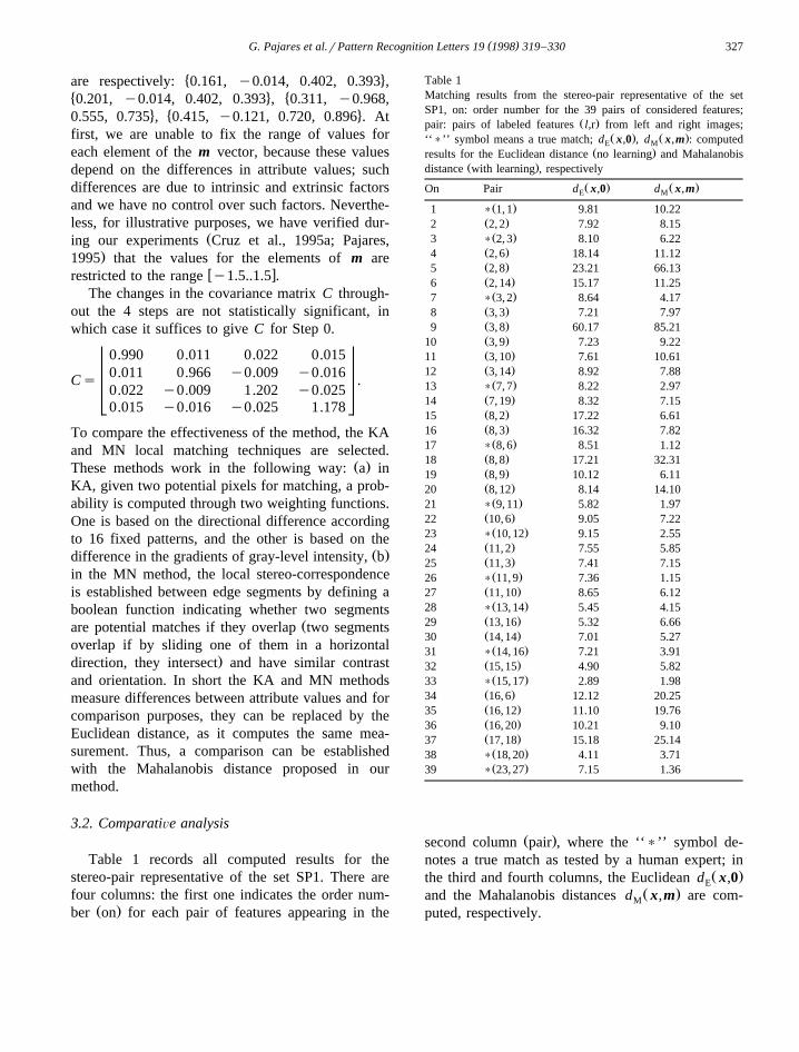
Table 1 records all computed results for thestereo-pair representative of the set SP1. There arefour columns: the first one indicates the order num-

Ž .ber on for each pair of features appearing in the

Table 1Matching results from the stereo-pair representative of the setSP1, on: order number for the 39 pairs of considered features;

Ž .pair: pairs of labeled features l,r from left and right images;Ž . Ž .‘‘)’’ symbol means a true match; d x,0 , d x,m : computedE M

Ž .results for the Euclidean distance no learning and MahalanobisŽ .distance with learning , respectively

Ž . Ž .On Pair d x,0 d x,mE M

Ž .1 ) 1, 1 9.81 10.22Ž .2 2, 2 7.92 8.15Ž .3 ) 2, 3 8.10 6.22

Ž .4 2, 6 18.14 11.12Ž .5 2, 8 23.21 66.13Ž .6 2, 14 15.17 11.25Ž .7 ) 3, 2 8.64 4.17

Ž .8 3, 3 7.21 7.97Ž .9 3, 8 60.17 85.21Ž .10 3, 9 7.23 9.22Ž .11 3, 10 7.61 10.61Ž .12 3, 14 8.92 7.88Ž .13 ) 7, 7 8.22 2.97

Ž .14 7, 19 8.32 7.15Ž .15 8, 2 17.22 6.61Ž .16 8, 3 16.32 7.82Ž .17 ) 8, 6 8.51 1.12

Ž .18 8, 8 17.21 32.31Ž .19 8, 9 10.12 6.11Ž .20 8, 12 8.14 14.10Ž .21 ) 9, 11 5.82 1.97

Ž .22 10, 6 9.05 7.22Ž .23 ) 10, 12 9.15 2.55

Ž .24 11, 2 7.55 5.85Ž .25 11, 3 7.41 7.15Ž .26 ) 11, 9 7.36 1.15

Ž .27 11, 10 8.65 6.12Ž .28 ) 13, 14 5.45 4.15

Ž .29 13, 16 5.32 6.66Ž .30 14, 14 7.01 5.27Ž .31 ) 14, 16 7.21 3.91

Ž .32 15, 15 4.90 5.82Ž .33 ) 15, 17 2.89 1.98

Ž .34 16, 6 12.12 20.25Ž .35 16, 12 11.10 19.76Ž .36 16, 20 10.21 9.10Ž .37 17, 18 15.18 25.14Ž .38 ) 18, 20 4.11 3.71Ž .39 ) 23, 27 7.15 1.36

Ž .second column pair , where the ‘‘)’’ symbol de-notes a true match as tested by a human expert; in

Ž .the third and fourth columns, the Euclidean d x,0EŽ .and the Mahalanobis distances d x,m are com-M

puted, respectively.


Of all the possible combinations of pairs ofmatches formed by segments of left and right im-ages, only 39 of them are considered, as the remain-der do not meet the initial restriction, which statesthat the value of the difference in the direction of thegradient must be less than "458 and the overlap rateŽ .percentage of overlapping coincidence greater than75%. These matches are directly classified as Falseby the system and omitted from the results’ table.The choice of such thresholds is supported by theparallel optical axis geometry with the given flexibil-ity in order to avoid errors during previous stages. Ofthe 39 pairs considered, there are unambiguous andambiguous ones, depending on whether a given leftimage segment corresponds to one and only one, orseveral right image segments, respectively. In anycase, the decision about the correct match is made bychoosing the result of the smaller value for each one

Žof the methods in the unambiguous case, there is.only one as long as it does not surpass a fixed

threshold, which coincides with the radius R of theŽ .hyper-sphere see Sections 2.2 and 2.3 . R is set to

10 in this paper.Table 2 shows results for the stereo-pair represen-

tative of set SP3 with the same symbols and criteriaas those explained in Table 1, although two values,identified by numbers 1 and 3, are obtained for theMahalanobis distance according to the processing forthis stereo-pair in Steps 1 and 3, respectively. Anoverview of the results in Table 2, allows us to checkthat, in general, for truerfalse matches the mini-mumrmaximum values for the Mahalanobis distanceare obtained during Step 3 as compared with thoseobtained in Step 1. These results are the best onesand correspond to a phase of increased learning.

From results in Tables 1 and 2 and results for theŽstereo-pair representative of set SP2 these last are

omitted because they are similar to those of the.stereo-pair representative of set SP3 in Step 1 we

build Table 3 in which the final results are summa-rized. It displays the number of successes and fail-ures for the stereo-pairs representing sets SP1, SP2and SP3 according to the decision process explainedabove. Also, it shows a coefficient m, which pro-vides a decision margin when ambiguities arise.

Ž .Such a coefficient is obtained as follows: a for eachambiguity case, we select two pairs of matches, one

Ž .is the true match ) and the other one the match

Table 2Results from stereo-pair representative of SP3; on: order number

Ž .for the 35 pairs of features; pair: pairs of labeled features l,rfrom left and right images, respectively, where ‘‘)’’ means a true

Ž . Ž .match; d x,m , d x,0 : computed results for the MahalanobisM EŽ . Ž .distance learning and Euclidean distance without learning ,

Ž . Ž .respectively, where 1 and 3 mean results computed accordingto test strategies in Steps 1 and 3, respectively

Ž . Ž . Ž .On Pair d x,0 d x,m d x,mE M1 M3

Ž .1 ) 1, 1 2.50 1.71 1.46Ž .2 ) 2, 4 3.08 3.01 2.82Ž .3 ) 3, 2 1.58 1.36 0.96

Ž .4 3, 6 3.40 4.01 4.26Ž .5 ) 4, 3 2.04 2.05 1.70

Ž .6 4, 5 11.14 12.11 12.50Ž .7 5, 1 80.12 91.00 94.60Ž .8 5, 2 6.76 12.18 13.11Ž .9 ) 5, 6 3.32 3.21 3.20

Ž .10 6, 3 12.70 13.36 13.68Ž .11 ) 6, 5 4.01 3.25 3.11Ž .12 ) 7, 8 2.30 2.35 1.66

Ž .13 8, 9 38.26 55.23 57.61Ž .14 10, 3 13.47 16.41 17.08Ž .15 11, 2 79.63 79.42 79.41Ž .16 11, 6 80.06 93.91 94.81Ž .17 ) 12, 11 0.51 0.51 0.48

Ž .18 12, 15 7.45 10.29 10.60Ž .19 ) 13, 12 28.55 23.12 18.10Ž .20 ) 14, 13 3.50 2.69 2.55Ž .21 ) 17, 16 8.86 6.23 6.12

Ž .22 18, 11 6.11 7.52 5.42Ž .23 ) 18, 15 7.89 7.76 4.96Ž .24 ) 21, 19 4.32 4.32 4.01

Ž .25 22, 19 2.06 4.68 5.11Ž .26 ) 22, 20 2.55 2.02 1.67Ž .27 ) 23, 21 4.08 4.12 3.75

Ž .28 23, 23 12.65 15.44 15.96Ž .29 ) 24, 22 15.78 11.12 8.22

Ž .30 25, 21 1.19 3.32 3.61Ž .31 ) 25, 23 2.03 2.04 1.83

Ž .32 26, 21 3.32 3.99 4.51Ž .33 26, 23 5.44 5.96 6.25Ž .34 ) 26, 24 2.35 2.15 2.08Ž .35 ) 27, 25 3.91 3.62 2.98

Ž .with the closest distance value to the true match, bwith the two selected pairs of matches we computethe difference between their corresponding distance

Ž .values, c finally, the coefficient m is the averagevalue for all ambiguity cases. Hence, a minimum

Ž .value most negative value for m indicates thatdecisions can be taken with a higher degree ofconfidence. The processing of set SP3 in Steps 1 and


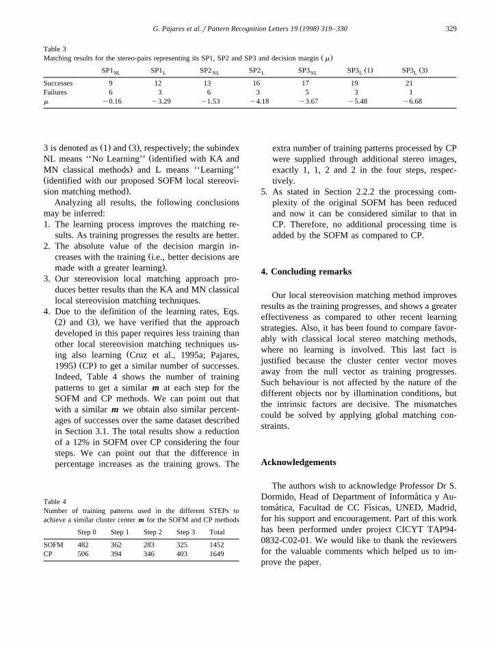
Table 3Ž .Matching results for the stereo-pairs representing its SP1, SP2 and SP3 and decision margin m

Ž . Ž .SP1 SP1 SP2 SP2 SP3 SP3 1 SP3 3NL L NL L NL L L

Successes 9 12 13 16 17 19 21Failures 6 3 6 3 5 3 1m y0.16 y3.29 y1.53 y4.18 y3.67 y5.48 y6.68

Ž . Ž .3 is denoted as 1 and 3 , respectively; the subindexŽNL means ‘‘No Learning’’ identified with KA and

.MN classical methods and L means ‘‘Learning’’Židentified with our proposed SOFM local stereovi-

.sion matching method .Analyzing all results, the following conclusions

may be inferred:1. The learning process improves the matching re-

sults. As training progresses the results are better.2. The absolute value of the decision margin in-

Žcreases with the training i.e., better decisions are.made with a greater learning .

3. Our stereovision local matching approach pro-duces better results than the KA and MN classicallocal stereovision matching techniques.

4. Due to the definition of the learning rates, Eqs.Ž . Ž .2 and 3 , we have verified that the approachdeveloped in this paper requires less training thanother local stereovision matching techniques us-

Žing also learning Cruz et al., 1995a; Pajares,. Ž .1995 CP to get a similar number of successes.

Indeed, Table 4 shows the number of trainingpatterns to get a similar m at each step for theSOFM and CP methods. We can point out thatwith a similar m we obtain also similar percent-ages of successes over the same dataset describedin Section 3.1. The total results show a reductionof a 12% in SOFM over CP considering the foursteps. We can point out that the difference inpercentage increases as the training grows. The

Table 4Number of training patterns used in the different STEPs toachieve a similar cluster center m for the SOFM and CP methods

Step 0 Step 1 Step 2 Step 3 Total

SOFM 482 362 283 325 1452CP 506 394 346 403 1649

extra number of training patterns processed by CPwere supplied through additional stereo images,exactly 1, 1, 2 and 2 in the four steps, respec-tively.

5. As stated in Section 2.2.2 the processing com-plexity of the original SOFM has been reducedand now it can be considered similar to that inCP. Therefore, no additional processing time isadded by the SOFM as compared to CP.

4. Concluding remarks

Our local stereovision matching method improvesresults as the training progresses, and shows a greatereffectiveness as compared to other recent learningstrategies. Also, it has been found to compare favor-ably with classical local stereo matching methods,where no learning is involved. This last fact isjustified because the cluster center vector movesaway from the null vector as training progresses.Such behaviour is not affected by the nature of thedifferent objects nor by illumination conditions, butthe intrinsic factors are decisive. The mismatchescould be solved by applying global matching con-straints.

Acknowledgements

The authors wish to acknowledge Professor Dr S.Dormido, Head of Department of Informatica y Au-´tomatica, Facultad de CC Fısicas, UNED, Madrid,´ ´for his support and encouragement. Part of this workhas been performed under project CICYT TAP94-0832-C02-01. We would like to thank the reviewersfor the valuable comments which helped us to im-prove the paper.


References

Ayache, N., Faverjon, B., 1987. Efficient registration of stereoimages by matching graph descriptions of edge segments.Internat. J. Comput. Vision 1, 107–131.

Breuel, T.M., 1996. Finding lines under bounded error. PatternŽ .Recognition 29 1 , 167–178.

Cruz, J.M., Pajares, G., Aranda, J., 1995a. A neural networkapproach to the stereovision correspondence problem by unsu-

Ž .pervised learning. Neural Networks 8 5 , 805–813.Cruz, J.M., Pajares, G., Aranda, J., Vindel, J.L.F., 1995b. Stereo

matching technique based on the perceptron criterion function.Pattern Recognition Letters 16, 933–944.

Dhond, A.R., Aggarwal, J.K., 1989. Structure from stereo – Areview. IEEE Trans. Systems Man Cybernet. 19, 1489–1510.

Duda, R.O., Hart, P.E., 1973. Pattern Classification and SceneAnalysis. Wiley, New York.

Flanagan, J.A., Hasler, M., 1995. Self-organising artificial neuralŽ .networks. In: Mira, J., Sandoval, F. Eds. , From Natural to

Artificial Neural Computation. Springer, Berlin.Fua, P., 1993. A parallel algorithm that produces dense depth

maps and preserves image features. Machine Vision Appl. 6,35–49.

Haykin, S., 1994. Neural Networks: A Comprehensive Founda-tion. Macmillan College Publishing, New York.

Hoff, W., Ahuja, N., 1989. Surface from stereo: Integratingfeature matching, disparity estimation and contour detection.IEEE Trans. Pattern Anal. Machine Intell. 11, 121–136.

Huertas, A., Medioni, G., 1986. Detection of intensity changeswith subpixel accuracy using Laplacian–Gaussian masks. IEEE

Ž .Trans. Pattern Anal. Machine Intell. 8 5 , 651–664.Kim, D.H., Aggarwal, J.K., 1987. Positioning three-dimensional

objects using stereo images. IEEE J. Robotics and Automation3, 361–373.

Kohonen, T., 1989. Self-Organization and Associative Memory.Springer, New York.

Kohonen, T., 1995. Self-Organizing Maps. Springer, Berlin.Kosko, B., 1992. Neural Networks and Fuzzy Systems. Prentice-

Hall, Englewood Cliffs, NJ.Krotkov, E.P., 1989. Active Computer Vision by Cooperative

Focus and Stereo. Springer, New York.Leu, J.G., Yau, H.L., 1991. Detecting the dislocations in metal

Ž .crystals from microscopic images. Pattern Recognition 24 1 ,41–56.

Lew, M.S., Huang, T.S., Wong, K., 1994. Learning and featureselection in stereo matching. IEEE Trans. Pattern Anal. Ma-

Ž .chine Intell. 16 9 , 869–881.Maravall, D., 1993. Reconocimiento de Formas y Vision Artifi-

cial. RA-MA, Madrid.Marr, D., Poggio, T., 1979. A computational theory of human

stereovision. Proc. Roy. Soc. London Ser. B 207, 301–328.Martin-Smith, P., Pelayo, F.J., Diaz, A., Ortega, J., Prieto, A.,

1993. A learning algorithm to obtain self-organizing mapsusing fixed neighbourhood Kohonen Networks. In: Mira, J.,

Ž .Cabestany, J., Prieto, A. Eds. , New Trends in Neural Com-putation. Springer, Berlin.

Medioni, G., Nevatia, R., 1985. Segment based stereo matching.Comput. Vision Graphics Image Process. 31, 2–18.

Mousavi, M.S., Schalkoff, R.J., 1994. ANN implementation ofstereo vision using a multi-layer feedback architecture. IEEE

Ž .Trans. Systems Man Cybernet. 24 8 , 1220–1238.Nevatia, R., Babu, K.R., 1980. Linear feature extraction and

description. Comput. Vision Graphics Image Process. 13,257–269.

Ozanian, T., 1995. Approaches for stereo matching – A review.Ž .Modeling Identification Control 16 2 , 65–94.

Pajares, G., 1995. Estrategia de Solucion al Problema de laCorrespondencia en Vision Estereoscopica por la Jerarquıa´ ´Metodologica y la Integracion de Criterios. Ph.D. Thesis,´ ´Dpto. Informatica y Automatica, Facultad Ciencias UNED,´ ´Madrid.

Patterson, D.W., 1996. Artificial Neural Networks. Prentice-Hall,Singapore.

Pollard, S.B., Mayhew, J.E.W., Frisby, J.P., 1981. PMF: A stereocorrespondence algorithm using a disparity gradient limit.Perception 14, 449–470.

Sonka, M., Hlavac, V., Boyle, R., 1995. Image Processing, Analy-sis and Machine Vision. Chapman-Hall, London.

Tanaka, S., Kak, A.C., 1990. A rule-based approach to binocularŽ .stereopsis. In: Jain, R.C., Jain, A.K. Eds. , Analysis and

Interpretation of Range Images. Springer, Berlin, pp. 33–139.Wuescher, D.M., Boyer, K.L., 1991. Robust contour decomposi-

tion using a constraint curvature criterion. IEEE Trans. PatternŽ .Anal. Machine Intell. 13 1 , 41–51.

Stereo matching based on the self-organizing feature-mapping algorithm

Documents

Transcript of Stereo matching based on the self-organizing feature-mapping algorithm