Statistics 150: Spring 2007

April 21, 2008

0-1

1 Continuous-Time Markov Chains

Consider a continuous-time stochastic process (Xt)t≥0 taking values in

the set of nonnegative integers. We say that the process (Xt)t≥0 is a

continuous-time Markov chain if for all sequences of times

t0 < t1 < · · · < tn and sequences of nonnegative integers

x0, x1, . . . , xn,

P{Xtn= xn | Xt0 = x0, Xt1 = x1, . . . , Xtn−1 = xn−1}

= P{Xtn= xn | Xtn−1 = xn−1}

= P{Xtn−tn−1 = xn | X0 = xn−1}.

This implies that for any 0 ≤ s < t, and any integer x,

P{Xt = x | Xu, 0 ≤ u ≤ s} = P{Xt = x | Xs}.

1

If we let τi denote the amount of time that the process stays in state i

before making a transition into a different state, then the Markov

property implies that

P{τi > s + t|τi > s} = P{τi > t},

for all s, t ≥ 0. Hence, the random variable τi is memoryless, so is

exponentially distributed.

2

The above gives us a way of constructing a continuous-time Markov

chain. Namely, it is a stochastic processes having the properties that

each time it enters state i:

(i) the amount of time it spends in that state before jumping to a

different state is exponentially distributed with some rate νi ≥ 0; and

(ii) when the process leaves state i, it will next enter state j with some

probability Pij , where∑

j 6=i Pij = 1.

A continuous-time Markov chain is said to be regular if, with

probability 1, the number of transitions in any finite length of time is

finite.

3

We shall, assume from now on that all Markov chains considered are

regular. Let qij be defined by

qij = νiPij , all i 6= j.

It follows that qij is the rate when in state i that the process makes a

transition into state j.

Finally, define the transition probabilities

Pij(t) = P{X(t + s) = j|X(s) = i},

not to be confused with the set of jump probabilities Pij . The quantity

does not depend on s by our assumption of homogeneity in time.

4

2 Birth and Death Processes

A continuous-time Markov chain with states 0, 1, · · · for which qij = 0whenever |i− j| > 1 is called a birth and death process. Let λi and µi

be given by

λi = qi,i+1, µi = qi,i−1.

The values {λi, i ≥ 0} and {µi, i ≥ 1} are called respectively the birth

rate and the death rate. We see that

νi = λi + µi, Pi,i+1 =λi

λi + µi= 1− Pi,i−1.

5

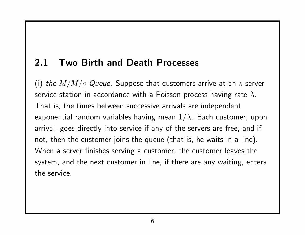
2.1 Two Birth and Death Processes

(i) the M/M/s Queue. Suppose that customers arrive at an s-server

service station in accordance with a Poisson process having rate λ.

That is, the times between successive arrivals are independent

exponential random variables having mean 1/λ. Each customer, upon

arrival, goes directly into service if any of the servers are free, and if

not, then the customer joins the queue (that is, he waits in a line).

When a server finishes serving a customer, the customer leaves the

system, and the next customer in line, if there are any waiting, enters

the service.

6

The successive service times are assumed to be independent

exponential random variables having mean 1/µ. If we let X(t) denote

the number in the system at time t, then {X(t), t ≥ 0} is a birth and

death process with

µn =

nµ, 1 ≤ n ≤ s

sµ, n > s,

λn = λ, n ≥ 0.

7

(ii)A Linear Growth Model with Immigration. A model in which

µn = nµ, n ≥ 1, λn = nλ + θ, n ≥ 0,

is called a linear growth process with immigration. Such processes

occur naturally in the study of biological reproduction and population

growth. Each individual in the population is assumed to give birth at

rate λ; in addition, there is a constant rate of increase θ due to an

external source such as immigration. Hence, the total birth rate where

there are n persons in the system is nλ + θ. Deaths are assumed to

occur at an exponential rate µ for each member of the population, and

hence µn = nµ.

8

A birth and death process is said to be a pure birth process if µn = 0for all n (that is, if death is impossible). The simplest example of a

pure birth process is the Poisson process, which has a constant birth

rate λn = λ, n ≥ 0.

9

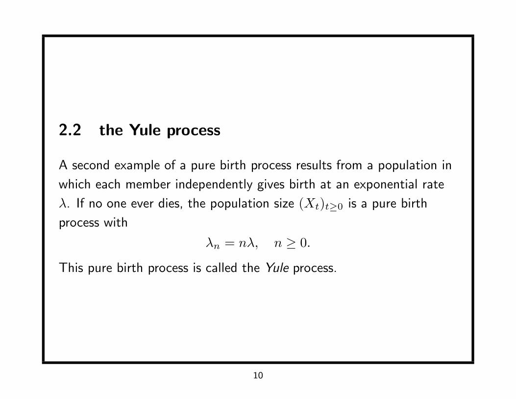
2.2 the Yule process

A second example of a pure birth process results from a population in

which each member independently gives birth at an exponential rate

λ. If no one ever dies, the population size (Xt)t≥0 is a pure birth

process with

λn = nλ, n ≥ 0.

This pure birth process is called the Yule process.

10

Consider a Yule process starting with a single individual at time 0, and

let Ti, i ≥ 1, denote the time between the (i− 1)th and ith birth. Now

P(T1 ≤ t) = 1− e−λt,

P{T1 + T2 ≤ t} =∫ t

0

P{T1 + T2 ≤ t|T1 = x}λe−λx d x

=∫ t

0

(1− e−2λ(t−x))λe−λx d x

= (1− e−λt)2,

11

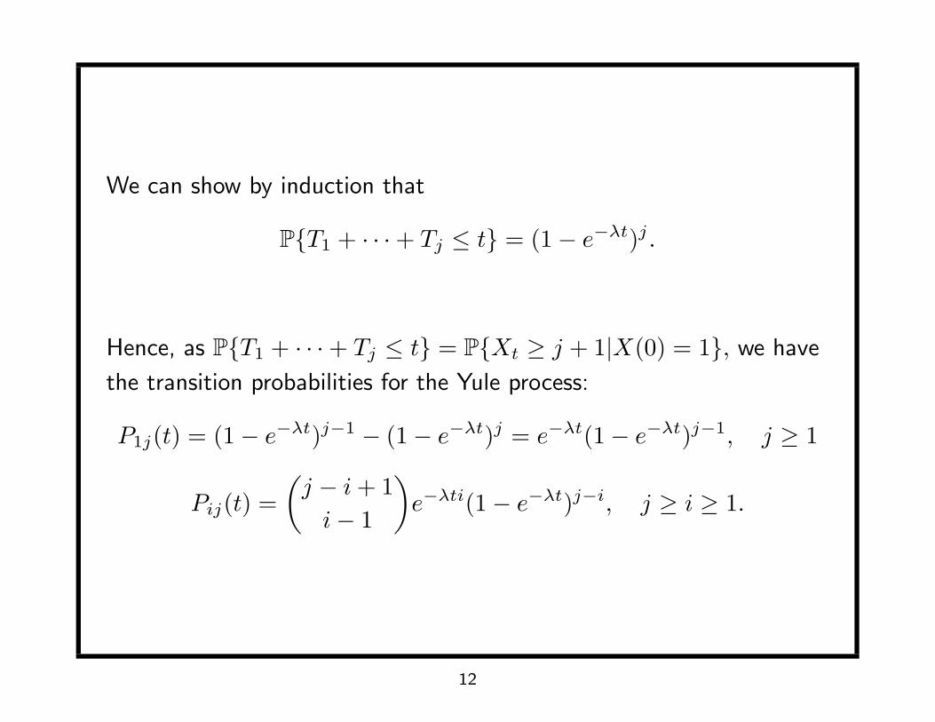
We can show by induction that

P{T1 + · · ·+ Tj ≤ t} = (1− e−λt)j .

Hence, as P{T1 + · · ·+ Tj ≤ t} = P{Xt ≥ j + 1|X(0) = 1}, we have

the transition probabilities for the Yule process:

P1j(t) = (1− e−λt)j−1 − (1− e−λt)j = e−λt(1− e−λt)j−1, j ≥ 1

Pij(t) =(

j − i + 1i− 1

)e−λti(1− e−λt)j−i, j ≥ i ≥ 1.

12

Let Sk =∑

i≤k Ti be the time of the kth birth. Reasoning

heuristically and treating densities as if they were probabilities yields

for 0 ≤ s1 ≤ s2 ≤ · · · ≤ sn ≤ t

P{S1 = s1, S2 = s2, · · · , Sn = sn|X(t) = n + 1}

=P{T1 = s1, T2 = s2 − s1, · · · , Tn = sn − sn−1, Tn+1 > t− sn}

P{X(t) = n + 1}

=λe−λs12λe−2λ(s2−s1) · · ·nλe−nλ(sn−sn−1)e−(n+1)λ(t−sn)

P{X(t) = n + 1}

=n! λn e−λ(t−s1)e−λ(t−s2) · · · e−λ(t−sn)

(1− e−λ)n.

13

Hence we see that the conditional density of (S1, · · · , Sn) given that

X(t) = n + 1 is given by n!∏n

i=1 f(si), 0 ≤ s1 ≤ s2 ≤ · · · ≤ sn ≤ t,

where f is the density function

f(x) =

λe−λ(t−x)

1−e−λt , 0 ≤ x ≤ t

0 otherwise.

14

Proposition 2.1. Consider a Yule process with X(0) = 1. Then,

given that X(t) = n + 1, the birth times S1, · · · , Sn are distributed as

the ordered values of n i.i.d. random variables whose density is

f(x) =

λe−λ(t−x)

1−e−λt , 0 ≤ x ≤ t

0 otherwise.

15

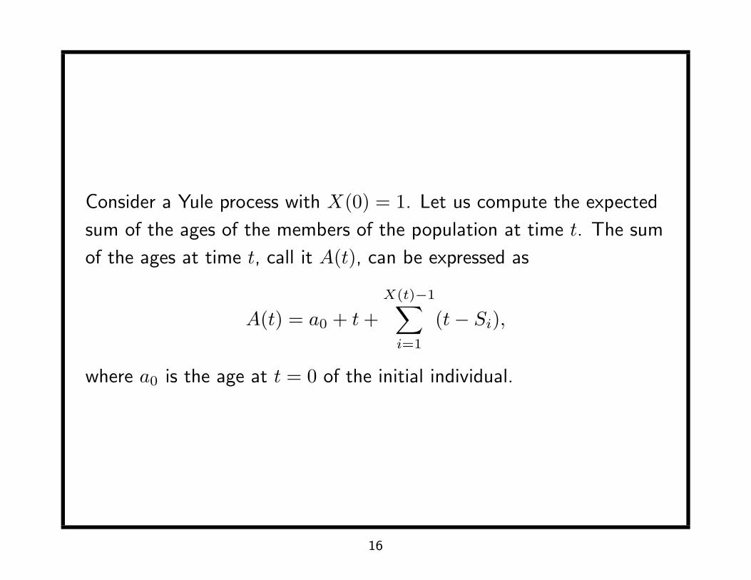
Consider a Yule process with X(0) = 1. Let us compute the expected

sum of the ages of the members of the population at time t. The sum

of the ages at time t, call it A(t), can be expressed as

A(t) = a0 + t +X(t)−1∑

i=1

(t− Si),

where a0 is the age at t = 0 of the initial individual.

16

First we compute E[A(t)] conditioned on X(t),

E[A(t)|X(t) = n + 1] = a0 + t + E[n∑

i=1

(t− Si)|X(t) = n + 1]

= a0 + t + n

∫ t

0

(t− x)λe−λ(t−x)

1− e−λtd x

or

E[A(t)|X(t)] = a0 + t + (X(t)− 1)1− e−λt − λte−λt

λ(1− e−λt).

Taking expectations and using the fact that X(t) has mean eλt yields

E[A(t)] = a0 + t +eλt − 1− λt

λ= a0 +

eλt − 1λ

.

17

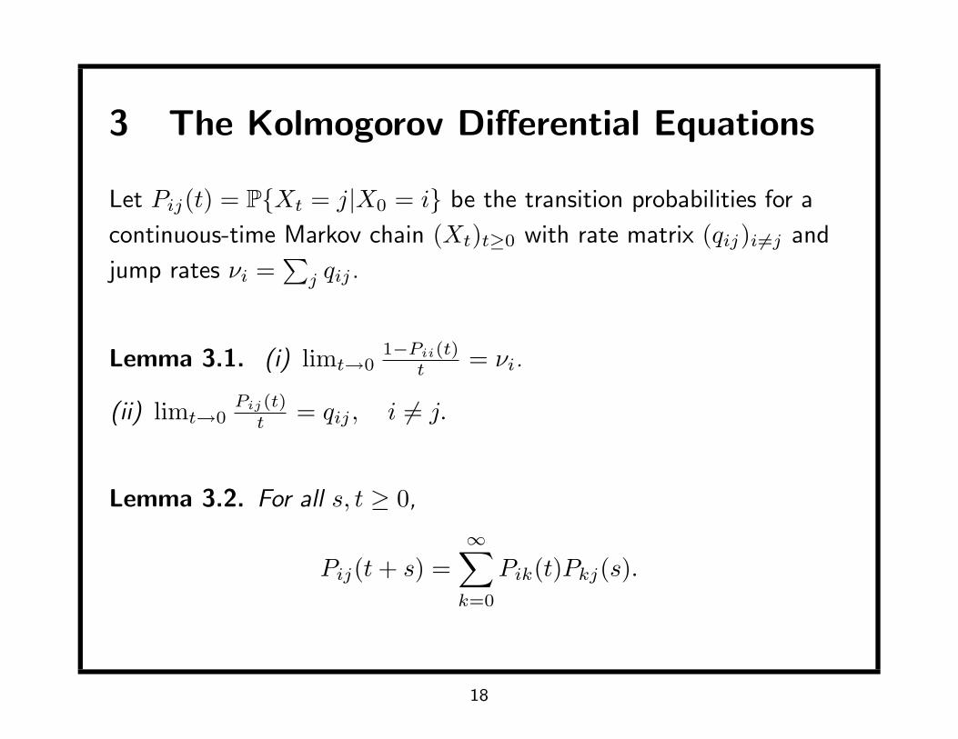
3 The Kolmogorov Differential Equations

Let Pij(t) = P{Xt = j|X0 = i} be the transition probabilities for a

continuous-time Markov chain (Xt)t≥0 with rate matrix (qij)i 6=j and

jump rates νi =∑

j qij .

Lemma 3.1. (i) limt→01−Pii(t)

t = νi.

(ii) limt→0Pij(t)

t = qij , i 6= j.

Lemma 3.2. For all s, t ≥ 0,

Pij(t + s) =∞∑

k=0

Pik(t)Pkj(s).

18

Theorem 3.3 (Kolmogorov’s Backward Equations). For all i, j, and

t ≥ 0,d

dtPij(t) =

∑k 6=i

qikPkj(t)− νiPij(t).

Proof: By the previous lemma, we have that

Pij(t + h)− Pij(t) =∑

k

(Pik(h)− δik)Pkj(t)

=∑k 6=i

Pik(h)Pkj(t) + (Pii(h)− 1)Pij(t),

where δik = 1 if i = k and is zero otherwise. By the preceeding lemma

then, if we can exchange the limit and the summation,

1h

(Pij(t + h)− Pij(t)) →∑k 6=i

qikPkj(t)− νiPij(t) as h → 0.

19

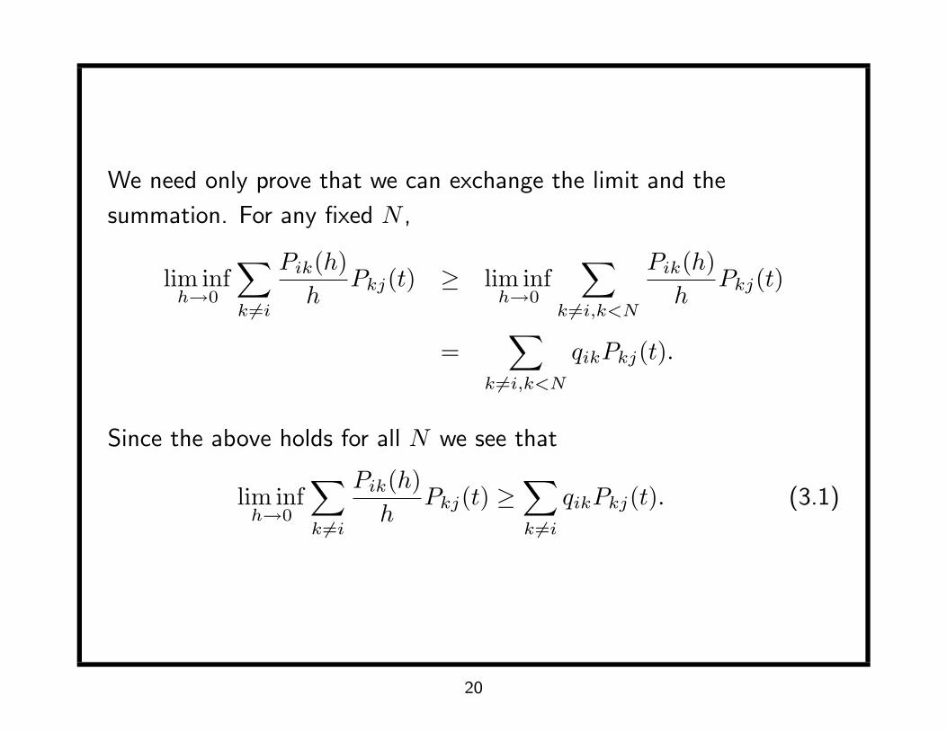
We need only prove that we can exchange the limit and the

summation. For any fixed N ,

lim infh→0

∑k 6=i

Pik(h)h

Pkj(t) ≥ lim infh→0

∑k 6=i,k<N

Pik(h)h

Pkj(t)

=∑

k 6=i,k<N

qikPkj(t).

Since the above holds for all N we see that

lim infh→0

∑k 6=i

Pik(h)h

Pkj(t) ≥∑k 6=i

qikPkj(t). (3.1)

20

To reverse the inequality note that for N > i, since Pkj(t) ≤ 1,

lim suph→0

∑k 6=i

Pik(h)h

Pkj(t)

≤ lim suph→0

∑k 6=i,k<N

Pik(h)

hPkj(t) +

∑k≥N

Pik(h)h

= lim sup

h→0

∑k 6=i,k<N

Pik(h)h

Pkj(t) +1− Pii(h)

h−

∑k 6=i,k<N

Pik(h)h

=

∑k 6=i,k<N

qikPkj(t) + νi −∑

k 6=i,k<N

qik,

where we have used Lemma 3.1 and the fact that∑

j Pij(t) = 1.

21

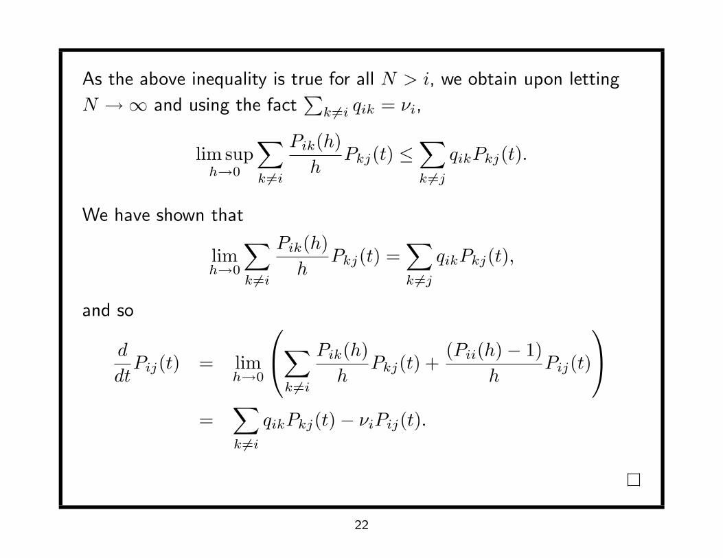
As the above inequality is true for all N > i, we obtain upon letting

N →∞ and using the fact∑

k 6=i qik = νi,

lim suph→0

∑k 6=i

Pik(h)h

Pkj(t) ≤∑k 6=j

qikPkj(t).

We have shown that

limh→0

∑k 6=i

Pik(h)h

Pkj(t) =∑k 6=j

qikPkj(t),

and so

d

dtPij(t) = lim

h→0

∑k 6=i

Pik(h)h

Pkj(t) +(Pii(h)− 1)

hPij(t)

=

∑k 6=i

qikPkj(t)− νiPij(t).

22

The set of differential equations for Pij(t) given in Theorem 3.3 are

known as the Kolmogorov backward equations. They are called the

backward equations because in computing the probability distribution

of the state at time t + h we conditioned on the state (all the way)

back at time h.

That is, we started our calculation with

Pij(t + h)

=∑

k

P{Xt+h = j |X0 = i, Xh = k}P{Xh = k|X0 = i}

=∑

k

Pik(h)Pkj(t).

23

We may derive another set of equations, known as the Kolmogorov’s

forward equations, by now conditioning on the state at time t. This

yields

Pij(t + h) =∑

k

Pik(t)Pkj(h)

or

Pij(t + h)− Pij(t) =∑

k

Pik(t)Pkj(h)− Pij(t)

=∑k 6=j

Pik(t)Pkj(h)− (1− Pjj(h))Pij(t).

24

Therefore,

limh→0

Pij(t + h)− Pij(t)h

= limh→0

∑k 6=j

Pik(t)Pkj(h)

h− 1− Pii(h)

hPij(t)

.

Assuming that we can interchange the limit with summation, we

obtain by Lemma 3.1 that

d

dtPij(t) =

∑k 6=j

qkjPik(t)− νjPij(t).

Theorem 3.4 (Kolmogorov forward equations). Under suitable

regularity conditions,

d

dtPij(t) =

∑k 6=j

qkjPik(t)− νjPij(t).

25

Example 3.5. The Kolmogorov forward equations for the birth and

death process are

d

dtPi0(t) = µ1Pi1(t)− λ0Pi0(t), for all i > 0,

d

dtPij(t) = λj−1Pi,j−1(t) + µj+1Pi,j+1(t)− (λj + µj)Pij(t), j 6= 0.

26

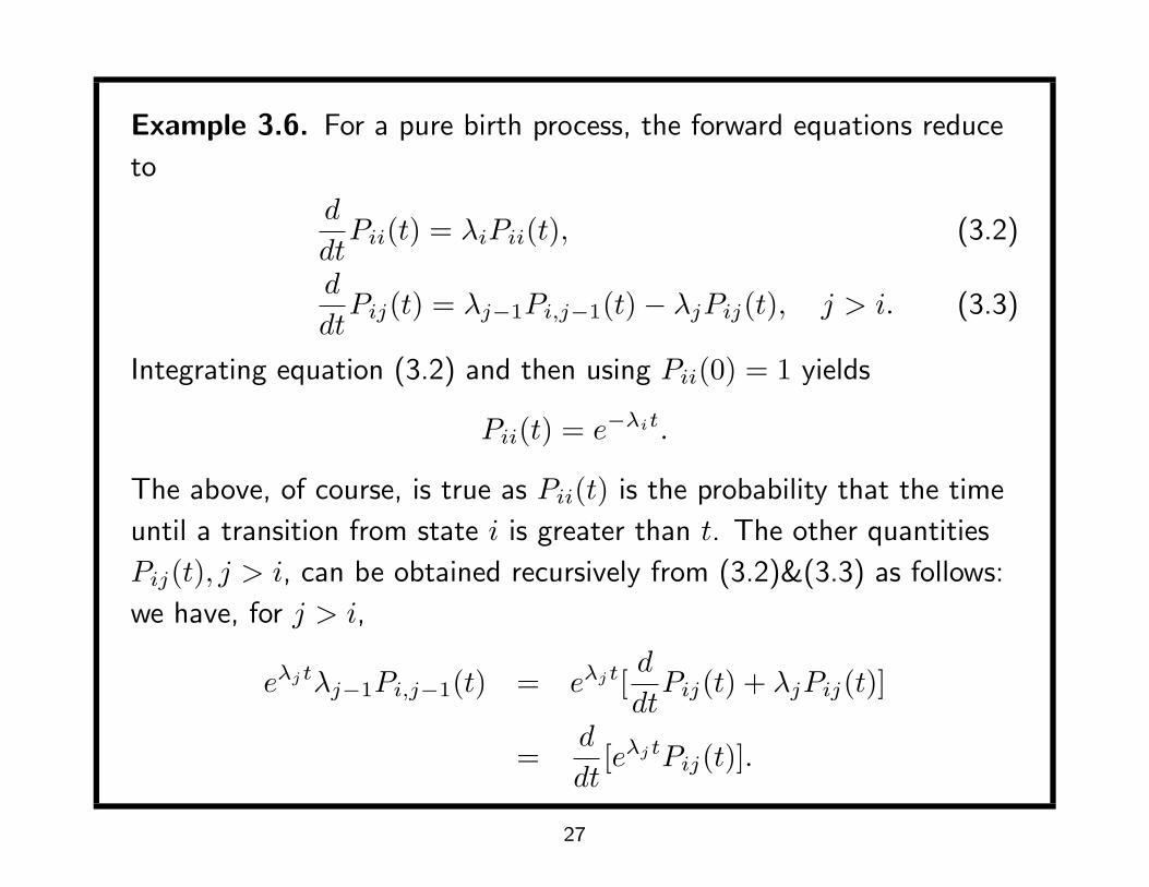
Example 3.6. For a pure birth process, the forward equations reduce

to

d

dtPii(t) = λiPii(t), (3.2)

d

dtPij(t) = λj−1Pi,j−1(t)− λjPij(t), j > i. (3.3)

Integrating equation (3.2) and then using Pii(0) = 1 yields

Pii(t) = e−λit.

The above, of course, is true as Pii(t) is the probability that the time

until a transition from state i is greater than t. The other quantities

Pij(t), j > i, can be obtained recursively from (3.2)&(3.3) as follows:

we have, for j > i,

eλjtλj−1Pi,j−1(t) = eλjt[d

dtPij(t) + λjPij(t)]

=d

dt[eλjtPij(t)].

27

Integration, using Pij(0) = 0, yields

Pij(t) = λj−1e−λjt

∫ t

0

eλjsPi,j−1(s) d s, , j > i.

In the special case of a Yule process, where λj = jλ, we can use the

above to verify our previous result,

Pij(t) =(

j − 1i− 1

)e−λti(1− e−λt)j−i, j ≥ i ≥ 1.

28

4 Exercises

1, A population of organisms consists of both male and female

members. In a small colony any particular male is likely to mate with

any particular female in any time interval of length h, with probability

λh + o(h). Each mating immediately produces one offspring, equally

likely to be male or female. Let N1(t) and N2(t) denote the number

males and females in the population at t. Derive the parameters of the

continuous-time Markov chain {N1(t), N2(t)}.

2, Suppose that a one-celled organism can be in one of two

states-either A or B. An individual in state A will change to state B

at an exponential rate α; an individual in state B divides into two new

individuals of type A at an exponential rate β. Define an appropriate

continuous-time Markov chain for a population of such organisms and

determine the appropriate parameters for this model.

29

3, Consider a Yule process with X(0) = i. Given that X(t) = i + k,

what can be said about the conditional distribution of the birth times

of the k individuals born in (0, t)?

4, Consider a Yule process starting with a single individual and

suppose that with probability P (s) and individual born at time s will

be robust. Compute the distribution of the number of robust

individuals born in (0, t).

30