Journal of Computational Physics 227 (2008) 8541–8550

Contents lists available at ScienceDirect

Journal of Computational Physics

journal homepage: www.elsevier .com/locate / jcp

Statistical moments of the random linear transport equation

Fábio A. Dorini a,*, M. Cristina C. Cunha b

a Department of Mathematics, DAMAT, Federal Technologic University of the Paraná - UTFPR, 80230-901, Curitiba, PR, Brazilb Department of Applied Mathematics, IMECC, University of Campinas - UNICAMP, 13083-970, Campinas, SP, Brazil

a r t i c l e i n f o a b s t r a c t

Article history:Received 30 May 2007Received in revised form 22 January 2008Accepted 9 June 2008Available online 18 June 2008

Keywords:Random linear transport equationRiemann problemStatistical momentsGodunov’s methodNumerical methods for random partialdifferential equations

0021-9991/$ - see front matter � 2008 Elsevier Incdoi:10.1016/j.jcp.2008.06.002

* Corresponding author.E-mail addresses: fabio.dorini@gmail.com (F.A. D

This paper deals with a numerical scheme to approximate the mth moment of the solutionof the one-dimensional random linear transport equation. The initial condition is assumedto be a random function and the transport velocity is a random variable. The scheme isbased on local Riemann problem solutions and Godunov’s method. We show that thescheme is stable and consistent with an advective–diffusive equation. Numerical examplesare added to illustrate our approach.

� 2008 Elsevier Inc. All rights reserved.

1. Introduction

Partial differential equations have been important models during the last centuries, mainly because they have the funda-mental support of differential calculus, numerical methods, and computers. However, the formulation of a physical processas a partial differential equation demands experiments to measure the data, for example, the diffusion coefficient, perme-ability of a porous media, initial conditions, boundary conditions and so on. This means that the interpretation of the dataas random variables is more realistic in some practical situations. Differential equations with random parameters are calledRandom Differential Equations; new mathematical methods have been developed to deal with this kind of problems (see[6,9,13,16], for example).

We are interested in the solution of the random linear transport equation

Q tðx; tÞ þ AQ xðx; tÞ ¼ 0; t > 0; x 2 R;

Qðx;0Þ ¼ Q0ðxÞ;

�ð1Þ

where A is a random variable and Q0ðxÞ is a random function.According to [1], the solution for the random Riemann problem (1) with

Q 0ðxÞ ¼QL if x < 0;QR if x > 0;

�ð2Þ

where QL and QR are random variables, is given by

Qðx; tÞ ¼ Q L þ Xxt

� �ðQ R � Q LÞ: ð3Þ

. All rights reserved.

orini), cunha@ime.unicamp.br (M.C.C. Cunha).

8542 F.A. Dorini, M.C.C. Cunha / Journal of Computational Physics 227 (2008) 8541–8550

In (3) X is the Bernoulli random variable with PfXðnÞ ¼ 1g ¼ FAðnÞ where FA is the cumulative probability function of A. Fur-thermore, in case of independence between A and both QL and Q R, the mth moment of Qðx; tÞ, hQ mðx; tÞi, m 2 N, m P 1, isgiven by

hQ mðx; tÞi ¼ hQ mL i þ FA

xt

� �Q m

R

� �� Qm

L

� �� �: ð4Þ

The closed solution (3) and Godunov’s ideas [7,10,11] are used in [2] and [4] to design numerical methods to compute themean and the variance of the solution to (1). These methods are explicit and neither demand generation of random numbers(as does the Monte Carlo method [5,12,15,17]), nor require differential equations governing the statistical moments (as inthe effective equations methodology [6,17]). Moreover, the schemes are stable and consistent with an advective–diffusiveequation which agrees with the effective equation to the expectation presented in the literature (see [6], for example). In[3] we use the idea of collecting deterministic realizations through their probability functions to solve the nonlinear randomRiemann–Burgers equation.

In this paper, we deal with the general moments of the solution to (1). The outline of this paper is as follows. In Section 2we use (3) and (4) to design a numerical method to the mth statistical moment of the solution to the general problem (1). Wepresent the CFL condition under which the local solutions do not interact between themselves. In Section 3 we show thestability of the numerical scheme and its consistency with an advective–diffusive equation. We show that the diffusion coef-ficient is related with the probability density function of the velocity by Eq. (18), which has a simple solution in the normalvelocity case. Furthermore, in Section 4 we present a decoupled system of partial differential equations to be satisfied by thecentral moments of the random solution. All the partial differential equations in this paper are linear. In fact, denoting byLðuÞ ¼ ut þ hAiux � muxx, the equations are: LðuÞ ¼ 0, for the moments, and LðuÞ ¼ f , for the central moments. Computationalexperiments and comparisons with the Monte Carlo method are presented in Section 5.

2. The numerical scheme

In this section, we present the numerical method for the mth statistical moment of the solution to (1). The method isbased on the juxtaposition of Riemann problems whose solutions are given by (3). We discretize both space and time assum-ing a uniform mesh spacing: xj ¼ jDx, xj�1=2 ¼ xj � ðDx=2Þ, tn ¼ nDt, tn�1=2 ¼ tn � ðDt=2Þ, for Dx;Dt > 0. In Fig. 1 we present aschematic diagram of the algorithm. Let us assume that the random variables Qn

j and the mth moments Qm;nj

D E¼ Qmðxj; tnÞ� �

are known at t ¼ tn.In the following we use the ideas of Reconstruct-Evolve-Average (REA), algorithm [7,11] to approximate

Qm;nþ1j

D E¼ Qmðxj; tnþ1Þ� �

.

Step 1 We reconstruct the piecewise random constant function eQ ðx; tnÞ from Q nj , i.e, eQ ðx; tnÞ ¼ Qn

j for x 2 ½xj�1=2; xjþ1=2�. Thepiecewise constant random function eQ ðx; tnÞ defines a set of local random Riemann problems, each one centered atx ¼ xj�1=2,

Q tðx; tÞ þ AQ xðx; tÞ ¼ 0; t > tn; x 2 R;

Qðx; tnÞ ¼Q n

j�1; if x < xj�1=2;

Q nj ; if x > xj�1=2:

(ð5Þ

Fig. 1. Schematic diagram of the algorithm.

F.A. Dorini, M.C.C. Cunha / Journal of Computational Physics 227 (2008) 8541–8550 8543

Step 2 From (3) and (4), the local solutions of (5) and the respective statistical moments are given by

Gj�1=2ðx; tnþ1=2Þ ¼ Q nj�1 þ X

x� xj�1=2

Dt=2

Q n

j � Q nj�1

h ið6Þ

and

Gmj�1=2ðx; tnþ1=2Þ

D E¼ Qm;n

j�1

D Eþ FA

x� xj�1=2

Dt=2

Qm;n

j

D E� Qm;n

j�1

D Eh i: ð7Þ

The global solution at t ¼ tnþ1=2, eQ ðx; tnþ1=2Þ, can be constructed by piecing together the local random Riemann solutions (6),provided that Dt=2 is sufficiently small such that adjacent local random Riemann solutions do not interact. Therefore, takinginto account the similarity property of the random Riemann solutions, Dx and Dt must be chosen such that

Gj�1=2ðx; tnþ1=2Þjx¼xj�1� Q n

j�1 and Gj�1=2ðx; tnþ1=2Þjx¼xj� Q n

j ;

where the symbol ‘‘�” means ‘‘sufficiently near to”. By substituting these conditions in (6) we must have

FA �DxDt

� 0 and FA

DxDt

� 1: ð8Þ

Remark 1. We may regard (8) as the CFL condition for the method: the interval ½�Dx=Dt;Dx=Dt� must contain an effectivesupport of the density probability function of A. This means that the probability of A outside of the interval ½�Dx=Dt;Dx=Dt� issufficiently near to zero, and then may be disregarded. The existence of an effective support is ensured by Chebyshev’sinequality: PfjA� hAijP krAg 6 1=k2, for all k > 0, where rA is the standard variation of A. If we take 1=k2 sufficiently closeto zero, to escape from the interaction between solutions of Riemann problems we must take ðjhAij þ krAÞDt=Dx 6 1.

Under condition (8) we conclude Step 2 by taking

eQ ðx; tnþ1=2Þ ¼X

j�1=2

Gj�1=2ðx; tnþ1=2Þ 1½xj�1 ;xj �

where 1½a;b� denotes the characteristic function of the interval ½a; b�. From (7) it follows that

eQ mðx; tnþ1=2ÞD E

¼X

j�1=2

Gmj�1=2ðx; tnþ1=2Þ

D E1½xj�1 ;xj �: ð9Þ

In a similar way, using the values at t ¼ tnþ1=2, we obtain

bQ mðx; tnþ1ÞD E

¼X

j

Gmj ðx; tnþ1Þ

D E1½xj�1=2 ;xjþ1=2 �: ð10Þ

Step 3 We use (10) to approximate Q m;nþ1j

D Eas the average value of bQ mðx; tnþ1Þ

D Eover the interval ½xj�1=2; xjþ1=2�:Z Z

Qm;nþ1j

D E’ 1

Dx

xjþ1=2

xj�1=2

bQ mðx; tnþ1ÞD E

dx ¼ 1Dx

xjþ1=2

xj�1=2

Gmj ðx; tnþ1Þ

D Edx

¼ 1Dx

Z xjþ1=2

xj�1=2

Q m;nþ1=2j�1=2

D Eþ FA

x� xj

Dt=2

Q m;nþ1=2

jþ1=2

D E� Q m;nþ1=2

j�1=2

D Eh i� �dx

¼ Q m;nþ1=2j�1=2

D Eþ Dt

2Dx

Z DxDt

�DxDt

FAðxÞdx

( )Qm;nþ1=2

jþ1=2

D E� Q m;nþ1=2

j�1=2

D Eh i: ð11ÞD E

Likewise, we use (9) to approximate Q m;nþ1=2j�1=2 :Z Z

Qm;nþ1=2j�1=2

D E’ 1

Dx

xj

xj�1

eQ mðx; tnþ1=2ÞD E

dx ¼ 1Dx

xj

xj�1

Gmj�1=2ðx; tnþ1=2Þ

D Edx

¼ 1Dx

Z xj

xj�1

Q m;nj�1

D Eþ FA

x� xj�1=2

Dt=2

Q m;n

j

D E� Q m;n

j�1

D Eh i� �dx

¼ Q m;nj�1

D Eþ Dt

2Dx

Z DxDt

�DxDt

FAðxÞdx

( )Q m;n

j

D E� Q m;n

j�1

D Eh i: ð12Þ

The following result is proved in [4]:

Lemma 2. Let Y be a random variable and ½�n; n� an effective support of the density probability function of Y, i.e., FY ð�nÞ � 0 andFYðnÞ � 1. Then

Z n

�nFYðxÞdx � n� hYi: ð13Þ

8544 F.A. Dorini, M.C.C. Cunha / Journal of Computational Physics 227 (2008) 8541–8550

Inserting (13) in (11) and (12), and denoting k ¼ DthAi=Dx, gives

Q m;nþ1j

D E¼ 1

2Q m;nþ1=2

j�1=2

D Eþ Q m;nþ1=2

jþ1=2

D Eh i� k

2Q m;nþ1=2

jþ1=2

D E� Q m;nþ1=2

j�1=2

D Eh ið14Þ

and

Q m;nþ1=2j�1=2

D E¼ 1

2Q m;n

j�1

D Eþ Q m;n

j

D Eh i� k

2Q m;n

j

D E� Q m;n

j�1

D Eh i: ð15Þ

Grouping these expressions we summarize the two-step scheme (14) and (15) in the one-step explicit method:

Q m;nþ1j

D E¼ Q m;n

j

D E� k

2Q m;n

jþ1

D E� Q m;n

j�1

D Eh iþ 1

4ð1þ k2Þ Q m;n

jþ1

D E� 2 Q m;n

j

D Eþ Q m;n

j�1

D Eh i: ð16Þ

Remark 3. The numerical scheme (16) is conservative, i.e., it can be rewritten as

Q m;nþ1j

D E¼ Q m;n

j

D E� Dt

DxFm;n

jþ1=2 � Fm;nj�1=2

h i;

where Fm;nj�1=2 ¼ ð1=2ÞhAi Q m;n

j�1

D Eþ Qm;n

j

D Eh i� ð1=4ÞhAið1=kþ kÞ Qm;n

j

D E� Q m;n

j�1

D Eh iis an approximation to the average flux at

x ¼ xj�1=2.

3. Numerical analysis of the scheme

The scheme (16) is a generalization of a previously studied scheme to the mean (m ¼ 1) of the solution to (1). Therefore,we can use the same arguments used in [4] to show

� Consistency: if m ¼ Dx2=ð4DtÞ is fixed then the numerical scheme (16) yields an OðDx2Þ approximation for the solution ofthe partial differential equation

ut þ hAiux ¼ m uxx;

uðx;0Þ ¼ hQ 0ðxÞmi;ð17Þ

� Stability: the numerical method (16) is stable under the CFL condition (8).

As a linear problem, the convergence of (16) to the differential equation (17) is a consequence of the Lax Equivalence The-orem, no matter what m ¼ Dx2=ð4DtÞ is. The following proposition gives additional information about the diffusion associatedwith the random velocity, A.

Proposition 4. The diffusion coefficient in (17) must satisfy

�f 0Axt

� �mðx; tÞ ¼ fA

xt

� �ðx� hAitÞ; ð18Þ

where fAðnÞ ¼ d½FAðnÞ�=dn is the density probability function of A.

Proof. As a general differential equation, (17) must be satisfied by every particular solution. The random Riemann problem(1)–(2) is a particular case of (1) with known moments given by (4):

hQ mðx; tÞi ¼ Q mL

� �þ FA

xt

� �Qm

R

� �� Q m

L

� �� �:

Direct derivations and substitution of this solution in (17) gives (18), a necessary condition to mðx; tÞ. h

3.1. The normal case

Let A � NðhAi;rAÞ. Using the normal probability density function in (18) we obtain m ¼ r2At. In this case, the differential

equation (17) turns to be

ut þ hAiux ¼ ðr2AtÞuxx; t > 0;

uðx;0Þ ¼ hQ 0ðxÞmi;ð19Þ

which agrees with the effective equation for the statistical mean presented by some authors (see [6], for example). Weemphasize that our convergence results show that the differential equation which describes the evolution of all the momentsis the same. Using (18) we may also show that if mðx; tÞ depends only on t then A is normally distributed.

F.A. Dorini, M.C.C. Cunha / Journal of Computational Physics 227 (2008) 8541–8550 8545

Now we use the consistency condition to define proper mesh spacing. Let t ¼ tf be fixed, and select Dt and Dx such that

Dx2

4Dt¼ m ¼ 1

2ðr2

Atf Þ: ð20Þ

The convergence results show that our method converges to the solution of the differential equation

ut þ hAiux ¼12ðr2

Atf Þuxx;

uðx;0Þ ¼ hQ 0ðxÞmi:ð21Þ

The solutions of (19) and (21), u1ðx; tÞ and u2ðx; tÞ, respectively, are equal at t ¼ tf . Indeed, according to [14] we have

u1ðx; tf Þ ¼1ffiffiffiffi

pp

n1ðtf Þ

Z þ1

�1exp � x� hAitf �x

n1ðtf Þ

2" #

hQ 0ðxÞmi dx; ð22Þ

where

n1ðtf Þ ¼ 2Z tf

0ðr2

AsÞ ds �1=2

¼ffiffiffi2p

rAtf :

On the other hand, the solution to (21) is also given by (22) with

n2ðtf Þ ¼ 2Z tf

0½ðr2

Atf Þ=2� ds �1=2

instead of n1ðtf Þ. Since n1ðtf Þ ¼ n2ðtf Þ then u1ðx; tf Þ ¼ u2ðx; tf Þ.Therefore (20) is more than a consistency condition: it guarantees the convergence of the method to the solution at t ¼ tf .For this particular example (normal velocity), we have shown that each moment of the solution to (1), hQðx; tÞmi, satisfies

the advection–diffusion Eq. (17) with m ¼ mðtÞ. As a consequence, the probability density function for the random solutionQðx; tÞ, fQ ðq; x; tÞ, also satisfies the advection–diffusion equation

ðfQ Þt þ hAiðfQ Þx ¼ mðtÞ ðfQ Þxx;

fQ ðq; x;0Þ ¼ fQ0ðq; xÞ:ð23Þ

Indeed, the Fourier transform of fQ ðq; x; tÞ, under the assumption that the probability density function is uniquely determinedby its moments (see e.g., [8] for conditions for uniqueness in the problems of moments), is

bfQ ðx; x; tÞ ¼X1j¼0

ðixÞj

j!hQ mðx; tÞi; ð24Þ

where hQ mðx; tÞit þ hAi Qmðx; tÞ� �

x ¼ mðtÞ Qmðx; tÞ� �

xx. Taking the derivative with respect to t and x in (24), we arrive at

bfQ

� �tþ hAi bfQ

� �x¼ mðtÞ bfQ

� �xx: ð25Þ

Since the variable x does not appear in the derivatives, we can go back to the variable u and find (23). The respective initialcondition follows from the probability density function of Q0ðxÞ.

4. The system of partial differential equations for the central moments

The central moments of a given random function Qðx; tÞ are deterministic functions defined by lm ¼ hðQ � hQiÞmi, m 2 N,

m P 2. The most used central moment is the variance, m ¼ 2, which was introduced by Gauss (1777–1855) as a measure ofdispersion of the distribution of Qðx; tÞ. But high order central moments are also useful information concerning random vari-ables [13,16]. In the following we show that the central moment lmðx; tÞ, if sufficiently smooth, satisfies an advective–dif-fusive equation with the source term defined by the expectation and the central moments lm�1ðx; tÞ and lm�2ðx; tÞ. Here, weextend the definition of central moments for m P 0 since l0 ¼ 1 and l1 ¼ 0.

We may use algebraic manipulations to show that

(i) If k 6 m� 2 then

m

kþ 2

ðkþ 1Þðkþ 2Þ ¼

m

k

ðm� kÞðm� k� 1Þ: ð26Þ

(ii) If k 6 m� 1 then

m

kþ 2

ðkþ 1Þ ¼

m

k

ðm� kÞ: ð27Þ

8546 F.A. Dorini, M.C.C. Cunha / Journal of Computational Physics 227 (2008) 8541–8550

(iii)

lm ¼ hQmi �

Xm�1

k¼2

m

k

lkhQi

m�k � hQim: ð28Þ

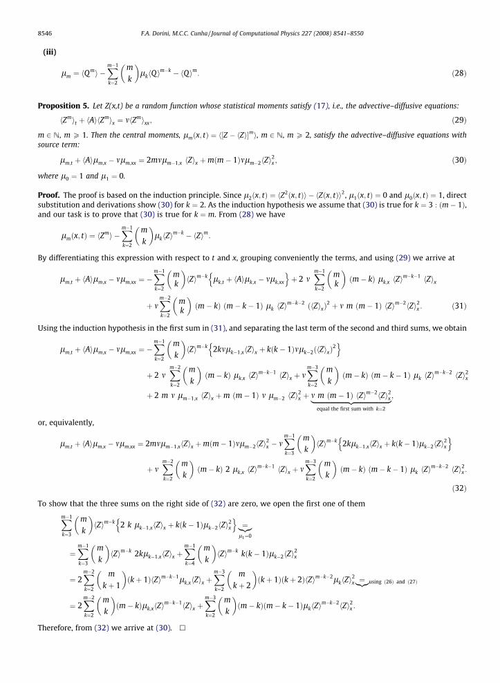
Proposition 5. Let Z(x,t) be a random function whose statistical moments satisfy (17), i.e., the advective–diffusive equations:

hZmit þ hAihZmix ¼ mhZmixx; ð29Þ

m 2 N, m P 1. Then the central moments, lmðx; tÞ ¼ h½Z � hZi�mi, m 2 N, m P 2, satisfy the advective–diffusive equations with

source term:

lm;t þ hAilm;x � mlm;xx ¼ 2mmlm�1;x hZix þmðm� 1Þmlm�2hZi2x ; ð30Þ

where l0 ¼ 1 and l1 ¼ 0.

Proof. The proof is based on the induction principle. Since l2ðx; tÞ ¼ hZ2ðx; tÞi � hZðx; tÞi2, l1ðx; tÞ ¼ 0 and l0ðx; tÞ ¼ 1, direct

substitution and derivations show (30) for k ¼ 2. As the induction hypothesis we assume that (30) is true for k ¼ 3 : ðm� 1Þ,and our task is to prove that (30) is true for k ¼ m. From (28) we have

lmðx; tÞ ¼ hZmi �

Xm�1

k¼2

m

k

lkhZi

m�k � hZim:

By differentiating this expression with respect to t and x, grouping conveniently the terms, and using (29) we arrive at

lm;t þ hAilm;x � mlm;xx ¼ �Xm�1

k¼2

mk

hZim�k lk;t þ hAilk;x � mlk;xx

n oþ 2 m

Xm�1

k¼2

mk

ðm� kÞ lk;x hZi

m�k�1 hZix

þ mXm�2

k¼2

mk

ðm� kÞ ðm� k� 1Þ lk hZi

m�k�2 ðhZixÞ2 þ m m ðm� 1Þ hZim�2hZi2x : ð31Þ

Using the induction hypothesis in the first sum in (31), and separating the last term of the second and third sums, we obtain

lm;t þ hAilm;x � mlm;xx ¼ �Xm�1

k¼2

m

k

hZim�k 2kmlk�1;xhZix þ kðk� 1Þmlk�2ðhZixÞ

2n o

þ 2 mXm�2

k¼2

m

k

ðm� kÞ lk;x hZi

m�k�1 hZix þ mXm�3

k¼2

m

k

ðm� kÞ ðm� k� 1Þ lk hZi

m�k�2 hZi2x

þ 2 m m lm�1;x hZix þm ðm� 1Þ m lm�2 hZi2x þ m m ðm� 1Þ hZim�2hZi2x|fflfflfflfflfflfflfflfflfflfflfflfflfflfflfflfflfflfflfflfflffl{zfflfflfflfflfflfflfflfflfflfflfflfflfflfflfflfflfflfflfflfflffl}

equal the first sum with k¼2

;

or, equivalently,

lm;t þ hAilm;x � mlm;xx ¼ 2mmlm�1;xhZix þmðm� 1Þmlm�2hZi2x � m

Xm�1

k¼3

m

k

hZim�k 2klk�1;xhZix þ kðk� 1Þlk�2hZi

2x

n oþ m

Xm�2

k¼2

m

k

ðm� kÞ 2 lk;x hZi

m�k�1 hZix þ mXm�3

k¼2

m

k

ðm� kÞ ðm� k� 1Þ lk hZi

m�k�2 hZi2x :

ð32Þ

To show that the three sums on the right side of (32) are zero, we open the first one of them

Xm�1

k¼3

m

k

hZim�k 2 k lk�1;xhZix þ kðk� 1Þlk�2hZi

2x

n o¼|{z}

l1¼0

¼Xm�1

k¼3

m

k

hZim�k 2klk�1;xhZix þ

Xm�1

k¼4

m

k

hZim�k kðk� 1Þlk�2hZi

2x

¼ 2Xm�2

k¼2

m

kþ 1

ðkþ 1ÞhZim�k�1lk;xhZix þ

Xm�3

k¼2

m

kþ 2

ðkþ 1Þðkþ 2ÞhZim�k�2lkhZi

2x ¼|{z}using ð26Þ and ð27Þ

¼ 2Xm�2

k¼2

m

k

ðm� kÞlk;xhZi

m�k�1hZix þXm�3

k¼2

m

k

ðm� kÞðm� k� 1ÞlkhZi

m�k�2hZi2x :

Therefore, from (32) we arrive at (30). h

F.A. Dorini, M.C.C. Cunha / Journal of Computational Physics 227 (2008) 8541–8550 8547

Remark 6. In Section 3 we have shown that the numerical method (16), for the moments, is stable and consistent with (17).Since we have used the same method (16) to compute the central moments, we conclude that the method for the centralmoments is stable and consistent with (30).

5. Computational tests

In this section, we present some examples to assess our approach. In Examples 1 and 2 the initial condition allows exactstatistical moments of the solution. We use Riemann initial conditions defined by bivariate normal distributions; in this casethe solutions for the moments are given by (4). In order to investigate the influence of the randomness we use two models: inExample 1 the velocity, A, is normally distributed, and in Example 2 the velocity is lognormally distributed. In both cases wecompare the exact solutions, given by (4), with the solutions yielded by the numerical scheme (16) for some statistical mo-ments. In Example 3 we apply our method in the problem (1) where the initial condition is a normal random function andthe transport velocity is a normal random variable. The numerical experiments presented in this section were done in doubleprecision with some MATLAB codes on a 3.0 GHz Pentium 4 with 512 Mb of memory.

Example 1. Let us consider the random Riemann problem (1)–(2) where the random velocity is normally distributed,A � Nð1:0;0:8Þ, and the random variables QL and QR have a bivariate normal distribution defined by: hQLi ¼ 1:0 (mean ofQL); hQRi ¼ 0:0 (mean of QR); rL ¼ 0:4 (standard deviation of QL); rR ¼ 0:5 (standard deviation of QR); and q ¼ 0:4(correlation coefficient between QL and QR). In Fig. 2 we compare the exact values for the mean, variance, 3rd centralmoment, and 4th central moment with the computations using (16) at tf ¼ 0:4, and Dt and Dx satisfying (20).

Example 2. To check the influence of the velocity distribution we consider the random Riemann problem (1)–(2) in whichthe random velocity is lognormally distributed, A ¼ expðnÞ, n � Nð0:5;0:35Þ. The initial condition (QL;QR) has a bivariate nor-mal distribution defined by: hQ Li ¼ 1:0; hQRi ¼ 0:15; rL ¼ 0:36; rR ¼ 0:25; and q ¼ 0:4. Taking the lognormal distribution,A ¼ expðnÞ, n � Nðln;rnÞ, in (18) we obtain

-2 -1 0 1 2 3 4-0.2

0

0.2

0.4

0.6

0.8

1

1.2

mean

numerical schemeexact solution

-2 -1 0 1 2 3 4

0.15

0.2

0.25

0.3

0.35

0.4

0.45

0.5

variance

-2 -1 0 1 2 3 4

-0.15

-0.1

-0.05

0

0.05

0.1

3rd central moment

-2 -1 0 1 2 3 4

-0.1

0

0.1

0.2

0.3

0.4

0.5

0.6

4th central moment

Fig. 2. A � Nð1:0;0:8Þ, Dx ¼ 0:01, Dt ¼ 0:000195, and tf ¼ 0:4.

8548 F.A. Dorini, M.C.C. Cunha / Journal of Computational Physics 227 (2008) 8541–8550

mðx; tÞ ¼r2

nxt

� �xt � hAit� �

r2n � ln

� �þ ln x

t

� � : ð33Þ

This mean that it is not possible to find constants Dx and Dt such that ðDx2Þ=ð4DtÞ ¼ m, the consistency condition. Moreover,the diffusion coefficient (33) may assume negative values loosing the physical meaning. Thus, although these arguments arenot conclusive, they suggest that an advective–diffusive equation is not a good model to the moments of the solution to (1)with a lognormal velocity. If we use (20) as in the previous example the results loose quality as shown in Fig. 3.

Example 3. In this example we test our method for the random partial differential equation (1) in which A is normal,A � Nð�0:5;0:6Þ, and Q0ðxÞ is a normal random function with mean

hQ 0ðxÞi ¼1; x 2 ð1:4; 2:2Þ;e�20ðx�0:25Þ2 ; otherwise;

(ð34Þ

and covariance Covðx; ~xÞ ¼ r2 expð�bjx� ~xjÞ, where Var½Q0ðxÞ� ¼ r2 is constant and b > 0 governs the decay rate of the spa-tial correlation. We use b ¼ 0:3 and r2 ¼ 0:16. The numerical results are compared with the Monte Carlo method using suitesof realizations of A and Q 0ðxÞ, where A and Q 0ðxÞ are statistically independents. Observe that each realization AðxÞ andQ0ðx;xÞ yields analytical solution given by Qðx; t;xÞ ¼ Q0ðx� AðxÞt;xÞ. To generate the realizations required by MonteCarlo simulations we use random numbers generator of MATLAB. Comparisons with the Monte Carlo method, with30,000 realizations, are plotted in Fig. 4.

6. Conclusions

In this paper, we have used the Godunov ideas to obtain a numerical scheme for the statistical moments of the solution ofthe one-dimensional random linear transport equation. We consider the velocity as a random variable and the initial con-dition as a random function. We have used an explicit solution of the random Riemann problem to evolve in the REA algo-

-1 0 1 2 3 40

0.2

0.4

0.6

0.8

1

1.2

mean

numerical schemeexact solution

-1 0 1 2 3 40.2

0.25

0.3

0.35

0.4

0.45

0.5

0.55

variance

-1 0 1 2 3 4-0.04

-0.02

0

0.02

0.04

0.06

0.08

0.1

0.12

0.14

3rd central moment

-1 0 1 2 3 4

0.2

0.3

0.4

0.5

0.6

0.7

0.8

0.94th central moment

Fig. 3. A ¼ expðnÞ, n � Nð0:5;0:35Þ, Dx ¼ 0:01, Dt ¼ 0:000312, and tf ¼ 0:4.

-2 -1 0 1 2 3

0

0.2

0.4

0.6

0.8

1

1.2

mean

numerical schemeMonte Carlomean of init. cond.

-2 -1 0 1 2 3

0.15

0.2

0.25

0.3

0.35

0.4

0.45

variance

-2 -1 0 1 2 3

-0.1

-0.05

0

0.05

0.1

3rd central moment 4th central moment

-2 -1 0 1 2 3

0

0.1

0.2

0.3

0.4

0.5

1

Fig. 4. A � Nð�0:5;0:6Þ, Dx ¼ 0:02, Dt ¼ 0:000138, and tf ¼ 0:4.

F.A. Dorini, M.C.C. Cunha / Journal of Computational Physics 227 (2008) 8541–8550 8549

rithm. Moreover, we have shown that the scheme is stable and consistent with an advective–diffusive equation. A particularRiemann problem solution is used to find the diffusion coefficient of the differential equations for the statistical moments.Also, we have obtained the differential equations for the central moments of the solution. Computational tests have illus-trated our theoretical results.

Acknowledgment

Our acknowledgments to the Brazilian Council for Development of Science and Technology (CNPq) through the Grant140406/2004-2.

References

[1] M.C.C. Cunha, F.A. Dorini, A note on the Riemann problem for the random transport equation, Comput. Appl. Math. 26 (3) (2007) 323–335.[2] M.C.C. Cunha, F.A. Dorini, A numerical scheme for the variance of the solution of the random transport equation, Appl. Math. Comput. 190 (1) (2007)

362–369.[3] M.C.C. Cunha, F.A. Dorini, Statistical moments of the solution of the random Burgers–Riemann problem, Math. Comput. Simulat. (2008), doi:10.1016/

j.matcom.2008.06.001.[4] F.A. Dorini, M.C.C. Cunha, A finite volume method for the mean of the solution of the random transport equation, Appl. Math. Comput. 187 (2) (2007)

912–921.[5] G.S. Fishman, Monte Carlo: Concepts, Algorithms and Applications, Springer-Verlag, New York, 1996.[6] J. Glimm, D. Sharp, Stochastic partial differential equations: selected applications in continuum physics, in: R.A. Carmona, B.L. Rozovskii (Eds.),

Stochastic Partial Differential Equations: Six Perspectives, Mathematical Surveys and Monographs, American Mathematical Society, No. 64, p. 03-44,Providence, 1998.

[7] S.K. Godunov, A difference method for numerical calculation of discontinuous solutions of the equations of hydrodynamics, Mat. Sb. 47 (1959) 271–306.

[8] M.G. Kendall, Conditions for uniqueness in the problems of moments, Ann. Math. Stat. 11 (1940) 402–409.[9] P.E. Kloeden, E. Platen, Numerical Solution of Stochastic Differential Equations, Springer, New York, 1999.

[10] R.J. LeVeque, Numerical Methods for Conservation Laws, Birkhäuser, Berlin, 1992.[11] R.J. LeVeque, Finite Volume Methods for Hyperbolic Problems, Cambridge University Press, Cambridge, 2002.

8550 F.A. Dorini, M.C.C. Cunha / Journal of Computational Physics 227 (2008) 8541–8550

[12] P. O’Leary, M.B. Allen, F. Furtado, Groundwater transport with stochastic retardation: numerical results, Comput. Methods Water Resources XII 1(1998) 255–261.

[13] B. Oksendal, Stochastic Differential Equations: An Introduction with Applications, Springer, New York, 2000.[14] A.D. Polyanin, Handbook of Linear Partial Differential Equations for Engineers and Scientists, Chapman and Hall/CRC, New York, 2002.[15] G.I. Schuëller, A state-of-the-art report on computational stochastic mechanics, Prob. Eng. Mech. 12 (4) (1997) 197–322.[16] T.T. Soong, Random Differential Equations in Sciences and Engineering, Academic Press, New York, 1973.[17] D. Zhang, Stochastic Methods for Flow in Porous Media – Coping with Uncertainties, Academic Press, San Diego, 2002.