Statistical analysis of eight surface ozone measurement seriesfor various sites in Ireland

O. P. Tripathi,1 S. G. Jennings,1 C. D. O’Dowd,1 L. Coleman,1 S. Leinert,2 B. O’Leary,2

E. Moran,3 S. J. O’Doherty,4 and T. G. Spain1

Received 10 February 2010; revised 13 April 2010; accepted 4 May 2010; published 1 October 2010.

[1] Data from various stations having different measurement record periods between1988 and 2007 are analyzed to investigate the surface ozone concentration, long‐termtrends, and seasonal changes in and around Ireland. Time series statistical analysis isperformed on the monthly mean data using seasonal and trend decomposition proceduresand the Box‐Jenkins approach (autoregressive integrated moving average). In general,ozone concentrations in the Irish region are found to have a negative trend at all sitesexcept at the coastal sites of Mace Head and Valentia. Data from the most polluted Dublincity site have shown a very strong negative trend of −0.33 ppb/yr with a 95% confidencelimit of 0.17 ppb/yr (i.e., −0.33 ± 0.17) for the period 2002−2007, and for the site near thecity of Cork, the trend is found to be −0.20 ± 0.11 ppb/yr over the same period. Thenegative trend for other sites is more pronounced when the data span is considered fromaround the year 2000 to 2007. Rural sites of Wexford and Monaghan have alsoshown a very strong negative trend of −0.99 ± 0.13 and −0.58 ± 0.12, respectively,for the period 2000−2007. Mace Head, a site that is representative of ozone changesin the air advected from the Atlantic to Europe in the marine planetary boundarylayer, has shown a positive trend of about +0.16 ± 0.04 ppb per annum over theentire period 1988−2007, but this positive trend has reduced during recent years (e.g., in theperiod 2001−2007). Cluster analysis for back trajectories are performed for the stationshaving a long record of data, Mace Head and Lough Navar. ForMace Head, the northern andwestern clean air sectors have shown a similar positive trend (+0.17 ± 0.02 ppb/yr for thenorthern sector and +0.18 ± 0.02 ppb/yr for the western sector) for the whole period, butpartial analysis for the clean western sector at Mace Head shows different trends duringdifferent time periods with a decrease in the positive trend since 1988 indicating adeceleration in the ozone trend for Atlantic air masses entering Europe.

Citation: Tripathi, O. P., S. G. Jennings, C. D. O’Dowd, L. Coleman, S. Leinert, B. O’Leary, E. Moran, S. J. O’Doherty, andT. G. Spain (2010), Statistical analysis of eight surface ozone measurement series for various sites in Ireland, J. Geophys. Res.,115, D19302, doi:10.1029/2010JD014040.

1. Introduction

[2] The study of the behavior of surface ozone is ofimportance mainly because it has a negative impact onhuman health, agricultural crops, forests, and damaging ofmaterials [World Health Organization (WHO), 1987;Musselman et al., 2006; US Environmental ProtectionAgency (EPA), 2006; Hazucha and Lefohn, 2007]. Ozonein the troposphere is also a greenhouse gas affecting radia-tive forcing that therefore contributes to the heat budget ofthe planet and is a significant contributor to climate change

[Ramaswamy et al., 2001]. Ozone (and its precursors) is oneof the air pollutant species that is identified as a trans-boundary pollutant, by the Task Force on HemisphericTransport of Air Pollution under the United Nations Eco-nomic Committee for Europe (UNECE) Convention onLong‐Range Transboundary Air Pollution. It is the mainprecursor of oxidizing agents in the atmosphere, thehydroxyl radicals [Levy, 1971], affecting the cleansingcapacity of the atmosphere. Most of the surface ozone ori-ginates from the troposphere itself, but a significant sourceof ozone is also transport from the stratosphere because of anumber of dynamical processes: seasonal variations at thetropopause, turbulence due to jet streams, and diffusionacross the tropopause causing stratospheric intrusion ofozone into the troposphere. This stratospheric flux is amaximum in the spring and through a large amount of tro-pospheric mixing contributes to the seasonal variation intropospheric ozone at a particular site. Stratospheric ozone

1School of Physics, Environmental Change Institute, NationalUniversity of Ireland, Galway, Ireland.

2Environmental Protection Agency, Dublin, Ireland.3Met Éireann, Dublin, Ireland.4Physical and Theoretical Chemistry, University of Bristol, UK.

Copyright 2010 by the American Geophysical Union.0148‐0227/10/2010JD014040

JOURNAL OF GEOPHYSICAL RESEARCH, VOL. 115, D19302, doi:10.1029/2010JD014040, 2010

D19302 1 of 20

depletion might have an impact on the influx from thestratosphere to the troposphere [Terao et al., 2008; Ordóñezet al., 2007], and according to Fusco and Logan [2003],using Goddard Earth Observing System‐Chemical TransportModel analysis for the period 1970–1995, this flux mayhave decreased by a maximum of about 30% from the early1970s to the mid 1990s. But studies have shown that thedecline in stratospheric ozone is stopped due to a ban inthe production and emission of ozone‐depleting chloro-fluorocarbons by the Montreal and subsequent protocols[Newchurch et al., 2003; WMO, 2007]. In the troposphere,ozone can be produced or destroyed by chemical reaction.Ozone concentrations close to emission sources can beaffected by destruction through NO titration (reaction ofozone with NO). Ozone is in equilibrium between its pro-duction and loss through NOx compounds. Anthropogenicallyemitted organic compounds can disturb this equilibrium byforming radicals. These radicals can provide an additionalnon‐ozone‐destroying route of NO to NO2 resulting in anotherwise extra ozone source in the troposphere. At verylow NOx concentrations, chemical destruction of ozone usu-ally takes place. Dry deposition provides an additional sinkof ozone. All these processes together with transport andmixing determine ozone concentrations at a particular site.Surface ozone changes daily (diurnal variation), monthly (sea-sonal changes), and annually (long‐term changes). The sea-sonal cycle with a spring maxima and a summer minima is avery distinctive feature of ground‐level ozone in the North-ern Hemisphere [Derwent et al., 1998; Monks, 2000; Wanget al., 2003]. Although it depends on the location, chemi-cal, and transport processes at a particular site, it is consistenton a regional scale. Local pollution and boundary levelmeteorology are mainly responsible for diurnal variations[Coyle et al., 2002; Tarasova et al., 2007]. Ozone changes atrural and remote locations might be affected by changes inhemispheric emissions and transport in the planetary bound-ary layer and changes in transport from the stratosphere.Jenkin [2008] discussed the effect of background ozone trendsand regional trends caused by decreasing ozone precursoremissions on the trends in ozone concentrations at a receptorsite.[3] Modeling and measurement studies have shown that

baseline surface ozone levels in Europe are changing withtime and are not consistent with changes in emission levelsof ozone precursors on a regional scale [Jonson et al., 2006,and references therein]. They suggested that the decrease inozone levels because of regional changes in precursors isannulled by an increasing background level. Previousstudies have indicated that background ozone levels areincreasing at the background North Atlantic site at MaceHead and in Europe [Naja et al., 2003]. Several other workssuggested that during the past century, anthropogenic pho-tochemical precursors have been increasing and so haveozone background levels [Volz and Kley, 1988; Staehelin etal., 1994; Simmonds et al., 2004]. Emission inventories andcorresponding measurements have shown that ozone pre-cursors such as NOx, CO, and nonmethane volatile organiccompounds (NMVOCs) have reduced significantly in NorthAmerica and Europe since the late 1980s [Vestreng et al.,2004; Derwent et al., 2003; Solberg et al., 2004], andsome authors suggested that this change may be ameliorat-ing the increase in surface ozone levels [Ordóñez et al., 2005;

Vingarzan, 1994; Oltmans et al., 2006; Lefohn et al., 2008].At the same time, emissions are found to be increasingfrom other parts of the world, mainly from Asia, andfrom other sources such as international shipping [Streetset al., 2003; Endresen et al., 2003]. Oltmans et al. [2006]investigated changes in ozone levels at a network ofsurface ozone and ozonesondes monitoring sites scatteredacross the globe and provided a mixed picture of ozonetrends at different sites suggesting significant regional dif-ferences. According to Oltmans et al. [2006], midlatitudesof the Northern Hemisphere (North America, ContinentalEurope, and Japan) exhibited significant increase in tropo-spheric ozone in the 1970s and 1980s but have leveled off ordeclined during the recent decades. IntergovernmentalPanel on Climate Change [2007] also suggested thatlong‐term background tropospheric ozone trends do notshow any coherent picture for the changes in both magnitudeas well as in sign and their possible causes. A recent study byParrish et al. [2009] on ozone in the marine boundary layerhas also indicated a stabilization in the ozone trend or even anegative trend (see Figure 12a of the above paper) at MaceHead after 2000. Another interesting result from the work ofParrish et al. [2009] is the difference in both the baselineozone level and trends between Pacific marine boundarylayer air masses entering the west coast of America andAtlantic marine boundary layer air masses entering Europe(Mace Head). This study indicates that Mace Head ozonemay not be considered as representative of hemisphericbackground ozone. Tarasova et al. [2009] studied ozonetrend patterns at the Caucasian Kislovodsk High Mountainstation site and at the Swiss Alpine site Jungfraujoch andshowed that trends at the two sites have changed during theperiod 1997–2006 in comparison to the earlier period 1991–2001. They attributed these opposite trends during the twoperiods to the dramatic decline in emissions during 1990sin the former USSR and the introduction of more stringentemission regulations in Western Europe. Under these sce-narios, there appears to be no coherent picture about thetrend in global or hemispheric background ozone. Thewidely changing scenarios in emissions of ozone precursorsand of tropospheric ozone levels shifted the problem from aregional scale to a global scale. Emissions from Asia caninfluence ozone levels in North America [Lin et al., 2000;Fiore et al., 2001; Jaffe et al., 2003], and North Americanemissions can change ozone levels in Europe [Parrish et al.,1993; Moody et al., 1995; Stohl and Trickl, 1999; Wild andAkimoto, 2001; Li et al., 2002].[4] Ground‐level ozone is currently measured in many

rural and urban areas of Ireland, but a long‐term record isonly available and analyzed for the coastal station of MaceHead. Work by Oltmans et al. [2006], Scheel et al. [1997],Simmonds et al. [2004], Carslaw [2005], Derwent et al.[2007], and by others on Mace Head ozone data haveshown varying trends depending on the length of dataconsidered and the methodology applied for their evalua-tion. In Ireland, ozone measurements are presently beingcarried out at 9 sites of the Environmental ProtectionAgency (EPA) ozone network, Valentia Observatory (MetEireann), and at Lough Navar in Co. Fermanagh. LoughNavar site is part of the national Automatic Urban and RuralNetwork set up by the UK Department of Environment,Food, and Rural Affairs [Jenkin, 2008]. The ozone instru-

TRIPATHI ET AL.: SURFACE OZONE IN IRELAND D19302D19302

2 of 20

mentation at Mace Head was set up by Peter G. Simmonds,funded through the UK Ministry of the Environment. Thereare many years of continuous records from these stationsscattered around Ireland. Among them, Mace Head andLough Navar have exceptionally long records with morethan 20 years of data. There has been apparently no knowncoordinated integrated effort to analyze these data withrespect to seasonal variability or with respect to medium andlong‐term changes. The objective of this paper is to presenta detailed assessment of ozone levels and trends in Irelandon the basis of the statistical analysis of available groundlevel ozone data.

2. Data and Methods

2.1. Ozone Data

[5] Ozone at EPA stations, at Mace Head, ValentiaObservatory, and Lough Navar is measured using a con-tinuous ozone analyzer by UV photometry. The instrument(API M400, M400A, and M400E) is microprocessor con-trolled that uses a system based on the Beer‐Lambert law formeasuring ozone in ambient air. Ozone concentration datafor Ireland are provided by the EPA for EPA measurementsites (Dublin Pottery Road, Dublin Rathmines, Cork,Wexford, and Monaghan). The ozone measurements atdifferent sites in Ireland started in different years. Mea-surement uncertainty for ozone is <15%. In this analysis, weconsider the stations on the basis of their longer record and arange of stations such as urban, suburban, rural, and marine

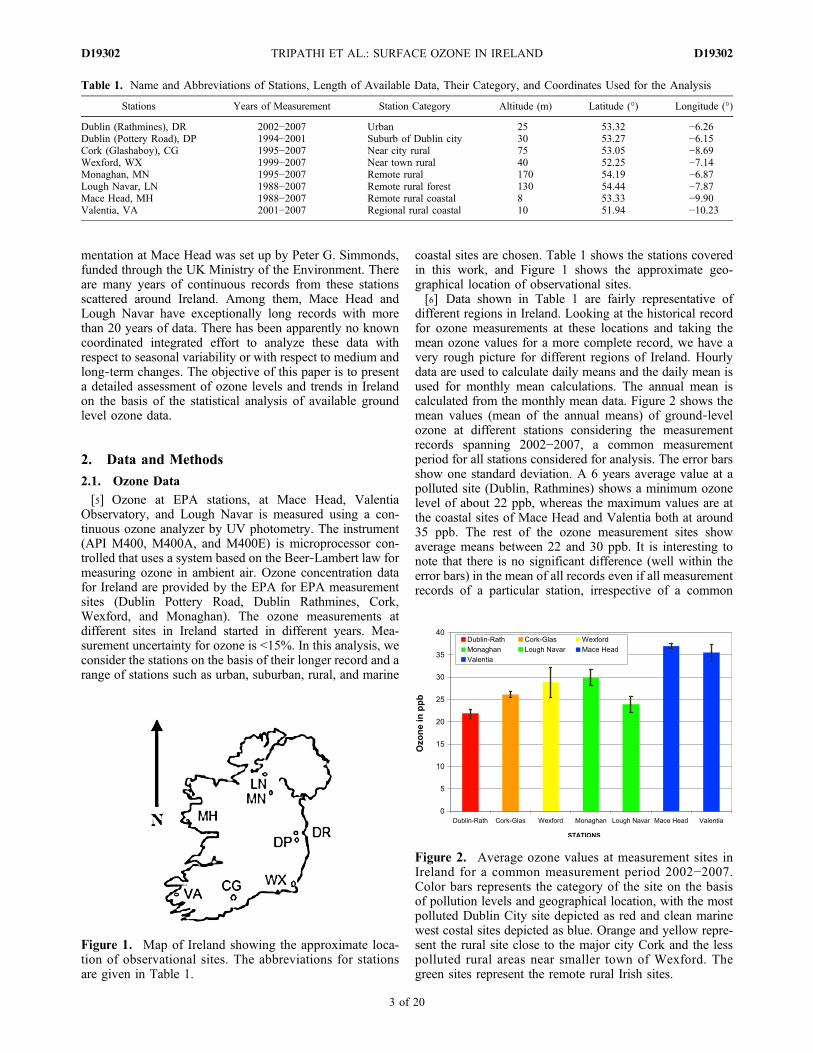
coastal sites are chosen. Table 1 shows the stations coveredin this work, and Figure 1 shows the approximate geo-graphical location of observational sites.[6] Data shown in Table 1 are fairly representative of

different regions in Ireland. Looking at the historical recordfor ozone measurements at these locations and taking themean ozone values for a more complete record, we have avery rough picture for different regions of Ireland. Hourlydata are used to calculate daily means and the daily mean isused for monthly mean calculations. The annual mean iscalculated from the monthly mean data. Figure 2 shows themean values (mean of the annual means) of ground‐levelozone at different stations considering the measurementrecords spanning 2002−2007, a common measurementperiod for all stations considered for analysis. The error barsshow one standard deviation. A 6 years average value at apolluted site (Dublin, Rathmines) shows a minimum ozonelevel of about 22 ppb, whereas the maximum values are atthe coastal sites of Mace Head and Valentia both at around35 ppb. The rest of the ozone measurement sites showaverage means between 22 and 30 ppb. It is interesting tonote that there is no significant difference (well within theerror bars) in the mean of all records even if all measurementrecords of a particular station, irrespective of a common

Table 1. Name and Abbreviations of Stations, Length of Available Data, Their Category, and Coordinates Used for the Analysis

Stations Years of Measurement Station Category Altitude (m) Latitude (°) Longitude (°)

Dublin (Rathmines), DR 2002−2007 Urban 25 53.32 −6.26Dublin (Pottery Road), DP 1994−2001 Suburb of Dublin city 30 53.27 −6.15Cork (Glashaboy), CG 1995−2007 Near city rural 75 53.05 −8.69Wexford, WX 1999−2007 Near town rural 40 52.25 −7.14Monaghan, MN 1995−2007 Remote rural 170 54.19 −6.87Lough Navar, LN 1988−2007 Remote rural forest 130 54.44 −7.87Mace Head, MH 1988−2007 Remote rural coastal 8 53.33 −9.90Valentia, VA 2001−2007 Regional rural coastal 10 51.94 −10.23

Figure 1. Map of Ireland showing the approximate loca-tion of observational sites. The abbreviations for stationsare given in Table 1.

Figure 2. Average ozone values at measurement sites inIreland for a common measurement period 2002−2007.Color bars represents the category of the site on the basisof pollution levels and geographical location, with the mostpolluted Dublin City site depicted as red and clean marinewest costal sites depicted as blue. Orange and yellow repre-sent the rural site close to the major city Cork and the lesspolluted rural areas near smaller town of Wexford. Thegreen sites represent the remote rural Irish sites.

TRIPATHI ET AL.: SURFACE OZONE IN IRELAND D19302D19302

3 of 20

measurement period, is considered for the calculation. Onthe basis of historical air quality data and from the geo-graphical point of view, Ireland can be divided into differentcategories. The EPA divides measurements sites accordingto the European Union (EU) Directive 96/62/EC [CEC,1996]. Stations are classified as either urban, suburban, orrural and then one of traffic, industrial, or background. Ruralsites are further classified as near‐city, regional, or remotesites. West coast rural sites of Mace Head and Valentia areconsidered separately as coastal marine sites.

2.2. Cluster Analysis of Trajectories

[7] Air samples measured for ozone at a particular site inIreland can have a wide range of histories. They may befrom maritime clean Atlantic air due to westerly or south‐westerly (190°−300°) winds or from polluted Europeanregions because of easterly winds. The calculated air masstrajectories arriving at a particular site provide informationabout the history of air masses for 4 days back. For MaceHead and Lough Navar, both having a long record of data,trajectories were calculated using Hybrid Single ParticleLagrangian Integrated Trajectory Model (HYSPLIT), atransport and dispersion model provided by the NOAA AirResources Laboratory (ARL) [Draxler and Rolph, 2003].National Centers for Environmental Prediction/NationalCenter for Atmospheric Research reanalysis data wereused for the meteorological fields. Ninety‐six hour back‐trajectories arriving at 1200 h (UT) each day were calculated,with a final height of 100 m, for the years 1987 until 2007.The algorithm used for the clustering process is given inAppendix A.

2.3. Statistical Analysis of Time‐Series of Ozone

[8] Ground‐level ozone data analyzed here are monthlyaveraged values of relatively long records (8 or more yearsof observations) of surface ozone measurements that form atime series. The data are averaged up to a monthly level to

form a univariate (considering 12 months of the year dis-tributed equally timewise that is a good approximation foraverage monthly ozone values) time series for statisticalanalysis. Gaps in the resultant time series are replaced by theaverage of the adjacent seasonal values, i.e., average of thevalues 12 months before and after. In time series analysis,one approach is to find a model that represents the data andcan be used for future predictions. If data consist of anestablished periodicity or seasonality and possible trends(as with ground‐level ozone), another approach may be todecompose the time series into trend, seasonal, and errorcomponents. The error components represent the periods inthe series that might be affected by episodic pollutionevents.[9] Surface ozone data analyzed here exhibit well an es-

tablished seasonal pattern with maxima during the springand minima in summer. To examine the data for any long‐term trend, a very good method is to decompose the timeseries into seasonal, trend, and remaining components[Cleveland et al., 1990]. The procedure used to decomposethe time series is called seasonal trend decomposition (STD)procedure, which is briefly described in Appendix B.[10] On the basis of the study by Box and Jenkins [1970],

another time series modeling approach used here is calledautoregressive integrated moving average (ARIMA). This isa step‐by‐step procedure to identify the possible model thatmay closely represent the data series. The ARIMA model fitdata contain the seasonal variation and trend components.To calculate the trend, the ARIMA fit data are seasonallyadjusted for deseasonalized data. Linear regression is thenperformed on this deseasonalized data, which gives thetrend prediction. A brief description of the ARIMA methodis given in Appendix C.

3. Results

[11] To be consistent and accommodating for all lows andhighs and to facilitate easier comparison between differentstations, ozone values on the y axis are plotted on the scalefrom 10 to 50 ppb for all inland stations including DublinRathmines (Figure 3), Dublin Pottery Road (Figure 5), CorkGlashaboy (Figure 6), Monaghan (Figure 8), Valentia(Figure 9), and for the Northern‐Western sector intercom-parison at Mace Head (Figure 13). Exceptions are forMace Head and Lough Navar. Mace Head is plotted for10−60 ppb to show its higher values, particularly for theEastern sector (Figures 11 and 12). Lough Navar has shownexceptionally low values, sometimes below 10 ppb, and areplotted on a scale from 0 to 50 ppb (Figure 15). The timeline on the x axis is in the form mm‐yy or yyyy, as needed.Trend lines shown in the following figures are from STDanalysis.[12] A comparison is made of the mean value of surface

ozone concentration between sites. Figure 2 shows the meanof the annual mean, with an error bar of one standarddeviation, for all sites that have a continuous record for theyears from 2002 to 2007 inclusive, which gives a fairlygood idea of ozone levels at a particular location. It is clearfrom this figure that the Rathmines site has the lowest ozonelevel of all sites.

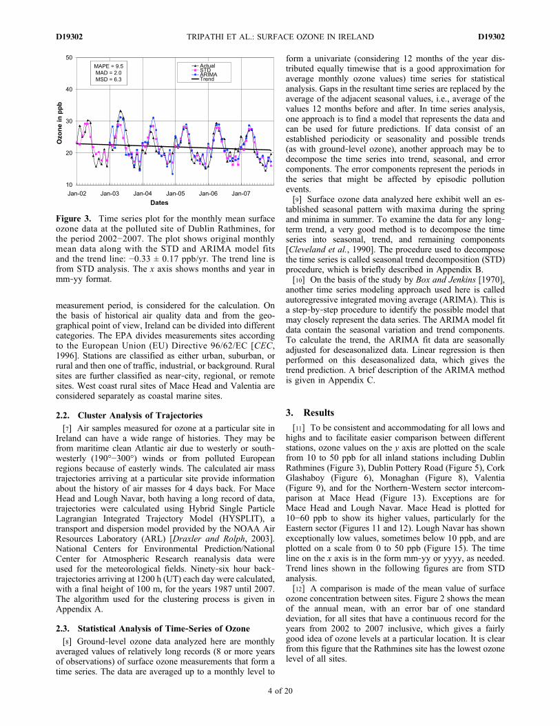
Figure 3. Time series plot for the monthly mean surfaceozone data at the polluted site of Dublin Rathmines, forthe period 2002−2007. The plot shows original monthlymean data along with the STD and ARIMA model fitsand the trend line: −0.33 ± 0.17 ppb/yr. The trend line isfrom STD analysis. The x axis shows months and year inmm‐yy format.

TRIPATHI ET AL.: SURFACE OZONE IN IRELAND D19302D19302

4 of 20

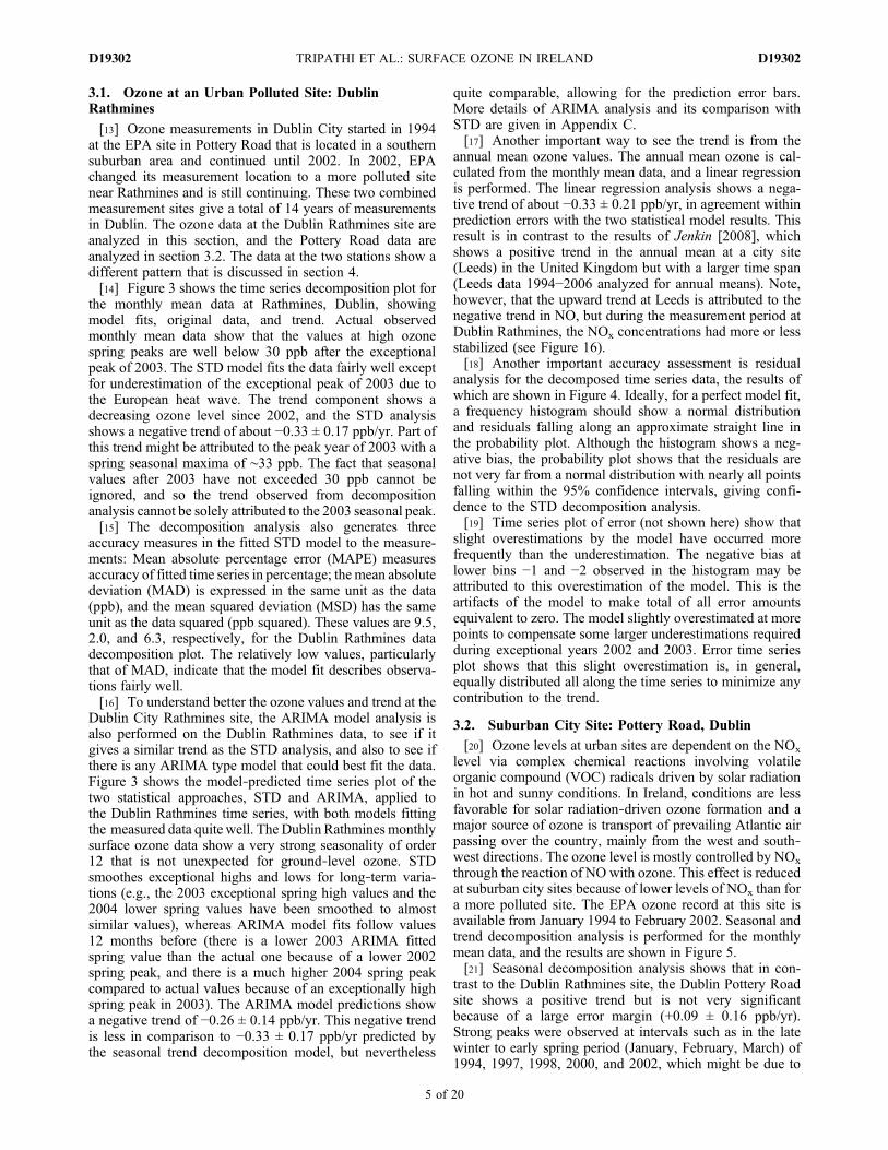
3.1. Ozone at an Urban Polluted Site: DublinRathmines

[13] Ozone measurements in Dublin City started in 1994at the EPA site in Pottery Road that is located in a southernsuburban area and continued until 2002. In 2002, EPAchanged its measurement location to a more polluted sitenear Rathmines and is still continuing. These two combinedmeasurement sites give a total of 14 years of measurementsin Dublin. The ozone data at the Dublin Rathmines site areanalyzed in this section, and the Pottery Road data areanalyzed in section 3.2. The data at the two stations show adifferent pattern that is discussed in section 4.[14] Figure 3 shows the time series decomposition plot for

the monthly mean data at Rathmines, Dublin, showingmodel fits, original data, and trend. Actual observedmonthly mean data show that the values at high ozonespring peaks are well below 30 ppb after the exceptionalpeak of 2003. The STD model fits the data fairly well exceptfor underestimation of the exceptional peak of 2003 due tothe European heat wave. The trend component shows adecreasing ozone level since 2002, and the STD analysisshows a negative trend of about −0.33 ± 0.17 ppb/yr. Part ofthis trend might be attributed to the peak year of 2003 with aspring seasonal maxima of ∼33 ppb. The fact that seasonalvalues after 2003 have not exceeded 30 ppb cannot beignored, and so the trend observed from decompositionanalysis cannot be solely attributed to the 2003 seasonal peak.[15] The decomposition analysis also generates three

accuracy measures in the fitted STD model to the measure-ments: Mean absolute percentage error (MAPE) measuresaccuracy of fitted time series in percentage; the mean absolutedeviation (MAD) is expressed in the same unit as the data(ppb), and the mean squared deviation (MSD) has the sameunit as the data squared (ppb squared). These values are 9.5,2.0, and 6.3, respectively, for the Dublin Rathmines datadecomposition plot. The relatively low values, particularlythat of MAD, indicate that the model fit describes observa-tions fairly well.[16] To understand better the ozone values and trend at the

Dublin City Rathmines site, the ARIMA model analysis isalso performed on the Dublin Rathmines data, to see if itgives a similar trend as the STD analysis, and also to see ifthere is any ARIMA type model that could best fit the data.Figure 3 shows the model‐predicted time series plot of thetwo statistical approaches, STD and ARIMA, applied tothe Dublin Rathmines time series, with both models fittingthe measured data quite well. The Dublin Rathmines monthlysurface ozone data show a very strong seasonality of order12 that is not unexpected for ground‐level ozone. STDsmoothes exceptional highs and lows for long‐term varia-tions (e.g., the 2003 exceptional spring high values and the2004 lower spring values have been smoothed to almostsimilar values), whereas ARIMA model fits follow values12 months before (there is a lower 2003 ARIMA fittedspring value than the actual one because of a lower 2002spring peak, and there is a much higher 2004 spring peakcompared to actual values because of an exceptionally highspring peak in 2003). The ARIMA model predictions showa negative trend of −0.26 ± 0.14 ppb/yr. This negative trendis less in comparison to −0.33 ± 0.17 ppb/yr predicted bythe seasonal trend decomposition model, but nevertheless

quite comparable, allowing for the prediction error bars.More details of ARIMA analysis and its comparison withSTD are given in Appendix C.[17] Another important way to see the trend is from the

annual mean ozone values. The annual mean ozone is cal-culated from the monthly mean data, and a linear regressionis performed. The linear regression analysis shows a nega-tive trend of about −0.33 ± 0.21 ppb/yr, in agreement withinprediction errors with the two statistical model results. Thisresult is in contrast to the results of Jenkin [2008], whichshows a positive trend in the annual mean at a city site(Leeds) in the United Kingdom but with a larger time span(Leeds data 1994−2006 analyzed for annual means). Note,however, that the upward trend at Leeds is attributed to thenegative trend in NO, but during the measurement period atDublin Rathmines, the NOx concentrations had more or lessstabilized (see Figure 16).[18] Another important accuracy assessment is residual

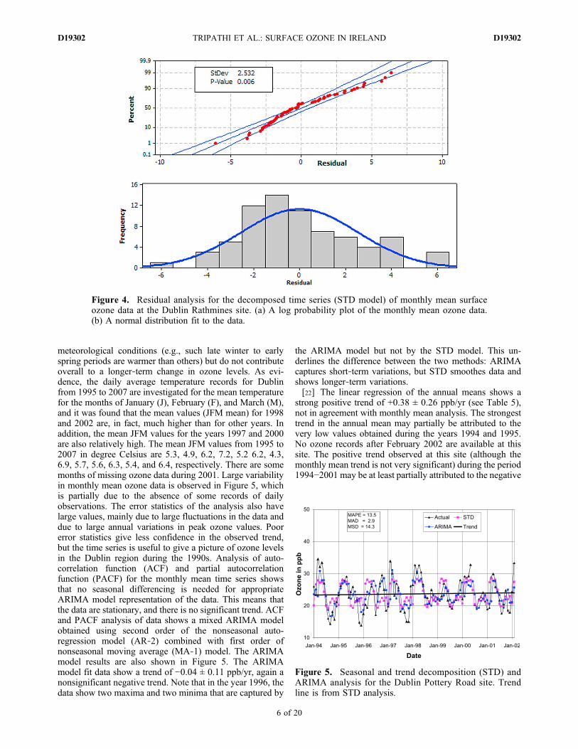
analysis for the decomposed time series data, the results ofwhich are shown in Figure 4. Ideally, for a perfect model fit,a frequency histogram should show a normal distributionand residuals falling along an approximate straight line inthe probability plot. Although the histogram shows a neg-ative bias, the probability plot shows that the residuals arenot very far from a normal distribution with nearly all pointsfalling within the 95% confidence intervals, giving confi-dence to the STD decomposition analysis.[19] Time series plot of error (not shown here) show that

slight overestimations by the model have occurred morefrequently than the underestimation. The negative bias atlower bins −1 and −2 observed in the histogram may beattributed to this overestimation of the model. This is theartifacts of the model to make total of all error amountsequivalent to zero. The model slightly overestimated at morepoints to compensate some larger underestimations requiredduring exceptional years 2002 and 2003. Error time seriesplot shows that this slight overestimation is, in general,equally distributed all along the time series to minimize anycontribution to the trend.

3.2. Suburban City Site: Pottery Road, Dublin

[20] Ozone levels at urban sites are dependent on the NOx

level via complex chemical reactions involving volatileorganic compound (VOC) radicals driven by solar radiationin hot and sunny conditions. In Ireland, conditions are lessfavorable for solar radiation‐driven ozone formation and amajor source of ozone is transport of prevailing Atlantic airpassing over the country, mainly from the west and south‐west directions. The ozone level is mostly controlled by NOx

through the reaction of NO with ozone. This effect is reducedat suburban city sites because of lower levels of NOx than fora more polluted site. The EPA ozone record at this site isavailable from January 1994 to February 2002. Seasonal andtrend decomposition analysis is performed for the monthlymean data, and the results are shown in Figure 5.[21] Seasonal decomposition analysis shows that in con-

trast to the Dublin Rathmines site, the Dublin Pottery Roadsite shows a positive trend but is not very significantbecause of a large error margin (+0.09 ± 0.16 ppb/yr).Strong peaks were observed at intervals such as in the latewinter to early spring period (January, February, March) of1994, 1997, 1998, 2000, and 2002, which might be due to

TRIPATHI ET AL.: SURFACE OZONE IN IRELAND D19302D19302

5 of 20

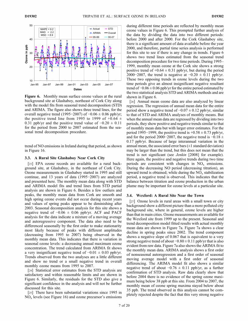
meteorological conditions (e.g., such late winter to earlyspring periods are warmer than others) but do not contributeoverall to a longer‐term change in ozone levels. As evi-dence, the daily average temperature records for Dublinfrom 1995 to 2007 are investigated for the mean temperaturefor the months of January (J), February (F), and March (M),and it was found that the mean values (JFM mean) for 1998and 2002 are, in fact, much higher than for other years. Inaddition, the mean JFM values for the years 1997 and 2000are also relatively high. The mean JFM values from 1995 to2007 in degree Celsius are 5.3, 4.9, 6.2, 7.2, 5.2 6.2, 4.3,6.9, 5.7, 5.6, 6.3, 5.4, and 6.4, respectively. There are somemonths of missing ozone data during 2001. Large variabilityin monthly mean ozone data is observed in Figure 5, whichis partially due to the absence of some records of dailyobservations. The error statistics of the analysis also havelarge values, mainly due to large fluctuations in the data anddue to large annual variations in peak ozone values. Poorerror statistics give less confidence in the observed trend,but the time series is useful to give a picture of ozone levelsin the Dublin region during the 1990s. Analysis of auto-correlation function (ACF) and partial autocorrelationfunction (PACF) for the monthly mean time series showsthat no seasonal differencing is needed for appropriateARIMA model representation of the data. This means thatthe data are stationary, and there is no significant trend. ACFand PACF analysis of data shows a mixed ARIMA modelobtained using second order of the nonseasonal auto-regression model (AR‐2) combined with first order ofnonseasonal moving average (MA‐1) model. The ARIMAmodel results are also shown in Figure 5. The ARIMAmodel fit data show a trend of −0.04 ± 0.11 ppb/yr, again anonsignificant negative trend. Note that in the year 1996, thedata show two maxima and two minima that are captured by

the ARIMA model but not by the STD model. This un-derlines the difference between the two methods: ARIMAcaptures short‐term variations, but STD smoothes data andshows longer‐term variations.[22] The linear regression of the annual means shows a

strong positive trend of +0.38 ± 0.26 ppb/yr (see Table 5),not in agreement with monthly mean analysis. The strongesttrend in the annual mean may partially be attributed to thevery low values obtained during the years 1994 and 1995.No ozone records after February 2002 are available at thissite. The positive trend observed at this site (although themonthly mean trend is not very significant) during the period1994−2001 may be at least partially attributed to the negative

Figure 5. Seasonal and trend decomposition (STD) andARIMA analysis for the Dublin Pottery Road site. Trendline is from STD analysis.

Figure 4. Residual analysis for the decomposed time series (STD model) of monthly mean surfaceozone data at the Dublin Rathmines site. (a) A log probability plot of the monthly mean ozone data.(b) A normal distribution fit to the data.

TRIPATHI ET AL.: SURFACE OZONE IN IRELAND D19302D19302

6 of 20

trend of NO emissions in Ireland during that period, as shownin Figure 16.

3.3. A Rural Site Glashaboy Near Cork City

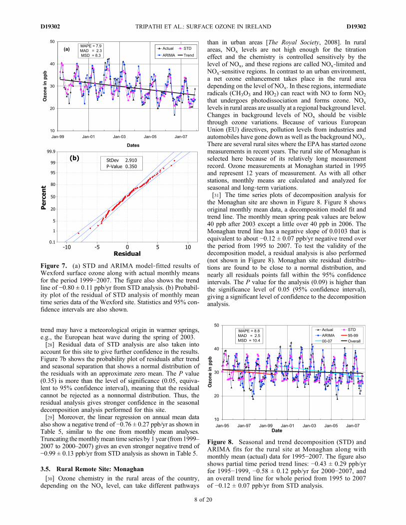
[23] EPA ozone records are available for a rural back-ground site, at Glashaboy, in the northeast of Cork City.Ozone measurements in Glashaboy started in 1995 and stillcontinue, and 13 years of data (1995−2007) are analyzedand presented here. The monthly mean data along with STDand ARIMA model fits and trend lines from STD partialanalysis are shown in Figure 6. Besides a few outliers andpeaks, the monthly mean data from Cork are smooth andhigh spring ozone events did not occur during recent yearsand values of spring peaks appear to be diminishing after2003. Seasonal decomposition analysis for this site shows anegative trend of −0.06 ± 0.06 ppb/yr. ACF and PACFanalysis for the data indicate a mixture of a moving averageand autoregressive component. The data also need to bedifferenced seasonally by the first order to make stationaritymost likely because of peaks with different amplitudes(decreasing from 1995 to 2007) being observed in themonthly mean data. This indicates that there is variation inseasonal ozone levels: a decreasing annual maximum ozoneconcentration. The trend calculated from ARIMA fit showsa very insignificant negative trend of −0.01 ± 0.03 ppb/yr.Trends observed from the two analyses are a little differentand show no trend or a small negative trend in overallmonthly ozone means from 1995 to 2007.[24] Statistical error estimates from the STD analysis are

satisfactory and within reasonable limits and are shown inFigure 6. Similarly, the residuals for the STD also give asignificant confidence in the analysis and will not be furtherdiscussed for this site.[25] There have been substantial variations since 1995 in

NOx levels (see Figure 16) and ozone precursor’s emissions

during different time periods are reflected by monthly meanozone values in Figure 6. This prompted further analysis ofthe data by dividing the data into two different periods:before 2000 and after 2000. For the Cork Glashaboy site,there is a significant amount of data available before the year2000, and therefore, partial time series analysis is performedfor this site to see if there is any change in trends. Figure 6shows two trend lines estimated from the seasonal trenddecomposition procedure for two time periods. During 1995–1999, monthly mean ozone at the Cork site shows a strongpositive trend of +0.64 ± 0.31 ppb/yr, but during the period2000−2007, the trend is negative at −0.20 ± 0.11 ppb/yr.These two opposing trends in ozone levels during the twotime periods give an almost insignificant negative resultanttrend of −0.06 ± 0.06 ppb/yr for the entire period estimated bythe two statistical analysis STD and ARIMAmethods and areshown in Figure 6.[26] Annual mean ozone data are also analyzed by linear

regression. The regression of annual mean data for the entireperiod show a negative trend of −0.07 ± 0.12 ppb/yr, similarto that of STD and ARIMA analyses of monthly means. Butwhen the annual mean data are regressed by dividing into twoperiods, they show positive and negative trends similar to thatof monthly mean data but with larger error estimates. For theperiod 1995−1999, the positive trend is +0.58 ± 0.73 ppb/yr,and for the period 2000−2007, the negative trend is −0.18 ±0.17 ppb/yr. Because of large interannual variation in theannual mean, the associated error bars (±1 standard deviation)may be larger than the trend, but this does not mean that thetrend is not significant (see Jenkin [2008] for example).Here again, the positive and negative trends during two timeperiods are consistent with changes in NOx emissions.During the decreasing NO period (decreasing titration), anupward trend is obtained; while during the NOx stabilizationperiod, a negative trend is observed. This indicates that thebalance between titration and ozone production in the urbanplume may be important for ozone levels at a particular site.

3.4. Wexford: A Rural Site Near the Town

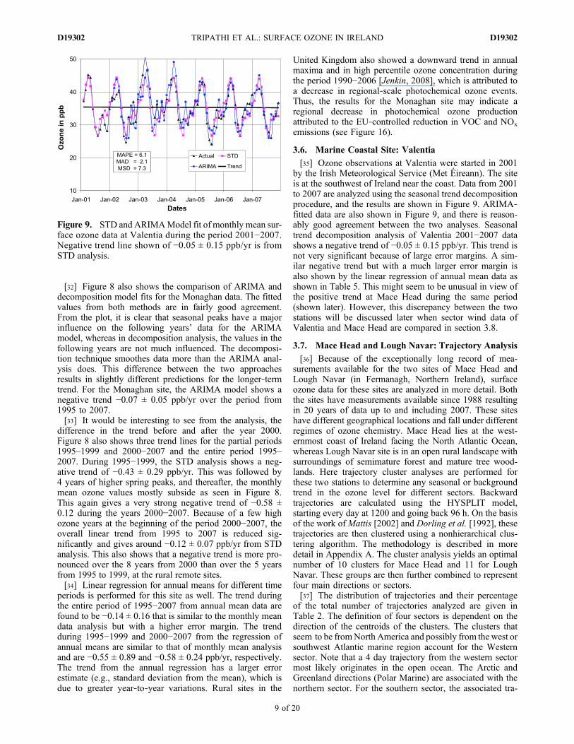
[27] Ozone levels in rural areas with a small town or citybackground show a different picture than a more polluted citybackground site, where in general, ozone levels are higherthan that inmain cities. Ozonemeasurements are available forthe Wexford site from 1999 up to the present. Seasonal andtrend decomposition model fitted results with actual monthlymean data are shown in Figure 7a. Figure 7a shows a cleardecline in spring peaks since 2002. The trend componentshows a negative slope of 0.067 that is equivalent to a verystrong negative trend of about −0.80 ± 0.11 ppb/yr that is alsoevident from raw data. Figure 7a also shows the ARIMA fit tothe monthly mean data. ARIMA analysis shows a first orderof nonseasonal autoregression and a first order of seasonalmoving average model with a first order of seasonaldifferencing. The ARIMA model fit also shows a similarnegative trend of about −0.76 ± 0.11 ppb/yr, as a furtherconfirmation of STD analysis. Raw data clearly show thatbefore 2004 there is no evidence of the spring ozone maxi-mum being below 38 ppb at this site. From 2004 to 2007, themonthly mean of ozone spring maxima stayed below about35 ppb. The trend observed in this analysis cannot be com-pletely rejected despite the fact that this very strong negative

Figure 6. Monthly mean surface ozone values at the ruralbackground site at Glashaboy, northeast of Cork City alongwith the model fits from seasonal trend decomposition (STD)and ARIMA. The figure also shows three trend lines, for theoverall negative trend (1995−2007) of −0.06 ± 0.06 ppb/yr;the positive trend line from 1995 to 1999 of +0.64 ±0.31 ppb/yr and the positive trend value of −0.20 ± 0.11for the period from 2000 to 2007 estimated from the sea-sonal trend decomposition procedure.

TRIPATHI ET AL.: SURFACE OZONE IN IRELAND D19302D19302

7 of 20

trend may have a meteorological origin in warmer springs,e.g., the European heat wave during the spring of 2003.[28] Residual data of STD analysis are also taken into

account for this site to give further confidence in the results.Figure 7b shows the probability plot of residuals after trendand seasonal separation that shows a normal distribution ofthe residuals with an approximate zero mean. The P value(0.35) is more than the level of significance (0.05, equiva-lent to 95% confidence interval), meaning that the residualcannot be rejected as a nonnormal distribution. Thus, theresidual analysis gives stronger confidence in the seasonaldecomposition analysis performed for this site.[29] Moreover, the linear regression on annual mean data

also show a negative trend of −0.76 ± 0.27 ppb/yr as shown inTable 5, similar to the one from monthly mean analyses.Truncating themonthlymean time series by 1 year (from1999–2007 to 2000–2007) gives an even stronger negative trend of−0.99 ± 0.13 ppb/yr from STD analysis as shown in Table 5.

3.5. Rural Remote Site: Monaghan

[30] Ozone chemistry in the rural areas of the country,depending on the NOx level, can take different pathways

than in urban areas [The Royal Society, 2008]. In ruralareas, NOx levels are not high enough for the titrationeffect and the chemistry is controlled sensitively by thelevel of NOx, and these regions are called NOx‐limited andNOx‐sensitive regions. In contrast to an urban environment,a net ozone enhancement takes place in the rural areadepending on the level of NOx. In these regions, intermediateradicals (CH3O3 and HO2) can react with NO to form NO2

that undergoes photodissociation and forms ozone. NOx

levels in rural areas are usually at a regional background level.Changes in background levels of NOx should be visiblethrough ozone variations. Because of various EuropeanUnion (EU) directives, pollution levels from industries andautomobiles have gone down as well as the background NOx.There are several rural sites where the EPA has started ozonemeasurements in recent years. The rural site of Monaghan isselected here because of its relatively long measurementrecord. Ozone measurements at Monaghan started in 1995and represent 12 years of measurement. As with all otherstations, monthly means are calculated and analyzed forseasonal and long‐term variations.[31] The time series plots of decomposition analysis for

the Monaghan site are shown in Figure 8. Figure 8 showsoriginal monthly mean data, a decomposition model fit andtrend line. The monthly mean spring peak values are below40 ppb after 2003 except a little over 40 ppb in 2006. TheMonaghan trend line has a negative slope of 0.0103 that isequivalent to about −0.12 ± 0.07 ppb/yr negative trend overthe period from 1995 to 2007. To test the validity of thedecomposition model, a residual analysis is also performed(not shown in Figure 8). Monaghan site residual distribu-tions are found to be close to a normal distribution, andnearly all residuals points fall within the 95% confidenceintervals. The P value for the analysis (0.09) is higher thanthe significance level of 0.05 (95% confidence interval),giving a significant level of confidence to the decompositionanalysis.

Figure 8. Seasonal and trend decomposition (STD) andARIMA fits for the rural site at Monaghan along withmonthly mean (actual) data for 1995−2007. The figure alsoshows partial time period trend lines: −0.43 ± 0.29 ppb/yrfor 1995−1999, −0.58 ± 0.12 ppb/yr for 2000−2007, andan overall trend line for whole period from 1995 to 2007of −0.12 ± 0.07 ppb/yr from STD analysis.

Figure 7. (a) STD and ARIMA model‐fitted results ofWexford surface ozone along with actual monthly meansfor the period 1999−2007. The figure also shows the trendline of −0.80 ± 0.11 ppb/yr from STD analysis. (b) Probabil-ity plot of the residual of STD analysis of monthly meantime series data of the Wexford site. Statistics and 95% con-fidence intervals are also shown.

TRIPATHI ET AL.: SURFACE OZONE IN IRELAND D19302D19302

8 of 20

[32] Figure 8 also shows the comparison of ARIMA anddecomposition model fits for the Monaghan data. The fittedvalues from both methods are in fairly good agreement.From the plot, it is clear that seasonal peaks have a majorinfluence on the following years’ data for the ARIMAmodel, whereas in decomposition analysis, the values in thefollowing years are not much influenced. The decomposi-tion technique smoothes data more than the ARIMA anal-ysis does. This difference between the two approachesresults in slightly different predictions for the longer‐termtrend. For the Monaghan site, the ARIMA model shows anegative trend −0.07 ± 0.05 ppb/yr over the period from1995 to 2007.[33] It would be interesting to see from the analysis, the

difference in the trend before and after the year 2000.Figure 8 also shows three trend lines for the partial periods1995–1999 and 2000−2007 and the entire period 1995–2007. During 1995−1999, the STD analysis shows a neg-ative trend of −0.43 ± 0.29 ppb/yr. This was followed by4 years of higher spring peaks, and thereafter, the monthlymean ozone values mostly subside as seen in Figure 8.This again gives a very strong negative trend of −0.58 ±0.12 during the years 2000−2007. Because of a few highozone years at the beginning of the period 2000−2007, theoverall linear trend from 1995 to 2007 is reduced sig-nificantly and gives around −0.12 ± 0.07 ppb/yr from STDanalysis. This also shows that a negative trend is more pro-nounced over the 8 years from 2000 than over the 5 yearsfrom 1995 to 1999, at the rural remote sites.[34] Linear regression for annual means for different time

periods is performed for this site as well. The trend duringthe entire period of 1995−2007 from annual mean data arefound to be −0.14 ± 0.16 that is similar to the monthly meandata analysis but with a higher error margin. The trendduring 1995−1999 and 2000−2007 from the regression ofannual means are similar to that of monthly mean analysisand are −0.55 ± 0.89 and −0.58 ± 0.24 ppb/yr, respectively.The trend from the annual regression has a larger errorestimate (e.g., standard deviation from the mean), which isdue to greater year‐to‐year variations. Rural sites in the

United Kingdom also showed a downward trend in annualmaxima and in high percentile ozone concentration duringthe period 1990−2006 [Jenkin, 2008], which is attributed toa decrease in regional‐scale photochemical ozone events.Thus, the results for the Monaghan site may indicate aregional decrease in photochemical ozone productionattributed to the EU‐controlled reduction in VOC and NOx

emissions (see Figure 16).

3.6. Marine Coastal Site: Valentia

[35] Ozone observations at Valentia were started in 2001by the Irish Meteorological Service (Met Éireann). The siteis at the southwest of Ireland near the coast. Data from 2001to 2007 are analyzed using the seasonal trend decompositionprocedure, and the results are shown in Figure 9. ARIMA‐fitted data are also shown in Figure 9, and there is reason-ably good agreement between the two analyses. Seasonaltrend decomposition analysis of Valentia 2001−2007 datashows a negative trend of −0.05 ± 0.15 ppb/yr. This trend isnot very significant because of large error margins. A sim-ilar negative trend but with a much larger error margin isalso shown by the linear regression of annual mean data asshown in Table 5. This might seem to be unusual in view ofthe positive trend at Mace Head during the same period(shown later). However, this discrepancy between the twostations will be discussed later when sector wind data ofValentia and Mace Head are compared in section 3.8.

3.7. Mace Head and Lough Navar: Trajectory Analysis

[36] Because of the exceptionally long record of mea-surements available for the two sites of Mace Head andLough Navar (in Fermanagh, Northern Ireland), surfaceozone data for these sites are analyzed in more detail. Boththe sites have measurements available since 1988 resultingin 20 years of data up to and including 2007. These siteshave different geographical locations and fall under differentregimes of ozone chemistry. Mace Head lies at the west-ernmost coast of Ireland facing the North Atlantic Ocean,whereas Lough Navar site is in an open rural landscape withsurroundings of semimature forest and mature tree wood-lands. Here trajectory cluster analyses are performed forthese two stations to determine any seasonal or backgroundtrend in the ozone level for different sectors. Backwardtrajectories are calculated using the HYSPLIT model,starting every day at 1200 and going back 96 h. On the basisof the work of Mattis [2002] and Dorling et al. [1992], thesetrajectories are then clustered using a nonhierarchical clus-tering algorithm. The methodology is described in moredetail in Appendix A. The cluster analysis yields an optimalnumber of 10 clusters for Mace Head and 11 for LoughNavar. These groups are then further combined to representfour main directions or sectors.[37] The distribution of trajectories and their percentage

of the total number of trajectories analyzed are given inTable 2. The definition of four sectors is dependent on thedirection of the centroids of the clusters. The clusters thatseem to be fromNorth America and possibly from the west orsouthwest Atlantic marine region account for the Westernsector. Note that a 4 day trajectory from the western sectormost likely originates in the open ocean. The Arctic andGreenland directions (Polar Marine) are associated with thenorthern sector. For the southern sector, the associated tra-

Figure 9. STD and ARIMAModel fit of monthly mean sur-face ozone data at Valentia during the period 2001−2007.Negative trend line shown of −0.05 ± 0.15 ppb/yr is fromSTD analysis.

TRIPATHI ET AL.: SURFACE OZONE IN IRELAND D19302D19302

9 of 20

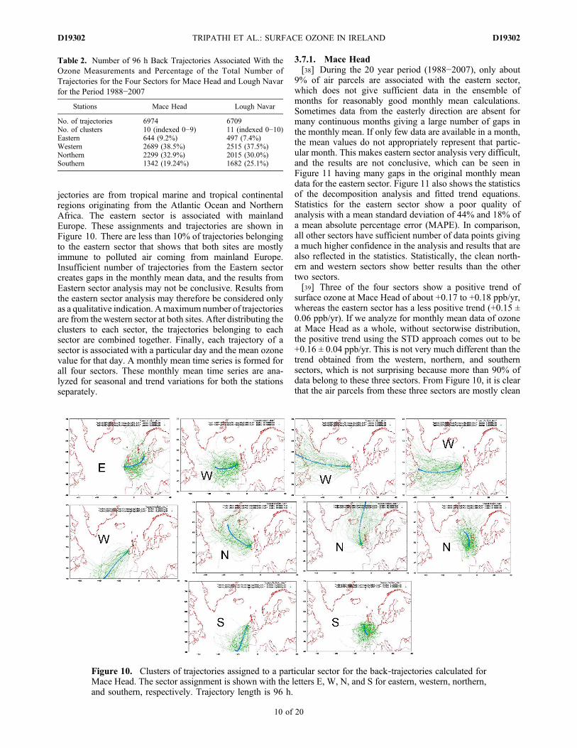
jectories are from tropical marine and tropical continentalregions originating from the Atlantic Ocean and NorthernAfrica. The eastern sector is associated with mainlandEurope. These assignments and trajectories are shown inFigure 10. There are less than 10% of trajectories belongingto the eastern sector that shows that both sites are mostlyimmune to polluted air coming from mainland Europe.Insufficient number of trajectories from the Eastern sectorcreates gaps in the monthly mean data, and the results fromEastern sector analysis may not be conclusive. Results fromthe eastern sector analysis may therefore be considered onlyas a qualitative indication. Amaximum number of trajectoriesare from the western sector at both sites. After distributing theclusters to each sector, the trajectories belonging to eachsector are combined together. Finally, each trajectory of asector is associated with a particular day and the mean ozonevalue for that day. A monthly mean time series is formed forall four sectors. These monthly mean time series are ana-lyzed for seasonal and trend variations for both the stationsseparately.

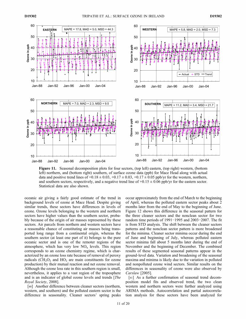
3.7.1. Mace Head[38] During the 20 year period (1988−2007), only about

9% of air parcels are associated with the eastern sector,which does not give sufficient data in the ensemble ofmonths for reasonably good monthly mean calculations.Sometimes data from the easterly direction are absent formany continuous months giving a large number of gaps inthe monthly mean. If only few data are available in a month,the mean values do not appropriately represent that partic-ular month. This makes eastern sector analysis very difficult,and the results are not conclusive, which can be seen inFigure 11 having many gaps in the original monthly meandata for the eastern sector. Figure 11 also shows the statisticsof the decomposition analysis and fitted trend equations.Statistics for the eastern sector show a poor quality ofanalysis with a mean standard deviation of 44% and 18% ofa mean absolute percentage error (MAPE). In comparison,all other sectors have sufficient number of data points givinga much higher confidence in the analysis and results that arealso reflected in the statistics. Statistically, the clean north-ern and western sectors show better results than the othertwo sectors.[39] Three of the four sectors show a positive trend of

surface ozone at Mace Head of about +0.17 to +0.18 ppb/yr,whereas the eastern sector has a less positive trend (+0.15 ±0.06 ppb/yr). If we analyze for monthly mean data of ozoneat Mace Head as a whole, without sectorwise distribution,the positive trend using the STD approach comes out to be+0.16 ± 0.04 ppb/yr. This is not very much different than thetrend obtained from the western, northern, and southernsectors, which is not surprising because more than 90% ofdata belong to these three sectors. From Figure 10, it is clearthat the air parcels from these three sectors are mostly clean

Figure 10. Clusters of trajectories assigned to a particular sector for the back‐trajectories calculated forMace Head. The sector assignment is shown with the letters E, W, N, and S for eastern, western, northern,and southern, respectively. Trajectory length is 96 h.

Table 2. Number of 96 h Back Trajectories Associated With theOzone Measurements and Percentage of the Total Number ofTrajectories for the Four Sectors for Mace Head and Lough Navarfor the Period 1988−2007

Stations Mace Head Lough Navar

No. of trajectories 6974 6709No. of clusters 10 (indexed 0−9) 11 (indexed 0−10)Eastern 644 (9.2%) 497 (7.4%)Western 2689 (38.5%) 2515 (37.5%)Northern 2299 (32.9%) 2015 (30.0%)Southern 1342 (19.24%) 1682 (25.1%)

TRIPATHI ET AL.: SURFACE OZONE IN IRELAND D19302D19302

10 of 20

oceanic air giving a fairly good estimate of the trend inbackground levels of ozone at Mace Head. Despite givingsimilar trends, these sectors have differences in levels ofozone. Ozone levels belonging to the western and northernsectors have higher values than the southern sector, proba-bly because of the origin of air masses represented by thesesectors. Air parcels from northern and western sectors havea reasonable chance of constituting air masses being trans-ported long range from a continental origin, whereas thesouthern sector (at least one part of it) belongs to the pureoceanic sector and is one of the remoter regions of theatmosphere, which has very low NOx levels. This regioncorresponds to an ozone chemistry regime, which is char-acterized by an ozone loss rate because of removal of peroxyradicals (CH2O2 and HO2 are main constituents for ozoneproduction) by their mutual reaction and net ozone removal.Although the ozone loss rate in this southern region is small,nevertheless, it applies to a vast region of the troposphereand is an indicator of global ozone levels and trends [TheRoyal Society, 2008].[40] Another difference between cleaner sectors (northern,

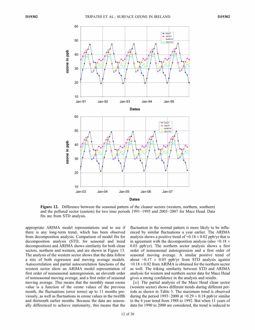
western, and southern) and the polluted eastern sector is thedifference in seasonality. Cleaner sectors’ spring peaks

occur approximately from the end of March to the beginningof April, whereas the polluted eastern sector peaks about 2months later from the end of May to the beginning of June.Figure 12 shows this difference in the seasonal pattern forthe three cleaner sectors and the nonclean sector for tworandom time periods of 1991−1995 and 2003−2007. The fitis from STD analysis. The shift between the cleaner sectorspatterns and the nonclean sector pattern is more broadenedfor the minima. Cleaner sector minima occur during the endof June and beginning of July, whereas polluted easternsector minima fall about 5 months later during the end ofNovember and the beginning of December. The combinedresults of these segmented seasonal patterns appear in theground‐level data. Variation and broadening of the seasonalmaxima and minima is likely due to the variation in pollutedand nonpolluted ozone wind sectors. Similar results on thedifferences in seasonality of ozone were also observed byCarslaw [2005].[41] As a further confirmation of seasonal trend decom-

position model fits and observed trend, the two cleanwestern and northern sectors were further analyzed usingARIMA methods. Autocorrelation and partial autocorrela-tion analysis for these sectors have been analyzed for

Figure 11. Seasonal decomposition plots for four sectors, (top left) eastern, (top right) western, (bottomleft) northern, and (bottom right) southern, of surface ozone data (ppb) for Mace Head along with actualdata and positive trend lines of +0.18 ± 0.03, +0.17 ± 0.03, +0.17 ± 0.05 ppb/yr for the western, northern,and southern sectors, respectively, and a negative trend line of +0.15 ± 0.06 ppb/yr for the eastern sector.Statistical data are also shown.

TRIPATHI ET AL.: SURFACE OZONE IN IRELAND D19302D19302

11 of 20

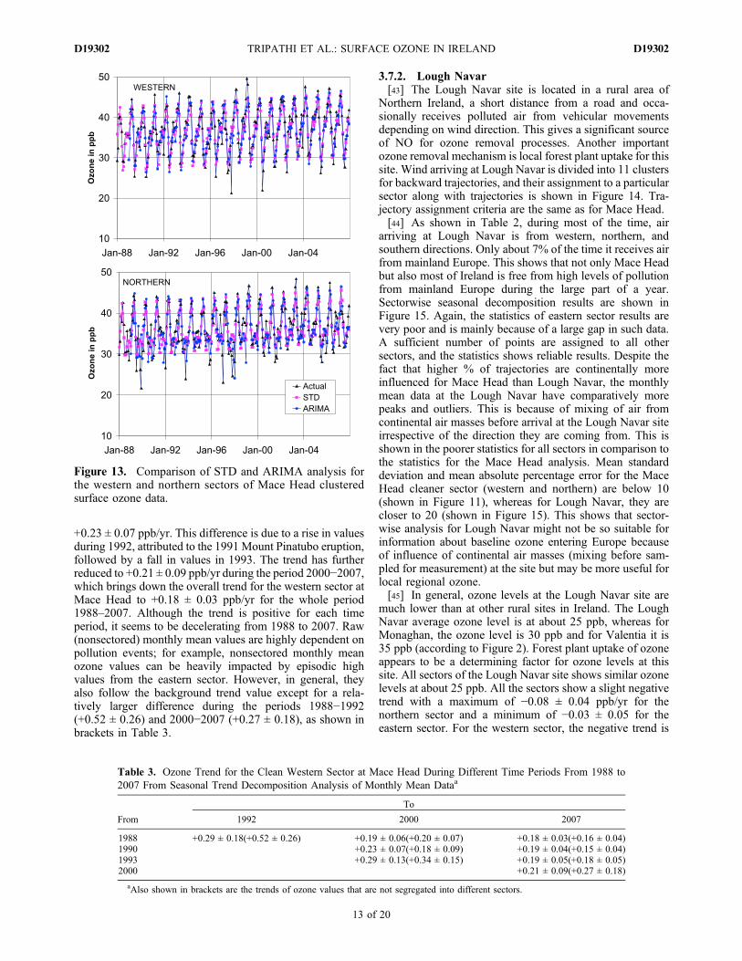
appropriate ARIMA model representations and to see ifthere is any long‐term trend, which has been observedfrom decomposition analysis. Comparison of model fits fordecomposition analysis (STD, for seasonal and trenddecomposition) and ARIMA shows similarity for both cleansectors, northern and western, and are shown in Figure 13.The analysis of the western sector shows that the data followa mix of both regression and moving average models.Autocorrelation and partial autocorrelation functions of thewestern sector show an ARIMA model representation offirst order of nonseasonal autoregression, an eleventh orderof nonseasonal moving average, and a first order of seasonalmoving average. This means that the monthly mean ozonevalue is a function of the ozone values of the previousmonth, the fluctuations (error terms) up to 11 months pre-viously, as well as fluctuations in ozone values in the twelfthand thirteenth earlier months. Because the data are season-ally differenced to achieve stationarity, this means that the

fluctuation in the normal pattern is more likely to be influ-enced by similar fluctuations a year earlier. The ARIMAanalysis shows a positive trend of +0.18 ± 0.02 ppb/yr that isin agreement with the decomposition analysis (also +0.18 ±0.03 ppb/yr). The northern sector analysis shows a firstorder of nonseasonal autoregression and a first order ofseasonal moving average. A similar positive trend ofabout +0.17 ± 0.03 ppb/yr from STD analysis against+0.18 ± 0.02 from ARIMA is obtained for the northern sectoras well. The triking similarity between STD and ARIMAanalysis for western and northern sector data for Mace Headgives a strong confidence in the analysis and results.[42] The partial analysis of the Mace Head clean sector

(western sector) shows different trends during different per-iods as shown in Table 3. The maximum trend is observedduring the period 1993−2000 at +0.29 ± 0.18 ppb/yr similarto the 4 year trend from 1988 to 1992. But when 11 years ofdata for 1990 to 2000 are considered, the trend is reduced to

Figure 12. Difference between the seasonal pattern of the cleaner sectors (western, northern, southern)and the polluted sector (eastern) for two time periods 1991−1995 and 2003−2007 for Mace Head. Datafits are from STD analysis.

TRIPATHI ET AL.: SURFACE OZONE IN IRELAND D19302D19302

12 of 20

+0.23 ± 0.07 ppb/yr. This difference is due to a rise in valuesduring 1992, attributed to the 1991 Mount Pinatubo eruption,followed by a fall in values in 1993. The trend has furtherreduced to +0.21 ± 0.09 ppb/yr during the period 2000−2007,which brings down the overall trend for the western sector atMace Head to +0.18 ± 0.03 ppb/yr for the whole period1988–2007. Although the trend is positive for each timeperiod, it seems to be decelerating from 1988 to 2007. Raw(nonsectored) monthly mean values are highly dependent onpollution events; for example, nonsectored monthly meanozone values can be heavily impacted by episodic highvalues from the eastern sector. However, in general, theyalso follow the background trend value except for a rela-tively larger difference during the periods 1988−1992(+0.52 ± 0.26) and 2000−2007 (+0.27 ± 0.18), as shown inbrackets in Table 3.

3.7.2. Lough Navar[43] The Lough Navar site is located in a rural area of

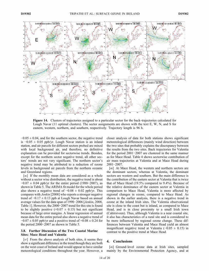
Northern Ireland, a short distance from a road and occa-sionally receives polluted air from vehicular movementsdepending on wind direction. This gives a significant sourceof NO for ozone removal processes. Another importantozone removal mechanism is local forest plant uptake for thissite. Wind arriving at Lough Navar is divided into 11 clustersfor backward trajectories, and their assignment to a particularsector along with trajectories is shown in Figure 14. Tra-jectory assignment criteria are the same as for Mace Head.[44] As shown in Table 2, during most of the time, air

arriving at Lough Navar is from western, northern, andsouthern directions. Only about 7% of the time it receives airfrom mainland Europe. This shows that not only Mace Headbut also most of Ireland is free from high levels of pollutionfrom mainland Europe during the large part of a year.Sectorwise seasonal decomposition results are shown inFigure 15. Again, the statistics of eastern sector results arevery poor and is mainly because of a large gap in such data.A sufficient number of points are assigned to all othersectors, and the statistics shows reliable results. Despite thefact that higher % of trajectories are continentally moreinfluenced for Mace Head than Lough Navar, the monthlymean data at the Lough Navar have comparatively morepeaks and outliers. This is because of mixing of air fromcontinental air masses before arrival at the Lough Navar siteirrespective of the direction they are coming from. This isshown in the poorer statistics for all sectors in comparison tothe statistics for the Mace Head analysis. Mean standarddeviation and mean absolute percentage error for the MaceHead cleaner sector (western and northern) are below 10(shown in Figure 11), whereas for Lough Navar, they arecloser to 20 (shown in Figure 15). This shows that sector-wise analysis for Lough Navar might not be so suitable forinformation about baseline ozone entering Europe becauseof influence of continental air masses (mixing before sam-pled for measurement) at the site but may be more useful forlocal regional ozone.[45] In general, ozone levels at the Lough Navar site are

much lower than at other rural sites in Ireland. The LoughNavar average ozone level is at about 25 ppb, whereas forMonaghan, the ozone level is 30 ppb and for Valentia it is35 ppb (according to Figure 2). Forest plant uptake of ozoneappears to be a determining factor for ozone levels at thissite. All sectors of the Lough Navar site shows similar ozonelevels at about 25 ppb. All the sectors show a slight negativetrend with a maximum of −0.08 ± 0.04 ppb/yr for thenorthern sector and a minimum of −0.03 ± 0.05 for theeastern sector. For the western sector, the negative trend is

Figure 13. Comparison of STD and ARIMA analysis forthe western and northern sectors of Mace Head clusteredsurface ozone data.

Table 3. Ozone Trend for the Clean Western Sector at Mace Head During Different Time Periods From 1988 to2007 From Seasonal Trend Decomposition Analysis of Monthly Mean Dataa

To

From 1992 2000 2007

1988 +0.29 ± 0.18(+0.52 ± 0.26) +0.19 ± 0.06(+0.20 ± 0.07) +0.18 ± 0.03(+0.16 ± 0.04)1990 +0.23 ± 0.07(+0.18 ± 0.09) +0.19 ± 0.04(+0.15 ± 0.04)1993 +0.29 ± 0.13(+0.34 ± 0.15) +0.19 ± 0.05(+0.18 ± 0.05)2000 +0.21 ± 0.09(+0.27 ± 0.18)

aAlso shown in brackets are the trends of ozone values that are not segregated into different sectors.

TRIPATHI ET AL.: SURFACE OZONE IN IRELAND D19302D19302

13 of 20

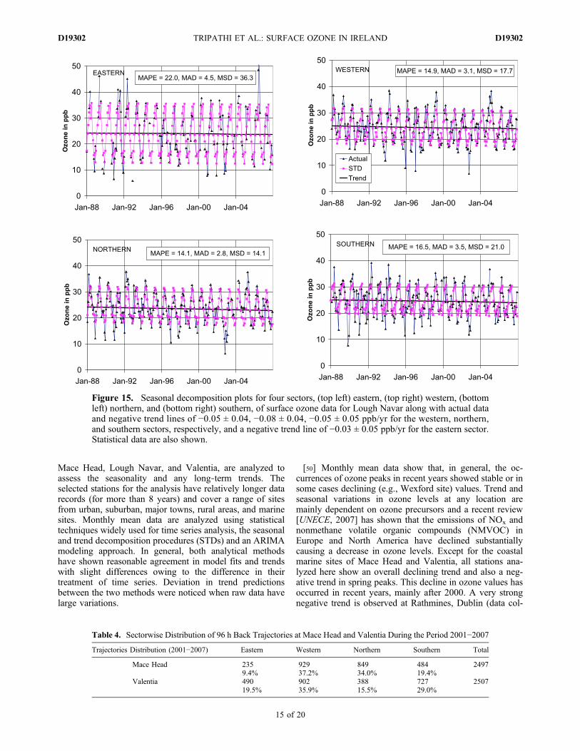
−0.05 ± 0.04, and for the southern sector, the negative trendis −0.05 ± 0.05 ppb/yr. Lough Navar station is an inlandstation, and air parcels for different sectors probed are mixedwith local background air, and therefore, no definitiveexplanation can be provided for sectorwise trends. Besides,except for the northern sector negative trend, all other sec-tors’ trends are not very significant. The northern sector’snegative trend may be attributed to a reduction of ozonelevels in background air parcels from the northern oceanicand Greenland regions.[46] If the monthly mean data are considered as a whole

without a sector wise distribution, the negative trend is about−0.07 ± 0.04 ppb/yr for the entire period (1988−2007), asshown in Table 5. The ARIMA fit model for the whole periodalso shows a negative trend of −0.08 ± 0.02 ppb/yr. Thiscompares with Jenkin [2008] who reports a stronger negativetrend of −0.17 ± 0.13 ppb at Lough Navar based on annualaverage values for the data span of 1990−2006 [Jenkin, 2008,Table 1]. However, the 2000−2007 trend for this site is foundto be slightly positive (+0.07 ± 0.15) but not significantbecause of large error margins. A linear regression of annualmean data for the entire period also shows a negative trend of−0.07 ± 0.05 ppb/yr and a positive trend of +0.08 ± 0.24 forthe period 2000−2007 as shown in Table 5.

3.8. Further Discussion of the Two Coastal MarineSites: Mace Head and Valentia

[47] From the above analysis of both sites, it seems theyshow a significant difference in the trend though they are bothon the west coast of Ireland and would appear to have similarmeteorological conditions throughout the year. However, a

closer analysis of data for both stations shows significantmeteorological differences (mainly wind direction) betweenthe two sites that probably explains the discrepancy betweenthe results from the two sites. Back trajectories for Valentiafor the period 2001−2007 are clustered in the same manneras for Mace Head. Table 4 shows sectorwise contribution ofair mass trajectories at Valentia and at Mace Head during2001–2007.[48] At Mace Head, the western and northern sectors are

the dominant sectors, whereas at Valentia, the dominantsectors are western and southern. But the main difference isthe contribution of the eastern sector at Valentia that is twicethat of Mace Head (19.5% compared to 9.4%). Because ofthe relative dominance of the eastern sector at Valentia incomparison to Mace Head, Valentia is more affected byregional changes in ozone, compared to Mace Head. Asshown in the earlier analysis, there is a negative trend inozone at the inland Irish sites. The Valentia observationalsite is close to the coast but is inland, as compared to MaceHead, and is in close proximity to a small Irish town(Cahirsiveen). Thus, although Valentia is a near coastal site,it also has characteristics of a rural site and is considered tobe more influenced by regional ozone change. These dif-ferences between Valentia and Mace Head yield an almostinsignificant negative trend at Valentia (−0.05 ± 0.15) incontrast to the positive trend at Mace Head.

4. Conclusions

[49] Ground‐level ozone data at Irish sites, sampledmainly by the Environmental Protection Agency, and at

Figure 14. Clusters of trajectories assigned to a particular sector for the back‐trajectories calculated forLough Navar (11 optimal clusters). The sector assignments are shown with the text E, W, N, and S foreastern, western, northern, and southern, respectively. Trajectory length is 96 h.

TRIPATHI ET AL.: SURFACE OZONE IN IRELAND D19302D19302

14 of 20

Mace Head, Lough Navar, and Valentia, are analyzed toassess the seasonality and any long‐term trends. Theselected stations for the analysis have relatively longer datarecords (for more than 8 years) and cover a range of sitesfrom urban, suburban, major towns, rural areas, and marinesites. Monthly mean data are analyzed using statisticaltechniques widely used for time series analysis, the seasonaland trend decomposition procedures (STDs) and an ARIMAmodeling approach. In general, both analytical methodshave shown reasonable agreement in model fits and trendswith slight differences owing to the difference in theirtreatment of time series. Deviation in trend predictionsbetween the two methods were noticed when raw data havelarge variations.

[50] Monthly mean data show that, in general, the oc-currences of ozone peaks in recent years showed stable or insome cases declining (e.g., Wexford site) values. Trend andseasonal variations in ozone levels at any location aremainly dependent on ozone precursors and a recent review[UNECE, 2007] has shown that the emissions of NOx andnonmethane volatile organic compounds (NMVOC) inEurope and North America have declined substantiallycausing a decrease in ozone levels. Except for the coastalmarine sites of Mace Head and Valentia, all stations ana-lyzed here show an overall declining trend and also a neg-ative trend in spring peaks. This decline in ozone values hasoccurred in recent years, mainly after 2000. A very strongnegative trend is observed at Rathmines, Dublin (data col-

Figure 15. Seasonal decomposition plots for four sectors, (top left) eastern, (top right) western, (bottomleft) northern, and (bottom right) southern, of surface ozone data for Lough Navar along with actual dataand negative trend lines of −0.05 ± 0.04, −0.08 ± 0.04, −0.05 ± 0.05 ppb/yr for the western, northern,and southern sectors, respectively, and a negative trend line of −0.03 ± 0.05 ppb/yr for the eastern sector.Statistical data are also shown.

Table 4. Sectorwise Distribution of 96 h Back Trajectories at Mace Head and Valentia During the Period 2001−2007

Trajectories Distribution (2001−2007) Eastern Western Northern Southern Total

Mace Head 235 929 849 484 24979.4% 37.2% 34.0% 19.4%

Valentia 490 902 388 727 250719.5% 35.9% 15.5% 29.0%

TRIPATHI ET AL.: SURFACE OZONE IN IRELAND D19302D19302

15 of 20

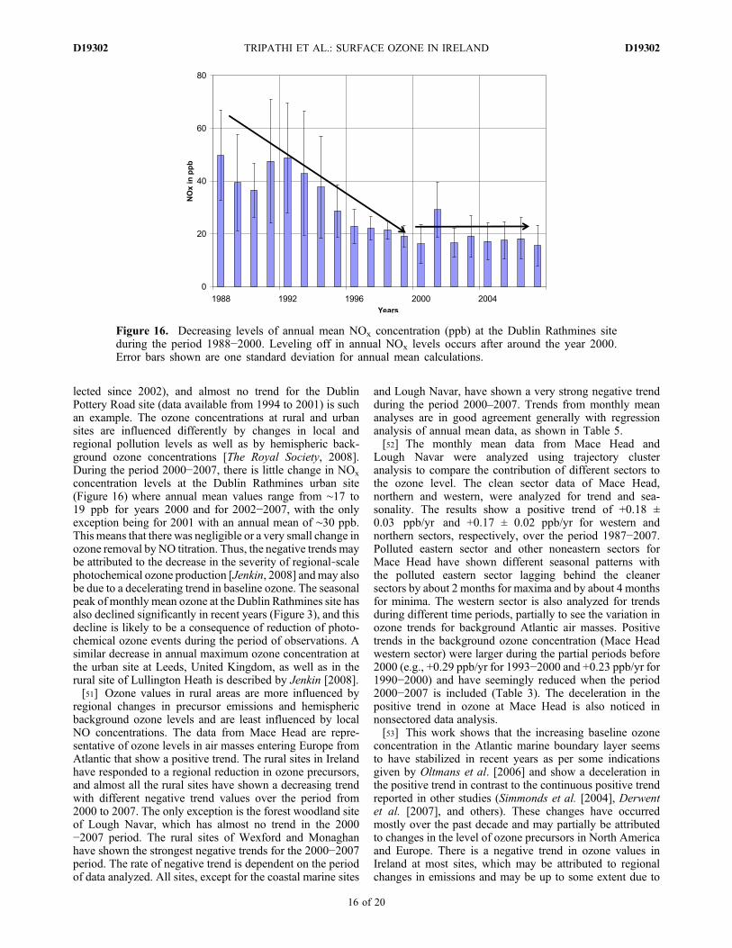
lected since 2002), and almost no trend for the DublinPottery Road site (data available from 1994 to 2001) is suchan example. The ozone concentrations at rural and urbansites are influenced differently by changes in local andregional pollution levels as well as by hemispheric back-ground ozone concentrations [The Royal Society, 2008].During the period 2000−2007, there is little change in NOx

concentration levels at the Dublin Rathmines urban site(Figure 16) where annual mean values range from ∼17 to19 ppb for years 2000 and for 2002−2007, with the onlyexception being for 2001 with an annual mean of ∼30 ppb.This means that there was negligible or a very small change inozone removal by NO titration. Thus, the negative trends maybe attributed to the decrease in the severity of regional‐scalephotochemical ozone production [Jenkin, 2008] andmay alsobe due to a decelerating trend in baseline ozone. The seasonalpeak of monthly mean ozone at the Dublin Rathmines site hasalso declined significantly in recent years (Figure 3), and thisdecline is likely to be a consequence of reduction of photo-chemical ozone events during the period of observations. Asimilar decrease in annual maximum ozone concentration atthe urban site at Leeds, United Kingdom, as well as in therural site of Lullington Heath is described by Jenkin [2008].[51] Ozone values in rural areas are more influenced by

regional changes in precursor emissions and hemisphericbackground ozone levels and are least influenced by localNO concentrations. The data from Mace Head are repre-sentative of ozone levels in air masses entering Europe fromAtlantic that show a positive trend. The rural sites in Irelandhave responded to a regional reduction in ozone precursors,and almost all the rural sites have shown a decreasing trendwith different negative trend values over the period from2000 to 2007. The only exception is the forest woodland siteof Lough Navar, which has almost no trend in the 2000−2007 period. The rural sites of Wexford and Monaghanhave shown the strongest negative trends for the 2000−2007period. The rate of negative trend is dependent on the periodof data analyzed. All sites, except for the coastal marine sites

and Lough Navar, have shown a very strong negative trendduring the period 2000–2007. Trends from monthly meananalyses are in good agreement generally with regressionanalysis of annual mean data, as shown in Table 5.[52] The monthly mean data from Mace Head and

Lough Navar were analyzed using trajectory clusteranalysis to compare the contribution of different sectors tothe ozone level. The clean sector data of Mace Head,northern and western, were analyzed for trend and sea-sonality. The results show a positive trend of +0.18 ±0.03 ppb/yr and +0.17 ± 0.02 ppb/yr for western andnorthern sectors, respectively, over the period 1987−2007.Polluted eastern sector and other noneastern sectors forMace Head have shown different seasonal patterns withthe polluted eastern sector lagging behind the cleanersectors by about 2 months for maxima and by about 4 monthsfor minima. The western sector is also analyzed for trendsduring different time periods, partially to see the variation inozone trends for background Atlantic air masses. Positivetrends in the background ozone concentration (Mace Headwestern sector) were larger during the partial periods before2000 (e.g., +0.29 ppb/yr for 1993−2000 and +0.23 ppb/yr for1990−2000) and have seemingly reduced when the period2000−2007 is included (Table 3). The deceleration in thepositive trend in ozone at Mace Head is also noticed innonsectored data analysis.[53] This work shows that the increasing baseline ozone

concentration in the Atlantic marine boundary layer seemsto have stabilized in recent years as per some indicationsgiven by Oltmans et al. [2006] and show a deceleration inthe positive trend in contrast to the continuous positive trendreported in other studies (Simmonds et al. [2004], Derwentet al. [2007], and others). These changes have occurredmostly over the past decade and may partially be attributedto changes in the level of ozone precursors in North Americaand Europe. There is a negative trend in ozone values inIreland at most sites, which may be attributed to regionalchanges in emissions and may be up to some extent due to

Figure 16. Decreasing levels of annual mean NOx concentration (ppb) at the Dublin Rathmines siteduring the period 1988−2000. Leveling off in annual NOx levels occurs after around the year 2000.Error bars shown are one standard deviation for annual mean calculations.

TRIPATHI ET AL.: SURFACE OZONE IN IRELAND D19302D19302

16 of 20

the decelerating trend in baseline ozone entering Europe asdiscussed above. But because the ozone precursor emissionsmay not necessarily have stopped or decreased substantiallyin around 2000, the possible stabilization in ozone levelobserved in this work may not completely be attributed tochanges in precursor emissions. Further observational andmodeling research is needed to address this complex prob-lem. Most of the Irish sites started observations after 2000,and relatively few years of data are available that does notnecessarily give a reliable long‐term trend in ozone levels,and accordingly, the trends are just indicative The analysisunderlines the need for further continuous measurements ofozone at different sites to assess long‐term ozone variationsin the region and to assess future impacts of government andEU directives for emission controls.

Appendix A: Algorithm Used for TrajectoriesClustering

[54] On the basis of the work of Mattis [2002] andDorling et al. [1992], the algorithm used here is a nonhi-erarchical clustering algorithm. It was implemented inAppendix C. It starts with a certain number of clusters andthen decreases the number of clusters by merging twoclusters at a time. After each merging step, centroids arerecalculated, and trajectories are reassigned if necessary.[55] Thirty synthetic trajectories (initializers I) are created,

to start the clustering procedure. The initializers I are tra-jectories arriving at the final destination in a straight line,from 30 different directions. Every trajectory T is assignedto its closest initializer I. In this way, 30 groups/clustersof trajectories are formed. At the end of this step, theinitializers I are no longer needed; they only served as aninitial assignment of the trajectories to groups.[56] As a metric, the distance between two trajectories

(e.g., trajectory T and initializer I) is calculated as the distancebetween the two trajectories on the surface of the earth,averaged over all time steps. The distance between two pointsis calculated as the real distance (as the crow flies).[57] For each group, a centroid C is calculated. The cen-

troid is a “trajectory” that is derived from the trajectories inthis group. It describes this group. It is calculated by aver-aging the latitude and longitude values for all the membersof this group, for each time step. For each trajectory, it is

tested if it is in the group with the centroid it is closest to. Ifa trajectory is closer to a centroid of a different group, thetrajectory is reassigned to this other group. Once all trajec-tories have been reassigned (if necessary), the centroids arerecalculated for the new groups.[58] This step, reassignment of trajectories and recalcu-

lation of centroids, is repeated, until no further reassign-ments are necessary. The mean distance of all trajectoriesfrom their centroid is calculated, for this clustering, notingthe number of groups/clusters at this step (initially 30).[59] Then those two groups with closest centroids are

merged, forming a new group of trajectories. The number ofgroups/clusters thus decreases by one. This process isrepeated until all trajectories end up in one group/cluster.[60] The algorithm can be summarized as follows:[61] 1. The creation of 30 group/cluster initializers I.[62] 2. Every trajectory T is assigned to the closest

initializer I.[63] 3. For each group, a centroid C is calculated.[64] 4. For each T: check if it is in the right group, otherwise

reassign; recalculate centroids. Repeat 4 until no reassign-ments are necessary.[65] 5. Mean distance (for T from itsC) for this clustering is

calculated and noted as a function of the number of clusters.[66] 6. Merge two groups with closest centroids.[67] 7. Repeat 4−6 until all T are in one group.

A1. Number of Groups/Clusters

[68] To determine the optimum number of clusters, therelative change in overall mean distance calculated for eachnumber of clusters, step 5 of the algorithm, is plotted as afunction of the number of clusters. The overall mean dis-tance usually increases slightly with decreasing number ofclusters. However, if there is a strong increase in overallmean distance, this is an indication that two clusters havebeen merged, which are dissimilar. The number of clustersjust before this merging is then a good choice.

Appendix B: Seasonal Trend Decomposition (STD)Procedure for Analysis of Time Series

[69] A time series can be decomposed into seasonal,trend, and remaining components [Cleveland et al., 1990],

Table 5. Ozone Trends at Irish Sites From Seasonal Trend Decomposition Analysis of Monthly Mean Dataa

Stations Trend in Monthly Mean (ppb/yr) Trend in Annual Mean (ppb/yr)

Dublin‐Rathmines (2002−2007) −0.33 ± 0.17 −0.33 ± 0.21Dublin‐Pottery Road (1994−2001) +0.09 ± 0.16 +0.38 ± 0.26Cork (1995−2007)2000−2007

−0.06 ± 0.06−0.20 ± 0.11

−0.07 ± 0.11−0.18 ± 0.17

Wexford (1999−2007)2000−2007

−0.80 ± 0.11−0.99 ± 0.13

−0.76 ± 0.27−0.99 ± 0.30

Monaghan (1995−2007)2000−2007

−0.12 ± 0.07−0.58 ± 0.12

−0.14 ± 0.16−0.58 ± 0.24

Lough Navar (1988−2007)2000−2007

−0.07 ± 0.04+0.07 ± 0.15

−0.07 ± 0.05+0.08 ± 0.24

Mace Head (1988−2007)2000−2007

+0.16 ± 0.04+0.27 ± 0.10

+0.16 ± 0.04+0.27 ± 0.18

Valentia (2001−2007) −0.05 ± 0.15 −0.06 ± 0.37

aTrends during 2000−2007 are shown separately. Corresponding trends in annual mean are also shown. The stations showreasonably good agreement for trends, analyzed from both monthly mean data and annual mean data, except for the Dublin‐Pottery Road site.

TRIPATHI ET AL.: SURFACE OZONE IN IRELAND D19302D19302

17 of 20

to assess a trend of longer‐term data. These componentscan be considered to be multiplied to give the originalseries or added to give the original series. Depending onthe approach of series modeling, they are called a multi-plicative or an additive model. In this work, the additivemodel is used for the decomposition and the series can beexpressed as (Series)t = (Trend)t + (Seasonal)t + (Error)t,where t is the point of time.[70] For decomposition of a time series, the commercial

software MINITAB is used for this analysis. The data arefirst seasonally adjusted, and then a linear trend line is fittedon this seasonally adjusted series using least squares linearregression. To adjust the series seasonally, the seasonalindices are first calculated for each month from smoothedseries. The series is smoothed with a central movingaverage procedure of the order of the length of seasonalcycle. The moving average is then subtracted from theoriginal data to obtain raw seasonal values. Medians of thecorresponding time periods (time periods 12 months apart)of this raw seasonal cycle are then adjusted to give theiraverage as zero. These adjusted medians are called sea-sonal indices and are used to adjust the data seasonally.This is called a seasonal trend decomposition (STD) pro-cedure, and the representative model of the time series iscalled a STD model.

Appendix C: Autoregressive Integrated MovingAverage (ARIMA) Model

[71] An autoregressive model is used to understand a timeseries and predict future values. The value of the variablein question at any point of time in a time series, say Xt,depends on the past history and can be expressed in terms ofone or more prior values and corresponding white noise orrandom shocks. The number to which we go back to andrepresent the present value is called the order of auto-regressive model. In a linear autoregressive model, thedependence of Xt on its past values and error terms aresupposed to be linear, and here we consider a linear model. Inmathematical terms, an autoregressive model for a timeseries Xt can be expressed as

Xt ¼Xp

i¼1

’iXt�i þ "t þ c; ðC1Þ

where ’ are the parameters of the model to be calculated, c isa constant (often omitted for simplicity of the model), and "is the error terms or random shocks with zero mean. For afirst‐order autoregression, the series can be expressed as alinear function of the previous value.

Xt ¼ ’Xt�1 þ "t : ðC2Þ

[72] The parameter ’ can be calculated using variousmethods, and the most commonly used method is a linearleast squares technique. So autoregression is simply alinear regression of the current value against previousvalue(s).[73] Another approach to represent a term in a time series

or predict future values is to represent it in the terms ofmoving averages. Here a term of the series is represented interms of the mean of the series and error terms of a past

number of values. The number here is called the order of themoving average model. Mathematically, a q‐order movingaverage model of a time series Xt can be expressed as

Xt ¼ �þ "t þXq

i¼i

�i"t�q; ðC3Þ

where � values are parameters, m is the mean of the series,and "t values are error terms. For the first‐order movingaverage, the series becomes

Xt ¼ �"t�1 þ �þ "t: ðC4Þ[74] Comparing the above two different model equations

(C1) and (C4), it is clear that the moving average model isthe linear regression of the current value against randomshocks of the preceding value(s). The difference between thetwo approaches is that in a moving average model, therandom shocks of prior values are propagated to the futurevalues of the time series.[75] To identify a possible model for a time series, the

plots of an autocorrelation function (ACF) and partialautocorrelation function (PACF) for the series are usefulmethods. They can also be used to identify the periodicity orseasonality in the time series if present. Autocorrelationplots are also useful in identifying nonstationarity in thedata, and in that case, initial differencing steps are requiredto make the data stationary. Sometimes both the auto-regressive (AR) and moving average (MA) terms are used tomodel the time series. The approach to identify the model, ifone or both models are needed, is called Box‐Jenkinsapproach [Box and Jenkins, 1970], to model a time series. Ifboth terms are used to model a time series, then the model iscalled the autoregressive moving average model or ARMAmodel, and a term in the time series is dependent on the pasthistory as well as on the past error terms. In case of anonstationary time series, if a differencing term is used tomake the series stationary, the model is called an auto-regressive integrated moving average (ARIMA) model. Theabove approach is used to identify the model using com-mercial statistical software SPSS for time series of groundozone data.[76] ARIMA analysis does not give a direct explanation

for the time series, but the model fitted data give an idea oftrend and seasonal variation. For ARIMA analysis, varioustests need to be performed to check what kind of model fitsbest the data series: whether it is a moving average orregression or a mixture of both. Note that the ARIMA‐predicted time series for the surface ozone monthly meanvalues starts at the thirteenth month and is explained in thefollowing paragraph as an example for Rathmines timeseries analysis. More details of the ARIMA procedure andrelevant references are given by Junker et al. [2004].[77] First transformation of the time series (e.g., for

Rathmines) is an order of seasonal differencing: The newseries starts at the series index 13 with the value equal to thevalue at series index 13 minus the value at series index 1.The new series has a lesser number of points (12 less) thanthe original series. Autocorrelation function (ACF) andpartial autocorrelation function (PACF) analysis of the newseries shows that the best fit model has a nonseasonalmoving average (MA) of first order and a seasonal MA offirst order. This means that the value of surface ozone at a

TRIPATHI ET AL.: SURFACE OZONE IN IRELAND D19302D19302

18 of 20

particular month is a function of its value at the precedingtwelfth month (because of seasonal differencing) and afunction of the fluctuations in the present month and pre-ceding month (both because of the presence of first order ofthe non‐seasonal MA), twelfth preceding month, and thethirteenth preceding months (for the presence of first orderof seasonal MA). The main difference between ARIMA andSTD approaches and their treatment of the time series isoutlined in the following points:[78] 1. STD uses smoothing technique to decompose time

series into trend and seasonal components and ARIMAlooks for any correlation in the time series, seasonal ornonseasonal.[79] 2. STD is useful in time series with a constant trend

and seasonal pattern, whereas ARIMA can be used for anykind of time series with or without a trend or seasonalpattern.[80] 3. STD model is independent of the original time

series, whereas ARIMA model is represented as a functionof the original time series.[81] 4. STD is useful in trend analysis and long‐range

forecasting, whereas ARIMA is more useful in modelingpatterns that are not easily detected in plotted data or STDmodels.[82] Besides these differences, both models can be used to

model a time series with a constant trend and seasonalpattern, and they are used here for monthly mean ozone timeseries. ARIMA treats seasonal fluctuations (particularly forexceptional values of surface ozone such as during spring of2003) as seasonal variations and next year’s values arecorrelated with these exceptional values. But in the STDapproach, high peak values in 2003 are adjusted (when dataare deseasoned) in a way that most of their values areattributed to the error terms, leaving the series with lessseasonal variation. This makes sense when there are largeannual variations and particularly seasonal variations ofground‐level ozone. But this comes with a cost: Part of theseasonal adjustment (deseasoning) goes toward the trendpart, and the deseasoned series show a stronger trend. Thiscompetition between seasonality and trend effects by twomodeling approaches might be smoothed if the length of theseries is longer, giving more importance to a continuous anda longer record of surface ozone at a site.

[83] Acknowledgments. The authors gratefully acknowledge theNOAA Air Resources Laboratory (ARL) for the provision of the HYSPLITtransport and dispersion model and/or READY website (http://www.arl.noaa.gov/ready.html) used in this publication. The Environment ProtectionAgency (EPA) is acknowledged for its support (EPA Project: Ozone levels,changes, and trends over Ireland—An integrated analysis). EPA staff:P. O’Brien and F. McGovern are also thanked for the supply of ozone dataand for their input. The support of the UK Department for Environment,Food, and Rural Affairs through contract EPG 1/1/130, CEPG 24 to P.G.Simmonds, and GA01081 to S. O’Doherty for operations at Mace Headis gratefully acknowledged. The authors also wish to thank anonymous re-viewers for their detailed critical comments and suggestions that signifi-cantly improved the quality of the paper.

ReferencesBox, G., and G. Jenkins (1970), Time Series Analysis: Forecasting andControl, Holden‐Day, San Francisco, Calif.

Carslaw, D. C. (2005), On the changing seasonal cycles and trends ofozone at Mace Head, Ireland, Atmos. Chem. Phys., 5, 3441–3450.

CEC (1996), Directive 96/62/EC of 27 September 1996 on ambient airquality assessment and management, O.J. L296, 11 November.

Cleveland, R. B., W. S. Cleveland, J. E. McRae, and I. Terpenning (1990),STL: A seasonal‐trend decomposition procedure based on loess, J. OfficialStat., 6(1), 3–75.

Coyle, M., R. I. Smith, J. R. Stedman, K. J. Weston, and D. Fowler (2002),Quantifying the spatial distribution of surface ozone concentration in theU.K., Atmos. Environ., 36, 1013–1024.

Derwent, R., M. Jenkin, S. Saunders, M. Pilling, P. Simmonds, N. Passant,G. Dollard, P. Dumitrean, and A. Kent (2003), Photochemical ozoneformation in north west Europe and its control, Atmos. Environ., 37,1983–1991.

Derwent, R. G., P. G. Simmonds, S. Seuring, and C. Dimmer (1998),Observation and interpretation of the seasonal cycles in the surface con-centrations of ozone and carbon monoxide at Mace Head, Ireland, from1990 to 1994, Atmos. Environ., 32(2), 145–157.

Derwent, R. G., P. G. Simmonds, A. J. Manning, and T. G. Spain (2007),Trend over a 20‐year period from 1987 to 2007 in surface ozone at theatmospheric research station, Mace Head, Ireland, Atmos. Environ., 41,9091–9098.

Dorling, S. R., T. D. Davies, and C. E. Pierce (1992), Cluster analysis: Atechnique for estimating the synoptic meteorological controls on air andprecipitation chemistry—Method and applications, Atmos. Environ.,26A, 2575–2581.

Draxler, R. R. and G. D. Rolph (2003), HYSPLIT (Hybrid Single‐ParticleLagrangian Integrated Trajectory) Model access via NOAA ARLREADY Website, NOAA Air Resources Laboratory, Silver Spring,MD. (Available at http://www.arl.noaa.gov/ready/hysplit4.html)

Endresen, Ø., E. Sørgård, J. Sundet, S. Dalsøren, I. Isaksen, T. Berglen, andG. Gravir (2003), Emission from internations sea transport and environ-mental impact, J. Geophys. Res., 108(D17), 4560, doi:10.1029/2002JD002898.

Fiore, A. M., D. J. Jacob, I. Ey, R. M. Yantosca, B. D. Field, and J. G.Wilkinson (2001), Background ozone over the United States in summer.Origin, trend and contribution to pollution episodes, J. Geophys. Res.,107(D15), 4279, doi:10.1029/2001JD000982.

Fusco, A., and J. A. Logan (2003), Analysis of 1970‐1995 trends in tropo-spheric ozone in northern hemisphere midlatitudes with the GEOS‐CHEM model, J. Geophys. Res., 108(D15), 4449, doi:10.1029/2002JD002742.

Hazucha, M., and A. S. Lefohn (2007), Nonlinearity in human healthresponse to ozone: Experimental laboratory considerations, Atmos. Envi-ron., 41, 4559–4570.

Intergovernmental Panel on Climate Change (2007), Changes in atmo-spheric constituents and in radiative forcing, in Climate Change 2007:The Physical Science Basis. Contribution of Working Group I to theFourth Assessment Report of the Intergovernmental Panel on ClimateChange, edited by S. Solomon et al., Cambridge Univ. Press, New York.

Jaffe, D., H. Price, D. Parrish, A. Goldstein, and J. Harris (2003), Increas-ing background ozone during spring on the west coast of North America,Geophys. Res. Lett., 30(12), 1613, doi:10.1029/2003GL017024.

Jenkin, M. E. (2008), Trends in ozone concentration distributions in the UKsince 1990: Local, regional and global influences, Atmos. Environ., 42,5434–5445.

Jonson, J. E., D. Simpson, H. Fagerli, and S. Solberg (2006), Can we explainthe trends in European ozone level?, Atmos. Chem. Phys., 6, 51–66.

Junker, C., J. N. Sheahan, S. G. Jennings, P. O’Brian, B. D. Hinds,E. Martinez‐Twary, A. D. A. Hansen, C. White, D. M. Garvey, and R. G.Pinnick (2004), Measurement and analysis of aerosol and black carbon inthe southwestern United States and Panama and their dependence onair mass origin, J. Geophys. Res., 109, D13201, doi:10.1029/2003JD004066.

Lefohn, A. S., D. Shadwick, and S. J. Oltmans (2008), Characterizing long‐term changes in surface ozone levels in the United States (1980−2005),Atmos. Environ., 42, 8252–8262.

Levy, H. (1971), Normal atmosphere: Large radical and formaldehyde con-centrations predicted, Science, 173, 141–143.

Li, Q., et al. (2002), Transatlantic transport of pollution and its effect on sur-face ozone in Europe and North America, J. Geophys. Res., 107(D13),4166, doi:10.1029/2001JD001422.

Lin, C.‐Y. C., J. Jacob, J. W. Munger, and A. M. Fiore (2000), Increasingbackground ozone in surface air over the United States, Geophys. Res.Lett., 27, 3465–3468.

Mattis, I. (2002), Aufbau eines Feuchte‐Temperatur‐Aerosol‐Ramanlidarsund Methodenentwicklung zur kombinierten Analyse von Trajectorienund Aerosolprofilen, PhD thesis, Leipzig Univ., Leipzig, Germany.

Monks, P. S. (2000), A review of the observations and origins of the springozone maximum, Atmos. Environ., 34(21), 3545–3561.

Moody, J. L., S. J. Oltmans, H. Levy, and J. T. Merrill (1995), Transportclimatology of tropospheric ozone: Bermuda 1988–1991, J. Geophys.Res., 100, 7179–7194.

TRIPATHI ET AL.: SURFACE OZONE IN IRELAND D19302D19302

19 of 20

Musselman, R. C., A. S. Lefohn, W. J. Massman, R. L. Heath (2006), A crit-ical review and analysis of the use of exposure‐ and flux‐based ozone indi-ces for predicting vegetation effects, Atmos. Environ., 40, 1869–1888.

Naja, N., H. Akimoto, and J. Staehelin (2003), Ozone in background andphotochemically aged air over central Europe: Analysis of long‐termozonesonde data from Hohenpeissenberg and Payerne, J. Geophys.Res., 108(D2), 4063, doi:10.1029/2002JD002477.

Newchurch, M., E. S. Yang, D. Cunnold, G. Reinsel, J. Zawodny, andJ. Russel III (2003), Evidence for slowdown in stratospheric ozone loss:First stage in ozone recovery, J. Geophys. Res., 108(D16), 4507,doi:10.1029/2003JD003471.

Oltmans, S. J., et al. (2006), Long‐term changes in tropospheric ozone,Atmos. Environ., 40, 3156–3173.

Ordóñez, C., H. Mathis, M. Furger, S. Henne, C. Hüglin, J. Staehelin, andA. S. H. Prévôt (2005), Changes of daily surface ozone maxima in Swit-zerland in all seasons from 1992 to 2002 and discussion of summer 2003,Atmos. Chem. Phys., 5, 1187–1203.

Ordóñez, C., D. Brunner, J. Staehelin, P. Hadjinicolaon, J. A. Pyle,M. Jonas, H. Wernli, and A. S. H. Prévôt (2007), Strong influence oflowermost stratospheric ozone on lower free tropospheric ozone changesover Europe, Geophys. Res. Lett. , 34 , L07805, doi:10.1029/2006GL029113.

Parrish, D. D., J. S. Holloway, M. Trainer, P. C. Murhy, G. L. Forbes, andF. C. Fehsenfeld (1993), Export of North American ozone pollution tothe North Atlantic Ocean, Science, 259, 1436–1439.

Parrish, D. D., D. B. Millet, and A. H. Goldstein (2009), Increasing ozonein marine boundary layer inflow at the west coasts of North America andEurope, Atmos. Chem. Phys., 9, 1303–1323.

Ramaswamy, V., et al. (2001), Radiative forcing of climate change, in Cli-mate Change 2001: The Scientific Basis, Contribution of Working GroupI to the Third assessment Report of the IPCC, Houghton et al., chap. 6,pp. 349–416.

Scheel, H. E., et al. (1997), On the spatial distribution and seasonal varia-tion of Lower‐Troposphere Ozone over Europe, J. Atmos. Chem., 28,11–28.

Simmonds, P. G., R. G. Derwent, A. J. Manning, and G. Spain (2004),Significant growth in surface ozone at Mace Head, Ireland, 1987–2003,Atmos. Environ., 38, 4769–4778.

Solberg, S., D. Simpson, J. Jonson, A. Hjellberekke, and R. Derwent(2004), Ozone in EMEP Assessment PART I: European Perspective,edited by G. Løvblad et al., Tech. Rep., The Norwegian MeteorologicalInstitute, Oslo, Norway.

Staehelin, J., J. Thudium, R. Buehler, A. Volz‐Thomas, and W. Graber(1994), Trends in surface ozone concentrations at Arosa (Switzerland),Atmos. Environ., 28, 75–87.

Stohl, A., and C. Trickl (1999), A textbook example of long‐range trans-port: Simultaneous observation of ozone maxima of stratospheric andnorth American origin in the free troposphere over Europe, J. Geophys.Res., 104, 30,445–30,462.

Streets, D., et al. (2003), An inventory of gaseous and primary aerosolemission in Asia in the year 2000, J. Geophys. Res., 108(D21), 8809,doi:10.1029/2002JD003093.

Tarasova, O. A., C. A. M. Brenninkmeijer, P. Jöckel, A. M. Zvyagintsev,and G. I. Kuznetsov (2007), A climatology of surface ozone in the extra

tropics: cluster analysis of observations and model results, Atmos. Chem.Phys., 7, 6099–6117.

Tarasova, O. A., I. A. Senik, M. G. Sosonkin, J. Cui, J. Staehelin, and A. S.H. Prévôt (2009), Surface ozone at the Caucasian site Kislovodsk HighMountain Station and the Swiss Alpine site Jungfaujoch: Data analysisand trends (1990–2006), Atmos. Chem. Phys., 9, 4157–4175.

Terao, Y., J. A. Logan, A. R. Douglass, and R.S. Stolarski (2008), Contri-bution of stratospheric ozone to the interannual variability of tropo-spheric ozone in the northern extratropics, J. Geophys. Res., 113,D18309, doi:10.1029/2008JD009854.

The Royal Society (2008), Ground level ozone in the 21st century: Futuretrends, impacts and policy implications, chap. 3, pp. 11–39.

UNECE (2007), Review of the 1999 Gothenburg Protocol. Report by theSecretariat, UNECE Executive Body for the Convention on Long‐RangeTransboundary Air Pollution, ECE/EB.AIR/2007/10.

US EPA (2006), Air quality criteria for ozone and related photochemicaloxidants, Report Nos. EPA/600/R‐05/004af, Office of Research andDevelopment, Research Triangle Park, NC. February 2006, US Environ.Protection Agency.

Vestreng, V., M. Adams, and J. Goodwin (2004), Inventory review 2004:Emission data reported to CLRTAP and under the NEC directive, EMEP/MSC‐W status report 1/04, The Norwegian Meteorological Institute,Oslo, Norway.

Vingarzan, R. (1994), A review of surface ozone background levels andtrends, Atmos. Environ., 28(1), 25–37.

Volz, A., and D. Kley (1988), Evaluation of the Montsouris series of ozonemeasurements made in the nineteenth century, Nature, 332, 240–242.

Wang, Y. H., et al. (2003), Springtime photochemistry at northern midand high latitude, J. Geophys. Res., 108(D4), 8358, doi:10.1029/2002JD002227.

WHO (1987), Air quality guidelines for Europe, WHO Regional Publica-tions, Euro. Ser. No. 23, WHO, Copenhagen, Denmark.

Wild, O., and H. Akimoto (2001), Intercontinental transport of ozone andits precursors in 3‐D global CTM, J. Geophys. Res., 106, 27,729–27,744.

WMO (2007), Scientific assessment of ozone depletion: 2006, GlobalOzone Research and Monitoring Project, Report No. 50, WMO, Geneva.

L. Coleman, S. G. Jennings, C. D. O’Dowd, T. G. Spain, and O. P.Tripathi, School of Physics, Environmental Change Institute, NationalUniversity of Ireland, University Rd., Galway, Ireland. (om.tripathi@nuigalway.ie)S. Leinert and B. O’Leary, Environmental Protection Agency,

Mccumiskey House, Richview Business Park, Clonskeagh D14, Co.Dublin, Ireland.E. Moran, Met Éireann, 9, Glasnevin Hill, Co. Dublin, Ireland.S. J. O’Doherty, Physical and Theoretical Chemistry, University of

Bristol, BS8 1TS, Bristol, UK.

TRIPATHI ET AL.: SURFACE OZONE IN IRELAND D19302D19302

20 of 20