
Static Analysis for BSPlib Programs
274
HAL Id: tel-02920363 https://tel.archives-ouvertes.fr/tel-02920363 Submitted on 24 Aug 2020 HAL is a multi-disciplinary open access archive for the deposit and dissemination of sci- entific research documents, whether they are pub- lished or not. The documents may come from teaching and research institutions in France or abroad, or from public or private research centers. L’archive ouverte pluridisciplinaire HAL, est destinée au dépôt et à la diffusion de documents scientifiques de niveau recherche, publiés ou non, émanant des établissements d’enseignement et de recherche français ou étrangers, des laboratoires publics ou privés. Static Analysis for BSPlib Programs Filip Jakobsson To cite this version: Filip Jakobsson. Static Analysis for BSPlib Programs. Distributed, Parallel, and Cluster Computing [cs.DC]. Université d’Orléans, 2019. English. NNT : 2019ORLE2005. tel-02920363
-
Upload
khangminh22 -
Category
Documents
-
view
1 -
download
0
Transcript of Static Analysis for BSPlib Programs
HAL Id: tel-02920363https://tel.archives-ouvertes.fr/tel-02920363
Submitted on 24 Aug 2020
HAL is a multi-disciplinary open accessarchive for the deposit and dissemination of sci-entific research documents, whether they are pub-lished or not. The documents may come fromteaching and research institutions in France orabroad, or from public or private research centers.
L’archive ouverte pluridisciplinaire HAL, estdestinée au dépôt et à la diffusion de documentsscientifiques de niveau recherche, publiés ou non,émanant des établissements d’enseignement et derecherche français ou étrangers, des laboratoirespublics ou privés.
Static Analysis for BSPlib ProgramsFilip Jakobsson
To cite this version:Filip Jakobsson. Static Analysis for BSPlib Programs. Distributed, Parallel, and Cluster Computing[cs.DC]. Université d’Orléans, 2019. English. NNT : 2019ORLE2005. tel-02920363

UNIVERSITÉ D’ORLÉANS
ÉCOLE DOCTORALE MATHÉMATIQUES, INFORMATIQUE,
PHYSIQUE THÉORIQUE ET INGÉNIERIE DES SYSTÈMES
LABORATOIRE D’INFORMATIQUE FONDAMENTALE D’ORLÉANSHUAWEI PARIS RESEARCH CENTER
THÈSE présentée par :
Filip Arvid JAKOBSSON
soutenue le : 28 juin 2019pour obtenir le grade de : Docteur de l’université d’Orléans
Discipline : Informatique
Static Analysis for BSPlib Programs
THÈSE DIRIGÉE PAR :Frédéric LOULERGUE Professeur, University Northern Arizona et
Université d’Orléans
RAPPORTEURS :
Denis BARTHOU Professeur, Bordeaux INP
Herbert KUCHEN Professeur, WWU Münster
JURY :
Emmanuel CHAILLOUX Professeur, Sorbonne Université, Président
Gaétan HAINS Ingénieur-Chercheur, Huawei Technologies, Encadrant
Wijnand SUIJLEN Ingénieur-Chercheur, Huawei Technologies, Encadrant
Wadoud BOUSDIRA Maître de conference, Université d’Orléans, Encadrante
Frédéric DABROWSKI Maître de conference, Université d’Orléans, Encadrant


Acknowledgments
Firstly, I am grateful to the reviewers for taking the time to read this doc-
ument, and their insightful and helpful remarks that have greatly helped its
quality.
I also thank my team of supervisors for guiding me through this PhD. Gaétan
for his imagination and deep theoretical knowledge — but firstly, for his big
heart. Wijnand for his impressive knowledge of parallel computing, his tireless
proofreading, and for keeping my innate laziness in check. Wadoud and Frédéric
D. for their rich insight in formal methods, and for our long discussions in front
of the whiteboard. To Frédéric L., for directing this thesis with endless optimism,
for overseeing the team of supervisors, and for his ever reliable advice. I hope
our collaboration remains as fruitful in the future.
I am also grateful to my colleagues at Huawei France Research Center. An-
thony, Thibaut and Jan-Willem, for sharing the delights and pains of the doctor-
ate since we first came to Huawei. To Pierre and Filip that joined later on, but
who merit no less mention. I wish you the best for the completion of your theses.
To Antoine, Arnaud, Alain, Mathias and Louise, and to all other colleagues that
I have failed to mention.
I also have debt of gratitude to Nikolai Kosmatov and Julien Signoles for
supervising my master’s internship at CEA. They initiated me to research, and
gave me confidence to continue its pursuit.
I thank Linus, Henrik, Per and Jonas, for their friendship. As well as all
the great friends I have made during my stay in France: Hai, Santiago, Michel,
Lawrence, Leah, Anaiz, Lucile and Yu. To my family and parents-in-law, for be-
ing there, for supporting and for encouraging me. But finally, and foremost, to
Laura. She made all this possible through her unwavering love and support,
without which I would have long since abandoned.
iii


Résumé étendu en français
Introduction
Les ordinateurs sont utilisés pour automatiser des calculs volumineux qui
seraient hors de portée d’un humain. La recherche et le développement en in-
formatique augmentent progressivement leur capacité à effectuer des calculs de
plus en plus grands, sans épuiser la patience de l’utilisateur. Ce processus per-
met l’analyse mathématique, assistée par ordinateur, d’un ensemble toujours
croissant de phénomènes naturels complexes. Pour citer un exemple parmi tant
d’autres, les chercheurs ont utilisé l’informatique pour obtenir une meilleure
compréhension de l’origine de l’univers et de la nature de la matière [97].
Dans certains cas, l’augmentation de la capacité de calcul permet de rem-
placer ou même de surpasser du matériel spécialisé. C’est le cas de la radio
logicielle1, composante essentielle des réseaux 5G [107], qui remplace le maté-
riel de télécommunication personnalisé et qui permet d’atténuer le problème de
rareté du spectre [177].
L’informatique parallèle2 est une méthode importante pour obtenir de
grandes capacités de calcul. Elle consiste à connecter plusieurs processeurs in-
formatique via un réseau électronique, et à les programmer pour collaborer à
la résolution d’une tâche commune. La plupart des ordinateurs modernes ex-
ploitent le parallélisme. Cela inclut les smartphones, comme le Huawei P303, qui
comporte 8 processeurs. Mais aussi, des superordinateurs, comme le Summit [14],
qui contient 2,4 millions de processeurs en réseau. Le Summit, entre autres utili-
sations, sert à effectuer des simulations du système terrestre qui produisent des
prévisions pour le climat du futur.
Comme dans tous projets, lorsque d’avantage de ressources sont mobilisées,
on s’attend à une efficacité plus grande. Ceci est également vrai dans le contexte
1En anglais, Software-defined radio2Dans cette thèse, nous distinguons le calcul parallèle du calcul concurrent. Dans le premier,
le parallélisme est utilisé de manière plus grossière pour exécuter simultanément des calculsreliés. Dans le dernier, le parallélisme est utilisé de manière fine pour exécuter simultanémentdes calculs non-reliés.
3https://en.wikipedia.org/wiki/Huawei_P30
v

de l’informatique parallèle. Quand on connecte plus de processeurs, on s’attend
à une augmentation de la capacité de calcul proportionnelle aux ressources ajou-
tées. Hélas, ce ne sera pas nécessairement le cas. Une analogie peut être faite avec
une organisation sociale. L’addition de ressources humaines ne résulte pas im-
médiatement en une organisation capable de faire plus de travail dans la même
unité de temps. Cela est dû à l’effort induit par la distribution et la coordination
du travail. Si fait maladroitement, l’addition de plus de travailleurs pourraient
même diminuer l’efficacité de l’organisation. Il en va de même dans le calcul pa-
rallèle, où le travail doit aussi être distribué et coordonné entre les processeurs
participants. Par conséquent, l’une des tâches fondamentales du calcul parallèle
est de concevoir des architectures et des programmes adaptés afin qu’ils passe
bien à l’échelle, c’est-à-dire que l’ajout de ressources provoque l’augmentation
souhaitée de la puissance de calcul. Ceci est le sujet du parallélisme évolutif 4.
Cette tâche est réputée difficile. Dans cette thèse nous allons attaquer cette
difficulté dans le contexte de BSPlib, une bibliothèque de programmation pour
Bulk Synchronous Parallelism (BSP). BSP est un modèle de parallélisme avec
des caractéristiques désirable en terme de structure, de sécurité et de perfor-
mance. Nos armes de prédilection sont des outils de vérification automatiques
appelés analyses statiques. Ces outils, spécifiés et éprouvés mathématiquement,
appartiennent aux méthodes formelles. Dans la suite de ce résumé, nous illustre-
rons les difficultés de la programmation parallèle évolutive. Nous introduirons le
modèle BSP, les méthodes formelles et l’analyse statique. Puis, nous énoncerons
notre thèse et résumerons nos contributions qui argumente notre thèse, avant de
conclure.
Défis de la programmation parallèle évolutive
Appliquer le parallélisme évolutif à un problème de calcul présente trois dif-
ficultés principale : concevoir l’algorithme, le mettre en œuvre correctement et
mesurer sa capacité de passer à l’échelle.
L’algorithme est la séquence d’étapes nécessaires pour résoudre le problème.
La conception d’un algorithme qui exploite le calcul parallèle, nécessite d’ana-
lyser le problème et de découvrir si, et comment, sa résolution peut être dé-
coupée et distribuée. Cela nécessite une idée créative qui est très spécifique à
chaque problème. Cependant, dans cette thèse, nous nous concentrons sur les
4En anglais, scalable parallelism
vi
deux difficultés restantes, c’est-à-dire la vérification de sa mise en œuvre et de
sa performance.
L’implémentation correcte de l’algorithme est rendu difficile par les erreurs
subtiles auxquelles la programmation parallèle est sujette. En plus des erreurs
possibles en programmation classique, dite séquentielle, comme la division par
zéro ou la déréférence d’un pointeur NULL, le parallélisme introduit une multi-
tude de nouvelles erreurs. Celles-ci sont dues à de mauvaises l’interaction entre
les processus ou à une coordination fautive.
Nous illustrons cela avec deux erreurs communes en calcul parallèle. Un in-
terblocage est un type d’erreur impliquant au moins deux processus, A et B. Les
deux processus exigent des informations l’un de l’autre pour procéder. Mais ce
que A doit fournir à B dépend de ce que B doit fournir à A, et vice versa. La
progression est bloquée et le calcul ne se termine jamais.
Une data race se produit lorsque deux processus tentent d’accéder, par lecture
ou par écriture, à la même ressource, dont au moins un des accès est une écriture,
et lorsque l’ordre avec lequel les accès se produisent n’est pas fixé. Dans le cas
où un processus lit et un autre écrit la ressource, la valeur lue dépend de l’ordre
des accès. Dans le cas où les deux processus écrivent la ressource, la valeur finale
écrite dépend également de l’ordre. Ces situations sont indésirables et peuvent
conduire à des erreurs de calcul subtiles, difficilement détectables et résolubles.
Les interblocages et les data races sont causés par des entrelacements imprévus
d’exécutions parallèles. Quand plusieurs processus exécutent un flux d’instruc-
tions en parallèle, le nombre de possibles entrelacements de ces flux augmente
de façon exponentielle. Le programmeur doit s’assurer que son programme est
correct sous chaque entrelacement possible. On peut comparer cela à un jeu
où le joueur (un processus) doit prévoir chaque coup possible des adversaires
(les autres processus) et planifier sa réponse en conséquence. Cela devient rapi-
dement impossible au-delà de quelques tours, et plus difficile encore de façon
exponentielle en fonction du nombre d’adversaires.
Pour compliquer les choses, l’entrelacement de chaque exécution est non dé-
terministe. Cela signifie que des exécutions différentes du même programme avec
la même entrée peuvent engendrer des entrelacements différents : certains qui
mettent en lumière des erreurs, d’autres non. La difficulté de reproduire les
entrelacements erronés se traduit par une recherche de bug et une réparation
difficile.
Troisièmement, après avoir conçu et développé correctement un algorithme
parallèle, reste la tâche d’évaluer son efficacité par rapport à une solution sé-
vii

quentielle. L’approche du benchmarking, c’est-à-dire exécuter et mesurer la du-
rée de l’exécution du programme, ne donne que des indications pour une ar-
chitecture parallèle et une instance du problème. Pour obtenir des résultats plus
globaux, qui prédisent la performance pour toutes les instance lors de l’ajout de
processeurs ou lorsque l’on passe à une architecture parallèle différente, il faut
modéliser à la fois l’algorithme et l’architecture. Cette modélisation est difficile :
le but est d’inclure uniquement les aspects essentiels pour la performance pour
obtenir un modèle suffisamment simple, apte à l’analyse mais qui reste réaliste.
Ajouter plus de processeurs pour obtenir une capacité de calcul plus éle-
vée donne donc, au mieux, une augmentation linéaire en efficacité avec chaque
processeur. Mais, à la lumière de ces trois difficultés, elle vient au prix d’une
augmentation exponentielle à la fois de la complexité conceptuelle et de la mise
en œuvre.
Le modèle BSP
Bulk Synchronous Parallel5 (BSP) [191] est un modèle pour la programmation pa-
rallèle évolutive qui aide à atténuer les problèmes discutés ci-dessus. De plus, ce
modèle a été implémenté à la fois dans des librairies de programmation [100] et
dans des langages dédiés [18].
Le calcul parallèle d’un programme BSP suit notamment une structure qui
exclut à la fois les interblocages et les data races, grâce à des restrictions sur
la synchronisation et la communication. En effet, dans BSP, le calcul est divisé
en grands pas, appellés « supersteps ». A son tour, chaque superstep est divisé
dans une phase de calcul locale, une phase de communication et une phase de
synchronisation. Les interblocages sont évités puisque tous les processus se syn-
chronisent en même temps, évitant la dépendance circulaire d’un interblocage.
Les data races sont empêchées car les communications dans un calcul BSP (telles
que les accès à une ressource commune) sont exécutées en vrac et en ordre fixe.
Malgré ces restrictions, BSP permet l’expression d’une grande variété d’algo-
rithmes parallèles [186].
Le modèle BSP facilite également le parallélisme évolutif en fournissant des
prévisions de performance pour des programmes parallèles grâce à son modèle
de coût. Ce modèle est simple mais réaliste. La performance d’une architecture
parallèle est caractérisée par quatre paramètres :
5Parfois traduit en parallélisme isochrone ou parallélisme quasi-synchrone en français. Dans cedocument nous écrierons « BSP ».
viii
p le nombre de processus
r la caractérisation du coût local
g la caractérisation du coût de communication
l la caractérisation du coût de synchronisation
Le temps d’exécution d’un programme parallèle est caractérisé par une for-
mule de coût. La formule est une fonction des paramètres de l’architecture
qui décrit les ressources consommées par l’exécution du programme. La durée
d’exécution estimée d’un programme est ainsi obtenue en appliquant sa fonction
de coût aux paramètres de l’architecture où il sera exécuté. Ainsi, les formules de
coût BSP sont portables : elles sont valables pour toutes architectures parallèles
dans le modèle BSP.
BSP aide à atténuer certaines des difficultés de l’application du parallélisme.
Mais ce n’est pas non plus une solution miracle. Dans cette thèse, nous porterons
notre attention sur BSPlib, une bibliothèque de programmation pour la mise
en œuvre des programmes BSP dans le langage général C. Nous aborderons
en particulier certaines erreurs et problèmes courants affectant les programmes
utilisants BSPlib.
Comme nous le verrons, ces problèmes résultent en partie de l’adjonction de
parallélisme sur un langage généraliste sous la forme d’une bibliothèque de pro-
grammation. L’avantage de telles bibliothèques de programmation est qu’elles
facilitent l’application de parallélisme dans des programmes séquentiels exis-
tants et, inversement, qu’elles permettent la réutilisation de code séquentiel dans
des programmes parallèles. Cependant, la généralité de ces langages permet
l’expression d’exécutions qui ne sont pas valides dans le modèle parallèle sous-
jacent et qui sont donc erronées. Ceci peut être opposé aux langages spécifiques
au domaine du parallélisme où de telles exécutions peuvent être restreintes.
Nous proposons d’utiliser l’analyse statique, un type de méthode formelle, pour
combler le fossé entre ces deux approches.
Méthodes formelles et analyse statique
Les méthodes formelles sont des techniques qui possèdent des fondements mathé-
matiques rigoureux servant à la modélisation, la spécification, le développement
et la vérification de programmes et de matériel informatique. L’analyse statique
est un type de méthode formelle. Les analyses statiques sont elles-mêmes des
ix

programmes informatiques qui ont pour but de découvrir des propriétés qui
sont valables pour chaque exécution dans le programme analysé. Le mot statique
fait référence au fait que les analyses statiques n’exécutent pas le programme. Ceci
s’oppose aux approches dynamiques, comme celles basées sur des tests.
Notre thèse est que l’analyse statique peut et doit être utilisée pour vérifier
l’absence d’erreurs dans les programmes BSPlib. En détectant des programmes
écrits dans un langage général transgressant un modèle parallèle exploité à tra-
vers une bibliothèque de programmation, nous pouvons combiner les avantages
des langages parallèles dédiés et des bibliothèques de parallélisme.
De plus, nous allons montrer qu’une majorité des programmes BSPlib est
structurée de manière à garantir l’absence d’erreurs de synchronisation. Cette
structure peut également être découverte par analyse statique et ensuite exploi-
tée pour vérifier d’autres propriétés au-delà de la bonne synchronisation, en par-
ticulier de sûreté et de performance. Enfin, nos analyses statiques découvrent des
propriétés qui sont valables dans un programme indépendamment du nombre
de processus qui l’exécutent : cela garantit que les analyses elles-mêmes s’ap-
pliquent aux programmes développés pour des architectures futures.
Alignement syntaxique
L’élaboration de ces analyses est une tâche ardue : en effet, il ne suffit pas de
vérifier la quantité exponentielle d’entrelacements pour un certain nombre fixe
de processus. Au contraire, il faut supposer un nombre quelconque de processus,
et vérifier tous les entrelacements possibles sous cette hypothèse.
Cependant, nous avons découvert que les programmes parallèles évolutifs et
réalistes sont en général structurés. Cette structure limite les divergence entre
la façon dont des processus différents exécutent les structures de contrôle du
programme. De plus, cette structure réduit le nombre d’entrelacements dont
l’interaction doit être vérifiée. Nous supposons que les programmeurs diligents
ont un œil prudent sur des patrons de programmation qui augmentent la diffi-
culté à mentalement exécuter leurs programmes, et donc naturellement écrivent
des programmes qui sont structurés6.
L’alignement syntaxique est un moyen de structurer des programmes parallèles
autour d’actions collectives. Ce sont des actions qui nécessitent la participation de
tous les processus. La synchronisation en barrière en BSP est un exemple d’une
action collective. Des programmes syntaxiquement alignés sont écrits de façon à
6Cela fait écho à l’idée que la paresse est une vertu du programmeur [41].
x

ce que chaque action collective résulte de l’exécution d’une instruction au même
point de programme par chaque processus.
La structure d’alignement syntaxique simplifie le raisonnement statique sur
les programmes parallèles pour deux raisons. Premièrement, l’alignement syn-
taxique assure que chaque processus exécute la même séquence d’actions collec-
tives. Par conséquent la vérification de l’utilisation correcte des actions collectives
se réduit à vérifier que chaque séquence possible est correcte quand répliqué par
tous les processus. Deuxièmement, elle limite les entrelacements aux séquences
d’instructions qui séparent chaque paire d’actions collectives.
Dans les travaux précédents, l’alignement syntaxique a été utilisé pour véri-
fier la synchronisation [204] et pour améliorer la précision d’une analyse may-
happen-in-parallel [121]. Notre thèse est que l’alignement syntaxique est égale-
ment une base utile pour l’analyse statique des programmes BSPlib.
Nous détaillons ci-dessous nos trois contributions qui argumentent cette
thèse. Premièrement, nous décrierons une analyse statique pour l’inférence de
l’alignement syntaxique dans des programmes BSPlib, qu’on applique à la véri-
fication de leur bonne synchronisation. Deuxièmement, nous expliquerons com-
ment nous avons exploité cette même structure dans le développement d’une
analyse statique de la performance des programmes BSPlib. Finalement, nous
parlerons de nos travaux sur l’enregistrement en BSPlib. L’enregistrement est
un composant important dans le système de communication en BSPlib. Notre
contribution finale est une condition suffisante pour l’utilisation correcte de l’en-
registrement basée sur l’alignement syntaxique.
Synchronisation répliquée
Nous abordons la thèse par le développement d’une analyse statique sous-
approchée pour la détection des points syntaxiquement alignés dans un pro-
gramme BSPlib. L’idée derrière cette analyse est de suivre les valeurs, variables
et expressions qui sont dépendants du pid, une expression symbolique en BS-
Plib qui identifie uniquement chaque processus. Dans notre formalisation, c’est
uniquement cette expression qui peut être évaluée différemment dans la mé-
moire initiale. En suivant les dépendances de cette expression, on peut détecter
les structures de contrôle dans le programme qui peuvent engendrer des diver-
gences dans le flux de contrôle entre chaque processus, mais aussi les points
de programme qui ne sont pas impactés par ces divergences. Ces derniers sont
aussi ceux qui sont syntaxiquement alignés.
Cette analyse est spécifiée grâce à une formalisation de BSPlib minimaliste :
xi
un langage séquentiel de type WHILE, étendu avec une sémantique BSP pour
permettre l’exécution parallèle et une primitive de synchronisation. Ainsi, un
programme de ce langage peut engendrer des erreurs dynamiques par l’utilisa-
tion non-collective de la synchronisation. Un exemple simple est donné par ce
programme court : if pid = 0 then sync else skip end.
Dans les contributions suivantes, nous étendrons cette formalisation pour
modéliser un sous-ensemble plus large de BSPlib. Cependant, cette version suffit
pour démontrer que l’alignement syntaxique de chaque point de programme
qui correspond à une primitive de synchronisation est un garant pour la bonne
synchronisation. Nous avons démontré cette propriété dans l’assistant de preuve
Coq.
Enfin, pour vérifier l’applicabilité de cette analyse, nous l’avons implémentée
en Frama-C, une plate-forme d’analyse des programmes C. Cette implémenta-
tion étend la formalisation de l’analyse en traitant des fonctions. Nous avons éga-
lement implémenté un traitement des pointeurs et de la communication. Sur un
échantillon de 20 programmes BSPlib, nous avons pu vérifier la bonne synchro-
nisation de 17 grâce à cette analyse, et trouver des erreurs de synchronisation
dans les 3 restants.
Analyse de coût
Nous nous intéressons ensuite à la question de la prévisibilité de performance.
Le modèle de coût de BSP donne un cadre pour raisonner sur la performance des
programmes. Bien entendu, ce modèle s’applique également aux programmes
BSPlib. Cependant, son utilisation nécessite une analyse manuelle des pro-
grammes pour inférer leurs formules de coût.
Dans cette contribution, nous avons automatisé cette inférence. D’abord, nous
étendons notre formalisation de BSPlib pour inclure les communications et nous
caractérisons le coût BSP dans cette formalisation. Nous avons développé une
transformation des programmes impératifs BSP en programmes séquentiels de
façon à ce qu’ils simulent de manière non déterministe un processus différent
à chaque superstep. Cette transformation exige et exploite le fait que les pro-
grammes analysés ont une synchronisation syntaxiquement alignée et elle nous
permet d’utiliser une analyse de coût classique adaptée pour des programmes
séquentiels de façon à faire ressortir le coût de calcul BSP pour des programmes
parallèles.
Néanmoins, le coût de communication nécessite une analyse plus fine, car,
dans le modèle BSP, ce coût dépend du comportement de l’ensemble des pro-
xii
cessus. En se basant uniquement sur la transformation décrite ci-dessus, nous
sommes obligé de faire des assomptions conservatrices punitives. Pour contour-
ner cette problématique nous utilisons le modèle polyédrique pour analyser la
communication, et nous insérons ensuite ces coûts dans le programme trans-
formé sous forme d’annotations.
Cette analyse a été implémentée dans un prototype que nous avons utilisé
pour obtenir la formule de coût de 8 algorithmes BSP classiques. Nous avons
testé empiriquement que ces formules donnent bien des bornes supérieures au
coût en comparant leurs prévisions avec le coût réel, spécifié par notre séman-
tique. C’est effectivement le cas, sauf pour l’un des programmes, dont le motif
de communications dépend des données qui sont communiquées.
Après avoir vérifié que nos formules de coût BSP étaient valides, nous avons
vérifié leur utilité pour prévoir la durée des calculs dans un cadre réaliste. Nous
avons comparé le temps prévu avec celui mesuré dans deux architectures paral-
lèles : un ordinateur de bureau multi-cœur et une grappe d’ordinateurs. Dans
des configurations qui remplissent l’hypothèse du modèle BSP sur le réseau de
communication, nous avons confirmé la précision de ces prévisions avec une
erreur inférieur à 50%.
Enregistrement sûr
Enfin, nous retournons à la vérification d’absence d’erreurs dans les programmes
BSPlib. Logiquement, ces programmes exécutent toujours en mémoire distri-
buée, et communiquent en réalisant des écritures et lectures à distance. L’en-
registrement est une procédure collective préalable aux accès, qui permet de re-
lier des objets de mémoire (variables, allocations dynamique etc.) existant dans
des processus différents. Malheureusement, ce mécanisme comporte plusieurs
écueils, et son utilisation nécessite une programmation prudente pour les éviter.
C’est pour cette raison que nous proposons une condition suffisante pour
l’enregistrement sûr. Une telle condition forme la base formelle d’une analyse
statique. Pour résumer, notre condition stipule que, sous l’hypothèse que les en-
registrements et les désenregistrements soient syntaxiquement alignés, et que
chaque enregistrement concerne le même objet dans chaque processus, la cor-
rection locale implique aussi la correction globale.
Nous spécifions cette condition grâce à une nouvelle formalisation de BSPlib,
cette fois étendue avec allocation dynamique et pointeurs ainsi qu’enregistre-
ment et communication. Nous caractérisons les exécutions qui sont correctes par
xiii

rapport l’API de BSPlib, et nous prouvons formellement que notre condition
suffisante est un garant de cette correction.
Conclusion
Contexte
Le calcul parallèle est un élément important pour obtenir de hautes capacités
de calcul. Il existe de nombreux domaines d’application qui profitent de l’appli-
cation du parallélisme, notamment dans le domaine des sciences naturelles où
une précision croissante dans les simulations permet une compréhension plus
précise de sujets aussi divers que l’origine de l’univers et la composition de la
matière [97], le fonctionnement du système terrestre [137] — avec des implica-
tions importantes pour la science du climat, la formation des galaxies [64], ou
encore le cerveau humain [136].
Cependant, encore plus que le calcul séquentiel, le calcul parallèle est chargé
d’erreurs. Les difficultés bien connues du développement correct des pro-
grammes séquentiels, et les effets désastreux quand il est traité à la légère (les
exemples spectaculaires abondent [65]), sont exacerbés par le nombre exponen-
tiel d’interactions entre processus dans le calcul parallèle. De plus, l’augmenta-
tion espérée de la puissance de calcul lors de l’application de parallélisme a un
prix. Sauf dans les cas basiques, une augmentation de la performance nécessite
une stratégie bien pensée pour paralléliser la résolution d’un problème. Il est
également difficile de garantir a priori que la parallélisation passe bien à l’échelle
et qu’elle est portable.
Le modèle BSP, et la bibliothèque BSPlib qui le met en œuvre, répond à cer-
taines de ces préoccupations en fournissant une structure de calcul parallèle qui
exclut plusieurs classes d’erreurs. Il permet également une performance fiable,
portable et prévisible. Cependant, il faut toujours prendre soin d’éviter des er-
reurs dans le développement de programmes BSPlib, et une analyse manuelle
des programmes est nécessaire pour profiter du modèle de performance BSP.
Les méthodes formelles apportent un cadre pour le développement de logi-
ciels qui sont garantis mathématiquement sûrs et efficaces. Des méthodes auto-
matiques, telles que l’analyse statique, sont particulièrement prometteuses car
elles ne nécessitent pas l’intervention d’experts en méthodes formelles. C’est
d’ailleurs le manque de méthodes formelles adaptées à BSPlib qui a motivé cette
xiv

thèse et nous a poussé à concevoir des outils automatisés pour aider au dévelop-
pement de programmes BSPlib qui soient à la fois corrects et efficaces.
Thèse
Notre thèse est que la majorité des programmes BSPlib se conforment à une
structure appelée alignement syntaxique. Nous avons fait valoir que l’alignement
syntaxique devait être imposé dans des programmes parallèles évolutifs et que
les analyses statiques devaient exploiter cette propriété. Cette approche atténue
avec élégance l’un des principaux problèmes d’analyse des programmes paral-
lèles, à savoir le grand nombre d’interactions entre processus.
Contributions
Pour argumenter l’importance et l’utilité de l’alignement syntaxique dans les
programmes BSPlib, nous avons premièrement conçu une analyse statique pour
vérifier l’alignement syntaxique de la synchronisation. Nous avons montré com-
ment cette propriété garantit une synchronisation correcte et nous avons forma-
lisé, certifié en Coq, mis en œuvre dans Frama-C et évalué cette analyse. Deuxiè-
mement, nous avons conçu, mis en œuvre comme prototype et évalué une ana-
lyse statique des coûts pour les programmes BSPlib qui exploitent l’alignement
syntaxique. Troisièmement, nous avons conçu une condition suffisante, basée
également sur l’alignement syntaxique. Nous avons prouvé que cette condition
garantit un enregistrement sûr dans des programmes BSPlib. Enfin, ces déve-
loppements reposent sur une série de formalisations progressivement plus com-
plexes des fonctionnalités de BSPlib, de la synchronisation à la communication
et l’enregistrement.
Perspectives
Nous concluons en discutant de pistes de recherche prometteuses. La préci-
sion de l’analyse statique de l’alignement syntaxique peut être améliorée. C’est
en particulier l’hypothèse conservatrice sur la communication qui nécessite une
révision. Une analyse fine des motifs de communication dans BSPlib (éventuelle-
ment basée sur des techniques polyédriques) pour étendre la reconnaissance des
expressions dépendantes sur pid permettrait de réduire le nombre d’annotations
actuellement requises.
xv
Le prototype actuel de l’analyse des coûts devrait être étendu à un outil
complet pour des programmes BSPlib réalistes, et évalué afin de valider son ap-
plicabilité. Son analyse du coût de la communication est précise, mais seulement
pour les motifs de communication « data-oblivious ». Une recherche plus pro-
fonde est nécessaire pour concevoir des analyses de coût de communications
dépendantes des données.
La condition suffisante pour l’enregistrement sûr devrait être la cible d’une
analyse statique. Cette analyse doit être conçue de manière à ce qu’elle approche
statiquement la condition suffisante et ensuit être mise en œuvre pour évaluer
son applicabilité.
Nous prévoyons également d’autres cas d’utilisation pour l’alignement syn-
taxique dans l’analyse des programmes BSPlib, par exemple, pour détecter les
écritures concurrentes, une erreur en BSPlib qui ressemble aux data races. Celles-
ci se produisent lorsque deux processus utilisent DRMA pour écrire à la même
zone de mémoire dans le même superstep. Le résultat final est spécifique à
chaque implémentation de BSPlib et présente donc une source possible d’er-
reurs. Une analyse statique pour la détection de ces écritures pourrait se baser
sur l’alignement syntaxique.
L’alignement syntaxique pourrait également être exploité en dehors de l’ana-
lyse statique. Des auteurs ont précédemment entamé des travaux en vue de la
vérification déductive des programmes parallèles évolutifs, notamment par l’in-
troduction des invariants sur tous les processus [175]. Ces invariants sont atta-
chés en tant qu’assertions aux primitives de synchronisation. Nous croyons que
ces assertions peuvent être attachées à tous les points de programme syntaxique-
ment alignés, et servir de base à un nouveau système de preuve compositionnelle
pour des programmes parallèles comme BSPlib.
Dans cette thèse, nous nous concentrons sur BSPlib. BSPlib peut être consi-
déré comme un modèle du sous-ensemble BSP dans d’autres bibliothèques pa-
rallèles comme MPI. Enfin, nous proposons des recherches sur l’exploitation de
l’alignement syntaxique pour les méthodes formelles pour ces bibliothèques.
xvi
Table des matières
Table des matières xvii
Table des figures xx
Liste des tableaux xxiii
1 Introduction 1
1.1 Challenges of Scalable Parallel Programming . . . . . . . . . 3
1.2 The BSP model . . . . . . . . . . . . . . . . . . . . . . . . . . . . . . 4
1.3 Formal Methods and Static Analysis . . . . . . . . . . . . . . . 5
1.4 Textual Alignment . . . . . . . . . . . . . . . . . . . . . . . . . . . 6
1.5 Contributions . . . . . . . . . . . . . . . . . . . . . . . . . . . . . . 6
1.6 List of Publications . . . . . . . . . . . . . . . . . . . . . . . . . . . 7
1.7 Outline of Thesis . . . . . . . . . . . . . . . . . . . . . . . . . . . . 8
2 Preliminaries 11
2.1 Notation . . . . . . . . . . . . . . . . . . . . . . . . . . . . . . . . . 12
2.2 The BSP Model . . . . . . . . . . . . . . . . . . . . . . . . . . . . . . 12
2.2.1 The BSP Computer . . . . . . . . . . . . . . . . . . . . . . . . . 14
2.2.2 The BSP Execution Model . . . . . . . . . . . . . . . . . . . . . 15
2.2.3 Example of a BSP Algorithm: reduce . . . . . . . . . . . . . . . . 16
2.2.4 The BSP Cost Model . . . . . . . . . . . . . . . . . . . . . . . . 18
2.3 BSPlib . . . . . . . . . . . . . . . . . . . . . . . . . . . . . . . . . . . 23
2.3.1 SPMD: Single Program, Multiple Data . . . . . . . . . . . . . . . 24
2.3.2 Memory Model and Communication . . . . . . . . . . . . . . . 26
2.3.3 BSPlib Program Structure . . . . . . . . . . . . . . . . . . . . . 26
2.3.4 BSPlib by Example . . . . . . . . . . . . . . . . . . . . . . . . . 27
2.3.5 The BSPlib API . . . . . . . . . . . . . . . . . . . . . . . . . . . 30
2.3.6 BSPlib Implementations . . . . . . . . . . . . . . . . . . . . . . 39
2.3.7 BSPlib Limitations . . . . . . . . . . . . . . . . . . . . . . . . . 39
2.3.8 Relationship to MPI . . . . . . . . . . . . . . . . . . . . . . . . . 42
xvii
2.4 The Data-Flow Approach to Static Analysis . . . . . . . . . . . 43
2.4.1 The Sequential Language Seq . . . . . . . . . . . . . . . . . . . 44
2.4.2 Control Flow Graph . . . . . . . . . . . . . . . . . . . . . . . . 46
2.4.3 Data-Flow Analysis . . . . . . . . . . . . . . . . . . . . . . . . . 47
2.4.4 Abstract Domain . . . . . . . . . . . . . . . . . . . . . . . . . . 49
2.4.5 Transfer Functions . . . . . . . . . . . . . . . . . . . . . . . . . 50
2.4.6 Calculating Solution Through Fixpoint Iteration . . . . . . . . . 51
2.5 Frama-C . . . . . . . . . . . . . . . . . . . . . . . . . . . . . . . . . . 52
3 State of the Art 55
3.1 Parallel Models . . . . . . . . . . . . . . . . . . . . . . . . . . . . . 56
3.1.1 Other than BSP . . . . . . . . . . . . . . . . . . . . . . . . . . . 56
3.1.2 BSP Extensions . . . . . . . . . . . . . . . . . . . . . . . . . . . 57
3.2 Parallel Programming . . . . . . . . . . . . . . . . . . . . . . . . . 60
3.2.1 Other than BSP . . . . . . . . . . . . . . . . . . . . . . . . . . . 60
3.2.2 BSP . . . . . . . . . . . . . . . . . . . . . . . . . . . . . . . . . 63
3.3 Formal Methods for Scalable Parallel Programming . . . . . 64
3.3.1 Deductive Verification . . . . . . . . . . . . . . . . . . . . . . . 65
3.3.2 Model Checking . . . . . . . . . . . . . . . . . . . . . . . . . . 68
3.3.3 Static Analysis . . . . . . . . . . . . . . . . . . . . . . . . . . . 70
3.3.4 Other Formal Methods . . . . . . . . . . . . . . . . . . . . . . . 79
3.4 Discussion . . . . . . . . . . . . . . . . . . . . . . . . . . . . . . . . . 79
4 Replicated Synchronization 81
4.1 Synchronization Errors in BSPlib Programs . . . . . . . . . . . 83
4.1.1 Textual Alignment and Replicated Synchronization . . . . . . . . 84
4.2 The BSPlite Language . . . . . . . . . . . . . . . . . . . . . . . . . . 85
4.2.1 Operational Semantics . . . . . . . . . . . . . . . . . . . . . . . 86
4.2.2 Denotational Semantics . . . . . . . . . . . . . . . . . . . . . . . 87
4.3 Static Approximation of Textual Alignment . . . . . . . . . . . 92
4.3.1 Pid-Independence Data-Flow Analysis . . . . . . . . . . . . . . 93
4.3.2 Replicated Synchronization Analysis . . . . . . . . . . . . . . . 101
4.4 Implementation . . . . . . . . . . . . . . . . . . . . . . . . . . . . . 102
4.4.1 Adapting the Analysis to Frama-C . . . . . . . . . . . . . . . . . 103
4.4.2 Edge-by-Edge Flow Fact Updates . . . . . . . . . . . . . . . . . 103
4.4.3 Frama-C Control Flow Graph . . . . . . . . . . . . . . . . . . . 105
4.4.4 Implementing Interprocedural Analysis Using Small Assump-
tion Sets . . . . . . . . . . . . . . . . . . . . . . . . . . . . . . . 111
xviii

4.5 Evaluation . . . . . . . . . . . . . . . . . . . . . . . . . . . . . . . . 114
4.6 Related Work . . . . . . . . . . . . . . . . . . . . . . . . . . . . . . . 116
4.7 Concluding Remarks . . . . . . . . . . . . . . . . . . . . . . . . . . 117
5 Automatic Cost Analysis 119
5.1 Seq With Cost Annotations . . . . . . . . . . . . . . . . . . . . . 121
5.1.1 Syntax . . . . . . . . . . . . . . . . . . . . . . . . . . . . . . . . 122
5.1.2 Semantics . . . . . . . . . . . . . . . . . . . . . . . . . . . . . . 123
5.1.3 Sequential Cost . . . . . . . . . . . . . . . . . . . . . . . . . . . 125
5.1.4 Sequential Cost Analysis . . . . . . . . . . . . . . . . . . . . . . 125
5.2 BSPlite With Cost Annotations and Communication . . . . . 126
5.2.1 Syntax . . . . . . . . . . . . . . . . . . . . . . . . . . . . . . . . 127
5.2.2 Semantics . . . . . . . . . . . . . . . . . . . . . . . . . . . . . . 127
5.2.3 Parallel Cost . . . . . . . . . . . . . . . . . . . . . . . . . . . . 131
5.3 Cost Analysis . . . . . . . . . . . . . . . . . . . . . . . . . . . . . . . 134
5.3.1 Sequential Simulator . . . . . . . . . . . . . . . . . . . . . . . . 135
5.3.2 Analyzing Communication Costs . . . . . . . . . . . . . . . . . 140
5.3.3 Analyzing Synchronization Costs . . . . . . . . . . . . . . . . . 145
5.3.4 Time Complexity of Analysis . . . . . . . . . . . . . . . . . . . . 146
5.4 Implementation and Evaluation . . . . . . . . . . . . . . . . . . . 147
5.4.1 Benchmarks . . . . . . . . . . . . . . . . . . . . . . . . . . . . . 148
5.4.2 Symbolic Evaluation . . . . . . . . . . . . . . . . . . . . . . . . 148
5.4.3 Concrete Evaluation . . . . . . . . . . . . . . . . . . . . . . . . 148
5.4.4 Conclusion of Evaluation . . . . . . . . . . . . . . . . . . . . . . 152
5.5 Related Work . . . . . . . . . . . . . . . . . . . . . . . . . . . . . . . 152
5.6 Concluding Remarks . . . . . . . . . . . . . . . . . . . . . . . . . . 154
6 Safe Registration in BSPlib 157
6.1 BSPlib Registration and its Pitfalls . . . . . . . . . . . . . . . . 158
6.2 BSPlite with Registration . . . . . . . . . . . . . . . . . . . . . . . 161
6.2.1 Local Semantics . . . . . . . . . . . . . . . . . . . . . . . . . . . 162
6.2.2 Global Semantics . . . . . . . . . . . . . . . . . . . . . . . . . . 167
6.3 Instrumented Semantics . . . . . . . . . . . . . . . . . . . . . . . . 170
6.3.1 Instrumented Global Semantics . . . . . . . . . . . . . . . . . . 176
6.4 Correct Registration . . . . . . . . . . . . . . . . . . . . . . . . . . 179
6.4.1 Correctness . . . . . . . . . . . . . . . . . . . . . . . . . . . . . 179
6.5 Sufficient Condition for Correct Registration . . . . . . . . . 182
6.6 Related Work . . . . . . . . . . . . . . . . . . . . . . . . . . . . . . . 183
xix
6.7 Concluding Remarks . . . . . . . . . . . . . . . . . . . . . . . . . . 184
7 Conclusion and Future Work 185
7.1 Context . . . . . . . . . . . . . . . . . . . . . . . . . . . . . . . . . . 185
7.2 Thesis . . . . . . . . . . . . . . . . . . . . . . . . . . . . . . . . . . . . 186
7.3 Contributions . . . . . . . . . . . . . . . . . . . . . . . . . . . . . . 186
7.4 Perspectives . . . . . . . . . . . . . . . . . . . . . . . . . . . . . . . . 187
A Proofs for Replicated Synchronization 191
A.1 Operational Semantics Simulates Denotational . . . . . . . . 191
A.1.1 Stable State Transformers . . . . . . . . . . . . . . . . . . . . . . 192
A.1.2 Simulation . . . . . . . . . . . . . . . . . . . . . . . . . . . . . 194
A.2 Correctness of PI . . . . . . . . . . . . . . . . . . . . . . . . . . . . 203
A.2.1 Domain . . . . . . . . . . . . . . . . . . . . . . . . . . . . . . . 204
A.2.2 Parameterized Constraint System . . . . . . . . . . . . . . . . . 204
A.2.3 Constraint System Facts . . . . . . . . . . . . . . . . . . . . . . 205
A.2.4 Marked Path Abstractions and pid-independent Variables . . . . 205
A.2.5 Correctness of the Analysis . . . . . . . . . . . . . . . . . . . . . 209
A.3 Correctness of RS . . . . . . . . . . . . . . . . . . . . . . . . . . . . 216
A.3.1 Safe State Transformers . . . . . . . . . . . . . . . . . . . . . . . 216
B Proof Sketches for Safe Registration in BSPlib 221
B.1 Proof Sketch For Lemma 1 . . . . . . . . . . . . . . . . . . . . . . . 221
B.2 Proof Sketch For Theorem 4 . . . . . . . . . . . . . . . . . . . . . 222
B.3 Proof Sketch For Theorem 5 . . . . . . . . . . . . . . . . . . . . . 224
Bibliography 225
Table des figures
2.1 A BSP computer and an execution with p = 4 . . . . . . . . . . . . 14
2.2 The algorithm reduce . . . . . . . . . . . . . . . . . . . . . . . . . . . 17
2.3 BSP computer characterization . . . . . . . . . . . . . . . . . . . . . 19
2.4 The alternative algorithm reduce’ . . . . . . . . . . . . . . . . . . . . 22
2.5 Snapshot of a Single Program, Multiple Data execution with p = 3 24
xx

2.6 BSPlib program structure . . . . . . . . . . . . . . . . . . . . . . . . 26
2.7 Implementing reduce in BSPlib . . . . . . . . . . . . . . . . . . . . . . 27
2.8 Schematic view of the DRMA operations in the BSPlib implemen-
tation of reduce . . . . . . . . . . . . . . . . . . . . . . . . . . . . . . . 29
2.9 Schema of the bsp_put remote memory write . . . . . . . . . . . . 35
2.10 Schema of the bsp_get remote memory read . . . . . . . . . . . . 37
2.11 A BSPlib program with a potential registration error . . . . . . . . 40
2.12 Over-approximations of program behaviors. The set of program
behaviors has been classified into safe and unsafe. The feasible
behaviors of the program is represented by a blob, nested in an
octagon representing their static over-approximation by a static
analysis. In the case (a), program can be safe. The analysis cannot
distinguish the cases (b) and (c), and thus cannot show that the
program in (b) is actually safe. . . . . . . . . . . . . . . . . . . . . . 44
2.13 The Seq program sdiv . . . . . . . . . . . . . . . . . . . . . . . . . . . 45
2.14 Semantics of expressions in Seq . . . . . . . . . . . . . . . . . . . . 46
2.15 Operational big-step semantics of Seq programs . . . . . . . . . . . 47
2.16 The control flow graph of sdiv . . . . . . . . . . . . . . . . . . . . . . 48
2.17 Frama-C architecture . . . . . . . . . . . . . . . . . . . . . . . . . . . 52
3.1 An OpenMP example . . . . . . . . . . . . . . . . . . . . . . . . . . . 61
3.2 An example of a data race in a OpenMP program . . . . . . . . . . 75
3.3 An example of a concurrent write in a BSPlib program . . . . . . . 75
4.1 Running examples for Replicated Synchronization Analysis . . . . 84
4.2 Semantics of arithmetic expressions . . . . . . . . . . . . . . . . . . 86
4.3 Semantics of boolean expressions . . . . . . . . . . . . . . . . . . . . 86
4.4 BSPlite local operational semantics . . . . . . . . . . . . . . . . . . 88
4.5 BSPlite global operational semantics . . . . . . . . . . . . . . . . . 89
4.6 Update, mask and combine operations . . . . . . . . . . . . . . . . . 90
4.7 Denotational semantics of textually aligned BSPlite programs . . . 91
4.8 Example program snok . . . . . . . . . . . . . . . . . . . . . . . . . . 93
4.9 Control flow graph of snok . . . . . . . . . . . . . . . . . . . . . . . . 93
4.10 Control flow graph and edge functions . . . . . . . . . . . . . . . . 94
4.11 Example of path abstraction ordering . . . . . . . . . . . . . . . . . 95
4.12 Examples of the functions exprs and free . . . . . . . . . . . . . . . . 97
4.13 The predicates φd and φc and the functions cdep and vdep . . . . . 97
4.14 Equation system PI(snok) and its solution . . . . . . . . . . . . . . . 100
xxi
4.15 Replicated synchronization analysis . . . . . . . . . . . . . . . . . . 101
4.16 Simplified signature of a Frama-C forward data-flow analysis . . . 104
4.17 A simple interprocedural BSPlib program. A naive interprocedural
analysis cannot verify the synchronization of this program. . . . . 111
5.1 Big-step semantics of Seq extended with cost annotations . . . . . 124
5.2 The work-annotated program sfact . . . . . . . . . . . . . . . . . . . 126
5.3 Local big-step semantics of BSPlite with cost annotations and
communication . . . . . . . . . . . . . . . . . . . . . . . . . . . . . . 128
5.4 Global big-step semantics of BSPlite with cost annotations and
communication . . . . . . . . . . . . . . . . . . . . . . . . . . . . . . 129
5.5 The program sscan implementing parallel prefix calculation . . . . . 133
5.6 An execution of the program sscan . . . . . . . . . . . . . . . . . . . 133
5.7 Parallel Cost Analysis pipeline . . . . . . . . . . . . . . . . . . . . . 135
5.8 Sequential simulator Sw(sscan) . . . . . . . . . . . . . . . . . . . . . . 139
5.9 The program sscan, recalled . . . . . . . . . . . . . . . . . . . . . . . 141
5.10 Polyhedral analysis of common communication patterns . . . . . . 144
5.11 Sequential simulator Sl(sscan), with annotations for communica-
tion bounds and synchronization costs . . . . . . . . . . . . . . . . . 146
5.12 BcastLog on Cluster, p = 8 . . . . . . . . . . . . . . . . . . . . . . . 151
5.13 BspFold on Desktop, p = 8 . . . . . . . . . . . . . . . . . . . . . . . 151
5.14 Bcast1 on Cluster, p = 128 . . . . . . . . . . . . . . . . . . . . . . . 151
6.1 Running examples for Safe Registration . . . . . . . . . . . . . . . . 160
6.2 Syntax of BSPlite with registration . . . . . . . . . . . . . . . . . . . 162
6.3 BSPlite arithmetic, pointer and boolean expression semantics . . . 164
6.4 Configurations of the local semantics . . . . . . . . . . . . . . . . . . 164
6.5 Local semantics of commands in BSPlite with registration . . . . . 166
6.6 Local multi-step semantics of BSPlite commands . . . . . . . . . . 167
6.7 The function R formalizing updates of the registration sequence . 167
6.8 Communication in BSPlite programs . . . . . . . . . . . . . . . . . 168
6.9 Global big-step semantics of BSPlite programs and the reachabil-
ity relation . . . . . . . . . . . . . . . . . . . . . . . . . . . . . . . . . 169
6.10 Illustration of paths by unfolding loops . . . . . . . . . . . . . . . . 171
6.11 Operators and functions on paths and nesting stack . . . . . . . . . 173
6.12 Source of expressions . . . . . . . . . . . . . . . . . . . . . . . . . . . 173
6.13 Local, instrumented, semantics of BSPlite commands . . . . . . . . 174
6.14 Local, instrumented, multi-step semantics of BSPlite commands . 175
xxii

6.15 Instrumented global big-step semantics of BSPlite programs and
the reachability relation . . . . . . . . . . . . . . . . . . . . . . . . . 176
6.16 Trace vectors from running examples with p = 2 . . . . . . . . . . . 177
6.17 Local correctness of an action trace . . . . . . . . . . . . . . . . . . . 180
6.18 Global correctness of a trace vector . . . . . . . . . . . . . . . . . . . 181
Liste des tableaux
2.1 The BSPlib API . . . . . . . . . . . . . . . . . . . . . . . . . . . . . . 31
2.2 An approximative and incomplete Rosetta Stone translating be-
tween MPI and BSPlib . . . . . . . . . . . . . . . . . . . . . . . . . . 43
2.3 Reaching Definitions in the program sdiv . . . . . . . . . . . . . . . 49
4.1 Evaluation results for Replicated Synchronization analysis . . . . . 115
5.1 Statically obtained upper bounds of benchmarks for cost analysis . 149
5.2 Maximal error in predictions on benchmarks by cost analysis . . . 151
xxiii

1Introduction
Contents
1.1 Challenges of Scalable Parallel Programming . . . . . . . . . 3
1.2 The BSP model . . . . . . . . . . . . . . . . . . . . . . . . . . . . . . . . . 4
1.3 Formal Methods and Static Analysis . . . . . . . . . . . . . . . . . 5
1.4 Textual Alignment . . . . . . . . . . . . . . . . . . . . . . . . . . . . . 6
1.5 Contributions . . . . . . . . . . . . . . . . . . . . . . . . . . . . . . . . . 6
1.6 List of Publications . . . . . . . . . . . . . . . . . . . . . . . . . . . . . 7
1.7 Outline of Thesis . . . . . . . . . . . . . . . . . . . . . . . . . . . . . . . 8
Computers are used to automate large calculations that would be pro-
hibitively time consuming or intractable for humans. Research and development
in computer science is progressively increasing their capacity to perform larger
and larger computations without exhausting the patience of the user. This pro-
cess enables computer-aided mathematical analysis of an ever-expanding set of
complex natural phenomena. To cite one of many examples, researchers have
used computers to obtain a finer understanding of the origin of the universe and
the nature of matter [97].
In some cases, increased computational capacity enables replacing and or
even surpassing special-purpose hardware. This is the case of Software-defined
Radio, an essential component of 5G networks [107], which replaces cus-
tom telecommunications hardware and alleviates the spectrum scarcity prob-
lem [177].
Parallel computing1 is an important method for obtaining large amounts of
computational capacity. It consists of connecting multiple computers via an elec-
tronic network, and programming them to collaborate on solving a common
1In this thesis we distinguish scalable parallel computing from concurrent computing,wherein parallelism is employed in a fine-grained manner to execute unrelated computationsin simultaneously.
1
2 Chapter 1. Introduction
task. Most modern computers exploit parallelism. This includes smartphones,
like the Huawei P30, which has 8 cores2. But also, supercomputers, like Sum-
mit [14], which contains 2.4 million networked compute cores. Amongst other
uses, Summit performs Earth System simulations that produce forecasts for the
climate of the future.
As in any project, when you put in more resources, you expect higher ef-
ficiency. This is also true in the world of parallel computing. As you connect
more computers, you expect an increase in computing power proportional to the
added resources. However, this will not necessarily be the case. An analogy can
be made with a social organization. Adding more human resources does not im-
mediately translate to an organization capable of doing more work in the same
time unit. This is due to the overhead involved in distributing and coordinating
work. If done clumsily, adding more workers might even decrease the organiza-
tion’s power. The same is true in parallel computing where work must also be
distributed and coordinated between the participating computers. Hence, one of
the fundamental tasks of parallel computing is to devise parallel architectures
and programs adapted for these architectures so that they scale well. In other
words, so that adding resources gives the desired increase in computing power.
This is the subject of scalable parallel programming.
This is a notoriously difficult task. In this thesis we will attack this difficulty
in the context of BSPlib. This is a programming library for Bulk Synchronous
Parallelism, a model of parallelism with salient features for structure, safety and
performance. Our weapons of choice are automated verification tools called static
analyses. Being mathematically specified and proven, these tools pertain to formal
methods. The applications of this work are wide-reaching due to the tight rela-
tionship between BSPlib and the Bulk Synchronous Parallel subset of MPI [89,
p. 55], a popular library for distributed-memory parallel programming [178].
In the remainder of this introduction we will illustrate the difficulties of scal-
able parallel programming. We introduce the Bulk Synchronous Parallel model,
formal methods and static analysis. We then state our thesis before concluding
2https://en.wikipedia.org/wiki/Huawei_P30
1.1. Challenges of Scalable Parallel Programming 3
with the list of our contributions, publications and the outline of the following
chapters.
1.1 Challenges of Scalable Parallel Program-
ming
There are three main difficulties in writing scalable parallel programs: de-
vising the algorithm, implementing it correctly and gauging its scalability. The
algorithm is the set of steps necessary to solve the problem at hand. Devising an
algorithm that exploits parallel computing requires analyzing the problem and
discovering if, and how, the work required to solve it can be distributed. This
requires creativity, and is highly problem-specific. However, in this thesis, we
focus on the remaining two difficulties.
Implementing the algorithm correctly is difficult since parallel programming
is error-prone. In addition to the errors that are possible in normal, sequen-
tial computing, such as attempting to divide by zero or dereferencing a NULL
pointer, parallelism enables a new set of errors. These are due to the interaction
and coordination of processors.
We illustrate this with two common errors in parallel computing. A deadlock
is a type of error that involves at least two processors, A and B. Both processors
require some information from the other in order to proceed. But, what A needs
to give B depends on what B needs to give to A, and vice versa. Progress is
stalled, and the computation never terminates.
A data race occurs when two processes attempt to access (read or write) to
the same resource, at least one of the accesses is a write, and the order with
which the accesses occur are not fixed. In the case where one process reads and
another writes the resource, the value read depends on the order of the access.
In the case where both processes write the resource, the final value written to
the resource depends on the order. Typically, neither situation is desired, and
can lead to subtle miscalculations.
Both deadlocks and data races are caused by unforeseen interleavings of par-
allel executions. When multiple processors executes a stream of instructions in
parallel, then the number of possible interleavings of these streams grows ex-
ponentially. The programmer must ensure that their program is correct under
any feasible interleaving. This is similar to the situation in a game, where the
player must predict each possible future move by the opponents and plan their
response accordingly. This quickly becomes intractable further than a few moves,
and grows exponentially more difficult with the number of opponents.
4 Chapter 1. Introduction
To complicate matters, the interleaving of each execution is indeterministic.
This means that different executions of the same program with the same input
may exhibit different interleavings: some of them erroneous and some of them
not. The difficulty of reproducing erroneous interleavings translates to difficult
debugging and repair.
Thirdly, having devised a parallel algorithm and implemented it correctly,
there is still the issue of gauging its efficiency compared to a sequential solution.
The approach of benchmarking, that is, executing and measuring the run time
of the program, only gives indications for a specific parallel architecture and
problem instance. To obtain more general results, predicting performance when
adding more processors or when moving to a different parallel architecture, one
needs to model both algorithm and architecture. This modeling is difficult, since
it requires a judicious choice of what aspects are essential to performance and
what aspects can be ignored to obtain a model simple enough to be analyzable.
Adding more processors to obtain higher computational capacity gives, at
best, a linear increase in efficiency with each processor. But, in the light of these
three difficulties, it comes at the price of an exponential increase in conceptual
and implementation complexity.
1.2 The BSP model
Bulk Synchronous Parallel (BSP) [191] is a model for scalable parallel program-
ming, with practical implementations, that help to alleviate the problems dis-
cussed above.
Notably, the parallel computation of a BSP program follows a structure that
precludes both deadlocks and data races, by restrictions on synchronization and
communication. Deadlocks are prevented since all processors synchronize at the
same time, preventing the circular dependency of a deadlock. Data races are pre-
vented since communications in a BSP computation (such as accessing a common
resource) are executed in bulk. Notwithstanding these restrictions, BSP allows
the expression of a large variety of parallel algorithms [186].
BSP also helps by providing portable performance predictions for parallel
programs, by its simple but realistic cost model. The performance of parallel ar-
chitectures are characterized by four parameters, and the run time of a parallel
program as a cost formula: a function of these parameters that describes the pro-
gram’s resource consumption. The estimated run time of a program is obtained

1.3. Formal Methods and Static Analysis 5
by applying its cost function to the parameters of the architecture where it will
be executed.
BSP helps to alleviate some of the difficulties of parallel programming. But it
is no panacea to all its headaches. In this thesis we will direct our attention to
BSPlib, a programming library for implementing BSP programs in the general
purpose language C. In particular, we will address some common errors and
issues that afflict BSPlib program.
As we will see, these issues result from grafting parallelism onto a general
purpose language in the form of a programming library. The advantage of such
programming libraries is that they ease the application of parallelism inside ex-
isting sequential programs and conversely, that they allow the reuse of sequential
code in parallel programs. However, the generality of those languages permits
the expression of executions that are not acceptable in the underlying parallel
model and hence erroneous. This can be opposed to domain specific languages
for parallelism where such executions can be restricted. We propose to use static
analysis, a type of formal method, to bridge the gap between the two approaches.
1.3 Formal Methods and Static Analysis
Formal methods are techniques with rigorous, mathematical foundations for
modeling, specifying, developing and verifying computer programs and hard-
ware. Static analysis is a type of formal method. Static analyses are themselves
computer programs that discover properties that hold for any execution in the
programs they analyze. The word static refers to the fact that static analyses do
not execute the program. This is opposed to dynamic approaches for discovering
properties of the executions of a program, such as testing.
Our thesis is that static analysis can and should be used to verify the ab-
sence of errors in BSPlib programs. By detecting general purpose programs that
transgress a parallel model exploited through a library, we can combine the ben-
efits of dedicated parallel languages and library embeddings of parallelism.
Furthermore, we show that a majority of BSPlib programs are structured in a
way that ensures the absence of synchronization errors, and that this structure
can be discovered and exploited by static analyses to verify other safety and per-
formance properties. Finally, our static analyses discover properties that hold in
a program independently on the number of processes executing it. This ensures
that the analyses themselves apply for future architectures.

6 Chapter 1. Introduction
1.4 Textual Alignment
Developing these analyses is a daunting task, as it does not suffice to verify
the exponential number of interleavings for some fixed number of processors.
Instead, all possible interleavings for any number of processors must be verified.
However, our intuition of realistic scalable parallel programs is that they tend
to be structured. This structure limits the divergence of parallel control flow (that
is, the differences between how different processes execute control structures of
the program). Additionally, this structure reduces the number of interleavings
whose interaction must be verified. We speculate that prudent parallel program-
mers have a wary eye towards programming patterns that increase the difficulty
of mentally executing the program, and so naturally write programs that are
structured3.
Textual alignment is a way of structuring parallel programs around collective
actions. These are actions that require the participation of all processes. Syn-
chronization in BSP is an example of a collective action. The incorrect usage of
collective actions is a common cause of errors in parallel programming. Tex-
tually aligned programs are written so that each collective action results from
executing an instruction at the same program point in each process.
The textual alignment structure simplifies static reasoning on parallel pro-
grams for two reasons. First, it ensures that each process executes the same se-
quence of collective actions. It follows that the task of verifying correct usage
of collectives is reduced to verifying that each feasible sequence of collective ac-
tions is correct when executed in replication by all processes. Second, it limits
interleavings to the sequence of instructions that separates each pair of collective
instructions.
1.5 Contributions
In previous work, textual alignment has been used to enforce correct syn-
chronization [204] and to improve the precision of May-Happen-in-Parallel anal-
ysis [121]. Our thesis is that textual alignment also serves as a useful basis for
static analysis of BSPlib programs. To argue our case, we statically infer textual
alignment of BSPlib programs. We then use it to verify synchronization and ob-
tain static cost predictions. Registration is an important component of BSPlib
3Echoing the idea that laziness is a virtue in programmers [41].
1.6. List of Publications 7
that enables communication. Our final contribution is a sufficient condition ex-
ploiting textual alignment that forms the basis of a future static analyses of safe
usage of registration in BSPlib.
More specifically, our contributions are the following:
• A static analysis for verifying textual alignment and its application to veri-
fying synchronization:
– A formalization of BSPlib
– A formalization of the analysis and its soundness proof, verified in the
proof assistant Coq
– An implementation for the C analysis framework Frama-C
– An evaluation on a set of 20 BSPlib programs
• A static cost analysis:
– A formalization of BSPlib with cost model
– A prototype implementation of the analysis
– An evaluation of the obtained cost formulas
• A sufficient condition for safe registration in BSPlib:
– A formalization of BSPlib with registration
– A sufficient condition based on textual alignment that ensures safe
registration
– A formal proof that this condition is sufficient for safe registration
1.6 List of Publications
The contributions detailed in this thesis have been the subject of the following
publications:
• A. Jakobsson, F. Dabrowski, W. Bousdira, F. Loulergue, and G. Hains.
Replicated Synchronization for Imperative BSP Programs. In Interna-
tional Conference on Computational Science (ICCS), Procedia Computer Sci-
ence, 108:535–544, Jan. 2017., Zürich, Switzerland, 2017. Elsevier. doi:
10.1016/j.procs.2017.05.123.
8 Chapter 1. Introduction
• A. Jakobsson. Automatic Cost Analysis for Imperative BSP Programs. In-
ternational Journal of Parallel Programming, 47(2):184–212, Apr. 2019. ISSN
0885-7458, 1573-7640. doi: 10.1007/s10766-018-0562-1.
• A. Jakobsson, F. Dabrowski, and W. Bousdira. Safe Usage of Registers
in BSPlib. In Proceedings of the 34th Annual ACM Symposium on Applied
Computing, SAC ’19, Limassol, Cyprus, Apr. 2019. ACM. ISBN 978-1-4503-
5933-7. doi: 10.1145/3297280.3297421.
1.7 Outline of Thesis
The rest of this thesis proceeds as follows:
• In Chapter 2, we give the preliminary notions necessary for reading the
main contributions:
– The notation used;
– The BSP Model;
– The BSPlib programming library;
– Data-Flow Analysis;
– The source-code analysis platform Frama-C;
– and the formalization of a small sequential language Seq that will be
used as a basis for the following formalizations.
• In Chapter 3, we review the state of the art in formal methods for scal-
able parallel programming in general, with a focus on static analysis in
particular.
• In Chapter 4, we define a static analysis for verifying textual alignment
and use it to verify synchronization of BSPlib programs. We also introduce
BSPlite, our formalization of BSPlib, and prove the analysis sound with
respect to this formalization.
• In Chapter 5, we extend BSPlite to include communication and then de-
fine its cost model. We then develop a static cost analysis, based on se-
quentialization of textually aligned programs and a communication vol-
ume analysis based on the polyhedral model. We implement and evaluate
this analysis.
1.7. Outline of Thesis 9
• In Chapter 6, we extend BSPlite further, adding pointers and primitives
to model BSPlib registrations. We then define a sufficient condition that we
prove ensures safe registration.
• Finally, in Chapter 7, we conclude this thesis, and give perspectives on
future research in the context of analysis on scalable parallel programming
exploiting textual alignment.


2Preliminaries
Contents
2.1 Notation . . . . . . . . . . . . . . . . . . . . . . . . . . . . . . . . . . . . 12
2.2 The BSP Model . . . . . . . . . . . . . . . . . . . . . . . . . . . . . . . . . 12
2.2.1 The BSP Computer . . . . . . . . . . . . . . . . . . . . . . . . . . . 14
2.2.2 The BSP Execution Model . . . . . . . . . . . . . . . . . . . . . . . 15
2.2.3 Example of a BSP Algorithm: reduce . . . . . . . . . . . . . . . . . 16
2.2.4 The BSP Cost Model . . . . . . . . . . . . . . . . . . . . . . . . . . 18
2.3 BSPlib . . . . . . . . . . . . . . . . . . . . . . . . . . . . . . . . . . . . . . . 23
2.3.1 SPMD: Single Program, Multiple Data . . . . . . . . . . . . . . . . 24
2.3.2 Memory Model and Communication . . . . . . . . . . . . . . . . . 26
2.3.3 BSPlib Program Structure . . . . . . . . . . . . . . . . . . . . . . . 26
2.3.4 BSPlib by Example . . . . . . . . . . . . . . . . . . . . . . . . . . . 27
2.3.5 The BSPlib API . . . . . . . . . . . . . . . . . . . . . . . . . . . . . 30
2.3.6 BSPlib Implementations . . . . . . . . . . . . . . . . . . . . . . . . 39
2.3.7 BSPlib Limitations . . . . . . . . . . . . . . . . . . . . . . . . . . . . 39
2.3.8 Relationship to MPI . . . . . . . . . . . . . . . . . . . . . . . . . . . 42
2.4 The Data-Flow Approach to Static Analysis . . . . . . . . . . . . 43
2.4.1 The Sequential Language Seq . . . . . . . . . . . . . . . . . . . . . 44
2.4.2 Control Flow Graph . . . . . . . . . . . . . . . . . . . . . . . . . . 46
2.4.3 Data-Flow Analysis . . . . . . . . . . . . . . . . . . . . . . . . . . . 47
2.4.4 Abstract Domain . . . . . . . . . . . . . . . . . . . . . . . . . . . . 49
2.4.5 Transfer Functions . . . . . . . . . . . . . . . . . . . . . . . . . . . 50
2.4.6 Calculating Solution Through Fixpoint Iteration . . . . . . . . . . 51
2.5 Frama-C . . . . . . . . . . . . . . . . . . . . . . . . . . . . . . . . . . . . . 52
11
12 Chapter 2. Preliminaries
In this section we give the preliminary notions necessary for reading the follow-
ing chapters that describe the main contributions of this thesis.
We begin by giving the notations used throughout the thesis. This is followed
by a presentation the Bulk Synchronous Parallel (BSP) model, its cost model and
the programming library BSPlib. We then present static program analysis and
in particular, data-flow analysis. We introduce the modern program analysis
framework Frama-C, used to implement the synchronization analysis.
2.1 Notation
We write A → B (respectively A → B) for the type of a partial (respectively
total) function from A to B. The domain of a function f : A → B is given by
Dom( f ) = x | ∀x ∈ A, f (x) 6= undef, where undef signifies lack of definition.
The composition of two functions f and g is given by g f .
We write A∗ to denote the type of a sequence of elements from the set A, and
for a sequence as ∈ A∗, we write |as| to obtain its length. The symbol ǫ denotes
the empty list of any type. The element a ∈ A concatenated to the list as ∈ A∗
is written a : as, and the concatenation of two sequences as1 and as2 is given by
as1 ++ as2. A literal sequence is written [a1, a2, a3, . . .]. To obtain the ith element of
a sequence as, we write as[i].
We write A× B for the Cartesian product of the sets A and B, and denote an
element thereof (a, b). For such an element, π1(a, b) = a and π2(a, b) = b.
We write P(A) for the power set of A. We write Ap to denote a vector of
dimension p, and often refer to such vectors as p-vectors. A literal vector is
written 〈a1, a2, a3, . . .〉. We also write 〈ai〉i∈p to denote the p-vector where the ith
element is ai. When the size of the vector is given by the context, we abbreviate
this to 〈ai〉i. To obtain the ith element of a vector V, we write V[i].
We write #(A) for the cardinality of the set A. We will use the sets Nat to
refer to the natural numbers, Int to the set of integers, and Bool for the set of
booleans, whose literals we denote tt and ff.
2.2 The BSP Model
BSP is a bridging model for parallel computation: it abstracts away implemen-
tation details leaving only those needed to realistically reason on the properties
of parallel computers, parallel programs and their executions.
2.2. The BSP Model 13
Bridging models are important for the success of any mode of computation,
but when Valiant proposed BSP in 1994, there was no realistic and widely used
model for parallel computation. Parallel programs would be implemented and
optimized for specific parallel architectures and their idiosyncrasies.
A bridging model is an ideal model for computation, with guarantees that
programs written for the model can be executed on real computers and with a
behavior as predicted by the model. The von Neumann architecture plays this
role for sequential computation and has been important in the success of com-
puting in general. This model gives a minimum set of components: a processing
unit for arithmetic, instruction register and program counter, short-term and
long-term memory and input-output devices. The bridging model can be seen
as a contract between the programmer and the hardware designer: The pro-
grammer promises to program with these components in mind, and in return,
their program can be executed on any computer that implements the model. The
hardware designer promises to provide this set of components, and in return has
access to all programs written with the model in mind.
BSP provides the same contract to programmers and hardware designers of
parallel architectures. The parallel programmer designs their algorithm with the
abstract BSP machine in mind, and the model guarantees that it will run on
any realistic parallel machine. The hardware designer implements the necessary
components of the BSP model, and in return, their machine can run any BSP
algorithms.
In addition to portability, the hallmark of any bridging model, BSP was de-
signed with three main design goals: predictability, safety and structure.
The model should be predictable, so that programmers can foresee the per-
formance of their algorithms on any BSP computer, and conversely, the hardware
designers foresee the performance of their architecture for any BSP algorithm.
The model should be safe, so that bugs such as deadlocks and data races can be
avoided. The model should be structured, as to simplify algorithm design and
comprehension.
A clarification before we present the BSP model and explain how it fulfills
these design goals: BSP was not designed to reason on concurrent programs.
It is not the model appropriate to reason about the concurrency exhibited, for
instance, by a modern web browser where many processes cooperate at disparate
tasks such as to rendering web pages, handling input output, etc. Rather, BSP
is deployed in data parallelism, where processes cooperate to solve a common
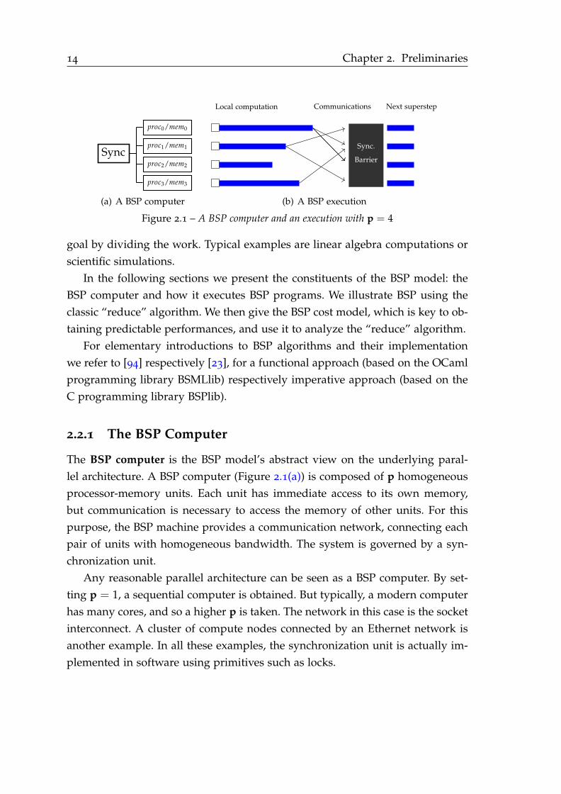
14 Chapter 2. Preliminaries
proc0/mem0
proc1/mem1
proc2/mem2
proc3/mem3
Sync
(a) A BSP computer
Sync.
Barrier
Local computation Communications Next superstep
(b) A BSP execution
Figure 2.1 – A BSP computer and an execution with p = 4
goal by dividing the work. Typical examples are linear algebra computations or
scientific simulations.
In the following sections we present the constituents of the BSP model: the
BSP computer and how it executes BSP programs. We illustrate BSP using the
classic “reduce” algorithm. We then give the BSP cost model, which is key to ob-
taining predictable performances, and use it to analyze the “reduce” algorithm.
For elementary introductions to BSP algorithms and their implementation
we refer to [94] respectively [23], for a functional approach (based on the OCaml
programming library BSMLlib) respectively imperative approach (based on the
C programming library BSPlib).
2.2.1 The BSP Computer
The BSP computer is the BSP model’s abstract view on the underlying paral-
lel architecture. A BSP computer (Figure 2.1(a)) is composed of p homogeneous
processor-memory units. Each unit has immediate access to its own memory,
but communication is necessary to access the memory of other units. For this
purpose, the BSP machine provides a communication network, connecting each
pair of units with homogeneous bandwidth. The system is governed by a syn-
chronization unit.
Any reasonable parallel architecture can be seen as a BSP computer. By set-
ting p = 1, a sequential computer is obtained. But typically, a modern computer
has many cores, and so a higher p is taken. The network in this case is the socket
interconnect. A cluster of compute nodes connected by an Ethernet network is
another example. In all these examples, the synchronization unit is actually im-
plemented in software using primitives such as locks.

2.2. The BSP Model 15
2.2.2 The BSP Execution Model
The BSP machine executes parallel programs in a series of computational steps
called of supersteps.
Each superstep (see Figure 2.1(b)) is composed of three phases corresponding
to the three components of the BSP machine: (1) asynchronous local computa-
tion, (2) communication and (3) barrier synchronization.
Let us examine each phase. In the first phase, asynchronous local compu-
tation, each process executes (sequentially) and without interference from the
other processes. The computation phase is followed by a communication phase.
At this point, the processes may read or write into the memory of the other pro-
cesses via the communication network. Finally, the processes synchronize. After
synchronization, global computation either continues with another superstep, or
terminates globally. This phase is often referred to as a synchronization barrier,
since each process must reach it before computation continues.
Some immediate implications of this execution model are the following: (1)
Logically, computation and communication do not overlap By removing such
interactions between processes in the same superstep, parallel algorithms be-
come simpler to understand. On the other hand, as long as this is opaque to the
programmer, a BSP implementation can interleave computation and communi-
cation under the hood. However, even in the ideal case where computation and
communication time of each process is the same, at most a factor of 2 speedup
can be obtained this way. (2) The algorithm designer must make sure that any
data a process requires in each superstep has been communicated to it during
the previous. (3) All processes participate in synchronization. This differs from
other models where processes can form groups that synchronize (called subset
synchronization). Again, this restriction simplifies program comprehension and
greatly facilitates the cost model presented below [93]. (4) Execution is deter-
ministic, modulo concurrent writes and environmental factors.
This execution model is key to obtaining safe, structured and predictable
parallelism. BSP programs are safe since a range of synchronization issues are
ruled out. For instance, a classic deadlock where process A waits for B, and
process B waits for A cannot occur in this model. Data races, in the form of con-
current writes, may occur, but they do so deterministically: the execution model
ensures that if a concurrent write happens, then it will happen on each execution.
If the model is implemented to resolve such write-write conflicts deterministi-
cally, then full determinism is obtained.
BSP programs are structured. The model forces the parallel algorithm designer

16 Chapter 2. Preliminaries
to think in terms of supersteps and phases. The resulting programs are easier to
understand and analyze.
BSP programs are predictable. First, in terms of behavior, as ensured by the
determinism, lack of data races and dead locks. Intuitively, the lack of interfering
interleavings and communications reduces the set of possible outcomes of the
BSP execution that the algorithm designer must consider. Second, in terms of
performance. The structured execution model of BSP enables its cost model,
which in turn permits the algorithm designer to predict the scalability of BSP
algorithms.
2.2.3 Example of a BSP Algorithm: reduce
In this section we illustrate the BSP model by implementing a classic parallel
algorithm: reduce.
Description of the Problem
The goal of reduce is to merge the elements of an array using an operator ⊕. We
require that ⊕ is associative, and that it has a neutral element 0. This operation is
also called fold, due to its similarity to the function available in many sequential,
functional languages that can be summarized thus:
fold([X1, . . . , Xn],⊕, 0) = X1 ⊕ X2 ⊕ . . . ⊕ XN ⊕ 0
By instantiating ⊕ with addition (whose neutral element 0 = 0), we obtain the
sum of all elements in X.
We wish to parallelize this operation in the algorithm reduce. We assume
that the input array X’s size is divisible by p, and that X is block distributed.
This means that the kth element of X is stored at process ⌊k/p⌋. In the source
text, each process has a local view of X. They see only their block through the
local variable X. An access to X[k] in this local view in process i corresponds
to accessing X[i ∗ (n/p) + k] in the global view. To simplify, we assume that
the associative operator is +, but updating the algorithm to change operator is
trivial.
The Algorithm reduce
We now give the algorithm of reduce in Figure 2.2. The idea is that the asso-
ciativity of the operator allow us to first sum up each block into a partial sum

2.2. The BSP Model 17
Algorithm reduce
Input The block distributed array X of whose length n, is divided by p, the num-ber of processes. The integer pid, containing the process identifier of theexecuting process.
Variables The array |Part| of length p for storing exchanged local reduction. Thevariable |local| for storing local reduction.
Output |S| = ∑n−1i=0 X[i]
1 (1) // compute local reductions
2 local = 0
3 for i in 0 ... n/p - 1:
4 local = local + X[i]
5
6 // exchange local reductions
7 for i in 0 ... p - 1:
8 put local in Part[pid] at process i
9
10 synchronize;
11
12 (2) // global reduction
13 S = 0
14 for i in 0 ... p - 1:
15 S = S + Part[i]
16
17 synchronize;
Figure 2.2 – The algorithm reduce
and then obtain the global sum by summing these. Each process executes this
program text, and all variables are private to that process.
The algorithm consists of two supersteps numbered (1) and (2) terminated
by a synchronization barriers. In the computation phase of the first superstep,
each process reduces their block of X into local (Lines 2 to 4). Each process then
schedules p remote write requests (called puts) so that the variable Part[i] of
each process contains the local reduction of each process i.
In the beginning of the second superstep, the transfer of all local reductions
is completed and available in Part at each process, as the BSP model guarantees.
The global reduction is now obtained by summing the local reductions, which
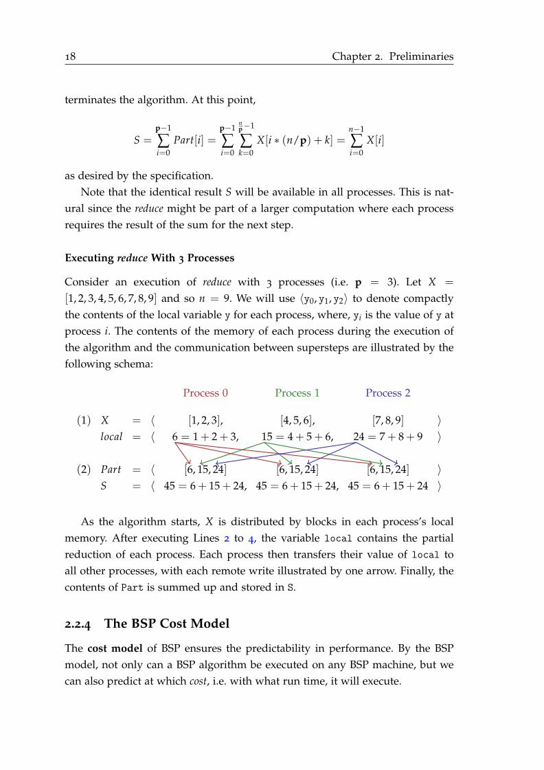
18 Chapter 2. Preliminaries
terminates the algorithm. At this point,
S =p−1
∑i=0
Part[i] =p−1
∑i=0
np−1
∑k=0
X[i ∗ (n/p) + k] =n−1
∑i=0
X[i]
as desired by the specification.
Note that the identical result S will be available in all processes. This is nat-
ural since the reduce might be part of a larger computation where each process
requires the result of the sum for the next step.
Executing reduce With 3 Processes
Consider an execution of reduce with 3 processes (i.e. p = 3). Let X =
[1, 2, 3, 4, 5, 6, 7, 8, 9] and so n = 9. We will use 〈y0, y1, y2〉 to denote compactly
the contents of the local variable y for each process, where, yi is the value of y at
process i. The contents of the memory of each process during the execution of
the algorithm and the communication between supersteps are illustrated by the
following schema:
Process 0 Process 1 Process 2
(1) X = 〈 [1, 2, 3], [4, 5, 6], [7, 8, 9] 〉
local = 〈 6 = 1 + 2 + 3, 15 = 4 + 5 + 6, 24 = 7 + 8 + 9 〉
(2) Part = 〈 [6, 15, 24] [6, 15, 24] [6, 15, 24] 〉
S = 〈 45 = 6 + 15 + 24, 45 = 6 + 15 + 24, 45 = 6 + 15 + 24 〉
As the algorithm starts, X is distributed by blocks in each process’s local
memory. After executing Lines 2 to 4, the variable local contains the partial
reduction of each process. Each process then transfers their value of local to
all other processes, with each remote write illustrated by one arrow. Finally, the
contents of Part is summed up and stored in S.
2.2.4 The BSP Cost Model
The cost model of BSP ensures the predictability in performance. By the BSP
model, not only can a BSP algorithm be executed on any BSP machine, but we
can also predict at which cost, i.e. with what run time, it will execute.

2.2. The BSP Model 19
proc0/mem0
proc1/mem1
proc2/mem2
proc3/mem3
Syncl
r
r
r
r
g p
Figure 2.3 – BSP computer characterization
The cost model consists of two parts: (1) a characterization of BSP computers,
which sums up the performance of a BSP machine with 4 parameters and (2) a
method for attributing costs to executions.
Characterizing the BSP Machine
The cost model characterizes the performance of a BSP machines by four param-
eters (see Figure 2.3):
p the number of processes
r a measure on local computation cost
g a measure on communication cost
l a measure on synchronization cost
We have already seen p, so let us study the latter three more closely. The
parameter r is the cost of taking one step of local computation. The notion of
computation step depends on the context. For instance, in scientific computation,
the steps of interest are floating-point operations (flops) and r is the time taken to
perform one such operation. Sometimes r is removed and we express the other
parameters in flops.
To understand g and l, we first define the concept of h-relations. An h-relation
is a communication phase where each process sends or receives at most h words.
Furthermore, there is at least one process which receives or sends h words. The
BSP model assumes that it is not the overall communication volume of the sys-
tem that determines the communication cost of a superstep, but rather, the con-
tention. This corresponds to the maximum number of words received or sent by
any process. Furthermore, BSP assumes separate reception and emission chan-
nels, thus h is the largest of the number of sent or received words at any proces-
sor and not their sum.
The underlying assumption of the communication cost model is that the time
taken for the BSP computer to communicate and synchronize an h-relation is
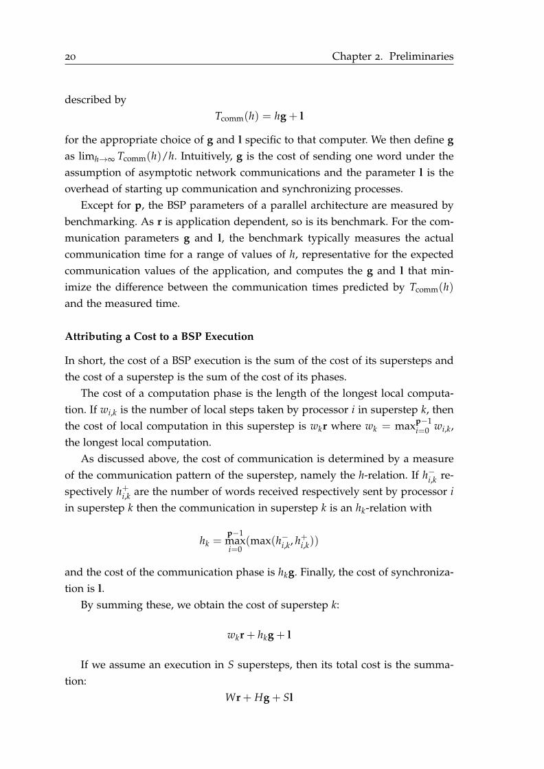
20 Chapter 2. Preliminaries
described by
Tcomm(h) = hg + l
for the appropriate choice of g and l specific to that computer. We then define g
as limh→∞ Tcomm(h)/h. Intuitively, g is the cost of sending one word under the
assumption of asymptotic network communications and the parameter l is the
overhead of starting up communication and synchronizing processes.
Except for p, the BSP parameters of a parallel architecture are measured by
benchmarking. As r is application dependent, so is its benchmark. For the com-
munication parameters g and l, the benchmark typically measures the actual
communication time for a range of values of h, representative for the expected
communication values of the application, and computes the g and l that min-
imize the difference between the communication times predicted by Tcomm(h)
and the measured time.
Attributing a Cost to a BSP Execution
In short, the cost of a BSP execution is the sum of the cost of its supersteps and
the cost of a superstep is the sum of the cost of its phases.
The cost of a computation phase is the length of the longest local computa-
tion. If wi,k is the number of local steps taken by processor i in superstep k, then
the cost of local computation in this superstep is wkr where wk = maxp−1i=0 wi,k,
the longest local computation.
As discussed above, the cost of communication is determined by a measure
of the communication pattern of the superstep, namely the h-relation. If h−i,k re-
spectively h+i,k are the number of words received respectively sent by processor i
in superstep k then the communication in superstep k is an hk-relation with
hk =p−1maxi=0
(max(h−i,k, h+i,k))
and the cost of the communication phase is hkg. Finally, the cost of synchroniza-
tion is l.
By summing these, we obtain the cost of superstep k:
wkr + hkg + l
If we assume an execution in S supersteps, then its total cost is the summa-
tion:
Wr + Hg + Sl

2.2. The BSP Model 21
with
W = ∑S−1k=0 wk H = ∑
S−1k=0 hk
Execution Cost of reduce With 3 Processes
To illustrate the cost model, consider the execution of the reduce algorithm given
in Section 2.2.3. We now calculate the cost of this execution, considering each
addition as one step of local computation.
In the first superstep, each process performs 2 additions to obtain local sums,
and so w1 = 2. Then each process sends their local reductions to all 3 processors1,
and each processor receives 3 local reductions, so h−i,1 = h−i,1 for all processes i,
hence h1 = 3, We add the synchronization cost and obtain 2r + 3g + l for the
first superstep.
In the second superstep, each process sums up the p local reductions in p− 1
steps, hence w2 = 2. There is no communication. Adding the synchronization
cost, we obtain 2r + l for the second superstep. The full cost of this execution is
then
(2 + 2)r + 3g + 2l
This result can be generalized to any BSP machine with p processors and
input array of size n by considering that the first superstep consists of n/p− 1
additions and p sends and receives per process. The second superstep entails
p − 1 additions. We can thus express the cost of reduce for any p or n by the
formula
(n/p + p− 2)r + pg + 2l
Such a formula, parameterized by BSP parameters and the size of the problem,
is referred to as the BSP algorithm’s cost formula.
As we noticed earlier, reduce has all processes calculate the global sum in the
last superstep. In addition to simplifying the algorithm, we can now argue for-
mally that it comes at no additional performance penalty: whether all or only
one processes calculate the global sum, the last superstep still has a local com-
putation cost of p− 1.
We could even consider an implementation where process 0 receives all lo-
cal reductions, computes the global reduction and sends it to the others (see
Figure 2.4). Even though the total number of transmitted words is smaller, the
communication cost of the first superstep is still p, since process 0 receives p
reductions, and so the cost of this superstep is still (n/p− 1)r + pg + l. In the
1For simplicity, we count each process’s put to itself.
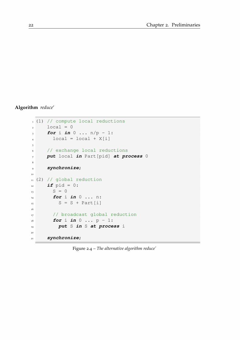
22 Chapter 2. Preliminaries
Algorithm reduce’
1 (1) // compute local reductions
2 local = 0
3 for i in 0 ... n/p - 1:
4 local = local + X[i]
5
6 // exchange local reductions
7 put local in Part[pid] at process 0
8
9 synchronize;
10
11 (2) // global reduction
12 if pid = 0:
13 S = 0
14 for i in 0 ... n:
15 S = S + Part[i]
16
17 // broadcast global reduction
18 for i in 0 ... p - 1:
19 put S in S at process i
20
21 synchronize;
Figure 2.4 – The alternative algorithm reduce’
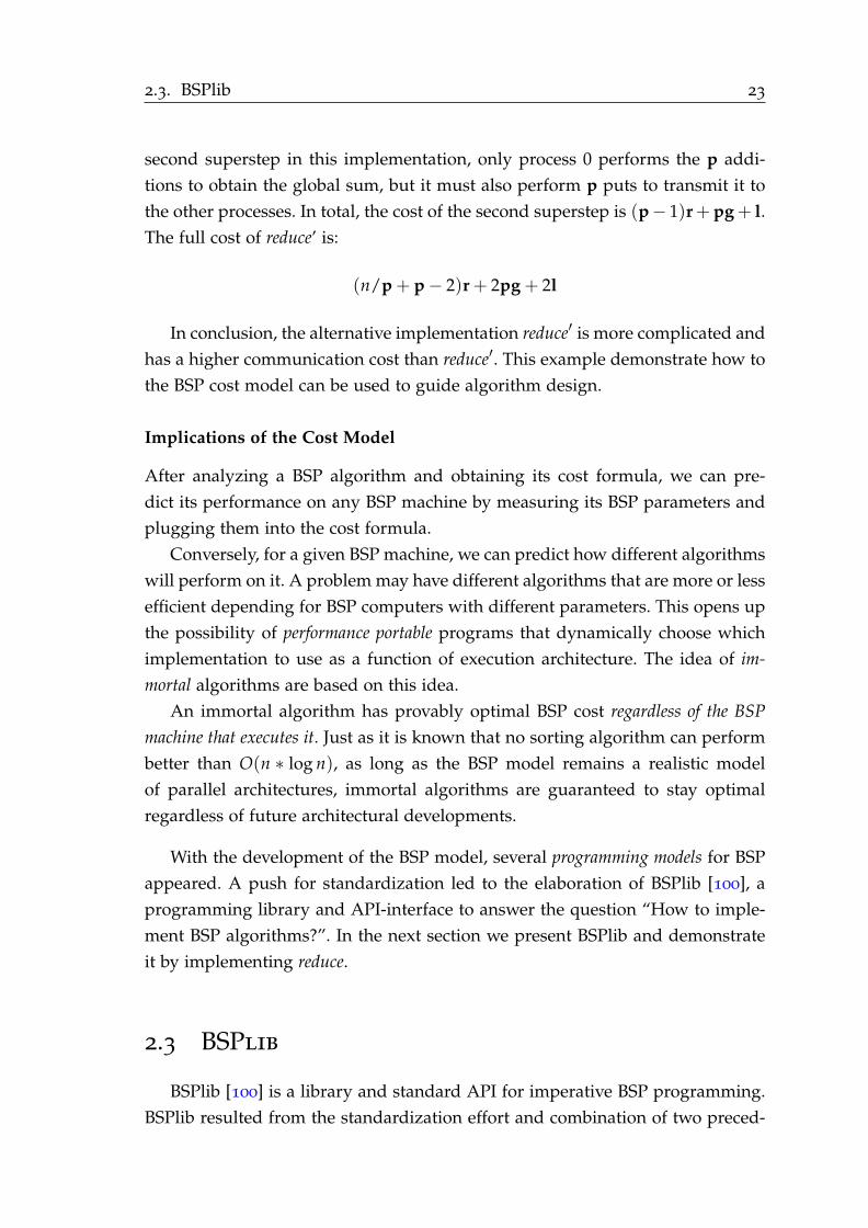
2.3. BSPlib 23
second superstep in this implementation, only process 0 performs the p addi-
tions to obtain the global sum, but it must also perform p puts to transmit it to
the other processes. In total, the cost of the second superstep is (p− 1)r+ pg+ l.
The full cost of reduce’ is:
(n/p + p− 2)r + 2pg + 2l
In conclusion, the alternative implementation reduce′ is more complicated and
has a higher communication cost than reduce′. This example demonstrate how to
the BSP cost model can be used to guide algorithm design.
Implications of the Cost Model
After analyzing a BSP algorithm and obtaining its cost formula, we can pre-
dict its performance on any BSP machine by measuring its BSP parameters and
plugging them into the cost formula.
Conversely, for a given BSP machine, we can predict how different algorithms
will perform on it. A problem may have different algorithms that are more or less
efficient depending for BSP computers with different parameters. This opens up
the possibility of performance portable programs that dynamically choose which
implementation to use as a function of execution architecture. The idea of im-
mortal algorithms are based on this idea.
An immortal algorithm has provably optimal BSP cost regardless of the BSP
machine that executes it. Just as it is known that no sorting algorithm can perform
better than O(n ∗ log n), as long as the BSP model remains a realistic model
of parallel architectures, immortal algorithms are guaranteed to stay optimal
regardless of future architectural developments.
With the development of the BSP model, several programming models for BSP
appeared. A push for standardization led to the elaboration of BSPlib [100], a
programming library and API-interface to answer the question “How to imple-
ment BSP algorithms?”. In the next section we present BSPlib and demonstrate
it by implementing reduce.
2.3 BSPlib
BSPlib [100] is a library and standard API for imperative BSP programming.
BSPlib resulted from the standardization effort and combination of two preced-

24 Chapter 2. Preliminaries
p1 p2 p3
(a) Program counter
1 if (x && y)
2 // ...
3 else
4 // ...
5
(b) Program
p1 p2 p3
x 0 1 1y 0 1 0
(c) Memory contents
Figure 2.5 – Snapshot of a Single Program, Multiple Data execution with p = 3
ing libraries: Oxford BSP Library [141], the first portable BSP library, and Green
BSP [88], which introduced Bulk Synchronous Message Passing.
The design goals of BSPlib can be resumed by minimalism and portability.
It provides a small but highly composable set of 20 primitives callable from C
and Fortran. Consequently, the implementation effort of porting BSPlib to new
platforms is reduced. In terms of size, BSPlib can be compared to the Message
Passing Interface (MPI) [139], a widely used communication library, that con-
tains well over 200 different primitives. In terms for functionality, BSPlib can be
seen as a nimble model of the Bulk Synchronous Parallel subset of MPI. Mod-
ern interconnects implement Remote Direct Memory Access operations directly,
and the parallel programmer accesses them through this subset. Hence, using
this part of MPI, and doing so correctly, is becoming essential for performance
in many applications [103, 132, 83]. We discuss this relationship more closely
in Section 2.3.8.
2.3.1 SPMD: Single Program, Multiple Data
BSPlib programs are written in Single Program, Multiple Data [59] (SPMD) style. In
this mode of programming, each process executes the same program, but execute
in separate memories and with their own program counter. Informally, this can
be understood as the parallel composition of the same program c, parameterized
by a unique process identifier:
c(0) ‖ . . . ‖ c(p− 1)
Figure 2.5 contains a SPMD [59] program under execution by 3 processes.
Each triangle represents the program counter of one process, and the memory
contents of each process are given by the table on the right. The program text is
the same, but the memory contents of each process admits a different evaluation
2.3. BSPlib 25
of the if-construct, allowing different processes to execute different parts of the
program.
The SPMD model enables parallelization of an initially sequential programs,
by decorating it with appropriate parallel primitives to distribute data and com-
putation and to insert communication and synchronization where necessary.
While the overlap is considerable, SPMD can be thought of as an alternative
to fork-join or master-slave parallelism. In the fork-join parallelism, process cre-
ation and destruction is explicit and controlled by primitives in the program. For
instance, new processes can be forked off to recursively solve sub-problems in
divide-and-conquer algorithms, or to treat parallel iterations of loops. In master-
slave parallelism, a master process controls the creation of slave processes and
distributes work between them.
SPMD can also be positioned with respect to Flynn’s taxonomy [71] that
classifies computer architectures based on their number of instruction streams
(Single or Multiple) and their number of data streams (Single or Multiple), giving
rise to the following classifications:
Single instruction stream, Single data stream (SISD)
A sequential computer with no parallel execution.
Single instruction stream, Multiple data streams (SIMD)
A computer that executes a single stream of instructions in lockstep over
multiple data streams.
Multiple instruction streams, Single data stream (MISD)
Multiple processes treat the same data. This architecture can be used to
implement is pipeline parallelism, where each process executes on stage of
a series of transformations on the input data. Or, to implement fault toler-
ance, where disparate results between processes is indicative of error [176].
Multiple instruction streams, Multiple data stream (MIMD)
An architecture with multiple processes executing different instruction
streams on different data streams. This corresponds to modern multi-core
processors or multi-node clusters where each node has its own memory.
In this context, SPMD can be viewed as a form of MIMD, but where the dif-
ferent instruction streams arise from (potentially) different source code locations
the same source program.
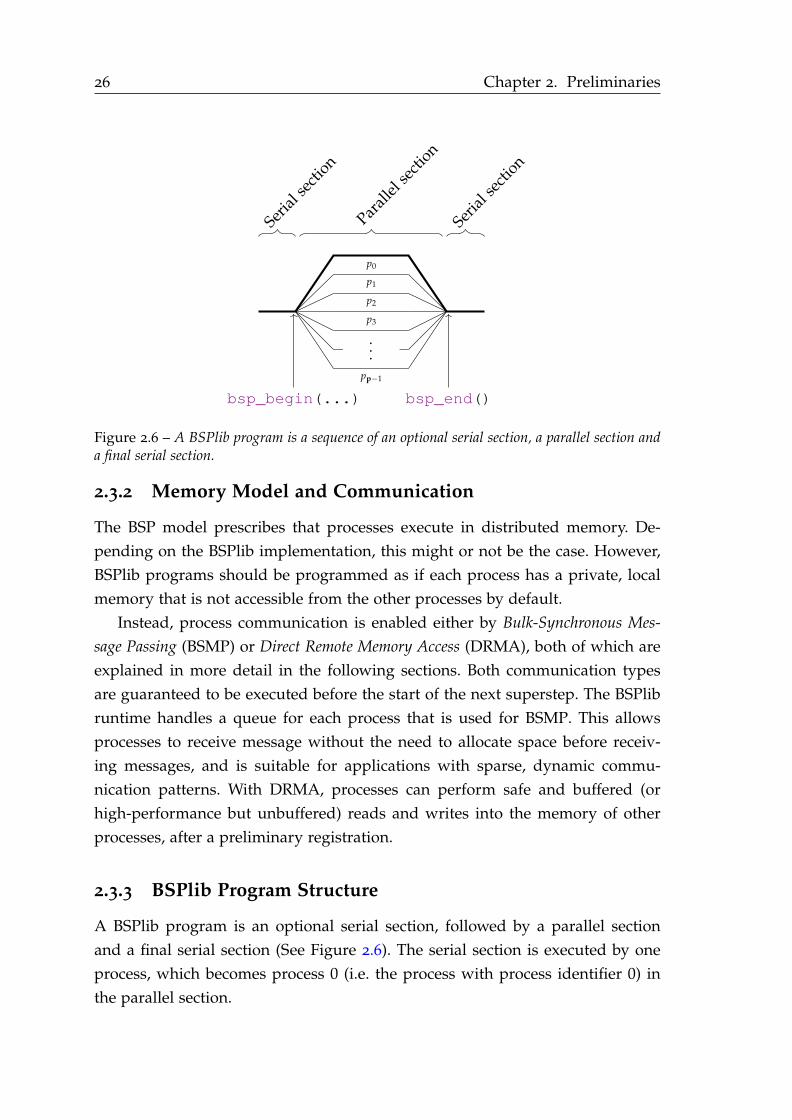
26 Chapter 2. Preliminaries
p1
p2
p3
···
pp−1
p0
bsp_begin(...) bsp_end()
Seria
l sect
ion
Seria
l sect
ion
Paral
lel se
ctio
n
Figure 2.6 – A BSPlib program is a sequence of an optional serial section, a parallel section anda final serial section.
2.3.2 Memory Model and Communication
The BSP model prescribes that processes execute in distributed memory. De-
pending on the BSPlib implementation, this might or not be the case. However,
BSPlib programs should be programmed as if each process has a private, local
memory that is not accessible from the other processes by default.
Instead, process communication is enabled either by Bulk-Synchronous Mes-
sage Passing (BSMP) or Direct Remote Memory Access (DRMA), both of which are
explained in more detail in the following sections. Both communication types
are guaranteed to be executed before the start of the next superstep. The BSPlib
runtime handles a queue for each process that is used for BSMP. This allows
processes to receive message without the need to allocate space before receiv-
ing messages, and is suitable for applications with sparse, dynamic commu-
nication patterns. With DRMA, processes can perform safe and buffered (or
high-performance but unbuffered) reads and writes into the memory of other
processes, after a preliminary registration.
2.3.3 BSPlib Program Structure
A BSPlib program is an optional serial section, followed by a parallel section
and a final serial section (See Figure 2.6). The serial section is executed by one
process, which becomes process 0 (i.e. the process with process identifier 0) in
the parallel section.
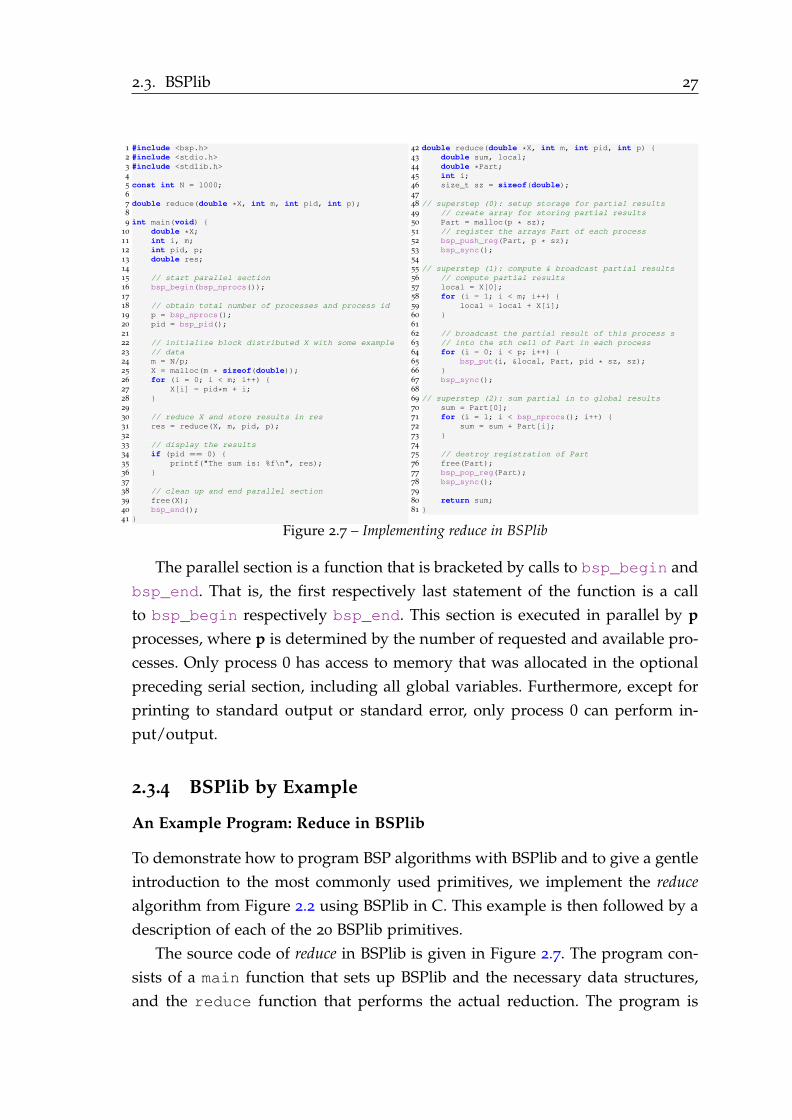
2.3. BSPlib 27
1 #include <bsp.h>
2 #include <stdio.h>
3 #include <stdlib.h>
45 const int N = 1000;
67 double reduce(double *X, int m, int pid, int p);
89 int main(void)
10 double *X;
11 int i, m;
12 int pid, p;
13 double res;
1415 // start parallel section
16 bsp_begin(bsp_nprocs());
1718 // obtain total number of processes and process id
19 p = bsp_nprocs();
20 pid = bsp_pid();
2122 // initialize block distributed X with some example
23 // data
24 m = N/p;
25 X = malloc(m * sizeof(double));
26 for (i = 0; i < m; i++)
27 X[i] = pid*m + i;
28
2930 // reduce X and store results in res
31 res = reduce(X, m, pid, p);
3233 // display the results
34 if (pid == 0)
35 printf("The sum is: %f\n", res);
36
3738 // clean up and end parallel section
39 free(X);
40 bsp_end();
41
42 double reduce(double *X, int m, int pid, int p)
43 double sum, local;
44 double *Part;
45 int i;
46 size_t sz = sizeof(double);
4748 // superstep (0): setup storage for partial results
49 // create array for storing partial results
50 Part = malloc(p * sz);
51 // register the arrays Part of each process
52 bsp_push_reg(Part, p * sz);
53 bsp_sync();
5455 // superstep (1): compute & broadcast partial results
56 // compute partial results
57 local = X[0];
58 for (i = 1; i < m; i++)
59 local = local + X[i];
60
6162 // broadcast the partial result of this process s
63 // into the sth cell of Part in each process
64 for (i = 0; i < p; i++)
65 bsp_put(i, &local, Part, pid * sz, sz);
66
67 bsp_sync();
6869 // superstep (2): sum partial in to global results
70 sum = Part[0];
71 for (i = 1; i < bsp_nprocs(); i++)
72 sum = sum + Part[i];
73
7475 // destroy registration of Part
76 free(Part);
77 bsp_pop_reg(Part);
78 bsp_sync();
7980 return sum;
81
Figure 2.7 – Implementing reduce in BSPlib
The parallel section is a function that is bracketed by calls to bsp_begin and
bsp_end. That is, the first respectively last statement of the function is a call
to bsp_begin respectively bsp_end. This section is executed in parallel by p
processes, where p is determined by the number of requested and available pro-
cesses. Only process 0 has access to memory that was allocated in the optional
preceding serial section, including all global variables. Furthermore, except for
printing to standard output or standard error, only process 0 can perform in-
put/output.
2.3.4 BSPlib by Example
An Example Program: Reduce in BSPlib
To demonstrate how to program BSP algorithms with BSPlib and to give a gentle
introduction to the most commonly used primitives, we implement the reduce
algorithm from Figure 2.2 using BSPlib in C. This example is then followed by a
description of each of the 20 BSPlib primitives.
The source code of reduce in BSPlib is given in Figure 2.7. The program con-
sists of a main function that sets up BSPlib and the necessary data structures,
and the reduce function that performs the actual reduction. The program is
28 Chapter 2. Preliminaries
a direct translation of the pseudocode of Figure 2.2 into C, with the additional
bookkeeping needed by BSPlib to set up parallel computation and communica-
tion. All BSPlib primitives are prefixed bsp_ and, in this document, colored (e.g.
bsp_pid).
Starting the Parallel Section: bsp_begin and bsp_nprocs
The first statement in main is a call to bsp_begin. The call bsp_begin(P)
denotes the start of the parallel section of the BSPlib program, and the argument
P the number of requested processes. The function bsp_nprocs has two uses:
before calling bsp_begin it returns the number of available processors. After
calling bsp_begin, it returns the number of processes p that participate in the
parallel section. Line 16 thus starts a parallel section with the maximum number
of available processes. From this point on, execution splits into p processes, each
with its own memory.
Queries: bsp_nprocs and bsp_pid
On Line 19, bsp_nprocs is called again, this time to obtain the number of
processes allocated to the computation. We then call bsp_pid, which returns its
process identifier (pid). On Lines 24 to 28 we allocate and initialize the globally
distributed array X: from the local point of view, X is a handle to each process’s
block of the global distributed variable X. We initialize X with some example
data.
On Line 31, each process calls the reduce function with a pointer to its
block of X, the local block length, its pid and the total number of processes as
arguments.
Setting up Communication: Registering with bsp_push_reg
The function reduce implements the reduce algorithm of Figure 2.2.
Before the actual algorithmics start, some setup is required. We implement
the communication of partial sums as DRMA, which enables processes to read
and write specific parts of each others memory. To do so BSPlib provides a mech-
anism for addressing remote memory called “registrations”. On Line 50, each
process allocates memory that will contain the partial sums of all processes,
pointed to by Part. We then call bsp_push_reg(Part, p * sz). This cre-
ates an association, called a registration, between each process’s memory area
for partial sums, the extending p * sz bytes.
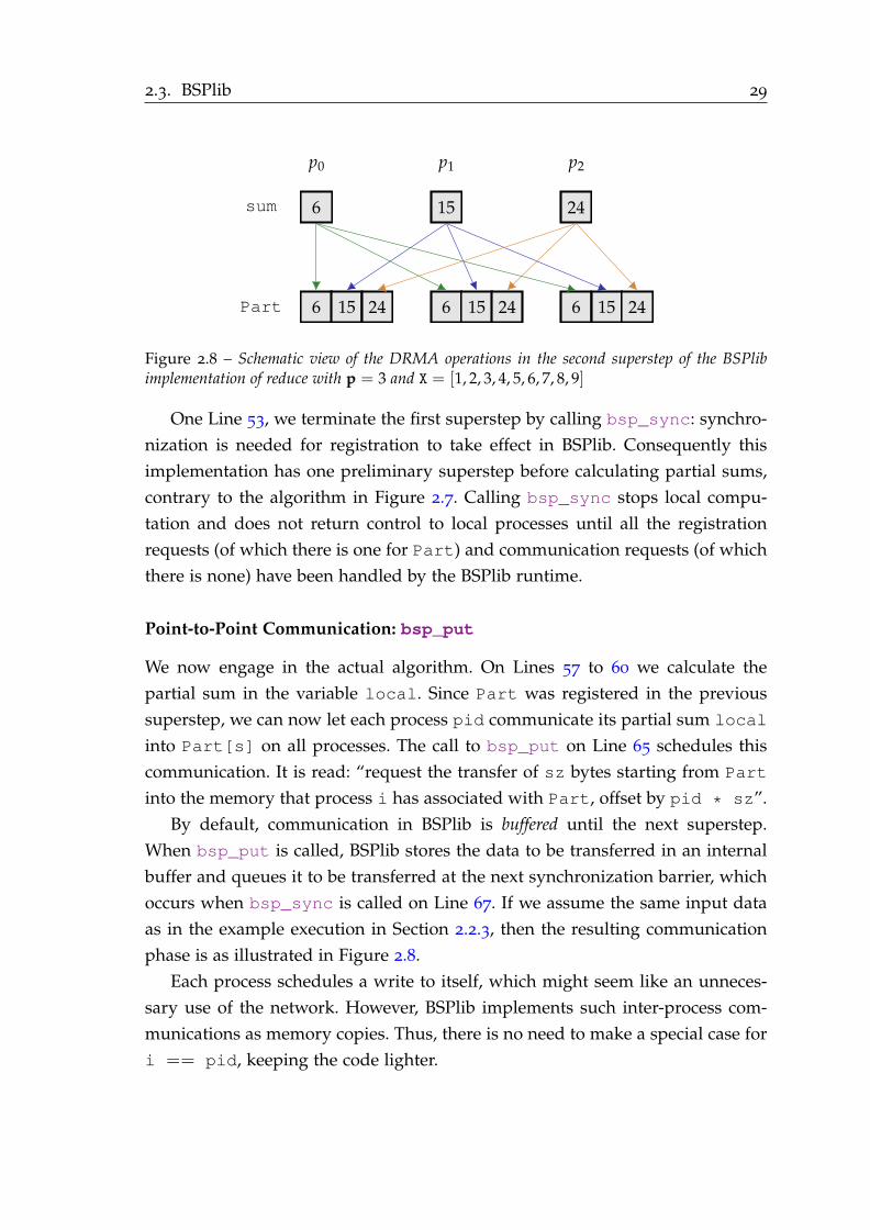
2.3. BSPlib 29
p0 p1 p2
sum 6 15 24
Part 6 15 24 6 15 24 6 15 24
Figure 2.8 – Schematic view of the DRMA operations in the second superstep of the BSPlibimplementation of reduce with p = 3 and X = [1, 2, 3, 4, 5, 6, 7, 8, 9]
One Line 53, we terminate the first superstep by calling bsp_sync: synchro-
nization is needed for registration to take effect in BSPlib. Consequently this
implementation has one preliminary superstep before calculating partial sums,
contrary to the algorithm in Figure 2.7. Calling bsp_sync stops local compu-
tation and does not return control to local processes until all the registration
requests (of which there is one for Part) and communication requests (of which
there is none) have been handled by the BSPlib runtime.
Point-to-Point Communication: bsp_put
We now engage in the actual algorithm. On Lines 57 to 60 we calculate the
partial sum in the variable local. Since Part was registered in the previous
superstep, we can now let each process pid communicate its partial sum local
into Part[s] on all processes. The call to bsp_put on Line 65 schedules this
communication. It is read: “request the transfer of sz bytes starting from Part
into the memory that process i has associated with Part, offset by pid * sz”.
By default, communication in BSPlib is buffered until the next superstep.
When bsp_put is called, BSPlib stores the data to be transferred in an internal
buffer and queues it to be transferred at the next synchronization barrier, which
occurs when bsp_sync is called on Line 67. If we assume the same input data
as in the example execution in Section 2.2.3, then the resulting communication
phase is as illustrated in Figure 2.8.
Each process schedules a write to itself, which might seem like an unneces-
sary use of the network. However, BSPlib implements such inter-process com-
munications as memory copies. Thus, there is no need to make a special case for
i == pid, keeping the code lighter.

30 Chapter 2. Preliminaries
Ending the Parallel Section: bsp_pop_reg and bsp_end
Each process will have the received the partial sums of all other processes in
Part after synchronization barrier. There are summed up in sum on Lines 70
to 73, concluding reduce’s implementation.
Before returning sum to main, we deallocate and destroy the registration
of Part using the bsp_pop_reg primitive on Lines 76 to 78. Like for their
creation, the destruction of registrations takes effect at the next synchronization.
To ensure the destruction of the Part’s registration we synchronize one last time
in reduce on Line 78.
Back in the main function, process 0 prints the results of the reduction. Then
bsp_end is called to terminate the parallel section.
2.3.5 The BSPlib API
The full API of BSPlib is summarized in Table 2.1. The rest of this section contains
an description of each primitive. The full description of BSPlib can be had in [100]
and in the BSPlib manual, available online2. For a full guide to programming in
BSPlib, the reader is referred to the textbook [23].
Initialization
void bsp_init(void (*startproc)(void), int argc, char **argv)
There are two ways of initializing BSPlib: either by having the main function
start the parallel section, or, when some serial processing is needed before the
parallel section starts, having a dedicated SPMD function.
In the latter case, the first statement in the main function of the program
must be a call to bsp_init, with a function pointer to the dedicated SPMD
function and the program arguments. In this mode, serial execution starts in the
main function and a call to the SPMD function initiates the parallel section.
void bsp_begin(int maxprocs)
A call to bsp_begin is used to initiate the parallel section in the SPMD function
of a BSPlib program, and must be the first statement of that function.
The argument maxprocs denotes the desired number of processes. BSPlib
might spawn fewer than the desired number (for instance, if the requested num-
ber of processes are fewer than the number of available processors).
2http://www.bsp-worldwide.org/implmnts/oxtool/man/

2.3.B
SP
lib31
Category Function Description
Initialization void bsp_init(void(*startproc)(void), int¸ argc, char **argv) Initialize the BSPlib system.
void bsp_begin(int maxprocs) Spawn a number of BSP processes.
void bsp_end() Terminate BSP processes.
Halt void bsp_abort(char *format, ...) Stop a BSP computation.
Inquiry int bsp_pid() Determine the process identifier of a BSP process.
int bsp_nprocs() Determine the total number of BSP processes.
double bsp_time() High-precision real-time clock.
Synchronization void bsp_sync() End a superstep.
DRMA void bsp_push_reg(const void *ident, int size) Register a data-structure as available for direct remote memory access.
void bsp_pop_reg(const void *ident) Remove the visibility of a previously registered data-structure.
void bsp_put(int pid, const void *src, void *dst, int offset, int nbytes) Write data into a remote process’s memory.
void bsp_get(int pid, const void *src, int offset, void *dst, int nbytes) Read data from a remote process’s memory.
BSMP void bsp_set_tagsize(int *tag_bytes) Set tag size of a BSMP message.
void bsp_send(int pid,const void *tag, const void *payload,int payload_bytes) Transmit a BSMP message to a remote process.
void bsp_qsize(int *packets, int *accum_nbytes) Check how many BSMP messages arrived.
void bsp_get_tag(int *status, void *tag) Retrieve the tag on a BSMP message.
void bsp_move(void *payload, int reception_bytes) Move a BSMP message from the queue.
High Performance void bsp_hpput(int pid, const void *src, void *dst, int offset, int nbytes) Unbuffered write data into a remote process’s memory.
void bsp_hpget(int pid,const void *src, int offset, void *dst, int nbytes) Unbuffered read data from a remote process’s memory.
int bsp_hpmove(void **tag_ptr_buf, void **payload_ptr_buf) A lean method for moving a BSMP message from the queue.
Table 2.1 – The BSPlib API. Primitives are hyper-linked to their corresponding online BSPlib manual page.
32 Chapter 2. Preliminaries
No BSPlib primitives, except bsp_nprocs and bsp_init, can be called be-
fore bsp_begin has been called.
void bsp_end()
A call to bsp_end must terminate the SPMD function of a BSPlib program. It
ends the parallel section and the last superstep. Note that outstanding commu-
nications and registration requests are not delivered by bsp_end. All processes
except process 0 are terminated.
No BSPlib primitives, except bsp_nprocs, can be called after bsp_end has
been called (see Section 2.3.3).
Halt
void bsp_abort(char *format, ...)
This function is used to terminate the BSP computation and signal an erroneous
situation. Any process can call bsp_abort, and the BSPlib runtime handles the
termination of the other processes with no need for the user to synchronize.
The first argument to bsp_abort specifies a C-style format message, remain-
ing arguments are interpreted as for printf. The formatted message is printed
before the termination of the program.
Inquiry
int bsp_pid()
The bsp_pid function returns the unique process identifier of the calling pro-
cess, which is between 0 and p− 1, where p is the number of processes in the
parallel section.
int bsp_nprocs()
Outside the parallel section of a BSPlib program, before bsp_begin has been
called, bsp_nprocs returns the number of available processors. Inside the par-
allel section, bsp_nprocs returns the number of processes participating in the
BSP computation
double bsp_time()
Returns the contents of a implementation-specific, high-precision clock. The
value of bsp_time is local to each process.
2.3. BSPlib 33
Synchronization
void bsp_sync()
The function bsp_sync is called collectively to end a superstep. Its call marks
the end of the local computation phase. The calling process is frozen until all
other processes have called bsp_sync. At that point, all registration and com-
munication requests are executed, control is returned to each process and the
next superstep starts. Calling bsp_sync also ensures the delivery of all out-
standing high-performance communication requests (see functions bsp_hpput and
bsp_hpget below).
The BSPlib program’s behavior is undefined if some process does not partic-
ipate in the call to bsp_sync. This can happen if it terminates the BSP compu-
tation by reaching bsp_end, if it diverges, or if it terminates due to a local error
(such as division by zero). In this case, depending on the implementation, the
BSP program will typically hang or terminate with a dynamic error.
Direct Remote Memory Access (DRMA)
BSPlib enables two communication types: Direct Remote Memory Access
(DRMA)3 and Bulk Synchronous Message Passing (BSMP). The former is more
commonly used, whereas the latter is useful for parallel computations with
sparse data communication patterns. This section describes the DRMA primi-
tives and the next deals with those for BSMP.
DRMA terminology Throughout this thesis, we will use the terms source, des-
tination, origin and source in accordance to how it is used by the MPI stan-
dard [139, p. 404].
The origin is the process that is calling the DRMA primitive, and the target is
the process whose memory is being remotely accessed. The source is the process
where the transferred data is located, and the destination is the process who will
receive the transferred data. Hence, in put-requests, the origin and the source
is the same process, and the target and destination is also the same process. In
get-requests, the origin is the destination and the target is the source.
The Registration Sequence The BSPlib registration sequence is an internal
data structure used by BSPlib to create associations between p memory areas:
3The equivalent terms “Remoted Direct Memory Access” (RDMA), and “Remote MemoryAccess” (RMA) are less commonly employed in the BSPlib community.
34 Chapter 2. Preliminaries
one per process in the parallel computation. These associations are called a reg-
istrations and can be understood as p-vectors of memory areas. A process uses
its local address in the registration as a handle to refer to the memory areas the
other processes registered for DRMA operations. Multiple registrations can be
created: the registration sequence is the list of these registrations.
The same address can be registered multiple times, but only the last reg-
istration of an address in the registration sequence is active and can be used
for referring to remote addresses. Hence the last registration shadows previous
registrations of the same address. The motivation is modularity: to allow ad-
dresses to be reused for communication in different parts of the code, possibly
unbeknownst to each other.
A collective call to bsp_push_reg requests the creation of a registration (a
push-request, or push for short) for the next superstep, and a collective call to
bsp_pop_reg request the destruction (a pop-request, or pop for short), for the
next superstep. These functions are detailed below.
Registration requests must be compatible: the order of all pushes must be
the same on all processes, and for the pops likewise. However, it does not matter
how requests are interleaved within one superstep.
void bsp_push_reg(const void *ident, int size)
The function bsp_push_reg requests the creation of a registration in the next
superstep (“pushing” the registration).
Calls to bsp_push_reg must be made collectively. When called collec-
tively with the arguments 〈(l0, s0), . . . , (lp−1, sp−1)〉, (i.e., each process i calls
bsp_push_reg(li, si)) then the registration 〈(li, si)〉i will be added to the reg-
istration sequence at the next synchronization barrier. The intuitive effect is that
the address li at process i is associated with the address lj in process j from the
next superstep, and that the memory area in process i starting at li and extending
si bytes is exposed for DRMA operations.
If some of the processes should not to expose any memory in the registration,
then they can provide NULL for ident. However, they will be unable to access
the memory exposed by the other processes.
As detailed above (Section 2.3.5), the sequence of pushes and pops in the
same superstep must be compatible.
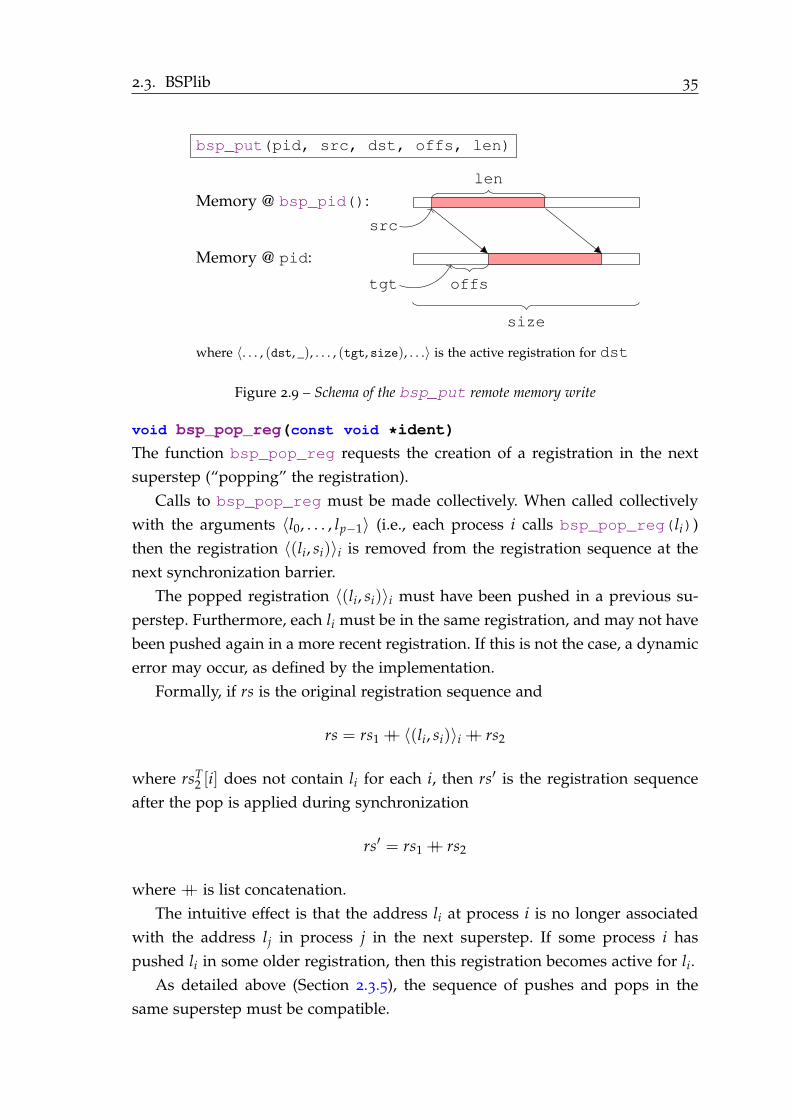
2.3. BSPlib 35
bsp_put(pid, src, dst, offs, len)
Memory @ bsp_pid():
Memory @ pid:
len
size
offs
src
tgt
where 〈. . . , (dst, _), . . . , (tgt, size), . . .〉 is the active registration for dst
Figure 2.9 – Schema of the bsp_put remote memory write
void bsp_pop_reg(const void *ident)
The function bsp_pop_reg requests the creation of a registration in the next
superstep (“popping” the registration).
Calls to bsp_pop_reg must be made collectively. When called collectively
with the arguments 〈l0, . . . , lp−1〉 (i.e., each process i calls bsp_pop_reg(li))
then the registration 〈(li, si)〉i is removed from the registration sequence at the
next synchronization barrier.
The popped registration 〈(li, si)〉i must have been pushed in a previous su-
perstep. Furthermore, each li must be in the same registration, and may not have
been pushed again in a more recent registration. If this is not the case, a dynamic
error may occur, as defined by the implementation.
Formally, if rs is the original registration sequence and
rs = rs1 ++ 〈(li, si)〉i ++ rs2
where rsT2 [i] does not contain li for each i, then rs′ is the registration sequence
after the pop is applied during synchronization
rs′ = rs1 ++ rs2
where ++ is list concatenation.
The intuitive effect is that the address li at process i is no longer associated
with the address lj in process j in the next superstep. If some process i has
pushed li in some older registration, then this registration becomes active for li.
As detailed above (Section 2.3.5), the sequence of pushes and pops in the
same superstep must be compatible.
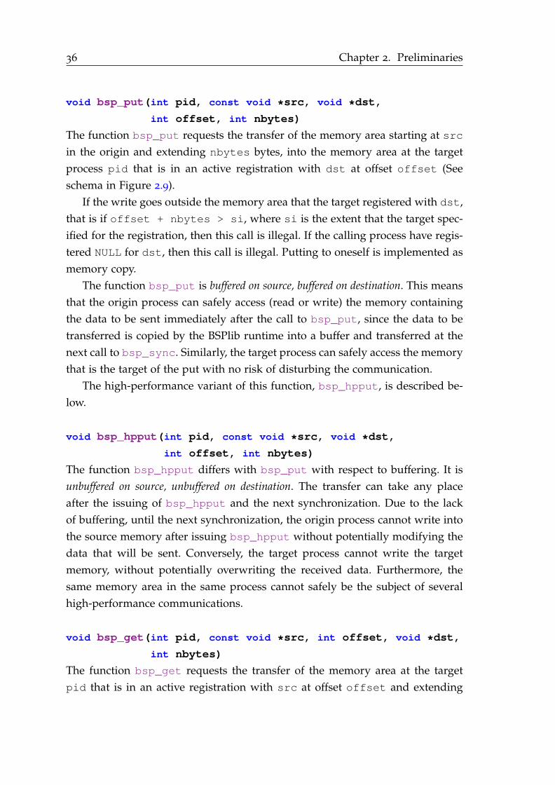
36 Chapter 2. Preliminaries
void bsp_put(int pid, const void *src, void *dst,
int offset, int nbytes)
The function bsp_put requests the transfer of the memory area starting at src
in the origin and extending nbytes bytes, into the memory area at the target
process pid that is in an active registration with dst at offset offset (See
schema in Figure 2.9).
If the write goes outside the memory area that the target registered with dst,
that is if offset + nbytes > si, where si is the extent that the target spec-
ified for the registration, then this call is illegal. If the calling process have regis-
tered NULL for dst, then this call is illegal. Putting to oneself is implemented as
memory copy.
The function bsp_put is buffered on source, buffered on destination. This means
that the origin process can safely access (read or write) the memory containing
the data to be sent immediately after the call to bsp_put, since the data to be
transferred is copied by the BSPlib runtime into a buffer and transferred at the
next call to bsp_sync. Similarly, the target process can safely access the memory
that is the target of the put with no risk of disturbing the communication.
The high-performance variant of this function, bsp_hpput, is described be-
low.
void bsp_hpput(int pid, const void *src, void *dst,
int offset, int nbytes)
The function bsp_hpput differs with bsp_put with respect to buffering. It is
unbuffered on source, unbuffered on destination. The transfer can take any place
after the issuing of bsp_hpput and the next synchronization. Due to the lack
of buffering, until the next synchronization, the origin process cannot write into
the source memory after issuing bsp_hpput without potentially modifying the
data that will be sent. Conversely, the target process cannot write the target
memory, without potentially overwriting the received data. Furthermore, the
same memory area in the same process cannot safely be the subject of several
high-performance communications.
void bsp_get(int pid, const void *src, int offset, void *dst,
int nbytes)
The function bsp_get requests the transfer of the memory area at the target
pid that is in an active registration with src at offset offset and extending

2.3. BSPlib 37
bsp_get(pid, src, offs, dst, len)
Memory @ bsp_pid():
Memory @ pid:
size
offs len
dst
tgt
where 〈. . . , (src, _), . . . , (tgt, size), . . .〉 is the active registration for src
Figure 2.10 – Schema of the bsp_get remote memory read
nbytes bytes, into the memory area of the origin process at dst (see schema in
Figure 2.10).
If the write goes outside the memory area that the target process registered
with src, that is if offset + nbytes > si where si is the extent that the
specified for the registration, then this call is illegal. Like for bsp_put, if the
origin process have registered NULL for src, then this call is illegal. Similarly,
getting from oneself is implemented as a memory copy.
Like bsp_put, read requests issued by bsp_get are buffered on source,
buffered on destination and delivered at the next synchronization. The high-
performance variant of this function that forgoes such buffering, bsp_hpget,
is described below.
void bsp_hpget(int pid, const void *src, int offset,
void *dst, int nbytes)
The function bsp_hpget differs with bsp_get with respect to buffering. The
function bsp_hpget is unbuffered on source, unbuffered on destination. When using
bsp_hpget, the same safety precautions apply as when using bsp_hpput.
Bulk Synchronous Message Passing (BSMP)
Message passing is the second way of communicating between processes in
BSPlib, but arguably less used. However, it is convenient in applications with
irregular and data-dependent communication patterns.
The idea is that each process has a queue handled by the BSPlib runtime.
During the computation phase of a superstep, processes can send messages into
the queue of other processes. As for DRMA communications, messages are guar-

38 Chapter 2. Preliminaries
anteed to be delivered after synchronization and the receiving process can then
read the messages from their queue. Messages are removed after being read, and
any unread messages are removed at the end of the superstep. Unlike DRMA,
the receiving process is not required pre-allocate memory, but can instead allo-
cate memory according to received messages.
Each message consists of a tag and a payload, both with user-defined contents.
The tag is fixed, user-defined size (0 bytes by default), where as the payload is
variable length.
void bsp_set_tagsize(int *tag_bytes)
Sets the size of the tag in bytes. This function must be called collectively and
with the same argument by each process. The change takes effect in the next
superstep. The previous tag size is stored in tag_bytes on return.
void bsp_send(int pid, const void *tag, const void *payload,
int payload_bytes)
Used to send tag and payload to the process specified by pid. Both payload and
tag are buffered. Messages are delivered in the next superstep, but there are no
guarantees on the delivery order. The tag size must conform to what has been
set by bsp_set_tagsize in previous superstep.
void bsp_qsize(int *packets, int *accum_nbytes)
Returns the number of messages that has been received (i.e. sent by to the calling
process in the previous superstep) and not yet read by bsp_move. Also writes
the total size of all received, not yet read, messages in the location pointed to by
accum_nbytes.
void bsp_get_tag(int *status, void *tag)
Reads the tag part of the next message in the queue. The location pointed to by
status is set to -1 if there are no more messages, otherwise it is set to the size
of the payload in the message. If there is a tag, then it is copied to the address
referred by tag.
void bsp_move(void *payload, int reception_bytes)
Reads and removes the next message in the queue. The payload of the
message is copied to the address referred to by payload. The argument

2.3. BSPlib 39
reception_bytes is used to specify an upper limit on the number of bytes
that can be written in to the memory referenced by payload.
Since bsp_move is used both to read and remove the message, it follows that
(1) bsp_move must be called even if only the tag is used (i.e. all messages are
fixed length), to be able to retrieve the next message; (2) bsp_get_tag must be
called before bsp_move.
int bsp_hpmove(void **tag_ptr_buf, void **payload_ptr_buf)
The high-performance primitive bsp_hpmove reads both tag and payload of the
next message without any copying, and removes the message from the queue.
Whereas bsp_move respectively bsp_get_tag copies the tag respectively pay-
load into specified memory areas, bsp_hpmove points its argument to the loca-
tion of these two in the BSPlib queue. In returns -1 if there is no next message,
and otherwise the length of the payload.
2.3.6 BSPlib Implementations
Thanks to the small size of the API, BSPlib has become the de facto standard
interface for imperative BSP programming, with several implementations.
Implementations for multi-node architectures include Oxford BSP
Toolset [141], The Paderborn University BSP library (PUB) [27] and BSPon-
MPI [182]. Implementations for multi-core architectures include MulticoreBSP
for Java [207] and C [208], Zefiros BSPlib [193], Bulk [34] and Epiphany BSP [33].
Lightweight Parallel Foundations has a BSPlib compatible interface and imple-
mentations for multi-node, multi-core and hybrid architectures [183].
2.3.7 BSPlib Limitations
Using int For Indices and Sizes
BSPlib uses the C type int for memory object sizes and indices (for instance, in
the arguments for bsp_push_reg, bsp_put, bsp_qsize in Table 2.1), instead
of the unsigned integer type size_t, which would be more appropriate for C.
This is also the case in the API of MPI, and a possible reason is to ensure that
primitives are callable from Fortran, which does not have unsigned integers.
However, this hinders working with objects whose size exceeds INT_MAX bytes,
the largest integer that can be represented by an int. For instance, the full extent
of such objects cannot be registered.
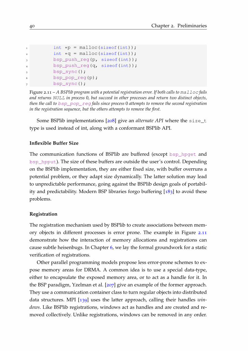
40 Chapter 2. Preliminaries
1 int *p = malloc(sizeof(int));
2 int *q = malloc(sizeof(int));
3 bsp_push_reg(p, sizeof(int));
4 bsp_push_reg(q, sizeof(int));
5 bsp_sync();
6 bsp_pop_reg(p);
7 bsp_sync();
Figure 2.11 – A BSPlib program with a potential registration error. If both calls to malloc failsand returns NULL in process 0, but succeed in other processes and return two distinct objects,then the call to bsp_pop_reg fails since process 0 attempts to remove the second registrationin the registration sequence, but the others attempts to remove the first.
Some BSPlib implementations [208] give an alternate API where the size_t
type is used instead of int, along with a conformant BSPlib API.
Inflexible Buffer Size
The communication functions of BSPlib are buffered (except bsp_hpget and
bsp_hpput). The size of these buffers are outside the user’s control. Depending
on the BSPlib implementation, they are either fixed size, with buffer overruns a
potential problem, or they adapt size dynamically. The latter solution may lead
to unpredictable performance, going against the BSPlib design goals of portabil-
ity and predictability. Modern BSP libraries forgo buffering [183] to avoid these
problems.
Registration
The registration mechanism used by BSPlib to create associations between mem-
ory objects in different processes is error prone. The example in Figure 2.11
demonstrate how the interaction of memory allocations and registrations can
cause subtle heisenbugs. In Chapter 6, we lay the formal groundwork for a static
verification of registrations.
Other parallel programming models propose less error-prone schemes to ex-
pose memory areas for DRMA. A common idea is to use a special data-type,
either to encapsulate the exposed memory area, or to act as a handle for it. In
the BSP paradigm, Yzelman et al. [207] give an example of the former approach.
They use a communication container class to turn regular objects into distributed
data structures. MPI [139] uses the latter approach, calling their handles win-
dows. Like BSPlib registrations, windows act as handles and are created and re-
moved collectively. Unlike registrations, windows can be removed in any order.

2.3. BSPlib 41
Lightweight Parallel Foundation’s [183] memory slots are similar to windows. An
idea that forgoes dedicated data-types is proposed in OpenSHMEM [36] where
DRMA operations are restricted to “symmetric” objects that the runtime system
ensures have the same relative address in each process.
Lack of High-Level Collectives
One drawback of the minimalism of BSPlib is that commonly used parallel pro-
gramming building blocks and high-level collective must be implemented by
the user. Notably, BSPlib contains no primitives for common communication
patterns such as broadcast, scatter, all-to-all, gather and reduction. A “Level 1”
BSPlib API with such high-level primitives has been proposed [100], but to the
best of our knowledge, no modern BSPlib libraries implement this API.
Lack of Composability and Fault Tolerance
In many situations, it would be desirable to be able to include BSPlib to speed
up computations in a larger application. However, three design flaws of BSPlib
render such use cases difficult, namely the restriction to one parallel section (see
Section 2.3.3), the lack of any provision to return data from this section to the
rest of the application and the lack of fault tolerance.
In a BSPlib program, either the parallel section is the main function, immedi-
ately precluding having it be a part of a larger application, as C programs have
at most one entry point. Or, a SPMD function containing the parallel section is
designated by a call to bsp_init. However, the function pointer that should be
passed to the bsp_init function has the void return type and no parameters.
Hence, the only way to return data from the parallel section to the following se-
rial section in this case is by global variables, whose usage is considered contrary
to good software engineering practices.
While the function bsp_abort can be used to terminate completely a pro-
gram using BSPlib in case of errors, there is no mechanism in BSPlib to recover
gracefully from faults. Should for instance memory allocation fail in some pro-
cess, then there is no simple way to propagate this error, terminate the parallel
computation and return to the serial section to clean up any other eventual re-
sources that have been allocated.

42 Chapter 2. Preliminaries
Loss of High-Level Structure
A critique that can be leveraged to any SPMD language implemented in imper-
ative language is the loss of the high-level structure of synchronization.
As noted by [179], a BSP program can either be seen as a sequence of super-
steps, each containing the parallel computation, or as the parallel composition
of sequential p instruction streams, equipped with a synchronization primitive.
BSPlib implements the latter approach, by giving users access to the bsp_sync
primitive.
The drawback of this approach is that there is no restriction from expressing
programs that have no sense in the BSP model, such as the following:
1 if (bsp_pid() == 0) bsp_sync(); else bsp_end();
which will cause a synchronization error when executed by at least 2 processes.
The first model can be implemented more easily in functional languages,
where computations (in the guise of functions) are first-class values. This is in-
deed similar to how programs are expressed in BSML [18]. There, programs are
divided into a global part which sequences a series of local parts, expressed as
functions and corresponding to supersteps. Errors such as the synchronization
error above are ruled out by forcing all collective operations to be performed in
the global part.
2.3.8 Relationship to MPI
In spirit, BSPlib can be seen as a model of the Bulk Synchronous subset of
the popular parallel programming library MPI [139]. Both BSPlib and MPI are
SPMD libraries for distributed memory programming. The unbuffered, high-
performance RDMA operations of BSPlib (bsp_hpput and bsp_hpget) corre-
sponds to the RMA operations of MPI [89, p. 55] (MPI_Put and MPI_Get) and
the synchronization primitive bsp_sync of BSPlib to the MPI_Barrier of MPI;
BSPlib registers corresponds to MPI windows; the BSPlib process identifier cor-
responds to ranks in the MPI. We summarize this approximate correspondence
in Table 2.2.
The reader should be aware that this correspondence should not be read
as a semantic equivalence as there are many subtle differences. To name two,
MPI implements communicators that group sets of processes, a feature with no
equivalent in BSPlib. Secondly, the registration sequence that enables DRMA in
BSPlib follows a stack-like semantics, as detailed above in Section 2.3.5. This is
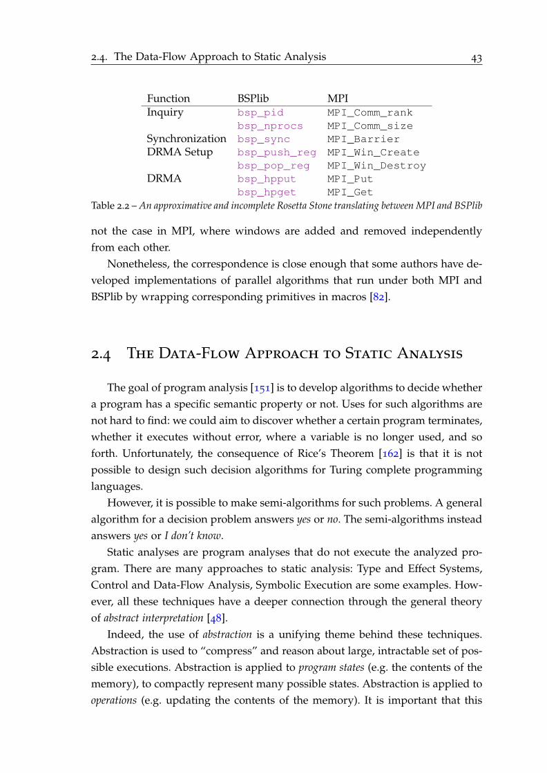
2.4. The Data-Flow Approach to Static Analysis 43
Function BSPlib MPIInquiry bsp_pid MPI_Comm_rank
bsp_nprocs MPI_Comm_size
Synchronization bsp_sync MPI_Barrier
DRMA Setup bsp_push_reg MPI_Win_Create
bsp_pop_reg MPI_Win_Destroy
DRMA bsp_hpput MPI_Put
bsp_hpget MPI_Get
Table 2.2 – An approximative and incomplete Rosetta Stone translating between MPI and BSPlib
not the case in MPI, where windows are added and removed independently
from each other.
Nonetheless, the correspondence is close enough that some authors have de-
veloped implementations of parallel algorithms that run under both MPI and
BSPlib by wrapping corresponding primitives in macros [82].
2.4 The Data-Flow Approach to Static Analysis
The goal of program analysis [151] is to develop algorithms to decide whether
a program has a specific semantic property or not. Uses for such algorithms are
not hard to find: we could aim to discover whether a certain program terminates,
whether it executes without error, where a variable is no longer used, and so
forth. Unfortunately, the consequence of Rice’s Theorem [162] is that it is not
possible to design such decision algorithms for Turing complete programming
languages.
However, it is possible to make semi-algorithms for such problems. A general
algorithm for a decision problem answers yes or no. The semi-algorithms instead
answers yes or I don’t know.
Static analyses are program analyses that do not execute the analyzed pro-
gram. There are many approaches to static analysis: Type and Effect Systems,
Control and Data-Flow Analysis, Symbolic Execution are some examples. How-
ever, all these techniques have a deeper connection through the general theory
of abstract interpretation [48].
Indeed, the use of abstraction is a unifying theme behind these techniques.
Abstraction is used to “compress” and reason about large, intractable set of pos-
sible executions. Abstraction is applied to program states (e.g. the contents of the
memory), to compactly represent many possible states. Abstraction is applied to
operations (e.g. updating the contents of the memory). It is important that this
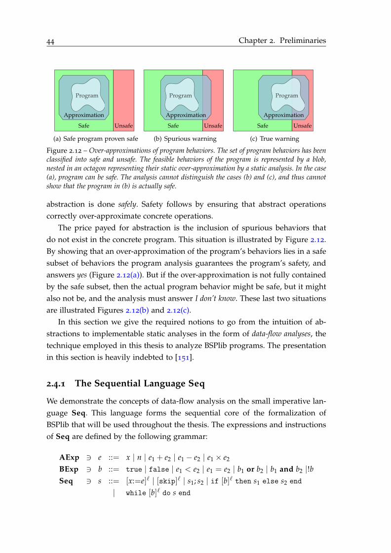
44 Chapter 2. Preliminaries
Safe Unsafe
Approximation
Program
(a) Safe program proven safe
Safe Unsafe
Approximation
Program
(b) Spurious warning
Safe Unsafe
Approximation
Program
(c) True warning
Figure 2.12 – Over-approximations of program behaviors. The set of program behaviors has beenclassified into safe and unsafe. The feasible behaviors of the program is represented by a blob,nested in an octagon representing their static over-approximation by a static analysis. In the case(a), program can be safe. The analysis cannot distinguish the cases (b) and (c), and thus cannotshow that the program in (b) is actually safe.
abstraction is done safely. Safety follows by ensuring that abstract operations
correctly over-approximate concrete operations.
The price payed for abstraction is the inclusion of spurious behaviors that
do not exist in the concrete program. This situation is illustrated by Figure 2.12.
By showing that an over-approximation of the program’s behaviors lies in a safe
subset of behaviors the program analysis guarantees the program’s safety, and
answers yes (Figure 2.12(a)). But if the over-approximation is not fully contained
by the safe subset, then the actual program behavior might be safe, but it might
also not be, and the analysis must answer I don’t know. These last two situations
are illustrated Figures 2.12(b) and 2.12(c).
In this section we give the required notions to go from the intuition of ab-
stractions to implementable static analyses in the form of data-flow analyses, the
technique employed in this thesis to analyze BSPlib programs. The presentation
in this section is heavily indebted to [151].
2.4.1 The Sequential Language Seq
We demonstrate the concepts of data-flow analysis on the small imperative lan-
guage Seq. This language forms the sequential core of the formalization of
BSPlib that will be used throughout the thesis. The expressions and instructions
of Seq are defined by the following grammar:
AExp ∋ e ::= x | n | e1 + e2 | e1 − e2 | e1 × e2
BExp ∋ b ::= true | false | e1 < e2 | e1 = e2 | b1 or b2 | b1 and b2 |!b
Seq ∋ s ::= [x:=e]ℓ | [skip]ℓ | s1; s2 | if [b]ℓ then s1 else s2 end
| while [b]ℓ do s end

2.4. The Data-Flow Approach to Static Analysis 45
[y:=57]1;[d:=8]2;[x:=0]3;
while [d < y or d = y]4 do
[x:=x + 1]5;[y:=y− d]6
end
Figure 2.13 – The Seq program sdiv
where x ∈ Var, the set of program variables, and n ∈ Nat, the set of natural
numbers. Instructions are labeled with labels ℓ ∈ Lab. We shall assume that all
programs are consistently labeled, i.e. that each label appears at most once.
The language contains arithmetic and boolean expressions, as defined by the
syntactic groups AExp and BExp. The instructions are formed by the syntactic
group Seq, and consists of assignments, the skip instruction that does nothing,
sequences of instructions, conditionals and loops. An example of a Seq program
is given in Figure 2.13. This program sdiv calculates the euclidean division of 57
by 8. At the end its execution x contains the quotient and y the remainder, so
that 8x + y = 57.
The Semantics of Seq
The precise meaning of Seq is defined by its formal semantics that describes how
the execution of programs transforms memory states. Memory states are repre-
sented by mappings from variables to natural integers. This is a standard, big-
step operational semantics [203]. The big-step semantics is a relation→ between
initial and final configurations of non-diverging and non-erroneous program ex-
ecutions. Initial configurations 〈s, σ〉, consists of a program s ∈ Seq to execute
and an initial memory state σ ∈ State. Final configurations are the memory state
at the end of execution. In sum, we have:
State = Var→ Nat
→ : Seq× State× State
The informal idea of a variable x containing the value n is formalized by σ(x) =
n. The updated memory state where x is set to contain m is written σ[x ← m]
and defined by
σ[x ← m] = λy.
m if x = y
σ(y) otherwise
Before defining→, we define the semantics of arithmetic respectively boolean
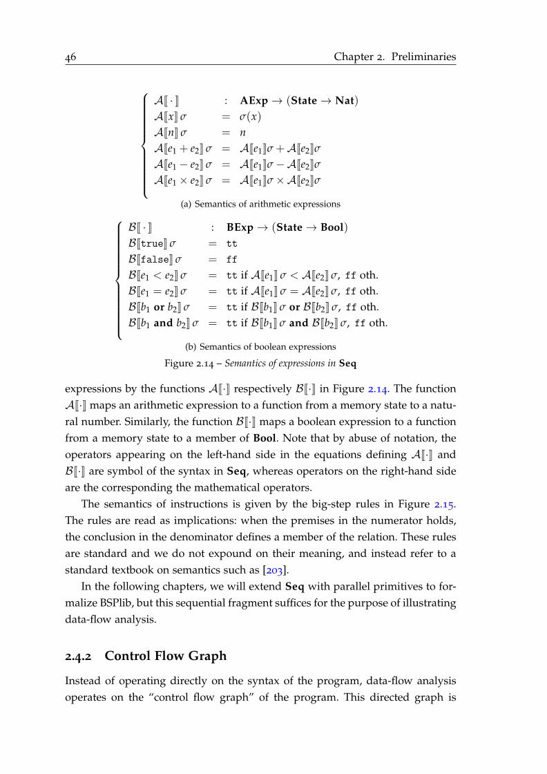
46 Chapter 2. Preliminaries
AJ · K : AExp→ (State→ Nat)
AJxK σ = σ(x)
AJnK σ = n
AJe1 + e2K σ = AJe1Kσ +AJe2Kσ
AJe1 − e2K σ = AJe1Kσ−AJe2Kσ
AJe1 × e2K σ = AJe1Kσ×AJe2Kσ
(a) Semantics of arithmetic expressions
BJ · K : BExp→ (State→ Bool)
BJtrueK σ = tt
BJfalseK σ = ff
BJe1 < e2K σ = tt if AJe1K σ < AJe2K σ, ff oth.
BJe1 = e2K σ = tt if AJe1K σ = AJe2K σ, ff oth.
BJb1 or b2K σ = tt if BJb1K σ or BJb2K σ, ff oth.
BJb1 and b2K σ = tt if BJb1K σ and BJb2K σ, ff oth.
(b) Semantics of boolean expressions
Figure 2.14 – Semantics of expressions in Seq
expressions by the functions AJ·K respectively BJ·K in Figure 2.14. The function
AJ·K maps an arithmetic expression to a function from a memory state to a natu-
ral number. Similarly, the function BJ·K maps a boolean expression to a function
from a memory state to a member of Bool. Note that by abuse of notation, the
operators appearing on the left-hand side in the equations defining AJ·K and
BJ·K are symbol of the syntax in Seq, whereas operators on the right-hand side
are the corresponding the mathematical operators.
The semantics of instructions is given by the big-step rules in Figure 2.15.
The rules are read as implications: when the premises in the numerator holds,
the conclusion in the denominator defines a member of the relation. These rules
are standard and we do not expound on their meaning, and instead refer to a
standard textbook on semantics such as [203].
In the following chapters, we will extend Seq with parallel primitives to for-
malize BSPlib, but this sequential fragment suffices for the purpose of illustrating
data-flow analysis.
2.4.2 Control Flow Graph
Instead of operating directly on the syntax of the program, data-flow analysis
operates on the “control flow graph” of the program. This directed graph is
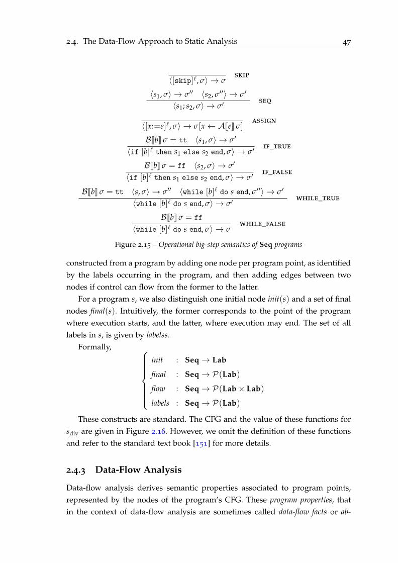
2.4. The Data-Flow Approach to Static Analysis 47
〈[skip]ℓ, σ〉 → σskip
〈s1, σ〉 → σ′′ 〈s2, σ′′〉 → σ′
〈s1; s2, σ〉 → σ′seq
〈[x:=e]ℓ, σ〉 → σ[x← AJeK σ]assign
BJbK σ = tt 〈s1, σ〉 → σ′
〈if [b]ℓ then s1 else s2 end, σ〉 → σ′if_true
BJbK σ = ff 〈s2, σ〉 → σ′
〈if [b]ℓ then s1 else s2 end, σ〉 → σ′if_false
BJbK σ = tt 〈s, σ〉 → σ′′ 〈while [b]ℓ do s end, σ′′〉 → σ′
〈while [b]ℓ do s end, σ〉 → σ′while_true
BJbK σ = ff
〈while [b]ℓ do s end, σ〉 → σwhile_false
Figure 2.15 – Operational big-step semantics of Seq programs
constructed from a program by adding one node per program point, as identified
by the labels occurring in the program, and then adding edges between two
nodes if control can flow from the former to the latter.
For a program s, we also distinguish one initial node init(s) and a set of final
nodes final(s). Intuitively, the former corresponds to the point of the program
where execution starts, and the latter, where execution may end. The set of all
labels in s, is given by labelss.
Formally,
init : Seq→ Lab
final : Seq→ P(Lab)
flow : Seq→ P(Lab× Lab)
labels : Seq→ P(Lab)
These constructs are standard. The CFG and the value of these functions for
sdiv are given in Figure 2.16. However, we omit the definition of these functions
and refer to the standard text book [151] for more details.
2.4.3 Data-Flow Analysis
Data-flow analysis derives semantic properties associated to program points,
represented by the nodes of the program’s CFG. These program properties, that
in the context of data-flow analysis are sometimes called data-flow facts or ab-

48 Chapter 2. Preliminaries
1 2 3 4
5 6
flow(sdiv) = (1, 2), (2, 3), (3, 4), (4, 5), (5, 6), (6, 4)init(sdiv) = 1final(sdiv) = 4labels(sdiv) = 1, 2, 3, 4, 5, 6
Figure 2.16 – The control flow graph of sdiv
stract states, move along the edges of the program’s CFG. Each program point
has an incoming, respectively outgoing, abstract state that represents what is al-
ways true in all executions before, respectively after, executing that node. The
incoming abstract state is an over-approximation of all incoming abstract states,
and the outgoing abstract state is calculated by applying a transfer function to the
input state.
The analysis is classified depending on the direction the data-flow facts run.
In a “forward analysis”, data-flow facts are propagated in the direction of control
flow. In a “backward analysis”, they are propagated against the control flow.
The former is used when the property to be computed is a function of all pos-
sible past actions, whereas the latter is used when the all future actions are of
interest. For instance, a forward analysis can be used to over-approximate the set
of variables that may have been defined up to a certain point (see Reaching Def-
initions below), whereas a backward analysis can be used to over-approximate
the set of variables that may be read at some later point (Live Variables analysis).
In addition to establishing safety properties as in this thesis, data-flow analy-
sis is commonly used in compilation. To give an example, “Reaching Definitions”
is a forward data-flow analysis useful for compilation. In an execution, a defi-
nition is a variable and a program point at which it was assigned. A definition
reaches another program point if there are no other assignments to that variable
between the definition and the program point.
Consider the assignment to x labeled 3 in sdiv. This definition (x, 3) may
reach program point 4 (in the first iteration of the loop) but so can the defini-
tion (x, 5) (for the remaining iterations). By the same reasoning (x, 3) and (x, 5)
reaches point 5. However, in all executions that reaches the assignment labeled
6, x must have been redefined at 5. Thus (x, 5) reaches this point, but not (x, 3).
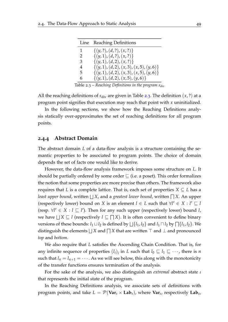
2.4. The Data-Flow Approach to Static Analysis 49
Line Reaching Definitions
1 (y, ?), (d, ?), (x, ?)2 (y, 1), (d, ?), (x, ?)3 (y, 1), (d, 2), (x, ?)4 (y, 1), (d, 2), (x, 3), (x, 5), (y, 6)5 (y, 1), (d, 2), (x, 3), (x, 5), (y, 6)6 (y, 1), (d, 2), (x, 5), (y, 6)
Table 2.3 – Reaching Definitions in the program sdiv
All the reaching definitions of sdiv are given in Table 2.3. The definition (x, ?) at a
program point signifies that execution may reach that point with x uninitialized.
In the following sections, we show how the Reaching Definitions analy-
sis statically over-approximates the set of reaching definitions for all program
points.
2.4.4 Abstract Domain
The abstract domain L of a data-flow analysis is a structure containing the se-
mantic properties to be associated to program points. The choice of domain
depends the set of facts one would like to derive.
However, the data-flow analysis framework imposes some structure on L. It
should be partially ordered by some order ⊑ (i.e. a poset). This order formalizes
the notion that some properties are more precise than others. The framework also
requires that L is a complete lattice. That is, each set of properties X ⊆ L has a
least upper bound, written⊔
X, and a greatest lower bound, writtend
X. An upper
(respectively lower) bound on X is an element l ∈ L such that ∀l′ ∈ X : l′ ⊑ l
(resp. ∀l′ ∈ X : l ⊑ l′). Then for any such upper (respectively lower) bound l,
we have⊔
X ⊑ l (respectively l ⊑d
X). It is often convenient to define binary
versions of these bounds: l1 ⊔ l2 is defined by⊔
l1, l2 and l1 ⊓ l2 bydl1, l2. We
distinguish the elements⊔
X andd
X that are written ⊤ and ⊥ and pronounced
top and bottom.
We also require that L satisfies the Ascending Chain Condition. That is, for
any infinite sequence of properties (li)i in L such that l0 ⊑ l1 ⊑ · · · , there is n
such that ln = ln+1 = · · · . As we will see below, this along with the monotonicity
of the transfer functions ensures termination of the analysis.
For the sake of the analysis, we also distinguish an extremal abstract state ι
that represents the initial state of the program.
In the Reaching Definitions analysis, we associate sets of definitions with
program points, and take L = P(Vars × Labs), where Vars, respectively Labs,
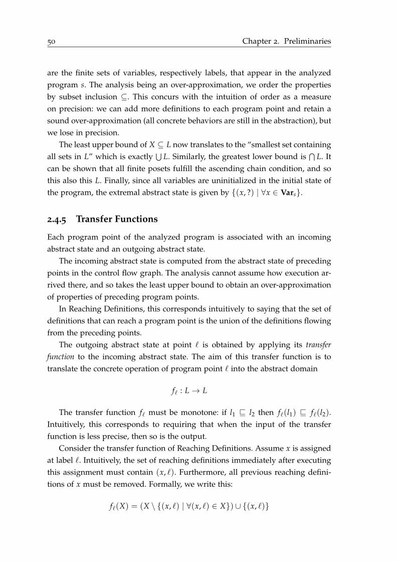
50 Chapter 2. Preliminaries
are the finite sets of variables, respectively labels, that appear in the analyzed
program s. The analysis being an over-approximation, we order the properties
by subset inclusion ⊆. This concurs with the intuition of order as a measure
on precision: we can add more definitions to each program point and retain a
sound over-approximation (all concrete behaviors are still in the abstraction), but
we lose in precision.
The least upper bound of X ⊆ L now translates to the “smallest set containing
all sets in L” which is exactly⋃
L. Similarly, the greatest lower bound is⋂
L. It
can be shown that all finite posets fulfill the ascending chain condition, and so
this also this L. Finally, since all variables are uninitialized in the initial state of
the program, the extremal abstract state is given by (x, ?) | ∀x ∈ Vars.
2.4.5 Transfer Functions
Each program point of the analyzed program is associated with an incoming
abstract state and an outgoing abstract state.
The incoming abstract state is computed from the abstract state of preceding
points in the control flow graph. The analysis cannot assume how execution ar-
rived there, and so takes the least upper bound to obtain an over-approximation
of properties of preceding program points.
In Reaching Definitions, this corresponds intuitively to saying that the set of
definitions that can reach a program point is the union of the definitions flowing
from the preceding points.
The outgoing abstract state at point ℓ is obtained by applying its transfer
function to the incoming abstract state. The aim of this transfer function is to
translate the concrete operation of program point ℓ into the abstract domain
fℓ : L→ L
The transfer function fℓ must be monotone: if l1 ⊑ l2 then fℓ(l1) ⊑ fℓ(l2).
Intuitively, this corresponds to requiring that when the input of the transfer
function is less precise, then so is the output.
Consider the transfer function of Reaching Definitions. Assume x is assigned
at label ℓ. Intuitively, the set of reaching definitions immediately after executing
this assignment must contain (x, ℓ). Furthermore, all previous reaching defini-
tions of x must be removed. Formally, we write this:
fℓ(X) = (X \ (x, ℓ) | ∀(x, ℓ) ∈ X) ∪ (x, ℓ)
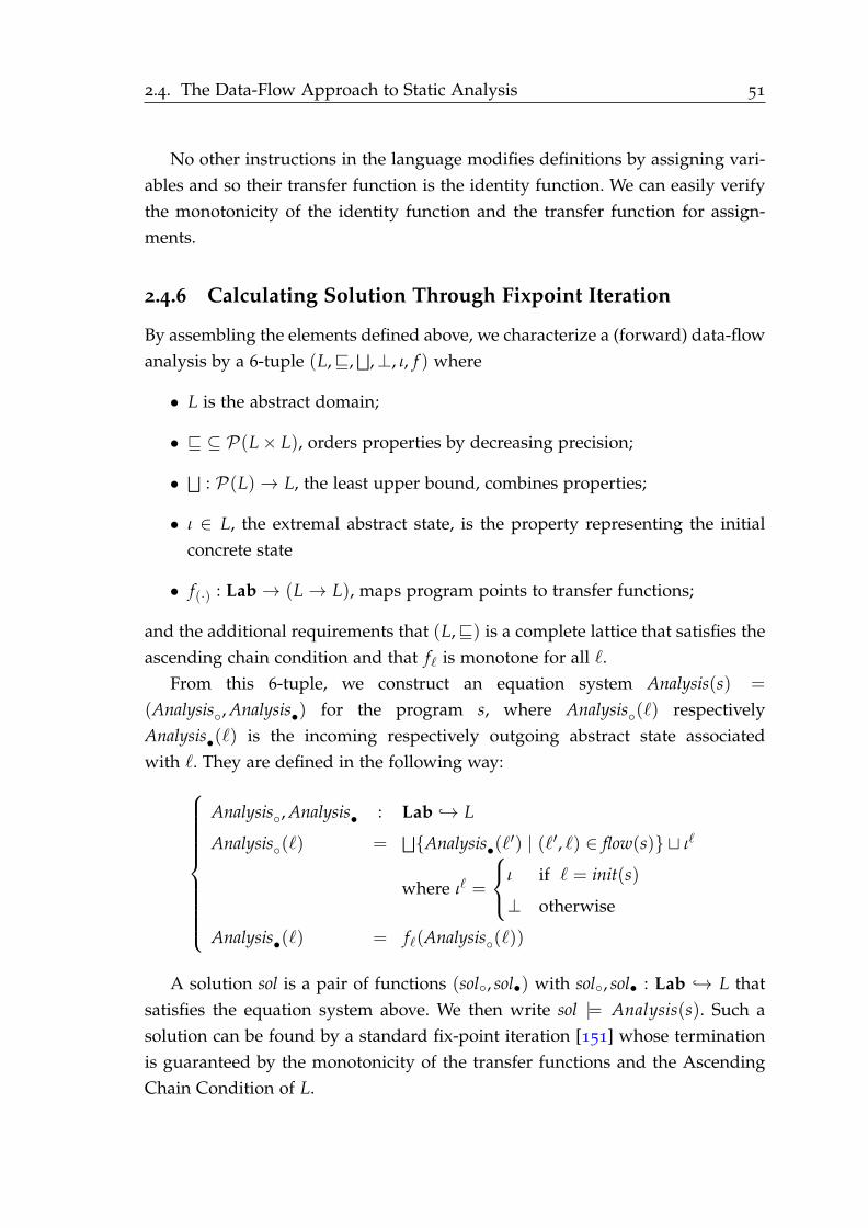
2.4. The Data-Flow Approach to Static Analysis 51
No other instructions in the language modifies definitions by assigning vari-
ables and so their transfer function is the identity function. We can easily verify
the monotonicity of the identity function and the transfer function for assign-
ments.
2.4.6 Calculating Solution Through Fixpoint Iteration
By assembling the elements defined above, we characterize a (forward) data-flow
analysis by a 6-tuple (L,⊑,⊔
,⊥, ι, f ) where
• L is the abstract domain;
• ⊑ ⊆ P(L× L), orders properties by decreasing precision;
•⊔
: P(L)→ L, the least upper bound, combines properties;
• ι ∈ L, the extremal abstract state, is the property representing the initial
concrete state
• f(·) : Lab→ (L→ L), maps program points to transfer functions;
and the additional requirements that (L,⊑) is a complete lattice that satisfies the
ascending chain condition and that fℓ is monotone for all ℓ.
From this 6-tuple, we construct an equation system Analysis(s) =
(Analysis, Analysis•) for the program s, where Analysis(ℓ) respectively
Analysis•(ℓ) is the incoming respectively outgoing abstract state associated
with ℓ. They are defined in the following way:
Analysis, Analysis• : Lab → L
Analysis(ℓ) =⊔
Analysis•(ℓ′) | (ℓ′, ℓ) ∈ flow(s) ⊔ ιℓ
where ιℓ =
ι if ℓ = init(s)
⊥ otherwise
Analysis•(ℓ) = fℓ(Analysis(ℓ))
A solution sol is a pair of functions (sol, sol•) with sol, sol• : Lab → L that
satisfies the equation system above. We then write sol |= Analysis(s). Such a
solution can be found by a standard fix-point iteration [151] whose termination
is guaranteed by the monotonicity of the transfer functions and the Ascending
Chain Condition of L.

52 Chapter 2. Preliminaries
Message Printer Property Status
Journal Parameter Project . . .
Visitor
Plug-ins Analyzer 1 Analyzer 2 Analyzer 3 . . .
Plug-in Database
Kernel Services
(Modified) CIL C + ACSL AST
Figure 2.17 – Frama-C architecture
2.5 Frama-C
This section is extracted from the author’s master’s thesis [113].
Frama-C [54] is an analysis platform for C code implemented in OCaml. It
consists of a kernel and a set of plug-ins (see Figure 2.17). The Frama-C kernel
parses input programs, and offers an abstract view of C programs to the plug-ins
that implement different analyses, or program transformations. The kernel also
provides several services that aid the implementation of new plug-ins, such as
several facilities for implementing data-flow analyses, and it ensures the consis-
tency of plug-ins.
One benefit of regrouping several tools in the same framework is that each
individual tool does not need to deal with the technical aspects of parsing C code
and can thus concentrate on implementing one specific analysis. In addition to
this, the kernel of Frama-C simplifies the input program and offers a slightly ab-
stracted view to the plug-in. Another positive aspect of the plug-in architecture
is that one plug-in can share its results with other plug-ins. For example, the
RTE plug-in identifies source code locations that can cause a run-time error. The
verification engineer can then use the deductive verification plug-in WP to rule
out the possibility of actual errors in these locations.
Since verification engineers often take a multi-pronged approach to verifying
a program, using both automatic, semi-automatic and manual techniques, it is
convenient to gather tools using different kinds of techniques under the same
umbrella.
Frama-C has a rich set of plug-ins. Some important ones are:
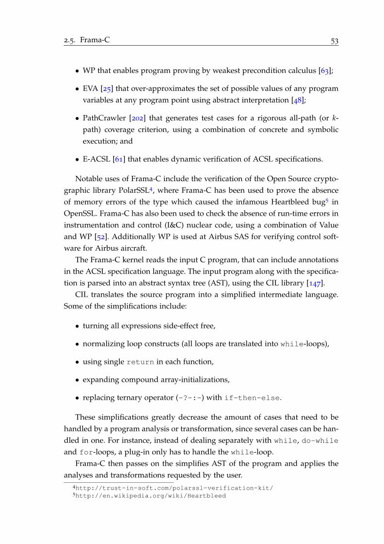
2.5. Frama-C 53
• WP that enables program proving by weakest precondition calculus [63];
• EVA [25] that over-approximates the set of possible values of any program
variables at any program point using abstract interpretation [48];
• PathCrawler [202] that generates test cases for a rigorous all-path (or k-
path) coverage criterion, using a combination of concrete and symbolic
execution; and
• E-ACSL [61] that enables dynamic verification of ACSL specifications.
Notable uses of Frama-C include the verification of the Open Source crypto-
graphic library PolarSSL4, where Frama-C has been used to prove the absence
of memory errors of the type which caused the infamous Heartbleed bug5 in
OpenSSL. Frama-C has also been used to check the absence of run-time errors in
instrumentation and control (I&C) nuclear code, using a combination of Value
and WP [52]. Additionally WP is used at Airbus SAS for verifying control soft-
ware for Airbus aircraft.
The Frama-C kernel reads the input C program, that can include annotations
in the ACSL specification language. The input program along with the specifica-
tion is parsed into an abstract syntax tree (AST), using the CIL library [147].
CIL translates the source program into a simplified intermediate language.
Some of the simplifications include:
• turning all expressions side-effect free,
• normalizing loop constructs (all loops are translated into while-loops),
• using single return in each function,
• expanding compound array-initializations,
• replacing ternary operator (-?-:-) with if-then-else.
These simplifications greatly decrease the amount of cases that need to be
handled by a program analysis or transformation, since several cases can be han-
dled in one. For instance, instead of dealing separately with while, do-while
and for-loops, a plug-in only has to handle the while-loop.
Frama-C then passes on the simplifies AST of the program and applies the
analyses and transformations requested by the user.
4http://trust-in-soft.com/polarssl-verification-kit/5http://en.wikipedia.org/wiki/Heartbleed

3State of the Art
Contents
3.1 Parallel Models . . . . . . . . . . . . . . . . . . . . . . . . . . . . . . . 56
3.1.1 Other than BSP . . . . . . . . . . . . . . . . . . . . . . . . . . . . . 56
3.1.2 BSP Extensions . . . . . . . . . . . . . . . . . . . . . . . . . . . . . 57
3.2 Parallel Programming . . . . . . . . . . . . . . . . . . . . . . . . . . . 60
3.2.1 Other than BSP . . . . . . . . . . . . . . . . . . . . . . . . . . . . . 60
3.2.2 BSP . . . . . . . . . . . . . . . . . . . . . . . . . . . . . . . . . . . . 63
3.3 Formal Methods for Scalable Parallel Programming . . . . . 64
3.3.1 Deductive Verification . . . . . . . . . . . . . . . . . . . . . . . . . 65
3.3.2 Model Checking . . . . . . . . . . . . . . . . . . . . . . . . . . . . . 68
3.3.3 Static Analysis . . . . . . . . . . . . . . . . . . . . . . . . . . . . . . 70
3.3.4 Other Formal Methods . . . . . . . . . . . . . . . . . . . . . . . . . 79
3.4 Discussion . . . . . . . . . . . . . . . . . . . . . . . . . . . . . . . . . . . 79
In this chapter we review the state of the art in formal methods for scalable
parallel programming to give the context of the three main contributions of this
thesis: static analysis of parallel structure and synchronization, static cost analy-
sis and a sufficient condition for safe registration in BSPlib programs.
We first review models of scalable parallel programming and how they relate
to BSP in Section 3.1. We focus in particular on models for data-parallelism.
Such models are implemented in libraries and programming languages, which
we review in the Section 3.2.
Our review then surveys the major families of formal methods and how they
have been adapted for scalable parallelism, both to BSP and other models in
Section 3.3. We take special interest in static analysis, and devote Section 3.3.3
to static analyses for scalable parallelism in the BSP model and other models.
55

56 Chapter 3. State of the Art
We close the chapter in Section 3.4 by positioning the main contributions of this
thesis with respect to the findings of the literature review.
3.1 Parallel Models
As the importance of parallelism to scalable computing became apparent,
several models of parallel computing have been proposed. As with any kind of
model, it is desirable that the model abstracts away enough irrelevant details
to allow simple reasoning on high-level properties such as correctness and per-
formance, while remaining realistic enough to be practical. In other words, the
high-level properties of the model should, at least to some degree, translate to
the concrete computation that is modeled.
An analogy can be made with static analysis: a key challenge when applying
formal methods to programs is finding appropriate abstractions that are abstract
enough to be computable, but concrete enough to give pertinent information to
the user.
Our study targets programs written in BSPlib for the BSP [191] model of
parallel computation. BSP is formulated as a bridging model for parallel com-
puting, analogous to the von Neumann model of sequential computing. It allows
for reasoning on parallel computation in a sufficiently abstract setting.
To situate BSP, we briefly review in the following sections other parallel mod-
els that have been proposed. This includes extensions of BSP (Multi-BSP [192]
and Scatter-Gather Language model [128]) but also other models (PRAM [75]
and LogP [51]). For a more extensive review of parallel models, we direct the
reader to [10].
3.1.1 Other than BSP
PRAM
The main purpose of the PRAM model [75], Parallel Random Access Machine,
is to model how parallel algorithms share work. A Parallel Random Access Ma-
chine consists of a fixed number p of processors that execute in lockstep with
equal (random) access to a shared memory. All communication go through this
shared memory. There is no synchronization mechanism.
The PRAM model allows reasoning on the amount of parallelism in pro-
grams. That is, to which degree increasing p speeds up the computation. How-
ever, PRAM does not allow to reason on the cost of communication, which is
often the bottleneck of parallel computations. The lockstep model of PRAM is

3.1. Parallel Models 57
also ill-adapted to modeling realistic architectures where, on the contrary, com-
putation nodes progress independently of each other.
LogP
The LogP model [51] aims to provide a more realistic model of parallel compu-
tation than PRAM by accounting for communication. LogP models distributed
architectures where processes execute asynchronously. Memory is distributed
and processes communicate by point-to-point message passing.
The model is named after the 4 parameters L, o, g, P used to characterize the
performance of the message passing network in the underlying parallel archi-
tecture. The parameter L quantifies the upper bound on communication latency;
the overhead o the “incompressible send or receive” cost; g the minimum “gap”
between each message, that is, the inverse of the bandwidth; P the number of
processes. By plugging the parameters of a specific parallel architecture into the
communication pattern of an algorithm, its designer can predict its performance
in that architecture.
Two main differences distinguish the LogP and the BSP model. First, while
both models account for communication costs, LogP does not consider con-
tention [76]. A communication pattern is modeled with the same cost whether
balanced or not. For instance, LogP does not distinguish the cost of the “all-to-
one” and the “shift” communication patterns. In the former, one process receives
one word from each process. In the latter, each process sends a word to a distinct
process. Shift is balanced, since each process sends and receives one word. All-
to-one is unbalanced, since one process receives P words and sends none, while
the others send one word and receive none. In LogP, only total communication
volume counts, and it is the same in both patterns. In reality, the contention at
the receiver gives all-to-one longer run time.
Second, LogP imposes less structure on the parallel computation. As result,
LogP is more flexible, but gives less insight into how computation and synchro-
nization affect the total cost. The more rigid superstep structure of BSP also
serves to guide algorithm design: no such guidance is given by the LogP model.
3.1.2 BSP Extensions
Several BSP extensions have been proposed to compensate for perceived short-
comings in its original formulation. A common critique is that it does not con-
58 Chapter 3. State of the Art
sider the hierarchality and heterogeneity that is common in modern parallel archi-
tectures.
BSP, like PRAM and LogP, models flat and homogeneous parallel computers,
where each computation node is identical in terms of computation capacities
and the bandwidth between each pair of nodes is the same. This view is often at
odds with concrete parallel computers that consist of heterogeneous computers
situated in hierarchical networks. A common example is multi-core nodes ar-
ranged in a tree-like network. Typically, inter-core communication is faster than
inter-node communication.
We here consider two extensions of BSP, Scatter-Gather Language model [128]
and Multi-BSP [192], that are tailored for this kind of heterogeneous and/or
hierarchical parallel computers, while retaining the portability and predictability
of BSP.
Scatter-Gather Language model
The Scatter-Gather Language (SGL) model [128] considers multi-level, heteroge-
neous parallel architectures. A SGL machine is a recursively defined tree struc-
ture, with a root-master at the top. The child nodes are either themselves SGL
machines or “leaf-workers”. As in BSP, parallel computation is arranged in su-
persteps. These are composed of four phases: (1) the master broadcasting data to
its child nodes (scatter); (2) local computation in the child nodes; (3) each child
node transfers data to its master (gather); (4) local computation in the master.
The local computation step of child nodes that are themselves SGL machines is
recursively composed of a sequence of supersteps.
The SGL cost model is parameterized by the scatter bandwidth g↓, the
gather bandwidth g↑ and the synchronization cost l of each SGL machine in
the network. The cost of a SGL execution is the sum of the cost of each su-
perstep. The cost of one SGL superstep is the sum of the cost of each phase:
(h↓g↓ + l) + wc + (h↑g↑ + l) + wm where h↓ respectively h↑ is the number of
words scattered respectively gathered, wc is the cost of the longest local compu-
tation of any child node and wm is the cost of local computation performed by
the master. The local computation cost of child nodes that are themselves SGL
machines is recursively defined in the same way.
The SGL model is simple yet expressive enough for several fundamental par-
allel algorithms. Elegantly, its hierarchical structure generalizes a restricted form
of flat BSP communication. Namely, a SGL computer with two levels (one root
node and its leaf-workers) can be seen as a BSP computer that alternates between
3.1. Parallel Models 59
scatter and gather supersteps. However, SGL does not as of yet have any imple-
mentations. In the next section, we discuss the Multi-BSP model [192] that can
be considered a generalization of SGL model and which has been implemented
in programming libraries and languages [208, 27, 11].
Multi-BSP
Multi-BSP generalizes BSP to a balanced tree of networked compute nodes with
homogeneous processing power but heterogeneous network speeds. Internal
nodes have memory, and leaf nodes have memory and compute power.
Like in Scatter & Gather, the Multi-BSP execution proceeds in nested super-
steps organized by levels. For a given node, the superstep is arranged in three
phases similar to those of BSP: (1) the children of the node perform local compu-
tation in parallel; (2) the children exchange messages with the parent node1; (3)
the children synchronize with each other. As in the Scatter & Gather model, the
children might themselves be internal nodes. In this case, their local computation
step is composed of a sequence of supersteps on the lower level.
The cost model is that of BSP applied recursively. Assume a Multi-BSP com-
puter in L levels. Let the bandwidth and latency parameters of level i be given
by parameters gi and li. Consider an execution where Ni is the number of su-
persteps at the ith level, hk,i is the maximum of all h-relations on the ith level
in superstep k and wk,i is the maximum local computation on the ith level in
superstep k. The cost of this execution is given by ∑L−1k=0 (∑
Nk−1i=0 wk,i + hk,igk + lk).
Discussion
Hierarchical models such as Scatter & Gather and Multi-BSP have received com-
paratively little attention compared to flat models such as BSP. One potential
reason is that many important parallel algorithms require all-to-all communica-
tion (e.g. Tiskin–McColl sort [186]). The performance bottleneck of the all-to-all
is the slowest link in the network of the parallel computer. Considering such
algorithms in a hierarchical model with more parameters than a flat model does
not give better performance predictions: the slowest network parameter can be
taken as a pragmatic upper bound on all network parameters, simplifying the
model while obtaining similar predictions.
1Compute nodes on the same level can exchange messages through the parent in two super-steps. Multi-BSP model is often extended to allow this type of communication directly.
60 Chapter 3. State of the Art
3.2 Parallel Programming
BSP and the other parallel models reviewed in the last section provide tools
for reasoning abstractly over parallel computers and computations. To actually
implement parallel programs, we need programming libraries and languages
with primitives for controlling the parallel execution. This thesis presents meth-
ods for analyzing programs using BSPlib, which is such a library for BSP pro-
gramming.
It is more rule than exception that formal methods for scalable parallel com-
puting applies directly on a specific language or library rather than on the un-
derlying abstract model. Hence, to better understand the context of BSPlib and
the formal methods presented in Section 3.3, we first review some notable lan-
guages and libraries for scalable parallel programming, without limiting us to
those based on the BSP model. We include domain specific languages for parallel
programming, as well as libraries extending general purpose languages.
3.2.1 Other than BSP
MPI
The Message Passing Interface (MPI), is a widely used library standard for writ-
ing scalable and portable message passing programs in distributed memory. Im-
plementations exists for C, C++ and Fortran, with bindings to other languages.
Notable implementations include MPICH and Open MPI.
As in BSPlib, MPI programs are written in SPMD-style. Unlike BSPlib’s spar-
tan interface and rigid synchronization structure, MPI offers a wide range of
different primitives supporting point-to-point communication as well as com-
monly used collective communication patterns such as broadcasts and reduc-
tions. Primitives typically come in different flavors, accommodating the type of
synchronization and buffering required by the application. MPI supports several
flexible primitives for synchronization: from point-to-point synchronization and
synchronization involving dynamically defined process sub-groups to barrier
synchronization. Like BSPlib, MPI also supports Direct Remote Memory Access,
allowing processes to access memory of remote processes.
While MPI is not explicitly based on any specific parallel model, it can be
thought of as an implementation of a message passing processes calculus such as
Communicating Sequential Processes (CSP) [102] or Calculus of Communicating
Systems [142]. As an aside, the language occam [119] was conceived to explicitly

3.2. Parallel Programming 61
1 #pragma omp parallel for reduction (+:psum)
2 for (i = 0; i < N; i++)
3 psum = psum + a[i];
4
Figure 3.1 – An example where OpenMP annotations are used to parallelize a program that addsup all elements of the array a in the variable psum. The annotation specifies to execute this forloop in parallel. Loop iterations are split up between threads. The reduction (+:sum)
annotation specifies that each thread shall have a private copy of the psum variable, and that thevalue of psum after the threads have joined at end of the loop should be the sum of each thread’scopy of psum.
implement CSP. MPI can also be used to write BSP programs by restricting the
type of communication and synchronization used.
The portability and flexibility of MPI is key to its success. It is commonly used
for implementing high-level parallel programming libraries and languages. This
is the case for BSPonMPI2, Multi-ML [11], BSML [18] and many others. However,
this same flexibility and the size of the interface coupled with informal semantics
(with subtle corner cases) renders MPI programs error-prone [129].
OpenMP
OpenMP is a library and annotation language for multi-threaded, shared mem-
ory parallelism. Compared to MPI or BSPlib, OpenMP offers a more fine-
grained, implicit and incremental approach to parallelism. Whereas a MPI or
BSPlib program can be seen as the parallel composition of the same program,
the execution of an OpenMP program is more similar to a sequential program,
that occasionally splits up in several threads, does parallel computing and then
joins and continues sequential computing. This forking and joining is controlled
by annotations. OpenMP can be seen as more structured than BSPlib in the sense
that the parallel sections are more clearly delineated. However, whereas the su-
perstep structure of BSP forbids one process from influencing another during
the local computation phase, concurrent accesses to shared memory in OpenMP
can lead to a variety of different behaviors, impeding program comprehension.
To execute the loop with an OpenMP annotation in Figure 3.1, execution forks
into a number of threads. Each thread executes a subset of the loop’s iterations.
When all iterations have been executed, execution joins into one thread and
sequential computation continues.
2http://github.com/wijnand-suijlen/bsponmpi

62 Chapter 3. State of the Art
In theory, the OpenMP approach allows a programmer to parallelize an exist-
ing sequential application incrementally and without having to think about how
to share work and distribute data between processes. In practice, the speedup ob-
tained depends both on the architecture and the OpenMP implementation and
is thus of limited portability. And without carefully considering the dependen-
cies between loop iterations, subtle data races may be introduced such that the
semantics of the parallelized programs is no longer the same as the semantics of
the sequential program.
One specific use case of OpenMP is in conjunction with MPI: MPI handles
multi-node parallelism, whereas OpenMP handles multi-core parallelism [183].
Parallel Skeletons
Compared to MPI or OpenMP, parallel skeletons [87] offer high-level building
blocks for constructing parallel programs.
Parallel skeletons were introduced by Cole [46], to simplify implementation
of parallel programs and to enable portable performance. Inspired by the obser-
vation that many scalable parallel programs repeat common patterns, Cole pro-
posed to extract these patterns in the form of higher-order functions, referred
to as skeletons. The parallel programmer can then construct their program by
composing such skeletons, simplifying implementation by reducing the amount
of boilerplate that must be written and verified. By giving skeletons optimized
implementations for different parallel architectures, performance portability is
ensured.
Two main categories of parallel skeletons are data- and task-parallel skele-
tons. Close to the Bird–Meertens formalism, data-parallel skeletons implement
data transformations and are close to higher-order functions familiar from func-
tional languages, such as map, scan and fold. Task-parallel skeletons imple-
ment coordination patterns common in task-based parallelism. For instance, the
pipeline skeleton can be used to implement computations that are a composition
of operations t1 . . . tn such that each ti is a task (or process) that executes the
corresponding operation.
A large variety of skeletons programming models exists, both in the form
of dedicated languages and as libraries. We highlight some examples, but re-
fer the reader to a survey [85] for more complete information. An early ex-
ample of a dedicated language is P3L [155] that features parallel skeletons as
first-class language constructs which are combined by sequential skeletons for
iteration and composition. Another two-layer approach is taken by the C++ pro-
3.2. Parallel Programming 63
gramming library Muesli [42]. Using Muesli, a program is constructed by nest-
ing data-parallel skeletons in task-parallel skeletons. Muesli supports heteroge-
neous architectures by a hybrid MPI/OpenMP implementation. Finally, we men-
tion Skepu 2 [67], another C++ library implementing data-parallel skeletons. It
also supports heterogeneous architectures, but is specialized for multi-core and
multi-GPU architectures.
3.2.2 BSP
BSP Implementations and Libraries for Imperative Languages
We here discuss libraries for imperative BSP programming preceding BSPlib,
libraries that have extended it as well as libraries outside the BSPlib family.
The direct ancestors of BSPlib are Green BSP [88] and Oxford BSP Li-
brary [141]. The former introduced Bulk Synchronous Message Passing and the
latter DRMA. The first BSPlib implementation was the Oxford BSP Toolset [100].
In addition to ports to a variety of platforms (reviewed in Section 2.3.6), later
libraries have extended BSPlib with new functionality.
The Paderborn University BSP library (PUB) for C [27] implements the BSPlib
interface, but with several extensions. First, PUB includes high-level collective
communications. PUB also provides an optimized barrier synchronization called
“oblivious synchronization” that can be used when the number of messages
that will be received in that superstep is known by each process. Finally, PUB
implements subset synchronization, simplifying the implementation of divide-
and-conquer algorithms, and improving performance in some cases.
MulticoreBSP [208] also extends the BSPlib interface with primitives for
Multi-BSP programming. Its Java implementation provides container classes for
distributed data objects that provides a similar function as BSPlib registrations,
but with a simpler API.
Lightweight Parallel Foundations [183] provides a BSPlib compatible inter-
face, in addition to a more general interface. Many of the limitations of BSPlib
mentioned in Section 2.3.7 are overcome by this library, as described in that sec-
tion.
Outside BSPlib descendants, a recent addition to the BSP family is
Pregel [135]: a C++ library for writing graph computations following the BSP
model. A Pregel program takes as input a directed graph, and the program
defines a computation that is carried out in parallel for each vertex of the graph.
Computation synchronizes with barriers, and vertices communicate amongst

64 Chapter 3. State of the Art
each other by message passing. A vertex becomes inactive when it locally votes
to halt computation. It can become re-activated by an incoming message. The
global computation is terminated when all vertices are inactive. Pregel is a
specialization of BSP, where the network topology is an input parameter of
the programs. The focus is on vertices, which are implicitly distributed over
processes.
BSP Implementations and Libraries for Functional Languages
BSMLlib [96] is a OCaml library that partially implements the BSML language
based on the BSλ-formalism [133].
Programs are constructed as an explicit composition of local computation
operating over parallel vectors and communication phases, with the latter im-
plicitly inducing barrier synchronizations. The parallel structure of the program
is thus explicit, which is not the case in SPMD programs using BSPlib or similar
libraries. BSλ does not allow the nesting of parallel values, effectively ruling out
dynamic process creation. BSMLlib, does not statically enforce this restriction.
This model-implementation mismatch has been remedied by later authors using
static analysis (see Section 3.3.3).
BSP Skeletons
Orléans Skeleton Library (OSL) [114] extends the idea of providing commonly
used programming parallel primitives, as PUB does, by implementing a set
bulk-synchronous algorithmic skeletons. OSL is implemented using C++ and
MPI [139] and lets programmers encode data-distributions using higher-order
functions, and defines common operations from functional programming such
as map, reduce and zip over the distributed data, in addition to commonly used
communication patterns.
3.3 Formal Methods for Scalable Parallel Pro-
gramming
Formal methods is the application of rigorous methods based on mathematical
tools for the specification, development and verification of computer software
and hardware. In this main section of this chapter, we review such research into
methods for scalable parallel computer programs in particular.

3.3. Formal Methods for Scalable Parallel Programming 65
The review is first split in two parts: a general overview of available meth-
ods focusing on deductive verification and model checking for scalable parallel
programs. This part is followed by a focus on formal methods based on static
analysis for verification of scalable parallel programs. In both parts, we consider
how the methods have been adapted to scalable programming models in general
and BSP in particular.
3.3.1 Deductive Verification
Verifying that a program fulfills its specification by manually providing a math-
ematical proof to this effect has been an important occupation of computer sci-
entists and programmers since the inception of computing [188]. This is often
referred to as deductive verification.
Such proofs can be carried out directly on the formal semantics of a pro-
gram [203], but is onerous. Hoare logic [101] offers an approach where the task
is decomposed by the structure of the program. Proving the program is reduced
to annotating the program with the appropriate specification in terms of a pre-
condition and post-condition and invariants to looping constructs: properties that
must hold at the beginning and end of each loop iteration.
A verification condition generator [68, 53] turns the thus annotated program
in to a set of sub-properties to be verified. Tools for automated reasoning, such
as SAT [144] and SMT [60] solvers, greatly reduce the charge of the verifier by
automatically proving some sub-properties. Nevertheless, verification condition
that are out of reach for automatic tools must be discharged by hand or with
proof assistants such as Coq [21].
With the advent of multi-processing, various authors proposed extensions to
the above procedure adapted for concurrent programs [153, 15, 70, 123, 125, 45].
These systems treat models with fine-grained interleavings concurrency and
shared memory. On the other hand, scalable parallel programs, as we are con-
cerned with in this study, are characterized by coarse-grained parallelism and
distributed memory.
One would think that these characteristics of scalable parallel programs
would simplify deductive verification and encourage the development of com-
positional proof systems with tool support for these languages. The above proof
systems often decompose the task of verifying a concurrent program into es-
tablishing an invariant on how processes may interfere with each other, and then
prove the desired specification under that interference. Naturally, coarse-grained
66 Chapter 3. State of the Art
distributed memory parallelism limits interference and simplifies the first task.
But as we shall see in the following two sections, there have been comparatively
little work in this direction. Indeed, as far as we have seen, there are currently
no tools that permits the deductive verification of applications written in MPI or
BSPlib, with some exceptions discussed below [74].
In the first of the following two sub-sections we review deductive verification
for scalable parallel programs in general, followed by a focus on the deductive
verification of Bulk Synchronous Parallel programs.
Deductive Verification Outside of BSP
To the best of our knowledge, there are no existing tools that allow deductive
verification of unstructured programming models for scalable parallelism such as
C or Fortran with MPI in the same way that tools like Frama-C [53] permit the
verification of sequential C and VCC [45] permits for concurrent C.
However, some foundations have been laid. The voluminous (and notoriously
subtle) MPI semantics has been partially formalized in the specification language
TLA+ [129]. A front end allows the extraction of C snippets using MPI primitives
to TLA+, which can be deductive verified [38]. In parallel, the Remote Memory
Access API of MPI-3 is being formalized [103].
Simpler, more compositional approaches have been proposed for more struc-
tured parallel programming models (where the parallel program is close to a
sequential program solving the same problem) than MPI such as subsets of
OpenMP [58]. In this framework, proving the sequential code correct suffices
to prove that the parallelization is correct. Another approach is given by Cou-
turier et al. [50]. They transform a sequential to a parallel program such that
the parallel program preserves the semantics of the sequential program. This is
done by specifying and proving the sequential code and a glue-code, that com-
bines the result of sequential computations from each process and thus proves
the complete parallel program.
We now consider the application of deductive verification to proving specific
properties instead of verifying arbitrary specifications. One approach is based on
treating the program like a sequential one, by axiomatizing, simulating or over-
approximating the influence of other processes. For instance, verifying that the
program does not write any resource that may be accessed by the other processes
proves race freedom. This approach has seen promising results for deductively
verifying data race absence and correct synchronization in GPU kernels [22, 19].

3.3. Formal Methods for Scalable Parallel Programming 67
Work in progress aims to extend this method to MPI programs using Frama-
C [214].
Finally, there is work for verifying deductively that MPI programs correctly
implement protocols [166]. Protocols give the overall communication pattern of
the application, and are specified using multi-party session types [150]. Such
programs are deadlock-free and enjoy communication safety, but give no other
guarantees on functional correctness.
Deductive Verification for BSP
Undoubtedly thanks to its highly structured nature, BSP has a relatively rich con-
nections with formal methods compared to other scalable parallel programming
models and methods. We first discuss the various formal semantics that have
been developed for BSP, then the existing work on the deductive verification of
BSP programs that has been built upon these theoretical underpinnings.
Semantics of BSP Programs A number of formal semantics for functional and
imperative BSP languages has been proposed: Loulergue formalizes BSML [133],
Tesson et al. formalize BSPlib [184] and Gava et al. formalize Paderborn’s
BSPlib [80].
A number of authors proposes axiomatic and algebraic semantics of BSP
programs. The first ones are Jifeng et al. [117]. They also give algebraic laws for
transformation and derivation of BSP programs. Chen et al. [40] present LOGS,
an algebraic framework to reason about BSP programs and refinements [117, 39].
Stewart et al. [179] expose the symmetry of a BSP computation by giving it two
semantics: either as a sequential composition of supersteps, or as a parallel com-
position of sequential processes. This duality was named “SEQ of PAR” versus
“PAR of SEQ” by Bougé [29], who explored it in the context of data-parallel pro-
grams.
Deductive Verification of BSP Programs With the exception of BSP-Why [74]
discussed below, there are no tools for the deductive verification of imperative
BSP programs. On the other hand, the structured and composable nature of
the functional BSML language has enabled a number of works on correct-by-
construction BSML programs [66], proof-and-extract methodology [79], and ver-
ified BSP skeletons [134, 31, 84, 185].
Fortin et al. [74] extends the WhyML-language [68], with BSP constructs to
obtain a verification condition generator for imperative BSP programs. The BSP
68 Chapter 3. State of the Art
constructs are translated to regular WhyML by sequentialization of the parallel
program, a semantics-preserving transformation certified in Coq. It is unclear
whether proving BSP programs is simpler with BSP-Why than with his earlier
Coq embedding [80]. The author provides no comparison between the two ap-
proaches.
A large number of proof obligations are generated by the sequentialization.
Many of them can be dismissed by automated SMT solvers. But, some big and
unwieldy proof obligations due to the translation must be dismissed by the user.
Because of the translation step, the link is lost between the input program and
the final proof obligations, and it might be difficult for the user to understand
what they are proving and why it is necessary.
In conclusion, whereas tools are widely available and being applied to de-
ductively verify sequential and even concurrent programs, the same cannot be
said for scalable parallel applications, with functional BSP programs as a notable
exception. While a rich theoretical groundwork in the form of formal semantics
has been laid, and while some initial work exists towards the practical deduc-
tive verification of BSP and MPI programs [74, 166], it is not yet mature for use
outside academic contexts. This is surprising, since highly structured and coarse-
grained nature of these applications should simplify their verification compared
to concurrent applications, as argued earlier.
Consequently, we propose as a future research direction the development of
new methods enabling the verification of scalable parallel programs that com-
bine the wealth of work on verifying sequential programs and the theoretical
ground work for scalable parallelism, to exploit the characteristics of scalable
parallel language to enable their verification.
3.3.2 Model Checking
Model checking consists of creating a logical model of the system being tested
using some formalism, usually Kripke structures, as well as a specification, usu-
ally using temporal logic [156], and then verifying that each reachable state in
the model conforms to the specification [43].
Model Checking for Scalable Parallelism
Naively model checking the parallel execution of a system with p processes can
be done by modeling the set of reachable states by the cartesian product of the
p process models and exploring all possible interleaving executions.

3.3. Formal Methods for Scalable Parallel Programming 69
The drawbacks of this approach are immediate. First, the model checking will
be bound in the number of processes: we can check the model of a program for
a given number of processes, but do not know how to generalize when scaling
the program to another number of processes.
Second, the number of states and interleavings to explore grows exponen-
tially with the number of processes p: an unacceptable limit when realistic scal-
able parallel applications use hundreds or even thousands of processes. This is
known as the “state explosion” problem.
Despite these drawbacks, model checking promises a “push-button solution”
to verification: unlike deductive verification, the verifier does not need to do
any work besides specifying the desired behavior of the program. Many authors
have applied model checking to scalable parallel languages, targeting MPI in
particular. In addition to adapting existing model checkers for sequential code
to parallel code [172, 91], specialized model checkers have been developed [91,
215, 211, 174, 129]
Authors have attempted to tackle the state explosion by applying clever
reductions [173, 171, 170], by considering limited subsets of scalable paral-
lel programs [108], or by combining dynamic methods with model check-
ing. In this hybrid approach, an instrumented program is executed, its exe-
cution trace is collected and then all possible variations of that trace are veri-
fied [146, 198, 190, 189, 168].
In addition to verifying assertions and general specifications, model check-
ing has been used to verify specific properties. Examples include detecting zero
buffer incompatibilities for single path MPI programs [72], deadlocks [198] and
irrelevant barriers [168]. Finally, model checking has been used to verify the
(bounded) equivalence of sequential and parallel programs [174] and to verify
whether one program calculates the derivative of another program [109].
Model Checking for BSP To the best of our knowledge, there are no model
checkers for BSP programs. However, the many model checkers that exist for
MPI could be used to check programs using the BSP subset of MPI. The down-
side of this approach is that the superstep structure of BSP programs is not used
to avoid exploring equivalent interleavings.
Naively model checking a bulk synchronous MPI program would explore
all possible interleavings of the local computing phases. To no avail, since BSP
semantics specifies that the processes do not influence each other in this phase,
and thus checking a single interleaving suffices.
70 Chapter 3. State of the Art
As our review above shows, one trend in model checking parallel programs
is special purpose checkers, that concentrate on detecting specific errors or prop-
erties (data race, deadlocks or irrelevant barriers) using problem-specific reduc-
tions. Another trend is exploiting structural properties of special classes of par-
allel programs that reduce the number of interleavings that must be explored.
As in the case of deductive verification, it is surprising that no authors have
yet to exploit the structural simplicity of BSP programs to implement efficient
model checkers. Along with intelligent problem specific reductions, this presents
a promising venue for future advances in the state of model checking realistic
scalable parallel applications.
Since interleavings pose no problem to verifying BSP programs, effort can
be redirected to reducing the state space of the model. State compression, sym-
bolical state representations [215] and the use of static analysis to detect single-
valued variables [5] are promising directions.
3.3.3 Static Analysis
The goal in deductive verification and model checking is often establishing full
correctness. Deductive verification requires significant manual intervention of
the verifier and model checking is inherently bounded by the state explosion
problem, which is exacerbated by parallelism. On the other hand, the aim of static
analysis [151], introduced in Section 2.4, is to automatically discover program
invariants: properties that hold for any execution. Furthermore, to do so with a
run time that scales tractably with the size of the analyzed program. The typical
approach of static analysis is finding appropriate abstractions of both states and
instructions. Besides verifying safety properties such as the absence of data races,
static analysis is also used for optimization [17], compilation [4] and security [16].
The main goal of this section is review static analyses for the verification of
scalable parallel programs. We will also point to static analyses of such programs
with other aims than verification when relevant. As many analyses for more fine-
grained parallelism could be transferred to scalable parallel programs, we shall
also on occasion point to such work.
This section proceeds as follows. We first review general frameworks for static
analysis: such frameworks do not target specific properties but instead aim for
generality and extensibility. We then proceed by considering specialized analy-
ses based on the type of properties they target. First, analyses that aim to un-
3.3. Formal Methods for Scalable Parallel Programming 71
derstand the parallel structure of programs are reviewed. Next, we review data
races analyses that often rely upon such structural analyses.
Whereas structural and data race analyses aim to answer how parallel pro-
grams execute and whether they do so correctly, the goal of cost analyses is to
deduce at what cost (in run time or other resources) a parallel program executes.
The section continues by reviewing such analyses.
Finally, we review static analyses that are specific for BSP programs.
Static Analysis Frameworks for Parallel Programs
Data-flow analysis and more generally abstract interpretation are general frame-
works for static analysis. A natural idea is to extend such frameworks to incor-
porate parallelism in such a way that more specialized analyses (such as the
sign analysis mentioned above) become parallelism-aware instantiations of the
framework.
One idea for data-flow analysis is constructing parallel control flow graphs.
The parallel control flow graph is formed by decorating the sequential control
flow graph of a program with edges from communication sources to communica-
tion destinations, so that data-flow facts pertaining to a communicated value can
be transferred from one program point to another [169, 180, 32]. This approach
requires an initial analysis to discover the nodes that should be connected by
such communication edges. This type of parallel data-flow analysis has been
used for constant propagation [180] and the detection of communication pat-
terns [32].
Data-flow analysis is an instance of the general framework of abstract in-
terpretation. Some authors propose parallelism-aware abstract interpretation
frameworks, such as Botbol’s transducer-based approach for MPI [28]. Botbol’s
approach is bounded in the number of processes but otherwise makes few as-
sumptions on the parallel structure of the analyzed program.
A possible future direction of research could be general analysis frameworks
that are process-identifier-sensitive: either by applying the independent attribute
method to combine an abstraction on the process identifier with an application-
specific abstraction, or by relational method so that the application-specific ab-
straction depends on the process identifier abstraction. This former approach has
been explored for MPI [32] and GPU programs [13].
Thread-modular verification[69], which has been successfully applied to fine-
grained forms of parallelism [143], is an approach where each process is ana-
lyzed in isolation and an over-approximation of the interference of this process

72 Chapter 3. State of the Art
on the other processes is calculated. Then the next process is analyzed with the
interference of the first process taken into account. The analysis continues in this
way until a fixpoint is obtained. This approach has been applied to synchronous
message passing programs [140] and its extension to scalable parallel program-
ming models could be a future research direction.
Structural Analysis
This section regroups a set of different analyses whose aim is to infer facts re-
garding the parallel structure of a parallel program. More specifically, these anal-
yses aim to answer questions such as:
• Is the program well-synchronized?
• Are there any deadlocks?
• Which instructions of the program may be executed in parallel (i.e. “at the
same time”)?
We also consider analyses that aim to find relationships between state of all pro-
cesses. For instance, are there any variables that always have the same value in
all processes? Lastly, there are a set of analyses that aim to infer the communica-
tion topology of the analyzed program. That is, which processes will communicate
with each other, how much and at which point? In MPI, which are the send and
receive-instructions that match? These analyses have a wide range of applicabil-
ity, from program comprehension and optimization to verification. Furthermore,
as we shall see in the section on data race analysis (Section 3.3.3), they are often
used as a building block for other analyses.
Synchronization Analysis A first, fundamental issue is to understand the
interaction of synchronization constructs in a parallel program. Examples of
such constructs are barrier synchronization in BSPlib, MPI and OpenMP, but
also point-to-point synchronization such as send and receive in MPI. A num-
ber of analyses have been proposed that match calls to send with calls to
recv [169, 180, 32].
Barrier synchronization is a coarse-grained form of synchronization that re-
quire the participation of all processes. All processes must execute the same num-
ber of barriers to ensure correct synchronization. Jeremiahs et al. [116] present an
initial work for verifying correct barrier synchronization for SPMD programs,
based on named barriers and control flow graph reachability. Aiken and Gay

3.3. Formal Methods for Scalable Parallel Programming 73
present the seminal Barrier Inference analysis [5] for verifying barrier synchro-
nization. It is formulated as a type and effect system based on the notions
of structurally correct programs and single-valued variables. Intuitively, a single-
valued variable has the same value in all processes at the same time. If the choice
to synchronize depends exclusively on such variables, then the same choice is
made by all processes. Intuitively, a program is structurally correct when each
sub-program (e.g. branches in conditionals) executes the same number of barri-
ers.
The work of Aiken and Gay is adapted by Zhang et al. [209] to verify bar-
rier synchronization in MPI programs by analyzing their program dependency
graphs. Additionally, they compute the barriers that match, i.e. that will be
reached at the same time. Barrier inference has also been implemented for Open-
SHMEM [158] and Titanium [121]. Hybrid analyses where barriers that cannot
be verified statically are instrumented and verified dynamically have also been
proposed [122, 165].
Throughout this thesis, we study textually aligned programs, and static anal-
ysis under the assumption of textual alignment. These programs form a subset
of structurally correct programs. Intuitively, in a program with textually aligned
synchronization, each barrier synchronization result from the same textual in-
stance of the synchronization primitive. Furthermore, should that instance be in
a loop, then all processes must be in the same iteration. This set of programs
has been formally defined by Dabrowski [56], by characterizing their execution
paths with an instrumented semantics. In a later work, he presents a denota-
tional semantics for such programs [55].
The idea of single-valued variables, which has its roots in the binding-time
analysis used for partial evaluation [17], has found other applications in the
analysis of parallel programs. The two-process reduction used in GPUVerify [22]
simulates the execution of two processes by, amongst other things, duplicating all
local variables. Single-value analysis is used to reduce the number of duplicated
variables. Laguna et al. [124] detect variables that depend on the process iden-
tifier (i.e., that are not single-valued) as potential causes of “scale-dependent”
bugs. In [3], single-valued variables serve as process-independent iteration coun-
ters that are used to produce debugging information. A complementary objec-
tive to single-value analysis is to detect exactly how non single-valued variables
depend on the process identifier [13, 32].
Later authors have considered less coarse synchronization mechanisms.
Clocks in X10 [167] generalize barriers in that the processes that adhere to each
74 Chapter 3. State of the Art
clock, and must participate in its synchronization, can be modified dynamically.
An analysis based on the polyhedral model for verifying the correct usage of
X10 clocks to avoid data races is given by Yuki et al. [205, 206].
Both barriers and X10 clocks are generalized by “phasers”, implemented in
Habanero-Java [35]. Ganjei et al. [78] contribute a reachability analysis for such
programs.
May-Happen-in-Parallel Analysis A second, fundamental task is may-
happen-in-parallel analysis (MHP). Which are the statements that may execute
in parallel, and for which statements are there synchronization mechanisms
precluding this possibility?
A general approach for SPMD programs with barrier synchronization is
given by Jeremiassen et al. [116]. Similar approaches have been proposed for
OpenMP [130, 210, 37] and X10 [2, 126, 205].
Typically, MHP analysis is based on identifying synchronization structures
in the control flow graph of the analyzed program, and by establishing a partial
execution order between statements [116, 130, 210, 2]. In models of fine-grained
parallelism such as OpenMP and X10, a strain of recent work relies on the poly-
hedral model to obtain a finer MHP-relation [205, 37].
An important client of MHP analyses is data race analyses. Static data race
analyses are reviewed more in detail in the next section. When verifying data
race freedom deductively, an initial MHP analysis can be used to reduce proof
obligations [187].
Communication Analysis Inferring the communication topology of a parallel
application is a third important aspect with use cases ranging from verification
and optimization to program comprehension.
One type of communication analysis aims to reconstruct high-level commu-
nication patterns (such as all-to-one, shift, etc.) from point-to-point interactions.
Di Martino detects communication patterns using the polyhedral model [62],
but data-flow based approaches have also been suggested [32, 118]. Use cases in-
clude optimization, by replacing “hand-written” communication patterns with
optimized library routines [160], by optimizing process placement [138] or opti-
mizing checkpointing [199].
The above analyses detect high-level collective patterns that are common in
scalable parallel programming. Analyses based on session types have been pro-
posed to verify intricate protocols. An example might include a program where

3.3. Formal Methods for Scalable Parallel Programming 75
1 #pragma omp parallel for
2 for (i = 0; i < N; i++)
3 psum = psum + a[i];
4
Figure 3.2 – An example of a data race in a OpenMP program: each iteration of the loop accessesthe shared variable psum but nothing guarantees the atomicity of this assignment. It is possiblethat process A writes psum just after another process B had read it but before B writes the sumback to psum. The write of B cancels the write of A, and the final result is invalid.
1 bsp_put(0, &x, &y, 0, sizeof(y));
Figure 3.3 – An example of a concurrent write in a BSPlib program: if at least two processesexecute this instruction and then both processes will write to the same memory area in process 0.The value that is ultimately written is implementation dependent.
a token is passed between processes in ring configuration. Session based type
systems have been proposed for C [149] and for Java [148].
New Research Directions Future work on structural analysis of scalable par-
allel programs could involve handling more advanced forms of synchronization
such as subset synchronization [26]. However, extending synchronization anal-
ysis to programs that are not structurally correct (in the sense of Aiken and
Gay) seems unnecessary: Zhang [209] finds the vast majority of the MPI pro-
grams they evaluate to be textually aligned, a subset of the structurally correct
programs. Inspired by the finer analysis of branching conditions in MHP anal-
ysis of OpenMP and X10 programs [2] we imagine that MHP can be combined
with analyses for active set analysis [13] to obtain finer MHP relations for SPMD
programs.
Data Race Analysis
A data race occurs when two processes access the same memory area in a con-
flictual manner (at least one of the accesses is a write) and there is no syn-
chronization between the two accesses. Data races occur in both distributed and
shared memory parallelism.
The OpenMP program in Figure 3.2 contains a data race. The program is
identical to the one in Figure 3.1, but the annotation reduction (+:psum) is
erroneously omitted. Now each process will read and write concurrently from
the same shared memory variable psum, and the final result in this variable will
depend on the order of their interleavings.
The BSPlib program in Figure 3.3 contains a concurrent write if executed by at
76 Chapter 3. State of the Art
least two processes in the same superstep.3 Concurrent writes are similar to data
races in that they are caused by two processes writing the same resource. They
differ in that if present, they occur independently of interleavings. In theory,
non-determinism can be avoided by imposing an ordering on the execution of
communication request (e.g. communications requests are executed in order of
increasing process identifier of issuer.) In practice, BSPlib imposes no such order.
The final result written thus depends on the BSPlib implementation.
Verifying the absence of data races and concurrent writes is important since
data races are often indicative of programming errors, but more importantly they
may be a source of non-determinism. A program is non-deterministic if the same
input may give rise to different outputs. As in the Figure 3.2 above, this may
happen due to different interleavings of the same program exposing a data race.
Unintended non-determinism is undesirable if some of the possible executions
are erroneous. Non-determinism may also be hard to track down, giving rise to
so-called heisenbugs that are visible in some executions but not in others.
Hence a large body of work on various methods for verifying the absence of
data races. Detecting data races can be decomposed into two tasks: (1) deducing
which instructions may happen in parallel (may-happen-in-parallel analysis) and
(2) deducing which memory areas will be accessed by those instructions. If all
instructions that may happen in parallel only access distinct memory areas or
only access the same memory area non-conflictually (i.e. read-read) then the
program is data race free. Hence data race analyses are important clients of
MHP analysis [205, 206, 37].
More generally, data race analysis can be seen as a specific form of commu-
nication analyses. However, it is less interested in the overall communication
pattern, and more interested in ruling out a specific kind potentially erroneous
behavior.
Unlike concurrent programs, for which type and effect systems have success-
fully been used to rule out data race errors [145], scalable parallel programs have
not yet seen many static data race analyses.
An exception can be made for finer grained models such as OpenMP [37] and
X10 programs [205, 2, 206] for which the polyhedral model has been deployed
to model the access pattern of the programs and then rule out data races. Key to
permitting this kind of analysis is the highly structured nature of these languages
compared to other programming models.
3Additionally, the address of x in the two processes must be associated with the same memoryarea in process 0 by a BSPlib registration, as explained in Section 2.3.5.

3.3. Formal Methods for Scalable Parallel Programming 77
We note the absence of static tools for detecting data races in coarse grained
parallel models. Presumably, this is due to the prevalence of send/receive mes-
sage passing and the use of collectives in MPI, which precludes the existence
of data races. However, later versions of MPI include one-sided RMA opera-
tions whose usage may cause races [103]. To the best of our knowledge, no static
analysis has been proposed for their detection. For instance, future work for
detecting races for scalable parallel programs might include combining exist-
ing structural analyses with the type of numerical analyses that has successfully
analyzed OpenMP and X10 programs. BSPlib, where remote memory access is
frequently used, would be a prime target for this kind of analysis. The struc-
tured nature of BSPlib would simplify MHP analysis that could be coupled to
numerical analyses for the detection of conflicting accesses.
Rinard [163] suggested that the data race analysis would use methods origi-
nally developed for automatic parallelization, and this has been proven true by
the widespread use of the polyhedral model. More inspiration might be found
from the community of parallelizing compilation. High level patterns that are
guaranteed to be data race free can be detected by detecting higher level commu-
nication patterns [62, 1], or by reversing methods for automatic parallelization.
Cost Analysis
The goal of cost analysis is to deduce, for a given program and input, a statistic
on the cost of executing that program. The exact cost of interest depends on the
context, but typically one is interested in measures on resources such as run
time, memory consumption or number of communicated bytes. Typically one is
interested in the upper bound of this cost, to allow provisioning for worst-case
scenarios, but deducing lower bounds and averages also have uses.
Cost analysis is often separated into Cost Analysis and Worst-Case Execu-
tion Time (WCET). This division is quite arbitrary: the difference lies rather in
community and domain of application than the actual methods used. The for-
mer aims to find asymptotic bounds in a more abstract setting, while the latter
has a more concrete view of hardware, taking into account architecture-specific
features such as caches and pipelines.
Cost analysis for sequential programs is a well-studied domain [201] with
extensions for concurrent programs [154, 92]. In this section we will give some
pointers on cost analysis adapted to scalable parallelism.
To the best of our knowledge, there are few published works contributing
cost analysis for coarse-grained parallel programs outside the world of BSP (with
78 Chapter 3. State of the Art
some recent exceptions [77]). A possible reason is the emphasis placed in the BSP
community on cost and the fact BSP has a cost model, a pre-requisite for formal
reasoning on cost.
Outside the world of scalable parallelism, we find cost analyses extended to
parallel, functional programs: Zimmermann [213] uses classic cost analysis for
treating functional programs with parallelism restricted to divide-and-conquer
algorithms. Resource Aware ML [104] implements a type-based approach to
amortized cost analysis for ML with parallel extensions [105]. We also find exten-
sions of classic cost analysis to task-based distributed programs with dynamic
spawning [8, 9].
More applicable to scalable parallelism, we also see methods for analyzing
communication loads: the polyhedral model has been used to automatically
evaluate the communication volumes produced by loops and evaluating their
different transformations by this measure [30, 44].
In summary, as algorithmic complexity analysis of sequential programs is
still quite immature, the same is even more true of parallel programs. The issues
that render cost analysis of sequential programs difficult are exacerbated by par-
allelism. However, we still foresee the adaption of techniques that have been
applied in sequential contexts, such as amortized cost analysis [104], to parallel
languages. We also think that the highly structured nature of SPMD programs
and BSP programs in particular could alleviate this difficulty by reducing the
amount of parallelism that must be considered [131].
Static Analysis of BSP Programs
Amongst the types of static analyses that are reviewed above, we have found
little work that applies explicitly to BSP, and in particular, no work at all that tar-
gets BSPlib programs. We discuss the exceptions in this section on static analyses
of other types of BSP programs.
In terms of structural analysis, a type system has been developed for
BSML [81] that precludes invalid nesting of parallel values. Recall from Sec-
tion 3.2.2 that the core data structure of BSML is the parallel vector, a parametric
type. Nested parallel vectors has no meaning (unless each node is itself a parallel
machine, a use case that is not considered) and should not be formed. However,
BSML is a OCaml library, and the type system of OCaml does not enable re-
strictions on type parameters. Hence implementing the restriction on a library
level is not feasible, motivating their extended type system. Multi-ML, the Multi-
BSP (Section 3.1.2) extension of BSML, imposes the same restriction on parallel
3.4. Discussion 79
vectors. Furthermore, the architecture programmed by Multi-ML imposes addi-
tional restrictions, such as forbidding the reference of data defined on a lower
level, that are enforced by Multi-ML’s type system [10].
Hayashi proposes a cost analysis for shapely skeletal BSP programs [98].
Shapely programs are written so that the size of data structures is always known
statically. Skeletons are ready-made parallel constructs that the programmer uses
as building blocks for their program. The cost function of each skeleton and the
input data size are a priori known and so the matter of computing the cost func-
tion for a program is obtained by statically composing the cost functions of each
skeleton. Recently, a cost semantics of Multi-ML has been proposed [12] as an
initial step towards automatic cost analysis of Multi-ML programs.
3.3.4 Other Formal Methods
To reduce the scope of this survey to a tractable size, we have not surveyed
runtime and dynamic analysis [197], hybrid analysis [165], a posteriori trace anal-
ysis [159], program refinement [212], symbolic execution [211], nor testing [181]
for scalable parallel programs.
3.4 Discussion
Our first conclusion of this review is that compared to the state of sequential
or concurrent programs, there is a lack of formal methods tools for developing
scalable parallel programs. In particular, we note the lack of automatic tools
to this effect. We argue that such tools are necessary to successfully develop
software for forthcoming large scale parallel computers since the programmers
will most probably not be verification experts [86].
We have observed that much of scalable computing performed in imperative
languages that permit a wide range of synchronization patterns, and that conse-
quently, a big effort of existing tools is spent in dealing with unstructured and
chaotic parallelism. However much of scalable parallel code is actually written
in a highly structured fragment of their implementation language: as we have
seen in the section on static analysis of parallel structure (Section 3.3.3), most
SPMD programs are structurally correct as per Aiken and Gay [5], or even textually
aligned [56, 209]. We have also seen that more structured parallelism frameworks
are more amenable to formal methods. Consider for instance the state of deduc-
tive verification of MPI vs. OpenMP vs. BSML programs. The more structured

80 Chapter 3. State of the Art
the language, the more formal methods have been developed. This can also be
observed for static race or static cost analysis. This hidden structure in scalable
parallel programs is a property that can and should be exploited to simplify and
promote the development of formal methods for such programs.
Specifically for BSP and BSPlib, we note that there is no formal connection
between the high-level properties promised by the BSP model (correctness and
predictable performance) and BSPlib programs. We argue that formal methods
can serve as a bridge between general purpose languages with libraries, such as
BSPlib, and the high-level model the libraries implement, such as BSP. Formal
methods can and should be used to ensure that the low-level program fulfills the
promises of the high-level model.

4Replicated Synchronization
Contents
4.1 Synchronization Errors in BSPlib Programs . . . . . . . . . . . . 83
4.1.1 Textual Alignment and Replicated Synchronization . . . . . . . . 84
4.2 The BSPlite Language . . . . . . . . . . . . . . . . . . . . . . . . . . . . 85
4.2.1 Operational Semantics . . . . . . . . . . . . . . . . . . . . . . . . . 86
4.2.2 Denotational Semantics . . . . . . . . . . . . . . . . . . . . . . . . 87
4.3 Static Approximation of Textual Alignment . . . . . . . . . . . . 92
4.3.1 Pid-Independence Data-Flow Analysis . . . . . . . . . . . . . . . . 93
4.3.2 Replicated Synchronization Analysis . . . . . . . . . . . . . . . . . 101
4.4 Implementation . . . . . . . . . . . . . . . . . . . . . . . . . . . . . . . . 102
4.4.1 Adapting the Analysis to Frama-C . . . . . . . . . . . . . . . . . . 103
4.4.2 Edge-by-Edge Flow Fact Updates . . . . . . . . . . . . . . . . . . . 103
4.4.3 Frama-C Control Flow Graph . . . . . . . . . . . . . . . . . . . . . 105
4.4.4 Implementing Interprocedural Analysis Using Small Assumption
Sets . . . . . . . . . . . . . . . . . . . . . . . . . . . . . . . . . . . . 111
4.5 Evaluation . . . . . . . . . . . . . . . . . . . . . . . . . . . . . . . . . . . 114
4.6 Related Work . . . . . . . . . . . . . . . . . . . . . . . . . . . . . . . . . 116
4.7 Concluding Remarks . . . . . . . . . . . . . . . . . . . . . . . . . . . . 117
This chapter is extracted from the author’s article [111].
Synchronization is a potential source of errors in imperative BSP programs.
BSPlib programs interleave the code that handles local computation and code
that handles synchronization. As a consequence, incorrect programs are easy to
write but hard to debug.
81

82 Chapter 4. Replicated Synchronization
It has already been noted that quality parallel code has strict synchronization
patterns that ensure correct synchronization, and there are static analyses that
enforce these patterns [5, 209]. However, our review of realistic BSPlib programs
suggests that the stricter convention of textually aligned barriers is sufficient to
capture a large majority of correct programs. In programs with textually aligned
barriers, each barrier is the result of a synchronization request from the same
source code location in all processes. In addition to ensuring correct synchroniza-
tion, such programs are conceptually simpler which help steer program design
toward correctness, and ease other validation steps such as code review.
In this chapter we present a static analysis that verifies whether a program
has replicated synchronization: a static approximation of textually aligned barriers.
Therefore, the analysis reconstitutes the backbone of a BSP algorithm, which is
its synchronization.
This static analysis poses higher requirements on the analyzed source code
than existing analyses such as Barrier Inference [5]. For this reason, it is defined
directly on the syntax of our language, assumes structured control flow and
allows fewer synchronization patterns. This is intentional, since our purpose is
to carve out a stricter subset of the language that complies with best practices
and that ensures correctness.
The main contributions of this chapter are:
• a formalization of C with BSPlib, building upon the language Seq intro-
duced in Section 2.4.1;
• a reformulation of the Barrier Inference static analysis [5] to identify pro-
grams with textually aligned barriers, which has been certified in the Coq
proof assistant;
• an implementation of this analysis as a Frama-C plug-in and its evaluation
on set of representative BSPlib programs.
Our formalization of C with BSPlib extends the language Seq presented in
Section 2.4.1 with parallel primitives. Hence, the formalization does not feature
functions, contains only scalar variables, and does not model pointers and nor
communication. We argue these simplifications by the hypothesis that synchro-
nization in BSPlib programs rarely depends on such features. This allows us to
retain simplicity in the model.
Nonetheless, to be usable for real BSPlib programs, our implementation of
the analysis must handle these language features, as they are present in C. We
4.1. Synchronization Errors in BSPlib Programs 83
do this using a mix of limitations, conservative assumptions and extensions.
Notably, we reject unstructured programs. The same for programs whose syn-
chronization depends on the contents of arrays, structures or on objects that may
be modified by pointer manipulations or communication. Finally, we extend the
formalization interprocedurally. We implement a standard extension based on
small assumption sets [151]. We detail these extension in Section 4.4. We eval-
uate this implementation in Section 4.5 and confirm that these implementation
decisions are not overly punitive, and thus also confirming the choice of a mini-
mal formalization.
This chapter is organized as follows. First, we discuss synchronization errors
and textual alignment in Section 4.1. We then present BSPlite, our modelization
of C with BSP, in Section 4.2 and give its operational semantics and use the deno-
tational semantics by Dabrowski [55] to formalize textual alignment. Section 4.3
is devoted to the replicated synchronization analysis. The implementation of the
analysis and its evaluation is discussed in Section 4.4 and Section 4.5 respec-
tively. We position our work with respect to previous work in Section 4.6. We
close this chapter by discussing limitations of the analysis and future research
directions in Section 4.7.
The properties of the semantics and the static analysis in this section have
been verified in the Coq proof assistant [21]. A natural language version of these
proofs is found in Appendix A.
4.1 Synchronization Errors in BSPlib Programs
The synchronization phase in the execution of a BSPlib program occurs when
all the processes call bsp_sync. Under correct dynamic use, bsp_sync gener-
ates the sequence of supersteps that is the structure of a BSP computation.
Yet, it is quite easy to write an BSPlib program with incorrect synchroniza-
tion. For example, consider Example 1 in Figure 4.1. This program is not well-
synchronized, because only half of the processes are calling the synchronization
barrier. In contrast, Examples 3 and 4 are well-synchronized, since all processes
produce the same number of barriers. Even Example 2 is well-synchronized, as
there is no requirement in BSPlib that all processes call bsp_sync() from the
same program point.

84 Chapter 4. Replicated Synchronization
BSPlib Program WS TAB RS
Example (1)if (2 * bsp_pid() < bsp_nprocs())
bsp_sync();
Example (2)if (bsp_pid()) bsp_sync();
else bsp_sync();
Example (3)if (bsp_pid() >= 0)
bsp_sync();
Example (4)for (i = 0; i < 100; i++)
bsp_sync();
Figure 4.1 – Running examples for the Replicated Synchronization Analysis. The right partof the table notes if the program is well-synchronized (WS), if it has textually aligned barri-ers (TAB), and if it has replicated synchronization (RS).
4.1.1 Textual Alignment and Replicated Synchronization
A sufficient condition for the absence of synchronization errors in a program
is having textually aligned barriers. Intuitively, a program has textually aligned
barriers when all processes agree on the evaluation of all guard expressions in
the program that lead up to any bsp_sync primitive. We say that these guard
expressions are uniform. As a consequence, either all processes synchronize or
none of them do. If they synchronize, all requests to synchronize come from the
same occurrence of a bsp_sync primitive: same occurrence both in terms of
source code location, and in terms of iteration count for bsp_sync primitives in
loops. For a formal definition of textual alignment, we refer to [56].
Examples 3 and 4 of Figure 4.1 are textually aligned. In Example 3, the con-
dition will evaluate to tt for all processes so they all synchronize. All barriers
in Example 4 result from the same iteration and the same program point. Note
that some programs, like Example 2, do not have textually aligned barriers, but
are still well-synchronized. However, from a Software Engineering best practices
point of view, this type of synchronization pattern is discouraged, since the di-
vergence of control flow between processes impedes program comprehension.
The proposed analysis of this chapter statically verifies whether a program
is a member of a static under-approximation of the set of textually aligned
programs, and thus is error-free. Replicated synchronization is a sufficient con-
dition for textual alignment. In programs with replicated synchronization, all
bsp_sync primitives are guarded by pid-independent conditions. A condition is
pid-independent if none of the variables in the expression are data or control
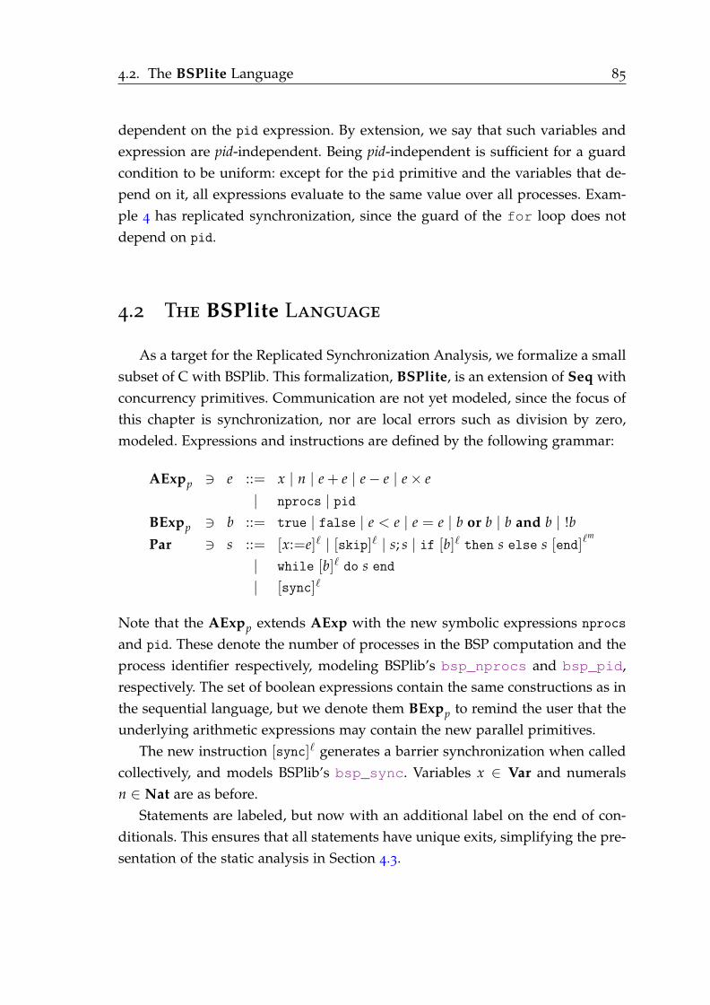
4.2. The BSPlite Language 85
dependent on the pid expression. By extension, we say that such variables and
expression are pid-independent. Being pid-independent is sufficient for a guard
condition to be uniform: except for the pid primitive and the variables that de-
pend on it, all expressions evaluate to the same value over all processes. Exam-
ple 4 has replicated synchronization, since the guard of the for loop does not
depend on pid.
4.2 The BSPlite Language
As a target for the Replicated Synchronization Analysis, we formalize a small
subset of C with BSPlib. This formalization, BSPlite, is an extension of Seq with
concurrency primitives. Communication are not yet modeled, since the focus of
this chapter is synchronization, nor are local errors such as division by zero,
modeled. Expressions and instructions are defined by the following grammar:
AExpp ∋ e ::= x | n | e + e | e− e | e× e
| nprocs | pid
BExpp ∋ b ::= true | false | e < e | e = e | b or b | b and b | !b
Par ∋ s ::= [x:=e]ℓ | [skip]ℓ | s; s | if [b]ℓ then s else s [end]ℓm
| while [b]ℓ do s end
| [sync]ℓ
Note that the AExpp extends AExp with the new symbolic expressions nprocs
and pid. These denote the number of processes in the BSP computation and the
process identifier respectively, modeling BSPlib’s bsp_nprocs and bsp_pid,
respectively. The set of boolean expressions contain the same constructions as in
the sequential language, but we denote them BExpp to remind the user that the
underlying arithmetic expressions may contain the new parallel primitives.
The new instruction [sync]ℓ generates a barrier synchronization when called
collectively, and models BSPlib’s bsp_sync. Variables x ∈ Var and numerals
n ∈ Nat are as before.
Statements are labeled, but now with an additional label on the end of con-
ditionals. This ensures that all statements have unique exits, simplifying the pre-
sentation of the static analysis in Section 4.3.

86 Chapter 4. Replicated Synchronization
AJ · Ki : AExpp → (State→ Nat) i ∈ Pid
AJxKi σ = σ(x)
AJnKi σ = n
AJe1 + e2Ki σ = AJe1Ki σ +AJe2Ki σ...
AJpidKi σ = i
AJnprocsKi σ = p
Figure 4.2 – Semantics of arithmetic expressions
BJ·Ki : BExpp → (State→ Bool) i ∈ Pid
BJtrueKi σ = tt
BJfalseKi σ = ff
BJe1 < e2Ki σ = tt if AJe1Ki σ < AJe2Ki σ, ff oth....
Figure 4.3 – Semantics of boolean expressions
4.2.1 Operational Semantics
The operational semantics of BSPlite models BSPlib, but is simplified due to the
exclusion of communication and local errors. The semantics is parameterized
by the number p > 0 of processors of the underlying BSP machine. The set of
process identifiers is Pid = 0, . . . , p− 1.
The semantics of numerical and boolean expressions, parameterized by the
local process number i, is given by AJ·Ki and BJ·Ki, respectively. These functions
extend AJ·K and BJ·K with the semantics of the primitives pid and nprocs, and
are partially given in Figures 4.2 and 4.3. Remaining cases can be derived in the
natural way.
The operational semantics for BSPlite programs is divided into local and
global rules operating on state p-vectors. Intuitively, the local rules, an extension
of the semantics of Seq, compute the new state of one component in the state
vector, corresponding to one processor. An optional continuation describes the
next step of local computation. The global rules compute the new state of a com-
plete state vector by applying the local rules to each component and, after syn-
chronization, possibly performing any remaining computations by re-applying
the global rules.
The semantics of local computation is given by the evaluation relation →i,
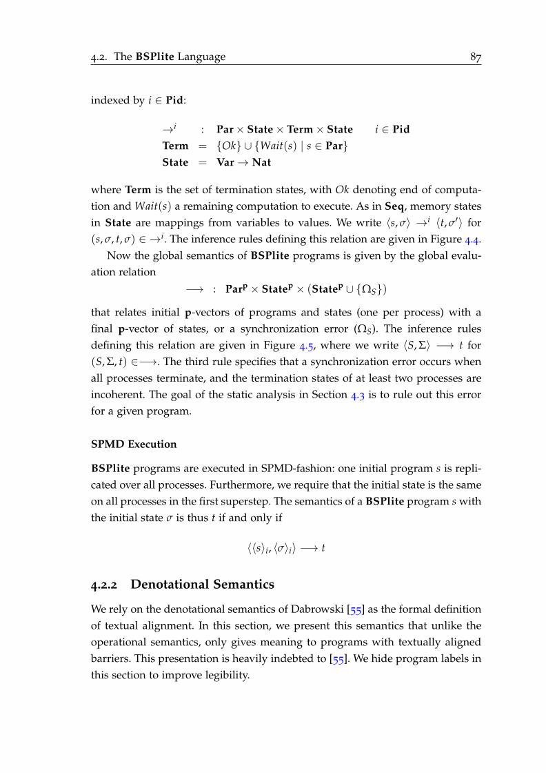
4.2. The BSPlite Language 87
indexed by i ∈ Pid:
→i : Par× State× Term× State i ∈ Pid
Term = Ok ∪ Wait(s) | s ∈ Par
State = Var→ Nat
where Term is the set of termination states, with Ok denoting end of computa-
tion and Wait(s) a remaining computation to execute. As in Seq, memory states
in State are mappings from variables to values. We write 〈s, σ〉 →i 〈t, σ′〉 for
(s, σ, t, σ) ∈ →i. The inference rules defining this relation are given in Figure 4.4.
Now the global semantics of BSPlite programs is given by the global evalu-
ation relation
−→ : Parp × Statep × (Statep ∪ ΩS)
that relates initial p-vectors of programs and states (one per process) with a
final p-vector of states, or a synchronization error (ΩS). The inference rules
defining this relation are given in Figure 4.5, where we write 〈S, Σ〉 −→ t for
(S, Σ, t) ∈−→. The third rule specifies that a synchronization error occurs when
all processes terminate, and the termination states of at least two processes are
incoherent. The goal of the static analysis in Section 4.3 is to rule out this error
for a given program.
SPMD Execution
BSPlite programs are executed in SPMD-fashion: one initial program s is repli-
cated over all processes. Furthermore, we require that the initial state is the same
on all processes in the first superstep. The semantics of a BSPlite program s with
the initial state σ is thus t if and only if
〈〈s〉i, 〈σ〉i〉 −→ t
4.2.2 Denotational Semantics
We rely on the denotational semantics of Dabrowski [55] as the formal definition
of textual alignment. In this section, we present this semantics that unlike the
operational semantics, only gives meaning to programs with textually aligned
barriers. This presentation is heavily indebted to [55]. We hide program labels in
this section to improve legibility.
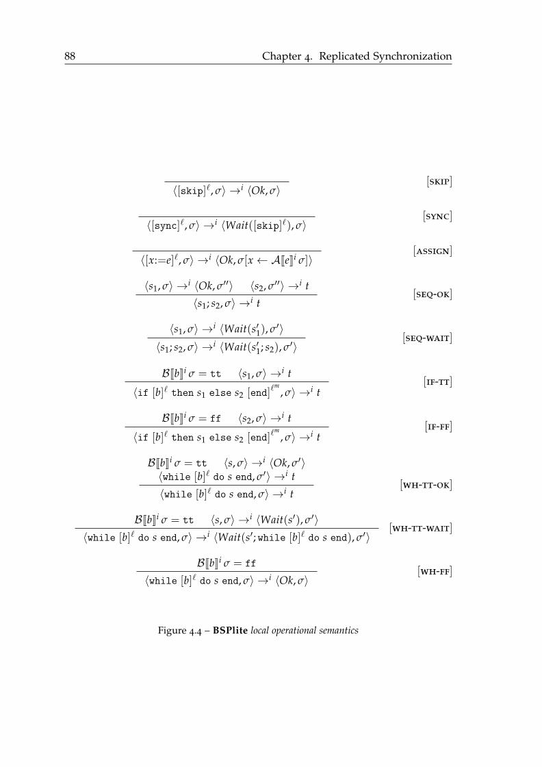
88 Chapter 4. Replicated Synchronization
〈[skip]ℓ, σ〉 →i 〈Ok, σ〉[skip]
〈[sync]ℓ, σ〉 →i 〈Wait([skip]ℓ), σ〉[sync]
〈[x:=e]ℓ, σ〉 →i 〈Ok, σ[x ← AJeKi σ]〉[assign]
〈s1, σ〉 →i 〈Ok, σ′′〉 〈s2, σ′′〉 →i t
〈s1; s2, σ〉 →i t[seq-ok]
〈s1, σ〉 →i 〈Wait(s′1), σ′〉
〈s1; s2, σ〉 →i 〈Wait(s′1; s2), σ′〉[seq-wait]
BJbKi σ = tt 〈s1, σ〉 →i t
〈if [b]ℓ then s1 else s2 [end]ℓm
, σ〉 →i t[if-tt]
BJbKi σ = ff 〈s2, σ〉 →i t
〈if [b]ℓ then s1 else s2 [end]ℓm
, σ〉 →i t[if-ff]
BJbKi σ = tt 〈s, σ〉 →i 〈Ok, σ′〉〈while [b]ℓ do s end, σ′〉 →i t
〈while [b]ℓ do s end, σ〉 →i t[wh-tt-ok]
BJbKi σ = tt 〈s, σ〉 →i 〈Wait(s′), σ′〉
〈while [b]ℓ do s end, σ〉 →i 〈Wait(s′; while [b]ℓ do s end), σ′〉[wh-tt-wait]
BJbKi σ = ff
〈while [b]ℓ do s end, σ〉 →i 〈Ok, σ〉[wh-ff]
Figure 4.4 – BSPlite local operational semantics

4.2. The BSPlite Language 89
∀i ∈ Pid, 〈S[i], Σ[i]〉 →i 〈Ok, Σ′[i]〉
〈S, Σ〉 −→ Σ′[all-ok]
∀i ∈ Pid, 〈S[i], Σ[i]〉 →i 〈Wait(S′[i]), Σ′[i]〉 〈S′, Σ′〉 −→ t
〈S, Σ〉 −→ t[all-wait]
∀i ∈ Pid, 〈S[i], Σ[i]〉 →i 〈T[i], Σ′[i]〉∃i ∈ Pid, T[i] = Ok ∃j ∈ Pid, T[j] = Wait(s)
〈S, Σ〉 −→ ΩS[glb-err]
Figure 4.5 – BSPlite global operational semantics
Semantic domain The denotational semantics of BSPlite programs is given
by functions ranging over p-vectors of environments, with optionally hidden
components. Vectors are the elements of D defined by
D = (State000)p ∪ ⊥, ΩS
where State000 stands for State ∪ 000 and 000 is a special constant denoting an
hidden component. As usual, ⊥ denotes non-termination, and as in the oper-
ational semantics, ΩS denotes a synchronization error. For I ⊆ Pid, we note
DI = θ ∈ D \ ⊥, ΩS | θ i = 000 ⇐⇒ i 6∈ I. We now define three operations
over vectors: update, mask and combine. These are formally defined in Figure 4.6.
Intuitively, they can be understood thus:
• The update function updates environments pointwise where visible.
• The mask function hides components at which the condition does not hold.
• The combine function combines two vectors which must not have common
visible components.
Semantic functions The semantic functions of BSPlite statements are given in
Figure 4.7.
• Functions Jx := eK, JskipK and Js1; s2K operate pointwise in the standard
way.
• The function JsyncK verifies that either all components or none are involved
in the computation. Otherwise, an error is returned: thus mimicking the
behavior of a global synchronization barrier.
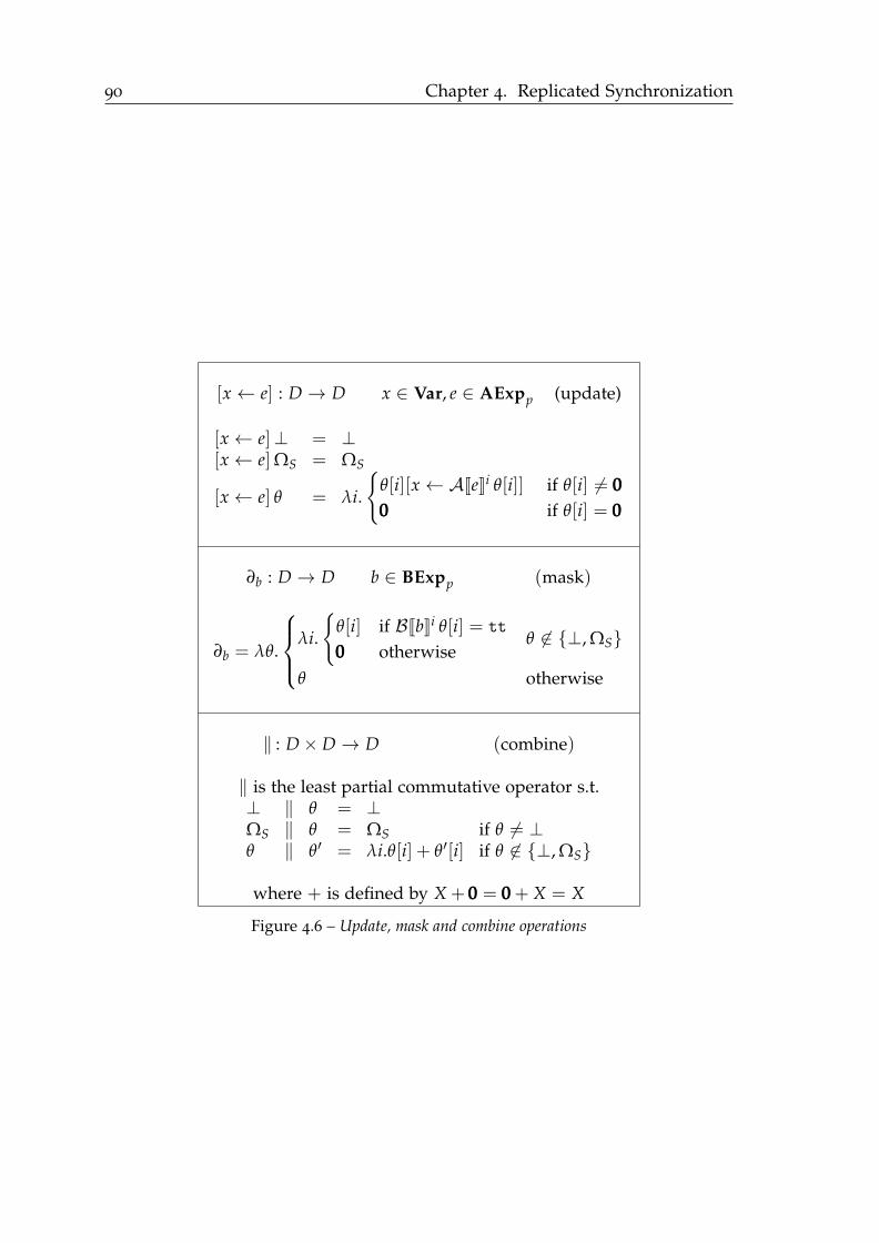
90 Chapter 4. Replicated Synchronization
[x ← e] : D → D x ∈ Var, e ∈ AExpp (update)
[x ← e]⊥ = ⊥[x ← e]ΩS = ΩS
[x ← e] θ = λi.
θ[i][x ← AJeKi θ[i]] if θ[i] 6= 000
000 if θ[i] = 000
∂b : D → D b ∈ BExpp (mask)
∂b = λθ.
λi.
θ[i] if BJbKi θ[i] = tt
000 otherwiseθ 6∈ ⊥, ΩS
θ otherwise
‖ : D× D → D (combine)
‖ is the least partial commutative operator s.t.⊥ ‖ θ = ⊥ΩS ‖ θ = ΩS if θ 6= ⊥θ ‖ θ′ = λi.θ[i] + θ′[i] if θ 6∈ ⊥, ΩS
where + is defined by X + 000 = 000 + X = X
Figure 4.6 – Update, mask and combine operations
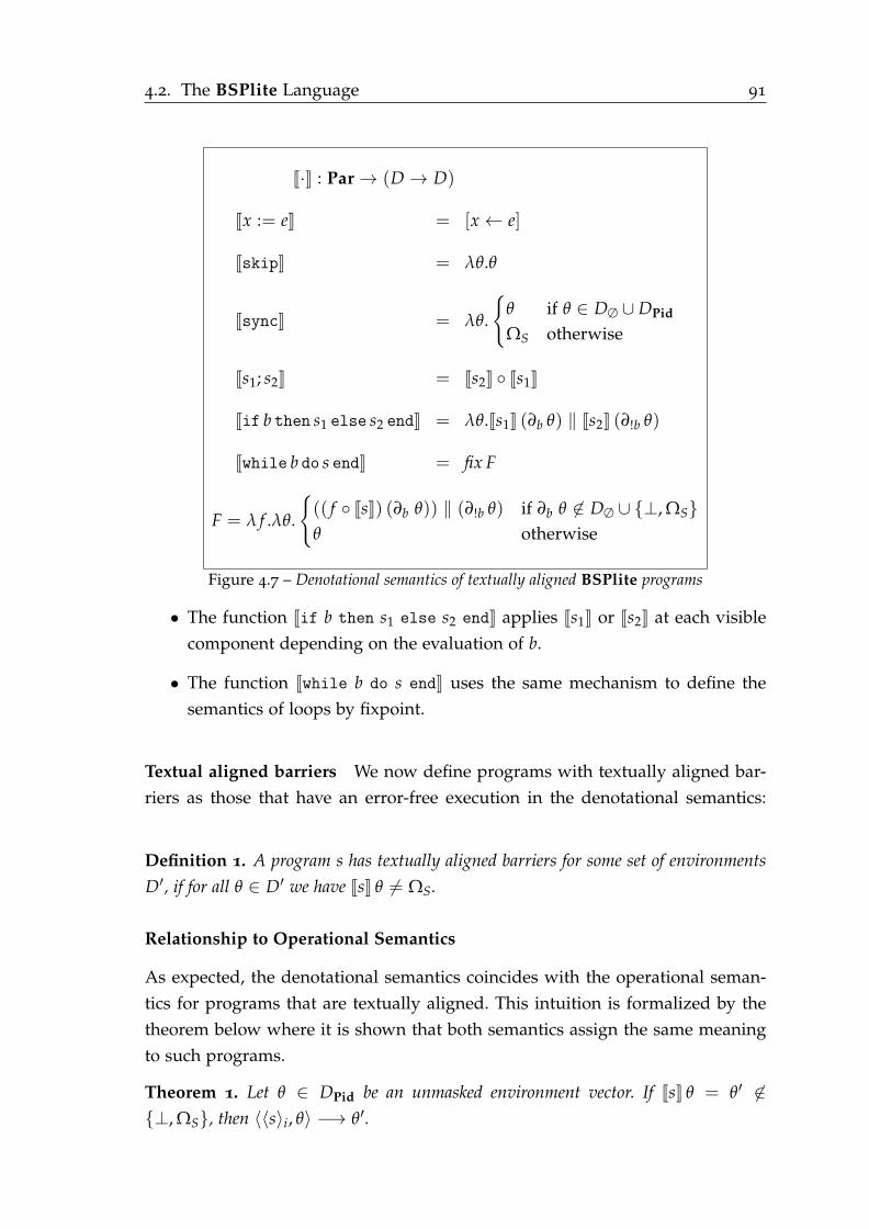
4.2. The BSPlite Language 91
J·K : Par→ (D → D)
Jx := eK = [x ← e]
JskipK = λθ.θ
JsyncK = λθ.
θ if θ ∈ D∅ ∪ DPid
ΩS otherwise
Js1; s2K = Js2K Js1K
Jif b then s1 else s2 endK = λθ.Js1K (∂b θ) ‖ Js2K (∂!b θ)
Jwhile b do s endK = fix F
F = λ f .λθ.
(( f JsK) (∂b θ)) ‖ (∂!b θ) if ∂b θ 6∈ D∅ ∪ ⊥, ΩS
θ otherwise
Figure 4.7 – Denotational semantics of textually aligned BSPlite programs
• The function Jif b then s1 else s2 endK applies Js1K or Js2K at each visible
component depending on the evaluation of b.
• The function Jwhile b do s endK uses the same mechanism to define the
semantics of loops by fixpoint.
Textual aligned barriers We now define programs with textually aligned bar-
riers as those that have an error-free execution in the denotational semantics:
Definition 1. A program s has textually aligned barriers for some set of environments
D′, if for all θ ∈ D′ we have JsK θ 6= ΩS.
Relationship to Operational Semantics
As expected, the denotational semantics coincides with the operational seman-
tics for programs that are textually aligned. This intuition is formalized by the
theorem below where it is shown that both semantics assign the same meaning
to such programs.
Theorem 1. Let θ ∈ DPid be an unmasked environment vector. If JsK θ = θ′ 6∈
⊥, ΩS, then 〈〈s〉i, θ〉 −→ θ′.

92 Chapter 4. Replicated Synchronization
Proof: See Appendix A.1.
It follows immediately that if a program that terminates without error under
the denotational semantics, then it also does so in the operational semantics:
Corollary 1. If ∀θ ∈ Statep, JsK θ 6∈ ⊥, ΩS then ∀θ ∈ Statep, 〈〈s〉i, θ〉 6−→ ΩS.
As noted in Section 4.1.1, a program may be well-synchronized, although
non-textually aligned. The relationship between the operational and denota-
tional semantics reflect this fact. Consider the Example 2, given in Figure 4.1.
The denotational semantics returns an error for this program in any environment
with at least two processes, as the sync primitives are executed with masked en-
vironments. The operational semantics, on the other hand, does not return an
error since each process executes exactly one sync. The denotational semantics
forbids such partial synchronization, and anything that happens after it is con-
sidered undefined behavior. The static analysis presented in the next section
rules out programs where such non-textually aligned synchronizations occur.
4.3 Static Approximation of Textual Alignment
Replicated synchronization, the static approximation of textual alignment,
is verified by a restricted version of the Type and Effect System of Aiken and
Gay for Barrier Inference [5]. We reformulate Barrier Inference as a data-flow
analysis, restricted to identify programs with replicated synchronization, and
prove it correct with respect to the semantics of BSPlite.
The analysis is divided into two phases: (1) a data-flow analysis which under-
approximates the set of “pid-independent” variables at each program point —
variables which do not have a data or control dependency on the special pid
primitive; (2) a structural analysis that uses the result of the data-flow analysis
to verify that each branching statement has a pid-independent guard expression,
or that its sub-statements are syntactically synchronization-free.
The program snok in Figure 4.8 is used as running example. This program
is erroneous, since the sync labeled 6 will only be executed by one process if
p ≥ 4. This happens since the condition labeled 3 is not pid-independent, due to
the data dependence of x on pid from the assignment labeled 2. As we will see
in the rest of this section, the analysis rejects this program for same reason.
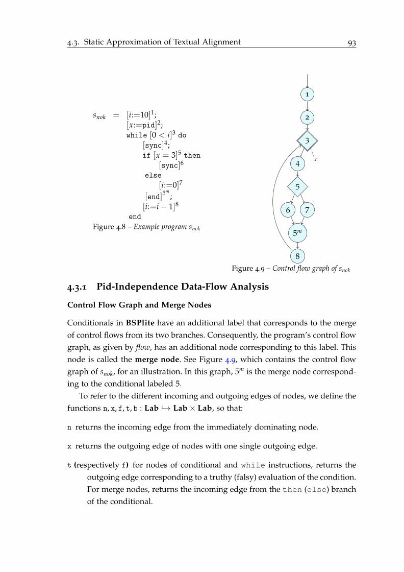
4.3. Static Approximation of Textual Alignment 93
snok = [i:=10]1;[x:=pid]2;while [0 < i]3 do
[sync]4;if [x = 3]5 then
[sync]6
else
[i:=0]7
[end]5m
;[i:=i− 1]8
end
Figure 4.8 – Example program snok
1
2
3
4
5
7
5m
8
6
Figure 4.9 – Control flow graph of snok
4.3.1 Pid-Independence Data-Flow Analysis
Control Flow Graph and Merge Nodes
Conditionals in BSPlite have an additional label that corresponds to the merge
of control flows from its two branches. Consequently, the program’s control flow
graph, as given by flow, has an additional node corresponding to this label. This
node is called the merge node. See Figure 4.9, which contains the control flow
graph of snok, for an illustration. In this graph, 5m is the merge node correspond-
ing to the conditional labeled 5.
To refer to the different incoming and outgoing edges of nodes, we define the
functions n, x, f, t, b : Lab → Lab× Lab, so that:
n returns the incoming edge from the immediately dominating node.
x returns the outgoing edge of nodes with one single outgoing edge.
t (respectively f) for nodes of conditional and while instructions, returns the
outgoing edge corresponding to a truthy (falsy) evaluation of the condition.
For merge nodes, returns the incoming edge from the then (else) branch
of the conditional.
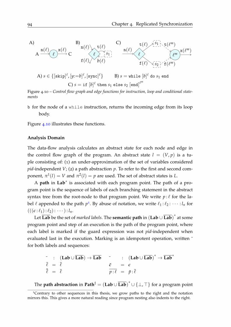
94 Chapter 4. Replicated Synchronization
A)
A ℓ Cn(ℓ) x(ℓ)
B)
ℓ s1
n(ℓ)
f(ℓ)
t(ℓ)
b(ℓ)
C)
ℓ
s1
s2
ℓmn(ℓ)
t(ℓ)
f(ℓ)
t(ℓm)
f(ℓm)
x(ℓm)
A) s ∈ [skip]ℓ, [y:=b]ℓ, [sync]ℓ B) s = while [b]ℓ do s1 end
C) s = if [b]ℓ then s1 else s2 [end]ℓm
Figure 4.10 – Control flow graph and edge functions for instruction, loop and conditional state-ments
b for the node of a while instruction, returns the incoming edge from its loop
body.
Figure 4.10 illustrates these functions.
Analysis Domain
The data-flow analysis calculates an abstract state for each node and edge in
the control flow graph of the program. An abstract state l = (V, p) is a tu-
ple consisting of: (1) an under-approximation of the set of variables considered
pid-independent V; (2) a path abstraction p. To refer to the first and second com-
ponent, π1(l) = V and π2(l) = p are used. The set of abstract states is L.
A path in Lab∗ is associated with each program point. The path of a pro-
gram point is the sequence of labels of each branching statement in the abstract
syntax tree from the root-node to that program point. We write p : ℓ for the la-
bel ℓ appended to the path p1. By abuse of notation, we write ℓ1 : ℓ2 : · · · : ln for
(((ǫ : ℓ1) : ℓ2) : · · · ) : ln.
Let Lab be the set of marked labels. The semantic path in (Lab ∪ Lab)∗
at some
program point and step of an execution is the path of the program point, where
each label is marked if the guard expression was not pid-independent when
evaluated last in the execution. Marking is an idempotent operation, written ¯
for both labels and sequences:
¯ : (Lab ∪ Lab)→ Lab
ℓ = ℓ¯ℓ = ℓ
¯ : (Lab ∪ Lab)∗→ Lab
∗
ǫ = ǫ
p : ℓ = p : ℓ
The path abstraction in Path♯ = (Lab ∪ Lab)∗∪ ⊥,⊤ for a program point
1Contrary to other sequences in this thesis, we grow paths to the right and the notationmirrors this. This gives a more natural reading since program nesting also indents to the right.
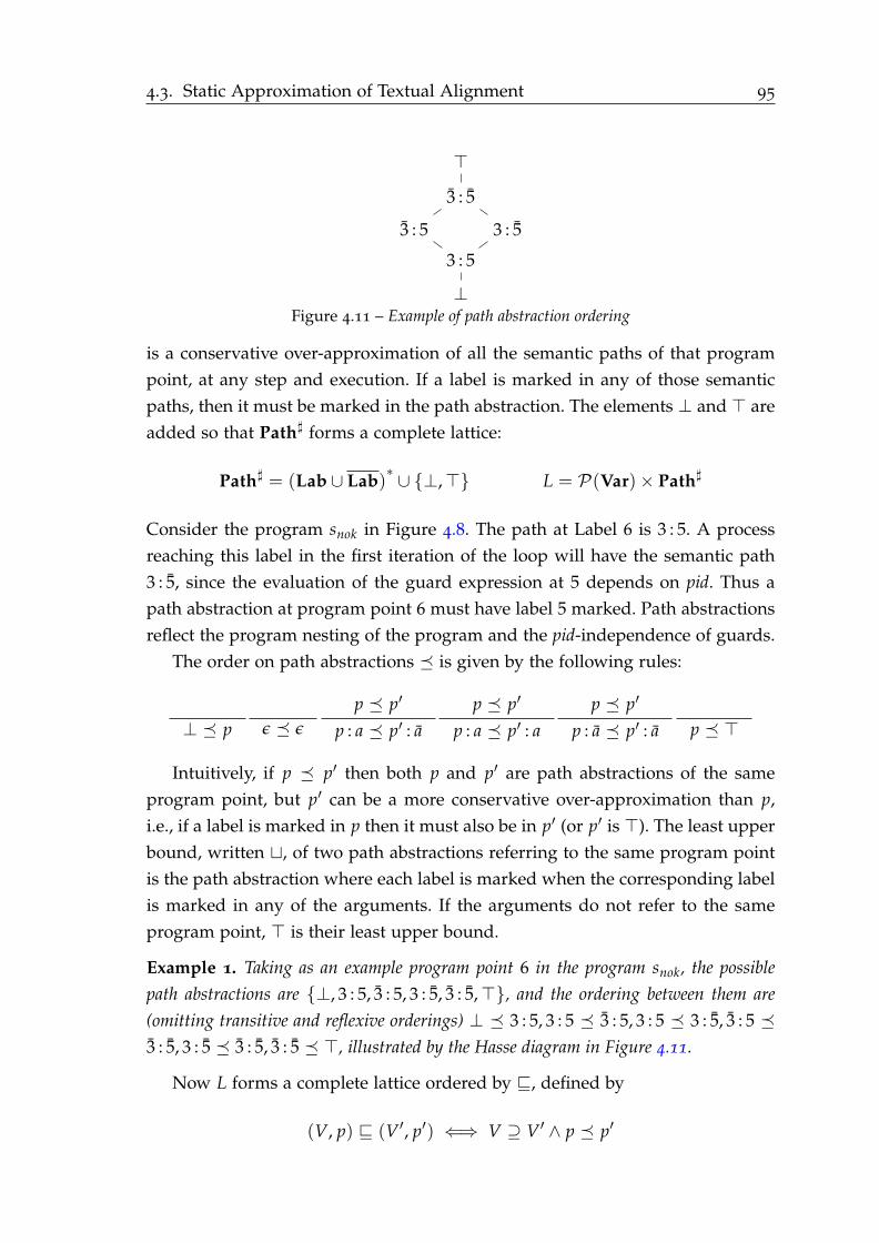
4.3. Static Approximation of Textual Alignment 95
⊤
3 : 5
3 : 53 : 5
3 : 5
⊥Figure 4.11 – Example of path abstraction ordering
is a conservative over-approximation of all the semantic paths of that program
point, at any step and execution. If a label is marked in any of those semantic
paths, then it must be marked in the path abstraction. The elements ⊥ and ⊤ are
added so that Path♯ forms a complete lattice:
Path♯ = (Lab ∪ Lab)∗∪ ⊥,⊤ L = P(Var)× Path♯
Consider the program snok in Figure 4.8. The path at Label 6 is 3 : 5. A process
reaching this label in the first iteration of the loop will have the semantic path
3 : 5, since the evaluation of the guard expression at 5 depends on pid. Thus a
path abstraction at program point 6 must have label 5 marked. Path abstractions
reflect the program nesting of the program and the pid-independence of guards.
The order on path abstractions is given by the following rules:
⊥ p ǫ ǫ
p p′
p : a p′ : a
p p′
p : a p′ : a
p p′
p : a p′ : a p ⊤
Intuitively, if p p′ then both p and p′ are path abstractions of the same
program point, but p′ can be a more conservative over-approximation than p,
i.e., if a label is marked in p then it must also be in p′ (or p′ is ⊤). The least upper
bound, written ⊔, of two path abstractions referring to the same program point
is the path abstraction where each label is marked when the corresponding label
is marked in any of the arguments. If the arguments do not refer to the same
program point, ⊤ is their least upper bound.
Example 1. Taking as an example program point 6 in the program snok, the possible
path abstractions are ⊥, 3 : 5, 3 : 5, 3 : 5, 3 : 5,⊤, and the ordering between them are
(omitting transitive and reflexive orderings) ⊥ 3 : 5, 3 : 5 3 : 5, 3 : 5 3 : 5, 3 : 5
3 : 5, 3 : 5 3 : 5, 3 : 5 ⊤, illustrated by the Hasse diagram in Figure 4.11.
Now L forms a complete lattice ordered by ⊑, defined by
(V, p) ⊑ (V′, p′) ⇐⇒ V ⊇ V′ ∧ p p′

96 Chapter 4. Replicated Synchronization
As data-flow analysis in our formulation aims to find the smallest abstract state
for each program point, this order rhymes with our intuition. Namely, that we
want find the largest set of pid-independent variables at each program point and
a path abstraction with the fewest marked guard expressions.
Path abstractions are modified by concatenating labels to existing path ab-
stractions using a concatenation operator (.), and by merging path abstractions
using the merge operator (), defined below. Merging removes the last label
from the two path abstractions of the same program point and returns the least
upper bound of the remaining path abstractions.
(.) : Path♯ × (Lab ∪ Lab)→ Path♯ (concatenation)
p.ℓ =
p : ℓ if p ∈ (Lab ∪ Lab)∗
p otherwise
: Path♯ × Path♯ → Path♯ (merge)
is the least commutative operator such that
p.ℓ p′.ℓ′ = p ⊔ p′ if p.ℓ = p′.ℓ′
⊥ p.ℓ = p
⊥ ⊥ = ⊥
p p′ = ⊤ otherwise
When the nesting of programs deepens, as in the body of while and if
statements, the concatenation operator is used to form the path abstraction of the
nested program points. As nesting becomes more shallow, such as when leaving
the body of while and if statements, the merge operator is used to form the
path abstraction of the program points following the branching statement.
Data-Flow Equations
The analysis computes an abstract state from L in each node in the control flow
graph of a program. The abstract state of each node of a program s is defined
by an equation system is given by PI(s). This system defines two functions,
which are defined in terms of each other. First, PI : Lab→ L that gives abstract
state stored in each node (the incoming state). This abstract state in each node
is defined in terms of the outgoing state on each label. The second function,
PI• : Lab × Lab → L, gives the outgoing state. It is obtained by applying a
transfer function that updates the abstract state of the source node according to
the nature of the edge.
Contrary to the presentation in Section 2.4, this formulation allows nodes to

4.3. Static Approximation of Textual Alignment 97
exprs((x = 3)) = (x = 3), (x), (3) free((x = 3)) = x
Figure 4.12 – Examples of the functions exprs and free
φd(e, V) = pid 6∈ exprs(e) ∧ free(e) ⊆ Vφc(p) = p ∈ Lab∗ ∪ ⊥
cdep(ℓ, e, V) =
ℓ if φd(e, V)
ℓ otherwise
vdep((V, p), e, x) =
V ∪ x if φd(e, V) ∧ φc(p)
V \ x otherwise
Figure 4.13 – The predicates φd and φc and the functions cdep and vdep
have distinct outgoing abstract states on different outgoing edges. Furthermore,
the incoming state will not be the least upper bound on the outgoing abstract
states of the predecessors, but a function on incoming abstract states that joins
incoming states in a node-dependent manner.
Before defining PI(s), we define the predicates φd (pid data-independent)
and φc (pid control-independent) and the functions cdep and vdep (Figure 4.13),
where exprs(e) gives the sub-expressions of an arithmetic or boolean expression e
and free(e) is the set of free variables (see Figure 4.12 for illustrations of the exprs
and free functions).
The function cdep(ℓ, e, V) is used at branching statements and marks the la-
bel ℓ when the guard expression e is not data-independent from pid, as deter-
mined by the predicate φd(e, V). This predicate holds if the expression e does not
contain the primitive pid nor any potentially pid-dependent variables. The func-
tion vdep((V, p), e, x) is used at assignments to conditionally add (respectively
remove) the assigned variable x to the set of pid-independent variables V, when
the assigned expression e is (respectively may not be) data and control indepen-
dent on pid, as determined by the predicates φd(e, V) and φc(p). The latter holds
for a non-⊤ path abstraction that contains no marked labels.
For each node labeled ℓ in flow(s), depending on the type of command s′
that ℓ belongs to, the equation system PI(s) defines the functions PI and PI• in

98 Chapter 4. Replicated Synchronization
terms of each other by the following scheme:
PI(ℓ) = (Vars, ǫ) if init(s) = ℓ
PI(ℓ) = PI•(n(ℓ))
PI•(x(ℓ)) = PI(ℓ)if s′ = [skip]ℓ or s′ = [sync]ℓ
PI(ℓ) = PI•(n(ℓ))
PI•(x(ℓ)) = (vdep((V, p), e, y), p)
where (V, p) = PI(ℓ)
if s′ = [y:=e]ℓ
PI(ℓ) = PI•(n(ℓ))
PI•(t(ℓ)) = (V, p.cdep(ℓ, b, V))
PI•(f(ℓ)) = (V, p.cdep(ℓ, b, V))
where (V, p) = PI(ℓ)
if s′ = if [b]ℓ then c1 else c2 [end]
PI(ℓm) = (Vt ∩Vf, pt pf)
where (Vt, pt) = PI•(t(ℓm))
(Vf, pf) = PI•(f(ℓm))
PI•(x(ℓm)) = PI(ℓm)
if s′ = if [b] then c1 else c2 [end]ℓm
PI(ℓ) = (Vn ∩Vb, pn.ℓ pb)
where (Vn, pn) = PI•(n(ℓ))
(Vb, pb) = PI•(b(ℓ))
PI•(t(ℓ)) = (V, p.cdep(ℓ, b, V))
where (V, p) = PI(ℓ)
PI•(f(ℓ)) = PI(ℓ)
if s′ = while [b]ℓ do c1 end
Each data-flow equation defines the set of pid-independent variables and the
path abstraction for the corresponding node or edge. In the initial node, we
consider all variables of s (as given by Vars) pid-independent, and the path ab-
straction is empty. The set of variables at a node is the intersection of the pid-
independent variables on all incoming edges, which ensures that the outgoing
edges contain the variables which must be independent on all incoming paths.
Additionally, at assignments, we add (or remove) the assigned variable when the
assigned expression is pid-independent (or may not be pid-independent) in the
abstract state on the incoming edge, using the vdep-function.
The data-flow equations define the path abstraction of each node so that it
follows the nesting structure of the program. Accordingly, skip, sync and assign-
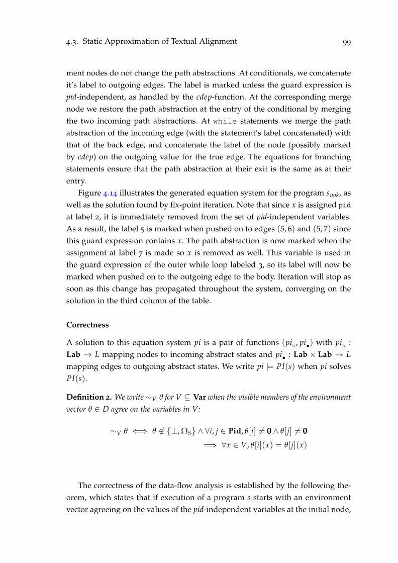
4.3. Static Approximation of Textual Alignment 99
ment nodes do not change the path abstractions. At conditionals, we concatenate
it’s label to outgoing edges. The label is marked unless the guard expression is
pid-independent, as handled by the cdep-function. At the corresponding merge
node we restore the path abstraction at the entry of the conditional by merging
the two incoming path abstractions. At while statements we merge the path
abstraction of the incoming edge (with the statement’s label concatenated) with
that of the back edge, and concatenate the label of the node (possibly marked
by cdep) on the outgoing value for the true edge. The equations for branching
statements ensure that the path abstraction at their exit is the same as at their
entry.
Figure 4.14 illustrates the generated equation system for the program snok, as
well as the solution found by fix-point iteration. Note that since x is assigned pid
at label 2, it is immediately removed from the set of pid-independent variables.
As a result, the label 5 is marked when pushed on to edges (5, 6) and (5, 7) since
this guard expression contains x. The path abstraction is now marked when the
assignment at label 7 is made so x is removed as well. This variable is used in
the guard expression of the outer while loop labeled 3, so its label will now be
marked when pushed on to the outgoing edge to the body. Iteration will stop as
soon as this change has propagated throughout the system, converging on the
solution in the third column of the table.
Correctness
A solution to this equation system pi is a pair of functions (pi, pi•) with pi :
Lab → L mapping nodes to incoming abstract states and pi• : Lab× Lab → L
mapping edges to outgoing abstract states. We write pi |= PI(s) when pi solves
PI(s).
Definition 2. We write∼V θ for V ⊆ Var when the visible members of the environment
vector θ ∈ D agree on the variables in V:
∼V θ ⇐⇒ θ 6∈ ⊥, ΩS ∧ ∀i, j ∈ Pid, θ[i] 6= 000∧ θ[j] 6= 000
=⇒ ∀x ∈ V, θ[i](x) = θ[j](x)
The correctness of the data-flow analysis is established by the following the-
orem, which states that if execution of a program s starts with an environment
vector agreeing on the values of the pid-independent variables at the initial node,
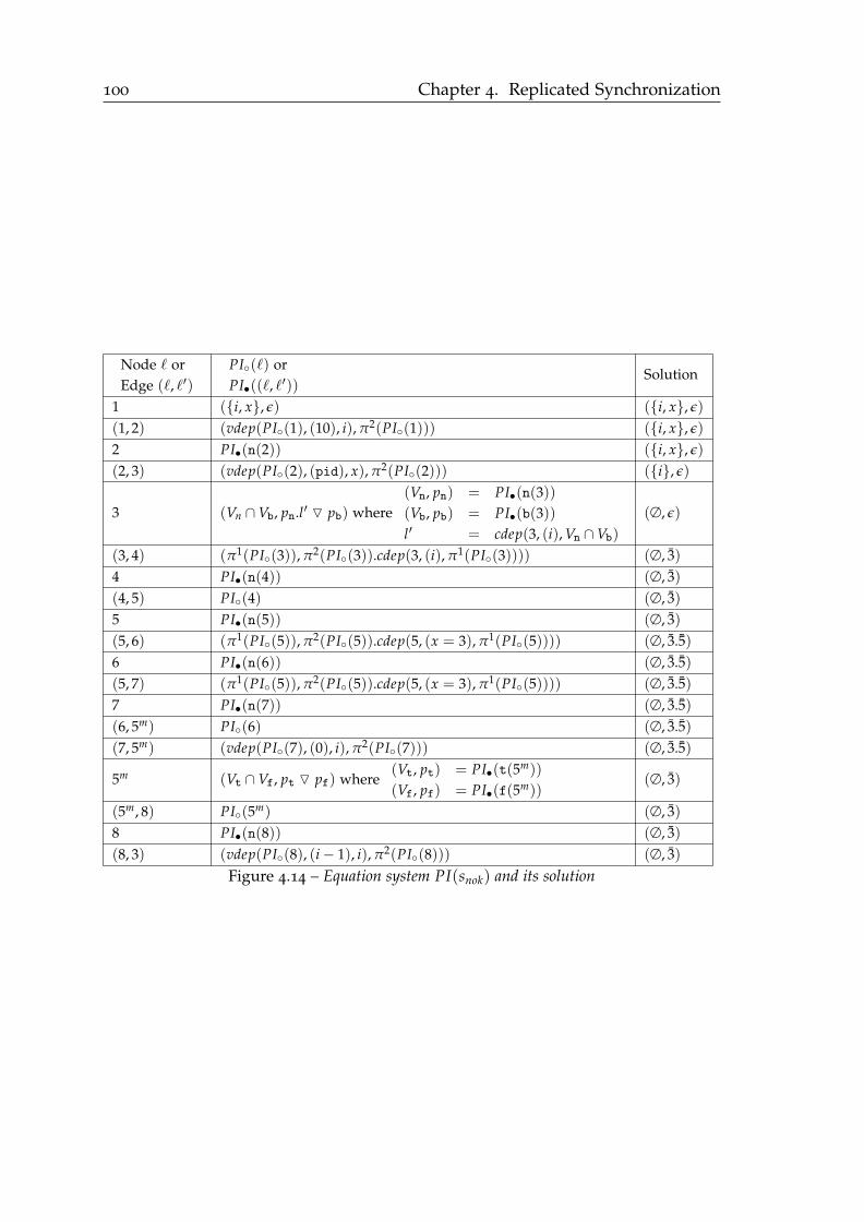
100 Chapter 4. Replicated Synchronization
Node ℓ or
Edge (ℓ, ℓ′)
PI(ℓ) or
PI•((ℓ, ℓ′))Solution
1 (i, x, ǫ) (i, x, ǫ)
(1, 2) (vdep(PI(1), (10), i), π2(PI(1))) (i, x, ǫ)
2 PI•(n(2)) (i, x, ǫ)
(2, 3) (vdep(PI(2), (pid), x), π2(PI(2))) (i, ǫ)
3 (Vn ∩Vb, pn.l′ pb) where
(Vn, pn) = PI•(n(3))
(Vb, pb) = PI•(b(3))
l′ = cdep(3, (i), Vn ∩Vb)
(∅, ǫ)
(3, 4) (π1(PI(3)), π2(PI(3)).cdep(3, (i), π1(PI(3)))) (∅, 3)
4 PI•(n(4)) (∅, 3)
(4, 5) PI(4) (∅, 3)
5 PI•(n(5)) (∅, 3)
(5, 6) (π1(PI(5)), π2(PI(5)).cdep(5, (x = 3), π1(PI(5)))) (∅, 3.5)
6 PI•(n(6)) (∅, 3.5)
(5, 7) (π1(PI(5)), π2(PI(5)).cdep(5, (x = 3), π1(PI(5)))) (∅, 3.5)
7 PI•(n(7)) (∅, 3.5)
(6, 5m) PI(6) (∅, 3.5)
(7, 5m) (vdep(PI(7), (0), i), π2(PI(7))) (∅, 3.5)
5m (Vt ∩Vf, pt pf) where(Vt, pt) = PI•(t(5m))
(Vf, pf) = PI•(f(5m))(∅, 3)
(5m, 8) PI(5m) (∅, 3)
8 PI•(n(8)) (∅, 3)
(8, 3) (vdep(PI(8), (i− 1), i), π2(PI(8))) (∅, 3)
Figure 4.14 – Equation system PI(snok) and its solution
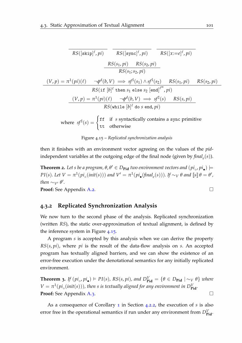
4.3. Static Approximation of Textual Alignment 101
RS([skip]ℓ, pi) RS([sync]ℓ, pi) RS([x:=e]ℓ, pi)
RS(s1, pi) RS(s2, pi)
RS(s1; s2, pi)
(V, p) = π1(pi)(ℓ) ¬φd(b, V) =⇒ sf ♯(s1) ∧ sf ♯(s2) RS(s1, pi) RS(s2, pi)
RS(if [b]ℓ then s1 else s2 [end]ℓm
, pi)
(V, p) = π1(pi)(ℓ) ¬φd(b, V) =⇒ sf ♯(s) RS(s, pi)
RS(while [b]ℓ do s end, pi)
where sf ♯(s) =
ff if s syntactically contains a sync primitive
tt otherwise
Figure 4.15 – Replicated synchronization analysis
then it finishes with an environment vector agreeing on the values of the pid-
independent variables at the outgoing edge of the final node (given by finale(s)).
Theorem 2. Let s be a program, θ, θ′ ∈ DPid two environment vectors and (pi, pi•) |=
PI(s). Let V = π1(pi(init(s))) and V′ = π1(pi•(finale(s))). If ∼V θ and JsK θ = θ′,
then ∼V′ θ′.
Proof: See Appendix A.2.
4.3.2 Replicated Synchronization Analysis
We now turn to the second phase of the analysis. Replicated synchronization
(written RS), the static over-approximation of textual alignment, is defined by
the inference system in Figure 4.15.
A program s is accepted by this analysis when we can derive the property
RS(s, pi), where pi is the result of the data-flow analysis on s. An accepted
program has textually aligned barriers, and we can show the existence of an
error-free execution under the denotational semantics for any initially replicated
environment.
Theorem 3. If (pi, pi•) PI(s), RS(s, pi), and DVPid = θ ∈ DPid | ∼V θ where
V = π1(pi(init(s))), then s is textually aligned for any environment in DVPid.
Proof: See Appendix A.3.
As a consequence of Corollary 1 in Section 4.2.2, the execution of s is also
error free in the operational semantics if run under any environment from DVPid.
102 Chapter 4. Replicated Synchronization
We now see that the property RS cannot be derived for the unsafe program
snok. The rule for while statements requires that either the guard expression is
pid-independent, φd(b, V), which is not the case since the set of pid-independent
at program point 3 is ∅ (see the solution to PI(snok) in Figure 4.14), or that the
body is syntactically synchronization free, which is clearly not the case for this
loop due to the sync primitives labeled 4 and 6. Furthermore, the if statement
labeled 5 is rejected for the same reason.
Consider also the running examples of Figure 4.1. The examples accepted
by RS (if translated to BSPlite in the obvious way) are indicated by the col-
umn RS. Clearly, the guards of the conditionals in Examples 1 to 3 are not pid-
independent, since they contain the bsp_pid. Therefore, and since these con-
ditionals contain the bsp_sync primitive, RS can not be derived for these ex-
amples. As expected, the Example 1, which is not well-synchronized, is rejected.
On the other hand, the program in Example 2 is well-synchronized. But, it falls
outside the model of textually aligned barriers, and so cannot be accepted by the
analysis. Nor is Example 3 accepted, even though it has textually aligned barri-
ers. It is a victim of the static under-approximation of replicated synchronization.
The program Example 4 is textually aligned, and hence well-synchronized. It is
included in the static approximation of replicated synchronization, and hence
accepted by RS.
4.4 Implementation
The analysis has been implemented as a Frama-C plug-in in ∼1200 lines of
OCaml. It verifies the synchronization of BSPlib programs and programs using
Lightweight Parallel Foundations [183], a forthcoming BSP library developed at
Huawei.
Structures and arrays are handled conservatively by always assuming they
may depend on pid. We apply the same approximation to reads from the point-
ers, as well as reads from local variables that may be affected by communication.
The set of such variables is conservatively assumed to be those who have had
their address taken, since this is a prerequisite for DRMA communication in
BSPlib. We have also extended the analysis interprocedurally using small as-
sumption sets [151].
In the remainder of this section we deal with the issues encountered when
implementing the analysis in Frama-C.
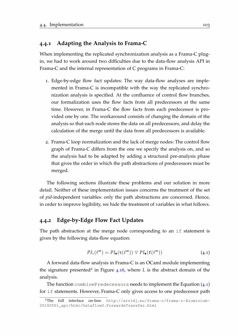
4.4. Implementation 103
4.4.1 Adapting the Analysis to Frama-C
When implementing the replicated synchronization analysis as a Frama-C plug-
in, we had to work around two difficulties due to the data-flow analysis API in
Frama-C and the internal representation of C programs in Frama-C:
1. Edge-by-edge flow fact updates: The way data-flow analyses are imple-
mented in Frama-C is incompatible with the way the replicated synchro-
nization analysis is specified. At the confluence of control flow branches,
our formalization uses the flow facts from all predecessors at the same
time. However, in Frama-C the flow facts from each predecessor is pro-
vided one by one. The workaround consists of changing the domain of the
analysis so that each node stores the data on all predecessors, and delay the
calculation of the merge until the data from all predecessors is available.
2. Frama-C loop normalization and the lack of merge nodes: The control flow
graph of Frama-C differs from the one we specify the analysis on, and so
the analysis had to be adapted by adding a structural pre-analysis phase
that gives the order in which the path abstractions of predecessors must be
merged.
The following sections illustrate these problems and our solution in more
detail. Neither of these implementation issues concerns the treatment of the set
of pid-independent variables: only the path abstractions are concerned. Hence,
in order to improve legibility, we hide the treatment of variables in what follows.
4.4.2 Edge-by-Edge Flow Fact Updates
The path abstraction at the merge node corresponding to an if statement is
given by the following data-flow equation:
PI(ℓm) = PI•(t(ℓ
m)) PI•(f(ℓm)) (4.1)
A forward data-flow analysis in Frama-C is an OCaml module implementing
the signature presented2 in Figure 4.16, where L is the abstract domain of the
analysis.
The function combinePredecessors needs to implement the Equation (4.1)
for if statements. However, Frama-C only gives access to one predecessor path
2The full interface on-line: http://arvidj.eu/frama-c/frama-c-Aluminium-
20160501_api/html/Dataflow2.ForwardsTransfer.html

104 Chapter 4. Replicated Synchronization
doInstr : Lab→ L→ LImplements the (forward) transfer function of an instruction.
combinePredecessors : Lab→ L→ L→ LReceives the label of a node ℓ, the previously stored data in this node(corresponding to PI(ℓ) in our presentation), and the outgoing datafrom some predecessor (corresponding to PI•(ℓ′, ℓ) for some unspecifiedpredecessor ℓ′). This function then returns the combination of the twoflow facts, which will be stored in the node.
doEdge : Lab→ Lab→ L→ LAllows the data-flow analysis to implement a specific transfer functionfor each outgoing edge. Can default to identity if no special handling isrequired.
Figure 4.16 – Simplified presentation of the signature of a module implementing a Frama-Cforward data-flow analysis
abstraction at a time. But, the Equation (4.1) depends on the path abstraction
from both incoming edges. Implementing the data-flow equation for loops is
hindered by the same problem. There, we need the path abstraction on the edge
of the immediate dominator node, and the path abstraction on the back edge of
the loop.
To overcome this problem, we change the analysis’s abstract domain of
our analysis to store the path abstractions on all incoming paths, as well as
their provenance, in each node. The implementation collects these values in
combinePredecessors, and then performs the merge in the transfer function
doEdge.
The modified abstract domain, ignoring variables, is given by path abstrac-
tion maps:
L′ = Lab→ Path♯
The interpretation of the abstract state l ∈ L′ at some program point ℓ in the
program s is that if l ℓ′ = p then PI•(ℓ′, ℓ) = p.
These total functions are implemented by finite maps from labels to path
abstractions with ⊥ taken as the default value for unmapped labels.
Path abstractions maps are partially ordered pointwise and the least upper
bound is pointwise:
l ⊑ l′ ⇐⇒ ∀ℓ ∈ Lab, l ℓ l′ ℓ
(l ⊔ l′) ℓ = (l ℓ) ⊔Path♯ (l′ ℓ)
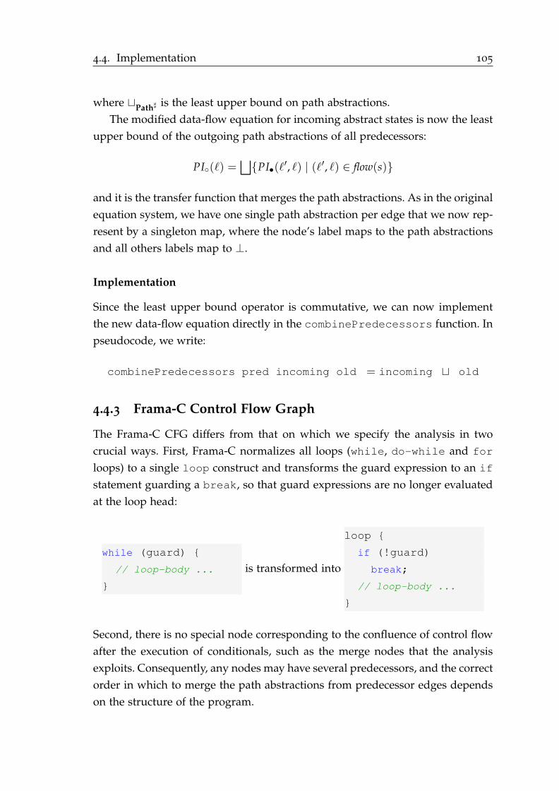
4.4. Implementation 105
where ⊔Path♯ is the least upper bound on path abstractions.
The modified data-flow equation for incoming abstract states is now the least
upper bound of the outgoing path abstractions of all predecessors:
PI(ℓ) =⊔
PI•(ℓ′, ℓ) | (ℓ′, ℓ) ∈ flow(s)
and it is the transfer function that merges the path abstractions. As in the original
equation system, we have one single path abstraction per edge that we now rep-
resent by a singleton map, where the node’s label maps to the path abstractions
and all others labels map to ⊥.
Implementation
Since the least upper bound operator is commutative, we can now implement
the new data-flow equation directly in the combinePredecessors function. In
pseudocode, we write:
combinePredecessors pred incoming old = incoming ⊔ old
4.4.3 Frama-C Control Flow Graph
The Frama-C CFG differs from that on which we specify the analysis in two
crucial ways. First, Frama-C normalizes all loops (while, do-while and for
loops) to a single loop construct and transforms the guard expression to an if
statement guarding a break, so that guard expressions are no longer evaluated
at the loop head:
while (guard)
// loop-body ...
is transformed into
loop
if (!guard)
break;
// loop-body ...
Second, there is no special node corresponding to the confluence of control flow
after the execution of conditionals, such as the merge nodes that the analysis
exploits. Consequently, any nodes may have several predecessors, and the correct
order in which to merge the path abstractions from predecessor edges depends
on the structure of the program.

106 Chapter 4. Replicated Synchronization
We work around this by (1) extending the merge operator to sets of path
abstractions and (2) implementing a structural analysis of the program, that as-
sociates a “merge tree” with each node. A merge tree specifies the correct order
in which merge the path abstractions at predecessor nodes should take place at
a specific node.
Consider the following examples:
s1 = if [b1]1
if [b2]2
[skip]3
else
[skip]4
else
[skip]5
;
[skip]6
s2 = [loop]1
if [b1]2 [break]3
if [b2]4 [break]5
if [b3]6
[skip]7
else
[skip]8
[skip]9
;
[skip]10
To calculate the path abstraction for statement 6 in s1, we need first merge
the path abstractions on the two edges (3, 6) and (4, 6) coming from the inner
if statement, before merging with the edge (5, 6) coming from the outer else
branch. Assuming that the path abstractions from the branches of the inner if
statement are p3 and p4 and that the one from the outer else branch is p5, then
the path abstraction for the last statement is given by the expression (p3 p4)
p5.
To obtain the correct path abstraction for the statement labeled 10 in s2, we
need to merge the path abstractions incoming from both break statements, but
before doing so we must remove the label corresponding to the if branches on
both path abstractions. Assuming these path abstractions are given by p3 and
p5, respectively, and that we extend the operator to single arguments such
that (p : ℓ) = p, then the path abstraction for the last statement is given by the
expression (p3) (p5).
“Merge trees”, defined below, correspond to the abstract syntax trees of such
expressions, with “holes” for incoming path abstractions, provided by the data-
flow analysis. Note that this approach assumes a structured control flow: a so-
lution for arbitrary control flow graphs would require a more sophisticated way
of tracking control dependencies [17].

4.4. Implementation 107
Merge Trees
First, we extend the merge operator to sets of path abstractions with the fol-
lowing definition:
`ps : P(Path♯)→ Path♯
`ps =
⊔
p∈ps
p′ p = p′ : ℓ
⊥ otherwise
We note that`p1, p2 equals p1 p2 as before, and that
`p1 : ℓ equals p1.
We will write p1 p2 as notation for the former and (p1 : ℓ) for the latter.
A merge tree corresponds to the abstract syntax tree of an expression over
path abstractions. For instance, consider the expression:
p = (p1 p2) p3
The corresponding merge tree needs to tell us that p1 and p2 must be merged,
before we can merge that result with p3. Merge trees are defined by the inductive
data-type M:
M ∋ m ::= I | T ms | J ms | L | N ℓ
where ms ∈ P(M) and ℓ ∈ Lab
The meaning of a merge tree is best explained by its interpretation, MJ · K,
which is given by evaluating the tree in an abstract state from L′:
MJ · K : M→ L′ → Path♯
MJIK l = ǫ
MJT msK l =`MJmK l | m ∈ ms
MJJ msK l =⊔
MJmK l | m ∈ ms
MJN ℓK l = l ℓ
MJLK l = ⊥
We assign the merge tree I (initial) to the initial node of the program, so its
interpretation is ǫ. When a node has several predecessors whose merge trees
should be merged, we use the constructor T (tree). The constructor J (join) is
used in the handling of loops. Its interpretation is the least-upper bound of its
arguments. The interpretation of the constructor N (node) is given by the ab-
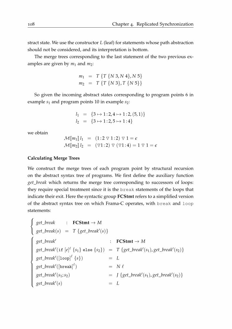
108 Chapter 4. Replicated Synchronization
stract state. We use the constructor L (leaf) for statements whose path abstraction
should not be considered, and its interpretation is bottom.
The merge trees corresponding to the last statement of the two previous ex-
amples are given by m1 and m2:
m1 = T T N 3, N 4, N 5
m2 = T T N 3, T N 5
So given the incoming abstract states corresponding to program points 6 in
example s1 and program points 10 in example s2:
l1 = 3 7→ 1 : 2, 4 7→ 1 : 2, (5, 1)
l2 = 3 7→ 1 : 2, 5 7→ 1 : 4
we obtainMJm1K l1 = (1 : 2 1 : 2) 1 = ǫ
MJm2K l2 = (1 : 2) (1 : 4) = 1 1 = ǫ
Calculating Merge Trees
We construct the merge trees of each program point by structural recursion
on the abstract syntax tree of programs. We first define the auxiliary function
get_break which returns the merge tree corresponding to successors of loops:
they require special treatment since it is the break statements of the loops that
indicate their exit. Here the syntactic group FCStmt refers to a simplified version
of the abstract syntax tree on which Frama-C operates, with break and loop
statements:
get_break : FCStmt→ M
get_break(s) = T get_break′(s)
get_break′ : FCStmt→ M
get_break′(if [e]ℓ s1 else s2) = T get_break′(s1), get_break′(s2)
get_break′([loop]ℓ s) = L
get_break′([break]ℓ) = N ℓ
get_break′(s1; s2) = J get_break′(s1), get_break′(s2)
get_break′(s) = L

4.4. Implementation 109
For example, for the program
[loop]1 if [b]2 [break]3 else [break]4; [break]5;
[skip]6;
the merge tree for label 6 is given by
m1 = get_break(if [b]2 [break]3 else [break]4; [break]5)
= T J T N 3, N 4, N 5
and assuming the environment
l1 = 3 7→ 1 : 2, 4 7→ 1 : 2, 5 7→ 1
we haveMJm1K l1 = (1 : 2 1 : 2) ⊔ 1 = ǫ.
The merge tree for programs preceded by the other statements is now given
by get_merge_tree:
get_merge_tree : M→ FCStmt→ (M× (Lab → M))
get_merge_tree(min, if [e]ℓ s1 else s2) =
let (m1, ms1) = get_merge_tree(N ℓ, s1) in
let (m2, ms2) = get_merge_tree(N ℓ, s2) in
(T [m1, m2], (ms1 ∪ms2)[ℓ← min])
get_merge_tree(min, [loop]ℓ s1) =
let (_, ms1) = get_merge_tree(N ℓ, s1) in
(get_break s1, ms1[ℓ← min])
get_merge_tree(min, s1; s2) =
let (m1, ms1) = get_merge_tree(min, s1) in
let (m2, ms2) = get_merge_tree(m1, s2) in
(m2, ms1 ∪ms2)
get_merge_tree(min, [break]ℓ) = (L, ℓ 7→ min)
get_merge_tree(min, s) = (N init(s), init(s) 7→ min)
This function takes an initial tree, a program and returns a pair where the
first component is the merge tree that should be associated to the successor of

110 Chapter 4. Replicated Synchronization
that program, and the second a mapping associating a merge tree to each point
in the program.
As we apply this function to example programs s1 and s2, we get the follow-
ing merge trees for their respective final statements:
(π2(get_merge_tree I s1)) 6 = T T N 3, N 4, N 6
(π2(get_merge_tree I s2)) 10 = T J T N 3, T N 5, T L, L, L
where we note that the last merge has the same interpretation as the desired
merge tree T T N 3, T N 5.
Applying Merge Trees
We let ms be the mapping returned in the second component of get_merge_tree,
giving the merge tree of each program point in the analyzed program. We use it
in the new transfer function PI′• as follows:
PI′•(ℓ, ℓ′) = let p =MJms ℓK PI(ℓ)
ℓ 7→ f(ℓ,ℓ′)(p)
where f(ℓ,ℓ′)(p) implements the original transfer function, so that PI•(ℓ, ℓ′) =
f(ℓ,ℓ′)(PI(ℓ)).
In other words, the modified transfer function calculates the path abstraction
for that edge by interpreting the associated merge tree in the environment which
is the incoming set of path abstractions of predecessors.
Handling Loop Guard Expressions
An additional problem caused by the representation of loops in Frama-C is that
the guard expression that determines whether to leave or to re-execute a loop
is no longer directly associated with the loop head. We solve this by another
pre-phase which scans the body of each loop, finds all conditionals that guard
break statements, and maps them to the corresponding loop statement.
In the transfer function for those conditional statements, in addition to mark-
ing the label of the conditional itself if the guard expression may be pid-
dependent, we also mark the label of the corresponding loop.

4.4. Implementation 111
1 int succ(int a)
2 return a + 1;
3
4
5
6
7
8
9
10
11
12
13 void shift()
14 int s = bsp_pid();
15 int p = bsp_nprocs();
16 int neighb = succ(s) % p;
17 int i = 0;
18 while (i < p)
19 // communicate to neighbor
20 bsp_put(neighb, /* ... */);
21 bsp_sync();
22 i = succ(i);
23
24
Figure 4.17 – A simple interprocedural BSPlib program. A naive interprocedural analysis cannotverify the synchronization of this program.
4.4.4 Implementing Interprocedural Analysis Using Small As-
sumption Sets
The language BSPlite does not contains functions. Consequently, nor does the
formalization of the analysis handle functions. However, realistic BSPlib pro-
grams are typically composed by a set of functions, and interprocedural analysis
is needed to verify them.
In this section we detail our interprocedural extension of the analysis as for-
malized. First, we describe how we extend the pid-independence data-flow anal-
ysis using the standard “small assumption set” approach [151], and the adap-
tations necessary to implement this approach in Frama-C. Second, we describe
how we adapt the second, replicated synchronization, phase of the analysis to
an interprocedural setting.
Theoretical Background
A naive implementation of interprocedural data-flow analysis can treat function
calls and returns as jumps, and input and output parameters as assignments.
The drawback of this approach is that the program points of any given function
have the same abstract state regardless of the context in which the function was
called.
To illustrate this problem in our setting, consider a trivial function succ that
takes an integer parameter a and returns its successor a+1 (See Figure 4.17). If
succ is invoked once with a pid-dependent argument, then the formal parameter
a will be considered pid-dependent in all invocations, and so also its return
value.

112 Chapter 4. Replicated Synchronization
Now consider the function shift in Figure 4.17. Here, the succ function is
used both at Line 16 compute pid-dependent identifier of each neighbor process
neighb, and at Line 22 to compute the next state of the loop index i. Due to the
first call, the result value of succ is always considered pid-dependent. Conse-
quently, the variable i and the guard condition of the while loop is considered
potentially pid-dependent and the synchronization in the loop is rejected.
A standard solution this problem is to introduce a context c ∈ ∆ that allows
the data-flow analysis to distinguish different calls to the same function. The idea
is that the intraprocedural abstract domain L is extended to an interprocedural
abstract domain
L = P(∆× L)
so that in each program point, we may have many different contexts c and their
corresponding abstract states.
Call paths and assumption sets are two ways of encoding such contexts. The
first represents control dependencies, and the latter data dependencies. Our as-
sumption is that pid dependency is mainly due to data dependency and opted
for the latter approach in our implementation.
Our intuition is that the context should contain the minimal set of informa-
tion that is important for pid-dependency, namely the pid-dependence of argu-
ments and the pid-dependency of the control point from which the call comes.
To increase precision further, we also distinguish calls from different callees by
adding the the function label from whence the call occurred. We use this label to
encode pid-dependency of the control point of the call by marking it when this
is the case.
∆ = P(Var)× (Lab ∪ Lab ∪ ℓ?)
The artificial label ℓ? is used for the initial context in the entry point of
the analyzed program, since, logically, the entry point function main has no
callee. As the initial abstract state of the intraprocedural analysis of a pro-
gram s is (Vars, ǫ) so the initial interprocedural abstract state of a program is
((Varmain, ℓ?), (Varmain, ǫ)) where Varmain is the set of local variables of the
entry point function.
Now, it remains to adapt the transfer functions to take into account the con-
text, and to formulate the transfer functions for function call and return to up-
date the contexts. The transfer function for function calls must install the new
context by transferring data-flow facts from the arguments to the formal pa-
rameters. Conversely, the transfer function for function returns must transfer
4.4. Implementation 113
data-flow facts from the return value to the recipient of the return value in the
corresponding context of the function call. The extensions of transfer functions
to as well as the transfer functions for function call and return are standard. We
do not detail them further and instead refer to a standard textbook [151, p. 82].
Implementation in Frama-C
Small assumption sets as described above are not directly implementable in
Frama-C since the data-flow functor of Frama-C operates on one function in
isolation. We circumvent this limitation by establishing a worklist algorithm. It
operators over two data-structures:
1. A worklist of function-context pairs to analyze.
2. A global abstract state, consisting of the set of analyzed contexts per func-
tion and the resulting abstract states.
The implementation analyzes each function in the worklist using the corre-
sponding context in isolation (intraprocedurally), and the result is then stored in
the global abstract state.
For each function call that is encountered during the intraprocedural anal-
ysis, the corresponding context in the called function is computed. When this
context is already present in the global abstract state, meaning that it has been
previously analyzed, then analysis continues. Otherwise, the function and the
corresponding context is added to the worklist.
After analyzing a function-context pair from the worklist, we verify whether
its final abstract state has been updated. This indicates that the return value must
be updated in all the callees of that context. When this is the case, we add all
callees to the worklist.
The algorithm continues thus until exhaustion of the worklist, at which point
all reachable functions have been analyzed.
A natural question is whether this procedures is guaranteed to terminate,
particularly in the presence of recursive function calls. While we have not for-
mally proved it, this should be assured by the fact that a function-context pair
is only analyzed if it has not been previously analyzed or if its the callee of
an function whose return state has been updated. As there is a finite number
of function calls and function returns, termination is argued by the absence of
infinite chains in the domain of contexts and the abstract states.
The second natural question is whether the precision afforded by this imple-
mentation is sufficient to treat realistic BSPlib program. And conversely, is this

114 Chapter 4. Replicated Synchronization
precision necessary? After all, situations as in the motivational example of this
section in Figure 4.17 might be rare in practice. We return to these questions in
the Section 4.5, where the implementation is evaluated.
Interprocedural Replicated Synchronization
We now turn to the replicated synchronization phase of the analysis.
First, we define an instruction as being potentially synchronizing if it is a call
to a function that is associated to bsp_sync in the transitive, reflexive transitive
call graph of the analyzed program. In other words, a potentially synchronizing
instruction is either a direct call to bsp_sync, or a call to a function that con-
tain bsp_sync, etc. We then modify definition of RS in Section 4.3.2, to reject
potentially synchronizing instructions that are guarded by pid-dependent guard
conditions.
Finally, we apply this modified RS to all functions in the reflexive transitive
closure of the call-graph from the entry function of the analyzed program, i.e. to
all reachable functions.
4.5 Evaluation
We have evaluated the analysis by applying it to a set of BSPlib programs
and verifying whether they have textually aligned barriers.
The set of analyzed programs are those distributed with BSPedupack [23]
(bspbench.c, bspfft.c, bspinprod.c, bsplu.c, bspmv.c); a Huawei-
developed BSP solution to the fixed-time constrained routing problem [95]
(SDN_BSP.c); a set of programs developed by Alexandros V. Gerbessiotis, in-
cluding a BSP parameter assessment program (assess.c), a comparison of dif-
ferent broadcast implementations (brdmain.c and ppfmain.c), an implemen-
tation of matrix multiplication (mulmain.c) and parallel radix sort (prmain.c);
the set of example programs distributed with the Oxford BSP Toolset [141]
(array_get.c, array_put.c, helloworld.c and helloworld_init.c,
helloworld_seq.c, reverse.c, sparse.c and sum.c); and a branch-and-
bound BSP algorithm for the 0− 1 Knapsack problem (knapsack.c).
The implementation does not handle switch statements and it requires that
functions have unique return statements. We have manually rewritten switch
to if statements, and functions with multiple returns to have one unique return
in the analyzed programs.

4.5. Evaluation 115
Program TAB PIA LOC Analysis time (s)BSPedupack/bspbench.c 0 271 0.27BSPedupack/bspfft.c 1 600 0.28BSPedupack/bspinprod.c 0 293 0.24BSPedupack/bsplu.c 1 438 0.30BSPedupack/bspmv.c 0 900 0.31Huawei/SDN_BSP.c 0 1584 0.65AlexG/as02a/assess.c 3 675 0.37AlexG/bp03v2/brdmain.c 8 865 0.39AlexG/bp03v2/ppfmain.c 6 1259 0.41AlexG/mult03v6/mulmain.c 4 1261 0.43AlexG/prdx14v06/prmain.c 1 556 0.34OxfBSPlib/array_get.c 0 88 0.27OxfBSPlib/array_put.c 0 85 0.23OxfBSPlib/helloworld.c 0 10 0.18OxfBSPlib/helloworld_init.c 0 25 0.18OxfBSPlib/helloworld_seq.c 0 15 0.18OxfBSPlib/reverse.c 0 55 0.20OxfBSPlib/sparse.c 0 109 0.23OxfBSPlib/sum.c 0 74 0.26knapsack.c 1 280 0.30
Table 4.1 – Evaluation results for Replicated Synchronization analysis. For each program, weindicate whether it is textually aligned (TAB), the number of pid-independence annotations added(PIA), and its size in number of lines of code (LOC). The two programs brdmain.c andprmain.c are not textually aligned due to a dependency on a non-initialized global variable.
Some of the programs surveyed would not have been accepted as textually
aligned by the implementation without further modification. Typically, their syn-
chronization depends on configuration parameters that are broadcast from pro-
cess 0 in the first superstep. As communicated variables, these are conservatively
assumed to be pid-dependent by the analysis. We add pid-independence annota-
tions to these variables that force the analysis to treat them as pid-independent.
The results of our evaluation is given in Table 4.1. For each program we mark
whether the program was accepted as textually aligned, indicate the number of
pid-independent annotations that were added. For each benchmark we also give
its size and analysis time.
All programs we have surveyed but three are textually aligned. However,
these three, brdmain.c, ppfmain.c and prmain.c are written with the intent
of being textually aligned. But, they read global variables that are not initialized
by all processes in the parallel section. By the BSPlib API, only process 0 is
allowed to read such variables – other processes doing so results in undefined
behavior, and hence nothing can be said about synchronization thereafter. In
116 Chapter 4. Replicated Synchronization
a typical BSPlib implementation however, execution continues but each process
may read different values from the uninitialized variables. Since synchronization
in these programs depends on these variables, this undefined behavior may lead
to synchronization errors. For these programs, we have indicated in Table 4.1 the
number of pid-independent annotations necessary to show the program textually
aligned if these uninitialized variables are repaired.
In sum, the results of our evaluation is in line with what previous authors
have noted: scalable parallel programs adhere to highly structured synchroniza-
tion patterns [5, 209] and moreover, they are typically textually aligned [209]. Our
evaluation also shows that in order to fully automatize synchronization analysis
and remove the need for annotations, more work is needed in the recognition of
pid-independent communication patterns such as broadcasts and reductions.
We also conclude that the precision enabled by the interprocedural analysis
is sufficient to analyze realistic programs, as none of the annotations introduced
is due to imprecision of interprocedural analysis. On the other hand, our evalua-
tion does not demonstrate that this precision is necessary. A naive solution might
also suffice to verify realistic programs, whereas our solution has an additional
cost in terms of implementation complexity and increased computation time.
Hence, more research in order to evaluate other precision trade-offs. Our contri-
bution provides an initial result by providing an upper bound on the precision
necessary for verifying realistic programs.
4.6 Related Work
Synchronization analysis of the parallel programs has been extensively stud-
ied for the purpose of deadlock and data-race detection as well as optimiza-
tion. We provide an overview of this work in Section 3.3.3. Notably, Aiken and
Gay [5] propose Barrier Inference: a system to verify the synchronization of
SPMD programs based on structural correctness and single-valued expressions
(another term for our pid-independent expressions). This analysis has been ex-
tended in [209] for MPI, also handling inter-procedurality and indicating how
non-textually aligned barriers match. Our contribution is inspired by [5], but dif-
fers in that we consider textually aligned programs, a subset of structurally correct
programs with formally defined underpinnings [56, 55]. Our intent is to enforce
textual alignment, with the intuition that the simplicity of this model will facil-
itate further analysis of other aspects of BSPlib programs. Similar ideas where
4.7. Concluding Remarks 117
explored in the Titanium project, a Java dialect for high-performance computing.
In [121], the author exploits that Titanium programs are statically guaranteed to
be structurally correct to construct a May-Happen-in-Parallel relation and uses
it for data race detection.
Several works propose operational semantics for BSPlib. Tesson et al. formal-
ize BSPlib [184], and the semantics in this chapter can be seen as a subset of their
semantics. Gava et al. formalize Paderborn’s BSPlib [80], and later extend their
formalization to consider subset synchronization [73]. The semantics we propose
in this chapter differs from previous ones as explicitly designed to model only
the features of BSPlib relevant to synchronization.
4.7 Concluding Remarks
In this chapter, we have presented our first contribution: the replicated syn-
chronization analysis. This static analysis identifies programs with textually
aligned barriers, a sufficient condition for correct synchronization. We have im-
plemented this analysis in Frama-C, extended it to handle interprocedural pro-
grams and evaluated it on a set of 20 BSPlib programs. We have also proved the
soundness of the analysis in the Coq proof assistant.
We identify the conservative treatment of communication as its main limi-
tation. A natural direction for future research into static structural analysis of
scalable parallel programs is thus applying communication analysis, in the goal
of recognizing pid-independent communication patterns.
Using the replicated synchronization analysis, we statically reconstruct the
synchronization pattern of the BSPlib program that constitutes the high-level
structure of BSP algorithms. This structural property of BSPlib programs will
be exploited in the following chapters to analyze the performance of BSPlib
programs and to analyze registration in BSPlib programs.


5Automatic Cost Analysis
Contents
5.1 Seq With Cost Annotations . . . . . . . . . . . . . . . . . . . . . . . 121
5.1.1 Syntax . . . . . . . . . . . . . . . . . . . . . . . . . . . . . . . . . . 122
5.1.2 Semantics . . . . . . . . . . . . . . . . . . . . . . . . . . . . . . . . . 123
5.1.3 Sequential Cost . . . . . . . . . . . . . . . . . . . . . . . . . . . . . 125
5.1.4 Sequential Cost Analysis . . . . . . . . . . . . . . . . . . . . . . . . 125
5.2 BSPlite With Cost Annotations and Communication . . . . . . 126
5.2.1 Syntax . . . . . . . . . . . . . . . . . . . . . . . . . . . . . . . . . . 127
5.2.2 Semantics . . . . . . . . . . . . . . . . . . . . . . . . . . . . . . . . . 127
5.2.3 Parallel Cost . . . . . . . . . . . . . . . . . . . . . . . . . . . . . . . 131
5.3 Cost Analysis . . . . . . . . . . . . . . . . . . . . . . . . . . . . . . . . . 134
5.3.1 Sequential Simulator . . . . . . . . . . . . . . . . . . . . . . . . . . 135
5.3.2 Analyzing Communication Costs . . . . . . . . . . . . . . . . . . . 140
5.3.3 Analyzing Synchronization Costs . . . . . . . . . . . . . . . . . . . 145
5.3.4 Time Complexity of Analysis . . . . . . . . . . . . . . . . . . . . . 146
5.4 Implementation and Evaluation . . . . . . . . . . . . . . . . . . . . 147
5.4.1 Benchmarks . . . . . . . . . . . . . . . . . . . . . . . . . . . . . . . 148
5.4.2 Symbolic Evaluation . . . . . . . . . . . . . . . . . . . . . . . . . . 148
5.4.3 Concrete Evaluation . . . . . . . . . . . . . . . . . . . . . . . . . . 148
5.4.4 Conclusion of Evaluation . . . . . . . . . . . . . . . . . . . . . . . 152
5.5 Related Work . . . . . . . . . . . . . . . . . . . . . . . . . . . . . . . . . 152
5.6 Concluding Remarks . . . . . . . . . . . . . . . . . . . . . . . . . . . . 154
This chapter is extracted from the author’s article [110].
119

120 Chapter 5. Automatic Cost Analysis
The BSP model ensures predictable scalability. However, manual performance
analysis of BSP programs, as demonstrated in Section 2.2.4, quickly becomes te-
dious and even intractable with growing program sizes. Furthermore, use cases
such as on-line scheduling, algorithm prototyping and evaluation motivate au-
tomatic performance prediction of programs as another desirable quality of any
parallel model.
To our knowledge, there are no methods for automatic cost analysis of im-
perative BSPlib programs: the BSPlib programmer is charged with manually de-
riving the cost of her program. In this chapter, we exploit textual alignment to
develop an automatic parametric cost analysis for BSPlib programs. We rely on
the static analysis of Chapter 4 to ensure this property.
Specifically, our contributions are:
• An adaptation of cost analysis for sequential programs [200, 6] to impera-
tive Bulk Synchronous Parallel programs by program transformation.
• The application of the polyhedral model to the estimation of communica-
tion costs of imperative BSP programs.
• A prototype implementation combining these two ideas into a tool for static
cost analysis of imperative BSP programs.
• Two evaluations, one symbolic and one concrete, of the implementation on
8 benchmarks.
The obtained cost formulas are parameterized by the input variables of the ana-
lyzed program. These variables can represent things such as the size of the prob-
lem instance size (e.g. the dimensions of a matrix for a matrix multiplication)
and other arguments. They can also include the special variable nprocs, which
corresponds to the BSP parameter p. Thus the obtained cost formula bound the
cost of running the program with any number of processes and with any input.
While not an inherent limitation of this work, the current implementation
requires that analyzed programs are structured, in addition to the textual align-
ment constraint. In practice, we have yet to see a BSPlib program that does not
fulfill these criteria.
We obtain a tight bound on communication cost when the input program
has textually aligned, polyhedral communications that are data-oblivious. In other
words, where the communication pattern does not depend on the contents of the
communicated data. When this is not the case, we still obtain safe upper bounds.

5.1. Seq With Cost Annotations 121
However, progress in the applicability of the polyhedral model [20] leads us to
believe that the communication of most real-world BSP programs can be repre-
sented in this model.
The chapter proceeds as follows. In Section 5.1 we add cost annotations to the
sequential language first introduced in Section 2.4.1 with which we formalize
the notion of sequential cost and sequential cost analysis. In the Section 5.2 we
bring these extensions to our BSPlib formalization of Section 4.2 to formalize the
notion of BSP cost. Since our cost analysis handles communication, we also ex-
tend our BSPlib formalization with DRMA primitives modeling those of BSPlib.
In Section 5.3, we present the main contribution: the cost analysis for imperative
BSPlib programs. In Section 5.4, we describes the prototype implementation and
its evaluation. In Section 5.5 we position our contributions with respect to the
state of the art. We conclude this chapter in Section 5.6 by discussing the lim-
itations of the presented method and proposing future research directions for
automatic cost analysis of BSPlib programs.
5.1 Seq With Cost Annotations
We begin by formalizing an extension of the sequential language Seq intro-
duced in Section 2.4.1 allowing us to reason on the cost of executing programs.
The semantics of the extended language is instrumented to return a trace of re-
source usage. With this, we compute the sequential cost of each execution. The cost
is a measure on what abstract computational resources are needed to complete
that execution. Units are used as arbitrary labels for different kinds of resources
(arithmetic operations, floating point operations, I/O, etc.). We assume that the
instructions of the input program are annotated with their individual cost and
unit. Such annotations could also be added by an automatic pre-analysis. This
scheme abstracts away from the specificities of different computer architectures
and allows for the segmentation of costs.
We assume the existence of a Sequential Cost Analysis, which is a static anal-
ysis giving a safe upper bound on the cost of any execution (as determined by
the annotation of each evaluated instruction in that execution) of a given pro-
gram. The computed worst-case cost is parameterized by the input variables of
the program. The description of such analyses can be found in literature [200, 6].
122 Chapter 5. Automatic Cost Analysis
5.1.1 Syntax
We extend Seq with annotations as defined by the following grammar:
AExp ∋ e ::= n | x | log e
Seq ∋ s ::= [x:=e]ℓ | [skip]ℓ | s; s | if [b]ℓ then s else s end
| while [b]ℓ do s end
| [x:=any]ℓ | [x:=[e1 .. e2]]ℓ | e u s
Arithmetic expressions have been extended to include the integer binary log-
arithm. Boolean expressions are unchanged and we refer to Section 2.4.1 for
their definition. In addition to those seen earlier, the set of instructions now
include non-deterministic updates, range-constricted non-deterministic updates
and work-annotated statements.
In addition to arithmetic expressions, variables can be assigned a non-
deterministic value (any). This value can be optionally constrained to a range
given by two arithmetic expressions ([e1..e2]), where e1, respectively e2, gives
a lower, respectively upper, limit of the assigned value. Bot types of non-
deterministic updates are used in Section 5.3 to sequentialize parallel programs.
Work annotations e u can be added to any statement, and consists of an
arithmetic expression e and a cost unit u ∈ Unit = a, b, . . .. The expression
gives the cost of the annotated statement and the unit gives the group of costs
in which it should be counted. For instance, let a ∈ Unit denote the cost of
arithmetic operations. Then the annotated assignment 1 a [x:=x + 1] signifies
that the cost of the assignment is 1 and that when executed this cost should be
added to the total cost of arithmetic operations. Statements can have multiple an-
notations, thereby enabling modeling of statements with costs in different units.
The cost of a program is given solely by these annotations: statements without
annotations do not contribute to the cost of an execution. This annotation-based
approach to specifying costly operations in a program is common in the cost
analysis community [106, 57].
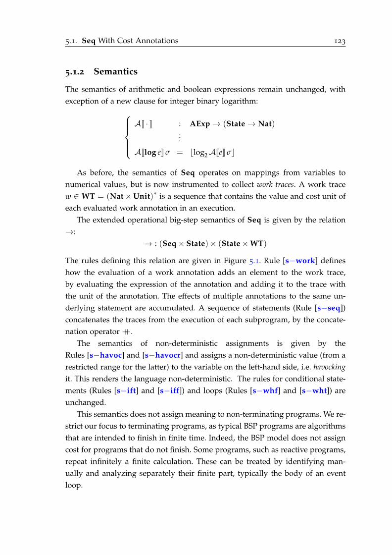
5.1. Seq With Cost Annotations 123
5.1.2 Semantics
The semantics of arithmetic and boolean expressions remain unchanged, with
exception of a new clause for integer binary logarithm:
AJ · K : AExp→ (State→ Nat)...
AJlog eK σ = ⌊log2AJeK σ⌋
As before, the semantics of Seq operates on mappings from variables to
numerical values, but is now instrumented to collect work traces. A work trace
w ∈ WT = (Nat×Unit)∗ is a sequence that contains the value and cost unit of
each evaluated work annotation in an execution.
The extended operational big-step semantics of Seq is given by the relation
→:
→ : (Seq× State)× (State×WT)
The rules defining this relation are given in Figure 5.1. Rule [s−work] defines
how the evaluation of a work annotation adds an element to the work trace,
by evaluating the expression of the annotation and adding it to the trace with
the unit of the annotation. The effects of multiple annotations to the same un-
derlying statement are accumulated. A sequence of statements (Rule [s−seq])
concatenates the traces from the execution of each subprogram, by the concate-
nation operator ++.
The semantics of non-deterministic assignments is given by the
Rules [s−havoc] and [s−havocr] and assigns a non-deterministic value (from a
restricted range for the latter) to the variable on the left-hand side, i.e. havocking
it. This renders the language non-deterministic. The rules for conditional state-
ments (Rules [s−ift] and [s−iff]) and loops (Rules [s−whf] and [s−wht]) are
unchanged.
This semantics does not assign meaning to non-terminating programs. We re-
strict our focus to terminating programs, as typical BSP programs are algorithms
that are intended to finish in finite time. Indeed, the BSP model does not assign
cost for programs that do not finish. Some programs, such as reactive programs,
repeat infinitely a finite calculation. These can be treated by identifying man-
ually and analyzing separately their finite part, typically the body of an event
loop.
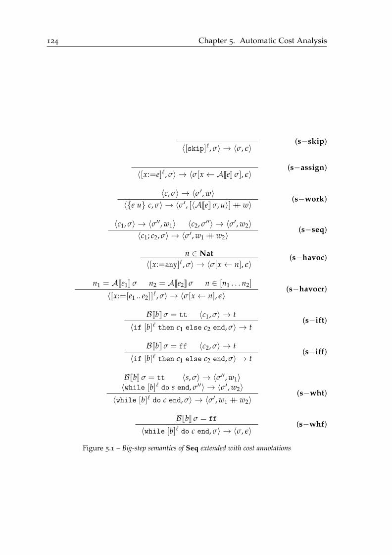
124 Chapter 5. Automatic Cost Analysis
〈[skip]ℓ, σ〉 → 〈σ, ǫ〉(s−skip)
〈[x:=e]ℓ, σ〉 → 〈σ[x ← AJeK σ], ǫ〉(s−assign)
〈c, σ〉 → 〈σ′, w〉
〈e u c, σ〉 → 〈σ′, [〈AJeK σ, u〉] ++ w〉(s−work)
〈c1, σ〉 → 〈σ′′, w1〉 〈c2, σ′′〉 → 〈σ′, w2〉
〈c1; c2, σ〉 → 〈σ′, w1 ++ w2〉(s−seq)
n ∈ Nat
〈[x:=any]ℓ, σ〉 → 〈σ[x ← n], ǫ〉(s−havoc)
n1 = AJe1K σ n2 = AJe2K σ n ∈ [n1 . . . n2]
〈[x:=[e1 .. e2]]ℓ, σ〉 → 〈σ[x ← n], ǫ〉
(s−havocr)
BJbK σ = tt 〈c1, σ〉 → t
〈if [b]ℓ then c1 else c2 end, σ〉 → t(s−ift)
BJbK σ = ff 〈c2, σ〉 → t
〈if [b]ℓ then c1 else c2 end, σ〉 → t(s−iff)
BJbK σ = tt 〈s, σ〉 → 〈σ′′, w1〉〈while [b]ℓ do s end, σ′′〉 → 〈σ′, w2〉
〈while [b]ℓ do c end, σ〉 → 〈σ′, w1 ++ w2〉(s−wht)
BJbK σ = ff
〈while [b]ℓ do c end, σ〉 → 〈σ, ǫ〉(s−whf)
Figure 5.1 – Big-step semantics of Seq extended with cost annotations

5.1. Seq With Cost Annotations 125
5.1.3 Sequential Cost
Given the work trace of an execution, we can obtain its cost. The cost is a map-
ping from units to numerical values:
Costseq : WT→ (Unit→ Nat)
Costseq(w) = λu.|w|−1
∑i=0
ni if w[i] = 〈ni, vi〉 and vi = u
0 otherwise
5.1.4 Sequential Cost Analysis
There are sound static analyses automatically deriving conservative upper
bounds on the cost of executing sequential, imperative programs [6]. Their basic
principle is that of synthesizing ranking functions [47, 157]. These functions relate
the semantics relation of the program to a well-ordered set, such that each ex-
ecution step of the semantics relates the terminating state to a smaller element
in this set. Intuitively, this can be understood as relating the program state to
a counter and ensuring that each step of the program decrements this counter.
This ensures termination, as the counter cannot decrement indefinitely. In ad-
dition to termination, the ranking functions also permit to obtain a measure on
the number of steps necessary to terminate, i.e. the desired upper bounds. We
refer to [161] for an elementary introduction to cost analysis, and to [47] for an
elementary introduction to the related field of termination analysis.
We let sca denote a sound sequential cost analysis for Seq. Given a program
it returns an upper bound on the cost of executing that program. The bound is
given as a cost expression from CExp that is parametric in the program’s input
parameters. Cost expressions CExp are arithmetic expressions extended with the
symbol ω denoting unbounded cost.
sca : Seq→ (Unit→ CExp)
CExp = AExp ∪ ω
The semantics of cost expressions is given by the function CJ·K : CExp× State→
Natω which is a natural extension of AJ·K with Natω = Nat ∪ ω.
Since the halting problem is undecidable in general, sca returns conservative
upper bounds. Consequently, it might return ω for a program that actually ter-
minates with any initial environment. However, since sca is sound, we have the
following for any unit u and program s:

126 Chapter 5. Automatic Cost Analysis
sfact =
[ f :=1]1;while [n > 0]2 do
log n a [ f := f ∗ n]3;[n:=n− 1]4
end
Figure 5.2 – The program sfact computes the factorial of the initial value of n. The work annotationat ?? 2 signifies that the assignment has a cost equal to the integer part of the binary logarithmof n, i.e. ⌊log2 n⌋, when executed. The unit in this annotation is a, signifying additions.
• If s terminates in any initial environment and the cost of its execution in
unit u is at most n, then sca(s)(u) = n′ and n ≤ n′ or sca(s)(u) = ω.
• If s is non-terminating in some initial environment, then sca(s)(u) = ω.
The intuitive understanding is that sca may sometimes overestimate the cost
needed to execute some program, but never underestimates it. And critically, it
never reports that executing a program has a finite cost when, in reality, it may
consume an unbounded amount of resources by running indefinitely.
Example 2. The sequential program sfact in Figure 5.2 computes the factorial of the
parameter n and stores it in the variable f . For the sake of providing a non-trivial exam-
ple, assume that n is of arbitrary precision so that multiplication by n consists of log n
additions, and that we are interested in the number of such additions performed in any
execution. We add a work annotation to the assignment at label 2 of value log n with
unit a (for addition). With our implementation of sca, based on [6], we have
sca(sfact) = λu.
n log n if u = a
0 otherwise
This is an upper bound on the cost of executing sfact, parameterized by the input variable
n, expressing that it performs at most n log n additions when calculating the factorial of
n.
5.2 BSPlite With Cost Annotations and Communi-
cation
We now extend the BSPlib formalization BSPlite to allow us to reason on the
parallel cost of programs. We add cost annotations and instrument the semantics
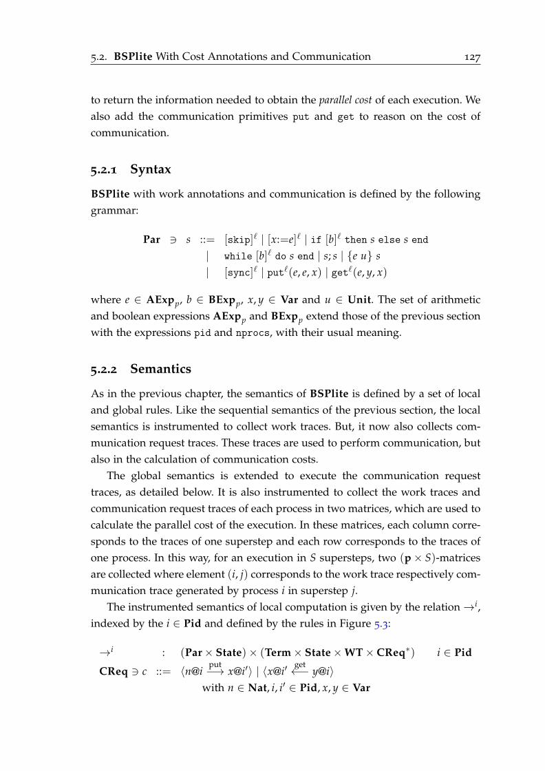
5.2. BSPlite With Cost Annotations and Communication 127
to return the information needed to obtain the parallel cost of each execution. We
also add the communication primitives put and get to reason on the cost of
communication.
5.2.1 Syntax
BSPlite with work annotations and communication is defined by the following
grammar:
Par ∋ s ::= [skip]ℓ | [x:=e]ℓ | if [b]ℓ then s else s end
| while [b]ℓ do s end | s; s | e u s
| [sync]ℓ | putℓ(e, e, x) | getℓ(e, y, x)
where e ∈ AExpp, b ∈ BExpp, x, y ∈ Var and u ∈ Unit. The set of arithmetic
and boolean expressions AExpp and BExpp extend those of the previous section
with the expressions pid and nprocs, with their usual meaning.
5.2.2 Semantics
As in the previous chapter, the semantics of BSPlite is defined by a set of local
and global rules. Like the sequential semantics of the previous section, the local
semantics is instrumented to collect work traces. But, it now also collects com-
munication request traces. These traces are used to perform communication, but
also in the calculation of communication costs.
The global semantics is extended to execute the communication request
traces, as detailed below. It is also instrumented to collect the work traces and
communication request traces of each process in two matrices, which are used to
calculate the parallel cost of the execution. In these matrices, each column corre-
sponds to the traces of one superstep and each row corresponds to the traces of
one process. In this way, for an execution in S supersteps, two (p× S)-matrices
are collected where element (i, j) corresponds to the work trace respectively com-
munication trace generated by process i in superstep j.
The instrumented semantics of local computation is given by the relation→i,
indexed by the i ∈ Pid and defined by the rules in Figure 5.3:
→i : (Par× State)× (Term× State×WT× CReq∗) i ∈ Pid
CReq ∋ c ::= 〈n@iput−→ x@i′〉 | 〈x@i′
get←− y@i〉
with n ∈ Nat, i, i′ ∈ Pid, x, y ∈ Var
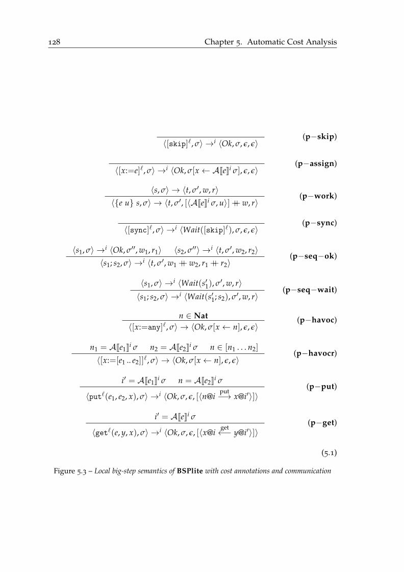
128 Chapter 5. Automatic Cost Analysis
〈[skip]ℓ, σ〉 →i 〈Ok, σ, ǫ, ǫ〉(p−skip)
〈[x:=e]ℓ, σ〉 →i 〈Ok, σ[x ← AJeKi σ], ǫ, ǫ〉(p−assign)
〈s, σ〉 → 〈t, σ′, w, r〉
〈e u s, σ〉 → 〈t, σ′, [〈AJeKi σ, u〉] ++ w, r〉(p−work)
〈[sync]ℓ, σ〉 →i 〈Wait([skip]ℓ), σ, ǫ, ǫ〉(p−sync)
〈s1, σ〉 →i 〈Ok, σ′′, w1, r1〉 〈s2, σ′′〉 →i 〈t, σ′, w2, r2〉
〈s1; s2, σ〉 →i 〈t, σ′, w1 ++ w2, r1 ++ r2〉(p−seq−ok)
〈s1, σ〉 →i 〈Wait(s′1), σ′, w, r〉
〈s1; s2, σ〉 →i 〈Wait(s′1; s2), σ′, w, r〉(p−seq−wait)
n ∈ Nat
〈[x:=any]ℓ, σ〉 → 〈Ok, σ[x ← n], ǫ, ǫ〉(p−havoc)
n1 = AJe1Ki σ n2 = AJe2Ki σ n ∈ [n1 . . . n2]
〈[x:=[e1 .. e2]]ℓ, σ〉 → 〈Ok, σ[x ← n], ǫ, ǫ〉
(p−havocr)
i′ = AJe1Ki σ n = AJe2Ki σ
〈putℓ(e1, e2, x), σ〉 →i 〈Ok, σ, ǫ, [〈n@iput−→ x@i′〉]〉
(p−put)
i′ = AJeKi σ
〈getℓ(e, y, x), σ〉 →i 〈Ok, σ, ǫ, [〈x@iget←− y@i′〉]〉
(p−get)
(5.1)
Figure 5.3 – Local big-step semantics of BSPlite with cost annotations and communication
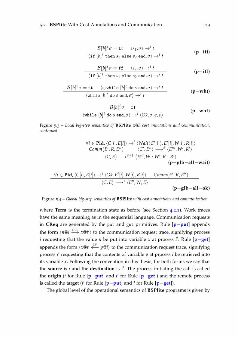
5.2. BSPlite With Cost Annotations and Communication 129
BJbKi σ = tt 〈s1, σ〉 →i t
〈if [b]ℓ then s1 else s2 end, σ〉 →i t(p−ift)
BJbKi σ = ff 〈s2, σ〉 →i t
〈if [b]ℓ then s1 else s2 end, σ〉 →i t(p−iff)
BJbKi σ = tt 〈s; while [b]ℓ do s end, σ〉 →i t
〈while [b]ℓ do s end, σ〉 →i t(p−wht)
BJbKi σ = ff
〈while [b]ℓ do s end, σ〉 →i 〈Ok, σ, ǫ, ǫ〉(p−whf)
Figure 5.3 – Local big-step semantics of BSPlite with cost annotations and communication,continued
∀i ∈ Pid, 〈C[i], E[i]〉 →i 〈Wait(C′[i]), E′[i], W[i], R[i]〉Comm(E′, R, E′′) 〈C′, E′′〉 −→S 〈E′′′, W ′, R′〉
〈C, E〉 −→S+1 〈E′′′, W : W ′, R : R′〉(p−glb−all−wait)
∀i ∈ Pid, 〈C[i], E[i]〉 →i 〈Ok, E′[i], W[i], R[i]〉 Comm(E′, R, E′′)
〈C, E〉 −→1 〈E′′, W, E〉(p−glb−all−ok)
Figure 5.4 – Global big-step semantics of BSPlite with cost annotations and communication
where Term is the termination state as before (see Section 4.2.1). Work traces
have the same meaning as in the sequential language. Communication requests
in CReq are generated by the put and get primitives. Rule [p−put] appends
the form 〈n@iput−→ x@i′〉 to the communication request trace, signifying process
i requesting that the value n be put into variable x at process i′. Rule [p−get]
appends the form 〈x@i′get←− y@i〉 to the communication request trace, signifying
process i′ requesting that the contents of variable y at process i be retrieved into
its variable x. Following the convention in this thesis, for both forms we say that
the source is i and the destination is i′. The process initiating the call is called
the origin (i for Rule [p−put] and i′ for Rule [p−get]) and the remote process
is called the target (i′ for Rule [p−put] and i for Rule [p−get]).
The global level of the operational semantics of BSPlite programs is given by
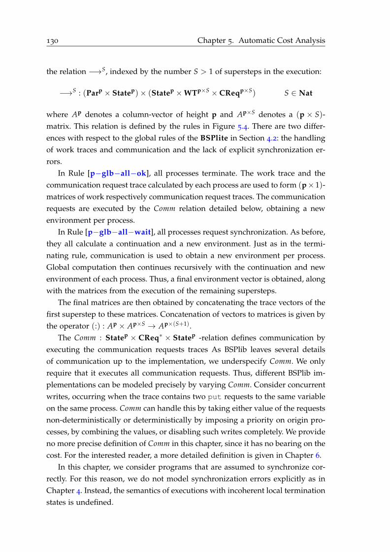
130 Chapter 5. Automatic Cost Analysis
the relation −→S, indexed by the number S > 1 of supersteps in the execution:
−→S : (Parp × Statep)× (Statep ×WTp×S × CReqp×S) S ∈ Nat
where Ap denotes a column-vector of height p and Ap×S denotes a (p × S)-
matrix. This relation is defined by the rules in Figure 5.4. There are two differ-
ences with respect to the global rules of the BSPlite in Section 4.2: the handling
of work traces and communication and the lack of explicit synchronization er-
rors.
In Rule [p−glb−all−ok], all processes terminate. The work trace and the
communication request trace calculated by each process are used to form (p× 1)-
matrices of work respectively communication request traces. The communication
requests are executed by the Comm relation detailed below, obtaining a new
environment per process.
In Rule [p−glb−all−wait], all processes request synchronization. As before,
they all calculate a continuation and a new environment. Just as in the termi-
nating rule, communication is used to obtain a new environment per process.
Global computation then continues recursively with the continuation and new
environment of each process. Thus, a final environment vector is obtained, along
with the matrices from the execution of the remaining supersteps.
The final matrices are then obtained by concatenating the trace vectors of the
first superstep to these matrices. Concatenation of vectors to matrices is given by
the operator (:) : Ap × Ap×S → Ap×(S+1).
The Comm : Statep × CReq∗ × Statep -relation defines communication by
executing the communication requests traces As BSPlib leaves several details
of communication up to the implementation, we underspecify Comm. We only
require that it executes all communication requests. Thus, different BSPlib im-
plementations can be modeled precisely by varying Comm. Consider concurrent
writes, occurring when the trace contains two put requests to the same variable
on the same process. Comm can handle this by taking either value of the requests
non-deterministically or deterministically by imposing a priority on origin pro-
cesses, by combining the values, or disabling such writes completely. We provide
no more precise definition of Comm in this chapter, since it has no bearing on the
cost. For the interested reader, a more detailed definition is given in Chapter 6.
In this chapter, we consider programs that are assumed to synchronize cor-
rectly. For this reason, we do not model synchronization errors explicitly as in
Chapter 4. Instead, the semantics of executions with incoherent local termination
states is undefined.
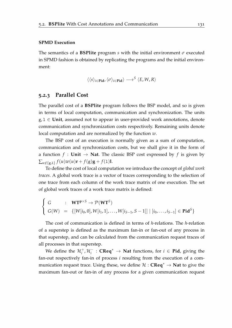
5.2. BSPlite With Cost Annotations and Communication 131
SPMD Execution
The semantics of a BSPlite program s with the initial environment σ executed
in SPMD fashion is obtained by replicating the programs and the initial environ-
ment:
〈〈s〉i∈Pid, 〈σ〉i∈Pid〉 −→S 〈E, W, R〉
5.2.3 Parallel Cost
The parallel cost of a BSPlite program follows the BSP model, and so is given
in terms of local computation, communication and synchronization. The units
g, l ∈ Unit, assumed not to appear in user-provided work annotations, denote
communication and synchronization costs respectively. Remaining units denote
local computation and are normalized by the function w.
The BSP cost of an execution is normally given as a sum of computation,
communication and synchronization costs, but we shall give it in the form of
a function f : Unit → Nat. The classic BSP cost expressed by f is given by
∑u 6∈g,l f (u)w(u)r + f (g)g + f (l)l.
To define the cost of local computation we introduce the concept of global work
traces. A global work trace is a vector of traces corresponding to the selection of
one trace from each column of the work trace matrix of one execution. The set
of global work traces of a work trace matrix is defined:
G : WTp×S → P(WTS)
G(W) = [W[i0, 0], W[i1, 1], . . . , W[iS−1, S− 1]] | [i0, . . . , iS−1] ∈ PidS
The cost of communication is defined in terms of h-relations. The h-relation
of a superstep is defined as the maximum fan-in or fan-out of any process in
that superstep, and can be calculated from the communication request traces of
all processes in that superstep.
We define the H+i ,H−i : CReq∗ → Nat functions, for i ∈ Pid, giving the
fan-out respectively fan-in of process i resulting from the execution of a com-
munication request trace. Using these, we define H : CReq∗ → Nat to give the
maximum fan-out or fan-in of any process for a given communication request
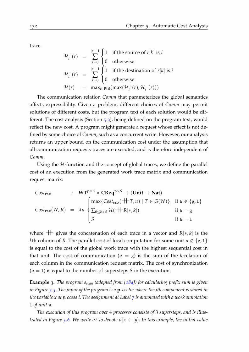
132 Chapter 5. Automatic Cost Analysis
trace.
H+i (r) =
|r|−1
∑k=0
1 if the source of r[k] is i
0 otherwise
H−i (r) =|r|−1
∑k=0
1 if the destination of r[k] is i
0 otherwise
H(r) = maxi∈Pid(max(H+i (r),H
−i (r)))
The communication relation Comm that parameterizes the global semantics
affects expressibility. Given a problem, different choices of Comm may permit
solutions of different costs, but the program text of each solution would be dif-
ferent. The cost analysis (Section 5.3), being defined on the program text, would
reflect the new cost. A program might generate a request whose effect is not de-
fined by some choice of Comm, such as a concurrent write. However, our analysis
returns an upper bound on the communication cost under the assumption that
all communication requests traces are executed, and is therefore independent of
Comm.
Using the H-function and the concept of global traces, we define the parallel
cost of an execution from the generated work trace matrix and communication
request matrix:
Costpar : WTp×S × CReqp×S → (Unit→ Nat)
Costpar(W, R) = λu.
maxCostseq(++T, u) | T ∈ G(W) if u 6∈ g, l
∑0≤k<SH(++R[∗, k]) if u = g
S if u = l
where ++ gives the concatenation of each trace in a vector and R[∗, k] is the
kth column of R. The parallel cost of local computation for some unit u 6∈ g, l
is equal to the cost of the global work trace with the highest sequential cost in
that unit. The cost of communication (u = g) is the sum of the h-relation of
each column in the communication request matrix. The cost of synchronization
(u = l) is equal to the number of supersteps S in the execution.
Example 3. The program sscan (adopted from [184]) for calculating prefix sum is given
in Figure 5.5. The input of the program is a p-vector where the ith component is stored in
the variable x at process i. The assignment at Label 7 is annotated with a work annotation
1 of unit w.
The execution of this program over 4 processes consists of 3 supersteps, and is illus-
trated in Figure 5.6. We write σy to denote σ[x ← y]. In this example, the initial value
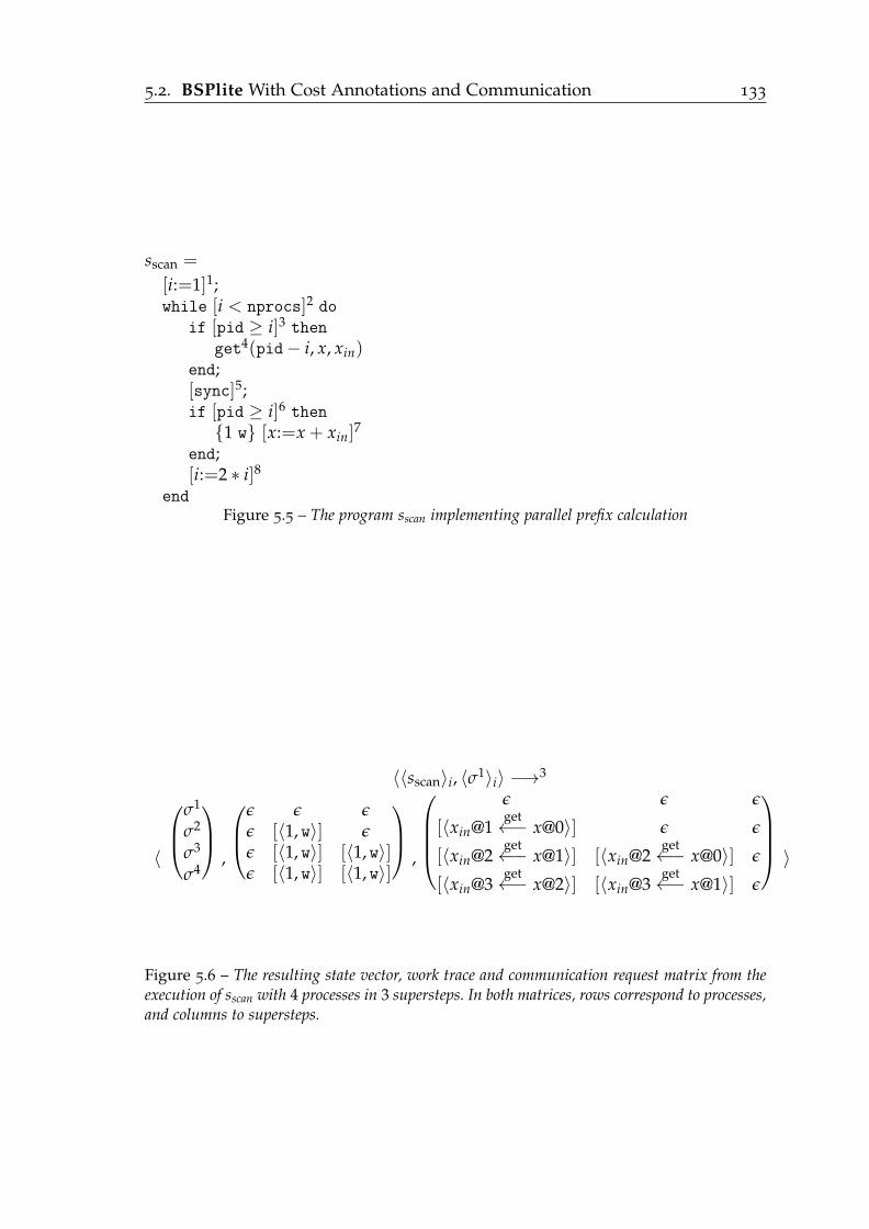
5.2. BSPlite With Cost Annotations and Communication 133
sscan =
[i:=1]1;while [i < nprocs]2 do
if [pid ≥ i]3 then
get4(pid− i, x, xin)end;[sync]5;if [pid ≥ i]6 then
1 w [x:=x + xin]7
end;[i:=2 ∗ i]8
end
Figure 5.5 – The program sscan implementing parallel prefix calculation
〈〈sscan〉i, 〈σ1〉i〉 −→
3
〈
σ1
σ2
σ3
σ4,
ǫ ǫ ǫǫ [〈1, w〉] ǫǫ [〈1, w〉] [〈1, w〉]ǫ [〈1, w〉] [〈1, w〉]
,
ǫ ǫ ǫ
[〈xin@1get←− x@0〉] ǫ ǫ
[〈xin@2get←− x@1〉] [〈xin@2
get←− x@0〉] ǫ
[〈xin@3get←− x@2〉] [〈xin@3
get←− x@1〉] ǫ
〉
Figure 5.6 – The resulting state vector, work trace and communication request matrix from theexecution of sscan with 4 processes in 3 supersteps. In both matrices, rows correspond to processes,and columns to supersteps.

134 Chapter 5. Automatic Cost Analysis
of x in all processes is 1. The values of the other variables are omitted for brevity. The
cost of this execution is
λu.
0 + 1 + 1 = 2 if u = w
1 + 1 + 0 = 2 if u = g
1 + 1 + 1 = 3 if u = l
where the local computation cost is given by the global work trace [ǫ, [〈1, w〉], [〈1, w〉]]
and communication cost is given by the fact that the h-relation is 1 in each superstep but
the last, where it is 0.
The cost of sscan as a function of the number of processes can be obtained manually
by rewriting the program as a recurrence relation. This relation is then solved to remove
the recurrence. When executed with p processes, the loop is executed ⌈log2 p⌉ times,
resulting in ⌈log2 p⌉+ 1 supersteps. The largest local computation is performed by the
process p − 1, which performs the work 1 w in each superstep. The h-relation of each
superstep but the last (which has no communication) is 1, since each process receives
at most one value and sends at most one value. Thus, the cost of sscan is given by the
function
λu.
⌈log2 p⌉ if u = w
⌈log2 p⌉ if u = g
⌈log2 p⌉+ 1 if u = l
which is parametric in the number of processes.
The next section describes our method for automatically obtaining bounds on
the parallel cost of programs like sscan.
5.3 Cost Analysis
This section describes the main contribution of this chapter: a method for
transforming a parallel program to a sequential program amenable to the pre-
existing sequential cost analysis. The transformation ensures that the worst-case
parallel cost of the original program is retained. The transformation, summa-
rized graphically in Figure 5.7, consists of 3 steps:
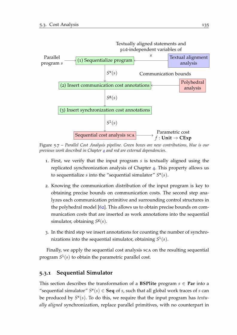
5.3. Cost Analysis 135
Parallelprogram s
(1) Sequentialize programTextual alignment
analysis
(2) Insert communication cost annotations
(3) Insert synchronization cost annotations
Polyhedralanalysis
Sequential cost analysis scaParametric cost
f : Unit→ CExp
Textually aligned statements andpid-independent variables of
s
Sw(s) Communication bounds
Sg(s)
Sl(s)
Figure 5.7 – Parallel Cost Analysis pipeline. Green boxes are new contributions, blue is ourprevious work described in Chapter 4 and red are external dependencies.
1. First, we verify that the input program s is textually aligned using the
replicated synchronization analysis of Chapter 4. This property allows us
to sequentialize s into the “sequential simulator” Sw(s).
2. Knowing the communication distribution of the input program is key to
obtaining precise bounds on communication costs. The second step ana-
lyzes each communication primitive and surrounding control structures in
the polyhedral model [62]. This allows us to obtain precise bounds on com-
munication costs that are inserted as work annotations into the sequential
simulator, obtaining Sg(s).
3. In the third step we insert annotations for counting the number of synchro-
nizations into the sequential simulator, obtaining Sl(s).
Finally, we apply the sequential cost analysis sca on the resulting sequential
program Sl(s) to obtain the parametric parallel cost.
5.3.1 Sequential Simulator
This section describes the transformation of a BSPlite program s ∈ Par into a
“sequential simulator” Sw(s) ∈ Seq of s, such that all global work traces of s can
be produced by Sw(s). To do this, we require that the input program has textu-
ally aligned synchronization, replace parallel primitives, with no counterpart in
136 Chapter 5. Automatic Cost Analysis
Seq, with skip instructions, and assign non-deterministic values to all variables
affected by the parallelism. This will allow us to use the sequential cost analysis
to get an upper bound on the local computation cost on the parallel program.
Sequentialization
The sequentialization transforms the parallel program so that it non-
deterministically chooses the identity and state of one local process before the
execution of each superstep. The underlying cost analysis will return the cost
of the worst-case choice, coinciding with the definition of the local computation
cost of one superstep.
The transformation relies on the textually aligned synchronization of the input
program. As we seen, this intuitively corresponds to all processes starting exe-
cution at the same source code location in the beginning of each superstep, and
then synchronizing at the same source code location at the end of the super-
step. In this case we can repeatedly apply the non-deterministic identity in the
beginning of each superstep.
The non-deterministic identity switch may switch to an identity that does
not correspond to any feasible state of a local process. To restrict the non-
determinism and improve precision, the identify switch does not modify the
variables that are pid-independent. This set is identified by the textual align-
ment analysis.
Textual Alignment Analysis
We reuse the textual alignment analysis of Chapter 4 to statically under-
approximate the set of pid-independent variables and the set of textually aligned
statements. This also serves to verify that synchronization is textually aligned.
We refer to the textual alignment analysis as rs, and treat it as a black box of the
following functionality:
rs : Par→ (⊤ ∪ (P(Lab)× (Lab→ P(Var))))
If a program s can be statically verified to have textually aligned synchroniza-
tion then rs(s) = (τ, π) where τ and π are under-approximations of textually
aligned statements and the set of pid-independent variables at each program
point, respectively.
If the analysis rs cannot verify statically the textual alignment of the program,
then RS(s) = ⊤. In this case, the parallel cost analysis cannot move forward and

5.3. Cost Analysis 137
returns λu.ω. In the remainder of this chapter we assume that programs have
statically verified textually aligned synchronization.
Example 4. Consider the program sscan in Figure 5.5. The textual alignment analysis
gives:
RS(sscan) = (τscan, πscan)
τscan = 1, 2, 3, 5, 6, 8
πscan(ℓ) =
i, x, xin if ℓ = 1
i otherwise
The program has textually aligned synchronization, since all statements in this program
are textually aligned except the statements labeled 4 and 7, corresponding to the body of
the conditionals in the loop. The body of these conditionals will not be executed by all
processes and this is statically detected since the value of the guard conditions depends
on the pid variable. The variables assigned at these statements and the variables affected
by communication, namely x and xin, will not be pid-independent at any statement
reachable by these assignments and communications. However, i has no dependency on
pid and so is pid-independent throughout the program.
Sequential Simulator
The sequential simulator Sw(s) of a parallel program s with textually aligned syn-
chronization is obtained by assigning a non-deterministic value to all variables
that are not pid-independent (including pid itself) after each sync primitive, and
then replacing all parallel primitives (sync, get and put) by a skip with the same
label.
We first define the function havoc that creates a program that assigns a non-
deterministic value to each variable given as argument:
havoc : P(Var)→ Seq
havoc(V) = (;) [x:=any]ℓ′| x ∈ V
where (;) gives a sequential composition of a set of statements and ℓ′ is a fresh
label for each assignment.
Now assume RS(s) = (τ, π), that Vars is the set of variables used in s and
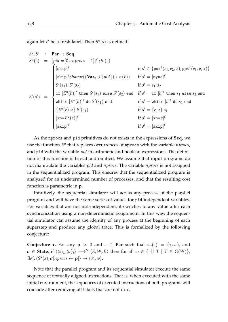
138 Chapter 5. Automatic Cost Analysis
again let ℓ′ be a fresh label. Then Sw(s) is defined:
Sw, S′ : Par→ Seq
Sw(s) = [pid:=[0 .. nprocs− 1]]ℓ′; S′(s)
S′(s′) =
[skip]ℓ if s′ ∈ putℓ(e1, e2, x), getℓ(e1, y, x)
[skip]ℓ; havoc((Vars ∪ pid) \ π(ℓ)) if s′ = [sync]ℓ
S′(s1); S′(s2) if s′ = s1; s2
if [Ew(b)]ℓ then S′(s1) else S′(s2) end if s′ = if [b]ℓ then s1 else s2 end
while [Ew(b)]ℓ do S′(s1) end if s′ = while [b]ℓ do s1 end
Ew(e) u S′(s1) if s′ = e u s1
[x:=Ew(e)]ℓ if s′ = [x:=e]ℓ
[skip]ℓ if s′ = [skip]ℓ
As the nprocs and pid primitives do not exists in the expressions of Seq, we
use the function Ew that replaces occurrences of nprocs with the variable nprocs,
and pid with the variable pid in arithmetic and boolean expressions. The defini-
tion of this function is trivial and omitted. We assume that input programs do
not manipulate the variables pid and nprocs. The variable nprocs is not assigned
in the sequentialized program. This ensures that the sequentialized program is
analyzed for an undetermined number of processes, and that the resulting cost
function is parametric in p.
Intuitively, the sequential simulator will act as any process of the parallel
program and will have the same series of values for pid-independent variables.
For variables that are not pid-independent, it switches to any value after each
synchronization using a non-deterministic assignment. In this way, the sequen-
tial simulator can assume the identity of any process at the beginning of each
superstep and produce any global trace. This is formalized by the following
conjecture:
Conjecture 1. For any p > 0 and s ∈ Par such that rs(s) = (τ, π), and
σ ∈ State, if 〈〈s〉i, 〈σ〉i〉 −→S 〈E, W, R〉 then for all w ∈ ++T | T ∈ G(W),
∃σ′, 〈Sw(s), σ[nprocs← p]〉 → 〈σ′, w〉.
Note that the parallel program and its sequential simulator execute the same
sequence of textually aligned instructions. That is, when executed with the same
initial environment, the sequences of executed instructions of both programs will
coincide after removing all labels that are not in τ.
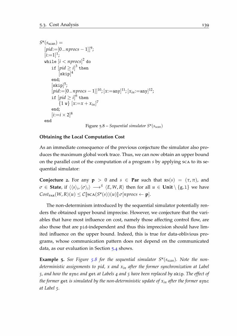
5.3. Cost Analysis 139
Sw(sscan) =
[pid:=[0 .. nprocs− 1]]9;[i:=1]1;
while [i < nprocs]2 do
if [pid ≥ i]3 then
[skip]4
end;[skip]5;[pid:=[0 .. nprocs− 1]]10; [x:=any]11; [xin:=any]12;
if [pid ≥ i]6 then
1 w [x:=x + xin]7
end;[i:=i× 2]8
end
Figure 5.8 – Sequential simulator Sw(sscan)
Obtaining the Local Computation Cost
As an immediate consequence of the previous conjecture the simulator also pro-
duces the maximum global work trace. Thus, we can now obtain an upper bound
on the parallel cost of the computation of a program s by applying sca to its se-
quential simulator:
Conjecture 2. For any p > 0 and s ∈ Par such that rs(s) = (τ, π), and
σ ∈ State, if 〈〈s〉i, 〈σ〉i〉 −→S 〈E, W, R〉 then for all u ∈ Unit \ g, l we have
Costpar(W, R)(u) ≤ CJsca(Sw(s))(u)K σ[nprocs← p].
The non-determinism introduced by the sequential simulator potentially ren-
ders the obtained upper bound imprecise. However, we conjecture that the vari-
ables that have most influence on cost, namely those affecting control flow, are
also those that are pid-independent and thus this imprecision should have lim-
ited influence on the upper bound. Indeed, this is true for data-oblivious pro-
grams, whose communication pattern does not depend on the communicated
data, as our evaluation in Section 5.4 shows.
Example 5. See Figure 5.8 for the sequential simulator Sw(sscan). Note the non-
deterministic assignments to pid, x and xin after the former synchronization at Label
5, and how the sync and get at Labels 4 and 5 have been replaced by skip. The effect of
the former get is simulated by the non-deterministic update of xin after the former sync
at Label 5.
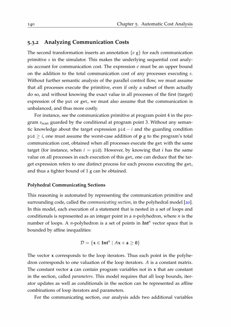
140 Chapter 5. Automatic Cost Analysis
5.3.2 Analyzing Communication Costs
The second transformation inserts an annotation e g for each communication
primitive s in the simulator. This makes the underlying sequential cost analy-
sis account for communication cost. The expression e must be an upper bound
on the addition to the total communication cost of any processes executing s.
Without further semantic analysis of the parallel control flow, we must assume
that all processes execute the primitive, even if only a subset of them actually
do so, and without knowing the exact value in all processes of the first (target)
expression of the put or get, we must also assume that the communication is
unbalanced, and thus more costly.
For instance, see the communication primitive at program point 4 in the pro-
gram sscan guarded by the conditional at program point 3. Without any seman-
tic knowledge about the target expression pid− i and the guarding condition
pid ≥ i, one must assume the worst-case addition of p g to the program’s total
communication cost, obtained when all processes execute the get with the same
target (for instance, when i = pid). However, by knowing that i has the same
value on all processes in each execution of this get, one can deduce that the tar-
get expression refers to one distinct process for each process executing the get,
and thus a tighter bound of 1 g can be obtained.
Polyhedral Communicating Sections
This reasoning is automated by representing the communication primitive and
surrounding code, called the communicating section, in the polyhedral model [20].
In this model, each execution of a statement that is nested in a set of loops and
conditionals is represented as an integer point in a n-polyhedron, where n is the
number of loops. A n-polyhedron is a set of points in Intn vector space that is
bounded by affine inequalities:
D = x ∈ Intn | Ax + a ≥ 0
The vector x corresponds to the loop iterators. Thus each point in the polyhe-
dron corresponds to one valuation of the loop iterators. A is a constant matrix.
The constant vector a can contain program variables not in x that are constant
in the section, called parameters. This model requires that all loop bounds, iter-
ator updates as well as conditionals in the section can be represented as affine
combinations of loop iterators and parameters.
For the communicating section, our analysis adds two additional variables

5.3. Cost Analysis 141
sscan =
[i:=1]1;while [i < nprocs]2 do
if [pid ≥ i]3 then
get4(pid− i, x, xin)end;[sync]5;if [pid ≥ i]6 then
1 w [x:=x + xin]7
end;[i:=2 ∗ i]8
end
Figure 5.9 – The program sscan, recalled
s and d to x, corresponding to the pid of the source and destination process.
The communicating section of a communication primitive is analyzable if the
section’s entry point is textually aligned, all its parameters are pid-independent
and it does not contain a sync. We also require that the communication primitive
has a target expression that is an affine combination of loop iterators
Finding sections of the code that is amenable to polyhedral representation is
the subject of “polyhedral extraction” [195], which is outside the scope of this
work. In our prototype, a simple algorithm is used to find the largest analyz-
able communicating section around each communication primitive. From this
approach stems the requirement that programs are structured. The algorithm
consists of starting with a communicating section containing only the commu-
nication primitive. Then, it adds as many contiguous statements around the sec-
tion as possible, until adding another would make it no longer analyzable. If
the section is nested in a loop, respectively a conditional, the algorithm attempts
to include the whole body, respectively both branches, if possible to do so and
keep the section analyzable. The algorithm continues thus recursively, until the
section can no longer grow. But, the method used for polyhedral extraction is
orthogonal to our contribution, and hence being structured is not an inherent
limitation of our approach.
Interaction Sets
From a polyhedral communicating section the analysis obtains a symbolic rep-
resentation of the exact set of communication requests that would be generated
if it is executed by any number of processes p, called the interaction set [62]. This
is not a literal set, but instead, a parameterized symbolic expression for which
each valuation of the parameters gives rise to a set.
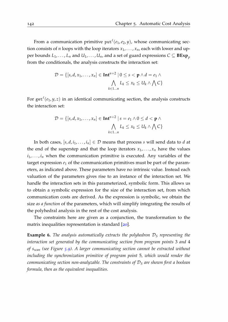
142 Chapter 5. Automatic Cost Analysis
From a communication primitive putℓ(e1, e2, y), whose communicating sec-
tion consists of n loops with the loop iterators x1, . . . , xn, each with lower and up-
per bounds L1, . . . , Ln and U1, . . . , Un, and a set of guard expressions C ⊆ BExpp
from the conditionals, the analysis constructs the interaction set:
D = [s, d, x1, . . . , xn] ∈ Intn+2 | 0 ≤ s < p ∧ d = e1 ∧∧
k∈1...n
Lk ≤ xk ≤ Uk ∧∧
C
For getℓ(e1, y, z) in an identical communicating section, the analysis constructs
the interaction set:
D = [s, d, x1, . . . , xn] ∈ Intn+2 | s = e1 ∧ 0 ≤ d < p ∧∧
k∈1...n
Lk ≤ xk ≤ Uk ∧∧
C
In both cases, [s, d, i1, . . . , in] ∈ D means that process s will send data to d at
the end of the superstep and that the loop iterators x1, . . . , xn have the values
i1, . . . , in when the communication primitive is executed. Any variables of the
target expression e1 of the communication primitives must be part of the param-
eters, as indicated above. These parameters have no intrinsic value. Instead each
valuation of the parameters gives rise to an instance of the interaction set. We
handle the interaction sets in this parameterized, symbolic form. This allows us
to obtain a symbolic expression for the size of the interaction set, from which
communication costs are derived. As the expression is symbolic, we obtain the
size as a function of the parameters, which will simplify integrating the results of
the polyhedral analysis in the rest of the cost analysis.
The constraints here are given as a conjunction, the transformation to the
matrix inequalities representation is standard [20].
Example 6. The analysis automatically extracts the polyhedron DS representing the
interaction set generated by the communicating section from program points 3 and 4
of sscan (see Figure 5.9). A larger communicating section cannot be extracted without
including the synchronization primitive of program point 5, which would render the
communicating section non-analyzable. The constraints of DS are shown first a boolean
formula, then as the equivalent inequalities.

5.3. Cost Analysis 143
. . .
if [pid ≥ i]3 then
get4(pid− i, x, xin)
end
. . .
DS = [s, d] ∈ Int2 | s = d− i ∧ 0 ≤ d < p ∧ d ≥ i
=
(
s
d
) (
s
d
)
∈ Int2,
1 −1
1 1
0 1
0 −1
0 1
(
s
d
)
+
−i
i
0
p− 1
−i
≥ 0
The two variables s and d of DS respectively correspond to the identifier of the source
respectively destination process of each request. This set is parameterized by the variable
i, which is constant in the section, and the BSP parameter p. The constraints are given by
the target expression (s = d− i), the domain of the pid variable (d ≥ 0 and p− 1 ≥ d),
and the condition on program point 3 (d ≥ i).
Example 7. Some common communication patterns and the interaction sets the analysis
obtains from these are illustrated in Figure 5.10.
From Interaction Sets to h-relations
From the interaction set, the analysis extracts an upper bound on the section’s
addition to the total communication cost of the execution, which is inserted as
an annotation at the section’s entry. This is done by creating two relations from
the interaction set D: from process identifier to the set of outbound (D+) respec-
tively inbound (D−) communication requests. The h-relation of this section is the
largest of the upper bounds on the cardinality of the image of these relations.
This is expressed by H:
D+(i) = [s, d, . . .] ∈ D | s = i D−(i) = [s, d, . . .] ∈ D | d = i
H = max(maxp−1i=0 #(D+(i)), max
p−1i=0 #(D−(i)))
Implementation of Communication Analysis
The analysis uses isl [194] to create the interaction set D as described earlier
and the two relations D+ and D− using isl’s operations for creating relations
and sets. It then asks isl to compute the expression corresponding to H, which
it does using integer volume counting techniques [196].

144
Ch
apter
5.A
uto
matic
Co
stA
naly
sis
One-to-one One-to-all All-to-one All-to-all
if [pid = src]1 then
put2(dest, e, x)
end
if [pid = src]1 then
[i:=0]2;
while [i < nprocs]3 do
put4(i, e, x);
[i:=i + 1]5
end
end
put1(dest, e, x)
[i:=0]1;
while [i < nprocs]2 do
put3(i, e, x);
[i:=i + 1]4
end
Pattern Interaction set h-relation
One-to-one D = [s, d] ∈ Int2 | 0 ≤ s < p ∧ d = dest ∧ s = src 1
One-to-all D = [s, d, i] ∈ Int3 | 0 ≤ s < p ∧ d = dest ∧ 0 ≤ i < p ∧ s = src p
All-to-one D = [s, d] ∈ Int2 | 0 ≤ s < p ∧ d = dest p
All-to-all D = [s, d, i] ∈ Int3 | 0 ≤ s < p ∧ d = i ∧ 0 ≤ i < p p
Figure 5.10 – Common communication patterns, their corresponding interaction set and statically inferred h-relation.

5.3. Cost Analysis 145
Example 8. For the interaction set DS from the example sscan, this technique obtains the
h-relation 1. The analysis inserts this bound before the if statement at program point
5 in the sequential simulator of sscan (see Figure 5.11). Figure 5.10 contains common
communication patterns and upper bounds extracted from their interaction sets using
isl.
Discussion
This method requires no pattern matching and automatically extracts a precise
upper bound on the communication cost of analyzable any communicating sec-
tion. When this is not the case, we fall back on the conservative but sound upper
bound cost of p g, which is added as an annotation to the communication prim-
itive in the sequential simulator.
Soundness
The following conjecture states that the sequential simulator with communica-
tion bounds soundly bounds from above the cost of the parallel program:
Conjecture 3. For any p > 0 and s ∈ Par such that rs(s) = (τ, π), and any
environment σ ∈ State and 〈〈s〉i, 〈σ〉i〉 −→S 〈E, W, R〉 then
Costpar(W, R)(g) ≤ CJsca(Sg(s))(g)K σ[nprocs← p].
5.3.3 Analyzing Synchronization Costs
Since we require that synchronization primitives are textually aligned in s, it
suffices to annotate each instruction that was sync in the original program with
1 l in the sequential simulator Sg(s) to account for synchronization costs. We
also add an annotated dummy skip instruction to the end of the program to
account for the implicit synchronization barrier at the end of all executions. We
refer to the resulting program as Sl(s).
Any execution of the parallel program evaluates the same sequence of tex-
tually aligned statements as the sequential simulator does on the same initial
environment. Thus, the simulator will evaluate exactly as many annotations of
unit l as there are synchronizations in the execution of the parallel program.
This intuition is formalized by the following conjecture:
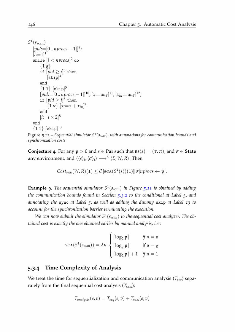
146 Chapter 5. Automatic Cost Analysis
Sl(sscan) =
[pid:=[0 .. nprocs− 1]]9;[i:=1]1
while [i < nprocs]2 do
1 gif [pid ≥ i]3 then
[skip]4
end
1 l [skip]5
[pid:=[0 .. nprocs− 1]]10; [x:=any]11; [xin:=any]12;if [pid ≥ i]6 then
1 w [x:=x + xin]7
end
[i:=i× 2]8
end
1 l [skip]13
Figure 5.11 – Sequential simulator Sl(sscan), with annotations for communication bounds andsynchronization costs
Conjecture 4. For any p > 0 and s ∈ Par such that rs(s) = (τ, π), and σ ∈ State
any environment, and 〈〈s〉i, 〈σ〉i〉 −→S 〈E, W, R〉. Then
Costpar(W, R)(l) ≤ CJsca(Sl(s))(l)K σ[nprocs← p].
Example 9. The sequential simulator Sl(sscan) in Figure 5.11 is obtained by adding
the communication bounds found in Section 5.3.2 to the conditional at Label 3, and
annotating the sync at Label 5, as well as adding the dummy skip at Label 13 to
account for the synchronization barrier terminating the execution.
We can now submit the simulator Sl(sscan) to the sequential cost analyzer. The ob-
tained cost is exactly the one obtained earlier by manual analysis, i.e.:
sca(Sl(sscan)) = λu.
⌈log2 p⌉ if u = w
⌈log2 p⌉ if u = g
⌈log2 p⌉+ 1 if u = l
5.3.4 Time Complexity of Analysis
We treat the time for sequentialization and communication analysis (Tseq) sepa-
rately from the final sequential cost analysis (Tsca):
Tanalysis(e, v) = Tseq(e, v) + Tsca(e, v)

5.4. Implementation and Evaluation 147
Here, e is the number of edges of the program’s control flow graph (which is
proportional to its size) and v the number of variables of the program.
Sequentialization is done in linear time but uses the result of a data-flow
analysis, which is computed in time bounded by O(ev) [151]. The analysis time
of each communication primitive is polynomial in the size of the polyhedra rep-
resenting it [196], which in turn is bounded by the maximum nesting level of
the program. The latter is often assumed to be bounded by some constant for
realistic programs. Hence, Tseq is bounded by some polynomial.
Analysis time for the sequentialized program, Tsca, depends on the details
of the implementation of sca. Our implementation translates the input pro-
gram into “cost relations” [7]. This step involves a data-flow analysis bounded
by O(ev) and an abstract interpretation in the domain of convex polyhedra
that is linear in e but exponential in the maximum number of variables in any
scope [49].
Finally, the cost relations are solved into a closed form upper bound by
PUBS [7] which is done in a time exponential in their bit size (Genaim, personal
communication, 2017).
In sum, Tanalysis grows exponentially with the size of the program. This is due
to our specific implementation of sca that uses PUBS: another sound sca with
lower complexity could be used. Note that the analysis complexity only depends
on the size of the analyzed program and is independent on run-time parameters
such as the number of processors executing the program.
5.4 Implementation and Evaluation
A prototype of the analysis has been implemented for BSPlite programs
in 3 KLOCs of Haskell. The underlying sequential cost analysis sca is imple-
mented as described in [6] and uses APRON [115] for abstract interpretation
and PUBS [7] for solving cost equations. The polyhedral analysis of communi-
cating sections uses isl [194].
We have performed two evaluations of the static upper bounds of the parallel
cost given by the implementation on 8 BSPlite benchmarks. The first evaluates
that they are indeed upper bounds and by what margin. The second evaluates
the quality of their power to predict actual run times in seconds. While finding
exact Worst-Case Execution Times [201] is not our goal, we demonstrate how BSP
costs relate to concrete run times.

148 Chapter 5. Automatic Cost Analysis
5.4.1 Benchmarks
Table 5.1 summarizes the benchmarks, their static bounds and analysis run
times. The second column indicates whether the program’s control flow is in-
dependent of the contents of the input arrays. We call such programs “data-
oblivious”, and when it is not the case, “data-dependent”. Note that no attempt
has been made to optimize the run time of the prototype. The benchmarks are
written in a variant of BSPlite (Section 5.2), extended with arrays. Array contents
are treated as non-deterministic values by the implementation. The benchmarks
are inner product (BspIp); parallel prefix in logarithmic and constant number
of supersteps (Scan2 and ScanCst2); parallel reduction (BspFold); array com-
pression (Compress); broadcast in one and logarithmic number of supersteps
(Bcast1 and BcastLog); and 2-phase broadcast (Bcast2ph).
Local computation is defined by work annotations added to costly array oper-
ations in loops. For simplicity, we only use the unit w and thus omit the normal-
ization function w. The static bounds obtained by the analysis on local computa-
tion, communication and synchronization are given in the columns W♯, H♯, and
S♯ of Table 5.1 respectively. Benchmarks and static bounds are parameterized by
BSP parameters and input sizes N.
5.4.2 Symbolic Evaluation
We verify whether that the static bounds are indeed bounds, and evaluate their
precision by executing each benchmark in an interpreter simulating p = 16. The
interpreter is instrumented to return the parallel cost (as defined in Section 5.2.3)
of each execution.
We found that the static bound is equal to the cost of each execution, except
for the communication cost of the program Compress, which is overestimated
by a factor of p. The communication distribution of Compress depends on the
values in the input array. The implementation treats these as non-deterministic
values, and returns the pessimistic static bound Ng on communication instead of
the tighter bound N/pg which can be found by analyzing the program manually.
5.4.3 Concrete Evaluation
To evaluate the quality of the static bounds’ capacity to predict actual run times
in seconds, we translate the benchmarks from BSPlite to C with BSPlib and com-
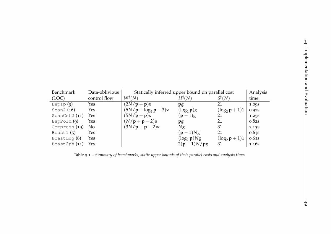
5.4.Im
plem
entatio
nan
dE
valu
ation
149
Benchmark Data-oblivious Statically inferred upper bound on parallel cost Analysis
(LOC) control flow W♯(N) H♯(N) S♯(N) timeBspIp (9) Yes (2N/p + p)w pg 2l 1.09sScan2 (16) Yes (5N/p + log2 p− 3)w (log2 p)g (log2 p + 1)l 0.92sScanCst2 (11) Yes (5N/p + p)w (p− 1)g 2l 1.25sBspFold (9) Yes (N/p + p− 2)w pg 2l 0.82sCompress (19) No (3N/p + p− 2)w Ng 3l 2.13sBcast1 (5) Yes (p− 1)Ng 2l 0.63sBcastLog (8) Yes (log2 p)Ng (log2 p + 1)l 0.61sBcast2ph (11) Yes 2(p− 1)N/pg 3l 1.16s
Table 5.1 – Summary of benchmarks, static upper bounds of their parallel costs and analysis times
150 Chapter 5. Automatic Cost Analysis
pare their run times on two different parallel environments with those predicted
by the static bounds in the BSP model.
Making such predictions is inherently difficult, especially when several trans-
lations are involved. For instance, our model supposes that the execution of one
individual operation takes a fixed amount of time. In reality, the time taken
depends on the state of caches, pipelines, and other hardware features. It also
depends on optimizations applied by the compiler. Another issue in the model is
the network. BSP assumes that the communication bottleneck will be at the end
points and, thus, that the time to deliver an h-relation will scale linearly. How-
ever, this is not true for current multi-core architectures, which usually have
tree-based network topologies, where bottlenecks can occur near the root. All
considering, at best we can hope to obtain run time predictions that are not too
far from the actual run time, but they may still be several factors off.
The first evaluation environment is a desktop computer with an 8-core, 3.20
GHz, Intel Xeon CPU E5-1660 processor, 32 GB RAM, and running Ubuntu 16.04.
We use gcc 5.4.0. The second environment is an 8-node Intel Sandy Bridge clus-
ter connected by FDR InfiniBand network cards. Each node has 2 Intel E5-2650
2 GHz CPUs with 8 cores each, 384 GB RAM and is running CentOS 7.2. Here
we use gcc 6.1.0. We use a Huawei-internal BSPlib implementation in both en-
vironments.
The same method is used to obtain the BSP parameters of both environments.
We modify bspbench to measure r as memory speed, which is the bottleneck
in all the benchmarks. To obtain g and l we measure the minimum time taken to
deliver all-to-all h-relations of size p, 2p, and hmaxp over a large set of samples,
where hmax is the size of the largest h-relation performed in the benchmarks.
Then the y-intercept of the line passing through the first two data-points is taken
as l, and the slope of the line passing through the last two is taken as g. Example
BSP parameters are given above Figures 5.12 to 5.14.
We find that the run time of all benchmarks grow linearly with input size as
predicted by the static bounds. See e.g. Figure 5.12. However, the static bounds
do not always accurately predict the run times. See e.g. Figure 5.14.
We calculate the error in prediction using the formula | Tmeasured − Tpredicted |
/ min(Tmeasured, Tpredicted). In this formulation, an overestimation of running time
by a factor 2 as well as an underestimation by a factor 2 will correspond to an
error of 100% [120]. The largest error factors for each environment-benchmark
combination are summarized in Table 5.2. The large errors in predictions for
Compress are explained by the inaccuracy of its statically found bound. For

5.4.Im
plem
entatio
nan
dE
valu
ation
151
Desktop Cluster Worst prediction for cluster, p = 8Benchmark p = 2 p = 4 p = 8 p = 8 p = 128 N predicted actual
BspIp 14.09% 7.98% 33.78% 15.49% 41.14% 1.68 · 108 0.12s 0.10sScan2 10.64% 16.79% 47.70% 34.63% 25.26% 1.68 · 108 0.29s 0.22sScanCst2 10.72% 16.85% 47.77% 35.36% 42.38% 1.26 · 108 0.22s 0.16sBspFold 11.86% 4.46% 39.72% 12.84% 48.76% 1.68 · 108 0.12s 0.10sCompress 396.78% 984.88% 2,449.87% 1,311.37% 15,388.60% 4.8 · 105 0.12s 0.01sBcast1 44.11% 90.83% 153.11% 47.75% 372.52% 1.6 · 105 0.03s 0.02sBcastLog 35.41% 59.50% 101.04% 13.03% 31.71% 1.6 · 105 0.01s 0.01sBcast2ph 32.84% 65.04% 97.08% 23.30% 48.58% 1.92 · 105 0.01s 0.01s
Table 5.2 – Maximal error in predictions per environment and benchmark. Sample times and predictions are for Cluster, p = 8.
0
0.005
0.01
0.015
0.02
20000 22000 24000 26000 28000 30000 32000
Run tim
e in s
econds
Input size in number of doubles
r=3.6e+02 Mflop/s, g=3e-08 s/b, l=0.00012 s
MeasuredPredicted
Figure 5.12 – BcastLog on Cluster, p = 8
0.002 0.003 0.004 0.005 0.006 0.007 0.008 0.009 0.01
6x10⁶
9.5x10⁶
1.3x10⁷
1.65x10⁷
2x10⁷
Run tim
e in s
econds
Input size in number of doubles
r=5e+02 Mflop/s, g=1.7e-08 s/b, l=8e-06 s
MeasuredPredicted
Figure 5.13 – BspFold on Desktop, p = 8
0
0.01
0.02
0.03
0.04
0.05
0.06
0.07
100 200 300 400 500 600 700
Run tim
e in s
econds
Input size in number of doubles
r=2.8e+02 Mflop/s, g=1e-07 s/b, l=0.00091 s
MeasuredPredicted
Figure 5.14 – Bcast1 on Cluster, p = 128
152 Chapter 5. Automatic Cost Analysis
the remaining benchmarks, error factors range from 4.46% for BspFold on the
desktop with 4 processes to 372.5% for Bcast1 on the cluster with 128 processes.
Indeed, Bcast1 has the worst predictions of the data-oblivious benchmarks.
This shows that in the considered environments, the communication pattern of
this benchmark (one-to-all) is faster than the one used to estimate g (all-to-all).
The discrepancy is even greater in the cluster with p = 128 as a consequence
of the cluster’s hierarchical topology. The 128 processes correspond to 8 cluster
nodes with 16 cores each, but the InfiniBand network is not 16 times faster than
the internal node communication. Thus when only one process communicates
with all other processes, it has much more bandwidth at its disposal then when
all processes communicate outside the node. The former case corresponds to the
communication pattern of Bcast1, and the latter to how the parameter g (which
is an estimation of the full bisection bandwidth) is measured, explaining the dif-
ference between measured and predicted running time. The discrepancy of the
other broadcast benchmarks, BcastLog and Bcast2ph, can also be explained
by considering the topology of the networks and the communication patterns
involved.
5.4.4 Conclusion of Evaluation
We find that (1) the static bounds of the implementation are indeed upper
bounds of the parallel cost of all evaluated executions; (2) they are exact for
data-oblivious benchmarks, but pessimistic for the one benchmark considered
with data-dependent communication distribution; (3) the static bounds predict
asymptotic behavior, and when tight static bounds are found, they accurately
predict actual run times: the error is less than 50% for networks with full bisec-
tion bandwidth and for the others the error is never more than the ratio between
the fastest link and the bisection bandwidth.
5.5 Related Work
Static cost analyses, as surveyed in Section 3.3.3, has previously been pro-
posed for Resource Aware ML [105], for concurrent and distributed programs
with dynamic task spawning [9], and for functional programs with divide-and-
conquer parallelism [213]. But, to the best of our knowledge, no previous work
exists on the automatic cost analysis of imperative BSP programs.

5.5. Related Work 153
Closest to our work is Hayashis’s cost analysis for shapely skeletal BSP pro-
grams [98]. However, this analysis is restricted to functional programs composed
of parallel skeletons with a priori known cost functions, whereas our analysis de-
duces cost functions automatically.
Sequentialization has been used widely in the analysis and verification of
parallel programs. We mention two examples, in the context of deductive ver-
ification. The Frama-C plugin Conc2Seq [24] uses sequentialization to verify
concurrent C programs. The memory context of each process is simulated by
translating each local variable to a p-vector. This vector maps process identifiers
to the corresponding process’s variable contents. A separate program counter is
maintained per process. Atomic instructions are translated to functions. A global
loop acts as a driver of the simulation, non-deterministically selecting a process
and, depending on the instruction it should execute next, calls the corresponding
function. This approach is aimed at fine-grained parallelism. For coarse-grained
parallel programs, that consist of large atomic sections like in BSP, it is possible
to create a less intrusive sequentialization. A translation that preserves more of
the structure of the original program should be simpler to verify deductively, as
the meaning of the original program is not lost in translation.
This idea is implemented in the tool BSP-Why [74], that uses sequentializa-
tion to verify imperative BSP programs. Again, a mapping is used to simulate
the memory of each process. However, the instructions of the program are seg-
mented into sequential blocks containing no parallel primitives. These are then
transformed into loops that executes the sequential block p times: once per pro-
cess and memory context.
Both of these sequentializations differ from ours in that we do not ex-
plicitly simulate the execution and memory of each process, but instead non-
deterministically execute one single process. This is due to the notion of local
computation cost in BSP. Sequential cost analysis applied to the sequentializa-
tions of Conc2Seq or BSP-Why would return an upper bound on the cumulative
cost of executing each local computation phase. Applied to ours, it returns an
upper bound on the local computation cost of executing the slowest process —
which is the relevant measure in BSP.
The polyhedral model has seen widespread usage in areas such as automatic
parallelization [127], verification and data-race analysis [37] and communication
analysis [44, 30, 99]. Our work is in the same vein as Clauss’ [44], who uses
polyhedra to model load distribution in communicating parallel programs. The
polyhedral model has also been used for automatically evaluating the communi-

154 Chapter 5. Automatic Cost Analysis
cation volumes produced by loops and evaluating their different transformations
by this measure [30, 30]. Our work differs in that we are first to exploit the poly-
hedral model to extract BSP communication costs and to integrate in a method
for automatically obtaining BSP cost functions.
5.6 Concluding Remarks
The cost model is one of the key advantages of the Bulk Synchronous Paral-
lel model. In this chapter we presented a method for automatic cost analysis of
imperative BSP programs, in the aim of relieving the programmer of manually
analyzing the cost of her algorithms. This method exploits the textual alignment
property statically detected by replicated synchronization analysis of Chapter 4
to rewrite parallel programs into sequential programs and analyzing the com-
munication distribution in the polyhedral model to obtain tight bounds on com-
munication cost. The rewritten programs can then be treated by existing methods
for cost analysis, obtaining the BSP cost of the original program.
We have evaluated the method and shown that the analysis obtains tight
bounds on the cost of data-oblivious BSP programs that accurately predicts their
actual run time in two different parallel environments. In addition to facilitating
algorithm development, one possibility opened up by this development is on-
line task scheduling in a system with evolving BSP parameters. Parallel straight-
line programs present another promising use case of the analysis in its current
form. Such programs are common in signal processing and are characterized by
simple control flow. However, they can scale to large sizes for which manual
analysis is intractable.
Our method puts specific requirements on the analyzed program, namely the
programs are structured and that all barriers are textually aligned. The former
requirement is incidental. It is both inherited from the textual alignment analy-
sis (developed in Chapter 4 and applied in Section 5.3.1) and due to the algo-
rithm for polyhedral extraction used in the communication analysis (described
in Section 5.3.2). Both of which require structured programs, but for which both
proposals have been made for the analysis of non-structured programs [5, 90].
The latter requirement is inherent to the sequentialization approach of Sec-
tion 5.3.1. To analyze the local computation cost of imperative BSP programs,
one must deduce which sequences of instructions may execute in parallel in
each superstep. The local computation cost is the costliest of these sequences.
5.6. Concluding Remarks 155
The structure of textual alignment ensures that this sequence starts, and ends,
at the same synchronization primitive in each process in each superstep. Con-
sequently, those sequences will only execute in parallel with themselves and
they can thus be analyzed in isolation. An alternative approach would require
a more involved may-happen-in-parallel analysis, extracting and analyzing each
potentially concurrent local computation phase.
The next step of our research includes the full implementation of the pro-
posed method and evaluation on larger programs. One axis of future develop-
ment is relaxing the constraints on the structure of the input programs, as well as
treating a larger fragment of C with BSPlib. Our analysis gives imprecise costs
for programs with data-dependent control flow. Treating such programs is an
interesting venue of future research. Lastly, we would like to treat other mea-
sures on BSP costs (lower bound, average case, etc.) as well as treating costs of
resources outside the BSP cost model, such as memory usage.


6Safe Registration in BSPlib
Contents
6.1 BSPlib Registration and its Pitfalls . . . . . . . . . . . . . . . . . 158
6.2 BSPlite with Registration . . . . . . . . . . . . . . . . . . . . . . . . . 161
6.2.1 Local Semantics . . . . . . . . . . . . . . . . . . . . . . . . . . . . . 162
6.2.2 Global Semantics . . . . . . . . . . . . . . . . . . . . . . . . . . . . 167
6.3 Instrumented Semantics . . . . . . . . . . . . . . . . . . . . . . . . . . 170
6.3.1 Instrumented Global Semantics . . . . . . . . . . . . . . . . . . . . 176
6.4 Correct Registration . . . . . . . . . . . . . . . . . . . . . . . . . . . . 179
6.4.1 Correctness . . . . . . . . . . . . . . . . . . . . . . . . . . . . . . . . 179
6.5 Sufficient Condition for Correct Registration . . . . . . . . . . 182
6.6 Related Work . . . . . . . . . . . . . . . . . . . . . . . . . . . . . . . . . 183
6.7 Concluding Remarks . . . . . . . . . . . . . . . . . . . . . . . . . . . . 184
This chapter is extracted from the author’s article [112].
In this chapter we study registration in BSPlib and exploit textual alignment
to define a sufficient condition for its correct usage. This dynamic characteri-
zation of correct registration forms the formal underpinnings of future work
towards a static analysis for verifying safe registration in BSPlib programs.
As introduced in Section 2.3.5, a BSPlib registration is an association between
p memory addresses, one per process. It allows one process to reference memory
objects on remote processes without knowing their address, thus enabling Direct
Remote Memory Access (DRMA). At synchronization, the BSPlib runtime uses
these registrations to route communication. Unfortunately, the BSPlib interface
for manipulating registrations is informally defined with subtle corner cases that
may provoke dynamic errors.
157

158 Chapter 6. Safe Registration in BSPlib
The first contribution of this chapter is an extension of BSPlite, formalizing
BSPlib with registrations, with which we characterize correct registration. To our
knowledge, ours is the first realistic formalization capturing the full idiosyn-
crasies of BSPlib registration.
The second contribution is a characterization of a subset of correct programs
based on textual alignment. We exploited the notion of textual alignment to
verify in synchronization Chapter 4 and to analyze BSP costs in Chapter 5. In this
chapter, we generalize this notion to all collective operations, and in a restricted
sense to memory locations. This requires an instrumentation of the semantics
of programs which is slightly more complex. We believe this is the first work
towards static verification of BSPlib registration.
This chapter proceeds as follows: In Section 6.1, we review the BSPlib registra-
tion mechanism and its pitfalls. Then, in Section 6.2, we extend our formalization
of BSPlib to model registration. We instrument this semantics in Section 6.3, al-
lowing us to define correct registration in Section 6.4. In Section 6.5, we describe
and prove our sufficient condition for correct registration. We discuss related
work in Section 6.6 and conclude in Section 6.7.
6.1 BSPlib Registration and its Pitfalls
BSPlib programs typically use DRMA for (buffered) communication, enabled
by the bsp_put and bsp_get primitives. Before a process can issue DRMA
requests to a remote memory area, this memory area must first have been as-
sociated to a local memory area using a registration. While a more extensive
overview of this mechanism is given in Section 2.3.5, we here recall the basic
notions.
A registration is an association between p addresses1, one per process,
that is stored in the registration sequence. Collectively calling the functions
bsp_push_reg, or bsp_pop_reg, requests the addition, or removal, of a regis-
tration from the registration sequence. Logically, a registration can be seen as a p-
vector of addresses 〈li〉i, where li is the argument of process i to bsp_push_reg.
Registration requests (removals, and then additions) are executed at synchro-
nization, and their effect is visible in the following superstep.
1In this chapter, we ignore the size of registered memory areas, which may vary per process.The size has no impact on the registration errors, so is left out to simplify the presentation.
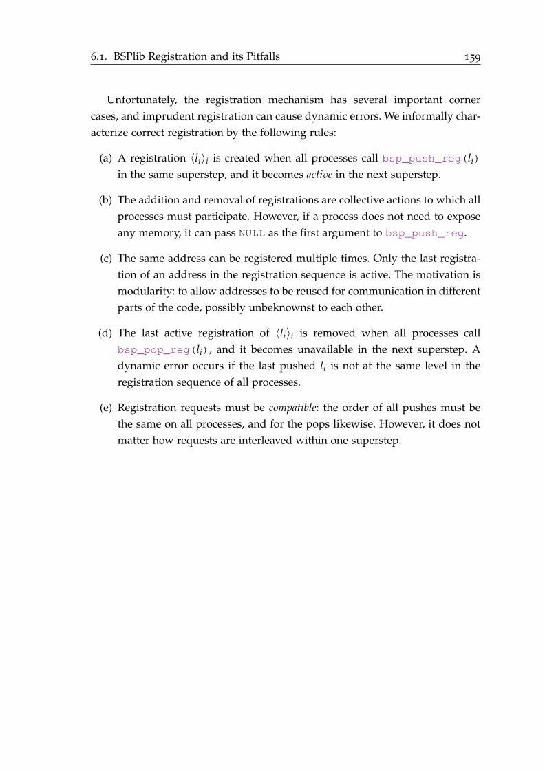
6.1. BSPlib Registration and its Pitfalls 159
Unfortunately, the registration mechanism has several important corner
cases, and imprudent registration can cause dynamic errors. We informally char-
acterize correct registration by the following rules:
(a) A registration 〈li〉i is created when all processes call bsp_push_reg(li)
in the same superstep, and it becomes active in the next superstep.
(b) The addition and removal of registrations are collective actions to which all
processes must participate. However, if a process does not need to expose
any memory, it can pass NULL as the first argument to bsp_push_reg.
(c) The same address can be registered multiple times. Only the last registra-
tion of an address in the registration sequence is active. The motivation is
modularity: to allow addresses to be reused for communication in different
parts of the code, possibly unbeknownst to each other.
(d) The last active registration of 〈li〉i is removed when all processes call
bsp_pop_reg(li), and it becomes unavailable in the next superstep. A
dynamic error occurs if the last pushed li is not at the same level in the
registration sequence of all processes.
(e) Registration requests must be compatible: the order of all pushes must be
the same on all processes, and for the pops likewise. However, it does not
matter how requests are interleaved within one superstep.
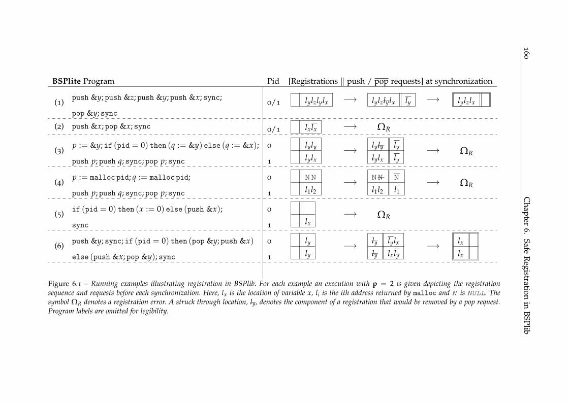
160
Ch
apter
6.S
afeR
egistratio
nin
BS
Plib
BSPlite Program Pid [Registrations ‖ push / pop requests] at synchronization
(1)push &y; push &z; push &y; push &x; sync;
pop &y; sync
0/1 lylzlylx −→ lylzlylx ly −→ lylzlx
(2) push &x; pop &x; sync 0/1 lxlx −→ ΩR
(3)p := &y; if (pid = 0) then (q := &y) else (q := &x);
push p; push q; sync; pop p; sync
0 lyly
lylx
−→lyly ly
lylx ly−→ ΩR
1
(4)p := malloc pid; q := malloc pid;
push p; push q; sync; pop p; sync
0 NN
l1l2−→
NN N
l1l2 l1−→ ΩR
1
(5)if (pid = 0) then (x := 0) else (push &x);
sync
0
lx
−→ ΩR1
(6)push &y; sync; if (pid = 0) then (pop &y; push &x)
else (push &x; pop &y); sync
0 ly
ly−→
ly lylx
ly lxly−→
lx
lx1
Figure 6.1 – Running examples illustrating registration in BSPlib. For each example an execution with p = 2 is given depicting the registrationsequence and requests before each synchronization. Here, lx is the location of variable x, li is the ith address returned by malloc and N is NULL. Thesymbol ΩR denotes a registration error. A struck through location, ly, denotes the component of a registration that would be removed by a pop request.Program labels are omitted for legibility.

6.2. BSPlite with Registration 161
The running examples in Figure 6.1, written in BSPlite extended with regis-
tration (detailed below in Section 6.2), illustrate these rules:
Example 1 Execution proceeds without error. The depicted registration se-
quence grows to the right. In the second superstep, the most recently
pushed registration of y is removed.
Example 2 the program attempts to remove a registration of x. While a registra-
tion of this variable is requested in the same superstep, it does not become
active until the next superstep, and so an error is produced (Rule (6.1)).
Example 3 A dynamic error occurs since the pop in the second superstep at-
tempts to remove at different levels in the registration sequence (Rule (6.1)).
Example 4 This example is a simplified version of real BSPlib code, illustrating
how the situation of Example 3 could be reproduced by dynamic allocation
as malloc may return NULL [164, p. 143].
Example 5 A dynamic error occurs when only process 1 pushes (Rule (6.1)).
Example 6 This example illustrates how the interleaving of requests in one su-
perstep is irrelevant as long as the requests are compatible (Rule (6.1)).
The goal of this chapter is to define a sufficient condition that forbids erro-
neous programs such as Examples 2 to 5. Just as textually aligned barriers is an
intuitive, sufficient condition that ensures correct synchronization, the sufficient
condition that we will develop in this chapter is intuitive and ensures correct
registration.
As a first step, we formalize an extension of BSPlite that we use to charac-
terize correct registration.
6.2 BSPlite with Registration
As we have done in the two previous chapters, we start by extending BSPlite
to model the aspects of BSPlib that we are studying. The version of BSPlite used
in this chapter has pointers, dynamic allocation, registration and communica-
tion (Figure 6.2). As in Chapter 5, we model DRMA communication, but in this
chapter our modelization is closer to the BSPlib in that it implements transfers
between memory areas, whereas the communication there is between variables.

162 Chapter 6. Safe Registration in BSPlib
AExpp ∋ e ::= pe | n | e1 opa e2 | nprocs | pid | &x
PExp ∋ pe ::= x | ∗eBExpp ∋ b ::= true | false | e1 opr e2 | b1 opb b2 |!b
Par ∋ s ::= [skip]ℓ | s1; s2 | if [b]ℓ then s1 else s2 | while [b]
ℓ do s1
| [sync]ℓ | [pe := e]ℓ | [pe := malloc e]ℓ
| [free e]ℓ | [push e]ℓ
| [pop e]ℓ | [put e1 e2 e3 e4 e5]ℓ | [get e1 e2 e3 e4 e5]
ℓ
x ∈ Var, n ∈ Nat, opr ∈ =,<, opb ∈ and, or, opa ∈ +,−,×
Figure 6.2 – Syntax of BSPlite with registration
Arithmetic expressions in AExpp are as before with the addition of pointer
expressions and the address-of operator. A pointer expression in PExp is either a
variable or the dereferencement of an arithmetic expression. Boolean expressions
are unchanged with respect to previous chapters.
Commands now also include dynamic allocation (malloc, whose argument
indicates desired allocation size) and deallocation (free, whose argument indi-
cates the memory area to deallocate). Assignments now assign to a location des-
ignated by the left-hand side pointer expression. The parallel primitives sync,
push, pop, put and get and their arguments2 model their BSPlib counterparts
(detailed in Section 2.3.5). In other words, [put epid esrc edst eoffs enb]ℓ requests the
transfer of the memory area starting at esrc in the origin process and extending
enb memory cells, into the memory area at the target process epid that is in an
active registration with edst, at offset eoffs. The primitive [get epid esrc eoffs edst enb]ℓ
requests the transfer of the memory area at the target epid that is in an active
registration with esrc at offset eoffs and extending enb bytes, into the memory area
of the origin process at edst.
We no longer include the command skip. It served as a default continuation
in previous chapters, but is no longer needed in this version of the language.
6.2.1 Local Semantics
In previous chapters we defined the local and global level of computation using
big-step semantics. In this chapter, we instead define local computation using a
small-step semantics. This change facilitates the instrumentation used to define
correctness and our sufficient condition.
2With exception of the ignored size argument to push, as explained in the previous chapter.
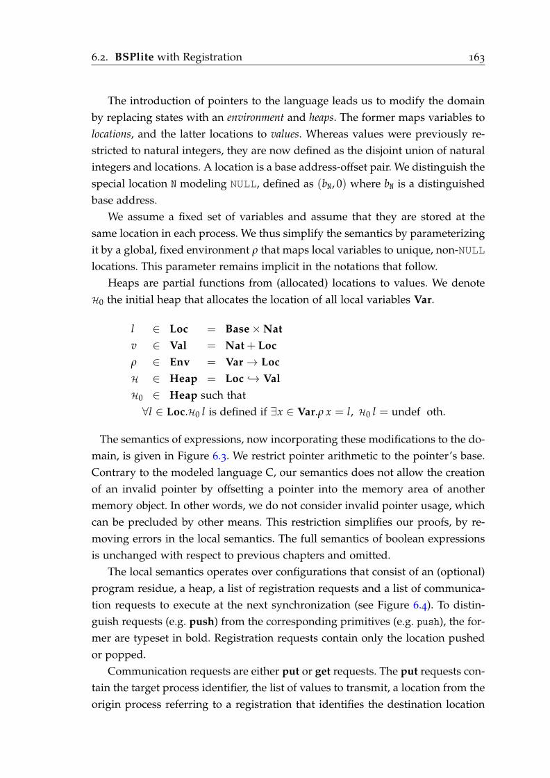
6.2. BSPlite with Registration 163
The introduction of pointers to the language leads us to modify the domain
by replacing states with an environment and heaps. The former maps variables to
locations, and the latter locations to values. Whereas values were previously re-
stricted to natural integers, they are now defined as the disjoint union of natural
integers and locations. A location is a base address-offset pair. We distinguish the
special location N modeling NULL, defined as (bN, 0) where bN is a distinguished
base address.
We assume a fixed set of variables and assume that they are stored at the
same location in each process. We thus simplify the semantics by parameterizing
it by a global, fixed environment ρ that maps local variables to unique, non-NULL
locations. This parameter remains implicit in the notations that follow.
Heaps are partial functions from (allocated) locations to values. We denote
H0 the initial heap that allocates the location of all local variables Var.
l ∈ Loc = Base×Nat
v ∈ Val = Nat + Loc
ρ ∈ Env = Var→ Loc
H ∈ Heap = Loc → Val
H0 ∈ Heap such that
∀l ∈ Loc.H0 l is defined if ∃x ∈ Var.ρ x = l, H0 l = undef oth.
The semantics of expressions, now incorporating these modifications to the do-
main, is given in Figure 6.3. We restrict pointer arithmetic to the pointer’s base.
Contrary to the modeled language C, our semantics does not allow the creation
of an invalid pointer by offsetting a pointer into the memory area of another
memory object. In other words, we do not consider invalid pointer usage, which
can be precluded by other means. This restriction simplifies our proofs, by re-
moving errors in the local semantics. The full semantics of boolean expressions
is unchanged with respect to previous chapters and omitted.
The local semantics operates over configurations that consist of an (optional)
program residue, a heap, a list of registration requests and a list of communica-
tion requests to execute at the next synchronization (see Figure 6.4). To distin-
guish requests (e.g. push) from the corresponding primitives (e.g. push), the for-
mer are typeset in bold. Registration requests contain only the location pushed
or popped.
Communication requests are either put or get requests. The put requests con-
tain the target process identifier, the list of values to transmit, a location from the
origin process referring to a registration that identifies the destination location
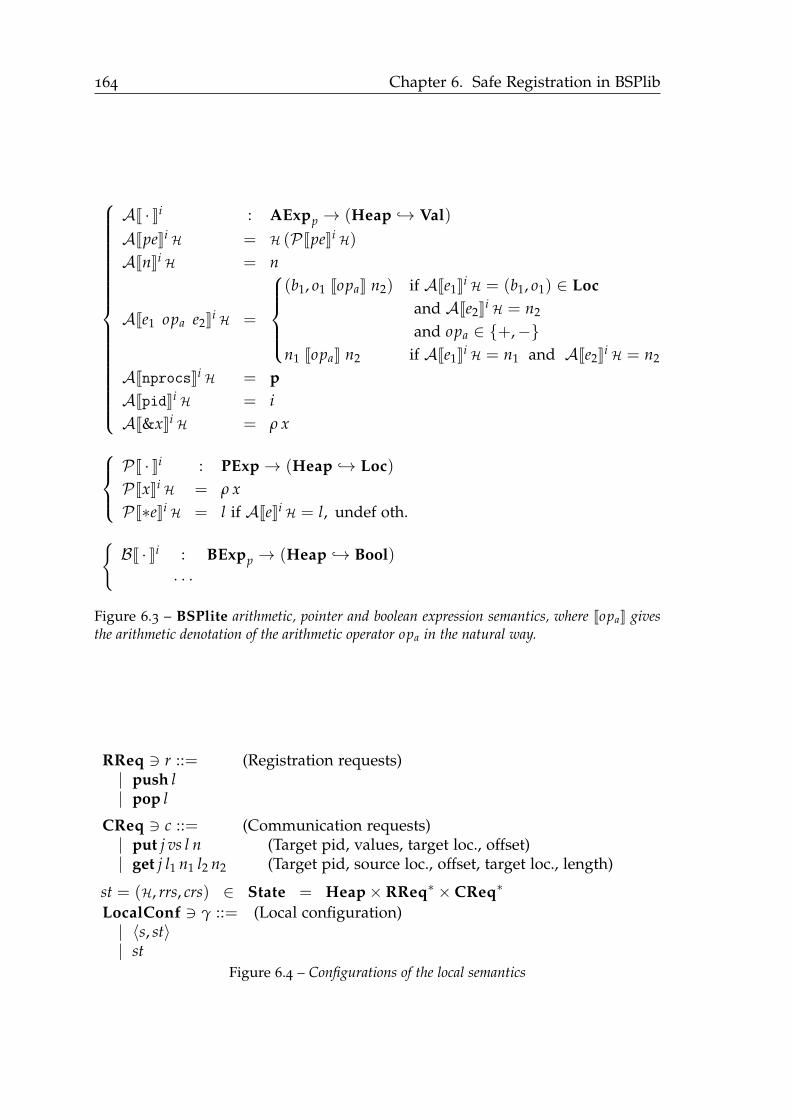
164 Chapter 6. Safe Registration in BSPlib
AJ · Ki : AExpp → (Heap → Val)
AJpeKi H = H (PJpeKi H)
AJnKi H = n
AJe1 opa e2Ki H =
(b1, o1 JopaK n2) if AJe1Ki H = (b1, o1) ∈ Loc
and AJe2Ki H = n2
and opa ∈ +,−
n1 JopaK n2 if AJe1Ki H = n1 and AJe2Ki H = n2
AJnprocsKi H = p
AJpidKi H = i
AJ&xKi H = ρ x
PJ · Ki : PExp→ (Heap → Loc)
PJxKi H = ρ x
PJ∗eKi H = l if AJeKi H = l, undef oth.
BJ · Ki : BExpp → (Heap → Bool)
· · ·
Figure 6.3 – BSPlite arithmetic, pointer and boolean expression semantics, where JopaK givesthe arithmetic denotation of the arithmetic operator opa in the natural way.
RReq ∋ r ::= (Registration requests)| push l| pop l
CReq ∋ c ::= (Communication requests)| put j vs l n (Target pid, values, target loc., offset)| get j l1 n1 l2 n2 (Target pid, source loc., offset, target loc., length)
st = (H, rrs, crs) ∈ State = Heap× RReq∗ × CReq∗
LocalConf ∋ γ ::= (Local configuration)| 〈s, st〉| st
Figure 6.4 – Configurations of the local semantics

6.2. BSPlite with Registration 165
in the target process, and an offset into this registration, while get requests con-
tain the target process identifier, a location from the origin process referring to
a registration that identifies the source location in the target process, an offset
into this registration, a destination location referring to the memory of the origin
process, and the number of values to transfer.
Local Rules
As before, a reduction step from configuration γ to γ′ is a judgment parame-
terized by the number of processes p and local process identifier i ∈ Pid and
written ⊢1 γ →iα γ′ where α ∈ κ, ι denotes termination type. As we are now
in a small-step semantics, there can be two reasons why the final configuration
contains a residue program. The termination type allows us to distinguish the
two cases. When α = κ the residue is the next step of local computation within
the current superstep. However, when α = ι, local computation is suspended
and requesting synchronization. Then the residue in γ′ is the continuation to be
executed in the next superstep.
We now comment upon the small-step rules (Figure 6.5) where they differ
from the semantics of previous chapters. We will not describe the differences be-
tween a big-step and a small-step semantics and refer instead to a textbook [203].
Assignments now update the heap at the location denoted by the left-hand
side pointer expression, which must be allocated (assign). Synchronization is
initiated in sync. Dynamic allocation in malloc is handled by the predicate
alloc, whose definition is omitted. Intuitively, alloc nHH′ b holds if H′ is identical
to H except that when n is positive, the locations (b, 0) . . . (b, n− 1) are defined
in the former and the base-address b does not occur in H. If n = 0, then b = N.
The new memory’s content is undetermined. This memory can be deallocated
by free (rule free). This requires that the expression given as argument denotes
a location that has been previously returned by malloc, that is, an allocated
location with offset 0 that does not belong to a local variable. Intuitively, the
predicate deallocH bH′ holds if H and H′ are identical, except that all locations
of base b is undefined in the latter. The rules push, pop, put and get append
registration requests and communication requests to the state.
Multi-Step Relation
We write γ →iα γ′ if there is a sequence of steps from γ such that γ′ lacks a
residue or the last step requests synchronization (defined in Figure 6.6).

166 Chapter 6. Safe Registration in BSPlib
⊢1 〈[skip]ℓ, st〉 →iκ st
skip
⊢1 〈[sync]ℓ, st〉 →iι st
sync
PJpeKi H = l ∈ Dom(H) AJeKi H = v H[l ← v] = H′
⊢1 〈[pe := e]ℓ, (H, rrs, crs)〉 →iκ (H′, rrs, crs)
assign
PJpeKi H = l ∈ Dom(H) alloc (AJeKi H)HH′ b
⊢1 〈[pe := malloc e]ℓ, (H, rrs, crs)〉 →iκ (H′[l ← (b, 0)], rrs, crs)
malloc
AJeKi H = (b, 0) ∈ Dom(H) b 6= bN ∄x, ρ x = (b, 0) deallocH bH′
⊢1 〈[free e]ℓ, (H, rrs, crs)〉 →iκ (H′, rrs, crs)
free
⊢1 〈s1, st〉 →iα st′
⊢1 〈s1; s2, st〉 →iα 〈s2, st′〉
seq_1
⊢1 〈s1, st〉 →iα 〈s
′1, st′〉
⊢1 〈s1; s2, st〉 →iα 〈s
′1; s2, st′〉
seq_2
BJbKi H = tt
⊢1 〈if [b]ℓ then s1 else s2, (H, rrs, crs)〉 →iκ 〈s1, (H, rrs, crs)〉
if_tt
BJbKi H = ff
⊢1 〈if [b]ℓ then s1 else s2, (H, rrs, crs)〉 →iκ 〈s2, (H, rrs, crs)〉
if_ff
BJbKi H = tt
⊢1 〈while [b]ℓ do s1, (H, rrs, crs)〉 →iκ 〈s1; while [b]ℓ do s1, (H, rrs, crs)〉
wh_tt
BJbKi H = ff
⊢1 〈while [b]ℓ do s1, (H, rrs, crs)〉 →iκ (H, rrs, crs)
wh_ff
AJeKi H = l rrs ++ [push l] = rrs′
⊢1 〈[push e]ℓ, (H, rrs, crs)〉 →iκ (H, rrs′, crs)
push
AJeKi H = l rrs ++ [pop l] = rrs′
⊢1 〈[pop e]ℓ, (H, rrs, crs)〉 →iκ (H, rrs′, crs)
pop
(AJe1Ki H, . . . ,AJe5Ki H) = (j, (b, offs), l, n1, n2)vs = [H (b, offs), . . . ,H (b, offs + n2 − 1)]
⊢1 〈[put e1 e2 e3 e4 e5]ℓ, (H, rrs, crs)〉 →iκ (H, rrs, crs ++ [put j vs l n1])
put
(AJe1Ki H, . . . ,AJe5Ki H) = (j, l1, n1, l2, n2)
⊢1 〈[get e1 e2 e3 e4 e5]ℓ, (H, rrs, crs)〉 →iκ (H, rrs, crs ++ [get j l1 n1 l2 n2])
get
Figure 6.5 – Local semantics of commands in BSPlite with registration
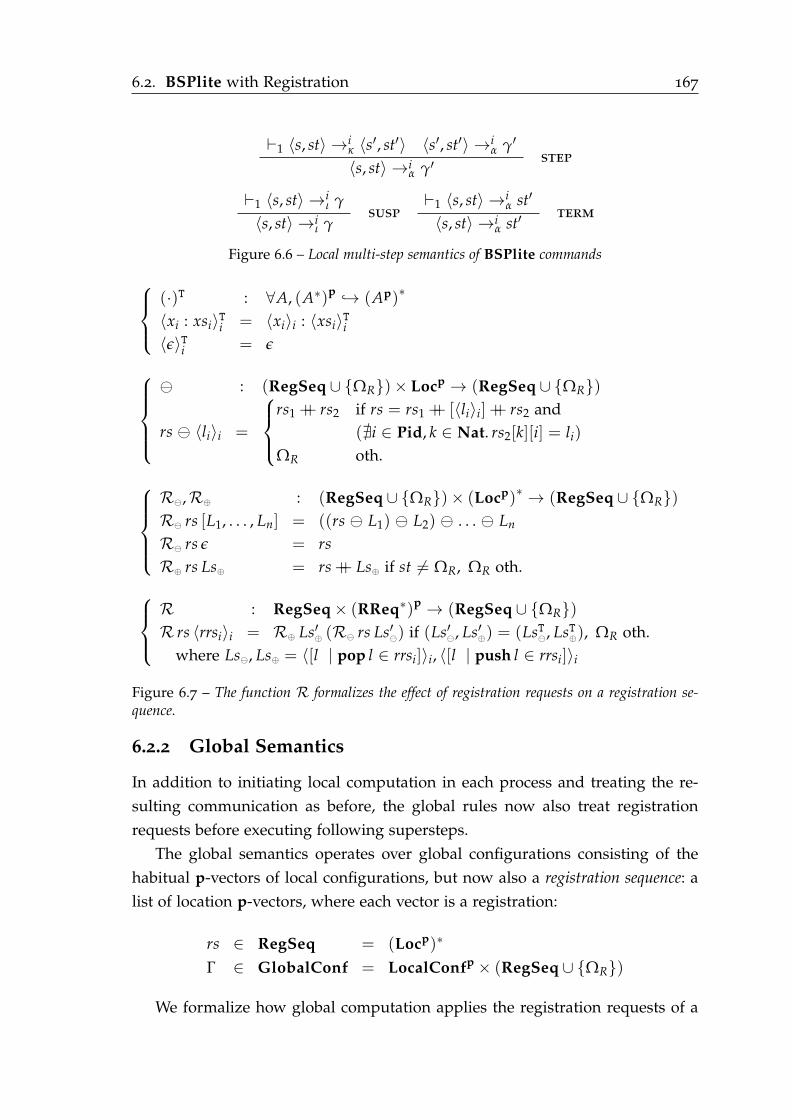
6.2. BSPlite with Registration 167
⊢1 〈s, st〉 →iκ 〈s′, st′〉 〈s′, st′〉 →i
α γ′
〈s, st〉 →iα γ′
step
⊢1 〈s, st〉 →iι γ
〈s, st〉 →iι γ
susp⊢1 〈s, st〉 →i
α st′
〈s, st〉 →iα st′
term
Figure 6.6 – Local multi-step semantics of BSPlite commands
(·)T : ∀A, (A∗)p → (Ap)∗
〈xi : xsi〉Ti = 〈xi〉i : 〈xsi〉
Ti
〈ǫ〉Ti = ǫ
⊖ : (RegSeq ∪ ΩR)× Locp → (RegSeq ∪ ΩR)
rs ⊖ 〈li〉i =
rs1 ++ rs2 if rs = rs1 ++ [〈li〉i] ++ rs2 and
(∄i ∈ Pid, k ∈ Nat. rs2[k][i] = li)
ΩR oth.
R⊖,R⊕ : (RegSeq ∪ ΩR)× (Locp)∗ → (RegSeq ∪ ΩR)
R⊖ rs [L1, . . . , Ln] = ((rs ⊖ L1) ⊖ L2) ⊖ . . . ⊖ Ln
R⊖ rs ǫ = rs
R⊕ rs Ls⊕ = rs ++ Ls⊕ if st 6= ΩR, ΩR oth.
R : RegSeq× (RReq∗)p → (RegSeq ∪ ΩR)
R rs 〈rrsi〉i = R⊕ Ls′⊕ (R⊖ rs Ls′⊖) if (Ls′⊖, Ls′⊕) = (LsT⊖, LsT⊕), ΩR oth.
where Ls⊖, Ls⊕ = 〈[l | pop l ∈ rrsi]〉i, 〈[l | push l ∈ rrsi]〉i
Figure 6.7 – The function R formalizes the effect of registration requests on a registration se-quence.
6.2.2 Global Semantics
In addition to initiating local computation in each process and treating the re-
sulting communication as before, the global rules now also treat registration
requests before executing following supersteps.
The global semantics operates over global configurations consisting of the
habitual p-vectors of local configurations, but now also a registration sequence: a
list of location p-vectors, where each vector is a registration:
rs ∈ RegSeq = (Locp)∗
Γ ∈ GlobalConf = LocalConfp × (RegSeq ∪ ΩR)
We formalize how global computation applies the registration requests of a
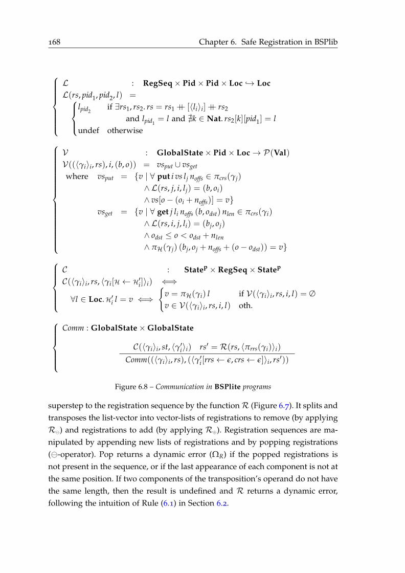
168 Chapter 6. Safe Registration in BSPlib
L : RegSeq× Pid× Pid× Loc → Loc
L(rs, pid1, pid2, l) =
lpid2if ∃rs1, rs2. rs = rs1 ++ [〈li〉i] ++ rs2
and lpid1= l and ∄k ∈ Nat. rs2[k][pid1] = l
undef otherwise
V : GlobalState× Pid× Loc→ P(Val)
V((〈γi〉i, rs), i, (b, o)) = vsput ∪ vsget
where vsput = v | ∀ put i vs lj noffs ∈ πcrs(γj)
∧ L(rs, j, i, lj) = (b, oi)
∧ vs[o− (oi + noffs)] = v
vsget = v | ∀ get j li noffs (b, odst) nlen ∈ πcrs(γi)
∧ L(rs, i, j, li) = (bj, oj)
∧ odst ≤ o < odst + nlen
∧ πH(γj) (bj, oj + noffs + (o− odst)) = v
C : Statep × RegSeq× Statep
C(〈γi〉i, rs, 〈γi[H← H′i]〉i) ⇐⇒
∀l ∈ Loc.H′i l = v ⇐⇒
v = πH(γi) l if V(〈γi〉i, rs, i, l) = ∅
v ∈ V(〈γi〉i, rs, i, l) oth.
Comm : GlobalState×GlobalState
C(〈γi〉i, st, 〈γ′i〉i) rs′ = R(rs, 〈πrrs(γi)〉i)
Comm((〈γi〉i, rs), (〈γ′i [rrs← ǫ, crs← ǫ]〉i, rs′))
Figure 6.8 – Communication in BSPlite programs
superstep to the registration sequence by the functionR (Figure 6.7). It splits and
transposes the list-vector into vector-lists of registrations to remove (by applying
R⊖) and registrations to add (by applying R⊕). Registration sequences are ma-
nipulated by appending new lists of registrations and by popping registrations
(⊖-operator). Pop returns a dynamic error (ΩR) if the popped registrations is
not present in the sequence, or if the last appearance of each component is not at
the same position. If two components of the transposition’s operand do not have
the same length, then the result is undefined and R returns a dynamic error,
following the intuition of Rule (6.1) in Section 6.2.
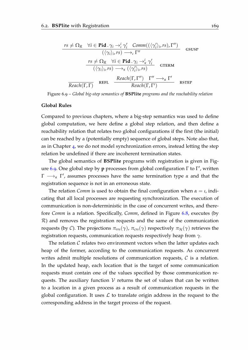
6.2. BSPlite with Registration 169
rs 6= ΩR ∀i ∈ Pid . γi →iι γ′i Comm((〈γ′i〉i, rs), Γ′′)
(〈γi〉i, rs) −→ι Γ′′gsusp
rs 6= ΩR ∀i ∈ Pid . γi →iκ γ′i
(〈γi〉i, rs) −→κ (〈γ′i〉i, rs)gterm
Reach(Γ, Γ)refl
Reach(Γ, Γ′′) Γ′′ −→α Γ′
Reach(Γ, Γ′)rstep
Figure 6.9 – Global big-step semantics of BSPlite programs and the reachability relation
Global Rules
Compared to previous chapters, where a big-step semantics was used to define
global computation, we here define a global step relation, and then define a
reachability relation that relates two global configurations if the first (the initial)
can be reached by a (potentially empty) sequence of global steps. Note also that,
as in Chapter 4, we do not model synchronization errors, instead letting the step
relation be undefined if there are incoherent termination states.
The global semantics of BSPlite programs with registration is given in Fig-
ure 6.9. One global step by p processes from global configuration Γ to Γ′, written
Γ −→α Γ′, assumes processes have the same termination type α and that the
registration sequence is not in an erroneous state.
The relation Comm is used to obtain the final configuration when α = ι, indi-
cating that all local processes are requesting synchronization. The execution of
communication is non-deterministic in the case of concurrent writes, and there-
fore Comm is a relation. Specifically, Comm, defined in Figure 6.8, executes (by
R) and removes the registration requests and the same of the communication
requests (by C). The projections πrrs(γ), πcrs(γ) respectively πH(γ) retrieves the
registration requests, communication requests respectively heap from γ.
The relation C relates two environment vectors when the latter updates each
heap of the former, according to the communication requests. As concurrent
writes admit multiple resolutions of communication requests, C is a relation.
In the updated heap, each location that is the target of some communication
requests must contain one of the values specified by those communication re-
quests. The auxiliary function V returns the set of values that can be written
to a location in a given process as a result of communication requests in the
global configuration. It uses L to translate origin address in the request to the
corresponding address in the target process of the request.
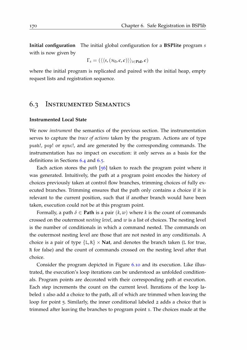
170 Chapter 6. Safe Registration in BSPlib
Initial configuration The initial global configuration for a BSPlite program s
with is now given by
Γs = (〈〈s, (H0, ǫ, ǫ)〉〉i∈Pid, ǫ)
where the initial program is replicated and paired with the initial heap, empty
request lists and registration sequence.
6.3 Instrumented Semantics
Instrumented Local State
We now instrument the semantics of the previous section. The instrumentation
serves to capture the trace of actions taken by the program. Actions are of type
push!, pop! or sync!, and are generated by the corresponding commands. The
instrumentation has no impact on execution: it only serves as a basis for the
definitions in Sections 6.4 and 6.5.
Each action stores the path [56] taken to reach the program point where it
was generated. Intuitively, the path at a program point encodes the history of
choices previously taken at control flow branches, trimming choices of fully ex-
ecuted branches. Trimming ensures that the path only contains a choice if it is
relevant to the current position, such that if another branch would have been
taken, execution could not be at this program point.
Formally, a path δ ∈ Path is a pair (k, w) where k is the count of commands
crossed on the outermost nesting level, and w is a list of choices. The nesting level
is the number of conditionals in which a command nested. The commands on
the outermost nesting level are those that are not nested in any conditionals. A
choice is a pair of type L, R ×Nat, and denotes the branch taken (L for true,
R for false) and the count of commands crossed on the nesting level after that
choice.
Consider the program depicted in Figure 6.10 and its execution. Like illus-
trated, the execution’s loop iterations can be understood as unfolded condition-
als. Program points are decorated with their corresponding path at execution.
Each step increments the count on the current level. Iterations of the loop la-
beled 1 also add a choice to the path, all of which are trimmed when leaving the
loop for point 5. Similarly, the inner conditional labeled 2 adds a choice that is
trimmed after leaving the branches to program point 1. The choices made at the
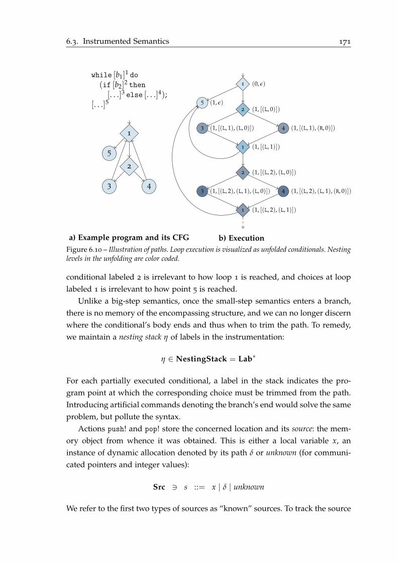
6.3. Instrumented Semantics 171
while [b1]1 do
(if [b2]2 then
[. . .]3 else [. . .]4);[. . .]5
1
2
3 4
5
1 (0, ǫ)
2 (1, [(L, 0)])
3 (1, [(L, 1), (L, 0)]) 4 (1, [(L, 1), (R, 0)])
5 (1, ǫ)
1 (1, [(L, 1)])
2 (1, [(L, 2), (L, 0)])
3 (1, [(L, 2), (L, 1), (L, 0)]) 4 (1, [(L, 2), (L, 1), (R, 0)])
1 (1, [(L, 2), (L, 1)])
a) Example program and its CFG b) Execution
Figure 6.10 – Illustration of paths. Loop execution is visualized as unfolded conditionals. Nestinglevels in the unfolding are color coded.
conditional labeled 2 is irrelevant to how loop 1 is reached, and choices at loop
labeled 1 is irrelevant to how point 5 is reached.
Unlike a big-step semantics, once the small-step semantics enters a branch,
there is no memory of the encompassing structure, and we can no longer discern
where the conditional’s body ends and thus when to trim the path. To remedy,
we maintain a nesting stack η of labels in the instrumentation:
η ∈ NestingStack = Lab∗
For each partially executed conditional, a label in the stack indicates the pro-
gram point at which the corresponding choice must be trimmed from the path.
Introducing artificial commands denoting the branch’s end would solve the same
problem, but pollute the syntax.
Actions push! and pop! store the concerned location and its source: the mem-
ory object from whence it was obtained. This is either a local variable x, an
instance of dynamic allocation denoted by its path δ or unknown (for communi-
cated pointers and integer values):
Src ∋ s ::= x | δ | unknown
We refer to the first two types of sources as “known” sources. To track the source
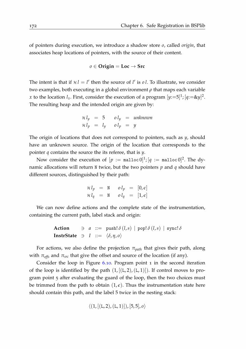
172 Chapter 6. Safe Registration in BSPlib
of pointers during execution, we introduce a shadow store o, called origin, that
associates heap locations of pointers, with the source of their content.
o ∈ Origin = Loc→ Src
The intent is that if H l = l′ then the source of l′ is o l. To illustrate, we consider
two examples, both executing in a global environment ρ that maps each variable
x to the location lx. First, consider the execution of a program [y:=5]1; [q:=&y]2.
The resulting heap and the intended origin are given by:
H ly = 5
H lp = ly
o ly = unknown
o lp = y
The origin of locations that does not correspond to pointers, such as y, should
have an unknown source. The origin of the location that corresponds to the
pointer q contains the source the its referee, that is y.
Now consider the execution of [p := malloc 0]1; [q := malloc 0]2. The dy-
namic allocations will return N twice, but the two pointers p and q should have
different sources, distinguished by their path:
H lp = N
H lq = N
o lp = [0, ǫ]
o lq = [1, ǫ]
We can now define actions and the complete state of the instrumentation,
containing the current path, label stack and origin:
Action ∋ a ::= push! δ (l, s) | pop! δ (l, s) | sync! δ
InstrState ∋ I ::= 〈δ, η, o〉
For actions, we also define the projection πpath that gives their path, along
with πoffs and πsrc that give the offset and source of the location (if any).
Consider the loop in Figure 6.10. Program point 1 in the second iteration
of the loop is identified by the path (1, [(L, 2), (L, 1)]). If control moves to pro-
gram point 5 after evaluating the guard of the loop, then the two choices must
be trimmed from the path to obtain (1, ǫ). Thus the instrumentation state here
should contain this path, and the label 5 twice in the nesting stack:
〈(1, [(L, 2), (L, 1)]), [5, 5], o〉
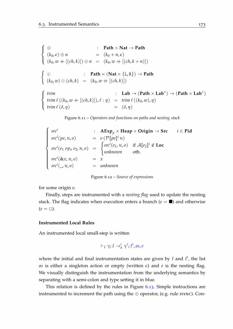
6.3. Instrumented Semantics 173
⊕ : Path×Nat→ Path
(k0, ǫ)⊕ n = (k0 + n, ǫ)
(k0, w ++ [(ch, k)])⊕ n = (k0, w ++ [(ch, k + n)])
⊙ : Path× (Nat× L, R)→ Path
(k0, w)⊙ (ch, k) = (k0, w ++ [(ch, k)])
trim : Lab→ (Path× Lab∗)→ (Path× Lab∗)
trim ℓ ((k0, w ++ [(ch, k)]), ℓ : η) = trim ℓ ((k0, w), η)
trim ℓ (δ, η) = (δ, η)
Figure 6.11 – Operators and functions on paths and nesting stack
srci : AExpp ×Heap×Origin→ Src i ∈ Pid
srci(pe,H, o) = o (PJpeKi H)
srci(e1 opa e2,H, o) =
srci(e1,H, o) if AJe2Ki /∈ Loc
unknown oth.
srci(&x,H, o) = x
srci(_,H, o) = unknown
Figure 6.12 – Source of expressions
for some origin o.
Finally, steps are instrumented with a nesting flag used to update the nesting
stack. The flag indicates when execution enters a branch (e = ) and otherwise
(e = 2).
Instrumented Local Rules
An instrumented local small-step is written
⊢1 γ; I →iα γ′; I′, as, e
where the initial and final instrumentation states are given by I and I′, the list
as is either a singleton action or empty (written ǫ) and e is the nesting flag.
We visually distinguish the instrumentation from the underlying semantics by
separating with a semi-colon and type setting it in blue.
This relation is defined by the rules in Figure 6.13. Simple instructions are
instrumented to increment the path using the ⊕ operator, (e.g. rule isync). Con-
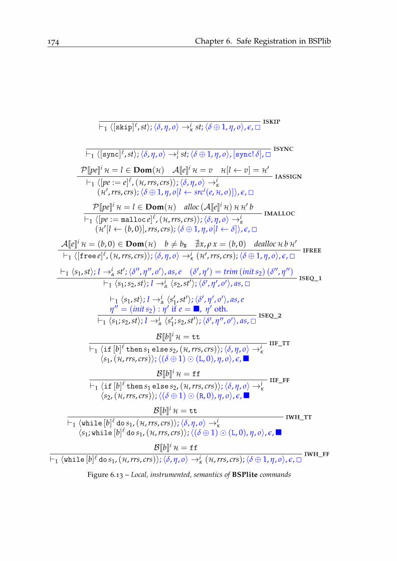
174 Chapter 6. Safe Registration in BSPlib
⊢1 〈[skip]ℓ, st〉; 〈δ, η, o〉 →iκ st; 〈δ⊕ 1, η, o〉, ǫ, 2
iskip
⊢1 〈[sync]ℓ, st〉; 〈δ, η, o〉 →iι st; 〈δ⊕ 1, η, o〉, [sync! δ], 2
isync
PJpeKi H = l ∈ Dom(H) AJeKi H = v H[l ← v] = H′
⊢1 〈[pe := e]ℓ, (H, rrs, crs)〉; 〈δ, η, o〉 →iκ
(H′, rrs, crs); 〈δ⊕ 1, η, o[l ← srci(e,H, o)]〉, ǫ, 2
iassign
PJpeKi H = l ∈ Dom(H) alloc (AJeKi H)HH′ b
⊢1 〈[pe := malloc e]ℓ, (H, rrs, crs)〉; 〈δ, η, o〉 →iκ
(H′[l ← (b, 0)], rrs, crs); 〈δ⊕ 1, η, o[l ← δ]〉, ǫ, 2
imalloc
AJeKi H = (b, 0) ∈ Dom(H) b 6= bN ∄x, ρ x = (b, 0) deallocH bH′
⊢1 〈[free e]ℓ, (H, rrs, crs)〉; 〈δ, η, o〉 →iκ (H′, rrs, crs); 〈δ⊕ 1, η, o〉, ǫ, 2
ifree
⊢1 〈s1, st〉; I →iα st′; 〈δ′′, η′′, o′〉, as, e (δ′, η′) = trim (init s2) (δ
′′, η′′)
⊢1 〈s1; s2, st〉; I →iα 〈s2, st′〉; 〈δ′, η′, o′〉, as, 2
iseq_1
⊢1 〈s1, st〉; I →iα 〈s
′1, st′〉; 〈δ′, η′, o′〉, as, e
η′′ = (init s2) : η′ if e = , η′ oth.
⊢1 〈s1; s2, st〉; I →iα 〈s
′1; s2, st′〉; 〈δ′, η′′, o′〉, as, 2
iseq_2
BJbKi H = tt
⊢1 〈if [b]ℓ then s1 else s2, (H, rrs, crs)〉; 〈δ, η, o〉 →i
κ
〈s1, (H, rrs, crs)〉; 〈(δ⊕ 1)⊙ (L, 0), η, o〉, ǫ,
iif_tt
BJbKi H = ff
⊢1 〈if [b]ℓ then s1 else s2, (H, rrs, crs)〉; 〈δ, η, o〉 →i
κ
〈s2, (H, rrs, crs)〉; 〈(δ⊕ 1)⊙ (R, 0), η, o〉, ǫ,
iif_ff
BJbKi H = tt
⊢1 〈while [b]ℓ do s1, (H, rrs, crs)〉; 〈δ, η, o〉 →i
κ
〈s1; while [b]ℓ do s1, (H, rrs, crs)〉; 〈(δ⊕ 1)⊙ (L, 0), η, o〉, ǫ,
iwh_tt
BJbKi H = ff
⊢1 〈while [b]ℓ do s1, (H, rrs, crs)〉; 〈δ, η, o〉 →iκ (H, rrs, crs); 〈δ⊕ 1, η, o〉, ǫ, 2
iwh_ff
Figure 6.13 – Local, instrumented, semantics of BSPlite commands
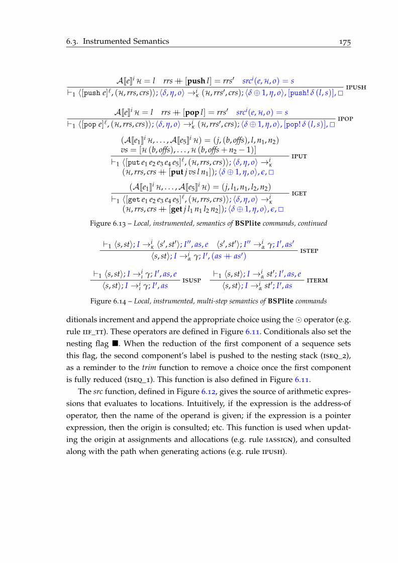
6.3. Instrumented Semantics 175
AJeKi H = l rrs ++ [push l] = rrs′ srci(e,H, o) = s
⊢1 〈[push e]ℓ, (H, rrs, crs)〉; 〈δ, η, o〉 →iκ (H, rrs′, crs); 〈δ⊕ 1, η, o〉, [push! δ (l, s)], 2
ipush
AJeKi H = l rrs ++ [pop l] = rrs′ srci(e,H, o) = s
⊢1 〈[pop e]ℓ, (H, rrs, crs)〉; 〈δ, η, o〉 →iκ (H, rrs′, crs); 〈δ⊕ 1, η, o〉, [pop! δ (l, s)], 2
ipop
(AJe1Ki H, . . . ,AJe5Ki H) = (j, (b, offs), l, n1, n2)vs = [H (b, offs), . . . ,H (b, offs + n2 − 1)]
⊢1 〈[put e1 e2 e3 e4 e5]ℓ, (H, rrs, crs)〉; 〈δ, η, o〉 →i
κ
(H, rrs, crs ++ [put j vs l n1]); 〈δ⊕ 1, η, o〉, ǫ, 2
iput
(AJe1Ki H, . . . ,AJe5Ki H) = (j, l1, n1, l2, n2)
⊢1 〈[get e1 e2 e3 e4 e5]ℓ, (H, rrs, crs)〉; 〈δ, η, o〉 →i
κ
(H, rrs, crs ++ [get j l1 n1 l2 n2]); 〈δ⊕ 1, η, o〉, ǫ, 2
iget
Figure 6.13 – Local, instrumented, semantics of BSPlite commands, continued
⊢1 〈s, st〉; I →iκ 〈s′, st′〉; I′′, as, e 〈s′, st′〉; I′′ →i
α γ; I′, as′
〈s, st〉; I →iα γ; I′, (as ++ as′)
istep
⊢1 〈s, st〉; I →iι γ; I′, as, e
〈s, st〉; I →iι γ; I′, as
isusp⊢1 〈s, st〉; I →i
α st′; I′, as, e
〈s, st〉; I →iα st′; I′, as
iterm
Figure 6.14 – Local, instrumented, multi-step semantics of BSPlite commands
ditionals increment and append the appropriate choice using the⊙ operator (e.g.
rule iif_tt). These operators are defined in Figure 6.11. Conditionals also set the
nesting flag . When the reduction of the first component of a sequence sets
this flag, the second component’s label is pushed to the nesting stack (iseq_2),
as a reminder to the trim function to remove a choice once the first component
is fully reduced (iseq_1). This function is also defined in Figure 6.11.
The src function, defined in Figure 6.12, gives the source of arithmetic expres-
sions that evaluates to locations. Intuitively, if the expression is the address-of
operator, then the name of the operand is given; if the expression is a pointer
expression, then the origin is consulted; etc. This function is used when updat-
ing the origin at assignments and allocations (e.g. rule iassign), and consulted
along with the path when generating actions (e.g. rule ipush).

176 Chapter 6. Safe Registration in BSPlib
rs 6= ΩR ∀i ∈ Pid . γi; Ii →iι γ′i ; I′i , asi IComm((〈γ′i ; I′i 〉i, rs), Γ′′)
(〈γi; Ii〉i, rs) −→ι Γ′ ; 〈asi〉iigsusp
rs 6= ΩR ∀i ∈ Pid . γi; Ii →iκ γ′i ; I′i , asi
(〈γi; Ii〉i, rs) −→κ (〈γ′i ; I′i 〉i, rs) ; 〈asi〉iigterm
Reach(Γ, Γ); 〈ǫ〉iirefl
Reach(Γ, Γ′′); A Γ′′ −→α Γ′ ; A′
Reach(Γ, Γ′); A ++ A′irstep
Figure 6.15 – Instrumented global big-step semantics of BSPlite programs and the reachabilityrelation
Instrumented Multi-Step Relation
We define an instrumented multi-step relation in Figure 6.14, which propagates
the instrumentation and accumulates actions. We write
γ; I →iα γ′; I′, as
if there is a sequence of instrumented sequence of small-steps from γ such that
γ′ lacks a residue or is suspended, with I and I′ as the sequence’s initial and
final instrumentation and where the final action trace is given by as.
6.3.1 Instrumented Global Semantics
Similarly, we instrument the global semantics, which is written:
Γ −→α Γ′ ; A
Here, the p-vector A collects each process’s action trace. The instrumented
global semantics and reachability relation, are defined in Figure 6.15. The in-
strumentation of the global semantics does three things: it propagates the in-
strumented states, it accumulates the action traces vectors by concatenation, and
it instruments communication so that the source of overwritten pointers is set to
unknown. This is done by the function IComm, whose definition is omitted.
The trace vectors resulting from executing the running examples with the in-
strumentation is given in Figure 6.16. The trace vectors of the first two programs
are unremarkable: registration is applied to the location of local variables with
the corresponding source. In the third example, we note how the difference in
source of the second push allows to distinguish registrations of distinct mem-
ory objects. This would not be directly possible from locations in the modeled

6.3.In
strum
ented
Sem
antics
177
Program Action trace vector LC TA SA SF GC
Example 1〈 [push! . . . (ly, y), push! . . . (lz, z), push! . . . (ly, y), push! . . . (lx, x), sync! . . . , pop! (ly, y), sync! . . .],
[push! . . . (ly, y), push! . . . (lz, z), push! . . . (ly, y), push! . . . (lx, x), sync! . . . , pop! (ly, y), sync! . . .] 〉
Example 2〈 [push! . . . (lx, x), pop! (lx, x), sync! . . .],
[push! . . . (lx, x), pop! (lx, x), sync! . . .] 〉
Example 3〈 [push! . . . (ly, y), push! . . . (ly, y), sync! . . . , pop! (ly, y), sync! . . .],
[push! . . . (ly, y), push! . . . (lx, x), sync! . . . , pop! (ly, y), sync! . . .] 〉
Example 4〈 [push! . . . (N , (0, ǫ)), push! . . . (N , (1, ǫ)), sync! . . . , pop! (N , (0, ǫ)), sync! . . .],
[push! . . . (l1, (0, ǫ)), push! . . . (l2, (1, ǫ)), sync! . . . , pop! (l1, (0, ǫ)), sync! . . .] 〉
Example 5〈 [sync! (1, ǫ)],
[push! (1, [(R, 0)]) (lx, x), sync! (1, ǫ)] 〉
Example 6〈 [push! (0, ǫ) (ly, y), sync! (1, ǫ), pop! (2, [(L, 0)]) (ly, y), push! (2, [(L, 1)]) (lx, x), sync! (2, ǫ)],
[push! (0, ǫ) (ly, y), sync! (1, ǫ), push! (2, [(R, 0)]) (lx, x), pop! (2, [(R, 1)]) (ly, y), sync! (2, ǫ)] 〉
Figure 6.16 – Trace vectors resulting from executing running examples with p = 2. The right part of the table evaluates the traces’ local correctness(LC), the vector’s textual collective alignment (TA), source alignment (SA) and safety (SF), and global correctness (GC) as defined in Sections 6.4and 6.5. Here, lx is the location of variable x and x its source and li is the ith address returned by malloc. For legibility, the paths in actions have beenreplaced by ellipses, in all examples but Example 5 and Example 6.

178 Chapter 6. Safe Registration in BSPlib
language, since the address of distinct local variables may be the same on dif-
ferent processes. Conversely, the address of the same local variable may differ
between processes. This is demonstrated by the fourth example. Here the two
pushes of each process concern different instances of memory allocation. Even
though the location of the push, as in the trace of the first process, concur, the
source allows to distinguish them. In the fifth example, we see immediately that
process 1 does not participate in the push, indicating a dynamic error. In the
final example, both processes participate in the push and the pop. However, the
distinct paths of the push! actions respectively pop! actions indicate that those
actions did not result from calls from the same instruction in the program.
An important property of the action trace vectors of the instrumentation is
that each known source is associated to at most one base in each process. We call
such action trace vectors consistent. Intuitively, the same base may be allocated
twice (i.e. bN), but the path of each execution step is unique and so by extension,
the source of each dynamic allocation is also unique. This is demonstrated in the
trace of Example 5 in Figure 6.16.
Conversely, an action trace where two distinct bases appear with two known
but different sources can not be generated by the instrumentation. It would either
contradict the requirement that the global environment assigns unique bases to
each local variable, or the fact that each distinct dynamic allocations comes from
a different path.
Lemma 1. If Reach(Γ, Γ′); A then the same source s 6= unknown never appears twice
in the same component of A associated with two locations of different base.
For the proof sketch of this lemma, and proof sketches of remaining proper-
ties in this chapter with omitted proofs, we refer to Appendix B.
The semantics also ensures that the source of each local variable x is always
associated with the fixed location of that variable, i.e. ρ x.
Instrumented initial configuration The initial instrumentation state has an
empty path, empty nesting stack and initial origin o0 = (λl.unknown). Hence,
the instrumented initial global configuration is given by
Γc = (〈〈c, (H0, ǫ, ǫ)〉; 〈(0, ǫ), ǫ, o0〉〉i, ǫ)
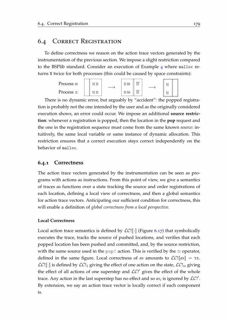
6.4. Correct Registration 179
6.4 Correct Registration
To define correctness we reason on the action trace vectors generated by the
instrumentation of the previous section. We impose a slight restriction compared
to the BSPlib standard. Consider an execution of Example 4 where malloc re-
turns N twice for both processes (this could be caused by space constraints):
Process 0: NN
NN
−→NN N
NN N
−→N
NProcess 1:
There is no dynamic error, but arguably by “accident”: the popped registra-
tion is probably not the one intended by the user and as the originally considered
execution shows, an error could occur. We impose an additional source restric-
tion: whenever a registration is popped, then the location in the pop request and
the one in the registration sequence must come from the same known source: in-
tuitively, the same local variable or same instance of dynamic allocation. This
restriction ensures that a correct execution stays correct independently on the
behavior of malloc.
6.4.1 Correctness
The action trace vectors generated by the instrumentation can be seen as pro-
grams with actions as instructions. From this point of view, we give a semantics
of traces as functions over a state tracking the source and order registrations of
each location, defining a local view of correctness, and then a global semantics
for action trace vectors. Anticipating our sufficient condition for correctness, this
will enable a definition of global correctness from a local perspective.
Local Correctness
Local action trace semantics is defined by LC !J·K (Figure 6.17) that symbolically
executes the trace, tracks the source of pushed locations, and verifies that each
popped location has been pushed and committed, and, by the source restriction,
with the same source used in the pop! action. This is verified by the ≃ operator,
defined in the same figure. Local correctness of as amounts to LC !JasK = tt.
LC !J·K is defined by LC !1 giving the effect of one action on the state, LC !ss giving
the effect of all actions of one superstep and LC !′ gives the effect of the whole
trace. Any action in the last superstep has no effect and so asi is ignored by LC !′.
By extension, we say an action trace vector is locally correct if each component
is.

180 Chapter 6. Safe Registration in BSPlib
r ∈ Map = Loc→ Src∗
LC !1J·K : Action→ Map → Map
LC !1Jpop! δ (l, s)K r = r[l ← ss] if (r[l] = s′ : ss) ∧ s ≃ s′, undef oth.
LC !1Jpush! δ (l, s)K r = r[l ← s : r[l]]
LC !1Jsync! δK r = undef
LC !ssJ·K : Action∗ → Map → Map
LC !ssJasK r = fold LC !1J·K as′ r
where as′ = [a | ∀a ∈ as, a = pop! _ _] ++ [a | ∀a ∈ as, a = push! _ _]
LC !′J·K : Action∗ → Map
LC !′JasK = fold LC !ssJ·K [as1, . . . , asn−1] (λl.ǫ)
where as1 ++ [sync! δ1] ++ . . . ++ [sync! δn−1] ++ asn = as
such that ∀1 ≤ i ≤ n, (sync! _) /∈ asi
LC !J·K : Action∗ → Bool
LC !JasK = tt if LC !′JasK is defined, ff oth.
s1 ≃ s2 ⇐⇒ unknown /∈ s1, s2 ∧ s1 = s2
fold f ǫ r = rfold f [a1, . . . , an] r = ( f an . . . f a1) r
Figure 6.17 – Local correctness of an action trace

6.4. Correct Registration 181
r ∈ MapI = Loc→ (Nat× Src∗)m ∈ Matching = (Nat×Nat∗)∗
GC !1 : Action→ (Nat×Nat∗ ×MapI) → (Nat×Nat∗ ×MapI
GC !1Jpop! δ (l, s)K (k, ps, r) =
(k, k′ : ps, r[l ← is]) if r[l] = (k′, s′) : is ∧ s ≃ s′
undef otherwise
GC !1Jpush! δ (l, s)K (k, ps, r) = (k + 1, ps, r[l ← (k, s) : r[l]])
GC !1Jsync! δK (k, ps, r) = undef
GC !ss : Action∗ → (Matching×MapI) → (Matching×MapI)
GC !ssJasK (m, r) = let k′ = k if m = m′ ++ [(k, _)], 0 oth. in
let (k′′, ps, r′) = fold GC !1J·K as′ (k′, ǫ, r) in
(m ++ [(k′′, ps)], r′)
where as′ = [a | ∀a ∈ as, a = pop! _ _] ++ [a | ∀a ∈ as, a = push! _ _]
GC !′ : Action∗ → (Matching×MapI)
GC !′JasK = fold GC !ssJ·K [as1, . . . , asn−1] (ǫ, λl.ǫ)
where as1 ++ [sync! δ1] ++ . . . ++ [sync! δn−1] ++ asn = as
GC ! : (Action∗)p → Bool
GC !J〈asi〉iK = tt if ∃ms, ∀i ∈ Pid.GC !′JasiK(ǫ, λl.ǫ) = (ms, _), ff oth.
Figure 6.18 – Global correctness of a trace vector
Global Correctness
As the executions of Examples 3 and 5 demonstrate, local correctness of a trace
vector does not suffice for its global correctness. They must also make compat-
ible sequences of actions (unlike Example 5), and pops must occur at the same
position in the registration sequence (unlike Example 3).
To capture these requirements, we abstract the effect of a trace into a matching
(see Figure 6.18). The matching is one pair (k, ps) per superstep, where k counts
the total number of pushes at the end of the superstep and ps is a list containing
the index of each push removed by a pop in the superstep. GC ! extends LC !
to index the pushes added to the state, and to return the matching of locally
correct traces. We then define a trace vector as being globally correct when each
component has the same matching.
Before going further, we reconnect global correctness of traces with the se-

182 Chapter 6. Safe Registration in BSPlib
mantics of BSPlite, and confirm that executions with globally correct traces do
not have registration errors:
Theorem 4. If Reach(Γc, (〈γi; Ii〉i, rs)); A and GC !JAK = tt then rs 6= ΩR.
This trace-based characterization of correctness is independent of the un-
derlying instrumented language. But, we have yet to simplify the task of writing
correct programs. In the next section we define our sufficient condition that guar-
antees safe registration.
6.5 Sufficient Condition for Correct Registra-
tion
The sufficient condition for registration imposes 3 conditions: (1) collective
calls to sync, push and pop should be textually aligned (2) the argument of col-
lective calls to push and pop should be source aligned, i.e., refer to the same mem-
ory object: the same local variable or the same instance of dynamically allocated
memory in all processes; (3) the trace of actions of each process should be locally
correct. These conditions in conjunction guarantee global correctness.
Consider again the running examples. The execution of Example 2 is not lo-
cally correct in any process, and hence disqualified. Due to the source restriction,
the execution of Example 4 by process 0 is not locally correct. In the execution of
Example 3, the memory object referred to by q is not the same in each process,
and hence the second push is not source aligned. The executions of Examples 5
and 6 are not textually aligned. Only Example 1 follows satisfies the sufficient
condition.
We now formalize the sufficient condition using action trace vectors:
Definition 3. A trace vector 〈asi〉i has textually aligned collectives if each compo-
nent has the same length and at each position, the same path:
∃m ∈ Nat. ∀i, j ∈ Pid. |asi| = |asj| = m ∧ ∀0 ≤ k < m. πpath(asi[k]) = πpath(asj[k])
Definition 4. A trace vector with textually aligned collectives 〈asi〉i is source aligned
if all components have the same (known) source and offset at each position:
∀i, j ∈ Pid. ∀0 ≤ k < |asi|.asi[k] 6= sync! _
=⇒ πsrc(asi[k]) ≃ πsrc(asj[k]) ∧ πoffs(asi[k]) = πoffs(asj[k])
6.6. Related Work 183
Definition 5. A consistent trace vector A that has textually aligned collectives, is source
aligned and locally correct is called safe.
By extension, a program in our sufficient condition is one that only produces
safe action trace vectors. The action trace vectors of the running examples are
evaluated against these conditions in Figure 6.16. As expected, the intuitions
given above are consistent with the formalization. Finally, we prove that the
sufficient condition guarantees global correctness:
Theorem 5. If A is safe then GC !JAK = tt.
As an immediate corollary, an execution that produces a safe action trace
vector does not have any registration errors:
Corollary 2. If Reach(Γc, (〈γi; Ii〉i, rs)); A and A is safe then rs 6= ΩR.
Proof: Immediate by Theorem 5 and Theorem 4.
This sufficient condition is inspired by examining realistic and correct BSPlib
code. We have manually inspected our corpus of BSPlib programs, and found
that programs appear to satisfy it. This intuition remains to be verified, prefer-
ably by the development and application of a static analysis targeting the con-
dition. However, our observations leads us to conjecture that in addition to en-
suring correctness, the condition is sufficiently permissive and coherent with the
programmer’s intuition of correctness.
6.6 Related Work
To the best of our knowledge, this is the first work towards automatically
verifying registrations in BSPlib. Closest to our work is BSP-Why [74], a tool for
deductive verification of BSPlib-like imperative BSP programs. While BSP-Why
can verify programs using registrations for communication, it is unclear to which
degree the modelization is true to the BSPlib standard, and while this work forms
the basis for automatic verification, the BSP-Why user must manually prove their
program correct.
Other languages and libraries for parallelism enjoy less error-prone schemes
than registrations for creating associations between local and remote memory for
DRMA communication. In the BSP paradigm, Yzelman et al. [207], use a commu-
nication container class to turn regular objects into distributed data-structures.

184 Chapter 6. Safe Registration in BSPlib
MPI [139, p. 403] uses window objects to allow a process to reference remote
memory. Like BSPlib registrations, windows act as handles and are created and
removed collectively. Unlike registrations, windows can be removed in any or-
der. In OpenSHMEM [36], DRMA operations are only allowed on “symmetric”
objects that the runtime system ensures have the same relative address in each
process.
Previous authors, such as Tesson et al. [184], have formalized BSPlib, but did
not consider registration. Gava et al. [80] formalize Paderborn’s BSPlib [27], with
DRMA but they do not formalize pointers and their modelization of registration
is simplified. This leads us to believe that ours is the first realistic formalization
of BSPlib registration.
6.7 Concluding Remarks
In this chapter, we have studied errors caused by registration in BSPlib. Reg-
istration is used to create associations between local and remote memory, but can
provoke errors if done incorrectly. We have formalized BSPlib with registration,
characterized correct executions, given a sufficient condition and proved that it
guarantees correctness with respect to our semantics.
The logical continuation of this work is to develop a static analysis targeting
this sufficient condition, and to evaluate it by verifying registration in real-world
BSPlib programs. This will prove our intuition that the sufficient condition is
permissive enough to include realistic programs.
7Conclusion and Future Work
Contents
7.1 Context . . . . . . . . . . . . . . . . . . . . . . . . . . . . . . . . . . . . . 185
7.2 Thesis . . . . . . . . . . . . . . . . . . . . . . . . . . . . . . . . . . . . . . . 186
7.3 Contributions . . . . . . . . . . . . . . . . . . . . . . . . . . . . . . . . . 186
7.4 Perspectives . . . . . . . . . . . . . . . . . . . . . . . . . . . . . . . . . . 187
7.1 Context
Parallel computing is an important component in achieving high computa-
tion capacities. Large calculations that require the application of parallel compu-
tation are now commonplace. Not exclusively, but notably, in the natural sciences
where increasing fidelity in simulations enable a more precise understanding of
subjects as diverse as the origin of the universe and the composition of mat-
ter [97]; the functioning of the earth system [137] — with important implications
for climate science; the formation of galaxies [64]; and the human brain [136].
However, even more so than sequential computing, parallel computing is
fraught with errors. The well-known difficulties of developing correct sequential
programs, and the disastrous effects when approached lightly (of which spectac-
ular examples abound [65]), are exacerbated by the exponential number of inter-
actions between processes. Additionally, the hoped for increase in computation
power when applying parallel computing does not come for free. In all but em-
barrassingly parallel cases, a performance increase requires a well-thought out
strategy for how to parallelize the problem at hand, demanding significant effort.
It is also difficult to a priori ensure scaling and portability of the parallelization.
The Bulk Synchronous Parallel model, and its commonly used implementa-
tion in the BSPlib library, answers some of these concerns by providing a struc-
ture of parallel computing that rules out certain classes of errors. Furthermore, it
185

186 Chapter 7. Conclusion and Future Work
enables reliable and portable performance predictions. However, care must still
be taken to develop correct BSPlib programs, and manual program analysis is
necessary to enjoy the BSP performance model.
Formal methods provide a framework for developing software that is math-
ematically guaranteed to be safe and efficient. Automatic push-button methods,
such as static analysis, are especially promising as they do not require the inter-
vention of experts in formal methods. It is the lack of such methods adapted for
BSPlib that has motivated this thesis. We have aimed to develop automated tools
to aid the development of BSPlib programs that are both correct and efficient.
7.2 Thesis
Our thesis is that the majority of BSPlib programs follows a structure called
textual alignment. We have argued that textual alignment should be enforced in
scalable parallel programs and that static analyses can be developed that exploit
this property. This approach elegantly alleviates one of the principal problems
when analyzing parallel programs, namely the large number of possible interac-
tions between processes.
7.3 Contributions
To argue the importance of textual alignment, we have first conceived a static
analysis verifying textual alignment of synchronization in BSPlib programs. We
have formalized, proved sound in Coq, implemented in Frama-C and evaluated
this analysis. Second, we have conceived, implemented as a prototype and eval-
uated a static cost analysis for BSPlib programs that exploits textual alignment.
Third, we have conceived a sufficient condition, based on textual alignment, for
BSPlib that we prove guarantees safe registration. Finally, these developments
are based on a series of progressively more involved formalizations of BSPlib
features, from synchronization to communication and registration.

7.4. Perspectives 187
7.4 Perspectives
We conclude by discussing some promising lines of research.
The precision of the static analysis for textual alignment can be improved. It
is in particular the conservative assumptions about communication that require
revision. A fine analysis of communication patterns in BSPlib, possibly based on
polyhedral techniques, to expand the recognition of pid-independent expressions
would reduce the amount of annotations currently required.
The current prototype implementation of the cost analysis should be im-
plemented and evaluated on realistic BSPlib programs, to further validate its
applicability. The analysis of communication costs is precise, but only for data-
oblivious communication patterns. Further research is needed to devise static
cost analyses of data-dependent communication.
The sufficient condition for safe registration should be the target of a static
analysis. This analysis must be conceived, proved to statically approximate the
sufficient condition and implemented to evaluate its practicality.
Textual alignment could also be exploited outside static analysis. Previous au-
thors have initiated work towards deductive verification of scalable parallel pro-
grams, notably by the introduction of invariants over all processes [175]. These
invariants are attached as assertions to synchronization primitives. We believe
such assertions can be attached to any textual aligned program point, and serve
as the basis of a new, compositional proof system for imperative, SPMD pro-
grams.
In this thesis we focus on BSPlib. BSPlib can be seen as a model of the Bulk
Synchronous subset of other parallel libraries based on the SPMD model such
as MPI. Finally, we propose applying the results in this thesis to MPI, and also,
exploiting textual alignment to develop new static analyses for MPI. Static anal-
ysis for synchronization based on the work on Barrier Inference has already
been implemented for MPI [209], and the authors note that MPI barriers tend to
be textually aligned. However, to the best of our knowledge, there is no work
on cost analysis for MPI. The BSP subset of MPI can be assumed to follow the
same cost model as BSPlib, opening up an extensions of our cost analysis to this
library.
The semantics of MPI windows are not afflicted by the same issues as the
homologue of BSPlib registrations. This limits the applicability of our contribu-
tions towards safe registration in the context of MPI. However, a static analysis
of registration is a first step towards verifying the correct usage of DRMA op-
erations in BSPlib. The high-performance primitives of BSPlib are similar to the
188 Chapter 7. Conclusion and Future Work
RMA primitives of MPI, and notably, the intermingling of remote and local ac-
cesses unprotected by synchronization can give implementation specific or erro-
neous behavior in both libraries [89]. We think that textual alignment could serve
as a framework towards formalizing a simplified programming model for safe
DRMA, as the one suggested by Gropp [89, p. 91]. This model could then serves
as the formal underpinnings for a static analysis verifying DRMA operation in
both BSPlib and MPI.

Appendix
189

AProofs for Replicated
Synchronization
Contents
A.1 Operational Semantics Simulates Denotational . . . . . . . . . 191
A.1.1 Stable State Transformers . . . . . . . . . . . . . . . . . . . . . . . 192
A.1.2 Simulation . . . . . . . . . . . . . . . . . . . . . . . . . . . . . . . . 194
A.2 Correctness of PI . . . . . . . . . . . . . . . . . . . . . . . . . . . . . . 203
A.2.1 Domain . . . . . . . . . . . . . . . . . . . . . . . . . . . . . . . . . . 204
A.2.2 Parameterized Constraint System . . . . . . . . . . . . . . . . . . . 204
A.2.3 Constraint System Facts . . . . . . . . . . . . . . . . . . . . . . . . 205
A.2.4 Marked Path Abstractions and pid-independent Variables . . . . 205
A.2.5 Correctness of the Analysis . . . . . . . . . . . . . . . . . . . . . . 209
A.3 Correctness of RS . . . . . . . . . . . . . . . . . . . . . . . . . . . . . . 216
A.3.1 Safe State Transformers . . . . . . . . . . . . . . . . . . . . . . . . . 216
In this section we give the soundness proof of the Replicated Synchronization
analysis, detailed in Chapter 4. These proofs have been mechanized and verified
in the Coq proof assistant. A natural language version of them follow.
In these proofs, we shall sometimes take the liberty of hiding program labels
to improve legibility.
A.1 Operational Semantics Simulates Denota-
tional
This section contains the proof of Theorem 1.
191

192 Appendix A. Proofs for Replicated Synchronization
A.1.1 Stable State Transformers
Recall the definition of DI : for I ⊆ Pid, we note
DI = θ ∈ D \ ⊥, ΩS | θ i = 000 ⇐⇒ i 6∈ I
Definition 6. A function f : D → D is stable if ∀I ⊆ Pid, ∀θ ∈ DI , F θ ∈ DI ⋒
⊥, ΩS, f ΩS = ΩS and f ⊥ = ⊥.
The composition of two stable functions is stable.
Lemma 2 (Stable Composition). Let f1, f2 : D → D be two stable functions. Then
f1 f2 is also stable.
Proof: Take any I ⊆ Pid and any θ ∈ DI , and show that ( f1 f2) θ ∈ DI ∪
⊥, ΩS.
Since f2 is stable, either f2 θ ∈ DI or f2 θ ∈ ⊥, ΩS. In the latter case, since f1
is stable, f1 ( f2 θ) = ( f2 θ) ∈ ⊥, ΩS, and in the former case, since f1 is stable,
we have f1 ( f2 θ) ∈ DI ∪ ⊥, ΩS.
Lemma 3 (Stable Mask Combine). Let f1, f2 : D → D be two stable functions. Let
b ∈ BExp. Then λθ. f1 (∂b θ) ‖ f2 (∂!b θ) is also stable.
Proof: Let f = λθ. f1 (∂b θ) ‖ f2 (∂!b θ). By the definition of ∂, the stability of f1
and f2 and the definition of ‖ we have f ΩS = ΩS and f ⊥ = ⊥. So let I ⊆ Pid
and θ ∈ DI , and show that f θ ∈ DI ∪ ⊥, ΩS.
Let I′ = i ∈ I | BJbKi θ[i] = tt. Then (∂b θ) ∈ DI′ and (∂!b θ) ∈ DI\I′ . Let
θ1 = f1 (∂b θ) and θ2 = f2 (∂!b θ). Since f1 and f2 are stable, θ1 ∈ DI′ ∪ ⊥, ΩS
and θ2 ∈ DI\I′ ∪ ⊥, ΩS.
Either
• θ1 ∈ ⊥, ΩS or θ2 ∈ ⊥, ΩS and then f θ = (θ1 ‖ θ2) ∈ ⊥, ΩS as well,
or
• θ1 ∈ DI′ and θ2 ∈ DI\I′ . In this case, f θ = λi.θ1[i] + θ2[i]. We show that
f θ ∈ DI . By the definition of DI , we must show that ( f θ)[i] = 000 ⇐⇒ i 6∈
I.
( =⇒ ) Then ( f θ)[i] = 000 . If ( f θ)[i] = θ1[i] + θ2[i] = 000 then θ1[i] = 000 and
θ2[i] = 000. Then by definition of DI′ and DI\I′ , i 6∈ I′ and i 6∈ I \ I′.
Thus i 6∈ I.
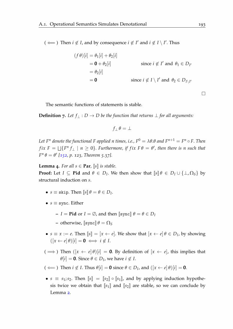
A.1. Operational Semantics Simulates Denotational 193
(⇐= ) Then i 6∈ I, and by consequence i 6∈ I′ and i 6∈ I \ I′. Thus
( f θ)[i] = θ1[i] + θ2[i]
= 000 + θ2[i] since i 6∈ I′ and θ1 ∈ DI′
= θ2[i]
= 000 since i 6∈ I \ I′ and θ2 ∈ DI\I′
The semantic functions of statements is stable.
Definition 7. Let f⊥ : D → D be the function that returns ⊥ for all arguments:
f⊥ θ = ⊥
Let Fn denote the functional F applied n times, i.e., F0 = λθ.θ and Fn+1 = Fn F. Then
f ix F =⊔
Fn f⊥ | n ≥ 0. Furthermore, if f ix F θ = θ′, then there is n such that
Fn θ = θ′ [152, p. 123, Theorem 5.37].
Lemma 4. For all s ∈ Par, JsK is stable.
Proof: Let I ⊆ Pid and θ ∈ DI . We then show that JsK θ ∈ DI ∪ ⊥, ΩS by
structural induction on s.
• s ≡ skip. Then JsK θ = θ ∈ DI .
• s ≡ sync. Either
– I = Pid or I = ∅, and then JsyncK θ = θ ∈ DI
– otherwise, JsyncK θ = ΩS
• s ≡ x := e. Then JsK = [x ← e]. We show that [x ← e] θ ∈ DI , by showing
([x ← e] θ)[i] = 000 ⇐⇒ i 6∈ I.
( =⇒ ) Then ([x ← e] θ)[i] = 000. By definition of [x ← e], this implies that
θ[i] = 000. Since θ ∈ DI , we have i 6∈ I.
(⇐= ) Then i 6∈ I. Thus θ[i] = 000 since θ ∈ DI , and ([x ← e] θ)[i] = 000.
• s ≡ s1; s2. Then JsK = Js2K Js1K, and by applying induction hypothe-
sis twice we obtain that Js1K and Js2K are stable, so we can conclude by
Lemma 2.

194 Appendix A. Proofs for Replicated Synchronization
• s ≡ if b then s1 else s2 end. Then
JsK = λθ.Js1K (∂b θ) ‖ Js2K (∂!b θ)
Since Js1K and Js2K are stable by the induction hypothesis, we have JsK from
Lemma 3.
• s ≡ while b do s1 end. Then JsK = f ix F =⊔
Fn f⊥ | n ≥ 0. By induction
on n, we first show that Fn f⊥ is stable.
– When i = 0, then (F0 f⊥) = f⊥, and for any I ⊆ Pid and any θ ∈ DI ,
f⊥ θ = ⊥.
– Let I ⊆ Pid and θ ∈ DI , and show (Fn+1 f⊥) θ ∈ DI ∪ ⊥, ΩS. Either
∗ (∂b θ) 6∈ D∅, and then
Fn+1 f⊥ = λθ. f1 (∂b θ) ‖ f2 (∂!b θ)
with f1 = (Fn f⊥) Js1K and f2 = λθ.θ. We have that f1 is sta-
ble by Lemma 2 since Fn f⊥ is stable by the inner induction hy-
pothesis and Js1K is stable by the outer induction hypothesis.
Since f2 is trivially stable, we can apply Lemma 3 and obtain
that λθ.(((Fn f⊥) Js1K) (∂b θ)) ‖ ∂!b θ is stable. As a consequence,
(Fn+1 f⊥) θ ∈ DI ∪ ⊥, ΩS.
∗ (∂b θ) ∈ D∅, and then (Fn+1 f⊥) θ = θ ∈ DI by definition.
Now, let I ⊆ Pid and θ ∈ DI . If JsK θ = θ′, then there is n such that
(Fn f⊥) θ = θ′. Since Fn f⊥ is stable for all n, we have that θ′ ∈ DI ∪⊥, ΩS
and thus JsK is stable.
A.1.2 Simulation
Some helpful lemmas about global rules.
Lemma 5 (Superstep Sequence). For all S1, S2 : Parp, θ, θ′, θ′′ ∈ DPid, if 〈S1, θ〉 −→
θ′′ and 〈S2, θ′′〉 −→ θ′ then 〈〈S1[i]; S2[i]〉i, θ〉 −→ θ′.
Proof: By rule induction on 〈S1, θ〉 −→ θ′′:
all-ok Then
∀i ∈ Pid, 〈S1[i], θ[i]〉 →i 〈Ok, θ′′[i]〉
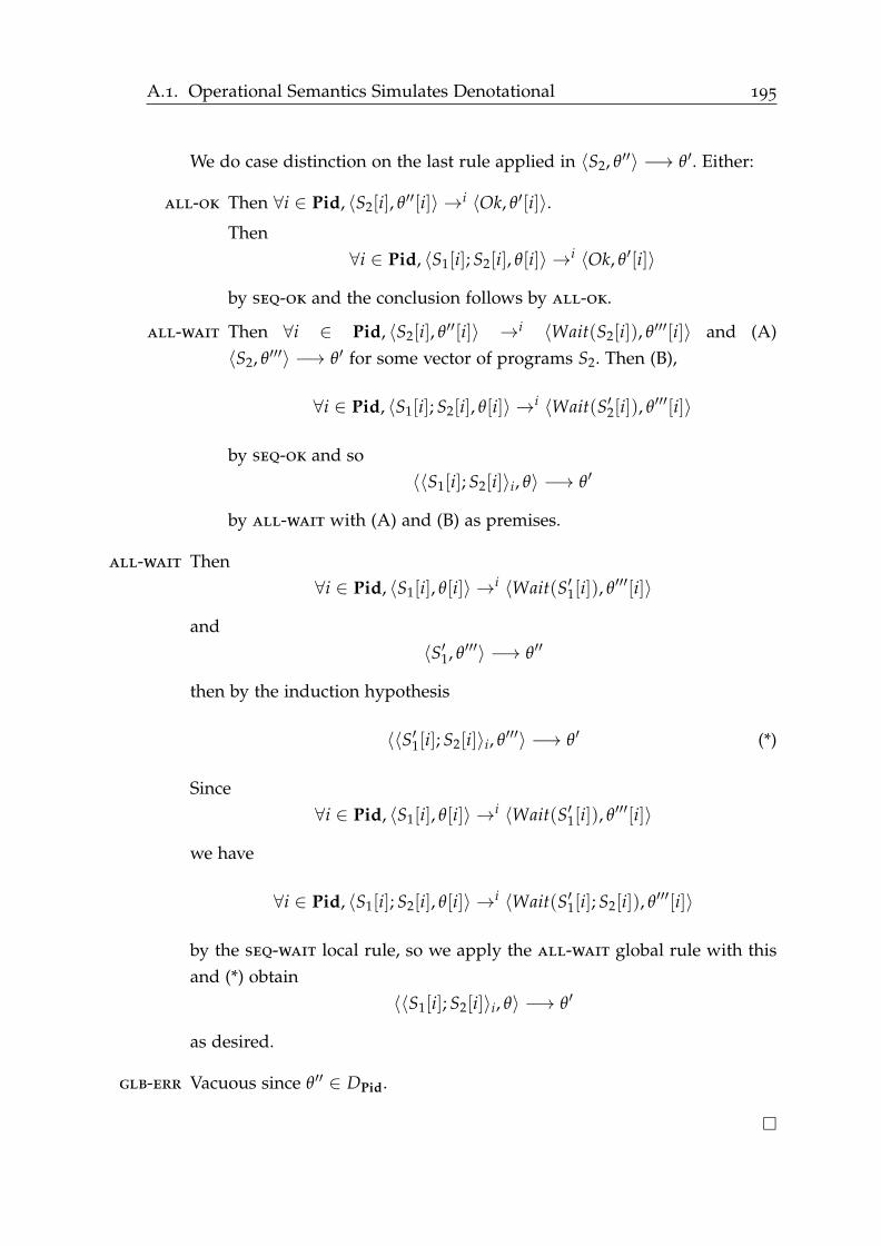
A.1. Operational Semantics Simulates Denotational 195
We do case distinction on the last rule applied in 〈S2, θ′′〉 −→ θ′. Either:
all-ok Then ∀i ∈ Pid, 〈S2[i], θ′′[i]〉 →i 〈Ok, θ′[i]〉.
Then
∀i ∈ Pid, 〈S1[i]; S2[i], θ[i]〉 →i 〈Ok, θ′[i]〉
by seq-ok and the conclusion follows by all-ok.
all-wait Then ∀i ∈ Pid, 〈S2[i], θ′′[i]〉 →i 〈Wait(S2[i]), θ′′′[i]〉 and (A)
〈S2, θ′′′〉 −→ θ′ for some vector of programs S2. Then (B),
∀i ∈ Pid, 〈S1[i]; S2[i], θ[i]〉 →i 〈Wait(S′2[i]), θ′′′[i]〉
by seq-ok and so
〈〈S1[i]; S2[i]〉i, θ〉 −→ θ′
by all-wait with (A) and (B) as premises.
all-wait Then
∀i ∈ Pid, 〈S1[i], θ[i]〉 →i 〈Wait(S′1[i]), θ′′′[i]〉
and
〈S′1, θ′′′〉 −→ θ′′
then by the induction hypothesis
〈〈S′1[i]; S2[i]〉i, θ′′′〉 −→ θ′ (*)
Since
∀i ∈ Pid, 〈S1[i], θ[i]〉 →i 〈Wait(S′1[i]), θ′′′[i]〉
we have
∀i ∈ Pid, 〈S1[i]; S2[i], θ[i]〉 →i 〈Wait(S′1[i]; S2[i]), θ′′′[i]〉
by the seq-wait local rule, so we apply the all-wait global rule with this
and (*) obtain
〈〈S1[i]; S2[i]〉i, θ〉 −→ θ′
as desired.
glb-err Vacuous since θ′′ ∈ DPid.
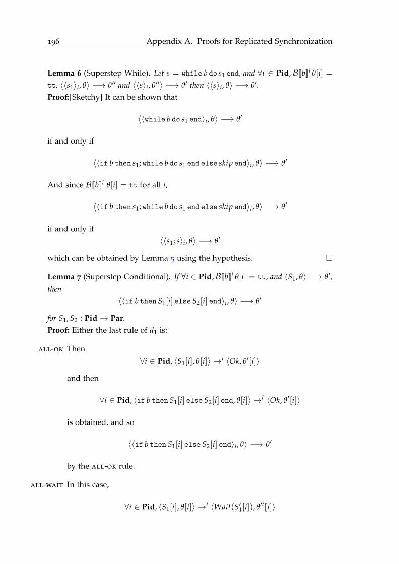
196 Appendix A. Proofs for Replicated Synchronization
Lemma 6 (Superstep While). Let s = while b do s1 end, and ∀i ∈ Pid,BJbKi θ[i] =
tt, 〈〈s1〉i, θ〉 −→ θ′′ and 〈〈s〉i, θ′′〉 −→ θ′ then 〈〈s〉i, θ〉 −→ θ′.
Proof:[Sketchy] It can be shown that
〈〈while b do s1 end〉i, θ〉 −→ θ′
if and only if
〈〈if b then s1; while b do s1 end else skip end〉i, θ〉 −→ θ′
And since BJbKi θ[i] = tt for all i,
〈〈if b then s1; while b do s1 end else skip end〉i, θ〉 −→ θ′
if and only if
〈〈s1; s〉i, θ〉 −→ θ′
which can be obtained by Lemma 5 using the hypothesis.
Lemma 7 (Superstep Conditional). If ∀i ∈ Pid,BJbKi θ[i] = tt, and 〈S1, θ〉 −→ θ′,
then
〈〈if b then S1[i] else S2[i] end〉i, θ〉 −→ θ′
for S1, S2 : Pid→ Par.
Proof: Either the last rule of d1 is:
all-ok Then
∀i ∈ Pid, 〈S1[i], θ[i]〉 →i 〈Ok, θ′[i]〉
and then
∀i ∈ Pid, 〈if b then S1[i] else S2[i] end, θ[i]〉 →i 〈Ok, θ′[i]〉
is obtained, and so
〈〈if b then S1[i] else S2[i] end〉i, θ〉 −→ θ′
by the all-ok rule.
all-wait In this case,
∀i ∈ Pid, 〈S1[i], θ[i]〉 →i 〈Wait(S′1[i]), θ′′[i]〉

A.1. Operational Semantics Simulates Denotational 197
and
〈S′1, θ′′〉 −→ θ′
for some vector of programs S′1 and environments θ′′. Then
∀i ∈ Pid, 〈if b then S1[i] else S2[i] end, θ[i]〉 →i 〈Wait(S′1[i]), θ′′[i]〉
and since 〈S′1, θ′′〉 −→ θ′ we have 〈〈if b then S1[i] else S2[i] end〉i, θ〉 → θ′
by the all-wait-rule.
glb-err In this case θ′ = ΩS and
∃i ∈ Pid,〈S1[i], θ[i]〉 →i 〈Ok, σi〉
∃j ∈ Pid,〈S1[j], θ[j]〉 →j 〈Wait(c′), σj〉
for some i, j, σi, c′ and σj. Then
〈if b then S1[i] else S2[i] end, θ[i]〉 →i 〈Ok, σi〉
〈if b then S1[j] else S2[j] end, θ[j]〉 →j 〈Wait(c′), σj〉
so
〈〈if b then S1[i] else S2[i] end〉i, θ〉 → ΩS
by the glb-err-rule.
Some helpful facts about the mask and combine operators:
Lemma 8 (Empty state is identity of combine). For all θ ∈ D and θ′ ∈ D∅, θ ‖
θ′ = θ.
Proof: If θ ∈ ⊥, ΩS, then the result is immediate from the definition. If not,
(θ ‖ θ′) = λi.(θ[i] + θ′[i])
= λi.θ[i] since θ′[i] = 000
= θ
Definition 8. Let D denote all partially visible environments, i.e.
D = D \ (DPid ∪ ΩS,⊥)

198 Appendix A. Proofs for Replicated Synchronization
Then partial equivalence between a function over states, and the local operational seman-
tics of a statement, written Psim, is defined:
Psim( f , s) ⇐⇒ ∀θ ∈ D, f θ = θ′ 6∈ ΩS,⊥ =⇒
∀i ∈ Pid, θ[i] 6= 000 =⇒
〈s, θ[i]〉 →i 〈Ok, θ′[i]〉
Lemma 9 (Loop partial simulation). Let F be the functional associated with s =
while b do s1 end, i.e.:
F = λ f .λθ.
( f Js1K) (∂b θ) ‖ ∂!b θ if ∂b θ 6∈ D∅ ∪ ⊥, ΩS
θ otherwise
and assume that Psim(Js1K, s1) then for all n ≥ 0, Psim(Fn f⊥, s).
Proof: By induction on n:
• If n = 0. Then F0 f⊥ = ⊥ for all θ, so Psim(F0 f⊥, s) vacuously holds.
• If n + 1. Take any θ ∈ D, and any i ∈ Pid such that θ[i] 6= 000. If no such i
exists then the conclusion holds vacuously. Either
– BJbKi θ[i] = tt, and then
(Fn+1 f⊥) θ[i] = ((Fn f⊥) Js1K) (∂b θ) i = θ′[i]
We need to show 〈s, θ[i]〉 →i 〈Ok, θ′ i〉, which we do by the wh-tt-ok
rule in the operational semantics. Let
θ′′[i] = (Js1K (∂b θ)) i = Js1K θ[i]
and
θ′[i] = (Fn f⊥) θ′′[i]
The premises of the rule wh-tt-ok which we need to prove
are 〈s1, θ[i]〉 →i 〈Ok, θ′′[i]〉, which follows from the assumption
Psim(Js1K, s1), and 〈s, θ′′[i]〉 →i 〈Ok, θ′[i]〉 which follows from the
induction hypothesis.
– BJbKi θ[i] = ff. Then
(Fn+1 f⊥) θ[i] = θ′[i] = θ[i]
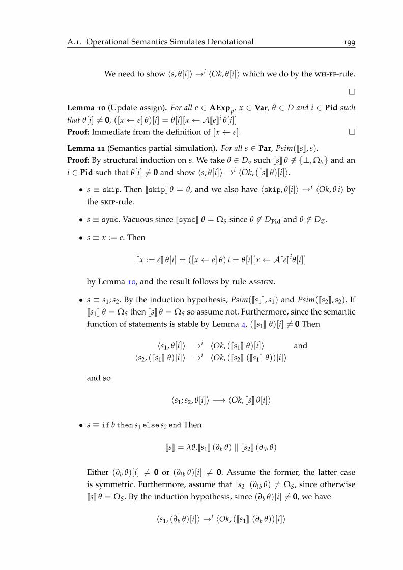
A.1. Operational Semantics Simulates Denotational 199
We need to show 〈s, θ[i]〉 →i 〈Ok, θ[i]〉 which we do by the wh-ff-rule.
Lemma 10 (Update assign). For all e ∈ AExpp, x ∈ Var, θ ∈ D and i ∈ Pid such
that θ[i] 6= 000, ([x ← e] θ)[i] = θ[i][x ← AJeKi θ[i]]
Proof: Immediate from the definition of [x ← e].
Lemma 11 (Semantics partial simulation). For all s ∈ Par, Psim(JsK, s).
Proof: By structural induction on s. We take θ ∈ D such JsK θ 6∈ ⊥, ΩS and an
i ∈ Pid such that θ[i] 6= 000 and show 〈s, θ[i]〉 →i 〈Ok, (JsK θ)[i]〉.
• s ≡ skip. Then JskipK θ = θ, and we also have 〈skip, θ[i]〉 →i 〈Ok, θ i〉 by
the skip-rule.
• s ≡ sync. Vacuous since JsyncK θ = ΩS since θ 6∈ DPid and θ 6∈ D∅.
• s ≡ x := e. Then
Jx := eK θ[i] = ([x ← e] θ) i = θ[i][x ← AJeKiθ[i]]
by Lemma 10, and the result follows by rule assign.
• s ≡ s1; s2. By the induction hypothesis, Psim(Js1K, s1) and Psim(Js2K, s2). If
Js1K θ = ΩS then JsK θ = ΩS so assume not. Furthermore, since the semantic
function of statements is stable by Lemma 4, (Js1K θ)[i] 6= 000 Then
〈s1, θ[i]〉 →i 〈Ok, (Js1K θ)[i]〉 and
〈s2, (Js1K θ)[i]〉 →i 〈Ok, (Js2K (Js1K θ))[i]〉
and so
〈s1; s2, θ[i]〉 −→ 〈Ok, JsK θ[i]〉
• s ≡ if b then s1 else s2 end Then
JsK = λθ.Js1K (∂b θ) ‖ Js2K (∂!b θ)
Either (∂b θ)[i] 6= 000 or (∂!b θ)[i] 6= 000. Assume the former, the latter case
is symmetric. Furthermore, assume that Js2K (∂!b θ) 6= ΩS, since otherwise
JsK θ = ΩS. By the induction hypothesis, since (∂b θ)[i] 6= 000, we have
〈s1, (∂b θ)[i]〉 →i 〈Ok, (Js1K (∂b θ))[i]〉

200 Appendix A. Proofs for Replicated Synchronization
Then by the rule if-tt, knowing that BJbKi θ[i] = tt,
〈if b then s1 else s2 end, θ[i]〉 →i 〈Ok, (Js1K (∂b θ))[i]〉
and since (JsK θ)[i] = (Js1K (∂b θ))[i] (since (∂b θ)[i] 6= 000) we conclude.
• s ≡ while b do s1 end. Then JsK = f ix F =⊔
Fn f⊥ | n ≥ 0.
By Lemma 9, since Psim(Js1K, s1) by the induction hypothesis, we have
Psim(Fn f⊥, s) for all n.
Now if JsK θ 6= ⊥, then there is n such that (Fn f⊥) θ = JsK θ, so
〈s, θ[i]〉 →i 〈Ok, (JsK θ)[i]〉
by Psim(Fn f⊥, s).
Theorem 1. Let θ ∈ DPid be an unmasked environment vector. If JsK θ = θ′ 6∈
⊥, ΩS, then 〈〈s〉i, θ〉 −→ θ′.
Proof: By structural induction on s.
• s ≡ skip. Then JskipK θ = θ, and since ∀i ∈ Pid, 〈skip, θ[i]〉 →i 〈Ok, θ[i]〉,
we obtain 〈〈skip〉i, θ〉 −→ θ by applying the all-ok-rule.
• s ≡ sync. Then JsK θ = θ since θ ∈ DPid. By the rule sync,
∀i ∈ Pid, 〈sync, θ[i]〉 →i 〈Wait(skip), θ[i]〉
and by the rule of skip,
∀i ∈ Pid, 〈skip, θ[i]〉 →i 〈Ok, θ[i]〉
so by applying the all-wait and then the all-ok-rule, we obtain
〈〈s〉i, θ〉 −→ θ.
• s ≡ x := e. By applying the all-ok-rule and showing that
∀i ∈ Pid, 〈x := e, θ[i]〉 →i 〈Ok, Jx := eKθ[i]〉
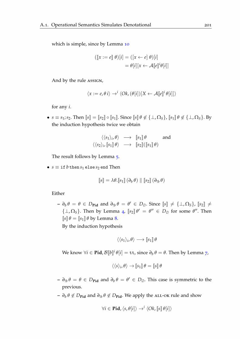
A.1. Operational Semantics Simulates Denotational 201
which is simple, since by Lemma 10
(Jx := eK θ)[i] = ([x ← e] θ)[i]
= θ[i][x ← AJeKiθ[i]]
And by the rule assign,
〈x := e, θ i〉 →i 〈Ok, (θ[i])[X ← AJeKi θ[i]]〉
for any i.
• s ≡ s1; s2. Then JsK = Js2K Js1K. Since JsK θ 6∈ ⊥, ΩS, Js1K θ 6∈ ⊥, ΩS. By
the induction hypothesis twice we obtain
〈〈s1〉i, θ〉 −→ Js1K θ and
〈〈s2〉i, Js1K θ〉 −→ Js2K(Js1K θ)
The result follows by Lemma 5.
• s ≡ if b then s1 else s2 end Then
JsK = λθ.Js1K (∂b θ) ‖ Js2K (∂!b θ)
Either
– ∂b θ = θ ∈ DPid and ∂!b θ = θ′ ∈ D∅. Since JsK 6= ⊥, ΩS, Js2K 6=⊥, ΩS. Then by Lemma 4, Js2K θ′ = θ′′ ∈ D∅ for some θ′′. Then
JsK θ = Js1K θ by Lemma 8.
By the induction hypothesis
〈〈s1〉i, θ〉 −→ Js1K θ
We know ∀i ∈ Pid,BJbKi θ[i] = tt, since ∂b θ = θ. Then by Lemma 7,
〈〈s〉i, θ〉 → Js1K θ = JsK θ
– ∂!b θ = θ ∈ DPid and ∂b θ = θ′ ∈ D∅. This case is symmetric to the
previous.
– ∂b θ 6∈ DPid and ∂!b θ 6∈ DPid. We apply the all-ok rule and show
∀i ∈ Pid, 〈s, θ[i]〉 →i 〈Ok, JsK θ[i]〉

202 Appendix A. Proofs for Replicated Synchronization
Take any i ∈ Pid. Assume BJbKi θ[i] = tt, the other case being sym-
metric, and we then have (∂b θ) i = θ[i] and JsK θ[i] = Js1K (∂b θ) i. By
Lemma 11,
〈s1, (∂b θ) i〉 →i 〈Ok, Js1K (∂b θ) i〉
⇐⇒ 〈s1, θ[i]〉 →i 〈Ok, JsK θ[i]〉
and so by the if-tt-rule, 〈s, θ[i]〉 →i 〈Ok, JsK θ[i]〉.
• s ≡ while b do s1 end. Then JsK = f ix F =⊔
Fn f⊥ | n ≥ 0. We proceed by
induction on n, to show
∀n ∈ Nat, θ ∈ DPid, (Fn f⊥) θ = θ′ 6∈ ⊥, ΩS =⇒ 〈〈s〉i, θ〉 −→ θ′
– n = 0. Holds vacuously since (F0 f⊥) θ = ⊥.
– n + 1. Either
∗ ∂b θ = θ ∈ DPid and ∂!b θ ∈ D∅. Then (Fn+1 f⊥) θ =
(Fn f⊥)(Js1K θ). Let θ′′ = Js1K θ. If θ′′ ∈ ⊥, ΩS, then θ′ ∈ ⊥, ΩS
and we are done. Otherwise, we have by the outer induction
hypothesis, 〈〈s1〉i, θ〉 −→ θ′′. Since the semantic function of state-
ments is stable by Lemma 4, θ′′ ∈ DPid, and so by the inner
induction hypothesis, 〈〈s〉i, θ′′〉 −→ θ′. We conclude by Lemma 6.
∗ ∂!b θ = θ ∈ DPid and ∂b θ ∈ D∅. Then (Fn+1 f⊥) θ = θ. To show
〈〈s〉i, θ〉 −→ θ, we apply the global all-ok-rule followed by the
if-ff local rule.
∗ ∂b θ 6∈ DPid and ∂!b θ 6∈ DPid. We apply the all-ok and show for
all
∀i ∈ Pid, 〈s, θ[i]〉 →i 〈Ok, θ′[i]〉
We take some i, and do case distinction on the evaluation of the
condition:
· Either BJbKi θ[i] = ff. Then θ′[i] = θ[i]. Apply the wh-ff-rule
to get 〈s, θ[i]〉 →i 〈Ok, θ[i]〉.
· Or BJbKi θ[i] = tt. Then
θ′[i] = ((Fn f⊥) Js1K) (∂b θ) i
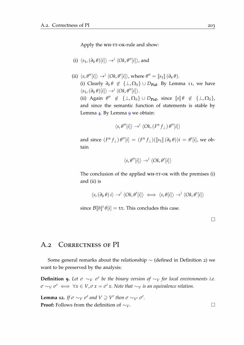
A.2. Correctness of PI 203
Apply the wh-tt-ok-rule and show:
(i) 〈s1, (∂b θ)[i]〉 →i 〈Ok, θ′′[i]〉, and
(ii) 〈s, θ′′[i]〉 →i 〈Ok, θ′[i]〉, where θ′′ = Js1K (∂b θ).
(i) Clearly ∂b θ 6∈ ⊥, ΩS ∪ DPid. By Lemma 11, we have
〈s1, (∂b θ)[i]〉 →i 〈Ok, θ′′[i]〉.
(ii) Again θ′′ 6∈ ⊥, ΩS ∪ DPid, since JsK θ 6∈ ⊥, ΩS,
and since the semantic function of statements is stable by
Lemma 4. By Lemma 9 we obtain:
〈s, θ′′[i]〉 →i 〈Ok, (Fn f⊥) θ′′[i]〉
and since (Fn f⊥) θ′′[i] = (Fn f⊥)(Js1K (∂b θ))i = θ′[i], we ob-
tain
〈s, θ′′[i]〉 →i 〈Ok, θ′[i]〉
The conclusion of the applied wh-tt-ok with the premises (i)
and (ii) is
〈s, (∂b θ) i〉 →i 〈Ok, θ′[i]〉 ⇐⇒ 〈s, θ[i]〉 →i 〈Ok, θ′[i]〉
since BJbKi θ[i] = tt. This concludes this case.
A.2 Correctness of PI
Some general remarks about the relationship ∼ (defined in Definition 2) we
want to be preserved by the analysis:
Definition 9. Let σ ∼V σ′ be the binary version of ∼V for local environments i.e.
σ ∼V σ′ ⇐⇒ ∀x ∈ V, σ x = σ′ x. Note that ∼V is an equivalence relation.
Lemma 12. If σ ∼V σ′ and V ⊇ V′ then σ ∼V′ σ′.
Proof: Follows from the definition of ∼V .
204 Appendix A. Proofs for Replicated Synchronization
Lemma 13. If φd(e, V) for e ∈ AExpp and σ ∼V σ′ then ∃v ∈ Nat, ∀i, j ∈
Pid,AJeKi σ = AJeKj σ′ = v. Similarly for boolean expressions, if φd(b, V) for
b ∈ BExp and σ ∼V σ′ then ∃v ∈ Bool, ∀i, j ∈ Pid,BJbKi σ = BJbKj σ′ = v.
Proof: We proceed by structural induction for e ∈ AExpp on numerical expres-
sions. If e is a constant (or nprocs), then n is that constant (or p). The case where
e is the special variable pid is absurd, since φd(e, V) forbids it. If e is the variable
x, then we note that x ∈ V since φd(e, V). The result then follows from σ ∼V σ′.
If e is some operation e1 op e2 with op ∈ +,−,×, then we apply the induction
hypothesis on e1 and e2, and result follows from the fact that all operators are
functions (and thus single-valued).
The same result can be shown for all b ∈ BExp, by structural induction and
by using the result on expressions in AExpp.
A.2.1 Domain
We assume a fixed program s⋆. We assume the existence of a final edge for each
node corresponding to a statement in the CFG, excluding merge nodes. This
edge is given by f inals⋆e (s), defined below. However, the final node of the pro-
gram, finals⋆ has no successor and hence no final edge by definition. To remedy,
we add a dummy node labeled ℓF , that corresponds to no statement. We then
define f inals⋆e (s):
Definition 10. The final edge of the sub-program s of s⋆ is given by f inals⋆e (s):
f inals⋆e : Par→ Lab× Lab s⋆ ∈ Par
f inals⋆e (s) =
( f inal(s), ℓ′) if ∃ℓ′ ∈ Lab, ( f inal(s), ℓ′) ∈ flow(s⋆)
(inits, ℓF ) otherwise
In what follows, we will drop the superscript on finale, and assume one fixed
program s⋆.
A.2.2 Parameterized Constraint System
Definition 11. PI ι(s) is a constraint system parameterized by ι ∈ L, so that:
(pi, pi•) PI ι(s) =⇒ pi(init(s)) ⊒ ι
All other constraint in the parameterized system is as in the non-parameterized. The
non-parameterized constraint system PI(s) is equivalent to PI ι(s) with ι = (Vars, ǫ).
A.2. Correctness of PI 205
A.2.3 Constraint System Facts
Definition 12. The subprograms sub(s) of s are:
sub(s) =
s1, s2 if c = s1; s2
s1, s2 if c = if b then s1 else s2 end
s1 if c = while b do s1 end
∅ otherwise
Lemma 14 (Solution extends to sub-programs). If (pi, pi•) PI ι(s) and s′ ∈
sub(s) and ι′ = pi(init(s′)) then (pi, pi•) PI ι′(s′).
Proof: The labels and edges of s′ are subsets of those of s. Except for pi(init(s′)),
any constraint on them is the same as in PI ι(s). The constraint on init(s′) must
hold by construction of PI ι′(s′).
Lemma 15 (Incoming state is coarser than incoming edge). If (pi, pi•) PI ι(s)
and ℓ ∈ labels(s) such that ℓ is not a merge node, then pi(ℓ) ⊒ pi•(n(ℓ)).
Proof: By structural induction on s. All cases follows trivially from the construc-
tion of the constraint system, except when s = while [b]ℓ do s1 end. In this case,
the result follows from Lemma 19.
Lemma 16 (Constraint system facts). Let (pi, pi•) PI ι(s). We then have:
(i) If s ≡ s1; s2, then pi(init(s2)) ⊑ pi•(finale(s1)).
(ii) s ≡ if [b]ℓ then s1 else s2 end, then pi(init(s1)) ⊑ pi•(t(ℓ)) and
pi(init(s2)) ⊑ pi•(f(ℓ)).
(iii) s ≡ while [b]ℓ do s1 end, then pi(init(s1)) ⊑ pi•(t(ℓ)).
Proof: In the three cases respectively, this is equivalent to showing pi(init(si)) ⊑
pi•(n(init(si))), for i = 2, i = 1, i = 2, and i = 1 respectively. This follows from
the from the construction of the control flow graph, and in the first case, from
the definition of finale. Now all cases are proved by applying Lemma 15.
A.2.4 Marked Path Abstractions and pid-independent Variables
Lemma 17 (Path concatenation is monotone). For all p, p′ ∈ Path♯ and ℓ ∈ Lab,
If p p′ then p.ℓ p′.ℓ.
Proof: Since, p p′, either:
206 Appendix A. Proofs for Replicated Synchronization
• p = ⊥, and so p.ℓ = ⊥.ℓ = ⊥ p′.ℓ.
• p = p′ = ǫ, p.ℓ = ǫ : ℓ = ℓ ℓ = ǫ : ℓ = p′.ℓ
• p = p0 : ℓ0, p′ = p′0 : ℓ′0 and p0 p′0. Then p.ℓ = p : ℓ p′ : ℓ = p′.ℓ.
• p′ = ⊤, and so p.ℓ ⊤ = ⊤.ℓ = p′.ℓ.
Lemma 18 (Path merging is monotone). For all p0, p1 and p2, if p0 p1 then
p0 p2 p1 p2.
Proof: By case distinction on p0 p1, and then case distinction on p2.
Lemma 19 (Merge Concat Order). For all ℓ, p and p0, p p.ℓ p0.
Proof: If p or p0 are in ⊥,⊤ the conclusion is immediate. Otherwise, we do
case distinction on whether p.ℓ p0, p.ℓ p0 or neither. In the first two cases,
the result follows by the monotonicity of ⊔. In the latter, the result follows by
the definition of .
Definition 13. A path p ∈ Path♯ is marked if it is ⊤ or if it contains any marked
labels. Formally, p 6∈ (⊥ ∪ Lab∗).
Definition 14. Let assigns : Par → P(Var) return the set of variable appearing on
the left-hand side of an assignment the given program.
Lemma 20 (Marked path kills all assigned). If (pi, pi•) PI ι(s) and
π2(pi(init(s))) is marked, then π1(pi•( f inale(s))) ⊆ π1(pi(init(s))) \ assigns(s).
Proof: Let (V, p) = pi(init(s)) and (V′, p′) = pi•( f inale(s)). We prove the
stronger property (V′, p′) ⊒ (V \ assigns(s), p) by structural induction on s.
• s ≡ [skip]ℓ and s ≡ [sync]ℓ. The constraint system gives us the following
inequality:
(V′, p′) = pi•(x(ℓ)) ⊒ pi(ℓ) = (V, p)
Then since assigns(s) = ∅, we have (V′, p′) ⊒ (V \ assigns(s), p).
• s ≡ [x:=e]ℓ. The constraint system gives us the following inequalities:
pi(ℓ) = (V, p)
(V′, p′) = pi•(x(ℓ)) ⊒ (vdep(pi(ℓ), e, X), π2(pi(ℓ)))
A.2. Correctness of PI 207
In this case, note that p is marked, and thus φc(p) does not hold. Thus
vdep((V, p), e, x) = V \ x (∗)
We then have:
(V′, p′) = pi•(x(ℓ)) by definition
⊒ (V \ x, p) by (∗) and constraint system
= (V \ assigns(s), p) since assigns(s) = X
• s ≡ s1; s2. Let (V′1, p′1) = pi•( f inale(s1)) = pi•(n(init(s2))), and (V2, p2) =
pi(init(s2)). Note that (V2, p2) ⊒ (V′1, p′1) by Lemma 16. Since (pi, pi•)
PI ι(s1; s2), we have (pi, pi•) PI ι(s1) and (pi, pi•) PI ι′(s2) with ι′ =
pi(init(s2)). We then have:
(V′, p′) ⊒ (V2 \ assigns(s2), p2) by the induction hypothesis
⊒ (V′1 \ assigns(s2), p′1) by the constraint system
⊒ ((V \ assigns(s1)) \ assigns(s2), p) by the induction hypothesis
= (V \ assigns(s), p) by definition of assigns
• s ≡ if b then s1 else s2 end. Let
(V1, p1) = pi(init(s1)) (V′1, p′1) = pi•( f inale(s1))
(V2, p2) = pi(init(s2)) (V′2, p′2) = pi•( f inale(s2))
The constraint system gives the following inequalities:
(V, p) = pi(ℓ)
(V1, p1) ⊒ pi•(t(ℓ)) ⊒ (π1(pi(ℓ)), π2(pi(ℓ)).cdep(ℓ, b, π1(pi(ℓ))))
(V2, p2) ⊒ pi•(f(ℓ)) ⊒ (π1(pi(ℓ)), π2(pi(ℓ)).cdep(ℓ, b, π1(pi(ℓ))))
pi(ℓm) ⊒ (π1(pi•(t(ℓ
m))) ∩ π1(pi•(f(ℓm))),
π2(pi•(t(ℓm))) π2(pi•(f(ℓ
m))))
= (V′1 ∩V′2, p′1 p′2)
(V′, p′) = pi•(x(ℓm)) ⊒ pi(ℓ
m)
208 Appendix A. Proofs for Replicated Synchronization
Since (pi, pi•) PI ι(s), we have (pi, pi•) PI ι1(s1) and (pi, pi•)
PI ι2(s2) with ι1 = pi(init(s1)) and ι2 = pi(init(s2)). The induction hy-
pothesis then gives us the following:
(V′1, p′1) ⊒ (V1 \ assigns(s1), p1) (1)
(V′2, p′2) ⊒ (V2 \ assigns(s2), p2) (2)
We show (i) V′ ⊆ V \ assigns(s) and (ii) p′ p separately.
(i) We have:
V′ ⊆ (V′1 ∩V′2) by constraint system
⊆ (V1 \ assigns(s1)) ∩ (V2 \ assigns(s2)) by (1) and (2)
⊆ (V \ assigns(s1)) ∩ (V \ assigns(s2)) since V1 ⊆ V and V2 ⊆ V
⊆ V \ assigns(s) by definition of assigns
(ii) Let ℓ′ = cdep(ℓ, b, π1(pi(ℓ))). Then
p′1 p1 p.ℓ′ (∗)
by (1) and the constraint system. So we have
p′ p′1 p′2 by constraint system
p.ℓ p′2 by (∗) and Lemma 18
p by Lemma 19
By (i) and (ii), we conclude (V′, p′) ⊒ (V \ assigns(s), p) as desired.
• s ≡ while b do s1 end. Let
(V0, p0) = pi•(n(ℓ)) (V1, p1) = pi(init(s1)) (V′1, p′1) = pi•( f inale(s1))

A.2. Correctness of PI 209
The constraint system gives the following inequalities:
(V, p) = pi(ℓ) ⊒ (π1(pi•(n(ℓ))) ∩ π1(pi•(b(ℓ))),
π2(pi•(n(ℓ))).ℓ π2(pi•(b(ℓ))))
= (V0 ∩V′1, p0.ℓ p′1)
(V1, p1) ⊒ pi•(t(ℓ)) ⊒ (π1(pi(ℓ)), π2(pi(ℓ)).cdep(ℓ, b, π1(pi(ℓ))))
(V′, p′) = pi•(f(ℓ)) ⊒ (π1(pi(ℓ)), π2(pi(ℓ)))
Since (pi, pi•) PI ι(s), we have (pi, pi•) PI ι1(s1) with ι1 =
pi(init(s1)). The induction hypothesis then gives us the following:
(V′1, p′1) ⊒ (V1 \ assigns(s1), p1) (1)
We show (i) V′ ⊆ V \ assigns(s) and (ii) p′ p separately.
(i) We have:
V′ ⊆ π1(pi(ℓ)) = V
⊆ V0 ∩V′1 by the constraint system
⊆ V′1
⊆ V1 \ assigns(s1) by (1)
⊆ V \ assigns(s1) since V1 ⊆ π1(pi(ℓ)) = V
= V \ assigns(s) by definition of assigns
(ii) We have
p′ π2(pi(ℓ)) = p by the constraint system
By (i) and (ii), we conclude (V′, p′) ⊒ (V \ (assigns(s), p)) as desired.
A.2.5 Correctness of the Analysis
We now turn to the correctness of the analysis:
Lemma 21. If 〈s, σ〉 →i 〈t, σ′〉 then ∀V ⊆ Var, σ ∼V\assigns(s) σ′.

210 Appendix A. Proofs for Replicated Synchronization
Proof: By a trivial rule induction on 〈s, σ〉 →i 〈t, σ′〉.
Lemma 22. If 〈s, σi〉 →i 〈Ok, σ′i 〉, 〈s, σj〉 →
j 〈Ok, σ′j 〉, σi ∼V σj, and V′ ⊆ V \
assigns(s) then σ′i ∼V′ σ′j .
Proof: By Lemma 21, σi ∼V′ σ′i and σj ∼V′ σ′j . Since V′ ⊆ V, we also have
σi ∼V′ σj by Lemma 12. The result follows from the transitivity of ∼V′ .
Theorem 6. Let (pi, pi•) PI ι(s), where π2(ι) 6= ⊥. Let V = π1(pi(init(s))),
V′ = π1(pi•( f inale(s))), and σi, σj two environments such that σi ∼V σj, and
〈s, σi〉 →i 〈Ok, σ′i 〉 and 〈s, σj〉 →
j 〈Ok, σ′j 〉. Then σ′i ∼V′ σ′j .
Proof: Proof by rule induction on 〈s, σi〉 →i 〈Ok, σ′i 〉.
skip Then s ≡ [skip]ℓ. By the constraint system, we have:
V = π1(pi(ℓ)) ⊇ π1(pi•(x(ℓ))) = V′
Since σ′i = σi and σ′j = σj, by the rule for skip, and since π1(pi(ℓ)) ⊇
π1(pi•(x(ℓ))), we have σ′i ∼V′ σ′j by Lemma 12.
sync Vacuous since 〈s, σi〉 →i 〈Ok, σ′i 〉.
assign Then s ≡ [x:=e]ℓ. The predicate φd(e, π1(pi(ℓ))) ∧ φc(π2(pi(ℓ))) gives
rise to two cases:
– It does not hold. Then we have the following constraint after simplifi-
cation of vdep:
V = π1(pi(ℓ))
π1(pi(ℓ)) \ x ⊇ π1(pi•(x(ℓ))) = V′
So V′ ⊆ V \ x. Since assigns(s) = x, we conclude by Lemma 22.
– It holds. By Lemma 13, for some n, AJeKi σi = AJeKj σj = n. The con-
straint system is then
V = π1(pi(ℓ))
π1(pi(ℓ)) ∪ x ⊇ π1(pi•(x(ℓ))) = V′
So V′ ⊆ V ∪ x. To show σ′i ∼V′ σ′j , take a y ∈ V′. Either y = x, and
then σ′i y = σ′j y = n, or y 6= x and then σ′i y = σi y and σ′j y = σj y.
Since y ∈ V and σi ∼V σj, we have σ′i y = σ′j y.

A.2. Correctness of PI 211
seq-ok In this case s ≡ s1; s2, and
〈s1, σi〉 →i 〈Ok, σ′′i 〉 〈s2, σ′′i 〉 →
i 〈Ok, σ′i 〉
〈s1, σj〉 →j 〈Ok, σ′′j 〉 〈s2, σ′′j 〉 →
j 〈Ok, σ′j 〉.
We apply the induction hypothesis to the execution of s1. Let
V1 = π1(pi(init(s1))), and V′1 = π1(pi•( f inale(s1))). Note that since
init(s1; s2) = init(s1), V1 = V and σi ∼V1σj. With (pi, pi•) PI ι′(s1)
where ι′ = pi(init(s1)), we obtain σ′′i ∼V′1σ′′j .
Let V2 = π1(pi(init(s2))), and V′2 = π1(pi•( f inale(s2))). By Lemma 16,
pi(init(s2)) ⊒ pi•( f inale(s1)), and so V2 ⊆ V′1. It follows by Lemma 12
that σ′′i ∼V2σ′′j . We can then apply the induction hypothesis to s2 and
obtain σ′i ∼V′2σ′j . Since f inale(s1; s2) = f inale(s2), V′2 = V′ and we conclude
σ′i ∼V′ σ′j .
seq-wait Vacuous since 〈s, σi〉 →i 〈Ok, σ′i 〉.
if-tt and if-ff In these cases, s ≡ if [b]ℓ then s1 else s2 [end]ℓ′
. The predicate
φd(b, π1(pi(ℓ))) gives rise to two cases:
– It holds, and then by Lemma 13 we have for some v ∈ Bool, BJbKj σi =
BJbKj σj = v. Assume v = tt, the other case being symmetric. Then
〈s1, σi〉 →i 〈Ok, σ′i 〉 and
〈s1, σj〉 →j 〈Ok, σ′j 〉
Let V1 = π1(pi(init(s1))), and V′1 = π1(pi•( f inale(s1))). Since
π1(pi•(t(ℓ))) ⊆ π1(pi(ℓ)) = V, and by Lemma 16, V1 ⊆
π1(pi•(t(ℓ))), so V1 ⊆ V and since σi ∼V σj, we have σi ∼V1σj. Since
(pi, pi•) PI ι′(s1) with ι′ = pi(init(s1)), we apply the induction
hypothesis and obtain σ′i ∼V′1σ′j .
By construction of the constraint system V′ = π1(pi•(x(ℓ′))) ⊆
π1(pi(ℓ′)) ⊆ π1(pi•(t(ℓ
′))) ∩ π1(pi•(f(ℓ′))) and by construction of
the CFG, π1(pi•(t(ℓ′))) = π1(pi•( f inale(s1))) = V′1, so V′ ⊆ V′1 and
we obtain σ′i ∼V′ σ′j .
– It does not hold, then by the constraint system :
π2(pi•(t(ℓ))) π2(pi(ℓ)).ℓ and π2(pi•(f(ℓ))) π2(pi(ℓ)).ℓ

212 Appendix A. Proofs for Replicated Synchronization
and so π2(pi•(t(ℓ))) and π2(pi•(f(ℓ))) are marked. Then
π1(pi•(t(ℓ′))) ⊆ π1(pi•(t(ℓ))) \ assigns(s1) and
π1(pi•(f(ℓ′))) ⊆ π1(pi•(f(ℓ))) \ assigns(s2) (∗)
by Lemma 20. Then, with X1 = assigns(s1) and X2 = assigns(s2), we
have
V′ = π1(pi•(x(ℓ′)))
⊆ π1(pi(ℓ′))
⊆ π1(pi•(t(ℓ′))) ∩ π1(pi•(f(ℓ
′)))
⊆ (π1(pi•(t(ℓ))) \ X1) ∩ (π1(pi•(f(ℓ))) \ X2) by (*)
⊆ (π1(pi(ℓ)) \ X1) ∩ (π1(pi(ℓ)) \ X2)
since π1(pi•(t(ℓ))) ⊆ π1(pi(ℓ)) and π1(pi•(f(ℓ))) ⊆ π1(pi(ℓ))
⊆ π1(pi(ℓ)) \ (X1 ∪ X2)
⊆ π1(pi(ℓ)) \ (assigns(s))
= V \ (assigns(s))
And so we conclude by Lemma 22.
wh-tt-ok and wh-ff. In these cases, s ≡ while [b]ℓ do s1 end. The predicate
φd(b, π1(pi(ℓ))) gives rise to two cases:
– It holds, and then for some v ∈ Bool, BJbKj σi = BJbKj σj = v.
∗ Assume v = tt. Then for some σ′′i and σ′′j , we have:
(A) 〈s1, σi〉 →i 〈Ok, σ′′i 〉 (B) 〈s, σ′′i 〉 →
i 〈Ok, σ′i 〉
〈s1, σj〉 →j 〈Ok, σ′′j 〉 〈s, σ′′j 〉 →
j 〈Ok, σ′j 〉
We know (pi, pi•) PI ι′(s1), with ι′ = pi(init(s1)). Let V1 =
π1(pi(init(s1))), and V′1 = π1(pi•(b(ℓ))) = π1(pi•( f inale(s1))).
Since pi(init(s1)) ⊒ pi•(t(ℓ)) by Lemma 16, and π1(pi•(t(ℓ))) ⊆
π1(pi(ℓ)) = V, we obtain V1 ⊆ V.
By Lemma 12, we have σi ∼V1σj. Then by applying the induction
hypothesis on (A) we obtain σ′′i ∼V′1σ′′j .
Since V′1 = π1(pi•(b(ℓ))), and V = π1(pi(ℓ)) ⊆ π1(pi•(b(ℓ))) ∩
π1(pi•(n(ℓ))), we have V ⊆ V′1. Thus σ′′i ∼V σ′′j .
A.2. Correctness of PI 213
We can now apply the induction hypothesis on (B) to obtain
σ′i ∼V′ σ′j , which concludes this case.
∗ Assume v = ff. Then σ′i = σi and σ′j = σj and since V′ =
π1(pi•(f(ℓ))) ⊆ π1(pi(ℓ)) = V we conclude by Lemma 12.
– It does not hold, then by the constraint system
π2(pi(init(s1))) π2(pi•(t(ℓ))) π2(pi(ℓ)).ℓ and (A.1)
V = π1(pi(init(s1))) ⊆ π1(pi•(t(ℓ))) ⊆ π1(pi(ℓ)) (A.2)
and so π2(pi(init(s1))) is marked. Then
V′ = π1(pi•(f(ℓ)))
⊆ π1(pi(ℓ))
⊆ π1(pi•(b(ℓ))) by the constraint system
⊆ π1(pi(init(s1))) \ assigns(s1) by Lemma 20
⊆ V \ assigns(s) by (A.2) and definition of assigns
So we conclude by Lemma 22.
wh-tt-wait Vacuous since 〈s, σi〉 →i 〈Ok, σ′i 〉.
To go from executing vectors of programs to two processes in isolation:
Definition 15. For a program s, let s f (s) be s with all sync-commands replaced by
skip:
s f (s) =
skip if c = sync
s f (s1); s f (s2) if c = s1; s2
if b then s f (s1) else s f (s2) end if c = if b then s1 else s2 end
while b do s f (s1) end if c = while b do s1 end
c otherwise
Lemma 23. If 〈s, σ〉 →i 〈Ok, σ′〉 then 〈s f (s), σ〉 →i 〈Ok, σ′〉.
Proof: Follows by a trivial rule induction on the hypothesis.
214 Appendix A. Proofs for Replicated Synchronization
Lemma 24. If 〈s, σ〉 →i 〈Wait(s′), σ′′〉 and 〈s f (s′), σ′′〉 →i 〈Ok, σ′〉 then
〈s f (s), σ〉 →i 〈Ok, σ′〉.
Proof: By rule induction on the first hypothesis. We do case distinction on the
last rule in the derivation.
sync Then σ = σ′ = σ′′, and s f (sync) = skip. By the skip-rule, 〈s f (s), σ〉 →i
〈Ok, σ〉.
if-tt Then s ≡ if b then s1 else s2 end and s f (s) ≡ if b then s f (s1) else s f (s2) end.
By the premises of this rule, BJbKj σ = tt and 〈s1, σ〉 →i 〈Wait(s′), σ′′〉.
By assumption 〈s f (s′), σ′′〉 →i 〈Ok, σ′〉. Thus, by the induction hypothesis,
〈s f (s1), σ〉 →i 〈Ok, σ′〉. We then obtain 〈s, σ〉 →i 〈Ok, σ′〉 by the if-tt rule.
if-ff Analogous to last case.
wh-tt-ok Then s ≡ while b do s1 end and s f (s) ≡ while b do s f (s1) end. By the
premises of this rule, BJbKj σ = tt and 〈s1, σ〉 →i 〈Ok, σ′′0 〉 for some σ′′0 and
〈s, σ′′0 〉 →i 〈Wait(s′), σ′′〉. By assumption 〈s f (s′), σ′′〉 →i 〈Ok, σ′〉. Thus,
by the induction hypothesis, 〈s f (s), σ′′0 〉 →i 〈Ok, σ′〉. By Lemma 23, we
have 〈s f (s1), σ〉 →i 〈Ok, σ′′0 〉 and so we obtain 〈s f (s), σ〉 →i 〈Ok, σ′〉 by the
wh-tt-ok rule.
wh-tt-wait Then s ≡ while b do s1 end and s f (s) ≡ while b do s f (s1) end. By the
premises of this rule, BJbKj σ = tt and 〈s1, σ〉 →i 〈Wait(s′1), σ′′〉 and so
〈s, σ〉 →i 〈Wait(s′1; c), σ′′〉. By assumption 〈s f (s′1; c), σ′′〉 →i 〈Ok, σ′〉. So
there must be some σ′′1 so that 〈s f (s′1), σ′′〉 →i 〈Ok, σ′′1 〉 and 〈s f (s), σ′′1 〉 →i
〈Ok, σ′〉.
By the induction hypothesis, 〈s f (s1), σ〉 →i 〈Ok, σ′′1 〉, and so we obtain
〈s f (s), σ〉 →i 〈Ok, σ′〉 by the wh-tt-ok rule.
seq-ok s ≡ s1; s2 and s f (s) ≡ s f (s1); s f (s2). By the premises of this rule,
〈s1, σ〉 →i 〈Ok, σ′′0 〉 〈s2, σ′′0 〉 →i 〈Wait(s′2), σ′′〉
for some σ′′0 , and by assumption
〈s f (s′2), σ′′〉 →i 〈Ok, σ′〉
By Lemma 23 we have
〈s f (s1), σ〉 →i 〈Ok, σ′′0 〉

A.2. Correctness of PI 215
and by the induction hypothesis
〈s f (s2), σ′′0 〉 →i 〈Ok, σ′〉
We then apply the seq-ok rule, and obtain 〈s f (s), σ〉 →i 〈Ok, σ′〉.
seq-wait s ≡ s1; s2 and s f (s) ≡ s f (s1); s f (s2). We then have:
〈s1, σ〉 →i 〈Wait(s′1), σ′′〉
〈s1; s2, σ〉 →i 〈Wait(s′1; s2), σ′′〉
and by assumption
〈s f (s′1; s2), σ′′〉 →i 〈Ok, σ′〉
Then there is σ′′0 so that
〈s f (s′1), σ′′〉 →i 〈Ok, σ′′0 〉 〈s f (s2), σ′′0 〉 →i 〈Ok, σ′〉
By the induction hypothesis, we obtain
〈s f (s1), σ〉 →i 〈Ok, σ′′0 〉
and so by seq-ok we have 〈s f (s), σ〉 →i 〈Ok, σ′〉.
skip , assign and wh-ff. Vacuous since the termination state is not Ok.
Lemma 25. If 〈S, θ〉 −→ θ′ then for all i ∈ Pid, 〈s f (S[i]), θ[i]〉 →i 〈Ok, θ′[i]〉.
Proof: By rule induction on the hypothesis. If the last rule used was:
all-ok Take any i ∈ Pid. By the premises of this rule, 〈S[i], θ[i]〉 →i 〈Ok, θ′[i]〉. By
Lemma 23, 〈s f (S[i]), θ[i]〉 →i 〈Ok, θ′[i]〉
all-wait Again, take any i ∈ Pid. By the premises of this rule,
〈S[i], θ[i]〉 →i 〈Wait(S′[i]), θ′′[i]〉 and 〈S′, θ′′〉 −→ θ′
By the induction hypothesis, 〈s f (S′[i]), θ′′[i]〉 →i 〈Ok, θ′[i]〉. Then by
Lemma 24, 〈s f (S[i]), θ[i]〉 →i 〈Ok, θ′[i]〉.
216 Appendix A. Proofs for Replicated Synchronization
Knowing that we can look at two processes in isolation, and that the analysis
is correct for two processes, we can extend the result to vectors and show the
main theorem:
Theorem 2. Let s be a program, θ, θ′ ∈ DPid two environment vectors and (pi, pi•) |=
PI(s). Let V = π1(pi(init(s))) and V′ = π1(pi•(finale(s))). If ∼V θ and JsK θ = θ′,
then ∼V′ θ′.
Proof: By Theorem 1, 〈〈s〉i, θ〉 −→ θ′.
Take any i, j ∈ Pid. Then by Lemma 25, we have 〈s f (s), θ[i]〉 →i 〈Ok, θ′[i]〉
and 〈s f (s), θ j〉 →j 〈Ok, θ′[j]〉.
Note that (pi, pi•) PI(s) ⇐⇒ (pi, pi•) PI ι(s) with ι = (Var, ǫ). By
Theorem 6, θ′[i] ∼V′ θ′[j]. Since this is true for any i and j, we conclude ∼V′ θ′
A.3 Correctness of RS
A.3.1 Safe State Transformers
Next, we show that programs that are syntactically synchronization free (see
Section 4.3.2) are also textually aligned.
Lemma 26. Let s ∈ Par such that s f ♯(s), then s is textually aligned for D \ ΩS.
Proof: The proof proceeds by structural induction on s. The only clause which
gives rise to ΩS in the definition of JsK is that for sync. However this clause
cannot be applied since s is statically synchronization free, and thus does not
contain the sync-command. In all other clauses, the lemma follows from defini-
tion and by applying the induction hypothesis to each commands constituents.
Lemma 27 (Single-valued case distinction). Let V ⊆ Var, θ ∈ D \ ⊥, ΩS and
b ∈ BExp. If ∼V θ and φd(b, V), then
(i) ∂b θ = θ and ∂!b θ ∈ D∅ or
(ii) ∂b θ ∈ D∅ and ∂!b θ = θ.
Proof: By Lemma 13 it follows that for all i and j such that θ[i] 6= 000 and θ[j] 6= 000,
either BJbKi θ[i] = BJbKj θ[j] = tt or BJbKi θ[i] = BJbKj θ[j] = ff. Then by the
definition of ∂, if it is the former, case (i) applies, and if it is the latter, case (ii)
applies,

A.3. Correctness of RS 217
Theorem 3. If (pi, pi•) PI(s), RS(s, pi), and DVPid = θ ∈ DPid | ∼V θ where
V = π1(pi(init(s))), then s is textually aligned for any environment in DVPid.
Proof:
We prove the stronger property P(s) by structural induction on s:
P(s) ⇐⇒ ∀ι ∈ L, ∀pi = (pi, pi•), pi PI ι(s) ∧ RS(s, pi) ∧ ∀θ ∈ Dπ1(pi(init(s)))Pid
=⇒ JsK θ 6= ΩS
We assume some ι and pi such that pi PI ι(s), RS(s, pi), let V =
π1(pi(init(s))), θ ∈ DVPid, and show that JsK θ 6= ΩS.
• s ≡ skip. Then JsK θ = θ 6= ΩS.
• s ≡ sync. Since θ ∈ DPid, JsK θ = θ and θ 6= ΩS.
• s ≡ X := e. Then JsK = [X ← e], and since θ ∈ DPid we have by the
definition of [X ← e], [X ← e] θ 6= ΩS .
• s ≡ s1; s2. In this case, JsK = Js2K (Js1K θ). We apply the induction hypothesis
twice: (i) first to show that (Js1K θ) 6= ΩS, and (ii) to show that Js2K (Js1K θ) 6=
ΩS.
(i) By Lemma 14, pi PI ι′(s1), with ι′ = pi(init(s1)). From the premises
of RS(s, pi) we have RS(s1, pi). Since init(s1; s2) = init(s1), V =
π1(pi(init(s1))) as well. Let Js1K θ = θ′. Then from the induction hy-
pothesis we have that θ′ 6= ΩS.
(ii) If θ′ = ⊥ then JsK θ = Js2K θ′ = ⊥ 6= ΩS and we are done, so assume
θ′ 6= ⊥. Then by Theorem 2
∼V′ θ′ where V′ = π1(pi•( f inale(s1))) ⊇ π1(pi(init(s2)))
where the last inclusion is follows from the construction of the con-
straint system.
By Lemma 14, pi PI ι′′(s2), with ι′′ = pi(init(s2)). From the premises
of RS(s, pi) we have RS(s2, pi). Let V′′ = π1(pi(init(s2))). By the
induction hypothesis we get that s2 is textually aligned for DV′′
Pid.
From the above inclusion, we have V′′ ⊆ V′, i.e. ∼V′′ θ′, and since the
semantic function of statements is stable by Lemma 4, i.e. θ′ ∈ DPid,
as a consequence θ′ ∈ DV′′
Pid, and so JsK θ = Js2K θ′ 6= ΩS.
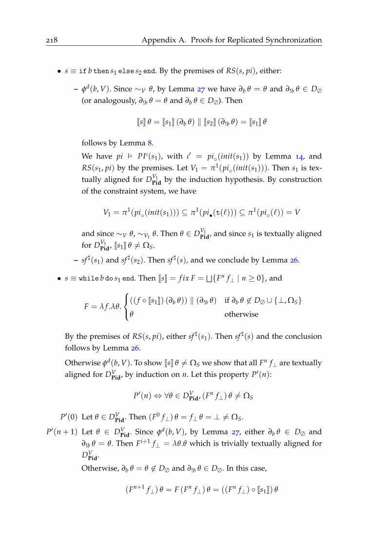
218 Appendix A. Proofs for Replicated Synchronization
• s ≡ if b then s1 else s2 end. By the premises of RS(s, pi), either:
– φd(b, V). Since ∼V θ, by Lemma 27 we have ∂b θ = θ and ∂!b θ ∈ D∅
(or analogously, ∂!b θ = θ and ∂b θ ∈ D∅). Then
JsK θ = Js1K (∂b θ) ‖ Js2K (∂!b θ) = Js1K θ
follows by Lemma 8.
We have pi PI ι(s1), with ι′ = pi(init(s1)) by Lemma 14, and
RS(s1, pi) by the premises. Let V1 = π1(pi(init(s1))). Then s1 is tex-
tually aligned for DV1Pid by the induction hypothesis. By construction
of the constraint system, we have
V1 = π1(pi(init(s1))) ⊆ π1(pi•(t(ℓ))) ⊆ π1(pi(ℓ)) = V
and since ∼V θ, ∼V1θ. Then θ ∈ DV1
Pid, and since s1 is textually aligned
for DV1Pid, Js1K θ 6= ΩS.
– sf ♯(s1) and sf ♯(s2). Then sf ♯(s), and we conclude by Lemma 26.
• s ≡ while b do s1 end. Then JsK = f ix F =⊔
Fn f⊥ | n ≥ 0, and
F = λ f .λθ.
(( f Js1K) (∂b θ)) ‖ (∂!b θ) if ∂b θ 6∈ D∅ ∪ ⊥, ΩS
θ otherwise
By the premises of RS(s, pi), either sf ♯(s1). Then sf ♯(s) and the conclusion
follows by Lemma 26.
Otherwise φd(b, V). To show JsK θ 6= ΩS we show that all Fn f⊥ are textually
aligned for DVPid, by induction on n. Let this property P′(n):
P′(n)⇔ ∀θ ∈ DVPid, (Fn f⊥) θ 6= ΩS
P′(0) Let θ ∈ DVPid. Then (F0 f⊥) θ = f⊥ θ = ⊥ 6= ΩS.
P′(n + 1) Let θ ∈ DVPid. Since φd(b, V), by Lemma 27, either ∂b θ ∈ D∅ and
∂!b θ = θ. Then Fi+1 f⊥ = λθ.θ which is trivially textually aligned for
DVPid.
Otherwise, ∂b θ = θ 6∈ D∅ and ∂!b θ ∈ D∅. In this case,
(Fn+1 f⊥) θ = F (Fn f⊥) θ = ((Fn f⊥) Js1K) θ

A.3. Correctness of RS 219
The outer induction hypothesis gives P(s1) and, since pi PI ι′(s1)
with ι′ = pi(init(s1)) by Lemma 14, and RS(s1, pi) by the premises
of RS(s, pi). Let V1 = π1(pi(init(s1))), and then we obtain that s1 is
textually aligned for DV1Pid.
The constraint system gives
V1 = π1(pi(init(s1))) ⊆ π1(pi•(t(ℓ))) ⊆ π1(pi(ℓ)) = V
so since ∼V θ we have ∼V1θ.
Let Js1K θ = θ′. Since ∼V1θ and s1 is textually aligned for DV1
Pid, θ′ 6=
ΩS. Let V′1 = π1( f inale(s1)). By Theorem 2, ∼V′1θ′.
By construction of PI ι(s), we have the following:
V = π1(pi(ℓ)) ⊆ π1(pi•(n(ℓ)))∩π1(pi•(b(ℓ))) ⊆ π1(pi•(b(ℓ))) = V′1
And so by ∼V′1θ′ we have ∼V θ′, thus θ′ ∈ DV
Pid.
By the induction hypothesis on n we have that Fn f⊥ is textually
aligned for DVPid, and so
JsK θ = (Fn f⊥)(Js1K θ) = (Fn f⊥) θ′ 6= ΩS


BProof Sketches for Safe
Registration in BSPlib
Contents
B.1 Proof Sketch For Lemma 1 . . . . . . . . . . . . . . . . . . . . . . . . 221
B.2 Proof Sketch For Theorem 4 . . . . . . . . . . . . . . . . . . . . . . . 222
B.3 Proof Sketch For Theorem 5 . . . . . . . . . . . . . . . . . . . . . . . 224
This section sketches the proofs of Lemma 1 and Theorems 4 and 5. While
the full proofs have been developed, we do not include them here due to their
length and lack of time. Instead, we defer their typesetting in a technical report
to future work.
B.1 Proof Sketch For Lemma 1
We recall Lemma 1:
Lemma 1. If Reach(Γ, Γ′); A then the same source s 6= unknown never appears twice
in the same component of A associated with two locations of different base.
Proof sketch: Before proving this lemma, we show an auxiliary fact. Namely,
that the path of each local execution step is a “fresh” path that has not appeared
before. We formalize freshness by establishing a strict order on paths with the
intention that, δ1 < δ2 if δ1 is produced “before” δ2 in the semantics and thus that
δ2 is fresh. We then show, by a standard rule induction on the local semantics,
that the initial and final path of each local step is strictly ordered.
The proof of Lemma 1 consists of showing that for each instrumented state
H, o and as in a local execution there exists a partial mapping ρ from sources to
bases such that for each location-source pair (l, s) where s 6= unknown and either
1. (l, s) appears in as, or
221
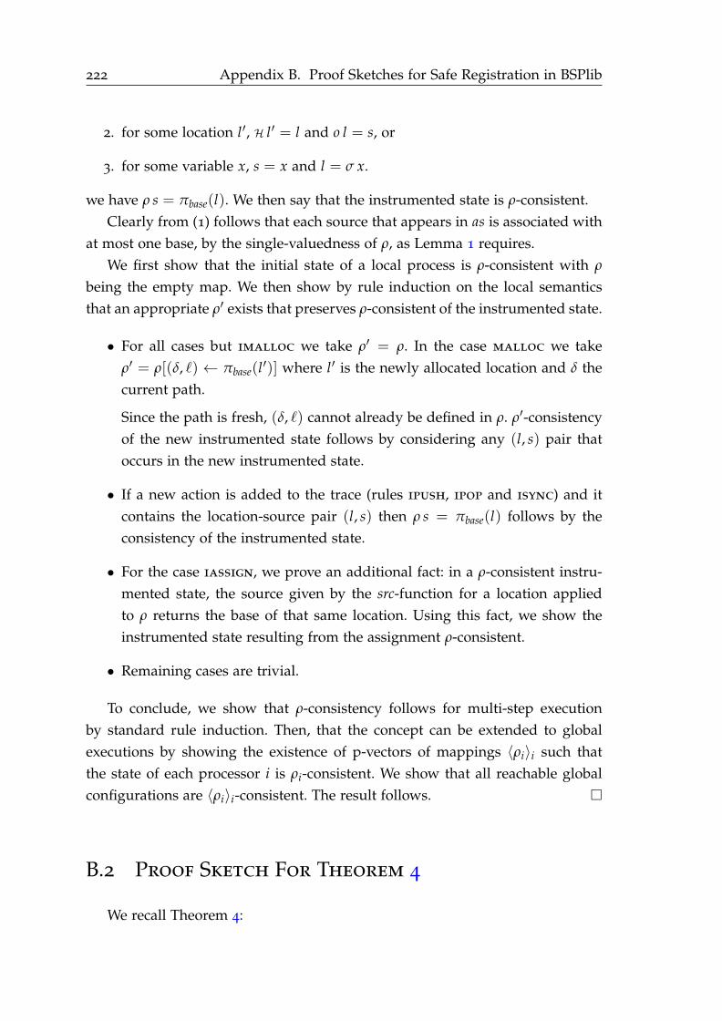
222 Appendix B. Proof Sketches for Safe Registration in BSPlib
2. for some location l′, H l′ = l and o l = s, or
3. for some variable x, s = x and l = σ x.
we have ρ s = πbase(l). We then say that the instrumented state is ρ-consistent.
Clearly from (1) follows that each source that appears in as is associated with
at most one base, by the single-valuedness of ρ, as Lemma 1 requires.
We first show that the initial state of a local process is ρ-consistent with ρ
being the empty map. We then show by rule induction on the local semantics
that an appropriate ρ′ exists that preserves ρ-consistent of the instrumented state.
• For all cases but imalloc we take ρ′ = ρ. In the case malloc we take
ρ′ = ρ[(δ, ℓ) ← πbase(l′)] where l′ is the newly allocated location and δ the
current path.
Since the path is fresh, (δ, ℓ) cannot already be defined in ρ. ρ′-consistency
of the new instrumented state follows by considering any (l, s) pair that
occurs in the new instrumented state.
• If a new action is added to the trace (rules ipush, ipop and isync) and it
contains the location-source pair (l, s) then ρ s = πbase(l) follows by the
consistency of the instrumented state.
• For the case iassign, we prove an additional fact: in a ρ-consistent instru-
mented state, the source given by the src-function for a location applied
to ρ returns the base of that same location. Using this fact, we show the
instrumented state resulting from the assignment ρ-consistent.
• Remaining cases are trivial.
To conclude, we show that ρ-consistency follows for multi-step execution
by standard rule induction. Then, that the concept can be extended to global
executions by showing the existence of p-vectors of mappings 〈ρi〉i such that
the state of each processor i is ρi-consistent. We show that all reachable global
configurations are 〈ρi〉i-consistent. The result follows.
B.2 Proof Sketch For Theorem 4
We recall Theorem 4:
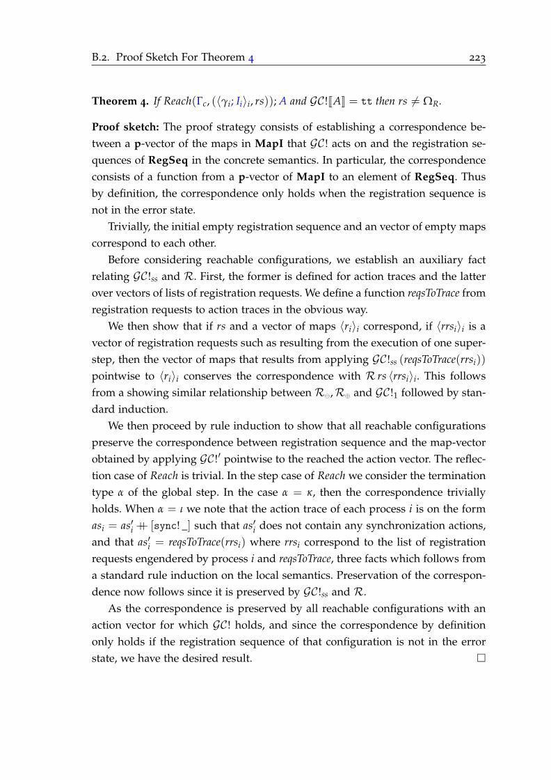
B.2. Proof Sketch For Theorem 4 223
Theorem 4. If Reach(Γc, (〈γi; Ii〉i, rs)); A and GC !JAK = tt then rs 6= ΩR.
Proof sketch: The proof strategy consists of establishing a correspondence be-
tween a p-vector of the maps in MapI that GC ! acts on and the registration se-
quences of RegSeq in the concrete semantics. In particular, the correspondence
consists of a function from a p-vector of MapI to an element of RegSeq. Thus
by definition, the correspondence only holds when the registration sequence is
not in the error state.
Trivially, the initial empty registration sequence and an vector of empty maps
correspond to each other.
Before considering reachable configurations, we establish an auxiliary fact
relating GC !ss and R. First, the former is defined for action traces and the latter
over vectors of lists of registration requests. We define a function reqsToTrace from
registration requests to action traces in the obvious way.
We then show that if rs and a vector of maps 〈ri〉i correspond, if 〈rrsi〉i is a
vector of registration requests such as resulting from the execution of one super-
step, then the vector of maps that results from applying GC !ss (reqsToTrace(rrsi))
pointwise to 〈ri〉i conserves the correspondence with R rs 〈rrsi〉i. This follows
from a showing similar relationship between R⊖,R⊕ and GC !1 followed by stan-
dard induction.
We then proceed by rule induction to show that all reachable configurations
preserve the correspondence between registration sequence and the map-vector
obtained by applying GC !′ pointwise to the reached the action vector. The reflec-
tion case of Reach is trivial. In the step case of Reach we consider the termination
type α of the global step. In the case α = κ, then the correspondence trivially
holds. When α = ι we note that the action trace of each process i is on the form
asi = as′i ++ [sync! _] such that as′i does not contain any synchronization actions,
and that as′i = reqsToTrace(rrsi) where rrsi correspond to the list of registration
requests engendered by process i and reqsToTrace, three facts which follows from
a standard rule induction on the local semantics. Preservation of the correspon-
dence now follows since it is preserved by GC !ss and R.
As the correspondence is preserved by all reachable configurations with an
action vector for which GC ! holds, and since the correspondence by definition
only holds if the registration sequence of that configuration is not in the error
state, we have the desired result.
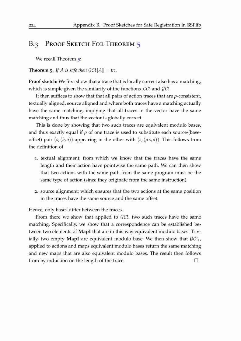
224 Appendix B. Proof Sketches for Safe Registration in BSPlib
B.3 Proof Sketch For Theorem 5
We recall Theorem 5:
Theorem 5. If A is safe then GC !JAK = tt.
Proof sketch: We first show that a trace that is locally correct also has a matching,
which is simple given the similarity of the functions LC ! and GC !.
It then suffices to show that that all pairs of action traces that are ρ-consistent,
textually aligned, source aligned and where both traces have a matching actually
have the same matching, implying that all traces in the vector have the same
matching and thus that the vector is globally correct.
This is done by showing that two such traces are equivalent modulo bases,
and thus exactly equal if ρ of one trace is used to substitute each source-(base-
offset) pair (s, (b, o)) appearing in the other with (s, (ρ s, o)). This follows from
the definition of
1. textual alignment: from which we know that the traces have the same
length and their action have pointwise the same path. We can then show
that two actions with the same path from the same program must be the
same type of action (since they originate from the same instruction).
2. source alignment: which ensures that the two actions at the same position
in the traces have the same source and the same offset.
Hence, only bases differ between the traces.
From there we show that applied to GC !, two such traces have the same
matching. Specifically, we show that a correspondence can be established be-
tween two elements of MapI that are in this way equivalent modulo bases. Triv-
ially, two empty MapI are equivalent modulo base. We then show that GC !1,
applied to actions and maps equivalent modulo bases return the same matching
and new maps that are also equivalent modulo bases. The result then follows
from by induction on the length of the trace.
Bibliography
[1] S. Aananthakrishnan, G. Bronevetsky, M. Baranowski, and G. Gopalakr-
ishnan. ParFuse: Parallel and Compositional Analysis of Message Passing
Programs. In C. Ding, J. Criswell, and P. Wu, editors, Languages and Compil-
ers for Parallel Computing, Lecture Notes in Computer Science, pages 24–39.
Springer International Publishing, 2017. ISBN 978-3-319-52709-3. 77
[2] S. Agarwal, R. Barik, V. Sarkar, and R. K. Shyamasundar. May-happen-
in-parallel Analysis of X10 Programs. In Proceedings of the 12th ACM SIG-
PLAN Symposium on Principles and Practice of Parallel Programming, PPoPP
’07, pages 183–193, New York, NY, USA, 2007. ACM. ISBN 978-1-59593-
602-8. doi: 10.1145/1229428.1229471. 74, 75, 76
[3] D. H. Ahn, B. R. de Supinski, I. Laguna, G. L. Lee, B. Liblit, B. P. Miller, and
M. Schulz. Scalable Temporal Order Analysis for Large Scale Debugging.
In Proceedings of the Conference on High Performance Computing Networking,
Storage and Analysis, SC ’09, pages 44:1–44:11, New York, NY, USA, 2009.
ACM. ISBN 978-1-60558-744-8. doi: 10.1145/1654059.1654104. 73
[4] A. V. Aho, R. Sethi, and J. D. Ullman. Compilers, Principles, Techniques.
Addison wesley Boston, 1986. 70
[5] A. Aiken and D. Gay. Barrier Inference. In Proceedings of the 25th
ACM SIGPLAN-SIGACT Symposium on Principles of Programming Languages,
POPL ’98, pages 342–354, New York, NY, USA, 1998. ACM. ISBN 0-89791-
979-3. doi: 10.1145/268946.268974. 70, 73, 79, 82, 92, 116, 154
[6] E. Albert, P. Arenas, S. Genaim, G. Puebla, and D. Zanardini. Cost Analysis
of Java Bytecode. In European Symposium on Programming, pages 157–172.
Springer, 2007. 120, 121, 125, 126, 147
[7] E. Albert, P. Arenas, S. Genaim, and G. Puebla. Closed-Form Upper
Bounds in Static Cost Analysis. Journal of Automated Reasoning, 46(2):161–
203, 2011. 147
225

226 Bibliography
[8] E. Albert, J. Correas, and G. Román-Díez. Peak cost analysis of distributed
systems. In International Static Analysis Symposium, pages 18–33. Springer,
2014. 78
[9] E. Albert, P. Arenas, J. Correas, S. Genaim, M. Gómez-Zamalloa, E. Martin-
Martin, G. Puebla, and G. Román-Díez. Resource Analysis: From Se-
quential to Concurrent and Distributed Programs. In FM 2015: Formal
Methods: 20th International Symposium, Oslo, Norway, June 24-26, 2015, Pro-
ceedings, pages 3–17. Springer International Publishing, June 2015. doi:
10.1007/978-3-319-19249-9_1. 78, 152
[10] V. Allombert. Functional Abstraction for Programming Multi-Level Architec-
tures : Formalisation and Implementation. PhD thesis, Université Paris-Est,
July 2017. 56, 79
[11] V. Allombert, F. Gava, and J. Tesson. Multi-ML: Programming Multi-BSP
Algorithms in ML. International Journal of Parallel Programming, page 20,
2015. 59, 61
[12] V. Allombert, F. Gava, and J. Tesson. Toward Performance Prediction for
Multi-BSP Programs in ML. In International Conference on Algorithms and
Architectures for Parallel Processing, pages 159–174. Springer, 2018. 79
[13] R. Alur, J. Devietti, O. S. Navarro Leija, and N. Singhania. GPUDrano:
Detecting Uncoalesced Accesses in GPU Programs. In R. Majumdar and
V. Kuncak, editors, Computer Aided Verification, Lecture Notes in Computer
Science, pages 507–525. Springer International Publishing, 2017. ISBN 978-
3-319-63387-9. 71, 73, 75
[14] J. Anderson, P. J. Burns, D. Milroy, P. Ruprecht, T. Hauser, and H. J. Siegel.
Deploying RMACC Summit: An HPC Resource for the Rocky Mountain
Region. In Proceedings of the Practice and Experience in Advanced Research
Computing 2017 on Sustainability, Success and Impact, PEARC17, pages 8:1–
8:7, New York, NY, USA, 2017. ACM. ISBN 978-1-4503-5272-7. doi: 10.
1145/3093338.3093379. v, 2
[15] E. A. Ashcroft. Proving assertions about parallel programs. Journal of
Computer and System Sciences, 10(1):110–135, Feb. 1975. ISSN 0022-0000.
doi: 10.1016/S0022-0000(75)80018-3. 65
Bibliography 227
[16] M. Assaf. From Qualitative to Quantitative Program Analysis: Permissive En-
forcement of Secure Information Flow. PhD thesis, Université Rennes 1, 2015.
70
[17] J. Auslander, M. Philipose, C. Chambers, S. J. Eggers, and B. N. Bershad.
Fast, effective dynamic compilation. In ACM SIGPLAN Notices, volume 31,
pages 149–159. ACM, 1996. 70, 73, 106
[18] O. Ballereau, F. Loulergue, and G. Hains. High-level BSP Programming:
BSML and BSλ. In P. Trinder and G. Michaelson, editors, Proceedings of
the First Scottish Functional Programming Workshop, Technical Report, pages
43–52, Edinburgh, Aug. 1999. Heriot-Watt University. viii, 42, 61
[19] E. Bardsley and A. F. Donaldson. Warps and Atomics: Beyond Barrier Syn-
chronization in the Verification of GPU Kernels. In NASA Formal Methods,
pages 230–245. Springer, Cham, Apr. 2014. doi: 10.1007/978-3-319-06200-
6_18. 66
[20] M.-W. Benabderrahmane, L.-N. Pouchet, A. Cohen, and C. Bastoul. The
Polyhedral Model Is More Widely Applicable than You Think. In Inter-
national Conference on Compiler Construction, pages 283–303. Springer, 2010.
121, 140, 142
[21] Y. Bertot and P. Castéran. Interactive Theorem Proving and Program Develop-
ment: Coq’Art: The Calculus of Inductive Constructions. Springer Science &
Business Media, 2013. 65, 83
[22] A. Betts, N. Chong, A. Donaldson, S. Qadeer, and P. Thomson. GPUVerify:
A verifier for GPU kernels. In ACM SIGPLAN Notices, volume 47, pages
113–132. ACM, 2012. 66, 73
[23] R. H. Bisseling. Parallel Scientific Computation: A Structured Approach Using
BSP and MPI. Oxford University Press on Demand, 2004. 14, 30, 114
[24] A. Blanchard, N. Kosmatov, M. Lemerre, and F. Loulergue. Conc2Seq: A
Frama-C Plugin for Verification of Parallel Compositions of C Programs.
In 2016 IEEE 16th International Working Conference on Source Code Analysis
and Manipulation (SCAM), pages 67–72. IEEE, 2016. 153
[25] S. Blazy, D. Bühler, and B. Yakobowski. Structuring Abstract Interpreters
Through State and Value Abstractions. In A. Bouajjani and D. Monni-
aux, editors, Verification, Model Checking, and Abstract Interpretation, Lecture

228 Bibliography
Notes in Computer Science, pages 112–130. Springer International Pub-
lishing, 2017. ISBN 978-3-319-52234-0. 53
[26] O. Bonorden, B. Juurlink, I. Von Otte, and I. Rieping. The Paderborn uni-
versity BSP (PUB) library-design, implementation and performance. In
Proceedings 13th International Parallel Processing Symposium and 10th Sympo-
sium on Parallel and Distributed Processing. IPPS/SPDP 1999, pages 99–104,
Apr. 1999. doi: 10.1109/IPPS.1999.760442. 75
[27] O. Bonorden, B. Juurlink, I. von Otte, and I. Rieping. The Paderborn Uni-
versity BSP (PUB) library. Parallel Computing, 29(2):187–207, Feb. 2003.
ISSN 0167-8191. doi: 10.1016/S0167-8191(02)00218-1. 39, 59, 63, 184
[28] V. Botbol, E. Chailloux, and T. Le Gall. Static Analysis of Communicating
Processes Using Symbolic Transducers. In International Conference on Ver-
ification, Model Checking, and Abstract Interpretation, pages 73–90. Springer,
2017. 71
[29] L. Bougé. The Data-Parallel Programming Model: A Semantic Perspective
(Final Version). Report RR-3044, INRIA, 1996. 67
[30] P. Boulet and X. Redon. Communication Pre-evaluation in HPF. In Proceed-
ings of the 4th International Euro-Par Conference on Parallel Processing, Euro-
Par ’98, pages 263–272, London, UK, UK, 1998. Springer-Verlag. ISBN
978-3-540-64952-6. 78, 153, 154
[31] W. Bousdira, F. Loulergue, and J. Tesson. A verified library of algorith-
mic skeletons on evenly distributed arrays. In International Conference on
Algorithms and Architectures for Parallel Processing, pages 218–232. Springer,
2012. 67
[32] G. Bronevetsky. Communication-Sensitive Static Dataflow for Parallel Mes-
sage Passing Applications. In Proceedings of the 7th Annual IEEE/ACM In-
ternational Symposium on Code Generation and Optimization, CGO ’09, pages
1–12, Washington, DC, USA, 2009. IEEE Computer Society. ISBN 978-0-
7695-3576-0. doi: 10.1109/CGO.2009.32. 71, 72, 73, 74
[33] J.-W. Buurlage, T. Bannink, and A. Wits. Bulk-synchronous pseudo-
streaming algorithms for many-core accelerators. arXiv:1608.07200 [cs],
Aug. 2016. 39

Bibliography 229
[34] J.-W. Buurlage, T. Bannink, and R. H. Bisseling. Bulk: A Modern C++ In-
terface for Bulk-Synchronous Parallel Programs. In Euro-Par 2018: Parallel
Processing, pages 519–532. Springer, Cham, Aug. 2018. doi: 10.1007/978-3-
319-96983-1_37. 39
[35] V. Cavé, J. Zhao, J. Shirako, and V. Sarkar. Habanero-Java: The new ad-
ventures of old X10. In Proceedings of the 9th International Conference on
Principles and Practice of Programming in Java, pages 51–61. ACM, 2011. 74
[36] B. Chapman, T. Curtis, S. Pophale, S. Poole, J. Kuehn, C. Koelbel, and
L. Smith. Introducing OpenSHMEM: SHMEM for the PGAS community.
In Proceedings of the Fourth Conference on Partitioned Global Address Space
Programming Model, page 2, New York, NY, USA, 2010. ACM. 41, 184
[37] P. Chatarasi, J. Shirako, M. Kong, and V. Sarkar. An Extended Polyhedral
Model for SPMD Programs and Its Use in Static Data Race Detection. In
Languages and Compilers for Parallel Computing, pages 106–120. Springer,
Cham, 2017. doi: 10.1007/978-3-319-52709-3_10. 74, 76, 153
[38] K. C. Chaudhuri, D. Doligez, L. Lamport, and S. Merz. A TLA+ proof
system. arXiv preprint arXiv:0811.1914, 2008. 66
[39] Y. Chen and J. W. Sanders. Top-down design of bulk-synchronous parallel
programs. Parallel Processing Letters, 13(03):389–400, 2003. 67
[40] Y. Chen and J. W. Sanders. Logic of global synchrony. ACM Transactions
on Programming Languages and Systems (TOPLAS), 26(2):221–262, 2004. 67
[41] T. Christiansen, L. Wall, and J. Orwant. Programming Perl: Unmatched Power
for Text Processing and Scripting. O’Reilly Media, Inc., 2012. x, 6
[42] P. Ciechanowicz, M. Poldner, and H. Kuchen. The Münster Skeleton Li-
brary Muesli: A comprehensive overview. Technical report, Working Pa-
pers, ERCIS-European Research Center for Information Systems, 2009. 63
[43] E. M. Clarke, O. Grumberg, and D. Peled. Model Checking. MIT press, 1999.
68
[44] P. Clauss. Counting Solutions to Linear and Nonlinear Constraints
Through Ehrhart Polynomials: Applications to Analyze and Transform
Scientific Programs. In Proceedings of the 10th International Conference on
Supercomputing, ICS ’96, pages 278–285, New York, NY, USA, 1996. ACM.
ISBN 978-0-89791-803-9. doi: 10.1145/237578.237617. 78, 153

230 Bibliography
[45] E. Cohen, M. Dahlweid, M. Hillebrand, D. Leinenbach, M. Moskal, T. San-
ten, W. Schulte, and S. Tobies. VCC: A practical system for verifying con-
current C. In Theorem Proving in Higher Order Logics, pages 23–42. Springer,
2009. 65, 66
[46] M. I. Cole. Algorithmic Skeletons: Structured Management of Parallel Compu-
tation. Pitman London, 1989. 62
[47] B. Cook. Principles of program termination. Engineering Methods and Tools
for Software Safety and Security, 22:161, 2009. 125
[48] P. Cousot and R. Cousot. Abstract Interpretation: A Unified Lattice Model
for Static Analysis of Programs by Construction or Approximation of Fix-
points. In Proceedings of the 4th ACM SIGACT-SIGPLAN Symposium on Prin-
ciples of Programming Languages, POPL ’77, pages 238–252, New York, NY,
USA, 1977. ACM. doi: 10.1145/512950.512973. 43, 53
[49] P. Cousot and N. Halbwachs. Automatic discovery of linear restraints
among variables of a program. In Proceedings of the 5th ACM SIGACT-
SIGPLAN Symposium on Principles of Programming Languages, pages 84–96.
ACM, 1978. 147
[50] R. Couturier and D. Méry. An experiment in parallelizing an applica-
tion using formal methods. In Computer Aided Verification, pages 345–356.
Springer, Berlin, Heidelberg, June 1998. doi: 10.1007/BFb0028757. 66
[51] D. Culler, R. Karp, D. Patterson, A. Sahay, K. E. Schauser, E. Santos, R. Sub-
ramonian, and T. Von Eicken. LogP: Towards a realistic model of parallel
computation. In ACM Sigplan Notices, volume 28, pages 1–12. ACM, 1993.
56, 57
[52] P. Cuoq, P. Hilsenkopf, F. Kirchner, S. Labbé, N. Thuy, and B. Yakobowski.
Formal verification of software important to safety using the Frama-C tool
suite. In Proceedings of the 8th International Topical Meeting on Nuclear Plant
Instrumentation, Control and Human Machine Interface Technologies, 2012. 53
[53] P. Cuoq, F. Kirchner, N. Kosmatov, V. Prevosto, J. Signoles, and
B. Yakobowski. Frama-c. In Software Engineering and Formal Methods, pages
233–247. Springer, 2012. 65, 66
[54] P. Cuoq, F. Kirchner, N. Kosmatov, V. Prevosto, J. Signoles, and
B. Yakobowski. Frama-C, A Program Analysis Perspective. In The 10th
Bibliography 231
International Conference on Software Engineering and Formal Methods (SEFM
2012), volume 7504 of LNCS, pages 233–247. Springer, 2012. 52
[55] F. Dabrowski. A Denotational Semantics of Textually Aligned SPMD Pro-
grams. In International Symposium on Formal Approaches to Parallel and Dis-
tributed Systems (4PAD 2018), 2018. 73, 83, 87, 116
[56] F. Dabrowski. Textual Alignment in SPMD Programs. In Proceedings of
the 33rd Annual ACM Symposium on Applied Computing, SAC ’18, pages
1046–1053, New York, NY, USA, 2018. ACM. ISBN 978-1-4503-5191-1. doi:
10.1145/3167132.3167254. 73, 79, 84, 116, 170
[57] N. A. Danielsson. Lightweight Semiformal Time Complexity Analysis
for Purely Functional Data Structures. In Proceedings of the 35th Annual
ACM SIGPLAN-SIGACT Symposium on Principles of Programming Languages,
POPL ’08, pages 133–144, New York, NY, USA, 2008. ACM. ISBN 978-1-
59593-689-9. doi: 10.1145/1328438.1328457. 122
[58] S. Darabi, S. C. C. Blom, and M. Huisman. A Verification Technique for
Deterministic Parallel Programs. In NASA Formal Methods, pages 247–264.
Springer, Cham, May 2017. doi: 10.1007/978-3-319-57288-8_17. 66
[59] F. Darema. SPMD computational model. In Encyclopedia of Parallel Comput-
ing, pages 1933–1943. Springer, 2011. 24
[60] L. De Moura and N. Bjørner. Z3: An efficient SMT solver. In International
Conference on Tools and Algorithms for the Construction and Analysis of Sys-
tems, pages 337–340. Springer, 2008. 65
[61] M. Delahaye, N. Kosmatov, and J. Signoles. Common Specification Lan-
guage for Static and Dynamic Analysis of C Programs. In The 28th Annual
ACM Symposium on Applied Computing (SAC 2013), pages 1230–1235. ACM,
2013. 53
[62] B. Di Martino, A. Mazzeo, N. Mazzocca, and U. Villano. Parallel Pro-
gram Analysis and Restructuring by Detection of Point-to-Point Interac-
tion Patterns and Their Transformation into Collective Communication
Constructs. Science of Computer Programming, 40(2–3):235–263, July 2001.
ISSN 0167-6423. doi: 10.1016/S0167-6423(01)00017-X. 74, 77, 135, 141
[63] E. W. Dijkstra. Guarded Commands, Nondeterminacy and Formal Deriva-
tion of Programs. Communications of the ACM, 18(8):453–457, 1975. 53

232 Bibliography
[64] Y. Dubois and R. Teyssier. On the onset of galactic winds in quiescent star
forming galaxies. Astronomy and Astrophysics, 477:79–94, Jan. 2008. ISSN
0004-6361. doi: 10.1051/0004-6361:20078326. xiv, 185
[65] J. Eloff and M. B. Bella. Software Failures: An Overview. In J. Eloff and
M. Bihina Bella, editors, Software Failure Investigation: A Near-Miss Analysis
Approach, pages 7–24. Springer International Publishing, Cham, 2018. ISBN
978-3-319-61334-5. doi: 10.1007/978-3-319-61334-5_2. xiv, 185
[66] K. Emoto, F. Loulergue, and J. Tesson. A Verified Generate-Test-Aggregate
Coq Library for Parallel Programs Extraction. In G. Klein and R. Gamboa,
editors, Interactive Theorem Proving, number 8558 in Lecture Notes in Com-
puter Science, pages 258–274. Springer International Publishing, July 2014.
ISBN 978-3-319-08969-0 978-3-319-08970-6. doi: 10.1007/978-3-319-08970-
6_17. 67
[67] A. Ernstsson, L. Li, and C. Kessler. SkePU 2: Flexible and type-safe skeleton
programming for heterogeneous parallel systems. International Journal of
Parallel Programming, 46(1):62–80, 2018. 63
[68] J.-C. Filliâtre and A. Paskevich. Why3—where programs meet provers. In
Programming Languages and Systems, pages 125–128. Springer, 2013. 65, 67
[69] C. Flanagan and S. Qadeer. Thread-modular model checking. In In-
ternational SPIN Workshop on Model Checking of Software, pages 213–224.
Springer, 2003. 71
[70] L. Flon and N. Suzuki. Consistent and complete proof rules for the total
correctness of parallel programs. In Foundations of Computer Science, 1978.,
19th Annual Symposium On, pages 184–192. IEEE, 1978. 65
[71] M. J. Flynn. Some computer organizations and their effectiveness. IEEE
transactions on computers, 100(9):948–960, 1972. 25
[72] V. Forejt, S. Joshi, D. Kroening, G. Narayanaswamy, and S. Sharma. Precise
predictive analysis for discovering communication deadlocks in MPI pro-
grams. ACM Transactions on Programming Languages and Systems (TOPLAS),
39(4):15, 2017. 69
[73] J. Fortin and F. Gava. Towards Mechanised Semantics of HPC: The BSP
with Subgroup Synchronisation Case. In G. Wang, A. Zomaya, G. Mar-
tinez, and K. Li, editors, Algorithms and Architectures for Parallel Processing,
Bibliography 233
Lecture Notes in Computer Science, pages 222–237. Springer International
Publishing, 2015. ISBN 978-3-319-27161-3. 117
[74] J. Fortin and F. Gava. BSP-Why: A Tool for Deductive Verification of BSP
Algorithms with Subgroup Synchronisation. International Journal of Parallel
Programming, 44(3):574–597, June 2016. ISSN 0885-7458, 1573-7640. doi:
10.1007/s10766-015-0360-y. 66, 67, 68, 153, 183
[75] S. Fortune and J. Wyllie. Parallelism in random access machines. In Pro-
ceedings of the Tenth Annual ACM Symposium on Theory of Computing, pages
114–118. ACM, 1978. 56
[76] M. I. Frank, A. Agarwal, and M. K. Vernon. Lopc: Modeling contention in
parallel algorithms. In Proceedings of the Sixth ACM SIGPLAN Symposium
on Principles and Practice of Parallel Programming, PPOPP ’97, pages 276–287,
New York, NY, USA, 1997. ACM. ISBN 0-89791-906-8. doi: 10.1145/263764.
263803. URL http://doi.acm.org/10.1145/263764.263803. 57
[77] M. Frieb, A. Stegmeier, J. Mische, and T. Ungerer. Employing MPI Collec-
tives for Timing Analysis on Embedded Multi-Cores. In M. Schoeberl,
editor, 16th International Workshop on Worst-Case Execution Time Analysis
(WCET 2016), volume 55 of OpenAccess Series in Informatics (OASIcs), pages
10:1–10:11, Dagstuhl, Germany, 2016. Schloss Dagstuhl–Leibniz-Zentrum
fuer Informatik. ISBN 978-3-95977-025-5. doi: 10.4230/OASIcs.WCET.2016.
10. 78
[78] Z. Ganjei, A. Rezine, L. Henrio, P. Eles, and Z. Peng. On Reachability in
Parameterized Phaser Programs. arXiv:1811.07142 [cs], Nov. 2018. 74
[79] F. Gava. Formal proofs of functional bsp programs. Parallel Process-
ing Letters, 13(03):365–376, Sept. 2003. ISSN 0129-6264. doi: 10.1142/
S0129626403001343. 67
[80] F. Gava and J. Fortin. Formal Semantics of a Subset of the Paderborn’s
BSPlib. In Ninth International Conference on Parallel and Distributed Comput-
ing, Applications and Technologies, 2008. PDCAT 2008, pages 269–276, Piscat-
away, NJ, USA, Dec. 2008. IEEE Press. doi: 10.1109/PDCAT.2008.43. 67, 68,
117, 184
[81] F. Gava and F. Loulergue. A static analysis for Bulk Synchronous Parallel
ML to avoid parallel nesting. Future Generation Computer Systems, 21(5):
665–671, 2005. 78

234 Bibliography
[82] A. V. Gerbessiotis and S.-Y. Lee. Remote memory access: A case for
portable, efficient and library independent parallel programming. Scientific
Programming, 12(3):169–183, 2004. 43
[83] R. Gerstenberger, M. Besta, and T. Hoefler. Enabling Highly-
Scalable Remote Memory Access Programming with MPI-3 One Sided.
https://www.hindawi.com/journals/sp/2014/571902/abs/, 2014. 24
[84] L. Gesbert, Z. Hu, F. Loulergue, K. Matsuzaki, and J. Tesson. Systematic
development of correct bulk synchronous parallel programs. In Parallel
and Distributed Computing, Applications and Technologies (PDCAT), 2010 In-
ternational Conference On, pages 334–340. IEEE, 2010. 67
[85] H. González-Vélez and M. Leyton. A survey of algorithmic skeleton frame-
works: High-level structured parallel programming enablers. Software:
Practice and Experience, 40(12):1135–1160, 2010. 62
[86] G. Gopalakrishnan, P. D. Hovland, C. Iancu, S. Krishnamoorthy, I. Laguna,
R. A. Lethin, K. Sen, S. F. Siegel, and A. Solar-Lezama. Report of the
HPC Correctness Summit, Jan 25–26, 2017, Washington, DC. arXiv preprint
arXiv:1705.07478, 2017. 79
[87] S. Gorlatch and M. Cole. Parallel Skeletons. In D. Padua, editor, Encyclope-
dia of Parallel Computing, pages 1417–1422. Springer US, Boston, MA, 2011.
ISBN 978-0-387-09766-4. doi: 10.1007/978-0-387-09766-4_24. 62
[88] M. W. Goudreau, K. Lang, S. B. Rao, and T. Tsantilas. The green BSP
library. Report CS TR, 95(11), 1995. 24, 63
[89] W. Gropp, T. Hoefler, R. Thakur, and E. Lusk. Using Advanced MPI: Modern
Features of the Message-Passing Interface. MIT Press, 2014. 2, 42, 188
[90] T. Grosser, A. Groesslinger, and C. Lengauer. Polly—performing poly-
hedral optimizations on a low-level intermediate representation. Parallel
Processing Letters, 22(04):1250010, 2012. 154
[91] I. Grudenic and N. Bogunovic. Modeling and verification of MPI based
distributed software. In European Parallel Virtual Machine/Message Passing
Interface Users’ Group Meeting, pages 123–132. Springer, 2006. 69
[92] A. Gustavsson, J. Gustafsson, and B. Lisper. Timing Analysis of Parallel
Software Using Abstract Execution. In K. L. McMillan and X. Rival, edi-
tors, Verification, Model Checking, and Abstract Interpretation, Lecture Notes
Bibliography 235
in Computer Science, pages 59–77. Springer Berlin Heidelberg, 2014. ISBN
978-3-642-54013-4. 77
[93] G. Hains. Subset synchronization in BSP computing. In PDPTA, volume 98,
pages 242–246, 1998. 15
[94] G. Hains. Algorithmes et programmation parallèles : Théorie avec BSP et pratique
avec OCaml. Ellipses Marketing, May 2018. ISBN 978-2-340-02466-3. 14
[95] G. Hains and A. Domínguez. Real-time parallel routing for telecom
networks: Graph algorithms and bulk-synchronous parallel acceleration.
In 2016 IEEE Canadian Conference on Electrical and Computer Engineering
(CCECE), pages 1–4. IEEE, 2016. 114
[96] G. Hains and F. Loulergue. Functional Bulk Synchronous Parallel Pro-
gramming using the BSMLlib Library. In Second International Workshop on
Constructive Methods for Parallel Programming, CMPP, Ponte de Lima, Por-
tugal, 2000. Uni. Passau (D) TR MIP-0007. 64
[97] V. Halyo, P. LeGresley, and P. Lujan. Massively parallel computing and
the search for jets and black holes at the LHC. Nuclear Instruments and
Methods in Physics Research Section A: Accelerators, Spectrometers, Detectors
and Associated Equipment, 744:54–60, Apr. 2014. ISSN 0168-9002. doi: 10.
1016/j.nima.2014.01.038. v, xiv, 1, 185
[98] Y. Hayashi and M. Cole. Static Performance Prediction of Skeletal Parallel
Programs. PARALLEL ALGORITHMS AND APPLICATION, 17(1):59–84,
2002. 79, 153
[99] F. Heine and A. Slowik. Volume Driven Data Distribution for NUMA-
Machines. In Euro-Par 2000 Parallel Processing, pages 415–424. Springer,
Berlin, Heidelberg, Aug. 2000. doi: 10.1007/3-540-44520-X_53. 153
[100] J. M. D. Hill, B. McColl, D. C. Stefanescu, M. W. Goudreau, K. Lang, S. B.
Rao, T. Suel, T. Tsantilas, and R. H. Bisseling. BSPlib: The BSP Program-
ming Library. Parallel Computing, 24(14):1947–1980, Dec. 1998. ISSN 0167-
8191. doi: 10.1016/S0167-8191(98)00093-3. viii, 23, 30, 41, 63
[101] C. A. R. Hoare. An axiomatic basis for computer programming. Commu-
nications of the ACM, 12(10):576–580, 1969. 65
236 Bibliography
[102] C. A. R. Hoare. Communicating sequential processes. Communications of
the ACM, 21(8):666–677, 1978. 60
[103] T. Hoefler, J. Dinan, R. Thakur, B. W. Barrett, P. Balaji, W. Gropp, and K. D.
Underwood. Remote Memory Access Programming in MPI-3. TOPC, 2:
9–9, 2015. doi: 10.1145/2780584. 24, 66, 77
[104] J. Hoffmann and M. Hofmann. Amortized resource analysis with poly-
nomial potential. In European Symposium on Programming, pages 287–306.
Springer, 2010. 78
[105] J. Hoffmann and Z. Shao. Automatic Static Cost Analysis for Parallel
Programs. In European Symposium on Programming Languages and Systems,
pages 132–157. Springer, 2015. 78, 152
[106] M. Hofmann and S. Jost. Static prediction of heap space usage for first-
order functional programs. In ACM SIGPLAN Notices, volume 38, pages
185–197. ACM, 2003. 122
[107] W. Hu, N. Huang, and T. Chiueh. Software Defined Radio Implementation
of an LTE Downlink Transceiver for Ultra Dense Networks. In 2018 IEEE
International Symposium on Circuits and Systems (ISCAS), pages 1–5, May
2018. doi: 10.1109/ISCAS.2018.8351109. v, 1
[108] Y. Huang and E. Mercer. Detecting MPI Zero Buffer Incompatibility by
SMT Encoding. In NASA Formal Methods, pages 219–233. Springer, Cham,
Apr. 2015. doi: 10.1007/978-3-319-17524-9_16. 69
[109] J. Hückelheim, Z. Luo, S. H. K. Narayanan, S. Siegel, and P. D. Hovland.
Verifying Properties of Differentiable Programs. In Static Analysis, pages
205–222. Springer, Cham, Aug. 2018. doi: 10.1007/978-3-319-99725-4_14.
69
[110] A. Jakobsson. Automatic Cost Analysis for Imperative BSP Programs. In-
ternational Journal of Parallel Programming, 47(2):184–212, Apr. 2019. ISSN
0885-7458, 1573-7640. doi: 10.1007/s10766-018-0562-1. 119
[111] A. Jakobsson, F. Dabrowski, W. Bousdira, F. Loulergue, and G. Hains.
Replicated Synchronization for Imperative BSP Programs. Procedia Com-
puter Science, 108:535–544, Jan. 2017. ISSN 1877-0509. doi: 10.1016/j.procs.
2017.05.123. 81

Bibliography 237
[112] A. Jakobsson, F. Dabrowski, and W. Bousdira. Safe Usage of Registers
in BSPlib. In Proceedings of the 34th Annual ACM Symposium on Applied
Computing, SAC ’19, Limassol, Cyprus, Apr. 2019. ACM. ISBN 978-1-4503-
5933-7. doi: 10.1145/3297280.3297421. 157
[113] F. A. Jakobsson. Optimized Support of Memory-Related Annotations for
Runtime Assertion Checking with Frama-C. Master’s thesis, Université de
Bordeaux, Aug. 2014. 52
[114] N. Javed and F. Loulergue. OSL: Optimized bulk synchronous parallel
skeletons on distributed arrays. In Advanced Parallel Processing Technologies,
pages 436–451. Springer, 2009. 64
[115] B. Jeannet and A. Miné. Apron: A Library of Numerical Abstract Domains
for Static Analysis. In International Conference on Computer Aided Verification,
pages 661–667. Springer, 2009. 147
[116] T. E. Jeremiassen and S. J. Eggers. Static analysis of barrier synchronization
in explicitly parallel programs. In IFIP PACT, pages 171–180. Citeseer,
1994. 72, 74
[117] H. Jifeng, Q. Miller, and L. Chen. Algebraic laws for BSP programming.
In L. Bougé, P. Fraigniaud, A. Mignotte, and Y. Robert, editors, Euro-Par’96
Parallel Processing, number 1124 in Lecture Notes in Computer Science,
pages 359–368. Springer Berlin Heidelberg, Aug. 1996. ISBN 978-3-540-
61627-6 978-3-540-70636-6. doi: 10.1007/BFb0024724. 67
[118] A. Jones, R. Melhem, and S. Shao. A compiler-based communication anal-
ysis approach for multiprocessor systems. In Parallel and Distributed Pro-
cessing Symposium, International(IPDPS), page 65, Apr. 2006. ISBN 978-1-
4244-0054-6. doi: 10.1109/IPDPS.2006.1639322. 74
[119] G. Jones and M. Goldsmith. Programming in Occam. Prentice-Hall Interna-
tional New York, NY, 1987. 60
[120] B. H. H. Juurlink and H. A. G. Wijshoff. A Quantitative Comparison of
Parallel Computation Models. In Proceedings of the Eighth Annual ACM
Symposium on Parallel Algorithms and Architectures, SPAA ’96, pages 13–24,
New York, NY, USA, 1996. ACM. ISBN 978-0-89791-809-1. doi: 10.1145/
237502.241604. 150
238 Bibliography
[121] A. Kamil and K. Yelick. Concurrency Analysis for Parallel Programs with
Textually Aligned Barriers. In Proceedings of the 18th International Conference
on Languages and Compilers for Parallel Computing, LCPC’05, pages 185–199,
Berlin, Heidelberg, 2006. Springer-Verlag. ISBN 978-3-540-69329-1. doi:
10.1007/978-3-540-69330-7_13. xi, 6, 73, 117
[122] A. Kamil and K. Yelick. Enforcing Textual Alignment of Collectives Using
Dynamic Checks. In G. R. Gao, L. L. Pollock, J. Cavazos, and X. Li, editors,
Languages and Compilers for Parallel Computing, Lecture Notes in Computer
Science, pages 368–382. Springer Berlin Heidelberg, Oct. 2009. ISBN 978-
3-642-13373-2 978-3-642-13374-9. doi: 10.1007/978-3-642-13374-9_25. 73
[123] R. M. Keller. Formal Verification of Parallel Programs. Commun. ACM, 19
(7):371–384, July 1976. ISSN 0001-0782. doi: 10.1145/360248.360251. 65
[124] I. Laguna and M. Schulz. Pinpointing scale-dependent integer overflow
bugs in large-scale parallel applications. In Proceedings of the International
Conference for High Performance Computing, Networking, Storage and Analysis,
page 19. IEEE Press, Nov. 2016. ISBN 978-1-4673-8815-3. 73
[125] L. Lamport. The ‘Hoare logic’of concurrent programs. Acta Informatica, 14
(1):21–37, 1980. 65
[126] J. K. Lee, J. Palsberg, R. Majumdar, and H. Hong. Efficient may happen in
parallel analysis for async-finish parallelism. In International Static Analysis
Symposium, pages 5–23. Springer, 2012. 74
[127] C. Lengauer. Loop Parallelization in the Polytope Model. In International
Conference on Concurrency Theory, pages 398–416. Springer, 1993. 153
[128] C. Li and G. Hains. A simple bridging model for high-performance com-
puting. In High Performance Computing and Simulation (HPCS), 2011 Inter-
national Conference On, pages 249–256. IEEE, 2011. 56, 58
[129] G. Li, R. Palmer, M. DeLisi, G. Gopalakrishnan, and R. M. Kirby. Formal
Specification of MPI 2.0: Case Study in Specifying a Practical Concurrent
Programming API. Sci. Comput. Program., 76(2):65–81, Feb. 2011. ISSN
0167-6423. doi: 10.1016/j.scico.2010.03.007. 61, 66, 69
[130] Y. Lin. Static Nonconcurrency Analysis of OpenMP Programs. In M. S.
Mueller, B. M. Chapman, B. R. de Supinski, A. D. Malony, and M. Voss,

Bibliography 239
editors, OpenMP Shared Memory Parallel Programming, Lecture Notes in
Computer Science, pages 36–50. Springer Berlin Heidelberg, 2008. ISBN
978-3-540-68555-5. 74
[131] B. Lisper. Towards Parallel Programming Models for Predictability. In
T. Vardanega, editor, 12th International Workshop on Worst-Case Execution
Time Analysis, volume 23 of OpenAccess Series in Informatics (OASIcs), pages
48–58, Dagstuhl, Germany, 2012. Schloss Dagstuhl–Leibniz-Zentrum fuer
Informatik. ISBN 978-3-939897-41-5. doi: 10.4230/OASIcs.WCET.2012.48.
78
[132] J. Liu, J. Wu, and D. K. Panda. High Performance RDMA-Based MPI Im-
plementation over InfiniBand. International Journal of Parallel Programming,
32(3):167–198, June 2004. ISSN 1573-7640. doi: 10.1023/B:IJPP.0000029272.
69895.c1. 24
[133] F. Loulergue. BSλppp: Functional BSP Programs on Enumerated Vectors.
In M. Valero, K. Joe, M. Kitsuregawa, and H. Tanaka, editors, High Per-
formance Computing, number 1940 in Lecture Notes in Computer Science,
pages 355–363. Springer Berlin Heidelberg, Oct. 2000. ISBN 978-3-540-
41128-4 978-3-540-39999-5. doi: 10.1007/3-540-39999-2_34. 64, 67
[134] F. Loulergue. A Verified Accumulate Algorithmic Skeleton. In 2017 Fifth
International Symposium on Computing and Networking (CANDAR), pages
420–426, Nov. 2017. doi: 10.1109/CANDAR.2017.108. 67
[135] G. Malewicz, M. H. Austern, A. J. Bik, J. C. Dehnert, I. Horn, N. Leiser, and
G. Czajkowski. Pregel: A system for large-scale graph processing. In Pro-
ceedings of the 2010 ACM SIGMOD International Conference on Management
of Data, pages 135–146. ACM, 2010. 63
[136] H. Markram. The blue brain project. Nature Reviews Neuroscience, 7(2):153,
2006. xiv, 185
[137] J. Marshall, A. Adcroft, C. Hill, L. Perelman, and C. Heisey. A finite-
volume, incompressible Navier Stokes model for studies of the ocean on
parallel computers. Journal of Geophysical Research: Oceans, 102(C3):5753–
5766, 1997. ISSN 2156-2202. doi: 10.1029/96JC02775. xiv, 185
[138] A. J. McPherson, V. Nagarajan, and M. Cintra. Static Approximation of
MPI Communication Graphs for Optimized Process Placement. In Lan-
240 Bibliography
guages and Compilers for Parallel Computing, Lecture Notes in Computer Sci-
ence, pages 268–283. Springer, Cham, Sept. 2014. ISBN 978-3-319-17472-3
978-3-319-17473-0. doi: 10.1007/978-3-319-17473-0_18. 74
[139] Message Passing Interface Forum. MPI: A Message-Passing Interface Stan-
dard, Version 3.0. High Performance Computing Center Stuttgart (HLRS),
Sept. 2012. 24, 33, 40, 42, 64, 184
[140] J. Midtgaard, F. Nielson, and H. R. Nielson. Process-local static analysis
of synchronous processes. In International Static Analysis Symposium, pages
284–305. Springer, 2018. 72
[141] R. Miller. A library for bulk-synchronous parallel programming. In Pro-
ceedings of the BCS Parallel Processing Specialist Group Workshop on General
Purpose Parallel Computing, pages 100–108, 1993. 24, 39, 63, 114
[142] R. Milner. A Calculus of Communicating Systems. Springer, Berlín, 1980.
ISBN 978-3-540-10235-9 978-0-387-10235-1. OCLC: 911368693. 60
[143] A. Miné. Relational Thread-Modular Static Value Analysis by Abstract
Interpretation. In Verification, Model Checking, and Abstract Interpretation,
pages 39–58. Springer, Berlin, Heidelberg, Jan. 2014. doi: 10.1007/978-3-
642-54013-4_3. 71
[144] M. W. Moskewicz, C. F. Madigan, Y. Zhao, L. Zhang, and S. Malik. Chaff:
Engineering an Efficient SAT Solver. In Proceedings of the 38th Annual Design
Automation Conference, DAC ’01, pages 530–535, New York, NY, USA, 2001.
ACM. ISBN 978-1-58113-297-7. doi: 10.1145/378239.379017. 65
[145] M. Naik and A. Aiken. Conditional must not aliasing for static race de-
tection. In ACM SIGPLAN Notices, volume 42, pages 327–338. ACM, 2007.
76
[146] R. Nakade, E. Mercer, P. Aldous, and J. McCarthy. Model-Checking Task
Parallel Programs for Data-Race. In NASA Formal Methods, pages 367–382.
Springer, Cham, Apr. 2018. doi: 10.1007/978-3-319-77935-5_25. 69
[147] G. C. Necula, S. McPeak, S. P. Rahul, and W. Weimer. CIL: Intermediate
language and tools for analysis and transformation of C programs. In
Compiler Construction, pages 213–228. Springer, 2002. 53

Bibliography 241
[148] N. Ng, N. Yoshida, O. Pernet, R. Hu, and Y. Kryftis. Safe parallel program-
ming with session java. In International Conference on Coordination Languages
and Models, pages 110–126. Springer, 2011. 75
[149] N. Ng, N. Yoshida, and K. Honda. Multiparty Session C: Safe parallel
programming with message optimisation. In International Conference on
Modelling Techniques and Tools for Computer Performance Evaluation, pages
202–218. Springer, 2012. 75
[150] N. Ng, N. Yoshida, and W. Luk. Scalable Session Programming for Het-
erogeneous High-Performance Systems. In Software Engineering and Formal
Methods, Lecture Notes in Computer Science, pages 82–98. Springer, Cham,
Sept. 2013. ISBN 978-3-319-05031-7 978-3-319-05032-4. doi: 10.1007/978-3-
319-05032-4_7. 67
[151] F. Nielson, H. R. Nielson, and C. Hankin. Principles of Program Analysis.
Springer Science & Business Media, Dec. 2004. ISBN 978-3-540-65410-0.
43, 44, 47, 51, 70, 83, 102, 111, 113, 147
[152] H. R. Nielson and F. Nielson. Semantics with Applications. Springer, 2007.
193
[153] S. Owicki and D. Gries. Verifying Properties of Parallel Programs: An
Axiomatic Approach. Commun. ACM, 19(5):279–285, May 1976. ISSN 0001-
0782. doi: 10.1145/360051.360224. 65
[154] H. Ozaktas, C. Rochange, and P. Sainrat. Automatic wcet analysis of real-
time parallel applications. In 13th Workshop on Worst-Case Execution Time
Analysis (WCET 2013), pages pp–11, 2013. 77
[155] S. Pelagatti. Structured Development of Parallel Programs, volume 102. Taylor
& Francis London, 1998. 62
[156] A. Pnueli. The temporal logic of programs. In Foundations of Computer
Science, 1977., 18th Annual Symposium On, pages 46–57. IEEE, 1977. 68
[157] A. Podelski and A. Rybalchenko. A complete method for the synthesis
of linear ranking functions. In Verification, Model Checking, and Abstract
Interpretation, pages 239–251. Springer, 2004. 125
[158] S. Pophale, O. Hernandez, S. Poole, and B. M. Chapman. Extending
the OpenSHMEM Analyzer to Perform Synchronization and Multi-valued

242 Bibliography
Analysis. In S. Poole, O. Hernandez, and P. Shamis, editors, OpenSHMEM
and Related Technologies. Experiences, Implementations, and Tools, number 8356
in Lecture Notes in Computer Science, pages 134–148. Springer Interna-
tional Publishing, Mar. 2014. ISBN 978-3-319-05214-4 978-3-319-05215-1.
doi: 10.1007/978-3-319-05215-1_10. 73
[159] R. Preissl, T. Köckerbauer, M. Schulz, D. Kranzlmüller, B. R. d Supinski,
and D. J. Quinlan. Detecting Patterns in MPI Communication Traces. In
2008 37th International Conference on Parallel Processing, pages 230–237, Sept.
2008. doi: 10.1109/ICPP.2008.71. 79
[160] R. Preissl, M. Schulz, D. Kranzlmüller, B. R. de Supinski, and D. J. Quin-
lan. Using MPI Communication Patterns to Guide Source Code Transfor-
mations. In M. Bubak, G. D. van Albada, J. Dongarra, and P. M. A. Sloot,
editors, Computational Science – ICCS 2008, number 5103 in Lecture Notes in
Computer Science, pages 253–260. Springer Berlin Heidelberg, June 2008.
ISBN 978-3-540-69388-8 978-3-540-69389-5. doi: 10.1007/978-3-540-69389-
5_29. 74
[161] J. Randmets. Static cost analysis, 2012. 125
[162] H. G. Rice. Classes of recursively enumerable sets and their decision prob-
lems. Transactions of the American Mathematical Society, 74(2):358–366, 1953.
ISSN 0002-9947, 1088-6850. doi: 10.1090/S0002-9947-1953-0053041-6. 43
[163] M. Rinard. Analysis of multithreaded programs. In Static Analysis, pages
1–19. Springer, 2001. 77
[164] D. M. Ritchie, B. W. Kernighan, and M. E. Lesk. The C Programming Lan-
guage. Prentice Hall, Englewood Cliffs, NJ, USA, 1988. 161
[165] E. Saillard, P. Carribault, and D. Barthou. PARCOACH: Combining static
and dynamic validation of MPI collective communications. The Inter-
national Journal of High Performance Computing Applications, 28(4):425–434,
2014. 73, 79
[166] C. Santos, F. Martins, and V. T. Vasconcelos. Deductive Verification of Par-
allel Programs Using Why3. Electronic Proceedings in Theoretical Computer
Science, 189:128–142, Aug. 2015. ISSN 2075-2180. doi: 10.4204/EPTCS.189.
11. 67, 68
Bibliography 243
[167] V. Saraswat, B. Bloom, I. Peshansky, O. Tardieu, and D. Grove. X10 lan-
guage specification. Specification, IBM, janvier, 2012. 73
[168] S. Sharma, S. Vakkalanka, G. Gopalakrishnan, R. M. Kirby, R. Thakur, and
W. Gropp. A formal approach to detect functionally irrelevant barriers in
MPI programs. In Recent Advances in Parallel Virtual Machine and Message
Passing Interface, pages 265–273. Springer, 2008. 69
[169] D. R. Shires, L. L. Pollock, and S. Sprenkle. Program flow graph construc-
tion for static analysis of MPI programs. In Proceedings of the International
Conference on Parallel and Distributed Processing Techniques and Applications,
PDPTA 1999, June 28 - Junlly 1, 1999, Las Vegas, Nevada, USA, pages 1847–
1853, 1999. 71, 72
[170] S. F. Siegel. Efficient Verification of Halting Properties for MPI Programs
with Wildcard Receives. In R. Cousot, editor, Verification, Model Checking,
and Abstract Interpretation, Lecture Notes in Computer Science, pages 413–
429. Springer Berlin Heidelberg, 2005. ISBN 978-3-540-30579-8. 69
[171] S. F. Siegel. Model Checking Nonblocking MPI Programs. In B. Cook and
A. Podelski, editors, Verification, Model Checking, and Abstract Interpretation,
number 4349 in Lecture Notes in Computer Science, pages 44–58. Springer
Berlin Heidelberg, Jan. 2007. ISBN 978-3-540-69735-0 978-3-540-69738-1.
doi: 10.1007/978-3-540-69738-1_3. 69
[172] S. F. Siegel. Verifying Parallel Programs with MPI-Spin. In F. Cappello,
T. Herault, and J. Dongarra, editors, Recent Advances in Parallel Virtual Ma-
chine and Message Passing Interface, Lecture Notes in Computer Science,
pages 13–14. Springer Berlin Heidelberg, 2007. ISBN 978-3-540-75416-9. 69
[173] S. F. Siegel and G. S. Avrunin. Verification of Halting Properties for MPI
Programs Using Nonblocking Operations. In F. Cappello, T. Herault, and
J. Dongarra, editors, Recent Advances in Parallel Virtual Machine and Mes-
sage Passing Interface, Lecture Notes in Computer Science, pages 326–334.
Springer Berlin Heidelberg, 2007. ISBN 978-3-540-75416-9. 69
[174] S. F. Siegel and T. K. Zirkel. TASS: The Toolkit for Accurate Scientific
Software. Mathematics in Computer Science, 5(4):395–426, Dec. 2011. ISSN
1661-8289. doi: 10.1007/s11786-011-0100-7. 69

244 Bibliography
[175] S. F. Siegel and T. K. Zirkel. Loop Invariant Symbolic Execution for Parallel
Programs. In D. Hutchison, T. Kanade, J. Kittler, J. M. Kleinberg, F. Mat-
tern, J. C. Mitchell, M. Naor, O. Nierstrasz, C. Pandu Rangan, B. Steffen,
M. Sudan, D. Terzopoulos, D. Tygar, M. Y. Vardi, G. Weikum, V. Kuncak,
and A. Rybalchenko, editors, Verification, Model Checking, and Abstract Inter-
pretation, volume 7148, pages 412–427. Springer Berlin Heidelberg, Berlin,
Heidelberg, 2012. ISBN 978-3-642-27939-3 978-3-642-27940-9. xvi, 187
[176] A. Spector and D. Gifford. The Space Shuttle Primary Computer System.
Commun. ACM, 27(9):872–900, Sept. 1984. ISSN 0001-0782. doi: 10.1145/
358234.358246. 25
[177] G. Staple and K. Werbach. The end of spectrum scarcity [spectrum alloca-
tion and utilization]. IEEE spectrum, 41(3):48–52, 2004. v, 1
[178] T. Sterling, M. Anderson, and M. Brodowicz. Chapter 8 - The Essential
MPI. In T. Sterling, M. Anderson, and M. Brodowicz, editors, High Per-
formance Computing, pages 249–284. Morgan Kaufmann, Boston, Jan. 2018.
ISBN 978-0-12-420158-3. doi: 10.1016/B978-0-12-420158-3.00008-3. 2
[179] A. Stewart, M. Clint, and J. Gabarró. Axiomatic frameworks for develop-
ing BSP-style programs. Parallel Algorithms And Application, 14(4):271–292,
2000. 42, 67
[180] M. M. Strout, B. Kreaseck, and P. D. Hovland. Data-flow analysis for MPI
programs. In Parallel Processing, 2006. ICPP 2006. International Conference
On, pages 175–184. IEEE, 2006. 71, 72
[181] W. Suijlen. Mock BSPlib for Testing and Debugging Bulk Synchronous
Parallel Software. Parallel Processing Letters, 27(01):1740001, 2017. 79
[182] W. J. Suijlen and P. Krusche. BSPonMPI. URL: http://bsponmpi. sourceforge.
net, 2013. 39
[183] W. J. Suijlen and A. N. Yzelman. Lightweight Parallel Foundations: A new
communication layer. Technical Report DPSL-PARIS-TR-2018-09, Huawei
Technologies France / 2012 Laboratories / CSI / DPSL / PADAL, 20 Quai
du Point du Jour, 92100 Boulogne-Billlancourt, France, 2018. 39, 40, 41, 62,
63, 102
[184] J. Tesson and F. Loulergue. Formal Semantics of DRMA-Style Program-
ming in BSPlib. In R. Wyrzykowski, J. Dongarra, K. Karczewski, and
Bibliography 245
J. Wasniewski, editors, Parallel Processing and Applied Mathematics, volume
4967, pages 1122–1129. Springer Berlin Heidelberg, Berlin, Heidelberg,
2008. ISBN 978-3-540-68105-2 978-3-540-68111-3. 67, 117, 132, 184
[185] J. Tesson and F. Loulergue. A verified bulk synchronous parallel ML heat
diffusion simulation. Procedia Computer Science, 4:36–45, 2011. 67
[186] A. Tiskin. The Design and Analysis of Bulk-Synchronous Parallel Algorithms.
PhD Thesis, University of Oxford, 1998. viii, 4, 59
[187] S. Tripakis, C. Stergiou, and R. Lublinerman. Checking Equivalence of
SPMD Programs Using Non-Interference. Technical Report UCB/EECS-
2010-11, CALIFORNIA UNIV BERKELEY DEPT OF ELECTRICAL ENGI-
NEERING AND COMPUTER SCIENCE, Jan. 2010. 74
[188] A. Turing. Checking a large routine. In The Early British Computer Confer-
ences, pages 70–72. MIT Press, 1989. 65
[189] S. Vakkalanka, G. Gopalakrishnan, and R. M. Kirby. Dynamic verification
of MPI programs with reductions in presence of split operations and re-
laxed orderings. In International Conference on Computer Aided Verification,
pages 66–79. Springer, 2008. 69
[190] S. S. Vakkalanka, S. Sharma, G. Gopalakrishnan, and R. M. Kirby. ISP:
A Tool for Model Checking MPI Programs. In Proceedings of the 13th
ACM SIGPLAN Symposium on Principles and Practice of Parallel Programming,
PPoPP ’08, pages 285–286, New York, NY, USA, 2008. ACM. ISBN 978-1-
59593-795-7. doi: 10.1145/1345206.1345258. 69
[191] L. G. Valiant. A Bridging Model for Parallel Computation. Commun. ACM,
33(8):103–111, Aug. 1990. ISSN 0001-0782. doi: 10.1145/79173.79181. viii,
4, 56
[192] L. G. Valiant. A Bridging Model for Multi-core Computing. J. Comput. Syst.
Sci., 77(1):154–166, Jan. 2011. ISSN 0022-0000. doi: 10.1016/j.jcss.2010.06.
012. 56, 58, 59
[193] M. van Duijn. Extending the BSP model to hierarchical heterogeneous
architectures. Master’s thesis, Utrecht University, 2018. 39
[194] S. Verdoolaege. Isl: An Integer Set Library for the Polyhedral Model. In In-
ternational Congress on Mathematical Software, pages 299–302. Springer, 2010.
143, 147
246 Bibliography
[195] S. Verdoolaege and T. Grosser. Polyhedral Extraction Tool. In Second Inter-
national Workshop on Polyhedral Compilation Techniques (IMPACT’12), Paris,
France, 2012. 141
[196] S. Verdoolaege, R. Seghir, K. Beyls, V. Loechner, and M. Bruynooghe.
Counting Integer Points in Parametric Polytopes Using Barvinok’s Ratio-
nal Functions. Algorithmica, 48(1):37–66, 2007. 143, 147
[197] J. S. Vetter and B. R. de Supinski. Dynamic Software Testing of MPI Ap-
plications with Umpire. In Proceedings of the 2000 ACM/IEEE Conference
on Supercomputing, SC ’00, Washington, DC, USA, 2000. IEEE Computer
Society. ISBN 978-0-7803-9802-3. 79
[198] A. Vo, S. Vakkalanka, M. DeLisi, G. Gopalakrishnan, R. M. Kirby, and
R. Thakur. Formal verification of practical MPI programs. ACM Sigplan
Notices, 44(4):261–270, 2009. 69
[199] P. Wang, Y. Du, H. Fu, X. Yang, and H. Zhou. Static Analysis for
Application-Level Checkpointing of MPI Programs. In 2008 10th IEEE In-
ternational Conference on High Performance Computing and Communications,
pages 548–555, Sept. 2008. doi: 10.1109/HPCC.2008.39. 74
[200] B. Wegbreit. Mechanical Program Analysis. Commun. ACM, 18(9):528–539,
Sept. 1975. ISSN 0001-0782. doi: 10.1145/361002.361016. 120, 121
[201] R. Wilhelm, J. Engblom, A. Ermedahl, N. Holsti, S. Thesing, D. Whalley,
G. Bernat, C. Ferdinand, R. Heckmann, T. Mitra, et al. The Worst-Case
Execution-Time Problem—overview of Methods and Survey of Tools. ACM
Transactions on Embedded Computing Systems (TECS), 7(3):36, 2008. 77, 147
[202] N. Williams, B. Marre, P. Mouy, and M. Roger. PathCrawler: Automatic
generation of path tests by combining static and dynamic analysis. In
M. Dal Cin, M. Kaâniche, and A. Pataricza, editors, Dependable Computing
- EDCC 5, volume 3463 of LNCS, pages 281–292, Berlin, Heidelberg, 2005.
Springer Berlin Heidelberg. ISBN 978-3-540-32019-7. 53
[203] G. Winskel. The Formal Semantics of Programming Languages: An Introduction.
MIT press, 1993. 45, 46, 65, 165
[204] K. Yelick, L. Semenzato, G. Pike, C. Miyamoto, B. Liblit, A. Krishnamurthy,
P. Hilfinger, S. Graham, D. Gay, P. Colella, and A. Aiken. Titanium: A high-
performance Java dialect. Concurrency: Practice and Experience, 10(11-13):
Bibliography 247
825–836, Sept. 1998. ISSN 1096-9128. doi: 10.1002/(SICI)1096-9128(199809/
11)10:11/13<825::AID-CPE383>3.0.CO;2-H. xi, 6
[205] T. Yuki, P. Feautrier, S. Rajopadhye, and V. Saraswat. Array dataflow anal-
ysis for polyhedral X10 programs. In ACM SIGPLAN Notices, volume 48,
pages 23–34. ACM, 2013. 74, 76
[206] T. Yuki, P. Feautrier, S. Rajopadhye, and V. Saraswat. Checking Race Free-
dom of Clocked X10 Programs. arXiv:1311.4305 [cs], Nov. 2013. 74, 76
[207] A. Yzelman and R. H. Bisseling. An object-oriented bulk synchronous
parallel library for multicore programming. Concurrency and Computation:
Practice and Experience, 24(5):533–553, Apr. 2012. ISSN 1532-0634. doi: 10.
1002/cpe.1843. 39, 40, 183
[208] A. N. Yzelman, R. H. Bisseling, and D. Roose. MulticoreBSP for C: A
High-Performance Library for Shared-Memory Parallel Programming. In-
ternational Journal of Parallel Programming, 42(4):619–642, Aug. 2014. ISSN
0885-7458, 1573-7640. doi: 10.1007/s10766-013-0262-9. 39, 40, 59, 63
[209] Y. Zhang and E. Duesterwald. Barrier Matching for Programs with Tex-
tually Unaligned Barriers. In Proceedings of the 12th ACM SIGPLAN Sym-
posium on Principles and Practice of Parallel Programming, PPoPP ’07, pages
194–204, New York, NY, USA, 2007. ACM. ISBN 978-1-59593-602-8. doi:
10.1145/1229428.1229472. 73, 75, 79, 82, 116, 187
[210] Y. Zhang, E. Duesterwald, and G. R. Gao. Concurrency Analysis for Shared
Memory Programs with Textually Unaligned Barriers. In V. Adve, M. J.
Garzarán, and P. Petersen, editors, Languages and Compilers for Parallel Com-
puting, Lecture Notes in Computer Science, pages 95–109. Springer Berlin
Heidelberg, 2008. ISBN 978-3-540-85261-2. 74
[211] M. Zheng, M. S. Rogers, Z. Luo, M. B. Dwyer, and S. F. Siegel. CIVL:
Formal verification of parallel programs. In Automated Software Engineer-
ing (ASE), 2015 30th IEEE/ACM International Conference On, pages 830–835.
IEEE, 2015. 69, 79
[212] J. Zhou and Y. Chen. Generating C Code from LOGS Specifications.
In D. Hutchison, T. Kanade, J. Kittler, J. M. Kleinberg, F. Mattern, J. C.
Mitchell, M. Naor, O. Nierstrasz, C. Pandu Rangan, B. Steffen, M. Su-
dan, D. Terzopoulos, D. Tygar, M. Y. Vardi, G. Weikum, D. Van Hung,

248 Bibliography
and M. Wirsing, editors, Theoretical Aspects of Computing – ICTAC 2005, vol-
ume 3722, pages 195–210. Springer Berlin Heidelberg, Berlin, Heidelberg,
2005. ISBN 978-3-540-29107-7 978-3-540-32072-2. 79
[213] W. Zimmermann. Automatic Worst Case Complexity Analysis of Parallel Pro-
grams. International Computer Science Institute, 1990. 78, 152
[214] S. F. S. Ziqing Luo. Towards Deductive Verification of Message-Passing
Parallel Programs, 2018. 67
[215] T. K. Zirkel, S. F. Siegel, and T. McClory. Automated Verification of Chapel
Programs Using Model Checking and Symbolic Execution. In NASA For-
mal Methods, pages 198–212. Springer, Berlin, Heidelberg, May 2013. doi:
10.1007/978-3-642-38088-4_14. 69, 70
This document has been written in the GNU Emacs editor and the LATEX 2ε document
preparation system.
Filip Arvid JAKOBSSONAnalyse statique des programmes BSPlib
Résumé : La programmation parallèle consiste à utiliser des architectures à multiples unités de traitement,
de manière à ce que le temps de calcul soit inversement proportionnel au nombre d’unités matérielles. Le
modèle de BSP (Bulk Synchronous Parallel) permet de rendre le temps de calcul prévisible. BSPlib est une
bibliothèque pour la programmation BSP en langage C. En BSPlib on entrelace des instructions de contrôle
de la structure parallèle globale, et des instructions locales pour chaque unité de traitement. Cela permet des
optimisations fines de la synchronisation, mais permet aussi l’écriture de programmes dont les calculs locaux
divergent et masquent ainsi l’évolution globale du calcul BSP.
Toutefois, les programmes BSPlib réalistes sont syntaxiquement alignés, une propriété qui garantit la conver-
gence du flot de contrôle parallèle. Dans ce mémoire nous étudions les trois dimensions principales des
programmes BSPlib du point de vue de l’alignement syntaxique : la synchronisation, le temps de calcul et la
communication. D’abord nous présentons une analyse statique qui identifie les instructions syntaxiquement
alignées et les utilise pour vérifier la sûreté de la synchronisation globale. Cette analyse a été implémentée
en Frama-C et certifiée en Coq. Ensuite nous utilisons l’alignement syntaxique comme base d’une analyse
statique du temps de calcul. Elle est fondée sur une analyse classique du coût pour les programmes sé-
quentiels. Enfin nous définissons une condition suffisante pour la sûreté de l’enregistrement des variables.
L’enregistrement en BSPlib permet la communication par accès aléatoire à la mémoire distante (DRMA) mais
est sujet à des erreurs de programmation. Notre développement technique est la base d’une future analyse
statique de ce mécanisme.
Mots-clés : Programmation parallèle • Bulk Synchronous Parallelism • SPMD • Analyse statique • Synchro-
nisation • Analyse de coût • Communication
Static Analysis for BSPlib Programs
Abstract: The goal of scalable parallel programming is to program computer architectures composed of mul-
tiple processing units so that increasing the number of processing units leads to an increase in performance.
Bulk Synchronous Parallel (BSP) is a widely used model for scalable parallel programming with predictable
performance. BSPlib is a library for BSP programming in C. In BSPlib, parallel algorithms are expressed
by intermingling instructions that control the global parallel structure, and instructions that express the local
computation of each processing unit. This lets the programmer fine-tune synchronization, but also implement
programs whose diverging parallel control flow obscures the underlying BSP structure. In practice however,
the majority of BSPlib program are textually aligned, a property that ensures parallel control flow convergence.
We examine three core aspects of BSPlib programs through the lens of textual alignment: synchronization,
performance and communication. First, we present a static analysis that identifies textually aligned statements
and use it to verify safe synchronization. This analysis has been implemented in Frama-C and certified in Coq.
Second, we exploit textual alignment to develop a static performance analysis for BSPlib programs, based on
classic cost analysis for sequential programs. Third, we develop a textual alignment-based sufficient condition
for safe registration. Registration in BSPlib enables communication by Direct Remote Memory Access but is
error prone. This development forms the basis for a future static analysis of registration.
Keywords: Parallel programming • Bulk Synchronous Parallelism • SPMD • Static Analysis • Synchroniza-
tion • Cost analysis • Communication
Laboratoire d’Informatique Fondamentale d’Orléans (LIFO), Université d’Orléans. Faculté des
Sciences, Bâtiment IIIA. Rue Léonard de Vinci B.P. 6759 F-45067 ORLEANS Cedex 2, France