Report R94:13b ISRN SICS-R--94/13b--SEISSN 0283-3638

Fixpoint Analysis of Type and Aliasin AKL Programs

by

Thomas Sjöland and Dan Sahlin

January 15, 1995

email: {alf,dan}@sics.se

telephone: +46 8 752 1542 or +46 8 752 1544

fax: +46 8 751 7230

Programming Systems Group

Swedish Institute of Computer Science

Box 1263, S-164 28 Kista, Sweden

Abstract

We have defined and implemented a method for analysis of theCCP language AKL in the spirit of abstract interpretation that uses astatic set of semantic equations which abstracts the concurrent execu-tion of an AKL program. The method strictly separates the setting upof the equation system from the solving of the system with a fixpointprocedure. The computation strategies used, results for a number oftest programs and the conclusions we draw from this experimentaleffort are reported.

The software implementing the system described herein, isdeliverable number D.WP.1.6.1.M2 in the ESPRIT project ParForce6707.

Keywords: Concurrent Constraint Programming, Analysis, AKL, fixpoint

computation

Note: This report replaces R94:13 (ISRN SICS-R--94/13--SE).

2

Table of contents

1. Introduction.......................................................................... 51.1. Brief description of AKL semantics ....................................................6

2. Structure of the analyser ...................................................... 62.1. The analyser ........................................................................................7

3. Notation ............................................................................... 8

4. Semantic equations .............................................................. 84.1. Program ...............................................................................................84.2. Abstract AKL syntax ...........................................................................84.3. Equation schema ................................................................................104.4. General description of the semantic functions...................................11

5. The domain and the domain functions .............................. 115.1. The domain ........................................................................................125.2. The domain functions ........................................................................135.3. Variants of the AT-domain ................................................................17

6. Fixpoint solver ................................................................... 186.1. Optimisations .....................................................................................18

7. Evaluation .......................................................................... 207.1. Example: naive reverse......................................................................207.2. Measurements ....................................................................................227.3. Conclusions........................................................................................337.4. Future work........................................................................................337.5. Experiences using AKL.....................................................................347.6. Summary............................................................................................34

8. Acknowledgements............................................................ 35

9. References.......................................................................... 35

10. Appendix: Implementation of the domain functions ......... 3810.1. The lub function.................................................................................3810.2. The conc function ..............................................................................3910.3. The unif function ............................................................................... 4010.4. call and return ....................................................................................4010.5. Some help routines ............................................................................42

3

4

1. Introduction

The Andorra Kernel Language, AKL, is defined in [JANSON & HARIDI 91].

The name has changed to ”Agents Kernel Language” and a thorough description of

the language and the rationale behind it is given in [JANSON 94]. There is a formal

description of the semantics of the language in [FRANZÉN 94]. An early sequential

implementation of the language was developed in the ESPRIT project PEPMA,

and this is being further developed partly within another ESPRIT project,

ACCLAIM. Some of that work is concerned with a parallel implementation of the

language and an optimising compiler. This system is the intended target of the

analysis tools provided by task T.WP.1.6.1 of the ParForce project.

Analysis of logic programs using abstract interpretation has been treated by

many authors, e.g. [BAGILE 93, BRUYMUWI N 93, COUSOT&COUSOT 92,

HANUS 92, MUTHUKUMAR & HERMENEGILDO 92, NILSSON 92]. For CCP

languages we note in particular [CODOGNET ET AL. 90]. When we started to

design an analysis system for use in the concurrent language AKL (Agents Kernel

Language) [JANSON & HARIDI 91, JANSON 94], we realised that we needed to

design an analysis framework that could be used to model also concurrency and

deep guards and not depend on the sequential execution order of Prolog.

Such an analysis framework has been specified and implemented (in AKL) for

the purpose of providing information guiding a more efficient compilation of AKL.

The analysis framework is based on fixpoint semantics, i.e. a system of semantic

equations for program points is set up and solved using a fixpoint iteration tech-

nique. This allows a clear division of the different parts. It enables experimentation

with different strategies for the solution of the analysis problem and replacement of

the domains with relative ease.

The focus of this activity is to produce a practically useful tool that will enhance

the compiler so that it will produce more efficient code. Thus, the following issues

are crucial:

• the analyser is to produce information relevant for the compiler [BRAND 94].

• the analyser must be sufficiently efficiently implemented so that the whole

compilation process is not slowed down unacceptably.

The rest of this report is structured as follows.

In section 2 we show how the analyser will be interfaced to the compiler. In

section 3 we introduce the formal notations used. In sections 4-6 the three main

parts of the analyser are described: in 4 the setting up of the semantic equations and

the intention of the semantic functions, in 5 the domain and its functions, and in 6

we describe the fixpoint solver. Section 7 contains a discussion of the work, show-

ing the results of running the analyser on a set of benchmarks. An appendix gives a

functional description of the central domain functions.

5

In this report, it will be assumed that the reader is somewhat acquainted with

AKL and abstract interpretation of logic programming languages.

1.1. Brief description of AKL semantics

AKL is a concurrent constraint logic programming language [SARASWAT 89].

Statements in the AKL language are definitions formed with a sequence of guarded

clauses of the form H :- G % B, where H is a head literal and G and B are

sequences of program literals or constraint literals and % is a guard operator. The

guard operators are either quiet or noisy, based on the notion of quietness of guard

computations. A guard is said to be quiet if the solution of the guard doesn’t con-

strain the value of any variable external to the guard computation. In clauses where

there is a quiet operator, the pruning performed by the operator is not done and the

execution will not proceed into the body part, until the guard is quiet. Ports are

used for communication. Aggregates, similar to ”bagof” in Prolog, are used to

handle the collection of multiple solutions. System primitives concerning ports and

bags can be understood as constraints [FRANZÉN 94].

An important difference in concurrent constraint logic programming languages

compared to Prolog is that subsets of deterministic literals can be executed with a

form of coroutining. This allows a process view of programs in contrast to the pro-

cedural view of SLD-resolution in Prolog. A difference in AKL compared to other

concurrent logic programming languages like KL1, Strand or FCP is that guard

literals may be recursively defined. Such guards are named deep guards and are

also found in the languages GHC and Parlog. In AKL the order of clauses (of the

conditional and wait-types) in a definition can be used to express control.

2. Structure of the analyser

Primarily the analyser is meant to be used in conjunction with the AKL com-

piler. Therefore the analyser must be able to accept the program in a form suitable

for the compiler as the compiler may have transformed the source program to facil-

itate compilation.

The interface between the compiler and the analyser is therefore an annotated

program. There are also annotations which are ”empty slots” (AKL variables) for

the places in the program where the compiler wants information from the analyser.

These slots are filled in by the analyser with information about the abstract bind-

ings of the program variables.

In order to be able to experiment with the analyser, the following stand-alone

setup has been implemented.

6

AKL abstract syntax(with empty annotations)

AKL abstract syntax(with filled in annotations)

Analyser

Annotator

AKL writerAKL abstract syntax(without annotations)

AKL reader

AKL source program Annotated AKL program

Stand-alone setup for the analyser

2.1. The analyser

AKL abstract syntax(with empty annotations)

setting up domain equations

AKL abstract syntax(with filled annotations)

fixpoint equations fixpoint solution

fix point solver

domain functions

functions with arguments function values

Analyser

Structure of the analyser

As can be seen from the above picture, the analyser consists of three different

parts: the first phase that sets up the domain equations, the fixpoint solver and the

domain functions which are called from the fixpoint solver.

The first module, which sets up the domain equations, takes a program anno-

tated with empty slots where analysis information is to be filled in. From the anno-

tated program a set of domain equations is produced which is then forwarded to the

fixpoint solver. A domain is a set equipped with an order relation and a set of do-

main functions monotonic with respect to the order relation. The fixpoint solver

finds an element in the domain that satisfies the equations by iteratively computing

the domain functions until no difference occurs between the input arguments to the

functions and their output.

7

In the following we will discuss these three parts in some detail.

Within the ParForce project, the AKL reader, writer and annotator have been

produced. It is intended that a future version of the compiler will use our reader so

that it can be easily interfaced with the analyser. The reader and annotator were re-

ported in the earlier deliverable, [SAHLIN&SJÖLAND 93C, SAHLIN&SJÖLAND

93D]. Before elaborating on the analyser, we will first discuss the notations used in

this report and the AKL abstract syntax.

3. Notation

We use {} for the empty set, {x1,…xn} for a set with n distinct members, {x |

p(x)} for the set of elements for which the predicate p(x) holds. Single elements

may be indexed, for instance we use Pi, Cij, Gij, Bij, Gijk, Bijl for definition head

literals, clause head literals, guards, bodies, guard literals and body (query) literals

respectively. We use ordinary set operations (∈, ∉, ⊆, ⊂, ⊇, ⊃, ∪, ∩, \), a\b stands

for set difference. We use the function elem(s) to pick an arbitrary element e from

a set s. Logical operations (∀, ∃, ∨, ∧, ¬, →, ↔) are used to combine atomic

predicates into formulas. Comparisons between (ordered) elements are expressed

with (=, >, <, ≥, ≤) where the order may be defined in the context and marked with

a subscript for clarity (e.g. <foo). The notation <A,B> stands for a tuple of two

elements (a pair), A and B, in the obvious way. <A,B,C> is a tuple of three

elements etc.

We use the conventional (in logic programming) notation for lists. The empty

list is written [], [H|T] is a list where H is the first element and T is the rest of the

list (another list). If L is a list, then L[i] is the i:th element in the list. A sequence or

list of elements ei where i∈{1…n} is sometimes written [e1…en].

4. Semantic equations

4.1. Program

A program is a set of definitions, each uniquely identified by a definition head

literal Pi. A definition contains a sequence of clauses, each uniquely identified by a

clause head literal Cij. A clause is divided into a guard and a body, named Gij and

Bij respectively. The guard and body respectively contain a sequence of literals,

Gijk, Bijl. A set of equations is produced which represents the semantics of the

program.

4.2. Abstract AKL syntax

The essential components of an AKL program are defined by an abstract syntax

disregarding details of the Agents system. The abstract syntax is also useful to

understand the connection between an AKL program and the fixpoint semantics.

8

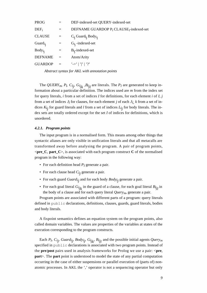
PROG = DEF-indexed-set QUERY-indexed-set

DEFi = DEFNAME GUARDOP Pi CLAUSEi-indexed-set

CLAUSE = Cij Guardij Bodyij

Guardij = Gij -indexed-set

Bodyij = Bij-indexed-set

DEFNAME = Atom/Arity

GUARDOP = ’->’ | ’|’ | ’?’

Abstract syntax for AKL with annotation points

The QUERYm, Pi, Cij, Gijk ,Bijl are literals. The Pi are generated to keep in-

formation about a particular definition. The indices used are m from the index set

for query literals, i from a set of indices I for definitions, for each element i of I, j

from a set of indices Ji for clauses, for each element j of each Ji, k from a set of in-

dices Kij for guard literals and l from a set of indices Lij for body literals. The in-

dex sets are totally ordered except for the set I of indices for definitions, which is

unordered.

4.2.1. Program points

The input program is in a normalised form. This means among other things that

syntactic aliases are only visible in unification literals and that all metacalls are

transformed away before analysing the program. A pair of program points,

<pre_C, part_C>, is associated with each program construct C of the normalised

program in the following way:

• For each definition head Pi generate a pair.

• For each clause head Cij generate a pair.

• For each guard Guardij and for each body Bodyij generate a pair.

• For each goal literal Gijk in the guard of a clause, for each goal literal Bijl in

the body of a clause and for each query literal Querym, generate a pair.

Program points are associated with different parts of a program: query literals

defined in public declarations, definitions, clauses, guards, guard literals, bodies

and body literals.

A fixpoint semantics defines an equation system on the program points, also

called domain variables. The values are properties of the variables at states of the

execution corresponding to the program constructs.

Each Pi, Cij, Guardij, Bodyij, Gijk, Bijl and the possible initial agents Querym

specified in public declarations is associated with two program points. Instead of

the pre/post pairs used in analysis frameworks for Prolog we use a pair: <pre,

part>. The part point is understood to model the state of any partial computation

occurring in the case of either suspensions or parallel execution of (parts of) non-

atomic processes. In AKL the ’,’ operator is not a sequencing operator but only

9

combines goals that can execute together if the corresponding computation is in a

determinate state. In order to model this concurrent or possibly parallel execution

we let the value of each pre-point of a literal depend on the part-points of all liter-

als in a guard (body) as well as on the input to the set of literals from the outside.

The result of possibly concurrent or parallel goal processes is modelled by the

function conc and the value is stored in the part-point. For a procedure that defines

alternative computations the possible results are modelled by the function lub.

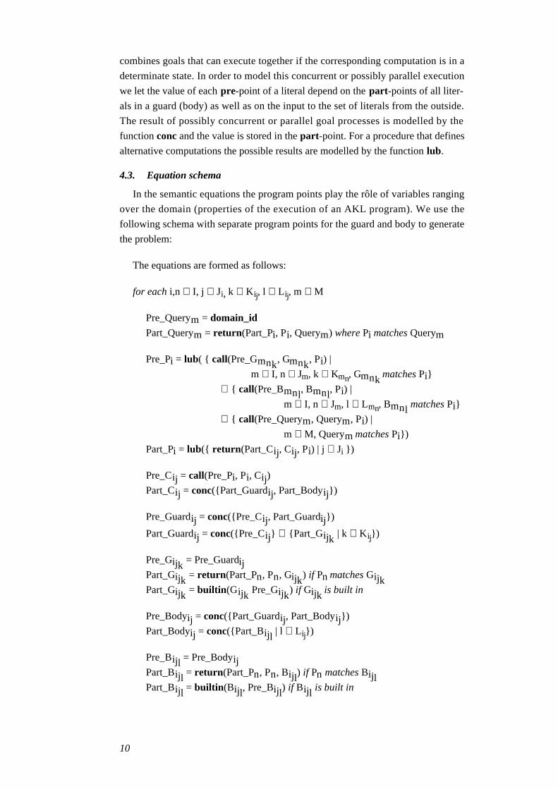
4.3. Equation schema

In the semantic equations the program points play the rôle of variables ranging

over the domain (properties of the execution of an AKL program). We use the

following schema with separate program points for the guard and body to generate

the problem:

The equations are formed as follows:

for each i,n ∈ I, j ∈ Ji, k ∈ Kij, l ∈ Lij, m ∈ M

Pre_Querym = domain_id

Part_Querym = return(Part_Pi, Pi, Querym) where Pi matches Querym

Pre_Pi = lub( { call(Pre_Gmnk, Gmnk, Pi) |

m ∈ I, n ∈ Jm, k ∈ Kmn, Gmnk matches Pi}

∪ { call(Pre_Bmnl, Bmnl, Pi) |

m ∈ I, n ∈ Jm, l ∈ Lmn, Bmnl matches Pi}

∪ { call(Pre_Querym, Querym, Pi) |

m ∈ M, Querym matches Pi})

Part_Pi = lub({ return(Part_Cij, Cij, Pi) | j ∈ Ji })

Pre_Cij = call(Pre_Pi, Pi, Cij)

Part_Cij = conc({Part_Guardij, Part_Bodyij})

Pre_Guardij = conc({Pre_Cij, Part_Guardij})

Part_Guardij = conc({Pre_Cij} ∪ {Part_Gijk | k ∈ Kij})

Pre_Gijk = Pre_GuardijPart_Gijk = return(Part_Pn, Pn, Gijk) if Pn matches GijkPart_Gijk = builtin(Gijk Pre_Gijk) if Gijk is built in

Pre_Bodyij = conc({Part_Guardij, Part_Bodyij})

Part_Bodyij = conc({Part_Bijl | l ∈ Lij})

Pre_Bijl = Pre_BodyijPart_Bijl = return(Part_Pn, Pn, Bijl) if Pn matches BijlPart_Bijl = builtin(Bijl, Pre_Bijl) if Bijl is built in

10

The functions domain_id, lub, conc, call, return and builtin are parameters to

the framework. The result of computing the least fixpoint of the system are

displayed as annotations to the program.

4.4. General description of the semantic functions

The system of equations express properties of constraints occurring in a pro-

gram execution.

The intention of the semantic functions is the following:

• D is a domain variable representing a statement over the execution states

corresponding to a program point. In our domain (see later) the state is

modelled by a set of pairs containing program variables and their correspond-

ing values, an abstract substitution.

• P, Q and B are literals.

• S is a multi-set of domain values, i.e. each value may occur several times in

the multi-set.

The result of each of these functions is a domain element.

domain_id returns the lowest domain element above ⊥, modelling a reachable

state without any bound variables, e.g. the starting state.

call(D, P, Q) generates a state description corresponding to a call of the defini-

tion with the head Q from the calling literal P using the state description D. This

function can be implemented as pairwise unification of the arguments in P and Q,

but also with a renaming of corresponding variables from P into Q, possibly

restricting the domain element to consider only program variables reachable from

the context of Q.

return(D, P, Q) generates a state description from D propagating information

from a clause defined by the literal P to the calling literal Q.

lub(S) computes the least upper bound to the values of the elements in S. This

function is used to collect results from alternative branches of the computation.

conc(S) is a composition of the values of elements in S that models any partial

computation of a group of literals.

builtin(D,B) constructs the result of execution of a built in literal B in a state

described by D. The result should model a partial execution of B.

5. The domain and the domain functions

In this section we will first in 5.1 define the mathematical form of the abstrac-

tion of the state of a computation and the order relation. In 5.2 we treat the domain

11

functions. In 5.3 we then turn to a discussion of possible variants of the domain

and its functions.

Domains are lattices of abstract values, equipped with a set of functions. In

order for the fixpoint computation to terminate, the lattice should contain only

finite chains and the domain functions should be monotone with respect to the

order in the domain.

In abstract interpretation for a logic programming language, i.e. a language with

logical variables, aliasing information is often needed as a part of the domain. The

constraints are normally expressions over Herbrand terms, i.e. the system is based

on simple syntactic equality of terms. In the case of AKL the compiler would

benefit if it was possible to ensure that two variables are definitely not aliased, as

unnecessary tests, code and data structures may then be removed. We have there-

fore defined a domain that captures aliasing and type information. For simplicity,

we will in the following assume that all variables in a program have unique names.

The normalisation of a program performed by our analyser ensures this.

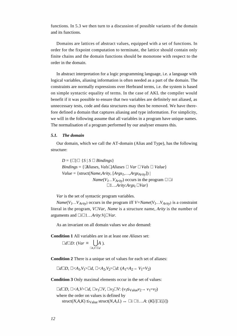
5.1. The domain

Our domain, which we call the AT-domain (Alias and Type), has the following

structure:

D = {⊥}∪ {S | S ⊆ Bindings}

Bindings = {⟨Aliases, Vals⟩ |Aliases ⊆ Var ∧ Vals ⊆ Value}

Value = {struct(Name,Arity, [Args1,…,ArgsArity]) |

Name(V1…VArity) occurs in the program ∧ ∀i∈1…Arity:Argsi ⊆Var}

Var is the set of syntactic program variables.

Name(V1…VArity) occurs in the program iff V=Name(V1…VArity) is a constraint

literal in the program, V∈Var, Name is a structure name, Arity is the number of

arguments and ∀i∈1…Arity:Vi∈Var.

As an invariant on all domain values we also demand:

Condition 1 All variables are in at least one Aliases set:

∀d∈D: (Var = A⟨ A,V ⟩∈d

).

Condition 2 There is a unique set of values for each set of aliases:

∀d∈D, ∀<A1,V1>∈d, ∀<A2,V2>∈d: (A1=A2→ V1=V2)

Condition 3 Only maximal elements occur in the set of values:

∀d∈D, ∀<A,V>∈d, ∀v1∈V, ∀v2∈V: (v1≤Valuev2→ v1=v2)

where the order on values is defined bystruct(N,A,K) ≤Value struct(N,A,L) ↔ ∀i ∈1…A: (K[i]⊆L[i])

12

Condition 4 Each program variable occurs in at most one set A of a pair <A,V> in

a domain value d:

∀d∈D, ∀<A,V>∈d, ∀v∈A, ∀<A',V'>∈d: (v∈A' → A=A')

From conditions 1 and 4 together we conclude that there is exactly one set A for

each program variable.

5.1.1. Interpretation of a domain value

A domain value d∈D that refers to a program point is interpreted as follows. If

d=⊥, then this point in the program cannot be reached. Otherwise d is a set of

possible equalities Eq defined

• (x=y)∈Eq if ∃<As,Vs> ∈d: (x ∈As ∧ y ∈As)

• (x=N(A1…AArity)) ∈Eq

if ∃<As,Vs>∈d: (x ∈As

∧ struct(N,Arity,[Arg1…ArgArity]) ∈Vs

∧ ∀i ∈1…Arity: Ai ∈Argi )

The finite equation set Eq thus formed is understood as the disjunctive proposi-tion about the (possibly infinitely many) runtime instances of the syntactic vari-ables formed from the elements of Eq (x1=t1∨ …∨ xn=tn∨ …).

5.1.2. Order relation

The order relation on the domain D is defined⊥ ≤ dd1 ≤ d2 ⇔ ∀x ∈Var: (values(x,d1) ≤Values values(x,d2))

∧ ∀x ∈Var: (aliased(x,d1) ⊆ aliased(x,d2))e ≤Values f⇔ ∀v∈e, ∃w∈f: (v ≤Values w)

wherealiased(x,d)= A where <A,V> ∈d ∧ x ∈A

andvalues(x,d)= V where <A,V> ∈d ∧ x ∈A

5.2. The domain functions

A number of domain functions are specified. We give a high-level specification

of the central functions. A functional implementation specification is given in the

appendix.

In the framework lub and conc are applied on non-empty multi-sets, whereas

here we define binary functions. These are related as follows:

For any multiset {A1…An}

fset({A1,A2,…,An}) = fbinary(A1,fset({A2,…,An}))

fset({A1}) = A1

In order for fset to be a well defined function its value must be the same for any

order of the sequence A1…An. This is assumed to hold for lub and conc.

13

5.2.1. The function domain_id

domain_id= {<{v},{}> | v∈Var }

is a function to model a state where no bindings have occurred.

5.2.2. The function lub

The function lub used to model alternative computationslub(d,⊥) = dlub(⊥,d) = dlub(d1,d2)=normalise(d1 ∪ d2)

where the function normalise ensures that conditions 1 to 4 above are fulfilled is

defined by

normalise(d)= {<As,Vs> |∃x∈Var: (As= {y | ∃<A,V>∈d: ( y∈A ∧ tr(x,y,d))} ∧ Vs=normvals({v | ∃<A,V>∈d, ∃y∈A: ( tr(x,y,d) ∧ v∈V)})) }

normvals(V)={struct(n,a,L) | struct(n,a,_)∈V

∧ ∀i∈1…a: (L[i] = ∪{M[i] | struct(n,a,M)∈V})}

and the relation tr is defined• tr(x,y,d) if ∃<A,V>∈d: (x∈A ∧ x=y)• tr(x,y,d) if ∃<A,V>∈d, ∃z∈A: (x∈A ∧ tr(z,y,d))

lub sometimes constructs irrelevant aliases in order for the resulting elements

not to violate the condition on domain elements that a variable should occur in at

most one A of a pair <A,V> in the element.

5.2.3. The function conc

The function conc used to model concurrent computationsconc(d,⊥) = dconc(⊥,d) = d

conc(d1,d2)=cnormalise(d1,d2)

where

cnormalise(d1,d2)= {<As,Vs> |∃x∈Var: (As= {y | y∈Var ∧ ctr(x,y,d1,d2)} ∧ Vs=normvals({v | ∃<A,V>∈d1∪d2, ∃y∈A:

( ctr(x,y,d1,d2) ∧ v∈V)})) }

and the relation ctr is defined• ctr(x,y,d1,d2) if ∃v: (tr(x,v,d1) ∧ tr(y,v,d2) )• ctr(x,y,d1,d2) if ∃<As,Vs>∈d1, ∃<Bs,Ws>∈d2, ∃v∈As, ∃z∈Bs:

(ctr(v,z,d1,d2) ∧ struct(n,a,A)∈Vs ∧ struct(n,a,B)∈Ws ∧ ∃i ∈ 1…a: (x∈Ai ∧ y∈Bi))

14

5.2.4. Definitions of builtin, call and return

builtin(D,B), call(D, P, Q) and return(D, P, Q) are implemented using some

help functions as described below.

Sequences of unification constraint literals of the form V=T are collected in a

list and wrapped as an argument to a 'virtual' builtin herbrand_equal/2. This

optimises the abstraction of sequences of unifications for which the order of simple

unifications is irrelevant to the computation by avoiding the construction of irrele-

vant program points.

We have:

builtin(D,herbrand_equal(Vs,Ts)) = reduce_unif(pairlist(Vs,Ts),D)

pairlist forms a list of pairs <V,T> from two equally sized lists of variables and

terms respectively.

reduce_unif applies the domain function unif(V,T) to a list of pairs <V,T> as

follows:

reduce_unif([<V,T> |VTs], D) = unif(V,T, reduce_unif(VTs, D))

reduce_unif([], D) = D

All other built in literals are simply given as argument B to builtin(D,B) in the

equation setup schema and will be treated by special domain functions as the need

arises.

unif(V, T, D) expresses the full execution of a unification constraint =/2

applied to a program variable V with the term T in the state represented by D.

The function unif may be defined as

unif(V,T,⊥) = ⊥unif(V,T,D) = conc(D,unif_to_domain(V,T))

whereunif_to_domain(V,T)= {<{v},{struct(N,Arity,Args)}> |

∀i∈1…Arity: ( Argsi={Ai})}

if T=N(A1…AArity)unif_to_domain(V,T)={<{V,T},{}> } if T ∈ Var.

To implement call and return we use pair_list, reduce_unif, replace and

restrict.

We have:

call(D,P,Q)=restrict(Q,replace(P,Q,reduce_unif(pairlist(P,Q),D)))

P,Q are understood as the argument lists of variables to the corresponding

literals.

15

replace(Vars1,Vars2,D) generates a domain element from D where occurrences

of variables from the list Vars1 are replaced with the corresponding variables in the

list Vars2.

restrict(Vars, D) uses the domain element D to construct a domain element

such that only those parts that refer to the variables in Vars remain.

return(D,P,Q) is identical to call(D,P,Q) but is given a special name to indicate

its intuitive meaning.

5.2.5. Explanation of restriction performed in call/return

The functions call and return should model the change in scope occurring in an

execution. This can most easily be achieved by using unif, but this will tend to

propagate numerous variables that are not relevant since many variables are not

reachable from within the scope of the called procedure. We therefore apply a

reachability algorithm and remove those parts of the domain element that are not

reachable from the calling/called atom using the functions replace and restrict.

Consider a program where we have a call p(X,Y) and a definition

p(A,B) :- Q % R.

If we e.g. have the domain value{

<{X,Z}, {struct(t,1,[{U}]),struct(s,1,[{Y}])}>,<{Y,U}, {}>,<{V,W}, {struct(f,1,[{S,T,M,N}])}>,<{S,T}, {}>,<{M,N}, {}>

}

in the program point immediately preceding the call (the pre-point) we could

achieve the state change conservatively by constructing

{<{A,X,Z}, {struct(t,1,[{U}]),struct(s,1,[{Y}])}>,<{B,Y,U}, {}>,<{V,W}, {struct(f,1,[{S,T,M,N}])}>,<{S,T}, {}>,<{M,N}, {}>

}

using reduce_unif. But this will tend to propagate numerous variables that are not

relevant since they are not reachable from within the scope of the called procedure.

First we note that we talk about the two variables A and X as if they were different

while we know that in an implementation we really rename the variable cell (or

register) referring to X to A. This can be avoided if we apply the replace function

after the unification yielding

16

{<{A,Z}, {struct(t,1,[{U}]),struct(s,1,[{B}])}>,<{B,U}, {}>,<{V,W}, {struct(f,1,[{S,T,M,N}])}>,<{S,T}, {}>,<{M,N}, {}>

}

We still have some parts of the domain value that are irrelevant since they are

not reachable from the variables in the head (via the terms with which the variables

are possibly unified). We therefore apply a reachability algorithm and remove

those parts of the domain element that are not reachable from the calling/called

literal using the function restrict. We then get:

{<{A}, {struct(t,1,[{U}]),struct(s,1,[{B}])}>,<{B,U}, {}>

}

We can safely ignore those variables that are not reachable from the literal since

they are not of interest in the scope of the program points after the call. They will

be reintroduced upon return.

The same mechanism of restricting the domain element to only those parts that

are reachable from the variables in the literal is used for built-in literals also, so

e.g. the 'true'-literal will always return the domain-id element (the set in which

all variables are unbound and unaliased). Since we ”reintroduce” all relevant

variables with their terms and aliases when computing domain elements for the

larger element in which the literal occurs (guard, body, clause, procedure) no

information relevant to the compiler is missed.

5.2.6. Implementation specification

In the appendix is given a functional implementation specification of the central

domain functions. Some of the following discussion might benefit from first

studying the code specification.

5.3. Variants of the AT-domain

It is possible to add the requirement that each variable set occurring in an argu-

ment to a term descriptor in Vs of a pair <As, Vs> should be identical to some

variable set As’ in a pair <As’, Vs’> in the domain element. This could lead to a

loss in precision so we avoid it in the current version of the code.

5.3.1. Built-in literals for arithmetic and constraints

The domain needs some changes to enable a treatment of some built-in literals.

E.g. it would be desirable to model possible functional dependencies between vari-

ables to handle the arithmetical constraints, is/2 and also other constraint literals

like finite domain constraints. Currently we add unique term descriptors denoting

17

the subsets of terms that are possible values emanating from the built-ins,

e.g.<{X},{number,…}> for ”X is possibly bound to a number”,

6. Fixpoint solver

The previous section produced a set of equations:

x1 = f1(x1,…,xn) … xn = fn(x1,…,xn)

where x i ∈D (some domain) and the fi are monotone functions. This set of equa-

tions may alternatively be written as the vector valued equation

x = f (x )

where x ∈Dn and the least1 fixpoint is sought. A fixpoint can be found by an

iteration which starts by setting x to the bottom element and then repeatedly

applies the function f until no change occurs.

The simplest method is to repeatedly scan through all functions and recompute

them until no change in any function occurs. A distinction can be made between

xi:s computed from the previous scan being used (Jacobi’s method) and the newly

computed xi:s being used immediately (Gauss-Seidel’s method).

For instance in [COUSOT92, NILSSON 92] it is proven that it is not necessary to

compute all components of the vector simultaneously. The same unique least fix-

point will be found even if the functions fi are applied one at a time, in an arbitrary

order (”chaotic iteration”), until a scan of all functions will not change the

computed values.

For a fixpoint computation be practical it is essential that the least fixpoint can

be efficiently found. It is expected that for a complex domain, each domain func-

tion application is fairly expensive. Thus it is important to avoid redundant domain

function applications in the fixpoint solver. The mechanism for doing this is

discussed in the following.

6.1. Optimisations

We analyse the fixpoint problem and try to find an order in which to compute

the domain functions which reduces the number of domain function applications.

The optimisations we present below guarantee an improvement.

6.1.1. Using dependencies

Fortunately, for equations produced by abstract interpretation most functions

just depend on a small subset of the variables, and this fact is utilised as follows.

Consider the following example:

1 In fact, any fixpoint to the equations is a correct approximation, but the least fixpointis the most informative.

18

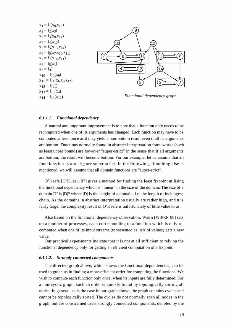
x1 = f1(x8,x12)x2 = f2(x3)x3 = f3(x8,x14)x4 = f4(x13)x5 = f5(x13,x14)x6 = f6(x7,x10,x11)x7 = f7(x10,x11)x8 = f8(x1)x9 = f9()x10 = f10(x9)x11 = f11(x6,x9,x12)x12 = f12()x13 = f13(x4)x14 = f14(x12)

1

4

5

67 8

9

10

11

12

13 14

2 3

Functional dependency graph

6.1.1.1. Functional dependency

A natural and important improvement is to note that a function only needs to be

recomputed when one of its arguments has changed. Each function may have to be

computed at least once as it may yield a non-bottom result even if all its arguments

are bottom. Functions normally found in abstract interpretation frameworks (such

as least upper bound) are however ”super-strict” in the sense that if all arguments

are bottom, the result will become bottom. For our example, let us assume that all

functions but f9 and f12 are super-strict. In the following, if nothing else is

mentioned, we will assume that all domain functions are ”super-strict”.

O’Keefe [O’KEEFE 87] gives a method for finding the least fixpoint utilising

the functional dependency which is ”linear” in the size of the domain. The size of a

domain Dn is |D|n where |D| is the height of a domain, i.e. the length of its longest

chain. As the domains in abstract interpretation usually are rather high, and n is

fairly large, the complexity result of O’Keefe is unfortunately of little value to us.

Also based on the functional dependency observation, Wærn [WÆRN 88] sets

up a number of processes, each corresponding to a function which is only re-

computed when one of its input streams (represented as lists of values) gets a new

value.Our practical experiments indicate that it is not at all sufficient to rely on the

functional dependency only for getting an efficient computation of a fixpoint.

6.1.1.2. Strongly connected components

The directed graph above, which shows the functional dependencies, can be

used to guide us in finding a more efficient order for computing the functions. We

wish to compute each function only once, when its inputs are fully determined. For

a non-cyclic graph, such an order is quickly found by topologically sorting all

nodes. In general, as is the case in our graph above, the graph contains cycles and

cannot be topologically sorted. The cycles do not normally span all nodes in the

graph, but are constrained to its strongly connected components, denoted by the

19

boxes in the graph. Fortunately, there exists a very efficient (linear in the number

of edges and nodes) algorithm for finding the strongly connected components in a

graph [TARJAN 72].

Once these components have been found a topological sort can be made, in

which a component is considered a single node. For the graph above, a topological

sort could give: 9, 10, 12, (6-7-11), (1-8), (4-13), 14, 5, (2-3), where the nontrivial

components are within parentheses.

When the fixpoint of a strongly connected component has been computed, the

nodes in that component need not be considered again. The computed values can

be considered as constants used in the further computations. But this leaves us with

a hard problem: how to find the least fixpoint of a strongly connected component

where all nodes (functions) depend on each other. Utilising the functional de-

pendency within each strongly connected component is still crucial for efficiency.

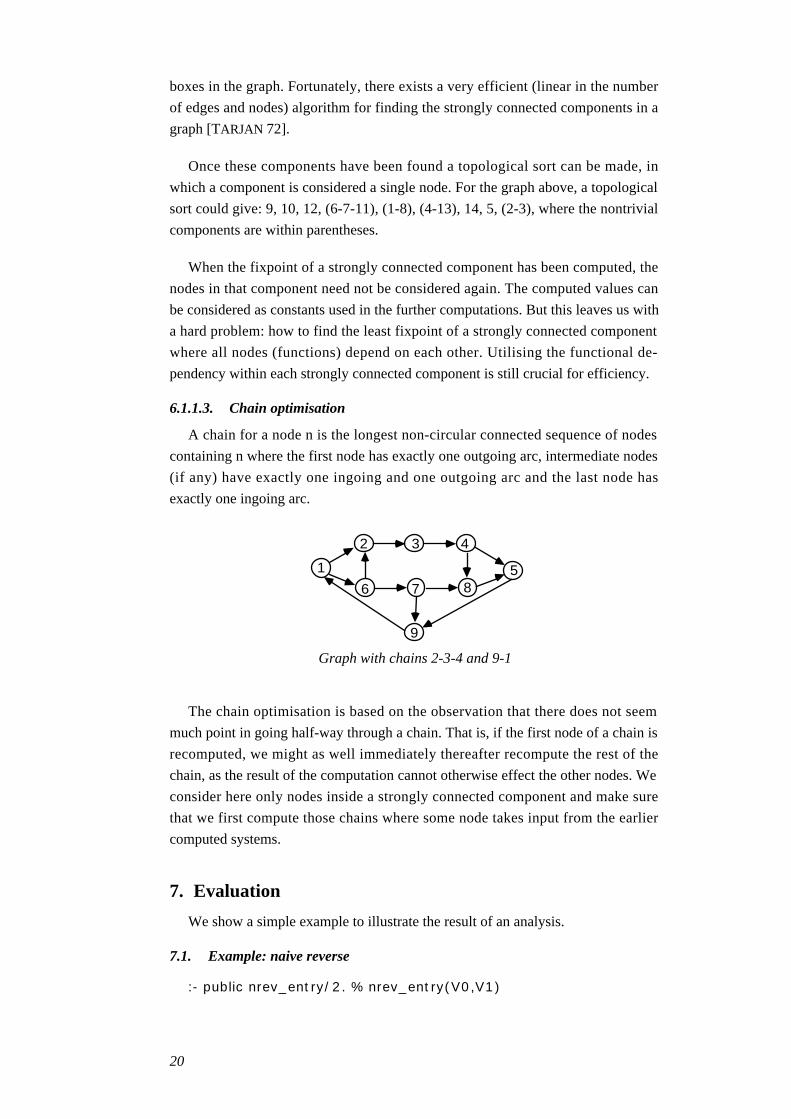
6.1.1.3. Chain optimisation

A chain for a node n is the longest non-circular connected sequence of nodes

containing n where the first node has exactly one outgoing arc, intermediate nodes

(if any) have exactly one ingoing and one outgoing arc and the last node has

exactly one ingoing arc.

2 3 4

6 7 81 5

9

Graph with chains 2-3-4 and 9-1

The chain optimisation is based on the observation that there does not seem

much point in going half-way through a chain. That is, if the first node of a chain is

recomputed, we might as well immediately thereafter recompute the rest of the

chain, as the result of the computation cannot otherwise effect the other nodes. We

consider here only nodes inside a strongly connected component and make sure

that we first compute those chains where some node takes input from the earlier

computed systems.

7. Evaluation

We show a simple example to illustrate the result of an analysis.

7.1. Example: naive reverse

:- public nrev_entry/2. % nrev_entry(V0,V1)

20

%nrev_entry(V2,V3)

nrev_entry(V4,V5) :- is_list(V4)

-> nrev(V4,V5).

%nrev(V6,V7)

nrev(V8,V9) :- herbrand_equal([(V8 = [])])

-> herbrand_equal([(V9 = V10),(V10 = [])]).

nrev(V11,V12) :- herbrand_equal([(V11 = [V13|V14])])

-> (nrev(V14,V15),

(herbrand_equal([(V18 = V17),(V17 = [V13|V16]),

(V16 = [])]),

append(V15,V18,V12))).

%append(V19,V20,V21)

append(V22,V23,V24) :- herbrand_equal([(V22 = [])])

-> herbrand_equal([(V24 = V23)]).

append(V25,V26,V27) :- herbrand_equal([(V25 = [V28|V29])])

-> (herbrand_equal([(V27 = V30),(V30 = [V28|V31])]),

append(V29,V26,V31)).

%is_list(V32)

is_list(V33) :- herbrand_equal([(V33 = [])])

? true.

is_list(V34) :- herbrand_equal([(V34 = [V35|V36])])

? is_list(V36).

Program after pre-processing: all program variables are uniquelyrenamed, all terms are unnested and sequences of unification literalsare collected in a 'virtual built-in', 'herbrand_equal/1' representingan atomic unification constraint.

Assuming nrev_entry(V0,V1) is called with V0 and V1 unbound and un-

aliased, the analysis will compute the following abstract domain value for the part

point of the literal nrev_entry(V0,V1):

{<{V1,V12,V15,V16,V25,V27,V29,V31},

{struct(.,2,[{V13,V28},{V1,V12,V15,V16,V25,V27,V29,V31}]),[]}>,

<{V13,V28,V35}, {}>,

<{V0,V11,V14,V34,V36},

{struct(.,2,[{V13,V35},{V0,V11,V14,V34,V36}]),[]}>}

We can draw some conclusions from the above abstract domain value, e.g.:

• V0 and V1 will remain unaliased after execution.

This can be inferred since V0 and V1 are in Aliased-set of different pairs.

21

• V1 can be bound to a possibly open list whose elements are all unbound.

This is inferred as follows. V1 can only be unbound, bound to [] or to ./2. In

the latter case, the first argument can only be a variable in {V13,V28}, both

of which must be unbound. The second argument can only be a variable in

{V1, V12, V15, V16, V25, V27, V29, V31}, and as all these variables occur

in the same ”Aliased” set as V1, it can be concluded that V1 is described by a

recursive type, namely an open list.

A similar argument can be made to show that V0 is also described by an open

list. Furthermore, we can draw the conclusion that it is possible for the elements in

a list bound to V0 to be aliased to those of a list bound to V1 (via V13) even though

V0 and V1 themselves cannot be aliased.

7.2. Measurements

We analysed a set of test examples. Some of these were very simple programs

constructed to inspect the result and follow the trace of an analysis session while

others were essentially unaltered demonstration programs picked from the demo

directory of the Agents system. We also picked a set of test examples from the ftp-

directory of UPM supplied by the CLIC group and ECRC and made a simple

syntactic transformation of these Prolog programs into Agents ”equivalents”, so

that they could be analysed. Although some of these examples are not sensible

Agents programs, the analysis complexity in a correctly translated version is

expected to be similar.

We present our results in a table. All measurements were based on the built-in

statistics procedure of the sequential Agents 0.9 system running on one of the pro-

cessors of our Sparc-10 based SC2000 SUN multiprocessor. The memory

management time is visible in the Total column. The memory consumed by an

analysis process was in the range of about 10-400 Mb of process space. Most of the

space requirements have to do with the highest amount of data used, since Agents

does not return used space to the UNIX system and with the heuristics used in the

Agents system to allocate various heaps and stacks. The I/O-routines also contain

some parts that generate nondeterministic choice points, which will keep the

memory allocated for longer than necessary. This should not affect the timing

results except that Total will contain an unnecessarily large component for memory

management overhead.

file is the file name.size is the number of lines (≈literals) in the program.eqs is the number of domain equations constructed from the program.sys is the number of strongly connected components.tprob is the time spent constructing the equations including program I/O.appl is the number of domain function applications.tfp is the time spent in the fixpoint solver.twr is the time spent printing the annotated program.total is the total time spent including loading, garbage collection and copying.All times are in milliseconds.

22

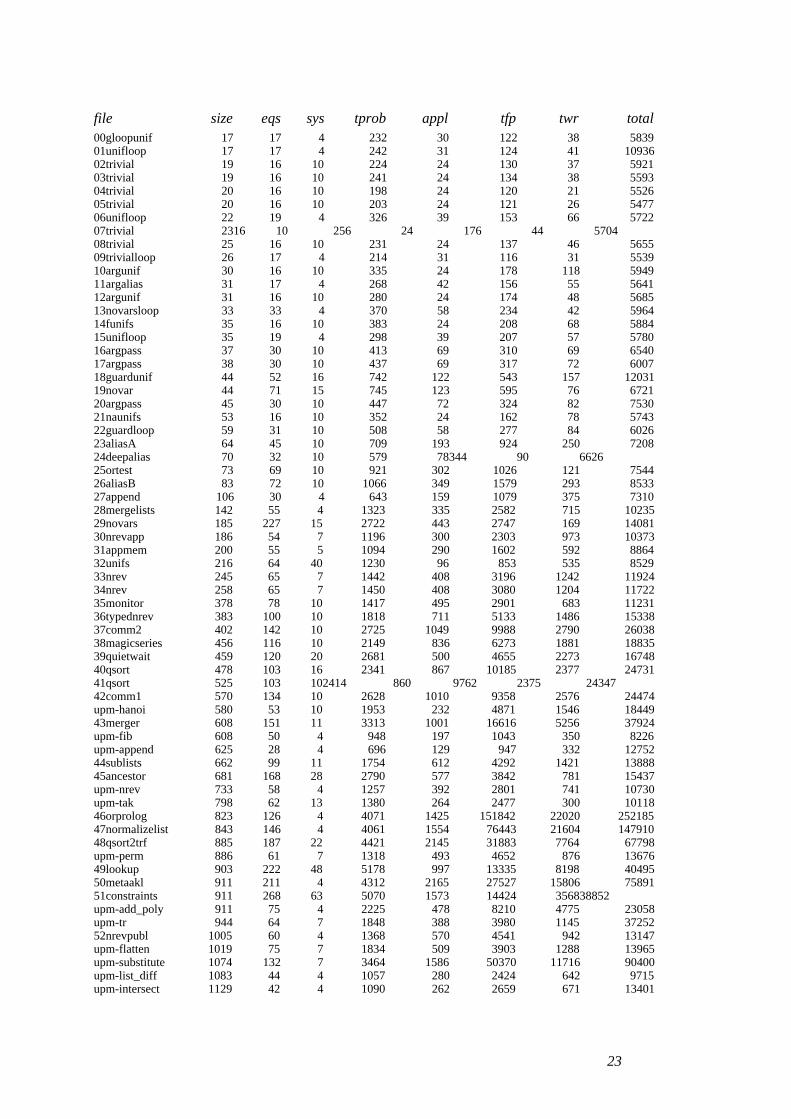
file size eqs sys tprob appl tfp twr total00gloopunif 17 17 4 232 30 122 38 583901unifloop 17 17 4 242 31 124 41 1093602trivial 19 16 10 224 24 130 37 592103trivial 19 16 10 241 24 134 38 559304trivial 20 16 10 198 24 120 21 552605trivial 20 16 10 203 24 121 26 547706unifloop 22 19 4 326 39 153 66 572207trivial 23 16 10 256 24 176 44 570408trivial 25 16 10 231 24 137 46 565509trivialloop 26 17 4 214 31 116 31 553910argunif 30 16 10 335 24 178 118 594911argalias 31 17 4 268 42 156 55 564112argunif 31 16 10 280 24 174 48 568513novarsloop 33 33 4 370 58 234 42 596414funifs 35 16 10 383 24 208 68 588415unifloop 35 19 4 298 39 207 57 578016argpass 37 30 10 413 69 310 69 654017argpass 38 30 10 437 69 317 72 600718guardunif 44 52 16 742 122 543 157 1203119novar 44 71 15 745 123 595 76 672120argpass 45 30 10 447 72 324 82 753021naunifs 53 16 10 352 24 162 78 574322guardloop 59 31 10 508 58 277 84 602623aliasA 64 45 10 709 193 924 250 720824deepalias 70 32 10 579 78 344 90 662625ortest 73 69 10 921 302 1026 121 754426aliasB 83 72 10 1066 349 1579 293 853327append 106 30 4 643 159 1079 375 731028mergelists 142 55 4 1323 335 2582 715 1023529novars 185 227 15 2722 443 2747 169 1408130nrevapp 186 54 7 1196 300 2303 973 1037331appmem 200 55 5 1094 290 1602 592 886432unifs 216 64 40 1230 96 853 535 852933nrev 245 65 7 1442 408 3196 1242 1192434nrev 258 65 7 1450 408 3080 1204 1172235monitor 378 78 10 1417 495 2901 683 1123136typednrev 383 100 10 1818 711 5133 1486 1533837comm2 402 142 10 2725 1049 9988 2790 2603838magicseries 456 116 10 2149 836 6273 1881 1883539quietwait 459 120 20 2681 500 4655 2273 1674840qsort 478 103 16 2341 867 10185 2377 2473141qsort 525 103 10 2414 860 9762 2375 2434742comm1 570 134 10 2628 1010 9358 2576 24474upm-hanoi 580 53 10 1953 232 4871 1546 1844943merger 608 151 11 3313 1001 16616 5256 37924upm-fib 608 50 4 948 197 1043 350 8226upm-append 625 28 4 696 129 947 332 1275244sublists 662 99 11 1754 612 4292 1421 1388845ancestor 681 168 28 2790 577 3842 781 15437upm-nrev 733 58 4 1257 392 2801 741 10730upm-tak 798 62 13 1380 264 2477 300 1011846orprolog 823 126 4 4071 1425 151842 22020 25218547normalizelist 843 146 4 4061 1554 76443 21604 14791048qsort2trf 885 187 22 4421 2145 31883 7764 67798upm-perm 886 61 7 1318 493 4652 876 1367649lookup 903 222 48 5178 997 13335 8198 4049550metaakl 911 211 4 4312 2165 27527 15806 7589151constraints 911 268 63 5070 1573 14424 3568 38852upm-add_poly 911 75 4 2225 478 8210 4775 23058upm-tr 944 64 7 1848 388 3980 1145 3725252nrevpubl 1005 60 4 1368 570 4541 942 13147upm-flatten 1019 75 7 1834 509 3903 1288 13965upm-substitute 1074 132 7 3464 1586 50370 11716 90400upm-list_diff 1083 44 4 1057 280 2424 642 9715upm-intersect 1129 42 4 1090 262 2659 671 13401

23

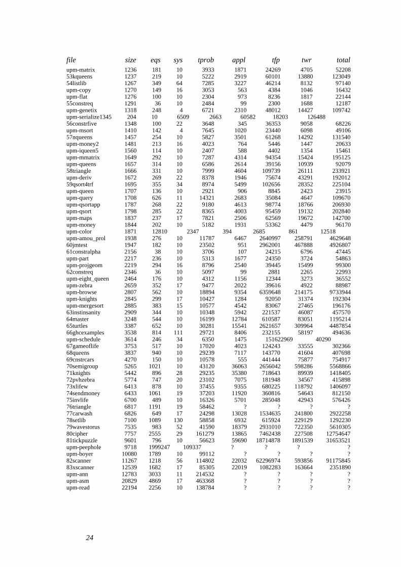
file size eqs sys tprob appl tfp twr totalupm-matrix 1236 181 10 3933 1871 24269 4705 5220853kqueens 1237 219 10 5222 2919 60101 13880 12304954listlib 1267 349 64 7285 3227 46214 8132 97140upm-copy 1270 149 16 3053 563 4384 1046 16432upm-flat 1276 100 10 2304 973 8236 1817 2214455constreq 1291 36 10 2484 99 2300 1688 12187upm-genetix 1318 248 4 6721 2310 48012 14427 109742upm-serialize 1345 204 10 6509 2663 60582 18203 12648856constrfive 1348 100 22 3648 345 36353 9058 68226upm-msort 1410 142 4 7645 1020 23440 6098 4910657nqueens 1457 254 10 5827 3501 61268 14292 131540upm-money2 1481 213 16 4023 764 5446 1447 20633upm-iqueen5 1560 114 10 2407 588 4402 1354 15461upm-mmatrix 1649 292 10 7287 4314 94354 15424 195125upm-queens 1657 314 10 6586 2614 39156 10939 9207958triangle 1666 331 10 7999 4604 109739 26111 233921upm-deriv 1672 269 22 8378 1946 75674 43291 19201259qsort4trf 1695 355 34 8974 5499 102656 28352 225104upm-queen 1707 136 10 2921 906 8845 2423 23915upm-query 1708 626 11 14321 2683 35084 4647 109670upm-qsortapp 1787 268 22 9180 4613 98774 18766 206930upm-qsort 1798 285 22 8365 4003 95459 19132 202840upm-maps 1837 237 17 7821 2506 62569 19672 142700upm-money 1844 202 10 5182 1931 53362 4479 96170upm-color 1871 128 10 2347 394 2685 861 12518upm-amou_prol 1938 276 10 11787 6467 2640997 258791 462964860jmtest 1947 182 10 23502 951 2962001 467888 492680761constralpha 2156 38 10 3706 107 24215 6796 47445upm-part 2217 236 10 5313 1677 24350 3724 54863upm-projgeom 2219 294 16 8796 2540 39445 15499 9930062constreq 2346 36 10 5097 99 2881 2265 22993upm-eight_queen 2464 176 10 4312 1156 12344 3273 36552upm-zebra 2659 352 17 9477 2022 39616 4922 88987upm-browse 2807 562 10 18894 9354 6359648 214175 9733944upm-knights 2845 299 17 10427 1284 92050 31374 192304upm-mergesort 2885 383 15 10577 4542 83067 27465 19617663instinsanity 2909 344 10 10348 5942 221537 46087 45757064master 3248 544 10 16199 12784 610587 83051 119521465turtles 3387 652 10 30281 15541 2621657 309964 448785466ghcexamples 3538 814 111 29721 8406 232155 58197 494636upm-schedule 3614 246 34 6350 1475 15162 2969 4029067gameoflife 3753 517 10 17020 4023 124243 33555 30236668queens 3837 940 10 29239 7117 143770 41604 40769869cnstrcars 4270 150 10 10578 555 441444 75877 75491770semigroup 5265 1021 10 43120 36063 2656042 598286 556886671knights 5442 896 28 29235 35380 718643 89939 141840572pvhzebra 5774 747 20 23102 7075 181948 34567 41589873xlifew 6413 878 10 37455 9355 680225 118792 140609774sendmoney 6433 1061 19 37203 11920 360816 54643 81215075invlife 6700 489 10 16326 5701 285048 42943 57642676triangle 6817 1191 19 58462 ? ? ? ?77carwash 6826 649 17 24298 13028 1534635 241800 292225878setlib 7100 1089 130 58858 6932 615924 229129 129223079wavestorus 7535 983 52 41590 18379 2931010 722350 561030580cipher 7757 2555 29 161279 13865 7462438 227508 1275464781tickpuzzle 9601 796 10 56623 59690 18714878 1891539 31653521upm-peephole 9718 1999 247 109337 ? ? ? ?upm-boyer 10080 1789 10 99112 ? ? ? ?82scanner 11267 1218 56 114802 22032 62296974 593856 9117584583xscanner 12539 1682 17 85305 22019 1082283 163664 2351890upm-ann 12783 3033 11 214532 ? ? ? ?upm-asm 20829 4869 17 463368 ? ? ? ?upm-read 22194 2256 10 138784 ? ? ? ?

24

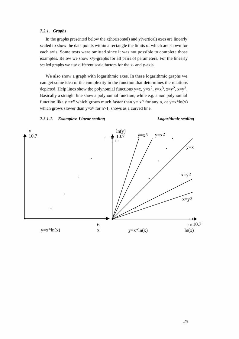
7.2.1. Graphs

In the graphs presented below the x(horizontal) and y(vertical) axes are linearly

scaled to show the data points within a rectangle the limits of which are shown for

each axis. Some tests were omitted since it was not possible to complete those

examples. Below we show x/y-graphs for all pairs of parameters. For the linearly

scaled graphs we use different scale factors for the x- and y-axis.

We also show a graph with logarithmic axes. In these logarithmic graphs we

can get some idea of the complexity in the function that determines the relations

depicted. Help lines show the polynomial functions y=x, y=x2, y=x3, x=y2, x=y3.

Basically a straight line show a polynomial function, while e.g. a non polynomial

function like y =xx which grows much faster than y= xn for any n, or y=x*ln(x)

which grows slower than y=xn for n>1, shows as a curved line.

7.3.1.1. Examples: Linear scaling Logarithmic scaling

y=x*ln(x) x6

y10.7

y=x*ln(x)

10

10

ln(x)10.7

ln(y)10.7 y=x3 y=x2

y=x

x=y2

x=y3

25

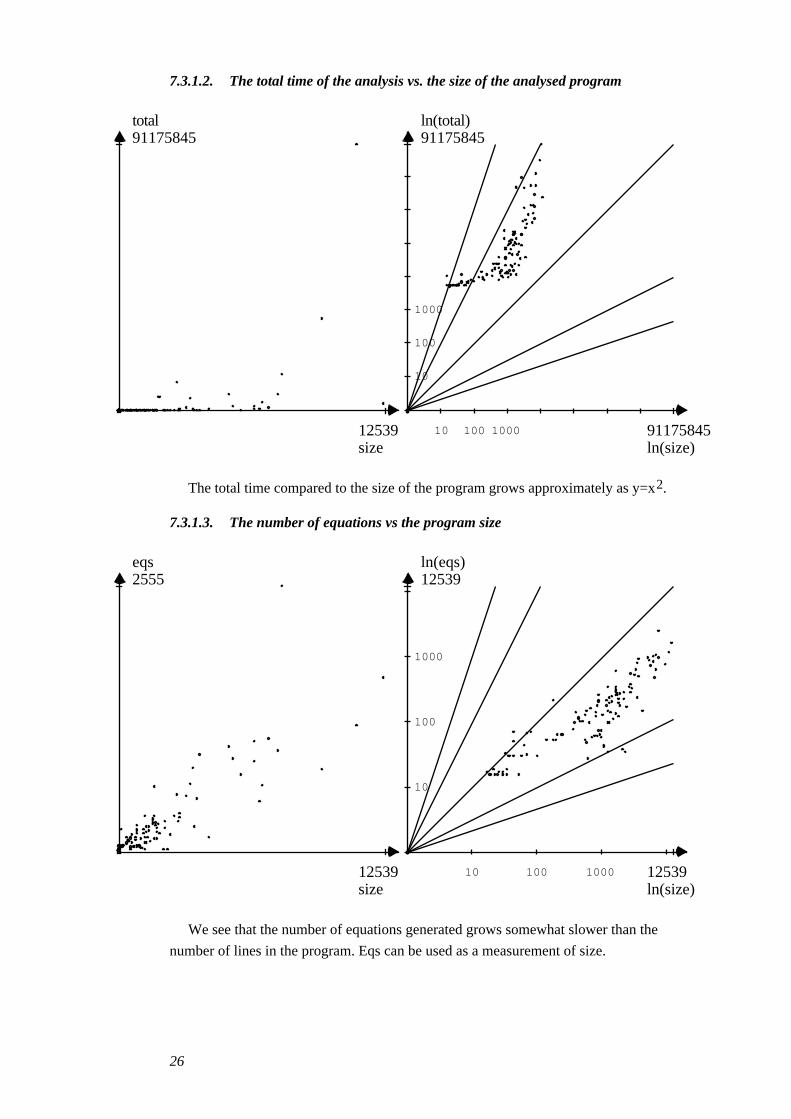
7.3.1.2. The total time of the analysis vs. the size of the analysed program

size12539

total91175845

10

100

1000

10 100 1000

ln(size)91175845

ln(total)91175845

The total time compared to the size of the program grows approximately as y=x2.

7.3.1.3. The number of equations vs the program size

size12539

eqs2555

10

100

1000

10 100 1000

ln(size)12539

ln(eqs)12539

We see that the number of equations generated grows somewhat slower than the

number of lines in the program. Eqs can be used as a measurement of size.

26

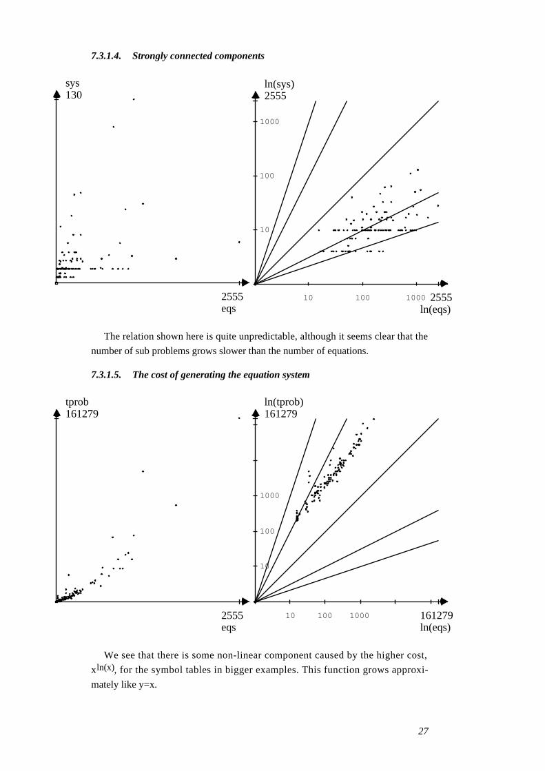
7.3.1.4. Strongly connected components

eqs2555

sys130

10

100

1000

10 100 1000

ln(eqs)2555

ln(sys)2555

The relation shown here is quite unpredictable, although it seems clear that the

number of sub problems grows slower than the number of equations.

7.3.1.5. The cost of generating the equation system

eqs2555

tprob161279

10

100

1000

10 100 1000

ln(eqs)161279

ln(tprob)161279

We see that there is some non-linear component caused by the higher cost,

xln(x), for the symbol tables in bigger examples. This function grows approxi-

mately like y=x.

27

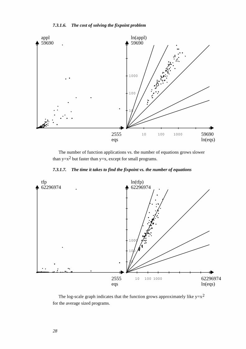
7.3.1.6. The cost of solving the fixpoint problem

eqs2555

appl59690

10

100

1000

10 100 1000

ln(eqs)59690

ln(appl)59690

The number of function applications vs. the number of equations grows slower

than y=x2 but faster than y=x, except for small programs.

7.3.1.7. The time it takes to find the fixpoint vs. the number of equations

eqs2555

tfp62296974

10

100

1000

10 100 1000

ln(eqs)62296974

ln(tfp)62296974

The log-scale graph indicates that the function grows approximately like y=x2

for the average sized programs.

28

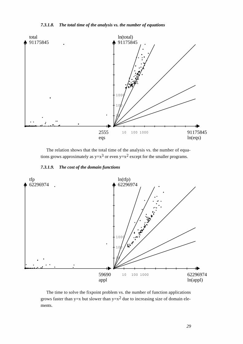
7.3.1.8. The total time of the analysis vs. the number of equations

eqs2555

total91175845

10

100

1000

10 100 1000

ln(eqs)91175845

ln(total)91175845

The relation shows that the total time of the analysis vs. the number of equa-

tions grows approximately as y=x3 or even y=x2 except for the smaller programs.

7.3.1.9. The cost of the domain functions

appl59690

tfp62296974

10

100

1000

10 100 1000

ln(appl)62296974

ln(tfp)62296974

The time to solve the fixpoint problem vs. the number of function applications

grows faster than y=x but slower than y=x2 due to increasing size of domain ele-

ments.

29

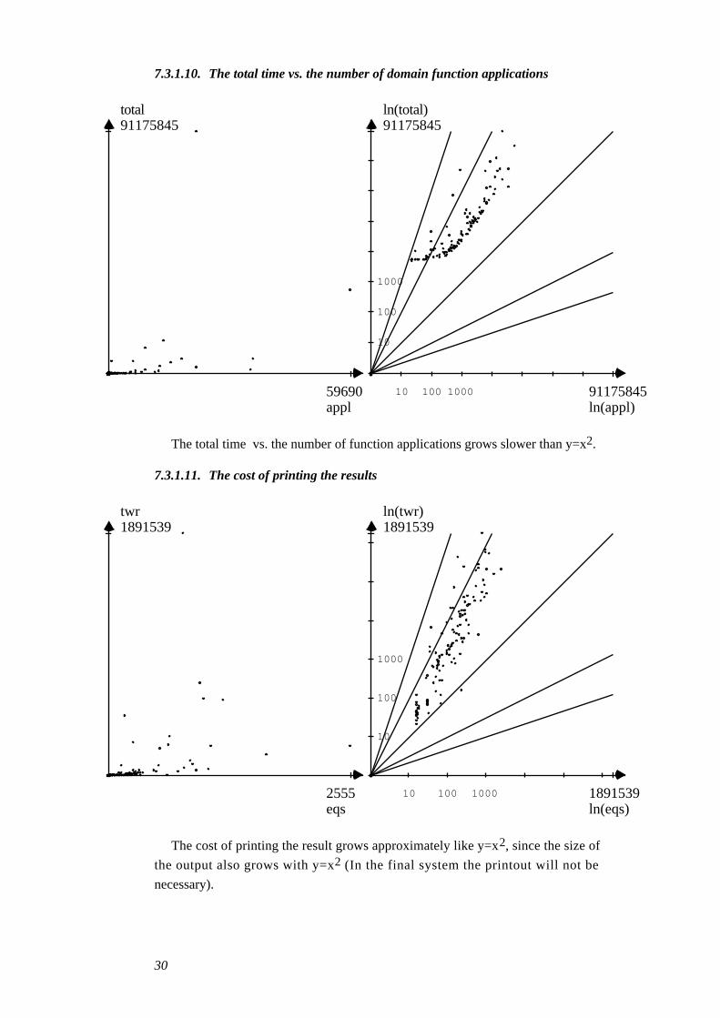
7.3.1.10. The total time vs. the number of domain function applications

appl59690

total91175845

10

100

1000

10 100 1000

ln(appl)91175845

ln(total)91175845

The total time vs. the number of function applications grows slower than y=x2.

7.3.1.11. The cost of printing the results

eqs2555

twr1891539

10

100

1000

10 100 1000

ln(eqs)1891539

ln(twr)1891539

The cost of printing the result grows approximately like y=x2, since the size of

the output also grows with y=x2 (In the final system the printout will not be

necessary).

30

7.3.1.12. The time to write the result vs. the time it takes to find the fixpoint

tfp62296974

twr1891539

10

100

1000

10 100 1000

ln(tfp)62296974

ln(twr)62296974

7.3.1.13. Relative costs for the total system

tfp62296974

total91175845

10

100

1000

10 100 1000

ln(tfp)91175845

ln(total)91175845

This graph shows that the total time for solving the problem in the case of the

larger examples grows linearly with the time it takes to find the fixpoint as

expected. For the smaller examples there is, as mentioned before, a significant

constant overhead of loading the analysis code into the agents system. In more sub-

stantial examples we spend most of the time in the fixpoint solver, which is

desired.

31

7.3. Conclusions

We consider our experiments to be successful in the sense that we were able to

improve the speed of the analyser significantly without loss of precision even with-

out resorting to a lower level language for more efficient, but less transparent im-

plementation techniques and that we succeeded in implementing a system that is

capable of analysing programs which are at least somewhat larger than the obvious

benchmark examples. The execution speed is, though, often prohibitive for global

analysis of more realistic programs. In addition to further improvements of the

code, we believe that it would be appropriate to pursue this analysis method by

adding syntax for analysed libraries. Thus it might be possible to achieve an

analyser that can analyse programs using results from analysis of parts defined

earlier rather than applying the global analysis to the program as a whole as soon as

a library is used as a building block of another program.

We have not been able to utilise the fact that deep guard computations are en-

capsulated in quiet guard computations in Agents, since we have only one class of

program variables to consider. It is also clear that the method at considerable cost

will give a level of detail that may not be motivated by the needs of the compiler,

while missing some information that the compiler would require in other cases.

The benchmark section shows that there are some parts of the system that need

to be looked into, with respect to complexity of the algorithms, but that the

essential cost of the analysis method grows polynomially like y=xn with n between

2 and 3. Whether an algorithm of such complexity can be of practical use depends

on whether there is a possibility to divide the problem of analysing a program into

less costly sub problems, e.g. library modules, where analysis results for the parts

analysed separately are used as a starting point for analysis of a complete applica-

tion program. Although we haven't yet devised the system in this manner, we fore-

see no problems in principle with such an approach.

7.4. Future work

A fruitful path to follow seems to be to extend the interpretation of the domain

elements to allow the value part to also contain functions expressing other relations

over the variables in the alias set than term equality, e.g. we could interpret a pair

<A, f(x)> as stating that it is possible that the variables in the set A are aliased and

that their possible values are described by the function f(x) representing a set of

values, where x is a list of sets of program variables, the values of whose instances

are determined from the domain element recursively. The currently implemented

system uses only sets of value descriptions, struct(Name,Arity,x), interpreted dis-

junctively. We consider 'unbound' to always be a possible value for the instances of

variables in A. struct/3 is interpreted as representing all possible runtime instances

of terms of the given form. Other descriptors could for instance be abstracted

arithmetic functions, e.g. 'plus(V1,V2)' where V1, V2 are sets of variables.

Constraint relations could be abstracted in similar ways. The set of all numbers

could easily be abstracted by a special value, number, as discussed before. This

32

would simplify the domain significantly, while sometimes giving the compiler the

important information that only numbers are possible values in certain argument

positions.

We can change the AT-domain so that it becomes more precise, at the cost of

more complex domain functions. The most straight forward way to do this is to

extend the set of values with more specialised descriptions of the values as

described previously. Functional dependencies could, e.g., be modelled with

special set-functions abstracting constraints and other built-ins of Agents. Another

example would be to tag the struct-objects so that it would be possible to see

exactly where in the source program each structure has been created. This infor-

mation might be useful for compile time garbage collection.

Alternatively, the values could be made more simple. The distinction between

the different argument positions in the struct-objects could be removed. It is also

possible to avoid distinguishing between different objects altogether.

Only further experimentation will reveal how refined the domain should be. Of

course, a more refined domain could degrade the execution speed, but the opposite

may also be the case, in particular if the size of the domain elements and the

computation cost in the domain functions can be kept reasonably small.

It would be interesting to look for ways of comparing the qualitative results of

the analysis in a more systematic manner.

7.5. Experiences using AKL

AKL as it is implemented today is a reasonably stable system. Although it has a

more flexible execution semantics, its performance is close to that of Prolog in

many cases. The major problems are in some suboptimal treatment of memory and

I/O, and since Agents is an evolving system, the program development environ-

ment is at this stage rather incomplete, although useful. We have found that most

definitions in our analysis program are written in a deterministic functional style,

i.e. the most common guard is the ”conditional” guard. The two most common

programming errors, failing computations and suspended computations, are nor-

mally easily detected and corrected. We found that errors can be found more easily

and at an earlier stage than in Prolog. The guards make it quite clear what goal is

the consumer of a result, and there is no danger that a consumer can become a pro-

ducer. Although the opposite error (a producer becomes a consumer) is not auto-

matically detectable, that situation does not seem to be as common.

7.6. Summary

We formulated a fixpoint semantics which should conservatively cover interest-

ing aspects of the execution of AKL. Each program is equipped with a finite set of

program points and a set of equations which express properties that hold at defined

positions of an AKL execution.

33

The fixpoint semantics defines an equation system on the program points, also

named domain variables when referring to the equation system. The values are

properties of the program states which express the data dependencies of the vari-

ables at states of the execution corresponding to the program points (domain vari-

ables).

Different fixpoint semantics formed thus can be compared using abstract inter-

pretation [COUSOT 92]. This would allow formal treatment of the comparison of

different analysers and the construction of formal proofs of the safeness of the

analysis, although this is not the object of this task.

We have also constructed a set of tools in the form of AKL definitions which

facilitates the practical implementation and integration of an analyser or other pro-

gram transformation tool. The usefulness of our analysis framework is to be

assessed in an effort to integrate this analyser with a compiler for AKL [BRAND

94].

8. Acknowledgements

This work which is carried out within the ESPRIT project ParForce 6707 is

funded by the government agency NUTEK on grants for participating in ESPRIT,

and via SICS from NUTEK and FDF – an association of companies: CelsiusTech

Systems AB, Telefonaktiebolaget LM Ericsson, Ellemtel, Telia AB, IBM Svenska

AB, Sun Microsystems AB, Försvarets Materielverk, FMV (Defense Material

Administration) and Asea Brown Bovery.

We especially wish to credit Björn Lisper of the Royal Institute of Technology,

Stockholm, for making us aware of Tarjan’s algorithm and also Per Brand, Sverker

Jansson, Johan Montelius, Seif Haridi, Torkel Franzén, Roland Karlsson, Per

Kreuger and Khayri M. Ali for various helpful discussions. The encouragement

and good advice provided by Manuel Hermenegildo and other participants in the

ParForce project is also greatly appreciated. The Agents development team (Ralph

Clarke Haygood, Björn Danielsson and Kent Boortz) gave help on various occa-

sions by quickly responding to various error reports and misconceptions on our

part about the evolving Agents system. We also wish to thank Torbjörn Granlund

for providing the GNU-MP package with efficient handling of integers of arbitrary

precision and Lennart E. Fahlén for some good advice on the presentation of the

benchmark results.

9. References

BaGiLe 93, R. Barbuti, R. Giacobazzi and G. Levi, A General Framework forSemantics-Based Bottom-Up Abstract Interpretation of Logic Programs, Univ.of Pisa, ACM Transactions on Programming Languages and Systems15(1):133-181, 1993

34

Brand 94, P. Brand, Optimisation for AKL with global analysis, DeliverableD.WP.2.1.3.M2 ParForce, SICS, Stockholm, Sweden, 1994

BRUYMUWIN 93, A. Mulkers, W. Winsborough, M. Bruynooghe, A Live-structure Data-flow Analysis for Prolog: Design and Evaluation, Report CW166, Katholieke Universiteit Leuven, Department of Computer Science,Leuven, Belgium, 1993

BRUYNOOGHE & WINSBOROUGH 92, M. Bruynooghe and W. Winsborough,Type Graph Unification, Report CW 160, Katholieke Universiteit Leuven,Belgium, 1992

JONESCLACK 87, S. Peyton Jones and C. Clack, Finding fixpoints in abstractinterpretation. In Abstract Interpretation of Declarative Languages, Editors S.Abramsky and C. Hankin, Ellis Horwood, 1987

CODOGNET, CODOGNET &CORSINI 90, C. Codognet, P. Codognet and M.-M.Corsini, Abstract Interpretation for Concurrent Logic Languages, in Proc. of.the North American Conference on Logic Programming, 1990, pp 215--232

COUSOT&COUSOT 92, P. Cousot and R. Cousot, Abstract Interpretation andApplication to Logic Programs, Journal of Logic Programming, 13(2&3):103-180, 1992

FRANZÉN 94, T., Some Formal Aspects of AKL, SICS Research Report R94:10,ISRN SICS R--94/10--SE

JANSON&HARIDI 91, S. Janson and S. Haridi, Programming Paradigms of theAndorra Kernel Language, in Logic Programming: Proceedings of the 1991International Symposium, MIT Press, 1991

JANSON94, S. Janson, AKL - A Multiparadigm Programming Language, UppsalaTheses in Computer Science 19 ISSN 0283-359X, ISBN 91-506-1046-5,Uppsala University, and SICS Dissertation Series 14, ISRN SICS/D--14--SE,ISSN 1101-1335

KING&SOPER 92, A. King and P. Soper, Schedule Analysis: a full theory, a pilotimplementation and a preliminary assessment, CSTR 92-06, University ofSouthampton

HANUS 92, M., An Abstract Interpretation Algorithm for Residuating LogicPrograms, MPI-I-92-217, Max-Planck-Institut für Informatik, Im Stadtwald,Saarbrücken, Germany

MUTHUKUMAR & HERMENEGILDO 92, K. Muthukumar and M. Hermenegildo,Compile-Time Derivation of Variable Dependency Using AbstractInterpretation, Journal of Logic Programming, 13(2&3):291-314, 1992

NILSSON 92, U., Abstract Interpretations and Abstract Machines: contributions toa methodology for the implementation of logic programs. Linköping Universitydissertation no 265, 1992

O’KEEFE 87, R.A., Finite Fixed-Point Problems, in Logic Programming:Proceedings. of the Fourth Internatonal Conference, MIT Press, 1987

SAHLIN 88, D., Finding the Least Fixed Point Using Wait-Declarations in Prolog,In Programming Language Implementation and Logic Programming, PLILP’90,Linköping, Lecture Notes in Compute Science 456, Springer-Verlag

35

Sahlin&Sjöland 93a, D. Sahlin and T. Sjöland, Towards Abstract Interpretation ofAKL, Extended abstract, in the Workshop of Concurrent ConstraintProgramming at the International Conference on Logic Programming 1993,Budapest, ed. Gert Smolka

SAHLIN&SJÖLAND 93B, D. Sahlin and T. Sjöland, Static Analysis of AKL,Demonstration and poster session, in the Workshop on Static Analysis, Padova1993, LNCS 724

SAHLIN&SJÖLAND 93C, D. Sahlin and T. Sjöland, D.WP.1.6.1.M1, Towards anAnalysis Tool for AKL, deliverable for the first year of the ParForce project

SAHLIN&SJÖLAND 93D, D. Sahlin and T. Sjöland, D.WP.1.6.1.M1, Syntax andNormalization of AKL programs, deliverable for the ParForce project, alsoavailable in the World Wide Web (WWW) of Internet, as a Uniform ResourceLocator (URL):http://www.sics.se/ps/agents/library_toc.html

SARASWAT 89, V. A., Concurrent Constraint Programming Languages, Ph.D.Thesis 1989, published by MIT Press 1993

TARJAN 72, R., Depth-First Search and Linear Graph Algorithms, SIAM Journalon Computation, Vol 1, No. 2, June 1972

WÆRN 88, A., An Implementation Technique for the Abstract Interpretation ofProlog, In Logic Programming:Proceedings of the fifth InternationalConference, pp. 700-710, MIT Press, 1988

36

10. Appendix: Implementation of the domain functions

Below is given a functional implementation specification of the central domain

functions which is close to the actual code implemented in AKL. A difference is

that we here talk about sets rather than their representation as lists and that

unification is not used to avoid confusion wrt. input/output arguments. We also

avoid the distinction between bit vector operations used for sets of variables and

list-based set operations used for sets of term descriptors. In many cases we have

expressed functions on sets in a non-recursive form in order to improve readability,

but this is not pursued where we find the recursive formulation equal or even

superior in terms of readability. The function syntax should be fairly obvious. The

function fst picks the first element in a pair, snd picks the second. Lists are either

the empty list [] or [h|t] where h is an element and t is a list. The functions head

and tail are used for list decomposition in the usual sense to make the intention

clear.

10.1. The lub function

lub is used to model the computation of alternative solutions along different

paths. Since we require each variable to occur in at most one A of a pair <A,V> in

a domain element we generate some immaterial aliases here.

The implementation of the lub function (without optimisations):lub(d1,d2) =

if (d1=⊥) then d2else if (d2=⊥) then d1else if (d1 ={}) then d2else if (d2 ={}) then d1else lub(d1r,merge_to_domain(av,d2))

where av=elem(d1) ∧ d1r=d1\{av}&merge_to_domain(<A,Vs>, d) =

merge_to_domain3(<A,Vs>, d,{})&merge_to_domain3(<A,Vs>,d,a)=

if (d={}) then {<A,Vs>} ∪ aelse if common_vars(A,B) thenmerge_to_domain3(<A ∪ B, merge_values(Vs,Vs')>, dr, a)else merge_to_domain3(<A,Vs>, dr, { <B,Vs'>} ∪ a)

where e=elem(d) ∧ B=fst(e) ∧ Vs'=snd(e) ∧ dr=d\{e}&merge_values(Vs1,Vs2)=

{v | v1 in Vs1∧ v2 in Vs2∧ n=name(v1) ∧ n=name(v2) ∧ a=arity(v1) ∧ a=arity(v2)

∧ v=struct(n,a,join_vars_lists(A1,A2)) } ∪

{v1 | v1 ∈Vs1∧ ¬ ∃v2∈Vs2(name(v1)=name(v2) ∧ arity(v1)=arity(v2))} ∪

{v2 | v2 ∈Vs2 ∧ ¬ ∃v1∈Vs1(name(v1)=name(v2) ∧

37

arity(v1)=arity(v2))}

10.2. The conc function

The function conc is similar to the least upper bound function. The difference is

that corresponding term descriptors in the values part of the domains are combined

to model all possible unifications of terms. Since conc models partial computations

we do not propagate the bottom value ⊥ representing a failed or necessarily

looping computation.

The implementation of the conc function (without optimizations):conc(d1,d2) =

if (d1=⊥) then d2else if (d2=⊥) then d1else if (d1 ={}) then d2else if (d2 ={}) then d1else conc(d1r, conc_to_domain(av,d2))

where av=elem(d1) ∧ d1r=d1\{av}&conc_to_domain(<A,Vs>,d) =

if (d={}) then {<A,Vs>}else domain_conc_unifs(fst(t),snd(t))

where t=conc_to_domain3(<A,Vs>,d,{},{})&conc_to_domain3(<A,Vs>,d,uacc,a)=

if (d={}) then <uacc,{<A,Vs>} ∪ a >else if common_vars(A,B) thenconc_to_domain3(<A ∪ B, Vs''>, dr, uacc ∪ unifs, a)else conc_to_domain3(<A,Vs>, dr, uacc, { <B,Vs'>} ∪ a)

where t1=elem(d) ∧ dr=d\{t1} ∧ B=fst(t1)∧ Vs'=snd(t1)∧ t2=conc_values(Vs,Vs') ∧ Vs''=fst(t2) ∧ unifs=snd(t2)

&conc_values(Vs1,Vs2)=conc_values(Vs1,Vs2,{},{})&conc_values(Vs1,Vs2,Vsacc,a)=c

where if Vs1={} then c=<Vsacc ∪ Vs2, a>else if Vs2={} then c=<Vsacc ∪ Vs1, a>elseif (name(V1)=name(V2) ∧ arity(V1)=arity(V2)) then

conc_values(Vs1c, Vs2c,Vsacc ∪ {struct(name(V1),

arity(V1),join_vars_lists(args(V1),

args(V2)))},products_lists(args(V1), args(V2), a))

else if (V1@<V2) thenconc_values( Vs1c, Vs2, Vsacc∪{V1}, a)elseconc_values(Vs1, Vs2c, Vsacc∪{V2}, a)

whereV1=elem(Vs1) ∧ Vs1c=Vs1\{V1} ∧

38

V2=elem(Vs2) ∧ Vs2c=Vs2\{V2}&join_vars_lists(l1,l2)=

if l1=[] ∧ l2=[] then []else cons(head(l1) ∪ head(l2), join_vars_lists(tail(l1),tail(l2)))

&products_lists(A1,A2,acc)=

if A1=[] ∧ A2=[] then accelse products_lists(tail(A1),tail(A2),{<head(A1)∪head(A2),{}> }∪ acc)

&domain_conc_unifs(u,d)=

if (u=[]) then delse domain_conc_unifs(tail(u),conc_to_domain(head(u),d))

10.3. The unif function

The function unif used to model partial or full unification (of some instances ofthe abstracted states) is defined using the help function conc_to_domain also usedby conc:

unif(v,t,d)=if d=⊥ then ⊥else conc_to_domain(unif_to_domain_pair(v,t),d)

&unif_to_domain_pair(v,t)=

if is_var(v) thenif is_var(t) then <{v} ∪ {t},{}>else <{v},{struct(name(t),arity(t),map(var_to_set,args(t)))}>

else unif_to_domain_pair(t,v)

10.4. call and return

The functions used to model procedure invocation and change of scope, call and

return, used to be implemented with an argumentwise application of unif. Now

they are defined using the help functions restrict and replace. call(a,b,d) will

return a domain element containing only variables reachable from the variables in

the call literal b, i.e. the callee, where a renaming of d is performed after the

unification to avoid mentioning variables in the scope of the calling literal unless

they are reachable from the scope of b (for instance via recursion). return i s

similar to call.call(a,b,d)=

restrict(b,smap_apply(replace,eq,smap_apply(domain_unif,eq,d)))where eq=build_pairs(get_pvars(a), get_pvars(b))

&smap_apply(f,l,d)=

if l=[] then delse smap_apply(f,tail(l),apply(f,fst(head(l)),snd(head(l)),d))

&apply(f(a1…an),c)=f(a1…an,c)&replace(v1,v2,d)=

{<replace_vars(v1,v2,A1),

39

map(replace_vals(v1,v2),Vs1)> | <A1,Vs1> ∈d}&replace_vars(v1,v2,s)= s\{v1} ∪ {v2}&replace_vals(v1,v2,e)=

struct(name(e),arity(e),map(replace_vars(v1,v2),args(e)))&restrict(lit,d)=

if d=⊥ then ⊥else restrict_to_vars_and_mask(vars_to_set(args(lit)),d)

&vars_to_set(l)=

if l=[] then {}else {head(l)} ∪ vars_to_set(tail(l))

&restrict_to_vars_and_mask(v,d)=

mask_away_vars(d,reachable_from_vars(d,v))&mask_away_vars(d,v)=

if d={} then {}else mask_away_vars0(v∩fst(e),snd(e),d\{e},v)where e=elem(d)

&mask_away_vars0(vs,ts,r,v)=

if vs={} then mask_away_vars(r,v)else {<vs,mask_away_vars_in_terms(v,ts)>} ∪ mask_away_vars(r,v)

&mask_away_vars_in_terms(v,ts)=

{struct(name(t),arity(t),mask_away_vars_in_args(v,args(t))) | t∈ts }&mask_away_vars_in_args(v,as)=map(and(v),as)&reachable_from_vars(d,v)=

v ∪ reachable_from_vars1(d,v,{})&reachable_from_vars1(d, vars, discarded)=

if d={} then varselse if fst(e) ∩ vars = {} then

reachable_from_vars1(d\{e},vars,{e} ∪ discarded)elsereachable_from_vars0(

d\{e},vars,union_vars_in_terms(fst(e) ∪ vars,snd(e)), discarded)

where e=elem(d)&reachable_from_vars0(d,vars1,vars2,discarded)=

if vars1=vars2 then reachable_from_vars1(d,vars2,discarded)else reachable_from_vars1(d ∪ discarded, vars2,{})

&

40

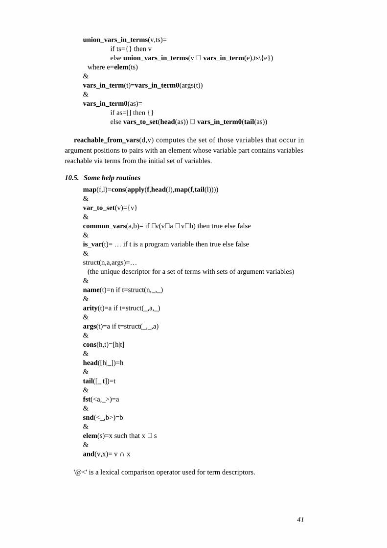
union_vars_in_terms(v,ts)=if ts={} then velse union_vars_in_terms(v ∪ vars_in_term(e),ts\{e})

where e=elem(ts)&vars_in_term(t)=vars_in_term0(args(t))&vars_in_term0(as)=

if as=[] then {}else vars_to_set(head(as)) ∪ vars_in_term0(tail(as))

reachable_from_vars(d,v) computes the set of those variables that occur in

argument positions to pairs with an element whose variable part contains variables

reachable via terms from the initial set of variables.

10.5. Some help routines

map(f,l)=cons(apply(f,head(l),map(f,tail(l))))&var_to_set(v)={v}&common_vars(a,b)= if ∃v(v∈a ∧ v∈b) then true else false&is_var(t)= … if t is a program variable then true else false&struct(n,a,args)=…

(the unique descriptor for a set of terms with sets of argument variables)&name(t)=n if t=struct(n,_,_)&arity(t)=a if t=struct(_,a,_)&args(t)=a if t=struct(_,_,a)&cons(h,t)=[h|t]&head([h|_])=h&tail([_|t])=t&fst(<a,_>)=a&snd(<_,b>)=b&elem(s)=x such that x ∈ s&and(v,x)= v ∩ x

'@<' is a lexical comparison operator used for term descriptors.

41