
Effective Interactive Resolution of Static Analysis Alarms
30
57 Efective Interactive Resolution of Static Analysis Alarms XIN ZHANG, Georgia Institute of Technology, USA RADU GRIGORE, University of Kent, UK XUJIE SI, University of Pennsylvania, USA MAYUR NAIK, University of Pennsylvania, USA We propose an interactive approach to resolve static analysis alarms. Our approach synergistically combines a sound but imprecise analysis with precise but unsound heuristics, through user interaction. In each iteration, it solves an optimization problem to fnd a set of questions for the user such that the expected payof is maximized. We have implemented our approach in a tool, Ursa, that enables interactive alarm resolution for any analysis specifed in the declarative logic programming language Datalog. We demonstrate the efectiveness of Ursa on a state-of-the-art static datarace analysis using a suite of 8 Java programs comprising 41-194 KLOC each. Ursa is able to eliminate 74% of the false alarms per benchmark with an average payofof 12× per question. Moreover, Ursa prioritizes user efort efectively by posing questions that yield high payofs earlier. CCS Concepts: · Theory of computation → Program analysis; Program verifcation; Additional Key Words and Phrases: Program Analysis, Alarm Resolution, Generalization, Prioritization ACM Reference Format: Xin Zhang, Radu Grigore, Xujie Si, and Mayur Naik. 2017. Efective Interactive Resolution of Static Analysis Alarms. Proc. ACM Program. Lang. 1, OOPSLA, Article 57 (October 2017), 30 pages. https://doi.org/10.1145/3133881 1 INTRODUCTION Automated static analyses make a number of approximations. These approximations are necessary because the static analysis problem is undecidable in general [Rice 1953]. However, they result in many false alarms in practice, which in turn imposes a steep burden on users of the analyses. A common pragmatic approach to reduce false alarms involves applying heuristics to suppress their root causes. For instance, such a heuristic may ignore a certain code construct that can lead to a high false alarm rate [Bessey et al. 2010]. While efective in alleviating user burden, however, such heuristics potentially render the analysis results unsound. In this paper, we propose a novel methodology that synergistically combines a sound but imprecise analysis with precise but unsound heuristics, through user interaction. Our key idea is that, instead of directly applying a given heuristic in a manner that may unsoundly suppress false alarms, the combined approach poses questions to the user about the truth of root causes that are targeted by the heuristic. If the user confrms them, only then is the heuristic applied to eliminate the false alarms, with the user’s knowledge. To be efective, however, the combined approach must accomplish two key goals: generalization and prioritization. We describe each of these goals and how we realize them. Permission to make digital or hard copies of all or part of this work for personal or classroom use is granted without fee provided that copies are not made or distributed for proft or commercial advantage and that copies bear this notice and the full citation on the frst page. Copyrights for components of this work owned by others than the author(s) must be honored. Abstracting with credit is permitted. To copy otherwise, or republish, to post on servers or to redistribute to lists, requires prior specifc permission and/or a fee. Request permissions from [email protected]. © 2017 Copyright held by the owner/author(s). Publication rights licensed to Association for Computing Machinery. 2475-1421/2017/10-ART57 https://doi.org/10.1145/3133881 Proc. ACM Program. Lang., Vol. 1, No. OOPSLA, Article 57. Publication date: October 2017.
-
Upload
khangminh22 -
Category
Documents
-
view
0 -
download
0
Transcript of Effective Interactive Resolution of Static Analysis Alarms
57
Effective Interactive Resolution of Static Analysis Alarms
XIN ZHANG, Georgia Institute of Technology, USA
RADU GRIGORE, University of Kent, UK
XUJIE SI, University of Pennsylvania, USA
MAYUR NAIK, University of Pennsylvania, USA
We propose an interactive approach to resolve static analysis alarms. Our approach synergistically combines a
sound but imprecise analysis with precise but unsound heuristics, through user interaction. In each iteration, it
solves an optimization problem to find a set of questions for the user such that the expected payoff is maximized.
We have implemented our approach in a tool, Ursa, that enables interactive alarm resolution for any analysis
specified in the declarative logic programming language Datalog. We demonstrate the effectiveness of Ursa
on a state-of-the-art static datarace analysis using a suite of 8 Java programs comprising 41-194 KLOC each.
Ursa is able to eliminate 74% of the false alarms per benchmark with an average payoff of 12× per question.
Moreover, Ursa prioritizes user effort effectively by posing questions that yield high payoffs earlier.
CCS Concepts: · Theory of computation→ Program analysis; Program verification;
Additional Key Words and Phrases: Program Analysis, Alarm Resolution, Generalization, Prioritization
ACM Reference Format:
Xin Zhang, Radu Grigore, Xujie Si, and Mayur Naik. 2017. Effective Interactive Resolution of Static Analysis
Alarms. Proc. ACM Program. Lang. 1, OOPSLA, Article 57 (October 2017), 30 pages.
https://doi.org/10.1145/3133881
1 INTRODUCTION
Automated static analyses make a number of approximations. These approximations are necessarybecause the static analysis problem is undecidable in general [Rice 1953]. However, they result inmany false alarms in practice, which in turn imposes a steep burden on users of the analyses.
A common pragmatic approach to reduce false alarms involves applying heuristics to suppresstheir root causes. For instance, such a heuristic may ignore a certain code construct that can leadto a high false alarm rate [Bessey et al. 2010]. While effective in alleviating user burden, however,such heuristics potentially render the analysis results unsound.In this paper, we propose a novel methodology that synergistically combines a sound but
imprecise analysis with precise but unsound heuristics, through user interaction. Our key idea isthat, instead of directly applying a given heuristic in a manner that may unsoundly suppress falsealarms, the combined approach poses questions to the user about the truth of root causes that aretargeted by the heuristic. If the user confirms them, only then is the heuristic applied to eliminatethe false alarms, with the user’s knowledge.
To be effective, however, the combined approach must accomplish two key goals: generalizationand prioritization. We describe each of these goals and how we realize them.
Permission to make digital or hard copies of all or part of this work for personal or classroom use is granted without fee
provided that copies are not made or distributed for profit or commercial advantage and that copies bear this notice and the
full citation on the first page. Copyrights for components of this work owned by others than the author(s) must be honored.
Abstracting with credit is permitted. To copy otherwise, or republish, to post on servers or to redistribute to lists, requires
prior specific permission and/or a fee. Request permissions from [email protected].
© 2017 Copyright held by the owner/author(s). Publication rights licensed to Association for Computing Machinery.
2475-1421/2017/10-ART57
https://doi.org/10.1145/3133881
Proc. ACM Program. Lang., Vol. 1, No. OOPSLA, Article 57. Publication date: October 2017.

57:2 Xin Zhang, Radu Grigore, Xujie Si, and Mayur Naik
Generalization. The number of questions posed to the user by our approach should be muchsmaller compared to the number of false alarms that are eliminated. Otherwise, the effort inanswering those questions could outweigh the effort in resolving the alarms directly. To realize thisobjective for analyses that produce many alarms, we observe that most alarms are often symptomsof a relatively small set of common root causes. For example, a method that is falsely deemedreachable can result in many false alarms in the body of that method. Inspecting this single rootcause is easier than inspecting multiple alarms.Prioritization. Since the number of false alarms resulting from different root causes may vary,
the user might wish to only answer questions with relatively high payoffs. Our approach realizesthis objective by interacting with the user in an iterative manner instead of posing all questions atonce. In each iteration, the questions asked are chosen such that the expected payoff is maximized.Note that the user may be asked multiple questions per iteration because single questions maybe insufficient to resolve any of the remaining alarms. Asking questions in order of decreasingpayoff allows the user to stop answering them when diminishing returns set in. Finally, the iterativeprocess allows incorporating the user’s answers to past questions in making better choices of futurequestions, and thereby further amplify the reduction in user effort.We formulate the problem to be solved in each iteration of our approach as a non-linear op-
timization problem called the optimum root set problem. This problem aims at finding a set ofquestions that maximizes the benefit-cost ratio in terms of the number of false alarms expected tobe eliminated and the number of questions posed. We propose an efficient solution to this problemby reducing it to a sequence of integer linear programming (ILP) instances. Each ILP instance encodesthe dependencies between analysis facts, and weighs the benefits and costs of questioning differentsets of root causes. Since our objective function is non-linear, we solve a sequence of ILP instancesthat performs a binary search between the upper bound and lower bound of the benefit-cost ratio.Our approach automatically generates the ILP formulation for any analysis specified in a con-
straint language. Specifically, we target Datalog, a declarative logic programming language thatis widely used in formulating program analyses [Madsen et al. 2016; Mangal et al. 2015; Smarag-dakis and Bravenboer 2010; Smaragdakis et al. 2014; Whaley et al. 2005; Zhang et al. 2014]. Ourconstraint-based approach also allows incorporating orthogonal techniques to reduce user effort,such as alarm clustering techniques that express dependencies between different alarms usingconstraints, possibly in a different abstract domain [Le and Soffa 2010; Lee et al. 2012].We have implemented our approach in a tool called Ursa and evaluate it on a static datarace
analysis using a suite of 8 Java programs comprising 41-194 KLOC each. Ursa eliminates 74% of thefalse alarms per benchmark with an average payoff of 12× per question. Moreover, Ursa effectivelyprioritizes questions with high payoffs. Further, based on data collected from 40 Java programmers,we observe that the average time to resolve a root cause is only half of that to resolve an alarm.Together, these results show that our approach achieves significant reduction in user effort.
We summarize our contributions below:
(1) We propose a new paradigm to synergistically combine a sound but imprecise analysis withprecise but unsound heuristics, through user interaction.
(2) We present an interactive algorithm that implements the paradigm. In each iteration, it solvesthe optimum root set problem which finds a set of questions with the highest expected payoffto pose to the user.
(3) We present an efficient solution to the optimum root set problem based on integer linearprogramming for a general class of constraint-based analyses.
(4) We empirically show that our approach eliminates a majority of the false alarms by asking onlya few questions. Moreover, it effectively prioritizes questions with high payoffs.
Proc. ACM Program. Lang., Vol. 1, No. OOPSLA, Article 57. Publication date: October 2017.
Effective Interactive Resolution of Static Analysis Alarms 57:3
1 public class FTPServer implements Runnable {
2 private ServerSocket serverSocket;
3 private List conList;
4
5 public void main(String args[]) {
6 ...
7 startButton.addActionListener(
8 new ActionListener() {
9 public void actionPerformed(...) {
10 new Thread(this).start();
11 }
12 });
13 stopButton.addActionListener(
14 new ActionListener() {
15 public void actionPerformed(...) {
16 stop();
17 }
18 });
19 }
20
21 public void run() {
22 ...
23 while (runner != null) {
24 Socket soc = serverSocket.accept();
25 connection = new RequestHandler(soc);
26 conList.add(connection);
27 new Thread(connection).start();
28 }
29 ...
30 }
31
32 private void stop() {
33 ...
34 for (RequestHandler con : conList)
35 con.close();
36 serverSocket.close();
37 }
38 }
39 public class RequestHandler implements Runnable {
40 private FtpRequestImpl request;
41 private Socket controlSocket;
42 ...
43
44 public RequestionHandler(Socket socket) {
45 ...
46 controlSocket = socket;
47 request = new FtpRequestImpl();
48 request.setClientAddress(socket.getInetAddress());
49 ...
50 }
51
52 public void run() {
53 ...
54 // log client information
55 clientAddr = request.getRemoteAddress();
56 ...
57 input = controlSocket.getInputStream();
58 reader = new BufferedReader(new
InputStreamReader(input));
59 while (!isConnectionClosed) {
60 ...
61 commandLine = reader.readLine();
62 // parse and check permission
63 request.parse(commandLine);
64 // execute command
65 service(request);
66 }
67 }
68
69 public synchronized void close() {
70 ...
71 controlSocket.close();
72 controlSocket = null;
73 request.clear();
74 request = null;
75 }
76 }
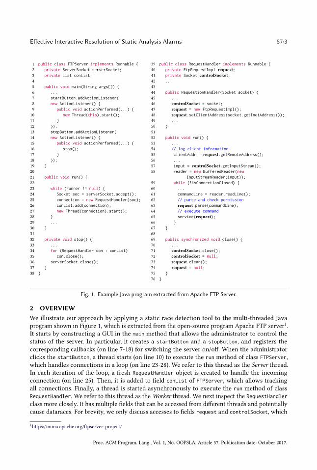
Fig. 1. Example Java program extracted from Apache FTP Server.
2 OVERVIEW
We illustrate our approach by applying a static race detection tool to the multi-threaded Javaprogram shown in Figure 1, which is extracted from the open-source program Apache FTP server1.It starts by constructing a GUI in the main method that allows the administrator to control thestatus of the server. In particular, it creates a startButton and a stopButton, and registers thecorresponding callbacks (on line 7-18) for switching the server on/off. When the administratorclicks the startButton, a thread starts (on line 10) to execute the run method of class FTPServer,which handles connections in a loop (on line 23-28). We refer to this thread as the Server thread.In each iteration of the loop, a fresh RequestHandler object is created to handle the incomingconnection (on line 25). Then, it is added to field conList of FTPServer, which allows trackingall connections. Finally, a thread is started asynchronously to execute the run method of classRequestHandler. We refer to this thread as the Worker thread. We next inspect the RequestHandler
class more closely. It has multiple fields that can be accessed from different threads and potentiallycause dataraces. For brevity, we only discuss accesses to fields request and controlSocket, which
1https://mina.apache.org/ftpserver-project/
Proc. ACM Program. Lang., Vol. 1, No. OOPSLA, Article 57. Publication date: October 2017.
57:4 Xin Zhang, Radu Grigore, Xujie Si, and Mayur Naik
Input Relations:
access(p,o) (program point p accesses some field of abstract object o)
alias(p1,p2) (program points p1 and p2 access same memory location)
escape(o) (abstract object o is thread-shared)
parallel(p1,p2) (program points p1 and p2 can be reached by different threads simultaneously)
unguarded(p1,p2) (program points p1 and p2 are not guarded by any common lock)
Output Relations:
shared(p) (program point p accesses thread-shared memory location)
race(p1,p2) (datarace between program points p1 and p2)
Rules:
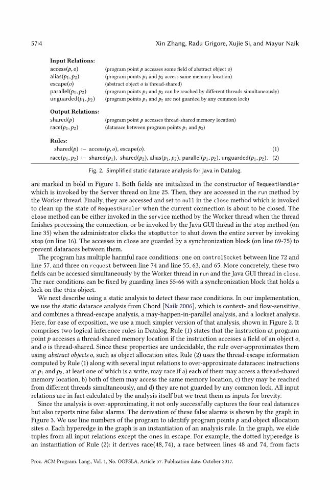
shared(p) :− access(p,o), escape(o). (1)
race(p1,p2) :− shared(p1), shared(p2), alias(p1,p2), parallel(p1,p2), unguarded(p1,p2). (2)
Fig. 2. Simplified static datarace analysis for Java in Datalog.
are marked in bold in Figure 1. Both fields are initialized in the constructor of RequestHandlerwhich is invoked by the Server thread on line 25. Then, they are accessed in the run method bythe Worker thread. Finally, they are accessed and set to null in the close method which is invokedto clean up the state of RequestHandler when the current connection is about to be closed. Theclose method can be either invoked in the service method by the Worker thread when the threadfinishes processing the connection, or be invoked by the Java GUI thread in the stop method (online 35) when the administrator clicks the stopButton to shut down the entire server by invokingstop (on line 16). The accesses in close are guarded by a synchronization block (on line 69-75) toprevent dataraces between them.The program has multiple harmful race conditions: one on controlSocket between line 72 and
line 57, and three on request between line 74 and line 55, 63, and 65. More concretely, these twofields can be accessed simultaneously by the Worker thread in run and the Java GUI thread in close.The race conditions can be fixed by guarding lines 55-66 with a synchronization block that holds alock on the this object.We next describe using a static analysis to detect these race conditions. In our implementation,
we use the static datarace analysis from Chord [Naik 2006], which is context- and flow-sensitive,and combines a thread-escape analysis, a may-happen-in-parallel analysis, and a lockset analysis.Here, for ease of exposition, we use a much simpler version of that analysis, shown in Figure 2. Itcomprises two logical inference rules in Datalog. Rule (1) states that the instruction at programpoint p accesses a thread-shared memory location if the instruction accesses a field of an object o,and o is thread-shared. Since these properties are undecidable, the rule over-approximates themusing abstract objects o, such as object allocation sites. Rule (2) uses the thread-escape informationcomputed by Rule (1) along with several input relations to over-approximate dataraces: instructionsat p1 and p2, at least one of which is a write, may race if a) each of them may access a thread-sharedmemory location, b) both of them may access the same memory location, c) they may be reachedfrom different threads simultaneously, and d) they are not guarded by any common lock. All inputrelations are in fact calculated by the analysis itself but we treat them as inputs for brevity.
Since the analysis is over-approximating, it not only successfully captures the four real dataracesbut also reports nine false alarms. The derivation of these false alarms is shown by the graph inFigure 3. We use line numbers of the program to identify program points p and object allocationsites o. Each hyperedge in the graph is an instantiation of an analysis rule. In the graph, we elidetuples from all input relations except the ones in escape. For example, the dotted hyperedge isan instantiation of Rule (2): it derives race(48, 74), a race between lines 48 and 74, from facts
Proc. ACM Program. Lang., Vol. 1, No. OOPSLA, Article 57. Publication date: October 2017.

Effective Interactive Resolution of Static Analysis Alarms 57:5
escape(25)
shared(46) shared(47) shared(48)shared(57) shared(71) shared(72) shared(55) shared(63) shared(65) shared(73) shared(74)
race(46,57) race(46,71) race(46,72) race(47,55) race(47,63) race(47,65) race(47,73) race(47,74) race(48,74)
Fig. 3. Derivation of dataraces in example program. We only show parts related to false alarms for brevity.
shared(48), shared(74), alias(48, 74), parallel(48, 74), and unguarded(48, 74), which in turn arethemselves derived or input facts.
Note that the above analysis does not report any datarace between accesses in the constructor ofRequestHandler. This is because, by excluding tuples such as parallel(46, 46), the parallel relationcaptures the fact that the constructor can be only invoked by the Server thread. Likewise, it doesnot report any datarace between accesses in the close method as it is able to reason about locks viathe unguarded relation. However, there are still nine false alarms among the 13 reported alarms.To find the four real races, the user must inspect all 13 alarms in the worst case.
To reduce the false alarm rate, Chord incorporates various heuristics, one of which is particularlyeffective in reducing false alarms in our scenario. This heuristic can be turned on by runningChord with option chord.datarace.exclude.init=true, which causes Chord to ignore all races thatinvolve at least one instruction in an object constructor. Internally, the heuristic suppresses all sharedtuples whose instruction lies in an object constructor. Intuitively, most of such memory accesses areon the object being constructed which typically stays thread-local until the constructor returns.Indeed, in our scenario, shared(46), shared(47), and shared(48) are all spurious (as the object onlybecomes thread-shared on line 27) and lead to nine false alarms. However, applying the heuristiccan render the analysis result unsound. For instance, the object under construction can becomethread-shared inside the constructor by being assigned to the field of a thread-shared object or bystarting a new thread on it. Applying the heuristic can suppress true alarms that are derived fromshared tuples related to such facts.We present a new methodology and tool, Ursa, to address this problem. Instead of directly
applying the above heuristic in a manner that may introduce false negatives, Ursa poses questionsto the user about root causes that are targeted by the heuristic. In our example, such causes are theshared tuples in the constructor of RequestHandler. If the user confirms such a tuple as spurious,only then it is suppressed in the analysis, thereby eliminating all false alarms resulting from it.
Ursa has two features that make it effective. First, it can eliminate a large number of false alarmsby asking a few questions. The key insight is that most alarms are often symptoms of a relativelysmall set of common root causes. For instance, false alarms race(47, 55), race(47, 63), race(47, 65),race(47, 73), and race(47, 74) are all derived due to shared(47). Inspecting this single root cause iseasier than inspecting all four alarms.
Second, Ursa interacts with the user in an iterative manner, and prioritizes questions with highpayoffs in earlier iterations. This allows the user to only answer questions with high payoffs andstop the interaction when the gain in alarms resolved has diminished compared to the effort inanswering further questions.Ursa realizes the above two features by solving an optimization problem called the optimum
root set problem, in each iteration. Recall that Chord’s heuristic identified as potentially spuriousthe tuples shared(46), shared(47), shared(48); these appear in red in the derivation graph. We wishto ask the user if these tuples are indeed spurious, but not in an arbitrary order, because a few
Proc. ACM Program. Lang., Vol. 1, No. OOPSLA, Article 57. Publication date: October 2017.

57:6 Xin Zhang, Radu Grigore, Xujie Si, and Mayur Naik
answers to well-chosen questions may be sufficient. We wish to find a small non-empty subset ofthose tuples, possibly just one tuple, which could rule out many false alarms. We call such a subsetof tuples a root set, as the tuples in it are root causes for the potential false alarms, according tothe heuristic. Each root set has an expected gain (how many false alarms it could rule out) and acost (its size, which is how many questions the user will be asked). The optimum root set problem is
to find a root set that maximizes the expected gain per unit cost.We refer to the gain per unit costas the payoff. We next describe each iteration of Ursa on our example. Here, we assume the useralways answers the question correctly. Later we discuss the case where the user occasionally givesincorrect answers (Section 4.7 and Section 6.2).
Iteration 1. Ursa picks {shared(47)} as the optimum root set since it has an expected payoff of5, which is the highest among those of all root sets. Other root sets like {shared(46), shared(47)}may resolve more alarms but end up with lower expected payoffs due to larger numbers of requiredquestions.Based on the computed root set, Ursa poses a single question about shared(47) to the user:
łDoes line 47 access any thread-shared memory location? If the answer is no, five races will besuppressed as false alarms.ž Here Ursa only asks one question, but there are other cases in which itmay ask multiple questions in an iteration depending on the size of the computed optimum rootset. Besides the root set, we also present the corresponding number of false alarms expected to beresolved. This allows the user to decide whether to answer the questions by weighing the gains inreducing alarms against the costs in answering them.
Suppose the user decides to continue and answers no. Doing so labels shared(47) as false, whichin turn resolves five race alarms race(47, 55), race(47, 63), race(47, 65), race(47, 73), and race(47, 74),highlighting the ability of Ursa to generalize user input. Next, Ursa repeats the above process, butthis time taking into account the fact that shared(47) is labeled as false.
Iteration 2. In this iteration, we have two candidates for the optimum root set: {shared(46)}withan expected payoff of 3 and {shared(48)} with an expected payoff of 1. While resolving {shared(46)}is expected to eliminate {race(46, 57), race(46, 71), race(46, 72)}, resolving {shared(48)} can onlyeliminate {race(48, 74)}.Ursa picks {shared(46)} as the optimum root set and poses the following question to the user:
łDoes line 46 access any thread-shared memory location? If the answer is no, three races will besuppressed as false alarms.ž Compared to the previous iteration, the expected payoff of the optimumroot set has reduced, highlighting Ursa’s ability to prioritize questions with high payoffs.We assume the user answers no, which labels shared(46) as false. As a result, race alarms
race(46, 57), race(46, 71), and race(46, 72) are eliminated. At the end of this iteration, eight out ofthe 13 alarms have been eliminated. Moreover, only one false alarm race(48, 74) remains.
Iteration 3. In this iteration, there is only one root set {shared(48)} which has an expectedpayoff of 1. Similar to the previous two iterations, Ursa poses a single question about shared(48)to the user along with the number of false alarms expected to be suppressed. At this point, the usermay prefer to resolve the remaining five alarms manually, as the expected payoff is too low andvery few alarms remain unresolved. Ursa terminates if the user makes this decision. Otherwise,the user proceeds to answer the question regarding shared(48) and therefore resolve the onlyremaining false alarm race(48, 74). At this point, Ursa terminates as all three tuples targeted bythe heuristic have been answered.
In summary, Ursa resolves, in a sound manner, 8 (or 9) out of 9 false alarms by only asking two(or three) questions. Moreover, it prioritizes questions with high payoffs in earlier iterations.
Proc. ACM Program. Lang., Vol. 1, No. OOPSLA, Article 57. Publication date: October 2017.

Effective Interactive Resolution of Static Analysis Alarms 57:7
C F c (program) c F l :− l (constraint)
l F r (a) (literal) a F v | d (argument)
(a) Syntax of Datalog (overline means list).
r ∈ R = {a, b, . . . } (relation) σ ∈ V→ D (substitution)
v ∈ V = {x ,y, . . . } (variable) a ∈ A ⊆ T (alarms)
d ∈ D = {0, 1, . . . } (constant) q ∈ Q ⊆ T (potential causes)
t ∈ T = R × D∗ (tuple) f ∈ F ⊆ Q (causes)
(b) Auxiliary definitions and notations.
JCK := lfp SC
SC (T ) := T ∪ { t | t ∈ sc (T ) and c ∈ C }
sl0:−l1, ...,ln (T ) := { σ (l0) | σ (l1) ∈ T , . . . ,σ (ln ) ∈ T }
(c) Semantics of Datalog.
JCKF := lfp SFFC
SFFC (T ) := SC (T ) \ F
(d) Augmented semantics of Datalog.
Fig. 4. Syntax and semantics of Datalog without and with causes.
3 THE OPTIMUM ROOT SET PROBLEM
In this section, we define the Optimum Root Set problem, abbreviated ORS, in the context of staticanalyses expressed in Datalog.
3.1 Declarative Static Analysis
Datalog is a logic programming language whose least fixed point semantics makes it suitableto implement static analyses. We say that an analysis is sound when it over-approximates theconcrete semantics. We augment the semantics of Datalog in a way that allows us to control theover-approximation.Figure 4(a) gives the syntax of Datalog: a list of constraints, each constraint having a head on
the left and a body on the right. The head is a literal; the body is a list of literals, which we view asa set and can be empty. A literal is a relation applied to a list of arguments, each argument beingeither a variable or a constant. A tuple is a literal whose arguments are all constants.Figure 4(b) introduces notations for relations, variables, constants, tuples, and substitutions.
It also introduces three special subsets of tuples: alarms, potential causes, and causes. An alarmcorresponds to a bug report. A potential cause is a tuple that is identified by a heuristic as possiblyspurious. A cause is a tuple that is identified by an oracle (e.g., a human user) as indeed spurious.Figure 4(c) shows the standard semantics of Datalog. It computes the least fixed point of con-
straints, which is a set of tuples. Suppose T is the set of derived tuples. Initially, T is empty andwe grow it iteratively by instantiating constraints to derive new tuples from existing tuples inT . In each iteration, for each rule l0 :− l1, . . . , ln , if there exists a substitution σ which is a mapfrom variables to constants such that all σ (l1), . . . ,σ (n ) are in T , then we add σ (l0) to T . In thefirst iteration, only constraints with empty bodies are triggered. We use function SC to denote thecomputation of one iteration. This process continues until T no longer changes. In other words,the Datalog semantics computes the least fixed point of SC (denoted by lfp SC ). A sound Dataloganalysis will derive all tuples that represent valid program facts, but may also derive tuples thatrepresent spurious program facts.
Proc. ACM Program. Lang., Vol. 1, No. OOPSLA, Article 57. Publication date: October 2017.

57:8 Xin Zhang, Radu Grigore, Xujie Si, and Mayur Naik
Figure 4(d) gives the augmented semantics of Datalog, which allows controlling the over-approximation with a set of causes F. It is similar to the standard Datalog semantics except that ineach iteration it removes tuples in causes F from derived tuples T (denoted by function SFFC ). Sincea cause in F is never derived, it is not used in deriving other tuples. In other words, the augmentedsemantics do not only suppress the causes but also spurious tuples that can be derived from them.
3.2 Problem Statement
We assume the following are fixed: a set C of Datalog constraints, a set A of alarms, a set Q ofpotential causes, and a set F of confirmed causes. Informally, our goal is to grow F such that JCKFcontains fewer alarms. To make this precise, we introduce a few terms. Given two sets T1 ⊇ T2 oftuples, we define the gain of T2 relative to T1, as the number of alarms that are in T1 but not in T2:
gain(T1,T2) :=���(T1 \T2) ∩ A
���A root set R is a non-empty subset of potential but unconfirmed causes: R ⊆ Q \ F. Intuitively, thename is justified because we will aim to put in R the root causes of the false alarms. The potentialcauses in R are those we will investigate, and for that we have to pay a cost |R|. The potential gainof R is the gain of JCKF∪R relative to JCKF. The expected payoff of R is the potential gain per unitcost. (The actual payoff depends on which potential causes in R will be confirmed.) With thesedefinitions, we can now formally introduce the ORS problem.
Problem 3.1 (Optimum Root Set). Given a set C of constraints, a set Q of potential causes,a set F of confirmed causes, and a set A of alarms, find a root set R ⊆ Q \ F that maximizes
gain(
JCKF, JCKF∪R)
/|R|, which is the expected payoff.
3.3 Monotonicity
The definitions from the previous two subsections (Section 3.1 and 3.2) imply certain monotonicityproperties. We list these here and refer to them in later sections.
Lemma 3.2. If T1 ⊆ T2 and F1 ⊇ F2, then SFF1C(T1) ⊆ SFF2
C(T2). In particular, if F1 ⊇ F2, then
JCKF1 ⊆ JCKF2 .
Lemma 3.3. IfT1 ⊆ T′1 andT
′2 ⊆ T2, then gain(T
′1 ,T
′2 ) ≥ gain(T1,T2). Also, gain(T ,T ) = 0 for allT .
3.4 NP-Completeness
Problem 3.1 is an optimization problem which can be turned into a decision problem in the usualway, by providing a threshold for the objective. The question becomes whether there exists a rootset R that can achieve a given gain. This decision problem is clearly in NP: the set R is a suitablepolynomial certificate.
The problem is also NP-hard, which we can show by a reduction from the minimum vertex coverproblem. Given a graph G = (V ,E), a subset U ⊆ V of vertices is said to be a vertex cover when itintersects all edges {i, j} ∈ E. The minimum vertex cover problem, which asks for a vertex cover ofminimum size, is well-known to be NP-complete. We reduce it to the ORS problem as follows. Werepresent the graphG with three relations R = {vertex, edge, alarm}. Without loss of generality,let V be the set {0, . . . ,n − 1}, for some n. Thus, we identify vertices with Datalog constants. Foreach edge {i, j} ∈ E we include two ground constraints:
edge(i, j ) :− vertex(i ), vertex(j )
alarm() :− edge(i, j )
Proc. ACM Program. Lang., Vol. 1, No. OOPSLA, Article 57. Publication date: October 2017.

Effective Interactive Resolution of Static Analysis Alarms 57:9
We set F = ∅, A := {alarm()}, and Q := { vertex(i ) | i ∈ V }. Since A has size 1, the gain canonly be 0 or 1. To maximize the ORS objective, the gain has to be 1. Further, the size of the rootset R has to be minimized. But, one can easily see that a root set leads to a gain of 1 if and only if itcorresponds to a vertex cover.
4 INTERACTIVE ANALYSIS
Our interactive analysis combines three ingredients: (a) a static analysis; (b) a heuristic; and (c) anoracle.We require the static analysis to be implemented in Datalog, which lets us track dependencies.The requirements on the heuristic and the oracle are mild: given a set of Datalog tuples they mustpick some subset. These are all the requirements. Suppose there is a ground truth that returns thetruth of each analysis fact based on the concrete semantics. It helps to think of the three ingredientsintuitively as follows:
(a) the static analysis is sound, imprecise with respect to the ground truth and fast;(b) the heuristic is unsound, precise with respect to the ground truth and fast; and(c) the oracle agrees with the ground truth and is slow.
Technically, we show a soundness preservation result (Theorem 4.4): if the given oracle agrees withthe ground truth and the static analysis over-approximates it, then our combined analysis alsoover-approximates the ground truth. Soundness preservation holds with any heuristic. When aheuristic agrees with the ground truth, we say that it is ideal; when it almost agrees with the groundtruth, we say that it is precise. Even though which heuristic one uses does not matter for soundness,we expect that more precise heuristics lead to better performance. We explore speed and precisionlater, through experiments (Section 6). Also later, we discuss what happens in practice when thestatic analysis is unsound or the oracle does not agree with the ground truth (Section 4.7).The high level intuition is as follows. The heuristic is fast. But, since the heuristic might be
unsound, we need to consult an oracle before relying on what the heuristic reports. However,consulting the oracle is an expensive operation, so we would like to not do it often. Here is wherethe static analysis specified in Datalog helps. On one hand, by analyzing the Datalog derivation, wecan choose good questions to ask the oracle. On the other hand, after we obtain information fromthe oracle, we can propagate that information through the Datalog derivation, effectively findinganswers to questions we have not yet asked.We begin by showing how the static analysis, the heuristic, and the oracle fit together (Section
4.1), and why the combination preserves soundness (Section 4.2). A key ingredient in our algorithmis solving the ORS problem. We do this by a sequence of calls to an ILP solver (Section 4.3). Eachcall to the ILP solver asks whether, given a Datalog derivation, a certain payoff is feasible (Section4.4 and 4.5). To improve performance, we preprocess the Datalog derivation before constructingthe ILP question (Section 4.6). Finally, we close with a short discussion (Section 4.7).
4.1 Main Algorithm
Algorithm 1 brings together our key ingredients:
(a) the set C of constraints and the set A of potential alarms represent the static analysis imple-mented in Datalog;
(b) Heuristic is the heuristic; and(c) Decide is the oracle.
The key to combining these ingredients into an analysis that is fast, sound, and precise is theprocedure OptimumRootSet, which solves Problem 3.1.From now on, the set C of constraints and the set A of potential alarms should be thought of
as immutable global variables: they do not change, and they will be available in subroutines even
Proc. ACM Program. Lang., Vol. 1, No. OOPSLA, Article 57. Publication date: October 2017.

57:10 Xin Zhang, Radu Grigore, Xujie Si, and Mayur Naik
Algorithm 1 Interactive Resolution of Alarms
INPUT constraints C , and potential alarms AOUTPUT remaining alarms1: Q := Heuristic()
2: F := ∅3: while Q , F do
4: R := OptimumRootSet(C,A,Q, F)
5: Y ,N := Decide(R)
6: Q := Q \ Y
7: F := Q \ JCKF∪N8: end while
9: return A ∩ JCKF
if not explicitly passed as arguments. In contrast, the set Q of potential causes and the set F ofconfirmed causes do change in each iteration, while maintaining the invariant F ⊆ Q. Initially, theinvariant holds because no cause has been confirmed, F = ∅.
In each iteration, we invoke the oracle for a set of potential causes that are not yet confirmed: wecall Decide(R) for some non-empty R ⊆ Q \ F. The result we get back is a partition (Y ,N ) of R. InY we have tuples that are in fact true, and therefore are not causes for false alarms; in N we havetuples that are in fact false, and therefore are causes for false alarms. We remove tuples Y from theset Q of potential causes (line 6); we insert tuples N into the set F of confirmed causes, and we alsoinsert all other potential causes that may have been blocked by N (line 7).At the end, we return the remaining alarms A ∩ JCKF.
4.2 Soundness
For correctness, we require that the oracle is always right. In particular, the answers given by theoracle should be consistent: if asked repeatedly, the oracle should give the same answer about atuple. Formally, we require that there exists a partition of all tuples T into two subsets True andFalse such that
Decide(T ) = (T ∩ True,T ∩ False) for all T ⊆ T (1)
We refer to the set True as the ground truth. We say that the analysis C is sound when
F ⊆ False implies JCKF ⊇ True (2)
That is, a sound analysis is one that over-approximates, as long as we do not explicitly block atuple in the ground truth.
Lemma 4.1. A sound analysis C can derive the ground truth; that is, True = JCKFalse.
The correctness of Algorithm 1 relies on the analysisC being sound and also on making progressin each iteration, which we ensure by requiring
∅ ⊂ OptimumRootSet(C,A,Q, F) ⊆ Q \ F (3)
Lemma 4.2. In Algorithm 1, suppose thatHeuristic returns all tuples T. Also, assume (1), (2), and (3).Then, Algorithm 1 returns the true alarms A ∩ True.
Proof sketch. The key invariant is that
F ⊆ False ⊆ Q (4)
Proc. ACM Program. Lang., Vol. 1, No. OOPSLA, Article 57. Publication date: October 2017.
Effective Interactive Resolution of Static Analysis Alarms 57:11
The invariant is established by setting F := ∅ and Q := T. By (1), we know that Y ⊆ True andN ⊆ False, on line 5. It follows that the invariant is preserved by removing Y from Q, on line 6. Italso follows that F∪N ⊆ False and, by (2), that JCKF∪N ⊇ True. So, the invariant is also maintainedby line 7. We conclude that (4) is indeed an invariant.
Because R is non-empty, the loop terminates (details in appendix). When it does, we have F = Q.Together with the invariant (4), we obtain that F = False. By Lemma 4.1, it follows that Algorithm 1returns A ∩ True. □
We can relax the requirement that Heuristic returns T because of the following result:
Lemma 4.3. Consider two heuristics which compute, respectively, the sets Q1 and Q2 of potential
causes. Let A1 and A2 be the corresponding sets of alarms computed by Algorithm 1. If Q1 ⊆ Q2, then
A1 ⊇ A2.
Proof sketch. Use the same strategy as in Lemma 4.2’s proof, but replace the invariant (4) with
F ⊆ Q0 ∩ False ⊆ Q
where Q0 ∈ {Q1,Q2} is the initial value of Q. □
From Lemmas 4.2 and 4.3, we conclude that Algorithm 1 is sound, for all heuristics.
Theorem 4.4. Assume that there is a ground truth, the analysis C is sound, and OptimumRootSet
makes progress; that is, assume (1), (2), and (3). Then, Algorithm 1 terminates and it returns at least
the true alarms A ∩ True.
Observe that there is no requirement on Heuristic. If Heuristic always returns ∅, then our methoddegenerates to simply using the imprecise but fast static analysis implemented in Datalog. IfHeuristic always returns T and the oracle is a precise analysis, then our method degenerates toan iterative combination between the imprecise and the precise analyses. Usually, we would use aheuristic that has demonstrated its effectiveness in practice, even though it may lack theoreticalguarantees for soundness. In our approach, soundness is inherited from the static analysis specifiedin Datalog and from the oracle. If the oracle is unsound, perhaps because the user makes mistakes,then so is our analysis. Thus, Theorem 4.4 is a relative soundness result.
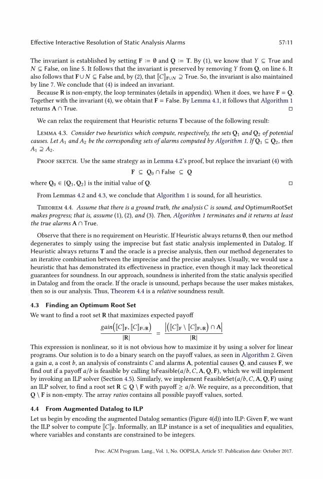
4.3 Finding an Optimum Root Set
We want to find a root set R that maximizes expected payoff
gain(
JCKF, JCKF∪R)
|R|=
���(
JCKF \ JCKF∪R)
∩ A���
|R|
This expression is nonlinear, so it is not obvious how to maximize it by using a solver for linearprograms. Our solution is to do a binary search on the payoff values, as seen in Algorithm 2. Givena gain a, a cost b, an analysis of constraints C and alarms A, potential causes Q, and causes F, wefind out if a payoff a/b is feasible by calling IsFeasible(a/b,C,A,Q, F), which we will implementby invoking an ILP solver (Section 4.5). Similarly, we implement FeasibleSet(a/b,C,A,Q, F) usingan ILP solver, to find a root set R ⊆ Q \ F with payoff ≥ a/b. We require, as a precondition, thatQ \ F is non-empty. The array ratios contains all possible payoff values, sorted.
4.4 From Augmented Datalog to ILP
Let us begin by encoding the augmented Datalog semantics (Figure 4(d)) into ILP: Given F, we wantthe ILP solver to compute JCKF. Informally, an ILP instance is a set of inequalities and equalities,where variables and constants are constrained to be integers.
Proc. ACM Program. Lang., Vol. 1, No. OOPSLA, Article 57. Publication date: October 2017.
57:12 Xin Zhang, Radu Grigore, Xujie Si, and Mayur Naik
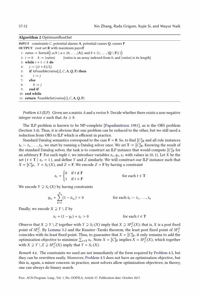
Algorithm 2 OptimumRootSet
INPUT constraints C , potential alarms A, potential causes Q, causes F
OUTPUT root set R with maximum payoff
1: ratios := Sorted(
{ a/b | a ∈ {0, . . . , |A|} and b ∈ {1, . . . , |Q \ F|} })
2: i := 0 k := |ratios | {ratios is an array indexed from 0, and |ratios | is its length}
3: while i + 1 < k do
4: j := ⌊(i + k )/2⌋
5: if IsFeasible(ratios[j],C,A,Q, F) then
6: i := j
7: else
8: k := j
9: end if
10: end while
11: return FeasibleSet(ratios[i],C,A,Q, F)
Problem 4.5 (ILP). Given are a matrixA and a vectorb. Decide whether there exists a non-negativeinteger vector x such that Ax ≥ b.
The ILP problem is known to be NP-complete [Papadimitriou 1981], as is the ORS problem(Section 3.4). Thus, it is obvious that one problem can be reduced to the other, but we still need areduction from ORS to ILP which is efficient in practice.
Standard Datalog semantics correspond to the case F = ∅. So, to find JCK∅ and all rule instancest0 :− t1, . . . , tn , we start by running a Datalog solver once. We set T := JCK∅. Knowing the result ofthe standard Datalog solver, the task is to construct an ILP instance that would compute JCKF foran arbitrary F. For each tuple t , we introduce variables xt ,yt , zt with values in {0, 1}. Let X be theset { t ∈ T | xt = 1 }, and define Y and Z similarly. We will construct our ILP instance such thatX = JCKF, Y = SC (X ), and Z = F. We encode Z = F by having a constraint
zt =
0 if t < F
1 if t ∈ Ffor each t ∈ T
We encode Y ⊇ SC (X ) by having constraints
yt0 +
n∑
k=1
(1 − xtk ) > 0 for each t0 :− t1, . . . , tn
Finally, we encode X ⊇ Y \ Z by
xt + (1 − yt ) + zt > 0 for each t ∈ T
Observe that X ⊇ Y \ Z together with Y ⊇ SC (X ) imply that X ⊇ SFZC (X ); that is, X is a post fixed
point of SFZC . By Lemma 3.2 and the KnasterśTarski theorem, the least post fixed point of SFZCcoincides with its least fixed point. Thus, to guarantee that X = JCKF, it only remains to add theoptimization objective to minimize
∑
t ∈T xt . Note X = JCKF implies X = SFZC (X ), which together
with X ⊇ Y \ Z ⊇ SFZC (X ) imply that Y = SC (X ).
Remark 4.6. The constraints we used are not immediately of the form required by Problem 4.5, butthey can be rewritten easily. Moreover, Problem 4.5 does not have an optimization objective, butthis is, again, a minor concern: in practice, most solvers allow optimization objectives; in theory,one can always do binary search.
Proc. ACM Program. Lang., Vol. 1, No. OOPSLA, Article 57. Publication date: October 2017.
Effective Interactive Resolution of Static Analysis Alarms 57:13
yt0 +
n∑
k=1
(1 − xtk ) > 0 for all t0 :− t1, . . . , tn (1)
xt + (1 − yt ) + zt > 0 for t ∈ T (2)
zt = 0 for t < Q (3)
zt = 1 for t ∈ F (4)∑
t ∈Q\F
zt > 0 (requires |R| > 0) (5)
b∑
t ∈A∩JCKF
(1 − xt ) − a∑
t ∈Q\F
zt ≥ 0 (requires payoff ≥ a/b) (6)
Fig. 5. Implementing IsFeasible and FeasibleSet as an ILP instance. All variables xt ,yt , zt take values in {0, 1}.
We use the ILP solver as follows. Given a set F, we create constraints as above. Then we run theILP solver, which will return a variable assignment. The desired JCKF is encoded in the assignmentof the variables {xt }t ∈T.
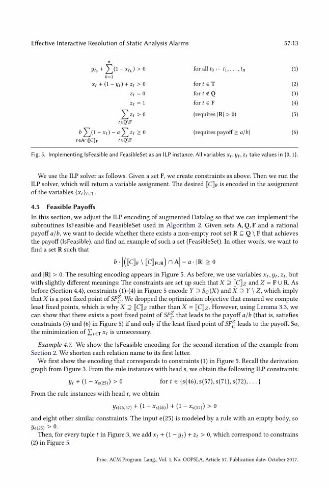
4.5 Feasible Payoffs
In this section, we adjust the ILP encoding of augmented Datalog so that we can implement thesubroutines IsFeasible and FeasibleSet used in Algorithm 2. Given sets A,Q, F and a rationalpayoff a/b, we want to decide whether there exists a non-empty root set R ⊆ Q \ F that achievesthe payoff (IsFeasible), and find an example of such a set (FeasibleSet). In other words, we want tofind a set R such that
b ·���(
JCKF \ JCKF∪R)
∩ A��� − a · |R| ≥ 0
and |R| > 0. The resulting encoding appears in Figure 5. As before, we use variables xt ,yt , zt , butwith slightly different meanings: The constraints are set up such that X ⊇ JCKZ and Z = F ∪ R. Asbefore (Section 4.4), constraints (1)-(4) in Figure 5 encode Y ⊇ SC (X ) and X ⊇ Y \ Z , which implythat X is a post fixed point of SFZC . We dropped the optimization objective that ensured we computeleast fixed points, which is why X ⊇ JCKZ rather than X = JCKZ . However, using Lemma 3.3, wecan show that there exists a post fixed point of SFZC that leads to the payoff a/b (that is, satisfies
constraints (5) and (6) in Figure 5) if and only if the least fixed point of SFZC leads to the payoff. So,the minimization of
∑
t ∈T xt is unnecessary.
Example 4.7. We show the IsFeasible encoding for the second iteration of the example fromSection 2. We shorten each relation name to its first letter.
We first show the encoding that corresponds to constraints (1) in Figure 5. Recall the derivationgraph from Figure 3. From the rule instances with head s, we obtain the following ILP constraints:
yt + (1 − xe(25) ) > 0 for t ∈ {s(46), s(57), s(71), s(72), . . . }
From the rule instances with head r, we obtain
yr(46,57) + (1 − xs(46) ) + (1 − xs(57) ) > 0
and eight other similar constraints. The input e(25) is modeled by a rule with an empty body, soye(25) > 0.
Then, for every tuple t in Figure 3, we add xt + (1−yt ) + zt > 0, which correspond to constrains(2) in Figure 5.
Proc. ACM Program. Lang., Vol. 1, No. OOPSLA, Article 57. Publication date: October 2017.

57:14 Xin Zhang, Radu Grigore, Xujie Si, and Mayur Naik
The potential causes returned by the heuristic are Q = {s(46), s(47), s(48)}. At the beginningof the second iteration one cause had been confirmed, F = {s(47)}. We have zt = 1 for t ∈ F, andzt = 0 for t < Q, which correspond to constraints (4) and (3) in Figure 5 respectively.
For constraints (5), we have zs(46) + zs(48) > 0.Finally,
b · (1 − xr(46,57) + 1 − xr(46,71) + 1 − xr(46,72) + 1 − xr(48,74) ) − a · (zs(46) + zs(48) ) ≥ 0
where the indices of x range over the four unresolved alarms at the start of the second iteration. □
Let us see what we need to write down the constraints from Figure 5. First, we need the result ofrunning a standard Datalog solver: the set JCK∅, and the corresponding rule instances t0 :− t1, . . . , tn .We obtain these by running the Datalog solver once, in the beginning. Second, we need the sets A,Q, and F. The set A is fixed, since it only depends on the analysis. Sets Q and F do change, but theyare sent as arguments to IsFeasible and FeasibleSet. Third, we need the ratio a/b, which is also sentas an argument. Fourth, we need the set JCKF; we can compute it as described earlier (Section 4.4).If the ILP solver finds the instance to be feasible, then it gives us an assignment for variables,
including for {zt }t ∈T. To implement FeasibleSet, we compute R as Z \ F.
4.6 Preprocessing
Using the encoding presented so far, we can solve the ORS problem by invoking an ILP solver.However, sometimes the ILP solver would take tens of minutes to reply. In this section, we see twopreprocessing techniques that, together, empirically reduce the time spent in the ILP solver by afactor of 62 on average.
Partial Evaluation. We evaluate JCKF several times, for the same set C of constraints but fordifferent sets F. Since we are always interested in potential causes, F ⊆ Q, we know by Lemma 3.2that JCKF ⊇ JCKQ. It is thus beneficial to precompute JCKQ. Then, for each tuple t ∈ JCKQ, weremove the constraints that have head t , and then we remove t from the remaining constraints.The resulting set of constraints, which is much smaller, is used for all future calls to the ILP solver.
Tuple Elimination. Since we are not interested in tuples that are intermediate between potentialcauses and potential alarms, we can sometimes take shortcuts. Suppose a tuple t < Q∪A appears inonly two constraints: t ′′ :− t and t :− t ′. Then, we can eliminate t by replacing the two constraintswith one: t ′′ :− t ′. More generally, if all occurrences of t are in them + n constraints
t ′′1 :− t t ′′2 :− t . . . t ′′m :− t and t :− T ′1 t :− T ′2 . . . t :− T ′n
then we can replace all these with themn constraints
t ′′i :− T ′j for all i ∈ {1, . . . ,m} and j ∈ {1, . . . ,n}
It is profitable to do so whenmn ≤ m + n.
These preprocessing techniques are simple but effective. They are both inspired by techniquesused in SAT solving: Partial evaluation is similar to unit propagation, and tuple elimination issimilar to variable elimination. We cannot simply use a SAT solver, though, for several reasons.First, constraints like (6) in Figure 5 are cumbersome to express as Boolean formulas because of theintegers a and b. Second, although SAT solvers usually implement variable elimination, MaxSATsolvers do not. We would need a MaxSAT solver because we want to find a small R (Section 4.7).And third, note that tuple elimination uses domain specific knowledge: which tuples are potentialcauses or potential alarms. Still, our main contribution here is to observe that applying theseknown techniques is crucial if one wants to use an off-the-shelf ILP solver on instances arisingfrom Datalog-based static analysis.
Proc. ACM Program. Lang., Vol. 1, No. OOPSLA, Article 57. Publication date: October 2017.

Effective Interactive Resolution of Static Analysis Alarms 57:15
4.7 Discussion
First, we discuss a few alternatives for the payoff, for the termination condition, and for the oracle.Then, we discuss the issue of soundness from the point of view of the mismatch between theoryand practice. Finally, we discuss how our approach could be applied in a non-Datalog setting.
Payoff. The algorithm presented above uses |R| as the cost measure. It might be, however, thatsome potential causes are more difficult to investigate than others. If the user provides us withan expected cost of investigating each potential cause, then we can adapt our algorithm, in theobvious way, so that it prefers calling Decide on cheap potential causes.
In situations when multiple root sets have the same maximum payoff, we may want to prefer onewith minimum size. Intuitively, small root sets let us gather information from the oracle quickly.To encode a preference for smaller root sets, we can extend the constraints in Figure 5 with theoptimization objective to minimize
∑
t ∈Q\F zt .
Termination. Algorithm 1 terminates when all potential causes have been investigated; thatis, when Q = F. Another option is to look at the current value of the expected payoff. SupposeAlgorithm 2 finds an expected payoff ≤ 1. This means that we expect that it will not be easier toinvestigate potential causes rather than investigate the alarms themselves. So, we could decideto terminate, as we do in our experiments (Section 6). Finally, instead of looking at the expectedpayoff computed by the ILP solver, we could track the actual payoff for each iteration. Then, wecould stop if the average payoff in the last few iterations is less than some threshold.
Oracle. By default, the oracle Decide is a human user. However, we can also use a precise yetexpensive analysis as the oracle, which enables an alternative use case of our approach. This usecase focuses on balancing the overall precision and scalability of combining the base analysis andthe oracle analysis, rather than reducing user effort in resolving alarms. Our approach allows theoracle analysis to focus on only the potential causes that are relevant to the alarms, especially theones with high expected payoffs. For example, the end user might find it too long a time to applythe oracle analysis to resolve all potential causes. By applying our approach, they can use the oracleanalysis to only answer the potential causes with high payoffs and resolve the rest alarms via othermethods (e.g., manual inspection). Appendix B includes a more detailed discussion of this use case.
Soundness. In practice, most static analyses are unsound [Livshits et al. 2015]. In addition, in oursetting, the user may answer incorrectly. We discuss each of these issues below.Many program analyses are designed to be sound in theory but are unsound in practice due
to engineering compromises. If certain language features were handled in a sound manner, thenthe analysis would be unscalable or exceedingly imprecise. For example, in Java, such featuresinclude reflection, dynamic class loading, native code, and exceptions. If we start from an unsoundstatic analysis, then our interactive analysis is also unsound. However, Theorem 4.4 gives evidencethat we do not introduce new sources of unsoundness. More importantly, our approach is stilleffective in suppressing false alarms and therefore reduces user effort, as we demonstrate throughexperiments (Section 6).In theory, the oracle never makes mistakes; in practice, users do make mistakes, of two kinds:
they may label a true tuple as spurious, and they may label a spurious tuple as true. If a true tupleis labeled as spurious, then the interactive analysis becomes unsound. However, if the user answersx% of questions incorrectly, then we expect that the fraction of false negatives is not far from x%.Our experiments show that, even better, the fraction of false negatives tends to be less than x%. Aconsequence of this observation is that, if potential causes are easier to inspect than alarms, thenour approach will decrease the chances that real bugs are missed.
Proc. ACM Program. Lang., Vol. 1, No. OOPSLA, Article 57. Publication date: October 2017.
57:16 Xin Zhang, Radu Grigore, Xujie Si, and Mayur Naik
If a spurious tuple is labeled as true, then the interactive analysis may ask more questions. Itis also possible that fewer false alarms are filtered out: the user could make the mistake on theonly remaining question with expected payoff > 1, which in turn would cause the interaction toterminate earlier. (See the previous discussion on termination.)Later, we analyze both kinds of mistakes quantitatively (Section 6.2 and Table 2).
Non-Datalog Analyses. We focus on program analyses implemented in Datalog for two reasons:(1) it is easy to capture provenance information for such analyses; and (2) there is a growing trendtowards specifying program analyses in Datalog [Jordan et al. 2016; Madsen et al. 2016; Mangalet al. 2015; Smaragdakis and Bravenboer 2010; Zhang et al. 2014]. However, not all analyses areimplemented in Datalog; for example, see Ayewah et al. [2008]; Bessey et al. [2010]; Copeland[2005]. In principle, it is possible to apply our approach to any program analysis. To do so, theanalysis designer would need to figure out how to capture provenance information of an analysis’execution. While this might be a cumbersome task, however, it constitutes a one-time effort.
5 INSTANCE ANALYSES
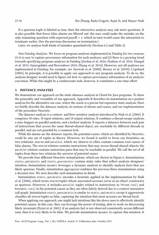
We demonstrate our approach on the static datarace analysis in Chord for Java programs. To showthe generality and versatility of our approach, Appendix B describes its instantiation on a pointeranalysis for the alternative use case, where the oracle is a precise but expensive static analysis. Next,we briefly describe the datarace analysis, its notions of alarms and causes, and our implementationof the procedure Heuristic.
The datarace analysis is a context- and flow-sensitive analysis introduced by Naik et al. [2006]. Itcomprises 30 rules, 18 input relations, and 18 output relations. It combines a thread-escape analysis,a may-happen-in-parallel analysis, and a lockset analysis. It reports a datarace between each pairof instructions that access the same thread-shared object, are reachable by different threads inparallel, and are not guarded by a common lock.
While the alarms are the datarace reports, the potential causes, which are identified by Heuristic,could be any set of tuples in theory. However, we found it useful to focus our heuristics ontwo relations: shared and parallel, which we observe to often contain common root causes offalse alarms. The shared relation contains instructions that may access thread-shared objects; theparallel relation contains instruction pairs that may be reachable in parallel. We call the set of alltuples from these two relations the universe of potential causes.We provide four different Heuristic instantiations, which are shown in Figure 6. Instantiations
static_optimistic and static_pessimistic contain static rules that reflect analysis designers’intuition. Instantiation dynamic leverages a dynamic analysis to identify analysis facts that arelikely spurious. Finally, instantiation aggregated combines the previous three instantiations usinga decision tree. We next describe each instantiation in detail.Instantiation static_optimistic encodes a heuristic applied in the implementation by Naik
et al. [2006], which treats shared tuples whose associated accesses occur in an object constructoras spurious. Moreover, it includes parallel tuples related to instructions in Thread.run() andRunnable.run() in the potential causes as they are often falsely derived due to a context-insensitivecall-graph. Instantiation static_pessimistic is similar to static_optimistic except it aggressivelyclassifies all shared tuples as false, capturing the intuition that most accesses are thread-local.
When applying our approach, one might lack intuitions like the above ones to effectively identifypotential causes. In this case, they can leverage the power of testing, akin to work on discoveringlikely invariants [Ernst et al. 2001]: if an analysis fact is not observed consistently across differentruns, then it is very likely to be false. We provide instantiation dynamic to capture this intuition. It
Proc. ACM Program. Lang., Vol. 1, No. OOPSLA, Article 57. Publication date: October 2017.

Effective Interactive Resolution of Static Analysis Alarms 57:17
static_optimistic() = {shared(i ) | instruction i is in a constructor} ∪
{parallel(i, t1, t2) | instruction i is in java.lang.Thread.run() or
java.lang.Runnable.run()}
static_pessimistic() = {shared(i ) | i is an instruction} ∪
{parallel(i, t1, t2) | instruction i is in java.lang.Thread.run() or
java.lang.Runnable.run()}
dynamic() = {shared(i ) | instruction i is executed and only accesses thread-local objects
during the runs} ∪
{parallel(i, t1, t2) | whenever thread t1 executes instruction i in the runs,
t2 is not running}
aggregated() = decisionTree(dynamic, static_optimistic, static_pessimistic)
Fig. 6. Heuristic instantiations for the datarace analysis.
Table 1. Benchmark characteristics. Column |A| shows the numbers of alarms. Column |QU | shows the sizes
of the universes of potential causes, where k stands for thousands. All the reported numbers except for |A|
and |QU | are computed using a 0-CFA call-graph analysis.
Description# Classes # Methods Bytecode (KB) Source (KLOC) |A| |QU |
app total app total app total app total false total false%
raytracer 3D raytracer 18 87 74 283 5.1 18 1.8 41.4 226 411 55% 5.3kmontecarlo financial simulator 18 114 115 442 5.2 23 3.5 50.8 37 38 97.4% 4.4ksor successive over relaxation 6 100 12 431 1.8 30 0.6 52.5 64 64 100% 940elevator discrete event simulator 5 188 24 899 2.3 52 0.6 88 100 100 100% 1.4kjspider web spider engine 113 391 422 1572 17.7 74.6 6.7 106 214 264 81.1% 82khedc web crawler from ETH 44 353 230 2,134 16 140 6.1 128 317 378 83.9% 38kftp Apache FTP server 119 527 608 2,705 36.5 142 18.2 162 594 787 75.5% 131kweblech website download/mirror tool 11 576 78 3,326 6 208 12 194 6 13 46.2% 6.2k
leverages a dynamic analysis and returns tuples whose associated program points are reached butassociated program facts are not observed across runs.Having multiple Heuristic instantiations is not unusual; we gain the benefits of each of them
using a combined instantiation aggregated, which decides whether to classify each given tupleas a potential cause by considering the results of all the individual instantiations. Instantiationaggregated realizes this idea by using a decision tree that aggregates the results of the otherinstantiations. We obtain such a decision tree by training it on benchmarks where the tuples in theuniverse of potential causes are fully labeled.
6 EMPIRICAL EVALUATION
This section evaluates the effectiveness of our approach by applying it to the datarace analysis ona suite of 8 Java programs. In addition, Appendix B discusses the evaluation results for the usecase where the oracle is a precise yet expensive analysis, by applying our approach to the pointeranalysis on the same benchmark suite.
6.1 Evaluation Setup
We implemented our approach in a tool called Ursa for analyses specified in Datalog that targetJava programs. We use Chord [Naik 2006] as the Java analysis framework, bddbddb [Whaley et al.2005] as the Datalog solver, and Gurobi [Gurobi Optimization, Inc. 2016] as the ILP solver. Allexperiments were done using Oracle HotSpot JVM 1.6 on a Linux machine with 64GB memory and2.7GHz processors.
Proc. ACM Program. Lang., Vol. 1, No. OOPSLA, Article 57. Publication date: October 2017.
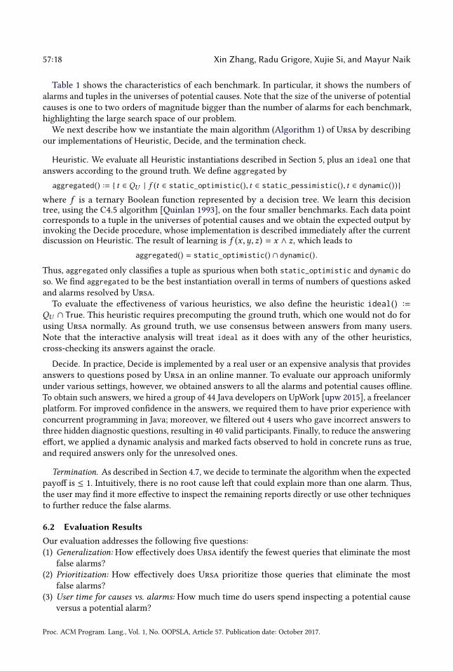
57:18 Xin Zhang, Radu Grigore, Xujie Si, and Mayur Naik
Table 1 shows the characteristics of each benchmark. In particular, it shows the numbers ofalarms and tuples in the universes of potential causes. Note that the size of the universe of potentialcauses is one to two orders of magnitude bigger than the number of alarms for each benchmark,highlighting the large search space of our problem.We next describe how we instantiate the main algorithm (Algorithm 1) of Ursa by describing
our implementations of Heuristic, Decide, and the termination check.
Heuristic. We evaluate all Heuristic instantiations described in Section 5, plus an ideal one thatanswers according to the ground truth. We define aggregated by
aggregated() := { t ∈ QU | f (t ∈ static_optimistic(), t ∈ static_pessimistic(), t ∈ dynamic())}
where f is a ternary Boolean function represented by a decision tree. We learn this decisiontree, using the C4.5 algorithm [Quinlan 1993], on the four smaller benchmarks. Each data pointcorresponds to a tuple in the universes of potential causes and we obtain the expected output byinvoking the Decide procedure, whose implementation is described immediately after the currentdiscussion on Heuristic. The result of learning is f (x ,y, z) = x ∧ z, which leads to
aggregated() = static_optimistic() ∩ dynamic().
Thus, aggregated only classifies a tuple as spurious when both static_optimistic and dynamic doso. We find aggregated to be the best instantiation overall in terms of numbers of questions askedand alarms resolved by Ursa.To evaluate the effectiveness of various heuristics, we also define the heuristic ideal() :=
QU ∩ True. This heuristic requires precomputing the ground truth, which one would not do forusing Ursa normally. As ground truth, we use consensus between answers from many users.Note that the interactive analysis will treat ideal as it does with any of the other heuristics,cross-checking its answers against the oracle.
Decide. In practice, Decide is implemented by a real user or an expensive analysis that providesanswers to questions posed by Ursa in an online manner. To evaluate our approach uniformlyunder various settings, however, we obtained answers to all the alarms and potential causes offline.To obtain such answers, we hired a group of 44 Java developers on UpWork [upw 2015], a freelancerplatform. For improved confidence in the answers, we required them to have prior experience withconcurrent programming in Java; moreover, we filtered out 4 users who gave incorrect answers tothree hidden diagnostic questions, resulting in 40 valid participants. Finally, to reduce the answeringeffort, we applied a dynamic analysis and marked facts observed to hold in concrete runs as true,and required answers only for the unresolved ones.
Termination. As described in Section 4.7, we decide to terminate the algorithm when the expectedpayoff is ≤ 1. Intuitively, there is no root cause left that could explain more than one alarm. Thus,the user may find it more effective to inspect the remaining reports directly or use other techniquesto further reduce the false alarms.
6.2 Evaluation Results
Our evaluation addresses the following five questions:(1) Generalization: How effectively does Ursa identify the fewest queries that eliminate the most
false alarms?(2) Prioritization: How effectively does Ursa prioritize those queries that eliminate the most
false alarms?(3) User time for causes vs. alarms: How much time do users spend inspecting a potential cause
versus a potential alarm?
Proc. ACM Program. Lang., Vol. 1, No. OOPSLA, Article 57. Publication date: October 2017.

Effective Interactive Resolution of Static Analysis Alarms 57:19
raytra
cer
monte
carlo so
r
elevator
jspider ftp
hedc
weblech0%
20%
40%
60%
80%
100%
cau
ses
an
d a
larm
s
10 2 2 4
23
18 22
1
15 4
2 4 22
19 12
2
226 37 64 100 214 594 317 6
URSA ideal
Ã# false alarms
Fig. 7. Number of questions asked over total number of false alarms (denoted by the lower dark bars) and
percentage of false alarms resolved (denoted by the upper light bars) by Ursa. Note that Ursa terminates
when the expected payoff is ≤ 1, which indicates that the user should stop looking at potential causes and
focus on the remaining alarms.
4 8 12 16 20# questions
0
50
100
150
200
250
# a
larm
s
raytracer
ideal
URSA
1 2 3 4 5# questions
0
10
20
30
40
50
# a
larm
s
montecarlo
1 2 3 4 5# questions
0
15
30
45
60
75
# a
larm
s
sor
1 2 3 4 5# questions
0
20
40
60
80
100
# a
larm
s
elevator
5 10 15 20 25# questions
0
40
80
120
160
200
# a
larm
s
jspider
4 8 12 16 20# questions
0
150
300
450
600
750
# a
larm
s
ftp
5 10 15 20 25# questions
0
25
50
75
100
125
# a
larm
s
hedc
1 2 3 4 5# questions
0
2
4
6
8
10
# a
larm
s
weblech
Fig. 8. Number of questions asked and number of false alarms resolved by Ursa in each iteration.
(4) Impact of incorrect user answers: How do incorrect user answers affect the effectiveness of Ursain terms of precision, soundness, and user effort?
(5) Scalability: Does the optimization procedure of Ursa scale to large programs?(6) Effect of different heuristics: What is the impact of different heuristics on generalization and
prioritization?We report all averages using arithmetic means except average payoffs and average speedups, whichare calculated using geometric means.
Generalization results. Figure 7 shows the generalization results of Ursa with aggregated, thebest available Heuristic instantiation. For comparison, we also include the ideal heuristic. Foreach benchmark under both settings, we show the percentage of resolved false alarms (the upperlight bars) and the number of asked questions over the total number of false alarms (the lowerdark bars). The figure also shows the absolute numbers of asked questions (denoted by the numbersover dark bars) and the numbers of false alarms produced by the input static analysis (denoted bythe numbers at the top).Ursa is able to eliminate 73.7% of the false alarms with an average payoff of 12× per question.
On ftp, the benchmark with the most false alarms, the gain is as high as 87% and the average payoff
Proc. ACM Program. Lang., Vol. 1, No. OOPSLA, Article 57. Publication date: October 2017.

57:20 Xin Zhang, Radu Grigore, Xujie Si, and Mayur Naik
increases to 29×. Note that Ursa does not resolve all alarms as it terminates when the expectedpayoff becomes 1 or smaller, which means there are no common root causes for the remainingalarms. These results show that most of the false alarms can indeed be eliminated by inspectingonly a few common root causes.
Ursa eliminates most of the false alarms for all benchmarks except hedc, where only 17.7% of thefalse alarms are eliminated. In fact, even under the ideal setting, only 34% of the false alarms can beeliminated. Closer inspection revealed that most alarms in hedc indeed do not share common rootcauses. However, the questions asked comprise only 7% of the false alarms. This shows that evenwhen there is scarce room to generalize, Ursa does not ask unnecessary questions.
In the ideal case, Ursa eliminates an additional 15.6% of false alarms on average, which modestlyimproves over the results with aggregated. We thus conclude the aggregated instantiation iseffective in identifying common root causes of false alarms.
Prioritization results. Figure 8 shows the prioritization results of Ursa. In the plots, each iterationof Algorithm 1 has a corresponding point, which represents the number of false alarms eliminated(y-axis) and the number of questions (x-axis) asked so far. As before, we compare the results ofUrsa to the ideal case, which has a perfect heuristic.We observe that a few causes often yield most of the benefits. For instance, three causes can
resolve 323 out of 594 false alarms on ftp, yielding a payoff of 108×. Ursa successfully identifiesthese causes with high payoffs and poses them to the user in the earliest few iterations. In fact,for the first three iterations on most benchmarks, Ursa asks exactly the same set of questionsas the ideal setting. The results of these two settings only differ in later iterations, where thepayoff becomes relatively low. We also notice that there can be multiple causes in the set that givesthe highest benefit (for instance, the aforementioned ftp results). The reason is that there can bemultiple derivations to each alarm. If we naively search the potential causes by fixing the numberof questions in advance, we can miss such causes. Ursa, on the other hand, successfully finds themby solving the optimal root set problem iteratively.
The fact that Ursa is able to prioritize causes with high payoffs allows the user to stop interactingafter a few iterations and still get most of the benefits. Ursa terminates either when the expectedpayoff drops to 1 or when there are no more questions to ask. But in practice, the user might chooseto stop the interaction even earlier. For instance, the user might be satisfied with the current resultor she may find limited payoff in answering more questions.We study these causes with high payoffs more closely. For our datarace analysis, the two
main categories of causes are (i) spurious thread-shared memory access (shared) tuples in objectconstructors of classes that extend the java.lang.Thread class or implement the java.lang.Runnableinterface, and (ii) spurious may-happen-in-parallel (parallel) tuples in the run methods of similarclasses. The objects whose constructors contain spurious (shared) tuples are mostly created in loopswhere a new thread is created and executes the run methods of these objects in each iteration. Thedatarace analysis is unable to distinguish the objects created in different iterations and considersthem all as thread-shared after the first iteration. This leads to many false datarace alarms betweenthe main thread which invokes the constructors and the threads created in the loops which alsoaccess the objects by executing their run methods. The spurious parallel tuples are produceddue to the context-insensitive call-graphs which mismatch the run methods containing them toThread.start invocations that cannot actually reach these run methods. This in turn leads to manyfalse alarms between multiple threads.
User time for causes vs. alarms. While Ursa can significantly reduce the number of alarms thata user must inspect, it comes at the expense of the user inspecting causes. We measured thetime consumed by each programmer when labeling individual causes and alarms for the datarace
Proc. ACM Program. Lang., Vol. 1, No. OOPSLA, Article 57. Publication date: October 2017.

Effective Interactive Resolution of Static Analysis Alarms 57:21
Table 2. Results of Ursa on ftp with noise in Decide. The baseline analysis produces 193 true alarms and 594
false alarms. We run each setting for 30 times and take the averages.
% Noise# Resolved
False Alarms
% Resolved
False Alarms
# False
Negatives
% Retained
True Alarms# Questions Payoff
0% 517.0 87.0% 0.0 100.0% 18.0 28.7
1% 516.4 86.9% 0.0 100.0% 18.1 28.6
5% 515.4 86.8% 4.9 97.4% 18.2 28.4
10% 505.0 85.0% 9.2 95.2% 19.4 26.3
analysis. Our measurements show that it takes 578 seconds on average for a user to inspect adatarace alarm but only 265 seconds on average to inspect a cause. This is because reasoning aboutan alarm often requires reasoning about multiple causes and other program facts that can derive it.To precisely quantify the reduction in user effort, a more rigorous user study is needed, which isbeyond the scope of the current paper. However, the massive reduction in the number of alarmsthat a user needs to inspect and the fact that a cause is on average much less expensive to inspectshows Ursa’s potential to significantly reduce overall user effort.In practice, there might be cases where the causes are much more expensive to inspect than
alarms. However, as discussed in Section 4.7, as long as the costs can be quantified in some way,we can naturally encode them in our optimization problem. As a result, Ursa will be able to findthe set of questions that maximizes the payoff in user effort.
Impact of incorrect user answers. As we discussed earlier (Section 4.7), users can make mistakes.We analyze the impact of mistakes quantitatively by injecting random noise in Decide: we flip itsanswer to each tuple with probability x%. We set x to 1, 5, 10, and apply Ursa on ftp, the benchmarkwith the most alarms. We run the experiment under each setting for 30 times and calculate theaverages of all statistics. Table 2 summarizes the results in terms of precision, soundness, and usereffort. We also show the results of Ursa without noise as a comparison.Columns 2 and 3 show, respectively, the number and the percentage of false alarms that are
resolved by Ursa with noise. When the amount of noise increases, both statistics drop. This is dueto Decide incorrectly marking certain spurious tuples posed by Ursa as true. These tuples mightwell be the only tuples that can resolve certain alarms and are with payoff > 1. However, we alsonotice that the drop is modest: a noise of 10% leads to a drop in resolved false alarms of 2% only.
Columns 4 and 5 show, respectively, the number of false negatives and the percentage of retainedtrue alarms. Ursa can introduce false negatives when a noisy Decide incorrectly marks a true tupleas spurious. The number of false negatives grows as the amount of noise increases, but the growthis not significant: a noise of 10% leads to missing 4.8% true alarms only. This shows that Ursa doesnot amplify user errors. It is especially true for datarace analysis, given that its alarms are harderto inspect compared to the root causes.Columns 6 and 7 show, respectively, the number of questions asked by Ursa and the payoff of
answering these questions. As expected, more noise leads to more questions and smaller payoffs.But, the effect is modest: a noise of 10% increases the number of questions by 7.7% and decreasesthe payoff by 8.4%.In summary, Ursa is resilient to user mistakes.
Scalability results. Figure 9 shows the distributions of the time consumed by Ursa in eachiteration (a) with and (b) without preprocessing. As Figure 9(a) shows, with preprocessing, almostall iterations finish within half a minute. After closer inspection, we find that most of the time isspent in the ILP solver. While each invocation only takes less than 5 seconds, one iteration consistsof up to 20 invocations. We note that while the user inspects causes (which takes 265 seconds on
Proc. ACM Program. Lang., Vol. 1, No. OOPSLA, Article 57. Publication date: October 2017.

57:22 Xin Zhang, Radu Grigore, Xujie Si, and Mayur Naik
raytracer
montecarlo sor
elevator
jspider ftp hedc
weblech0
10
20
30
40
50
60
70
run
tim
e (
in s
eco
nd
s)
(a) With preprocessing.
raytracer
montecarlo sor
elevator
jspider ftp hedc
weblech0
50010001500200025003000350040004500
run
tim
e (
in s
eco
nd
s)
(b) Without preprocessing.
Fig. 9. Time consumed by Ursa in each iteration.
average), Ursa would have time to speculate what the answers will be, and prepare the next set ofquestions accordingly. There are two cases in which Ursa spent more than half a minute: the firstiterations of jspider and ftp. This iteration happens after the static analysis runs and before theuser interaction starts. So, from the point of view of the user, it is the same as having a slightlylonger static analysis time. Moreover, on the smaller four benchmarks, each iteration of Ursa takesonly a few seconds. Such fast response times ensure Ursa’s usability in an interactive setting.
The fact that the Optimum Root Set problem is NP-complete (Section 3.4) precludes us from usingapproaches with lower complexity than ILP. Nevertheless, we significantly reduce solving timeby employing preprocessing techniques that exploit domain knowledge. As a comparison, Ursatakes significantly more time per iteration without preprocessing, which is shown in Figure 9(b).While each iteration of Ursa across all benchmarks consumes an average time of 826 secondswithout preprocessing, it only consumes 8 seconds with preprocessing. The average speedup withpreprocessing is as high as 62× and the maximum speedup goes up to 202× (from 1,011 seconds to5 seconds). The effectiveness of preprocessing is also reflected by the reduction in problem sizes:the largest ILP instance reduces from 7 million variables and 17 million constraints to 0.1 millionvariables and 0.3 million constraints. Therefore, we conclude that the preprocessing techniques areessential to Ursa’s efficiency.
Effect of different heuristics. The results of running the datarace analysis under each heuristic(Section 5) are shown in Figure 10: (a) generalization and (b) prioritization.
Generalization. We begin with a basic sanity check. By Lemma 4.3, if a heuristic returns asubset of potential causes, then it cannot resolve more false alarms. Thus, aggregated can neverresolve more false alarms than static_optimistic or dynamic, and static_optimistic can neverresolve more false alarms than static_pessimistic. This is indeed the case, as we can see from thewhite bars in Figure 10(a).
Wemake twomain observations: (i) dynamic haswide variation in performance, and (ii) aggregatedhas the best average performance. As before, we measure generalization performance by payoff.The variation in payoff under the dynamic heuristic can be explained by a variation in test coverage:dynamic performs well for montecarlo and elevator (which have good test coverage), and poorlyfor raytracer and hedc (which have poor test coverage). The good average payoff of aggregatedshows that aggressive heuristics guide our approach towards asking good questions.
Prioritization. Figure 10(b) shows the prioritization result for each instantiation on raytracer.For comparison, we also show the result with a baseline Heuristic instantiation which returnsall tuples in the shared and parallel relations as potential causes. Instantiation aggregated yieldsthe best result: the first six questions posed under it are same as those under the ideal case, and
Proc. ACM Program. Lang., Vol. 1, No. OOPSLA, Article 57. Publication date: October 2017.

Effective Interactive Resolution of Static Analysis Alarms 57:23
raytra
cer
monte
carlo so
r
elevator
jspider ftp
hedc
weblech0%
20%
40%
60%
80%
100%
cau
ses
an
d a
larm
s
226 37 64 100 214 594 317 6
static_pessimistic
static_optimistic
dynamic
aggregated
ideal
Ã# false alarms
(a) Overall for each benchmark.
0 20 40 60 80 100 120# questions
0
50
100
150
200
250
# a
larm
s
static_pessimistic
static_optimistic
dynamic
aggregated
ideal
baseline
(b) Across iterations on raytracer.
Fig. 10. Number of questions asked and number of false alarms eliminated by Ursa with different Heuristics.
answering these questions resolves 177 out of 226 false alarms. The other instantiations performslightly worse but still prioritize the top three questions in terms of payoff in the first 10 questions.On the other hand, the baseline fails to resolve any alarms for the first 107 iterations, highlightingthe effectiveness of using any of our Heuristic instantiations over using none of them.
7 RELATED WORK
We survey techniques for reducing user effort in inspecting static analysis alarms. Then, we explainthe relation with techniques for combining analyses.
Models for interactive analysis. Different usage models have been proposed to counter the im-pact of approximations [Dillig et al. 2012; Kremenek et al. 2004; Mangal et al. 2015] or missingspecifications [Bastani et al. 2015; Zhu et al. 2013] on the accuracy of static analyses.
In the approaches proposed by Kremenek et al. [2004] and Mangal et al. [2015], user annotationson inspected alarms are generalized to re-rank or re-classify the remaining alarms. These approachesare probabilistic and do not guarantee soundness. Also, users inspect alarm reports rather thanintermediate causes.The technique proposed by Dillig et al. [2012] asks users to resolve intermediate causes that
are guaranteed to resolve individual alarms soundly. It aims to minimize user effort needed toresolve a single alarm. In contrast, our approach aims to minimize user effort to resolve all alarmsconsidered together, making it more suitable for static analyses that report large numbers of alarmswith shared underlying causes of imprecision.
Instead of approximations, the approaches proposed by Bastani et al. [2015] and Zhu et al. [2013]target specifications for missing program parts that result in mis-classified alarms. In particular,
Proc. ACM Program. Lang., Vol. 1, No. OOPSLA, Article 57. Publication date: October 2017.
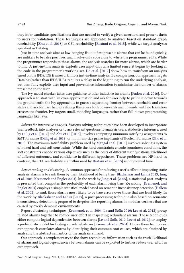
57:24 Xin Zhang, Radu Grigore, Xujie Si, and Mayur Naik
they infer candidate specifications that are needed to verify a given assertion, and present themto users for validation. These techniques are applicable to analyses based on standard graphreachability [Zhu et al. 2013] or CFL reachability [Bastani et al. 2015], while we target analysesspecified in Datalog.
Just-in-time analysis aims at low-hanging fruit: it first presents alarms that can be found quickly,are unlikely to be false positives, and involve only code close to where the programmer edits. Whilethe programmer responds to these alarms, the analysis searches for more alarms, which are harderto find. A just-in-time analysis exploits user input only in a limited sense: it begins by looking atthe code in the programmer’s working set. Do et al. [2017] show how to transform an analysisbased on the IFDS/IDE framework into a just-in-time analysis. By comparison, our approach targetsDatalog (rather than IFDS/IDE), requires a delay in the beginning to run the underlying analysis,but then fully exploits user input and provenance information to minimize the number of alarmspresented to the user.
The Ivy model checker takes user guidance to infer inductive invariants [Padon et al. 2016]. Ourapproach is to start with an over-approximation and ask for user help to prune it down towardsthe ground truth; the Ivy approach is to guess a separating frontier between reachable and errorstates and ask for user help in refining this guess both downwards and upwards, until no transitioncrosses the frontier. Ivy targets small, modeling languages, rather than full-blown programminglanguages like Java.
Solvers for interactive analysis. Various solving techniques have been developed to incorporateuser feedback into analyses or to ask relevant questions to analysis users. Abductive inference, usedby Dillig et al. [2012] and Zhu et al. [2013], involves computing minimum satisfying assignments toSMT formulae [Dillig et al. 2012] or minimum-size prime implicants of Boolean formulae [Zhu et al.2013]. The maximum satisfiability problem used by Mangal et al. [2015] involves solving a systemof mixed hard and soft constraints. While the hard constraints encode soundness conditions, thesoft constraints encode various objectives such as the costs of different user questions, likelihoodof different outcomes, and confidence in different hypotheses. These problems are NP-hard; incontrast, the CFL reachability algorithm used by Bastani et al. [2015] is polynomial time.
Report ranking and clustering. A common approach for reducing a user’s effort in inspecting staticanalysis alarms is to rank them by their likelihood of being true [Blackshear and Lahiri 2013; Junget al. 2005; Kremenek and Engler 2003]. In the work by Jung et al. [2005], a statistical post-analysisis presented that computes the probability of each alarm being true. Z-ranking [Kremenek andEngler 2003] employs a simple statistical model based on semantic inconsistency detection [Hallemet al. 2002] to rank those alarms most likely to be true errors over those that are least likely. Inthe work by Blackshear and Lahiri [2013], a post-processing technique also based on semanticinconsistency detection is proposed to de-prioritize reporting alarms in modular verifiers that arecaused by overly demonic environments.Report clustering techniques [Kremenek et al. 2004; Le and Soffa 2010; Lee et al. 2012] group
related alarms together to reduce user effort in inspecting redundant alarms. These techniqueseither compute logical dependencies between alarms [Le and Soffa 2010; Lee et al. 2012], or employa probabilistic model for finding correlated alarms [Kremenek et al. 2004]. Unlike these techniques,our approach correlates alarms by identifying their common root causes, which are obtained byanalyzing the abstract semantics of the analysis at hand.
Our approach is complementary to the above techniques; information such as the truth likelihoodof alarms and logical dependencies between alarms can be exploited to further reduce user effort inour approach.
Proc. ACM Program. Lang., Vol. 1, No. OOPSLA, Article 57. Publication date: October 2017.
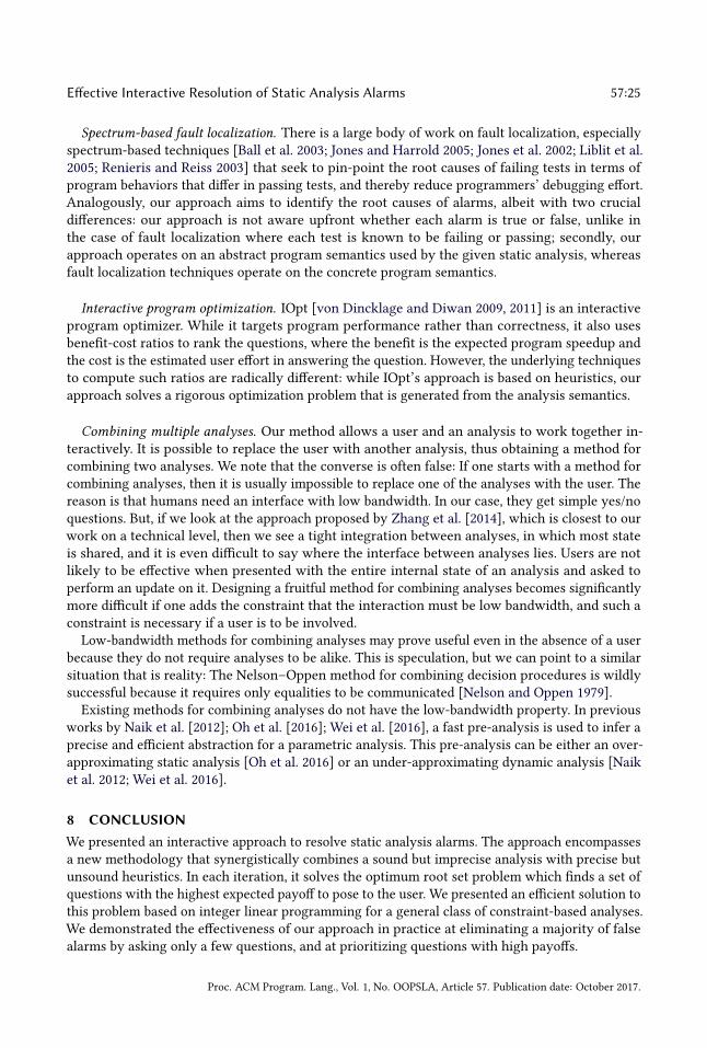
Effective Interactive Resolution of Static Analysis Alarms 57:25
Spectrum-based fault localization. There is a large body of work on fault localization, especiallyspectrum-based techniques [Ball et al. 2003; Jones and Harrold 2005; Jones et al. 2002; Liblit et al.2005; Renieris and Reiss 2003] that seek to pin-point the root causes of failing tests in terms ofprogram behaviors that differ in passing tests, and thereby reduce programmers’ debugging effort.Analogously, our approach aims to identify the root causes of alarms, albeit with two crucialdifferences: our approach is not aware upfront whether each alarm is true or false, unlike inthe case of fault localization where each test is known to be failing or passing; secondly, ourapproach operates on an abstract program semantics used by the given static analysis, whereasfault localization techniques operate on the concrete program semantics.
Interactive program optimization. IOpt [von Dincklage and Diwan 2009, 2011] is an interactiveprogram optimizer. While it targets program performance rather than correctness, it also usesbenefit-cost ratios to rank the questions, where the benefit is the expected program speedup andthe cost is the estimated user effort in answering the question. However, the underlying techniquesto compute such ratios are radically different: while IOpt’s approach is based on heuristics, ourapproach solves a rigorous optimization problem that is generated from the analysis semantics.
Combining multiple analyses. Our method allows a user and an analysis to work together in-teractively. It is possible to replace the user with another analysis, thus obtaining a method forcombining two analyses. We note that the converse is often false: If one starts with a method forcombining analyses, then it is usually impossible to replace one of the analyses with the user. Thereason is that humans need an interface with low bandwidth. In our case, they get simple yes/noquestions. But, if we look at the approach proposed by Zhang et al. [2014], which is closest to ourwork on a technical level, then we see a tight integration between analyses, in which most stateis shared, and it is even difficult to say where the interface between analyses lies. Users are notlikely to be effective when presented with the entire internal state of an analysis and asked toperform an update on it. Designing a fruitful method for combining analyses becomes significantlymore difficult if one adds the constraint that the interaction must be low bandwidth, and such aconstraint is necessary if a user is to be involved.
Low-bandwidth methods for combining analyses may prove useful even in the absence of a userbecause they do not require analyses to be alike. This is speculation, but we can point to a similarsituation that is reality: The NelsonśOppen method for combining decision procedures is wildlysuccessful because it requires only equalities to be communicated [Nelson and Oppen 1979].
Existing methods for combining analyses do not have the low-bandwidth property. In previousworks by Naik et al. [2012]; Oh et al. [2016]; Wei et al. [2016], a fast pre-analysis is used to infer aprecise and efficient abstraction for a parametric analysis. This pre-analysis can be either an over-approximating static analysis [Oh et al. 2016] or an under-approximating dynamic analysis [Naiket al. 2012; Wei et al. 2016].
8 CONCLUSION
We presented an interactive approach to resolve static analysis alarms. The approach encompassesa new methodology that synergistically combines a sound but imprecise analysis with precise butunsound heuristics. In each iteration, it solves the optimum root set problem which finds a set ofquestions with the highest expected payoff to pose to the user. We presented an efficient solution tothis problem based on integer linear programming for a general class of constraint-based analyses.We demonstrated the effectiveness of our approach in practice at eliminating a majority of falsealarms by asking only a few questions, and at prioritizing questions with high payoffs.
Proc. ACM Program. Lang., Vol. 1, No. OOPSLA, Article 57. Publication date: October 2017.

57:26 Xin Zhang, Radu Grigore, Xujie Si, and Mayur Naik
A PROOFS
Lemma 4.1. A sound analysis C can derive the ground truth; that is, True = JCKFalse.
Proof. By (2), we have JCKFalse ⊇ True. By the augmented semantics (Figure 4(d)), we also knowthat JCKFalse and False are disjoint. The result follows. □
Lemma 4.2. In Algorithm 1, suppose thatHeuristic returns all tuples T. Also, assume (1), (2), and (3).Then, Algorithm 1 returns the true alarms A ∩ True.
Proof. The key invariant is thatF ⊆ False ⊆ Q (4)
The invariant is established by setting F := ∅ and Q := T. By (1), we know that Y ⊆ True andN ⊆ False, on line 5. It follows that the invariant is preserved by removing Y from Q, on line 6. Italso follows that F∪N ⊆ False and, by (2), that JCKF∪N ⊇ True. So, the invariant is also maintainedby line 7. We conclude that (4) is indeed an invariant.
For termination, let us start by showing that |Q \ F| is nonincreasing. According to lines 6 and 7,the values of Q and F in the next iteration will be Q′ := Q \ Y and F′ := (Q \ Y ) \ JCKF∪N . We nowshow that F ⊆ F′ and Q′ ⊆ Q. Consider an arbitrary f ∈ F. By (4), f ∈ Q. Using Y ⊆ True and (4),we conclude that Y and F are disjoint; using the augmented semantics in Figure 4(d), we concludethat JCKF∪N and F are disjoint. Thus, f ∈ F′, and, since f was arbitrary, we conclude F ⊆ F′. ForQ′ \ Q, it suffices to notice that Y ⊆ True.Now let us show that |Q \ F| is not only nonincreasing but in fact decreasing. By (3), we know
that R is non-empty, and thus at least one of Y or N is non-empty. If Y is non-empty, then Q′ ⊂ Q.If N is non-empty, then F ⊂ F′. We can now conclude that Algorithm 1 terminates.
When the main loop terminates, we have F = Q. Together with the invariant (4), we obtain thatF = False. By Lemma 4.1, it follows that Algorithm 1 returns A ∩ True. □
B ALTERNATIVE USE CASE: COMBINING TWO STATIC ANALYSES
While our approach targets interactive alarm resolution, it can be also applied to combine twoanalyses and balance the overall precision and scalability. We can enable this use case by replacingthe human user with a precise yet expensive analysis. Such an iterative combination of the twoanalyses is beneficial as it may take a significant amount of time to apply the precise analysis toresolve all potential causes in the base analysis. Ursa allows the precise analysis to resolve only thecauses that are relevant to the alarms and focus on causes with high payoffs. We next demonstratethis use case by using combining two pointer analyses as an example. We first describe the baseanalysis, its notions of alarms and causes, and our implementation of the procedure Heuristic. Thenwe describe the oracle analysis. Finally, we empirically evaluate our approach.
Base Analysis. Our base pointer analysis is a flow/context-insensitive, field-sensitive, Anderson-style analysis with on-the-fly call-graph construction [Lhoták 2002]. It uses object allocation sitesas the heap abstraction. It comprises 46 rules, 29 input relations, and 18 output relations.
We treat points-to facts (denoted by relation pointsTo) and call-graph edges (denoted by callEdge)as the alarms as they are directly consumed by client analyses built atop PointerAnalysis. Given thelarge number of tuples in these two relations, we further limit the alarms to tuples in the application(as opposed to library) code. We treat the same set of tuples as the universe of potential causessince the tuples in these two relations are used to derive each other in a recursive manner.
We are not aware of effective static heuristics for pointer analysis alarms that are client-agnostic.Therefore, we only provide a Heuristic instantiation that leverages a dynamic analysis:
dynamic() = {pointsTo(v,o) | variable v is accessed in the runs and never points to object o} ∪
{callEdge(p,m) | invocation site p is reached and never invokes methodm in the runs }
Proc. ACM Program. Lang., Vol. 1, No. OOPSLA, Article 57. Publication date: October 2017.
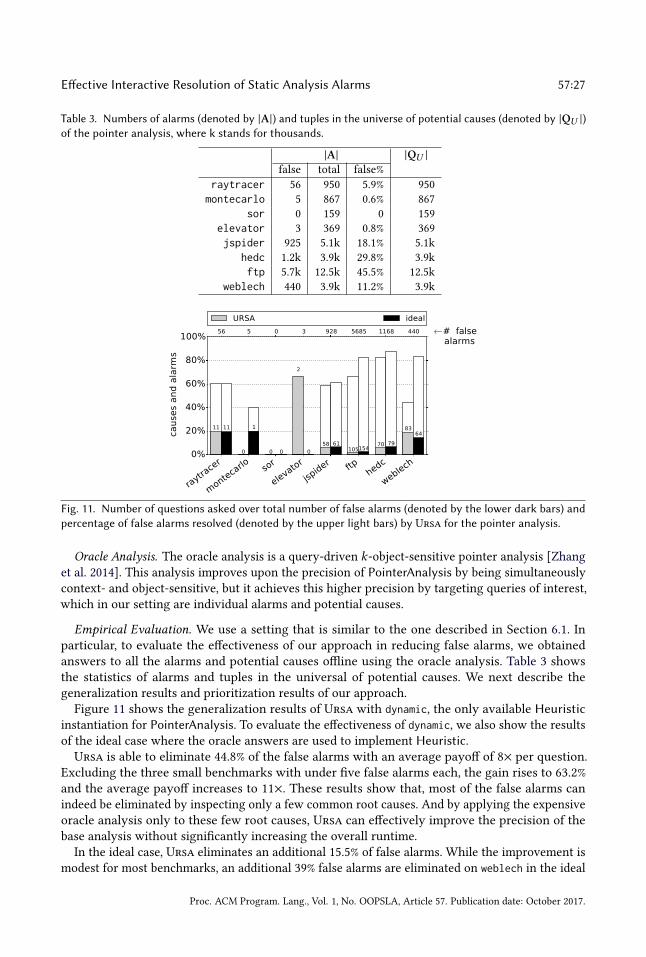
Effective Interactive Resolution of Static Analysis Alarms 57:27
Table 3. Numbers of alarms (denoted by |A|) and tuples in the universe of potential causes (denoted by |QU |)
of the pointer analysis, where k stands for thousands.
|A| |QU |
false total false%
raytracer 56 950 5.9% 950
montecarlo 5 867 0.6% 867
sor 0 159 0 159
elevator 3 369 0.8% 369
jspider 925 5.1k 18.1% 5.1k
hedc 1.2k 3.9k 29.8% 3.9k
ftp 5.7k 12.5k 45.5% 12.5k
weblech 440 3.9k 11.2% 3.9k
raytra
cer
monte
carlo so
r
elevator
jspider ftp
hedc
weblech0%
20%
40%
60%
80%
100%
cau
ses
an
d a
larm
s
11
0 0
2
58 105
70
83 11 1
0 0
61 154
79
64
56 5 0 3 928 5685 1168 440
URSA ideal
Ã# false alarms
Fig. 11. Number of questions asked over total number of false alarms (denoted by the lower dark bars) and
percentage of false alarms resolved (denoted by the upper light bars) by Ursa for the pointer analysis.
Oracle Analysis. The oracle analysis is a query-driven k-object-sensitive pointer analysis [Zhanget al. 2014]. This analysis improves upon the precision of PointerAnalysis by being simultaneouslycontext- and object-sensitive, but it achieves this higher precision by targeting queries of interest,which in our setting are individual alarms and potential causes.
Empirical Evaluation. We use a setting that is similar to the one described in Section 6.1. Inparticular, to evaluate the effectiveness of our approach in reducing false alarms, we obtainedanswers to all the alarms and potential causes offline using the oracle analysis. Table 3 showsthe statistics of alarms and tuples in the universal of potential causes. We next describe thegeneralization results and prioritization results of our approach.Figure 11 shows the generalization results of Ursa with dynamic, the only available Heuristic
instantiation for PointerAnalysis. To evaluate the effectiveness of dynamic, we also show the resultsof the ideal case where the oracle answers are used to implement Heuristic.Ursa is able to eliminate 44.8% of the false alarms with an average payoff of 8× per question.
Excluding the three small benchmarks with under five false alarms each, the gain rises to 63.2%and the average payoff increases to 11×. These results show that, most of the false alarms canindeed be eliminated by inspecting only a few common root causes. And by applying the expensiveoracle analysis only to these few root causes, Ursa can effectively improve the precision of thebase analysis without significantly increasing the overall runtime.
In the ideal case, Ursa eliminates an additional 15.5% of false alarms. While the improvement ismodest for most benchmarks, an additional 39% false alarms are eliminated on weblech in the ideal
Proc. ACM Program. Lang., Vol. 1, No. OOPSLA, Article 57. Publication date: October 2017.

57:28 Xin Zhang, Radu Grigore, Xujie Si, and Mayur Naik
3 6 9 12 15# questions
0
10
20
30
40
50#
ala
rms
raytracer
ideal
URSA
1 2 3 4 5# questions
0
1
2
3
4
5
# a
larm
s
montecarlo
1 2 3 4 5# questions
0
1
2
3
4
5
# a
larm
s
sor
no false alarms
1 2 3 4 5# questions
0
1
2
3
4
5
# a
larm
s
elevator
15 30 45 60 75# questions
0
150
300
450
600
750
# a
larm
s
jspider
40 80 120 160 200# questions
0
1000
2000
3000
4000
5000#
ala
rms
ftp
20 40 60 80 100# questions
0
250
500
750
1000
1250
# a
larm
s
hedc
20 40 60 80 100# questions
0
80
160
240
320
400
# a
larm
s
weblech
Fig. 12. Number of questions asked and number of false alarms resolved by Ursa in each iteration.
case. The reason for this anomaly is that the input set used in dynamic does not yield sufficient codecoverage to produce accurate predictions for the desired root causes. We thus conclude that overall,the dynamic instantiation is effective in identifying common root causes of false alarms.
Figure 12 shows the prioritization results of Ursa. Every point in the plots represents the numberof false alarms eliminated (y-axis) and the number of questions (x-axis) asked up to the currentiteration. As before, we compare the results of Ursa to the ideal case.We observe that a few causes often yield most of the benefits. For instance, four causes can
resolve 1,133 out of 5,685 false alarms on ftp, yielding a payoff of 283×. Ursa successfully identifiesthese causes with high payoffs and poses them to the oracle analysis in the earliest few iterations. Infact, for the first three iterations on most benchmarks, Ursa asks exactly the same set of questionsas the ideal setting. The results of these two settings only differ in later iterations, where thepayoff becomes relatively low. We also notice that there can be multiple causes in the set that givesthe highest benefit (for instance, the aforementioned ftp results). The reason is that there can bemultiple derivations to each alarm. If we naively search the potential causes by fixing the numberof questions in advance, we can miss such causes. Ursa, on the other hand, successfully finds themby solving the optimal root set problem iteratively.
The fact that Ursa is able to prioritize causes with high payoffs allows us to stop the interactionof the two analyses after a few iterations and still get most of the benefits. Ursa terminates eitherwhen the expected payoff drops to one or when there are no more questions to ask. But in practice,we might choose to stop the interaction even earlier. For instance, we might be satisfied with thecurrent result, or we may find limited payoff in running the oracle analysis, which can take a longtime comparing to inspecting the rest alarms manually.We study these causes with high payoffs more closely. The main causes are the points-to facts
and call-graph edges that lead to one or multiple spurious call-graph edges, which in turn lead tomany false tuples. Such spurious tuples are produced due to context insensitivity of the analysis.
ACKNOWLEDGMENTS
We thank Aditya Nori for discussions. We also thank the anonymous reviewers for insightfulcomments. This work was supported by DARPA under agreement #FA8750-15-2-0009, NSF awards#1253867 and #1526270, MIT Lincoln Laboratory, and a Facebook Fellowship. The U.S. Governmentis authorized to reproduce and distribute reprints for Governmental purposes notwithstanding anycopyright thereon.
Proc. ACM Program. Lang., Vol. 1, No. OOPSLA, Article 57. Publication date: October 2017.

Effective Interactive Resolution of Static Analysis Alarms 57:29
REFERENCES
2015. UpWork. http://www.upwork.com. (2015). Accessed: 2015-11-19.
Nathaniel Ayewah, David Hovemeyer, J. David Morgenthaler, John Penix, and William Pugh. 2008. Using static analysis to
find bugs. IEEE Software (2008).
Thomas Ball, Mayur Naik, and Sriram K. Rajamani. 2003. From symptom to cause: localizing errors in counterexample
traces. In POPL.
Osbert Bastani, Saswat Anand, and Alex Aiken. 2015. Specification inference using context-free language reachability. In
POPL.
Al Bessey, Ken Block, Benjamin Chelf, Andy Chou, Bryan Fulton, Seth Hallem, Charles-Henri Gros, Asya Kamsky, Scott
McPeak, and Dawson R. Engler. 2010. A few billion lines of code later: using static analysis to find bugs in the real world.
Commun. ACM (2010).
Sam Blackshear and Shuvendu Lahiri. 2013. Almost-correct specifications: a modular semantic framework for assigning
confidence to warnings. In PLDI.
Tom Copeland. 2005. PMD applied. (2005).
Isil Dillig, Thomas Dillig, and Alex Aiken. 2012. Automated error diagnosis using abductive inference. In PLDI.
Lisa Nguyen Quang Do, Karim Ali, Benjamin Livshits, Eric Bodden, Justin Smith, and Emerson Murphy-Hill. 2017. Just-in-
time static analysis. In ISSTA.
Michael D. Ernst, Jake Cockrell, William G. Griswold, and David Notkin. 2001. Dynamically discovering likely program
invariants to support program evolution. IEEE Trans. Software Eng. (2001).
Gurobi Optimization, Inc. 2016. Gurobi optimizer reference manual. http://www.gurobi.com. (2016).
Seth Hallem, Benjamin Chelf, Yichen Xie, and Dawson R. Engler. 2002. A system and language for building system-specific,
static analyses. In PLDI.
James A. Jones and Mary Jean Harrold. 2005. Empirical evaluation of the tarantula automatic fault-localization technique.
In ASE.
James A. Jones, Mary Jean Harrold, and John T. Stasko. 2002. Visualization of test information to assist fault localization. In
ICSE.
Herbert Jordan, Bernhard Scholz, and Pavle Subotic. 2016. Soufflé: on synthesis of program analyzers. In CAV.
Yungbum Jung, Jaehwang Kim, Jaeho Shin, and Kwangkeun Yi. 2005. Taming false alarms from a domain-unaware C
analyzer by a bayesian statistical post analysis. In SAS.
Ted Kremenek, Ken Ashcraft, Junfeng Yang, and Dawson Engler. 2004. Correlation exploitation in error ranking. In FSE.
Ted Kremenek and Dawson Engler. 2003. Z-Ranking: using statistical analysis to counter the impact of static analysis
approximations. In SAS.
Wei Le and Mary Lou Soffa. 2010. Path-based Fault Correlations. In FSE.
Woosuk Lee, Wonchan Lee, and Kwangkeun Yi. 2012. Sound non-statistical clustering of static analysis alarms. In VMCAI.
Ondrej Lhoták. 2002. Spark: A flexible points-to analysis framework for Java. (2002).
Ben Liblit, Mayur Naik, Alice X. Zheng, Alexander Aiken, and Michael I. Jordan. 2005. Scalable statistical bug isolation. In
PLDI.
Benjamin Livshits, Manu Sridharan, Yannis Smaragdakis, Ondrej Lhoták, José Nelson Amaral, Bor-Yuh Evan Chang, Samuel Z.
Guyer, Uday P. Khedker, Anders Mùller, and Dimitrios Vardoulakis. 2015. In defense of soundiness: a manifesto. CACM
(2015).
Magnus Madsen, Ming-Ho Yee, and Ondrej Lhoták. 2016. From Datalog to Flix: a declarative language for fixed points on
lattices. In PLDI.
Ravi Mangal, Xin Zhang, Aditya V. Nori, and Mayur Naik. 2015. A user-guided approach to program analysis. In FSE.
Mayur Naik. 2006. Chord: A Program Analysis Platform for Java. http://jchord.googlecode.com/. (2006).
Mayur Naik, Alex Aiken, and John Whaley. 2006. Effective static race detection for Java. In PLDI.
Mayur Naik, Hongseok Yang, Ghila Castelnuovo, and Mooly Sagiv. 2012. Abstractions from tests. In POPL.
Greg Nelson and Derek C. Oppen. 1979. Simplification by cooperating decision procedures. ACM TOPLAS (1979).
Hakjoo Oh, Wonchan Lee, Kihong Heo, Hongseok Yang, and Kwangkeun Yi. 2016. Selective X-sensitive analysis guided by
impact pre-analysis. ACM TOPLAS (2016).
Oded Padon, Kenneth McMillan, Aurojit Panda, Mooly Sagiv, and Sharon Shoham. 2016. Ivy: safety verification by interactive
generalization. In PLDI.
Christos H. Papadimitriou. 1981. On the complexity of integer programming. J. ACM (1981).
J. Ross Quinlan. 1993. C4.5: Programs for Machine Learning. Morgan Kaufmann.
Manos Renieris and Steven P. Reiss. 2003. Fault localization with nearest neighbor queries. In ASE.
Henry Gordon Rice. 1953. Classes of recursively enumerable sets and their decision problems. Trans. Amer. Math. Soc.
(1953).
Proc. ACM Program. Lang., Vol. 1, No. OOPSLA, Article 57. Publication date: October 2017.

57:30 Xin Zhang, Radu Grigore, Xujie Si, and Mayur Naik
Yannis Smaragdakis and Martin Bravenboer. 2010. Using Datalog for fast and easy program analysis. In Datalog 2.0
Workshop.
Yannis Smaragdakis, George Kastrinis, and George Balatsouras. 2014. Introspective analysis: context-sensitivity, across the
board. In PLDI.
Daniel von Dincklage and Amer Diwan. 2009. Optimizing programs with intended semantics. In OOPSLA.
Daniel von Dincklage and Amer Diwan. 2011. Integrating program analyses with programmer productivity tools. Softw.,
Pract. Exper. (2011).
Shiyi Wei, Omer Tripp, Barbara G. Ryder, and Julian Dolby. 2016. Revamping JavaScript static analysis via localization and
remediation of root causes of imprecision. In FSE.
John Whaley, Dzintars Avots, Michael Carbin, and Monica S. Lam. 2005. Using Datalog with binary decision diagrams for
program analysis. In APLAS.
Xin Zhang, Ravi Mangal, Radu Grigore, Mayur Naik, and Hongseok Yang. 2014. On abstraction refinement for program
analyses in Datalog. In PLDI.
Haiyan Zhu, Thomas Dillig, and Isil Dillig. 2013. Automated inference of library specifications for source-sink property
verification. In APLAS 2013.
Proc. ACM Program. Lang., Vol. 1, No. OOPSLA, Article 57. Publication date: October 2017.