Standard finite element techniques for efficient stress analysis of adhesive joints

ARTICLE IN PRESS

International Journal of Adhesion & Adhesives 29 (2009) 125– 135

Contents lists available at ScienceDirect

International Journal of Adhesion & Adhesives

0143-74

doi:10.1

� Corr

E-m

journal homepage: www.elsevier.com/locate/ijadhadh

Standard finite element techniques for efficient stress analysisof adhesive joints

D. Castagnetti �, E. Dragoni

Dipartimento di Scienze e Metodi dell’Ingegneria, Universita di Modena e Reggio Emilia, Italy

a r t i c l e i n f o

Article history:

Accepted 11 January 2008

The paper documents ongoing research in the field of stress analysis of adhesive bonded joints and aims

at developing efficient and accurate finite element techniques for the simplified calculation of adhesive
Available online 21 March 2008
Keywords:

C. Finite element stress analysis

E. Joint design

C. Lap shear

96/$ - see front matter & 2008 Elsevier Ltd. A

016/j.ijadhadh.2008.01.005

esponding author. Tel.: +39 0522 52 2634; fax

ail address: [email protected] (D

a b s t r a c t

stresses. Goal of the research is to avoid the major limitations of existing methods, in particular their

dependency on special elements or procedures not supported by general purpose analysis packages.

Two simplified computational methods, relying on standard modelling tools and regular finite elements

are explored and compared with the outcome of theoretical solutions retrieved from the literature and

with the results of full, computationally intensive, finite element analyses. Both methods reproduce the

adherends by means of structural elements (beams or plates) and the adhesive by a single layer of solid

elements (plane-stress or bricks). The difference between the two methods resides in the thickness and

in the elastic properties given to the adhesive layer. In one case, the adhesive thickness is extended up to

the midplane of the adherends and its elastic modulus is proportionally increased. In the other case, the

adhesive layer is maintained at its true properties and the connection to the adherends is enforced by

standard kinematic constraints. The benchmark analyses start from 2D single lap joints and are then

extended to 3D configurations, including a wall-bonded square bracket undergoing cantilever loading.

One of the two simplified methods investigated provides accurate results with minimal computational

effort for both 2D and 3D configurations.

& 2008 Elsevier Ltd. All rights reserved.

1. Introduction

This paper deals with the development of finite elementtechniques for efficient stress analysis of structural bonded joints.The increased application of adhesive bonding for structuraljoining was accompanied by the development of mathematicaland numerical models to analyse or predict the behaviour of thosejoints. Among the numerical models, the finite element methodhas been extensively used. Different special adhesive elementshave been formulated both in two and three dimensions, tocapture the main features of stresses in the adhesive layer,through a simple, efficient and cost-effective procedure. One ofthe first two-dimensional (2D) adhesive elements was presentedby Rao et al. [1]. They developed a special six-noded isoparametricelement for the adhesive layer, compatible with the eight-nodedisoparametric quadratic element used to model the adherends. Ina subsequent work, Yadagiri et al. [2] modified that element toinclude longitudinal and normal stresses and linear viscoelasticresponse. Hereditary integrals were used to represent the

ll rights reserved.

: +39 0522 52 2609.

. Castagnetti).

stress–strain relations. Reddy and Roy [3] proposed a special 2Dfinite element based on the updated Lagrangian formulation ofelastic solids, for geometric and material nonlinear analysis.Amijima and Fujii [4] developed a simple one-dimensional FEMwhich can be used to calculate normal and shear stresses in theadhesive layer of adhesive bonded structures. Thermal expansionof both adherends and shrinkage of the adhesive are considered.Carpenter [5] presented a special 2D adhesive element to modelthe viscoelastic behaviour of the adhesive. Lin and Lin [6]presented a 2D finite element formulation for single lap adhesivejoints which can analyse the distribution of the shear and normalstresses in a variety of configurations with any possible adhesive-layer conditions and non-identical adherends. Edlund and Klarbr-ing [7] developed a special element for geometric nonlinearanalysis. Andruet et al. [8] developed an ad hoc model for three-dimensional (3D) analysis of adhesive joints based on shell andsolid elements. The shell elements are used to model theadherends and the adhesive layer is modelled as a solid elementwith offset nodes in the midplane of the adherends. The elementformulation includes geometric nonlinearities, together withthermal and moisture effects. Goncalves et al. [9] proposed anew 3D finite element model to study the behaviour of adhesivejoints. The model includes an interface element previously

www.sciencedirect.com/science/journal/jaad

www.elsevier.com/locate/ijadhadh

dx.doi.org/10.1016/j.ijadhadh.2008.01.005

mailto:[email protected]

ARTICLE IN PRESS

Nomenclature

E Young’s modulus of the adherendsEa Young’s modulus of the adhesive layerE0a increased Young’s modulus of the adhesive layer in

method B

Ga shear modulus of the adhesive layerM0 bending moment at the transition sections between

free adherends and overlapping portion of the jointP concentrated load applied to the jointT axial force at the transition sections between free

adherends and overlapping portion of the jointV0 shear force at the transition sections between free

adherends and overlapping portion of the jointc half of the overlap length of the jointe eccentricity between adherendsk dimensionless parameter in Goland and Reissner’s

analytical modelk0 dimensionless parameter in Goland and Reissner’s

analytical model

l length of the non-overlapping portion of the adher-ends

p axial stress applied to the adherendssa thickness of the adhesive layers0a extended thickness of the adhesive layer in method B

t adherend thicknessu longitudinal displacementv transverse displacementb dimensionless parameter in Goland and Reissner’s

analytical modeln Poisson’s ratio of the adherendsna Poisson’s ratio of the adhesives peel stress in the adhesive layersmax peak value of peel stresses in the adhesive layert shear stress in the adhesive layertmax peak value of shear stresses in the adhesive layertres resultant shear stresses in the adhesive layero degree of non linearity in Goland and Reissner’s

analytical model

D. Castagnetti, E. Dragoni / International Journal of Adhesion & Adhesives 29 (2009) 125–135126

developed compatible with brick solid elements from the ABAQUSsoftware. The main objective was to calculate the stresses at theinterfaces between adherends and adhesive. Tong and Sun [10]developed a novel finite element formulation for adhesiveelements specific for conducting quick stress analysis of bondedrepairs to curved structures. They proposed three adhesiveelements (8-node, 16-node and 18-node) referred to as 2.5-D.The elements comprise a pseudo-brick adhesive element and twoshell elements located on either side of the adhesive layer. Shellelements are offset by half the thickness of the corresponding wallthickness of the element. The adhesive element provides anefficient and cost effective way to model the overlap area inbonded repairs.

The major drawback of available methods for the simplifiedcalculation of adhesive stresses is their dependency on specialelements or algorithms which are not readily implemented ingeneral purpose finite element systems for the analysis ofcomplex structures.

This paper aims at overcoming that limitation by exploring themerits of two simplified computational approaches relying onstandard modelling tools and regular finite elements, routinelysupported by most commercial packages. The work is part of awider research program dealing with the development ofsimple, general, portable, efficient and accurate finite elementprocedures for the mechanical analysis of thin-walled bondedconstructions [11].

Table 1Reference geometry and simplified models for the single lap joint

Model Sketch

Reference geometry

Full model (A)

Reduced model (B)

Reduced model (C)

2. Method

Table 1 schematically displays the different methods used inthe paper for the analysis of bonded joints. The first row depictsthe real configuration which is, for the sake of example, embodiedby a 2D single lap joint. The second row (model A) describes theclassical approach consisting in a refined, computationallyintensive, full finite element model. That model is used in thepaper to provide an exact reference solution. The third and thefourth rows (models B and C) illustrate the novel reducedtechniques proposed by this investigation.

Both reduced models B and C reproduce the adherends withstructural beam elements and describe the adhesive with a singlelayer of continuum plane-stress elements. The beam elements lieon the adherend axes and are mutually offset by distance e, equal

to the eccentricity of the bonded plates. In reduced model B, theadhesive is extended up to the beam axes (thickness s0a ¼ e4sa),and the Young’s modulus of the adhesive is increased up toE0a ¼ Eas0a=sa. That correction is introduced to conserve the samestiffness, under peel and shear deformations, as in the originallayer (see below). In reduced model C, the adhesive conserves itstrue thickness, sa, and is connected, on both sides, to the nodes ofthe adherend beams with kinematics constraints (tied lines) thatenforce equality of the corresponding degrees of freedom.

The assessment of the methods under scrutiny is performed intwo steps: a first 2D exploration step and a second 3D validationstep.

In the first step, the popular single lap joint geometry, welldocumented in literature [8,12], is used as a 2D benchmark test.The stress response provided by the two reduced methods iscompared systematically with Goland and Reissner’s analyticalresults [12] and with the outcome of a conventional finiteelements analysis for a wide range of geometries and materialproperties. In this step, Goland and Reissner’s solution is used asthe only analytical term of comparison because, despite muchwork on the single lap joint in the last decades [13–17], theirmodel still represents the most authoritative theoretical referencefor this joint configuration [18].

In the second step, the reduced model performing best in thefirst step is applied to two 3D geometries and the results arechecked against the prediction of full finite element analyses.

All the finite element calculations described in the followingwere performed with ABAQUS software, version 6.5 [19].

ARTICLE IN PRESS

D. Castagnetti, E. Dragoni / International Journal of Adhesion & Adhesives 29 (2009) 125–135 127

2.1. Step 1: 2D analyses

This is an exploration step devoted to 2D analyses of single lapjoints. The step is divided into two parts. The first part involvesthe preliminary analysis of a specific joint configuration and it hasbeen mainly performed to practice with the proposed methodsand to carry out mesh convergence iterations. The second partexplores systematically a number of joint geometries and materialcombinations and has been performed to assess the sensitivity ofthe methods to variations of joint properties.

2.1.1. Preliminary 2D analysis

All three different methods (full model A, reduced model B andreduced model C) are applied to the reference geometry of Table 1with dimensions, loading and constraints given in Fig. 1. Unitthickness in the direction normal to the page is assumed. Young’smodulus and Poisson’s ratio of the adherends are, respectively,E ¼ 69,000 MPa, and n ¼ 0.3 corresponding to aluminium-alloy.A Young’s modulus Ea ¼ 2500 MPa and a Poisson’s ratio na ¼ 0.3are assumed for the adhesive layer, corresponding to a two-part,high strength, epoxy adhesive. Constraints are applied to theadherends’ axes so as to reproduce a fixed support on the left endand a guided support on the right end of the joint. To the guidedend, a concentrated load, P, is applied in five increments whichproduces a geometrically nonlinear response of the joint. Inaccordance with Goland and Reissner’s analytical model [12], thedegree of nonlinearity is a function of the parameter o ¼ c=t

ffiffiffiffiffiffiffiffip=E

p,

where c represents one-half of the overlap length of the joint, t

represents the adherend thickness and p is the axial stress appliedto the adherends (see Appendix A). In this preliminary analysis ois varied from 0.1 to 0.5 by increments of 0.1. The correspondingconcentrated loads are P ¼ 19.2, 76.7, 172.5, 306.7, and 479.2 N,respectively. The chosen interval of parameter o produces avariation of the bending factor k (Appendix A) ranging from 0.75to 0.40. Parameter o instead of k has been used as a measure ofthe nonlinearity because it depends in a more straightforwardway on the design variables of the joint.

All the finite element analyses performed include nonlineargeometric effects in the solution procedure.

2.1.1.1. Full finite element model. The full model (A of Table 1) ex-actly reproduces the geometry of the joint of Fig. 1 and in-corporates the material properties given above. The mesh is basedon quadratic, plane-stress, rectangular elements with a length of0.05 mm and a height of 0.025 mm, evenly distributed throughoutthe model. As a result, four elements are stacked through thethickness of the adhesive layer. Plane-stress rather than plain-strain elements have been adopted because this condition is im-plied by the beam elements used to describe the adherends inreduced models B and C (see below). In order to check the effect ofthe plane-stress assumption on the stress results, the convergedfull finite element model has also been analysed in a plain-staincondition (see Section 4).

The element dimensions adopted in the analysis have beenchosen after a mesh convergence procedure focused on the peak

e=1.1 mm sa=0.1 mm

2c=12mm

P

t=1 mm

t=1 mm

l=25 mm l=25mm

x

Fig. 1. Benchmark geometry for the single lap joint.

stresses arising on the midline of the adhesive. A stressconvergence is meaningful along this path, because the midlineis free from the theoretical singularities which affect the adhesive/adherend interface at the edges of the overlap. The convergedmesh, showing no improvement of results upon further gridrefinement, contains 3400 elements and 11,649 nodes for a totalof 21,298 degrees of freedom.

2.1.1.2. Reduced method B. Reduced model B reproduces the geo-metry of the reference joint by using beams for the adherends andby extending the adhesive layer up to the beam nodes. As a result,the adhesive layer has thickness equal to the adherends eccen-tricity. The mesh consists of quadratic beam elements along theadherends, having a length equal to the adherends eccentricity.The adhesive layer is modelled by a single strip of quadratic,plane-stress, square elements with a side length equal to the ex-tended thickness of the adhesive layer. The longitudinal dimen-sion of the elements was chosen after several mesh refinementiterations showed converging results. With regard to the materialproperties, the adherends maintain the previously defined elasticproperties while Young’s modulus of the adhesive is increased upto E0a ¼ Eas0a=sa ¼ 27;500 MPa, in accordance with the previouslydefined criterion (conservation of peel and shear stiffness). Themodel contains 79 elements and 196 nodes for a total of 530degrees of freedom, about 40 times less than the full model.

2.1.1.3. Reduced method C. Reduced model C reproduces the re-ference joint geometry by using beams for the adherends and byconserving the real thickness of the adhesive layer. This choicecreates a gap between the adherends, modelled with quadraticbeam elements, and the corresponding edges of the adhesivelayer, which is discretized by a single row of quadratic, plane-stress, quadrilateral elements. The connectivity between adhesiveand adherend meshes is enforced by means of internal constraintslinking the corresponding nodes of the parts. These constraints,realized through the tied mesh option of ABAQUS and available inall FE packages, make the active degrees of freedom of any node ofa chosen feature (surface or line) equal to the degrees of freedomof a parent node belonging to another feature.

The mesh convergence analysis has been carried out in thiscase too, indicating an optimal element length (for both beamsand quadrilaterals) equal to the eccentricity between theadherends. The converged model contains 79 elements and 196nodes for a total of 530 degrees of freedom.

2.1.2. Systematic 2D analyses

The systematic analyses are aimed at comparing the results ofmethod A (benchmark), method B and method C (new proposals)for a wider range of geometries and elastic properties of the joint.The scope of the preliminary analysis is extended to a broad set ofconfigurations, planned according to the criteria of designedexperiments [20]. The variables involved in the analyses arecollected in Table 2. The choice of type and values of thesevariables was guided by the analytical model for the single lapjoint developed by Goland and Reissner [12] and detailed inAppendix B.

Table 2Values of the joint parameters used in the analysis plan

t (mm) 0.3 1 3

c/t 1.5 3 6

E (MPa) 23,000 69,000 206,000

n 0.3 0.3 0.3

Material GFRP: 25%, 01; 50%, 7451; 25%, 901 Aluminium-alloy Steel

ARTICLE IN PRESS

Fig. 2. Geometry of the 3D test problem.


A full factorial analysis plan, consisting of 27 geometricconfigurations, is obtained by combining, in all possible ways,the variables of Table 2. Following the indications of thedimensional analysis of Appendix B, the properties of the adhesivelayer maintain, without loss of generality, the values of step 1through all the systematic screening (thickness sa ¼ 0.1 mm,Young’s modulus Ea ¼ 2500 MPa, Poisson’s ratio na ¼ 0.3). Inaddition, the ratio between the length of the non-overlappingportion of the adherends, l, and the adherends thickness, t, is heldconstant at l/t ¼ 25. Each parameter in Table 2 varies over threelevels and covers a range sufficiently wide to embrace most realsituations. The only exception to this rule is represented by theratio c/t which was limited up to 6 due to the impossibility tomanage the numerical models arising from the longest overlaps(c/tX10) that can occur in practice.

By choosing in Table 2 the specific combination of variablest ¼ 1 mm, c/t ¼ 6, E ¼ 69,000 MPa, the same configuration exam-ined in Section 2.1.1 is obtained. In addition to those systematicanalyses, several runs have also been performed assumingthe same elastic modulus for the adherends and for theadhesive (E ¼ 2500 MPa), to simulate joining between polymericadherends.

Models A, B and C have been implemented with the samecriteria described in the previous section. For each configuration,three load levels were applied in subsequent increments to thejoint. The load levels were calculated with Goland and Reissner’sequations, to generate peak values of the peel stress in the ratio of0.001, 0.01 and 0.1 to Young’s modulus, Ea, of the adhesive. Thisinterval of expected stresses in the adhesive was chosen so as tocover a wide range of output stresses, independently of thestrength of real structural adhesives, and to test the effect ofsevere nonlinearity on the accuracy of the proposed methods.

2.2. Step 2: 3D analyses

This is a validation step dealing with 3D analyses of bondedjoints. The step is divided into two parts. The first part involvesthe analysis of the same single lap joint examined in Section 2.1.1,seen as a 3D structure. The second part deals with the analysis of asquare bracket bonded to a wall and undergoing cantileverloading.

On the basis of the results obtained in Step 1, showing thatmethod B provides poor results in comparison with method C (seeSection 3) the investigation of Step 2 is focused on the comparisonbetween method A (benchmark) and method C (new proposal).

2.2.1. Analysis of 3D single lap

As first validation test of reduced method C, the same single lapjoint configuration considered in Section 2.1.1 (Fig. 1) wasexamined as a 3D structure. A 5 mm width is assumed in thedirection normal to the page and, because of the symmetry ofthe 3D configuration, both models A and C consider only half ofthe joint in the width direction.

Method A has been implemented by extruding the plane-stresselements of the 2D model into linear brick elements with a sidelength in the width direction equal to the length in thelongitudinal direction. As a consequence, the model contains189,440 elements and 206,000 nodes for a total of 620,058degrees of freedom. Linear elements instead of quadratic elementswere used for the impossibility to handle the full quadratic modelwith the available hardware. Confidence in the linear model wasgained by running also the 2D joint with linear elements andobtaining results very close to the quadratic model.

To implement method C on the 3D single lap joint, beamelements on the adherends have been replaced by structural

quadratic shell elements, while the adhesive layer was discretizedwith one layer of quadratic brick elements as thick as the trueadhesive layer. Element dimensions are the same as in the 2Dmodel and, similarly to method A, an element side length isassumed in the width direction equal to the one in thelongitudinal direction. Internal constraints (tied mesh) are appliedbetween shell elements and the corresponding adhesive surfacesto enforce a material link between adhesive and adherends alongthe overlap. The model contains 158 elements and 778 nodes for atotal of 4002 degrees of freedom, that is over 150 times less thanfull model A.

The joint was loaded with same load levels per unit widthadopted in Section 2.1.2 for the corresponding 2D joint with thesame plan dimensions.

2.2.2. Analysis of 3D bracket

As second validation test for simplified method C, the 3Dconfiguration of Fig. 2 was considered. An aluminium bracket(E ¼ 69,000 MPa, n ¼ 0.3) is bonded to a steel wall (E ¼ 210,000MPa, n ¼ 0.3) through an epoxy adhesive layer (sa ¼ 0.1 mm,Ea ¼ 2500 MPa, na ¼ 0.3) and undergoes an asymmetric cantileverload (P ¼ 100 N). The wall is built-in along its boundary. A singleload level was applied to the structure because geometricnonlinearity is not significant for this joint configuration.

The quality of the simplified analysis is assessed by comparingthe results of method C with the output of a conventional finiteelement model (method A). Due to the remarkable amount ofcomputational resources needed to run method A, discretizationof the adherends (square bracket and wall) have been performedwith quadratic bricks having side lengths of 0.15 mm in the planeof the adherends and a length through the thickness uniformlyvarying from 0.03 mm (near to the adhesive) to about 0.45 mm(on the opposite face). In method C, bracket and wall plate weremodelled with quadratic shell elements placed on the midsurfaces of the parts and tied to a single layer of quadratic bricksdescribing the adhesive. As for the reduced 2D model, also in this3D reduced model the dimension of all elements in the plane ofthe parts was made equal to the distance between the mid-surfaces of the adherends. Method A contains 178,984 elements

ARTICLE IN PRESS

0.045


and 207,720 nodes for a total of 623,160 degrees of freedom whilemethod C contains 118 elements and 589 nodes for a total of 2850degrees of freedom, about 220 times less than the full model.

0.038

0.039

0.040

0.041

0.042

0.043

0.044

x (mm)u

(mm

)

-0.15

-0.10

-0.05

0.00

0.05

0.10

0.15

0.0

x (mm)

v (m

m)

Method C

Method C

2.0 4.0 6.0 8.0 10.0 12.0

0.0 2.0 4.0 6.0 8.0 10.0 12.0

Method AMethod B

Method AMethod B

Fig. 3. Displacements along the midline of the adhesive layer in the 2D single lap

for o ¼ 0.2: (a) distribution of longitudinal displacements and (b) distribution of

transverse displacements.

3. Results

3.1. Step 1

3.1.1. Preliminary analysis

The results of the preliminary analysis on the 2D single lap arepresented in two sets, one showing the distribution of stressesand displacements over the bondline for a given load and theother showing the evolution of peak stresses for increasingapplied loads. In both cases, a comparison between the predic-tions of finite element methods A, B and C is provided and, limitedto the stress results, the forecasts of Goland and Reissner’sanalytical model [12] are also included.

The first set of results, corresponding to a degree ofnonlinearity o ¼ 0.2 (P ¼ 76.7 N), are collected in Fig. 3a (dis-tribution of longitudinal displacements, u), in Fig. 3b (distributionof transverse displacements, v), in Fig. 4a (distribution of peelstresses, s) and in Fig. 4b (distribution of shear stresses, t). All thevalues of finite element stresses and displacements refer to themidline of the adhesive layer.

The second set of results is displayed in Fig. 5a, for theevolution with the load of the peak peel stress, smax, and in Fig. 5b,for the evolution with the load of the peak shear stress, tmax. Thereported peak values indicate the maximum value reached by thatparticular variable anywhere along the midline of the adhesivelayer. The reported peel and shear stresses were read in the nodeslying on the midline but represent the extrapolation, automati-cally provided by ABAQUS, of the accurate stress values calculatedin the Gauss points.

3.1.2. Systematic analyses

The results presented for the systematic analyses involvemethods A, B and C. The peak stresses (peel and shear) predictedby reduced methods B and C on the midline of the adhesive arecompared with the corresponding stresses provided by fullmethod A. The comparison is performed in terms of relative error.For both peel and shear stresses, the relative error is defined as theratio over the peak stress from method A of the differencebetween the peak stress from either reduced method (B or C) andthe peak stress from method A.

The overall picture of the relative error affecting method B ispresented in Fig. 6a (peel stresses) and in Fig. 6b (shear stresses)in the form of a bar chart. Similar diagrams are presented inFig. 7a (peel stresses) and in Fig. 7b (shear stresses) for method C.For each joint geometry (numbered along the horizontal axis),three columns are provided in Figs. 6 and 7, one for each value ofthe adherends’ elastic modulus (Table 2). The single columnrepresents the mean value of the relative errors produced by thethree load increments considered in the analysis of that particularjoint. The scatter of the results over the load level is measured bythe vertical lines extending for one standard deviation above andbelow the mean value.

The evolution of the relative error with the load applied to thejoint is presented in Fig. 8a for the peel stresses and in Fig. 8b forthe shear stresses. The load on the joint is measured by thedimensionless stress smax/Ea, ratio of the expected peak peel stressin the adhesive (see Section 2.1.2) and the elastic modulus of theadhesive itself. For each dimensionless stress, two columns areprovided, one referred to reduced method B (dark grey) and onereferred to reduced method C (light grey). The single column ateach stress level quantifies the mean relative error affecting either

reduced method, average of all the joint configurations under-going that particular load. The scatter of the results over the jointsis measured by the lines extending for one standard deviationabove and below the mean value.

For all the 2D analyses performed in this step, the computa-tional time consumed by the full models was in the average ratioof about 600:1 with respect to the reduced models, either B or C.

3.2. Step 2

3.2.1. Three-dimensional single lap

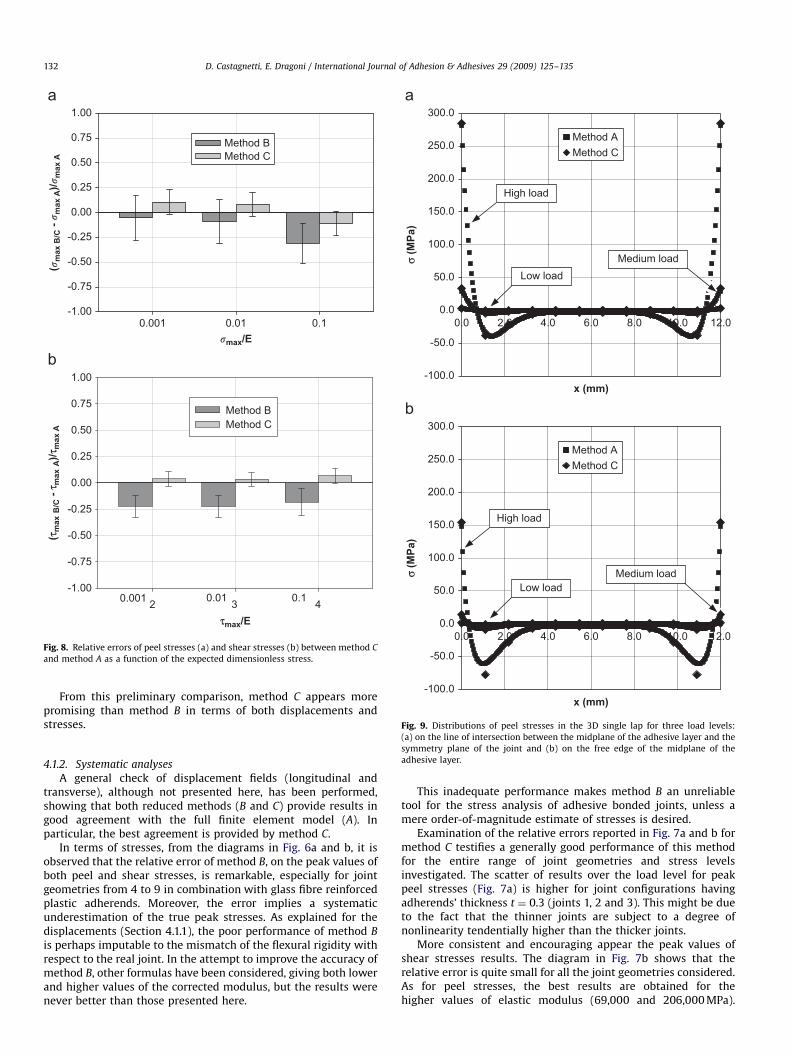
The stress results of methods A and C for the 3D single lap jointare compared in Figs. 9 and 10 for the three load levels considered.

ARTICLE IN PRESS

-10.0

-5.0

0.0

5.0

10.0

15.0

20.0

25.0

30.0

35.0

40.0

x (mm)

σσ (M

Pa)

0.0

5.0

10.0

15.0

20.0

25.0

30.0

35.0

x (mm)

ττ (M

Pa)

Goland & ReissnerMethod AMethod BMethod C


0.0 2.0 4.0 6.0 8.0 10.0 12.0

0.0 2.0 4.0 6.0 8.0 10.0 12.0

Fig. 4. Stresses on the midline of the adhesive layer in the 2D single lap for

o ¼ 0.2: (a) distribution of peel stresses and (b) distribution of shear stresses.

0

20

40

60

80

100

120

140

160

180

P (N)σ m

ax (M

Pa)

0

20

40

60

80

100

120

140

160

180

0P (N)

� max

(MPa

)



100 200 300 400 500

0 100 200 300 400 500

Fig. 5. Peak values of peel stresses (a) and shear stresses (b) on the midline of the

adhesive layer in the 2D single lap as a function of the applied load.


All plotted values are retrieved from the midplane of the adhesivelayer.

The distributions of peel stresses, s, of Fig. 9a, and of shearstresses, t, of Fig. 10a, refer to the line of intersection between themidplane of the adhesive layer and the symmetry plane of thejoint. To appraise the three-dimensionality of the problem, Figs.9b and 10b show the distributions of peel and shear stresses alongthe longitudinal free edge of the midplane of the adhesive layer.

A comparison of 3D results with 2D finite element predictionsand with Goland and Reissner’s results for the single lap joint inthe nominal conditions of Figs. 9 and 10 was performed, showinga very good degree of agreement for all distributions along themidplane of the joint. For the sake of clarity of the charts, thiscomparison is not proposed in Figs. 9a and 10a.

In the analysis of the 3D single lap the computational timeconsumed by the full model was about 2100 times the time usedby reduced method C.

3.2.2. Three-dimensional bracket

The distributions of stresses acting on the midplane of theadhesive layer of the 3D bracket are presented in the charts ofFig. 11, with Fig. 11a referring to the peel stresses and Fig. 11baddressing the resultant shear stresses. Each chart contains twosurfaces, one corresponding to method A (fine grid) and onerelating to method C (coarse grid). The corners of the x–y plane inthe charts in Fig. 11 correspond to the corners of the bonded areain Fig. 2 as shown by the letters.

ARTICLE IN PRESS

-1.00

-0.75

-0.50

-0.25

0.00

0.25

0.50

0.75

1.00

-1.00

-0.75

-0.50

-0.25

0.00

0.25

0.50

0.75

1.00

t=0.3c/t=3

t=1c/t=1.5

t=1c/t=6

t=3c/t=3

t=0.3c/t=1.5

t=0.3c/t=6

t=1c/t=3

t=3c/t=1.5

t=3c/t=6

t=0.3c/t=3

t=1c/t=1.5

t=1c/t=6

t=3c/t=3

t=0.3c/t=1.5

t=0.3c/t=6

t=1c/t=3

t=3c/t=1.5

t=3c/t=6

E=23000 MPaE=69000 MPaE=206000 MPa

E=23000 MPaE=69000 MPaE=206000 MPa

987654321

987654321

(�m

ax B

- � m

ax A

)/�m

ax A

(�m

ax B

- � m

ax A

)/�m

ax A

Fig. 6. Relative errors of peel stresses (a) and shear stresses (b) between method B

and method A for the entire set of 2D single lap joints.

-1.00

-0.75

-0.50

-0.25

0.00

0.25

0.50

0.75

1.00

-1.00

-0.75

-0.50

-0.25

0.00

0.25

0.50

0.75

1.00

t=0.3c/t=3

t=1c/t=1.5

t=1c/t=6

t=3c/t=3

t=0.3c/t=1.5

t=0.3c/t=6

t=1c/t=3

t=3c/t=1.5

t=3c/t=6

t=0.3c/t=3

t=1c/t=1.5

t=1c/t=6

t=3c/t=3

t=0.3c/t=1.5

t=0.3c/t=6

t=1c/t=3

t=3c/t=1.5

t=3c/t=6

E=23000 MPaE=69000 MPaE=206000 MPa

E=23000 MPaE=69000 MPaE=206000 MPa

987654321

987654321

(�m

ax C

- � m

ax A

)/�m

ax A

(�m

ax C

- � m

ax A

)/�m

ax A

Fig. 7. Relative errors of peel stresses (a) and shear stresses (b) between method C

and method A for the entire set of 2D single lap joints.


In this analysis, the computational time of the full model wasabout 3000 times that of reduced model C.

4. Discussion

4.1. Step 1

4.1.1. Preliminary analysis

As a first comment, the preliminary analysis shows that interms of longitudinal displacement (Fig. 3a) reduced method C

provides overall results in close agreement with full method A.The predictions of reduced method B, on the contrary, areprogressively lower than expected as the right edge of theoverlap is approached (x ¼ 12) and do not capture the peakdisplacements arising at both edges of the distribution.A possible explanation of this disagreement can be tracedto the formula used to correct the elastic modulus of the expandedlayer in method B (Section 2.1.1). Although the correctedmodulus of the adhesive reproduces correctly the peel and theshear stiffnesses of the original adhesive layer, it fails to reproduceits flexural rigidity. As a matter of fact, the extended layerwith increased thickness and increased modulus is flexurallystiffer than the original layer with lower thickness and lowermodulus.

The calculated values of transverse displacements (Fig. 3b) arenearly coincident throughout the bondline for all numericalmethods. That can be explained by observing that the transversecomponent of the displacement is mainly affected by thedeformation of the adherends, which is adequately described inall three models.

A generally good correspondence between the three finiteelement models and Goland and Reissner’s solution is also foundin Fig. 4 for peel and shear stress distributions under a given load.However, by close examination of the peak stresses at the edges ofthe bondline (see insets) it is perceivable how method B provideslower stresses than the other methods, in particular as concernsthe shear stress. The disagreement is emphasized in the diagramsin Fig. 5a and b, where the peak values of peel and shear stressesare plotted against the applied load. Those diagrams highlight thatthe maximum stresses supplied by method C, are located exactlybetween the stress predictions of Goland and Reissner’s analyticalmodel and those of the full finite element model, A. By contrast,the peak stresses values provided by method B are systematicallylower than the values of the other models. The maximumdifference between peak values from model B and C is about20%, for both peel and shear stresses.

As a final remark, it is observed that the analysis performed onmodel A considering a plane-strain condition, produced the samestress values as in the plane-stress state, all over the bondline.

ARTICLE IN PRESS

�max/E

(�m

ax B

/C -

� max

A)/�

max

A

-1.00

-0.75

-0.50

-0.25

0.00

0.25

0.50

0.75

1.00

Method B Method C

0.001 0.01 0.1

2 3 4

(τm

ax B

/C -

τ max

A)/τ

max

A

-1.00

-0.75

-0.50

-0.25

0.00

0.25

0.50

0.75

1.00

Method BMethod C

0.001 0.01 0.1

τmax/E

Fig. 8. Relative errors of peel stresses (a) and shear stresses (b) between method C

and method A as a function of the expected dimensionless stress.

-100.0

-50.0

0.0

50.0

100.0

150.0

200.0

250.0

300.0

0.0

x (mm)

-100.0

-50.0

0.0

50.0

100.0

150.0

200.0

250.0

300.0

x (mm)

σ (M

Pa)

σ (M

Pa)

High load

Medium loadLow load

High load

Low loadMedium load

Method AMethod C

Method AMethod C

12.010.08.06.04.02.0

0.0 12.010.08.06.04.02.0

Fig. 9. Distributions of peel stresses in the 3D single lap for three load levels:


From this preliminary comparison, method C appears morepromising than method B in terms of both displacements andstresses.

(a) on the line of intersection between the midplane of the adhesive layer and the

symmetry plane of the joint and (b) on the free edge of the midplane of the

adhesive layer.
4.1.2. Systematic analyses
A general check of displacement fields (longitudinal andtransverse), although not presented here, has been performed,showing that both reduced methods (B and C) provide results ingood agreement with the full finite element model (A). Inparticular, the best agreement is provided by method C.

In terms of stresses, from the diagrams in Fig. 6a and b, it isobserved that the relative error of method B, on the peak values ofboth peel and shear stresses, is remarkable, especially for jointgeometries from 4 to 9 in combination with glass fibre reinforcedplastic adherends. Moreover, the error implies a systematicunderestimation of the true peak stresses. As explained for thedisplacements (Section 4.1.1), the poor performance of method B

is perhaps imputable to the mismatch of the flexural rigidity withrespect to the real joint. In the attempt to improve the accuracy ofmethod B, other formulas have been considered, giving both lowerand higher values of the corrected modulus, but the results werenever better than those presented here.

This inadequate performance makes method B an unreliabletool for the stress analysis of adhesive bonded joints, unless amere order-of-magnitude estimate of stresses is desired.

Examination of the relative errors reported in Fig. 7a and b formethod C testifies a generally good performance of this methodfor the entire range of joint geometries and stress levelsinvestigated. The scatter of results over the load level for peakpeel stresses (Fig. 7a) is higher for joint configurations havingadherends’ thickness t ¼ 0.3 (joints 1, 2 and 3). This might be dueto the fact that the thinner joints are subject to a degree ofnonlinearity tendentially higher than the thicker joints.

More consistent and encouraging appear the peak values ofshear stresses results. The diagram in Fig. 7b shows that therelative error is quite small for all the joint geometries considered.As for peel stresses, the best results are obtained for thehigher values of elastic modulus (69,000 and 206,000 MPa).

ARTICLE IN PRESS

0.0

50.0

100.0

150.0

200.0

250.0

300.0

0.0x (mm)

τ (M

Pa)

0.0

50.0

100.0

150.0

200.0

250.0

300.0

0.0

τ (M

Pa)

High load

Low load

Medium load

High load

Low load

Medium load

Method AMethod C

Method AMethod C

12.010.08.06.04.02.0

12.010.08.06.04.02.0x (mm)

Fig. 10. Distributions of shear stresses in the 3D single lap for three load levels:

(a) on the line of intersection between the midplane of the adhesive layer and the

symmetry plane of the joint and (b) on the free edge of the midplane of the

adhesive layer.

Fig. 11. Fields of peel stresses (a) and of resultant shear stresses (b) in the

midplane of the adhesive layer for the bracket of Fig. 2 (fine grid ¼ full model A,

coarse grid ¼ reduced model C).


The maximum mean value of the relative error is about 15%(joint 9) and the scatter of results over the load level is very low.

The bar charts in Fig. 8 show that the relative error of bothreduced methods is substantially unaffected by the load appliedto the joint. This is especially true for method C which, besidesbeing more accurate than method B (see above), also proves morerobust with respect to the nonlinearity associated with the load.

As a last comment, it is noted that in the runs simulatingadherends with the same elastic modulus (E ¼ 2500 MPa) as theadhesive, method C provided accurate results for both stressesand displacements. For the joint geometry of the preliminaryanalysis, subjected to the intermediate load level, the peak peeland shear stresses provided by method C are, respectively, equal

to 25.16 and 37.25 MPa. The corresponding values of peak stressesprovided by method A are 25.99 MPa for the peel stress and23.50 MPa for the shear stress.

4.2. Step 2

On the basis of the results obtained in Step 1, showing thatmethod B provides poorer results than method C, the investigationof Step 2 is focused on the comparison between method A

(benchmark) and method C (new proposal).

4.2.1. Three-dimensional single lap

A general check of displacement fields (longitudinal andtransverse), although not presented here for brevity, has beenperformed, showing good agreement between methods A and C.Results provided by reduced method C and the full finite elementmodel A, are nearly coincident all over the bondline for all thethree load increments considered, in particular with regard totransverse displacement, v.

Also the comparison of the stress distributions (Figs. 9 and 10)appears particularly corroborating. The patterns of peel stresses(Fig. 9) provided by full model A and reduced model C are quiteclose all over the bondline, independently of the load applied. Theagreement between the two models is achieved also with regard

ARTICLE IN PRESS


to the peak peel stresses even when, under the highest load, theyreach values well beyond what a good structural adhesive canwithstand in practice. The good correlation holds both along theline of intersection between the midplane of the adhesive and thesymmetry plane of the joint (Fig. 9a) and along the free edge ofthe adhesive layer (Fig. 9b). The 50% decrease of the peak peelstress which is observed on passing from the centreline to theedge of the joint is possibly explained by the anticlastic bending ofthe adherends. The quality of the solution in both locationsdemonstrates the ability of the reduced model to cope with 3Deffects of real joints.

A good agreement between methods C and A appears also interms of shear stress distributions (Fig. 10) which are nearlycoincident all over the bondline, both along the symmetry plane(Fig. 10a) and on the free edge (Fig. 10b). Again, the accuracy isexcellent for each of the three load levels applied, including thehighest one which generates peak shear stresses greater than thestrength of any real adhesive. With regard to the peak values, therelative error between results provided by the reduced method C

and the full model A is lower than 10% on the symmetry plane andalso on the free edge. In this case, 3D effects are not significant, ascan be perceived from a comparison between peak values ofFig. 10a and b. This result strengthens the conclusion (seeSection 4.1.1) that the particular state of stress adopted in 2Dmodels (plane stress or plane strain) does not affect much thestress distributions in the joint.

4.2.2. Three-dimensional bracket

The performance of method C in terms of stress prediction isvery good with regard to the distributions of peel stresses(Fig. 11a) and resultant shear stresses (Fig. 11b). As for the 2Danalyses, the general 3D trend of the stress distributions is wellcaptured by the reduced model, with main deviations from thefull model arising along the contour of the adhesive layer.

Although not shown here for brevity, the in-plane and out-of-plane displacement fields on the midsurface of the adhesive layerpredicted by method C were also found in excellent agreementwith method A all over the bonded area.

Table 3Values of k and k0 for various o

o ¼ ct

ffiffipE

qk ¼ 2M0

Tt k0 ¼ V0 cTt

0 1 0

0.1 0.75 0.039

0.2 0.61 0.064

0.3 0.51 0.080

0.4 0.45 0.094

0.5 0.40 0.104

0.6 0.37 0.116

0.65 0.36 0.122

5. Conclusions

To the aim of developing efficient numerical methods for thestructural analysis of complex adhesive joints, two simplifiedcomputational approaches, relying on standard modelling toolsand regular finite elements, are explored and compared withanalytical solutions retrieved from the literature and with fullfinite element analyses. Both simplified methods describe theadherends with structural elements (beams or shells) and thebondline with a single layer of solid elements (plane-stress orbrick). The adhesive elements either have a modified thickness,expanded up to the midline of the adherends (method B), ormaintain the original thickness of the true adhesive layer (methodC). For both methods the length of the elements in the plane of theadhesive equals the distance between the mid surfaces of theadherends. Connection of the adhesive to the adherends isachieved by means of node merging (method B) or by standardkinematic constraints (method C). The benchmark analyses startfrom 2D single lap joints and are then extended to 3D configura-tions, including a square bracket bonded to a wall and subjected toasymmetric cantilever loading. Both methods allow a reduction inthe number of degrees of freedom ranging from 50 to 150 timeswith respect to a full finite element analysis. On average, thecomputational time is reduced by a factor of about 600 for 2Dgeometries and of about 2500 for 3D geometries. Althoughmethod B is affected by remarkable errors, method C provides

fairly accurate results for both 2D and 3D geometries. Accuracyand straightforward implementation make this method veryattractive for the efficient mechanical analysis of large, thin-walled bonded constructions. The research is now taking intoaccount the adhesive plasticity in order to assess the performanceof reduced model C in predicting the post elastic behaviour of thejoint.

Acknowledgement

The financial support of Italy’s Ministero dell’Universita e della

Ricerca is gratefully acknowledged.

Appendix A. Nonlinearity index according to the analyticalmodel of Goland and Reissner

Referring to Goland and Reissner’s work [12] the stressdistribution in the adhesive is governed by the axial force, T, theshear force, V0, and the bending moment, M0, existing at the left-hand transition sections between the free adherends and theoverlapping portion of the joint. Under the hypothesis that thethickness of the overlap equals twice the thickness of eachadherend sheet, then the moment and shearing force can beexpressed in the following simplified form:

M0 ¼ kTt

2(A.1)

V0 ¼ kTt

co

ffiffiffiffiffiffiffiffiffiffiffiffiffiffiffiffiffiffiffiffi3ð1� n2Þ

q¼ k0

Tt

c(A.2)

where t is thickness of the adherends (Fig. 1), c is half the length ofthe overlap, p ( ¼ T/t) is the stress on the sheet and

o ¼c

t

ffiffiffip

E

r(A.3)

k ¼coshðo

ffiffiffiffiffiffiffiffiffiffiffiffiffiffiffiffiffiffiffiffiffiffiffiffiffiffiffiffið3ð1� n2ÞÞ=2

pÞ

coshðoffiffiffiffiffiffiffiffiffiffiffiffiffiffiffiffiffiffiffiffiffiffiffiffiffiffiffiffið3ð1� n2ÞÞ=2

pÞ þ 2

ffiffiffi2p

sinhðoffiffiffiffiffiffiffiffiffiffiffiffiffiffiffiffiffiffiffiffiffiffiffiffiffiffiffiffið3ð1� n2ÞÞ=2

pÞ

(A.4)

k0 ¼ koffiffiffiffiffiffiffiffiffiffiffiffiffiffiffiffiffiffiffiffi3ð1� n2Þ

q(A.5)

Values of k and k0 provided by Eqs. (A.4) and (A.5) are given inTable 3 for several values of o, given by Eq. (A.3). From k and k0,the values of the bending moment (M0) and of the shear force (V0)are recovered by means of Eqs. (A.1) and (A.2).

A practical lower limit of about 0.35 is established for k comingfrom the average values of overlap and from plate stresses injoints composed of bonded aluminium-alloy. Hence this analyticalmodel considers the geometrically nonlinear response of the jointin terms of reduction of joint-edge moments. This is a conse-quence of the rotation of the joint due to the load. At the same

ARTICLE IN PRESS


time small transverse shearing forces are introduced at the jointedges. The degree of nonlinearity is measured by the parameter o.

Appendix B. Choice of variables for the systematicinvestigation of Step 1

Referring to Goland and Reissner’s work [12], the peak shearstress, tmax, and the peak peel stress, smax, arising in the adhesivelayer can be expressed by the following equations:

tmax

p

c

t¼ �

1

8

bc

tð1þ 3kÞ coth

bc

tþ 3ð1� kÞ

� �(B.1)

smax

p¼

k

2

ffiffiffiffiffiffiffiffiffiffiffiffiffiffi6

Ea

E

t

sa

sþ k0

t

c

ffiffiffiffiffiffiffiffiffiffiffiffiffiffi6

Ea

E

t

sa

4

s(B.2)

where

b ¼ 2

ffiffiffiffiffiffiffiffiffiffiffiffiffiffiffiffiffiffiffiffiffiffiffiffi1

1þ na

Ea

E

t

sa

s(B.3)

and parameters k and k0 in Eqs. (A.3)–(A.5) are defined inAppendix A.

Examination of Eqs. (A.3)–(A.5) and (B.1)–(B.3), shows that fora given dimensionless load, p/E (see Eq. (A.3)), applied to the joint,the dimensionless peak stresses, tmax/p and smax/p (see Eqs. (B.1)and (B.2)), only depends on the dimensionless variables

n; na;Ea

E;

t

sa;

c

t

Since Poisson’s ratios of the adherends, n, and of the adhesive, na,are almost the same (E0.3) for most materials, the above listreduces to the following dimensionless ratios

Ea

E;

t

sa;

c

t

which describe all the possible configurations of the joints interms of geometry and material.

Once the elastic modulus, Ea, and the thickness of the adhesive,sa, have been chosen, the peak stresses depend only on theYoung’s modulus of the adherends, E, on the thickness ofthe adherends, t, on the ratio c/t between the half length of the

overlap and the adherend thickness and on the stress p applied tothe adherends.

This is the rationale behind the systematic analysis of Step 2,with Ea and sa fixed to typical epoxy values, E, t, and c/t varying asgiven by Table 2 and the stress p used as an arbitrary loadingfactor as described in Section 2.1.2.

References

[1] Rao BN, Rao YVKS, Yadagiri S. Analysis of composite bonded joints. Fibre SciTechnol 1982;17:77–90.

[2] Yadagiri S, Reddy CP, Reddy TS. Viscoelastic analysis of adhesively bondedjoints. Comput Struct 1987;27(4):445–54.

[3] Reddy JN, Roy S. Non-linear analysis of adhesively bonded joints. Int J Non-Linear Mech 1988;23:97–112.

[4] Amijima S, Fujii T. A microcomputer program for stress analysis of adhesive-bonded joints. Int J Adhes Adhes 1987;7:199–204.

[5] Carpenter WC. Viscoelastic analysis of bonded connections. Comput Struct1990;36(6):1141–52.

[6] Lin CC, Lin YS. A finite element model of single-lap adhesive joints. Int J SolidsStruct 1992;30(12).

[7] Edlund U, Klarbring A. A geometrically nonlinear model of the adhesive jointproblem and its numerical treatment. Comput Meth Appl Mech Eng1992;96:329–50.

[8] Andruet RH, Dillard DA, Holzer SM. Two- and three-dimensional geometricalnonlinear finite elements for analysis of adhesive joints. Int J Adhes Adhes2001;21:17–34.

[9] Goncalves JPM, Moura MFSF, Castro PMST. A three-dimensional finite elementmodel for stress analysis of adhesive joints. Int J Adhes Adhes 2002;22:357–65.

[10] Tong L, Sun X. Adhesive elements for stress analysis of bonded patch tocurved thin walled structures. Comput Mech 2003;30:143–54.

[11] Castagnetti D, Dragoni E. Efficient stress analysis of adhesively bonded jointsby finite elements techniques. In: Proceedings of ESDA 2006, 8th biennialASME Conference, 2006.

[12] Goland M, Reissner E. The stresses in cemented joints. J Appl Mech.[13] Adams RD, Peppiatt NA. Stress analysis of adhesively bonded lap joints.

J Strain Anal 1974;9:185–96.[14] Allman DJ. A theory for elastic stresses in adhesive bonded lap joints.

Q J Mech Appl Math 1977;30:415–36.[15] Hart-Smith LJ. Adhesive-bonded single-lap joints. NASA, CR-I 12236; 1973.[16] Oplinger DW. A layered beam theory for single lap joints. Army Materials

Technology Laboratory report MTL TRY l-23, 1991.[17] Sneddon I. The distribution of stress in adhesive joints. In: Eley DD, editor.

Adhesion. Oxford University Press; 1961 [chapter 9].[18] Tsai MY, Morton J. An evaluation of analytical and numerical solutions to the

single lap joint. Int J Solids Struct 1994;31(18):2537–63.[19] ABAQUS 6.5. Users’ manual. HKS Inc.; 2004.[20] Montgomery DC. Design and analysis of experiments. 6th ed. USA: John Wiley

and Sons; 2005 ISBN 0417661597.

Standard finite element techniques for efficient stress analysis of adhesive joints

Documents

Transcript of Standard finite element techniques for efficient stress analysis of adhesive joints