A lattice-theoretical perspective on adhesive categories
24
Journal of Symbolic Computation ( ) – Contents lists available at ScienceDirect Journal of Symbolic Computation journal homepage: www.elsevier.com/locate/jsc A lattice-theoretical perspective on adhesive categories ✩ Paolo Baldan a , Filippo Bonchi b , Andrea Corradini c , Tobias Heindel d , Barbara König e,1 a Dipartimento di Matematica Pura e Applicata, Università di Padova, Italy b INRIA Saclay - LIX, École Polytechnique, France c Dipartimento di Informatica, Università di Pisa, Italy d Laboratoire d’Informatique de Paris-Nord, Université Paris 13, France e Abteilung für Informatik und Angewandte Kognitionswissenschaft, Universität Duisburg-Essen, Germany article info Article history: Received 1 October 2009 Accepted 19 June 2010 Available online xxxx Keywords: Adhesive categories Van Kampen colimits Lattice theory abstract It is a known fact that the subobjects of an object in an adhesive category form a distributive lattice. Building on this observation, in the paper we show how the representation theorem for finite distributive lattices applies to subobject lattices. In particular, we introduce a notion of irreducible object in an adhesive category, and we prove that any finite object of an adhesive category can be obtained as the colimit of its irreducible subobjects. Furthermore we show that every arrow between finite objects in an adhesive category can be interpreted as a lattice homomorphism between subobject lattices and, conversely, we characterize those homomorphisms between subobject lattices which can be seen as arrows. © 2010 Elsevier Ltd. All rights reserved. 1. Introduction Adhesive categories (Lack and Sobociński, 2005) have been shown to provide a general categorical setting in which double-pushout rewriting (Corradini et al., 1997) can be defined in such a way that some fundamental properties of rewriting (e.g., the local Church–Rosser theorem based on the notions of parallel and sequential independence) hold without the need for further assumptions. As a notable example, standard directed graphs and graph morphisms form an adhesive category, but ✩ Supported by the MIUR Projects SisteR and AIDA2007, and the project AVIAMO of the University of Padova. Carried out during the second author’s tenure of an ERCIM ‘‘Alain Bensoussan’’ Fellowship Programme. E-mail addresses: [email protected] (P. Baldan), [email protected] (F. Bonchi), [email protected] (A. Corradini), [email protected] (T. Heindel), [email protected], [email protected] (B. König). 1 Tel.: +49 203 3793397; fax: +49 203 3793557. 0747-7171/$ – see front matter © 2010 Elsevier Ltd. All rights reserved. doi:10.1016/j.jsc.2010.09.006
Transcript of A lattice-theoretical perspective on adhesive categories

Journal of Symbolic Computation ( ) –
Contents lists available at ScienceDirect
Journal of Symbolic Computation
journal homepage: www.elsevier.com/locate/jsc
A lattice-theoretical perspective on adhesive categories✩
Paolo Baldan a, Filippo Bonchi b, Andrea Corradini c, Tobias Heindel d,Barbara König e,1
a Dipartimento di Matematica Pura e Applicata, Università di Padova, Italyb INRIA Saclay - LIX, École Polytechnique, Francec Dipartimento di Informatica, Università di Pisa, Italyd Laboratoire d’Informatique de Paris-Nord, Université Paris 13, Francee Abteilung für Informatik und Angewandte Kognitionswissenschaft, Universität Duisburg-Essen, Germany
a r t i c l e i n f o
Article history:Received 1 October 2009Accepted 19 June 2010Available online xxxx
Keywords:Adhesive categoriesVan Kampen colimitsLattice theory
a b s t r a c t
It is a known fact that the subobjects of an object in an adhesivecategory form a distributive lattice. Building on this observation,in the paper we show how the representation theorem for finitedistributive lattices applies to subobject lattices. In particular, weintroduce a notion of irreducible object in an adhesive category,and we prove that any finite object of an adhesive categorycan be obtained as the colimit of its irreducible subobjects.Furthermore we show that every arrow between finite objects inan adhesive category canbe interpreted as a lattice homomorphismbetween subobject lattices and, conversely, we characterize thosehomomorphisms between subobject lattices which can be seen asarrows.
© 2010 Elsevier Ltd. All rights reserved.
1. Introduction
Adhesive categories (Lack and Sobociński, 2005) have been shown to provide a general categoricalsetting in which double-pushout rewriting (Corradini et al., 1997) can be defined in such a waythat some fundamental properties of rewriting (e.g., the local Church–Rosser theorem based on thenotions of parallel and sequential independence) hold without the need for further assumptions. Asa notable example, standard directed graphs and graph morphisms form an adhesive category, but
✩ Supported by the MIUR Projects SisteR and AIDA2007, and the project AVIAMO of the University of Padova. Carried outduring the second author’s tenure of an ERCIM ‘‘Alain Bensoussan’’ Fellowship Programme.
E-mail addresses: [email protected] (P. Baldan), [email protected] (F. Bonchi), [email protected] (A. Corradini),[email protected] (T. Heindel), [email protected], [email protected] (B. König).1 Tel.: +49 203 3793397; fax: +49 203 3793557.
0747-7171/$ – see front matter© 2010 Elsevier Ltd. All rights reserved.doi:10.1016/j.jsc.2010.09.006
2 P. Baldan et al. / Journal of Symbolic Computation ( ) –
by the closure properties of adhesive categories many other graphical structures which are usefulin the modelling of concurrent and distributed systems, including hypergraphs, hierarchical graphs,and Petri nets (Sassone and Sobociński, 2005; Ehrig et al., 2006), can be captured in the realm ofadhesive categories. As a consequence, the interest in the theory of adhesive categories goes beyondthe mathematical aspects and it is motivated also by its potential applications to concurrency and tothe theory of distributed systems.
It is known that the subobjects of an object in an adhesive category form a distributive lattice.Exploiting this fact, several proofs in the theory of adhesive categories can be carried out at a lattice-theoretical level. Still, while the theory of distributive lattices has been extensively studied andliterature on the subject abounds (Davey and Priestley, 2002), to the best of our knowledge thepossibility of applying such theory to adhesive categories has not been systematically investigated.
In general terms, this paper aims at strengthening the connection between the theory of adhesivecategories and of distributive lattices, by showing that some relevant lattice-theoretic concepts andresults find a natural counterpart in the setting of adhesive categories.
The long-term goal of this research is the development of a representation theorem for adhesivecategories, at least for the finite case. We are interested in having a characterization theoremfor objects of adhesive categories that would allow us to view them as instances of ‘‘graph-likestructures’’. Several techniques for rewriting can be formulated in the abstract setting of adhesivegrammars (Ehrig et al., 2006; Baldan et al., 2009) and a representation theorem would allowus to obtain a much more intuitive characterization of structures which are instances of thisgeneral framework. Since most of the insights provided by a representation theorem arise fromthe representation of the morphisms, we specifically study arrows in adhesive categories andshow how they can be viewed as lattice homomorphisms. Conversely we characterize those latticehomomorphisms between subobject lattices which correspond to arrows. For this we build uponthe classical representation theory of lattices (Birkhoff, 1967; Davey and Priestley, 2002) and knownresults for adhesive categories (Lack and Sobociński, 2005). In particular, we will exploit the notion ofVan Kampen colimit introduced in Cockett and Guo (2007). Adhesive categories are a relatively newconcept andwe are not aware of anywork in this direction, especially concerning the duality betweenlattice homomorphisms and arrows in adhesive categories.
Since in adhesive categories only finite colimits are sufficiently well-behaved, we will restrictourselves to the theory of finite distributive lattices, which is much simpler than the infinite case.Hence, in several places, we will consider only (subobject) finite objects, i.e., objects that have onlyfinitely many subobjects.
Summary. We first show that the concept of irreducible element from lattice theory can be used toidentify the basic building blocks for objects in adhesive categories. More specifically, after definingthe notion of irreducible object in an adhesive category, we prove that, as any element of a finitedistributive lattice can be obtained as the join of its irreducibles, similarly, any (finite) object of anadhesive category can be obtained as the colimit of its irreducible subobjects. Additionally, such acolimit turns out to be Van Kampen (Cockett and Guo, 2007; Heindel and Sobociński, 2009), i.e.,roughly speaking, it is well-behaved w.r.t. pullbacks.
The representation theory for distributive lattices in Birkhoff (1933); Davey and Priestley (2002)is then exploited in order to establish a correspondence between arrows in adhesive categories andlattice homomorphisms between the corresponding subobject lattices. We first show that any arrowϕ : A → B in an adhesive category induces a lattice homomorphism from Sub(B) to Sub(A), which isessentially given by the inverse image functor (or pullback functor) ϕ−1. While preservation of meetsholds for any category with pullbacks, preservation of joins is strictly related to adhesivity.
Vice versa, not all lattice homomorphisms γ : Sub(B) → Sub(A) correspond to some arrowϕ : A → B. We discuss two possible characterizations of classes of lattice homomorphism whichensure that they correspond to ϕ−1 for some arrow ϕ : A → B. Such characterization relies onthe fact that an object can be obtained as Van Kampen colimit of sets of subobjects which enjoy asuitable closure property (weakmeet-closedness). The second characterization is based on the notionof cover and on the existence of cover–mono factorizations in adhesive categories, which leads to acharacterization of functor ∃ϕ , the left adjoint to the inverse image functor ϕ−1.

P. Baldan et al. / Journal of Symbolic Computation ( ) – 3
Finally the special case of adhesive categories with a strict initial object, which are thusextensive (Carboni et al., 1993), is discussed, where one can obtain stronger results.
2. Background
2.1. Van Kampen colimits and adhesive categories
Adhesive categories have been introduced in Lack and Sobociński (2005), as categories wherepushouts along monomorphisms are so-called Van Kampen squares. In Cockett and Guo (2007);Heindel and Sobociński (2009), the notion of Van Kampen square has been generalized to that of VanKampen colimit. Since these notionswill often recur in the rest of the paper,we start by introducingVanKampen colimits, thenwe focus on Van Kampen squares and finallywe introduce adhesive categories.
We start by recalling the definition of a cartesian natural transformation, which will befundamental for the definition of Van Kampen colimits.
Definition 1 (Cartesian Natural Transformation). Let F ,G : C → D be two functors. A naturaltransformation β : F ⇒ G associates with every object x in C an arrow βx : F(x) → G(x) in Dsuch that, for every morphism d : x → y in C, the following diagram commutes.
F(x)F(d)
//
βx
��
F(y)
βy
��
G(x)G(d)
// G(y)
We say that β is a cartesian natural transformation if the above diagram is a pullback for every arrowd : x → y in C.
Given two natural transformations β : F ⇒ G and γ : G ⇒ H , we use β; γ : F ⇒ H to denotetheir composition defined as (β; γ )x = βx; γx for each object x of C.
In the following, overloading the notation, given two categories I and C and an object A of C, wewill denote simply by A the constant functor ∆I(A) : I → C, which maps each object to A and eacharrow to the identity idA. Similarly, for an arrow d : B → A we will write simply d : B → A to denotethe natural transformation δ : ∆I(B) ⇒ ∆I(A)with δx = d for all x in I. The category I will always beclear from the context.
Definition 2 (Colimit). Let D : I → C be a diagram, i.e., a functor from a given scheme category I intoC. A cocone for D is a natural transformation ϕA
: D ⇒ A to a constant functor A : I → C. A colimitfor D is a cocone ϕA such that for every other cocone ϕB there exists a unique arrow ψ : A → B withϕA
;ψ = ϕB.
It is instructive, for later use, to spell out how this definition subsumes that of a pushout. Considerthe scheme category Ipo and the diagram D : Ipo → C, depicted in Fig. 1. A cocone is a naturaltransformation ϕA
: D ⇒ A for the constant functor A : Ipo → C. Hence it consists of an object Aand three arrows ϕA
x , ϕAy , ϕ
Az of C such that ϕA
x ; idA = D(f );ϕAz and ϕA
x ; idA = D(g);ϕAy , i.e., such that
the diagram in the right part of Fig. 1 commutes. Now the cocone ϕA is a colimit if for every othercocone ϕB there exists a unique arrow ψ such that ϕA
x ;ψ = ϕBx , ϕ
Ay ;ψ = ϕB
y and ϕAz ;ψ = ϕB
z . But thefirst equality can be omitted, as it is implied by the other two: therefore the definition of colimit for adiagram over Ipo coincides with the usual definition of pushout.
We nowdefine the notion of a Van Kampen colimit, introduced in Cockett and Guo (2007); Heindeland Sobociński (2009).
Definition 3 (Van Kampen Colimit). LetD : I → C be a diagramwith colimit ϕA: D ⇒ A. We say that
ϕA is a Van Kampen colimit (VK-colimit) if – given another diagramD′: I → C, a cocone ϕB
: D′⇒ B,

4 P. Baldan et al. / Journal of Symbolic Computation ( ) –
y z
xf
CC����g
[[6666D(y) D(z)
D(x)D(f )
==|||||D(g)
aaBBBBB
A
D(y)
ϕAy=={{{{{
D(z)
ϕAzaaCCCCC
D(x)D(f )
==|||||D(g)
aaBBBBB
ϕAx
OO
Ipo D ϕA
Fig. 1. Pushout as an instance of colimit.
a cartesian natural transformation β : D′⇒ D and an arrow d : B → A in C, such that ϕB
; d = β;ϕA
(see the diagram on the left) – it holds that ϕB is a colimit if and only if the square on the right belowis a pullback for every object x of I.
D′ϕB +3
β
��
B
d��
DϕA +3 A
D′(x)ϕBx //
βx
��
B
d
��
D(x)ϕAx // A
The above definition coincides, when I is the scheme category Ipo of Fig. 1, with that of Van Kampensquares, that are defined as follows in Lack and Sobociński (2005):
D′(x) D′(f ) //
D′(g)HH
##HHβx
��
D′(z)ϕBz
BB
!!BBβz
��
D′(y) ϕBy//
βy
��
B
d
��
D(x) D(f ) //
D(g)HH
$$HH
D(z)ϕAz
CC
!!CC
D(y) ϕAy// A
A Van Kampen square is a pushout ϕA: D ⇒ A as in Fig. 1, satisfying the following condition: given
a commuting cube (as shown above) with ϕA: D ⇒ A as bottom face and such that the back and the
left faces are pullbacks, it holds that the top face is a pushout if and only if the front and the right faceare pullbacks.
In fact, the bottom face of the cube is the colimit ϕA, and the top face is the cocone ϕB. The leftand the back faces are induced by the natural transformation β; hence they commute and they arepullbacks since β is cartesian. The front and the right faces are induced by the arrow d. The conditionϕB
; d = β;ϕA (in Definition 3) means that the front and the right faces of the cube commute (i.e.,ϕBy ; d = βy;ϕ
Ay and ϕB
z ; d = βz;ϕAz ).
Van Kampen squares will be called Van Kampen pushouts in the following. We are now ready tointroduce adhesive categories (Lack and Sobociński, 2005).
Definition 4 (Adhesive Category). A category C is called adhesive if
(1) C has pullbacks;(2) C has pushouts along monos;(3) pushouts along monos are VK-pushouts.
2.2. The representation theorem for finite distributive lattices
In this section we review the duality theory for finite distributive lattices and finite partiallyordered sets, following mainly the presentation in Davey and Priestley (2002).

P. Baldan et al. / Journal of Symbolic Computation ( ) – 5
Fig. 2. A distributive lattice, the corresponding poset of weak irreducibles and the isomorphic lattice of subsets.
We first recall some basic definitions. A partially ordered set (or poset) is a set P equipped with areflexive, transitive and antisymmetric relation ⊑. The maximum and the minimum in P , when theyexist, are called top and bottom and denoted by⊤P and⊥P , respectively (the subscript will be omittedwhen clear from the context). A poset with a bottom element will be called a pointed poset.
Given two posets (Pi,⊑i), i ∈ {1, 2}, a mapping f : P1 → P2 is called monotone if a ⊑1 b fora, b ∈ P1 implies f (a) ⊑2 f (b). If P1 and P2 are pointed, the mapping f : P1 → P2 is called strict if itpreserves the bottom element, i.e., if f (⊥P1) = ⊥P2 .
In this paper, we will focus on finite pointed posets, i.e., pointed posets where the underlying set isfinite. Finite pointed posets and strict monotone maps form the category FPOS.
A lattice is a poset (L,⊑)where any pair of elements a, b ∈ L admitsmeet and join, denoted as a⊓band a⊔b respectively. The lattice is called distributive if for any a, b, c ∈ L, a⊓(b⊔c) = (a⊓b)⊔(a⊓c)(or, equivalently, a ⊔ (b ⊓ c) = (a ⊔ b) ⊓ (a ⊔ c)).
Note that a non-empty finite lattice always has a bottom element ⊥ and a top element ⊤ (whichare the meet and the join, respectively, of all elements).
Given two lattices (Li,⊑i), i ∈ {1, 2}, a mapping α : L1 → L2 is called a lattice homomorphism ifit preserves binary (and hence, finite non-empty) meets and joins. The mapping α is called a {⊥,⊤}-homomorphism if in addition it preserves ⊥ and ⊤. Similarly, it is called a ⊤-homomorphism (⊥-homomorphism) if it preserves ⊤ (⊥). Note that lattice homomorphisms are always monotone. Non-empty finite distributive lattices and ⊤-homomorphisms form the category FDL.
The duality between finite distributive lattices and finite partially ordered sets essentially statesthat FPOS and FDL are equivalent via a contravariant functor. The original theory slightly differs fromours in the fact that FDL has {⊥,⊤}-homomorphisms instead of ⊤-homomorphisms as arrows and,dually, in FPOS objects are general, possibly non-pointed, posets and arrows aremonotonemappings.We need to consider these variations since lattice homomorphisms which arise naturally as pullbackfunctors in adhesive categories do not necessarily preserve the bottom element (but they alwayspreserve the top element). The situation is different if we assume that the adhesive category underconsideration has a strict initial object (for the treatment of this special case see Section 6).
A pivotal definition is the following, which identifies those elements of a lattice which cannot bedecomposed as the join of other elements and thus, intuitively, can be seen as the basic building blocksof the lattice.
Definition 5 (Irreducible). A lattice element a ∈ L is said to be weak (join) irreducible whenevera = b ⊔ c for some b, c ∈ L implies a = b or a = c. An irreducible is any weak irreducible a ∈ Ldifferent from the bottom element. The (pointed) poset of weak irreducibles of L with the orderinginduced by L is denoted by J⊥(L), while J(L) denotes the poset of irreducibles.
A lattice L and the poset J⊥(L) of its weak irreducibles, represented as Hasse diagrams, can befound in Fig. 2 (left and center). Note, in particular, that the element 3 is not a weak irreducible since3 = 1 ⊔ 2.

6 P. Baldan et al. / Journal of Symbolic Computation ( ) –
For a finite lattice it can be easily seen that an element a is weak irreducible if and only if ithas at most one direct predecessor with respect to @ (where a @ b ⇐⇒ a ⊑ b ∧ a = b).Furthermore in a finite lattice every element b can be written as the join of weak irreducibles, namelyb =
{a ∈ J⊥(L) | a ⊑ b}. Note however that this representation is not unique since some
irreducibles could be subsumed by others.This leads us directly to (a slight variation of) Birkhoff’s representation theorem for finite
distributive lattices (Birkhoff, 1933). We first need some notation: let (P,⊑) be any poset. Then wedenote by One(P) the lattice consisting of the non-empty downward-closed subsets of P , ordered bysubset inclusion ⊆.
Theorem 1 (Birkhoff’s Representation Theorem). Let (L,⊑) be a finite distributive lattice and let J⊥(L)be the poset of its weak irreducibles. Then the mapping αL : L → One(J⊥(L)) given by
αL(a) = {x ∈ J⊥(L) | x ⊑ a}
is a lattice isomorphism.
This means that every finite distributive lattice is isomorphic to a lattice of sets: the isomorphismmaps every element a to the maximal set of weak irreducibles which generates a. An example of thisconstruction can be found in Fig. 2 (right).
Analogously, any finite pointed poset P is isomorphic to J⊥(One(P)). The isomorphism ιP : P →
J⊥(One(P)) maps every x ∈ P to {y | y ⊑ x} (which is a weak irreducible of One(P)). This defines aclose relation between the objects of FPOS and FDL. The duality theorem extends this relation alsoto their arrows.
Theorem 2 (Duality). Given two finite distributive lattices L and K , a ⊤-homomorphism γ : K → Linduces a strict monotone map fγ : J⊥(L) → J⊥(K) defined as
fγ (y) = min{x ∈ J⊥(K) | y ⊑ γ (x)}
for all y ∈ J⊥(L).Conversely, given two finite pointed posets P and Q , a strict monotone map f : P → Q induces a
⊤-homomorphism γf : One(Q ) → One(P), defined as
γf (Y ) = {x ∈ P | f (x) ∈ Y }
for all Y ∈ One(Q ).Furthermore, for any ⊤-homomorphism γ : K → L it holds that γfγ = α−1
K ; γ ;αL, where αK andαL are the isomorphisms in Theorem 1. Conversely, for any monotone map f : P → Q it holds thatfγf = ι−1
P ; f ; ιQ .
This leads to an equivalence between the categories FPOS and FDL, via a contravariant functor.For an example consider the mappings γ and fγ in Fig. 3. (The mapping α is explained later.)
2.3. Galois connections
We now review a closely related notion of duality: Galois connections on lattices.
Definition 6 (Galois Connection). Let L, K be two lattices and let α : L → K , γ : K → L be monotonemaps. Then ⟨α, γ ⟩ is a Galois connection if
• for every ℓ ∈ Lwe have γ (α(ℓ)) ⊒ ℓ;• for every k ∈ K we have α(γ (k)) ⊑ k.
In this case α and γ are called the left and right adjoint, respectively.
If we consider the lattices themselves as categories, Galois connections exactly correspond toadjoint pairs. The following properties will be relevant.
Lemma 1. (1) Every monotone map has at most one right adjoint and at most one left adjoint.

P. Baldan et al. / Journal of Symbolic Computation ( ) – 7
Fig. 3. A ⊤-homomorphism γ , the dual map fγ on irreducibles and its left adjoint α.
(2) Left adjoints preserve arbitrary joins (and thus ⊥) and right adjoints preserve arbitrary meets (andthus ⊤).
(3) Every mapping α : L → K that preserves arbitrary joins has a right adjoint γ : K → L defined asγ (k) = max{ℓ ∈ L | α(ℓ) ⊑ k}. Dually, every mapping γ : K → L that preserves arbitrary meetshas a left adjoint α : L → K, defined as α(ℓ) = min{k ∈ K | ℓ ⊑ γ (k)}.
The use of max (resp. min) in the statement is justified by the observation that the set indicatedhas a maximal (resp. minimal) element. An example of a Galois connection consisting of mappings αand γ is given in Fig. 3.
When dealing with finite lattices, every ⊤-lattice homomorphism γ has a left adjoint α(preservation of the top element is needed as it corresponds to preservation of the meet of the emptyset), and similarly every ⊥-lattice homomorphism α has a right adjoint γ . The left adjoint of a latticehomomorphism enjoys interesting properties with respect to irreducibles, establishing a clear linkwith Theorem 2.
Proposition 1. Let K , L be finite lattices, let γ : K → L be a ⊤-lattice homomorphism and let α : L → Kbe its left adjoint. Then α preserves weak irreducibles, i.e., for any l ∈ J⊥(L) we have that α(l) ∈ J⊥(K).
Hence the restriction α|J⊥(L) : J⊥(L) → J⊥(K) of α to the weak irreducibles can be defined as
α|J⊥(L)(l) = min{k ∈ J⊥(K) | l ⊑ γ (k)},
i.e., α|J⊥(L) = fγ .
Proof. For the proof we use an equivalent alternative definition of weak irreducibles in distributivelattices: b is a weak irreducible whenever b ⊑ b1 ⊔ b2 implies that b ⊑ b1 or b ⊑ b2, for all b1, b2.
Assume that l is an irreducible and α(l) ⊑ k1 ⊔ k2. Then we have
l ⊑ γ (α(l)) ⊑ γ (k1 ⊔ k2) = γ (k1) ⊔ γ (k2)
where the last equality ismotivated by the fact that γ is a lattice homomorphism and thus it preservesjoins. Since l is an irreducible, we deduce that l ⊑ γ (k1) or l ⊑ γ (k2). By applying α on both sides we

8 P. Baldan et al. / Journal of Symbolic Computation ( ) –
obtain
α(l) ⊑ α(γ (k1)) ⊑ k1 or α(l) ⊑ α(γ (k2)) ⊑ k2
which proves that α(l) is irreducible. �
Since any element can be expressed as the join of weak irreducibles, α|J⊥(L) determines the leftadjoint α : L → K as α(x) =
{α|J⊥(L)(l) | l ∈ J⊥(L) ∧ l ⊑ x}.
3. Subobject lattices and irreducibles in adhesive categories
As a first step, in this section, we study the subobject lattices arising in adhesive categories. Morespecifically, we show that a notion of an irreducible object can be definedwhich is independent of thespecific subobject lattice.Moreoverwe show that irreducible objects can be seen as the building blocksfor (finite) objects of adhesive categories in the sense that any object can be obtained as a colimit ofirreducibles and such a colimit is VK.
Hereafter, C denotes an adhesive category, and � and∼→ denote monos and isos respectively.
3.1. Irreducibles in adhesive categories
Definition 7 (Subobject). Let A be an object in C. Two monos b : B � A, c : C � A are calledisomorphic if there is an iso ψ : B
∼→ C such that ψ; c = b. A subobject of A is an isomorphism class
of monos into A. It is denoted [b : B � A] or simply [b], where b : B � A is any representative.
It is known that the subobjects of an object in an adhesive category form a distributive lattice, wherethe order ⊑ is given by [b : B � A] ⊑ [c : C � A] whenever there is a mono ϕ : B � C with ϕ; c = b(note that the mono ϕ is unique, if it exists). The meet of two subobjects [b : B � A], [c : C � A]
is realized by taking their pullback, whereas the join can be obtained by taking a pushout over theirmeet (Lack and Sobociński, 2005).
Bb
''OOOOOOOOO
B ⊓ C
::uuuuuu
$$IIIII PB A
Cc
77ooooooooo
Bb
++VVVVVVVVVVVVVVVVV
''NNNNNNN
B ⊓ C
77ppppppp
''NNNNNNN PO B ⊔ C // // A
Cc
33hhhhhhhhhhhhhhhhh
77ppppppp
Furthermore the top element is represented by [idA : A∼→ A]. In the sequel, given an object A in an
adhesive category, we will write Sub(A) to denote the subobject lattice of A.
Definition 8 (Forgetful Functor from a Subobject Lattice). Viewing the subobject lattice as a category,we denote by |·|A : Sub(A) → C a functor that maps any [b : B � A] to the domain B of a chosenrepresentative and, similarly, any arrow [b : B � A] ⊑ [b′
: B′ � A] to the corresponding mono|[b]|A � |[b′
]|A.
In the sequel, we will often write |·| instead of |·|A as the object Awill be clear from the context.In the next example, which is then developed throughout the paper, we will consider as adhesive
category the category of directed graphs and graphmorphisms (Lack and Sobociński, 2005; Ehrig et al.,2006). Fig. 4 shows a graph A and the corresponding lattice of subobjects Sub(A). Here each elementof Sub(A), i.e., each [b] such that b : B � A, is represented just by the source graph B. Themonic arrowb : B � A is implicitly expressed by the position of nodes and edges. For example, the two graphs inSub(A) consisting of one node and no edges are isomorphic, but they represent different subobjects ofA. Indeed, the leftmost subgraph implicitly describes a monic arrow that maps the unique node intothe leftmost node of A, while the rightmost subobject maps the node into the rightmost node of A.
The notion of a (weak) irreducible in subobject lattices will play a fundamental role in the restof the paper. The following proposition shows that, in an adhesive category, this notion is ‘‘global’’,

P. Baldan et al. / Journal of Symbolic Computation ( ) – 9
Fig. 4. A graph, its subobject lattice and its weak irreducibles.
i.e., whenever an object is irreducible in some subobject lattice then it is irreducible in any subobjectlattice of the category.
Proposition 2. Let A, B, I be objects of C and let iA : I � A, iB : I � B be two monos. Then [iA] is a weakirreducible if and only if [iB] is a weak irreducible.
Proof. Let us assume that [iA] is a weak irreducible.Let [iB] be the join of two subobjects [c : C � B], [d : D � B] of B. That is, there exists a pushout of
the following form with all arrows mono and c ′; iB = c , d′
; iB = d. Furthermore C ⊓ D is the pullbackof c, d.
C ⊓ D // //��
��
C��
c′
��
##
c
��
D //
d′
//��
d //
I ��
iB
��>>
>>>>
>>
B
If we post-compose this pullback with iA : I � A (instead of iB : I � B), we obtain that [iA] is the joinof two subobjects [d′
; iA], [c ′; iA]. Since [iA] is irreducible we have that [iA] = [c ′
; iA] or [iA] = [d′; iA].
Let us assume without loss of generality that the former is the case. Then, since iA is a mono and canbe eliminated, c ′ is an iso and thus [iB] = [c ′
; iB] = [c]. �
As an example, in the category of directed (unlabeled) graphs, the irreducibles are the single node,the single edge and the loop (see Fig. 4, right). If graphs are labeled, the irreducibles are essentially thesame, but we must take a copy of the single node, edge and loop for any distinct label. If we considergraphs with higher-order edges where an edge of order k may connect edges of order ℓ < k, then alltypes of edges, with their connections fused in arbitrary ways, are irreducibles.
3.2. Finite objects as VK-colimits of irreducibles
In adhesive categories, the union of two subobjects is realized as a pushout (along theirintersection). Such a pushout is particularly well-behaved, i.e., it is a VK-square. In this section weshow that, more generally, we can relate the notion of join in lattices with the notion of colimit (thatalso represents some form of union). More specifically we will show that, similarly to how everyelement of a finite lattice can be obtained as the join of its irreducibles, any finite object of an adhesive

10 P. Baldan et al. / Journal of Symbolic Computation ( ) –
category can be obtained as the colimit of the diagram consisting of its irreducibles, and such colimitis VK.
This is stated by Corollary 1 at the end of this section. In order to prove it we employ the followingproof strategy: we start with a diagram that has a ‘‘largest’’ object (for instance the diagram consistingof all subobjects of a given object) and show that it is a VK-colimit. Then, step by step, we remove allobjects which are not weak irreducibles.
Lemma 2 (Partial-Order Diagrams with ⊤ are VK-colimits). Let I be a partial order with a largestelement ⊤ and let D : I → C be a diagram. We set T = D(⊤) and define the cocone ϕT
: D ⇒ Tby setting ϕT
x = D(x ⊑ ⊤) for every object x of I.Then ϕT is a VK-colimit.
Proof. We first show that ϕT is well-defined, i.e., it is indeed a natural transformation. Let x, y withx ⊑ y be two objects of I. Then it holds that D(x ⊑ y);ϕT
y = D(x ⊑ y);D(y ⊑ ⊤) = D(x ⊑ ⊤) =
D(x ⊑ ⊤); idT = ϕTx ; idT = ϕT
x .In the next step we show that ϕT is a colimit. Take any other natural transformation ϕA
: D ⇒ A.Then define ψ = ϕA
⊤: T → A. Commutativity follows from ϕT
x ;ψ = D(x ⊑ ⊤);ϕA⊤
= ϕAx ; idT = ϕA
x .In order to show that the arrow ψ is unique, take any other arrow ψ ′
: T → A with ϕTx ;ψ ′
= ϕAx , for
all x. Then we have that ψ = ϕA⊤
= ϕT⊤;ψ ′
= idT ;ψ ′= ψ ′.
Finally we prove that ϕT is VK: let D′: I → C be another diagram with cocone ϕT ′
: D′⇒ T ′ and
let β : D′⇒ Dwhere β is cartesian and d : T ′
⇒ T with ϕB; d = β;ϕA. We show both implications in
the definition of VK-pushout. First, let the squares consisting ofmorphismsϕT ′
x , βx, ϕTx , d be pullbacks.
Observe that for x = ⊤ we have ϕT⊤
= idT and hence ϕT ′
⊤must be an iso. It now holds that
ϕT ′
x = ϕT ′
x ; idT ′ = D′(x ⊑ ⊤);ϕT ′
⊤and hence – by the first part of this proof – it is a colimit. In
order to show the other direction, assume that ϕT ′
is a colimit and, without loss of generality, assumeT ′
= D′(⊤) and ϕT ′
x = D′(x ⊑ ⊤). Since β is a cartesian natural transformation we have that for eacharrow x ⊑ y the following squares are pullbacks:
D′(x)D′(x⊑y)
//
βx
��
D′(y)
βy
��
D(x)D(x⊑y)
// D(y)
If we set y = ⊤ we obtain D(y) = D(⊤) = T , D′(y) = D′(⊤) = T ′, D(x ⊑ y) = D(x ⊑ ⊤) = ϕTx and
D′(x ⊑ y) = D′(x ⊑ ⊤) = ϕT ′
x , thus obtaining the required pullback squares. �
Note that this proof holds for any category C (not necessarily adhesive). Now, in order to prove ourmain result, we will show that if we remove objects that are not weak irreducible from a VK-colimit,then the result is still a VK-colimit. First, we have to formally definewhatwemean by removing objectsfrom a diagram.
Definition 9 (Removing Objects from Diagrams). Let I be a scheme category and let x be an arbitraryobject of I. By I − xwe denote the scheme that is obtained by removing x – and all arrows which havex as source or target – from I. This gives rise to an obvious embedding functor Ex
I : (I − x) → I.For a diagram D : I → C we denote by Dx the diagram Dx
= ExI ;D : (I − x) → C.
For a natural transformation ϕ : D ⇒ D′ let ϕx: Dx
⇒ D′x be the natural transformation withϕxy = ϕy for every object y of (I − x).
Lemma 3 (Removing Unions from VK-colimits). Let D : I → C be a diagram where I is a partial order,and let ϕA
: D ⇒ A be a VK-colimit.Let x ∈ I be an object such that
(i) the full subcategory of I with objects {y ∈ I | y ⊑ x} is Sub(D(x));
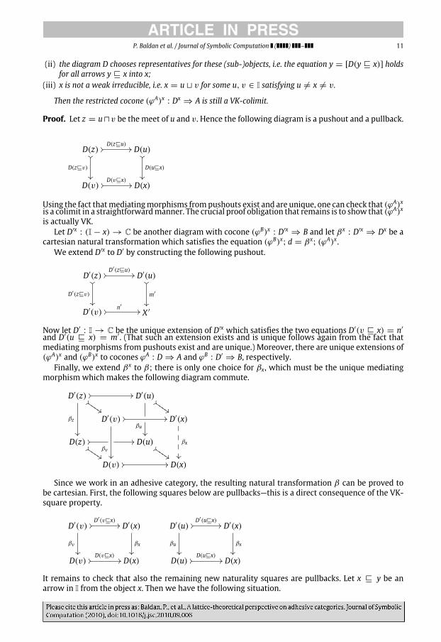
P. Baldan et al. / Journal of Symbolic Computation ( ) – 11
(ii) the diagram D chooses representatives for these (sub-)objects, i.e. the equation y = [D(y ⊑ x)] holdsfor all arrows y ⊑ x into x;
(iii) x is not a weak irreducible, i.e. x = u ⊔ v for some u, v ∈ I satisfying u = x = v.
Then the restricted cocone (ϕA)x : Dx⇒ A is still a VK-colimit.
Proof. Let z = u⊓ v be the meet of u and v. Hence the following diagram is a pushout and a pullback.
D(z) //D(z⊑u)
//
��
D(z⊑v)
��
D(u)��
D(u⊑x)
��
D(v) //D(v⊑x)
// D(x)
Using the fact thatmediatingmorphisms frompushouts exist and are unique, one can check that (ϕA)x
is a colimit in a straightforwardmanner. The crucial proof obligation that remains is to show that (ϕA)x
is actually VK.Let D′x
: (I − x) → C be another diagram with cocone (ϕB)x : D′x⇒ B and let βx
: D′x⇒ Dx be a
cartesian natural transformation which satisfies the equation (ϕB)x; d = βx; (ϕA)x.
We extend D′x to D′ by constructing the following pushout.
D′(z) //D′(z⊑u)
//
��
D′(z⊑v)��
D′(u)��
m′
��
D′(v) // n′
// X ′
Now let D′: I → C be the unique extension of D′x which satisfies the two equations D′(v ⊑ x) = n′
and D′(u ⊑ x) = m′. (That such an extension exists and is unique follows again from the fact thatmediating morphisms from pushouts exist and are unique.) Moreover, there are unique extensions of(ϕA)x and (ϕB)x to cocones ϕA
: D ⇒ A and ϕB: D′
⇒ B, respectively.Finally, we extend βx to β; there is only one choice for βx, which must be the unique mediating
morphism which makes the following diagram commute.
D′(z) // //
βz
��
$$
$$IIII
D′(u)
βu��
$$
$$IIII
D′(v) // //
βv��
D′(x)
βx
������
D(z) // //$$
$$IIII
D(u)$$
$$IIII
D(v) // // D(x)
Since we work in an adhesive category, the resulting natural transformation β can be proved tobe cartesian. First, the following squares below are pullbacks—this is a direct consequence of the VK-square property.
D′(v) //D′(v⊑x)
//
βv
��
D′(x)
βx
��
D(v) //D(v⊑x)
// D(x)
D′(u) //D′(u⊑x)
//
βu
��
D′(x)
βx
��
D(u) //D(u⊑x)
// D(x)
It remains to check that also the remaining new naturality squares are pullbacks. Let x ⊑ y be anarrow in I from the object x. Then we have the following situation.

12 P. Baldan et al. / Journal of Symbolic Computation ( ) –
Fig. 5. X is a weakly ⊓-closed subset of Sub(A) (in Fig. 4), while Y is not.
D′(z) // //
��
$$
$$IIII
D′(u)
��
$$
$$IIII
��
D′(v) // //
��
66D′(x)
��
// D′(y)
��
D′(x)
��
// D′(y)
��
D(z) // //$$
$$IIII
D(u)$$
$$IIII
��
D(v) // //66
D(x) // D(y) D(x) // D(y)
PB?
All vertical squares are known to be pullbacks, except for the rightmost square in the display above.However, reusing the proof idea of Proposition 4.4 of Heindel (2009), this square can also be shownto be a pullback. For arrows y ⊑ x in I, the relevant naturality square can similarly be shown to be apullback, this time using the pushouts based on the I-objects z ⊓ y, u ⊓ y, v ⊓ y, y.
We also need to show that ϕB; d = β;ϕA, which can be derived as follows:
D′(u ⊑ x);ϕBx ; d = ϕB
u; d = βu;ϕAu = βu;D(u ⊑ x);ϕA
x = D′(u ⊑ x);βx;ϕAx
and D′(v ⊑ x);ϕBx ; d = D′(v ⊑ x);βx;ϕ
Ax is obtained in the same way. Then the uniqueness of
mediating morphisms implies the desired ϕBx ; d = βx;ϕ
Ax .
Finally, we can show both implications of the VK-property: first, let the squares consisting ofmorphisms (ϕB)xy, β
xy , (ϕ
A)xy, d be pullbacks. This means that all squares of the form ϕBy , βy, ϕ
Ay , d
for y = x are pullbacks by assumption and by the above argument, all other squares must also bepullbacks. Hence, since ϕA is a VK-colimit, ϕB must be a colimit and thus (ϕB)x is a colimit for D′x. Forthe other direction let (ϕB)x be a colimit. This means that ϕB is also a colimit and hence the squaresϕBy , βy, ϕ
Ay , d are pullbacks and – a fortiori – the same is true for the squares (ϕB)xy, β
xy , (ϕ
A)xy, d for ally ∈ (I − x). �
The result stating that any finite object of an adhesive category can be obtained as the colimit of itsweak irreducibles will be obtained as a corollary of a more general result. For this, we need the notionof weak ⊓-closure.
Definition 10 (Weakly ⊓-closed). Let (D,⊑) be a lattice. We say that X ⊆ D is weakly ⊓-closed if forall x, y ∈ X there exists Y ⊆ X with Y = ∅ such that x ⊓ y =
Y .
Intuitively, X is weakly ⊓-closed if for any two elements, their meet is possibly not in X , but it can begenerated as the join of elements in X . Fig. 5 shows two subsets of Sub(A) (in Fig. 4): one is weakly⊓-closed and the other is not.
Additionally, given a subset of the subobject lattice of an object,wewill need to view it as a diagram.This is formalized below.

P. Baldan et al. / Journal of Symbolic Computation ( ) – 13
Definition 11 (Diagram of Subobjects). Given a subset of the subobject lattice X ⊆ Sub(A), we willwrite D[X] to refer to the diagram |·||X : (X,⊑) → C.
That is, D[X] is a diagram whose scheme is given by the underlying partial order and subobjectinclusions as arrows, i.e., D[X](a′) = |a′
| for any a′∈ X and, if a′
⊑ a′′, then D[X](a′⊑ a′′) is the
corresponding inclusion arrow.We can now prove the desired result.
Proposition 3. Let A be an object of C and let X ⊆ Sub(A) be a finite subset with X = ∅, which is weakly⊓-closed. Then D[X] has ϕ : D[X] ⇒
X, where each ϕx is the inclusion arrow, as a VK-colimit.
Proof. Set
X =
X ′
| X ′⊆ X, X ′
= ∅
.
Clearly X is a finite set. Since X is weakly ⊓-closed we can easily show that X is a sublattice ofSub(A). In fact, let a′, a′′
∈ X; hence a =
X ′ and a′′=
X ′′, with X ′, X ′′⊆ X . Then their meet is
a′⊓ a′′
=
X ′
⊓
X ′′
=
{b′
⊓ b′′| b′
∈ X ′∧ b′′
∈ X ′′} [by distributivity]
=
{c ∈ X | c ⊑ b′
⊓ b′′} | b′
∈ X ′∧ b′′
∈ X ′′
[by weak ⊓-closure]
=
{c ∈ X | c ⊑ b′
⊓ b′′ for some b′∈ X ′
∧ b′′∈ X ′′
}
∈ X [by construction].
Similarly, their join is a′⊔ a′′
= (
X ′) ⊔ (
X ′′) =(X ′
∪ X ′′) ∈ X . Thus by Lemma 2 the diagramD[X] is VK and has colimit
X , which, by construction, is the top of X .
Now take any linearization of X\X , listing elements in descending order with respect to ⊑, i.e.,z1, . . . , zn with zi ⊑ zk if i < k. We will remove these objects from D[X] one after the other: assumethat z1, . . . , zj−1 have already been removed; the resulting diagram D has a colimit object
X and it
is VK.Now, in the next step, we remove zj which has the form zj =
X ′ for some X ′
⊆ X , |X ′| > 1 (in
fact, note that if |X ′| = 1 then zj would be in X , contradicting the fact that by construction zj ∈ X\X).
Therefore zj is the join of two elements of X\{z1, . . . , zj−1} and can be removed by using Lemma 3. �
For an example take the graph A in Fig. 4 and the subset X in Fig. 5. The colimit of D[X] coincideswith
X in Sub(A) (which, in this particular instance, is A itself). Now, consider the subset Y (in Fig. 5)
that is not weakly ⊓-closed. The colimit of D[Y ] consists of a graph with four nodes, while
Y is theoriginal graph A. This example shows that the above proposition does not hold if the set is not weakly⊓-closed.
We are now ready to prove the main result of this section.
Corollary 1. Let A be a finite object in C. Then A is the colimit of D[J⊥(A)] and the colimit is VK.
Proof. Immediate from Proposition 3, as J⊥(A) is weakly ⊓-closed. In fact any element of the latticecan be expressed as the join of weak irreducibles, and thus this holds in particular for the meet of twoweak irreducibles.
For an example, look at Fig. 4. The colimit of D[J⊥(A)] is A itself.

14 P. Baldan et al. / Journal of Symbolic Computation ( ) –
Fig. 6. An arrow ϕ : A → B, the lattice homomorphism ϕ−1 and its left adjoint ∃ϕ . The arrow ϕ maps both the nodes of A intothe leftmost node of B, the self-loop into the upper self-loop of B and the edge into the lower self-loop B.
4. From arrows to lattice homomorphisms
4.1. On the homomorphism induced by an arrow
In this and the next section, we establish a close relationship between arrows in an adhesivecategory and lattice homomorphisms between the corresponding subobject lattices. We start byproving that for any arrow ϕ : A → B in an adhesive category, we can define a map ϕ−1
: Sub(B) →
Sub(A) that is a ⊤-lattice homomorphism.Definition 12 (ϕ−1). Let ϕ : A → B be an arrow inC. Themapping ϕ−1
: Sub(B) → Sub(A) is definedas follows: every subobject [b′
: B′ � B] is mapped to a subobject [a′: A′ � A] obtained by taking
the following pullback.
A′ //��
a′
��
B′
��
b′
��
A ϕ// B
As an example, Fig. 6 depicts an arrow ϕ : A → B in the category of graphs and the correspondingmap ϕ−1
: Sub(B) → Sub(A).Wewill now show thatϕ−1 is always a⊤-lattice homomorphism. Note thatwhile the preservation
ofmeets is obvious, the preservation of joins is specific to adhesive categories as it depends on the VK-square property discussed after Definition 3.Proposition 4 (Arrows Induce ⊤-homomorphisms). For any arrow ϕ : A → B in C, the mappingϕ−1
: Sub(B) → Sub(A) is a ⊤-homomorphism.Proof. The mapping preserves the ⊤ element. In fact the following square is a pullback:
A��
idA��
ϕ// B
��
idB��
Aϕ
// B
which means that ϕ−1(⊤Sub(B)) = ϕ−1([idB]) = [idA] = ⊤Sub(A).

P. Baldan et al. / Journal of Symbolic Computation ( ) – 15
We now show that the mapping preserves meets. Let [b3] = [b1] ⊓ [b2]; hence the square belowon the right (B, B1, B2, B3) is a pullback. Furthermore by using ϕ−1 and standard pullback splittingwe obtain the four squares in the middle which are also pullbacks. Now it can be shown that thesquare B, B2, A1, A3 is a pullback (as it arises as the combination of two pullbacks B1, B3, A1, A3 andB, B1, B2, B3). Then since B, B2, A, A2 is also a pullback, it follows that the square (A, B, A2, A3) on theleft is also a pullback.
A3��
����������
@@
@// B3
��
����
������
@@
@
A2��
a2����������
// B2��
b2����������
A1
a1 AAAA
// B1
b1 AA
AA
A ϕ// B
Thus [a1] = ϕ−1([b1]), [a2] = ϕ−1([b2]), [a3] = ϕ−1([b3]) and [a3] = [a1] ⊓ [a2].In a second step we show that ϕ−1 also preserves joins, so let [b′
] = [b1] ⊔ [b2] with [b3] =
[b1] ⊓ [b2]. Hence we can construct a diagram as above with all squares pullbacks. Now take thepushout of B3 � B1, B3 � B2, obtaining B′ with mediating arrow b′
: B′ � B. Then take the pullbackof b′ and ϕ, obtaining A′ with arrow a′
: A′ � A and mediating morphisms a′
1 : A1 � A′, a′
2 : A2 � A′.Due to pullback splitting we have that the squares B′, B1, A′, A1 and B′, B2, A′, A2 are pullbacks. Hence,since the right-hand pushout over B′ is a VK-square we can infer that A′, A1, A2, A3 is also a pushout.
A3��
����������
@@
@// B3
��
����
������
@@
@
A2��
a2~~
��
a′2����������
// B2��
b2~~
��
����������
A1
a1
''
a′1
AAAA
// B1
b1
''
@@@
@
A′ //��
a′ ��
B′
��b′
��
A ϕ// B
This gives us [a1] = ϕ−1([b1]), [a2] = ϕ−1([b2]), [a′] = ϕ−1([b′
]) and [a′] = [a1]⊔[a2], as desired. �
Ashinted at earlier, arrows in adhesive categories are not necessarily⊥-homomorphisms. Considerfor instance the category of pointed sets, i.e., the category of sets having a distinguished element • andfunctions which preserve •. Now consider the unique morphism ϕ: A → B with A = {a, •}, B = {•}
(note that B is the final object). Subobject lattices here consist of pointed subsets ordered by subsetinclusion. The bottom element of the subobject lattice Sub(B) is [idB], but the pullback of ϕ and idBgives us [idA], which is not the bottom element of Sub(A). In Section 6, we will show that by requiringthe existence of a strict initial object, we can prove that ϕ−1 also preserves the bottom.
4.2. On the left adjoint of the homomorphism induced by an arrow
In this subsection we present a characterization of ∃ϕ , the left adjoint of ϕ−1, which exists byLemma 1 because we just proved that ϕ−1 is a lattice ⊤-homomorphism, and thus it preservesarbitrary meets. At the same time, we show that for finite objects adhesive categories enjoy uniquecover–mono factorization that we exploit to characterize ∃ϕ . This result will be used later inSection 5.2.
Let us start by introducing the notion of cover (Freyd and Scedrov, 1990).

16 P. Baldan et al. / Journal of Symbolic Computation ( ) –
Definition 13 (Cover). An arrow c : A → B is called a cover if whenever c = a; b with b mono, thenb is an iso.
Covers will in the following be denoted by arrows of type �. It can be easily seen that every iso isa cover. Additionally, one can prove the following facts about covers.
Lemma 4. All epis are covers in adhesive categories. In a category with equalizers all covers are epis.
Proof. We first show that in an adhesive category all epis are covers. Assume that c is an epi andc = a; b with b mono. Then b is also an epi (as second arrow in the decomposition of an epi). Since itis mono and epi it must be iso (in fact, as shown in Lack and Sobociński (2005), in adhesive categoriesarrows that are both mono and epi are isos).
Next, we prove that in a categorywith equalizers all covers are epis. Take a cover c : A � B and twoarrows a, b : B → C such that c; a = c; b. Now take the equalizer e : E � B of a, b, which must be amono (since all equalizers are mono). Due to the universal property there exists a unique mediatingarrowm : A → E. Then e must be an iso and from e; a = e; b it follows that a = b.
Ac // //
m
��
Ba //
b// C
E@@
e
@@��������
The exact relationship between epis and covers in adhesive categories is still not completelyunderstood, although the two notions coincide in many cases. In the following we use the notionof cover, instead of epi, as it integrates much better with the rest of the theory.
Proposition 5 (∃ϕ Induces Covers). Let A, B be finite objects in C, and ϕ : A → B be an arrow, considerthe ⊤-homomorphism ϕ−1
: Sub(B) → Sub(A) and let ∃ϕ be the corresponding left adjoint. Then, for anypair of monos a : A′ � A, b : B′ � B with [b] = ∃ϕ([a]), there exists an arrow ϕ′
: A′→ B′ such that
ϕ′; b = a;ϕ (obviously unique, as b is mono) and ϕ′ is a cover.
A′
��
a
��
ϕ′
// B′
��
b��
Aϕ
// B
Proof. Take the pullback of ϕ and b, resulting in the pullback object A. Since a = ϕ−1(∃ϕ([a])) ⊒ [a]there exists a mono m : A′ � A making everything commute. Define ϕ′
= m; f where f is the upperleg of the pullback.
The arrow ϕ′ is a cover. In fact, let ϕ′= f ′
;m′ wherem′ is a mono.
A′′
��
a′
��
// B′′
��
m′
��
A′
f ′
&&
??
��
a��
@@@@
@@@
//m
// A��
a
��
f// B′
��
b
��
Aϕ
// B
Take the pullback of f and m′, resulting in the pullback object A′′. Consider the subobject a′′= a′
; aand observe that a′′
= ϕ−1([m′; b]) since the square A′′, B′, B, A is a pullback (by pullback chasing).

P. Baldan et al. / Journal of Symbolic Computation ( ) – 17
Note that the mediating arrow from A′ to A′′ must be a mono, since m is a mono. Hence a ⊑ a′′=
ϕ−1([m′; b]). Thus, by definition of ∃ϕ ,
b = ∃ϕ([a]) ⊑ ∃ϕ(ϕ−1([m′
; b])) ⊑ m′; b ⊑ b
which implies thatm′ is an iso. �
The above proposition allows us to prove that each arrow between finite objects in an adhesivecategory can be uniquely factorized into a cover and a mono.Proposition 6 (Cover–Mono Factorizations in Adhesive Categories). Let A, B be finite objects in C and letϕ: A → B be an arrow. Then there exists a unique cover–mono factorization of ϕ, i.e., there is a uniquecover c and a unique mono m such that ϕ = c;m.Proof. Existence of a cover–mono factorization can be shown as follows. Let ϕ : A → B be an arrowand let ∃ϕ : Sub(A) → Sub(B) be the left adjoint to ϕ−1. Take ∃ϕ([idA : A → A]) = [b : B′ � B]. Then,by Proposition 5, there is a cover c : A � B′ such that the diagram below commutes, thus providingthe desired cover–mono factorization.
A��
idA��
// c // // B′
��
b��
A ϕ// B
As far as uniqueness is concerned, we derive it by showing that the diagonalization property holds:assume the square on the left below commuteswhere c is a cover and b ismono. Now take the pullbackof b and d and obtain the square in the middle. Since c is a cover, b′ must be an iso and b′−1
; d′ is therequired diagonal arrow.
•c // //
a
��
•
d
��• //
b// •
•c // //
a
��
c′
��
•
d
��
•
d′
��~~~~
~~~
??
b′
??~~~~~~~
• //b
// •
•c // //
a
��
c′
��
•
d
��
b′−1
∼
��~~~~
~~~
•
d′
��~~~~
~~~
• //b
// •
We now show the uniqueness of the diagonal arrow. Assume that there were two diagonal arrowsd′
1, d′
2. Since d′
1; b = d = d′
2; b and b is mono we can conclude that d′
1 = d′
2. �
An immediate consequence of the uniqueness of cover–mono factorization is that the left adjoint tothe ⊤-homomorphism induced by an arrow is uniquely determined by the cover–mono factorizationin C.Corollary 2 (Characterization of ∃ϕ). Let ϕ : A → B be an arrow in C where A, B are finite objects, letϕ−1
: Sub(B) → Sub(A) be the induced ⊤-homomorphism, and let ∃ϕ : Sub(A) → Sub(B) be its leftadjoint. Then for every [a : A′ � A] ∈ Sub(A), it holds that ∃ϕ([a]) = [b : B′ � B], where c; b is thecover–mono factorization of a;ϕ:
A′
��
a
��
// c // // B′
��
b��
A ϕ// B
Proof. Immediate, by Propositions 5 and 6. �
An example for a mapping ∃ϕ arising from a graph morphism ϕ is shown in the right part of Fig. 6.Note that, while ϕ−1 is a ⊤-homomorphism, ∃ϕ is not, since it does not preserve meets and top.

18 P. Baldan et al. / Journal of Symbolic Computation ( ) –
5. From lattice homomorphisms to arrows
The converse of Proposition 4 does not hold, i.e., not every lattice homomorphism from Sub(B) toSub(A) is induced as the inverse image functor of an arrow of C. This should not be surprising: in fact,a morphism ϕ : A → B induces not simply a lattice ⊤-homomorphism ϕ−1
: Sub(B) → Sub(A), buta much richer structure. In fact, for any [b1 : B1 � B], we also get a morphism Φb1 : ϕ−1(B1) → B1,and for any pair of subobjects [b1 : B1 � B] and [b2 : B2 � B], such that [b1] ⊑ [b2], the followingsquare is a pullback:
ϕ−1(B1)
Φb1
��
// // ϕ−1(B2)
Φb2
��
B1 // // B2
In other words, we have a cartesian natural transformationΦ : ϕ−1; |·|A ⇒ |·|B.
As an immediate consequence, a ⊤-homomorphism Sub(B) → Sub(A) cannot be induced by amorphism ϕ : A → B if such additional structure does not exist. For instance, in a category of labeledgraphs with label preserving homomorphisms, consider two graphs each consisting of a single node,which is labeled a in the first graph and b in the second one. The two subobject lattices are clearlyisomorphic, but of course there is no homomorphism between these graphs.
We next identify suitable conditions under which a⊤-homomorphism between subobject latticesis induced by an arrow between the corresponding objects. Note that we concentrate on finite objectsin order to exploit Birkhoff’s representation theorem. Throughout the section, C is implicitly assumedto be an adhesive category.
5.1. Arrows and cartesian natural transformations
We look for sufficient conditions to show that a given lattice homomorphism γ : Sub(B) → Sub(A)is induced by an arrow A → B. With inspiration from the above considerations, the first solutionconsists of requiring the existence of a cartesian natural transformation between the image under γof the diagram of irreducibles of B and the diagram itself, i.e., for each irreducible B′ of B we ask forthe existence of an arrow from γ (B′) to B′, in such a way that the resulting squares are all pullbacks.
We first need to introduce some notation. Let A, B be objects in C, let X ⊆ Sub(B) and letf : Sub(B) → Sub(A) be a monotone mapping. Let D[X] be the diagram as in Definition 11. We denoteby f ∗D[X] : X → C the diagramwith the same scheme of D[X] and whichmaps any b ∈ X to |f (b)|A.An example is provided in the left part of Fig. 7, which represents the diagram γ ∗D[J⊥(B)] where γis the homomorphism ϕ−1 in Fig. 6. Note that the scheme category of this diagram is a poset, whilethe target is the category of graphs. In order to stress this difference we have used dashed lines in thegraphical representation of the former category and straight lines for the latter.
Proposition 7. Let A, B be finite objects in C. Let γ : Sub(B) → Sub(A) be a ⊤-homomorphism such thatthere exists a cartesian natural transformationΦ : γ ∗D[J⊥(B)] ⇒ D[J⊥(B)]. Then there exists a uniquearrow ϕ : A → B such that ϕ−1
= γ .
Proof. The colimit of D[J⊥(B)] is B and it is a VK-colimit by Corollary 1.Similarly, we can prove that the colimit of γ ∗D[J⊥(B)] is A and it is VK. In fact, this diagram
obviously has the same colimit as D[γ (J⊥(B))] (they are the same apart from the fact that in the firstdiagram some objects, which arise as the non-injective image of different irreducibles through γ , arerepeated). Now, we know that γ (J⊥(B)) is weakly ⊓-closed, since γ is a lattice homomorphism (andthus it preserves meets and joins). Thus, by Proposition 3, D[γ (J⊥(B))] has colimit
γ (J⊥(B)) and
γ (J⊥(B)) =
I∈J⊥(B)
γ (I) = γ
I∈J⊥(B)
I
= γ ([idB]) = [idA]
as γ preserves joins and the top element. Again by Proposition 3, the colimit A is VK.

P. Baldan et al. / Journal of Symbolic Computation ( ) – 19
Fig. 7. The diagram γ ∗D[J⊥(B)] (left) and the cartesian natural transformationΦ of Proposition 7 (right).
Then we can get ϕ as a mediating arrow
γ ∗D[J⊥(B)]
Φ
��
+3 A
ϕ
��D[J⊥(B)] +3 B
Since Φ is cartesian, the top row γ ∗D[J⊥(B)] ⇒ A is a VK-colimit and the bottom rowD[J⊥(B)] ⇒ B is a VK-colimit, we deduce that for any weak irreducible I ∈ J⊥(B) the followingsquare is a pullback:
|γ (I)|
Φγ (I)
��
// // A
ϕ
��|I| // // B
This means that ϕ−1 coincides with γ on the weak irreducibles. But since they both are ⊤-homomorphisms, they are determined by their value on the weak irreducibles and thus γ = ϕ−1,as desired. �
The right part of Fig. 7 shows an example of the cartesian natural transformationΦ , where γ is themap ϕ−1 in Fig. 6. The scheme category of the two diagrams is J⊥(B), depicted in the left part of thefigure. For each I ∈ J⊥(B), there is a graph morphismΦI : γ ∗D[J⊥(B)](I) → D[J⊥(B)](I). Note thatall the squares in the figure are commuting (i.e.,Φ is a natural transformation) and, most importantly,they are all pullbacks (i.e.,Φ is cartesian).
5.2. Arrows, covers and natural transformations
An alternative characterization is based on the notion of cover and on the existence of cover–monofactorizations in adhesive categories, which, as shown in Corollary 2, leads to a characterization of theleft adjoint to the inverse image functor.
Proposition 8. Let A, B be finite objects in C and assume that there exists a ⊤-lattice homomorphismγ : Sub(B) → Sub(A). Let α : Sub(A) → Sub(B) be the corresponding left adjoint (which maps weakirreducibles to weak irreducibles, by Proposition 1).
If there exists a natural transformation Φ : D[J⊥(A)] ⇒ α ∗D[J⊥(A)], made of covers, then thereexists a unique arrow ϕ : A → B with ϕ−1
= γ .

20 P. Baldan et al. / Journal of Symbolic Computation ( ) –
Fig. 8. The cartesian natural transformationΦ of Proposition 8.
Proof. Weproceed by showing the existence of an arrowϕ : A → B such that for anyweak irreducible[a′
: A′ � A], if [b′] = α([a′
]) thenΦ[a′]; b′= a′
;ϕ.
A′
��
a′
��
Φ[a′]
// // B��
b′
��
Aϕ
// B
Hence, by Corollary 2, sinceΦ[a′] is a cover, ∃ϕ([a′]) = [b′
] = α([a′]). Since α and ∃ϕ coincide onweak
irreducibles, they preserve joins and every element is the join of weak irreducibles, we conclude thatthey coincide on any element, i.e., ∃ϕ = α. Finally, since the left adjoint determines the right adjoint,as a further consequence, also the corresponding right adjoints coincide, i.e., γ = ϕ−1, as desired.
In order to prove the existence of an arrow ϕ : A → B with the desired properties, first note thatby Corollary 1, A is the colimit of D[J⊥(A)].
Moreover, consider α ∗D[J⊥(A)] which clearly has a cone α ∗D[J⊥(A)] ⇒ B, given by theinclusions into B. Note that this is not necessarily a colimit.
The diagram below summarizes the situation, whereΦ is the natural transformation of covers thatwe have by hypothesis.
D[J⊥(A)]
Φ
��
+3 A
ϕ
��α ∗D[J⊥(A)] +3 B
Since A is a colimit, we deduce the existence of ϕ as mediating arrow and note that ϕ satisfies exactlythe desired commutativity property. �
Fig. 8 shows an example of the cartesian natural transformationΦ , where α is the map ∃ϕ in Fig. 6.The scheme category of the two diagrams is J⊥(A) (depicted in Fig. 4). For each A′
∈ J⊥(A), there is agraph morphismΦA′ : D[J(A)](A′) → α ∗D[J(A)](A′). Note that each of these morphisms is a cover.Moreover,Φ is a natural transformation since all the squares in the figure are commuting.
6. Adhesive categories with a strict initial object
As discussed in Section 4, the lattice morphism ϕ−1 induced by an arrow ϕ of an adhesive categorydoes not preserve ⊥, in general. This is why, in Section 2, we needed to consider a variation of thestandard theory of duality. In the ordinary presentation, the category of finite distributive latticeshas {⊥,⊤}-homomorphisms as arrows, each lattice L corresponds to J(L) and each (possibly non-pointed) poset P corresponds to O(P) (the lattice consisting of the possibly empty downward-closedsubsets of P).

P. Baldan et al. / Journal of Symbolic Computation ( ) – 21
In this sectionwe specialize our theory by focusing on adhesive categorieswith a strict initial object.According to a result in Lack and Sobociński (2005) these are exactly those adhesive categories whichare extensive. In this case, for any arrow ϕ the lattice morphism ϕ−1 also preserves⊥, and thus we canbase our results on the standard Birkhoff duality.
Definition 14 (Strict Initial Object). Let C be a category. An initial object is an object 0 such that forany other object A there exists a unique arrow ?A : 0 → A. A strict initial object is an initial object 0such that every arrow into 0 is an iso.
It is worth noting that not all adhesive categories have a strict initial object (and hence not alladhesive categories are extensive). For instance, the category of sets and partial maps, which isisomorphic to the category of pointed sets discussed in Section 4, is adhesive but does not have a strictinitial object. In fact, the empty set (or the set containing only the distinguished point, for pointed sets)is initial, but not strict initial.
We observe that the following properties hold.
Lemma 5 (Properties of Strict Initial Objects). For a strict initial object 0 the following hold:
(1) From each object there is at most one iso to 0.(2) Every arrow ?A : 0 → A is a mono.(3) The diagram below is always a pullback.
0 //id0 //
?A��
0
?B��
A ϕ// B
Proof. (1) Assume that there is an object N and two isos ψ1, ψ2 : N∼→ 0. Then we have ψ−1
2 ;ψ1 :
0 → 0 and since there is a unique arrow from 0 into itself (by initiality) we have ψ−12 ;ψ1 = id0.
Hence we have ψ1 = ψ2.(2) Trivial, using (1).(3) Consider the commuting diagram below:
N ψ
��
α
##
��
0 //id0 //
?A��
0
?B��
A ϕ// B
We require the existence of a uniquemediatingmorphismN → 0. The only possibility formakingthe upper right triangle commute is to chooseψ as themediatingmorphism. Sinceψ is an iso andarrows from 0 are unique we have thatψ−1
;α =?A, which implies α = ψ; ?A, which implies thatthe lower right triangle commutes as well. �
From item (2) above, we have that for any object A (of an adhesive category with strict initialobject), the isomorphism class [?A : 0 � A] is in Sub(A). Moreover, [?A] is the bottom element ofSub(A), since for any other [b : B � A], ?A = ?B; b, i.e., [?A] ⊑ [b].
From item (3), we have that for any arrow ϕ : A → B, the homomorphism ϕ−1 maps [?B] into [?A],i.e., it preserves ⊥. For this reason, we have that Proposition 4 can be rephrased as follows (hereafterC denotes an adhesive category with a strict initial object).
Proposition 9 (Arrows are {⊥,⊤}-homomorphisms). For any arrow ϕ : A → B in C, the mappingϕ−1
: Sub(B) → Sub(A) is a {⊥,⊤}-homomorphisms.

22 P. Baldan et al. / Journal of Symbolic Computation ( ) –
Now, we can rephrase our theory by employing J(A) in place of J⊥(A). First of all, we need tochange Corollary 1 as follows.
Corollary 3. Let A be a finite object in C. Then A is the colimit of D[J(A)] and the colimit is VK.
Proof (Sketch). This follows from Corollary 1. According to this corollary A is the colimit of D[J⊥(A)]and the colimit is VK. As a consequence of strict initiality (in particular of Lemma 5(2)) the bottomelement in the diagramD[J⊥(A)] corresponds to the subobject [?A: 0 → A]. Hence removing or addingthe initial element does not modify the colimit, since the diagramwill still commute with the cocone.Note also that the colimit of an empty diagram is 0.
Furthermore the colimit is still VK. Given a cartesian natural transformation β:D ⇒ D[J(A)] itcan be converted into a cartesian natural transformation β ′:D′
⇒ D[J⊥(A)] by adding strict initialobjects. According to Lemma 5(3) the new squares are all pullbacks. Hence we can apply Corollary 1and we know that a cocone ϕ for D′ is a colimit whenever the relevant squares are pullbacks. Finally,the fact that ϕ is a colimit of D′ is equivalent to ϕ being a colimit of D. �
This is all that we need to translate Proposition 7 as follows.
Proposition 10. Let A, B be finite objects in C. Let γ : Sub(B) → Sub(A) be a {⊥,⊤}-homomorphismsuch that there exists a cartesian transformationΦ : γ ∗D[J(B)] ⇒ D[J(B)]. Then there exists a uniquearrow ϕ : A → B such that ϕ−1
= γ .
Proof (Sketch). An easy consequence of Proposition 7. First, the cartesian natural transformationwithout the strict initial object can be extended to a cartesian natural transformation with thestrict initial object. By Lemma 5 adding strict initial objects automatically gives us pullback squares.(Compare also with the proof of Corollary 3.) �
In order to translate Proposition 8, we have first to translate Proposition 1 into the followingstatement.
Proposition 11. Let L, K be finite distributive lattices, let γ : K → L be a {⊥,⊤}-lattice homomorphismand let α : L → K be its left adjoint. Then α preserves irreducibles.
Proof. We first observe that, given l ∈ L, if α(l) = ⊥ then l = ⊥. In fact, from α(l) = ⊥,since γ preserves ⊥ we derive γ (α(l)) = ⊥. Using the fact that γ is a right adjoint, we have thatl ⊑ γ (α(l)) = ⊥, i.e., l = ⊥.
Now, by Proposition 1, we know that α preserves weak irreducibles. Thus if l ∈ J(L) is anirreducible (i.e., weak irreducible and different from ⊥), then α(l) is also a weak irreducible and, bythe consideration above, α(l) = ⊥ since l = ⊥. Therefore α(l) ∈ J(K). �
Proposition 12. Let A, B be finite objects in C and assume that there exists a {⊥,⊤}-latticehomomorphism γ : Sub(B) → Sub(A). Let α : Sub(A) → Sub(B) be the corresponding left adjoint(which maps irreducibles to irreducibles, by Proposition 11).
If there exists a natural transformationΦ : D[J(A)] ⇒ α ∗D[J(A)], made of covers, then there existsa unique arrow ϕ : A → B with γ = ϕ−1.
Proof (Sketch). The result follows from Proposition 8: the natural transformation can be extended byadding the strict initial object 0. All squares automatically commute and the arrow 0 → 0 is an iso(and hence a cover). �
7. Conclusion
Duality results such as the well-known Stone duality (Johnstone, 1982) are recurrent inmathematics and theoretical computer science. In this paper we have presented a representationtheorem for adhesive categories, related to the Birkhoff duality. There is a huge amount of workon duality, but to our knowledge no one has so far studied the exact relationship between adhesivecategories and Birkhoff’s representation theorem.We are also not aware of characterization theoremsin the formof Propositions 7 and 8. For simplicitywe havemainly restricted ourselves to finite lattices,

P. Baldan et al. / Journal of Symbolic Computation ( ) – 23
but a generalization to infinite lattices – including the topological concepts that come with it – wouldbe an interesting direction for future work.
Naturally, our work is closely related to Lack and Sobociński (2005) – since we take adhesivecategories as our basis – but also to Cockett and Guo (2007), which studies join restriction categories.The latter work describes under which conditions parallel partial maps can be assembled into asingle partial map, which is slightly similar in spirit to the characterization of lattice homomorphismswhich are arrows. Furthermore the notion of VK-colimit that we use is introduced in this paper. OurProposition 3 is a generalization of a Proposition 4.8 of Cockett and Guo (2007), which requires meet-closure (instead of only weak meet-closure as is considered here). However, no direct connection tolattice theory is made in Cockett and Guo (2007).
There is also a connection to Freyd and Scedrov (1990)which studies pre-logoi and especially logoi.A logos is a regular categorywhere the subobjects form a lattice and the inverse image operation has aright adjoint. In those categories the inverse image operation is necessarily a lattice homomorphism.In addition Freyd and Scedrov (1990) uses the notion of cover. In order to clarify the exact relation tologoi itwould be necessary to determinewhether adhesive categories are always regular (i.e., whethercovers are preserved by pullbacks). So far we have not been able to prove that this is the case.
As a side remark, an interesting question for which we do not have a definite answer yet is that ofwhether any finite lattice homomorphism could be proved to be induced by an arrow of an adhesivecategory. More formally, given a⊤-lattice homomorphism γ : K → L between finite distributive lattices,is there an adhesive category C with two objects AL and AK and an arrow ϕ : AL → AK , such thatL ≃ Sub(AL), K ≃ Sub(AK ), and γ = ϕ−1? We expect the answer to this question to be negative, andthe preservation of covers by pullbacks would be sufficient to provide a counterexample. Note alsothat an obvious candidate, the category of partially ordered sets and monotone maps, is not adhesive.
As regards other relatedwork, the set of all irreducibles in a category is a generating set in the senseofMac Lane (1971). That is, for every pair f , g: A → B of parallel arrowswith source A and f = g thereis an arrow i: I � A – where I is an irreducible – with i; f = i; g . This is true since, by Corollary 1, anobject A can be obtained as the colimit of its irreducibles and hence the arrows from the irreduciblesinto A are jointly epi. However, the two notions do not fully coincide since there could be generatingsets containing non-irreducible objects and the arrows into A need not be mono (by the definition ofgenerating sets).
From a more practical perspective we are especially interested in providing new tools that canbe employed for the theory of adhesive rewriting systems and hence for graph transformation (Lackand Sobociński, 2005; Ehrig et al., 2006). We believe that (graph) rewriting theory can benefit fromestablishing an explicit connection with lattice theory. For this it is also interesting to study theright adjoint of the inverse image functor, which basically takes greatest pullback complements (asdescribed in Corradini et al. (2006)).
The characterization theorems (Propositions 7 and 8) describe arrows as mappings of atomicunits (i.e., irreducibles) to other atomic units. This is fairly close in spirit to the definition of graphmorphisms which map nodes and edges to nodes and edges. As such, it suggests the possibilityof obtaining more explicit representation theorems for objects in adhesive categories, that allowus to view them as some kind of ‘‘graph-like’’ structure. We believe that this could provide adeeper understanding of adhesive categories and of their role in the theory of rewriting of graphicalstructures.
References
Baldan, P., Corradini, A., Heindel, T., König, B., Sobociński, P., 2009. Unfolding grammars in adhesive categories. In: Lenisa, M.,Kurz, A., Tarlekci, A. (Eds.), Proceedings of CALCO’09. In: LNCS, vol. 5728. Springer, pp. 350–366.
Birkhoff, G., 1933. On the combination of subalgebras. Proceedings of the Cambridge Philosophical Society 29, 441–464.Birkhoff, G., 1967. Lattice Theory, 3rd ed. American Mathematical Society.Carboni, A., Lack, S., Walters, R., 1993. Introduction to extensive and distributive categories. Journal of Pure and Applied Algebra
84 (2), 145–158.Cockett, R., Guo, X., 2007. Join restriction categories and the importance of being adhesive. Presented at CT’07.Corradini, A., Heindel, T., Hermann, F., König, B., 2006. Sesqui-pushout rewriting. In: Corradini, A., Ehrig, H., Montanari, U.,
Ribeiro, L., Rozenberg, G. (Eds.), Proceedings of ICGT’06. In: LNCS, vol. 4178. Springer, pp. 30–45.

24 P. Baldan et al. / Journal of Symbolic Computation ( ) –
Corradini, A., Montanari, U., Rossi, F., Ehrig, H., Heckel, R., Löwe, M., 1997. Algebraic approaches to graph transformation I: basicconcepts and double pushout approach. In: Rozenberg, G. (Ed.), Handbook of Graph Grammars and Computing by GraphTransformation. Volume 1: Foundations. World Scientific, pp. 163–246.
Davey, B.A., Priestley, H.A., 2002. Introduction to Lattices and Order. Cambridge University Press.Ehrig, H., Ehrig, K., Prange, U., Taentzer, G., 2006. Fundamentals of Algebraic Graph Transformation. In: Monographs in
Theoretical Computer Science, Springer.Freyd, P.J., Scedrov, A., 1990. Categories, Allegories. North-Holland.Heindel, T., 2009. Towards secrecy for rewriting inweakly adhesive categories. ElectronicNotes in Theoretical Computer Science
229 (3), 97–115.Heindel, T., Sobociński, P., 2009. Van Kampen colimits as bicolimits in span. In: Proceedings of CALCO’09. In: LNCS, vol. 5728.
Springer, pp. 335–349.Johnstone, P.T., 1982. Stone spaces. In: Cambridge Studies in Advanced Mathematics, vol. 3. Cambridge University Press.Lack, S., Sobociński, P., 2005. Adhesive and quasiadhesive categories. RAIRO—Theoretical Informatics and Applications 39 (3).Mac Lane, S., 1971. Categories for the Working Mathematician. Springer.Sassone, V., Sobociński, P., 2005. A congruence for Petri nets. Electronic Notes in Theoretical Computer Science 127 (2), 107–120.