QUEEN MARY

DEPARTMENT OF

MATHEMATICAL SCIENCES

The undersigned hereby certify that they have read and

recommend to the Faculty of Graduate Studies for acceptance a

thesis entitled “Categories: History, Basics and Developments”

by Theofanis Alexoudas in partial fulfillment of the requirements for

the degree of Master of Science.

Dated: 10 September

Supervisor:P. J. Cameron

Readers:

ii

To Tina Pavlou and Dr. Wilfried K. Kohler

iv

Table of Contents

Table of Contents v

Abstract vii

Acknowledgements viii

Preface ix

1 Categories, Functors and Natural Transformations 11.1 Introduction . . . . . . . . . . . . . . . . . . . . . . . . . . . . . . . . 11.2 Basic Notions of Category Theory . . . . . . . . . . . . . . . . . . . . 11.3 Examples of Categories . . . . . . . . . . . . . . . . . . . . . . . . . . 31.4 Functors . . . . . . . . . . . . . . . . . . . . . . . . . . . . . . . . . . 51.5 Initial and Terminal Objects . . . . . . . . . . . . . . . . . . . . . . . 91.6 Products and Coproducts of Categories . . . . . . . . . . . . . . . . . 101.7 Examples of Products and Coproducts . . . . . . . . . . . . . . . . . 131.8 Hom-Sets . . . . . . . . . . . . . . . . . . . . . . . . . . . . . . . . . 171.9 Natural Transformations . . . . . . . . . . . . . . . . . . . . . . . . . 21

2 Category Theory in Algebraic Topology 262.1 Introduction . . . . . . . . . . . . . . . . . . . . . . . . . . . . . . . . 262.2 Homology and Cohomology Groups as Functors . . . . . . . . . . . . 272.3 Duality . . . . . . . . . . . . . . . . . . . . . . . . . . . . . . . . . . . 322.4 Equivalences of Functors . . . . . . . . . . . . . . . . . . . . . . . . . 342.5 Cech homology groups as Functors . . . . . . . . . . . . . . . . . . . 37

3 Further Developments 413.1 Introduction . . . . . . . . . . . . . . . . . . . . . . . . . . . . . . . . 413.2 Adjoint Functors in One Variable . . . . . . . . . . . . . . . . . . . . 42

v

3.3 Adjoint Functors in Several Variables . . . . . . . . . . . . . . . . . . 453.4 Applications of Adjoint Functors to C.S.S. Complexes . . . . . . . . . 50

Bibliography 58

vi

Abstract

This project was an opportunity for the author to be introduced to the basic notions of

Category Theory and their applications to Algebraic Topology during the early stages

of the development of the theory. In terms of the basics, the notions of Category,

Functor and Natural Transformation are introduced. Within this context, the process

of formulation of various Homology and Cohomology groups in terms of Functors are

examined. The notion of Adjoint Functors are also developed to some extent. Finally,

the applications of Adjoint Functors to Complexes are examined.

vii

Acknowledgements

It is inevitable, in such an emotional moment, that there will be a great many to

whom I owe my thanks and my gratitude. What I mean is that there are a lot of

people who helped me in various ways in order to be in this position today.

First of all, I would like to thank my parents for supporting me from the first

moment I took the decision to continue my studies at Queen Mary College in the

University of London. Without their support and encouragement, I would never be

able to be in this position today.

I would also like to specially thank my supervisor, Prof. Peter J. Cameron for

giving me the opportunity to do my MSc Thesis under his supervision. I would like to

thank him for being such a great teacher, being patient, generous, having extensively

read my drafts, pointing out a lot of mistakes and guiding me every time I had

problems. Also I would like to thank him for the time he spent, trying to satisfy my

infinite curiosity.

Furthermore, I owe my gratitude to my course director, Prof. Leonard H. Soicher

for supporting me every time I had problems this year. Without his support and

encouragement I would never be able to be in this position today.

Moreover, I would like to thank Dimitrios Manolopoulos and Irene Galstian for

showing me how to use Latex and Johanna Ramo for her invaluable support this year.

Last but not least, I would like to express my gratitude from the bottom of my

heart to Tina Pavlou and Dr. Wilfried K. Kohler who both showed me the road in

order to come back to life.

Queen Mary, University of London Theofanis Alexoudas

September 10, 2007

viii

Preface

The basic concepts of what later became called Category Theory were introduced

in 1945 by Samuel Eilenberg and Saunders Mac Lane. During the 1950s and 1960s,

Category Theory became an important conceptual framework in many areas of math-

ematical research, especially in algebraic topology and algebraic geometry. Later,

connections to questions in mathematical logic emerged. The theory was subject to

some discussions by set theorists and philosophers of science, since on the one hand

some di�culties in its set-theoretic presentation arose, while on the other hand it

became interpreted itself as a suitable foundation of mathematics.

In particular, it was only after some time of development that a corpus of concepts,

methods and results deserving the name “theory” was arrived at. For example, the

introduction of the concept of adjoint functor which is due to Kan was important,

since it brought about nontrivial questions to be answered inside the theory. The

characterization of certain constructions in diagram language had a similar e↵ect

since thus a carrying out of these constructions in general categories became possible,

and this led to the question of the “existence” of these constructions in given cate-

gories. Hence, Category Theory arrived at its own problems, for example problems

of classification, problems to find existence criteria for objects with certain properties

etc.

This project concentrates on the introduction of the basic notions of Category

Theory and their applications to Algebraic Topology during the early stages of the

development of the theory.

In chapter 1, the reader is introduced to the concepts of Category, Functor and

Natural Transformation. This is achieved by giving various examples which arose in

the first place from algebra. Also the concept of products is discussed in terms of

categorical language.

Chapter 2 presents a coherent summary of the last section of Eilenberg-Mac Lane’s

ix

x

article [7] where the first applications of Category Theory to Algebraic Topology

emerged. In Section 2.2, the process of formulation of homology and cohomology

groups in terms of functors is discussed. In Section 2.3, various duality properties

of such functors are presented. In the last two section, it is shown that the basic

constructions of group extensions may be regarded as functors and that the Cech

homology theory may be treated in terms of functors.

In chapter 3, the reader is introduced to the concept of adjoint functor and its

applications to functors involving complexes. In Section 3.2 the notion of adjoint

functor in one variable is developed. Section 3.3 deals with the concept of adjoint

functors in several variables. Finally, the applications of adjoint functors to complexes

are discussed.

Chapter 1

Categories, Functors and NaturalTransformations

1.1 Introduction

Category Theory begins with the observation that the collection of all mathematical

structures of a given type, together with all the maps between them, is itself an in-

stance of a nontrivial structure which can be studied in its own right [7]. In keeping

with this idea, the real objects of study are not so much categories themselves as

the maps between them—functors, natural transformations and adjunctions. Cate-

gory Theory has had great success in the unification of ideas from di↵erent ares of

mathematics. It has now become an indispensable tool for anyone doing research in

topology, algebra, logic and theoretical computer science. In this chapter we introduce

the basic notions of Category Theory based on [1] and [14].

1.2 Basic Notions of Category Theory

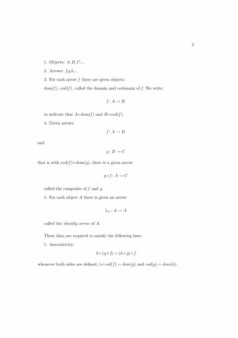
Definition 1.2.1. A category consists of the following data:

1

2

1. Objects: A, B, C, ...

2. Arrows: f,g,h,...

3. For each arrow f there are given objects:

dom(f ), cod(f ), called the domain and codomain of f. We write:

f : A ! B

to indicate that A=dom(f ) and B=cod(f ).

4. Given arrows

f : A ! B

and

g : B ! C

that is with cod(f )=dom(g), there is a given arrow:

g � f : A ! C

called the composite of f and g.

5. For each object A there is given an arrow:

1A : A ! A

called the identity arrow of A.

These data are required to satisfy the following laws:

1. Associativity:

h � (g � f) = (h � g) � f

whenever both sides are defined, i.e cod(f) = dom(g) and cod(g) = dom(h).

3

2. Unit:

f � 1A = f = 1B � f

for all f : A ! B.

1.3 Examples of Categories

Let consider a few examples of categories:

1. 0 is the empty category (no objects, no arrows).

2. The category 1 looks like ⇤, it has one object and its identity arrow.

3. The category 2 looks like this:

⇤ �! ?

It has two objects, their required identity arrows, and exactly one arrow between the

objects.

4. The category 3 looks like this:

⇤

•

g

��???

????

????

???⇤ ?

f // ?

•

h

��

��

��

��

It has three objects, their required identity arrows, exactly one arrow from the first

to the second object f : ⇤ �! ? , exactly one arrow from the second to the third

object h : ? �! •, and exactly one arrow from the first to the third object g : ⇤ �! •

(which is therefore the composite to the other two, g = h � f).

5. The category Sets of sets and functions. There is also the category Setsfin of

all finite sets and functions between them. There are many categories like this, given

4

by restricting the sets that are to be the objects and the functions that are to be

the arrows. For example, take finite sets as objects and injective functions as arrows.

Since the composition of injective functions is injective and identity functions are by

definition injective, this also gives a category.

6. Another kind of example one often sees in mathematics is categories of struc-

tured sets , that is, sets with some further “structure” and functions which “preserve”

it. Familiar examples of this kind are:

- Groups and group homomorphisms,

- Vector Spaces and linear mappings,

- Graphs and graph homomorphisms,

- The set R of real numbers and continuous functions R �! R,

- Open subsets U ✓ R and continuous functions f : U �! V ✓ R defined on them,

- Topological Spaces and continuous mappings,

- Di↵erential Manifolds and smooth mappings.

7. Monoids. A monoid is a category with just one object. Each monoid is thus

determined by the set of all its arrows, by the identity arrow, and by the rule for

the composition of arrows. Since any two arrows in a monoid have a composite, a

monoid can be described as a set M with a binary operation M⇥M �! M which is

associative and has an identity. Thus a monoid is exactly a semigroup with identity

element. For any category C and any object ↵ 2 C, the set hom(↵,↵) of all arrows

↵ �! ↵ is a monoid.

5

1.4 Functors

Like many mathematical “abstract” objects (such as groups, rings, topological spaces

etc.) are equipped with mappings between them (homomorphisms in the case of

groups and rings, and continuous functions in the case of topological spaces), the

notion of a mapping between categories is coming in the natural way.

Definition 1.4.1. A functor

F : C �! D

between categories C and D is a mapping of objects to objects and arrows to arrows,

in such a way that:

1.F (f : A ! B) = F (f) : F (A) ! F (B),

2.F (g � f) = F (g) � F (f),

3.F (1A) = 1F (A).

Now, one can check that functors compose in the expected way, and that every

category C has an identity functor 1C : C ! C. So we have another example of a

category, namely C, the category of all categories and functors.

Functors were first explicitly recognized in algebraic topology, where they arise

naturally when geometric properties are described by means of algebraic invariants.

For example, singular homology in a given dimension n (n a natural number) assigns

to each topological space X an abelian group Hn(X), the n-th homology group of X,

and also to each continuous map f : X ! Y of spaces a corresponding homomorphism

Hn(f) : Hn(X) ! Hn(Y) of groups, and in this way Hn becomes a functor between the

category of topological spaces and the category of abelian groups.

6

Also, functors arise naturally in algebra. For any commutative ring K with iden-

tity, the set of all non-singular n⇥ n matrices with entries in K is the usual general

linear group GLn(K). Moreover, each homomorphism f : K ! K0 of rings produces

in the evident way a homomorphism GLnf : GLn(K) ! GLn(K0) of groups. These

data define for each natural number n a functor between the category of commutative

rings and the category of finite groups.

For any group G the set of all products of commutators x yx�1y�1(x, y 2 G) is

clearly a normal subgroup, written [G, G], of G called the commutator subgroup

of G (For more on the theory of Finite Groups see [19]). Since any homomorphism

f : G ! H of groups carries commutators to commutators, the assignment G 7! [G, G]

defines a functor F : Grp ! Grp (the category of groups), while G 7! G/[G, G] defines

a functor G : Grp ! Ab, the functor commutator between the category of groups and

the category of abelian groups. However, the centre Z(G) of G does not naturally

define a functor F : Grp ! Grp, because a homomorphism f : G ! H may carry an

element in the centre of G to one not in the centre of H.

A functor which simply “forgets” some or all of the structures of an algebraic

object is called a forgetful functor. Thus the forgetful functor U : Grp ! Set (where

Set is the category of sets), assigns to each group G the set UG of its elements

(“forgetting” the multiplication and hence the group structure), and assigns to each

morphism f : G ! G0 of groups the same function f, regarded just as function between

sets. The forgetful functor U : Rng ! Ab (where Rng is the category of rings), assigns

to each ring R the additive abelian group of R and to each morphism R ! R0 of rings

the same function, regarded just as a morphism of addition.

Definition 1.4.2. An isomorphism T : C ! B of categories is a functor T from

7

C to B which is a bijection, both on objects and arrows. Equivalently, a functor

T : C ! B is an isomorphism if and only if there is a functor S : B ! C for which

both composites S �T and T � S are the identity functors 1C and 1B respectively. We

say that C is isomorphic to B, written C ⇠= B, if there exists an isomorphism between

them.

A functor T : C ! B is called full when to every pair (A,A0) of objects of C

and to every arrow g : T(A) ! T(A0) of B, there is an arrow f : A ! A0 of C with

g = T(f). Clearly, the composite of two full functors is a full functor.

A functor T : C ! B is called faithful when to every pair (A,A0) of objects of C

and to every pair f1, f2 : A ! A0 of parallel arrows of C, the equality T(f1) = T (f2) :

T(A) ! T(A0) implies f1 = f2. Again, the composite of two faithful functors is a

faithful functor.

As usual in mathematics, when we define an “abstract” mathematical object, it

is natural to look for its subobjects (subgroups in the case of groups, subrings in the

case of rings etc.).

Definition 1.4.3. A subcategory S of a category C is a collection of some of the

objects and some of the arrows of C, which includes with each arrow f both the

objects dom(f ) and cod(f ), with each object A its identity arrow 1A and with each

pair of composable arrows f ! g ! h their composite.

These conditions ensure that these collections of objects and arrows themselves

constitute a category S. Moreover, the inclusion map S ! C which sends each object

and arrow of S to itself in C is a functor, called the inclusion functor. This inclusion

functor is clearly faithful. We say that S is a full subcategory of C when the inclusion

functor S ! C is full. A full subcategory, given C, is thus determined by giving just

8

the set of its objects, since the arrows between any two of these objects A, A0 are all

morphisms A ! A0 in C.

Various properties of groups are reflected by properties of functors with values in

the category of groups. The simplest such case is the fact that subgroups can give rise

to the notions of “subfunctors”. The concept of “subfunctor” thus developed applies

with equal force to functors whose values are in the category of rings, spaces and so

on.

Definition 1.4.4. In the category D of all topological groups, a mapping �0 : G01 !

G02 is a submapping of a mapping � : G1 ! G2, written �0 �, whenever G01 G1,

G02 G2 and �0(g1) = �(g1) for all g1 2 G01.

Definition 1.4.5. Given functors T (A, B) and T 0(A, B) in two variables on the cat-

egories U and W with values in the category D (where U and W are any categories

and D is the category of topological groups), T 0 is called a subfunctor of T , written

T 0 T , if T 0(A, B) T (A, B) (where means a subgroup of) for each pair of objects

A 2 U , B 2 W and T 0(↵, �) T (↵, �) for each pair of mappings ↵ 2 U , � 2 W .

Clearly T 0 T and T T 0 implies T 0 = T . Furthermore this inclusion satisfies

the transitive law. If T 0 and T 00 are both subfunctors of the same functor T , then in

order to prove that T 0 T 00 it is su�cient to verify that T 0(A, B) T 00(A, B) for all

A and B.

The operation of forming a quotient group leads to an analogous operation of

taking the “quotient functor” of a functor T by a normal subfunctor T 0.

Definition 1.4.6. Let T be a functor covariant in the category U and contravariant

in the category W with values in the category D (where U and W are any categories

9

and D is the category of topological groups). A normal subfunctor T 0 is a subfunctor

T 0 T such that each T 0(A, B) is a normal subgroup of T (A, B), written T 0 � T .

Thus if T 0�T , the quotient functor Q = T/T 0 has an object function given as the

factor group

Q(A, B) = T (A, B)/T 0(A, B).

For homomorphisms ↵ : A1 ! A2 and � : B1 ! B2 the corresponding mapping

function Q(A, B) is defined for each coset xT 0(A, B) as

Q(↵, �)[xT 0(A1, B2)] = [T (↵, �)x]T 0(A2, B1).

One may easily verify that Q gives a uniquely defined homomorphism

Q(↵, �) : Q(A1, B2) ! Q(A2, B1).

As one might expect, the next obvious task is to formulate the isomorphism theorems

of group theory in terms of functors. This will not be discussed here (For a detailed

discussion see [7, pg.260–265]).

1.5 Initial and Terminal Objects

We now consider abstract characterizations of the empty set and the one-element sets

in the category Sets and structurally similar objects in general categories.

Definition 1.5.1. In any category C, an object A is called initial, if for any object

B there is a unique morphism

A ! B.

D is called terminal, if for any object B there is a unique morphism

B ! D.

10

Note that there is a kind of “duality” in these definitions. Precisely, a terminal

object in the category C is exactly an initial object in the category Cop (where Cop

is the opposite category, in vague terms the category with all arrows reversed).

Definition 1.5.2. An isomorphism f : A ! B of objects A and B in a category C

is just a bijective morphism from A to B.

Proposition 1.5.1. Initial (terminal) objects are unique up to isomorphism.

Proof. See [1, pg.28]

Examples

1. In the category Sets the empty set is initial and any singleton set is terminal.

Observe that Sets has just one initial object but many terminal objects.

2. In the category Grp, the one element group is both initial and terminal (sim-

ilarly for the category of vector spaces and linear transformations, as well as the

category of monoids and monoid homomorphisms).

1.6 Products and Coproducts of Categories

Next we are going to see the categorical definition of a product of two objects in

a category. This was first given by Mac Lane [13], and it is probably the earliest

example of category theory being used to define a fundamental mathematical notion.

Let us begin by considering products of sets. Given sets A and B the cartesian product

of A and B is the set of ordered pairs

A⇥ B = {(a, b)|a 2 A, b 2 B}.

11

Observe that there are two “coordinate projections”

A oo ⇡1A⇥B

⇡2 // B

with

⇡1(a, b) = a, ⇡2(a, b) = b.

Indeed, given any element c 2 A⇥ B we have

c = (⇡1c, ⇡2c).

The situation is captured concisely in the following diagram:

A A⇥Boo⇡1

A⇥B B⇡2//

1

A

a

��

��

��

�1

A⇥B

(a,b)

✏✏

1

B

b

��???

????

????

??

Definition 1.6.1. In any category C, a product diagram for the objects A and B

consists of an object P and arrows

A oo p1P

p2 // B

satisfying the following Universal Mapping Property:

Given any diagram of the form

A oo x1 Xx2 // B

there exists a unique u : X ! P, making the diagram

A Poop1

P Bp2//

X

A

x1

��

��

��

�X

P

u

✏✏

X

B

x2

��???

????

????

??

commutative, that is, such that x1 = p1u and x2 = p2u.

12

Proposition 1.6.1. Products are unique up to isomorphism.

Proof. See [1, pg.35].

If the objects A and B have a product, we write

A oo p1A⇥B

p2 // B.

for one such product. Then given X, x1, x2 as in the definition, we write

(x1, x2) for u : X ! A⇥ B.

However, a pair of objects may have many di↵erent products in a category. For

example, given a product A ⇥ B, p1, p2, and any isomorphism h : A ⇥ B ! Q, the

diagram Q, p1 � h, p2 � h is also a product of A and B.

Now an arrow into a product

f : X ! A⇥ B

is “the same thing” as a pair of arrows

f1 : X ! A, f2 : X ! B.

So we can essentially forget about such arrows, in that they are uniquely determined

by pairs of arrows.

There is a “dual” version of the notion of products in a category, called the

“coproduct” of two objects. One can think of coproducts as products with the arrows

reversed.

Definition 1.6.2. In any category C, a coproduct diagram for the objects A and B

consists of an object Q and arrows

Aq1 // Q oo q2

B

13

satisfying the following Universal Mapping Property:

Given any diagram of the form

Az1 // Z oo z2

B

there exists a unique u : Q ! Z, making the diagram

A Qq1// Q Boo

q2

Z

A

??

z1

��

��

��

�Z

Q

OO

u

Z

B

__

z2

????

????

????

?

commutative, that is, such that z1 = q1u and z2 = q2u.

1.7 Examples of Products and Coproducts

1. One can show that the product of two topological spaces X and Y, as usually

defined, is a product in Top (the category of topological spaces and continuous func-

tions). Thus, suppose that X and Y are two topological spaces and consider their

product space X⇥ Y with its projections

X oo p1X ⇥ Y

p2 // Y .

Recall that X⇥Y is generated by basic open sets of the form U⇥V where U is open in

X and V is open in Y . Therefore every W 2 X⇥Y is a union of open sets. Firstly, it

is obvious that p1 is continuous, since p�11 U = U⇥Y. Secondly, given any continuous

mappings f1 : Z ! X and f2 : Z ! Y, let f : Z ! X ⇥ Y be the function f = (f1, f2).

Now one needs to show that f is continuous. Given any W =S

i(Ui ⇥ Vi) 2 X⇥ Y,

14

f�1(W) =S

i f�1(Ui ⇥ Vi), so it su�ces to show that f�1(U⇥ V) is open. But

f�1(U⇥ V) = f�1((U⇥ Y) \ (X⇥ V))

= f�1(U⇥ Y) \ f�1(X⇥ V)

= f�1 � p�11 (U) \ f�1 � p�1

2 (V)

= (f1)�1(U) \ (f2)

�1(U) \ (f2)�1(V)

(1.7.1)

where (f1)�1(U)) and (f2)

�1(V) are open, since f1 and f2 are continuous.

The following diagram concisely captures the situation at hand:

X X ⇥ Yp�11

// X ⇥ Y Yoop�12

Z

X

??

f�11

��

��

��

�Z

X ⇥ Y

OO

f�1

Z

Y

__

f�12

????

????

????

?

Next, consider the following example of a coproduct:

2. For abelian groups A and B, the free product A � B need not be abelian.

One could take a quotient of A�B to get a coproduct in the category Ab of abelian

groups, but there is a more convenient presentation, which we now consider.

Definition 1.7.1. Let X = A � B, choose a set disjoint from X with the same

cardinality: for notational reasons we shall denote this by X�1 = {x�1|x 2 X} where

x�1 is merely a symbol. By a word in X we mean a finite sequence of symbols from

X [X�1, written in the form

w = xe11 ...xer

r

where xi 2 X, ei = ±1, and r � 0 (see [17, pg.45]).

Since the words in the free product A � B must be forced to satisfy the further

commutativity conditions

(a1b1b2a2...) ⇠ (a1a2...b1b2...)

15

we can shu✏e all the a0s to the front, and the b0s to the back, of the words. Further-

more, we already have

(a1a2...b1b2...) ⇠ (a1 + a2 + ... + b1 + b2 + ...).

Thus, we in e↵ect have pairs of elements (a, b). So we take the product set as the

underlying set of the coproduct

|A + B| = |A⇥B|.

As inclusions, we use the homomorphisms

iA(a) = (a, 0B)

iB(b) = (0A, b).

Then given any homomorphisms Af // X oo g

B, we let (f, g) : A + B ! X be

defined by

(f, g)(a, b) = f(a) +X g(b).

Proposition 1.7.1. In the category Ab of abelian groups, there is a canonical iso-

morphism between the binary coproduct and product,

A + B ⇠= A⇥B

Proof. See [1, pg.53].

This in fact was first observed by Mac Lane [13], and it was shown to lead to

a binary operation on parallel arrows f, g : A ! B between abelian groups (and

related structures like modules and vector spaces). In fact, the group structure of a

particular abelian group A can be recovered from this operation on arrows into A.

16

More generally, the existence of such an addition operation on arrows can be used

as the basis of an abstract description of categories like Ab, called abelian categories,

which are suitable for axiomatic homology theory (see [13]).

A very interesting situation arises in categories in which products and coproducts

di↵er.

First, consider the category Set of sets and mappings. The product of a family

(Ci)i2I of sets for some indexed set I, is just the cartesian product

Y

i2I

Ci = {(xi)i2I |xi 2 Ci}

with the obvious projection maps pi((xi)i2I) = xi.

The coproduct of a family (Ci)i2I of sets for some indexed set I, is its disjoint

union, i.e. the union of sets (Ci)i2I considered as disjoint sets. When various sets Ci

are not disjoint, one may replace them by an isomorphic disjoint set

C 0i = {(x, i)|x 2 Ci, i 2 I}

and then perform the usual union of these sets C 0i. Thus in short

[

i2I

Ci = {(x, i)|x 2 Ci, i 2 I}

with the obvious inclusion maps si(x) = (x, i).

Another very interesting example of a category in which products and coproducts

di↵er arises in the category Grp of groups and group homomorphisms. The product

of a family of groups in Grp is just their direct product with componentwise binary

operation. For example,Y

i2I

Gi = {(gi)i2I |gi 2 Gi}

17

is defined by

(gi)i2I + (hi)i2I = (gi + hi)i2I for gi, hi 2 Gi.

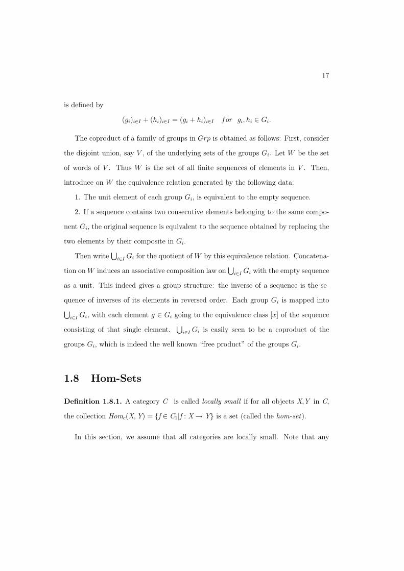
The coproduct of a family of groups in Grp is obtained as follows: First, consider

the disjoint union, say V , of the underlying sets of the groups Gi. Let W be the set

of words of V . Thus W is the set of all finite sequences of elements in V . Then,

introduce on W the equivalence relation generated by the following data:

1. The unit element of each group Gi, is equivalent to the empty sequence.

2. If a sequence contains two consecutive elements belonging to the same compo-

nent Gi, the original sequence is equivalent to the sequence obtained by replacing the

two elements by their composite in Gi.

Then writeS

i2I Gi for the quotient of W by this equivalence relation. Concatena-

tion on W induces an associative composition law onS

i2I Gi with the empty sequence

as a unit. This indeed gives a group structure: the inverse of a sequence is the se-

quence of inverses of its elements in reversed order. Each group Gi is mapped intoS

i2I Gi, with each element g 2 Gi going to the equivalence class [x] of the sequence

consisting of that single element.S

i2I Gi is easily seen to be a coproduct of the

groups Gi, which is indeed the well known “free product” of the groups Gi.

1.8 Hom-Sets

Definition 1.8.1. A category C is called locally small if for all objects X,Y in C,

the collection Homc(X,Y) = {f 2 C1|f : X ! Y} is a set (called the hom-set).

In this section, we assume that all categories are locally small. Note that any

18

arrow g : B ! B0 in C induces a function:

Hom(A, g) : Hom(A,B) ! Hom(A,B0)

(f : A ! B) 7! (g � f : A ! B ! B0).

Thus Hom(A, g) = g � f. One sometimes writes g⇤ instead of Hom(A, g), so

g⇤(f) = g � f.

Let us show that this determines a functor

Hom(A,�) : C ! Sets

called the (covariant) representable functor of A. We need to show that

Hom(A, 1X) = 1Hom(A,X)

and that

Hom(A, g � f) = Hom(A, g) � Hom(A, f).

Taking an argument x : A ! X, we clearly have

Hom(A, 1X)(x) = 1X � x

= x

= 1Hom(A,X)(x)

(1.8.1)

and

Hom(A, g � f)(x) = (g � f) � x

= g � (f � x)

= Hom(A, g)(Hom(A, f)(x))

(1.8.2)

19

Also, there is a “dual” version of the covariant functor, which is of the form

F : Cop ! D and is called the contravariant functor of a category C. Explicitly, such

a functor takes f : A ! B to F(f) : F(B) ! F(A) and F(g � f) = F(f) �F(g). A typical

example of a contravariant functor is a representable functor of the form

HomC(�,C) : Cop ! Sets

for any C 2 C (where C is any locally small category). Such a contravariant repre-

sentable functor takes f : X ! Y to

f⇤ : Hom(Y,C) ! Hom(X,C)

by

f ⇤(g : X ! C) = g � f.

Now let see how how one can use the notion of Hom-sets to give another definition

of product.

An object P with arrows p1 : P ! A and p2 : P ! B gives an element (p1, p2) of

the set

Hom(P,A)⇥ Hom(P, B)

and similarly for any set X in place of P. Now, given any arrow

x : X ! P

composing with p1 and p2 gives a pair of arrows x1 = p1 �x : X ! A and x2 = p2 �x :

X ! B, as indicated in the following diagram:

A Poop1

P Bp2//

X

A

x1

��

��

��

�X

P

x

✏✏

X

B

x2

��???

????

????

??

20

In this way, we have a function

@X = (Hom(X, p1), Hom(X, p2)) : Hom(X, P ) ! Hom(X, A)⇥Hom(X, B)

defined by

@X(x) = (x1, x2).

This function @X can be used to express concisely the condition of being a product

as follows.

Proposition 1.8.1. A diagram of the form

A oo p1P

p2 // B

is a product for A and B if and only if for every object X, the canonical function

@X(x) = (x1, x2) is an isomorphism

@X : Hom(X, P ) ⇠= Hom(X, A)⇥Hom(X, B)

Proof. By the Universal Mapping Property, for every element (x1, x2) 2 Hom(X, A)⇥

Hom(X,B), there is a unique x 2 Hom(X, P ) such that @X = (x1, x2), that is, @X is

bijective.

Definition 1.8.2. Let C,D be categories with binary products. A functor F : C ! D

is said to preserve binary products if it takes every product diagram

A oo p1A⇥B

p2 // B

in the category C, to a product diagram

FA oo Fp1F (A⇥B)

Fp2 // FB

21

in the category D. It follows that F preserves products just if

F (A⇥B) ⇠= FA⇥ FB

that is, if and only if the canonical “comparison arrow”

(Fp1, Fp2) : F (A⇥B) ! FA⇥ FB

is an isomorphism.

For example, the forgetful functor U : Mon ! Sets preserves binary products.

Corollary 1.8.2. For any object X in a category C with products, the covariant

functor

HomC(X,�) : C ! Sets

preserves products.

Proof. For any A, B 2 C, the foregoing proposition says that there is a canonical

isomorphism:

HomC(X, A⇥B) ⇠= HomC(X,A)⇥HomC(X, B)

1.9 Natural Transformations

Eilenberg and Mac Lane first observed, that the notion of “category” has been defined

in order to be able to define the notion of “functor” and the notion of “functor” has

been defined in order to be able to define the notion of “natural transformation”. One

22

can think of natural transformations as morphisms of functors. For fixed categories C

and D we can regard the functors C ! D as the objects of a new category, and the

arrows between these objects are what we are going to call natural transformations.

Definition 1.9.1. Given two functors S, T : C ! B, a natural transformation ⌧ :

S ! T is a function which assigns to each object A of C an arrow ⌧A = ⌧A : SA ! TA

of B in such a way that every arrow f : A ! A0 in C yields a commutative diagram:

A

A0

f

✏✏SA0 TA0

⌧A0//

SA

SA0

Sf

✏✏

SA TA⌧A // TA

TA0

Tf

✏✏

we call ⌧A, ⌧B, ... the components of the natural transformation ⌧ .

When this holds, we also say that ⌧A : SA ! TA is natural in A. If we think

of the functor S as giving a picture in B of all the objects and arrows of C, then a

natural transformation ⌧ is a set of arrows mapping the picture S to the picture T.

Definition 1.9.2. A natural transformation ⌧ with every component ⌧A invertible

in B is called a natural equivalence or a natural isomorphism, written as ⌧ : S ⇠= T .

In this case, the inverses (⌧A)�1 in B are the components of a natural isomorphism

⌧�1 : T ! S.

Examples of Natural Transformations

1. The determinant is a natural transformation. To be explicit, let detKM be the

determinant of the n⇥n matrix M with entries in the commutative ring K, while K⇤

denotes the group of units (invertible elements) of K. Thus, M is non-singular when

detKM is a unit, and detK is a morphism GLnK ! K⇤ of groups, an arrow in Grp,

23

(where GLn is obviously the general linear group). Because the determinant is defined

by the same formula for all rings K, each morphism f : K ! K 0 of commutative rings

leads to a commutative diagram

GLnK0 K 0⇤

detK0//

GLnK

GLnK0

GLnf

✏✏

GLnK K⇤detK // K⇤

K 0⇤

f⇤

✏✏

This states that the transformation det : GLn ! (⇤) is natural between two functors

C, T : Rng ! Grp.

2. For each group G the projection pG : G ! G/[G, G] to the factor-commutator

group, defines the transformation p from the identity functor on Grp to the factor-

commutator functor Grp ! Ab ! Grp. Moreover, p is natural because each group

homomorphism f : G ! H defines the evident homomorphism f 0 for which the

following diagram commutes:

H H/[H, H]pH

//

G

H

f

✏✏

G G/[G, G]pG // G/[G, G]

H/[H, H]

f 0

✏✏

3. Consider the category V ect(R) of real vector spaces and linear transformations

f : V ! W . Every vector space V has a dual space

V ⇤ = V ect(V, R)

of linear transformations and every linear transformation f : V ! W gives rise to a

dual linear transformation f ⇤ : W ⇤ ! V ⇤ defined by pre-composition, f ⇤(A) = A � f

for A : W ! R. In brief (�) : V ect(�, R) : V ectop ! V ect is the contravariant

24

representable functor endowed with vector space structure. There is a canonical

linear transformation from each vector space to its dual

⌘V : V ! V ⇤⇤

x 7! (evx : V ⇤ ! R)

where evV (A) = A(x) for every A : V ! R. This map is the component of a natural

transformation ⌘ : 1V ect ! ⇤⇤, since the following diagram always commutes in Vect

W W ⇤⇤⌘W

//

V

W

f

✏✏

V V ⇤⇤⌘V // V ⇤⇤

W ⇤⇤

f⇤⇤

✏✏

Indeed, given any v 2 V and A : W ! R in W ⇤, we have

(f ⇤⇤ � ⌘V (v)(A) = f ⇤⇤(evv)(A)

= evv(f⇤(A)

= evv(A � f)

= (A � f)(v)

= A(fv)

= evfv(A)

= (⌘W � f)(v)(A).

(1.9.1)

Now, it is well-known fact in linear algebra that every finite dimensional vector space

V is isomorphic to its dual space V ⇠= V ⇤, just for reasons of dimension. However,

there is no “natural” way to choose such an isomorphism. On the other hand, the

natural transformation

⌘V : V ! V ⇤⇤

25

is a natural isomorphism when V is finite dimensional. Thus, the formal notion of

naturality captures the informal fact that V ⇠= V ⇤⇤, “naturally”, unlike V ⇠= V ⇤.

Chapter 2

Category Theory in Algebraic

Topology

2.1 Introduction

In the years before 1945, Eilenberg and Mac Lane had been working intensively on

some homological problems within which natural transformations appear quite often,

some of them explicitly on the form of commutative diagrams. Broadly speaking,

homological procedures provide techniques for associating a suitably defined group

to every given topological space, so that properties of the space may be drawn from

more easily deducible properties of the homology groups. These procedures also

involve associating a group homomorphism to every continuous function between the

given topological spaces ([5, pg.347]).

In order to “translate” topological problems in the context of the new language

which category theory provided, Eilenberg and Mac Lane developed in the last chapter

of [7] a new framework by formulating well known concepts from algebraic topology

26

27

in terms of categorical language. Firstly, they formulated the homology group as a

functor from the category of complexes to the category of discrete abelian groups and

the cohomology group as a functor from the category of complexes to the category

of topological abelian groups. Secondly, they proved that the cohomology group is

isomorphic, indeed “naturally” isomorphic, to the character group of the homology

group (as functors). Thirdly, they showed that the basic constructions of group

extensions may be regarded as functors. Finally, they presented a new treatment of

the Cech homology theory in terms of functors. The aim of this chapter is to present

a coherent summary of the above developments and to show their significance in later

developments in Algebraic Topology.

2.2 Homology and Cohomology Groups as Func-

tors

Definition 2.2.1. An abstract complex K is a collection

{Cq(K)}, q = 0,±1,±2, ...

of free abelian discrete groups, together with a collection of homomorphisms

@q : Cq(K) ! Cq�1(K)

called boundary homomorphisms, such that

@q@q+1 = 0.

By selecting for each of the free abelian groups Cq a fixed basis {�qi }, called q-

dimensional cells, we obtain an abstract complex. The boundary operator @ can be

28

written as a finite sum

@�q =X

�q�1

[�q : �q�1]�q�1.

The integers [�q : �q�1] are called incidence numbers, and satisfy the following con-

ditions:

1. Given �q, [�q : �q�1] 6= 0 only for a finite number of (q � 1)� cells �q�1,

2. Given �q+1 and �q�1,P

�q [�q+1 : �q][�q : �q�1] = 0.

Definition 2.2.2. Given two abstract complexes K1 and K2, a chain transformation

k : K1 ! K2

is a collection k = {kq} of homomorphisms,

kq : Cq(K1) ! Cq(K2)

such that

kq�1@q = @qkq,

as the following diagram indicates

Cq(K2) Cq�1(K2)@q//

Cq(K1)

Cq(K2)

kq

✏✏

Cq(K1) Cq�1(K1)@q

// Cq�1(K1)

Cq�1(K2)

kq�1

✏✏

In this way one gets the category ⌦ whose objects are the abstract complexes and

whose mappings are the chain transformations with obvious definition of the compo-

sition of chain transformations. The consideration of simplicial complexes and sim-

plicial transformations leads to a category ⌦s. Every simplicial complex determines

uniquely an abstract complex and every simplicial transformation a chain transfor-

mation. This leads to a covariant functor on ⌦s to ⌦.

29

Definition 2.2.3. For every complex K in the category ⌦ and every group G in

the category D0a of discrete abelian groups, define the groups Cq(K,G) of the q-

dimensional chains of K over G as the tensor product (of abelian groups)

Cq(K, G) = G⌦ Cq(K),

that is, Cq(K,G) is the group with the symbols

gcq, g 2 G, cq 2 Cq(K)

as generators, and

(g1 + g2)cq = g1c

q + g2cq, g(cq

1 + cq2) = gcq

1 + gcq2

as relations.

For every chain transformation k : K1 ! K2 and for every homomorphism � :

G1 ! G2 define a homomorphism

Cq(k, �) : Cq(K1, G1) ! Cq(K2, G2)

by setting

Cq(k, �)(g1cq1) = �(g1)k

q(c1q)

for each generator g1cq1 of Cq(K1, G1).

These definitions of Cq(K, G) and Cq(k, �) yield a functor Cq covariant in ⌦ and

D0a with values in D0a. This functor is called q-chain functor.

Define a homomorphism

@q(K, G) : Cq(K, G) ! Cq�1(K, G)

30

by setting

@q(K, G)(gcq) = g@cq

for each generator g1cq1 of Cq(K1, G1). Thus the boundary operator becomes a natural

transformation of the functor Cq into the functor Cq�1

@q : Cq ! Cq�1.

The kernel of this transformation is denoted Zq and is called the q-cycle functor. Its

object function is the group Zq(K, G) of the q-dimensional cycles of the complex K

over G. The image of Cq under the transformation @q is a subfunctor Bq�1 = @q(Cq)

of Cq�1. Its object function is the group Bq�1(K, G) of the (q � 1)-dimensional

boundaries in K over G.

The fact that @q@q+1 = 0 implies that Bq(K, G) is a subgroup of Zq(K, G). Con-

sequently Bq is a subfunctor of Zq. The quotient functor

Hq = Zq/Bq

is called the qth homology functor. Its object function associates with each complex K

and with each discrete abelian coe�cient group G the qth homology group Hq(K, G)

of K over G. The functor Hq is covariant in ⌦ and D0a with values in D0a.

Now in order to define the cohomology groups as functors, consider the category

⌦ as before and the category Da of topological abelian groups. Given a complex K

in ⌦ and a group G in Da define the group Cq(K,G) of the q-dimensional cochains

of K over G as

Cq(K, G) = Hom(Cq(K), G).

Given a chain transformation k : K1 ! K2 and a homomorphism � : G1 ! G2, define

31

a homomorphism

Cq(k, �) : Cq(K2, G1) ! Cq(K1, G2)

by associating with each homomorphism f 2 Cq(K2, G1) the homomorphism f 0 =

Cq(k, �)f defined as follows:

f 0(cq1) = �[f(kqcq

1)], cq1 2 Cq(K1).

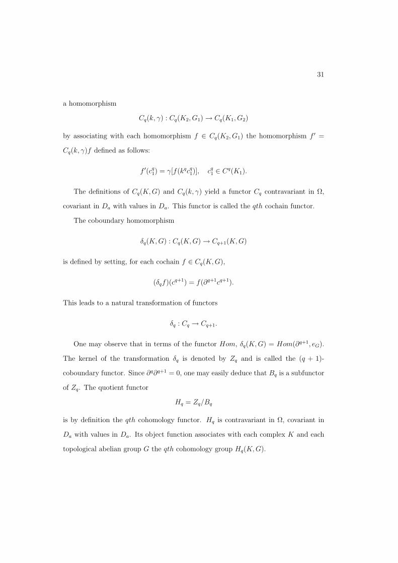
The definitions of Cq(K, G) and Cq(k, �) yield a functor Cq contravariant in ⌦,

covariant in Da with values in Da. This functor is called the qth cochain functor.

The coboundary homomorphism

�q(K, G) : Cq(K, G) ! Cq+1(K, G)

is defined by setting, for each cochain f 2 Cq(K, G),

(�qf)(cq+1) = f(@q+1cq+1).

This leads to a natural transformation of functors

�q : Cq ! Cq+1.

One may observe that in terms of the functor Hom, �q(K,G) = Hom(@q+1, eG).

The kernel of the transformation �q is denoted by Zq and is called the (q + 1)-

coboundary functor. Since @q@q+1 = 0, one may easily deduce that Bq is a subfunctor

of Zq. The quotient functor

Hq = Zq/Bq

is by definition the qth cohomology functor. Hq is contravariant in ⌦, covariant in

Da with values in Da. Its object function associates with each complex K and each

topological abelian group G the qth cohomology group Hq(K, G).

32

2.3 Duality

Let G be a discrete abelian group and CharG be its character group. Given a chain

cq 2 Cq(K, G) = G⌦ Cq(K)

where

cq =X

i

gicqi , gi 2 G, cq

i 2 Cq(K)

and given a cochain

f 2 Cq(K, CharG) = Hom(Cq(K), Char)

one may define the Kronecker index

KI = (f, cq) =X

i

(f(cqi ), gi).

Since f(cqi ) is an element of CharG, its application to gi gives an element of the group

P of reals reduced mod1. The continuity of KI(f, cq) as a function of f follows from

the definition of the topology in CharG and in Cq(K, CharG).

Theorem 2.3.1. The cohomology group Cq(K,CharG) is naturally isomorphic to

the character group of the homology group Cq(K, G).

Proof. Define an isomorphism

⌧ q(K, G) : Cq(K, CharG) � CharCq(K, G) (2.3.1)

by defining for each cochain f 2 Cq(K, CharG) a character

⌧ q(K, G)f : Cq(K, G) ! P

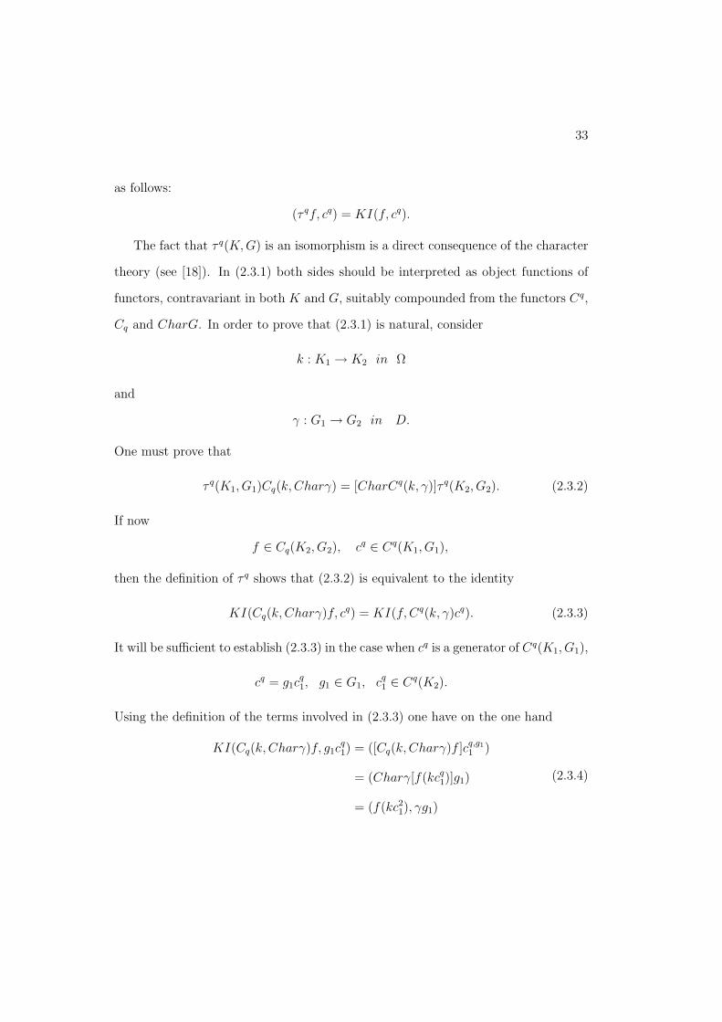
33

as follows:

(⌧ qf, cq) = KI(f, cq).

The fact that ⌧ q(K, G) is an isomorphism is a direct consequence of the character

theory (see [18]). In (2.3.1) both sides should be interpreted as object functions of

functors, contravariant in both K and G, suitably compounded from the functors Cq,

Cq and CharG. In order to prove that (2.3.1) is natural, consider

k : K1 ! K2 in ⌦

and

� : G1 ! G2 in D.

One must prove that

⌧ q(K1, G1)Cq(k, Char�) = [CharCq(k, �)]⌧ q(K2, G2). (2.3.2)

If now

f 2 Cq(K2, G2), cq 2 Cq(K1, G1),

then the definition of ⌧ q shows that (2.3.2) is equivalent to the identity

KI(Cq(k, Char�)f, cq) = KI(f, Cq(k, �)cq). (2.3.3)

It will be su�cient to establish (2.3.3) in the case when cq is a generator of Cq(K1, G1),

cq = g1cq1, g1 2 G1, cq

1 2 Cq(K2).

Using the definition of the terms involved in (2.3.3) one have on the one hand

KI(Cq(k, Char�)f, g1cq1) = ([Cq(k, Char�)f ]cq,g1

1 )

= (Char�[f(kcq1)]g1)

= (f(kc21), �g1)

(2.3.4)

34

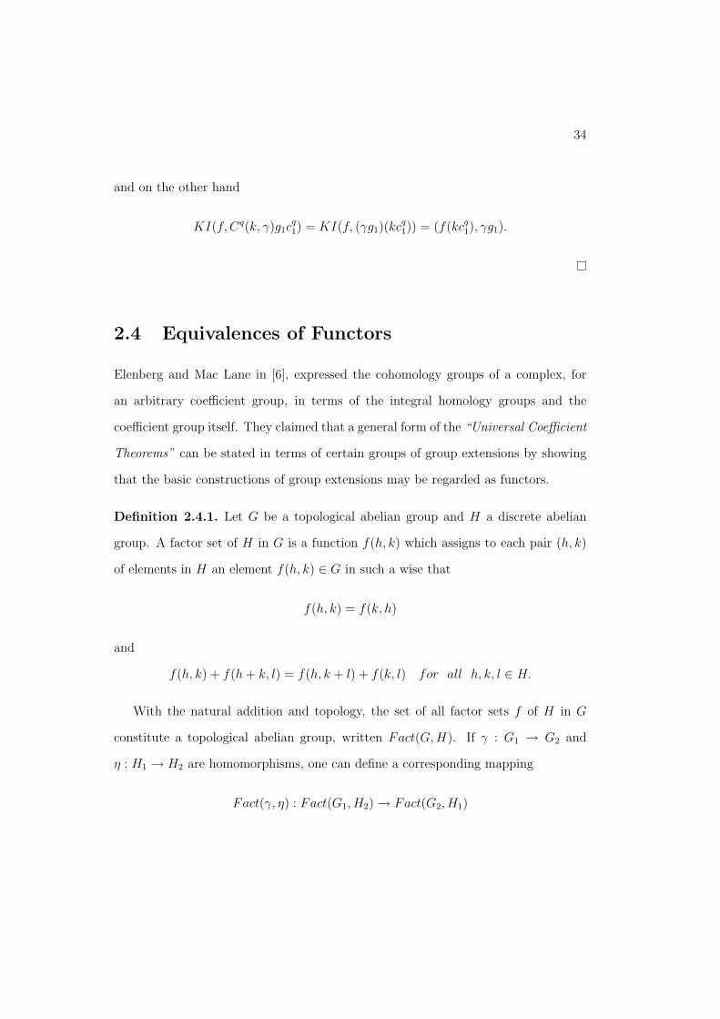
and on the other hand

KI(f, Cq(k, �)g1cq1) = KI(f, (�g1)(kcq

1)) = (f(kcq1), �g1).

2.4 Equivalences of Functors

Elenberg and Mac Lane in [6], expressed the cohomology groups of a complex, for

an arbitrary coe�cient group, in terms of the integral homology groups and the

coe�cient group itself. They claimed that a general form of the “Universal Coe�cient

Theorems” can be stated in terms of certain groups of group extensions by showing

that the basic constructions of group extensions may be regarded as functors.

Definition 2.4.1. Let G be a topological abelian group and H a discrete abelian

group. A factor set of H in G is a function f(h, k) which assigns to each pair (h, k)

of elements in H an element f(h, k) 2 G in such a wise that

f(h, k) = f(k, h)

and

f(h, k) + f(h + k, l) = f(h, k + l) + f(k, l) for all h, k, l 2 H.

With the natural addition and topology, the set of all factor sets f of H in G

constitute a topological abelian group, written Fact(G, H). If � : G1 ! G2 and

⌘ : H1 ! H2 are homomorphisms, one can define a corresponding mapping

Fact(�, ⌘) : Fact(G1, H2) ! Fact(G2, H1)

35

by setting

(Fact(�, ⌘)f)(h1, k1) = �f(⌘h1, ⌘k1)

for each factor set f in Fact(G1, H2). Thus it appears that Fact is a functor, covariant

in the category Da of topological abelian groups and contravariant in the category

D0a of discrete abelian groups.

Guven any g(h) with values in G, the combination

f(h, k) = g(h) + g(k)� g(h + k)

is always a factor set, the sets of this form are called transformation sets and the set

of all such sets is a subgroup, written Trans(G, H), of the group Fact(G, H). This

subgroup is the object function of a subfunctor. The corresponding quotient functor

Ext = Fact/Trans

is thus covariant in Da and contravariant in D0a with values in Da. Its object function

assigns to the group G and H the group Ext(G, H) of the so-called abelian group

extension of G by H.

Since Cq(K, G) = Hom(Cq(K), G) and since Cq(K, I) = I ⌦ Cq(K) = Cq(K),

where I is the additive group of integers, one gets

Cq(K, G) = Hom(Cq(K, I), G).

Therefore, one may define a subgroup

Aq(K, G) = AnnihZq(K, I)1

1AnnihZq(K, I) is the set of all characters x 2 CharZq(K, I) with (x, g) = 0 for each g 2Zq(K, I).

36

of Cq(K, G), consisting of all homomorphisms f such that f(zq) = 0 for zq 2 Zq(K, I).

Thus one gets a subfunctor Aq of Cq, and one may show that the coboundary functor

Bq is a subfunctor of Aq, which is a subfunctor of the cocycle functor Zq. Therefore,

the quotient functor

Qq = Aq/Bq

is a subfunctor of the cohomology functor Hq, and one may consider the quotient

functor Hq/Qq. The functors Qq and Hq/Qq have the following object functions:

Qq(K, G) = Aq(K, G)/Bq(K, G),

(Hq/QQ)(K, G) = Hq(K, G)/Qq(K, G) ⇠= Zq(K, G)/Aq(K, G).

Based on [6], Eilenberg and Mac Lane made the following assertions, interpreting

the isomorphisms as equivalences of functors.

1. Qq(K, G) is a direct factor of Hq(K,G).

2. Qq(K, G) ⇠= Ext(G, Hq+1(K, I)).

3. Hq(K, G)/Qq(K, G) ⇠= Hom(Hq(K, I), G).

The procedure of forming the topological abelian group Fact and its subgroup

Trans comes directly from the theory of group extensions as follows:

Let A be an abelian group with a normal subgroup isomorphic to a group G such

that A/G ⇠= H. Let f be a function which assigns to each pair (h, k) of elements

in H an element f(h, k) 2 G. Choose a set {t(h)|h 2 H} of coset representatives

for G in A. Then f(h) + t(k) lies in the coset with representatives t(h + k), so

f(h) + t(k) = f(h, k) + t(h + k) for some f(h, k) 2 G. It is straightforward to check

that f is a factor set.

Now suppose that {t0(h)|h 2 H} is another set of coset representatives, defining

a factor set f 0. Then, t0(h) = t(h) + g(h) for some g(h) 2 G and then one may easily

37

check that

f 0(h, k) = f(h, k) + g(h) + g(k)� g(h, k).

In other words, f and f 0 di↵er by a transformation set.

Conversely, given a factor set, one may define a group A whose elements are

ordered pairs (g, h) for g 2 G, h 2 H with addition

(g1, h1) + (g2, h2) = (g1 + g2 + f(h1, h2), h1 + h2).

This has a normal subgroup {(g, 0)|g 2 G} isomorphic to G, with A/G ⇠= H. There-

fore elements of Ext(H, G) define extensions of G by H, i.e. groups A as above.

2.5 Cech homology groups as Functors

In the final subsection of the last chapter of [7], Eilenberg and Mac Lane presented a

new treatment of the Cech homology theory in terms of functors.

Definition 2.5.1. An open covering U of a topological space X is a finite collection

U = {A1, A2, ..., An}

of open sets whose union is in X.

The sets Ai i = 1, ..., n may appear with repetitions, and some of them may be

empty. If U1 and U2 are two such coverings, write U1 < U2 whenever U2 is a refinement

of U1, that is, whenever each set of the covering U2 is contained is some set of the

covering U1. With this definition the coverings U of X form a directed set 2, say P .

2A directed set is a set of elements p1, p2,.. with a reflexive and transitive binary relation suchthat for each pair of elements p1, p2 2 P there exists an element p3 2 P with p1 < p3 and p2 < p2

which is denoted by C(X).

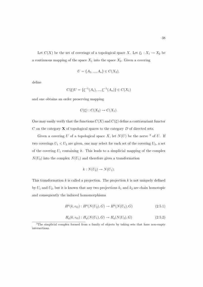
38

Let C(X) be the set of coverings of a topological space X. Let ⇠1 : X1 ! X2 be

a continuous mapping of the space X1 into the space X2. Given a covering

U = {A1, ..., An} 2 C(X2),

define

C(⇠)U = {⇠�1(A1), ..., ⇠�1(An)} 2 C(X1)

and one obtains an order preserving mapping

C(⇠) : C(X2) ! C(X1).

One may easily verify that the functions C(X) and C(⇠) define a contravariant functor

C on the category X of topological spaces to the category D of directed sets.

Given a covering U of a topological space X, let N(U) be the nerve 3 of U . If

two coverings U1 < U2 are given, one may select for each set of the covering U2, a set

of the covering U1 containing it. This leads to a simplicial mapping of the complex

N(U2) into the complex N(U1) and therefore gives a transformation

k : N(U2) ! N(U1).

This transformation k is called a projection. The projection k is not uniquely defined

by U1 and U2, but it is known that any two projections k1 and k2 are chain homotopic

and consequently the induced homomorphisms

Hq(k, eG) : Hq(N(U2), G) ! Hq(N(U1), G) (2.5.1)

Hq(k, eG) : Hq(N(U1), G) ! Hq(N(U2), G) (2.5.2)

3The simplicial complex formed from a family of objects by taking sets that have non-emptyintersections.

39

of the homology and cohomology groups do not depend upon the particular choice of

the projection k.

Given a topological group G, consider the collection of the homology groups

Hq(N(U), G) for U 2 C(X). These groups together with the mappings (2.5.1) form

a inverse system of groups defined on the directed set C(X). This inverse system

is denoted by Cq(X,G) and is treated as an object function of the category Inb of

directed sets.

For a discrete topological group G, the cohomology groups Hq(N(U), G) together

with the mappings (2.5.2) form a direct system of groups Cq(X, G) defined on the

directed set C(X). The system Cq(X, G) is treated as an object function of the

category Dir of directed sets.

The functions Cq(X, G) and Cq(X, G) are the object functions of the functors

Cq

and Cq. Now, by defining the mapping functions Cq(⇠, �) and Cq(⇠, �) for given

mappings

⇠ : X1 ! X2, � : G1 ! G2,

one gets the order preserving mapping

C(⇠) : C(X2) ! C(X1) (2.5.3)

which with each covering

U = {A1, ..., An} 2 C(X2)

associates the covering

V = C(⇠)U = {⇠�1A1, ..., ⇠�1An} 2 C(X1).

40

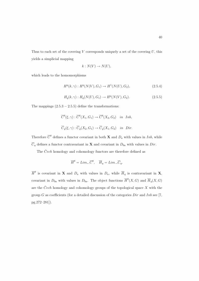
Thus to each set of the covering V corresponds uniquely a set of the covering U , this

yields a simplicial mapping

k : N(V ) ! N(U),

which leads to the homomorphisms

Hq(k, �) : Hq(N(V ), G1) ! H1(N(U), G2), (2.5.4)

Hq(k, �) : Hq(N(U), G1) ! Hq(N(V ), G2). (2.5.5)

The mappings (2.5.3� 2.5.5) define the transformations:

Cq(⇠, �) : C

q(X1, G1) ! C

q(X2, G2) in Inb,

Cq(⇠, �) : Cq(X2, G1) ! Cq(X1, G2) in Dir.

Therefore Cq

defines a functor covariant in both X and Da with values in Inb, while

Cq defines a functor contravariant in X and covariant in D0a with values in Dir.

The Cech homology and cohomology functors are therefore defined as

Hq

= Lim Cq, Hq = Lim!Cq.

Hq

is covariant in X and Da with values in Da, while Hq is contravariant in X,

covariant in D0a with values in D0a. The object functions Hq(X,G) and Hq(X, G)

are the Cech homology and cohomology groups of the topological space X with the

group G as coe�cients (for a detailed discussion of the categories Dir and Inb see [7,

pg.272–281]).

Chapter 3

Further Developments

3.1 Introduction

The first article of Eilenberg and Mac Lane [7] on categories and functors was not

followed by an intensive development of the theory. On the contrary, even the authors

did not divert themselves from their current research in order to develop the ideas

involved in that article. Several years needed before category theory began to be

considered as an object of mathematical interest deserving specific research.

After the contributions of Eilenberg and Mac Lane to the first stages of category

theory, the next milestone in the development of the theory was the publication of a

handful of articles which transformed the theory into an autonomous research field

by the end of the fifties. First, the definition and study of “Abelian Categories”

in separate articles by Alexander Grothendieck and David Buchsbaum. Second, the

introduction of “Adjoint Functors” by Daniel Kan. Third, and somewhat later, the

41

42

first foundational attempts based on categorical ideas by William Lawvere [5, pg.351–

364]. The aim of this chapter is to present the development of the notion of “Ad-

joint Functors” which is due to Kan [10] and its applications on functors involving

C.S.S. Complexes which is due to the same author [11].

3.2 Adjoint Functors in One Variable

Definition 3.2.1. Let X and Z be categories, let S : X ! Z and T : Z ! X be

covariant functors and let

↵ : Hom(S(X), Z) ! Hom(X, T (Z))

be a natural equivelence. Then S is called “the left adjoint of T under ↵” and T “the

right adjoint of S under ↵”, written ↵ : S a T .

An important property of two adjoint functors is that each of them determines

the other up to a unique natural equivalence. This is expressed by the following

uniqueness theorem.

Theorem 3.2.1. Let S, S 0 : X ! Z and T, T 0 : Z ! X be covariant functors and let

↵ : S 0 a T 0. Let � : S 0 ! S be a natural transformation. Then there exists a unique

natural transformation ⌧ : T ! T 0 such that the following diagram is commutative

Hom(S 0(X), Z) Hom(X, T 0(Z))↵0

//

Hom(S(X), Z)

Hom(S 0(X), Z)

Hom(�(X),Z)

✏✏

Hom(S(X), Z) Hom(X, T (Z))↵ // Hom(X, T (Z))

Hom(X, T 0(Z))

Hom(X,⌧(Z))

✏✏

If � is a natural equivalence, then so is ⌧ .

43

Proof. Suppose ⌧ : T ! T 0 is a natural transformation such that the above diagram

is commutative. Then for every object A 2 X and B 2 Z and for every map

f 2 H(A, T (B))

⌧B � f = Hom(A, ⌧B)f = ↵0(Hom(�A, B)↵�1f) = ↵0(↵�1f � �A).

In particular if A = T (B) and f = 1T (B), then

⌧B = ↵0(↵�11T (B) � �T (B)). (3.2.1)

Consequently if a natural transformation ⌧ : T ! T 0 exists such that the above

diagram is commutative, then it must satisfy (3.2.1) and therefore is unique.

It follows from the naturality of ↵0 that for every map g : B ! B0 2 Z the

following diagrams are commutative

T (A)

T 0(B0)

↵0(g�↵�11T (B)��T (B))

��???

????

????

?T (A) T 0(B)

↵0(↵�11T (B)��T (B))// T 0(B)

T 0(B0)

T 0g

��

��

��

T (B)

T 0(B0)

↵0(↵�11T (B0)��T (B0)�S0Tg)

��???

????

????

?T (B) T (B0)

Tg // T (B0)

T 0(B0)

↵0(↵�11T (B0)��T (B0))

��

��

��

Also, in view of the naturality of ↵ and � one easily sees that the following diagram

is also commutative

S 0T (B0) ST (B0)�T (B0)

//

S 0T (B)

S 0T (B0)

S0Tg

✏✏

S 0T (B) ST (B)�T (B)// ST (B)

ST (B0)

STg

✏✏ST (B0) B0

↵�11T (B0)

//

ST (B)

ST (B0)

ST (B)

ST (B0)

ST (B) B↵�11T (B) // B

B0

g

✏✏

44

Consequently,

⌧B0 � Tg = ↵0(↵�11T (B0) � �T (B0)) � Tg

= ↵0(↵�11T (B0) � �T (B0) � S 0Tg)

= ↵0(g � ↵�11T (B) � �T (B))

= T 0g � ↵0(↵�11T (B) � �T (B))

= T 0g � ⌧B0.

(3.2.2)

i.e. the function ⌧ defined by (3.2.1) is a natural transformation.

Now let � be a natural equivalence and let ⌧ 0 be a natural transformation induced

by ��1. Then ⌧⌧ 0 and ⌧ 0⌧ are natural transformations induced by ��1 and ��1�,

and the uniqueness of ⌧⌧ 0 and ⌧ 0⌧ together with the fact that ��1 and ��1� are

identities yields that ⌧⌧ 0 and ⌧ 0⌧ are also identities, i.e. ⌧ is a natural equivalence

with inverse ⌧ 0.

One of the main features of “adjointness” is that many duality theorems hold.

Theorem 3.2.2. Let ↵ : S(X) a T (Z) and define for every object A⇤ 2 Xop and

B⇤ 2 Zop a map

↵⇤(B⇤, A⇤) : Hom(T ⇤(B⇤), A⇤) ! Hom(B⇤, S⇤(A⇤))

by

↵⇤(B⇤, A⇤) = ↵�1(A, B). (3.2.3)

Then the function

↵⇤ : Hom(T ⇤(Zop), Xop) ! Hom(Zop, S⇤(Xop))

is a natural equivalence, i.e. ↵⇤ : T ⇤ a S⇤. Also ↵⇤⇤ = ↵.

45

Proof. Let x⇤ : A⇤ ! X 0⇤ 2 Xop and z⇤ : B0⇤ ! B⇤ 2 Zop be maps. Then it follows

from the naturality of ↵ that for every map f ⇤ : Hom(T ⇤(B⇤), A⇤)

↵⇤(B0⇤, A0⇤)Hom(T ⇤z⇤, x⇤)f ⇤ = ↵⇤(B0⇤, A0⇤)(x⇤ � f ⇤ � T ⇤z8)

= (↵�1(A0, B0)(Tz � f � x))⇤

= (↵�1(A0, B0)H(x, Tz)f)⇤

= (Hom(Sx, z)↵�1(A, B)f)⇤

= (z � ↵�1(A, B)f � Sx)⇤

= S⇤x⇤ � ↵⇤(B⇤, A⇤)f ⇤ � z⇤

= Hom(z⇤, S⇤x⇤)↵⇤(B⇤, A⇤)f ⇤.

(3.2.4)

i.e. ↵⇤ is a natural transformation. The fact that ↵ and hence ↵�1 is a natural

equivalence now implies that ↵⇤ is so. The fact that ↵⇤⇤ = ↵ follows immediately

from (3.2.3).

3.3 Adjoint Functors in Several Variables

After the introduction of the notion of the adjoint functor in one variable, Kan [10]

generalised his results to functors of several variables.

A covariant functor S : X, Y ! Z may be regarded as a collection consisting of

1. A covariant functor S(�, A) : X ! Z for every object B 2 Y and

2. A natural transformation S(�, b) : S(�, B) ! S(�, B0) for every map b : B !

B0 2 Y.

Now suppose that for every object B 2 Y , a covariant functor TB : Z ! X and a

46

natural equivalence

↵Y : Hom(S(X, B), Z) ! Hom(X, TB(Z))

are given i.e. ↵B : S(�, B) a TB. Then it follows from Theorem (3.2.1) that for every

map b : B ! B0 2 Y there exists a unique natural transformation Tb : TB0 ! TB such

that the following diagram is commutative

Hom(S(X, B0), Z) Hom(X, TB0(Z))↵B0//

Hom(S(X, B), Z)

Hom(S(X, B0), Z)

OO

Hom(S(X,b),Z)

Hom(S(X, B), Z) Hom(X,TB(Z))↵B // Hom(X,TB(Z))

Hom(X, TB0(Z))

OO

Hom(X,Tb(Z))

Let b0 : B0 ! B00 2 Y . Then the uniqueness of the natural transformation TB, TB0

and TB0B implies that TBTB0 = TB0B. Similarly if 1 : B ! B is the identity map,then

T1 : TB ! TB is the identity natural transformation. Therefore the function T defined

by

T (B, C) = TBC,

T (b, z) = TBz � TbC

for every object B 2 Y and C 2 Z and every map b : B ! B0 2 Y and z : C ! C 0 2

Z, is a functor T : Y, Z ! X, contravariant in Y and covariant in Z.

Clearly the function ↵ defined by

↵(A, B, C) = ↵Y (A, C)

for every object A 2 X, B 2 Y and C 2 Z, is a natural equivalence

↵ : Hom(S(X, Y ), Z) ! Hom(X, T (Y, Z))

thus we have the following theorem

47

Theorem 3.3.1. Let S : X, Y ! Z be a covariant functor and let for every object

B 2 Y be given a covariant functor TB : Z ! X and a natural transformation

↵B : Hom(S(X,B), Z) ! Hom(X, TB(Z)),

i.e. ↵B : S(�, B) a TB. Then there exists a unique functor

T : Y, Z ! X

contravariant in Y and covariant in Z and a unique natural equivalence

↵ : Hom(S(X, Y ), Z) ! Hom(X, T (Y, Z))

such that for every object A 2 X, B 2 Y and C 2 Z

T (B, C) = TBC, ↵(A, B, C) = ↵B(A, C)

i.e. ↵ : S a T .

Definition 3.3.1. Let S : X, Y ! Z be a covariant functor, let T : Y, Z ! X be a

functor contravariant in Y and covariant in Z and let

↵ : Hom(S(X, Y ), Z) ! Hom(X, T (Y, Z))

be a natural equivalence. The S is called “the left adjoint of T under ↵” and T is

called “the right adjoint of S under ↵”, written ↵ : S a T .

As in the case of functors of one variable, adjoint functors in two variables deter-

mine each other up to a unique natural equivalence. This is expressed by the following

uniqueness theorem.

48

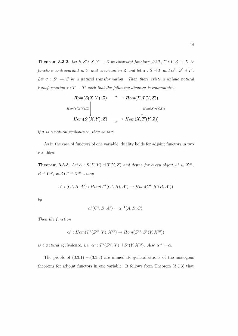
Theorem 3.3.2. Let S, S 0 : X, Y ! Z be covariant functors, let T, T 0 : Y, Z ! X be

functors contravariant in Y and covariant in Z and let ↵ : S a T and ↵0 : S 0 a T 0.

Let � : S 0 ! S be a natural transformation. Then there exists a unique natural

transformation ⌧ : T ! T 0 such that the following diagram is commutative

Hom(S 0(X, Y ), Z) Hom(X, T 0(Y, Z))↵0

//

Hom(S(X, Y ), Z)

Hom(S 0(X, Y ), Z)

Hom(�(X,Y ),Z)

✏✏

Hom(S(X, Y ), Z) Hom(X, T (Y, Z))↵ // Hom(X, T (Y, Z))

Hom(X, T 0(Y, Z))

Hom(X,⌧(Y,Z))

✏✏

if � is a natural equivalence, then so is ⌧ .

As in the case of functors of one variable, duality holds for adjoint functors in two

variables.

Theorem 3.3.3. Let ↵ : S(X, Y ) a T (Y, Z) and define for every object A⇤ 2 Xop,

B 2 Y op, and C⇤ 2 Zop a map

↵⇤ : (C⇤, B, A⇤) : Hom(T ⇤(C⇤, B), A⇤) ! Hom(C⇤, S⇤(B, A⇤))

by

↵⇤(C⇤, B, A⇤) = ↵�1(A, B, C).

Then the function

↵⇤ : Hom(T ⇤(Zop, Y ), Xop) ! Hom(Zop, S⇤(Y,Xop))

is a natural equivalence, i.e. ↵⇤ : T ⇤(Zop, Y ) a S⇤(Y, Xop). Also ↵⇤⇤ = ↵.

The proofs of (3.3.1) � (3.3.3) are immediate generalisations of the analogous

theorems for adjoint functors in one variable. It follows from Theorem (3.3.3) that

49

for every Theorem say V involving a natural equivalence ↵ : S(X, Y ) a T (Y, Z), a

dual Theorem V ⇤ may be obtained by applying Theorem V to the natural equivalence

↵⇤ : T ⇤(Zop, Y ) a S⇤(Y, Xop) and then writing the result in terms of the categories

X, Y and Z, the functors S and T and the natural equivalence ↵, i.e. “reversing all

arrows” in the categories Xop and Zop.

Next, consider functors in more than two variables. Let

S : X, K1, K2, ..., Km, L1, L2, ..., Ln ! Z

be a functor covariant in X,K1, ..., Km and contravariant in L1, ..., Ln and let

T : K1, ..., Km, L1, ..., Ln, Z ! X

be a functor contravariant in K1, ..., Km and covariant in L1, ..., Ln, Z. Then S and

T may be considered as functors in two variables as follows:

Let Y be the cartesian product category

Y = (Y

i

Ki)⇥ (Y

j

L⇤j) for i = 1, ...,m and j = 1, ..., n.

Then S may be considered as a covariant functor

S 0 : X, Y ! Z

and T as a functor

T 0 : Y, Z ! X

contravariant in Y and covariant in Z. Therefore the case of functors in more than

two variables may be brought back to that of functors in two variables only.

50

3.4 Applications of Adjoint Functors to C.S.S. Com-

plexes

Based on the theory of adjoint functors, Kan [11] gave a procedure by which functors

and natural transformations may be constructed using c.s.s. complexes. He also

introduced a functor Hv(�,�) from chain complexes to c.s.s. abelian groups with the

following properties:

1. The functor Hv(�,�) sets up a one-to-one correspondence between chain com-

plexes which are zero in dimension < 0 and c.s.s. abelian groups.

2. For every chain complex K

Hn(K) ⇠= ⇡n(Hv(�, K))

3. Let (⇡, n) be a chain complex which has the abelian group ⇡ in dimension n

and 0 in the others. Then

Hv(�, (⇡, n)) = K(⇡, n)

i.e. Hv(�, (⇡, n)) is the Eilenberg-Mac Lane complex1 of ⇡ on level n.

Definition 3.4.1. For each integer n = 0, let [n] denote the ordered set (0, ..., n). By

a monotone function ↵ : [m] ! [n] denote a function such that

↵(i) 5 ↵(j) 0 5 i 5 j 5 m.

Clearly the composition of two monotone functions is again a monotone function

and for every integer n = 0 the identity map en : [n] ! [n] is also monotone. Therefore

1Let G be a group and n a positive integer. A connected topological space is called an Eilenberg-Mac Lane space of type K(G, n) if it has nth homotopy group ⇡n(X) isomorphic to G and all otherhomotopy groups trivial. Such spaces were first introduced by Samuel Eilenberg and Saunders MacLane in 1950 (see [8]).

51

the ordered sets [n] and the monotone functions ↵ : [m] ! [n] form a category, say

V .

Let M be the category of sets and M v the category of contravariant functors

V ! M .

Definition 3.4.2. A c.s.s. complex K is a contravariant functor K : V ! M , i.e.

an object of the category M v. Similarly a c.s.s. map f : K ! L is a natural

transformation from K to L, i.e. a map of the category M v. The elements of the set

K[n] are called n-simplices of K.

Let Z be a category which has direct limits (see [7, pg. 277] and [10, pg.313]).

Then with every covariant functor ⌃ : V ! Z, one can associate two covariant

functors

(�⌦ ⌃) : M v ! Z, Hv(⌃,�) : Z ! M v

where (� ⌦ ⌃) is a left adjoint of Hv(⌃,�). Conversely, every pair of covariant

functors

S : M v ! Z, T : Z ! M v

where S is a left adjoint of T , may (up to natural equivalences) be obtained in this

manner.

Because Z has direct limits, the embedding functor Ed : Z ! Zd has a left

adjoint. Let limd : Zd ! Z be an arbitrary but fixed such left adjoint and let ↵d

be an arbitrary but fixed natural equivalence ↵d : limd(Zd) a Ed(Z). Consider the

functor ⌦d : M v, Zv ! Zd and the natural equivalence

� : Hom(M v ⌦d Zv, Ed(Z)) �! Hom(M v, Hv(Zv, Z)).

52

Composition of the natural equivalence ↵d with the functor ⌦d yields a natural equiv-

alence

↵d⌦d : Hom(limd(Mv ⌦d Zv), Z) �! Hom(M v ⌦d Zv, Ed(Z)).

Composition of the natural equivalences ↵d⌦d and � yields the natural equivalence

� : Hom(limd(Mv ⌦d Zv), Z) �! Hom(M v, Hv(Zv, Z)).

It follows that � is completely determined by the choice of limd and ↵d. Now, denote

by

⌦ : M v, Zv ! Z

the composite functor limd⌦d : M v, Zv ! Z and write S instead of M v. Then � is a

natural equivalence

� : Hom(S ⌦ Zv, Z) ! Hom(S, Hv(Zv, Z)).

Hence, given the functor limd : Zd ! Z and the natural equivalence ↵d : limd a Ed,

one may associate with every object ⌃ 2 Zv

1. The covariant functor

Hv(⌃,�) : Z ! S

which is the right adjoint of

2. The covariant functor

(�⌦ ⌃) : S ! Z

under

3. The natural equivalence

�⌃ = �(S, ⌃, Z) : Hom(S ⌦ ⌃, Z) ! Hom(S, Hv(⌃, Z)),

53

4. The natural transformation induced by �⌃

k⌃ : E(S) ! Hv(⌃, S ⌦ ⌃)

satisfying the relation

�⌃f = Hv(⌃, f) � k⌃K

for every object K 2 ⌃ and A 2 Z and every map f : K ⌦ ⌃ ! A 2 Z, and

5. The natural transformation induced by ��1⌃

µ⌃ : Hv(⌃, Z)⌦ ⌃ ! E(Z)

satisfying the relation

��1⌃ g = µ⌃A � g ⌦ ⌃

for every object K 2 S, A 2 Z and every map g : K ! Hv(⌃, A) 2 S.

The main striking results of Kan [11], are the introduction of the functor Hv(�,�)

from chain complexes to c.s.s abelian groups and the proof that the functor Hv(�, (⇡, n))

(where (⇡, n) is a chain complex) is indeed the Eilenberg-Mac Lane complex of ⇡ on

level n.

For every object A 2 @G (where @G is the category of abelian chain complexes),

the c.s.s complex Hv(�, A) may be converted into a c.s.s. abelian group as follows:

Let �, ⌧ : �[n] ! A be two n-simplices of Hv(�, A). Then the sum �+⌧ : �[n] ! A

is defined by

(� + ⌧)� = �� + ⌧�, � 2 �[n].

For every chain map f : A ! B the c.s.s. map Hv(�, f) : Hv(�, A) ! Hv(�, B) then

becomes a c.s.s. homomorphism. Hence Hv(�,�) may be regarded as a functor

Hv(�,�) : @G ! Gv.

54

Let @G0 be the full subcategory of @G generated by the chain complexes which

are 0 in dimension < 0, i.e. A 2 @G0 if and only if Ai = 0 for i < 0. Let

M : Gv ! @G0

be the functor which assigns to every c.s.s. abelian group G the chain complex

MG = eG and to every c.s.s. homomorphism f : G ! H the chain map Mf : eG ! eH

given by (Mf)� = f� for � 2 eG.

Roughly speaking, the functor Hv(�,�) sets up a one-to-one correspondence be-

tween the objects and maps of @G0 and those of Gv. An exact formulation is given

in the following theorems, in which E denotes the identity functor.

Theorem 3.4.1. There exists a natural equivalence

↵ : MHv(�, @G0) ! E(@G0).

Proof. For each non-degenerate simplex ↵ 2 �[n], let CN↵ be the corresponding

generator of �[n]. Let A 2 @G0 be an object and let G = Hv(�, A). For each simplex

� : �[n] ! A 2 fGn define an element ↵� 2 An by

↵� = �(Cnen),

where en : [n] ! [n] is the identity map, i.e. the only non-degenerate n-simplex of

�[n]. As the addition in G was induced by that of A, it follows that the function

↵ : eGn ! An is a homomorphism for each n.

It follows from the definition of fGn that a simplex � : �[n] ! A is in fGn if and

only if �ei : �[n�1] ! A is the zero map for i 6= 0, i.e. � maps all generators of �[n],

with the possible exception of Cnen and Cne0, into zero. Consequently

55

@n(↵�) = @n(�(Cnen))

=X

(�1)i(�(Cnei))

= �(Cne0)

= (�e0)(Cnen�1)

= (e@�)(Cnen�1)

= ↵(e@�),

(3.4.1)

i.e. the function ↵ : eG ! A is a chain map. It also follows that � is completely

determined by �(Cnen) 2 An. Hence ↵ : eG ! A is an isomorphism. Naturality is

easily verified.

An immediate consequence of Theorem (3.4.1) is that for each object A@ 2 G and

for every integer n = 0

j⇤↵⇤ : ⇡n(Hv(�, A)) ⇠= Hn(A)

i.e. the nth homology group of the c.s.s. group Hv(�, A) is isomorphic with the nth

homology group of the chain complex A.

Now let X be a topological space. The homotopy groups of X are by definition

those of its simplicial singular complex K = Hv(⌃, X), and the singular homology

groups of X are the homology groups of the chain complex CnK (For more on Ho-

mology and Homotopy Theory see [9]). Let � be a 0-simplex of K, let

h⇤ : ⇡n(K,�) ! Hn(CnK)

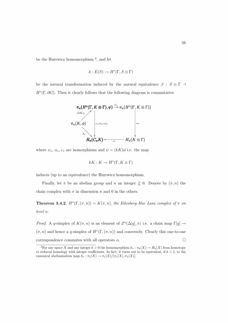
56

be the Hurewicz homomorphism 2, and let

k : E(S) ! Hv(�, S ⌦ �)

be the natural transformation induced by the natural equivalence � : S ⌦ � a

Hv(�, @G). Then it clearly follows that the following diagram is commutative

⇡n(K,�)

Hn(CnK)

h⇤ ��???

????

??

⇡n(Hv(�, K ⌦ �), )

⇡n(K,�)

??(kK)⇤

��

��

�⇡n(Hv(�, K ⌦ �), )

Hn(CnK)

c⇤�↵⇤� ⇤

✏✏Hn(CnK) Hn(K ⌦ �)oo

c⇤

⇡n(Hv(�, K ⌦ �), )

Hn(CnK)

⇡n(Hv(�, K ⌦ �), )

Hn(CnK)

⇡n(Hv(�, K ⌦ �), ) ⇡n(Hv(�, K ⌦ �)) ⇤ // ⇡n(Hv(�, K ⌦ �))

Hn(K ⌦ �)

↵⇤

✏✏

where ⇤, ↵⇤, c⇤ are isomorphisms and = (kK)� i.e. the map

kK : K ! Hv(�, K ⌦ �)

induces (up to an equivalence) the Hurewicz homomorphism.

Finally, let ⇡ be an abelian group and n an integer = 0. Denote by (⇡, n) the

chain complex with ⇡ in dimension n and 0 in the others.

Theorem 3.4.2. Hv(�, (⇡, n)) = K(⇡, n), the Eilenberg-Mac Lane complex of ⇡ on

level n.

Proof. A q-simplex of K(⇡, n) is an element of Zn(�[q], ⇡) i.e. a chain map �[q] !

(⇡, n) and hence a q-simplex of Hv(�, (⇡, n)) and conversely. Clearly this one-to-one

correspondence commutes with all operators ↵.

2For any space X and any integer k > 0 the homomorphism h⇤ : ⇡k(X) ! Hk(X) from homotopyto reduced homology with integer coe�cients. In fact, it turns out to be equivalent, if k = 1, to thecanonical abelianisation map h⇤ : ⇡1(X) ! ⇡1(X)/[⇡1(X),⇡1(X)].

57

The introduction of the concept of Eilenberg-Mac Lane space by Samuel Eilen-

berg and Saunders Mac Lane in 1950 had a great impact on questions concerning

constructions of topological invariants, i.e. computing the cohomology group for a

given topological space (see [8]). Thus, the introduction of the functor Hv(�, (⇡, n))

and the proof that this functor gives the Eilenberg-Mac Lane complex, led to great

simplifications in computing such spaces by applying the functor Hv(�, (⇡, n)) to a

very simple chain complex without the need of complicated explicit construction.

Bibliography

[1] Steve Awodey, Category Theory, Oxford Science Publications, Oxford, 2006.

[2] Francis Borceux, Handbook of Categorical Algebra 1: Basic Category Theory,

Cambridge University Press, Cambridge, 1994.

[3] Peter J. Cameron, Sets, Logic and Categories, Springer-Verlag, London, 1999.

[4] Henri Cartan and Samuel Eilenberg, Homological Algebra, Princeton Landmarks

in Mathematics, Princeton, 1956.

[5] Leo Corry, Modern Algebra and the Rise of Mathematical Structure, Birkhauser,

Basel, 2004.

[6] Samuel Eilenberg and Saunders Mac Lane, Group Extensions and Homology, An-

nals of Mathematics. 43 (1942), no.5, 757–831.

[7] Samuel Eilenberg and Saunders Mac Lane, General Theory of Natural Equiva-

lences, Transactions of the Americal Mathematical Society. 58 (1945), no.2, 231–

294.

[8] Samuel Eilenberg and Saunders Mac Lane, Relations Between Homology and Ho-

motopy Groups of Spaces.II, Annals of Mathematics. 51 (1950), no.3, 514–533.

58

59

[9] Allen Hatcher, Algebraic Topology, Cambridge University Press, Cambridge, 2001.

[10] Daniel M. Kan, Adjoint Functors, Transactions of the Americal Mathematical

Society. 87 (1958), no.2, 294–329.

[11] Daniel M. Kan, Functors Involving C.S.S Complexes, Transactions of the Amer-

ical Mathematical Society. 87 (1958), no.2, 330–346.

[12] Ralf Kromer, Tool and Object: A History and Philosophy of Category Theory,

Birkhauser, Basel, 2007.

[13] Saunders Mac Lane, Duality for Groups, Bull. Amer. Math. Soc. 56, 485–516.

[14] Saunders Mac Lane, Categories for the Working Mathematican, Springer-Verlag,

New York, 1998.

[15] Colin McLarty, Elementary Categories Elementay Toposes, Oxford Science Pub-

lications, Oxford, 1992.

[16] Joseph J. Rotman, An Introduction to Homological Algebra, Academic Press,

New York, 1979.

[17] Derek J.S Robinson, A Course in the Theory of Groups, Springer-Verlag, New

York, 1993.

[18] Jean-Pierre Serre, Linear Representations of Finite Groups, Springer-Verlag,

New York, 1977.

[19] B.A.F Wehrfritz, Finite Groups: A Second Course on Group Theory, World

Scientific, London, 1998.

Categories: History, basic and developments

Documents

Transcript of Categories: History, basic and developments