TECHNISCHE UNIVERSITAT MUNCHEN

Lehrstuhl fur Numerische Mechanik

Stabilized Cut Finite Element Methods forComplex Interface Coupled Flow Problems

Benedikt Schott

Vollstandiger Abdruck der von der Fakultat fur Maschinenwesen der Technischen UniversitatMunchen zur Erlangung des akademischen Grades eines

Doktor-Ingenieurs (Dr.-Ing.)

genehmigten Dissertation.

Vorsitzender: Univ.-Prof. dr.ir. Daniel J. Rixen

Prufer der Dissertation:

1. Univ.-Prof. Dr.-Ing. Wolfgang A. Wall

2. Prof. Erik Burman, Ph.D.

University College London / UK

Die Dissertation wurde am 23. Mai 2016 bei der Technischen Universitat Munchen eingereichtund durch die Fakultat fur Maschinenwesen am 15. Marz 2017 angenommen.

ABSTRACT

Novel computational methodologies for complex interface coupled flow problems are developedin this thesis. Computational models for incompressible single-phase flow and interactions be-tween fluid and solid phases rely on the framework of cut finite element methods which allowdomains and computational meshes to be chosen geometrically unfitted.

A broad range of multiphysics problems arising from various engineering and scientific fieldsare dominated by interactions of fluid phases with each other as well as with structural bodies.For complex practical problem configurations, involved computational domains are often sub-jected to large deformations or even undergo topological changes. Most if not all establishedexisting computational approaches are limited in their applicability for such scenarios. Cutfinite element methods (CUTFEMs) are promising discretization techniques and allow for asharp representation of the solution fields based on computational grids which are not forcedto be aligned with the respective subdomain geometry. This way, such approaches providepowerful simulation tools to substantially simplify mesh generation for complex geometries.While highly increasing versatility, decoupling of the finite dimensional approximation spacesfrom the physical domains entails additional complexity for such numerical approaches whichmanifests in numerical instabilities arising in boundary and interface zones.

The main contribution of this thesis is to theoretically analyze the sources of encounteredinstabilities, to support the made statements by comprehensive numerical studies and, as aconsequence, to introduce novel stabilization mechanisms to counteract these issues. The centralfocus is directed to the development of numerical approaches which guarantee inf-sup stabilityand allow to establish spatially optimal a priori error estimates for flow problems governed by thenon-linear incompressible Navier-Stokes equations. All novel computational methods developedthroughout this work utilize weak variational constraint enforcement of boundary and interfacecoupling conditions based on the well-established Nitsche method. The enhancement of differentso-called ghost-penalty stabilization techniques for velocity and pressure solutions is of decisiveimportance to ensure stability for transient low- and high-Reynolds-number flows independentof the boundary position within the computational grid. Besides a sound mathematical proofof stability and optimality for a linear auxiliary problem governed by the Oseen equations,comprehensive numerical convergence studies and the simulation of transient single-phase flowsthrough complex-shaped non-moving as well as moving fluid domains demonstrate accuracy,robustness and the high capabilities of the developed CUTFEM flow solver.

A further major contribution of the present thesis constitutes in the extension of theoreticalanalyses from single-phase flows to coupled flow problem configurations. In a first step, overlap-ping unfitted discretization concepts for fluid domain decomposition are considered. A Nitsche-type coupling strategy, which is able to sufficiently control convective mass transport acrossinterfaces, is introduced and validated for challenging test examples: two- and three-dimensionalcylinder benchmarks and the turbulent recirculating flow in a lid-driven cavity at Re = 10000.In a second step, adaption of this computational methodology to different modelings of incom-

i

Abstract

pressible two-phase flow is elaborated. Special emphasis is put on the accurate representability ofsolutions in topologically degenerated situations and on the robustness of coupling methods forinteracting fluids which exhibit strong differences in the numerical resolution of their respectivephysics. These can be characterized in terms of involved fluid viscosities related to respectivemesh sizes. Predicting exponential growth rates for a Rayleigh–Taylor instability as well asinvestigation of damping effects due to surface tension demonstrates excellent performance.As an outlook, to illustrate the extensibility of the proposed flow solvers to more sophisticatedincompressible two-phase flows and to point out the major improvements made in this work, thesimulation of the temporal evolution of a separating flame front for a flame-vortex interactionserves as test example.

Having developed computational methods for the simulation of interactions between fluidphases, extensions to different geometrically unfitted discretizations for fluid-structure interac-tion (FSI) can be made. Fundamentals on interface modeling for FSI and a standard Galerkinformulation for solid mechanics are reviewed. Numerically stabilized coupled systems of fluidsand solids are set up and tailored non-linear solution strategies are proposed which allow forchanging approximation spaces during iterative procedures. Finally, highly dynamic FSI prob-lems show the high capabilities of the developed monolithic FSI solvers and highlight theirsuperiority over a multitude of other computational approaches.

Concluding, the diversity of already successfully realized single-phase and coupled flow prob-lem settings demonstrates the high versatility of CUTFEMs. These achievements give rise tohope for further extensibility of the framework of unfitted cut finite element discretizations aswell as of developed stabilization techniques to other challenging multiphysics problems.

ii

ZUSAMMENFASSUNG

In der vorliegenden Arbeit werden neuartige numerische Verfahren zur Berechnung komplexerInterface-gekoppelter Stromungsprobleme entwickelt. Die Berechnungsmodelle fur inkompres-sible Einphasenstromungen sowie fur Wechselwirkungen zwischen fluiden Phasen und Fest-korpern verwenden schnittbasierte Finite-Elemente-Methoden, die es erlauben, dass physikali-sche Gebiete und Berechnungsgitter geometrisch nicht passend zueinander gewahlt werden.

Eine große Bandbreite an Multiphysics-Anwendungen aus unterschiedlichen Bereichen derIngenieurswissenschaften und anderen Wissenschaftsbereichen werden durch Interaktionen zwi-schen verschiedenen Fluiden sowie deren Wechselwirkungen mit Strukturkorpern beschrieben.In komplexen praktischen Problemstellungen unterliegen die entsprechenden Teilgebiete oftmalsgroßen Deformationen oder sind sogar topologischen Anderungen unterworfen. Die meisten,wenn nicht sogar alle etablierten rechnergestutzten Berechnungsverfahren sind fur solche Pro-blemstellungen nicht geeignet. Finite-Elemente-Methoden, die auf dem Schneiden von Berech-nungsnetzen basieren (CUTFEM), stellen dabei leistungsfahige Diskretisierungsansatze dar, dieeine genaue Darstellung der Losungsfelder ermoglichen und dabei nicht erfordern, dass dasBerechnungsnetz und das Gebiet aneinander angepasst sind. Auf diese Art und Weise stellensolche Ansatze effektive Simulationswerkzeuge dar, welche die Netzerstellung fur komplexeGeometrien maßgeblich vereinfachen. Wahrend das Entkoppeln endlich-dimensionaler Ansatz-funktionenraume von physikalischen Gebieten die Vielseitigkeit solcher Berechnungsverfahrenstark erhoht, so zieht dies jedoch auch weitere Schwierigkeiten in Form von numerischen Insta-bilitaten nach sich, welche sich in den Randbereichen und Phasengrenzflachen ausbilden.

Der wichtigste Beitrag dieser Arbeit liegt in der theoretischen numerischen Analyse vonUrsachen fur auftretende Instabilitaten sowie deren umfassende Untersuchung mithilfe von nu-merischen Studien und in Folge dessen in der Einfuhrung von neuartigen Stabilisierungsmecha-nismen, um diesen Instabilitaten entgegen zu wirken. Dabei liegt das Hauptaugenmerk auf derEntwicklung von numerischen Verfahren, die inf-sup-Stabilitat und raumlich optimale a priori-Fehlerabschatzungen fur Stromungsprobleme garantieren, denen die nichtlinearen inkompres-siblen Navier-Stokes Gleichungen zugrunde liegen. Die in dieser Arbeit entwickelten neuar-tigen numerischen Verfahren verwenden ein schwaches, variationelles Aufbringen von Rand-und Interface-Kopplungsbedingungen mithilfe der etablierten Nitsche-Methode. Um fur zeitab-hangige Stromungen mit niedrigen wie auch mit hohen Reynolds-Zahlen numerische Stabilitatunabhangig von der Interface-Position zu gewahrleisten, spielt die Weiterentwicklung von ver-schiedenen sogenannten Ghost-Penalty-Stabilisierungen, angewandt auf Geschwindigkeits- undDrucklosungen, eine entscheidende Rolle. Neben dem mathematischen Beweis von numerischerStabilitat und Optimalitat fur ein lineares Hilfsproblem, welches durch die Oseen-Gleichungenbeschrieben ist, weisen umfassende numerische Konvergenzstudien sowie die Simulation vonzeitabhangigen Einphasenstromungen durch komplex geformte unbewegte wie auch bewegteFluid-Berechnungsgebiete die Genauigkeit und Robustheit des entwickelten CUTFEM-Fluid-Losers nach und zeigen dessen großes Potenzial auf.

iii

Zusammenfassung

Ein weiterer wichtiger Beitrag der vorliegenden Arbeit besteht in der Erweiterung theoreti-scher Analysen von Einphasenstromungen auf Problemstellungen gekoppelter Stromungen. Ineinem ersten Schritt werden Konzepte fur Fluid-Gebietszerlegungen basierend auf uberlappen-den, nicht zueinander passenden Diskretisierungen betrachtet. Eine Nitsche-artige Kopplungs-methode, die es erlaubt konvektiven Massentransport uber Interfaces hinweg zu kontrollieren,wird hierzu eingefuhrt und mithilfe anspruchsvoller Testbeispiele validiert: Dazu dienen zwei-und dreidimensionale Zylinder-Benchmarks sowie eine turbulente Stromung in einer sogenann-ten ”lid-driven cavity“ (Re = 10000). In einem zweiten Schritt werden Anpassungen dieses Be-rechnungsverfahrens auf verschieden geartete inkompressiblen Zweiphasenstromungen erortert.Besonderes Augenmerk liegt dabei zum einen auf der exakten Darstellbarkeit von Losungen intopologisch entarteten Situationen, und zum anderen auf der Robustheit der Kopplungsmethodenfur wechselwirkende fluide Phasen, die starke Unterschiede in der numerischen Auflosung derenjeweiliger Physik aufweisen. Diese lassen sich anhand der Verhaltnisse von Viskositaten zuNetzweiten beschreiben. Herausragende Ergebnisse wurden bei der Bestimmung von exponenti-ellen Wachstumsraten fur Rayleigh-Taylor-Instabilitaten sowie von Dampfungseffekten in Folgevon Oberflachenspannung erzielt. Um als Ausblick die Erweiterungsmoglichkeiten des vorge-stellten Fluid-Losers auf anspruchsvollere inkompressible Zweiphasenstromungen aufzuzeigenund dabei die wichtigsten Verbesserungen, die in dieser Arbeit erzielt wurden, zu verdeutlichen,wird beispielhaft die zeitliche Entwicklung der Phasengrenze einer Flammen-Wirbel-Interaktionsimuliert.

Die Weiterentwicklung numerischer Verfahren fur die Simulation von Wechselwirkungenfluider Phasen ermoglicht Anpassungen auf verschiedene, geometrisch nicht zusammenpassendeDiskretisierungen, die auf die Simulation von Fluid-Struktur-Interaktionen (FSI) anwendbarsind. Hierfur werden Grundlagen zu Grenzschicht-Modellierungen fur FSI sowie eine Standard-Galerkin Formulierung fur Strukturmechanik erortert. Es werden numerisch stabilisierte gekop-pelte Systeme, bestehend aus Fluiden und Strukturkorpern, formuliert und maßgeschneiderte,nichtlineare Losungsstrategien vorgestellt, die es erlauben, dass sich Ansatzfunktionenraumewahrend des iterativen Verfahrens verandern. Abschließend zeigen hochdynamische FSI-Prob-leme die besonderen Fahigkeiten der entwickelten FSI-Loser auf und verdeutlichen deren Uber-legenheit gegenuber einer Vielzahl anderer numerischer Ansatze.

Zusammenfassend zeigen sich die enormen Einsatzmoglichkeiten schnittbasierter Finite-Ele-mente-Methoden in der Vielzahl der bereits erfolgreich umgesetzten Einphasenstromungen wieauch gekoppelter Stromungsprobleme. Diese geben Anlass zur Hoffnung auf Weiterentwicklun-gen von schnittbasierten Finite-Elemente-Diskretisierungsansatzen sowie entwickelter Stabili-sierungstechniken fur weitere anspruchsvolle Mehrfeldprobleme.

iv

TABLE OF CONTENTS

Nomenclature ix

1 Introduction 11.1 Motivation . . . . . . . . . . . . . . . . . . . . . . . . . . . . . . . . . . . . . 11.2 Research Objectives and Accomplishments . . . . . . . . . . . . . . . . . . . . 4

1.2.1 Specification of Requirements . . . . . . . . . . . . . . . . . . . . . . . . 41.2.2 Contribution of this Work . . . . . . . . . . . . . . . . . . . . . . . . . . 7

1.3 Outline of the Thesis . . . . . . . . . . . . . . . . . . . . . . . . . . . . . . . . 10

2 Spatial Discretization Techniques for Multiphysics using Cut Finite Elements 112.1 Domain Decomposition - General Aspects and an Overview of Concepts . . . . 12

2.1.1 Abstract Domain Decomposition Problem Setting . . . . . . . . . . . . . 132.1.2 Fundamentals of Continuum Mechanics . . . . . . . . . . . . . . . . . . . 14

2.1.2.1 Introducing Domains, Observers and Frames of Reference . . . . . . 142.1.2.2 Deducing Conservation Laws . . . . . . . . . . . . . . . . . . . . . 17

2.1.3 Representation and Approximation of Boundaries and Interfaces . . . . . 212.1.3.1 Explicit Front-Tracking using a Trace Mesh Representation . . . . . 212.1.3.2 Implicit Front-Capturing Level-Set Method . . . . . . . . . . . . . 23

2.1.4 General Concepts of Domain Decomposition Techniques . . . . . . . . . 272.1.4.1 Notation and Terminology on Computational Domains and Meshes . 282.1.4.2 Limitations of Fitted Mesh Discretization Techniques . . . . . . . . 292.1.4.3 Capabilities of Unfitted Mesh Techniques for Multiphysics . . . . . 31

2.2 Finite-Dimensional Cut Finite Element Approximations . . . . . . . . . . . . . 392.2.1 An Overview of eXtended and Cut Finite Element Methods . . . . . . . . 402.2.2 Cutting Finite Elements - Notation and Fundamentals of Cut-Entities . . . 412.2.3 Strategies for Enriching Function Spaces in the XFEM . . . . . . . . . . 442.2.4 CUTFEM-based DOF-Management for Complex Domains . . . . . . . . 462.2.5 Expansion of Cut Finite Element Function Spaces to Multiphysics Settings 512.2.6 Notes on Numerical Quadrature on Cut Meshes . . . . . . . . . . . . . . 53

3 Developing Stabilized Cut Finite Element Methods for Incompressible Flow 553.1 Finite Element Formulations for Incompressible Flow . . . . . . . . . . . . . . 56

3.1.1 Governing Equations for Fluid Mechanics . . . . . . . . . . . . . . . . . 563.1.2 Variational Fluid Problem . . . . . . . . . . . . . . . . . . . . . . . . . . 573.1.3 Stabilized Discrete Formulations for Boundary-Fitted Meshes . . . . . . . 58

3.1.3.1 The Residual-based Variational Multiscale (RBVM) Method . . . . 603.1.3.2 The Continuous Interior Penalty (CIP) Method . . . . . . . . . . . 61

v

Table of Contents

3.2 Preliminaries to Numerical Analysis . . . . . . . . . . . . . . . . . . . . . . . . 653.2.1 Assumptions on Computational Domains, Meshes and Function Spaces . . 663.2.2 Approximation Properties . . . . . . . . . . . . . . . . . . . . . . . . . . 67

3.2.2.1 Trace Inequalities and Inverse Estimates . . . . . . . . . . . . . . . 673.2.2.2 Interpolation Operators . . . . . . . . . . . . . . . . . . . . . . . . 68

3.2.3 Concepts of Stability Analysis in a Nutshell . . . . . . . . . . . . . . . . 703.3 Weak Imposition of Boundary Conditions for Boundary-Fitted Meshes . . . . . 73

3.3.1 Poisson Problem with Weak Dirichlet Boundary Conditions . . . . . . . . 743.3.2 A Survey on Weak Dirichlet Constraint Enforcement . . . . . . . . . . . . 74

3.3.2.1 Babuska’s Classical Method of Lagrange Multipliers -The Issue of Violating Inf-Sup Conditions . . . . . . . . . . . . . . 75

3.3.2.2 Residual-based Stabilized Lagrange Multipliers -Circumvent the Babuska–Brezzi Condition . . . . . . . . . . . . . 77

3.3.2.3 A Stabilized Mixed/Hybrid Stress-based Formulation . . . . . . . . 783.3.2.4 Nitsche’s Method . . . . . . . . . . . . . . . . . . . . . . . . . . . 82

3.4 CUTFEM - An Analysis of General Stability Issues . . . . . . . . . . . . . . . 863.4.1 Conditioning and Stability Issues of Cut Approximation Spaces . . . . . . 873.4.2 Nitsche’s Method and the Role of the Trace Inequality . . . . . . . . . . . 90

3.4.2.1 The Decisive Role of the Trace Inequality . . . . . . . . . . . . . . 913.4.2.2 Nitsche’s Method using Cut-Cell Information . . . . . . . . . . . . 933.4.2.3 Analogies to the Mixed/Hybrid Stress-based Formulation . . . . . . 94

3.4.3 Ghost Penalty - Controlling Polynomials in the Interface Region . . . . . . 963.4.3.1 The Fundamental Idea of Ghost-Penalty Operators . . . . . . . . . . 983.4.3.2 Properties from a Mathematical Point of View . . . . . . . . . . . . 1003.4.3.3 Implementation and Practical Aspects . . . . . . . . . . . . . . . . 1003.4.3.4 Nitsche’s Method Supported by Ghost Penalties . . . . . . . . . . . 101

3.4.4 Numerical Studies for Incompressible Flow . . . . . . . . . . . . . . . . . 1033.4.4.1 Stabilizing the Ghost Domain - The Role of Interface-Zone Penalties 1053.4.4.2 Weak Dirichlet Constraint Enforcement - A Comparison of Methods 1073.4.4.3 Nitsche’s Method - Studies on the Penalty Parameters . . . . . . . . 113

3.5 A Cut Finite Element Method for Oseen’s Problem - A Numerical Analysis . . . 1163.5.1 Oseen’s Equations - A Linear Model Problem . . . . . . . . . . . . . . . 1163.5.2 A Nitsche-type CIP/GP Cut Finite Element Method . . . . . . . . . . . . 1183.5.3 Assumptions and Preliminaries . . . . . . . . . . . . . . . . . . . . . . . 1203.5.4 Norms and Ghost Penalties . . . . . . . . . . . . . . . . . . . . . . . . . 1223.5.5 Stability Properties . . . . . . . . . . . . . . . . . . . . . . . . . . . . . . 1273.5.6 A Priori Error Estimates . . . . . . . . . . . . . . . . . . . . . . . . . . . 1423.5.7 Numerical Convergence Studies . . . . . . . . . . . . . . . . . . . . . . . 147

3.5.7.1 Two-Dimensional Taylor Problem . . . . . . . . . . . . . . . . . . 1473.5.7.2 Three-Dimensional Beltrami Flow . . . . . . . . . . . . . . . . . . 150

3.6 Stabilized CUTFEMs for Transient Incompressible Navier-Stokes Equations . . 1533.6.1 Stabilized Discrete Formulations . . . . . . . . . . . . . . . . . . . . . . 154

3.6.1.1 A Nitsche-type CIP/GP Cut Finite Element Method . . . . . . . . . 1543.6.1.2 A Nitsche-type RBVM/GP Cut Finite Element Method . . . . . . . 1563.6.1.3 Time-Stepping for Fluids . . . . . . . . . . . . . . . . . . . . . . . 157

vi

Table of Contents

3.6.2 Numerical Tests for Incompressible Flow in Non-Moving Domains . . . . 1583.6.2.1 Two-Dimensional Incompressible Flow around a Cylinder . . . . . . 1593.6.2.2 Laminar Helical Pipe Flow . . . . . . . . . . . . . . . . . . . . . . 1633.6.2.3 Flow in a Complex-Shaped Domain Composed of Level-Set Fields . 165

3.6.3 Extension to Flow in Moving Domains . . . . . . . . . . . . . . . . . . . 1673.6.3.1 Discrete Nitsche-type CUTFEM in Moving Domains . . . . . . . . 1693.6.3.2 Solution Projection between Function Spaces . . . . . . . . . . . . 1703.6.3.3 Solution Algorithm for Flow in Time-Dependent Moving Domains . 175

3.6.4 Numerical Tests for Incompressible Flow in Moving Domains . . . . . . . 1763.6.4.1 Taylor Problem in a Moving Domain . . . . . . . . . . . . . . . . . 1763.6.4.2 Flow over a Rotating Beam . . . . . . . . . . . . . . . . . . . . . . 1773.6.4.3 Flow over a Moving Cylinder . . . . . . . . . . . . . . . . . . . . . 178

4 Unfitted Domain Decomposition Methods for Incompressible Single- and Two-Phase Flows 1834.1 Domain Decomposition Problem Setup for Coupled Flows . . . . . . . . . . . . 184

4.1.1 Multiple Fluid Phases - Domains and Interfaces . . . . . . . . . . . . . . 1844.1.2 Coupled Interface Initial Boundary Value Problem . . . . . . . . . . . . . 1864.1.3 Coupled Variational Formulation . . . . . . . . . . . . . . . . . . . . . . 187

4.2 A Stabilized Cut Finite Element Method for Coupled Incompressible Flows . . . 1884.2.1 Nitsche-type Cut Finite Element Methods for Domain Decomposition . . . 1894.2.2 Enforcing Interfacial Constraints - The Role of Weighted Averages . . . . 1914.2.3 Controlling Convective Effects at Interfaces . . . . . . . . . . . . . . . . 195

4.3 Fluid Mesh Tying - An Overlapping Mesh Domain Decomposition Approach . . 1974.3.1 Benchmark Computations of Laminar Flows around Cylinders . . . . . . 1994.3.2 Turbulent Recirculating Flow in a Lid-Driven Cavity . . . . . . . . . . . . 201

4.4 Outlook towards Incompressible Two-Phase Flow - An Unfitted Mesh Method . 2044.4.1 A Rayleigh-Taylor Instability including Surface Tension . . . . . . . . . . 2064.4.2 Premixed Combustion - A Flame-Vortex Interaction . . . . . . . . . . . . 210

5 Stabilized Approaches to Fluid-Structure Interaction using Cut Finite Elements 2135.1 A Finite Element Method for Structures . . . . . . . . . . . . . . . . . . . . . . 216

5.1.1 Governing Equations for Solid Mechanics . . . . . . . . . . . . . . . . . 2165.1.2 Variational Structure Problem . . . . . . . . . . . . . . . . . . . . . . . . 2195.1.3 Spatial Finite Element Discretization . . . . . . . . . . . . . . . . . . . . 2205.1.4 Structural Time Stepping . . . . . . . . . . . . . . . . . . . . . . . . . . 221

5.2 The Coupled Fluid-Structure-Interaction Problem . . . . . . . . . . . . . . . . . 2245.2.1 Domains and the Fluid-Solid Interface . . . . . . . . . . . . . . . . . . . 2245.2.2 Coupled Initial Boundary Value Problem . . . . . . . . . . . . . . . . . . 2255.2.3 Coupled Variational Formulation . . . . . . . . . . . . . . . . . . . . . . 226

5.3 An Unfitted Full-Implicit Nitsche-type Approach for Fluid-Structure Interaction 2275.3.1 Semi-Discrete Nitsche-type Cut Finite Element Method . . . . . . . . . . 2275.3.2 Time Stepping for Nitsche-Coupled Fluid-Structure Systems . . . . . . . . 2295.3.3 Monolithic Solution Algorithm for Unfitted Non-Linear Systems . . . . . 2315.3.4 Pulsating Flow over a Bending Flexible Flap . . . . . . . . . . . . . . . . 236

vii

Table of Contents

5.4 Unfitted Fluid-Structure Interaction Combined with Fluid Domain Decomposition 2415.4.1 Nitsche-type Formulation of Coupled System . . . . . . . . . . . . . . . . 2415.4.2 Vibrating of a Flexible Structure - Unfitted Fluid-Fluid-Structure Interaction 243

6 Summary and Outlook 249

A Overview of Level-Set Representations 255A.1 Level-Set Functions for Basic Geometric Objects . . . . . . . . . . . . . . . . . 255A.2 Translational and Rotational Mappings . . . . . . . . . . . . . . . . . . . . . . 259A.3 Composed Level-Set Representation of Boundaries - An Example . . . . . . . . 260

Bibliography 263

viii

NOMENCLATURE

Domains, Observers and Frames of Reference

N integersR real numbers(·)d dimension of vector-valued quantityf, g f , g scalar and vector-valued quantitiese1, e2, e3 orthonormal basis of Euclidean space R3

RX ,Rx,Rχ material, spatial, referential domainsX,x,χ material, spatial, referential coordinates(·)X , (·)x, (·)χ quantities with respect to material, spatial, referential coordinatesI identity mappingϕ bijective mapping from material to spatial domainΦ bijective mapping from referential to spatial domainΨ bijective mapping from referential to material domainJX 7→x Jacobian of bijective mapping from material to spatial domainJχ7→x Jacobian of bijective mapping from referential to spatial domainu convective velocityw velocity of a fixed particleX in referential coordinate systemu grid velocityc ALE convective velocityVX , Vx, Vχ, observed material control volume, mapped to spatial and referential domains∇X ,∇x,∇χ material, spatial, referential gradient operators∇X ·,∇x·,∇χ· material, spatial, referential divergence operatorsM(t) time-dependent mass of a continuumP (t) time-dependent linear momentum of a continuumρX , ρx, ρχ density of a continuum in material, spatial, referential coordinatesρ0X , ρx, ρ

Gχ material, spatial, referential density of a continuum

f external volumetric body forcest, tx external surface tractions in spatial coordinatestX pseudo surface traction in material coordinatesσσσx two-point spatial stress tensor, Cauchy stress tensorσσσX ,P material stress tensor, first Piola–Kirchhoff stress tensor

ix

Nomenclature

Domains, Boundaries and Interfaces

d spatial dimension of domainΩ,Ωi,Ωj domain, subdomains∂Ω, ∂Ωi domain and subdomain boundaryΓ,Γij,Γi interface (between Ωi and Ωj), exterior subdomain boundary Γi ⊂ ∂ΩNdom number of subdomainsn,ni,nij outward-pointing unit normal vector at boundaries and interfaces

Boolean Set Operators and Level-Set Method

φ scalar level-set functiond signed distance function()c complementary operator for subdomains∩ Boolean intersection operator for level-set represented subdomains∪ Boolean union operator for level-set represented subdomains\ Boolean difference operator for level-set represented subdomainsM Boolean symmetric difference operator for level-set represented subdomains

Mathematical Operators

[[·]] jump operator over discontinuous functions across interface or interior faces· , 〈·〉 weighted average operators over discontinuous functionswi, wj weights for averaging·m mean average operator over discontinuous functionslim limitsign sign function(·) (·) concatenation of operationsd·dt

total time derivative∂·∂t, ∂·∂x

partial time derivative and derivative with respect to xabs absolute valuespan linear span of a set, closed subspace spanned by a setδr,s Kronecker-δ⊕ operator for composing function spaces associated with several subdomains× operator for product spaces associated with a single subdomainsupp support of a functionconst constant function∇ spatial gradient∇· divergence operator∆ Laplace operatortr () trace operator∂jnv j-th normal derivative of function vα multi-index α = (α1, ... , αd) for derivativesa . b equivalent to a 6 Cb with a generic positive constant Ccard(x) cardinality (number) of elements in the set x

x

Nomenclature

Finite Element Spatial Discretization

Th set of finite elements with mesh size parameter h, the computational meshTh active part of a finite element mesh, subset of ThT finite element of mesh ThT d-simplicial, d-rectangular or d-wedge-shaped reference elementnnodT number of nodes of element TST bijective mapping from element parameter space to current coordinatesξ = (ξ1, ... , ξd) d-dimensional parameter space of reference finite elementsNs(ξ) Lagrange interpolation function defined at node s of reference element TNs global basis function, hat function, at node sN set of nodes of computational meshs node s ∈ NhT , h characteristic element length, piecewise constant mesh size functionΩh,Γh mesh dependent domain and interface approximationsX,xh,dh material coordinates, spatial coordinates and displacementsXs,xs,ds node-wise material coordinates, spatial coordinates and displacementsFh set of interior and boundary faces of computational mesh ThFi, Fe set of interior inter-element faces and set of exterior boundary faces of meshF face of finite element meshF reference face in (d− 1)-dimensional parameter space ηnnodF number of nodes of face Fη = (η1, ... , ηd) (d− 1)-dimensional trace parameter space for faces of reference elementsNl(η) Lagrange interpolation function defined at node l of reference face FEi set of interior edges of computational mesh ThE edge of finite element meshk polynomial degree of finite element interpolationVk(T ) set of polynomials on d-simplices, d-rectangles, d-wedges of order at most kPk(T ) set of polynomials on d-simplices T of order at most kQk(T ) set of polynomials on d-rectangles T of order at most kWk(T ) set of polynomials on d-wedges T of order at most kdim dimension of finite dimensional space

xi

Nomenclature

Terminology and Notation on Extended and Cut Finite Element Spatial Discretizations

Th background finite element mesh/triangulation with mesh size parameter hTh active part of cut finite element mesh/triangulation ThTΓ set of finite elements intersected by the interfaceFΓ set of faces adjacent to cut elements in the interface zoneΩ∗h fictitious domainXh continuous finite element function space consisting of piecewise polynomialsXdch discontinuous function space consisting of piecewise polynomials

()i superscripts indicating association of mesh quantities to subdomain Ωi

ΓT interface within element TF face between two elementsT+F , T

−F two elements which share the face F

f facet, polygonal segment of a face F or an interface segment of ΓTV volume-cell, polyhedral part of finite element due to intersectionΩT physical volume of element T consisting of sets of polyhedral volume-cellsN ′ subset of enriched nodes in the XFEMs′ enriched node in the XFEMNs′ global enriched basis function for node s′ in the XFEMψs′ node enrichment function in the XFEMI abs-enrichment function in the XFEMS Heaviside-enrichment function in the XFEMXΓh extended function space for two subdomains enriched at the interface

Xh composed discontinuous function space for multidomain problem settingsC volume-cell connection within the support of a nodal shape functionCs set of volume-cell connections Ci around a node snumdof (s) number of DOFs per node s for a scalar cut function spacePATHC(V, V ) path between V, V consisting of volume-cells Vi ∈ C and connecting facets f

Function Spaces, Inner Products and Norms

C0(U) space of continuous functions on Um order of function spaceW k,p(U) Sobolev space up to order k based on Lp(U)-semi-norms on UHm(U) standard Sobolev space of order m ∈ R on UL2(U) Sobolev space of order m = 0 on UHdiv(U) Sobolev space of L2-functions on U for which their divergence is in L2(U)(·, ·)m,U inner product associated with Hm(U) defined in a domain U〈·, ·〉m,U inner product associated with Hm(U) defined on a face or an interface U(·, ·)U inner product associated with L2(U) defined in a domain U〈·, ·〉U inner product associated with L2(U) defined on a face or an interface U‖ · ‖k,p,U norm associated with W k,p(U)‖ · ‖m,U , | · |m,U norms and semi-norms associated with Hm(U)‖ · ‖U norm associated with L2(U)‖ · ‖±1/2,h,Γ discrete h-scaled semi-norms on H1/2(Γ) and H−1/2(Γ)

xii

Nomenclature

Numerical Analysis - Weak Enforcement of Constraints and Oseen’s Problem

B,Bh,L,Lh left- and right-hand sides of continuous/discrete variational formulationsSh discrete stabilization operatorf, g scalar external volumetric loads, Dirichlet boundary dataV, VgD

, V0 variational trial/test function spaces (including Dirichlet conditions)Vh, VgD

, V0 discrete trial/test function spaces (including Dirichlet conditions)u, uh, v, vh continuous/discrete trial and test functions||| · |||, ||| · |||∗ continuous energy norm w.r.t the domain, discrete energy norm w.r.t the meshcs,Ccons,Ccont lower bound stability and upper bound consistency/continuity constants∂jn normal derivative of order jDj total derivative of order jE extension operator for functions in W k,p(Ω) to fictitious domain Ω∗

Ih, I∗h interpolation operator and its extension into fictitious domain

π∗h,π∗h,Π

∗h Clement interpolation operator for scalars, vectors, products

Oh Oswald interpolation operatorCP Poincare constantΦp pressure L2-norm scaling constantωh norm scaling constantΛ,Λh continuous and discrete Lagrange-multiplier function spaceλh, µh trial and test function boundary Lagrange-multiplier|||(·, ·)||| triple norm for product space of bulk field and Lagrange multiplierhVh , hΛh characteristic element lengths of bulk and boundary discretizations Vh,Λh

BBHh ,LBH

h left- and right-hand side operator for method by Barbosa and Hughes||| · |||BH triple norm for method by Barbosa and HughesBNITh ,LNIT

h left- and right-hand side operator for Nitsche’s method||| · |||NIT triple norm for Nitsche’s methodBMHSh ,LMHS

h left- and right-hand side operator for mixed/hybrid stress-based method|||(·, ·)|||MHS triple norm for mixed/hybrid stress-based methodΣ,Σh continuous/discrete function space for stress-based Lagrange-multiplierσσσh, τττh stress-based trial and test function Lagrange-multipliersU ,Σ finite-dimensional vectors of nodal values for uh and σσσhKxy,Gxy volume/boundary coupling matrices between fields x, y ∈ u,σσσ for MHSΠh face-wise L2-projectionδ, δ2, δ3, n stabilization parameters for BH method and MHS methodγ non-dimensional stabilization parameters for Nitsche’s methodCT non-dimensional constant resulting from trace inequalityfT dimensional scaling function resulting from trace inequalityα dimensional scaling function for the Nitsche penalty termρmaxT maximum eigenvalue of generalized eigenvalue problem for estimating f 2

T

ε scaling for Young’s inequality||| · ||| energy norms according to various methods for weak constraint enforcementκ(A) L2-norm condition number of matrixAvh,V , vs discrete function, finite-dimensional vector of nodal values, nodal values

xiii

Nomenclature

Time Discretization

t, T0, Ti, T time, initial time, intermediate time levels, final time∆t time-step lengthtn discrete time levels for time steppingJn time interval (tn−1, tn]()n, ()n−1, ()n−2 superscripts indicating current and previous time levels()n−αf , ()n−αm generalized mid-point quantities in generalized-α schemeγ, β, αf , αm, ρ∞ parameters for generalized-α time-stepping schemeθ parameter for one-step-θ time-stepping schemeN number of discrete time intervalsσ, σθ, σBDF2 pseudo-reaction scalings resulting from discretizing time derivativesH,Hθ, HBDF2 operator comprising history terms of discrete form of previous time levelsΥ test function operator for discrete time derivativeF operator comprising right-hand side of variational formulation in ODE formVn,Qn, Wn function spaces for velocity and pressure and its product space at tn

Xnh , Vn

h ,Qnh , Wn

h discrete cut finite element function spaces associated with discrete time tn

unh, pnh,a

nh discrete time-level approximations on velocity, pressure, acceleration at tn

un−1h , pn−1

h , an−1h projected approximations between discrete function spaces from tn−1 to tn

P n projection operator between function spaces of different time levels tn−1, tn

E∗ extension operator for newly activated ghost-DOFsEnh face-jump penalty-based operator for linear extension system at tn

Xnh ,X

nh,0 discrete trial/test function space for extension systems at tn

uΓ interface normal velocity

Dimensionless Quantities

Re Reynolds numberReT element Reynolds numberReτ wall Reynolds numberCo Courant numberCoT element Courant numberAt Atwood numberCFL Courant–Friedrichs–Lewy number

xiv

Nomenclature

Fluid - Governing Equations and Variational Formulation

(·)f superscript denoting fluid quantityρ density of fluidν, µ kinematic and dynamic viscosity of fluidσσσ,σσσ(u, p) Cauchy stress tensorτττ symmetric deviatoric viscous stress part of Cauchy stress tensorεεε symmetric strain rate tensoru,uh fluid velocity and discrete finite element approximationp, ph dynamic fluid pressure and discrete finite element approximationUh, Vh product of velocity and pressure solution or test functionsc relative convective velocityu grid velocityA,L,Ah,Lh left- and right-hand sides of continuous/discrete variational formulationsc, a, b, ch, ah, bh continuous/discrete operators comprising terms of variational formulationsl, lh right-hand side linear forms including loads and Neumann termsu0 initial condition for transient initial boundary value problemsgD, g

iD Dirichlet boundary data for velocity field (for fluid phase i)

hN,hiN Neumann boundary data (for fluid phase i)

f external body force load acting on fluid volumeV, VgD

, V0 trial/test function spaces for velocity (including Dirichlet conditions)Q trial/test function space for pressureW, WgD

, W0 trial/test velocity-pressure product spaces (including Dirichlet conditions)Vh,Vh,gD

,Vh,0 discrete trial/test function spaces for velocityQh discrete trial/test function space for pressureWh, Wh,gD

, Wh,0 discrete trial/test velocity-pressure product spaces

Coupled Flow Problems

M mass flow rate across interfacesnij, tijr interface normal/tangential unit vectorsuΓ interface velocity in its normal directiongijΓ ,h

ijΓ abstract jump conditions for interface velocities and tractions

κ interface curvatureιst surface-tension coefficient for two-phase flowssL laminar flame speed for premixed combustionAXih ,LXi

h left- and right-hand sides of discrete subdomain fluid formulationsCijh ,L

ijh left- and right-hand sides of Nitsche-type coupling terms

ϕ scaling function for average weightsγupw upwinding stabilization parameterl number of fluid subdomains

xv

Nomenclature

Fluid - Stabilized Formulations

usgsh , psgs

h velocity and pressure sub-grid scale components for RBVM methodrM, rC linear momentum/incompressibility strong residual part for RBVM methodτM, τC SUPG/PSPG and LSIC stabilization scaling functions for RBVM methodG second rank covariant metric tensor for RBVM methodCI inverse estimate constant for RBVM methodch, ah, bh discrete stabilized operators comprising terms of Nitsche formulationlh right-hand side linear forms including loads and Neumann termsARBVMh ,LRBVM

h left- and right-hand sides of discrete RBVM fluid formulationβ,β∗,βh advective velocity, its extension and discrete interpolated counterpartnF , ti unit normal vector and orthonormal tangential vectors on inter-element facesACIPh ,LCIP

h left- and right-hand sides of discrete CIP fluid formulationSCIPh comprised CIP fluid stabilization operator

sβ, su, sp CIP operators for streamline derivative, incompressibility and pressureφβ, φu, φp element-wise scaling functions for CIP/GP stabilizationsφβ, φu, φp smoothed stabilization parameter scaling functions for CIP/GP stabilizationsγβ, γu, γp non-dimensional stabilization parameters for CIP/GP stabilizationsφ, cν , cσ scalings and constants for weighting different regimes in CIP/GP methodg, g face-jump-based and L2-projection-based ghost-penalty stabilizationsγg dimensionless ghost-penalty-stabilization parameterπP , P patch-wise L2-projection and patches for projection-based ghost penaltiesGh, GGP

h comprised GP stabilization operatorα, αν , αu different Nitsche penalty term scaling functionsγν , γσ dimensionless stabilization parameter for viscous/reactive ghost penaltiesgβ, gu, gp CIP related GP operatorsgν , gp viscous and (pseudo-)reactive GP operatorsACIP,GPh left-hand side of discrete CIP/GP-CUTFEM fluid formulation

LCIP,GPh right-hand side of discrete CIP/GP-CUTFEM fluid formulation

ARBVM,GPh left-hand side of discrete RBVM/GP-CUTFEM fluid formulation

LRBVM,GPh right-hand side of discrete RBVM/GP-CUTFEM fluid formulation

xvi

Nomenclature

Solid - Governing Equations and Variational Formulation

(·)s superscript denoting solid quantityρs, ρ0

X material density of structure defined in initial referential configurationd,dh displacement field and discrete approximationu,uh velocity field and discrete approximationa,ah acceleration field and discrete approximationDh,Wh product of discrete displacement and velocity solution or test functionsF deformation gradient tensorJX 7→x determinant of deformation gradient tensorR,U rigid body rotation and stretch part of polar decomposition of FC symmetric right Cauchy-Green tensorE Green-Lagrange strain tensorP non-symmetric first Piola–Kirchhoff stress tensorS symmetric second Piola–Kirchhoff stress tensorΨ, Ψ strain-energy function depending on E and Cλs, µs Lame parametersEs, νs Young’s modulus and Poisson’s ratiof external body force load acting on structural volumegD, g

iD Dirichlet boundary data for displacement field (for body i)

hN,hiN Neumann boundary data (for body i)

d0, d0 initial conditions for displacement and velocityA,L,Ah,Lh left- and right-hand sides of continuous/discrete variational formulationsa, ah continuous/discrete operators comprising terms of variational formulationsl, lh right-hand side linear forms including loads and Neumann termsDgD

,D0 trial/test function spaces for displacement (including Dirichlet conditions)Z trial/test function spaces for velocityW product space of discrete displacements and velocitiesDh,gD

,Dh,0 discrete trial/test function spaces for displacementsZh discrete trial/test function space for velocitiesWh,gD

, Wh,0 trial/test product function space of discrete displacements and velocitiesD,U ,A vectors of nodal values for displacement, velocity and accelerationM ,Fint,Fext mass matrix, internal and external force vectorsC, cM , cK Rayleigh-damping matrix, linear scaling parameters

xvii

Nomenclature

Fluid-Structure Interaction

Ωs,Ωsh solid domain and discrete approximation

Ωf ,Ωfh,Ω

f∗h fluid domain, discrete approximation and fictitious fluid domain

Afh,A

sh,L

fh,L

sh operators comprising discrete formulations for fluids and structures

Cfsh Nitsche-coupling terms at fluid-structure interface

Rf ,Rs fluid and structural non-linear residuals without interface termsH f ,Hs history terms occurring in fluid and structural residualsF f ,F s boundary and interfacial force terms on fluid and structural sideC fs,Csf matrix notation of Nitsche-coupling terms for fluid and structural blocksRfs global non-linear residual for coupled fluid-structure systemRU ,RP ,RD residual blocks for fluid velocity and pressure and structural displacementsLfs global system matrix resulting from (pseudo-)linearization of FSI residualLxy (pseudo-)linearization of residualRx with respect to vector yUΓ structural interface velocity

Numerical Examples

clift, cdrag lift and drag coefficients∆p pressure difference(·)max maximum value(·)min minimum value(·)in inflow quantity(·)eff effective quantity(·)mean mean valuef sl nodal forces at structural node lH,B height, thicknessR, ϑ, ω rotation matrix, rotation angle, angular velocityd diameterr radiusa0, a (initial) amplitudeα∗, α (non-dimensioned) growth ratek∗, k (non-dimensioned) wave numberΨ stream-functionuvort vortex induced velocity

xviii

Nomenclature

Abbreviations

ALE Arbitrary Lagrangean–EulerianAMG Algebraic MultiGridBACI Bavarian Advanced Computational InitiativeBB Babuska–BrezziBDF Backward Differentiation FormulaBH Barbosa–HughesCAD Computer-Aided DesignCIP Continuous Interior PenaltyCUTFEM Cut Finite Element MethodDD Domain DecompositionDFS Depth-First-SearchDG Discontinuous GalerkinDNS Direct Numerical SimulationDOF Degree Of FreedomFEM Finite Element MethodFSI Fluid-Structure InteractionGFEM Generalized Finite Element MethodGMR Generalized Mid-point RuleGMRES Generalized Minimal RESidualGP Ghost PenaltyGTR Generalized Trapezoidal RuleIB Immersed Boundary methodIBVP Initial Boundary Value ProblemLSIC Least-Squares Incompressibility ConstraintMHS Mixed/Hybrid Stress-based methodNH Neo-HookeanNIT NITsche’s methodODE Ordinary Differential EquationOST One-Step-ThetaPDE Partial Differential EquationPUFEM Partition of Unity Finite Element MethodPUM Partition of Unity MethodPSPG Pressure-Stabilizing/Petrov–GalerkinRBVM Residual-Based Variational MultiscaleSGFEM Stable Generalized Finite Element MethodSUPG Streamline Upwind/Petrov–GalerkinSVK Saint Venant–KirchhoffXFEM eXtended Finite Element Method

xix

Chapter 1Introduction

Physical phenomena which are dominated by fluids and structures in motion have always fasci-nated mankind. A glance into nature shows the greatest variety of complex interactions betweenliquids, gases and solids. Continuous materials, which naturally occur, range from viscous slow-moving liquids to chaotic and highly turbulent flows of gases and from rigid bodies to highlycompressible and largely non-linearly deforming structural materials. Now, as ever, humanstry to reproduce and realize what the laboratories of nature have already done over thousandsof years. Observing and studying the environment build the basis to acquire new levels ofknowledge and experience. For instance, the impressive ability of birds to fly through the airor of fishes to perform elegant and fast swim maneuvers in the water excited people to attemptconstructing aircrafts and hot air balloons or boats and sailing vessels - technical inventions thatlater made a great advance in mobility.

1.1 Motivation

Interfacial mutual interactions of different gas, liquid and solid phases are omnipresent phe-nomena in nature and science and cover a wide range of multiphysics problems in continuummechanics. To a large extent urged on the ongoing technological development in science andengineering, the necessity for a profound understanding of complex coupled flow problemshighly increased in the last century. Fluid dynamics in general find a huge field of relevantapplications in different scientific fields like engineering, geophysics, astrophysics, meteorologyor medicine. Even if the investigation of isolated single-phase flows already enables to grasp alarge amount of transport phenomena, most if not all physical flow phenomena require to takeinteractions with other involved phases into account.

Gas-liquid combinations, which are very often air-water systems and exhibit a large contrastin the physical parameters like density and viscosity, play an important role in meteorologyfor predicting the formation of clouds and a reliable weather forecast. Air-water interactionsoccur also for falling raindrops, the formation of water droplets owing to condensation andfor rising bubbles in surrounding liquid columns. These often come along with capillary andsurface-tension effects at the separating phase boundaries. Moreover, the formation of oceanwaves, water sloshing or combustion of liquids are examples for gas-liquid interactions in nature.

1

1 Introduction

In engineering, such phenomena are of great importance in the development of, for example,pipeline systems for oil-gas mixtures, boilers, condensers, air-conditioning and refrigerationplants, ink-jet printers or spin-stabilization of satellites in orbit, to name just a few. An examplefor liquid-liquid interaction in nature is the tremendous impact of oil spill extent after oil-platform or oil-tanker accidents.

The range of interface-coupled multiphysics flow phenomena present in nature and sciencehighly widens when considering occurrences of gas-solid and liquid-solid combinations. Bothphenomena are summarized under the term fluid-structure interaction (FSI). Examples of fre-quent prevalences in nature, which are known to everyone, are leaves of a deciduous tree float-ing in the wind, a flag fluttering in the wind or slender branches floating down a stream. Ingeneral, FSI is often designated as one-sided, if fluid flow dominates the structural motionwhose response to the flow is low resulting in a stable behavior. This is mostly the case if thestructural material is relatively stiff and flow can be characterized by a low Reynolds number.In contrast, if the flow highly excites the structural body such that it largely deforms or evenvibrates, this, in return, can strongly impact the flow pattern in the sense of an oscillatory FSI.Such mutual interactions between fluids, gases and solids have a ubiquitous presence in natureand, particularly, find widespread applications in science and engineering.

Whether by land, sea or air, FSI plays a decisive role in aero- or hydrodynamics of mostvehicles. Tire hydroplaning or aerodynamic fluttering of flexible components in the automotivesector, the flow-induced vibration of airplane wings or the drag acting on vessels are importantaspects which need to be well understood to allow for continuous advancements and optimiza-tion. Interactions of fluids with rotating structural components gained great attention, as theyoccur in rotating turbine blades of jet aircraft engines or propellers, the rotor system and enginesof helicopters and vessels. A further important application area for such types of fluid-structureinteraction is given by the energy sector. In the field of renewable energies, electricity can beextracted from rotating turbines of wind power plants and hydroelectric power stations, whichare driven by wind or falling water. Further potential applications in industrial engineering arepumps, seals, flaps, membrane valves or hydromounts. Many of these are not dominated by onlytwo interacting phases, but rather define even three- or multifield problems incorporating severalgas, liquid and solid phases. As such examples, one could think about oil and gas pipelineswhere there might be a significant fraction of solids or swimming structures, like sailing boats,which mutually interact with air and water simultaneously.

For a very long period of time, the investigation of such complex interface coupled multi-physics phenomena mainly relied on comprehensive experimentation or prototyping. Owingto the rapid advances in computer technology, the enormous increase in computing capacityand further enhancements of complex numerical algorithms, the development of computationalapproaches towards the simulation of such phenomena has become an important research fieldin science and engineering. Computational modeling of complex effects allows for faster andmore cost-effective developments of engineering products. Moreover, due to the complexityof multiphysics and the expense of setups, experiments on interactions are limited and reliablepredictions of the studied behavior often fail. Computational approaches are thus often superiorand allow for more effective investigations and more accurate analyses of physical or calculatedquantities of interest.

Moreover, the advantages of simulation tools go much beyond the aspect of cost-effectiveness.Over the recent years, computational modelings reap significant benefits in fields of environmentprotection and medicine, two of the probably most important research fields for humankind. As

2

1.1 Motivation

an example, modeling of so-called biofilms became an active research area [28, 29, 96, 204].Focus is thereby directed to get a deeper understanding of their macro-scale dynamics to allowfor reliable predictions of their interaction with surrounding flow environments [77, 242, 249,250]. Biofilm structures are communities of microorganisms surrounded by an extracellularself-secreted polymer matrix. Their formation is desirable in some applications, while beingcompletely penalizing in other cases. Great success has been already achieved in the targeteduse of biofilms to aid improving the biological treatment of wastewater. This allows to makeeffective steps to save water - one of the most important natural resources on this planet. Incontrast, biofilms are also involved in a wide variety of microbial infections in the human body[92, 238]. They can cause venous catheter infections, middle-ear infections and the formation ofdental plaque. Besides delayed wound healing, their growth can even result in lethal processessuch as infective endocarditis and infections of permanent indwelling devices such as jointprostheses or heart valves. One of the major aims of applying advanced computational modelsfor FSI is to study short- and long-time consequences without the need of performing oftenethically questionable experiments, which could damage the sensitive natural environment oreven cause the loss of human life. The use of computational modeling for advanced multiphysicsapplications involving FSI is of greatest interest for research in medicine and the developmentof medical devices [83, 169]. A deep understanding of blood flow through veins or the humanheart including the opening and closing of valves as the heart contracts and relaxes are importantfor the development of stents and prosthetic heart valves. An active research field is the com-putational prediction of the rupture risk for so-called abdominal aortic aneurysms [177, 251],which are among the most common causes of death in western countries. Strokes can be mostoften traced back to the rupture of an atherosclerotic plaque in the carotid bifurcation, whichprovides a further application area for FSI. First attempts have been even made on research onthe respiratory system [261, 269, 273]. The huge impact of computational FSI offers a betterunderstanding of respiratory mechanics and in that way can contribute to protect human healthand save lives in future.

This overview shows a great variety of different research areas which require deeper under-standings of multiphysics in which different gas, fluid and solid phases mutually interact andthereby exhibit complex and highly dynamic behavior. Most of these physical relevant phe-nomena can be modeled by coupled non-linear governing partial differential equations (PDEs),which are defined on the variety of mentioned complex geometries. A powerful framework forthe computational approximation of the topologies and the respective solution fields is providedby the finite element method (FEM). Its ability to simulate single-phase problems and selectedcoupled problems has been impressively demonstrated over the recent decades. Nowadays, therapidly increasing complexity of multiphysics configurations, however, takes them often to thelimit of their capabilities. Most severe limitations arise from their inability to deal with topo-logical changes of the computational geometry as omnipresent in many of the above-mentionedapplications. For instance, breaking up and merging of fluid and gas phases or contacting anddetachment processes of solid phases are challenging situations computational approaches arecurrently faced with. Moreover, now and in future, novel computational methods need to be ableto flexibly combine different approximation techniques, which are best-suited for the respectivesingle phases.

A powerful discretization technique, which provides an extension of classical finite elementapproaches to deal with such shortcomings, are so-called geometrically unfitted finite element

3

1 Introduction

methods. These rely on the fundamental idea of choosing FEM-based approximations of thephysical fields independently of, or more precisely, unfitted to the actual physical geometry.Cutting-off finite elements and their associated discrete approximations at boundaries and in-terfaces gives rise for the naming cut finite element method (CUTFEM) [63]. It needs to bepointed out, that this computational technology has its origin in the famous extended finiteelement method (XFEM) [21, 188] - two designations which are often used as synonyms owingto their close relation. Even though their high capabilities have been already demonstrated bymeans of highly complex multiphysics applications, with certain respects these methods arestill in their infancy. In fact, many computational algorithms based on these methodologiesexhibit severe fundamental issues. Their elucidation and further advancements with regard tofundamental properties of numerical stability and their application to complex interface coupledflow problems constitute the major objective of the present thesis.

1.2 Research Objectives and AccomplishmentsThe overall objective of this thesis lies in the substantial improvement of cut/extended finiteelement methods existing so far with regard to a multitude of various aspects. Emphasis is puton single-phase flow as well as on coupled multiphysics flow problems, even though in certainrespects the actual physics plays only a subordinate role rather than the type of partial differentialequation (PDE) to be approximated. Resuming the previous elaborations, incompressible flowsespecially as part of multiphysics interactions show an enormous complexity from a physicalpoint view and, moreover, exhibit a multitude of characteristic numerical issues which need tobe dealt with. Besides their undisputed importance, such multiphysics are perfectly suited todemonstrate methodological refinements and developments.

1.2.1 Specification of RequirementsIn a large number of earlier works on related topics preceding this thesis, it was indicated that,to a large extent, it is crucial to strike new paths to make further progress in the applicabilityof geometrically unfitted finite element methods to advanced problem settings. Most restrictivelimitations and unresolved issues so far, which need to be lifted, are summarized next.

Accuracy of Cut Finite Element Approximations. Geometrically unfitted cut finite elementmethods feature an extreme variability of potential discretization concepts. Mainly the factof approximating geometry independent from computational meshes and associated solutionapproximations allows for a multitude of novel computational approaches. In particular theirmaintenance of applicability in topologically challenging scenarios, that is largely changing anddeforming physical domains including topological changes, renders this computational frame-work highly attractive. Accurate solution approximations based on the underlying computationalgrid are crucial for their practical applicability. As one of the major issues of most enrichmentstrategies available for extended finite element methods so far, a lack of representability ofsolutions for high curvature interfaces has been pointed out, e.g., in the work by Henke [147].Due to the rapidly increasing complexity of multiphysics problem settings, generalizations andrefinements of intersection-based approximation techniques are essential.

4

1.2 Research Objectives and Accomplishments

Numerical Stability and Optimality Requirements. Over the last decade, the framework ofcut finite element methods gained great attention and a multitude of applications to complexmultiphysics problems have been developed. However, due to the major emphasis on complexapplication fields, the fundamental development of robust and accurate unfitted schemes wasgiven scant consideration, even though severe issues have been frequently observed and reportedin literature. Two major challenges could be identified: First, due to the intersection of finiteelements and integration of variational formulations on the actual physical geometry, result-ing finite-dimensional systems exhibit severe conditioning issues rendering in almost singularlinearized matrix systems and, as a result, in poor solution accuracy and deteriorated lineariterative solver efficiency. Second, numerical accuracy and stability behavior of most existingformulations show severe dependencies on the boundary/interface location within computa-tional meshes. In particular for highly sensitive applications like incompressible flows, thislack of robustness significantly decreases performance of such algorithms. Concerning weakconstraint enforcement of boundary and coupling conditions, even though being well-suited forsome interface-fitted discretizations, Lagrange-multiplier-based mortar methods (see, e.g., Popp[209] and Bechet et al. [18]) lost importance caused by strong difficulties to ensure inf-supstability. Even many stabilized approaches like mixed/hybrid stress-based Lagrange-multipliermethods (see, e.g., Gerstenberger [123]) or straightforward attempts of the usage of the Nitschemethod [196] lack optimality or even stability in topologically pathological situations. Froma numerical point of view, fundamental requirements of guaranteeing inf-sup stability and es-tablishing a priori error estimates, which are crucial for all computational approaches, requirefurther consideration. Techniques for the weak constraint enforcement and for sufficiently con-trolling solutions in the vicinity of the interface are of greatest importance. Fundamentalsfor these research objectives have been laid by the development of so-called ghost-penaltystabilizations (see the pioneering works by Burman [50] and Burman and Hansbo [44, 45, 60])which in combination with Nitsche’s method constitute the theoretical basis for all computationalapproaches proposed throughout this thesis.

Suitability for Interface Coupled Flow Problems. Unfitted finite element methods have de-monstrated their high capabilities for single-phase flows and particularly for important chal-lenging interface coupled flow problems. Over the recent years, many different computationalapproaches have been developed towards different applications, however, many of them exhibitsevere issues with regard to robustness of the interface couplings. Depending on involved physicsin each subdomain and their numerical resolution, different aspects are crucial for the perfor-mance of such methodologies and require adaption and refinement to obtain optimal suitabilityfor different settings. Specific requirements which are of great importance for different flowproblems are discussed below.

Single-phase flows: Approximating single-phase flows on geometries, whose boundaries are un-fitted to the mesh, demand stabilization techniques to account for different sources of numericalinstabilities. Due to the unfittedness, Dirichlet boundary conditions need to be enforced weakly.Nitsche-type techniques, as exclusively used throughout this thesis, require specific adaptionto account for accurate constraint enforcement in low- and high-Reynolds-number flows andto thereby guarantee inf-sup stability and retain optimality of the approximation independentof the interface location. Moreover, three well-known fluid instabilities need to be controlled

5

1 Introduction

for continuous Galerkin approximations and require specific adaption in the boundary zone:Convective effects need to be controlled, inf-sup stability is to be guaranteed due to the use ofequal-order approximations for velocity and pressure and further control on the incompressibilityis crucial for highly convective flows.

Extensibility to Single-Phase Domain Decomposition: The capability of unfitted domain de-composition techniques for single fluid phases has been indicated in a first work by Shahmiriet al. [236] on an overlapping mesh technique applied to mainly laminar viscous flows. Itssignificance for the development of novel approaches towards fluid-structure interaction hasbeen demonstrated by Shahmiri [235]. Nevertheless, if the flow in the vicinity of the interfaceis characterized by convective mass transport across the interface or even turbulence occurs,the interface coupling demands further adaption. Different applicable techniques to establishfurther control on the coupling are drawn in the framework of Discontinuous Galerkin (DG)methods (see, e.g., works by Di Pietro and Ern [85]). Moreover, focus needs to be turned to thedevelopment of methods which allow to retain stability and optimality properties if meshes withhighly different resolutions are coupled at interfaces. This is crucial to fully exploit the highcapability of domain decomposition.

Coupling of Fluids with High Material Contrast. Highly different material properties in two-phase flows often cause further difficulties for interface coupling methods. Weak constraintenforcement appeals with considerable advantages in numerically under-resolved regions, as thecase, for instance, in turbulent flows (see, e.g., works by Burman and Zunino [61], Burmanand Zunino [62] and Bazilevs and Hughes [15]). Accuracy in the vicinity of boundaries andinterfaces gets improved when weakening the constraint enforcement. This way, spurious oscil-lations as often arising from strong enforcement techniques can be avoided, while the strengthof imposition can be automatically regularized depending on the resolution of physical effectsmeasured in terms of density, viscosity and the characteristic element size. Guaranteeing theserequirements uniformly, that is, independent of the intersection of the mesh, can be achieved byspecific flux averaging strategies for Nitsche’s method, supported by individual sets of ghost-penalty operators for all involved fluid phases. Such techniques will be theoretically discussedin this work.

Interaction of Fluids and Solids. Unfitted XFEM-based approaches for fluid-structure interac-tion have been originally considered in works by Gerstenberger and Wall (see, e.g., in [124]).This promising discretization strategy gave rise to many further developments on unfitted finite-element based FSI methodologies. Recent developments have been made by, e.g., Burmanand Fernandez [58] and Alauzet et al. [1]. One of the major difficulties consists in developingrobust couplings for a large variety of material combinations consisting of viscous or convectiveflows with almost rigid or strongly compressible structures incorporating non-linear constitutiverelations. Moreover, the need for different temporal discretizations of the distinct physical fieldsdemands further consideration. Another issue arises from the strong non-linearities in fluid andsolid fields. These put high demands on the non-linear solution techniques and on the robustnessof the coupling over time. Refinements of previously mentioned approaches to highly convectiveflows in three spatial dimensions require robust geometric treatment of the mesh intersection andefficient solution techniques of the full-implicitly coupled systems as well as implementationsof algorithms in a fully parallelized code framework.

6

1.2 Research Objectives and Accomplishments

Requirements regarding Treatment of Moving and Topologically Changing Domains. Asindicated by the aforementioned coupled multiphysics flow problems, the development of un-fitted computational approaches aims at their application to problems in which domains largelydeform and are allowed to topologically change. Moreover, even if approaches indicate spatialrobustness, its full evidence is constituted for problems in which physical domains are subjectedto large changes over time. For such purposes, different methodologies have been investigated(see, e.g., works by Fries and Zilian [117], Codina et al. [76], Henke et al. [148], Zunino [279]).Nevertheless, to the best of the author’s knowledge, all of these methods are limited to first-order accuracy in time. Major issues arise from the use of finite-difference based temporal timestepping schemes. Higher-order approximations could be achieved, for instance, by the use ofvery costly discontinuous space-time approximations (see, e.g., a recent work by Lehrenfeld[174]). This topic is of active current research and raises many outstanding issues as will beelaborated throughout this work. However, the development of satisfactory higher-order accuratesolution strategies goes beyond the scope of this thesis. Moreover, a full-implicit coupling ofnon-linear multiphysics problems arise further issues with respect to the use of changing unfittedapproximation spaces within non-linear solution procedures. Its necessity, in particular for fluid-structure interaction and more advanced application fields of fluid-structure-contact interactionor fluid-structure-fracture interaction (as addressed in parts by Mayer et al. [184] and Sudhakar[244]), is undisputed and needs further consideration.

Flexibility and Extensibility to Multiphysics Applications. Requirements which go beyondthe theoretical development of computational methods and algorithms consist in their imple-mentation in a flexible and efficient code environment. Particularly the framework of unfittedmethods and their versatility with regard to combinations with other fitted or unfitted approxima-tions, which are best-suited for the respective single-fields, enables to develop powerful coupledmultiphysics solvers. Such algorithms demand efficiency and flexibility in the computational set-up of such problem settings. Highest flexibility with regard to combinability of approximationsfor several fluid phases and structural bodies, the ability to incorporate domain decompositiontechniques and enabling the usage of unfitted boundaries within one implementation frameworkare desirable aspects. These would allow to fully exploit the advantages of geometrically unfitteddiscretizations.

1.2.2 Contribution of this WorkThe present Ph.D. thesis summarizes scientific results accomplished within the project “In-terdisciplinary Modeling of Biofilms”1 of the International Graduate School for Science andEngineering (IGSSE) at the Institute for Computational Mechanics headed by Prof. Dr.-Ing.Wolfgang A. Wall of the Technical University of Munich. Some aspects with regard to numericalanalysis of computational approaches proposed in this work have been achieved in collaborationwith Ph.D. Andre Massing during a three month research stay at the Center for BiomedicalComputing headed by Ph.D. Marie E. Rognes hosted by Simula Research Laboratory in Oslo,Norway.

1Support via the International Graduate School for Science and Engineering (IGSSE) of the Technical Universityof Munich (TUM) is gratefully acknowledged.

7

1 Introduction

Concerning the previously elaborated requirements on future cut/extended finite element meth-ods and unfitted discretization concepts for coupled multiphysics applications, the followingmajor scientific contributions of the present thesis can be summarized:

A Face-Oriented Stabilized XFEM Approach for Incompressible Navier-Stokes Equations:This approach (see Schott and Wall [230]) constitutes, to the best of the authors’ knowledge, thefirst stable extended finite-element-based computational approach for the simulation of low- andhigher-Reynolds-number single-phase flows governed by the non-linear incompressible Navier-Stokes equations. It utilizes a Nitsche-type method for the weak enforcement of boundaryconditions and so-called continuous interior penalty (CIP) stabilizations to counteract insta-bilities in the interior of the fluid domain (see Burman et al. [48]). To overcome issues ofill-conditioning due to bad intersections of finite elements and to stabilize fluid and pressuresolutions in the vicinity of the boundary, the technique of so-called ghost-penalty (GP) stabi-lizations (see Burman and Hansbo [60]) has been expanded to the incompressible Navier-Stokesequations. Comprehensive numerical studies show optimal error convergence and demonstratethe superiority of this novel methodology in the vast field of unfitted finite-element-based ap-proaches for flow problems existing so far. The main outcomes can be summarized as follows: Asubstantial improvement of accuracy and system conditioning has been achieved. The approachexhibits optimal error convergence behavior and highly reduced sensitivity with respect to thepositioning of the boundary. Stability for low- and high-Reynolds-number flows in two- andthree spatial dimensions can be guaranteed. Moreover, a generalized framework for setting upcut finite element approximation spaces has been developed to overcome the issue with lowrepresentability of solutions in domains which exhibit high curvature boundaries or interfaces.

A Stabilized Nitsche Cut Finite Element Method for the Oseen Problem:The previously introduced approach is proven to be inf-sup stable and allows to establish optimala priori error estimates in an energy norm for a linearized auxiliary problem governed by theso-called Oseen equations (see Massing et al. [183]). All stability and error estimates hold uni-formly, that is, independent of the positioning of the boundary within the computational mesh. Asubstantial contribution compared to earlier related numerical analyses (see Burman et al. [48]),constitutes in the extension of a CIP-stabilized Nitsche-type method to geometrically unfittedapproximations by incorporating a set of ghost-penalty operators for velocity and pressure in thevicinity of the boundary. The proposed analysis provides a novel framework for ghost-penaltystabilizations involving non-constant coefficients. Moreover, the ghost-penalty technique guar-antees stability and optimality also for higher-order spatial approximations provided that the ge-ometry approximation ensures the required order of accuracy. Besides corroborating theoreticalstatements by numerical convergence studies for the Oseen problem, extensibility to the tran-sient incompressible Navier-Stokes equations is confirmed by simulations of challenging three-dimensional low- and high-Reynolds-number single-phase flows through complex geometries.

An Extended Embedding Mesh Approach for 3D Low- and High-Reynolds-Number flows:This approach (see Schott and Shahmiri et al. [232]) constitutes an extended domain decomposi-tion approach for single-phase flows based on overlapping fluid meshes. Embedding an arbitraryfluid patch, whose mesh boundary defines the interface, into a fixed background fluid mesh

8

1.2 Research Objectives and Accomplishments

renders in a discretization concept which is highly beneficial when it comes to computationalgrid generation for complex domains (see Hansbo et al. [139] for the conceptual idea). It allowsfor locally increased resolutions independent from size and structure of the background meshand is best-suited to efficiently resolve boundary-layers in complex fluid-structure interactionproblems (see Shahmiri [235]). A residual-based variational multiscale (RBVM) formulation inthe interior of the fluid subdomains is supported by interface-zone ghost-penalty stabilizationsto overcome issues related to cutting finite element meshes. Nitsche’s method is extended bytechniques known from Discontinuous Galerkin methods (see, e.g., Di Pietro and Ern [85])to sufficiently account for discontinuous approximation spaces and to control convective masstransport across the interface.

A Stabilized Nitsche-type Extended Variational Multiscale Method for Two-Phase Flow:This novel methodology (see Schott and Rasthofer et al. [231]) utilizes the RBVM technique tostabilize immiscible fluid phases in incompressible two-phase flows. A Nitsche-type interfacecoupling is adapted to account for high contrast in material properties. Emphasis is put onthe definition of the flux-averaging strategy incorporated in Nitsche’s method (see Burman andZunino [62]) to fully reap the benefits of weak constraint enforcement for numerically under-resolved fluid phases. Independent sets of supporting ghost-penalty terms (see Schott and Wall[230]) ensure stability with respect to the interface location. For capturing the evolution of theinterface, a level-set method is applied.

In summary, the present thesis marks a decisive step in the development of geometrically un-fitted cut/extended finite element methods and makes substantial progress towards novel method-ologies for the simulation of interface coupled problems in computational fluid dynamics (CFD).Different fields of computational mathematics, computer sciences and engineering are broughttogether in this work. Comprehensive simulation problem studies and a sound mathemati-cal numerical analysis of existing approaches build the basis for developing new fundamen-tal concepts and computational approaches in this research area. The development of novelstabilization techniques for transient low- and higher-Reynolds-number single-phase flows incomplex non-moving as well as moving domains are the basis for establishing numericallystable and optimally convergent simulation tools. Due to the highly improved accuracy andstability, it allows for the first time to fully exploit the high capabilities of unfitted discretizationconcepts and provides application to multiphysics flow problems like domain decomposition,incompressible two-phase flow and fluid-structure interaction. This work lays the foundationfor extensibility to further coupled multiphysics problems in different fields of computationalscience and engineering.

Besides the theoretical developments, the implementation of all computational methods andalgorithms proposed throughout this work is a further major contribution of this thesis. Allmethods are implemented in the in-house software environment BACI (see Wall et al. [262]),developed at the Institute for Computational Mechanics of the Technical University of Munich.At this stage, the contribution of Dipl.-Ing. Christoph Ager, Dipl.-Ing. Michael Hiermeier, Dr.-Ing. Yogaraj Sudhakar and Dr.-Ing. Ulrich Kuttler to the development of a Geometric CUT

Library is gratefully acknowledged. As indicated, major parts of the thesis have been alreadypublished in peer-reviewed journals.

9

1 Introduction

1.3 Outline of the ThesisAll conceptual ideas, computational methods and algorithms devised in the present work andtheir application to a variety of flow problems are presented with increasing complexity. Theremainder of this thesis is organized as follows.

Chapter 2 is devoted to basic concepts of classical finite element discretizations and to thepresentation of the high capabilities of geometrically unfitted finite element methods. After re-viewing fundamentals of continuum mechanics, different common strategies for approximatingboundaries, interfaces and subdomains in multiphysics problems are discussed. Closely con-nected to this topic is Appendix A. It provides an overview of level-set representations of basicgeometric objects whose combinations allow for easily setting up highly complex geometries.Afterwards, different concepts of domain decomposition in the framework of classical FEMsare compared and severe limitations are drawn. This builds the basic motivation for developingdifferent composed unfitted strategies for complex multifield problems discussed subsequently.As a major contribution, in this chapter, novel strategies to guarantee accurate representabilityof solution fields in topologically challenging geometric situations are proposed.

Establishing stabilized CUTFEMs for incompressible single-phase flows throughout Chap-ter 3 constitutes the major contribution of this work and serves as theoretical basis for all furtherextensions to multiphysics flow problems in the subsequent chapters. After reviewing well-established fluid formulations for classical fitted-mesh FEMs, preliminary mathematical resultsrequired for numerical analyses of CUTFEMs are recalled. The weak constraint enforcementof boundary conditions for fitted mesh approximation is analyzed in very detail and majordifferences to unfitted approximations and arising issues from that are pointed out. This allowsto develop a precise understanding of issues of most CUTFEMs existing so far, as observedin comprehensive numerical studies. On this basis, novel Nitsche-type CUTFEMs for incom-pressible single-phase flows have been developed. Adding so-called ghost-penalty stabilizationsin the vicinity of the intersected boundary allows to establish uniform inf-sup stability andoptimal a priori energy norm error estimates independent of the mesh intersection. Numericalconvergence studies, simulations of transient flows through complex geometries and extensionsto setups in moving domains finalize this chapter.

Extensions of introduced fluid formulations to various unfitted composed discretizations forcoupled flow problems are provided in Chapter 4. Main focus is turned to domain decompo-sition for single-phase flows, based on the concept of overlapping interface-fitted meshes withnon-interface-fitted background meshes, as well as to interactions of different fluid phases attemporally evolving interfaces. Theoretical refinements on Nitsche-type couplings are madewith emphasis on stability and optimality in presence of high contrast in material parameters orhighly different mesh resolutions. Concluding, various challenging two- and three-dimensionalsimulations validate these computational approaches.

Chapter 5 demonstrates the successful application of proposed interface coupling methodsbeyond pure flow problems. Unfitted monolithic approaches to fluid-structure interaction, evenincorporating techniques of fluid domain decomposition, are devised and algorithms to dealwith non-linearities inherent in the description of interacting fluids and solids are discussed.Numerical tests for highly dynamic FSI support the theoretical explanations.

Finally, Chapter 6 summarizes major results and developments achieved in this thesis andgives perspectives of potential and promising research fields for CUTFEMs in the future.

10

Chapter 2Spatial Discretization Techniques for Multiphysics

using Cut Finite Elements

Coupled multiphysics problem configurations governed by partial different equations (PDEs)put highest demands on computational approaches. Different involved physical fields and mod-eling approaches at common interfaces often require highly different approximation proper-ties regarding computational grids and discrete function spaces used for representing the fieldsolutions. Finite element methods (FEMs), which build the basis for all numerical schemesdeveloped and analyzed throughout this thesis, provide a multitude of approximation propertiesthat can be appropriately chosen for the considered problem. While for single-field problems,different well-suited FEM-based numerical approximation techniques have been developed overthe last decades, the design of FEMs for interface coupled multiphysics configurations remainsfurther challenging. The necessity of taking into account specific requirements for the differentinvolved physics highly increases the complexity of constructing well-suited computational ap-proaches for the entire coupled configuration. In particular, when domains and computationalgrids are moving or are even topologically changing over time, classical FEMs are strictlylimited in their applicability.

Complex physical configurations build the motivation for developing advanced compositefinite-element-based approaches, which are simple in their construction and, in particular, highlyversatile for a wide range of applications. For a long time, the use of interface-fitted meshes forrespective subdomains, while retaining the nodal connectivity at interfaces, was standard in com-putational science and engineering. The natural idea of decomposing the overall computationaldomain into physically reasonable subregions, which are of specific interest and put specialdemands on their spatial approximation, opened a new era in the development of computationalmethods. Using well-suited computational grids for each subdomain individually together withappropriate techniques to connect the solution fields, provide highly competitive approaches.However, such techniques are often still limited when meshes largely move or domains undergotopological changes.

Motivation of the present work is to develop FEM-based computational methods which arenot subjected to such limitations anymore and in that way deliver new levels of flexibility incomposing discretization techniques for multiphysics configurations. Fundamental idea for real-izing this purpose is to choose fixed computational grids which do not account for the interface

11

2 Spatial Discretization Techniques for Multiphysics using Cut Finite Elements

motion between the physical subdomain. Even if grid motion is allowed, it does not need to beadapted to the movement of the physical subdomains anymore. However, to retain consistencywith the underlying physics, such FEMs, which are designated to be geometrically unfitted,then require the geometric subdivision of computational meshes into active and inactive parts,sharply separated by the phase boundary within finite elements. Moreover, discrete functionspaces defined on cut meshes have to be constructed appropriately to enable complex topologicalsituations. In general, such novel composite unfitted mesh techniques are not limited to anyspecific combination of physical fields, however, require thoroughly studied discrete variationalformulations according to the governing PDEs. The development of finite element methodson cut meshes require special consideration in particular in view of numerical stability andoptimality, as will be elaborated in detail for incompressible flows in Chapter 3. Althoughall techniques proposed in this chapter are not limited to any specific physics or governingequations, the algorithmic methods and methodologies are elaborated by means of single-phaseand coupled multiphysics flow problems; special consideration is given to different compositediscretization techniques for fluid-structure(-contact) interactions and couplings of fluid phasesas they occur in different configurations of single-phase and multiphase flows.

The present chapter, on the one hand, reviews fundamentals on finite element discretizationsand computational domains. On the other hand, it addresses a multitude of general aspectsregarding domain decomposition and cut finite element approximation spaces. The outline isgiven as follows: After introducing basics on computational domains, their decomposition intosubregions and on different techniques for interface representation, fundamentals on referenceframes are recalled. An overview of existing domain decomposition techniques and a discussionof the high capabilities of novel cut-finite-element-based approaches finalize Section 2.1. Acomprehensive survey on different enrichment strategies for standard finite element functionspaces will be given in Section 2.2. Moreover, novel strategies to manage multiple sets ofdegrees of freedom (DOFs) for improved representability of solutions in topologically complexconfigurations will be proposed. Notes on implementation aspects of cut finite element methodsconclude this chapter.

2.1 Domain Decomposition - General Aspects and an Overviewof Concepts

Decomposing the overall computational domain into subregions provides a powerful techniqueto combine well-suited approximation technique specifically adapted for each physical subdo-main. FEM-based approximations, which are the basis for all numerical techniques developedand analyzed throughout this thesis, provide a high number of properties that can be individuallychosen for the subproblems. Approximation properties like polynomial orders or the choicebetween continuous and element-wise discontinuous Galerkin schemes, the possibility of lo-cally adapted grids or the variety of options between different element shapes and technologiesform the basis of all advanced FEMs. Combining different approximations for the respectivesubdomains opens a broad variety of computational approaches which show their flexibilityparticularly in constructing finite-dimensional approximations of the computational domains onthe one hand and of the physical quantities on the other hand. Such composite techniques are

12

2.1 Domain Decomposition - General Aspects and an Overview of Concepts

∂Ω Ω

Ω4

Γ23

Γ3n13

n34n23

n13

Γ13

Γ14

n3

Γ1n1

Γ13

Γ34Ω3

n14

Ω1

Ω2

Figure 2.1: Example of a multifield problem setting (d = 2) consisting of subdomains Ωi, i = 1 ... 4, exteriorboundaries Γ1,Γ3 and interfaces Γ13,Γ14,Γ23,Γ34 with respective unit normal vectors.

well-suited for coupled multiphysics problems, like for instance fluid-structure interaction orthe coupling of incompressible flows involving high contrast in the material properties or evencombinations of such coupled problems - applications that are in the main focus of this work.

In the following sections, first, an abstract domain decomposition problem setting includinggeneral notation is introduced and fundamentals of continuum mechanics regarding differentframes of references are reviewed. Second, interface representation techniques commonly usedfor discretization approaches which are based on the idea of cutting finite elements are discussed.Afterwards, an overview of classical FEM-based domain decomposition approaches with par-ticular focus on their capabilities and limitations for different coupled flow problems is given.Finally, different aspects of geometrically unfitted domain decomposition techniques, which usecut finite elements, are worked out to highlight the potential of these numerical schemes forvarious coupled multiphysics configurations.

2.1.1 Abstract Domain Decomposition Problem Setting

Let Ωdef=

⋃16i6NdomΩi be the physical domain consisting of a partition into Ndom > 1 disjoint

subdomains Ωi ⊂ Rd, 1 6 i 6 Ndom, with d = 2, 3 and Γijdef= Ωi ∩ Ωj (i < j) the interfaces,

respectively. For the subdomain boundaries ∂Ωi, which are assumed as (d− 1)-manifolds,partitions ∂Ωi = Γi ∪ (

⋃j 6=i Γ

ij) with exterior boundaries Γi ⊂ ∂Ω are considered. Outward-pointing unit normal vectors defined on the manifolds are denoted with ni for boundaries andwith nij def

= ni = −nj for interfaces, respectively. This generalized multifield setting is depictedin Figure 2.1.

For scalar quantities f : Ω→ R, which may exhibit a discontinuity between subdomains Ωi

and Ωj , like for instance material parameters, weighted average operators and a jump operatorare defined at all points x ∈ Γij as

f(x) = limt→0+

(wif(x− tnij) + wjf(x+ tnij)), (2.1)

〈f(x)〉 = limt→0+

(wjf(x− tnij) + wif(x+ tnij)), (2.2)

[[f(x)]] = limt→0+

(f(x− tnij)− f(x+ tnij)) (2.3)

13

2 Spatial Discretization Techniques for Multiphysics using Cut Finite Elements

with positive weights wi, wj ∈ [0, 1] and wi = 1− wj . These weights are specified later de-pending on the subdomain problems. Furthermore, it can be easily shown that for two scalarquantities f, g the following relationship holds

[[fg]] = [[f ]] g+ 〈f〉[[g]]. (2.4)

Vector-valued equivalences can be defined component-wise. These notations and conventionsserve as a basis for all considered multiphysics problems considered throughout this thesis.

2.1.2 Fundamentals of Continuum MechanicsThe purpose of this section is to review basic kinematic descriptions mainly used in continuummechanics. Depending on the problem setting, for each physical field defined on temporallymoving domains, an appropriate description of motion has to be chosen. In general, threedifferent frames of reference can be distinguished: the Lagrangean frame of reference, theEulerian frame of reference and the Arbitrary Lagrangean-Eulerian (ALE) description.

In the following, the conceptual ideas of these different kinematic descriptions are elabo-rated and mathematical notations are introduced that are necessary to develop more generalizeddomain decomposition techniques for general multifield settings. Afterwards, fundamental con-servation laws for continua are derived. The explanations in this section are kept short. For amore comprehensive overview, the interested reader is referred to, e.g., the textbook by Doneaand Huerta [91].

2.1.2.1 Introducing Domains, Observers and Frames of Reference

Descriptions of Motion. The most general case, the Arbitrary Lagrangean-Eulerian (ALE)description of motion is presented first, from which the Lagrangean and the Eulerian viewpointscan be deduced as particular cases afterwards. For the considered description, three domainconfigurations are introduced: a material domain RX ⊂ Rd, a spatial domain Rx ⊂ Rd and areferential domain Rχ ⊂ Rd.

The material domain RX is made up of material particles X ∈ Rd which are under consid-eration, often defined at starting time t = T0. Following these particles in their motion alongtime-dependent paths x(X, t) for times t ∈ (T0, T ), the spatial domain Rx(t) is formed. Themotion of particles with material coordinates X to spatial coordinates x(X, t) can be trackedand mathematically expressed in terms of a bijective mapping

ϕ(X, t) :

RX × (T0, T ) → Rx × (T0, T ),

(X, t) 7→ ϕ(X, t) = (xX(X, t), t),(2.5)

provided that JX 7→xdef= det(∂xX(X, t)/∂X) > 0 ∀ (X, t) ∈ RX × (T0, T ), i.e. no singularities

along the particle paths.To define the region of interest to be observed, together with its computational approximation,

it is required to introduce an independent referential domain Rχ(t) and reference coordinates χ,with respect to which physical quantities, like for example mass and momentum in fluid andstructural mechanics, are measured by the observer. Note that in general the referential config-uration is arbitrary and independent of the material or spatial configurations. In particular, the

14

2.1 Domain Decomposition - General Aspects and an Overview of Concepts

ΦΨ−1

ϕ

X

χ

Rχ

RX

Rx

x

e1

e3

e2

Figure 2.2: Different reference configurations: a material domain RX ⊂ Rd, a spatial domain Rx ⊂ Rd and areferential domain Rχ ⊂ Rd. Bijective mappings ϕ,Φ,Ψ−1 allow transformations between differentdescriptions.

observer can move independently of the particles under consideration. In classical finite elementmethods, it is common to fit the computational grid to the referential domain at any time t. Inthat way, the grid points follow the observer in its motion, which finally enables classical one-or multistep time-integration schemes for the temporal discretization of often resulting systemsof ordinary differential equations (ODEs). Application of non-geometry-fitted discretizations isone of the main aspects to be addressed throughout this thesis.

The referential configuration is commonly defined such that it coincides with the materialconfiguration and the spatial configuration at initial time T0, i.e. Rχ(T0)

def= Rx(T0) = RX .

Then, a second bijective mapping between reference and spatial domain, which describes themotion of grid points in the spatial configuration, can be defined as

Φ(χ, t) :

Rχ × (T0, T ) → Rx × (T0, T ),

(χ, t) 7→ Φ(χ, t) = (xχ(χ, t), t).(2.6)

Combining the two mappings ϕ and Φ enables to define a bijective mapping Ψ−1 def= Φ−1 ϕ

relating material and referential configuration as

Ψ−1(X, t) :

RX × (T0, T ) → Rχ × (T0, T ),

(X, t) 7→ Ψ−1(X, t) = (χX(X, t), t).(2.7)

The different configurations X,x,χ including the mappings ϕ,Φ,Ψ−1 are visualized in Fig-ure 2.2.

Time Derivative Relations for Physical Quantities. In the following, relationships betweenmaterial time derivative and time derivatives in the referential configuration are deduced, whichare the basis for conservation laws to be expressed in a general ALE frame of reference.

15

2 Spatial Discretization Techniques for Multiphysics using Cut Finite Elements

A quantity f to be observed carries equal values independent of the viewpoint, expressed byfX , fx, fχ with respect to the different reference systems as indicated by the subscriptsX,x,χ,respectively. Making use of the mappings Ψ−1,ϕ and of fX = fχ Ψ−1 = fx ϕ yields

fX(X, t) = fχ(χX(X, t), t) ∀ (X, t), (2.8)fX(X, t) = fx(xX(X, t), t) ∀ (X, t). (2.9)

Calculating the total derivative of (2.8) relates time derivatives in the material and in the refer-ential frame of reference

dfXdt

(X, t) =∂fχ∂t

(χX(X, t), t) +∂fχ∂χ

(χX(X, t), t) ·wX(X, t), (2.10)

where wX(X, t)def= ∂χX

∂t(X, t) is the velocity of a fixed particle X in the referential coordinate

system.Depending on the considered conservation law it can be advantageous to rewrite (2.10) in

terms of spatial gradients ∂fx∂x

instead of referential gradients ∂fχ∂χ

, as it is common for fluids forexample,

dfXdt

(X, t) =∂fχ∂t

(χX(X, t), t) +∂fx∂x

(xX(X, t), t) · cX(X, t) (2.11)

withcX(X, t)

def=∂xχ∂χ

(χX(X, t), t) ·wX(X, t). (2.12)

Here, the total derivative of ϕ = Φ Ψ−1 yields the relationship

uX(X, t)def=∂xX∂t

(X, t) =∂xχ∂χ

(χX(X, t), t) ·wX(X, t) +∂xχ∂t

(χX(X, t), t) (2.13)

such thatcX(X, t) = uX(X, t)− uχ(χX(X, t), t) (2.14)

is the relative velocity between particle velocity uX and grid velocity

uχ(χX(X, t), t)def=∂xχ∂t

(χX(X, t), t). (2.15)

Combining (2.11) and (2.14), the total time variation of a quantity f for a fixed particle X inmaterial coordinates is equal to the local time variation in the referential system plus an addi-tional convective effect accounting for the relative movement of referential system and materialreference system. On the basis of the introduced Arbitrary Lagrangean-Eulerian framework,classical observer viewpoints can be easily deduced.

In the Lagrangean description, the observer follows material particles X in their motion,resulting in previously defined mappings Ψ−1 = I , where I denotes the trivial identity mapping,and Φ = ϕ such that χ ≡X . As there is no relative motion between material configuration andreference system, no convective effects occur resulting in c = 0 and u = u. For a physicalquantity measured in material coordinates it holds

dfXdt

(X, t) =∂fX∂t

(X, t). (2.16)

16

2.1 Domain Decomposition - General Aspects and an Overview of Concepts

In particular in structure mechanics with moderate material deformations of the bodies, theLagrangean description is commonly used as it easily enables describing boundaries and allowsfor history-dependent materials. In contrast, for instance, for fluid flows incorporating strongvortices, the mesh cannot follow the complex motion of Lagrangean particles, otherwise themesh distorts.

For this purpose, the Eulerian viewpoint, in which the referential configuration is fixed andnon-varying in time, is an appropriate choice and it holds χ = x. In this description, at a givenspatial point of a fixed non-moving computational domain, the observer measures a physicalquantity associated with the material particle passing through this point at the current time. Dueto the fact that material particle and spatial point do not belong to each other, convective effectsoccur when observing the deforming material in a fixed computational frame. The previously in-troduced mappings then simplify to Φ = I , ϕ = Ψ−1 and the grid velocity vanishes, i.e. u = 0and c = u. For a physical quantity measured in spatial coordinates it holds

dfXdt

(X, t) =∂fx∂t

(xX(X, t), t) +∂fx∂x

(xX(X, t), t) · uX(X, t) (2.17)

with uX the velocity of a particleX passing the spatial point x at time t.

2.1.2.2 Deducing Conservation Laws

Fundamentals of continuum mechanics state the conservation of mass and the balance of lin-ear and angular momentum. These quantities are commonly formulated in terms of volumeintegrals. Deriving conservation laws for these mechanical quantities requires the observationof their temporal change in relationship with the mechanical action of external volumetric andsurface loads. In the following, conservation laws are deduced for the most general case, that isthe ALE description of motion, which serves as starting point for the different kinematics andspecific constitutive laws commonly used for scalar quantities, fluids and solids as considered inthis work; see Section 2.1.3.2, Section 3.1.1 and Section 5.1.1 for the field specific derivations.The subsequent elaborations are kept very short and only recall the statements required through-out the thesis. More detailed explanations can be found in textbooks by Gurtin [137] and byTruesdell and Noll [254] or in the theses by Kloppel [163] and Gamnitzer [119].

The Reynolds Transport Theorem. Conservation of quantities holds for control volumesVx(t) which can be tracked via their particle motion as (Vx(t), t) = ϕ(VX(t), t) or equivalentlyexpressed in referential coordinates as (Vx(t), t) = Φ(Vχ(t), t) for all t ∈ (T0, T ). In the follow-ing a volumetric integral over a physical quantity f , which is defined as

F (t)def=

∫

Vx(t)

fx(x, t) dx =

∫

VX(t)

(fXJX→x)(X, t)︸ ︷︷ ︸def=f0

X(X,t)

dX =

∫

Vχ(t)

(fχJχ→x)(χ, t)︸ ︷︷ ︸def=fGχ (χ,t)

dχ, (2.18)

is considered.

17

2 Spatial Discretization Techniques for Multiphysics using Cut Finite Elements

The temporal change of F (t) can be mathematically described by the ALE transport theoremby Reynolds (see, e.g., [119])

dF (t)

dt=

∫

Vχ(t)

∂fGχ∂t

(χ, t) +∂fGχ∂χ

(χ, t) ·wχ(χ, t) + fGχ (χ, t)(∇χ ·wχ)(χ, t)

︸ ︷︷ ︸=(∇χ·(fGχ wχ))(χ,t)

dχ, (2.19)

where ∇χ · (·) denotes the divergence operator with respect to referential coordinates χ andwχ(χ, t) = wX(Xχ(χ, t), t) = ∂χX

∂t(Xχ(χ, t), t) the domain velocity. The divergence part in

(2.19) can be alternatively expressed as the flux over the moving boundary ∂Vχ(t), when apply-ing Gauss’ divergence theorem. Utilizing (2.11) and following elaborations in [119], the ALEtransport theorem can be equivalently written in spatial coordinates

dF (t)

dt=

∫

Vx(t)

∂fχ∂t

(Φ−1(x, t)) +∂fx∂x

(x, t) · cx(x, t) + fx(x, t)(∇x · ux)(x, t) dx (2.20)

with Vx(t) the spatial coordinates of the control volume as previously defined.In a Lagrangean description, i.e. Ψ−1 = I andχ = X , the Reynolds transport theorem (2.19)

simplifies with fGχ ≡ f 0X = fXJX 7→x to

dF (t)

dt=

∫

VX(t)=VX(T0)

∂f 0X

∂t(X, t) dX =

∫

VX(t)=VX(T0)

∂(fXJX 7→x)

∂t(X, t) dX (2.21)

due to the vanishing domain velocity of the referential coordinate system (wX ≡ 0), as theobserved control volume contains the same material particles all the time.

In an Eulerian setting, i.e. Ψ−1 = ϕ and Φ = I with χ = x and cx = ux, the Reynoldstransport theorem emerges as

dF (t)

dt=

∫

Vx(t)

∂fx∂t

(x, t) +∂fx∂x

(x, t) · ux(x, t) + fx(x, t)(∇x · ux)(x, t)︸ ︷︷ ︸

=(∇x·(fxux))(x,t)

dx. (2.22)

For classical finite element based approximation techniques of fluids, for instance, the observedcontrol volume is often chosen being fixed over time, i.e. Vx(t) = Vx(T0), however, then containsdifferent particles VX(t) at different time levels, which causes convective effects.

Conservation of Mass. Mass of a continuum defined by a spatial control volume Vx(t) can bewritten in integral form with respect to different frames of reference as

M(t) =

∫

Vx(t)

ρx(x, t) dx =

∫

VX(t)

(ρXJX 7→x)(X, t)︸ ︷︷ ︸def=ρ0

X(X,t)

dX =

∫

Vχ(t)

(ρχJχ7→x)(χ, t)︸ ︷︷ ︸def=ρGχ (χ,t)

dχ, (2.23)

where ρ(·) denotes the spatial density of the volume with a subscript indicating the differentcoordinate systems and ρ0

X , ρGχ the material and referential densities. Using the ALE transport

18

2.1 Domain Decomposition - General Aspects and an Overview of Concepts

theorem to express the change of this volumetric quantity, mass conservation in a general ALEformulation emerges as

0 =dM(t)

dt=

∫

Vχ(t)

∂ρGχ∂t

(χ, t) +∂ρGχ∂χ

(χ, t) ·wχ(χ, t) + ρGχ (χ, t)(∇χ ·wχ)(χ, t) dχ,

(2.24)

0 =dM(t)

dt=

∫

Vx(t)

∂ρχ∂t

(Φ−1(x, t)) +∂ρx∂x

(x, t) · cx(x, t) + ρx(x, t)(∇x · ux)(x, t) dx,

(2.25)

expressed with respect to referential coordinates (χ) and spatial coordinates (x), respectively.This can be derived from (2.19) and (2.20) with fGχ = ρGχ and fx = ρx.

Based on (2.24), mass conservation in a Lagrangean description simplifies to

0 =

∫

VX(t)=VX(T0)

∂ρ0X

∂t(X, t) dX =

∫

VX(t)=VX(T0)

∂(ρXJX 7→x)

∂t(X, t) dX (2.26)

similarly to (2.21), which can be written even in local form as

0 =∂ρ0

X

∂t(X, t) =

∂(ρXJX 7→x)

∂t(X, t) ∀ (X, t). (2.27)

Based on (2.25) with cx ≡ ux, mass conservation in an Eulerian description simplifies to

0 =

∫

Vx(t)

∂ρx∂t

(x, t) +∂ρx∂x

(x, t) · ux(x, t) + ρx(x, t)(∇x · ux)(x, t) dx, (2.28)

which in local form can be rewritten similar as done in (2.22) as

0 =∂ρx∂t

(x, t) +∇x · (ρxux)(x, t) ∀ (x, t). (2.29)

Balance of Linear Momentum. Following Newton’s second law, in continuum mechanics thechange of linear momentum of a transported control volume Vx(t) is balanced by external forceswhich act on the volume and on its boundary ∂Vx(t). Thereby, the body forces are denotedby f(·) and surface tractions by t(·) with subscripts denoting the coordinate system. The linearmomentum P (t) in global form is given as a volume integral

P (t) =

∫

Vx(t)

(ρxux)(x, t) dx =

∫

VX(t)

(ρ0XuX)(X, t) dX =

∫

Vχ(t)

(ρGχuχ)(χ, t) dχ. (2.30)

Combining the ALE variant of the Reynolds transport theorem (2.19), the product rule and massconservation (2.24) or their equivalences in spatial coordinates (2.20) and (2.25), the materialtime derivative of linear momentum emerges as

0 =dP (t)

dt=

∫

Vχ(t)

ρGχ (χ, t)

(∂uχ∂t

(χ, t) +∂uχ∂χ

(χ, t) ·wχ(χ, t)

)dχ, (2.31)

0 =dP (t)

dt=

∫

Vx(t)

ρx(x, t)

(∂uχ∂t

(Φ−1(x, t)) +∂ux∂x

(x, t) · cx(x, t)

)dx, (2.32)

19

2 Spatial Discretization Techniques for Multiphysics using Cut Finite Elements

expressed with respect to referential and spatial coordinates, respectively. For further elabora-tions, see derivations in [119, 163]. The existence of a unique Cauchy stress tensor σσσx for givensurface traction tx which satisfies

σσσx(x, t) · nx(x, t) = tx(x, t) (2.33)

is stated by Cauchy’s fundamental lemma. This allows to apply Gauss’ divergence theorem tothe surface traction.

Balancing the time derivative (2.32) with external loads, the ALE balance of linear momentumin spatial representation results in

0 =

∫

Vx(t)

ρx(x, t)

(∂uχ∂t

(Φ−1(x, t)) +∂ux∂x

(x, t) · cx(x, t)

)dx

−∫

Vx(t)

(ρxfx +∇x · σσσx)(x, t) dx. (2.34)

The Eulerian version of linear momentum balance simplifies to

0 =

∫

Vx(t)

ρx(x, t)

(∂ux∂t

(x, t) +∂ux∂x

(x, t) · ux(x, t)

)dx

−∫

Vx(t)

(ρxfx +∇x · σσσx)(x, t) dx. (2.35)

The Lagrangean version of linear momentum balance expressed in material coordinates is

0 =

∫

VX(T0)

ρ0X(X, t)

∂uX∂t

(X, t) dX −∫

VX(T0)

(ρ0XfX +∇X · σσσX)(X, t) dX, (2.36)

where ∇X · (·) denotes the material divergence operator and σσσX a material stress tensor whichemerges to (σσσX · nX)(X, t) = tX(X, t), the pseudo surface traction in material configuration atthe boundary ∂VX(T0). The material stress tensor σσσX is also called first Piola–Kirchhoff stresstensor and is often notated with P . Commonly used constitutive laws for the stress tensorswill be proposed in the respective sections, see Section 3.1.1 for fluids and Section 5.1.1 forstructures. For the sake of completeness, the balance of linear momentum is also called Cauchy’sfirst equation of motion.

Remarks on Balance of Angular Momentum. A law for the balance of angular momen-tum can be deduced analogously to the balance of linear momentum. This finally results ina symmetry requirement for the Cauchy stress tensor σσσx defined with respect to spatial coor-dinates in (2.33). While the first Piola–Kirchhoff stress tensor P in material coordinates isnon-symmetric due to the mapping between spatial and material coordinates, balance of angularmomentum demands symmetry for the Cauchy stress tensor σσσx

σσσx = σσσTx . (2.37)

This result is designated as Cauchy’s second equation of motion.

20

2.1 Domain Decomposition - General Aspects and an Overview of Concepts

2.1.3 Representation and Approximation of Boundaries and InterfacesOver the past years different powerful numerical interface representation techniques and relatedtemporal evolution algorithms have been devised for a host of complex problem settings. Suchmethods find their application in different application fields ranging from computational geom-etry, computer vision through to challenging setups in computational fluid mechanics. For thelatter one, several numerical techniques like Particle Methods, as proposed, e.g., by Sethian[233] or Volume-of-fluid (VOF) approaches, see early works by Hirt and Nichols [151] and byNoh and Woodward [197] on a former technique, the Simple Line Interface Calculation (SLIC)method, have been developed to simulate temporally evolving interfaces in flows - to name but afew. For a more comprehensive overview, the interested reader is referred to, e.g., the textbookby Sethian [234]. Having in mind the major coupled flow problems to be addressed in the presentwork - the simulation of interactions between fluid phases with different material properties andthe interaction between fluids and solids - focus is directed to the following two widely usedtechniques.

As a first approach, explicitly parametrized interfaces are considered. Tracking evolving inter-faces using trace mesh approximations belongs to the class of so-called front-tracking methods.As a second technique, an implicit front-capturing method for evolving interfaces is introduced:the well-established Level-Set Method, as described, e.g., in the textbook by Sethian [234]. Inthe subsequent paragraphs the aforementioned approaches are introduced in some more detailand differences regarding the view of geometric perspective are elaborated. Moreover, the ap-plicability to different flow problems with focus on the time-dependent evolution of boundaries,which the respective approaches entail, are discussed.

2.1.3.1 Explicit Front-Tracking using a Trace Mesh Representation

One of the most natural approaches to moving interface representations is the Lagrangeaninterface tracking. In the following, the evolving interface Γ(t) is assumed to be the boundaryof a moving domain Ω(t). Under the assumption of moderate deformations of the domainduring t ∈ (T0, T ), a Lagrangean description of the kinematics is an appropriate choice, seeexplanations in Section 2.1.2. Then, the motion from reference configuration Ω(T0) defined atthe initial time t = T0 to the current configuration Ω(t) can be expressed in terms of the bijectivemapping ϕ, as described in (2.5). Alternatively, for a material particleX given in the referentialconfiguration, which is equal to the initial configuration for this viewpoint, total displacementscan be defined as

d(X, t)def= xX(X, t)−X ∀X ∈ Ω(T0). (2.38)

The initial configuration Ω(T0) is approximated geometrically as Ωh(T0) with a computationalgrid Th consisting of a family of isoparametric finite elements T ∈Th such that

Ω(T0) ≈ Ωh(T0)def=⋃

T∈ThT, (2.39)

where for each possibly curvilinear element T ∈Th a bijective mapping ST : T 7→ T froma referential d-simplex or a d-rectangle T exists. While an affine mapping ST is assumedas a polynomial that is linear in all coordinates ξ = (ξ1, ... , ξd) spanning the parameter spaceof the reference element T , isoparametric mappings ST are based on interpolation functions

21

2 Spatial Discretization Techniques for Multiphysics using Cut Finite Elements

dh(t)

xh(t)

ST (t)

ST (T0)

xh(T0) = Xhe3

e1

T

T Γh(t)

ξ2

ξ1

e2

T

Γ(t)

Ωh(t)

Ω(T0)

Γ(T0)

Ω(t)

Ωh(T0)

Γh(T0)

Figure 2.3: Basic notation for kinematic relations described in a Lagrangean frame of reference for a two-dimensional (d = 2) moving body approximated with a family of isoparametric finite elements.

Ns(ξ) ∈ Vk(T ) (s = 1, ... , nnodT ) of the reference element, which are often referred to as shapefunctions. The set of nodes in element T is denoted with N(T ), the number of nodes withnnodT . For the element-wise interpolation in the parameter space ξ, Lagrangean polynomialsof order at most k > 1 are used. These constitute a basis of the polynomial function spacesVk(T ), i.e. Pk(T ),Qk(T ),Wk(T ) for simplices, rectangles or wedges T , respectively. Domainapproximations can then be composed of element-wise descriptions with respect to the elementparameter spaces ξ as

Xh|T (ξ) =∑nnodT

s=1Ns(ξ)Xs, (2.40)

xh|T (ξ, t) =∑nnodT

s=1Ns(ξ)xs(t) t ∈ (T0, T ), (2.41)

where Xs,xs(t) denote the location of the grid nodes in referential and spatial configurations.Defining node displacements ds(t)

def= xs(t)−Xs, the time-dependent displacement field d can

be approximated and parametrized element-wise by ξ as

dh|T (ξ, t) =∑nnodT

s=1Ns(ξ)ds(t). (2.42)

In a non-element-wise context, notations dh(Xh, t) and xh(Xh, t) for Xh ∈ Ωh(T0) are com-monly used. A visualization of the isoparametric domain approximation is given in Figure 2.3.Finally, based on this concept, continuous isoparametric function spaces for piecewise polyno-mial approximations can be formulated in spatial coordinates as

Xh(t)def=xh ∈ C0(Ωh(t)) : xh|T = vT S−1

T (t) with vT ∈ Vk(T )∀T ∈Th, (2.43)

where S−1T (t) denote mappings of spatial coordinates of Ωh(t) at time t to the respective element

parameter spaces ξ.Having introduced an approximation of the moving domain Ω(t), an approximate interface

Γh(t) can be easily defined. Based on the domain approximation Ωh(t) with isoparametric

22

2.1 Domain Decomposition - General Aspects and an Overview of Concepts

elements T ∈Th, for elements T sharing faces with the boundary Γ, the d-dimensional elementparameter spaces ξ can be restricted to (d− 1)-dimensional trace parameter spaces η. Thereby,a trace parameter space defines a parametrization of the facet of a d-dimensional referenceelement T , which is a face for d = 3 and an edge for d = 2. Denoting the set of all faces ofthe computational mesh Th with Fh and the set of exterior faces which are aligned with theboundary of domain Ωh(t) with Fe, an approximation of the interface Γ(t) is

Γ(t) ≈ Γh(t)def=⋃

F∈FeF. (2.44)

Alternatively, considering an interface Γ as (d− 1)-manifold independent of a domain Ω, aninterface approximation can be defined directly, provided a unique orientation is given. Assum-ing an isoparametric family of (d− 1)-dimensional faces Fe embedded into the d-dimensionalcoordinate space, face-wise descriptions of coordinates and displacements with respect to theunderlying face parameter space η can be expressed as

Xh|F (η) =∑nnodF

l=1Nl|F (η)Xl, (2.45)

xh|F (η, t) =∑nnodF

l=1Nl|F (η)xl(t) t ∈ (T0, T ), (2.46)

dh|F (η, t) =∑nnodF

l=1Nl|F (η)dl(t) t ∈ (T0, T ), (2.47)

where Xl,xl(t) are the d-dimensional coordinates of the nnodF interfacial grid nodes in ref-erential and spatial configurations. It can be defined further dl(t)

def= xl(t)−Xl. Note that the

parameter space η is (d− 1)-dimensional. The manifold, however, carries d-dimensional co-ordinates. Interface/domain approximations and their according face/element parameter spacesare exemplarily shown for d = 3 in Figure 2.4.

This explicit front-tracking technique is useful in particular for problem situations where theinterface evolves naturally as the boundary of a subdomain which is geometrically approximatedwith a fitted mesh and where kinematic relations are described in moving reference systemsχ, asit is the case for Lagrangean and Arbitrary-Lagrangean-Eulerian methods. Prerequisite for suchan interface tracking technique, as well as for the underlying kinematic descriptions, is a mod-erate deformation of the computational grid preserving the mesh quality during the simulation.Promising application areas within the scope of complex coupled flow problems are discussedin Section 2.1.4 and applied to different flow problem settings in Chapters 4 and 5.

2.1.3.2 Implicit Front-Capturing Level-Set Method

Level-set methods are based on an implicit description of an evolving (d− 1)-dimensionalmanifold by embedding its initial position as a zero-level-set of a scalar function, which isdenoted by φ(x, t) in the present work. This function is defined in a d-dimensional domain Ωenclosing the interface. At any time, Lagrangean particles X follow the moving interfacefront Γij(t) along time-dependent paths x(X, t) ∈ Ω, which allows to describe the interfaceas

Γij(t)def= x ∈ Ω | φ(x, t) = 0 . (2.48)

23

2 Spatial Discretization Techniques for Multiphysics using Cut Finite Elements

Γ(t)

S

Γ(T0)

e1

e2

ξ1

ξ3

η1

η2F

ξ2

T

e3

T

T

F

F

xP (t)

dP (t)

XP

Figure 2.4: Explicit front-tracking based on a trace mesh approximation of a 2-manifold embedded into the three-dimensional space (d = 3). Isoparametric family of 4-node face-elements F ∈ Fe with referencefaces F parametrized with (d− 1)-dimensional parameter space η constructed as the trace of referenceelements T with corresponding element parameter coordinates ξ.

For such a level-set function φ, the following sign convention holds at any time t ∈ (T0, T ) whichenables to separate two subdomains Ωi,Ωj (i < j) in a univocal manner

φ(x, t)

> 0 ∀x ∈ Ωj(t),

= 0 ∀x ∈ Γij(t),

< 0 ∀x ∈ Ωi(t).

(2.49)

Following the explanations in Section 2.1.2, particlesX moving with the interface front requirethat φx(x(X, t), t) = φX(X, t) ∀ t ∈ (T0, T ), which implies an initial value formulation for itstemporal evolution

∂φ

∂t

∣∣∣∣x

+ u · ∇φ = 0 ∀ (x, t) ∈ Ω× (T0, T ), (2.50)

∂φ

∂t

∣∣∣∣χ

+ c · ∇φ = 0 ∀ (x, t) ∈ Ω× (T0, T ), (2.51)

written in an Eulerian and an ALE-frame of reference, respectively. Note that all gradientsdenote spatial derivatives, i.e. ∇(·) = ∇x(·). Initially, the solution of these transport equationshas to satisfy the initial condition φ(t = T0) = φ0. Assuming a moving reference system in anALE description, the relative transport velocity occurring in (2.51) is defined as c def

= u− u,where u is the velocity of the moving reference system. This simplifies to c def

= u for a fixedEulerian configuration in (2.50). When dealing with moving boundaries, the advective transportvelocity u can be predefined externally, can depend on the geometrical description itself or can

24

2.1 Domain Decomposition - General Aspects and an Overview of Concepts

be the solution of a surrounding flow field. The latter is the case, for instance, when the frontis transported as separating interface between two fluid phases. For an overview about possiblediscretization techniques of equations (2.50) and (2.51), the reader is referred to textbooks by,e.g., Sethian [234] or Donea and Huerta [91].

The level-set function φ is assumed to be a signed-distance function and is initially defined as

φ(x, T0) = minx∈Γij(T0)

(sign

((x− x) · nij

)‖x− x‖

)∀x ∈ Ω, (2.52)

implying ‖∇φ(x, T0)‖ = 1. Due to different transport velocities near the interface front, whenthe interface evolves, the signed-distance property can get lost. To guarantee accurate ap-proximations of the zero-isocontour and to avoid mass loss, interface-preserving re-distancingmeasures have to be performed periodically; for an introduction to this topic, see the textbook bySethian [234]. Recent applications to advanced multiphase-flow settings can be found in worksby, e.g., Henke [147] or Rasthofer [215] and references therein.

Due to the implicit representation of the interface, geometric quantities like interface unitnormal vector n and interface curvature κ can be computed ∀x ∈ Γ(t) as

n(x) =∇φ(x)

‖∇φ(x)‖ and κ(x) = −∇ ·( ∇φ(x)

‖∇φ(x)‖

), (2.53)

where∇ · (·) denotes the spatial divergence operator.For the numerical discretization, let Thh>0 be a family of meshes with mesh size parame-

ter h > 0, which approximate the entire open and bounded domain Ω. Continuous finite elementspaces used for the approximation of the level-set function φh are defined as

Shdef=φh ∈ C0(Ωh) : φh|T ∈ Vk(T )∀T ∈Th

, (2.54)

based on piecewise polynomials of order k > 1 on tetrahedral, hexahedral or wedge-shaped(V ∈ P,Q,W) elements T ∈Th. The extension to isoparametric finite element discretizationswould be straightforward.

For the approximation of the smooth zero-isocontour Γ a piecewise planar surface Γh consist-ing of linear triangles (d = 3) or lines (d = 2) is assumed. Depending on the finite elements andthe polynomial degree k, continuous piecewise linear function approximations I(φh) of φh onregular refinements and subdivisions of non-planar interface segments are required, as proposed,e.g., by Groß and Reusken [135]. If not stated otherwise, in the present work, affine linearelements (k = 1) are used exclusively. The interface approximation is then given as

Γh(t)def= x ∈ Ω | I(φh)(x, t) = 0 . (2.55)

Note that, in particular for higher-order approximations Sh, the geometric approximation of Ωh

and Γh needs to be computed sufficiently accurate to retain optimal error convergence propertiesin the overall a priori error estimates; see, e.g., recent works by Lehrenfeld [175], Fries andOmerovic [116] and Burman et al. [65] on related topics. As an example, the implicit represen-tation of a complex torus-shaped manifold together with a potential interface approximation andits construction within one finite element is shown in Figure 2.5.

In particular for multifield problem settings, as introduced in Section 2.1.1, the level-set frame-work for embedded interfaces and boundaries provides a powerful tool. As one decisive feature,

25

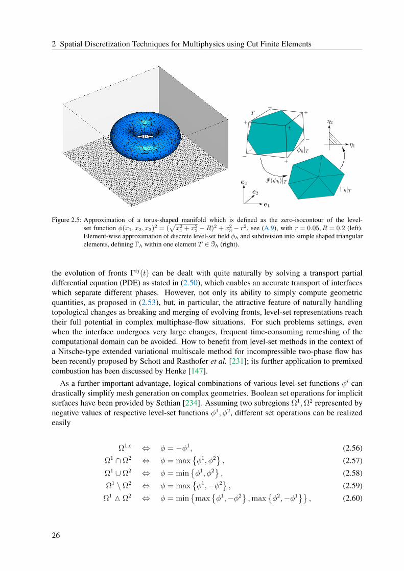
2 Spatial Discretization Techniques for Multiphysics using Cut Finite Elements

e1

e2

e3

T +

+

−

−

−

+

+

η2

η1

Γh|T

φh|T

I(φh)|T

Figure 2.5: Approximation of a torus-shaped manifold which is defined as the zero-isocontour of the level-set function φ(x1, x2, x3)2 = (

√x2

1 + x22 −R)2 + x2

3 − r2, see (A.9), with r = 0.05, R = 0.2 (left).Element-wise approximation of discrete level-set field φh and subdivision into simple shaped triangularelements, defining Γh within one element T ∈Th (right).

the evolution of fronts Γij(t) can be dealt with quite naturally by solving a transport partialdifferential equation (PDE) as stated in (2.50), which enables an accurate transport of interfaceswhich separate different phases. However, not only its ability to simply compute geometricquantities, as proposed in (2.53), but, in particular, the attractive feature of naturally handlingtopological changes as breaking and merging of evolving fronts, level-set representations reachtheir full potential in complex multiphase-flow situations. For such problems settings, evenwhen the interface undergoes very large changes, frequent time-consuming remeshing of thecomputational domain can be avoided. How to benefit from level-set methods in the context ofa Nitsche-type extended variational multiscale method for incompressible two-phase flow hasbeen recently proposed by Schott and Rasthofer et al. [231]; its further application to premixedcombustion has been discussed by Henke [147].

As a further important advantage, logical combinations of various level-set functions φi candrastically simplify mesh generation on complex geometries. Boolean set operations for implicitsurfaces have been provided by Sethian [234]. Assuming two subregions Ω1,Ω2 represented bynegative values of respective level-set functions φ1, φ2, different set operations can be realizedeasily

Ω1,c ⇔ φ = −φ1, (2.56)

Ω1 ∩ Ω2 ⇔ φ = maxφ1, φ2

, (2.57)

Ω1 ∪ Ω2 ⇔ φ = minφ1, φ2

, (2.58)

Ω1 \ Ω2 ⇔ φ = maxφ1,−φ2

, (2.59)

Ω1 M Ω2 ⇔ φ = min

maxφ1,−φ2

,max

φ2,−φ1

, (2.60)

26

2.1 Domain Decomposition - General Aspects and an Overview of Concepts

where (·)c denotes the complementary set and M the symmetric difference of two sets. Concate-nation of Boolean operations for an arbitrary number of subregions can be used then to easilycreate complex regions by simply replacing the set operators with min/max-operations on therespective level-set functions. It is assumed thereby that all level-set fields φij are discretizedon the same approximation space Sh. Otherwise, additional projections between different gridshave to be introduced. Note that even combinations with evolving interfaces can be performed.The signed-distance properties of each level-set field are preserved by these operations, theaccuracy of the approximation, however, is limited to the mesh size h of the underlying grid.

Recently, Burman et al. [63] proposed some examples based upon logical combinations oflevel-set functions describing basic geometric forms. An overview of implicit descriptions ofmost common geometric objects up to more advanced shapes, like a helical pipe, is given inAppendix A. An example for a complex-shaped computational domain exclusively describedby Boolean combinations of several level-set functions is shown in Figure A.2; its definingcomposed level-set function is provided in Appendix A.3. This example of a composed geometrywill be later utilized for flow simulations in Section 3.6.2.3.

2.1.4 General Concepts of Domain Decomposition TechniquesMultiphysics problems typically put highest demands on their discretization spaces. Coupledproblems consisting of several physics like, e.g., fluids, solids, transport phenomena of scalarquantities or many others, require different specific mesh qualities for the involved single fields.The field solutions strongly dependent on material laws and properties as well as on given dataand the governing equations. Depending on the physical field, well-suited finite-element-baseddiscretizations have been developed which often make use of individual mesh features, like size,shape and polynomial degree of finite elements, or differ in the choice between a continuous anda discontinuous Galerkin scheme. Several approaches are also based on specific finite elementfamilies. Such range from spectral elements to enriched function spaces and others are designedto directly incorporate certain approximation features, as they arise, e.g., from the div- and curl-operators. For an overview of the enormous variety of finite element technologies, the interestedreader is referred to, e.g., [3, 37, 78, 195, 216, 217].

In that way, it seems a logical conclusion to make the attempt to combine optimal singlefield discretizations within a domain decomposition approach and to couple the different ap-proximation spaces at common interfaces. The domain of a multiphysics problem setting, asintroduced in Section 2.1.1, can be thereby either composed of subdomains associated withdifferent physics, or a domain, which belongs to one physical field, can be artificially de-composed into subregions in order to compose several specific meshes. As the meaning ofthe term domain decomposition changes in literature depending on the context it is used, itneeds to be pointed out that throughout the present thesis this naming solely designates the splitof the physical domain into subregions, which comes along with interface couplings governedby certain coupling constraints. In the following, an overview of finite-element-based domaindecomposition strategies is given and general concepts are introduced. Focus is directed totheir applicability to multiphysics problems, which involve, among others, incompressible flows.Further emphasis is put on their ability to deal with time-dependent phase boundaries.

Considering a single domain Ω, the basic concept of FEMs consists in a decomposition ofthe approximated computational domain Ωh into simple-shaped finite elements, as introduced

27

2 Spatial Discretization Techniques for Multiphysics using Cut Finite Elements

in (2.39). Throughout this thesis, low-order two- and three-dimensional finite elements basedon Lagrangean interpolation functions of degree k = 1, 2 are exclusively used. Their element-wise polynomial finite element spaces are denoted by Pk for simplices, by Qk for hexahedraland by Wk for wedge-shaped elements. For simplices, the index k denotes the total degreeof the polynomial. In contrast, for hexahedral elements, k specifies the polynomial degree ineach coordinate direction. Accordingly, the notation holds for wedge-shaped elements. In thepresent work, these different element types are also referred to as 3-node triangular (tri3), 6-node triangular (tri6), 4-node quadrilateral (quad4), 8-node quadrilateral (quad8) and 9-nodequadrilateral (quad9) in 2D and as 4-node tetrahedral (tet4), 10-node tetrahedral (tet10), 8-node hexahedral (hex8), 20-node hexahedral (hex20) and 27-node hexahedral (hex27) in 3D.The three-dimensional wedge-shaped elements are called 6-node wedge (wedge6) and 15-nodewedge (wedge15).

2.1.4.1 Notation and Terminology on Computational Domains and Meshes

First of all, terminology and notation frequently used in the context of domain decompositiontechniques are introduced. In literature, some terms describing the mesh location with respect tothe physical domain and the positioning of different meshes relative to each other often differ.Their meanings often depend on the considered application and on the specific utilized numericalscheme. To avoid misunderstandings, the following terminology on computational domains andmeshes is used throughout this thesis:

Let Th be a background mesh with mesh size parameter h > 0 which covers an open andbounded physical domain Ω. The active part of this mesh is defined as

Th = T ∈ Th : T ∩ Ω 6= ∅ (2.61)

consisting of all elements in Th which intersect Ω. Denoting the union of all elements T ∈Thby Ω∗h, then Th is called a (geometrically) fitted or more precisely a boundary-fitted mesh ifΩh = Ω∗h and an unfitted or non-boundary-fitted mesh if Ωh ( Ω∗h. In the latter case it is referredto Ω∗h as fictitious domain. To each mesh, the subset of elements that intersect the boundary Γ

TΓ = T ∈Th : T ∩ Γ 6= ∅ (2.62)

is associated, which plays a particular role for unfitted meshes. Notations related to fitted andunfitted computational meshes are depicted in Figure 2.6. For a given mesh Th, the space

Xhdef=vh ∈ C0(Ω∗h) : vh|T ∈ Vk(T )∀T ∈Th

(2.63)

denotes the finite element approximation space consisting of continuous piecewise polynomialsof order k > 1 and

Xdch

def=vh ∈ L2(Ω∗h) : vh|T ∈ Vk(T )∀T ∈Th

(2.64)

the space of discontinuous piecewise polynomials. In contrast to the continuous space, wheredegrees of freedom at common nodes of neighboring elements are shared by all adjacent ele-ments, in a discontinuous function space, each element T ∈ Th carries own degrees of freedomfor all its nodes. The concept of element-wise continuous and discontinuous function spaces canbe analogously transferred when domains are decomposed into subregions, which is referred toas domain decomposition in this work.

28

2.1 Domain Decomposition - General Aspects and an Overview of Concepts

Ω

Γ = ∂Ω

Th

Ω

Γ = ∂Ω

TΓ

Th,Ωh = Ω∗h

Ω

Γ = ∂Ω

Th

Ω

Γ = ∂Ω

TΓ

Th,Ω∗h

∂Ω∗h

Figure 2.6: Boundary-fitted versus non-boundary-fitted meshes: A computational grid Th is (geometrically) fittedto the boundary Γ of a physical domain Ω (upper left) and its active part Th fits to the domain suchthat Ωh = Ω∗h (upper right). The physical domain Ω is defined as the interior of a given boundary Γ

embedded into an unfitted background mesh Th (lower left), the fictitious domain Ω∗h is the union of theminimal subset Th ⊂ Th covering Ω (lower right).

2.1.4.2 Limitations of Fitted Mesh Discretization Techniques

Considering a domain Ω decomposed into two disjoint subdomains Ω1,Ω2, as introduced inSection 2.1.1, two covering meshes T1

h ,T2h which are assumed to be fitted to the common inter-

face Γ12 are called matching or node-matching whenever all nodes located at the interface areshared by both meshes. This, however, does not necessarily imply that the two meshes evenhave to carry identical sets of degrees of freedom associated with these nodes. If additionally allinterfacial degrees of freedom are shared by both discretizations, a natural continuity conditionis built in the discrete finite element function space Xh. In contrast, having two independent setsof interface DOFs, the composed space Xh = X1

h ⊕X2h is discontinuous by construction and,

in that way, allows for capturing sharp discontinuities in the physical fields across the interface.Then, however, additional measures are required to impose interface coupling conditions. Forthis purpose, different techniques will be elaborated in detail and examined carefully with focuson stability and optimality properties in Chapters 3–5.

Computational grids which are all fitted to the interface, however, non-node-matching to eachother, are denoted as non-matching meshes. Different possible domain decomposition conceptsbased upon interface-fitted matching and non-matching meshes are depicted in Figure 2.7. Notethat all domain decomposition methods considered in this work are based on continuous subdo-main functions spaces Xi

h.

29

2 Spatial Discretization Techniques for Multiphysics using Cut Finite Elements

Γ12

∂Ω

Ω1

T2h ,Ω

2h = Ω2∗

hT1h ,Ω

1h = Ω1∗

h

Ω2

T2ΓT1

Γ

Xh

Ω2

T2h ,Ω

2h = Ω2∗

hT1h ,Ω

1h = Ω1∗

h

Ω1

Γ12

(a) Subdomain meshes are node-matching. The finite element function space Xh is stronglycontinuous across the interface Γ12 as all interfacial DOFs are shared by the two meshes.

Γ12

∂Ω

Ω1

T2h ,Ω

2h = Ω2∗

hT1h ,Ω

1h = Ω1∗

h

Ω2

T2ΓT1

Γ

X1h X2

h

Ω2

T1h ,Ω

1h = Ω1∗

h T2h ,Ω

2h = Ω2∗

h

Ω1

Γ12

(b) Fitted domain decomposition with node-matching subdomain meshes T1h ,T

2h at the

interface Γ12. Discrete composed function space Xh = X1h ⊕X2

h allows for strongdiscontinuities across Γ12.

Ω2

∂Ω

T1h ,Ω

1h = Ω1∗

h T2h ,Ω

2h = Ω2∗

h

Ω1

Γ12

T2ΓT1

Γ

X1h X2

h

Ω2

T1h ,Ω

1h = Ω1∗

h T2h ,Ω

2h = Ω2∗

h

Ω1

Γ12

(c) Fitted domain decomposition with non-node-matching subdomain meshes T1h and T2

h atthe interface Γ12. Discrete composed function space Xh = X1

h ⊕X2h allows for strong

discontinuities across Γ12 and different mesh sizes.

Figure 2.7: Domain decomposition strategies for Ωh = Ω1h∪Ω2

h based upon interface-fitted meshes, i.e. Ω1h = Ω1∗

h

and Ω2h = Ω2∗

h .

30

2.1 Domain Decomposition - General Aspects and an Overview of Concepts

To demonstrate the capabilities and limitations of interface-fitted domain decomposition strate-gies in the following, the example of fluid-structure interaction (FSI), which is one of theprimary coupled multiphysics applications considered in the present work, is predestined. Infact, the use of a single matching continuous finite element function space for the entire do-main Ω, for which the continuity of the fields is strongly incorporated in the discrete space, isone of the most easiest and feasible finite element discretization methods. Regarding stabilityno additional measures are required at the interface and continuity requirements are automati-cally fulfilled. This choice, however, comes along with very restrictive limitations for transientproblems with moving domains. For instance for fluid-structure interaction, where the fluidis classically described with an ALE moving mesh approach and the solid is formulated in aLagrangean frame of reference (see, e.g., works by Kuttler [168] and Mayr et al. [185] for suchapproaches), the temporal motion and deformation of the solid is strictly limited. Otherwise, thefluid mesh can distort and time consuming remeshing and projection steps have to be performedregularly. Limitations of matching approximations for moving domain problems are indicatedin Figure 2.8.

Using non-matching fluid and structural meshes instead, already extends the applicabilityof FSI algorithms to a greater multitude of problem settings, as also shown in Figure 2.8.Relaxation of the strong node-matching constraint allows for independent mesh movementsin interface-tangential directions and thus enables for instance large structural rotations in anembedded fluid and thereby allows for different mesh sizes. Such a technique has been consid-ered, e.g., by Kloppel et al. [164] in combination with an inf-sup stable dual mortar Lagrange-multiplier approach to weakly impose the required continuity of the field solutions. For flowproblems, non-matching mesh methods rather show their high potential in situations when masstransport across the interface is allowed. This is the case for mesh-tying problems when aninterface is introduced to artificially separate a single physical domain into different phases car-rying the same material. Such problem settings will be considered in more detail in Section 4.3.However, when phase change across the interface is not physically motivated due to massconservation constraints, as it would be the case for fluid-structure interaction or immiscibletwo-phase flow, the interface is naturally largely driven in interface-normal direction followingthe material particles in their motion. In that way, approaches which utilize interface-fittedmeshes are still limited in domain motions and deformations. As already indicated in Figure 2.8,a powerful strategy to overcome such limitations consists in decoupling computational meshesfrom the geometries.

2.1.4.3 Capabilities of Unfitted Mesh Techniques for Multiphysics

The main focus in this thesis is to develop computational approaches to multiphysics problemsthat involve incompressible flows and thereby reduce restrictions on the interface location andits temporal movement. The fundamental idea is to construct finite-element-based computa-tional grids, which serve as basis for the discrete function spaces used for the approxima-tion of the solutions, however, may be independent of the location of the separating phaseboundary. Due to the temporal interface motion, which may be prescribed by given data orbe naturally computed from the field solutions, the overall domain Ωh gets separated into time-dependent subregions Ω1

h(t) and Ω2h(t). The background meshes T1

h and T2h associated with

the subdomains, however, are now assumed to be non-fitted to the moving interface Γ(t). Each

31

2 Spatial Discretization Techniques for Multiphysics using Cut Finite Elements

Figure 2.8: Multiphysics with moving domains: (Left) Node-matching moving meshes are subjected to strictlimitations regarding their interface motion and deformation, otherwise the meshes can distort. (Mid-dle) Interface-fitted non-node-matching meshes enable mesh motion in interface-tangential directions,but can fail for large mesh movement in interface-normal directions. (Right) Unfitted non-matchingmeshes allow for arbitrary motion of the meshes relative to each other.

mesh can be either fixed in space or even moving over time, if a general ALE-framework isapplied, as introduced in Section 2.1.2. Thereby, interface and mesh motions can be treated fullydecoupled from each other. It has to be remarked that for time-dependent domains the activeparts T1

h ,T2h of the respective background meshes are changing over time, see definition (2.61).

As introduced in (2.62), respective sets of elements intersected by the interface are given byT1

Γ = T ∈T1h : T ∩ Γ 6= ∅ and T2

Γ = T ∈T2h : T ∩ Γ 6= ∅. Related fictitious subdomains

Ω1∗h ,Ω

2∗h are defined accordingly. This serves as starting point for specific strategies considered

subsequently. A visualization of this generalized unfitted domain decomposition discretizationstrategy is shown in Figure 2.9.

While interface-fitted approaches are often also referred to as non-overlapping mesh methodsin literature, numerical schemes where the boundary of the finite element grid does not fit to theinterface include terms like overlapping mesh method. Throughout this work, this classificationis only used to describe the positioning of the meshes relative to each other. Moreover, in liter-ature, the term overlapping meshes often automatically implies that weak formulations relatedto the field governing equations are evaluated not only in the physically meaningful part of therespective active mesh, namely Ωi ∩Ti

h, but twice in the overlap region of the two meshes. Thisimplication, however, is expressly not desired for all formulations presented in this work.

Treating interface motions independent of the computational grids now widens the range offeasible interface-coupled multiphysics problems. In this thesis, focus is put on applicationswhere incompressible flows are involved in one or two subdomains. In the following, someexamples for coupled flow problems, which will be considered in more detail later in this work,are sketched in view of the applicability of different geometrically unfitted mesh approaches.More detailed elaborations on these problem settings, stabilized weak formulations, numericalexamples as well as discussions with regard to their placement within a more general context ofother related methods are provided in respective paragraphs in Chapters 3–5.

32

2.1 Domain Decomposition - General Aspects and an Overview of Concepts

Ω2

T1h ,Ω

1h ( Ω1∗

h T2h ,Ω

2h ( Ω2∗

h

T1h

T2h

Ω1

Γ12

Ω2

T1h ,Ω

1h ( Ω1∗

h T2h ,Ω

2h ( Ω2∗

h

T2h

T1h

Ω1

Γ12

Figure 2.9: Generalized unfitted domain decomposition technique based on computational meshes which do notnecessarily need to fit to the interface Γ12. In that way, restrictions on the interface location and itstemporal movement are highly reduced.

Unfitted Boundaries. Considering a single fluid phase, enforcing different essential and nat-ural constraints of Dirichlet-, Neumann- or Robin-type on boundaries which do not fit to theunderlying background mesh Th defines the starting point for developing unfitted finite elementmethods for coupled multiphysics flow problems. For complex three-dimensional fluid domains,generating high quality computational grids which are conform with the domain boundary canoften get time-consuming and difficult. This becomes particularly cumbersome and costly forgeometries given by, for instance, CAD data from industrial applications or by image data from,e.g., geological or biological sources. For this purpose, utilizing finite element methods thatcompute the solution to the problem on the active part Th of mostly fixed grids, which areintersected by the boundary, can drastically simplify meshing of the computational domain, asshown in Figure 2.10a. Special measures are required to impose the different types of boundaryconditions in a consistent weak sense. However, ensuring robustness, stability and accuracy ofthe numerical scheme becomes more challenging due to the intersection of elements. As onemajor issue, depending on the interface location, small parts of intersected elements are oftennot sufficiently controlled by the weak formulation, which for consistency reasons is definedonly on the physical domain Ωh. To overcome this issue, inf-sup stable and optimally convergentmethods need to be developed, analyzed and studied, as done in very detail throughout Chapter 3.

33

2 Spatial Discretization Techniques for Multiphysics using Cut Finite Elements

ΓN

ΓR

Ω

ΓD

Th

(a) Using computational meshes Th which are unfitted to the fluid domain boundary candrastically simplify mesh generation. Dirichlet-, Neumann- and Robin-type boundaryconditions at ΓD,ΓN,ΓR ⊂ ∂Ω need to be imposed weakly.

Γ12

Ω1

T2h

T1h

Ω2

(b) Overlapping mesh fluid domain decomposition for a single fluid phase: a fine resolvedmesh T2

h = T2h is embedded into an unfitted background mesh T1

h . Mass transport acrossthe artificial interface is allowed while the embedded mesh can arbitrarily move.

Γ12

Ω1

Ω2

T1h = T2

h

(c) Unfitted approach to incompressible two-phase flow based upon the same underlyingmeshes T1

h = T2h , however, different non-interface-fitted active mesh parts T1

h ,T2h . No

restriction on the movement of the phase-separating interface due to the possibility ofrespective time-varying active mesh parts.

Figure 2.10: Discretization strategies for coupled flow problems based upon non-interface-fitted meshes associatedwith the subdomains.

34

2.1 Domain Decomposition - General Aspects and an Overview of Concepts

Fluid Mesh Tying - Unfitted Overlapping Mesh Domain Decomposition. Complex fluiddomains require appropriate mesh qualities in certain subregions for the spatial discretizationof the problem specific characteristics. In particular high-Reynolds-number flows, which mayexhibit near-wall turbulent boundary layers, put highest demands on the mesh quality. Local highmesh resolutions are important to capture steep gradients in the solution fields. Mesh adaptivitytechniques are often used for such scenarios, however, are computationally very expensive dueto iterative procedures in the construction of well-suited meshes and thus their application totime-dependent moving domains is of limited use; see, for instance, the publication by Oden andDemkowicz [199] for a survey on early works.

Overlapping mesh domain decomposition techniques are highly beneficial in such situations.In general, any combination of unfitted active overlapping meshes T1

h ,T2h , which cover the

subregions Ω1h,Ω

2h of the overall fluid domain Ωh, can be used. In this work, one specific

setting of composite grids is investigated in more detail. Embedding a boundary-fitted fluidpatch T2

h such that Ω2h = Ω2∗

h into an unfitted background mesh T1h with Ω1

h ( Ω1∗h , as depicted

in Figure 2.10b, exhibits many powerful features for complex fluid domains, as will be explainedin the following.

When it comes to computational grid generation for a complex region, for which a boundarydescription is given, constructing a boundary-fitted layer of fluid elements elongated in wall-normal direction is an easy task in general. Overlapping such a patch with a background meshand coupling them in an unfitted non-node-matching manner even allows for the use of locallyincreased resolutions within the fluid patch independent of the background mesh properties.Adapted to the specific problem situation, mesh properties like grid size, shape and polynomialdegree of finite elements and the structuring of the meshes can be chosen independently. Such anoverlapping domain decomposition technique comes to its full extent when domain boundariesstart to move. Then, the embedded fluid patch is able to follow the boundary independentof its location within the background mesh. The fundamental idea of this technique in thecontext of finite element methods traces back to a work by Hansbo et al. [139], which hasbeen adapted to flows in a publication by Shahmiri et al. [236]. Further developments regardinginterface stabilizations, which ensure inf-sup stability and optimal convergence properties forlow- and high-Reynolds-number flows, have been proposed by Schott and Shahmiri et al. [232].Stabilization techniques and a numerical analysis with particular emphasis on issues related tointerface stability and mass transport across the introduced artificial interface will be presentedin detail in Section 4.2, supported by various challenging numerical simulations in Section 4.3.

Incompressible Two-Phase Flow. Considering immiscible two-phase flows with high con-trast in the material properties of the fluid phases, a method of choice could be to use twounfitted meshes T1

h and T2h , which overlap in the interface region. The underlying background

meshes can thereby be chosen identically for both subdomains, i.e. T1h = T2

h . To preservemass conservation of the immiscible fluid phases, the interface, which can be defined implicitlyby a level-set field, moves in interface-normal direction following the fluid particles in theirmotion. Thereby, the interface is not restricted in its movement and function spaces for eachfluid phase are defined on time-changing active sets of the underlying finite element grid. Avisualization of this unfitted scheme is shown in Figure 2.10c. Based on this discretizationtechnique, a stabilized Nitsche-type extended variational multiscale method has been proposed

35

2 Spatial Discretization Techniques for Multiphysics using Cut Finite Elements

by Schott and Rasthofer et al. [231]. Stability requirements in case of high material contrastin conjunction with the interface coupling scheme and particular interface-zone stabilizationtechniques are addressed in Section 4.2. Moreover, an outlook to its applicability to classicaltwo-phase flow including surface tension and to an advanced premixed-combustion applicationis given in Section 4.4.

Fluid-Structure Interaction. For the numerical simulation of mutual interactions of fluids andsolids, different competitive approaches are considered in the current work. While for solids aLagrangean description together with boundary-fitted meshes is the most reasonable choice, forflows, an Eulerian or a more general ALE description is preferable. The use of non-interface-fitted approximations for the fluid allows for various overlapping mesh strategies between fittedstructural meshes and unfitted fluid meshes, which show their capabilities in several differentsituations.

In a first approach, similar to the embedded fluid-fluid overlapping mesh approach describedpreviously, now a structural mesh Ts

h fitted to the boundary of the solid overlaps with an unfittedbackground fluid mesh T f

h such that

Ωsh = Ωs∗

h , Ωfh ( Ωf∗

h , Ωs∗h ∩ Ωf∗

h 6= ∅, (2.65)

as visualized in Figure 2.11a. Such an overlapping mesh technique enables arbitrary solid mo-tions and interactions with the surrounding fluid, whose mesh is not subjected to any distor-tion. Moreover, this technique even allows for additional interactions between several structuralbodies in a surrounding fluid. Contact of submersed structures, as considered in algorithmsdeveloped by Mayer et al. [184], is supported in general. Such problem settings, however,go beyond the scope of this thesis. Based on these mesh configurations, different couplingschemes for fluid-structure interaction have been considered. To name just a few, Burman andFernandez [58] developed a Nitsche-type coupling for viscous Stokes’ flow coupled to linearelastic material or Gerstenberger [123] developed fluid-structure coupling schemes based onstress-based Lagrange-multiplier interface methods in combination with partitioned solutionalgorithms. A comprehensive overview of related works will be given in Chapter 5. In Sec-tion 5.3, a full-implicit Nitsche-type fluid-structure coupling for low- and high-Reynolds-numberflows governed by the incompressible Navier-Stokes equations and interacting with non-linearstructural materials will be proposed.

Nevertheless, in some cases the previously introduced unfitted technique is not perfectlysuited. As regular background fluid meshes are usually used to simplify meshing, for manyapplications the mesh resolution can be very high even in regions far from the fluid-structureinterface. This might result in enormous computational costs, in particular, for simulations inthree spatial dimensions. Otherwise, when using a coarser mesh in the overall fluid domain,the quality of the solution next to the fluid-structure interface would decrease considerably.For this reason, a second expanded domain decomposition approach is proposed. It providesa powerful simulation tool and combines capabilities of the overlapping fluid-structure couplingand the aforementioned unfitted overlapping fluid-fluid mesh-tying technique. Approximatingthe vicinity of the solid with a finer mesh resolution and the far-field with a coarser mesh canbe easily realized as depicted in Figure 2.11b and explained in the following: In a first step,the fitted solid mesh Ts

h overlaps with a high resolution background mesh T f2h . This is usually

36

2.1 Domain Decomposition - General Aspects and an Overview of Concepts

T fh ( T f

h

Tsh = Ts

h

Ωh = Ωfh ∪ Ωs

h

Ωsh ≡ Ts

h

Ωfh ( Ωf∗

h

(a) Using an unfitted fluid mesh Tfh overlapped by an interface-fitted structural mesh Ts

h

allows for simulating fluid-structure interaction where the solid can undergo largedeformations and motions; even contact of submersed bodies and topological changesare supported.

T f1h ( T f1

h T f2h ( T f2

h

Tsh = Ts

h

Ωh = Ωf1h ∪ Ωf2

h ∪ Ωsh

Ωsh ≡ Ts

h

Γf1f2h

Ωf2h ( Ωf2∗

h

Ωf1h ( Ωf1∗

h

(b) Combination of an unfitted overlapping fluid-structure coupling with an overlappingfluid-fluid domain decomposition technique. This technique enables different meshresolutions in the vicinity of the solid Ts

h with a finer fluid grid Tf2h and a coarser fluid

discretization Tf1h far form the fluid-solid interface.

T f1h ( T f1

h

Tsh = Ts

h

T f2h = T f2

h

Ωh = Ωf1h ∪ Ωf2

h ∪ Ωsh

Γf1f2h

Ωf2h ≡ T f2

hΩf1h ( Ωf1∗

h

Ωsh ≡ Ts

h

(c) Fitting a surrounding patch of fluid elements to the fluid-structure interface Γf2s andembedding it unfitted into a background fluid meshTf1

h with the help of overlapping meshdomain decomposition techniques provides a powerful simulation tool. It drasticallysimplifies meshing of complex geometries and allows to perfectly capture steep near-wall gradients in the boundary layer region around the solid. ALE-techniques allow theembedded mesh to follow the solid in its movement.

Figure 2.11: Different fluid-structure-interaction domain decomposition approaches based upon the use of unfittedoverlapping meshes (left) with according decomposition of the entire domain (right).

37

2 Spatial Discretization Techniques for Multiphysics using Cut Finite Elements

defined in a region of expected structural motion. In second step, this fluid mesh is embeddedinto a coarse background fluid meshT f1

h using unfitted overlapping mesh techniques. This resultsin the following domain and mesh configurations

Ωf1h ( Ωf1∗

h , Ωf2h ( Ωf2∗

h , Ωsh = Ωs∗

h (2.66)

with

Ωf1∗h ∩ Ωf2∗

h 6= ∅ Ωf2∗h ∩ Ωs∗

h 6= ∅. (2.67)

This approach will be considered in more detail in Section 5.4. Such composed techniques highlyincrease efficiency and accuracy of computational algorithms and still retain the capability withrespect to dealing with large structural motions. The major limitation, which has been newlyintroduced by incorporating a priori knowledge on the expected structural motion, can be relaxedby enabling moving mesh techniques to allow the inner embedded fluid patch to follow thestructure in its motion. This could be easily realized by applying ALE concepts and is partcurrent research.

For fluid-structure interactions, in which (self-)contact of structural bodies or even topolog-ical changes do not have to be supported, the aforementioned overlapping fluid-fluid-structurecoupling can be adapted, resulting in a third powerful approach: Instead of using an unfittedoverlapping mesh approach at the fluid-solid interface Γf2s, one can also use interface-fittedmeshes Ts

h and T f2h . They may be chosen either non-node-matching or node-matching at Γf2s.

The latter variant is considered in this work. The usually finer resolved fluid patch T f2h is thereby

embedded into a coarser background grid T f1h in an unfitted way, based upon the introduced

overlapping fluid domain decomposition approach. This setup results in

Ωf1h ( Ωf1∗

h , Ωf2h = Ωf2∗

h , Ωsh = Ωs∗

h (2.68)

with

Ωf1∗h ∩ Ωf2∗

h 6= ∅ Ωf2∗h ∩ Ωs∗

h = ∅. (2.69)

A visualization of this approach is given in Figure 2.11c. Applying an ALE-framework to theembedded fluid patch, the solid-fitted fluid mesh T f2

h can follow the body in its movement. Thisenables to accurately capture effects at the fluid-structure interface independent of the fluid patchlocation within the background mesh T f1

h . This renders such approaches highly attractive, e.g.,for interactions of solids with turbulent incompressible flows, in which capturing boundary layereffects in the vicinity of solids is a crucial task. Successful application of this technique to FSIhas been already shown by Shahmiri [235]. The contribution of present thesis to this topic mainlyconsists in the further enhancement of the required stabilization techniques for the incorporatedfluid-domain decomposition technique. Theoretical aspects will be discussed in Section 4.2 andexamples will be provided in Section 4.3 to demonstrate the high capabilities of this method.

This presented overview indicates the high flexibility of novel discretization techniques whichmake use of non-interface-fitted computational meshes. The various number of feasible meshconfigurations for different physical fields in combination with the possibility to incorporate

38

2.2 Finite-Dimensional Cut Finite Element Approximations

artificial domain decomposition for single fields allow for easily constructing mesh compositeswhich are appropriately designed for the respective multiphysics problem setting. This is mainlythanks to the fact that meshes can be chosen independent of the respective subdomains, providedthat stable weak formulations are available for the physical fields. To allow to approximateincompressible low- and high-Reynolds number flows on unfitted meshes, accurate, inf-supstable and optimally convergent discrete formulations are developed throughout Chapter 3 ofthis thesis. One of the main difficulties consists in the fact that strongly consistent subdomainweak formulations are evaluated only in the respective physical regions, i.e. in Ωi ∩Ti

h. As thisis only a part of the respective active computational mesh, this can result in inf-sup instabilities,in loss of optimality and in a potential ill-conditioning due to the intersection of elements in theinterface zone - issues that have to specifically treated by appropriate stabilization techniques.

It needs to be highlighted that such domain decomposition methods are no longer limited tomultiphysics applications where incompressible flows are involved, as exclusively consideredin this work. Enhancements to, for instance, the solution of any transport phenomena of scalarquantities like heat transfer, chemical concentration processes or many others is straightforward.Considering such problem settings, however, goes beyond the scope of this thesis.

All unfitted non-matching discretization approaches introduced in this section require therepresentation of discrete solutions based upon finite element spaces whose underlying compu-tational grids do not fit to the respective subdomain boundaries in a classical node-wise manner.For this purpose, before introducing techniques for imposing boundary or coupling conditions,in the subsequent section, general concepts of so-called cut finite element function spaces areintroduced.

2.2 Finite-Dimensional Cut Finite Element Approximations

The fundamental idea of applying finite-element-based methods which allow to sharply take careof boundaries and interfaces that do not fit to computational grids and intersect finite elements,is twofold. On the one hand, as pointed out in previous sections, decoupling of physical subdo-mains from their respective computational meshes widens the flexibility of coupling schemes formany multiphysics problems. On the other hand, physical models often assume solutions beingdiscontinuous when local length scales at phase boundaries are not fully resolved by the mesh.Thus, an accurate representation of non-smooth features with the numerical approach is desirablefor a multitude of coupled physical models. For this purpose, FEM-based approximations usingcut elements will be introduced.

First, an overview about different numerical techniques to incorporate discontinuities into thediscrete function spaces is given. Emphasis is put on enriching classical finite element spaceswith the eXtended Finite Element Method (XFEM) and to a specific class of related methodswhich are often referred to as Cut Finite Element Methods (CUTFEM). Quantities related toelement intersections are introduced and techniques for enriching finite elements are brieflyelaborated. Afterwards, a generalized concept for constructing cut finite element function spacesto sharply approximate discontinuous fields on complex geometries is presented. As motivatingapplications, advanced fluid-solid interactions or multiphase flow configurations are considered.

39

2 Spatial Discretization Techniques for Multiphysics using Cut Finite Elements

2.2.1 An Overview of eXtended and Cut Finite Element Methods

From a macroscopic point of view, solution fields to physical phenomena which involve highlydifferent length scales within subdomains or near phase boundaries are often predestined tobe modeled being discontinuous. Non-smooth material characteristics and steep gradients inthe transition zone then require being sharply approximated by discrete functions. Potentialapplications range from dislocations and cracks in solid mechanics to boundary layers, phaseboundaries, shocks and flame fronts in fluid mechanics. In fluids, separated liquid and gas phasesoften exhibit high contrast in their material properties and come along with strong surface-tension effects, which motivates to model fields as discontinuous. In that way, interactionsbetween those fluids, solids or even porous media are potential application areas.

Classical FEMs can represent discontinuous fields only when meshes associated with sub-domains fit to the interface. This, however, limits interfaces in their motion as discussed forvarious multiphysics problems in previous sections. In contrast, enriching classical polynomialfinite spaces by functions that are able to represent desired discontinuities within finite elementsallows to sharply capture non-smooth characteristics of the physical problem. Thereby, thedesired discontinuity is assumed to be known a priori from modeling to get incorporated into theextended finite element function space depending on the interface location within the computa-tional grid. In a review article by Fries and Belytschko [115] such methods are called enrichedmethods. When constructing enriched function spaces, it is desirable to guarantee the so-calledpartition-of-unity property, which ensures that an enrichment function ψ, which mimics the dis-continuity, can be trivially recovered by means of enriched nodal shape functionsNsψ, whenever∑

sNs(x) = 1. A method featuring this property with compact support of the shape functionsis the Partition of Unity Method referred to as PUM and PUFEM in the works by Melenk andBabuska [186] and Babuska and Melenk [6], respectively. A few years after establishing thisconcept, the PUM was referred to as Generalized Finite Element Method (GFEM) (see, e.g.,Duarte et al. [94] and Strouboulis et al. [243]). Almost one decade later, Babuska and Banerjee[5] picked up the fundamental methodology of GFEMs and proposed an adaption to get rid of ill-conditioning of the resulting global stiffness matrices and so to improve severe loss of accuracydepending on the interface position; the proposed technique was called Stable GeneralizedFinite Element Method (SGFEM). Parallel to the development of the GFEM, the partition-of-unity concept based on hat-functions was also used in fracture mechanics by Belytschkoand Black [21] and Moes et al. [188] to predict crack propagation. They introduced differentenrichments to represent the discontinuity along the crack and at the crack tip. In the context offracture mechanics, for the latter partition-of-unity methods the naming eXtended Finite ElementMethod (XFEM) was introduced by Dolbow et al. [88]. This designation became a synonymwhenever function spaces are enriched by specific shape functions that exhibit compact support.

Over the last years, XFEMs became very popular and were adapted to a wide area of ap-plication fields. A survey on XFEMs in the context of material modeling was proposed byBelytschko et al. [24]. Solidification processes involving moving interfaces were considered,e.g., by Chessa et al. [72] and Ji et al. [159]. In particular in the field of multiphase flows theXFEM became a competitive numerical method. Originally proposed for two-phase flows byChessa and Belytschko [71], different enrichment strategies were investigated to capture pressurejumps caused by surface tension effects as well as kinks in the velocity solution which arise dueto a discontinuity in the material properties; see, e.g., Groß and Reusken [133], Diez et al.

40

2.2 Finite-Dimensional Cut Finite Element Approximations

[86], Sauerland and Fries [225], Rasthofer et al. [214] and Schott and Rasthofer et al. [231] fordifferent combinations of enrichments for velocity and pressure approximations. For premixedcombustion, which requires to additionally account for a jump in the velocity field across theflame front, the XFEM was adapted by van der Bos and Gravemeier [255] and Henke [147].Enriched function spaces for the flow field in fluid-structure interactions have been utilized, e.g.,by Zilian and Legay [278], Gerstenberger and Wall [125], Legay et al. [173] and Burman andFernandez [58]. Moreover, embedding mesh techniques for resolving boundary layers in fluid-solid interaction configurations which are based on fluid domain decomposition techniques weredeveloped by Shahmiri et al. [236], Massing et al. [182] and Schott and Shahmiri et al. [232].Approximating two-phase Darcy flows with the XFEM was considered by Fumagalli and Scotti[118] and a mixed finite element method for Darcy flow in fractured porous media using non-matching grids was proposed by D’Angelo and Scotti [97]. Duddu et al. [95] introduced anXFEM-based approach towards modeling of growth of biofilms.

Over the recent years, FEM-based discretization techniques utilizing fixed background gridswhich are non-fitting to embedded boundaries or interfaces to represent approximate solutionsof governing PDEs were summarized under the term Cut Finite Element Method (CUTFEM),see, e.g., Burman et al. [63] and references therein. These methods utilize finite elements whichare cut by the boundary or interface similar to the XFEM. There, for the solution approximation,most often a classical continuous or discontinuous polynomial finite element function space isused which is then simply cut-off at the interface. This procedure is equivalent to multiplyingthe classical finite element function space by a Heaviside enrichment function in the XFEM.This equivalence explains the parallel usage of both designations for such enriched or cut finiteelement techniques - XFEMs and CUTFEMs.

References and a comprehensive overview of the multitude of different techniques with regardto enforcing boundary or coupling constraints will be first given for boundary-fitted meshes inSection 3.3. Enhancement of the imposition of boundary conditions in the XFEM or CUTFEMis made in Sections 3.4–3.6. Further developments for coupling constraints in fluid-coupledproblems will be proposed later in Sections 4.2 and 5.3.

2.2.2 Cutting Finite Elements - Notation and Fundamentals of Cut-Entities

Suitable CUTFEMs for the sharp representation of discontinuities within cut finite elementsof unfitted meshes require a unique belonging of physical points and their material propertiesto active and inactive parts of the computational mesh. For this purpose, subdivision of finiteelements, which are intersected by the boundary or interface, into physical parts associated withthe different subdomains and into according non-physical parts is required.

Cut-related mesh entities and according notation for intersected elements will be introducedin the following. All proposed terms remain valid, however, simplify for the case when elementsare not bisected, but the interface “touches” one of the element surfaces; this recovers the usageof interface-fitted meshes. Subsequent elaborations are strongly based on the publications bySchott and Wall [230] and Massing et al. [183]. Without limiting generality, explicit interfacerepresentations are used for visualization exclusively in the following.

Based on notation for computational meshes introduced in Section 2.1.4.1, let Th be an inter-face-fitted or a non-interface-fitted background mesh such that the domain Ω is covered by the

41

2 Spatial Discretization Techniques for Multiphysics using Cut Finite Elements

T1

T3

T2

T4

T1, T2 ∈ TΓ

T3, T4 6∈ TΓ

ΓT2

Ω

ΓT1

(a)

V1

V2

V3

ΩT1= V1

ΩT2= V2, V3

ΩT3= V4

ΩT4= V5

V4 ≡ T3 V5 ≡ T4

T1 T2

T3 T4

(b)

Figure 2.12: Polyhedral representation of domain Ωh with so-called volume-cells: (a) Cut situation, subdivisionof Γ into element-wise parts ΓTi = Γ ∩ Ti associated with background elements Ti. (b) Partition ofphysical domain Ω into volume-cells Vi.

mesh Ω ⊂ Th. Recalling definitions on the active mesh part Th, the fictitious domain Ω∗h and theset of all intersected finite elements T of the underlying background mesh TΓ ⊂ Th, the part ofthe interface Γ which lies in an element T ∈TΓ is called interface segment and is denoted byΓT

def= Γ ∩ T , as shown in Figure 2.12a.

For inter-element faces in Th in three spatial dimensions (d = 3), i.e. for edges in two spatialdimensions (d = 2), let Fi be the set of interior faces F which are shared by exactly twoelements, denoted by T+

F and T−F . Furthermore, introduce the notation FΓ for the set of allinterior faces belonging to elements intersected by the boundary Γ,

FΓ = F ∈ Fi | T+F ∩ Γ 6= ∅ ∨ T−F ∩ Γ 6= ∅. (2.70)

If an interface Γ intersects elements T ∈TΓ of a non-interface-fitted mesh, it subdivides theminto several arbitrary formed polyhedra. In this work, such polyhedra are called volume-cellsand are notated with Vi. Volume-cells can be either associated with the physical volume Ω or tothe ghost domain Th\Ω. Cells which are part of the physical volume Ω are denoted as physicalvolume-cells. The physical volume for an element T is then given by

ΩT = polyhedra Vi ⊆ (T ∩ Ω) | Vi ∩ Vj = ∅ for i 6= j (2.71)

and consists of only volume-cells Vi, Vj which are not connected within T ∩ Ω, as depictedin Figure 2.12b. Otherwise, two volume-cells would conflate to one single volume-cell. Allpolyhedra that are not contained in Ω lie within the ghost domain and are not considered forCUTFEMs anymore. For uncut elements T ∈Th\TΓ, a unique volume-cell can be identifiedwith the element itself, i.e. VT ≡ T .

Based on this volume-cell representation the physical volume can now be rewritten as

Ωh =⋃

T∈Th

⋃

V ∈ΩT

V . (2.72)

42

2.2 Finite-Dimensional Cut Finite Element Approximations

facet f1

facet f2

T+F

T−F

face F

Γ

V +

V −

Figure 2.13: Facets of a face F ∈ Fi between two three-dimensional intersected elements T+F , T

−F with respective

volume-cells V +, V −: Intersecting surface Γ (red), facets f1, f2 (yellow). Facets fi between three-dimensional elements are arbitrary formed two-dimensional polygons which form disjoint segments ofthe two-dimensional face F .

Similarly, boundaries and interfaces Γ can be composed of segments associated with the ele-ment’s volume-cells

Γh =⋃

T∈TΓ

⋃

V ∈ΩT

(ΓT ∩ V ). (2.73)

Disjoint segments of a face F ∈ Fi which is intersected by Γ are called facets f throughout thiswork. Facets belonging to the physical domain Ωh and to the ghost domain Th\Ωh are visualizedin Figure 2.13.

Cut-related geometric objects are constructed in consecutive steps. In a first step, intersectionpoints between all faces F of the background mesh and all interface segments are identified.For a level-set representation, intersection points can be simply computed by interpolating nodallevel-set values (see, e.g., Burman et al. [63] or Groß and Reusken [134]). Afterwards, inter-section points together with nodes of background and interface representations are connected tolines, i.e. edge segments of the intersecting meshes, respectively. Closed polygons consisting oflines then build up facets f and are associated with either faces F of the background mesh or withinterface segments in ΓT . Finally, facets which are connected to each other via lines and belongto the same side with respect to the interface form the boundary of three-dimensional polyhedra.There are active physical volume-cells V and inactive volume-cells. The latter ones are locatedin the ghost part of the computational mesh. For details with regard to algorithms related to theintersection and construction of intersection-related geometric objects, the interested reader isreferred to, e.g., textbooks by de Berg et al. [82] and Schneider and Eberly [228] or the articleby Massing et al. [179] and references therein.

For implicit interface descriptions, the positioning of volume-cells with respect to the interfaceorientation can be simply determined by the sign of level-set values. Otherwise, a predefinedorientation of the interface mesh by means of a unit normal vector is assumed. In the lattercase, for a node of the background mesh which is located next to the interface, the anglebetween interface normal vector and a cut-line of the background mesh which connects the

43

2 Spatial Discretization Techniques for Multiphysics using Cut Finite Elements

node with a point on Γ allows to determine the positioning. Once positioning with respectto the interface of a single node is known, this information can be propagated through theintersected computational mesh for all geometric entities associated to one subdomain. Thiscan be efficiently realized using a “DEPTH-FIRST-SEARCH (DFS)”-algorithm applied to anabstract graph consisting of geometric volume-cells V and pairwise connecting facets f utilizedas graph-nodes and graph-edges (see, e.g., the textbook by Goodrich and Tamassia [128] for anintroduction). The depth-search is stopped at a certain level whenever an interface-aligned facetf ⊂ Γ is reached. Otherwise, positioning information would be incorrectly propagated acrossinterfaces. For remaining nodes with undetermined positioning, the algorithm can be restartedat another node which is located next to the interface.

2.2.3 Strategies for Enriching Function Spaces in the XFEMThe fundamental idea of the XFEM is to extend, or enrich, a standard finite element functionspace with additional functions which enable to accurately represent desired features withinfinite elements T ∈TΓ in the boundary or interface zone. These are usually problem dependentand can be, for example, discontinuities, singularities or logarithmic functions to name just a few.Focusing on interface coupled flow problems in this thesis, the desired features to be representedare discontinuous fields in the interface zone. The conceptual idea can be described as follows.

Principle for Interface Problems. Considering the finite element space

Xh =vh ∈ C0(Th) : vh|T ∈ Pk(T )∀T ∈ Th

(2.74)

consisting of continuous piecewise approximations of order k > 1, a nodal basis Bdef= Nss∈N

can be defined, where N = s = 1, ... , dim(Xh) is an index-set and dim(Xh) denotes thedimension of the discrete space. The nodal basis functions Ns satisfy partition-of-unity and itholds Ns(xr) = δr,s for r, s ∈ N at all nodes xr ∈ Rd of the computational mesh Th, where δr,sis the Kronecker-δ. Then, a classical finite element space can be written as Xh = span Nss∈N .

The original function space Xh can now be enriched with additional basis functions Ns′ whichare constructed of multiplying nodal basis functions Ns′ with so-called enrichment functions ψs′

Ns′(x, t)def= Ns′(x) · ψs′(x, t) (2.75)

for a subset of nodes s′ ∈ N ′ ⊂ N . Thereby, N ′ usually denotes the set of all nodes of elementsT ∈TΓ intersected by Γ. Note that for evolving interfaces or boundaries this subset may changeover time t. The enrichment function ψs′ introduces the desired sharp discontinuity to thefunction space and depends on the interface location and on point coordinates x ∈ Rd. Theenriched function space can be defined as

XΓh

def= spanNss∈N ∪ spanNs′s′∈N ′ . (2.76)

Different types of strong and weak discontinuities can be represented by appropriate choices forthe enrichment function. An overview of common strategies can be found, e.g., in Fries [114].

44

2.2 Finite-Dimensional Cut Finite Element Approximations

An example for an enrichment type to capture a weak discontinuity, namely the jump inderivatives of the solution field across Γ, is the so-called abs-enrichment. Assuming a signed-distance function d : Ω→ R based on the interface Γ, the enrichment function is defined as

ψs′(x, t)def= I(x, t)−I(xs′ , t) (2.77)

with

I(x, t)def=∑

s∈Nabs(ds(t))Ns(x)− abs(

∑s∈N

ds(t)Ns(x)), (2.78)

where abs(z) = |z| is the absolute value and ds denotes nodal values of the signed-distancelevel-set field for s ∈ N . As by construction the discontinuity occurs only in the derivative butnot in the field itself, no additional measures are required to ensure continuity of functions acrossthe interface.

Discontinuities in the primal variable itself are called strong discontinuities. Modeling jumpsacross the interface can be realized by means of an enrichment function which involves a piece-wise constant step function

ψs′(x, t)def= S(x, t)−S(xs′ , t) (2.79)

with

S(x, t)def=

−1 if d(x, t) < 0,

+1 if d(x, t) > 0.(2.80)

For both enrichment functions ψ, (2.77) and (2.79), the respective first parts introduce the desireddiscontinuity, whereas the second parts are constant shifts which do not introduce new basisfunctions into the function space, however, guarantee that the enrichment function vanishesat grid nodes, i.e. ψ(xs, t) = 0. On the one hand, this simplifies the strong incorporation ofDirichlet conditions into the function space as well as post-processing, as no reinterpretation ofnodal degrees of freedom vs for s ∈ N is necessary. On the other hand, in doing so, enrichmentfunctions contribute just locally to elements T ∈TΓ intersected by Γ.

Single-Phase Problems and Extension to Multifield Problems. For single-phase problems,the terminology of extending or enriching function spaces, as intended by the naming XFEM,is often misleading. Function spaces for single phase problems are rather modified or, more pre-cisely, cut-off at the interface. Therefore, the designation cut finite element method (CUTFEM)is utilized with growing frequency whenever non-interface-fitted meshes are used to representdiscrete solutions and intersected elements are subdivided for purposes of weak form integration.This naming is preferred and used throughout this work.

Note that performing integration just on the physical domain is equivalent to cutting-off thestandard function space at the boundary or interface. This technique even allows to easilyrecover the previously introduced step-enriched function space XΓ

h , which is based on a singlebackground mesh Th to represent solutions associated with two subdomains Ω1

h and Ω2h. Utilizing

notation from Section 2.1.4.1, this space can be rewritten equivalently and, furthermore, easily

45

2 Spatial Discretization Techniques for Multiphysics using Cut Finite Elements

expanded to several subdomains Ωih, 1 6 i 6 Ndom. A function space composed of subspaces

associated with each subdomain can be constructed as

Xh = X1h ⊕X2

h ⊕ ...⊕XNdomh , (2.81)

where Xih = spanNss∈Ni is the cut finite element space of subdomain Ωi

h. All subspacesare defined on identical meshes T1

h = T2h = ... = TNdom

h , however, have different index sets N i

which include only nodes of active elements T ∈Tih for i = 1, ... , Ndom, respectively. Note that

a discrete function vh ∈ Xh then satisfies vh|Ωih = vih|Ωih with vih ∈Xih for all i = 1, ... , Ndom.

By construction, vh exhibits the desired discontinuity across Γijh .Multiphysics settings, as introduced in Section 2.1.1, which incorporate several subdomains Ωi

h

separated by interfaces Γijh and utilize composite function spaces Xh for discretization, requirespecial consideration. The representability of solutions on complex geometries, incorporating,for instance, thin-shaped structural bodies in fluid-structure interaction or complex-shaped two-phase-flow interfaces which undergo topological changes, have to be carefully thought out.Within the next section, a general strategy for flexibly managing multiple sets of nodal degreesof freedom (DOFs) will be presented. In a first step, single-phase problems are considered andafterwards, in a second step, an extension to multifield settings is proposed. Numerical exampleswill demonstrate the capabilities of this technique for composite discrete cut function spaces.

2.2.4 CUTFEM-based DOF-Management for Complex DomainsTo obtain accurate cut finite element approximations for arbitrary-shaped embedded interfaces,in the following, a general technique to manage multiple DOFs associated with nodes of theunderlying computational mesh Th in the interface zone will be proposed. Multiple cuts withinfinite elements and special topological cases will be supported as well. The subsequent elabora-tions are based on work published by Schott and Wall [230].

Expanded Cut Finite Element Function Space. Accurate cut finite element function spaceswhich account for topological changes and multiple element intersections are based on thevolume-cell partitioning (2.72) of the domain Ωh. A continuous function space expanded byvolume-cell information can be written as

Xhdef=vh ∈ C0(Ωh) : v|V ∈ Qk(T ) ∀V ∈ ΩT ,∀T ∈Th

. (2.82)

Approximations restricted to an elemental volume-cell V ∈ ΩT are based on standard polyno-mial shape functions Ns of the underlying element T

vh|V =∑nnodT

s=1Ns|V · vs. (2.83)

In order to enable independent solution approximations on two sides of the interface within onefinite element, as depicted in Figure 2.14, it is necessary to take into account independent sets ofDOFs, respectively. Using continuous approximations, the decision whether two volume-cellsshare one nodal DOF depends on their physical connectivity. For sharing a DOF, a physicalconnection of two volume-cells within the support of the DOF’s nodal shape function Ns needs

46

2.2 Finite-Dimensional Cut Finite Element Approximations

2

2

2

1

1 1

1

1

11

1

1 1 1

1

1

1

11

2

2

2

2

22

ΩhΩh

(a)

1

1 1

1

1

11

1

1 1 1

11

1

1 1

11

1

(b)

1

1

1

1

11

1

1

11

1

1

1

1

1

(c)

Figure 2.14: Enrichment strategy: (a) Number of required nodal DOFs to represent independent solutions ondifferent sides of the interface. (b) Continuous solution on left side of the interface represented withone set of DOFs (standard-DOFs in black, ghost-DOFs in red). (c) Continuous solution on right sideof the interface represented with a second set of DOFs (standard-DOFs in black, ghost-DOFs in red).

to exist. To approximate a solution accurately when the support of Ns (supp (Ns)) is subdividedinto more than one physical volume-cell, multiple sets of DOFs have to be used at those nodes, asindicated in Figures 2.14a–2.14c. Then, for the volume-cell-based approximation of a solutionin (2.83), respective DOFs vs, s = 1, ... , nnodT , which represent the solution in the volume-cell V , have to be used. The algorithmic procedure is described in detail in the following.

The Algorithmic Setup. Considering continuous scalar approximations vh ∈Xh, in a firststep (PHASE I), the required number of DOFs per node has to be determined. The influenceregion of a DOF, assigned to a node s, and of its nodal shape functionNs is defined by its supportsupp (Ns). For continuous Galerkin approximations, the support of a nodal shape function Ns isgiven by all elements sharing node s. Thus, all the physical volume-cells covered by supp (Ns)can be influenced by an associated nodal DOF, see Figure 2.15a.

In order to determine the total number of required DOFs for a single node s ∈ N , volume-cells which are connected within its shape function support (supp (Ns)) have to be found.Such connections between volume-cells V ⊂ supp (Ns) are identified with common, delimitingfacets f . Note that three-dimensional volume-cells which share only vertices or edges areclassified as non-connected, since such connections do not reflect the physical connectivityrequired for a continuous solution. Mathematically, disjoint connections of volume-cells aredefined as

Cdef=V ⊂ supp (Ns) ∩ Ωh | ∀V ∈ C : ∃PATHC(V, V )

, (2.84)

where PATHC(V, V ) denotes a path consisting of volume-cells and common connecting facets

PATHC(V, V )def= (V = V0, V1, ..., Vk−1, Vk = V )

with facetsfj = Vj ∩ Vj+1, where Vi ∈ C ∀ i = 0, ... , k.(2.85)

Note that a connection can even consist of only a single volume-cell. Furthermore, Cs denotesall determined connections C covered by supp (Ns). For the example of a thin structure shownin Figure 2.15b, two disjunct volume-cell connections (C1 and C2) within the support of node s

47

2 Spatial Discretization Techniques for Multiphysics using Cut Finite Elements

Ωh

supp(Ns)

s ∈ N

(a)

C1 C2

Ωh

Cs = C1, C2

s ∈ N

(b)

C1 C2

Ωh

Cs = C1, C2

s ∈ N

(c)

2

2

22

2

2

2

2

1

1 1

1

1

11

1

1 1 1

1

1

1

11

2

Ωh

numdof(s) = |Cs|

(d)

V

k1

k4

k2

(k1, k2, k3, k4) = (1, 2,1, 1)

k3

Ωh

V ⊂ C1 ∈ Cs

s ∈ N

(e)

V

k1

k4 k3

k2

(k1, k2, k3, k4) = (1,2, 1, 1)

Ωh

s ∈ N

V ⊂ C2 ∈ Cs

(f)

Figure 2.15: DOF-management: (a) Elements cut by a thin structure and support of shape function Ns atnode s. (b) Identified volume-cell connections Cs = C1, C2 around node s. (c) Identifiedvolume-cell connections Cs = C1, C2 around node s. (d) Determined number of nodal DOFsnumdof(s) = |Cs|. (e) Assignment of DOF with index k3 = 1 to volume-cell V for node s.(f) Assignment of DOF with index k2 = 2 to volume-cell V for node s.

could be determined, i.e. Cs = (C1, C2). As a further example, volume-cell connections belong-ing to a second node s are visualized in Figure 2.15c.

Finally, each volume-cell connection C ∈ Cs comes along with either a physical DOF or aghost-DOF at the respective node. Thus, each node s ∈ N carries at most one physical DOFand potentially several ghost-DOFs. The total number of DOFs for each node s ∈ N is thendefined as numdof(s)

def= |Cs|, see visualization in Figure 2.15d.

In a second step (PHASE II), to each volume-cell, respective DOF indices for all of the cell’selemental nodes have to be assigned. In the preceding PHASE I, DOFs have been alreadyassigned to connections of volume-cells C ∈ Cs, which could be identified in the vicinity of therespective nodes. Note, for each element node s ∈ N(T ), a volume-cell V ∈ ΩT is containedin exactly one connection Ck ∈ Cs, 1 6 k 6 |Cs|. As a direct consequence, for each nodes ∈ N(T ), to a volume-cell V ∈ Ck the respective volume-cell connection index k gets assigned.This assignment procedure of DOF indices is visualized for a certain volume-cell V and twoadjacent nodes s and s in Figure 2.15e and Figure 2.15f. Finally, a volume-cell-based tuple ofDOF indices (k1, k2, ..., knnodT ) can be used during the assembly procedure of volume-cell-based

48

2.2 Finite-Dimensional Cut Finite Element Approximations

element stiffness matrices when evaluating the discrete variational formulation. Algorithm 2.1gives an overview of the different steps of the proposed DOF-management technique.

Algorithm 2.1 CutFEM-based DOF-management algorithm

1: INPUT: volume-cells V for all elements T ∈Th.2: PHASE I (build volume-cell connections in supp (Ns) and determine number of required

DOFs per node)3: for each node s ∈ N do4: Connect volume-cells V ⊂ supp (Ns) between elements via common facets f :

Cdef= V ⊂ supp (Ns) ∩ Ω | ∀V ∈ C : ∃PATHC(V, V ) with

PATHC(V, V )def= (V = V0, V1, ..., Vk−1, Vk = V ) where Vj ∩ Vj+1 = f are facets,

Vi ∈ C, i = 0, ..., k.5: Connections around node s: Cs

def=(C1, C2, ..., C|Cs|

).

6: Get number of DOFs: numdof(s)def= |Cs|.

7: Assign DOFs to the volume-cell connections Ck ∈ Cs, 1 6 k 6 |Cs|.8: end for9: PHASE II (assign DOFs to volume-cells)

10: for all elements T ∈Th do11: for each volume-cell V ∈ ΩT do12: for all s ∈ N(T ) (nodes of element T where nnodT

def= |N(T )|) do

13: Find V ∈ Ck where Ck ∈ Csdef=(C1, C2, ..., C|Cs|

), 1 6 k 6 |Cs| to get index k.

14: Assign the determined DOF-index k of this volume-cell connection to the volume-cell V as the respective DOF for its element node s.

15: end for16: end for17: end for18: OUTPUT: numdof(s)

def= |Cs| and (k1, k2, ..., knnodT ) set of DOF-indices for each volume-

cell V .

Without loss of generality, all visualizations in Figures 2.14 and 2.15 use 4-node quadrilateralelements in two dimensions. However, the proposed technique summarized in Algorithm 2.1 isapplicable to any spatial dimension and element type Pk,Qk,Wk of order k > 1.

Moreover, piecewise discontinuous volume-cell-based cut finite element function spaces couldbe defined as well. As no nodal connectivity has to be accounted for in such cases, independentsets of elemental DOFs can be created for each physical volume-cell V ∈ ΩT . Nevertheless, thefacet-volume-cell connectivity is though required for weak coupling strategies of the elementaldomain parts. Piecewise discontinuous functions spaces, however, are not further consideredwithin the scope of this thesis.

In the following, the necessity of an expanded function space Xh as defined in (2.82) isexemplarily shown for the flow around multiple structure.

A Numerical Example - Flow around Multiple Structures. The intention of this example isto demonstrate the applicability of the proposed method to complex-shaped domains build upof different embedded structural obstacles. A computed two-dimensional flow around different

49

2 Spatial Discretization Techniques for Multiphysics using Cut Finite Elements

Figure 2.16: Flow around multiple structures: velocity solution (left) and pressure solution (right).

structures serves for the validation of the DOF-management strategy for unfitted cut approxima-tion spaces in different topological situations.

For the fluid field a square domain of dimensions (−0.5, 0.5)2 is discretized with a relativelycoarse 40× 40 background mesh consisting of linearly interpolated hexahedral Q1 elementsas shown in Figure 2.16. Three different rigid obstacles are located within the fluid domain:a rectangular block with sharp corners discretized with a similar mesh size compared to thebackground mesh, a rotated thin plate approximated with only one hexahedral element and afine meshed cylinder. In x1-direction, a quadratic inflow is enforced strongly and zero Dirichletboundary conditions for velocity are set at the top and bottom walls. The velocity at the inflowis given as u1(x1, x2) = 4(0.5 + x2)(0.5− x2) and u2 = 0. At the outflow, a zero-traction Neu-mann boundary condition is applied. The resulting velocity and pressure approximations uh, pharound the three obstacles are visualized in Figure 2.16 for a fluid with kinematic viscosityν = 0.1m2/s. For further details on the discrete stabilized flow field formulation, the readeris referred to Sections 3.5 and 3.6.

A close-up view of the vicinity of the left upper tip of the embedded thin structure in Fig-ure 2.17 depicts the number of DOFs determined by Algorithm 2.1. To represent independentsolutions on different sides of this thin obstacle, several DOFs are required for nodes located nextto the interface, as there the structural surface splits the support of respective nodal shape func-tions into independent non-connected volume-cells. Numbers of nodal volume-cell connections,which determine the number of DOFs per node (numdof(s)

def= |Cs|), are shown in Figure 2.17a.

As a foresight, in Figure 2.17b the number of physical facets f per intersected face F ∈ Fi isdepicted. In the interface region, faces are subdivided into several polygonal segments. Thesewill play an important role for different stabilization techniques later. Further elaborationswith regard to the stabilization topic and the current numerical example will be provided inSection 3.4.3 and Section 3.4.4.1.

The resulting pressure solution approximation ph in the vicinity of the thin structural bodyis presented in Figure 2.17c. Its smoothness near the structural tip, indicated by the pressure

50

2.2 Finite-Dimensional Cut Finite Element Approximations

(a) (b) (c)

Figure 2.17: Flow around the tip of a thin structure: (a) Number of DOFs numdof(s) = |Cs|. (b) Uncut facesF ∈ Fi\FΓ (green), number of facets f for faces F ∈ FΓ which are located within the physical domainnext to intersected elements (red). This classification of facets is required for different continuousinterior penalty CIP and ghost penalty GP stabilization techniques proposed in Section 3.1.3.2 andSection 3.4.3. (c) Pressure contours around the tip of an embedded thin structure.

contour lines, has to be highlighted. This is, first, due to the sufficient number of DOFs, whichallows to accurately represent the solution and, second, due to the use of appropriate stabilizationtechniques for cut finite elements, as will be elaborated in detail in Section 3.4.3.

2.2.5 Expansion of Cut Finite Element Function Spaces to MultiphysicsSettings

The CUTFEM-based DOF-management handling proposed in Algorithm 2.1 can be easily ex-tended from one physical subdomain to multidomain settings with two or more subdomains Ωi

h

and respective solution field approximations vih, i = 1, ... , Ndom, which are defined on a singlebackground mesh, i.e.

Thdef= T1

h = ... = TNdomh , (2.86)

as introduced in Section 2.1.1, on the basis of a composed function space (2.81).Assuming unique positioning information for all volume-cells associated with a certain sub-

domain Ωih, PHASE I of Algorithm 2.1 can be enhanced to construct volume-cell connections

only between physical volume-cells with equal positioning. Once PHASE I is finished with a setof connections Cs = (C1, C2, ..., C|Cs|) for all nodes s ∈ N , where connections Ck can now beassociated with possibly different subdomains Ωi

h, PHASE II can be run in an unchanged way.When integrating weak formulations on a specific volume-cell V ⊂ Ωi

h, respective sets ofDOFs (k1, k2, ... , knnodT ), which are associated with the subdomain function space Xi

h (2.81)of Ωi

h the volume-cell belongs to, are used for the assembly process. A possible setting withseveral subdomains Ω1

h,Ω2h,Ω

3h including the construction of volume-cell connections for each

subdomain Ωih is exemplarily depicted in Figure 2.18 for a single node s.

This strategy has been already successfully applied to two-phase flow by Schott and Rasthoferet al. [231], where several advantages over classical XFEM-based enrichment strategies origi-nally used, e.g., in the work by Chessa and Belytschko [71], could be shown. Classical strategies

51

2 Spatial Discretization Techniques for Multiphysics using Cut Finite Elements

4 4

33

3

Ω3h

Ω1h

Ω2h

2

numdof(s) = |Cs|

1

1 1

1 1 1 1

1

1

2

2

2

2

2 2 2

2

2

1

(a)

Ω1h

Ω3h

Ω2h

C1

C3

C2

C4

s ∈ N

Cs = C1, C2, C3, C4

(b)

V

k1

k4

k2

k3Ω3h

Ω1h

Ω2h

V ⊂ C4 ∈ Cs

s ∈ N

(k1, k2, k3, k4) = (1, x,4, x)

(c)

Figure 2.18: Multidomain DOF-management: (a) Multidomain setting with subdomains Ω1h,Ω

2h,Ω

3h and de-

termined number of nodal DOFs numdof(s) = |Cs|. (b) Identified volume-cell connectionsCs = C1, C2, C3, C4 around node s, built individually for each subdomain Ωih. Connections C3

and C4 belong to the same subdomain Ω1h. (c) Assignment of DOF with index k3 = 4 to volume-

cell V for node s; x denote DOF indices which cannot be seen from the visualization.

often show severe limitations in situations of complex topological changes, like merging andbreaking of fluid phases. Moreover, this framework allows for configurations which involvean arbitrary number of subdomains Ωi

h. Possible applications might be, for example, immis-cible multiphase flows and interactions of those with arbitrary shaped solids. Enhancements toproblem settings involving different complex-shaped phases and demanding physics are straight-forward to realize.

Reduced Volume-Cell-Composite Multifield Enrichment. While independent nodal DOFsfor different physical fields in Ωi

h are essential to accurately represent solutions vih that belong todifferent physics, also the use of slightly reduced subdomain approximation spaces Xi

h can beadvantageous in some specific situations, as will be elaborated in the following.

For continuous approximations, all nodes located within one specific subdomain Ωih carry one

unique physical DOF to represent the solution field vih inside the domain. However, followingAlgorithm 2.1, nodes which are located outside this subdomain often carry several DOFs, so-called ghost-DOFs, to accurately represent the solution in the interface region. Algorithmically,this is caused by non-connected volume-cells. This strategy is reasonable and essential forsituations where topological changes occur or complex-shaped interfaces are not well-resolvedby the background mesh, as discussed before. More precisely, the necessity of multiple ghost-DOFs associated with one physical subdomain depends on the approximation of highly curvedinterfaces by the mesh. Large changes in the direction of unit normal vectors associated withinterface segments between non-connected cells can be used as an indicator for that. Otherwise,whenever interfaces are well-resolved, it might be advantageous to avoid frequent changes ofapproximation spaces and as a result strongly varying numbers of ghost-DOFs when interfacesevolve in time. In such cases, ghost-DOFs can be merged by formally constructing compositesof volume-cells within the shape function support, which are in fact not connected by facets f ,but belong to the same subdomain and exhibit only small variations in the direction of interface

52

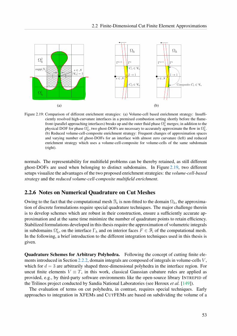
2.2 Finite-Dimensional Cut Finite Element Approximations

supp(Ns)

|Cs| = 3

Ω1h

Ω2h

s ∈ N

(a)

Γn+1 Γn+1 ΓnΓn

2 → 1 1 → 1

Ωh Ωh

s ∈ N s ∈ N

C1 ∈ Cs

C2 ∈ Cs Composite C1 ∈ Cs

(b)

Figure 2.19: Comparison of different enrichment strategies: (a) Volume-cell based enrichment strategy: Insuffi-ciently resolved high-curvature interfaces in a premixed combustion setting shortly before the flame-front (parallel approaching interfaces) breaks up and the outer fluid phase Ω2

h merges; in addition to thephysical DOF for phase Ω1

h, two ghost-DOFs are necessary to accurately approximate the flow in Ω2h.

(b) Reduced volume-cell-composite enrichment strategy: Frequent changes of approximation spacesand varying number of ghost-DOFs for an interface with almost zero curvature (left) and reducedenrichment strategy which uses a volume-cell-composite for volume-cells of the same subdomain(right).

normals. The representability for multifield problems can be thereby retained, as still differentghost-DOFs are used when belonging to distinct subdomains. In Figure 2.19, two differentsetups visualize the advantages of the two proposed enrichment strategies: the volume-cell-basedstrategy and the reduced volume-cell-composite multifield enrichment.

2.2.6 Notes on Numerical Quadrature on Cut MeshesOwing to the fact that the computational mesh Th is non-fitted to the domain Ωh, the approxima-tion of discrete formulations require special quadrature techniques. The major challenge thereinis to develop schemes which are robust in their construction, ensure a sufficiently accurate ap-proximation and at the same time minimize the number of quadrature points to retain efficiency.Stabilized formulations developed in this thesis require the approximation of volumetric integralsin subdomains Ωi

h, on the interface Γh and on interior faces F ∈ Fi of the computational mesh.In the following, a brief introduction to the different integration techniques used in this thesis isgiven.

Quadrature Schemes for Arbitrary Polyhedra. Following the concept of cutting finite ele-ments introduced in Section 2.2.2, domain integrals are composed of integrals in volume-cells V ,which for d = 3 are arbitrarily shaped three-dimensional polyhedra in the interface region. Foruncut finite elements V ≡ T , in this work, classical Gaussian cubature rules are applied asprovided, e.g., by third-party software environments like the open-source library INTREPID ofthe Trilinos project conducted by Sandia National Laboratories (see Heroux et al. [149]).

The evaluation of terms on cut polyhedra, in contrast, requires special techniques. Earlyapproaches to integration in XFEMs and CUTFEMs are based on subdividing the volume of a

53

2 Spatial Discretization Techniques for Multiphysics using Cut Finite Elements

polyhedron into simple-shaped cells, like tetrahedra or hexahedra, for which again cubature rulesfor polynomials are existing. Such techniques are often referred to as subtetrahedralizationor tessellation in literature and have been suggested, e.g., by Sukumar et al. [247]. Theseprocedures are easy to implement whenever the interface is represented implicitly by a level-set field defined on the underlying finite element mesh. In such cases, a limited number ofdifferently shaped polyhedra exists for which a tessellation can be explicitly constructed (see,e.g., in Burman et al. [63] and references therein).

Things can become more sophisticated for overlapping mesh methods. Intersecting back-ground mesh with trace meshes can render in an unlimited number of intersection scenariosdepending on mesh locations and, in particular, depending on the different grid sizes. In suchcases, decomposition techniques often lack robustness for concave polyhedra, as reported, e.g.,by Sudhakar and Wall [245]. Moreover, for fine-resolved intersecting trace meshes this oftenrenders in high numbers of sub-cells and makes integration on polyhedra an expensive task, asdiscussed, e.g., by Mousavi et al. [191]. In the meanwhile, different other types of quadratureschemes have been developed.

For so-called moment-fitting methods, cubature rules are constructed on the basis of predefinedlocations of integration points, for which respective integration weights are computed by fittingthem in a way such that single monomials are integrated in a best-approximation sense. As amajor drawback of such methods, least-squares systems with non-sparsity patterns have to besolved and their conditioning can deteriorate depending on the distribution of integration pointswithin the polyhedra. For such techniques, see the works by, e.g., Mousavi et al. [191], Mousaviand Sukumar [190] and Muller et al. [193].

Various novel strategies make use of the divergence theorem to perform integration on poly-hedra. A detailed overview of different techniques based on this idea can be found in Sudhakaret al. [246]. The approach devised in the latter publication is used for all simulations proposed inthis thesis. Fundamental idea is to convert critical volumetric integrals into quadrature problemsdefined on polygonal facets f which delimit the volumes. Surface integrals on facets can beeasily dealt with by subdividing them into planar two-dimensional triangular cells, a task forthat the complexity is highly reduced compared to three-dimensional decompositions. Utilizingthis procedure renders in a competitive integration method with highly reduced complexity. Forfurther theoretical and algorithmic details and comparisons to other techniques, the reader isreferred to the original publication [246].

Quadrature on Interface Segments. When constructing volume-cell based cubature rules bytransforming them into surface integrals, as discussed before, interface-segment quadrature rulesfor ΓT ∩ V related to a polyhedra V within a finite element T are simultaneously built. Facets ofvolume-cells which are aligned with the interface are then split into simple-shaped planar cellsfor which Gaussian cubature rules are given. Concerning details on required transformationsbetween parameter and physical coordinate systems of elements and the triangulated sub-cells,the interested reader is referred to, e.g., the theses by Henke [147] or Gerstenberger [123].

Quadrature on Faces. Evaluating discrete operators along entire faces F ∈ Fi, related in-tegrals can be approximated with standard Gaussian quadrature rules defined on respectivereference faces as provided by the open-source library INTREPID (see Heroux et al. [149]).

54

Chapter 3Developing Stabilized Cut Finite Element Methods for

Incompressible Flow

Resuming Chapter 2, the high versatility and the great benefit of cut finite element methods(CUTFEMs) for approximating solutions to multiphysics problems which incorporate fluid flowsis undisputed. The possibility of approximating laminar and turbulent flows with non-boundary-fitted finite element meshes expands the potential of such discretization techniques to a widerange of biomedically and industrially relevant applications. In particular, their capabilities withregard to moving boundaries and interfaces without having to deal with potential mesh distortionsimplifies grid generation substantially.

Before developing unfitted finite element methods for coupled flow problems, this chapter isdevoted to a detailed numerical analysis of some issues of CUTFEMs in general, and to thedevelopment of stabilized CUTFEMs for incompressible single-phase flows with stationary andmoving boundaries in particular. When approximating Navier-Stokes equations on boundary-fitted finite element meshes, depending on the choice of function spaces and the flow regime,discrete variational formulations often require additional stabilization techniques to guaranteeexistence and uniqueness of approximative solutions and their optimal convergence to the exactsolution with mesh refinement. The price to be paid for the flexibility provided by unfitted meshtechniques is the additional effort that has to be put on developing stable and optimal convergentnumerical schemes. Besides well-established stabilization techniques known from classicalcontinuous finite element approximation, additional measures are required on cut elements. Asthe computational meshes are non-fitted to the domain boundary, boundary conditions haveto be imposed in a weak variational form. Most if not all cut finite element methodologieswhich have been developed over the last decade suffer from a lack of inf-sup stability andsuboptimal convergence rates that often strongly depend on the location of the boundary withinfinite elements. Furthermore, such discretization techniques are often accompanied by a negativeside effect of rendering in ill-conditioned global system matrices which deteriorates the accuracyof these methods as well as the efficiency of iterative solution techniques for related systems.Such characteristics are undesirable and have to be taken into consideration for the design ofCUTFEMs.

This chapter is organized as follows: After reviewing the governing equations and stabilizationtechniques applicable to classical fitted-mesh finite element approximations in Section 3.1, an

55

3 Developing Stabilized Cut Finite Element Methods for Incompressible Flow

overview of useful mathematical tools and concepts required for numerically analyzing cut finiteelement methods is given in Section 3.2. A survey of weakly imposing boundary conditionson boundary-fitted meshes is given in Section 3.3. Therein, focus is directed towards stabilityproperties of different techniques as well as on analogies and differences between those, whichserves as starting point for developing CUTFEMs for incompressible flows. General numericalissues inherent in cut finite element approximations are numerically analyzed and discussedin Section 3.4. Derived theoretical results will be verified by several numerical simulationsand studies. A so-called ghost penalty interface zone stabilization technique is introducedwhich provides the basis for robust and accurate CUTFEMs. In Section 3.5, a novel stabilizeddiscrete formulation is proposed for a linear auxiliary problem to the Navier-Stokes equations,the so-called Oseen problem. Inf-sup stability and optimal a priori error estimates will bemathematically proven and corroborated by comprehensive convergence studies. Extensionsof stabilized formulations to single-phase flows with stationary as well as moving boundariesgoverned by the transient incompressible Navier-Stokes equations are proposed in Section 3.6.Extensive numerical simulations demonstrate accuracy and robustness of the stabilized CUT-FEMs. The great potential of unfitted approximation techniques for fluid flows will have beenshown already for single-phase problems before extensions are made to coupled flow problems.Domain decomposition for single- and multiphase flows are considered in Chapter 4 and unfitteddiscretization techniques for fluid-structure interaction problems are proposed in Chapter 5. Thepresent chapter is based on work published by Schott and Wall [230] and Massing et al. [183].

3.1 Finite Element Formulations for Incompressible Flow

In this section, fundamentals on governing equations for laminar and turbulent low-Mach-numberflows, the incompressible Navier-Stokes equations, are addressed. Furthermore, well-establishedstabilization techniques applicable to classical boundary-fitted finite element discretization meth-ods utilizing continuous approximation spaces for velocity and pressure will be reviewed.

3.1.1 Governing Equations for Fluid Mechanics

Throughout this thesis, all considered flows are assumed as incompressible flows of Newtonianfluids. Based on fundamental conservation laws for continua proposed in Section 2.1.2.2, gov-erning equations are derived in the following and an initial boundary value problem (IBVP)for incompressible Navier-Stokes equations is formulated. Independent of the kinematic de-scription, all flow equations are described in spatial coordinates; for respective quantities theindicating subscript (·)x will be omitted.

Incompressibility Constraint. For low Mach number flows, a reasonable assumption on thedensity of continua is to not change in space and time such that ρ(x, t) = const. Mathematically,the ALE form of conservation of mass (2.25) expressed in spatial coordinates then reduces to anincompressibility constraint for the flow field

∇ · u = 0. (3.1)

56

3.1 Finite Element Formulations for Incompressible Flow

Constitutive Law for Newtonian Fluids. Recalling Cauchy’s fundamental lemma, the Cauchystress tensor σσσ defined in the balance of linear momentum (2.33) is composed of a hydrostaticand a viscous stress state as

σσσ = −pI + τττ . (3.2)

Thereby, p = − tr (σσσ)/d is called the dynamic fluid pressure, which can be considered as La-grange multiplier enforcing the incompressibility constraint, and τττ is the deviatoric viscous stresspart satisfying tr (τττ) = 0. For Newtonian fluids, viscous stresses are modeled being linearlyrelated to the velocity gradient which, combined with the symmetry requirement resulting fromthe balance of angular momentum (2.37) and the assumption of isotropic material, results in theconstitutive relation

τττ = 2µε(u). (3.3)

Therein, ε(u)def= 1/2

(∇u+ (∇u)T

)denotes the symmetric strain rate tensor. The unique

material parameter which linearly relates stress and strain is the dynamic viscosity µ > 0. Itcan be expressed in terms of a kinematic viscosity ν as µ = νρ.

Incompressible Navier-Stokes Equations in ALE Form. Combining the constitutive lawwith the ALE form of balance of linear momentum (2.34) and the incompressibility (3.1), theALE version of the transient incompressible Navier-Stokes equations emerges to

ρ∂uχ∂tΦ−1 + ρ(c · ∇)u+∇p− 2µ∇ · ε(u) = ρf ∀ (x, t) ∈ Ω× (T0, T ], (3.4)

∇ · u = 0 ∀ (x, t) ∈ Ω× (T0, T ], (3.5)

where f is an external body force load and ((c · ∇)u)idef=∑

j cj · ∂ui∂xjwith the ALE convective

velocity c, see (2.14). Assuming the fluid domain boundary ∂Ω to be split into disjunct Dirichletand Neumann parts at all times t, i.e. ΓD and ΓN, conditions for the flow can be prescribed as

u = gD ∀(x, t) ∈ ΓD × (T0, T ], (3.6)σ · n = hN ∀(x, t) ∈ ΓN × (T0, T ]. (3.7)

Here, n denotes the outward pointing unit normal on the boundary and gD and hN are givenvelocity field and surface traction on corresponding boundary parts. An initial flow field

u(x, 0) = u0(x) ∀x ∈ Ω(T0) (3.8)

is defined in the initial domain and closes the IBVP for incompressible flow.

3.1.2 Variational Fluid ProblemDeriving a weak formulation for incompressible flow requires the definition of appropriatefunctional spaces. For any time t ∈ (T0, T ] and U ∈ Ω(t),Γ(t), let Hm(U) and [Hm(U)]d bethe standard Sobolev space of orderm ∈ R and their Rd-valued equivalents. Their corresponding

57

3 Developing Stabilized Cut Finite Element Methods for Incompressible Flow

inner products are denoted by (·, ·)m,Ω for the domain and by 〈·, ·〉m,Γ for the boundary. Normsand semi-norms are notated with ‖ · ‖m,U and | · |m,U , respectively. If unmistakable, it isoccasionally written (·, ·)U , 〈·, ·〉U and ‖ · ‖U for the inner products and norms associated withL2(U), with U being a Lebesque-measurable subset of Rd. For m > 1/2, the notation [Hm

g (Ω)]d

is used to designate the set of all functions in [Hm(Ω)]d whose Rd-valued boundary traces areequal to g. Later in the numerical analysis simplified problem settings with only Dirichletboundaries will be considered, i.e. ΓN = ∅, for those the pressure is determined only up to aconstant. For this purpose, let L2

0(Ω) be the function space which consists of functions in L2(Ω)with zero average.

The functional space for admissible fluid velocities is VgD

def= [H1

ΓD,gD(Ω(t))]d ⊂ [H1(Ω(t))]d

which satisfies the Dirichlet boundary condition (3.6). The related space of admissible testfunctions Vf

0 exhibits zero trace on ΓD. For the pressure field the trial and test function space isgiven by Q = L2(Ω(t)) if ΓN 6= ∅ and by Q = L2

0(Ω(t)) if ΓN = ∅. The non-linear variationalformulation for incompressible flow then reads as follows: for all t ∈ (T0, T ], find fluid velocityand pressure U(t) = (u(t), p(t)) ∈ VgD

×Q such that for all V = (v, q) ∈ V0 ×Q

A(U, V ) = L(V ), (3.9)

where

A(U, V )def= (ρ

∂uχ∂tΦ−1(t),v)Ω(t) + c(u− u;u,v) + a(u,v) + b(p,v)− b(q,u), (3.10)

L(V )def= l(v) (3.11)

with the following trilinear, bilinear and linear forms c, a, b and l to shorten the presentation

c(β;u,v)def= (ρ(β · ∇)u,v)Ω(t), (3.12)

a(u,v)def= (2µε(u), ε(v))Ω(t), (3.13)

b(p,v)def= −(p,∇ · v)Ω(t), (3.14)

l(v)def= (ρf ,v)Ω(t) + 〈hN,v〉ΓN(t). (3.15)

Therein, u denotes the grid velocity as introduced in (2.15) for formulations in an ALE frame.

3.1.3 Stabilized Discrete Formulations for Boundary-Fitted Meshes

The discrete functional space for the velocity field is defined by Vh,gD= [Xh]

d ∩ VgDand for the

pressure field by Qh = Xh ∩Q, where Xh is the isoparametric finite element space as definedin (2.43). In this work, for the spatial discretization with fitted as well as unfitted meshes, con-tinuous approximations of equal order k > 1 are considered exclusively. The velocity-pressuretrial and test product spaces are defined as Wh,gD

= Vh,gD×Qh and Wh,0 = Vh,0 ×Qh.

Different flow regimes, that is dominating advection or diffusion, can be specified by theso-called Reynolds number which in its global and local element-wise form is defined as

Redef=‖β‖0,Ω,∞ · L

νand ReT

def=‖β‖0,T,∞ · hT

ν(3.16)

58

3.1 Finite Element Formulations for Incompressible Flow

with a flow characteristic global length scale L and approximation specific element lengths hTfor all elements T ∈Th. Therein, β denotes a characteristic advective or convective flow veloc-ity. While the Reynolds number is physically motivated and quantifies the ratio of inertia forcesto viscous forces, an additional space and time approximation related characteristic numberquantifies the ratio of advection to (pseudo-)reaction arising from temporal discretization, theso-called Courant number. In the context of finite element discretizations with characteristicelement lengths hT and a temporal approximation with a time-step length ∆t ∝ σ−1, the Courantnumber is defined as

CoTdef=‖β‖0,Ω,∞ ·∆t

hT∝ ‖β‖0,Ω,∞

σ · hT. (3.17)

It is well-known that the standard Galerkin formulation (3.9) for the incompressible Navier-Stokes equations approximated with finite-dimensional subspaces suffers from different sourcesof instabilities:

• Due to the saddle-point structure and the use of equal-order interpolation spaces in thedefinition of Wh = Vh ×Qh, the resulting approximation violates the discrete inf-supcondition and thus is not stable in the sense of Babuska–Brezzi [36].

• Numerical solutions exhibit unphysical oscillations and sub-optimal error estimates in caseof locally convection-dominant flow, i.e. if ReT 1 for certain elements T ∈Th. On theone hand, this is due to insufficient control on the convective term compared to the ellipticviscous term. On the other hand, in the limit case µ→ 0, the velocity function spacechanges from H1(Ω) to Hdiv(Ω), that is the space of L2(Ω)-functions whose divergenceis also in L2(Ω), and further control on the incompressibility needs to be recovered.

• When Dirichlet boundary conditions need to be enforced weakly, consistent stabilizationterms at the boundary Γ are required to guarantee stability and optimal error convergencefor low and high Reynolds numbers.

To counteract these numerical effects, the variational form (3.9) needs to be stabilized. Theaforementioned instability arising from the weak imposition of boundary conditions will beconsidered separately in Section 3.3. Within this section, Dirichlet boundary conditions areassumed to be enforced strongly via the discrete function space.

A recent overview of various stabilization techniques to account for the first and secondinstability can be found in Braack et al. [31]. Throughout this thesis, two different classes offluid stabilizations are used for fitted and unfitted finite-element-based approximations:

• the well-known residual-based variational multiscale framework, which combines a stream-line upwind/ Petrov–Galerkin (SUPG) method and a pressure-stabilizing/Petrov–Galerkin(PSPG) method, supported by a least-squares incompressibility constraint (LSIC, grad-div) stabilization, and

• the class of continuous interior penalty (CIP) stabilizations, which controls the discreteconvective derivative, the pressure gradient and the discrete divergence operator acrossinter-element faces in the interior of the computational mesh.

59

3 Developing Stabilized Cut Finite Element Methods for Incompressible Flow

Both techniques can be used to control the same sources of instabilities introduced before.However, the methods are based on different discrete control mechanisms and provide desirableaspects from different perspectives, as will be discussed below. First, the two techniques areintroduced for the fitted mesh case and can be finally combined and extended to obtain stableand accurate numerical approximations schemes for unfitted meshes as will be shown later inSection 3.6.

3.1.3.1 The Residual-based Variational Multiscale (RBVM) Method

One of the most frequently used stabilization techniques of the Galerkin scheme (3.9) is thewell-known residual-based technique. All required element-wise stabilization terms of the wellestablished SUPG/PSPG/LSIC approach can be derived from the variational multiscale frame-work. Velocity and pressure (u, p) ∈ WgD

, as well as the corresponding weighting functions(v, q) ∈ W0, can be decomposed in the weak formulation as u = uh + usgs

h , p = ph + psgsh into

resolved components uh, ph and subgrid-scale components usgsh , psgs

h . As explained in, e.g., thetextbook by Gresho and Sani [131], the latter two can be approximated as element-wise discreteresiduals of momentum and continuity equation (3.4) and (3.5) as

usgsh

def= −τM(ρ

∂uχ,h∂tΦ−1(t) + rM(uh, ph)− ρf) and psgs

h

def= −τCrC(uh) (3.18)

with element-wise defined functions

rM(uh, ph)def= ρ((uh − uh) · ∇)uh +∇ph − 2µ∇ · ε(uh), (3.19)

rC(uh)def= ∇ · uh, (3.20)

and appropriate piecewise constant stabilization scaling functions

τM,T =1√(

2ρ∆t

)2+ (ρ(uh − uh)) ·G(ρ(uh − uh)) + CIµ2G : G

, (3.21)

τC,T =1

τM,Ttr (G), (3.22)

as defined in Taylor et al. [252] and Whiting and Jansen [267] for all elements T ∈Th. Hereby,the stabilization parameters take into account the definition of the relative convective velocity(uh − uh) and the second rank covariant metric tensor Gkl(x) =

∑di=1(∂ξi/∂xk

∣∣x)(∂ξi/∂xl

∣∣x)

is related to the mapping of the parent element domain to its reference element with local coor-dinate system ξ. This tensor serves as a measure for the characteristic element length requiredto guarantee stable and optimal convergent schemes for low- and high-Reynolds-number flows.The time-step length of the temporal discretization is denoted by ∆t and CI is set to 36.0 for(tri-)linearly and to 60.0 for (tri-)quadratically interpolated hexahedral finite elements. For moredetailed elaborations on the parameter scaling between convective and diffusive limit in terms ofthe inverse estimate constant CI for different element types and polynomial orders, the interestedreader is referred to Franca and Frey [112] and Whiting [266].

60

3.1 Finite Element Formulations for Incompressible Flow

The combined SUPG/PSPG/LSIC stabilized discrete formulation for the incompressible Navier-Stokes equations then reads as follows: for all t ∈ (T0, T ], find fluid velocity and pressureUh(t) = (uh(t), ph(t)) ∈ Vh,gD

×Qh such that for all Vh = (vh, qh) ∈ Vh,0 ×Qh

ARBVMh (Uh, Vh) = LRBVM

h (Uh, Vh), (3.23)

where

ARBVMh (Uh, Vh)

def= A(Uh, Vh)

+∑

T∈Th

(ρ∂uχ,h∂tΦ−1(t) + rM(uh, ph), τM,u(ρ(uh − uh) · ∇)vh + τM,p∇qh

)T

+∑

T∈Th

(rC(uh), τC∇ · vh

)T, (3.24)

LRBVMh (Uh, Vh)

def= L(Vh)

+∑

T∈Th

(ρf , τM,u(ρ(uh − uh) · ∇)vh + τM,p∇qh

)T

(3.25)

with τM,u = τM,p = τM. The first term in (3.24) and (3.25) contains the standard Galerkinformulation, respectively. In the second line of those equations, an SUPG term which accountsfor stability issues in convection-dominated flows by adding artificial diffusion is combinedwith a PSPG term which makes the formulation inf-sup stable for equal-order-interpolatedapproximations for velocity and pressure. The last term in (3.24) ensures sufficient control overdiscrete mass conservation for convection-dominated flows with µ→ 0. Fundamental idea of thestrongly consistent residual-based techniques is to add element-wise semi-norm control over un-controlled parts of the standard Galerkin formulation. The combination of SUPG/PSPG/LSICstabilizations ensures additional control over

∑T∈Th‖τ

12

M(ρ(βh · ∇)vh +∇qh)‖20,T +

∑T∈Th‖τ

12

C∇ · vh‖20,T , (3.26)

with βh = (uh − uh) the advective velocity (see, e.g., Braack et al. [31] or the textbook by Rooset al. [222]). A more detailed derivation of the proposed stabilization terms and its interpretationin the context of the residual-based variational multiscale concept can be found, e.g., in thetextbook by Hughes et al. [156].

3.1.3.2 The Continuous Interior Penalty (CIP) Method

One promising stabilization technique for incompressible flow approximated with continuousequal-order interpolations for velocity and pressure is the CIP technique. Compared to theRBVM technique which adds terms in the bulk and is consistent with respect to the strongresidual of the Navier-Stokes equations, this method uses weakly consistent least squares sta-bilization of the gradient jumps across inter-element boundaries, i.e. edges in two and faces inthree spatial dimensions. Thus, such operators are often referred to as edge/face-based/orientedstabilizations. The methodology has its origin in the early work by Douglas and Dupont [93]where it was used as an improvement for elliptic and parabolic Galerkin approximations byadding jump-penalty least squares terms. Burman and Hansbo [46] picked up this idea and usedsuch a term to stabilize advection–diffusion problems. In the following years, this technique

61

3 Developing Stabilized Cut Finite Element Methods for Incompressible Flow

gained great importance and was further developed for different problem fields. A generalhp-framework was proposed by Burman and Ern [54]. CIP stabilizations for the generalizedStokes problem were proposed by Burman and Hansbo [47] and for Stokes and Darcy equationsby Burman and Hansbo [42]. For incompressible high-Reynolds number flows, adaption wasmade by Burman et al. [48] for the Oseen equations and by Burman and Fernandez [41] for thetime-dependent Navier-Stokes equations. Considerations and investigations on this stabilizationtechnique in the context of variational multiscale methods for turbulent flows were proposed inBurman [49]. Many further theoretical work on specific numerical aspects of this technique isavailable in literature. More details on existing literature with regard to different specific aspectsof this class of stabilizations will be proposed in corresponding sections later in this work.

The CIP method for fitted meshes employed in this thesis is based on the publications [41, 48].Symmetric stabilization terms penalize the jump of the velocity and pressure gradients over inter-element faces. More precisely, the jump over an interior face F ∈ Fi is defined by

[[f(x)]] = limt→0+

(f(x− tnF )− f(x+ tnF )), (3.27)

where nF is a unit normal vector on F and x ∈ F , with the natural component-wise extension tovector-valued functions. The main idea in the CIP method is to augment the discrete variationalform (3.9) with the stabilization form

SCIPh (Uh, Vh) = sβ(uh − uh;uh,vh) + su(uh − uh;uh,vh) + sp(uh − uh; ph, qh), (3.28)

consisting of the (weakly) consistent symmetric jump-penalty stabilization operators

sβ(β;uh,vh)def= γβ

∑F∈Fi

φβ,Fρh〈[[(βh · ∇)uh]], [[(βh · ∇)vh]]〉F , (3.29)

su(β;uh,vh)def= γu

∑F∈Fi

φu,Fρh〈[[∇ · uh]], [[∇ · vh]]〉F , (3.30)

sp(β; ph, qh)def= γp

∑F∈Fi

φp,Fρ−1h〈[[∇ph]], [[∇qh]]〉F (3.31)

with non-dimensional stabilization parameters γβ, γu, γp > 0, element-wise scaling functions

φT = ν + cu(‖β‖0,∞,ThT ) + cσ(σh2T ), φβ,T = φp,T = h2

Tφ−1T , φu,T = φT , (3.32)

and the according face averages φβ,F , φu,F , φp,F at interior faces F ∈ Fi. For βhdef= uh − uh the

ALE convective velocity is used, which further introduces a non-linearity into the stabilizationform. The mesh size parameter h measures the maximal distance of points x in adjacentelements T+

F , T−F to the face F . Furthermore, σ denotes a pseudo-reactive scaling resulting from

temporal discretization and is defined as σθ = (θ∆t)−1 for a one-step-θ time-stepping schemeand as σBDF2 = (2/3∆t)−1 for a BDF2 scheme; for fluids, these time integration schemes areexclusively used in this work and will be further considered in Section 3.6.1.3. For details onthe temporal discretization of CIP stabilizations, the reader is referred to extensive numericalanalyses by Burman and Fernandez [40, 55], D’Angelo and Zunino [81] and Burman et al. [67].The parameter scaling shifts for convective and reactive limits are set to cu = 1/6 and cσ = 1/12as suggested in [231, 232]. For more detailed elaborations on scalings for different elementtypes and polynomial orders, the interested reader is referred to Braack et al. [31] and Burman

62

3.1 Finite Element Formulations for Incompressible Flow

and Ern [54]. The CIP scalings are set to γβ = γp = 0.05 for hexahedral and wedge elementsand to 0.01 for tetrahedral elements. Furthermore, it is chosen γu = 0.05γβ . For the sake ofcompleteness, it should be mentioned that also weighting strategies of the edge stabilizationapplicable to conservation equations with non-smooth data have been investigated by Ern andGuermond [102], however, are not applied for the simulations in the present work.

The principal stabilization mechanism of CIP operators consists in penalizing fluctuations.Note that for the aforementioned discrete derivatives it holds that

(βh · ∇)uh /∈ [Xh]d, ∇ · uh /∈Xh, ∇ph /∈ [Xh]

d. (3.33)

These polynomials are not fully controlled in the underlying continuous finite element ap-proximation space Xh, since they exhibit discontinuities across inter-element faces due to theincorporated spatial gradients. Control on these discontinuities can be retained by stabilizingfluctuations between the discontinuous polynomials and certain interpolation functions whichagain are contained in the finite element approximation space. Such control can be recoveredby jump-penalties (3.29)–(3.31). The role of these stabilization operators in terms of controllingcertain fluctuations will be elucidated by Lemma 3.1 and Corollary 3.2 in Section 3.2.2.2 and bya detailed analysis in Section 3.5.

Remark 3.1 It has to be pointed out that the stabilization parameters (3.32) are scaled differ-ently in Burman et al. [48]. The present choice corresponds to the scaling proposed by Codina[75] for the orthogonal sub-scale method and Knobloch and Tobiska [165] for the local projec-tion scheme. Compared to [48], a reactive scaling is added to the stabilization parameters whichhas two effects. First, it allows us to establish stability and approximation properties using normswith contributions which are more typical for residual-based stabilization methods, see (3.224).Second, for ‖β‖, µ→ 0, inf-sup condition and the a priori estimates do not degenerate as theyformally would do in [48]. A numerical analysis of this CIP method based on the proposedscalings will be proposed in Section 3.5 in the context of unfitted approximations.

Remark 3.2 Note that similar to the definition of stabilization parameters for the residual-basedvariational multiscale method (3.21), the sum over different scalings in (3.32) reflects which termof the governing PDE is dominating others. Therein, the first sum, i.e. ν + cu(‖β‖0,∞,ThT ),is related to the Reynolds number and characterizes the ratio between resolved convectionand diffusion in a local element-wise sense. The second sum, i.e. cu(‖β‖0,∞,ThT ) + cσ(σh2

T ),corresponds to the Courant number and relates convection to (pseudo-)reaction, where the latterone can be alternatively expressed in terms of the time-step length ∆t.

Remark 3.3 Note that for the classical CIP method on fitted meshes it is sufficient to penalizeonly the discontinuities of first-order derivatives of the mentioned polynomials, independent ofthe polynomial order of the approximation space, see the definitions in (3.29)–(3.31). The needfor penalizing also the higher-order derivatives in the vicinity of the boundary will be one of themajor adaption of the CIP method for unfitted meshes. An analysis is given in Section 3.5.

63

3 Developing Stabilized Cut Finite Element Methods for Incompressible Flow

The final CIP stabilized discrete formulation for the incompressible Navier-Stokes equationsreads as follows: for all t ∈ (T0, T ], find fluid velocity and pressure Uh(t) = (uh(t), ph(t)) ∈Vh,gD

×Qh such that for all Vh = (vh, qh) ∈ Vh,0 ×Qh

ACIPh (Uh, Vh) = LCIP

h (Vh), (3.34)

where

ACIPh (Uh, Vh)

def= A(Uh, Vh) + SCIP

h (Uh, Vh) and LCIPh (Vh)

def= L(Vh) (3.35)

in which the classical variational formulation is augmented by the CIP form SCIPh . The right-

hand side remains unchanged.

Remarks on Alternative Formulations. In the following, some useful equivalent and alter-native formulations for the jump penalty terms for continuous interpolation spaces are reviewed,see also Burman [38].

Due to the continuity of discrete functions in Xh, inter-element jumps in face-tangentialdirections t1, ... , td−1 vanish and normal derivative jumps are equivalent to full-gradient jumps,i.e. for scalar functions it holds

[[∂1nph]][[∂

1nqh]] = [[n · ∇ph]][[n · ∇qh]] = [[∇ph]] · [[∇qh]], (3.36)

where n = nF denotes the normal vector with respect to the face F . Furthermore, the j-thnormal derivative ∂jnv is given by ∂jnv =

∑|α|=j D

αv(x)nα for multi-index α = (α1, ... , αd),|α| = ∑i αi and nα = nα1

1 nα22 · · ·nαdd . Analogously, for vector-valued functions it holds

[[∂1nuh]][[∂

1nvh]] = [[n · ∇uh]][[n · ∇vh]] = [[∇uh]] : [[∇vh]]. (3.37)

Furthermore, velocity gradient jumps can be split component-wise as

〈[[∇uh]], [[∇vh]]〉F = 〈[[(eβ · ∇)uh]], [[(eβ · ∇)vh]]〉F + 〈[[(eorthβ,j · ∇)uh]], [[(e

orthβ,j · ∇)vh]]〉F (3.38)

with eβ = βh‖βh‖

and respective orthonormal vectors eorthβ,j . The first term reflects a streamline part

and the second part represents a crosswind part. As for stability only the streamline direction(3.29) needs to be sufficiently controlled, the crosswind part can be usually neglected. However,the latter part can be used in the context of variational multiscale modeling of unresolved scalesin turbulent flows. Otherwise, it can be utilized to increase accuracy near interior layers asdiscussed by [38]; see also references therein.

Note that due to the continuity of βh, for streamline derivative jumps, by decomposing βhand ∇uh on a face F ∈ Fi in tangential and normal directions one can deduce

[[(βh · ∇)uh]] = (βh · n)[[n · ∇uh]] (3.39)

such that for the advective derivative jump penalty (3.29) holds

[[(βh · ∇)uh]][[(βh · ∇)vh]] = (βh · n)2[[n · ∇uh]][[n · ∇vh]]. (3.40)

To reduce the non-linearity in the definition of the stabilization parameter scaling (3.32), thescalings (βh · n)2/‖βh‖ can be replaced by |βh · n| or further by the maximum value at the face,

64

3.2 Preliminaries to Numerical Analysis

i.e. βn,∞,Fdef= ‖βh · n‖0,∞,F . Finally, the streamline character of this term is still incorporated

in terms of the face-normal velocity |βh · n|. As a consequence, the following alternative CIPstabilization term can be used

sβ(β;uh,vh) = γβ∑

F∈Fiφβ,Fρβ

2n,∞,Fh〈[[∇uh]], [[∇vh]]〉F . (3.41)

Note that the divergence jump penalty can be controlled by a stronger full-velocity-gradientjump penalty as suggested, e.g., by Burman [49]. In contrast to streamline control given by(3.40), which scales with |βh · n|, full control in terms of a scaling with |βh| of φu is required.The combined velocity CIP stabilization can be then defined as

sβ(β;uh,vh)def=∑

F∈Fiρφβ,Fh〈[[∇uh]], [[∇vh]]〉F with (3.42)

φβ,Fdef= γβφβ,Fβ

2n,∞,F + γuφu,F . γββn,∞,F + γuφu,F . (3.43)

The advantage of this alternative control is a reduced matrix pattern and number of non-zeroentries in the global system matrix for the full-velocity-gradient operator compared to the diver-gence operator (3.30). Note that the latter one introduces additional couplings between differentvelocity components arising from the divergence term multiplication. Using the velocity-jumpcontrol instead of the divergence operator and utilizing equality (3.40), all CIP stabilizationoperators are of the same matrix type for pressure and all single velocity components. Thedifferent operators then only differ in their scaling functions. This aspect can be exploited forefficient implementations.

For an comprehensive survey on advantages and drawbacks of these two introduced stabi-lization techniques, the reader is referred to an overview article by Braack et al. [31]. In thelatter publication, different aspects like strong versus weak consistency of the stabilization op-erators, symmetry and decoupling of velocity and pressure stabilizations for the CIP technique,increased computational costs due to the enlarged matrix bandwidth or due to extra evaluationroutines for inter-element-face terms are discussed. Further interesting investigations with regardto behavior for small time-step lengths or artificially induced boundary or interfacial conditionsfor the low-order RBVM method are addressed in references therein. Some of these aspects arerecalled and discussed later in this work in the context of unfitted CUTFEMs.

3.2 Preliminaries to Numerical Analysis

In this section, analytical tools are collected which will be used in the forthcoming numericalanalysis of cut finite element methods and are required to develop inf-sup stability and a priori er-ror estimates. First, assumptions on computational meshes and functional spaces are introduced.Second, a number of useful trace and inverse inequalities are collected before the interpolationoperators are presented which are suitable for establishing the approximation properties of cutfinite element schemes. Finally, a brief overview of general concepts of numerical analyses andkey ideas of inf-sup stability and a priori error estimates are given.

65

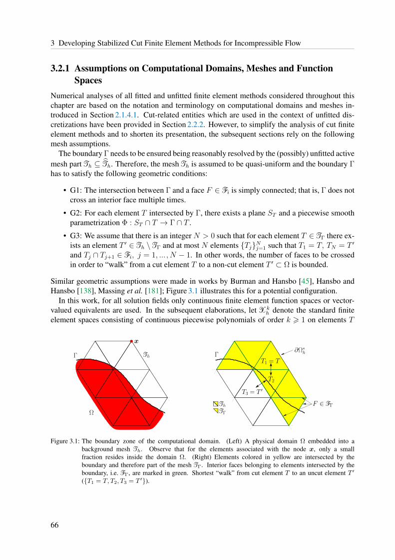
3 Developing Stabilized Cut Finite Element Methods for Incompressible Flow

3.2.1 Assumptions on Computational Domains, Meshes and FunctionSpaces

Numerical analyses of all fitted and unfitted finite element methods considered throughout thischapter are based on the notation and terminology on computational domains and meshes in-troduced in Section 2.1.4.1. Cut-related entities which are used in the context of unfitted dis-cretizations have been provided in Section 2.2.2. However, to simplify the analysis of cut finiteelement methods and to shorten its presentation, the subsequent sections rely on the followingmesh assumptions.

The boundary Γ needs to be ensured being reasonably resolved by the (possibly) unfitted activemesh part Th ⊆ Th. Therefore, the mesh Th is assumed to be quasi-uniform and the boundary Γhas to satisfy the following geometric conditions:

• G1: The intersection between Γ and a face F ∈ Fi is simply connected; that is, Γ does notcross an interior face multiple times.

• G2: For each element T intersected by Γ, there exists a plane ST and a piecewise smoothparametrization Φ : ST ∩ T → Γ ∩ T .

• G3: We assume that there is an integer N > 0 such that for each element T ∈TΓ there ex-ists an element T ′ ∈Th \TΓ and at most N elements TjNj=1 such that T1 = T, TN = T ′

and Tj ∩ Tj+1 ∈ Fi, j = 1, ... , N − 1. In other words, the number of faces to be crossedin order to “walk” from a cut element T to a non-cut element T ′ ⊂ Ω is bounded.

Similar geometric assumptions were made in works by Burman and Hansbo [45], Hansbo andHansbo [138], Massing et al. [181]; Figure 3.1 illustrates this for a potential configuration.

In this work, for all solution fields only continuous finite element function spaces or vector-valued equivalents are used. In the subsequent elaborations, let Xk

h denote the standard finiteelement spaces consisting of continuous piecewise polynomials of order k > 1 on elements T

x

F ∈ FΓ

Ω

Γ ThT1 = T

T2

T3 = T ′

F ∈ FΓ

x

TΓ

Γ∂Ω∗

h

Th

Figure 3.1: The boundary zone of the computational domain. (Left) A physical domain Ω embedded into abackground mesh Th. Observe that for the elements associated with the node x, only a smallfraction resides inside the domain Ω. (Right) Elements colored in yellow are intersected by theboundary and therefore part of the mesh TΓ. Interior faces belonging to elements intersected by theboundary, i.e. FΓ, are marked in green. Shortest “walk” from cut element T to an uncut element T ′

(T1 = T, T2, T3 = T ′).

66

3.2 Preliminaries to Numerical Analysis

of a given active mesh Th, as introduced in (2.74). Extensions to expanded cut finite elementfunctions spaces as considered in Section 2.2.4 may be realized with slightly weakened geomet-ric assumptions G1–G3. Due to the highly increased technicality of resulting analyses, only thestandard continuous discrete cut finite element spaces Xk

h under aforementioned assumptionsare considered:

Xkh

def=vh ∈ C0(Ω∗h) : vh|T ∈ Vk(T )∀T ∈Th

(3.44)

with V ∈ P,Q,W for simplices, quadrilaterals and wedge-shaped elements. For flow prob-lems, velocity and pressure are assumed to be interpolated with equal order, i.e.

Vhdef= [Xk

h ]d, Qhdef= Xk

h , Whdef= Vh ×Qh. (3.45)

3.2.2 Approximation PropertiesIn the following, fundamental approximation properties for continuous finite element functionspaces are presented. Important trace inequalities and inverse estimates which will be instru-mental in the stability and a priori error analysis of cut finite element methods are introducedand interpolation estimates for boundary-fitted meshes and their extension to cut finite elementdiscretizations are recalled. The subsequent estimates are heavily used throughout this chapter.

3.2.2.1 Trace Inequalities and Inverse Estimates

Throughout this work, the notation a . b is used for a 6 Cb for some generic positive constantCwhich varies with the context but is always independent of the mesh size h and the position ofthe boundary or interface Γ relative to the mesh Th.

For discrete functions vh ∈ Xh, the following generalized inverse and trace inequalities arewell-known

‖Djvh‖T . hi−j‖Divh‖T ∀T ∈Th, 0 6 i 6 j, (3.46)

‖∂jnvh‖∂T . hi−j−1/2‖Divh‖T ∀T ∈Th, 0 6 i 6 j (3.47)

with their counterparts for elements T arbitrarily intersected by the boundary Γ

‖∂jnvh‖Γ∩T . hi−j−1/2‖Divh‖T ∀T ∈Th, 0 6 i 6 j (3.48)

proven in the publications by Hansbo and Hansbo [138] and Burman et al. [66].For functions v ∈ H1(Ω∗h), it will be made use of trace inequalities of the form

‖v‖∂T . h−1/2‖v‖T + h1/2‖∇v‖T ∀T ∈Th, (3.49)

‖v‖Γ∩T . h−1/2‖v‖T + h1/2‖∇v‖T ∀T ∈Th, (3.50)

see [66, 138] for a proof of the second one. Finally, the well-known Poincare and Korn inequal-ities (see Brenner and Scott [34]) are recalled, which state that

‖v‖0,Ω . CP‖∇v‖0,Ω ∀v ∈ [H10 (Ω)]d, (3.51)

‖∇v‖0,Ω . ‖εεε(v)‖0,Ω ∀v ∈ [H10 (Ω)]d (3.52)

67

3 Developing Stabilized Cut Finite Element Methods for Incompressible Flow

with the following variants if the boundary trace of v is not vanishing

‖v‖0,Ω . CP (‖∇v‖0,Ω + ‖v‖Γ), ∀v ∈ [H1(Ω)]d, (3.53)

‖v‖1,Ω . ‖εεε(v)‖0,Ω + ‖v‖0,Ω ∀v ∈ [H1(Ω)]d, (3.54)

‖v‖1,Ω . ‖εεε(v)‖0,Ω + ‖v‖0,Γ ∀v ∈ [H1(Ω)]d. (3.55)

The hidden constants in (3.52)–(3.55) depend on the domain Ω and the boundary ∂Ω. Theconstant CP is called the Poincare constant and scales as the diameter of the domain Ω.

3.2.2.2 Interpolation Operators

Subsequently, common interpolation operators for boundary-fitted finite element approximationsand their extensions to cut finite element approximations are introduced.

Extension Operator for Sobolev Spaces. To construct an appropriate interpolation operatorL2(Ω)→Xh, that is from the space of L2(Ω)-functions into the finite element function spacedefined on the active (background) mesh Th, first an extension from Ω to an enlarged domain Ω∗

is required. This domain is assumed to be fixed and Lipschitz, containing all fictitious domainsΩ∗h ⊂ Ω∗ for h . 1. For Sobolev spaces W k,p(Ω) which are defined with respect to the physicaldomain, 0 6 k <∞, 1 6 p 6∞, an extension operator can be defined

E : W k,p(Ω)→ W k,p(Ω∗) (3.56)

which is bounded as‖Ev‖k,p,Ω∗ . ‖v‖k,p,Ω, (3.57)

see the work by Stein [240] for a proof. Occasionally, it is written v∗def= Ev. Utilizing this

extension operator, for any interpolation operator πh : Hs(Ω∗h)→Xh, i.e. k = s and p = 2, its“fictitious domain” variant π∗h : Hs(Ω)→Xh can be defined by simply requiring that

π∗hudef= πh(u

∗) = πh(Eu) (3.58)

for functions u ∈ Hs(Ω).

Clement Interpolant. Choosing πh to be the Clement operator (see for instance Ern andGuermond [101] for an introduction), for v ∈ Hr(Ω∗) and s, t ∈ N, m def

= minr, k + 1 thefollowing interpolation estimates hold:

‖v − πhv‖s,T . ht−sT ‖v‖t,ω(T ), ∀T ∈Th, 0 6 s 6 t 6 m, (3.59)

‖v − πhv‖s,F . ht−s−1/2T ‖v‖t,ω(T ), ∀F ∈ Fi, 0 6 s 6 t− 1/2 6 m− 1/2. (3.60)

Here, ω(T ) is the set of elements in Th sharing at least one vertex with T (for (3.59)) andsharing at least one vertex with F ∈ Fi (for (3.60)), respectively. Due to the boundedness of theextension operator (3.57), it can be observed that the extended Clement interpolant π∗h satisfies

‖v∗ − π∗hv‖s,Th . ht−s‖v‖t,Ω, 0 6 s 6 t 6 m, (3.61)

‖v∗ − π∗hv‖s,Fi . ht−s−1/2‖v‖t,Ω, 0 6 s 6 t− 1/2 6 m− 1/2. (3.62)

68

3.2 Preliminaries to Numerical Analysis

In particular, use is made of the stability property

‖π∗hv‖s,Th . ‖v‖s,Ω, 0 6 s 6 m. (3.63)

To shorten the notation, it is written ‖v‖2s,Th

def=∑

T∈Th ‖v‖2s,T for the sum over elements and

similarly ‖v‖2s,Fi

def=∑

F∈Fi‖v‖2

s,F for the sum over faces. The Clement interpolant is denotedby π∗h for vector-valued functions v and by Π∗h for functions in a product space.

Oswald Interpolant. A main ingredient in the analysis of the continuous interior penaltymethod (see for instance the works by Burman et al. [48] and Burman and Ern [54]) was theuse of the Oswald interpolation operator. By construction, the Oswald interpolation operatordefines a mapping Oh : Xdc,k

h (Th)→Xkh(Th), with Xdc,k

h (Th) and Xkh(Th) denoting the space

of discontinuous and continuous piecewise polynomials of order k on meshes Th, see defini-tions (2.63) and (2.64). More precisely, for vh ∈Xdc,k

h (Th), the function Ohvh ∈Xkh(Th) is

constructed in each interpolation node xs by the average value

Ohvh(xs) =1

card(Th(xs))

∑T∈Th(xs)

vh|T (xs), (3.64)

where Th(xs) is the set of all elements T ∈Th sharing the node xs. In particular, it was shownin [54] that for vh ∈Xdc,k

h , the fluctuation vh − Ohvh between the element-wise discontinuouspolynomial vh and its Oswald interpolation Ohvh can be controlled in terms of jump-penalties:

Lemma 3.1 Let φ be a piecewise constant function and vh ∈Xdc,kh . Then, the fluctuation

between vh and its Oswald interpolant Ohvh can be bounded by face-jump penalty terms

‖φ 12 (vh − Ohvh)‖2

T .∑

F∈Fi(T )φTh‖[[vh]]‖2

F ∀ vh ∈Xdc,kh , (3.65)

where Fi(T ) denotes the set of all faces F ∈ Fi with F ∩ T 6= ∅, and the hidden constantdepends only on the shape-regularity of the mesh, the order k of the finite element space andthe dimension d.

For a proof and a more precise statement which exhibits the dependency on the polynomial order,the interested reader is referred to the work by Burman and Ern [54].

The previous lemma elucidates the role of the continuous interior penalty stabilization op-erators (3.29)–(3.31) (see Section 3.1.3.2). Recalling the fact that the advective derivative, thedivergence of the velocity and the pressure gradient are discontinuous polynomials, see (3.33),their fluctuation to the respective Oswald interpolation can be controlled by face-jump penaltyterms:

Corollary 3.2 Under the assumptions of Lemma 3.1 it holds that

‖φ12β ((βh · ∇)vh − Oh((βh · ∇)vh))‖2

T .∑

F∈Fi(T )

φβ,Th‖[[(βh · ∇)vh]]‖2F , (3.66)

‖φ12u (∇ · vh − Oh(∇ · vh))‖2

T .∑

F∈Fi(T )

φu,Th‖[[∇ · vh]]‖2F , (3.67)

‖φ12p (∇qh − Oh(∇qh))‖2

T .∑

F∈Fi(T )

φp,Th‖[[∇qh]]‖2F , (3.68)

with piecewise constant scaling functions φβ, φu, φp and restrictions to elements φβ,T , φu,T , φp,T .

The role of the CIP stabilization terms sβ, su, sp is to control these discontinuities betweenneighboring elements.

69

3 Developing Stabilized Cut Finite Element Methods for Incompressible Flow

3.2.3 Concepts of Stability Analysis in a NutshellThe following section is primarily aimed at mathematically unexperienced readers who are notthat familiar with fundamental concepts of inf-sup stability analysis and mathematical techniqueswhich are commonly used for deriving optimal a priori error estimates. The following elabora-tions are intended to provide readers with knowledge required to allow them to follow the majorsteps through the analysis and to understand most important aspects resulting from that. Readerswho are familiar with these concepts may skip this section.

Many issues of numerical cut finite element approximations of PDE’s already occur in thelinear elliptic case. For this reason, Poisson’s problem serves as model problem to introduceproperties of numerical approximation, like consistency, Galerkin orthogonality, continuity andinf-sup stability which are fundamental for deriving stability and a priori error estimates.

Definition 3.1 (Variational and discrete formulation for Poisson’s problem)Let Ω ⊂ Rn be an open bounded domain, f ∈ L2(Ω) and g ∈ H1/2(Γ) given right-hand sideand boundary data. The second-order elliptic Poisson problem reads: Find u : Ω 7→ R such that

−∆u = f in Ω and u = g on Γ (3.69)

with its variational continuous and discrete form

B(u, v) = L(v) ∀ v ∈ V0 = H10 (Ω), (3.70)

Bh(uh, vh) = Lh(vh) ∀ vh ∈ Vh = Xh ∩ V0, (3.71)

where u ∈ Vg = H1g (Ω) and uh ∈ Vh,g = Xh ∩ Vg with

B(u, v) = Bh(u, v) = (∇u,∇v) and L(v) = Lh(v) = (f, v). (3.72)

Note that in general continuous and discrete forms are not identical, i.e. B 6= Bh and L 6= Lh.For stabilized discrete formulations, Bh and Lh often include additional (weakly) consistentstabilization forms Sh such that, for instance, Bh = B + Sh.

Definition 3.2 (Consistency of discrete formulation)For a discrete formulation Bh = Lh to be (strongly) consistent, it is required that the solutionu ∈ V of the continuous problem B = L is also solution of the discrete problem

Bh(u, vh)−Lh(vh) = 0 ∀ vh ∈ Vh (strongly consistent). (3.73)

Weak consistency requires the error introduced by the modified Galerkin scheme to convergewith optimal order for h→ 0

limh→0

(Bh(u, vh)−Lh(vh)) = 0 ∀ vh ∈ Vh (weakly consistent). (3.74)

Note that the standard Galerkin approximation of the Poisson problem based on continuousapproximations does not require additional terms and thus is strongly consistent.

70

3.2 Preliminaries to Numerical Analysis

Definition 3.3 (Galerkin orthogonality of a formulation)Related to the definition of consistency, a discrete variational formulation is said to satisfy a(weak) Galerkin orthogonality property if the error u− uh is Bh-orthogonal on the discretetrial space Vh

Bh(u− uh, vh) = 0 ∀ vh ∈ Vh (strongly orthogonal), (3.75)limh→0

(Bh(u− uh, vh)) = 0 ∀ vh ∈ Vh (weakly orthogonal). (3.76)

To guarantee existence and uniqueness of a solution of a discrete variational formulation, itis required that the bilinear form satisfies a discrete inf-sup condition on the discrete space Vh,see the textbooks by Braess [33] and Boffi et al. [25] for details. Furthermore, the definition ofan energy-norm ||| · ||| on the discrete space is required, which most often is closely related tothe discrete bilinear form. In many simpler cases, it is possible to prove a stronger coercivitycondition which implies inf-sup stability.

Definition 3.4 (Inf-sup stability and coercivity)A discrete variational formulation satisfies an inf-sup condition if there exists a positive lowerbounded constant cs > c > 0 that is independent of the mesh size h such that

cs 6 infvh∈Vh\0

supwh∈Vh\0

Bh(vh, wh)

|||vh||||||wh|||(3.77)

with |||vh||| an energy norm on Vh that is related to the discrete form Bh. For inf-sup stability itis sufficient to prove the bilinear form of being coercive, i.e. ∃cs > c > 0 such that

cs|||vh|||2 6 Bh(vh, vh) ∀ vh ∈ Vh. (3.78)

Coercivity directly implies an inf-sup condition. It clearly ensures: ∃cs > c > 0 such that

cs|||vh||| 6Bh(vh, vh)

|||vh|||6 sup

wh∈Vh\0

Bh(vh, wh)

|||wh|||∀ vh ∈ Vh\0, (3.79)

which remains also valid for the infimum over vh ∈ Vh\0, since cs is independent of vh and h.

Definition 3.5 (Continuity of a discrete variational formulation)The Vh-continuity (upper boundedness) of Bh is given provided that

Bh(vh, wh) 6 Ccont|||vh||| · |||wh||| ∀vh, wh ∈ Vh. (3.80)

with a constant Ccont > 0 independent of h.

Note that for the standard Galerkin discrete formulation of the Poisson problem (3.69), anenergy norm is defined by the bilinear form itself, i.e. |||vh||| def

= (Bh(vh, vh))1/2. Then, Bh

is coercive, inf-sup stable and continuous by definition with constants cs = Ccont = 1, whichensures uniqueness and existence of a solution uh, respectively.

Among uniqueness and existence of a solution to the discrete problem, it is desired to ensureoptimal convergence of the error between continuous and discrete solution without knowing

71

3 Developing Stabilized Cut Finite Element Methods for Incompressible Flow

both solutions a priori. Using introduced properties of satisfying an inf-sup condition, (weak)Galerkin orthogonality and continuity in combination with optimal estimates for interpolationor projection errors between solution u and an appropriate projection Πhu ∈ Vh into the discretespace enables to derive an a priori error estimate measured in the energy norm of the form

|||u− uh||| 6 Chr‖u‖s (a priori energy norm error estimate) (3.81)

The optimal order r depends on the polynomial order of the approximation space and theregularity s of the solution u ∈ Hs(Ω). This can be proven for the Poisson problem as follows:

Proof. The error between discrete solution uh and any other discrete function vh ∈ Vh can beestimated by combining inf-sup stability, continuity and Galerkin orthogonality of the form

Bh(u− uh, wh) = Rh(u,wh) with |Rh(u,wh)| 6 Cconshr‖u‖s|||wh||| (3.82)

such that the consistency error Rh does not deteriorate the optimal convergence; it holds Rh ≡ 0in case of strong consistency. Let wh be the discrete function that takes the supremum in the inf-sup condition (3.77) for given uh − vh, then

|||uh − vh||| 61

cssup

wh∈Vh\0

Bh(uh − vh, wh)|||wh|||

=1

cs

Bh(uh − vh, wh)|||wh|||

=1

cs

(Bh(u− vh, wh)− Rh(u, wh)

|||wh|||

)

6

(Ccont

cs|||u− vh|||+

Ccons

cshr‖u‖s

) |||wh||||||wh|||

. (3.83)

Splitting the error |||u− uh||| using triangle inequality into an interpolation/projection error foru− vh /∈ Vh and a discrete error for vh − uh ∈ Vh results in

|||u− uh||| 6 |||u− vh|||+ |||vh − uh||| 6 (1 +Ccont

cs)|||u− vh|||+

Ccons

cshr‖u‖s. (3.84)

It is assumed that for interpolation/projection errors u− Πhu optimal error estimates can beestablished based on estimates as proposed in Section 3.2.2, such that |||u− Πhu||| 6 CIh

r‖u‖s.Thanks to this optimality, by choosing vh

def= Πhu, an a priori error estimate in the energy norm

is obtained

|||u− uh||| 6(

(1 +Ccont

cs)CI +

Ccons

cs

)hr‖u‖s. (3.85)

This estimate clearly shows the dependency of error estimates on the stability, continuity andconsistency constants which have to be ensured being independent of h to not deteriorate theoptimality O(hr).

72

3.3 Weak Imposition of Boundary Conditions for Boundary-Fitted Meshes

3.3 Weak Imposition of Boundary Conditions for Boundary-Fitted Meshes

Weak enforcement of boundary conditions for PDEs in the context of finite element methodsbecame an active research field over the last decades. Methodologies have been developedfor different problem settings ranging from a single-phase elliptic Poisson problem up to cou-pling techniques for several phases in complex time-dependent multiphysics settings governedby often non-linear parabolic PDEs. In particular the variety of application fields and theiradaption to various discretization concepts as, for instance, extensions from boundary-fitted tonon-boundary-fitted computational meshes, highly increased the number of different techniquesand related variants.

Neumann boundary conditions can be naturally enforced within a standard Galerkin formu-lation without introducing further sources of instabilities. However, additional constraints onthe primal variable in terms of Dirichlet- or mixed Robin-type boundary conditions requirespecial measures to control induced boundary instabilities. In particular for highly convective-dominated problems, for that not all physically meaningful length scales can be always resolvedappropriately by the mesh, a weak constraint enforcement may be superior to strongly enforcedconditions. Spurious currents, which in flow problems often arise near boundaries, can gethighly reduced by weakening the fulfillment of constraints depending on the mesh resolution.For an example, steep near-wall gradients in boundary layer regions of turbulent flows requirefinest mesh resolution, on the one hand, to capture the physics and, on the other hand, notto suffer from artificial numerical effects arising from under-resolved flow characteristics; forfurther discussion on the capabilities of such techniques in that context, see, e.g., the work byBazilevs and Hughes [15] or the thesis by Gamnitzer [119].

The complexity and difficulties in the design of accurate, stable and optimally convergentschemes, however, become more severe for unfitted discretizations. This section is aimed atgiving an overview of different fundamental principles of weak constraint enforcement in thecontext of continuous Galerkin approximations. To examine strengths and weaknesses of amultitude of different techniques developed over the last decades, a survey on techniques re-garding weak constraint enforcement will be given. Having in mind the need for a stable andoptimally convergent weak enforcement technique for cut finite elements, the subsequent reviewon well-established methods shall give a clear understanding of capabilities and limitations of theconsidered methods. Many of these methods are closely related to each other and exhibit only aslight difference. Analogies between the considered methods will be elaborated by means of thelinear elliptic Poisson problem. Adaption of these techniques and their usability to unfitted finiteelement methods are discussed later in Section 3.4. Further considerations are made throughoutthis chapter for single-phase flows and in Chapter 4 for single-phase mesh-tying problems andincompressible two-phase flows. Weak constraint enforcement techniques for fluid-structureinteraction will be addressed in Chapter 5.

73

3 Developing Stabilized Cut Finite Element Methods for Incompressible Flow

3.3.1 Poisson Problem with Weak Dirichlet Boundary Conditions

For investigations on techniques for weak Dirichlet constraint enforcement, Poisson’s equationserves as linear model problem. The weak Dirichlet problem formulation in its strong and weakvariational formulation is stated as follows:

Definition 3.6 (Strong and variational formulation of Poisson’s boundary value problem)Let Ω ⊂ Rn be an open bounded domain with Γ = ∂Ω. Right-hand side and boundary data aregiven by f ∈ L2(Ω) and g ∈ H1/2(Γ). The Poisson problem governed in strong form is: findu : Ω 7→ R such that

−∆u = f in Ω and u = g on Γ. (3.86)

Its variational continuous form reads: find u ∈ V = H1(Ω) and λ ∈ Λ = H−1/2(Γ) such that

B(u, λ; v, µ) = L(v, µ) ∀ (v, µ) ∈ V × Λ (3.87)

with B(u, λ; v, µ)def= (∇u,∇v)− 〈λ, v〉 − 〈u, µ〉, (3.88)

L(v, µ)def= (f, v)− 〈g, µ〉. (3.89)

Note that by applying Green’s formula one obtains λ−∇u · n = 0. Concerning well-posednessas well as existence and uniqueness of this problem, the reader is referred to, e.g., Babuska [4].

3.3.2 A Survey on Weak Dirichlet Constraint Enforcement

In this section, different methodologies for the weak constraint enforcement of Dirichlet bound-ary conditions are proposed. The most straightforward technique is the classical method ofLagrange multipliers by Babuska [4] and Brezzi [35]. It consists of choosing appropriate inf-supstable pairs Vh × Λh ⊂ V × Λ for discretizing the mixed formulation (3.87), which becomes anon-trivial task on unfitted meshes, as will be discussed later. Another class of methods consistsof choosing specific Lagrange-multiplier spaces accompanied by adding stabilization terms tothe variational form. In doing so, limiting constraints on the choice of pairs for discrete functionspaces can be circumvented. The following stabilized methods are discussed within this section:

• a minimally stabilized method based on residual techniques proposed by Barbosa andHughes [12, 13] and modified by Stenberg [241],

• a stabilized mixed/hybrid stress-based Lagrange-multiplier technique by Gerstenbergerand Wall [125] and Baiges et al. [10], and

• variants of the classical Nitsche method, originally introduced by Nitsche [196].

Subsequently, these methods are introduced and reviewed regarding stability and optimality oferror estimates. Differences between those will be identified and analogies will be drawn forboundary-fitted approximations. Limitations and capabilities of the different techniques for theunfitted mesh case will be discussed and further elaborated in Section 3.4.

74

3.3 Weak Imposition of Boundary Conditions for Boundary-Fitted Meshes

3.3.2.1 Babuska’s Classical Method of Lagrange Multipliers - The Issue ofViolating Inf-Sup Conditions

The theoretical basis for the weak enforcement of Dirichlet boundary conditions is laid down inthe early work by Babuska [4]. The classical method of Lagrange multipliers, proposed in thatwork, consists of choosing appropriate discrete subspaces in (3.87) for the primal field Vh ⊂ Vin the domain and for the multiplier field Λh ⊂ Λ on the boundary:

Definition 3.7 (Discrete form of Babuska’s method of Lagrange multipliers)For f ∈ L2(Ω) and g ∈ H1/2(Γ), the discrete form reads: find (uh, λh) ∈ Vh × Λh such that

B(uh, λh; vh, µh) = L(vh, µh) ∀ (vh, µh) ∈ Vh × Λh. (3.90)

For stability of this discrete problem, an inf-sup-condition similar to (3.77) needs to be satis-fied, which strongly restricts the choice of admissible pairs of discrete subspaces. This conditionis also known as Babuska–Brezzi (BB) condition, named after the pioneering works by Babuska[4] and Brezzi [35]. A closer look at these restrictions was given in the work by Pitkaranta [205,206]. In [205] a discrete inf-sup condition based on mesh-dependent norms was formulated andproven being equivalent to the original inf-sup condition with respect to norms of the continuousSobolev spaces as originally formulated in [4]. Following [205], existence and uniqueness relieson a discrete inf-sup condition as summarized in the following theorem:

Theorem 3.3 (Existence and uniqueness of a discrete solution; see, e.g., [4, 35, 206, 241])Suppose that the finite element subspaces satisfy the so-called inf-sup condition or Babuska–Brezzi (BB) condition for the off-diagonal term

supvh∈Vh\0

〈µh, vh〉(|vh|21,Ω + ‖vh‖2

1/2,h,Γ)1/2> cs‖µh‖−1/2,h,Γ ∀µh ∈ Λh (3.91)

with cs > 0 independent of h and

|vh|21,Ω > C(|vh|21,Ω + ‖vh‖21/2,h,Γ) ∀ vh ∈ vh ∈ Vh | 〈µh, vh〉 = 0 ∀µh ∈ Λh . (3.92)

Therein, the mesh-dependent boundary norms are defined as

‖µh‖±1/2,h,Γdef= ‖h∓1/2µh‖0,Γ. (3.93)

For the solution (uh, λh) to (3.90) it then holds the following a priori error estimate in the energynorm |||v, µ||| def

= (|v|21,Ω + ‖v‖21/2,h,Γ + ‖µ‖2

−1/2,h,Γ)1/2

|||(u− uh), (λ− λh)||| 6 C(hk‖u‖k+1 + hl+3/2‖λ‖l+1,Γ), (3.94)

provided that u ∈ Hk+1(Ω) and λ ∈ H l+1(Γ).

75

3 Developing Stabilized Cut Finite Element Methods for Incompressible Flow

Ω

VhΛh

Γ

(a)

Vh Λh

ΓΩ

(b)

Figure 3.2: Classical method of Lagrange multipliers for the weak imposition of Dirichlet constraints: (a) Satisfyingan inf-sup condition for boundary-fitted meshes requires the boundary discretization Λh to be coarserthan the primal field discretization Vh, (b) Constructing stable Lagrange-multiplier spaces for unfittedmeshes is based on a selection of intersection points which serve as a function basis.

Remark 3.4 (Inf-sup condition for fitted and unfitted meshes)

• For boundary-fitted meshes, inf-sup stability requires the Lagrange-multiplier space Λh tobe approximated coarser than the space Vh to ensure stability and optimal convergence:

hΛh > ChVh (3.95)

with hΛh , hVh the mesh size parameters of the boundary and bulk discretizations Λh and Vh.As shown in the work by Pitkaranta [205, 206], the constant C > 1 required to guaranteethe inf-sup condition (3.91) depends on Ω and is not straightforward to determine. Apossible discretization for Vh and Λh is visualized in Figure 3.2a.

• For non-boundary-fitted meshes, Ji and Dolbow [158] showed that a Lagrange-multiplierbasis constructed of intersection points between boundary Γh and mesh Th might resultin oscillations of the multiplier field. Instabilities arise due to a violated inf-sup conditionas the Lagrange-multiplier space might be too rich depending on the element intersection.Constructing stable Lagrange-multiplier spaces relies on counter criteria to guaranteean inf-sup condition and thereby requires preserving reasonable rates of convergence.Algorithms have been proposed, e.g., by Moes et al. [189] and Bechet et al. [18] for two-dimensional problems with extensions to three spatial dimensions by Hautefeuille et al.[146]. A visualization of this Lagrange-multiplier technique for an unfitted mesh is givenin Figure 3.2b.

As discussed above, most convenient choices of Lagrange-multiplier spaces are not stable ingeneral. Moreover, the design of stable Lagrange-multiplier spaces becomes more challengingwhen boundary conditions or interfacial constraints need to be enforced on unfitted meshes.To circumvent limiting constraints on the function spaces stated by the Babuska–Brezzi condi-tion (3.91), stabilized Lagrange-multiplier methods are often preferable.

76

3.3 Weak Imposition of Boundary Conditions for Boundary-Fitted Meshes

Among the class of residual-based stabilization techniques, which will be discussed in moredetail subsequently, different stabilization types have been developed for boundary and interfaceproblems over the recent years. An extensive overview about Lagrange-multiplier methods forinterface problems in the context of domain decomposition is given by Wohlmuth [271]. Toenable choosing the discretization of the interface multiplier field independent of the two bulkdiscretizations, which can be advantageous to increase accuracy in particular for corner cases,Burman and Hansbo [43] proposed interior-penalty-stabilized Lagrange-multiplier methods forelliptic interface problems. This stabilization technique has been extended for the weak impo-sition of boundary conditions on unfitted meshes by Burman and Hansbo [44]. One drawbackof these techniques, however, might be that Lagrange multipliers can not be condensed fromthe global system anymore, even though when discretized discontinuously. This is due to thestabilizing inter-element coupling. Recently, Burman [53] reviewed projection stabilizationapplied to Lagrange-multiplier methods and discussed its relation to classical residual-basedmethods, like the method by Barbosa and Hughes or Nitsche’s method, a class of stabilizationtechniques which will be elaborated in more detail within the next sections.

3.3.2.2 Residual-based Stabilized Lagrange Multipliers - Circumvent theBabuska–Brezzi Condition

The idea of the original residual-based stabilized method by Barbosa and Hughes [12, 13]was to provide stability to the multiplier independent of the combination of discrete functionspaces by adding terms to the original Galerkin formulation constructed from residuals of theEuler-Lagrange equations. Thereby, consistency of the discrete formulation is to be preserved.In the mentioned works, several stabilization operators were derived for the Poisson problemresulting in a symmetric discrete form: one term enforces the interface normal flux equalityλh −∇uh · n = 0, a second term accounts for the boundary condition uh − g = 0 and a thirdterm for the strong residual within the domain. As analyzed by Stenberg [241], this formulationexhibits an over-stabilization in general. Only the first part, the interface flux stabilization, isrequired to obtain a minimally stabilized inf-sup stable and optimal convergent scheme.

Definition 3.8 (Residual-based stabilized formulations)The original method by Barbosa and Hughes [12, 13] reads: find (uh, λh) ∈ Vh × Λh such that

BBHh (uh, λh; vh, µh) = LBH

h (vh, µh) ∀ (vh, µh) ∈ Vh × Λh, (3.96)

whereBBHh (uh, λh; vh, µh)

def= B(uh, λh; vh, µh) + Bδ

h(uh, λh; vh, µh) (3.97)

with residual-based stabilizations Bδh for interface normal flux, boundary condition and strong

residual R(uh)− f = 0, where R(vh) = −∆vh and ri indicate optimally chosen powers of h,

Bδh(uh, λh; vh, µh)

def= −δh〈λh −∇uh · n, µh ∓∇vh · n〉

+ δ2h2r2〈uh, vh〉+ δ3h

2r3(R(uh), R(vh))Ω,

LBHh (vh, µh)

def= L(vh, µh)

+ δ2h2r2〈g, vh〉+ δ3h

2r3(f,R(vh))Ω.

(3.98)

Here, δ > 0 and δ2, δ3 > 0 are user-defined stabilization parameters. For a reduced stabilizationsuggested by Stenberg [241], the second and third residual terms are dropped, i.e. δ2 = δ3 = 0.

77

3 Developing Stabilized Cut Finite Element Methods for Incompressible Flow

Remark 3.5 (Symmetric versus non-symmetric formulations)Characteristic stability and optimality properties of different variants can be reviewed as fol-lows:

• Residual-based stabilized methods are strongly consistent by construction.

• The different signs (∓) in Bδh considerably affect inf-sup stability

sup(z,η)∈Vh×Λh\0

BBHh (z, η; v, µ)

|||(z, η)|||BH> cs|||(v, µ)|||BH ∀ (v, µ) ∈ Vh × Λh (3.99)

with |||(v, µ)|||BH def= (|v|21,Ω + ‖v‖2

1/2,h,Γ + ‖µ‖2−1/2,h,Γ)1/2 the energy norm controlling the

bulk, the boundary condition and the Lagrange multiplier (see, e.g., in Stenberg [241]).

• The symmetric variant of Bδh obtained by testing with µh −∇vh · n in (3.98) yields condi-

tional inf-sup stability provided that the stabilization parameter is positive and sufficientsmall, i.e. 0 < δ 6 1/(2C2

T ) with CT the constant resulting from a trace inequality

‖∇vh · n‖Γ∩T 6 CTh−1/2T ‖∇vh‖T , (3.100)

see also (3.47), relating the normal derivative of vh on the element boundary to its gradientwithin the element T . This constant strongly depends on the shape, type and polynomialdegree of the finite element T . Further elaborations in Section 3.4.2 will elucidate itsimportant role in the context of unfitted meshes.

• Testing with µh +∇vh · n in Bδh makes the discrete formulation BBH

h non-symmetric.This, however, ensures unconditional inf-sup stability for all positive δ, i.e. ∀ δ > 0.

• Compared to the classical method by Babuska, under the aforementioned assumptionson δ, the stabilized methods [12, 13, 241] are stable without constraints on the choice of Λh

with respect to Vh and allows for natural definitions of Λh as visualized in Figure 3.3a.

• The symmetric variant is adjoint-consistent and ensures optimal L2-error estimates com-pared to the adjoint-inconsistent non-symmetric form.

3.3.2.3 A Stabilized Mixed/Hybrid Stress-based Formulation

Another class of stabilized techniques to circumvent the Babuska–Brezzi condition has beenproposed by Gerstenberger and Wall [125]. In contrast to Stenberg’s modification of the methodby Barbosa and Hughes, an additional independent bulk stress field was introduced in the senseof a mixed/hybrid formulation. This stress field takes over the role of the trace Lagrangemultipliers used in the methods proposed in [12, 13, 241]. In [125] such a technique hasbeen originally used to impose Dirichlet conditions on unfitted meshes for incompressible flowsgoverned by the Navier-Stokes equations. While the original method was non-symmetric evenfor symmetric problems, Baiges et al. [10] developed a variant which preserves symmetry inthe discrete form for symmetric problems as, for instance, Stokes’ problem. An adaption ofthose methods to large-eddy simulations for turbulent flows approximated on boundary-fittedmeshes has been made by Gamnitzer [119]. Different variants for incompressible flow havebeen developed and studied by Kruse [167]. It has to be mentioned that all of these variantsprovide identical discrete forms for the linear elliptic Poisson equation.

78

3.3 Weak Imposition of Boundary Conditions for Boundary-Fitted Meshes

ΛhVh

Γ

Ω

(a)

Vh

Γ

Ω

Σh

(b)

Vh

Γ

Ω

(c)

Figure 3.3: Stabilized Lagrange-multiplier methods for the weak imposition of Dirichlet boundary conditionson boundary-fitted meshes: (a) Residual-stabilized Lagrange-multiplier techniques by Barbosa andHughes [12, 13] and Stenberg [241] circumvent the Babuska–Brezzi condition by adding stabilizationterms on Γ and so allow to define Λh on the trace of Vh. (b) The mixed/hybrid stress-based formulationby Gerstenberger and Wall [125] utilizes an additional element-wise discontinuous stress field Σh asa multiplier which is stabilized using additional volumetric balance equations. The space Σh can bedefined either only for elements T near the boundary Γ or for all elements of the mesh Th. Note, thedouble-circled markers indicate discontinuous approximations of Σh. (c) Nitsche’s method [196] usesthe element-wise discontinuous gradients of the continuous function space Vh as multiplier space whichis stabilized by an additional symmetric penalty term to guarantee inf-sup stability.

Definition 3.9 (Stabilized mixed/hybrid stress-based formulation by [123, 125])Let Vh ⊂ V and Σh ⊂ [L2(Ω)]d be the discrete function space for approximating the stressfield ∇uh. Then, the discrete stabilized mixed/hybrid formulation by Gerstenberger and Wall[125] reads as follows: find (uh,σh) ∈ Vh × Σh such that

BMHSh (uh,σh; vh, τh) = LMHS

h (vh, τh) ∀ (vh, τh) ∈ Vh × Σh, (3.101)

where

BMHSh (uh,σh; vh, τh)

def= B(uh,σh · n; vh, τh · n) + Bn

h (uh,σh; vh, τh) (3.102)

with a stabilization operator Bnh and standard Galerkin operators B,L from (3.88)–(3.89), i.e.

B(uh,σh · n; vh, τh · n) = (∇uh,∇vh)− 〈σh · n, vh〉 − 〈uh, τh · n〉, (3.103)

Bnh (uh,σh; vh, τh)

def= − 1

n

∑T∈Th

(σh −∇uh, τh ∓∇vh)Ω∩T , (3.104)

LMHSh (vh, τh)

def= L(vh, τh · n) = (f, vh)− 〈g, τh · n〉. (3.105)

Here, n is a stabilization factor that has to be chosen sufficiently large which, however, dependsonly on the sign ∓ in Bn

h , as will be discussed below.

79

3 Developing Stabilized Cut Finite Element Methods for Incompressible Flow

Remark 3.6 (Theoretical results)The following theoretical inf-sup stability and optimality results can be summed up as follows:

• The mixed/hybrid formulation ensures strong consistency.

• Note that the different signs (∓) in Bnh affect inf-sup stability

sup(z,η)∈Vh×Λh\0

BMHSh (z,η; v, τττ)

|||(z,η)|||MHS> cs|||(v, τττ)|||MHS ∀ (v, τττ) ∈ Vh × Σh (3.106)

with |||(v, τττ)|||MHS def= (|v|21,Ω + ‖v‖2

1/2,h,Γ +∑

T∈Th ‖τττ‖20,h,T )1/2 the energy norm related to

the mixed/hybrid discrete formulation.

• Note that in contrast to most residual-stabilized methods, the stabilization parameter n isindependent of any trace inequality and independent of the polynomial order and elementshape of the underlying finite element mesh Th; see Baiges et al. [10] as well as the relatedwork by Barbosa and Hughes [13] for a stability analysis.

• The symmetric variant of Bnh with testing τh −∇vh yields conditional inf-sup stability

provided that 2 < n <∞. By fixing n, this method is often interpreted of being free of anyuser-defined penalty or stabilization parameters. A more important aspect which needs tobe highlighted, however, is the inherently contained information of trace estimates due tothe volumetric stress-field projection.

• Testing with τh +∇vh in Bnh makes the formulation unconditionally inf-sup stable for

any choice of n > 0, however, results in a non-symmetric discrete system even for sym-metric variational formulations.

• Note that the additional stress field σσσ is not required to be defined on the entire domain Ω.In particular the choice of element-wise discontinuous approximations for Σh allows torestrict its definition to boundary-aligned elements T ∈ TΓ, see (2.62). A visualization ofa potential choice of function spaces is given in Figure 3.3b.

For a profound understanding of limitations and issues of different types of stabilized methodsfor unfitted meshes, outlining similarities and differences of the methods for fitted meshes seemshelpful. In a first step, analogies between the mixed/hybrid method and Stenberg’s variant of themethod by Barbosa and Hughes will be identified and drawn. In a second step, further relationsbetween these two techniques and the well-established method by Nitsche [196] will be derived.Afterwards, considerations for the unfitted mesh case will be made.

Remark 3.7 (Analogies between the stabilized methods [125] and [12, 13, 241])Symmetric and non-symmetric variants of the two methodologies for Poisson’s problem can bedirectly opposed to each other

(∇uh,∇vh)− 〈σh · n, vh〉 − 〈uh, τh · n〉 −1

n

∑T∈TΓ

(σh −∇uh, τh ∓∇vh)Ω∩T

= (f, vh)− 〈g, τττh · n〉,(3.107)

(∇uh,∇vh)− 〈λh, vh〉 − 〈uh, µh〉 − δ∑

T∈TΓ

hT 〈λh −∇uh · n, µh ∓∇vh · n〉Γ∩T= (f, vh)− 〈g, µh〉.

(3.108)

80

3.3 Weak Imposition of Boundary Conditions for Boundary-Fitted Meshes

All subsequent statements can be proven using tools presented in [10, 12, 13, 241], however,are not presented in this work to shorten the presentation. Analogies and differences can besummarized as follows:

• The used volumetric multiplier field in (3.107) can be identified as σh = ∇uh, whereasthe multiplier used in (3.108) approximates the normal stress λh = ∇uh · n on the trace.Alternatively, also a vector-valued multiplier λh approximating λh · n = ∇uh · n couldbe introduced into (3.108) without changing stability and optimality properties.

• Both stabilized approaches enable the choice of piecewise discontinuous multiplier ap-proximations. Element-wise condensation of the multiplier is then possible, resulting in asystem without additional unknowns.

• Both methods are stabilized by filling the diagonal block of the saddle-point formulationwith 〈λh, µh〉 and (σσσh · n, τττh · n) in a strongly consistent way.

• The dimensionality gap between stabilizing terms on the bulk ΩΓ in (3.107) and on theboundary Γ in (3.108) is compensated by the additional h-scaling in the latter form.

• The respective stabilization parameters are directly linked via δ ∝ 1/n.

• Both non-symmetric approaches ((−)-signs) are unconditionally stable under equivalentrestrictions 0 < n = 1/δ <∞.

• Both symmetric variants ((+)-signs) are conditional stable. While (3.107) requires that2 < n <∞, where n is independent of element shape and polynomial order of the approx-imation space Vh, the choice of δ in (3.108) depends on the constant CT of a generalizedtrace inequality 0 < δ < 1/(2C2

T ). In contrast, for (3.107) this mesh related informationis incorporated in the element-wise L2-projection between stress-field and gradient of theprimal variable followed by its restriction to Γ. The projection automatically accounts forshape and polynomial order of the element and its approximation space. This makes thistechnique superior in particular for approximation spaces with higher-order polynomialdegrees and for elements with irregular shape.

In the following, one specific choice of function spaces Vh × Λh for Stenberg’s variant of themethod by Barbosa and Hughes is considered which allows element-wise condensation of themultiplier variable. Note that a similar procedure allows for element-wise condensation in themixed/hybrid stress-based formulation.

Condensation of Lagrange Multipliers on Element Level. Let Vh be a continuous finiteelement space of order k > 1. Furthermore, let Λh be a discontinuous space of piecewisepolynomials of order l for all boundary elements such that vh|Γh ∈ Λh and ∇vh · n ∈ Λh forall vh ∈ Vh. Assuming element-wise constant normal vectors n in the following, this holdswhenever l > k.

Following the elaborations by Stenberg [241], for each boundary-aligned element T specificfunctions (vh, µh) = (0, µh) are selected, whose boundary test function vanishes outside thecurrent boundary segment, i.e. µh ≡ 0 for x /∈ ΓT = Γ ∩ T . Inserting this into (3.108), for each

81

3 Developing Stabilized Cut Finite Element Methods for Incompressible Flow

element T ∈TΓ in the boundary zone one obtains

−〈uh, µh〉+∑

T∈TΓ

δhT 〈∂uh∂n

, µh〉ΓT −∑

T∈TΓ

δhT 〈λh, µh〉ΓT = −〈g, µh〉 (3.109)

s.t. λh|ΓT (uh) = Πh

(∂uh∂n|ΓT −

1

δhT(uh − g)|ΓT

)∀T ∈TΓ, (3.110)

where Πh denotes a face-wiseL2-projection on boundary segments ΓT for which holds Πhvh = vhand Πh(

∂vh∂n

) = ∂vh∂n

. Inserting this into (3.108), the condensed formulation reads

(∇uh,∇vh)−∑

T∈TΓ

〈Πh

(∂uh∂n|ΓT −

1

δhT(uh − g)|ΓT

), vh〉ΓT

∓∑

T∈TΓ

δhT 〈∂uh∂n

,∂vh∂n〉ΓT

±∑

T∈TΓ

δhT 〈Πh

(∂uh∂n|ΓT −

1

δhT(uh − g)|ΓT

),∂vh∂n〉ΓT = (f, vh).

(3.111)

Resorting and exploiting the aforementioned properties of Πh for vh and ∂vh∂n

yields

(∇uh,∇vh)∓ 〈uh,∂vh∂n〉 − 〈∂uh

∂n, vh〉+ 〈1/(δh)uh, vh〉

= (f, vh) + 〈1/(δh)g, vh〉 ∓ 〈g,∂vh∂n〉,

(3.112)

which is the classical Nitsche method proposed in [196]. This method will be investigated inmore detail in the next section and further throughout this thesis. A visualization of the multiplierfunction space given in terms of Vh is shown in Figure 3.3c. Note that due its close relation tothe method by Barbosa and Hughes also the mixed/hybrid method (3.107) can serve as startingpoint to derive Nitsche’s method by an analogous procedure as shown by Baiges et al. [10].

3.3.2.4 Nitsche’s Method

Over the last decades, Nitsche’s method has gained great attention and adaption to differentproblem settings regarding weak enforcement of boundary or interface coupling constraintshas been made for various application fields. Originally applied to weakly impose Dirichletconditions on boundaries by Nitsche [196], the method has been reviewed by Stenberg [241]in the context of the stabilized method by Barbosa and Hughes and by Baiges et al. [10] inthe context of the mixed/hybrid stress-based Lagrange-multiplier method. Further extensions toenforce constraints for elliptic interface problems were introduced by Hansbo and Hansbo [138]for unfitted non-matching meshes and on composite overlapping grids by Hansbo et al. [139].A survey on Nitsche techniques to enforce interfacial constraints on unfitted meshes includingcontrast in the material parameters was published by Burman and Zunino [62]. An extensiveoverview of literature about Nitsche’s method and related topics addressing various aspects forboundary or interfacial constraint enforcement will be given throughout this thesis; for instancein Section 3.4.2 in the context of unfitted boundaries, in Section 4.2 for interfacial constrainttechniques in flow problems and in Chapter 5 in the context of fluid-structure applications. Forthe sake of completeness, besides classical Dirichlet-type boundary and interfacial constraints,

82

3.3 Weak Imposition of Boundary Conditions for Boundary-Fitted Meshes

Nitsche’s method can be also adapted to treat generalized boundary/interfacial conditions ofRobin-type; see, e.g., the work by Juntunen and Stenberg [161].

Main reasons for the great success and popularity are its simplicity and the advantage tonot introduce further unknowns into the system, as it is the case for Lagrange-multiplier-basedtechniques with non-condensable multiplier function spaces. Moreover, the method is variationalconsistent and ensures fundamental requirements like inf-sup stability and optimal a priori esti-mates. As derived in the previous section, Nitsche’s method can be characterized as a stabilizedLagrange-multiplier method for which the multiplier variable is replaced by its physical repre-sentation, the boundary flux, or more precisely its numerical approximation. Nevertheless, anoften criticized characteristic of this approach is the fact that, at least for the symmetric variant,a user-defined parameter has to be specified to ensure stability; this aspect will be examined inmore detail within this section. The classical Nitsche method for Poisson’s problem with weakDirichlet constraints is reviewed in the following.

Definition 3.10 (Nitsche’s method for Poisson’s problem)Let be Vh ⊂ V, then Nitsche’s method [196] reads as follows: find uh ∈ Vh such that

BNITh (uh, vh) = LNIT

h (vh) ∀ vh ∈ Vh, (3.113)

where

BNITh (uh, vh)

def= (∇uh,∇vh)− 〈∇uh · n, vh〉Γ ∓ 〈uh,∇vh · n〉Γ + 〈(γ/h)uh, vh〉Γ, (3.114)

LNITh (vh)

def= (f, vh)∓ 〈g,∇vh · n〉Γ + 〈(γ/h)g, vh〉Γ. (3.115)

The first term in (3.114) corresponds to the standard Galerkin formulation and the second termresults from integration by parts as vh|Γ 6= 0. The latter one is therefore called standard con-sistency term. The third term is consistently added to the discrete form to enforce the Dirichletconstraint uh − g. According to the choice of the signs (∓), two variants are commonly used:a symmetric adjoint-consistent Nitsche method (−) and a non-symmetric adjoint-inconsistentNitsche method (+). The non-symmetric Nitsche-method further is called penalty-free if thefourth term in (3.114), the so-called penalty term, is omitted, i.e. γ = 0.

Stability and Optimality for (Non-)symmetric and Penalty-free Nitsche Methods. Sub-sequently, advantages and drawbacks of different variants of Nitsche’s method are discussed.While all variants are variationally consistent, they exhibit major differences regarding inf-supstability. Theoretical results being reviewed in the following are based on Burman’s work ona penalty-free non-symmetric Nitsche method [52] and on a recent article about stabilizationtechniques for Lagrange multipliers [53]. Fundamentals on stability of Nitsche’s method will bediscussed after providing coercivity statements which form the basis for further developmentson unfitted cut finite element methods.

The symmetric method: The classical Nitsche method proposed in [196] exhibits a symmetricstructure and so preserves symmetry of the underlying elliptic Poisson problem; an aspect whichmay be desirable from the iterative solvers point of view, but also for L2-optimality reasons.Stability of that variant is obtained thanks to the penalty term for which a user-defined penaltyparameter γ has to exceed a lower bound to ensure coercivity and thus inf-sup stability of the

83

3 Developing Stabilized Cut Finite Element Methods for Incompressible Flow

formulation. This lower bound depends on a constant resulting from the trace inequality (3.100)which incorporates information about the polynomial degree and shape of the elements of theunderlying finite element mesh. Inf-sup stability can be guaranteed by proving coercivity. Anappropriate energy-norm can be defined as

|||vh|||NIT def= (|vh|21,Ω + ‖vh‖2

1/2,h,Γ)1/2, (3.116)

which controls the standard Galerkin formulation within the domain and on the boundary. Forthe definition of the mesh-dependent boundary norm, see (3.93). Note that the superscript (·)NIT

is omitted for the rest of this section. Coercivity can be recalled as follows:

Proof.

Bh(vh, vh) = |vh|21,Ω − 2〈vh,∇vh · n〉+ γ‖vh‖21/2,h,Γ

> |vh|21,Ω − 2‖vh‖1/2,h,Γ‖∇vh · n‖−1/2,h,Γ + γ‖vh‖21/2,h,Γ

> |vh|21,Ω − 1/ε‖∇vh · n‖2−1/2,h,Γ + (γ − ε)‖vh‖2

1/2,h,Γ

> (1− C2T/ε)|vh|21,Ω + (γ − ε)‖vh‖2

1/2,h,Γ

> min 1− C2T/ε, γ − ε|||vh|||2

> cs|||vh|||2.

(3.117)

In a first step, uncontrolled boundary inner products, which arise from the standard and adjointconsistency terms, are split via the Cauchy-Schwarz inequality. Next, an ε-scaled Young’sinequality (2ab 6 a2/ε+ εb2, for a, b ∈ R, ε > 0) is applied to the product of norms. Now,utilizing the trace inequality (3.100) enables to compensate the negative amount of the boundaryflux by the bulk gradient, provided ε is chosen large enough such that (1− C2

T/ε) > cs > 0with cs independent of h. This limits the choice of ε to ε > C2

T to preserve control on the H1-semi-norm. Finally, the larger ε needs to be, which depends on CT , the larger the stabilizationparameter γ has to be chosen to recover control on vh on the boundary. As a result, one obtainsthat inf-sup stability for the symmetric variant is guaranteed with a constant cs provided that

γ > ε > 2C2T , (3.118)

which clearly indicates the dependency of γ on the trace inequality and thus on the shape andpolynomial degree of the finite element mesh. Concluding, the symmetric Nitsche method isconditionally stable equivalent to the symmetric method by Barbosa and Hughes, see [12, 13].

Note that if precise statements for boundary flux errors with respect to the boundary semi-norm ‖∇vh · n‖2

−1/2,h,Γ have to be made, which is an important measure for coupled problemslike, for instance, fluid-structure interaction, one can recover such control by utilizing the traceinequality again. By applying (3.100), the following norm equivalences hold

|vh|21,Ω 6 |vh|21,Ω + ‖∇vh · n‖2−1/2,h,Γ 6 (1 + C2

T )|vh|21,Ω, (3.119)

|||vh|||2 6 |vh|21,Ω + ‖∇vh · n‖2−1/2,h,Γ + ‖vh‖2

1/2,h,Γ 6 (2 + C2T )|||vh|||2, (3.120)

84

3.3 Weak Imposition of Boundary Conditions for Boundary-Fitted Meshes

which remain bounded as long as CT does not deteriorate and is independent of h. Furthermore,coercivity can be extended to an energy-norm which additionally accounts for the flux control

Bh(vh, vh) > (1− C2T/ε)|vh|21,Ω + (γ − ε)‖vh‖2

1/2,h,Γ

> (1− 2C2T/ε)|vh|21,Ω + C2

T/ε|vh|21,Ω + (γ − ε)‖vh‖21/2,h,Γ

> min 1− 2C2T/ε, γ − ε, 1/ε(|||vh|||2 + ‖∇vh · n‖2

−1/2,h,Γ)

> cs(|||vh|||2 + ‖∇vh · n‖2−1/2,h,Γ).

(3.121)

Remark 3.8 (Stability and error dependency on the trace inequality) From the last estimatethe strong dependency of the stability constant cs on the constant CT is clearly visible. Asrecalled in (3.85), the smaller the stability constant, the larger the error in the final a priori errorestimate. The constant CT , which is a measure of the quality of elements T in the underlyingmesh, in that way directly influences the error in the boundary region. Expecting a uniformcontrol in the bulk with, for instance, cs = 1/2, requires to choose ε = 4C2

T and γ > 4C2T to

provide sufficient control on the boundary condition. While control on the boundary conditioncan be regularized by adapting γ, the quality of the interface fluxes directly correlates to the traceinequality constant CT . In summary, large constants CT decrease control over the boundaryfluxes and require high penalty scalings in terms of γ to ensure stability. This, however, can fur-ther negatively affect the conditioning of the discrete system matrix. More detailed elaborationsand graphical interpretations on the role of trace inequalities as well as numerical estimationtechniques will be provided in the next section in the context of unfitted cut finite elements.

The non-symmetric method with penalty parameter γ > 0: The strong dependency ofthe penalty parameter γ for the symmetric formulation is greatly reduced for a non-symmetricNitsche method. Non-symmetric methods with γ > 0 were first considered by Stenberg [241]as variants of the method by Barbosa and Hughes. In Oden et al. [200] a non-symmetricDiscontinuous Galerkin (DG) method was proposed and analyzed by Riviere et al. [220] withregard to stability and optimality of a priori error estimates.

Provided that γ > 0, i.e. γ 6= 0, the coercivity proof proposed above can be simplified. Dueto the skew-symmetry of the consistency and adjoint consistency terms, these consistency termscancel out when testing diagonally. As a result, no split via Young’s inequality needs to beperformed and coercivity directly results as

Bh(vh, vh) = |vh|21,Ω + γ‖vh‖21/2,h,Γ > min 1, γ|||vh|||2 > cs|||vh|||2. (3.122)

Similar to the symmetric version in (3.121), control over boundary fluxes can be recovereddepending on the constant CT of the trace inequality such that

Bh(vh, vh) = 1/2|vh|21,Ω + 1/2|vh|21,Ω + γ‖vh‖21/2,h,Γ

> min 1/2, γ, 1/(2C2T )(|||vh|||2 + ‖∇vh · n‖2

−1/2,h,Γ)

> cs(|||vh|||2 + ‖∇vh · n‖2−1/2,h,Γ).

(3.123)

In summary, the non-symmetric method is unconditionally stable for arbitrary positive γ > 0.This stability result is equivalent to that for the non-symmetric method by Barbosa and Hughes.

85

3 Developing Stabilized Cut Finite Element Methods for Incompressible Flow

For the present work on incompressible flows, the loss of symmetry seems to be non-detrimentalin a first view, since, due to the presence of the convective term in the incompressible Navier-Stokes equations, symmetry is not given anyway. Besides the symmetry, the adjoint-incon-sistency seems to be a more important aspect, as it negatively affects the L2-optimality, seediscussion below and Remark 3.24 in Section 3.5. Bazilevs and Hughes [15] compared a sym-metric and a non-symmetric Nitsche method for the incompressible Navier-Stokes equations. Intheir work, they observed that the adjoint-inconsistent non-symmetric method exhibits a non-monotonous error behavior and slightly reduced convergence rates with respect to the L2-norm.

The penalty-free non-symmetric method with γ = 0: When considering the non-symmetricvariant of Nitsche’s method, which guarantees stability and optimality as long as γ > 0 is strictlypositive, the natural question arises whether stability and optimality are preserved even in thelimit case γ = 0. Burman [53] worked on a penalty-free non-symmetric method. Such a methodcan be interpreted as a Lagrange-multiplier method where the multiplier is replaced by thenormal derivative ∇uh · n. While for classical Lagrange-multiplier approaches the spaces ofbulk and multiplier field are decoupled, here, both spaces are strongly coupled as the trace ofthe bulk approximation is used for the multiplier. Whenever it is chosen γ = 0, the coercivityargumentation does not hold anymore, as diagonally testing only recovers control of the bulksemi-norm |uh|1Ω. Control on the trace of uh, usually introduced by the penalty term, is notobvious anymore. However, Burman [53] proved inf-sup stability of the penalty-free methodwith respect to the same energy-norm |||vh||| as defined in (3.116) together with the same op-timal convergence in the H1-norm. However, the convergence rate proven in the L2-norm issuboptimal with half a power of h. On the other hand, numerical studies showed that eventhe penalty-free non-symmetric method converges optimally in the L2-norm. Only the absoluteerror was observed being larger for the non-symmetric variant compared to the symmetric one.This, however, would be just a larger constant in the a priori result. This mismatch betweennumerical analysis and observations in simulation results has not been fully understood yet (see,e.g., [53] for discussions on this topic). Further studies on penalty-free non-symmetric Nitsche-type methods have been proposed by Schott and Shahmiri et al. [232] for fluid mesh-tyingapplications governed by the incompressible Navier-Stokes equations; see also Chapter 4 forsuch problem settings. Recently, analyses of penalty-free Nitsche methods have been proposedby Boiveau and Burman [27] for the weak the imposition of boundary conditions in compressibleand incompressible elasticity and by Boiveau [26] for fitted and unfitted domain decompositionapproximations of the Poisson problem.

3.4 CUTFEM - An Analysis of General Stability Issues

As already discussed in Chapter 2, discretizing variational formulations on non-boundary- ornon-interface-fitted meshes via intersecting grids and defining associated approximation spacesrenders cut finite element approaches particularly promising for coupled multiphysics problems.Even though already the approximation of incompressible flows with fitted meshes requiresdifferent stabilization techniques in the bulk, as shown in Section 3.1.3, and further techniques toweakly impose constraints at boundaries, as discussed in Section 3.3.2, the difficulty of ensuringstability and optimal error estimates becomes more severe for unfitted meshes.

86

3.4 CUTFEM - An Analysis of General Stability Issues

In particular pathological intersections of the finite element mesh result in conditioning issuesand in intersection-dependent instabilities and suboptimal error estimates. Most if not all issuesalready occur for linear elliptic boundary-value or interface-coupled Poisson problems. Theseserve as model problems to mathematically analyze different aspects. Sources of instabilitieswill be illuminated and effective counteracting measures will be proposed. At the end of thissection, numerical investigations will corroborate the theoretical statements for incompressibleflow examples, which serve as preliminary studies for the next sections. The subsequent expla-nations are the basis for developing a stable and optimally convergent cut finite element methodfor incompressible flows, which will be then introduced and analyzed in Sections 3.5 and 3.6.

3.4.1 Conditioning and Stability Issues of Cut Approximation SpacesIll-Conditioning Issue of Global System Matrix. For standard boundary-fitted finite elementapproximations of second-order linear elliptic problems, it is expected that the condition num-ber κ(A) of the resulting global system matrix A is bounded from above by κ(A) 6 Ch−2,provided that the meshes are quasi-uniform. Proofs on that can be found in works by, e.g.,Bank and Scott [11] or Ern and Guermond [101]. The relation between a discrete finite ele-ment formulation and its global system matrix can be summarized as follows: For a discretefunction vh ∈ Vh, let V ∈ Rn be the vector of nodal values vs such that vh =

∑ns=1Nsvs for

a nodal basis B = Nsns=1 associated with the discrete finite element space Vh. Furthermore,|V | denotes the Euclidean norm of the vector V and |A| = supV ∈Rn\0 |A · V |/|V | its inducedmatrix norm. The associated condition number is defined as

κ(A) = |A||A−1|. (3.124)

For estimating κ(A) it is common to use the following relation between L2-norm of a functionvh ∈ Vh on the computational mesh Ω∗h and its n-dimensional vector representation V

c1hd/2|V | 6 ‖vh‖0,Ω∗h

6 c2hd/2|V | (3.125)

with c1, c2 positive constants that only depend on the mesh uniformness and the polynomialdegree in Vh (see, e.g., Massing et al. [180]). Bounded conditioning in the aforementionedsense can now be guaranteed when the discrete variational formulation controls the mesh-relatedL2-norm ‖vh‖0,Ω∗h

. Such control can be deduced in terms of mesh-related inf-sup stability andcontinuity. Note that for this purpose stability estimates are needed to be established with respectto energy norms |||vh|||∗ defined on the entire computational mesh Ω∗h. Such a relation then linksdiscrete stability to the matrix stability. For details on such proofs, the reader is referred toaforementioned literature. Extensions to cut finite element methods can be found in the workby Burman and Hansbo [45] and Massing et al. [180]. Establishing mesh-related energy normestimates for a CUTFEM for the Oseen problem will be further discussed in Section 3.5.

Cut finite element methods without any additional measures do not ensure such estimates ingeneral and the conditioning of the matrix system becomes strongly dependent on the locationof the boundary within the computational mesh. Such dependencies have been often reportedin literature, see, e.g., in [218, 225]. As a result, the loss of performance of iterative solutiontechniques can get significantly and the solution becomes sensitive to perturbations in the data.

87

3 Developing Stabilized Cut Finite Element Methods for Incompressible Flow

Γ

Ω

T2

|Γ ∩ T1| ≪ |∂T1|

|Ω ∩ T2| ≪ |T2|

|Ω ∩ T1| ≪ |T1|

|Γ ∩ T2| ≪ |∂T2|

Th

T1

xs′

(a)

Ω

Th

|Ω ∩ T | ≪ |T ||Γ ∩ T | ≈ 1/3|∂T |

Γ

T

xs′

(b)

Figure 3.4: Pathological intersection scenarios: Only a small fraction of the intersected support of the basisfunction Ns′ (gray colored regions) associated with node s′ remains inside the physical volume,i.e. | supp(Ns′) ∩ Ω| | supp(Ns′)|. (a) The “dotted cut” case with vanishing physical volume|Ω ∩ T | and vanishing physical boundary |Γ ∩ T | in an element T ∈Th leads to poor conditioningof the linear matrix system. (b) The “sliver cut” situation with vanishing physical volume |Ω ∩ T |,however, non-vanishing physical boundary |Γ ∩ T | may lead to stability issues in the boundary region.Blocking or stabilizing the DOF associated with node s′ with vanishing physical support can improvethese issues.

The reason for ill-conditioning of CUTFEM matrix systems can be explained as follows: Fornon-boundary-fitted meshes, i.e. Th ⊂ Th, the domain Ωh is only a subset of the active compu-tational mesh Th. Then, in the interface region different pathological intersection scenarios mayoccur. In particular, two specific interface locations play an important role for conditioning andstability in cut finite element methods:

• the “dotted cut” case, for that the element’s physical volume |Ω ∩ T | and its physicalboundary |Γ ∩ T | are much smaller compared to the entire element volume |T | and itsboundary |∂T |, i.e. |Ω ∩ T | |T | and |Γ ∩ T | |∂T |, as visualized in Figure 3.4a, and

• the “sliver cut” situation, in that the element’s physical volume is smaller than the ele-ment, however, the boundary Γ ∩ T is of comparable magnitude to the element boundary,i.e. |Ω ∩ T | |T | and |Γ ∩ T | ≈ |∂T |, see visualization in Figure 3.4b.

For “dotted cuts”, the contribution of inner products of classical discrete formulation, whichare defined within the physical domain Ω and on the physical boundary Γ, may drasticallydecrease. Such cases directly imply poor conditioning of the linear system. This is due tothe fact that only a small portion of the volume and boundary integrals remain within thesupport of some shape functions associated with nodes in the ghost domain Th\Ωh, as shownin Figure 3.4. In contrast, element intersections which produce small “sliver”-type fractionsdo not automatically cause ill-conditioning. Depending on whether polynomials vh or theirgradients are integrated along the boundary, the effect on the conditioning is different. As forelliptic problems, standard consistency terms of the form ∇uh · n are contained in the discreteformulation, integrals over gradients usually contribute significantly to ghost-DOFs. In contrast,when integrating Lagrangean shape functions Ns itself, the polynomials tend to be zero near

88

3.4 CUTFEM - An Analysis of General Stability Issues

the boundary of the support, i.e. ∂(supp(Ns)), and conditioning gets worse again. Sliver cutsplay an even more critical role from the stability point of view, as will be elaborated further inSection 3.4.2.1.

Different strategies have been developed to deal with the conditioning issue arising for cutfinite element spaces. Among classical preconditioning strategies to improve bad conditionings,as for example diagonal scaling of the global system matrix, an additional effective measureto obtain L2-stable function spaces is to remove basis functions which exhibit small physicalsupport from the function space. Reusken [218] introduced a strategy to block ill-conditionedbasis functions. The key idea is to design a blocking criterion such that conditioning for thereduced space is improved and best approximation properties of the modified function spaceare thereby preserved. The main difficulty of that technique is to achieve a satisfactory bal-ance between conditioning improvement and loss of accuracy caused by the reduced functionspace. For interface problems, so-called stable XFEM-enrichments have been introduced byBabuska and Banerjee [5]. This modified enrichment strategy has been compared to classicalpreconditioning strategies in the context of incompressible two-phase flow by Sauerland andFries [226]. However, as could be shown by Henke [147], the approximation space definedby Babuska’s Stable Generalized Finite Element Method (SGFEM) [5] is not able to accuratelyapproximate strong discontinuities. While decoupling of two field solutions is possible, gradientsof subdomain solutions are artificially coupled and cannot be adjusted independently. Otherhighly advantageous and promising strategies to circumvent the problem of ill-conditioning withthe CUTFEM is to use specific stabilization operators in the interface region. Such a techniquewill be introduced in Section 3.4.3 and, later in this work, extended to different single- andmultiphase problems for the incompressible Navier-Stokes equations.

On Mesh-dependent Stability and A Priori Error Estimates. As mentioned in the contextof the conditioning issue, when deducing bounds for the matrix conditioning, special focushas to be directed towards establishing stability and continuity estimates. For such purposes,inf-sup stability and continuity estimates demand to be derived with respect to energy normsdefined on the entire computational mesh Ω∗h, instead of only on the physical domain Ωh. Incontrast, estimates for pure inf-sup stability and a priori error purposes could be also derivedbased on norms defined only on the physical domain. Nevertheless, it is of utmost importancethat all constants involved in stability and a priori estimates are independent of the locationof the boundary or interface Γh within the computational mesh Th. Otherwise, for a family ofmeshes Thh all constants would vary with the mesh size parameter h and so possibly worsenthe optimality of the error estimates. This dependency can be clearly seen from the exemplaryestimate (3.85). Further attention has to be paid in defining energy-norms and incorporateddependencies on the cut configuration have to be avoided. Otherwise, the weighting of differentparts in the energy-norm, in particular interface error measures like the traces or interface fluxes,may lead to suboptimal rates, which often strongly vary depending on the different cut scenarios.Many if not all existing CUTFEMs developed over the last decade lack of these importantproperties. Further insight into this aspect will be given within the next section and will beillustrated by a various number of numerical examples in Section 3.4.4.

89

3 Developing Stabilized Cut Finite Element Methods for Incompressible Flow

3.4.2 Nitsche’s Method and the Role of the Trace Inequality

Enforcing Dirichlet boundary conditions on embedded surfaces using cut finite elements hasbecome an active research field over the last years. As most Lagrange-multiplier methodsare not guaranteed to fulfill an inf-sup condition on unfitted meshes and stabilized Lagrangemultipliers often lose the possibility of element-wise condensation of the additional multiplierdegrees of freedom, Nitsche’s method became very popular for such problem settings. Oftenthis methodology is also favored by its simplicity from an implementation point of view.

Regarding stability of Nitsche’s method for boundary-value as well as interface problemson unfitted meshes, several publications are available in literature. Hansbo and Hansbo [138]utilized Nitsche’s method for Poisson interface problems with discontinuous coefficients dis-cretized on unfitted meshes. To ensure inf-sup stability, weighted averages of interfacial normalfluxes are used. Their definition is based on information about the location of the interfacewithin the element. Mathematically spoken, this cut-cell weighting has to be chosen to fulfill acertain trace inequality as will be elaborated in more detail later in this section. A Nitsche-typedomain decomposition technique based on composite grids, where a classical finite elementmesh overlaps with another non-interface-fitted mesh, was developed by Hansbo et al. [139].When an uncut mesh overlaps an unfitted mesh, stability can be easily ensured similar to theoriginal Nitsche method by defining interface fluxes at the boundary of the uncut mesh. Dif-ferent strategies for enforcing interfacial constraints and evaluating jump conditions within theextended finite element method were investigated by Ji and Dolbow [158] with focus on inf-sup stability issues. An overview about the high versatility of Nitsche’s method for differentlyapproximated interface problems in computational mechanics can be found in a review articleby Hansbo [140].

Stability issues occurring in the weak constraint enforcement of Dirichlet boundary conditionsin the extended and cut finite element method has been analyzed by Moes et al. [189] forLagrange-multiplier methods. Fernandez-Mendez and Huerta [109] used Nitsche’s method toimpose Dirichlet boundary conditions in the context of meshfree approximations, and Embaret al. [99] utilized it for second- and fourth-order boundary-value problems with spline-basedapproximations. Nitsche’s method for boundary and embedded interface problems using cut-cell information were analyzed by Dolbow and Harari [87], Harari and Dolbow [144] andHautefeuille et al. [146]. An adaption of flux weighting strategies for elliptic interface problems,which allows to account also for high contrast in the material parameters, has been made byBarrau et al. [14] and Annavarapu et al. [2]. A detailed review article on Nitsche’s methodfor the numerical treatment of Dirichlet boundary conditions as well as the coupling betweenelliptic sub-problems including contrast in their characteristic material parameters was publishedby Burman and Zunino [62]. Most of the aforementioned variants of Nitsche’s method do notaccount for the often reported conditioning issue for the linear matrix system. Such problemsarise for particular intersection scenarios when classical PDE approximations are applied, whichhave been originally developed for boundary-fitted meshes, and certain stabilization measuresin the boundary or interface zone are not added. Furthermore, most of these methods also lackoptimal uniform control of important interface quantities as investigated by Schott and Wall[230] in the context of incompressible single-phase flow and fluid-structure interaction. Toovercome such issues, Burman [50] developed a novel stabilization technique which is calledghost penalty. An extensive literature overview of this technique will be given in Section 3.4.3.

90

3.4 CUTFEM - An Analysis of General Stability Issues

In the following, the role of so-called trace estimates on cut elements is revised before itssignificant impact on inf-sup stability estimates for Nitsche’s method will be pointed out. Af-terwards, the so-called ghost-penalty stabilization technique will be introduced and its improve-ments regarding system conditioning, stability and optimality of convergence rates will be dis-cussed. Its enhanced stability behavior will be theoretically investigated and numerically vali-dated by means of several simulation studies for incompressible flows.

3.4.2.1 The Decisive Role of the Trace Inequality

As already shown for the coercivity estimate of Nitsche’s method on boundary-fitted meshesin Section 3.3.2.4, there is a strong dependency of stability statements on trace inequalities forfunctions vh ∈ Vh. Furthermore, such numerical tools are also required throughout the numericalanalysis of CIP-stabilizations as introduced in Section 3.1.3.2. Therefore, a closer insight intotrace inequalities as introduced in (3.47) for element boundaries and in (3.48) for arbitrarilyintersected elements, needs to be given in the following.

To simplify the subsequent elaborations, the role of the trace inequalities is explained exem-plarily for simplicial elements of order k = 1. For linear triangular and tetrahedral elementsT ∈Th, the gradients ∇vh|T = kT = const reduce to element-wise constant vectors. Thefollowing relation between trace normal derivatives and bulk gradients can be easily shown

‖∇vh · n‖2Γh∩T 6

∫

Γh∩T|∇vh|2 · |n|2 ds = |Γh ∩ T | · |kT |2 =

|Γh ∩ T ||Ωh ∩ T |

· |kT |2∫

Ωh∩T1 dx

=|Γh ∩ T ||Ωh ∩ T |

∫

Ωh∩T|∇vh|2 dx =

|Γh ∩ T ||Ωh ∩ T |

‖∇vh‖2Ωh∩T .

(3.126)

In this case the trace inequality relating element-wise physical boundary and domain emerges to

‖∇vh · n‖Γh∩T 6 fT‖∇vh‖Ωh∩T , where fT = (|Γh ∩ T ||Ωh ∩ T |

)1/2 (3.127)

is a piecewise constant, dimensional function which depends on the intersection of T .

The Fitted Mesh Case. For boundary-fitted shape regular meshes, which guarantee bounded-ness of f 2

T 6 C2Th−1T , the trace inequality stated in (3.47) can be recovered as

‖∇vh · n‖0,Γh∩T 6 ‖∇vh · n‖0,∂T 6 CTh−1/2T ‖∇vh‖0,T (3.128)

with a non-dimensional constant CT which depends only on type, shape regularity and polyno-mial order of elements T ∈ Th and Vh; proofs for k > 1 have been provided, e.g., by Burmanand Ern [54].

91

3 Developing Stabilized Cut Finite Element Methods for Incompressible Flow

Ω ∩ T

Γ

T

|Γ∩T ||Ω∩T |hT → ∞

(a)

Γ

Ω ∩ T

|Γ∩T ||Ω∩T |hT → ∞

T

(b)

Figure 3.5: Trace inequalities for pathological element intersections of unfitted meshes: The “dotted cut” case (a)and the “sliver cut” situation (b) exhibit critical scalings f2

ThT = |Γ ∩ T |/|Ω ∩ T |hT →∞ in contrastto the fitted mesh case, where f2

ThT = |Γ ∩ T |/|Ω ∩ T |hT 6 C2T is bounded by a certain constant. This

is due to the vanishing physical volume and may lead to stability issues in the boundary region.

The Unfitted Mesh Case. Assuming that the boundary Γ does not intersect an element Tmultiple times, i.e. basic assumptions specified in Section 3.2.1 hold, then |Γh ∩ T | . |∂T |. Inthis case, similar to the fitted mesh case the following generalized trace inequality for intersectingboundaries holds

‖∇vh ·n‖0,Γh∩T . ‖∇vh ·n‖0,∂T 6 CTh−1/2T ‖∇vh‖0,T (weakened trace inequality). (3.129)

Note that ∇vh on the right-hand side is measured in the entire element T . It has to be pointedout that the inequality does not keep valid with a scaling CTh

−1/2T if the control on the entire

element T gets reduced to the physical element volume Ωh ∩ T . This often would be desirable,as variational formulations without further particular measures in the interface region can onlyguarantee control on the physical part of the element. Such an inequality, however, remains validonly with a non-dimensional scaling fT , which depends on the interface location

‖∇vh · n‖0,Γh∩T 6 fT‖∇vh‖0,Ωh∩T . (3.130)

Considering the two pathological intersection scenarios introduced in Section 3.4.1, i.e. “dottedcuts” and “sliver cuts”, the scaling fT exhibits the following behavior:

While the “dotted cut” case is particularly critical for the conditioning, as physical boundaryand physical volume are vanishing at the same time, both cases show severe issues due todeteriorating scalings f 2

ThT . Let d denote the distance of the cut boundary segment to the nextinterior mesh node, the ratio of element boundary to associated physical volume behaves asω(d−1), i.e.

f 2ThT =

|Γh ∩ T ||Ωh ∩ T |

hT & hT/d→∞ for d→ 0, (3.131)

and as a result this may lead to unbounded scalings. Inf-sup stability and optimality of a priori er-ror estimates are thus highly endangered, as will be discussed in the next section. A visualizationfor the dotted and sliver cut scenarios are given in Figure 3.5a and Figure 3.5b, respectively.

92

3.4 CUTFEM - An Analysis of General Stability Issues

Note that all preceding elaborations were based on linear simplicial elements. In general,all statements remain valid even for higher polynomial orders as well as non-simplicial elementtypes, however, with modified constants that take into account these additional properties. For anaccurate prediction of the scalings fT , in particular for curvilinear elements and boundaries, itis recommended to utilize element-wise estimation procedures, as suggested, e.g., by Embaret al. [99] and Hautefeuille et al. [146]. The fundamental idea therein was first proposedby Griebel and Schweitzer [132]. For each element T ∈TΓ, the scaling f 2

T can be estimatedby the maximum eigenvalue ρmax

T of a generalized eigenvalue problem AT VT = ρmaxT BT VT ,

whereAT ,BT are the element matrices

AT = 〈∇vh · n,∇vh · n〉0,Γh∩T and BT = (∇vh,∇vh)0,X (3.132)

resulting from the trace and bulk L2-norms belonging to the desired trace inequality

‖∇vh · n‖20,Γh∩T 6 f 2

T‖∇vh‖20,X . (3.133)

Therein, X ⊆ T denotes the element part of interest. The corresponding eigenvector is denotedwith VT . Alternatively, instead of solving eigenvalue problems, the scaling fT for the weakenedtrace estimate (3.129) can be approximated as

f 2T = C2

Th−1T ρsafety (3.134)

with constants CT as provided by Burman and Ern [54] or pre-estimated from fitted-mesheigenvalue problems to account for element type and polynomial degree. Herein, ρsafety is asafety margin to account for possibly inclined element intersections. An overview of estimatedconstants C2

T is given in Table 3.1.

Table 3.1: Estimates for non-dimensional trace inequality constants C2T provided by Burman and Ern [54] and

estimated via approximative eigenvalue problems for different element types and polynomial orders k(P simplices, Q quadrilaterals and W wedge-shaped elements).

C2T Pkd=2 Qk

d=2 Pkd=3 Qkd=3 Wk

d=3

k = 1 1 1.4 1 1.6 1.6k = 2 3 4.2 8/3 4.3 4.3

3.4.2.2 Nitsche’s Method using Cut-Cell Information

Subsequently, the impact of the trace inequality on the weak imposition of boundary conditionswith Nitsche’s method will be theoretically analyzed. Results will be corroborated by numericalsimulations later in Section 3.4.4.

From coercivity proofs in Section 3.3.2.4, strong dependencies of the stability estimates on thetrace inequality could be deduced already for boundary-fitted meshes. Utilizing an equivalentenergy norm defined with respect to the physical domain Ω and its boundary Γ,

|||vh||| def= (|vh|21,Ω + ‖vh‖2

1/2,h,Γ + ‖∇vh · n‖2−1/2,h,Γ)1/2, (3.135)

93

3 Developing Stabilized Cut Finite Element Methods for Incompressible Flow

an equivalent argumentation to (3.121) yields a stability estimate for unfitted meshes

Bh(vh, vh) > min 1− 2f 2ThT/ε, γ

′ − ε, 1/ε|||vh|||2. (3.136)

Note that for the discrete formulation (3.113), bulk control |vh|1,Ω is guaranteed only within thephysical domain Ω and a coercivity proof is based on a trace estimate as stated in (3.130). Then,however, the incorporated scaling function depends on h and, thus, on the cut configuration.For instance, when desiring a uniform control within the bulk, it requires that ε = 4f 2

ThT andtherefore the stabilization parameter has to be chosen depending on the interface location withinthe element, i.e. γ′ > 4f 2

ThT . Note that the included hT -scaling cancels out with h−1 in the def-inition of the Nitsche penalty term such that this term is finally scaled with cut-cell informationas

〈α(uh − g), vh〉Γ with α = γf 2T , (3.137)

as suggested in various works by, e.g., Dolbow and Harari [87], Harari and Dolbow [144], Haute-feuille et al. [146].

Note that both critical scenarios, “dotted cuts” and “sliver cuts”, show scalings f 2T which are

not bounded from above by a certain constant for fixed hT , see (3.131). This requires unboundedpenalty scalings α and can deteriorate the stability estimate and as a further consequence evenconvergence rates, as stated in relation (3.85). Furthermore, this again can cause ill-conditioningof the system matrix and induce local over-penalization of the boundary condition.

These issues can be drastically reduced for the non-symmetric method, as shown in (3.122).As no lower bound for γ depending on fT needs to be exceeded for that variant, but γ > 0is sufficient, a uniformly chosen γ = const > 0 guarantees inf-sup stability with respect to thenorm |vh|21,Ω + ‖vh‖2

1/2,h,Γ with stability constant cs = min 1, γ > 0 independent of h and theinterface location.

Nevertheless, all these variants still lack control on the interfaces fluxes. Following (3.121)and (3.123), additional flux-control ‖∇vh · n‖2

−1/2,h,Γ in the energy-norm can be recovered byutilizing the trace inequality. Note that most discrete formulations control the gradients |vh|1,Ωjust within Ωh, however, not sufficiently within Ω∗h. Furthermore, the stability constant, whichemanates from the additional flux control, becomes 1/(f 2

ThT ) and depends on the interfacelocation. Thus, critical cuts may lack control over interface fluxes as 1/(f 2

ThT )→ 0, resultingin stability constants which tend to zero. As a consequence, following relation (3.85), thisdeteriorates the constant arising from the a priori error estimate. Indeed, this dependency ofthe interface flux errors on the interface location can be clearly observed in numerical simula-tions. Moreover, all these cut-cell-based variants of Nitsche’s method do not guarantee controlover |vh|1,Ω∗h on the entire computational mesh Ω∗h, but only on Ωh, which results again in aconditioning issue for the global system matrix as described in Section 3.4.1.

3.4.2.3 Analogies to the Mixed/Hybrid Stress-based Formulation

From the discussions of the last sections about the role of the trace inequality, it is obviousthat the residual-stabilized Lagrange-multiplier method by Stenberg and Barbosa and Hughes[12, 13, 241] exhibit equivalent issues with regard to inf-sup stability and their sensitivity ofa priori error estimates on the interface location as cut-cell-based Nitsche methods reviewedin the previous section. Similar stability issues for the mixed/hybrid stress-based formulation

94

3.4 CUTFEM - An Analysis of General Stability Issues

by Gerstenberger [123], see Section 3.3.2.3, were observed by Schott and Wall [230] for weakDirichlet boundary value problems and by Kruse [167] and Shahmiri [235] for interface flowproblems. These can be theoretically explained as follows:

Following the analysis in Baiges et al. [10] and Stenberg [241], formulation (3.101) can berewritten in matrix form with vectors of nodal values U and Σ as

((1∓ 1

n)Kuu ± 1

nKuσ −Guσ

1nKσu −Gσu − 1

nKσσ

)·(UΣ

)=

(f−g

)(3.138)

with different matrices Kuu ⇔ (∇uh,∇vh), Guσ ⇔ 〈σh · n, vh〉, Gσu ⇔ 〈uh, τh · n〉, Kσu ⇔∑T∈Th (∇uh, τh)Ω∩T ,Kuσ ⇔

∑T∈Th (σh,∇vh)Ω∩T andKσσ ⇔

∑T∈Th (σh, τh)Ω∩T . The right-

hand-side vectors are given as f ⇔ (f, vh) and g ⇔ 〈g, τh · n〉. Choosing the function space Σh

being element-wise discontinuous allows to condense the multiplier unknowns from the systemwith

Σ(U) = K−1σσ [(Kσu − nGσu)U + ng] (3.139)

provided thatKσσ is invertible. Then, the solution can be expressed purely in unknowns U[(1∓ 1

n)Kuu −GuσK

−1σσKσu ∓KuσK

−1σσGσu + nGuσK

−1σσGσu ±

1

nKuσK

−1σσKσu

]U

= f + [(∓Kuσ + nGuσ)K−1σσ g]. (3.140)

Assuming that the Lagrange-multiplier space is rich enough to represent gradients ∇vh exactly,i.e. there exists τττh ∈ Σh such that τττh = ∇vh, the following equivalences from [10] hold:

GuσK−1σσKσu ⇔ 〈∇uh · n, vh〉, (3.141)

KuσK−1σσGσu ⇔ 〈uh,∇vh · n〉, (3.142)

KuσK−1σσKσu ⇔ (∇uh,∇vh)⇔Kuu. (3.143)

The proofs are based on the exactness properties of the element-wise L2-projections Kσu,Kuσ

between the additional stress field τττh and ∇vh on elements T ∩ Ωh. Note that this property cannumerically get lost for pathological intersections |T ∩ Ωh| → 0, which render in ill-conditionedunstable cut-cell-wise L2-projections with projection mass matricesKσσ. Note that the last term(3.143) cancels out with the ∓1/n contribution of the elliptic term in (3.140). The first term(3.141) is equivalent to the standard consistency term of Nitsche’s method. The second term(3.142) is related to the term that makes a Nitsche formulation adjoint (in-)consistent. Hereby,the signs ∓ in (3.138) reflect the symmetric and non-symmetric variants of Nitsche’s method.

Special consideration is required for the symmetric positive term nGuσK−1σσGσu. Under the

assumption of constant normals n within each element and equal order interpolations for Vhand Σh, the element matrices Gσu,Guσ are boundary-cell-wise L2-projections of vh onto thespace of normal stresses τττh · n = vh on Γh ∩ T and vice versa. The element matrix K−1

σσ isan interposed volume-cell based L2-projection in Ωh ∩ T . For linear triangular or tetrahedralelements T , this allows to directly relate this term to the cut-cell-based Nitsche penalty termproposed in Section 3.4.2.2 as

n Guσ︸︷︷︸|Γh∩T |

K−1σσ︸︷︷︸

|Ωh∩T |−1

Gσu︸︷︷︸|Γh∩T |

⇔ γ|Γh ∩ T ||Ωh ∩ T |︸ ︷︷ ︸

f2T

〈uh, vh〉Γh∩T (3.144)

95

3 Developing Stabilized Cut Finite Element Methods for Incompressible Flow

with n, γ dimensionless parameters which are both independent of the element shape, type orpolynomial order and independent of the interface position. For both methods, these terms,which are of comparable magnitude, introduce the required control on the boundary ‖uh‖1/2,h,Γ

to ensure inf-sup stability, respectively. However, as already discussed in the previous sectionfor Nitsche’s method, the final stability constant cs and therewith the control over the enforce-ment of the boundary condition and finally the control over the boundary fluxes depend on theinterface location; even though the fact that cs > 0, together with continuity, guarantees at leastexistence of a unique discrete solution. Both methods allow to switch between a symmetricand a non-symmetric variant with analogous stability properties. The mixed/hybrid stress-based formulation, however, incorporates this penalty-like term by construction, also for thenon-symmetric formulation. In particular for “sliver cuts” its presence renders in an additionalsource for unbounded condition numbers as |Γh ∩ T |2/|Ωh ∩ T | → ∞, although this term is notrequired to ensure inf-sup stability.

While the mixed-hybrid method shows many advantages in particular for higher-order ap-proximations for boundary-fitted meshes due to its incorporated stability features given in termsof the stable element-wise L2-projections, for unfitted meshes it exhibits an even worse behaviorthan cut-cell-based Nitsche methods. This manifests in several aspects: first, the interfacial errormeasures exhibit dependencies on the interface position and, second, in addition to the alreadybad system conditioning further issues arise from the unbounded penalty-like term; and third,the incorporated cut-cell and boundary-cell based L2-projections, given in terms of Kσu,Kuσ

and Kσσ, may become ill-posed and unstable. This behavior will be further elucidated withnumerical studies in Section 3.4.4.

Fortunately, the predominant issues of cut-cell-based Nitsche methods can be avoided byutilizing certain interface zone stabilization techniques, as will be elaborated in the next section.Unfortunately, such a technique cannot be applied to the mixed/hybrid stress-based formulationin a straightforward manner to overcome all the mentioned issues. For unfitted meshes, this factmakes Nitsche’s method superior to the mixed/hybrid stress-based formulation, as will be shownsubsequently.

3.4.3 Ghost Penalty - Controlling Polynomials in the Interface RegionTo overcome the previously discussed main issues of CUTFEMs all at once, that is the ill-conditioning of the global system matrix due to bad intersections of the computational grid andthe dependency of stability and a priori error estimates on the interface position, Burman [50]introduced a stabilization technique which is called “Ghost penalty – La penalisation fantome”.

This technique consists of adding weakly consistent stabilization operators in the boundaryzone to control the solution outside the physical domain, i.e. in Ω∗h\Ωh. For elements intersectedby the boundary, this is done by computing a natural smooth extension of the solution whichis sufficiently controlled in the interior of the physical domain Ωh. Ideas for developing thismethodology can be found, for instance, in the CIP-stabilization technique, see Section 3.1.3.2,or in the usage of CIP-related jump-penalty terms to stabilize interface Lagrange multipliers.For the first time, Becker et al. [20] utilized CIP stabilizations for unfitted meshes to stabilizethe pressure field for incompressible elasticity interface problems. Key idea therein was tostabilize the pressure solution of each subdomain by integrating the whole intersected face inthe intersected region. In another context, similar interior jump penalty terms were proposed

96

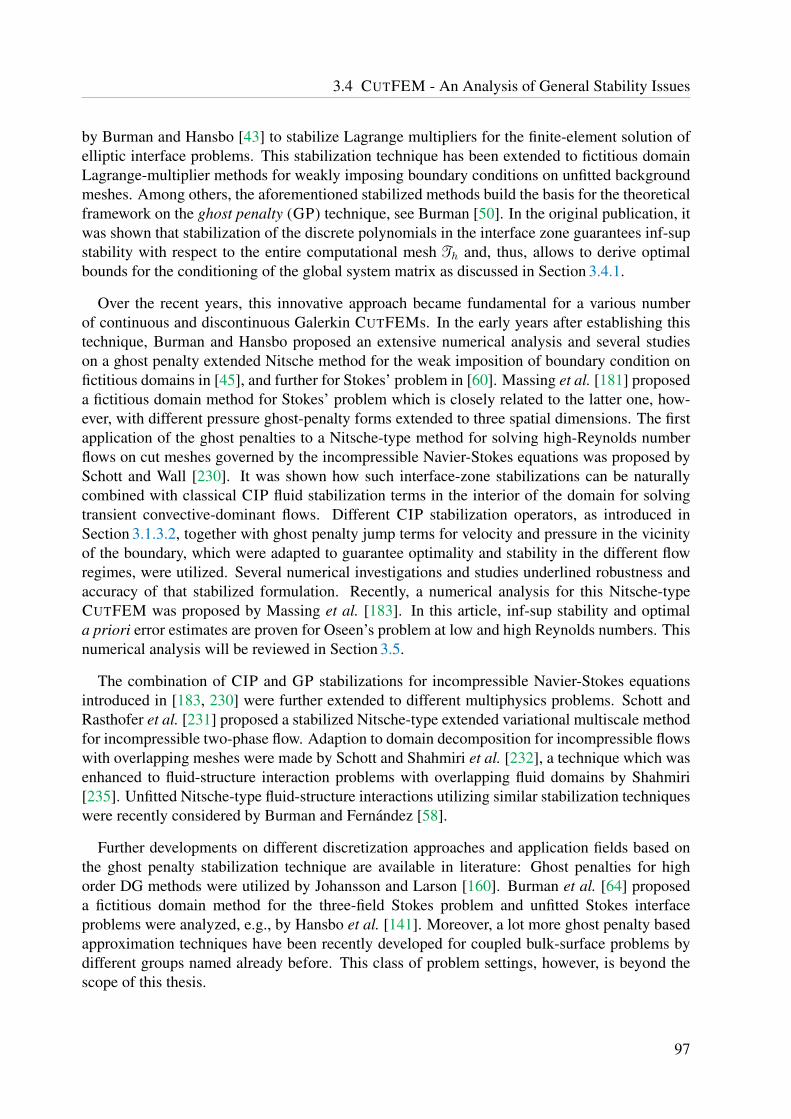
3.4 CUTFEM - An Analysis of General Stability Issues

by Burman and Hansbo [43] to stabilize Lagrange multipliers for the finite-element solution ofelliptic interface problems. This stabilization technique has been extended to fictitious domainLagrange-multiplier methods for weakly imposing boundary conditions on unfitted backgroundmeshes. Among others, the aforementioned stabilized methods build the basis for the theoreticalframework on the ghost penalty (GP) technique, see Burman [50]. In the original publication, itwas shown that stabilization of the discrete polynomials in the interface zone guarantees inf-supstability with respect to the entire computational mesh Th and, thus, allows to derive optimalbounds for the conditioning of the global system matrix as discussed in Section 3.4.1.

Over the recent years, this innovative approach became fundamental for a various numberof continuous and discontinuous Galerkin CUTFEMs. In the early years after establishing thistechnique, Burman and Hansbo proposed an extensive numerical analysis and several studieson a ghost penalty extended Nitsche method for the weak imposition of boundary condition onfictitious domains in [45], and further for Stokes’ problem in [60]. Massing et al. [181] proposeda fictitious domain method for Stokes’ problem which is closely related to the latter one, how-ever, with different pressure ghost-penalty forms extended to three spatial dimensions. The firstapplication of the ghost penalties to a Nitsche-type method for solving high-Reynolds numberflows on cut meshes governed by the incompressible Navier-Stokes equations was proposed bySchott and Wall [230]. It was shown how such interface-zone stabilizations can be naturallycombined with classical CIP fluid stabilization terms in the interior of the domain for solvingtransient convective-dominant flows. Different CIP stabilization operators, as introduced inSection 3.1.3.2, together with ghost penalty jump terms for velocity and pressure in the vicinityof the boundary, which were adapted to guarantee optimality and stability in the different flowregimes, were utilized. Several numerical investigations and studies underlined robustness andaccuracy of that stabilized formulation. Recently, a numerical analysis for this Nitsche-typeCUTFEM was proposed by Massing et al. [183]. In this article, inf-sup stability and optimala priori error estimates are proven for Oseen’s problem at low and high Reynolds numbers. Thisnumerical analysis will be reviewed in Section 3.5.

The combination of CIP and GP stabilizations for incompressible Navier-Stokes equationsintroduced in [183, 230] were further extended to different multiphysics problems. Schott andRasthofer et al. [231] proposed a stabilized Nitsche-type extended variational multiscale methodfor incompressible two-phase flow. Adaption to domain decomposition for incompressible flowswith overlapping meshes were made by Schott and Shahmiri et al. [232], a technique which wasenhanced to fluid-structure interaction problems with overlapping fluid domains by Shahmiri[235]. Unfitted Nitsche-type fluid-structure interactions utilizing similar stabilization techniqueswere recently considered by Burman and Fernandez [58].

Further developments on different discretization approaches and application fields based onthe ghost penalty stabilization technique are available in literature: Ghost penalties for highorder DG methods were utilized by Johansson and Larson [160]. Burman et al. [64] proposeda fictitious domain method for the three-field Stokes problem and unfitted Stokes interfaceproblems were analyzed, e.g., by Hansbo et al. [141]. Moreover, a lot more ghost penalty basedapproximation techniques have been recently developed for coupled bulk-surface problems bydifferent groups named already before. This class of problem settings, however, is beyond thescope of this thesis.

97

3 Developing Stabilized Cut Finite Element Methods for Incompressible Flow

3.4.3.1 The Fundamental Idea of Ghost-Penalty Operators

The objective of ghost penalty stabilization is to control discrete polynomials in the vicinityof the boundary. Sufficient control on degrees of freedom which are associated with ghostnodes located in the unphysical domain Ω∗h\Ωh needs to be added. For this purpose, physicalinformation from the interior of the domain is utilized and transferred to the interface zone.Provided that a sufficient number of uncut elements are located next to small and tiny elementparts, which result from the intersection of elements and are the reason for critical conditioningand stability, a smooth natural extension for discrete polynomials vh ∈ Vh in the boundary zonecan be guaranteed. In practice, two different types of ghost-penalty terms are utilized to providesuch an extension: inter-element face-jump penalties or patch-wise L2-projection-based ghostpenalties.

Inter-Element Face-Jump Ghost Penalties. In particular for low order finite elements, jumppenalties acting on inter-element faces similar to the CIP stabilization technique introduced inSection 3.1.3.2 are useful, as suggested, e.g., by Burman and Hansbo [45]. A face-jump ghost-penalty operator, which allows to extend L2-norm control, is defined as

g(uh, vh) =∑

F∈FΓ

∑

06j6k

h2j+1F 〈[[∂jnuh]], [[∂jnvh]]〉F . (3.145)

Such jump-penalty terms act on all discontinuous normal derivatives ∂jnvh of order 0 6 j 6 kfor piecewise polynomials vh ∈ Vh of order at most k. In a sum over all derivative orders,each addend tries to minimize corresponding inter-element derivative jumps in a facewise L2-least-squares sense, i.e. roughly spoken ‖[[∂jnvh]]‖2

0,F!

= min. The different orders are therebyweighted with appropriate h-scalings to guarantee weak consistency and full L2-norm control ofthe operator g. The aspect of weak consistency of the different GP stabilizations will be analyzedin more detail in Section 3.5.6 (see Lemma 3.17) in the context of the Oseen problem.

The penalty mechanism of such face-jump terms is visualized in Figure 3.6 for continuous anddiscontinuous finite element approximations. In the one-dimensional case, such terms reduceto point evaluations at nodes next to the interface. The zero-order derivative term, i.e. j = 0,simplifies to a jump penalty on the polynomial vh itself and remains active only for discontinuousGalerkin approximations. In contrast, continuous Galerkin approximations guarantee continuityby construction. The first-order derivative jump, i.e. j = 1, penalizes kinks between the twolinear polynomials of adjacent elements, whereas for a second-order approximation (k = 2),even changes in the curvature of the two polynomials need to be controlled additionally. Sum-marizing all derivative orders yields a smooth extension of the solution vh|Ωh\ΩΓ

from uncutelements to the entire computational mesh Ω∗h. By stabilizing all faces F ∈ FΓ, elements whichare intersected by Γ are connected to the physical domain, which is sufficiently controlled byuncut finite elements.

It has to be emphasized that in three spatial dimensions, for faces which are intersected bythe interface, jump terms have to be evaluated on the whole faces F ∈ FΓ and not only on theirphysical segments. This ensures that discrete derivatives are integrated on a sufficient large partof the boundary of cut elements. This improves the system conditioning and ensures discretestability with respect to the entire enlarged computational mesh. A visualization of this is shownin Figure 3.1. For details on the analysis, the reader is referred, e.g., to the publications [50, 181].

98

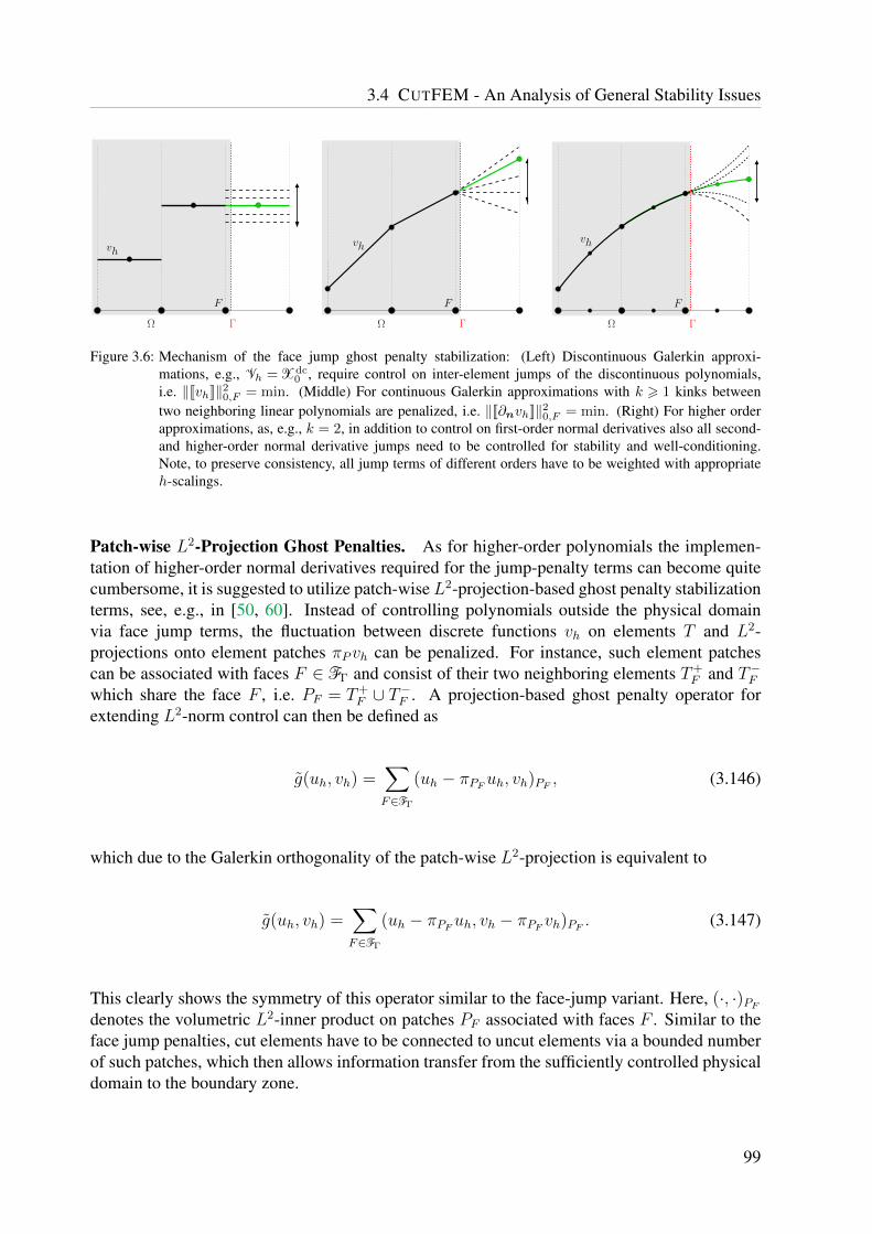
3.4 CUTFEM - An Analysis of General Stability Issues

Γ

F

Ω

vh

ΓΩ

vh

F

Γ

F

vh

Ω

Figure 3.6: Mechanism of the face jump ghost penalty stabilization: (Left) Discontinuous Galerkin approxi-mations, e.g., Vh = Xdc

0 , require control on inter-element jumps of the discontinuous polynomials,i.e. ‖[[vh]]‖20,F = min. (Middle) For continuous Galerkin approximations with k > 1 kinks betweentwo neighboring linear polynomials are penalized, i.e. ‖[[∂nvh]]‖20,F = min. (Right) For higher orderapproximations, as, e.g., k = 2, in addition to control on first-order normal derivatives also all second-and higher-order normal derivative jumps need to be controlled for stability and well-conditioning.Note, to preserve consistency, all jump terms of different orders have to be weighted with appropriateh-scalings.

Patch-wise L2-Projection Ghost Penalties. As for higher-order polynomials the implemen-tation of higher-order normal derivatives required for the jump-penalty terms can become quitecumbersome, it is suggested to utilize patch-wise L2-projection-based ghost penalty stabilizationterms, see, e.g., in [50, 60]. Instead of controlling polynomials outside the physical domainvia face jump terms, the fluctuation between discrete functions vh on elements T and L2-projections onto element patches πPvh can be penalized. For instance, such element patchescan be associated with faces F ∈ FΓ and consist of their two neighboring elements T+

F and T−Fwhich share the face F , i.e. PF = T+

F ∪ T−F . A projection-based ghost penalty operator forextending L2-norm control can then be defined as

g(uh, vh) =∑

F∈FΓ

(uh − πPFuh, vh)PF , (3.146)

which due to the Galerkin orthogonality of the patch-wise L2-projection is equivalent to

g(uh, vh) =∑

F∈FΓ

(uh − πPFuh, vh − πPF vh)PF . (3.147)

This clearly shows the symmetry of this operator similar to the face-jump variant. Here, (·, ·)PFdenotes the volumetric L2-inner product on patches PF associated with faces F . Similar to theface jump penalties, cut elements have to be connected to uncut elements via a bounded numberof such patches, which then allows information transfer from the sufficiently controlled physicaldomain to the boundary zone.

99

3 Developing Stabilized Cut Finite Element Methods for Incompressible Flow

3.4.3.2 Properties from a Mathematical Point of View

The key mathematical properties implied by both GP techniques are norm equivalences fordiscrete functions, as proven by Burman and Hansbo [45] and Massing et al. [181]:

Lemma 3.4 Let Ω, Ω∗h and FΓ be defined as in Section 2.1.4.1 and Section 2.2.2. Then for scalarfunctions qh ∈ Vh as well as for vector-valued equivalents vh ∈ [Vh]d the following estimateshold

‖qh‖2Ω∗h

.(‖qh‖2

Ω +∑

F∈FΓ

∑

16j6k

h2j+1〈[[∂jnqh]], [[∂jnqh]]〉F). ‖qh‖2

Ω∗h, (3.148)

‖vh‖2Ω∗h

.(‖vh‖2

Ω +∑

F∈FΓ

∑

16j6k

h2j+1〈[[∂jnvh]], [[∂jnvh]]〉F). ‖vh‖2

Ω∗h, (3.149)

‖∇vh‖2Ω∗h

.(‖∇vh‖2

Ω +∑

F∈FΓ

∑

16j6k

h2j−1〈[[∂jnvh]], [[∂jnvh]]〉F). ‖∇vh‖2

Ω∗h, (3.150)

where the hidden constants in the relation (.) depend only on the shape-regularity and thepolynomial order, but not on the mesh or the location of Γh within Th.

Fundamental assumption for this norm equivalence is assumption (G3) from Section 3.2.1, whichroughly spoken states that the number of faces to be crossed in order to “walk” from an uncutelement to a cut element requires being upper bounded and, in particular, being independentof h. As a result of the previous Lemma, adding appropriate ghost-penalty terms to an existingdiscrete formulation defined on Ωh, allows to extend different norm controls onto the enlargeddomain Ω∗h, as shown here for the L2-norm and H1-semi-norm for scalar and vector-valuedpolynomials.

3.4.3.3 Implementation and Practical Aspects

Whereas both types of ghost-penalty operators ensure the same desirable features, from a prac-tical point of view the different operators show certain advantages and drawbacks. Stabilizationcontrol of all orders of normal derivatives for the face-based variant requires high implementa-tion effort in particular for higher order elements as well as additional evaluate and assemblyroutines for face-jump terms. Especially weighting of the different derivative levels with high-order h2j+1-scalings can become critical when anisotropic meshes are used, like, for instance, incombination with ALE-based moving mesh techniques. Then a precise definition of the char-acteristic mesh size parameter h becomes crucial. In contrast, these issues are highly improvedfor projection-based ghost penalties. The entire information about higher order elements, theirshape as well as polynomial degree are contained in the patch-wise L2-projections. In particularthe sensitivity on h is highly reduced for that operator. Nevertheless, both techniques requireadditional data structures providing information about elements and their neighbors. Whileface-jump penalties require topological mesh information about faces and adjacent elements,projection-based methods require the construction of function spaces on element patches orat least the evaluation of polynomials of neighboring elements. In this sense, compared toclassical continuous Galerkin finite element approximations, both techniques require additionalmeasures for parallel computing. Furthermore, both operators g and g entail expanded couplings

100

3.4 CUTFEM - An Analysis of General Stability Issues

between polynomials of neighboring elements, which, on the one hand, is the desired key effectof these stabilization techniques in terms of controlling polynomials via neighbors. On the otherhand, this results in an enlarged pattern of non-zero entries in the global system matrix. Incontrast to standard continuous finite element methods, changes in existing code frameworkswith regard to parallel computing and evaluation as well as assembly strategies for additionalghost penalty terms is indispensable. For the sake of completeness, it has to be emphasizedthat the computational costs for solvers can increase and the changed pattern can influencethe efficiency of preconditioners similar to CIP fluid stabilizations. Nevertheless, the gain instability and the improved conditioning of the system matrix exceeds all mentioned drawbacksby a multiple.

Despite the large number of advantages of the projection-based method over the face-jumppenalties, throughout this work only face-jump ghost penalty terms are analyzed further andconsidered for all numerical simulations. This is due to implementational reasons and dueto their close relation to face-oriented CIP stabilizations, which allows to simplify numericalanalyses. For low-order approximations on regular meshes, as exclusively used in this work,no larger differences between these two different ghost penalty stabilization techniques areexpected.

3.4.3.4 Nitsche’s Method Supported by Ghost Penalties

As discussed in Section 3.4.2.2, the classical Nitsche method on unfitted meshes without anyadditional measures exhibit different issues regarding inf-sup stability, ill-conditioning and sub-optimality of a priori error estimates; even though cut-cell information is incorporated in therespective Nitsche penalty term.

In the following, the effect of ghost-penalty stabilizations and its interrelation with Nitsche’smethod is reviewed. This serves as basis for a CUTFEM for Oseen’s problem proposed later inSection 3.5. More theoretical details can be found in the original publication Burman [50].

Definition 3.11 (Nitsche’s method stabilized with ghost penalties)Let be Vh ⊂ V, then the discrete stabilized form of Nitsche’s method using ghost penalty stabi-lization, see [50], reads as follows: find uh ∈ Vh such that

BNITh (uh, vh) + GGP

h (uh, vh) = LNITh (vh) ∀ vh ∈ Vh, (3.151)

where

BNITh (uh, vh)

def= (∇uh,∇vh)Ω − 〈∇uh · n, vh〉Γ ∓ 〈uh,∇vh · n〉Γ + 〈(γ/h)uh, vh〉Γ, (3.152)

GGPh (uh, vh)

def= γg

∑F∈FΓ

∑16j6k

h2j−1〈[[∂jnuh]], [[∂jnvh]]〉F , (3.153)

LNITh (vh)

def= (f, vh)Ω ∓ 〈g,∇vh · n〉Γ + 〈(γ/h)g, vh〉Γ. (3.154)

Compared to the classical Nitsche method, see Definition 3.10, the role of the additional ghostpenalty stabilization term GGP

h is to extend control on theH1-semi-norm, which is given in termsof the elliptic bulk term, to the enlarged domain Ω∗h by exploiting norm equivalence (3.150).

As already discussed in Section 3.4.2.1, for intersected elements a weakened trace inequality

‖∇vh · n‖0,Γh∩T 6 CTh−1/2T ‖∇vh‖0,T , (3.155)

101

3 Developing Stabilized Cut Finite Element Methods for Incompressible Flow

see (3.48) and (3.129), holds with respect to the entire element T . Therein, CT only depends onthe element shape and its polynomial degree, however, not on the intersection of the element. Ap-plying this suboptimal inequality to estimate standard and adjoint consistency boundary terms,leads to a momentary uncontrolled lack of coercivity within the unphysical domain Ω∗h\Ωh

2〈vh,∇vh · n〉 6 1/ε‖∇vh · n‖2−1/2,h,Γ + ε‖vh‖2

1/2,h,Γ

6 C2T/ε|vh|21,Ω∗h + ε‖vh‖2

1/2,h,Γ

6 CGC2T/ε(|vh|21,Ω + GGP

h (vh, vh)) + ε‖vh‖21/2,h,Γ,

(3.156)

with CG denoting the hidden constant in the norm equivalence (3.150), which depends on γg.This is due to the fact that the elliptic bulk term allows to compensate ∇vh just within thephysical domain Ωh. Now, thanks to the additional ghost-penalty term and the H1-semi-normequivalence, this negative norm control can be balanced and inf-sup stability can be recoveredon the entire computational mesh with an energy norm defined as

|||vh|||2∗def= |||vh|||2 + GGP

h (vh, vh) = |vh|21,Ω + ‖vh‖21/2,h,Γ + GGP

h (vh, vh) (3.157)

such that|vh|21,Ω∗h + ‖vh‖2

1/2,h,Γ . |||vh|||2∗ . |vh|21,Ω∗h + ‖vh‖21/2,h,Γ. (3.158)

Stability of Nitsche’s Method with respect to |||vh|||∗. Utilizing estimate (3.156), coercivityfor the symmetric Nitsche method can be proven as

BNITh (vh, vh) + GGP

h (vh, vh) = |vh|21,Ω + GGPh (vh, vh)− 2〈vh,∇vh · n〉Γ + γ‖vh‖2

1/2,h,Γ

> (1− CGC2T/ε)(|vh|21,Ω + GGP

h (vh, vh)) + (γ − ε)‖vh‖21/2,h,Γ

> min 1− CGC2T/ε, γ − ε|||vh|||2∗

> cs|||vh|||2∗ (3.159)

and stability is guaranteed for ε = CGC2T/2 and γ > ε. Note that for the symmetric Nitsche

method, again, the Nitsche penalty parameter γ has to be sufficiently large, however, nowdepending on the weakened trace inequality. Provided that the mesh assumptions from Sec-tion 3.2.1 are fulfilled, this constant is upper bounded and does not deteriorate in contrast tocut-cell-based variants.

It should be mentioned that the hidden constant CG of the norm equivalence (3.150) entersthe coercivity estimate and thus introduces a dependency on γg . In practice, it is suggested tochoose γg < 1 to not worsen the accuracy near the boundary due to strong smoothing effectsof the jump penalties. As a consequence, the Nitsche penalty parameter has to be large enoughdepending on the size of γg to still ensure coercivity.

Such dependencies vanish for the non-symmetric Nitsche method and any positive γg, γ > 0are sufficient to guarantee stability with respect to |||vh|||∗. For the non-symmetric variant thecoercivity estimate simplifies due to out-canceling boundary terms

BNITh (vh, vh) + GGP

h (vh, vh) = |vh|21,Ω + GGPh (vh, vh) + γ‖vh‖2

1/2,h,Γ

> min 1, γ|||vh|||2∗> cs|||vh|||2∗. (3.160)

The conditioning issue for γg → 0, however, still remains due to the deterioration of the norm.

102

3.4 CUTFEM - An Analysis of General Stability Issues

Similar to the elaborations in Section 3.3.2.4, for both variants additional control on the in-terface flux can be recovered by applying a trace inequality. As now stability is ensured on theenlarged domain Ω∗h, the weakened estimate (3.155) guarantees uniform control on the interfacefluxes in terms of CT . In fact, this constant depends on the element shape and the polynomialdegree, however, does not dependent on the interface location. The modified coercivity estimatethen emerges to

BNITh (vh, vh) + GGP

h (vh, vh) > cs(|||vh|||2∗ + ‖∇vh · n‖2−1/2,h,Γ) (3.161)

with cs independent of the interface position and h.

For the sake of completeness, it has to be mentioned that even the non-symmetric penalty-free method is proven to be stable on unfitted meshes, as shown by Boiveau and Burman [27]and Boiveau [26]. However, the proof in how to gain the required control over ‖vh‖1/2,h,Γ thensubstantially differs.

3.4.4 Numerical Studies for Incompressible Flow

All theoretically analyzed aspects concerning different techniques for the weak imposition ofDirichlet boundary conditions on unfitted grids, which have been discussed within the lastsections, will be corroborated now by several numerical studies. Although most effects werenumerically analyzed for the linear elliptic Poisson problem, all discussed stability issues equiv-alently occur for solutions to the incompressible Navier-Stokes equations. Since main focusof the present work is directed towards developing CUTFEMs for incompressible flows, allinvestigations presented subsequently are performed for the incompressible Navier-Stokes equa-tions. To mimic major stability issues from the Poisson problem, low-Reynolds-number flowsare considered such that the elliptic viscous term in (3.4) is dominating. Further effects that arecharacteristic for convective-dominated flows will be studied afterwards as well.

First, in Section 3.4.4.1, issues arising from pathological element intersections, which mayrender in stability and conditioning issues at nodes located outside the physical domain, areshown. In Section 3.4.4.2 different methods for the weak constraint enforcement are compared.The claimed close relation between the stabilized mixed/hybrid stress-based formulation by Ger-stenberger [123] and the cut-cell-weighted Nitsche method discussed in Section 3.4.2.3 will beaffirmed. Furthermore, different variants of Nitsche’s method and their effects on accuracy androbustness are numerically investigated to support the theoretical statements provided throughoutSection 3.4.2.2. Their different behavior is compared by means of a spatial error convergencestudy. Moreover, the influence of different fluid stabilizations provided in Section 3.1.3, togetherwith the influence of additional stabilizing measures in the interface region, will be pointed out.The great improvement of stability and system conditioning for face-jump ghost penalty stabi-lizations in the interface zone is demonstrated. Finally, in Section 3.4.4.3, additional studies arepresented regarding the sensitivity of Nitsche’s method on involved stabilization parameters, thatis the Nitsche penalty parameter as well as the parameter of a viscous ghost-penalty stabilization.

103

3 Developing Stabilized Cut Finite Element Methods for Incompressible Flow

The following different discrete formulations are examined in this section:

• The original mixed/hybrid Cauchy-stress-based formulation by Gerstenberger [123] usedfor the weak imposition of boundary conditions. In the interior fluid domains the standardGalerkin formulation is stabilized by a PSPG residual-based variational multiscale term,as introduced in Section 3.1.3.1. Note that no CIP or GP stabilizations are applied here.This formulation is abbreviated with MHS throughout the studies.

• A classical symmetric Nitsche method (NIT) with penalty term 〈(ανρ)uh,vh〉Γ supportedby a PSPG fluid stabilization. The scaling αν is chosen as defined for boundary-fittedmeshes, i.e. αν = γν/h, see Section 3.3.2.4.

• A symmetric Nitsche-type method using penalty term scalings based on element-wisecut-cell information, i.e. αν = γν|ΓT |/|ΩT | with ΓT = Γ ∩ T and ΩT = Ω ∩ T , to appro-priately account for trace estimates on the physical domain, see Section 3.4.2.2.

• Additionally, combinations with different types of pressure stabilizations are investigated:a residual-based PSPG stabilization form Section 3.1.3.1 and a face-oriented stabilizedpressure CIP method (p-CIP) from Section 3.1.3.2. Note, for the latter one, intersectedfaces in the interface zone are stabilized entirely.

• A symmetric Nitsche-type method supported by a viscous ghost penalty stabilization (GP)for the velocity field

GGPh (uh,vh) = γν

∑

F∈FΓ

∑

16j6k

νρh2j−1〈[[∂jnuh]], [[∂jnvh]]〉F , (3.162)

as proposed in Section 3.4.3.4. For this variant, the Nitsche penalty term scaling is chosenas αν = γν/h based on the weakened trace inequality (3.155).

• A fully stabilized CUTFEM including further stabilizations for low- and high-Reynolds-number flows proposed by Schott and Wall [230]. CIP fluid stabilizations for low- andhigh-Reynolds-number flows from Section 3.1.3.2 are used and the Nitsche-penalty scal-ing is extended to account for mass conservation and inflow instabilities for high Reynoldsnumbers

〈(αuρ)uh,vh〉Γ with αu = maxγν/h, |uh · n|, 1. (3.163)

A closely related method will be analyzed for Oseen’s problem in Section 3.5 and finallyreviewed in Section 3.6 for transient incompressible Navier-Stokes equations.

The subsequent numerical studies are based on work published in Schott and Wall [230]. If notindicated otherwise, for Nitsche’s method, the stabilization parameters are chosen as γ = 35.0for the penalty terms and γν = 0.05 for the viscous ghost penalty stabilization equivalent toscalings in the CIP method. Stabilization parameters for CIP and RBVM terms are takenunchanged from Section 3.1.3. For all subsequent simulations the density is set to ρ = 1.0.

104

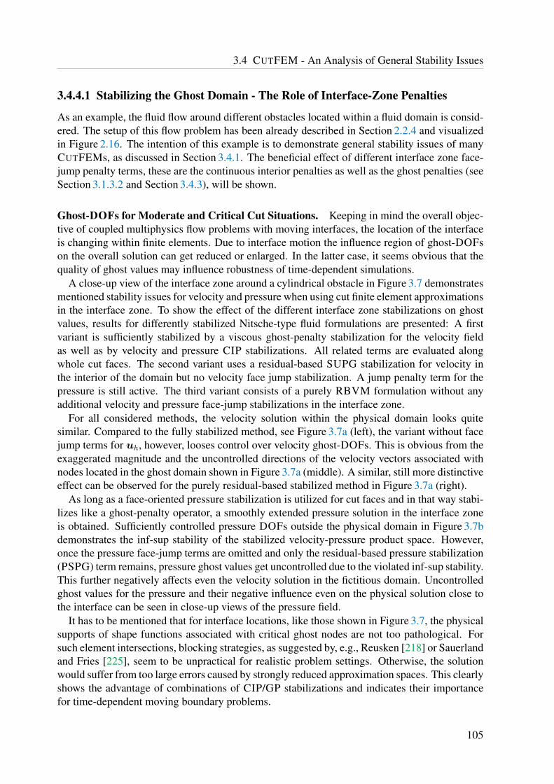
3.4 CUTFEM - An Analysis of General Stability Issues

3.4.4.1 Stabilizing the Ghost Domain - The Role of Interface-Zone Penalties

As an example, the fluid flow around different obstacles located within a fluid domain is consid-ered. The setup of this flow problem has been already described in Section 2.2.4 and visualizedin Figure 2.16. The intention of this example is to demonstrate general stability issues of manyCUTFEMs, as discussed in Section 3.4.1. The beneficial effect of different interface zone face-jump penalty terms, these are the continuous interior penalties as well as the ghost penalties (seeSection 3.1.3.2 and Section 3.4.3), will be shown.

Ghost-DOFs for Moderate and Critical Cut Situations. Keeping in mind the overall objec-tive of coupled multiphysics flow problems with moving interfaces, the location of the interfaceis changing within finite elements. Due to interface motion the influence region of ghost-DOFson the overall solution can get reduced or enlarged. In the latter case, it seems obvious that thequality of ghost values may influence robustness of time-dependent simulations.

A close-up view of the interface zone around a cylindrical obstacle in Figure 3.7 demonstratesmentioned stability issues for velocity and pressure when using cut finite element approximationsin the interface zone. To show the effect of the different interface zone stabilizations on ghostvalues, results for differently stabilized Nitsche-type fluid formulations are presented: A firstvariant is sufficiently stabilized by a viscous ghost-penalty stabilization for the velocity fieldas well as by velocity and pressure CIP stabilizations. All related terms are evaluated alongwhole cut faces. The second variant uses a residual-based SUPG stabilization for velocity inthe interior of the domain but no velocity face jump stabilization. A jump penalty term for thepressure is still active. The third variant consists of a purely RBVM formulation without anyadditional velocity and pressure face-jump stabilizations in the interface zone.

For all considered methods, the velocity solution within the physical domain looks quitesimilar. Compared to the fully stabilized method, see Figure 3.7a (left), the variant without facejump terms for uh, however, looses control over velocity ghost-DOFs. This is obvious from theexaggerated magnitude and the uncontrolled directions of the velocity vectors associated withnodes located in the ghost domain shown in Figure 3.7a (middle). A similar, still more distinctiveeffect can be observed for the purely residual-based stabilized method in Figure 3.7a (right).

As long as a face-oriented pressure stabilization is utilized for cut faces and in that way stabi-lizes like a ghost-penalty operator, a smoothly extended pressure solution in the interface zoneis obtained. Sufficiently controlled pressure DOFs outside the physical domain in Figure 3.7bdemonstrates the inf-sup stability of the stabilized velocity-pressure product space. However,once the pressure face-jump terms are omitted and only the residual-based pressure stabilization(PSPG) term remains, pressure ghost values get uncontrolled due to the violated inf-sup stability.This further negatively affects even the velocity solution in the fictitious domain. Uncontrolledghost values for the pressure and their negative influence even on the physical solution close tothe interface can be seen in close-up views of the pressure field.

It has to be mentioned that for interface locations, like those shown in Figure 3.7, the physicalsupports of shape functions associated with critical ghost nodes are not too pathological. Forsuch element intersections, blocking strategies, as suggested by, e.g., Reusken [218] or Sauerlandand Fries [225], seem to be unpractical for realistic problem settings. Otherwise, the solutionwould suffer from too large errors caused by strongly reduced approximation spaces. This clearlyshows the advantage of combinations of CIP/GP stabilizations and indicates their importancefor time-dependent moving boundary problems.

105

3 Developing Stabilized Cut Finite Element Methods for Incompressible Flow

(a) Velocity solution uh around a cylinder.

(b) Pressure solution ph around a cylinder.

Figure 3.7: Close-up view of the flow around a cylinder with x1 ∈ [0.05; 0.225], x2 ∈ [0.05; 0.225]: (Left) ANitsche-type method with velocity and pressure face-jump-penalty stabilizations. (Middle) A variantwith SUPG stabilization within the domain, but without face-jump penalties for the velocity uh. Aface-oriented pressure stabilization term (p-CIP) still controls the pressure solution in the interface zone.(Right) Insufficiently controlled solution of a pure residual-based stabilized formulation (SUPG/PSPG)without ghost penalties for uh and ph. Note the different scales.

Face-Jump Penalties for Expanded Cut Finite Element Function Spaces Considering solu-tions to the incompressible Navier-Stokes equations approximated in complex domains utilizingthe expanded cut finite element function space introduced in Section 2.2.4, evaluation and as-sembly of face-jump-penalty terms in the interface zone requires special consideration.

A close-up view around the left upper tip of the thin structural obstacle of the previousexample has been visualized in Figure 2.17. As already elaborated in Section 2.2.4, to representindependent solutions on different sides of thin structures accurately, multiple DOFs per nodeare required. The structural surface subdivides the support of the nodal shape function near theinterface into independent non-connected volume-cells. Following Algorithm 2.1, the number ofvolume-cell connections around nodes then determines the number of nodal DOFs, as depictedin Figure 2.17a. Within the support of a node’s shape function, volume-cells Vi, Vj are connectedto physically meaningful contiguous regions if and only if there is a common (possibly cut)facet f ⊆ F ∈ Fi in between, such that f = Vi ∩ Vj . The number of such physical facets fper face F determines how often face-jump-penalty terms have to be evaluated along the entireparent face F ∈ FΓ.

106

3.4 CUTFEM - An Analysis of General Stability Issues

In Figure 2.17b, all uncut internal faces F ∈ Fi\FΓ as well as faces f ∈ FΓ in the interfacezone are exemplarily shown for the previous example. Away from the interface only classicalface-oriented CIP fluid stabilizations, as defined in Section 3.1.3.2, have to be evaluated. Suchfaces are marked with green color in Figure 2.17b. For faces near the interface, i.e. F ∈ FΓ

(colored red), in addition to the CIP fluid stabilizations also ghost-penalty terms (GP) becomeactive. Numbers shown in Figure 2.17b indicate how many times faces in the interface zonehave to be evaluated. Each evaluation thereby corresponds to a physical face segment f ⊂ Fof intersected faces and thus stabilizes fluid regions on different sides of the structure. Moreprecisely, the different evaluations stabilize disjunct volume-cell connections.

The resulting pressure distribution around the thin structural obstacle is shown in Figure 2.17c.Therein, the smoothness of the pressure contour lines around the structural tip needs to bepointed out which is due to the sufficient stability control given by face-jump-penalty terms.

3.4.4.2 Weak Dirichlet Constraint Enforcement - A Comparison of Methods

In subsequent numerical convergence studies, different variants for weak imposition of Dirichletconstraints are compared to confirm theoretical results on inf-sup stability and error convergenceof the different techniques listed at the beginning of Section 3.4.4.

2D Taylor Problem. The convergence of errors is investigated for the frequently used two-dimensional Taylor problem, see, e.g., in [73, 162, 213]. Periodic time-dependent analyticalvelocity and pressure fields (u, p) are given as

u1(x1, x2, t) = − cos(aπx1) sin(aπx2) · gu(t), (3.164)u2(x1, x2, t) = sin(aπx1) cos(aπx2) · gu(t), (3.165)p(x1, x2, t) =−0.25(cos(2aπx1) + cos(2aπx2)) · gp(t), (3.166)

such that∇ · u = 0. It is chosen a = 2. The time-scaling factors gp(t) and gu(t) will be specifiedbelow for the different studies. Numerical solutions are computed within a circular fluid domain

Ωf =x = (x1, x2) ∈ R2

∣∣ |x− (0.5, 0.5)| < 0.45

(3.167)

approximated with unfitted background fluid meshes Th defined on [0, 1]2, which are rotated by45 about the x3-axis, as shown in Figure 3.8. All background meshes consist of regular quadri-lateral Q1-elements. The mesh size parameters are h = 1/nx = 1/ny with nx = ny the varyingnumber of elements in each direction, as specified below. The boundary Γh is approximatedexplicitly by the inner trace mesh of the ring-shaped domain

Ωs =x = (x1, x2) ∈ R2

∣∣ 0.45 < |x− (0.5, 0.5)| < 0.9, (3.168)

where the circular interface line Γ consists of 6nx regular intervals.Dirichlet boundary conditions given by the analytical solution are imposed on the entire

boundary of the fluid domain, i.e. Γ = ΓD. To remove the uncontrolled constant pressure mode,the pressure is fixed at the middle node (0.5, 0.5) using the value from (3.166). The right-handside f in the Navier-Stokes equations is adapted such that (3.164)–(3.166) are solution of thestationary or transient incompressible Navier-Stokes equations, respectively.

107

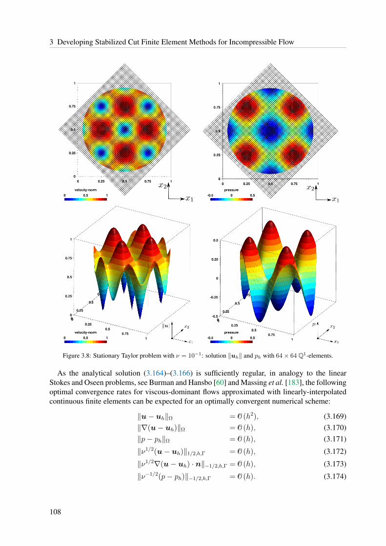
3 Developing Stabilized Cut Finite Element Methods for Incompressible Flow

Figure 3.8: Stationary Taylor problem with ν = 10−1: solution ‖uh‖ and ph with 64× 64 Q1-elements.

As the analytical solution (3.164)–(3.166) is sufficiently regular, in analogy to the linearStokes and Oseen problems, see Burman and Hansbo [60] and Massing et al. [183], the followingoptimal convergence rates for viscous-dominant flows approximated with linearly-interpolatedcontinuous finite elements can be expected for an optimally convergent numerical scheme:

‖u− uh‖Ω = O(h2), (3.169)‖∇(u− uh)‖Ω = O(h), (3.170)‖p− ph‖Ω = O(h), (3.171)

‖ν1/2(u− uh)‖1/2,h,Γ = O(h), (3.172)

‖ν1/2∇(u− uh) · n‖−1/2,h,Γ = O(h), (3.173)

‖ν−1/2(p− ph)‖−1/2,h,Γ = O(h). (3.174)

108

3.4 CUTFEM - An Analysis of General Stability Issues

In addition to the standard bulk norms for velocity and pressure, also mesh-dependent interfacenorms as considered in the context of Nitsche’s method in Section 3.4.2.2 are analyzed. TheH1/2-interface norm defined in (3.172) accounts for the imposition of the boundary condition.For advanced coupling algorithms, such as fluid-structure interaction, boundary fluxes on Γ areof special interest, since these are quite sensitive to perturbations and to the interface location, asalready discussed in Section 3.4.2.2. For fluids, flux errors can be split into viscous and pressureparts as defined in (3.173) and (3.174).

For more detailed information on the expected convergence rates in the different flow regimes,the reader is referred to the numerical analysis part in Section 3.5, in particular to the definitionof appropriate weighted graph based energy-type norms in (3.250), to the a priori error estimatefrom Theorem 3.19 and interpretations of that in Remark 3.23 and Remark 3.24.

Viscous-Dominated Flow - Convergence Study. For a higher viscosity, which here is givenas ν = 10−1m2/s resulting in Re = 9 based on domain diameter and maximum velocity, theflow is assumed to be steady and the time derivative u in the Navier-Stokes equations canbe omitted. The scaling factors included in (3.164)–(3.166) are set gu(t) = gp(t) = 1.0. Asno convective-dominant effects are expected, additional stability measures which account forrelated instabilities in the interior of the domain or near the boundary can be neglected. Thepressure solution and the Euclidean norm of the velocity solution obtained for a fully stabilizedNitsche-type method based on CIP and GP stabilizations are visualized for a 64× 64 mesh Th inFigure 3.8. For the velocity and pressure field, smoothness along the circular boundary Γ has tobe highlighted. This is a result of the jump penalty stabilizations acting on cut faces as explainedin Section 3.4.3.

For the spatial convergence study, an equal number of elements in each coordinate direction isused, i.e. n = nx = ny ∈ 10, 16, 24, 48, 64, 100, 160, 240. Convergence results for all bulk andinterface errors are shown in Figure 3.9. As can be seen, the velocity errors measured in the L2-norm and H1-semi-norm (Figure 3.9a, Figure 3.9b) are comparable for all different stabilizationtechniques and variants of imposing boundary conditions and exhibit optimal rates as expected in(3.169) and (3.170). In contrast, the pressure solution (Figure 3.9c) and the interface fluxes (Fig-ure 3.9e, Figure 3.9f) react much more sensitive to instabilities arising from insufficient pressureor interface control of some methods. As can be seen from the pressure error, the Cauchy-stress-based Lagrange-multiplier approach exhibits a clear lack of inf-sup stability, whereasall variants of Nitsche’s method lead to similar pressure errors independent of the definitionof αν . The stability issue of Nitsche’s method related to the trace inequality, as explained inSection 3.4.2, is clearly visible for a uniform element-length-based definition of αν ∝ ν/h (bluecurve in Figure 3.9e). Depending on the interface-location, the viscous flux-errors vary overa very large range as the trace estimate is not appropriately accounted for, which results ininterface instabilities in particular for the so-called “sliver cut” cases. A significantly improvederror behavior for viscous and pressure fluxes (Figure 3.9e and Figure 3.9f) can be observed forthe stress-based Lagrange-multiplier approach and the Nitsche variant using cut-cell informationαν ∝ ν|ΓT |/|ΩT |. The close relationship between these methods has been already indicated inSection 3.4.2.3. The reduced errors of those methods compared to the uniform Nitsche scalingare due to the ensured coercivity of the elliptic part of the PDE, see (3.136), even though theenergy norms or the stability constants incorporate dependencies on the interface location. This

109

3 Developing Stabilized Cut Finite Element Methods for Incompressible Flow

10−3

10−2

10−1

10−4

10−3

10−2

10−1

‖u − uh‖Ω

mesh size h

abserror

MHS-(PSPG)-no-GPNIT-(PSPG)-no-GP-αν ∝ ν

hT

NIT-(PSPG)-no-GP-αν ∝ ν|ΓT ||ΩT |

NIT-(p-CIP)-no-GP-αν ∝ ν|ΓT ||ΩT |

NIT-(p-CIP)-GP-αν ∝ ν

hT

Schott and Wall 2014slope 2

(a)

10−3

10−2

10−1

10−2

10−1

100

‖∇(u − uh)‖Ω

mesh size h

abserror

MHS-(PSPG)-no-GPNIT-(PSPG)-no-GP-αν ∝ ν

hT

NIT-(PSPG)-no-GP-αν ∝ ν|ΓT ||ΩT |

NIT-(p-CIP)-no-GP-αν ∝ ν|ΓT ||ΩT |

NIT-(p-CIP)-GP-αν ∝ ν

hT

Schott and Wall 2014slope 1

(b)

10−3

10−2

10−1

10−4

10−3

10−2

10−1

‖p− ph‖Ω

mesh size h

abserror

MHS-(PSPG)-no-GPNIT-(PSPG)-no-GP-αν ∝ ν

hT

NIT-(PSPG)-no-GP-αν ∝ ν|ΓT ||ΩT |

NIT-(p-CIP)-no-GP-αν ∝ ν|ΓT ||ΩT |

NIT-(p-CIP)-GP-αν ∝ ν

hT

Schott and Wall 2014slope 2

(c)

10−3

10−2

10−1

10−4

10−3

10−2

10−1

‖ν1/2(u − uh)‖1/2,h,Γ

mesh size h

abserror

MHS-(PSPG)-no-GPNIT-(PSPG)-no-GP-αν ∝ ν

hT

NIT-(PSPG)-no-GP-αν ∝ ν|ΓT ||ΩT |

NIT-(p-CIP)-no-GP-αν ∝ ν|ΓT ||ΩT |

NIT-(p-CIP)-GP-αν ∝ ν

hT

Schott and Wall 2014slope 1.5

(d)

10−3

10−2

10−1

10−3

10−2

10−1

‖ν1/2∇(u − uh) · n‖−1/2,h,Γ

mesh size h

abserror

MHS-(PSPG)-no-GPNIT-(PSPG)-no-GP-αν ∝ ν

hT

NIT-(PSPG)-no-GP-αν ∝ ν|ΓT ||ΩT |

NIT-(p-CIP)-no-GP-αν ∝ ν|ΓT ||ΩT |

NIT-(p-CIP)-GP-αν ∝ ν

hT

Schott and Wall 2014slope 1.5

(e)

10−3

10−2

10−1

10−4

10−3

10−2

10−1

‖ν−1/2(p− ph)‖−1/2,h,Γ

mesh size h

abserror

MHS-(PSPG)-no-GPNIT-(PSPG)-no-GP-αν ∝ ν

hT

NIT-(PSPG)-no-GP-αν ∝ ν|ΓT ||ΩT |

NIT-(p-CIP)-no-GP-αν ∝ ν|ΓT ||ΩT |

NIT-(p-CIP)-GP-αν ∝ ν

hT

Schott and Wall 2014slope 2

(f)

Figure 3.9: Stationary Taylor problem with ν = 10−1: spatial error convergence versus element length h, differentnorms (a)–(f). A mixed/hybrid stress-based Lagrange-multiplier approach (MHS) with PSPG pressurestabilization without ghost penalty (red). Nitsche’s method (NIT) with PSPG pressure stabilization,without ghost penalty (GP) stabilization, however, with different Nitsche-penalty scalings: αν ∝ ν/h(blue), αν ∝ ν|ΓT |/|ΩT | (magenta). Two variants of Nitsche’s method with p-CIP pressure stabi-lization: without ghost penalty using a Nitsche penalty scaling αν ∝ ν|ΓT |/|ΩT | (green), with ghostpenalty using a Nitsche penalty scaling αν ∝ ν/h (turquoise). Stabilized method by Schott and Wall[230] (black).

manifests itself in a rather uneven error convergence for the viscous fluxes. The enforcement ofthe boundary conditions (Figure 3.9d) is similar for all shown variants of Nitsche’s method. Aclear improvement regarding the pressure fluxes can be obtained using a face-oriented pressurestabilization (p-CIP) instead of a residual-based pressure stabilization (PSPG) only. Finally, toobtain optimal error convergence independent of the interface location also for the viscous fluxes(Figure 3.9e), an additional ghost penalty stabilization for the velocity (GP) (3.162) is required.As elaborated in Section 3.4.3.4, combining this interface control with the uniform Nitschepenalty scaling, which ensures equally distributed control on the boundary condition without

110

3.4 CUTFEM - An Analysis of General Stability Issues

10−3

10−2

10−1

105

1010

1015

1020

condition number estimate

mesh size h

conditionnumber

MHS-(PSPG)-no-GPNIT-(PSPG)-no-GP-αν ∝ ν

hT

NIT-(PSPG)-no-GP-αν ∝ ν|ΓT ||ΩT |

NIT-(p-CIP)-no-GP-αν ∝ ν|ΓT ||ΩT |

NIT-(p-CIP)-GP-αν ∝ ν

hT

Schott and Wall 2014slope -3

10−3

10−2

10−1

105

1010

1015

1020

condition number estimate

mesh size hconditionnumber

MHS-RBVM-no-GP-αu =max(1, |u · n|)NIT-CIP-no-GP-αu = αν

NIT-CIP-GP-αu = αν

NIT-CIP-GP-αu =max(|u · n|in,αν)NIT-CIP-GP-αu =max(|u · n|,αν)Schott and Wall 2014slope -2

Figure 3.10: Taylor problem: condition numbers for viscous dominated flow (left) and for convective-dominatedflow (right).

losing inf-sup stability, guarantees uniform optimal convergence for all considered interface errormeasures. Moreover, it has to be mentioned that the additional interface stabilizations (3.163)according to the convective limit and related additional CIP fluid stabilizations do not deteriorateconvergence rates in the viscous regime. It has to be mentioned that the rate for the velocityinterface norms (Figure 3.9d, Figure 3.9e) is half an order better than the expected rate in (3.170)and (3.171). This effect has been addressed in the work by Horger et al. [153]. With respectto all investigated measures, the method proposed by Schott and Wall [230] leads to optimalconvergence rates independent of the interface location and to smaller error levels comparedto other considered methods. Furthermore, a clear improvement of the system conditioningdue to all incorporated face-jump-penalty terms next to the boundary, the GP and the CIPstabilizations for pressure and velocity, can be seen in Figure 3.10. Note that the observedsuboptimal rate κ = O(h−3) for the conditioning in the low-Reynolds-number case instead ofthe optimal rate κ = O(h−2) is most likely due to the setup of this simulation as a pseudo-two-dimensional example approximated with one layer of three-dimensional finite elements andstrong Dirichlet values for the third spatial dimension. Obviously, these negatively affect the finalsystem conditioning. The latter formulation will be analyzed in detail in Sections 3.5 and 3.6.

Convective-Dominated Flow - Convergence Study. In addition to the study on inf-sup sta-bility and convergence behavior of different methods for viscous-dominated flows, the fol-lowing investigation serves as a preliminary study on interface instabilities which might arisein locally convective-dominated boundary regions. For the subsequent study the viscosity isν = 10−4m2/s and the transient incompressible Navier-Stokes equations are solved for t ∈ [0, T ]with T = 0.1 s and ∆t = 0.01 s. The time-dependent scaling factors are now chosen as

gu(t) = exp(−2a2π2νt) and gp(t) = exp(−4a2π2νt) (3.175)

and indicate an exponential decay of the initial flow field. In the following, the stabilizedNitsche-type method by Schott and Wall [230] is applied, which includes all CIP fluid stabiliza-

111

3 Developing Stabilized Cut Finite Element Methods for Incompressible Flow

tions for velocity and pressure proposed in Section 3.1.3.2. In the interface zone, these terms actlike ghost penalties when jump penalties are evaluated on the entire cut faces. In this study, theinfluence of different contributions to the Nitsche penalty term in (3.163) is investigated. For thetemporal discretization, a backward Euler scheme is applied. Errors are evaluated at final time Tand plotted against the element length h for different methods and variants in Figure 3.11. Thefirst curve shows the error behavior for the Cauchy-stress-based Lagrange-multiplier approach(MHS) from [123] supported by an additional Nitsche-like penalty term with convective scalingsfrom (3.163). For Nitsche’s method (NIT) different definitions for αu are compared: the secondand third curves show results without and with the viscous ghost penalty (GP) operator (3.162),however, both variants without any additional convective or penalty contributions from (3.163).Curve four shows the variant with additional convective stabilizations active only at inflow parts|uh · n|in where uh · n < 0. The fifth curve activates the convective stabilization term alsoat outflow parts and the last curve shows results of a stabilized formulation based on the fullparameter definition (3.163) from [230] which sufficiently accounts for mass conservation evenfor convective-dominant flows.

Within the domain, for almost all variants optimal error convergence can be observed inFigures 3.11a–3.11c, except for the mixed/hybrid Cauchy-stress-based method that lacks pres-sure stability. Similar to the viscous case, for the interface errors again convergence rates areobtained better than expected, see (3.172)–(3.174). The influence of the different convectivestabilization variants is clearly visible from the boundary condition errors (Figure 3.11d) andthe flux errors (Figure 3.11e). Missing convective interface stabilizations compared to (3.163)lead to increased interfacial errors, especially for coarse meshes, as those exhibit higher localelement Reynolds numbers. Balancing these convective interface instabilities by appropriatescalings for the Nitsche penalty term, a clear improvement of the stability and accuracy can beobserved. Best results are obtained when adding additional control on the mass conservation,here specified by the safety factor of 1.0 from (3.163), which corresponds to ‖β‖ in the scaling(3.467), see Section 3.6. This ensures uniform penalty on the boundary condition for convective-dominated flows. For a closer understanding of the different scalings, the reader is referred tothe numerical analysis of a CUTFEM for the Oseen problem in Section 3.5.

It needs to be mentioned that for convective-dominated flows the ghost penalty control ofthe velocity field is overtaken by the face-oriented CIP stabilizations (3.29) and (3.30). Theseadditionally ensure streamline and incompressibility control. Replacing CIP fluid stabilizationsby a purely residual-based RBVM approach (PSPG/SUPG/LSIC) results in no or poor conver-gence of the Newton-scheme. This behavior indicates an unstable configuration as no controlover ghost values can be retained. Note that in this case the viscous ghost penalty term (3.162)is not sufficient anymore owing to the too small scaling ν |uh|h. However, combinations ofthe RBVM stabilization in the domain Ω supported by CIP/GP stabilizations, which need to beactivated in the boundary zone only, can render formulations stable, as will be investigated laterin Section 3.6.1.2.

A comparison of estimated condition numbers for the different investigated methods is shownin Figure 3.10. The improvement for CIP/GP stabilized methods is clearly visible. This iscaused by the aforementioned fact that face-jump-penalty terms are integrated along the entireintersected faces, see also elaborations in Section 3.4.3. Note that for similar reason as for theviscous case, again a suboptimal rate κ = O(h−2) compared to the expected rate of κ = O(h−1)was obtained for the conditioning. The gain of one power of h compared to the viscous case,however, could be confirmed.

112

3.4 CUTFEM - An Analysis of General Stability Issues

10−3

10−2

10−1

10−4

10−3

10−2

10−1

‖u − uh‖Ω

mesh size h

abserror

MHS-RBVM-no-GP-αu =max(1, |u · n|)NIT-CIP-no-GP-αu = αν

NIT-CIP-GP-αu = αν

NIT-CIP-GP-αu =max(|u · n|in,αν)NIT-CIP-GP-αu =max(|u · n|,αν)Schott and Wall 2014slope 2

(a)

10−3

10−2

10−1

10−2

10−1

100

‖∇(u − uh)‖Ω

mesh size h

abserror

MHS-RBVM-no-GP-αu =max(1, |u · n|)NIT-CIP-no-GP-αu = αν

NIT-CIP-GP-αu = αν

NIT-CIP-GP-αu =max(|u · n|in,αν)NIT-CIP-GP-αu =max(|u · n|,αν)Schott and Wall 2014slope 1

(b)

10−3

10−2

10−1

10−4

10−3

10−2

10−1

‖p− ph‖Ω

mesh size h

abserror

MHS-RBVM-no-GP-αu =max(1, |u · n|)NIT-CIP-no-GP-αu = αν

NIT-CIP-GP-αu = αν

NIT-CIP-GP-αu =max(|u · n|in,αν)NIT-CIP-GP-αu =max(|u · n|,αν)Schott and Wall 2014slope 2

(c)

10−3

10−2

10−1

10−5

10−4

10−3

10−2

‖ν1/2(u − uh)‖1/2,h,Γ

mesh size h

abserror

MHS-RBVM-no-GP-αu =max(1, |u · n|)NIT-CIP-no-GP-αu = αν

NIT-CIP-GP-αu = αν

NIT-CIP-GP-αu =max(|u · n|in,αν)NIT-CIP-GP-αu =max(|u · n|,αν)Schott and Wall 2014slope 1.5

(d)

10−3

10−2

10−1

10−4

10−3

10−2

‖ν1/2∇(u − uh) · n‖−1/2,h,Γ

mesh size h

abserror

MHS-RBVM-no-GP-αu =max(1, |u · n|)NIT-CIP-no-GP-αu = αν

NIT-CIP-GP-αu = αν

NIT-CIP-GP-αu =max(|u · n|in,αν)NIT-CIP-GP-αu =max(|u · n|,αν)Schott and Wall 2014slope 1.5

(e)

10−3

10−2

10−1

10−3

10−2

10−1

100

101

‖ν−1/2(p− ph)‖−1/2,h,Γ

mesh size h

abserror

MHS-RBVM-no-GP-αu =max(1, |u · n|)NIT-CIP-no-GP-αu = αν

NIT-CIP-GP-αu = αν

NIT-CIP-GP-αu =max(|u · n|in,αν)NIT-CIP-GP-αu =max(|u · n|,αν)Schott and Wall 2014slope 2.5

(f)

Figure 3.11: Instationary Taylor problem with ν = 10−4 at time T = 0.1 s with ∆t = 0.01 s: spatial errorconvergence versus element length h, different norms (a)–(f). A residual-based stabilized (RBVM)mixed/hybrid stress-based Lagrange-multiplier approach (MHS) with additional convective stabiliza-tion (red), Nitsche’s method (NIT) with face-oriented stabilization (CIP) (without ghost penalty (GP)and only viscous part of αu (turquoise), additional ghost penalty (blue), additional convective inflowinterface stabilization on Γin (magenta), convective interface stabilization on whole Γ (green), Schottand Wall [230] (black)).

3.4.4.3 Nitsche’s Method - Studies on the Penalty Parameters

The following studies aim at investigating the sensitivity of Nitsche-type methods with regard toinf-sup stability and accuracy depending on the Nitsche penalty parameter γ in (3.163) and theviscous ghost-penalty parameter γν in (3.162).

Inf-Sup Stability of a Symmetric Nitsche Method Depending on the Penalty Parameter γ.The influence of the Nitsche parameter γ is tested for viscous flows such that γν/h plays thedominating part in the definition of αu in (3.163). The convective contributions therein can beneglected, i.e. αu = γν/h. For this purpose norms (3.169)–(3.174) are calculated for a wide

113

3 Developing Stabilized Cut Finite Element Methods for Incompressible Flow

range of γ ∈ 5, 7, 10, 20, 35, 50, 100, 500, 1000, 10000. All simulations are run with a fixedghost-penalty parameter γν = 0.01. Results are shown in Figure 3.12 for three different mesheswith n ∈ 16, 64, 240.

Bulk errors for velocity and pressure are almost constant over a wide range of γ (Figure 3.12a-Figure 3.12c). Slightly increasing L2-errors for the pressure can be observed for parametersγ > 100. Values of γ < 10 indicate the expected instability of a symmetric Nitsche method.This can be seen for all considered (semi-)norms and is more distinctive for interface errors. Forall analyzed meshes, decreasing interface errors can be observed for increasing γ up to γ ≈ 20.Between γ = 20 and γ = 50 a clear minimum of the viscous flux errors (Figure 3.12e) as wellas a plateau for the boundary condition error (Figure 3.12d) can be identified. The latter onecould be further reduced using a stronger penalty effect of γ > 100 which, however, results inlarge viscous flux errors. Moreover, the pressure-flux errors monotonously increase, the larger γis chosen (Figure 3.12f). Qualitatively comparable error behavior for all considered mesh sizesindicates the appropriate scaling αν ∝ 1/hK as obtained from the analysis. If not indicatedotherwise, for all simulations throughout the rest of this work the Nitsche parameter is chosenequal to γ = 35.0. Choosing the stabilization parameter γ in this range ensures inf-sup stabilityas well as accurate results within the bulk and in the vicinity of the boundary.

100

101

102

103

104

105

10−4

10−3

10−2

10−1

100

‖u − uh‖Ω

Nitsche parameter γ

abserror

h=1/16h=1/64h=1/240

(a)

100

101

102

103

104

105

10−2

10−1

100

101

102

‖∇(u − uh)‖Ω

Nitsche parameter γ

abserror

h=1/16h=1/64h=1/240

(b)

100

101

102

103

104

105

10−4

10−3

10−2

10−1

100

101

‖p− ph‖Ω

Nitsche parameter γ

abserror

h=1/16h=1/64h=1/240

(c)

100

101

102

103

104

105

10−4

10−3

10−2

10−1

100

‖ν1/2(u − uh)‖1/2,h,Γ

Nitsche parameter γ

abserror

h=1/16h=1/64h=1/240

(d)

100

101

102

103

104

105

10−3

10−2

10−1

100

101

102

‖ν1/2∇(u − uh) · n‖−1/2,h,Γ

Nitsche parameter γ

abserror

h=1/16h=1/64h=1/240

(e)

100

101

102

103

104

105

10−4

10−3

10−2

10−1

100

101

‖ν−1/2(p− ph)‖−1/2,h,Γ

Nitsche parameter γ

abserror

h=1/16h=1/64h=1/240

(f)

Figure 3.12: Stationary Taylor problem with ν = 10−1 and fixed γν = 0.01: error behavior for varying Nitscheparameter γ.

114

3.4 CUTFEM - An Analysis of General Stability Issues

10−4

10−3

10−2

10−1

100

101

102

10−4

10−3

10−2

10−1

100

‖u − uh‖Ω

ghost penalty γν

abserror

h=1/16h=1/64h=1/240

(a)

10−4

10−3

10−2

10−1

100

101

102

10−2

10−1

100

101

‖∇(u − uh)‖Ω

ghost penalty γν

abserror

h=1/16h=1/64h=1/240

(b)

10−4

10−3

10−2

10−1

100

101

102

10−4

10−3

10−2

10−1

100

‖p− ph‖Ω

ghost penalty γν

abserror

h=1/16h=1/64h=1/240

(c)

10−4

10−3

10−2

10−1

100

101

102

10−4

10−3

10−2

10−1

‖ν1/2(u − uh)‖1/2,h,Γ

ghost penalty γν

abserror

h=1/16h=1/64h=1/240

(d)

10−4

10−3

10−2

10−1

100

101

102

10−3

10−2

10−1

100

‖ν1/2∇(u − uh) · n‖−1/2,h,Γ

ghost penalty γν

abserror

h=1/16h=1/64h=1/240

(e)

10−4

10−3

10−2

10−1

100

101

102

10−4

10−3

10−2

10−1

100

‖ν−1/2(p− ph)‖−1/2,h,Γ

ghost penalty γν

abserror

h=1/16h=1/64h=1/240

(f)

Figure 3.13: Stationary Taylor problem with ν = 10−1 and fixed γ = 35.0: error behavior for varying ghost-penaltyparameter γν .

Influence of the Ghost Penalty Stabilization Parameter γν . A similar study for the ghostpenalty parameter γν from (3.162) is presented next. To ensure stability, the Nitsche penaltyparameter is set unchanged equal to γ = 35.0. Again, studies are presented for three differentgrid sizes h = 1/n with n ∈ 16, 64, 240 using a varying ghost-penalty parameter within areasonable range of γν ∈ [0.001, 10]. Results are shown in Figure 3.13.

For all considered values of γν results are stable. While the domain errors for the velocity (Fig-ure 3.13a, Figure 3.13b) as well as the boundary condition enforcement (Figure 3.13d) remainalmost unaffected for γν < 0.5, the pressure L2-norm error (Figure 3.13c) increases already forγν > 0.1. As expected, most sensitive measures regarding the interface position but also regard-ing artificial penalty effects are the boundary fluxes. A negative influence of the ghost-penaltystabilization on the viscous fluxes (Figure 3.13e) and the pressure fluxes (Figure 3.13f) can beobserved already for γν > 0.05. From this study it is recommended to choose the ghost-penaltyparameter γν within a moderate range of [0.01, 0.05], which coincides with recommended valuesfor CIP fluid stabilizations, see Section 3.1.3.2.

115

3 Developing Stabilized Cut Finite Element Methods for Incompressible Flow

3.5 A Cut Finite Element Method for Oseen’s Problem -A Numerical Analysis

In this section, a stabilized Nitsche-type CUTFEM for a linear model problem of the non-linear incompressible Navier-Stokes equations, the so-called Oseen problem, is proposed. Itserves as linear auxiliary problem for the theoretical analysis and numerical convergence studiesproposed within the next sections. Therein, the technique of CIP fluid stabilizations introducedin Section 3.1.3.2 is recalled and adapted to unfitted meshes. The need for additional ghost-penalty stabilizations in the vicinity of the boundary zone for flows with low and high Reynoldsnumbers is discussed. After introducing fundamentals on the Oseen equations in Section 3.5.1,the stabilized CUTFEM will be proposed in Section 3.5.2 and major differences to the classicalCIP method by Burman et al. [48] for fitted meshes will be pointed out. Sections 3.5.5 and3.5.6 are devoted to the stability and a priori error analysis of the proposed method. Therein,main focus is directed to stability and optimality in all flow regimes. Finally, in Section 3.5.7theoretical results of the provided analysis are confirmed by two- and three-dimensional testcases. Extensions of this CUTFEM to the transient incompressible Navier-Stokes equationswith stationary and moving boundaries are proposed in Section 3.6 afterwards. Elaborations andthe numerical analysis provided next are based on work by Massing et al. [183].

3.5.1 Oseen’s Equations - A Linear Model ProblemIn the following, a linear auxiliary problem is introduced which serves as a model problemfor the non-linear incompressible Navier-Stokes equations, the generalized Oseen problem. Itis well known that finite-element-based approximation techniques to the solution of the weakform of the Navier-Stokes equations (3.9) suffer from different instabilities which are introducedby spatial discretization schemes. Thereby, the numerical analysis of discrete formulationssimplifies when linearized problems are considered, while most of the numerical issues re-main. A standard numerical treatment of such transient non-linear problems consists in semi-discretizing the problem formulation in time via time-stepping methods and approximating thenon-linearity within each time step by a sequence of fix-point Picard iterations or Newton-likeiterative schemes until convergence between iterations is reached. Such auxiliary problemsare often of Oseen type which in their strong form are governed by the following system ofequations:

σu+ (β · ∇)u−∇ · (2νεεε(u)) +∇p = f in Ω, (3.176)∇ · u = 0 in Ω, (3.177)

u = gD on Γ, (3.178)∫Ω p = 0. (3.179)

The Oseen equations are defined in an open and bounded domain Ω ⊂ Rd, d = 2, 3 with Lips-chitz boundary Γ = ∂Ω. For simplicity with regard to the numerical analysis, a pure Dirichletproblem setting, i.e. ΓN = ∅ and Γ ≡ ΓD, with boundary data gD ∈ [H1/2(Γ)]d is considered.Additionally, the pressure is constrained to exhibit a zero mean average. Stabilized discreteformulations can be easily extended to boundary value problems with ΓN 6= ∅ by applying

116

3.5 A Cut Finite Element Method for Oseen’s Problem - A Numerical Analysis

standard techniques, as will be shown in Section 3.6. To shorten the notation, compared to theNavier-Stokes system the constant density ρ is omitted. The Oseen-type momentum equation iscomprised of a (pseudo-)reactive part with reaction coefficient σ > 0 that usually arises fromtemporal discretization of the time derivative ∂tu with a finite difference based scheme, anelliptic term ∇ · (2νεεε(u)) with kinematic viscosity ν = µ/ρ > 0 and a volumetric force termf ∈ [L2(Ω)]d. The non-linear convective term in the Navier-Stokes equations is linearizedto an advective term (β · ∇)u with advective velocity field β ∈ Rd, which is assumed to beindependent of the flow u and solenoidal, i.e. ∇ · β = 0. Even the steady-state Navier-Stokesequations can be approximated with the Oseen problem by setting σ ≡ 0, provided that viscousflow effects dominate over advective transport, i.e. ‖β‖0,∞,ΩL < ν.

The weak formulation of the Oseen problem (3.176)–(3.179) is related to (3.9) and reads: findthe velocity and the pressure field (u, p) ∈ VgD

×Q = [H1gD

(Ω)]d × L20(Ω) such that

a(u,v) + b(p,v)− b(q,u) = l(v) ∀ (v, q) ∈ V0 ×Q, (3.180)

where

a(u,v)def= (σu,v)Ω + ((β · ∇)u,v)Ω + (2νεεε(u), εεε(v))Ω, (3.181)

b(p,v)def= −(p,∇ · v)Ω, (3.182)

l(v)def= (f ,v)Ω. (3.183)

Similar to the non-linear incompressible Navier-Stokes equations, a standard Galerkin finiteelement approximation for velocity and pressure to the Oseen problem (3.180) suffers fromdifferent sources of instabilities:

• it leads to unphysical oscillations in the numerical solution and sub-optimal error estimatesin the case of locally convection-dominant flow, i.e. ReT 1 for T ∈Th,

• due to the saddle-point structure and the use of equal-order interpolation spaces in thedefinition of Vh ⊂ V and Qh ⊂Q, the resulting discretization violates the discrete inf-sup condition and thus is not stable in the sense of Babuska–Brezzi [36], and

• to impose Dirichlet boundary conditions weakly, consistent stabilization terms at the bound-ary Γ, which guarantee stability and optimal error estimates in the low- as well as in thehigh-Reynolds-number regime, are required.

Compared to the full Navier-Stokes system, the complexity of the numerical analysis is reducedfor Oseen’s system of equations: first, due to the linearity with respect to the velocity field u and,second, due to the higher regularity assumption onβ which is not guaranteed for the discrete con-vective velocity uh ∈ Vh. Furthermore, the assumption∇ · β = 0 almost everywhere (a.e.) in Ωis not satisfied in general for the discrete velocity, i.e. ∇ · uh 6= 0. The well-posedness andsolvability of the continuous problem (3.180) is well-known (see, for instance, the textbooks byGirault and Raviart [127] and Roos et al. [222]).

117

3 Developing Stabilized Cut Finite Element Methods for Incompressible Flow

3.5.2 A Nitsche-type CIP/GP Cut Finite Element MethodThe presentation of the discrete stabilized formulation with cut finite element meshes relieson generalized notation on CUTFEMs introduced in Sections 2.1.4.1 and 2.2.2 and utilizesstabilization operators introduced in the context of CIP and GP stabilizations in Sections 3.1.3.2and 3.4.3. Moreover, throughout the subsequent numerical analysis, computational meshesare assumed to fulfill geometric assumption (G1)–(G3) as provided in Section 3.2.1. Discretecontinuous cut finite element function spaces

Xhdef=vh ∈ C0(Ω∗h) : vh|T ∈ Pk(T )∀T ∈Th

(3.184)

defined therein as well as their vector-valued equivalents are basis for the discrete approximationspaces of velocity and pressure, which are assumed to be interpolated with equal order, i.e.

Vhdef= [Xk

h ]d, Qhdef= Xk

h , Whdef= Vh ×Qh. (3.185)

For these function spaces, approximation properties introduced in Section 3.2.2 hold.Starting from the continuous weak formulation (3.180)–(3.183), a possible discrete cut fi-

nite element formulation of the Oseen problem including Nitsche-type weak enforcement ofDirichlet-type boundary conditions, CIP-type fluid stabilizations in the interior of the domainand boundary-zone GP stabilizations reads as follows:

Definition 3.12 (Nitsche-type CIP/GP-CUTFEM for Oseen’s problem)Find velocity and pressure Uh = (uh, ph) ∈ Vh ×Qh such that for all Vh = (vh, qh) ∈ Vh ×Qh

ACIP/GPh (Uh, Vh) = LCIP/GP

h (Vh), (3.186)

where

ACIP/GPh (Uh, Vh)

def= (Bh + SCIP

h + GGPh )((uh, ph), (vh, qh)), (3.187)

LCIP/GPh (Vh)

def= Lh(vh, qh) (3.188)

with

Bh((uh, ph), (vh, qh)) = ah(uh,vh) + bh(ph,vh)− bh(qh,uh), (3.189)

SCIPh ((uh, ph), (vh, qh)) = (sβ + su + sp)((uh, ph), (vh, qh)), (3.190)

GGPh ((uh, ph), (vh, qh)) = (gβ + gu + gp + gν + gσ)((uh, ph), (vh, qh)), (3.191)

Lh(vh, qh) = (f ,vh)− 〈(β · n)gD,vh〉Γin

∓ 〈gD, 2νεεε(vh)n〉Γ + 〈γ(ν/h)gD,vh〉Γ− 〈gD · n, qh〉Γ + 〈γ(φ/h)gD · n,vh · n〉Γ. (3.192)

The Dirichlet-type boundary condition (3.178) is imposed weakly using a Nitsche-type method,which results in additional boundary terms to the standard Galerkin formulation

ah(uh,vh) = (σuh,vh)Ω + ((β · ∇)uh,vh)Ω − 〈(β · n)uh,vh〉Γin

+ (εεε(uh), 2νεεε(vh))Ω − 〈2νεεε(uh)n,vh〉Γ ∓ 〈uh, 2νεεε(vh)n〉Γ+ 〈γ(ν/h)uh,vh〉Γ + 〈γ(φ/h)uh · n,vh · n〉Γ, (3.193)

bh(ph,vh) = −(ph,∇ · vh)Ω + 〈ph,vh · n〉Γ, (3.194)

118

3.5 A Cut Finite Element Method for Oseen’s Problem - A Numerical Analysis

with Γin = x ∈ Γ : (β · n)(x) < 0. CIP stabilization terms are as defined in Section 3.1.3.2

sβ(uh,vh) = γβ∑

F∈Fiφβ,Fh〈[[(βh · ∇)uh]], [[(βh · ∇)vh]]〉F , (3.195)

su(uh,vh) = γu∑

F∈Fiφu,Fh〈[[∇ · uh]], [[∇ · vh]]〉F , (3.196)

sp(ph, qh) = γp∑

F∈Fiφp,Fh〈[[∇ph]], [[∇qh]]〉F . (3.197)

As a last ingredient to formulate a CIP-based CUTFEM for the Oseen problem on unfittedmeshes, different ghost penalties (GP) for velocity and pressure are required

gβ(uh,vh) = γβ∑

F∈FΓ

∑06j6k−1

φβ,Fh2j+1〈[[(βh · ∇)∂jnuh]], [[(βh · ∇)∂jnvh]]〉F , (3.198)

gu(uh,vh) = γu∑

F∈FΓ

∑06j6k−1

φu,Fh2j+1〈[[∇ · ∂jnuh]], [[∇ · ∂jnvh]]〉F , (3.199)

gp(ph, qh) = γp∑

F∈FΓ

∑16j6k

φp,Fh2j−1〈[[∂jnph]], [[∂jnqh]]〉F , (3.200)

gν(uh,vh) = γν∑

F∈FΓ

∑16j6k

νh2j−1〈[[∂jnuh]], [[∂jnvh]]〉F , (3.201)

gσ(uh,vh) = γσ∑

F∈FΓ

∑16j6k

σh2j+1〈[[∂jnuh]], [[∂jnvh]]〉F . (3.202)

Included piecewise constant scaling functions φ, φβ, φu, φp are recalled from Section 3.1.3.2 as

φT = ν + cu(‖β∗‖0,∞,ThT ) + cσ(σh2T ), φβ,T = φp,T = h2

Tφ−1T , φu,T = φT , (3.203)

where for the respective face averages it is written φβ,F , φu,F , and φp,F .For the choice of CIP stabilization parameters it is referred to Section 3.1.3.2. Equivalent pa-

rameters are used for related ghost-penalty terms (3.198)–(3.200). As studied in Section 3.4.4.3,it is chosen γ = 35.0 for the Nitsche-penalty terms and γν = γβ = γp for the viscous ghost-penalty term (3.201). The (pseudo-)reactive ghost-penalty term (3.202), however, is scaled witha considerably smaller value of γσ = 0.05γν . Assumptions on the functions β∗ and βh in theboundary zone are specified below in Section 3.5.3. Note that to shorten the presentation, thescalings cu, cσ in the definition of φ (3.203) are set to 1.0 throughout the numerical analysis.

Remark 3.9 Note that the classical CIP method by Burman et al. [48] was introduced on fittedmeshes and that only the gradient and no higher-order derivatives are penalized. That is, forfitted meshes, all ghost-penalty terms comprised in operator GGP

h can be neglected. The controlon higher-order derivatives is only required to overcome stability and ill-conditioning issues inthe vicinity of the boundary on unfitted meshes, as elaborated in Section 3.4.

Remark 3.10 Note that for low-order linear approximations, i.e. P1, the GP stabilizations(3.198)–(3.200) reduce to the CIP stabilizations (3.195)–(3.197). In this case, fitted and unfittedformulations only differ in the additional terms gν , gσ. It has to be mentioned that these are of thesame type and only differ in their parameters and h-scalings. The different ghost-penalty termsin (3.198)–(3.202) are presented separately just to point out their respective meaning throughoutthe analysis. For implementations, however, several terms are of the same type and only exhibitdifferent effective scaling functions. On this topic, see also alternative formulations for sβ andsu discussed in Section 3.1.3.2.

119

3 Developing Stabilized Cut Finite Element Methods for Incompressible Flow

Remark 3.11 The different orders of derivatives appearing in the ghost-penalty operators in-troduced in (3.198)–(3.202) can be scaled differently. In this work, second-order derivativesoccurring in terms (3.198)–(3.202) are scaled with γ2nd = 0.05γ1st for all relevant numericalsimulations.

Remark 3.12 Compared to Nitsche’s method for the Poisson problem, as introduced in Sec-tion 3.4.3.4, locally high-Reynolds-number flows require to weaken the fulfillment of the wall-tangential parts of the Dirichlet constraint (3.178), but still to preserve mass conservation in theconvective limit, i.e. u · n = gD · n for ν ‖β‖0,∞,ThT . Note that this adjustment between thedifferent mesh-related flow regimes is provided by the scaling φ in the mass conserving Nitschepenalty term and by the different adjoint boundary terms in (3.193)–(3.194).

Remark 3.13 Note that the different signs (∓) in (3.192) and (3.193) allow to choose betweena symmetric adjoint-consistent and a non-symmetric adjoint-inconsistent viscous elliptic partin this Nitsche-type formulation. Following elaborations from Section 3.3.2.4, the subsequentstability analysis is valid for both variants, provided that γ > 0 is chosen sufficiently large. Ananalysis of a penalty-free adjoint-inconsistent formulation is not presented in this work. Forfurther details on this topic, see elaborations and reference given in Section 3.3.2.4.

3.5.3 Assumptions and Preliminaries

To reduce technicality throughout the analysis, the meshes Th are assumed to be shape-regularand quasi-uniform, consisting of linear triangular or tetrahedral elements for d = 2, 3. That is, allelements T, T ′ ∈Th are of regular shape and have comparable mesh sizes hT ′ . hT . hT ′ ∼ h.

Similar to Burman et al. [48], in addition to the condition on β being divergence-free a.e. in Ωwith respect to the Lebesgue measure on Rd, it is required that β ∈ [W 1,∞(Ω)]d. Utilizing theextension operator E defined in (3.56) (see Section 3.2.2.2), there exists a β∗ def

= Eβ extendedfrom Ω to a fixed Lipschitz-domain Ω∗ satisfying Ω∗ ⊃ Ω∗h ∀h with

‖β∗‖1,∞,Ω∗h . ‖β∗‖1,∞,Ω∗ . ‖β‖1,∞,Ω. (3.204)

Note that since β∗ ∈ [W 1,∞(Ω∗)]d ⊆ [C0,1(Ω∗)]d it holds that β∗ is (Lipschitz-)continuous byassumption and therefore β∗ · nF single-valued on faces F ∈ Fi. To simplify the notation, it issimply written β, which implies to use the extension β∗ whenever necessary.

Throughout the analysis, it is made use of a piecewise constant discrete vector field β0h, which

is assumed to approximate β such that

‖β − β0h‖0,∞,T . h|β|1,∞,T and ‖β0

h‖0,∞,T . ‖β‖0,∞,T ∀T ∈Th. (3.205)

The simple choice of taking the value of β at some point in T guarantees both, the approximationand boundedness property (3.205) and the possibility to define β0

h on cut elements T ∈TΓ evenwithout explicit knowledge of the extension β∗.

Remark 3.14 It needs to be commented on the construction of βh appearing in the definition ofthe stabilization forms (3.195)–(3.202) in the unfitted mesh case. The discrete vector field βh isassumed to be a continuous approximation of β for which hold approximation properties as in(3.205). From a practical point of view, β will be either given as analytical expression allowing

120

3.5 A Cut Finite Element Method for Oseen’s Problem - A Numerical Analysis

to construct βh by interpolation, or as the finite element approximation of u from a previoustime or iteration step, as the case when solving the incompressible Navier-Stokes equations.From a theoretical point of view, owing to the existence of an extension β∗ ∈ [W 1,∞(Ω∗)]d, a βhsatisfying (3.205) can be constructed by proper interpolation.

Remark 3.15 Following the discussion of Braack et al. [31] and Burman [38], and (3.43) inSection 3.1.3.2, it is possible to replace the convection and incompressibility related stabilizationforms ((3.195), (3.198) and (3.196), (3.199)) by a single stabilization and ghost penalty operatorof the form

sβ(uh,vh)def=∑

F∈Fi

φ1,1

β,Fh〈[[∂nuh]], [[∂nvh]]〉F , (3.206)

gβ(uh,vh)def=∑

F∈FΓ

∑

16j6k

φj,k

β,Fh2j−1〈[[∂jnuh]], [[∂jnvh]]〉F , (3.207)

with

φj,k

β,Fdef=

γβφβ,F‖β‖2

0,∞,F + γuφu,F for j < k,

γβφβ,F‖β · n‖20,∞,F + γuφu,F for j = k.

(3.208)

We refer to Lemma 3.9 for the details. Note that employing ‖β‖0,∞,F in φj,k

β,F introduces someadditional (order preserving) cross-wind diffusion. The use of sβ and gβ greatly simplifiesthe implementation of the purposed method as each employed stabilization is then the sum ofproperly scaled face contributions of the form 〈[[∂jnuh]], [[∂jnvh]]〉F .

As assumed in [48], it is additionally required that the flow field β is sufficiently resolved bythe mesh in the sense that for some constant cβ > 1 and ∀T ∈Th

c−1β ‖β‖0,∞,T ′ 6 ‖β‖0,∞,T 6 cβ‖β‖0,∞,T ′ ∀T ′ ∈ ω(T ). (3.209)

Here, ω(T ) denotes a local patch of elements neighboring T . Assumption (3.209) can be ensuredif, e.g., an inverse-estimate-like property

|β|1,∞,ω(T ) 6 dβh−1‖β‖0,∞,ω(T ) ∀T ∈Th (3.210)

is satisfied for some patch constant cωdef= h/ diam(ω(T )) > dβ . Then

‖β‖0,∞,ω(T ) 6 ‖β‖0,∞,T ′ + diam(ω(T ))|β|1,∞,ω(T ) 6 ‖β‖0,∞,T ′ + c−1ω dβ‖β‖0,∞,ω(T ) (3.211)

and, consequently, assumption (3.209) holds with c−1β

def= 1− c−1

ω dβ , since for any T, T ′ ∈ ω(T )

(1− c−1ω dβ)‖β‖0,∞,T 6 (1− c−1

ω dβ)‖β‖0,∞,ω(T ) 6 ‖β‖0,∞,T ′ . (3.212)

Due to assumption (3.209), the piecewise constant stabilization parameters are comparable inthe sense that for φ ∈ φu, φβ, φp

(cβcTh)−1φT ′ 6 φT 6 (cβcTh)φT ′ ∀T ′ ∈ ω(T ), (3.213)

where cTh characterizes the quasi-uniformness of Th. With this in mind, throughout this work, itis therefore simply written

φT ∼ φT ′ ∀T ′ ∈ ω(T ), φF ∼ φT ′ ∀T ′ ∈ ω(F ). (3.214)

121

3 Developing Stabilized Cut Finite Element Methods for Incompressible Flow

In the forthcoming stability and a priori error analysis it will be made heavy use of certaincontinuous, piecewise linear versions of the stabilization parameters defined by

φdef= O1

h(φ), φ ∈ φβ, φu, φp, (3.215)

where O1h : Xdc,0

h →X1h denotes the Oswald interpolation onto linear functions, see elaborations

in Section 3.2.2.2 for details. Then by the definition of the Oswald interpolant and the localcomparability of the stabilization parameters (3.214) it holds

φT ∼ φT , φ ∈ φβ, φu, φp. (3.216)

The following lemma states quasi-local stability of the Oswald interpolation (3.64) from Sec-tion 3.2.2.2 in certain weighted norms.

Lemma 3.5 Let vh ∈Xdch and let φ be a piecewise constant function defined on Th, which

satisfies the local comparability property (3.214). Then

‖φ 12 Oh(vh)‖T . ‖φ 1

2vh‖ω(T ) ∀T ∈Th, (3.217)

where ω(T ) denotes a sufficiently large patch of elements surrounding element T .

Proof. The proof is a simple consequence of the Lemma 3.1 from Section 3.2.2.2 and the inverseinequality (3.47):

‖φ 12 Oh(vh)‖2

T 6 ‖φ 12vh‖2

T + ‖φ 12 (Oh(vh)− vh)‖2

T . ‖φ 12vh‖2

T + h‖φ12T [[vh]]‖2

Fi(T ) (3.218)

. ‖φ 12vh‖2

T + ‖φ 12vh‖2

ω(T ). (3.219)

3.5.4 Norms and Ghost PenaltiesNorms for Boundary-Fitted Meshes. Following the works by Burman et al. [48] and Braacket al. [31], natural norms required for stability and a priori estimates are associated with thediscrete variational formulation. For boundary-fitted meshes, this is given by ACIP

h = LCIPh ,

with ACIPh

def= Bh + SCIP

h and LCIPh

def= Lh from (3.189), (3.190) and (3.192).

For the velocity uh ∈ Vh and the pressure ph ∈Qh, suitable norms and semi-norms are in-duced by terms of the discrete variational formulation and are defined by

|||uh|||2 def= ‖σ 1

2uh‖2Ω + ‖ν 1

2∇uh‖2Ω + ‖(γ(ν/h))

12uh‖2

Γ + su(uh,uh)

+ ‖|β · n| 12uh‖2Γ + ‖(γ(φ/h))

12uh · n‖2

Γ + sβ(uh,uh), (3.220)

|||ph|||2 def= Φp‖ph‖2

Ω + |ph|2Ω, (3.221)

with the pressure semi-norm

|ph|2Ωdef= sp(ph, ph), (3.222)

122

3.5 A Cut Finite Element Method for Oseen’s Problem - A Numerical Analysis

where the pressure L2-norm scaling in (3.221) is defined as

Φ−1p

def= ν + ‖β‖0,∞,ΩCP + σC2

P +

(‖β‖0,∞,ΩCP√ν + σC2

P

)2

. (3.223)

The norm for the product space Wh = Vh ×Qh from (3.185) is given as

|||Vh|||2 def= |||uh|||2 + |||ph|||2 ∀Vh def

= (uh, ph) ∈ Vh ×Qh. (3.224)

The involved semi-norms reflect the reactive and viscous bulk terms, the CIP stabilizations andthe different symmetric Nitsche-type boundary terms of the stabilized formulation. Note that theso-called Poincare constant CP (see (3.51)) appearing the definition of Φp scales as the diameterof the domain. Using similar norms, inf-sup stability and energy-type error estimates for fittedmeshes were proven by Burman et al. [48].

Extension of Control to Non-Boundary-Fitted Meshes. As elaborated in Section 3.4, themain challenge in developing Nitsche-type cut finite element methods is to establish stability anda priori error estimates which are independent of the positioning of the unfitted boundary withinthe background mesh. The key idea now is to add certain (weakly) consistent ghost-penaltystabilization terms in the vicinity of the boundary which allow to extend suitable norms for finiteelement functions from the physical domain Ω to the entire fictitious domain Ω∗h, which is givenby the active (background) mesh Th. Their fundamental idea and mathematical properties havebeen introduced in Section 3.4.3.

Recalling Lemma 3.4 from Section 3.4.3 on norm equivalences for scalar and vector-valueddiscrete functions, the following Corollary on estimates for scaled semi-norms included in (3.220)and (3.221) can be stated:

Corollary 3.6 Let Ω, Ω∗h and FΓ be defined as in Section 2.1.4.1 and Section 2.2.2. Then foruh ∈ Vh the following scaled estimates hold

‖ν 12∇uh‖2

Ω∗h.(‖ν 1

2∇uh‖2Ω +

∑

F∈FΓ

∑

16j6k

νh2j−1〈[[∂jnuh]], [[∂jnuh]]〉F︸ ︷︷ ︸

∼gν(uh,uh)

). ‖ν 1

2∇uh‖2Ω∗h

(3.225)

‖σ 12uh‖2

Ω∗h.(‖σ 1

2uh‖2Ω +

∑

F∈FΓ

∑

16j6k

σh2j+1〈[[∂jnuh]], [[∂jnuh]]〉F︸ ︷︷ ︸

∼gσ(uh,uh)

). ‖σ 1

2uh‖2Ω∗h, (3.226)

where the ghost-penalty operators gν and gσ are as defined in (3.201) and (3.202). Note that thehidden constants depend only on the shape-regularity and the polynomial order, but not on themesh or the positioning of the boundary within the mesh.

Remark 3.16 The previous Corollary 3.6 shows that the ghost-penalties gν and gσ extend con-trol over the viscous H1-semi-norm and over the reactive L2-norm contained in the velocitynorm (3.220) from Ω to Ω∗h, which is fundamental to ensure stability and to improve systemconditioning, see also discussion in Section 3.4.3.

123

3 Developing Stabilized Cut Finite Element Methods for Incompressible Flow

One major difference to the numerical analysis proposed by Burman et al. [48] consists in theextended inf-sup stability derived in this work. In [48] inf-sup stability was proven with respectto a weaker semi-norm and orthogonality and approximation properties of the L2-projectionwere exploited to establish a priori error estimates. An extension of this projection operatorto cut finite element approximations has been considered, e.g., in the work by Burman et al.[64]. As its use for higher-order approximations, i.e. k > 1, causes difficulties in controllingboundary-zone inconsistency terms, in the subsequent stability analysis, further control overweakly scaled semi-norms

‖φ12u∇ · uh‖Ω, ‖φ

12β ((β · ∇)uh +∇ph)‖Ω, ‖ph‖Ω (3.227)

is gained with the help of the CIP stabilization operators sβ, su, sp. To ensure stability andoptimality for cut finite element approximations in the different flow regimes, these semi-normsneed to be extended to the enlarged domain Ω∗h with the help of related ghost-penalty operatorsgβ, gu, gp. For this purpose, useful estimates according to the aforementioned norms are derivedin the following.

Corollary 3.7 Let Ω, Ω∗h and FΓ be defined as in Section 2.1.4.1 and Section 2.2.2. Then forph ∈Qh and uh ∈ Vh with Φp from (3.223), the following estimates hold

Φp‖ph‖2Ω∗h

. Φp‖ph‖2Ω +

∑

F∈FΓ

∑

16j6k

φp,Fh2j−1〈[[∂jnph]], [[∂jnph]]〉F

︸ ︷︷ ︸∼gp(ph,ph)

, (3.228)

‖φ12u∇ · uh‖2

Ω∗h. ‖φ

12u∇ · uh‖2

Ω +∑

F∈FΓ

∑

06j6k−1

φu,Fh2j+1〈[[∇ · ∂jnuh]], [[∇ · ∂jnuh]]〉F

︸ ︷︷ ︸∼gu(uh,uh)

(3.229)

with piecewise constant stabilization functions φp, φu (3.203) and their face averages φp,F , φu,F .

Proof. The estimate for the scaled pressure L2-norm follows from applying Lemma 3.4 to Φ12p ph

and the fact that Φph2 . φp,T ∼ φp,F , see definitions (3.223) and (3.203), together with h . CP .

The estimate for the weakly scaled incompressibility results from a localized variant of theghost-penalty lemma 3.4, the comparability assumption φu,T ∼ φu,T ′ ∼ φu,F (3.214) on patchesof elements T ′ ∈ ω(T ) surrounding intersected elements T ∈TΓ. Note that the size of theboundary-zone patches ω(T ) required to walk from a cut element to an uncut element is boundedindependent of h owing to the mesh assumption G3, see Section 3.2.1.

More subtle is the role of the mixed norm incorporating the advective term and the pressuregradient. Estimates using the ghost-penalty operators gβ and gp can be deduced as follows.

Lemma 3.8 Let the scaling functions φβ, φp be defined as in (3.203), i.e. φβ,T = φp,T = h2/φTbeing piecewise constant on Th. For a continuous approximation βh and a piecewise constant

124

3.5 A Cut Finite Element Method for Oseen’s Problem - A Numerical Analysis

approximation β0h ∈ [Xdc,0

h ]d to β on Th, which both guarantee the approximation propertiesspecified in (3.205), the following estimates for the streamline diffusion norm hold

‖φ12β ((βh − β) · ∇)uh‖2

Ω∗h. ωh

(‖ν 1

2∇uh‖2Ω∗h

+ ‖σ 12uh‖2

Ω∗h

), (3.230)

‖φ12β ((β0

h − β) · ∇)uh‖2Ω∗h

. ωh(‖ν 1

2∇uh‖2Ω∗h

+ ‖σ 12uh‖2

Ω∗h

). (3.231)

The mixed advective-pressure-gradient semi-norm can be estimated as

‖φ12β ((β0

h · ∇)uh +∇ph)‖2Ω∗h

. ‖φ12β ((β · ∇)uh +∇ph)‖2

Ω + gβ(uh,uh) + gp(ph, ph)

+ ωh(‖ν 1

2∇uh‖2Ω∗h

+ ‖σ 12uh‖2

Ω∗h

), (3.232)

with the non-dimensional scaling function

ωhdef= h2|β|1,∞,Ω∗h(ν + σh2)−1. (3.233)

Proof.Estimates (3.230) and (3.231): Both estimates can be derived analogously under the sameoptimality assumptions on βh and β0

h. From a simple application of the Cauchy-Schwarzinequality, it can be obtained

‖φ12β ((β0

h − β) · ∇)uh‖2Ω∗h

.∑

T∈Thφβ‖β0

h − β‖20,∞,T‖∇uh‖2

T . (3.234)

Now using the interpolation property of β0h (3.205) and the simple fact that φβ‖β‖0,∞,T . h (see

definition (3.203)), it can be further estimated that

φβ‖β0h − β‖2

0,∞,T . φβ‖β‖0,∞,Th|β|1,∞,T . h2|β|1,∞,T (3.235)

while a simple application of the inverse inequality (3.46) shows that

‖∇uh‖T =ν + σh2

ν + σh2‖∇uh‖2

T .1

ν + σh2(‖ν 1

2∇uh‖2T + ‖σ 1

2uh‖2T ). (3.236)

This gives the desired estimate by taking the maximum over all elements and by defining ωh asin (3.233). The estimate for βh can be derived analogously.

Estimate (3.232): Note that the function vhdef= φβ((β0

h · ∇)uh +∇ph) is a piecewise polyno-mial function of order k − 1 owing to the fact that φβ and β0

h are piecewise constant. Applyingthe norm equivalence from Lemma 3.4 to vh and using that φβ ∼ φp, as assumed in (3.203), andthe local comparability of φ (3.214) consequently yields

‖φ12β ((β0

h · ∇)uh +∇ph)‖2Ω∗h

. ‖φ12β ((β0

h · ∇)uh +∇ph)‖2Ω +

∑k−1

j=0φβh

2j+1‖[[∂jn((β0h · ∇)uh +∇ph)]]‖2

FΓ(3.237)

. ‖φ12β,F ((β0

h · ∇)uh +∇ph)‖2Ω +

∑k−1

j=0φβ,Fh

2j+1‖[[∂jn∇ph]]‖2FΓ

+∑k−1

j=0φβ,Fh

2j+1‖[[(β0h · ∇)∂jnuh]]‖2

FΓ(3.238)

125

3 Developing Stabilized Cut Finite Element Methods for Incompressible Flow

. ‖φ12β ((β0

h · ∇)uh +∇ph)‖2Ω +

∑k−1

j=0φβ,Fh

2j+1‖[[∂jn∇ph]]‖2FΓ

+∑k−1

j=0φβ,Fh

2j+1‖[[((β0h − βh) · ∇)∂jnuh]]‖2

FΓ

+∑k−1

j=0φβ,Fh

2j+1‖[[(βh · ∇)∂jnuh]]‖2FΓ

(3.239)

. ‖φ12β ((β0

h · ∇)uh +∇ph)‖2Ω + gβ(uh,uh) + gp(ph, ph)

+ ωh(‖ν 1

2∇uh‖2Ω∗h

+ ‖σ 12uh‖2

Ω∗h

). (3.240)

Here, in the last step, the gradient ∇ph = (∂nph)nF + PF∇ph has been decomposed into itsnormal and tangential gradient part using the tangential projection PF

def= I − nF ⊗ nF and

the inverse estimate ‖[[PF∇∂jnph]]‖2F = ‖PF∇[[∂jnph]]‖2

F . h−2‖[[∂jnph]]‖2F has been employed

on the tangential part to obtain

h2j+1‖[[∂jn∇ph]]‖2F . h2j+1‖[[∂j+1

n ph]]‖2F + h2j−1‖[[∂jnph]]‖2

F . (3.241)

Choosing the stabilization parameters γβ, γp > 0 sufficiently large allows to control the facetterms in the vicinity of Γ by the two higher-order ghost penalty terms gβ, gp. For the facet termwhich includes the difference β0

h − βh, a trace inequality can be applied, followed by a triangleinequality and the estimates (3.230) and (3.231), which completes the proof of (3.232).

Finally, following up on Remark 3.15, a short proof is presented showing how the convectiveand divergence related ghost penalties (3.198) and (3.199) can be simplified and replaced by thesimple ghost-penalty form gβ (3.207).

Lemma 3.9 Let uh ∈ Vh and define φj,k

β,F as in (3.208). Then

gβ(uh,uh) + gu(uh,uh) .∑

F∈FΓ

∑

16j6k

φj,k

β,Fh2j−1〈[[∂jnuh]], [[∂jnuh]]〉F , (3.242)

Similar estimates hold for sβ and su.

Proof. Similar to the derivation of (3.241), the first estimate in (3.242) follows from decomposingthe higher-order stream-line derivative into a face-normal and face-tangential part. While thelatter part vanishes for j = 0 in (3.198), for the higher order contributions 1 6 j < k − 1 a face-based inverse estimate can be applied:

φβ,Fh2j+1‖[[β · ∇∂jnuh]]‖2

F (3.243)

. φβ,Fh2j+1

(‖β · n‖2

0,∞,F‖[[∂j+1n uh]]‖2

F + ‖PFβ‖20,∞,F‖[[PF∇∂jnuh]]‖2

F

)(3.244)

. φβ,Fh2j+1

(‖β · n‖2

0,∞,F‖[[∂j+1n uh]]‖2

F + ‖β‖20,∞,Fh

−2‖[[∂jnuh]]‖2F

). (3.245)

Note that the last estimate introduces order-preserving crosswind diffusion also for the sum-mands j < k of (3.242), see definition of φ

j,k

β,F in (3.208). The second estimate in (3.242) followsafter similar calculations directly from definition (3.32) of φu.

126

3.5 A Cut Finite Element Method for Oseen’s Problem - A Numerical Analysis

Norms related to the CIP/GP Cut Finite Element Method. The final extended versions ofsemi-norms and energy-norms provided in (3.220)–(3.224) according to the Nitsche-type cutfinite element formulation (3.189) for velocity uh ∈ Vh and pressure ph ∈Qh are defined by

|||uh|||2∗def= |||uh|||2 + gσ(uh,uh) + gν(uh,uh) + gβ(uh,uh) + gu(uh,uh), (3.246)

|||ph|||2∗def= Φp‖ph‖2

Ω + |ph|2∗ = |||ph|||2 + gp(ph, ph) (3.247)

with an extended pressure semi-norm with respect to Ω∗h

|ph|2∗def= sp(ph, ph) + gp(ph, ph), (3.248)

a semi-norm for the product space Wh

|Uh|2∗def= |(uh, ph)|2∗ = |||uh|||2∗ + |ph|2∗, ∀Uh = (uh, ph) ∈ Vh ×Qh (3.249)

and, finally, a full energy-type norm

|||Uh|||2∗def= |Uh|2∗ + ‖φ

12u∇ · uh‖2

Ω +1

1 + ωh‖φ

12β ((β · ∇)uh +∇ph)‖2

Ω + Φp‖ph‖2Ω (3.250)

with ωh defined as in (3.233).

3.5.5 Stability PropertiesIn this section, the numerical analysis of the proposed cut finite element method (3.186) is startedby proving that the bi-linear form ACIP/GP

h

def= Bh + SCIP

h + GGPh satisfies an inf-sup condition

with respect to a suitable norm |||Uh|||∗ (3.250), with the inf-sup constant being independent ofhow the boundary cuts the underlying background mesh. The proof of the inf-sup stability issplit into three major steps. First, the coercivity from Lemma 3.10 in a semi-norm (3.249) isused

|Uh|2∗ = |(uh, ph)|2∗ = |||uh|||2∗ + |ph|2∗ with |ph|2∗ = sp(ph, ph) + gp(ph, ph). (3.251)

In a second step, control over additional norm terms

‖φ12u∇ · uh‖Ω, ‖φ

12β ((β · ∇)uh +∇ph)‖Ω, ‖ph‖Ω (3.252)

is gained in Lemma 3.11, 3.12 and 3.14. Finally, the previous two parts are combined to obtainthe desired inf-sup stability with respect to the full energy norm |||Uh|||∗ in Theorem 3.15.

Coercivity Estimate of ACIP/GPh with respect to Semi-Norm |Uh|∗. The stability estimate is

started by proving coercivity of the stabilized formulation on Wh with respect to |Uh|∗, as statedby the following lemma.

127

3 Developing Stabilized Cut Finite Element Methods for Incompressible Flow

Lemma 3.10 For Uh = (uh, ph) ∈ Wh the cut finite element formulation is coercive with respectto |Uh|∗, i.e. it holds

|Uh|2∗ . Bh(Uh, Uh) + SCIPh (Uh, Uh) + GGP

h (Uh, Uh) (3.253)

whenever the stability parameters γ, γν , γσ, γβ, γu, γp > 0 are chosen large enough.

Proof. Starting from the definition of Bh in (3.189), diagonal testing Vh = Uh yields

Bh(Uh, Uh) = ah(uh,uh) (3.254)

= ‖σ 12uh‖2

Ω + ((β · ∇)uh,uh)− 〈(β · n)uh,uh〉Γin+ ‖(γ(φ/h))

12uh · n‖2

Γ

+ ‖(2ν)12εεε(uh)‖2

Ω − 4〈νεεε(uh)n,uh〉Γ + ‖(γ(ν/h))12uh‖2

Γ. (3.255)

Integration by parts for the advective term together with continuity of β (see assumptions inSection 3.5.2) yields

((β · ∇)uh,uh) =1

2〈(β · n)uh,uh〉Γ −

1

2((∇ · β)uh,uh). (3.256)

Using the assumption∇ · β = 0, the advective terms can be rewritten as

((β · ∇)uh,uh)− 〈(β · n)uh,uh〉Γin=

1

2〈(β · n)uh,uh〉Γ − 〈(β · n)uh,uh〉Γin

(3.257)

=1

2‖|β · n| 12uh‖2

Γ. (3.258)

Applying a δ-scaled Cauchy-Schwarz inequality and a trace inequality (3.48) yields

〈νεεε(uh)n,uh〉Γ . δ‖(νh)12εεε(uh)n‖2

Γ + δ−1‖(γ(ν/h))12uh‖2

Γ (3.259)

. δ‖ν 12∇uh‖2

Ω∗h+ δ−1‖(γ(ν/h))

12uh‖2

Γ (3.260)

. δ(‖ν 1

2∇uh‖2Ω + gν(uh,uh)

)+ δ−1‖(γ(ν/h))

12uh‖2

Γ, (3.261)

where in the last estimate the norm equivalence from Corollary 3.6 is used. Now observe thatthanks to the Nitsche boundary penalty with 0 < h . 1 and Korn’s inequality (3.55), the viscousbulk term can be estimated by

‖ν 12εεε(uh)‖2

Ω +1

2‖(γ(ν/h))

12uh‖2

Γ & ‖ν 12εεε(uh)‖2

Ω + ‖ν 12uh‖2

Γ & ‖ν 12∇uh‖2

Ω, (3.262)

which combined with the previous inequality (3.261) shows that

‖(2ν)12εεε(uh)‖2

Ω + gν(uh,uh)− 4〈νεεε(uh)n,uh〉Γ + ‖(γ(ν/h))1/2uh‖2Γ

& ‖ν 12∇uh‖2

Ω +1

2‖(γ(ν/h))1/2uh‖2

Γ + gν(uh,uh) (3.263)

for δ > 0 sufficiently small and the Nitsche penalty parameter γ > 0 large enough. The claimfollows by combining estimates (3.255), (3.256), (3.263) and incorporating the stabilizationterms SCIP

h , GGPh .

128

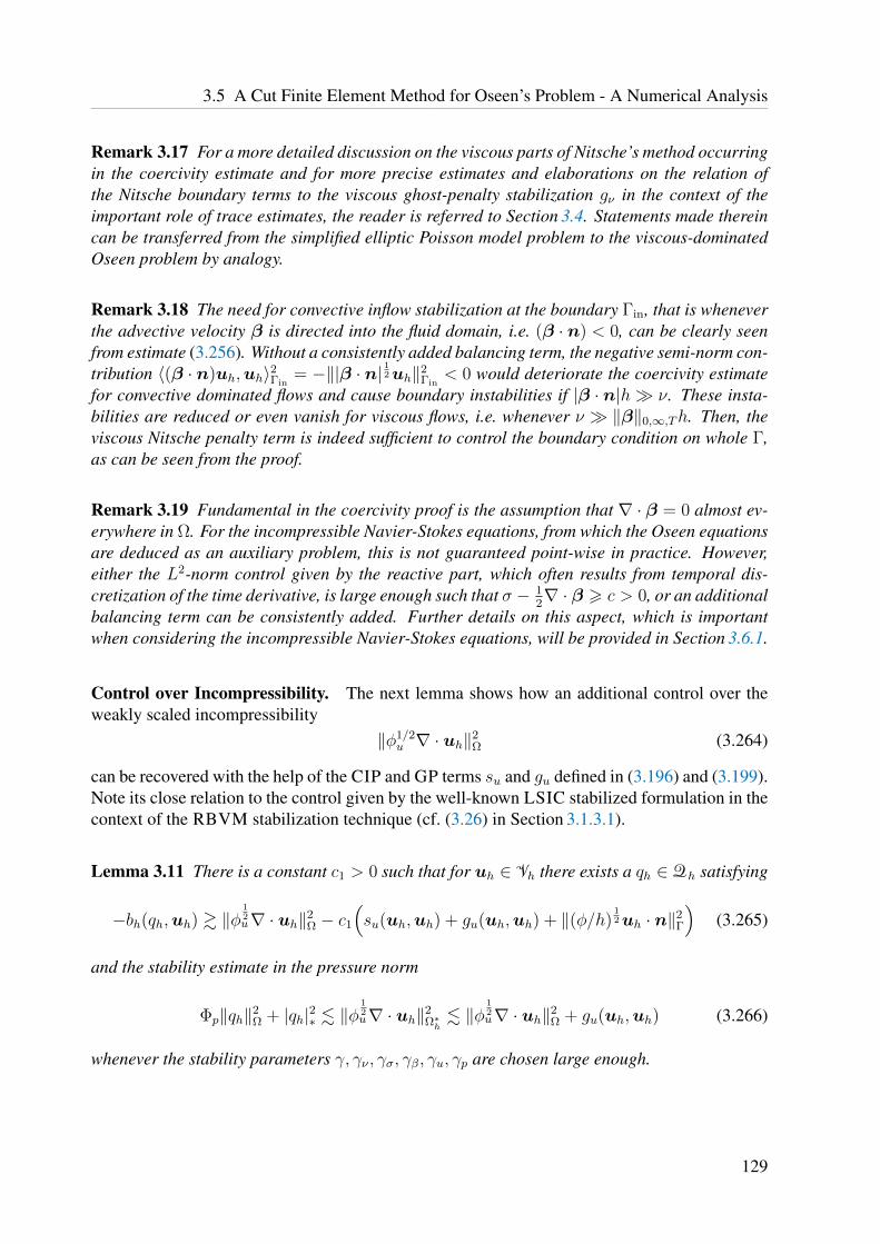
3.5 A Cut Finite Element Method for Oseen’s Problem - A Numerical Analysis

Remark 3.17 For a more detailed discussion on the viscous parts of Nitsche’s method occurringin the coercivity estimate and for more precise estimates and elaborations on the relation ofthe Nitsche boundary terms to the viscous ghost-penalty stabilization gν in the context of theimportant role of trace estimates, the reader is referred to Section 3.4. Statements made thereincan be transferred from the simplified elliptic Poisson model problem to the viscous-dominatedOseen problem by analogy.

Remark 3.18 The need for convective inflow stabilization at the boundary Γin, that is wheneverthe advective velocity β is directed into the fluid domain, i.e. (β · n) < 0, can be clearly seenfrom estimate (3.256). Without a consistently added balancing term, the negative semi-norm con-tribution 〈(β · n)uh,uh〉2Γin

= −‖|β · n| 12uh‖2Γin

< 0 would deteriorate the coercivity estimatefor convective dominated flows and cause boundary instabilities if |β · n|h ν. These insta-bilities are reduced or even vanish for viscous flows, i.e. whenever ν ‖β‖0,∞,Th. Then, theviscous Nitsche penalty term is indeed sufficient to control the boundary condition on whole Γ,as can be seen from the proof.

Remark 3.19 Fundamental in the coercivity proof is the assumption that ∇ · β = 0 almost ev-erywhere in Ω. For the incompressible Navier-Stokes equations, from which the Oseen equationsare deduced as an auxiliary problem, this is not guaranteed point-wise in practice. However,either the L2-norm control given by the reactive part, which often results from temporal dis-cretization of the time derivative, is large enough such that σ − 1

2∇ · β > c > 0, or an additional

balancing term can be consistently added. Further details on this aspect, which is importantwhen considering the incompressible Navier-Stokes equations, will be provided in Section 3.6.1.

Control over Incompressibility. The next lemma shows how an additional control over theweakly scaled incompressibility

‖φ1/2u ∇ · uh‖2

Ω (3.264)

can be recovered with the help of the CIP and GP terms su and gu defined in (3.196) and (3.199).Note its close relation to the control given by the well-known LSIC stabilized formulation in thecontext of the RBVM stabilization technique (cf. (3.26) in Section 3.1.3.1).

Lemma 3.11 There is a constant c1 > 0 such that for uh ∈ Vh there exists a qh ∈Qh satisfying

−bh(qh,uh) & ‖φ12u∇ · uh‖2

Ω − c1

(su(uh,uh) + gu(uh,uh) + ‖(φ/h)

12uh · n‖2

Γ

)(3.265)

and the stability estimate in the pressure norm

Φp‖qh‖2Ω + |qh|2∗ . ‖φ

12u∇ · uh‖2

Ω∗h. ‖φ

12u∇ · uh‖2

Ω + gu(uh,uh) (3.266)

whenever the stability parameters γ, γν , γσ, γβ, γu, γp are chosen large enough.

129

3 Developing Stabilized Cut Finite Element Methods for Incompressible Flow

Proof. Define qhdef= Oh(φu∇ · uh) with φu

def= O1

h(φu) being a smoothed, piecewise linear versionof φu as defined in (3.215), for which local comparability in the sense of φu|T ∼ φu|T (3.216)holds. Then

−bh(qh,uh) = ‖φ12u∇ · uh‖2

Ω

+ (Oh(φu∇ · uh)− φu∇ · uh,∇ · uh)Ω − 〈Oh(φu∇ · uh),uh · n〉Γ (3.267)

= ‖φ12u∇ · uh‖2

Ω + I + II. (3.268)

By using φ−1u,T φ

2u,T . φu,F , now the first term can be treated as follows

I = (φ− 1

2u (Oh(φu∇ · uh)− φu∇ · uh), φ

12u∇ · uh)Ω (3.269)

& −δ‖φ12u∇ · uh‖2

Ω − δ−1‖φ−12

u (Oh(φu∇ · uh)− φu∇ · uh)‖2Ω (3.270)

& −δ‖φ12u∇ · uh‖2

Ω − δ−1∑

F∈Fiφu,Fh‖[[∇ · uh]]‖2

F (3.271)

& −δ‖φ12u∇ · uh‖2

Ω − δ−1su(uh,uh). (3.272)

The second one can be dealt with using the mass conserving Nitsche boundary terms and φu ∼ φ

II = −〈h 12φ− 1

2u Oh(φu∇ · uh), h−

12φ

12uuh · n〉Γ (3.273)

& −δ‖h 12φ− 1

2u Oh(φu∇ · uh)‖2

Γ − δ−1‖h− 12φ

12uuh · n‖2

Γ (3.274)

& −δ‖φ−12

u Oh(φu∇ · uh)‖2Ω∗h− δ−1‖(φ/h)

12uh · n‖2

Γ (3.275)

& −δ‖φ12u∇ · uh‖2

Ω∗h− δ−1‖(φ/h)

12uh · n‖2

Γ (3.276)

& −δ(‖φ12u∇ · uh‖2

Ω + gu(uh,uh))− δ−1‖(φ/h)12uh · n‖2

Γ, (3.277)

where after applying a δ-scaled Young’s inequality and the trace inequality (3.48), the quasi-local stability property of the Oswald interpolation (3.217) and the local averaging propertyφ− 1

2u φu . φ

12u (3.216) was used. Recalling the norm equivalence (3.229) from Corollary 3.7

‖φ12u∇ · uh‖2

Ω∗h. ‖φ

12u∇ · uh‖2

Ω + gu(uh,uh), (3.278)

which was applied in the last step, results in

−bh(qh,uh) & (1− 2δ)‖φ12u∇ · uh‖2

Ω

− (δ + δ−1)(su(uh,uh) + gu(uh,uh) + ‖(φ/h)

12uh · n‖2

Γ

)(3.279)

& ‖φ12u∇ · uh‖2

Ω − c1

(su(uh,uh) + gu(uh,uh) + ‖(φ/h)

12uh · n‖2

Γ

)(3.280)

130

3.5 A Cut Finite Element Method for Oseen’s Problem - A Numerical Analysis

and completes the estimate (3.265) by choosing δ > 0 sufficiently small for some constantc1 > 0. Finally, the stability bound can be easily proven by observing that

Φp‖qh‖2Ω + |qh|2∗ . Φp‖Oh(φu∇ · uh)‖2

Ω +∑

F∈Fi

k−1∑

j=0

φp,Fh2j+1‖[[∂jnOh(φu∇ · uh)]]‖2

F (3.281)

. Φp‖φu∇ · uh‖2Th

+∑

T∈Th

φp,T‖Oh(φu∇ · uh)‖2T (3.282)

.∑

T∈Th

‖φ12u∇ · uh‖2

T . ‖φ12u∇ · uh‖2

Ω + gu(uh,uh), (3.283)

where the trace inequality (3.47), the quasi-local stability of the Oswald interpolant (3.217) andthe averaging property φpφ2

u . φu (3.216) and Φpφ2u . φu were used. The last step results from

applying the norm equivalence from Lemma 3.229.

Control over Mixed Advective-Pressure-Gradient Norm. In a next step, the subsequentlemma shows how additional control over a semi-norm of the form

‖φ12β ((β · ∇)uh +∇ph)‖2

Ω (3.284)

can be recovered, which is closely related to the well-known mixed norm control given bya SUPG/PSPG stabilized formulation in the context of the RBVM stabilization technique(cf. (3.26) in Section 3.1.3.1).

Lemma 3.12 There is a constant c2 > 0 such that for a given functionUh = (uh, ph) ∈ Wh thereexists a vh ∈ Vh satisfying

((β · ∇)uh +∇ph,vh)Ω & ‖φ12β ((β · ∇)uh +∇ph)‖2

Ω − c2(1 + ωh)|Uh|2∗ (3.285)

whenever the stability parameters γ, γν , γσ, γβ, γu, γp are chosen large enough. Note that thefirst part on the right-hand side exhibits the desired norm control. Moreover, the test functionvh, the streamline-diffusion and the incompressibility terms satisfy the stability estimate

|||vh|||2∗ + ‖φ12β (β · ∇)vh‖2

Ω + ‖φ12u∇ · vh‖2

Ω . ‖φ12β ((β · ∇)uh +∇ph)‖2

Ω + (1 + ωh)|Uh|2∗.(3.286)

Proof. To gain control of the ‖φ12β ((β · ∇)uh +∇ph)‖2

Ω term, a suitable test function vh ∈ Vh isconstructed. First, an element-wise constant, vector-valued function β0

h is introduced whichsatisfies the approximation property and stability bound from (3.205). The simplest choiceis to take the value of β at some point of T for each T ∈Th. Set wh

def= (β0

h · ∇)uh +∇phand note that wh is a piecewise polynomial function of order k − 1, however, is discontinuousbetween elements. For the piecewise constant stabilization parameter function φβ from (3.203),introduce the smoothed, continuous, piecewise linear stabilization parameter φβ

def= O1

h(φβ) as

131

3 Developing Stabilized Cut Finite Element Methods for Incompressible Flow

defined in (3.215) such that φβwh is a polynomial of order k. Finally, define the test functionvh

def= Oh(φβwh) ∈ Vh, where Oh : Xdc,k

h →Xkh denotes the Oswald interpolation onto polyno-

mials of order k as defined in (3.64) (see Section 3.2.2.2).Testing with vh and consistently adding and subtracting

± (((β · ∇)uh +∇ph), φβ(β0h · ∇)uh)Ω, (3.287)

± (((β · ∇)uh +∇ph), φβ(β · ∇)uh)Ω, (3.288)

± (((β · ∇)uh +∇ph), φβ∇ph)Ω, (3.289)

it can now be observed that

((β · ∇)uh +∇ph,vh) = ‖φ12β ((β · ∇)uh +∇ph)‖2

Ω

+ ((β · ∇)uh +∇ph,Oh(φβwh)− φβwh)Ω

+ ((β · ∇)uh +∇ph, φβ(β0h − β) · ∇uh)Ω (3.290)

= ‖φ12β ((β · ∇)uh +∇ph)‖2

Ω + I + II (3.291)

& ‖φ12β ((β · ∇)uh +∇ph)‖2

Ω − |I| − |II|, (3.292)

where in the last step the local equivalence (3.216) was used. It remains to estimate the twoterms I , II and, finally, to prove the stability bound for |||vh|||∗.Estimate of I . From successively applying a δ-Cauchy-Schwarz inequality, Lemma 3.1 toestimate the fluctuation Oh(φβwh)− φβwh, the local comparability φβ,T ∼ φβ,T and a Cauchy-Schwarz inequality, it can be deduced that

|I| = |(φ12β ((β · ∇)uh +∇ph), φ−

12

β (Oh(φβwh)− φβwh))Ω| (3.293)

. δ‖φ12β ((β · ∇)uh +∇ph)‖2

Ω + δ−1∑

T∈Th

‖φ−12

β,T (Oh(φβwh)− φβwh)‖2T∩Ω (3.294)

. δ‖φ12β ((β · ∇)uh +∇ph)‖2

Ω + δ−1∑

T∈Th

φ−1β,Th‖[[φβwh]]‖2

Fh(T ) (3.295)

. δ‖φ12β ((β · ∇)uh +∇ph)‖2

Ω + δ−1∑

T∈Th

φ−1β,T φ

2β,Fh‖[[wh]]‖2

Fh(T ) (3.296)

. δ‖φ12β ((β · ∇)uh +∇ph)‖2

Ω + δ−1∑

T∈Th

φβ,Fh‖[[(βh · ∇)uh +∇ph]]‖2Fh(T )

+ δ−1∑

T∈Th

φβ,Fh‖[[((β0h − βh) · ∇)uh]]‖2

Fh(T ) (3.297)

. δ‖φ12β ((β · ∇)uh +∇ph)‖2

Ω + δ−1(sβ(uh,uh) + sp(ph, ph) + ωh|||uh|||2∗). (3.298)

In the last step, a combination of the inverse estimate (3.47), a triangle inequality for

‖((β0h − βh) · ∇)uh‖T 6 ‖((β0

h − β) · ∇)uh‖T + ‖((β − βh) · ∇)uh‖T (3.299)

132

3.5 A Cut Finite Element Method for Oseen’s Problem - A Numerical Analysis

and estimates (3.230) and (3.231) were used to obtain∑

T∈Th

φβ,Fh‖[[((β0h − βh) · ∇)uh]]‖2

Fh(T ) . ωh|||uh|||2∗. (3.300)

Splitting the facet terms

‖[[(βh · ∇)uh +∇ph]]‖2F . ‖[[(βh · ∇)uh]]‖2

F + ‖[[∇ph]]‖2F (3.301)

for all facets F ∈ Fh(T ) and using φβ ∼ φp (3.203), these can be bounded by the CIP stabiliza-tion operators sβ and sp defined in (3.195) and (3.197). Note that estimating the fluctuation in(3.294) on T ∩ Ω requires to integrate facets F ∈ Fh(T ) in the boundary region entirely. Owingto this fact, the CIP stabilization operators gβ, gp need to be evaluated along the whole facetwhenever it is intersected by Γ.Estimate of II . By a simple application of a δ-Cauchy-Schwarz inequality and estimate (3.231)

|II| . δ‖φ12β ((β · ∇)uh +∇ph)‖2

Ω + δ−1‖φ12β ((β0

h − β) · ∇)uh‖2Ω (3.302)

. δ‖φ12β ((β · ∇)uh +∇ph)‖2

Ω + δ−1ωh(‖ν 1

2∇uh‖2Ω∗h

+ ‖σ 12uh‖2

Ω∗h

)(3.303)

. δ‖φ12β ((β · ∇)uh +∇ph)‖2

Ω + δ−1ωh|||uh|||2∗. (3.304)

Estimate of (3.285). Now choose δ > 0 small enough and combine the estimates for I and IIto conclude that

((β · ∇)uh +∇ph,vh)& ‖φ

12β ((β · ∇)uh +∇ph)‖2

Ω − |I| − |II| (3.305)

& ‖φ12β ((β · ∇)uh +∇ph)‖2

Ω − c1(sβ(uh,uh) + sp(ph, ph))− ωh|||uh|||2∗ (3.306)

& ‖φ12β ((β · ∇)uh +∇ph)‖2

Ω − c2(1 + ωh)|Uh|2∗ (3.307)

for some constant c2 > 0, where for the last step the definition of the semi-norm |Uh|∗ from(3.249) was used.Estimate of |||vh|||∗. Throughout the next steps, it will be made heavy use of the fact that

(νh−2 + ‖β‖0,∞,Th−1 + σ)φβ ∼ φuh

−2φβ ∼ φh−2φβ . 1 (3.308)

by the very definition of φβ, φu, φp and φ from (3.203).Due to the pseudo-local L2-stability property of the Oswald interpolant (3.217) and the local

comparability φβ ∼ φβ (3.216), for vh it holds

‖φOh(vh)‖Ω∗h. ‖φvh‖Ω∗h

= ‖φφβ((β0h · ∇)uh +∇ph)‖Ω∗h

(3.309)

. ‖φφβ((β0h · ∇)uh +∇ph)‖Ω∗h

. (3.310)

Starting with the viscous and reaction terms from the norm definition (3.246), it holds

ν‖∇vh‖2Ω∗h

+ σ‖vh‖2Ω∗h

. (νh−2 + σ)‖φβ((β0h · ∇)uh +∇ph)‖2

Ω∗h(3.311)

. (νh−2 + σ)φβ︸ ︷︷ ︸.1 see (3.308)

‖φβ12 ((β0

h · ∇)uh +∇ph)‖2Ω∗h, (3.312)

133

3 Developing Stabilized Cut Finite Element Methods for Incompressible Flow

where for the reaction term an inverse inequality (3.46) has been applied, followed by (3.310).Turning to the boundary terms appearing in ||| · |||∗, the convective boundary part is bounded by

‖|β · n| 12vh‖2Γ .

∑

T∈TΓ

‖β‖0,∞,T‖Oh(vh)‖2T∩Γ (3.313)

.∑

T∈TΓ

‖β‖0,∞,T‖Oh(φβ((β0h · ∇)uh +∇ph))‖2

T∩Γ (3.314)

.∑

T∈TΓ

‖β‖0,∞,Th−1φβ︸ ︷︷ ︸

.1 see (3.308)

‖φ12β ((β0

h · ∇)uh +∇ph)‖2T , (3.315)

where the trace inequality (3.48) was used to pass from T ∩ Γ to T . The remaining boundaryterms can be similarly bounded:

‖(ν/h)12vh‖2

Γ + ‖(φ/h)12vh · n‖2

Γ .∑

T∈TΓ

(ν + φ)h−2φβ︸ ︷︷ ︸.1 see (3.308)

‖φ12β ((β0

h · ∇)uh +∇ph)‖2T . (3.316)

Next, the velocity related norm terms contributed from the stabilization operators SCIPh and GGP

h

need to be estimated. A bound for sβ(vh,vh) and su(vh,vh) can be derived by first employingthe trace and inverse inequalities (3.47) and (3.46) and then recalling the definition of vh andestimate (3.308):

sβ(vh,vh) .∑

F∈Fi

φβ,Fh‖[[(βh · ∇)vh]]‖2F .

∑

T∈Th

‖β‖20,∞,Th

−2φβ,T‖vh‖2T (3.317)

.∑

T∈Th

‖β‖20,∞,Th

−2φ2β,T︸ ︷︷ ︸

.1 see (3.308)

‖φ12β ((β0

h · ∇)uh +∇ph)‖2T , (3.318)

su(vh,vh) .∑

F∈Fi

φu,Fh‖[[∇ · vh]]‖2F .

∑

T∈Th

φu,Th−2‖vh‖2

T (3.319)

.∑

T∈Th

φu,Th−2φβ,T︸ ︷︷ ︸

.1 see (3.308)

‖φ12β ((β0

h · ∇)uh +∇ph)‖2T . (3.320)

The corresponding ghost-penalty terms can be estimated in the exact same manner, yielding

gβ(vh,vh) + gu(vh,vh) . ‖φ12β ((β0

h · ∇)uh +∇ph)‖2Ω∗h, (3.321)

where it was applied a trace inequality (3.47). Finally, another application of the inverse es-timate (3.47) in combination with the already established bound (3.312) for the viscous andreaction norm terms gives

gν(vh,vh) + gσ(vh,vh) . ‖ν12∇vh‖2

Ω∗h+ ‖σ 1

2vh‖2Ω∗h

. ‖φ12β ((β0

h · ∇)uh +∇ph)‖2Ω∗h. (3.322)

Estimate of ‖φ12β (β · ∇)vh‖Ω. Similarly, the streamline-diffusion term in (3.286) can be bounded

‖φ12β (β · ∇)vh‖2

Ω .∑

T∈Th

‖β‖20,∞,Th

−2φβ,T‖vh‖2T (3.323)

.∑

T∈Th

‖β‖20,∞,Th

−2φ2β,T︸ ︷︷ ︸

.1 see (3.308)

‖φ12β ((β0

h · ∇)uh +∇ph)‖2T . (3.324)

134

3.5 A Cut Finite Element Method for Oseen’s Problem - A Numerical Analysis

Estimate of ‖φ12u∇ · vh‖Ω. The incompressibility term can be estimated similarly

‖φ12u∇ · vh‖2

Ω = ‖φ12u∇ · Oh(φβ((β0

h · ∇)uh +∇ph))‖2Ω (3.325)

. ‖φ−12

β φβ((β0h · ∇)uh +∇ph)‖2

Ω∗h(3.326)

. ‖φ12β ((β0

h · ∇)uh +∇ph)‖2Ω∗h, (3.327)

where an inverse inequality, the stability of the Oswald interpolant and φu ∼ h2φ−1β was used.

Estimate of (3.286). After collecting all terms and employing estimate (3.232), the desiredstability bound is obtained:

|||vh|||2∗ + ‖φ12β (β · ∇)vh‖2

Ω + ‖φ12u∇ · vh‖2

Ω

. ‖φ12β ((β0

h · ∇)uh +∇ph)‖2Ω∗h

(3.328)

. ‖φ12β ((β · ∇)uh +∇ph)‖2

Ω

+ gβ(uh,uh) + gp(ph, ph) + ωh(‖ν 1

2∇uh‖2Ω∗h

+ ‖σ 12uh‖2

Ω∗h

)(3.329)

. ‖φ12β ((β · ∇)uh +∇ph)‖2

Ω + (1 + ωh)|Uh|2∗. (3.330)

The following lemma provides useful estimates of the velocity energy norm |||vh|||∗ and theadvective term (uh, (β · ∇)vh)Ω and motivates the definition of the pressure L2-norm scalingΦp from (3.223).

Lemma 3.13 Let uh,vh ∈ Vh, then the following estimates hold

|||vh|||∗ + (1 + ωh)− 1

2‖φ12β (β · ∇)vh‖Ω + ‖φ

12u∇ · vh‖Ω

.(ν + ‖β‖0,∞,Ωh+ σC2

P

) 12(‖∇vh‖Ω∗h

+ ‖h− 12vh‖Γ

)(3.331)

. Φ− 1

2p

(‖∇vh‖Ω∗h

+ ‖h− 12vh‖Γ

), (3.332)

|(uh,β · ∇vh)Ω| . |||uh|||∗‖β‖0,∞,ΩCP√ν + σC2

P

‖∇vh‖Ω . |||uh|||∗Φ−12

p ‖∇vh‖Ω. (3.333)

Proof. It is started with estimate (3.332). The reactive term in the norm definition (3.246) can bebounded using the Poincare inequality (3.53) showing that

‖ν 12∇vh‖2

Ω + ‖σ 12vh‖2

Ω . (ν + σC2P )(‖∇vh‖2

Ω + ‖h− 12vh‖2

Γ). (3.334)

The remaining bulk terms can be estimated as

(1 + ωh)−1‖φ

12β (β · ∇)vh‖2

Ω + ‖φ12u∇ · vh‖2

Ω

. ‖β‖0,∞,Ωh‖∇vh‖2Ω∗h

+ (ν + ‖β‖0,∞,Ωh+ σh2)‖∇vh‖2Ω∗h. (3.335)

135

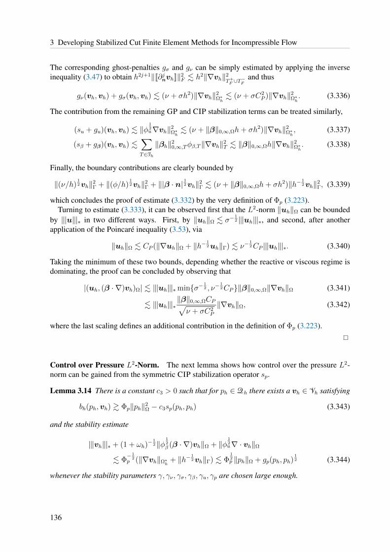
3 Developing Stabilized Cut Finite Element Methods for Incompressible Flow

The corresponding ghost-penalties gσ and gν can be simply estimated by applying the inverseinequality (3.47) to obtain h2j+1‖[[∂jnvh]]‖2

F . h2‖∇vh‖2T+F ∪T

−F

and thus

gν(vh,vh) + gσ(vh,vh) . (ν + σh2)‖∇vh‖2Ω∗h

. (ν + σC2P )‖∇vh‖2

Ω∗h. (3.336)

The contribution from the remaining GP and CIP stabilization terms can be treated similarly,

(su + gu)(vh,vh) . ‖φ12u∇vh‖2

Ω∗h. (ν + ‖β‖0,∞,Ωh+ σh2)‖∇vh‖2

Ω∗h, (3.337)

(sβ + gβ)(vh,vh) .∑

T∈Th

‖βh‖20,∞,Tφβ,T‖∇vh‖2

T . ‖β‖0,∞,Ωh‖∇vh‖2Ω∗h. (3.338)

Finally, the boundary contributions are clearly bounded by

‖(ν/h)12vh‖2

Γ + ‖(φ/h)12vh‖2

Γ + ‖|β · n| 12vh‖2Γ . (ν + ‖β‖0,∞,Ωh+ σh2)‖h− 1

2vh‖2Γ, (3.339)

which concludes the proof of estimate (3.332) by the very definition of Φp (3.223).Turning to estimate (3.333), it can be observed first that the L2-norm ‖uh‖Ω can be bounded

by |||u|||∗ in two different ways. First, by ‖uh‖Ω . σ−12 |||uh|||∗, and second, after another

application of the Poincare inequality (3.53), via

‖uh‖Ω . CP (‖∇uh‖Ω + ‖h− 12uh‖Γ) . ν−

12CP |||uh|||∗. (3.340)

Taking the minimum of these two bounds, depending whether the reactive or viscous regime isdominating, the proof can be concluded by observing that

|(uh, (β · ∇)vh)Ω| . |||uh|||∗minσ− 12 , ν−

12CP‖β‖0,∞,Ω‖∇vh‖Ω (3.341)

. |||uh|||∗‖β‖0,∞,ΩCP√ν + σC2

P

‖∇vh‖Ω, (3.342)

where the last scaling defines an additional contribution in the definition of Φp (3.223).

Control over Pressure L2-Norm. The next lemma shows how control over the pressure L2-norm can be gained from the symmetric CIP stabilization operator sp.

Lemma 3.14 There is a constant c3 > 0 such that for ph ∈Qh there exists a vh ∈ Vh satisfying

bh(ph,vh) & Φp‖ph‖2Ω − c3sp(ph, ph) (3.343)

and the stability estimate

|||vh|||∗ + (1 + ωh)− 1

2‖φ12β (β · ∇)vh‖Ω + ‖φ

12u∇ · vh‖Ω

. Φ− 1

2p (‖∇vh‖Ω∗h

+ ‖h− 12vh‖Γ) . Φ

12p ‖ph‖Ω + gp(ph, ph)

12 (3.344)

whenever the stability parameters γ, γν , γσ, γβ, γu, γp are chosen large enough.

136

3.5 A Cut Finite Element Method for Oseen’s Problem - A Numerical Analysis

Proof. For given ph ∈ Qh, the test function vh is constructed in two steps following Verfurth’stechnique.Step 1. Due to the surjectivity of the divergence operator ∇· : [H1

0 (Ω)]d → L2(Ω) there existsa function vp ∈ [H1

0 (Ω)]d such that ∇ · vp = −Φpph and ‖vp‖1,Ω ∼ ‖∇vp‖Ω . Φp‖ph‖Ω. Toobtain a discrete test function, set v1

hdef= π∗hvp ∈ Vh based on the Clement interpolant (see Sec-

tion 3.2.2.2). Recall that vp|Γ = 0, since vp ∈ H10 (Ω), to get

bh(ph,v1h) = bh(ph,vp) + bh(ph,π

∗hvp − vp) (3.345)

= −(ph,∇ · vp)Ω + (∇ph, (π∗hvp − vp))Ω (3.346)

= Φp‖ph‖2Ω +

(Φ

12p h∇ph,Φ−

12

p h−1(π∗hvp − vp))

Ω, (3.347)

where the second term in (3.345) was integrated by parts using the fact that ph ∈ C0(Ω). Nowa combination of a δ-scaled Cauchy-Schwarz inequality, the interpolation estimate (3.61), andfinally, the stability bound ‖∇vp‖Ω . Φp‖ph‖Ω yields

bh(ph,v1h) & Φp‖ph‖2

Ω − δ−1‖Φ12p h∇ph‖2

Ω − δΦ−1p ‖vp‖2

1,Ω (3.348)

& (1− δ)Φp‖ph‖2Ω − δ−1‖Φ

12p h∇ph‖2

Ω. (3.349)

Step 2. Next, it is shown how to compensate for the ‖Φ12p h∇ph‖2

Ω term appearing in (3.349) usingthe stabilization form sp. To construct a suitable test function, set v2

hdef= Φph

2Oh(∇ph) ∈ Vh,where Oh denotes the Oswald interpolation (3.64) (see Section 3.2.2.2). Then inserting v2

h into bhshows after an integration by parts that

bh(ph,v2h) = −(ph,∇ · v2

h)Ω + 〈ph,v2h · n〉Γ (3.350)

= (∇ph,Φph2Oh(∇ph))Ω (3.351)

= ‖Φ12p h∇ph‖2

Ω +(Φ

12p h∇ph,Φ

12p h(Oh(∇ph)−∇ph)

)Ω

(3.352)

& (1− δ)‖Φ12p h∇ph‖2

Ω − δ−1sp(ph, ph), (3.353)

where it was combined a δ-scaled Young’s inequality and the Oswald interpolant Lemma 3.1 togain control over the fluctuation in terms of the pressure CIP operator

‖Φ12p h(Oh(∇ph)−∇ph)‖2

Ω .∑

F∈Fi

Φph2

︸︷︷︸.φp,F

h‖[[∇ph]]‖2F . sp(ph, ph). (3.354)

Finally, using the same δ ∼ 0.5 in (3.349) and (3.353), it is set vhdef= v1

h + 2δ−1v2h yielding

bh(ph,vh) & Φp‖ph‖2Ω − c3sp(ph, ph) (3.355)

for some constant c3 > 0.Estimate (3.344). Utilizing the stability bound (3.332) for vh it is sufficient to prove

‖∇v1h‖Ω∗h

+ ‖h− 12v1

h‖Γ = ‖∇π∗hvp‖Ω∗h+ ‖h− 1

2 (π∗hvp − vp)‖Γ (3.356)

. ‖∇π∗hvp‖Ω∗h+ ‖h−1(π∗hvp − vp)‖Ω∗h

(3.357)

. ‖∇vp‖Ω . Φp‖ph‖Ω, (3.358)

137

3 Developing Stabilized Cut Finite Element Methods for Incompressible Flow

where it was used the fact that vp|Γ = 0, followed by a trace inequality and the interpolationand stability properties of the Clement interpolant (3.61) and (3.63). After applying inverseinequalities (3.46) and (3.48), the pseudo-local stability property of the Oswald interpolant(3.217) and an inverse estimate, it equivalently holds

‖∇v2h‖Ω∗h

+ ‖h− 12v2

h‖Γ . ‖h−1v2h‖Ω∗h

. ‖h−1Oh(h2Φp∇ph)‖Ω∗h

(3.359)

. ‖hΦp∇ph‖Ω∗h. ‖Φpph‖Ω∗h

(3.360)

. Φp‖ph‖Ω + Φ12p gp(ph, ph)

12 , (3.361)

where in the last step, the ghost-penalty norm equivalence for the pressure from Corollary 3.7was applied. Consequently, combing the stability bounds (3.358) and (3.361) with stabilitybound (3.332) from Lemma 3.13 gives

|||vh|||∗ + (1 + ωh)− 1

2‖φ12β (β · ∇)vh‖Ω + ‖φ

12u∇ · vh‖Ω

. Φ− 1

2p (‖∇vh‖Ω∗h

+ ‖h− 12v‖Γ) . Φ

12p ‖ph‖Ω + gp(ph, ph)

12 . (3.362)

Global Inf-Sup Stability of ACIP/GPh with respect to |||Uh|||∗. As a consequence of the previ-

ous lemmas it can be now proven that the bilinear form ACIP/GPh defined in (3.186) satisfies an

inf-sup condition with respect to the energy-type norm (3.250)

|||Uh|||2∗ = |Uh|2∗ + ‖φ12u∇ · uh‖2

Ω +1

1 + ωh‖φ

12β (β · ∇uh +∇ph)‖2

Ω + Φp‖ph‖2Ω, (3.363)

which is constructed from the semi-norm |Uh|2∗ (3.249) and additional norm parts ‖φ1/2u ∇ · uh‖2

Ω,‖φ1/2

β (β · ∇uh +∇ph)‖2Ω and Φp‖ph‖2

Ω as treated in Lemma 3.11, 3.12 and 3.14. This finallyguarantees existence and uniqueness of a discrete velocity and pressure solution of the cut finiteelement formulation (3.186). The global inf-sup stability estimate reads as follows:

Theorem 3.15 (Global Inf-Sup Stability) Let Uh = (uh, ph) ∈ Wh be a pair of discrete veloc-ity and pressure functions. Then, under the assumptions of Lemma 3.10, 3.11, 3.12 and 3.14 onthe stabilization parameters, the cut finite element formulation is inf-sup stable

|||Uh|||∗ . supVh∈Wh\0

Bh(Uh, Vh) + SCIPh (Uh, Vh) + GGP

h (Uh, Vh)

|||Vh|||∗, (3.364)

where the hidden stability constant is independent of the mesh size h and the position of theboundary relative to the background mesh.

Proof. For given Uh ∈ Wh a suitable test function Vh ∈ Wh is constructed on basis of statementsprovided in Lemma 3.10, 3.11, 3.12 and 3.14. Fundamental idea thereby is to combine the

138

3.5 A Cut Finite Element Method for Oseen’s Problem - A Numerical Analysis

semi-norm control given by the Nitsche terms and the viscous and reactive ghost penalties(see Lemma 3.10) with additional control gained by the convective and pressure stabilizationssβ, gβ, sp, gp (see Lemma 3.12) and by the divergence stabilizations su, gu (see Lemma 3.11).Moreover, control over the pressure L2-norm is obtained by utilizing the pressure stabilizationssp, gp (see Lemma 3.14).Step 1. In a first step, control of the weakly scaled divergence ∇ · uh is gained by testing withthe function V 1

hdef= (0, q1

h) with q1h chosen as in Lemma 3.11. Then

(Bh + SCIPh + GGP

h )(Uh, V1h )

= −bh(q1h,uh) + sp(ph, q

1h) + gp(ph, q

1h) (3.365)

& ‖φ12u∇ · uh‖2

Ω − c1

(su(uh,uh) + gu(uh,uh) + ‖(φ/h)

12uh · n‖2

Γ

)

− δ−1(sp(ph, ph) + gp(ph, ph)

)− δ(sp(q

1h, q

1h) + gp(q

1h, q

1h))

(3.366)

& (1− δ)‖φ12u∇ · uh‖2

Ω − (c1 + δ + δ−1)|Uh|2∗ (3.367)

& ‖φ12u∇ · uh‖2

Ω − C1(δ)|Uh|2∗, (3.368)

where in (3.366) the stability estimate (3.266) was used for |q1h|2∗ = sp(q

1h, q

1h) + gp(q

1h, q

1h) (see

definition (3.248)).Step 2. Next, for the same Uh it is set V 2

hdef= (v2

h, 0) with v2h taken from Lemma 3.12 and q2

h = 0.Inserting V 2

h into Bh and integrating the remaining bh by parts leads to

Bh(Uh, V2h )

= ah(uh,v2h) + bh(ph,v

2h) (3.369)

& −|||uh|||∗|||v2h|||∗ + ((β · ∇)uh +∇ph,v2

h)Ω (3.370)

& −δ−1|||uh|||2∗ − δ|||v2h|||2∗ + ‖φ

12β ((β · ∇)uh +∇ph)‖2

Ω − c2(1 + ωh)|Uh|2∗ (3.371)

& (1− δ)‖φ12β ((β · ∇)uh +∇ph)‖2

Ω − (c2(1 + ωh) + δ−1 + δ(1 + ωh))|Uh|2∗. (3.372)

To obtain (3.370), the boundedness of ah with respect to ||| · |||∗ is used, which is obtainedby simply applying Cauchy-Schwarz inequalities to all terms except for the non-symmetricadvective bulk term. The latter one is comprised with the pressure gradient resulting fromintegration by parts for bh. Utilizing estimate (3.285) and applying a δ-scaled Young’s inequalityyields (3.371). After employing the stability bound (3.286) and the estimate |||uh|||∗ . |Uh|∗(see definition (3.249)) and resorting of the resulting terms, the estimate (3.372) is obtained.Performing the same steps to the remaining stabilization terms SCIP

h + GGPh shows that

(SCIPh + GGP

h )(Uh, V2h )

& −δ−1|||uh|||2∗ − δ|||v2h|||2∗ (3.373)

& −δ‖φ12β ((β · ∇)uh +∇ph)‖2

Ω − (δ−1 + δ(1 + ωh))|Uh|2∗, (3.374)

where for (3.374) the stability estimate (3.286) for v2h was used. Thus after combining (3.372)

and (3.374) and choosing δ ∼ 0.25 sufficiently small, it holds

(Bh + SCIPh + GGP

h )(Uh, V2h ) & ‖φ

12β ((β · ∇)uh +∇ph)‖2

Ω − C2(δ)(1 + ωh)|Uh|2∗, (3.375)

owing to the fact that (1 + c2)(1 + ωh) + 2δ−1 + 2δ(1 + ωh) . (1 + ωh).

139

3 Developing Stabilized Cut Finite Element Methods for Incompressible Flow

Step 3. The pressure L2-norm term can be constructed by testing with V 3h = (v3

h, 0) where v3h

is now chosen as in Lemma 3.14. Then, by making use of the estimates (3.332), (3.333) and(3.344) and after integrating the advective term by parts

Bh(Uh, V3h ) = ah(uh,v

3h) + bh(ph,v

3h) (3.376)

& −|||uh|||∗|||v3h|||∗ − (uh,β · ∇v3

h)Ω + Φp‖ph‖2Ω − c3sp(ph, ph) (3.377)

& −δ−1|||uh|||2∗ − δΦ−1p (‖∇v3

h‖2Ω∗h

+ ‖h− 12v3

h‖2Γ)

− δ−1|||uh|||2∗ − δΦ−1p ‖∇v3

h‖2Ω + Φp‖ph‖2

Ω − c3sp(ph, ph) (3.378)

& (1− 2δ)Φp‖ph‖2Ω − 2δ−1|||uh|||2∗ − c3sp(ph, ph)− 2δgp(ph, ph) (3.379)

& (1− 2δ)Φp‖ph‖2Ω − (c3 + 2δ + 2δ−1)|Uh|2∗. (3.380)

Analogously to Step 2, by using (3.344) the stabilization terms can be estimated as

(SCIPh + GGP

h )(Uh, V3h ) & −|||uh|||∗|||v3

h|||∗ (3.381)& −δΦp‖ph‖2

Ω − δgp(ph, ph)− δ−1|||uh|||2∗ (3.382)& −δΦp‖ph‖2

Ω − (δ + δ−1)|Uh|2∗ (3.383)

such that after combining (3.380) and (3.383)

(Bh + SCIPh + GGP

h )(Uh, V3h ) & Φp‖ph‖2

Ω − C3(δ)|Uh|2∗. (3.384)

Step 4. To gain control over the last missing |Uh|2∗ term in the definition of (3.250), set V 4h

def= Uh.

The coercivity estimate from Lemma 3.10 shows that

Bh(Uh, V4h ) + SCIP

h (Uh, V4h ) + GGP

h (Uh, V4h ) & |Uh|2∗. (3.385)

Step 5. Finally it is chosen δ sufficiently small. For given Uh, the final test function is defined as

V 5h

def= η(V 1

h + (1 + ωh)−1V 2

h + V 3h ) + V 4

h . (3.386)

Choosing η > 0 sufficiently small for some 2η ∼ (C1(δ) + C2(δ) + C3(δ))−1 allows to gaincontrol over all desired norm parts in |||Uh|||∗ and at the same time to absorb the defective |Uh|∗-contribution, which results from testing with V 1

h , V2h , V

3h , by the |Uh|∗-control obtained from

testing with V 4h . Consequently,

(Bh + SCIPh + GGP

h )(Uh, V5h )

& (1− η(C1(δ) + C2(δ) + C3(δ)))|Uh|2∗+ η

(‖φ

12u∇ · uh‖2

Ω +1

1 + ωh‖φ

12β ((β · ∇)uh +∇ph)‖2

Ω + Φp‖ph‖2Ω

)(3.387)

& |||Uh|||2∗. (3.388)

For inf-sup stability, it still remains to proof that |||V 5h |||∗ . |||Uh|||∗, where

|||V 5h |||∗ 6 |||Uh|||∗ + η|||V 1

h |||∗ +η

1 + ωh|||V 2

h |||∗ + η|||V 3h |||∗. (3.389)

140

3.5 A Cut Finite Element Method for Oseen’s Problem - A Numerical Analysis

Thanks to the stability estimate (3.286) and norm definitions (3.249) and (3.250) it holds

|||V 2h |||2∗ = |V 2

h |2∗ +1

1 + ωh‖φ

12β ((β · ∇)v2

h + 0)‖2Ω + ‖φ

12u∇ · v2

h‖2Ω (3.390)

= |||v2h|||2∗ + gp(0, 0) + sp(0, 0) +

1

1 + ωh‖φ

12β (β · ∇)v2

h‖2Ω + ‖φ

12u∇ · v2

h‖2Ω (3.391)

. (1 +1

1 + ωh)(‖φ

12β ((β · ∇)u2

h +∇ph)‖2Ω + (1 + ωh)|Uh|2∗) (3.392)

. (1 +1

1 + ωh)(1 + ωh)|||Uh|||2∗ (3.393)

. (1 + ωh)|||Uh|||2∗. (3.394)

Similarly, the stability bound (3.266) for q1h implies that |||V 1

h |||2∗ = Φp‖q1h‖2

Ω + |q1h|2∗ . |||Uh|||2∗

and from (3.344) it is obtained that

|||V 3h |||2∗ = |||v3

h|||2∗ + (1 + ωh)−1‖φ

12β (β · ∇)v3

h‖2Ω + ‖φ

12u∇ · v3

h‖2Ω (3.395)

. Φ−1p (‖∇v3

h‖2Ω∗h

+ ‖v3hh− 1

2‖2Γ) . |||Uh|||2∗. (3.396)

As a result it holds

|||V 5h |||∗ . (1 + η + η(1 + ωh)

− 12 + η)|||Uh|||∗ . |||Uh|||∗. (3.397)

This concludes the proof of inf-sup stability with

(Bh + SCIPh + GGP

h )(Uh, V5h ) & |||Uh|||∗|||V 5

h |||∗, (3.398)

followed by a division by |||V 5h |||∗ and choosing the supremum over Vh ∈ Wh\0.

Remark 3.20 As a major consequence of the previous inf-sup stability theorem, existence anduniqueness of a discrete solution Uh = (uh, ph) ∈ Wh of the stabilized Nitsche-type cut finiteelement method is guaranteed.

Remark 3.21 Note that in the previous theorem inf-sup stability is proven with respect to anenergy-norm |||Uh|||∗, which is based on the underlying (active) background mesh Th. Thereby,the different ghost-penalty operators gν , gσ, gβ, gu, gp ensure sufficient control over discrete poly-nomials defined on the entire (active) computational mesh and so significantly improve thesystem conditioning of the resulting linear matrix system - for all different flow regimes andindependent of how the boundary intersects the mesh. For further details on the improvementof the system conditioning owing to the use of ghost-penalties, the reader is referred to Sec-tions 3.4.1 and 3.4.3 with regard to detailed elaborations and to works by Burman and Hansbo[45] and Massing et al. [180] for numerical analyses.

141

3 Developing Stabilized Cut Finite Element Methods for Incompressible Flow

3.5.6 A Priori Error EstimatesEquipped with the inf-sup condition (3.364), the main a priori error estimates can be proven asstated in Theorem 3.19 at the end of this section. It is proceeded in four steps. First, a weakGalerkin orthogonality property for Bh is provided. Second, a further lemma is concerned withpotential consistency errors introduced by the CIP and GP stabilization forms SCIP

h and GGPh

and, third, interpolation error estimates are derived. Finally, the previous steps are combined andan a priori estimate is proven for the velocity and pressure error.

Galerkin Orthogonality. The first lemma shows that the discrete formulation (3.186) satisfiesa weakened form of the Galerkin orthogonality.

Lemma 3.16 Suppose that the solution Udef= (u, p) of the variational formulation (3.180) is

in [H2(Ω)]d ×H1(Ω) and let Uhdef= (uh, ph) ∈ Vh ×Qh be the finite element solution to the

discrete weak formulation (3.186). Then

Bh(U − Uh, Vh) = SCIPh (Uh, Vh) + GGP

h (Uh, Vh). (3.399)

Proof. The proof follows immediately from the fact that the continuous solution U satisfiesBh(U, Vh) = Lh(Vh) due to the definition of the weak problem (3.180) and the strong consis-tency of all boundary terms related to the Nitsche method.

Consistency Error Estimates. The next lemma ensures that the remainder term arising inthe weakened Galerkin orthogonality (3.399) does not deteriorate the convergences rate of theproposed scheme and thus is weakly consistent.

Lemma 3.17 Assume that the solution U provides the regularity (u, p) ∈ [Hr(Ω)]d ×Hs(Ω)

and let rudef= minr, k + 1 and sp

def= mins, k + 1, where k is the polynomial degree of the

approximation spaces for the velocity and pressure. Then

SCIPh (Π∗hU,Π

∗hU) + GGP

h (Π∗hU,Π∗hU) . (ν + ‖β‖0,∞,Ωh+ σh2)h2ru−2‖u‖2

ru,Ω

+ maxT∈Th

1

ν + ‖β‖0,∞,Th+ σh2

h2sp‖p‖2

sp,Ω, (3.400)

where Π∗hU ∈ Wh denotes the Clement interpolant of the velocity and pressure solution U .

Proof. Recall the definition of the GP operators

GGPh (Π∗hU,Π

∗hU) = gσ(π∗hu,π

∗hu) + gν(π

∗hu,π

∗hu) + gβ(π∗hu,π

∗hu) + gu(π

∗hu,π

∗hu)

+ gp(π∗hp, π

∗hp), (3.401)

it is enough to derive the desired estimate for gβ and gp. All other terms can be bounded similarly.

142

3.5 A Cut Finite Element Method for Oseen’s Problem - A Numerical Analysis

Owing to the fact that p ∈ Hsp(Ω), its traces ∂jnp|F at interior faces F ∈ Fi are uniquelydefined for 0 6 j 6 sp − 1 and therefore, [[∂jnp]] = 0. Consequently

gp(π∗hp, π

∗hp) .

∑

F∈FΓ

k∑

j=1

φp,Fh2j−1〈[[∂jnπ∗hp]], [[∂jnπ∗hp]]〉F (3.402)

=∑

F∈FΓ

(sp−1∑

j=1

φp,Fh2j−1〈[[∂jn(π∗hp− p)]], [[∂jn(π∗hp− p)]]〉F (3.403)

+k∑

j=sp

φp,Fh2j−1〈[[∂jnπ∗hp]], [[∂jnπ∗hp]]〉F

)= Ip + IIp, (3.404)

where Ip and IIp represents the consistent and inconsistent part of the ghost-penalty term gp,respectively. Now, using trace and inverse inequalities (3.49) and (3.46), the interpolationestimate for π∗h (3.61) and the definition of φp (3.203)

Ip .∑

F∈FΓ

sp−1∑

j=1

φp,Fh2j−1‖Dj(π∗hp− p)‖2

F (3.405)

.∑

T∈TΓ

sp−1∑

j=1

φp,Th2j−1

(h−1‖Dj(π∗hp− p)‖2

T + h‖Dj+1(π∗hp− p)‖2T

)(3.406)

.∑

T∈TΓ

(φp,Th2j−1h−1h2sp−2j)‖p∗‖2

sp,ω(T ) (3.407)

. maxT∈Th

1

ν + ‖β‖0,∞,Th+ σh2

h2sp‖p∗‖2

sp,Ω. (3.408)

To estimate IIp, the trace and inverse inequalities (3.47) and (3.46) are simply combined withthe stability (3.63) of the interpolator π∗h

IIp .∑

F∈FΓ

k∑

j=sp

φp,Fh2j−1([[∂jnπ

∗hp]], [[∂

jnπ∗hp]])F (3.409)

.∑

T∈TΓ

k∑

j=sp

φp,Th2j−2‖Djπ∗hp‖2

T (3.410)

.∑

T∈TΓ

φp,Th2sp−2‖Dspπ∗hp‖2

T . maxT∈Th

1

ν + ‖β‖0,∞,Th+ σh2

h2sp‖p∗‖2

sp,Ω. (3.411)

Together with the stability of the extension operator (3.57), this yields the desired estimate.The corresponding estimates for gν , gσ and gu can be derived analogously, resulting in

gν(π∗hu,π

∗hu) . νh2ru−2‖u‖2

ru,Ω, (3.412)

gσ(π∗hu,π∗hu) . (σh2)h2ru−2‖u‖2

ru,Ω, (3.413)

gu(π∗hu,π

∗hu) . φuh

2ru−2‖u‖2ru,Ω (3.414)

. (ν + ‖β‖0,∞,Ωh+ σh2)h2ru−2‖u‖2ru,Ω. (3.415)

143

3 Developing Stabilized Cut Finite Element Methods for Incompressible Flow

Special attention has to be directed to gβ . Since u ∈ [Hr(Ω)]d, its traces ∂jnu|F are uniquelydefined for 0 6 j 6 ru − 1 and therefore [[(βh · ∇)∂jnu]] = 0 for 0 6 j 6 ru − 2. Consequently

gβ(π∗hu,π∗hu) .

∑

F∈FΓ

(ru−2∑

j=0

h2j−1‖φ12β,F [[(βh · ∇)∂jn(π∗hu− u)]]‖2

F

+k−1∑

j=ru−1

h2j−1‖φ12β,F [[(βh · ∇)∂jnπ

∗hu]]‖2

F

)= Iβ + IIβ. (3.416)

The interpolation estimate (3.62) together with the fact that by definition of the stabilizationparameter φβ,T . ‖β‖0,∞,Th implies now that the first term can be bounded by

Iβ .∑

T∈Th

ru−2∑

j=0

h2j−1φβ,T‖βh‖20,∞,T‖∇∂jn(π∗hu− u)‖2

∂T (3.417)

.∑

T∈Th

‖β‖0,∞,Th2ru−1‖u∗‖2

ru,ω(T ) . ‖β‖0,∞,Ωh2ru−1‖u‖2

ru,Ω. (3.418)

Turning to the second term IIβ , a simple application of the inverse estimate (3.47) shows that

IIβ .∑

T∈Th

φβ,T‖β‖20,∞,Th

2ru−2‖Druπ∗hu‖2T . ‖β‖0,∞,Ωh

2ru−1‖u‖2ru,Ω (3.419)

after observing that π∗h is stable thanks to (3.63).The estimate for GGP

h being replaced by SCIPh now follows simply by applying the same

estimates to all interior facets F ∈ Fi.

Interpolation Error Estimates. The next lemma ensures that the interpolation error betweencontinuous solution and its Clement interpolation converges with optimal rates.

Lemma 3.18 Assume that u ∈ [Hr(Ω)]d and p ∈ Hs(Ω) and let rudef= minr, k + 1 > 2 and

spdef= mins, k + 1 > 1 where k is the polynomial degree of the approximation spaces. Let

|||u||| be the natural energy norm as defined in (3.220) andπ∗hu ∈ Vh and π∗hp ∈Qh the extendedClement interpolant of u and p, then

|||u∗ − π∗hu||| . (ν + ‖β‖0,∞,Ωh+ σh2)12hru−1‖u‖ru,Ω, (3.420)

‖p∗ − π∗hp‖Ω . hsp‖p‖sp,Ω. (3.421)

Proof. The proof is only sketched. First, recall the definition of φu (3.203) and use the traceinequality (3.50) together with the interpolation estimate (3.61) to show that the boundary termscan be estimated in terms of the element contributions:

‖(ν + φ)12h−

12 (u∗ − π∗hu)‖2

Γ . (ν + ‖β‖0,∞,Ωh+ σh2)(h−2‖u∗ − π∗hu‖2

Ω∗h

+ ‖∇(u∗ − π∗hu)‖2Ω∗h

)(3.422)

. (ν + ‖β‖0,∞,Ωh+ σh2)h2(ru−1)‖u‖2ru,Ω, (3.423)

144

3.5 A Cut Finite Element Method for Oseen’s Problem - A Numerical Analysis

‖|β · n| 12 (u∗ − π∗hu)‖2Γ . ‖β‖0,∞,Ω(h−1‖u∗ − π∗hu‖2

Ω∗h+ h‖∇(u∗ − π∗hu)‖2

Ω∗h) (3.424)

. (‖β‖0,∞,Ωh)h2ru−2‖u‖2ru,Ω. (3.425)

The viscous and reactive parts can be estimated analogously as

‖ν 12∇(u∗ − π∗hu)‖2

Ω + ‖σ 12 (u∗ − π∗hu)‖2

Ω . (ν + σh2)h2ru−2‖u‖2ru,Ω. (3.426)

The remaining sβ and su terms can be estimated exactly in the same way as in the consistent partin the error estimate for gβ and gu, see (3.417)–(3.418). The estimate for the pressure followsdirectly from (3.61).

Energy-type A Priori Error Estimates. The subsequent theorem states the main a priori errorestimate for the velocity in a natural energy norm and for the pressure in an L2-norm.

Theorem 3.19 Assume that U def= (u, p) ∈ [Hr(Ω)]d ×Hs(Ω) is the weak solution of the Oseen

problem (3.180) and let Uhdef= (uh, ph) ∈ Vh ×Qh be the discrete solution of the Nitsche-type

cut finite element formulation (3.186). Then

|||u∗ − uh||| . (1 + ωh)12

(ν + ‖β‖0,∞,Ωh+ σh2

) 12hru−1‖u‖ru,Ω

+ maxT∈Th

1

ν + ‖β‖0,∞,Th+ σh2

12

hsp‖p‖sp,Ω, (3.427)

‖p∗ − ph‖Ω . Φ− 1

2p (1 + ωh)

12

(ν + ‖β‖0,∞,Ωh+ σh2

) 12hru−1‖u‖ru,Ω

+

(1 + Φ

− 12

p maxT∈Th

1

ν + ‖β‖0,∞,Th+ σh2

12

)hsp‖p‖sp,Ω, (3.428)

where rudef= minr, k + 1 and sp

def= mins, k + 1. The constant Φp and the bounded scaling

function ωh are defined as in (3.223) and (3.233). Note that the hidden constants are independentof h and particularly independent of how the boundary intersects the mesh Th.

Proof. The two estimates are obtained by splitting the error into projection and discrete errors

|||u∗ − uh||| . ‖u∗ − π∗hu‖Ω + ‖π∗hu− uh‖Ω . ‖u∗ − π∗hu‖Ω + |||Π∗hU − Uh|||∗, (3.429)

‖p∗ − ph‖Ω . ‖p∗ − π∗hp‖Ω + ‖π∗hp− ph‖Ω . ‖p∗ − π∗hp‖Ω + Φ− 1

2p |||Π∗hU − Uh|||∗. (3.430)

Thanks to the interpolation estimates (3.427) and (3.428), it is enough to estimate the discreteerror |||Π∗hU − Uh|||∗. The inf-sup condition (3.364) from Theorem 3.15 ensures that there existsa Vh with |||Vh|||∗ = 1 such that together with the weak Galerkin orthogonality (3.399) fromLemma 3.16

|||Π∗hU − Uh|||∗ . Bh(Π∗hU − Uh, Vh) + SCIP

h (Π∗hU − Uh, Vh) + GGPh (Π∗hU − Uh, Vh)

= Bh(Π∗hU − U, Vh) + SCIP

h (Π∗hU, Vh) + GGPh (Π∗hU, Vh). (3.431)

145

3 Developing Stabilized Cut Finite Element Methods for Incompressible Flow

After applying a Cauchy-Schwarz inequality in combination with Lemma 3.17, the last two termsin (3.431) can be bounded by

SCIPh (Π∗hU, Vh) + GGP

h (Π∗hU, Vh)

.

((ν + ‖β‖0,∞,Ωh+ σh2)

12hru−1‖u‖ru,Ω

+ maxT∈Th

1

ν + ‖β‖0,∞,Th+ σh2

12

hsp‖p‖sp,Ω)· |||Vh|||∗︸ ︷︷ ︸

=1

, (3.432)

and thus it remains to estimate Bh(Π∗hU − U, Vh). Recalling definition (3.189), it holds that

Bh(Π∗hU − U, Vh)= ah(π

∗hu− u,vh) + bh(π

∗hp− p,vh)− bh(qh,π∗hu− u) (3.433)

. |||π∗hu− u||||||vh||| − (π∗hu− u, (β · ∇)vh +∇qh) + bh(π∗hp− p,vh) (3.434)

= I + II + III (3.435)

after integrating bh(qh,π∗hu− u) and the convective part in ah by parts and applying a Cauchy-Schwarz inequality to the remaining terms in ah.Term I . A simple application of the interpolation estimate (3.427) together with the inequality|||vh||| . |||Vh|||∗ gives the desired estimate

I . (ν + ‖β‖0,∞,Ωh+ σh2)12hru−1‖u‖ru,Ω · |||Vh|||∗︸ ︷︷ ︸

=1

. (3.436)

Term II . Applying a Cauchy-Schwarz inequality, followed by the interpolation estimate (3.59)together with the definition of φβ (3.203), yields

II . (1 + ωh)12‖φ−

12

β (π∗huh − u)‖Ω · (1 + ωh)− 1

2‖φ12β ((β · ∇)vh +∇qh)‖Ω (3.437)

. (1 + ωh)12 (ν + ‖β‖0,∞,Ωh+ σh2)

12hru−1‖u‖ru,Ω · |||Vh|||∗︸ ︷︷ ︸

=1

. (3.438)

Term III . Similarly, by applying a Cauchy-Schwarz inequality, a trace inequality (3.50) andthe interpolation estimate (3.59) together with the definition of φu, it is obtained that

III = −(π∗hp− p,∇ · vh)Ω + 〈π∗hp− p,vh · n〉Γ (3.439)

.(‖φ−

12

u (π∗hp− p)‖Ω + ‖h 12φ− 1

2u (π∗hp− p)‖Γ

)(‖φ

12u∇ · vh‖Ω + ‖(φu/h)

12vh · n‖Γ

)

(3.440)

. ‖φ−12

u (π∗hp− p)‖Ω∗h|||Vh|||∗ .

∑

T∈Th

h2sp‖p∗‖2sp,ω(T )

ν + ‖β‖0,∞,Th+ σh2

12

· |||Vh|||∗ (3.441)

. maxT∈Th

1

ν + ‖β‖0,∞,Th+ σh2

12

hsp‖p∗‖sp,Ω · |||Vh|||∗︸ ︷︷ ︸=1

, (3.442)

146

3.5 A Cut Finite Element Method for Oseen’s Problem - A Numerical Analysis

which shows the need for the mass conserving Nitsche penalty term and introduces the depen-dency of the energy-norm estimate on the pressure solution.

Combining (3.429), (3.430), (3.431), (3.432) with the estimates for I , II and III and theinterpolation error estimates (3.420) and (3.421) from Lemma 3.18 concludes the final a pri-ori error estimates (3.427) and (3.428).

Remark 3.22 It has to be noted that the derived a priori error estimate shows similar errorconvergence behavior, as proven by Burman et al. [48] for boundary-fitted meshes. Dependingon the dominant part in the Oseen equations, the velocity part of the energy norm error scalesas expected with ν for viscous flows, with ‖β‖0,∞,Ωh for advective dominant flows and with σh2

if reaction dominates in the partial differential equation. The dependency on the pressure errorthereby behaves the exact inverse. The scaling ωh (3.233) appearing in the estimate reflectsthe approximation of the advective velocity β by a discrete counterpart βh as indicated by theincorporated norm |β|1,∞,Ω∗h in relation to the viscous and reactive parts.

Remark 3.23 For high Reynolds-number flows, i.e. ν 6 ‖β‖0,∞,Ωh, from the a priori errorestimate the velocity is expected to converge with suboptimal rate ‖u∗ − uh‖Ω = O(hk+ 1

2 ) inthe L2-norm, as usual for convective-dominant problems, if for the pressure holds p ∈ Hk+1(Ω).

Remark 3.24 Note that the energy-norm estimate would yield just ‖u∗ − uh‖Ω = O(hk) for thelow-Reynolds-number case, i.e. ν > ‖β‖0,∞,Ωh. However, similar as shown in the work by Bur-man et al. [48], for the low-Reynolds-number case, an optimal error convergence with respect tothe velocity L2-norm ‖u∗ − uh‖Ω = O(hk+1) can be derived for the adjoint-consistency Nitscheformulation. A proof of this uses the standard Aubin–Nitsche duality technique and the deducedenergy-norm estimate. A detailed presentation, however, goes beyond the scope of this thesis.

3.5.7 Numerical Convergence StudiesTo validate the proposed stabilized unfitted finite element method different numerical examplesare investigated. Theoretical results for the Oseen equations obtained from the a priori erroranalysis stated in Theorem 3.19 will be confirmed by several basic test examples, the Taylorproblem in two dimensions and the Beltrami-flow problem in three dimensions. Thereby, con-vergence properties are examined for the low- and the high-Reynolds-number regime.

3.5.7.1 Two-Dimensional Taylor Problem

To confirm the optimal order a priori error estimate proposed in Theorem 3.19, error conver-gence for the two-dimensional Taylor problem is studied. The periodic steady velocity andpressure fields (u, p) have been already introduced in Section 3.4.4.2, see (3.164)–(3.166) withgu(t) = gp(t) = 1.0. A numerical approximation is computed on a circular fluid domain

Ωf = x = (x1, x2) ∈ R2 | φ(x) =√

(x1 − 0.5)2 + (x2 − 0.5)2 − 0.45 < 0, (3.443)

where the boundary Γ is represented implicitly by the zero-level set of the function φ. The field

147

3 Developing Stabilized Cut Finite Element Methods for Incompressible Flow

is defined within a background square [0, 1]2 and approximated on a background mesh Th con-sisting of linear right-angled triangular elements P1(T ). The right-hand side f is adapted suchthat (3.164)–(3.166) are solution to the Oseen problem (3.176)–(3.178) which then emerges tof = u/∆t+ u · ∇u−∇ · (2νεεε(u)) +∇p. The boundary condition gD is given by the analyti-cal solution (3.164)–(3.166) and is imposed using the unfitted Nitsche-type technique introducedin Section 3.5.2. The constant pressure mode is filtered out in the iterative solver, such that∫

Ωph − p dx = 0. The resulting Oseen system can be interpreted as a single time step of a

backward Euler time-discretization scheme applied to the linearized Navier-Stokes equations,where σ = 1/∆t is the inverse of the time-step length. The advective velocity is given by theexact solution β = u with βh = Ihu its nodal interpolation.

All background meshes Th consist of equal-sized triangles with mesh sizes h = 1/n andn ∈ [10; 240], where h denotes the short length of the triangles, respectively. It has to benoted that the set of active elements Th used for approximating uh and ph varies with meshrefinement since all background meshes are non-boundary-fitted. In the following, linear equal-order approximations P1 for velocity and pressure in V1

h ×Q1h are investigated.

Related to the triple norm ||| · ||| defined in (3.220)–(3.224), different L2- and H1-semi-normsare computed to measure velocity and pressure approximation errors (uh − u) and (ph − p)in the bulk Ω and on the boundary Γ, respectively. To examine convergence rates for differ-ent Reynolds-number regimes, all errors are computed for two different viscosities of ν = 0.1and ν = 0.0001. Furthermore, to investigate the effect of possibly dominating σ-scalings in thefluid stabilizations and the mass-conservation boundary terms, but also to demonstrate the im-portance of the (pseudo-)reactive ghost-penalty term gσ, the studies are carried out for varying σ.

Viscous-Dominated Flow. In the viscous case with ν = 0.1, for all considered meshes ele-ment Reynolds numbers are small, i.e. ReT = ‖β‖0,∞,Th/ν 6 1 since ‖β‖0,∞,Ω 6 1. While allviscous scalings appearing in the boundary terms related to Nitsche’s method as well as in thepressure-stabilization terms, i.e. φ, φβ, φu, φp (3.203), are highly important to guarantee inf-supstability, all advective contributions to incorporated scalings are not required for this setting.Furthermore, the CIP terms sβ, su as well as related ghost-penalty terms gβ, gu are not essentialto guarantee stability in this case. Note that the applied scalings (3.32) only contribute a littleand so do not deteriorate convergence rates or increase the error levels. In Figure 3.14 computederrors for the stabilized CUTFEM from (3.186) are presented. As desired, optimal convergenceis obtained for all considered velocity norms, while for the pressure a super-convergent rateof order 3/2 can be observed in the asymptotic range; this is due to the high regularity of thesolution as has been already frequently reported in literature before, see, e.g., in Burman et al.[48]. Moreover, the L2-optimality O(h2) of the velocity in the low-Reynolds-number regimecould be confirmed, see Remark 3.24.

To further investigate the effect of large scalings σ 1, which corresponds to the choiceof small time steps when σ results from temporal discretization, the error behavior is shownfor different σ ∈ 1, 100, 10000. While the velocity errors are robust when σ becomes large,the pressure L2 error shows deteriorating convergence behavior. This is most likely due to theeffect that, even though the right hand side is adapted being solution to the strong form ofthe Oseen problem, the right hand side contains a discrete initial velocity field which is notdiscrete divergence-free, particularly due to the presence of the symmetric pressure stabilization

148

3.5 A Cut Finite Element Method for Oseen’s Problem - A Numerical Analysis

10−3

10−2

10−1

10−4

10−3

10−2

10−1

‖u − uh‖L2(Ω)

mesh size h

abserror

µ = 0.1,σ = 1µ = 0.1,σ = 100µ = 0.1,σ = 10000slope 2

10−3

10−2

10−1

10−2

10−1

100

‖∇(u − uh)‖L2(Ω)

mesh size h

abserror

µ = 0.1,σ = 1µ = 0.1,σ = 100µ = 0.1,σ = 10000slope 1

10−3

10−2

10−1

10−4

10−3

10−2

10−1

100

‖p− ph‖L2(Ω)

mesh size h

abserror

µ = 0.1,σ = 1µ = 0.1,σ = 100µ = 0.1,σ = 10000slope 2

10−3

10−2

10−1

10−4

10−3

10−2

10−1

100

‖uh − u‖L2(Γ)

mesh size h

abserror

µ = 0.1,σ = 1µ = 0.1,σ = 100µ = 0.1,σ = 10000slope 2

10−3

10−2

10−1

10−2

10−1

100

‖∇(u − uh) · n‖L2(Γ)

mesh size h

abserror

µ = 0.1,σ = 1µ = 0.1,σ = 100µ = 0.1,σ = 10000slope 1

10−3

10−2

10−1

10−4

10−3

10−2

10−1

100

‖(p− ph) · n‖L2(Γ)

mesh size h

abserror

µ = 0.1,σ = 1µ = 0.1,σ = 100µ = 0.1,σ = 10000slope 2

Figure 3.14: Low-Reynolds-number 2D Taylor problem with ν = 0.1: Convergence rates in L2-norms for velocity,velocity gradient and pressure in the domain (top row) and on the boundary (bottom row).

terms. The effect of a polluted incompressibility rendering in an unstable problem for thepressure has been analyzed by Burman and Fernandez [55] for the transient Stokes problem.The numerical results presented in the latter work are quite similar to the behavior observed inFigure 3.14–Figure 3.15. Note that for practical flow problems, for which the transient incom-pressible Navier-Stokes equations are solved and the simulation usually starts from a quiescentflow, i.e. u = 0, it is expected that this effect does not occur.

Convection-Dominant Flow. The same studies are carried out for convection-dominant flowwith ν = 0.0001. For this setting the resulting Oseen system exhibits highly varying elementReynolds numbers ReT due to the locally dominating advective term (β · ∇)u. In contrast tothe study before, now, the full stabilization parameter scalings φ, φβ, φu, φp (3.203), includingadvective and reactive contributions, are required in all CIP and related GP stabilizations aswell as in the mass-conserving Nitsche penalty term to ensure inf-sup stability and optimalityof the error convergence. In Figure 3.15 errors are reported for an equivalent family of trian-gulations as for the viscous study. Again, velocity approximations exhibit optimality in thedomain and on the boundary. Even the velocity shows second-order accuracy in the L2-norm

149

3 Developing Stabilized Cut Finite Element Methods for Incompressible Flow

10−3

10−2

10−1

10−4

10−3

10−2

10−1

‖u − uh‖L2(Ω)

mesh size h

abserror

µ = 0.0001,σ = 1µ = 0.0001,σ = 100µ = 0.0001,σ = 10000slope 2

10−3

10−2

10−1

10−2

10−1

100

‖∇(u − uh)‖L2(Ω)

mesh size h

abserror

µ = 0.0001,σ = 1µ = 0.0001,σ = 100µ = 0.0001,σ = 10000slope 1

10−3

10−2

10−1

10−4

10−3

10−2

10−1

100

101

‖p− ph‖L2(Ω)

mesh size h

abserror

µ = 0.0001,σ = 1µ = 0.0001,σ = 100µ = 0.0001,σ = 10000slope 2

10−3

10−2

10−1

10−4

10−3

10−2

10−1

100

‖uh − u‖L2(Γ)

mesh size h

abserror

µ = 0.0001,σ = 1µ = 0.0001,σ = 100µ = 0.0001,σ = 10000slope 2

10−3

10−2

10−1

10−2

10−1

100

‖∇(u − uh) · n‖L2(Γ)

mesh size h

abserror

µ = 0.0001,σ = 1µ = 0.0001,σ = 100µ = 0.0001,σ = 10000slope 1

10−3

10−2

10−1

10−7

10−6

10−5

10−4

10−3

10−2

10−1

‖(p− ph) · n‖L2(Γ)

mesh size h

abserror

µ = 0.0001,σ = 1µ = 0.0001,σ = 100µ = 0.0001,σ = 10000slope 2

Figure 3.15: High-Reynolds-number 2D Taylor problem with ν = 0.0001: Convergence rates in L2-norms forvelocity, velocity gradient and pressure in the domain (top row) and on the boundary (bottom row).

(compare Remark 3.23), which is due to the smoothness of the continuous solution. Also, forthe pressure, second-order convergence is observed, which confirms the potential gain of half anorder compared to the viscous flow regime, similar to observations made by Burman et al. [48];see also the a priori estimate (3.428). Results for second-order interpolated elements have beenpresented in [183] and show analogous behavior.

3.5.7.2 Three-Dimensional Beltrami Flow

To support the theoretical results also in three spatial dimensions, the well-studied Beltrami-flowis considered, see, e.g., descriptions in [48, 103]. The steady Beltrami flow is given as

u1(x) = bea(x1−x3)+b(x2−x3) − aea(x3−x2)+b(x1−x2), (3.444)

u2(x) = bea(x2−x1)+b(x3−x1) − aea(x1−x3)+b(x2−x3), (3.445)

u3(x) = bea(x3−x2)+b(x1−x2) − aea(x2−x1)+b(x3−x1), (3.446)

p(x) = (a2 + b2 + ab)[ea(x1−x2)+b(x1−x3) + ea(x2−x3)+b(x2−x1) + ea(x3−x1)+b(x3−x2)] (3.447)

150

3.5 A Cut Finite Element Method for Oseen’s Problem - A Numerical Analysis

10−2

10−1

10−4

10−3

10−2

10−1

‖u − uh‖L2(Ω)

mesh size h

abserror

µ = 0.1,σ = 1µ = 0.1,σ = 100µ = 0.1,σ = 10000slope 2

10−2

10−1

10−2

10−1

100

‖∇(u − uh)‖L2(Ω)

mesh size h

abserror

µ = 0.1,σ = 1µ = 0.1,σ = 100µ = 0.1,σ = 10000slope 1

10−2

10−1

10−4

10−3

10−2

10−1

100

101

‖p− ph‖L2(Ω)

mesh size h

abserror

µ = 0.1,σ = 1µ = 0.1,σ = 100µ = 0.1,σ = 10000slope 2

10−2

10−1

10−4

10−3

10−2

10−1

100

‖uh − u‖L2(Γ)

mesh size h

abserror

µ = 0.1,σ = 1µ = 0.1,σ = 100µ = 0.1,σ = 10000slope 2

10−2

10−1

10−2

10−1

100

‖∇(u − uh) · n‖L2(Γ)

mesh size h

abserror

µ = 0.1,σ = 1µ = 0.1,σ = 100µ = 0.1,σ = 10000slope 1

10−2

10−1

10−4

10−3

10−2

10−1

100

101

‖(p− ph) · n‖L2(Γ)

mesh size h

abserror

µ = 0.1,σ = 1µ = 0.1,σ = 100µ = 0.1,σ = 10000slope 2

Figure 3.16: Low-Reynolds-number 3D Beltrami flow with ν = 0.1: Convergence rates in L2-norms for velocity,velocity gradient and pressure in the domain (top row) and on the boundary (bottom row).

with x = (x1, x2, x3) and a = b = π/4. The velocity field u is solenoidal by construction. Theright-hand side f and the boundary data gD are adapted to the Oseen problem accordingly.

Numerical solutions are computed on a spherical fluid domain with radius r = 0.45, where itscenter is located at (1.0, 0.5, 0.5). The domain is given implicitly as

Ωf = x ∈ R3 | φ(x) =√

(x1 − 1.0)2 + (x2 − 0.5)2 + (x3 − 0.5)2 − 0.45 < 0. (3.448)

The level-set field φ and all solution fields are approximated on respective active parts of afamily of background meshes Th covering a background cube [0.5, 1.5]× [0, 1]2. Thereby, allmeshes are constructed of n3 cubes, where each cube is subdivided into six tetrahedra P1(T ).Here, n denotes the number of cubes in each coordinate direction and h = 1/n is the shortlength of each tetrahedra T . Similar to the two-dimensional Taylor problem, a low- and ahigh-Reynolds-number setting is considered, characterized by two different viscosities ν = 0.1and ν = 0.0001. Computed velocity and pressure approximation errors (uh − u) and (ph − p)are shown in Figure 3.16 for the low-Reynolds-number case and in Figure 3.17 for the high-Reynolds-number case. The same optimal rates for velocity errors as well as super-convergencefor the pressure can be observed similar to the two-dimensional example.

151

3 Developing Stabilized Cut Finite Element Methods for Incompressible Flow

10−2

10−1

10−4

10−3

10−2

10−1

‖u − uh‖L2(Ω)

mesh size h

abserror

µ = 0.0001,σ = 1µ = 0.0001,σ = 100µ = 0.0001,σ = 10000slope 2

10−2

10−1

10−2

10−1

100

‖∇(u − uh)‖L2(Ω)

mesh size h

abserror

µ = 0.0001,σ = 1µ = 0.0001,σ = 100µ = 0.0001,σ = 10000slope 1

10−2

10−1

10−4

10−3

10−2

10−1

100

101

‖p− ph‖L2(Ω)

mesh size h

abserror

µ = 0.0001,σ = 1µ = 0.0001,σ = 100µ = 0.0001,σ = 10000slope 2

10−2

10−1

10−4

10−3

10−2

10−1

100

‖uh − u‖L2(Γ)

mesh size h

abserror

µ = 0.0001,σ = 1µ = 0.0001,σ = 100µ = 0.0001,σ = 10000slope 2

10−2

10−1

10−2

10−1

100

‖∇(u − uh) · n‖L2(Γ)

mesh size h

abserror

µ = 0.0001,σ = 1µ = 0.0001,σ = 100µ = 0.0001,σ = 10000slope 1

10−2

10−1

10−6

10−5

10−4

10−3

10−2

10−1

100

‖(p− ph) · n‖L2(Γ)

mesh size h

abserror

µ = 0.0001,σ = 1µ = 0.0001,σ = 100µ = 0.0001,σ = 10000slope 2

Figure 3.17: High-Reynolds-number 3D Beltrami flow with ν = 0.0001: Convergence rates in L2-norms forvelocity, velocity gradient and pressure in the domain (top row) and on the boundary (bottom row).

To underline the stability of the velocity and pressure solutions for the high-Reynolds-numbersetting, in Figure 3.18, velocity streamlines and the pressure solution along cross-sections com-puted on a coarse non-boundary-fitted mesh are visualized. It is clearly visible that the solutionsdo not exhibit any oscillatory behavior, neither in the interior of the domain nor near the boundarywhich is due the different proposed CIP and GP stabilizations. That fact underlines the stabilityof the proposed formulation even though the solution exhibits highly varying element Reynoldsnumbers within the computational domain.

152

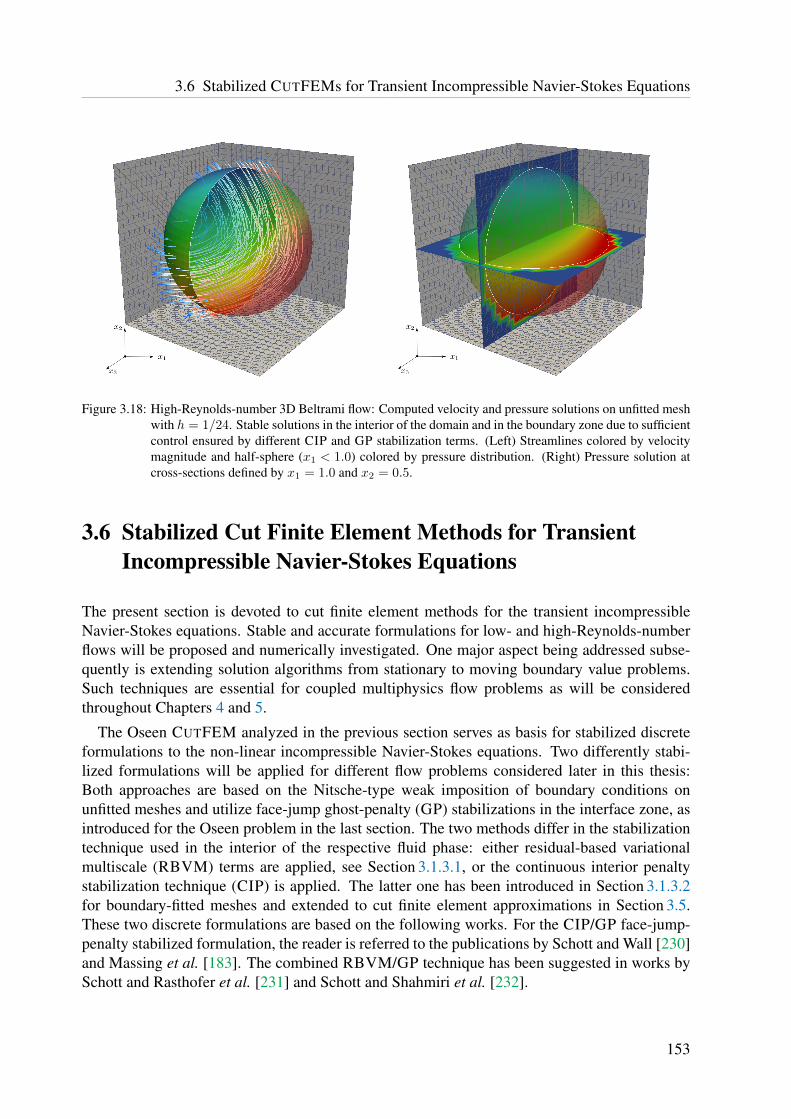
3.6 Stabilized CUTFEMs for Transient Incompressible Navier-Stokes Equations

Figure 3.18: High-Reynolds-number 3D Beltrami flow: Computed velocity and pressure solutions on unfitted meshwith h = 1/24. Stable solutions in the interior of the domain and in the boundary zone due to sufficientcontrol ensured by different CIP and GP stabilization terms. (Left) Streamlines colored by velocitymagnitude and half-sphere (x1 < 1.0) colored by pressure distribution. (Right) Pressure solution atcross-sections defined by x1 = 1.0 and x2 = 0.5.

3.6 Stabilized Cut Finite Element Methods for TransientIncompressible Navier-Stokes Equations

The present section is devoted to cut finite element methods for the transient incompressibleNavier-Stokes equations. Stable and accurate formulations for low- and high-Reynolds-numberflows will be proposed and numerically investigated. One major aspect being addressed subse-quently is extending solution algorithms from stationary to moving boundary value problems.Such techniques are essential for coupled multiphysics flow problems as will be consideredthroughout Chapters 4 and 5.

The Oseen CUTFEM analyzed in the previous section serves as basis for stabilized discreteformulations to the non-linear incompressible Navier-Stokes equations. Two differently stabi-lized formulations will be applied for different flow problems considered later in this thesis:Both approaches are based on the Nitsche-type weak imposition of boundary conditions onunfitted meshes and utilize face-jump ghost-penalty (GP) stabilizations in the interface zone, asintroduced for the Oseen problem in the last section. The two methods differ in the stabilizationtechnique used in the interior of the respective fluid phase: either residual-based variationalmultiscale (RBVM) terms are applied, see Section 3.1.3.1, or the continuous interior penaltystabilization technique (CIP) is applied. The latter one has been introduced in Section 3.1.3.2for boundary-fitted meshes and extended to cut finite element approximations in Section 3.5.These two discrete formulations are based on the following works. For the CIP/GP face-jump-penalty stabilized formulation, the reader is referred to the publications by Schott and Wall [230]and Massing et al. [183]. The combined RBVM/GP technique has been suggested in works bySchott and Rasthofer et al. [231] and Schott and Shahmiri et al. [232].

153

3 Developing Stabilized Cut Finite Element Methods for Incompressible Flow

In this thesis, these two stabilized formulations are referred to as

• a Nitsche-type face-jump-penalty stabilized cut finite element method,denoted as CIP/GP-CUTFEM, and

• a Nitsche-type residual-based variational multiscale cut finite element method,denoted as RBVM/GP-CUTFEM.

Temporal and spatial discretizations for both variants will be proposed in Section 3.6.1. Stabilityand accuracy of the formulations are examined with different two- and three-dimensional flowsimulations in complex-shaped domains with stationary boundaries. Finally, issues arising fordomains with moving boundaries discretized on non-boundary-fitted fixed grids will be elabo-rated in Section 3.6.3. Possible solution strategies are provided and discussed. To indicate theapplicability of those methods to multiphysics problems, simulations for incompressible single-phase flows at low and higher Reynolds numbers with boundaries which undergo large motionswill demonstrate the capability of CUTFEMs for incompressible fluid flows.

3.6.1 Stabilized Discrete FormulationsIn the following, temporal and spatial semi-discrete formulations of the aforementioned unfittedCUTFEM for the transient incompressible Navier-Stokes equations will be proposed. Within thissection, boundaries are assumed to be stationary. Computational meshes are fixed in time andthe variational formulation A(U, V ) = L(U, V ) of the incompressible Navier-Stokes equationsfrom Section 3.1.2 is described in an Eulerian formalism, i.e. u = 0 and ∂uχ

∂tΦ−1(·, T ) = ∂u(t)

∂t.

To simplify the notation on function spaces, Dirichlet-type boundary conditions on ΓD areexclusively enforced weakly. Combinations with strongly incorporated conditions at boundaryparts which fit to the mesh is straightforward and functions spaces would change accordingly,see Section 3.1.2.

3.6.1.1 A Nitsche-type CIP/GP Cut Finite Element Method

The spatial semi-discrete Nitsche-type cut finite element formulation for the incompressibleNavier-Stokes equations (3.9) with stabilizing continuous interior penalty (CIP) terms in theinterior of the domain and ghost penalty (GP) terms in the boundary zone reads as follows:

Definition 3.13 (Semi-discrete formulation of the Nitsche-type CIP/GP-CUTFEM)For all t ∈ (T0, T ), find fluid velocity and pressure Uh(t) = (uh(t), ph(t)) ∈ Vh ×Qh such thatfor all Vh = (vh, qh) ∈ Vh ×Qh

ACIP/GPh (Uh, Vh) = LCIP/GP

h (Uh, Vh), (3.449)

where

ACIP/GPh (Uh, Vh)

def= (ρ

∂uh(t)

∂t,vh)Ω + (Bh + SCIP

h + GGPh )(uh; (uh, ph), (vh, qh)), (3.450)

LCIP/GPh (Uh, Vh)

def= Lh(uh; (vh, qh)) (3.451)

154

3.6 Stabilized CUTFEMs for Transient Incompressible Navier-Stokes Equations

with

Bh(uh; (uh, ph), (vh, qh)) = (ch + ah)(uh;uh,vh) + bh(ph,vh)− bh(qh,uh), (3.452)

SCIPh (uh; (uh, ph), (vh, qh)) = (sβ + su + sp)(uh; (uh, ph), (vh, qh)), (3.453)

GGPh (uh; (uh, ph), (vh, qh)) = (gβ + gu + gp + gν + gσ)(uh; (uh, ph), (vh, qh)), (3.454)

Lh(uh; (vh, qh)) = (ρf ,vh)Ω + 〈hN,vh〉ΓN− 〈ρ(uh · n)gD,vh〉Γin

∓ 〈gD, 2µεεε(vh)n〉ΓD+ 〈γ(µ/h)gD,vh〉ΓD

(3.455)− 〈gD · n, qh〉ΓD

+ 〈γ(φρ/h)gD · n,vh · n〉ΓD.

Terms according to the standard Galerkin formulation and to Nitsche’s method are given as

ch(uh;uh,vh) = (ρ(uh · ∇)uh,vh)Ω − 〈ρ(uh · n)uh,vh〉Γin+ 1

2(ρ(∇ · uh)uh,vh), (3.456)

ah(uh;uh,vh) = (εεε(uh), 2µεεε(vh))Ω − 〈2µεεε(uh)n,vh〉ΓD∓ 〈uh, 2µεεε(vh)n〉ΓD

+ 〈γ(µ/h)uh,vh〉ΓD+ 〈γ(φρ/h)uh · n,vh · n〉ΓD

, (3.457)bh(ph,vh) = −(ph,∇ · vh)Ω + 〈ph,vh · n〉ΓD

, (3.458)

and continuous interior penalty stabilization terms are defined with un,∞,Fdef= ‖uh · n‖0,∞,F as

sβ(uh;uh,vh) = γβ∑

F∈Fiφβ,Fρu

2n,∞,FhF 〈[[∇uh]], [[∇vh]]〉F , (3.459)

su(uh;uh,vh) = γu∑

F∈Fiφu,FρhF 〈[[∇ · uh]], [[∇ · vh]]〉F , (3.460)

sp(uh; ph, qh) = γp∑

F∈Fiφp,Fρ

−1hF 〈[[∇ph]], [[∇qh]]〉F , (3.461)

Defining u∞,Fdef= ‖uh‖0,∞,F , interface zone face-jump ghost-penalty terms are given by

gβ(uh;uh,vh) = γβ∑

F∈FΓ

∑16j6k

φβ,Fρu2∞,Fh

2j−1F 〈[[∂jnuh]], [[∂jnvh]]〉F , (3.462)

gu(uh;uh,vh) = γu∑

F∈FΓ

∑06j6k−1

φu,Fρh2j+1F 〈[[∇ · ∂jnuh]], [[∇ · ∂jnvh]]〉F , (3.463)

gp(uh; ph, qh) = γp∑

F∈FΓ

∑16j6k

φp,Fρ−1h2j−1

F 〈[[∂jnph]], [[∂jnqh]]〉F , (3.464)

gν(uh,vh) = γν∑

F∈FΓ

∑16j6k

νρh2j−1F 〈[[∂jnuh]], [[∂jnvh]]〉F , (3.465)

gσ(uh,vh) = γσ∑

F∈FΓ

∑16j6k

σρh2j+1F 〈[[∂jnuh]], [[∂jnvh]]〉F . (3.466)

Moreover, uh has to fulfill the initial condition uh(T0) = u0 in Ω. Note, to shorten the presenta-tion of the stabilized formulation, the time variable in Uh(t) = (uh(t), ph(t)) has been omitted.The scaling σ denotes a (pseudo-)reaction which results from temporal discretization of thespatial semi-discrete form (3.449) as will be introduced later in Section 3.6.1.3, see (3.476) and(3.479). Stabilization parameters for CIP terms and CIP-related GP terms are taken from theOseen problem, see Section 3.5.2. The scaling functions related to the Nitsche’s method, the CIPterms as well as all GP terms are recalled from Section 3.1.3.2 and Section 3.5.2

φT = ν + cu(‖uh‖0,∞,ThT ) + cσ(σh2T ), φβ,T = φp,T = h2

Tφ−1T , φu,T = φT . (3.467)

155

3 Developing Stabilized Cut Finite Element Methods for Incompressible Flow

Remark 3.25 The CIP/GP-CUTFEM formulation proposed in Definition 3.13 is an extensionof the stabilized formulation for Oseen’s problem analyzed and numerically investigated inSection 3.5. Here, the advective velocity β therein is replaced by the discrete convective velocityuh ∈ Vh which introduces a non-linearity into all stabilization operators. For ALE-based for-mulations, β is the relative convective velocity uh − uh. Furthermore, the formulation is scaledwith the density ρ as required for coupled problem settings and includes Neumann boundaryconditions on ΓN, see (3.455). Note that the definition of the advective ghost-penalty operator(3.462) is based on elaborations provided in Remark 3.15.

Remark 3.26 Due to the weak enforcement of the incompressibility constraint, in general, itdoes not hold∇ · uh = 0 a.e. in Ω. Recalling Remark 3.19 and the coercivity proof of Lemma 3.10in Section 3.5.5, the need for the last term added in (3.456) arises from (3.256). In practice,however, it often holds σ − 1

2∇ · uh > c > 0 provided the time-step length ∆t ∼ 1/σ is chosen

sufficiently small (see (3.476) and (3.479) for definitions). Then, this additional term can beneglected as done for all simulations considered in this work.

Remark 3.27 Note that similar to the elaborations for the Oseen problem in Section 3.5, seeRemark 3.15, also the incompressibility ghost-penalty term (3.463) can be replaced by a purevelocity based jump-penalty term similar to (3.462).

For further detailed elaborations on the meaning of the Nitsche-based boundary terms and thedifferent CIP and GP stabilizations, the reader is referred to Section 3.5.

3.6.1.2 A Nitsche-type RBVM/GP Cut Finite Element Method

Definition 3.14 (Semi-discrete formulation of the Nitsche-type RBVM/GP-CUTFEM)For all t ∈ (T0, T ], find fluid velocity and pressure Uh(t) = (uh(t), ph(t)) ∈ Vh ×Qh such thatfor all Vh = (vh, qh) ∈ Vh ×Qh

ARBVM/GPh (Uh, Vh) = LRBVM/GP

h (Uh, Vh), (3.468)

where

ARBVM/GPh (Uh, Vh)

def= (ρ

∂uh(t)

∂t,vh) + (Bh + GGP

h )(uh; (uh, ph), (vh, qh))

+∑

T∈Th

(ρ∂uh(t)

∂t+ rM(uh, ph), τM(ρ(uh · ∇)vh +∇qh)

)T∩Ω

(3.469)

+∑

T∈Th

(rC(uh), τC∇ · vh

)T∩Ω

,

LRBVM/GPh (Uh, Vh)

def= Lh(vh, qh)

+∑

T∈Th

(ρf , τM(ρ(uh · ∇)vh +∇qh)

)T∩Ω

(3.470)

with

rM(uh, ph) = ρ(uh · ∇)uh +∇ph − 2µ∇ · ε(uh) and rC(uh) = ∇ · uh. (3.471)

The operators Bh and GGPh are defined in (3.452) and (3.454). The stabilization scaling func-

tions τM, τC are introduced in (3.21)–(3.22).

156

3.6 Stabilized CUTFEMs for Transient Incompressible Navier-Stokes Equations

3.6.1.3 Time-Stepping for Fluids

The stabilized semi-discrete CUTFEM formulations proposed in Section 3.6.1.1–3.6.1.2 can bewritten in an abstract form as first order ordinary differential equations (ODE) as follows: forany time t ∈ (T0, T ] find fluid velocity and pressure fields uh(t) ∈ Vh and ph(t) ∈Qh such thatfor all (vh, qh) ∈ Vh ×Qh

(ρ∂uh(t)

∂t,Υ(vh, qh)) + F (t, (uh(t), ph(t)), (vh, qh)) = 0, (3.472)

where Υ is linear with respect to (vh, qh). For the CIP/GP-CUTFEM this function is givenby Υ(vh, qh) = vh and by Υ(vh, qh) = vh + τM(ρ(uh · ∇)vh + ∇qh) for the RBVM/GP-CUTFEM formulation. The respective functions F , which incorporate standard Galerkin terms,stabilization operators and external loads, i.e. Bh, Gh,Sh,−Lh, can be defined accordingly anddo not include further time derivatives of uh. Then, a multitude of one- and multi-step timediscretization schemes are applicable to such spatial semi-discrete finite dimensional systems ofODEs. In this thesis, two well-established techniques are utilized for fluids: a one-step-θ method(OST) and a two-step backward differentiation formula (BDF2).

For time stepping, let the time domain (T0, T ] be partitioned into N equal-sized time-stepintervals Jn = (tn−1, tn] of size ∆t. The discrete time levels are defined as tn = T0 + n∆t andtN = T . Discrete velocity and pressure fields are then approximated by temporal approximationsunh ≈ uh(tn) and pnh ≈ ph(t

n).The subsequent elaborations are based on work published by Dettmer and Peric [84] and

Forster [110]. In the latter work, both schemes are written in the form

(ρunh,Υ(vh, qh)) + σ−1F n((unh, pnh), (vh, qh))−Hn−1(vh, qh) = 0, (3.473)

where σ represents a time-dependent scalar which is characteristic for the temporal discretiza-tion. The function H contains history data from one or several old time steps.

The One-Step-θ Family (OST). For an ODE of type y(t) = f(t, y(t)), the one-step-θ schemewith θ ∈ [0, 1] is classically given as

yn = yn−1 + θ∆tf(tn, yn) + (1− θ)∆tf(tn−1, yn−1). (3.474)

For fluid problems of type (3.472) this scheme can be equivalently rewritten in terms of un-knowns unh, p

nh and an additional unknown acceleration approximation anh ≈ ∂uh(t)

∂tas: find

approximations unh, pnh,a

nh such that

(ρunh,Υ(vh, qh)) + σ−1θ F n((unh, p

nh), (vh, qh))−Hn−1

θ (vh) = 0 (3.475)

with

σθ = (θ∆t)−1 and Hn−1θ (vh) = (ρun−1

h ,Υ(vh, qh)) + (1− θ)∆t(ρan−1h ,vh). (3.476)

For given unh, the acceleration vector can be updated by utilizing a OST-scheme (3.474) for∂uh(t)∂t

= ah(t)

anh =unh − un−1

h

∆t− 1− θ

θan−1h . (3.477)

157

3 Developing Stabilized Cut Finite Element Methods for Incompressible Flow

Note that using this technique, the stabilized formulations to the incompressible Navier-Stokesequations hidden in F n have to be evaluated only for the current time step tn. The one-step-θfamily is unconditionally A-stable for θ ∈ [1/2, 1] and guarantees first-order accuracy for allθ 6= 1/2. The scheme is second-order accurate if and only if θ = 1/2. The latter variant is calledCrank-Nicolson method.

The Two-Step Backward Differentiation Formula (BDF2). The well-known BDF2 time-stepping scheme utilizes a second-order backward differentiation formula at tn to approximatethe time derivative and therefore requires history data from two previous time levels tn−1, tn−2:

(ρunh,Υ(vh, qh)) + σ−1BDF2F

n((unh, pnh), (vh, qh))−Hn−1

BDF2(vh) = 0 (3.478)

with

σBDF2 = (2

3∆t)−1 and Hn−1

BDF2(vh) = −4

3(ρun−1

h ,Υ(vh, qh)) +1

3(ρun−2

h ,Υ(vh, qh)).

(3.479)The BDF2 scheme is of second-order accuracy and provides unconditional A-stability.

Remarks on Temporal Discretization. Such fully discretized finite element methods for theincompressible Navier-Stokes equations render in non-linear systems of equations for the solu-tion approximations unh, p

nh of each time step. Non-linearities given in terms of the convective

velocity in the standard Galerkin formulation and corresponding stabilization terms can then beapproximated with a series of Picard or Newton-like iterations. Thereby, velocities occurring indifferent stabilization parameters are evaluated at the last iteration step.

Temporal discretizations of such stabilized formulations have been written down more de-tailed in, e.g., Schott [229]. For an analysis of different time integration algorithms for thefinite element solutions of incompressible Navier-Stokes equations based on residual-stabilizedformulations, the interested reader is referred to the work by Dettmer and Peric [84]. Furtheranalysis of stabilized schemes for transient problems have been provided by Burman [51] for theSUPG stabilization and by Burman and Fernandez [57] for the PSPG stabilization. Numericalanalyses of time-discrete CIP-stabilized methods can be found in, e.g., Burman and Fernandez[56], Burman and Fernandez [55] or Burman et al. [67].

Note that using the temporal discretization techniques provided above, all involved stabiliza-tion operators as well as Nitsche terms used for imposing the boundary conditions, which arehidden in F n, have to be evaluated at the current time level tn. For the one-step-θ scheme, historydata from previous time steps are then incorporated in the acceleration variable anh.

3.6.2 Numerical Tests for Incompressible Flow in Non-Moving DomainsThe Nitsche-type cut finite element methods introduced in Section 3.6.1 are validated for station-ary and transient flows in domains with non-moving boundaries. While numerical convergencetests in Section 3.5.7 already confirmed optimality and stability of the stabilized Oseen scheme,the following test cases demonstrate applicability of the formulations to transient flows governedby the incompressible Navier-Stokes equations. A comparison of the CIP/GP scheme with othercomputational approaches is provided for a well-established stationary two-dimensional laminar

158

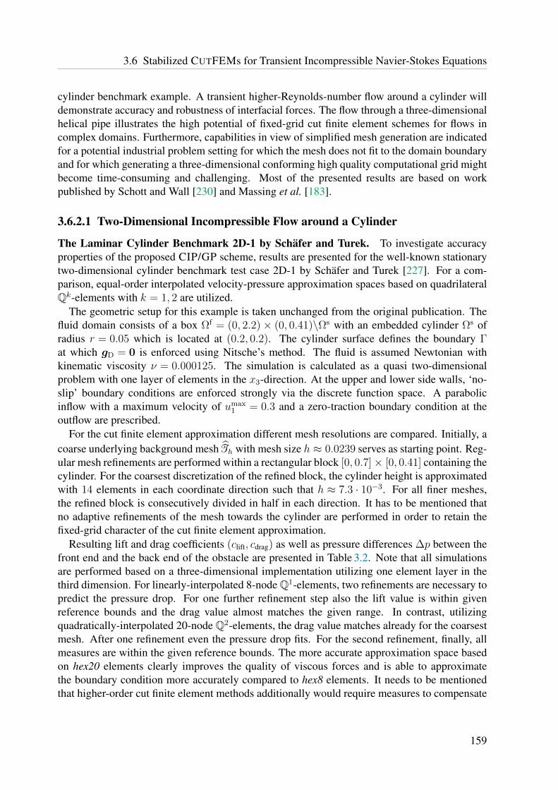
3.6 Stabilized CUTFEMs for Transient Incompressible Navier-Stokes Equations

cylinder benchmark example. A transient higher-Reynolds-number flow around a cylinder willdemonstrate accuracy and robustness of interfacial forces. The flow through a three-dimensionalhelical pipe illustrates the high potential of fixed-grid cut finite element schemes for flows incomplex domains. Furthermore, capabilities in view of simplified mesh generation are indicatedfor a potential industrial problem setting for which the mesh does not fit to the domain boundaryand for which generating a three-dimensional conforming high quality computational grid mightbecome time-consuming and challenging. Most of the presented results are based on workpublished by Schott and Wall [230] and Massing et al. [183].

3.6.2.1 Two-Dimensional Incompressible Flow around a Cylinder

The Laminar Cylinder Benchmark 2D-1 by Schafer and Turek. To investigate accuracyproperties of the proposed CIP/GP scheme, results are presented for the well-known stationarytwo-dimensional cylinder benchmark test case 2D-1 by Schafer and Turek [227]. For a com-parison, equal-order interpolated velocity-pressure approximation spaces based on quadrilateralQk-elements with k = 1, 2 are utilized.

The geometric setup for this example is taken unchanged from the original publication. Thefluid domain consists of a box Ωf = (0, 2.2)× (0, 0.41)\Ωs with an embedded cylinder Ωs ofradius r = 0.05 which is located at (0.2, 0.2). The cylinder surface defines the boundary Γat which gD = 0 is enforced using Nitsche’s method. The fluid is assumed Newtonian withkinematic viscosity ν = 0.000125. The simulation is calculated as a quasi two-dimensionalproblem with one layer of elements in the x3-direction. At the upper and lower side walls, ‘no-slip’ boundary conditions are enforced strongly via the discrete function space. A parabolicinflow with a maximum velocity of umax

1 = 0.3 and a zero-traction boundary condition at theoutflow are prescribed.

For the cut finite element approximation different mesh resolutions are compared. Initially, acoarse underlying background mesh Th with mesh size h ≈ 0.0239 serves as starting point. Reg-ular mesh refinements are performed within a rectangular block [0, 0.7]× [0, 0.41] containing thecylinder. For the coarsest discretization of the refined block, the cylinder height is approximatedwith 14 elements in each coordinate direction such that h ≈ 7.3 · 10−3. For all finer meshes,the refined block is consecutively divided in half in each direction. It has to be mentioned thatno adaptive refinements of the mesh towards the cylinder are performed in order to retain thefixed-grid character of the cut finite element approximation.

Resulting lift and drag coefficients (clift, cdrag) as well as pressure differences ∆p between thefront end and the back end of the obstacle are presented in Table 3.2. Note that all simulationsare performed based on a three-dimensional implementation utilizing one element layer in thethird dimension. For linearly-interpolated 8-node Q1-elements, two refinements are necessary topredict the pressure drop. For one further refinement step also the lift value is within givenreference bounds and the drag value almost matches the given range. In contrast, utilizingquadratically-interpolated 20-node Q2-elements, the drag value matches already for the coarsestmesh. After one refinement even the pressure drop fits. For the second refinement, finally, allmeasures are within the given reference bounds. The more accurate approximation space basedon hex20 elements clearly improves the quality of viscous forces and is able to approximatethe boundary condition more accurately compared to hex8 elements. It needs to be mentionedthat higher-order cut finite element methods additionally would require measures to compensate

159

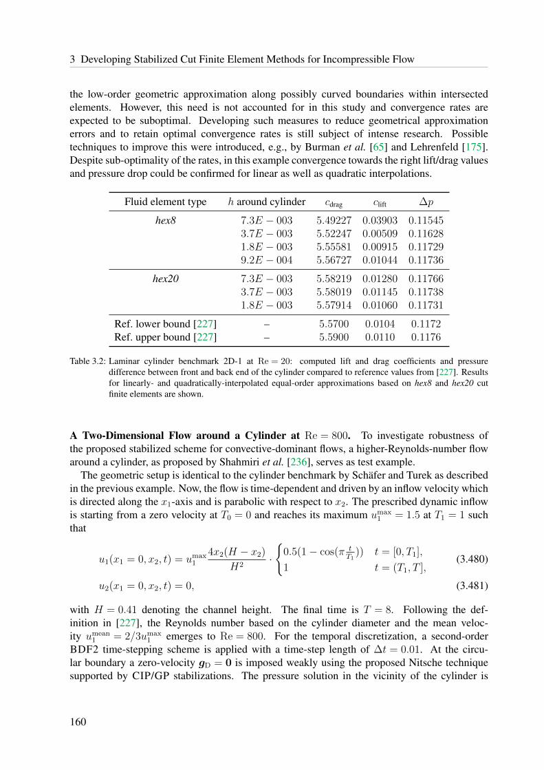
3 Developing Stabilized Cut Finite Element Methods for Incompressible Flow

the low-order geometric approximation along possibly curved boundaries within intersectedelements. However, this need is not accounted for in this study and convergence rates areexpected to be suboptimal. Developing such measures to reduce geometrical approximationerrors and to retain optimal convergence rates is still subject of intense research. Possibletechniques to improve this were introduced, e.g., by Burman et al. [65] and Lehrenfeld [175].Despite sub-optimality of the rates, in this example convergence towards the right lift/drag valuesand pressure drop could be confirmed for linear as well as quadratic interpolations.

Fluid element type h around cylinder cdrag clift ∆p

hex8 7.3E − 003 5.49227 0.03903 0.115453.7E − 003 5.52247 0.00509 0.116281.8E − 003 5.55581 0.00915 0.117299.2E − 004 5.56727 0.01044 0.11736

hex20 7.3E − 003 5.58219 0.01280 0.117663.7E − 003 5.58019 0.01145 0.117381.8E − 003 5.57914 0.01060 0.11731

Ref. lower bound [227] – 5.5700 0.0104 0.1172Ref. upper bound [227] – 5.5900 0.0110 0.1176

Table 3.2: Laminar cylinder benchmark 2D-1 at Re = 20: computed lift and drag coefficients and pressuredifference between front and back end of the cylinder compared to reference values from [227]. Resultsfor linearly- and quadratically-interpolated equal-order approximations based on hex8 and hex20 cutfinite elements are shown.

A Two-Dimensional Flow around a Cylinder at Re = 800. To investigate robustness ofthe proposed stabilized scheme for convective-dominant flows, a higher-Reynolds-number flowaround a cylinder, as proposed by Shahmiri et al. [236], serves as test example.

The geometric setup is identical to the cylinder benchmark by Schafer and Turek as describedin the previous example. Now, the flow is time-dependent and driven by an inflow velocity whichis directed along the x1-axis and is parabolic with respect to x2. The prescribed dynamic inflowis starting from a zero velocity at T0 = 0 and reaches its maximum umax

1 = 1.5 at T1 = 1 suchthat

u1(x1 = 0, x2, t) = umax1

4x2(H − x2)

H2·

0.5(1− cos(π tT1

)) t = [0, T1],

1 t = (T1, T ],(3.480)

u2(x1 = 0, x2, t) = 0, (3.481)

with H = 0.41 denoting the channel height. The final time is T = 8. Following the def-inition in [227], the Reynolds number based on the cylinder diameter and the mean veloc-ity umean

1 = 2/3umax1 emerges to Re = 800. For the temporal discretization, a second-order

BDF2 time-stepping scheme is applied with a time-step length of ∆t = 0.01. At the circu-lar boundary a zero-velocity gD = 0 is imposed weakly using the proposed Nitsche techniquesupported by CIP/GP stabilizations. The pressure solution in the vicinity of the cylinder is

160

3.6 Stabilized CUTFEMs for Transient Incompressible Navier-Stokes Equations

shown in Figure 3.19. Indicated by the smoothness of the pressure contour lines, no pertur-bation of the pressure field in the vicinity of the interface could be observed. In view ofenvisioned fluid-structure-interaction applications, the temporal robustness of boundary forcesis investigated, which are visualized in Figure 3.20. Forces resulting from fluid normal stressesσ(uf

h, pfh) = −pf

hI + 2µε(ufh) are projected onto the structural trace mesh. Nodal forces acting

on structural interface nodes l are defined as

f sl =

∫

Γ

N sl σ(uf

h, pfh) · nf ds, (3.482)

where N sl denotes finite element basis function at node l of the structural trace mesh. Fig-

ure 3.20a illustrates the force vectors at time t = 0.85 during the initial phase when the inflowvelocity gets raised. The maximum inflow velocity is reached at time T1 = 1.0. The corre-sponding state is shown in Figure 3.20b. Further discrete time levels t = 3.25 and t = 3.40are picked out to visualize the periodically recurring pattern of tensile and compressive forceswhen the vortex shedding is fully developed, see Figure 3.20c and Figure 3.20d. Over the entiresimulation time, interface forces are smoothly distributed along the structural surface. Thisunderlines accuracy and stability of the pressure solution as well as of the velocity gradients inthe vicinity of the cylinder. Figure 3.21 illustrates the Euclidean norm of the velocity and theevolution of the vortex shedding in the backflow of the structure at different times t.

(a) t = 1.35 (b) t = 2.25 (c) t = 3.15

Figure 3.19: Two-dimensional flow around a cylinder at RE = 800: close-up views of the pressure field withcontour lines at different times t.

(a) t = 0.85 (b) t = 1.00 (c) t = 3.25 (d) t = 3.40

Figure 3.20: Two-dimensional flow around a cylinder atRE = 800: interface forces acting on the structural surfaceat different times t.

161

3 Developing Stabilized Cut Finite Element Methods for Incompressible Flow

(a) t = 0.7

(b) t = 1.35

(c) t = 1.95

(d) t = 2.25

(e) t = 2.85

(f) t = 3.15

Figure 3.21: Two-dimensional flow around a cylinder at RE = 800: velocity norm ‖u‖ and vortex shedding in thebackflow of the cylinder at different times t.

162

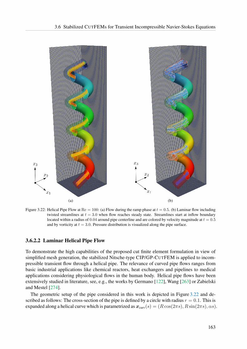
3.6 Stabilized CUTFEMs for Transient Incompressible Navier-Stokes Equations

(a) (b)

Figure 3.22: Helical Pipe Flow at Re = 100: (a) Flow during the ramp phase at t = 0.5. (b) Laminar flow includingtwisted streamlines at t = 3.0 when flow reaches steady state. Streamlines start at inflow boundarylocated within a radius of 0.04 around pipe centerline and are colored by velocity magnitude at t = 0.5and by vorticity at t = 3.0. Pressure distribution is visualized along the pipe surface.

3.6.2.2 Laminar Helical Pipe Flow

To demonstrate the high capabilities of the proposed cut finite element formulation in view ofsimplified mesh generation, the stabilized Nitsche-type CIP/GP-CUTFEM is applied to incom-pressible transient flow through a helical pipe. The relevance of curved pipe flows ranges frombasic industrial applications like chemical reactors, heat exchangers and pipelines to medicalapplications considering physiological flows in the human body. Helical pipe flows have beenextensively studied in literature, see, e.g., the works by Germano [122], Wang [263] or Zabielskiand Mestel [274].

The geometric setup of the pipe considered in this work is depicted in Figure 3.22 and de-scribed as follows: The cross-section of the pipe is defined by a circle with radius r = 0.1. This isexpanded along a helical curve which is parametrized asxcurv(s) = (R cos(2πs), R sin(2πs), αs).

163

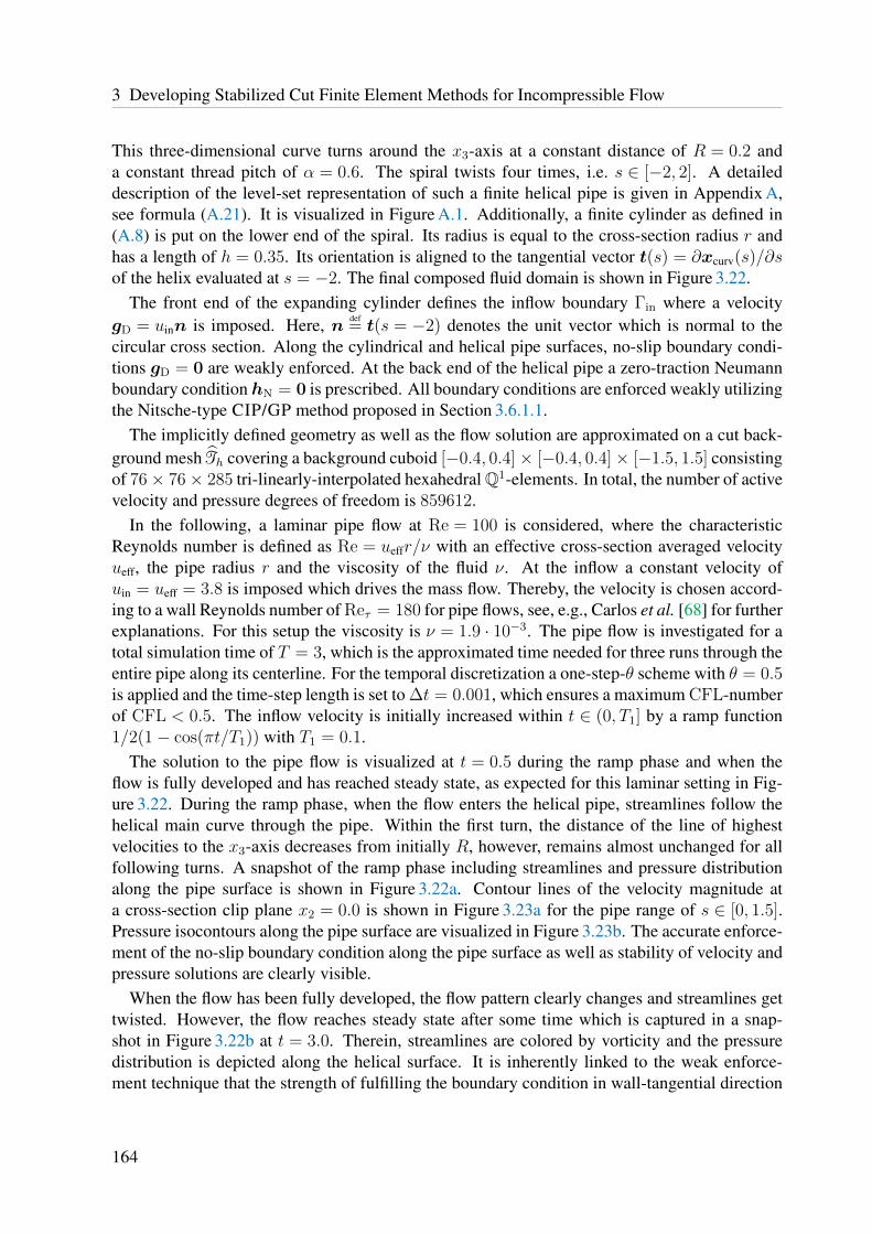
3 Developing Stabilized Cut Finite Element Methods for Incompressible Flow

This three-dimensional curve turns around the x3-axis at a constant distance of R = 0.2 anda constant thread pitch of α = 0.6. The spiral twists four times, i.e. s ∈ [−2, 2]. A detaileddescription of the level-set representation of such a finite helical pipe is given in Appendix A,see formula (A.21). It is visualized in Figure A.1. Additionally, a finite cylinder as defined in(A.8) is put on the lower end of the spiral. Its radius is equal to the cross-section radius r andhas a length of h = 0.35. Its orientation is aligned to the tangential vector t(s) = ∂xcurv(s)/∂sof the helix evaluated at s = −2. The final composed fluid domain is shown in Figure 3.22.

The front end of the expanding cylinder defines the inflow boundary Γin where a velocitygD = uinn is imposed. Here, n def

= t(s = −2) denotes the unit vector which is normal to thecircular cross section. Along the cylindrical and helical pipe surfaces, no-slip boundary condi-tions gD = 0 are weakly enforced. At the back end of the helical pipe a zero-traction Neumannboundary condition hN = 0 is prescribed. All boundary conditions are enforced weakly utilizingthe Nitsche-type CIP/GP method proposed in Section 3.6.1.1.

The implicitly defined geometry as well as the flow solution are approximated on a cut back-ground mesh Th covering a background cuboid [−0.4, 0.4]× [−0.4, 0.4]× [−1.5, 1.5] consistingof 76× 76× 285 tri-linearly-interpolated hexahedral Q1-elements. In total, the number of activevelocity and pressure degrees of freedom is 859612.

In the following, a laminar pipe flow at Re = 100 is considered, where the characteristicReynolds number is defined as Re = ueffr/ν with an effective cross-section averaged velocityueff, the pipe radius r and the viscosity of the fluid ν. At the inflow a constant velocity ofuin = ueff = 3.8 is imposed which drives the mass flow. Thereby, the velocity is chosen accord-ing to a wall Reynolds number of Reτ = 180 for pipe flows, see, e.g., Carlos et al. [68] for furtherexplanations. For this setup the viscosity is ν = 1.9 · 10−3. The pipe flow is investigated for atotal simulation time of T = 3, which is the approximated time needed for three runs through theentire pipe along its centerline. For the temporal discretization a one-step-θ scheme with θ = 0.5is applied and the time-step length is set to ∆t = 0.001, which ensures a maximum CFL-numberof CFL < 0.5. The inflow velocity is initially increased within t ∈ (0, T1] by a ramp function1/2(1− cos(πt/T1)) with T1 = 0.1.

The solution to the pipe flow is visualized at t = 0.5 during the ramp phase and when theflow is fully developed and has reached steady state, as expected for this laminar setting in Fig-ure 3.22. During the ramp phase, when the flow enters the helical pipe, streamlines follow thehelical main curve through the pipe. Within the first turn, the distance of the line of highestvelocities to the x3-axis decreases from initially R, however, remains almost unchanged for allfollowing turns. A snapshot of the ramp phase including streamlines and pressure distributionalong the pipe surface is shown in Figure 3.22a. Contour lines of the velocity magnitude ata cross-section clip plane x2 = 0.0 is shown in Figure 3.23a for the pipe range of s ∈ [0, 1.5].Pressure isocontours along the pipe surface are visualized in Figure 3.23b. The accurate enforce-ment of the no-slip boundary condition along the pipe surface as well as stability of velocity andpressure solutions are clearly visible.

When the flow has been fully developed, the flow pattern clearly changes and streamlines gettwisted. However, the flow reaches steady state after some time which is captured in a snap-shot in Figure 3.22b at t = 3.0. Therein, streamlines are colored by vorticity and the pressuredistribution is depicted along the helical surface. It is inherently linked to the weak enforce-ment technique that the strength of fulfilling the boundary condition in wall-tangential direction

164

3.6 Stabilized CUTFEMs for Transient Incompressible Navier-Stokes Equations

(a) (b)

Figure 3.23: Helical Pipe Flow at Re = 100 at t = 0.5: (a) Isocontours of velocity magnitude at a cross sectiondefined by a clip plane x2 = 0.0 for a helix range of s ∈ [0, 1.5] indicate higher velocities withdecreasing distance to the x3-axis due to higher mass flow rate. The zero boundary condition at thehelix surface is accurately enforced and the velocity solution is stable in the interior of the fluid domainas well as near the boundary. (b) Pressure contour lines at the helix surface underline the stability ofthe pressure solution near the boundary.

gets weakened, the higher the local element Reynolds number becomes in the vicinity of theboundary. Though, the non-penetration condition in wall-normal direction of the pipe, whichensures mass conservation, is still sufficiently enforced. Moreover, the solution exhibits non-oscillatory stable velocity and pressure due to stabilizing effects of the different applied CIP/GPstabilization operators in the interior of the fluid domain as well as near the boundary zone. Atsteady state, contour lines are visualized in Figure 3.24a for the velocity and in Figure 3.24b forthe pressure.

3.6.2.3 Flow in a Complex-Shaped Domain Composed of Level-Set Fields

In order to demonstrate the high capabilities of the proposed fluid solver, a complex three-dimensional flow setting is considered. Its full benefits are reaped when cut finite element fluidformulations are combined with simple boundary representation techniques.

In this example, the flow through a complex-shaped fluid domain is simulated. Its boundaryis implicitly defined by the zero-level of the function defined in (A.36), see Appendix A.3.Visualizations of the domain Ωf and of its construction steps are given in Figure A.2. It consistsof a hollow cylindrical inflow region from which the flow is entering a channel composed ofcylinders, a sphere and several limiting boundary planes. Furthermore, a spiral-shaped obstacleis embedded into the channel. For the approximation of the level-set field and of the fluid fields aregularly meshed background grid Th covering a cuboid [−0.7, 0.1]× [−0.5, 0.5]× [−1.5, 1.5]

165

3 Developing Stabilized Cut Finite Element Methods for Incompressible Flow

(a) (b)

Figure 3.24: Helical Pipe Flow at Re = 100 at t = 3.0 when the flow has reached steady state: (a) Isocontours ofvelocity magnitude at a cross section defined by a clip plane x2 = 0.0 for a helix range of s ∈ [0, 1.5]indicate stable velocity solution in the interior of the fluid domain as well as near the boundary.(b) Pressure contour lines at the helix surface demonstrate a stable pressure solution in the vicinityof the boundary.

is utilized. The mesh consists of tri-linearly-interpolated hexahedral Q1-elements with a meshsize of h = 0.02 in each coordinate direction.

All boundary conditions are enforced weakly using the Nitsche-type technique combined withthe RBVM/GP stabilization technique as described in Section 3.6.1.2. At the circular inflowboundary, which is located at x3 = −1.49, a rotationally symmetric parabolic velocity fieldgD(x) = (0, 0, u3)(x) is imposed. It is directed along the positive x3-coordinate with a maximalvelocity of umax

3 = 1 reached at the center point xmax = (−0.2, 0,−1.49). The parabolic profileis given as

u3(x1, x2, x3 = −1.49) = umax3 (1− ((x1 − xmax

1 )2 + (x2 − xmax2 )2)/r2), (3.483)

where r = 0.14 denotes the inner radius of the cylindrical inflow region. At the outflow, whichis limited by the halfspace φHSpace,out at x3 = 1.5, a zero-traction Neumann boundary conditionhN = 0 is prescribed. For all remaining boundaries and along the surface of the spiral-shapedobstacle, which are all defined by the zero-isocontour of φFluid in (A.36), ‘no-slip’ Dirichletboundary conditions gD = 0 are weakly imposed. The inflow is initially ramped utilizing thefunction 1/2(1 − cos(πt/T1)) within t ∈ (0, T1] with T1 = 1. The overall simulation time isset to T = 18 and is temporally resolved with a time-step length of ∆t = 0.01 using an OSTscheme without numerical damping, i.e. θ = 0.5. The flow is highly convective-dominatedbased on a viscosity of ν = 10−4. The resulting complex flow pattern, which develops whenentering the bulk and hitting the spiral, is visualized in Figure 3.25 with the help of streamlines.These start at the inflow and wind around the spiral object through the fluid domain. Boundaryconditions along the entire surface are accurately enforced. Stability at boundaries, inflow

166

3.6 Stabilized CUTFEMs for Transient Incompressible Navier-Stokes Equations

Figure 3.25: Flow through a complex-shaped fluid domain:bThe boundary of this fluid domain is defined implicitlyutilizing Boolean set operations for various level-set fields as defined in (A.36), see in Appendix A.3.Level-set field and fluid solutions are approximated with an unfitted mesh consisting of Q1-elements.The highly convective-dominated flow is computed with the RBVM/GP-CUTFEM based on anOST(θ = 0.5) time stepping scheme. Streamlines are colored by the velocity magnitude and thedomain boundary is colored by the pressure distribution at time T = 18.

regions as well as in the interior domain is underlined by means of the applied temporal dis-cretization scheme which does not introduce any numerical damping over the entire simulationtime. As demonstrated, combining the proposed CUTFEM formulation with simple techniquesto describe domain boundaries allows to easily setup and simulate challenging incompressibleflows without any effort with regard to computational grid generation. The next task is to extendthis methodology to flows in moving domains.

3.6.3 Extension to Flow in Moving DomainsCut finite element methods show their high capabilities in particular for incompressible flowswhere the domain boundaries or interfaces evolve in time. Unfitted approximation techniquesfor one- or multiphase problems like free-surface flows, two-phase flows, fluid domain de-composition settings or fluid-structure interaction are prominent and well-established fields ofapplication. While for boundary-fitted meshes ALE-based formulations are the method ofchoice when dealing with moving domains, unfitted mesh techniques mainly aim at utilizing pureEulerian reference frames for the description of the fluid phases. Particularly the advantage offixed-grid techniques to avoid mesh distortion and thus the change of the spatial approximationspace at each time step cause severe issues for the temporal discretization based on classicaltime-stepping schemes. Due to the change of the spatial approximation, for such schemes,

167

3 Developing Stabilized Cut Finite Element Methods for Incompressible Flow

which are usually based on finite difference approximations of the time derivative as introducedin Section 3.6.1.3, it is reasonable to first discretize in time and then in space, a technique whichis called a Rothe method, see Rothe [223]. When solving for a discrete approximation to thenew time step, all terms are then evaluated at the corresponding new time level. As discussedby Zunino [279], the so-called method of lines, i.e. to first discretize in space and afterwardsin time, is not applicable anymore. Furthermore, related numerical analyses only allow toproof convergence rates for spatial L2-errors measured at the final time which may becomesub-optimal with O(h2(∆t)−1) compared to an optimal rate O(h2 + ∆t) which would at leastbe expected for linearly interpolated approximations in space and first-order approximations intime. Although no numerical analysis for such schemes has been provided for a long time,such discretizations gained rapidly increasing attention even for many practical applications.As an example, a rigorous analysis for the backward Euler scheme in combination with anyspatial interpolation order k > 1 was provided by Zunino [279]. Spatial and temporal errors areproven being decoupled and optimal as O(hk+1 + ∆t). Approximating all integrals at one timelevel, however, theoretically restricts time-stepping scheme to first order temporal accuracy. Forsecond-order ODE time-stepping schemes, Fries and Zilian [117] observed reduced convergencerates in the unfitted case. While higher-order spatial discretizations improve related spatialestimates as expected, provided that numerical integration on cut elements ensures the requiredorder of accuracy, extensions to higher-order temporal accuracy becomes more delicate.

Different techniques have been developed for related problem settings in moving domains.However, most of them were presented without numerical analysis. Among simple and sub-optimal projection techniques as introduced, e.g., by Gerstenberger [123], a semi-Lagrangeantechnique has been introduced by Henke et al. [148] and applied to an extended finite elementmethod for premixed combustion problems by Henke [147]. A fixed-mesh ALE approach, inwhich virtual ALE techniques within single time steps are combined with data transfer operatorsto project discrete solutions between finite element meshes, has been proposed by Codina et al.[76]. The projections utilized therein take the strong form of the respective governing equationsinto consideration. Recently, a space-time Galerkin technique based on linearly-interpolatedcontinuous approximations for the temporal dimension, which ensures second-order accuracyeven in time, has been developed by Frei and Richter [113]. Characteristic Galerkin techniquesfor CUTFEMs on time dependent surfaces have been considered by Hansbo et al. [142]. Space-time approximations for coupled bulk-surface problems on time-dependent domains utilizingdiscontinuous linear approximations for the discrete time slabs have been introduced by Hansboet al. [143]. Recently, a Nitsche-based discontinuous Galerkin space-time method has beenproposed by Lehrenfeld [174]. Even though optimal rates of convergence are guaranteed for thelatter method provided that the numerical integration is accurate enough, space-time techniquesare often difficult to implement in existing finite element code frameworks. For domains withthree spatial dimensions, a linear approximation of the interface motion in time then requirescutting four-dimensional space-time slabs. The resulting four-dimensional polytopes finallyform the physical space-time domain. It has to be mentioned that already for level-set-basedinterface descriptions the intersection of elements in four dimensions is a challenging task asdemonstrated in [174]. Moreover, adaption to composite mesh techniques, where the interfaceis given explicitly by a moving trace mesh, renders in an unlimited number of intersectionscenarios and robust implementations seem difficult to realize. Furthermore, for space-timeapproaches the size of the final discrete system is approximately doubled compared to time-

168

3.6 Stabilized CUTFEMs for Transient Incompressible Navier-Stokes Equations

stepping schemes. Also developing optimal preconditioners for such linear systems is stillsubject of current research. Even though space-time CUTFEMs provide attractive featuresfor flow problems, their incorporation into most if not all existing FEM-based multiphysicscode environments is not straightforward and further demands other physical fields of coupledproblems to be also formulated in a space-time framework.

It has to be mentioned that developing CUTFEMs which ensure higher-order temporal accu-racy is not in the focus of the present work. For reasons of simplicity and practicality with regardto coupling of fluids with other physical fields, the one-step-θ time-stepping scheme based onthe Rothe discretization technique is exclusively considered in this work. A possibly reducedtemporal accuracy of first order even for the Crank-Nicolson scheme, i.e. θ = 1/2, is thereby tobe accepted.

3.6.3.1 Discrete Nitsche-type Cut Finite Element Method in Moving Domains

In this section, the motion of the boundary Γ(t) of a fluid domain Ω(t) is assumed beingpredefined for all times t ∈ (T0, T ]. Coupled problem settings in which the location of Γ(t)depends on the flow solution itself will be addressed in Chapters 4 and 5. Boundary condi-tions are assumed to be defined accordingly for each time level as u(t) = gD(t) on ΓD(t) andσσσ(u(t), p(t)) · n(t) = hN(t) on ΓN(t).

Let the time domain (T0, T ] be partitioned into N equal-sized time intervals Jn = (tn−1, tn]of size ∆t with discrete time levels tn = T0 + n∆t and tN = T . Within each interval Jn,let Vn

h ⊂ V(tn) and Qnh ⊂Q(tn) be the respective discrete cut finite element subspace with

discrete velocity and pressure approximations unh ≈ u(tn) and pnh ≈ p(tn). The physical domainapproximation is assumed fixed within each time slab Qn def

= Ωh(tn)× Jn associated with Jn.

Note that all function spaces Vnh ,Q

nh of different time intervals Jn are constructed on the same

mesh Th. The active parts Tnh , however, usually change and the number of DOFs is varying.

Furthermore, due to changing mesh intersections all boundary-/interface-dependent cut-relatedentities become time-dependent; i.e., for instance, interface zone elements Tn

Γ , face sets Fni ,F

nΓ

and related facets f or volume-cells V , see also in Section 2.2.2.In the following, a fully discretized Nitsche-type CIP/GP-CUTFEM, as introduced in Sec-

tion 3.6.1.1, is presented for moving domains. The temporal discretization follows (3.475)and is based on a one-step-θ scheme. Analogously, a fully-discrete Nitsche-type RBVM/GP-CUTFEM from Section 3.6.1.2 could be derived which, however, is not presented explicitlyhere.

Definition 3.15 (The OST-discretized Nitsche-type CIP/GP-CUTFEM)Find a sequence of discrete velocity and pressure functions Un

h = (unh, pnh) ∈ Vn

h ×Qnh associ-

ated with time intervals Jn such that for all Vh = (vh, qh) ∈ Vnh ×Qn

h

(ρunh,vh)Ωnh+ θ∆t(Bh + SCIP

h + GGPh −Lh)((u

nh, p

nh), (vh, qh))

− (ρun−1h ,vh)Ωnh

− (1− θ)∆t(ρan−1h ,vh)Ωnh

= 0(3.484)

with acceleration approximation

anh =unh − un−1

h

∆t− 1− θ

θan−1h ∈ Vn

h . (3.485)

169

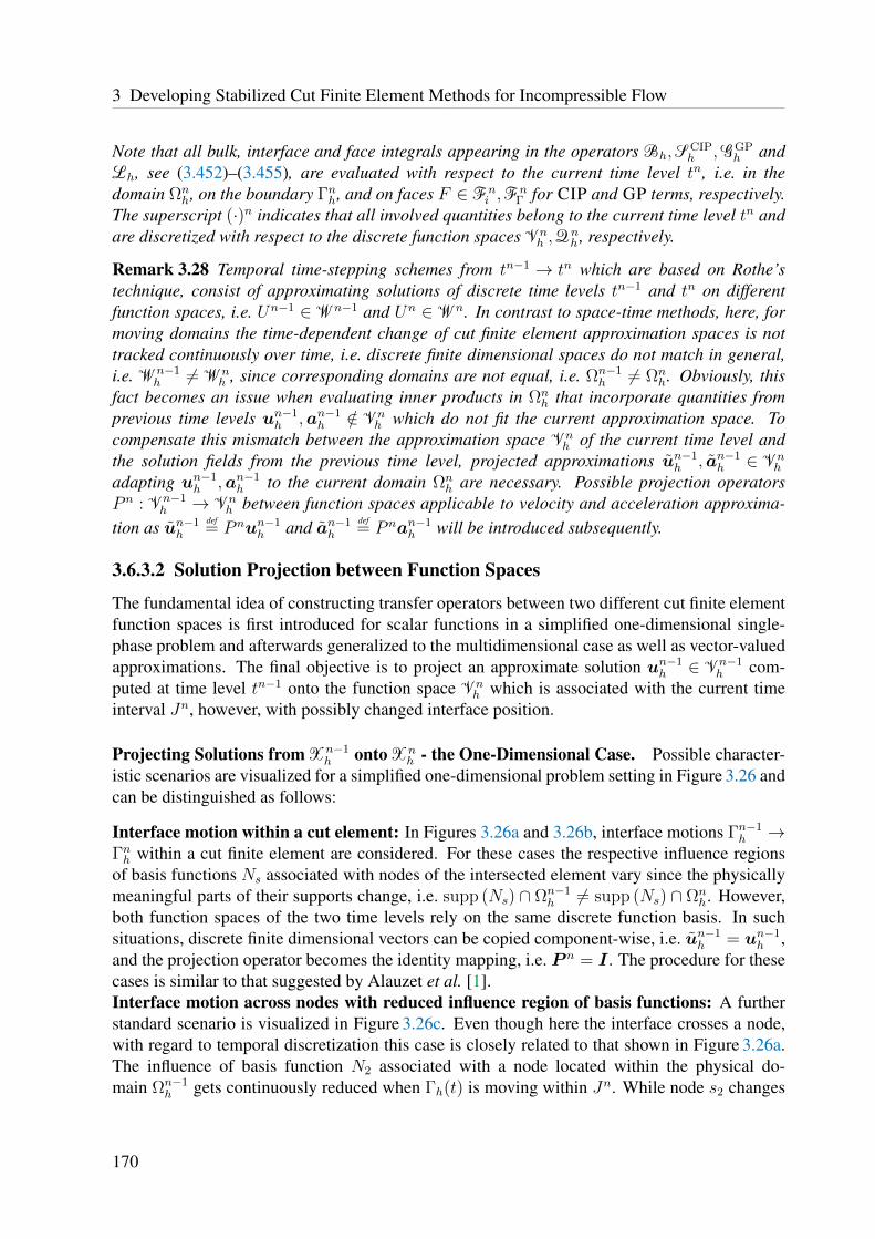
3 Developing Stabilized Cut Finite Element Methods for Incompressible Flow

Note that all bulk, interface and face integrals appearing in the operators Bh,SCIPh , GGP

h andLh, see (3.452)–(3.455), are evaluated with respect to the current time level tn, i.e. in thedomain Ωn

h, on the boundary Γnh, and on faces F ∈ Fni ,F

nΓ for CIP and GP terms, respectively.

The superscript (·)n indicates that all involved quantities belong to the current time level tn andare discretized with respect to the discrete function spaces Vn

h ,Qnh , respectively.

Remark 3.28 Temporal time-stepping schemes from tn−1 → tn which are based on Rothe’stechnique, consist of approximating solutions of discrete time levels tn−1 and tn on differentfunction spaces, i.e. Un−1 ∈ Wn−1 and Un ∈ Wn. In contrast to space-time methods, here, formoving domains the time-dependent change of cut finite element approximation spaces is nottracked continuously over time, i.e. discrete finite dimensional spaces do not match in general,i.e. Wn−1

h 6= Wnh , since corresponding domains are not equal, i.e. Ωn−1

h 6= Ωnh. Obviously, this

fact becomes an issue when evaluating inner products in Ωnh that incorporate quantities from

previous time levels un−1h ,an−1

h /∈ Vnh which do not fit the current approximation space. To

compensate this mismatch between the approximation space Vnh of the current time level and

the solution fields from the previous time level, projected approximations un−1h , an−1

h ∈ Vnh

adapting un−1h ,an−1

h to the current domain Ωnh are necessary. Possible projection operators

P n : Vn−1h → Vn

h between function spaces applicable to velocity and acceleration approxima-tion as un−1

h

def= P nun−1

h and an−1h

def= P nan−1

h will be introduced subsequently.

3.6.3.2 Solution Projection between Function Spaces

The fundamental idea of constructing transfer operators between two different cut finite elementfunction spaces is first introduced for scalar functions in a simplified one-dimensional single-phase problem and afterwards generalized to the multidimensional case as well as vector-valuedapproximations. The final objective is to project an approximate solution un−1

h ∈ Vn−1h com-

puted at time level tn−1 onto the function space Vnh which is associated with the current time

interval Jn, however, with possibly changed interface position.

Projecting Solutions from Xn−1h onto Xn

h - the One-Dimensional Case. Possible character-istic scenarios are visualized for a simplified one-dimensional problem setting in Figure 3.26 andcan be distinguished as follows:

Interface motion within a cut element: In Figures 3.26a and 3.26b, interface motions Γn−1h →

Γnh within a cut finite element are considered. For these cases the respective influence regionsof basis functions Ns associated with nodes of the intersected element vary since the physicallymeaningful parts of their supports change, i.e. supp (Ns) ∩ Ωn−1

h 6= supp (Ns) ∩ Ωnh. However,

both function spaces of the two time levels rely on the same discrete function basis. In suchsituations, discrete finite dimensional vectors can be copied component-wise, i.e. un−1

h = un−1h ,

and the projection operator becomes the identity mapping, i.e. P n = I . The procedure for thesecases is similar to that suggested by Alauzet et al. [1].Interface motion across nodes with reduced influence region of basis functions: A furtherstandard scenario is visualized in Figure 3.26c. Even though here the interface crosses a node,with regard to temporal discretization this case is closely related to that shown in Figure 3.26a.The influence of basis function N2 associated with a node located within the physical do-main Ωn−1

h gets continuously reduced when Γh(t) is moving within Jn. While node s2 changes

170

3.6 Stabilized CUTFEMs for Transient Incompressible Navier-Stokes Equations

uh

Γnh

Ωnh

Ωn−1h

Γn−1h

uh

s1 s2 s3 s4

(a)

F

uh

uh

Γn−1h

Γnh

Ωn−1h

Ωnh

s1 s2 s3 s4

(b)

uh

Γnh

Γn−1h

Ωnh

uh

Ωn−1h

s1 s2 s3 s4

(c)

uh

Γnh

Γn−1h

uh

Ωn−1h

Ωnh

s1 s2 s3 s4

(d)

Figure 3.26: Standard scenarios for the TRANSFER/COPY-PHASE: (a) and (b) Interface motion withinan intersected finite element with identical function spaces at tn−1 and tn, DOFs can betranscribed from Xn−1

h to Xnh , i.e. un−1

h = un−1h . (c) Reduced influence region of ba-

sis function N2 associated with node s2, which changes its location from inside the phys-ical domain Ωn−1

h to outside of the physical domain Ωnh such that un−1h = P nun−1

h with(un−1

1 , un−12 ) = (un−1

1 , un−12 ). (d) Interface motion across node and newly activated DOF at node s4.

Until time t∗ ∈ (tn−1, tn) when Γ(t) crosses s3, a natural extension via transcribing DOFs isgiven by (un−1

1 , un−12 , un−1

3 ) = (un−11 , un−1

2 , un−13 ). For t ∈ (t∗, tn), basis function N4 requires

reconstructing u4 via an extension technique un−14 = E∗(un−1

2 , un−13 ), for instance, defined by a

face-jump penalty extension operator (3.486). The final projection from Xn−1h to Xn

h results inun−1h = P nun−1

h with (un−11 , un−1

2 , un−13 , un−1

4 ) = (un−11 , un−1

2 , un−13 ,E∗(un−1

2 , un−13 )).

its location from inside the physical domain Ωn−1h to outside of the physical domain Ωn

h, the shapefunction N3, which was located within the ghost domain Ωn−1,∗

h \Ωn−1h already at tn, completely

lost its influence region, i.e. supp (N3) ∩ Ωnh = ∅. Its associated nodal value is not utilized for the

function space projection which is defined as un−1h = P nun−1

h with (un−11 , un−1

2 ) = (un−11 , un−1

2 ).

Interface motion with newly activated degrees of freedom: A contrary and much morechallenging situation is indicated in Figure 3.26d. Here, the physical domain increases andone node, which is located outside the physical domains at tn−1 and tn, however, did notcarry a DOF at the previous time step tn−1, gets activated and contributes to the approxima-tion space at the current time level tn. As no natural extension in terms of already existingdegrees of freedom is available, an expansion of un−1

h to Ωnh needs to be computed similar to

the configuration depicted in Figure 3.26b. When virtually moving the interface continuouslyfrom Γn−1

h to Γnh, a natural extension is defined by copying DOFs as long as the boundary hasnot crossed node s3 yet, i.e. (un−1

1 , un−12 , un−1

3 ) = (un−11 , un−1

2 , un−13 ). When continuing with

interface tracking from an intermediate time t∗, which is defined as the time level when theboundary crosses node s3, the existent approximation would become sub-optimal if the newlyactivated DOF associated with node s4 would be neglected. An extension beyond node s3

can be obtained, for instance, by defining un−14 such that the kink between the two piece-

wise polynomials gets minimized, as demonstrated in Figure 3.26d. Based on the key ideato control DOFs associated with ghost-nodes in pathological element intersection cases viaghost-penalty (GP) operators, a similar technique can be utilized to compute a natural ex-tension even for purposes of time stepping. Such a technique applicable to arbitrary spatialdimensions will be proposed and elaborated within the next paragraph. Once the newly cre-ated ghost-DOF associated with N4 has been computed, the final projection can defined as

171

3 Developing Stabilized Cut Finite Element Methods for Incompressible Flow

un−1h = P nun−1

h with (un−11 , un−1

2 , un−13 , un−1

4 ) = (un−11 , un−1

2 , un−13 ,E∗(un−1

2 , un−13 )). Therein,

un−14 = E∗(un−1

2 , un−13 ) denotes the computed value based on an aforementioned extension tech-

nique, which usually depends on the DOFs of all neighboring uncut elements. Note that such aprocedure requires ∆t being chosen sufficiently small such that interface motions per time stepbecome less than the length of one element, i.e. ‖uΓ‖∆t 6 h, where uΓ denotes the interfacenormal velocity. This restriction is related to the so-called Courant–Friedrichs–Lewy conditionwhich is a common stability condition for discretization schemes in fluid mechanics.

Algorithmic Procedure for Function Space Projections from Xn−1h onto Xn

h . The funda-mental idea of projecting solutions between two distinct function spaces associated with twoconsecutive time levels tn and tn−1 is subsequently generalized to the multidimensional case,i.e. d = 2, 3, based on the expanded cut finite element approximation space introduced in Sec-tion 2.2.4. For each DOF un−1

k , i.e. 1 6 k 6 numdof (s), of active nodes s ∈ N at the currenttime level tn an appropriate value has to be constructed on basis of the solution un−1

h ∈Xn−1h .

The final procedure suggested for this task is summarized in Algorithm 3.1 and is split into twophases:

• a first TRANSFER/COPY-PHASE and

• a second EXTENSION-PHASE.

The TRANSFER/COPY-PHASE comprises standard transfer techniques applicable to nodes andtheir associated DOFs as visualized in Figures 3.26a–3.26c for the one-dimensional setting.These configurations aim at directly copying DOFs from the previous configuration to the cur-rent configuration. The previously introduced transcription techniques for selected DOFs can beadapted to expanded function spaces Xh, which have been defined in Section 2.2.4, as follows:being applicable to a DOF un−1

k of the current function space Xnh , which belongs to a grid

node s, requires to identify another DOF un−1i associated with the space Xn−1

h at the same nodelocation. Thereby, reasonable DOF-pairs (un−1

k , un−1i ) have to exhibit a related meaning for

the solution approximation in their respective physical domains. Identifying such DOF-pairsrelies on information about DOF-associated volume-cell connections C ∈ Cs located withinthe support of its shape function Ns, see also elaborations in Section 2.2.4. As indicated inFigures 3.26a–3.26c, different pairs between standard and ghost-DOFs of current and previoustime levels might be reasonable. Common scenarios where the TRANSFER/COPY-PHASE yieldsreasonable DOF-pairs are visualized in Figure 3.27. Note that identification of DOF-pairsshould be possible for all DOFs at the current time level tn whose node is located within thephysical domain Ωn

h. If supp (Ns) for a given DOF is intersected at the current time level, it wasalso intersected at the previous time level. Otherwise, the CFL-like condition on the interfacemotion has been violated.

After performing the TRANSFER/COPY-PHASE there may remain some ghost-DOFs whichhave been newly activated compared to the previous intersection configuration. Such DOFs be-long to the scenario Figure 3.26d, i.e. toXn

h \Xn−1h , and are visualized exemplarily in Figure 3.27

for d = 2. For multidimensional problem settings, missing ghost-DOFs can be computed in asecond step, called the EXTENSION-PHASE. Fixing values which have been already determinedduring the TRANSFER/COPY-PHASE by setting Dirichlet constraints toXn

h , whose resulting trialand test function spaces are then denoted as Xn

h and Xnh,0, a linear global extension system can

172

3.6 Stabilized CUTFEMs for Transient Incompressible Navier-Stokes Equations

Algorithm 3.1 Function space projection fromXn−1h toXn

h for CUTFEMs with moving domains

1: INPUT: function spaces Xn−1h and Xn

h including cut-related entities, discrete scalar fielduh ∈Xn−1

h to be projected onto Xnh .

2: TRANSFER/COPY-PHASE (identify related node-wise DOF pairs (u, u) associated with thefunction spaces Xn

h ,Xn−1h which are reasonable to transcribe/copy their DOFs u 7→ u)

3: for each active node s ∈ N with numdof (s)def= |Cs| > 1 at current time level tn do

4: for each DOF uk (1 6 k 6 numdof (s)) with associated volume-cell connectionCk ∈ Csdo

5: Identify DOF ui ∈ (u1, ... , us) from uh ∈Xn−1h with s = |Cs(tn−1)| the number of

DOFs for node s at the previous time level tn−1.6: if (identification successful) then7: Set DOF pair (uk, ui) and copy value ui 7→ uk.8: else if (identification not successful for ghost-DOF uk) then9: Mark DOF uk for EXTENSION-PHASE.

10: else11: Throw exception (“the CFL-like condition is not satisfied!”).12: end if13: end for14: end for15: EXTENSION-PHASE (extend solution into the interface zone)16: Build constraint function space Xn

h with Dirichlet values for all DOFs successfullyidentified in the TRANSFER/COPY-PHASE.

17: Solve linear global extension system: Find uh ∈ Xnh such that Enh(uh, vh) = 0∀ vh ∈ Xn

h,0.18: OUTPUT: final projection P n : Xn−1

h →Xnh with solution un−1

h = P nun−1h .

be set up as follows: find uh ∈ Xnh such that

Enh(uh, vh) =∑

F∈FnΓ

∑

06j6k

h2j+1F 〈[[∂jnuh]], [[∂jnvh]]〉F = 0 ∀ vh ∈ Xn

h,0, (3.486)

which is a face-jump ghost-penalty operator, as defined in (3.145). Note that even though thelinear system to be solved is defined globally, in average the number of non-zero entries permatrix row is much less compared to those which result from the non-linear discrete systemsto be solved in each time step for the incompressible Navier-Stokes equations. This is dueto the fact that for practical situations only a few ghost-DOFs have to be determined via thisextension technique. At least all standard DOFs associated with nodes located in the interior ofthe domain Ωn

h have been determined previously in the TRANSFER/COPY-PHASE and are treatedas Dirichlet values in the extension system. These DOFs can be either completely removed fromthe global linear system or can be simply deactivated by setting trivial diagonal 1-entries in thecorresponding matrix rows and adapting the right-hand side accordingly.

Combining the TRANSFER/COPY-PHASE with a consecutive EXTENSION-PHASE allows todefine the final projection P n : Xn−1

h →Xnh with un−1

h = P nun−1h . Adaption to vector-valued

function spaces, i.e. sets of DOFs as required for velocities and accelerations, is straightforward.Note that this extension technique retains the optimal order of the spatial approximation. Due

173

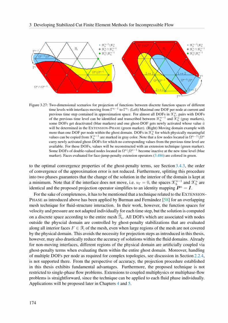
3 Developing Stabilized Cut Finite Element Methods for Incompressible Flow

Ωn ∩ Ωn−1

Ωn\Ωn−1

Ωn−1\Ωn

Γn

Γn−1Th

Xn−1h \Xn

h

Xnh ∩Xn−1

h

Xnh\Xn−1

h

Th

Xn−1h \Xn

h

Xnh ∩Xn−1

h

Xnh\Xn−1

h

2 7→ 1

2 7→ 1 1 7→ 2

1 7→ 2

Ωn−1\Ωn

Ωn ∩ Ωn−1

Ωn\Ωn−1

Γn

Γn−1

Figure 3.27: Two-dimensional scenarios for projection of functions between discrete function spaces of differenttime levels with interfaces moving from Γn−1 to Γn: (Left) Maximal one DOF per node at current andprevious time step contained in approximation space. For almost all DOFs in Xn

h , pairs with DOFsof the previous time level can be identified and transcribed between Xn−1

h and Xnh (gray markers),

some DOFs get deactivated (blue markers) and one ghost-DOF gets newly activated whose value uwill be determined in the EXTENSION-PHASE (green marker). (Right) Moving domain example withmore than one DOF per node within the ghost domain. DOFs in Xn

h for which physically meaningfulvalues can be copied from Xn−1

h are marked in gray color. Note that a few nodes located in Ωn−1\Ωncarry newly activated ghost-DOFs for which no corresponding values from the previous time level areavailable. For these DOFs, values will be reconstructed with an extension technique (green marker).Some DOFs of double-valued nodes located in Ωn\Ωn−1 become inactive at the new time level (bluemarker). Faces evaluated for face-jump-penalty extension operators (3.486) are colored in green.

to the optimal convergence properties of the ghost-penalty terms, see Section 3.4.3, the orderof convergence of the approximation error is not reduced. Furthermore, splitting this procedureinto two phases guarantees that the change of the solution in the interior of the domain is kept ata minimum. Note that if the interface does not move, i.e. uΓ = 0, the spaces Xn−1

h and Xnh are

identical and the proposed projection operator simplifies to an identity mapping P n = I .For the sake of completeness, it has to be mentioned that a technique related to the EXTENSION-

PHASE as introduced above has been applied by Burman and Fernandez [58] for an overlappingmesh technique for fluid-structure interaction. In their work, however, the function spaces forvelocity and pressure are not adapted individually for each time step, but the solution is computedon a discrete space according to the entire mesh Th. All DOFs which are associated with nodesoutside the physcial domain are controlled by ghost-penalty stabilizations that are evaluatedalong all interior faces F ∈ Fi of the mesh, even when large regions of the mesh are not coveredby the physical domain. This avoids the necessity for projection steps as introduced in this thesis,however, may also drastically reduce the accuracy of solutions within the fluid domains. Alreadyfor non-moving interfaces, different regions of the physical domain are artificially coupled viaghost-penalty terms when evaluating them within the entire ghost domain. Moreover, handlingof multiple DOFs per node as required for complex topologies, see discussion in Section 2.2.4,is not supported there. From the perspective of accuracy, the projection procedure establishedin this thesis exhibits fundamental advantages. Furthermore, the proposed technique is notrestricted to single-phase flow problems. Extensions to coupled multiphysics or multiphase-flowproblems is straightforward, since the technique can be applied to each fluid phase individually.Applications will be proposed later in Chapters 4 and 5.

174

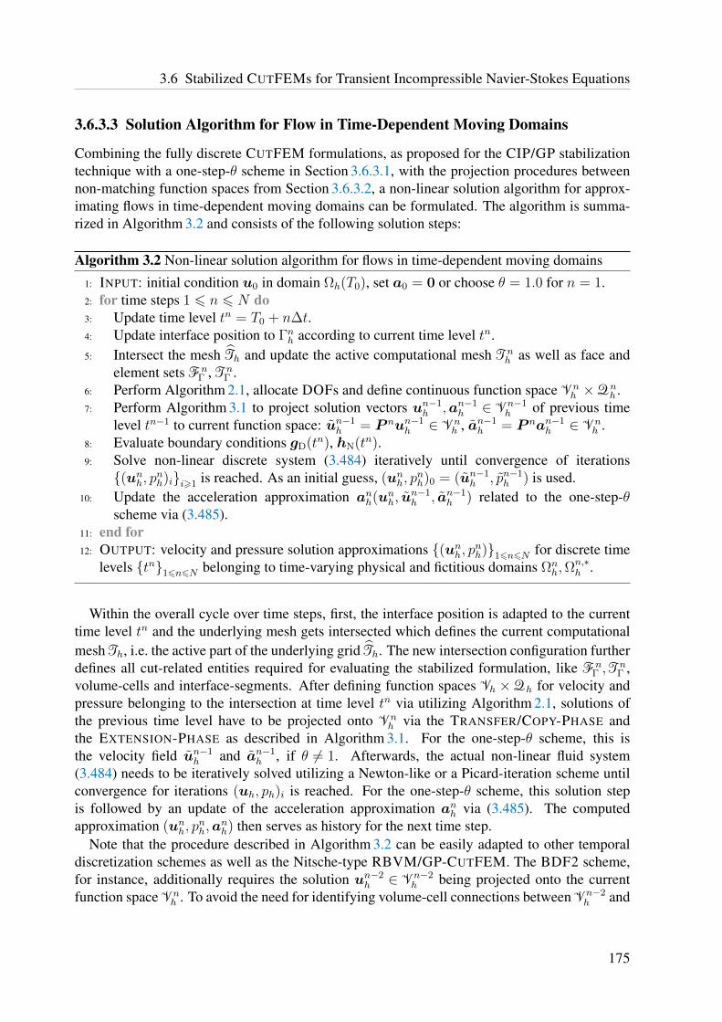
3.6 Stabilized CUTFEMs for Transient Incompressible Navier-Stokes Equations

3.6.3.3 Solution Algorithm for Flow in Time-Dependent Moving Domains

Combining the fully discrete CUTFEM formulations, as proposed for the CIP/GP stabilizationtechnique with a one-step-θ scheme in Section 3.6.3.1, with the projection procedures betweennon-matching function spaces from Section 3.6.3.2, a non-linear solution algorithm for approx-imating flows in time-dependent moving domains can be formulated. The algorithm is summa-rized in Algorithm 3.2 and consists of the following solution steps:

Algorithm 3.2 Non-linear solution algorithm for flows in time-dependent moving domains

1: INPUT: initial condition u0 in domain Ωh(T0), set a0 = 0 or choose θ = 1.0 for n = 1.2: for time steps 1 6 n 6 N do3: Update time level tn = T0 + n∆t.4: Update interface position to Γnh according to current time level tn.5: Intersect the mesh Th and update the active computational mesh Tn

h as well as face andelement sets Fn

Γ , TnΓ .

6: Perform Algorithm 2.1, allocate DOFs and define continuous function space Vnh ×Qn

h .7: Perform Algorithm 3.1 to project solution vectors un−1

h ,an−1h ∈ Vn−1

h of previous timelevel tn−1 to current function space: un−1

h = P nun−1h ∈ Vn

h , an−1h = P nan−1

h ∈ Vnh .

8: Evaluate boundary conditions gD(tn), hN(tn).9: Solve non-linear discrete system (3.484) iteratively until convergence of iterations(unh, pnh)ii>1 is reached. As an initial guess, (unh, p

nh)0 = (un−1

h , pn−1h ) is used.

10: Update the acceleration approximation anh(unh, un−1h , an−1

h ) related to the one-step-θscheme via (3.485).

11: end for12: OUTPUT: velocity and pressure solution approximations (unh, pnh)16n6N for discrete time

levels tn16n6N belonging to time-varying physical and fictitious domains Ωnh,Ω

n,∗h .

Within the overall cycle over time steps, first, the interface position is adapted to the currenttime level tn and the underlying mesh gets intersected which defines the current computationalmesh Th, i.e. the active part of the underlying grid Th. The new intersection configuration furtherdefines all cut-related entities required for evaluating the stabilized formulation, like Fn

Γ ,TnΓ ,

volume-cells and interface-segments. After defining function spaces Vh ×Qh for velocity andpressure belonging to the intersection at time level tn via utilizing Algorithm 2.1, solutions ofthe previous time level have to be projected onto Vn

h via the TRANSFER/COPY-PHASE andthe EXTENSION-PHASE as described in Algorithm 3.1. For the one-step-θ scheme, this isthe velocity field un−1

h and an−1h , if θ 6= 1. Afterwards, the actual non-linear fluid system

(3.484) needs to be iteratively solved utilizing a Newton-like or a Picard-iteration scheme untilconvergence for iterations (uh, ph)i is reached. For the one-step-θ scheme, this solution stepis followed by an update of the acceleration approximation anh via (3.485). The computedapproximation (unh, p

nh,a

nh) then serves as history for the next time step.

Note that the procedure described in Algorithm 3.2 can be easily adapted to other temporaldiscretization schemes as well as the Nitsche-type RBVM/GP-CUTFEM. The BDF2 scheme,for instance, additionally requires the solution un−2

h ∈ Vn−2h being projected onto the current

function space Vnh . To avoid the need for identifying volume-cell connections between Vn−2

h and

175

3 Developing Stabilized Cut Finite Element Methods for Incompressible Flow

Vnh , one can simply project the solution un−2

h ∈ Vn−2h twice. In a first step it is transcribed from

Vn−2h to Vn−1

h and in a second step from Vn−1h to Vn

h , i.e. ˜un−2h

def= P n(P n−1un−2

h ). Comparedto the one-step-θ scheme, which requires to project un−1

h ,an−1h ∈ Vn−1

h onto Vnh in each time

step, for the BDF2 time stepping scheme un−1h , un−2

h ∈ Vn−1h have to be adapted to Vn

h . Thecomputational costs for projecting vectors remain the same for both schemes.

3.6.4 Numerical Tests for Incompressible Flow in Moving DomainsDifferent temporal discretization schemes in combination with the solution technique for flowsin time-dependent moving domains, as summarized in Algorithms 3.1 and 3.2, are validated forthe different Nitsche-type CUTFEM formulations proposed in Sections 3.6.1.1 and 3.6.1.2. Todemonstrate the accuracy and the robustness of the proposed function space projection techniqueintroduced in Section 3.6.3.2, a test example with analytical solution is considered. For thispurpose, the already well-studied Taylor problem is solved on a time-dependent domain whichundergoes large variations. In order to illustrate the performance and the capabilities of thestabilized discrete fluid formulations in largely changing fluid domains for viscous- as well asconvective-dominated flows, two simulations inspired by fluid-structure interactions are investi-gated: A beam-like structure is embedded into a viscous surrounding incompressible flow andsubjected to a time-dependent rigid body rotation. To investigate the quality of the fluid solutionnear the boundary zone, a higher-Reynolds-number flow around a translationally moved rigidcylinder serves as test example.

3.6.4.1 Taylor Problem in a Moving Domain

As a first test case, the two-dimensional Taylor problem (3.164)–(3.166) with gu(t) = gp(t) = 1.0and ν = 0.0001, introduced in Section 3.4.4.2, is considered. While the solution is steady, thefluid domain is temporally moving and boundary conditions are imposed at the fluid boundaryusing the proposed Nitsche technique. The time-dependent fluid domain is of ellipsoidal shapefor all times t ∈ (0, 1] with time-varying main axes a1(t), a2(t) which are pre-defined as

a1(t) = r(0.75 + 0.25 cos(4πt)) and a2(t) = r(0.75 + 0.25 cos(2πt)) (3.487)

such that initial and final configuration coincide and are of circular shape with radius r = 0.45.For the domain approximation an implicit level-set representation φ(x− c; a1(t), a2(t)) is uti-lized as stated in (A.6) with center point c = (0.5, 0.5). The level-set field and the solution fieldsare approximated with a coarse unfitted background mesh Th which covers the square domain[0, 1]2 and consists of linear right-angled triangular elements P1 with h = 1/56 denoting theirshort lengths. The spatial discretization is based on the Nitsche-type CIP/GP-CUTFEM asformulated in Section 3.6.1.1. For the temporal discretization, the time-step length is chosen as∆t = 0.005. This test case is performed for three different time-stepping schemes: the OST-scheme with θ = 1.0 and θ = 0.5 as well as the BDF2 scheme. The computed solutions arealmost indistinguishable and the results for the OST variant with θ = 0.5 are visualized atdifferent intermediate time levels in Figure 3.28. It is obvious that the large variations in thecomputational domain and the projections of discrete solutions between function spaces do notdeteriorate accuracy and robustness. Initial and final solution are almost identical. For thesake of completeness, the L2-velocity error for the visualized solution at the final time T = 1is ‖u− uh‖Ω = 8.611 · 10−4 and comparable to a setting with a non-moving domain.

176

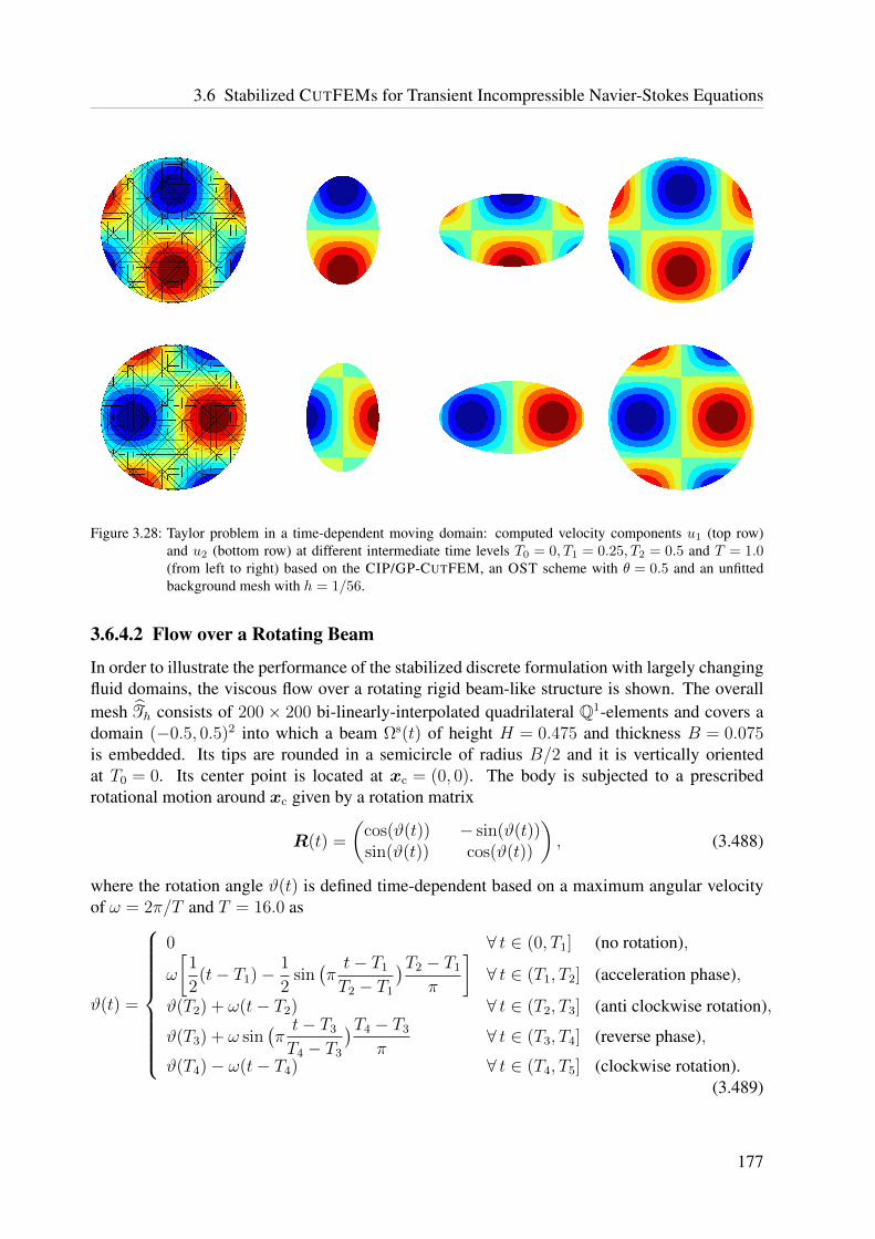
3.6 Stabilized CUTFEMs for Transient Incompressible Navier-Stokes Equations

Figure 3.28: Taylor problem in a time-dependent moving domain: computed velocity components u1 (top row)and u2 (bottom row) at different intermediate time levels T0 = 0, T1 = 0.25, T2 = 0.5 and T = 1.0(from left to right) based on the CIP/GP-CUTFEM, an OST scheme with θ = 0.5 and an unfittedbackground mesh with h = 1/56.

3.6.4.2 Flow over a Rotating Beam

In order to illustrate the performance of the stabilized discrete formulation with largely changingfluid domains, the viscous flow over a rotating rigid beam-like structure is shown. The overallmesh Th consists of 200× 200 bi-linearly-interpolated quadrilateral Q1-elements and covers adomain (−0.5, 0.5)2 into which a beam Ωs(t) of height H = 0.475 and thickness B = 0.075is embedded. Its tips are rounded in a semicircle of radius B/2 and it is vertically orientedat T0 = 0. Its center point is located at xc = (0, 0). The body is subjected to a prescribedrotational motion around xc given by a rotation matrix

R(t) =

(cos(ϑ(t)) − sin(ϑ(t))sin(ϑ(t)) cos(ϑ(t))

), (3.488)

where the rotation angle ϑ(t) is defined time-dependent based on a maximum angular velocityof ω = 2π/T and T = 16.0 as

ϑ(t) =

0 ∀ t ∈ (0, T1] (no rotation),

ω

[1

2(t− T1)− 1

2sin(πt− T1

T2 − T1

)T2 − T1

π

]∀ t ∈ (T1, T2] (acceleration phase),

ϑ(T2) + ω(t− T2) ∀ t ∈ (T2, T3] (anti clockwise rotation),

ϑ(T3) + ω sin(πt− T3

T4 − T3

)T4 − T3

π∀ t ∈ (T3, T4] (reverse phase),

ϑ(T4)− ω(t− T4) ∀ t ∈ (T4, T5] (clockwise rotation).(3.489)

177

3 Developing Stabilized Cut Finite Element Methods for Incompressible Flow

The first interval (0, T1] with T1 = 1.0 is a ramp phase to let the flow develop around the fixedobstacle. During (T1, T2] with T2 = T1 + 1.0, the beam starts increasing its velocity until amaximum angular velocity ω is reached at T2. Afterwards, the beam rotates counter clockwisewith constant ω in (T2, T3] with T3 = T2 + 12.0. Next, the rotation turns its direction. Within(T3, T4] the rotation decreases and the angular velocity turns its sign until a negative angularvelocity of−ω is reached at T4 = T3 + 2.0. Finally, the beam rotates clockwise one full cycle of2π until T5 = 32.0. Note that ϑ(t) is defined such that ϑ(t), ϑ(t) are continuous within [0, T5].

The time-dependent fluid domain is then defined as Ωf(t)def= (∪

T∈ThT )\Ωs(t). At the movingboundary Γ(t), the structural velocity is imposed as Dirichlet boundary condition for the fluid uti-lizing the Nitsche-type technique. The boundary condition is given as gD = uh(t) = xs

h(t). Thissetup can be seen as a one-sided fluid-structure interaction with prescribed rigid body rotationalmotion. Similar to fluid-structure interaction algorithms, as will be considered later in Chapter 5,the structural velocity us

h(t) is approximated based on the current structural coordinates xsh(t)

utilizing a one-step-θ scheme for the ODE xsh(t) = us

h(t) resulting in

us,nh =

xsh(t

n)− xsh(t

n−1)

θ∆t− 1− θ

θus,n−1h . (3.490)

For the rotational motion, the coordinates of the structural body are defined as

xsh(t) = R(t)(xs

h(T0)− xc) + xc. (3.491)

Further boundary conditions at the outer fluid boundary need to be imposed: a Dirichlet in-flow boundary condition is strongly set at x1 = −0.5 defined by a parabolic profile for the u1-component as u1 = 4(0.5 + x2)(0.5− x2) and by u2 = 0. The velocity is increased during theinitial ramp phase (0, T1] utilizing the function 1/2(1− cos(πt/T1)). At the top and bottom walls(x2 = ±0.5) no-slip is enforced, i.e. u = 0, and a zero-traction Neumann outflow condition isimposed at x1 = 0.5. For temporal discretization a one-step-θ scheme is applied with θ = 1.0and a time-step length of ∆t = 0.03. The kinematic viscosity is set to ν = 0.1. The resulting vis-cous flow around the rotating beam-like structure computed with the Nitsche-type RBVM/GP-CUTFEM introduced in Section 3.6.1.2 and approximated by the solution procedure proposed inAlgorithms 3.1 and 3.2 is shown in Figure 3.29. This example clearly demonstrates the generalapplicability of this established CUTFEM to industrially relevant problem settings where, forinstance, structural components are subjected to large rotations in surrounding fluids and under-lines the obvious superiority over classical ALE-based moving fitted-mesh FEM approaches.

3.6.4.3 Flow over a Moving Cylinder

A translationally moved rigid cylinder in a rectangular fluid domain serves as test case to demon-strate the robustness of the proposed cut finite element method for highly dynamic higher-Reynolds-number flows. The setup of this example is inspired by a setting proposed by Co-dina et al. [76]. A cylindrical rigid body Ωs with diameter d = 0.2 and initial center posi-tion (0.3, 0.23) at t = T0 is embedded into an unfitted regular mesh Th consisting of 450× 90linearly-interpolated quadrilateral Q1 finite elements which defines a domain (0, 2.2)× (0, 0.44).Note that compared to the setup considered in [76], the initial location of the cylinder is chosenslightly more non-symmetric with respect to the background domain. This makes the test

178

3.6 Stabilized CUTFEMs for Transient Incompressible Navier-Stokes Equations

Figure 3.29: Flow over a rotating two-dimensional rigid beam-like structure: velocity norm ‖uh‖ (top) andpressure ph (bottom) at different time levels t = 0.9, t = 3.0, t = 7.5 and t = 10.5 (from left to right)(velocity color scale [0, 1.56], pressure color scale [−3.9, 10.7]).

case much more demanding due to stronger vortex shedding which arises when starting tomove the body. The structure is pulled in x1-direction with a prescribed displacement fieldd1(t) = 1.1 + 0.8 sin (2

3π(t− 0.75)) such that it will be returned to its starting position after a

simulation time of T = 3. The flow is initially at rest and no-slip wall boundary conditionsu = 0are set strongly at top, bottom and left side of the fluid domain. At x1 = 2.2 the square fluiddomain is opened and a zero-traction boundary condition is imposed, i.e. hN = 0. At the circularinterface Γ(t), the structural velocity is computed utilizing the same approximation technique asproposed for the previous example in (3.490). For the spatial and temporal discretization, theNitsche-type RBVM/GP-CUTFEM introduced in Section 3.6.1.2 has been applied in combina-tion with the moving domain Algorithms 3.1 and 3.2. The temporal discretization is based on aone-step-θ scheme with θ = 1.0 and ∆t = 0.001.

Compared to the previous rotating beam example, due to a lower viscosity of ν = 0.001, astrongly non-symmetric flow pattern develops in the backflow of the cylinder when moving it inpositive x1-direction. The Reynolds number emerges to a maximum of approximately Re ≈ 300where its definition is based on the diameter d and the maximum cylinder velocity. The resultinghighly dynamic velocity and pressure solutions are visualized in Figure 3.30. While movingthe structure in opposite direction during t ∈ (1.5, 3), highly dynamic time-dependent forcesact on the structural surface. Visualizations of interfacial forces f s

l computed at nodes l of thestructural trace mesh utilizing formula (3.482) underline the complexity of the flow and therobustness of the stabilized CUTFEM in the vicinity of the moving interface zone. Additionally,in Figure 3.31, forces f = (f1, f2) acting at the left-most and top-most points of the circularinterface are plotted over time for two different time-step sizes ∆t = 0.001 and ∆t = 0.002.Particularly in view of fluid-structure-interaction problem settings, the quality of this interfacialmeasure is an important indicator for the robustness and the high capability of the proposed fluidsolver as well as of the algorithmic procedure for convective-dominated flow in time-dependentmoving domains. Such problem configurations will be considered further in Chapter 5.

179

3 Developing Stabilized Cut Finite Element Methods for Incompressible Flow

Figure 3.30: Flow over a two-dimensional moving cylinder with a maximumRE ≈ 300: (Left) velocity norm ‖uh‖and pressure ph at times t = 1.18, t = 1.97, t = 2.29 and t = 2.46 (from top to bottom) (velocity colorscale [0, 3], pressure color scale [−5.6, 3.5]). (Right) forces acting on moving interface Γ (color scale[0, 0.000443]) at aforementioned times t (from top to bottom).

180

3.6 Stabilized CUTFEMs for Transient Incompressible Navier-Stokes Equations

0 1 2 3−0.025

−0.02

−0.015

−0.01

−0.005

0

0.005

0.01

0.015

0.02

0.025

time t

force

Left-point force (f1, f2)

force f1 ∆t = 0.002force f1 ∆t = 0.001force f2 ∆t = 0.002force f2 ∆t = 0.001

0 1 2 3−0.005

0

0.005

0.01

0.015

0.02

0.025

0.03

0.035

0.04

time t

force

Top-point force (f1, f2)

force f1 ∆t = 0.002force f1 ∆t = 0.001force f2 ∆t = 0.002force f2 ∆t = 0.001

Figure 3.31: Flow over a two-dimensional moving cylinder with a maximum RE ≈ 300: nodal forcesfl = (f1, f2)l acting at selected points of the cylindrical surface Γ(t) over time t ∈ (0, 3) computedwith two different time-step sizes ∆t = 0.001 and ∆t = 0.002. (Left) force for the most-left structuralpoint. (Right) force for the most-top structural point.

181

Chapter 4Unfitted Domain Decomposition Methods for

Incompressible Single- and Two-Phase Flows

This chapter aims at developing numerical cut finite element approaches for incompressible flowproblems in which fluid phases interact. The key idea is to combine the generalized frameworkof domain decomposition based on non-interface-fitted computational meshes, as introducedin Section 2.1.4, with stabilized cut finite element methods for the respective subregions, asdeveloped throughout Chapter 3.

Allowing for different unfitted approximation spaces in distinct regions of the entire computa-tional domain, together with sharp approximations of the subdomains and their discrete solutionswith cut finite element techniques, makes such approaches attractive for a wide range of coupledflow problems. Their applicability ranges from mesh-tying techniques for single-phase flowsto the interaction of several fluid phases with different material properties. For single-phaseflows, the domain can be split into separate subregions such that unfitted techniques play totheir strengths in utilizing appropriate approximation spaces in particular regions of interest.As an example, boundary layers around structural bodies can be efficiently captured with thisapproach. Since mass transport across the interfaces is supported due to the same materialproperties in the subdomains, interfaces can then be considered either stationary or arbitrarilymoving. Immiscible two-phase flows, in contrast, are usually subjected to large interfacialmotions and the interface remains the separating manifold between the two different physicalfluid phases. The use of unfitted techniques allows for largely changing topologies and theirstability and optimality properties are guaranteed independent of the interface locations for low-and high-Reynolds-number flows. These aspects render such approaches highly promising.

In this chapter, the focus is turned to physics at separating phase boundaries in Section 4.1 andthe numerical treatment of modeled coupling constraints within the framework of Nitsche-typemethods utilized for their weak constraint enforcement in Section 4.2. A stabilized formulationfor coupling solution fields which belong to different subdomains and discrete approximationspaces will be proposed. Moreover, numerical issues concerning interface stability are exam-ined from a mathematical point of view and possible solution techniques are developed anddiscussed. Later on, the performance of the computational approach will be demonstrated for anoverlapping mesh domain decomposition method applied to fluid mesh-tying problem settingsin Section 4.3. The high capabilities of unfitted mesh methods for incompressible two-phase

183

4 Unfitted Domain Decomposition Methods for Incompressible Single- and Two-Phase Flows

flows will finally be shown as an outlook in Section 4.4. The subsequent elaborations are mainlybased on work available in Schott and Wall [230], Massing et al. [183], Schott and Rasthofer etal. [231] and Schott and Shahmiri et al. [232].

4.1 Domain Decomposition Problem Setup for Coupled FlowsThis section provides fundamentals on physical models applicable to mesh-tying approaches forsingle-phase flows as well as immiscible multiphase flows. Such problem settings are formulatedin terms of an abstract coupled interface initial boundary value problem. A presentation of suchflow setups based on decomposing domains will be given in strong and variational forms.

4.1.1 Multiple Fluid Phases - Domains and InterfacesComputational Domains. The notation and terminology on single fluid phases, associatedsubdomains and interfaces for coupled flows used throughout the subsequent sections are basedon the abstract multidomain problem setting introduced in Section 2.1.1. The overall compu-tational domain is given by Ω

def=

⋃16i6NdomΩi with possibly moving interfaces Γij

def= Ωi ∩ Ωj

(i < j) which separate fluid phases with possibly different material parameters µi, ρi or splitsingle phases into artificial partitions for mesh-tying purposes; an overview about possible strate-gies was given in Section 2.1.4.3. Respective Dirichlet and Neumann boundary parts of thefluid subdomains are denoted with ΓiD,Γ

iN and satisfy ∂Ωi = (ΓiD ∪ ΓiN)

⋃j 6=i Γ

ij . Note that allgeometric entities are possibly time-dependent. For sake of clarity, if unmistakable, occasionallythe temporal index t as well as the superscript (·)f denoting fluid quantities are omitted. Weightedaverage and jump operators · , 〈·〉 and [[·]] are as defined in (2.1)–(2.3). The normal vector at Γij

follows the convention from Section 2.1.1 being outward pointing from Ωi to Ωj , where i < j.

Interfacial Constraints between Fluid Phases. At fluid-fluid interfaces, which is an umbrellaterm for interfaces between two fluid phases, i.e. liquids or gases, different physical modelscan be deduced to account for different physical phenomena which may emanate from highlyvarying length scales. Hereby, modeling approaches range from molecular to microscopicup to macroscopic view points. Commonly used modeling approaches deduce kinematic anddynamic relations from basic conservation principles for mass, linear and angular momentum ona macroscopic level as shown below.

Observing conservation of mass and momentum on a time-dependent control volume includ-ing a part of the interface Γij , which moves in its own normal direction nij with an interfacialspeed uijΓ , allows to state conservation laws for those ∀x ∈ Γij(t) as

ρi(ui · nij − uijΓ ) = −M = ρj(uj · nij − uijΓ ), (4.1)

ρiui(ui · nij − uijΓ )− σσσ(ui, pi) · nij = ρjuj(uj · nij − uijΓ )− σσσ(uj, pj) · nij (4.2)

with the mass flow rate M for Ωi across the interface Γij . Mass conservation (4.1) can bereformulated by means of a jump condition for fluid velocities in interface normal direction to

[[u]] · nij = (ui − uj) · nij = uijΓ −M/ρi − (uijΓ −M/ρj) = −M [[ρ−1]] ∀x ∈ Γij(t). (4.3)

184

4.1 Domain Decomposition Problem Setup for Coupled Flows

Furthermore, for viscous fluids, i.e. µi, µj > 0, interface tangential velocities are modeled beingcontinuous

[[u]] · tijr = 0 ∀x ∈ Γij(t) (4.4)

in all interface-tangential directions (r = 1, ... , (d− 1)). Combining momentum balance (4.2)with mass conservation (4.3) and (4.4) results in jump conditions for normal and tangential partsof interface tractions

nij · [[σσσ(u, p)]] · nij = −M [[u]] · nij = M2[[ρ−1]] ∀x ∈ Γij(t), (4.5)

tijr · [[σσσ(u, p)]] · nij = −M [[u]] · tijr = 0 ∀x ∈ Γij(t). (4.6)

Combining the resulting interfacial constraints, from a macroscopic point of view, kinematic anddynamical constraints between fluid phase i and fluid phase j can then be modeled as

[[u]] = −M [[ρ−1]]nij ∀x ∈ Γij(t), (4.7)

[[σσσ(u, p)]] · nij = M2[[ρ−1]]nij ∀x ∈ Γij(t). (4.8)

Depending on the material combination at the common fluid-fluid interface and on the mass flowrateM across the interface, for different problem settings like fluid mesh-tying or incompressibletwo-phase flow, commonly used interfacial constraints are reviewed subsequently.

Fluid mesh tying: Considering same fluid properties on both sides of the interface, i.e. ρi = ρj

and µi = µj > 0, which holds when one single fluid phase is artificially split for discrete approx-imation purposes, the interfacial constraints previously deduced from conservation of mass andlinear momentum simplify due to [[ρ−1]] = 0 to

[[u]] = 0 ∀x ∈ Γij(t), (4.9)

[[σσσ(u, p)]] · nij = 0 ∀x ∈ Γij(t). (4.10)

These conditions keep valid independent of the motion of the interface. If the interface followsthe fluid particles in their motion, no mass flow across the interface is present, i.e. M = 0.If M 6= 0, fluid particles are convected across the interface which is allowed due to the samephysical fluid properties in both subdomains.

Two-phase flow including surface tension: Different immiscible fluid or gas phases are char-acterized by discontinuous material properties µi 6= µj and ρi 6= ρj such that [[ρ−1]] 6= 0. Forincompressible two-phase flow the phase boundaries Γij(t) are advected with the fluid particlessuch that no mass flow across the interface occurs, i.e. M = 0 and [[u]] = 0. Additionally, dueto the fact that fluid properties change discontinuously, molecular forces of attraction betweenmolecules of the same type, so-called cohesion forces, are stronger than attraction betweenmolecules of different type, so-called adhesion forces. From a microscopic point of view theseforces imply surface tension; more detailed elaborations can be found, e.g., in the work byBrackbill et al. [32]. Surface-tension effects depend on the curvature κ = −∇ · nij of thephase surface and the combination of material properties expressed in terms of a surface-tensioncoefficient ιst, which is assumed to be constant along the manifold throughout this thesis. The

185

4 Unfitted Domain Decomposition Methods for Incompressible Single- and Two-Phase Flows

interfacial constraints for incompressible two-phase flows including surface tension are thenmodeled as

[[u]] = 0 ∀x ∈ Γij(t), (4.11)

[[σσσ(u, p)]] · nij = ιstκnij ∀x ∈ Γij(t). (4.12)

Modeling of premixed combustion: One example for two-phase flow including mass flow ininterface normal direction across the interface, i.e. M 6= 0, can be found in the modeling ofpremixed combustion. For such applications, the mass change from the unburned (i) to theburned (j) fluid phase emanates from the chemical combustion processes in the vicinity of theinterface. The combustion zone can be thereby assumed infinitesimal thin. The mass flow itselfcan be expressed as M = −ρisL in terms of a so-called laminar flame speed sL. This denotesthe relative speed of the propagating flame front with respect to the velocity in the unburnedfluid phase in negative normal direction, i.e. sL = −(uΓ − ui · nij). The interfacial constraints(4.7)–(4.8) can be formulated based on the laminar flame speed and the material densities as

[[u]] = ρisL[[ρ−1]]nij ∀x ∈ Γij(t), (4.13)

[[σσσ(u, p)]] · nij = (ρisL)2[[ρ−1]]nij ∀x ∈ Γij(t). (4.14)

More details on this modeling approach for premixed combustion can be found, e.g., in the worksby van der Bos and Gravemeier [255] or Henke [147].

Generalized abstract form of interfacial constraints: All of the above introduced kinematicand dynamical constraints can be embedded into an abstract form as

[[u]] = gijΓ ∀x ∈ Γij(t), (4.15)

[[σσσ(u, p)]] · nij = hijΓ ∀x ∈ Γij(t) (4.16)

with functions gijΓ and hijΓ which are characteristic for the different fluid-fluid interface types andmodeling approaches.

4.1.2 Coupled Interface Initial Boundary Value Problem

The coupled system consisting of several incompressible fluids can be composed of initialboundary value problems, see Section 3.1.1, for each fluid phase in Ωi, which are governedby the incompressible Navier-Stokes equations with possibly different material properties andcomplemented with outer Dirichlet and Neumann boundary conditions at respective boundariesΓiD,Γ

iN. Furthermore, initial conditions ui0 for the velocities ui at t = T0 are assumed. Addi-

tionally, at Γij the different fluid phases are coupled together via previously derived conditions(4.15)–(4.16) and prescribed conditional functions gijΓ ,h

ijΓ .

186

4.1 Domain Decomposition Problem Setup for Coupled Flows

The strong formulation of the non-linear coupled initial boundary value problem reads: forany time t ∈ (T0, T ], find fluid velocity and pressure u(t) : Ω(t) 7→ Rd, p(t) : Ω(t) 7→ R withrestrictions ui(t) = u(t)

∣∣Ωi(t)

and pi(t) = p(t)∣∣Ωi(t)

such that

ρi∂ui

∂t+ ρi(ui · ∇)ui +∇pi − 2µi∇ · ε(ui) = ρif i ∀x ∈ Ωi(t), (4.17)

∇ · ui = 0 ∀x ∈ Ωi(t), (4.18)

ui = giD ∀x ∈ ΓiD(t), (4.19)

σσσ(ui, pi) · ni = hiN ∀x ∈ ΓiN(t), (4.20)

[[u]] = ui − uj = gijΓ ∀x ∈ Γij(t), (4.21)

[[σσσ(u, p)]] · nij = (σσσ(ui, pi)− σσσ(uj, pj)) · nij = hijΓ ∀x ∈ Γij(t), (4.22)

ui(T0) = ui0 ∀x ∈ Ωi(T0). (4.23)

For the sake of simplicity, note that all fluid phases governed by the incompressible Navier-Stokes equations are here formulated in an Eulerian frame of reference. Analogously, applyingan ALE formalism with adapted time derivative and a relative convective term as introducedin (3.4) would be straightforward.

4.1.3 Coupled Variational FormulationThe variational formulation for the coupled system of incompressible fluid phases comprisesthe variational formulations of each fluid subdomain as proposed in Section 3.1.2. The func-tional spaces for admissible velocity and pressure fields are given by the broken Sobolev spacesVgD

= H1ΓD,gD

(Ω(t)) ⊆ H1(Ω(t)) and Q = L2(Ω(t)) if ΓN 6= ∅with Ω(t) = ∪16i6NdomΩi(t). Therespective test function spaces are denoted with V0 and Q.

The coupled non-linear variational formulation then reads as follows: for all t ∈ (T0, T ], findfluid velocity and pressureU(t) = (u(t), p(t)) ∈ VgD

×Q withU i(t) = (ui(t), pi(t)) = U(t)∣∣Ωi(t)

such that for all V (t) ∈ V0 ×Q

A(U, V ) = L(V ) (4.24)

with [[u]]∣∣Γij(t)

, where

A(U, V )def=∑

16i6NdomAi(U, V ), (4.25)

L(V )def=∑

16i6Ndom

(Li(V ) +

∑j>i〈hijΓ , 〈v〉〉Γij(t)

)(4.26)

and

Ai(U, V )def= (ρi

∂ui

∂t,vi)Ωi(t) + ci(ui;ui,vi) + ai(ui,vi) + bi(pi,vi)− bi(qi,ui), (4.27)

Li(V )def= li(vi) (4.28)

denote the standard variational formulations of single-phase flows with operators ci, ai, bi and li

as defined in (3.12)–(3.15). The superscript (·)i indicates incorporated integrals and material

187

4 Unfitted Domain Decomposition Methods for Incompressible Single- and Two-Phase Flows

parameters being evaluated in respective subdomains Ωi(t) and on boundaries ΓiN(t). Notethat for this variational formulation, the flux coupling constraints [[σσσ(u, p)]] · nij = hijΓ and theNeumann boundary conditions hiN are already included in the right-hand-side term L(V ). Thiscan be seen as follows:

Starting as for deriving variational formulations (3.9) for each subdomain Ωi, after multiplyingthe strong formulation with test functions vi and integrating all viscous and pressure bulk termsby parts, the following boundary terms arise on ∂Ωi(t) which can be rewritten as∑

16i6Ndom

(−〈σσσ(ui, pi) · ni,vi〉∂Ωi

)(4.29)

=∑

16i6Ndom

(−〈hiN,vi〉ΓiN −

∑j>i

∫

Γij(σσσ(ui, pi) · ni) · vi + (σσσ(uj, pj) · nj) · vj dΓ

)

=∑

16i6Ndom

(−〈hiN,vi〉ΓiN −

∑j>i

∫

Γij[[(σσσ(u, p) · nij) · v]] dΓ

)

=∑

16i6Ndom

(−〈hiN,vi〉ΓiN −

∑j>i

∫

Γij([[σσσ(u, p)]] · nij) · 〈v〉+ (σσσ(u, p) · nij) · [[v]] dΓ

).

For splitting the jump term in line three, relation (2.4) has been utilized. The second term inthe last line allows to incorporate the flux coupling condition [[σσσ(u, p)]] · nij = hijΓ . Note thatthe last term vanishes due to [[v]]|Γij = 0, provided the coupling [[u]] = gijΓ is incorporated inthe continuous function space VgD

. This is no longer valid for composed discrete approxima-tion spaces, as will be discussed in the context of Nitsche-type techniques in the next section.Therein, the importance of the choice of average weights wi, wj incorporated in the definitionof · , 〈·〉 will be elucidated. Finally, shifting all remaining terms to the right-hand side resultsin definition (4.26) of L(V ) and operators therein.

4.2 A Stabilized Cut Finite Element Method forCoupled Incompressible Flows

This section is devoted to cut finite element methods for coupled transient incompressible Navier-Stokes flows with stationary or moving subdomains and interfaces. Stabilized semi-discretefluid formulations will be proposed for the general multidomain problem setting introducedin Section 4.1.2 including possibly different material parameters and characteristic interfacialconstraints. The major objective of discretization methods to be developed is to support indepen-dent finite dimensional approximation spaces for the different fluid subdomains and associatedsolution fields. All computational meshes are thereby allowed to be chosen independently, eitherfitted or unfitted to the phase boundaries and to outer boundaries as visualized in Figure 2.9. Af-ter introducing stabilized formulations for this generalized problem setting, remarks on stabilityproperties for certain mesh and material combinations will be made. The proposed formulationwill be tested for overlapping fluid mesh-tying approaches including combinations of fitted andunfitted meshes in Section 4.3 and for incompressible two-phase flows based on unfitted meshesin Section 4.4. Simplifications with regard to stabilization techniques for these applications aswell as related peculiarities will be addressed later in the respective sections.

188

4.2 A Stabilized Cut Finite Element Method for Coupled Incompressible Flows

4.2.1 Nitsche-type Cut Finite Element Methods for Domain Decomposition

Let Vih and Qi

h be the discrete approximation spaces for velocity and pressure associated with thedifferent fluid phases in possibly time-dependent subdomains Ωi

h. Moreover, let Wih

def= Vi

h ×Qih

denote their product spaces. In general, the associated meshes are assumed to be non-fitted todomain boundaries ΓiD,Γ

iN and, in particular, non-node-matching at interfaces Γijh . The overall

discrete approximation space defined in the entire domain Ωh can be composed of subdomainproduct spaces as Wh

def= ⊕Ndom

i=1 Wih = ⊕Ndom

i=1 (Vih ×Qi

h) such that Vh = (vh, qh) ∈ Wh is a pair ofvelocity and pressure solutions defined on Ωh for which holds

Vh|Ωi = V ih = (vih, q

ih) ∈ Vi

h ×Qih, 1 6 i 6 Ndom. (4.30)

Note that the overall function space may in that way incorporate different element types, polyno-mial orders of approximation and different mesh sizes on their respective sub-grids Ti

h. Due tothis construction, functions Vh ∈ Wh are in general discontinuous at interfaces Γij . This requiresinterfacial constraints being enforced weakly with, for instance, Nitsche-type techniques. Tounify the notation in this section, also all boundary conditions on ∂Ω are assumed to be imposedweakly. If parts of the meshes Ti

h match the domain boundary, Dirichlet boundary conditionscan be also straightforwardly incorporated into the respective trial and test function spaces.

A Nitsche-type Domain Decomposition CUTFEM for Coupled Flows. In the following,a spatial semi-discrete formulation for a system of fluid phases (4.17)–(4.23) governed by theincompressible Navier-Stokes equations will be proposed. All outer boundary conditions andinterfacial constraints between different fluid phases are enforced with Nitsche-type techniques.To stabilize the flow in the interior of the respective subdomains and on their potentially unfit-ted sub-grids, either CIP/GP or RBVM/GP stabilization approaches can be utilized; detailedelaborations on stabilizing the single phases on unfitted grids have been provided throughoutChapter 3.

Definition 4.1 (Semi-discrete Nitsche-type CUTFEM for coupled flows)Let Wh

def= ⊕Ndom

i=1 Wih, then a Nitsche-type stabilized formulation for coupling incompressible flows

reads as follows: for all t ∈ (T0, T ], find fluid velocity and pressure Uh(t) = (uh(t), ph(t)) ∈ Wh

such that for all Vh = (vh, qh) ∈ Wh

Ah(Uh, Vh) = Lh(Uh, Vh), (4.31)

where

Ah(Uh, Vh)def=

∑

16i6Ndom

(Ai,Xih (Uh, Vh) +

∑

j>i

Cijh (uh; (uh, ph), (vh, qh))

), (4.32)

Lh(Uh, Vh)def=

∑

16i6Ndom

(Li,Xih (Uh, Vh) +

∑

j>i

Lijh (uh; (vh, qh))

). (4.33)

The coupled formulation includes stabilized single-phase formulations Ai,Xih −Li,Xi

h for eachfluid phase, where Xi indicates the respective stabilized method, i.e. a CIP/ GP or a RBVM/ GP

189

4 Unfitted Domain Decomposition Methods for Incompressible Single- and Two-Phase Flows

technique; see Section 3.6.1.1 and Section 3.6.1.2 for the corresponding formulations. Therein,the operators Ai

h and Lih comprise the standard Galerkin formulation, fluid stabilization in

the interior of the subdomain (RBVM or CIP), ghost-penalty operators (GP) in the respectiveboundary/interface zones of ∂Ωi and Nitsche-type boundary terms for the weak imposition ofDirichlet boundary conditions on ΓiD, respectively. Note that the superscript (·)i indicates thatincluded quantities like domains, interfaces, integrals, element- and face-sets as well as materialparameters ρi, µi and functions (vih, q

ih) ∈ Wi

h belong to the respective fluid phase.To impose the required coupling constraints (4.21)–(4.22) at interfaces Γij , further Nitsche-

type interfacial coupling terms Cijh −Lij

h need to be consistently added:

Cijh (uh; (uh, ph), (vh, qh)) = −〈2µεεε(uh)nij, [[vh]]〉Γij + 〈ph , [[vh]] · nij〉Γij (4.34)

∓ 〈[[uh]], 2µεεε(vh)nij〉Γij − 〈[[uh]] · nij, qh〉Γij (4.35)+ 〈γ(ϕ /2)[[uh]], [[vh]]〉Γij (4.36)

+ 〈γ(ρφ/h /2)[[uh]] · nij, [[vh]] · nij〉Γij (4.37)

+ 〈(ρuhm · nij)[[uh]], vhm〉Γij (4.38)

+ 〈γupw|(ρuhm · nij)|[[uh]], [[vh]]〉Γij , (4.39)

Lijh (uh; (vh, qh)) = 〈hijΓ , 〈vh〉〉Γij (4.40)

∓ 〈gijΓ , 2µεεε(vh)nij〉Γij − 〈gijΓ · nij, qh〉Γij (4.41)

+ 〈γ(ϕ /2)gijΓ , [[vh]]〉Γij (4.42)

+ 〈γ(ρφ/h /2)gijΓ · nij, [[vh]] · nij〉Γij (4.43)

+ 〈(ρuhm · nij)gijΓ , vhm〉Γij (4.44)

+ 〈γupw|(ρuhm · nij)|gijΓ , [[vh]]〉Γij . (4.45)

The terms (4.34) and (4.40) are so-called standard consistency terms as they result form integra-tion by parts performed on the adjacent subdomains Ωi,Ωj , as derived in (4.29). Note that due toa possible discontinuity between vih ∈ Vi

h and vjh ∈ Vjh , all interface terms derived there do not

vanish in the discrete case. Neumann boundary terms remaining at ΓiN are included in Li,Xih , see

(3.455). The terms (4.35) and (4.41) comprise consistently added viscous and pressure terms.Thereby, the sign choice (∓) allows to switch between a symmetric adjoint-consistent (−) anda non-symmetric adjoint-inconsistent (+) viscous elliptic part of the formulation. The differentvariants result in changes of inf-sup stability properties and restrictions on the choice of γ,as already discussed in Section 3.3.2.4 and Section 3.4.3.4 in the context of single-phase flowproblems. In contrast, the sign of the pressure term is fixed to guarantee inf-sup stability.In (4.36)–(4.37) and (4.42)–(4.43), Nitsche-like penalty terms guarantee inf-sup stability withregard to the interfacial constraints for low- and high-Reynolds-number flows. The scaling φoccurring in the latter term is the stabilization scaling from (3.467) to account for the differentflow regimes. To cope with instabilities arising from the convective terms, to control masstransport across interfaces and to deal with issues due to the discontinuity of the convectivevelocity uh, additional control on the interfacial constraint is ensured by the terms (4.38)–(4.39) and (4.44)–(4.45). These are so-called upwinding terms which are well known from

190

4.2 A Stabilized Cut Finite Element Method for Coupled Incompressible Flows

discontinuous Galerkin methods. The equal structure of terms (4.36) and (4.39) has to be noted.Due to their different role concerning stability, however, these terms are presented separately.

Note, the weights occurring in the weighted average operators · , 〈·〉 are defined as

widef= ϕj/(ϕi + ϕj) and wj

def= ϕi/(ϕi + ϕj), (4.46)

where ϕi def= µi(f i)2 and f i is the scaling obtained from a weakened trace inequality (3.129), for

which in the simplest case holds (f i)2 ≈ 1/hi. More detailed elaborations will be provided laterin Section 4.2.2. Furthermore, ·m denotes the mean average with wim = wjm = 1/2.

Moreover, the solution Uh needs to fulfill the initial condition uh(T0) = u0 in Ω. Note thatthis requires being conform to the coupling constraints gijΓ at Γij and boundary conditions giDon ΓiD at t = T0. To shorten the presentation of the coupled formulation, the time variable isoccasionally omitted in Uh(t) = (uh(t), ph(t)). For further details on the stabilized single-phaseformulations for each fluid phase, the reader is referred to Sections 3.6.1.1 and 3.6.1.2

The semi-discrete formulation (4.31) can be straightforwardly discretized in time using tech-niques proposed in Section 3.6.1.3. Resulting non-linear systems of equations for each discretetime step can be approximated using Newton-Raphson-like iterations. Further possible issuesdue to changing function spaces during iterative procedures will be discussed in the context ofunfitted CUTFEMs for fluid-structure interaction in Chapter 5. Possible solution techniques aresuggested in Section 5.3 and supported by numerical simulations in Sections 5.3 and 5.4. Withinthis chapter, interfaces are assumed either non-moving, as sometimes the case for mesh-tyingapplications, or fixed during the Newton-Raphson-like non-linear iterative solution procedure,as common for multiphase flows.

4.2.2 Enforcing Interfacial Constraints - The Role of Weighted AveragesAs already discussed in detail in the context of weak imposition of boundary conditions inSections 3.4–3.6, for non-boundary-fitted meshes, Nitsche-type approaches provide powerfultechniques. These come along with desired inf-sup stability and optimal a priori error estimateswhich hold independent of the location of the interface within an underlying unfitted mesh.These optimality properties need to be preserved when imposing interfacial constraints betweennon-matching cut approximation spaces. The key idea of subsequently provided techniques isto exploit the stability control gained over the respective active computational meshes Ti

h. Foreach fluid phase which is equipped with an unfitted approximation space, subdomain-relatedghost-penalty operators known from single-phase flows can be utilized, respectively.

One can proceed similar to the stability estimate for single-phase problems as proposed inSection 3.5.5. Starting as in the proof of coercivity in Lemma 3.10, the viscous standard andadjoint consistency terms occurring in (4.34) and (4.35) can be estimated as follows

2〈2µεεε(uh)nij, [[uh]]〉Γij6 ε−1‖ µεεε(uh)nij‖2

Γij + 4ε‖[[uh]]‖2Γij

6 ε−1((wi)2‖µiεεε(uih)nij‖2

Γij + (wj)2‖µjεεε(ujh)nij‖2Γij

)+ 4ε‖[[uh]]‖2

Γij

6 ε−1(

(wi)2(µi(f i)2)‖(µi)1/2∇uih‖2Ωi∗h

+ (wj)2(µj(f j)2)‖(µj)1/2∇ujh‖2Ωj∗h

)+ 4ε‖[[uh]]‖2

Γij

6 ε−1(

(wi)2ϕi‖(µi)1/2∇uih‖2Ωi∗h

+ (wj)2ϕj‖(µj)1/2∇ujh‖2Ωj∗h

)+ 4ε‖[[uh]]‖2

Γij (4.47)

191

4 Unfitted Domain Decomposition Methods for Incompressible Single- and Two-Phase Flows

by applying an ε-scaled Young’s inequality, a triangle inequality and the weakened trace inequal-ities (3.129) to estimate normal derivatives by the bulk gradients on the respective entire com-putational meshes Ωi∗

h . Hereby, f i denote the piecewise constant scaling functions f = CTh−1/2T

from (3.129) for the respective phase i. Note that ϕi is a scaling which needs to guarantee

µi(f i)2 6 ϕi and µj(f j)2 6 ϕj (4.48)

and will be specified below. Appropriate choices of the weights wi = 1− wj allow to define suf-ficiently small bounded ε-scalings such that the stabilizing Nitsche-penalty term scales as smallas possible. To allow absorbing the viscous subdomain semi-norms from (4.47) by respectiveenergy-norms |||(ρi) 1

2uih|||2∗ from (3.246), it is required that

ε−1(wi)2ϕi 6 c and ε−1(wj)2ϕj 6 c (4.49)

with c sufficiently small. It has to be remarked that applying the weakened trace estimate waspossible as viscous ghost-penalty operators for each subdomain ensure control ‖(µi)1/2∇uih‖Ωi∗h

on the respective entire active computational mesh Ωi∗h .

A common choice for wi, wj are the ϕ-harmonic weights

widef=

ϕj

ϕi + ϕjand wj

def=

ϕi

ϕi + ϕj. (4.50)

These fulfill wi + wj = 1 and guarantee boundedness of (wi)2ϕi in terms of the average ϕ

(wi)2ϕi =(ϕj)2

(ϕi + ϕj)2ϕi =

ϕiϕj

ϕi + ϕj· ϕj

ϕi + ϕj6

ϕiϕj

ϕi + ϕj=ϕ

2. (4.51)

It equivalently holds (wj)2ϕj 6 ϕ /2. Defining ε = ϕ /(2c) yields the required property

ε−1(wi)2ϕi 6 c and ε−1(wj)2ϕj 6 c (4.52)

such that the coercivity estimate (4.47) can be finalized

2〈2µεεε(uh)nij, [[uh]]〉Γij 6 c(‖(µi)1/2∇uih‖2

Ωi∗h+ ‖(µj)1/2∇ujh‖2

Ωj∗h

)

+ γ(ϕ /2)‖[[uh]]‖2Γij . (4.53)

Combining the techniques provided in the proof of Lemma 3.10 and adding the consistent penaltyterm introduced in (4.36) and (4.42) to the coupled formulation guarantees coercivity of theviscous part of the discrete formulation (4.31) with respect to the following energy norm

|||uh|||2∗ =∑

16i6Ndom

(|||(ρi) 1

2uih|||2∗ +∑

j>i

‖(γ ϕ /2)1/2[[uh]]‖2Γij

), (4.54)

provided that the stabilization parameter γ > 4/c is chosen sufficiently large. Therein, |||uih|||2∗is as defined in (3.246) for single-phase flows. Note that the resulting penalty scaling based onϕ-harmonic weights ensures to be limited by the minimum of both values

ϕ2

=ϕiϕj

ϕi + ϕj6 minϕi, ϕj. (4.55)

192

4.2 A Stabilized Cut Finite Element Method for Coupled Incompressible Flows

The property to ensure small penalty scalings is desired in particular for problem settings withhigh contrast in the functions ϕ, as will be elaborated subsequently.

It remains the question of how to define ϕi, ϕj for the different coupled flow problems ad-dressed in Section 4.1.1. The most natural way to define those functions is to claim equality in(4.48). Such a definition takes possibly highly different material properties µi, µj into consider-ation. And, moreover, it accounts for different mesh properties like types, shapes, polynomialorders or aspect ratios of elements of adjacent fluid phases, characteristics which are hidden inthe scaling functions f i resulting from the trace inequalities (3.129), respectively. For differentspecific problem settings this definition simplifies and can be interpreted as follows:

Fluid Mesh Tying. For mesh-tying applications with equal material properties µi = µj , theintroduced scalings ϕi = µ(f i)2 only differ in the mesh properties. Considering the coupling oftwo meshes, where hj hi with almost regular elements satisfying Cj

T . CiT . Cj

T , it holdsf j f i and thus ϕj ϕi. Then, it holds wi → 1, wj → 0 for the weights. That is, the fluxaverage weighting is shifted to the coarser one of the two meshes Ti

h,Tjh .

A similar shift occurs when meshes with highly different aspect ratios are coupled. This isoften the case when a boundary layer mesh Tj

h with strong refinement in wall-normal direc-tions, i.e. Cj

T 1, is embedded into a mostly regular unfitted background mesh Tih. Then,

again, f j f i and a flux weighting is suggested on that mesh which exhibits the lower aspectratios to avoid ill-conditioning or too strong penalty effects on the coupling constraints dueto large penalty scalings γ ϕ. Such a behavior has been discussed in detail in the work bySchott and Shahmiri et al. [232]. Simulation results for fluid mesh-tying applications based onthe latter work will be proposed in Section 4.3.

Multiphase Flows. Characteristic for two-phase flow is the high contrast in material parame-ters, i.e. 0 < µi µj , which often results in steep gradients of the physical velocity solution inthat fluid phase which is equipped with the lower viscosity. To numerically resolve such effectswould demand a very fine mesh resolution in Ti

h. Otherwise, in such cases, the key idea of weakconstraint enforcement is to relax the strength of imposing the interfacial constraint to the benefitof improved accuracy in the vicinity of Γij . Such techniques often highly improve robustnessand eliminate oscillations which otherwise would artificially develop as a result of an insufficientresolution of the present physical effects.

Since cut finite element approximations of multiphase flows like, for instance, incompressibletwo-phase flows or premixed combustion applications, are usually based on identical meshesTih ≡ Tj

h such that f i ≡ f jdef= f ij holds for the weakened trace estimate scalings, the proposed

ϕ-harmonic weighting simplifies to a purely viscosity-based µ-harmonic weighting

wi =µj

µi + µj, wj =

µi

µi + µjand

ϕ2

=µiµj

µi + µj(f ij)2, (4.56)

as suggested, e.g., by Schott and Rasthofer et al. [231] for a Nitsche-type extended variationalmultiscale method for incompressible two-phase flow.

193

4 Unfitted Domain Decomposition Methods for Incompressible Single- and Two-Phase Flows

Remark 4.1 Based on the assumption that uih ≈ ujh and hi = hj , this µ-weighting can beinterpreted as a weighting strategy based on local element Reynolds numbers ReiT ,RejT . Theseare an appropriate measure for resolving physical convective effects by the mesh on both sidesof the interface. Then, the higher RejT ReiT , the more the flux weights tend to wi → 1 andwj → 0 such that the Nitsche penalty term scales with ϕ . ‖uh‖/maxReiT ,RejT.

Remark 4.2 It has to be further noted that the proposed ϕ-weighting is conform with the im-position of Dirichlet constraints for single-phase flows. That is when ϕi = const and ϕj →∞,which limits in coupling with an infinite viscous/stiff phase j or with a numerically fully resolvedphase with mesh size parameter hj → 0.

Neglecting for a moment the convective term, total inf-sup stability of the formulation (4.31)can be proven following the concept shown for single-phase flows in Section 3.5.5. By analogyto Lemma 3.10, to finalize the coercivity estimate with respect to a composed semi-norm

|Uh|2∗def=

∑

16i6Ndom

(|U i

h|2∗ +∑

j>i

(‖(γ ϕ /2)12 [[uh]]‖2

Γij + ‖(γ ρφ/h) 12 [[uh]] · nij‖2

Γij))

(4.57)

where |U ih|2∗ = |||(ρi) 1

2uih|||2∗ + |pih|2∗ is based on (3.249), a pressure adjoint consistency termis consistently added in (4.35) and (4.41). This cancels out with the standard consistencypressure term (4.34) when testing diagonally for the coercivity proof, i.e. Vh = Uh. Similarto Lemma 3.11, control over the divergence semi-norm for each subdomain ‖(ρiφiu)

12∇ · uih‖2

Ωi

is gained from testing with Vh = (V ih , V

jh ) with V i

h = (0, qih). Following the proof of this lemma,in (3.273) now an additional interface term arises, which can be estimated analogously as

II = −〈ρφ/h− 12 Oh(ρφu∇ · uh), ρφ/h

12 [[uh]] · nij〉Γij (4.58)

& −δ(‖(ρiφiu)12∇ · uih‖2

Tih+ ‖(ρjφju)

12∇ · ujh‖2

Tjh)− δ−1‖ ρφ/h 1

2 [[uh]] · nij‖2Γij (4.59)

by using the fact that ωi ρφ/h− 12 (hi)−

12 φiu . (ρiφi)−

12 φiu . (ρiφiu)

12 . This ensures the desired

divergence control and the remaining interface term can be compensated by the Nitsche interfacepenalty terms (4.37) and (4.43) when finalizing the inf-sup stability proof similar to that of Theo-rem 3.15, as proposed in Section 3.5.5. Note, the scalings (ρφ/h)i = µi/hi + cuρ

i|uih|+ cσρiσhi

from (3.467) belong to the different subdomains and occur ϕ-weighted in the interface semi-norm ‖ ρφ/h 1

2 [[uh]] · nij‖Γij .Further attention has to be devoted to the optimality of the formulation with respect to the

pressure solution. Similar to single-phase flows, as provided in the a priori estimate in (3.439)in the proof of Theorem 3.19, the need for the additional mass conservation interface terms (4.37)and (4.43) can be boiled down to an estimate of the form

〈ρφu/h−12 π∗hp− p , ρφu/h

12 [[vh]] · nij〉Γij (4.60)

. (‖(ρiφiu)−12 (π∗hp− p)i‖Tih + ‖(ρjφju)−

12 (π∗hp− p)j‖Tjh ) · ‖ ρφ/h 1

2 [[vh]] · nij‖Γij ,

where again the aforementioned relation for the weighted coefficients was used and yields thedesired a priori error estimate thanks to the Nitsche interface terms.

194

4.2 A Stabilized Cut Finite Element Method for Coupled Incompressible Flows

A full inf-sup stability proof and an a priori error analysis for the coupled problem goesbeyond the scope of this thesis. For such purposes, however, different techniques proposed inliterature could be combined straightforwardly: see Massing et al. [183] and Sections 3.5.5 and3.5.6 concerning the Oseen single-field problem, the work by Hansbo et al. [141] on Stokes’interface problems and the publication by Massing et al. [180] for overlapping domain decom-position for Stokes’ problem.

For the sake of completeness, similar to single-phase problems, also a non-symmetric adjoint-inconsistent viscous formulation can be utilized as defined for the (+)-signs in (4.35) and (4.41).This variant has been investigated in more detail for viscous-dominated domain decompositionproblems in Schott and Shahmiri et al. [232]. For details on a penalty-free version, the reader isreferred to works by Boiveau [26] and Boiveau and Burman [27].

To conclude, it has to be recalled that the proposed weighting strategy is founded on uti-lizing ghost-penalty stabilizations GGP,i

h for each fluid phase. In particular the viscous ghost-penalty stabilizations giν (3.465) allow to estimate the viscous boundary terms despite the useof weakened trace inequalities. In contrast, other techniques which take into account cut-cellinformation for their weighting strategies, i.e. scalings f i as proposed in (3.130) and suggestedfor interface problems, e.g., by Annavarapu et al. [2], Barrau et al. [14] or Hansbo et al. [141],still suffer from the well-known issues to render in ill-conditioned system matrices, interface-position dependent flux errors and strong penalty effects on the coupling constraints. Theseissues have been elucidated in detail in Section 3.4.2.

4.2.3 Controlling Convective Effects at InterfacesCoupled flow problems require special measures with regard to mass conservation and convec-tive mass transport across interfaces Γij . Interface instabilities which emanate from the non-linear convective terms need to be balanced. The stabilization terms provided in (4.38)–(4.39)and (4.44)–(4.45) account for these and can be derived as follows:

Recalling the continuity of the advective velocity βih ∈ Vih within each subdomain Ωi, it can be

proceeded as in the coercivity proof of Lemma 3.10. Testing diagonally for the convective terms,which are notated with tri-linear forms ci(βih;u

ih,v

ih) (3.12) and included in the operator Ai

(4.27), together with integration by parts yields∑

16i6Ndom

ci(βih;uih,u

ih) =

∑

16i6Ndom

−1

2(ρi(∇ · βih)uih,uih)Ωi +

1

2〈ρi(βih · ni)uih,uih〉∂Ωi∩∂Ω

+∑

16i6Ndom

∑

j>i

1

2

∫

Γij[[ρ(βh · nij)uhuh]] dΓ. (4.61)

Note, the first two terms on the right-hand side are already known from single-phase flows andare stabilized by consistently added bulk and boundary terms included in cih, see (3.456). Ithas to be recalled that in practice only the boundary terms at inflow regions are required beingcontrolled. The difficulty of uh being divergence-free just in a weak sense can be compen-sated by discretizing the time-derivative with a sufficiently small time-step size ∆t satisfyingσ − 1

2∇ · uh > c > 0, where σ = σ(∆t) from (3.476) or (3.479). For coupled problems, the

interface terms summed up in the second line can be estimated utilizing an extension of (2.4)

[[ab2]] = am [[b2]] + [[a]]b2

m= 2 am [[b]] bm + [[a]]

b2

m, (4.62)

195

4 Unfitted Domain Decomposition Methods for Incompressible Single- and Two-Phase Flows

uh

Ω2

Γ12

n12

Ω1

uh · n1 < 0

uhm · n12 < 0uhm · n12 > 0

n1

Γ1in

Figure 4.1: Convective upwinding flux scheme for fluid mesh tying at interface: Upwinding with respect to thesubdomain Ωi the flow is directed into. In case of ρ uhm · n12 > 0, upwinding with respect to Ω2,and in case of ρ uhm · n12 < 0, upwinding with respect to Ω1 is chosen. Inflow into subdomain Ω1

at Γ1in is controlled by c1h, see (3.456).

which allows to rewrite each interface term as

1

2

∫

Γij[[ρ(βh · nij)uhuh]] dΓ

= 〈(ρβhm · nij)[[uh]], uhm〉Γij +1

2〈([[ρβh]] · nij), uhuhm〉Γij = I + II, (4.63)

as shown, e.g., in the textbook by Di Pietro and Ern [85]. In the latter work the subsequentadaption of the discrete formulation is called Temam’s modification; for further details see alsothe references therein. The interface term I on the right-hand side can be easily balanced byconsistently adding

Ia =− 〈(ρβhm · nij)[[uh]], vhm〉Γij + 〈(ρβhm · nij)gijΓ , vhm〉Γij , (4.64)

Ib = + γupw〈|(ρβhm · nij)|[[uh]], [[vh]]〉Γij − γupw〈|(ρβhm · nij)|gijΓ , [[vh]]〉Γij , (4.65)

where (4.64) is indeed sufficient to circumvent the difficulty arising from I . Furthermore, adding(4.65) with γupw > 0 renders these two lines in a so-called upwinding flux scheme. This can beeasily shown for the common choice γupw = 1

2in Ia + Ib for which then holds

Ia + Ib = −(ρβhm · nij)([[uh]]− gijΓ ) vhm +1

2|(ρβhm · nij)|([[uh]]− gijΓ )[[vh]]

=

(ρβhm · nij)vjh(ujh − uih + gijΓ ) if (ρβhm · nij) > 0,

| ρβhm · nij|vih(uih − ujh − gijΓ ) if (ρβhm · nij) 6 0.(4.66)

Such a scheme controls inflow into the respective subdomain depending on the flow direction asdiscussed, e.g., in Schott and Shahmiri et al. [232]. A visualization of the upwinding schemewith mass transport across Γij for a fluid mesh-tying setting is given in Figure 4.1. In terms ofestablishing inf-sup stability and a priori estimates, the upwinding part Ib introduces semi-normcontrol in addition to the already defined energy-type semi-norm from (4.57), i.e.

|Uh|2∗ +∑

16i6Ndom

(∑

j>i

‖(γupw| ρβhm · nij|)1/2[[uh]]‖2Γij

). (4.67)

196

4.3 Fluid Mesh Tying - An Overlapping Mesh Domain Decomposition Approach

The part Ia directly cancels out with I when testing diagonally for the coercivity proof. Forfurther explanations, the reader is also referred to, e.g., [10, 61, 91].

Balancing the remaining term II in (4.63) is more delicate. For mesh-tying applications withρi = ρj

def= ρij , a counteracting term can be easily constructed in a consistent way as

−1

2〈(ρij[[uh]] · nij), uhvhm〉Γij +

1

2〈(ρijgijΓ · nij), uhvhm〉Γij , (4.68)

which cancels out with II when proving coercivity; the close relation to issues occurring indiscontinuous Galerkin approximations as discussed, e.g., in [85] has to be noted. However,constructing consistent terms for the cases ρi 6= ρj requires information about the interfacetransport velocity uijΓ to ensure mass conservation in terms of [[ρuh]] · nij − [[ρ]]uijΓ as claimedin (4.1). Then, a potential balancing term could be constructed as

−1

2〈([[ρuh]] · nij), uhvhm〉Γij +

1

2〈([[ρ]]uijΓ ), uhvhm〉Γij . (4.69)

Since uΓ is most commonly given implicitly and depends non-linearly on the convective flowvelocity uh, such a term would introduce further non-linearities and dependencies between thetransport solver for interfaces and the flow solver. Moreover, numerical simulations proposedlater in this thesis, but also extensive tests in related published works by Schott and Shahmiri etal. [232] and by Schott and Rasthofer et al. [231], demonstrate robustness even without such aterm. Therefore, this term is neglected throughout this thesis even though the resulting formula-tion is not proven to be fully controlled in terms of a strong mathematical numerical analysis.

4.3 Fluid Mesh Tying - An Overlapping Mesh DomainDecomposition Approach

This section aims at demonstrating the high capabilities of the proposed stabilized Nitsche-type method from Section 4.2 for domain decomposition applied to single-phase flows. Forthe approach investigated subsequently, a fluid domain Ω is decomposed and approximated withoverlapping meshes as introduced in Section 2.1.4.3 and visualized in Figure 2.10b. A fluid patchT2h ≡ T2

h with Ω2h ≡ Ω2∗

h is embedded into a potentially unfitted background fluid mesh T1h ⊆ T1

h

with Ω1h ⊆ Ω1∗

h such that Γ12h

def= ∂Ω2

h. Furthermore, it holds ρ1 = ρ2 = 1.0 and µ1 = µ2.

Different domain decomposition ideas have been widely considered in literature and are basedon different coupling strategies. Former developed embedding mesh techniques like Chimeramethods, as proposed, e.g., by Wang and Parthasarathy [265], Gamnitzer and Wall [120] orSteger et al. [239], make use of the overlapping zone of the two meshes to get a convergedsolution. While iterating between both fluid domains, the solutions are often coupled weakly bya Dirichlet/Neumann strategy as proposed, e.g., in Houzeaux and Codina [154]. This, however,introduces an additional step in the solution procedure and increases computational costs. Be-sides, to achieve a converged solution, the overlapping domain has to be large enough which,thus, results in a mesh dependency for such techniques as discussed, e.g., by Wall et al. [260]. Incontrast, using cut finite element approximations on the background mesh enables the coupling

197

4 Unfitted Domain Decomposition Methods for Incompressible Single- and Two-Phase Flows

of the subdomain solutions to take place just at the interface and allows to solve the coupledsystem at once. Such embedding mesh approaches do not incorporate mesh dependencies andallow for a joint solution of the entire fluid field without the need for iterating between the twosubdomains.

Different coupling techniques for composed approximation spaces have been developed, how-ever, many of them were originally designed for interface-fitted meshes or just for flow-relatedproblems. Domain decomposition for incompressible Navier-Stokes equations with non-over-lapping meshes in the framework of discontinuous Galerkin methods has been considered byGirault et al. [126]. Mesh tying for advection-diffusion-reaction problems utilizing Nitsche’smethod has been analyzed and investigated by Burman and Zunino [61]. A mesh-tying methodfor incompressible flows based on a dual mortar approach for interface-fitted meshes has beenrecently published by Ehrl et al. [98]. The basic idea of using composite grids together with cutfinite element approximations dates back to the works by Hansbo et al. [139] and Becker et al.[19]. Their idea was picked up and extended to incompressible viscous flow problems by Shah-miri et al. [236]. A similar overlapping mesh formulation for Stokes’ problem including also anumerical analysis has been developed by Massing et al. [180]. The great advantages of suchunfitted techniques are clearly pointed out considering computational grid generation in complexdomains. They allow for locally increased resolutions in embedded fluid patches independentfrom size and structure of the background mesh. Their highly promising extensibility to FSIapplications has been demonstrated by Shahmiri [235] and Massing et al. [182].

Recently, Schott and Shahmiri et al. [232] investigated robustness and accuracy of the Nitsche-type CUTFEM introduced in Section 4.2 with regard to different flux weighting strategies andprovided extensive numerical studies. Therein, the authors confirmed stability and optimalconvergence for the RBVM/GP stabilization technique. For details on these studies, whichare closely related to those shown for single-phase flows in Sections 3.4.4.2 and 3.4.4.3, theinterested reader is referred to the latter publication. Further numerical simulations for fluiddomain decomposition applications will be proposed subsequently and are based on the workpublished in [232].

The introduced Nitsche-type RBVM/GP approach is tested for two challenging numericalexamples: To analyze the quality of the fluid-fluid coupling for laminar flows, results of two-and three-dimensional benchmark computations of stationary as well as transient flows aroundcylinders are compared to reference values known from literature. Furthermore, to validate thestabilized fluid formulation in the high-Reynolds-number regime, a complex three-dimensionalfully turbulent recirculating flow in a lid-driven cavity at Re = 10000 is studied. The highpotential of this methodology in combination with fluid-structure interaction approaches willbe demonstrated later in Chapter 5.

If not indicated otherwise, all considered meshes consist of tri-linearly-interpolated Q1 ele-ments. An adjoint-consistent Nitsche coupling is applied with γ = 35.0 in combination with anupwinding scheme, i.e. γupw = 1/2. As very low aspect ratios and almost equal-sized elementsin the background grid T1

h and the embedded fluid patch T2h are used, the flux weighting can be

arbitrarily chosen and is set to w2 = 1− w1 = 1 in the following.

198

4.3 Fluid Mesh Tying - An Overlapping Mesh Domain Decomposition Approach

Figure 4.2: Problem configurations for cylinder benchmarks: CUTFEM-based overlapping mesh fluid domaindecomposition technique consisting of an embedded boundary layer mesh T2

h around the cylinder and abackground mesh T1

h . Close-up view of the different meshes around the cylinder for configuration 2D-x(x=1,2,3) and velocity magnitude for case 2D-1 (top left) as well as for configuration 3D-1Z (top right).Full geometric setup and velocity magnitude for case 3D-1Z (bottom).

4.3.1 Benchmark Computations of Laminar Flows around Cylinders

To verify the proposed fluid domain decomposition formulation for laminar flows, stationary aswell as transient 2D and 3D benchmark computations simulating the incompressible flow aroundcylinders at Re = 20–100 are investigated. The configurations 2D-1, 2D-2, 2D-3 and 3D-1Z, asoriginally introduced by Schafer and Turek [227], are considered in the following.

The problem configurations are taken unchanged from the original publication: For the 2Dbenchmarks, a circular cylinder Ωs with diameter d = 0.1 is located at (0.2, 0.2) inside a channelwith dimensions (0, 2.2)× (0, 0.41). For the 3D-1Z case, the flow in a channel with dimensions(0, 2.5)× (0, 0.41)× (0, 0.41) is computed where a cylinder with circular cross-section of di-ameter d = 0.1 and a length of 0.41 is centered at (0.5, 0.2, 0.205). Similar to [236], a boundarylayer meshT2

h around the cylinder is embedded into a regular background meshT1h , as visualized

in Figure 4.2 for the different configurations.For all simulations, the viscosity is given as ν = 10−3 and traction-free Neumann conditions

at the outflow and no-slip conditions at the side walls are applied. At the inflow, a parabolicvelocity field in x1-direction is prescribed with a maximum velocity umax

1 . For the test case

199

4 Unfitted Domain Decomposition Methods for Incompressible Single- and Two-Phase Flows

2D-1, a maximum velocity umax1 = 0.3 is given which results in Re = 20, where Re = umean

1 d/νis based on the cylinder diameter d and the mean velocity umean

1 = 2/3umax1 . For the transient con-

figuration 2D-2, the parabolic velocity profile is increased by a ramp function 1/2(1− cos(πt))within 0 6 t 6 1 until umax

1 = 1.5 is reached, which then yields Re = 100. For the case 2D-3with a maximum velocity of umax

1 = 1.5, the parabolic inflow is varied by a sinusoidal functionsin(πt/8) in a time-interval 0 6 t 6 8 resulting in a varying Reynolds number 0 6 Re 6 100.For the stationary 3D configuration, the maximum velocity is set to umax

1 = 0.45 which leads toa Reynolds number of Re = 20. For both time-dependent 2D setups, a Crank-Nicolson scheme,i.e. θ = 0.5, has been applied with a time-step length of ∆t = 0.002.

In Table 4.1, computed (maximum) lift and drag values (clift, cdrag) as well as the pressuredifference ∆p between front and back end of the cylinder are compared to reference values from[227]. Moreover, the effective number of degrees of freedom NDOF

u,p for the 2D and 3D cases arereported. For the time-dependent 2D configurations, lift and drag coefficients are plotted overtime in Figure 4.3. For all configurations, a perfect agreement with the given reference boundscould be achieved. The high quality of the results already for this low number of required degreesof freedom underlines the high potential of the proposed technique, which enables to use a fine-resolved embedded mesh in the region of interest around the cylinders embedded into a coarserbackground fluid mesh. On the one hand, this allows to reduce the total number of degrees offreedom, but also simplifies mesh generation as the respective embedded meshes for a givenstructural mesh can be generated quite easily. On the other hand, this technique becomes stillmore powerful when moving structures are considered as issues of mesh distortion do not occuranymore.

In addition, to visualize the robust coupling between the two meshes, velocity magnitude andpressure solution around the cylinder are depicted for the time-dependent benchmark simulation2D-2 in Figure 4.4 at t = 6.0. The quality of the interface coupling between embedded andunfitted background mesh is independent of the interface location. This is mainly thanks tothe stable Nitsche-type coupling (4.34)–(4.45) and the accompanying interface zone fluid andghost-penalty stabilization terms (3.453) and (3.454).

0.0 2.0 4.0 6.0 8.0 10.0

−1.0

−0.5

0.0

0.5

1.0

1.5

2.0

2.5

3.0

3.5

time t/s

cdragclift

0.0 2.0 4.0 6.0 8.0

−1.0

−0.5

0.0

0.5

1.0

1.5

2.0

2.5

3.0

3.5

time t/s

cdragclift

Figure 4.3: Cylinder benchmark 2D-2 (left) and 2D-3 (right): Computed lift and drag coefficients clift(t) and cdrag(t)over time t.

200

4.3 Fluid Mesh Tying - An Overlapping Mesh Domain Decomposition Approach

Table 4.1: Laminar cylinder benchmarks: Computed lift and drag values and pressure difference between front andback end of cylinders compared to reference values from [227]. NDOF

u,p denotes the total number of nodalvelocity and pressure degrees of freedom used for the simulations.

Configuration approach NDOFu,p cdrag clift ∆p

2D-1 Ref. lower bound [227] - 5.5700 0.0104 0.1172Ref. upper bound [227] - 5.5900 0.0110 0.1176Nitsche-RBVM/GP method ' 47351 5.5836 0.0108 0.1175

2D-2 Ref. lower bound [227] - 3.2200 0.9900 2.4600Ref. upper bound [227] - 3.2400 1.0100 2.5000Nitsche-RBVM/GP method ' 47351 3.2271 1.0020 2.4856

2D-3 Ref. lower bound [227] - 2.9300 0.4700 −0.1150Ref. upper bound [227] - 2.9700 0.4900 −0.1050Nitsche-RBVM/GP method ' 47351 2.9513 0.4974 −0.1061

3D-1Z Ref. lower bound [227] - 6.0500 0.0080 0.1650Ref. upper bound [227] - 6.2500 0.0100 0.1750Nitsche-RBVM/GP method 102148 6.1717 0.0096 0.1712

Figure 4.4: Cylinder benchmark 2D-2: Close up view around the cylinder showing velocity magnitude (left) andthe pressure field (right) at t = 6.0. The smooth continuity of the velocity and pressure solution at theinterface Γ demonstrates an accurate and stable coupling independent of the interface position.

4.3.2 Turbulent Recirculating Flow in a Lid-Driven CavityThe second example consists of a complex turbulent three-dimensional flow in a lid-drivencavity, which has been established as a numerical test example: see, e.g., the works by Zanget al. [275], Bouffanais et al. [30] or Gravemeier et al. [130]. Results of numerical simulationscan be compared with experimental data provided, e.g., by Prasad and Koseff [210] and withdata available from direct numerical simulations (DNS) by, e.g., Leriche and Gavrilakis [176].

In this example, a cubic cavity Ω = (−L/2, L/2)3 with edge length L = 1 is considered.Following [130] and references therein, the Reynolds number is defined as Re = (U0L)/ν basedon the lid velocity U0. Choosing U0 = 1.0 and the viscosity as ν = 10−4, the Reynolds number

201

4 Unfitted Domain Decomposition Methods for Incompressible Single- and Two-Phase Flows

Figure 4.5: Lid-driven cavity flow at Re = 10000: Cubic cavity discretized with 32 elements in each direction forthe background mesh T1

h and a cubic, centrally located, regular embedded mesh T2h with 16 elements

along each edge. Position of the embedded mesh in 3D (left) and visualization of mesh size and gradingtowards walls and lid in the background fluid mesh (right).

is given as Re = 10000 and the flow becomes fully turbulent and exhibits a complex three-dimensional vortex distribution in the entire domain; see, e.g., the work by Shankar and Desh-pande [237] for elaboration.

As suggested in [130], the background mesh T1h is discretized with 32 elements in each

direction including a refinement towards the walls and the lid, resulting in a minimum elementlength of hmin = 0.01. To adapt this setup to a fluid domain decomposition configuration, acubic fluid patch T2

h with an edge length of l = 0.5 is embedded into the cavity. The finalconfiguration is obtained by rotating the initially concentric embedded mesh by 45 around thex3-axis, see Figure 4.5. Statistics are evaluated along the x1- and x2-coordinate axes. Eachevaluation path therefore crosses the embedded domain. Except for the driven lid, no-slipboundary conditions are assumed on all cavity walls. Starting from a quiescent flow, the lid-velocity is increased within the first 100 steps using a time-step length of ∆t = 0.1 and a rampfunction Ulid(t) = 1/2(1− cos(πt/10))U0. It is expected that the flow becomes fully developedwithin the first 3000 time-steps. Afterwards, statistics are collected in the time period duringsteps 3001–10000, which is a sampling period that is highly recommended to obtain reliablestatistical data. For the temporal discretization, a Crank-Nicolson scheme with θ = 0.5 has beenapplied.

As statistical measures, mean stream-wise velocities 〈u1〉, 〈u2〉, stream-wise root-mean-squarevelocities rmsu1, rmsu2 and the Reynolds-stress component 〈u′1, u′2〉 along the centerlines of themid-plane x3 = 0 are analyzed. The results are compared with experimental data from [210],referred to as “EXP”, and with DNS-data from [176], denoted by “DNS” in the following.As indicated in [130], it may be difficult to adequately capture the turbulent statistics, as evenDNS exhibits significant differences to experimental data. It has to be emphasized that it isnot the objective of the present work to discuss the need for turbulence models or to addressthe differences between experiments and DNS, but rather to demonstrate the robustness andaccuracy of the proposed interface coupling technique for high-Reynolds-number flows. Tofurther examine these effects, the proposed domain-decomposition approach, denoted as “CUT-FEM-DD” in the following, is compared to a classical RBVM stabilized fitted-mesh FEM, as

202

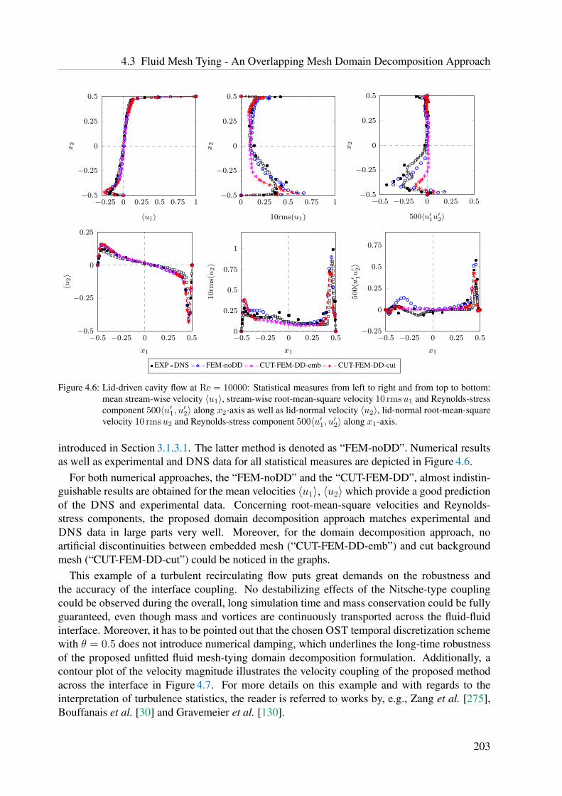
4.3 Fluid Mesh Tying - An Overlapping Mesh Domain Decomposition Approach

−0.25 0 0.25 0.5 0.75 1−0.5

−0.25

0

0.25

0.5

〈u1〉

x2

0 0.25 0.5 0.75 1−0.5

−0.25

0

0.25

0.5

10rms(u1)x

2

−0.5 −0.25 0 0.25 0.5−0.5

−0.25

0

0.25

0.5

500〈u′1u′2〉

x2

−0.5 −0.25 0 0.25 0.5−0.5

−0.25

0

0.25

x1

〈u2〉

−0.5 −0.25 0 0.25 0.50

0.25

0.5

0.75

1

x1

10rm

s(u

2)

−0.5 −0.25 0 0.25 0.5−0.25

0

0.25

0.5

0.75

x1500〈u′ 1u′ 2〉

EXP DNS FEM-noDD CUT-FEM-DD-emb CUT-FEM-DD-cut

Figure 4.6: Lid-driven cavity flow at Re = 10000: Statistical measures from left to right and from top to bottom:mean stream-wise velocity 〈u1〉, stream-wise root-mean-square velocity 10 rmsu1 and Reynolds-stresscomponent 500〈u′1, u′2〉 along x2-axis as well as lid-normal velocity 〈u2〉, lid-normal root-mean-squarevelocity 10 rmsu2 and Reynolds-stress component 500〈u′1, u′2〉 along x1-axis.

introduced in Section 3.1.3.1. The latter method is denoted as “FEM-noDD”. Numerical resultsas well as experimental and DNS data for all statistical measures are depicted in Figure 4.6.

For both numerical approaches, the “FEM-noDD” and the “CUT-FEM-DD”, almost indistin-guishable results are obtained for the mean velocities 〈u1〉, 〈u2〉 which provide a good predictionof the DNS and experimental data. Concerning root-mean-square velocities and Reynolds-stress components, the proposed domain decomposition approach matches experimental andDNS data in large parts very well. Moreover, for the domain decomposition approach, noartificial discontinuities between embedded mesh (“CUT-FEM-DD-emb”) and cut backgroundmesh (“CUT-FEM-DD-cut”) could be noticed in the graphs.

This example of a turbulent recirculating flow puts great demands on the robustness andthe accuracy of the interface coupling. No destabilizing effects of the Nitsche-type couplingcould be observed during the overall, long simulation time and mass conservation could be fullyguaranteed, even though mass and vortices are continuously transported across the fluid-fluidinterface. Moreover, it has to be pointed out that the chosen OST temporal discretization schemewith θ = 0.5 does not introduce numerical damping, which underlines the long-time robustnessof the proposed unfitted fluid mesh-tying domain decomposition formulation. Additionally, acontour plot of the velocity magnitude illustrates the velocity coupling of the proposed methodacross the interface in Figure 4.7. For more details on this example and with regards to theinterpretation of turbulence statistics, the reader is referred to works by, e.g., Zang et al. [275],Bouffanais et al. [30] and Gravemeier et al. [130].

203

4 Unfitted Domain Decomposition Methods for Incompressible Single- and Two-Phase Flows

Figure 4.7: Lid-driven cavity flow at Re = 10000: Isosurface plot of velocity magnitude at t = 440.0.

4.4 Outlook towards Incompressible Two-Phase Flow -An Unfitted Mesh Method

The objective of this section is to give an outlook towards two-phase-flow applications for whichthe stabilized Nitsche-type formulation proposed in Section 4.2 can be utilized and shows severeadvantages over other computational approaches. Expansion to several fluid phases would bestraightforward, the subsequent presentation, however, is simplified to two fluid phases for whichρ1 6= ρ2 and µ1 6= µ2 holds in general. Characteristic for two-phase flow is the dependency ofthe interface motion on the surrounding fluid flow. This can cause large and complex interfacedeformations as well as topological changes. To allow the interface to arbitrarily move andthereby to sharply capture the phase limit, the separate fluid phases are approximated using theunfitted technique introduced in Section 2.1.4.3, as visualized in Figure 2.10c. The geometricapproximation of the two immiscible fluid subdomains and their associated flow fields rely onidentical coinciding non-interface-fitted background meshes T1

h ≡ T2h . The active mesh parts

T1h 6= T2

h , however, as well as their associated fictitious domains Ω1∗h ⊇ Ω1

h differ. The set ofelements intersected by the interface is Ω2∗

h ⊇ Ω2h, where T1

h ∩T2h = T1

Γ = T2Γ .

204

4.4 Outlook towards Incompressible Two-Phase Flow - An Unfitted Mesh Method

Different computational approaches applicable to highly convective transient incompressibletwo-phase flow including high contrast in material properties have been developed. ClassicalFEM-based techniques make use of smoothed material properties and the interface is artificiallythickened over a few element layers in the vicinity of the interface. This enables to numericallyapproximate smooth transitions of material characteristics as well as solution fields based on theunderlying discrete finite element approximation space; see, e.g., works by Nagrath et al. [194],Groß et al. [136] and Marchandise and Remacle [178]. Surface-tension forces can be incorpo-rated via a local volume force modeled by the continuum surface force approach established byBrackbill et al. [32]. Similar approaches in finite difference or finite volume frameworks havebeen proposed, e.g., by Sussman et al. [248]. An extensive survey of numerical methods fortwo-phase incompressible flows can be found in the textbook by Groß and Reusken [133].

Over the recent years, different XFEM/CUTFEM-based approaches to multiphase flows havebeen proposed. Originally established by Chessa et al. [72], Groß and Reusken [134] intro-duced a pressure enriched function space to sharply capture pressure discontinuities arising fromsurface-tension effects. Rasthofer et al. [214] developed an extended residual-based variationalmultiscale method utilizing a kink-enrichment strategy for the velocity field and different en-richment strategies for the pressure. Related works have been published by Sauerland and Fries[225]. Furthermore, enriched approaches towards premixed combustion applications have beenconsidered; as first by van der Bos and Gravemeier [255]. In the context of this application field,Nitsche-type coupling techniques utilizing cut-cell-based flux averaging strategies for mainlylaminar two-phase flow settings have been developed by Schott [229] and further enhanced toturbulent premixed combustion problem settings by Henke [147]. Further related works can befound in the literature overview provided in Section 2.2.1.

As discussed in the previous sections, the Nitsche-type RBVM/GP method analyzed in Sec-tion 4.2 in combination with the expanded cut finite element approximation space is expected toexhibit higher accuracy compared to the aforementioned FEMs but also improved stability overother CUTFEMs due to the GP stabilization technique and the use of expanded approximationspaces. To investigate the proposed Nitsche-type coupling, it is exemplarily applied to twodifferent challenging examples incorporating fluid phases which exhibit highly different materialproperties: For classical incompressible two-phase flows, the well-established Rayleigh-Taylorinstability is analyzed for different Atwood numbers including the effect of surface tension.Results for exponential growth rates obtained from numerical simulations can be comparedto analytically deduced solutions. To emphasize the possibility of enforcing non-zero jumpconstraints even for the velocity field, an outlook towards premixed combustion applicationsis given by means of a laminar flame-vortex-interaction example. The subsequent elaborationson two-phase flows are based on work published by Schott and Rasthofer et al. [231] and withregard to premixed combustion the reader is referred to Schott [229] and Henke [147].

All subsequently presented simulations are computed with the stabilized Nitsche-type CUT-FEM from Section 4.2 utilizing RBVM/GP stabilizations for both fluid phases on the respec-tive time-dependent active mesh parts T1

h ,T2h . Their spatial approximations are based on non-

interface-fitted computational grids consisting of linearly-interpolated Q1-elements. Interfacialconstraints are weakly imposed using the adjoint-consistent Nitsche-type method. Upwindingschemes at the fluid interface are not applied for these examples. As identical meshes are utilized

205

4 Unfitted Domain Decomposition Methods for Incompressible Single- and Two-Phase Flows

in both fluid subdomains, the proposed flux weighting strategy reduces to a harmonic weightingwhich is purely based on the viscosities as elaborated in (4.56). The interface transport iscomputed by solving a scalar transport PDE for the level-set field φ, whose zero-isocontourrepresents the interface front as introduced in (2.50). Therein, the advective transport velocity uis given by the continuous flow solution for classical incompressible two-phase flows and by theabsolute flame speed u = ui − sL · nij for the considered premixed combustion application; fordetails see also elaborations in Section 4.1.1. The purely advective transport PDE is stabilizedwith an SUPG term and is constructed analogously to fluids as elaborated in Section 3.1.3.1.For the temporal discretizations, the OST scheme is applied with θ = 0.5 for the transportsolver and with θ = 1.0 for the CUTFEM flow solver. Fluid flow and interface transport arealternately solved. For evaluating surface tension, the interface curvature κ is calculated basedon formula (2.53). For further details, the reader is referred to works by Schott and Rasthofer etal. [231], Schott [229] and Henke [147].

4.4.1 A Rayleigh-Taylor Instability including Surface TensionAs a first example, the well-studied Rayleigh-Taylor-instability problem is considered to validatethe proposed CUTFEM for classical two-phase flows. The evolution of a hydrodynamic insta-bility of an interface separating two immiscible fluids, which are subjected to a gravitationalforce, is investigated. The goal is to quantify the accuracy of the computational approach interms of growth rates obtained from the numerical simulations compared to analytical solutions.Moreover, the stabilizing effect of surface tension can be studied. This test case has been alreadyestablished for such purposes in literature; see, e.g., works by Nourgaliev et al. [198], Popinetand Zaleski [208], Puckett et al. [212] and Pochet et al. [207].

The geometric and computational setup is described as follows: Within a rectangular domainΩ = (−L/2, L/2)× (−H/2, H/2) with L = 1.0 and H = 4.0, two fluids are separated by ahorizontal interface which is initially located at x2 = −h/2 where h denotes the characteristicelement length of the computational background mesh Th. The heavier of both fluids with adensity ρ+ is placed on top of the lighter fluid with density ρ− (i.e. ρ− < ρ+). The flow issubjected to gravitational acceleration g = 10.0 which is initially perpendicular to the interfacesuch that f = (0,−g)T in both fluid phases. Assuming a slight imperfection of the interface interms of a single-mode perturbation a0 cos(kx1), where a0 denotes its initial amplitude reachedat x1 = 0 and k = 2π/L its wave number such that φ0(x1, x2) = x2 − a0 cos(kx1) + h/2, thegravitational force causes evolution of this disturbance in time. Depending on the materialproperties, the interface evolves differently and eventually becomes unstable over time. Incontrast, if surface tension is present, this instability gets stabilized and its growth is damped.This instability can be characterized by two non-dimensional numbers, the Reynolds numberand the Atwood number, which are defined as

Redef=ρ+√HgL

µ+and At

def=ρ+ − ρ−ρ+ + ρ−

.

For all simulations, the unfitted discretization consists of 64× 256 Q1-elements. Periodicboundary conditions are applied at the side walls to mimic the periodicity of analytical referencesolutions and no-slip boundary conditions are set at top and bottom walls. The velocity field is

206

4.4 Outlook towards Incompressible Two-Phase Flow - An Unfitted Mesh Method

Figure 4.8: Rayleigh-Taylor instability with initial amplitude a0 = 0.005, Re = 1000 and At = 0.2 at timest = 1.5, 2.0, 2.5 and 3.0 (from left to right): instantaneous velocity magnitude distribution are visu-alized on left half (red color indicates high velocity and blue color low velocity) and subdomains areindicated on right half of the figures, where Ω+ is colored in red and Ω− in blue.

initially at rest and for the temporal discretization a time-step length of ∆t = 0.005 is used. Forall considered settings, kinematic viscosities are assumed being equal, i.e. ν = ν+ = ν−, anddefined as ν+ = µ+/ρ+ and ν− = µ−/ρ−. In Figure 4.8, the evolution of an interface instabilityfor a low density ratio is exemplarily depicted at various times t. For the visualized setting,the densities are chosen as ρ+ = 1.5 and ρ− = 1.0 and the kinematic viscosity is ν = 0.006349resulting in dynamic viscosities µ+ = 0.009535 and µ− = 0.006349 for the two fluids. The twodimensionless numbers yield to Re = 1000 and At = 0.2. The initial amplitude for this settingwas set equal to a0 = 0.005.

207

4 Unfitted Domain Decomposition Methods for Incompressible Single- and Two-Phase Flows

Following the elaborations by Chandrasekhar [70], in the initial stage the growth of the interfacedisturbance is in accordance with linear stability theory. An initial perturbation a0 is expected togrow exponentially in time, i.e.

a(t, x1 = 0) = a0 exp(αt) (4.70)

with a growth rate α. An analytical relation between the growth of the initial perturbation a0 andcharacteristic properties has been deduced in [70]. Defining a non-dimensional wave numberas k∗ = (ν2/g)

13k and a non-dimensional growth rate as α∗ = (ν/g2)

13α, the following relation

holdsα∗ = [(y(k∗))2 − 1] · (k∗)2, (4.71)

where y(k∗) is the solution of the fourth-order polynomial

y4 + y3(4δ∗) + y2(2− 12δ∗)− y(4− 12δ∗) + (1− 4δ∗)− (k∗)−3 At +(k∗)−1ι∗ = 0. (4.72)

Therein, the surface-tension coefficient ι is non-dimensioned as ι∗ = ι/[(ρ+ + ρ−)(gν4)1/3] andthe parameter δ∗ is defined as δ∗ = δ+δ−, where δ+ = ρ+/(ρ− + ρ+) and δ− = ρ−/(ρ− + ρ+).For given k∗ and densities, equation (4.72) can be numerically solved for its root y(k∗) usingNewton’s method.

The growth of an initial disturbance is examined for two different ratios of densities: for alower density ratio ρ+/ρ− = 1.5 with ρ− = 1.0 resulting in At = 0.2 and for a higher densityratio of ρ+/ρ− = 1000 with ρ+ = 1.0 and ρ− = 0.001 resulting in At = 0.998. Initial ampli-tudes are chosen as a0 = 0.005 for the lower density ratio and as a0 = 0.0001 for the higherone.

For all simulations, k∗ is adapted by varying the kinematic viscosity ν = ν+ = ν−. To deter-mine α corresponding to the numerical simulations, a linear least-squares fit is utilized within thetime interval which exhibits the exponential growth. The analytical relation between k∗ and α∗

for the low-density-ratio case ρ+/ρ− = 1.5 is displayed in Figure 4.9a, and the computed growthrates are indicated by markers. Figure 4.9b illustrates the linear fit of the simulation data. Resultsfor the high-density-ratio case ρ+/ρ− = 1000 are shown in Figure 4.10a and Figure 4.10b,respectively. An excellent agreement between analytical solution and numerical results overa wide range of wave numbers can be observed for both density ratios. This underlines the highaccuracy of the proposed CUTFEM solver.

In Figure 4.11, the effect of surface tension on growth rates of such instabilities is demon-strated. For this study, the dimensionless wave number is fixed to k∗ = 1.0 and densities aretaken from the low density ratio, set to ρ+ = 1.5 and ρ− = 1.0. Increasing the surface-tensioncoefficient ι damps the evolution of the instability until the unstable behavior converts intoa stable one. At a certain critical surface-tension coefficient, the initial perturbation of theinterface remains constant over time with α∗ = 0. This value is perfectly matched by thecomputational approach and results for varying surface tension are in excellent agreement withthe analytically predicted damping behavior which highlights the accuracy provided by thiscomputational approach. This example clearly demonstrates the high capabilities of the proposedCUTFEM fluid solver for classical incompressible two-phase flow including surface tension.

208

4.4 Outlook towards Incompressible Two-Phase Flow - An Unfitted Mesh Method

0 0.5 1 1.5 20

0.02

0.04

0.06

0.08

0.1

0.12

0.14

0.16

0.18

wavenumber k∗

growth

rate

α∗

analytical solutionsimulation

(a)

0 0.5 1 1.5 2−0.5

0

0.5

1

1.5

2

2.5

3

3.5

4

4.5

5

time t

ln(a(t,x

1=

0)/a

0)

k∗ = 0.10 ln-transformedk∗ = 0.10 linear fitk∗ = 0.25 ln-transformedk∗ = 0.25 linear fitk∗ = 0.50 ln-transformedk∗ = 0.50 linear fitk∗ = 0.75 ln-transformedk∗ = 0.75 linear fitk∗ = 1.00 ln-transformedk∗ = 1.00 linear fitk∗ = 1.25 ln-transformedk∗ = 1.25 linear fitk∗ = 1.50 ln-transformedk∗ = 1.50 linear fitk∗ = 1.75 ln-transformedk∗ = 1.75 linear fitk∗ = 2.00 ln-transformedk∗ = 2.00 linear fit

(b)

Figure 4.9: Rayleigh-Taylor instability with a low density ratio ρ+/ρ− = 1.5 (At = 0.2, a0 = 0.005): (a) compari-son of non-dimensional growth rates α∗ obtained from simulations with analytical solution for differentnon-dimensional wave numbers k∗, (b) linear fit of transformed amplitudes ln(a(t, x1 = 0)/a0) atinterface front over time.

0 0.5 1 1.5 20

0.05

0.1

0.15

0.2

0.25

0.3

0.35

0.4

0.45

0.5

wavenumber k∗

growth

rate

α∗

analytical solutionsimulation

(a)

0 0.2 0.4 0.6 0.8 1 1.2−1

0

1

2

3

4

5

6

7

8

9

time t

ln(a(t,x

1=

0)/a

0)

k∗ = 0.10 ln-transformedk∗ = 0.10 linear fitk∗ = 0.25 ln-transformedk∗ = 0.25 linear fitk∗ = 0.50 ln-transformedk∗ = 0.50 linear fitk∗ = 0.75 ln-transformedk∗ = 0.75 linear fitk∗ = 1.00 ln-transformedk∗ = 1.00 linear fitk∗ = 1.25 ln-transformedk∗ = 1.25 linear fitk∗ = 1.50 ln-transformedk∗ = 1.50 linear fitk∗ = 1.75 ln-transformedk∗ = 1.75 linear fitk∗ = 2.00 ln-transformedk∗ = 2.00 linear fit

(b)

Figure 4.10: Rayleigh-Taylor instability with a high density ratio ρ+/ρ− = 1000 (At = 0.998, a0 = 0.0001):(a) comparison of non-dimensional growth rates α∗ obtained from simulations with analyticalsolution for different non-dimensional wave numbers k∗, (b) linear fit of transformed amplitudesln(a(t, x1 = 0)/a0) at interface front over time.

209

4 Unfitted Domain Decomposition Methods for Incompressible Single- and Two-Phase Flows

0 0.02 0.04 0.06 0.08 0.1 0.120

0.01

0.02

0.03

0.04

0.05

0.06

0.07

0.08

0.09

0.1

surface tension ι

growth

rate

α∗

analytical solutionsimulation

(a)

0 0.5 1 1.5 2−0.2

0

0.2

0.4

0.6

0.8

1

1.2

1.4

1.6

time t

ln(a(t,x

1=

0)/a

0)

ι = 0.000 ln-transformedι = 0.000 linear fitι = 0.020 ln-transformedι = 0.020 linear fitι = 0.040 ln-transformedι = 0.040 linear fitι = 0.060 ln-transformedι = 0.060 linear fitι = 0.080 ln-transformedι = 0.080 linear fitι = 0.100 ln-transformedι = 0.100 linear fitι = 0.120 ln-transformedι = 0.120 linear fitι = 0.125 ln-transformedι = 0.125 linear fit

(b)

Figure 4.11: Rayleigh-Taylor instability with a low density ratio ρ+/ρ− = 1.5 (k∗ = 1.0, At = 0.2, a0 = 0.005):(a) damping of non-dimensional growth rate α∗ for increasing dimensional surface tension ι comparedto analytical relation, (b) linear fit of transformed amplitudes ln(a(t, x1 = 0)/a0) at interface frontover time.

4.4.2 Premixed Combustion - A Flame-Vortex Interaction

To finally highlight the versatility of the two-phase CUTFEM solver developed throughout thischapter, as a last example for incompressible two-phase flows a premixed combustion modelproblem is investigated. Fundamentals of a potential and rather elementary modeling approachto the underlying physics based on the conservation laws for mass and momentum have beenintroduced in Section 4.1.1. At this stage it should be pointed out that details of premixedcombustion modeling and its underlying physics cannot be comprehensively presented withinthe scope of this thesis. For further details, the reader is referred to extensive derivations by,e.g., Williams [270]. The subsequent considerations rather shall give an outlook to possibleapplication fields for the cut finite element methodology and demonstrate the contribution andfurther developments of this work in view of more robust and accurate unfitted computationalapproaches required for such demanding applications.

A detailed survey on different computational methods as well as modeling approaches towardspremixed combustion is given in the thesis by Henke [147]. Moreover, in the latter work,an extended finite element method has been developed and algorithmically coupled with a G-equation approach for the transport of the flame front. The fundamental techniques introducedand observations made therein are the basis for further developments made throughout this thesis,as will be discussed subsequently. As concluding remarks, two fundamental issues of XFEM-based approaches existing so far have been formulated by Henke [147]: a limited representabilityof the fluid fields in zones of high interface curvature and the numerical issue of providing astable cut finite element approximation in the vicinity of the interface. Both of these aspects are

210

4.4 Outlook towards Incompressible Two-Phase Flow - An Unfitted Mesh Method

highly improved by the present CUTFEM solver. The first issue is accounted for by the usage ofan expanded cut finite element approximation space introduced in Section 2.2.5, and the secondone by developing the stabilized Nitsche-type RBVM/GP formulation for moving domains asproposed in Section 4.2 and analyzed for single-phase flows throughout Chapter 3.

The well-studied flame-vortex interaction serves as test example in which a pair of counter-rotating vortices interacts with a premixed flame front. Such types of interactions have beeninvestigated in various settings. While experiments have been presented in works by, e.g.,Roberts and Driscoll [221] and Mueller et al. [192], computational approaches based on differentframeworks have been developed, for which this vortex interaction has been studied; see, exem-plarily, Hartmann et al. [145] for a cut-cell flow solver in a finite volume framework, Gravemeierand Wall [129] for a finite-element-based progress-variable approach and Henke [147] for anextended finite element method.

The setup of this example follows the description by Henke [147]. An initially horizontalflame front with flame speed sL = 1.0 is embedded into a box-shaped overall domain of sizeΩh = (0, 100)× (0, 200). It is defined implicitly by the isocontour of φ(x, t0) = x2 − 100. Thesubdomain Ω1

h ⊂ Ωh is defined by points carrying negative level-set values and contains theunburned fluid phase, whereas Ω2

h = Ωh\Ω1h denotes the burned gas correspondingly. At x2 = 0,

an inlet of unburned fluid into the domain is given by u = (0, sL). As the flame speed equals theinflow speed, the interface is in a steady state initially. Furthermore, no-slip boundary conditionsare prescribed at the side-walls x1 = 0 and x1 = 100 as well as a zero-traction Neumann outflowcondition at x2 = 200. Due to the combustion process, the fluid gets accelerated in normaldirection to the flame front. For given fluid properties ρ1 = 1.16, ρ2 = 0.157 and µ1 = 0.812,µ2 = 2.88 taken from [147], utilizing relation (4.13) the initial unperturbed flow velocity for theunburned phase is constant, i.e. upc|Ω2

h= (0, sL − ρ1sL[[ρ−1]]). The resulting piecewise constant

flow field upc is superposed by two counter-rotating vortices, which interact with the flame.Their centers are located at xl = (37.5, 75) and xr = (62.5, 75) with stream functions

Ψl,r(x)def= Cl,r exp (−‖x− xl,r‖2

2R2) (4.73)

with center peak values Cl = 70, Cr = −70 and a radius R = 4. The resulting vortex inducedvelocity components are given as uvort

1 = ∂(Ψl+Ψr)∂y

and uvort2 = −∂(Ψl+Ψr)

∂xsuch that the final initial

flow field in Ωh can be prescribed as u0 = upc + uvort, which exhibits the desired jump arisingfrom the combustion model. The initial flow setting and its evolution over time is depicted inFigure 4.12. The visualized results have been computed on a relatively coarse regular mesh Thconsisting of 65× 129 Q1-elements; see [147] for studies on the effect of different mesh sizes oncapturing topological characteristics of this flame-vortex interaction. The approximation is basedon the stabilized RBVM/GP technique and an OST scheme with θ = 1.0 and ∆t = 0.15 for anoverall simulation time of T = 30. Reinitialization of the level-set field has been performedevery time step. For its need and impact on the interface shape, the reader is referred to [147].

Initially, due to the inlet of fresh gas at the bottom boundary, the vortices are convectedupwards to the horizontal flame front. When their area of influence reaches the flame front,the higher flow velocity between the two vortices first cause the formation of a tongue-shapedinterface. For the given strength of vortices, it is expected to elongate and form a mushroom-shaped pocket, which afterwards secludes. In this computation, the pinch-off time for this drop-like structure is given as t ≈ 23.1 and takes place slightly earlier than reported by Henke [147].

211

4 Unfitted Domain Decomposition Methods for Incompressible Single- and Two-Phase Flows

Similar to [147], this pocket moves upwards and is fully burned after t ≈ 24.6. The earlierdetachment is due to a more accurate flow representation for high-curvature interfaces enabledby the expanded approximation space at times when flame fronts are approaching, as visualizedin Figure 2.19. The flow solution of the burned fluid phase in the vicinity of the thin-neck-shaped unburned fluid subdomain can be accurately captured due to independent sets of DOFsfor both sides of the burned subdomain. Details of this advantageous novel enriching strategyfor CUTFEMs have been presented in Section 2.2.5. As a second substantial improvementcompared to the approach established in [147], the stability of the proposed CUTFEM flowsolver is highlighted. Independent of the position of the flame front with respect to the underlyingunfitted computational grid, stable velocity and pressure solutions are obtained for both fluidphases, in particular, also in the vicinity of the interface and despite the presence of topologicalchanges. This is due to the introduced ghost-penalty stabilization technique and the adaptedNitsche-type coupling for two-phase flows.

Figure 4.12: Flame-vortex interaction: time evolution of the flame front at different times T0 = 0.0, T1 = 15.0,T2 = 19.5, T3 = 20.25, T4 = 21.0, T5 = 21.75, T6 = 22.5, T7 = 23.25, T8 = 24.0, T9 = 24.75(from left to right and from top to bottom). Inlet of fresh gas at bottom side drives the evolutionand convects the vortices. The flame front is indicated by a white line at which the flow solutionexhibits a jump in velocity and pressure. Subdomains belonging to unburned and burned fluid phasesare colored by velocity magnitude (gray/red colors indicate low/high velocity scaled within [0, 20]).

212

Chapter 5Stabilized Approaches to Fluid-Structure Interaction

using Cut Finite Elements

This chapter aims at extending cut finite element approaches and coupling techniques, whichhave been developed throughout Chapter 3 for single-phase flows and adapted to domain de-composition and multiphase flows in Chapter 4, to one of the most frequent and importantmultiphysics phenomena – fluid-structure interaction (FSI). Internal flows which interact withdeformable structural boundaries or surround movable and compressible structures occur invarious different fields of industrial, biological and medical engineering. Depending on flowcharacteristics and material properties of fluids and solids, different and often highly dynamicaleffects may appear which are in general too complex to get analytically predicted. In particularin biomedical settings, even experiments are limited in their applicability and measuring physicalquantities of interest is often difficult to realize. In such cases numerical simulations provide apowerful tool to support such purposes. Among many others, due to these reasons the benefit ofcomputational approaches for capturing such challenging physical phenomena is undisputed.

Over the recent years, their range of applicability has been expanded to various biomedicalsettings [169], for instance, considering the blood flow in arteries and veins, simulating openingand closing processes of heart valves, up to predicting rupture risks of abdominal aortic aneurysmin the human body [177]. Examples in industrial environments are flows induced by largelymoving or rotating components, like ship or helicopter propellers. But also the other way around,studying the impact of fluid flow on structural motions as, for instance, on rotor blades of windturbines [16] or aircraft wings is of high interest. The usability of computational FSI approachesincludes also biological and chemical scientific fields. As an example, recent developments havebeen made to support investigations on different formations of biofilm architectures living incomplex flow environments. There, computational approaches are applied to reliably predicttheir growth within a surrounding fluid as well as their interaction with that [77, 249]. Furtherpotential application fields are summarized in the introduction Chapter 1.

An Overview of Computational Approaches for Fluid-Structure Interaction. Most pop-ular and widely used computational FSI approaches are based on ALE techniques and useinterface-fitted grids for the fluid and solid subdomains as described in Section 2.1.4.2 andvisualized in Figures 2.7 and 2.8. This well-established technique dates back to early works

213

5 Stabilized Approaches to Fluid-Structure Interaction using Cut Finite Elements

by Hirt et al. [150], Donea et al. [89], Belytschko and Kennedy [22], Belytschko et al. [23],Hughes et al. [155] and Donea et al. [90]. Therein, a Lagrangean formalism for the structureis combined with an arbitrary Eulerian description of the flow field whose computational gridfollows the fluid-solid interface in its motion. The major advantage of this technique is that thecomputational meshes are not changed over time and utilizing refined meshes in the vicinityof the interface allows to accurately capture flow characteristics. This methodology has beenfurther developed over the recent decades with regard to different aspects. Stabilized finiteelement methods for FSI have been established by Wall [258] and Forster [110]. Efficiency ofdifferent solution strategies has been investigated by Kuttler [168] and the effect of single-fieldpredictors on monolithically solved fluid-structure-interaction systems has been studied by Mayret al. [185]. An overview of general challenges and directions in computational fluid-structureinteraction has been given by Bazilevs et al. [17].

As elaborated in Section 2.1.4.2, interface-fitted moving mesh approaches lack accuracy androbustness or even may totally fail due to mesh distortion in case of too large structural motionsor deformations. Such issues have been addressed in several publications, see, e.g., the articleby Le Tallec and Mouro [171] and the publication by Wall et al. [259] for an introduction to thistopic. Different attempts to relax the strong constraints on interface motion in FSI have beenmade. Kloppel et al. [164] integrated dual mortar interface coupling methods into ALE-basedFSI frameworks to cope with non-conforming meshes at the fluid-structure interface and so toenable large rotational motions. Non-matching discretizations in the framework of isogeometricFSI have been considered by Bazilevs et al. [16] and successfully applied to simulate the FSIof wind turbines. Recently, Farhat and Lakshminarayan [104] proposed an ALE formulation ofembedded boundary methods for tracking boundary layers in turbulent FSI problems. The keyidea of this approach is that non-interface-fitted embedded meshes are rigidly translated and/orrotated to track the rigid component of the dynamic body motion.

A class of FSI approaches which enables to overcome the difficulty of mesh distortion inher-ent to moving mesh techniques are the so-called fixed-grid methods. While structural dynamicsare still described in a Lagrangean formalism, the fluid flow is approximated on a fixed non-interface-fitted non-moving computational grid. This allows the structure to arbitrarily movewithin the fluid mesh. The solid mesh, which overlaps with the fluid grid, decomposes the latterone into an active physical fluid subdomain and an inactive subdomain covered by the structuraldomain. This part of the fluid mesh is often referred to as fictitious domain. Fixed-grid schemesdiffer in the numerical treatment of this overlap region, i.e. in the enforcement of the couplingconstraints at the FSI interface as well as in the solution technique applied to the overall fluid-solid system.

Early fixed-grid schemes, for which lots of modifications and variations have been proposedover many decades, belong to the class of Immersed Boundary (IB) methods. This methodologycan be traced back to methods by Peskin [201] and Peskin [202], which were used to simulateflow patterns around heart valves. An introduction to the IB method can be found in the workby Peskin [203]. Therein, structural variables are formulated in a Lagrangean frame of referenceand fluid variables are observed from an Eulerian view point. These are linked by equivalentvolumetric force terms within the fluid domain. Such incorporated interaction equations involvesmoothed approximations to the Dirac-delta function. Further, appropriate transfer operators fordata between the two meshes are required. Adaption based on higher-order reproducing kernelapproximations to the incorporated delta function has been proposed by Zhang et al. [276], called

214

the Immersed Finite Element Method, and developments on an Extended Immersed BoundaryMethod have been provided by Wang and Liu [264]. An extensive survey on IB methods andother Cartesian grid methods can be found in an overview article by Mittal and Iaccarino [187].

For most of the IB approaches, the coupling of fluid and solid phases takes place at thefictitious fluid domain which does not exhibit physical meaning. Smeared approximations andoften induced artificial incompressibility to the structural field are sources of inaccuracy andare desired to be avoided, as discussed by Wall et al. [260]. In the latter publication, differentdomain decomposition ideas for fluid-structure interaction based on fixed fluid grids have beenintroduced. As reviewed in Section 2.1.4.3, utilizing unfitted cut finite element approximationsfor the fluid field, overlapped by a structural mesh which fits to the fluid-solid interface, allowsfor sharp approximations of the flow field. Different XFEM-based interface-coupling strategieshave been developed over the recent years and applied to FSI problems. Gerstenberger andWall [124] investigated the use of Lagrange multipliers with unfitted overlapping discretizationsfor FSI. A combination of fixed-grid and ALE techniques applied to FSI has been proposedby Baiges and Codina [9], a technique which is called fixed-mesh ALE approach. Gersten-berger [123] established a stress-based Lagrange-multiplier method for the weak constraintenforcement of coupling conditions. The latter methodology has been expanded to XFEM-based fluid-structure-contact-interaction problem settings by Mayer et al. [184], which enablessimulating contact of submersed bodies. Extensions of related methods towards fluid-structure-fracture interaction have been developed by Sudhakar [244]. Fully Eulerian formulations havebeen introduced by Wick [268] and Richter [219]. Court et al. [80] developed a stabilizedLagrange-multiplier-based fictitious domain approach applicable to XFEM-based Stokes flowapproximations. This has been extended to FSI by Court and Fournie [79] in which the flow isgoverned by the incompressible Navier-Stokes equations. Recently, a Nitsche-based CUTFEMfor FSI has been analyzed by Burman and Fernandez [58] for Stokes flow interacting with linearelastic structures. A comparison of various coupling strategies of an incompressible fluid withimmersed thin-walled structures has been recently provided by Alauzet et al. [1]. Moreover, dif-ferent formulations applicable to fixed-grid methods based on utilizing an additional embeddedfluid patch, which fits to the fluid-structure interface but overlaps with a fixed background fluidgrid in an unfitted fashion, as visualized in Figure 2.11c, have been developed in the thesis byShahmiri [235] and considered further in an article by Massing et al. [181].

Computational FSI approaches require strategies for coupling the fluid and the structuralsubproblems. Two different classes of coupling techniques can be distinguished: staggered orpartitioned schemes and full-implicitly or monolithically solved schemes. For latter methods,fluid and structural equations including coupling constraints are set up as one global non-linearsystem which is solved for discrete fluid and structural approximations at once. The advantageof this methodology is the incorporated robustness and temporal stability for time-steppingschemes, even though their solution entails high computational costs. Newton or pseudo-Newtonmethods for approximating the solution of resulting global systems have been considered, e.g.,in works by Fernandez and Moubachir [107], Kuttler and Wall [170] or Mayr et al. [185].Monolithic algebraic multigrid techniques have been developed by Gee et al. [121] and pre-conditioning techniques for the efficient solution of such coupled systems have been introducedby Verdugo and Wall [256]. To reduce computational complexity and to allow for flexibility incoupling different code environments for the single fluid and structural subproblems, partitionedschemes are often attractive and widely used. However, in contrast to full-implicitly coupled

215

5 Stabilized Approaches to Fluid-Structure Interaction using Cut Finite Elements

methods, time advancing schemes which only explicitly couple the two subproblems, withoutiterating until convergence between the two fields has been achieved, exhibit stability issues.Strong added-mass effects have been observed and studied in the works by, e.g., Causin et al.[69] and Forster et al. [111]. Fixed-point iteration schemes incorporating dynamic relaxationfor convergence acceleration have been investigated by Kuttler and Wall [170] and partitionedprocedures utilizing Robin transmission conditions and algebraic splitting schemes have beendeveloped by Badia et al. [7] and Badia et al. [8]. To cope with instabilities arising from timeadvancing schemes, stabilized explicit coupling schemes have been introduced by Burman andFernandez [39] and further developed by Burman and Fernandez [40, 59], Fernandez et al. [106]and Fernandez et al. [108]. A comprehensive comparison of full-implicit, semi-implicit andexplicit coupling strategies for fitted mesh FSI approaches has been presented by Fernandez[105]. Extensions to unfitted mesh methods have been recently made by Alauzet et al. [1]. Forthe sake of completeness, besides classical time-stepping schemes, also space-time FEM-basedcomputational FSI approaches have been developed; see, e.g., the works by Tezduyar et al.[253], Legay et al. [172], Zilian and Legay [278] and Legay et al. [173].

This chapter is outlined as follows: In Section 5.1, a classical finite element formulationfor non-linear structural elastodynamics is reviewed. An initial boundary value problem isformulated in its strong and variational form and a FEM-based spatial approximation combinedwith a temporal generalized-α time-stepping scheme is provided. Afterwards, in Section 5.2fundamentals of modeling physics at fluid-structure interfaces are presented and an initial bound-ary value problem for the coupled FSI system is formulated. Section 5.3 is devoted to thedevelopment of a stabilized CUTFEM-based FSI solver. In analogy to the coupling betweendistinct fluid phases, a semi-discrete stabilized Nitsche-type method for the coupling of a singleincompressible fluid with a compressible elastic structural body is introduced. Peculiaritieswith regard to stability will be pointed out. Afterwards, the final full-implicitly coupled finite-dimensional system of non-linear residuals is formulated and iterative solution techniques aresuggested. Therein, focus is turned to the issue of potential changes of the fluid approximationspace. The performance of the proposed unfitted FSI solver is demonstrated by challenging testexamples. In Section 5.4, the unfitted FSI coupling scheme is enhanced by combining it with theunfitted fluid domain decomposition technique provided in Sections 4.2 and 4.3 and a powerfulunfitted Nitsche-type fluid-fluid-structure coupling is set up. Concluding, its high versatility fora variety of FSI applications is demonstrated by means of a challenging FSI problem.

5.1 A Finite Element Method for StructuresIn the following, fundamentals on structural dynamics and kinematics are recalled. An initialboundary value problem is formulated and a classical FEM approximation utilizing boundary-fitted structural meshes is reviewed. Details on structural time-stepping are discussed.

5.1.1 Governing Equations for Solid MechanicsThroughout this thesis, the structural field is assumed to be governed by the non-linear elastody-namics equations. Fundamentals of solid mechanics are briefly reviewed in the following. Moredetailed explanations can be found in textbooks by, for example, Wriggers [272] or Zienkiewiczand Taylor [277].

216

5.1 A Finite Element Method for Structures

Kinematic Relations. Under the assumption of moderate structural deformations it is commonto observe structural dynamics from a Lagrangean view point. The observer then follows amaterial particle X in its motion from reference configuration Ωs

0 = Ωs(T0) to current configu-ration Ωs(t) which mathematically can be expressed in terms of the mapping ϕ, as introducedin (2.5). Then, kinematics can be formulated by means of the unknown displacement field dbetween current and initial particle position and its first- and second-order time derivatives, thevelocity and acceleration fields u, a, as

d(X, t)def= xX(X, t)−X ∀X ∈ Ωs(T0), (5.1)

u(X, t)def=

dd(X, t)

dt= d(X, t) ∀X ∈ Ωs(T0), (5.2)

a(X, t)def=

d2d(X, t)

dt2= d(X, t) ∀X ∈ Ωs(T0) (5.3)

with d,u and a given in material description at any time t. In continuum mechanics, thegradient tensor of the spatial part of the invertible mapping ϕ, i.e. xX from (2.5), is often calleddeformation gradient tensor

F (X, t) =∂xX(X, t)

∂X= (I +

∂d

∂X)(X, t) (5.4)

and depends on d. Its determinant is notated with JX 7→xdef= det(F (X, t)). Performing polar

decomposition into a volume-preserving orthonormal rigid body rotation R and a symmetricpositive definite stretch part U such that

F = R ·U , (5.5)

the symmetric right Cauchy-Green tensor can be defined as

Cdef= F T · F = UT ·RT ·R ·U = UT ·U = U 2, (5.6)

which clearly exhibits an invariance under rigid body rotations. For solids subjected to largedeformations but moderate stretching or compressing, the Green-Lagrange strain tensor

Edef=

1

2(F T · F − I) =

1

2(C − I) (5.7)

serves as suitable strain measure defined in material configuration. This measure further ensureszero strain in the initial configuration.

Constitutive Laws. Introducing constitutive laws starts from Cauchy’s first equation of mo-tion, which results from balance of linear and angular momentum and was deduced for materialconfiguration in (2.36) and (2.37). Transforming between current and reference configuration,the following relation between the physical symmetric Cauchy stress tensor σσσx, which is as-sociated to the a priori unknown current configuration, as obtained from Cauchy’s fundamentallemma in (2.33), and the non-symmetric two-point first Piola–Kirchhoff stress tensor P emergesas

Pdef= σσσX = JX 7→xσσσx · F−T . (5.8)

217

5 Stabilized Approaches to Fluid-Structure Interaction using Cut Finite Elements

Equivalently, a symmetric stress tensor in reference configuration can be constructed as

Sdef= F−1 · P = JX 7→xF

−1 · σσσx · F−T , (5.9)

which is called second Piola–Kirchhoff stress tensor.Depending on the material model, different relations between strain and stress measures can

be employed. An extensive overview about different constitutive laws can be found in, e.g., thetextbook by Holzapfel [152]. For the sake of simplicity only homogeneous structural bodiesthat exhibit hyper-elastic material behavior are considered throughout this thesis. Assuming theexistence of a so-called strain-energy function Ψ(C) = Ψ(E) the second Piola–Kirchhoff stresstensor is defined as

S = 2∂Ψ

∂C=∂Ψ

∂E, (5.10)

where the dependency solely on the Cauchy-Green tensor implies objectivity and thus indepen-dence of rigid body rotationsR.

Exemplarily, strain energy functions for two material models used in this work are presentednext. The St.-Venant–Kirchhoff (SVK) material behavior is modeled with a strain energy func-tion which is quadratic in the strain variable and thus relates Green-Lagrange strains E andsecond Piola–Kirchhoff stresses S linearly as

ΨSVK(E)def=λs

2(tr (E))2 + µsE : E (5.11)

with λs and µs the Lame parameters, which can be expressed in terms of Young’s modulusEs > 0 and Poisson’s ratio νs ∈ (−1, 0.5) as

λs =Esνs

(1 + νs)(1− 2νs)and µs =

Es

2(1 + νs). (5.12)

In contrast to the St.-Venant–Kirchhoff model, which exhibits non-linearity only in a geomet-ric sense, the strain energy function for Neo-Hookean (NH) materials introduces a non-linearrelationship between strains and stresses as

ΨNH(C)def=µs

2(tr (C)− 3)− µs ln(JX 7→x) +

λs

2(ln(JX 7→x))2 (5.13)

with JX 7→x = det(F ) = (det(C))1/2.

Initial Boundary Value Problem. Combining kinematic description in a Lagrangean con-figuration with balance equations for mass, linear and angular momentum, i.e. (2.26), (2.36)and (2.37), in this work structural dynamics are assumed to be governed by the non-linearelastodynamics PDEs

ρs d2d

dt2−∇ · (F · S)(d) = ρsf s ∀ (X, t) ∈ Ωs

0 × (T0, T ] (5.14)

with the unknown time-dependent displacement field d(t) defined in reference configuration Ωs0.

Therein, ρs denotes the structural material density ρs def= ρ0,s

X = ρsXJX 7→x, which is defined in

218

5.1 A Finite Element Method for Structures

the initial referential configuration X and is constant over time due to mass conservation, seealso the derivation in (2.27). Further, ∇ · (·) = ∇X · (·) is the divergence operator with respectto material referential coordinates. Appropriate Dirichlet and Neumann boundary conditions ondisjunct parts of the possibly moving solid boundary ∂Ωs(t) = Γs

D(t)∪ΓsN(t) and its equivalents

in referential configuration ∂Ωs0 = Γs

D,0∪ΓsN,0 read

d = gsD ∀(X, t) ∈ Γs

D,0 × (T0, T ], (5.15)

(F · S) ·N = hsN ∀(X, t) ∈ Γs

N,0 × (T0, T ], (5.16)

where N denotes the outward pointing unit normal on the boundary in reference configurationand gs

D and hsN are prescribed displacements and surface tractions on the respective boundaries.

The second order initial boundary value problem (IBVP) is complemented with given initialvalues for displacements and velocities

d(X, T0) = d0(X) ∀X ∈ Ωs0, (5.17)

dd

dt(X, T0) = d0(X) ∀X ∈ Ωs

0. (5.18)

Equations (5.14)–(5.18) can be referred to as strong form of non-linear solid mechanics.

5.1.2 Variational Structure ProblemFor deriving the weak formulation of the structural initial boundary value problem, appropriatefunction space have to be introduced. For the solid weak formulation, the space of admissi-ble displacements DgD

def= [H1

ΓD,gD(Ωs

0)]d ⊂ [H1(Ωs0)]d satisfies the Dirichlet boundary condition

(5.15), whereas the space of admissible test functions D0 exhibits zero trace on ΓD. Furthermore,Z ⊆ [H1(Ωs

0)]d denotes the admissible space for structural velocities.The weak formulation of the non-linear structural problem (5.14)-(5.18) then reads as follow:

for any time t ∈ (T0, T ], find solid displacements d(t) ∈ DgDand velocities d(t) ∈ Z such that

for all (w, z) ∈ D0 ×Z

(ρs(dd

dt− d), z) + (ρs dd

dt,w) + ((F · S)(d),∇w) = (ρsf s,w) + 〈hs

N,w〉ΓsN,0, (5.19)

where (·, ·), 〈·, ·〉ΓsN,0

denote the inner products associated with L2 in the domain Ωs0 and on the

boundary part ΓsN,0. Introducing the following operators

as(d,w)def= ((F · S)(d),∇w)Ωs

0, (5.20)

ls(w)def= (ρsf s,w) + 〈hs

N,w〉ΓsN,0, (5.21)

where the elastic form as is linear in the variable w, however, in general non-linear in thedisplacement field d. The weak formulation (5.19) can be rewritten in operator form as

(ρs(dd

dt− d), z) + (ρs dd

dt,w) + as(d,w) = ls(w). (5.22)

219

5 Stabilized Approaches to Fluid-Structure Interaction using Cut Finite Elements

5.1.3 Spatial Finite Element Discretization

The space semi-discretization of the structural weak formulation (5.19) follows the conceptsprovided in Section 2.1.3.1 for PDEs formulated with respect to Lagrangean descriptions onboundary-fitted meshes and uses the notation and terminology introduced in Section 2.1.4.1.

For the finite-dimensional spatial discretization of the solid domain Ωs0, let Ts

hh be a familyof boundary-fitted quasi-uniform meshes with mesh size parameter h > 0. Each mesh Ts

h con-sists of a family of isoparametric possibly curvilinear finite elements T ∈Ts

h with existing bijec-tive mappings ST (t) : T 7→ T with respect to the element parameter space and approximates thestructural domain in referential configuration Ωs

0 ≈ Ωs0,h = ∪T∈Ts

hT . For the approximation of

solid displacements and velocities d, d, standard continuous isoparametric finite element spaces

X0,h =xh ∈ C0(Ωs

0,h) : xh|T = vT S−1T (t) with vT ∈ Vk(T )∀T ∈Ts

h

(5.23)

were introduced in (2.43). The discrete displacement and velocity approximation and test func-tion spaces are defined as Dh,gD

def= [X0,h]

d ∩ DgD, Zh

def= [X0,h]

d ∩Z and Dh,0def= [X0,h]

d ∩ D0

taking into account the respective trace values.The space semi-discrete approximation to problem (5.22) reads: for any t ∈ (T0, T ], find solid

displacements dh(t) ∈ Dh,gDand velocities dh(t) ∈ Zh such that for all (wh, zh) ∈ Dh,0 ×Zh

(ρs(ddhdt− dh), zh)Ωs

0,h+ (ρs ddh

dt,wh)Ωs

0,h+ as

h(dh,wh) = lsh(wh), (5.24)

with ash = as and lsh = ls as defined in (5.20) and (5.21). All domain and boundary integrals

associated with inner products are defined on the discrete counterparts Ωs0,h,Γ

sN,0,h, respectively.

After performing transformations to simplicial reference elements T , Gaussian quadrature rulescan be applied.

Assembly of local element-wise contributions of the discrete weak formulation on elements Tinto global finite-dimensional vector-valued displacement and velocity fields D(t) ∈ Rndof andV (t) ∈ Rndof allows to rewrite the discrete weak formulation of structural dynamics (5.24) interms of 2 · ndof non-linear ordinary differential equations (ODEs) of first order

MU +CD + Fint(D)− Fext = 0, (5.25)

D −U = 0, (5.26)

whereM is the global mass matrix, Fint the vector of non-linear internal forces resulting from ash

and Fext external forces resulting from lsh. Furthermore, C is an additional global dampingmatrix which introduces the widely used Rayleigh model for viscous damping. Hereby, C def

=cMM + cKK0 can be defined as a linear combination of mass matrix M and an initial tangentstiffness matrix K0, which denotes the partial derivative of the internal forces vector Fint withrespect to the displacements D in reference configuration at D = 0. It has to be noted that dueto the regularity of the mass matrix M the system of differential equations M (D −U ) = 0,which results from (5.24), can be resolved to D −U = 0 in (5.26).

220

5.1 A Finite Element Method for Structures

5.1.4 Structural Time SteppingAfter introducing a spatial discretization, the resulting system of ordinary differential equationscan be discretized in time applying the method of lines. For time stepping, the time interval(T0, T ] is partitioned into N ∈ N equal-sized time-step intervals Jn = (tn−1, tn] of size ∆twith discrete time steps tn = T0 + n∆t and tN = T . There exists a multitude of one- andmulti-step time discretization schemes applicable to systems of stiff initial value problems.However, throughout this thesis only one-step algorithms are considered for structural dynamicswhich require only solution history from the last discrete time step tn−1 for approximatingdisplacements and velocitiesDn ≈D(tn) and V n ≈ V (tn).

The Generalized-α Family for Temporal Discretization. In the following, the so-calledfamily of Generalized-α (G-α) time-stepping schemes is considered, as established by Chungand Hulbert [74]. This class of time-integration schemes is commonly used in structural me-chanics as it endows several desired properties. Among classical requirements as unconditionalA-stability or second-order accuracy, numerical schemes are often desired to entail numericaldissipation in the high-frequency range to damp insufficiently resolved spurious high-frequencymodes introduced for instance by insufficient temporal or spatial discretization of the physicalproblem. To keep damping of low-frequency modes at a minimum at the same time is ofgreatest importance. Regarding numerical dissipation, the G-α method achieves a optimumbetween these two requirements. This matter of fact makes the family of G-α algorithms veryrobust compared to for instance the classical Crank-Nicolson scheme which does not introducenumerical damping at all. Concerning a detailed numerical analysis and studies of the G-αscheme, the interested reader is referred to Erlicher et al. [100].

The G-αmethod is classified as one-step, three-stage time integration scheme, where the latterdesignation refers to the three solution vectors Dn,V n,An which occur during construction.Assuming given initial data for dh(T0) and dh(T0), i.e. for D0,V 0, from the initial boundaryvalue problem, an initial acceleration can be computed satisfying the elastodynamics equationsat T0

A0 def= −M−1(CV 0 + Fint(D

0)− Fext(T0)). (5.27)

ApproximationsDn,V n,An associated with a new time step tn are then constructed as follows

Dn(An) = Dn−1 + ∆tV n−1 + (∆t)2((1/2− β)An−1 + βAn

), (5.28)

V n(An) = V n−1 + ∆t((1− γ)An−1 + γAn

)(5.29)

and

MAn−αm +CV n−αf + Fn−αfint (Dn)− Fext(t

n−αf ) = 0 (5.30)

with γ ∈ (0, 1] and β ∈ (0, 1/2]. The generalized mid-point quantities are defined by means oflinear interpolations with generalized trapezoidal rules

Dn−αf (Dn) = (1− αf )Dn + αfDn−1, (5.31)

V n−αf (V n) = (1− αf )V n + αfVn−1, (5.32)

An−αm(An) = (1− αm)An + αmAn−1, (5.33)

221

5 Stabilized Approaches to Fluid-Structure Interaction using Cut Finite Elements

and the generalized mid-point time

tn−αf = (1− αf )tn + αf tn−1, (5.34)

characterized with two parameters αf , αm ∈ [0, 1). The internal and external forces can beapproximated either by a generalized mid-point rule (GMR) or by a generalized trapezoidalrule (GTR) as

F n−αf (Dn) = F ((1− αf )Dn + αfDn−1) (GMR), (5.35)

F n−αf (Dn) = (1− αf )F (Dn) + αfF (Dn−1) (GTR). (5.36)

The latter option is exclusively used throughout this thesis.Using the linear relations between quantities associated with time step tn in (5.28), (5.29) and

(5.31)–(5.33), the three-stage system for non-linear elastodynamics can be conflated resulting ina non-linear formulation depending solely on the unknown approximationDn.

0 = R(Dn)def= M

[1− αmβ∆t2

(Dn −Dn−1)− 1− αmβ∆t

V n−1 − 1− αm − 2β

2βAn−1

]

+C

[(1− αf )γβ∆t

(Dn −Dn−1)− (1− αf )γ − ββ

V n−1

−(γ − 2β)(1− αf )∆t2β

An−1

]

+ (1− αf )(F nint(D

n)− F next) + αf (F

n−1int (Dn−1)− F n−1

ext )

=

(M

1− αmβ∆t2

+C(1− αf )γβ∆t

)Dn + (1− αf )(F n

int(Dn)− F n

ext)

−Hn−1(Dn−1,V n−1,An−1). (5.37)

For the last equation, all terms which belong to the old time-level are comprised inHn−1. OnceDn is computed, approximations to V n andAn can be recovered, viz.

An(Dn) = [Dn − (Dn−1 + ∆tV n−1 + (1/2− β)(∆t)2An−1)] · (β(∆t)2)−1, (5.38)V n(An) = V n−1 + (1− γ)∆tAn−1 + γ∆tAn. (5.39)

Afterwards it can be proceeded with the next time step.To guarantee second-order accuracy for the displacement approximation, the G-α scheme is

required to be consistent in the accelerations which requires

γ =1

2− αm + αf . (5.40)

Furthermore, maximizing high-frequency dissipation of the schemes results in a condition for β

β =1

4(1− αm + αf )

2. (5.41)

The two remaining free parameters αf , αm have to be chosen such that unconditional stability isguaranteed. This holds provided that

αm 6 αf 61

2. (5.42)

222

5.1 A Finite Element Method for Structures

The high-frequency dissipation can be regularized in terms of the spectral radius ρ∞ which canbe interpreted as user-defined value. Following Chung and Hulbert [74], the spectral radius canbe obtained as

ρ∞ =

∣∣∣∣αf − αm − 1

αf − αm + 1

∣∣∣∣ ∈ [0, 1]. (5.43)

For a given desired high-frequency damping, the low-frequency damping is minimized wheneverαf = (αm + 1)/3 such that an optimal setting of parameters (αm, αf , β, γ) can be formulated interms of a single user-defined spectral radius as

αm =2ρ∞ − 1

ρ∞ + 1and αf =

ρ∞ρ∞ + 1

(5.44)

together with (5.40) and (5.41). It has to be noted that a spectral radius of ρ∞ = 1 does notintroduce any numerical high-frequency damping, whereas for ρ∞ = 0 the algorithm is in theso-called case of asymptotic annihilation. The resulting G-α schemes are unconditionally A-stable, guarantee second-order accuracy in the displacements and thereby provide an optimalcombination of high-frequency and low-frequency numerical dissipation. For further details, thereader is referred to the original publication by Chung and Hulbert [74] and an extensive analysisprovided by Erlicher et al. [100]. In these publications, also the relation between G-α schemesand other implicit time stepping schemes is comprehensively discussed. Widely used sets of G-αparameters are provided in Table 5.1.

Table 5.1: Optimal parameter settings for the G-α scheme without (ρ∞ = 1.0), with medium (ρ∞ = 0.8) and withstrong (ρ∞ = 0.5) numerical dissipation in the high-frequency range.

ρ∞ αm αf γ β

1.0 1/2 1/2 1/2 1/40.8 1/3 4/9 11/18 25/810.5 0 1/3 10/12 4/9

For the sake of completeness, different other implicit time-stepping schemes can be consid-ered as special cases of the G-α family. The classical Newmark method can be obtained forαm = αf = 0, which shifts the evaluation of terms of the ODE to the end of the time interval,i.e. to tn. The well-known one-step-θ scheme can be interpreted as a special representative ofthe G-α family with αm = αf = 1− γ and γ = θ. Condition (5.40) reflects the property thatthe one-step-θ scheme exhibits second-order accuracy if and only if θ = 1/2 together with theA-stability property provided θ ∈ [0.5, 1]. The popular Crank-Nicolson method with θ = 1/2 soguarantees second-order accuracy and unconditional A-stability, however, does not provide anynumerical damping. This is due to the fact that ρ∞ = 1 in contrast to the previously introducedmore general G-α scheme.

223

5 Stabilized Approaches to Fluid-Structure Interaction using Cut Finite Elements

Linearization and Non-linear Solution Techniques. Due to the non-linearity of the inter-nal force vector Fint(D) in the displacement field, the computation of new displacements Dn

requires non-linear iterative solution techniques. In this work, the discrete vector Dn, whichis defined as solution of the effective structural equation (5.37), the well-established Newton-Raphson algorithm is applied. For a given start approximationDn

i=1, the solutionDn is approx-imated iteratively for i > 1 by solving linearized systems for increments ∆Dn

i

∂R(D)

∂D

∣∣∣∣D=Dn

i

·∆Dni = −R(Dn

i ) (5.45)

followed by updates with these incremental solutions

Dni+1 = Dn

i + ∆Dni (5.46)

until convergence up to a certain tolerance is reached in iteration k such thatDnk −→Dn.

5.2 The Coupled Fluid-Structure-Interaction Problem

In this section, fundamentals of coupled systems between incompressible fluids and elasticdeformable structures are introduced. First, physical modeling at the fluid-solid phase boundaryis addressed and coupling constraints are formulated. Afterwards, governing equations for therespective bulk phases are complemented with these interfacial constraints and boundary as wellas initial conditions. All together, an initial boundary value problem for coupled fluid-structureinteraction problems is composed. Finally, a variational formulation of that will be presented.

5.2.1 Domains and the Fluid-Solid Interface

The notation and terminology on domains and interfaces used in the subsequent sections for thecoupled FSI problem is based on the abstract setting introduced in Section 2.1.1.

Computational Domains. For the sake of clarity, in the following, the interaction betweenonly one fluid phase Ωf = Ω1 ⊂ Rd and one structural body Ωs = Ω2 ⊂ Rd are considered.Note that the extension to multiple fluid and solid phases is straightforward, see Section 4.1.1.Following Section 2.1.1, the overall computational domain is given by Ω = Ωf(t) ∪ Ωs(t) withmoving fluid-solid interface Γfs(t)

def= Ωf(t) ∩ Ωs(t) and respective outer Dirichlet and Neumann

boundary parts of the fluid and solid subdomains ΓfD,Γ

sD,Γ

fN,Γ

sN such that ∂Ωf = Γf

D ∪ ΓfN ∪ Γfs

and ∂Ωs = ΓsD ∪ Γs

N ∪ Γfs. The normal vector at Γfs follows the convention nfs = nf = −ns.For scalar or vector-valued quantities f which are continuous within Ωf and Ωs, however, exhibita discontinuity across Γfs, the usual average and jump operators f, 〈f〉 and [[f ]] are defined asin (2.1)–(2.3).

224

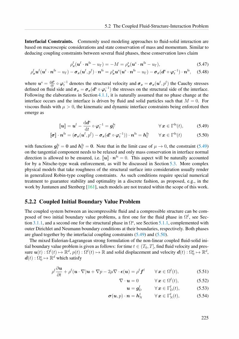
5.2 The Coupled Fluid-Structure-Interaction Problem

Interfacial Constraints. Commonly used modeling approaches to fluid-solid interaction arebased on macroscopic considerations and state conservation of mass and momentum. Similar todeducing coupling constraints between several fluid phases, these conservation laws claim

ρfx(uf · nfs − uΓ) = −M = ρs

x(us · nfs − uΓ), (5.47)

ρfxu

f(uf · nfs − uΓ)− σσσx(uf , pf) · nfs = ρsxu

s(us · nfs − uΓ)− σσσx(ds ϕ−1t ) · nfs, (5.48)

where us = dds

dtϕ−1

t denotes the structural velocity and σσσx = σσσx(uf , pf) the Cauchy stressesdefined on fluid side and σσσx = σσσx(ds ϕ−1

t ) the stresses on the structural side of the interface.Following the elaborations in Section 4.1.1, it is naturally assumed that no phase change at theinterface occurs and the interface is driven by fluid and solid particles such that M = 0. Forviscous fluids with µ > 0, the kinematic and dynamic interface constraints being enforced thenemerge as

[[u]] = uf − dds

dtϕ−1

t = gfsΓ ∀x ∈ Γfs(t), (5.49)

[[σσσ]] · nfs = (σσσx(uf , pf)− σσσx(ds ϕ−1t )) · nfs = hfs

Γ ∀x ∈ Γfs(t) (5.50)

with functions gfsΓ = 0 and hfs

Γ = 0. Note that in the limit case of µ→ 0, the constraint (5.49)on the tangential component needs to be relaxed and only mass conservation in interface normaldirection is allowed to be ensured, i.e. [[u]] · nfs = 0. This aspect will be naturally accountedfor by a Nitsche-type weak enforcement, as will be discussed in Section 5.3. More complexphysical models that take roughness of the structural surface into consideration usually renderin generalized Robin-type coupling constraints. As such conditions require special numericaltreatment to guarantee stability and optimality in a discrete fashion, as proposed, e.g., in thework by Juntunen and Stenberg [161], such models are not treated within the scope of this work.

5.2.2 Coupled Initial Boundary Value ProblemThe coupled system between an incompressible fluid and a compressible structure can be com-posed of two initial boundary value problems, a first one for the fluid phase in Ωf , see Sec-tion 3.1.1, and a second one for the structural phase in Ωs, see Section 5.1.1, complemented withouter Dirichlet and Neumann boundary conditions at their boundaries, respectively. Both phasesare glued together by the interfacial coupling constraints (5.49) and (5.50).

The mixed Eulerian-Lagrangean strong formulation of the non-linear coupled fluid-solid ini-tial boundary value problem is given as follows: for time t ∈ (T0, T ], find fluid velocity and pres-sure u(t) : Ωf(t) 7→ Rd, p(t) : Ωf(t) 7→ R and solid displacement and velocity d(t) : Ωs

0 7→ Rd,d(t) : Ωs

0 7→ Rd which satisfy

ρf ∂u

∂t+ ρf(u · ∇)u+∇p− 2µ∇ · ε(u) = ρff f ∀x ∈ Ωf(t), (5.51)

∇ · u = 0 ∀x ∈ Ωf(t), (5.52)

u = gfD ∀x ∈ Γf

D(t), (5.53)

σ(u, p) · n = hfN ∀x ∈ Γf

N(t), (5.54)

225

5 Stabilized Approaches to Fluid-Structure Interaction using Cut Finite Elements

and

ρs dd

dt−∇ · (F · S)(d) = ρsf s ∀X ∈ Ωs

0, (5.55)

ρs(dd

dt− d) = 0 ∀X ∈ Ωs

0, (5.56)

d = gsD ∀X ∈ Γs

D,0, (5.57)

(F · S) ·N = hsN ∀X ∈ Γs

N,0, (5.58)

with coupling and initial conditions

[[u]] = u− (d ϕ−1t ) = 0 ∀x ∈ Γfs(t), (5.59)

[[σσσ]] · nf = (σσσx(u, p)− σσσx(d ϕ−1t )) · nf = 0 ∀x ∈ Γfs(t), (5.60)

u(T0) = u0 ∀x ∈ Ωf(T0), (5.61)d(T0) = d0 ∀X ∈ Ωs(T0), (5.62)

d(T0) = d0 ∀X ∈ Ωs(T0). (5.63)

The mixture between Eulerian and Lagrangean formulation is clearly visible from the mappingϕt = (I + d(t), 1) for solid quantities between reference and current configuration. Note furtherthe different meaning of gradient and divergence operators for fluids and solids in spatial andmaterial coordinates x,X , respectively, as well as ρs = ρs

X as in (5.14).

5.2.3 Coupled Variational FormulationThe variational formulation of the coupled fluid-structure-interaction problem comprises varia-tional formulations for fluid and solid phases proposed in Section 3.1.2 and Section 5.1.2. Thefunctional spaces for fluid and solid are given as for the single phase problems to VgD

, Q for fluidvelocity and pressure and DgD

, Z for solid displacement and velocity. The respective test func-tion spaces are given by V0,Q for the fluid and by D0,Z for the solid. The coupled non-linearvariational formulation then reads as follows: for all t ∈ (T0, T ], find fluid velocity and pressureas well as solid displacement and velocity (u(t), p(t),d(t), d(t)) ∈ (VgD

×Q)⊕ (DgD×Z)

such that

(ρf ∂u

∂t,v)Ωf(t) + cf(u;u,v) + af(u,v) + bf(p,v)− bf(q,u)

+ (ρs(dd

dt− d), z)Ωs

0+ (ρs dd

dt,w)Ωs

0+ as(d,w) = lf(v) + ls(w),

[[u]]∣∣Γfs(t)

= 0 with uf = u and us = d ϕ−1t ,

(5.64)

for all (v, q,w, z) ∈ (V0 ×Q)⊕ (D0 ×Z), with fluid operators cf , af , bf , lf as defined in equa-tions (3.12)–(3.15) and structural operators as, ls as defined in (5.20) and (5.21). Note thatby proceeding analogously to (4.29) for fluid-fluid interfaces, after integration by parts on thetwo bulk phases, the traction coupling constraint hfs

Γ = 0 is incorporated into the variationalformulation. Enforcement of coupling constraints on discrete subspaces which do not inherentlyguarantee continuity as claimed in (5.49) and (5.50) across Γfs will be discussed in the nextsection.

226

5.3 An Unfitted Full-Implicit Nitsche-type Approach for Fluid-Structure Interaction

5.3 An Unfitted Full-Implicit Nitsche-type Approach forFluid-Structure Interaction

The objective in this section is to establish an unfitted FSI solver which allows to relax stronglimitations of most computational FSI approaches and builds the basis for future developmentson more advanced fluid-solid-interaction applications. Approximating the structure in a La-grangean setting with an interface-fitted moving mesh which overlaps with a non-interface-fittedcut Eulerian background fluid mesh, as depicted in Figures 2.11a, allows for arbitrary motionsof compressible structural bodies in surrounding flow environments. Additionally, it enablesto accurately capture the flow solution without smearing the solution fields in contrast to manyother fixed-grid schemes as the case, for instance, for many IB methods. It has to be mentionedthat this approach has been developed in view of more advanced coupled problem settings likefluid-structure-contact interaction, as considered in works by Gerstenberger [123] and Mayeret al. [184], or fluid-structure-fracture interaction addressed in the work by Sudhakar [244].Major differences to incorporated FSI solvers of the aforementioned approaches consist in theimproved stability behavior of the fluid field combined with a more accurate cut finite elementapproximation space as well as a full-implicit coupling strategy for a more robust and efficientbehavior of iterative solution procedures. Iterative approximation techniques which are able tocope with the issue of potential changes of the discrete fluid function space are suggested inthis section. The subsequently introduced unfitted FSI solver represents a significant furtherdevelopment compared to closely related FSI approaches recently published by Burman andFernandez [58] and Alauzet et al. [1]. Compared to [58], non-linearities are incorporated intothe fluid field as the flows are governed by the non-linear transient incompressible Navier-Stokes equations. Compared to Alauzet et al. [1], further complexity is introduced by the usageof structural materials which exhibit non-linear material behavior. Unlike in the latter work,in which thin-walled bodies are considered exclusively, in the present work, numerical testsare carried out not only for two-dimensional but also for challenging highly dynamic three-dimensional flows interacting with full-dimensional structural bodies. Particularly the adaptionof this solver to fully three-dimensional FSI problem settings highly increases complexity ofcode implementations with regard to computational geometry on the one hand, as well as withregard to different aspects of efficient parallel computing on the other hand. Further differencesexist in the use of different time-stepping schemes for fluids and solids as well as the treatmentof varying fluid approximation spaces. Moreover, this FSI solver is investigated for flows in thelow- as well as the higher-Reynolds-number regime where embedded structures undergo largedeformations.

5.3.1 Semi-Discrete Nitsche-type Cut Finite Element MethodIn the following, a semi-discrete coupled formulation for fluid-structure interaction problemsettings as introduced in (5.64) will be proposed. Thereby, different non-conforming approxi-mation spaces between the structural body and the fluid phase are enabled. Structural governingequations are formulated in Lagrangean description and related approximation spaces for dis-placement and velocity Ws

h,gD

def= Dh,gD

×Zh as well as test spaces Wsh,0

def= Dh,0 ×Zh are based

on interface-fitted triangulations Tsh , as described in Section 5.1.3. For solids, Dirichlet boundary

227

5 Stabilized Approaches to Fluid-Structure Interaction using Cut Finite Elements

conditions are imposed strongly via the function space. In contrast, the fluid subdomain may beeither approximated with interface-fitted meshes utilizing ALE techniques for discretizing thetime derivative, or with computational meshes that do not necessarily fit to the fluid-solid inter-face Γfs, i.e. T f

h ⊂ T fh with Ωf

h ( Ωf∗h . Associated function spaces are denoted as Wf

hdef= Vh ×Qh

with boundary conditions assumed enforced weakly. An overview about possible discretizationtechniques for fluid-structure-interaction problem settings, to which the subsequently proposedcoupling strategy is applicable, or can be easily extended to, was given in Section 2.1.4.3, see(2.65)–(2.68). Furthermore, incorporating fluid domain decomposition techniques as providedin Chapter 4 is also possible. Visualizations of potential settings are given in Figure 2.11.

A spatial semi-discrete formulation for the coupled fluid-structure system (5.64) can be com-posed of a classical finite approximation for the solid from Section 5.1.3, a stabilized flow for-mulation on possibly unfitted meshes with moving boundaries from Section 3.6.3 and additionalNitsche-type coupling terms for the fluid-structure interface. Coupling constraints at the fluid-structure interface can be imposed in analogy to the coupling of different fluid phases as providedin Section 4.2.1.

Definition 5.1 (Semi-discrete Nitsche-type formulation for fluid-structure interaction)Let Wh,gD

def= Wf

h ⊕ Wsh,gD

be the admissible space for discrete solutions, then a Nitsche-typestabilized formulation for the fluid-structure problem setting reads as follows: for all t ∈ (T0, T ],find fluid velocity and pressure Uh(t) = (uh(t), ph(t)) ∈ Wf

h as well as solid displacement andvelocity Dh(t) = (dh(t), dh(t)) ∈ Ws

h,gDsuch that ∀ (Vh,Wh) = (vh, qh,wh, zh) ∈ Wf

h ⊕ Wsh,0

Af,Xh (Uh, Vh) + As

h(Dh,Wh) + Cfsh ((Uh, Dh), (Vh,Wh)) = Lf,X

h (Uh, Vh) + Lsh(Wh), (5.65)

where the coupled formulation includes the stabilized single-phase fluid formulation Af,Xh −Lf,X

h

where X indicates the type of fluid stabilization, i.e. a CIP/ GP or a RBVM/ GP technique, asintroduced in Sections 3.6.1.1 and 3.6.1.2, respectively. The incorporated form As

h −Lsh denotes

the structural discrete formulation proposed in (5.24) evaluated in the structural subdomain.Nitsche-type fluid-solid coupling terms at Γfs are comprised in the operator Cfs

h . The formu-lation is similar to couplings between fluid phases, see (4.34)–(4.39), and emerges to

Cfsh ((Uh, Dh), (Vh,Wh)) = −〈2µεεε(uh)nfs, [[vh]]〉Γfs + 〈ph, [[vh]] · nfs〉Γfs (5.66)

∓ 〈[[uh]], 2µεεε(vh)nfs〉Γfs − 〈[[uh]] · nfs, qh〉Γfs (5.67)+ 〈γ(µ/h)[[uh]], [[vh]]〉Γfs (5.68)

+ 〈γ(ρfφ/h)[[uh]] · nfs, [[vh]] · nfs〉Γfs (5.69)

with [[uh]] = ufh − us

h = uh − dh ϕ−1t and [[vh]] = vf

h − vsh = vh − zh. It has to be noted that

due to the constraints gfsΓ = 0 and hfs

Γ = 0, all right-hand-side terms provided in (4.40)–(4.45)vanish, i.e. Lfs

h ≡ 0. In contrast to the proposed Nitsche coupling between two fluids, at fluid-solid interfaces the average weights are chosen as wf = 1− ws = 1, which renders in a fluid-sided flux weighting strategy. This choice simplifies ensuring stability for couplings with non-linear elastic structural materials. Since throughout this thesis fluids are assumed being lessviscous/stiff than solids, these weights conform to the optimality of harmonic weighting whenhigh contrast in material properties are present, as discussed in Section 4.2.2. Due to this choice,material parameters occuring in stabilization scalings of (5.68) and (5.69) belong to the fluid

228

5.3 An Unfitted Full-Implicit Nitsche-type Approach for Fluid-Structure Interaction

phase only. Furthermore, the stabilization scaling function φ is defined in (3.467). Note thatutilizing fluid elements with high aspect ratios or higher polynomial orders, the characteristicelement length scaling 1/h = 1/hf should be replaced by a more precise piecewise constantscaling (f f)2 which emanates from the weakened trace inequality for fluid elements, as sug-gested in (3.134). It has to be recalled that inf-sup stability for unfitted fluid meshes, proven interms of coercivity, is founded on using ghost-penalty stabilizations as contained in the opera-tors Af,X

h (Uh, Vh), see Sections 3.6.1.1 and 3.6.1.2. The Nitsche penalty parameter γ is chosenas suggested in Section 3.4.4.3. Again, the different signs in (5.67) allow to switch betweenan adjoint-consistent (−) and an adjoint-inconsistent formulation (+), see Section 3.3.2.4 forfurther elaborations.

The question for convective interface stabilizations as proposed in (4.38) and (4.39) requiresfurther discussion. Note that due to the Lagrangean formalism utilized for the structural dy-namics, no convective term occurs for the solid phase and the treatment of possible convectiveinstabilities would reduce to the fluid side similar to single-phase flows. However, addinginflow control on the fluid side analogously to the boundary term in (3.456), that is, consistentlyimposing uf − us = 0, may possibly render in a destabilizing effect for the solid. This can beseen from the term−〈ρf (uh · nfs)(−vs),vf〉, which then remains mathematically unbalanced inproving coercivity; a situation which might become critical when the solid displaces fluid. Notefurther that such issues do not arise when interface-fitted fluid and solid meshes are used and thefluid is consistently formulated in an ALE description. Then, no relative convective velocitiesoccur at Γfs, since uh = uh.

5.3.2 Time Stepping for Nitsche-Coupled Fluid-Structure SystemsThis section aims at formulating a fully discrete finite-dimensional system of non-linear equa-tions for the Nitsche-coupled system (5.65) consisting of one fluid and one structural phase,which is to be solved for each discrete time level.

For time stepping, let the time domain (T0, T ] be partitioned into N equal-sized time stepintervals Jn = (tn−1, tn] of size ∆twith discrete time levels tn = T0 + n∆t and tN = T . For thetemporal discretization of the coupled system, different single-field time-stepping schemes canbe utilized. Subsequently, a discrete coupled formulation is exemplarily provided for the combi-nation of a G-α method for the structural elastodynamics equations As

h −Lsh and a one-step-θ

scheme for the stabilized fluid formulation Af,Xh −Lf,X

h . Neglecting the Nitsche couplings Cfsh

in (5.65) for a moment, the temporally discretized non-linear decoupled systems for fluids andsolids,Rf(Un,P n) andRs(Dn), can be recalled as

Rf(Un,P n) = M f,n(Un,P n) + σ−1F f,n(Un,P n)

−H f,n−1(Un−1, An−1), (5.70)

Rs(Dn) =

(M s 1− αm

β∆t2+Cs (1− αf )γ

β∆t

)Dn + (1− αf )(F s,n

int (Dn)− F s,next )

−Hs,n−1(Dn−1,V n−1,An−1). (5.71)

The fluid residual is recalled from (3.473) where the matrixM f,n results from the time derivativeterm (ρfunh,Υ(vh, qh)) with Υ depending on the type of fluid stabilization, as elaborated inSection 3.6.1.3. Furthermore, F f,n denotes all operators to be evaluated at time level tn, i.e. all

229

5 Stabilized Approaches to Fluid-Structure Interaction using Cut Finite Elements

standard Galerkin terms, stabilization operators as well as Nitsche terms according to the weakimposition of boundary conditions. Terms belonging to the previous time levels are comprisedin H f,n−1. The structural residual is defined as in (5.37) based on a generalized trapezoidalrule (GTR) approximation for internal and external forces, see (5.36), and Hs,n−1 comprisesall terms evaluated at the previous time level tn−1. Note that the system of first-order structuralODEs could be expressed solely in the unknown displacement vectorDn.

Expressing structural interface velocities ush = dh ϕ−1

t , which are defined in spatial coordi-nates, in terms of structural displacements D, which are defined with respect to the referencesystem, an independent temporal discretization at the fluid-solid interface can be introduced.Applying a one-step-θ scheme to this ODE yields

U s,nΓ (Dn

Γ) =Dn

Γ −Dn−1Γ

θΓ∆t− 1− θΓ

θΓ

U s,n−1Γ , (5.72)

whereU s,nΓ is a vector-valued approximation on the structural interface velocities at time level tn,

i.e. ush ϕtn = dh(t

n). Denoting internal forces, which have to be in equilibrium at the fluid-solid interface Γfs, with F s,n

Γfs and F f,nΓfs for the solid and fluid phase, respectively, residuals can

be formulated as

Rf(Un,P n)− σ−1F f,nΓfs , (5.73)

Rs(Dn)− ((1− αf )F s,nΓfs + αfF

s,n−1Γfs ) (5.74)

with σ the characteristic temporal factors as defined in (3.476) and (3.479). The interfacialforces are replaced by numerical forces in the discrete setting. These are given by the stronglyconsistent Nitsche-coupling terms (5.66)–(5.69), for which holds F f,n

Γfs = −C fs((Un,P n),Dn)and F s,n

Γfs = −Csf((Un,P n),Dn), where

C fs((Un,P n),Dn) ⇔ − 〈2µεεε(uh)nfs,vh〉Γfs

+ 〈ph,vh · nfs〉Γfs

∓ 〈[[uh]], 2µεεε(vh)nfs〉Γfs

− 〈[[uh]] · nfs, qh〉Γfs

+ 〈γ(µ/h)[[uh]],vh〉Γfs

+ 〈γ(ρfσh+ ρf |ufh|+ µ/h)[[uh]] · nfs,vh · nfs〉Γfs , (5.75)

Csf((Un,P n),Dn) ⇔ − 〈2µεεε(uh)nfs, (−zh)〉Γfs

+ 〈ph, (−zh) · nfs〉Γfs

+ 〈γ(µ/h)[[uh]], (−zh)〉Γfs

+ 〈γ(ρfσh+ ρf |ufh|+ µ/h)[[uh]] · nfs, (−zh) · nfs〉Γfs . (5.76)

These can be identified by splitting contributions into fluid and structural residuals, i.e. withrespect to vh and zh. Furthermore, the structural interface force from the previous time level tn−1

occurring in (5.73) can be recovered from the respective structural coupling matrix

F s,n−1Γfs(tn−1)

= −Csf,n−1((Un−1,P n−1),Dn−1). (5.77)

230

5.3 An Unfitted Full-Implicit Nitsche-type Approach for Fluid-Structure Interaction

After rescaling the single non-linear fluid and solid residuals (5.73) and (5.74), the finalNitsche-coupled finite-dimensional fluid-structure system of equations, which is to be solved forthe current time level tn, reads as follows: find discrete finite-dimensional vectors Un,P n,Dn

such that

[R(U,P )

RD

]n=

[C fs((Un,P n),Dn) + σRf(Un,P n)

11−αf

Rs(Dn) +Csf((Un,P n),Dn)− αf1−αf

F s,n−1Γfs(tn−1)

]n=

[00

](5.78)

with given solid approximationsDn−1,V n−1,An−1 and fluid approximationsUn−1,P n−1 fromthe previous time level tn−1 as well as projected fluid solutions Un−1(Un−1), An−1(An−1) withrespect to the current interface location Γfs(tn). Note, the fluid residualR(U,P ) = [RU ,RP ]T canbe further split into velocity and pressure residuals.

5.3.3 Monolithic Solution Algorithm for Unfitted Non-Linear Systems

In this subsection, a monolithic solution procedure for the non-linear coupled fluid-structuresystem is derived. For the sake of clarity, the overall final algorithm is split into two nested al-gorithms. The substantial solution procedure for non-linear FSI residuals is given by a Newton-Raphson-like iterative method and is presented in Algorithm 5.2. This main sub-algorithm isapplicable to interface-fitted as well as unfitted mesh configurations as long as the fluid functionspace does not change while iterating. An extension of the classical time loop to the unfittedmesh case, which even allows to adapt the function space during the iterative procedure at afixed time level, is summarized in Algorithm 5.1.

First, solution techniques which are well-established for full-implicitly coupled non-linearFSI systems will be examined. Afterwards, an overview of the overall algorithmic procedure,the final monolithic solution algorithm will be given. Therein, focus is directed to peculiaritiesof unfitted mesh configurations.

Newton-Raphson-like Approximation for Non-linear FSI Residuals. The solution approx-imation to the coupled fluid-solid system at a discrete time level tn is given in terms of the finite-dimensional system of non-linear equations (5.78) for fluid velocities and pressure (U ,P )n andfor structural displacementsDn. Therein, non-linearities emanate from geometrical and materialnon-linear relations in the structural dynamics PDE on the one hand, and from the non-linearconvective fluid term together with its occurrence in related fluid stabilizations on the otherhand. Moreover, while structural equations are integrated in referential configuration, furthernon-obvious non-linearities are hidden in the change of the integration volume and surface areaassociated with the fluid subdomain, which depend on the non-linear interface motion.

Neglecting for a short term that due to the unfittedness of fluid and solid computational meshesthe discrete fluid function space can change for structural/interfacial motions, the solution of thenon-linear system (5.78) can be approximated iteratively by performing a Newton-Raphson-likemethod. The subsequent approximation procedure poses a mixture of fixed-point iterations forthe fluid and a full Newton-Raphson method for the structural residual.

231

5 Stabilized Approaches to Fluid-Structure Interaction using Cut Finite Elements

Algorithm 5.1 Monolithic solution algorithm for non-linear unfitted FSI-systems

1: INPUT: initial conditions ds0, d

s0,u

f0 at T0.

2: Initialize structuralAs0 for G-α scheme and set fluidAf

0 for OST or θ = 1.0 for n = 1.3: for time steps 1 6 n 6 N do4: Update time level tn = T0 + n∆t. Reset cycle counter to c = 1.5: // cycle over fluid function space changes6: while (not converged) do7: if (c > Cmax) then8: Throw exception (“maximum number of function space changes at tn exceeded!”).9: end if

10: if (c = 1) then11: Structural Solver:12: Perform predictor (D,U ,A)nc=1 ← P (D,U ,A)n−1.13: Fluid Solver:14: Update interface position (Γh)

nc=1 according to predictedDn

c=1, intersect Th to obtainactive mesh (Th)nc=1 and update face and element sets (FΓ)nc=1, (TΓ)nc=1.

15: Perform Algorithm 2.1 to allocate DOFs and set up fluid function space ( Wfh)nc=1.

16: Perform Algorithm 3.1 and transcribe solution vectors between function spaces( Wf

h)n−1 → ( Wfh)nc=1 between time levels s.t. (U , P , A)n−1

c=1 ∈ (Vfh ×Qf

h × Vh)nc=1.17: Perform fluid predictor, e.g., (U ,P )nc=1,i=1 = (U , P )n−1 ∈ ( Wf

h)nc=1,i=1.18: else // The fluid function space has changed within the last cycle c− 119: Perform Algorithm 3.1 and transcribe solution vectors between function spaces

( Wfh)n−1 → ( Wf

h)nc between time levels s.t. (U , P , A)n−1c ∈ (Vf

h ×Qfh × Vf

h)nc .20: Use recent solution approximation from interrupted pass c− 1 as initial guess for the

following Newton-Raphson procedure. Note that (U ,P )nc,i=1 ∈ ( Wfh)nc .

21: end if22: // previous time level solution available as: (D,V ,A)n−1

c (solid), (U , A)n−1c (fluid)

23: // prediction for current time level available as ((U ,P ),D)nc,i=1

24: Perform Algorithm 5.2. // (Re-)start NEWTON-RAPHSON-like iterations25: if (Newton-Raphson converged) then26: break while27: end if28: c← c+ 129: end while30: // Inner Newton-Raphson loop converged with non-changing fluid function space31: Update structural vectorsAn,Un based onDn for G-α scheme via (5.38)–(5.39).32: Update fluid acceleration approximation An for OST-scheme via (3.485),

i.e. anh(unh, un−1c , an−1

c ) with un−1c , an−1

c the recent projections of un−1c ,an−1

c ∈ Vn−1h to

the fluid function space Vnc belonging to the converged state.

33: Store the structural force vector F s,nΓfs(tn)

(5.77) for the next time level.34: Store final approximations: (D,U ,A)n for the solid and (U ,P ,A)n for the fluid.35: end for36: OUTPUT: solid displacement and fluid velocity and pressure solution approximations((U ,P ),D)n16n6N for discrete time levels tn16n6N . Note the possibly time-varyingfluid approximation spaces Wf

h16n6N .

232

5.3 An Unfitted Full-Implicit Nitsche-type Approach for Fluid-Structure Interaction

Algorithm 5.2 Newton-Raphson-like solution procedure for non-linear FSI-system

1: INPUT: initial guess of structural displacements, fluid velocity and pressure ((U ,P ),D)ni=1

for iterative solution procedure. Previous time-step solutions for structure (D,V ,A)n−1,for fluid (U , A)n−1, interfacial velocities U s,n−1

Γ and structural forces F s,n−1Γfs(tn−1)

.2: for Newton-Raphson-like iterations 1 6 i 6 Nmax do3: FSI Solver:4: Update structural interface velocity (U s

Γ)ni based on (DΓ)ni with OST-scheme (5.72).5: Apply current iterations to structural solver and to CUTFEM fluid solver.6: Structural Solver:7: Evaluate structural contribution to matrix LDD|Dn

iand to residualRD|Dn

i, see (5.79).

8: Fluid Solver:9: if (i > 1) then

10: Update interface position to (Γh)ni according to last iterationDn

i .11: Intersect the mesh Th and obtain the active computational mesh (Th)ni and construct

updated face and element sets (FΓ)ni , (TΓ)ni .12: Perform Algorithm 2.1 to allocate DOFs and set up new fluid function spaces ( Wf

h)ni .13: Perform TRANSFER/COPY-PHASE of Algorithm 3.1 and transcribe solution vectors

between function spaces ( Wfh)ni−1 → ( Wf

h)ni of previous and current iteration.14: if (TRANSFER/COPY-PHASE not successful) then15: // Change in fluid function space occurred, i.e. ( Wf

h)ni−1 6= ( Wfh)ni .

16: Perform EXTENSION-PHASE of Algorithm 3.1 and utilize the resultingapproximation as initial guess for the next Newton-Raphson cycle c+ 1:((U ,P ),D)n ∈ ( Wf

h)nc+1,i=1 × Dh

17: return false.18: end if19: end if20: Evaluate fluid boundary conditions gf

D(tn), hfN(tn) with respect to (Γh)

ni .

21: Evaluate stabilized fluid system, coupling matrices contributing to Lxy and to residualsRU ,RP ,RD, see (5.79).

22: FSI Solver:23: Set up final linear fluid-structure system Lfs ·∆((U ,P ),D)ni = −Rfs (5.79).24: Apply strong Dirichlet boundary conditions from function spaces Wf

h,gDand Ds

h,gD.

25: Build block preconditioner and apply to (5.79).26: Solve preconditioned linearized fixed-point like system (5.79) for ∆((U ,P ),D)ni .27: Check convergence: ‖∆((U ,P ),D)ni ‖ < TOL and ‖(Rfs)ni ‖ < TOL.28: if (FSI system converged) then29: return true30: end if31: Update Newton-Raphson iteration via (5.80) to ((U ,P ),D)ni+1.32: end for33: Throw exception (“maximum number of Newton-Raphson iterations reached!”).34: OUTPUT:35: return false with iteration ((U ,P ),D)ni ∈ ( Wf

h)ni × Dsh based on changed fluid function

space ( Wfh)ni 6= ( Wf

h)ni−1, or36: return true with converged velocity, pressure and displacement solution approximations

((Un,P n),Dn) for time level tn.

233

5 Stabilized Approaches to Fluid-Structure Interaction using Cut Finite Elements

The solution ((U ,P ),D)n is approximated iteratively for i > 1 by solving linear systems forincrements ∆((U ,P ),D)ni satisfying

LUU LUPLPU LPP

LUDLPD

LDU LDP LDD

n

i︸ ︷︷ ︸Lfs

·

∆U∆P∆D

n

i

= −

RU

RP

RD

n

i︸ ︷︷ ︸Rfs

(5.79)

followed by a Newton-Raphson incremental update step for the next iterationUPD

n

i+1

=

UPD

n

i

+

∆U∆P∆D

n

i

. (5.80)

Note that the subscript ()i in matrix and right-hand side of the linear system (5.79) indicatessub-matrices and residuals being evaluated on basis of the current approximation ((U ,P ),D)ni .Therein, let Lxy = ∂Rx

∂ydenote (pseudo)-directional derivatives of residualsRx from (5.78) with

respect to the finite dimensional solution approximation y, where x, y ∈ U ,P ,D. Exemplar-ily, approximation LDD for neglected Rayleigh damping is given as

LDD|((U ,P ),D)ni=

1

1− αf

(M s 1− αm

β∆t2+∂F s,n

int (D)

∂D

∣∣∣∣D=Dn

i

)+G|((U ,P ),D)ni

, (5.81)

where

G|((U ,P ),D)ni

def=∂Csf((U ,P ),D)

∂D

∣∣∣∣((U ,P ),D)=((U ,P ),D)ni

(5.82)

⇔ + 〈γ(µ/h)(−∂D(ush)|Dn

i, (−zh)〉Γfs(Dn

i )

+ 〈γ(ρfσh+ ρf |ufh|+ µ/h)(−∂D(us

h)|Dni) · nfs(Dn

i ), (−zh) · nfs(Dni )〉Γfs(Dn

i ),

with ∂D(ush)|Dn

i=

∂ush(D)

∂D

∣∣D=Dn

i⇔ 1

θΓ∆tDn

i . Note that change of integration area and interfaceunit normal vectors are treated fixed-point-like. All other approximations Lxy can be derived byanalogy but are not presented here.

Newton-Raphson-like Algorithmic Procedure for Non-changing Function Spaces. The so-lution procedure for the non-linear FSI residual (5.78) is summarized in Algorithm 5.2. Itassumes that the fluid function space remains unchanged during the iteration loop. Relaxingthis assumption will be addressed afterwards within a subsequent paragraph.

For starting the iterative solution procedure, an initial guess for the solution fields is requiredwhich is denoted with ((U ,P ),D)ni=1. These may be given, for instance, in terms of a predicteddisplacement field and the velocity solution of the previous time level as discussed, e.g., byMayr et al. [185]. Furthermore, evaluating FSI residuals requires history from the previous timelevel for structural fields, i.e. (D,V ,A)n−1, as well as structural forces F s,n−1

Γfs(tn−1)as defined in

(5.77). Note that due to unfitted approximation of the fluid field, approximations have to be first

234

5.3 An Unfitted Full-Implicit Nitsche-type Approach for Fluid-Structure Interaction

projected onto the current function space ( Wfh)ni=1 associated with the time level tn by applying

Algorithm 3.1, which provides approximations (U , A)n−1 ∈ (Vh)ni=1 × (Vh)ni=1.Newton-Raphson-like iterations are performed until convergence of residuals (Rfs)ni and of

increments ∆((U ,P ),D)ni is achieved. For a current displacement iteration Dni , structural

interface velocities (U sΓ)ni can be updated via (5.72). After setting current approximations to

the structural and the fluid solver, their contributions to matrices (Lxy)ni and right-hand-side

blocks (Rx)ni of the linearized FSI system (5.79) can be evaluated and finally assembled into the

global system Lfs ·∆((U ,P ),D)ni = −Rfs. After applying strong Dirichlet constraints fromWfh,gD

and Wsh,gD

and setting up a block preconditioner, the linear FSI system can be solved forthe Newton-Raphson increments. Finally, the approximations can be updated to ((U ,P ),D)ni+1

via (5.80). If convergence checks fail, it has to be proceeded with the next iteration i+ 1.This procedure is summarized in Algorithm 5.2. Note that for unfitted fluid approximationstheir function spaces might change due to displacing the fluid-structure interface. This demandsfurther measures as will be addressed later in Algorithm 5.1.

Solving Linear Matrix Systems. For approximating the incremental solution of each linearFSI iteration (5.79), a preconditioned GMRES solver is utilized. Building specific precondi-tioners is based on a unified framework recently proposed by Verdugo and Wall [256] whichis applicable to different monolithically solved n-field coupled problems. Preconditioners usedthroughout this thesis use generic block Gauss–Seidel iterations for uncoupling the subproblems.For the decoupled structural and fluid blocks, any combination of either one-level domain de-composition preconditioners of incomplete factorization type, as developed by Sala and Heroux[224], or algebraic multigrid (AMG) methods, as proposed by Prokopenko et al. [211], isapplicable. Both applied preconditioning techniques are developed under the Trilinos projectconducted by Sandia National Laboratories.

Cycle over Possible Function Space Changes for Unfitted Fluid Approximations. Recall-ing the issue of applicability of iterative solution techniques for unfitted mesh methods, whichconsists in potentially varying fluid approximation spaces during the iterative procedure, thefollowing generalization of the Newton-Raphson scheme for such problem settings is suggested:

As described in Algorithm 5.2, for each iteration the updated interface displacements are set tothe CUTFEM fluid solver on which basis the computational mesh T f

h is intersected, associatedface and element sets (FΓ)ni and (TΓ)ni are built and the fluid function space ( Wf

h)ni is con-structed. After updating the discrete function space via Algorithm 2.1, previous fluid iterations(U ,P )ni−1 ∈ ( Wf

h)ni−1 have to be transcribed to ( Wfh)ni . This can be carried out DOF-wise

using the TRANSFER/COPY-PHASE of Algorithm 3.1 whenever ( Wfh)ni−1 ≡ ( Wf

h)ni . However,if ( Wf

h)ni−1 6= ( Wfh)ni , the current Newton-Raphson cycle c has to be interrupted. Algorithm 3.1,

that is including the EXTENSION-PHASE, can be applied to (U ,P )nc,i ∈ ( Wfh)nc,i−1 to obtain a

predicted approximation ((U ,P ),D)nc+1,i=1 = (P ni (U ,P )nc,i,D) for the next pass c+ 1. These

preparation steps for restarting the Newton-Raphson procedure in a new cycle are comprised inAlgorithm 5.2.

As summarized in Algorithm 5.1, within a subsequent run, i.e. c > 1, the previous time levelfluid solution has to be adapted according to the changed function space. For this purpose, aprojection step as provided by Algorithm 3.1 can be performed such that (U , P , A)n−1

c ∈ (Vfh×

235

5 Stabilized Approaches to Fluid-Structure Interaction using Cut Finite Elements

Qfh× Vf

h)nc . Note that for unchanged DOFs the Newton-Raphson is interrupted just formally andthe current solution approximation remains unmodified due to the DOF-wise copy-technique.However, theoretically it might happen that DOFs get repeatedly activated and deactivatedfor subsequent cycle runs c, c+ 1, c+ 2, .... Together with continuously modified projectedsolutions (U , P , A)n−1

c such situations could worsen or even totally destroy convergence. Assuch behavior did not occur for the numerical simulations considered in this thesis, a precisedescription of counteracting measures was dispensed. However, straightforward techniqueslike freezing the fluid function space, i.e. ( Wf

h)ni = ( Wfh)ni+1 = ( Wf

h)ni+2 = ..., could be simplyrealized and DOFs which are located outside of the integrated fluid domain can be sufficientlycontrolled by expanding the interface zone FΓ for ghost-penalty-stabilization operators.

After achieving a converged solution from the proposed nested Newton-Raphson procedure,further time-stepping related quantities need to be updated. For an OST scheme in the fluidsolver, an acceleration approximation An is obtained from (3.485), where anh(unh, u

n−1c , an−1

c )incorporates projected velocity and acceleration approximations un−1

c , an−1c belonging to the

converged cycle run c of the previous time level. For the structural field, acceleration andvelocity fields An and Un according to the G-α scheme are refreshed via (5.38)–(5.39). Afterstoring the structural forces for the next time steps as specified in (5.77), all quantities requiredfor proceeding with the next time level tn+1 are available, i.e. (U ,P ,A)n for the fluid and(D,U ,A)n and F s,n

Γfs(tn)for the solid.

5.3.4 Pulsating Flow over a Bending Flexible Flap

In the following, the proposed unfitted FSI solver is validated for a challenging three-dimensionaltest case which exhibits highly dynamic transient fluid-structure interaction. Robustness of thefluid solver and the ability to deal with large fluid domain changes has been already demonstratedin Section 3.6.4 for fluid-structure-interaction-like test examples. Therein, convective fluid flowinduced by a moving cylinder and viscous flow around a moving beam-like structure are investi-gated, both were not compressible or deformable in fact, however, were subjected to large rigidbody motions. In the following focus is directed to the full non-linear interaction between fluidsand solids.

Problem Setup. The geometric setting of this problem is inspired by FSI test examples in-vestigated in works by Gerstenberger and Wall [125] and Shahmiri [235]. While in the latterpublications the considered fluid-solid interactions reach steady state, in the present work, mate-rial properties of the fluid and solid are weakened. This allows to demonstrate the performanceof the proposed CUTFEM-based FSI solver for highly dynamic interactions between a mainlyconvective-dominated flow and a flexible structure.

Initially inlet-driven fluid flow in a cuboid-shaped domain Ω = [0, 1.8]× [0, 0.6]× [−0.6, 0.6]around a rubbery flexible flap of initial dimensions Ωs = [0.49, 0.56]× [0, 0.35]× [−0.3, 0.3] isconsidered, which is clamped by the bottom wall of Ωh at x2 = 0. The top and the four sidewalls of the flap defines the interface Γfs at which fluid and solid interact. Fluid is periodi-cally pushed into the domain Ω at the inlet x1 = 0 where uin = (u1, 0, 0) · g(t) with u1(x) =umax(81/2500)x2(x2 − 0.6)(x3 + 0.6)(x3 − 0.6) parabolic in directions x2 and x3. The peak

236

5.3 An Unfitted Full-Implicit Nitsche-type Approach for Fluid-Structure Interaction

Figure 5.1: Pulsating flow over a bending flexible flap: geometric setup at T0 = 0. Unfitted fixed-grid fluid mesh Tfh

consisting of Q1-elements indicated at inlet side and side wall with partially refined middle block. Aflexible structural flap is clamped by the bottom wall and interacts with the surrounding flow (coloredby parallel distribution over 16 processors).

velocity is umax = 2.0 and varied by a temporal factor

g(t) =

12(1− cos(πt)) ∀ t ∈ [0, T1],

0 ∀ t ∈ (T1, T ],(5.83)

where T1 = 10 denotes the final time of the excitation phase and T = 30.0 the end of thesimulation. This flow entering the domain excites the structural flap to initially bend and deform,while later its periodicity causes highly dynamic stimulations of fluid and solid to each other.No-slip wall boundary conditions at the four sides perpendicular to the inlet prevent the flow toescape. It is pushed outwards at the outlet at x1 = 1.8 where a zero-traction Neumann conditionhN = 0 defines the pressure level. All boundary conditions for fluid velocity and structuraldisplacements are enforced strongly and are incorporated into the respective fluid and solidtrial and test function spaces Wf

h,gD, Wf

h,0 and Wsh,gD

, Wsh,0. The material properties are chosen

as follows: The flow is assumed incompressible with kinematic fluid viscosity νf = 0.01 anda density of ρf = 1.0. Based on the maximum inflow velocity and the width of the flap, theReynolds number Re ranges from 0–120. The structure exhibits a Neo-Hookean material with aYoung’s modulus of E = 500, a Poisson’s ratio of νs = 0.4 and a density of ρs = 250 for whichlarge and dynamic deformations are expected. External volume loads are not present such thatf f = f s = 0. A sketch of the problem setting is drawn in Figure 5.1.

Computational Approach. For the spatial approximation of the structural subdomain Ωs afluid-solid-interface fitted computational grid Ts

h is used. It consists of 3720 8-node Q1-elementswhich in reference configuration are distributed in the three coordinate directions as 8× 15× 31

such that Ω0,h ≡ Ω∗0,h ≡ Ω0. This mesh overlaps with a background fluid grid T fh which fits to the

237

5 Stabilized Approaches to Fluid-Structure Interaction using Cut Finite Elements

outer boundaries, however, does not fit to the fluid-solid interface Γfsh , neither in the initial state

nor when the structure displaces, i.e. Ωfh ( Ωf∗

h . The mesh T fh is constructed as follows: a Carte-

sian grid consisting of 30× 13× 26 elements covers the domain Ω and is subsequently refined ina middle block dimensioned by [0.3, 0.9]× [0, 0.6]× [−0.6, 0.6] with one stage of element split-ting in x1 and x2 direction. This increases the flow resolution in the region of main interest wherethe structure is expected to move and deform in. The final fluid mesh T f

h contains 21632 8-nodeQ1-elements. Note that its active computational mesh T f

h changes over time due to the displacinginterface Γfs

h . For the approximation of fluid velocity and pressure the reduced volume-cell-composite enrichment strategy proposed in Section 2.2.5 is utilized. Temporal discretization forthe fluid is based on a OST-scheme with θ = 1.0. Similarly, the approximation of structuralinterface velocities from displacements (see equation (5.72)) uses θΓ = 1.0. Moving fluid do-mains are treated as summarized in Algorithms 3.1 and 3.2. For structural time-stepping, the G-αscheme could be applied with characteristic parameters αm = 1/2, αf = 1/2, γ = 1/2, β = 1/4,i.e. ρ∞ = 1.0 without numerical high-frequency dissipation (see also Table 5.1). Moreover,Rayleigh damping is neglected in this example, i.e. cM = cK = 0. The time-step length is chosenequal-sized as ∆t = 0.01 resulting in 3000 time steps within [0, T ].

For the interface coupling of fluid and structural phase, the proposed monolithic CUTFEM-based FSI solver developed in Sections 5.3.1–5.3.3 is applied. For the Nitsche-type couplingstrategy, in this example, an adjoint-inconsistent formulation is studied (see sign choice in(5.67)). To sufficiently control mass conservation, the Nitsche penalty parameter in (5.68) and(5.69) is not neglected, however, chosen relatively small with γ = 10.0. Inf-sup stability in thevicinity of the intersected fluid mesh is ensured by different GP stabilization terms, whereasfor efficiency reasons, the fluid formulation in the interior of its subdomain Ωf

h is controlledby the RBVM technique, as summarized in Section 3.6.1.2. For each time step, the non-linear FSI residuals (5.78) are approximated iteratively as outlined in Algorithm 5.1. Conver-gence checks for increments and residuals are performed separately for the distinct solutionapproximations, i.e. for RU ,RP ,RD and ∆U ,∆P ,∆D based on relative l2- and l∞-vector-norms with a uniform tolerance of TOL = 10−8. Solutions to all involved global linear systems(5.79) are approximated by a block-preconditioned GMRES solver. For preconditioning, oneblock-Gauss–Seidel sweep is utilized with incomplete factorization type field preconditionersfor the fluid and solid blocks. While for the solid a so-called fill-pattern (0) is sufficient, thefluid requires a fill-pattern (1) or even higher due to the enlarged bandwidth caused by GPterms; for details see documentation by Sala and Heroux [224] and advanced literature by, e.g.,Verdugo and Wall [256]. The subsequent results have been computed with the fully parallelizedcode environment BACI (see [262]) based on Ncore = 16 cores. The parallel distribution overprocessors is visualized in Figure 5.1.

Results. Simulation results on the temporal evolution of the flap bending and its surroundingflow are shown in Figure 5.2 at different significant times. Flow entering the fluid domain at theinlet streams around the flap and forces acting on the structural front-surface cause bending inmean flow direction as depicted at times T1 = 0.5 and T2 = 1.0. When inflow is decreased tozero for the first time at T3 = 2.0, the deformed structure tends to turn back to its undeformedinitial state. At this stage, the flow is dominated by the structural motion and different swirlsare induced as indicated by streamlines. Increasing again the mass flow rate at the inlet reaching

238

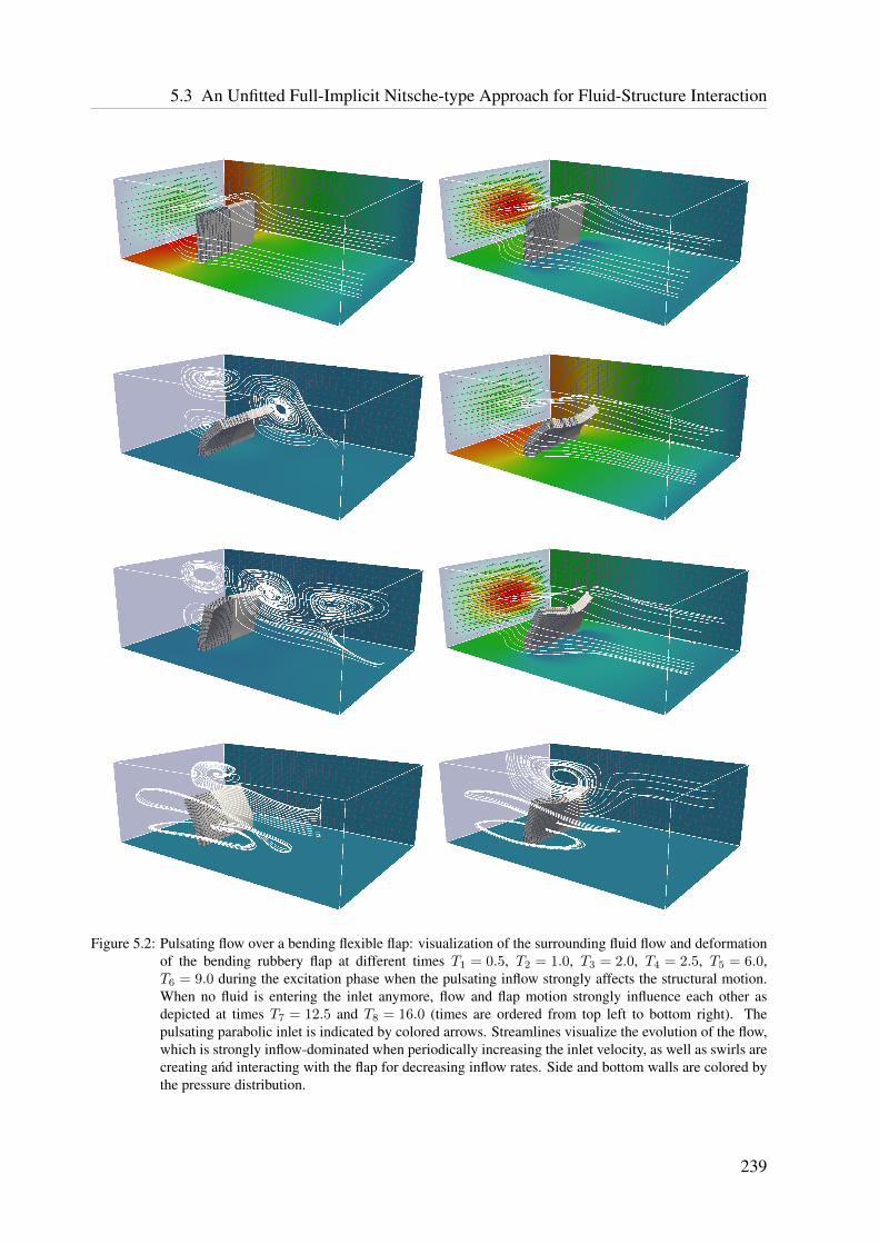
5.3 An Unfitted Full-Implicit Nitsche-type Approach for Fluid-Structure Interaction

Figure 5.2: Pulsating flow over a bending flexible flap: visualization of the surrounding fluid flow and deformationof the bending rubbery flap at different times T1 = 0.5, T2 = 1.0, T3 = 2.0, T4 = 2.5, T5 = 6.0,T6 = 9.0 during the excitation phase when the pulsating inflow strongly affects the structural motion.When no fluid is entering the inlet anymore, flow and flap motion strongly influence each other asdepicted at times T7 = 12.5 and T8 = 16.0 (times are ordered from top left to bottom right). Thepulsating parabolic inlet is indicated by colored arrows. Streamlines visualize the evolution of the flow,which is strongly inflow-dominated when periodically increasing the inlet velocity, as well as swirls arecreating and interacting with the flap for decreasing inflow rates. Side and bottom walls are colored bythe pressure distribution.

239

5 Stabilized Approaches to Fluid-Structure Interaction using Cut Finite Elements

0 10 20 30−0.2

−0.15

−0.1

−0.05

0

0.05

0.1

0.15

0.2

0.25

0.3

time t

displacement

Point X = (0.49, 0.35, 0.0)

d1 displacementd2 displacement

0 10 20 30−0.2

−0.15

−0.1

−0.05

0

0.05

0.1

0.15

0.2

0.25

time t

displacement

Point X = (0.525, 0.35, 0.3)

d1 displacementd2 displacement

Figure 5.3: Pulsating flow over a bending flexible flap: history of displacement components d1, d2 of selected pointslocated at top surface of the bending flap. Computed displacements for point X = (0.49, 0.35, 0.0)(left) and for point X = (0.525, 0.35, 0.3) (right) defined in referential configuration at T0 = 0.Numerical results are computed with the RBVM/GP FSI solver based on ∆t = 0.01 over t ∈ [0, 30.0].

its peak at T4 = 2.5, due to strong induced viscous and pressure forces acting on the flap thisundergoes again deformations in mainly stream direction. Whenever, inflow is strong enough thestructural motion is dominated by the flow and tries to minimize resistance in the surroundingflow. In contrast, when the structure is deformed and no flow is entering through the inletanymore, its motion towards its undeformed configuration dominates the flow. States at latertimes during the excitation phase depict this highly dynamic fluid-structure interaction. Theperiodically recurring dominance of the pulsating inflow and the strongly deformed structuralstate is exemplarily shown at times T5 = 6.0 and T6 = 9.0. Upon the excitation phase, differentlow-velocity vortices are present in the fluid domain and continuously interact with the rubberystructure. Positive and negative deflections in x1-direction occur as indicated at times T7 = 12.5and T8 = 16.0. Due to the higher Poisson’s ratio, even larger deformations perpendicular to themain stream direction arise. Due to the viscous effects, the amplitude of motion slowly decaysover time. For two selected points located at the flap’s top surface, the history of displacementsin x1- and x2-directions is reported in Figure 5.3. Their coordinates are specified in initialconfiguration at X = (0.49, 0.35, 0.0) for the front top point and at X = (0.525, 0.35, 0.3) forthe right top point.

Robustness of the proposed unfitted CUTFEM FSI solver is demonstrated for this challenginghighly dynamic three-dimensional fluid-structure-interaction setting incorporating large motionsand deformations of the compressible structure. The algorithmic treatment of time-changingfluid approximation spaces successfully works and convergence of the Newton-Raphson-likescheme applied to the non-linear residuals up to the specified tolerance was obtained duringthe overall simulation time. Moreover, due to the use of different ghost-penalty stabilizationoperators according to the RBVM/GP formulation, uniform well-conditioning of all linearizedFSI systems could be achieved.

240

5.4 Unfitted Fluid-Structure Interaction Combined with Fluid Domain Decomposition

5.4 Unfitted Fluid-Structure Interaction Combined with FluidDomain Decomposition

Particularly higher-Reynolds-number flows interacting with structures often exhibit high velocitygradients in the boundary layer of moving fluid-solid interfaces. Pure fixed-grid schemes usuallylack accuracy when physics in the vicinity of the interface are not sufficiently captured, as mightbe also the case for the previously introduced unfitted CUTFEM FSI solver. While, in fact,in under-resolved situations weak constraint enforcement of FSI coupling conditions alreadyhighly improves quality of the flow solution and thus of the entire fluid-structure interactioncompared to strong DOF-wise couplings, sufficient resolution of the flow characteristics in thevicinity of the interface is indispensable to capture physics appropriately. To avoid the need forfinest mesh resolutions in the overall fluid domain and thereby to retain simplicity of mesh gen-eration, if a priori knowledge on the approximate region of expected structural motion is given,a powerful FSI solver can be simply set up by combining the unfitted FSI solver with techniquesof unfitted fluid domain decomposition as provided in Sections 4.2 and 4.3. Combining these twocoupling techniques widens extensibility of existing fitted and unfitted approaches to a multitudeof novel coupled FSI solvers. Possibly realizable composed discretization concepts based on theproposed fluid-solid and fluid-fluid couplings have been visualized in Figure 2.11 exemplarily fora single structural mesh and two overlapping fluid meshes. It has to be mentioned that furtherextensions to various fluid phases and structural bodies are straightforward from the couplingpoint of view. While the combination of fitted fluid-solid couplings with unfitted fluid domaindecomposition (see Figure 2.11c) has been extensively studied in the thesis by Shahmiri [235],the following elaborations turn focus on a generalization of that which allows to utilize unfittedapproximations at both interfaces, i.e. between fluid and solid subdomains as well as betweenthe two fluid subdomains (see Figure 2.11b).

5.4.1 Nitsche-type Formulation of Coupled System

In the following, the semi-discrete Nitsche-type formulations for fluid-structure interaction fromSection 5.3.1 and the fluid domain decompositions formulation for several fluid phases or sub-domains from Section 4.2.1 are combined. In a first step, the final discrete coupled formulationis presented. Afterwards, in analogy to the fluid-structure coupling introduced in Section 5.3.3,the non-linear discrete residuals are formulated and the block matrix structure of resulting linearNewton-Raphson-like systems of equations are presented.

Extension of Nitsche-type Fluid-Structure Coupling to Several Fluid Phases. Let the spaceof admissible discrete solutions be denoted with Wh,gD

def= (⊕li=1 Wfi

h )⊕ Wsh,gD

. This combinedfunction space consists of l def

= Ndom − 1 fluid subdomain spaces and, without loss of generality,one structural function space, which altogether are coupled in a fitted or an unfitted way. Thesubspaces are as defined in Section 4.2.1 and Section 5.1.3. The Nitsche-coupled stabilizedformulation for this multidomain FSI problem setting reads as follows: for all t ∈ (T0, T ],find fluid velocities and pressure approximations Uh(t) = (uh(t), ph(t)) ∈ (⊕li=1 Wfi

h ), whereUh(t)|Ωi = U i

h(t) ∈ Wfih , and solid displacement and velocity Dh(t) = (dh(t), dh(t)) ∈ Ws

h,gD

241

5 Stabilized Approaches to Fluid-Structure Interaction using Cut Finite Elements

such that for all (Vh,Wh) ∈ (⊕li=1 Wfih )⊕ Ws

h,0

Ah((Uh, Dh), (Vh,Wh)) = Lh(Uh, (Vh,Wh)), (5.84)

where

Ah((Uh, Dh), (Vh,Wh))def=∑

16i6l

(Ai,Xih (Uh, Vh) +

∑

l>j>i

Cijh (Uh, Vh) + Cis

h ((Uh, Dh), (Vh,Wh)))

+ Ash(Dh,Wh), (5.85)

Lh(Uh, Vh)def=∑

16i6l

(Li,Xih (Uh, (Vh,Wh)) +

∑

l>j>i

Lijh (Uh, Vh)

)

+ Lsh(Wh) (5.86)

with operators for the single fluid phases Ai,Xih −Li,Xi

h , see Sections 3.6.1.1 and 3.6.1.2, respec-tive fluid-fluid Nitsche-type couplings Cij

h −Lijh from (4.34)–(4.45), and the structural varia-

tional form Ash −Ls

h (5.24) which is coupled to the fluid phases with Nitsche-type couplings Cish

as proposed in (5.66)–(5.69).

Non-linear Residuals. In analogy to (5.78), the final Nitsche-type coupled finite-dimensionalsystem of equations consisting of l fluid blocks and one structure block for a discrete time level tn

reads: find discrete finite-dimensional vectors ((U ,P )1, ... , (U ,P )l,Ds)n such that

R1(U,P )...

Rl(U,P )

RD

n

=

σR1((U ,P )1) +l∑

i=1

C1i((U ,P )1, (U ,P )i) +C1s((U ,P )1,Ds)

...

σRl((U ,P )l) +l∑

i=1

C li((U ,P )i, (U ,P )l) +C ls((U ,P )l,Ds)

11−αf

Rs(Ds) +l∑

i=1

Csi((U ,P )i,Ds)− αf1−αf

F s,n−1Γfs(tn−1)

n

= 0

(5.87)

whereCis,Csi denote the splits of fluid-structure Nitsche couplings as defined in (5.75)–(5.76).Similar splits for Nitsche coupling terms (4.34)–(4.45) between fluid phases are denoted withCij , Cji. Furthermore, Rs denotes the structural residual and Ri, i = 1, ... , l, the l fluid subdo-main residuals without interface coupling terms.

Linearized Block Matrix Structure for Newton-Raphson Iterations. The algorithmic treat-ment of issues with regard to changing function spaces of unfitted mesh approximations pro-posed in Algorithm 5.1 and discussed in Section 5.3.3 can be straightforwardly adapted to avarious number of unfitted computational meshes.

242

5.4 Unfitted Fluid-Structure Interaction Combined with Fluid Domain Decomposition

Following the procedure introduced in Section 5.3.3, the (pseudo-)linearized Newton-Raphson-like coupled system, which needs to be solved for each iteration step as described in Algo-rithm 5.2, becomes

L11UU L11

UP

L11PU L11

PP

· · · L1lUU L1l

UP

L1lPU L1l

PP

L1sUD

L1sPD

... . . . ......

Ll1UU Ll1UPLl1PU Ll1PP

· · · LllUU LllUPLllPU LllPP

LlsUDLlsPD

Ls1DU Ls1

DP · · · LslDU Lsl

DP LssDD

n

i︸ ︷︷ ︸L

·

∆U 1

∆P 1

...∆U l

∆P l

∆Ds

n

i

= −

R1U

R1P

...RlU

RlP

RsD

n

i︸ ︷︷ ︸R

(5.88)

with an incremental update step for the next iteration

U 1

P 1

...U l

P l

Ds

n

i+1

=

U 1

P 1

...U l

P l

Ds

n

i

+

∆U 1

∆P 1

...∆U l

∆P l

∆Ds

n

i

. (5.89)

For details on the applied fixed-point-like treatment of stabilization scalings and geometricinterface quantities in Lijxy as well as linearization of bulk and interface terms, the reader isreferred to Section 5.3.3.

5.4.2 Vibrating of a Flexible Structure - Unfitted Fluid-Fluid-StructureInteraction

The test example of a tail-shaped flexible structure which is vibrating due to vortex-sheddinginduced by a surrounding higher-Reynolds-number flow is perfectly suited to demonstrate thehigh capabilities of the composed unfitted discretization concept for FSI. The considered prob-lem setting has been originally introduced by Wall and Ramm [257] and extensively studied fora classical ALE-based interface-fitted moving mesh FSI solver in the thesis by Wall [258].

Problem Setup. The problem setting of this test example is taken unchanged from [258]. Aschematic sketch is drawn in Figure 5.4. A two-dimensional flexible structure of length 4.0and height 0.06 is clamped at its front end by a square-shaped obstacle of edge-length 1.0which is assumed fixed. The rest of the tail can arbitrarily move in a surrounding fluid withina domain Ω of length 19.5 and height 12.0. The entire structural surface defines the fluid-structure interface Γfs. However, along the fixed head the fluid-solid interaction simplifies toa no-slip boundary condition for the fluid to be enforced weakly. The origin of the setting isset to the front end of the flexible structure. Constant inlet at x1 = −5.5 with a fluid velocity ofumax = 51.3 drives the flow around the fixed structural head. For higher Reynolds numbers,vortices detach in its backflow and strongly interact with the flexible structural tail. Theseexcite the structure to vibrate which in return cause further creation and detachment of vortices

243

5 Stabilized Approaches to Fluid-Structure Interaction using Cut Finite Elements

5.5

12.0

12.0

Ωf1

Γf1f27.2

4.0

Γfs

1.0

0.06

7.0

1.0

1.0

slip

slip

Ωf2

Ωs

uin

Figure 5.4: Vibrating of a flexible structure: geometric setup for unfitted fluid-fluid-solid interaction. A flexible tailis clamped by a fixed head and embedded into a surrounding flow fluid. Fluid domain is artificiallydecomposed into an inner domain Ωf1 and outer template-shaped domain Ωf2 .

from the structure. The flow velocity entering the domain is initially ramped up smoothly bya time curve factor g(t) = 1

2(1− cos(πt/0.1)) within t ∈ [0, 0.1] and kept constant afterwards.

At the boarders perpendicular to the inlet, i.e. x2 = ±6.0, slip-conditions prevent the flow toescape and a zero-traction Neumann boundary condition hN = 0 is enforced at x1 = 12.0. Thematerials are chosen as follows: for the fluid, viscosity and density are set to µf = 1.82 · 10−4

and ρf = 1.18 · 10−3 resulting in an approximate Reynold number of Re ≈ 333 based on thestructural head dimension. For the structural tail, Neo-Hookean material is considered with aPoisson’s ratio of νs = 0.35 and two different characteristic material sets:

(A) a Young’s modulus of E = 2.5 · 10−6 with a density ρs = 0.1 and

(B) a Young’s modulus of E = 2.0 · 10−6 with a density ρs = 2.0.

Computational Approach. The structural tail is approximated by 20× 2 two-dimensional8-node Q2-elements. The fluid domain is decomposed at an artificial fluid-fluid interface Γf1f2

given by the boundary of the box [−2.0, 5.0]× [−3.6, 3.6] which defines Ωf1h ∪ Ωs

h. In the currentimplementation of the applied fluid-fluid-structure solver the intersection of only one fluid meshis enabled. For this reason, the inner fluid domain Ωf1

h is approximated unfitting by a fine-resolved fluid mesh consisting of 80× 80 bilinearly-interpolated Q1-elements which covers aslightly enlarged fictitious domain Ωf1∗

h = [−2.05, 5.05]× [−3.65, 3.65] and is unfitted to bothinterfaces, the fluid-solid interface Γfs and the fluid-fluid interface Γf1f2 . The outer template-shaped fluid subdomain Ωf2

h = Ω\(Ωf1h ∪ Ωs

h) is approximated by a mesh T f2h which fits to its

outer and inner subdomain boundary ∂Ωf2h . Note, the latter one is the fluid-fluid interface Γf1f2 .

The mesh T f2h exhibits a mesh size of h1 = 0.1625 in x1-direction and h2 = 0.3 in x2-direction.

This fluid mesh and the structural mesh overlap in an unfitted way with the inner fluid gridT f1h . The different approximations are visualized in Figure 5.5. As all meshes exhibit perfect

symmetry with respect to the x1-axis, the entire structure needs to be slightly displaced with aperturbation of ε = 0.001 in positive x2-direction to introduce a small imperfection to later causevortex detachment. Otherwise, the flow would remain perfectly symmetric all over the time. It

244

5.4 Unfitted Fluid-Structure Interaction Combined with Fluid Domain Decomposition

Figure 5.5: Vibrating of a flexible structure: (Left) Fitted mesh approximations Tsh,T

f2h for structural domain

and outer fluid subdomain. Inner fluid domain is approximated with a finer computational grid Tf1h ,

which is unfitted to the fluid-solid interface Γfs as well as to the fluid-fluid interface Γf1f2 (colored byparallel distribution over 16 processors). Constant inlet indicated by arrows. (Right) Close-up view ofoverlapping meshes in the vicinity of the structural head and the fluid-fluid interface.

has to be mentioned that intersecting of multiple overlapped unfitted meshes would allow tosimplify meshing of such a problem setting still more.

As a structural temporal discretization the G-α scheme without damping, i.e. ρ∞ = 1.0, baseon a trapezoidal-like approximation of internal and external forces is used. Furthermore, struc-tural Rayleigh damping is neglected. To reduce numerical damping of the vortex shedding in thefluid field, the OST scheme is applied with a parameter θ = 0.55. At the interface it is chosenθΓ = 1.0 and the time-step length is set to ∆t = 0.001.

Similar to the computational approach for the bending flap example in Section 5.3.4, anadjoint-inconsistent Nitsche method with low stabilization (γ = 10) for the fluid-solid as well asthe fluid-fluid coupling is applied. To demonstrate robustness of the adjoint-inconsistent Nitscheformulation on cut meshes, the average weighting at the fluid-fluid interface is shifted to the finerinner intersected mesh T f1

h equivalently to the weighting at the fluid-structure interface. Addi-tionally, at the interface Γf1f2 an upwinding with γupw = 1/2 is used (see Equations (4.39) and(4.45)). Within the fluid subdomain Ωf2

h the classical RBVM formulation (see Section 3.1.3.1) isused, while for the intersected mesh T f1

h the RBVM/GP method (see Section 3.6.1.2) is applied,supported by ghost-penalty operators in both interface zones T f1

Γ . Stabilization parameters aredefined therein. Solving the non-linear residuals (5.87) is treated in analogy to the examplefrom Section 5.3.4 with single-field tolerances TOL = 10−8. For implementational reasons, a2× 2 block-Gauss–Seidel preconditioner for the linearized FSI systems (5.88) incorporatingone single-field preconditioner for the entire fluid system and another single-field preconditionerfor the structural block is applied. Splitting into 3× 3 blocks is expected to further improveefficiency, see discussions in the work by Verdugo and Wall [256]. The final simulation has beenperformed with Ncore = 16 processors.

Results. Simulation results for the two different material settings (A) and (B) are visualizedin Figure 5.6 and Figure 5.7 for different significant times, respectively. For both settings, theflow is driven by the inlet and fluid is convected from the inflow across the fluid-fluid interface.Accuracy of the fluid-fluid coupling is indicated by continuous streamlines crossing Γf1f2 . Flow

245

5 Stabilized Approaches to Fluid-Structure Interaction using Cut Finite Elements

Figure 5.6: Vibrating of a flexible structure for setting (A): visualization of the surrounding fluid flow anddeformation of the vibrating tail at different times T1 = 0.35, T2 = 2.250, T3 = 2.415 and T4 = 2.560.Streamlines indicate the flow field in the vicinity of the vibrating structure. Fluid is convected frominflow across the fluid-fluid interface (colored as black lines) and streams around the structural head.Due to the higher-Reynolds-number flow, vortices detach in its backflow and excite the tail to vibrate.Created swirls are again convected across the fluid-fluid interface. Vibration dominated by the firsteigenfrequency is depicted.

streams around the structural head at which no-slip boundary conditions are enforced weaklyusing the Nitsche-type technique developed throughout this thesis. Due to the introduced smallimperfection, flow develops slightly non-symmetric on the two sides of the flexible tail; seestreamlines in Figure 5.6 at T1 = 0.35. For this higher Reynolds number, vortices develop behindthe structural step and are transported along the tail towards its end where they finally detach atslightly different times. As a result, the tail is excited to deform which further induces strongdetaching vortices. The oscillation amplitude of the flexible tail increases and it starts to highlydynamically vibrate. Following elaborations in [258], for setting (A) vibration is expected tobe dominated by the first structural eigenfrequency, whereas for setting (B) even higher modesare present. This can be clearly seen from the simulation results for the two different materialsettings in Figure 5.6 and Figure 5.7.

246

5.4 Unfitted Fluid-Structure Interaction Combined with Fluid Domain Decomposition

Figure 5.7: Vibrating of a flexible structure for setting (B): visualization of the surrounding fluid flow anddeformation of the vibrating tail at different times T1 = 2.670, T2 = 3.015, T3 = 3.520 and T4 = 3.880.Streamlines indicate the flow field in the vicinity of the vibrating structure. Fluid is convected frominflow across the fluid-fluid interface (colored as black lines) and streams around the structural head.Due to the higher-Reynolds-number flow, vortices detach in its backflow and excite the tail to vibrate.Created swirls are again convected across the fluid-fluid interface. In contrast to setting (A), vibrationexhibits even higher eigenfrequencies.

The great advantage of the proposed CUTFEM-based discretization concept is, on the onehand, to allow for large structural deformations and motions independent of the structural po-sitioning within its surrounding fluid mesh. On the other hand, decomposing the fluid domainenables to utilize highly refined meshes in specific regions of interest, while computational costscan be kept at a minimum. Meshing is as simple as possible due to the fixed-grid character of theapproximation and due to the possibility of unfittedness of the meshes with respect to boundariesand interfaces. In particular when motion of fluid meshes is taken into account, which can beeasily realized by utilizing ALE techniques, this CUTFEM approximation concept allows fora multitude of further developments and adaption to different coupled problem settings in thefuture.

247

Chapter 6Summary and Outlook

Summary. In this thesis, computational methodologies for simulating complex interface cou-pled flow problems are developed. The proposed methods aim at approximating multiphysicsphenomena in which subdomains and interfaces are subjected to large deformations over timeor even undergo topological changes. Novel composed non-interface-fitted discretization con-cepts based on the cut finite element methodology constitute the framework for various multi-physics applications considered in this work, which range from incompressible single-phase flowand mesh-tying techniques to incompressible two-phase flow up to advanced fluid-structure-interaction problem settings. The central focus of this thesis is a comprehensive mathematicaland numerical investigation of selected cut-finite-element-based approaches existing to date, adetailed analysis of major issues arising from them and the development of novel stabilized cutfinite element formulations for incompressible flows, which exhibit substantial improvementsover a majority of existing methods with regard to numerical stability and accuracy.

Computational approximations of natural phenomena and various applications in engineeringand physics have gained great attention over the last decades. However, the complexity ofproblem settings, which are of major interest nowadays, rapidly increases and goes far beyondthe vast of single-field problems. As discussed in very detail throughout this thesis, manycomputational methods and approximation techniques which are in fact well-suited for single-field approximations are often limited in their applicability as part of a coupled multiphysicssetting. In particular, when topological changes of the subdomains are involved, most if not allexisting computational methods can not deal with such scenarios. As impressively demonstrated,cut finite element methodologies open up a great multitude of novel approximation techniquesand provide accurate representations of geometry and the involved physical fields simultane-ously. Even though not limited to those, in the present work, cut finite element methods wereconsidered for incompressible flows and, moreover, for coupled problems in which fluid andsolid phases mutually interact. All discretization concepts and finite-element-based formulationsproposed and investigated throughout this thesis have been developed in consideration of theirextensibility to more advanced multiphysics applications in the future. In the following, thevarious contributions of the present work are summarized in detail.

Most existing computational methodologies of coupled problems are based on the natural ideaof decomposing the considered domain into subregions related to the different modeled physics.

249

6 Summary and Outlook

Various approaches thereby mainly differ in approximations utilized for the single fields and theircoupling strategies. After recalling common techniques for interface representations and generalconcepts of domain decomposition, the high capabilities of cut-finite-element-based composeddiscretizations were discussed and different aspects with regard to various flow problem settingsconsidered in this thesis were highlighted. To ensure high accuracy of solution approximationseven for topologically challenging scenarios, a generalized strategy of enriching function spacesin CUTFEMs was introduced. Throughout this work, all discrete variational formulations devel-oped for flow problems rely on such unfitted FEM-based approximation spaces.

The major contribution of this thesis consists in the development of stabilized discrete for-mulations based on geometrically unfitted approximations for flow problems governed by thenon-linear incompressible Navier-Stokes equations. As the majority of existing computationalapproaches lacks robustness and accuracy particularly for pathological intersections of the com-putational grids by boundaries or interfaces, different measures were taken. In a first step, arigorous mathematical analysis corroborated by various numerical studies on established cutfinite element methods for flow problems was provided. After introducing two classical fluidstabilization techniques for FEM-based fitted mesh approaches, that is the residual-based varia-tional multiscale (RBVM) technique and the continuous interior penalty (CIP) method, funda-mental concepts of establishing stability and a priori error estimates of FEMs were reviewed.Due to the unfittedness of geometry and computational mesh, weak constraint enforcement ofboundary and interface coupling conditions is favored. For this purpose, different methodologieswere compared and analogies and differences were pointed out. These preliminary analysesallowed to theoretically identify major difficulties of discrete cut finite element formulationswhich were observed in several numerical studies. Two major issues of most existing formula-tions can be summarized: first, discrete linearized systems of equations render in ill-conditionedand often almost singular matrix systems, which deteriorate the accuracy of the solutions aswell as the solver performance. Second, due to the unfittedness of mesh and domain, inf-supstability gets lost and yields uncontrolled error behavior for critical intersections of the finiteelements. Mathematically, one major origin of such issues can be boiled down to suboptimaltrace estimates for discrete polynomials in the vicinity of the subdomain boundary on inter-sected elements. An extremely effective counteracting measure is the usage of so-called ghost-penalty (GP) stabilizations, as originally introduced in the work by Burman [50]. In particular,its use in combination with a powerful Nitsche-type weak enforcement of boundary or couplingconstraints emerged as a powerful approximation strategy. Discrete stability control and, asa result of this, optimal error estimates with respect to the entire computational mesh can berecovered. Furthermore, this enables to improve system conditioning and thus efficiency ofthe iterative solvers. A set of face-jump ghost-penalty stabilizations, which is activated in theinterface region, was developed in this thesis and proven to ensure stability and optimality oferror convergence for incompressible flow in the low- and the high-Reynolds-number regimeindependent of the positioning of interfaces within intersected elements. In summary, threeghost-penalty terms for velocity and pressure closely related to CIP-stabilizations, which havebeen originally developed for the interior of fluid domains, balance three major instabilities:one arising for convective-dominated flows, a second due to the use of equal-order approxi-mations for velocity and pressure and a third caused by vanishing elliptic bulk control arisingfor small viscosities. Two further ghost-penalty terms sufficiently extend control of standardGalerkin formulations from the physical domain to the entire computational mesh: one for the

250

viscous elliptic part and another for the pseudo-reactive part of the formulation arising fromdiscretizing the time derivative. Stability and optimal convergence for the Oseen problem wereproven through a numerical analysis and corroborated by numerical convergence studies: a two-dimensional Taylor problem and a three-dimensional Beltrami flow at low and higher Reynoldsnumbers. An extension of the Nitsche-type CIP/GP formulation to the non-linear incompress-ible Navier-Stokes equations was proposed and, to reduce computational costs, an alternativeRBVM/GP approach combining RBVM-techniques in the interior of the fluid domain withGP-operators in the boundary zone is suggested. The different formulations were validated forvarious challenging test examples in non-moving domains. These demonstrate robustness andpoint out the significant advantages of CUTFEMs with regard to simplified mesh generation.Considerable benefits of unfitted approximations are reaped for flows in moving domains: amainly convective-dominated flow induced by a translationally moving cylinder and the viscousflow over a rotating beam-like structure. For such purposes, extensions of solution algorithms tomoving domains were proposed.

Having established a stabilized CUTFEM flow solver for incompressible single-phase flows,extensions to coupled flow problems could be made. For problem settings in which fluid phaseswith equal or even high contrast in the fluid material parameters interact, focus needs to be turnedto the interface coupling of the different subdomain solutions. Initially, fundamental modelingapproaches towards interface coupled flow problems based on principles of conservation of massand momentum were reviewed. Three applications of increasing complexity with regard todemands on representability of discontinuities in the flow fields were considered: mesh tying ofan incompressible single-phase flow, two-phase flow exhibiting large density and viscosity ratiosincluding surface-tension effects and modeling of premixed combustion. For all applications, en-forcing coupling constraints can be realized within a unified unfitted computational framework.Independent of the choice of cut approximation spaces for the subdomain solutions, a Nitsche-type cut finite element method was utilized. By analogy to single-phase problems, stabilizedformulations were developed and peculiarities of different applications were pointed out. Thedefinition of average flux weighting plays a decisive role for the coupling of fields which exhibithigh differences in material properties or in the respective mesh resolutions. For such problemsettings, a harmonic weighting strategy accounting for these characteristics is suggested and itsadvantage was analyzed. Applying independent sets of ghost-penalty operators for all intersectedsubdomain-related approximation spaces ensures uniform inf-sup stability and optimality withrespect to mesh intersections. Numerical examples for unfitted mesh-tying applications, whichutilize overlapping fluid meshes, demonstrated the high capabilities of this discretization conceptfor the flow around obstacles and indicated its benefit in view of fluid-structure interactionto which this technique has been successfully extended by Shahmiri [235]. As an outlook,the analyzed formulation was validated for complex incompressible two-phase flows: differentRayleigh–Taylor instabilities with various material combinations including investigations ofdamping effects due to surface tension and the complex temporal flame-front evolution owingto a flame-vortex interaction. The latter example is strongly based on the work by Henke [147]to which the present work provides further developments on a more accurate cut approximationspace, which is useful in situations of topological changes, and on discrete formulations withhighly improved stability behavior for the respective single phases.

In a further step, the Nitsche-type coupling methodology introduced for two fluid phases wasadapted to fluid-structure interaction (FSI), natural phenomena which are of high importance

251

6 Summary and Outlook

for various industrial and biomedical applications. Unfitted approaches towards FSI are supe-rior over classical moving mesh approaches as large structural motions and deformations aresupported. Moreover, the extensibility to advanced related multiphysics problems like fluid-structure-fracture interaction, as considered in the work by Sudhakar [244], or fluid-structure-contact interaction, as addressed in parts by Mayer et al. [184], render such discretizationtechniques highly attractive. Besides a review of fundamentals on non-linear computationalstructural mechanics and a corresponding standard Galerkin finite element method, a stabilizedNitsche-type FSI formulation was developed. Stability issues of the fluid field are overcome bythe proposed RBVM/GP and CIP/GP CUTFEM flow solvers. Unlike in previously mentionedworks, monolithic solution algorithms which are able to treat difficulties arising from changesof the fluid approximation spaces were suggested and validated for a challenging transienthighly dynamic three-dimensional pulsating flow over a bending flexible flap. Finally, advanceddevelopments of composed discretization techniques, which combine unfitted fluid-structure-interaction approaches with the powerful tool of fluid domain decomposition, allow to easilyrealize locally increased resolutions of certain flow regions of interest. The high capabilitiesof such an advanced unfitted CUTFEM-based FSI solver were indicated by a challenging two-dimensional example, a higher-Reynolds-number flow surrounding a flexible structure at whichvortices detach and excite the body to highly dynamically vibrate.

Outlook. As summarized before, a substantial progress towards unfitted approximation tech-niques for single-phase and interface coupled flow problems could be achieved in the presentwork. Fundamentals on a theoretical side were provided and the high potential of proposedmethodologies for a variety of important applications could be demonstrated by challengingsimulations. Nevertheless, to allow for further extensions to more complex practical scenarios,the following aspects should be considered in future.

From a numerical point of view, it seems to be worthwhile to put further effort in developingcut finite element approximations which ensure higher-order accuracy in space as well as intime. Fundamental issues are the low-order geometric approximation as well as the applicationof finite-difference based time-stepping schemes. First attempts on these topics are alreadyavailable in literature as discussed within this thesis. From a stabilization point of view, forhigher-order spatial approximations, the mentioned projection-based ghost-penalty stabilizationsoffer desired properties which can be developed in analogy to the face-jump penalty based termsutilized in this work. Moreover, an error analysis of the fully discretized scheme with respect tospace and time and particular focus on moving domains is still outstanding. In a similar fashion,a numerical analysis of the RBVM/GP technique could be derived.

From an implementation point of view, the subsequent adaption should be made in future.Even though the current code framework is fully parallelized, more practical problem settingsrequire very fine resolutions. As active parts of the computational mesh largely vary, dynamicload balancing is demanded for the fluid solver and continuous parallel redistribution seemsnecessary. Owing to permanent changes of the function spaces, matrix and vector data containersrequire clever memory management strategies to further reduce computational time for allocat-ing memory and to reduce memory fragmentation during simulations. To increase flexibility inthe coupling of approximation spaces for multiphysics, intersecting multiple overlapping meshesneeds to be enabled. To fully exploit the benefit of fluid domain decomposition for capturing

252

boundary layer effects around structures, automated mesh generation of embedded body-fittedfluid patches would be desirable. According to this topic, further valuable extension with re-gard to efficiency and accuracy could be made in future when combining the proposed domaindecomposition techniques with enrichment strategies for the function space of the embeddedfluid patch. For instance, logarithmic enrichment functions which take into account the law-of-the-wall due to Spalding, as proposed in novel methodologies by Krank and Wall [166], wouldenable to efficiently capture high-gradient velocity profiles in turbulent boundary layers withrelatively coarse resolved embedded body-fitted fluid patches. Potential industrial applicationfields for such computational approaches are the simulation of turbulent FSI. These occur, forinstance, for rotating turbine blades of propellers, aircraft engines or wind and water powerplants.

To fully reap the benefits of the high flexibility of the developed CUTFEMs, which mainlyconsists in combining different fitted and unfitted discretizations independent of the actual sub-domain geometry, various composed discretization methods for a variety of multifield applica-tions are thinkable. The proposed unfitted monolithic FSI solver could be applied and algorith-mically enhanced to aforementioned fluid-structure-contact interactions. Allowing for contactof submersed solids would enable computational modeling of, for example, tire hydroplaning orindustrial pipe valves. In a biomedical setting, this would allow to simulate the reduced bloodflow due to clamping a human artery during surgery or the opening and closing of cardiac valvesin a pumping heart. The benefit for further inventions on prosthetic stents and heart valves seemsobvious. Furthermore, incorporating algorithms for fluid-structure-fracture interaction enablesthe development of advanced methodologies which allow for making further progress in thecomputational modeling of biofilm architectures. Simulation of contacting biofilm streamersincluding growth and detachment processes caused by surrounding flow effects would be apotential application area. The versatility of introduced unfitted FSI solvers could be highlyincreased when unfitted fluid grids are allowed to arbitrarily move, which could be simplyrealized by incorporating ALE techniques. For instance, attaching fluid grids to structuralmotions would guarantee fine mesh resolutions in regions of interest and at the same time highlyincrease efficiency. Concerning the developed two-phase flow couplings, further extension offluid-structure interaction to two-phase-structure interaction would open a new field of multi-physics applications, like the simulation of sailing boats or sloshing inside flexible tanks. Forsuch applications, the Nitsche-type weak constraint enforcement can be adapted to allow for theimposition of more general Robin-type couplings, which enable reliable numerical modeling ofcontact lines between two fluid phases and a potential interacting solid. Furthermore, challengingmultifield interactions of fluids with contacting structures and deformable porous media providepotential research directions.

The high versatility and capability of cut finite element methods demonstrated by computa-tional approaches developed throughout this thesis gives rise to hope for further extensibility toimportant multiphysics problem settings in future. The variety of possible application fields inscience and engineering seems unlimited and technological progress in many of these researchareas are of considerable benefit to humankind.

253

Appendix A

Overview of Level-Set Representations

In this section, a review of level-set representations for simple-shaped basic geometric objectsis given. For all objects considered in the following, the interior of the characterized point set isdefined by points x ∈ R3 which carry negative level-set values, i.e.

ΩObjdef=x ∈ R3 | φObj(x) < 0

, (A.1)

where the function φObj is specific for different objects. A selection of frequently used geometricshapes is proposed subsequently. All objects are defined at a certain reference location, mostlycentered at the origin 0 ∈ R3. However, using translational and rotational operations, theseobjects can be transformed to arbitrary positions and orientations, see Appendix A.2 below. Incombination with Boolean operations, as proposed in (2.56)–(2.60), complex domains can beeasily created without any meshing algorithm. Besides a classical static boundary representation,such an implicit definition can be simply adapted for dynamic boundaries by introducing a time-dependency in the definition of φObj(x, t). Furthermore, all subsequent definitions can be used asinitial configurations for moving interface problems, where the motion is determined by solvingevolution equations, as proposed for instance in (2.50).

A.1 Level-Set Functions for Basic Geometric Objects

Plane/Halfspace. An infinite space can be limited by a plane containing the origin 0 ∈ R3.Defining its orthonormal unit vector n allows to describe a halfspace implicitly by

φHSpace(x;n)def= n · x. (A.2)

Applying a translational transformation T : x 7→ x− x0 yields

φHSpace(x;n,x0)def= n · (x− x0), (A.3)

which defines a parallel plane including a specified point x0 ∈ R3.

255

A Overview of Level-Set Representations

Cuboid. An axis-aligned cuboid is described by a variant of the l∞-norm

φCuboid(x; a1, a2, a3)def= max

(2|x1|a1

,2|x2|a2

,2|x3|a3

)− 1, (A.4)

where a1, a2, a3 > 0 are the lengths of the edges.

Sphere. A three-dimensional sphere with radius r > 0 is defined via the l2-norm

φSphere(x; r)def=√x2

1 + x22 + x2

3 − r. (A.5)

Ellipsoid. The sphere can be generalized to an ellipsoid by scaling along the main axes

φEllipsoid(x; a1, a2, a3)def=√

(x1/a1)2 + (x2/a2)2 + (x3/a3)2 − 1 (A.6)

with radii a1, a2, a3 > 0.

Infinite Cylinder. A cylinder infinitely extended along its mean axis, which is characterizedby a unit normal vector n, is described by

φCyl∞(x;n, r)def=√

(x1 − n1(x · n))2 + (x2 − n2(x · n))2 + (x3 − n3(x · n))2 − r, (A.7)

where r > 0 defines the radius of the cylinder. Hereby, the mean axis is crossing the origin 0.

Finite Cylinder. Using the Boolean set operation (2.57), an infinite cylinder can be limited bytwo cutting-off planes oriented to the mean axis of the cylinder

φCyl(x;n, r, h+, h-)def= max

φCyl∞(x;n, r), φHSpace+(x;n, h+n), φHSpace-(x;−n,−h-n)

(A.8)defining ΩCyl = ΩCyl∞ ∩ ΩHSpace+ ∩ ΩHSpace- . Here, n is the unit vector defining the mean axis,r > 0 the radius and h+, h- the height of the cylinder in positive (+) and negative (−) normaldirection.

Torus. A torus radially symmetric about the x3-axis is represented implicitly by

φTorus(x;R, r)def=

√(√x2

1 + x22 −R)2 + x2

3 − r (A.9)

with r > 0 the radius of the tube and R > 0 the radius measuring the distance from the center ofthe tube to the center of the torus. The latter is assumed being located at the origin 0.

Tube along Parametrized Curve. In general, a tube can be aligned along an arbitrary curvewhich is parametrized sufficiently smooth. Hereby, a parametrization of the curve xcurv(s) withs ∈ R is assumed, where ∂xcurv(s)

∂sdescribes the tangential vector along the curve. The interior of

a curve-aligned tube can be covered by moving an implicitly defined cross section φcross alongthe curve such that the cross section normal vector follows the curve tangential vector t(s) fors ∈ R. Then, for any s ∈ R the cross-section lies in a plane which is defined by

φPlane(x;∂xcurv

∂s(s),xcurv(s)) =

∂xcurv

∂s(s) · (x− xcurv(s)) = 0. (A.10)

256

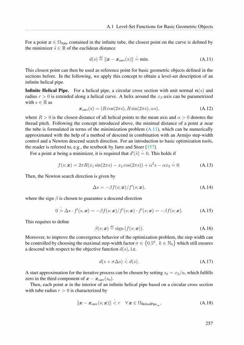
A.1 Level-Set Functions for Basic Geometric Objects

For a point x ∈ ΩTube contained in the infinite tube, the closest point on the curve is defined bythe minimizer s ∈ R of the euclidean distance

d(s)def= ‖x− xcurv(s)‖ !

= min. (A.11)

This closest point can then be used as reference point for basic geometric objects defined in thesections before. In the following, we apply this concept to obtain a level-set description of aninfinite helical pipe.

Infinite Helical Pipe. For a helical pipe, a circular cross section with unit normal n(s) andradius r > 0 is extended along a helical curve. A helix around the x3-axis can be parametrizedwith s ∈ R as

xcurv(s) = (R cos(2πs), R sin(2πs), αs), (A.12)

where R > 0 is the closest distance of all helical points to the mean axis and α > 0 denotes thethread pitch. Following the concept introduced above, the minimal distance of a point x nearthe tube is formulated in terms of the minimization problem (A.11), which can be numericallyapproximated with the help of a method of descend in combination with an Armijo step-widthcontrol and a Newton descend search direction. For an introduction to basic optimization tools,the reader is referred to, e.g., the textbook by Jarre and Stoer [157].

For a point x being a minimizer, it is required that d′(s) != 0. This holds if

f(s;x) = 2πR(x1 sin(2πs)− x2 cos(2πs)) + α2s− αx3!

= 0. (A.13)

Then, the Newton search direction is given by

∆s = −βf(s;x)/f ′(s;x), (A.14)

where the sign β is chosen to guarantee a descend direction

0!> ∆s · f ′(s,x) = −βf(s;x)/f ′(s;x) · f ′(s;x) = −βf(s;x). (A.15)

This requires to defineβ(s;x)

def= sign (f(s;x)). (A.16)

Moreover, to improve the convergence behavior of the optimization problem, the step width canbe controlled by choosing the maximal step-width factor σ ∈

0.5k, k ∈ N0

which still ensures

a descend with respect to the objective function d(s), i.e.

d(s+ σ∆s)!< d(s). (A.17)

A start approximation for the iterative process can be chosen by setting s0 = x3/α, which fulfillszero in the third component of x− xcurv(s0).

Then, each point x in the interior of an infinite helical pipe based on a circular cross sectionwith tube radius r > 0 is characterized by

‖x− xcurv(s;x)‖ !< r ∀x ∈ ΩHelicalPipe∞ , (A.18)

257

A Overview of Level-Set Representations

which then leads to the implicit representation

φHelicalPipe∞(x)def=√

(x1 −R cos(2πs(x)))2 + (x2 −R sin(2πs(x)))2 + (x3 − αs(x))2− r !< 0

(A.19)with s(x) solution to the aforementioned distance optimization problem, which can be approx-imated at all nodes of the underlying computational mesh Th. In Figure A.1a, the level-setapproximation of an infinite helical pipe is shown.

Finite Helical Pipe. Similar to the finite cylinder, also the infinite helical pipe can be cut-offby planes. Considering limitations which yield circular cross sections defined by the helicaltangential vector t(s) = ∂xcurv

∂s(s) in the helical point xcurv(s), limiting halfspaces can be defined

as

φHSpace(x;±∂xcurv(s)

∂s,xcurv(s)). (A.20)

In addition to the cross-section planes, additional limitations in x3-direction are required to cutthe helical pipe not at all turns, but only at two specific heights. An example for an x3-axisoriented helical pipe with a total height of 4 turns, based on a centerline range of x3 ∈ [−2α, 2α],is given by

ΩHelicalPipe = ΩHelicalPipe∞\ (Ωlim,bot ∪ Ωlim,top) , (A.21)

φHelicalPipe = maxφHelicalPipe∞ ,− (min φlim,bot, φlim,top)

. (A.22)

The stairs-like limitations Ωlim,bot and Ωlim,top are defined as

Ωlim,bot = (ΩHSpacex3,1∩ ΩHSpacecross, bot

) ∪ ΩHSpacex3,2, (A.23)

Ωlim,top = (ΩHSpacex3,3∩ ΩHSpacecross, top

) ∪ ΩHSpacex3,4(A.24)

with respective level-set functions

φlim,bot = min

maxφHSpacex3,1

, φHSpacecross, bot

, φHSpacex3,2

, (A.25)

φlim,top = min

maxφHSpacex3,3

, φHSpacecross, top

, φHSpacex3,4

. (A.26)

The bounding halfspaces therein are defined as

φHSpacex3,1(x) = φHSpace(x; (0, 0, 1)T , (R, 0,−2α + 1.1r)T ), (A.27)

φHSpacex3,2(x) = φHSpace(x; (0, 0, 1)T , (R, 0,−2α− 1.1r)T ), (A.28)

φHSpacex3,3(x) = φHSpace(x; (0, 0,−1)T , (R, 0, 2α− 1.1r)T ), (A.29)

φHSpacex3,4(x) = φHSpace(x; (0, 0,−1)T , (R, 0, 2α + 1.1r)T ), (A.30)

φHSpacecross, bot(x) = φHSpace(x;n, (R, 0,−2α)T ), (A.31)

φHSpacecross, top(x) = φHSpace(x;−n, (R, 0, 2α)T ). (A.32)

Hereby, the unit normal vector for the limiting cross section planes is given by

n = 1/√

4π2R2 + α2 · (0, 2πR, α)T (A.33)

and is equal to the tangential vectors along the helix for s = ±2. In Figure A.1b, the finitehelical pipe is exemplarily shown with a thread pitch of α = 0.6, a helix radius R = 0.2 and atube radius r = 0.05 discretized on a domain Ω = [−0.4, 0.4]2 × [−1.5, 1.5] with a regular meshconsisting of tri-linearly-interpolated hexahedral Q1-elements and a mesh size of h = 0.8/75.

258

A.2 Translational and Rotational Mappings

(a) (b)

Figure A.1: Level-set-boundary representation of an infinite and a finite helical pipe with circular cross sectionwithin a background domain Ω = [−0.4, 0.4]2 × [−1.5, 1.5]: (a) Infinite helical pipe ΩHelicalPipe∞ with athread pitch of α = 0.6, a helix radiusR = 0.2 and a tube radius r = 0.05 (colored in green). (b) Finitehelical pipe constructed of an infinite helical pipe ΩHelicalPipe∞ (colored in blue) limited by two stairs-like half spaces Ωlim,bot and Ωlim,top, which are implicitly described by functions φlim,bot (colored in red)and φlim,top (colored in orange) as defined in (A.25) and (A.26). The final pipe domain is defined asΩHelicalPipe = ΩHelicalPipe∞\ (Ωlim,bot ∪ Ωlim,top).

A.2 Translational and Rotational MappingsAll geometric objects ΩObj can be easily transformed by utilizing translational and rotationaltransformations T : R3 → R3, which can be defined as

T :

R3 → R3,

x 7→ RT · (x− c) (A.34)

consisting of a rotational and a translational part. Considering rotations in the reference config-uration, R ∈ R3×3 denotes a orthonormal rotation matrix with column vectors r1, r2, r3 ∈ R3

which are the target vectors of the coordinate unit vectors. Furthermore, c ∈ R3 defines thetarget position of the origin 0 when translating the object. Concatenation of the transformationand the level-set function in the form φObj T yields an implicit representation of the translatedand rotated object.

259

A Overview of Level-Set Representations

Figure A.2: Level-set-boundary representation of a complex composite fluid domain. (Top) Final fluid domainfrom (A.35) composed of different subdomains represented by level-set functions using Booleanset operations. The domain is approximated on an unfitted background mesh covering a cuboid[0.7, 0.1]× [0.5, 0.5]× [1.5, 1.5] consisting of Q1-elements with h = 0.02. (Bottom) Composedsubdomain Ωouter surf from (A.41) consisting of a finite cylinder ΩCyl (colored in blue and gray), aspherical subdomain ΩSphere (colored in yellow), and a plane which limits the bottom side ΩHSpace,bot(colored in green). Next, the domain is expanded by a finite cylinder ΩCyl,Fluid (colored in red), see(A.47).

A.3 Composed Level-Set Representation of Boundaries - AnExample

In the following, an example is given how complex domains can be created by simply combiningbasic geometric objects as introduced in Appendix A.1. With the help of Boolean operations(2.56)-(2.60) and transformations (A.34), subdomains can be composed. In Figure A.2 a visual-ization of the considered final domain is given.

260

A.3 Composed Level-Set Representation of Boundaries - An Example

The overall domain ΩFluid is composed as the intersection of the exterior of a finite spiraland the interior of an outer limiting surface. The latter consists of cylinders, a sphere and severalhalfspaces. In addition, the inflow region is characterized by a hollow cylinder. The final domaincan be composed as follows:

ΩFluid = (((ΩcSpiral ∩ Ωouter surf) ∪ ΩCyl,Fluid)\ΩCyl,hollow) ∩ ΩHSpace,in, (A.35)

φFluid = max max min max −φSpiral, φouter surf, φCyl,Fluid,−φCyl,hollow, φHSpace,in. (A.36)

The interior of a finite spiral can be created with the help of an infinite helical pipe and limitinghalf spaces as

ΩSpiral = ΩHelicalPipe∞ ∩ (Ωlim,back ∩ Ωlim,front) , (A.37)

φSpiral = maxφHelicalPipe∞ ,max φlim,back, φlim,front

, (A.38)

with φHelicalPipe∞ as defined in (A.19) based on a thread pitch of α = 0.6, a helix radius R = 0.2and a tube radius r = 0.05 and

φlim,back(x) = φHSpace(x; 1/√

2(0, 1, 1)T , (0, 0, 1.2)T ), (A.39)

φlim,front(x) = φHSpace(x;−1/√

2(0, 1, 1)T , (0, 0,−0.6)T ). (A.40)

The outer surface is composed of a finite cylinder and a sphere limited in x1- and x3-directionby halfspaces as

Ωouter surf = ((ΩCyl ∪ ΩSphere) ∩ ΩHSpace,bot) ∩ ΩHSpace,out, (A.41)φouter surf = max max min φCyl, φSphere, φHSpace,bot, φHSpace,out (A.42)

with

φCyl(x) = φCyl(T1x;n = (0, 0, 1)T , r = 0.45, h+ = 1.5, h- = 1.0), (A.43)φSphere(x) = φSphere(T1x; r = 0.45), (A.44)

φHSpace,bot(x) = φHSpace(x;n = (1, 0, 0)T ,x0 = (0.05, 0, 0)), (A.45)

φHSpace,out(x) = φHSpace(x;n = (0, 0, 1)T ,x0 = (0, 0, 1.5)), (A.46)

where T1xdef= x+ (0.15, 0, 0)T shifts the cylinder and the sphere along the negative x1-direction.

To construct the hollow-cylindrical inflow region, first, the fluid domain is expanded by acylinder ΩCyl,Fluid given by

φCyl,Fluid(x) = φCyl(T2x;n = (0, 0, 1)T , r = 0.14, h+ = −0.9, h- = 1.5) (A.47)

with a translation T2xdef= x+ (0.2, 0, 0)T . Second, an obstacle ΩCyl,hollow with the shape of a

hollow cylinder is subtracted, which is constructed as

ΩCyl,hollow = ΩCyl\ΩCyl∞ , (A.48)

φCyl,hollow = maxφCyl,−φCyl∞

, (A.49)

261

A Overview of Level-Set Representations

with

φCyl(x) = φCyl(T2x;n = (0, 0, 1)T , r = 0.22, h+ = −0.9, h- = 1.5), (A.50)

φCyl∞(x) = φCyl∞(T2x;n = (0, 0, 1)T , r = 0.14). (A.51)

Third, the fluid domain is limited at the cylindrical inflow region in x3-direction by a halfspace

φHSpace,in(x) = φHSpace(x;n = (0, 0,−1)T ,x0 = (0, 0,−1.49)). (A.52)

Combining all level-set fields as proposed in (A.36) defines the final fluid domain.

262

BIBLIOGRAPHY

[1] F. Alauzet, B. Fabreges, M. A. Fernandez, and M. Landajuela, Nitsche-XFEM for thecoupling of an incompressible fluid with immersed thin-walled structures, ComputerMethods in Applied Mechanics and Engineering 301, 300–335, 2016.

[2] C. Annavarapu, M. Hautefeuille, and J. E. Dolbow, A robust Nitsche’s formulation forinterface problems, Computer Methods in Applied Mechanics and Engineering 225, 44–54, 2012.

[3] D. N. Arnold, R. S. Falk, and R. Winther, Finite element exterior calculus, homologicaltechniques, and applications, Acta numerica 15, 1–155, 2006.

[4] I. Babuska, The finite element method with Lagrangian multipliers, Numerische Mathe-matik 20, 179–192, 1973.

[5] I. Babuska and U. Banerjee, Stable Generalized Finite Element Method (SGFEM),Computer Methods in Applied Mechanics and Engineering 201-204, 91–111, 2012.

[6] I. Babuska and J. M. Melenk, The Partition of Unity Method, International Journal forNumerical Methods in Engineering 40, 727–758, 1997.

[7] S. Badia, F. Nobile, and C. Vergara, Fluid–structure partitioned procedures based onRobin transmission conditions, Journal of Computational Physics 227, 7027–7051, 2008.

[8] S. Badia, A. Quaini, and A. Quarteroni, Splitting methods based on algebraic factorizationfor fluid-structure interaction, SIAM Journal of Scientific Computing 30, 1778–1805,2008.

[9] J. Baiges and R. Codina, The fixed-mesh ALE approach applied to solid mechanicsand fluid-structure interaction problems, International Journal for Numerical Methodsin Engineering 81, 1529–1557, 2009.

[10] J. Baiges, R. Codina, F. Henke, S. Shahmiri, and W. A. Wall, A symmetric methodfor weakly imposing Dirichlet boundary conditions in embedded finite element meshes,International Journal for Numerical Methods in Engineering 90, 636–658, 2012.

[11] R. E. Bank and L. R. Scott, On the Conditioning of Finite Element Equations with HighlyRefined Meshes, SIAM Journal on Numerical Analysis 26, 1383–1394, 1989.

[12] H. J. C. Barbosa and T. J. R. Hughes, The finite element method with Lagrange multiplierson the boundary: circumventing the Babuska-Brezzi condition, Computer Methods inApplied Mechanics and Engineering 85, 109–128, 1991.

263

Bibliography

[13] H. J. C. Barbosa and T. J. R. Hughes, Boundary Lagrange multipliers in finite elementmethods: error analysis in natural norms, Numerische Mathematik 62, 1–15, 1992.

[14] N. Barrau, R. Becker, E. Dubach, and R. Luce, A robust variant of NXFEM for theinterface problem, Comptes Rendus Mathematique 350, 789–792, 2012.

[15] Y. Bazilevs and T. J. R. Hughes, Weak imposition of Dirichlet boundary conditions influid mechanics, Computers and Fluids 36, 12–26, 2007.

[16] Y. Bazilevs, M. Hsu, and M. A. Scott, Isogeometric Fluid–Structure Interaction Analysiswith Emphasis on Non-Matching Discretizations, and with Application to Wind Turbines,Computer Methods in Applied Mechanics and Engineering 252, 28–41, 2012.

[17] Y. Bazilevs, K. Takizawa, and T. E. Tezduyar, Challenges and directions in computationalfluid–structure interaction, Mathematical Models and Methods in Applied Sciences 23,215–221, 2013.

[18] E. Bechet, N. Moes, and B. Wohlmuth, A stable Lagrange multiplier space for stiffinterface conditions within the extended finite element method, International Journal forNumerical Methods in Engineering 78, 931–954, 2009.

[19] R. Becker, P. Hansbo, and R. Stenberg, A finite element method for domain decompositionwith non-matching grids, ESAIM: Mathematical Modelling and Numerical Analysis 37,209–225, 2003.

[20] R. Becker, E. Burman, and P. Hansbo, A Nitsche extended finite element method forincompressible elasticity with discontinuous modulus of elasticity, Computer Methods inApplied Mechanics and Engineering 198, 3352–3360, 2009.

[21] T. Belytschko and T. Black, Elastic crack growth in finite elements with minimalremeshing, International Journal for Numerical Methods in Engineering 45, 601–620,1999.

[22] T. Belytschko and J. M. Kennedy, Computer models for subassembly simulation, NuclearEngineering and Design 49, 17–38, 1978.

[23] T. Belytschko, J. M. Kennedy, and D. F. Schoeberle, Quasi-Eulerian Finite ElementFormulation for Fluid-Structure Interaction, Journal of Pressure Vessel Technology 102,62–69, 1980.

[24] T. Belytschko, N. Moes, S. Usui, and C. Parimi, Arbitrary discontinuities in finiteelements, International Journal for Numerical Methods in Engineering 50, 993–1013,2001.

[25] D. Boffi, M. Fortin, and F. Brezzi, Mixed finite element methods and applications,Springer-Verlag, Berlin-Heidelberg, 2013.

[26] T. Boiveau, Fitted and unfitted domain decomposition using penalty free Nitschemethod for the Poisson problem with discontinuous material parameters, ArXiv e-prints,http://arxiv.org/abs/1509.00542, 2015.

264

Bibliography

[27] T. Boiveau and E. Burman, A penalty-free Nitsche method for the weak impositionof boundary conditions in compressible and incompressible elasticity, IMA Journal ofNumerical Analysis 36, 770–795, 2016.

[28] M. Bol, R. B. Mohle, M. Haesner, T. R. Neu, H. Horn, and R. Krull, 3D finiteelement model of biofilm detachment using real biofilm structures from CLSM data,Biotechnology and Bioengineering 103, 177–186, 2009.

[29] M. Bol, A. E. Ehret, A. Bolea Albero, J. Hellriegel, and R. Krull, Recent advancesin mechanical characterisation of biofilm and their significance for material modelling,Critical Reviews in Biotechnology 33, 145–171, 2013.

[30] R. Bouffanais, M. O. Deville, and E. Leriche, Large-eddy simulation of the flow in alid-driven cubical cavity, Physics of Fluids 19, 055108, 2007.

[31] M. Braack, E. Burman, V. John, and G. Lube, Stabilized finite element methods for thegeneralized Oseen problem, Computer Methods in Applied Mechanics and Engineering196, 853–866, 2007.

[32] J. U. Brackbill, D. B. Kothe, and C. Zemech, A continuum method for modeling surfacetension, Journal of Computational Physics 100, 335–354, 1992.

[33] D. Braess, Finite Elemente: Theorie, schnelle Loser und Anwendungen in der Elastizitats-theorie, Springer-Verlag, Berlin-Heidelberg, 2000.

[34] S. C. Brenner and L. R. Scott, The mathematical theory of finite element methods,Volume 15 of Texts in Applied Mathematics, Springer-Verlag, Berlin-Heidelberg, 3.Edition, 2008.

[35] F. Brezzi, On the Existence, Uniqueness and Approximation of Saddle-Point ProblemsArising from Lagrangian Multipliers, ESAIM: Mathematical Modelling and NumericalAnalysis R–2, 129–151, 1974.

[36] F. Brezzi and M. Fortin, Mixed and hybrid finite element methods, Volume 15 of SpringerSeries in Computational Mathematics, Springer-Verlag, New York, 1991.

[37] F. Brezzi, J. Douglas Jr., and L. D. Marini, Two families of mixed finite elements forsecond order elliptic problems, Numerische Mathematik 47, 217–235, 1985.

[38] E. Burman, A unified analysis for conforming and nonconforming stabilized finiteelement methods using interior penalty, SIAM Journal on Numerical Analysis 43, 2012–2033, 2005.

[39] E. Burman and M. A. Fernandez, Stabilized explicit coupling for fluid–structure interac-tion using Nitsche’s method, Comptes Rendus Mathematique 345, 467–472, 2007.

[40] E. Burman and M. A. Fernandez, Stabilization of explicit coupling in fluid–structureinteraction involving fluid incompressibility, Computer Methods in Applied Mechanicsand Engineering 198, 766–784, 2009.

265

Bibliography

[41] E. Burman and M. A. Fernandez, Continuous interior penalty finite element methodfor the time-dependent Navier–Stokes equations: space discretization and convergence,Numerische Mathematik 107, 39–77, 2007.

[42] E. Burman and P. Hansbo, A unified stabilized method for Stokes’ and Darcy’s equations,Journal of Computational and Applied Mathematics 198, 35–51, 2007.

[43] E. Burman and P. Hansbo, Interior-penalty-stabilized Lagrange multiplier methods for thefinite-element solution of elliptic interface problems, IMA Journal of Numerical Analysis30, 870–885, 2010.

[44] E. Burman and P. Hansbo, Fictitious domain finite element methods using cut elements: I.A stabilized Lagrange multiplier method, Computer Methods in Applied Mechanics andEngineering 199, 2680–2686, 2010.

[45] E. Burman and P. Hansbo, Fictitious domain finite element methods using cut elements:II. A stabilized Nitsche method, Applied Numerical Mathematics 62, 328–341, 2012.

[46] E. Burman and P. Hansbo, Edge stabilization for Galerkin approximations of convection–diffusion–reaction problems, Computer Methods in Applied Mechanics and Engineering193, 1437–1453, 2004.

[47] E. Burman and P. Hansbo, Edge stabilization for the generalized Stokes problem:A continuous interior penalty method, Computer Methods in Applied Mechanics andEngineering 195, 2393–2410, 2006.

[48] E. Burman, M. A. Fernandez, and P. Hansbo, Continuous interior penalty finite elementmethod for Oseen’s equations, SIAM Journal on Numerical Analysis 44, 1248–1274,2006.

[49] E. Burman, Interior penalty variational multiscale method for the incompressibleNavier–Stokes equation: Monitoring artificial dissipation, Computer Methods in AppliedMechanics and Engineering 196, 4045–4058, 2007.

[50] E. Burman, Ghost penalty, Comptes Rendus Mathematique 348, 1217–1220, 2010.

[51] E. Burman, Consistent SUPG-method for transient transport problems: stability andconvergence, Computer Methods in Applied Mechanics and Engineering 199, 1114–1123,2010.

[52] E. Burman, A penalty-free nonsymmetric Nitsche-type method for the weak impositionof boundary conditions, SIAM Journal on Numerical Analysis 50, 1959–1981, 2012.

[53] E. Burman, Projection stabilization of Lagrange multipliers for the imposition ofconstraints on interfaces and boundaries, Numerical Methods for Partial DifferentialEquations 30, 567–592, 2014.

[54] E. Burman and A. Ern, Continuous interior penalty hp-finite element methods foradvection and advection-diffusion equations, Mathematics of Computation 76, 1119–1140, 2007.

266

Bibliography

[55] E. Burman and M. A. Fernandez, Galerkin Finite Element Methods with SymmetricPressure Stabilization for the Transient Stokes Equations: Stability and ConvergenceAnalysis, SIAM Journal on Numerical Analysis 47, 409–439, 2009.

[56] E. Burman and M. A. Fernandez, Finite element methods with symmetric stabilizationfor the transient convection–diffusion–reaction equation, Computer Methods in AppliedMechanics and Engineering 198, 2508–2519, 2009.

[57] E. Burman and M. A. Fernandez, Analysis of the PSPG method for the transient Stokes’problem, Computer Methods in Applied Mechanics and Engineering 200, 2882–2890,2011.

[58] E. Burman and M. A. Fernandez, An unfitted Nitsche method for incompressiblefluid–structure interaction using overlapping meshes, Computer Methods in AppliedMechanics and Engineering 279, 497–514, 2014.

[59] E. Burman and M. A. Fernandez, Explicit strategies for incompressible fluid-structureinteraction problems: Nitsche type mortaring versus Robin-Robin coupling, InternationalJournal for Numerical Methods in Engineering 97, 739–758, 2014.

[60] E. Burman and P. Hansbo, Fictitious domain methods using cut elements: III. A stabilizedNitsche method for Stokes’ problem, ESAIM: Mathematical Modelling and NumericalAnalysis 48, 859–874, 2014.

[61] E. Burman and P. Zunino, A Domain Decomposition Method Based on Weighted InteriorPenalties for Advection-Diffusion-Reaction Problems, SIAM Journal on NumericalAnalysis 44, 1612–1638, 2006.

[62] E. Burman and P. Zunino, Numerical approximation of large contrast problems withthe Unfitted Nitsche method, In J. Blowey and M. Jensen (eds.), Lecture Notes inComputational Science and Engineering, Volume 85 LNCSE, pages 227–282, Springer-Verlag, Berlin-Heidelberg, 2012.

[63] E. Burman, S. Claus, P. Hansbo, M. G. Larson, and A. Massing, CutFEM: Discretizinggeometry and partial differential equations, International Journal for Numerical Methodsin Engineering 104, 472–501, 2015.

[64] E. Burman, S. Claus, and A. Massing, A Stabilized Cut Finite Element Method for theThree Field Stokes Problem, SIAM Journal on Scientific Computing 37, A1705–A1726,2015.

[65] E. Burman, P. Hansbo, and M. G. Larson, A Cut Finite Element Method with BoundaryValue Correction, ArXiv e-prints, http://arxiv.org/abs/1507.03096, 2015.

[66] E. Burman, P. Hansbo, M. G. Larson, and A. Massing, Cut Finite Element Methods forPartial Differential Equations on Embedded Manifolds of Arbitrary Codimensions, ArXive-prints, http://arxiv.org/abs/1610.01660v1, 2016.

267

Bibliography

[67] E. Burman, A. Ern, and M. A. Fernandez, Fractional-step methods and finite elementswith symmetric stabilization for the transient Oseen problem, ESAIM: MathematicalModelling and Numerical Analysis 51, 487–507, 2017.

[68] H. Carlos, L. Kleiser, and R. Friedrich, Subgrid-scale energy transfer in the near-wallregion of turbulent flows, Physics of Fluids 6, 3130–3143, 1994.

[69] P. Causin, J. F. Gerbeau, and F. Nobile, Added-mass effect in the design of partitionedalgorithms for fluid-structure problems, Computer Methods in Applied Mechanics andEngineering 194, 4506–4527, 2005.

[70] S. Chandrasekhar, Hydrodynamic and Hydromagnetic Stability, Dover Publ., New York,1981.

[71] J. Chessa and T. Belytschko, An extended finite element method for two-phase fluids,Journal of Applied Mechanics 70, 10–17, 2003.

[72] J. Chessa, P. Smolinski, and T. Belytschko, The extended finite element method (XFEM)for solidification problems, International Journal for Numerical Methods in Engineering53, 1959–1977, 2002.

[73] A. J. Chorin, Numerical solutions of the Navier-Stokes equations, Mathematics ofComputation 22, 745–762, 1968.

[74] J. Chung and G. M. Hulbert, A Time Integration Algorithm for Structural DynamicsWith Improved Numerical Dissipation: The Generalized-α Method, Journal of AppliedMechanics 60, 371–375, 1993.

[75] R. Codina, Analysis of a stabilized finite element approximation of the Oseen equationsusing orthogonal subscales, Applied Numerical Mathematics 58, 264–283, 2008.

[76] R. Codina, G. Houzeaux, H. Coppola-Owen, and J. Baiges, The fixed-mesh ALEapproach for the numerical approximation of flows in moving domains, Journal ofComputational Physics 228, 1591–1611, 2009.

[77] M. Coroneo, L. Yoshihara, and W. A. Wall, Biofilm growth: A multi-scale and coupledfluid-structure interaction and mass transport approach, Biotechnology and Bioengineer-ing 111, 1385–1395, 2014.

[78] R. Courant, Variational Methods for the Solution of Problems of Equilibrium andVibrations, Bulletin of the American Mathematical Society 49, 1–24, 1943.

[79] S. Court and M. Fournie, A fictitious domain finite element method for simulations offluid-structure interactions: The Navier-Stokes equations coupled with a moving solid,Journal of Fluids and Structures 55, 398–408, 2015.

[80] S. Court, M. Fournie, and A. Lozinski, A fictitious domain approach for the Stokes prob-lem based on the extended finite element method, International Journal for NumericalMethods in Fluids 74, 73–99, 2014.

268

Bibliography

[81] C. D’Angelo and P. Zunino, Numerical approximation with Nitsche’s coupling oftransient Stokes’/Darcy’s flow problems applied to hemodynamics, Applied NumericalMathematics 62, 378–395, 2012.

[82] M. de Berg, O. Cheong, M. van Kreveld, and M. Overmars, Computational Geometry:Algorithms and Applications, Volume 40, Springer-Verlag, Berlin-Heidelberg, 2008.

[83] M. H. de Vaal, M. W. Gee, U. A. Stock, and W. A. Wall, Computational evaluation ofaortic occlusion and the proposal of a novel, improved occluder: Constrained endo-aorticballoon occlusion (CEABO), International Journal for Numerical Methods in BiomedicalEngineering 32, n/a–n/a, 2016.

[84] W. Dettmer and D. Peric, An analysis of the time integration algorithms for the finiteelement solutions of incompressible Navier–Stokes equations based on a stabilisedformulation, Computer Methods in Applied Mechanics and Engineering 192, 1177–1226,2003.

[85] D. A. Di Pietro and A. Ern, Mathematical Aspects of Discontinuous Galerkin Methods,Volume 69 of Mathematiques et Applications, Springer-Verlag, Berlin-Heidelberg, 2012.

[86] P. Diez, R. Cottereau, and S. Zlotnik, A stable extended FEM formulation for multi-phaseproblems enforcing the accuracy of the fluxes through Lagrange multipliers, InternationalJournal for Numerical Methods in Engineering 96, 303–322, 2013.

[87] J. E. Dolbow and I. Harari, An efficient finite element method for embedded interfaceproblems, International Journal for Numerical Methods in Engineering 78, 229–252,2009.

[88] J. E. Dolbow, N. Moes, and T. Belytschko, Discontinuous enrichment in finite elementswith a partition of unity method, Finite Elements in Analysis and Design 36, 235–260,2000.

[89] J. Donea, P. Fasoli–Stella, and S. Giuliani, Lagrangian and Eulerian Finite ElementTechniques for Transient Fluid–Structure Interaction Problems, In Transactions of the4th Int. Conference on SMIRT, San Francisco, 1977.

[90] J. Donea, S. Giuliani, and J. P. Halleux, An arbitrary Lagrangian-Eulerian finite elementmethod for transient dynamic fluid-structure interactions, Computer Methods in AppliedMechanics and Engineering 33, 689–723, 1982.

[91] J. Donea and A. Huerta, Finite Element Methods for Flow Problems, John Wiley & Sons,Ltd, Chichester, 2003.

[92] R. M. Donlan, Biofilms and device-associated infections, In Emerging Infectious Dis-eases, pages 277–281, 7th Edition, 2001.

[93] J. Douglas and T. Dupont, Interior Penalty Procedures for Elliptic and Parabolic GalerkinMethods, In R. Glowinski and J. Lions (eds.), Computing Methods in Applied Sciences,Lecture Notes in Physics, pages 207–216, Springer-Verlag, Berlin-Heidelberg, 1976.

269

Bibliography

[94] C. Duarte, I. Babuska, and J. Oden, Generalized finite element methods for three-dimensional structural mechanics problems, Computers & Structures 77, 215–232, 2000.

[95] R. Duddu, S. Bordas, D. Chopp, and B. Moran, A combined extended finite elementand level set method for biofilm growth, International Journal for Numerical Methods inEngineering 74, 848–870, 2008.

[96] R. Duddu, D. L. Chopp, and B. Moran, A two-dimensional continuum model of biofilmgrowth incorporating fluid flow and shear stress based detachment, Biotechnology andBioengineering 103, 92–104, 2009.

[97] C. D’Angelo and A. Scotti, A mixed finite element method for Darcy flow in fracturedporous media with non-matching grids, ESAIM: Mathematical Modelling and NumericalAnalysis 46, 465–489, 2012.

[98] A. Ehrl, A. Popp, V. Gravemeier, and W. Wall, A dual mortar approach for mesh tyingwithin a variational multiscale method for incompressible flow, International Journal forNumerical Methods in Fluids 76, 1–27, 2014.

[99] A. Embar, J. E. Dolbow, and I. Harari, Imposing Dirichlet boundary conditions withNitsche’s method and spline-based finite elements, International Journal for NumericalMethods in Engineering 83, 877–898, 2010.

[100] S. Erlicher, L. Bonaventura, and O. S. Bursi, The analysis of the Generalized-α methodfor non-linear dynamic problems, Computational Mechanics 28, 83–104, 2002.

[101] A. Ern and J. L. Guermond, Theory and Practice of Finite Elements, Volume 159 ofApplied Mathematical Sciences, Springer-Verlag, New York, 2004.

[102] A. Ern and J. L. Guermond, Weighting the Edge Stabilization, SIAM Journal onNumerical Analysis 51, 1655–1677, 2013.

[103] C. R. Ethier and D. A. Steinman, Exact fully 3D Navier–Stokes solutions for benchmark-ing, International Journal for Numerical Methods in Fluids 19, 369–375, 1994.

[104] C. Farhat and V. K. Lakshminarayan, An ALE formulation of embedded boundarymethods for tracking boundary layers in turbulent fluid-structure interaction problems,Journal of Computational Physics 263, 53–70, 2014.

[105] M. A. Fernandez, Coupling schemes for incompressible fluid-structure interaction:implicit, semi-implicit and explicit, SeMa Journal 55, 59–108, 2011.

[106] M. A. Fernandez, M. Landajuela, and M. Vidrascu, Fully decoupled time-marchingschemes for incompressible fluid/thin-walled structure interaction, Journal of Computa-tional Physics 297, 156–181, 2015.

[107] M. A. Fernandez and M. Moubachir, A Newton method using exact jacobians for solvingfluid–structure coupling, Computers & Structures 83, 127–142, 2005.

270

Bibliography

[108] M. A. Fernandez, J. Mullaert, and M. Vidrascu, Generalized Robin-Neumann explicitcoupling schemes for incompressible fluid-structure interaction: stability analysis andnumerics, International Journal for Numerical Methods in Engineering 101, 199–229,2015.

[109] S. Fernandez-Mendez and A. Huerta, Imposing essential boundary conditions in mesh-free methods, Computer Methods in Applied Mechanics and Engineering 193, 1257–1275, 2004.

[110] C. Forster, Robust methods for fluid-structure interaction with stabilised finite elements,Phd thesis, Universitat Stuttgart, 2007.

[111] C. Forster, W. A. Wall, and E. Ramm, Artificial added mass instabilities in sequentialstaggered coupling of nonlinear structures and incompressible viscous flows, ComputerMethods in Applied Mechanics and Engineering 196, 1278–1293, 2007.

[112] L. P. Franca and S. L. Frey, Stabilized finite element methods: II. The incompressibleNavier-Stokes equations, Computer Methods in Applied Mechanics and Engineering 99,209–233, 1992.

[113] S. Frei and T. Richter, A second order time-stepping scheme for parabolic interfaceproblems with moving interfaces, ESAIM: Mathematical Modelling and NumericalAnalysis, doi: 10.1051/m2an/2016072, 2016.

[114] T. P. Fries, Overview and comparison of different variants of the XFEM, PAMM 14, 27–30, 2014.

[115] T. P. Fries and T. Belytschko, The extended/generalized finite element method: Anoverview of the method and its applications, International Journal for Numerical Methodsin Engineering 84, 253–304, 2010.

[116] T. P. Fries and S. Omerovic, Higher-order accurate integration of implicit geometries,International Journal for Numerical Methods in Engineering 106, 323–371, 2016.

[117] T. P. Fries and A. Zilian, On time integration in the XFEM, International Journal forNumerical Methods in Engineering 79, 69–93, 2009.

[118] A. Fumagalli and A. Scotti, Numerical modelling of multiphase subsurface flow in thepresence of fractures, Communications in Applied and Industrial Mathematics 3, doi:10.1685/journal.caim.380, 2011.

[119] P. Gamnitzer, Residual-based variational multiscale methods for turbulent flows, Phdthesis, Institute for Computational Mechanics, Technical University of Munich, 2010.

[120] P. Gamnitzer and W. A. Wall, An ALE-Chimera method for large deformation fluid-structure interaction, In Proceedings of the European Conference on Computational FluidDynamics, ECCOMAS CFD, The Netherlands, TU Delft, pages 1–14, 2006.

271

Bibliography

[121] M. W. Gee, U. Kuttler, and W. A. Wall, Truly monolithic algebraic multigrid for fluid-structure interaction, International Journal for Numerical Methods in Engineering 85,987–1016, 2011.

[122] M. Germano, On the effect of torsion on a helical pipe flow, Journal of Fluid Mechanics125, 1–8, 1982.

[123] A. Gerstenberger, An XFEM based fixed-grid approach to fluid-structure interaction, Phdthesis, Institute for Computational Mechanics, Technical University of Munich, 2010.

[124] A. Gerstenberger and W. A. Wall, An eXtended Finite Element Method/Lagrangemultiplier based approach for fluid-structure interaction, Computer Methods in AppliedMechanics and Engineering 197, 1699–1714, 2008.

[125] A. Gerstenberger and W. A. Wall, An embedded Dirichlet formulation for 3D continua,International Journal for Numerical Methods in Engineering 82, 537–563, 2010.

[126] V. Girault, B. Riviere, and M. F. Wheeler, A discontinuous Galerkin method withnonoverlapping domain decomposition for the Stokes and Navier-Stokes problems,Mathematics of Computation 74, 53–84, 2005.

[127] V. Girault and P. A. Raviart, Finite Element Methods for Navier-Stokes Equations,Volume 5 of Springer Series in Computational Mathematics, Springer-Verlag, Berlin-Heidelberg, 1986.

[128] M. T. Goodrich and R. Tamassia, Algorithm Design: Foundations, Analysis, and InternetExamples, John Wiley & Sons, Inc., Chichester, 2002.

[129] V. Gravemeier and W. A. Wall, Variational multiscale methods for premixed combustionbased on a progress-variable approach, Combustion and Flame 158, 1160–1170, 2011.

[130] V. Gravemeier, M. W. Gee, M. Kronbichler, and W. A. Wall, An algebraic variationalmultiscale-multigrid method for large eddy simulation of turbulent flow, ComputerMethods in Applied Mechanics and Engineering 199, 853–864, 2010.

[131] P. M. Gresho and R. L. Sani, Incompressible Flow and the Finite Element Method, JohnWiley & Sons, Chichester, 2000.

[132] M. Griebel and M. A. Schweitzer, A Particle-Partition of Unity Method Part V: BoundaryConditions, In Geometric Analysis and Nonlinear Partial Differential Equations, pages519–542, Springer-Verlag, Berlin-Heidelberg, 2003.

[133] S. Groß and A. Reusken, Numerical Methods for Two-phase Incompressible Flows,Springer Series in Computational Mathematics, Volume 40, Springer-Verlag, Berlin-Heidelberg, 2011.

[134] S. Groß and A. Reusken, An extended pressure finite element space for two-phaseincompressible flows with surface tension, Journal of Computational Physics 224, 40–58, 2007.

272

Bibliography

[135] S. Groß and A. Reusken, Finite element discretization error analysis of a surface tensionforce in two-phase incompressible flows, SIAM Journal on Numerical Analysis 45, 1679–1700, 2007.

[136] S. Groß, V. Reichelt, and A. Reusken, A finite element based level set method for two-phase incompressible flows, Computing and Visualization in Science 9, 239–257, 2006.

[137] M. E. Gurtin, An Introduction to Continuum Mechanics, Volume 158 of Mathematics inScience and Engineering, Elsevier, New York, 1981.

[138] A. Hansbo and P. Hansbo, An unfitted finite element method, based on Nitsche’s method,for elliptic interface problems, Computer Methods in Applied Mechanics and Engineering191, 5537–5552, 2002.

[139] A. Hansbo, P. Hansbo, and M. G. Larson, A finite element method on composite gridsbased on Nitsche’s method, ESAIM: Mathematical Modelling and Numerical Analysis37, 495–514, 2003.

[140] P. Hansbo, Nitsche’s method for interface problems in computational mechanics, GAMM-Mitteilungen 28, 183–206, 2005.

[141] P. Hansbo, M. G. Larson, and S. Zahedi, A cut finite element method for a Stokes interfaceproblem, Applied Numerical Mathematics 85, 90–114, 2014.

[142] P. Hansbo, M. G. Larson, and S. Zahedi, Characteristic cut finite element methods forconvection–diffusion problems on time dependent surfaces, Computer Methods in AppliedMechanics and Engineering 293, 431–461, 2015.

[143] P. Hansbo, M. G. Larson, and S. Zahedi, A cut finite element method for coupled bulk-surface problems on time-dependent domains, Computer Methods in Applied Mechanicsand Engineering 307, 96–116, 2016.

[144] I. Harari and J. Dolbow, Analysis of an efficient finite element method for embeddedinterface problems, Computational Mechanics 46, 205–211, 2010.

[145] D. Hartmann, M. Meinke, and W. Schroder, A level-set based adaptive-grid method forpremixed combustion, Combustion and Flame 158, 1318–1339, 2011.

[146] M. Hautefeuille, C. Annavarapu, and J. E. Dolbow, Robust imposition of Dirichletboundary conditions on embedded surfaces, International Journal for Numerical Methodsin Engineering 90, 40–64, 2012.

[147] F. Henke, An extended finite element method for turbulent premixed combustion, Phdthesis, Institute for Computational Mechanics, Technical University of Munich, 2012.

[148] F. Henke, M. Winklmaier, V. Gravemeier, and W. A. Wall, A semi-Lagrangean time-integration approach for extended finite element methods, International Journal forNumerical Methods in Engineering 98, 174–202, 2014.

273

Bibliography

[149] M. A. Heroux, E. T. Phipps, A. G. Salinger, H. K. Thornquist, R. S. Tuminaro, J. M.Willenbring, A. Williams, K. S. Stanley, R. A. Bartlett, V. E. Howle, R. J. Hoekstra, J. J.Hu, T. G. Kolda, R. B. Lehoucq, K. R. Long, and R. P. Pawlowski, An overview of theTrilinos project, ACM Transactions on Mathematical Software 31, 397–423, 2005.

[150] C. W. Hirt, A. A. Amsden, and J. L. Cook, An arbitrary Lagrangian-Eulerian computingmethod for all flow speeds, Journal of Computational Physics 14, 227–253, 1974.

[151] C. W. Hirt and B. D. Nichols, Volume of fluid (VOF) method for the dynamics of freeboundaries, Journal of Computational Physics 39, 201–225, 1981.

[152] G. A. Holzapfel, Nonlinear Solid Mechanics: A Continuum Approach for Engineering,John Wiley & Sons, Chichester, 2000.

[153] T. Horger, J. M. Melenk, and B. Wohlmuth, On optimal L2 and surface flux convergencein FEM, Computing and Visualization in Science 16, 231–246, 2013.

[154] G. Houzeaux and R. Codina, A Chimera method based on a Dirichlet/Neumann(Robin)coupling for the Navier-Stokes equations, Computer Methods in Applied Mechanics andEngineering 192, 3343–3377, 2003.

[155] T. J. R. Hughes, W. K. Liu, and T. K. Zimmermann, Lagrangian-Eulerian finite elementformulation for incompressible viscous flows, Computer Methods in Applied Mechanicsand Engineering 29, 329–349, 1981.

[156] T. J. R. Hughes, G. Scovazzi, and L. P. Franca, Multiscale and Stabilized Methods, InEncyclopedia of Computational Mechanics, John Wiley & Sons, Chichester, 2007.

[157] F. Jarre and J. Stoer, Optimierung, Springer-Verlag, Berlin-Heidelberg, 2004.

[158] H. Ji and J. E. Dolbow, On strategies for enforcing interfacial constraints and evaluatingjump conditions with the extended finite element method, International Journal forNumerical Methods in Engineering 61, 2508–2535, 2004.

[159] H. Ji, D. Chopp, and J. E. Dolbow, A hybrid extended finite element/level set methodfor modeling phase transformations, International Journal for Numerical Methods inEngineering 54, 1209–1233, 2002.

[160] A. Johansson and M. G. Larson, A high order discontinuous Galerkin Nitsche method forelliptic problems with fictitious boundary, Numerische Mathematik 123, 607–628, 2013.

[161] M. Juntunen and R. Stenberg, Nitsche’s method for general boundary conditions,Mathematics of Computation 78, 1353–1374, 2009.

[162] J. Kim and P. Moin, Application of a Fractional-Step Method to Incompressible Navier-Stokes Equations, Journal of Computational Physics 59, 308–323, 1985.

[163] T. Kloppel, A Finite Element Model for the Human Red Blood Cell, Phd thesis, Institutefor Computational Mechanics, Technical University of Munich, 2012.

274

Bibliography

[164] T. Kloppel, A. Popp, U. Kuttler, and W. A. Wall, Fluid–structure interaction for non-conforming interfaces based on a dual mortar formulation, Computer Methods in AppliedMechanics and Engineering 200, 3111–3126, 2011.

[165] P. Knobloch and L. Tobiska, Improved stability and error analysis for a class of localprojection stabilizations applied to the Oseen problem, Numerical Methods for PartialDifferential Equations 29, 206–225, 2013.

[166] B. Krank and W. A. Wall, A new approach to wall modeling in LES of incompressibleflow via function enrichment, Journal of Computational Physics 316, 94–116, 2016.

[167] R. Kruse, Enforcing coupling conditions on embedded interfaces using stress-basedLagrange multipliers in the XFEM for incompressible flow, Master’s thesis, TechnicalUniversity of Munich, 2013.

[168] U. Kuttler, Effiziente Losungsverfahren fur Fluid-Struktur-Interaktions-Probleme, Phdthesis, Institute for Computational Mechanics, Technical University of Munich, 2009.

[169] U. Kuttler, M. Gee, C. Forster, A. Comerford, and W. A. Wall, Coupling strategiesfor biomedical fluid-structure interaction problems, International Journal for NumericalMethods in Biomedical Engineering 26, 305–321, 2010.

[170] U. Kuttler and W. A. Wall, Fixed-point fluid-structure interaction solvers with dynamicrelaxation, Computational Mechanics 43, 61–72, 2008.

[171] P. Le Tallec and J. Mouro, Fluid-structure interaction with large structural displacements,Computer Methods in Applied Mechanics and Engineering 190, 3039–3067, 2001.

[172] A. Legay, J. Chessa, and T. Belytschko, An Eulerian–Lagrangian method forfluid–structure interaction based on level sets, Computer Methods in Applied Mechanicsand Engineering 195, 2070–2087, 2006.

[173] A. Legay, A. Zilian, and C. Janssen, A rheological interface model and its space-time finiteelement formulation for fluid-structure interaction, International Journal for NumericalMethods in Engineering 86, 667–687, 2011.

[174] C. Lehrenfeld, The Nitsche XFEM-DG Space-Time Method and its Implementation inThree Space Dimensions, SIAM Journal on Scientific Computing 37, A245–A270, 2015.

[175] C. Lehrenfeld, High order unfitted finite element methods on level set domains usingisoparametric mappings, Computer Methods in Applied Mechanics and Engineering 300,716–733, 2016.

[176] E. Leriche and S. Gavrilakis, Direct numerical simulation of the flow in a lid-drivencubical cavity, Physics of Fluids 12, 1363–1376, 2000.

[177] J. H. Leung, A. R. Wright, N. Cheshire, J. Crane, S. A. Thom, A. D. Hughes, and Y. Xu,Fluid structure interaction of patient specific abdominal aortic aneurysms: a comparisonwith solid stress models, BioMedical Engineering OnLine 5, 1–15, 2006.

275

Bibliography

[178] E. Marchandise and J. F. Remacle, A stabilized finite element method using a dis-continuous level set approach for solving two phase incompressible flows, Journal ofComputational Physics 219, 780–800, 2006.

[179] A. Massing, M. G. Larson, and A. Logg, Efficient implementation of finite elementmethods on non-matching and overlapping meshes in 3D, SIAM Journal of ScientificComputing 35, C23–C47, 2013.

[180] A. Massing, M. G. Larson, A. Logg, and M. E. Rognes, A stabilized Nitsche overlappingmesh method for the Stokes problem, Numerische Mathematik 128, 73–101, 2014.

[181] A. Massing, M. G. Larson, A. Logg, and M. E. Rognes, A Stabilized Nitsche FictitiousDomain Method for the Stokes Problem, Journal of Scientific Computing 61, 1–28, 2014.

[182] A. Massing, M. G. Larson, A. Logg, and M. E. Rognes, A Nitsche-based cut finiteelement method for a fluid-structure interaction problem, Communications in AppliedMathematics and Computational Science 10, 97–120, 2015.

[183] A. Massing, B. Schott, and W. A. Wall, A stabilized Nitsche cut finite element methodfor the Oseen problem, Computer Methods in Applied Mechanics and Engineering, ArXive-prints http://arxiv.org/abs/1611.02895v2, submitted, 2017.

[184] U. M. Mayer, A. Popp, A. Gerstenberger, and W. A. Wall, 3D fluid-structure-contact inter-action based on a combined XFEM FSI and dual mortar contact approach, ComputationalMechanics 46, 53–67, 2010.

[185] M. Mayr, T. Kloppel, W. A. Wall, and M. W. Gee, A Temporal Consistent MonolithicApproach to Fluid-Structure Interaction Enabling Single Field Predictors, SIAM Journalon Scientific Computing 37, B30–B59, 2015.

[186] J. Melenk and I. Babuska, The partition of unity finite element method: Basic theory andapplications, Computer Methods in Applied Mechanics and Engineering 139, 289–314,1996.

[187] R. Mittal and G. Iaccarino, Immersed Boundary Methods, Annual Review of FluidMechanics 37, 239–261, 2005.

[188] N. Moes, J. E. Dolbow, and T. Belytschko, A finite element method for crack growthwithout remeshing, International Journal for Numerical Methods in Engineering 46, 131–150, 1999.

[189] N. Moes, E. Bechet, and M. Tourbier, Imposing Dirichlet boundary conditions inthe extended finite element method, International Journal for Numerical Methods inEngineering 67, 1641–1669, 2006.

[190] S. E. Mousavi and N. Sukumar, Generalized Gaussian quadrature rules for discontinuitiesand crack singularities in the extended finite element method, Computer Methods inApplied Mechanics and Engineering 199, 3237–3249, 2010.

276

Bibliography

[191] S. E. Mousavi, H. Xiao, and N. Sukumar, Generalized Gaussian quadrature rules onarbitrary polygons, International Journal for Numerical Methods in Engineering 82, 99–113, 2010.

[192] C. J. Mueller, J. F. Driscoll, D. L. Reuss, M. C. Drake, and M. E. Rosalik, Vorticitygeneration and attenuation as vortices convect through a premixed flame, Combustionand Flame 112, 342–358, 1998.

[193] B. Muller, F. Kummer, and M. Oberlack, Highly accurate surface and volume integrationon implicit domains by means of moment-fitting, International Journal for NumericalMethods in Engineering 96, 512–528, 2013.

[194] S. Nagrath, K. E. Jansen, and R. T. Lahey, Computation of incompressible bubbledynamics with a stabilized finite element level set method, Computer Methods in AppliedMechanics and Engineering 194, 4565–4587, 2005.

[195] J. Nedelec, Mixed finite elements in R3, Numerische Mathematik 35, 315–341, 1980.

[196] J. Nitsche, Uber ein Variationsprinzip zur Losung von Dirichlet-Problemen bei Verwen-dung von Teilraumen, die keinen Randbedingungen unterworfen sind, Abhandlungen ausdem Mathematischen Seminar der Universitat Hamburg 36, 9–15, 1971.

[197] W. Noh and P. Woodward, SLIC (Simple Line Interface Calculation), In Lecture Notesin Physics, Proceedings of the Fifth International Conference on Numerical Methods forFluid Dynamics, Volume 59, pages 330–340, 1976.

[198] R. R. Nourgaliev, M. S. Liou, and T. G. Theofanous, Numerical prediction of interfacialinstabilities: Sharp interface method (SIM), Journal of Computational Physics 227, 3940–3970, 2008.

[199] J. T. Oden and L. Demkowicz, Advances in Adaptive Improvements: A Survey ofAdaptive Finite Element Methods in Computational Mechanics, In State of the Art Surveysin Computational Mechanics, American Society of Mechanical Engineers (ASME), NewYork, 1986.

[200] J. T. Oden, I. Babuska, and C. E. Baumann, A Discontinuous hp Finite Element Methodfor Diffusion Problems, Journal of Computational Physics 146, 491–519, 1998.

[201] C. S. Peskin, Flow patterns around heart valves: A numerical method, Journal ofComputational Physics 10, 252–271, 1972.

[202] C. S. Peskin, Numerical analysis of blood flow in the heart, Journal of ComputationalPhysics 25, 220–252, 1977.

[203] C. S. Peskin, The immersed boundary method, Acta Numerica 11, 479–517, 2002.

[204] C. Picioreanu, M. van Loosdrecht, and J. Heinen, Discrete-differential modelling ofbiofilm structure, Water Science and Technology 39, 115–122, 1999.

277

Bibliography

[205] J. Pitkaranta, Boundary subspaces for the finite element method with Lagrange multipli-ers, Numerische Mathematik 289, 273–289, 1979.

[206] J. Pitkaranta, Local stability conditions for the Babuska method of Lagrange multipliers,Mathematics of Computation 35, 1113–1129, 1980.

[207] F. Pochet, K. Hillewaert, P. Geuzaine, J. F. Remacle, and E. Marchandise, A 3D stronglycoupled implicit discontinuous Galerkin level set-based method for modeling two-phaseflows, Computers and Fluids 87, 144–155, 2013.

[208] S. Popinet and S. Zaleski, A front-tracking algorithm for accurate representation ofsurface tension, International Journal for Numerical Methods in Fluids 30, 775–793,1999.

[209] A. Popp, Mortar Methods for Computational Contact Mechanics and General InterfaceProblems, Phd thesis, Institute for Computational Mechanics, Technical University ofMunich, 2012.

[210] A. K. Prasad and J. R. Koseff, Reynolds number and end-wall effects on a lid-drivencavity flow, Physics of Fluids A: Fluid Dynamics 1, 208–218, 1989.

[211] A. Prokopenko, J. J. Hu, T. A. Wiesner, C. M. Siefert, and R. S. Tuminaro, MueLu User’sGuide 1.0, Technical report, Sandia National Labs, SAND2014-18874, 2014.

[212] E. G. Puckett, A. S. Almgren, J. B. Bell, D. L. Marcus, and W. J. Rider, A High-Order Projection Method for Tracking Fluid Interfaces in Variable Density IncompressibleFlows, Journal of Computational Physics 130, 269–282, 1997.

[213] S. Rand and C. E. Pearson, A computational method for viscous flow problems, Journalof Fluid Mechanics 21, 611–622, 1966.

[214] U. Rasthofer, F. Henke, W. A. Wall, and V. Gravemeier, An extended residual-basedvariational multiscale method for two-phase flow including surface tension, ComputerMethods in Applied Mechanics and Engineering 200, 1866–1876, 2011.

[215] U. Rasthofer, Computational Multiscale Methods for Turbulent Single and Two-PhaseFlows, Phd thesis, Institute for Computational Mechanics, Technical University ofMunich, 2015.

[216] P. A. Raviart and J. M. Thomas, A mixed finite element method for 2nd order ellipticproblems, In Mathematical Aspects of the Finite Element Method, Lecture Notes inMathematics 606, Springer-Verlag, Berlin-Heidelberg, 1977.

[217] W. H. Reed and T. R. Hill, Triangluar mesh methods for the neutron transport equation,Technical report, Los Alamos Scientific Lab, New Mexico (USA), 1973.

[218] A. Reusken, Analysis of an extended pressure finite element space for two-phaseincompressible flows, Computing and Visualization in Science 11, 293–305, 2008.

278

Bibliography

[219] T. Richter, A Fully Eulerian formulation for fluid–structure-interaction problems, Journalof Computational Physics 233, 227–240, 2013.

[220] B. Riviere, M. F. Wheeler, and V. Girault, A Priori Error Estimates for Finite ElementMethods Based on Discontinuous Approximation Spaces for Elliptic Problems, SIAMJournal on Numerical Analysis 39, 902–931, 2001.

[221] W. L. Roberts and J. F. Driscoll, A laminar vortex interacting with a premixed flame:Measured formation of pockets of reactants, Combustion and Flame 87, 245–256, 1991.

[222] H. G. Roos, M. Stynes, and L. Tobiska, Robust Numerical Methods for SingularlyPerturbed Differential Equations, Volume 24 of Springer Series in ComputationalMathematics, Springer, Berlin-Heidelberg, 2008.

[223] E. Rothe, Zweidimensionale parabolische Randwertaufgaben als Grenzfall eindimension-aler Randwertaufgaben, Mathematische Annalen 102, 650–670, 1930.

[224] M. Sala and M. Heroux, Robust Algebraic Preconditioners with IFPACK 3.0, Technicalreport, Sandia National Laboratories, SAND-0662, 2005.

[225] H. Sauerland and T. P. Fries, The extended finite element method for two-phase and free-surface flows: A systematic study, Journal of Computational Physics 230, 3369–3390,2011.

[226] H. Sauerland and T. P. Fries, The stable XFEM for two-phase flows, Computers and Fluids87, 41–49, 2013.

[227] M. Schafer and S. Turek, Benchmark Computations of Laminar Flow Around a Cylinder,Flow Simulation with High-Performance Computers II, Volume 52 of Notes on NumericalFluid Mechanics, Vieweg 52, 547–566, 1996.

[228] P. J. Schneider and D. H. Eberly, Geometric Tools for Computer Graphics, ElsevierScience (USA), 2003.

[229] B. Schott, Enforcing interface conditions with Nitsche’s method in the XFEM, Diplomathesis, Institute for Computational Mechanics, Technical University of Munich, 2010.

[230] B. Schott and W. A. Wall, A new face-oriented stabilized XFEM approach for 2D and 3Dincompressible Navier-Stokes equations, Computer Methods in Applied Mechanics andEngineering 276, 233–265, 2014.

[231] B. Schott, U. Rasthofer, V. Gravemeier, and W. A. Wall, A face-oriented stabilizedNitsche-type extended variational multiscale method for incompressible two-phase flow,International Journal for Numerical Methods in Engineering 104, 721–748, 2015.

[232] B. Schott, S. Shahmiri, R. Kruse, and W. A. Wall, A stabilized Nitsche-type extendedembedding mesh approach for 3D low- and high-Reynolds-number flows, InternationalJournal for Numerical Methods in Fluids 82, 289–315, 2016.

279

Bibliography

[233] J. A. Sethian, Curvature and the evolution of fronts, Communications in MathematicalPhysics 101, 487–499, 1985.

[234] J. Sethian, Level Set Methods and Fast Marching Methods: Evolving interfaces in com-putational geometry, fluid mechanics, computer vision, and material science, CambridgeUniversity Press, New York, 1999.

[235] S. Shahmiri, A Hybrid Fixed-Grid-ALE Approach for Fluid-Structure Interaction, Phdthesis, Institute for Computational Mechanics, Technical University of Munich, 2014.

[236] S. Shahmiri, A. Gerstenberger, and W. A. Wall, An XFEM-based embedding meshtechnique for incompressible viscous flows, International Journal for Numerical Methodsin Fluids 65, 166–190, 2011.

[237] P. Shankar and M. Deshpande, Fluid mechanics in the driven cavity, Annual Review ofFluid Mechanics 32, 93–136, 2000.

[238] M. Shirtliff and J. G. Leid (eds.), The Role of Biofilms in Device-Related Infections,Volume 3 of Springer Series on Biofilms, Springer-Verlag, Berlin-Heidelberg, 2009.

[239] J. L. Steger, F. C. Dougherty, and J. A. Benek, A chimera grid scheme, Advances in GridGeneration ASME FED5 5, 59–69, 1983.

[240] E. Stein, Singular Integrals and Differentiability Properties of Functions, PrincetonUniversity Press, Princeton, 1970.

[241] R. Stenberg, On some techniques for approximating boundary conditions in the finiteelement method, Journal of Computational and Applied Mathematics 63, 139–148, 1995.

[242] P. Stoodley, Z. Lewandowski, J. D. Boyle, and H. M. Lappin-Scott, Oscillation character-istics of biofilm streamers in turbulent flowing water as related to drag and pressure drop,Biotechnology and Bioengineering 57, 536–544, 1998.

[243] T. Strouboulis, K. Copps, and I. Babuska, The generalized finite element method: anexample of its implementation and illustration of its performance, International Journalfor Numerical Methods in Engineering 47, 1401–1417, 2000.

[244] Y. Sudhakar, An embedded interface finite element method for fluid-structure-fractureinteraction, Phd thesis, Institute for Computational Mechanics, Technical University ofMunich, 2015.

[245] Y. Sudhakar and W. A. Wall, Quadrature schemes for arbitrary convex/concave volumesand integration of weak form in enriched partition of unity methods, Computer Methodsin Applied Mechanics and Engineering 258, 39–54, 2013.

[246] Y. Sudhakar, J. Moitinho de Almeida, and W. A. Wall, An accurate, robust, and easy-to-implement method for integration over arbitrary polyhedra: Application to embeddedinterface methods, Journal of Computational Physics 273, 393–415, 2014.

280

Bibliography

[247] N. Sukumar, N. Moes, B. Moran, and T. Belytschko, Extended finite element methodfor three-dimensional crack modelling, International Journal for Numerical Methods inEngineering 48, 1549–1570, 2000.

[248] M. Sussman, P. Smereka, and S. Osher, A level set approach for computing solutions toincompressible two-phase flow, Journal of Computational Physics 114, 146–159, 1994.

[249] D. Taherzadeh, C. Picioreanu, U. Kuttler, A. Simone, W. A. Wall, and H. Horn,Computational study of the drag and oscillatory movement of biofilm streamers in fastflows, Biotechnology and Bioengineering 105, 600–610, 2010.

[250] D. Taherzadeh, C. Picioreanu, and H. Horn, Mass Transfer Enhancement in MovingBiofilm Structures, Biophysical Journal 102, 1483–1492, 2012.

[251] F. Tanios, M. Gee, J. Pelisek, S. Kehl, J. Biehler, V. Grabher-Meier, W. A. Wall,H.-H. Eckstein, and C. Reeps, Interaction of Biomechanics with Extracellular MatrixComponents in Abdominal Aortic Aneurysm Wall, European Journal of Vascular andEndovascular Surgery 50, 167–174, 2015.

[252] C. A. Taylor, T. J. R. Hughes, and C. K. Zarins, Finite element modeling of blood flow inarteries, Computer Methods in Applied Mechanics and Engineering 158, 155–196, 1998.

[253] T. E. Tezduyar, S. Sathe, R. Keedy, and K. Stein, Space–time finite element techniquesfor computation of fluid–structure interactions, Computer Methods in Applied Mechanicsand Engineering 195, 2002–2027, 2006.

[254] C. Truesdell and W. Noll, The Non-Linear Field Theories of Mechanics, Springer-Verlag,Berlin-Heidelberg, 2004.

[255] F. van der Bos and V. Gravemeier, Numerical simulation of premixed combustion usingan enriched finite element method, Journal of Computational Physics 228, 3605–3624,2009.

[256] F. Verdugo and W. A. Wall, Unified framework for the efficient solution of n-fieldcoupled problems with monolithic schemes, Computer Methods in Applied Mechanicsand Engineering 310, 335–366, 2016.

[257] W. A. Wall and E. Ramm, Fluid–Structure Interaction Based upon a Stabilized (ALE)Finite Element Method, Computational Mechanics – New Trends and Applications,In S. R. Idelsohn, E. Onate, and E. N. Dvorkin (eds.), Proc. 4th World Congress onComputational Mechanics, Buenos Aires, 1998, CIMNE, Barcelona.

[258] W. A. Wall, Fluid-Struktur-Interaktion mit stabilisierten Finiten Elementen, Dissertation,Universitat Stuttgart, 1999.

[259] W. A. Wall, A. Gerstenberger, P. Gamnitzer, C. Forster, and E. Ramm, Large deformationfluid-structure interaction–advances in ALE methods and new fixed grid approaches, InFluid-structure interaction, pages 195–232, Springer-Verlag, Berlin-Heidelberg, 2006.

281

Bibliography

[260] W. A. Wall, P. Gamnitzer, and A. Gerstenberger, Fluid–structure interaction approacheson fixed grids based on two different domain decomposition ideas, International Journalof Computational Fluid Dynamics 22, 411–427, 2008.

[261] W. A. Wall, L. Wiechert, A. Comerford, and S. Rausch, Towards a comprehensivecomputational model for the respiratory system, International Journal for NumericalMethods in Biomedical Engineering 26, 807–827, 2010.

[262] W. A. Wall, C. Ager, M. Grill, M. Kronbichler, A. Popp, B. Schott, and A. Seitz, BACI:A multiphysics simulation environment, Technical report, Institute for ComputationalMechanics, Technical University of Munich, 2017.

[263] C. Y. Wang, On the low-Reynolds-number flow in a helical pipe, Journal of FluidMechanics 108, 185–194, 1981.

[264] X. Wang and W. K. Liu, Extended immersed boundary method using FEM and RKPM,Computer Methods in Applied Mechanics and Engineering 193, 1305–1321, 2004.

[265] Z. J. Wang and V. Parthasarathy, A fully automated Chimera methodology for multiplemoving body problems, International Journal for Numerical Methods in Fluids 33, 919–938, 2000.

[266] C. H. Whiting, Stabilized finite element methods for fluid dynamics using a hierarchicalbasis, Phd thesis, Rensselaer Polytechnic Institute, 1999.

[267] C. H. Whiting and K. E. Jansen, A stabilized finite element method for the incompressibleNavier-Stokes equations using a hierarchical basis, International Journal for NumericalMethods in Fluids 35, 93–116, 2001.

[268] T. Wick, Fully Eulerian fluid–structure interaction for time-dependent problems, Com-puter Methods in Applied Mechanics and Engineering 255, 14–26, 2013.

[269] L. Wiechert, Computational Modeling of Multi-Field and Multi-Scale Phenomena inRespiratory Mechanics, PhD thesis, Technical University of Munich, 2011.

[270] F. A. Williams, Combustion Theory, Westview Press, 2nd Edition, 1985.

[271] B. Wohlmuth, Discretization Methods and Iterative Solvers Based on Domain Decompo-sition, Volume 17 of Lecture Notes in Computational Science and Engineering, Springer-Verlag, Berlin-Heidelberg, 2001.

[272] P. Wriggers, Nonlinear Finite Element Methods, Springer-Verlag, Berlin-Heidelberg,2008.

[273] L. Yoshihara, C. J. Roth, and W. A. Wall, Fluid-structure interaction including vol-umetric coupling with homogenized subdomains for modeling respiratory mechanics,International Journal for Numerical Methods in Biomedical Engineering 33, doi:10.1002/cnm.2812, 2017.

282

Bibliography

[274] L. Zabielski and A. J. Mestel, Steady flow in a helically symmetric pipe, Journal of FluidMechanics 370, 297–320, 1998.

[275] Y. Zang, R. L. Street, and J. R. Koseff, A dynamic mixed subgrid-scale model and itsapplication to turbulent recirculating flows, Physics of Fluids A: Fluid Dynamics 5, 3186–3196, 1993.

[276] L. Zhang, A. Gerstenberger, X. Wang, and W. K. Liu, Immersed finite element method,Computer Methods in Applied Mechanics and Engineering 193, 2051–2067, 2004.

[277] O. C. Zienkiewicz and R. L. Taylor, The Finite Element Method: Solid mechanics,Butterworth-Heinemann, Oxford, 5th Edition, 2000.

[278] A. Zilian and A. Legay, The enriched space–time finite element method (EST) forsimultaneous solution of fluid–structure interaction, International Journal for NumericalMethods in Engineering 75, 305–334, 2008.

[279] P. Zunino, Analysis of backward Euler/extended finite element discretization of parabolicproblems with moving interfaces, Computer Methods in Applied Mechanics and Engi-neering 258, 152–165, 2013.

283

VERZEICHNIS DER BETREUTEN STUDIENARBEITEN

Im Rahmen dieser Dissertation entstanden am Lehrstuhl fur Numerische Mechanik (LNM) inden Jahren von 2011 bis 2016 unter wesentlicher wissenschaftlicher, fachlicher und inhaltlicherAnleitung des Autors die im Folgenden aufgefuhrten studentischen Arbeiten. Der Autor danktallen Sudierenden fur Ihr Engagement bei der Unterstutzung dieser wissenschaftlichen Arbeit.

Studierende(r) StudienarbeitRaffaela Kruse Enforcing coupling conditions on embedded interfaces us-

ing stress-based Lagrange multipliers in the XFEM forincompressible flow, Masterarbeit, 2013

285