Stability of Linsted Using Shtokalo
20
SIAM J. APPL. MATH. Vol. 30, No. 4, June 1976 (1.2) where INVESTIGATION OF THE STABILITY OF dY+o ( b, cos t) dt-" y = e 2a y USING SHTOKALO’S METHOD* SAMUEL KOHN? Abstract. The perturbation technique of Shtokalo shows that we can approximate the solution vector of the Lindstedt equation by X ueiRt+ ., e"yn(t) exp e n=l The main result in this paper is that for all but a finite number of w, the approximations to the Lindstedt equation are stable for e small enough. 1. Introduction. We convert ( (1.1) / + y e where b, and e are real, a a, a > O, and there is no set of rationals m not all equal to zero such that ma O, into a system of linear differential equations dx B= _0)2 0 x-- Y and f(t) bi cos 2ait i-----1 The method of Shtokalo ( 2) shows that there exists a formal transformation which converts (1.2) into a system e A ,, (1.3) dt where A are 2 2 constant matrices. DEFINITION 1.1. Equations (1.1), (1.2), and (1.3) are formally stable for fixed and e if for every positive integer m > 1 all solutions to (1.4) --=d ( eA) dt are bounded for > O. * Received by the editors November 24, 1972, and in revised form April 11, 1975. Department of Mathematics, New York Institute of Technology, Old Westbury, New York, 11568. 749
Transcript of Stability of Linsted Using Shtokalo

SIAM J. APPL. MATH.Vol. 30, No. 4, June 1976
(1.2)
where
INVESTIGATION OF THE STABILITY OF
dY+o ( b, cos t)dt-" y = e 2a y
USING SHTOKALO’S METHOD*SAMUEL KOHN?
Abstract. The perturbation technique of Shtokalo shows that we can approximate the solutionvector of the Lindstedt equation by
X ueiRt+ ., e"yn(t) exp en=l
The main result in this paper is that for all but a finite number of w, the approximations to theLindstedt equation are stable for e small enough.
1. Introduction. We convert
((1.1) / + y e
where b, and e are real, a a, a > O, and there is no set of rationals m not allequal to zero such that ma O, into a system of linear differential equations
dx
B= _0)2 0x--
Yand
f(t)bi cos 2ait
i-----1
The method of Shtokalo ( 2) shows that there exists a formal transformationwhich converts (1.2) into a system
eA ,,(1.3)dt
where A are 2 2 constant matrices.DEFINITION 1.1. Equations (1.1), (1.2), and (1.3) are formally stable forfixed
and e if for every positive integer m > 1 all solutions to
(1.4) --=d ( eA)dt
are bounded for > O.
* Received by the editors November 24, 1972, and in revised form April 11, 1975.Department of Mathematics, New York Institute of Technology, Old Westbury, New York,
11568.
749
750 SAMUEL KOHN
DEFINITION 1.2. Equations (1.1), (1.2) and (1.3) are formally stable at tOo forsmall e if there exists an eo > 0 such that all solutions to (1.4) are bounded for
when to too.DEFINITION 1.3. Equations (1.1), (1.2) and (1.3) are formally unstable at tOo
for small e for m >= mo if there exists an mo and eo > 0 such that for m -> too, (1.4)has an unbounded solution for le[ -< eo when tO tOo.
Note that Definition 1.3 is not the contrapositive of Definition 1.2, and thateo may vary with m and tO.
Remark. Note that only Definition 1.1 fixes e.The main results in this paper are (see 4) now given.THEOREM 1. Equations (1.1), (1.2) and (1.3) are formally stable for all e if
tO 7 miai,i=1
where mi are integers.For the remaining cases we have the following theorem.THEOIEM 2. Equations (1.1), (1.2) and (1.3) are "formally stable for small
e" iftO # +ai+aj
and "formally unstable for small e for m >= 1" for ItOl ai. When
tO + ai + ai,
(1.4) is stable (i.e., all solutions to (1.4) are bounded) ]:or all when m 1.However, [or m >-2 all possibilities occur.
We shall also compare the results obtained by Shtokalo’s method to thoseobtained by Floquet theory (standard theory of differential equations withperiodic coefficients) for the Mathieu equation
(1.5) dZY I-tO2y e(cos 2t)y.dt2
(i.e., (1.1) with bl, al 1, bi =0 for # 1.)We shall show that (1.5) is formally stable for all e when ItOl is not equal to an
integer, "formally stable for small e" if ItO] is an integer not equal to one or two andis "unstable for small e" when ItOl 1, 2.
The instability at ItOl 1, 2 is consistent with information obtained by Floquettheory.
However, if we graph the regions of stability and instability in the (tO, e)-plane the Shtokalo method does not yield a description of the instability regionsobtained by Floquet theory about the integers greater than two.
In particular, the Shtokalo method does not show the existence of aninstability point in the (tO, e)-plane, (tOo, eo), if there exists e’, 0 < e’ < eo, such that(1.1) is formally stable for tOo and e’. The instability regions in the (tO, e)-planewhich do not contain a vertical line segment from (tO, 0) on up, in particularinstability regions about the integers greater than two, are not picked up.
STABILITY OF (d2y/dt2)+to2y e(Y.i= bi cos 2ait)y 751
For (1.1) we conjecture that the regions of instability are dense in the(to, e)-plane. (We will publish evidence of this conjecture in a forthcomingpaper [5].)
Equation (1.1) arises in the study of the orbits of celestial bodies, oscillationof a pendulum, parametric excitation of electrical circuits, deviation of geodesics,etc.
The most obvious way to attack (1.1) would be by a straightforward perturba-tion technique as developed by Poisson.
In this method, we would try to find a solution to
x" + to2x ef(t)x,(1.6)
where
(1.7) f(t) Z bi cos 2a,t,i=1
by trying to find a solution up to an accuracy of e"+l of the form
(1.8) x X0 -- EX + 2X2 " -- g nXby substituting (1.8) into (1.7), writing out the results in powers of e, neglectingterms containing powers of e higher than n, equating coefficients of like powers ofe, and solving for x0, x l, , x,.
The first difficulty encountered is that of secular terms like k sin nt ork cos nt, where a appears outside the sine or cosine symbol. The magnitude ofthese terms increases rapidly with increasing values of t.
The following example,u2 2 t3t3
(1.9) sin(w+u)t=sinwt+utcoswt---, sin wt---. coswt...,
shows that it is impossible to build enough terms to obtain a good approximationfor large t.
To remove the secular terms, Lindstedt [5] used integration constants in eachstep of the perturbation approximation technique. Lindstedt applied his tech-nique directly to (1.1).
The second difficulty encountered was that of convergence. Poincar6 stated,without proof, that for Lindstedt’s equation the series in powers of e obtained byperturbation technique diverged [6].
Shtokalo studied somewhat more general systems of differential equations ofthe form
dx1.1 O) d-- [B + ef(t)]x,
where B is a constant matrix and f(t) is a matrix with quasi-periodic coefficients.His method uses the technique of Lyapunov: converting (1.10) by a formal
change of variables (i.e., by a power series in e, where convergence is notexamined) into a system
dt k 0
752 SAMUEL KOHN
where the Ak are constant matrices.To avoid dealing with the problem of convergence, Shtokalo (as the best
available substitute) used the asymptotic method to approximate the solution(1.10) on any finite interval [0, T]. (See 5.)
Shtokalo applied his method to what he called the "generalized" Mathieuequation
(1.11) x" + eP(t)x’ +[to2 + eO(t)]x O,
where
P(t) . Pk COS (tokt + k),k=0
O(t) Ok COS (tokt + ak), toO O,k=0
and Ok, ak, k, Pk and Qk are real constants. He obtained conditions for stabilityand instability for the first approximation to the solutions of (1.11) only whenPo > 0 (i.e., he gave conditions for stability and instability when m 1): Shtokalodid not pursue the case P(t) 0 (the so-called neutral case) which is dealt with inthis paper.
Roughly summarized, our results show that, except for a finite number of to,
every Shtokalo approximation of the solutions to the Lindstedt equation (1.1) isstable for small e (of course, e depends on to).
2. Perturbation technique. In this section we shall describe the formalperturbation technique of Shtokalo. It is interesting to note that this method is astraightforward method which does not require the guesswork of the two-timetechnique [3].
THEOREM 2.1 (Shtokalo). There exists a 2x I continuously differentiablecolumn matrix (t), 2 2 bounded continuously differentiable matrices yn(t), and2 x 2 constant matrices Ak such that
(2.1) x= Ue’R’+ Y. e"y,(t) (t),n=l
where
dt k=l
[1U=ito -ito
and
is the [ormal solution (see below) to (1.2),
dxd--- [B + ef(t)]x.
STABILITY OF (dZy/dtZ)+to2y e(’,i= bi cos 2ait)y 753
In other words, when we substitute (2.1) and (2.2) into (1.2), then ]:or any givenn >= 1, the coefficients of e" on the two sides o[ (1.2) are equal.
Proof. Substituting (2.1), (2.2) into (1.2) we obtain
(t) kg eiRt-+ e Y e Akn=l k=l
(2.3) + UiR eiRt + Z e"y’,(t)n=l
=[B+ef(t Ue’R’+ E e"y,(t) :.We shall now define by induction An and Yn (t) so that the coefficients of e on
th6 two sides of (2.3) will be equal. Observe that it is sufficient to establish that thematrix coefficients of sc on both sides of (2.3) are equal.
Define
(2.4) hi(t) aef= e-iRtu-lf(t)Ue iRt
and the Fourier matrix expansion of hi(t),
def (1) itt(2.5) h2(t) a, e
where a, are constant matrices. Note that the parameter is not integer-valuedbut runs through the possible exponents [see Defs. (3.1, 2, 3)]. Going further,define
(2.6)def
(01) (the constant term of (2.4))Al=a
and
(2.7) z’def
(t)- hl(t)-A,
and the Fourier matrix expansion of
def
(2.8) Zl(t) b (1), e ’’’,
where b, are 22 constant matrices. Using (2.5), (2.7) and (2.8), we see bycomparing terms that
(1)
Define
def iRtyl(t) Ue Zl(t).
754 SAMUEL IOHN
To show that the coefficients of e are equal we need to show
Ue’mA1 + y’(t)=f(t)Uem‘ + Byl(t),
which is equivalent to showing
which is equivalent to
y’(t)-By(t) f(t)Uemr- UemtA1,
z ’(t) e-’mU-lf(t) U e’m Aa
which is just (2.7). Thus the coefficients of e are equal.Assume we have defined An and Yn (t) for all n < no such that the coefficients
of e are equal. We shall show that there exist yno(t) and A,o which make thecoefficients of en equal.
We shall define zn (t) and let
(2.9) y,(t)def iR,Ue zn(t) for n < no.
Let
(2.10) hno(t) de=_e h(t)Zno-l(t)-Zno-l(t)A1 Zl(t)Ao_l,
where the Fourier matrix expansion of h,o(t) is
(2.11) ho(t) de2 an) e
(no)where a. are constant 2 x 2 matrices,
ilzt
def _(no (the constant term of h.o(t)),A,o "o
z ’no(t) def= h,o(t) A
and the Fourier matrix expansion of Z,o(t),
(2.12) Zo(t)def
, etx=O
where .., are constant 22 matrices. Upon comparing terms of (2.12) and(2.11), we obtain
(no)
i/x0.
Now, to show that the A,o and Y,o(t) just defined allow us to make the coefficientsof e n equal, we must show that (noting Ao 0)
Y’no(t)-Byno(t)+ Yno-l(t)A, + + yl(t)Ao-1 =f(t)Yo-,(t) Ue
STABILITY OF (d2y/dt2)+to2y e(,i= bi cos 2ait)y 755
Using (2.9), we have that this is the same as showing
z ’no(t) h,(t)Zo_l(t)-Zno_l(t)A1 z(t)A_l-Ao
but this is just (2.10), Thus we have proved by induction the existence of An andYn (t) which would make coefficients of e equal.
Observation. Note that the above method avoids the problem of secularterms by siphoning off the terms that would cause secular terms (i.e., the constantterms of h,(t)) and placing them in (2.2).
3. Main lemma. The main purpose of this section is to obtain the structure ofthe Aj’s [see (3.8) of the main lemma and Lemma 4.1 of 4]. Unfortunately, toobtain this we must give a detailed structure of hn (t) and zn (t).
To help with the bookkeeping, we shall let to and e be transcendentalelements, i.e., to and e are to be treated as formal variables.
Before proceeding, we introduce the following.DEFINITION 3.1. to-type A exponents are exponents of the form
2(to + miai) (mi are integers).i=1
DEFINITION 3.2. to-type B exponents are exponents of the form
-2(to+ mla).i=1
DEFINITION 3.3. INT exponents are exponents of the form
DEFIYrrIOY 3.4. C is [ormally real (F.R.) if C is of the form k/toJ, where is anonnegative integer and k is a real number. We also introduce the followingnotation:
ZI= 1 0’ Z2-- 0
MAN LEMMA. For the Linstedt equation
y"+to y e bi cos 2ai y"
(3.1) All exponents
hn(t) =Y, an) e i’’, z,(t) 2 bn) e
are o] the form to-Type A, to-Type B, or INT.(3.2) Ift is an exponent ofh(t) and z,(t) with a nonzero coefficient, then
756 SAMUEL KOHN
is an exponent with a nonzero coefficient.(3.3) If tx is an INT exponent, then u-(") and b(, are diagonal.(3.4) Ifix is an oo- Type A exponent, thenan) are of the form iCZ1, and b(f are
of the form CZ1 (C is F.R.).(n) h(n)(3.5) If Ix is an oo- Type B exponent, then a are of the form iCZ2, and
are of the form CZ2 (C is F.R.).(3.6) If ao,, is the term in the ith row, ]th column of a(, then
(We shall call this "Property A".)(3.7) If bq,, is the term in the ith row, jth column ofb), then bi, b,_,. (We
shall call this "Property B".)(3.8) The Ai are of the form
Proof. The proof is by induction.The Main Lemma was discovered by calculating the first few terms of h (t),
z(t), A1 and A2 and noting a pattern.The calculations leading up to A2 are listed in the Appendix.We now begin the proof of the lemma.Assume the lemma is true for n < no. We shall prove the statement for n no.
Recall (2.1 1):
(n ilta, e hl(t)Zno_(t)-[Zno_2(t)A2+ + Zl(t)Ano-1].
Now consider the matrix M defined by
defM [Zno-2(t)A2 4r h- za(t)A,o_].
We will break the proof that the lemma holds for n no into a number ofstatements.
Statement 1. M has exponents only of o-Type A, o-Type B, or INT.Proof of Statement 1. This follows by noting that Z,o_A (] 2,. , no) has
the same exponents as Z,o-.Statement 2. The coefficient matrices of the exponents of INT-type are
diagonal and satisfy Property A.Proof of Statement 2. Multiplication of Aj by a term of Z,o(t) with coefficient
Ix, where Ix is a term with an INT exponent of Z,o-i, yields a term of the form
0 D 0e’=iF.
0 -D e"’
where E, C, and D are F.R. The induction hypothesis (3.6) implies the existenceof a term with exponent -ix:
iE[DO ;][01 _01]e-’:iE[l ?c]e_,"Statement 3. The coefficients of exponents of w-Type A are of the form iCZ1
STABILITY OF (d2y/dt2)+o2y E(-q=l bi cos 2ait)y 757
and coefficients of o-Type B are of the form -iCZ2. The coefficients of o-Typesatisfy Property A.
Proof of Statement 3. If Ix is of o-Type A, the multiplication by Aj yields
iC[ 00][ -EO ]e’=ic[OE 00]ewhich is of o-Type A. Similar analysis holds for Ix of o-Type B.
The induction hypothesis (3.6) and analysis similar to that above establishesthat the coefficients of o-Type satisfy Property A.
Statement 4. The elements of the coefficients of M are purely imaginary.Proof of Statement 4. The proof is trivial.Statement 5. In this statement, we shall need
def
L,,o(t) h(t)Z,o_(t) for n->2.
If Ix is an exponent of L,,(t) with a nonzero coefficient, then -ix is also anexponent with a nonzero coefficient. The coefficients of L,,(t) are purely imagi-nary. If tx is INT, then the coefficients are diagonal. If Ix is of w-Type A, thecoefficients are of the form iCZ1. If Ix is of o-Type B, the coefficients are of theform iCZ2. Furthermore, the coefficient matrices satisfy Property A. (C is F.R.)
Proof of Statement 5. The FME of L,o(t) comes fromCase A. INT term of ha(t) times an INT term ofCase B. INT term of h(t) times an o term of Z,o-a(t).Case C. w term of h(t) times an INT term of Z,o-a(t).Case D. o term of ha(t) times an o term of Zo-a(t).We shall proceed to analyze the four cases separately.Case A. The terms that come from Case A are INT terms with coefficients
that are formal imaginary, diagonal matrices satisfying Property A.Proof. Let Ix be an INT exponent of the term
i[ B0]eof ha(t).
Let v be an INT exponent of the term
0
of z,_(t). (A, B, C and D are F.R.) Multiplying, we obtain
[ O]eo[ 0] [0 B 0 De=i
BDe"/’
which is an INT term with exponent Ix + v. Now the induction hypothesis (3.6)implies the existence of a -ix term of ha(t) of the form
[-0 -A
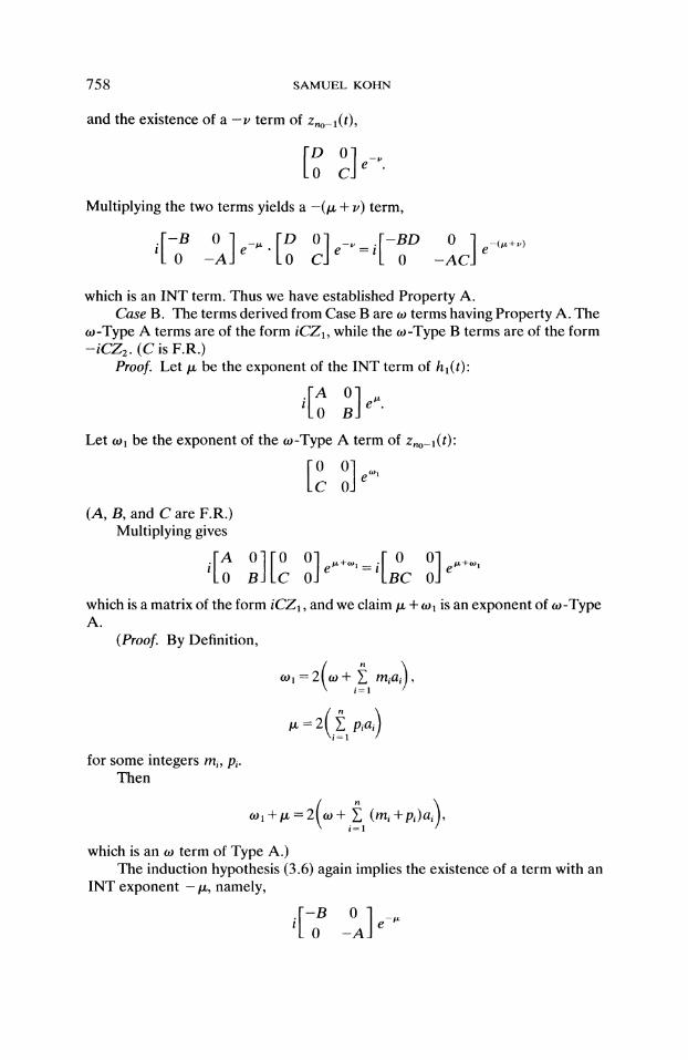
758 SAMUEL KOHN
and the existence of a -v term of Z,o_l(t),
Multiplying the two terms yields a -(/ + u) term,
0 -A 0e-" -BD 0 ]=i
0 -ACe-(+,)
which is an INT term. Thus we have established Property A.Case B. The terms derived from Case B are to terms having Property A. The
to-Type A terms are of the form iCZ1, while the to-Type B terms are of the form-iCZ2. (C is F.R.)
Proof. Let/x be the exponent of the INT term of hi(t):
i[A 0] e"0 B
Let to1 be the exponent of the to-Type A term of Z,o-l(t):
(A, B, and C are F.R.)Multiplying gives
0
0 O] ,CO
e
which is a matrix of the form iCZl, and we claim/ + tol is an exponent of to-TypeA.
(Proof. By Definition,
for some integers mi, pi.
Then
)Iz 2 pa
which is an to term of Type A.)The induction hypothesis (3.6) again implies the existence of a term with an
INT exponent -/x, namely,
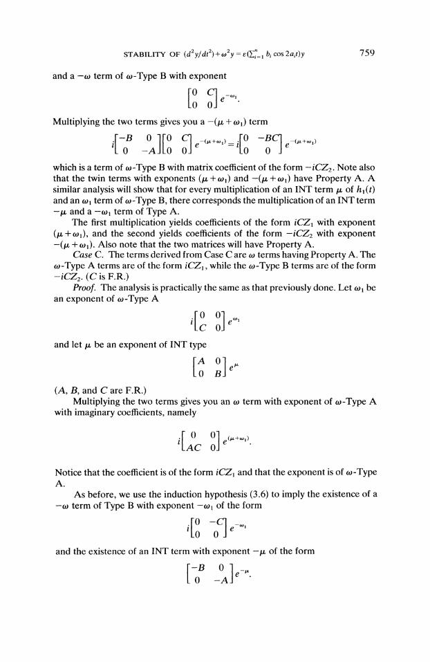
STABILITY OF (dZy/df)+to2y E(ZT_ bi cos 2ait)y 759
and a -to term of to-Type B with exponent
0
Multiplying the two terms gives you a -(/x + to) term
0 -A 0 0 0e
which is a term of w-Type B with matrix coefficient of the form -iCZ2. Note alsothat the twin terms with exponents ( + Wl) and -( + Wl) have Property A. Asimilar analysis will show that for every multiplication of an INT term of hi(t)and an w term of w-Type B, there corresponds the multiplication of an INT term- and a -1 term of Type A.
The first multiplication yields coefficients of the form iCZ with exponent( + Wl), and the second yields coefficients of the form -iCZ2 with exponent-( + w). Also note that the two matrices will have Property A.
Case C. The terms derived from Case C are w terms having Property A. Thew-Type A terms are of the form iCZ, while the w-Type B terms are of the form-iCZ2. (C is F.R.)
Pro@ The analysis is practically the same as that previously done. Let w bean exponent of w-Type A
C 0e
and let be an exponent of INT type
[ B0] e"
(A, B, and C are F.R.)Multiplying the two terms gives you an w term with exponent of w-Type A
with imaginary coefficients, namely
[AOc 0] (./,o,)
0e
Notice that the coefficient is of the form iCZ1 and that the exponent is of to-TypeA.
As before, we use the induction hypothesis (3.6) to imply the existence of a-to term of Type B with exponent -tol of the form
0e
and the existence of an INT term with exponent -/x of the form
0 -Ae-".
760 SAMUEL KOHN
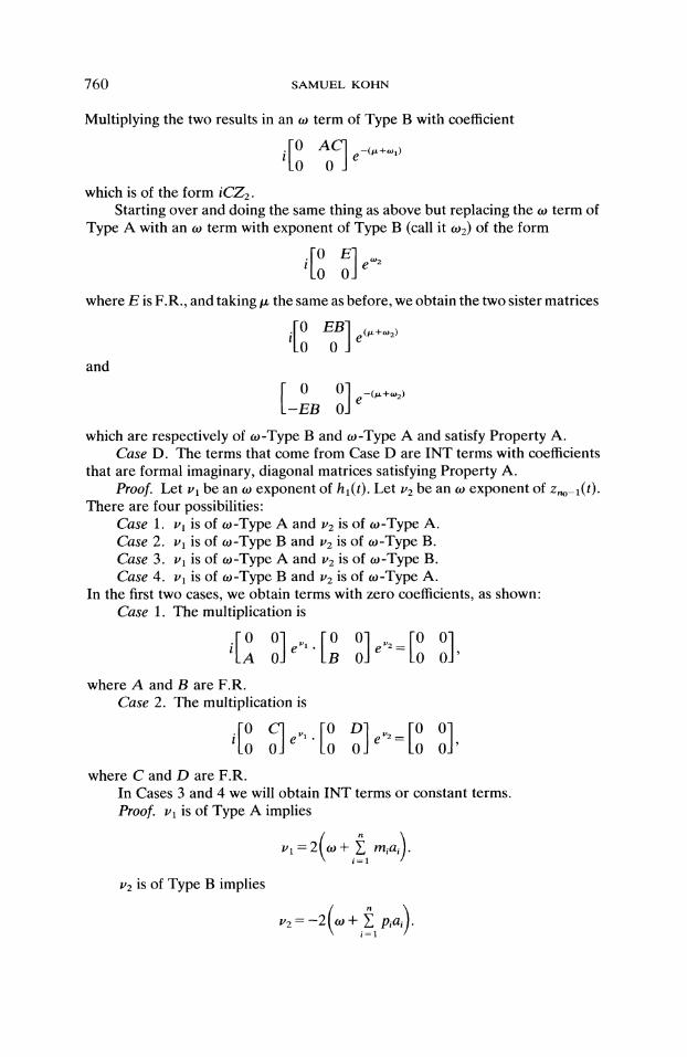
Multiplying the two results in an o term of Type B with coefficient
which is of the form iCZ.Starting over and doing the same thing as above but replacing the w term of
Type A with an o) term with exponent of Type B (call it ) of the form
where N is F.R., and taking the same as before, we obtain the two sister matrices
and
0 0]-JEB 0e
which are respectively of w-Type B and w-Type A and satisfy Property A.Case D. The terms that come from Case D are INT terms with coefficients
that are formal imaginary, diagonal matrices satisfying Property A.Proo]’. Let ul be an o exponent of h(t). Let/’2 be an o exponent of Z,o-a(t).
There are four possibilities:Case 1. , is of w-Type A and ’2 is of w-Type A.Case 2. v is of o-Type B and v2 is of o-Type B.Case 3. u is of o-Type A and u2 is of w-Type B.Case 4. v is of w-Type B and ’2 is of o-Type A.
In the first two cases, we obtain terms with zero coefficients, as shown:Case 1. The multiplication is
iAoe BOe
00’
where A and B are F.R.Case 2. The multiplication is
where C and D are F.R.In Cases 3 and 4 we will obtain INT terms or constant terms.
Pro@ , is of Type A implies
/22 is of Type B implies
STABILITY OF (d2y/dt2)+to2y e(i= bi cos 2ait)y 761
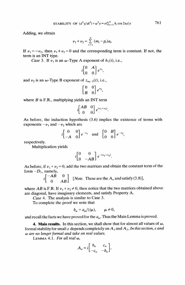
Adding, we obtain
ul + u2 (mi--pi)ai.i=1
If ul =-u2, then u + v2 0 and the corresponding term is constant. If not, theterm is an INT t3pe.
Case 3. If Ul is an to-Type A exponent of hi(t), i.e.,
0 0e
and t, is an to-Type B exponent of Zo-(t), i.e.,
B 0 e’
where B is F.R., multiplying yields an INT term
As before, the induction hypothesis (3.6) implies the existence of terms withexponents-t, and-u which are
0i_A
respectively.Multiplication yields
0e and
0 0e
-0 0 ]_0 -ABe-(+:)"
As before, if u + u2 0, add the two matrices and obtain the constant term of theform -D, namely,
[-B 0] [Note. These are the an and satisfy (3 8)],AB
where AB is F.R. If ul + u2 0, then notice that the two matrices obtained aboveare diagonal, have imaginary elements, and satisfy Property A.
Case 4. The analysis is similar to Case 3.To complete the proof we note that
b. a,/(ilx), /x 0,
and recall the facts we have proved for the a,. Thus the Main Lemma is proved.
4. Main results. In this section, we shall show that for almost all values of to,
formal stability for small e depends completely on A and A2, In this section, e andto are no longer formal and take on real values.
LEMMA 4.1. For all real to,
762 SAMUFI KOHN
where b, and c, take on real values. If oo # Yi= mia, mi integers,
0 -bThe proof is by induction using Property A of the Main Lemma.(For every exponent of o-Type A which becomes zero there is an exponent of
-Type B which becomes zero.)If = ma, m integers, then none of the -Type A or -Type B
exponents become zero, and the Main Lemma implies
A=i 0 -bUsing the above lemma we easily see the following.
LEMMA 4.2. A has two real or two purely imaginary eigenvalues.Now we shall analyze A and A using calculations (A.1), (A.2), (A.3) and
(A.4) found in the Appendix.If I1 a,
ib [ -](4.
with real eigenvalues bJ(4a).If I1 a, then A1 0.f I1 a and I1 a, a, then
(4.2) A=1=-a 0 1
and the eigenvalues of A are purely imaginary.If 1 a a (a e a), then
_1]}(4.3) A2=32(aai) (aa)2 a2+2 += 1 0
If ]w] 2, then
(4.4) A2=(.3 1 ( 2b )+)[ -1]2(2a,),= ,(2a 0
A surprising result is that A2 does not necessarily have real eigenvalues form a m a. In fact, consider the Mathieu equation
y,, + 2y e(COS 2a)t.
When o) 2a,
A2 32{a)2(2 [-10 a
and has real eigenvalues when a > 1/3 and purely imaginary eigenvalues whena < 1/3. When a 1/3, the eigenvalues are zero.
STABILITY OF (dZy/dt2)+toZy e(Y’.i= bi cos 2ait)y 763
When a 1/3 it would be necessary to study higher orders of A (i.e., j >- 3).We have not pursued this investigation.
When a 1, this the Mathieu equation whose stability and instability havebeen analyzed [2].
Define
def
Cn eA14- e2A2 4- 4- enA..
We now prove the theorems introduced in 1.THEOREM 1. I[ Itol Y-i=1 miai, (1.1) is formally stable [or all e.
Proof. By Lemma 4.1 and (4.2), C, is of the form
i=1i+10 Z e c
i=1
and the eigenvalues are purely imaginary.THEOREM 2. Equation (1.1) is "formally stable for small e" if to + ai + ai,
Proof. Using (4.2) and Lemma 4.1,
2. k=l 16to2(to2- ak) /=1 j=lc,,, e
m-2 b ,,,-2
i=1 =1162(w2-) =a
where b, are real numbers.If e is chosen small enough, the eigenvalues are purely imaginary. Similarly,
using Lemma 4.1 and (4.1) we have the following theorem.THEOREM 3. Equation (1.1) is "formally unstable ]:or small e" ]:or m > 1 and
Using Lemma 4.1 with (4.3) and (4.4) we have the following.THEOREM 4. When to + ai +/- aj [or some to, (1.1) is "formally unstable [or
small e ]’or m >-2" and ]:or some to, (1.1) is "formally stable for small e."
5. Asymptotic results.THEOREM 5.1. (Shtokalo). There exists an R > 0 such that the transforma-
tion
X UeiRt+ e"y,(t)n=l
converts
(1.2) dxd--- [B +ef(t)]x
764 SAMUEL KOHN
into the differential equation
(5.1) ekAk+ R,,(t, e) x,dt =1
where m is any positive integer, R,(t, e) is holomorphic in and e for lel < R, andR,, t, e) is bounded for all real t.
Proof. The proof can be found in [8, p. 34] or in [4, p. 121].What we would like to say is that
x,=expt Ake k
k=l
is a good approximation to the solutions of (5.1) thus implying that the solutionsare stable (except for the finite number of values mentioned previously). If wecould do this, it would be quite clear that since m is finite,
UeiR’+ Y’. e"y,,(t)
are bounded. Thus stability of the solutions of (1.2) would depend on theeigenvalues of Y’k= e kAk
Unfortunately, there does not seem to be any method that allows us to saythat x,, is a good approximation to x on the entire positive real axis. The best wecan do is to rely on the following theorem which allows us to approximate x withx,, on any finite interval [0, t].
THEOREM 5.2. There exists an e > 0 such that in a given interval [0, t], thesolution of systems
dx(1.2) d--=[B + e]:(t)]x
with initial condition x Xo is given approximately in the form
)) kAkX= UeiR’+ y e"v,(t exp Y. en=l k=l
fore<-R.The error does not exceed
]xo(exp Mmera+l- 1) exp , ekAk UeiR’ + , e"y,(t),k=l n=l
where M,, is defined as the least upper bound ofRm(t, e) for Itl T, e R, andM isa fixed integer.
Proof. The proof is found in [4, p. 129].

STABILITY OF (dZy/dtZ)+to2y E(Zi= bi cos 2ait)y 765
(A.1)
(A.2)
Appendix. Calculations.
-i . biD exp (2iait) + biD exp (-2iait)h’(/) -w i=
+ biZ2 exp {- 2i(to + ai)t} + biZ2 exp {-2i(to ai)t}
biZ exp {2i(to + ai)t}- biZ exp {2i(to ai)t}.
A= 0 0’
(A.3)
(A.4)
1 b,D exp (-2iait)-biDa exp (2iait)Z(t) --= ai a
+ bi Z2exp{-2i(to+ai)t}+ bito+ai to+ai
Z exp {2i(to + ai)t}
+ bi Z2 exp {-2i(to- ai)t}+to aj
bi Z exp {2i(w ai)t}.
h2(t) bbk2 D2exp{2i(ai16oo j,k a
a)t}- bib-----k D2 exp {- 2i(ai + a)t}a
bib Z2 exp {- 2i(to + ai + a)t}to+a
bbk-}- Z exp {2i(to + ai ak)t}to+ai
bib Zz exp {- 2i(to ai + a)t}
bbk+ Zlexp{2i(to-a--ak)t}to aj
bibD2 exp {2i(ak ai)t} + bib---kD2 exp {2i(ai + a)t}a abibk Z2 exp {- 2i(to + ai a)t}
bbk-1-" Z exp {2i(to + ai + ak)t}to+a
bibk Z2 exp {- 2i(to ai ak)t}to-a
bib+ Z exp {2i(to a + ak)t}to--ai
bibk+Zexp {- 2i(o + ak + ai)t}abibk Z2 exp {- 2i(to + ak ai)t}a
766 SAMUEL KO/-IN
REFERENCES
[1] N. A. BOGOLYUBOV AND Yu. A. MITROPOLSKY, Asymptotic Methods in the Theory ofNonlinear Oscillation, English transl., Hindustan Publishing Corp., Delhi, 1961, (Gordonand Breach, New York).
STABILITY OF (d2y/dt2)+to2y e(i= bi cos 2ait)y 767
[2] L. CESARI, Asymptotic Behavior and Stability Problems in Ordinary Differential Equations,Academic Press, New York, 1963.
[3] D. COLE, Perturbation Methods in Applied Mathematics, Blaisdell, Waltham, Mass., 1968.[4] N. P. ERLGIN, LinearSystems ofOrdinary Differential Equations with Periodic and Quasi-Periodic
Coefficients, Academic Press, New York, 1966.[5] M. KOHN AND S. KOHN, Investigation o]" the stability o[ the Lindstedt equation using Struble’s
technique, to appear.[6] A. LINDSrEDr, Differential Gleichungen der StOrungstheorie, Mem. Science of St. Petersbourgh,
31 (1883).[7] H. POINCARE, Les Methodes Nouvelles de la Mechanique Celeste, vol. II,, Dover, 1889.[8] I. Z. Srrroi,:ALO, Linear differential equations with variable coefficients, Criteria of Stability and
Instability of their Solutions, English transl. Hindustan Publishing Corp. Delhi, 1961,(Gordon and Breach, New York).
[9] R. A. STRUBLE, Nonlinear Differential Equations, McGraw-Hill, New York, 1962.
Reproduced with permission of the copyright owner. Further reproduction prohibited without permission.