Stability and performance of overlay multicast systems employing forward error correction

Performance Evaluation 67 (2010) 80–101

Contents lists available at ScienceDirect

Performance Evaluation

journal homepage: www.elsevier.com/locate/peva

Stability and performance of overlay multicast systems employingforward error correctionGyörgy Dán ∗, Viktória FodorACCESS Linnaeus Centre, School of Electrical Engineering, KTH, Royal Institute of Technology, Stockholm, Sweden

a r t i c l e i n f o

Article history:Received 13 November 2007Received in revised form 30 September2008Accepted 6 September 2009Available online 12 September 2009

Keywords:Overlay multicastFECData distribution performanceStabilityPerformance bounds

a b s t r a c t

The two main sources of impairment in overlay multicast systems are packet losses andnode churn. Yet, little is known about their effects on the data distribution performance.In this paper we develop an analytical model of a large class of peer-to-peer streamingarchitectures based on decomposition and non-linear recurrence relations.We analyze thestability properties of these systems using fixed-point analysis. We derive bounds on theprobability that nodes in the overlay receive an arbitrary packet of the stream. Based on themodel, we explain the effects of the overlay’s size, node heterogeneity, loss correlationsand node churn on the overlay’s performance. Our findings lead us to the definition ofan overlay structure with improved stability properties. We show how and under whatconditions overlays can benefit from the use of error control solutions, prioritization andtaxation schemes. Based on our results, we identify the components that are needed toachieve good data distribution performance in multi-tree-based overlay multicast.

© 2009 Elsevier B.V. All rights reserved.

1. Introduction

The peer-to-peer paradigm has proved to be an efficient means both for file distribution, and for lookup serviceswithout the need for expensive infrastructure. Peer-to-peer multicast streaming overlays could serve content providersas a cheap and efficient alternative to commercial content distribution networks for delivering live media to a large numberof spectators. In peer-to-peer multicast, peers are organized or organize themselves into an application layer overlay anddistribute the data among themselves. The main advantages are that the multicast is easy to deploy and it reduces the loadof the content provider, since the distribution cost in terms of bandwidth and processing power is shared by the nodes ofthe overlay.A large number of overlay multicast architectures have been proposed by the research community ([1–7] and references

therein), and a number of large-scale commercial deployments of peer-to-peer streaming systems were also recorded[8,9]. There is however not much analytical understanding of the data distribution performance of these systems, suchas the packet reception probability of the participating nodes. Most of the results in the literature are based on simulations,and focus on metrics like the depth of the overlay, the amount of control overhead and the link stress. There is a lack ofunderstanding of how the parameters of the overlay (e.g., the error control solutions employed) and the environmentaldynamics (e.g., the number of nodes, node churn and losses due to network failures) affect the end-to-end delays and thepacket reception probability.The goals of this paper are twofold. First, to give an understanding of how and why the above factors and the policies

proposed in the literature influence the data distribution performance of overlay multicast. Second, to give a tool for systemdesigners to evaluate the performance of their proposals, and give guidelines on how to achieve good performance.

∗ Corresponding author. Tel.: +46 87904253.E-mail addresses: [email protected] (G. Dán), [email protected] (V. Fodor).

0166-5316/$ – see front matter© 2009 Elsevier B.V. All rights reserved.doi:10.1016/j.peva.2009.09.004

http://www.elsevier.com/locate/peva

http://www.elsevier.com/locate/peva

mailto:[email protected]

mailto:[email protected]

http://dx.doi.org/10.1016/j.peva.2009.09.004

G. Dán, V. Fodor / Performance Evaluation 67 (2010) 80–101 81

We consider overlaymulticast systems based onmultiple distribution trees and the pushmodel, such as the ones in [2–6,10–12]. Multiple trees offer two advantages: they ensure graceful quality degradation in dynamic overlays, in which peerscan leave during the streaming session and they enable nodes to contribute to the overlay with fractions of the streambandwidth. The higher the number of trees, the smaller the fractions, so that nodes’ output capacities can be better utilized.Withmulti-path transmission, parts of the stream reach the peers through independent overlay paths. Consequently a nodereceives large part of the streaming data even if some of its parent peers stop forwarding.The contributions of the paper are the following. (i) We present a model to describe the probability that a peer in

the overlay possesses an arbitrary packet of the data stream. We describe the model applied to multi-tree-based overlaymulticast, but the modeling approach can generally be applied to multicast data distribution employing FEC in multi-hopenvironments. For example, in overlays that employ the pull model, data reach the nodes via spanning trees of the overlaygraph, and hence we believe that some of our results can be applied to pull-based overlays by adapting the packet lossmodel. (ii) We show that node churn can be treated as a form of packet losses. (iii) Based on the model, we show howfactors, such as the overlay’s size, heterogeneous loss probabilities, heterogeneous input and output capacities and losscorrelations influence the data distribution performance of the overlays. (iv) We explain how the parameters of the overlay,such as the number of distribution trees, the error control schemes employed, the prioritization and taxation schemes affectthe performance. (v) Based on our findings we propose a tree structure that improves the scalability of the overlay withrespect to the number of nodes.The rest of the paper is organized as follows. We review related work in Section 2. In Section 3 we give a description

of the considered overlays. We develop the analytical model of the overlay in Section 4 and derive asymptotic bounds onthe system performance in Section 5. We describe the simulation methodology used to validate the model in Section 6. Weevaluate the effects of packet losses in Section 7 and apply the model to node churn in Section 8. We conclude our work inSection 9.

2. Related work

Peer-to-peer streaming systems utilizing a single transmission tree were analyzed in [13]. The authors derived resultson the number of levels as a function of the upload capacities of the peers, and evaluated the probability of blocking arrivingnodes in the overlay. The first models that describe the data distribution performance of multi-tree-based overlay multicastwere proposed in [14,15] and showed that these systems exhibit a phase transition when using FEC. The model we presenthere generalizes the above models, and makes it possible to evaluate the effects of node heterogeneity, churn and differentoverlay management policies. The effect of the forwarding capacity on multi-tree-based overlays was investigated in [16]using a queuing theoretic approach, and in [17] based on a fluid model.The effect of node dynamics on the connectivity of peers was evaluated in [18] for peer-to-peer file sharing systems. The

authors derived results for the time to isolation and the probability of isolation for various node lifetime distributions. Theauthors in [19] proposedmaster equations tomodel the evolution of the number of neighbors of the peers in an overlay, theydid not provide however any closed form solution. To the best of our knowledge, ours is the first work to propose a generalframework for modeling the data distribution performance of multi-tree-based peer-to-peer streaming systems employingFEC in a dynamic environment.

3. System description

In this sectionwe describe the considered general overlay structure in Section 3.1, our assumptions regarding the overlaymaintenance and the data distribution in Sections 3.2 and 3.3 respectively.

3.1. Overlay model

The overlay consists of a source node and N peer nodes. The peer nodes are organized in τ distribution trees, and thesource is the root of all trees. Each peer node is member of at least one tree, and in each tree it has a different predecessornode (called parent) from which it receives data. We say that a node that is l hops away from the source node in tree e is inlevel l of tree e. We denote the maximum outdegree (the maximum number of children) of the source node in each tree bym, and the maximum outdegree of a node r by dr .m is limited by the ratio of the source’s upload capacity and the stream’sbitrate. dr is limited by the ratio of the node’s upload capacity and the stream’s bitrate divided by the number of trees τ .Nodes can split their forwarding capacity between s trees. In our model the nodes balance their forwarding capacity

between the s trees, i.e., a node can have up to ddr/se children in each of the s trees. One gets the minimum breadth treesdescribed in [3] for s = τ , and the minimum depth trees evaluated in [2,3,11] for s = 1. The case 1 < s < τ was proposedin [16] to improve the overlay’s stability under churn. Fig. 1 shows an overlay in which each node forwards data in one treeonly (s = 1), and the source has two child nodes in each tree (m = 2). The solid black lines show the parent–child relationsbetween the nodes in the overlay.We introduce the notion of well-maintained overlay: the number of nodes that forward data is maximal in every level of

its trees. Well-maintained overlays have the smallest depth for given N , τ and s. For instance, in a well-maintained overlay

82 G. Dán, V. Fodor / Performance Evaluation 67 (2010) 80–101

Fig. 1. Nodes, levels and parent–child relationships for an overlay with N = 11, τ = 2,m = 2. The square indicates that the node forwards data in thetree.

with L levels, each node is 1 ≤ l ≤ L hops away from the source node in the trees inwhich it forwards data, and L−1 ≤ l ≤ Lhops away in the trees in which it does not. Furthermore, for s < τ the number of levels L in the trees is O(logN).It is however not necessary for an overlay to be well maintained. Motivated by our modeling work, we propose a tree

structurewith limited level spread. In an overlaywith level spread limit∆l a node that forwards data in level l in a tree shouldbe located no deeper than level l + ∆l in the other trees. We do not discuss here how to implement such a tree structure,our goal is to show its possible benefits assumed it can be implemented.

3.2. Tree management

The construction and the maintenance of the trees can be done either by a distributed protocol (structured, like in [2] orunstructured, like in [4]) or by a central entity, like in [3]. The results presented in this paper do not depend on the particularalgorithm used, our focus is on the performance of the overlay as a function of the overlay’s structure, rather than on theefficiency of the tree maintenance algorithm.The purpose of the tree maintenance algorithm is to find eligible parents for the nodes based on the parent selection

criteria (e.g., closest to the source) and the nodes’ priorities. Priorities were introduced inmulti-tree-based overlays in orderto allow the most important nodes to be closest to the source. In the simplest case nodes that forward data in a tree havehigh priority, and hence can preempt nodes that do not forward data in that tree. Such a strategy was proposed in [3] inorder to push contributing nodes close to the source and non-contributing nodes to the last levels of the trees. Prioritizationcan also be based on more complex criteria, such as the packet reception probability of a node, the level spread of a node,the input capacity of a node or the maximum outdegree of a node (e.g., [5]).We consider three aspects of the tree maintenance algorithm. First, it influences the number of levels in the overlay and

the distribution of the nodes among the levels. Second, it influences how often a node loses its parent in a tree dependingon the node’s priority in the tree. We call this the inter-disconnection time of node r in tree e, and model it with a randomvariable Ω re . Third, it influences how long it takes for a node to find a parent in a tree depending on its priority. We callthis the reconnection time, and model it with a random variable Ξ re . The reconnection time consists of the time neededfor the detection of the loss of the parent node, the time needed for searching for a new eligible parent node, and the timeneeded for connecting to the eligible parent. The expected value E[Ξ re ] of the reconnection time can be up to tens of secondsdepending on the tree management and the forwarding capacity in the tree [11].

3.3. Data transmission and error resilience

The source splits the data stream into τ stripes, with every τ th packet belonging to the same stripe, and it sends thepackets in round-robin to its children in the different trees. Peer nodes relay the packets upon reception to their respectivechild nodes. Consequently, subsequent packets of the stream reach a node via different overlay paths.The source uses block-based FEC, e.g., Reed–Solomon codes [20], so that nodes can recover from packet losses due to

network congestion and node departures. To every k consecutive packets of information c packets of redundant informationare added resulting in a block length of n = k+c. We denote this FEC scheme by FEC(n, k). Lost packets can be reconstructedas long as no more than c packets are lost out of n packets. Once a node receives at least k packets of a block of n packets, itmay recover the remaining c packets. If a packet, which should have been received in the treewhere the node forwards data,is recovered, then it is sent to the respective children. Duplicate packets are discarded by the nodes. Since subsequent packetsof an FEC block reach a node via different overlay paths, the packet loss process as seen by a node is close to independent,which improves the efficiency of FEC in reconstructing lost packets [21]. Using this FEC scheme one can implement unequalerror protection (UXP), priority encoding transmission (PET), or the multiple description coding (MDC) scheme consideredin [3]. If the source would like to increase the ratio of redundancy while maintaining its bitrate unchanged, then it has todecrease the source rate.


Table 1List of notations frequently used in the paper.

Var. Definition Var. Definition

N # of nodes in the overlay τ ,m # of trees and outdegree of the source respectivelys # of trees in which a node can forward data n, k FEC block length and number of data pkts respectivelyH f Set of trees that nodes in cluster f connect to, |H f

| = τ f C l Set of clusters that forward data in level lN f # of nodes in cluster f N(l) # of nodes that forward data in level ldf Maximum outdegree of nodes in cluster f w

fe Average # of children of nodes of cluster f in tree e

J(j) # of lost pkts in a block of j pkts, P(J(j) = i) = P(i, j) We(l) # of pkts successfully departing from nodes that forward in level lin tree e (not lost on output link)

X fe # of pkts a node in cluster f can receive from its parent in tree e Y fe # of pkts a node in cluster f receives from its parent in tree eV fe # of tree e pkts possessed by a node in cluster f in tree e Z fe # of pkts that depart from a node in cluster f in tree eπ(l) Packet possession probability of nodes that forward data in level l π Packet possession probability of an arbitrary node

4. Performance metrics and data distribution model

The building blocks of the overlay are the individual nodes, so first we describe the model of a single node in Section 4.1.Using the notations introduced there we define the performance metrics we consider in Section 4.2. We define clusters ofnodes in Section 4.3, and describe the model of the overlay in Section 4.4. We then turn to the modeling of node dynamicsin Section 4.5, and describe how to estimate the overlay’s structure in Section 4.6. Table 1 summarizes the most frequentlyused notations.

4.1. Node model

The input capacity of a node determines the number of trees the node can connect to. We denote the set of trees thatnode r can connect to byH r ,H r

⊆ 1 . . . τ , |H r| ≤ τ . The maximum outdegree of the node in tree e is dre, its number of

children iswre . Our model captures three sources of disturbances in the overlay.First, a node cannot receive data in a tree if it is not connected to a parent node in that tree. We model whether a node

is connected with the binary r.v. Dre, such that Dre = 0 corresponds to node r being disconnected in tree e. We assume that

whether a node is disconnected in a tree is independent of it being disconnected in another tree, i.e., Dre is independent ofDrh (h ∈ H r

\ e). The independence assumption is reasonable if nodes do not have the same node as parent in differenttrees. We show how to calculate the probability P(Dre = 0) in Section 4.5.Second, a node might experience losses on its input link. (We refer as input link of a node to the part of the network that

is shared between data arriving from all parent nodes.) We denote the probability that i out of j packets are lost on the inputlink of a node by P rI (i, j). P

rI (i, j) can be calculated using loss models such as the Bernoulli model or the Gilbert model [22].

Third, a nodemight experience losses on its output link. (We refer as output link of a node to the part of the network thatis shared between data departing to all child nodes.) We denote the probability that i out of j packets are lost on the outputlink of a node by P rO(i, j). P

rO(i, j) can be calculated in a similar way as P

rI (i, j). We model these two loss processes separately

because the correlations in the two loss processes will have different effects on the performance of the overlay.

4.2. Performance metrics

To measure the performance of the data distribution in the overlay we use the probability π that an arbitrary nodereceives or can reconstruct (i.e., possesses) an arbitrary packet. If we denote by the randomvariable Rr the number of packetspossessed by node r in an arbitrary block of n packets, then π can be expressed as the average ratio of packets possessed ina block over all nodes, i.e., π = 1

N E[∑r Rr/n]. Typically, multimedia applications require π > 0.99.

We do not consider the delay performance in thismodel.We assume that delay jitters can be compensated at the playoutbuffers of the nodes, and end-to-end delays are controlled by keeping the depth of the transmission trees low.

4.3. Decomposition and clustering

Modeling large-scale overlays on a per node basis is computationally not feasible, hence we introduce two techniques inorder to make the data distribution model scalable.Clustering of nodes:We introduce the notion of clusters of nodes. Nodes belonging to a cluster forward data in the same

trees, have their parents in the same trees in the same levels, have the same input capacities, and experience the sameinput and output loss probabilities. Consequently, a level of a tree possibly consists of several clusters, the different clusterscorrespond to sets of nodes with different characteristics. We treat nodes within a cluster as stochastically identical, so thatwe only have to calculate the packet possession probabilities for clusters of nodes. Consequently, we can use the randomvariables introduced for individual nodes in Section 4.1 for clusters of nodes, e.g., we use the random variable Dfe to model


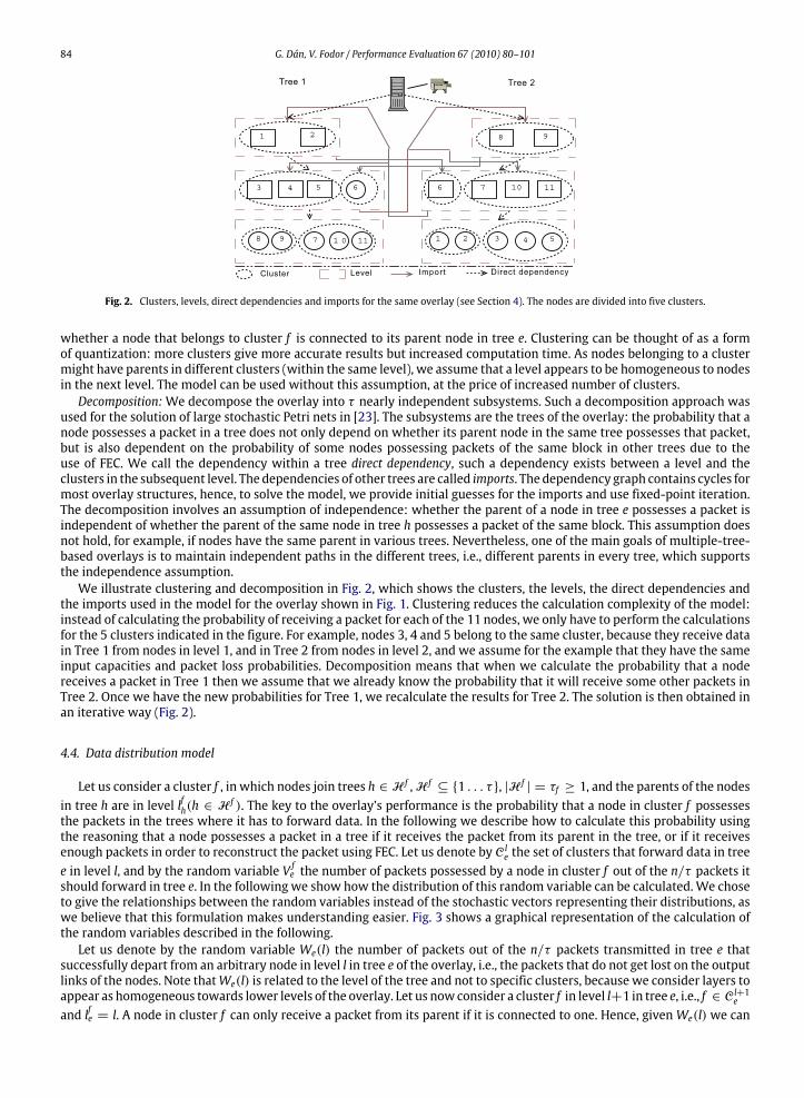
Fig. 2. Clusters, levels, direct dependencies and imports for the same overlay (see Section 4). The nodes are divided into five clusters.

whether a node that belongs to cluster f is connected to its parent node in tree e. Clustering can be thought of as a formof quantization: more clusters give more accurate results but increased computation time. As nodes belonging to a clustermight have parents in different clusters (within the same level), we assume that a level appears to be homogeneous to nodesin the next level. The model can be used without this assumption, at the price of increased number of clusters.Decomposition:We decompose the overlay into τ nearly independent subsystems. Such a decomposition approach was

used for the solution of large stochastic Petri nets in [23]. The subsystems are the trees of the overlay: the probability that anode possesses a packet in a tree does not only depend on whether its parent node in the same tree possesses that packet,but is also dependent on the probability of some nodes possessing packets of the same block in other trees due to theuse of FEC. We call the dependency within a tree direct dependency, such a dependency exists between a level and theclusters in the subsequent level. The dependencies of other trees are called imports. The dependency graph contains cycles formost overlay structures, hence, to solve the model, we provide initial guesses for the imports and use fixed-point iteration.The decomposition involves an assumption of independence: whether the parent of a node in tree e possesses a packet isindependent of whether the parent of the same node in tree h possesses a packet of the same block. This assumption doesnot hold, for example, if nodes have the same parent in various trees. Nevertheless, one of the main goals of multiple-tree-based overlays is to maintain independent paths in the different trees, i.e., different parents in every tree, which supportsthe independence assumption.We illustrate clustering and decomposition in Fig. 2, which shows the clusters, the levels, the direct dependencies and

the imports used in the model for the overlay shown in Fig. 1. Clustering reduces the calculation complexity of the model:instead of calculating the probability of receiving a packet for each of the 11 nodes, we only have to perform the calculationsfor the 5 clusters indicated in the figure. For example, nodes 3, 4 and 5 belong to the same cluster, because they receive datain Tree 1 from nodes in level 1, and in Tree 2 from nodes in level 2, and we assume for the example that they have the sameinput capacities and packet loss probabilities. Decomposition means that when we calculate the probability that a nodereceives a packet in Tree 1 then we assume that we already know the probability that it will receive some other packets inTree 2. Once we have the new probabilities for Tree 1, we recalculate the results for Tree 2. The solution is then obtained inan iterative way (Fig. 2).

4.4. Data distribution model

Let us consider a cluster f , in which nodes join trees h ∈ H f ,H f⊆ 1 . . . τ , |H f

| = τf ≥ 1, and the parents of the nodesin tree h are in level lfh(h ∈ H f ). The key to the overlay’s performance is the probability that a node in cluster f possessesthe packets in the trees where it has to forward data. In the following we describe how to calculate this probability usingthe reasoning that a node possesses a packet in a tree if it receives the packet from its parent in the tree, or if it receivesenough packets in order to reconstruct the packet using FEC. Let us denote by C le the set of clusters that forward data in treee in level l, and by the random variable V fe the number of packets possessed by a node in cluster f out of the n/τ packets itshould forward in tree e. In the following we show how the distribution of this random variable can be calculated. We choseto give the relationships between the random variables instead of the stochastic vectors representing their distributions, aswe believe that this formulation makes understanding easier. Fig. 3 shows a graphical representation of the calculation ofthe random variables described in the following.Let us denote by the random variable We(l) the number of packets out of the n/τ packets transmitted in tree e that

successfully depart from an arbitrary node in level l in tree e of the overlay, i.e., the packets that do not get lost on the outputlinks of the nodes. Note thatWe(l) is related to the level of the tree and not to specific clusters, because we consider layers toappear as homogeneous towards lower levels of the overlay. Let us now consider a cluster f in level l+1 in tree e, i.e., f ∈ C l+1eand lfe = l. A node in cluster f can only receive a packet from its parent if it is connected to one. Hence, givenWe(l) we can


Fig. 3. Random variables and their relations used for the calculation of We(l + 1) from We(l) through cluster f ∈ C l+1e , Hf= e, h1, h2. Wh1 (l

fh1) and

Wh2 (lfh2) are imports. Eqs. (1)–(8) give the relationships between the random variables.

express the random variable X fe , the number of packets that nodes in cluster f can receive from their parents in tree e

X fe = We(lfe)D

fe. (1)

Similarly, we can define the number of packets that can be received in other trees based on the importsWh(lfh), h ∈ H f

\ eand Dfh. Eq. (1) is approximate if n/τ > 1, it assumes that D

fe does not change during the transmission of a block of packets,

even though a parent can depart and a parent can be found during the transmission of a block. Themodel can be extended sothat this assumption does not have to be made, but this approximation works well if the time to transmit a block of packetsis much shorter than the inter-disconnection and the reconnection times.The number of packets actually received by a node depends on the loss probability on the input link of the node, so we

define the random variable Y fe as the number of packets received by nodes of cluster f in tree e

Y fe = Xfe − J

fI (X

fe ), (2)

where J fI (j) is the number of lost packets out of j packets on the input link, and it is a random variable with distributionP(J fI (j) = i) = P

fI (i, j). Similarly, we can approximate the total number of packets received in the other trees

Y fe =∑

h∈H f \e

X fh −∑

h∈H f \e

J fI (Xfh). (3)

If FEC(n, k) is used to recover missing packets then the relationship between the number of packets possessed in tree e, thenumber of packets received in tree e and the number of packets received in the other trees is

V fe =n/τ if Y fe + Y

fe ≥ k

Y fe otherwise.(4)

Nowwhat remains is to show howWe(l+ 1) can be calculated. We express the random variableWfe , the number of packets

out of n/τ packets that do not get lost on the output link of a node of cluster f

W fe = Vfe − J

fO(V

fe ), (5)

where J fO(j) is the number of lost packets out of j packets on the output link, and is a random variable with distributionP(J fO(j) = i) = P

fO(i, j). Based on theW

fe for all f ∈ C l+1 we can expressWe(l+ 1)

We(l+ 1) =

∑f∈Cl+1e

W fe N fwfe∑

f∈Cl+1e

N fwfe, (6)

where N f is the number of nodes in cluster f andwfe is the number of children in tree e of the nodes that belong to cluster f .We start the calculation of the distributions of the above random variables by using the initial condition P(V srce = n/τ) =

1 (1 ≤ e ≤ τ ), i.e., the source node possesses all data in all trees, and the imports P(We(l)(0) = 0) = 1, 1 ≤ e ≤ τ .Then, in iteration i, we calculate the distribution of We(l)(i), (1 ≤ l < L and 1 ≤ e ≤ τ ) using the direct dependenciesand the imports from iteration i − 1. The iteration stops when |E[We(L − 1)(i−1)] − E[We(L − 1)(i)]| < ε, where ε > 0.E[We(l)(i)] ismonotonically increasing as long as (1)–(6) aremonotonically increasing functions in their respective variables.Consequently, as E[We(l)(i)] ≤ n/τ the iteration converges.


The iterative solutionwe outlined here can be interpreted as the application of the belief propagation algorithm to a loopyBayesian network partitioned into τ trees [24]. A Bayesian network is a graphical representation of conditional dependenciesbetween random variables. The nodes of the graph are the random variables, in our case the V fe , and the arcs represent thedependencies that we have described above. The belief propagation algorithm is an iterative algorithm used to calculatethe marginals of the joint distribution of the random variables represented by the nodes of the graph, i.e., in our case thedistributions of the random variables V fe . The algorithm starts from the leaf nodes of the graph, in our case the leaf nodesare the source of the trees and the imports, and calculates the marginals in an iterative way.Based on the final value ofWe(le)(i), we can express the random variable Z f , the number of packets out of n that a node

belonging to cluster f receives

Z f =∑e∈H f

Y fe . (7)

Finally, we define the packet possession probability π f , as the ratio of packets in a block that a node belonging to cluster fpossesses

π f =1nRf =

1nE[Z f + ρ(Z f )], (8)

where ρ(i) is the number of reconstructed packets if i packets are received in a block of n packets

ρ(i) =0 0 ≤ i < kn− i k ≤ i ≤ n.

Finally, we define the packet possession probability of nodes that forward data in level l as the weighted average of the π ffor f ∈ C l

π(l) =

∑f∈Cl

π fN f∑f∈ClN f

, (9)

and the packet possession probability of an arbitrary node in the overlay as the weighted average of the π f

π =

∑fπ fN f∑fN f

. (10)

4.5. Modeling node dynamics

In the following section we calculate the probability that a node in cluster f is disconnected in tree e, i.e., the probabilityP(Dfe = 0). This probability is influenced by how often a node in cluster f loses its parent in tree e, and for how long it hasto look for a new one. These twomeasures are influenced by the priority of the nodes of cluster f in tree e, because a node islikely to find a parent faster in a tree in which it has a high priority, and it is less often disconnected from its parent due topreemption. Consequently, we consider a set of treesH f

b , |Hfb | = τb, in which the nodes of cluster f have the same priority.

As an example, consider that nodes forward data in one tree only (s = 1), and nodes that forward data in tree e obtain aparent in tree e faster than those that do not forward data in tree e because of a prioritization scheme such as the one weexplained in Section 3.2. Then for a cluster f that consists of nodes forwarding data in tree e, H f consists of two sets oftrees, the tree in which the nodes forward dataH

fF = e, and the trees in which they do not forward dataH

fS = H f

\HfF .

Consequently, τF = 1 and τS = τ − 1, and Hfb refers to one of these two sets. Since in the remainder of this section all

random variables refer to the same cluster of nodes, we omit the superscript f in order to simplify the notation.Let us denote by u = u0, . . . , uτb the stochastic vector who is ith component contains the probability that a node is

not connected to a parent in i of the τb trees that belong to Hb upon joining the overlay. The probability of a node beingdisconnected given the initial state distribution u can be expressed using the law of total probability

P(De = 0|u) =τb∑i=0

uiP(De = 0|ui), (11)

where ui is the initial state distribution with exactly i disconnected parents.In order to develop a closed formsolution for P(De = 0|ui), we assume that the distribution of thenodes’ lifetimes (M), the

inter-disconnection times (Ωb) and the reconnection times (Ξb) can be modeled as exponential. That is, M is exponentialdistributed with parameter µ, E[M] = 1/µ, Ωb is exponential distributed with parameter ωb, E[Ωb] = 1/ωb, and Ξb is


exponential distributed with parameter ξb, E[Ξb] = 1/ξb. Without preemptions and if preemptions are graceful,Ωb andMare equal in distribution due to the exponential assumption. If preemptions are ungraceful, then the disconnection intensityωb of a node is the sum of the preemption intensity and the death intensity of the parents of the node. We will evaluate theaccuracy of the exponential modeling assumption in Section 8. Using the exponential assumptions, in the following we givea closed form expression for the probability P(De = 0|ui).

Theorem 1. For initial state distribution ui the probability of a node being disconnected in tree e ∈ Hb is

P(De = 0|ui) =τb + iαb

τb(κb + αb + 1), (12)

where κb = ξb/ωb and αb = µb/ωb.

Proof. We canmodel the evolution of the number of disconnected parents in trees e ∈ Hb of a node with a continuous timediscrete state space Markov process X(h) ∈ S, S = [0 . . . τb]. The transition intensities of the Markov process are

qi,i+1 = (τb − i)ωb 0 ≤ i ≤ τb − 1 (13)

qi,i−1 = iξb 1 ≤ i ≤ τb. (14)

The ratio of disconnected parents is ri = i/τb in state i (0 ≤ i ≤ τb) of the Markov process. The conditional probabilityP(De = 0|ui) can be expressed as the average ratio of disconnected parents in trees e ∈ Hb of a node as seen by a randomobserver given ui. Without loss of generality we can denote the arrival time of the observer by 0,

P(De = 0|ui) = E[∆b|ui] =τb∑j=0

jτbP(X(0) = j|ui). (15)

The above model is an Engset system [25], and we are interested in the probability P(X(0) = j|ui) that a random observerfinds an arbitrary node in state j, given that the node was started with initial state distribution ui. Let us denote by t the ageof the node when the random observer arrives and by A(t) its distribution function, then

P(X(0) = j|ui) =∫∞

0pi,j(t)dA(t). (16)

pi,j(t) is given by pi,j(t) = P(X(0) = j|X(−t) = i) = eQti,j, where Q is the intensity matrix Q = qi,j. We use zero-

based indexing for the rows and columns of thematrices. The evolution of pi,j(t) is governed by the differential–differenceequations

p′i,0(t) = −τbωbpi,0(t)+ ξbpi,1(t)

p′i,j(t) = −((τb − j)ωb + jξb)pi,j(t)+ (τb − j)ωbpi,j−1(t)+ (j+ 1)ξbpi,j+1(t)

p′i,τb(t) = −τbξbpi,τb(t)+ ωbpi,τb−1(t).

The generating function of the probabilities pi,j(t) is

Pi(z, t) =τb∑j=0

pi,j(t)z j =1

(1+ κ)τb(B+ Az)τb−i(D+ Cz)i, (17)

where A = 1−M(t), B = M(t)+ κb, C = κbM(t)+ 1, D = κb(1−M(t)), andM(t) = e−ωb(1+κb)t .The age of an arbitrary node as seen by a random observer is the backward recurrence time of a renewal process with

exponentially distributed inter-renewal times. Hence, the distribution of t is exponential with parameter µ. Consequently,after substituting (16) into (15) we get

E[∆b|ui] =τb∑j=0

jτb

∫∞

0pi,j(t)µe−µtdt

=

∫∞

0

τb∑j=0

jτbpi,j(t)

µe−µtdt. (18)

We can substitute the inverse z-transform of (17) into the sum on the right hand side of (18) to getτb∑j=0

jτbpi,j(t) =

(τb − i)(1−M(t))+ i(κbM(t)+ 1)τb(1+ κb)

, (19)

and by substituting (19) into (18) we get the theorem

E[∆b|ui] =τb + iαb

τb(κb + αb + 1).


Discussion of the result: The parameter κb = ξb/ωb in (12) reflects the self-healing capability of the overlay: the higher itsvalue, the more resilient is the overlay to node churn. Similarly, the parameter αb = µb/ωb in (12) reflects the likelihoodof that a node will depart before one of its parents will be disconnected: the higher its value, the more likely that the nodewill depart before it gets disconnected. For uτb and u0 evaluating (17) leads to the well-known product form solution [25],but we are not aware of any results for the general case described here. For α→∞ (12) reduces to i/τb, while for α→ 0 itconverges to the steady state solution of the mean number of jobs in an Engset system [25]. Based on (12) one can calculatethe mean number of the children of a node as well, if one substitutes ω by the arrival rate of the children as seen by thenode, and ξ by the departure rate of the children of the node.

4.6. Overlay structure

Important parameters of the model are the depth L of the overlay and the number of nodes per cluster N f . These can beestimated for given overlay sizeN , maximum source degreem, number of trees τ , number of trees in which a node forwardsdata s and node parameters, such as input and output capacities.The number of nodes that forward in level l of a well-maintained tree can be approximated by the recurrence Nl =∑r∈R(l−1) d

r/swith initial condition N1 = min(N/(τ/s),m), whereR(l− 1) denotes the set of nodes that forward in levell− 1. Prioritization schemes affect the probability that nodes with certain properties (e.g., high output capacity) are locatedclose to the source, and hence they influence the depth of the trees. Without prioritization, one can assume that nodes withdifferent parameters are distributed uniformly among the levels. With prioritization, we assume that prioritized nodes areas close as possible to the source. There is a difference between the overlay structure estimated this way and the real overlaystructure due to node churn and the distributed treemaintenance, but the simulationswe present later show that the effectsof these differences are negligible.

4.7. Example

Consider a well-maintained minimum depth overlay in which nodes are organized in τ = 3 trees. The outdegree of thesource is m = 2, and an FEC(3, 2) code is used for error resilience. There are N = 24 nodes in the overlay in L = 3 levels.Assume that packet losses between nodes are i.i.d. with probability p, and the losses happen on the input links of the nodes,i.e., P fI (i, j) follows a binomial distribution with parameter p. Since n = τ , every node receives one packet of a block of npackets in a tree, and consequently the V fe are binary random variables. In each tree there are two clusters: the nodes thatforward data in level 1, and the nodes that forward data in level 2.Consider now tree e, in which the two clusters are E1 and E2. The source possesses all packets, hence we have P(V srce =

1) = 1, and since there are no losses on the output link of the source, we have P(We(0) = 1) = 1 from (5) and (6).Since we do not consider node churn in the example, we have P(XE1e = 1) = P(We(0) = 1) = 1 from (1). Nevertheless,packets get lost with probability p on the input links of the nodes, so that P(Y E1e = 1) = P(X

E1e = 1)(1 − p) from (2).

Nodes that forward packets in level 1 are in level 3 of the other trees, so that they receive both of the other packets in theFEC block from their parent nodes in level 2 with probability P(Y E1e = 2) = P(X

E1e = 2)(1 − p)

2 from (1)–(2). A node inlevel 1 possesses a packet if it receives it from the source, or if it receives the two other packets in the FEC block in level3, i.e., P(V E1e = 1) = P(Y

E1e = 1) + (1 − P(Y

E1e = 1))P(Y

E1e = 2) from (4). The trees are statistically identical, there is

only one cluster per level in every tree, and there are no losses on the output links of the nodes, so that for tree h 6= e wehave P(Wh(2) = 1) = P(We(2) = 1) = P(V E2e = 1) from (5) and (6). For the same reason we can also omit the subscriptsdenoting the trees, so that for the probability that a node in level 1 possesses a packet that it should forward we get

P(V 1 = 1) = P(V src = 1)(1− p)+ [1− P(V src = 1)(1− p)]P(V 2 = 1)2(1− p)2

= 1− p+ p(1− p)2P(V 2 = 1)2. (20)

Similarly, we can express the probability that a node in level 2 possesses a packet that it should forward, i.e., P(V 2 = 1), as

P(V 2 = 1) = P(V 1 = 1)(1− p)+ [1− P(V 1 = 1)(1− p)]P(V 2 = 1)2(1− p)2. (21)

For this simple example we do not need an iterative solution, but we can substitute (20) into (21), and solve for P(V 1 = 1)and P(V 2 = 1). For example, for p = 0.1 we get P(V 1 = 1) = 0.9764 and P(V 2 = 1) = 0.9714. We can use these resultsto calculate the distribution of Z1 and Z2, and finally π .

5. Overlay stability

In the following we analyze the stability of a class of overlays, and we establish bounds on the packet possessionprobability π as a function of the loss probability and the depth of the overlay. We observe that in all overlays proposedin the literature, nodes should be at least as close to the source in the trees in which they forward data as they are in theother trees. We consider the case n = τ , so that the random variables V fe are binary. We consider overlays consistingof homogeneous nodes in terms of loss probability and input capacity. We restrict ourselves to the case when nodes can


receive data in every tree, thus |H f| = τ . A consequence of this assumption is that all trees are statistically identical, i.e., the

We(l), 1 ≤ e ≤ τ are equal in distribution. We assume independent packet losses, so that losses due to node departures, onthe input links and on the output links can be treated together as independent losses on the input links. If we denote the lossprobability on the path between two nodes by p, then the number of lost packets i in a block of j packets follows a binomialdistribution.

5.1. Upper bound of the packet possession probability

Using the above simplifying assumptions, from (1)–(6) and the initial condition E[V srce ] = n/τ (1 ≤ e ≤ τ ) it followsthat E[We(l)] is a non-increasing function of l. Hence, we can give an upper bound on E[V

fe ] = P(V

fe = 1) (V

fe is a binary

r.v. because τ = n) by assuming that the parents of the nodes forwarding in a tree in level l are in level l = minh∈H lfh in

all trees. Since nodes are homogeneous, we only have to consider one cluster of nodes per level. Furthermore, since V fe is abinary random variable, (1)–(6) implies that a packet is possessed by a node if it receives it from its parent or if it receivesat least k packets of the other n − 1 packets of the block from its other parents, at most one packet from each parent. Thatis, if we denote the upper bound of the packet possession probability in level l by π(l), then

π(l+ 1) = π(l)(1− p)+ (1− π(l)(1− p))n−1∑j=k

(n− 1j

)π(l)j(1− π(l))n−1−j

j−k∑i=0

P(i, j). (22)

The π(l) can be calculated using the initial condition π(0) = 1. Similar to (10), the upper bound of the packet possessionprobability for an overlay with L levels and N(l) nodes in level l can be calculated as

π =

L∑l=1π(l)N(l)

N. (23)

5.2. Asymptotic behavior

Eq. (22) defines a non-linear recurrence relation for π(l), consequently we are interested in the existence of the fixedpoints of (22) on (0, 1].

Theorem 2 (Existence of Fixed Points). For the i.i.d Bernoulli loss model the number of fixed points of (22) is 0, 1 or 2. For k = 1a fixed point exists and is asymptotically stable iff p < (n− 1)/n. For k > 1 the number of fixed points is 0 if p > (n− k+ 1)/n.If there are 2 fixed points r1 and r2 (r1 < r2) then r2 is asymptotically stable and r1 is unstable.

Proof. At the fixed point of the discrete dynamic system the mean number of lost packets has to equal the mean number ofreconstructed packets. The mean number of packets that a node can reconstruct is given by

r(π, p, n, k) =n∑j=k

(nj

)π j(1− π)n−j

j−k∑z=0

(n− j+ z)(jz

)pz(1− p)j−z . (24)

The mean number of lost packets is nπp, so that

nπp = r(π, p, n, k). (25)

Our goal is to show that the number of intersections of the lines nπp and r(π, p, n, k) on (0, 1] is nomore than two, i.e., thereare at most two fixed points. Fig. 4 illustrates the solution of (25) on four examples.We start the proof by showing that r(1, p, n, k) < np. We substitute π = 1 into (25)

np =n∑i=0

iP(i, n) >n−k∑i=0

iP(i, n) = r(1, p, n, k) (26)

for any loss distribution that satisfies∑ni=n−k+1 P(i, n) > 0, e.g., the Bernoulli loss model with p > 0.

For k = 1 we know that r(π, p, n, 1) is concave on (0, 1], as

r (1)(π, p, n, 1)|π=0 = n(n− 1)(1− p) > 0,r (2)(π, p, n, 1)|π=0 = −n2(n− 1)(1− p)2 < 0,

and the second derivative has one nonzero root at 1/(1−p) > 1, so that there can be no inflection point on (0, 1]. Due to theconcavity of r(π, p, n, 1) on (0, 1], the two curves intersect in one point, denoted by r2, iff r (1)(0, p, n, 1) > np, i.e., p < (n−1)/n. If it exists, r2 is asymptotically stable and its domain of attraction is (0, 1]. (E.g., the solid and the dashed lines in Fig. 4.)


Fig. 4. Number of lost and reconstructed packets vs. π for independent losses.

Fig. 5. c vs. p for various objectives for the stable fixed point.

For 1 < k < n we start by showing that there is a π∗∗ for which r(π, p, n, k) is convex for 0 < π < π∗∗. We knowthat r(0, p, n, k) = 0, r (1)(0, p, n, k) = 0, and that there is π for which r(π, p, n, k) > 0. Since r(π, p, n, k) is a continuousfunction, r (1)(π, p, n, k) > 0 for some π > 0 and hence r (2)(π, p, n, k) > 0 as well. Thus, π∗∗ exists and is the smallestpositive inflection point.If π∗∗ > 1, that is, r(π, p, n, k) has no inflection point on (0, 1], then r(π, p, n, k) is convex on (0, 1], so that the number

of intersection points is 0, because of (26) and r(0, p, n, k) = 0.For π∗∗ ≤ 1 it is enough to show that r(π, p, n, k) has exactly one inflection point on (0, 1], and hence it is the combina-

tion of a convex and a concave curve. For any k > 1, r (2)(π, p, n, k) has n− k nonzero real roots: π∗∗1 =11−p of multiplicity

n−k−1 andπ∗∗2 =k−1n(1−p) . Bothπ

∗∗

1 andπ∗∗

2 are inflection points as r(3)(π∗∗1 , p, n, k) > 0 and r

(3)(π∗∗2 , p, n, k) < 0 (i.e., thesecond derivatives change sign). 1/(1− p) > 1, so that r(π, p, n, k) has an inflection point on (0, 1] iff p ≤ (n− k+ 1)/n,and then π∗∗ = π∗∗2 . Consequently, if p ≤ (n− k+ 1)/n then r(π, p, n, k) has one inflection point on (0, 1] and the numberof fixed points can be 0, 1 or 2. (E.g., the dotted line in Fig. 4.)If there is 1 fixed point r1 then r (1)(r1, p, n, k) = np, and the fixed point is unstable. If there are two fixed points r1 and

r2 (r1 < r2), then r2 is asymptotically stable (r(π, p, n, k) > nπp for π ∈ (r1, r2), and r(π, p, n, k) < nπp for π > r2). Forr1 the contrary is true, hence it is unstable. Furthermore, the domain of attraction of r2 is (r1, 1]. (E.g., the dash-dotted linein Fig. 4.)

A consequence of the proof is that for any p and ε > 0 there is an n, k pair for which r2 exists and r2 > 1− ε. Fig. 5 showsthe number of redundant packets needed in a block of packets in order to achieve various objectives for the asymptoticallystable fixed point r2 as a function of the loss probability p.If (22) has an asymptotically stable fixed point on (0, 1] then π(l) converges to that fixed point, and we say that the

overlay is potentially stable: for the given loss probability and FEC parameters there exists an overlay structure for which alower bound on π (the stable fixed point of (22)) can be given independent of the overlay’s size. This overlay is a minimumbreadth overlay (s = τ ) in which the nodes are in the same level in all trees. Otherwise, π(l) converges to 0, and the overlayis unstable: for the given loss probability and FEC parameters there is no overlay structure for which a lower bound on π canbe given independent of the overlay’s size.Fig. 6 shows the theoretical upper bound of the packet possession probability as a function of the loss probability. The

bound is obtained by combining π(l) from (22) with the node distribution N(l) of a minimum depth overlay (s = 1) with N


Fig. 6. Upper bound of the performance vs. p for various number of trees and overlay sizes (n = τ ).

nodes. The upper bound of the performance of an unstable overlay decreases as the overlay’s size increases, while that of apotentially stable overlay is insensitive to the overlay’s size. For large overlays (N = ∞) the upper bound is approximatelyequal to the stable fixed point of (22) if that exists, and is 0 otherwise.

5.3. Sufficient condition for stability

We call an overlay stable if it is potentially stable and for given overlay size, loss probability and FEC parameters thepacket possession probability is no less than the asymptotically stable fixed point of (22). We can get a sufficient conditionfor the overlay to be stable using similar reasoning as used to obtain the necessary conditions.

Theorem 3 (Sufficient Condition for Stability). For k = 1 if p < (n− 1)/n then the overlay is stable. For k > 1, if the numberof fixed points of (22) is 2 and (1− p)L > r1 then the overlay is stable.

Proof. Let us denote the lower bound of the packet possession probability in level l byπ(l). If there is no FEC reconstruction,thenπ(l) = (1−p)L. Using FEC, if k = 1 then according to Theorem 2 for p < (n−1)/n there exists an asymptotically stablefixed point r2 of (22) with domain of attraction (0, 1]. Hence, after successive iterations of the model π(l) ≥ π(L) ≥ r2.For k > 1, if the number of fixed points of (22) is 2 and (1 − p)L > r1 then after successive iterations of the modelπ(l) ≥ π(L) ≥ r2, the stable fixed point of (22).

Consequently, the deeper the overlay, the smaller the range of loss probabilities for which an overlay with arbitrarystructure is stable.

5.4. Examples

Example 1. Consider that an FEC(3, 2) code is used to distribute data. We can calculate the fixed points of (22) analyticallyon (0, 1]. The mean number of packets that can be reconstructed, (24), is

r(π, p, 3, 2) = 3π2(1− π)[(1− p)2] + π3[3p(1− p)2]. (27)

In order to find the fixed points of (22) we solve the equation 3πp = r(π, p, 3, 2), which yields

r1 =1− p−

√1− 6p+ 5p2

2(1− p)2r2 =

1− p+√1− 6p+ 5p2

2(1− p)2.

In order for two fixed points to exist we need 1− 6p+ 5p2 > 0, i.e., p < 0.2. Consequently, for p < 0.2 one can construct

an overlay of arbitrary size such that π ≥ 1−p+√1−6p+5p2

2(1−p)2. For p > 0.2 this is however not possible.

Example 2. Consider a minimum depth overlay in which nodes are organized in τ = 3 trees. The outdegree of the source ism = 2, and an FEC(3, 2) code is used for error resilience. There are N = 24 nodes in the overlay, so that if the overlay is well

maintained then L = 3, and the sufficient condition for stability is (1 − p)3 ≥ 1−p−√1−6p+5p2

2(1−p)2, i.e., p ≤ 0.1957. The same

condition for an overlay with N = 105, L = 10 would be p ≤ 0.137.


6. Simulation methodology

Before presenting numerical results, we briefly describe the simulation environment we used to validate the results.We developed a packet level event-driven simulator to validate our model. We used the GT-ITM topology generator [26]to generate a transit–stub network with 104 nodes and average node degree 6.2. We placed each node of the overlayat random at one of the 104 nodes of the topology and used the one way delays given by the generator between thenodes. The delay between overlay nodes residing on the same node of the topology was set to 1 ms. We assume that theinterarrival times between the nodes are exponentially distributed, this assumption is supported by several measurementstudies [27,28]. We consider two distributions for the session holding times M: the log-normal distribution [27] with CDFFM(x) = 0.5 + 0.5erf ((ln (x) − a)/(b

√2)), a = 4.93, b = 1.26; and the shifted Pareto distribution [28] with CDF

FM(x) = 1− (1+ x/b)−a, b = 612, a = 3. In both cases the mean lifetime is E[M] = 306 s [27].Tree maintenance:We assume that a distributed algorithm, such as gossip based algorithms, is used by the nodes to learn

about other nodes.We do not simulate the information dissemination, but assume that it provides randomknowledge of theoverlay such as in [29]. Since our focus is not on the structure of the resulting overlays, this assumption does not influenceour conclusions.When a nodewants to join the overlay, it contacts the source and obtains a random list of g = 100members of every tree.

The source tells to the arriving node in which trees it should forward data: in the ones with the least amount of forwardingcapacity. The arriving node then uses the following parent selection procedure to find a parent.To select a parent in a tree, the node sorts the g members it is aware of into increasing order according to their distances

from the source, and looks for the first node that has available capacity or has a child that can be preempted, i.e., which haslower priority.We describe the considered priority schemes below. If the node has to preempt a child, but itself has availablecapacity, then the preempted child can immediately become a child of the preempting node. Otherwise, the preempted childhas to follow the parent selection procedure just like the child nodes of a departed node. As opposed to [29,30], we do notforce all nodes in the subtree of a departed node to reconnect individually. We believe that forcing all nodes in a subtree todisconnect in a large overlay creates large control overhead and can lead to scalability issues.Node priority:We consider two node preemption strategies. For simplicity we represent a node’s priority as an unsigned

32 bit integer b consisting of 4 bytes b0 (MSB) to b3 (LSB). Higher bmeans higher priority. In the following we specify howthese bytes are set to reflect the priority of a node, which can depend both on the tree and on the level where it looks for aparent.In the non-prioritized preemption strategy the only preemption is when nodes that forward data in a tree can preempt

nodes that do not forward data in that tree. This is necessary to push contributing nodes close to the source and non-contributing nodes to the last levels of the trees. b1 is 1 if the node forwards data in the tree and it is 0 otherwise. Thisstrategy was proposed in [3], and we will refer to it as NP.The second preemption strategy is specific to some performance measure, such as the packet reception probability, the

maximum outdegree of a node or the input capacity of the node. We set b0 proportional to the performance measure of thenode in the tree, b1 is the forwarding capacity of the node in the tree, b2 is proportional to the performance measure of thenode in the overlay, and b3 is the total forwarding capacity of the node. For example, if wewant to prioritize nodes accordingto the packet loss probabilities they experience, we set b0 to d255(1− p)e. Another example for a strategy that fits into thisframework is the one proposed in [5], in which prioritization is based on the maximum forwarding capacities of the peers.We will refer to this strategy by P .Data distribution:We consider the streaming of a 112.8 kbps data stream. The particular choice of the bitrate does not

affect the validity of our conclusions, as we express the links’ capacities relative to the bitrate. The packet size is 1410 bytes.Nodes have a playout buffer capable of holding 140 packets, which corresponds to 14 s delay with the given parameters.Every node has an input and an output buffer of 80 packets each to absorb the bursts of incoming and outgoing packets.Apart from packet losses due to the overflow of the input and output buffers and due to late arriving packets, we simulatepacket losses on the input and the output links of the nodes via two-state Markovianmodels, often referred to as the Gilbertmodel [31]. For given stationary loss probability p and conditional loss probability (the probability that a packet is lost giventhat the previous packet was lost) pω|ω we set the parameters of the model as described in [14].To obtain the results for a given overlay sizeN , we start the simulationwithN nodes in its steady state as described in [32].

We set λ = N/E[M] and let nodes join and leave the overlay for 5000 s. The purpose of this warm-up period is to introducerandomness into the trees’ structure. The measurements are made after the warm-up period for 1000 s and the presentedresults are the averages of 10 simulation runs. The results have less than 5% margin of error at a 95% level of confidence.

7. Performance evaluation: Packet loss

We start the evaluation by considering the simplest case, homogeneous nodes with independent packet losses. Whenconsidering heterogeneous systems, we follow the ‘‘ceteris paribus’’ principle, i.e., we change one property at a time andkeep all other properties equal. Doing so allows us to understand and explain the effects of different types of heterogeneity.The results we present were obtained with the mathematical model presented in Section 4, we show simulation results tovalidate the simplifying assumptions of the model when necessary. Most figures we show are composed of two sub-figures.


Fig. 7. π(l) vs. l. N = 50 000, n = τ = 4, k = 3,m = 50, homogeneous case.

Fig. 8. π vs. loss probability for n = τ ,m = 50, homogeneous case.

The sub-figure on the left shows the behavior of the overlay for a large interval of the input parameter. The one on the rightis zoomed on values of π of practical interest and can show both analytical and simulation results.

7.1. The minimum depth overlay

We start the evaluation with the minimum depth overlay, that is s = 1, as this is the most common multi-tree-basedoverlay structure in the literature [2,3,5,11,29,30]. We begin with a homogeneous overlay, and in the following subsectionswe show how heterogeneity influences the overlay’s performance. To keep the number of clusters low, when calculatingthe trees’ structure, we assume that a node is in the same level in all trees in which it does not forward data, i.e., either thepenultimate or the last level. Thus the nodes that forward data in a level of the tree belong to one of two clusters dependingon the level where they are in the trees in which they do not forward data. The nodes are members of all τ trees and theoutdegree of each node is dr = τ . We consider independent, homogeneous losses on the overlay links, so that P fI (i, j) followsa binomial distribution with parameters j, p, and P fO(0, j) = 1 for all clusters.Fig. 7 shows the packet possession probability as a function of the level where nodes are in the tree inwhich they forward

data for two loss probabilities p = 0.1 and p = 0.14. The stability threshold is pmax = 0.129 for the given FEC parameters,i.e., for p = 0.14 the overlay is unstable. For p = 0.1 the analytical results show a perfect match with the simulation results.For the unstable overlay the analytical results slightly overestimate the simulation results, because the trees are deeper inthe simulations than calculated for a well-maintained tree. The upper bound of the packet possession probability given by(22) is tight for the potentially stable overlay only: in the unstable overlay the poor reception in the last level impacts theperformance of the uppermost level. The lower bound given in Section 5.3 is far below in the unstable state, which showsthat FEC reconstruction improves π significantly in the unstable state as well.Fig. 8 plots π as a function of the loss probability. Fig. 9 shows simulation results for the same scenarios. The simulations

verify that the decomposition approach gives accurate results even for small overlays. The overlays are unstable whereπ(∞) = 0 for the corresponding FEC parameters and number of trees. In the unstable state π drops suddenly. The drop isfaster for larger overlays, hence good results obtained with a small overlay do not necessarily hold as the number of nodesincreases. The results are however independent of the overlay’s size in the stable state. Comparing results for differentredundancy rates (c/n) shows that a higher redundancy rate results in a wider region of stability and higher values of π .


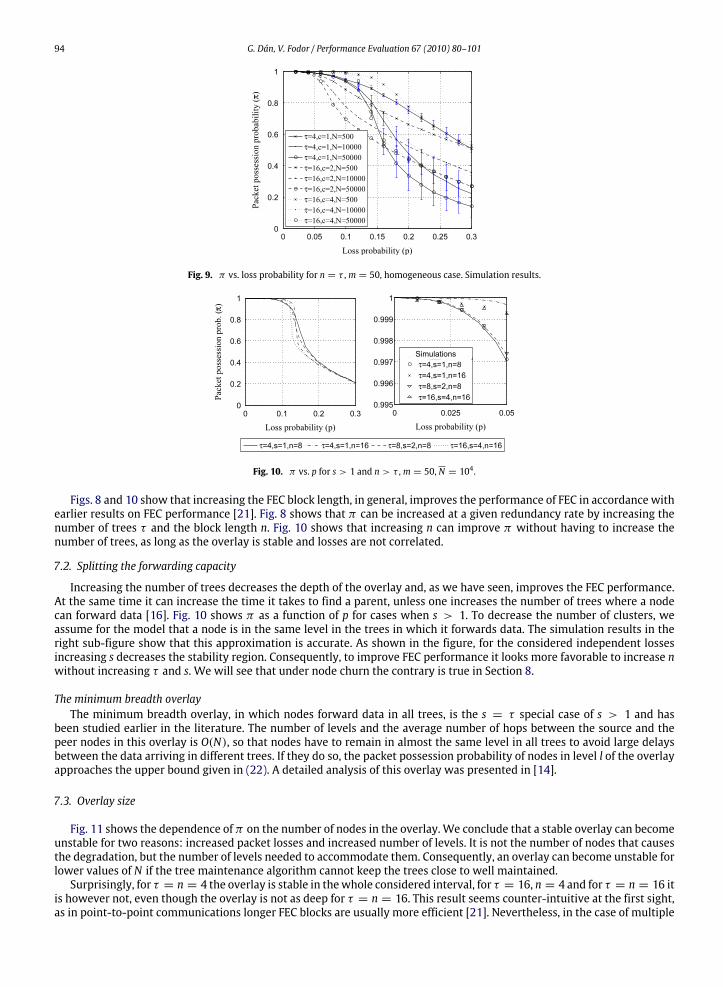
Fig. 9. π vs. loss probability for n = τ ,m = 50, homogeneous case. Simulation results.

Fig. 10. π vs. p for s > 1 and n > τ ,m = 50, N = 104 .

Figs. 8 and 10 show that increasing the FEC block length, in general, improves the performance of FEC in accordance withearlier results on FEC performance [21]. Fig. 8 shows that π can be increased at a given redundancy rate by increasing thenumber of trees τ and the block length n. Fig. 10 shows that increasing n can improve π without having to increase thenumber of trees, as long as the overlay is stable and losses are not correlated.

7.2. Splitting the forwarding capacity

Increasing the number of trees decreases the depth of the overlay and, as we have seen, improves the FEC performance.At the same time it can increase the time it takes to find a parent, unless one increases the number of trees where a nodecan forward data [16]. Fig. 10 shows π as a function of p for cases when s > 1. To decrease the number of clusters, weassume for the model that a node is in the same level in the trees in which it forwards data. The simulation results in theright sub-figure show that this approximation is accurate. As shown in the figure, for the considered independent lossesincreasing s decreases the stability region. Consequently, to improve FEC performance it looks more favorable to increase nwithout increasing τ and s. We will see that under node churn the contrary is true in Section 8.

The minimum breadth overlayThe minimum breadth overlay, in which nodes forward data in all trees, is the s = τ special case of s > 1 and has

been studied earlier in the literature. The number of levels and the average number of hops between the source and thepeer nodes in this overlay is O(N), so that nodes have to remain in almost the same level in all trees to avoid large delaysbetween the data arriving in different trees. If they do so, the packet possession probability of nodes in level l of the overlayapproaches the upper bound given in (22). A detailed analysis of this overlay was presented in [14].

7.3. Overlay size

Fig. 11 shows the dependence of π on the number of nodes in the overlay. We conclude that a stable overlay can becomeunstable for two reasons: increased packet losses and increased number of levels. It is not the number of nodes that causesthe degradation, but the number of levels needed to accommodate them. Consequently, an overlay can become unstable forlower values of N if the tree maintenance algorithm cannot keep the trees close to well maintained.Surprisingly, for τ = n = 4 the overlay is stable in thewhole considered interval, for τ = 16, n = 4 and for τ = n = 16 it

is however not, even though the overlay is not as deep for τ = n = 16. This result seems counter-intuitive at the first sight,as in point-to-point communications longer FEC blocks are usually more efficient [21]. Nevertheless, in the case of multiple


Fig. 11. π vs. number of nodes at p = 0.10, k/n = 0.75,m = 50.

Fig. 12. π vs. p for τ = 4, k/n = 0.75,m = 50, N = 104 , pω|ω = 0.3 correlated losses on the input or on the output links.

trees, FEC reconstruction close to the source requires packet reception in the trees, in which nodes are located in the lastlevels, and consequently are likely not to receive the packets unless FEC reconstruction works close to the source. Thus, alonger FEC code leads to higher possession probability if the system is stable, the region of stability is however smaller.

7.4. Limiting the level spread

Our model reveals a significant deficiency of the minimum depth overlay. The depth of the overlay influences theprobability of reconstruction even in nodes close to the source in the tree in which they forward, since reconstructionrequires packet reception in the other trees, in which nodes are located in the last levels. Motivated by this deficiency,we consider how our proposal to limit the level spread influences the overlay’s performance. Limiting the level spread canof course increase the number of levels in the overlay, but it makes FEC reconstruction more efficient. Fig. 11 shows thatlimiting the level spread does not decrease the performance of a stable overlay, but, as expected, the overlays with limitedlevel spread remain stable for larger values of N .

7.5. Sensitivity to correlated losses

One of the major detriments of FEC is its poor performance when losses are correlated. In order to evaluate how losscorrelations affect the performance of overlay multicast employing FEC we show π for correlated losses on the input linksor on the output links of the nodes in Fig. 12. We used the Gilbert model with a conditional loss probability of pω|ω = 0.3 tocalculate P fI (i, j) and P

fO(i, j), respectively. Correlations on the output links of the nodes have no effect on the performance

if n = τ , since the consecutive packets will be received by different child nodes. Correlations on the input links decreasehowever the performance compared to the case of independent losses for n = τ . A longer FEC block (n > τ ) increasesthe packet possession probability for both kinds of correlations when the overlay is stable. Based on the model we knowthat for correlated losses on the output links and for n > τ the performance approaches that of n = τ as pω|ω increases.Correlated losses affect the overlay’s performancemostly at low loss probabilities as correlations decrease themean numberof reconstructed packets. Consequently, correlations decrease the system’s region of stability and its region of potentialstability. The simulations shown in the right sub-figure showagoodmatchwith themodel for correlated losses on the outputlinks. There is amismatch in the case of correlations on the input links, as packets of the same block do not necessarily arrivesuccessively in the simulation (and in real systems), hence the loss correlation between packets in a block in the simulationis lower than pω|ω .


Fig. 13. π(l) vs. l for inhomogeneous losses. N = 104 ,m = 50, τ = n = 4, k = 3, s = 1. Model and simulations.

Fig. 14. π vs. packet loss probability for inhomogeneous losses and prioritization. N = 104 ,m = 50, τ = n = 4, k = 3, s = 1.

7.6. Inhomogeneous losses

Fig. 13 compares the performance of an overlay with N = 104 for four distributions of the loss probability experiencedby nodes and with the Bernoulli loss model. We use homogeneous (H) losses with probability p as the reference, andcompare that to the following scenarios: 80 percent of the nodes experience 0.75p while the rest 2p; uniform distributionon [0, 2p]; 50% of the nodes experience 0 while the rest 2p. We used 100 clusters per level to approximate the uniformdistribution in the model. Both the model and the simulations show that π(i) decreases as the variance of the lossesincreases.To see whether prioritization could help to alleviate the negative effects of loss inhomogeneity, Fig. 14 compares the

average packet possession probability in the overlay for four cases: homogeneous losses, for inhomogeneous losses withoutany priority scheme (Inhom-NP), for inhomogeneous losses prioritizing nodes with low packet loss probability (Inhom-P)and for inhomogeneous losses and prioritization, also limiting the level spread (Inhom-PL) with∆l = 2.We consider τ = 4,and N = 104 of which 50% experience 2p and 50% experience no losses. Prioritizing nodes based on the packet lossesthey experience can be difficult in practice, but it is still interesting if one could improve the system by such a scheme atall. Surprisingly, prioritization does not improve π in the stable region of the system. Nevertheless, nodes with no lossesexperience better performance due to prioritization, limiting the level spread giving slightly larger gain. In the unstableregion, prioritization pays off as the decrease of π becomes much slower.

7.7. Inhomogeneous capacities

We start by showing the effects of inhomogeneous output capacities. We consider prioritization based on the outputcapacities of the nodes. A practical alternative would be to consider the number of children of a node [11], as that is easierto estimate, but it would not help high contributor nodes joining the overlay for the first time.Fig. 15 considers an overlay with τ = 4, and N = 104, of which 65% are low contributors (LC) with dr = 2 and 35%

are high contributors (HC) with dr = 8. This ratio of high and low contributors is similar to that considered in [11] basedon a measured trace. The figure shows a scenario with homogeneous output capacities as reference, the inhomogeneouscase without priority, with priority, and also limiting the level spread with ∆l = 2. Prioritization does not make anydifference for a stable overlay, as the number of levels does not influence the performance of the overlay in the stableregion. High and low contributors experience the same performance too. We note that as the number of levels decreasesdue to prioritization based on the output capacities, the stability region might increase. For the same reason, prioritizationgives superior performance in the unstable state of the overlay. The simulations show a goodmatch with the model, though


Fig. 15. π vs. p for inhomogeneous output capacities. N = 104 ,m = 50, τ = n = 4, k = 3.

Fig. 16. π vs. p for inhomogeneous input capacities. N = 104 ,m = 50, τ = n = 4, k = 3.

for high losses the model somewhat overestimates π which is due to the difference between the number of levels in thesimulation and the one we calculated with.Next, we consider inhomogeneous input capacities in Fig. 16 for τ = 4 and N = 104. 65% of the nodes have |H r

| = 2and the rest |H r

| = 4. Prioritization is based on the input capacities of the nodes. Prioritization does not improve theperformance of the overlay in the stable state, though it proves to be beneficial in the unstable regime. Nevertheless, usingprioritization, nodes with high input capacity experience significantly better performance.As a next step, we combine the previous two scenarios in Fig. 17: for the low contributors we use |H r

| = 2, and forthe high contributors we use |H r

| = 4. The results show that the effects of prioritization are similar to those in Fig. 16,i.e., prioritization can give incentives to high contributors but does not improve the overall performance in the stable state.Limiting the level spread slightly improves the performance seen by high contributors, as expected.

8. Performance evaluation: Node churn

We start by evaluating the sensitivity of the mean ratio of disconnected parents, E[∆] to the node lifetime and thereconnection time distributions. We consider homogeneous input and output capacities and E[ΞF ] = E[ΞS], that is, thereconnection times are the same in the different trees. The simplicity of this scenario allows us to focus on the sensitivityof the results to the distributions. We simulated two node lifetime and three reconnection time distributions, and foreach combination we considered two scenarios, corresponding to u0 and uτ with graceful preemptions (α = 1). We setN = 104, m = 50. Figs. 18–20 show that the exponential approximation is accurate, and gives a lower bound for otherdistributions. Using a heavy-tailed distribution the proportion of short lived nodes is high, but they have fewer childrenupon their departure, hence their impact is lower on E[∆].

8.1. Effects on the data distribution

Next we apply the data distribution model to calculate π in the presence of node churn: for given κ we set P(Dfe = 0) =E[∆]. The simulation results shown for u0 for the data distribution performance show a similarly good match in Fig. 21.For packet losses due to network failures increasing the block lengthwithout increasing the number of trees does improve

the performance in a stable overlay as seen in Section 7. Fig. 22 shows that in the case of node departures this is notnecessarily true. For τ = 4, n = 16 the performance is equal to that of τ = 4, n = 8, and in fact is equal to that ofτ = n = 4. Increased block length gives however increased performance if the number of trees and the number of trees inwhich a node forwards data increase as well, as shown in the figure for s > 1. The simulations were performed using thePareto lifetime and normal reconnection time distributions and show that the approximation for n > τ is accurate.


Fig. 17. π vs. p for inhomogeneous input and output capacities. N = 104 ,m = 50, τ = n = 4, k = 3.

Fig. 18. E[∆] vs. 1/κ for log-normal lifetime and deterministic reconnection time distribution.

Fig. 19. E[∆] vs. 1/κ for Pareto lifetime and normal reconnection time distribution.

Fig. 20. E[∆] vs. 1/κ for Pareto lifetime and uniform reconnection time distribution.


Fig. 21. π vs. 1/κ for N = 104 , n = τ , k/n = 0.75,m = 50, u0 , the model and simulated lifetime distribution-reconnection time distribution pairs.

Fig. 22. π vs. 1/κ for s > 1 and n > τ .m = 50, N = 104 , k/n = 0.75.

8.2. Why does preemption improve the performance?

We showed in Section 7 that not even the ideal preemption strategies can significantly improve the average performanceof an overlay in its stable state in the case of packet losses. Nevertheless, simulation and measurement studies [5,11] showthat preemption does improve the overlay’s stability. The two are not contradictory.Fig. 23 showsπ as a function of the ratio of themean reconnection times of nodes in the trees in which they forward data

(E[ΞF ]) and in the ones in which they do not (E[ΞS]). For given E[Ξ ]we set E[ΞF ]+ (t−1)E[ΞS] = E[Ξ ] and consider twocases. The best case, graceful preemptions (E[ΩS] = E[M], α = 1), and the worst case, non-graceful preemptions occurringafter the departure of every node that forwards data (E[ΩS] = (t − 1)/tE[M], α = 0). The performance significantlyimproves as E[ΞS]/E[ΞF ] increases in both scenarios with a decreasing marginal gain, i.e., any preemption scheme thatdecreases E[ΞF ]without increasing E[Ξ ] is beneficial.Finally we look at the effects of taxation and contribution aware parent allocation [11] in Fig. 24. We consider an overlay

with τ = n = 8, k = 6, and N = 104. 75% of the nodes are low contributors (LC) with maximum outdegree dr = 4 andthe rest are high contributors (HC) with maximum outdegree dr = 16. The sum of all outdegrees is not enough for all nodesto connect to all trees. Hence, we consider four scenarios. In scenario NP 25% of the nodes connect to τ trees, 50% of themconnect to τ − 1 trees, and the rest to τ − 2 trees independent of their contribution. In scenarios P , Tax-P and CA-P nodesare prioritized based on their maximum outdegrees. In scenario P the number of trees the nodes can join is random as inNP . In scenario Tax-P every node connects to τ − 1 trees (taxation). In scenario CA-P HC nodes connect to τ trees, 67% ofLC nodes connect to τ − 1 trees, the remaining 33% connect to τ − 2 trees (contribution aware parent allocation). We useE[ΞS]/E[ΞF ] = 11 for all scenarios, that is, the reconnection time is shorter in the trees in which a node forwards data, butprioritizing HC nodes does not decrease their reconnection times. Based on Fig. 23 a further increase of E[ΞS]/E[ΞF ]wouldnot significantly influence the results. We do not model the decrease of E[ΞHCF ] and E[Ξ

HCS ], neither the possible increase

of E[Ξ LCF ] and E[ΞLCS ]. The effect of such inhomogeneity is like that of decreasing the loss probability seen by HC nodes and

increasing that seen by LC nodes. Hence, it is equivalent to the case of inhomogeneous losses, for which we showed earlierthat prioritization does not improve the overall performance in the stable state of the system (Fig. 14).The best average performance is achieved by the Tax-P scheme, the CA-P scheme performs slightly better than the NP

scheme. CA-P achieves the best performance for HC nodes, but the worst for LC nodes. Consequently, giving incentives toHC nodes can contradict to the goal of improving the average performance of the overlay.

9. Conclusion and practical consequences

In this paper, we presented an analytical model of the data distribution performance of multiple-tree-based overlaymulticast architectures. We developed lower and upper bounds for a class of overlays, and showed that the overlay’sperformance shows a phase transition depending on the packet loss probabilities and the size of the overlay. Our findingsled us to the definition of an overlay architecture with limited level spread that shows improved stability and scalability


Fig. 23. π vs. the ratio of reconnection times for the NP preemptive scheme.m = 50, N = 104 .

Fig. 24. π vs. E[Ξ ] form = 50, N = 104 , τ = n = 8, k = 6. Taxation and contribution aware parent allocation.

properties. Using the model, we evaluated the effects of inhomogeneous and correlated losses, heterogeneous input andoutput capacities, and investigated how prioritization can improve the overlay’s performance. We showed that the effectsof node churn are determined by the ratio of the reconnection time and parent disconnection intensity, and are similar innature to those of packet losses. Based on our results we can draw a number of practical consequences that can serve asdesign guidelines for future systems.FEC performance in overlaymulticast is determinedbymany systemparameters, a number ofwhich (e.g., loss probability,

node churn and overlay size) change dynamically. Hence, the FEC block length and the ratio of redundancy have to beadjusted adaptively in order to maintain the system in a stable state. Albeit FEC can provide arbitrarily good performance,the necessary ratio of redundancy can be high if retransmissions are not used to decrease the packet loss rate between nodes.Retransmissions and FEC are both needed to define an efficient and scalable overlay architecture. Nodes should maintain

a list of backup parents in order to decrease the losses caused by node departures. Backup parents can be asked occasionallyto retransmit a piece of data, and should be located no deeper in the tree than the parents of the node. Otherwise, ifretransmission requests are limited to the parent within the tree, then retransmissions do not decrease the loss probabilitycaused by the disconnections after node departures.Prioritization: The primary benefit of prioritization is the decrease of disturbances in the trees in which a node forwards

data. Prioritization does not always significantly improve the overall system performance, but it gives incentives to nodeswith good performance.Stability: If the overlay is stable, the number of levels does not influence the performance significantly. The number of

levels influences however the region of stability, so that the number of levels has to be kept low, e.g., by prioritizing highcontributor nodes. The stability region can be increased by using shorter FEC codes, though shorter FEC codes give inferiorperformance in the case of stability.Limited level spread: It is possible to increase the stability region of large overlays by limiting the spread between the

levels where nodes receive data. Limiting the level spread also helps to decrease the effects of nodes with poor connectionson the performance of high contributors.While one can argue about the fairness of this solution, it definitely gives incentivesto nodes to contribute.The proposed model can easily be extended, and can be a useful tool for future system designers. It is an open question

how the model can be applied to pull-based (a.k.a swarming) overlay multicast systems. We believe that there are manysimilarities between the two approaches, but we leave this as an area of future work.

References

[1] Y. Chu, S. Rao, S. Seshan, H. Zhang, A case for end system multicast, IEEE J. Select. Areas Commun. 20 (8) (2002).[2] M. Castro, P. Druschel, A. Kermarrec, A. Nandi, A. Rowstron, A. Singh, SplitStream: High-bandwidth multicast in a cooperative environment, in: Proc.of ACM SOSP, Oct. 2003.


[3] V. Padmanabhan, H. Wang, P. Chou, Resilient peer-to-peer streaming, in: Proc. of IEEE ICNP, 2003, pp. 16–27.[4] E. Setton, J. Noh, B. Girod, Rate-distortion optimized video peer-to-peer multicast streaming, in: Proc. of ACM APPMS, 2005, pp. 39–48.[5] M. Bishop, S. Rao, K. Sripanidkulchai, Considering priority in overlay multicast protocols under heterogeneous environments. in: Proc. of IEEEINFOCOM, April 2006.

[6] V. Venkataraman, K. Yoshida, P. Francis, Chunkyspread: Heterogeneous unstructured end system multicast, in: Proc. of IEEE ICNP, Nov. 2006.[7] X. Zhang, J. Liu, B. Li, T. Yum, Coolstreaming/donet: A data-driven overlay network for peer-to-peer live media streaming, in: Proc. of IEEE INFOCOM,2005.

[8] X. Hei, C. Liang, J. Liang, Y. Liu, K. Ross, A measurement study of a large-scale P2P IPTV system, IEEE Trans. Multimedia 9 (8) (2007) 1672–1687.[9] C. Wu, B. Li, Characterizing peer-to-peer streaming flows, IEEE J. Select. Areas Commun. 25 (9) (2007) 1612–1626.[10] Y. Shan, I. Bajić, S. Kalyanaraman, J.Woods, Overlaymulti-hop FEC scheme for video streaming, Signal Process.: Image Commun. 20 (8) (2005) 710–727.[11] Y. Sung, M. Bishop, S. Rao, Enabling contribution awareness in an overlay broadcasting system, in: Proc. of ACM SIGCOMM, 2006, pp. 411–422.[12] G. Wang, S. Futemma, E. Itakura, Multiple description coding for overlay network streaming, IEEE Multimedia 14(1)(2007)74–82.[13] T. Small, B. Liang, B. Li, Scaling laws and tradeoffs in peer-to-peer live multimedia streaming, in: ACMMultimedia, October 2006.[14] G. Dán, V. Fodor, G. Karlsson, On the stability of end-point-based multimedia streaming, in: Proc. of IFIP Networking, May 2006, pp. 678–690.[15] G. Dán, V. Fodor, I. Chatzidrossos, Streaming performance in multiple-tree-based overlays, in: Proc. of IFIP Networking, May 2007, pp. 617–627.[16] G. Dán, V. Fodor, I. Chatzidrossos, On the performance of multiple-tree-based peer-to-peer live streaming, in: Proc. of IEEE INFOCOM, May 2007.[17] R. Kumar, Y. Liu, K. Ross, Stochastic fluid theory for P2P streaming systems, in: Proc. of IEEE INFOCOM, May 2007.[18] D. Leonard, Z. Yao, V. Rai, D. Loguinov, On lifetime-based node failure and stochastic resilience of decentralized peer-to-peer networks, IEEE/ACM

Trans. Netw. 15 (3) (2007).[19] D. Carra, R. Lo Cigno, E. Biersack, Graph based modeling of P2P streaming systems, in: IFIP/TC6 Networking, May 2007.[20] I. Reed, G. Solomon, Polynomial codes over certain finite fields, SIAM J. Appl. Math. 8 (2) (1960) 300–304.[21] G. Dán, V. Fodor, G. Karlsson, On the effects of the packet size distribution on FEC performance, Comput. Netw. 50 (8) (2006) 1104–1129.[22] E. Elliott, Estimates of error rates for codes on burst-noise channels, Bell Syst. Tech. J. 42 (September) (1963) 1977–1997.[23] G. Ciardo, K.S. Trivedi, A decomposition approach for stochastic reward net models, Perform. Eval. 18 (1) (1993) 37–59.[24] J. Yedidia, W. Freeman, Y. Weiss, Understanding Belief Propagation and its Generalizations, in: Exploring Artifical Intelligence in the New Millenium,

ISBN: 1-55860-811-7, 2003.[25] D. Gross, C.M. Harris, Fundamentals of Queueing Theory, Wiley, New York, 1998.[26] E.W. Zegura, K. Calvert, S. Bhattacharjee, How to model an internetwork, in: Proc. of IEEE INFOCOM, March 1996, pp. 594–602.[27] E. Veloso, V. Almeida, W. Meira, A. Bestavros, S. Jin, A hierarchical characterization of a live streaming media workload, IEEE/ACM Trans. Netw. 14 (1)

(2006) 133–146.[28] K. Sripanidkulchai, B. Maggs, H. Zhang, An analysis of live streaming workloads on the Internet, in: Proc. of ACM IMC, 2004, pp. 41–54.[29] K. Sripanidkulchai, A. Ganjam, B. Maggs, H. Zhang, The feasibility of supporting large-scale live streaming applications with dynamic application

end-points, in: Proc. of ACM SIGCOMM, 2004, pp. 107–120.[30] P. Godfrey, S. Shenker, I. Stoica, Minimizing churn in distributed systems, in: Proc. of ACM SIGCOMM, 2006, pp. 147–158.[31] E. Gilbert, Capacity of a burst-noise channel, Bell Syst. Tech. J. 69 (Sept.) (1960) 1253–1265.[32] J.-Y. Le Boudec, M. Vojnovic, Perfect simulation and stationarity of a class of mobility models, in: Proc. of IEEE INFOCOM, March 2004.

GyörgyDán received theM.Sc. degree in Computer Engineering from the Budapest University of Technology and Economics (BME),Hungary in 1999 and the M.Sc. degree in Business Administration from the Corvinus University of Budapest, Hungary in 2003. Hereceived his Ph.D. in Telecommunications in 2006 from KTH, Royal Institute of Technology, Stockholm, Sweden. He worked asa consultant in the field of access networks, streaming media and videoconferencing 1999-2001. Currently, he is an assistantprofessor at KTH, Royal Institute of Technology. His research interests include the measurement, the design and the performanceevaluation of distributed multimedia systems.

Viktória Fodor has been an associate professor at the Laboratory for Communication Networks at KTH since 2007. She receivedher M.Sc. and Ph.D. degrees in Informatics from the Budapest University of Technology and Economics, Hungary in 1993 and1998 respectively. She worked as senior research engineer at the Hungarian Telecommunications Company in 1997–1998 andjoined KTH in 1999. She conducted research in the areas of all-optical networking, end-to-end traffic control and multimediacommunication. Her current interests include protocol design and performance evaluation of multimedia content distributionsystems.

Stability and performance of overlay multicast systems employing forward error correction

Documents

Transcript of Stability and performance of overlay multicast systems employing forward error correction