AN ABSTRACT OF THE THESIS OF

Haiping Zhou for the degree of Doctor of Philosophy in Civil

Engineering presented on March 12, 1990

Title: Development of a Mechanistic Overlay Design Procedure for

Flexible PavementsA

Redacted for Privacy

Abstract approved

R. GL'y Hicks

This dissertation describes the development of a mechanistic

overlay design procedure. The mechanistic analysis represents a new

trend in both new pavement and overlay design. The greatest advantage

of the mechanistic pavement analysis is that it considers the

fundamental characteristics of materials to be used, is capable of

considering changes in loading and tire pressure, and characterizes

the response of the pavement to traffic loads in terms of strains

and/or stresses. This type of analysis allows practicing engineers to

more realistically address pavement structure, materials, and other

influential variables such as environmental impacts so that the

behavior of the pavement may be better understood.

One of the critical steps in using the mechanistic type pavement

analysis is the determination of pavement layer properties (e.g,

resilient modulus). In this study, methods commonly used for

determining resilient modulus have been reviewed. Three existing

mechanistic overlay design procedures were also reviewed. Based on

the review, improved procedures for determining pavement layer moduli

and overlay design seem to be necessary.

Significant contributions of this study are the development and

computerization of an improved backcalculation procedure (BOUSDEF)

for determining pavement layer moduli and an improved mechanistic

overlay design procedure (MECHOD).

Initial evaluations on both procedures were performed. For

BOUSDEF, three approaches were used: 1) comparing with hypothesized

theoretical moduli, 2) comparing with other developed backcalculation

programs, and 3) comparing with laboratory tested modulus values. The

evaluation showed BOUSDEF provided favorable comparisons. Therefore,

the program can be effectively used as a tool to make initial

evaluation of deflection testing data for determining pavement layer

moduli. For MECHOD, actual pavement data from the states of Oregon

and Alaska were used. All pavements evaluated are conventional

structures consisting of an asphalt concrete surface, an aggregate

base and/or a subbase, over subgrade. The evaluation showed that the

improved method provided very similar results to those of standard

procedures (ODOT, AASHTO, and The Asphalt Institute).

The BOUSDEF and MECHOD programs can be implemented together as a

pavement evaluation and overlay design system. That is; 1) use

BOUSDEF to backcalculate pavement layer moduli, and 2) use MECHOD to

perform overlay design.

DEVELOPMENT OF A MECHANISTIC OVERLAY DESIGN PROCEDURE

FOR FLEXIBLE PAVEMENTS

by

Haiping Zhou

A Thesis

submitted toOregon State University

in partial fulfillment of

the requirements for the

degree of

Doctor of Philosophy

Completed March 12, 1990

Commencement June 10, 1990

Approved:

Redacted for Privacy

Professor of Civil Engineering in Charge of Major

Redacted for PrivacyHead of Department of Civil Engine97ng

Redacted for Privacy

Dean of School d

Date thesis is presented March 12, 1990

Typed by Haiping Zhou for Haiping Zhou

ACKNOWLEDGEMENTS

I wish to express my sincere appreciation to my major professor,

Dr. Gary Hicks, for his invaluable direction, guidance, and

consultation during the course of this study. In particular, his

knowledge and experience is greatly acknowledged.

My appreciation is also expressed to the members of my graduate

committee, Professors Robert Layton, David Rogge, and Ken Funk, and

to the graduate school representative, Professor David Thomas, for

their assistance in developing my academic program.

I would also like to thank Professor Frank Schaumburg, head of

Civil Engineering Department, for providing assistantship throughout

the entire period of this research. Most importantly, the friendship,

care, and encouragement given by Frank and his wife Judy, will never

be forgotten.

Thanks also go to Jim Huddleston, pavement design engineer of

Oregon State Highway Division, for his guidance and advice. His

experience in the pavements area provided very helpful assistance to

this research and is greatly acknowledged.

I also wish to thank the following people:

1) Ted Vinson, Professor of Civil Engineering Department, for

providing pavement project data and valuable consultation.

2) Andy and Nancy Brickman, Gail Barnes, and Linda Rowe, faculty

of Civil Engineering Department, for their help and assistance in

various aspects, and most importantly, their friendship.

3) "Bud" Furber, Principal of the Pavement Services, Inc. of

Portland, for providing pavement materials for the laboratory

testing.

4) Billy Connor and David Esch, senior research engineers of the

Alaska Department Transportation and Public Facilities, for providing

pavement project data and part of the research funds.

5) Doug Hedlund and the field crew, of Oregon State Highway

Division, for performing the deflection tests.

Finally, I thank my wife, son, and my parents for their support

all these years.

TABLE OF CONTENTS

1.0

2.0

INTRODUCTION

1.1 Problem Statement

1.2 Objectives

1.3 Scope

BACKGROUND ON MECHANISTIC ANALYSIS FOR FLEXIBLE PAVEMENTS

Page

1

1

4

4

12

2.1 Stresses, Strains and Deformations in Pavements 12

2.1.1 Basic Law 13

2.1.2 Elastic Half-Space System(Boussinesq Equations) 13

2.1.3 Layered Systems 15

2.1.4 Comparison Between Layered Theory andBoussinesq Theory 28

2.2 Non-Linearity of Pavement Materials 43

2.3 Consideration of Overburden Stresses 45

2.4 Summary 46

3.0 DETERMINATION OF PAVEMENT MODULI USING NDT METHODS 48

3.1 Background 48

3.2 Some Existing Approaches 53

3.2.1 Equivalent Thickness Methods 533.2.2 Elastic Layer Methods 573.2.3 Finite Element Method 78

3.3 Summary 85

4.0 DEVELOPMENT OF AN IMPROVED BACKCALCULATION PROGRAM 86

4.1 Program Development and Description 874.1.1 Program Flowchart 874.1.2 Program Output 904.1.3 Example 914.1.4 Sensitivity to the User Input 91

4.2 Evaluation of the BOUSDEF Program 954.2.1 Comparison with Theoretical Values 954.2.2 Comparison with Other Developed Programs 994.2.3 Comparison with Laboratory Test Results 99

5.0

4.3 Summary

DETERMINATION OF RESILIENT MODULUS USING LABORATORY TESTSAND CORRELATIONS

Page.

133

134

5.1 Resilient Modulus from Laboratory Tests 1345.1.1 Diametral Tests 1355.1.2 Triaxial Tests 139

5.2 Correlations 1395.2.1 Subgrade Soil 1425.2.2 Untreated Granular Materials 1475.2.3 Asphalt Concrete 152

5.3 Summary 154

6.0 DEVELOPMENT OF AN IMPROVED MECHANISTIC OVERLAY DESIGNPROCEDURE FOR FLEXIBLE PAVEMENTS 158

6.1 Review of Current Mechanistic Overlay Design Methods 1586.1.1 ARE Method 1586.1.2 WSDOT Method 1706.1.3 Alaska Method 181

6.1.4 Summary of Review 186

6.2 Development of An Improved Mechanistic Overlay DesignProcedure 1876.2.1 Framework 1876.2.2 Condition Survey 1876.2.3 Nondestructive Testing 1916.2.4 Delineation of Analysis Section 1916.2.5 Material Characterization 1926.2.6 Consideration of Seasonal Effect 1926.2.7 Critical Pavement Strains 2026.2.8 Determination of Allowable Traffic

Repetitions 2026.2.9 Determination of Pavement Damage 2166.2.10 Overlay Thickness Design 217

6.3 Summary 219

7.0 EVALUATION OF THE DEVELOPED PROCEDURE 221

7.1 Overlay Design Using MECHOD 2217.1.1 Selection of Project Sites 2217.1.2 Deflection Tests 2247.1.3 Determination of Pavement Moduli for

Overlay Design 2247.1.4 Traffic Analysis 2317.1.5 Overlay Design 232

Page

7.2 Overlay Design Using Standard Procedures 2377.2.1 ODOT Procedure 2377.2.2 1986 AASHTO Design Procedure 2407.2.3 The Asphalt Institute Design Procedure 253

7.3 Comparison of Design Results 256

7.4 Summary 260

8.0 CONCLUSIONS AND RECOMMENDATIONS 261

8.1 Conclusions 262

8.2 Recommendations for Implementation 264

8.3 Recommendation for Further Research 266

9.0 REFERENCES 268

APPENDICES

Appendix A. BOUSDEF User's Guide 280

Appendix B. Deflection Test Results for Selected Projects 285

Appendix C. AMOD User's Guide 308

Appendix D. FWD Data Delineation Program User's Guide 310

Appendix E. MECHOD User's Guide 324

Appendix F. Backcalculation Results 330

Appendix G. Overlay Design Output from the MECHOD Program 344

Appendix H. Deflection Data Used in ODOT andTAI Procedures 350

Appendix I. Calculation of Structural Numbers Used inAASHTO Procedure 357

LIST OF FIGURES

Figure Page

1.1 Study Approach 11

2.1 Definition of Coefficient of Elasticity and Poisson'sRatio for the Uniaxial Case 14

2.2 Conceptual Representation of Boussinesq's Half SpaceLoading Condition 16

2.3 Generalized Multi-Layered Elastic System 19

2.4 Conceptual Representation of the Method of EquivalentThicknesses 21

2.5 Pavement Structures Used for Comparing Surface DeflectionsUsing Layered Theory and Boussinesq Equations 31

2.6 Deflection Comparison for Three-Layer ConventionalFlexible Pavements 34

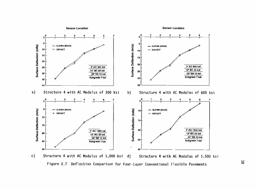
2.7 Deflection Comparison for Four-Layer ConventionalFlexible Pavements 38

2.8 Deflection Comparison for Pavements with a CementTreated Base 40

2.9 Deflection Comparison for Portland Cement Concrete Pavements 42

2.10 Modulus-Bulk Stress Relationship for Coarse-GrainedMaterials 44

2.11 Modulus-Bulk Stress Relationship for Fine-Grained Materials 44

3.1 Conceptual Illustration of Backcalculation Approach 52

3.2 Four Layer Elastic Representation of a Pavement System 58

3.3 CHEVDEF/BISDEF Program Flowchart 61

3.4 Simplified Description of the Deflection Matching Procedure 62

3.5 Interpolation of Modulus Using Calculated and MeasuredDeflections in MODCOMP2 Program 68

3.6 Pavement Model Showing Line of 95% Deflection 70

3.7 Simplified Flowchart of FPEDDI 73

3.8 Subgrade Soil Material Models for ILLI-PAVE Analysis 83

Figure Page

4.1 Flowchart of the BOUSDEF Program 88

4.2 Plot of the Example Output 94

4.3 Location of Selected Project Sites 104

4.4 Backcalculated Base and Subgrade Moduli forthe Rufus-Quinton Project (Eastbound) 113

4.5 Backcalculated Base and Subgrade Moduli forthe Rufus-Quinton Project (Westbound) 114

4.6 Backcalculated Base and Subgrade Moduli for theCentennial Blvd Project (Station 200 to 400, Eastbound) 115

4.7 Backcalculated Base and Subgrade Moduli for theCentennial Blvd Project (Station 4200 to 7000, Eastbound) 116

4.8 Backcalculated Base and Subgrade Moduli for theCentennial Blvd Project (Station 6900 to 2700, Westbound) 117

4.9 Backcalculated Base and Subgrade Moduli for theCentennial Blvd Project (Station 2500 to 100, Westbound) 118

4.10 H&V Diametral Testing System 120

4.11 H&V Triaxial Testing System 120

4.12 Moisture-Density Relationship for the Rufus-QuintonProject 122

4.13 Laboratory Tested Moduli for the Rufus-Quinton Project 124

4.14 Laboratory Tested Moduli for the Centennial Blvd Project 128

4.15 Comparison Between Laboratory Tested and BackcalculatedAC Moduli for the Rufus-Quinton Project 129

4.16 Comparison Between Laboratory Tested and BackcalculatedAC Moduli for the Centennial Blvd Project 130

4.17 Comparison Between Laboratory Tested and BackcalculatedBase Moduli for the Rufus-Quinton Project 131

4.18 Comparison Between Laboratory Tested and BackcalculatedBase Moduli for the Centennial Blvd Project 132

5.1 Diametral Resilient Modulus Device Yoke and Alignment Stand 136

5.2 Test Specimen with Diametral Yoke and Loading Ram 137

Figure Page

5.3 Schematic of Asphalt Concrete Laboratory ResilientModulus Test 138

5.4 Triaxial Cell Suitable for Repeated Load Testing of Soils 140

5.5 Schematic Diagram of Resilient Modulus Test 141

5.6 Relation Between Dynamic Modulus and CBR 143

5.7 Crude Empirical Relationships Between the Dynamic Modulusof Elasticity and Routine Tests 148

6.1 Flowchart for the Mechanistic Method 159

6.2 Photographs of Class 2 and Class 3 Cracking 165

6.3 Relationship of Resilient Modulus and Repeated DeviatorStress 166

6.4 Fatigue Curve for 18-kip Load Applications to Time ofClass 2 Cracking 167

6.5 Sample Overlay Thickness Design Curves 171

6.6 Pavement Overlay Design Concept 172

6.7 General Stiffness-Temperature Relationship with 90 and95% Prediction Intervals for Class B Asphalt Concrete InWashington State 176

6.8 Estimation of Pavement Temperature 178

6.9 Overlay Design Procedure by EVERPAVE 180

6.10 Flowchart for the Simplified Mechanistic Procedure 182

6.11 Flowchart for the Improved Overlay Design Approach 188

6.12 Comparison of MS-1 Prediction Equation to Modulus-Temperature Relationship Used in MS-11 193

6.13 Computed Relations Between Mixture Stiffness andTemperature 194

6.14 Seasonal Influence on Asphalt Concrete Layer Modulus 195

6.15 Temperature Influence on Poisson's Ratio 195

6.16 Influence of Degree of Saturation on StiffnessCharacteristics of Untreated Granular Material 197

Figure Page

6.17 Water Content Dry Density Resilient ModulusRelationship for Subgrade Soil 198

6.18 Concept of Seasonal Roadbed Soil Variation 199

6.19 Effect of Freeze-Thaw, Additional Loading, and AdditionalCuring on Resilient Response of a Natural Tama B Soil 200

6.20 Concept of Seasonal Variation on Traffic Distribution 201

6.21 Location of the Critical Strains 203

6.22 Fatigue Curves for Some California Mixes Using DifferentFailure Criteria 205

6.23 Fatigue Curves for Asphaltic Concrete 206

6.24 Fatigue Curves Developed by Nottingham 211

6.25 Critical Strain Locations for Overlay Design 215

6.26 MECHOD Program Flowchart 218

7.1 Location of Selected Project Sites 222

7.2 Asphalt Modulus Temperature Adjustment Factor 227

7.3 Temperature Correction Factors Used in ODOT OverlayDesign Procedure 239

7.4 Tolerable Deflection Chart Used in ODOT OverlayDesign Procedure 241

7.5 Percent Deflection Reduction Chart Used in ODOTOverlay Design Procedure 242

7.6 Relationship Serviceability-Capacity Condition Factorand Traffic 245

7.7 AASHTO Overlay Design Steps 246

7.8 Chart for Estimating Structural Layer Coefficient of Dense-graded Asphalt Concrete Based on the Resilient Modulus 248

7.9 Variation in Granular Base Layer Coefficient (a2) withVarious Base Strength Parameters

7.10 Variation in Granular Base Layer Coefficient (a3) withVarious Subbase Strength Parameters

249

250

Figure Page

7.11 Design Chart for Flexible Pavements Based on Using MeanValues for Each Input

7.12 Remaining Life Factor

7.13 Temperature Correction Factors Used in The AsphaltInstitute Procedure

7.14 Asphalt Concrete Overlay Thickness Required to ReducePavement Deflections from a Measured to a DesignDeflection Value (Rebound Test)

252

254

257

258

A-1 BOUSDEF Menu Screen 281

A-2 BOUSDEF Data Input/Edit Screen 282

D-1 Concepts of Cumulative Difference Approach to AnalysisUnit Delineation 311

D-2 Title Screen 316

D-3 Asking for File Name 316

D-4 Heading for TEST.DAT 317

D-5 Program Main Menu 317

D-6 Bar Chart Representation of Pavement Response 319

D-7 Options for Defining Delineation Units 320

D-8 Screen Display for Option 1 320

E-1 MECHOD Program Main Menu 325

E-2 MECHOD Screen Data Input/Edit 325

E-3 Screen for Data Analysis 328

E-4 Example Output Showing Overlay is Needed 328

E-5 Modulus of Overlay Material Can Be Considered 329

E-6 Example Output 329

LIST OF TABLES

Table Page

1.1 Advantages and Disadvantages of Overlay Design Procedures 3

2.1 Boussinesq Equations for a Point Load 17

2.2 Boussinesq Equations for a Distribute Load 18

2.3 Summary of Flexible Pavement Models 26

2.4 Stresses, Strains, and Displacements Calculated by BISAR 29

2.5 Summary of Deflection Calculations 32

3.1 Typical Poisson's Ratio Values 49

3.2 Summary of Self-Iterative Procedures for Evaluation ofPavement Moduli from Deflection Basins 54

3.3 Material Characterization for ILLI-PAVE Program 82

4.1 Pavement and Deflection Data for the Example 92

4.2 Summary of Backcalculation Results for the Example 93

4.3 Data Used for Evaluating Sensitivity on Initial Modulus 96

4.4 Effect of Initial Moduli on Calculated Moduli Using BOUSDEF 97

4.5 Comparison Between Theoretical and Backcalculated ModulusValues 98

4.6 Pavement Data Used for Backcalculation 100

4.7 Deflection Data Used for Backcalculation 100

4.8 Summary of Backcalculation Results 101

4.9 Comparison of Computing Time and Backcalculated Results 102

4.10 Summary of Selected Project Sites 104

4.11 Backcalculated Modulus for the Rufus-Quinton Project(EB and WB) 107

4.12 Backcalculated Modulus for the Centennial Blvd Project 109

4.13 Summary of AC Resilient Modulus Test for Rufus-QuintonProject 121

Table Page

4.14 Summary of AC Resilient Modulus Test for Centennial BlvdProject 121

4.15 Moisture-Density Relationship for the Rufus-QuintonProject 122

4.16 Density Results for the Rufus-Quinton Project 123

4.17 Summary of Base Material Resilient Modulus Test forthe Rufus-Quinton Project 123

4.18 Water Content and Density at Time of Testing forCentennial Blvd Project 126

4.19 Summary of Base Material Resilient Modulus Testfor Centennial Blvd Project 127

5.1 Comparison of R, CBR, and Resilient Modulus Data 145

5.2 Various Regression Equations for Subgrade Modulus 146

5.3 Correlations Between MR, CBR, or R and Stress State 149

5.4 Summary of Repeated Load Triaxial Compression LaboratoryTest Data for Untreated Granular Materials 150

5.5 Typical Values for kl and k2 for Unbound Base and SubbaseMaterials 151

5.6 Typical Values of Stress State 153

5.7 Variables Affecting Materials Response 156

6.1 Analytical Based Overlay Design Procedures 160

6.2 Guidelines for Nondestructive Testing 161

6.3 Classes of Cracking 164

6.4 Coefficients for Seasonal Variations 175

6.5 Summary of Some Fatigue Criteria 208

6.6 Summary of Some Rutting Criteria 213

7.1 Summary of Selected Projects 223

7.2 Summary of Backcalculated Moduli 226

7.3 Backcalculated AC Moduli Converted to 70°F 228

Table Page

7.4 Representative Temperature Used for Evaluation 228

7.5 Modulus Values Corrected for Temperature for AC 229

7.6 Modulus Values Used in Overlay Design Analysis 230

7.7 Traffic Data for Overlay Design 233

7.8 Traffic Distribution for Each Season 234

7.9 Modulus Data for Overlay Materials 236

7.10 Overlay Design from MECHOD 236

7.11 Overlay Thickness Design Using ODOT Procedure 243

7.12 Overlay Thickness Design Using AASHTO Procedure 255

7.13 Overlay Thickness Design Using TAI Procedure 259

7.14 Comparison of Overlay Design Results 259

D-1 Tabular Solution Sequence Cumulative Difference Approach 314

D-2 Example Output for User Defined Delineation Units 321

D-3 Example Output for Program Defined Delineation Units 321

D-4 Example Output for TEST.FWD File 323

DEVELOPMENT OF A MECHANISTIC OVERLAY DESIGN PROCEDURE

FOR FLEXIBLE PAVEMENTS

1.0 INTRODUCTION

1.1 Problem Statement

As the nation's highways age and are subjected to ever

increasing loads and volume of traffic, they will inevitably

deteriorate and eventually require some type of treatment to be able

to provide a safe and serviceable facility for the user (Finn, 1984).

The types of treatment that are appropriate to maintain pavement

serviceability can range from relatively simple maintenance to

complete reconstruction. For pavements subjected to moderate and

heavy traffic, asphalt overlays provide one of the most cost-

effective methods of improving existing pavements (The Asphalt

Institute, 1983). Asphalt overlays can be used to strengthen existing

pavements, to reduce maintenance costs and increase pavement life, to

provide a smooth ride, and to reduce safety hazards by improving

pavement surface skid resistance.

The design approach used to determine the thickness of the

overlay can range from engineering judgement to a fully mechanistic

analysis. Generally, the design procedures may be categorized into

four types: 1) engineering judgement, 2) component analysis, 3)

nondestructive testing with limiting deflection criteria, and 4)

mechanistic analysis based on interpretation of nondestructive

testing or laboratory data with appropriate failure criteria.

Current overlay design procedures generally fall in the first

2

three categories. The major limitations for each of the current

design procedure are listed below:

1) Engineering judgement no theoretical background,

subjective, and vulnerable to personnel changes.

2) Component analysis primarily based on empirical

relationships developed from the AASHO Road Test and is

difficult to evaluate changes in loads and environmental

impacts.

3) Limiting deflection methods maximum deflection does not

reflect individual layer properties and is limited to

materials and constructions for which correlations are

established.

The mechanistic type of analysis represents a new trend for

overlay design. The greatest advantage of the mechanistic type of

pavement analysis is that it considers the fundamental

characteristics of materials to be used, is capable of considering

changes in loading and tire pressure, and characterizes the response

of the pavement to traffic loads in terms of strains and /or

stresses. This type of analysis allows practicing engineers to more

realistically address pavement structure, material, and other

influential factors such as environmental impacts so that the

behavior of the pavement may be better understood. Some of the

advantages and disadvantages of these four types of overlay design

procedures are summarized in Table 1.1.

3

Table 1.1 Advantages and Disadvantages of Overlay Design Procedures

(Hicks, 1988)

Procedure Advantages Disadvantages

EngineeringJudgment

Simple. No theoretical basis.

Subjective.

ComponentAnalysis

Assesses individual layers as they existin the pavement.

Related to existing conventional designprocedures that have large amount ofbackground information.

Limited amount of sampling and testing (tominimize cost).

Conditions at the time of sampling may notrepresent general state of materials.

Time required for sampling and testing.

Oriented to distress mode for whichassociated design procedure was developed;e.g., CBR procedure associated with plasticdeformation.

Not applicable to new materials

DeflectionBased

Areal coverage.

Measurements representative of insituconditions.

Relatively inexpensive.

Relatively fast.

Relatively high degree of reliabilitypossible.

Does not measure materials properties.

Limited to materials and constructions forwhich correlations are established.

Related to one mode of distress; e.g.,fatigue cracking.

AnalyticallyBased

(mechanistic)

Appropriate distress modes can beconsidered individually; e.g., fatigue,rutting, lowtemperature cracking.

Capable of considering:

changed loading and tire pressureeffects,new materials,

environmental influences,aging effects, andinfluence of changed subsurfacedrainage conditions.

Unfamiliar to most current designers.

Requires new and different equipment.

Limited experience to date.

May require the use of a computer.

4

1.2 Objectives

The major objectives of this study are to develop a fully

mechanistic overlay design procedure for flexible pavements and a

fully computerized procedure for routine design work. Specifically,

the objectives are to:

1. develop an improved mechanistic overlay design procedure,

2. develop an improved backcalculation procedure for

determining existing pavement structural capacity,

3. evaluate the developed backcalculation procedure,

4. evaluate the developed overlay design procedure on

selected projects, and

5. prepare recommendations for implementation of the

procedures.

1.3 Scope

To accomplish the objectives, the following tasks were

undertaken:

1. review of stresses, strains, and deformations in pavement

structures, including consideration of non-linearity of

pavement materials and overburden stresses (Chapter 2),

2. review of current methods for backcalculating layer moduli

(Chapter 3),

3. development and evaluation of an improved backcalculation

procedure for determining pavement layer moduli (Chapter

4),

4. Review of modulus determination using laboratory tests and

correlations (Chapter 5),

5

5. review of current mechanistic overlay design procedures

and development of an improved mechanistic overlay design

procedure, (Chapter 6),

6. evaluation of the improved procedures on selected projects

(Chapter 7), and

7. recommendations for implementation (Chapter 8).

Task 1: This task reviewed background information necessary

for mechanistic analysis of pavement structures. In particular,

stresses, strains, and deformations in pavements resulting from

traffic loads were reviewed. Methods that are commonly used to

calculate stresses, strains, and deformations were discussed.

Many researchers have shown that pavement materials, especially

coarse-grained and fine-grained, are load dependent. That is, these

materials behave differently under different stress conditions. For

coarse-grained materials, which are usually used for base layers, the

resilient modulus increases as the applied load or stress increases.

For fine-grained materials, which are usually used for subgrade, the

resilient modulus decreases as the stress magnitude increases. These

non-linear properties of pavement materials should be carefully

considered for the design condition. Static pressure or overburden

stress of pavement materials were also reviewed.

Task 2: In using a mechanistic approach, one of the most

important considerations is the determination of resilient modulus

values for each pavement layer. This fundamental material property

represents the structural capacity of the material and has a great

impact on design thicknesses needed to carry the anticipated traffic

applications. Two methods have been used for determining the modulus

6

values of a pavement material, laboratory tests and backcalculation.

Laboratory tests are performed on materials sampled from field using

specialized equipment. Backcalculation is conducted using a computer

program to calculate modulus values for each layer from deflection

basin data which can be measured using a non-destructive device.

Several backcalculation programs have been developed and are widely

used for determining modulus values. These existing procedures can be

broadly categorized into three groups: 1) equivalent thicknesses

methods, 2) elastic layer methods, and 3) finite element methods. Two

programs in the category of method of equivalent thicknesses were

reviewed. They are ELMOD and SEARCH. Several programs in the group of

elastic layer method were also looked into. These programs are

CHEVDEF/BISDEF, ELSDEF, MODCOMP2, MODULUS, PFEDDI, and ISSEM4. A

single backcalculation procedure ILLI-CALC which uses finite element

method was also reviewed.

It is difficult to conclude if one program is superior to the

others. In general, the programs which use the method of equivalent

thicknesses take much less computing time than both elastic layer

theory and finite element methods.

Task 3: Preliminary use of three backcalculation programs,

BISDEF, ELSDEF, and MODCOMP2, shows that both BISDEF and ELSDEF do

not consider the non-linearity of the pavement materials. MODCOMP2 is

capable of handling non-linearity of the pavement materials; however,

this capability does not always operate properly. Very often, unknown

errors occur during computation. And all three programs take a fair

amount of computing time to solve a data set. This significantly

impairs the use of the backcalculation method. Task 3, therefore, was

7

to develop an improved method for backcalculation. This improved

backcalculation method uses much less computing time for

backcalculation and also considers the non-linearity of the base and

subgrade materials.

Initial evaluation on the developed backcalculation procedure

was made. The evaluation was performed using three approaches: 1)

comparing backcalculated moduli with preassumed theoretical moduli,

2) comparing with other backcalculation programs, and 3) comparing

backcalculated moduli with laboratory test results. The evaluation

shows that the moduli backcalculated using the BOUSDEF program

compare very well with the preassumed theoretical values and are very

compatible with the other programs used for comparison. The

comparison with the laboratory test results on the two projects also

compared favorably.

Task 4: This task reviewed several techniques for

determining resilient modulus through laboratory tests and using

developed correlations, which are widely used around the United

States. These techniques include laboratory tests to determine

resilient moduli of pavement materials and correlations to estimate

the resilient modulus.

The advantage of the laboratory tests to determine resilient

modulus is its ability to measure the strength of a particular

material directly. The disadvantage is that the samples tested in the

laboratory may represent a portion of pavement material rather than

an average condition one would find in the field. Moreover,

laboratory tests require sophisticated equipment and well trained

personnel to perform the tests, and laboratory tests usually take a

8

significant amount of time.

The advantage of using developed correlations is their

availability. However, one must be aware that the correlations were

developed based on certain laboratory conditions. Therefore, these

correlations are best suited to situations similar to those for which

the correlations were developed. Caution should be exercised when

using these correlations.

Task 5: In the past years, several overlay design procedures

using the mechanistic approach have been developed such as the Alaska

DOT&PF, Washington State DOT, and ARE methods. This task reviewed

these three methods. The review indicated that one common ground for

these developed procedures is that they all use multi-layered elastic

theory to model a flexible pavement structure and to determine

pavement life using various design criteria. This kind of approach is

also being used by an on-going research activity, NCHRP project 1-26

(Thompson, 1989). It is expected that the next edition of the AASHTO

Guide on flexible pavement design will also move in this direction.

A shortcoming in all three procedures is that of characterizing

the seasonal effects on the pavement materials properties. In both

the ARE and the Alaska methods, pavement properties at a

representative temperature of 70°F are recommended for design

purposes rather than those at different seasons. In the WSDOT method,

seasonal variations are considered. However, for the base and

subgrade materials, modulus ratios between the dry and wet materials

are used rather than a direct consideration of the base and subgrade

material properties for each season. Since the seasonal effects have

great influence on pavement layer properties (and some other factors

9

such as traffic distribution), which in turn may result in varying

pavement damage, therefore, an improved approach to address the

seasonal effects seems to be necessary.

Based on the review, an improved mechanistic overlay design

procedure was developed. The major improvement over the above three

procedures is in the direct consideration of seasonal effects on

pavement material properties and pavement damage due to traffic

loadings within each season.

The improved procedure has been computerized and can be operated

on IBM or compatible microcomputers. The resulted computer program

MECHOD is easy to use and user friendly.

Task 6: This task evaluated the improved mechanistic overlay

design procedure. The evaluation included the following steps:

1. Select projects for evaluation.

2. Perform deflection test using FWD.

3. Determine pavement layer moduli for overlay design.

4. Perform overlay design using the improved procedure.

5. Compare overlay design results from the improved procedure

with those from standard procedures.

The initial evaluation of the improved mechanistic overlay design

procedure was performed using actual pavement data from the states of

Oregon and Alaska. All pavements evaluated are conventional pavements

consisting of an asphalt concrete surface, an aggregate base and/or a

subbase, and subgrade. The overlay design results from the improved

procedure were compared with three standard procedures developed by

ODOT, AASHTO, and The Asphalt Institute. The results showed that the

improved method provided very compatible results to those of the

10

standard procedures.

Task 7: This task summarizes the work accomplished during

this study and provides recommendations for implementation.

Specifically, these recommendations include the use of BOUSDEF, a

backcalculation program, and MECHOD, an improved mechanistic overlay

design program, both developed during the course of the study.

For additional research recommendations, verification of the

backcalculated results and development of design criteria for local

conditions are suggested. Further improvements to BOUSDEF and MECHOD

programs are also discussed. The overall study approach for

conducting this research is summarized in Figure 1.1.

LiteratureReview

Review and Evaluation ofExisting Procedures

iDevelopment of An Improved

Backcalculation Method

iEvaluation of the Developed

Backcalculation Method

iDevelopment of An

Improved MechanisticOverlay Design Procedure

iEvaluation of the DevelopedOverlay Design Procedure

Conclusions andRecommendations

Figure 1.1 Study Approach

I

11

12

2.0 BACKGROUND ON MECHANISTIC ANALYSIS FOR FLEXIBLE PAVEMENTS

Pavement analysis, design and evaluation, as other engineering

techniques, might be better accomplished if the engineer had the

ability to analyze the pavement structure in terms of some

fundamental concepts such as the stresses, strains, or deformations

and the characteristics of the pavement material due to the

application of traffic, environment, and the effects of aging. This

chapter describes some of these basic concepts related to this

research.

2.1 Stresses, Strains, and Deformations in Pavements

Pavements under traffic load application experience stresses,

strains or deformations. The pavement response can be determined

quantitatively using theoretical analysis. Analysis theories that

have been developed or are being developed include elastic half-space

system, layered elastic theory, finite element analysis, and

viscoelastic analysis. The theory of elasticity is by far the most

wide spread method. This research uses the theory of elasticity as a

tool for the development of a mechanistic overlay design procedure.

Before developing an improved mechanistic overlay design

procedure, a backcalculation program (based on elastic half-space

system) is developed to determine pavement layer moduli, a key

element in pavement analysis using a mechanistic approach. The

following paragraphs describe first the solution techniques used to

develop the backcalculation program.

13

2.1.1 Basic Law

The basic law used in the theory of elasticity is that developed

by Hookes. Two material parameters are needed to use the theory: the

coefficient of elasticity (Young's modulus, E) and Poisson's ratio

(j). The coefficient of elasticity is defined as the ratio of stress

(a) over strain (c) and is a constant as stated by Hookes's law.

Poisson's ratio is defined as the ratio of lateral and axial strains

as shown in Figure 2.1. In the sample case, the Poisson's ratio is a

constant. For the three dimensional case, generalized Hookes's law

may be expressed as:

E * ex = ax A (ay

+ az

)

E * cy = ay A (ux+ a

z)

E * cz

= az L (ax

+ ay

)

(2-1)

where:

E = coefficient of elasticity

A = Poisson's ratio

a = stress in indexed axis

E = strains in indexed axis

For real pavement materials, neither the modulus (E) nor Poisson's

ratio (A) are constants but vary as functions of a number of

different factors such as temperature, moisture content, and stress

conditions. Therefore, care must be taken in applying elastic theory

to pavement structures.

2.1.2 Elastic Half-Space System (Boussinesq Equations)

Boussinesq formulated a set of equation in 1885 for calculating

14

Stress = a

4 4 42r

2(r-i-Ar)

4

Strain: E1= AL / L

Young's Modulus: E = a / EL

Poisson's Ratio:A Er / EL

ON-

A

L-AL

A

L

Figure 2.1 Definition of Coefficient of Elasticity andPoisson's Ratio for the Uniaxial Case

15

the stresses, strains, and deflections for a homogeneous, isotropic,

linear elastic semi-infinite space. In the development of these

equations, two loading conditions were considered: a point load and a

distributed load, as described below.

2.1.2.1 Point Load

Figure 2.2a shows a point load condition together with the

geometrical descriptions required for solution of the equations.

Various equations for calculating normal stresses (a), normal strains

(c), shear stresses (r), and displacements (8) are given in Table

2.1.

2.1.2.2 Distributed Load

For a load uniformly distributed over a certain area as shown in

Figure 2.2b, the stresses, strains, and displacement under the center

line of the load can be found through numeric integration. The

analytical solutions are given in Table 2.2.

For an off-axle location, solution for a uniformly distributed

load can be obtained numerically. However, unless such a location is

close to the point of contact of load, the point load equations can

be used without serious error (Ullidtz ,1980).

2.1.3 Layered systems

Flexible pavements normally consist of several layers of

material, therefore, it is natural to use the theory of layered

systems for the analysis of a pavement structure. A generalized layer

system is illustrated in Figure 2.3. In a multi-layer system, each

layer is represented by layer thickness, modulus of elasticity, and

Poisson's ratio. Under the action of loads, stress distribution is

16

P

a) Point Load

P

a.I

(I1111111111111L1111

b) Distributed Load

Figure 2.2 Conceptual Representation of Boussinesq's Half SpaceLoading Condition

17

Table 2.1 Boussinesq's Equations for a Point Load

(Ullidtz, 1987)

Normal Stresses

a =3P *

cos38

z27[R

2

P 1-2Aar

= * cos sn2827111

23 8 i

l+cos8

at

P9

'

* (1-2A)[ cos° + 1

2701

1

l+cos8

Q1 =3P9 * cos8

2701'

av -I- (al + a2 + a3)P

37tR2

* (1+A)cos8

Shear Stresses

T =3P

* cos2()sin()

rz2701

2

Trt Ttz0

Normal Strains

(1+A)P 3cz

= * (3cos 8 2Acos8)(2711

2E)

er

= (1+14)P * 3cos38 + (3 2A)cos8(27TR

2E)

E = (1+14)1) * cos8 +1-2g

t(2701

2E) l+cos8

e = E + e + e = (11-14)13 * (1-2A)cos8v z r t

(7012E)

Displacements

dz (701

(12 111)1)E)

* [2(1-A) + cos20]

(1-2A)sin8 1d (1411)P * [cosesinEir (2701E) l+cos8 _I

dt = 0

+cos8l

(2-2)

(2-3)

(2-4)

(2-5)

(2-6)

(2-7)

(2-12)

(2-13)

18

Table 2.2 Boussinesq Equations for Distributed Load

(Ullidtz, 1987)

1oz

=o

* [1

[1+(a/z)2] 1 51

ar

= at

= ao2

*[1+(a/z) 1.5 [1+(a/z)

0.51+2g l+g

(l+g)a,,

u* z/a z/a

[1+(z/a)13-5(1-2g)

z= *[

[1+(z/a)2P

dz

(l+g)a_u*

E

(2-14)

(2-15)

(2-16)

1 (1-2g)*[[1+(z/a) 2].5 -(z/a)] (2-17)

[1+(z/a)11'5

1er

= EtE

=(az E * ez) A * az]2 g (2-18)

Interlace

Figure 2.3 Generalized Multi-Layered Elastic System

20

also shown in Figure 2.3. Because of the complexity of pavement

material properties, each pavement layer usually does not behave as a

totally elastic body, therefore, certain basic assumptions are often

made to idealize a pavement structure so that layered elastic theory

can be applied.

2.1.3.1 Theoretical Assumptions

The following assumptions are generally used to idealize a

pavement structure:

1) Material properties in each layer are homogeneous

(elastic properties are the same at all points in a

given material).

2) Material properties in each layer are isotropic

(elastic properties are the same in all directions

at any point).

3) Each layer has a finite thickness except the lowest

layer (presumable the subgrade) and all are infinite

in the lateral dimensions.

2.1.3.2 Odemark's Method

Odemark's method (1949) is often referred as the method of

equivalent thickness (MET). The MET assumes that any two layers with

similar structure stiffness will distribute loading in the same way.

Based on this assumption, the MET can be used to transform a system

consisting of layers with different moduli into an equivalent system

where all layers have the same modulus. A conceptual representation

of the MET is shown in Figure 2.4. The transformation is proceeded by

the following relationship,

1o1.".1,06,01A.S. E2,

A"....SA'AAAAA'..A.SAAAAA.SA^AAAAAAAAAAAA A A A... AAAA A AA. A AAAAAAAAAAAb. 4AA A A A A A

kAAM"WVWVVWVWVVWA. . . . . . . ......... . . . . . . .

. . . . . . hn, En, Lin . . . . . . . . .. . . . . . .

tatitekttletakftuktInnAttentunglitartettAMI

VV~AMNWNVWtkWAPV~AAN~MV~~~AM~kAAVWWV~AAAAWWWWVWOMM. . . . . . ........... . . . . . .

he, En, linWotttiVtoktAckookkAMMAAAMMAANVAtokAAMMilkk4AMANOMMANVoittotiMMOVIAAAVVOMMAAAVANIONVAkokMAAAWAAMMAAAMMAWAttetatotAW~AAMAAMkokftkouksktAkikAAVANtgatintetethnukAhntettgUEMPAVAitthAt

Figure 2.4 Conceptual Representation of the Method of Equivalent Thicknesses

D -

Eh3

12(1-A2

)

22

(2-19)

where:

D = stiffness,

h = layer thickness,

E = modulus of elasticity, and,

A = Poisson's ratio.

For a two layer system, the equivalent thickness of a layer with

modulus (E2) and Poisson's ratio (A2) relative to a layer of

thickness (h1), modulus (E1) and Poisson's ratio (AI), may be

expressed by equating the stiffness of both layers, that is, D1 = D2.

Therefore,

3 3E1h1

E2h2

12(1 -µi) 12(1 -µ2)

or rearranging the equation:

h2 = h * [ El (1-4) I 1/3

2 1*

E2 (1_4)

By expanding this concept for a multi-layer system as

conceptually illustrated in Figure 2.4, a general form of the

equation may be written:

n-1 E.; (1-A2) I 1/3h = E * -2- *

nhet h

1

i=1 En (1-A2 )

where:

het = equivalent thickness for i-th layer,

(2-20)

(2-21)

23

h.1

= thickness of i-th layer,

E.1

= modulus of i-th layer,

En

= modulus of n-th layer,

Ai = Poisson's ratio for i-th layer, and

An = Poisson's ratio for n-th layer.

2.1.3.3 Correction Factors for the Use of Odemark's Method with

Boussinesq Equations

The use of the method of equivalent thicknesses allows the

Boussinesq theory to be applied in a multi-layer system. Stresses,

strains, and deformation at any point in an elastic half-space can be

determined by using corresponding Boussinesq equations. In order to

obtain good agreement between the stresses, strains, and deflections

calculated by the Boussinesq approach and by exact elastic theory,

Ullidtz and Peattie (1980) suggest that correction factors should be

applied to the equivalent thicknesses. For the simple case of

calculations on the axis of an uniformly distributed load, equation

(2-21) is modified as follows:

n-1 E; (1-An2 )1/3

hei

'= f * E h. * [I *

i=11 2

En

(1-A)(2-22)

where:

f = correction factor. For a two-layer system, f =

0.9. For a multi-layer system (>2), f = 1.0 for

the first layer, and f = 0.8 for the rest of

layers.

Additional correction factors are required when using the point

load equation for more general analysis, since the assumption that

the uniformly distributed load can be approximated by a point load

produces inaccuracies near the surface of the pavement. These

corrections are as follows (Ullidtz, 1979):

for Z. < a:

and

Z=1.5 a

2 22(1-Ai) (2(1-Ai) 0.7) * (Zi/2a)

for Zi a:

a2Zi= Zi+ 0.6

Z.

where:

Z. = hei

a = load radius

It must be kept in mind that these correction factors only

improve the agreement with layered elastic theory, and not

necessarily the actual stresses or strains in real pavement

structures.

24

(2-23a)

(2-23b)

2.1.3.4 Limitations of Use of the MET

There are a number of limitations with regard to the use of the

method of equivalent thicknesses. One is that the moduli should

decrease with depth, preferably by a factor of at least two between

consecutive layers. Another is that the equivalent thickness of a

layer, preferably, should be larger than the radius of the loaded

area (Ullidtz, 1987).

25

2.1.3.5 Computer Solution to Layered Systems

Burmister (1943) provided analytical expressions for determining

stresses and displacements in a two-layer system. Based on

Burmister's method, Fox (1948) and Acum and Fox (1951) presented

exact solutions for the boundary stresses in the center line of a

circular uniformly distributed load acting on the surface of a three-

layer system. Since then a large number of computer programs have

been developed for calculating stresses, strains, and deflections of

layered elastic systems, as listed in Table 2.3. The following

briefly describes two such computer programs; ELSYM5 (Hicks, 1982)

and BISAR (De Jong, 1973).

2.1.3.5.1 The ELSYM5 Program

The ELSYM5 (Elastic Layered SYsteM) program determines the

various component stresses, strains, and displacements along with

principal values in a three-dimensional ideal elastic layered system

(Hicks, 1982). The layered system can be loaded with one or more

identical uniform circular loads normal to the surface of the system.

Each layer of the system is described by its modulus of elasti-

city, Poisson's ratio and has a uniform thickness extending infinite-

ly in the horizontal direction. The top of the surface is free of

shear. The bottom elastic layer may be semi-infinite in thickness or

may be given a finite thickness, in which case the program assumes

the bottom layer is supported by a rigid base. With a rigid base, the

interface between the bottom elastic layer and the base may have

either a full friction interface or a non-friction interface. All

elastic layer interfaces are continuous. Stresses, strains, and

deformations at any location of the system may be calculated.

Table 2.3 Summary of Flexible Pavement Models

Program Date NumberLayers

Inter-face

Loads' Load- Outputing2

PC Stress YLDVers Depend Crit

SolutionTechnique

CHEV 1963 5 Rough Vert SWL cr,e No No No Linear Elas.

BISTRO 1968 5 Rough Vert MWL p,e0S No No No Linear Elas.

CHEV5L 1971 5 Rough Vert DUALS a,c,s5 No Yes No Linear Elas.

BISAR 1972 10 Any Tng/Vert MWL u,c,6 Yes No No Linear Elas.

ELSYM5 1972 5 SM/Rough Vert MWL cr,c05 No No No Linear Elas.1986 5 SM/Rough Vert MWL (J,E,6 Yes No No Linear Elas.

MWELP 1972 15 Rough Vert MWL cr,c,S No No No Linear Elas.

ELP-15 1973 15 Rough Vert SWL u,c,6 No No No Linear Elas.

SDEL 1974 5 Rough Vert SWL (J,E05 Yes No No Linear Elas.

CHEVIT 1976 Any Rough Vert MWL cr,c,6 No Yes No Linear Elas.

ILLI-PAVE 1980 Any Rough Radial/ SWL cr,c05 Yes Yes Yes Finite Elem.Vert

1 All solutions are for axysymmetrical conditions

2SWL=Single Wheel Loading; MWL=Multi-Wheel Loading

27

The program requires the following information for calculating

the stresses, strains and displacements:

1. The number of layers;

2. Modulus and Poisson's ratio of each layer;

3. The thickness of each layer, except for the subgrade;

4. The interface friction description at the bottom layer if

this layer has finite depth;

5. The number of loads, the vertical and tangential component

of each load, and the position of the loads;

6. The stress, strain and displacement components to be

calculated;

7. The number of places where calculations are required along

with their position (Cartesian coordinates).

2.1.3.5.2 The BISAR Program

The BISAR (BItumen Structures Analysis in Roads) program (De

Jong, 1973) is a general purpose program for computing stresses,

strains, and displacements in elastic layered systems subjected to

one or more vertical uniform circular loads applied at the surface of

the system. In this program, all layers extend infinitely in the

horizontal direction. The top surface of the system is free of shear

as in ELSYM5. All interfaces between layers have an interface

friction factor which can vary between zero (full continuity) and one

(frictionless slip) between the layers.

Stresses, strains and displacements are calculated in a

cylindrical coordinate system for each vertical load. For more than

one load, the cylindrical components are transformed to a Cartesian

coordinate system and the effect of the multiple load found by

28

summarizing the stresses, strains and displacements of each wheel.

Further, the program calculates only those components that are

requested as listed in Table 2.4. If all stresses and strains are

calculated, the program calculates the principal stresses and strains

and their accompanying directions. The principal directions denote

the normals of the planes through the point considered, which are

free of shear stress (strain). The highest and lowest of the three

principal values give the maximum and minimum normal stresses

(strains), and the difference between the principal values divided by

two, gives the maximum shear stresses (strains).

The program requires the following information for calculating

the stresses, strains and displacements:

1. The number of layers;

2. Modulus and Poisson's ratio of each layer;

3. The thickness of each layer, except for the subgrade;

4. The interface friction at each interface;

5. The number of loads, the vertical and tangential component

of each load, and the position of the loads;

6. The stress, strain and displacement components to be

calculated;

7. The number of places where calculations are required along

with their position (Cartesian coordinates).

2.1.4 Comparison Between Layered Theory and Boussinesq Theory

Initial comparisons were made between the layered elastic theory

and Boussinesq equations on the surface deflection calculation. This

29

Table 2.4 Stresses, Strains and Displacements Calculated by BISAR

(Hicks, 1982)

Displacements UR Radial displacementUT Tangential displacementUZ Vertical displacement

Stresses SRR Radial stressSTT Tangential stressSZZ Vertical stress

SRT Radial/TangentialSRZ Radial/VerticalSTZ Tangential/Vertical

Strains ERR Radial strainETT Tangential strainEZZ Vertical strain

ERT Radial/TangentialERZ Radial/VerticalETZ Tangential/Vertical

Total displacements UX X-displacementUY Y-displacement

Total stresses SXX XX component of total stressSXY XY component of total stressSXZ XZ component of total stressSYY YY component of total stressSYZ YZ component of total stress

Total strains EXX XX component of total strainEXY XY component of total strainEXZ XZ component of total strainEYY YY component of total strainEYZ YZ component of total strain

30

comparison illustrates that the Boussinesq equations can be used as a

valid approach for calculating the deflections under the application

of a load as compared to layered elastic theory.

The comparison was performed using three computer programs with

several pavement structures. The three programs used are ELSYM5,

BISAR, and DEFLECT, a program which uses Boussinesq equations to

calculate pavement surface deflection. Figure 2.5 shows ten pavement

structures used for comparison. Among these pavement structures, five

are conventional pavement systems, with three 3-layer structures and

two 4-layer structures. Two pavement systems have a cement treated

base. Three are portland cement concrete (PCC) pavement structures.

Resilient modulus for flexible pavements range from 100 ksi to 1,500

ksi to represent typical field conditions. For cement treated base

layers and PCC, typical design values are also used.

A 9,000 lb load with radius of 6 inches, representing a typical

18-kip single axle load, is used in the calculation. For flexible

pavements, six radial distances were selected for deflection

calculation. These were located at 0", 8", 12", 24", 36", and 58".

For PCC pavements, seven distances were selected, which were located

at 0", 12", 24", 36", 48", 60", and 84". The selection of radial

distances was aimed to obtain a deflection basin that would include

pavement response from all pavement layers.

Table 2.5 summarizes the calculation results. Results from the

BISAR program are basically identical to those from ELSYM5 for the

ten pavement structures analyzed. The results are plotted in Figures

2.6 to 2.9. As can be seen from these figures, both layered theory

and Boussinesq equations generate very similar results for the

31

(1)

.kSubgarde: : :

(2)a) Flexible 3-layer systems

\ \ \ \ \ \ \" Subbase*,\/.../

1:'Subgrade5i.

(4)

7.7\7\724" Subbase,',','

Subgrade

(5)b) Flexible 4-layer systems

Aggigr

(6)

4" AC

(7)c) Stabilized base systems

(8)

d) PCC systems

(9)

10" AC

.

1 6 Aggregate%-,.%.A.A A A eA nnnn A A A

A A A A A A A A A A A

Subgrade

(3)

(10)

Figure 2.5 Pavement Structures Used for Comparing SurfaceDeflections Using Layered Theory and BoussinesqEquations

Table 2.5 Summary of Deflection Calculations

Results from ELSYM5 (BISAR)Eac Deflections @ sensor locations (mils)

Results from DEFLECTDeflections @ sensor locations (mils)

(ksi) 1 2 3 4 5 6 7 1 2 3 4 5 6

Structure 1100 26.40 19.00 15.70 9.96 7.02 4.33 27.35 18.92 15.97 10.00 6.91 4.27300 19.60 16.20 14.30 9.82 7.06 4.37 19.71 16.17 14.32 9.67 6.88 4.30600 16.30 14.30 13.00 9.54 7.08 4.44 16.17 14.17 12.93 9.29 6.79 4.32

1,000 14.10 12.80 11.90 9.17 7.03 4.51 13.98 12.69 11.80 8.90 6.68 4.321,500 12.60 11.60 11.00 8.78 6.92 4.56 12.44 11.54 10.88 8.53 6.55 4.31

Structure 2100 38.20 23.20 16.80 9.71 6.86 4.29 41.13 23.04 17.66 10.10 6.86 4.23300 32.30 22.30 16.90 9.60 6.77 4.26 30.16 21.51 17.22 10.10 6.89 4.25600 28.50 21.30 16.80 9.65 6.73 4.24 27.05 20.52 16.74 10.03 6.89 4.26

1,000 25.70 20.20 16.50 9.75 6.74 4.23 24.56 19.53 16.25 9.96 6.89 4.271,500 23.60 19.20 16.10 9.84 6.78 4.23 22.57 18.59 15.75 9.88 6.88 4.28

Structure 3200 17.00 13.60 12.10 8.89 6.74 4.41 17.20 13.60 12.36 8.99 6.67 4.31600 12.10 10.70 10.10 8.13 6.54 4.48 11.97 10.67 10.09 8.09 6.35 4.28

1,000 10.40 9.46 9.03 7.60 6.31 4.48 10.21 9.40 9.02 7.55 6.11 4.241,500 9.26 8.51 8.20 7.12 6.05 4.45 9.01 8.46 8.19 7.06 5.87 4.19

Structure 4300 34.50 25.30 20.30 12.80 9.36 6.08 34.18 25.93 21.63 13.68 9.67 6.10600 31.10 24.30 20.00 12.80 9.30 6.05 31.05 24.67 20.87 13.49 9.62 6.10

1,000 28.50 23.20 19.70 12.80 9.28 6.03 28.50 23.47 20.15 13.30 9.57 6.111,500 26.50 22.20 19.20 12.80 9.30 6.03 26.42 22.38 19.48 13.12 9.52 6.11

7

Table 2.5 Summary of Deflection Calculations (cont.)

Results from ELSYM5 (BISAR)Eac Deflections @ sensor locations (mils)

Results from DEFLECTDeflections @ sensor locations (mils)

(ksi) 1 2 3 4 5 6 7 1 2 3 4 5 6 7

Structure 5100 28.90 20.60 16.90 10.90 8.01 5.29 29.31 21.16 17.95 11.56 8.29 5.31300 22.30 18.20 15.80 10.80 7.96 5.25 22.67 18.79 16.52 11.20 8.18 5.31

600 19.00 16.40 14.70 10.60 7.99 5.27 19.17 16.85 15.22 10.83 8.06 5.301,000 16.80 15.00 13.70 10.40 7.99 5.31 16.87 15.32 14.11 10.47 7.92 5.28

Structure 6300 11.50 10.20 9.86 8.35 6.88 4.74 11.81 10.42 10.03 8.27 6.51 4.33600 10.30 9.36 9.09 7.84 6.59 4.71 10.91 9.94 9.57 8.00 6.40 4.32

1,000 9.53 8.71 8.49 7.42 6.34 4.65 10.29 9.51 9.16 7.76 6.29 4.30

Structure 7300 10.00 8.70 8.47 7.44 6.36 4.66 10.15 8.89 8.66 7.48 6.16 4.28600 9.09 8.08 7.87 7.01 6.08 4.58 9.43 8.56 8.31 7.24 6.03 4.26

1,000 8.50 7.60 7.36 6.64 5.83 4.48 8.93 8.24 8.01 7.03 5.92 4.23

Structure 84,000 9.04 8.30 7.30 6.26 5.31 4.49 3.24 9.30 8.66 7.45 6.13 5.01 4.14 3.00

Structure 94,000 8.81 8.03 7.08 6.09 5.18 4.40 3.21 8.85 8.27 7.18 5.98 4.93 4.11 2.99

Structure 104,000 6.63 5.62 5.29 4.83 4.37 3.92 3.14 6.19 5.89 5.47 4.92 4.34 3.80 2.93

5

10

15

20

25

30

Sensor Location

2 3 4 5 6 7

a) Structure 1 with AC Modulus of 100 ksi

Sensor Location

2 3 4 6 7

b) Structure 1 with AC Modulus of 300 ksi

20 1 2 3 4 5 6 7

4

6

8

10

12

14

16

c) Structure 1 with AC Modulus of 600 ksi d) Structure 1 with AC Modulus of 1,000 ksi

Figure 2.6 Deflection Comparison for Three-Layer Conventional Flexible Pavements

Sensor Location Sensor Location

e) Structure 1 with AC Modulus of 1,500 ksi f) Structure 2 with AC Modulus of 100 ksi

g) Structure 2 with AC Modulus of 300 ksi h) Structure 2 with AC Modulus of 600 ksi

Figure 2.6 Deflection Comparison for Three-Layer Conventional Flexible Pavements (cont.)

1 )

Sensor Location Sensor Location

Structure 2 with AC Modulus of 1,000 ksi j) Structure 2 with AC Modulus of 1,500 ksi

2

4

6

8

10

12

14

16

18

0 i 2 3 4 5 6 72

4

6

8

10

12

14

0 I 2 3 4 5 6 7

k) Structure 3 with AC Modulus of 200 ksi 1) Structure 3 with AC Modulus of 600 ksi

Figure 2.6 Deflection Comparison for Three-Layer Conventional Flexible Pavements (cont.)

37

30

4Cl)

5

C6

a)

irD

O 8

ea

9

10

11

1 2

Sensor Location

3 4 5 6 7

e-- ELSYM5 (B1SAR)

- E.- DEFLECT

10" AC 1000 ksi16" BC 25 ksi

Subgrade 10 ksi

m) Structure 3 with AC Modulus of 1,000 ksi

30 1 2 3

4

5CO0 6a)

0 7

ca't 8=Cl)

9

10

4 5 6 7

n) Structure 3 with AC Modulus of 1,500 ksi

Figure 2.6 Deflection Comparison for Three-Layer ConventionalFlexible Pavements (cont.)

Sensor Location

3" AC 300 ksl

12" BC 25 ksi

20" SB 10 ksl

Subgrade 7 ksl

5

10

15

20

25

30

35

00 1 2

Sensor Location

3 4 5 6 7

ELSYM5 (BISAR)

DEFLECT

3" AC 600 ksi

12" BC 25 ksl

20" SB 10 ksl

Subgrade 7 ksl

a) Structure 4 with AC Modulus of 300 ksi b) Structure 4 with AC Modulus of 600 ksi

00

5

10

15

20

25

30

1 2 3 4 5 6 7

ELSYM5 (BISAR)

-B- DEFLECT

3" AC 1000 ksl

12" BC 25 ksl

20" SB 10 ksi

Subgrade 7 ksl

12" BC 25 ksl

20" SB 10 ksi

Subgrade 7 ksl

c) Structure 4 with AC Modulus of 1,000 ksi d) Structure 4 with AC Modulus of 1,500 ksi

Figure 2.7 Deflection Comparison for Four-Layer Conventional Flexible Pavements

Sensor Location

6" AC 100 ksl

12" BC 25 ksl

24" SB 12 ksl

Subgrade 8 ksl

Sensor Location

6" AC 300 ks1

12" BC 25 ksl

24" SB 12 ksi

Subgrade 8 ksi

e) Structure 5 with AC Modulus of 100 ksi f) Structure 5 with AC Modulus of 300 ksi

6" AC 600 ksl

12" BC 25 ksl

24" SB 12 ksiSubgrade 8 ksl

04

6

8

10

12

14

16

18

1 2 3 4 5 6 7

6' AC 1000 ksi

12" BC 25 ksl

24" SB 12 ksl

Subgrade 8 ks1

g) Structure 5 with AC Modulus of 600 ksi h) Structure 5 with AC Modulus of 1,000 ksi

Figure 2.7 Deflection Comparison for Four-Layer Conventional Flexible Pavements (cont.)

Sensor Location

2

4

6

8

10

12

1 2

Sensor Location

3 4 5 6 7

4" AC 600 ksl8" CTB 1200 ksi

Subgrade 10 ksl

a) Structure 6 with AC Modulus of 300 ksi b) Structure 6 with AC Modulus of 600 ksi

4' AC 1000 ksl8" CTB 1200 ksl

Subgrade 10 ksi

4" AC 300 ksl

10" CTB 1200 ksl

Subgrade 10 ksl

c) Structure 6 with AC Modulus of 1,000 ksi d) Structure 7 with AC Modulus of 300 ksi

Figure 2.8 Deflection Comparison for Pavements with Cement Treated Base

Cl)

6C0=00 7=e0(0 80cait=

Cl) 9

4

5

N--E......

C0

7..C)e

1504)0CaIt=(i)

10

3

4

5

6

7

8

9

10

0 1 2

Sensor Location

3 4 5 6 7

4" AC 600 ksi

10" CTB 1200 ksi

Subgrade 10 ksi

0

e) Structure 7 with AC Modulus of 600 ksi

1 2 3 4 5 6 7

4" AC 1000 ksi

10" CTB 1200 ksi

Subgrade 10 ksi

f) Structure 7 with AC Modulus of 1,000 ksi

Figure 2.8 Deflection Comparison for Pavements with CementTreated Base (cont.)

41

Sensor Location

a) Structure 8: PCC with 6" Base

20 1

3

4

5

6

7

8

9

10

2 3 4 5 6 7 8

8" PCC 4000 ksl12" BC 20 ks1

Subgrade 10 ksl

c) Structure 10: PCC with 12" Base

Sensor Location

12" PCC 4000 ks1

12" BC 20 ksl

Subgrade 10 ksl

b) Structure 9: PCC with 12" Base

Figure 2.9 Deflection Comparison for Portland Cement Concrete Pavements

43

conventional and PCC pavements. However, for pavements containing a

cement treated base, greater differences are also observed.

2.2 Non-linearity of Pavement Materials

The theory of elasticity provides an exact solution for an

elastic body. It gives, at least, an approximation to the real

behavior of pavement structures. This is because when a real pavement

material is subjected to a load, the deformations are not only

elastic but also plastic, viscous and/or visco-elastic. The stress-

strain relationship, or stress-strain rate relationship, is usually

not linear (Ullidtz, 1987). Many materials are anisotropic, often as

a result of the stress condition, and none of the materials are

homogeneous, many even consist of discrete particles.

Many researchers (Hicks, 1970; Dunlap, 1966; Seed et al, 1967;

Thompson, 1969; and Biarez, 1962) have shown that the resilient

properties of pavement materials, especially those coarse-grained and

fine-grained, are stress dependent. The resilient modulus of the

these materials vary according to stress states within the layers.

Numerous researchers indicate that modulus of these materials can be

approximated by the following relationships;

for coarse-grained materials (Figure 2.10):

MR

= k1

81(2 (2-24a)

for fine-grained materials (Figure 2.11):

MR = kl adk2

where:

(2-24b)

44

Figure 2.10

Sulk Stress 8 (8 a 0. +era +0'3 )

Modulus-Bulk Stress Relationship for Coarse-GrainedMaterials (Mahoney et al, 1983)

K wd n

Deviator Stress w.d (wd wi

Figure 2.11 Modulus-Bulk Stress Relationship for Fine-GrainedMaterials (Mahoney et al, 1983)

45

MR

Resilient modulus (psi),

8 = Bulk stresses (psi),

adDeviator stress (psi), and

ki,k2 = Regression coefficients depending on materials

properties.

Most often, these coefficients are determined through laboratory

tests.

2.3 Consideration of Overburden Stresses

Actual stresses in a pavement structure consist of two parts:

load induced and overburden stresses. For vertical stresses, the

overburden pressure is calculated by multiplying the layer

thicknesses by their respective densities and summing these to the

desired depth. The total vertical stress, avt, is the sum of the load

induced stress, avl,

plus overburden pressure:

n

avt

=vl

+

i2 1

h./.

=

where:

h. = thickness of i-th layer, and

= density of i-th layer.

The total horizontal stress, aht'

is a function of the load

induced horizontal stress, ahl'

plus horizontal stress due to

overburden pressure:

n

ht °hl + Ko.

E hi/i1=1

where:

(2-25)

(2-26)

46

Ko

= coefficient of at-rest earth pressure.

It should be noted that these expressions do not include a term for

pore water pressure. This is because pore water pressure is a

function of ground water table depth. The assumption is made that the

ground water table is at depth below the top of the subgrade and

therefore does not affect the results.

The coefficient of at-rest earth pressure, Ko, is a function of

the angle of friction, 0, for a given soil as determined by a

triaxial compression test. For granular soils:

Ko

= 1 sin0 (2-27a)

and for fine grained soils (Brooker and Ireland, 1965):

Ko

= 0.95 sinO (2-27b)

Das (1984) reported an approximate range of 0 from 25 to 38° for

normally consolidated clays and from 26 to 46° for sands. Overall,

this represents a range of Ko from 0.28 to 0.56. For most

geotechnical work, when triaxial compression test data are not

available, a value of 0.5 is assumed for Ko (Newcomb, 1986).

2.4 Summary.

This chapter reviews some background on mechanistic analysis for

flexible pavements, including the use of Boussinesq theory, the

method of equivalent thicknesses, and layered elastic theory.

Nonlinearity of pavement materials, in particular the granular and

fine material, and the stresses induced by the static load, are also

briefly described.

Deflections calculated using Boussinesq equations together with

47

the method of equivalent thicknesses and layered theory are compared.

The comparison shows that both Boussinesq equations and elastic layer

theory produce similar deflection results for the conventional and

PCC pavements. This would indicate that using Boussinesq equations to

calculate the surface deflection is a valid approach for these two

types of pavements. This comparison also provide theoretical support

for the development of an improved backcalculation procedure as is

described in Chapter Four. Greater difference in computing surface

deflections is also observed for pavements with a cement treated

base. This appears to be one of the limitations in using the method

of equivalent thicknesses to calculate surface deflections for the

pavement structure with a very stiff base layer.

Nonlinearity of coarse grained materials and stresses from

overburden materials are also discussed. As is seen in Chapter 4,

these discussions are used in an improved backcalculation procedure.

48

3.0 DETERMINATION OF PAVEMENT MODULI USING NDT METHODS

In mechanistic pavement analysis and evaluation procedures, as

discussed in Chapter 2, there are three material parameters involved:

modulus of elasticity, Poisson's ratio, and layer thickness. To

perform the analysis, the modulus of elasticity must be known. For a

pavement structure with multi-layers, the modulus value for each

pavement layer must be determined. Two other material parameters must

also be known; the Poisson's ratio may be assumed, typical values as

given in Table 3.1 may be used and the thickness of each pavement

layer may be obtained from construction records or coring pavement

samples. Among the three material parameters, two can be easily

obtained. However, determination of modulus values for pavement

materials requires much more effort. Over the years, tremendous

effort has been put in developing methods that are efficient and

economical in determining modulus of pavement materials from

destructive tests to nondestructive testing. This chapter reviews

some of these developments, focusing on determination of pavement

layer moduli using nondestructive testing methods.

3.1 Background

Highway and transportation agencies have an increasing

responsibility for the maintenance, rehabilitation, and management of

highways, particularly with regard to asphaltic concrete pavements.

Efficient and economical methods are required for determining the

structural properties of existing flexible pavements.

Pavement structural properties may be generally stated in terms

49

Table 3.1 Typical Poisson's Ratio Values (AASHTO, 1986)

Material General Remarks

Portland cementconcrete

Asphalt concrete/Asphalt treated bases

Cement stabilizedbases

Granular base/subbase

Subgrade

0.10-0.20

Typical

0.15

0.15-0.45 Highly dependent upon 0.35temperature; use lowvalue (0.15) for coldtemperatures (lessthan 30°F) and highvalue (0.45) for warmpavement (120°F plus)

0.15-0.30 Degree of cracking in 0.20stabilized layer tendsto increase valuetowards 0.30 from sound(crack free) valueof 0.15

0.30-0.40 Use lower value forcrushed material andhigh value for unpro-cessed rounded gravel/sands

0.35

0.30-0.50 Value dependent upon 0.40type of subgrade soil.For cohesionless soil,use value near 0.30. Avalue of 0.50 isapproached for veryplastic clays(cohesive soils)

50

of resilient modulus which is a key element in mechanistic pavement

analysis and evaluation procedures. For a multi-layer pavement

structure, resilient modulus of each pavement layer may be determined

by two possible methods: destructive testing and nondestructive

testing. Destructive testing is generally done by obtaining cores

from an existing pavement and testing them using laboratory

equipment. Nondestructive tests, on the other hand, use deflection

basin data generated from a non-destructive testing (NDT) device to

quantify the response of a pavement structure due to a known load.

Among the different load responses, only surface deflections are

easily measurable. Deflection is a basic response of the whole system

to the applied load. It is frequently used as an indicator of the

load carrying capacity of the pavement. Also, surface deflection

measurements are rapid, relatively cheap, and nondestructive.

Nondestructive test results can be used directly with a minimum

of analysis, in designing overlay thickness, or they can be used to

"backcalculate" material properties using mechanical analyses.

Backcalculation is, to an extent, an inverted design process. If the

cross section and properties of the paving materials and support

system are known, it is possible to compute the pavement response

(stresses, strains, and displacements) for a given loading condition.

In the evaluation process, the response of the pavement is observed

and the material properties are backcalculated.

Nondestructive testing of asphalt concrete pavements is one of

the most useful and cost-effective methods that has been developed by

engineers to assist in the management of pavements. With the

increased responsibility that highway agencies have for effectively

51

apportioning funds and efficiently designing major rehabilitation

projects, the use of nondestructive testing methods has become, or in

some cases, can become, an invaluable aid in determining the actual

condition of pavement sections in a highway network (Lytton, 1986).

The emphasis in the 1986 AASHTO Guide for Design of Pavement

Structures (AASHTO, 1986) on the use of the resilient moduli of

pavement materials in pavement design and on the use of

nondestructive testing in overlay design also suggests that these

methods will have increased usage in the future.

The analysis of nondestructive test data to determine pavement

layer properties requires the use of mechanistic methods. The

principal objective of the mechanistic analysis of nondestructive

test data is to produce moduli of the pavement layers for in-service

temperatures, and at various load levels. These mechanistic methods

assume that the stresses, strains, and deformations in pavements can

be modeled as multilayered linear or non-linear elastic structures,

as shown in Figure 2.3, resting on linear or non-linear elastic

foundations. This capability makes it possible to use a trial-and-

error procedure to assume the layer properties, calculate the surface

deflection, compare these with the measured deflections as

illustrated in Figure 3.1, and repeat the procedure until the

calculated and measured deflections are acceptably close. Several

such backcalculation methods of analysis have been developed using

different assumptions or algorithms concerning the layer material

properties, all of which have a trial-and-error procedure as their

basis.

52

FWDLoad

/ThooratkalSurfaci Distribution

of LoadE1

Base

Subbaje

E2

E3

/77/A\ !Z/7"Roadbed Soil

SurfaceDeflection

Measured

I

I

E4I

I II

1 !Radial DistanceI I il

I1

II

Theoretical

Figure 3.1 Conceptual Illustration of Backcalculation Approach(Mahoney, 1987)

53

3.2 Some Existing Approaches

There are a number of different analysis methods that can be

used to determine the moduli of pavement layers using the deflection

data measured with an NDT device. They fall broadly into three

categories namely; 1) equivalent thickness methods, 2) layered

elastic methods, and 3) finite element methods. Most of the

procedures currently in use fall in one of the above categories.

Table 3.2 shows some of the methods that can be used to determine the

modulus automatically from NDT deflection data.

3.2.1 Equivalent Thickness Methods

This group of methods is based on Odemark's assumption as

described in the previous sections. The advantage of the equivalent

thickness method is that it greatly simplifies the layered structure

so that rapid trial and error calculations of layer moduli can be

obtained. The following describes two such programs; ELMOD and

SEARCH.

3.2.1.1 ELMOD

The ELMOD program (Evaluation of Layer Moduli and Overlay

Design) is a proprietary program of Dynatest Consulting, Inc

(Dynatest, Undated). In this program, the method of equivalent

thicknesses is used together with Boussinesq's equations (Ullidtz and

Stubstad, 1986) to calculate the layer moduli of a pavement structure

using load deflection data generated by a FWD. Once the deflection

basin has been input, the ELMOD program automatically calculates the

modulus for each layer and will also carry out an overlay design for

given loading and climatic conditions.

54

Table 3.2 Summary of Self-Iterative Procedures for Evaluationof Layer Moduli from Deflection Basins for FlexiblePavements

Procedure Source Pavement Layered Number of OutputTitle Modell Theory Deflection Layer

Programfor

Readings2 Modulus

Analysis

BISDEF Bush-WES 4-layers BISAR Up to 7 E1

to E4

CHEVDEF Bush-WES 4-layers CHEVRON Up to 4 E1

to E4

ELMOD Dynatest 4-layers MET Variable E1

to E4

ELSDEF Lytton, 4-layers ELSYM5 Variable E to ERoberts &

1 4

Stoeffels,1986

EVERCALC Mahoney, 4-layers CHEVRON Variable E to E1987

1 4

FPEDDI Uddin et al 3 or 4- ELSYM5 Variable Up to E41985 layers

ISSEM4 Sharma & 4-layers ELSYM5 Variable E to EStubstad,1980

1 4

MODCOMP2 Irwin, 8-layers CHEVRON Variable E to E1983

1 8

MODULUS Lytton, 3-layersRoberts &

BISAR,ELSYM5 or

Up to 3 E1to E

3

Stoeffels,1986

CRANLAY

OAF Majidzadeh 3 or 4- ELSYM5 Variable Up to E4& Ilves, layers1981

SEARCH Lytton, 3-layers MET Up to 4 E to ERoberts & 1 3

Stoeffels,1986

1

2

Subgrade assumed in input.

Other input include thickness, Poisson's ratio, and/or initial,range of modulus.

55

Two empirical relationships are used in ELMOD, one for

predicting cracking of bound layers and one for predicting permanent

deformations, and they are of the exponential form:

N = KSa (3-1)

where:

N = the number of loads to cause a certain deterioration at a

stress or strain level,

S = stress or strain level at the critically loaded position

in the layer, and

K,a = user-controlled input parameters.

Seasonal variation of the critical stresses and strains are also

considered. As many as 12 "seasons" may be specified in the program,

and the moduli of all layers (including the subgrade) may be varied

with season. The damage caused in each season is calculated and

summed using Miner's Hypothesis. If the remaining life of a pavement

is insufficient, the program will determine the needed overlay

thickness of a given material to satisfy the empirical equation above

as specified for each layer in the structure. In addition, the

program uses the following model to predict the future functional

condition of the pavement (Ullidtz and Stubstad, 1986):

N , sa * Eb * pT)C

where:

(3-2)

N = the number of load repetitions to cause the performance

measure to change from PI to PT,

PI

= the initial level,

PT = the terminal level, and

S = critical stress or strain,

56

E = the modulus of the material, and

K,a,b,c = constants.

For bedrock or frozen layers close to the surface, the ELMOD program

also contains a subprogram called ELROC which calculates the

(equivalent) depth to any hard layer, along with the requisite E-

values of the materials above this layer.

In summary, it may be said that ELMOD could be useful for the

maintenance and rehabilitation of a road network because of its

simplicity. For more complex structures, particularly where the non-

linear elastic properties of granular materials are important,

Dynatest recommends that other programs be used.

3.2.1.2 SEARCH

The SEARCH program was developed at the Texas Transportation

Institute by Lytton and Michalak (1979). This program uses a pattern

search technique to fit deflection basins with elliptic integral

function-shaped curves. These curves are solutions to the

differential equations used in elastic layered theory. The deflection

equation used in SEARCH is based on work that was done by two

Russians, Vlasov and Leont'ev (1966), who were interested in the

behavior of an elastic layer resting on a rigid incompressible layer.

In addition, a generalized form of Odemark's assumption is used.

The non-linearity of the response of pavement materials to a

load is accounted for by letting the coefficients of vertical

displacement distribution with depth and radius depend upon the

geometry of the pavement. These coefficients were determined by non-

linear regression analysis upon displacements that were measured at

the Texas Transportation Institute's Pavement Test Facility. The

57

program searches for the elastic moduli that fits the measured

deflection basin to the calculated deflection basin with the least

average error. The outputs of the program include the calculated

moduli, computed and measured deflections, force applied and the

squared error of the fitted basin.

3.2.2 Elastic Laver Methods

In the elastic layer approach, the pavement is usually

represented by elastic layers of known thicknesses, as shown in

Figure 2.3. The subgrade is assumed to have an infinite depth. When a

load of known intensity is applied over a known area, deflections are

created at some distance from the center of the loaded area. It is

normally assumed that the load is distributed through the pavement

system by a truncated zone represented by the dashed line as shown in

Figure 3.2. Based on this concept, the deflection d4 at a distance r4

from the center of the load can only be due to the elastic

compression of layer 4 since layers 1, 2 and 3 are outside the

influence zone created by the load as illustrated in Figure 3.2.

Likewise, the deflection, d3, at distance r3 is due to compression of

layers 3 and 4; the deflection at distance r2 is due to compression

in layers 2, 3 and 4 and the deflection, d1 is due to the compression

of all layers. This general approach is used to backcalculate

properties of pavement layers. Examples of some developed

backcalculation programs using elastic layer theory are described in

the following sections.

3.2.2.1 CHEVDEF/BISDEF

These two programs were developed by the U.S. Army Corps of

58

r1 =0

Surface Deflectionsd1

rrrITT11d2 d3 d4

Ahi, gl, El

4sr

0,1

h2, 112, E2

h3, p3, E3

V

0,44, E4

Figure 3.2 Four Layer Elastic Representation of a PavementSystem (Lytton and Smith, 1985)

59

Engineers, Waterways Experiment Station (Bush, 1980). They use a

deflection basin from nondestructive testing (NDT) results to predict

the elastic moduli of up to four pavement layers. This is

accomplished by matching the calculated deflection basin to the

measured deflection basin. The basic assumption of the method is that

dynamic deflections correspond to those from the layered elastic

theory. The CHEVDEF program uses the Chevron (Michelow, 1963) layered

elastic program to compute the deflections, stresses and strains of

the structure under investigation. While the BISDEF program uses the

BISAR program to calculate the surface deflections. The procedures

were verified using the Model 2008 Road Rater.

To test the applicability of the deflection basin to the layered

elastic analysis, analyses were carried out on test sections using

both the BISAR (SHELL, 1972) and CHEVIT (Chevron program with

iteration) programs. It was found that there was good agreement

between computed and measured deflections when a rigid layer 20 ft

from the surface was assumed.

The inputs required for determining layer moduli include the

elastic layer pavement characteristics as well as deflection basin

data, as described below:

1. Poisson's ratio,

2. Thickness of each layer,

3. Range of allowable modulus,

4. Initial estimate of modulus,

5. Deflection at a number of sensor locations (ND),

6. Maximum acceptable error in deflections, and

7. Number of iterations.

60

The programs, by an iterative process, provide the best fit between

measured deflection and computed deflection basins. This is done by

determining the set of E's that will minimize the error sum between

the computed deflection and measured deflections. A flowchart of the

two programs is given in Figure 3.3.

The basic steps in the analysis are described in the following:

1. A set of initial modulus values (Ei) is assumed and the

deflection (A) is computed corresponding to the measured

deflection (RRy.

2. Each unknown modulus is varied, and a new set of deflections

is computed for each variation.

3. Using the two computed deflections and the two values of each

E, a relationship is determined for each deflection as a

function of slope and intercept of the log Modulus versus

Deflection curve. Figure 3.4 is an illustration for one

deflection and one layer. An equation is developed that

defines the slope and intercept for each deflection and each

variable layer as follows:

Aj = Aji + Sji (log Ei)

where:

Aj = surface deflection at position for Ei,

E.1

= modulus of layer i,

Aji = intercept,

Sji = slope,

j = 1 to number of deflections, and

i = 1 to number of variable layers.

4. For multiple deflections and layers, the solution is obtained

(3-3)

61

INPUT, TITLE. DEFLECTIONS & UMITSCOMPUTE WEIGHTING FACTOR

Inpu-r, INITIAL ES ASBASEUNE E'S

COMPUTE SUM CF ERROR FROM% DIFF OF DEFLECTIONS COMPUTE BASELINE

DEFLECTIONS

ISERROR < TOL

ISSUM ERROR 3.E

ISTHS FIRSTITERATION

COMPUTE FOR EACHLAYER AN E - ALT

IE - ALT EMAX

CALL CHEVRONFOR EACH LAYER

COMPUTE DEFLECTIONFOR CHANGED E - ALT

COMPUTE S A MATRICES

CONSTRUCT B AND CMATRICES DIRECTLY

IS THE NUMBER OFDEFLECTIONS. THE NUMBER OF

VARIABLE LAYERS

BASED ON LEAST SQUARE SUMMATIONAND WEIGHTING FACTOR CONSTRUCT

B & C MATRICES

SOLVE SET OF SIMULTANEOUSEQUATIONS FOR COMPUTED ES

(131 LEI IQ

RECONSTRUCT B AND CMATRICES TO SET es

EQUAL LIMITS

ARECOMPUTED ES WITH-

IN UNITS

SET COMPUTED ES ASNEW BASEUNE

COMPUTE NEW BASEUNEDEFLECTIONS

ISERROR < TOL

PRINT ANALMODULUS VALUES

HAS PROGRAMREACtED MAXIMUM NUMBER

OF ITERATIONS

CALCULATE ANOPRINT STRESS

Figure 3.3 CHEVDEF/BISDEF Program Flowchart (Bush, 1980)

MeasuredDef.

Calculated from layeredelastic program

Def = A + S *LOG E

62

E (min) E (est) E (max)

Log Modulus

Figure 3.4 Simplified Description of the Deflection MatchingProcedure (Bush, 1980)

by developing a set of equations similar to the above:

NL .

A. = A. + 2 S.. (logEi logEi)J i=1 J1

where:

63

(3-4)

. .

Ai = computed deflection at position j for,

E.1

and

NL = number of variable layers.

5. Next the error between the calculated and measured value is

determined:

NL

i

RRD. A. = RRD. [A. + 2 S.(logEi logEi)]J J

J 1=1 J(3-5)

where:

RRDJ. = measured deflection value.

6. If the equations derived are put in a matrix form, then the

following is obtained:

[B][E] = [D] (3-6)

where:

D = the constant part of the equation, and

B = a function of Sii and measured deflection RRDi.

7. Solution of the above equations for minimum error cases

yields the values of E's. Errors are minimized by weighing

deflections so that the smaller deflections away from the

applied load contribute equally to those near the load.

Normally, three iterations within the program produce a set

of modulus values that yield a deflection basin within an

average of three percent difference of the measured

64

deflections. This accuracy appears to be well within the

accuracy of most NDT deflection measuring sensors.

The modulus of any surface layer may be assigned or computed. If

assigned, the resilient modulus value of the material at the time of

testing may be used. The number of layers with unknown modulus values

cannot exceed the number of measured deflections. Best results are

obtained when not more than three layers are allowed to vary.

The limitations of this approach are mostly related to the use

of the elastic layer theory. First, the elastic layer theory assumes

a uniform pressure applied to the surface of the pavement. With some

deflection test equipment, the load is applied through a rigid

circular plate with the center deflection measured on top of that

plate. Therefore, a difference does exist in the measured center

deflection and the deflection computed from layer elastic procedures

at the center of the load area. Use of the linear elastic layer

theory also limits the approach in that it cannot directly

characterize the non-linear behavior of granular and subgrade

materials. The final limitation of this procedure and all deflection

curve fitting procedures is that the modulus derived is not unique.

It is generally sensitive to the initial assumed seed moduli,

especially if these values are drastically different from actual

moduli. For gravel roads, the program has difficulty matching the

computed to measured deflections even after more than five iterations

(Rwebangira, 1987).

A microcomputer version of the programs is available for use on

personal computers. Running time for a three layer pavement system

with four deflection readings takes about five minutes, on an IBM AT

65

computer with a math-coprocessor. The running time will be

substantially increased with more pavement layers and deflections

used in backcalculation analysis.

3.2.2.2 ELSDEF

The ELSDEF program (Lytton et al., 1986) was modified from the

program BISDEF. The modification was performed by Brent Rauhut

Engineers and instead of using the BISAR subroutine in BISDEF, ELSYM5

was substituted. The Elastic Layered System computer program (ELSYM5)

which was developed at the University of California at Berkeley is

used to determine the various component stresses, strains and

displacements along with principal values in a three-dimensional

ideal elastic-layered system. ELSDEF has been compiled with the

Microsoft Fortran Compiler to run on IBM-compatible microcomputers.

Two versions are available, the standard version and an 8087 math

coprocessor chip version. Running time for a three layer pavement

system with four deflection readings takes about eight minutes, on an

IBM AT computer with a math-coprocessor. The running time will be

significantly increased with more pavement layers and deflections

used in backcalculation analysis.

3.2.2.3 MODCOMP2

The MODCOMP2 (Irwin, 1983) program was developed at Cornell

University. As with BISDEF and ELSDEF, the purpose of this program is

to determine the moduli for pavement layers from surface deflection

data. The program specifications include:

1. The program is capable of accepting data from several typical

non-destructive testing devices such as the Falling Weight

Deflectometer, the Road Rater, and the Dynaflect.

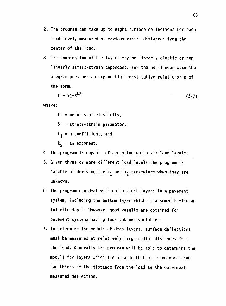
66

2. The program can take up to eight surface deflections for each

load level, measured at various radial distances from the

center of the load.

3. The combination of the layers may be linearly elastic or non-

linearly stress-strain dependent. For the non-linear case the

program presumes an exponential constitutive relationship of

the form:

E = kl*Sk2

where:

(3-7)

E = modulus of elasticity,

S = stress-strain parameter,

k1 = a coefficient, and

k2= an exponent.

4. The program is capable of accepting up to six load levels.

5. Given three or more different load levels the program is

capable of deriving the k1 and k2 parameters when they are

unknown.

6. The program can deal with up to eight layers in a pavement

system, including the bottom layer which is assumed having an

infinite depth. However, good results are obtained for

pavement systems having four unknown variables.

7. To determine the moduli of deep layers, surface deflections

must be measured at relatively large radial distances from

the load. Generally the program will be able to determine the

moduli for layers which lie at a depth that is no more than

two thirds of the distance from the load to the outermost

measured deflection.

67

8. The computed results of the program are sensitive to

variations in the layer thickness. The layer thicknesses

should be determined to a degree of precision of five percent

or better.

MODCOMP2 utilizes the Chevron elastic layer computer program for

determining the stresses, strains and deformations in the pavement

system. Since there is no closed-form solution for determining layer

moduli from surface deflection data, an iterative approach is used in

the computations. The procedure is as follows:

I. Input a set of "seed" moduli from which surface deflections

are computed using the Chevron program.

2. The computed deflections are compared to the measured

deflections and the seed moduli adjusted as a function of the

magnitude of the difference in deflections.

3. The modulus for the layer is interpolated to obtain one which

agrees with the measured deflection (Figure 3.5).

4. This process is repeated for each layer until the agreement

between the calculated and measured deflection is within the

specified tolerance or until the specified number of

iterations has been reached.

Where unknown nonlinear models are to be determined, the program

evaluates a modulus for the layer for each of several load levels.

The moduli and associated stresses in the layer are then passed to a

subroutine which performs a regression analysis to determine the kl

and k2parameters. A hypothesis test is performed to assure that the

nonlinear model is significant. If the model is not found to be

significant, the layer is treated as being linearly elastic for the

Eseeda)c1

CD

Einterp.

o Enew2

OMNI

=1.

dcalc d m eas

Deflection (log scale)

I

dca lc

Figure 3.5 Interpolation of Modulus Using Calculated and Measured Deflections in MODCOMP2 Program(Irwin, 1983)

69

rest of the iteration. If the model is significant, it is used for

the remainder of the calculations in the iteration. One of four non-

linear model types can be specified.

Figure 3.6 shows the depth beneath which 95% of the surface

deflection occurs. The actual shape and position of this line is a

function of the moduli and thicknesses of the pavement layers. Most

of the registered surface deflection is attributable to compression

that occurs in the layers that are below this line. While the actual

location of the line is unknown for a particular problem, in MODCOMP2

its position is approximated by a 34° line. Deflections are assigned

to given layers from the set of input data using this line. The

deflection that falls closest to the intersection between the upper

layer interface and 34° line will generally be used.

Sensitivity analyses with the MODCOMP2 program have found that

an extremely small tolerance must be specified in order to get

accurate results. In general, a deflection tolerance on the order of

0.5 percent is required. This is recommended to avoid compounding

measurement uncertainties with calculation uncertainties. This means

a large number of iterations is required to converge to a solution.

The actual number varies depending on the number of variable layers

and whether a linear or non-linear solution is required.

An initial run of this program was performed to backcalculate

pavement layer moduli from FWD deflection basin data. Many

difficulties were encountered. Unknown errors appeared for some

deflection data for no apparent reason. The procedure for determining

the nonlinearity of materials did not work properly, errors or no

solutions often occurred.

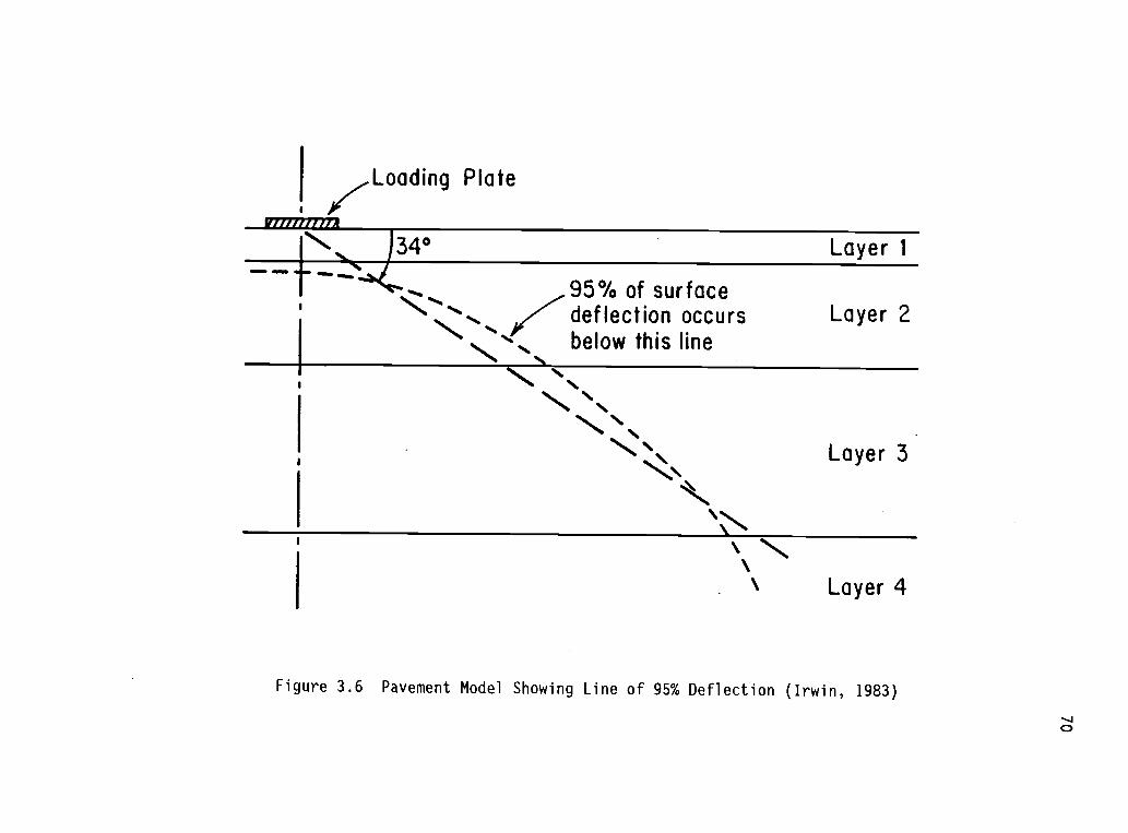
Loading Plate1 ii

...2240

95% of surface

Layer 1

deflection occursbelow this line

N

Layer 2

Layer 3

Layer 4

Figure 3.6 Pavement Model Showing Line of 95% Deflection (Irwin, 1983)

71

3.2.2.4 FPEDDI

FPEDDI (Uddin et al., 1985, Uddin, 1984) is a flexible pavement

structural evaluation system using dynamic deflections. It evaluates

NDT data to determine in situ pavement moduli and applies relevant

corrections for the temperature dependency of the asphalt concrete

layer and the nonlinear stress-dependent behavior of granular layers

and subgrade. An option for determining the remaining life is also

provided. The system utilizes the ELSYM5 computer program for

calculating theoretical response of a pavement structure. FPEDDI is

designed to handle a three or four layer flexible pavement.

Currently, the program is capable of analyzing 50 deflection basins

in one run.

The input data required for running the program include the

following:

1. Number of total deflection basins for analyses.

2. Test site and date.

3. Station (test location) and name of NDT device.

4. Switch for NDT device, number of deflection sensors, peak

force, peak stress of NDT device, and radius of loading.

5. Options for:

a) summary output of basin fitting subroutine,

b) remaining life analysis,

c) default procedure for creating a rigid layer at a finite

depth of subgrade,

d) type of base material,

e) average unit weight of subgrade soil, and

f) surface condition of pavement.

72

6. Measured deflections in mils.

7. Number of layers including subgrade layer, pavement test

temperature (°F), and design temperature (°F).

8. Information about each layer, starting from the top layer.

Layer number, thickness, Poisson's ratio, initial seed

modulus, maximum allowable modulus, and minimum permissible

value of modulus.

9. Maximum allowable number of iterations and five types of

tolerances for use in the self-iterative basin fitting

procedure.

10.Indicator for user specified design load configuration,

design load per tire, tire pressure, and past traffic in

cumulative 18-kip ESAL.

A simplified flow chart of FPEDDI is presented in Figure 3.7. The

principal analysis models and methodology are briefly described

herein.

The following assumptions are made in order to validate the

application of layered elastic theory for use in determining in situ

moduli. These are listed below:

1. The existing pavement is considered to be a layered elastic

system. Therefore, the principle of superposition is valid

for calculating response due to more than one load.

2. The peak to peak dynamic force of the Dynaflect is modeled as

two pseudo-static loads of 500 lb, each uniformly distributed

on circular areas (3 in2). The peak dynamic force of the FWD

is assumed to equal the static load uniformly distributed on

a circular area representing the FWD loading plate.

73

START

XREAD NUMBER OF PROBLEMS, NSYM

NSY 1

/READ INPUT DATA

Nil

CALL BASINF(SELF ITERATIVE PROCEDURE

TO CALCULATE YOUNG'S MODULI)

/PRINT ITERATIONS AND SUMMARY/OF BEST ITERATION

CALL ELANALEQUIVALENT LINEAR ANALYSIS OF SUBGRADE,

GRANULAR SUBBASE MODULI

CALL TEMPTFTEMPERATURE CORRECTION PROCEDURE FOR AC MODULUS

le

CALL RRLIFEREMAINING LIFE ANALYSIS

NO

NSY . NSY + 1

YES/ PRINT TABULATED RESULTS/FOR EACH TEST LOCATION

Figure 3.7 Simplified Flowchart of FPEDDI (Uddin, 1984)

74

3. Thickness of each layer is assumed to be known.

4. Subgrade is characterized by assigning an average value to

its modulus of elasticity.

The methodology of determining the in situ moduli relies on

generating theoretical deflection basins with ELSYM5 and changing the

initial values of assumed moduli through a procedure of successive

corrections until a best fit of the measured basin is obtained. A

conceptual treatment of the procedure of successive corrections is

presented in the following paragraph.

To start with, deflections are calculated from the initial input

or default values of moduli. In the first cycle, the number of

iterations is equal to the number of layers in the pavement. In each

cycle, the first iteration is made to correct the subgrade modulus.

ELSYM5 is then called to calculate theoretical deflections.

Corrections are then applied to the modulus of the next upper layer

and ELSYM5 is again called to calculate theoretical deflections. This

procedure of successive corrections is continued until the moduli of

all layers have been checked for corrections. Then, another cycle of

iterations begins anew from the subgrade layer. The generalized form

of the relationship used in the procedure of successive corrections

is given as:

ENEWi = Ei (1.0 CORRi * ERRPk * 0.5) (3-8)

where:

ENEWi = corrected value of Young's modulus of ith layer,

Ei = value of Young's modulus of ith layer in the

previous iteration.

CORK. = correction factor for the ith layer, and

75

ERRPk = discrepancy in measured deflection and predicted

deflection as percent error.

The discrepancy in measured and theoretical deflections at the

furthest sensor can be used to correct the subgrade modulus. The

moduli of intermediate layers are related to discrepancies in the

deflection of one or more of the intermediate sensors. Finally, the

surface layer modulus can be corrected using the discrepancy at the

first sensor and Equation (3-8). Only half of the discrepancy is

removed in each iteration. A set of three factors is used in the

self-iterative procedure; one is for the subgrade modulus, the second

is for the intermediate layers, and the third is associated with the

surface layer. Iterations are stopped when one of the following

criteria is reached: 1) the maximum absolute discrepancy among

calculated and measured deflections is equal to or less than the

permissible tolerance, 2) any further correction in the modulus value

causes the discrepancies in calculated and measured deflections to

increase, and 3) the specified number of iterations is achieved.

3.2.2.5 MODULUS

The MODULUS program is an interpolation program that was written

by Uzan (Lytton, Roberts & Stoeffels, 1985). It is based on data

calculated using an elastic layered program such as BISAR and ELSYM5.

Numerous elastic layered problems must be run for the specific layer

thicknesses and loading radii for the pavement sections in question.

Therefore, MODULUS is recommended for use when a large number of

pavements with similar cross-sections are to be run or when an

appropriate data base is already available. MODULUS is written in

FORTRAN and compiled with the Microsoft FORTRAN compiler for use on

76

an IBM microcomputer. Two versions are available, one utilizing the

presence of an 8087 math-coprocessor chip and the other without. A

maximum of three pavement layers, including subgrade, and four sensor

locations can be defined in the program.

3.2.2.6 ISSEM4

The ISSEM4 (In Situ Stress-dependent Elastic Moduli, 4 layers

maximum) program was developed for use on data generated with the

Dynatest FWD by Sharma and Stubstad (1979, 1980). The original

concepts used in the program were first published by Ullidtz (1977).

The ISSEM4 program backcalculates resilient modulus values for a

layered, non-linear elastic system from the surface deflections

generated by a FWD (Dynatest, 1986). The process is iterative, and a

set of seed moduli values is used to initiate each program run.

From the deflection basin, a deflection reading which reflects

the contribution of the subgrade alone is picked. A minimum of seven

deflection readings is advised to obtain a full deflection basin

profile. Using the ELSYM5 subprogram, the subgrade modulus value is

then obtained when the calculated deflection basin fits the measured

deflection basin. This process is then repeated with another

deflection reading that is farther away from the load, and another

subgrade modulus value obtained. The two moduli are then combined to

obtain a composite modulus which can be related to the major

principal stress level at or near the surface of the subgrade.

Similarly, two modulus values can be found for layer i and so on. The

modulus and stress relationship is of the general form:

E = k1*S(1) k2.(3-9)

77

where:

E. = modulus of the ith layer,

S(1)i = principal stress at or near surface of layer i, and

k1i, k2i = constants for layer i.

The underlying layer moduli represented by the above equation

are appropriately adjusted to reflect their actual moduli at the

deflection position being processed. Finally, the above modulus

relationships for each layer below the surface layer are used to

calculate the corresponding centerline E-values, and the E-value

under the load for the surface layer (E1) is derived.

The above process describes the first iteration to arrive at a

set of modulus versus stress levels relationships for layers 2 to the

subgrade, and a set of centerline modulus values for all layers.

Next, the ISSEM4 program uses the matrix of E-values obtained from

the first iteration loop to re-initiate the next iteration. The

relationships and modulus values derived from the second iteration

are then compared with those from the first iteration and if the

percentage tolerance is less than the user-specified amount, a

satisfactory solution has been obtained for the given deflection

basin and structural cross section. If not, a new iteration loop is

initiated until the percentage tolerance is met. The better the

initial seeded modulus values, the quicker the convergence to .a

solution.

All values of stress used in the above equation are calculated

based on the linear elastic theory. However, the non-linearity of a

material will not significantly affect the major principal stress

magnitudes in a layered, non-linear elastic system, although the

78

strains may be affected markedly (Dynatest, 1986).

As with all backcalculation programs, ISSEM4 is not perfect. In

particular, there are a few points to look out for:

1. If the AC layer is less than 3 in. (75 mm), the modulus value

for that layer may be quite unreliable.

2. The thickness of layer 2 should be greater than layer 1, or

the results may likewise be unreliable.

3. Each layer in the pavement should have a decreasing modulus

from the top on downwards, unless E1 is fixed, in which case

E1 may be less than E2.

4. If a four-layer system is to be analyzed, the results for

layer 3 may be inaccurate unless it is constrained. ISSEM4

functions most reliably in two or three-layered systems.

5. A unique solution may not always be possible, due to the fact

that the models used in the layered-elastic programs are

merely an approximation of actual pavement layers conditions.

3.2.3 Finite Element Method

Linear elastic layer assumptions do not consider the stress

dependent nature of the modulus of most pavement materials. It has

been shown that the modulus of granular materials is a function of

the bulk stress and also that the modulus of fine material is a

function of the deviator stress. The advantage of using a finite

element program is that non-linear stress-strain properties of each

pavement layer may be used, and these properties can be changed with

stress levels. However, the computing time required to reach a

solution using a finite element program is much greater than that

79

using the linear elastic layer programs.

There are no known automated methods which use a finite element

program to calculate layer moduli to match a measured deflection

basin. Instead, the approach that is commonly followed is to select a

typical pavement type and NDT loading device and make a series of

computer runs to determine the surface deflections of that type of

pavement as the layer thicknesses and material properties of the

layer materials change. An experimental design is used to set the

high, low and medium levels of the pavement properties that vary. The

surface deflections are then related to thickness and material

properties by linear regression analysis. A widely known method

utilizing this approach is the set of equations developed by Hoffman

and Thompson (1982), as described below.

3.2.3.1 ILLI-CALC

ILLI-CALC (Hoffman & Thompson, 1981, 1982) is a method developed

at the University of Illinois and is used to evaluate nonlinear

resilient moduli based on the interpretation of the measured surface

deflection basin. The method is not a true backcalculation procedure

in the sense of the methods mentioned earlier. Instead it utilizes

regression equations and nomographs developed from selected pavement

types and materials. The regression equations and nomographs are

based on the results of the stress-dependent finite element model

ILLI-PAVE. Solutions are possible for conventional flexible pavements

composed of an asphalt concrete layer with a typical crushed stone

base layer and a fine grained subgrade soil.

The method is based on a deflection basin measured with either

the Road Rater or the Falling Weight Deflectometer. The Road Rater

80

deflection values are converted to FWD values using the correlations

developed during the Illinois study (Hoffman & Thompson, 1981). The

deflection basin is characterized as follows;

1. D0= The maximum deflection at the center of the applied

load.

2. D1,D2, 03 = Deflections at 1, 2 and 3 ft. from the center of

the load plate.

3. The deflection basin "area" is defined as follows:

Area (in2) = 6 * (1 + 21311/D0 + 2D2/D0 + D3/D0)

4. The deflection basin shape factors, Fl and F2, are defined

as:

Fl = (Do D2)/D1 and F2 = (D1 D3)/D2

In the evaluation procedure, Road Rater center deflections (D0) at 8

kips and 15 Hz are converted to equivalent FWD deflections by using

the given correlations between the two devices.

The greatest advantage of this procedure is its ability to

characterize the non-linear stress-strain relationships exhibited by

most pavement materials. The ILLI-PAVE model is an axisymmetric solid

of revolution based on the finite-element method. The model

incorporates nonlinear stress-dependent material models and failure

criteria for granular materials and fine grained soils. The principal

stresses in the granular base and subgrade layers are modified at the

end of each iteration so that they do not exceed the strength of the

materials as defined by the Mohr-Coulomb theory of failure. Raad and

Figueroa (1980) in their study showed that measured and ILLI-PAVE

predicted load deformation responses yielded favorable results.

81

Material characterizations for the ILLI-PAVE model are shown in

Table 3.3. The asphalt concrete (AC) material is assumed to be linear

elastic with a modulus ranging from 100 to 1400 ksi. Two material

models are used to characterize the granular base materials. The

general model is of the form:

Er

= kOn (3-10)

where:

Er

= resilient modulus (psi),

9 = first stress invariant or bulk stress (psi), and

k,n = material constants determined in repetitive triaxial

tests.

Four different fine-grained subgrade soil models were used. These

models are given in Figure 3.8. The "breaking point" of the curves at

a deviator stress of 6 psi corresponds to a resilient modulus denoted

Eri. For each of the subgrade chosen, Eri is the main parameter

characterizing the nonlinear subgrade soil.

By using the material properties and cross-sections summarized

in Table 3.3, ILLI-PAVE deflection basin data were generated for a

total of 144 combinations. Using multiple-regression techniques,

deflection-basin predictive equations were developed as a function of

the four ILLI-PAVE inputs (Eac, Eri, Tac' Tgr) for conventional

flexible pavements, where;

Eac

= Modulus of asphalt concrete layer,

Eri = Breaking point of subgrade moduli (Figure 3.8),

Tac

= Thickness of asphalt concrete layer, and

Tgr

= Thickness of granular layer.

The crushed stone material model is kept constant. The regression

Table 3.3 Material Characterization for ILLI-PAVE Program (Thompson, 1982)

a) Summary of Material Properties

Asphalt Concrete CrushedStone Gravel

Subgrade40*F 70*F 100*F Stiff Medium Soft V. Soft

Unit Weight (psf) 145.00 145.00 145.00 135.00 135.00 125.00 120.00 115.00 110.0

Lateral PressureCoeff. at Rest 0.37 0.67 0.85 0.60 0.60 0.82 0.82 0.82 0.82

Poisson's Ratio 0.27 0.40 0.46 0.38 0.38 0.45 0.45 0.45 0.45

Unconfined Compress.Strength (psi) 32.80 22.85 12.90 6.21

Deviator StressUpper limit (psi) 32.80 22.85 12.90 6.21Lower limit (psi) 2.00 2.00 2.00 2.00

°di (Psi) 6.20 6.20 6.20 6.20

Eri (ksi) 12.34 7.68 3.02 1.00

Efailure (ksi) 4.00 4.00 7.605 4.716 1.827 1.00

Econst. mod. (ksi) 1400.00 500.00 100.00 -

Er-model (Psi) - 90000.33 65000.30

Friction angle (*) - 40.0 40.0 0.0 0.0 0.0 0.0

Cohesion (psi) 0.0 0.0 16.4 11.425 6.45 3.105

b) Layer Thickness (inches)

Asphalt Concrete Layer Granular Base

0.0 4.0

1.5 6.0

3.0 9.0

12.0

83

18

16

14

12

10

8

6

4

2

0

....

\-- -1.11ksi/psi

Stiff,

-.178 ksi/psi

.----\

ivedium

1 Soft

Very Soft

.i

0 5 10 15 20 25 30 35

Repeated Deviator Stress, psi

Figure 3.8 Subgrade Soil Material Models for ILLI-PAVE Analysis(Hoffman and Thompson, 1981)

84

equations show that it is possible to predict ILLI-PAVE deflection-

basin parameters with reasonable accuracy. (R2 ranges from 0.90 to

0.95)

The backcalculation procedure, given that Tgr

and Tac

are known,

is as follows:

1. Determine the mean RR (Road Rater) maximum deflection D0.

2. Determine mean RR area (in2).

3. Determine mean RR shape factors Fl and F2.

4. Determine the predicted FWD values for steps 1-3.

5. Determine D0

for ILLI-PAVE interpretation.

6. Using nomograph with Tac and Tgr, determine Eri and Eac.

7. Check the ratio of measured and computed Fl and F2

The advantages of this method are:

1. The deflection-basin predictive models can be used in lieu of

expensive and frequently unavailable computer runs.

2. The model used to generate the equations takes into account

the non-linear behavior of base and subgrade material.

The limitations of this method are:

1. The method lacks universality in that it requires the use of

specific testing devices, one of which is owned by the

Illinois DOT and the other (FWD) which is still to be used on

a large scale in the United States.

2. The method assumes a subgrade material relationship which

might not be typical of subgrade soils in other areas.

3. The method assumes one relationship for the unbound aggregate

layer, which might not apply to all aggregate materials.

4. The model used is only capable of one loading configuration.

85

5. Because of its reliance on regression equations, this method

cannot be transferred to another area without having to go

through the development of new regression models.

3.3 Summary

This chapter reviews some of the existing backcalculation

procedures for determining pavement layer moduli using NDT methods.

The existing procedures can be broadly categorized into three

classes: 1) equivalent thicknesses methods, 2) elastic layer methods,

and 3) finite element method. Two programs in the category of method

of equivalent thicknesses are reviewed. They are ELMOD and SEARCH.

Several programs in the group of elastic layer method are also looked

into. These programs are CHEVDEF/BISDEF, ELSDEF, MODCOMP2, MODULUS,

PFEDDI, and ISSEM4. A backcalculation procedure ILLI-CALC which uses

finite element method is also reviewed.

It is difficult to conclude which program is more superior than

others. In general, the programs which use the method of equivalent

thicknesses take less computing time than both elastic layer theory

and finite element method.

A severe limitation in any deflection basin fitting method is

the non-uniqueness of the backcalculated moduli. In general, the

subgrade modulus can be uniquely related to the farthest sensor

deflection readings. However, for a multi-layered pavement structure,

more than one combination of moduli which match calculated deflection

basin with the measured deflection basin with reasonable error

tolerance could be obtained. In addition, a basin matching procedure

is generally sensitive to the initial or seed moduli, especially if

these values are drastically different from actual moduli.

86

4.0 DEVELOPMENT OF AN IMPROVED BACKCALCULATION PROGRAM

It has been seen in Chapter 3 that the nondestructive testing of

asphalt concrete pavement has become one of the most useful and cost-

effective methods for pavement structural evaluation and that the use

of deflection measurements for the estimation of pavement layer

moduli is rapidly gaining popularity and application.

For these reasons, considerable effort has been applied to

develop computer programs that would allow engineers to determine

pavement material characteristics from the use of the deflection

testing data. Many such computer programs have been developed using

different assumptions or algorithms as described in the previous

chapter. After reviewing the available programs, one major drawback

of each program is its computing efficiency. In the evaluation of a

large quantity of deflection data, the requisite of too much

computing time could seriously impact the use of these programs in

routine design work.

This chapter presents an improved backcalculation program

(BOUSDEF). The major advantage of this improved program is its

computing speed, which allows engineers to make a quick and initial

evaluation of the deflection testing data for the determination of

pavement layer moduli. The BOUSDEF program uses the method of

equivalent thicknesses and modified Boussinesq equations to compute

the surface deflections. The validation of using Boussinesq equations

together with the MET to calculate surface deflections is presented

in Chapter 2.

87

4.1 Program Development and Description

4.1.1 Program Flowchart

The BOUSDEF program was developed for determining in-situ moduli

of a pavement structure using deflection data through a

backcalculation technique. Figure 4.1 shows a flow diagram of the

program, while the user's guide can be found in Appendix A.

To start with, the program first reads input data sets which

include: 1) NDT load force and load radius, 2) pavement layer

thicknesses, 3) Poisson's ratio, 4) minimum, maximum, and initial

modulus, 5) density of pavement materials, 6) deflection data (up to

seven sensor readings), 7) percent of tolerance to stop the

deflection matching process and 8) number of iterations. By calling a

subroutine DEFLECTION, the initial modulus and layer thickness

information are used to determine the equivalent thicknesses.

Deflections for the given NDT load and load radius are then

calculated. The calculated deflections are compared to measured

deflections. If the sum of the differences is greater than the

tolerance specified by the user, the program will start an iteration

by changing the moduli to compute a new set of deflections.

A simplified description of the deflection matching procedure is

illustrated in Figure 3.4. This process repeats until the sum of the

differences is less than the tolerance or the maximum number of

iterations has been reached. This procedure is repeated for each load

level until all deflection data are used.

The moduli determined from each set of deflection basin data are

used to calculate normal stresses induced by load. Stresses under the

deadload of the upper pavement materials are also determined. For the

88

Start

$Input data sets

Load level 1.1

$Call DEFLECTION

Compute sum of error from% difference of deflections

No

E- AIt =Emax

E-Alt=Emin

Compute for eachlayer an E-Alt

Construct B and Cmatrices directly

Compute baselinedeflection

Call DEFLECTION 1-10,

ICompute S & A matrices

Is the numberof deflection=the number of

variable layers

Yes

Based on least square summationand weighting factor construct

B & C matrices

Compute deflectionfor changed E-Alt

Figure 4.1 Flowchart of the BOUSDEF Program

Reconstruct B & Cmatrices to set Es

equal limits

0

0

Call SIMEQU

Are ComputedE's within limits

Set computed E's asnew baseline Es

*Call DEFLECTION

0'

Compute sum of percent error

Yes

Has programreached maximum

of iterations

i=i+1Yes

Yes

More deflection

N

Calculate stresses undereach load level

VCalculate stresses under

deadload

VCalculate bulk stresses

VCalculate deviate stresses

VDetermine kl & k2 for both

base and subgrade

VPrint summary results

Solve set of similtaneousequations for computed E's

(S}{E} = {C}

No

Compute new baselinedeflections

Figure 4.1 Flowchart of the BOUSDEF Program (cont.)

89

90

base layer, bulk stresses in the middle of the layer are calculated.

For the subgrade, deviator stresses on the top of subgrade are

determined. These stress values and moduli are then regressed to find

coefficients k1and k

2for both base layer and subgrade.

It should be noted that the backcalculated modulus corresponds

to an average condition in the pavement material while the bulk and

deviator stresses are calculated under the load at the middle of the

base layer and top of the subgrade rather than the entire body of the

base and subgrade. Therefore, the nonlinear analysis is limited to

the stress condition at a specific location rather than at different

depth of base and subgrade. Also, the method of equivalent

thicknesses/Boussinesq approach is least reliable in predicting

horizontal stresses (Ullidtz, 1980).

4.1.2 Program Output

The program has the capability of determining the following:

1. Resilient modulus for each pavement layer.

2. Bulk stresses and deviator stresses induced by both load

and deadload of upper layer pavement materials.

3. Coefficients k1and k

2for base and subgrade materials

with a form of relationship shown below:

for coarse-grained materials,

MR

= k1Ok2

or for fine-grained materials

MR

= k1ad

k2

where:

MR

= Resilient modulus (psi),

(4 -la)

(4-1b)

91

8 = Bulk stresses (psi),

ad

= Deviator stress (psi), and

k k2= Regression coefficients of material properties.

4.1.3 Example.

An example is provided to illustrate the use of the program.

Table 4.1 summarizes the pavement and deflection test data for the

example. The pavement is a conventional flexible structure with an

eight-inch asphalt concrete surface, twelve-inch aggregate base and

infinite depth of subgrade. Deflection testing was performed using a

falling weight deflectometer (FWD) on one short section of a road.

Various load levels were applied in order to obtain pavement

responses under different stress conditions. At least two load levels

of FWD should be used to define the modulus versus stress

relationship. However, it is preferable to have several stress

conditions so that a more representative relation can be better

defined.

By using the BOUSDEF program, resilient modulus for each

pavement layer is determined and presented in Table 4.2. Bulk

stresses in the middle of the base layer and deviator stresses on the

top of subgrade are calculated. Regression coefficients kl and k2 for

both base and subgrade are also determined. As can be seen in Table

4.2, both base and subgrade materials appear to have a non-linear

property with k2 = 0.58 for base and -0.13 for subgrade. The results

are plotted in Figure 4.2.

4.1.4 Sensitivity to the User Input

The initial moduli specified by the user should have a minor

effect on the final backcalculated moduli. This feature would

minimize the variation in the final moduli because of the user's

input and would result in a more reliable solution. An initial

92

Table 4.1 Pavement and Deflection Data for the Example

Pavement Data

Laver Thickness Poisson's Density

iinch l ratio (pcf)

AC 8 0.35 144

Agg. Base 12 0.40 120

Subgrade 0.40 100

Deflection Data Distance to sensor (inch)

Load

(lbs)

0 8 18 36 58

Deflection Readings (mils)

2789 6.07 4.04 2.41 1.25 0.91

3035 6.59 4.02 2.41 1.37 0.94

3055 6.55 3.89 2.28 1.50 0.94

6521 12.92 8.26 6.47 3.19 1.82

6644 13.18 8.81 7.23 3.53 1.82

6562 13.82 9.57 6.47 3.88 1.72

6521 13.31 8.26 7.10 3.53 1.94

6480 13.05 8.48 5.58 3.65 1.93

6480 13.44 12.72 7.48 5.59 3.50

11442 22.09 14.35 11.92 5.81 3.76

11770 22.48 15.44 13.19 6.38 3.96

11606 23.77 16.74 11.79 6.84 3.83

11442 22.99 14.78 12.68 6.84 3.97

11770 22.35 14.78 10.65 6.84 3.91

Note: Load radius is 5.9 inches

93

Table 4.2 Summary of Backcalculation Results for the Example

Summary of Non-linear Characteristics of Lower Layers

For base layer: kl= 8069 k2= 0.58(MR kl (31(2)

For subgrade: kl= 18687 k2= -0.13 (MR

= kl ad k2)

Load (lb) E(1)

Summary of Moduli and Stresses *

E(2) E(3) BSTRS DSTRS

2,789 106,432 26,911 16,377 7.29 5.59

3,035 83,362 38,107 16,870 8.99 5.76

3,055 74,978 49,985 16,606 9.88 5.59

6,480 104,087 48,343 14,961 16.81 7.75

6,480 399,359 17,074 9,462 7.74 5.96

6,521 117,982 39,666 15,393 15.41 8.01

6,521 99,314 54,258 13,863 17,67 7.44

6,562 142,581 24,546 15,015 12.58 8.40

6,644 158,740 29,287 14,770 13.00 7.96

11,442 117,180 53,092 14,045 27.83 10.55

11,442 100,939 69,773 12,518 31.35 9.65

11,606 136,673 35,135 13,533 23.61 11.16

11,770 156,599 41,680 13,376 24.18 10.46

11,770 105,657 69,787 13,774 31.79 10.18

Average135,994 42,689 14,326

* Moduli and stresses are in psi.

100000

10001

95

evaluation on the sensitivity to input modulus was performed using

data in Table 4.3. The results are summarized in Table 4.4. As

indicated, the program provides very similar results regardless of

what initial modulus values would be.

4.2 Evaluation of the BOUSDEF Program

To evaluate the BOUSDEF program, three approaches were used: 1)

comparing backcalculated moduli with preassumed theoretical values,

2) comparing backcalculated moduli with results from other developed

programs, and 3) comparing backcalculated moduli with the laboratory

test results. The following discusses the process.

4.2.1 Comparison With Theoretical Values

The BOUSDEF program was evaluated by comparing the

backcalculated results with hypothesized theoretical values. This is

done by assuming a set of pavement structures with different

combination of layer thicknesses and different resilient modulus. Ten

pavement structures, as described in Section 2.1.4, are used for the

comparison.

Table 4.5 summarizes calculation results. The backcalculated

moduli for all structures are very close to those of theoretical

values. This would indicate the BOUSDEF program has the capability of

backcalculating the layer moduli from known deflections and layer

thicknesses and load data. However, it should be noted that the MET

is not recommended for pavements with base layers that are very stiff

compared to the surface (Ullidtz, 1987) as mentioned earlier. The

pavements with CTB layers were included here to illustrate that

BOUSDEF is capable of providing an initial evaluation for such

pavements. Alternative means of backcalculation should also be

carried out to improve this evaluation.

Table 4.3 Data Used for Evaluating Sensitivity on Initial Modulus

LAYER THICKNESS POISSON'S RATIO

1 11.0" 0.30

2 15.0" 0.35

3 m 0.45

MEASURED DEFLECTIONS

DISTANCE FROM LOAD (IN) 0.0 18.0 36.0 60.0

DEFLECTION (MILS) 6.47 4.27 2.34 1.47

LOAD = 14696 pounds

LOADING RADIUS = 9.0 inches

DEVICE = WES Vibrator

(Lytton, 1986)

96

97

Table 4.4 Effect of Initial Moduli on Calculated ModuliUsing BOUSDEF

Initial Moduli (psi) Calculated Moduli (psi)Surface Base Subgrade Surface Base Subgrade

Variation of surface modulus200,000 50,000 25,000 768,422 57,228 46,810300,000 50,000 25,000 768,455 57,248 46,803400,000 50,000 25,000 768,485 57,248 46,803500,000 50,000 25,000 764,142 57,702 46,766600,000 50,000 25,000 764,203 57,693 46,768700,000 50,000 25,000 764,250 57,689 46,769800,000 50,000 25,000 772,642 56,432 46,914900,000 50,000 25,000 769,176 56,987 46,8351,000,000 50,000 25,000 764,989 57,592 46,791Variation of base modulus500,000 10,000 10,000 728,648 56,086 46,783500,000 20,000 10,000 739,009 54,808 46,863500,000 30,000 10,000 738,916 54,843 46,837500,000 40,000 10,000 738,827 54,860 46,830500,000 50,000 10,000 738,859 54,845 46,842500,000 60,000 10,000 738,985 54,813 46,861500,000 70,000 10,000 728,289 56,131 46,770500,000 80,000 10,000 735,888 54,997 47,021500,000 90,000 10,000 740,119 54,560 47,021500,000 100,000 10,000 739,447 54,540 46,980

Variation of subgrade modulus500,000 30,000 10,000 738,916 54,843 46,837500,000 30,000 20,000 735,079 55,446 46,847500,000 30,000 30,000 728,013 56,166 46,759500,000 30,000 40,000 743,267 54,092 46,998500,000 30,000 50,000 733,450 55,287 47,091500,000 30,000 60,000 736,109 53,809 48,243500,000 30,000 70,000 735,286 54,468 47,642500,000 30,000 80,000 735,390 54,333 47,767500,000 30,000 90,000 735,356 54,292 47,814500,000 30,000 100,000 739,984 53,871 47,754

98

Table 4.5 Comparison Between Theoretical andBackcalculated Modulus Values *

PavementStructure 1 2 3

Theoretical Values4 5 1 2 3

Backcalculated Values4 5

Three -Layer Conventional

7" AC 100.0 300.0 600.0 1000.0 1500.0 101.9 289.9 602.7 1022.1 1551.112" Agg. 25.0 25.0 25.0 25.0 25.0 24.7 25.0 25.1 24.6 24.4Subgrade 10.0 10.0 10.0 10.0 10.0 10.0 10.1 9.9 9.9 9.9

3" AC 100.0 300.0 600.0 1000.0 1500.0 100.7 310.1 594.3 1017.2 1538.218" Agg. 20.0 20.0 20.0 20.0 20.0 20.0 19.8 20.1 19.9 19.8Subgrade 10.0 10.0 10.0 10.0 10.0 10.0 9.9 9.9 9.9 9.9

10" AC 200.0 600.0 1000.0 1500.0 202.6 615.5 1017.5 1566.516" Agg. 25.0 25.0 25.0 25.0 31.1 31.9 31.6 30.8Subgrade 10.0 10.0 10.0 10.0 10.0 9.9 10.1 9.9

Four -Layer Conventional

3" AC 300.0 600.0 1000.0 1500.0 357.3 638.8 1024.9 1493.512" Base 25.0 25.0 25.0 25.0 23.6 24.3 24.6 25.020" Subbs 10.0 10.0 10.0 10.0 9.7 10.0 10.0 10.0Subgrade 7.0 7.0 7.0 7.0 7.2 7.0 7.0 7.0

6" AC 100.0 300.0 600.0 1000.0 101.3 298.5 615.6 1027.312" Base 25.0 25.0 25.0 25.0 24.9 25.1 24.0 23.924" Subbs 12.0 12.0 12.0 12.0 12.0 12.0 12.1 12.1Subgrade 8.0 8.0 8.0 8.0 8.0 8.0 8.0 8.0

Cement Treated Base

4" AC 300.0 600.0 1000.0 294.8 588.3 1158.58" CTB 1200.0 1200.0 1200.0 1216.1 1205.4 1107.7Subgrade 10.0 10.0 10.0 10.0 10.0 10.0

4" AC 300.0 600.0 1000.0 292.7 584.0 1081.810" CTB 1200.0 1200.0 1200.0 1215.0 1225.8 1081.8Subgrade 10.0 10.0 10.0 10.0 10.0 10.0

PCC

8" PCC 4000.0 4172.86" Base 20.0 21.2Subgrade 10.0 9.9

8" PCC 4000.0 4028.612" Base 20.0 19.8Subgrade 10.0 9.9

12" PCC 4000.0 4015.512" Base 20.0 20.0Subgrade 10.0 10.0

* Moduli are in ksi.

99

4.2.2 Comparison With Other Developed Programs

The BOUSDEF program was compared with four developed programs.

The programs used are: BISDEF (Bush, 1985), CHEVDEF (Bush, 1980),

ELSDEF (Lytton, 1986), and MODCOMP2 (Irwin, 1983). Pavement data and

deflection test data used for the comparison are presented in Tables

4.6 and 4.7, respectively. The computed layer moduli for the various

programs are presented in Table 4.8. Results from BOUSDEF seem to be

very compatible with those from the other developed programs.

One major advantage of the BOUSDEF program over the other

programs is its computation speed. In using a deflection data set

presented in Table 4.3, the BOUSDEF program takes only three seconds

to find the solution, using an IBM-AT microcomputer with a math-

coprocessor. The same data would take significantly longer time using

other programs, as can be seen in Table 4.9. This feature makes use

of the program to evaluate a large amount of deflection data easy and

possible.

BOUSDEF is a user-friendly program. The program has a built-in

data file creating and editing routine. This significantly eases the

data input and edit process and avoids possible calculation errors

due to improper data entry.

4.2.3 Comparison With Laboratory Test Results

The BOUSDEF program was also evaluated by comparing the

backcalculated results with the resilient modulus tested in the

laboratory. This was accomplished by selecting actual projects in the

state of Oregon. The general procedures followed are described below:

1. Select project sites for evaluation.

100

Table 4.6 Pavement Data Used for Backcalculation

Pavement Layer Material Thickness Poisson's Ratio(inch)

1 Asphalt Concrete 9.0 0.35

2 Aggregate Base 16.0 0.40

3 Soil Subgrade co 0.40

Table 4.7 Deflection Data Used for Backcalculation

Test Site FWD Load(lb)

Deflection @ Sensor Location0" 8" 18" 30" 60"

1 11,729 22.99 16.74 12.81 9.81 4.57

2 11,647 27.39 21.68 14.96 11.06 5.33

3 11,442 20.54 17.28 12.30 9.69 4.90

4 11,073 24.16 20.33 14.08 10.83 5.77

5 11,688 16.28 13.70 8.88 6.95 3.92

Note: FWD Load Radius is 5.9 inches.

101

Table 4.8 Summary of Backcalculation Results *

Test Site Program AC Surface Aggregate Base Subgrade

1 BISDEF 194.0 25.1 11.5BOUSDEF 163.0 25.7 11.2CHEVDEF 175.8 24.7 12.1ELSDEF 200.0 23.6 11.7MODCOMP2 162.8 33.4 10.5

2 BISDEF 173.7 15.4 10.5BOUSDEF 157.7 15.2 9.9CHEVDEF 150.7 16.6 10.5ELSDEF 174.0 15.2 10.4MODCOMP2 131.5 27.1 9.3

3 BISDEF 288.3 20.1 11.2BOUSDEF 262.2 19.3 10.9CHEVDEF 257.8 23.3 11.3ELSDEF 286.9 20.0 11.3MODCOMP2 184.0 50.6 9.3

4 BISDEF 206.4 19.0 9.4BOUSDEF 196.5 17.0 9.2CHEVDEF 182.3 21.7 9.2ELSDEF 205.7 18.9 9.4MODCOMP2 431.8 1.0 N/S**

5 BISDEF 259.1 37.7 14.8BOUSDEF 266.0 30.5 14.8CHEVDEF 260.9 36.4 15.0ELSDEF 258.2 37.2 14.8MODCOMP2 165.8 89.7 12.9

* Moduli are in ksi.

** N/S = No Solution.

102

Table 4.9 Comparison on Computing Time and Backcalculated Results

PROGRAMCOMPUTED LAYER MODULI (KSI)

LAYER 1 LAYER 2 LAYER 3

COMPUTINGTIME

(SECONDS)

BISDEF* 685.7 55.4 48.8 285

BOUSDEF 764.1 57.7 46.8 3

CHEVDEF 527.8 28.6 29.9 327

ELSDEF 632.1 84.7 34.2 485

MODCOMP2 772.5 35.9 53.0 495

*Contains proprietary BISAR program

103

2. For selected sites, perform deflection test using FWD.

3. Obtain samples from same road section where deflections

were measured.

4. Backcalculate pavement layer moduli from deflection basin

data using the BOUSDEF program.

5. Perform laboratory tests on samples.

6. Compare results from backcalculated and laboratory tests.

The following paragraphs discuss this process in more detail.

4.2.3.1 Selection of Project Sites

Two project sites in the state of Oregon were selected for

evaluating the BOUSDEF program. These two projects are typical

conventional pavement structures consisting of an asphalt concrete

surface layer over an aggregate base and subgrade. Figure 4.3 shows

the location of the two projects. Table 4.10 summarizes the pavement

parameters of the two projects.

4.2.3.2 Deflection Test

Deflection tests were performed on selected project sites using

KUAB Falling Weight Deflectometer (FWD). For the Rufus-Quinton

project, the deflection tests were conducted using the FWD owned by

the Oregon State Highway Division. For the Centennial Boulevard

project, the FWD tests were performed using equipment (KUAB FWD)

owned by Pavement Services Inc. of Portland.

The KUAB FWD is trailer-mounted and towed by a 3/4-ton van. The

impulse force is created by dropping a set of two weights from

different heights. By varying the drop height, the load at the

pavement surface was varied from approximately 3,000 to 15,000 lbs. A

smooth load pulse similar to that created by a moving wheel load is

104

Eugene OREGON

Selected Projects

Figure 4.3 Location of Selected Project Sites

Table 4.10 Summary of Selected Project Sites

Project Location Pavement Structure LayerThickness *

Rufus-Quinton SectionColumbia River Hwy No.2MP110.8 MP124.0

Centennial BoulevardCoburg 1-5Eugene

AC 6.8"Aggregate 18.0"

AC 4.0"Aggregate 16.0

* Average thickness

105

generated by using the two-mass system (Tholen, 1980; Tholen et al,

1985). Surface deflections were measured with seismic transducers

that are lowered automatically with the loading plate. The sensor

locations may be adjusted for the job requirement. For the Rufus-

Quinton project, the sensors were set at 0", 8", 12", 24", 36", and

58". For the Centennial Boulevard project, the sensors were set at

0", 12", 24", 36", 60", and 99". There is no standard procedure for

where the sensors should be located. However, it is important to have

one sensor which is located far enough away from the load to obtain

the pavement response from the subgrade.

The actual Rufus-Quinton project is thirteen-mile long. For the

purpose of comparing the results between backcalculated results and

the laboratory test, an one-mile long section was selected. The

deflections were measured at 250-ft intervals. Three FWD load levels,

ranging from approximately 3,000 to 12,000 lbs, were applied at each

test spot. Deflections were recorded with a personal computer.

Pavement temperatures at time of testing were also recorded. The

detailed output may be found in Appendix B-1.

The Centennial Boulevard project is approximately 1.3 mile long.

The deflections were measured at 200-ft intervals. Two load levels at

each test location were applied ranging from 8,000 to 14,000 lbs.

Recorded data included test locations, pavement temperature, load

applied and deflections at each sensor location. The detailed output

may be found in Appendix B-2.

4.2.3.3 Materials Sampling

Best efforts were made to acquire material samples from the

project sites. Pavement materials sampled at both sites included

106

asphalt concrete cores and base aggregates. Subgrade soil were not

obtained because of difficulties in obtaining undisturbed soil

samples.

Eight four-inch diameter asphalt concrete cores and two bags of

aggregates were obtained for the Rufus-Quinton project. The same

amount of asphalt concrete cores and four bags of aggregates were

received from the Centennial Boulevard project.

4.2.3.4 Backcalculation of Laver Moduli

The BOUSDEF program was used to backcalculate the moduli for

each pavement layer from the deflection data. Raw data, without

correcting for temperature, were used calculate the pavement moduli

at time of testing. Table 4.11 summarizes the backcalculated results

for the Rufus-Quinton project. Table 4.12 presents the results for

the Centennial Boulevard project. Figures 4.4 and 4.5 illustrate the

backcalculated results for Rufus-Quinton, both eastbound and

westbound directions. Figures 4.6 to 4.9 present the backcalculation

results for Centennial Boulevard project.

4.2.3.5 Laboratory Tests on Samples

Laboratory tests were performed on the actual pavement samples

for modulus. For the AC cores, the diametral test (ASTM D-4123) was

followed. For the aggregate base, the triaxial test (AASHTO T-274)

was used. For the purpose of testing, the AC core samples were

trimmed to a height of approximately 1.5 to 2.5 inches, depending on

the thickness of the top lift.

The AC cores were tested at three temperatures: 42°F, 73°F, and

95°F, to determine the influence of the temperature on the modulus of

the asphalt concrete. An H&V diametral testing system (H&V Materials

107

Table 4.11 Backcalculated MR for the Rufus-Quinton Project (EB)

Station Load(lb)

AC(psi)

Base(psi)

Subgrade(psi)

Bulkstress

Deviatorstress

1 3,199 302,658 87,337 14,847 8.42 4.271 6,398 1,257,591 14,555 23,882 6.07 7.031 11,934 1,268,846 30,659 22,929 12.67 9.212 3,158 509,816 34,371 24,822 6.11 5.132 11,811 173,076 48,314 19,659 25.80 11.513 3,199 610,269 33,422 33,890 5.86 5.483 6,726 492,083 28,512 30,505 10.41 8.634 2,953 259,183 26,058 30,547 6.39 5.934 6,603 267,678 35,667 25,531 12.86 8.484 11,852 324,543 36,048 31,620 20.52 13.675 3,158 353,341 20,003 25,054 5.86 5.805 6,603 709,493 11,538 24,949 6.92 8.535 11,811 176,235 10,351 29,877 16.93 19.866 6,521 266,598 12,658 31,552 9.58 11.157 2,830 161,216 20,294 24,605 6.51 6.027 11,893 363,088 40,729 25,635 20.65 11.898 6,439 243,075 36,564 15,768 12.97 7.098 12,016 386,336 17,561 31,867 15.83 15.709 3,076 287,092 17,354 39,274 5.85 6.829 6,480 267,245 27,931 29,528 11.89 9.3010 3,076 244,209 13,748 32,867 5.75 6.8610 6,480 332,561 13,664 28,046 9.13 10.0410 11,770 153,986 13,075 30,703 18.88 19.5711 6,439 326,903 11,389 20,418 8.64 9.2011 11,893 526,235 11,665 22,739 12.26 13.5412 3,076 253,026 16,343 29,930 5.94 6.4812 6,398 329,310 14,050 24,271 9.14 9.4012 11,975 346,906 19,621 22,916 16.93 13.5813 3,035 254,005 18,565 18,566 6.06 5.5313 6,357 376,159 10,805 23,589 8.06 9.4313 11,852 329,116 28,234 21,706 19.06 12.2714 2,871 195,491 16,824 15,610 6.05. 5.3914 6,357 319,128 16,976 15,848 9.70 7.8014 11,893 503,199 21,622 18,842 15.40 11.2016 3,117 193,967 26,817 33,926 7.12 6.4916 12,139 571,760 21,556 35,889 15.01 14.6117 12,180 620,775 17,300 37,613 13.56 15.3118 3,076 230,240 35,813 32,091 7.23 5.9318 6,685 497,033 39,748 27,553 11.35 7.7718 11,975 809,831 40,781 25,952 16.32 10.1919 3,117 572,716 32,391 34,328 5.80 5.5019 6,644 680,060 19,775 33,094 8.37 8.8320 3,117 269,346 21,742 32,117 6.31 6.3320 6,726 473,480 15,311 29,783 8.73 9.6321 3,035 924,348 13,054 24,918 4.06 5.1821 6,685 570,617 44,089 13,831 11.24 5.9021 12,016 380,178 126,956 11,562 27.26 6.57

Average 424,767 27,060 26,278STD 248,301 20,108 6,585

108

Table 4.11 Backcalculated MR for the Rufus-Quinton Project (WB)(cont.)

Station Load(lb)

AC(psi)

Base(psi)

Subgrade(psi)

Bulkstress

Deviatorstress

1 3,240 340,993 12,043 31,568 4.94 6.511 6,521 666,413 13,607 24,690 6.59 7.681 12,057 882,720 18,052 24,040 10.29 9.942 3,158 399,510 15,647 25,811 4.98 5.832 6,685 359,843 22,021 20,414 9.06 7.492 11,975 450,584 25,414 21,510 14.10 10.123 3,199 491,324 22,562 25,731 5.19 5.493 6,480 657,531 19,015 23,906 7.23 7.233 12,385 885,645 26,625 24,856 11.92 9.544 3,076 396,075 21,830 22,061 5.27 5.384 6,808 377,011 27,770 19,762 9.64 7.144 12,262 516,346 29,416 21,705 14.42 9.765 3,199 365,477 31,656 32,607 5.91 5.725 6,808 601,823 21,182 32,505 7.90 8.175 12,057 706,802 25,741 33,820 12.39 11.136 6,767 810,309 63,150 28,590 9.73 6.296 12,303 869,746 77,331 26,934 16.46 7.987 3,199 401,272 20,879 39,374 5.32 6.257 6,849 546,094 18,504 36,591 7.85 8.877 12,303 691,963 21,264 39,325 11.94 12.538 6,644 467,614 11,154 20,492 6.97 8.008 12,221 569,319 14,296 20,966 11.12 10.889 3,199 464,359 20,343 20,264 5.14 5.319 6,767 617,598 16,485 18,818 7.29 7.099 12,098 806,569 15,690 22,057 10.14 10.0612 3,076 244,263 18,082 19,262 5.59 5.5912 6,726 428,882 13,792 21,249 7.64 8.0012 12,262 637,104 13,400 27,265 10.52 11.9713 3,117 209,438 28,711 19,979 6.37 5.4213 6,808 351,754 23,308 21,679 9.38 7.6513 12,344 426,199 33,843 22,354 15.99 9.9414 3,199 366,653 29,561 32,745 5.83 5.7714 6,767 503,474 21,672 35,231 8.32 8.5814 12,344 652,950 25,325 40,620 12.89 12.4319 3,158 419,703 31,587 34,765 5.70 5.7021 3,158 400,430 37,071 27,611 5.95 5.3421 6,685 594,077 23,851 28,384 8.09 7.6121 12,139 785,417 28,260 30,241 12.41 10.2822 3,158 643,400 15,778 25,774 4.52 5.5222 6,726 513,236 20,965 25,605 8.16 7.7222 11,852 674,652 21,580 28,103 11.73 10.6823 3,117 588,250 19,544 27,662 4.78 5.5123 6,726 555,988 17,631 28,134 7.61 8.0823 12,139 690,632 19,644 29,886 11.52 11.2824 3,117 257,551 28,055 28,818 6.09 5.7824 6,685 374,314 19,633 31,491 8.69 8.75

Average 536,115 23,978 27,071STD 172,033 11,600 5,792

109

Table 4.12 Backcalculated Modulus for Centennial ProjectEASTBOUND FROM LOCATION 200 TO 4000

Station Load(lb)

AC(psi)

Base(psi)

Subgrade Bulk Deviator(psi) Stress Stress

200 8,821 1,192,686 35,389 10,619 13.2 6.3200 14,269 1,074,783 44,632 10,656 22.3 8.1400 8,821 383,337 33,174 12,131 17.3 7.9400 14,297 280,833 50,940 11,598 31.6 9.9600 8,763 446,242 33,644 10,133 16.7 7.2600 14,269 498,348 44,397 10,037 27.1 9.0800 8,705 524,632 37,849 10,832 16.4 7.0800 14,153 1,140,917 30,466 10,620 19.5 8.71000 8,849 677,562 21,917 10,991 13.6 7.71000 14,240 647,469 29,774 10,578 22.9 9.81200 8,763 339,800 29,463 12,337 17.2 8.31200 14,240 395,530 38,190 11,842 27.6 10.41400 8,792 576,179 23,206 13,901 14.3 8.51400 14,211 625,636 28,086 13,105 22.7 10.91600 8,734 364,318 24,634 11,208 16.2 8.21600 14,182 315,199 32,533 11,030 27.9 10.91800 8,734 429,492 28,801 9,912 16.2 7.41800 14,153 380,923 36,522 9,931 27.4 9.82000 8,763 898,118 32,653 10,838 13.9 6.72000 14,211 656,243 44,998 10,683 25.3 8.82200 8,676 476,446 20,870 9,959 14.4 7.82200 14,067 537,890 25,928 9,760 22.9 10.02400 8,763 676,194 20,354 12,914 13.2 8.32400 14,182 564,264 29,181 12,294 23.5 10.72600 8,734 666,228 25,826 23,487 14.1 9.92600 14,269 648,552 33,947 25,003 23.7 13.82800 8,705 383,872 16,507 17,944 14.4 10.82800 14,124 458,096 19,922 18,146 22.4 14.53000 8,676 641,011 33,459 23,180 15.1 9.33000 14,211 568,411 49,657 22,162 26.9 12.03200 8,648 982,052 31,485 32,579 13.3 10.03200 14,067 964,432 42,288 32,492 22.3 13.43400 8,648 583,606 30,334 17,083 15.1 8.53400 13,923 382,669 46,799 16,351 28.4 11.13600 8,705 666,593 26,030 25,630 14.1 10.23600 14,182 851,510 27,606 25,665 20.7 13.93800 8,676 502,722 47,255 19,749 17.4 8.33800 14,240 413,078 68,918 19,793 30.9 10.84000 8,705 904,828 40,382 24,621 14.6 8.64000 14,211 609,647 60,128 24,355 27.6 11.7

AVERAGE 608,259 34,454 15,904STD 229,872 11,032 6,581

110

Table 4.12 Backcalculated Modulus for Centennial ProjectEASTBOUND FROM LOCATION 4200 TO 7000 (cont.)

Station Load(lb)

AC

(psi)

Base(psi)

Subgrade Bulk Deviator(psi) Stress Stress

4200 8,648 733,522 44,104 19,073 15.6 7.94200 14,124 604,680 67,282 19,012 28.2 10.14400 8,648 578,668 45,958 17,889 16.7 7.94400 14,096 524,224 64,597 17,972 28.8 10.24600 8,532 676,229 42,831 10,781 15.6 6.54600 13,951 680,957 56,206 10,770 26.1 8.24800 8,561 858,319 47,075 18,196 15.1 7.44800 14,009 479,265 77,869 18,668 30.3 9.95000 8,561 1,054,069 45,675 15,151 14.3 6.85000 14,038 1,102,778 60,950 15,907 23.7 8.85200 8,619 1,154,214 48,720 15,489 14.2 6.75200 14,096 872,094 74,352 15,633 26.5 8.65400 8,792 1,185,558 26,500 13,516 12.1 7.25400 13,980 995,197 36,552 12,831 21.1 9.25600 8,676 918,746 35,486 15,219 14.0 7.45600 14,096 777,984 49,862 14,379 24.7 9.45800 8,590 623,626 54,045 9,928 16.9 6.15800 14,038 758,515 64,979 10,062 26.4 7.66000 8,561 1,287,120 34,744 10,354 12.5 6.16000 14,009 1,256,945 42,694 10,303 20.7 7.86200 8,705 274,332 57,679 13,491 20.5 7.46200 14,124 420,490 61,997 13,297 29.9 9.46400 8,648 917,159 34,679 12,716 13.9 6.96400 14,096 868,758 48,870 11,850 23.9 8.56600 8,619 648,294 46,532 8,220 16.2 5.96600 14,009 528,858 56,056 8,724 27.7 7.87000 8,734 633,344 36,933 13,752 15.6 7.57000 14,124 547,457 50,960 12,784 27.1 9.4

AVERAGE 784,336 50,507 13,785STD 259,845 12,384 3,177

111

Table 4.12 Backcalculated Modulus for Centennial ProjectWESTBOUND FROM LOCATION 6900 TO 2700 (cont.)

Station Load(lb)

AC(psi)

Base(psi)

Subgrade Bulk Deviator(psi) Stress Stress

6900 8,705 549,293 86,849 16,120 19.4 6.66900 14,182 505,870 110,433 16,033 32.4 8.46700 8,705 311,068 82,928 13,055 21.3 6.66700 14,182 393,500 93,740 12,641 33.0 8.26500 8,648 604,949 32,495 16,002 15.2 8.16500 14,096 588,483 41,301 15,352 25.3 10.66300 8,676 567,289 33,848 23,922 15.6 9.56300 14,182 620,694 42,163 24,353 25.2 12.86100 8,676 361,100 34,291 20,897 17.4 9.66100 14,153 351,517 43,914 21,888 29.0 13.25900 8,648 720,605 28,884 16,867 14.1 8.35900 14,096 703,185 34,819 15,889 23.1 10.95700 8,590 484,190 48,198 14,289 17.4 7.35700 14,096 338,452 67,074 14,020 31.7 9.65500 8,648 874,525 48,054 21,573 15.3 7.95500 14,211 624,465 74,903 21,459 28.9 10.35100 8,676 774,804 57,989 16,033 16.5 6.95100 14,153 776,411 70,602 16,035 27.0 9.04900 8,648 706,615 47,964 16,225 16.1 7.34900 14,124 604,709 66,351 16,016 28.1 9.44700 8,619 795,417 61,138 15,027 16.5 6.64700 14,182 724,053 78,649 15,175 28.2 8.64500 8,619 902,274 25,244 12,929 12.7 7.44500 14,153 786,905 35,892 13,110 22.7 9.83700 8,619 530,502 44,536 20,145 16.8 8.43700 14,153 736,687 49,111 20,853 25.1 11.23500 8,619 1,263,788 22,439 26,557 11.1 9.43500 14,124 1,182,953 29,387 25,427 19.0 12.73300 8,561 920,650 18,988 15,307 11.6 8.33300 14,096 1,080,032 22,397 15,850 17.9 11.23100 8,532 1,277,277 16,303 17,317 10.0 8.43100 14,038 1,418,923 21,726 15,827 16.2 10.62900 8,561 1,202,374 22,991 10,836 11.3 6.82900 14,067 1,388,525 25,879 10,491 17.3 8.62700 8,590 983,678 25,082 14,033 12.3 7.52700 14,096 938,722 35,231 13,158 21.4 9.5

AVERAGE 766,513 46,716 16,964STD 298,557 23,418 4,008

112

Table 4.12 Backcalculated Modulus for Centennial ProjectWESTBOUND FROM LOCATION 2500 TO 100 (cont.)

Station Load(lb)

AC(psi)

Base(psi)

Subgrade Bulk Deviator(psi) Stress Stress

2500 8,561 696,691 30,281 17,457 14.3 8.32500 14,038 508,317 47,227 16,663 26.9 10.82100 8,532 485,466 34,521 11,670 16.1 7.3

2100 14,009 512,793 40,242 10,969 25.9 9.41900 8,676 1,070,951 27,632 13,658 12.5 7.3

1900 14,182 1,192,106 32,396 12,922 19.6 9.31700 8,561 640,110 37,988 10,675 15.4 6.7

1700 14,067 337,358 59,504 10,487 30.9 8.81500 8,619 525,731 39,137 14,395 16.4 7.6

1500 14,038 295,918 64,070 13,622 32.1 9.81300 8,648 201,822 38,022 13,687 19.9 8.51300 14,067 201,950 51,226 12,949 33.1 10.71100 8,590 618,645 28,924 15,765 14.6 8.31100 14,067 625,296 36,771 14,750 24.1 10.6

900 8,648 337,715 44,163 14,580 18.6 7.9900 14,096 353,862 54,817 13,782 30.2 10.1

700 8,648 1,102,055 27,453 17,099 12.3 7.9700 14,182 840,150 41,470 15,911 23.2 10.2500 8,648 142,658 49,225 15,638 22.1 8.7500 14,096 226,980 65,390 14,904 33.9 10.4299 8,648 271,970 70,620 11,342 21.1 6.6299 14,067 306,764 85,021 10,933 33.6 8.2100 8,705 522,935 74,902 12,136 19.0 6.2100 14,153 871,873 69,792 12,004 26.2 7.9

AVERAGE 537,088 47,950 13,667STD 293,206 16,195 2,061

113

100

50

u) 30_Ne

=u ) 20

3ao2 10Ea)

(7) 5a)

CC

3

2

1

200

100

50

20

10

5

2

1 2 3 5 10 20

Bulk Stress (psi)30 50 100

1.1

au,m, o 0

Liz 0 LI El alli Id 0° LP

o 01

5 10 15

Deviator Stress (psi)20 25

Figure 4.4 Backcalculated Base and Subgrade Moduli for the Rufus-Quinton Project (Eastbound)

114

100

50

rz, 300200

m3'00 102

4ae= 5ma)cc

3

2

1

200

100

,...(I) 50

CO

=3130 202a)

1 0Toa)

CC

5

2

1 2 3 5 10 20Bulk Stress (psi)

30 50 100

Wl

o

5 10 15Deviator Stress (psi)

20 25

Figure 4.5 Backcalculated Base and Subgrade Moduli for the Rufus-Quinton Project (Westbound)

200

100

50

co

0 202

10

Q5

2

100

50

10

2 3 5 10 20 30

Bulk Stress (psi)50 100

2 4 6 8 10 12 14

Deviator Stress (psi)

115

Figure 4.6 Backcalculated Base and Subgrade Moduli for the CentennialBlvd Project (Station 200 to 400, Eastbound)

200

100

5

2

100

50

2 3 5 10 20 30Bulk Stress (psi)

50 100

3

20 2 4 6 8 10

Deviator Stress (psi)12 14

116

Figure 4.7 Backcalculated Base and Subgrade Moduli for the CentennialBlvd Project (Station 4200 to 7000, Eastbound)

200

100

50

20

10

5

2

100

50

30

20

10

2 3 5 10 20 30Bulk Stress (psi)

50 100

nn

2 4 6 8 10 12 14Deviator Stress (psi)

117

Figure 4.8 Backcalculated Base and Subgrade Moduli for the CentennialBlvd Project (Station 6900 to 2700, Westbound)

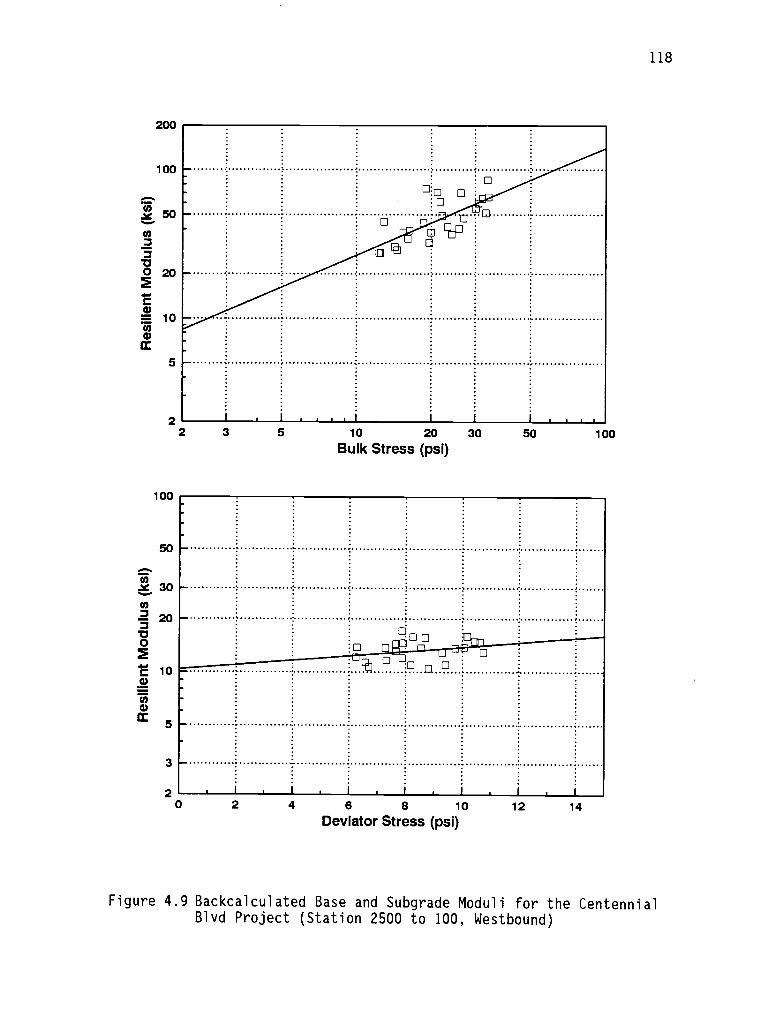
200

100

3-ao 202E07)a)cc

10

5

2

100

50

2 3 5 10 20 30Bulk Stress (psi)

50 100

4- 10a)

2 4 6 8 10 12 14Deviator Stress (psi)

118

Figure 4.9 Backcalculated Base and Subgrade Moduli for the CentennialBlvd Project (Station 2500 to 100, Westbound)

119

Research and Development, Inc., 1989) was employed for the test. The

H&V testing system can be used for both diametral and triaxial

resilient modulus tests. For the diametral test, a temperature

chamber was used for the control of the temperature. The set up of

the system is illustrated in Figures 4.10 and 4.11. The data

acquisition and modulus calculation were accomplished by a

microcomputer.

Table 4.13 summarizes the test results for the Rufus-Quinton

project, while results for the Centennial Boulevard project are

presented in Table 4.14. Actual temperatures at time of testing were

recorded.

The triaxial resilient modulus test on aggregate was performed

by following AASHTO T-274. For the Rufus-Quinton project, the

moisture-density relationship for the aggregate was determined by

following the AASHTO T-99 method C. The results are summarized in

Table 4.15, and plotted in Figure 4.12. The samples for the resilient

modulus test were prepared according to the moisture-density

relationship determined in the laboratory. Two samples were made.

Both were prepared at optimum moisture content. The actual moisture

content at time of testing was slightly less than the optimum. The

actual moisture content and dry density were measured right after the

triaxial test and are summarized in Table 4.16. Resilient modulus

test results for both samples are presented in Table 4.17 and plotted

in Figure 4.13. The test results from this project indicate an

important fact that the resilient modulus values seem to be

proportional to the sample density achieved in the process of sample

preparation.

120

Figure 4.10 H&V Diametral Testing System

Figure 4.11 H&V Triaxial Testing System

Table 4.13 Summary of AC Resilient Modulus Test forRufus-Quinton Project

Sample No.42 °F

Testing Temperature73 °F 95 °F

1 2,521,010 476,677 183,4202 2,886,430 834,289 515,5803 3,563,450 727,813 538,0104 2,316,240 848,096 600,6305 2,733,340 624,261 261,8706 3,441,240 718,098 403,8407 2,535,850 811,157 559,7908 2,054,130 653,839 158,980

Average 2,756,461 711,779 402,765Standard Dev. 491,013 117,289 166,666

121

Table 4.14 Summary of AC Resilient Modulus Testfor Centennial Boulevard Project

Sample ID.42 °F

Testing Temperature73 °F 95 °F

C2 2,874,350 1,634,000 792,140C4 2,673,370 1,295,980 469,040C5 2,897,700 1,724,670 841,080C6 2,262,320 1,372,710 515,250C7 2,723,470 1,383,540 696,050B1 2,369,490 1,482,210 602,180B3 2,793,980 1,678,240 714,690B4 2,794,100 1,754,010 752,380

Average 2,673,598 1,540,670 672,851Standard Dev. 218,990 167,032 123,752

122

Table 4.15 Moisture-Density Relationship for the Rufus-Quinton Project

Water Content Wet Density Dry Density

(%) (pcf) (pcf)

3.8 131.48 126.674.5 136.11 130.245.2 143.69 136.596.2 144.60 136.16

140

138

136

CZ 134C.)

132

2:1

fn 130ca)

C) 128

2,'0 126

124

122

1203 3.5 4 4.5 5 5.5 6

Water Content (%)6.5 7

Figure 4.12 Moisture-Density Relationship for the Rufus-QuintonProject

123

Table 4.16 Density Results for the Rufus-Quinton Project

Sample ID Optimum Maximum Actual Actual RelativeDry Dry to Max

Moisture Density Moisture Density Density

(.) (pcf) ( %) (pcf) (%)

A 5.2 136.59 5.09 136.33 99.8

B 5.2 136.59 5.00 131.29 96.1

Table 4.17 Summary of Base Material Resilient Modulus Testfor the Rufus Project

No. ConfiningStresses(psi)

Bulk S(psi)

Sample AModulus(ksi)

Bulk S(psi)

Sample BModulus(ksi)

1 20 61.7 23.6 61.2 18.02 20 62.5 28.4 62.1 18.43 20 64.7 32.8 65.3 19.74 20 69.6 37.9 70.3 20.55 20 74.7 40.7 74.4 21.56 20 80.0 42.9 79.6 22.47 15 46.8 26.2 46.5 16.28 15 47.3 29.5 47.3 16.49 15 49.6 31.0 50.1 17.310 15 54.3 33.0 54.9 17.911 15 59.6 36.5 59.4 19.112 15 64.3 39.4 64.4 20.513 10 31.6 27.3 31.4 14.214 10 32.1 27.1 32.4 14.515 10 34.5 27.6 34.8 15.316 10 39.6 30.2 39.7 16.017 10 44.4 33.5 44.3 17.218 5 16.6 23.6 16.0 12.519 5 17.2 23.6 17.0 12.620 5 20.0 24.5 19.4 13.421 5 24.2 27.3 24.6 14.322 5 29.3 30.6 29.2 15.723 1 4.6 21.0 4.1 11.224 1 5.5 21.2 4.8 11.425 1 7.7 22.2 7.8 12.426 1 9.7 23.8 9.8 12.727 1 12.7 26.2 12.4 13.2

100

50

30

I I 1

2 3 5 10 20 30 50 100Bulk Stress (psi)

Figure 4.13 Laboratory Tested Moduli for the Rufus-Quinton Project

125

For the Centennial Boulevard project, the samples were prepared

at the field moisture condition. The aggregate materials were

delivered to the laboratory directly from the field, and samples were

made immediately. Four samples were made and similar compaction

efforts were applied to each sample. A potential problem with this

type of preparation is that the samples may not be compacted to the

maximum density or to the predetermined density. Table 4.18 presents

the moisture content and density results that were measured

immediately after the modulus testing, while the resilient modulus

test results are summarized in Table 4.19 and plotted in Figure 4.14.

The test results from this project seem to indicate that for similar

materials, the relationship between the modulus and stress would be

similar if the density variations are not substantial.

4.2.3.6 Comparing Backcalculated and Lab Tested Results

Figures 4.15 and 4.16 provide a comparison of the asphalt

concrete layer material between the backcalculated and lab tested

results, for both Rufus-Quinton and Centennial Blvd projects. The

comparison on the two selected projects shows that for asphalt

concrete, the backcalculated moduli are generally lower than the lab

tested and also seem to be less susceptible to temperature variation.

In the same temperature range, the difference can be expected to be

20 to 30 percent. For the aggregate base material, the backcalculated

modulus slope (k2) is slightly higher than lab tested, as can be seen

in Figures 4.17 and 4.18, for both projects respectively. However, in

the range of bulk stress from 7 psi to 20 psi where actual pavement

stresses generally fall, a favorable comparison can be found.

Table 4.18 Water Content and Density at Time of Testing forCentennial Project

Sample ID Water Content Wet Density DryDensity

(%) (pcf) (pcf)

A 5.33 131.61 124.95

B 4.79 132.01 125.98

C 7.72 131.23 121.82

D 6.68 132.81 124.28

126

Table 4.19 Summary of Base Material Resilient Modulus Test for Centennial Blvd Project

No. Confin.Stress

Sample ABulk S Modulus

Sample BBulk S Modulus

Sample CBulk S Modulus

Sample DBulk S Modulus

1 20 61.9 41.1 61.4 45.8 61.5 40.1 61.3 47.32 20 63.1 40.9 62.4 45.8 62.8 39.1 62.6 46.73 20 65.6 40.9 65.4 46.7 65.9 38.2 65.5 46.54 20 70.1 41.5 70.0 47.7 70.1 39.1 70.3 47.45 20 74.5 42.5 74.5 49.2 74.8 40.6 74.5 48.36 20 79.4 43.6 79.4 49.7 79.9 41.9 79.8 49.27 15 46.0 36.6 46.2 42.6 46.3 36.7 46.3 42.18 15 47.3 36.3 47.2 42.5 47.4 36.2 47.2 41.69 15 49.9 36.3 49.8 42.3 50.8 35.1 50.1 41.810 15 54.9 37.6 54.8 43.4 55.2 36.4 54.8 42.811 15 59.3 39.1 59.4 44.8 59.7 37.8 59.1 44.312 15 64.2 40.8 64.2 46.1 64.4 39.5 64.5 45.513 10 31.3 33.5 31.3 38.8 31.3 34.1 31.1 38.614 10 32.6 33.3 32.6 37.9 32.8 32.9 32.1 38.115 10 34.4 32.8 35.1 38.0 35.3 32.5 34.9 38.016 10 39.2 34.4 40.0 39.3 39.9 33.6 39.5 39.217 10 43.7 36.2 44.4 41.0 44.4 35.4 44.2 41.018 10 16.3 29.9 16.0 34.7 16.2 31.5 16.4 34.519 5 17.4 29.5 17.0 34.1 17.6 30.3 17.1 34.320 5 20.0 30.0 19.6 33.9 20.2 29.8 20.3 34.621 5 25.1 32.1 24.4 35.5 24.4 31.2 24.8 36.222 5 29.4 34.3 28.8 37.5 29.1 33.6 29.0 37.723 1 4.2 28.3 4.3 31.2 4.1 28.7 4.2 31.024 1 4.9 27.6 5.1 31.0 4.9 28.7 5.1 31.125 1 8.0 27.9 7.5 30.8 8.1 27.9 8.0 31.326 1 9.9 28.7 9.4 31.5 9.6 28.5 9.5 31.927 1 13.3 30.2 12.6 32.9 12.5 29.9 12.9 33.5

2 3 5 10 20 30Bulk Stress (psi)

50

Figure 4.14 Laboratory Tested Moduli for the Centennial Blvd Project

100

4,000

al`CA

"...° 3,0000=

2 000

E0......,u) 1,000a)

Ce

030 40 50 60 70 80 90 100

Temperature at Time of testing (F)

0

o0

0.

Lab Tested

0 Backcalcu lated

0

,1111 1111 Ill1Illt1 l lilt l flitnElit

Figure 4.15 Comparison Between Laboratory Tested and Backcalculated AC Moduli for the Rufus-Quinton Project

3,500

r".3,0000-V

25000 'M

2,000

o2 1,500

(1)- 1,000_.

a)ix 500

040 50 60 70 80 90 100

00

O Lab TestedO Backcaloulated

11110

HD

1111 I 1111

00

0

gH

Temperature at Time of Testing (F)

Figure 4.16 Comparison Between Laboratory Tested and Backcalculated AC Moduli for theCentennial Blvd Project

100

50

30

3 20

0 102

.4) 5

a)

.u) 3

2

1

10

BaRiscalwAtate.4 (Wei

A IA A

Backcalcolated (E13)

III1 2 3 5 10 20 30

Bulk Stress (psi)50

Figure 4.17 Comparison Between Laboratory Tested and Backcalculated BaseModuli for the Rufus-Quinton Project

100

200

22 3 5 10 20 30

Bulk Stress (psi)50

Figure 4.18 Comparison Between Laboratory Tested and Backcalculated BaseModuli for the Centennial Blvd Project

100

133

4.3 Summary

This chapter described the development of a new and improved

backcalculation procedure for determining pavement layer moduli.

Initial evaluation on the developed procedure was made. The

evaluation was performed using in three approaches: 1) comparing

backcalculated moduli with preassumed theoretical moduli, 2)

comparing with other backcalculation programs, and 3) comparing

backcalculated moduli with laboratory test results. The evaluation

shows that the moduli backcalculated using the BOUSDEF program

compare very well with the preassumed theoretical values and are very

compatible with some developed programs used for comparison. The

comparison with the laboratory test results on the two projects also

compared favorably.

134

5.0 DETERMINATION OF RESILIENT MODULUS USING LABORATORY TESTS

AND CORRELATIONS

One of the key elements in using a mechanistic type pavement

analysis is to determine the modulus of all pavement materials.

Generally, three approaches have been employed:

1. Backcalculate resilient modulus from deflection

test data.

2. Determine resilient modulus by laboratory test

on cores and soil samples.

3. Estimate resilient modulus using correlations

developed by research investigators.

The backcalculation techniques have been described in great detail in

Chapters .3 and 4. Theoretically, pavement layer moduli determined

using this method represent the in-situ pavement material properties

at time of testing. However, the backcalculation procedures, at the

present time, are not fully capable of determining layer moduli for

all circumstances. Further, the reliability of the backcalculated

results still needs to be examined; therefore, the backcalculation

techniques are recommended for only initial evaluation of pavement

materials.properties. This chapter describes briefly the second and

third approaches.

5.1 Resilient Moduli from Laboratory Tests

The resilient modulus of pavement materials may also be

determined through laboratory tests on undisturbed or disturbed

samples. At present, there are at least two type of standard

135

laboratory procedures for determining modulus of pavement materials.

Typically, the diametral test (ASTM D4123) is used to determine the

resilient modulus for asphalt concrete samples. For untreated

granular materials, the triaxial test (AASHTO T-274) may be used.

5.1.1 Diametral Tests

The mechanism of this test procedure is illustrated in Figures

5.1 and 5.2. To determine the modulus of an asphalt concrete sample,

the specimen is placed in the diametral yoke (Figure 5.1). The yoke,

with specimen, is then placed in the load frame on a load platen with

bottom loading strip attached to the cell (Figure 5.2). A load, which

can be either impulse or haversine, is applied vertically to the

specimen having a diameter of 4 inches and a height of 1 to 3 inches.

The lateral displacement during repeated load is measured by a pair

of linear variable differential transducer (LVDT) gauge heads which

are mounted on the diametral yoke as shown in Figure 5.3. The

resilient modulus of the specimen is calculated with the following

relationship:

MR =0.62 * P

t * H

where:

MR = resilient modulus, psi,

repeated load, lbs,

sample thickness, inches, and

total recoverable horizontal displacement, inches.

The resilient modulus of the asphalt concrete specimen over a range

P =

t =

H =

(5-1)

136

Teflon FridlonRing G

Transducer Tip C

TransducerHousing B

Figure 5.1 Diametral Resilient Modulus Device Yoke and AlignmentStand

137

LVDTGauge Head

LVDTAdjustmentKnob

DiametralYoke

Loading Ram

Diametral Attachment

LPTop loading Strip

To Strip ChartRecorder

Thumb Screws

Bottom Loading Strip

Platen (Rests OnLoad Frame BasePlate)

Figure 5.2 Test Specimen with Diametral Yoke and Loading Ram

Specimen

Loading Strip

Rubber membrane

Airilk_(optional)

1

LVDT

Rubber membrane(optional)

138

Figure 5.3 Schematic of Asphalt Concrete Laboratory Resilient ModulusTest (ASTM, 1984)

139

of temperatures may also be evaluated by testing the sample in a

temperature chamber.

5.1.2 Triaxial Tests

The triaxial test as illustrated in Figure 5.4 is usually used

to determine the resilient modulus of granular and fine materials. A

schematic diagram of this resilient modulus test and definitions are

illustrated in Figure 5.5. In this test, a vertical load is applied.

Rather than measuring the horizontal displacement of the test sample,

the vertical deformation is measured. Varying deviator and confining

stresses can be applied to determine the resilient modulus at

different stress conditions. The resilient modulus is calculated by

dividing the vertical strain by the deviator stress applied with the

following relationship:

MR =

where:

ad

ev

MR = resilient modulus, (psi)

ad = repeated axial stress, (psi)

v= recoverable axial strain, (in/in)

(5-2)

5.2 Correlations

In cases where either backcalculation or laboratory test results

are not available, other developed correlations may also be used to

estimate the modulus. There are several developed correlations or

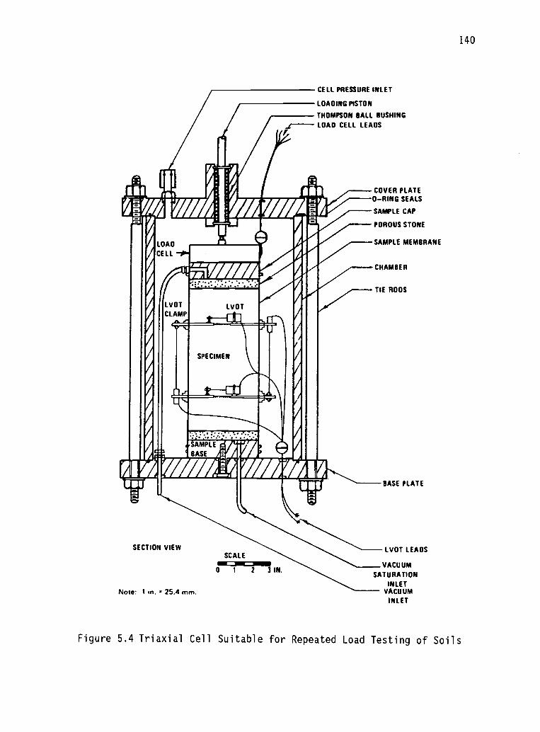
I

41,f A ,r A Ap lii

/LOAD !We FOrAilApo

piLVOT LVOTCLAMP 0

iSPECIMEN

I

I0

SAMPLE zronkaid gilikiff ; ill2... "I

CELL PRESSURE INLET

LOADING PISTON

THOMPSON BALL BUSHING

LOAD CELL LEADS

SECTION VIEW

Note: 1 in. = 25.4 mm.

SCALEliCiwpm110 1 2 3 IN.

VACUUMSATURATION

INLETVACUUM

INLET

COVER PLATE0-RING SEALS

SAMPLE CAP

POROUS STONE

SAMPLE MEMBRANE

CHAMBER

TIE ROOS

BASE PLATE

LVOT LEADS

140

Figure 5.4 Triaxial Cell Suitable for Repeated Load Testing of Soils

141

(Repeated Axial)

//A\ //A\

(Confining)

SOILBORESAMPLE

L

0

Resilient ERStrain

DeviatorStress

AL

Resilient 0d= MR =Modulus E-R

Figure 5.5 Schematic Diagram of Resilient Modulus Test

142

methods which can be used for estimating the resilient modulus of the

pavement materials. The following describe a few of these

relationships.

5.2.1 Subgrade Soil

5.2.1.1 Resilient Modulus versus CBR

The first relationship between resilient modulus and CBR was

that developed by Shell (Heukelom and Klomp, 1962) and used in their

design procedure. This correlation can be used to estimate subgrade

resilient modulus from a known CBR value. Figure 5.6 illustrates the

data used to develop the correlation. Field modulus values were

obtained using vibratory loading. The developed equation is as

follows:

MR = 1500 CBR (5-3)

where:

CBR = California Bearing Ratio.

It should be noted that the coefficient (1500) can vary from 750 to

3000 as shown in Figure 5.6. Available data indicate the equation

provides better results (at least within the correlation limits) at

values of CBR less than about 10, i.e. the correlation appears to

give more reasonable results for fine-grained soil and fine sands

rather than granular materials (The Asphalt Institute, 1982).

5.2.1.2 Resilient Modulus versus R Value

The relationship between resilient modulus and R-value was

originally derived from data collected on the San Diego County

experiment base project (Kallas and Shook, 1977). This relationship

U)Q.

4

2

108

vi 6.

4

02 2

.1cc 10

4

co(19 6

4

_Mr (MPa) =20 CBR //0 0 ,c1 /Mr (psi) )= 3000 CBR/D8/ o ° / _

_ /o oo o0./.° iii, 0 0°

0/ _/0 E 0 0 / ° -

_

/d3 .%7 ///411/ 0

/o\A / 41 o / Mr (MPa) =10 CBR7 a oe *// Mr (Psi ) =1500 CBR?g, / _as °I, 0 '

114 Mr (MPa) = 5 CBR/Mr (psi) =750 CBR/ 'lid I I if mi

143

20

3 a-10 M

6

4 (1)

_J

2 00

102

cc6 o

co

4

2

2 5 10 20 50 100 200 500CBR VALUE

Figure 5.6 Relation Between Dynamic Modulus and CBR (Heukelomand Klomp, 1962)

144

is expressed as follows:

MR(psi) = A + B * R (5-4)

where:

A = 772 to 1155,

B = 369 to 555, and

R = stabilimeter R-value.

In general, the following correlation may be used (AASHTO, 1986):

MR(psi) = 1000 + 555 R (5-5)

Table 5.1 illustrates a comparison of R-value, CBR, and resilient

modulus data and shows a probable range for different type of soils.

The MS-1 (TAI, 1981) indicates that CBR and R-value correlations

are considered applicable to materials classified as CL, CH, ML, SC,

SM, and SP (Unified Soil Classification, ASTM D2487) or for materials

that are estimated to have a resilient modulus of 30,000 psi or less

(TAI, 1981)

5.2.1.3 Resilient Modulus versus Deflection

The subgrade modulus may also be estimated from deflection test

data. Several regression equations have been developed for the

estimation of subgrade modulus. Table 5.2 shows a few of such

equations. It should be noted that the deflection measured at

distance r should be far enough to reflect the subgrade response. A

procedure described by Hicks et al (1988) may be used to determine

the last sensor location.

145

Table 5.1 Comparison of R, CBR, and Resilient Modulus Data(The Asphalt Institute, 1982)

Soil

DescriptionR-value Test CBR Test Triaxial Testa

R EstimatedMr'

psi

CBR EstimatedMr'

psi

EstimatedMr'

psi

Sand 60 34,500 31 46,500 16,900

Silt 59 33,900 20 30,000 11,200

Sandy loam 21 12,800 25 37,500 11,600

Silt-clayloam

21 12,800 25 37,500 17,600

Silty-clay 18 11,000 7.6 11,400 8,200

Heavy clay <5 <3,900 5.2 7,800 1,600

Deviator stress = 6.0 psi, confining stress = 2.0 psi, optimummoisture and density

146

Table 5.2 Various Regression Equations for Subgrade Modulus

Investigator Equation Description

AASHTO Es PSf /(drr) P = Load (lbs)" ' '(AASHTO, 1986) S

f= Subgrade modulus

prediction factor,which is a function ofthe Poisson ration andhas value of:

Ullidtz Es =

(Ullidtz, 1982) " dr

r

(1-A1) P a2

Washington E = 1.61(P/D3

)

(Newcomb, 1986) "

dr=

r=

A Sf

0.30 0.2970.35 0.2930.40 0.2870.45 0.2790.50 0.269

Deflection at distancer

Distance to sensor

A.= Poisson's ratio-r - Contact stressa = Plate radiusr = Distance to sensordr= Deflection at distance

r

P = Load (lbs)

Esg

= 5.77(P/D4

) Dx= Deflection at x feet

from center of NDTload, (mils)

147

5.2.1.4 Resilient Modulus versus Soil Classification

Soil classification infirmation may also be used to estimate the

resilient modulus value. Crude empirical relationships between the

modulus and soil classifications, as shown in Figure 5.7, may also be

used as a reference.

5.2.2 Untreated Granular Materials

Untreated materials are most often used for base and subbase

layers. The strength of the granular base or subbase is related to

the stress state which will occur under operating conditions. The

stiffness characteristics of the granular materials are dependent on

the stress state, which is a function of pavement thickness, load,

and the resilient modulus of each layer. Table 5.3 shows correlations

between modulus and CBR or R-value under different stress conditions

for untreated granular materials that are used for base and subbase.

Another expression which is more commonly used to describe the

relationship between stress state and modulus is represented by the

equation MR = klk2. Numerous studies have been conducted and

typical values developed. Table 5.4 lists the ranges in kl and k2

obtained by different investigators for a number of different

aggregates representative of untreated base and subbase materials.

The 1986 AASHTO Guide (AASHTO, 1986) also provides some typical

values for k1

and k2for unbound base and subbase materials. Table

5.5 shows a range of values based on moisture condition. Therefore,

the base modulus is a function of not only moisture but also the

stress state, and values for the stress state within the base course

vary with the subgrade modulus and thickness of the surface layer.

148

DESIGNCHARTNO. 4 5 6 7

I liI I I I I 1 I I 1 111PSI

5000 10,000 20,000 50,000 100,000Kg/cm2 DYNAMIC MODULUS

200 500 1000 2000 5000 10,000I 1 1 ttill I I I I 1 Iitti

CBR

2 3 4 6 8 10 20 40 60 80 100I I I It'll! I 'I'll

BEARING VALVE, PSI (12 IN. DIA. PLATE, 0.2 IN. DEFLECTION, 10 REPETITIONS)

20 25 30 40 60 80 100 200 300 400I I I 1 1 1

GENERAL SOIL RATING AS SUBGRADE, SUB-BASE OR BASE

Very PoorSobered*

PoorSob-

ered*

Fair Med.Sub- Sub-grade grade

GoodSob-ered.

Mb.Sub-base

GoodSub-base

Med.Base

GoodBasta

Excell*MBar

A.A.S.H.O. SOIL CLASSIFICATION

A-1-1) L A4 4A-2-7 A-2-6 A-2-5 I A-24

A3

A4

A5

A6

A-7-6 i A-7-5

OH CH

MH OL1

UNIFIED SOIL CLASSIFICATION

GM-u

CL

ML

GM-d

GC

SW

SM-d

SC

SM-u

SP

GP

Figure 5.7 Crude Empirical Relationships Between the Dynamic Modulusof Elasticity and Routine Tests (Hicks, et al, 1980)

149

Table 5.3 Correlations Between MR, CBR or R and Stress State

(AASHTO, 1986)

Stress State, 0 MR (psi) MR (psi)

100 740 * CBR 1000 + 780 * R

30 440 * CBR 1000 + 450 * R

20 340 * CBR 1000 + 350 * R

10 250 * CBR 1000 + 250 * R

150

Table 5.4 Summary of Repeated Load Triaxial CompressionLaboratory Test Data for Untreated GranularMaterials (The Asphalt Institute, 1982)

Investigator(s) Material(s) kl k2

Hicks, 1970 Partially crushed gravel;crushed rock

1,600-5,000 0.57-0.73

Hicks, et al Untreated base San 2,100-5,400 0.611970 Diego Test Road

Allen, 1973 Gravel, crushed stone 1,800-8,000 0.32-0.70

Kalcheff & Crushed stone 4,000-9,000 0.46-0.64Hicks, 1973

Boyce, Brown, & Well graded crushed 8,000 0.67Pell, 1976

U.C. Berkeley(Monismith,

In service base andsubbase materials

2,900-7,750 0.46-0.65

1972)

Albright, 1986 Crushed aggregate 1,300-2,000 0.69-0.78(Saturated)Crushed aggregate 2,000-2,600 0.70-0.73(Optimum water content)

MR = k10k2

'

where MR and 0 are in psi.

151

Table 5.5 Typical values for kl and k2 for Unbound Base and

Subbase Material (AASHTO, 1986)

(a) Base

Moisture kl* kk2*

Dry 6,000 - 10,000 0.5 0.7

Damp 4,000 - 6,000 0.5 0.7

Wet 2,000 4,000 0.5 0.7

(b) Subbase

Dry 6,000 8,000 0.4 0.6

Damp 4,000 - 6,000 0.4 0.6

Wet 1,500 4,000 0.4 0.6

* Range in kl and k2 is a function of the material quality.

Typical values for use in design are given in Table 5.6.

5.2.3 Asphalt Concrete

The Asphalt Institute (1982) developed a relationship that can

be used to determine resilient modulus of asphalt concrete. The

relation has the following form:

20Log 1E1 = 5.553833 + 0.028829

f0.17033

0.03476 (Vv)

where:

152

(5-6)

+0.070377(n70°F,

106 )+0.000005[tp (1.3+0.498251og f)

p0.5]

t(1.3+0.498251og f) p%5

-0.00189 + 0.931757[1.1

f0 02774

f

1E1 = dynamic modulus of asphalt concrete, psi

percent aggregate passing No. 200 sieve

frequency, Hz

P200

=

f =

Vv

= percent air voids

n70°F,106 absolute viscosity at 70°F, poises x 106

Pac

= asphalt content, percent by weight of mix

t = temperature, °F (1.8°C + 32)

If sufficient viscosity data are not available to estimate

then the following relationship may be used:

n70°F,106 = 29508.2 pen

939

The value of pac may be estimated as follows:

pac

= 0.483 Vbe

where:

p70°F,106'

(5-7)

(5-8)

Table 5.6 Typical Values of Stress State(AASHTO, 1986)

Roadbed Soil Resilient Modulus (psi)AsphaltConcrete Thickness (in) 3,000 7,500 15,000

less than 2 20 25 30

2 4 10 15 20

4 6 5 10 15

Greater than 6 5 5 5

153

154

Vbe

= Effective volume of asphalt, percent, defined as the

total asphalt content minus the quantity of asphalt

lost by absorption into the aggregate particles.

or

= 0.434 VbPac

where:

(5-9)

Vb

= total volume of asphalt, percent.

This equation has been computerized for use on microcomputers.

The resulting program (AMOD) and its user's guide may be found in

Appendix C.

5.3 Summary

This chapter describes several techniques that are widely used

around the United States to determine modulus of pavement layers.

These techniques include laboratory tests and correlations to

determine/estimate the resilient modulus of pavement materials.

The advantage of the laboratory tests to determine resilient

modulus is that it is a direct measurement of the strength of a

particular material. The disadvantage is that the samples tested in

the laboratory may represent only a portion of pavement material

rather than an average condition that would find in the field. For

example, for a badly cracked asphalt concrete surface, the cores

tested in the laboratory may not truly reflect the field situation.

Moreover, the laboratory tests require sophisticated equipment as

well as trained personnel to perform the tests, and the laboratory

tests usually take a significant amount of time. Lastly, there are

several test related variables which affect test results. These

155

variables are summarized in Table 5.7.

The advantage of using developed correlations is their

availability. However, one must be aware that correlations were

developed based on certain laboratory conditions. Therefore, these

correlations are best suitable to situations that are similar to

where the correlations were developed. Caution should be exercised

when using these correlations.

In any case, material characterization is an extremely important

and difficult issue. There are many variables that would affect

material response both in the laboratory and in field tests. These

variables, as summarized and presented in Table 5.7, must be fully

realized when determining the resilient modulus values.

Table 5.7 Variables Affecting Materials Response (Hicks et al, 1980)

I. LOADING VARIABLES

A. Stress history (nature of prior loading)

1. Non-repetitive loading (such as preconsolidation)2. Repetitive loading

a. Nature

(1) Simple(2) Compound

b. Number of repetitive applications

B. Initial stress state (magnitude and direction of normal and shear stresses)

C. Incremental loading

1. Mode of loading

a. Controlled stress (or load)b. Controlled strain (or deformation)c. Intermediate modes

2. Intensity (magnitude and direction of incremental normal and shear stresses)3. Stress path (relation among stresses - both normal and shear as test progresses)4. Time path

a. Static

(1) Constant rate of stress or load)(2) Constant rate of strain or deformation)(3) Creep4) Relaxation

b. Dynamic

(1) Impact(2) Resonance(3) Other

(a) Sinusoidal (rate of loading is variable)(b) Pulsating (duration, frequency, and shape of load curve are variables)

Table 5.7 Variables Affecting Materials Response (cont.)

5. Type of behavior observed

a. Strength (limiting stresses and strains)b. Deformability

6. Homogeneity of stresses7. Drainage (drained or undrained)

II. MIXTURE VARIABLES

A. Mineral particles

I. Maximum and minimum size.

2. Gradation3. Shape4. Surface texture5. Angularity6. Mineralogy7. Adsorbed ions8. Quantity

B. Binder

1. Type

2. Hardness3. Quantity

C. Water

1. Quantity

D. Voids

1. Quantity2. Size3. Shape

E. Construction Process

1. Density2. Structure3. Degree of anisotrophy4. Temperature

F. Homogeneity

III. ENVIRONMENTAL VARIABLES

A. Temperature

B. Moisture

C. Alteration of MaterialProperties

1. Thixotropy2. Aging3. Curing4. Densification

158

6.0 DEVELOPMENT OF AN IMPROVED MECHANISTIC OVERLAY DESIGN

PROCEDURE FOR FLEXIBLE PAVEMENTS

One of the major objectives of this study is to develop an

improved mechanistic overlay design procedure for routine design

work. To achieve this objective, this chapter first reviews some

mechanistic design procedures developed in the past and then presents

an improved overlay design procedure.

6.1 Review of Current Mechanistic Overlay Design Methods

Several mechanistic overlay design have been developed in the

past few years. These methods generally follow a framework presented

by Finn and Monismith (1984) as shown in Figure 6.1. Table 6.1

summarizes some of these developments, while the following sections

review three of the procedures developed by: 1) ARE (Austin Research

Engineers, Inc., 1975), 2) WSDOT (Mahoney, et al., 1988), and 3)

ADOT&PF (Yapp, et al., 1988).

6.1.1 ARE Method

This method was developed for the Federal Highway Administration

by Austin Research Engineers (ARE). The following describes some of

the major steps involved in this overlay design procedure.

6.1.1.1 Nondestructive Testing

Nondestructive testing can be performed using any type of

deflection equipment that provides satisfactory deflection results.

The frequency of deflection measurement is dependent on the terrain,

as shown in Table 6.2. Condition surveys are conducted at the same

159

CONDITIONSURVEYS

NON-DESTRUCTIVE TESTING(E.G.. DEFLECTION. CURVATURE)

4,

ADJUSTMATERIALPROPERTIES

ANALYSISSECTIONS

A

NOT ACCEPTABLE

SAMPLINGTESTING

MATERIALSCHARACTERIZATION

COMPUTE:DEFLECTIONSCURVATUREETC

ADJUST MATERIALPROPERTIES:

SEASONAL EFFECTSLOAD

COMPUTE DISTRESSDETERMINANTS

1'

RUTTING(UNIT DEFORMATION)

TRAFFIC

REMAINING LFE

OVERLAYTRIAL SECTIONS

COMPUTEDISTRESSDETERMINANTS

4,

Final Design

Figure 6.1 Flowchart for the Mechanistic Method (Finn &Monismith, 1984)

Table 6.1 Analytically Based Overlay Design Proceduresa (Hicks and Zhou, 1988)

Procedure

NondestructivePavementEvaluation

StiffnessDeterminations Distress

MechanismsProvisionfor

ExistingPavement Overlay Thickness Determination

In-SituMeasurement

LabTesting

AnalysisProcedure Fatigue Rutting

Shell

ResearchFalling weightdeflectometer

Yes No BISAR

computerprogram

Yes Yes Yes Overlay thickness selected to (a) limit fatigueand (b) limit rutting for anticipated traffic;thickness also selected assuming existing pave-ment is cracked

FHWA-ARE Dynaflect;Benkelman beam

No Yes ELSYMcomputerprogram

Yes Yes Yes Overlay thickness selected to (a) limit fatigueand (b) limit rutting for anticipated traffic;

asphalt concrete assigned different stiffnessvalues depending on conditions

FHWA-RII Dynaflectand others

Yes Opt. ELSYMcomputerprogram

Yes No Yes Overlay thickness selected to limit fatigue foranticipated traffic; asphalt concrete assigneddifferent stiffness values depending on condi-tions.

Kentucky Road Rater Yes No Graphic ,solution'

les No Yes Overlay thickness selected as difference betweenpavement thickness required to accommodate alltraffic (both applied and anticipated) andeffective thickness of existing pavement asdetermined by nondestructive evaluation ofexisting pavement.

Alaska Falling weightdeflectometer

Yes Opt. ELSYMcomputerprogram

Yes Yes Yes Overlay thickness selected to (a) limit fatigueand (b) limit rutting for anticipated traffic;thickness also selected considering seasonaleffect as well as traffic for each season.

Washing-ton DOT

Falling weightdeflectometer

Yes Opt. CHEVRONcomputerprogram

Yes Yes Yes Overlay thickness selected to (a) limit fatigueand (b) limit rutting for anticipated traffic;

thickness also selected based on sum of damageratio.

aAll procedures require a condition survey, represent the pavement as a multilayer elastic solid, and provide an estimate of remaining life.bBased on Chevron computer solution for multilayer elastic solid.

161

Table 6.2 Guidelines for Nondestructive Testing(Finn and Monismith, 1984)

Type of Location Spacing

Rolling terrain

Numerous cut-to-fill transitions

Level with uniform grading

100 ft

100 ft

250 ft

162

time that the deflection measurements are made. Cracking and rutting

are recorded and measured. Other general information, such as soil

type, drainage conditions, and cut/fill transitions, are also noted.

Deflection profiles are generated for the entire length of the

project to assist in establishing the analysis sections. Statistical

procedures are used to compare adjacent sections to ensure that the

sections are different. The design deflection for each section is

determined from:

Sd=S+Z* S

where:

Sd

= design deflection

(6-1)

6 = average deflection

Z = deviation from mean to selected significance level on a

normal distribution curve.

S = standard deviation

6.1.1.2 Material Characterization

The pavement structure is represented as a multi-layer elastic

system. Each layer's properties are defined by modulus (stiffness)

and Poisson's ratio. For the asphalt-bound layer(s), modulus values

should be defined over a range in temperatures at a time of loading

corresponding to moving traffic. For design purposes, the stiffness

at a temperature of 70°F is recommended for use. Poisson's ratio is

assumed to be 0.3 for the asphalt concrete, 0.4 for the base and

subbase, and 0.45 for subgrade. For a cracked asphalt concrete layer,

it is assigned a modulus of 70,000 psi if the cracking is defined as

class 2; or a value equal to the base modulus (or 20,000 psi),

163

whichever is greater, if the cracking is defined as class 3. Table

6.3 presents the definitions for both classes of cracking. Figure 6.2

illustrates the pattern of the cracking of the two classes.

Treated base course materials can be tested in the same way as

the asphalt concrete. Unbound base course materials should be tested

at representative conditions of water content and dry density in

repeated loading by following AASHTO test procedures. Subgrade

materials should be tested over a range in deviator stresses to

permit defining a relationship of the form:

MR

= A CO (6-2)

where:

MR = resilient modulus, psi

ad = applied deviator stress, psi, and

A, b = laboratory determined coefficients.

To select an appropriate subgrade modulus for analysis, it is

necessary to use the design deflection selected for the particular

analysis section and with an iterative procedure, select a modulus

value from equation (6-2) that provides the same value for the

computed as measured deflection. As seen in Figure 6.3, some

adjustments in the laboratory data may be required to achieve

compatibility.

6.1.1.3 Distress Determinants

Two major structural distresses are considered in this method;

fatigue and rutting. Fatigue cracking in the asphalt-bound layer is

controlled by limiting tensile strain on the underside of the asphalt

concrete layer using the following relationship, which is also

plotted in Figure 6.4:

164

Table 6.3 Classes of Cracking(ARE, 1975)

Class Cracking Definition AC Modulus

Uncracked

2

3

No cracks Overlay MR

Cracking that has progressed to thepavement where cracks have connectedtogether to form a grid-type pattern.(mildly cracked, failed in fatigue)

When the asphalt concrete segmentshave become loose.(severely cracked, failed in fatigue)

70,000 psi

20,000 psi

Note: Variation of the modulus with temperature is notapplied to the class 2 and class 3 crackedsurface.

165

Class 2 Cracking

Class 3 Cracking

Figure 6.2 Photographs of Class 2 and Class 3 Cracking (ARE, 1975)

NM4La

AO

W

166

10,000

MI

I m.

I I 1 I 1111 i

AnalysisCurve

LabCurve

I I I I Ili! i

1,000

1000.2

eO

...11

4.1

tsL41aa

'0s.

en

1 1 1 1 1111 1 1 1 1 1

0.4 1.0 4 0Deviator Stress, psi

m I

MI

mg

.m.

MI

m I

MO

m 1

10 40

Figure 6.3 Relationship of Resilient Modulus and Repeated DeviatorStress (ARE, 1975)

1111111110,000 100,000

inal

0

ro

0

xro

0

ro

ro

1.4.10

1.

GI

ro

1,000

100

I I I 1 1 1 1 1 11 1 I I 1 1 1 1 1 1 I WI I I 1 l I

Pl

)

5.16(

N 9.73 x 10-15 1

1 I 1 1 1 1 1 I 1 1 Ili till100 1,000

18-kip Equivalent Axle Loads, N x 103

Figure 6.4 Fatigue Curve for 18-kip Load Applications to Time of Class 2 Cracking (ARE, 1975)

N189.73 * 10-15 * ft-5.16

168

(6 -3)

where:

N18

= allowable number of 18-kip single-axle load

applications and,

Et horizontal tensile strain on the underside of

asphalt-bound layer being analyzed.

Rutting is controlled by a regression equation of the general form:

log N18 = 7.5145 + 0.96831 R + 0.01173 (eiz/aiz)

+ 0.04322a2z 0.01687a2x

+ 0.05608a3z + 0.108034,

+ 0.18032a5z + 0.102265, + log(365/dT)

where:

(6-4)

N18

the allowable 18-kip equivalent load applications

allowable rut depth, in.

flz

= vertical strain at bottom of the top layer x104,

in/in

alz

vertical stress at bottom of the top layer, psi

02z = vertical stress (psi) at the bottom of the second

layer, psi

a2x = horizontal stress, parallel to the axle load, at the

bottom of the second layer, psi

a3z vertical stress at the bottom of the third layer,

psi

e4z vertical strain at the bottom of the fourth layer,

x104, in/in

169

a5z = vertical stress at the top of the fifth (subgrade)

layer, psi

e5z

vertical strain at the top of fifth (subgrade) layer

x104, in/in

dT

number of days per year when average daily

temperature is equal to greater than 64°F (should be

a five year average)

The sign convention used is positive for tension and negative for

compression. In a pavement system, vertical stresses and strains are

compressive.

When using the equation, a five layer pavement analysis must be

used where the first layer is the proposed overlay, the second layer

is the existing surface layer, the third and fourth layers are the

granular base and subbase, and the fifth layer is the subgrade. If

either the base or subbase layer is not present, then the granular

layer which is present is divided into two layers of equal thickness.

An 18-kip single axle is used in the analysis of the stresses

and strains. The stresses and strains are analyzed both under and

between the dual tires. The maximum value of the stress or strain is

then used in the equation. Depending upon the geometry of the

pavement, the maximum value can occur either under a tire or between

the tires. Also an allowable rut depth must be selected.

6.1.1.4 Remaining Life Estimation and Overlay Design

Remaining life can be determined for an uncracked pavement. This

requires an estimation of the amount of traffic, in terms of 18-kip

single axle loads applied to date, and the tensile strain(s) on the

underside of the asphalt-bound layer.

170

Mixed traffic is converted to repetitions of the 18-kip single

axle using AASHTO equivalency factors. Tensile strains can be

computed using ELSYM computer program with the knowledge of modulus

values and Poisson's ratios for the various layers. The total number

of load repetitions (N18) can be estimated using equation (6-3). The

remaining life is then calculated using the cumulative damage

hypothesis, i.e.,

nr

N1

where:

1

nD

N1

nr

= number of additional 18-kip single-axle loads can be

(6-5)

carried at the computed strain level,

N1

= allowable number of applications of 18-kip EAL's according

to fatigue criteria, and

np = number of 18-kip EAL's applications to date.

If the value for nr

is less than the additional traffic to be

carried, an overlay will be needed. Example overlay thickness design

curves using this method are shown in Figure 6.5.

The above procedures have been combined into two computer

programs termed DEFANL and OVLANL.

6.1.2 WSDOT Method

This mechanistic-based overlay design procedure was developed by

the University of Washington (Mahoney, 1988) for the state of

Washington (WSDOT). The concept for this method is illustrated in

Figure 6.6.

100 1,000 10,000

Allowable 18-kip equivalent load applications. N x 103

Figure 6.5 Sample Overlay Thickness Design Curves (ARE, 1975)

100,000

AnalysisSection

PavementRating

NoFurtherAction

Failed?

Yes

NondestructiveTesting

MaterialSampling

PavementAnalysis

AlgorithmsLaboratory

Testing

TrafficHistory

ProjectedTraffic

FailureCriteria

MaterialProperties

StructuralAnalysis

Overlay DesignThicknessLife

172

Figure 6.6 Pavement Overlay Design Concept (Mahoney, 1987)

173

6.1.2.1 Analysis Section and Pavement Rating

There is no description in the report how the pavement analysis

section and pavement rating were carried out. However, it is believed

that the pavement rating is conducted based on field condition survey

information to classify the pavement serviceability. If the pavement

rating for the analysis section is below acceptable level, further

overlay design steps are recommended.

6.1.2.2 Nondestructive Testing and Pavement Analysis

Algorithms

Nondestructive testing is performed through deflection

measurements using falling weight deflectometer (FWD). The deflection

were measured every 50 ft within each test site, with four load

levels at each test stop and two drops at each load level. The load

levels were approximately 6000, 9000, 12000, and 15000 lbs. There is

no indication whether this is a standard practice. Evaluation of

layer moduli is accomplished through backcalculation of pavement

surface deflection basins. EVERCALC (Mahoney, 1987), a pavement

analysis algorithm based on CHEVRON N-LAYER program and developed at

the University of Washington, is used for backcalculating the layer

moduli.

6.1.2.3 Material Sampling and Laboratory Testing

Material sampling and laboratory testing were used primarily to

verify the backcalculation results. Material sampling also provide

layer thickness information to be used in backcalculation. Extensive

laboratory testings were performed on asphalt concrete, base course,

and subgrade materials. These tests include resilient modulus tests,

174

bulk and maximum specific gravity tests, asphalt extraction tests,

asphalt recovery, aggregate gradation, Lottman conditioning tests,

and asphalt penetration, and viscosity tests. Laboratory tests which

are direct measures of the resilient modulus are diametral test (ASTM

D4123) for asphalt bound material, and triaxial test (AASHTO T-274)

for unbound materials.

6.1.2.4 Traffic History and Projected Traffic

Traffic volume is expressed in terms of 18-kip equivalent single

axle loads (ESAL). AASHTO's load equivalent factor is used for mixed

traffic. Traffic load information is accumulated in the format of the

Federal Administration's W-4 loadometer tables, which include the

number of axles observed with a series of category.

Design traffic volume is determined from average daily traffic

(ADT), truck percentage, and the ESAL per truck for each road

section. Both historical and projected traffic are used in the

overlay design method.

6.1.2.5 Material Properties

Seasonal adjustments for the asphalt-bound materials are

obtained using the relationship between the modulus and temperature.

Seasonal variations for unbound material are determined using the

ratios as given in Table 6.4. These ratios were developed using the

backcalculated moduli from three years of FWD test data and climatic

data (Mahoney, 1987).

For AC bound material, the relationship between the modulus and

temperature for WSDOT class B AC, as shown in Figure 6.7, was used to

determine the AC material properties. This relationship is expressed

as follows:

175

Table 6.4 Coefficients for Seasonal Variations(Mahoney, 1987)

Region Base Subgrade

Wet/Thaw Dry/Other Wet/Thaw Dry/Other

Eastern Washington 0.65 1.00 0.95 1.00

Western Washington 0.80 1.00 0.90 1.00

107

106

2

/BM

=lb

176

95% Prediction Intervals

90% Prediction Intervals

Ea' \2 \\tx \\10 \\\\\

Ms 101647210 - 0.000147362 (T)2]

le 1 L11110 20 40 60 80 100 120

Temperature ( °F)

Figure 6.7 General Stiffness-Temperature Relationship with 90 and 95%Prediction Intervals for Class B Asphalt Concrete InWashington State (Bu-Bushait, 1985)

log Eac = 6.4721 0.000147362 (Tp)2

177

(6-6)

where:

Eac

= resilient modulus of AC (psi), and

TP

= pavement temperature (°F).

The pavement temperature is estimated from Figure 6.8, knowing

pavement surface temperature, the previous five-day mean air

temperature, and pavement thickness.

For unbound materials, the following relationships are used:

Ebs

= k18k2 for coarse-grained materials (6-7)

for fine-grained materials (6-8)MR = k3 adk4

where:

Ebs

= resilient modulus of coarse-grained materials and

soils (psi),

MR

= Resilient modulus of fine-grained soil (psi),

9 = Bulk stresses (psi),

ad

= Deviator stress (psi), and

kl'

k2'

k3'

k4

= Regression coefficients.

6.1.2.6 Failure Criteria

The two pavement failure criteria used are fatigue cracking and

subgrade rutting. Monismith's laboratory model (Monismith and Epps,

1969) is used for fatigue, as shown below:

log Nf = 14.82 3.291 log(et) 0.854 log(Eac/1000) (6-9)

where:

Nf

= loads to failure,

Et

= initial tensile strain (10-6 in/in), and,

Eac

= modulus of asphalt-bound material (psi).

0

70

60

50

40

30

20

10

-10

Pavement Surface Temperature Plus 5-day Mean Air Temperature (°F)20 40 60 80 100 120 140 160 180 200 220 240 260160III 11

25mm (1 in.)

50mm (2 in.)

100mm (4 in.)

150mm (6 in.)

200mm (8 in.)

300mm (12 in.)

1 1 I 1 I I I I I I I I I

140

120

100

-10 0 10 20 30 40 50 60 70 80 90 100 110 120Pavement Surface Temperature Plus 5-day Mean Air Temperature (°C)

Figure 6.8 Estimation of Pavement Temperature (Southgate, 1975)

80

60

40

20

179

The laboratory model is adjusted to field conditions, by multiplying a

shift factor. For the state of Washington, a factor of 3 to 5 is

used.

The Chevron equation (Santucci, 1977) was used to design for

rutting. It is as follows:

Nr

= 1.077 * 1018

* (cv)-4 4843

where:

Nr

= number of loads needed to cause approximately a

0.75-inch deep rut,

ev

= vertical compressive strain at the top of the

(6-10)

subgrade (10-6 in/in).

6.1.2.7 Structural Analysis

Structural analysis is based on a multilayered linear elastic

model. The CHEVRON N-LAYER, which was developed by the Chevron

Research Company (Michelow, 1963), is used for pavement structural

analysis.

6.1.2.8 Overlay Design

Overlay design is conducted using a computer program EVERPAVE

(Mahoney, 1987) which is based on multilayered elastic analysis and

the design criteria for fatigue and rutting failure. A flowchart of

this program is shown in Figure 6.9. The input data include design

traffic volume, seasonal variations of material properties,

temperature, the shift factor for fatigue failure, the minimum

overlay thickness, thickness increment, and unbound material

properties, which include coefficients kl, k2, k3, and k4, as

indicated in equations (6-7) and (6-8).

Read Input DataMaterial propertiesSeasonal var.Traffic

1

Assume overlaythickness

al* Determine seasonalmaterial properties

' Analyze pavementstructure (e ev )

Calculate performancelife (N f , N )

Increase overlaythickness

Calculate seasonaltraffic volume

Determine DamageRatio

Compute Sum ofDamage Ratio (SDR)

Repeat for four seasons

180

Produce overlaydesign

Figure 6.9 Overlay Design Procedure by EVERPAVE (Mahoney, 1988)

181

6.1.3 Alaska Method

This mechanistic overlay design procedure was developed by

Oregon State University for the State of Alaska (Yapp et al, 1987).

The original procedure include two approaches; one is a simplified

mechanistic procedure and another is a fully mechanistic approach.

6.1.3.1 Simplified Procedure

The proposed simplified approach was developed by Fernando

(1986) at Pennsylvania State University. A flowchart of this

simplified mechanistic procedure is illustrated in Figure 6.10.

In using this procedure, once the critical analysis section has

been determined, which is done by conducting condition survey and

deflection test, design of the overlay can begin. The past and future

traffic, together with the AC modulus, are needed to compute the

tolerable pavement strains using appropriate fatigue and permanent

deformation criteria. Remaining life of the existing pavement can

then be determined. For overlay design, an overlay thickness is first

assumed and tensile strain at the bottom of the existing asphalt

layer and the compressive strain at the top of subgrade are

calculated. The calculated overlay strains are then compared with the

tolerable strains, which are determined based on a fatigue

relationship developed by ARE (ARE, 1985) and a subgrade strain

criterion developed by Luhr et al (1983). Iterative procedures are

used to determine the final overlay thickness. Since the method was

developed based on a regression analysis for conditions in

Pennsylvania, it may not be valid for use in the state of Alaska.

(BEGIN)4,

ISelect analysis section

182

1Layer

ThicknessConditioning

Rating

1Pavement

Temperature

Determine trafficand AC properties

1PavementDefelection

Adjust S fortemperature

1Calculate ex sting strains

Et, Ec = f(8, H)

1Calculate remaining life

Nf = f(et,Ec,EAL,PSI,TSE)

Assume ho

Compute tolerable stragem

Et& = f(N,E)

NO

Calculate overlay strains

Eov= f(Et,EoMov H1)

Figure 6.10 Flowchart for the Simplified mechanistic Procedure(Yapp, 1987)

183

6.1.3.2 Mechanistic Procedure

The proposed mechanistic overlay design procedure follows the

flowchart developed by Finn (1984), as shown in Figure 6.1. The

following discusses some of the main points.

6.1.3.2.1 Nondestructive Testing and Material

Characterization

In the procedure, nondestructive pavement tests, condition

survey, and traffic data are required as inputs. In addition, some

knowledge of the stiffness properties and distress characteristics of

various materials comprising the pavement structure are needed.

Stiffness characteristics of the various pavement components can

either be determined by test on undisturbed or disturbed specimens of

the pavement materials, or backcalculated from NDT measurements.

Nondestructive testing is performed using the Dynatest FWD. For

determining pavement properties from NDT test data, the programs

ELSDEF, developed by Brent Rauhnt Engineers (Lytton, et al., 1986),

and ELMOD, developed by Dynatest (Ullidtz, 1987), are used.

6.1.3.2.2 Distress Determinants

In this procedure, the ELSYM5 program is recommended to

determine the critical strains in the pavement. The tensile strain at

the bottom of the asphalt concrete layer is used to control fatigue

while the compressive strain on the top of the subgrade is used to

control rutting. Currently, the equations developed by the Asphalt

Institute (The Asphalt Institute, 1982) are adopted as fatigue

criteria. These equations are:

a) For fatigue:

N = 18.4 * C * 0.004325 * et

-3 291*E

ac-0 854

(6-11)

184

where:

number of 18-kip equivalent single axle loads,

et

horizontal tensile strain on underside of AC layer,

Eac

modulus of AC layer, psi, and

a function of voids and volume of asphalt in the mix

design, and can be determined by following:

C = 10M

where:

4.84 * [Vb/(Vv+Vb) 0.69]

Vb volume of asphalt, %, and

Vv

volume of air voids, %.

b) For permanent deformation:

N = 1.36 * 10-9 * ev

4.48(6-12)

where:

ev

= vertical compressive strain on the top of the subgrade.

For determining the tolerable strains, the equations (6-11) and (6-

12) can be rearranged and et and ev solved. In this procedure, these

two strains are used in determining the required overlay thickness.

6.1.3.2.3 Remaining Life and Overlay Design

Cumulative historic traffic data are necessary to determine the

remaining life of the existing pavement. The percentage of remaining

life is determined using Miner's Hypothesis:

or

Nr 1 NA

ND

ND

Rf

I N / NA -D

where:

(6-13)

185

Nr/ND = Rf = percentage of remaining life,

Nr

= additional number of applications of EALs that can be

applied to the existing pavement,

NA = number of applications of EALs to date,

ND = allowable number of applications of EALs according to

fatigue relations.

If a negative Rf value occurs, it indicates that the life of the

pavement has been used up and an overlay or reconstruction may be

required.

The required overlay thickness for carrying anticipated traffic

volume is a function of the remaining life, the reliability level

desired, and design EALs. The reliability of a pavement design-

performance process is defined as the probability that a pavement

section designed using the process will perform satisfactorily over

the traffic and environmental conditions for the design period

(AASHT0,1986). The selection of reliability is based on functional

class. In general, a higher reliability level would lead to a thicker

overlay.

With a knowledge of the allowable traffic applications and

pavement design life, the tolerable pavement strains can be

determined using equations (6-11) and (6-12). If the calculated

strains are greater than the tolerable ones, the overlay thickness

needs to be increased. The determination of an overlay thickness

involves re-iteration. The following procedures are followed:

1) Assumed an overlay thickness.

2) Use the ELSYM5 program to compute the pavement strains.

3) Determine tolerable strains for projected traffic.

186

4) Compare pavement strains with the tolerable strains.

5) If the pavement strains are greater than the tolerable

strains, increase the overlay thickness and go to step 2.

The above procedure is repeated until the pavement strains are less

than the tolerable ones, and the final overlay thickness is then

recommended.

6.1.4 Summary of Review

Review of the three mechanistic design procedures indicates that

one common ground for these developed procedures is that they all use

multi-layered elastic theory to model a flexible pavement structure

and to determine pavement life using various design criteria. This

kind of approach is also being used by an on-going research activity,

NCHRP project 1-26 (Thompson, 1989). It is expected that the next

edition of the AASHTO Guide on Flexible Pavement Design will move in

this direction.

One weak aspect in all three procedures is characterizing the

seasonal effects on the pavement materials properties. In both the

ARE and the Alaska methods, pavement properties at a representative

temperature of 70°F is recommended for design purposes rather than

those at different seasons. In the WSDOT method, seasonal variations

are considered. However, for the base and subgrade materials, modulus

ratios between the dry and wet materials are used rather than a

direct consideration of the base and subgrade material properties for

each season.

Since the seasonal effects have great influence on pavement

layer properties (and some other factors such as traffic

187

distribution), this results in varying pavement damage during the

year. Therefore, an improved approach to address the seasonal effects

seems to be necessary.

6.2 Development of an Improved Mechanistic Overlay Design Procedure

6.2.1 Framework

Figure 6.10 illustrates, in a flowchart format, an improved

mechanistic overlay design procedure for flexible pavements. This

improved procedure is based on the concept similar to that of Alaska

method. The following sections describe some of the major points in

more detail.

6.2.2 Condition Survey

The first step in the overlay design is to perform a condition

survey. The purpose of the condition survey is to obtain information

regarding the existing pavement condition. Condition surveys usually

involve a fair amount of detail. They generally include not only the

type of distress that has occurred, but also its severity, its

extent, and the location (Haas and Hudson, 1982). Typically, for

flexible pavements, the pavement condition survey includes rutting,

alligator cracking, longitudinal cracking, transverse cracking, block

cracking, bleeding, ravelling, potholes, patches, and punchouts. The

condition survey results may provide very important information in

estimating qualitatively the structural capacity of the existing

pavements.

188

Backcalculation

Conditionsurveys

Pavementrating

Need an

overlay ?

No furtheraction

Nondestructivetesting

Delineation ofanalysis sections

,---110Material

characterization

TAdjust material

properties

4 Laboratorytests

Figure 6.11 Flowchart for the Improved Overlay Design Approach

189

Seasonal Effect

Compute pavement strainsfor each season

Traffic applicationsto date

Calculate allowabletraffic

Compute remaininglife R

Is R>20% orfatigue cracks <40%

Total trafficvolume

Yes

Future seasonaltraffic applications

Remove andreplace pavement

Allowable trafficvolume

No

Yes

Overlaydesign

No overlayrequired

Figure 6.11 Flowchart for the Improved Overlay Design Approach(cont.)

Overlay materialproperties

Existing pavementMaterials data

Assume overlaythickness

Increaseoverlay

thickness

Compute pavementstrains for each season

Compute allowabletraffic for each season

Determine damageratio for each season

190

Traffic datafor each season

Compute sum ofdamage ratio

Produce overlaydesign

Figure 6.11 Flowchart for the Improved Overlay Design Approach(cont.)

191

6.2.3 Nondestructive Testing

The second step is to perform nondestructive testing. The

nondestructive testing should be conducted using a falling weight

deflectometer (FWD) since this device has the highest utility

(Lytton, 1986) and may provide test results which are closer to a

standard axle loading. Frequency of the measurements should be based

on designers' requirement. Typically, the deflections should be

measured at a space of 200 to 250 ft. In some cases, an interval of

50 ft may be specified.

6.2.4 Delineation of Analysis Section

With the use of the FWD, a large quantity of deflection data can

be obtained. These data generally include description of the

milepoint, test location, pavement temperature at time of testing,

FWD load plate radius, load levels, sensor spaces, and deflection

readings at corresponding sensor locations. In many cases, use of all

the deflection test data to backcalculate material properties for a

specific project is impractical, because it may require too much time

for analyzing the data.

A better approach is to use statistical analysis to define

delineation units so that pavement sections having similar response

may be characterized by representative values. The cumulative

differences technique, as recommended by AASHTO (1986), can be used

for this purpose. The concept of the cumulative differences technique

and a computer program which uses this technique for delineating

analysis sections are presented in Appendix D.

192

6.2.5 Material Characterization

Materials characterization can be achieved through

backcalculation using NDT deflection test data. The BOUSDEF program

described in Chapter 4 is recommended for initial evaluation of the

deflection data to determine moduli for each pavement layer.

Laboratory tests should be performed on a limited scale and primarily

used for verification purposes. The backcalculated and/or laboratory

tested modulus should be carefully evaluated using engineering

judgement or experience for the type of materials.

6.2.6 Consideration of Seasonal Effect

The major seasonal effects on pavement structures are

temperature variation and moisture changes in the pavement layers.

The strength and deformation properties of bituminous materials and

bituminous mixtures are substantially influenced by temperature. The

effect of temperatures on the dynamic modulus is illustrated in

Figure 6.12. The stiffness of bituminous mixtures is also dependent

on both temperature and time of loading as shown in Figure 6.13. In

general, the seasonal effects on the resilient modulus of bituminous

materials can be illustrated in Figure 6.14. As the temperature

increases, the modulus value decreases. The higher the temperature,

the lower the modulus would be. Therefore, the resilient modulus of

the bituminous materials in summer is much lower than in winter.

Poisson's ratio of the asphalt concrete can also be affected by

the temperature variation as illustrated in Figure 6.15. For

mechanistic pavement analysis, typical values of Poisson's ratio in

Table 3.1 may be used.

le

ToiQ.

106

M_JM00

(..)

KYig

2!>-0

410

-20 0 20 40 60 80TEMPERATURE , °F

TEMPERATURE, °C-20 HO 0 10 20 30 40

ti I 1

1 1I I 1 1

- -0 --

......

TYPICAL RELATIONSHIP

ASPHALT INSTITUTE EQUATIONFOR AVERAGE MIX PROPERTIESUSED IN MS II

I I 1 I 1 I I i I 1 I t

1

100

Io4

193

102

120

Figure 6.12 Comparison of MS-1 Prediction Equation to Modulus-Temperature Relationship Used in MS-11 (TAI, 1982)

194

Penetration = 31 dmmSoftening Point = 136°FRing and BallAir Voids = 7.8%Cv

= 0.88

MeasuredFlexural Stiffness(Field specimens)

Loading time0.1 sec

Loading time0.02 sec

10 30 50 70 90 /10

Mixture Temperature, °F

/30 /50

Figure 6.13 Computed Relations Between Mixture Stiffness andTemperature (Monismith, 1973)

V02

Winter

Spring

SummerFall

Time of Year

195

Figure 6.14 Seasonal Influence on Asphalt Concrete Layer Modulus(Hicks et al, 1988)

0.6

0.5

0.4

0.3

02

0.1

30 40 55 70 100

ASPHALT CONCRETE TEMPERATURE, T rF)

EFFECT OF VARIATIONIN STRESS STATE

140 150

Figure 6.15 Temperature Influence on Poisson's Ratio (Barksdaleand Hicks, 1973)

196

Water content is the major climatic factor influencing the

strength and deformation properties of granular materials. As the

degree of saturation increases, the resilient modulus decreases, as

illustrated in Figure 6.16.

Moisture content also has a pronounced effect on the strength

and deformation properties of subgrade materials. A general trend can

be found in Figure 6.17. As the water content increases, the dry

density of the subgrade soil would decrease. Consequently, the

resilient modulus is also reduced.

It is expected that moisture content would vary during the year,

and this would result in a variation of the subgrade modulus, as

conceptually illustrated in Figure 6.18. In areas where freezing and

thawing are expected, variation of the resilient modulus could be

vary dramatic, as can be seen in Figure 6.19.

The above discussion addresses the importance of considering

seasonal effects in pavement design and the various factors that have

considerable impacts on pavement material properties. In the improved

procedure, pavement material properties for each season are directly

considered in terms of the pavement layer moduli, which as discussed

above, are directly influenced by temperature and moisture content

Traffic distribution may also vary with the season as

illustrated in Figure 6.20. The varying traffic distribution may

result in varying pavement damage within each season. Traffic

applications (in terms of 18-kip EAL's) for each season are taken

into consideration in the improved approach. This allows a better

estimation of pavement damage occurred in each season of the year.

MR

= k1

8k2

Increasing degreeof saturation, S

Figure 6.16

log 8

Influence of Degree of Saturation on StiffnessCharacteristics of Untreated Granular Material(Monismith, 1989)

197

140

138

136

134

0>: 132

(7)z 1300

w>- 1280

126

124

RESILIENT \ I

MODULUS Mr\

345 /(50700 psi)

k APO..., ./re 6 . \ P'90

I_ VOP-jj----,n os% i / N ./ .0 I

/"(s)

/ 0?:`/. sX

20.:---' PSI00 /// /

-5(31°°C1 / // \ ///

0.,01C)sr\-1,, .00 . ///\ ..) .........

" 9 .. \1200_

6'`

oF°C

.,,o, s

_ 0-) DEVIATOR STRESS 14 kPa (2 psi)' CELL PRESSURE 21 kPa (3 psi)

1000 STRESS APPLICATIONS , 0.1 sec DURATION, 20PER

niin. 1 I 1 1

2242

2210

2178

2146

2114

2082

2050

2018

1986

122 19544 5 6 7 8 9 10 11

WATER CONTENT, °A)

Figure 6.17 Water Content Dry Density Resilient ModulusRelationship for Subgrade Soil (Monismith, 1973)

198

AWINTER

,(FROZEN)SPRING(THAW)

SPRING(WEI)

SUMMER(DRY)

FALL(WET)

.1111.11111,110.600114.110.1.114.116. INNIIMI 41 1111.0111

Effective M

WINTER(FREEZING)/

11.111.106.11141111101.1111

Figure 6.18 Concept of Seasonal Roadbed Soil Variation

200

DEVIATOR STRESS, a-d , kPa

10 20 40 60 80 100 120

14

2 10

criD_ID0 802Iz 6w_

Zi)

LL.1Q 4

2

00

Figure 6.19

TAMA B

NO FREEZE-THAWCYCLES

4 FREEZE-THAW CYCLESPLUS 10,000 lb. LOAD

4 FREEZE-THAW CYCLESPLUS 28 DAY CURE _

*.. --.-... --.

-.. -.-__4 FREEZE-THAW CYCLES--

I I 1

110

100

90

80

70 2L*

cri

60 m_JD0

50 0

F-

40 ujwLi

30 w(.75

w

20

I0

05 10 15 20

DEVIATOR STRESS, o-d , psi

Effect of Freeze-Thaw, Additional Loading, andAdditional Curing on Resilient Response of a NaturalTama B Soil (Monismith, 1989)

201

AverageDailyESAL

Month

Figure 6.20 Concept of Seasonal Variation on TrafficDistribution

202

6.2.7 Critical Pavement Strains

Under traffic load, the pavement structure experiences stresses,

strains, and deformations. For flexible pavements, it is generally

accepted that two pavement strains are critical and used for design

purposes (Figure 6.21): 1) the horizontal tensile strain on the

underside of asphalt-bound layer, and 2) the vertical compressive

strain on the top of the subgrade.

These two critical strains are considered to be associated with

the major causes of pavement fatigue and rutting. If the horizontal

tensile strain (Et) is excessive, fatigue cracking of the asphalt-

bound layer will result. If the vertical compressive strain (cv) is

excessive, rutting or permanent deformation will result at the

surface of the pavement structure from overloading the subgrade. In

the development of this improved procedure, a linear elastic layer

computer program (ELSYM5) is modified and used as a subroutine for

the determination of the critical strains. Rutting in the asphalt

layer and/or in the base layer is not considered at present. Future

improvement of the developed procedure will take this into

consideration.

6.2.8 Determination of Allowable Traffic Repetition

6.2.8.1 Fatigue Evaluation

The most prevalent mode of distress in flexible pavements in the

U.S. was reported to be fatigue cracking resulting from repeated

traffic loads (Highway Research Board, 1973) and it is still believed

to be the case. The fatigue properties of the pavements may be

determined from 1) laboratory tests conducted directly on the asphalt

203

Asphalt Concrete.... :.::: .:::: .:::: ......... .:::: :::::....... ........ ........ ......... :.:.

A A A A A A A A A A A A A A A A A A A 411111110° Et A A A A A A A A A A A A A A A

... . . . .. .. .... ..... .. . .. . .............. -

Figure 6.21 Location of the Critical Strains

204

concrete mixture under consideration, or 2) analysis of pavements in

service compared with observed cracking. A very large amount of

information has been published on such fatigue properties for various

materials, test conditions, and test methods. The data are usually

presented as plots of initial tensile strain, et, versus log of

number of load repetitions to failure, Nf.

Finn et al (Finn, 1973) summarized, in Figure 6.22, a set of

fatigue curves for some California mixes. For cold climate

conditions, Bergan and Pulles (1973) developed a group of curves by

varying temperatures rather than the varying moduli, as shown in

Figure 6.23. In general, the pavement fatigue performance can be

expressed as a function of tensile strain and/or resilient modulus of

the asphalt concrete as follows:

i

b(Nf

= AH [ let '

where:

Nf

=

Et

=

Eac

=

(6-14)

number of load applications to failure,

tensile strain on the underside of asphalt bound

layer,

modulus of asphalt bound material, and

A,b,c = constants for specific asphalt mix.

If the resilient modulus is ignored, the relationship expressed

in equation (6-14) may be rewritten as:

1Nf = AH

Et

In the above equations, A, b, and/or c for a pavement design

(6-15)

10,000

2000

50004000

3000 E 01)1002000

260-.1000

700

7x- 500400

300

z 200M

gV70

5040

30

20

100.1 p.2 V.

Figure 6.22

1.0

PETITIONS TO FAILURE (t4 x

nt Failure Criteria

10 30 40 50 10020

FatigueCurves for Some California Mixes Using Differe

PE

Wnn et al, 1913)

104

1

5 1 8 6

10

10

P.M

h

4 2 7 3

1

1 1 111-1-

1. N1 - 8.66 x 106(1/c)291 Constant Strain at 21°C (7001)2. N f - 4 39 x 1010(1/c)401 Constant Stress at 21°C (70°F)

_ 3. Nf - 9.26 x 1615(1/e)5'24Constant Stress at 0° C (32°F)4. N - 4.21 x 1(ii°(f 1/e)413Constant Strain at 0° C (32°F)5. N

I - 1.70 x 10 7 (1/e)141Constant Stress at 32°C (90°F)6. N f 4.42 x 10 4 (lie )7.50Constant Strain at 32°C (90°F)7. N1- 3.10 x 1010(1/0425Constant Stress at 12°C (53°F)8. Nf 2.70 x 107 (1/e)3'33Constant Strain at 12°C (53°F)

1001 1 1 11111 I 1 1 1 1 1 1 1 1 I 1 1 1 1 1111 1 I 1 1 1 111

1000 10,000

FATIGUE LIFE , N (cycles)

Figure 6.23 Fatigue Curves for Asphaltic Concrete(Bergan and Pulles, 1973)

100,000 1,000,000

207

procedure are usually established based on laboratory fatigue tests

and "field calibration" studies or "derived" by relating "structural

model response data" to observed pavement performance. Quite a few of

such asphalt concrete fatigue relations have been developed (Table

6.5), and the following describes some of the more important.

6.2.8.1.1 The Asphalt Institute

The fatigue equation used in the Asphalt Institute MS-1

thickness design manual (The Asphalt Institute, 1981) is based on

previous work done by Finn et al in NCHRP Project 1-10B (Finn, 1986),

and modified to reflect the effect of air void content and asphalt

content based on laboratory determined fatigue data developed by Pell

and Cooper (Pell, 1975), and Epps (Epps, 1968). The fatigue

relationship is expressed by the following equation:

N = 18.4 * C * 0.004325 *t

-3 291*E

ac-0 854

where:

et

=

Eac

=

C =

number of 18-kip equivalent single axle loads,

(6-16)

horizontal tensile strain on underside of AC layer,

modulus of AC layer, psi, and

a function of voids and volume of asphalt in the mix

design, and can be determined by the following:

C = 10

where:

M = 4.84 * [Vb/(Vv+Vb) 0.69]

Vb

= volume of asphalt, %, and

Vv

= volume of air voids, %.

208

Table 6.5 Summary of Some Fatigue Criteria

Investigator Fatigue Criteria Reference

Asphalt Concrete

AASHORoad test

AASHORoad test

FHWA-ARE

FHWA-RII

Shell

Illinois

TRRL

Log Nf(10%) = 15.947 3.291 Loge /10 -6) Finn,1986

0.854 Log(E/103)

Log Nf(45%) = 16.086 3.291 Log(e/10-6) Finn,1986

0.854 Log(E/103)

Nf

= 9 73 * 10-15

(6)-5.16

Nf= 7.56 * 10

-12(6)

-4.68

ARE, 1975

Majidzadehand Ilves,1980

N = 4.91*10-13

(0.86 Vb + 1.08)0.5

(e)5

She11,1978

* (Emix)1'8

N = 5 * 10-6

(e)-3.0

N = 4.17*10-10

(6)-4.16

N = 1.66*10-10

(e)-4.32

Thompson,1987

Powell,1984

Emulsified Asphalt Mixes

Santucci Nf = 13.31 3.7058 Log(6/10-6) Santucci,1977

0.6384 Log(E/103)

Soil Cement

Mitchell Nf = 30.91 13.874 Log(010-6) Mitchell,1974

Ullidtz Nf= 3 4*10

-21Vb

5 62E-5 62

Ullidtz,1977

209

6.2.8.1.2 PDMAP NCHRP Project 1-10B

The models used in the PDMAP program developed in NCHRP project

1-10B (Finn, 1986) are:

a) For 10% cracking

Log N = 15.947 3.291 Log(E) 0.854 Log(E) (6-17)

b) For 45% cracking

Log N = 16.086 3.291 Log(e) 0.854 Log(E) (6-18)

where:

E = AC tensile strain, microstrain, and

E = AC modulus, ksi.

6.2.8.1.3 Illinois DOT and University of Illinois

The model used in the Illinois Department of Transportation

thickness design procedure (Thompson, 1986) is a deflection-based

fatigue algorithm for full-depth asphalt concrete pavements. For a

typical Illinois DOT Class I AC, a dense-graded mixture, the fatigue

equation is as follows:

N = 5*10-6

(1/e)3.0

(6-19)

The equation was developed based on consideration of mixture

composition factors, split strength characteristics, and field

calibration studies (Thompson, 1986).

6.2.8.1.4 SHELL Pavement Design Manual

The model used in the SHELL pavement design manual (SHELL, 1978)

is expressed by the following relationship:

N = 4.91*10-13

(0.86Vb + 1.08) 5.0(1/e)

5.0(1/S

MiX)1.8

(6-20)

where:

Vb

= volume of asphalt in the mix, in percent,

= maximum tensile asphalt concrete strain, in/in; and

210

Smix= dynamic modulus of the asphalt mix, in ksi.

6.2.8.1.5 Nottingham

The fatigue model developed at the University of Nottingham has

the following form:

Log N = 15.8 Log(et) 40.7 (5.13 Log(et) 14.39) * Log(VB)

(8.83 Log(et) 24.2)*Log(SPO (6-21)

where:

et

tensile strain in asphalt concrete,

VB

volume of bitumen, and

SP. = softening point of bitumen.

A plot of this equation may be found in Figure 6.24.

6.2.8.1.6 Transport and Road Research Laboratory (TRRL)

The AC fatigue cracking model developed by the TRRL was based on

an analysis of the field performance of several experimental flexible

pavements (Powell, 1984). For 85% probability of survival and an

equivalent temperature at 68°F, the fatigue equation is as follows:

a) For dense bitumen Macadam roadbase

form:

N = (4.17*10-10) (1/04.16

b) For rolled asphalt road base

N = (1.66*10-10) (1/04.32

6.2.8.1.7 Denmark

(6-22)

(6-23)

The fatigue model developed by Ullidtz (1977) has the following

N = (3.4*1021

) (Vb)5.62

(1/e)5.62

where:

Vb

= percentage of bitumen by volume.

(6-24)

500

200

100

50

20

10

103

I$4I

Focus Method : Connect vt, ( %)----.. to SP, (°C) and produce

to the 100 Microstrain Line

II 11111112.

Join the Focus to the

resulting intersection point

pp.11 1 .JU Illin

.. EC to give the Fatigue Line.

1111SI111100 MicrostrainLine I

i ammoMa1

el

!

umNMI

I

ill I

I

SP( °C) 1

20

I I 1

30 40 56 60 701

1 IL 1 1

1

i Ht11II1 I \\

,k

I

%IBM) '

1 1 I

20

1 I

15

I I I

.

1

.

1

AO

1 11

i

7

104 105 106 107 108

NUMBER OF LOAD APPLICATIONS TO FAILURE

Figure 6.24 Fatigue Curves Developed by Nottingham (Brown, 1980)

log

212

6.2.8.1.8 BELGIAN Road Research Center

The fatigue model used in Belgium is expressed by the following

equation:

N = (4.92*10-14) (1/0 4.76

(6-25)

6.2.8.2 Rutting Evaluation

Another major distress mode is the rutting or permanent

deformation. Excessive rutting in highway pavements can accelerate

other forms of structural deterioration and can create a safety

hazard. With increasing magnitudes and repetitions of loads, the

problem may become more severe.

One approach to preventing excessive rutting is to limit the

vertical compressive strain on the subgrade. The compressive strain

can be calculated by elastic layer theory. The allowable subgrade

strain criteria are generally represented by a form which is similar

to that of asphalt concrete:

1 d

Nf = cHEy (6-26)

where:

ev

= vertical compressive strain on the top of subgrade,

c,d = parameters.

Table 6.6 presents some criteria developed by different agencies.

It does not appear feasible at this time to accurately predict

AC rutting depth development, which may be contributed by a variate

of factors such as construction variability, asphalt source, and

gradation variability. A procedure which classifies the rutting

213

Table 6.6 Summary of Some Rutting Criteria

Method Rutting Criteria RutDepth

Reference

The AsphaltInstitute

Chevron

Shell50% Reliability

85% Reliability

95% Reliability

Nottingham *& Mobil Design

Nottingham *

TRRL **

Belgian RoadResearch Center

N = 1.365 * 10-9

cv

-4 477

N = 1.3379 * 10-9

cv

-4 4843

-7 -4.0N = 6.1466 * 10

-7

N = 1.9448 * 10-7ev-4.0

N = 1.0498 * 10-7ev-4.0

N = 1.1262 * 10 -6 'v

-3.5714

N = 4.5256 * 10-8

cv

-3 7037

N = 6.178 * 10-8

ev

-3 9527

N = 3.05 * 10-9

cv

-4.3478

0.5

0.8

0.4

0.4

TAI, 1982

Santucci, 1977

Shell, 1978

Brown, 1984

Brown, 1984

Powell, 1984

Verstraeten,1982

* For "Hot Rolled Asphalt" base. Increased strains are permittedfor AC mixture that display "better resistance" to permanentdeformation

** For 85% reliability design level

214

resistance of AC mixtures appears to be better suited for a pavement

design process.

6.2.8.3 Criteria Used in the Improved Procedure

6.2.8.3.1 Fatigue Criterion

In the improved procedure, Finn's fatigue model (1986) is used.

This model is expressed by the following relationship:

log N = 16.086 3.291 log (et) 0.854 log (Eac) (6-27)

where:

N = load applications to failure,

et = tensile strain on the underside of asphalt-bound layer, in

A-strain, and

Eac

= stiffness modulus of asphalt-bound material, in ksi.

This particular relationship was obtained from laboratory fatigue

data (Monismith et al., 1972) which had been adjusted to provide an

indication of approximately 45 percent fatigue cracking (based on

total pavement area) in selected sections of the AASHTO Road Test.

For the evaluation of fatigue performance, the critical tensile

strain considered in the improved method is that occurring on the

bottom either of the existing pavement surface layer or the overlay.

Two cases are considered, as shown in Figure 6.25. For existing

surface with resilient modulus greater than 70,000 psi, tensile

strain in the existing surface is used to estimate the fatigue life.

For existing surface with modulus less than 70,000 psi, tensile

strain in the overlay is used.

6.2.8.3.2 Rutting Criterion

Rutting or permanent deformation is controlled by limiting the

215

Overlay

...0.:45:_64545.:45.4w.45.4s:45:4Yaaaaaaaaaaaaaaaaaaaaaaaaaa-Ma'Existing ACY->;al*X ';->P.-msYaa, 5:45zszs. y5:2ntoz 5:04105;4_>;aaaaa5:494-90.4949Asz aaa5. YYY "5:45;4

SPfi.4 .4 .4 .4 .4 4 4 4 .4 .4 .4 .4 .4 .4a5Z=5:24V5:45Z5z5zo5:45:45:4aaaaaaaaaaaaaaYaaa5. Yaaaaaaaaaa5;?:...P Yaaaaaaaa

A A A A A A A A A A A A A A A AA AAA. A A A A A A A A A A A A A A A A A A A A A A A A A A. A A A AA A A A A A A A A A A A A A A A A A A A A A A A A A A A A A A A A A A A A A A A A A

Aggregate Base."*"...""""."""."""""""AA A A A A A A A A A A A A A A A A A A A A A A AA A A A. A A A A A A A A A A A A A A A A A A A A A A A A A

A A A A A A A A A A A A A A A A A A A A A A A A A A A A A *AAA A AAAA A AA A A A A A A A A A A A A A AAA A A A A A AA AO6A AAAAAAAAAAAA AA A A A A A A A A A A A A A A A AAA A A. A AA A A A A A A A A A A A A A A

ubgrade.......

a) Modulus of Existing Surface >70,000 psi

Overlay.4 4'4 .4 .4 .4 .4 4 4 .4 4says

ypypypy..yry.swv.swefysyrve,y,-sz,..45.,45:4! Existing AC

P,45:445:2;S:4tk;a5:4'5.avaP

,452;

sagagasypys:2;94

Y5.4 .4Y

yap.2;a5:45:42;

5:45z5z5:452:5;?;52.;5;45;?;52,162;3:2;

A A A A A A A A A A A A. A A A A A A A A A A A A A A A AA A A A A A A A A A A A AA A A A A A A. A ,AAA A A A A A A A A A A A A A A A A A A A A A A A A A A A AA A A A A A A A A A A A A AA A A A A A A A A A A A A A A A A A A A A A AA A A A A A A A A A A A A A A A A A A A A A A A A A A A A A A A A A A A A A A A AA A A A A A A A A A A A A A A A A A AAA A A A A A A A A A A A A A A A A A A

.Aggregate Base A AAA

AA

AA A "AA

AA

AA

AA

AA

AA

AA.

AA

AA

AA

AA

AA

AA

AA A A A

A AA. AA A A A A A A A A A A A A A A A A A A A A AA A A A A A A A A A A A A A A A A A AAA A A A A A A A A A A A A A A A A A A A A AAA A A A AA A A A A A A A A A AA A A "A AAA A A A A A A A A A A A A A AAA A AA AA A A A A A A A A A A A A A As A A A A A A A A A A A A A A A A A AA A A A A A A. A A A A A A A A A A A AAA A A A AA A A A A A AA. A A A

b) Modulus of Existing Surface <=70,000 psi

Figure 6.25 Critical Strain Locations for Overlay Design

216

vertical compressive strain at the top of the subgrade. A

relationship developed by the Asphalt Institute (1982) is used in the

improved procedure. The relationship is expressed as follows:

N = 1.36 * 10-9

(cv)-4.48

(6-28)

where:

N = number of load applications, and

cv= vertical compressive strain on the top of the subgrade.

Figure 6.25 also shows the location of the critical strain for

rutting analysis.

6.2.9 Determination of Pavement Damage

For every load application, there is some pavement damage.

Pavements fail when the total damage accumulates to a point that the

pavement serviceability is unsatisfactory. Miner's rule, a cumulative

damage theory, is commonly used to assess the damage caused by mixed

traffic loads. In the improved method, Miner's rule is also used and

it has the following form:

7 ni

2 N 1

i=1 i

(6-29)

where:

i = season i in analysis,

ni = actual number of cycles of load applied to the pavement

with season i,

Ni = allowable number of cycles to failure, based on failure

criteria for season i, and

7 = up to 4 seasons can be considered for analysis.

217

6.2.10 Overlay Thickness Design

The overlay design steps, as described above, have been

computerized. The resulted computer program MECHOD (Zhou et al,

1989), stands for MECHanistic Overlay Design, can now be used for

routine design work. Figure 6.26 shows a flowchart of this program,

while the User's guide may be found in Appendix E.

To begin with, the MECHOD program first reads input data related

to pavement structure, traffic, material characteristics. Seasonal

effects are considered in traffic distribution and resilient modulus

variation for four seasons. However, the pavement damage that occurs

in a particular season of the year may also be evaluated. A layered

elastic program (ELSYM5) is then called to calculate critical

pavement strains as shown in Figure 6.21. The allowable traffic for

each season is then calculated and pavement damage evaluated.

The pavement condition rating is not being used in this program

because the relationship between the pavement condition rating and

the pavement structural characteristics is unclear. However, the

importance of a condition survey prior to overlay design should not

be underestimated. For the existing pavement, if the damage is

greater than 80% or its remaining life less than 20% (either fatigue

or rutting), an overlay is required. If the existing pavement still

has more than 20% of remaining life, the program will further

consider projected future traffic to determine if the existing

pavement is able to carry those future load applications. The total

pavement damage is determined at this stage. If this total pavement

damage is greater than unity, it indicates that the existing pavement

is not capable of carrying the projected traffic. In such a case, the

218

oil Call ELSYM5 to determine pavementstrains for season(s) evaluated

( start

iRead input dataPavement structure dataTraffic dataMaterial characteristicsSeasonal effects

Call ELSYM5 to calculatecritical strains

*Calculate allowable traffic N

4Calculate pavement damage for

season(s) evaluated

iCalculate remaining life R

Assume overlay thickness

Remove andreplace pavement

tDetermine required life n

I

Calculate allowable traffic N I

Calculate pavement damage forseason(s) evaluatedTotal damage- (WM

Increase overlay thickness

StopPrint out results

Figure 6.26 MECHOD Program Flowchart

219

program will also perform an overlay design.

In the process of overlay design, the program first asks for the

resilient modulus of the overlay material for the seasons being

considered, and uses an initial overlay thickness of 1 inch as a

starting value. As shown in Figure 6.26, ELSYM5 is used to calculate

critical pavement strains for the season(s) considered. Equations (6-

27) and (6-28) are then used to determine the allowable traffic

application for the season(s) considered. Total pavement damage is

determined for overlaid pavement by using Miner's rule. Both fatigue

and rutting are checked. If either has a total pavement damage

greater than unity, it is used as the controlling factor.

Determination of overlay thickness is an iterative process. An

increment of half-inch overlay thickness is used in the program for

the next iteration. The above process is repeated automatically until

the total pavement damage is less than unity. This overlay thickness

is then recommended.

6.3 Summary

This chapter first reviewed three developed mechanistic overlay

design procedures. These procedures included the 1) ARE procedure for

the Federal Highway Administration, 2) University of Washington

procedure for the state of Washington, and 3) Oregon State University

procedure for the state of Alaska. Based on the review, an improved

mechanistic overlay design procedure was presented. The major

improvement over the three developed procedures is in the direct

consideration of seasonal effects on pavement material properties and

pavement damage due to traffic loadings within each season.

220

The improved procedure has been computerized and can be operated

on IBM or compatible microcomputers. The resulting computer program

MECHOD is easy to use and is user friendly. An initial evaluation was

performed on several actual pavements from the states of Oregon and

Alaska, as will be described in greater detail in the next chapter.

221

7.0 EVALUATION OF THE DEVELOPED PROCEDURE

Evaluation of the developed overlay design procedure (MECHOD)

was accomplished by selecting actual projects in the states of Oregon

and Alaska. The general procedures followed are described below:

1. Select projects for evaluation.

2. Perform condition survey and deflection tests using FWD.

3. Determine pavement layer moduli for overlay design.

4. Perform overlay design using the developed procedure.

5. Compare overlay design results with standard procedures.

The following describes the evaluation process in more detail.

7.1 Overlay Design Using MECHOD

7.1.1 Selection of Project Sites

Two projects in Oregon and two in the state of Alaska were

selected for the evaluation of the developed procedure. These

projects are typical conventional pavement structures consisting of

an asphalt concrete, an aggregate base, and subgrade. One project

(Nelchina) in the state of Alaska contains an aggregate subbase.

Figure 7.1 shows the location of these projects. Two projects, the

Rufus-Quinton project and the Centennial Boulevard project that were

selected for the purpose of evaluating the BOUSDEF program, were

again used as candidates for the evaluation of the MECHOD program.

Pavement parameters for these projects are summarized in Table 7.1.

Condition survey information are also presented in Table 7.1.

The condition survey on the Nelchina project indicates that the

existing pavement is totally alligator cracked in 3 to 6" blocks from

ALASKA

Fairbanks.

Anchorage

Selected Projects

Pirtland 1-84 Rufus Pendleton

C rvallis

Salem

Eugene

1-5 OREGON

Medford

Ontario

Figure 7.1 Location of Selected Project Sites

223

Table 7.1 Summary of Selected Projects

Project Name LayerThickness

Conditionsurvey

Rufus-Quinton (OR) 6.8" AC18.0" Aggregate Base

Centennial Blvd (OR) 4.0" AC16.0" Aggregate Base

Nelchina (AK)

Tudor (AK)

Fair to poorModeraterutting,extensivecracking, andapparentdelamination

Fair to poorLight tomoderatealligatorcracking,moderatetransversecracking

1.5" AC Fair to poor4.5" Crushed Gravel Base Heavy alligator6.0" Gravel Subbase cracking and18.0" Selected "Clean" Gravel rutting between

stations 62 and81. Other areasare inrelatively goodto excellentcondition.

2.5 5.0" AC (avg. 3.2")10.5-15.0" Aggregate Base

(avg. 12.0" Aggregate Base)

Fair to GoodModerate tosevererutting

224

station 62 to 81, while from stations 0 to 61 and stations 82 to 127

the pavements is in relatively good to excellent condition.

Therefore, the following analysis focuses on pavement section from

station 62 to 81.

Pavement thicknesses for each layer listed in Table 7.1 are

average values. It is expected the thickness varies in the field.

From the data received, the asphalt concrete thicknesses for the

Rufus-Quinton Project vary from 5 to 9 inches. For the Nelchina

project, the AC thickness is expected to vary by ±0.5 inch. For the

Tudor project, the AC thicknesses are in the range 2.5 to 5 inches.

7.1.2 Deflection Tests

Deflection tests for the two Oregon projects are described in

Section 4.3.3.2. For the Alaska projects, the Dynatest FWD was used

for the deflection measurements. Detailed deflection data may be

found in Appendix B. For the Nelchina project, deflection tests were

performed on a hundred-foot intervals from station 62 to 81. One NDT

load, approximately 9,000 lbs, was dropped at each test spot.

Deflection tests at the same sites were conducted both in May

(Spring) and August (Summer) of 1989. For the Tudor project,

deflections were measured for each station. Four NDT loads, ranging

from 6,000 to 14,000 lbs, were used to measure deflections at varying

load levels. The deflection measurements were also performed for both

spring and summer of 1989.

7.1.3 Determination of Pavement Moduli for Overlay Design

BOUSDEF was used to backcalculate pavement moduli using the FWD

225

deflection data at the time of testing. Table 7.2 summarizes the

backcalculation results for the projects evaluated. Detailed

backcalculation results may be found in Appendix F.

The backcalculated moduli represent the material properties

corresponding to the temperature at the time of NDT testing. These

modulus values may be converted to a standard design temperature of

70°F, using a relationship shown in Figure 7.2. For instance, in the

AASHTO design procedure, the backcalculated moduli are used to

determine the "effective" in situ structural layer coefficient (ai),

the determined moduli must be corrected to a common 70°F temperature

sothatOecorrecteda.correlation value can be obtained. The

converted moduli for each project are presented in Table 7.3.

In order to consider seasonal effects on the pavement materials,

a representative temperature for each season can be selected based on

local weather data. This representative temperature can be an average

temperature for each season, as used in this study. Table 7.4

presents the temperature values used for characterizing the material

properties within each season.

Knowing the temperature for each season, the resilient modulus

for each season can be determined by adjusting the asphalt concrete

modulus to the corresponding temperature, using Figure 7.2. Modulus

values corrected for temperature for the asphalt concrete are

presented in Table 7.5.

Based on the backcalculated resilient moduli and temperature

information, modulus values used for overlay design analysis can be

determined, as shown in Table 7.6. It should be noted that

engineering judgement is necessary to determine what moduli should be

226

Table 7.2 Summary of Backcalculated Moduli

Project Name AC Base Subbase Subgrade Temperatureat time ofNDTtesting

(ksi) (ksi) (ksi) (ksi) (°F)

Rufus-Quinton 479,843a 25,536 26,670 72221,124b 16,531 6,218 6

Centennial Blvd 677,940 43,945 15,319 71287,039 17,825 4,791 12

Nelchinac (spr) 1,200,000d 35,425 14,439 11,831 440 8,401 4,145 1,969 0

(sum) 1,000,000d 63,982 46,088 12,167 500 20,984 20,216 2,675 0

Tudor (spr) 1,751,905 17,505 51,419 45591,186 7,574 18,279 0

(sum) 1,200,162 28,850 44,856 56571,821 12,059 16,267 0

a

b

C

d

Average modulus

Standard Deviation

From station 62 to station 82.

Fixed AC values, due to difficulties in obtaining reasonableresults from backcalculation. These fixed values wereestimated based on the temperature at the time of NDTtesting from Figure 6.12. It should be noted these valuesmight be dramatically different from the actual condition,since the existing pavement is severely cracked.

227

100.0

10.0

1.0

0.1

NEM

10

1 1 1 1 1 1

100 200

Pavement Temperature at Time of NDT Test, to (°F)

Figure 7.2 Asphalt Modulus Temperature Adjustment Factor(AASHTO, 1966)

228

Table 7.3 Backcalculated AC Moduli Converted to 70°F

Project Name NDT Test Conversion AC Modulus Average MRSeason Factor (psi) (psi)

Rufus-Quinton Summer 1.10 436,221 436,221

Centennial Blvd Spring 1.05 645,657 645,657

Nelchina Spring 0.44 528,000 524,000Summer 0.52 520,000

Tudor Spring 0.45 788,357 778,231Summer 0.64 768,104

Table 7.4 Representative Temperature Used for Evaluation

Project Name Spring Summer Fall Winter°F °F °F °F

Rufus-Quinton 49 70 48 37(0.50)8 (1.00) (0.48) (0.34)

Centennial Blvd 50 64 49 42(0.52) (0.83) (0.50) (0.41)

Nelchina 39 50 N/C 20(0.35) (0.52) N/C (0.24)

Tudor 39 50 N/C 20(0.35) (0.52) N/C (0.24)

a Conversion Factor relative to 70°F (From Figure 7.2).

N/C= Not Considered.

229

Table 7.5 Modulus Values (psi) Corrected for Temperature for AC

Project Name Spring SummerSeasonsFall Winter

Rufus-Quinton 872,000 436,000 908,000 1,283,000

Centennial Blvd 1,246,000 777,000 1,291,000 1,574,000

Nelchina 1,497,000 1,007,000 N/C 2,183,000

Tudor Road 2,223,000a 1,496,000a N/C 3,242,000a

N/C= Not considered.

a These numbers are unreasonable, engineering judgement needs tobe made. The adjusted modulus values may be seen in Table 7.6.

230

Table 7.6 Modulus Values Used in Overlay Design Analysis

Project Name Layer SpringName

SummerSeasonsFall Winter

Rufus-Quinton AC 872,000 436,000 909,000 1,283,000Base 20,000a 25,600a 27,000a 20,000aSubg 15,000a 20,500a 21,000a 15,000a

Centennial Blvd AC 1,242,000 778,000 1,291,000 1,575,000Base 43,900 50,000a 45,000a 40,000aSubg 15,300 20,000a 21,000a 16,000a

Nelchina AC 70,000b 70,000 70,000bBase/sub 25,000c 55,000' 60,000aSubg 11,800c 12,200' 30,000a

Tudor AC 1,500,000d 1,000,000d 2,000,000dBase 35,000a 60,000a 80,0008Subg 20,000a 25,000a 60,000a

aAdjusted modulus based on backcalculated results andexperience. Engineering judgement was made in determiningthese values.

This value is assigned because the existing pavement surface istotally cracked.

Average backcalculated modulus for base and subbase.

Adjusted modulus based on engineering judgement

231

used in the design analysis. In the case of the Rufus-Quinton and

Centennial Blvd projects, the backcalculated values play an important

role of reference. The final modulus values determined were primarily

based on the backcalculated results. For the Nelchina project, the

selection of the design resilient moduli was also based on the

backcalculated results. Considering the effect of the badly cracked

surface, the modulus, used in the overlay design analysis (for the

existing asphalt concrete layer) is assigned a value of 70,000 psi.

This is done to consider that the severely cracked surface layer

would perform as a granular material layer.

Engineering judgement was made in selecting the moduli for the

Tudor project. The backcalculated AC moduli seemed to be in the right

range; however, the backcalculated results for the base and subgrade

provided unreasonable numbers. In many cases, the subgrade modulus

values are much higher than the base modulus values. It is generally

expected that the modulus for the base would be higher than that for

the subgrade (except in the spring season when base layer material

thawed while the subgrade is still frozen).

7.1.4 Traffic Analysis

Traffic repetitions are expressed in terms of 18 kip equivalent

axial loads (EAL's). Mixed traffic can be converted to repetitions of

the 18 kip EAL using the AASHTO equivalency factors.

It is ideal if the historical traffic data are available. This

data helps the designer evaluate the remaining life of an existing

pavement prior to an overlay. However, the historic traffic data are

usually difficult to obtain which makes the analysis of remaining

232

pavement life extremely difficult. In this study, only one project

(Nelchina) had an estimate of the historic traffic applications.

Future traffic application data are also needed for overlay design.

In the following evaluation, all traffic applications before the year

1989 are considered as historical traffic repetitions.

Traffic data for the Rufus-Quinton project was furnished by the

Oregon State Highway Division (OSHD) traffic section. The data came

from a 16-hour manual count taken in 1988. For the Centennial

Boulevard project, the traffic data were provided by the city of

Eugene. Traffic data for the Alaska projects were developed by the

Alaska Department of Transportation and Public Facilities (ADOT&PF).

Table 7.7 summarizes both historical traffic data (if they are

available) and projected 20-year traffic applications. The traffic

distribution for each season is presented in Table 7.8, and as can be

seen it varies with the season. For the projects evaluated, a large

percentage of the traffic applications are in the summer season. A

fifty percent reliability factor, meaning no modification on traffic

applications, was used for the overlay design. The same reliability

level was also used in the analysis using the AASHTO design

procedure, as is seen in a later section.

7.1.5 Overlay Design

After establishing the necessary inputs for overlay design, the

MECHOD program was used to determine the thickness of overlay. The

inputs required to run MECHOD included design load, load radius,

moduli and Poisson ratios for each pavement layer and season,

historical and projected traffic applications for each season,

233

Table 7.7 Traffic Data for Overlay Design (ESAL's)

Project Name Historical FutureTraffic Traffic

Rufus-Quinton N/A 27,104,357a

Centennial Blvd N/A 4,604,526b

Nelchina 501,840` 1,056,000d

Tudor N/A 1,812,000e

aEstimated using a five percent growth rate for the first fifteenyears and a three percent growth rate for the last five years.

b

C

d

e

Estimated using a five percent truck and a three percent growthrate for twenty years design.

Calculated as 1,230 EAL/month/way * 12 month/yr * 17 yr * 2 ways

Calculated as 2,200 EAL/month/way * 12 month/yr * 20 yr * 2 ways

Provided by Alaska DOT&PF.

234

Table 7.8 Traffic Distribution for Each Season (ESAL's)

Project NameSeasons

Spring Summer Fall Winter

Rufus-Quinton

Centennial Blvd

Nelchina

Tudor

4,526,428 11,275,413 4,526,428 6,776,0892a 5 2 3

16.7b 41.6 16.7 25.0

1,151,132 1,533,307 768,956 1,151,1323 4 2 3

25.0 33.3 16.7 25.0

87,648 528,000 440,352(41,653)c (250,920) (209,267)

1 6 5

8.3 50.0 41.7

154,020 947,676 710,3041 6 5

8.5 52.3 39.2

aLength of the season in month.

bPercent distribution of the total traffic for the season.

Historical traffic for the season.

235

reliability factor, and standard deviation. Since a fifty percent

reliability level was selected for the analysis, this factor had no

effect on the overlay design.

The MECHOD program first uses the given data to evaluate the

existing pavement. If an overlay is needed, based on total pavement

damage, the program would ask for the modulus of overlay material.

Table 7.9 presents modulus data for the overlay material. The moduli

in the Table 7.9 were estimated using the AMOD program.

Several assumptions were made in using the AMOD program. For the

Oregon projects, these include an 8% voids for the asphalt concrete

overlay mix, an AC-20 grading of asphalt, a 6% of asphalt content by

weight of total mix, a 5% fine passing the No. 200 sieve, and a

vehicle travel speed of 35 mph. With the above assumptions, the

modulus value at temperature of 70°F was computed to be 1,200,000

psi. This value seems to be high for the Oregon projects. Therefore,

a modulus value of 450,000 psi, which is typically used in Oregon for

new asphalt material, was selected. By using the representative

temperature data shown in Table 7.4, the modulus value of overlay

material for each season was determined and presented in Table 7.9.

For the Alaska projects, the overlay material modulus was estimated

using data from Kodiak Airport runway design (Vinson et al, 1989).

The overlay thickness design is an iterative process. For

practical purposes, an initial overlay thickness of one-inch is used

in the MECHOD program, with a half-inch increment for each iteration.

The process is repeated until the total pavement damage is less than

unity. The design results for the four projects are summarized in

Table 7.10, while detailed output each project may be found in

236

Table 7.9 Modulus Data (psi) for Overlay Material'

Project Name SpringSeasons

Summer Fall Winter

Rufus-Quinton 900,000 450,000 937,500 1,324,000

Centennial Blvd 865,400 542,200 900,000 1,097,600

Nelchina 1,360,000 915,400 N/C 1,983,000

Tudor 1,360,000 915,400 N/C 1,983,000

aPoisson's ratio is assumed to equal 0.35 for all seasons.

N/C = Not Considered

Table 7.10 Overlay Design from MECHOD

Project Name Overlay Thickness(in)

Total Pavement Damage (%)Surface Subgrade

Rufus-Quinton 4.0 96.5 2.2

Centennial Blvd 2.0 98.3 11.3

Nelchina 3.0 85.7 0.6

Tudor 1.0 45.4 9.3

237

Appendix G. Total pavement damage is also presented in the table.

This value indicates that after 20 years of service, the design

overlay would use up certain percentage of its design life. For all

the projects evaluated, the results seem to indicate that fatigue

damage in the asphalt concrete layer is a major concern in these

projects, while the rutting in the subgrade is not significant. The

rutting problems, as indicated in Table 7.2, very likely occurred in

the asphalt concrete and/or base layers. At present, the MECHOD

program is not capable of determining rutting for these

circumstances.

(

7.2 Overlay Design Using Standard Procedures

Three standard overlay design procedures were used for the

purposes of evaluating the developed procedure. These procedures are

currently used in both Oregon and Alaska States. These procedures are

the Oregon DOT, 1986 AASHTO, and ADOT&PF methods. The following

briefly describe these procedures.

7.2.1 ODOT Design Procedure

The present procedure used to determine overlay requirements in

Oregon is based on deflection measurements of the existing pavement.

The design procedure is essentially that of the California Division

of Highways, with modifications for Oregon's Traffic and Crushed Base

Equivalenci-es. The procedure suggests that tolerable deflection is a

function of traffic and pavement thickness, and that additional

overlay thickness will reduce measured deflection. The deflections

are measured using either a Falling Weight Deflectometer (FWD) or the

238

Dynaflect test equipment. Deflections are typically measured every

250 ft. within a section. However, different spacings may be

specified if requested by the designer. The measured deflections are

normalized to an equivalent deflection for a 9,000 pound load at

70°F. For deflections measured using the FWD, the equivalent

deflections are determined by interpolating between the deflections

measured at loads above and below 9,000 pounds. Once the equivalent

deflections have been determined, they must be adjusted to account

for the in-place pavement temperature. This adjustment is a function

of both the pavement temperature at the time the deflections were

measured and the thickness of the existing pavement. Knowing these

two factors, Figure 7.3 is used to determine the appropriate

temperature correction factor. The equivalent deflections are

multiplied by the temperature correction factor to establish the

final normalized deflection. For pavements over six inches thick, no

temperature correction is required.

The normalized deflection is determined for each location where

deflections were measured. Statistical analysis is performed to

delineate analysis unit. For each unit, the 80th percentile

deflection is calculated and used as design value to determine the

overlay requirement. The 80th percentile deflection is computed using

the following equation:

D80

= X + 0.84 S (7-1)

where:

D80 = design deflection value (80th percentile deflection),

X = mean deflection, and,

LL

a)a)0)a)

C

1°2

a)

Ea)I-

130

120-

110-

100-

90-

80-

70-

60-

50-

40-

300.6

2" 4" 6" For A.C. Pavements greater than 6" thick orA.C. pavements with bituminous or portlandcement treated bases, no correction factoris needed

0.7 0.8 0.9 1.0 1.1 1.2 1.3

Temperature Correction

1.4

Figure 7.3 Temperature Correction Factors Used in ODOT Overlay Design Procedure(Oregon State Highway Division (OSHD), 1951)

240

S = standard deviation of the deflections.

The 80th percentile deflection, for a particular project length,

is then compared with a tolerable deflection (determined from Figure

7.4), which is a function of future equivalent axle load repetition

and the thickness of the in-place pavement which has remaining

fatigue life. An iterative procedure is then used to find the overlay

thickness. For pavements which are substantially or wholly failed in

fatigue, the tolerable deflection is based on the proposed overlay

thickness only. If the 80th percentile deflection is less than the

tolerable deflection, then an overlay is not needed. If the 80th

percentile deflection is greater than the tolerable deflection, then

the percent reduction in deflection is calculated as follows:

% reduction = 100 * 080 DO/D80 (7-2)

where

Dt

= tolerable deflection.

The value of % reduction is used in Figure 7.5 to determine the

Crushed Base Equivalence factor, which means one inch thick of

asphalt concrete is equivalent to a certain thickness of gravel. The

equivalent factor ranges from 1.52 to 2.5. A factor of 2.0 is used by

Oregon DOT.

Deflection data used in the overlay design can be found in

Appendix H. The final overlay design results are summarized in Table

7.11.

7.2.2 1986 AASHTO Design Procedure

The 1986 AASHTO overlay design procedure (AASHTO, 1986) is based

100

80

60

50

40

30

20

10

8

6

5

4 5 6

Traffic Index7 8 9 10 11 12 13 14 15

..._ 1......

Ellkm.._ 411111111111

alibb._1.1--wo.0.40,dic_

00.40.....1 --iimamiliisiebbibizkilibbh 0.20,,_

mil.1.11,11:,...00.30,z.:.250.4e_ww.___,.50'n,-_ibiSTIOMMIMillEmulsified

01.61Alliqb-

iris

11%gilq

... al

lb

111111

OGEM = OpenAsphalt

AC = Asphalt

GradedPavementConcrete

CTB = Cement Treated Base

I

0.001 0.01 0.1 1.0 10.0

Equivalent 18,000 Lb Axle Loads (E.A.L.), Millions100.0

Figure 7.4 Tolerable Deflection Chart Used in ODOT Overlay Design Procedure (OSHD, 1951)

242

90

80

70

60

50

40

20

10

1111 111111111111 111111111111111 11 II III ill I Illililidlill

IIIIIIIIIIIIIIIIIIIIIIIIIIIIIIIIIIIIIIIIIIII IMONimmIllmill

IIIIIIIIIIIIIIIIIIIIIIIIIIIIIIIIIIIIIIIIIIII I 11111111111111111111111

111111111111111111111111111111111111111111111111111111111111111111immommommummommomonmsmummommommommiummommummommummommummomumumomminsimmmommommommiummionammummmummimmummummumummommmummommommemommommonammummornommommommommig pommmummomMOMMIMMIMMEMMIMMNIMMEMMEMMEMONNIMMEMMENNOMMONNEmm mormommiummmummommMINEMEMMINIMMENNMENIMMEMMEMMIMMEMEMMOMME EMOUNENNIMMEMNNOMENNENmilmommommummisommommummmmommernmommon mammommummommosommmomminummommilimmommummommuummommommummpummumummomm mow=IIIIIIII 111111111111111:110111111111111 11 IA 1111 1111111 1111............................m. II. i MIME MINIMOf IIMOMMIMINEEMEMINEMMONEMMINIMMONEMMOM M ONle mommummommommomminumnimspoommommunins mommummiumm gm momi

ow Kmmemmanammumsmummimmolsommumummumumummen Is ummilmummommum muwommummummommminumm mommmermommuramilmm

1111111111101111111111111111101111115 IIIIIIIIIIII:III:IIIIIIIIIIIIIIIIIIIIIIiall

/ IIIIIIIIIIIIIIIIIIIIorm ummummommommommummomommummum immullumullmmummmommomommomommommummmummrAmmemmgm Immlnmmummummommmmummemmommumomm mu mmmumummmummommsmmummum mmmummiromommoummm III MEMMEMEEMMENENMMMMMMMMOMNNMMMMMMMMMMNNMNMIMMMMMMM IMMENEMENEMONNEENNOmilimmmi mimmumilmMIMOMIENIMI 11111111:MINEEMOMMEMENNEMEMENEMMENOMMOMMENEM N 11111:11111IMMOMMOMMENOMMEMMEMONNOMMINOMMEMI II

I11IIIIIIIIIIII

LIMINIMOMMEMNNIMENNMONEMMEMNMEMIMM N M INOMmEMMEMMEMENNEMEMMEMINEEMOMMEMEMMEMENNIMEMENNOMMINEMOMMINNIMEMINOMMEN

SENNMENMENNEEMMEMMEMMONEMMONOMMEMENEmmMOMMENMEMMENEMENIMENNUMMENEMENEENOMMENOM 1111.11111111111111111p MENNOMMOMMIN NM p

NOMMIMMeMINNMENNIMMEMINENNIMMEMMENEMN

IIMMMNMMmmmmmMMMNNMMMMMMMMNMNMMMMM II 1 1111111111111111 INIIMENNOMMOMEMMEMINNOIMNOM EMENNIMMEMINEMON M mMMINIMMINNOmmommanimm

E

E MEON

liiiiiiiiiiiMEiiiiiiiiiiiigiiiiiiiiiiiiiiiiiiiiiiiii liliiiiiiiMii

m

MEMMINNENNOMMINNEMMEMENMEMMOMMENNENNOmmum MmmmMNNEEMMMMMMMMMONNEmmENOMMEMONNOMMONOMMINMENOMMENEMNIMMINM MINIMMENEMMENOMENNENNOMMINNENEWIMENEMMONNEMENNMEMENNEMMENNIMMEN ENNEMMENNOMMEMENNENEMmmMMMmmmmmMmmmmmmmMmMmmmmmmmMmmMMMM MMMMMMNNMNNMmmmmmIMMIMMOMMENEENNEMMENEM ..tint MEMOMMMMMMAMMMMMMMMMEMMI IMMilm MEMENE11111111M11111:1:11111111111111111 11111111 li I I 11111111111111111 III:

IMO MENOMONIE; OEMEMMEMMIENN mum

II

mmummummommammummign miamma uppolum ago millimull mulinammammommommwomma..m mamomm mm.msamiommummionmamommasomme mom.111 11111111111051111mmo m Igo ism

Imiummammeammasamommul mum Ewa is. imm..mommo 0.mm.MMONflimEmmONNMONNMINE EMMEN NOMMEM IIMNIMMEMOMMIIMINMEMMENOMENNONEMMEME MEM magmomum1:11:1111:1111111111111:1 IIIIIIIIIIIIIIIIII 1111111:1111111111191

memonasamsamaa a

I

MINNAmmEMONOMMINEN OM MMONNOMMINIM MN ImENOMMEMMONNO mm

I

ONMENOMMINEMEMMINE MME IMONNEEEME ME NOMMENEMEMENE ofMilmommimmmOMMEN MIN NEMENEENNEME NO

op :::::::::::::: ::

mommormenummaam ow mmumemammaami a umaamanammog ma

I

MENNEMMINENEMEMEN ONEMMMNNON M MEMEMOMMENOM MTIMMEMMOMMEMEMOMMINNIM MOMMONEMENNE pmummilmmommummmummEMMEMMIMINNO mmummmlimmli mI

mummEmmOMMEMMENMEN MEMNON MEMNONMANNIMMImmomMENIMOMMIN MMINMEmm MEM.MIMIMMOMENNIMONMEMMEENEENNIMMINIMMONVNNNmmmmmmmmmmmmmmmmmmmmmmmmmmMmmmmm 1

I Epp NOMMEN MINMEN NOMMEN MNEMMENOMMINOMME IIEmMEMEMMEmmEm M

giiiiiiiiiiiiiiiiiiiiiiiiiiiiiiiiiiiiiii ill 1 1 iiiiiiiiiiiiiiiiiii

1.0 2.0 3.0 4.0 5.0 6.0 7.0 8.0 9.0 10.0 11.0 1 .0 1 .0 1 .0

Increase in Crushed Base Equivalent (inches)

Figure 7.5 Percent Deflection Reduction Chart Used in ODOT OverlayDesign Procedure (OSHD, 1951)

243

Table 7.11 Overlay Thickness Design Using ODOT Procedure

Project Name TO b0 D c Deflection Overlay80 tReduction Thickness

(mils) % (inch)

Rufus-Quinton 13.33 14.12 8.0 43.3 2.8

Centennial Blvd 10.79 22.14 14.0 36.8 2.0

Nelchina 9.06 42.82 24.0 44.0 2.8

Tudor 9.66 16.53 17.0 0.0 0.0

a Traffic Coefficient = 9 * (18-kip traffic/10-6) 0.119

b 80th percentile deflection

CTolerable deflection

244

on the serviceability versus traffic and structural capacity versus

traffic relationships developed at the AASHO Road Test. Determination

of an overlay is accomplished by using a deficiency approach. Figure

7.6 illustrates the basic concepts used in the developing the

procedure, while Figure 7.7 lists seven steps that are generally

involved in overlay design analysis. Of these steps, materials

characterization and effective structural capacity analysis require

the most effort. Two nondestructive test methods are presented in the

Guide and can be used to analyze the existing pavement structure.

They include 1) determination of pavement layer moduli (NDT Method 1)

or 2) determination of the total structural capacity (NDT Method 2).

Both methods rely upon the use of deflection data generated from a

nondestructive testing device.

7.2.2.1 NDT Method 1

NDT Method 1 is a technique used to determine the structural

capacity of an existing pavement. This technique uses measured

deflection basin data from an NDT device to backcalculate the in-situ

layer elastic moduli and is applicable to both flexible and rigid

pavements. The fundamental premise of this solution is that a unique

set of layer moduli exist such that the theoretically predicted

deflection basin is equivalent to the measured deflection basin. To

implement this technique, a computer program that backcalculates the

elastic modulus for each pavement layer is necessary. The obtained

moduli are related to layer coefficients using various charts given

in the Guide. The structural number is then determined using the

equation:

SN = Eai h.1

(7-3)

ts-

Po

P11

Pt2

P1

SC0

1.0

0

Existing Pavement

Overlaid Pavement

x

SCOL

SCxeff

S

N fy

SCIeff

IN Repetitions)

x

N

245

Figure 7.6 Relationship Serviceability-Capacity Condition Factor andTraffic (AASHTO, 1986)

STEP 1

ANALYSIS UNITDELINEATION

STEP 2

TRAFFICANALYSIS

STEP 3

MATERIALS ANDENVIRONMENT

STUDY

STEP 4

EFFECTIVE STRUCTURALCAPACITY ANALYSIS

+STEP 5

FUTURE OVERLAYSTRUCTURAL CAPACITY

ANALYSIS

sSTEP 6

REMAINING LIFE FACTORDETERMINATION

STEP 7

OVERLAYDESIGN

ANALYSIS

Figure 7.7 AASHTO Overlay Design Steps (AASHTO, 1986)

247

where:

a. = layer coefficient for each layer, and,

h. = thickness of each layer above subgrade.

Figures 7.8 to 7.10 show the layer coefficients versus resilient

modulus for asphalt concrete, granular base, and granular subbase,

since they will be used in later analysis.

7.2.2.2 NDT Method 2

NDT Method 2 is based upon the maximum measured deflection from

the dynamic NDT equipment and, as such, does not require a

computerized model to backcalculate layer moduli (Ei). With NDT

Method 2, the maximum measured deflection is used to determine SNxeff

from Burmister's two-layer deflection theory. The relationship

between deflection and structural number is given by the following

equations:

[2P(.0043*ht)31do

= 1 + Fb

3.1416 acSN

where:

SN3(1 A

q)

s1

Esg

(.0043*ht

)3

do

= deflection value,

P = NDT device load (lbs),

ht

= total layer thickness (above subgrade),

Asg

= subgrade Poisson's ratio,

Esg

= subgrade modulus,

SN = SNxeff' the effective structural number, and,

Fb = Boussinesq one layer deflection factor and is given by

(7-4)

0

fo

U

Co

O

a)

fo

0.5

0.4

0.3

0.2

0.1

0.0

0

0,0

100,000 200,000 300,000

Elastic Modulus,EAC (psi), of

Asphalt Concrete (at 68°F)

400,000 500,000

Figure 7.8 Chart for Estimating Structural Layer Coefficient of Dense-graded Asphalt Concrete Basedon the Resilient Modulus (AASHTO, 1986)

0.20 -

0.18 -

0.16

0.14

0 12 -

0.10

0.08 -

0 06

0.04 -

0.02 -

0

100 86- 2.070 -60

50 -40

30 -

20

80

70cc

60

50

cv

To

cc

40

30 "T-

25 -F3

2.5 - . 2077,

1.=

3.5 -15 -I

4.0 -

249

111 Scale derived by averaging correlations obtained from Illinois.(2) Scale derived by averaging correlations obtained from California, New Mexico and Wyoming.131 Scale derived by averaging correlations obtained from Texas.14) Scale derived on NCHRP project

Figure 7.9 Variation in Granular Base Layer Coefficient (a2) withVarious Base Strength Parameters (AASHTO, 1986)

0.20

0.14

0.12

0.10

0.08

0.06

100--7050 -40 -

=0-U

30

90 _-

80

70 -cc

Uco

so -

20 -

10 -50

ao -

5 - 30

25

7_7 2

Co

a

cC

3-

4-

5-

20

MII=0 1111m ,

250

(11 Scale derived from correlations from Illinois.(2) Scale derived from correlations obtained from The Asphalt Institute, California, New

Mexico and Wyoming.

(3) Scale derived from correlations obtained from Texas.(41 Scale derived on NCHRP project

Figure 7.10 Variation in Granular Base Layer Coefficient (al)with Various Subbase Strength Parameters (AASHIO,1986)

and

Fb

he

ac

11if [125l4- a

c

209.3*SN

hiac

(1 g2

)

sg

1 +

(he/ac)

251

(7-5)

(7-6)

2(1-gsg) 1 +

he

ac

2 .5

ac

Esg

where:

he = equivalent transformed thickness, and,

ac

= radius of load plate.

The SNxeff value for a particular pavement structure can be

determined by a trial-and-error process. This is done by assuming an

SNxeff and computing the deflection d

o. If the calculated d

odoes not

agree with the maximum measured deflection (temperature adjusted), a

new SNxeff is assigned. The process is repeated until the calculated

deflection matches the maximum measured deflection. A computer

program has been developed to solve these equations (Zhou, 1987).

For this study, the NDT method 1 was used, because the resilient

modulus for each pavement layer could be determined using

backcalculation procedures. Therefore, the structural number (SNxeff)

was easily calculated.

With the knowledge of reliability and overall standard deviation

(a function of traffic, project location), design serviceability

loss, resilient modulus of the subgrade, and projected traffic

applications, the structural number for the future traffic loadings

(SNY) was determined using Figure 7.11.

NCtIOGRAPH SOLVES: a PSI

logio4.2 - 1.5

[1,a VV+ 2.32--,10 18 Za*S0+ 9.36 *loglo(SN+1) - 0.20 +

*1°910MR8.07

1094

99.9coo

-99S. ''o e

C)1)

.4O

-90 .6

-80

70

-60- 50

TL o TL=

co

3tr

5.0 UlgR

Tct

-E, 4

5-6

1 0-o -10 a)E

Lu.05 .c

(/)

0.40 +(0.1-1)

5.19

Example.

W18 =5x106R = 95%

So = 0.35

MR 1: 5000 psi

APSI = 1.9

Solution: SN = 5.0

-40-20

=10

Design Serviceabili y Loss, APSI

.05

1.0

1.5

2.0 3.01 ' 1

9 8 7 6 51

4 3 2

Design Structural Number, SN

Figure 7.11 Design Chart for Flexible Pavements Based on Using Mean Values for Each Input(AASHTO, 1986)

253

The remaining life factor (FRL) is a function of remaining life

of the existing pavement (RLX) and the remaining life of the overlaid

pavement (R0). The RLX may be determined using one of five

approaches: NDT approach, traffic approach, time approach,

serviceability approach, or visual condition survey approach. In this

study, the NDT approach was used. The RAY can be determined using

Figure 7.11 and projected traffic applications. The FRL can then be

estimated using Figure 7.12.

The following equation is used to determine structural capacity

required by an overlay:

SNOL

= SNy

FRL

* SNxeff (7-8)

where:

SNOB = structural number required by an overlay, and

SNy'

FRL'

and SNexff are defined in text.

Table 7.12 summarizes the overlay design results for the four

projects using the AASHTO NDT Method 1. Calculations of the

structural numbers (SNOB and SNxeff

) may be found in Appendix I. The

layer coefficient for the overlay material was assumed to be 0.42, a

value typically used in Oregon.

7.2.3 The Asphalt Institute Design Procedure

The Asphalt Institute design procedure was used (prior to 1987)

by the Alaska Department of Transportation and Public Facilities

(ADOT&PF) as the official approach for flexible overlay design. This

approach is a deflection-based method. In Alaska, pavement

deflections are measured using FWD equipment. The recorded pavement

deflections are used to determine a Representative Rebound Deflection

0

CD

cc

1.0

8

7

.6

5

4

RLy Remaining Life (Overlaid Pavement) %

Figure 7.12 Remaining Life Factor (AASHTO, 1986)

255

Table 7.12 Overlay Thickness Design Using AASHTO Procedure

Project Name SNxeff

SNy

SNOB OverlayThickness

Rufus-Quinton 4.20 3.69 1.11 2.6

Centennial Blvd 3.24 2.75 0.78 1.9

Nelchina 2.19 2.57 1.21 2.9

Tudor 2.96 2.11 0.00 0.0

256

(RRD) for the design section. This value is the mean of the measured

deflections which have been multiplied by a temperature adjustment

factor for reference to 70°F and if necessary, a critical period

adjustment factor, plus two standard deviations. The RRD is

calculated using the following equation:

RRD = (X + 2S)*f*c (7-9)

where:

X = mean deflection adjusted for temperature,

S = Standard deviation,

f = temperature adjustment factor (Figure 7.13), and

c = critical period adjustment factor.

With the knowledge of the RRD and projected traffic applications,

Figure 7.14 is used to determine required overlay thickness. Table

7.13 summarizes the overlay designs for the four projects. Detailed

deflection data used in this procedure may be found in Appendix H.

7.3 Comparison of Design Results

The results of overlay design from four procedures are

summarized and presented in Table 7.14. It appears that the results

from MECHOD, ODOT, and AASHTO procedures are very compatible. Overlay

thicknesses from The Asphalt Institute Method seem to be consistently

less than the other procedures. Although there is no conclusion as to

which method provides the best solution, the results from MECHOD for

the four projects evaluated are compared favorably with those

standard procedures. This indicates that the improved procedure has

the capability of determining the overlay design thickness, which

compares reasonably well to those using the standard procedures. The

50

45

40

35

30

25

20

15

10

5

1

0

THICKNESS OF UNTREATED AGGREGATE BASE)00 500 MILLIMETERS' s "'' INCHES0 5 n 5 10 2`.

0 I

0.0 0.2

120

DEFLECTION ADJUSTMENT FACTORS FOR110BENKELMAN BEAM TESTING

100

90

80

70

60

50

40

0.4 0.6 0.8 1.0 1.2 1.4 1.6 1.8

TEMPERATURE ADJUSTMENT FACTOR (F)

' 302.0 2.2 2.4

Figure 7.13 Temperature Correction Factors Used in The Asphalt Institute Procedure (TAI, 1983)

U)cc

2w

J CC

zcif 0WZ

<Z

E 0-

Li-_I 0CC

0

400

375

350

325

300

275

250

225

200

175

150

125

100

75

50

25

RRD, MM

16 0.50 1.00 1.50 2.00 2.50 3.00 3.50 4.00 4.50

14

12

10

8

U)

z

50,000,000 20,000,000

258

EAL

10,000,000

5,000,000

2,000,000

1,000,000

500,000

200,000

100,000

50,00020,00010,0005,000

0.000 0.020 0.040 0.060 0.080 0.100 0.120 0.140 0.160 0.180

RRD, INCHES

Figure 7.14 Asphalt Concrete Overlay Thickness Required toReduce Pavement Deflections from a Measured to aDesign Deflection Value (Rebound Test) (TAI, 1983)

259

Table 7.13 Overlay Thickness Design Using TAI Procedure

Project Name X S f RRD Overlay

Rufus-Quinton 12.06 2.46 0.98 16.63 1.5

Centennial Blvd 18.67 4.12 0.99 26.65 1.0

Nelchina 27.79 5.89 1.30 51.44 2.5

Tudor 11.11 3.14 1.30 22.62 0.0

Table 7.14 Comparison of Overlay Design Results

Project Name Overlay Thickness (in)

MECHOD ODOT AASHTO TAI

Rufus-Quinton 4.0 2.8 2.6 1.5

Centennial Blvd 2.0 2.0 1.9 1.0

Nelchina 3.0 2.8 2.9 2.5

Tudor 1.0 0.0 0.0 0.0

260

results also indicate that the failure criteria used in MECHOD are

appropriate for the projects evaluated.

7.4 Summary

This chapter accomplished an initial evaluation of the improved

mechanistic overlay design procedure using actual pavement data from

the states of Oregon and Alaska. All pavements evaluated are

conventional pavements consisting of an AC surface, an aggregate base

and/or a subbase, and subgrade. The overlay design results from the

improved procedure are compared with three standard procedures

developed by ODOT, AASHTO, and The Asphalt Institute. The results

show that the improved method provides results very close to those of

the standard procedures.

However, the advantages or benefits of using mechanistic type of

analysis is not just limited to the conventional overlay thickness

design. As indicated in Chapter 1, the mechanistic approach allows

the designer to consider the fundamental properties of pavement

materials used, to consider changes in loading and tire pressure, to

consider the environmental impact on material properties as well as

to consider pavement structural performance in terms of stresses and

strains. These characteristics of mechanistic approach provide the

designer with better means to address pavement structural design more

realistically and rationally. The standard overlay design procedures

are not able to address these issues fully.

261

8.0 CONCLUSIONS AND RECOMMENDATIONS

As stated at the beginning of this dissertation, the major

objectives of the research are to develop a mechanistic overlay

design procedure for flexible pavements and to computerize the

procedure for routine design work. These objectives have been

successfully accomplished. The work completed in this study includes

the following:

I. A through review of some fundamental concepts and

techniques used in this research (Chapter 2).

2. An extensive review of backcalculation methods for

determining pavement layer moduli using NDT methods

(Chapter 3).

3. Development of an improved backcalculation program

(Chapter 4).

4. Determination of pavement moduli using laboratory tests

and developed correlations (Chapter 5).

5. Review of existing mechanistic overlay design methods and

development of an improved mechanistic overlay design

procedure (Chapter 6).

6. Evaluation of the improved mechanistic overlay design-

procedure (Chapter 7).

Two microcomputer programs have been developed as a result of this

study, 1) BOUSDEF, a backcalculation program for determining pavement

layer moduli, and 2) MECHOD, a computerized mechanistic overlay

design procedure. Copies of these are available from the author for a

nominal charge.

262

Based on the research performed, the following conclusions,

recommendations for implementation, and recommendations for further

study appear warranted.

8.1 Conclusions

Specific conclusions resulting from this study include:

1. The multi-layered elastic theory has been successfully used to

model a flexible pavement structure for many years, and it will

still be used as a primary model for the flexible pavements. An

on-going research effort (NCHRP project 1-26), suggests that

this pavement model will be used in the future editions of the

AASHTO Pavement Design Guide.

2. The use of method of equivalent thicknesses (MET) simplifies a

multi-layer pavement system. A representative modulus is used to

convert the multi-layer system into a half-space system so that

Boussinesq theory can be applied to calculate stresses, strains,

and deformations for the pavement structure under the action of

loads. Initial comparisons on ten pavement structures indicate

that both the multi-layer elastic and Boussinesq theories

provide very similar results in conventional and PCC pavements.

This comparison provides a solid indication that Boussinesq

theory can be used for calculating pavement stresses, strains,

and deformations.

3. From the above conclusion, an improved backcalculation program

(BOUSDEF) has been developed. It includes the use of the method

263

of equivalent thicknesses and Boussinesq theory. Significant

improvements of this backcalculation procedure over other

backcalculation methods include the consideration of non-

linearity of pavement materials and consideration of overburden

pressure on stress calculation, particularly the computing

speed. Evaluation of the program was performed using three

approaches: 1) comparing with hypothesized theoretical moduli,

2) comparing with other developed backcalculation programs, and

3) comparing with laboratory tested modulus values. The

evaluation shows that the moduli backcalculated using the

BOUSDEF program compare very well with the theoretical moduli

and also are very comparable to results from other developed

programs. The backcalculated results on selected projects also

compare favorably with the laboratory test results. The BOUSDEF

program is very fast when compared to other backcalculation

programs. Therefore, the program can be effectively used as a

tool to make initial evaluation of deflection testing data for

determining pavement layer moduli.

4. An improved mechanistic overlay design procedure has been

developed. The developed procedure uses a linear elastic program

(ELSYM5) as its subroutine to calculate pavement stresses and

strains, and fatigue criteria developed by the Asphalt Institute

to evaluate pavement life. Significant improvement of this

design procedure is in the consideration of seasonal effects

which have substantial influence on pavement structural

performance. This improvement allows practicing engineers to

264

analyze, design, and evaluate a pavement structure more

realistically and closer to the actual environmental condition.

Design results from this procedure were compared with the

results from standard methods: Oregon DOT's, AASHTO's, and the

Asphalt Institute's. A favorable comparison was observed.

8.2 Recommendations for Implementation

Much of the work accomplished appears ready for implementation.

This includes:

1. For deflection tests, at least four deflection sensors should be

used to measure the pavement deflection, and at least one sensor

should be located far enough away to obtain the response purely

from the subgrade. A procedure, as described by Hicks, et al

(1988), can be used for determining the location of the last

sensor. The use of four sensors is to ensure that the deflection

response from all pavement layers is obtained and a better

deflection basin is defined.

2. Deflection tests should be carefully performed. Deflections

should be measured as accurately as possible. Specifically, the

deflections should be measured to the 100th of a mil

(±0.00001"). Also, pavement thickness should be measured as

accurately as possible, specifically, to the 10th of an inch.

Since these two factors are crucial in the backcalculation

analysis. The output cannot be good if the input is not good.

3. Although in the initial evaluation stage, the BOUSDEF program

265

provided favorable results as compared to those of theoretical

values, other developed programs, and laboratory tests, caution

should still be exercised. At present time, the BOUSDEF program

is recommended to make initial evaluation of the NDT test data.

Other developed programs (e.g., BISDEF and ELSDEF) are suggested

for verification.

4. Laboratory tests on resilient modulus of pavement materials

should be performed, particularly the subgrade soils. The number

of samples to be tested may be determined based on project size.

The tests are used primarily for verification purposes.

Correlations described in Chapter 5 may also be used as a

reference in case neither backcalculation nor laboratory test

results are available.

5. The BOUSDEF and MECHOD programs can be used together as a

pavement evaluation and overlay design system. The use of these

two programs provides engineers with a better means to evaluate

existing pavements and to perform overlay designs. The

procedures to use the programs are as follows:

a. Once the deflection data are obtained, one may use

the BOUSDEF program to backcalculate pavement layer

moduli.

b. Traffic data and design load, and the backcalculated

moduli (after engineering judgement or

modification), can be used as inputs to the MECHOD

program to perform overlay design.

266

6. The MECHOD program can be used for several purposes. By select-

ing the number of season(s), pavement damage incurred in a

particular period of the year may be determined. By considering

overlay material properties, evaluation of the use of different

paving materials becomes possible. By equating the materials

properties for the overlay and existing pavement, the program

may also be used for new pavement structural design.

8.3 Recommendations for Further Research

Based on the studies to date, it appears additional study is

needed in the following areas:

I. Further verification of the backcalculation with laboratory test

results should be conducted, and on a relatively large scale.

The purpose of this verification is to gain experience or

confidence in using the backcalculation technique to determine

pavement layer moduli. The verification can be conducted by

selecting more pavement projects and following the procedures

used in this study. On the same project, both deflection and

laboratory tests should be performed for each season, if

possible. This is done to evaluate the seasonal effects on

pavement material properties determined through both

backcalculation and laboratory tests. It is not expected that

the backcalculated results will perfectly match the laboratory

results, however, a correlation between the two might be

developed.

267

2. The selection of design criteria seems to be a major issue in

mechanistic pavement design. It is encouraged that agencies

develop their own fatigue criteria for the materials they use.

The criteria may be developed in the laboratory where an

accelerated field simulation can be conducted. However, the

laboratory results must be calibrated to the field condition so

that a more reasonable prediction of pavement performance can be

obtained. In recent years, Accelerated Loading Facility (ALF) is

used to evaluate in-service pavement performance. The ALF test

is expected to be very useful for developing design criteria,

which can be used in a mechanistic design procedure.

3. For BOUSDEF, the nonlinear analysis of granular base should

consider the average base stress rather than stress at a

specific location. An algorithm needs to be developed to resolve

this issue. Also, it would be ideal if the program would be able

to determine the rock depth based on NDT deflection test data,

since the pressure of a rock layer has considerable influence on

the backcalculated results. The determination of the rock depth

may improve the backcalculated results.

4. For MECHOD, the program at present time accepts only one design

load (e.g. use one 9,000 lb wheel load to represent two 4,500 lb

dual wheel loads). It is recommended that the program be

improved to accept at least two loads so that dual wheel loads

can be analyzed.

268

9.0 REFERENCES

AASHTO, "Guide for the Design of Pavement Structures," WashingtonD.C., 1986.

AASHTO, "Methods of Sampling and Testing," 1984.

AASHTO, "Standard Recommended Practice for Pavement DeflectionMeasurements," AASHTO Designation T-256-77, Standard Specificationsfor Transportation Materials and Methods for Sampling and Testing,Part II, AASHTO, 1982.

Acum, W.E.A., and L. Fox, "Computation of Load Stresses in a Three-Layer Elastic System," Geotechnique, Vol. 2, 1951, pp.293-300.

Albright, S., "Evaluation of Crushed Aggregate Specifications Used bythe Alaska Department of Transportation and Public Facilities," MS.Thesis, Department of Civil Engineering, Oregon State University,Corvallis, Oregon, 1986.

Ali N and N.P. Khosla, "Determination of Layer Moduli Using a FallingWeight Deflectometor," Transportation Research board, TransportationResearch Record 1117, Washington D.C., 1987, pp.1-10.

Allen, J.J., "The Effects of Non-Constant Lateral Pressures on theResilient Response of Granular Materials," Ph.D. Dissertation,University of Illinois at Urbana-Champaign, 1973.

American Society for Testing and Minerals, "Annual Book of ASTMStandards, Section 4," Volume 04.03, Philadelphia, Pennsylvania,1984.

Austin Research Engineers, Inc., "Asphalt Concrete Overlays ofFlexible Pavements," Volume 1 Development of New Design Criteria,FHWA Report No. FHWA-RD-75-75, August, 1975.

Barksdale, R.D. and R.G. Hicks, "Material Characterization andLayered Theory for Use in Fatigue Analysis," Highway Research Board,Special Report No. 140, 1973, pp.20-48.

Bazin, P., and J. Saunier, "Deformability, Fatigue and HealingProperties of Asphalt Mixes," Proceedings, Second InternationalConference on the Structural Design of Asphalt Pavements, Universityof Michigan, 1967.

Bergan, A.T. and B.C. Pulles, "Fatigue Design Procedures for ColdClimate," Proceedings, Canada Tech. Asphalt Association, 1973.

Biarez, J., "Construction a l'Etude des Properietes Mecaniques desSols et des Meteriau Pulverulents," D.Sci. Thesis, University ofGrenoble, 1962.

269

Bonnaure, F., A. Gravois, and J. Udron, "A New Method for Predictingthe Fatigue Behavior of Asphalt Paving Mixtures," Proceedings, TheAssociation of Asphalt Paving Technologists, Vol. 49, 1980.

Boussinesq, V.J., "Application des Potentials a l'etude del'equilibre, et du mouvement des solides elastiques avec des notesetendues sur divers points de physique mathematique et d'analyse,"Paris, 1885. (Gauthies-Villars)

Boyce, J.R., S.F. Brown, and P.S. Pell, "The Resilient Behavior of aGranular Materials Under Repeated Loading," Proceedings, AustralianRoad Research Board, 1976.

Brooker, E.W. and Ireland, H.O., "Earth Pressure at Rest Related toStress History," Canadian Geotechnical Journal, Vol. 2, No.1, 1965,pp.1-15.

Brown, S.F., "An Introduction to the Analytical Design of BituminousPavements," University of Nottingham, 1980.

Brown, S.F. and J.M. Brunton, "Improvements to Pavement SubgradeStrain Criterion," Journal of Transportation Engineering, ASCE,Volume 110, No.6, 1984.

Brown, S.F., Pell, P.S., and Stock A.F., "The Application ofSimplified, Fundamental Design Procedures for Flexible Pavements,"Proceedings, Fourth International Conference on the Structural Designof Asphalt Pavements, University of Michigan, Ann Arbor, August 1977,pp. 3-38.

Brunton, J.M., S.F. Brown, and P.S. Pell, "Developments to theNottingham Analytical Design Method for Asphalt Pavements,"Proceedings, Sixth International Conference on the Structural Designof Asphalt Pavements, University of Michigan, Ann Arbor, Michigan,1987.

Bu-bushait, A.A., "Development of a Flexible Pavement Fatigue Modelfor Washington State," Ph.D. Dissertation, Department of CivilEngineering, University of Washington, Seattle, 1985.

Burmister, D.M., "The Theory of Stresses and Displacements in LayeredSystems and Applications to the Design of Airport Runways,"Proceedings, Highway Research Board, Vol. 23, 1943, p126.

Bush, A.J., "Computer Program BIS-DEF," U.S. Army Engineer WaterwaysExperiment Station, November 1985.

Bush, A.J., "Nondestructive Testing for Light Aircraft Pavements,Phase II: Development of the Nondestructive Evaluation Methodology,"U.S. Army Engineer Waterways Experiment Station, Prepared for U.S.Department of Transportation, November 1980.

270

Claessen, A.I.M. and Ditmarsch, R., "Pavement Evaluation and OverlayDesign," Proceedings, Fourth International Conference on StructuralDesign of Asphalt Pavements, Ann Arbor, Michigan, 1977.

Das, B.M., "Principles of Foundation Engineering," Brooks/ColeEngineering Division, Wadsworth, Inc., Monterey, California, 1984.

Davis, T.G. and Mamlouk, M.S., "Theoretical Response of MultilayerPavement Systems to Dynamic Non-Destructive Testing," Presented atthe Annual Transportation Research Board Meeting, Washington D.C.,January 1985.

De Jong, D.L., Peutz, MGF, and A.R. Korswagen, "Computer ProgramBISAR, Layered System Under Normal and Tangential Surface Loads,"Koninklijke/Shell Loboratory, Amsterdam, External Report, AMSR.0006.73, 1973.

Deacon, J.A., "Fatigue Life Prediction," In Structural Design ofAsphalt Concrete Pavements to Pavement Fatigue Cracking, SpecialReport No. 140, Highway Research Board, 1973.

Dorman, G.M. and C.T. Metcalf, "Design Curves for Flexible PavementsBased on Layered System Theory," Highway Research Record 71, HighwayResearch Board, 1965.

Duncan, J.M. and C.Y. Chang, "Non-Linear Analysis of Stress andStrain in Soils," Journal, Soil Mechanics and Foundations Division,ASCE, Vol. 96, No. SM5, September 1970, pp.1629-1653.

Dunlap, W.A., "Deformation Characteristics of Granular MaterialsSubjected to Rapid Repetitive Loading," Research Report 27-4, TexasTransportation Institute, 1966.

Dynatest Consulting, Inc., "Description of and Users Guide for theDynatest ISSEM4 Computer Program," June, 1986.

Epps, J., "Influence of Mixture Variables on the Flexural Fatigue andTensile Properties of Asphalt Concrete," Ph.D. Dissertation,University of California, Berkeley, 1968.

Fernando, E., D. Luhr, and D. Anderson, "Development of A SimplifiedMechanistic Pavement Evaluation for Flexible PAvements," Prepared forpresentation at the 65th Annual Meeting of Transportation ResearchBoard, January, 1986.

Finn, F.N, K. Nair, and J. Hilliard, "Minimizing Premature Crackingof Asphalt Concrete Pavements", Final Report, NCHRP Project 9-4,1973.

Finn, F.N. and C.L. Monismith, "Asphalt Overlay Design Procedures,"NCHRP Synthesis of Highway Practice 116, Transportation ResearchBoard, National Research Council, Washington, DC. December 1984.

271

Finn, F.N., C. Saraf, R. Kulkarni, K. Nair, W. Smith, and A.Abdullah, "The Use of Distress Prediction Subsystems for the Designof Pavement Structures," Vol. 1, Proceedings, Fourth InternationalConference on the Structural Design of Asphalt Pavements, Universityof Michigan, Ann Arbor, August 1977, pp.3-38.

Finn, F.N., C. Saraf, R. Kulkarni, K. Nair, W. Smith, and A.Abdullah, "Development of Pavement Structural Subsystems," NCHRPReport 291, Transportation Research Board, Washington D.C., December,1986.

Fox, L., "Computation of Traffic Stresses in a Simple RoadStructure," Department of Scientific and Industrial Research, RoadResearch Technical Paper 9, 1948.

Freeme, C.R., and C.P. Marais, "Thin Bituminous Surface: TheirFatigue Behavior and Prediction," Highway Research Board, SpecialReport No. 140, 1973, pp.158-179.

Germann, F.P., and R.L. Lytton, "Methodology for Predicting theDeflection Cracking Life of Asphalt Concrete Overlays," ResearchReport No. 207-5, Texas Transportation Institute, March, 1979, 147pp.

Guozheng, Y., "The Radius of Curvature and the Fatigue Design ofBituminous Pavements," Proceedings, Bearing Capacity of Roads andAirfields, The Norwegian Institute of Technology, Trondheim, Norway,1982.

H&V Materials and Development Inc., "Resilient Modulus Repeated LoadTest System," Proceedings, The Workshop on Resilient Modulus Testing,Oregon State University, Corvallis, March, 1989.

Haas, R. and W.R. Hudson, "Pavement Management Systems," Robert E.

Krieger Publishing Company, Malabar, Florida, 1982.

Heukelom, W. and A.J.G. Klomp, "Dynamic Testing As a Means ofControlling Pavements During and After Construction," Proceedings,The First International Conference on Structural Design of AsphaltPavements, University of Michigan, 1962.

Hicks, R.G., "Factors Influencing the Resilient Properties ofGranular Materials," Ph.D. Dissertation, University of California,Berkeley, 1970.

Hicks, R.G., "Use of Layered Theory in the Design and Evaluation ofPavement Systems," Report No. FHWA-AK-RD-83-8, July, 1982.

Hicks, R.G. and C.H. Oglesby, "Highway Engineering," Fourth Edition,John Wiley & Sons, 1982.

272

Hicks, R.G. and F.N. Finn, "Analysis of Results from the DynamicMeasurements Program on the San Diego Test Road," Proceedings, TheAssociation of Asphalt Paving Technologists, Vol. 39, 1970, pp.153-185

Hicks, R.G. and H. Zhou, "Use of Improved Design Procedures forAsphalt Concrete Overlays," Proceedings, 1988 CALTRANS R&D ProgramConference, Sacramento, California, September 13-14, 1988.

Hicks, R.G., H. Zhou, and B. Connor, "Development of An ImprovedOverlay Design Procedure for the State of Alaska," Volume III FieldManual, Report No. FHWA-AK-RD-88-06B, January, 1989.

Hicks, R.G., R.L. Terrel, J. Mahoney, and F.N. Finn, "PavementDesign, Evaluation, and Management Short Course," Oregon StateUniversity, March, 1980.

Highway Research Board, "Structural Design of Asphalt ConcretePavements to Prevent Fatigue Cracking," Highway Research Board,Special Report 140, 1973.

Hoffman, M.S. and M.R. Thompson, "Backcalculating Nonlinear ResilientModuli from Deflection Data," Transportation Research Record 852,Transportation Research Board, 1982.

Hoffman, M.S., and M.R. Thompson, "Mechanistic Interpretation ofNondestructive Pavement Testing Deflections," Illinois Department ofTransportation, Department of Civil Engineering, University ofIllinois, 1981.

Husain, S. and K.P. George, "In-Situ Pavement Moduli from DynaflectDeflection," Transportation Research Record 1043, TransportationResearch Board, 1985, pp.102-110.

Irwin, L.H., "User's Guide to MODCOMP2," Report No. 83-8, CornellUniversity Local Roads Program, Cornell University, Ithaca, New York,November 1983.

Kalcheff, I.V. and R.G. Hicks, "A Test Procedure for Determining theResilient Properties of Granular Materials," Journal of Testing andEvaluation, ASTM, Vol. I, No.6, 1973.

Kallas, B.F., "Elastic and Fatigue Behavior of Emulsified AsphaltPaving Mixes," Research Report No. 79-1, The Asphalt Institute,November, 1979.

Kallas, B.F. and J.F. Shook, "San Diego County Experimental BaseProject," Final Report, The Asphalt Institute, Research Report, 77-1(RR-77-1), November, 1977.

273

Kingham, R.I., "Failure Criteria Developed from AASHO Road TestData," In Structural Design of Asphalt Concrete Pavements to PavementFatigue Cracking, Special Report No. 140, Highway Research Board,1973.

Kingham R.I. and B.F. Kallas, "Laboratory Fatigue and ItsRelationship to Pavement Performance," Proceedings, ThirdInternational Conference on the Structural Design of AsphaltPavements, University of Michigan, 1972.

Kirk, J.M., "Results of Fatigue Tests on Different Types ofBituminous Mixtures," Proceedings, Second International Conference onthe Structural Design of Asphalt Pavements, University of Michigan,1967.

Koole, R.C., "Overlay Design Based on Falling Weight DeflectometerMeasurements," Transportation Research Record No. 700, TransportationResearch Board, Washington, D.C., 1979; pp.59-72.

Luhr, D.R., B.F. McCullough, and A. Pelzner, "Simplified RationalPavement Design Procedure for Low-Volume Roads," TransportationResearch Record 898, 1983, pp.202-206.

Lytton, R.D. and R.E. Smith, "Use of Nondestructive Testing in theDesign of Overlays for Flexible Pavements," Transportation ResearchRecord 1007, Transportation Research Board, Washington D.C., 1985,pp.11-20.

Lytton, R.L. and C.H. Michalak, "Flexible Pavement DeflectionEquation Using Elastic Moduli and Field Measurements," TexasTransportation Institute, Research Report 207-7F, 1979.

Lytton, R.L., F.L. Roberts, and S. Stoffels, "Determination ofAsphaltic Concrete Pavement Structural Properties by NondestructiveTesting," Final Report, Prepared for NCHRP, TRB, and NRC, TexasTransportation Institute, April, 1986.

Mahoney, J.P., L.A. Lary, J. Sharma, and N. Jackson, "Investigationof Seasonal Load Restrictions in Washington State," TransportationResearch Record 1043, Transportation Research Board, Washington D.C.,1985, pp.58-67.

Mahoney, J.P., R.G. Hicks, and N.C. Jackson, "Pavement Design andRehabilitation," Short Course Notes, Western Direct Federal Division,FHWA, December, 1987.

Mahoney, J.P., S.W. Lee, N.C. Jackson, and D.E. Newcomb,"Mechanistic-Based Overlay Design Procedure for Washington StateFlexible Pavements," Draft Final Report, Research Project GC8286,Task 29, Washington State Transportation Center (TRAC), University ofWashington, July 1988.

274

Majidzadeh, K and G. Ilves, "Flexible Pavement Overlay DesignProcedures," Volume 1 and 2, FHWA-RD-81-032 and 81-033, FHWA,Washington D.C., August 1981.

Majidzadeh, K., and D.V. Ramsamooj, "Mechanistic Approach to theSolution of Cracking in Pavements," Special Report No. 140,Transportation Research Board, Washington, D.C., 1973.

Mamlouk, et al, "Rational Characterization of Pavement StructuresUsing Deflection Analysis," Vol. I Research Results and FindingsFinal Report, FHWA-AZ-88-254.I, December, 1988.

Mamlouk, M.S., "Use of Dynamic Analysis in Predicting FieldMultilayer Pavement Moduli," Transportation Research Record 1043,Transportation Research Board, Washington D.C., January 1985, pp.113-119.

Marchionna, A., et al, "Pavement Elastic Characteristics Measured byMeans of Tests Conducted with the Falling Weight Deflectometer,"Transportation Record 1007, Transportation Research Board,Washington, D.C., 1985, pp.46-53.

Michelow, J., "Analysis of Stresses and Displacements in an N-LayeredElastic System Under a Load Uniformly Distributed on a CircularArea," California Research Corporation, Richmond, California, 1963.

Miner, M.A., "Cumulative Damage in Fatigue," Journal of AppliedMechanics, September, 1945.

Mitchell, J.M., P. Dzwilewski, and C.L. Monismith, "Behavior ofStabilized Soils Under Repeated Loadings Report 6 A SummaryReport with a Suggested Structural Pavement Design Procedure," U.S.Army Engineer Waterways Experiment Station, Vicksburg, Miss.,October, 1974.

Molenaar, A.A.A. and Van Gurp, C.A.P.M., "Structural PerformanceModel and Overlay Design Method for Asphalt Concrete Pavements,"Structural Performance of Pavement Systems, Transportation ResearchRecord 888, Transportation Research Board, 1982, pp.31-37.

Monismith, C.L, "Pavement Design: The Fatigue Subsystem," HighwayResearch Board, Special Report No. 140, 1973, pp.1-19.

Monismith, C.L., "Fatigue Characteristics of Asphalt Paving Mixturesand Their Use in Pavement Design," Paper prepared for Symposium,"Fatigue of Asphalt Concrete Pavement," University of New Mexico,Albuquerque, New Mexico, January 7, 1981

Monismith, C.L., "Resilient Modulus Testing: Interpretation ofLaboratory Results for Design Purposes," Proceedings, Workshop onResilient Modulus Testing, Oregon State University, Corvallis, March,1989.

275

Monismith, C.L., and J.A. Deacon, "Fatigue of Asphalt PavingMixtures," ASCE Transportation Engineering Journal, Vol. 95:2, 1969,pp.317-346.

Monismith, C.L. and J.A. Epps, "Asphalt Mixture Behavior in RepeatedFlexure," Transportation and Traffic Engineering, University ofCalifornia, Berkeley, California, 1969.

Monismith, C.L., J.A. Epps, D.A. Kasianchuk, and D.B. McLean,"Asphalt Mixture Behavior in Repeated Flexure," Report No. TE 70-5,University of California, Berkeley, Jan., 1972.

Newcomb, D., et al., "Washington State Pavement Design Overview,"University of Washington, 1986.

Newcomb, D.E., "Development and Evaluation of a Regression Method toInterpret Dynamic Pavement Deflections," PhD Dissertation, Universityof Washington, 1986.

Odemark, N, "Undersokning av elasticitetegenskaperna hos olikajordarter samt teori for berakning av belagningar enligt

elasticitetsteorin," statens Vaginstitut, meddelande 77, 1949 (inSwedish).

Oregon State Highway Division (OSHD), "Flexible Pavement DesignProcedure," 1951.

Pell, P.S., and K.E. Cooper, "The Effect of Testing and Mix Variableson the Fatigue Performance of Bituminous Materials," Proceedings, TheAssociation of Asphalt Paving Technologists, Vol. 44, 1975, pp.1-37.

Pell, P.S., Discussion of Paper by Lister and Powell in Proceedings,The Association of Asphalt Paving Technologists, Vol. 44, 1975.

Powell, W.D., et al, "The Structural Design of Bituminous Pavements,"TRRL Laboratory Report 1132, Transport and Road Research Laboratory,U.K., 1984.

Raad, L. and J.L. Figueroa, "Load Response of Transportation SupportSystems," Transportation Engineering Journal of ASCE, Vol. 106, No.TE1, January, 1980, pp.171-178.

Rauhut, J.B and W.K. Thomas, "Characterizing Fatigue Life for AsphaltConcrete Pavements," Transportation Research Record 888, 1981, pp.47-56

Rwebangira, T, R.G. Hicks, and M. Truebe, "Sensitivity Analysis ofSelected Backcalculation Procedures," Transportation Research Record1117, Transportation Research Board, Washington D.C., 1987, pp.25-37.

Salam, Y.M., "Characterization of Deformation and Fracture of AsphaltConcrete," Ph.D. Dissertation, University of California, Berkeley,1971.

276

Santucci, L.E., "Thickness Design Procedure for Asphalt andEmulsified Asphalt Mixture," Proceedings, Vol. 1, FourthInternational Conference on the Structural Design of AsphaltPavement, University of Michigan, Ann Arbor, Michigan, 1977, pp.424-456.

Schmidt, R.J., "A Practical Method for Measuring the ResilientModulus of Asphalt Treated Mixes," Highway Research Record No. 404,Highway Research Board, 1972.

Scriner, F.H., C.H. Michalak, and W.M. Moore, "Calculation of theElastic Moduli of a Two-layer Pavement System from Measured SurfaceDeflections," Highway Research Record No. 431, TransportationResearch Board, 1973.

Seed, H.B., F.G. Mitry, C.L. Monismith and C.K. Chan, "Predication ofFlexible Pavement Deflections from Laboratory Repeated Load Tests,"National Cooperative Highway Research Program, Report 35, HRB, 1967.

Sharma, J and R.N. Stubstad, "Evaluation of Pavements in Florida byUsing the Falling Weight Deflectometer," Transportation ResearchRecord 755, Transportation Research Board, Washington D.C., 1980,pp.42-48.

Shell International Petroleum Co., "Shell Pavement Design Manual,"London, England, 1978.

Smith, R.E., R.P. Palmieri, M.I. Darter, and R.L. Lytton, "PavementOverlay Design Procedures and Assumptions," Volume I: Analysis ofExisting Procedures, FHWA-RD-85-006, August, 1986.

Southgate, H.F., "An Evaluation of Temperature Distribution WithinAsphalt Pavements and Its Relationship to Pavement Design," HPR-1,Part II; KYHPR-64-20, Kentucky Department of Highway Research Report,Division of Research, Lexington, 1964.

Southgate, H.F. and R.G. Deen, "Temperature Distributions in AsphaltConcrete Pavements," Transportation Research Record 549, TRB,Washington D.C. 1975, pp.39-46.

Stubstad, R and J. Sharma, "Deriving Mechanistic Properties ofPavements from Surface Deflections," Proceedings, InternationalConference on Computer Applications in Civil Engineering, Roorkee,India, 1979.

Tam, W.S., "Pavement Evaluation and Overlay Design," Ph.D.Dissertation, University of Nottingham, October, 1987.

The Asphalt Institute, "Asphalt Overlays for Highway and StreetRehabilitation," Manual Series No. 17 (MS-17), June 1983 Edition.

277

The Asphalt Institute, "Research and Development of the AsphaltInstitute's Thickness Design Manual (MS-1)," 9th Edition, ResearchReport 82-2, August, 1982.

The Asphalt Institute, "Soils Manual for the Design of AsphaltPavement Structures," Manual Series No. 10, Second Edition, 1978.

The Asphalt Institute, "Thickness Design Asphalt Pavements forHighways and Streets," Manual Series No.1 (MS-1), September, 1981.

Tholen, 0, "Falling Weight Deflectometer, A Device for BearingCapacity Measurements: Properties and Performance," Department ofHighway Engineering, Royal Institute of Technology, Stockholm,Sweden, 1980.

Tholen, 0, J. Sharma, and R. Terrel, "Comparison of Falling WeightDeflectometer with Other Deflection Testing Devices," TransportationResearch Record 1007, Transportation Research Board, Washington D.C.,1985, pp.20-26.

Thompson, M.R., "ILLI-PAVE Based Full-Depth Asphalt Concrete PavementDesign Procedure," Proceedings, Sixth International Conference on theStructural Design of Asphalt Pavements, University of Michigan, AnnArbor, Michigan, 1987.

Thompson, M.R., and K. Cation, "A Proposed Full-Depth AsphaltConcrete Thickness Design Procedure," Civil Engineering Studies.Transportation Engineering Series No. 45, University of Illinois atUrbana-Champaign, 1986.

Thompson, M.R., et al, "Calibrated Mechanistic Structural AnalysisProcedures for Pavements," Preliminary Draft; Final Report, NCHRPProject 1-26, Transportation Research Board, National ResearchCouncil, University of Illinois at Urbana-Champaign, March, 1989.

Thompson, 0.0., "Evaluation of Flexible Pavement Behavior withEmphasis on the Behavior of Granular Layers," Ph.D. Dissertation,University of Illinois, 1969.

Uddin, W, "A Structural Evaluation Methodology for Pavements Based onDynamic Deflections," Ph.D. Thesis, University of Texas at Austin,December, 1984.

Uddin, W., A.H. Meyer, W.R. Hudson, and K.H. Stokoe, "Project LevelStructural Evaluation of Pavements Based on Dynamic Deflections,"Transportation Research Record 1007, Transportation Research Board,Washington D.C., 1985, pp.37-45.

Ullidtz, P and K. Peattie, "Programmable Calculations in theAssessment of Overlays and Maintenance Strategies," Proceedings,Fifth International Conference on the Structural Design of AsphaltPavements, Vol. 1, 1982.

278

Ullidtz, P., "A Fundamental Method for Prediction of Roughness,Rutting and Cracking of Pavements," Proceedings, The Association ofAsphalt Paving Technologists, Vol. 48, 1979, pp.557-586.

Ullidtz, P. and R.N. Stubstad, "Analytical Empirical PavementEvaluation Using the Falling Weight Deflectometer," TransportationResearch Record 1022, Transportation Research Board, Washington D.C.,1985, pp.36-44.

Ullidtz, Per, "Overlay and Stage by Stage Design," Proceedings,Fourth International Conference on the Structural Design of AsphaltPavements, University of Michigan, Ann Arbor, Michigan, 1977, pp.722-735.

Ullidtz, Per and K.R. Peattie, "Pavement Analysis by ProgrammableCalculators," Transportation Engineering Journal, ASCE, September,1980, pp.581-597.

Ullidtz, Per., "A Fundamental Method for Prediction of Roughness,Rutting and Cracking of Pavements," The Association of Asphalt PavingTechnologists, Vol. 48, 1979, pp.557-586.

Ullidtz, Per., "Pavement Analysis", ELSEVIER, 1987.

University of Washington, "EVERCALC User's Guide," Washington StateTransportation Center, Seattle, Washington, April 1987.

University of Washington, "EVERPAVE User's Guide," Washington StateTransportation Center, Seattle, 1987.

Van Dijk, W., "Practical Fatigue Characterization of BituminousMixes," Proceedings, The Association of Asphalt Paving Technologists,Vol. 44, 1975, pp.38-74.

Verstraeten, J., V. Veverka, and L. Francken, "Rational and PracticalDesigns of Asphalt Pavements to Avoid Cracking and Rutting,"Proceedings, Fifth International Conference on the Structural Designof Asphalt Pavements, Vol. 1, 1982.

Vinson, T.S., H. Zhou, R. Alexander, and R.G. Hicks, "Backcalculationof Layer Moduli and Runway Overlay Design: U.S. Coast Guard AirStation, Kodiak, Alaska," Proceedings, The CRREL Colloquium onPerformance Monitoring Systems for Roads and Airfields, March, 1989.

Vlasov, V.Z and N.N. Leont'ev, "Beams, Plates and Shells on ElasticFoundation," (Translated from Russian), Israel Program for ScientificTranslations, Jerusalem, 1966.

Weiss, R.A., "Pavement Evaluation and Overlay Design: A Method ThatCombines Layer Elastic Theory and Vibratory Nondestructive Testing,"Transportation Research Record No. 700, Transportation ResearchBoard, Washington D.C., 1979, pp.20-34.

279

Yang, Nai C, "Design of Functional Pavements," McGraw-Hill, Inc.,1972

Yapp, M. and R.G. Hicks, "Development of An Improved Overlay DesignProcedure for the State of Alaska," Volume II: Final Report, ReportNo. FHWA-AK-RD-88-06, October, 1987.

Yoder, E.J. and M.W. Witczak, "Principles of Pavement Design," SecondEdition, John Wiley & Sons, 1975.

Zhou, H., R.G. Hicks, and B. Connor, "Development of An ImprovedOverlay Design Procedure for the State of Alaska," Volume IV ComputerPrograms, Transportation Research Report 88-25, September 1988.

Zhou, H., R.G. Hicks, and B. Connor, "MECHOD: A mechanistic OverlayDesign Program for Flexible Pavements," Presented at the ThirdInternational Conference on Microcomputers In Transportation, SanFrancisco, California, June 21-23, 1989.

Zhou, H., R.G. Hicks, and C.A. Bell, "BOUSDEF: A BackcalculationProgram for Determining Moduli of a Pavement Structure," Presented atthe 69th Annual Meeting of Transportation Research Board, WashingtonD.C. Jan., 1990.

APPENDICES

280

APPENDIX A BOUSDEF USER'S GUIDE

A-1 Introduction

BOUSDEF was developed at Oregon State University to determine

in-situ pavement layer moduli using deflection data through

backcalculation technique. The program is based on the method of

equivalent thicknesses and Boussinesq theory. The backcalculated

moduli may be used for evaluating the existing pavement and/or

mechanistic overlay design.

BOUSDEF can be operated on any IBM or compatible microcomputers

with a DOS version 3.1 or higher. BOUSDEF is an integrated program

which includes creating, editing, and analyzing a data file

functions. A menu screen of the program is shown in Figure A-1. Three

selections can be made and each of them is discussed in the

following.

A-2 Create Data File

This option allows the user to create a data file for later

analysis. By pressing key C (Create) or 2 in the main menu, the

program will ask for a file name and display a data input screen as

shown in Figure A-2. The data input screen provides a friendly

environment for data entry. The user may use cursor keys to move the

cursor to any fields and enter required data. If the [Fl] key is

pressed, the program will display a brief explanation of what

information is required for the field. After entering all necessary

information, the user may press function key [F8] to run the data

right away. The analysis results will be displayed and the program

will return to the data input screen for possible edit. Function key

[F10] allows the user to save a data file under same filename or

under a new filename. If the data is not going be saved, press Esc

key.

The following information are needed to create a file:

1. Number of layer (required) total pavement layers,

including subgrade.

2. Number of layer for modulus (required).

This program allows user to backcalculate pavementlayer moduli from deflection basin data. The programwas developed for use with Falling Weight Deflectometer (FWD) data. However, other NDT data may alsobe used with some modification of the data.

[1]. Edit a Data File

[2]. Create a Data File

[3]. Analyze a Data File

Enter your selection

Press Esc to Exit

Figure A-1 BOUSDEF Menu Screen

Pavement Structure DataNumber of Layers: 0 File Name: EXAMPLE

Layer Layer Thickness PoissonNo. for M (inch.) Ratio

Minimum MaximumModulus Modulus

InitialModulus

Density(pcf)

1. 1 0.00 0.00 0 0 0 0.02. 1 0.00 0.00 0 0 0 0.03. 1 0.00 0.00 0 0 0 0.04. 0 0.00 0.00 0 0 0 0.05. 0 0.00 0.00 0 0 0 0.0

Deflection Measurement DataLoad Plate Radius: 0.00Number of Sensors: 0

Sensor Locations : 0.0 0.0 0.0 0.0 0.0 0.0 0.0Load (lb) Deflection Readings at Corresponding Sensor Locations

Test 1: 0 0.00 0.00 0.00 0.00 0.00 0.00 0.00Test 2: 0 0.00 0.00 0.00 0.00 0.00 0.00 0.00Test 3: 0 0.00 0.00 0.00 0.00 0.00 0.00 0.00Test 4: 0 0.00 0.00 0.00 0.00 0.00 0.00 0.00

Tolerance (%) : 10 Number of Iterations: 3

Fl-Help F8-Run F10::;ave

Figure A-2 BOUSDEF Data Input/Edit Screen

E:Jc-Exit (No :3ave)

283

3. Tolerance (required) deflection error tolerance to stop

program execution. Usually set at 5-10 percent.

4. Number of iterations (required) usually set at three

iterations.

5. Layer for modulus (required) 1 for calculating modulus

for the layer. In this case, minimum, maximum, and initial

modulus must be provided. 0 for not calculating modulus

for the layer. In this case, minimum and maximum moduli

are not required. Initial modulus must be given and is

treated as fixed value for the layer.

6. Layer thickness (required, except subgrade) in inches.

7. Poisson's ratio (required) for asphalt concrete,

Poisson's ratio = 0.35.

8. Minimum and maximum modulus (required if modulus for the

layer needs to be calculated) in psi. These values are

used to set up the range of possible modulus.

9. Initial modulus (required) if layer for modulus is set

at 0, this value will be used as a fixed modulus for the

layer.

10. Number of sensors (required) maximum 7.

11. Sensor spacings (required) in inches. Starts from load

center line.

12. Test (required) Four tests can be entered. Load in

pounds, deflection in mils. Maximum 7 deflections allowed.

The input data are saved in a text file in ASCII form and can be

accessed and edited be the program or by other word processor

software.

A-3 Edit Data File

This option allows the user to edit a data file that has been

created previously. By pressing key E (Edit) or 1 in the menu screen

(Figure A-1) and providing a file name to be edited, the same screen

used to create the data file will be displayed. The information saved

in the existing data file will be shown in corresponding fields. The

user may use cursor keys to move to each filed and edit. After

284

editing all necessary information, the user may press function key

[F8] to run the data right away. The analysis results will be

displayed and the program will return to the data edit screen for

further edit. Function key [F10] allows the user to save a data file

under same filename or under a new filename. If the edited data is

not going be saved, press Esc key.

A-4 Analyze Data File

This option allows the user to analyze a data file created

previously. By pressing key A (Analyze) or 3 and giving the file name

to be analyzed, the calculation will begin.

A-5 Output

The output will be displayed on the screen. The output include

pavement modulus for each layer, bulk stress (BSTRS) and deviator

stress (DSTRS), NDT load, and material coefficient 1(1 and k2.

285

APPENDIX B

DEFLECTION TEST RESULTS FOR SELECTED PROJECTS

This appendix presents detailed deflection data used in this study.

These data include:

B-1 Rufus Quinton Project

B-2 Centennial Boulevard Project

B-3 Nelchina Project

B-4 Tudor Project

The deflection data on the Rufus-Quinton project were provided by

Oregon Department of Transportation (ODOT). The Centennial Project data

were provided by Pavement Services, Inc. of Portland. Alaska Department

of Transportation and Public Facilities (ADOT&PF) furnished deflection

data test data for both Nelchina and Tudor projects.

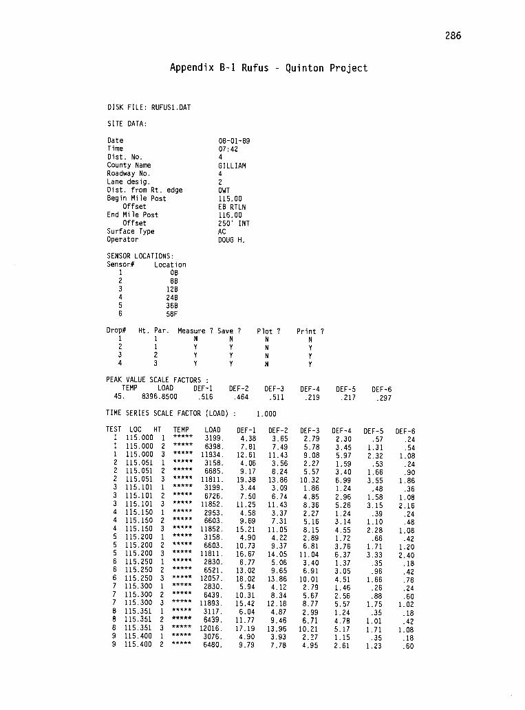
286

Appendix B-1 Rufus Quinton Project

DISK FILE: RUFUS1.DAT

SITE DATA:

Date 08-01-89Time 07:42Dist. No. 4

County Name GILLIAMRoadway No. 4

Lane desig. 2

Dist. from Rt. edge OWTBegin Mile Post 115.00

Offset EB RTLNEnd Mile Post 116.00

Offset 250' INTSurface Type ACOperator DOUG H.

SENSOR LOCATIONS:

Sensor# Location1 OB2 883 12B4 24B5 36B6 58F

Drop# Ht. Par. Measure ? Save ? Plot ? Print ?1 1 N N N N

2 1 Y Y N Y

3 2 Y Y N Y

4 3 Y Y N Y

PEAK VALUE SCALE FACTORS :

TEMP LOAD DEF-1 DEF-2 DEF-3 DEF-4 DEF-5 DEF-645. 8396.8500 .516

TIME SERIES SCALE FACTOR (LOAD)

TEST LOC HT TEMP LOAD

.464

:

DEF-1

.511

1.000

DEF-2

.219

DEF-3

.217

DEF-4

.297

DEF-5 DEF-61 115.000 1 ***** 3199. 4.38 3.65 2.79 2.30 .57 .241 115.000 2 ***** 6398. 7.81 7.49 5.78 3.45 1.31 .541 115.000 3 ***** 11934. 12.61 11.43 9.08 5.97 2.32 1.082 115.051 1 ***** 3158. 4.06 3.56 2.27 1.59 .53 .242 115.051 2 ***** 6685. 9.17 8.24 5.57 3.40 1.66 .902 115.051 3 ***** 11811. 19.38 13.86 10.32 6.99 3.55 1.863 115.101 1 ***** 3199. 3.44 3.09 1.86 1.24 .48 .363 115.101 2 ***** 6726. 7.50 6.74 4.85 2.96 1.58 1.083 115.101 3 ***** 11852. 11.25 11.43 8.36 5.26 3.15 2.164 115.150 1 ***** 2953. 4.58 3.37 2.27 1.24 .39 .244 115.150 2 ***** 6603. 9.69 7.31 5.16 3.14 1.10 .484 115.150 3 ***** 11852. 15.21 11.05 8.15 4.55 2.28 1.085 115.200 1 ***** 3158. 4.90 4.22 2.89 1.72 .66 .425 115.200 2 ***** 6603. 10.73 9.37 6.81 3.76 1.71 1.205 115.200 3 ***** 11811. 16.67 14.05 11.04 6.37 3.33 2.406 115.250 1 ***** 2830. 6.77 5.06 3.40 1.37 .35 .186 115.250 2 ***** 6521. 13.02 9.65 6.91 3.05 .96 .426 115.250 3 ***** 12057. 18.02 13.86 10.01 4.51 1.66 .787 115.300 1 ***** 2830. 5.94 4.12 2.79 1.46 .26 .247 115.300 2 ***** 6439. 10.31 8.34 5.67 2.56 .88 .607 115.300 3 ***** 11893. 15.42 12.18 8.77 5.57 1.75 1.028 115.351 1 ***** 3117. 6.04 4.87 2.99 1.24 .35 .188 115.351 2 ***** 6439. 11.77 9.46 6.71 4.78 1.01 .428 115.351 3 ***** 12016. 17.19 13.96 10.21 5.17 1.71 1.089 115.400 1 ***** 3076. 4.90 3.93 2.27 1.15 .35 .189 115.400 2 ***** 6480. 9.79 7.78 4.95 2.61 1.23 .60

287

9 115.400 3 ***** 11852. 13.33 11.90 7.84 3.94 1.97 1.0210 115.451 1 ***** 3076. 5.94 4.97 2.68 1.41 .48 .1810 115.451 2 ***** 6480. 11.88 9.93 6.60 3.23 1.40 .6010 115.451 3 ***** 11770. 17.61 15.27 10.52 6.41 2.94 1.2611 115.500 1 ***** 2871. 6.67 5.43 3.71 1.64 .53 .3611 115.500 2 ***** 6439. 14.27 11.62 8.56 4.38 1.62 .6611 115.500 3 ***** 11893. 21.88 18.17 13.93 7.38 3.24 1.2612 115.551 1 ***** 3076. 5.73 4.31 2.89 1.41 .48 .2412 115.551 2 ***** 6398. 12.40 9.84 7.22 3.58 1.62 .6612 115.551 3 ***** 11975. 19.79 15.93 12.48 6.85 3.42 1.3813 115.600 1 ***** 3035. 6.35 5.06 3.61 1.99 .70 .0613 115.600 2 ***** 6357. 13.13 10.49 7.94 3.94 1.75 .6013 115.600 3 ***** 11852. 18.96 15.27 10.83 6.63 3.15 .7214 115.651 1 ***** 2871. 7.19 5.62 3.92 2.30 .96 .6614 115.651 2 ***** 6357. 13.75 11.34 8.46 4.91 2.37 1.2014 115.651 3 ***** 11893. 19.90 16.58 12.90 7.65 4.07 2.2215 115.700 1 ***** 2912. 4.38 3.09 1.86 .84 .00 .1215 115.700 2 ***** 6439. 8.86 6.46 4.13 1.86 .57 .6015 115.700 3 ***** 12016. 13.33 9.56 6.60 3.14 1.27 .9616 115.751 1 ***** 3117. 5.00 3.65 2.06 1.24 .31 .3616 115.751 2 ***** 6644. 9.69 7.31 4.95 2.34 1.01 .6616 115.751 3 ***** 12139. 14.79 11.71 8.36 4.20 2.23 1.4417 115.802 1 ***** 3035. 5.00 4.31 2.27 .88 .35 .3017 115.802 2 ***** 6398. 9.90 7.96 5.06 2.12 1.14 .8417 115.802 3 ***** 12180. 15.11 12.46 8.77 4.29 2.54 1.8018 115.851 1 ***** 3076. 2.71 2.81 1.86 1.33 .44 .6618 115.851 2 ***** 6685. 7.81 6.56 4.54 2.96 1.66 1.2618 115.851 3 ***** 11975. 12.50 10.77 8.36 5.39 3.29 2.4619 115.904 1 ***** 3117. 3.44 3.00 1.86 1.19 .31 .3619 115.904 2 ***** 6644. 8.23 6.93 4.64 2.56 1.05 .8419 115.904 3 ***** 12221. 11.46 11.15 8.25 4.69 2.41 1.6220 115.958 1 ***** 3117. 5.00 3.75 2.48 1.28 .35 .1220 115.958 2 ***** 6726. 10.52 8.34 5.78 2.92 1.27 .6020 115.958 3 ***** 12221. 16.36 12.93 9.90 5.22 2.54 1.3221 116.000 1 ***** 3035. 4.58 3.93 2.89 1.64 .70 .4821 116.000 2 ***** 6685. 10.11 8.99 6.91 5.22 2.06 1.4421 116.000 3 ***** 12016. 16.15 14.15 11.45 10.08 4.07 2.34

TEST .LOC. HT COMMENTS ====>

1 115.0000 3 PAVEMENT TEMPERATURE IS 66 DEGREES.21 116.0000 3 END TEST SECTION.

DISK FILE: RUFUS2.DAT

SITE DATA:

Date 08-01-89Time 09:08Dist. No. 4

County Name GILLIAMRoadway No. 2

Lane desig. 2

Dist. from Rt. edge OWTBegin Mile Post 116.00

Offset WB. RTLNEnd Mile Post 115.00

Offset 250' INTSurface Type ACOperator DOUG H.

SENSOR LOCATIONS:Sensor# Location

1 08

2 8B3 12B4 24B5 36B6 58F

Drop# Ht. Par. Measure ? Save ? Plot ? Print ?1 1 N N N N

2 1 Y Y N r3 2 Y Y N r4 3 Y r N Y

PEAK VALUE SCALE FACTORS :

TEMP LOAD DEF-1 DEF-2 DEF-3 DEF-4 DEF-5 DEF-645. 8396.8500 .516 .464 .511 .219 .217 .297

TIME SERIES SCALE FACTOR (LOAD) : 1.000

TEST LOC HT

1 116.000 1

1 116.000 2

1 116.000 3

2 115.950 1

2 115.950 2

2 115.950 3

3 115.920 1

3 115.920 2

3 115.920 3

4 115.850 1

4 115.850 2

4 115.850 3

5 115.800 1

5 115.800 2

5 115.800 3

6 115.750 1

6 115.750 2

6 115.750 3

7 115.715 1

7 115.715 2

7 115.715 3

8 115.650 1

8 115.650 2

8 115.650 3

9 115.600 1

9 115.600 2

9 115.600 3

10 115.550 1

10 115.550 2

10 115.550 3

11 115.500 1

11 115.500 2

11 115.500 3

12 115.450 1

12 115.450 2

12 115.450 3

13 115.400 1

13 115.400 2

13 115.400 3

14 115.350 1

14 115.350 2

14 115.350 3

15 115.300 1

15 115.300 2

15 115.300 3

16 115.250 1

16 115.250 2

16 115.250 3

19 115.200 1

19 115.200 2

19 115.200 3

20 115.150 1

20 115.150 2

20 115.150 3

21 115.100 1

21 115.100 2

21 115.100 3

22 115.100 1

22 115.100 2

TEMP**********

********************

**********

************************************************************

**************************************************

**********

****************************************

**************************************************

******************************

***************

LOAD DEF-1 DEF-2 DEF-3 DEF-4 DEF-5 DEF-63240. 4.27 4.12 2.99 1.72 .70 .48

6521. 9.58 8.81 6.50 3.94 2.15 1.14

12057. 15.11 13.58 10.83 6.81 3.90 2.22

3158. 5.21 4.50 3.10 1.77 .74 .60

6685. 11.15 8.81 6.91 4.07 2.02 1.3211975. 17.40 14.24 11.04 6.81 3.68 2.52

3199. 4.38 3.75 2.68 1.64 .70 .60

6480. 8.75 7.78 5.88 3.63 1.88 1.20

12385. 13.65 11.80 9.70 6.15 3.55 2.043076. 4.79 4.22 2.79 1.81 .79 .66

6808. 10.42 8.62 6.29 4.11 1.97 1.38

12262. 16.25 13.49 10.52 6.72 3.81 2.52

3199. 3.96 3.19 2.06 1.28 .39 .18

6808. 8.23 7.03 5.16 2.96 1.23 .48

12057. 12.92 10.59 8.46 4.82 2.23 .84

3199. 2.40 2.15 .93 1.19 .44 .30

6767. 5.52 4.87 3.51 2.61 1.23 .72

12303. 9.58 7.96 6.60 4.73 2.58 1.86

3199. 4.17 3.65 2.17 1.24 .35 .00

6849. 8.65 7.31 5.26 2.87 1.10 .12

12303. 13.33 11.43 8.36 4.69 2.02 .42

3117. 5.94 5.15 3.71 2.12 .79 .42

6644. 12.61 11.05 8.36 4.86 2.23 1.1412221. 19.90 17.52 13.52 8.14 4.16 2.28

3199. 5.00 4.50 3.10 2.03 1.01 .54

6767. 10.63 9.65 7.33 4.69 2.28 1.32

12098. 16.77 14.99 12.07 7.52 4.03 2.763076. 3.02 2.53 1.44 .71 .04 .12

6808. 6.67 5.25 3.61 1.99 .92 .30

12180. 11.25 9.37 6.40 3.58 1.58 .66

3117. 3.96 3.19 2.17 .84 .04 -.126808. 6.77 5.90 4.02 1.86 .39 .24

12344. 9.69 8.71 6.29 2.92 1.05 .42

3076. 6.25 5.15 3.40 2.08 .74 .36

6726. 12.08 10.59 7.63 4.51 2.02 .90

12262. 18.02 15.46 12.28 6.94 3.50 1.563117. 5.63 4.12 2.99 1.86 .70 .36

6808. 10.94 8.81 6.50 3.94 1.75 .78

12344. 16.36 13.12 10.11 6.46 3.20 1.563199. 4.06 3.19 2.17 1.28 .31 .06

6767. 8.44 6.84 5.06 2.74 1.10 .30

12344. 12.81 10.40 7.94 4.33 2.10 .72

3199. 4.27 3.37 2.48 1.11 .22 .12

6767. 8.33 6.46 4.54 2.12 .88 .12

12385. 11.77 9.46 7.33 3.58 1.40 .36

3117. 5.52 4.22 2.99 1.37 .39 .24

6849. 10.31 8.71 6.50 2.87 1.23 .66

12303. 15.31 12.74 10.11 4.91 2.32 1.38

3158. 3.65 3.00 1.96 1.19 .48 .42

6767. 6.98 6.56 4.64 2.96 1.45 .84

12098. 11.46 10.59 8.05 5.13 2.89 1.923158. 3.13 2.44 1.34 .84 .13 .00

6685. 6.67 5.06 3.40 1.95 .74 .36

12221. 11.25 8.34 5.98 3.49 1.62 .84

3158. 3.75 3.56 1.86 1.46 .57 .24

6685. 8.13 7.21 5.06 3.14 1.58 1.02

12139. 12.61 10.87 8.36 5.17 2.67 1.92

3158. 4.48 3.84 2.58 1.59 .57 .48

6726. 9.38 7.78 5.98 3.49 1.66 1.02

288

289

22 115.100 3 ***** 11852 14.48 12.37 9.59 5.70 2.94 2.0423 115.050 1 ***** 3117 4.06 3.84 2.48 1.59 .66 .4223 115.050 2 ***** 6726 9.27 8.24 5.78 3.45 1.53 .9023 115.050 3 ***** 12139 14.79 12.93 9.70 5.75 2.98 1.7424 115.000 1 ***** 3117 4.69 3.65 2.27 1.41 .35 .3024 115.000 2 ***** 6685 9.90 7.78 5.67 3.01 1.23 .7824 115.000 3 ***** 12180 14.17 12.18 9.80 5.35 2.72 1.74

TEST ..LOC. HT COMMENTS ====>1 116.0000 3 PAVEMENT TEMPERATURE IS 78 DEGREES.

24 115.0000 3 END TEST SECTION.

290

B-2 Centennial Boulevard Project

DISK FILE: CENT3.DAT

SITE DATA:

DateTime

Dist. No.County NameRoadway No.Lane desig.

Dist. from Rt. edgeBegin Mile Post

OffsetEnd Mile Post

OffsetSurface TypeOperator

SENSOR LOCATIONS:Sensor# Location

1 OF

2 12B3 2484 36B5 60F

6 99B

04-03-8909:57

E

BRIDGE

DB

Drop# Ht. Par. Measure ? Save ? Plot ? Print ?

1 3

2 2

3 3

PEAK VALUE SCALE FACTORS :

TEMP LOAD DEF-1O. 5902.0000 .521

TIME SERIES SCALE FACTOR (LOAD)

TEST LOC HT TEMP LOAD

DEF-2 DEF-3.512 .509

: 5902.000

DEF-1 DEF-2

DEF-4.251

DEF-3

DEF-5.280

DEF-4

DEF-6.280

DEF-5 DEF-61 200. 2 54. 8821. 16.09 12.09 8.53 6.18 2.88 7.071 200. 3 54. 14269. 24.72 18.61 13.57 9.88 4.92 12.212 400. 2 53. 8821. 19.35 12.61 7.60 5.88 3.17 5.942 400. 3 52. 14297. 28.40 18.81 12.33 9.63 5.77 10.063 600. 2 55. 8763. 20.30 13.85 9.25 6.59 2.43 7.633 600. 3 55. 14269. 29.98 21.29 14.90 10.69 4.52 13.624 800. 2 62. 8705. 18.72 13.13 8.43 6.03 2.71 7.464 800. 3 61. 14153. 27.24 20.26 13.57 9.98 4.81 12.385 1000. 2 59. 8849. 21.35 14.58 9.15 6.13 2.83 7.185 1000. 3 58. 14240. 31.66 22.12 14.49 10.29 4.35 12.726 1200. 2 59. 8763. 20.41 12.71 8.02 5.42 2.20 5.886 1200. 3 57. 14240. 29.77 19.64 13.05 9.17 3.90 12.047 1400. 2 57. 8792. 19.25 12.30 7.60 4.76 1.64 6.167 1400. 3 56. 14211. 29.24 19.33 12.64 8.11 3.90 12.498 1600. 2 60. 8734. 22.72 14.37 8.63 6.08 2.71 7.808 1600. 3 59. 14182. 33.98 21.81 14.18 9.78 4.81 14.259 1800. 2 54. 8734. 21.77 14.58 9.87 6.54 2.71 8.319 1800. 3 54. 14153. 32.92 22.33 15.31 10.74 4.92 15.7710 2000. 2 58. 8763. 17.15 12.30 8.63 5.93 2.32 7.1810 2000. 3 57. 14211. 26.82 19.23 13.87 9.83 4.24 12.7811 2200. 2 62. 8676. 23.88 15.82 9.87 6.64 2.26 7.4611 2200. 3 60. 14067. 35.24 24.19 15.83 10.95 4.30 14.3012 2400. 2 59. 8763. 20.09 13.23 8.22 5.12 2.66 7.1812 2400. 3 59. 14182. 30.19 20.05 13.15 8.67 4.81 13.6813 2600. 2 64. 8734. 14.41 8.48 4.73 2.79 1.07 3.22

291

13 2600. 3 64. 14269. 20.83 12.30 6.89 4.36 1.92 6.5014 2800. 2 55. 8705. 21.67 12.09 6.27 3.70 1.13 4.1314 2800. 3 55. 14124. 30.82 17.78 9.56 5.83 2.37 8.5915 3000. 2 56. 8676. 13.15 7.86 4.52 2.84 1.24 3.1115 3000. 3 56. 14211. 19.25 11.78 7.50 4.81 2.20 5.9416 3200. 2 53. 8648. 10.73 6.41 3.39 2.03 .62 2.3216 3200. 3 53. 14067. 15.67 9.41 5.34 3.29 1.47 4.2417 3400. 2 52. 8648. 15.67 9.82 5.96 3.85 1.53 3.9617 3400. 3 52. 13923. 23.46 14.68 9.45 6.54 2.60 7.0718 3600. 2 60. 8705. 13.88 8.17 4.11 2.64 1.19 3.1118 3600. 3 61. 14182. 20.83 12.82 6.68 4.21 1.92 6.5619 3800. 2 62. 8676. 12.83 7.96 4.93 3.40 2.04 3.9019 3800. 3 60. 14240. 18.72 11.89 7.71 5.63 3.45 7.5220 4000. 2 61. 8705. 11.15 7.03 4.21 2.69 1.36 3.2820 4000. 3 60. 14211. 16.94 10.54 6.47 4.56 2.71 5.77

DISK FILE: CENT4.DAT

SITE DATA:

DateTimeDist. No.

County NameRoadway No.Lane desig.

Dist. from Rt. edgeBegin Mile Post

OffsetEnd Mile Post

OffsetSurface TypeOperator

SENSOR LOCATIONS:Sensor# Location

1 OF

2 1283 24B4 36B5 6OF6 99B

04-03-89

11:03

E

DB

Drop# Ht. Par. Measure ? Save ? Plot ? Print ?

1 3

2 2

3 3

PEAK VALUE SCALE FACTORS :

TEMP LOAD DEF-10. 5902.0000 .521

TIME SERIES SCALE FACTOR (LOAD)

TEST LOC HT TEMP LOAD

DEF-2 DEF-3.512 .509

: 5902.000

DEF-1 DEF-2

DEF-4.251

DEF-3

DEF-5.280

DEF-4

DEF-6.280

DEF-5 DEF-61 4200. 2 67. 8648. 12.41 8.17 4.93 3.60 2.04 4.521 4200. 3 67. 14124. 17.99 11.99 7.81 5.83 3.39 8.312 4400. 2 63. 8648. 13.15 8.48 5.34 3.75 2.04 4.242 4400. 3 64. 14096. 19.14 12.61 8.43 6.03 3.34 8.143 4600. 2 69. 8532. 16.20 11.68 8.02 6.03 3.11 5.993 4600. 3 68. 13951. 24.30 17.88 12.85 9.73 5.26 11.084 4800. 2 63. 8561. 11.89 8.06 5.14 3.65 2.04 2.944 4800. 3 63. 14009. 17.67 11.68 8.02 5.73 3.39 5.035 5000. 2 58. 8561. 12.52 8.99 5.96 4.36 2.09 5.035 5000. 3 58. 14038. 18.09 13.13 9.15 6.69 3.67 8.716 5200. 2 60. 8619. 11.99 8.68 5.86 4.26 2.04 5.20

292

6 5200. 3 57. 14096. 17.88 12.92 9.15 6.84 3.62 8.54

7 5400. 2 67. 8792. 15.78 11.27 7.50 4.92 1.70 6.507 5400. 3 68. 13980. 24.09 17.26 11.92 8.16 3.22 11.76

8 5600. 2 55. 8676. 14.20 9.82 6.37 4.36 2.09 5.99

8 5600. 3 54. 14096. 21.77 15.20 10.58 7.35 3.73 11.59

9 5800. 2 59. 8590. 16.09 11.78 8.63 6.39 3.34 7.079 5800. 3 60. 14038. 24.09 18.09 13.57 10.24 5.71 12.21

10 6000. 2 59. 8561. 15.67 11.89 8.53 6.13 2.88 5.88

10 6000. 3 59. 14009. 24.30 18.61 13.77 9.98 4.86 10.68

11 6200. 2 68. 8705. 15.46 10.03 6.99 4.86 2.26 6.11

11 6200. 3 68. 14124. 23.14 15.82 11.10 8.06 4.18 11.6512 6400. 2 71. 8648. 15.46 11.06 7.30 5.22 2.43 6.84

12 6400. 3 70. 14096. 23.25 16.85 12.02 8.67 4.47 12.61

13 6600. 2 73. 8619. 18.51 13.96 10.38 7.75 3.96 7.80

13 6600. 3 70. 14009. 27.98 21.09 16.13 12.31 6.56 12.7814 6801. 2 75. 8763. 10.62 8.79 6.89 5.37 2.83 5.26

14 6801. 3 76. 14240. 16.62 13.75 11.20 8.72 4.58 8.5415 7000. 2 74. 8734. 15.88 10.75 6.89 4.92 2.20 6.39

15 7000. 3 73. 14124. 24.30 16.85 11.51 8.46 4.13 12.32

DISK FILE: CENT5.DAT

SITE DATA:

Date 04-03-89Time 11:41

Dist. No.County NameRoadway No.Lane desig.

Dist. from Rt. edgeBegin Mile Post 6900

OffsetEnd Mile Post

Offset

Surface TypeOperator DB

SENSOR LOCATIONS:Sensor# Location

1 OF

2 12B

3 24B4 36B

5 6OF6 99B

Drop# Ht. Par. Measure ? Save ? Plot ? Print ?

1 3 N N N N

2 2 Y Y N Y

3 3 Y Y N Y

PEAK VALUE SCALE FACTORS :

TEMP LOAD DEF-1 DEF-2 DEF-3 DEF-4 DEF-5 DEF-6O. 5902.0000 .521 .512 .509 .251 .280 .280

TIME SERIES SCALE FACTOR (LOAD) : 5902.000

TEST LOC HT TEMP LOAD DEF-1 DEF-2 DEF-3 DEF-4 DEF-5 DEF-61 6900. 2 74. 8705. 11.04 7.75 5.45 4.16 2.26 4.521 6900. 3 75. 14182. 16.72 11.99 8.74 6.74 3.79 8.032 6700. 2 77. 8705. 13.67 9.30 6.78 5.02 2.77 5.262 6700. 3 76. 14182. 20.62 14.68 10.89 8.21 4.81 8.71

3 6500. 2 74. 8648. 15.57 10.03 6.17 4.16 1.75 5.093 6500. 3 72. 14096. 23.77 15.71 10.07 7.09 3.17 10.464 6300. 2 78. 8676. 13.25 7.75 4.32 2.79 1.13 2.944 6300. 3 77. 14182. 19.35 11.68 6.68 4.56 1.92 6.505 6100. 2 77. 8676. 15.15 8.48 4.93 3.14 1.19 4.07

293

5 6100. 3 76. 14153. 21.98 12.61 7.19 5.17 2.43 7.586 5900. 2 72. 8648. 15.36 9.92 6.06 3.90 1.87 4.866 5900. 3 71. 14096. 24.09 15.92 10.07 6.79 3.28 9.897 5700. 2 73. 8590. 14.62 9.72 6.47 4.61 2.49 5.267 5700. 3 73. 14096. 22.51 15.09 10.58 7.65 4.18 9.678 5500. 2 75. 8619. 12.31 8.99 5.96 4.05 1.92 5.038 5500. 3 74. 14182. 19.04 13.85 9.45 6.79 3.34 10.409 5300. 2 76. 8648. 11.04 7.24 4.52 3.09 1.41 3.969 5300. 3 76. 14211. 16.41 10.75 7.19 5.07 2.49 7.29

10 5100. 2 75. 8676. 12.10 8.37 5.86 4.05 1.70 4.9710 5100. 3 75. 14153. 18.41 13.02 9.15 6.69 3.00 9.3811 4900. 2 78. 8648. 13.04 8.79 5.86 4.05 2.09 4.8111 4900. 3 77. 14124. 19.57 13.44 9.25 6.74 3.62 8.3112 4700. 2 77. 8619. 12.10 8.58 5.96 4.36 2.15 5.0912 4700. 3 76. 14182. 18.41 13.23 9.45 7.09 3.79 9.1013 4500. 2 72. 8619. 17.04 11.99 7.50 5.17 2.88 6.6713 4500. 3 72. 14153. 25.46 17.78 11.72 8.26 4.81 11.3114 4300. 2 69. 8648. 12.52 9.51 6.06 4.26 2.15 4.8614 4300. 3 69. 14182. 18.93 14.16 9.66 6.94 3.73 8.8815 4100. 2 85. 8648. 13.04 10.13 6.68 4.51 2.15 5.3715 4100. 3 84. 14153. 19.57 14.99 10.28 7.45 3.84 10.5716 3900. 2 86. 8590. 10.83 8.68 6.06 4.31 2.26 4.5816 3900. 3 85. 14124. 16.72 13.02 9.56 7.04 3.96 8.5917 3700. 2 83. 8619. 12.83 7.86 5.04 3.19 1.64 3.1717 3700. 3 82. 14153. 18.83 12.09 7.81 5.12 2.94 6.3918 3500. 2 90. 8619. 12.20 7.86 4.32 2.53 1.02 2.2618 3500. 3 89. 14124. 18.72 12.20 6.78 4.36 1.87 5.9919 3300. 2 90. 8561. 17.25 11.47 7.09 4.21 1.64 4.1819 3300. 3 89. 14096. 25.56 17.47 10.89 6.79 3.05 8.3120 3100. 2 90. 8532. 15.78 10.96 6.37 3.90 1.13 4.3520 3100. 3 88. 14038. 24.51 17.37 10.79 6.64 2.49 10.0121 2900. 2 85. 8561. 17.67 13.02 8.94 5.93 2.83 6.9521 2900. 3 85. 14067. 27.45 20.57 14.59 9.93 4.75 12.8322 2700. 2 85. 8590. 16.09 11.06 7.30 4.56 1.87 5.4322 2700. 3 84. 14096. 24.61 17.37 11.92 8.01 3.45 11.25

DISK FILE: CENT6.DAT

SITE DATA:

DateTime

Dist. No.

County NameRoadway No.Lane desig.

Dist. from Rt. edgeBegin Mile Post

OffsetEnd Mile Post

OffsetSurface TypeOperator

SENSOR LOCATIONS:

Sensor# Location1 OF

2 12B3 24B4 36B5 6OF6 99B

04-03-8912:34

2500

DB

Drop# Ht. Par. Measure ? Save ? Plot ? Print ?

1 3

2 2

294

3 3

PEAK VALUE SCALE FACTORS :

TEMP LOAD DEF-1

O. 5902.0000 .521

TIME SERIES SCALE FACTOR (LOAD)

TEST LOC HT TEMP LOAD

DEF-2 DEF-3.512 .509

: 5902.000

DEF-1 DEF-2

DEF-4

.251

DEF-3

DEF-5

.280

DEF-4

DEF-6.280

DEF-5 DEF-61 2500. 2 88. 8561. 14.83 9.51 5.75 3.75 1.92 4.811 2500. 3 86. 14038. 22.30 14.37 9.35 6.44 3.34 8.932 2299. 2 88. 8561. 11.89 9.92 6.27 4.56 2.26 5.202 2299. 3 88. 13923. 18.09 15.30 10.17 7.70 3.90 10.063 2100. 2 92. 8532. 17.99 11.99 8.22 5.42 2.20 6.563 2100. 3 91. 14009. 28.19 19.43 13.57 9.43 3.90 12.724 1900. 2 89. 8676. 15.67 11.06 7.30 4.81 2.09 5.824 1900. 3 88. 14182. 24.30 17.78 11.92 8.36 3.67 11.025 1700. 2 85. 8561. 17.15 12.09 8.53 5.93 2.66 6.675 1700. 3 84. 14067. 27.03 18.92 13.77 10.03 4.86 12.496 1500. 2 81. 8619. 15.57 10.23 6.58 4.61 2.09 5.376 1500. 3 81. 14038. 23.56 15.61 10.89 7.85 3.73 9.727 1300. 2 83. 8648. 18.41 11.16 7.09 4.86 1.98 5.377 1300. 3 82. 14067. 28.09 17.47 11.61 8.41 3.56 10.858 1100. 2 81. 8590. 16.20 10.34 6.47 4.10 1.47 4.588 1100. 3 80. 14067. 24.93 16.44 10.89 7.15 3.00 9.389 900. 2 76. 8648. 15.99 10.03 6.68 4.46 2.15 4.929 900. 3 76. 14096. 24.40 16.02 11.10 7.70 3.56 10.06

10 700. 2 87. 8648. 14.10 9.61 6.06 3.85 1.87 5.0310 700. 3 84. 14182. 21.98 14.99 9.97 6.74 3.39 10.2911 500. 2 90. 8648. 16.83 9.61 6.27 4.16 2.49 4.4711 500. 3 89. 14096. 25.03 14.78 10.28 7.09 4.24 8.2012 299. 2 92. 8648. 15.46 10.65 7.91 5.68 2.83 6.5612 299. 3 91. 14067. 24.19 16.85 12.85 9.48 4.92 11.8213 100. 2 92. 8705. 13.46 9.61 7.19 5.17 2.26 5.1413 100. 3 89. 14153. 20.83 15.40 11.82 8.36 4.18 9.16

295

B -3 Nelchina Project

NELCHINA SPRING DATA NELCHINA SUMMUR DATA

R32 18 225 890511nelchina29F8*70001...800-002 .3111 8150 0 211 300 601 899 11991501

100 C: .FWD

nelchina 89 #2000+0.0 000+0.0 00

R32 18 281 890802neltwo 29F8*70001...800-002 .3111 8150 0 211 300 601 899 11991501

100 C: .FWD

nelch 89 #2 aug 2+0.0 000+0.0 00S127 1 4.5 100 0

S128 1 4.5 100 0

0' 100'0' 100'018 15 3.5 5 2 15

00224 S127 10 100 0 0028000226 S128 10 100 0 00282

127 0' 100'0' 100'0 1272 8 18 15 3.5 5 2 15 2 8

Ld 084 1 87.8 Ld 084 1 87.8D1 621 1 1.049 D1 621 1 1.049D2 622 1 1.004 D2 622 1 1.004D3 623 1 1.040 03 623 1 1.04004 624 1 1.033 D4 624 1 1.033D5 625 1 1.085 D5 625 1 1.085D6 626 1 1.053 D6 626 1 1.053D7 627 1 1.049 D7 628 1 1.018DO 628 1 1.018 DO 627 1 1.049DO 638 1 1.037 DO 638 1 1.037D* ***** 1 1 D* ***** 1 1

David L. Swaim David L. Swaim1110101011111111

12 1110101011111111

12

SO.x 1 4.5 000 0 000000 S0.0 10 100 0 000000608 324 257 181 99 47 25 1 562 273 202 144 79 44 29 23

S2 1 4.5 000 0 000000 S2 10 100 0 000000597 345 263 191 106 51 29 5 570 399 247 164 83 46 33 25

S4 1 4.5 100 0 000000 S4 10 100 0 000000604 278 220 157 89 46 27 1 571 206 154 108 60 35 24 15

S6 1 4.5 100 0 000000 S6 10 100 0 000000601 355 276 201 117 59 32 1 569 442 330 230 130 79 60 48S8 1 4.5 100 0 000000 S8 10 100 0 000000610 277 173 95 51 29 21 1 579 323 200 115 59 37 27 19SIO 1 4.5 100 0 000000 S10 10 100 0 000000597 323 202 103 53 31 22 7 585 256 157 84 44 29 22 12

S12 1 4.5 100 0 000000 S12 10 100 0 000000596 377 227 120 59 35 21 2 576 301 170 82 38 23 18 14

S14 1 4.5 100 0 000000 S14 10 100 0 000000583 370 205 107 55 30 20 1 578 296 182 97 46 27 19 13S16 1 4.5 100 0 000000 S16 10 100 0 000000582 341 213 119 58 31 20 1 577 292 181 90 42 25 19 14S18 1 4.5 100 0 000000 S18 10 100 0 000000577 308 186 97 49 27 17 1 574 321 176 94 45 27 20 15S20 1 4.5 100 0 000000 S20 10 100 0 000000583 311 207 110 57 30 20 2 575 240 149 78 36 21 14 12

S22 1 4.5 100 0 000000 S22 10 100 0 000000583 362 219 122 58 31 19 1 584 263 140 73 34 18 13 9

S24 1 4.5 100 0 000000 S24 10 100 0 000000584 350 191 107 54 29 17 1 574 243 142 76 37 23 17 11

S26 1 4.5 100 0 000000 S26 10 100 0 000000587 360 232 134 71 38 21 1 564 293 173 89 44 27 20 15S28 1 4.5 100 0 000000 S28 10 100 0 000000580 315 181 95 48 26 17 1 563 255 156 89 45 27 19 11S30 1 4.5 100 0 000000 S30 10 100 0 000000576 271 167 88 40 22 16 2 569 285 155 85 40 21 13 14

S32 1 4.5 100 0 000000 S32 10 100 0 000000580 298 206 128 68 38 24 1 576 284 154 73 36 21 14 10

S34 1 4.5 100 0 000000 S34 10 100 0 000000582 322 207 123 64 34 21 2 577 283 134 71 36 21 14 11

296

S36 1 4.5 100 0 000000 S36 10 100 0 000000577 281 212 108 60 34 21 1 577 201 137 81 43 26 19 15

S38 1 4.5 100 0 000000 S38 10 100 0 000000579 312 215 130 71 37 22 2 574 235 118 59 28 16 12 8

S40 1 4.5 100 0 000000 S40 10 100 0 000000580 318 201 110 57 35 20 5 581 231 142 76 36 20 15 9

S42 1 4.5 100 0 000000 S42 10 100 0 000000571 351 213 120 60 33 21 3 571 241 129 63 30 20 14 11

S44 1 4.5 100 0 000000 S44 10 100 0 000000571 395 253 136 69 40 27 1 574 327 206 115 60 35 24 19

S46 1 4.5 100 0 000000 S46 10 100 0 000000577 364 209 114 62 37 23 2 570 307 166 98 50 30 23 17

S48 1 4.5 100 0 000000 S48 10 100 0 000000571 327 201 104 54 29 18 1 572 269 157 90 25 18 16 10

S50 1 4.5 100 0 000000 S50 1 10 100 0 000000570 418 276 161 87 48 27 1 556 271 163 89 46 29 22 16

S51 1 4.5 100 0 000000 S51 1 10 100 0 000000567 517 358 209 112 58 32 1 513 368 216 111 50 28 21 17

S52 1 4.5 100 0 000000 S52 1 10 100 0 000000570 494 289 166 87 43 24 1 579 292 162 90 46 30 23 19

S53 1 4.5 100 0 000000 S53 1 10 100 0 000000568 407 250 150 84 52 35 1 583 281 164 95 52 33 24 19

S54 1 4.5 100 0 000000 S54 1 10 100 0 000000570 455 304 188 108 63 38 3 580 293 159 93 52 33 24 18

S55 1 4.5 100 0 000000 S55 1 10 100 0 000000562 642 467 289 148 76 41 2 565 318 193 118 66 41 28 21

S56 1 4.5 100 0 000000 S56 1 10 100 0 000000568 487 315 192 104 54 31 1 567 377 243 140 72 44 33 25

S57 1 4.5 100 0 000000 S57 1 10 100 0 000000572 409 274 159 88 53 36 1 575 279 178 101 53 33 26 21

S58 1 4.5 100 0 000000 S58 1 10 100 0 000000568 338 218 125 71 42 28 3 573 313 180 105 56 34 24 19

S59 1 4.5 100 0 000000 S59 1 10 100 0 000000561 338 203 108 57 34 23 1 584 263 154 79 39 26 20 14

S60 1 4.5 100 0 000000 S60 1 10 100 0 000000567 314 187 111 56 30 18 1 568 212 134 72 37 25 21 17

S61 1 4.5 100 0 000000 S61 1 10 100 0 000000560 467 348 210 102 52 27 1 564 352 227 145 82 50 37 30

S62 1 4.5 100 0 000000 S62 1 10 100 0 000000554 506 368 224 122 63 37 2 560 450 302 183 106 72 54 41

S63 1 4.5 100 0 000000 S63 1 10 100 0 000000550 624 436 279 147 66 35 1 572 288 190 130 84 58 41 27S64 1 4.5 100 0 000000 S64 1 10 100 0 000000561 488 331 201 107 53 31 1 561 359 223 159 97 63 44 34S65 1 4.5 100 0 000000 S65 1 10 100 0 000000550 703 423 260 136 60 24 2 564 326 176 122 80 53 37 31S66 1 4.5 100 0 000000 S66 1 10 100 0 000000550 782 477 260 120 43 14 1 551 393 239 158 98 64 44 34S67 1 4.5 100 0 000000 S67 1 10 100 0 000000546 680 484 258 133 59 23 2 562 385 226 132 77 50 36 26S68 1 4.5 100 0 000000 S68 1 10 100 0 000000549 636 412 240 120 54 26 1 556 358 181 105 59 39 26 22

S69 1 4.5 100 0 000000 S69 1 10 100 0 000000554 572 362 209 117 58 31 1 556 331 171 98 61 38 27 20S70 1 4.5 100 0 000000 S70 1 10 100 0 000000540 925 632 341 174 61 17 1 561 257 180 119 71 43 31 22

S71 1 4.5 100 0 000000 S71 1 10 100 0 000000561 692 433 269 150 68 27 1 558 358 217 130 80 52 37 29

S72 1 4.5 100 0 000000 S72 1 10 100 0 000000552 801 509 301 164 78 36 2 552 397 242 142 86 53 39 29

S73 1 4.5 100 0 000000 S73 1 10 100 0 000000560 777 517 326 170 79 35 3 557 433 262 161 93 55 37 27

S74 1 4.5 100 0 000000 S74 1 10 100 0 000000551 843 541 327 166 71 27 1 547 486 314 201 118 69 46 34

S75 1 4.5 100 0 000000 S75 1 10 100 0 0000005411009 714 439 214 87 27 1 541 485 307 191 108 65 43 33

S76 1 4.5 100 0 000000 S76 1 10 100 0 00000054913711143 701 430 206 108 2 543 511 330 194 113 68 45 33

S77 1 4.5 100 0 000000 S77 1 10 100 0 000000531 959 693 339 165 71 27 1 543 456 293 185 113 68 46 35S78 1 4.5 100 0 000000 S78 1 10 100 0 000000

297

543 918 536 294 156 71 34 1 546 367 271 181 111 68 47 31S79 1 4.5 100 0 000000 S79 1 10 100 0 000000

557 707 478 258 136 64 31 1 547 406 260 163 100 64 46 35S80 1 4.5 100 0 000000 S80 1 10 100 0 000000558 633 433 276 149 67 33 1 550 376 242 142 83 48 34 25

S81 1 4.5 100 0 000000 S81 1 10 100 0 000000564 459 294 177 100 48 26 1 545 495 316 211 129 77 52 39

S82 1 4.5 100 0 000000 S82 1 10 100 0 000000576 373 243 146 77 39 21 3 552 335 234 138 74 49 34 24

S83 1 4.5 100 0 000000 S83 1 10 100 0 000000546 273 211 136 76 38 20 5 522 492 367 245 129 74 53 40

S84 1 4.5 100 0 000000 S84 1 10 100 0 000000557 592 384 202 91 38 19 3 522 507 366 241 129 73 51 39

S85 1 4.5 100 0 000000 S85 1 10 100 0 000000532 765 509 348 200 103 59 3 529 586 399 254 142 89 63 49

S86 1 4.5 100 0 000000 S86 1 10 100 0 000000559 569 414 260 162 112 81 1 562 517 321 205 108 74 58 48

S87 1 4.5 100 0 000000 S87 1 10 100 0 000000548 544 345 191 103 5B 38 4 552 472 329 204 111 71 48 36

S88 1 4.5 100 0 000000 S88 1 10 100 0 000000546 368 265 159 76 39 22 1 562 368 239 159 87 30 25 19

S89 1 4.5 100 0 000000 S89 1 10 100 0 000000571 308 201 115 61 33 19 3 590 284 167 89 45 27 19 13

S90 1 4.5 100 0 000000 S90 1 10 100 0 000000574 317 220 96 57 29 18 3 593 256 151 85 43 26 19 9

S91 1 4.5 100 0 000000 S91 1 10 100 0 000000567 345 243 151 87 51 35 1 588 320 173 100 53 30 22 17

S92 1 4.5 100 0 000000 S92 1 10 100 0 000000573 286 193 111 57 33 22 1 591 236 172 104 57 38 29 18

S93 1 4.5 100 0 000000 S93 1 10 100 0 000000573 304 221 140 75 42 26 1 581 304 210 133 70 41 28 21

S94 1 4.5 100 0 000000 S94 1 10 100 0 000000577 287 209 136 79 29 15 1 584 325 203 110 51 29 20 15

S98 1 4.5 100 0 000000 S98 1 10 100 0 000000563 555 374 214 112 54 29 1 570 446 334 253 152 88 59 47

S99 1 4.5 100 0 000000 S99 1 10 100 0 000000558 467 360 225 127 66 38. 1 582 484 352 237 142 87 61 48

S100 1 4.5 100 0 000000 S100 1 10 100 0 000000570 496 352 226 119 59 31 1 570 536 381 249 135 76 52 39

5101 1 4.5 100 0 000000 S101 1 10 100 0 000000570 578 401 249 126 54 26 1 578 625 435 282 153 90 64 49

S102 1 4.5 100 0 000000 S102 1 10 100 0 000000566 478 320 207 125 72 45 1 568 492 366 250 157 103 74 58

S103 1 4.5 100 0 000000 S103 1 10 100 0 000000562 537 397 256 129 59 28 3 565 649 437 287 165 98 66 48

S104 1 4.5 100 0 000000 S104 1 10 100 0 000000562 523 378 226 107 41 17 1 580 553 381 231 115 63 43 34

S105 1 4.5 100 0 000000 S105 1 10 100 0 000000547 500 363 245 142 79 52 1 558 557 423 307 186 112 76 50

S106 1 4.5 100 0 000000 S106 1 10 100 0 000000553 621 432 262 123 51 22 5 567 376 285 217 138 82 57 42

S107 1 4.5 100 0 000000 S107 1 10 100 0 000000566 434 282 166 90 46 27 1 566 515 376 237 127 69 47 32

S108 1 4.5 100 0 000000 S108 1 10 100 0 000000571 290 184 102 54 33 22 1 569 395 251 150 84 50 36 25

S109 1 4.5 100 0 000000 5109 1 10 100 0 000000558 354 223 125 65 33 20 1 584 340 150 82 51 34 26 25

S110 1 4.5 100 0 000000 S110 1 10 100 0 000000536 428 314 196 114 66 42 2 557 299 182 112 68 46 35 22

S111 1 4.5 100 0 000000 S111 1 10 100 0 000000556 357 308 259 192 128 91 2 567 337 286 238 169 112 80 60

S112 1 4.5 100 0 000000 S112 1 10 100 0 000000553 592 461 313 189 107 65 3 567 494 344 230 133 80 54 37

S113 1 4.5 100 0 000000 S113 1 10 100 0 000000555 444 293 179 99 48 26 1 564 406 247 157 92 58 39 36

S114 1 4.5 100 0 000000 5114 1 10 100 0 000000558 433 298 185 100 49 27 1 567 468 322 207 112 65 44 30

S115 1 4.5 100 0 000000 S115 1 10 100 0 000000552 269 181 110 72 44 28 2 566 267 186 130 83 54 41 39

S116 1 4.5 100 0 000000 5116 1 10 100 0 000000547 529 371 238 130 66 39 1 561 453 321 216 132 79 57 45

298

5117 1 4.5 100 0 000000 S117 1 10 100 0 000000547 426 302 197 117 69 45 1 562 465 230 155 97 65 44 26

S118 1 4.5 100 0 000000 S118 1 10 100 0 000000562 388 169 116 95 64 44 1 597 284 182 175 1951020 53 41

S121 1 4.5 100 0 000000 S121 1 10 100 0 000000538 377 283 198 105 49 27 1 577 464 364 249 129 63 42 35

S122 1 4.5 100 0 000000 S122 1 10 100 0 000000551 457 339 227 136 73 40 1 559 380 236 156 98 61 42 34

S123 1 4.5 100 0 000000 S123 10 100 0 000000558 180 138 101 60 33 23 1 571 291 201 133 73 49 38 31

S124 1 4.5 100 0 000000 S124 10 100 0 000000559 409 296 193 97 43 21 1 567 358 267 178 107 72 53 38

S125 1 4.5 100 0 000000 S125 10 100 0 000000559 366 275 186 95 46 24 2 560 346 281 209 129 81 59 47

S126 1 4.5 100 0 000000 S126 10 100 0 000000565 187 149 111 70 38 25 1 566 247 179 122 68 42 33 27

S127 1 4.5 100 0 000000 S127 10 100 0 000000564 189 141 97 55 29 21 1 568 312 211 132 73 46 35 23

EOF EOF

299

6-4 Tudor Project

Tudor Spring Data Tudor Summer Data

R32 18 579 800101tudor4 29F8* R32 18 579 800101tudor7 29F8*70001...800-003 .3111 8 70001...800-003 .3111 8150 0 200 300 450 650 900 1200 150 0 200 300 450 650 900 1200

100 B: .FWD 100 B: .FWD00000 SH0000 000+0.0 000+0.0 00 00000 SH0000 000+0.0 000+0.0 00S110 1

S111 1

0' 100'0'

18 15 3.5

13 000 0

13 000 0

100'1

6 2 15

00575 5110 1

00580 S111 1

110 0' 100'0'2 8 18 15 3.5

13 0 0 0057513 0 0 00580

100'1 1106 2 15 2 8

Ld 085 1 87.5 Ld 085 1 87.5D1 631 1 .9918 01 631 1 .9918D2 632 1 1.011 D2 632 1 1.011D3 633 1 1.055 03 633 1 1.055D4 634 1 1.056 D4 634 1 1.056D5 635 1 1.033 D5 635 1 1.033D6 636 1 1.045 D6 636 1 1.045D7 637 1 1.078 D7 637 1 1.078DO 638 1 1.037 DO 638 1 1.037DO 628 1 1.018 DO 628 1 1.0180* ***** 1

1 D* ***** 1 1

chip chip11110010....1234 11110010. .123411111223******** 11111223********

S1.0 1 11 000 0 000010 S1.0 1 13 000 0 000009403 212 161 148 97 66 37 20 382 223 181 146 91 60 33 20564 272 215 189 126 87 49 27 544 294 237 191 120 81 46 29557 268 211 187 126 86 48 26 550 294 237 191 121 82 46 29888 407 296 284 189 130 73 40 851 422 335 269 174 118 69 45S2.0 1 11 000 0 000011 S2.0 1 13 000 0 000011405 157 96 94 56 36 21 13 375 203 149 114 63 39 22 14561 198 144 120 74 48 27 17 545 262 194 148 84 54 29 19554 194 142 118 71 48 27 17 552 262 195 150 86 54 30 19887 290 212 175 108 71 42 26 852 367 272 209 119 76 44 29

S3 1 11 000 0 000012 S3 1 13 000 0 000012404 187 136 115 70 42 23 14 382 171 123 93 50 30 17 12555 235 176 145 88 55 29 17 545 222 160 119 65 42 24 16551 228 174 143 88 55 29 18 548 221 160 119 67 41 24 16884 347 257 213 130 83 45 27 842 314 225 170 96 61 37 27

S4 1 11 000 0 000016 S4 1 13 000 0 000013398 199 167 121 72 43 27 18 381 189 146 110 62 38 22 15549 244 197 148 91 53 36 23 551 241 185 139 79 51 30 20553 244 201 148 92 53 34 23 554 239 185 139 79 52 32 22868 342 263 204 124 76 50 31 846 327 251 188 109 71 43 30S5 1 11 000 0 000017 S5 1 13 000 0 000014393 210 161 137 88 55 24 10 370 186 131 102 58 37 21 14545 258 197 169 108 69 32 12 537 242 171 132 77 50 29 19546 255 199 168 108 69 32 12 540 239 169 131 78 50 29 19868 375 278 241 151 96 44 14 827 338 237 183 108 71 44 30

S6 1 11 000 0 000018 S6 1 13 000 0 000015399 187 160 110 67 39 21 12 371 174 112 81 43 27 16 12550 234 173 140 83 53 27 16 540 226 148 109 61 40 26 19547 233 169 139 83 53 28 16 541 223 147 107 60 39 25 18877 340 251 200 120 76 41 24 834 319 207 153 89 60 39 29

S7 1 11 000 0 000019 S7 1 13 000 0 000016398 132 107 90 62 43 25 13 381 142 100 76 50 32 19 13549 173 130 119 80 60 34 20 546 188 132 104 67 46 29 20549 170 129 118 80 61 34 20 548 186 132 104 67 46 30 22875 271 211 186 128 92 54 30 845 276 193 154 99 71 48 34

S8 1 11 000 0 000021 S8 1 13 000 0 000017

300

397 115 90 75 49 32 18 10 380 119 88 69 44 29 16 11541 145 107 97 62 42 24 14 550 156 116 93 59 39 25 17545 145 108 97 62 43 24 14 551 156 116 93 58 40 26 17875 214 163 142 93 64 37 22 845 221 164 132 84 60 39 26

S9 1 11 000 0 000022 59 1 13 000 0 000018394 185 142 119 72 43 21 11 374 139 100 76 42 28 16 11

545 231 184 148 90 48 27 14 546 181 130 100 59 38 23 16544 229 173 149 90 55 28 14 550 181 130 100 59 38 23 17867 338 248 217 130 81 42 20 840 255 183 142 87 59 37 27SIO 1 11 000 0 000023 S10 1 13 000 0 000019389 218 177 135 84 54 27 14 379 201 153 119 74 49 30 23542 274 205 173 108 69 38 22 546 258 198 157 99 69 45 33539 270 204 172 108 70 38 22 548 256 198 157 99 69 45 33863 404 302 253 159 104 56 32 839 362 280 225 147 104 70 52

511 1 11 000 0 000024 S11 1 13 000 0 000020397 194 170 126 80 50 26 14 375 178 139 105 63 40 23 16545 245 188 160 99 65 34 20 546 235 181 141 83 57 34 22544 243 193 158 99 65 34 19 548 233 180 140 84 57 34 23873 367 284 234 147 96 51 28 838 333 256 199 124 85 53 38S12 1 11 000 0 000025 S12 1 13 000 0 000021399 170 129 112 71 46 25 14 369 173 128 100 65 43 26 20542 211 164 139 89 58 32 17 541 226 167 132 88 62 40 30542 208 159 138 88 59 32 18 540 223 166 132 89 62 41 30873 313 239 203 129 86 47 26 834 317 235 188 129 93 63 47S13 1 11 000 0 000026 S13 1 13 000 0 000022400 134 103 88 55 34 19 11 371 130 99 76 48 30 16 14542 169 127 110 69 44 24 14 545 177 133 105 65 45 28 22542 166 124 109 68 44 25 15 552 176 133 107 65 45 29 22866 251 186 161 101 67 38 22 840 258 194 153 98 68 44 33S14 1 11 000 0 000027 S14 1 13 000 0 000023399 81 76 54 36 24 14 9 378 91 69 51 34 22 10 9558 106 75 71 48 34 19 10 550 122 89 73 43 29 21 11545 102 74 70 46 33 19 10 548 121 89 71 44 29 18 11866 155 126 102 70 48 29 18 846 174 125 98 63 44 27 18S15 1 11 000 0 000029 S15 1 13 000 0 000023388 282 206 159 54 31 15 10 358 238 145 98 43 25 15 11538 329 245 194 68 37 19 12 530 305 190 131 60 36 23 17531 324 236 194 68 38 20 12 531 300 188 131 61 36 23 17841 464 328 266 93 52 25 16 823 421 261 183 88 54 36 27

S16 1 11 000 0 000030 S16 1 13 000 0 000024396 230 168 139 81 48 22 12 374 179 130 97 53 30 15 11545 279 200 168 98 58 27 15 547 230 170 124 69 40 21 15541 277 198 166 97 58 27 15 543 227 167 122 68 39 22 15845 384 258 227 129 76 37 20 840 319 231 172 94 58 33 24S17 1 11 000 0 000030 S17 1 13 000 0 000025397 149 120 100 69 45 27 16 372 144 112 88 56 37 23 16547 186 143 128 88 60 36 20 540 195 151 121 78 56 34 24547 184 136 127 87 60 34 20 542 193 151 121 79 57 36 25821 263 201 181 121 85 49 29 836 282 218 177 116 85 54 38S18 1 11 000 0 000031 S18 1 13 000 0 000026381 93 67 59 36 23 11 6 377 102 72 55 29 18 9 5512 119 86 76 46 29 15 9 545 136 96 73 40 25 14 10512 118 93 74 46 28 14 9 550 135 96 72 40 25 14 10834 183 133 117 73 46 24 13 844 196 136 103 58 36 20 14

S19 1 11 000 0 000032 S19 1 13 000 0 000027385 173 125 102 61 38 20 11 371 149 102 74 41 25 14 10519 210 155 126 75 46 24 14 538 192 133 99 55 35 20 14519 209 158 123 76 45 24 14 543 191 132 99 56 35 20 14841 308 224 185 112 70 38 22 839 274 187 138 80 52 31 23S20 1 11 000 0 000034 S20 1 13 000 0 000028388 189 129 116 70 43 23 13 384 147 101 73 42 27 16 12513 224 162 139 83 53 27 15 542 186 128 96 55 37 25 18511 221 160 138 82 53 27 14 548 184 128 96 56 38 26 19821 326 229 199 120 77 40 22 840 262 182 137 82 58 40 30

S21 1 11 000 0 000035 S21 1 13 000 0 000029372 147 109 88 51 31 16 10 366 152 101 77 39 25 15 11510 183 136 110 65 40 21 13 539 196 132 100 54 35 20 16511 182 134 110 65 40 21 13 540 194 132 99 54 35 21 16823 275 202 161 96 61 32 19 833 276 186 140 79 53 33 25S22 1 11 000 0 000036 S22 1 13 000 0 000030338 195 216 128 86 68 32 24 378 216 162 127 80 54 33 24

301

491 259 234 173 117 83 47 31 532 274 209 166 106 73 46 32506 261 236 175 119 84 49 32 538 274 209 166 106 74 46 32822 407 343 270 183 129 77 52 832 400 302 239 157 111 71 51

S23 1 11 000 0 000037 S23 1 13 000 0 000031346 175 164 116 75 50 26 14 372 210 162 132 76 51 29 18496 238 207 158 103 67 37 20 545 276 217 173 107 71 42 26498 236 209 156 103 68 39 20 545 272 214 172 106 71 42 26817 375 315 249 164 108 61 32 835 391 304 242 153 105 63 40

S24 1 11 000 0 000038 S24 1 13 000 0 000032323 160 146 104 68 44 22 12 361 185 133 103 61 40 23 15480 217 181 145 93 60 32 17 533 230 177 138 84 56 32 22485 214 170 145 93 61 33 18 535 233 175 138 83 57 32 22823 329 263 218 143 93 51 28 827 322 247 195 121 84 50 33

S25 1 11 000 0 000039 S25 1 13 000 0 000032314 135 133 87 54 33 15 5 370 186 143 111 68 43 25 16467 180 167 118 76 45 23 12 548 245 189 148 92 61 36 25479 180 164 119 75 46 24 13 541 237 185 146 91 61 36 25819 280 231 179 112 69 36 19 833 340 261 206 131 90 55 39

S26 1 11 000 0 000040 S26 1 13 000 0 000033320 183 161 115 69 42 21 11 371 226 174 137 80 52 30 20477 246 195 155 96 57 28 13 536 294 226 179 107 71 44 28483 245 189 156 95 58 29 14 536 289 223 177 107 71 44 29820 381 299 236 144 76 43 20 826 418 320 252 155 105 67 45

S27 1 11 000 0 000041 S27 1 13 000 0 000034319 145 122 100 64 41 22 12 371 175 135 108 71 51 33 26471 198 169 135 89 58 30 15 538 236 184 148 97 73 50 34475 195 167 135 89 58 30 16 531 230 180 145 97 71 49 36808 318 253 215 138 90 46 24 823 354 271 219 148 111 76 58

S28 1 11 000 0 000044 S28 1 13 000 0 000035312 166 132 92 54 31 15 9 375 179 120 89 54 35 21 12467 216 170 121 74 43 21 11 539 228 159 121 73 50 32 25472 214 173 121 74 43 21 12 535 224 156 119 72 50 31 23803 324 243 179 108 63 31 17 829 319 219 168 105 73 48 36

S29 1 13 000 0 000046 S29 1 13 000 0 000036316 218 154 122 63 34 16 10 374 203 144 104 57 39 27 22467 285 202 159 84 46 22 14 538 268 190 141 79 57 40 30474 284 198 158 86 46 22 14 530 261 187 137 79 56 39 30797 437 293 235 127 69 32 20 816 387 275 205 120 89 64 50

S30 1 13 000 0 000047 S30 1 13 000 0 000037323 183 135 108 63 36 20 11 365 194 144 109 59 39 23 15470 235 181 142 84 52 28 16 536 253 190 143 81 55 33 23469 231 179 140 83 51 28 16 532 251 189 143 81 56 36 25801 358 258 217 130 81 45 29 819 355 265 203 117 83 53 38

S31 1 13 000 0 000048 S31 1 13 000 0 000038308 169 123 103 63 37 20 12 373 189 134 99 55 36 23 16464 228 171 146 90 56 31 16 525 241 174 130 75 50 32 24476 229 168 147 91 56 31 17 534 240 175 131 77 52 33 24802 351 257 223 139 87 50 29 814 338 249 191 112 81 52 37

S32 1 13 000 0 000049 S32 1 13 000 0 000038320 284 203 169 94 56 29 14 388 221 163 123 74 52 32 20464 374 286 225 127 76 37 20 537 285 213 164 100 70 45 29471 374 284 226 128 79 39 23 536 281 213 162 100 70 45 30814 607 440 362 208 126 62 28 827 409 309 239 152 108 70 47

S33 1 13 000 0 000050 S33 1 13 000 0 000039319 209 151 134 82 54 30 19 378 206 161 122 76 49 26 19473 279 220 180 113 73 42 28 545 272 210 165 100 67 41 28471 273 212 177 112 73 43 28 543 267 208 164 100 67 42 28812 430 334 276 177 116 69 42 824 375 290 229 144 98 62 43

S34 1 13 000 0 000052 S34 1 13 000 0 000040322 203 177 139 91 59 33 19 388 173 137 108 69 48 29 23474 268 237 188 124 81 47 26 553 226 186 150 94 67 44 27478 268 239 188 124 81 47 26 558 225 186 150 94 68 45 28814 415 361 290 196 130 76 41 847 320 266 216 142 102 68 43

S35 1 13 000 0 000053 S35 1 13 000 0 000041335 187 161 109 65 39 22 12 378 227 163 122 71 46 28 19476 244 194 146 88 54 31 19 547 282 210 159 96 64 39 27471 239 188 143 87 55 31 18 550 280 210 159 96 65 40 28811 376 293 226 139 89 52 30 834 378 286 220 136 94 60 42

S36 1 13 000 0 000054 S36 1 13 000 0 000042318 217 197 126 77 48 26 18 381 230 161 122 77 53 32 23464 286 242 171 107 66 39 25 540 285 214 168 107 75 49 34

302

469 285 246 171 107 67 39 26 526 277 208 166 103 73 50 37803 440 346 268 170 108 65 41 825 406 304 243 161 117 78 57

S37 1 13 000 0 000055 S37 1 13 000 0 000043303 314 194 148 79 46 24 14 373 277 182 134 88 68 43 36460 402 274 191 105 60 31 16 534 349 240 181 120 95 71 51461 398 274 191 106 61 32 18 545 349 243 184 124 96 70 52805 604 389 287 161 93 48 26 826 500 350 269 186 148 108 81S38 1 13 000 0 000056 S38 1 13 000 0 000044319 164 153 82 45 25 18 13 387 164 125 93 54 34 19 14473 214 166 113 65 37 24 15 551 205 162 124 72 49 31 22474 209 169 112 65 35 24 15 550 204 161 126 72 50 37 23806 328 238 176 103 62 38 25 838 283 223 174 105 73 50 34S39 1 13 000 0 000057 S39 1 13 000 0 000045313 154 106 88 46 30 16 13 389 181 125 97 61 45 34 29464 198 145 112 63 38 23 18 529 223 163 128 83 64 50 43472 195 147 112 64 41 23 19 528 219 162 127 83 64 50 43806 307 224 174 103 66 44 33 823 307 234 187 128 100 79 68S40 1 13 000 0 000058 S40 1 13 000 0 000045318 187 148 119 68 43 27 22 375 207 147 113 69 48 31 24469 246 195 157 94 63 42 31 539 264 194 153 96 68 46 34471 245 190 157 92 64 42 32 525 259 190 150 95 67 46 34809 378 294 241 150 104 72 55 819 361 273 218 145 105 74 57S41 1 13 000 0 000059 S41 1 13 000 0 000046315 276 217 189 128 88 60 39 370 301 248 202 137 99 64 42463 375 301 260 178 125 85 56 538 391 330 272 188 138 93 64468 373 298 260 180 127 86 57 535 386 326 269 187 138 93 64807 582 451 401 281 201 140 93 820 545 457 380 266 202 140 97S42 1 13 000 0 000101 S42 1 13 000 0 000047321 182 166 119 76 43 25 14 379 191 150 116 70 46 26 17478 246 218 161 103 63 36 20 543 241 192 151 93 63 37 25475 243 208 161 102 63 36 20 544 238 192 151 93 64 39 27817 376 312 245 155 98 57 34 838 341 269 211 133 92 56 40

S43 1 13 000 0 000102 S43 1 13 000 0 000048308 187 147 121 78 54 37 26 385 190 144 113 73 53 36 28467 250 209 167 113 77 51 39 548 245 193 153 101 75 55 42466 249 205 166 112 77 53 39 550 243 194 154 101 76 55 42806 397 306 264 182 129 93 68 836 352 279 224 153 117 87 67

S44 1 13 000 0 000103 S44 1 13 000 0 000049318 144 112 88 51 31 17 12 375 174 132 100 62 42 25 18474 191 153 116 70 42 25 17 540 222 171 135 84 59 39 27474 189 159 115 70 42 25 17 533 219 169 134 84 59 39 27807 291 229 174 106 66 41 26 833 312 238 190 121 88 60 42S45 1 13 000 0 000104 S45 1 13 0 0 000050312 201 160 134 87 54 34 23 377 231 182 146 94 66 41 30467 278 244 186 125 76 49 32 543 302 246 199 131 95 65 46469 276 237 185 124 77 49 32 544 298 245 199 131 96 66 47803 445 364 301 202 131 85 56 827 432 356 291 199 146 99 74S46 1 13 000 0 000105 S46 1 13 0 0 000051316 196 146 132 83 59 37 22 384 235 190 154 102 71 44 30468 266 224 178 118 79 48 31 544 306 253 207 138 100 65 46470 264 210 178 117 81 49 32 528 299 247 202 136 98 65 46811 429 339 287 191 132 84 56 823 437 362 296 204 151 101 73

S47 1 13 000 0 000106 S47 1 13 0 0 000052310 194 140 132 80 55 32 20 383 263 198 159 102 70 41 27464 267 212 179 116 76 48 30 541 329 258 207 136 94 60 40467 264 207 177 114 77 47 30 542 326 256 206 135 95 60 41807 422 320 281 184 125 78 53 819 446 352 285 190 135 87 61S48 1 13 000 0 000107 S48 1 13 0 0 000053313 192 155 133 84 55 32 19 375 232 177 140 90 63 38 26472 260 229 178 118 76 46 29 551 302 233 186 121 85 54 37470 258 225 176 117 76 46 30 540 294 226 181 118 83 52 34808 398 327 271 180 120 75 47 832 416 318 255 169 120 77 53

S49 1 13 000 0 000108 S49 1 13 0 0 000054310 202 159 129 82 58 38 28 374 280 220 177 116 84 56 41465 283 239 180 119 88 57 44 538 357 286 232 155 114 78 57465 277 232 179 118 88 57 43 540 354 284 231 155 114 78 57800 457 352 295 200 145 100 73 829 495 396 322 220 163 114 84

S50 1 13 000 0 000109 S50 1 13 0 0 000054316 186 126 119 72 49 31 19 373 223 170 134 83 59 37 25467 264 202 169 108 73 47 30 531 296 232 185 119 84 52 36469 261 187 170 109 74 48 31 534 293 231 183 119 84 53 37

303

806 433 321 284 186 128 83 52 814 418 335 269 178 128 82 56

S51 1 13 000 0 000110 S51 1 13 0 0 000055

310 188 135 132 90 65 40 27 376 218 172 145 91 67 43 29

468 268 219 190 132 92 60 40 538 280 231 193 125 91 60 41

467 264 219 188 131 91 60 40 542 279 229 192 125 91 60 41

808 444 359 316 222 156 103 69 831 401 333 276 186 136 89 63

S52 1 13 000 0 000112 S52 1 13 0 0 000056319 196 128 130 78 52 27 16 372 231 174 140 89 60 37 26

474 267 209 174 111 72 39 24 513 292 224 183 116 81 52 36

474 265 214 174 111 72 41 24 535 296 228 186 118 84 53 37

813 415 328 269 171 113 63 38 819 418 326 264 173 124 80 57

S53 1 13 000 0 000114 S53 1 13 0 0 000057

320 208 163 139 86 56 30 18 378 254 209 169 106 71 44 29

480 287 227 193 121 79 44 26 542 332 280 225 144 98 61 40

478 283 229 192 121 79 45 27 546 330 279 225 145 99 62 41

820 444 376 299 191 123 70 41 833 475 399 322 211 148 93 64

S54 1 13 000 0 000115 S54 1 13 0 0 000058317 169 101 97 54 37 23 17 382 182 120 84 50 33 22 18

473 227 171 134 81 55 37 27 544 228 157 116 68 49 34 25

474 226 172 133 80 55 37 27 541 227 157 116 68 50 34 25

811 364 273 215 136 95 65 49 822 317 223 167 103 75 52 40

S55 1 13 000 0 000116 S55 1 13 0 0 000059

313 189 119 110 60 40 25 22 376 221 156 111 61 41 27 22

473 245 192 149 88 62 40 30 525 273 199 149 83 60 42 31

472 244 186 148 89 61 41 32 539 274 203 151 86 61 43 32

809 365 296 226 145 104 73 52 829 380 284 215 130 95 67 50

S56 1 13 000 0 000117 S56 1 13 0 0 000059316 199 136 108 59 37 22 16 370 216 130 89 46 32 22 16

473 268 191 147 83 54 33 23 535 272 173 120 67 45 31 24472 264 184 146 84 55 33 24 523 265 168 118 64 44 31 23

808 407 294 225 135 90 59 42 823 373 244 173 100 71 49 37

S57 1 13 000 0 000118 S57 1 13 0 0 000100316 179 139 117 73 52 32 23 378 191 139 105 65 46 31 23

476 249 210 166 109 76 50 33 537 252 188 146 93 68 46 32

474 247 204 164 108 76 49 33 531 248 185 143 91 67 46 32

809 397 320 265 177 129 86 58 827 366 275 217 142 105 73 52

S58 1 13 000 0 000119 S58 1 13 0 0 000101312 212 141 145 95 77 48 37 351 237 186 151 96 69 44 30

472 307 252 212 148 108 72 51 533 329 264 216 143 104 66 45

470 302 253 209 147 106 72 51 536 326 263 216 143 104 66 45

796 518 392 359 250 187 125 87 827 463 378 312 211 158 101 71

S59 1 13 000 0 000120 S59 1 13 0 0 000102309 175 144 105 64 41 24 16 379 173 120 90 52 35 22 16

466 242 179 150 94 61 37 24 542 223 162 121 73 50 32 24

461 238 189 148 93 59 36 24 542 221 161 122 73 50 33 24

793 401 294 244 155 103 64 42 834 323 236 181 109 79 53 39

S60 1 13 000 0 000121 S60 1 13 0 0 000103301 179 129 127 79 55 31 16 344 194 150 121 77 57 34 26

452 251 206 174 116 77 43 23 527 280 221 179 117 87 59 42

452 247 205 173 116 77 43 23 532 278 220 180 115 89 56 40

780 421 341 291 196 133 75 40 813 417 336 275 184 138 93 68

S61 1 13 000 0 000123 S61 1 13 0 0 000104298 150 111 90 53 32 17 11 374 188 131 101 58 39 26 20

455 207 158 126 76 46 26 17 538 242 175 138 75 56 38 29

443 203 155 123 75 46 27 17 521 234 170 131 76 54 38 29804 332 251 198 121 77 46 32 819 342 250 197 113 85 59 45

S62 1 13 000 0 000124 S62 1 13 0 0 000008290 228 160 111 60 36 21 15 404 245 186 136 83 58 40 31

451 310 232 154 88 53 32 23 567 300 235 176 108 79 55 41

449 304 214 153 87 54 32 23 556 294 231 172 107 79 55 40789 481 335 239 142 91 57 41 852 408 323 246 158 119 85 66

S63 1 13 000 0 000125 S63 1 13 0 0 000008291 123 89 63 33 24 13 10 382 150 97 70 35 25 18 14

448 168 113 90 50 33 20 15 559 192 128 94 50 35 26 20

444 168 116 91 51 33 20 15 559 192 129 94 51 35 26 20795 260 186 143 83 55 36 26 854 262 182 133 78 55 40 31

S64 1 13 000 0 000126 S64 1 13 0 0 000009299 171 124 96 52 31 16 11 387 188 132 95 52 31 21 17

456 228 180 131 74 42 23 15 557 242 172 127 70 45 29 23

459 226 179 131 73 42 24 15 557 240 171 124 69 45 29 23

792 348 268 197 113 69 40 28 847 338 242 178 102 69 47 38

304

S65 1 13 000 0 000127 S65 1 13 0 0 000010299 303 228 164 91 59 36 26 377 355 247 177 106 76 52 40456 387 293 216 127 82 54 39 547 448 320 235 146 106 75 58455 384 294 215 127 83 54 39 545 441 316 232 145 105 75 58788 568 425 325 200 134 94' 71 833 605 442 330 211 160 116 91

S66 1 13 000 0 000128 S66 1 13 0 0 000011305 156 120 101 59 40 24 17 389 201 158 120 75 52 34 27460 211 172 136 84 55 34 25 559 261 204 159 100 71 49 38458 208 166 135 82 54 33 24 560 259 203 158 100 71 49 38799 335 263 217 138 93 62 46 854 366 288 228 150 109 78 61

S67 1 13 000 0 000129 S67 1 13 0 0 000011298 186 159 113 71 45 27 18 385 284 213 168 102 71 47 36457 268 207 169 103 69 44 28 554 366 281 224 140 100 68 51456 264 214 165 103 69 44 29 558 364 281 224 142 101 69 51792 437 352 271 173 116 72 50 845 512 399 320 209 155 110 82

S68 1 13 000 0 000130 S68 1 13 0 0 000012299 166 86 101 54 39 24 15 389 241 176 137 83 59 40 30456 233 220 131 88 54 38 30 559 309 233 181 114 82 54 41459 230 198 133 84 55 38 28 553 304 231 181 114 83 56 43795 373 339 215 145 95 69 53 842 430 332 261 171 125 88 68

S69 1 13 000 0 000131 S69 1 13 0 0 000013294 166 121 121 84 65 41 25 373 217 178 153 111 82 52 34449 234 178 169 122 91 60 37 539 285 236 202 148 111 72 51452 232 183 166 121 90 60 37 539 281 233 199 147 111 72 51780 377 311 270 200 148 100 66 833 410 337 290 214 163 111 79

S70 1 13 000 0 000132 S70 1 13 0 0 000014301 268 190 179 112 81 46 32 384 270 209 167 108 77 49 36456 391 314 263 170 117 70 46 552 364 287 233 153 112 77 55458 385 309 261 169 116 70 46 551 361 285 233 154 113 79 56791 670 543 449 299 200 126 80 839 544 430 352 237 177 122 86

S71 1 13 000 0 000133 S71 1 13 0 0 000015298 211 139 135 89 67 45 30 382 260 196 154 98 69 47 36456 317 246 209 140 98 67 46 546 352 272 216 139 101 69 53457 311 250 207 139 95 65 45 552 349 271 216 140 102 70 54789 562 432 372 256 179 122 84 842 530 413 328 219 160 112 86

S72 1 13 000 0 000134 S72 1 13 0 0 000015300 231 169 150 97 66 44 31 379 243 186 149 94 69 48 39455 333 266 222 149 101 69 50 546 327 258 207 134 99 71 54463 332 263 223 151 103 70 50 548 326 258 207 136 101 73 55789 579 459 390 268 186 129 91 841 489 394 315 212 160 115 89

S73 1 13 000 0 000135 S73 1 13 0 0 000016295 249 162 178 117 88 57 38 368 340 274 227 150 109 74 54451 351 281 252 177 127 89 64 538 452 367 304 208 154 105 74453 345 285 249 177 126 89 64 541 451 366 305 209 156 107 78791 563 441 407 294 218 158 112 831 629 521 435 305 232 162 118S74 1 13 000 0 000136 S74 1 13 0 0 000017289 302 254 205 136 92 61 42 365 416 334 274 181 128 83 57443 438 381 302 206 138 92 63 533 551 451 373 252 183 120 85444 431 372 294 203 136 92 63 536 545 449 372 253 185 122 87778 744 618 511 353 242 166 113 824 781 639 532 366 272 182 132

S75 1 13 000 0 000137 S75 1 13 0 0 000018291 252 177 112 53 33 21 19 368 303 194 131 71 49 32 24454 326 235 151 76 44 30 24 537 379 248 172 94 65 44 32450 322 235 150 78 46 32 26 537 372 246 172 95 66 47 33790 483 334 226 122 74 52 41 826 518 347 244 142 100 68 52S76 1 13 000 0 000138 S76 1 13 0 0 000019284 218 176 142 89 58 33 18 379 297 236 188 117 80 46 27440 301 246 199 130 85 52 28 550 378 305 250 159 113 69 42442 297 237 197 128 85 49 28 539 373 300 245 157 109 68 42782 448 349 302 201 135 83 47 832 491 402 330 220 156 96 60

S77 1 13 000 0 000139 S77 1 13 0 0 000021292 218 162 137 83 51 27 16 394 304 242 194 116 74 40 25456 302 233 193 120 73 41 25 548 371 296 237 145 94 53 34458 299 235 191 120 74 42 26 552 366 294 238 145 95 57 38811 478 363 304 192 121 70 45 838 497 403 322 203 134 80 55S78 1 13 000 0 000140 S78 1 13 0 0 000021285 195 128 119 75 55 37 28 374 237 182 140 99 74 53 42448 284 221 180 122 85 60 42 544 317 255 211 144 114 83 61455 282 223 180 122 86 61 44 544 315 256 212 146 116 86 65791 481 376 316 221 160 113 82 833 480 392 327 232 184 136 102S79 1 13 000 0 000141 S79 1 13 0 0 000022

305

289 151 232 89 48 39 25 24 374 169 123 92 60 43 31 26448 212 157 128 81 54 41 29 551 224 169 131 87 66 50 40449 209 154 127 79 53 40 29 550 222 169 131 87 66 50 40794 348 270 218 147 99 76 57 850 334 260 209 144 113 87 67

S80 1 13 000 0 000143 S80 1 13 0 0 000023296 149 112 69 38 22 16 11 379 171 109 72 40 28 19 15457 195 153 98 57 34 24 16 549 206 141 97 55 41 28 18453 193 162 97 57 33 24 16 550 204 140 96 55 41 28 18797 280 219 150 91 58 41 28 851 276 195 139 84 63 44 32

S81 1 13 000 0 000144 S81 1 13 0 0 000024292 162 71 82 43 27 18 12 382 182 122 88 50 35 24 17448 211 151 114 68 41 27 19 551 227 159 118 69 52 36 27448 210 144 114 67 42 28 19 552 225 159 118 70 51 36 26793 313 209 178 109 73 51 34 847 307 221 168 106 79 55 41

S82 1 13 000 0 000145 S82 1 13 0 0 000025288 184 118 90 46 32 20 15 390 227 149 104 59 40 26 19451 248 182 129 74 46 29 20 549 278 193 140 81 57 39 28454 246 175 128 74 46 29 20 549 275 192 140 81 57 38 28797 370 267 203 122 81 52 38 847 371 271 203 124 89 61 45

S83 1 13 000 0 000146 S83 1 13 0 0 000025289 184 119 96 50 35 19 15 378 224 158 112 65 44 29 22450 252 182 136 78 52 30 22 549 284 209 155 92 66 45 34452 250 169 135 78 51 31 20 547 279 206 153 90 64 45 32802 389 254 21.6 130 87 54 36 850 389 291 222 138 101 70 52

S84 1 13 000 0 000147 S84 1 13 0 0 000026274 167 99 87 42 36 19 16 383 214 145 102 62 41 27 17440 242 171 129 75 48 31 20 546 269 191 140 86 60 39 27445 242 171 131 77 49 32 22 544 265 189 139 86 59 38 27793 382 271 211 129 83 54 37 846 374 271 205 129 92 61 42

S85 1 13 000 0 000148 S85 1 13 0 0 000027280 197 121 101 51 33 23 15 392 216 151 109 69 51 32 24448 273 204 143 83 53 31 22 549 268 197 148 94 70 50 37450 272 200 143 84 54 33 24 546 263 193 143 92 68 47 33791 422 294 230 137 90 59 38 855 380 284 218 147 113 77 57

S86 1 13 000 0 000149 S86 1 13 0 0 000028280 184 120 90 42 32 18 17 378 210 139 96 54 38 27 22449 245 178 126 68 41 28 22 543 258 179 129 74 54 40 31448 241 177 124 67 41 28 22 557 258 182 131 76 56 40 31789 363 258 195 112 72 52 40 853 346 254 189 117 86 63 50

S87 1 13 000 0 000150 S87 1 13 0 0 000028277 172 91 74 36 24 15 12 397 208 133 89 48 31 18 14447 226 167 104 56 35 20 15 556 252 172 119 65 44 30 22447 223 161 104 56 34 21 15 557 248 171 119 65 44 30 22791 332 217 161 90 60 38 26 852 321 234 168 98 68 46 33

S88 1 13 000 0 000151 S88 1 13 0 0 000029278 188 114 105 43 33 15 14 385 229 155 107 54 32 19 12450 257 193 136 72 41 23 16 557 275 193 138 72 44 25 19446 253 191 134 72 41 22 15 544 268 188 134 70 42 25 18796 381 269 211 114 72 43 30 837 353 254 186 100 65 39 29

S89 1 13 000 0 000152 S89 1 13 0 0 000030280 242 167 128 57 32 15 11 393 291 206 141 68 38 22 16447 333 239 179 86 50 27 18 541 352 255 176 86 51 30 22448 330 244 176 86 48 25 19 554 354 258 179 88 51 30 22788 504 351 258 129 74 41 31 850 479 350 245 121 74 45 34

S90 1 13 000 0 000153 S90 1 13 0 0 000031276 104 82 66 41 25 13 8 387 145 97 74 43 26 13 8441 152 115 96 59 37 19 10 531 180 125 96 56 36 21 16439 150 113 94 59 36 19 10 529 177 122 96 55 37 21 16785 254 193 156 97 61 31 16 830 265 181 137 81 52 30 20

S91 1 13 000 0 000156 S91 1 13 0 0 000032267 98 50 91 50 45 45 12 363 137 112 96 67 49 32 23425 146 113 114 79 60 37 20 543 188 158 134 95 71 49 36421 143 113 112 79 62 37 20 548 188 158 134 96 72 49 37772 246 190 188 136 107 71 41 833 276 231 195 143 107 75 56

S92 1 13 000 0 000157 S92 1 13 0 0 000033271 73 49 53 27 21 10 6 389 103 72 55 34 21 8 8434 105 89 66 44 28 16 10 553 133 96 74 45 30 21 14432 104 85 68 44 28 17 11 556 131 95 74 45 30 20 14776 176 150 113 76 51 29 19 846 193 139 109 68 46 31 23

S93 1 13 000 0 000158 S93 1 13 0 0 000034276 74 50 49 32 26 10 9 402 111 81 64 39 26 15 12

306

438 108 77 73 49 33 17 12 563 142 105 85 51 34 23 18

439 108 82 74 50 34 19 13 565 140 105 85 51 35 23 17

789 187 141 127 84 57 34 24 856 206 155 122 76 51 31 25

S94 1 13 000 0 000200 S94 1 13 0 0 000036274 87 63 69 42 57 19 15 353 130 95 77 53 36 22 16

434 127 113 89 62 42 27 19 546 174 130 110 72 54 37 25

435 125 108 88 62 43 28 19 521 168 125 103 69 51 32 23

771 201 159 140 99 71 47 32 813 243 180 148 101 74 49 36

S95 1 13 000 0 000201 S95 1 13 0 0 000037275 127 94 81 48 33 17 8 382 170 140 100 64 42 24 15

433 183 162 113 75 49 28 16 546 218 180 132 82 55 31 19

436 181 153 112 72 48 27 15 549 216 179 131 83 56 31 19

775 299 253 178 118 76 45 26 835 305 250 184 116 77 46 29

S96 1 13 000 0 000202 S96 1 13 0 0 000037275 88 58 71 42 31 19 11 381 149 108 89 58 40 23 16

439 129 107 95 65 44 28 17 546 187 141 116 76 54 32 20441 128 109 94 65 44 28 17 547 184 140 114 76 54 32 22

785 207 162 151 105 73 47 28 822 257 193 157 107 76 47 31

S97 1 13 000 0 000203 S97 1 13 0 0 000038274 77 50 52 36 25 14 10 384 144 108 87 58 39 22 14

444 121 113 84 57 36 22 14 557 181 143 117 74 52 31 19

440 118 104 82 56 36 22 14 554 179 140 114 73 50 30 18

785 201 158 137 95 63 40 24 828 250 194 158 103 71 42 26S98 1 13 000 0 000204 S98 1 13 0 0 000039274 85 57 61 39 28 15 9 360 115 90 73 48 32 18 11

439 129 120 91 64 40 24 15 549 159 126 103 67 46 27 16

437 126 123 88 62 39 23 13 535 156 122 99 65 44 27 16

786 213 180 148 103 68 42 24 834 224 179 147 97 67 40 25S99 1 13 000 0 000205 S99 1 13 0 0 000040273 181 123 78 40 28 18 13 363 226 148 96 52 38 28 22439 250 181 119 67 45 32 23 535 286 195 134 74 55 41 29437 248 173 118 68 46 33 25 527 281 193 133 74 56 42 30781 395 283 199 121 84 61 43 822 387 278 197 116 90 67 50

S100 1 13 000 0 000208 S100 1 13 0 0 000041273 158 91 83 43 34 24 18 380 183 120 85 54 41 31 27

431 221 159 124 74 51 37 28 523 220 156 116 73 58 46 38433 220 150 124 73 52 38 28 521 215 154 113 71 55 44 36772 355 250 214 134 98 72 53 833 313 234 179 120 95 74 605101 1 13 000 0 000209 5101 1 13 0 0 000042275 141 82 74 37 30 18 14 390 191 126 88 51 36 27 20440 196 137 103 60 39 27 20 556 238 162 117 69 52 41 34441 195 130 104 60 42 29 23 558 235 163 117 69 51 40 33

779 311 219 172 103 74 51 39 825 324 225 165 101 77 60 47S102 1 13 000 0 000210 S102 1 13 0 0 000043277 164 109 68 32 24 15 12 383 179 109 72 41 34 26 22438 218 144 98 50 34 23 18 552 219 144 98 60 49 40 33

437 216 141 96 50 33 23 18 532 212 139 94 56 46 37 31

781 328 215 154 86 60 43 33 841 300 202 142 92 75 61 51

S103 1 13 000 0 000211 S103 1 13 0 0 000044274 194 125 98 48 38 23 17 385 190 126 89 53 39 27 22

433 269 197 141 79 52 34 26 536 233 164 117 72 54 40 31

433 265 192 139 78 53 36 27 550 234 167 119 74 56 41 31

781 419 293 233 136 '94 65 46 844 328 239 176 112 86 63 47S104 1 13 000 0 000211 S104 1 13 0 0 000045271 234 140 91 38 23 17 14 375 227 157 103 53 37 28 23433 309 188 129 59 37 28 23 551 286 208 140 75 53 41 32432 302 184 127 57 36 26 20 530 277 200 137 73 53 40 32776 465 287 198 98 66 49 40 841 390 288 200 114 83 62 50

S105 1 13 000 0 000212 S105 1 13 0 0 000045275 206 112 93 50 35 23 17 393 329 220 154 84 60 41 29

434 295 197 141 79 54 39 29 553 407 285 204 117 84 57 42437 288 191 139 78 54 39 29 546 398 281 202 116 85 60 42782 481 329 247 147 102 74 55 846 542 392 288 173 129 91 67S106 1 13 000 0 000213 S106 1 13 0 0 000046280 152 88 77 44 33 24 16 392 218 144 104 61 45 33 26445 211 148 113 72 52 39 27 549 270 190 140 87 65 48 37444 210 151 112 72 52 40 28 553 268 190 140 87 65 48 37789 337 244 194 131 96 73 51 844 368 270 207 134 103 76 575107 1 13 000 0 000214 S107 1 13 0 0 000047288 153 125 62 33 20 16 13 393 189 115 76 43 33 26 23440 198 191 84 50 28 21 18 543 226 148 101 59 44 36 29

307

437 197 161 89 50 31 23 19 542 223 147 99 58 44 34 28778 301 268 140 88 55 42 34 826 302 206 148 90 69 53 43

S108 1 13 000 0 000216 S108 1 13 0 0 000048279 246 177 131 70 43 27 18 362 319 233 181 113 80 51 36436 334 248 179 102 64 41 28 553 420 314 249 161 122 84 56439 328 246 176 102 63 41 28 551 417 314 249 163 123 86 58774 540 388 295 175 114 75 52 820 562 428 340 227 173 120 83

S109 1 13 000 0 000217 S109 1 13 0 0 000049283 253 196 168 103 67 38 20 350 268 213 173 112 83 55 38436 338 276 227 148 94 53 29 517 348 282 232 156 118 82 53416 323 264 220 145 94 54 31 518 343 278 229 155 117 78 55772 532 440 359 241 156 91 53 826 501 415 345 241 186 130 88

S110 1 13 000 0 000218 S110 1 13 0 0 000050274 206 129 126 74 55 39 31 380 306 236 185 117 84 53 41437 299 209 181 113 81 57 45 521 376 297 235 153 111 78 57435 293 207 177 110 80 57 45 545 383 305 244 159 117 82 60785 503 363 310 200 145 107 82 833 545 441 350 238 175 120 92

EOF EOF

308

APPENDIX C AMOD USER'S GUIDE

C-1 Introduction

AMOD is a computer program developed by Alaska DOT&PF. AMOD

computes the modulus of asphalt concrete mix for the given properties

of the asphalt and aggregate using a relationship developed by the

Asphalt Institute. The computed modulus can be used for the following

purpose:

1. provide reference information for estimating

asphalt concrete layer modulus,

2. provide input to mechanistic pavement design.

C-2 Program Input

The program inputs include the following:

1. void ratio (%),

2. asphalt penetration,

3. percent of asphalt by weight,

4. percent aggregate passing the 200 sieve,

5. temperature at time of test (F), and

6. frequency of loading (Hz).

The program includes a set of default data. These are:

1. void ratio = 3%,

2. asphalt penetration = 200,

3. asphalt content = 6%,

4. percent aggregate passing the 200 sieve = 5%,

5. temperature at time of test (F) = 50%, and

6. frequency of loading (Hz) = 40 Hz.

C-3 Program Output

The output of this program is modulus of an asphalt concrete mix.

For the above default data, the modulus is calculated to 1,371,823

(psi). By changing any of these parameters, a corresponding modulus

will be calculated and displayed on the computer screen.

309

C-4 Program Execution

To execute the program, type AMOD and press ENTER key; the

following screen will then be displayed.

PRESS APPROPRIATE NUMBER TO CHANGE DaAULT VARIABLES

1. VOID RATIO - 32. PENETRATION = 2003. ABSOLUTE VISCOSITY @ 70 DEG F. .26406624. % ASPHALT BY WT. OF TOTAL MIX = 65. PERCENT PASSING THE 200 SIEVE = 5

6. TEMPERATURE AT TIME OF TEST (F) = 507. FREQUENCY OF LOADING IN HZ. = 408. END

THE MODULUS FOR THE ASPHALTIC CONCRETE MIX IS: 1,371,823 (PSI)

By pressing an appropriate number to change default variables (for

example, press 1 to change void ratio), the corresponding modulus for

the asphalt concrete mix will be calculated and displayed.

310

APPENDIX D FWD DATA DELINEATION PROGRAM USER'S GUIDE

This appendix describes a statistical procedure (cumulative

difference) for delineating pavement response measurements. A

computer program, which was developed by using the cumulative

difference, is also described.

D-1 Approach Fundamentals

The cumulative difference approach (AASHTO, 1986) is a

relatively straightforward and powerful analytical method for

delineating statistically homogenous units from pavement response

measurements along a highway system. The methodology is fundamentally

easy, however, the manual implementation for large data bases becomes

very time consuming and cumbersome.

The cumulative difference approach can be used for a wide

variety of measured pavement response variables such as deflection,

serviceability, skid resistance, pavement distress-severity index,

etc

Figure D-1 illustrates the overall approach concept using the

initial assumptions of a continuous and constant responses value (ri)

within various intervals (0 to xl; xl to x2; x2to x3) along a project

length. Form this figure, it is obvious that three unique units

having different response magnitudes (r1, r2, and r3) exist along the

project. Figure D-1(a) illustrates such a response-distance result.

The solid line in Figure D-1(b) indicates the results of actual

response curves. Because the functions are continuous and constant

within a unit, the cumulative area, at and x, is simply the integral

or

x1

x

Ax = j rl dx + j r2dx

0 x1

(D-1)

with each integral being continuous within the respective intervals:

(0D(D(1) and ()yxx2)

In Figure D-1(b), the dashed line represents the cumulative area

311

(a)

(b)

(c)

zx

ri

r2

r3

X = 0

AT

;=;

0

A

X1 x x2 X3 = Lo

X X2

Zx =Ax -Ax

1

x3 = Lp

Figure D-1 Concepts of Cumulative Difference Approach to AnalysisUnit Delineation (AASHTO, 1986)

312

caused by the overall average project response. It should be

recognized that the slope (derivatives) of the cumulative area curves

are simply the response value for each unit (r1, r2, and r3) while

the slope of the dashed line is the overall average response value of

the entire project length considered. At the distance, x, the

cumulative area of the average project response is:

with

x

Ax

= j rdx0

lr1

x x

dx + j 2 r2dx + j 3 r

3dx

0 x1

x2

r- L

AT

-LP

p

(D-2)

(D-3)

Knowing both Ax

and Ax'

the cumulative difference variable Zx

can be determined from:

Zx = AX AX (D-4)

As noted in Figure D-1(b), Zx is the difference in cumulative

areas, at given x, between the actual and project average lines. If

the Zxvalue is, in turn, plotted against distance, x, Figure D-1(c)

results. An examination of this plot illustrates that the location of

unit boundaries always coincides with the location (along x) where

the slope of the Zx function change algebraic signs (i.e., from

negative to positive or vice versa). This fundamental concept is the

basis used to analytically determine the boundary location for the

analysis units.

D-2 Application to Discontinuous Variables

The schematic figures shown in Figure D-1 are obviously highly

idealized. In practice, measurements are normally discontinuous

(point measurements), frequently obtained at unequal intervals and

313

never constant, even within a unit. In order to apply the foregoing

principles into a solution methodology capable of dealing with these

conditions, a numerical difference approach must be used. The form of

the Zx

function is:

n

n .E,1

a.1

n1=

Z =1.E,a1. .E,x.x =1 L =1

p1 1

( ri + r.) * x.a.

2

1

-

(note: let r0 = r1 for first interval)

where:

the nth

pavement response measurement,

nt = total number of pavement response measurements taken

in project,

ri = pavement response value of the ith measurement,

ri_l = average of the pavement response values between the

(i-1) and i

thtests, and

total project length.

If equal pavement testing intervals are used, then:

n

Z =.E,a.x 11 1

nt

n.2

nt

1=a.

D-3 Tabulation Solution Sequence

Table D-1 is a table illustrating how the solution sequence

progresses and the necessary computational steps required for an

unequal interval analysis.

(D-7)

D-4 Program Description

FWD is a program developed for analyzing deflection data

collected from Falling Weight Deflectometer (FWD). The purpose of

analyzing the deflection data is to define delineation units so that

pavement sections have similar response may be characterized by

Table D-1 Tabular Solution Sequence Cumulative Difference Approach (AASHTO, 1986)

Col. (1) Col. (2) Col. (3) Col. (4) Col. (5) Col. (6) Col. (7) Col. (8) Col. (9)Pavement Cumulative Average Actual Z ValueResponse Interval Interval Interval Interval Interval Cumulative = Col.-(8) F*Col.(5)

Station Value Number Distance Distance Response Area Area(Distance) (ri) (n) (Ax1) (IAxi) (ri) (al) Ea

I

0

2

3

1p

r 2

r3

rn

1

2

3

Nt

°xi

Lx2

Ax3

Axnt

LX1

(Ax1 +Ax2)

(Ax1 +Ax2+Ax3)

(Ax1+-Axnt)

1 r1

- (r1 +r2)

al = ilAxi

a2r2Ax2

a3 = r3Ax3

ant intAxnt

a 1

a1 +a2

a1 +a2 +a3

a1 +-ant

Zxl

= al F*Axl

Zx2 (a1 +a2) F(AxItAx2)

zxnt (a1++ant) F*(Lp)

r2 2

(r2+r3)r3

(rn_i+rn)

fnt = 2

A = a.t 1

i=1

At

F* = -1

note F* =

315

representative values. Specifically, the FWD program has the

following functions:

1. Convert deflection data collected at different load level

to that of 9000-lb load.

2. Delineate analysis unit based on area function.

3. Delineate analysis unit based on maximum deflection.

4. Delineate analysis unit based on subgrade modulus.

5. Display normalized deflection basin area, or maximum

deflection, or subgrade modulus at each test location in a

bar chart form.

The FWD program can be used to analyze deflection data for any length

of a project. This allows delineation to be performed in a single

analysis.

D-5 Program Execution

To execute the program, type FWD and press Enter key. A screen

as shown in Figure D-2 will be displayed. By pressing any key, the

program will prompt for a file to be analyzed as shown in Figure D-3.

The following shows an example file named TEST.DAT is being analyzed.

Figure D-4 illustrates a title screen for the file TEST.DAT,

showing information related to test date, location, milepost, surface

type, and operator. Pavement thickness data need to be input

manually. The program will ask for this information for each test

section (not each test spot, e.g. a test section contains 21 test

spots). Deflection data are corrected for temperature effect for

those asphalt pavements with less than 6-inch thick of surface using

method recommended by ODOT and converted to a 9,000-lb load level.

Figure D-5 shows the program main menu which includes five

options: delineation on area function; delineation on maximum

deflection; delineation on subgrade modulus; operating system; and

quit

1) Delineation on area function: This method considers the

entire deflection basin area as an indicator of the

pavement response.

316

FWD DEFLECTION DATA DELINEATION PROGRAM

Developed forOregon State Highway Division

Oregon Department of TransportationOregon State University

Version 1.0 Oct. 1988

Press any key to continue

Figure D-2 Title Screen

FWD DEFLECTION DATA DELINEATION PROGRAM

Developed forOregon State Highway Division

Oregon Department of TransportationOregon State University

II File name:

Press 4_J or Esc to Exit

Figure D-3 Asking for File Name

317

Test Date: 10-17-88 Dist. No: 04County: KLAMATHLane Desig: 2Begin MP: 204.00End MP: 207.00Surface: AC

Roadway No: 4

Dist from Edge: OWTOffset: S.B.Offset:Operator: DOUG H.

File name: TEST.DATPavement Thickness:

Figure D-4 Heading for TEST.DAT

PROGRAM MAIN MENU1. DELINEATION ON AREA FUNCTION2. delineation on Maximum deflection3. delineation on Subgrade modulus4. Operating System (DOS)5. Quit

File name: TEST.DAT

U

Use t or 1 to Select .4.1 to Activate Esc to Exit

Figure D-5 Program Main Menu

318

2) Delineation on maximum deflection: This method considers

the maximum deflection as an indicator of the pavement

response.

3) Delineation on subgrade modulus: This method considers the

subgrade modulus as an indicator of the pavement response.

All three delineation methods are based on the cumulative difference

technique described above.

4) Operating System: This option allows a user to leave the

program temporarily and work on something else while still

keep the program in computer memory. To return to the

program, type EXIT under DOS prompt.

5) Quit: This option terminates the program execution.

To select a delineation method, the user may use cursor keys to

highlight a option and press Enter key to activate it or type in a

number corresponding to an option to invoke it. For the above

example, option 1 (delineation on area function) is selected and a

bar chart showing the pavement response variation is displayed as

presented in Figure D-6. This bar chart may be printed by using

PrintScreen Key on keyboard. This bar chart representation allows the

user to look at the pavement response variations along the roadway

and also allows to define an analysis unit by user itself. As shown

in Figure D-7, two options are provided to select the method for

defining the units. Figure D-8 shows a display for option 1 (user

defines units). There are a total of 61 tests in the TEST.DAT file,

and 6 units have been defined by the user. Based on user defined

units, the average deflections at sensor locations 1 to 6, 80th

deflection value, standard deviation for the maximum deflection,

subgrade modulus at sensor 4, 5, and 6, and average subgrade modulus

at those three location are printed as shown in Table D-2.

Table D-3 shows delineation units defined by the program by

selecting option 2 as shown in Figure D-7. The delineation method is

based the cumulative difference approach as described previously.

There is one file created during the analysis. This file is

named as filename with an extension of FWD. For example, to analyze a

file named TEST.DAT, a new file will be created as TEST.FWD. This

a

g

n

1

tU

e

38

Area Function

J

38 GI 50 60

Test Locations

Press SPACE BAR to continue

Figure D-6 Bar Chart Representation of Pavement Response

320

0 Select delineation methods

. User define delineation units

. Program define delineation units

Selection --a 1

Figure D-7 Options for Defining Delineation Units

Number of Units: 6 Total tests = 61Unit 1 From: 1 To: 10Unit 2 From: 11 To: 20Unit 3 From: 21 To: 30Unit 4 From: 31 To: 40Unit 5 From: 41 To: 50Unit 6 From: 51 To: 61

Figure D-8 Screen Display for Option 1

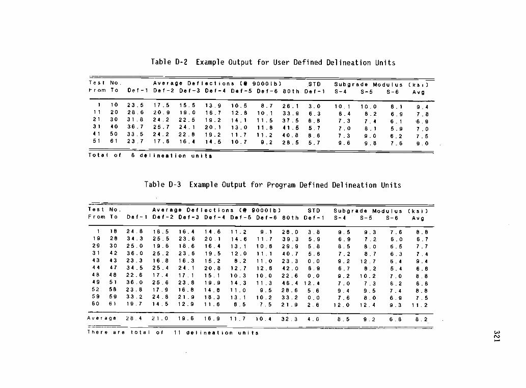
Table D-2 Example Output for User Defined Delineation Units

TestFrom

No.To Def-1

Average Deflections (kt 90001b)Def-2 Def-3 Def-4 Def-5 Def-6 80th

.STD

Def-1Subgrade ModulusS-4 S-5 S-6

(ksi)Avg

1 10 23.5 17.5 15.5 13.9 10.5 8.7 26.1 3.0 10.1 10.0 8.1 9.411 20 28.6 20.9 19.0 16.7 12.8 10.1 33.9 6.3 8.4 8.2 6.9 7.821 30 31.8 24.2 22.5 19.2 14.1 11.5 37.5 6.8 7.3 7.4 6.1 6.931 40 36.7 25.7 24.1 20.1 13.0 11.8 41.5 5.7 7.0 8.1 5.9 7.041 50 33.5 24.2 22.8 19.2 11.7 11.2 40.8 8.6 7.3 9.0 6.2 7.551 61 23.7 17.8 16.4 14.5 10.7 9.2 28.5 5.7 9.6 9.8 7.6 9.0

Total of 6 delineation unite

Table D-3 Example Output for Program Defined Delineation Units

TestFrom

No.To Def-1

Average Deflections (@ 90001b)Def-2 Def-3 Def-4 Def-5 Def-6 80th

STDDef-1

Subgrade ModulusS-4 S-5 S-6

(ksi)Avg

1 18 24.8 18.5 16.4 14.6 11.2 9.1 28.0 3.8 9.5 9.3 7.6 8.819 28 34.3 25.5 23.6 20.1 14.6 11.7 39.3 5.9 6.9 7.2 6.0 6.729 30 25.0 19.6 18.6 16.4 13.1 10.8 29.9 5.8 8.5 8.0 6.5 7.731 42 36.0 25.2 23.6 19.5 12.0 11.1 40.7 5.6 7.2 8.7 6.3 7.443 43 23.3 16.8 16.3 15.2 8.2 11.0 23.3 0.0 9.2 12.7 6.4 9.444 47 34.5 25.4 24.1 20.8 12.7 12.8 42.0 8.9 6.7 8.2 5.4 6.848 48 22.6 17.4 17.1 15.1 10.3 10.0 22.6 0.0 9.2 10.2 7.0 8.849 51 36.0 25.6 23.8 19.9 14.3 11.3 46.4 12.4 7.0 7.3 6.2 6.852 58 23.8 17.9 16.8 14.8 11.0 9.5 28.6 5.6 9.4 9.5 7.4 8.859 59 33.2 24.8 21.9 18.3 13.1 10.2 33.2 0.0 7.6 8.0 6.9 7.560 61 19.7 14.5 12.9 11.6 8.5 7.5 21.9 2.6 12.0 12.4 9.3 11.2

Average 28.4 21.0 19.6 16.9 11.7 10.4 32.3 4.6 8.5 9.2 6.8 8.2

There are total of 11 delineation units

322

file contains information such as test number, test location

(mileage), and deflection values converted to 9,000-lb load at each

sensor location. Table D-4 shows a typical output.

D-6 Usage of the Output

Tables D-2 and D-3 shows typical program output. The information

contained in these tables may be used in several purposes. The

average deflection values may be used for backcalculation analysis.

The 80th deflection may used for overlay design using the ODOT

procedure. The subgrade modulus may be used in backcalculation as a

fixed value or as a reference for checking the backcalculated result.

D-7 Recommendation for Implementation

To obtain a best result from using the program , it is

recommended that the user:

I. Obtain pavement surface thickness data before using the

program, since the program will need these data for

correcting the deflection values.

2. Combine necessary files into one single file (same

project). For example, deflections collected at shoulder may

be combined to a file, while deflections collected at out

wheel track may be saved to another file.

3. Print out the graph. This graph may help the user to

define manually the delineation units.

4. Print out the file with an extension FWD. This file

includes test number, test location, and deflections that

are converted to 9,000-lb load.

323

Table D-4 Example Output for TEST.FWD File

Test # Location Deflection Values

Sensor Location: 0 8 12 18 24 361, 204.050, 25.89, 19.96, 18.31, 16.42, 11.89, 9.662, 204.100, 20.52, 15.23, 14.05, 12.82, 9.62, 8.513, 204.151, 24.50, 18.55, 17.04, 15.64, 12.36, 10.204, 204.152, 26.54, 19.87, 18.05, 16.51, 13.06, 10.335, 204.200, 27.70, 20.40, 17.87, 15.40, 11.67, 9.086, 204.251, 23.37, 17.26, 14.98, 13.19, 9.79, 8.327, 204.300, 20.65, 15.07, 12.65, 10.87, 8.14, 6.358, 204.351, 18.82, 14.65, 12.14, 10.96, 7.92, 6.889, 204.400, 21.33, 16.66, 14.64, 13.19, 9.84, 8.7610, 204.451, 25.88, 17.77, 15.49, 13.69, 10.62, 8.4711, 204.500, 32.10, 25.90, 21.43, 18.36, 14.14, 10.7812, 204.550, 24.95, 17.77, 16.13, 14.52, 11.59, 9.2613, 204.600, 17.73, 12.78, 11.88, 10.86, 8.88, 7.0514, 204.650, 29.13, 20.97, 18.56, 16.38, 12.29, 9.7715, 204.700, 27.10, 19.43, 17.86, 16.46, 13.40, 10.7916, 204.751, 24.23, 18.57, 16.98, 15.25, 11.55, 9.8217, 204.800, 26.54, 19.89, 17.93, 16.09, 11.81, 9.6718, 204.850, 28.71, 21.42, 20.07, 16.97, 13.32, 10.5219, 204.900, 40.87, 28.02, 26.32, 22.37, 16.63, 12.6620, 204.951, 34.66, 24.34, 22.81, 19.51, 14.25, 10.8221, 205_000, 34.66, 25.45, 24.54, 19.75, 14.35, 10.3822, 205.051, 33.29, 25.45, 21.85, 19.29, 14.39, 12.0523, 205.100, 36.19, 26.58, 24.22, 20.83, 14.92, 12.2124, 205.150, 34.69, 25.28, 23.41, 20.41, 14.51, 11.8025, 205.200, 38.81, 29.78, 28.56, 23.53, 17.72, 13.1326, 205.250, 21.44, 16.74, 15.78, 14.05, 8.65, 8.5427, 205.304, 40.68, 31.08, 28.79, 23.79, 16.73, 13.4828, 205.350, 28.11, 22.52, 20.18, 17.76, 13.87, 11.7029, 205.400, 29.16, 22.13, 20.85, 17.78, 14.35, 11.4130, 205.450, 20.94, 17.05, 16.41, 14.92, 11.76, 10.2031, 205.500, 41.02, 28.26, 26.28, 21.65, 17.30, 12.2632, 205.5501 33.15, 23.18, 21.94, 18.48, 13.18, 11.4233, 205.600, 32.24, 21.59, 19.84, 17.30, 10.21, 10.5034, 205.653, 48.24, 33.01, 30.50, 24.35, 14.54, 12.8335, 205.702, 34.76, 25.88, 24.28, 20.60, 13.09, 12.2236, 205.751, 35.61, 25.94, 24.69, 20.81, 14.66, 13.3637, 205.800, 36.54, 24.89. 23.61, 19.72, 11.92, 11.7738. 205.859, 43.04, 30.06, 28.48, 23.39, 15.75, 12.5839, 205.900, 31.76, 22.50, 21.13, 18.17, 10.19, 11.6040, 205.950, 30.34, 21.49, 19.86, 16.15. 8.69, 9.50

324

APPENDIX E MECHOD USER'S GUIDE

E-1 Introduction

The MECHOD program is a computerized procedure for MECHanistic

Overlay Design. The MECHOD program consists of two parts: one is for

determining pavement damage and the other named MECHSUB is for

calculating pavement strains. MECHSUB is a modified ELSYM5 program.

The main program MECHOD uses the strains determined using MECHSUB

program to calculate failure repetitions and total pavement damage.

For existing pavements with remaining life less than 80 %, an overlay

is requested and the modulus for the overlay is needed as an input.

The MECHOD program then calculates automatically the pavement strains

and determines the pavement damage after overlay. This procedure is

repeated until an overlay thickness that provides pavement with

damage less than unity is determined.

Seasonal variations in traffic and pavement materials properties

are also considered in this program. This is done by breaking traffic

applications and pavement layer properties into four seasons and

considering the pavement damage separately for each season. The total

pavement damage is then the sum of damage within each season.

The MECHOD program was developed considering the use of an FWD

loading condition; therefore, only one load is required. Figure E-1

shows the program main menu. Four selections can be made and each of

them is discussed in the following.

E-2 Create Data File

This selection allows the user to create a data file for later

analysis. By pressing key C (Create) or 2 in the main menu, the

program will ask for a file name and display a data input screen as

shown in Figure E-2. The data input screen provides an easy data

entry environment. The user may use cursor keys to move the cursor to

any field and enter required data. After entering all necessary

information, the user may press function key [F10] to save the data,

or [F8] key to analyze the data right away, or [Esc] key to exit

without saving the data. The following information is needed.

325

PROGRAM MAIN MENU

1. EDIT A DATA FILE2. Create a data file3. Analyze a data file4. Operating system (DOS)

Figure E-1 MECHOD Program Main Menu

Load Data:Load Force (lbe): 0 Load Radius (in.): 0.00

File in UseEXAMPLE

Layer Properties:Number of Layers: 0

Layer ThicknessNo. (inch.)

Spring (Y)Modulus Pois

Season(s) for AnalysisSummer (N) Fall (N)

Modulus Pois Modulus PoisWinter (N)Modulus Pois

1. 0.0 1000000 0.35 0 0.00 0 0.00 0 0.002. 0.0 12500 0.45 0 0.00 0 0.00 0 0.003. 0.0 500000 0.40 0 0.00 0 0.00 0 0.004. 0.0 0 0.00 0 0.00 0 0.00 0 0.005. 0.0 0 0.00 0 0.00 0 0.00 0 0.00

Traffic Data:Hist. Repetitions: 0 0 0Future Repetitions: 0 0 0Reliability Level (%): 50 (Optional, default @ 50 %)Standard Deviation: 0.45 (Optional, default @ 0.45)

0

0

(F10) - Save & Exit [FB] -Run (Esc( - Exit (No save)

Figure E-2 MECHOD Screen Data Input/Edit

326

1. Load force (required) in lbs.

2. Load radius (required) in inches.

3. Number of layer (required) total pavement

layers, including subgrade.

4. Seasons for analysis (required) can be one

season or all seasons. Y stands for yes and N

for no.

5. Layer thickness (required, except subgrade) in

inches.

6. Modulus and Poisson's ratio (required) for

seasons that will be analyzed, the modulus and

Poisson's ratio are required.

7. Traffic data (required) both historical and

future traffic repetitions. If the historical

data is not given, the program may also be used

for new pavement design.

8. Reliability level (optional) percent, default

is set at 50%.

9. Standard deviation (optional) for flexible

pavement, it ranges from 0.4 to 0.5.

E-3 Edit Data File

This option allows the user to edit a data file that has been

created previously. By pressing key E (Edit) or 1 in the main menu

and giving a file name to be edited, the same screen (Figure E-2)

used for creating a data file will be displayed. The information

saved in the existing data file will be shown in corresponding

fields. The user may use cursor keys to move to any field and edit

the existing information. Again, follow the bottom menu for next

step.

E-4 Analyze Data File

This option allows the user to analyze a data file that has been

created previously. By pressing key A (Analyze) or 3 and giving the

file name to be analyzed, a message "Computing ..." will be shown on

327

screen (Figure E-3). Analysis results will be displayed. An example

is shown in Figure E-4. If an overlay is needed, the program will

assume an one-inch overlay and ask the user for modulus of overlay

materials for the season(s) being analyzed (Figure E-5). This allows

different paving materials to be considered for overlay designs.

The overlay design procedure is a repeated process. with an

increment of 0.5 inch. This procedure is carried out by the program

automatically until the total pavement damage is less than unity and

the recommended overlay thickness will then be displayed. The output

will be saved in a file with an extension OUT. For example, if a file

has name TEST.DAT, the output will be saved to TEST.OUT. An example

output is shown in Figure E-6.

E-5 Operating System (DOS)

This option allows the user to leave the MECHOD program

temporarily and work in the DOS environment. To return to the MECHOD

program, type EXIT in DOS and press ENTER key.

328

PROGRAM MAIN MENU

1. Edit a data file2. Create a data file3. ANALYZE A DATA FILE4. Operating system (DOS)

File name: example

Computing

Figure E-3 Screen for Data Analysis

Reliability - 50 Standard Dev. = 0.45Layer Thickness (inches): 5.0 12.0

Seasons Surface Calculated Traffic Failure Repetitions DamageModulus Starins Repetitions Surface Subgrade Ratio%(ksi) AC. Subg. Past Future AC Subg

Spring 400 324 -603 500000 1000000 4.00E+05 3.61E+05 375 415

Total damage - 375.4 % for surface, 415.3 % for subgrade

OVERLAY OR RECONSTRUCTION. 11 REMAINING LIFE OF SURFACE IS LESS THAN 20 %OVERLAY OR RECONSTRUCTION. THE REMAINING LIFE OF SUBGRADE IS LESS THAN 20 %

Figure E-4 Example Output Showing Overlay Is Needed

Modulus of Overlay Material for season(s)being analyzed is required and should beinput in the following (in psi).

For Spring < 400000 > ? 600000

-4.

Figure E-5 Modulus of Overlay Material Can Be Considered

Reliability - 50 Standard Dev. = 0.45Layer Thickness (indhes): 5.0 12.0

Seasons Surface Calculated TrafficModulus Starins Repetitions(ksi) AC. Subg. Past Future

329

'Failure Repetitions DamageSUrface Subgrade Ratio%

AC Subg

Spring 400 324 -603 500000 1000000 4.00E4705 3.61E+05 375 415

Total damage 375.4 % for surface, 415.3 % for subgrade

OVERLAY OR RECONSTRUCTION. THE REMAINING LIFE OF SURFACE IS LESS THAN 20 %OVERLAY OR RECONSTRUCTION. THE REMAINING LIFE OF SUBS:RADE IS LESS THAN 20 %

Overlay thickness - 1.0 in.

Spring 400 261 -468 500000 1000000 8.14E+05

Total damage - 184.3 % for surface,

Overlay thickness = 1.5 in.

Spring 400 237 -421

1.12E+06 184 133

133.4 % for subgrade

500000 1000000 1.12E+06 1.81E+06 134 83

Total damage - 134.1 % for surface,

Overlay thickness = 2.0 in.

Spring 400 216 -381

83.0 % for subgrade

500000 1000000 1.52E+06 2.82E+06 99 53

Total damage - 98.8 % for surface,

Recommendation: use 2.0 in. overlay.

53.1 % for subgrade

Figure E-6 Example Output

330

APPENDIX F

BACKCALCULATION RESULTS

This appendix presents detailed output

from backcalculation analysis for the following

projects:

F-1 Rufus Quinton Project

F-2 Centennial Boulevard Project

F-3 Nelchina Project

F-4 Tudor Road Project

331

F-1 Rufus Quinton Project (Eastbound)

Station Load

(lb)

AC

(psi)

Base

(psi)

Subgrade

(psi)

Bulk

stress

Deviator

stress

1 3,199 302,658 87,337 14,847 8.42 4.27

1 6,398 1,257,591 14,555 23,882 6.07 7.03

1 11,934 1,268,846 30,659 22,929 12.67 9.21

2 3,158 509,816 34,371 24,822 6.11 5.13

2 11,811 173,076 48,314 19,659 25.80 11.51

3 3,199 610,269 33,422 33,890 5.86 5.48

3 6,726 492,083 28,512 30,505 10.41 8.63

4 2,953 259,183 26,058 30,547 6.39 5.93

4 6,603 267,678 35,667 25,531 12.86 8.48

4 11,852 324,543 36,048 31,620 20.52 13.67

5 3,158 353,341 20,003 25,054 5.86 5.80

5 6,603 709,493 11,538 24,949 6.92 8.53

5 11,811 176,235 10,351 29,877 16.93 19.86

6 6,521 266,598 12,658 31,552 9.58 11.15

7 2,830 161,216 20,294 24,605 6.51 6.02

7 11,893 363,088 40,729 25,635 20.65 11.89

8 6,439 243,075 36,564 15,768 12.97 7.09

8 12,016 386,336 17,561 31,867 15.83 15.70

9 3,076 287,092 17,354 39,274 5.85 6.82

9 6,480 267,245 27,931 29,528 11.89 9.30

10 3,076 244,209 13,748 32,867 5.75 6.86

10 6,480 332,561 13,664 28,046 9.13 10.04

10 11,770 153,986 13,075 30,703 18.88 19.57

11 6,439 326,903 11,389 20,418 8.64 9.20

11 11,893 526,235 11,665 22,739 12.26 13.54

12 3,076 253,026 16,343 29,930 5.94 6.48

12 6,398 329,310 14,050 24,271 9.14 9.40

12 11,975 346,906 19,621 22,916 16.93 13.58

13 3,035 254,005 18,565 18,566 6.06 5.53

13 6,357 376,159 10,805 23,589 8.06 9.43

13 11,852 329,116 28,234 21,706 19.06 12.27

14 2,871 195,491 16,824 15,610 6.05 5.39

14 6,357 319,128 16,976 15,848 9.70 7.80

14 11,893 503,199 21,622 18,842 15.40 11.20

16 3,117 193,967 26,817 33,926 7.12 6.49

16 12,139 571,760 21,556 35,889 15.01 14.61

17 12,180 620,775 17,300 37,613 13.56 15.31

18 3,076 230,240 35,813 32,091 7.23 5.93

18 6,685 497,033 39,748 27,553 11.35 7.77

18 11,975 809,831 40,781 25,952 16.32 10.19

19 3,117 572,716 32,391 34,328 5.80 5.50

19 6,644 680,060 19,775 33,094 8.37 8.83

20 3,117 269,346 21,742 32,117 6.31 6.3320 6,726 473,480 15,311 29,783 8.73 9.63

21 3,035 924,348 13,054 24,918 4.06 5.1821 6,685 570,617 44,089 13,831 11.24 5.9021 12,016 380,178 126,956 11,562 27.26 6.57

Average 424,767 27,060 26,278

STD 248,301 20,108 6,585

332

F-1 Rufus Quinton Project (Westbound)

Station Load

(lb)

AC

(psi)

Base

(psi)

Subgrade

(psi)

Bulk

stress

Deviator

stress

1 3,240 340,993 12,043 31,568 4.94 6.51

1 6,521 666,413 13,607 24,690 6.59 7.68

1 12,057 882,720 18,052 24,040 10.29 9.94

2 3,158 399,510 15,647 25,811 4.98 5.83

2 6,685 359,843 22,021 20,414 9.06 7.49

2 11,975 450,584 25,414 21,510 14.10 10.12

3 3,199 491,324 22,562 25,731 5.19 5.49

3 6,480 657,531 19,015 23,906 7.23 7.23

3 12,385 885,645 26,625 24,856 11.92 9.54

4 3,076 396,075 21,830 22,061 5.27 5.38

4 6,808 377,011 27,770 19,762 9.64 7.14

4 12,262 516,346 29,416 21,705 14.42 9.76

5 3,199 365,477 31,656 32,607 5.91 5.72

5 6,808 601,823 21,182 32,505 7.90 8.17

5 12,057 706,802 25,741 33,820 12.39 11.13

6 6,767 810,309 63,150 28,590 9.73 6.29

6 12,303 869,746 77,331 26,934 16.46 7.98

7 3,199 401,272 20,879 39,374 5.32 6.25

7 6,849 546,094 18,504 36,591 7.85 8.87

7 12,303 691,963 21,264 39,325 11.94 12.53

8 6,644 467,614 11,154 20,492 6.97 8.00

8 12,221 569,319 14,296 20,966 11.12 10.88

9 3,199 464,359 20,343 20,264 5.14 5.31

9 6,767 617,598 16,485 18,818 7.29 7.09

9 12,098 806,569 15,690 22,057 10.14 10.06

12 3,076 244,263 18,082 19,262 5.59 5.59

12 6,726 428,882 13,792 21,249 7.64 8.00

12 12,262 637,104 13,400 27,265 10.52 11.97

13 3,117 209,438 28,711 19,979 6.37 5.42

13 6,808 351,754 23,308 21,679 9.38 7.65

13 12,344 426,199 33,843 22,354 15.99 9.94

14 3,199 366,653 29,561 32,745 5.83 5.77

14 6,767 503,474 21,672 35,231 8.32 8.58

14 12,344 652,950 25,325 40,620 12.89 12.43

19 3,158 419,703 31,587 34,765 5.70 5.70

21 3,158 400,430 37,071 27,611 5.95 5.34

21 6,685 594,077 23,851 28,384 8.09 7.61

21 12,139 785,417 28,260 30,241 12.41 10.28

22 3,158 643,400 15,778 25,774 4.52 5.52

22 6,726 513,236 20,965 25,605 8.16 7.72

22 11,852 674,652 21,580 28,103 11.73 10.68

23 3,117 588,250 19,544 27,662 4.78 5.51

23 6,726 555,988 17,631 28,134 7.61 8.08

23 12,139 690,632 19,644 29,886 11.52 11.28

24 3,117 257,551 28,055 28,818 6.09 5.78

24 6,685 374,314 19,633 31,491 8.69 8.75

Average 536,115 23,978 27,071

STD 172,033 11,600 5,792

333

F-2 Centennial Boulevard Project

(Eastbound from location 200 to 4000)

Station Load

(lb)

AC

(psi)

Base

(psi)

Subgrade

(psi)

Bulk

Stress

Deviator

Stress

200 8,821 1,192,686 35,389 10,619 13.2 6.3

200 14,269 1,074,783 44,632 10,656 22.3 8.1

400 8,821 383,337 33,174 12,131 17.3 7.9

400 14,297 280,833 50,940 11,598 31.6 9.9

600 8,763 446,242 33,644 10,133 16.7 7.2

600 14,269 498,348 44,397 10,037 27.1 9.0

800 8,705 524,632 37,849 10,832 16.4 7.0

800 14,153 1,140,917 30,466 10,620 19.5 8.7

1000 8,849 677,562 21,917 10,991 13.6 7.7

1000 14,240 647,469 29,774 10,578 22.9 9.8

1200 8,763 339,800 29,463 12,337 17.2 8.3

1200 14,240 395,530 38,190 11,842 27.6 10.4

1400 8,792 576,179 23,206 13,901 14.3 8.5

1400 14,211 625,636 28,086 13,105 22.7 10.9

1600 8,734 364,318 24,634 11,208 16.2 8.2

1600 14,182 315,199 32,533 11,030 27.9 10.9

1800 8,734 429,492 28,801 9,912 16.2 7.4

1800 14,153 380,923 36,522 9,931 27.4 9.8

2000 8,763 898,118 32,653 10,838 13.9 6.7

2000 14,211 656,243 44,998 10,683 25.3 8.8

2200 8,676 476,446 20,870 9,959 14.4 7.8

2200 14,067 537,890 25,928 9,760 22.9 10.0

2400 8,763 676,194 20,354 12,914 13.2 8.3

2400 14,182 564,264 29,181 12,294 23.5 10.7

2600 8,734 666,228 25,826 23,487 14.1 9.9

2600 14,269 648,552 33,947 25,003 23.7 13.8

2800 8,705 383,872 16,507 17,944 14.4 10.8

2800 14,124 458,096 19,922 18,146 22.4 14.5

3000 8,676 641,011 33,459 23,180 15.1 9.3

3000 14,211 568,411 49,657 22,162 26.9 12.0

3200 8,648 982,052 31,485 32,579 13.3 10.0

3200 14,067 964,432 42,288 32,492 22.3 13.4

3400 8,648 583,606 30,334 17,083 15.1 8.5

3400 13,923 382,669 46,799 16,351 28.4 11.1

3600 8,705 666,593 26,030 25,630 14.1 10.2

3600 14,182 851.510 27,606 25,665 20.7 13.9

3800 8,676 502,722 47,255 19,749 17.4 8.3

3800 14,240 413,078 68,918 19,793 30.9 10.8

4000 8,705 904,828 40,382 24,621 14.6 8.6

4000 14,211 609,647 60,128 24,355 27.6 11.7

AVERAGE 608,259 34,454 15,904

STD 229,872 11,032 6,581

334

F-2 Centennial Boulevard Project

(Eastbound from location 4200 to 7000)

Station Load

(lb)

AC

(psi)

Base

(psi)

Subgrade Bulk

(psi) Stress

Deviator

Stress

4200 8,648 733,522 44,104 19,073 15.6 7.9

4200 14,124 604,680 67,282 19,012 28.2 10.1

4400 8,648 578,668 45,958 17,889 16.7 7.9

4400 14,096 524,224 64,597 17,972 28.8 10.2

4600 8,532 676,229 42,831 10,781 15.6 6.5

4600 13,951 680,957 56,206 10,770 26.1 8.2

4800 8,561 858,319 47,075 18,196 15.1 7.4

4800 14,009 479,265 77,869 18,668 30.3 9.9

5000 8,561 1,054,069 45,675 15,151 14.3 6.8

5000 14,038 1,102,778 60,950 15,907 23.7 8.8

5200 8,619 1,154,214 48,720 15,489 14.2 6.7

5200 14,096 872,094 74,352 15,633 26.5 8.6

5400 8,792 1,185,558 26,500 13,516 12.1 7.2

5400 13,980 995,197 36,552 12,831 21.1 9.2

5600 8,676 918,746 35,486 15,219 14.0 7.4

5600 14,096 777,984 49,862 14,379 24.7 9.4

5800 8,590 623,626 54,045 9,928 16.9 6.1

5800 14,038 758,515 64,979 10,062 26.4 7.6

6000 8,561 1,287,120 34,744 10,354 12.5 6.1

6000 14,009 1,256,945 42,694 10,303 20.7 7.8

6200 8,705 274,332 57,679 13,491 20.5 7.4

6200 14,124 420,490 61,997 13,297 29.9 9.4

6400 8,648 917,159 34,679 12,716 13.9 6.9

6400 14,096 868,758 48,870 11,850 23.9 8.5

6600 8,619 648,294 46,532 8,220 16.2 5.9

6600 14,009 528,858 56,056 8,724 27.7 7.8

7000 8,734 633,344 36,933 13,752 15.6 7.5

7000 14,124 547,457 50,960 12,784 27.1 9.4

AVERAGE 784,336 50,507 13,785

STD 259,845 12,384 3,177

335

F-2 Centennial Boulevard Project

(Westbound from location 6900 to 2700)

Station Load

(lb)

AC

(psi)

Base

(psi)

Subgrade Bulk

(psi) Stress

Deviator

Stress

6900 8,705 549,293 86,849 16,120 19.4 6.6

6900 14,182 505,870 110,433 16,033 32.4 8.4

6700 8,705 311,068 82,928 13,055 21.3 6.6

6700 14,182 393,500 93,740 12,641 33.0 8.2

6500 8,648 604,949 32,495 16,002 15.2 8.1

6500 14,096 588,483 41,301 15,352 25.3 10.6

6300 8,676 567,289 33,848 23,922 15.6 9.5

6300 14,182 620,694 42,163 24,353 25.2 12.8

6100 8.676 361,100 34,291 20,897 17.4 9.6

6100 14,153 351,517 43,914 21,888 29.0 13.2

5900 8,648 720,605 28,884 16,867 14.1 8.3

5900 14,096 703,185 34,819 15,889 23.1 10.9

5700 8,590 484,190 48,198 14,289 17.4 7.3

5700 14,096 338,452 67,074 14,020 31.7 9.6

5500 8,648 874,525 48,054 21,573 15.3 7.9

5500 14,211 624,465 74,903 21,459 28.9 10.3

5100 8,676 774,804 57,989 16,033 16.5 6.9

5100 14,153 776,411 70,602 16,035 27.0 9.0

4900 8,648 706,615 47,964 16,225 16.1 7.3

4900 14,124 604,709 66,351 16,016 28.1 9.4

4700 8,619 795,417 61,138 15,027 16.5 6.6

4700 14,182 724,053 78,649 15,175 28.2 8.6

4500 8,619 902,274 25,244 12,929 12.7 7.4

4500 14,153 786,905 35,892 13,110 22.7 9.8

3700 8,619 530,502 44,536 20,145 16.8 8.4

3700 14,153 736,687 49,111 20,853 25.1 11.2

3500 8,619 1,263,788 22,439 26,557 11.1 9.4

3500 14,124 1,182,953 29,387 25,427 19.0 12.7

3300 8,561 920,650 18,988 15,307 11.6 8.3

3300 14,096 1,080,032 22,397 15,850 17.9 11.2

3100 8,532 1,277,277 16,303 17,317 10.0 8.4

3100 14,038 1,418,923 21,726 15.827 16.2 10.6

2900 8,561 1,202,374 22,991 10,836 11.3 6.8

2900 14,067 1,388,525 25,879 10,491 17.3 8.6

2700 8,590 983,678 25,082 14,033 12.3 7.5

2700 14,096 938,722 35,231 13,158 21.4 9.5

AVERAGE 766,513 46,716 16,964

STD 298,557 23,418 4,008

336

F-2 Centennial Boulevard Project

(Westbound from location 2500 to 100)

Station Load

(lb)

AC

(psi)

Base

(psi)

Subgrade Bulk

(psi) Stress

Deviator

Stress

2500 8,561 696,691 30,281 17,457 14.3 8.3

2500 14,038 508,317 47,227 16,663 26.9 10.8

2100 8,532 485,466 34,521 11,670 16.1 7.3

2100 14,009 512,793 40,242 10,969 25.9 9.4

1900 8,676 1,070,951 27,632 13,658 12.5 7.3

1900 14,182 1,192,106 32,396 12,922 19.6 9.3

1700 8,561 640,110 37,988 10,675 15.4 6.7

1700 14,067 337,358 59,504 10,487 30.9 8.8

1500 8,619 525,731 39,137 14,395 16.4 7.6

1500 14,038 295,918 64,070 13,622 32.1 9.8

1300 8,648 201,822 38,022 13,687 19.9 8.5

1300 14,067 201,950 51,226 12,949 33.1 10.7

1100 8,590 618,645 28,924 15,765 14.6 8.3

1100 14,067 625,296 36,771 14,750 24.1 10.6

900 8,648 337,715 44,163 14,580 18.6 7.9

900 14,096 353,862 54,817 13,782 30.2 10.1

700 8,648 1,102,055 27,453 17,099 12.3 7.9

700 14,182 840,150 41,470 15,911 23.2 10.2

500 8,648 142,658 49,225 15,638 22.1 8.7

500 14,096 226,980 65,390 14,904 33.9 10.4

299 8,648 271,970 70,620 11,342 21.1 6.6

299 14,067 306,764 85,021 10,933 33.6 8.2

100 8,705 522,935 74,902 12,136 19.0 6.2

100 14,153 871,873 69,792 12,004 26.2 7.9

AVERAGE 537,088 47,950 13,667

STD 293,206 16,195 2,061

337

F-3 Nelchina Project

(Spring)

Station Load AC MR Base MR Subbs MR Subgrade Average

8 9,699 1,200,000 90,477 54,622 27,841 Base 67,355

10 9,492 1,200,000 69,206 48,598 26,060 Subbase 37,030

12 9,476 1,200,000 56,414 43,701 23,125 Subgrade 22,054

14 9,270 1,200,000 51,100 54,185 24,716

16 9,254 1,200,000 69,246 36,032 25,111

18 9,174 1,200,000 69,633 48,772 28,461

20 9,270 1,200,000 86,932 26,905 32,904

22 9,270 1,200,000 62,007 36,358 25,064

24 9,286 1,200,000 57,088 53,025 25,556

26 9,333 1,200,000 59,863 46,651 14,825

28 9,222 1,200,000 64,998 53,655 29,286

30 9,158 1,200,000 83,972 46,612 37,407

32 9,222 1,200,000 112,928 22,173 26,130

34 9,254 1,200,000 87,553 25,857 28,010

36 9,174 1,200,000 112,259 23,243 31,221

38 9,206 1,200,000 103,689 22,173 25,360

40 9,222 1,200.000 72,201 46,324 22,510

42 9,079 1,200,000 62,941 39,103 22,786

44 9,079 1,200,000 55,439 34,195 19,168

46 9,174 1,200,000 54,026 55,616 19,959

48 9,079 1,200,000 65,104 44,797 25,722

50 9,063 1,200,000 58,499 28,141 15,348

51 9,015 1,200,000 48,894 18,656 12,964

52 9,063 1,200,000 40,966 30,029 16,252

53 9,031 1,200,000 54,068 40,556 13,847

54 9,063 1,200,000 56,348 26,816 11,617

55 8,936 1,200,000 42,671 11,225 10,491

56 9,031 1,200,000 49,824 23,139 13,312

57 9,095 1,200,000 59,849 31,616 14,139

58 9,031 1,200,000 70,092 42,525 17,444

59 8,920 1,200,000 59,369 50,114 21,818

60 9,015 1,200,000 73,265 42,123 24,611

61 8,904 1,200,000 61,782 14,446 14,716

62 8,809 1,200,000 55,382 15,403 11,981 Base 35,425

63 8,745 1,200,000 43,817 10,692 11,562 Subbase 14,439

64 8,920 1,200,000 54,479 16,777 15,152 Subgrade 11,831

65 8,745 1,200,000 28,565 16,216 11,037

66 8,745 1,200,000 23,633 12,344 15,864 8,401

67 8,681 1,200,000 32,259 11,999 12,495 4,145

68 8,729 1,200,000 33,851 14,794 13,161 1,969

69 8,809 1,200,000 36,678 22,198 11,714

70 8,586 1,200,000 21,417 7,826 11,942

71 8,920 1,200,000 31,852 16,008 9,923

72 8,777 1,200,000 25,081 14,238 8,660

338

73 8,904 1,200,000 30,647 10,846 9,293

74 8,761 1,200,000 24,969 10,595 9,885

79 8,856 1,200,000 29,255 14,766 11,127

80 8,872 1,200,000 42,219 11,875 11,065

81 8,968 1,200,000 52,698 24,441 14,432

82 9,158 1,200,000 74,213 22,604 22,359 Base 67,288

83 8,681 1,200,000 122,536 30,442 16,323 Subbase 22,757

84 8,856 1,200,000 34,604 15,626 19,404 Subgrade 15,762

85 8,459 1,200,000 31,527 11,820 6,381

86 8,888 1,200,000 46,323 23,300 6,119

87 8,713 1,200,000 35,989 26,454 12,008

88 8,681 1,200,000 67,508 25,010 16,626

89 9,079 1,200,000 88,825 26,766 29,010

90 9,127 1,200,000 68,044 45,318 25,353

91 9,015 1,200,000 72,271 46,141 11,177

92 9,111 1,200,000 103,066 24,787 31,933

93 9,111 1,200,000 116,148 21,914 21,351

98 8,952 1,200,000 42,413 17,518 13,628

99 8,872 1,200,000 70,519 14,051 11,841

100 9,063 1,200,000 60,855 14,755 13,448

101 9,063 1,200,000 48,202 11,732 14,995

102 8,999 1,200,000 55,360 25,704 9,642

103 8,936 1,200,000 59,370 9,989 14,989

104 8,936 1,200,000 55,157 9,981 20,877

105 8,697 1,200,000 62,051 15,747 9,025

106 8,793 1,200,000 41,403 9,823 16,477

107 8,999 1,200,000 55,715 25,868 15,612

108 9,079 1,200,000 80,372 49,585 23,297

109 8,872 1,200,000 64,261 33,597 21,669

110 8,522 1,200,000 66,321 20,585 10,598

112 8,793 1,200,000 59,382 11,254 6,841

115 8,777 1,200,000 98,082 54,434 15,452

116 8,697 1,200,000 52,118 14,892 11,025

117 8,697 1,200,000 67,733 23,360 10,045

122 8,761 1,200,000 73,164 16,148 9,858

124 8,888 1,200,000 73,245 16,973 16,328

125 8,888 1,200,000 106,439 12,044 20,702

AVERAGE 8,982 1,200,000 61,021 26,929 17,549

STD 225 0 22,687 14,191 7,109

339

(Summer)

2 9,063 1,000,000 66,692 28,045 16,396 Base 80,469

6 9,047 1,000,000 83,500 17,706 9,647 Subbase 56,117

8 9,206 1,000,000 74,866 44,610 21,670 Subgrade 29,991

10 9,302 1,000,000 91,169 66,077 28,567

12 9,158 1,000,000 64,502 61,209 35,326

14 9,190 1,000,000 79,336 44,289 30.985

16 9,174 1,000,000 75,913 48,008 33,680

18 9,127 1,000,000 61,591 58,348 28,982

20 9,143 1,000,000 99,593 53,249 39,988

22 9,286 1,000,000 77,788 68,052 43,553

24 9,127 1,000,000 91,263 66,744 35,484

26 8,968 1,000,000 70,326 56,823 29,152

28 8,952 1,000,000 94,668 52,638 29,260

30 9,047 1,000,000 72,884 56,068 36,056

32 9,158 1,000,000 65,364 75,796 37,230

36 9,174 1,000,000 150,640 55,138 31,303

38 9,127 1,000,000 78,718 95,621 48,974

40 9,238 1,000,000 107,945 53,657 42,078

42 9,079 1,000,000 77,562 92,412 41,533

44 9,127 1,000,000 74,140 40,680 22,401

46 9,063 1,000,000 67,605 61,756 24,998

48 9,095 1,000,000 85,747 35,016 65,758

50 8,840 1,000,000 80,433 58,654 26,539

51 8,157 1,000,000 49,560 35,094 25,671

52 9,206 1,000,000 70,484 70,472 26,333

53 9,270 1,000,000 81,202 66,837 23,304

54 9,222 1,000,000 70,634 78,799 22,623

55 8,984 1,000,000 75,056 49,868 17,888

56 9,015 1,000,000 63,899 34,282 17,579

57 9,143 1,000,000 91,109 48,203 24,314

58 9,111 1,000,000 70,404 56,370 22,181

59 9,286 1,000,000 81,283 70,371 32,434

60 9,031 1,000,000 113,806 70,769 33,230

61 8,968 1,000,000 76,277 36,312 14,583

62 8,904 1,000,000 54,472 32,283 10,091 Base 63,982

63 9,095 1,000,000 102,870 58,233 11,781 Subbase 46,088

64 8,920 1,000,000 75,264 44,453 10,647 Subgrade 12,167

65 8,968 1,000,000 64,743 87,635 11,971

66 8,761 1,000,000 59,229 46,776 10,290 20,994

67 8,936 1,000,000 53,718 53,268 14,202 20,216

68 8,840 1,000,000 48,071 84,302 17,825 2,675

69 8,840 1,000,000 53,324 93,451 17,445

70 8,920 1,000,000 129,296 41,040 16,814

71 8,872 1,000,000 61,289 55,248 13,238

72 8,777 1,000,000 53,930 45,740 12,831

73 8,856 1,000,000 51,509 37,241 12,522

74 8,697 1,000,000 50,507 26,455 9,796

75 8,602 1,000,000 46,647 28,111 10,489

76 8,634 1,000,000 42,675 28,223 9,990

340

77 8,634 1,000,000 52,039 31,525 9,689

78 8,681 1,000,000 91,713 25,228 10,159

79 8,697 1,00.0,000 58,755 38,749 10,506

80 8,745 1,000,000 63,549 35,882 14,569

81 8,666 1,000,000 49,937 27,920 8,476

82 8,777 1,000,000 80,085 33,632 15,742 Base 75,951

83 8,300 1,000,000 62,972 13,126 10,035 Subbase 31,061

84 8,300 1,000,000 56,711 14,443 9,806 Subgrade 13,369

85 8,411 1,000,000 40,874 18,970 7,656

86 8,936 1,000,000 43,869 29,532 10,056

87 8,777 1,000,000 56,159 23,126 10,393

89 9,381 1,000,000 79,070 59,525 30,189

90 9,429 1,000,000 93,884 62,501 31,636

91 9,349 1,000,000 66,228 62,038 25,035

92 9,397 1,000,000 142,564 45,900 22,055

93 9,238 1,000,000 104,324 31,793 19,835

94 9,286 1,000,000 73,523 38,605 28,568

98 9,063 1,000,000 97,435 15,352 8,428

99 9,254 1,000,000 69,816 20,653 8,460

100 9,063 1,000,000 56,970 15,979 10,097

101 9,190 1,000,000 45,373 15,853 8,490

102 9,031 1,000,000 69,463 21,501 6,761

103 8,984 1,000,000 40,380 17,812 7,209

104 9,222 1,000,000 49,092 16,728 12,792

105 8,872 1,000,000 69,182 13,178 6,373

106 9,015 1,000,000 122,605 19,625 8,572

107 8,999 1,000,000 59,812 15,100 11,334

108 9,047 1,000,000 62,145 35,040 14,743

110 8,856 1,000,000 77,261 64,403 15,232

112 9,015 1,000,000 60,892 21,036 9,027

113 8,968 1,000,000 57,590 41,832 12,079

114 9,015 1,000,000 61,337 21,120 11,580

115 8,999 1,000,000 129,238 46,707 12,704

116 8,920 1,000,000 69,473 22,969 8,832

117 8,936 1,000,000 36,842 82,673 9,579

121 9,174 1,000,000 90,303 9,523 15,756

122 8,888 1,000,000 65,507 44,251 10,905

123 9,079 1,000,000 107,804 39,194 15,659

124 9,015 1,000,000 97,435 28,708 10,149

125 8,904 1,000,000 146,257 17,790 9,067

127 9,031 1,000,000 91,758 37,995 16,466

AVERAGE 8,992 1,000,000 74,819 43,866 19,381

STD 238 0 23,803 21,119 11,435

341

F-4 Tudor Road Project

STATION LOAD

Spring (TUDOR4)

El E2 E3 STATION LOAD

Summer (TUDOR])

El E2 E3

2 8,809 2,522,758 25,914 69,621 2 8,777 1,483,561 18,283 62,2723 8,761 1,627,281 16,591 69,186 3 8,713 822,610 23,977 76,7804 8,793 1,802,737 21,365 53,422 4 8,809 1,384,514 23,791 57,356

5 8,586 932,227 23,897 60,3146 8,697 1,485,981 17,608 71,213 6 8,602 430,447 32,590 68,1677 8,729 1,366,869 18,885 64,758 7 8,713 446,591 39,512 59,1218 8,666 1,265,272 24,362 88,533 8 8,761 636,704 39,332 72,6649 8,650 1,905,893 12,374 88,809 9 8,745 936,550 35,129 74,918

10 8,570 1,394,032 13,408 53,943 10 8,713 802,435 27,164 39,38911 8,713 800,108 23,056 53,973

12 8,618 2,357,785 15,916 67,794 12 8,586 769,889 37,622 41,82313 8,618 1,678,070 22,906 80,988 13 8,777 834,381 38,911 61,10216 8,602 1,437,052 12,180 77,800 16 8,634 983,233 21,164 80,77517 8,697 1,187,702 11,161 69,539 17 8,618 667,208 25,094 49,99318 8,141 2,449,590 19,715 68,919 18 8,745 658,243 70,153 28,18819 8,252 2,506,592 13,038 78,964 19 8,634 1,478,342 24,300 83,33520 8,125 1,732,664 10,403 77,357 20 8,713 699,197 37,517 67,74921 8,125 2,549,027 15,457 85,380 21 8,586 1,038,107 27,573 77,30822 8,045 1,807,402 11,171 36,362 22 8,554 1,020,985 19,615 37,50623 7,918 1,959,808 8,278 56,016 23 8,666 1,623,364 16,142 39,698

24 8,507 1,793,133 18,258 53,26125 8,602 572,325 16,327 49,889

26 7,680 2,764,867 7,409 76,514 26 8,522 1,865,138 14,807 40,68027 8,443 1,255,065 36,887 34,738

28 7,505 1,449,724 10,594 82,566 28 8,507 749,118 29,615 52,84529 7,537 1,091,509 8,999 71,703 29 8,427 577,615 28,125 43,45930 7,457 1,854,921 10,668 61,970 30 8,459 1,093,926 21,263 47,783

31 8,491 1,232,821 24,043 50,71533 7,489 2,716,261 10,895 38,138 33 8,634 2,284,115 16,921 42,96635 7,489 1,617,430 11,240 55,032 35 8,745 1,052,558 18,911 43,71336 7,457 1,544,495 10,318 40,658 36 8,363 1,060,087 26.306 33,65537 7,330 1,068,741 8,028 47,32638 7,537 1,661,123 17,013 64,64639 7,505 1,605,133 20,135 60,620 39 8,395 400,962 67,906 35,56540 7,489 1,687,449 23,511 34,042 40 8,348 1,001,495 30,987 36,26541 7,441 2,409,085 11,976 18,490 41 8,507 2,427,190 15,138 19,08742 7,553 2,657,302 8,244 53,629 42 8,650 2,292,126 18,815 45,43543 7,409 1,808,887 21,091 28,534 43 8,745 1,058,242 42,985 32,53045 7,457 1,890,126 10,158 34,054 44 8,475 1,632,499 42,600 37,78146 7,473 1,489,547 11,772 33,356 45 8,650 1,423,907 23,370 26,97847 7,425 2,049,189 11,448 34,961 47 8,618 1,372,367 16,126 29,49948 7,473 2,005,324 8,642 36,261 48 8,586 1,208,240 17,396 34,30949 7,394 1,545,986 20,542 25,917 49 8,586 1,263,911 22,332 22,283

50 8,491 2,672,311 18,752 32,34351 8,618 2,441,484 19,147 30,183

52 7,537 2,510,644 8,688 44,481 52 8,507 1,611,574 18,999 32,38853 7,600 2,250,639 8,002 40,759 53 8,681 2,071,876 11,089 30,59654 7,537 1,430,387 24,028 41,114 54 8,602 652,180 36,092 51,03255 7,505 1,196,969 23,146 36,235 55 8,570 812,480 25,184 40,98856 7,505 1,125,882 17,316 44,03857 7,537 2,643,775 16,693 32,346 57 8,443 1,053,473 33,550 37,55458 7,473 2,921,515 17,909 21,401 58 8,522 2,766,370 16,034 26,701

59 8,618 2,255,674 30,188 51,87760 8,459 1,679,145 24,010 30,261

61 7,044 2,685,954 13,843 56,750 61 8,284 1,040,752 31,667 44,12362 7,139 944,906 13,344 42,865 62 8,840 1,330,767 27,295 33,06163 7,060 1,461,267 26,235 67,467 63 8,888 692,090 40,016 70,82164 7,298 1,575,921 11,720 66,785 64 8,856 931,207 24,605 59,30165 7,235 685,008 11,552 26,972 65 8,666 298,004 21,556 23,432

66 8,904 2,024,227 30,748 36,25567 7,250 1,887,403 13,865 35,010 67 8,872 1,114,934 20,803 25,91368 7,298 2,022,767 22,641 37,842 68 8,793 1,365,438 28,150 31,066

70 8,761 2,284,900 23,617 22,76271 7,266 2,095,090 15,263 23,311 71 8,777 1,123,460 25,379 24,946

342

72 7,362 2,211,743 14,847 21,535 72 8,713 1,078,698 31,617 24,39973 8,602 2,308,693 18,636 16,261

74 7,060 1,825,387 8,384 16,427 74 8,522 1,512,029 11,036 14,25875 7,155 1,290,507 13,386 44,097 75 8,538 719,268 19,581 37,25677 7,282 2,602,516 9,129 39,681 77 8,777 2,320,696 11,070 33,04078 7,235 2,360,181 24,855 24,301 78 8,650 1,706,427 44,185 20,86279 7,139 2,541,853 34,492 37,214 79 8,745 561,242 70,967 36,15780 7,203 2,790,473 22,027 64,968 80 8,745 1,213,308 39,649 65,55881 7,123 2,557,446 24,894 51,407 81 8,777 1,300,460 40,932 50,01582 7,219 2,250,358 19,165 49,662 82 8,729 1,301,419 28,725 45,61883 7,187 1,577,923 19,399 46,356 83 8,697 1,226,260 28,047 40,05884 7,076 2,013,220 20,719 44,438 84 8,650 1,650,895 28,037 44,84685 7,155 1,633,844 17,145 42,417 85 8,681 1,066,652 37,085 37,79086 7,123 1,907,352 19,783 50,927 86 8,856 869,683 36,340 45,36087 7,107 1,823,650 19,502 66,589 87 8,856 1,369,885 29,012 59,30288 7,091 2,385,923 12,738 64,685 88 8,650 1,967,969 18,576 67,58889 7,123 1,453,364 9,651 55,153 89 8,809 1,328,289 12,991 57,769

91 8,713 915,164 36,619 35,94893 6,980 1,554,789 23,859 81,886 93 8,984 739,475 42,926 79,98194 6,917 1,614,053 27,362 53,781 94 8,284 724,144 41,649 51,37595 6,932 745,912 13,094 63,566 95 8,729 716,071 15,743 64,29696 7,012 1,886,152 17,296 62,599 96 8,697 860,502 28,018 55,68397 6,996 1,526,651 19,546 76,068 97 8,809 973,691 21,397 66,962

98 8,507 1,382,052 26,577 70,10199 6,948 928,742 25,511 42,842 99 8,379 513,774 30,720 42,964

100 6,885 727,055 37,580 36,932 100 8,284 371,029 56,885 41,364101 7,012 1,281,148 39,651 47,049 101 8,872 813,162 46,196 47,634102 6,948 1,352,291 26,481 59,627 103 8,745 354,199 51,655 44,177104 6,869 499,520 16,639 53,095 104 8,427 873,424 28,898 44,225105 6,948 623,102 23,732 36,168 105 8,681 893,421 21,595 29,988106 7,060 639,732 43,769 37,865 106 8,793 590,042 41,952 38,166107 6,948 1,313,258 24,670 62,887108 6,980 1,607,984 13,172 34,879 108 8,761 1,105,127 24,935 21,122110 6,917 490,209 32,783 24,102AVERAGE 7,520 1,751,905 17,505 51,419 AVERAGE 8,642 1,200,162 28,850 44,856

STATION TUDOR40.45

TUDOR70.64

TUDOR4 TUDOR7 AVERAGE THICKNESSMODULUS CONVERTED TO 70F (INCH)

EXISTING PAVEMENTSPRING SUMMER0.35 0.52

WINTER

0.242 1,135,241 949,492 2-6 2-63 732,276 526,470 836,860 646,833 741,846 3.69 2,119,561 1,426,628 3,091,0264 811,232 886,0895 596,6256 668,691 275,4867 615,091 285,818 7-8 7-88 569,372 407,491 615,091 285,818 450,455 5.88 1,287,013 866,259 1,876,8949 857,652 599,392 9-12 9-12 4.1610 627,314 513,558 848,657 529,437 689,047 1,968,705 1,325,090 2,871,02811 512,06912 1,061,003 492,72913 755,132 534,004 755,132 534,004 644,568 5.13 1,841,622 1,239,553 2,685,69916 646,673 629,269 646,673 629,269 637,971 3.44 1,822,775 1,226,868 2,658,21417 534,466 427,013 818,391 424,144 621,268 5.75 1,775,050 1,194,745 2,588,61518 1,102,316 421,27619 1,127,966 946,139 19-24 19-24 3.7320 779,699 447,486 949,994 816,334 883,164 2,523,326 1,698,392 3,679,85021 1,147,062 664,38822 813,331 653,43023 881,914 1,038,95324 1,147,60525 366,288 366,288 366,288 5.63 1,046,537 704,400 1,526,20026 1,244,190 1,193,688 26-50 26-5027 803,242 826,984 893,558 860,271 3.38 2,457,917 1,654,367 3,584,46328 652,376 479,43629 491,179 369,67430 834,714 700,11331 789,00533 1,222,317 1,461,83435 727,844 673,63736 695,023 678,45637 480,933

343

38 747,50539 722,310 256,61640 759,352 640,95741 1,084,088 1,553,40242 1,195,786 1,466,96143 813,999 677,27545 850,557 1,044,79946 670,296 911,30047 922,135 878,31548 902,396 773,27449 695,694 808,90350 1,710,27951 1,562,550 51-76 51-7652 1,129,790 1,031,407 819,144 893,883 856,514 3.1 2,447,182 1,647,142 3,568,80753 1,012,788 1,326,00154 643,674 417,39555 538,636 519,98756 506,64757 1,189,699 674,22358 1,314,682 1,770,47759 1,443,63160 1,074,65361 1,208,679 666,08162 425,208 851,69163 657,570 442,93864 709,164 595,97265 308,254 190,72366 1,295,50567 849,331 713,55868 910,245 873,88070 1,462,33671 942,791 719,01472 995,284 690,36773 1,477,56474 821,424 967,69975 580,728 460,33277 1,171,132 1,485,245 77-90 77-9078 1,062,081 1,092,113 965,704 880,403 923,053 2.52 2,637,295 1,775,102 3,846,05579 1,143,834 359,19580 1,255,713 776,51781 1,150,851 832,29482 1,012,661 832,90883 710,065 784,80684 905,949 1,056,57385 735,230 682,65786 858,308 556,59787 820,643 876,72688 1,073,665 1,259,50089 654,014 850,10591 585,705 91-100 91-10093 699,655 473,264 577,501 511,709 544,605 4.84 1,556,014 1,047,317 2,269,18794 726,324 463,45295 335,660 458,28596 848,768 550,72197 686,993 623,16298 884,51399 417,934 328,815

100 327,175 237,459101 576,517 520,424 101-110 101-110102 608,531 226,687 439,157 493,800 466,479 2.29 1,332,796 897,074 1,943,661104 224,784 558,991105 280,396 571,789 OVERLAY MODULUS @ 55F 850,000106 287,879 377,627 MODULUS AT 70 F 476,000107 590,966 SPRING SUMMER WINTER108 723,593 707,281 1,360,000 915,385 1,983,333110 220,594AVERAGE 788,357 768,104

344

APPENDIX G

OVERLAY DESIGN OUTPUT FROM THE MECHOD PROGRAM

This appendix presents overlay design output from

the MECHOD program for the following projects:

G-1 Rufus Quinton Project

G-2 Centennial Boulevard Project

G-3 Nelchina Project

G-4 Tudor Road Project

345

G-1 Rufus Quinton Project

Filename: RUFUSReliability = 50 Standard Dev. = 0.40Layer Thickness (inches): 6.8 18.0

Seasons Surface Calculated TrafficModulus Strains Repetitions(ksi) AC. Subg. Past Future

Failure Repetitions DamageSurface Subgrade Ratio%

AC Subg

Spring 872 130 -180 0 4526428 4.15E+06 8.13E+07 109 6

Summer 436 191 -184 0 11275413 2.11E+06 7.36E+07 533 15

Fall 909 115 -143 0 4526428 5.99E+06 2.28E+08 76 2

Winter 1283 98 -154 0 6776089 7.64E+06 1.63E+08 89 4

Total damage = 806.9 % for surface, 27.0 % for subgrade

OVERLAY OR RECONSTRUCTION. THE REMAINING LIFE OF SURFACE IS LESS THAN 20 %

Overlay thickness = 1.0 in.

Spring 872 108 -151 0 4526428 7.63E+06 1.79E+08 59 3

Summer 436 162 -160 0 11275413 3.63E+06 1.38E+08 310 8

Fall 909 96 -122 0 4526428 1.09E+07 4.64E+08 42 1

Winter 1283 80 -127 0 6776089 1.45E+07 3.88E+08 47 2

Total damage = 458.0 % for surface, 13.4 % for subgrade

Overlay thickness = 1.5 in.

Spring 872 99 -139 0 4526428 1.03E+07 2.59E+08 44 2

Summer 436 149 -150 0 11275413 4.79E+06 1.84E+08 236 6

Fall 909 88 -112 0 4526428 1.44E+07 6.81E+08 31 1

Winter 1283 73 -116 0 6776089 1.96E+07 5.82E+08 35 1

Total damage = 345.5 % for surface, 9.7 % for subgrade

Overlay thickness = 2.0 in.

Spring 872 90 -128 0 4526428 1.37E+07 3.74E+08 33 1

Summer 436 138 -140 0 11275413 6.16E+06 2.51E+08 183 5

Fall 909 81 -104 0 4526428 1.90E+07 9.49E+08 24 0

Winter 1283 67 -107 0 6776089 2.62E+07 8.35E+08 26 1

Total damage = 265.8 % for surface, 7.0 % for subgrade

Overlay thickness = 2.5 in.

Spring 872 83 -118 0 4526428 1.80E+07 5.39E+08 25 1

Summer 436 127 -132 0 11275413 8.10E+06 3.26E+08 139 3

Fall 909 75 -97 0 4526428 2.48E+07 1.31E+09 18 0

Winter 1283 62 -98 0 6776089 3.48E+07 1.24E+09 19 1

Total damage = 202.1 % for surface, 5.2 % for subgrade

346

Overlay thickness = 3.0 in.

Spring 872 77 -110 0 4526428 2.34E+07 7.38E+08 19 1

Summer 436 118 -124 0 11275413 1.03E+07 4.32E+08 109 3

Fall 909 69 -90 0 4526428 3.22E+07 1.82E+09 14 0

Winter 1283 57 -90 0 6776089 4.58E+07 1.79E+09 15 0

Total damage = 157.5 % for surface, 3.9 % for subgrade

Overlay thickness = 3.5 in.

Spring 872 71 -102 0 4526428 3.04E+07 1.04E+09 15 0

Summer 436 110 -116 0 11275413 1.30E+07 5.82E+08 87 2

Fall 909 64 -84 0 4526428 4.14E+07 2.50E+09 11 0

Winter 1283 52 -84 0 6776089 5.97E+07 2.54E+09 11 0

Total damage = 124.0 % for surface, 2.8 % for subgrade

Overlay thickness = 4.0 in.

Spring 872 66 -95 0 4526428 3.92E+07 1.43E+09 12 0

Summer 436 102 -110 0 11275413 1.67E+07 7.38E+08 68 2

Fall 909 59 -78 0 4526428 5.30E+07 3.40E+09 9 0

Winter 1283 48 -78 0 6776089 7.76E+07 3.54E+09 9 0

Total damage = 96.5 % for surface, 2.2 % for subgrade

Recommendation: use 4.0 in. overlay.

347

G-2 Centennial Boulevard Project

Filename: CENTINReliability = 50 Standard Dev. = 0.45Layer Thickness (inches): 4.0 16.0

Seasons Surface Calculated Traffic Failure Repetitions DamageModulus Strains Repetitions Surface Subgrade Ratio%(ksi) AC. Subg. Past Future AC Subg

Spring 1247 145 -279 0 1151132 2.13E+06 1.14E+07 54 10

Summer 777 186 -309 0 1533307 1.41E+06 7.22E+06 109 21

Fall 1291 142 -276 0 768956 2.22E+06 1.20E+07 35 6

Winter 1575 127 -263 0 1151132 2.70E+06 1.49E+07 43 8

Total damage = 240.2 % for surface, 45.5 % for subgrade

OVERLAY OR RECONSTRUCTION. THE REMAINING LIFE OF SURFACE IS LESS THAN 20 %

Overlay thickness = 1.0 in.

Spring 1247 121 -236 0 1151132 3.87E+06 2.41E+07 30 5

Summer 777 161 -272 0 1533307 2.26E+06 1.28E+07 68 12

Fall 1291 119 -233 0 768956 3.97E+06 2.56E+07 19 3

Winter 1575 104 -216 0 1151132 5.22E+06 3.59E+07 22 3

Total damage = 139.0 % for surface, 23.0 % for subgrade

Overlay thickness = 1.5 in.

Spring 1247 111 -216 0 1151132 5.14E+06 3.59E+07 22 3

Summer 777 149 -253 0 1533307 2.92E+06 1.77E+07 53 9

Fall 1291 108 -214 0 768956 5.46E+06 3.74E+07 14 2

Winter 1575 94 -196 0 1151132 7.28E+06 5.55E+07 16 2

Total damage = 104.8 % for surface, 16.0 % for subgrade

Overlay thickness = 2.0 in.

Spring 1247 101 -198 0 1151132 7.01E+06 5.30E+07 16 2

Summer 777 137 -236 0 1533307 3.85E+06 2.41E+07 40 6

Fall 1291 99 -196 0 768956 7.32E+06 5.55E+07 11 1

Winter 1575 85 -179 0 1151132 1.00E+07 8.33E+07 11 1

Total damage = 78.3 % for surface, 11.3 % for subgrade

Recommendation: use 2.0 in. overlay.

348

G-3 Nelchina Project

Filename: NELCHINAReliability = 50 Standard Dev. = 0.45Layer Thickness (inches): 1.5 1.5 28.5

Seasons Surface Calculated Traffic Failure Repetitions DamageModulus Strains Repetitions Surface Subgrade Ratio%(ksi) AC. Subg. Past Future AC Subg

Spring 1360 243 -235 41653 87648 3.62E+05 2.46E+07 36 1

Summer 915 152 -162 250920 528000 2.38E+06 1.30E+08 33 1

Winter 1983 140 -100 209267 440352 1.61E+06 1.15E+09 40 0

Total damage = 108.8 % for surface, 1.2 % for subgrade

OVERLAY OR RECONSTRUCTION. THE REMAINING LIFE OF SURFACE IS LESS THAN 20 %

Overlay thickness = 1.0 in.

Spring 1360 218 -206 41653 87648 5.18E+05 4.44E+07 25 0

Summer 915 177 -148 250920 528000 1.44E+06 1.95E+08 54 0

Winter 1983 130 -90 209267 440352 2.06E+06 1.86E+09 32 0

Total damage = 110.6 % for surface, 0.7 % for subgrade

Overlay thickness = 1.5 in.

Spring 1360 194 -192 41653 87648 7.60E+05 6.09E+07 17 0

Summer 915 169 -141 250920 528000 1.68E+06 2.43E+08 46 0

Winter 1983 117 -84 209267 440352 2.91E+06 2.44E+09 22 0

Total damage = 85.7 % for surface, 0.6 % for subgrade

Recommendation: use 1.5 in. overlay.

349

G-4 Tudor Project

Filename: TUDORReliability = 50 Standard Dev. = 0.45Layer Thickness (inches): 3.2 12.0

Seasons Surface Calculated Traffic

Modulus Strains Repetitions(ksi) AC. Subg. Past Future

Failure Repetitions DamageSurface Subgrade Ratio%

AC Subg

Spring 1500 174 -383 0 154020 1.00E+06 2.76E+06 15 6

Summer 1000 162 -335 0 947676 1.79E+06 5.03E+06 53 19

Winter 2000 99 -162 0 710304 4.99E+06 1.30E+08 14 1

Total damage = 82.6 % for surface, 25.0 % for subgrade

OVERLAY OR RECONSTRUCTION. THE REMAINING LIFE OF SURFACE IS LESS THAN 20 %

Overlay thickness = 1.0 in.

Spring 1500 137 -294 0 154020 2.20E+06 9.02E+06 7 2

Summer 1000 138 -272 0 947676 3.03E+06 1.28E+07 31 7

Winter 2000 80 -127 0 710304 9.97E+06 3.88E+08 7 0

Total damage = 45.4 % for surface, 9.3 % for subgrade

Recommendation: use 1.0 in. overlay.

350

APPENDIX H

DEFLECTION DATA USED IN ODOT AND TAI PROCEDURES

This appendix presents deflection data used in Oregon

Department Of Transportation and The Asphalt Institute overlay

design procedures. The data include deflections for the

following projects:

H-1 Rufus Quinton Project

H-2 Centennial Boulevard Project

H-3 Nelchina Project

H-4 Tudor Road Project

351

H-1 Rufus Quinton Project

PROJECT: RUFUS QUINTON (DEFLECTIONS CONVERTED TO 9000 LB LEVEL)

TEST # STATION DEF-1 DEF-2 DEF-3 DEF-4 DEF-5 DEF-6 DEF-7

1 15.000 10.07 10.07 9.34 7.33 4.63 1.78 0.79

2 15.051 13.78 13.78 10.78 7.72 5.02 2.51 1.33

3 15.101 9.16 9.16 8.82 6.41 3.98 2.28 1.56

4 15.150 12.21 12.21 9.02 6.53 3.78 1.64 0.75

5 15.200 13.46 13.46 11.52 8.76 4.96 2.46 1.75

6 15.250 15.26 15.26 11.54 8.30 3.70 1.27 0.58

7 15.300 12.71 12.71 10.14 7.13 3.97 1.29 0.80

8 15.351 14.26 14.26 11.53 8.32 4.96 1.33 0.72

9 15.400 11.45 11.45 9.71 6.31 3.23 1.58 0.80

10 15.451 14.61 14.61 12.47 8.47 4.74 2.13 0.91

11 15.500 17.84 17.84 14.70 11.08 5.79 2.38 0.94

12 15.551 15.85 15.85 12.68 9.67 5.11 2.46 1.00

13 15.600 15.93 15.93 12.79 9.33 5.23 2.42 0.66

14 15.651 16.69 16.69 13.84 10.58 6.22 3.18 1.69

15 15.700 10.91 10.91 7.88 5.26 2.45 0.89 0.77

16 15.751 11.88 11.88 9.20 6.41 3.14 1.53 0.99

17 15.802 12.24 12.24 9.99 6.73 3.10 1:77 1.27

18 15.851 9.86 9.86 8.40 6.21 4.02 2.37 1.79

19 15.904 9.59 9.59 8.71 6.17 3.46 1.62 1.17

20 15.958 12.94 12.94 10.24 7.48 3.87 1.80 0.90

21 16.000 12.73 12.73 11.23 8.88 7.33 2.93 1.83

22 16.000 12.06 12.06 10.95 8.44 5.23 2.93 1.62

23 15.950 13.89 13.89 11.19 8.72 5.27 2.75 1.85

24 15.920 10.84 10.84 9.50 7.51 4.71 2.59 1.56

25 15.850 12.76 12.76 10.58 7.99 5.16 2.71 1.84

26 15.800 10.19 10.19 8.52 6.54 3.74 1.65 0.63

27 15.750 7.16 7.16 6.12 4.76 3.47 1.77 1.18

28 15.715 10.50 10.50 8.93 6.48 3.59 1.46 0.24

29 15.650 15.69 15.69 13.78 10.54 6.25 3.05 1.62

30 15.600 13.20 13.20 11.89 9.32 5.88 3.01 1.92

31 15.550 8.54 8.54 6.93 4.75 2.64 1.19 0.45

32 15.500 7.93 7.93 7.01 4.92 2.28 0.65 0.31

33 15.450 14.52 14.52 12.59 9.54 5.51 2.63 1.17

34 15.400 13.09 13.09 10.52 7.93 4.94 2.32 1.09

35 15.350 10.19 10.19 8.27 6.21 3.38 1.50 0.47

36 15.300 9.70 9.70 7.65 5.65 2.70 1.09 0.22

37 15.250 12.28 12.28 10.30 7.92 3.67 1.66 0.94

38 15.200 8.86 8.86 8.25 6.07 3.87 2.05 1.29

39 15.150 8.59 8.59 6.43 4.48 2.59 1.11 0.56

40 15.100 10.03 10.03 8.76 6.46 4.00 2.04 1.40

41 15.100 11.64 11.64 9.82 7.58 4.47 2.23 1.47

42 15.050 11.59 11.59 10.21 7.43 4.42 2.14 1.25

43 15.000 11.70 11.70 9.63 7.41 4.00 1.86 1.18

ODOT

AVERAGE 12.06 12.06 10.05 7.44 4.29 2.00 1.10

STD 2.46 2.46 1.99 1.60 1.12 0.63 0.47

80%TILE 14.12 14.12 11.72 8.78 5.23 2.53 1.50

TAI

RRD 16.97 16.97 14.03 10.64 6.53 3.26 2.05

RRD(T) 16.63 16.63 13.75 10.43 6.40 3.19 2.01

352

H-2 Centennial Boulevard Project

PROJECT: Centennial BLVD (DEFLECTIONS CONVERTED TO 9000 LB LEVEL)

(EASTBOUND)

TEST # STATION DEF-1 DEF-2 DEF-3 DEF-4 DEF-5 DEF-6 DEF-7

1 200 18.27 16.37 12.30 8.70 6.30 2.95 7.24

2 400 21.92 19.65 12.81 7.75 6.00 3.25 6.07

3 600 23.12 20.72 14.17 9.49 6.77 2.52 7.89

4 800 21.40 19.18 13.52 8.71 6.24 2.82 7.73

5 1000 24.14 21.64 14.79 9.30 6.25 2.87 7.34

6 1200 23.23 20.82 13.01 8.24 5.58 2.27 6.15

7 1400 21.91 19.63 12.57 7.79 4.89 1.73 6.40

8 1600 25.96 23.27 14.73 8.90 6.26 2.81 8.11

9 1800 24.90 22.32 14.96 10.14 6.75 2.82 8.68

10 2000 19.61 17.57 12.60 8.86 6.10 2.40 7.42

11 2200 27.41 24.56 16.32 10.23 6.90 2.38 7.87

12 2400 22.91 20.53 13.53 8.44 5.28 2.75 7.46

13 2600 16.42 14.72 8.66 4.83 2.87 1.11 3.38

14 2800 24.73 22.17 12.40 6.45 3.82 1.20, 4.37

15 3000 15.07 13.51 8.09 4.69 2.96 1.30 3.28

16 3200 12.33 11.05 6.60 3.52 2.11 0.68 2.44

17 3400 18.06 16.19 10.14 6.19 4.03 1.60 4.17

18 3600 15.90 14.25 8.42 4.25 2.72 1.23 3.30

19 3800 14.70 13.17 8.19 5.09 3.53 2.12 4.11

20 4000 12.79 11.46 7.22 4.33 2.79 1.43 3.41

21 4200 14.25 12.77 8.42 5.12 3.74 2.13 4.76

22 4400 15.10 13.54 8.75 5.54 3.90 2.12 4.49

23 4600 18.86 16.90 12.22 8.44 6.35 3.30 6.43

24 4800 13.79 12.36 8.35 5.37 3.82 2.15 3.11

25 5000 14.47 12.97 9.32 6.22 4.55 2.22 5.32

26 5200 13.84 12.40 8.97 6.09 4.44 2.15 5.43

27 5400 17.98 16.11 11.51 7.68 5.05 1.76 6.71

28 5600 16.35 14.65 10.14 6.62 4.54 2.19 6.32

29 5800 18.62 16.69 12.25 9.00 6.68 3.52 7.46

30 6000 18.26 16.37 12.43 8.95 6.44 3.04 6.27

31 6200 17.72 15.88 10.35 7.21 5.03 2.36 6.41

32 6400 17.81 15.96 11.43 7.60 5.44 2.56 7.21

33 6600 21.40 19.18 14.46 10.79 8.07 4.14 8.15

34 6801 12.14 10.88 9.00 7.08 5.51 2.91 5.40

35 7000 18.18 16.30 11.05 7.12 5.09 2.30 6.68

ODOT

AVERAGE 18.67 16.74 11.25 7.28 5.05 2.32 5.91

STD 4.12 3.70 2.51 1.88 1.43 0.74 1.71

80%TILE 22.14 19.84 13.35 8.85 6.26 2.94 7.35

TAI

RRD 26.92 24.13 16.26 11.03 7.92 3.79 9.34

RRD(T) 26.65 23.88 16.10 10.92 7.84 3.75 9.25

353

H-3

PROJECT: NELCHINATEST # LOAD (L8) DEF-1

Nelchina Project

DEF-2 DEF-3 DEF-4 DEF-5 DEF-60 9,667 12.76 10.12 7.13 3.90 1.85 0.982 9,492 13.58 10.35 7.52 4.17 2.01 1.144 9,604 10.94 8.66 6.18 3.50 1.81 1.06

6 9,556 13.98 10.87 7.91 4.61 2.32 1.268 9,699 10.91 6.81 3.74 2.01 1.14 0.83

10 9,492 12.72 7.95 4.06 2.09 1.22 0.8712 9,476 14.84 8.94 4.72 2.32 1.38 0.8314 9,270 14.57 8.07 4.21 2.17 1.18 0.7916 9,254 13.43 8.39 4.69 2.28 1.22 0.7918 9,174 12.13 7.32 3.82 1.93 1.06 0.6720 9,270 12.24 8.15 4.33 2.24 1.18 0.7922 9,270 14.25 8.62 4.80 2.28 1.22 0.7524 9,286 13.78 7.52 4.21 2.13 1.14 0.6726 9,333 14.17 9.13 5.28 2.80 1.50 0.8328 9,222 12.40 7.13 3.74 1.89 1.02 0.67

30 9,158 10.67 6.57 3.46 1.57 0.87 0.6332 9,222 11.73 8.11 5.04 2.68 1.50 0.9434 9,254 12.68 8.15 4.84 2.52 1.34 0.8336 9,174 11.06 8.35 4.25 2.36 1.34 0.8338 9,206 12.28 8.46 5.12 2.80 1.46 0.8740 9,222 12.52 7.91 4.33 2.24 1.38 0.7942 9,079 13.82 8.39 4.72 2.36 1.30 0.8344 9,079 15.55 9.96 5.35 2.72 1.57 1.0646 9,174 14.33 8.23 4.49 2.44 1.46 0.9148 9,079 12.87 7.91 4.09 2.13 1.14 0.7150 9,063 16.46 10.87 6.34 3.43 1.89 1.0651 9,015 20.35 14.09 8.23 4.41 2.28 1.2652 9,063 19.45 11.38 6.54 3.43 1.69 0.9453 9,031 16.02 9.84 5.91 3.31 2.05 1.3854 9,063 17.91 11.97 7.40 4.25 2.48 1.5055 8,936 25.28 18.39 11.38 5.83 2.99 1.61

56 9,031 19.17 12.40 7.56 4.09 2.13 1.2257 9,095 16.10 10.79 6.26 3.46 2.09 1.4258 9,031 13.31 8.58 4.92 2.80 1.65 1.1059 8,920 13.31 7.99 4.25 2.24 1.34 0.9160 9,015 12.36 7.36 4.37 2.20 1.18 0.7161 8,904 18.39 13.70 8.27 4.02 2.05 1.0662 8,809 19.92 14.49 8.82 4.80 2.48 1.4663 8,745 24.57 17.17 10.98 5.79 2.60 1.3864 8,920 19.21 13.03 7.91 4.21 2.09 1.2265 8,745 27.68 16.65 10.24 5.35 2.36 0.9466 8,745 30.79 18.78 10.24 4.72 1.69 0.5567 8,681 26.77 19.06 10.16 5.24 2.32 0.9168 8,729 25.04 16.22 9.45 4.72 2.13 1.0269 8,809 22.52 14.25 8.23 4.61 2.28 1.2270 8,586 36.42 24.88 13.43 6.85 2.40 0.6771 8,920 27.24 17.05 10.59 5.91 2.68 1.0672 8,777 31.54 20.04 11.85 6.46 3.07 1.4273 8,904 30.59 20.35 12.83 6.69 3.11 1.3874 8,761 33.19 21.30 12.87 6.54 2.80 1.0676 8,729 14.61 5.63 27.60 16.93 8.11 4.2577 8,443 37.76 27.28 13.35 6.50 2.80 1.0678 8,634 36.14 21.10 11.57 6.14 2.80 1.3479 8,856 27.83 18.82 10.16 5.35 2.52 1.2280 8,872 24.92 17.05 10.87 5.87 2.64 1.3081 8,968 18.07 11.57 6.97 3.94 1.89 1.0282 9,158 14.69 9.57 5.75 3.03 1.54 0.8383 8,681 10.75 8.31 5.35 2.99 1.50 0.7984 8,856 23.31 15.12 7.95 3.58 1.50 0.7585 8,459 30.12 20.04 13.70 7.87 4.06 2.3286 8,888 22.40 16.30 10.24 6.38 4.41 3.1987 8,713 21.42 13.58 7.52 4.06 2.28 1.5088 8,681 14.49 10.43 6.26 2.99 1.54 0.8789 9,079 12.13 7.91 4.53 2.40 1.30 0.7590 9,127 12.48 8.66 3.78 2.24 1.14 0.7191 9,015 13.58 9.57 5.94 3.43 2.01 1.38

354

92 9,111 11.26 7.60 4.37 2.24 1.30 0.87

93 9,111 11.97 8.70 5.51 2.95 1.65 1.02

94 9,174 11.30 8.23 5.35 3.11 1.14 0.59

98 8,952 21.85 14.72 8.43 4.41 2.13 1.14

99 8,872 18.39 14.17 8.86 5.00 2.60 1.50100 9,063 19.53 13.86 8.90 4.69 2.32 1.22

101 9,063 22.76 15.79 9.80 4.96 2.13 1.02

102 8,999 18.82 12.60 8.15 4.92 2.83 1.77

103 8,936 21.14 15.63 10.08 5.08 2.32 1.10104 8,936 20.59 14.88 8.90 4.21 1.61 0.67

105 8,697 19.69 14.29 9.65 5.59 3.11 2.05106 8,793 24.45 17.01 10.31 4.84 2.01 0.87

107 8,999 17.09 11.10 6.54 3.54 1.81 1.06

108 9,079 11.42 7.24 4.02 2.13 1.30 0.87

109 8,872 13.94 8.78 4.92 2.56 1.30 0.79

110 8,522 16.85 12.36 7.72 4.49 2.60 1.65

111 8,840 14.06 12.13 10.20 7.56 5.04 3.58112 8,793 23.31 18.15 12.32 7.44 4.21 2.56

113 8,825 17.48 11.54 7.05 3.90 1.89 1.02

114 8,872 17.05 11.73 7.28 3.94 1.93 1.06

115 8,777 10.59 7.13 4.33 2.83 1.73 1.10

116 8,697 20.83 14.61 9.37 5.12 2.60 1.54

117 8,697 16.77 11.89 7.76 4.61 2.72 1.77

118 8,936 15.28 6.65 4.57 3.74 2.52 1.73

121 8,554 14.84 11.14 7.80 4.13 1.93 1.06122 8,761 17.99 13.35 8.94 5.35 2.87 1.57

123 8,872 7.09 5.43 3.98 2.36 1.30 0.91

124 8,888 16.10 11.65 7.60 3.82 1.69 0.83

125 8,888 14.41 10.83 7.32 3.74 1.81 0.94126 8,984 7.36 5.87 4.37 2.76 1.50 0.98127 8,968 7.44 5.55 3.82 2.17 1.14 0.83

ODOTAVERAGE 8,987 17.77 11.92 7.43 4.03 2.06 1.16

STD 255 6.65 4.55 3.41 2.00 0.98 0.5880%TILE 23.36 15.74 10.30 5.71 2.88 1.65

TAI

RRD 31.07 21.02 14.25 8.03 4.02 2.32RRD(T) 40.39 27.32 18.53 10.43 5.23 3.02

355

H-4 Tudor Road Project

PROJECT: TUDOR ROAD (DEFLECTIONS CONVERTED TO 9000 LB LEVEL)STATION DEF-1 DEF-2 DEF-3 DEF-4 DEF-5 DEF-6 DEF-7

1 10.70 8.40 7.46 5.03 3.44 1.92 1.04

2 7.78 5.69 4.73 2.85 1.92 1.08 0.68

3 9.19 7.00 5.75 3.53 2.22 1.17 0.73

4 9.77 8.01 5.92 3.67 2.13 1.37 0.92

5 10.33 8.02 6.79 4.36 2.79 1.29 0.47

6 9.41 6.84 5.61 3.35 2.14 1.13 0.65

7 6.90 5.25 4.79 3.25 2.46 1.38 0.81

8 5.88 4.39 3.93 2.52 1.74 0.97 0.57

9 9.31 7.01 6.05 3.65 2.24 1.14 0.57

10 11.07 8.35 7.04 4.42 2.87 1.56 0.90

11 9.90 7.84 6.42 4.03 2.64 1.38 0.77

12 8.49 6.49 5.62 3.58 2.40 1.30 0.73

13 6.79 5.06 4.44 2.78 1.80 1.02 0.61

14 4.16 3.04 2.84 1.87 1.34 0.78 0.41

15 13.38 9.70 7.96 2.79 1.56 0.81 0.49

16 11.26 7.99 6.74 3.92 2.34 1.09 0.6117 7.46 5.53 5.15 3.52 2.43 1.38 0.81

18 5.08 3.93 3.20 1.99 1.22 0.62 0.38

19 8.80 6.60 5.20 3.20 1.91 1.02 0.60

20 9.43 6.78 5.86 3.49 2.26 1.15 0.61

21 7.82 5.75 4.68 2.78 1.72 0.91 0.55

22 11.37 10.09 7.60 5.17 3.65 2.14 1.41

23 10.46 9.12 6.92 4.57 3.01 1.72 0.89

24 9.51 7.57 6.40 4.13 2.70 1.47 0.80

25 8.10 7.13 5.29 3.32 2.04 1.06 0.57

26 10.97 8.51 6.92 4.22 2.45 1.28 0.61

27 9.00 7.50 6.17 4.03 2.62 1.35 0.71

28 9.66 7.59 5.41 3.29 1.91 0.94 0.53

29 12.90 8.87 7.08 3.85 2.07 0.98 0.62

30 10.55 7.96 6.40 3.81 2.35 1.30 0.7831 10.35 7.58 6.62 4.10 2.54 1.43 0.80

32 17.26 12.88 10.38 5.91 3.62 1.79 0.96

33 12.47 9.69 8.06 5.12 3.34 1.98 1.25

34 12.07 10.67 8.45 5.62 3.70 2.15 1.17

35 10.92 8.56 6.54 4.00 2.54 1.45 0.8436 12.99 10.83 7.84 4.93 3.11 1.84 1.19

37 18.15 12.17 8.67 4.83 2.78 1.45 0.8038 9.53 7.40 5.11 2.98 1.67 1.10 0.70

39 8.92 6.64 5.10 2.95 1.89 1.14 0.90

40 11.12 8.63 7.11 4.26 2.96 1.98 1.52

41 17.07 13.47 11.85 8.24 5.84 4.00 2.65

42 10.96 9.28 7.22 4.57 2.85 1.64 0.9443 11.52 9.24 7.67 5.22 3.63 2.55 1.88

44 8.55 7.02 5.17 3.15 1.91 1.15 0.7745 12.80 10.78 8.61 5.77 3.65 2.34 1.53

46 12.22 9.70 8.22 5.43 3.76 2.32 1.5247 12.20 9.45 8.16 5.29 3.58 2.21 1.4548 11.73 10.00 7.99 5.31 3.48 2.13 1.3749 13.04 10.56 8.43 5.62 4.14 2.75 2.0550 12.23 8.88 7.98 5.16 3.52 2.29 1.4651 12.45 10.22 8.86 6.20 4.32 2.85 1.9052 12.03 9.65 7.87 5.01 3.27 1.85 1.0953 12.77 10.51 8.64 5.47 3.56 2.02 1.2054 10.38 7.86 6.12 3.75 2.60 1.76 1.3055 10.94 8.53 6.69 4.12 2.87 1.96 1.4856 11.97 8.45 6.62 3.87 2.55 1.59 1.1457 11.34 9.29 7.55 5.00 3.56 2.33 1.5758 14.39 11.57 9.97 6.98 5.11 3.45 2.4359 11.40 8.75 7.03 4.43 2.87 1.77 1.1660 12.10 9.93 8.43 5.67 3.80 2.13 1.1461 9.72 7.39 5.85 3.57 2.23 1.32 0.8762 14.37 10.07 7.19 4.17 2.63 1.60 1.1563 7.87 5.53 4.29 2.45 1.60 1.01 0.7464 10.44 8.18 6.00 3.38 1.99 1.14 0.7565 17.53 13.29 9.91 5.96 3.94 2.65 1.9666 9.77 7.75 6.33 3.93 2.61 1.66 1.22

356

67 12.62 10.21 7.87 4.96 3.33 2.09 1.41

68 10.85 9.57 6.27 4.07 2.67 1.89 1.42

69 11.12 8.95 7.96 5.84 4.34 2.91 1.8670 18.80 15.16 12.68 8.31 5.64 3.47 2.2471 15.49 12.20 10.29 6.98 4.83 3.30 2.2872 16.14 12.79 10.86 7.40 5.09 3.49 2.4873 16.45 13.27 11.88 8.51 6.17 4.41 3.1574 21.47 18.19 14.69 10.15 6.88 4.69 3.2075 14.84 10.58 6.93 3.66 2.19 1.53 1.2276 13.86 10.94 9.27 6.09 4.06 2.42 1.3777 13.93 10.79 8.88 5.59 3.48 1.99 1.2578 13.69 10.77 8.86 6.09 4.35 3.08 2.23

79 10.09 7.61 6.21 4.02 2.70 2.05 1.51

80 8.72 7.12 4.51 2.68 1.62 1.16 0.7881 9.66 6.55 5.35 3.20 2.07 1.41 0.9582 11.28 8.07 6.00 3.53 2.26 1.44 1.02

83 11.62 7.74 6.35 3.74 2.47 1.52 1.0084 11.45 8.10 6.26 3.74 2.40 1.56 1.0885 12.72 9.13 6.80 4.02 2.61 1.65 1.1386 11.15 8.07 5.85 3.25 2.03 1.43 1.1187 10.26 7.10 4.87 2.66 1.69 1.06 0.7488 11.69 8.57 6.32 3.40 2.03 1.15 0.7989 15.37 11.07 8.05 3.98 2.24 1.20 0.9190 7.41 5.61 4.60 2.87 1.78 0.92 0.4891 7.31 5.70 5.65 4.04 3.17 2.01 1.1392 5.20 4.35 3.37 2.22 1.45 0.85 0.5593 5.38 4.07 3.67 2.46 1.67 0.96 0.6794 6.09 5.03 4.26 3.01 2.12 1.39 0.9595 8.91 7.53 5.41 3.53 2.31 1.33 0.7596 6.17 5.05 4.51 3.13 2.14 1.37 0.8397 5.84 4.87 4.02 2.76 1.81 1.13 0.6998 6.23 5.67 4.34 3.04 1.96 1.18 0.6799 11.93 8.43 5.84 3.46 2.37 1.71 1.25

100 10.75 7.45 6.27 3.82 2.76 2.02 1.49

101 9.37 6.41 5.08 2.99 2.12 1.46 1.14102 10.15 6.64 4.64 2.50 1.70 1.20 0.93103 12.75 9.08 6.88 3.94 2.71 1.86 1.35104 14.39 8.82 6.09 2.87 1.88 1.37 1.09105 14.18 9.55 7.06 4.09 2.84 2.05 1.53106 10.04 7.24 5.55 3.65 2.66 2.03 1.42107 9.31 7.93 4.26 2.53 1.58 1.19 0.97108 16.08 11.81 8.70 5.11 3.24 2.12 1.46109 16.18 13.31 10.97 7.30 4.73 2.74 1.59110 14.63 10.45 8.93 5.66 4.11 2.98 2.32

ODOT

AVERAGE 11.11 8.55 6.82 4.27 2.82 1.75 1.15STD 3.14 2.48 2.06 1.47 1.07 0.77 0.5680% 13.75 10.63 8.55 5.51 3.72 2.39 1.62

TAI

RRD 17.40 13.50 10.94 7.22 4.96 3.28 2.27RRD(T) 22.62 17.55 14.22 9.39 6.45 4.27 2.96

APPENDIX I CALCULATION OF STRUCTURAL NUMBERS USED IN AASHTO PROCEDURE

For original design (SNoriginal)

Project Name AC Layer Base Layer Subbase Layer SN

Thickness Coeff. Thickness Coeff. Thickness Coeff.

(inch) (inch) (inch)

Rufus-Quinton 6.8 0.42 18.0 0.14 5.38

Centennial Blvd 4.0 0.42 16.0 0.14 3.92

Nelchina 1.5 0.42 10.5 0.14 18.0 0.10 3.90

Tudor 3.2 0.42 12.0 0.14 3.02

For existing pavements after many years of service (SNxeff)

Project Name AC Layer Base Layer Subbase Layer SN

Thickness Coeff. Thickness Coeff. Thickness Coeff.

(inch) (inch) (inch)

Rufus-Quinton 6.8 0.30 18.0 0.12 4.20

Centennial Blvd 4.0 0.25 16.0 0.14 3.24

Nelchina 1.5 0.14 10.5 0.12 18.0 0.04 2.19

Tudor 3.2 0.40 12.0 0.14 2.96