Stability and Performance of a Light Unmanned Airplane in Ground Effect

American Institute of Aeronautics and Astronautics

1

Stability and Performance of a Light Unmanned Airplane in Ground Effect

Pedro J. Boschetti, 1 Elsa M. Cárdenas,2 Andrea Amerio 3 Universidad Simón Bolívar, Naiguatá, Estado Vargas, 1160, Venezuela

and

Ángela Arévalo4 Universidad Simón Bolívar, Caracas, 1080, Venezuela

The objective of the present work is to understand the effect of ground proximity on the aerodynamic performance and stability of a light unmanned aerial vehicle. The flowfield around the airplane was computed by PAN AIR and Athena Vortex Lattice. The ground effect was simulated using the method of images. The stability coefficients and other aerodynamic characteristics were obtained at different heights above ground and in free flight. The results demonstrate that the airplane is lateral-directional statically stable, longitudinal statically stable in free flight and longitudinal statically unstable in ground effect. The dynamic stability characteristics of the airplane were obtained at different heights above ground. The phugoid mode is considerable influenced by ground effect and a divergent and non-oscillatory mode appears when the airplane is near to the ground. This is called non-dimensional height mode. The short-period, the Dutch roll, the roll and the spiral modes are slightly affected by ground effect. Significant differences were obtained when the z derivatives were neglected in the dynamic analysis for longitudinal motion. The present work demonstrates that the performance and stability of the unmanned airplane are considerably influenced by ground effect.

Nomenclature AS = acceleration sensitivity b = wingspan CAP = control anticipation parameter CDi = induced drag coefficient CDo = viscous drag coefficient or parasite drag coefficient CL = lift coefficient CLmax = maximum lift coefficient CLo, CMo = lift and pitching moment coefficient at zero angle of attack CLq, CMq = variation of lift, and pitching moment coefficients with pitch rate CLu, CDu. CMu = variation of lift, drag, and pitching moment coefficients with non-dimensional speed CLz, CDz, CMz = variation of lift, drag, and pitching moment coefficients with non-dimensional height CLα, CDα, CMα = lift, drag, and pitching moment slopes

α&LC , α&MC = variation of lift, and pitching moment coefficients with rate of change of angle of attack CLδe, CMδe = variation of lift, and pitching moment coefficients with elevator deflection Cℓp, Cnp, CYp = variation of rolling, yawing and side force coefficients with roll rate Cℓr, Cnr, CYr = variation of rolling, yawing and side force coefficients with yaw rate Cℓβ, Cnβ, CYβ = variation of rolling, yawing and side force coefficients with sideslip angle

1 Assistant Professor, Department of Industrial Technology, Camurí Grande, Senior Member AIAA. 2 Assistant Professor, Department of Industrial Technology, Camurí Grande, Senior Member AIAA. 3 Aggregate Professor, Department of Industrial Technology, Camurí Grande, Senior Member AIAA. 4 Graduate Student, Coordination of Mechanical and Civil Engineer, Valle de Sartenejas.

48th AIAA Aerospace Sciences Meeting Including the New Horizons Forum and Aerospace Exposition4 - 7 January 2010, Orlando, Florida

AIAA 2010-293

Copyright © 2010 by Pedro J. Boschetti. Published by the American Institute of Aeronautics and Astronautics, Inc., with permission.


2

Cℓδr, Cnδr, CYδr = variation of rolling, yawing and side force coefficients with rudder angle Cℓδa, Cnδa, CYδa = variation of rolling, yawing and side force coefficients with aileron angle c = medium chord e = Oswald efficiency factor en = criterion for transition G = drag reduction factor g = gravity acceleration Ix, Iy, Iz = rolling, pitching and yawing moments of inertia H = height of mean aerodynamic chord above ground ho = stick fixed neutral point HS = static height stability k = lift dependent drag factor or induced drag factor, k=(π·e·RA)–1

L, M, N = dynamic derivatives about rolling, pitching and yawing moment m = aircraft mass n = fixed parameter for two–dimensional free transition criterion p, q, r = roll, pitch and yaw rate Q = dynamic pressure RA = wing aspect ratio S = wing surface T = period t1/2, N1/2 = time and number of cycles to-half amplitude t2 = time to-double amplitude u, w = longitudinal and vertical components of velocity uo = initial forward speed X, Y, Z = dynamic derivatives about forces x, y and z orientations ze = non-dimensional height above ground, ze=H/b β = sideslip angle δe, δr, δa = elevator, rudder and aileron deflection ζ = damping ratio θ, φ = pitch and bank angle θo = initial pitch angle σ–1 = maximum time constant ωn = undamped natural frequency

Subscribes OGE = out-of-ground effect p, q, r = derivative with respect to roll, pitch and yaw rate u, w = derivative with respect to longitudinal and vertical components of velocity w& = derivative with respect to rate of change of vertical velocity β = derivative with respect to sideslip angle δe, δr, δa = derivative with respect to elevator, rudder and aileron deflection

I. Introduction URING take-off and landing, the distances between the airplane and the ground are relatively small in comparison with the dimensions of the aircraft, and the airplane aerodynamic coefficients are influenced by the

ground proximity. The three-dimensional wing flowfield is considerable affected by ground effect. This phenomenon was early studied by Wieselberger,1 who achieved a simple model based on Prandtl’s multiplanes theory2 to determine the influence of ground in induced drag. More recently, Suh and Ostowari3 and Laitone4 obtained models to estimate the drag reduction factor due to ground effect. The static and dynamic stability of airplanes in ground effect was clearly stated by Staufenbiel and Schlichting.5

The ground effect is essentially a non-viscous problem, and a satisfactory solution could be achieved by potential flow methods.6 For this reason, panel methods (including the vortex lattice method) are widely used to study ground effects in complete airplane configurations.7-9 Syms8 achieved good agreement between wind tunnel data and values computed by a panel method code for lift coefficient in a three-dimensional configuration. Curry and Owens

D


3

combined flight tests, wind tunnel tests, and the vortex lattice method to improve understanding of the ground effect characteristics of the supersonic transport Tupolev Tu-144.9

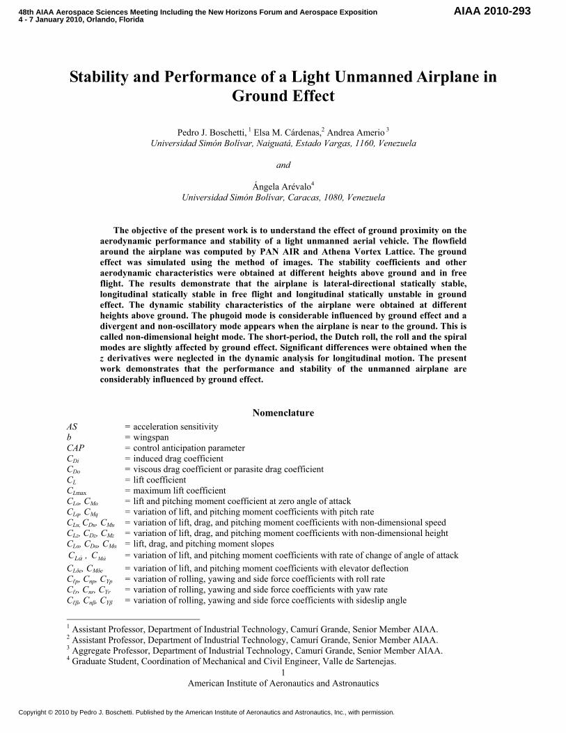
The aim of the present research is to understand the effect of ground proximity on the aerodynamic performance and stability of light unmanned aerial vehicles by means of the Unmanned Airplane for Ecological Conservation (ANCE, for its Spanish acronym). The dynamic stability, aircraft response and flying qualities are especially interesting in this paper. The ANCE is a monoplane twin-boom, pusher–propeller airplane with a rectangular wing of 3.13 m2 of surface area, 5.187 m of wingspan, and a wing aspect ratio of 8.57, with a maximum take-off mass of 182.055 kg, and with the center of gravity at 0.25c. The aircraft was originally designed to look for oil leakages from offshore facilities and transporting pipelines at 41.18 m/s at 2,438 m above sea level, for a wing Reynolds number of 1.413×106.10,11 Figure 1 shows a three-dimensional view of the ANCE.

In order to understand the aerodynamic performance of the ANCE, early wind tunnel test,12,13 and computational fluid dynamic simulation based on potential flow theory14 had been carried out to date. The stability and flying qualities had been studied using the vortex lattice method.15 Some modifications had been done over the original design in order to reduce drag.11-14

II. General Characteristics of Wings and Airplanes in Ground Proximity The ground effect on the airplanes is a complex phenomenon. The complete flowfield is modified by the ground

plane. Generally, when a wing approaches the ground, its lift curve slope increases and the induced drag decreases. The trailing vortices of a wing are reflected in the ground plane. This reduces the strength of the vortices16 and the image vortices induce an up-wash at the real wing so that the total induced incidence for a wing in ground proximity is smaller than in an unbounded stream.17 The induced drag coefficient for a wing of large aspect ratio flying in proximity to the ground is equal to G·k·CL

2. The drag reduction factor describes how the induced drag is affected by the ground effect. In free flight, G is equal to one. This concept was introduced by Wieselberger1 who presented an expression of drag reduction factor based on a previous Prandtl work.2 In this paper, more exact expressions of G were extracted from Suh and Ostowari3 and Laitone4, and these are shown in Eqs. (1) and (2), respectively.

( ) ( )( )[ ]22 241ln21 −+−= ezeG ππ (1)

( )[ ] ( )[ ]22 1611621 ee zzG ⋅+⋅+−= πππ (2)

A. Effects on Airplanes Stability While the lateral-directional stability is not expected to be significantly influenced by ground proximity, the

longitudinal stability is considerably affected by the ground effect. The downwash angle value at the tail in a conventional airplane in ground effect is less than the one in free flight. This augments the lift curve slope of the horizontal tail, and the tail effectiveness is increased, and the airplane becomes more stable.16

The condition of “static height stability” presented by Staufenbiel and Schlichting,5 is shown in Eq. (3). This represents the variations of static stability when the aircraft approaches the ground.

( ) 0<⋅−= αα LMMzLz CCCCHS (3)

The equations of motion which describe the longitudinal dynamic response of an airplane in ground effect are formulated in state space as x’= Ax + Bη, where x=[Δu, Δw, Δq, Δθ, Δze]T is the state vector, η=[Δδe] is the control vector, and the matrices A and B contain the stability and control derivatives. This system of equations was original presented by Etkin18 to describe the effect of variations of height above ground in the longitudinal mode. Atmospheric density variations and ground effect were considered by Etkin to express the “height above ground”.18

Figure 1. The Unmanned Airplane for Ecological Conservation.


4

In this work, Etkin’s original system of equations was adapted to consider only ground effect. Equations (4) and (5) present matrices A and B.

⎥⎥⎥⎥⎥⎥

⎦

⎤

⎢⎢⎢⎢⎢⎢

⎣

⎡

−

++++

−

=

00000100

00

0

0

oo

zwzwqwwwuwu

zowu

zwu

uu

ZMMuMMZMMZMMZuZZXgXX

A &&&& (4)

⎥⎥⎥⎥⎥⎥

⎦

⎤

⎢⎢⎢⎢⎢⎢

⎣

⎡

+=

00

ewe

e

e

ZMMZX

B δδ

δ

δ

& (5)

Matrix A has five eigenvalues: two complex pairs associated with two oscillatory modes, the short-period and the phugoid, and one is real representing a first order mode.19 This system of equations considers the variations of height above ground using the z derivatives. When these derivatives are zero, the system of equations becomes the classical equation of motion in free flight.

The lateral-directional equations of motion are formulated in state space x’= Cx + Dη, where x=[Δβ, Δp, Δr, Δφ]T is the state vector, and η=[Δδa, Δδr] T is the control vector.19 No consideration was taken about ground effect for the lateral-directional mode, as it is not expected that perturbations in this mode affect the non-dimensional height. The ground effect influences this mode by the potential change in the derivatives caused by the ground proximity. Equations (6) and (7) express matrices C and D, respectively.19

⎥⎥⎥⎥⎥⎥

⎦

⎤

⎢⎢⎢⎢⎢⎢

⎣

⎡⎟⎟⎠

⎞⎜⎜⎝

⎛−−

=

001000

cos1

rp

rp

ooo

r

o

p

o

NNNLLL

ug

uY

uY

uY

C

β

β

β θ

(6)

⎥⎥⎥⎥⎥⎥

⎦

⎤

⎢⎢⎢⎢⎢⎢

⎣

⎡

=

00

0

ra

ra

o

r

NNLLuY

Dδδ

δδ

δ

(7)

From matrix C, four eigenvalues are obtained: a pair of complex roots which represents the Dutch Roll mode, and two real roots for roll and spiral modes. Appendix A shows the mathematical expressions of dimensional derivatives contained in matrices A, B, C and D.

III. Aerodynamic Analysis Methods The Panel Aerodynamics (PAN AIR)20 and the Athena Vortex Lattice (AVL)21 open source codes were used to

compute the fluid flowfield around the airplane with and without ground effect. PAN AIR is a high-order panel method code capable of solving a variety of boundary value problems in steady

subsonic or supersonic inviscid flow by the classic three–dimensional Prandtl–Glauert equation for linearized compressible flow. The configuration is represented by a distribution of linear source and quadratic double singularities, each of which is a solution of the Prandtl–Glauert equation. The singularity strength parameters are determined by solving the appropriate boundary condition equations. Once these are known, the velocity and


5

potential fields are computed. The pressure field can then be calculated from an appropriate pressure–velocity relationship, and forces and moments calculated by pressure integration.22-24 In order to improve the accuracy of the induced drag calculation, the version A502i can calculate it by Trefftz plane analysis.20,25 The PAN AIR pilot code and later versions have been used and validated to compute aerodynamic forces and moments, and pressure distribution on arbitrary configurations in free flight,23,24 and validated against experimental data to calculate the influence of ground proximity on a single wing.26 A complete discussion of the method may be found in Ref 27.

The Athena Vortex Lattice is a code capable of solving the non-viscous flowfield around the aerodynamic configurations which consists mainly of thin lifting surfaces at small angles of attack and sideslip. The lifting surfaces are represented as single-layer vortex sheets, discretized into horseshoe vortex filaments.21 At a specific control point, the velocities induced by each horseshoe vortex are calculated by the law of Biot–Savart. A set of linear algebraic equations for the horseshoe-vortex strengths is obtained when all control points on the wing are summed, satisfying the boundary condition of no flow through the wing. The wing circulation and the pressure differential between the upper and lower surfaces are connected to the vortex strengths. The forces are obtained by integration of the pressure differentials.28,29 AVL could also model slender bodies via source and doublet filaments, and force and moment predictions are consistent with slender-body theory.25 Athena Vortex Lattice assumes quasi-steady flow and treats the compressibility using the Prandtl-Glauert transformation.21

To verify the capability of PAN AIR and Athena to simulate ground effect, a rectangular wing with similar aspect ratio and airfoil section of the ANCE wing with no twist was tested using both codes at eight different distances above ground (ze equal to 0.1, 0.16667, 0.25, 0.5, 1.0, 1.5, 2.0, and 2.5), and in free flight.

The ground effect is simulated by PAN AIR and AVL through the use of the method of images. The ground plane is represented by an image of the paneled geometry, placed and oriented as though it is reflected on the surface of the ground,6 so that, the ground plane does not have normal velocity, only tangential component.

The semi-span wing simulated by PANAIR is divided in 979 panels, and consists of five surface networks defined as indirect condition on impermeable thick surface and four wake surface networks. The wing simulated by AVL has a vortex lattice with 920 control points, twenty lattice chordwise divisions and forty-six spanwise divisions in a cosine distribution. The Mach number was equal to 0.15 for both simulations.

A. Simulation the Flowfield around the ANCE The potential flowfield around the airplane was simulated by PANAIR and AVL codes. Using both codes, the

airplane was modeled excluding the landing gear and the camera due to the fact that the contribution of these components to inviscid forces and moments is assumed negligible.

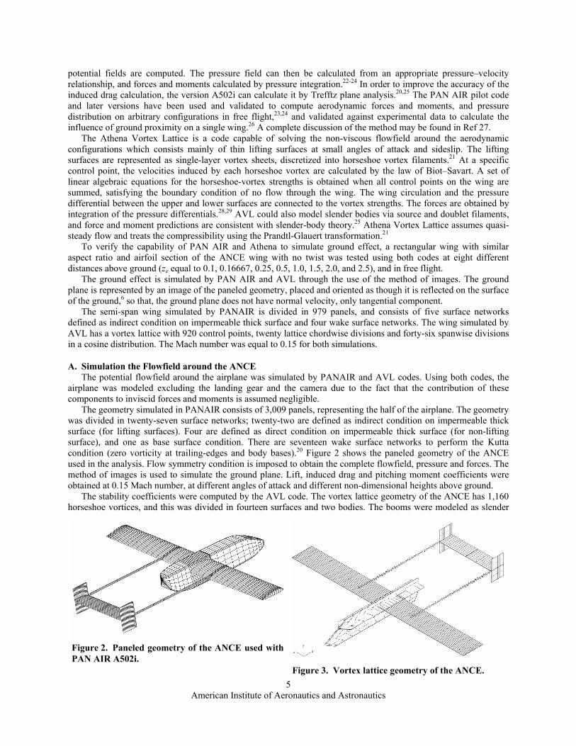
The geometry simulated in PANAIR consists of 3,009 panels, representing the half of the airplane. The geometry was divided in twenty-seven surface networks; twenty-two are defined as indirect condition on impermeable thick surface (for lifting surfaces). Four are defined as direct condition on impermeable thick surface (for non-lifting surface), and one as base surface condition. There are seventeen wake surface networks to perform the Kutta condition (zero vorticity at trailing-edges and body bases).20 Figure 2 shows the paneled geometry of the ANCE used in the analysis. Flow symmetry condition is imposed to obtain the complete flowfield, pressure and forces. The method of images is used to simulate the ground plane. Lift, induced drag and pitching moment coefficients were obtained at 0.15 Mach number, at different angles of attack and different non-dimensional heights above ground.

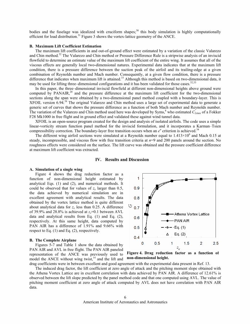
The stability coefficients were computed by the AVL code. The vortex lattice geometry of the ANCE has 1,160 horseshoe vortices, and this was divided in fourteen surfaces and two bodies. The booms were modeled as slender

Figure 3. Vortex lattice geometry of the ANCE.

Figure 2. Paneled geometry of the ANCE used with PAN AIR A502i.


6

bodies and the fuselage was idealized with cruciform shapes;30 this body simulation is highly computationally efficient for load distribution.31 Figure 3 shows the vortex-lattice geometry of the ANCE.

B. Maximum Lift Coefficient Estimation The maximum lift coefficients in and out-of-ground effect were estimated by a variation of the classic Valarezo

and Chin method.32 The Valarezo and Chin method or Pressure Difference Rule is a stripwise analysis of an inviscid flowfield to determine an estimate value of the maximum lift coefficient of the entire wing. It assumes that all of the viscous effects are generally local two-dimensional natures. Experimental data indicates that at the maximum lift condition, there is a pressure difference between the suction peak of the airfoil and its trailing-edge at a given combination of Reynolds number and Mach number. Consequently, at a given flow condition, there is a pressure difference that indicates when maximum lift is attained.33 Although this method is based on two-dimensional data, it may be used for lifting three–dimensional configurations and it has been validated for those cases.32,33

In this paper, the three–dimensional inviscid flowfield at different non-dimensional heights above ground were computed by PANAIR,20 and the pressure difference at the maximum lift coefficient for the two-dimensional sections along the span were obtained by a two-dimensional panel method coupled with a boundary-layer. This is XFOIL version 6.94.34 The original Valarezo and Chin method uses a large set of experimental data to generate a generic set of curves that shows the pressure difference as a function of both Mach number and Reynolds number. The variation of the Valarezo and Chin method used here was developed by Syms,8 who estimated CLmax of a Fokker F28 Mk1000 in free flight and in ground effect and validated these against wind tunnel data.

XFOIL is an open-source program created for the design and analysis of isolated airfoils. The code uses a simple linear-vorticity stream function panel method for the inviscid formulation, and it incorporates a Karman–Tsien compressibility correction. The boundary-layer free transition occurs when an en criterion is achieved.34

The different wing airfoil sections were simulated at a Reynolds number equal to 1.413×106 and Mach 0.15 at steady, incompressible, and viscous flow with free transition criteria at n=9 and 200 panels around the section. No roughness effects were considered on the surface. The lift curve was obtained and the pressure coefficient difference at maximum lift coefficient was extracted.

IV. Results and Discussion

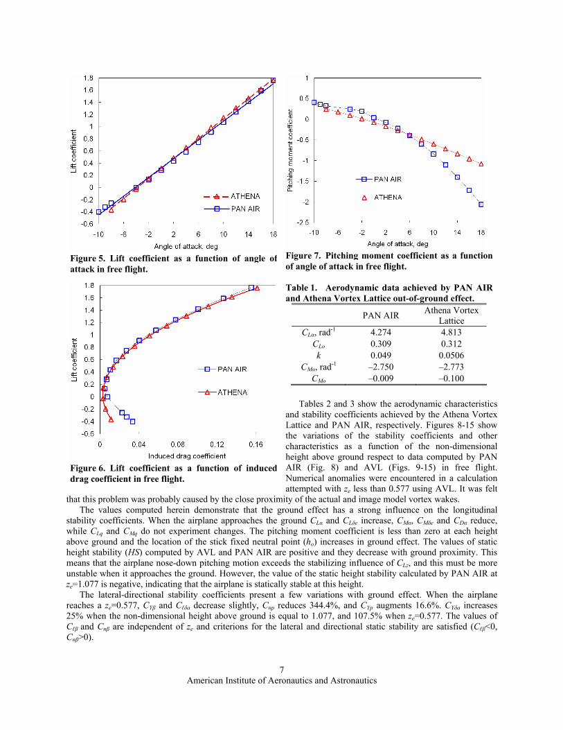
A. Simulation of a single wing Figure 4 shows the drag reduction factor as a

function of non-dimensional height estimated by analytical Eqs. (1) and (2), and numerical methods. It could be observed that for values of ze larger than 0.5, the data achieved by numerical simulation are in excellent agreement with analytical results. The data obtained by the vortex lattice method is quite different about analytical data for ze less than 0.25. A difference of 39.9% and 28.8% is achieved at ze=0.1 between AVL data and analytical results from Eq. (1) and Eq. (2), respectively. At this same height, data computed by PAN AIR has a difference of 1.91% and 9.66% with respect to Eq. (1) and Eq. (2), respectively.

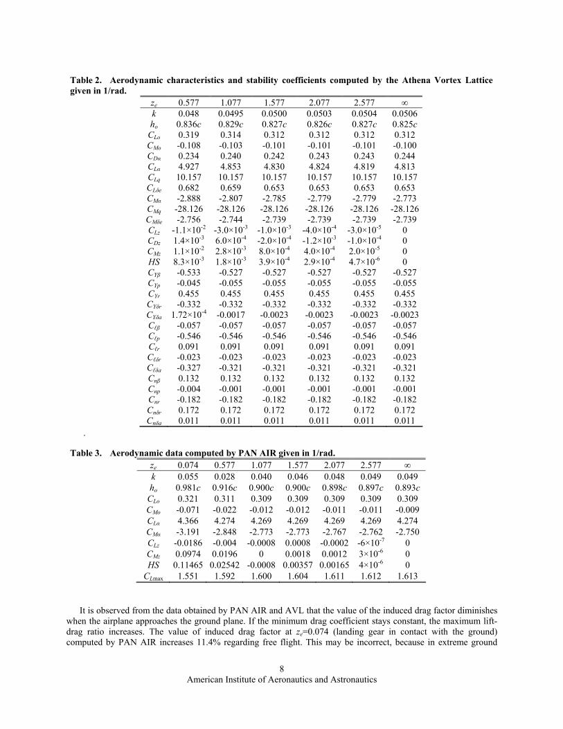
B. The Complete Airplane Figures 5-7 and Table 1 show the data obtained by

PAN AIR and AVL in free flight. The PAN AIR paneled representation of the ANCE was previously used to model the ANCE without wing twist,14 and the lift and drag coefficients were in between excellent and good agreement with the experimental data present in Ref. 13.

The induced drag factor, the lift coefficient at zero angle of attack and the pitching moment slope obtained with the Athena Vortex Lattice are in excellent correlation with data achieved by PAN AIR. A difference of 12.61% is observed between the lift slope predicted by the panel method code and that one computed using AVL. The value of pitching moment coefficient at zero angle of attack computed by AVL does not have correlation with PAN AIR data.

Figure 4. Drag reduction factor as a function of non-dimensional height.


7

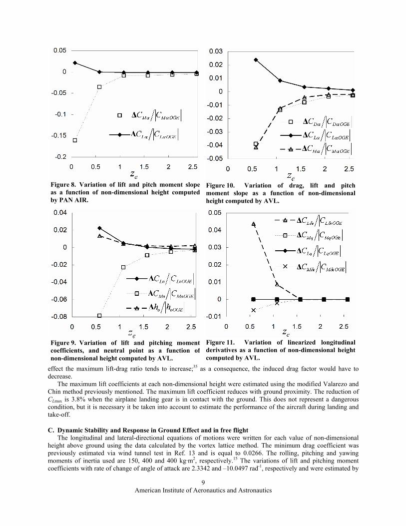
Tables 2 and 3 show the aerodynamic characteristics and stability coefficients achieved by the Athena Vortex Lattice and PAN AIR, respectively. Figures 8-15 show the variations of the stability coefficients and other characteristics as a function of the non-dimensional height above ground respect to data computed by PAN AIR (Fig. 8) and AVL (Figs. 9-15) in free flight. Numerical anomalies were encountered in a calculation attempted with ze less than 0.577 using AVL. It was felt

that this problem was probably caused by the close proximity of the actual and image model vortex wakes. The values computed herein demonstrate that the ground effect has a strong influence on the longitudinal

stability coefficients. When the airplane approaches the ground CLα and CLδe increase, CMα, CMδe and CDα reduce, while CLq and CMq do not experiment changes. The pitching moment coefficient is less than zero at each height above ground and the location of the stick fixed neutral point (ho) increases in ground effect. The values of static height stability (HS) computed by AVL and PAN AIR are positive and they decrease with ground proximity. This means that the airplane nose-down pitching motion exceeds the stabilizing influence of CLz, and this must be more unstable when it approaches the ground. However, the value of the static height stability calculated by PAN AIR at ze=1.077 is negative, indicating that the airplane is statically stable at this height.

The lateral-directional stability coefficients present a few variations with ground effect. When the airplane reaches a ze=0.577, CYβ and Cℓδa decrease slightly, Cnp reduces 344.4%, and CYp augments 16.6%. CYδa increases 25% when the non-dimensional height above ground is equal to 1.077, and 107.5% when ze=0.577. The values of Cℓβ and Cnβ are independent of ze and criterions for the lateral and directional static stability are satisfied (Cℓβ<0, Cnβ>0).

Figure 5. Lift coefficient as a function of angle ofattack in free flight.

Figure 7. Pitching moment coefficient as a function of angle of attack in free flight.

Figure 6. Lift coefficient as a function of induceddrag coefficient in free flight.

Table 1. Aerodynamic data achieved by PAN AIR and Athena Vortex Lattice out-of-ground effect.

PAN AIR Athena Vortex Lattice

CLα, rad-1 4.274 4.813 CLo 0.309 0.312 k 0.049 0.0506

CMα, rad-1 –2.750 –2.773 CMo –0.009 –0.100


8

It is observed from the data obtained by PAN AIR and AVL that the value of the induced drag factor diminishes when the airplane approaches the ground plane. If the minimum drag coefficient stays constant, the maximum lift-drag ratio increases. The value of induced drag factor at ze=0.074 (landing gear in contact with the ground) computed by PAN AIR increases 11.4% regarding free flight. This may be incorrect, because in extreme ground

Table 2. Aerodynamic characteristics and stability coefficients computed by the Athena Vortex Lattice given in 1/rad.

ze 0.577 1.077 1.577 2.077 2.577 ∞ k 0.048 0.0495 0.0500 0.0503 0.0504 0.0506 ho 0.836c 0.829c 0.827c 0.826c 0.827c 0.825c

CLo 0.319 0.314 0.312 0.312 0.312 0.312 CMo -0.108 -0.103 -0.101 -0.101 -0.101 -0.100 CDα 0.234 0.240 0.242 0.243 0.243 0.244 CLα 4.927 4.853 4.830 4.824 4.819 4.813 CLq 10.157 10.157 10.157 10.157 10.157 10.157 CLδe 0.682 0.659 0.653 0.653 0.653 0.653 CMα -2.888 -2.807 -2.785 -2.779 -2.779 -2.773 CMq -28.126 -28.126 -28.126 -28.126 -28.126 -28.126 CMδe -2.756 -2.744 -2.739 -2.739 -2.739 -2.739 CLz -1.1×10-2 -3.0×10-3 -1.0×10-3 -4.0×10-4 -3.0×10-5 0 CDz 1.4×10-3 6.0×10-4 -2.0×10-4 -1.2×10-3 -1.0×10-4 0 CMz 1.1×10-2 2.8×10-3 8.0×10-4 4.0×10-4 2.0×10-5 0 HS 8.3×10-3 1.8×10-3 3.9×10-4 2.9×10-4 4.7×10-6 0 CYβ -0.533 -0.527 -0.527 -0.527 -0.527 -0.527 CYp -0.045 -0.055 -0.055 -0.055 -0.055 -0.055 CYr 0.455 0.455 0.455 0.455 0.455 0.455 CYδr -0.332 -0.332 -0.332 -0.332 -0.332 -0.332 CYδa 1.72×10-4 -0.0017 -0.0023 -0.0023 -0.0023 -0.0023 Cℓβ -0.057 -0.057 -0.057 -0.057 -0.057 -0.057 Cℓp -0.546 -0.546 -0.546 -0.546 -0.546 -0.546 Cℓr 0.091 0.091 0.091 0.091 0.091 0.091 Cℓδr -0.023 -0.023 -0.023 -0.023 -0.023 -0.023 Cℓδa -0.327 -0.321 -0.321 -0.321 -0.321 -0.321 Cnβ 0.132 0.132 0.132 0.132 0.132 0.132 Cnp -0.004 -0.001 -0.001 -0.001 -0.001 -0.001 Cnr -0.182 -0.182 -0.182 -0.182 -0.182 -0.182 Cnδr 0.172 0.172 0.172 0.172 0.172 0.172 Cnδa 0.011 0.011 0.011 0.011 0.011 0.011

.

Table 3. Aerodynamic data computed by PAN AIR given in 1/rad. ze 0.074 0.577 1.077 1.577 2.077 2.577 ∞ k 0.055 0.028 0.040 0.046 0.048 0.049 0.049 ho 0.981c 0.916c 0.900c 0.900c 0.898c 0.897c 0.893c

CLo 0.321 0.311 0.309 0.309 0.309 0.309 0.309 CMo -0.071 -0.022 -0.012 -0.012 -0.011 -0.011 -0.009 CLα 4.366 4.274 4.269 4.269 4.269 4.269 4.274 CMα -3.191 -2.848 -2.773 -2.773 -2.767 -2.762 -2.750 CLz -0.0186 -0.004 -0.0008 0.0008 -0.0002 -6×10-7 0 CMz 0.0974 0.0196 0 0.0018 0.0012 3×10-6 0 HS 0.11465 0.02542 -0.0008 0.00357 0.00165 4×10-6 0

CLmax 1.551 1.592 1.600 1.604 1.611 1.612 1.613


9

effect the maximum lift-drag ratio tends to increase;35 as a consequence, the induced drag factor would have to decrease.

The maximum lift coefficients at each non-dimensional height were estimated using the modified Valarezo and Chin method previously mentioned. The maximum lift coefficient reduces with ground proximity. The reduction of CLmax is 3.8% when the airplane landing gear is in contact with the ground. This does not represent a dangerous condition, but it is necessary it be taken into account to estimate the performance of the aircraft during landing and take-off.

C. Dynamic Stability and Response in Ground Effect and in free flight The longitudinal and lateral-directional equations of motions were written for each value of non-dimensional

height above ground using the data calculated by the vortex lattice method. The minimum drag coefficient was previously estimated via wind tunnel test in Ref. 13 and is equal to 0.0266. The rolling, pitching and yawing moments of inertia used are 150, 400 and 400 kg·m2, respectively.15 The variations of lift and pitching moment coefficients with rate of change of angle of attack are 2.3342 and –10.0497 rad-1, respectively and were estimated by

Figure 8. Variation of lift and pitch moment slopeas a function of non-dimensional height computedby PAN AIR.

Figure 10. Variation of drag, lift and pitch moment slope as a function of non-dimensional height computed by AVL.

Figure 9. Variation of lift and pitching momentcoefficients, and neutral point as a function ofnon-dimensional height computed by AVL.

Figure 11. Variation of linearized longitudinal derivatives as a function of non-dimensional height computed by AVL.


10

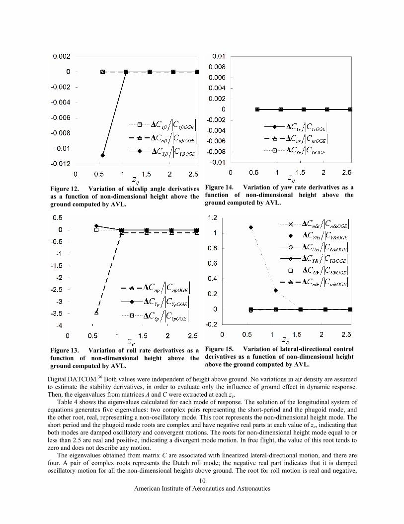
Digital DATCOM.36 Both values were independent of height above ground. No variations in air density are assumed to estimate the stability derivatives, in order to evaluate only the influence of ground effect in dynamic response. Then, the eigenvalues from matrices A and C were extracted at each ze.

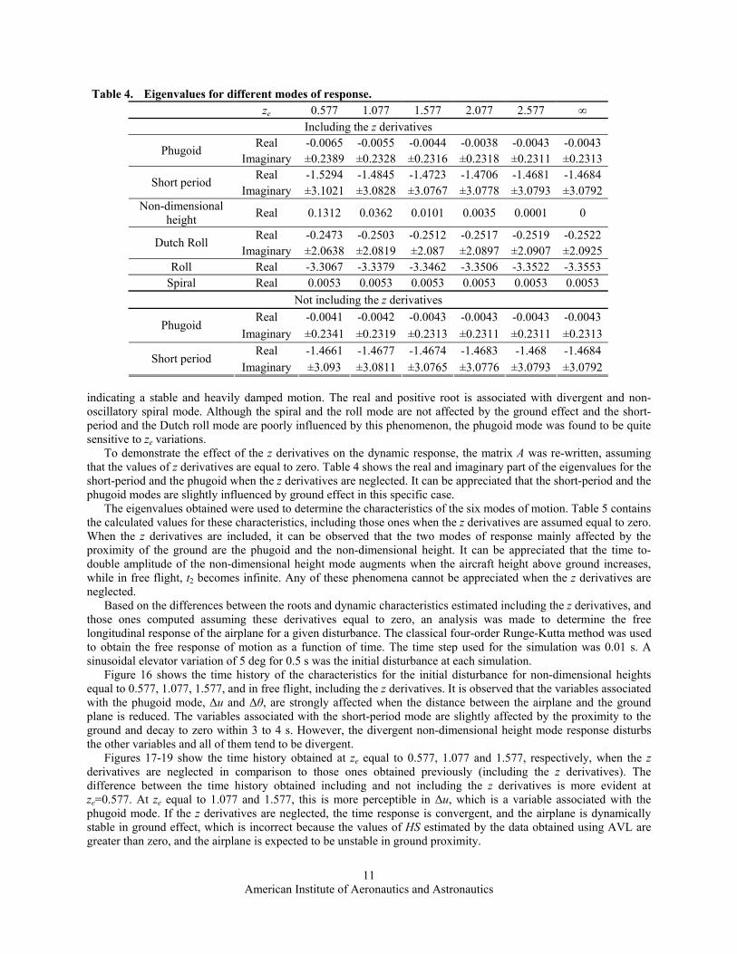
Table 4 shows the eigenvalues calculated for each mode of response. The solution of the longitudinal system of equations generates five eigenvalues: two complex pairs representing the short-period and the phugoid mode, and the other root, real, representing a non-oscillatory mode. This root represents the non-dimensional height mode. The short period and the phugoid mode roots are complex and have negative real parts at each value of ze, indicating that both modes are damped oscillatory and convergent motions. The roots for non-dimensional height mode equal to or less than 2.5 are real and positive, indicating a divergent mode motion. In free flight, the value of this root tends to zero and does not describe any motion.

The eigenvalues obtained from matrix C are associated with linearized lateral-directional motion, and there are four. A pair of complex roots represents the Dutch roll mode; the negative real part indicates that it is damped oscillatory motion for all the non-dimensional heights above ground. The root for roll motion is real and negative,

Figure 12. Variation of sideslip angle derivativesas a function of non-dimensional height above theground computed by AVL.

Figure 14. Variation of yaw rate derivatives as a function of non-dimensional height above the ground computed by AVL.

Figure 13. Variation of roll rate derivatives as afunction of non-dimensional height above theground computed by AVL.

Figure 15. Variation of lateral-directional control derivatives as a function of non-dimensional height above the ground computed by AVL.


11

indicating a stable and heavily damped motion. The real and positive root is associated with divergent and non-oscillatory spiral mode. Although the spiral and the roll mode are not affected by the ground effect and the short-period and the Dutch roll mode are poorly influenced by this phenomenon, the phugoid mode was found to be quite sensitive to ze variations.

To demonstrate the effect of the z derivatives on the dynamic response, the matrix A was re-written, assuming that the values of z derivatives are equal to zero. Table 4 shows the real and imaginary part of the eigenvalues for the short-period and the phugoid when the z derivatives are neglected. It can be appreciated that the short-period and the phugoid modes are slightly influenced by ground effect in this specific case.

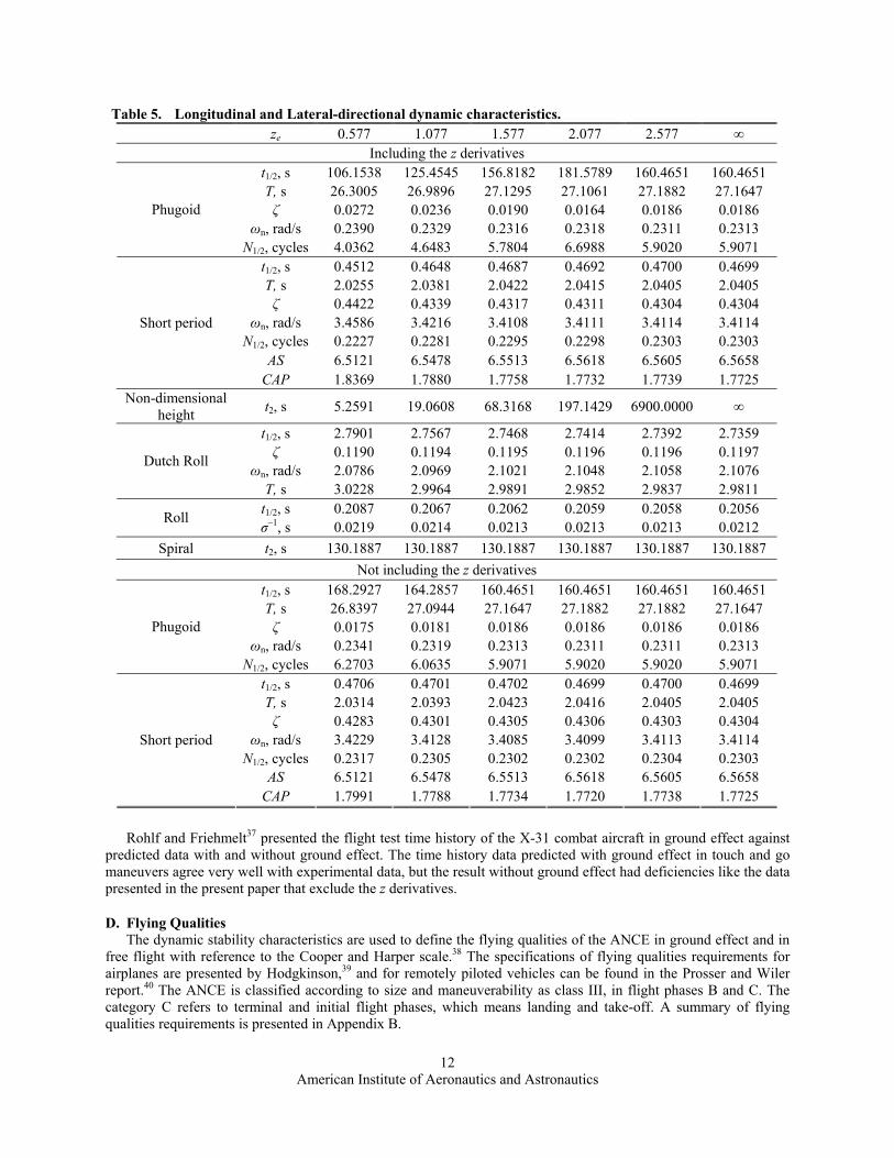
The eigenvalues obtained were used to determine the characteristics of the six modes of motion. Table 5 contains the calculated values for these characteristics, including those ones when the z derivatives are assumed equal to zero. When the z derivatives are included, it can be observed that the two modes of response mainly affected by the proximity of the ground are the phugoid and the non-dimensional height. It can be appreciated that the time to-double amplitude of the non-dimensional height mode augments when the aircraft height above ground increases, while in free flight, t2 becomes infinite. Any of these phenomena cannot be appreciated when the z derivatives are neglected.

Based on the differences between the roots and dynamic characteristics estimated including the z derivatives, and those ones computed assuming these derivatives equal to zero, an analysis was made to determine the free longitudinal response of the airplane for a given disturbance. The classical four-order Runge-Kutta method was used to obtain the free response of motion as a function of time. The time step used for the simulation was 0.01 s. A sinusoidal elevator variation of 5 deg for 0.5 s was the initial disturbance at each simulation.

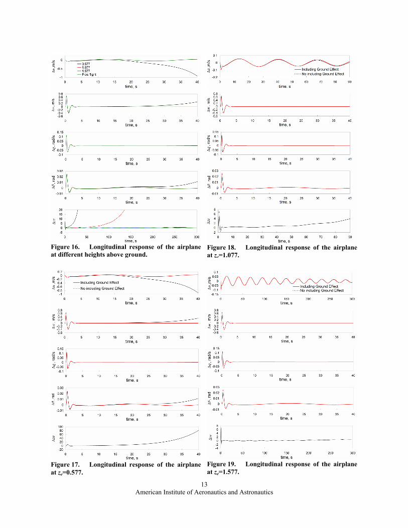
Figure 16 shows the time history of the characteristics for the initial disturbance for non-dimensional heights equal to 0.577, 1.077, 1.577, and in free flight, including the z derivatives. It is observed that the variables associated with the phugoid mode, Δu and Δθ, are strongly affected when the distance between the airplane and the ground plane is reduced. The variables associated with the short-period mode are slightly affected by the proximity to the ground and decay to zero within 3 to 4 s. However, the divergent non-dimensional height mode response disturbs the other variables and all of them tend to be divergent.

Figures 17-19 show the time history obtained at ze equal to 0.577, 1.077 and 1.577, respectively, when the z derivatives are neglected in comparison to those ones obtained previously (including the z derivatives). The difference between the time history obtained including and not including the z derivatives is more evident at ze=0.577. At ze equal to 1.077 and 1.577, this is more perceptible in Δu, which is a variable associated with the phugoid mode. If the z derivatives are neglected, the time response is convergent, and the airplane is dynamically stable in ground effect, which is incorrect because the values of HS estimated by the data obtained using AVL are greater than zero, and the airplane is expected to be unstable in ground proximity.

Table 4. Eigenvalues for different modes of response. ze 0.577 1.077 1.577 2.077 2.577 ∞

Including the z derivatives Real -0.0065 -0.0055 -0.0044 -0.0038 -0.0043 -0.0043 Phugoid

Imaginary ±0.2389 ±0.2328 ±0.2316 ±0.2318 ±0.2311 ±0.2313Real -1.5294 -1.4845 -1.4723 -1.4706 -1.4681 -1.4684 Short period

Imaginary ±3.1021 ±3.0828 ±3.0767 ±3.0778 ±3.0793 ±3.0792Non-dimensional

height Real 0.1312 0.0362 0.0101 0.0035 0.0001 0

Real -0.2473 -0.2503 -0.2512 -0.2517 -0.2519 -0.2522 Dutch Roll Imaginary ±2.0638 ±2.0819 ±2.087 ±2.0897 ±2.0907 ±2.0925

Roll Real -3.3067 -3.3379 -3.3462 -3.3506 -3.3522 -3.3553 Spiral Real 0.0053 0.0053 0.0053 0.0053 0.0053 0.0053

Not including the z derivatives Real -0.0041 -0.0042 -0.0043 -0.0043 -0.0043 -0.0043

Phugoid Imaginary ±0.2341 ±0.2319 ±0.2313 ±0.2311 ±0.2311 ±0.2313

Real -1.4661 -1.4677 -1.4674 -1.4683 -1.468 -1.4684 Short period

Imaginary ±3.093 ±3.0811 ±3.0765 ±3.0776 ±3.0793 ±3.0792


12

Rohlf and Friehmelt37 presented the flight test time history of the X-31 combat aircraft in ground effect against predicted data with and without ground effect. The time history data predicted with ground effect in touch and go maneuvers agree very well with experimental data, but the result without ground effect had deficiencies like the data presented in the present paper that exclude the z derivatives.

D. Flying Qualities The dynamic stability characteristics are used to define the flying qualities of the ANCE in ground effect and in

free flight with reference to the Cooper and Harper scale.38 The specifications of flying qualities requirements for airplanes are presented by Hodgkinson,39 and for remotely piloted vehicles can be found in the Prosser and Wiler report.40 The ANCE is classified according to size and maneuverability as class III, in flight phases B and C. The category C refers to terminal and initial flight phases, which means landing and take-off. A summary of flying qualities requirements is presented in Appendix B.

Table 5. Longitudinal and Lateral-directional dynamic characteristics. ze 0.577 1.077 1.577 2.077 2.577 ∞

Including the z derivatives t1/2, s 106.1538 125.4545 156.8182 181.5789 160.4651 160.4651 T, s 26.3005 26.9896 27.1295 27.1061 27.1882 27.1647 ζ 0.0272 0.0236 0.0190 0.0164 0.0186 0.0186

ωn, rad/s 0.2390 0.2329 0.2316 0.2318 0.2311 0.2313 Phugoid

N1/2, cycles 4.0362 4.6483 5.7804 6.6988 5.9020 5.9071 t1/2, s 0.4512 0.4648 0.4687 0.4692 0.4700 0.4699 T, s 2.0255 2.0381 2.0422 2.0415 2.0405 2.0405 ζ 0.4422 0.4339 0.4317 0.4311 0.4304 0.4304

ωn, rad/s 3.4586 3.4216 3.4108 3.4111 3.4114 3.4114 N1/2, cycles 0.2227 0.2281 0.2295 0.2298 0.2303 0.2303

AS 6.5121 6.5478 6.5513 6.5618 6.5605 6.5658

Short period

CAP 1.8369 1.7880 1.7758 1.7732 1.7739 1.7725 Non-dimensional

height t2, s 5.2591 19.0608 68.3168 197.1429 6900.0000 ∞

t1/2, s 2.7901 2.7567 2.7468 2.7414 2.7392 2.7359 ζ 0.1190 0.1194 0.1195 0.1196 0.1196 0.1197

ωn, rad/s 2.0786 2.0969 2.1021 2.1048 2.1058 2.1076 Dutch Roll

T, s 3.0228 2.9964 2.9891 2.9852 2.9837 2.9811 t1/2, s 0.2087 0.2067 0.2062 0.2059 0.2058 0.2056 Roll σ–1, s 0.0219 0.0214 0.0213 0.0213 0.0213 0.0212

Spiral t2, s 130.1887 130.1887 130.1887 130.1887 130.1887 130.1887 Not including the z derivatives

t1/2, s 168.2927 164.2857 160.4651 160.4651 160.4651 160.4651 T, s 26.8397 27.0944 27.1647 27.1882 27.1882 27.1647 ζ 0.0175 0.0181 0.0186 0.0186 0.0186 0.0186

ωn, rad/s 0.2341 0.2319 0.2313 0.2311 0.2311 0.2313 Phugoid

N1/2, cycles 6.2703 6.0635 5.9071 5.9020 5.9020 5.9071 t1/2, s 0.4706 0.4701 0.4702 0.4699 0.4700 0.4699 T, s 2.0314 2.0393 2.0423 2.0416 2.0405 2.0405 ζ 0.4283 0.4301 0.4305 0.4306 0.4303 0.4304

ωn, rad/s 3.4229 3.4128 3.4085 3.4099 3.4113 3.4114 N1/2, cycles 0.2317 0.2305 0.2302 0.2302 0.2304 0.2303

AS 6.5121 6.5478 6.5513 6.5618 6.5605 6.5658

Short period

CAP 1.7991 1.7788 1.7734 1.7720 1.7738 1.7725


13

Figure 18. Longitudinal response of the airplane at ze=1.077.

Figure 16. Longitudinal response of the airplaneat different heights above ground.

Figure 17. Longitudinal response of the airplaneat ze=0.577.

Figure 19. Longitudinal response of the airplane at ze=1.577.


14

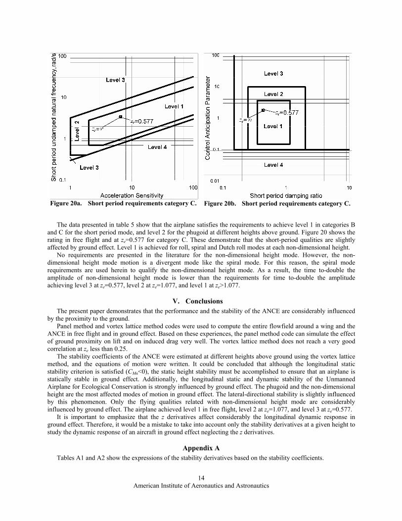
The data presented in table 5 show that the airplane satisfies the requirements to achieve level 1 in categories B

and C for the short period mode, and level 2 for the phugoid at different heights above ground. Figure 20 shows the rating in free flight and at ze=0.577 for category C. These demonstrate that the short-period qualities are slightly affected by ground effect. Level 1 is achieved for roll, spiral and Dutch roll modes at each non-dimensional height.

No requirements are presented in the literature for the non-dimensional height mode. However, the non-dimensional height mode motion is a divergent mode like the spiral mode. For this reason, the spiral mode requirements are used herein to qualify the non-dimensional height mode. As a result, the time to-double the amplitude of non-dimensional height mode is lower than the requirements for time to-double the amplitude achieving level 3 at ze=0.577, level 2 at ze=1.077, and level 1 at ze>1.077.

V. Conclusions The present paper demonstrates that the performance and the stability of the ANCE are considerably influenced

by the proximity to the ground. Panel method and vortex lattice method codes were used to compute the entire flowfield around a wing and the

ANCE in free flight and in ground effect. Based on these experiences, the panel method code can simulate the effect of ground proximity on lift and on induced drag very well. The vortex lattice method does not reach a very good correlation at ze less than 0.25.

The stability coefficients of the ANCE were estimated at different heights above ground using the vortex lattice method, and the equations of motion were written. It could be concluded that although the longitudinal static stability criterion is satisfied (CMα<0), the static height stability must be accomplished to ensure that an airplane is statically stable in ground effect. Additionally, the longitudinal static and dynamic stability of the Unmanned Airplane for Ecological Conservation is strongly influenced by ground effect. The phugoid and the non-dimensional height are the most affected modes of motion in ground effect. The lateral-directional stability is slightly influenced by this phenomenon. Only the flying qualities related with non-dimensional height mode are considerably influenced by ground effect. The airplane achieved level 1 in free flight, level 2 at ze=1.077, and level 3 at ze=0.577.

It is important to emphasize that the z derivatives affect considerably the longitudinal dynamic response in ground effect. Therefore, it would be a mistake to take into account only the stability derivatives at a given height to study the dynamic response of an aircraft in ground effect neglecting the z derivatives.

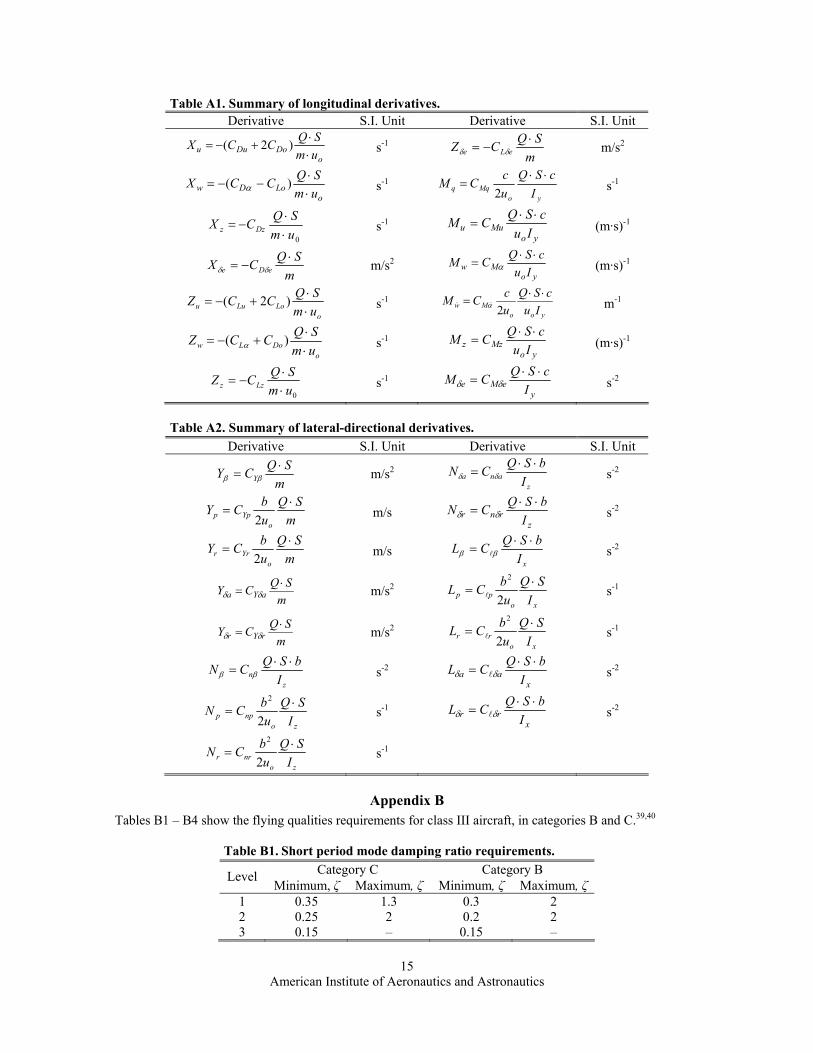
Appendix A Tables A1 and A2 show the expressions of the stability derivatives based on the stability coefficients.

Figure 20a. Short period requirements category C. Figure 20b. Short period requirements category C.


15

Table A1. Summary of longitudinal derivatives. Derivative S.I. Unit Derivative S.I. Unit

oDoDuu um

SQCCX⋅⋅

+−= )2( s-1 m

SQCZ eLe⋅

−= δδ m/s2

oLoDw um

SQCCX⋅⋅

−−= )( α s-1 yo

Mqq IcSQ

uc

CM⋅⋅

=2

s-1

0umSQCX Dzz ⋅⋅

−= s-1 yo

Muu IucSQCM ⋅⋅

= (m·s)-1

mSQCX eDe⋅

−= δδ m/s2 yo

Mw IucSQCM ⋅⋅

= α (m·s)-1

oLoLuu um

SQCCZ⋅⋅

+−= )2( s-1 yoo

Mw IucSQ

ucCM ⋅⋅

=2α&& m-1

oDoLw um

SQCCZ⋅⋅

+−= )( α s-1 yo

Mzz IucSQCM ⋅⋅

= (m·s)-1

0umSQCZ Lzz ⋅⋅

−= s-1 y

eMe IcSQCM ⋅⋅

= δδ s-2

Table A2. Summary of lateral-directional derivatives.

Derivative S.I. Unit Derivative S.I. Unit

mSQCY Y⋅

= ββ m/s2 z

ana IbSQCN ⋅⋅

= δδ s-2

mSQ

ubCY

oYpp

⋅=

2 m/s

zrnr I

bSQCN ⋅⋅= δδ s-2

mSQ

ubCY

oYrr

⋅=

2 m/s

xIbSQCL ⋅⋅

= ββ l s-2

mSQCY aYa⋅

= δδ m/s2 xo

pp ISQ

ubCL ⋅

=2

2

l s-1

mSQCY rYr⋅

= δδ m/s2 xo

rr ISQ

ubCL ⋅

=2

2

l s-1

zn I

bSQCN ⋅⋅= ββ s-2

xaa I

bSQCL ⋅⋅= δδ l s-2

zonpp I

SQu

bCN ⋅=

2

2

s-1 x

rr IbSQCL ⋅⋅

= δδ l s-2

zonrr I

SQu

bCN ⋅=

2

2

s-1

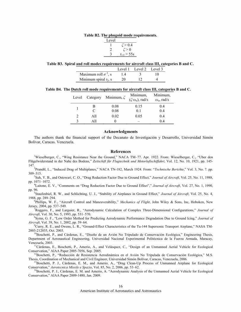
Appendix B Tables B1 – B4 show the flying qualities requirements for class III aircraft, in categories B and C.39,40

Table B1. Short period mode damping ratio requirements.

Category C Category B Level Minimum, ζ Maximum, ζ Minimum, ζ Maximum, ζ

1 0.35 1.3 0.3 2 2 0.25 2 0.2 2 3 0.15 – 0.15 –


16

Table B2. The phugoid mode requirements.

Level 1 ζ > 0.4 2 ζ > 0 3 t1/2 > 55s

Table B3. Spiral and roll modes requirements for aircraft class III, categories B and C.

Level 1 Level 2 Level 3 Maximum roll σ–1, s 1.4 3 10 Minimum spiral t2, s 20 12 4

Table B4. The Dutch roll mode requirements for aircraft class III, categories B and C.

Level Category Minimum, ζ Minimum,(ζ·ωn), rad/s

Minimum, ωn, rad/s

1 B C

0.08 0.08

0.15 0.1

0.4 0.4

2 All 0.02 0.05 0.4 3 All 0 – 0.4

Acknowledgments The authors thank the financial support of the Decanato de Investigación y Desarrollo, Universidad Simón

Bolívar, Caracas. Venezuela.

References 1Wieselberger, C., “Wing Resistance Near the Ground,” NACA TM–77. Apr. 1922. From: Wieselberger, C., “Uber den

Flügelwiderstand in der Nahe des Bodens,” Zeitschift für Flugtechnik und Motorluftschiffahrt, Vol. 12, No. 10, 1921, pp. 145-147.

2Prandtl, L., “Induced Drag of Multiplanes,” NACA TN-182, March 1924. From: “Technische Berichte,” Vol. 3, No. 7. pp. 309–315.

3Suh, Y. B., and Ostowari, C. O., “Drag Reduction Factor Due to Ground Effect,” Journal of Aircraft, Vol. 25, No. 11, 1988, pp. 1071–1072.

4Laitone, E. V., “Comments on “Drag Reduction Factor Due to Ground Effect”,” Journal of Aircraft, Vol. 27, No. 1, 1990, pp. 96.

5Staufenbiel, R. W., and Schlichting, U. J., “Stability of Airplanes in Ground Effect,” Journal of Aircraft, Vol. 25, No. 4, 1988, pp. 289–294.

6Phillips, W. F., “Aircraft Control and Maneuverability,” Mechanics of Flight, John Wiley & Sons, Inc, Hoboken, New Jersey, 2004, pp. 537–549.

7Roggero, F., and Larguier, R., “Aerodynamic Calculation of Complex Three-Dimensional Configurations,” Journal of Aircraft, Vol. 30, No. 5, 1993, pp. 531–570.

8Syms, G. F., “Low Order Method for Predicting Aerodynamic Performance Degradation Due to Ground Icing,” Journal of Aircraft, Vol. 39, No. 1, 2002, pp. 59–64.

9Curry, R. E., and Owens, L. R., “Ground-Effect Characteristics of the Tu-144 Supersonic Transport Airplane,” NASA TM-2003-212035, Oct. 2003.

10Boschetti, P., and Cárdenas, E., “Diseño de un Avión No Tripulado de Conservación Ecológica,” Engineering Thesis, Department of Aeronautical Engineering, Universidad Nacional Experimental Politécnica de la Fuerza Armada, Maracay, Venezuela, 2003.

11Cárdenas, E., Boschetti, P., Amerio, A., and Velásquez, C., “Design of an Unmanned Aerial Vehicle for Ecological Conservation,” AIAA Paper 2005-7056, Sep. 2005.

12Boschetti, P., “Reducción de Resistencia Aerodinámica en el Avión No Tripulada de Conservación Ecológica,” M.S. Thesis, Coordination of Mechanical and Civil Engineer, Universidad Simón Bolívar, Caracas, Venezuela, 2006.

13Boschetti, P. J., Cárdenas, E. M., and Amerio, A., “Drag Clean-Up Process of Unmanned Airplane for Ecological Conservation,” Aerotecnica Missile e Spazio, Vol. 85, No. 2, 2006, pp. 53–62.

14Boschetti, P. J., Cárdenas, E. M. and Amerio, A. “Aerodynamic Analysis of the Unmanned Aerial Vehicle for Ecological Conservation,” AIAA Paper 2009-1480, Jan. 2009.


17

15Cárdenas, E., Boschetti, P., and Amerio, A., “Stability and Flying Qualities of an Unmanned Airplane using Vortex Lattice Method,” Journal of Aircraft, Vol. 46, No. 4, 2009, pp. 1461-1465.

16Pamudi, B. N., “Static Stability and Control,” Performance, Stability, Dynamics and Control of Airplanes, 2nd ed., AIAA Educational Series, AIAA, Reston, Virginia, 2004, pp. 216-218.

17Thwaites, B. (ed.) “Some Miscellaneous Topics,” Incompressible Aerodynamics, Dover Publications, New York City, NY, 1960, pp. 529.

18Etkin, B., Dynamics of Atmospherics Flight, John Wiley & Sons, Inc., New York City, NY, 1972, pp. 162–163, 186–187, 285.

19Nelson, R. C., Flight Stability and Automatic Control, 2nd ed., McGraw Hill, Boston, MA, 1998, pp. 193–195, 231–232. 20Saaris, G. R., “A501i User’s Manual – PAN AIR Technology Program for Solving Problems of Potential Flow about

Arbitrary Configurations,” The Boeing Company, Report D6–54703, Seattle, Washington, Feb. 1992. 21Drela, M., and Youngren. H., “AVL 3.26 User Primer,” Massachusetts Institute of Technology, Cambridge, MA, 2006. 22Derbyshire T. y Sidwell K. W., “PAN AIR Summary Document (Version 1.0),” NASA CR-3250, Apr. 1982. 23Tinoco, E. N., Johnson, F. T., and Freeman, L. M., “Application of a Higher Order Panel Method to Realistic Supersonic

Configurations,” Journal of Aircraft, Vol. 17, No. 1, 1980, pp. 38–44. 24Cenko, A., Tinoco, E. N., Dyer, R.D., and DeJongh, J., “PAN AIR Application to Weapons and Separation,” Journal of

Aircraft, Vol. 18, No. 2, 1981, pp. 128–134. 25Katz, J., and Plotkin, A., “Three-Dimensional Small-Disturbance Solutions,” Low-Speed Aerodynamics, 2nd ed., Cambridge

University Press, New York City, NY, 2001, pp. 195–204. 26Goetz, A. R., Osborn, R. F., and Smith, M. L., “Wing-in-Ground Effect Aerodynamic Predictions Using PANAIR,” AIAA

Paper 84-2429, Nov. 1984. 27Epton, M. A. and Magnus, A. E. “PAN AIR- A Computer Program for Predicting Subsonic or Supersonic Linear Potential

Flows About Arbitrary Configurations Using a Higher Order Panel Method Volume I - Theory document (Version 3.0),” NASA CR-3251, 1990.

28Bertin, J. J., and Smith, M. L., “Incompressible Flow About Wings of Finite Span,” Aerodynamics for Engineers, 3rd ed., Prentice–Hall, Upper Saddle River, New Jersey, 1998, pp. 287–288.

29Moran, J., “Wings of finite span,” An Introduction to Theoretical and Computational Aerodynamics, Dover, New York City, NY, 2003, pp. 130–135.

30Kier, T. M., “Comparison of Unsteady Aerodynamic Modelling Methodologies with respect to Flight Loads Analysis,” AIAA Paper 2005-6027, Aug. 2005.

31Miranda, L. R., Elliott, R. D., and Baker, W. M., “A Generalized Vortex Lattice Method for Subsonic and Supersonic Flow Applications,” NASA CR-2865, Dec. 1977.

32Valarezo, W. O., and Chin, V. D., “Method for Prediction of Wing Maximum Lift,” Journal of Aircraft, Vol. 31, No. 1, 1994, pp. 103–109.

33Cebeci, T., Shao, J. P., Kafyeke, F., and Laurendeau, E., Computational Fluid Dynamics for Engineers, Horizons Publishing and Springer, Long Beach, CA, 2005, pp. 10–19.

34Drela, M., and Youngren, H., “XFOIL 6.9 User Primer,” Massachusetts Institute of Technology, Cambridge, MA, 2001. 35Chun, H. H. and Chang, C. H., “Longitudinal Stability and Dynamic Motion of a Small Passenger WIG craft,” Ocean

Engineering, Vol. 29, No. 10, 2002, pp. 1145–1162. 36Williams, J. E., and Vukelich, S. R., “The USAF Stability and Control Digital Datcom, Vol. 1, Users Manual,” McDonnell

Douglas Astronautics Company, Rept. AFFDL-TR-79-3032, Saint Louis, Missouri, 1979. 37Rohlf, D., and Friehmelt, H., “High Fidelity Ground Effect Model Based on DGPS Data,” Aerospace Science and

Technology, Vol. 9, No. 6, 2005, pp. 543–552. 38Cooper, G. E., and Harper, R. P., “The Use of Pilot Rating in the Evaluation of Aircraft Handling Qualities,” NASA TN D-

5153, 1969. 39Hodgkinson, J., Aircraft Handling Qualities, AIAA Educational Series, AIAA, Reston, Virginia, 1998, Chap. 4, 5. 40Prosser, C. F. and Wiler, C. D., “RPV Flying Qualities Design Criteria,” U.S. Air Force Flight Dynamics Laboratory and

Rockwell International Corporation, Rept. AFFDL-TR-76-125, Columbus, Ohio, 1976.

Stability and Performance of a Light Unmanned Airplane in Ground Effect

Documents

Transcript of Stability and Performance of a Light Unmanned Airplane in Ground Effect