This article was downloaded by: [Izmir Ekonomi Universitesi]On: 30 October 2013, At: 06:46Publisher: Taylor & FrancisInforma Ltd Registered in England and Wales Registered Number: 1072954 Registeredoffice: Mortimer House, 37-41 Mortimer Street, London W1T 3JH, UK

Journal of Biological DynamicsPublication details, including instructions for authors andsubscription information:http://www.tandfonline.com/loi/tjbd20

Stability and invariant manifolds of ageneralized Beddington host-parasitoidmodelSinan Kapçaka, Ünal Ufuktepea & Saber Elaydiba Ḋepartment of Mathematics, Izmir University of Economics,İzmir, Turkeyb Department of Mathematics, Trinity University, San Antonio, TX,USA

To cite this article: Sinan Kapçak, Ünal Ufuktepe & Saber Elaydi (2013) Stability and invariantmanifolds of a generalized Beddington host-parasitoid model, Journal of Biological Dynamics, 7:1,233-253

To link to this article: http://dx.doi.org/10.1080/17513758.2013.849764

PLEASE SCROLL DOWN FOR ARTICLE

Taylor & Francis makes every effort to ensure the accuracy of all the information (the“Content”) contained in the publications on our platform. Taylor & Francis, our agents,and our licensors make no representations or warranties whatsoever as to the accuracy,completeness, or suitability for any purpose of the Content. Versions of publishedTaylor & Francis and Routledge Open articles and Taylor & Francis and Routledge OpenSelect articles posted to institutional or subject repositories or any other third-partywebsite are without warranty from Taylor & Francis of any kind, either expressedor implied, including, but not limited to, warranties of merchantability, fitness for aparticular purpose, or non-infringement. Any opinions and views expressed in this articleare the opinions and views of the authors, and are not the views of or endorsed byTaylor & Francis. The accuracy of the Content should not be relied upon and should beindependently verified with primary sources of information. Taylor & Francis shall not beliable for any losses, actions, claims, proceedings, demands, costs, expenses, damages,and other liabilities whatsoever or howsoever caused arising directly or indirectly inconnection with, in relation to or arising out of the use of the Content.

This article may be used for research, teaching, and private study purposes. Anysubstantial or systematic reproduction, redistribution, reselling, loan, sub-licensing,systematic supply, or distribution in any form to anyone is expressly forbidden. Terms &

Conditions of access and use can be found at http://www.tandfonline.com/page/terms-and-conditions

Taylor & Francis and Routledge Open articles are normally published under a CreativeCommons Attribution License http://creativecommons.org/licenses/by/3.0/. However,authors may opt to publish under a Creative Commons Attribution-Non-CommercialLicense http://creativecommons.org/licenses/by-nc/3.0/ Taylor & Francis and RoutledgeOpen Select articles are currently published under a license to publish, which is basedupon the Creative Commons Attribution-Non-Commercial No-Derivatives License, butallows for text and data mining of work. Authors also have the option of publishingan Open Select article under the Creative Commons Attribution License http://creativecommons.org/licenses/by/3.0/. It is essential that you check the license status of any given Open and OpenSelect article to confirm conditions of access and use.

Dow

nloa

ded

by [

Izm

ir E

kono

mi U

nive

rsite

si]

at 0

6:46

30

Oct

ober

201

3

Journal of Biological Dynamics, 2013Vol. 7, No. 1, 233–253, http://dx.doi.org/10.1080/17513758.2013.849764

Stability and invariant manifolds of a generalized Beddingtonhost-parasitoid model

Sinan Kapçaka∗ Ünal Ufuktepea and Saber Elaydib

aDepartment of Mathematics, Izmir University of Economics, Izmir, Turkey; bDepartment of Mathematics,Trinity University, San Antonio, TX, USA

(Received 20 May 2013; accepted 20 September 2013)

We will investigate the stability and invariant manifolds of a new discrete host-parasitoid model. It is ageneralization of the Beddington–Nicholson–Bailey model. Our study establishes analytically, for the firsttime, the stability of the coexistence fixed point.

Keywords: host-parasitoid; Beddington; Nicholson–Bailey; stability; centre manifold

AMS Subject Classification: 39A11; 92D25

1. Introduction

Ecological systems and their component biological populations exhibit a broad spectrum ofnon-equilibrium dynamics ranging from characteristic natural cycles to more complex chaoticoscillations. One of the most well-known models for many experimental and theoretical investi-gations in ecology is Nicholson–Bailey host-parasitoid model [4,11–13]. This is a discrete-timemodel of a biological system involved two insects, a parasitoid and its host. Nicholson and Baileydeveloped the model (1935) and applied it to the parasitoid, Encarsia formosa, and the host,Trialeurodes vaporariorum. The term ‘parasitoid’ refers to a parasite which is free living as anadult but lays eggs in the larvae or pupae of the host. Hosts that are not parasitized give rise totheir own progeny. Hosts that are successfully parasitized die but the eggs laid by the parasitoidmay survive to be the next generation of parasitoids.

For the host-parasitoid model of Nicholson–Bailey, the basic variables and parameters aredefined as follows:

Nt = density of host species in generation t.Pt = density of parasitoid species in generation t.f (Nt , Pt) = fraction of hosts not parasitized.r = number of eggs laid by a host that survive through the larvae, pupae, and adult stages.e = number of eggs laid by a parasitoid on a single host that survive through larvae, pupae, andadult stages.

∗Corresponding author. Email: skapcak@trinity.eduAuthor Emails: unal.ufuktepe@ieu.edu.tr; selaydi@trinity.edu

© 2013 The Author(s). Published by Taylor & Francis.This is an Open Access article distributed under the terms of the Creative Commons Attribution License (http://creativecommons.org/licenses/by/3.0), which permits unrestricted use, distribution, and reproduction in any medium, provided the original work is properlycited. The moral rights of the named author(s) have been asserted.

Dow

nloa

ded

by [

Izm

ir E

kono

mi U

nive

rsite

si]

at 0

6:46

30

Oct

ober

201

3

234 S. Kapçak et al.

The parameter r and e are positive.Applying these definitions, the general host-parasitoid modelhas the form:

Nt+1 = rNtf (Nt , Pt),

Pt+1 = eNt(1 − f (Nt , Pt)).

The function f can be interpreted as the probability that each individual host escapes the parasites,so that the complementary term 1 − f in the second equation is the probability of being parasitized.Note that if Nt = 0, then Pt = 0 that is the parasitoid cannot survive without the host. That is whyparasitoids are good biological control agents.

Nicholson and Bailey model assumes a simple functional form for f (Nt , Pt). f depends on thesearching behaviour of the parasitoid. The number of encounters of the parasitoids Pt with thehosts Nt is directly proportional to the host density Nt and thus follows the law of mass actionaNtPt . The parameter a is the searching efficiency of the parasitoid which is the probability thata given parasitoid will encounter a given host during its searching lifetime. Since the number ofencounters are distributed randomly among the available hosts Nicholson and Bailey used thePoisson distribution: p(n) = e−μμn/n!, where n is the number of encounters and μ is the meanof encounters per host in one generation. Once the host is parasitized, it will not be parasitizedagain. Host with no encounters p(0), are separated from those with more than one encounter,1 − p(0). The probability of encounters of the host by parasitoid represents the fraction of hoststhat are not parasitized, that is, p(0) = e−μμ0/0! = eμ, where μ = encounters/Nt = aPt , thusp(0) = f (Nt , Pt) = exp(−aPt):

Nt+1 = rNt exp(−aPt),

Pt+1 = eNt(1 − exp(−aPt)).(1)

The following density-dependent predator-prey model was investigated by Beddington et al. [2]:

Nt+1 = Nt exp

[r

(1 − Nt

K

)− aPt

],

Pt+1 = eNt[1 − exp(−aPt)],(2)

where K is the carrying capacity and represents the maximum population size that can be supportedby the available and potential limited resources. Note that Model (1) reduces to the densityindependent one-species model Nt+1 = rNt if the parasitoid is not present. Since this is not realisticfor most of the species, Model (2) rectifies this situation by adopting the density-dependentRicker model Nt+1 = Nt exp[r(1 − Nt/K)], where K is the carrying capacity of the host and isthe sustainable size of the host. Moreover, in the absence of the parasitoid, the equilibrium Kis globally asymptotically stable for 0 < r < 2 on (0, ∞) [5]. It is assumed that the parametersa, r, e, and K are all positive real numbers.

Hone et al. [8] have studied the following predator-prey system, which generalizes the modelin Equation (1):

Nt+1 = rNt exp(−aPt),

Pt+1 = eNt(1 − exp(−bPt)).(3)

We consider the following density-dependent predator-prey model which is a generalized versionof the discrete systems (1)–(3). In [8], the authors introduced the model as an open problem.

Nt+1 = Nt exp

[r

(1 − Nt

K

)− aPt

],

Pt+1 = eNt[1 − exp(−bPt)],(4)

where the parameters a, b, e, K , and r are positive.

Dow

nloa

ded

by [

Izm

ir E

kono

mi U

nive

rsite

si]

at 0

6:46

30

Oct

ober

201

3

Journal of Biological Dynamics 235

Notice that in Equation (4), when a = b we obtain the Beddington model. With unlimitedcapacity, for which the term Nt/K vanishes, Equation (4) becomes the model discussed by Honeet al. Further, if a = b and the capacity is unlimited, we have Nicholson–Bailey model.

Now, we eliminate some of the parameters by changing the variables. Taking xt = Nt/K , andyt = bPt , we obtain

xt+1 = xt exp[r(1 − xt) − qyt],yt+1 = μxt[1 − exp(−yt)],

(�)

where μ = beK and q = a/b.All the procedures we maintain for the case a �= b in this paper can be done for the case a = b

by taking q = 1.

2. Equilibrium points

The fixed points of the discrete system (�) are obtained:

Lemma 2.1 For the system given in (�),

(a) if μ ≤ 1, then there exist two non-negative fixed points which are (0, 0) and (1, 0).(b) if μ > 1, there exist three fixed points which are (0, 0), (1, 0) and (�, (r/q)(1 − �)) where

0 < � < 1. In this case, (�, (r/q)(1 − �)) is the coexistence (positive) fixed point.

Proof To find the fixed points of the system given in (�), the following system of equations mustbe solved:

x = x exp[r(1 − x) − qy],y = μx[1 − exp(−y)]. (5)

If x = 0, we have the extinction fixed point (0, 0) and if x �= 0, the system of Equations (5)becomes

0 = r(1 − x) − qy,

y = μx[1 − exp(−y)]. (6)

It is easy to find the exclusion fixed point (1, 0) by taking y = 0 in the first equation of the systemgiven in Equations (6).

Eliminating y in Equations (6), we obtain

r = (r + qμ)x − qμx exp

[− r

q(1 − x)

]. (7)

Let us denote z = F(x) = (r + qμ)x − qμx exp[−(r/q)(1 − x)]. When this curve intersects thehorizontal line z = r, some fixed points are obtained. Notice that x = 1 is a solution of Equation (7),i.e. the curves z = F(x) and z = r have an intersection at the point (1, r) on xz-plane whichcorresponds to the fixed point (1, 0) of the system in Equations (5).

Dow

nloa

ded

by [

Izm

ir E

kono

mi U

nive

rsite

si]

at 0

6:46

30

Oct

ober

201

3

236 S. Kapçak et al.

0.5 1.0 1.5 2.0

–0.2

–0.1

0.1

0.2

0.3

0.4

(a) (b) (c)

0.5 1.0 1.5 2.0

0.5

1.0

1.5

2.0

0.5 1.0 1.5 2.0

–0.4

–0.2

0.2

0.4

Figure 1. z = F(x), z = r: (a) μ = 1, (b) μ < 1, and (c) μ > 1.

Notice that F is continuous, F ′′(x) < 0 for all x, limx→∞ F(x) = −∞, F ′(0) > 0. Since F ′(1) =r(1 − μ), we have the following cases:

(a) If μ = 1, then F ′(1) = 0 and the only intersection point is at x = 1. From Equations (6) weobtain y = 0. Hence, the fixed points are (0, 0) and (1, 0). There are no positive fixed pointsfor this case (Figure 1(a)).

If μ < 1, then F ′(1) > 0. We know that F ′′(x) < 0 and limx→∞ F(x) = −∞ for all x. Thismeans that there exists another fixed point which is different from (1, 0). Let us denote thex-component of this fixed point by x = ω, then ω > 1. We have y = (r/q)(1 − ω) < 0 byEquations (6) (Figure 1(b)). Since one component of (ω, (r/q)(1 − ω)) is negative, this fixedpoint is not of interest in biology and hence it will be omitted.

(b) If μ > 1, then F ′(1) < 0. We know that F ′′(x) < 0 for all x and F ′(0) > 0. Hence, there existsanother fixed point which is different from (1, 0). Let us denote the x-component of this fixedpoint by x = �. Then � < 1 and hence y = (r/q)(1 − �) > 0 by Equations (6) (Figure 1(c)).Hence (�, (r/q)(1 − �)) is the coexistence fixed point.

�

Note that it is not possible to have an explicit expression of the coexistence fixed point(�, (r/q)(1 − �)). However, in order to compute the stability region, we need to approximateit. The remainder of the section will be devoted to estimate the coexistence fixed point and toprepare the ground work needed to estimate the stability region.

Lemma 2.2 Let f : R → R be in C2 where f ′(x) > 0, f ′′(x) < 0 for all x ∈ R, and let g(x) =αx + β where α, β ∈ R and α < 0. Furthermore, assume that y = f (x) and y = g(x) have anintersection point at (x, y) (Note that, there is not another intersection point.). Take any point(x0, y0) on the curve y = f (x) such that x0 > x.

Then, the line tangent to the curve y = f (x) at the point (x0, y0) intersects g(x) at the point(x1, y1) where y < y1 < y0.

Proof Firstly, let us define the regions

R1 = {(x, y) : x < x, y > y},R2 = {(x, y) : x < x, y < y},R3 = {(x, y) : x > x, y < y},R4 = {(x, y) : x > x, y > y}.

Figure 2.By using the monotonicity of the functions, it is easy to show that every point on the curve y =

f (x) lay in the set R2 ∪ R4 ∪ {(x, y)}. Similarly, the line y = g(x) lays in the set R1 ∪ R3 ∪ {(x, y)}.

Dow

nloa

ded

by [

Izm

ir E

kono

mi U

nive

rsite

si]

at 0

6:46

30

Oct

ober

201

3

Journal of Biological Dynamics 237

x, y

R1

R2 R3

R4

Figure 2. Regions R1, R2, R3, and R4.

0.0 0.5 1.0 1.5 2.0 2.5 3.0

0.5

1.0

1.5

2.0

Figure 3. f (x), g(x).

Take any point (x0, y0) on the curve y = f (x) such that x0 > x. Since f ′′(x) < 0, except the tangentpoint, every point of the tangent line at (x0, y0) is above the curve y = f (x). The tangent line andthe line y = g(x) intersect at some point (xg, y1) since the slopes of the lines have different signs.The point (xg, y1) is above the function y = f (x). The points on the line y = g(x) which are abovethe curve y = f (x) must be in the set R1. Hence, the intersection occurs in that region whichguaranties that y < y1. And, since the tangent line is monotonically increasing, xg < x0 impliesy1 < y0. So, we have the desired result, y < y1 < y0 (Figure 3). �

Now we construct an iteration in order to approach the intersection point of the graphs of thetwo functions in Lemma 2.2.

Let (x0, y0) be a point in the region R4. Now, the tangent line to the curve y = f (x) and passingthrough the point (x0, y0) will intersect the line y = g(x) at a point, let us call it (x1g, y1). Now thehorizontal line passing through the point (x1g, y1) will intersect the curve y = f (x) at a point whichwill be denoted by (x1, y1). Next we find the point of intersection of the tangent line to y = f (x)passing through the point (x1, y1) and the line y = g(x) and we call this point (x2g, y2). Now thehorizontal line through (x2g, y2) will intersect y = f (x) at the point (x2, y2). Hence, iteratively we

Dow

nloa

ded

by [

Izm

ir E

kono

mi U

nive

rsite

si]

at 0

6:46

30

Oct

ober

201

3

238 S. Kapçak et al.

construct a sequence of points {(xt , yt)} on the curve y = f (x) in which every point (xt , yt) lies in theRegion R4. Consequently, we have a monotonically decreasing sequences y0 > y1 > y2 > · · · > yand x0 > x1 > x2 > · · · > x. Moreover, one may show that

y1 = βf ′(x0) − αy0 + αf ′(x0)x0

f ′(x0) − α. (8)

The next result establishes the above iteration procedure.

Theorem 2.3 Let f : R → R be in C2 where f ′(x) > 0, f ′′(x) < 0 for all x ∈ R. Consider g(x) =αx + β where α, β ∈ R and α < 0. Furthermore, assume that f and g intersect at the point (x, y).If x0 > x, then for any initial value y0 = f (x0), y is the only fixed point of the difference equation

Yt+1 = β + αu(Yt) − αYtu′(Yt)

1 − αu′(Yt),

where u = f −1. Moreover, this fixed point is asymptotically stable.

Proof In order to find the fixed points we solve the following equation:

Y = β + αu(Y) − αYu′(Y)

1 − αu′(Y).

Hence, we obtain

Y = αf −1(Y) + β. (9)

It is clear that y is a solution. Since the function f is increasing (f ′(x) > 0), so is f −1. Hence, bythe fact that the function at the left-hand side of Equation (9) is increasing and the one on theright-hand side is decreasing, there can be only one solution. We conclude that Y = y is the onlysolution, which is the y-component of the intersection point.

By Lemma 2.2, Yt is decreasing and bounded below. Hence, its limit is the fixed point Y = y. �

Now, we are ready to focus on the isoclines of system (�):

y = − r

qx + r

q,

y = μx(1 − e−y).(10)

By Theorem 2.3 we have

g(x) = − r

qx + r

q,

f −1(y) = y

μ(1 − e−y).

(11)

By Lemma 2.1, if μ > 1 we have a positive fixed point which means that the isoclines have apoint of intersection. We have α = −r/q < 0 and β = r/q. Moreover, f ′(x) > 0 and f ′′(x) < 0.Hence, by Theorem 2.3, the difference equation that have y as its fixed point is given by

yt+1 = r(μ + e2yt μ − eyt (y2t + 2μ))

qμ + e2yt (r + qμ) − eyt (r + ryt + 2qμ)= G(yt). (12)

The graph of the function yt+1 = G(yt), in Equation (12), is given in Figure 4 for some particularvalues of parameters.

Dow

nloa

ded

by [

Izm

ir E

kono

mi U

nive

rsite

si]

at 0

6:46

30

Oct

ober

201

3

Journal of Biological Dynamics 239

y = x

0.2 0.4 0.6 0.8 1.0yn

0.2

0.4

0.6

0.8

1.0

G yn

Figure 4. yt+1 = G(yt) where μ = 2.1, r = 2.7, and q = 1.2.

The iteration is shown in Figure 5.The iteration in Equation (12) gives rise to the sequence {(Xt , Yt)} with Yt > y∗, where y∗ is

the y-component of the coexistence fixed point of the system (�). We now create a new sequence{(Xt , Yt)}, where Yt is the y-component of the point on the isocline y = (r/q)(1 − x) with thex-component equals to Xt .

Now Xt = f −1(Yt) = Yt/μ(1 − e−Yt ). Hence, the equation for Yt is given by

Yt = r

q

(1 − Yt

μ(1 − e−Yt )

).

So for Y0 > y∗, we have

Yt < y∗ < Yt for all t ≥ 0. (13)

We will use this fact in studying the stability of the coexistence fixed point (x∗, y∗).

3. Stability of system (�)

3.1. Stability of extinction and exclusion fixed points

Theorem 3.1 For system (�), the following statements hold true:

(a) (0, 0) is unstable.(b) (1, 0) is asymptotically stable if 0 < μ < 1 and 0 < r ≤ 2 or 0 < μ ≤ 1 and 0 < r < 2.

Proof The Jacobian matrix of the map

G(x, y) = (x exp[r(1 − x) − qy], μx[1 − exp(−y)])

is

JG(x, y) =(

er−rx−qy(1 − rx) −qer−rx−qyxμ − e−yμ e−yμx

).

Dow

nloa

ded

by [

Izm

ir E

kono

mi U

nive

rsite

si]

at 0

6:46

30

Oct

ober

201

3

240 S. Kapçak et al.

x0

1, 1

0,y

x y

0.871 0.872 0.873

0.088

0.090

0.092

0.094

Figure 5. Isoclines and the iterations of yt = G(yt).

(a) The Jacobian evaluated at the point (0, 0) is

JG(0, 0) =(

er 00 0

).

Dow

nloa

ded

by [

Izm

ir E

kono

mi U

nive

rsite

si]

at 0

6:46

30

Oct

ober

201

3

Journal of Biological Dynamics 241

The eigenvalues of JG(0, 0) are 0 and er . Since r > 0, er > 1. Thus (0, 0) is unstable. Wealso notice that any point with the form (0, y) is eventually fixed point, because starting with(0, y), we get G(0, y) = (0, 0).

(b) The Jacobian evaluated at (1, 0) is

JG(1, 0) =(

1 − r −q0 μ

).

The eigenvalues for this matrix are λ1 = 1 − r and λ2 = μ. Thus ρ(JG(1, 0)) < 1 if and onlyif 0 < r < 2 and 0 < μ < 1. Hence (1, 0) is locally asymptotically stable if 0 < r < 2 and0 < μ < 1.

Two issues remain unresolved. The first is the case when μ = 1 and r < 2 in which theeigenvalue |λ1| < 1 and λ2 = 1. The second case is when μ < 1 and r = 2 in which theeigenvalue λ1 = −1 and |λ2| < 1.

Let us now consider the first case. In order to apply the center manifold theorem [3,5,7,10],it is more convenient to make a change of variables in system (�) so we can have a shift fromthe point (1, 0) to (0, 0). Let u = x − 1 and v = y. Then the new system is given by

ut+1 = (ut + 1) exp[−rut − qvt] − 1,

vt+1 = μ(ut + 1)[1 − exp(−vt)].(14)

The Jacobian of the planar map given in Equations (14) is

JG(u, v) =(

cc − e−ru−qv(−1 + r + ru) −e−ru−qvq(1 + u)

μ − e−vμ e−v(1 + u)μ

).

At (0, 0), JG has the form

JG(0, 0) =(

1 − r −q0 μ

).

When μ = 1, we have

JG(0, 0) =(

1 − r −q0 1

).

Now we can write the equations in system (14) as

ut+1 = (1 − r)ut − qvt + f (ut , vt),

vt+1 = vt + g(ut , vt),(15)

where

f (ut , vt) = −1 + (−1 + r)ut + e−rut−qvt (1 + ut) + qvt

and

g(ut , vt) = μ(1 + ut) − μe−vt (1 + ut) − vt .

Let us assume that the map h takes the form

h(v) = −q

rv + αv2 + βv3 + O(v4), α, β ∈ R.

Now we are going to compute the constants α and β. The function h must satisfy the centermanifold equation

h(v + g(h(v), v)) − [(1 − r)h(v) − qv + f (h(v), v)] = 0.

Dow

nloa

ded

by [

Izm

ir E

kono

mi U

nive

rsite

si]

at 0

6:46

30

Oct

ober

201

3

242 S. Kapçak et al.

The Taylor series expansions, at the point v = 0, are evaluated for the equation above. Equatingthe coefficients of the series, we obtain the system of equations

q2

r2+ q

2r+ αr = 0

and

3q2 + 6r2(α − βr) + qr(1 + 6α(3 + r)) = 0.

Solving the system we get

α = −q(2q + r)

2r3, β = q(−15qr + (−3 + r)r2 − 6q2(3 + r))

6r5. (16)

Thus on the center manifold u = h(v) we have the following map:

P(v) = 1

6

(6 − 6qv

r− 3q(2q + r)v2

r3+ q(−15qr + (−3 + r)r2 − 6q2(3 + r))v3

r5

)× (1 − e−v).

Calculations show that P′(0) = 1 and P′′(0) = −1 − 2q/r < 0. Hence, for the map P, theorigin is semistable from the right (Figure 6).

The numerical evidence that u = h(v) is a good candidate for a center manifold is shownin Figure 7.

–0.10 –0.05 0.05 0.10

–0.10

–0.05

0.05

0.10

v, P

Figure 6. The map P on the center manifold u = h(v) where μ = 1, q = 1.6, and r = .8.

Dow

nloa

ded

by [

Izm

ir E

kono

mi U

nive

rsite

si]

at 0

6:46

30

Oct

ober

201

3

Journal of Biological Dynamics 243

0.75 0.80 0.85 0.90 0.95 1.00 1.05u

0.05

0.10

0.15

0.20

0.25

0.30

vu, v

Figure 7. The center manifold u = h(v) (the dashed curve) when μ = 1, q = 1.6, and r = .8.

Thus, for this case the exclusion fixed point is asymptotically stable.Note that the actual center manifold at the point (1, 0)which is given in Figure 7 is following:

x = 1 − q

ry + αy2 + βy3 + O(y4),

where α and β are given in Equation (16).Now, let us consider the case that μ < 1 and r = 2 in which the eigenvalue λ1 = −1 and

|λ2| < 1.When r = 2 we have

JG(0, 0) =(−1 −q

0 μ

).

Now we can write the equations in system (14) as

ut+1 = −ut − qvt + f (ut , vt),

vt+1 = μvt + g(ut , vt),(17)

where

f (ut , vt) = −1 + ut + e−2ut−qvt (1 + ut) + qvt

and

g(ut , vt) = (1 − e−vt )μ(1 + ut) − μvt .

Let us assume that the map h takes the form

h(u) = αu2 + βu3 + O(u4), α, β ∈ R.

Dow

nloa

ded

by [

Izm

ir E

kono

mi U

nive

rsite

si]

at 0

6:46

30

Oct

ober

201

3

244 S. Kapçak et al.

Now we are going to compute the constants α and β. The function h must satisfy the centermanifold equation

h(−u − qh(u) + f (u, h(u))) − μh(u) − g(u, h(u)) = 0.

Solving the above functional equation yields:

α − αμ = 0

and

2α2q − αμ − β(1 + μ) = 0.

Hence, α = β = 0. Hence h(u) = 0. Thus on the center manifold v = 0, we have the followingmap:

Q(u) = −1 + e−2u(1 + u).

Simple calculations show that Q′(0) = −1. The Schwarzian derivative of the map Q at theorigin is −4 < 0. Hence, the exclusion fixed point (1, 0) is asymptotically stable.

Notice that the center manifolds estimated are only locally defined.

�

3.2. The estimation of the stability region of the coexistence fixed point in the parameterspace

In this section, the estimation of the stability region of the coexistence fixed point in r-μ parameterspace is presented.

Lemma 3.2 For the functions f , g, f , g : R2 → R, let

A = {(a, b) : f (a, b) < g(a, b)},A = {(a, b) : f (a, b) < g(a, b)}.

If f (a, b) < f (a, b) and g(a, b) < g(a, b) for all a, b ∈ R, then A ⊂ A.

Proof For A = ∅, it is trivial. Now let A �= ∅. Take (x0, y0) ∈ A. Then f (x0, y0) < g(x0, y0).Hence, f (x0, y0) < f (x0, y0) < g(x0, y0) < g(x0, y0) from which we conclude that (x0, y0) ∈ A.Thus, A ⊂ A. �

In Section 2, we give a symbolic approximation of the coexistence fixed point. To obtainthe stability region for the fixed point, we use Equation (13), Lemma 3.2 and the followingTrace-Determinant Formula [5]:

|Tr(J∗)| − 1 < Det(J∗) < 1,

where J∗ is the Jacobian matrix evaluated at the coexistence fixed point.

Dow

nloa

ded

by [

Izm

ir E

kono

mi U

nive

rsite

si]

at 0

6:46

30

Oct

ober

201

3

Journal of Biological Dynamics 245

It is equivalent to

Det(J∗) < 1 ∧ Det(J∗) > Tr(J∗) − 1 ∧ Det(J∗) > −Tr(J∗) − 1.

Firstly, we convert the Jacobian of the system at the coexistence fixed point (x∗, y∗) to the followingform in which, x∗ is eliminated:

J∗ =⎛⎜⎝1 − r + qy∗ −q + q2y∗

rry∗

r − qy∗ μ − y∗ − μqy∗

r

⎞⎟⎠ .

The determinant and the trace of J∗ are

Det(J∗) = 1

r[r2(y∗ − μ) − qy∗(1 + qy∗)μ + r(−qy∗2 + μ + y∗(−1 + q + 2qμ))],

Tr(J∗) = 1 − r + (−1 + q)y∗ + μ − qy∗μr

.

3.2.1. Case 1. Det(J∗) < 1

The region on r-μ parameter space for the condition Det(J∗) < 1 is given by

A = {(r, μ) : μr − μr2 − r + (2μrq + r2 + qr)y∗ < (qr + q2μ)y∗2 + (r + qμ)y∗}.Let

At = {(r, μ) : μr − μr2 − r + (2μrq + r2 + qr)Yt < (qr + q2μ)Y 2t + (r + qμ)Yt}. (18)

By Lemma 3.2 and the bounds in Equation (13), we have At ⊂ A for all t ≥ 0. Similarly, weobtain A0 ⊂ A1 ⊂ A2 ⊂ · · · ⊂ At ⊂ · · · ⊂ A. Hence, for every point (r, μ) in the region At , thecondition Det(J∗) < 1 is satisfied for any t.

3.2.2. Case 2. Tr(J∗) < 1 + Det(J∗)

By using the similar idea as Case 1, we convert this inequality to the form where both sides aremonotonic functions with respect to y∗ and use the bounds in Equation (13) to obtain the region

Bt = {(r, μ) : r2 − μr2 + (2μqr + r2)Yt > (μq2 + qr)Yt2}. (19)

3.2.3. Case 3. −1 − Det(J∗) < Tr(J∗)

For this case, similarly we obtain the region

Ct = {(r, μ) : −2r − 2μr + r2 + μr2 + (2μq + 2r)Yt + (mq2 + qr)Yt2 < (2mqr + r2 + 2qr)Yt}.

(20)

In order to obtain the stability region in the (r, μ) plane, let us take q = 1.6. By numericcomputations, we obtain the regions A5, B5, and C5 which are subsets of the regions sat-isfying Det(J∗) < 1, Det(J∗) > Tr(J∗) − 1 and Det(J∗) > −Tr(J∗) − 1, respectively. Sincethe intersection of the sets A5, B5, and C5 is a subset of the stability region, finally, we obtain theapproximated stability region of the coexistence fixed point. Furthermore, on the borderline of

Dow

nloa

ded

by [

Izm

ir E

kono

mi U

nive

rsite

si]

at 0

6:46

30

Oct

ober

201

3

246 S. Kapçak et al.

0 2 4 6 8 10

0

2

4

6

µ8

10

r

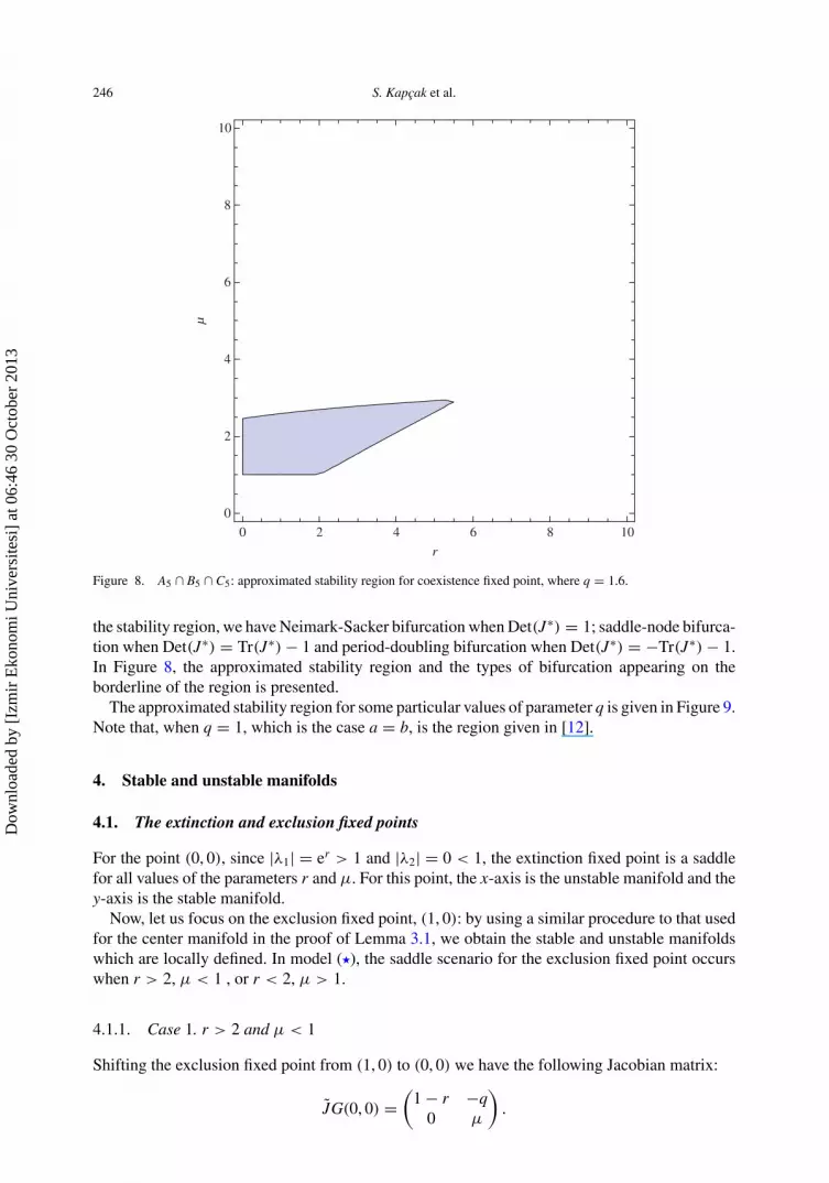
Figure 8. A5 ∩ B5 ∩ C5: approximated stability region for coexistence fixed point, where q = 1.6.

the stability region, we have Neimark-Sacker bifurcation when Det(J∗) = 1; saddle-node bifurca-tion when Det(J∗) = Tr(J∗) − 1 and period-doubling bifurcation when Det(J∗) = −Tr(J∗) − 1.In Figure 8, the approximated stability region and the types of bifurcation appearing on theborderline of the region is presented.

The approximated stability region for some particular values of parameter q is given in Figure 9.Note that, when q = 1, which is the case a = b, is the region given in [12].

4. Stable and unstable manifolds

4.1. The extinction and exclusion fixed points

For the point (0, 0), since |λ1| = er > 1 and |λ2| = 0 < 1, the extinction fixed point is a saddlefor all values of the parameters r and μ. For this point, the x-axis is the unstable manifold and they-axis is the stable manifold.

Now, let us focus on the exclusion fixed point, (1, 0): by using a similar procedure to that usedfor the center manifold in the proof of Lemma 3.1, we obtain the stable and unstable manifoldswhich are locally defined. In model (�), the saddle scenario for the exclusion fixed point occurswhen r > 2, μ < 1 , or r < 2, μ > 1.

4.1.1. Case 1. r > 2 and μ < 1

Shifting the exclusion fixed point from (1, 0) to (0, 0) we have the following Jacobian matrix:

JG(0, 0) =(

1 − r −q0 μ

).

Dow

nloa

ded

by [

Izm

ir E

kono

mi U

nive

rsite

si]

at 0

6:46

30

Oct

ober

201

3

Journal of Biological Dynamics 247

0 2 4 6 8 100

2

4

6

µ µ µ

µµ

µµ µ

µ

8

10(a) (b) (c)

(d) (e) (f)

(g) (h) (i)

r0 2 4 6 8 10

0

2

4

6

8

10

r 0 2 4 6 8 100

2

4

6

8

10

r

0 2 4 6 8 100

2

4

6

8

10

r0 2 4 6 8 10

0

2

4

6

8

10

r0 2 4 6 8 10

0

2

4

6

8

10

r

0 2 4 6 8 100

2

4

6

8

10

r0 2 4 6 8 10

0

2

4

6

8

10

r0 2 4 6 8 10

0

2

4

6

8

10

r

Figure 9. Approximated stability region for coexistence fixed point: (a) q = .00001, (b) q = .01, (c) q = .1, (d) q = .15,(e) q = .5, (f) q = .6, (g) q = 1, (h) q = 2.4, and (i) q = 10.

Now we can write the equations in system (14) as

ut+1 = (1 − r)ut − qvt + f (ut , vt),

vt+1 = μvt + g(ut , vt),(21)

where

f (ut , vt) = −1 + (−1 + r)ut + e−rut−qvt (1 + ut) + qvt

and

g(ut , vt) = (1 − e−vt )μ(1 + ut) − μvt .

Let us assume that the map h takes the form

h(v) = q

1 − μ − rv + αv2 + βv3 + O(v4), α, β ∈ R.

Dow

nloa

ded

by [

Izm

ir E

kono

mi U

nive

rsite

si]

at 0

6:46

30

Oct

ober

201

3

248 S. Kapçak et al.

0.8 0.9 1.0 1.1 1.2

–0.1

0.1

0.2

0.3

Figure 10. Stable manifold for the exclusion fixed point (1, 0) (the dashed curve). r = 2.03 > 2, μ = .9 < 1, andq = 1.2.

Notice that since μ < 1, the stable manifold is tangent to the corresponding eigenspace at thefixed point.

The function h must satisfy the equation

h(μv + g(h(v), v)) − (1 − r)h(v) + qv − f (h(v), v) = 0.

In order to solve the functional equation, the Taylor series expansions of required functions arecalculated and solving the system we get α and β which locally determine the stable manifoldu = h(v) for the exclusion fixed points. Due to the big size of the formulas for the constants α andβ we omit them. In Figure 10, the stable manifold is presented. There are two orbits with initialpoints (.888, .2) and (.98, .2). The first initial point is on the stable manifold.

In order to find the unstable manifold for the exclusion fixed point, we use the same idea.However, we assume here that the map h takes the form

h(u) = αu2 + βu3 + O(u4), α, β ∈ R.

We obtain that α = 0 and β = 0.When yt = 0 in Equation (�), the dynamics of population xn is determined by the one-

dimensional Ricker map. If 2 < r < r2, where r2 ≈ 2.5264, the fixed point (1, 0) loses its stabilityand a new asymptotically periodic orbit {x1, x2} of period 2 is born. the unstable manifold is theopen interval (x1, x2) that lies on the x-axis. As r increases, period-doubling bifurcation occursuntil r ≈ 2.6294, after which we enter the chaotic region. Hence, the boundary of the unstablemanifold shrinks to 0 as r > 2 increases. More details on the periodic points of the Ricker mapand the basin of attractions of its periodic orbits may be found in [6].

Dow

nloa

ded

by [

Izm

ir E

kono

mi U

nive

rsite

si]

at 0

6:46

30

Oct

ober

201

3

Journal of Biological Dynamics 249

0.85 0.90 0.95 1.00 1.05 1.10x

–0.05

0.05

0.10

0.15

0.20

yx, y

Figure 11. Stable and unstable manifolds for the exclusion fixed point (1, 0). μ = 1.2 > 1, r = .5 < 2, and q = .5

4.1.2. Case 2. r < 2 and μ > 1

In order to find the unstable manifold for this case, let us assume that the map h takes the form

h(v) = q

1 − μ − rv + αv2 + βv3 + O(v4), α, β ∈ R.

Since μ > 1, the unstable manifold is tangent to the corresponding eigenvector at the fixed point.Since the method we use for this case is the same as in the previous case, we omit the details.In order to find the stable manifold for the exclusion fixed point, we assume that the map h

takes the form

h(u) = αu2 + βu3 + O(u4), α, β ∈ R.

Figure 11.

5. Bifurcation scenarios

In this section, a bifurcation diagram for the positive fixed point is presented. In Figure 12, Tr–Det Diagram for a general system is shown. We give the corresponding regions for system (�) inFigure 13: Bi is the corresponding region for Ai.

We can see from these figures that on the border between the stability region and region B3,we have period-doubling bifurcation. The saddle-node bifurcation occurs when the point (r, μ)

moves from the stability region to region B7. We find that the map u = P(v) obtained by thecenter manifold theorem satisfies the conditions (∂P/∂μ)(μ∗, v∗) = 0 and (∂2P/∂μ2)(μ∗, v∗) =0, where μ∗ = 1 and v∗ = 0 for the case. Hence, this bifurcation is a transcritical bifurcation [5].

The system also possesses a Neimark-Sacker bifurcation [5] when the parameters are on theborder between the stability region and region B1. as shown in Figure 14.

Dow

nloa

ded

by [

Izm

ir E

kono

mi U

nive

rsite

si]

at 0

6:46

30

Oct

ober

201

3

250 S. Kapçak et al.

A1

A2

A3

A3

A4

A5

A6

A7

A7

A8

–3 –2 –1 0 1 2 3

–3

–2

–1

0

1

2

3

Trace

Det

erm

inan

t

Figure 12. Tr–Det diagram for general two-dimensional discrete-time system.

B1

B6

B5

B7 B4

B3

B3

B2

0 2 4 6 80

2

4

6

8

r

µ

Figure 13. Corresponding regions for system (�).

Dow

nloa

ded

by [

Izm

ir E

kono

mi U

nive

rsite

si]

at 0

6:46

30

Oct

ober

201

3

Journal of Biological Dynamics 251

Neimark-sacker bifurcation

Period-doubling bifurcation

Saddle-node bifurcation

0 2 4 6 8 10

0

2

4

6

µ

8

10

r

Figure 14. Types of bifurcation on the borderline of the stability region q = 1.6.

0 2 4 6 80

2

4

6

8(a) (b)

0.2 0.4 0.6 0.8 1.0

0.2

0.4

0.6

0.8

1.0

Figure 15. (r, μ) is inside the stability region: (a) bifurcation diagram, (b) phase diagram.

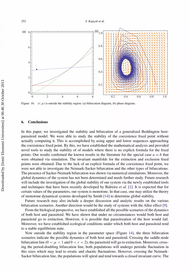
Figure 15 depicts the phase-space diagram and regions in the parameter space when (r, μ) is inthe stability region and close to the border of the Neimark-Sacker bifurcation. The case when thepoint (r, μ) passes the bifurcation curve is given in Figure 16. The black points in Figures 15(a)and 16(a) represent the point (r, μ).

Dow

nloa

ded

by [

Izm

ir E

kono

mi U

nive

rsite

si]

at 0

6:46

30

Oct

ober

201

3

252 S. Kapçak et al.

0 2 4 6 80

2

4

6

8

0.2 0.4 0.6 0.8 1.0

0.2

0.4

0.6

0.8

1.0(a) (b)

Figure 16. (r, μ) is outside the stability region: (a) bifurcation diagram, (b) phase diagram.

6. Conclusions

In this paper, we investigated the stability and bifurcation of a generalized Beddington host-parasitoid model. We were able to study the stability of the coexistence fixed point withoutactually computing it. This is accomplished by using upper and lower sequences approachingthe coexistence fixed point. By this, we have established the mathematical analysis and providednovel tools to study the stability of of models where there is no explicit formula for the fixedpoints. Our results confirmed the known results in the literature for the special case a = b thatwere obtained via simulation. The invariant manifolds for the extinction and exclusion fixedpoints were obtained. Due to the lack of an explicit formula of the coexistence fixed point, wewere not able to investigate the Neimark-Sacker bifurcation and the other types of bifurcations.The presence of Sacker-Neimark bifurcation was shown via numerical simulations. Moreover, theglobal dynamics of the system has not been determined and needs further study. Future researchwill include the investigation of the global stability of our system via the newly established toolsand techniques that have been recently developed by Balreira et al. [1]. It is expected that forcertain values of the parameters, our system is monotone. In that case, one may utilize the theoryof monotone dynamical systems developed by Smith [14] to determine global stability.

Future research may also include a deeper discussion and analytic results on the variousbifurcation scenarios. Another direction would be the study of systems with the Allee effect [9].

From the biological perspective, we have established all the possible scenarios of the dynamicsof both host and parasitoid. We have shown that under no circumstances would both host andparasitoid go to extinction. However, it is possible that parasitization of the host would fail.Moreover, we have established ecological conditions under which both host and parasitoid tendto a stable equilibrium state.

Now outside the stability region in the parameter space (Figure 14), the three bifurcationscenarios indicate the possible dynamics of both host and parasitoid. Crossing the saddle-nodebifurcation line (0 < μ < 1 and 0 < r < 2), the parasitoid will go to extinction. Moreover, cross-ing the period-doubling bifurcation line, both populations will undergo periodic fluctuation inthis sizes which may lead to erratic and chaotic fluctuations. However, crossing the Neimark-Sacker bifurcation line, the populations will spiral and tend towards a closed invariant curve. The

Dow

nloa

ded

by [

Izm

ir E

kono

mi U

nive

rsite

si]

at 0

6:46

30

Oct

ober

201

3

Journal of Biological Dynamics 253

oscillation is caused by having a pair of complex conjugate eigenvalues of the Jacobian of ourplane maps.

In conclusion, parasitization succeeds and both species persist under most ecological conditions.

Acknowledgements

The first author thanks the financial support from TUBITAK for his stay at Trinity University during the period this paperwas written.

Funding

This work was supported by the Scientific & Technological Research Council of Turkey (TUBITAK).

References

[1] E. Balreira, S. Elaydi, and R. Luis, Local stability implies global stability for the planar Ricker competition model,preprint (2013).

[2] J.R. Beddington, C.A. Free, and J.H. Lawton, Dynamic complexity in predator-prey models framed in differenceequations, Nature 225 (1975), pp. 58–60.

[3] J. Carr, Application of Center Manifolds Theory, Applied Mathematical Sciences, 3rd ed., Springer-Verlag, NewYork, 1981.

[4] S. Elaydi, An Introduction to Difference Equations, Springer, New York, 2005.[5] S. Elaydi, Discrete Chaos: With Applications in Science and Engineering, 2nd ed., Chapman and Hall/CRC, London,

2008.[6] S. Elaydi and R. Sacker, Basin of attraction of periodic orbits of maps on the real line, J. Differ. Equ. Appl. 10(10)

(2004).[7] M. Guzowska, R. Luis, and S. Elaydi, Bifurcation and invariant manifolds of the logistic competition model, J. Differ.

Equ. Appl. 17(12) (2010), pp. 1851–1872.[8] A.N.W. Hone, M.V. Irle, and G.W. Thurura, On the Neimark–Sacker bifurcation in a discrete predator-prey system,

J. Biol. Dyn. 4(6) (2010), pp. 594–606.[9] S.R.-J. Jang and S.L. Diamond, A host-parasitoid interaction with Allee effects on the host, Comput. Math. Appl.

53 (2007), pp. 89–103.[10] R. Luís, S. Elaydi, and S. Oliveira, Stability of Ricker-type competition model and the competitive exclusion principle,

J. Biol. Dyn. 5(6) (2011), pp. 636–660.[11] J.D. Murray, Mathematical Biology, Vol. 5, Springer, New York, 2002, pp. 636–660.[12] M.G. Neubert and M. Kot, The subcritical collapse of predator populations in discrete-time predator-prey models,

Math. Biosci. 110 (1992), pp. 45–66, ISSN 0025-5564, doi:10.1016/0025-5564(92)90014-N.[13] A. Nicholson and V. Bailey, The balance of animal population, Proc. Zool. Soc. Lond. 3 (1935), pp. 551–598.[14] H. Smith, Planar competitive and cooperative difference equations, J. Differ. Equ.Appl. 3(5–6) (1998), pp. 335–357.

Dow

nloa

ded

by [

Izm

ir E

kono

mi U

nive

rsite

si]

at 0

6:46

30

Oct

ober

201

3