Stability analysis of sonic horizons in Bose-Einstein condensates

C. Barcelo,1 A. Cano,1 L. J. Garay,2, 3 and G. Jannes1, 3

1Instituto de Astrofisica de Andalucia, CSIC, Camino Bajo de Huetor 50, 18008 Granada, Spain2Departamento de Fisica Teorica II, Universidad Complutense de Madrid, 28040 Madrid, Spain

3Instituto de Estructura de la Materia, CSIC, Serrano 121, 28006 Madrid, Spain

(Dated: February 7, 2008)

We examine the linear stability of various configurations in Bose-Einstein condensates with sonichorizons. These configurations are chosen in analogy with gravitational systems with a black holehorizon, a white hole horizon and a combination of both. We discuss the role of different boundaryconditions in this stability analysis, paying special attention to their meaning in gravitational terms.We highlight that the stability of a given configuration, not only depends on its specific geometry,but especially on these boundary conditions. Under boundary conditions directly extrapolated fromthose in standard General Relativity, black hole configurations, white hole configurations and thecombination of both into a black hole–white hole configuration are shown to be stable. However,we show that under other (less stringent) boundary conditions, configurations with a single blackhole horizon remain stable, whereas white hole and black hole–white hole configurations developinstabilities associated to the presence of the sonic horizons.

PACS numbers: 04.80.-y, 04.70.Dy, 03.75.Kk

I. INTRODUCTION

It is widely expected that underneath the general rel-ativity description of gravitational phenomena there isa deeper layer in which quantum physics plays an im-portant role. However, at this stage we don’t haveenough intertwined theoretical and observational knowl-edge to know how an appropriate description of whatunderlies gravity is or should be. Moreover, startingfrom structurally-complete quantum theories of gravity,it could still be very difficult to extract the specific way inwhich the first “quantum” modifications to classical gen-eral relativity might show up (this happens for examplewithin the Loop Quantum Gravity approach [1]).

Analogue models of General Relativity (GR) [2, 3] pro-vide specific and clear examples in which effective space-time structures ultimately emerge from (non-relativistic)quantum many-body systems. For certain (semiclassi-cal) configurations and low levels of resolution, one canappropriately describe the physical behaviour of the sys-tem by means of a classical (or quantum) field theory ina curved (Lorentzian) background geometry. However,when one probes the system with higher and higher res-olution, the geometrical structure progressively dissolvesinto a purely quantum regime [4]. Therefore, althoughanalogue models cannot be considered at this stage com-plete models of quantum gravity (they do not lead tothe Einstein equations in any regime or approximation),they provide specific and tractable models that repro-duce many aspects of the overall scenario expected inthe realm of real gravity.

The main objective of this and similar studies is toobtain specific indications about the type of deviationsfrom the GR behaviour to be expected when quantumgravitational effects become important. All, under theassumption that the underlying structure to GR is some-what similar to that in condensed matter systems. In

particular, in this paper we are interested in the be-haviour of gravity-like configurations containing horizonswithin Bose–Einstein condensates (BECs). (See, e.g.,Refs. [5, 6, 7] and [4, 8, 9] for reviews on BECs and fortheir usefulness as analogue models respectively). A nicefeature of these systems is that their theoretical descrip-tion in terms of the Gross-Pitaevskii (GP) equation canbe interpreted as incorporating, from the start, the first“quantum” corrections to the behaviour of the system.Linear perturbations over a background BEC configura-tion satisfy an equation which is a standard wave equa-tion over a curved effective spacetime plus correctionscontaining ~. These corrections cause the dispersion re-lations in BEC to be “superluminal” (strictly speaking,supersonic): some perturbations can travel faster thanthe speed of sound in the system. The effects of thesecorrections in the linearized dynamical evolution of aconfiguration are especially relevant in the presence ofhorizons as their one-way-membrane nature simply dis-appears. This is in tune with the idea that a horizon canserve as a magnifying glass of the physics at high energies(see, e.g., Ref. [10]).

The specific objective of this paper is to analyze the dy-namical behaviour of (effectively) one-dimensional BECswith density and velocity profiles containing one or twosonic horizons. In particular, we search for the presenceof dynamical instabilities and analyze how their existenceis related to the occurrence of these horizons. The stabil-ity analysis presented in Ref. [9] for black hole-like config-urations with fluid sinks in their interior, concluded thatthese configurations were intrinsically unstable. How-ever, the WKB analysis of the stability of horizons inRef. [11] suggested that black hole horizons might wellbe stable, while configurations with white hole horizonsseem to posses unstable modes. Regarding configurationsin which a black hole horizon is connected with a whitehole horizon in a straight line, the analysis presented in

2

Ref. [12] concluded, also within a WKB approximation,that these configurations were intrinsically unstable, pro-ducing a so-called “black hole laser”. However, when thewhite hole horizon is connected back to the black holehorizon to produce a ring, it was found that these con-figurations can be stable or unstable depending on theirspecific form [8, 9]. This suggests that periodic boundaryconditions can eliminate some of the instabilities associ-ated with the black hole laser.

In this paper we will try to shed some light on allof these issues and clear up some of the apparent con-tradictions. To simplify matters, we will consider one-dimensional profiles that are piecewise uniform with ei-ther one or two step-like discontinuities. As has beendiscussed in Ref. [9], in terms of dynamical (in)stability,there seems to be no crucial qualitative difference be-tween the present case and a profile with smooth transi-tions between regions with an (asymptotically) uniformdensity distribution. Therefore the idealized case that weconsider here should contain all the essential informationrelevant to more complicated profiles as well. The spe-cific way to examine the kind of instability we are inter-ested in, consists basically in seeking whether, under ap-propriate boundary conditions, there are complex eigen-frequencies of the system which lead to an exponentialincrease with time of the associated perturbations, i.e.a dynamical instability. Throughout the paper we willuse a language and notation as close to GR as possible.In particular, we will use boundary conditions similar tothose imposed in the standard quasi-normal mode anal-ysis of black holes in GR [13]. One of the main results ofour analysis is to highlight the fundamental importanceof the boundary conditions in determining whether a con-figuration is stable or unstable.

The structure of this paper is as follows. In the nextsection we will review the basic ingredients of gravita-tional analogies in BECs. At the same time, we will setup the conceptual framework for our discussion, based ona parametrization well adapted for an acoustic interpre-tation (a brief comparison with the Bogoliubov represen-tation is presented in appendix B). Section III containsa detailed formulation of our specific problem. This in-cludes the mode expansion in uniform sections, a deriva-tion of the matching conditions at each discontinuity anda discussion of the various boundary conditions to be ap-plied. Then, in section IV we proceed case by case, an-alyzing different situations and presenting the results wehave obtained for each of them. This includes a briefdescription of the numerical algorithm we have used. Fi-nally, in section V we discuss our results, compare themwith other results available in the literature, and drawsome conclusions.

II. PRELIMINARIES

In second quantization, a dilute gas of interacting

bosons can be described by a quantum field Ψ satisfy-

ing the equation

i~∂

∂tΨ =

(− ~

2

2m∇2 + Vext(x) + gΨ†Ψ

)Ψ, (2.1)

where m is the boson mass, Vext the external potentialand g the coupling constant which is related to the cor-responding scattering length a through g = 4π~

2a/m.In this manner all quantum effects can, in principle, betaken into account. Once the Bose-Einstein condensationhas taken place, the quantum field can be separated intoa macroscopic wave function ψ (the corresponding orderparameter) and a field operator ϕ describing quantum

fluctuations over it: Ψ = ψ + ϕ. The macroscopic wavefunction satisfies the Gross-Pitaevskii (GP) equation

i~∂

∂tψ(t,x) =

(− ~

2

2m∇2 + Vext(x) + g |ψ|2

)ψ(t,x),

(2.2)

while for the linear quantum perturbation we have theBogoliubov equation

i~∂

∂tϕ =

(− ~

2

2m∇2 + Vext(x) + g 2|ψ|2

)ϕ+ g ψ2 ϕ†.

(2.3)

Adopting the Madelung representation for the order pa-rameter

ψ =√neiθ/~e−iµt/~ (2.4)

(here n is the condensate density, µ the chemical poten-tial and θ a phase factor which is related to the velocitypotential), and substituting in (2.2) we arrive at

∂tn = − 1

m∇ · (n∇θ), (2.5a)

∂tθ = − 1

2m(∇θ)2 − g n− Vext − µ− Vquantum, (2.5b)

where the so-called “quantum potential” is defined as

Vquantum = − ~2

2m

∇2√n√n

. (2.6)

In most situations the quantum potential in Eq. (2.5b)can be neglected (see below). The resulting equations(2.5a) and (2.5b) are then equivalent to the continuityequation and the Bernoulli equation for a classical fluid.In this case, it is well known that the propagation ofacoustic waves in the system can be described by meansof an effective metric, thus providing the analogy with thepropagation of fields in curved spacetimes [14, 15]. Givena background configuration (n0 and θ0), this metric canbe written as

(gµν) =m

gc

(v2 − c2 −v

T

−v 11

), (2.7)

3

where c2 ≡ gn0/m and v ≡ ∇θ0/m. These magnitudes,c and v, represent the local velocity of sound and thelocal velocity of the fluid flow respectively.

The functions c(t,x) and v(t,x) completely charac-terize the acoustic metric. In GR any metric has tobe obtained by solving the Einstein equations. Here,however, the magnitudes c(t,x) and v(t,x), and so theacoustic metric, are those satisfying the continuity andBernoulli equations of hydrodynamics [Eqs. (2.5) with-out the quantum potential]. Thus, these equations playa role analogous to the vacuum Einstein equations inGR. Of course, at the global non-linear level these equa-tions are completely different from the real Einstein equa-tions. But their way of acting when linearized around abackground solution captures the essence of a proper lin-earized GR behaviour.

There exist, however, situations in which the quantumpotential in Eq. (2.5) cannot be neglected. This is evi-dently the case if the characteristic length of the spatialvariations of the condensate density is much smaller thanthe so-called healing length: ξ ≡ ~/(mc). But this case isnot the only one. To illustrate this point, let us considerthe dispersion law obtained for a homogeneous BEC (seebelow):

(ω − vk)2 = c2k2 +1

4c2ξ2k4. (2.8)

This is a “superluminally modified” dispersion relationdue to the presence of the term with k4. For ξk ≪ 1 wecan rewrite this expression as

ω =

(v ± c

√1 +

1

4ξ2k2

)k ≃ (v±c)k+1

8cξ2k3+O(ξ4k5).

(2.9)Here we clearly see that the (relative) importance of theterm ∝ k3, given by c

8(v±c)ξ2k2, depends not only on

the ratio between the corresponding wavelength and thehealing length, ξk, but also on the specific features of thebackground magnitudes [note that the factor c/(v ± c)may be quite large]. In other words, the smallness ofthe corresponding wavelength is a necessary condition inorder to neglect the contribution of the quantum poten-tial, but it is not a sufficient condition. One has to bearthis issue in mind, especially when the system possesseshorizons (i.e. points at which c2 = v2).

Summarizing, there are background configurationswhich, when probed with sufficiently large wavelengths,act as if they were effective Lorentzian geometries. Butthere are other configurations for which this geometri-cal interpretation fails, irrespective of the probing wave-length. The latter situation occurs when there are hori-zons in the configuration: strictly speaking, we cannottalk about an “effective Lorentzian geometry” in the re-gions surrounding these horizons.

Without forgetting this subtlety, we will continue tocall (2.7) the “effective metric” in the system, even whenanalyzing the full GP equation. Then, we can consider

the equations (2.5) to play the role of some sort of semi-classical vacuum Einstein equations. Their treatment isclassical, but they incorporate corrections containing ~.Therefore, BECs’ standard treatment based on the GPequation provides an example of a way of incorporat-ing quantum corrections to the dynamics of a systemwithout recurring to the standard procedures of back-reaction. Again, although at the global non-linear levelthese equations bear no relationship whatsoever with anysort of ”semiclassical” Einstein equations, at the linearlevel, that is, in terms of linear tendencies of depart-ing from a given configuration, equations (2.5) encodethe essence of the linearized GR behaviour (a Lorentzianwave equation in a curved background), semiclassicallymodified to incorporate a superluminal dispersion term,as we have already discussed.

We will now proceed to describe the details of our spe-cific calculations.

III. DYNAMICAL ANALYSIS

As a first step in our calculations, let us linearize theEqs. (2.5). Let us write

n(x, t) = n0(x) + g−1n1(x, t), (3.1a)

θ(x, t) = θ0(x) + θ1(x, t), (3.1b)

where n1 and θ1 are small perturbations of the densityand phase of the BEC. The Eqs. (2.5) then separate intotwo time-independent equations for the background,

0 = −∇ · (c2v), (3.2a)

0 = −1

2mv

2 −mc2 − Vext − µ+~

2

2m

∇2c

c, (3.2b)

plus two time-dependent equations for the perturbations,

∂tn1 = −∇ ·(n1v + c2∇θ1

), (3.3a)

∂tθ1 = −v · ∇θ1 − n1 +1

4ξ2∇ ·

[c2∇

(n1

c2

)]. (3.3b)

We will restrict ourselves to work in (1+1) dimensions.This means that we consider perturbations propagatingin a condensate in such a way that the transverse degreesof freedom are effectively frozen. In other words, theonly allowed motions of both the perturbations and thecondensate itself are along the x-axis.

We will examine two types of one-dimensional back-ground profiles. The first type consists of two regionseach with a uniform density and velocity, connectedthrough a step-like discontinuity. The second type of pro-files consists of three homogeneous regions, and hence twodiscontinuities. We wish to know whether these profilesdo or do not present dynamical instabilities. The un-derlying question is the relation between the presence ofhorizons and these dynamical instabilities. At each dis-continuity, matching conditions apply that connect the

4

magnitudes describing the condensate at both sides ofthe discontinuity. Furthermore, we need a set of bound-ary conditions, which determine what happens at the farends of the condensate. Finally, in the uniform sections ofthe condensate, the regime can either be subsonic or su-personic, and of course there will be an acoustic horizonat each transition between a subsonic and a supersonicregion. All these elements determine the characteristicsof the system, and hence its eigenfrequencies.

We will now describe these elements one by one indetail.

A. Plane-wave expansion in uniform regions

In order to study the dynamics of the system, let usfirst consider a region in which the condensate is homo-geneous (with c and v constant), and seek for solutionsof Eqs. (3.3) in the form of plane waves:

n1(x, t) = Aei(kx−ω)t, (3.4a)

θ1(x, t) = Bei(kx−ω)t, (3.4b)

where A and B are constant amplitude factors. Our aimis to elucidate about the possible instabilities of the sys-tem, so the frequency ω and the wavevector k in theseexpressions will be considered as complex hereafter [theexistence of solutions with Im(ω) > 0 would indicate theinstability of the system]. Substituting into Eqs. (3.3)we find

i(ω − vk) c2k2

1 + 14ξ

2k2 −i(ω − vk)

A

B

= 0. (3.5)

For a non-trivial solution to exist, the determinant of theabove matrix must vanish. This condition gives the dis-

persion law (2.8) and since this is a fourth order polyno-mial in k, its roots will, in general, give four independentsolutions for the equations of motion in the form (3.4).

B. Matching conditions at a discontinuity

Let us take x = 0 to be a point of discontinuity. Thevalues of v and c both undergo a finite jump when cross-ing this point. These jumps have to satisfy the back-ground constraint vc2 = const [see Eq. (3.2a)]. The so-lutions of Eqs. (3.3) in the regions x < 0 and x > 0 havethe form of plane waves which are then subject to match-ing conditions at x = 0. It is not difficult to see that θ1has to be continuous at the jump but with a discontin-uous derivative, while the function n1 has to undergoa finite jump. The exact conditions can be obtained byintegrating Eqs. (3.3) about an infinitesimal interval con-taining the point x = 0. This results in the following fourindependent, generally valid matching conditions:

[θ1] = 0, [vn1 + c2∂xθ1] = 0, (3.6a)[n1

c2

]= 0,

[c2∂x

(n1

c2

)]= 0. (3.6b)

The square brackets in these expressions denote, for in-stance, [θ1] = θ1|x=0+−θ1|x=0− . We can simplify the sec-ond condition in Eq.(3.6a) to [c2∂xθ1] = 0 by noting that[vn1] = 0 because of the background continuity equation(3.2a), while for our choice of a homogeneous backgroundthe last condition becomes simply [∂xn1] = 0.

For a given frequency ω, the general solution of Eqs.(3.3) can be written as

n1 =

4∑

j=1

Ajei(kjx−ωt) (x < 0),

8∑

j=5

Ajei(kjx−ωt) (x > 0),

θ1 =

4∑

j=1

Ajω − vLkj

ic2Lk2j

ei(kjx−ωt) (x < 0),

8∑

j=5

Ajω − vRkj

ic2Rk2j

ei(kjx−ωt) (x > 0),

(3.7)

where {kj} are the roots of the corresponding dispersion equations (four roots for each homogeneous region), andthe constants Aj have to be such that the matching conditions (3.6) are satisfied. The subscripts L and R indicatethe values of c and v in the left-hand-side (lhs) and the right-hand-side (rhs) region respectively. We can write down

5

these conditions in matrix form ΛijAj = 0, where

(Λij) =

ω−vLk1

c2Lk21

ω−vLk2

c2Lk22

ω−vLk3

c2Lk23

ω−vLk4

c2Lk24

−ω−vRk5

c2R

k25

−ω−vRk6

c2R

k26

−ω−vRk7

c2R

k27

−ω−vRk8

c2R

k28

ωk1

ωk2

ωk3

ωk4

− ωk5

− ωk6

− ωk7

− ωk8

1c2L

1c2L

1c2L

1c2L

− 1c2R

− 1c2R

− 1c2R

− 1c2R

k1 k2 k3 k4 −k5 −k6 −k7 −k8

. (3.8)

Furthermore, these conditions have to be complementedwith conditions at the boundaries of the system and thenwe will obtain the solution of a particular problem.

C. Boundary conditions

In order to extract the possible intrinsic instabilities ofa BEC configuration, we have to analyze whether thereare linear mode solutions with positive Im(ω) that satisfyoutgoing boundary conditions. By “outgoing” boundaryconditions we mean that the group velocity is directedoutwards (toward the boundaries of the system). Thegroup velocity for a particular k-mode is defined as

vg ≡ Re

(dω

dk

)= Re

(c2k + 1

2ξ2c2k3

ω − vk+ v

), (3.9)

where we have used the dispersion relation (2.8). Thephysical idea behind this outgoing boundary condition isthat only disrupting disturbances originated inside thesystem can be called instabilities.

To illustrate this assertion, let us look at the classi-cal linear stability analysis of a Schwarzschild black holein GR. When considering outgoing boundary conditionsboth at the horizon and in the asymptotic region at in-finity [13], only negative Im(ω) modes (the quasi-normalmodes) are found, and thus the black hole configurationis stable. If the presence of ingoing waves at infinity wereallowed, there would also exist positive Im(ω) solutions.In other words, the Schwarzschild solution in GR is sta-ble when considering only internal rearrangements of theconfiguration. If instead the black hole were allowed toabsorb more and more energy coming from infinity, itsconfiguration would continuously change and appear tobe unstable.

The introduction of modified dispersion relations addsan important difference with respect to the traditionalboundary conditions used in linearized stability analy-sis in GR. Consider for example a black hole configura-tion. In a BEC black hole, one boundary is the stan-dard asymptotic region, just like in GR. For an acoustic(quadratic) dispersion relation, nothing can escape fromthe interior of a sonic black hole (the acoustic behaviouris analogous to linearized GR). But due to the superlu-minal corrections, information from the interior of the

acoustic black hole can escape through the horizon andaffect its exterior. Therefore, since we are taking thispermeability of the horizon into consideration, the otherboundary is not the black hole horizon itself (usually de-scribed in GR by an infinite value of the “tortoise” coor-dinate; see for example [13]), but the internal singularity.The outgoing boundary condition at such a singularityreflects the fact that no information can escape from it.

There is another complication that deserves some at-tention. In the case of a phononic dispersion relation, thesigns of vg ≡ v ± c and Im(k) ≡ (v ± c)Im(ω) coincidefor Im(ω) > 0. For example, in an asymptotic x→ +∞subsonic region, an outgoing k-mode has vg > 0, so thatIm(k) > 0 and, therefore, the mode is damped towardsthis infinity (giving a finite contribution to its norm).Owing to this fact, in the linear stability analysis ofblack hole configurations, it is usual to assume that sta-ble modes correspond to non-normalizable perturbations(think of the standard quasi-normal modes), while un-stable modes correspond to normalizable perturbations.

When considering modified dispersion relations, how-ever, this association no longer holds. In particular,with the BEC dispersion relation, in an asymptoticx→ +∞ region, among the unstable (Im(ω) > 0) out-going (vg > 0) k-modes, there are modes with Im(k) > 0as well as modes with Im(k) < 0. An appropriate in-terpretation of these two possibilities seems to be thefollowing. The unstable outgoing modes that are con-vergent at infinity (those with Im(k) > 0) are associatedwith perturbations of the system that are initiated in aninternal compact region of the system. Unstable outgo-ing modes that are divergent at infinity are associatedwith initial perturbations acting also at the boundary atinfinity itself.

Take for example a black hole-like configuration of theform described in Fig. 1. The right asymptotic region,which can be interpreted as containing a “source” ofBEC gas in our analogue model, simulates the asymp-totic infinity outside the black hole in GR. The conver-gence condition at the rhs then implies that the perturba-tions are not allowed to affect this asymptotic infinity ini-tially. However, for the left asymptotic region, this con-dition is less obvious. In our BEC configuration, this leftasymptotic region can be seen as representing a “sink”.It corresponds to the GR singularity of a gravitationalblack hole. The fact that in GR this singularity is sit-

6

FIG. 1: Flow and sound velocity profiles with step-like dis-continuities simulating a black hole-like configuration. Thenegative value of v indicates that the fluid is left-moving. Atthe rhs, the fluid is subsonic since c > |v|. At the lhs it hasbecome supersonic. At x = 0, there is a sonic horizon.

uated at a finite distance (strictly speaking, at a finiteamount of proper time) from the horizon, indicates thatit might be sensible to allow the perturbations to affectthis left asymptotic region from the start. We will there-fore consider two possibilities for the boundary conditionat x → −∞. (a) Either we impose convergence in bothasymptotic regions, thereby eliminating the possibilitythat perturbations have an immediate initial effect on thesink, or (b) we allow the perturbations to affect the sinkright from the start, i.e. we don’t impose convergenceat the left asymptotic region. The option of imposingthe convergence at the left asymptotic region could beinterpreted as excluding the influence of the singularityon the stability of the system. In other words, condition(b) would then be equivalent to examining the stabilitydue to the combined influence of the horizon and the sin-gularity, while under condition (a) only the stability ofthe horizon would be taken into account.

As a final note to this discussion, since we are inter-ested in the analogy with gravity, we have assumed aninfinite system at the rhs. In a realistic condensate otherboundary conditions could apply, for example taking intoaccount the reflection at the ends of the condensate (seee.g. [8, 9]).

IV. CASE BY CASE ANALYSIS AND RESULTS

We will now briefly describe the general calculationmethod which we have used, and then discuss case bycase the specific configurations we have analyzed.

A. Numerical method

We first consider background flows and sound velocityprofiles with one discontinuity. We will always assumeleft-moving flows.

We are seeking for possible solutions of the linearizedEqs. (3.3) with Im(ω) > 0. We use the following numer-ical method:

1. For each frequency ω in a grid covering an appro-

priate region of the upper-half complex plane, wecalculate its associated k-roots [by solving the dis-persion relation (2.8)] and their respective groupvelocities (3.9) at both the lhs and the rhs of theconfiguration.

2. We then take the four equations ΛijAj = 0, whereΛ is the 4×8 matrix (3.8) determined by the match-ing conditions at the discontinuity. For each modekj that does not satisfy the boundary conditionsin the relevant asymptotic region, we add an equa-tion of the form Aj = 0. Thus we have a total set

of equations which can be written as ΛijAj = 0,

where Λ is now a (4+N)×8 matrix the number Nof forbidden modes can in principle vary between 0and 8). Numerically it is convenient to normalize

Λ in such a way that its rows are unit vectors.

3. We can then define a non-negative function F (ω),where F (ω) = 0 means that the frequency ω is aneigenfrequency of the system, in the following way.

• If N < 4, then F (ω) = 0. Indeed, we have 8variables Aj and 4 + N equations. Then, itis obvious that there will always exist a non-trivial solution {Aj}.

• If N = 4, then F (ω) = |det(Λ)|. In this casethere will be a non-trivial solution only if the

determinant of the matrix Λ vanishes.

• If N = 5, then F (ω) is taken to be the sum ofthe modulus of all possible determinants that

are obtained from Λ by eliminating one row.

Notice that in this case Λ is a non-square 9 × 8matrix because there are more conditions thanvariables. In this situation it is highly unex-pectable to find zeros in F as this would meana double degeneracy.

• If N > 5, F (ω) is defined by a straightforwardgeneralization of the procedure for N = 5.

4. We plot the function F (ω) in the upper half of thecomplex plane, and look for its zeros. Each of thesezeros indicates an unstable eigenfrequency, and sothe presence (or absence) of these zeros will indicatethe instability (or stability) of the system.

In all our numerical calculations we have chosen val-ues for the speed of sound and the fluid velocity closeto unity. Moreover, we set vc2 = 1 and choose units suchthat ξ c = 1. The typical values of the velocity of sound inBECs range between 1mm/s–10mm/s, while the healinglength lies between 10−3mm – 10−4mm. In consequence,our numerical results can be translated to realistic phys-ical numbers by using nanometres and microseconds asnatural units. For example, the typical lifetime for thedevelopment of an instability with Im(ω) ≃ 0.1 would beabout 10 microseconds. We have checked that our re-sults do not depend on the particular values chosen forthe velocities of the system.

7

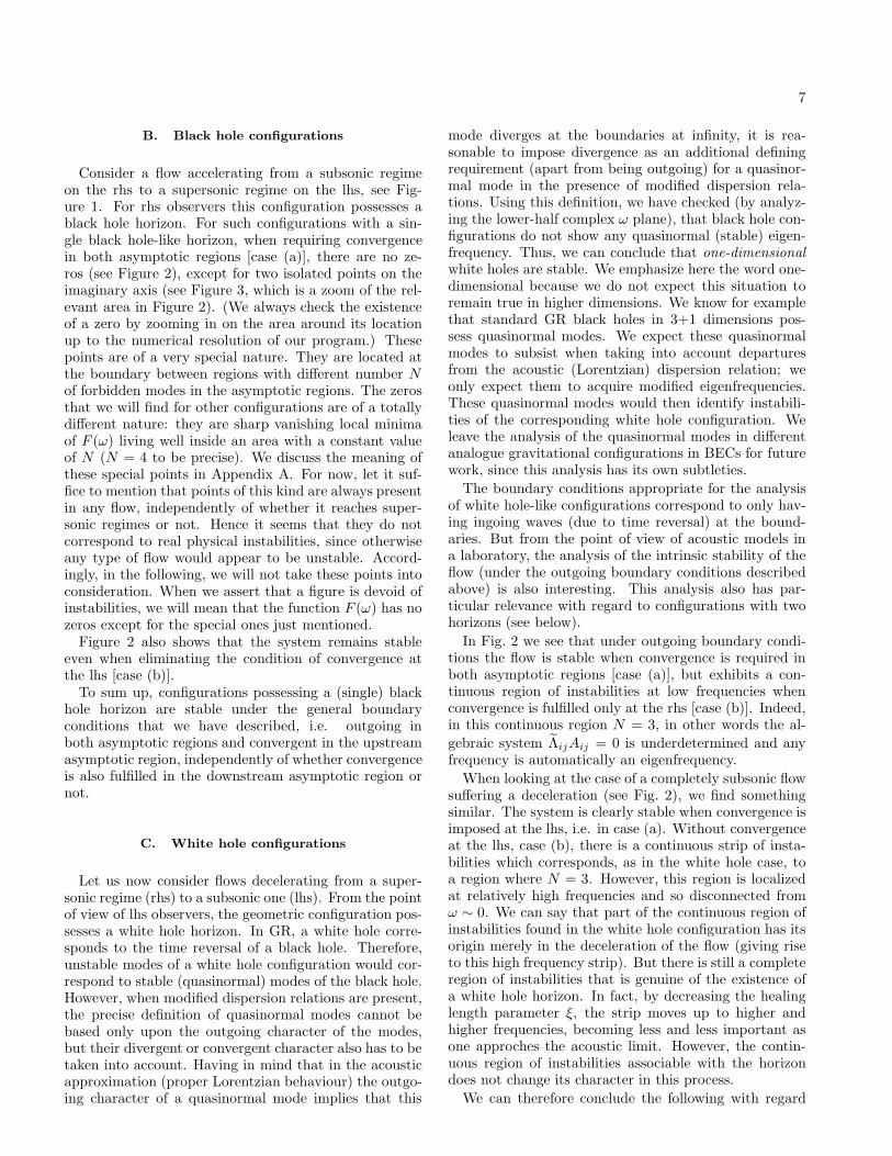
B. Black hole configurations

Consider a flow accelerating from a subsonic regimeon the rhs to a supersonic regime on the lhs, see Fig-ure 1. For rhs observers this configuration possesses ablack hole horizon. For such configurations with a sin-gle black hole-like horizon, when requiring convergencein both asymptotic regions [case (a)], there are no ze-ros (see Figure 2), except for two isolated points on theimaginary axis (see Figure 3, which is a zoom of the rel-evant area in Figure 2). (We always check the existenceof a zero by zooming in on the area around its locationup to the numerical resolution of our program.) Thesepoints are of a very special nature. They are located atthe boundary between regions with different number Nof forbidden modes in the asymptotic regions. The zerosthat we will find for other configurations are of a totallydifferent nature: they are sharp vanishing local minimaof F (ω) living well inside an area with a constant valueof N (N = 4 to be precise). We discuss the meaning ofthese special points in Appendix A. For now, let it suf-fice to mention that points of this kind are always presentin any flow, independently of whether it reaches super-sonic regimes or not. Hence it seems that they do notcorrespond to real physical instabilities, since otherwiseany type of flow would appear to be unstable. Accord-ingly, in the following, we will not take these points intoconsideration. When we assert that a figure is devoid ofinstabilities, we will mean that the function F (ω) has nozeros except for the special ones just mentioned.

Figure 2 also shows that the system remains stableeven when eliminating the condition of convergence atthe lhs [case (b)].

To sum up, configurations possessing a (single) blackhole horizon are stable under the general boundaryconditions that we have described, i.e. outgoing inboth asymptotic regions and convergent in the upstreamasymptotic region, independently of whether convergenceis also fulfilled in the downstream asymptotic region ornot.

C. White hole configurations

Let us now consider flows decelerating from a super-sonic regime (rhs) to a subsonic one (lhs). From the pointof view of lhs observers, the geometric configuration pos-sesses a white hole horizon. In GR, a white hole corre-sponds to the time reversal of a black hole. Therefore,unstable modes of a white hole configuration would cor-respond to stable (quasinormal) modes of the black hole.However, when modified dispersion relations are present,the precise definition of quasinormal modes cannot bebased only upon the outgoing character of the modes,but their divergent or convergent character also has to betaken into account. Having in mind that in the acousticapproximation (proper Lorentzian behaviour) the outgo-ing character of a quasinormal mode implies that this

mode diverges at the boundaries at infinity, it is rea-sonable to impose divergence as an additional definingrequirement (apart from being outgoing) for a quasinor-mal mode in the presence of modified dispersion rela-tions. Using this definition, we have checked (by analyz-ing the lower-half complex ω plane), that black hole con-figurations do not show any quasinormal (stable) eigen-frequency. Thus, we can conclude that one-dimensional

white holes are stable. We emphasize here the word one-dimensional because we do not expect this situation toremain true in higher dimensions. We know for examplethat standard GR black holes in 3+1 dimensions pos-sess quasinormal modes. We expect these quasinormalmodes to subsist when taking into account departuresfrom the acoustic (Lorentzian) dispersion relation; weonly expect them to acquire modified eigenfrequencies.These quasinormal modes would then identify instabili-ties of the corresponding white hole configuration. Weleave the analysis of the quasinormal modes in differentanalogue gravitational configurations in BECs for futurework, since this analysis has its own subtleties.

The boundary conditions appropriate for the analysisof white hole-like configurations correspond to only hav-ing ingoing waves (due to time reversal) at the bound-aries. But from the point of view of acoustic models ina laboratory, the analysis of the intrinsic stability of theflow (under the outgoing boundary conditions describedabove) is also interesting. This analysis also has par-ticular relevance with regard to configurations with twohorizons (see below).

In Fig. 2 we see that under outgoing boundary condi-tions the flow is stable when convergence is required inboth asymptotic regions [case (a)], but exhibits a con-tinuous region of instabilities at low frequencies whenconvergence is fulfilled only at the rhs [case (b)]. Indeed,in this continuous region N = 3, in other words the al-

gebraic system ΛijAij = 0 is underdetermined and anyfrequency is automatically an eigenfrequency.

When looking at the case of a completely subsonic flowsuffering a deceleration (see Fig. 2), we find somethingsimilar. The system is clearly stable when convergence isimposed at the lhs, i.e. in case (a). Without convergenceat the lhs, case (b), there is a continuous strip of insta-bilities which corresponds, as in the white hole case, toa region where N = 3. However, this region is localizedat relatively high frequencies and so disconnected fromω ∼ 0. We can say that part of the continuous region ofinstabilities found in the white hole configuration has itsorigin merely in the deceleration of the flow (giving riseto this high frequency strip). But there is still a completeregion of instabilities that is genuine of the existence ofa white hole horizon. In fact, by decreasing the healinglength parameter ξ, the strip moves up to higher andhigher frequencies, becoming less and less important asone approches the acoustic limit. However, the contin-uous region of instabilities associable with the horizondoes not change its character in this process.

We can therefore conclude the following with regard

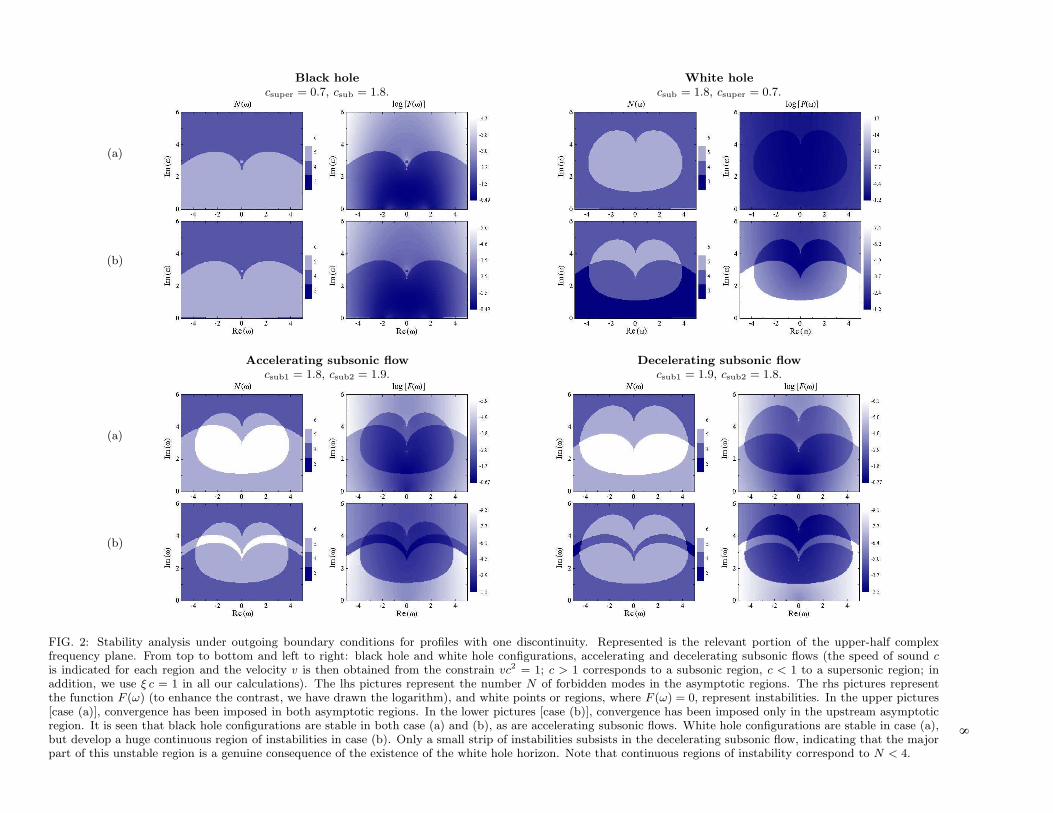
8Black hole White hole

csuper = 0.7, csub = 1.8. csub = 1.8, csuper = 0.7.

(a)

(b)

Accelerating subsonic flow Decelerating subsonic flowcsub1 = 1.8, csub2 = 1.9. csub1 = 1.9, csub2 = 1.8.

(a)

(b)

FIG. 2: Stability analysis under outgoing boundary conditions for profiles with one discontinuity. Represented is the relevant portion of the upper-half complexfrequency plane. From top to bottom and left to right: black hole and white hole configurations, accelerating and decelerating subsonic flows (the speed of sound cis indicated for each region and the velocity v is then obtained from the constrain vc2 = 1; c > 1 corresponds to a subsonic region, c < 1 to a supersonic region; inaddition, we use ξ c = 1 in all our calculations). The lhs pictures represent the number N of forbidden modes in the asymptotic regions. The rhs pictures representthe function F (ω) (to enhance the contrast, we have drawn the logarithm), and white points or regions, where F (ω) = 0, represent instabilities. In the upper pictures[case (a)], convergence has been imposed in both asymptotic regions. In the lower pictures [case (b)], convergence has been imposed only in the upstream asymptoticregion. It is seen that black hole configurations are stable in both case (a) and (b), as are accelerating subsonic flows. White hole configurations are stable in case (a),but develop a huge continuous region of instabilities in case (b). Only a small strip of instabilities subsists in the decelerating subsonic flow, indicating that the majorpart of this unstable region is a genuine consequence of the existence of the white hole horizon. Note that continuous regions of instability correspond to N < 4.

9

FIG. 3: Two special zeros of the function F (ω) appear in thestability analysis of a black hole configuration (this plot is azoom of the corresponding plot in Fig. 2). They are locatedat the boundary between regions with different number N ofprohibited modes. These points do not seem to represent realinstabilities of the system (see appendix A).

to decelerating configurations. When convergence is ful-filled downstream, the configuration is stable, regardlessof whether it contains a white hole horizon or not. Whenthis convergence condition is dropped, there is a tendencyto destabilization. In the presence of a white hole hori-zon, the configuration actually becomes dramatically un-stable, since there is a huge continuous region of instabil-ities, and even perturbations with arbitrarily small fre-quencies destabilize the configuration. In the absence ofsuch a horizon, only a small high-frequency part of thisunstable region subsists.

D. Black hole–white hole configurations

Consider flows passing from being subsonic to super-sonic and then back to subsonic (Figure 4). The numer-ical algorithm we have followed to deal with this prob-lem is equivalent to the one presented above, but with alarger set of equations. In this case we have 12 arbitraryconstants Aj , which have to satisfy 8 + N equations: 4matching conditions at each discontinuity and N(0 − 8)additional conditions of the form Aj = 0, correspondingto modes that do not fulfill the boundary conditions in aparticular asymptotic region.

When convergence is imposed at the lhs, we do notfind any instabilities, regardless of whether the fluid isglobally accelerating or decelerating [the final lhs fluidvelocity is larger or smaller than the initial rhs one re-spectively, see Figure 5 cases (a)]. Also when replac-ing the intermediate supersonic region by a subsonic one,thereby removing the acoustic horizons, the fluid is sta-ble, independently of whether it is globally acceleratingor decelerating.

FIG. 4: Flow and sound velocity profiles with step-like dis-continuities simulating a black hole–white hole configuration.

When dropping the convergence condition at the lhsthe situation changes completely. When the intermedi-ate region is supersonic, i.e. in a black hole–white holeconfiguration, a discrete set of instabilities appears atlow frequencies [Fig. 5 cases (b)]. It is worth mentioningthat, when carefully looking at plots of type (a)-cases,we observe some traces of these zeros in the form of lo-cal minima which can be understood as particularly softregions. These regions, although very close to zero insome situations, never give rise to real zeros, as we havecarefully checked by zooming in. Notice that these localminima appear in regions with N = 5 where a zero wouldmean a double degeneracy within the row vectors in thecorresponding matrix Λij . When the fluid is globally de-celerating, additionally there is a continuous region ofinstabilities at higher frequencies. Indeed, in this region,as in the case of the white hole configuration, N < 4, andso every frequency in this region automatically representsan instability. When the intermediate region is subsonic,the discrete set of local minima at low frequencies disap-pears, but the continuous strip of instabilities at higherfrequencies persists in the case of a globally decelerat-ing fluid. The discrete set of instabilities is therefore agenuine consequence of the existence of horizons.

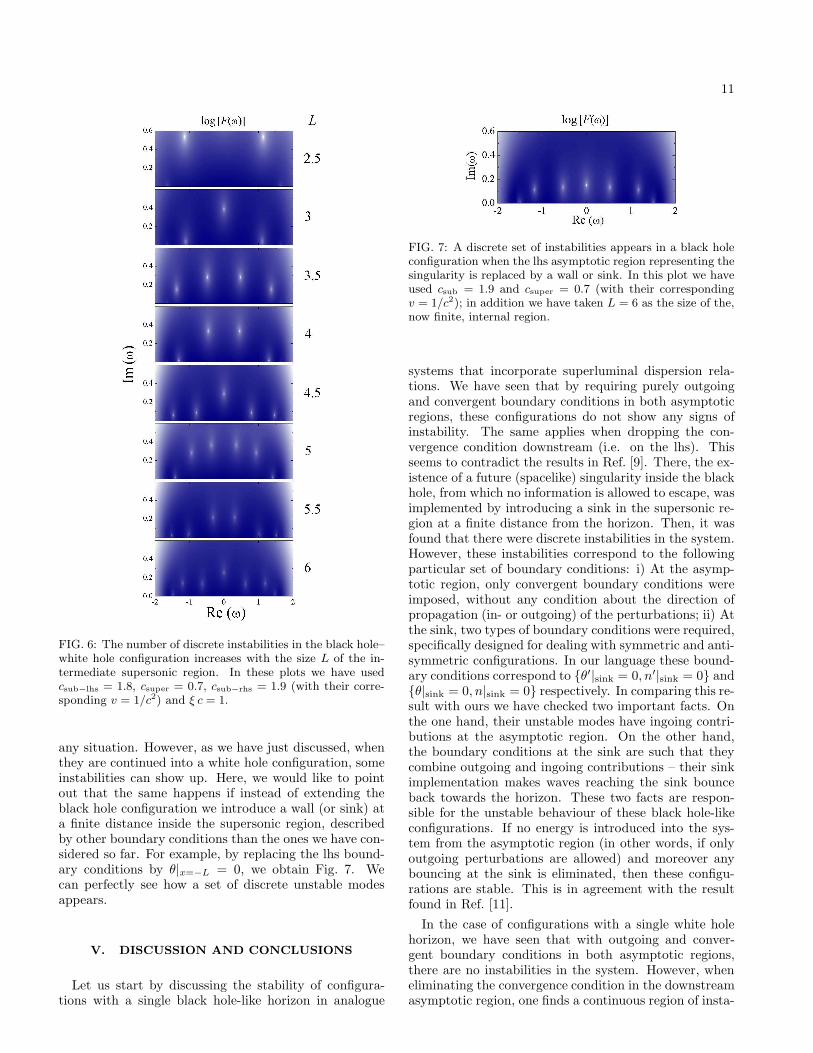
The number of discrete zeros we find in the black hole–white hole configuration increases with the size L of thesupersonic region (see Fig. 6), while their Im(ω) de-creases. This suggests that the region between the hori-zons acts as a sort of well discretizing some of the in-stabilities found for the white hole configurations. Thelarger the well, the larger the amount of instabilities, butthe longer-lived these instabilities.

To summarize, when requiring convergence in bothasymptotic regions, all the types of configurations withtwo discontinuities that we have discussed are stable.When not requiring convergence at the lhs, discretizedinstabilities appear associated with the presence of hori-zons.

E. Black hole configurations with modifiedboundary conditions

We have seen in section IV B that configurations witha single black hole horizon do not possess instabilities in

10

Black hole–white hole (globally accelerating) Black hole–white hole (globally decelerating)csub-lhs = 1.8, csuper = 0.7, csub-rhs = 1.9. csub-lhs = 1.9, csuper = 0.7, csub-rhs = 1.8.

(a)

(b)

Globally accelerating subsonic flow Globally decelerating subsonic flowcsub-lhs = 1.7, csub = 1.8, csub-rhs = 1.9. csub-lhs = 1.9, csub = 1.8, csub-rhs = 1.7.

(a)

(b)

FIG. 5: Stability analysis for profiles with two discontinuities. From top to bottom and left to right: globally accelerating and decelerating black hole–white holeconfigurations, globally accelerating and decelerating subsonic configurations. In all these plots we have used L = 2.5 as the size of the intermediate region (seealso caption under Fig. 2). When convergence is imposed in both asymptotic regions [case (a)], all the configurations are stable. When convergence is only imposedupstream [case (b)], the configurations with sonic horizons present a discrete set of instabilities at low frequencies, while the decelerating configurations show a smallcontinuous unstable strip at high frequencies. The decelerating configuration with sonic horizons combines both types of instabilities.

11

FIG. 6: The number of discrete instabilities in the black hole–white hole configuration increases with the size L of the in-termediate supersonic region. In these plots we have usedcsub−lhs = 1.8, csuper = 0.7, csub−rhs = 1.9 (with their corre-sponding v = 1/c2) and ξ c = 1.

any situation. However, as we have just discussed, whenthey are continued into a white hole configuration, someinstabilities can show up. Here, we would like to pointout that the same happens if instead of extending theblack hole configuration we introduce a wall (or sink) ata finite distance inside the supersonic region, describedby other boundary conditions than the ones we have con-sidered so far. For example, by replacing the lhs bound-ary conditions by θ|x=−L = 0, we obtain Fig. 7. Wecan perfectly see how a set of discrete unstable modesappears.

V. DISCUSSION AND CONCLUSIONS

Let us start by discussing the stability of configura-tions with a single black hole-like horizon in analogue

FIG. 7: A discrete set of instabilities appears in a black holeconfiguration when the lhs asymptotic region representing thesingularity is replaced by a wall or sink. In this plot we haveused csub = 1.9 and csuper = 0.7 (with their correspondingv = 1/c2); in addition we have taken L = 6 as the size of the,now finite, internal region.

systems that incorporate superluminal dispersion rela-tions. We have seen that by requiring purely outgoingand convergent boundary conditions in both asymptoticregions, these configurations do not show any signs ofinstability. The same applies when dropping the con-vergence condition downstream (i.e. on the lhs). Thisseems to contradict the results in Ref. [9]. There, the ex-istence of a future (spacelike) singularity inside the blackhole, from which no information is allowed to escape, wasimplemented by introducing a sink in the supersonic re-gion at a finite distance from the horizon. Then, it wasfound that there were discrete instabilities in the system.However, these instabilities correspond to the followingparticular set of boundary conditions: i) At the asymp-totic region, only convergent boundary conditions wereimposed, without any condition about the direction ofpropagation (in- or outgoing) of the perturbations; ii) Atthe sink, two types of boundary conditions were required,specifically designed for dealing with symmetric and anti-symmetric configurations. In our language these bound-ary conditions correspond to {θ′|sink = 0, n′|sink = 0} and{θ|sink = 0, n|sink = 0} respectively. In comparing this re-sult with ours we have checked two important facts. Onthe one hand, their unstable modes have ingoing contri-butions at the asymptotic region. On the other hand,the boundary conditions at the sink are such that theycombine outgoing and ingoing contributions – their sinkimplementation makes waves reaching the sink bounceback towards the horizon. These two facts are respon-sible for the unstable behaviour of these black hole-likeconfigurations. If no energy is introduced into the sys-tem from the asymptotic region (in other words, if onlyoutgoing perturbations are allowed) and moreover anybouncing at the sink is eliminated, then these configu-rations are stable. This is in agreement with the resultfound in Ref. [11].

In the case of configurations with a single white holehorizon, we have seen that with outgoing and conver-gent boundary conditions in both asymptotic regions,there are no instabilities in the system. However, wheneliminating the convergence condition in the downstreamasymptotic region, one finds a continuous region of insta-

12

bilities surrounding ω = 0. Thus, we see that these whitehole configurations are stable only when the boundaryconditions are sufficiently restrictive.

When analyzing configurations connecting two differ-ent subsonic regions, we have also seen that, again,when convergence is required at the lhs, they are stable.But when this convergence condition is relaxed, glob-ally decelerating configurations tend to become unstable,whereas globally accelerating ones remain stable. Theinstabilities of these decelerating configurations withouthorizons (i.e. purely subsonic ones) show up, however, ina small strip at high frequencies. In contrast, white holeconfigurations present instabilities for a wide range offrequencies, starting from arbitrarily small values. Thispoints out that the presence of a white hole horizon dras-tically stimulates the instability of the configuration.

With regard to the black hole–white hole configura-tions, we have seen that, as before, with outgoing andconvergent boundary conditions, they are stable. How-ever, when relaxing the convergence condition down-stream, they develop a discrete set of unstable modes.

In the analysis of the black hole laser instability inRef. [12], the authors found that these black hole–whitehole configurations were intrinsically unstable. However,they did not analyze what happens to the modes atthe lhs infinity. Our analysis shows that by restrictingthe possible behaviour of the modes in the downstreamasymptotic region, one can eliminate the unstable be-haviour of the black hole laser. This is in agreementwith the results in Refs. [8, 9]. There, the instabilitiescan in some cases be removed by requiring periodicity,that is, by imposing additional boundary conditions tothe modes.

To sum up, we have shown the high sensibility of thestability not only on the type of configuration (the pres-ence of a single horizon or of two horizons, the acceler-ating or decelerating character of the fluid), but particu-larly on the boundary conditions. With outgoing bound-ary conditions, when requiring convergence at the down-stream asymptotic region, both black hole and white holeconfigurations are stable (and also the combination ofboth into a black hole–white hole configuration). Whenrelaxing this convergence condition at the lhs, configu-rations with a single black hole horizon remain stable,whereas white hole and black hole–white hole configura-tions develop instabilities not present in (subsonic) flowswithout horizons.

Acknowledgements

C.B. has been funded by the Spanish MEC underproject FIS2005-05736-C03-01 with a partial FEDERcontribution. G.J. was supported by CSIC grants I3P-BGP2004 and I3P-BPD2005 of the I3P programme, co-financed by the European Social Fund, and by the Span-ish MEC under project FIS2005-05736-C03-02. L.G. wassupported by the Spanish MEC under the same projectand FIS2004-01912.

APPENDIX A: ZEROS AT THE BOUNDARIESOF THE REGIONS IN N(ω)

Given an ω, one can find its four associated k roots,{kj}. If instead of ω one takes ω = −ω∗, it can be seen

that the new roots {kj} are just {−k∗j }. For this reasonthe function F (ω) is mirror symmetric with respect tothe imaginary axis (this is seen in all our figures). Now,when ω is pure imaginary (ω = −ω∗), the set {kj} has tobe equal to the set {−k∗j }. There are three posibilities.Either all four roots are pure imaginary, two are imag-inary and the other two complex satisfying kj = −k∗l ,with j 6= l, or there are two pairs of complex roots sat-isfying kj = −k∗l . When moving through the imaginaryω axis, there are points at which there is a transitionfrom one of these possibilities to another. At any transi-tion point there has to be a pair of imaginary roots withequal value. Defining ω′′ ≡ Im(ω) and κ ≡ −ik, thedispersion equation (2.8) can be written as

(ω′′ − vκ)2 −(c2 − 1

4c2ξ2κ2

)κ2 = 0. (A1)

This is a fourth order polynomial in κ with real coeffi-cients. If this polynomial has two equal real roots thenwe know that the derivative with respect to κ of the poly-nomial has to be zero at that point. It is not difficult tosee that this also implies that the derivative with respectto κ of the function

(w − vκ) ∓(c2 − 1

4c2ξ2κ2

)1/2

κ (A2)

has to be zero at this same point. But this derivativecoincides with the definition of the group velocity givenin (3.9) (when ω and k are pure imaginary, dω/dk isdirectly real). Therefore, we conclude that at any transi-tion point on the imaginary ω-axis we have degeneracy:at least two imaginary k roots with equal value. At thesame time, the group velocity associated with them be-comes zero. This is why these points are located at theboundary between regions with a different number of for-bidden modes: these are places in which outgoing modestransform into ingoing ones. The zero that appears inthe function F (ω) at these points is due to the degener-acy and does not tell us anything about the existence ornot of a real instability there. To know whether a realinstability appears, one first has to find the actual fourindependent solutions of equations (3.3) at the point thatled to the degeneracy. Let us check under which circum-stances one can find a solution of the form

n1(x, t) = A1 x ei(kx−ω)t, (A3a)

θ1(x, t) = B1 x ei(kx−ω)t +B2e

i(kx−ω)t. (A3b)

For these expressions to be a solution of Eqs. (3.3), thefollowing conditions have to be satisfied:

13

i(ω − vk) c2k2

1 + 14ξ

2k2 −i(ω − vk)

A1

B1

= 0, (A4)

i(ω − vk) c2k2

1 + 14ξ

2k2 −i(ω − vk)

0

B2

+

−v −2ic2k

− 12 iξ

2k v

A1

B1

= 0. (A5)

From the first condition we obtain that the dispersionrelation (2.8) has to be fulfilled. As a consequence wealso find that B1 = A1(ω − vk)/(ic2k2). Now, from thesecond condition we obtain

−c2k2

i(ω − vk)

=

A1

B2

−v −2ic2k

− 12 iξ

2k v

1

(ω−vk)ic2k2

(A6)

This is a system of two equations from which, eliminatingA1/B2 and after some rearranging, we obtain:

c2k +1

2c2ξ2k3 + v(ω − vk) = 0. (A7)

This is exactly the condition for a vanishing group ve-locity (3.9). Therefore, when functions in the form ofplane waves do not lead to four linearly independent so-lutions, but for example two are “degenerate”, then wecan use the previous solution (A3) avoiding this degener-acy. Once we have the actual four independent solutionsof the problem, they have to be matched with the foursolutions in the other region (typically these will havethe form of plane waves, unless we are in a very specialsituation in which degeneracy occurs in both regions atthe same time) and see whether there is a combinationsatisfying all the boundary conditions.

Although we haven’t made such a full detailed calcu-lation, the fact that this kind of situation occurs in anytype of flow indicates that it is safe to assume that theydo not represent real instabilities, as already mentioned.

APPENDIX B: BOGOLIUBOVREPRESENTATION

All calculations and numerical simulations presentedin the text have been performed independently by usingthe acoustic representation and the Bogoliubov represen-tation [8, 9] described in this appendix. We have foundidentical results with the two methods, double checkingin this way the absence of numerical artifacts.

Consider a one-dimensional setup with a potential Vext

that produces a profile for the speed of sound of the form

c(x) =

c0, x < 0c0[1 + (σ − 1)x/ǫ], 0 < x < ǫσc0, ǫ < x

. (B1)

We will assume σ > 1 and a flow velocity in the inward(x → −∞) direction, i.e. a black hole-like configurationfor a rhs observer. The limit ǫ → 0 provides the sameprofile we have discussed in the main text.

The condensate wave function can be written as thesum of a stationary background state ψ0 and a pertur-bation φ satisfying

i∂tφ = −∂2xφ/2 + (c2 − v2/2 + ∂2

xc/2c)φ+ c2e2i∫

x vφ∗,(B2)

that will then be expanded into Bogoliubov modes

φ = uω(x)e−iωt + w∗ω(x)eiω∗t. (B3)

¿From now on, we drop the subindex ω, but rememberthat all equations should be valid for every (complex)frequency ω separately.

The assumption of a small ǫ leads to a linear solu-tion for the modes u and w in the intermediate region0 < x < ǫ. Together with the transition conditions atx = 0 and x = ǫ, which substitute the singular charac-ter of ∂2

xc/c at those points, this leads to the followingconnection formulas (in the limit ǫ→ 0), see Ref. [9]:

[u/c] =0, [∂x(cu)] =0, (B4)

[w/c] =0, [∂x(cw)] =0, (B5)

where as before we have used the notation[u] = u|x→0+ − u|x→0− .

Let us write the density and phase in terms of thestationary values plus perturbations:

n = n0 + g−1n1, θ = θ0 + θ1, (B6)

and note that the matching condition for the backgroundvelocity potential is [θ0] = 0.

The relation between the acoustic and the Bogoliubovrepresentation of the perturbations can easily be ob-tained by noting that, to first order,

φ =√m/g c(n1/2mc

2 + iθ1)eiθ0 , (B7)

14

where we have used the fact that c2 = gn0/m. Note thatn1 and θ1 are real. Then, comparison of Eq. (B7) withthe Bogoliubov mode expansion φ = ue−iωt + w∗eiω∗t

yields

u =√m/g c(n1/2mc

2 + iθ1)eiθ0 , (B8)

w =√m/g c(n1/2mc

2 − iθ1)e−iθ0 . (B9)

We then have

[u/c] ∝ [(n1/2c2 + iθ1)e

iθ0 ] ∝ [n1/2c2 + iθ1] (B10)

and likewise for w. Comparing with Eq. (B4), we obtain

[n1/c2] ∝ [u/c] + [w/c] = 0, (B11)

[θ1] ∝ [u/c] − [w/c] = 0, (B12)

which correspond to two of the conditions in Eqs. (3.6).Taking into account that [θ0] = [c2v] = [θ1] = 0 and

that ∂xcL = ∂xcR = 0, we can write

[∂x(cu)] ∝ i[vn1]/2 + [∂xn1]/2 + i[c2∂xθ1], (B13)

[∂x(cw)] ∝− i[vn1]/2 + [∂xn1]/2 − i[c2∂xθ1]. (B14)

In other words [∂xn1] = 0 and [vn1/2 + c2∂xθ1] = 0. Be-cause of the continuity equation vc2 = const, we have[vn1] ∝ [n1/c

2] = 0, so that the boundary conditions ul-timately become

[∂xn1] = 0, [c2∂xθ1] = 0, (B15)

i.e. the other two conditions in Eqs. (3.6) with the cor-responding simplifications.

[1] A. Ashtekar and J. Lewandowski, “Background indepen-dent quantum gravity: A status report,” Class. Quant.Grav. 21, R53 (2004) [arXiv:gr-qc/0404018].

[2] C. Barcelo, S. Liberati and M. Visser, “Analogue Grav-ity,” Living Rev. Relativity 8, (2005), 12. URL (citedon 02-20-06): http://www.livingreviews.org/lrr-2005-12[arXiv:gr-qc/0505065].

[3] M. Novello, M. Visser and G. Volovik (eds.), Artificial

black holes, World Scientific, Singapore (2002).[4] C. Barcelo, S. Liberati and M. Visser, “Analog gravity

from Bose-Einstein condensates,” Class. Quant. Grav.18, 1137 (2001) [arXiv:gr-qc/0011026].

[5] F. Dalfovo, S. Giorgini, L. Pitaevskii andS. Stringari, “Theory of Bose-Einstein condensa-tion in trapped gases, Rev. Mod. Phys. 71, 463 (1999)[arXiv:cond-mat/9806038].

[6] Y. Castin, “Bose-Einstein condensates in atomic gases:simple theoretical results,” in: Coherent atomic matter

waves, Lecture Notes of Les Houches Summer School,edited by R. Kaiser, C. Westbrook, and F. David, EDPSciences and Springer-Verlag (2001).

[7] W. Ketterle, D.S. Durfee and D.M. Stamper-Kurn,“Making, probing and understanding Bose-Einstein con-densates, in: Bose-Einstein condensation in atomic

gases, Proceedings of the International School of Physics‘Enrico Fermi’, edited by M. Inguscio, S. Stringari

and C.E. Wieman, IOS Press, Amsterdam (1999)[arXiv:cond-mat/9904034].

[8] L. J. Garay, J. R. Anglin, J. I. Cirac and P. Zoller, “Blackholes in Bose-Einstein condensates,” Phys. Rev. Lett. 85,4643 (1999) [arXiv:gr-qc/0002015].

[9] L. J. Garay, J. R. Anglin, J. I. Cirac and P. Zoller, “Sonicblack holes in dilute Bose-Einstein condensates,” Phys.Rev. A 63, 023611 (2001) [arXiv:gr-qc/0005131].

[10] T. Padmanabhan, “Event horizon: Magnifying glass forPlanck length physics,” Phys. Rev. D 59, 124012 (1999)[arXiv:hep-th/9801138].

[11] U. Leonhardt, T. Kiss, and P. Ohberg, “Theory of el-ementary excitations in unstable Bose-Einstein conden-sates and the instability of sonic horizons,” Phys. Rev. A67, 033602 (2003).

[12] S. Corley and T. Jacobson, “Black hole lasers,” Phys.Rev. D 59, 124011 (1999) [arXiv:hep-th/9806203].

[13] K. D. Kokkotas and B. G. Schmidt, “Quasi-normalmodes of stars and black holes,” Living Rev. Rel. 2, 2(1999) [arXiv:gr-qc/9909058].

[14] W. G. Unruh, “Experimental Black Hole Evaporation,”Phys. Rev. Lett. 46, 1351 (1981).

[15] M. Visser, “Acoustic black holes: Horizons, ergospheres,and Hawking radiation,” Class. Quant. Grav. 15, 1767(1998) [arXiv:gr-qc/9712010].