306 IEEE TRANSACTIONS ON IMAGE PROCESSING, VOL. 19, NO. 2, FEBRUARY 2010

Squigraphs for Fine and CompactModeling of 3-D Shapes

Djamila Aouada, Member, IEEE, and Hamid Krim, Fellow, IEEE

Abstract—We propose to superpose global topological andlocal geometric 3-D shape descriptors in order to define onecompact and discriminative representation for a 3-D object.While a number of available 3-D shape modeling techniques yieldsatisfactory object classification rates, there is still a need for arefined and efficient identification/recognition of objects amongthe same class. In this paper, we use Morse theory in a two-phaseapproach. To ensure the invariance of the final representation toisometric transforms, we choose the Morse function to be a simpleand intrinsic global geodesic function defined on the surface ofa 3-D object. The first phase is a coarse representation througha reduced topological Reeb graph. We use it for a meaningfuldecomposition of shapes into primitives. During the second phase,we add detailed geometric information by tracking the evolutionof Morse function’s level curves along each primitive. We thenembed the manifold of these curves into �, and obtain a singlecurve. By combining phase one and two, we build new graphsrich in topological and geometric information that we refer toas squigraphs. Our experiments show that squigraphs are moregeneral than existing techniques. They achieve similar classifica-tion rates to those achieved by classical shape descriptors. Theirperformance, however, becomes clearly superior when finer clas-sification and identification operations are targeted. Indeed, whileother techniques see their performances dropping, squigraphsmaintain a performance rate of the order of 97%.

Index Terms—Iso-geodesic curves, object matching, Reeb graph,shape geometry, topo-geometric modeling, Whitney embedding.

I. INTRODUCTION

A S a result of a fast development of 3-D data renderingand acquisition techniques, applications of 3-D mod-

eling (e.g., security, multimedia, biometrics) have, over thelast decade, received a great deal of attention from both thescientific and the engineering communities. Important effortsaim to achieve simpler representations of 3-D objects in orderto efficiently carry out operations such as object classification,recognition, identification and retrieval, with acceptable errorrates. Numerous 3-D representation approaches have recentlybeen proposed, as overviewed in [1] and [2]. In the presentwork, we propose a 3-D object representation model that offers

Manuscript received February 03, 2009; revised September 11, 2009. Firstpublished October 16, 2009; current version published January 15, 2010. Thiswork was supported in part by the U.S. Air Force Office of Scientific Researchunder Grant FA9550-07-1-0104. The associate editor coordinating the review ofthis manuscript and approving it for publication was Dr. Arun Abraham Ross.

The authors are with the Electrical and Computer Engineering Department,North Carolina State University, Raleigh, NC, 27695 USA (e-mail: djamila.aouada@ieee.org; ahk@ncsu.edu).

Color versions of one or more of the figures in this paper are available onlineat http://ieeexplore.ieee.org.

Digital Object Identifier 10.1109/TIP.2009.2034693

different levels of discrimination. This model invokes an ob-ject’s geometric and topological information. This rather recenttechnique, henceforth referred to as topo-geometric modelingof 3-D objects, was first exploited in [3], where Yu et al. si-multaneously define topological and geometrical feature maps.They show that these feature maps are invariant to all affinetransforms. This invariance includes, by definition, non uniformscaling transforms. This, in turn, implies an inaccurate dissimi-larity measure between the geometry of shapes, as the geometryof shapes is only invariant to Euclidean transforms. Tung andSchmitt [4] and Baloch et al. [5] present a different theme byfirst representing the topology of a 3-D shape, and subsequentlyenhancing with its geometrical representation. The advantageof separating the modeling into two distinct steps is twofold:First it provides two levels of discrimination; a) a coarse levelwith a simple topological skeleton called a Reeb graph [6], [7],and b) a fine level with geometric weights assigned to each edgeor node of the previously extracted topological graph. Anotheradvantage of a topological graph representation of an objectis its ability of matching objects by parts, thereby enabling atransition from a global to a localized correspondence betweenshapes (e.g., mechanical parts, manufactured solids). In rep-resenting an object, one ideally avoids choosing a referencepoint extrinsic to its surface [11]–[14]. To that end, we addressthis limitation, evident in [3], [5], by adopting an integratedgeodesic distance function as defined in [11]. Such a functionensures the invariance of the Reeb graph of an object subjectedto any isometric transform. As first proposed in [11], thisfunction was limited to only providing topological informationof an object surface. Tung and Schmitt [4], in an attempt tomitigate this limitation, proposed to revert back to a Euclideanreference frame to compute differential geometric featureswhich they use as weight attributes on the Reeb graph. In thispaper, we propose a novel alternative technique that is efficient,theoretically sound, practically complete, and computationallysimple. Our proposed approach is rooted in modeling thegeometry along edges of the object representative graph. Wesubsequently define a new topo-geometric skeleton that we callsquigraph. The key idea for the geometric modeling of shapesis to embed in Euclidean space a manifold of new characteristiccurves (we refer to as iso-geodesic curves) of an object surface.The resulting embedding space, as we show below, is , andthe curve manifold is 1-D, i.e., a space curve in . As a result,all topological and geometric information we exploit remainsintrinsic to the modeled object, hence preserving all desiredinvariance properties alluded to earlier.

The remainder of the paper is organized as follows: In Sec-tion II, we briefly overview the topological modeling phase, and

1057-7149/$26.00 © 2010 IEEE

AOUADA AND KRIM: SQUIGRAPHS FOR FINE AND COMPACT MODELING OF 3-D SHAPES 307

define the notation used throughout this paper. In Section III, wedescribe our technique of embedding the geometry in andpresent the resulting modeling curve. In Section IV, we explainhow we construct squigraphs and use them to quantify the geo-metric dissimilarity between 3-D shapes. We finally substantiatethe development with many examples, and discuss the attributesof our proposed model in Section V.

II. TOPOLOGICAL REEB GRAPHS

In this work, we view 3-D objects as 2-D smooth and compactsurfaces embedded in . In order to extract topological fea-tures of 3-D objects, we make an extensive use of Morse theory[15], [16]. Morse theory states that it is possible to define a par-ticular smooth function on a smooth surface , and track itscritical points in order to study the topology of . Such a func-tion is called Morse function and is defined as follows.

Definition 1 (Morse Function): A smooth functionon a smooth manifold is called Morse if all of its critical

points are nondegenerate.A standard Morse function is a height function [5], [7], [12],

[16], [18]. The image of a point on via the height functionis reduced to its coordinate as shown in Fig. 1(b). Any repre-sentation that is based on the height function is clearly geomet-rically variant, as critical points of a surface in will changeas a result of its mere rotation. Since shape descriptors are, fora large number of applications, required to be invariant to sim-ilarity transforms1, a choice of an appropriate Morse functionis critical. In [11], Hilaga et al. define a Morse function forgeneric metrics on surface, that is invariant to isometric trans-forms. Specifically, this function is defined at every point on

as the integral of the geodesic distance from to allother points on

(1)

A discrete approximation of (1) is defined in [8], and re-ferred to as Global Geodesic Function (GGF), such that

(2)

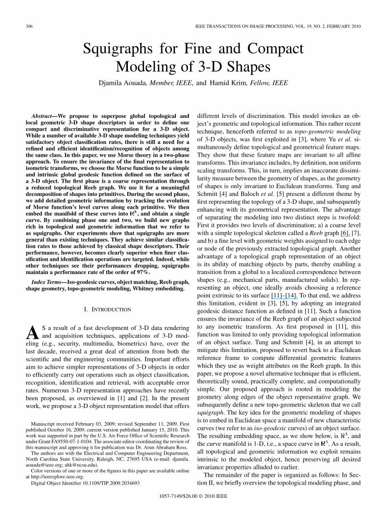
We choose the GGF to be our Morse function and show an ex-ample in Fig. 1(c), where the considered surface is the doubletorus illustrated in Fig. 1(a). In addition to its independenceof any reference point, an important property of this Morsefunction is its invariance to isometric transformations, thusyielding a consistent and unique characterization of an objectsurface. The independence of reference points is achieved bythe geodesic integration procedure at each point. The normal-ization of the functional shown in (2) ensures an invariance toscaling by making the range of coincide with , with

and

. In Fig. 1(c), we show the color coding map for

1Similarity transforms include: translation, rotation, and scaling, or any com-bination thereof.

Fig. 1. Illustration of Reeb graph extraction. (a) Initial object. (b) Height func-tion on the surface. (c) GGF function on the surface. (d) Iso-geodesic curves.(e) Extracted topological Reeb graph. (Best visualized in color).

used on all our objects. Additional analytical and computationaldetails on the GGF may be found in [8]. With in hand,we proceed to construct a topological Reeb graph for [4],[11]. Mathematically, a Reeb graph is a quotient space ,where the equivalence relation is given by if and onlyif with and being two points on andbelonging to the same connected component of .Practically, we sample the surface of a 3-D object by wayof level sets of a Morse function, and in our case thereof aGGF . As illustrated in Fig. 1(d), the level sets of areclosed curves, which we refer to as iso-geodesic curves. Wepresent the resulting Reeb graph in Fig. 1(e), where each closediso-geodesic curve is replaced by a node colored in black.

III. REPRESENTATION OF A SURFACE GEOMETRY

We note that, just as in [4] and [5], our 3-D object modelingapproach starts with a topological analysis followed by a geo-metrical analysis step. In our present work, however, we strive toachieve a topo-geometric representation that is both discrimina-tive and efficient. This is why we proceed by economically ex-ploiting, for the geometric modeling, the same entities used ear-lier for the topological modeling with Reeb graphs. The entitiesin question are the level sets of the GGF, i.e., the iso-geodesicsets defined on the surface of an object. Using iso-geodesic setsallows us to further extend the invariance properties of the GGFto the geometric phase.

In addition, unlike the usual global shape descriptors, a morecomplete geometric representation is one which provides a localdescription taking into account the spatial location of points orvertices [3]. The iso-geodesic curves used in the topological rep-resentation consequently appear, once again, to be able to offerperfect local geometric descriptors. We, therefore, take advan-tage of these already extracted entities, and use them for thesecond phase of our modeling as described in what follows.

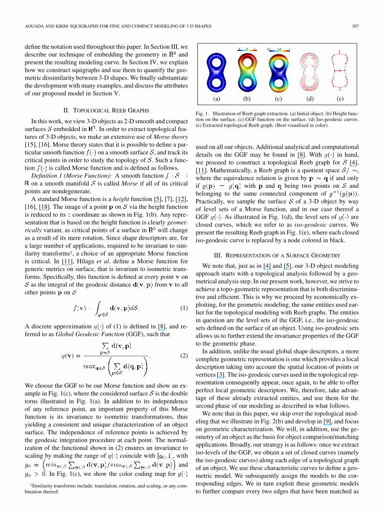
We note that in this paper, we skip over the topological mod-eling that we illustrate in Fig. 2(b) and develop in [9], and focuson geometric characterization. We will, in addition, use the ge-ometry of an object as the basis for object comparison/matchingapplications. Broadly, our strategy is as follows: once we extractiso-levels of the GGF, we obtain a set of closed curves (namelythe iso-geodesic curves) along each edge of a topological graphof an object. We use these characteristic curves to define a geo-metric model. We subsequently assign the models to the cor-responding edges. We in turn exploit these geometric modelsto further compare every two edges that have been matched as

308 IEEE TRANSACTIONS ON IMAGE PROCESSING, VOL. 19, NO. 2, FEBRUARY 2010

Fig. 2. Overview of the targeted problem (Best visualized in color): the four3-D models (Princeton data set [31]) in (a) are from the same class because theyare topologically similar as shown in (b). There is still a difference to be de-tected at the geometrical level. In (c), the part by part comparison is illustrated.We measure the dissimilarity between homogeneous parts that have been topo-logically matched. They are represented by edges in (b), and by the same colorin (c).

part of two topologically similar graphs. In Fig. 2(c), we showall matched edges in the same color.

We compactly represent the final topo-geometric modelthrough a new spatial graph that we call squigraph (Fig. 6(d)).A squigraph graph differs from a classical Reeb graph by its“squiggling” curves that replace the standard straight edges andencode the geometric information about the shapes.

A. Level Set Characterization of a Surface

Generically, we can reconstruct a 2-D surface from the setof 1-D iso-levels of the GGF. A surface is then a disjointunion of all iso-geodesic sets for , where

, and is the minimal value of

(3)

For smooth and compact objects, an iso-geodesic set is theunion of closed curves (i.e., iso-geodesic curves). The numberof these distinct curves at the same geodesic level is the car-dinality of the corresponding iso-geodesic set .

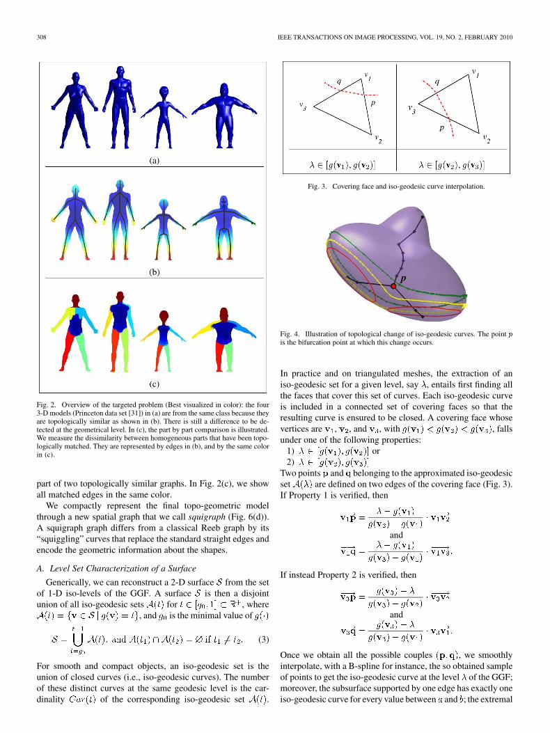
Fig. 3. Covering face and iso-geodesic curve interpolation.

Fig. 4. Illustration of topological change of iso-geodesic curves. The point �is the bifurcation point at which this change occurs.

In practice and on triangulated meshes, the extraction of aniso-geodesic set for a given level, say , entails first finding allthe faces that cover this set of curves. Each iso-geodesic curveis included in a connected set of covering faces so that theresulting curve is ensured to be closed. A covering face whosevertices are , , and , with , fallsunder one of the following properties:

1) or2)

Two points and belonging to the approximated iso-geodesicset are defined on two edges of the covering face (Fig. 3).If Property 1 is verified, then

and

If instead Property 2 is verified, then

and

Once we obtain all the possible couples , we smoothlyinterpolate, with a B-spline for instance, the so obtained sampleof points to get the iso-geodesic curve at the level of the GGF;moreover, the subsurface supported by one edge has exactly oneiso-geodesic curve for every value between and ; the extremal

AOUADA AND KRIM: SQUIGRAPHS FOR FINE AND COMPACT MODELING OF 3-D SHAPES 309

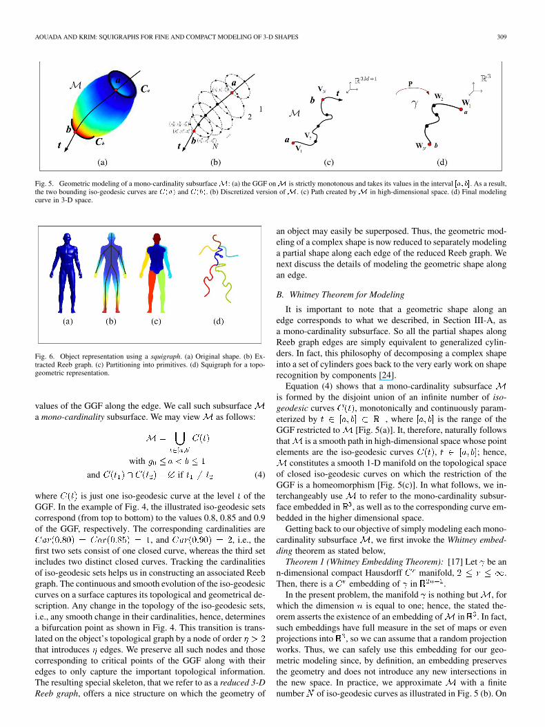
Fig. 5. Geometric modeling of a mono-cardinality subsurface�: (a) the GGF on� is strictly monotonous and takes its values in the interval ��� ��. As a result,the two bounding iso-geodesic curves are ���� and ����. (b) Discretized version of�. (c) Path created by� in high-dimensional space. (d) Final modelingcurve in 3-D space.

Fig. 6. Object representation using a squigraph. (a) Original shape. (b) Ex-tracted Reeb graph. (c) Partitioning into primitives. (d) Squigraph for a topo-geometric representation.

values of the GGF along the edge. We call such subsurfacea mono-cardinality subsurface. We may view as follows:

with

and if (4)

where is just one iso-geodesic curve at the level of theGGF. In the example of Fig. 4, the illustrated iso-geodesic setscorrespond (from top to bottom) to the values 0.8, 0.85 and 0.9of the GGF, respectively. The corresponding cardinalities are

, and , i.e., thefirst two sets consist of one closed curve, whereas the third setincludes two distinct closed curves. Tracking the cardinalitiesof iso-geodesic sets helps us in constructing an associated Reebgraph. The continuous and smooth evolution of the iso-geodesiccurves on a surface captures its topological and geometrical de-scription. Any change in the topology of the iso-geodesic sets,i.e., any smooth change in their cardinalities, hence, determinesa bifurcation point as shown in Fig. 4. This transition is trans-lated on the object’s topological graph by a node of orderthat introduces edges. We preserve all such nodes and thosecorresponding to critical points of the GGF along with theiredges to only capture the important topological information.The resulting special skeleton, that we refer to as a reduced 3-DReeb graph, offers a nice structure on which the geometry of

an object may easily be superposed. Thus, the geometric mod-eling of a complex shape is now reduced to separately modelinga partial shape along each edge of the reduced Reeb graph. Wenext discuss the details of modeling the geometric shape alongan edge.

B. Whitney Theorem for Modeling

It is important to note that a geometric shape along anedge corresponds to what we described, in Section III-A, asa mono-cardinality subsurface. So all the partial shapes alongReeb graph edges are simply equivalent to generalized cylin-ders. In fact, this philosophy of decomposing a complex shapeinto a set of cylinders goes back to the very early work on shaperecognition by components [24].

Equation (4) shows that a mono-cardinality subsurfaceis formed by the disjoint union of an infinite number of iso-geodesic curves , monotonically and continuously param-eterized by , where is the range of theGGF restricted to [Fig. 5(a)]. It, therefore, naturally followsthat is a smooth path in high-dimensional space whose pointelements are the iso-geodesic curves , ; hence,

constitutes a smooth 1-D manifold on the topological spaceof closed iso-geodesic curves on which the restriction of theGGF is a homeomorphism [Fig. 5(c)]. In what follows, we in-terchangeably use to refer to the mono-cardinality subsur-face embedded in , as well as to the corresponding curve em-bedded in the higher dimensional space.

Getting back to our objective of simply modeling each mono-cardinality subsurface , we first invoke the Whitney embed-ding theorem as stated below,

Theorem 1 (Whitney Embedding Theorem): [17] Let be ann-dimensional compact Hausdorff manifold, .Then, there is a embedding of in .

In the present problem, the manifold is nothing but , forwhich the dimension is equal to one; hence, the stated the-orem asserts the existence of an embedding of in . In fact,such embeddings have full measure in the set of maps or evenprojections into , so we can assume that a random projectionworks. Thus, we can safely use this embedding for our geo-metric modeling since, by definition, an embedding preservesthe geometry and does not introduce any new intersections inthe new space. In practice, we approximate with a finitenumber of iso-geodesic curves as illustrated in Fig. 5 (b). On

310 IEEE TRANSACTIONS ON IMAGE PROCESSING, VOL. 19, NO. 2, FEBRUARY 2010

each curve, we take uniformly spaced points defined bytheir Euclidean coordinates , , and

. Each curve is now a point in repre-sented by the column vector , [Fig. 5(c)],such that

(5)

The sample set of iso-geodesic curves on is a matrix ofdimension where . Applying theWhitney theorem on reduces the embedding problem to asimple linear formulation

(6)

where is a set of points in resulting from the projectionof via into . In other words, as illustrated in Fig. 5(d), themanifold is reduced to a space curve whose sample pointsare represented by the columns of the matrix . In Fig. 6, weillustrate the idea of a topo-geometric modeling via the spacemodeling curves that we just defined; hence, we intrinsicallyenhance the typical 3-D Reeb graph of Fig. 6(b). To that end,we assign one modeling curve to each edge of the Reeb graph.By so doing, we may view the final representation as a new kindof graph, that we refer to as a squigraph, as shown in Fig. 6(d).The Whitney embedding theorem guarantees that almost anyprojection of is an embedding. In [19] and [20], the notionof good Whitney embedding is introduced to identify a classof projections. For many applications, such as recognition, aunique representation of an object is required. As a result, weapply the notion of optimal embedding with the performancecriterion presented in [20] and defined in (8) being maximized.

We recall that an embedding gives us a one-to-one mappingbetween the path in high-dimensional space , andthe path , so that no two points in will collapse as aresult of the mapping in (6). An implementation of this principleis presented in [20] and referred to as a secant based method. Asjust explained, no two points in are mapped to the samepoint in . This means that the projecting vector is linearlyindependent from any possible secant2 in . We define theset of all possible unit secant vectors from the initial data asfollows:

and

(7)

with .The performance of the projection operator is then reflected

by

(8)

The closer is to 1, the better spread out the projected points inare, and the better the choice of is; hence, finding a good

estimate of the optimal projection is reduced to the followingminimization problem:

2Secant or secant line is a line that intersects two points from a curve.

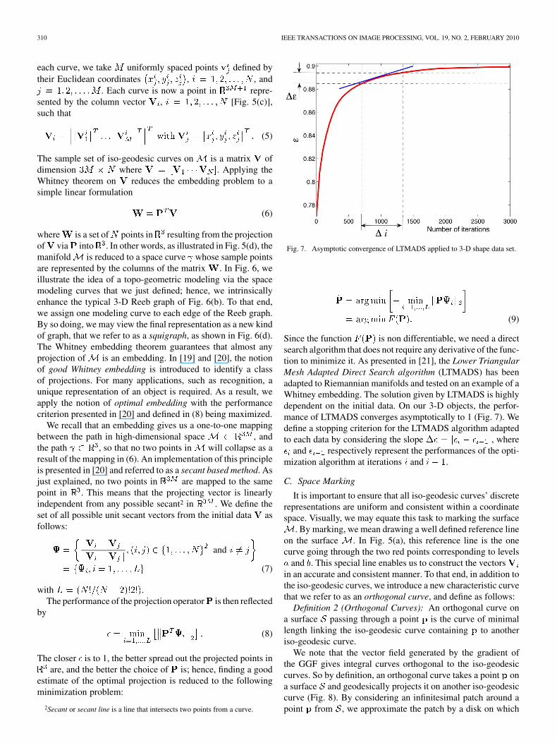
Fig. 7. Asymptotic convergence of LTMADS applied to 3-D shape data set.

(9)

Since the function is non differentiable, we need a directsearch algorithm that does not require any derivative of the func-tion to minimize it. As presented in [21], the Lower TriangularMesh Adapted Direct Search algorithm (LTMADS) has beenadapted to Riemannian manifolds and tested on an example of aWhitney embedding. The solution given by LTMADS is highlydependent on the initial data. On our 3-D objects, the perfor-mance of LTMADS converges asymptotically to 1 (Fig. 7). Wedefine a stopping criterion for the LTMADS algorithm adaptedto each data by considering the slope , where

and respectively represent the performances of the opti-mization algorithm at iterations and .

C. Space Marking

It is important to ensure that all iso-geodesic curves’ discreterepresentations are uniform and consistent within a coordinatespace. Visually, we may equate this task to marking the surface

. By marking, we mean drawing a well defined reference lineon the surface . In Fig. 5(a), this reference line is the onecurve going through the two red points corresponding to levels

and . This special line enables us to construct the vectorsin an accurate and consistent manner. To that end, in addition tothe iso-geodesic curves, we introduce a new characteristic curvethat we refer to as an orthogonal curve, and define as follows:

Definition 2 (Orthogonal Curves): An orthogonal curve ona surface passing through a point is the curve of minimallength linking the iso-geodesic curve containing to anotheriso-geodesic curve.

We note that the vector field generated by the gradient ofthe GGF gives integral curves orthogonal to the iso-geodesiccurves. So by definition, an orthogonal curve takes a point ona surface and geodesically projects it on another iso-geodesiccurve (Fig. 8). By considering an infinitesimal patch around apoint from , we approximate the patch by a disk on which

AOUADA AND KRIM: SQUIGRAPHS FOR FINE AND COMPACT MODELING OF 3-D SHAPES 311

Fig. 8. Orthogonal curve extraction using infinitesimal patches around eachpoint at increasing values of the GGF.

the iso-geodesic curve becomes a segment passing through. This segment represents the direction of zero variation of the

GGF. We find that the projection of on the next iso-geodesicsegment follows the perpendicular to on . Under the as-sumption that all points are uniformly distributed on the surfaceand since the iso-geodesic curve represents the direction of zerovariation of the GGF, we conclude, by duality, that the orthog-onal projection of is equivalent to finding the direction ofhighest variation of the GGF; hence, we construct an orthogonalcurve by progressively tracking, at a point level, the direction ofthe highest variation of the GGF. We determine the directionthat maximizes the directional derivative of at a point ; thus,we extract an orthogonal curve by progressively estimating anew direction starting at each new iso-geodesic level. We maywrite:

(10)

We note that we only need a starting point to extract an orthog-onal curve. This point, however, is not unique as it is only re-quired to be a point from a bounding iso-geodesic curve (or in Fig. 5). In fact, thanks to the construction proposed in(5), choosing a different starting point will only result in a mererotation of the reference axes in . Besides, because in thepresent geometric modeling we require a full invariance to Eu-clidean transforms, this rotation will have no effect on the finalmodeling curve [ in Fig. 5(d)]. Starting from a point with thelowest value of the GGF, and by progressively finding , we con-struct an orthogonal curve with respect to iso-geodesic curves.By construction, iso-geodesic curves are transversal to an or-thogonal curve. Consequently, a subset of the surface can bemodeled by a fiber bundle whose base curve is an orthogonalcurve and whose bundles are the associated iso-geodesic curvesas illustrated in Fig. 5(b).

IV. THREE-DIMENSIONAL SHAPE COMPARISON

Our proposed squigraph model provides a topological anda geometric representation. The topological representation iscoarse, and, hence, initiates a shape comparison procedure. Wecall upon the additional geometric enhancement once there isa minimally significant similarity score that is attained whencomparing topological Reeb graphs. In what follows, we define

the necessary and applied measures at the different comparisonlevels.

A. Comparison of Reeb Graphs3

Reeb graphs being topological descriptors, we require a con-nectivity information to define a distance between them. We ac-tually use reduced Reeb graphs where the node order is never2. We herein define a distance measure that is in the same spiritas the edit-distance for shape matching as defined in [23]. Wecompute in (11) the similarity score between two reducedReeb graphs and with and nodes, respectively, and

. We denote by the nodes of , andthe nodes of . We define the similarity between these twographs as follows:

(11)

with

iffotherwise

and

(12)

where is a strictly positive constant of our choosing andand are the orders of nodes and , respectively. Thefunction plays the role of a registration operator basedon the order of graph nodes. We also choose a kernel func-tion that is strictly decreasing; hence, the choice of theGaussian kernel in (12). The intuition behind choosing the factor

is the assignment of a high similarity weight to registerednodes if they correspond to GGF levels that are close. The choiceof can greatly affect the graph matching process. Indeed, it de-fines a margin for a good match, after which the similarity scoreis supposed to decay. Too large values of incur no selectivity,and the matching becomes inaccurate. Too small values makethe comparison rigid, and only allow high similarity scores be-tween perfectly overlapping shapes which defeats the purpose ofa multilevel comparison (coarse and fine). For our experiments,the empirical value of 0.2 provided good results. In general, andfor data sets with no prior knowledge, a leaning strategy canhelp find a good choice for .

B. Comparison of Squigraphs

In Section III, we proposed to represent the geometry ofsmooth 2-D mono-cardinality surfaces captured by charac-teristic curves by just one curve in , namely, the modelingcurve. The problem of comparing 3-D objects may hence bereduced to measuring the dissimilarity between space curvesup to a similarity transform. The measure we choose appearsto be critical in assessing the effectiveness of the modelingcurves in accurately reflecting the geometric properties of3-D shapes. To ensure a good performance, we define a newtechnique for space curve comparison. The key objective of thistechnique is to select geometric features that are appropriate

3Section IV-A appeared in [22].

312 IEEE TRANSACTIONS ON IMAGE PROCESSING, VOL. 19, NO. 2, FEBRUARY 2010

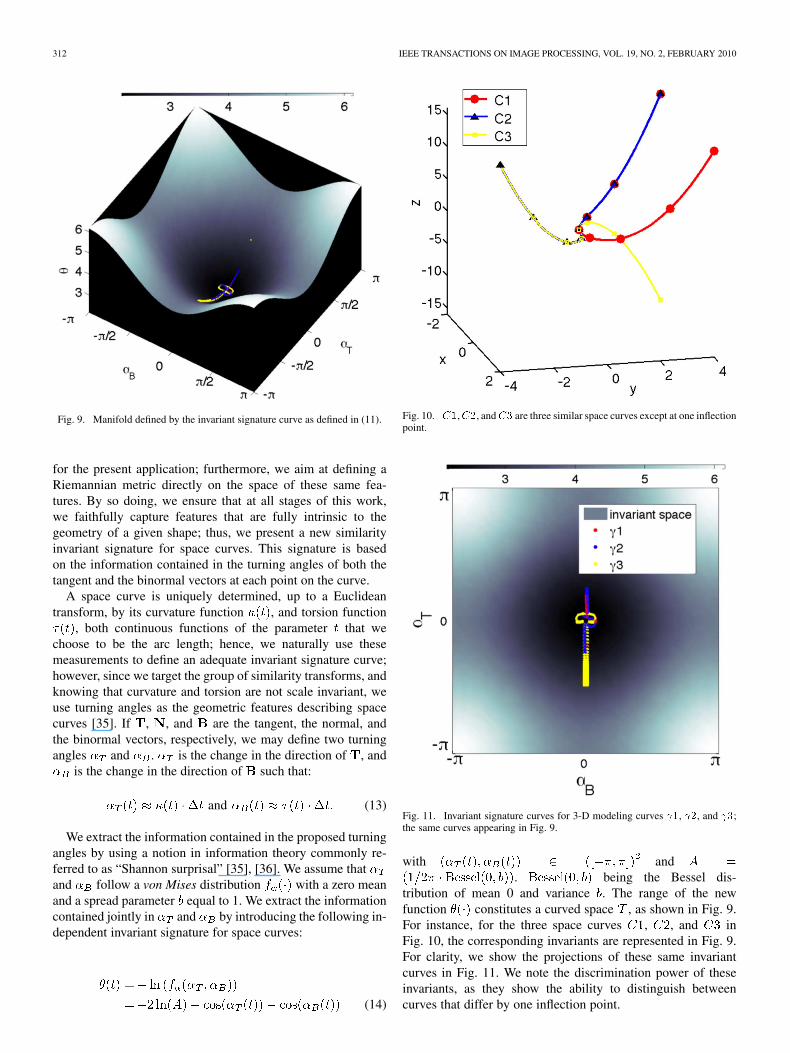
Fig. 9. Manifold defined by the invariant signature curve as defined in (11).

for the present application; furthermore, we aim at defining aRiemannian metric directly on the space of these same fea-tures. By so doing, we ensure that at all stages of this work,we faithfully capture features that are fully intrinsic to thegeometry of a given shape; thus, we present a new similarityinvariant signature for space curves. This signature is basedon the information contained in the turning angles of both thetangent and the binormal vectors at each point on the curve.

A space curve is uniquely determined, up to a Euclideantransform, by its curvature function , and torsion function

, both continuous functions of the parameter that wechoose to be the arc length; hence, we naturally use thesemeasurements to define an adequate invariant signature curve;however, since we target the group of similarity transforms, andknowing that curvature and torsion are not scale invariant, weuse turning angles as the geometric features describing spacecurves [35]. If , , and are the tangent, the normal, andthe binormal vectors, respectively, we may define two turningangles and . is the change in the direction of , and

is the change in the direction of such that:

and (13)

We extract the information contained in the proposed turningangles by using a notion in information theory commonly re-ferred to as “Shannon surprisal” [35], [36]. We assume thatand follow a von Mises distribution with a zero meanand a spread parameter equal to 1. We extract the informationcontained jointly in and by introducing the following in-dependent invariant signature for space curves:

(14)

Fig. 10. ��,��, and�� are three similar space curves except at one inflectionpoint.

Fig. 11. Invariant signature curves for 3-D modeling curves ��, ��, and ��;the same curves appearing in Fig. 9.

with and. being the Bessel dis-

tribution of mean 0 and variance . The range of the newfunction constitutes a curved space , as shown in Fig. 9.For instance, for the three space curves , , and inFig. 10, the corresponding invariants are represented in Fig. 9.For clarity, we show the projections of these same invariantcurves in Fig. 11. We note the discrimination power of theseinvariants, as they show the ability to distinguish betweencurves that differ by one inflection point.

AOUADA AND KRIM: SQUIGRAPHS FOR FINE AND COMPACT MODELING OF 3-D SHAPES 313

All the invariant signatures are thus constrained to live on thedefined invariant space. We view an invariant signature curveas the trace for the corresponding geometry. Defining as thespace of possible traces is a natural way to register them. As aconsequence, we may directly apply a distance measure to com-pare these traces with no need for worrying about prior registra-tion of the traces. We thus choose to compare two traces and

, corresponding to two modeling curves and , by con-sidering the oriented curve . We use tools frommeasure theory and choose to refer to their physical intuitionin relating them to our problem [25], [26]. We start by viewing

the oriented version of the space as a vector field on theplane defined by the variables and . We di-

rectly relate to , and define it as follows:

This may also be written as

(15)

We define ; the projection of on the plane.is a 1-current in the space dual to the space of 1-forms

. This means that

(16)

With these notions in hand, we naturally use the flat normas the intrinsic distance between two mono-cardinality

surfaces and whose modeling curves are and , andwhose traces are and , respectively. We thus may write

for all (17)

where . The advantages of defining this com-parison technique are clearly presented in a different paper. Wefurthermore define a global metric for the comparison of com-plex squigraphs. So we consider that and are now twocompound 2-D surfaces such that each one is composed ofmono-cardinality surfaces and ,

and (18)

We define the new distance between the two surfaces andas follows:

(19)

We run the topological matching of objects with the distancedefined in (11) prior to running the geometrical comparison

with the distance . In our experiments we use both distancesbut will only analyze the geometric comparison as it is the focusof this paper.

V. EXPERIMENTS

We experimentally investigate the performance of the pro-posed shape modeling technique. Throughout our definition andpresentation of squigraphs, we have shown how rich they are ininformation. In what follows, we illustrate how to exploit this in-formation for different levels of discrimination and for differentapplication objectives; furthermore, we investigate the robust-ness properties of squigraphs through some pertinent examples.

A. Discrimination Power

To assess the overall discrimination power of squigraphs,we compare their performance to those of well establishedapproaches. Our comparison involves the following techniques.

• Probability density function (PDF) descriptors: Using thedistributions of surface features is a technique that was firstclearly defined and analyzed by Funkhouser et al. [30].In our experiments, we use the GGF as the surface fea-ture, and its distribution as the shape descriptor. We choosethe Jensen-Shannon Divergence (JSD) as the dissimilaritymeasure between the GGF distributions [12], [28]–[30].

• Classification by Characteristic Resolution (CCR) [8]: Wehave shown in [8] that each class of shapes determinesa characteristic resolution.4 This parameter is extractedthrough a global comparison of the distribution of theGGF for each class of 3-D objects. In short, we may definethe characteristic resolution as being the lowest resolutionat which all class members will be accurately represented.

• Augmented Multiresolution Reeb Graph (aMRG) [4]: Thistechnique is the closest to squigraphs because of its two-level philosophy, and because of the similar Morse func-tion it primarily uses in defining a Reeb graph. aMRG is atechnique that has been experimentally established to out-perform many 3-D classification techniques including themethod of spherical harmonics [37].

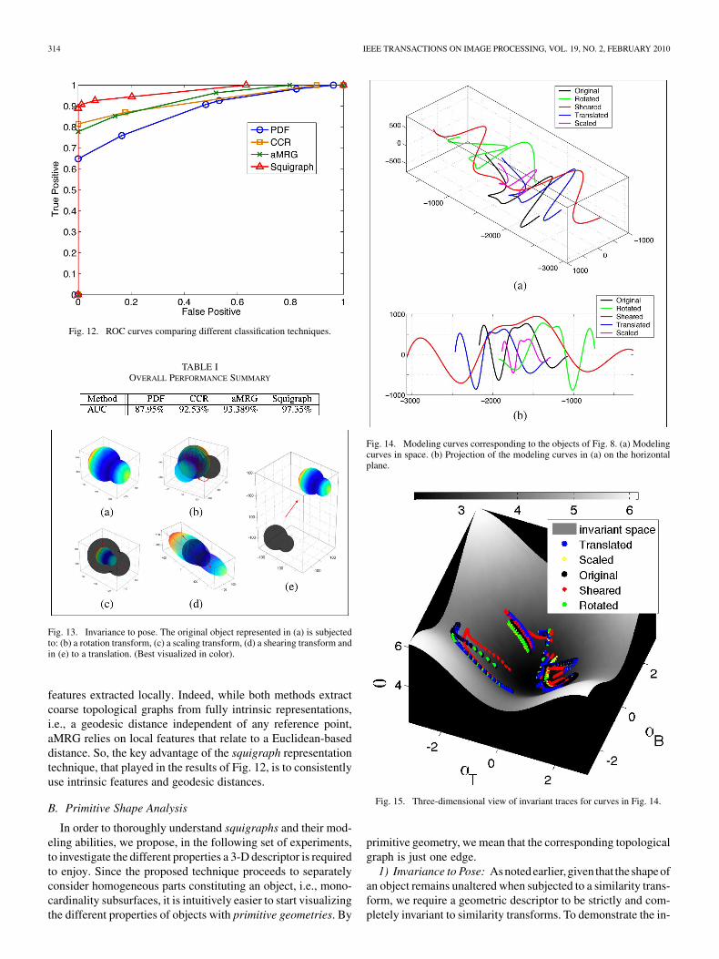
To be able to compare all these different techniques on the samebasis we use Receiver Operating Characteristic curves (ROC)as illustrated in Fig. 12. We then use the Area Under the Curve(AUC) as our measure for classification performance. We usethe Princeton [31] and the Technion data sets [32]–[34] for atotal of 17 classes and 239 objects. The overall performanceAUC for each technique is summarized in Table I. With a littlemore than 97% of overall performance, we note that squigraphsoutperform other techniques. Doing better than PDF and CCRis quite expected as these two techniques only provide a globaldescription of a complex shape. It becomes more challengingto clearly distinguish between two objects whose global shapesare very similar. As presented earlier in Section I, aMRG andsquigraphs are multilevel descriptors which enable them tocapture global, as well as local features. We explain the betterperformance of squigraphs over aMRG by the nature of the

4Resolution: is the number of vertices used to describe a given shape.

314 IEEE TRANSACTIONS ON IMAGE PROCESSING, VOL. 19, NO. 2, FEBRUARY 2010

Fig. 12. ROC curves comparing different classification techniques.

TABLE IOVERALL PERFORMANCE SUMMARY

Fig. 13. Invariance to pose. The original object represented in (a) is subjectedto: (b) a rotation transform, (c) a scaling transform, (d) a shearing transform andin (e) to a translation. (Best visualized in color).

features extracted locally. Indeed, while both methods extractcoarse topological graphs from fully intrinsic representations,i.e., a geodesic distance independent of any reference point,aMRG relies on local features that relate to a Euclidean-baseddistance. So, the key advantage of the squigraph representationtechnique, that played in the results of Fig. 12, is to consistentlyuse intrinsic features and geodesic distances.

B. Primitive Shape Analysis

In order to thoroughly understand squigraphs and their mod-eling abilities, we propose, in the following set of experiments,to investigate the different properties a 3-D descriptor is requiredto enjoy. Since the proposed technique proceeds to separatelyconsider homogeneous parts constituting an object, i.e., mono-cardinality subsurfaces, it is intuitively easier to start visualizingthe different properties of objects with primitive geometries. By

Fig. 14. Modeling curves corresponding to the objects of Fig. 8. (a) Modelingcurves in space. (b) Projection of the modeling curves in (a) on the horizontalplane.

Fig. 15. Three-dimensional view of invariant traces for curves in Fig. 14.

primitive geometry, we mean that the corresponding topologicalgraph is just one edge.

1) Invariance to Pose: Asnotedearlier,given that theshape ofan object remains unaltered when subjected to a similarity trans-form, we require a geometric descriptor to be strictly and com-pletely invariant to similarity transforms. To demonstrate the in-

AOUADA AND KRIM: SQUIGRAPHS FOR FINE AND COMPACT MODELING OF 3-D SHAPES 315

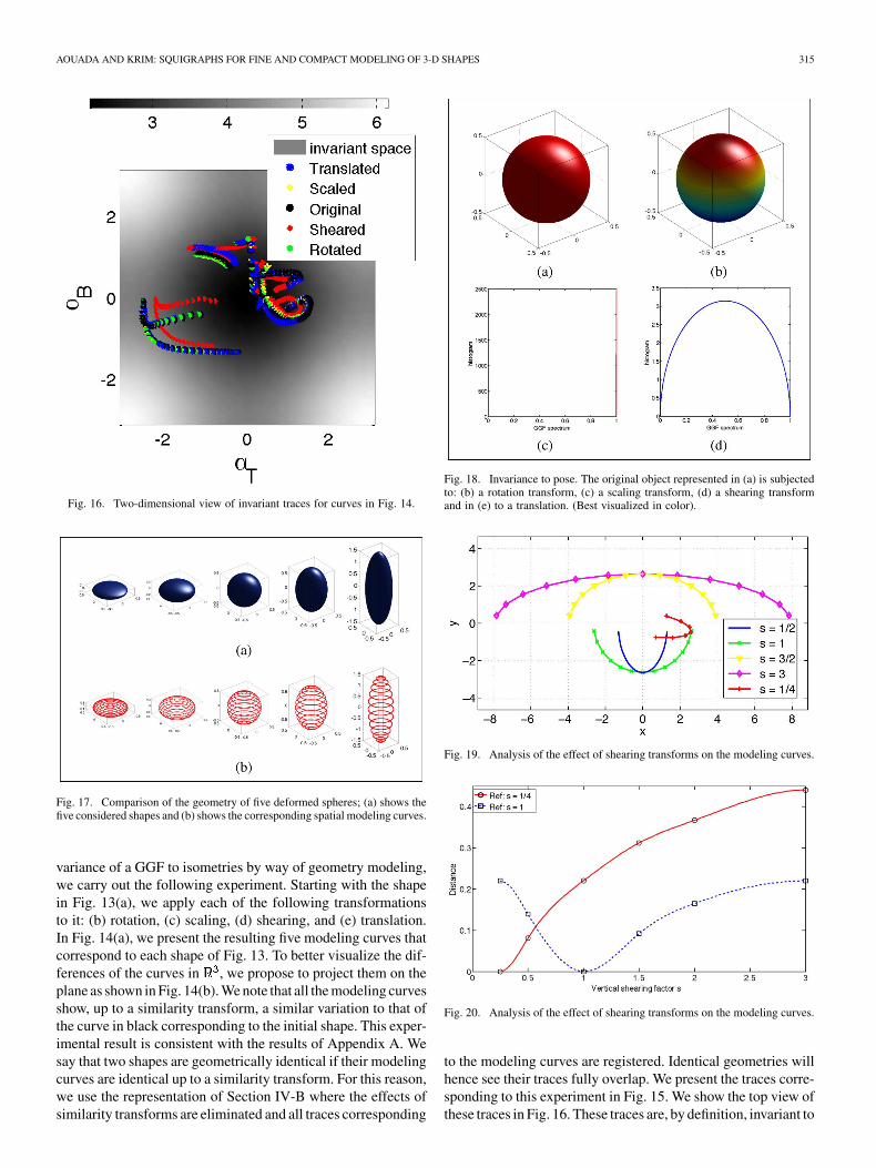
Fig. 16. Two-dimensional view of invariant traces for curves in Fig. 14.

Fig. 17. Comparison of the geometry of five deformed spheres; (a) shows thefive considered shapes and (b) shows the corresponding spatial modeling curves.

variance of a GGF to isometries by way of geometry modeling,we carry out the following experiment. Starting with the shapein Fig. 13(a), we apply each of the following transformationsto it: (b) rotation, (c) scaling, (d) shearing, and (e) translation.In Fig. 14(a), we present the resulting five modeling curves thatcorrespond to each shape of Fig. 13. To better visualize the dif-ferences of the curves in , we propose to project them on theplane as shown in Fig. 14(b). We note that all the modeling curvesshow, up to a similarity transform, a similar variation to that ofthe curve in black corresponding to the initial shape. This exper-imental result is consistent with the results of Appendix A. Wesay that two shapes are geometrically identical if their modelingcurves are identical up to a similarity transform. For this reason,we use the representation of Section IV-B where the effects ofsimilarity transforms are eliminated and all traces corresponding

Fig. 18. Invariance to pose. The original object represented in (a) is subjectedto: (b) a rotation transform, (c) a scaling transform, (d) a shearing transformand in (e) to a translation. (Best visualized in color).

Fig. 19. Analysis of the effect of shearing transforms on the modeling curves.

Fig. 20. Analysis of the effect of shearing transforms on the modeling curves.

to the modeling curves are registered. Identical geometries willhence see their traces fully overlap. We present the traces corre-sponding to this experiment in Fig. 15. We show the top view ofthese traces in Fig. 16. These traces are, by definition, invariant to

316 IEEE TRANSACTIONS ON IMAGE PROCESSING, VOL. 19, NO. 2, FEBRUARY 2010

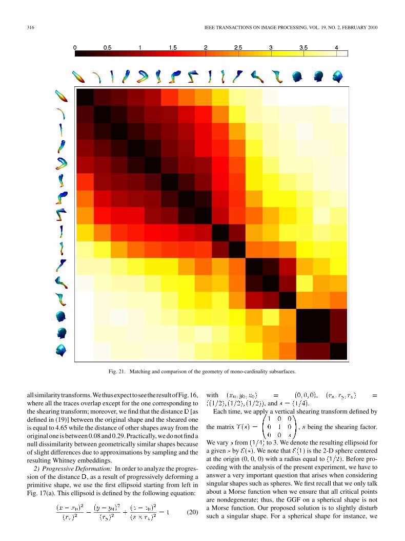
Fig. 21. Matching and comparison of the geometry of mono-cardinality subsurfaces.

allsimilaritytransforms.WethusexpecttoseetheresultofFig.16,where all the traces overlap except for the one corresponding tothe shearing transform; moreover, we find that the distance [asdefined in (19)] between the original shape and the sheared oneis equal to 4.65 while the distance of other shapes away from theoriginal one is between 0.08 and 0.29. Practically, we do not findanull dissimilarity between geometrically similar shapes becauseof slight differences due to approximations by sampling and theresulting Whitney embeddings.

2) Progressive Deformation: In order to analyze the progres-sion of the distance , as a result of progressively deforming aprimitive shape, we use the first ellipsoid starting from left inFig. 17(a). This ellipsoid is defined by the following equation:

(20)

with ,, and .

Each time, we apply a vertical shearing transform defined by

the matrix , being the shearing factor.

We vary from to 3. We denote the resulting ellipsoid fora given by . We note that is the 2-D sphere centeredat the origin (0, 0, 0) with a radius equal to . Before pro-ceeding with the analysis of the present experiment, we have toanswer a very important question that arises when consideringsingular shapes such as spheres. We first recall that we only talkabout a Morse function when we ensure that all critical pointsare nondegenerate; thus, the GGF on a spherical shape is nota Morse function. Our proposed solution is to slightly disturbsuch a singular shape. For a spherical shape for instance, we

AOUADA AND KRIM: SQUIGRAPHS FOR FINE AND COMPACT MODELING OF 3-D SHAPES 317

may disconnect a polar point from other points. As illustratedin Fig. 18, the distribution of the GGF on a spherical surfacequickly changes from a simple Dirac function to the distribu-tion shown in Fig. 18(d).

We apply this same perturbation technique to all the shapesin Fig. 17(a), and extract a modeling curve for each set of iso-geodesic curves in Fig. 17(b). Fig. 19 illustrates the resultingmodeling curves. Our first observation is that these curves areplanar, i.e., in , while the proposed Whitney modeling tech-nique is in . This is due to the simplicity of the evolution ofthe iso-geodesic curves. Very briefly, we state that more varia-tions imply more dimensions.

Focussing on this important aspect of predicting and under-standing the modeling curves constitutes a future research direc-tion. Indeed, the present experiment and its results lead to fur-ther investigations toward defining the applicability and limita-tions of the strong Whitney embedding versus the easy Whitneyembedding theorem.5

Our choice of a simple progressive vertical shearing trans-form is motivated by two points: first, applying a simple direc-tional geometric deformation, and second, being able to quan-titatively describe this deformation. In the present example weuse the shearing factor for this quantification; hence, we areable to visualize the variation of versus ; thus, the red fullcurve in Fig. 20 shows the smooth evolution of the distance be-tween and other ellipsoids with . Takinga sphere as the reference, i.e., , we may see the effect of thevertical deformation in the two directions and . Theresulting distance curve is illustrated in Fig. 20 with a dottedblue line. We note that the distance follows an exponentialbehavior as it starts slowing down for large values of . Onemay explain this tendency by referring back to the human per-ception. In fact, looking at Fig. 17(a), we may classify these el-lipsoids into two categories: category 1, corresponding to ;and category 2, corresponding to , the sphere rep-resenting the transition point. We then may say that when anellipsoid is deformed to be away from its category, the distance

is relatively high, but once it reaches a new category, addi-tional deformations in the same direction will only add slightdistances. We find, for instance, thatwhile , that is about 5 times the firstdistance and for the same . The present result constitutes animportant step in understanding the geometry of shapes, andtranslating the human perception of geometry.

3) Mono-Cardinality Subsurfaces: In this experiment wecontinue our observation and analysis of mono-cardinalitysubsurfaces, but this time we consider more complex shapesfound in real-world objects. We thus compare selected partsthat constitute the edges of the squigraphs extracted for thedata sets used in Section V-A.

We summarize our comparison results with the confusionmatrix in Fig. 21. We note that when legs are bent, the modelingcurves are still able to detect a difference between stretchedand bent legs. This phenomenon is equivalent to the exampleof Section IV-B where we illustrated how the modeling curves,

5Indeed, while the easy Whitney embedding theorem allows embedding ann-dimensional Hausdorff manifold into , the strong Whitney embeddingallows going lower and defining an embedding in [17].

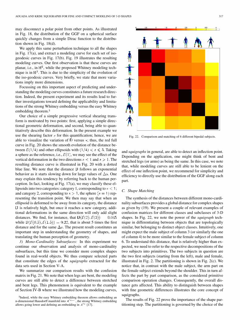
Fig. 22. Comparison and matching of 6 different bipedal subjects.

and squigraphs in general, are able to detect an inflection point.Depending on the application, one might think of bent andstretched legs (or arms) as being the same. In this case, we notethat, while modeling curves are still able to be lenient on theeffect of one inflection point, we recommend for simplicity andefficiency to directly use the distribution of the GGF along eachpart.

C. Shape Matching

The synthesis of the distances between different mono-cardi-nality subsurfaces provides a global distance for complex shapesas given by (19). We present a couple of relevant examples ofconfusion matrices for different classes and subclasses of 3-Dshapes. In Fig. 22, we note the power of the squigraph tech-nique in differentiating between objects that are topologicallysimilar, but belonging to distinct object classes. Intuitively, onemight expect the male subject of column 3 (or similarly the oneof column 4) to be more similar to the female subject of column6. To understand this distance, that is relatively higher than ex-pected, we need to refer to the respective decompositions of thetwo subjects into primitives. The two subjects in question arethe two first subjects (starting from the left), male and female,illustrated in Fig. 2. The partitioning is shown in Fig. 2(c). Wenotice that, in contrast with the male subject, the arm part onthe female subject extends beyond the shoulder. This in turn af-fects the part by part comparison, as the considered primitivecomparison operation changes. Consequently, the overall dis-tance gets affected. This ability to distinguish between shapeswith fine geometric differences illustrates the core concept ofsquigraphs.

The results of Fig. 22 prove the importance of the shape par-titioning step. The partitioning is governed by the choice of the

318 IEEE TRANSACTIONS ON IMAGE PROCESSING, VOL. 19, NO. 2, FEBRUARY 2010

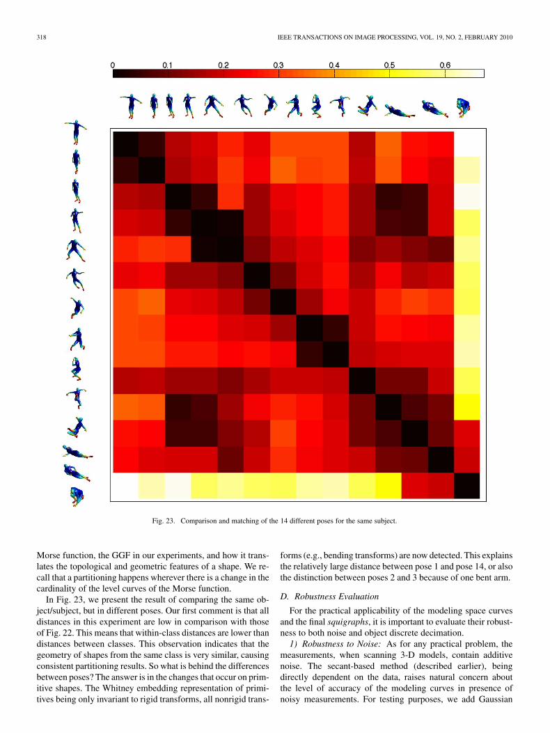
Fig. 23. Comparison and matching of the 14 different poses for the same subject.

Morse function, the GGF in our experiments, and how it trans-lates the topological and geometric features of a shape. We re-call that a partitioning happens wherever there is a change in thecardinality of the level curves of the Morse function.

In Fig. 23, we present the result of comparing the same ob-ject/subject, but in different poses. Our first comment is that alldistances in this experiment are low in comparison with thoseof Fig. 22. This means that within-class distances are lower thandistances between classes. This observation indicates that thegeometry of shapes from the same class is very similar, causingconsistent partitioning results. So what is behind the differencesbetween poses? The answer is in the changes that occur on prim-itive shapes. The Whitney embedding representation of primi-tives being only invariant to rigid transforms, all nonrigid trans-

forms (e.g., bending transforms) are now detected. This explainsthe relatively large distance between pose 1 and pose 14, or alsothe distinction between poses 2 and 3 because of one bent arm.

D. Robustness Evaluation

For the practical applicability of the modeling space curvesand the final squigraphs, it is important to evaluate their robust-ness to both noise and object discrete decimation.

1) Robustness to Noise: As for any practical problem, themeasurements, when scanning 3-D models, contain additivenoise. The secant-based method (described earlier), beingdirectly dependent on the data, raises natural concern aboutthe level of accuracy of the modeling curves in presence ofnoisy measurements. For testing purposes, we add Gaussian

AOUADA AND KRIM: SQUIGRAPHS FOR FINE AND COMPACT MODELING OF 3-D SHAPES 319

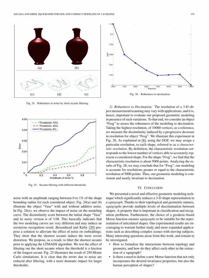
Fig. 24. Robustness to noise by short secants filtering.

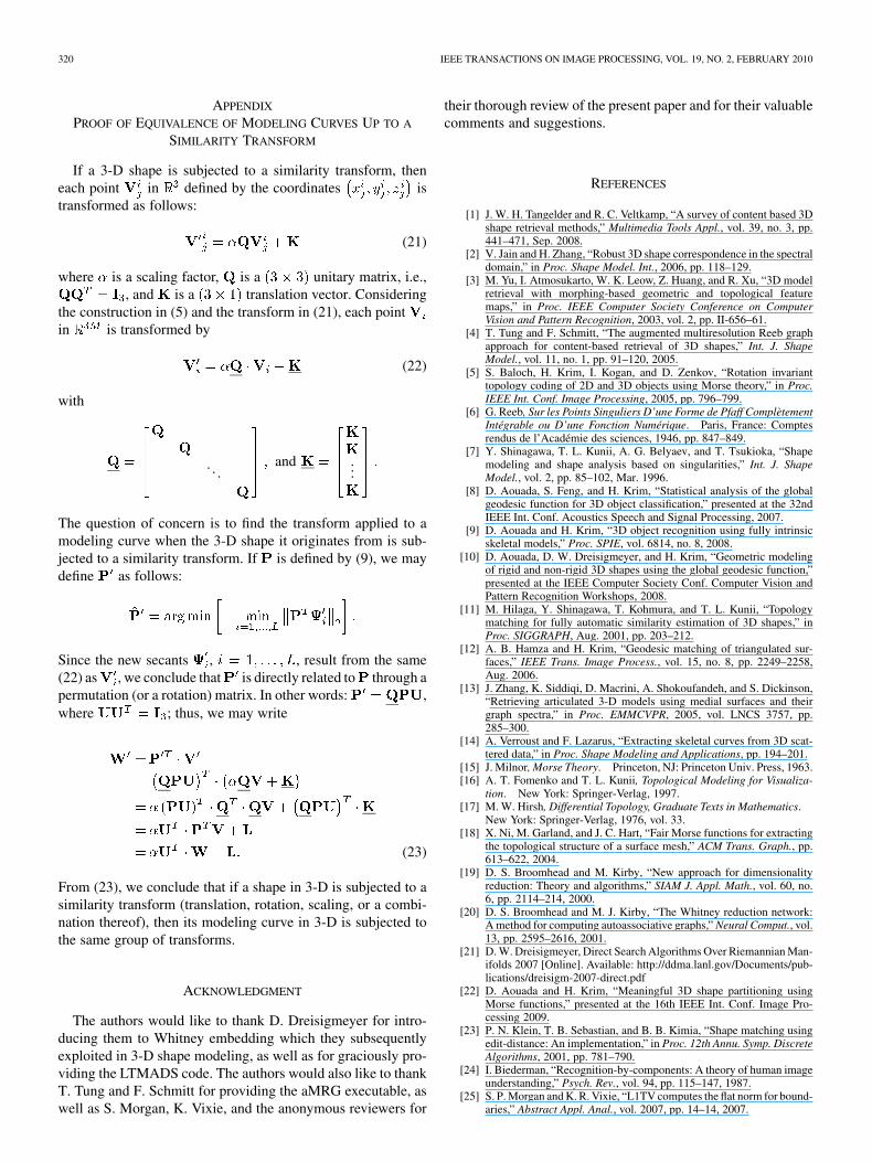
Fig. 25. Secants filtering with different thresholds.

noise with an amplitude ranging between 0 to 1% of the shapebounding radius for each considered object. Fig. 24(a) and (b)illustrate the object “Vase” with and without additive noise.In Fig. 24(e), we observe the impact of noise on the modelingcurve. The dissimilarity score between the initial shape “Vase”and its noisy version is of 3.08. This basically indicates thatthe two modeling curves are very different and may induce anerroneous recognition result. Broomhead and Kirby [20] pro-pose a solution to alleviate the effect of noise on embeddings.They show that the shortest secants induce the most severedistortion. We propose, as a result, to filter the shortest secantsprior to applying the LTMADS algorithm. We test the effect offiltering out the short secants where the threshold is a fractionof the longest secant. Fig. 25 illustrates the result of 250 MonteCarlo simulations. It is clear that the errors due to noise arereduced after filtering, with a more dramatic impact for largerthresholds.

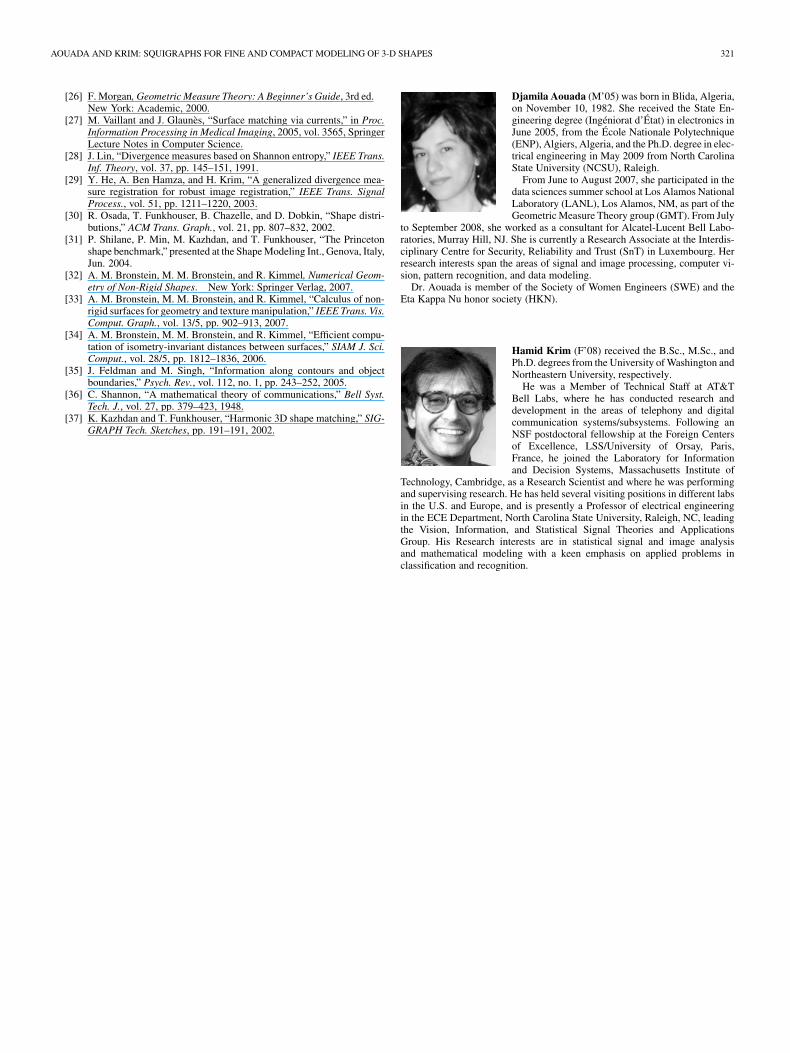
Fig. 26. Robustness to decimation.

2) Robustness to Decimation: The resolution of a 3-D ob-ject measurement/scanning may vary with applications, and it is,hence, important to evaluate our proposed geometric modelingin presence of such variations. To that end, we consider an object“Frog” to assess the robustness of the modeling to decimation.Taking the highest resolution, of 10000 vertices, as a reference,we measure the dissimilarity induced by a progressive decreasein resolution for object “Frog”. We illustrate this experiment inFig. 26. As explained in [8], using the GGF, we may assign aparticular resolution, to each shape, referred to as a character-istic resolution. By definition, the characteristic resolution cor-responds to the lowest number of vertices able to accurately rep-resent a considered shape. For the shape “Frog”, we find that thecharacteristic resolution is about 5000 points. Analyzing the re-sults of Fig. 26, we may conclude that for “Frog”, our modelingis accurate for resolutions greater or equal to the characteristicresolution of 5000 points. Thus, our geometric modeling is con-sistent and nearly invariant to decimation.

VI. CONCLUSION

We presented a novel and effective geometric modeling tech-nique which significantly reduces a 3-D shape representation toa squigraph. Thanks to their topological and geometric natures,squigraphs provide multiple levels of discrimination betweenshapes. A property that is important in classification and recog-nition problems. Furthermore, the choice of a geodesic-basedMorse function ensures squigraphs to be suitable for the repre-sentation of articulated shapes. Our experimental results are en-couraging to warrant further study and more expanded applica-tions such as describing complex scenes with moving subjects.Many interesting questions arose from this work, and remain tobe investigated.

• How to formalize the interactions between topology andgeometry, and how do they affect each other in the extrac-tion of a squigraph?

• Is there a need to define a new Morse function that not onlyincorporates the desired invariance properties, but also thehuman perception of shapes?

320 IEEE TRANSACTIONS ON IMAGE PROCESSING, VOL. 19, NO. 2, FEBRUARY 2010

APPENDIX

PROOF OF EQUIVALENCE OF MODELING CURVES UP TO A

SIMILARITY TRANSFORM

If a 3-D shape is subjected to a similarity transform, theneach point in defined by the coordinates istransformed as follows:

(21)

where is a scaling factor, is a unitary matrix, i.e.,, and is a translation vector. Considering

the construction in (5) and the transform in (21), each pointin is transformed by

(22)

with

. . .and ...

The question of concern is to find the transform applied to amodeling curve when the 3-D shape it originates from is sub-jected to a similarity transform. If is defined by (9), we maydefine as follows:

Since the new secants , , result from the same(22) as , we conclude that is directly related to through apermutation (or a rotation) matrix. In other words: ,where ; thus, we may write

(23)

From (23), we conclude that if a shape in 3-D is subjected to asimilarity transform (translation, rotation, scaling, or a combi-nation thereof), then its modeling curve in 3-D is subjected tothe same group of transforms.

ACKNOWLEDGMENT

The authors would like to thank D. Dreisigmeyer for intro-ducing them to Whitney embedding which they subsequentlyexploited in 3-D shape modeling, as well as for graciously pro-viding the LTMADS code. The authors would also like to thankT. Tung and F. Schmitt for providing the aMRG executable, aswell as S. Morgan, K. Vixie, and the anonymous reviewers for

their thorough review of the present paper and for their valuablecomments and suggestions.

REFERENCES

[1] J. W. H. Tangelder and R. C. Veltkamp, “A survey of content based 3Dshape retrieval methods,” Multimedia Tools Appl., vol. 39, no. 3, pp.441–471, Sep. 2008.

[2] V. Jain and H. Zhang, “Robust 3D shape correspondence in the spectraldomain,” in Proc. Shape Model. Int., 2006, pp. 118–129.

[3] M. Yu, I. Atmosukarto, W. K. Leow, Z. Huang, and R. Xu, “3D modelretrieval with morphing-based geometric and topological featuremaps,” in Proc. IEEE Computer Society Conference on ComputerVision and Pattern Recognition, 2003, vol. 2, pp. II-656–61.

[4] T. Tung and F. Schmitt, “The augmented multiresolution Reeb graphapproach for content-based retrieval of 3D shapes,” Int. J. ShapeModel., vol. 11, no. 1, pp. 91–120, 2005.

[5] S. Baloch, H. Krim, I. Kogan, and D. Zenkov, “Rotation invarianttopology coding of 2D and 3D objects using Morse theory,” in Proc.IEEE Int. Conf. Image Processing, 2005, pp. 796–799.

[6] G. Reeb, Sur les Points Singuliers D’une Forme de Pfaff ComplètementIntégrable ou D’une Fonction Numérique. Paris, France: Comptesrendus de l’Académie des sciences, 1946, pp. 847–849.

[7] Y. Shinagawa, T. L. Kunii, A. G. Belyaev, and T. Tsukioka, “Shapemodeling and shape analysis based on singularities,” Int. J. ShapeModel., vol. 2, pp. 85–102, Mar. 1996.

[8] D. Aouada, S. Feng, and H. Krim, “Statistical analysis of the globalgeodesic function for 3D object classification,” presented at the 32ndIEEE Int. Conf. Acoustics Speech and Signal Processing, 2007.

[9] D. Aouada and H. Krim, “3D object recognition using fully intrinsicskeletal models,” Proc. SPIE, vol. 6814, no. 8, 2008.

[10] D. Aouada, D. W. Dreisigmeyer, and H. Krim, “Geometric modelingof rigid and non-rigid 3D shapes using the global geodesic function,”presented at the IEEE Computer Society Conf. Computer Vision andPattern Recognition Workshops, 2008.

[11] M. Hilaga, Y. Shinagawa, T. Kohmura, and T. L. Kunii, “Topologymatching for fully automatic similarity estimation of 3D shapes,” inProc. SIGGRAPH, Aug. 2001, pp. 203–212.

[12] A. B. Hamza and H. Krim, “Geodesic matching of triangulated sur-faces,” IEEE Trans. Image Process., vol. 15, no. 8, pp. 2249–2258,Aug. 2006.

[13] J. Zhang, K. Siddiqi, D. Macrini, A. Shokoufandeh, and S. Dickinson,“Retrieving articulated 3-D models using medial surfaces and theirgraph spectra,” in Proc. EMMCVPR, 2005, vol. LNCS 3757, pp.285–300.

[14] A. Verroust and F. Lazarus, “Extracting skeletal curves from 3D scat-tered data,” in Proc. Shape Modeling and Applications, pp. 194–201.

[15] J. Milnor, Morse Theory. Princeton, NJ: Princeton Univ. Press, 1963.[16] A. T. Fomenko and T. L. Kunii, Topological Modeling for Visualiza-

tion. New York: Springer-Verlag, 1997.[17] M. W. Hirsh, Differential Topology, Graduate Texts in Mathematics.

New York: Springer-Verlag, 1976, vol. 33.[18] X. Ni, M. Garland, and J. C. Hart, “Fair Morse functions for extracting

the topological structure of a surface mesh,” ACM Trans. Graph., pp.613–622, 2004.

[19] D. S. Broomhead and M. Kirby, “New approach for dimensionalityreduction: Theory and algorithms,” SIAM J. Appl. Math., vol. 60, no.6, pp. 2114–214, 2000.

[20] D. S. Broomhead and M. J. Kirby, “The Whitney reduction network:A method for computing autoassociative graphs,” Neural Comput., vol.13, pp. 2595–2616, 2001.

[21] D. W. Dreisigmeyer, Direct Search Algorithms Over Riemannian Man-ifolds 2007 [Online]. Available: http://ddma.lanl.gov/Documents/pub-lications/dreisigm-2007-direct.pdf

[22] D. Aouada and H. Krim, “Meaningful 3D shape partitioning usingMorse functions,” presented at the 16th IEEE Int. Conf. Image Pro-cessing 2009.

[23] P. N. Klein, T. B. Sebastian, and B. B. Kimia, “Shape matching usingedit-distance: An implementation,” in Proc. 12th Annu. Symp. DiscreteAlgorithms, 2001, pp. 781–790.

[24] I. Biederman, “Recognition-by-components: A theory of human imageunderstanding,” Psych. Rev., vol. 94, pp. 115–147, 1987.

[25] S. P. Morgan and K. R. Vixie, “L1TV computes the flat norm for bound-aries,” Abstract Appl. Anal., vol. 2007, pp. 14–14, 2007.

AOUADA AND KRIM: SQUIGRAPHS FOR FINE AND COMPACT MODELING OF 3-D SHAPES 321

[26] F. Morgan, Geometric Measure Theory: A Beginner’s Guide, 3rd ed.New York: Academic, 2000.

[27] M. Vaillant and J. Glaunès, “Surface matching via currents,” in Proc.Information Processing in Medical Imaging, 2005, vol. 3565, SpringerLecture Notes in Computer Science.

[28] J. Lin, “Divergence measures based on Shannon entropy,” IEEE Trans.Inf. Theory, vol. 37, pp. 145–151, 1991.

[29] Y. He, A. Ben Hamza, and H. Krim, “A generalized divergence mea-sure registration for robust image registration,” IEEE Trans. SignalProcess., vol. 51, pp. 1211–1220, 2003.

[30] R. Osada, T. Funkhouser, B. Chazelle, and D. Dobkin, “Shape distri-butions,” ACM Trans. Graph., vol. 21, pp. 807–832, 2002.

[31] P. Shilane, P. Min, M. Kazhdan, and T. Funkhouser, “The Princetonshape benchmark,” presented at the Shape Modeling Int., Genova, Italy,Jun. 2004.

[32] A. M. Bronstein, M. M. Bronstein, and R. Kimmel, Numerical Geom-etry of Non-Rigid Shapes. New York: Springer Verlag, 2007.

[33] A. M. Bronstein, M. M. Bronstein, and R. Kimmel, “Calculus of non-rigid surfaces for geometry and texture manipulation,” IEEE Trans. Vis.Comput. Graph., vol. 13/5, pp. 902–913, 2007.

[34] A. M. Bronstein, M. M. Bronstein, and R. Kimmel, “Efficient compu-tation of isometry-invariant distances between surfaces,” SIAM J. Sci.Comput., vol. 28/5, pp. 1812–1836, 2006.

[35] J. Feldman and M. Singh, “Information along contours and objectboundaries,” Psych. Rev., vol. 112, no. 1, pp. 243–252, 2005.

[36] C. Shannon, “A mathematical theory of communications,” Bell Syst.Tech. J., vol. 27, pp. 379–423, 1948.

[37] K. Kazhdan and T. Funkhouser, “Harmonic 3D shape matching,” SIG-GRAPH Tech. Sketches, pp. 191–191, 2002.

Djamila Aouada (M’05) was born in Blida, Algeria,on November 10, 1982. She received the State En-gineering degree (Ingéniorat d’État) in electronics inJune 2005, from the École Nationale Polytechnique(ENP), Algiers, Algeria, and the Ph.D. degree in elec-trical engineering in May 2009 from North CarolinaState University (NCSU), Raleigh.

From June to August 2007, she participated in thedata sciences summer school at Los Alamos NationalLaboratory (LANL), Los Alamos, NM, as part of theGeometric Measure Theory group (GMT). From July

to September 2008, she worked as a consultant for Alcatel-Lucent Bell Labo-ratories, Murray Hill, NJ. She is currently a Research Associate at the Interdis-ciplinary Centre for Security, Reliability and Trust (SnT) in Luxembourg. Herresearch interests span the areas of signal and image processing, computer vi-sion, pattern recognition, and data modeling.

Dr. Aouada is member of the Society of Women Engineers (SWE) and theEta Kappa Nu honor society (HKN).

Hamid Krim (F’08) received the B.Sc., M.Sc., andPh.D. degrees from the University of Washington andNortheastern University, respectively.

He was a Member of Technical Staff at AT&TBell Labs, where he has conducted research anddevelopment in the areas of telephony and digitalcommunication systems/subsystems. Following anNSF postdoctoral fellowship at the Foreign Centersof Excellence, LSS/University of Orsay, Paris,France, he joined the Laboratory for Informationand Decision Systems, Massachusetts Institute of

Technology, Cambridge, as a Research Scientist and where he was performingand supervising research. He has held several visiting positions in different labsin the U.S. and Europe, and is presently a Professor of electrical engineeringin the ECE Department, North Carolina State University, Raleigh, NC, leadingthe Vision, Information, and Statistical Signal Theories and ApplicationsGroup. His Research interests are in statistical signal and image analysisand mathematical modeling with a keen emphasis on applied problems inclassification and recognition.