Faculty of Natural Resources and Agricultural Sciences

Spreading of Persistent Organic Pollutants from Fiber Bank Sediments

Lisa Vogel

Department of Aquatic Sciences and Assessment Master´s thesis • 30 ECTS • Second cycle, A2E EnvEuro - European Master in Environmental Sciences Uppsala, 2015

Spreading of Persistent Organic Pollutants from Fiber Bank Sediment in English

Lisa Vogel

Supervisor: Sarah Josefsson, Swedish University of Agricultural Sciences (SLU),Uppsala, Department of Aquatic Sciences and Assessment Prof. Dr. Andreas Paul Loibner, University of Natural Resources and Life Sciences (BOKU), Vienna Institute for Environmental Biotechnology

Examiner: Karin Wiberg,

Swedish University of Agricultural Sciences (SLU), Uppsala Department of Aquatic Sciences and Assessment

Credits: 30 ECTS Level: A2E Course title: Independent Project in Environmental Science – Master’s thesis Course code: EX0431 Programme/education: EnvEuro - European Master in Environmental Sciences Place of publication: Uppsala, Sweden Year of publication: 2015 Cover picture: Sarah Josefsson Online publication: http://stud.epsilon.slu.se Keywords: persistent organic pollutants, PCB, DDT, HCB, fiber bank, paper and pulp, sediment, POM, log Kd, log Kow, bioaccumulation, pore water concentration, Marenzelleria ssp., Saduria entomon

Sveriges lantbruksuniversitet

Swedish University of Agricultural Sciences

Faculty of Natural Resources and Agricultural Sciences Department of Aquatic Sciences and Assessment Section of Organic Environmental Chemistry and Ecotoxicology

I

Abstract

Discharge of untreated wastewater from paper and pulp industries have led to

large environmental impacts on the coastal sediments in Västernorrland, Sweden.

Dissolved fibers caused the formation of large fiber banks and fiber influenced

sediment areas, which proved to be highly affected by contamination with persis-

tent organic pollutants (POPs). Concentrations of hexachlorobenzene (HCB), 21

polychlorinated biphenyls (PCB) congeners and 6 substances of the dichlorodi-

phenyltrichloroethane (DDT) group were determined in sediment, pore water (ex-

tracted with polyoxymethylene (POM) strips) and two benthic biota species (Ma-

renzelleria ssp., Saduria entomon). Contaminants were extracted using Soxhlet

(sediment), shaking with acetone:n-hexane (POM) and cold column extraction

(biota). Multilayer clean-up columns were used for sediment and biota, before

instrumental analysis with GC-MS/MS.

Several sediment samples were classified with very high contamination levels for

HCB and PCB7, which is an indicator value of the seven most common PCBs in

nature. Different contaminant distribution patterns at the investigated sites indicat-

ed that contaminant composition varied at different local sources. Pore water con-

centrations were higher for less hydrophobic contaminant groups (HCB, DDT and

its derivates (DDX)). Sorption (log Kd) increased significantly with increasing

hydrophobicity (log Kow) and was significantly higher in fiber bank sediments than

in fiber rich sediments and less affected sediments. Bioaccumulation, measured

with biota-sediment-accumulation factors (BSAF), seemed to have a bell-shaped

distribution for Marenzelleria BSAFs when related to contaminant hydrophobi-

city; however, results observed were not significant. For Saduria entomon, bioac-

cumulation increased linearly with increasing contaminant hydrophobicity. Signif-

icant positive correlations between contaminant concentrations in biota and sedi-

ment or pore water was observed between concentrations in Marenzelleria on a

lipid weight basis and concentrations in sediment on a dry weight basis.

Keywords: persistent organic pollutants, PCB, DDT, HCB, fiber bank, paper and

pulp, sediment, POM, log Kd, log Kow, bioaccumulation, pore water concentration,

Marenzelleria ssp., Saduria entomon

Department of Aquatic Sciences and Assessment, Swedish University of Agricul-

tural Sciences (SLU), Lennart Hjelms väg 9, SE-75007 Uppsala

II

Popular science summary Sweden is among the world leaders in the production of paper and pulp. However,

this industry generates large quantities of wastewater that get discharged into the

Baltic Sea and thus potentially affects the aquatic environment. Effluent water

from the paper and pulp production contains contaminated cellulose or wood fi-

bers that can accumulate on the seafloor and lead to the formation of so called

fiber banks. Depending on the extent of fiber impact, these sediments can be cate-

gorized into 3 types: fiber bank sediment (consisting of 100% fibers), fiber rich

sediment and less affected sediment. The substances that have been investigated in

this study belong to the group of persistent organic pollutants (POPs) which are

difficult to degrade (persistent), can accumulate in living organisms (bioaccumula-

tive) and can be toxic. They are also hydrophobic, which means that they are re-

pelled by the water phase. Consequently, these contaminants prefer to sorb to par-

ticles and fat in living organisms. The contaminants analyzed in this study were 21

polychlorinated biphenyls (PCBs), dichlorodiphenyltrichloroethane (DDT) and its

5 closely related substances (all together named DDX) as well as hexachloroben-

zene (HCB). All contaminants had various applications (e.g. insulation, pesticide)

but all of them were also related to the paper and pulp production. Although their

production is banned nowadays, they are still found in the environment due to

their persistence. Concentrations of these pollutants were analyzed in the sedi-

ment, in the sediment pore water and in sediment biota in fiber bank areas near

Kramfors, Västernorrland. Generally, relatively high levels of contamination were

found in the fiber banks. In sediment and biota, the PCBs concentrations were

especially high. In the pore water, the less hydrophobic pollutants (HCB, DDX)

were found in higher concentrations, compared to the more hydrophobic ones (i.e.

PCBs). Moreover, the strength of the sorption of the contaminants and the tenden-

cy to accumulate in animals (bioaccumulation) was determined. The sorption was

higher in fiber bank sediments than in fiber rich sediments and less affected sedi-

ments because of differences in organic carbon content. The sorption of the con-

taminants increased with increasing hydrophobicity. The bioaccumulation of con-

taminants in the biota Marenzelleria and Saduria entomon generally increased

with increasing hydrophobicity, but declined again for the most hydrophobic ones

in Marenzelleria, possibly because the most hydrophobic contaminants are strong-

ly sorbed to the sediment. Reasons for the differences in bioaccumulation between

the two species could be due to differences in the feeding behavior.

In conclusion, the high pollution levels of POPs in the fiber banks and the high

accumulation in biota show that the fiber banks are an environmental concern.

More research is needed, in order to better understand and determine the impacts

of the spreading of these contaminants from fiber banks, as well as the related

risks for environment and society.

III

Table of contents List of tables V

List of figures VI

Abbreviations VII

1 Introduction and objectives 1

1.1 Introduction 1

1.2 Objectives 2

2 Background 3

2.1 Fiber banks 3

2.2 Target analytes and properties 4

2.2.1 Polychlorinated biphenyls (PCBs) 5

2.2.2 Dichlorodiphenyltrichloroethane (DDT) and its metabolites DDE and DDD 6

2.2.3 Hexachlorobenzene (HCB) 7

2.3 Biota species studied 8

2.4 Processes affecting the fate of POPs in the aquatic environment 9

2.4.1 POPs in sediments 9

2.4.2 Bioavailability 10

2.4.3 Uptake in biota, bioaccumulation and biomagnification 11

3 Material and methods 12

3.1 Chemicals and materials 12

3.1.1 Target analytes 12

3.1.2 Standards and calibration solutions 14

3.1.3 Other chemicals and equipment 14

3.2 Study area and sampling 15

3.3 Sample extraction and clean-up 18

3.3.1 Sediment 18

3.3.2 Pore water 19

3.3.3 Biota 20

3.4 Instrumental analysis 21

3.5 Quality assurance 21

3.6 Data analysis and calculations 23

4 Results 25

4.1 Method recovery 25

IV

4.2 POP concentrations and organic carbon content in sediment 25

4.3 Classification of sediments 30

4.4 POP relative distributions in sediments 31

4.5 POP concentrations in pore water 34

4.6 POP concentrations in biota 35

4.7 Relation between sorption or bioaccumulation and hydrophobicity (hypothesis 1) 36

4.7.1 Sorption 36

4.7.2 Bioaccumulation 36

4.8 Relation between sorption or bioaccumulation and sediment composition (hypothesis 2) 39

4.8.1 Sorption 39

4.8.2 Bioaccumulation 39

4.9 Relations between POP concentration in biota and concentration in pore water or total concentration (hypothesis 3) 41

5 Discussion 44

5.1 General findings 44

5.2 POP concentrations and organic carbon content in sediment 44

5.3 Classification of sediments 46

5.4 POP relative distributions in sediments 46

5.5 POP concentrations in pore water 47

5.6 POP concentrations in biota 47

5.7 Relation between sorption or bioaccumulation and hydrophobicity (hypothesis 1) 48

5.8 Relation between sorption or bioaccumulation and sediment composition (hypothesis 2) 50

5.9 Relations between POP concentration in biota and concentration in pore water or total concentration (hypothesis 3) 51

6 Conclusions and outlook 53

7 Acknowledgements 54

References 56

Appendix 60

V

List of tables

Table 1: Target analytes and their characteristics 13

Table 2: Method recoveries 25

Table 3: Percentage of total carbon content and the organic carbon content in each of the sediment samples. 28

Table 4: Level of contamination in sediment samples in ng/g dw classified based on the Swedish assessment criteria for organic pollutants in sediments along the Swedish coast. 31

Table 5: Properties of biota samples found at different sampling sites 35

Table 6: Results of the correlations between the concentrations in the two biota types and the concentrations in sediment and pore water. 41

VI

List of figures

Figure 1: Chemical structure of a biphenyl molecule with numbers indicating positions for configuration. 5

Figure 2: Chemical structures of the three para, para configured DDX compounds. 7

Figure 3: Chemical structure of hexachlorobenzene. 8

Figure 4: Location of the 3 fiber bank areas studied near Väja, Sandviken and Kramfors in Västernorrland, Sweden. 16

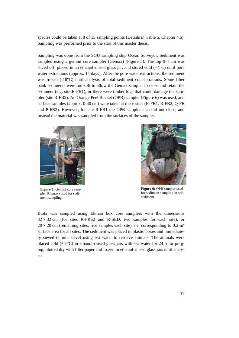
Figure 5: Gemini core sampler used for sediment sampling. 17

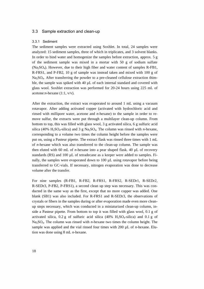
Figure 6: OPB sampler used for sediment sampling in soft sediment. 17

Figure 7: Contamination levels [ng/g dw] of the different compound groups in sediment samples. 26

Figure 8: Contamination levels [ng/g OC] of the different compound groups in sediment samples. 29

Figure 9: Distribution of analyzed compounds in each sediment sample. 33

Figure 10: Relationship between average sorption of contaminants and contaminant hydrophobicity. 37

Figure 11: Relationship between average Marenzelleria biota-sediment-accumulation factors of contaminants and contaminant hydrophobicity. 38

Figure 12: Relationship between average Saduria entomon biota-sediment-accumulation factors of contaminants and contaminant hydrophobicity. 38

Figure 13: Average sorption expressed in log Kd values in different sediment types. 40

Figure 14: Marenzelleria biota-sediment-accumulation factors in different sediment types, shown as an average BSAF of all compounds at one (FB) or more sites (FRS and SED). 40

Figure 15: Correlation between contaminant concentrations in Marenzelleria and a) sediment based on sediment dry weight, b) sediment based on organic carbon and c) pore water. 42

Figure 16: Correlation between contaminant concentrations in Saduria entomon and a) sediment based on sediment dry weight, b) sediment based on organic carbon and c) pore water. 43

VII

Abbreviations

∑PCBs Sum of the 21 PCBs analyzed in this study

Ah Aryl hydrocarbon (Ah receptor)

BSAF Biota-sediment-accumulation factor

Cfree Freely dissolved concentration

CL Subcooled liquid solubility

DDD Dichlorodiphenyldichloroethane

DDE Dichlorodiphenyldichloroethene

DDT Dichlorodiphenyltrichloroethane

DDX Sum of the six DDT related compounds analyzed

dw Dry weight

FB Fiber bank (sample name abbreviation)

FRS Fiber rich sediment (sample name abbreviation)

GC Gas chromatograph

HCB Hexachlorobenzene

IS Internal standards

Kd Solid-water partition coefficient

KOC Organic carbon-water partition coefficient

KOW Octanol-water partition coefficient

KPOM POM-water partition coefficient

LOD Limit of detection

LOI Loss on ignition

VIII

LOQ Limit of quantification

LW Lipid weight

MS Mass spectrometer

MW Molecular weight

OC Organic carbon

OPB sampler Orange peel bucket sampler

PCB Polychlorinated biphenyl

PCB7 Indicator parameter that sums up the most common PCBs in na-

ture (PCB 28, 52, 101, 118, 138, 153, 180)

PE Polyethylene

PES Performance evaluation standard

POM Polyoxymethylene

POP Persistent organic pollutant

RS Recovery standards

S/N Signal to noise ratio

SED Less affected sediment (sample name abbreviation)

SGU Swedish Geological Survey

(Sveriges geologiska undersökningar)

SLU Swedish University of Agricultural Sciences

(Sveriges lantbruksuniversitet)

SPME Solid phase microextraction

TCDD 2,3,7,8-tetrachlorodibenzo-p-dioxin

TEF Toxicity equivalent factor

v/v Volume per volume

ww Wet weight

1

1 Introduction and objectives

1.1 Introduction The forest industry is one of the main industries in Sweden and plays an important

role in Swedish economy. Various subindustries are comprised under this term:

forestry, pulp and paper industry, sawmill industry, carpentry industry, wood

board industry, manufacturing of refined wood fuel as well as the packaging pro-

duction from wood, paper and board. All together the forest industry in Sweden

provides around 55000 jobs (Swedish Forest Industries Federation, 2014). Among

the different parts of forest industry, the paper and pulp industry is the largest. In

2014, the production of 41 pulp mills summed up to a total production of 11.5

million tons (Swedish Forest Industries Federation, 2014). Almost 90 per cent of

the paper and pulp is exported, and combined with the sawn wood products, this

made Sweden the third largest exporter globally (Swedish Forest Industries

Federation, 2014).

However, the pulp and paper industry is not only accountable for jobs and eco-

nomic contribution, but also for the generation of pollutants. The high water de-

mand during the production process leads to the generation of large quantities of

waste water (Pokhrel & Viraraghavan, 2004). These polluted effluents impact the

environment, when not or insufficiently treated before being discharged into re-

ceiving waters.

On the seafloor around pulp and paper mills in Västernorrland, Sweden, large

accumulations of fibers have been observed. These so called fiber banks are

formed from fiber residues in the discharged wastewater. As part of the Fiberbank

project, the Swedish geological survey (SGU) mapped and sampled these fiber

banks. Within the scope of this master thesis, samples from the Formas project

TREASURE were analyzed in order to investigate the potential spreading of per-

2

sistent organic pollutants (POPs) from these fiber banks. However, sampling was

conducted within TREASURE before the start of this thesis project. This thesis

work consisted of chemical extraction of the contaminants, sample clean-up and

analysis, and analysis of the results.

1.2 Objectives The aim of this project was to investigate the presence and fate of persistent organ-

ic pollutants in three different fiber bank areas. The objective was to determine

how available the pollutants in the sediment are for uptake in living organisms and

transport to the water column. In order to do this, the amount of POPs was investi-

gated in different matrices, namely sediment, sediment pore water and biota.

As a basis for this research, three hypotheses were formulated:

1. There is a correlation between contaminant physical-chemical proper-

ties and sorption to sediment as well as between physical-chemical

properties and bioaccumulation. Sorption is lowest for compounds with

low hydrophobicity. Bioaccumulation is highest for compounds with

medium hydrophobicity.

2. There is a relationship between the sediment composition and sorption

as well as between sediment composition and bioaccumulation. High

fiber impacted sediments exhibit high organic carbon content and there-

fore sorption is high and bioaccumulation low.

3. Pollutant concentrations in biota correlate better to pore water concen-

trations than to total sediment concentrations.

3

2 Background

2.1 Fiber banks The forest industry is an important industry in Sweden. It has provided work and

generated export incomes, but it has also affected the environment. For example,

the high density of pulp and paper factories in Västernorrland county has had seri-

ous impacts on the coastal environment in the area. Wastewater from the industries

was discharged without cleaning for a long term period. The production-related

wood and cellulose fibers that were suspended in the water accumulated and

formed fiber banks in the water outside the factories. The Swedish Geological

Survey (SGU), in cooperation with the Västernorrland county administration,

identified and examined the fiber bank areas within the Fiberbank project (Apler

et al., 2014). In addition to looking at the spatial distribution of the banks, levels of

pollutants were determined. The fiber banks proved to be contaminated with e.g.

persistent organic pollutants (POPs) with levels classified as very high contamina-

tion (Apler et al., 2014). Contaminants found, e.g. polychlorinated biphenyls

(PCB) and dichlorodiphenyltrichloroethane (DDT), are linked to usage in forestry

as well as to pulp and paper production. Apler et al. (2014) differentiates between

pure fiber banks, which consist of 100% fiber material, and fiber rich sediments.

The fiber banks are usually located close to the factories, but can also be present

further away from the shoreline due to dredging activities to facilitate ship traffic

to the factories (Apler et al., 2014).

The Västernorrland coast, also known as the High Coast, lies within the region that

exhibits the fastest uplift of land (8-10 mm/year) nationwide (Apler et al., 2014).

This will cause the fibers banks to rise closer to the water surface and consequent-

ly be more prone to erosion from for example waves. In consequence, it might

lead to resuspension and spreading of the accumulated contamination. Further-

more, landslide scars and erosion channels have been detected by SGU in some of

4

the fiber banks in shallow water indicating that the pollutants present in the fiber

banks can disperse suddenly and in high amounts.

Apler et al. (2014) linked the contamination of the organic pollutants that are also

investigated in this work directly with the pulp and paper mills. Therefore the level

of contamination can be assessed as the impact of the local sources. Nevertheless,

high levels of pollutants not directly related to the paper production have been

detected as well. Saw mills, which are also present in the area, could be additional

potential pollution sources (Apler et al., 2014).

The contamination of the area combined with the described geological circum-

stances pose a serious risk for the coastal ecosystem in the area and the ecosystem

in the Gulf of Bothnia (Apler et al., 2014). It is to be suspected that areas around

other current or former paper mills are likely to have the same formation of fiber

banks, and fiber banks are therefore likely to be present along the northern Baltic

Sea coast, where the forest industry has been important. Despite the fact that the

impacts of fiber banks are a highly pressing issue and should be focused on, no

research or further investigations have been conducted on this topic so far. For this

reason the investigations of this project regarding the presence and fate of pollu-

tants in the fiber banks is of high relevance for the society.

2.2 Target analytes and properties All the contaminants investigated in this thesis are toxic organic chemicals that are

classified as Persistent Organic Pollutants (POP) according to the Stockholm Con-

vention (United Nations Environment Programme, 2004). Although many differ-

ent POPs exist, they exhibit some common characteristics: they are persistent,

bioaccumulative and toxic. Partitioning of these compounds usually takes place to

solids, especially organic matter, in aquatic ecosystems and into lipids in organ-

isms avoiding the aqueous milieu. This is due to their hydrophobicity and lipo-

philicity, which in combination with their persistence leads to the ability for accu-

mulation in organisms (bioaccumulation) and along the food chain (biomagnifica-

tion) (Jones, 1999). Bioaccumulative and biomagnifying properties contribute to

render POPs to pollutants of major concern regarding impacts on top predators,

which includes humans (Jones, 1999).

5

2.2.1 Polychlorinated biphenyls (PCBs) Polychlorinated biphenyls are a group of anthropogenic toxic pollutants that con-

sists of 209 congeners. The basic structure is a biphenyl that after being chlorinat-

ed incorporates between one to ten chlorine atoms instead of hydrogen atoms. The

different congeners are distinguished by different numbering according to the po-

sition of their chlorine atoms on the biphenyl rings (Baird & Cann, 2012) (Figure

1). Due to their chemical and physical stable characteristics, PCBs found a wide

range of applications. The main application was in capacitors and transformers as

electrical insulating fluids as well as for heat transfer and lubrication. Among oth-

ers, PCBs were also used in carbonless copy paper, paints and plastics (Erickson &

Kaley, 2011). Even though PCBs are no longer intentionally produced in the

world, the combination of their persistence together with widespread use and in-

appropriate disposal has made PCBs significant pollutants in the environment still

today (Baird & Cann, 2012). Being suspected of being endocrine disruptors as

well as carcinogenic, PCBs are recorded on several lists including the US EPA

List of Priority Pollutants and the Stockholm Convention (Tehrani & Van Aken,

2014).

The toxicity of PCBs is connected with their three-dimensional structure deter-

mined by the position of the chlorine atoms and their consequent ability to bind to

a cellular receptor in animals and humans. Planar congeners are dioxin-like and

therefore exhibit the same binding function to the aryl hydrocarbon (Ah) receptor,

which is connected to different toxic effects (Erickson & Kaley, 2011). PCB con-

geners that take on planar configuration and bind to the Ah receptor have at least

four chlorine atoms incorporated but none of them in the ortho position which is

the carbon atom next to the one that binds to the second aromatic ring. Similarly,

mono-ortho PCBs bind to the Ah receptor but less strongly. They also have at least

four chlorine atoms in any position but only one in an ortho position (Erickson &

Figure 1: Chemical structure of a biphenyl molecule with numbers indicating positions for

configuration.

6

Kaley, 2011). The twelve congeners that exist in these configurations have been

given toxicity equivalent factors (TEF) which express their binding ability to the

Ah receptor and therefore their toxicity in relation to TCDD

(2,3,7,8-tetrachlorodibenzo-p-dioxin), the most toxic dioxin (Van den Berg et al.,

2006).

2.2.2 Dichlorodiphenyltrichloroethane (DDT) and its metabolites DDE and DDD

DDT

The chemical formula of dichlorodiphenyltrichloroethane (DDT) is C14H9Cl5. It is

a substituted ethane, where at one of the carbon atoms all hydrogen atoms are re-

placed by chlorine atoms and two benzene rings substitute two hydrogen atoms at

the other carbon as shown in Figure 2 (Baird & Cann, 2012). DDT is an organo-

chlorine insecticide that has been used vastly for public health purposes for exam-

ple to fight malaria and other pests by killing mosquitos, fleas, and, lice. In even

higher amounts it was used as a pesticide in agriculture and forestry (Turusov et

al., 2002). In the environment, levels increased strongly due to overuse during the

1950s and 1960s (Baird & Cann, 2012). Due to its hydrophobic character it tends

to bind to organic matter and bioaccumulate in lipids. In the environment it can

therefore accumulate in tissues and in soils, which exhibit a strong sorptive capaci-

ty for this compound (Turusov et al., 2002). DDT is not acutely toxic (Turusov et

al., 2002) but due to ecological concerns and toxic effects on freshwater and ma-

rine organisms as well as on birds, Sweden banned the usage of DDT in 1970 and

many other countries followed (Turusov et al., 2002). Nevertheless, it is still used

for public health purposes in some developing countries (Turusov et al., 2002).

DDE

By elimination of HCl, DDT can be metabolized or degraded to dichlorodiphe-

nyldichloroethene (DDE), shown in Figure 2 (Baird & Cann, 2012). This metabo-

lite of DDT has been linked to eggshell thinning for birds (Baird & Cann, 2012;

Jones, 1999). DDE persists even longer in the body and is more relevant regarding

bioaccumulation than DDT, therefore the presence of DDE is an indicator for

chronic exposure to DDT (Jaga & Dharmani, 2003).

DDD

Another environmental degradation product of DDT that is also studied in this

project is dichlorodiphenyldichloroethane (DDD) (Figure 2). One of the three

chlorine atoms that bind to one of the carbon atoms in DDT is substituted with a

hydrogen atom in DDD. Due to their similarities regarding shape and size, DDD is

7

likewise toxic to insects and therefore was earlier also applied as an insecticide

(Baird & Cann, 2012).

The most important difference between these three compounds is their

three-dimensional structure. DDT and DDD are very similar and propeller-shaped,

while DDE has a more planar structure due to its carbon double bound. It does not

interfere with the insects’ nerve channel and consequently has no insecticidal func-

tion (Baird & Cann, 2012).

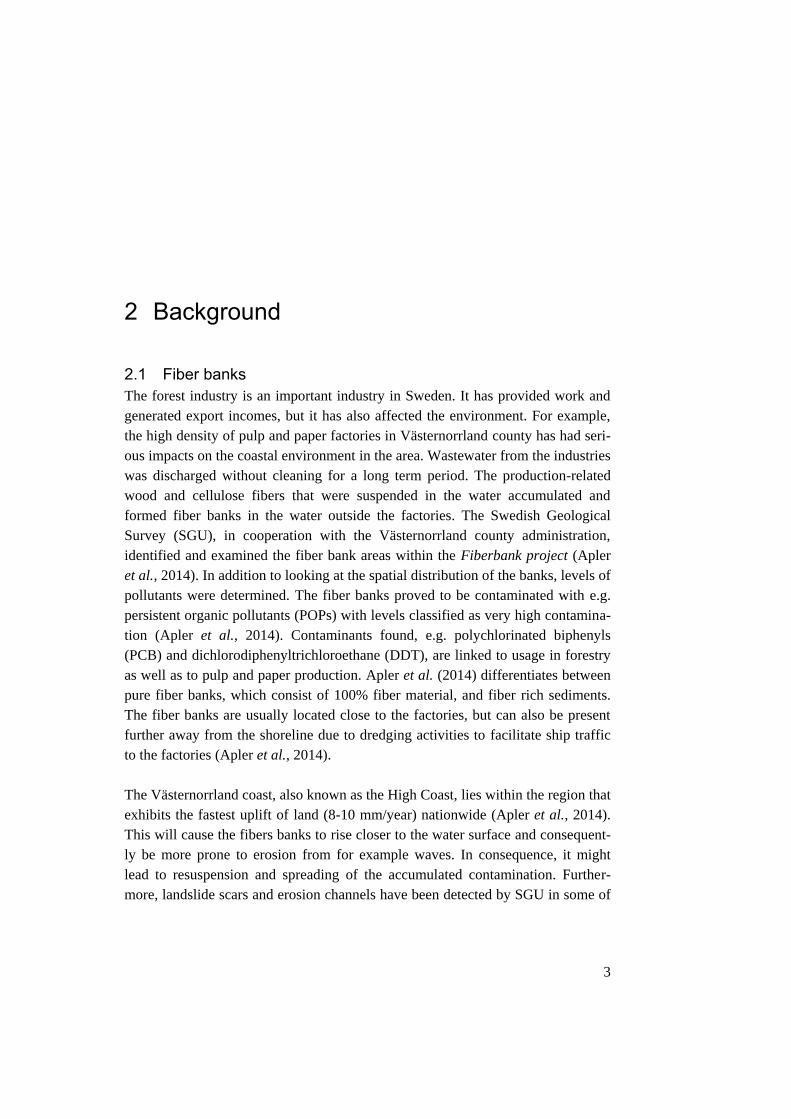
For each of the three contaminants, two isomers were analyzed. The name of the

isomer corresponds to the configuration of the molecule. The positions of the chlo-

rine atom on the ring are named ortho, meta or para, as for the PCBs. For all com-

pounds in this project the isomers with chlorine atoms on either both para posi-

tions (p,p’-DDT, p,p’-DDE, p,p’-DDD) (Figure 2) or chlorine atoms on ortho and

para positions (o,p’-DDT, o,p’-DDE, o,p’-DDD) were examined.

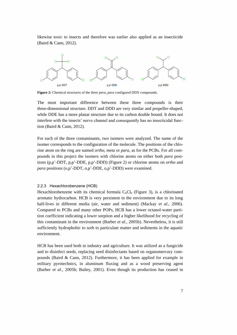
2.2.3 Hexachlorobenzene (HCB) Hexachlorobenzene with its chemical formula C6Cl6 (Figure 3), is a chlorinated

aromatic hydrocarbon. HCB is very persistent in the environment due to its long

half-lives in different media (air, water and sediment) (Mackay et al., 2006).

Compared to PCBs and many other POPs, HCB has a lower octanol-water parti-

tion coefficient indicating a lower sorption and a higher likelihood for recycling of

this contaminant in the environment (Barber et al., 2005b). Nevertheless, it is still

sufficiently hydrophobic to sorb to particulate matter and sediments in the aquatic

environment.

HCB has been used both in industry and agriculture. It was utilized as a fungicide

and to disinfect seeds, replacing seed disinfectants based on organomercury com-

pounds (Baird & Cann, 2012). Furthermore, it has been applied for example in

military pyrotechnics, in aluminum fluxing and as a wood preserving agent

(Barber et al., 2005b; Bailey, 2001). Even though its production has ceased in

Figure 2: Chemical structures of the three para, para configured DDX compounds.

8

most parts of the world (Bailey, 2001), HCB is still formed unintentionally as a

by-product or impurity in the chemical industry, as well as in combustion process-

es (Baird & Cann, 2012; Barber et al., 2005b).

According to several studies compiled by Barber et al. (2005a), HCB emissions

have also been detected from pulp and paper mills, but were suspected to be

caused by the use of HCB contaminated products, rather than with the actual pro-

duction of this hazardous compound.

2.3 Biota species studied Two biota species were found in the samples taken in this study: The isopod crus-

tacean Saduria entomon and the polychaete worm Marenzelleria spp. Organisms

were sampled in this study in order to measure contaminant concentrations in bio-

ta. Both biota types are benthic species and dig in the sediment they live in

(Josefsson et al., 2010; Haahtela, 1990). While the predator Saduria entomon,

feeds on other benthic fauna (Haahtela, 1990), Marenzelleria is a surface deposit-

feeder but can also make use of suspended particles in the water phase (Dauer et

al., 1981).

Figure 3: Chemical structure of hexachlorobenzene (HCB).

9

2.4 Processes affecting the fate of POPs in the aquatic environment

Many POPs started to be synthesized in the 1930/1940s and were thereafter widely

used. Due to concerns about their persistency and their accumulation in the food

chain, many POPs were banned or restricted in usage between the 1970s and

1990s (Jones, 1999). However, due to their persistence they can still be found

ubiquitously in the environment, where they are subject to various processes.

2.4.1 POPs in sediments A major part of the POPs in the environment is found in soils and sediment (Jones,

1999). In the aquatic environment, the pollutants are mostly sorbed to particles due

to their hydrophobicity and consequently deposit in the sediment. Sediments can

function as a sink for these contaminants as they can become buried in areas where

sediment accumulates.

The amount of pollutants in the sediment is influenced by various processes. Bio-

logical or abiotic degradation decrease the amount of pollutants, and ageing effects

can make the compounds less extractable with increasing time (Jones, 1999).

Stronger sorption, or bound forms, decreases the proportion of POPs that is avail-

able for transportation processes in the environment, including possible transfer

into the food chain.

Regarding sorption and desorption to and from sediment particles, it has been

shown that organic matter content and particle porosity play a major role. The

former being very heterogeneous leads to a variation in sorption affinities

(Birdwell et al., 2007), which is natural, considering that hydrophobic compounds

prefer to sorb to organic matter instead of being dissolved in water.

The partitioning of the chemicals between the different phases in sediment, and

therefore their behavior, is dependent on the chemicals’ hydrophobicity. Besides

compound solubility (Reid et al., 2000), the octanol-water partition coefficient

(Kow) is a commonly used parameter to evaluate their behavior in environmental

systems (Hawker & Connell, 1988). It describes the ratio between the compound

concentration in octanol to its concentration in water, at equilibrium (i.e. its solu-

bilities). Values are usually expressed as log Kow and can be used to derive other

compound properties as well (Hawker & Connell, 1988). Two other partition coef-

ficients give information about the partitioning of the compound between organic

carbon and water (Koc) and between solids and water (Kd). All three of them corre-

10

late and can be calculated from each other theoretically (Birdwell et al., 2007).

However, Koc and Kd can also be calculated empirically from environmental data.

2.4.2 Bioavailability Sorption has an influence on contaminant bioavailability. The definition of this

term varies within different research areas (Alexander, 2000). According to

Reichenberg and Mayer (2006), the prevalent way is to understand bioavailability

as the part of the total concentration that is not irreversibly bound, and therefore is,

or can, be available for processes like biodegradation or uptake into biota. It needs

to be mentioned that the bioavailable fraction is subject of changes over time. Be-

sides removal processes, compound availability can be reduced by intra-soil pro-

cesses (Reid et al., 2000). These can cause an increase of the irreversibly bound

fraction of the contaminant. This effect influences bioavailability in soils and sed-

iment and is termed chemical ageing (Hatzinger & Alexander, 1995).

In order to be able to measure bioavailability, Reichenberg and Mayer (2006) de-

fine the term even further by distinguishing between accessibility and chemical

activity. Differences in chemical activity are the driving factor for the processes

that determine the partitioning and mobility of the pollutant. One option to assess

chemical activity is the measurement of the freely dissolved concentration of a

specific compound (Reichenberg & Mayer, 2006). It can be determined analytical-

ly by the method of passive sampling. The samplers measure the chemical activity

when in equilibrium with the sampling device. This gives insight about the con-

centration of pollutant that is freely dissolved in the water or soil or sediment pore

water (Lydy et al., 2014). Sampling devices for this purpose are coatings, thin

films or membranes. Polyethylene (PE), polyoxymethylene (POM), solid phase

microextraction (SPME) or polymer-coated vials and jars can be used in order to

assess freely dissolved contaminant concentration in pore water (Cfree). Cfree is the

bioavailable concentration, since it is not bound to particles and is therefore avail-

able for uptake into biota.

In this study, passive sampling with POM was used in order to measure pore water

concentrations, i.e. the bioavailable, freely dissolved concentrations. The freely

dissolved concentration in pore water was used, together with the concentration in

sediment, to calculate corresponding Kd values. The determination of compound

sorption (log Kd values) thus provided insight in bioavailability.

11

2.4.3 Uptake in biota, bioaccumulation and biomagnification POPs can be taken up by biota via gills or dermally and through the gastrointesti-

nal tract (Boese et al., 1990). Once taken up by biota, POPs partition into tissue,

which functions as storage for the compounds (Jones, 1999).

While bioconcentration describes the accumulation of a compound in organisms

from the environmental medium it is exposed to, e.g. from the water for fishes

(Meylan et al., 1999), bioaccumulation takes all exposure pathways into account,

including feeding (Burkhard, 2003). An empirical measure for bioaccumulation of

compounds for sediment-dwelling organisms is the biota-sediment-accumulation

factor (BSAF). It describes the tendency of an organic compound to partition into

organisms from the sediment. For benthic invertebrates, this factor can be applied

to assess potential bioaccumulation of contaminants present in sediment (National

Research Council of the National Academies, 2003). It needs to be noted that this

parameter is site- and species specific (Burkhard, 2003; Lake et al., 1990) due to

differences in for example food web structure, organism trophic level or com-

pound bioavailability in the surrounding water (Burkhard, 2003).

Besides accumulation of contaminants in one organism, this process takes place in

the food web as well. The increase in concentrations along the food chain is

known as biomagnification. This process is driven by the fact that POPs are ex-

creted or metabolized slowly (Braune et al., 2005). Biomagnification has been

shown to be food web specific (Kelly et al., 2007). For example, biomagnification

tends to be higher in aquatic food webs, where more trophic levels exist compared

to terrestrial food webs (Dietz et al., 2000). When magnified along food chains,

the compounds may reach concentrations that can harm organisms at high trophic

level (Kelly et al., 2007). Evidently, this also concerns humans.

12

3 Material and methods

3.1 Chemicals and materials

3.1.1 Target analytes In total, 28 compounds were analyzed: HCB, six DDT compounds and 21 PCBs.

They are listed in Table 1 with compound characteristics. Included characteristics

are the chemical formula, molecular weight (MW), water solubility, log Kow, and

the partition coefficient between POM and water (log KPOM). The water solubility

is given as subcooled liquid solubility (CL) to enable comparison of solubility val-

ues between different congeners (Shiu & Mackay, 1986). For comparison of re-

sults between studies, seven PCB congeners are commonly summed up. This indi-

cator, named PCB7, includes PCB 28, 52, 101, 118, 138, 153, 180. Throughout

this thesis work the sum of the six DDT compounds is referred to as DDX.

13

Table 1: Target analytes and their characteristics

Compound Chemical

formula

MW

[g/mol]

CL

[mmol/m3]

Log Kow

c

Log KPOM

d

HCB C6Cl6 284.8 0.002 a 5.50 4.96

o,p’-DDD C14H10Cl4 320.0 - a 6.00 5.46

o,p’-DDE C14H8Cl4 318.0 1.35 x 10-3 a 5.80 5.26

o,p’-DDT C14H9Cl5 354.5 4.96 x 10-4 a 6.98 6.45

p,p’-DDD C14H10Cl4 320.0 1.08 x 10-3 a 5.50 4.96

p,p’-DDE C14H8Cl4 318.0 5.40 x 10-4 a 5.70 5.44

p,p’-DDT C14H9Cl5 354.5 1.11 x 10-4 a 6.19 5.66

PCB 28† C12H7Cl3 257.5 1.281 a 5.67 5.68

PCB 52† C12H6Cl4 292.0 0.418 a 5.84 5.65

PCB 77* C12H6Cl4 292.0 0.114 a 6.36 6.05

PCB 81 C12H6Cl4 292.0 0.360 b 6.36 6.05

PCB 101† C12H5Cl5 326.4 0.102 a 6.38 5.90

PCB 105 C12H5Cl5 326.4 0.110 b 6.65 6.38

PCB 114 C12H5Cl5 326.4 0.110 b 6.65 6.32

PCB 118† C12H5Cl5 326.4 0.110 b 6.74 6.28

PCB 123 C12H5Cl5 326.4 0.110 b 6.74 6.35

PCB 126* C12H5Cl5 360.9 0.034 b 6.89 6.47

PCB 138† C12H4Cl6 360.9 0.034 b 6.83 6.35

PCB 153† C12H4Cl6 360.9 0.016 a 6.92 6.50

PCB 156 C12H4Cl6 360.9 0.034 b 7.18 6.64

PCB 157 C12H4Cl6 360.9 0.034 b 7.18 6.59

PCB 167&

PCB128 C12H4Cl6 360.9

0.034 b

0.029 a 6.74** 6.70**

PCB 169* C12H4Cl6 360.9 0.034 b 7.42 6.89

PCB 170 C12H3Cl7 395.3 0.010 b 7.27 6.54

PCB 180† C12H3Cl7 395.3 0.010 b 7.36 6.67

PCB 189 C12H3Cl7 395.3 0.010 b 7.71 7.12

PCB 209 C12Cl10 498.7 0.012 a 8.18 7.49

*Non-ortho-substituted PCBs (co-planar congeners, i.e. dioxin-like);

**Coeluting compounds PCB 167 and PCB 128 can only be analyzed combined. Log Kow and

log KPOM values of PCB 128 were used.

†PCB7

a. Mackay et al. (2006)

b. Calculated based on Schenker et al. (2005)

c. Log Kow for HCB & DDX from Mackay et al. (2006); log Kow for PCBs from Hawker and Connell

(1988)

d. Log KPOM forHCB & DDX from Endo et al. (2011); log KPOM for PCBs from Hawthorne et al.

(2009)

14

3.1.2 Standards and calibration solutions For HCB and all the PCB congeners corresponding mass labeled (

13C) compounds

were used as internal standards (IS) for analysis. Mass labelled p,p’-DDE was

used as IS for p,p’-DDE, o,p’-DDE and o,p’-DDD, and p,p’-DDT was used as IS

for p,p’-DDT, o,p’-DDT and p,p’-DDD. Both IS mixtures used (HCB/PCB and

DDX) had a concentration of 25 pg µL-1, and 40 µL were added to each sample

and calibration solution, resulting in an addition of 1 ng absolute.

A mixture of 13C-PCB 97 and 13C-PCB 188 was used as recovery standard (RS),

and 1 ng absolute was added to each sample and calibration solution prior to the

instrumental analysis.

For the calibration curve, seven calibration concentrations were used for most

compounds: 0.005, 0.05, 0.25, 1, 2.5, 30 and 120 ng absolute of native compounds

in 100 µL tetradecane. Due to non-linearity, the two highest concentrations were

removed for HCB, o,p’-DDE, p,p’-DDE, o,p’-DDD, p,p’-DDD, o,p’-DDT and

o,p’-DDT. Additionally, for o,p’-DDT and p,p’-DDT the lowest calibration level

(0.005 ng/sample) did not exceed the limit of detection (LOD) (For further infor-

mation see Chapter 3.5). Consequently, for these two compounds the lowest cali-

bration level was 0.05 ng/sample. Due to the fact that PCB 118 was present in two

native standard mixes used for the calibration solutions, the calibration curve for

these compounds ranged from 0.01 to 240 ng/sample.

Native and mass labeled standards were purchased from Wellington Laboratories,

Cambridge Isotope Laboratories, and Sigma-Aldrich.

3.1.3 Other chemicals and equipment Acetone (SupraSolv), n-hexane (SupraSolv), diethyl ether (SupraSolv), hydrochlo-

ric acid 30% (Suprapur) and silica gel 60 (0,063 – 0,200 mm) were purchased

from Merck KGaA, Darmstadt (Germany). Tetradecane and copper (ACS reagent,

granular, 10-40 mesh, ≥99,90%) were from Sigma-Aldrich (Steinheim, Germany

and St. Louis, USA). Sulphuric acid 96%, sodium sulphate anhydrous (AnalaR

NORMAPUR) as well as extraction thimbles (501, cellulose) were purchased from

VWR France.

For evaporation of solvents from the samples a rotary evaporator (Buechi, Swit-

zerland: Rotavapor R-210 in combination with Vacuum Pump V-700, Vacuum

15

Controller V-855 and Heating Bath B-491) as well as a nitrogen evaporator (Or-

ganomation Associates, Inc., Berlin (MA, USA): N-EVAP™112) were used.

All the glassware, Soxhlet equipment, mortar and other equipment used was

burned at 400°C over night and rinsed at least three times with acetone:n-hexane

(1:1, v/v) before use. Silica, Na2SO4 and glass wool were burned at 400°C over-

night. The silica was stored at 130°C. The Soxhlet and extraction thimbles were

cleaned by extracting with acetone:n-hexane (1:1, v/v) over night, after which the

thimbles were dried in a vacuum desiccator.

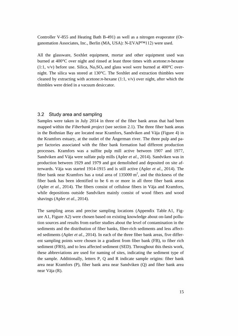
3.2 Study area and sampling Samples were taken in July 2014 in three of the fiber bank areas that had been

mapped within the Fiberbank project (see section 2.1). The three fiber bank areas

in the Bothnian Bay are located near Kramfors, Sandviken and Väja (Figure 4) in

the Kramfors estuary, at the outlet of the Ångerman river. The three pulp and pa-

per factories associated with the fiber bank formation had different production

processes. Kramfors was a sulfite pulp mill active between 1907 and 1977,

Sandviken and Väja were sulfate pulp mills (Apler et al., 2014). Sandviken was in

production between 1929 and 1979 and got demolished and deposited on site af-

terwards. Väja was started 1914-1915 and is still active (Apler et al., 2014). The

fiber bank near Kramfors has a total area of 135000 m2, and the thickness of the

fiber bank has been identified to be 6 m or more in all three fiber bank areas

(Apler et al., 2014). The fibers consist of cellulose fibers in Väja and Kramfors,

while depositions outside Sandviken mainly consist of wood fibers and wood

shavings (Apler et al., 2014).

The sampling areas and precise sampling locations (Appendix Table A1, Fig-

ure A1, Figure A2) were chosen based on existing knowledge about on-land pollu-

tion sources and results from earlier studies about the level of contamination in the

sediments and the distribution of fiber banks, fiber-rich sediments and less affect-

ed sediments (Apler et al., 2014). In each of the three fiber bank areas, five differ-

ent sampling points were chosen in a gradient from fiber bank (FB), to fiber rich

sediment (FRS), and to less affected sediment (SED). Throughout this thesis work,

these abbreviations are used for naming of sites, indicating the sediment type of

the sample. Additionally, letters P, Q and R indicate sample origins: fiber bank

area near Kramfors (P), fiber bank area near Sandviken (Q) and fiber bank area

near Väja (R).

16

Two additional replicates of sediment were sampled for one of the sampling points

in each area. At every location sediment and biota was sampled, but at some sites

(mostly fiber bank sites), no biota could be found. Biota samples of two different

Figure 4: Location of the 3 fiber bank areas studied (indicated with red triangles) near Väja (R), Sandviken (Q)

and Kramfors (P) in Västernorrland, Sweden.

17

species could be taken at 8 of 15 sampling points (Details in Table 5, Chapter 4.6).

Sampling was performed prior to the start of this master thesis.

Sampling was done from the SGU sampling ship Ocean Surveyor. Sediment was

sampled using a gemini core sampler (Gemax) (Figure 5). The top 0-4 cm was

sliced off, placed in an ethanol-rinsed glass jar, and stored cold (+4°C) until pore

water extractions (approx. 14 days). After the pore water extractions, the sediment

was frozen (-18°C) until analysis of total sediment concentrations. Some fiber

bank sediments were too soft to allow the Gemax sampler to close and retain the

sediment (e.g. site R-FB1), or there were timber logs that could damage the sam-

pler (site R-FB2). An Orange Peel Bucket (OPB) sampler (Figure 6) was used, and

surface samples (approx. 0-40 cm) were taken at these sites (R-FB1, R-FB2, Q-FB

and P-FB2). However, for site R-FB1 the OPB sampler also did not close, and

instead the material was sampled from the surfaces of the sampler.

Biota was sampled using Ekman box core samplers with the dimensions

32 × 32 cm (for sites R-FRS2 and R-SED, two samples for each site), or

20 × 20 cm (remaining sites, five samples each site), i.e. corresponding to 0.2 m2

surface area for all sites. The sediment was placed in plastic boxes and immediate-

ly sieved (1 mm sieve) using sea water to retrieve animals. The animals were

placed cold (+4 °C) in ethanol-rinsed glass jars with sea water for 24 h for purg-

ing, blotted dry with filter paper and frozen in ethanol-rinsed glass jars until analy-

sis.

Figure 5: Gemini core sam-

pler (Gemax) used for sedi-

ment sampling.

Figure 6: OPB sampler used

for sediment sampling in soft

sediment.

18

3.3 Sample extraction and clean-up

3.3.1 Sediment The sediment samples were extracted using Soxhlet. In total, 24 samples were

analyzed: 15 sediment samples, three of which in triplicates, and 3 solvent blanks.

In order to bind water and homogenize the samples before extraction, approx. 5 g

of the sediment sample was mixed in a mortar with 50 g of sodium sulfate

(Na2SO4). However, due to their high fiber and water content of samples R-FB1,

R-FRS1, and P-FB2, 10 g of sample was instead taken and mixed with 100 g of

Na2SO4. After transferring the powder to a pre-cleaned cellulose extraction thim-

ble, the sample was spiked with 40 µL of each internal standard and covered with

glass wool. Soxhlet extraction was performed for 20-24 hours using 225 mL of

acetone:n-hexane (1:1, v/v).

After the extraction, the extract was evaporated to around 1 mL using a vacuum

rotavapor. After adding activated copper (activated with hydrochloric acid and

rinsed with millipore water, acetone and n-hexane) to the sample in order to re-

move sulfur, the extracts were put through a multilayer clean-up column. From

bottom to top, this was filled with glass wool, 3 g activated silica, 6 g sulfuric acid

silica (40% H2SO4-silica) and 3 g Na2SO4. The column was rinsed with n-hexane,

corresponding to a volume two times the column height before the samples were

put on, using a Pasteur pipette. The extract flask was rinsed three times with 1 mL

of n-hexane which was also transferred to the clean-up column. The sample was

then eluted with 60 mL of n-hexane into a pear shaped flask. 40 µL of recovery

standards (RS) and 100 µL of tetradecane as a keeper were added to samples. Fi-

nally, the samples were evaporated down to 100 µL using rotavapor before being

transferred to GC-vials. If necessary, nitrogen evaporation was done to decrease

volume after the transfer.

For nine samples (R-FB1, R-FB2, R-FRS1, R-FRS2, R-SEDr1, R-SEDr2,

R-SEDr3, P-FB2, P-FRS1), a second clean up step was necessary. This was con-

ducted in the same way as the first, except that no more copper was added. One

blank (SB1) was also included. For R-FRS1 and R-SEDr3, the observations of

crystals or fibers in the samples during or after evaporation made even more clean-

up steps necessary, which was conducted in a miniaturized clean-up column, in-

side a Pasteur pipette. From bottom to top it was filled with glass wool, 0.1 g of

activated silica, 0.2 g of sulfuric acid silica (40% H2SO4-silica) and 0.1 g of

Na2SO4. The column was rinsed with n-hexane two times the column height. The

sample was applied and the vial rinsed four times with 200 µL of n-hexane. Elu-

tion was done using 8 mL n-hexane.

19

The water content of the sediment was determined as the weight loss after heating

to 105°C for 24 h, and the loss on ignition (LOI) as the weight loss after heating to

550°C for 4 h. Both parameters were determined before the start of this thesis

work, and the organic carbon content was determined by the laboratory at the De-

partment of Soil and Environment, Swedish University of Agricultural Sciences

(SLU).

3.3.2 Pore water Polyoxymethylene (POM) strips were used to determine the concentration of

POPs in sediment pore water. In total 24 samples, including three solvent blanks,

were analyzed (corresponding to the samples for determination of total concentra-

tions in sediment).

POM sheets (76 µm thick, CS Hyde, Lake Villa, IL, USA) were cut into 2 * 3 cm

strips and cleaned by immersing in acetone/n-hexane (1/1, v/v) for 2*24 hours

(solvent exchange after 24 h), followed by methanol 2 * 24 h (solvent exchange

after 24 h). They were then rinsed with Millipore water, dried in a vacuum desic-

cator, and stored in a sealed glass scintillation vial until use.

Sediment (20-30 g wet weight (ww), corresponding to 1-10 g dry weight (dw) was

placed in a 40 mL amber glass jar with Teflon-lined cap. A POM strip was added

to each jar, and Millipore water with 0.001 M CaCl2 and 0.015 M NaN3 was added

to fill the vials, leaving a small head space. The water volume added was 10-22

mL for the different samples. The samples were shaken for 28 days in the dark

using an end-over-end shaker. The pore water extractions was then terminated, and

the POM strips were retrieved, wiped clean using Millipore water and tissue paper,

and stored in scintillation vials at -18°C until extraction for POPs.

For extraction, 20 mL of acetone:n-hexane (1:1, v/v) and 40 µL of each IS were

added to the vial containing the POM sample. The samples were shaken for 24 h

in the end-over-end shaker at a speed of 30 rounds/min. The first aliquot of each

sample was collected in a pear shaped flask. Another 20 mL of the solvent mixture

was added to the vials and shaken at the same speed over the same time again. The

second aliquot was collected into the same pear shaped flask. After addition of

40 µL RS and 100 µL tetradecane, the samples were evaporated to 100 µL using

the rotavapor and transferred to GC vials. If necessary, samples were further evap-

orated using N2. The POM strips were dried and weighed.

20

One of the POM samples (P-FB2) turned milky in the GC vial after the nitrogen

evaporation step. Therefore, a miniaturized clean up in a Pasteur pipette (the same

as for some of the sediment samples) was used for this extract as well as on one of

the blanks (PB1). Apart from this, no cleanup was performed.

3.3.3 Biota The biota analyzed for POPs was the isopod crustacean Saduria entomon and the

polychaete worms Marenzelleria spp. These were the only species found at the

sampling locations. Biota samples could not be found for all of the sampling loca-

tions. For sites R-FB1, R-FRS1, R-FB2, P-FB2, P-FRS3 and Q-FB, no biota was

found. Only at the sampling spots P-FRS1, Q-FRS1 and Q-FRS2, both of the spe-

cies were found. However, only Marenzelleria samples were found at R-FRS2

(not analysed due to too low amounts of tissue), R-SED, Q-SED1, Q-SED2,

P-FB1 and P-FRS2.

The samples were weighed, and a known amount was taken for dry weight and

lipid weight determination. The remaining sample was mixed and mortared with

Na2SO4. For the Marenzelleria samples, 30 g of Na2SO4 were used, whereas Sadu-

ria was mortared with only 5 g, due to the difference in weight. The samples were

left for an hour, mortared again and packed into solvent-rinsed glass columns con-

taining glass wool at the bottom. Internal standards were added on top, and the

samples were extracted into a round bottom flask using cold-column extraction

with 75 mL acetone:n-hexane (5:2, v/v) and 75 mL n-hexane:diethylether (9:1,

v/v). Extracts were evaporated to 1 mL, followed by a clean-up step. This was

conducted in the same way as the clean-up of the sediment samples; however, an

additional layer of 3 g 20% H2SO4-silica was placed between the 40% H2SO4-

silica and the Na2SO4. After clean-up, recovery standard and 100 µL tetradecane

was added. The samples were concentrated using rotary evaporation, transferred

into GC-vials, and if necessary further concentrated using nitrogen evaporation.

The dry weight of the Marenzelleria samples was determined by drying an aliquot

of the biota sample (0.13-0.64 g) at 60°C for 24 hours. The lipid content was then

determined by mortaring the sample (re-wetted with a few drops of Millipore wa-

ter) with 4 g of Na2SO4, placing the mixture in pasteur pipettes with glass wool in

the bottom and eluting with 6 mL acetone:n-hexane (5:2, v/v) and 6 mL

n-hexane:diethylether (9:1, v/v). For Saduria entomon samples, it was not possible

to take an aliquot of the original samples since they consisted of very few animals.

Instead, an aliqout of the extract obtained after cold-column extraction for POPs

was taken. Both Marenzelleria and S. entomon extracts were evaporated in a rota-

21

vapor until approx. 0.5 mL and placed on pre-weighed, warm aluminum cups for

the solvent to evaporate. The lipid weight was then determined by re-weighing the

aluminum cups.

3.4 Instrumental analysis The instrumental analysis was conducted using a gas chromatograph (Agilent

Technologies 7890 A GC System) combined with a triple quadrupole mass spec-

trometer (Agilent Technologies, 7010 GC/MS Triple Quad), thus GC-MS/MS.

The GC was equipped with a DB5 capillary column (60 m × 250 µm × 0.25 µm,

Agilent Technologies) and helium was used as a carrier gas (2 mL min-1). Extract

aliquots of 2 µL was injected in splitless mode at an injector temperature of

275°C. The oven temperature program started at 190°C for 2 min, increased with

3°C/min to 250°C, and then with 6°C/min to 310°C, which was held for 1 min,

resulting in a total run time of 33 min. For the MS/MS, electron impact ionization

was used. N2 was used as collision gas and He as quench gas in the collision cell.

The MS/MS was operated in MRM mode, and two transitions were monitored for

each compound. For data evaluation the software Agilent MassHunter Quantita-

tive Analysis (for QQQ) was used.

3.5 Quality assurance For each batch of samples of every sampling area, a solvent blank was run and

treated the same way as the other samples. For the biota samples an additional

blank was run consisting of only the solvents used in the biota extraction method.

At the start of the extraction, isotopically labelled compounds were added to each

sample as internal standard in order to be able to correct for losses during the pro-

cess of sample analysis.

The performance of the method was checked by calculating the recovery of the

internal standard with the help of a recovery standard which was added before

GC-MS/MS analysis. The recovery was calculated as the fraction of the ratios

between the peak area of internal standard in the sample to the one in the calibra-

tion solution and the peak areas of recovery standard in the sample to the one in

the calibration solution (Equation 1). The areas for the IS and RS in the calibration

22

solution were the average value of the 1 ng calibration solution that was run nine

times during instrumental analysis.

𝑅 (%) =𝐴𝐼𝑆(𝑠𝑎𝑚𝑝𝑙𝑒)

𝐴𝐼𝑆(𝑐𝑎𝑙𝑖𝑏𝑟 𝑠𝑜𝑙)×

𝐴𝑅𝑆(𝑐𝑎𝑙𝑖𝑏𝑟 𝑠𝑜𝑙)

𝐴𝑅𝑆(𝑠𝑎𝑚𝑝𝑙𝑒)× 100

Equation 1: Calculation of method recovery.

In order to measure the target analyte, it must be present in a concentration that

exceeds the method’s limit of detection (LOD). This is necessary in order to dis-

tinguish reliably between analytical signal and noise. In the chromatographic

method applied, the LOD used was a signal-to-noise ratio of 3. Compounds were

considered detected if their respective peak was 3 times higher than the back-

ground noise of the instrument. However, the analyte could only be quantified if

its concentration exceeds the method’s limit of quantification (LOQ), which was

the lowest of the calibration solution concentrations which could still be detected

reliably by the GC-MS/MS. For all compounds analyzed, the LOQ was 0.005 ng

absolute with the exception of o,p’-DDT and p,p’-DDT. These two compounds

could only be quantified if the amount in the vial exceeded 0.05 ng absolute. On

average, the 0.005 ng absolute limit of quantification correspond to 0.0036 ng/g

sediment dw, 0.073 ng/g POM, 0.0015 ng/g ww Marenzelleria and 0.014 ng/g ww

Saduria entomon. For any concentration lower than LOQ, the compound was not

quantified and the concentration of that compound was set to zero.

Average values were taken of all compound concentrations in the blanks for each

matrix. Sample concentration values were corrected for any contamination found

in the blanks of the corresponding matrix. Concentrations found in blanks com-

pared to sample concentrations were generally low. However, in a few samples

contaminant concentrations did not exceed two times the value found in the blank.

This was the case for PCB 28 in one sediment sample and for HCB, PCB 28, 52,

77 and 101 in a total of six biota samples. Among the analytes, these compounds

have high volatility and water solubility and are therefore more likely to be found

in blanks. The data is included in the study but are related to some uncertainties.

23

3.6 Data analysis and calculations The biota-sediment-accumulation factor (BSAF) was calculated by dividing the

contaminant level in the biota per lipid weight by the contaminant level in the

sediment per organic carbon weight. This ratio shows to which extent a certain

compound bioaccumulates.

𝐵𝑆𝐴𝐹 =𝐶𝑏

𝑓𝑙

𝐶𝑠

𝑓𝑂𝐶⁄

Equation 2: Calculation of biota-sediment-accumulation factor (BSAF). Cb is the concentration of

the contaminant in the organism, while CS is the concentration in the sediment. fl expressed the lipid

fraction of the tissue while fOC is the fraction of organic carbon in the sediment (National Research

Council of the National Academies, 2003).

The concentration in the pore water (Cpw) was calculated by dividing the concen-

tration in the passive sampler (CPOM) by the passive sampler-water partition coeffi-

cient (KPOM) assuming that equilibrium between the phases had been reached.

Compound specific KPOM values were taken from or calculated based on Endo et

al. (2011) for DDX and HCB and Hawthorne et al. (2009) for PCBs. For detailed

values see Table 1.

𝐶pw = 𝐶POM

𝐾POM

Equation 3: Calculation of pore water concentration [unit: ng/Lpw]. (Based on Lydy et al. (2014)).

Besides the equilibrium requirement, non-depletive conditions are a requisite for

passive sampling with POM. In order to check for depletion, the amount of con-

taminant found in the POM extract was divided by the amount of contaminant in

the sediment it was exposed to. Non-depletive conditions are ensured if that ratio

is smaller than 0.05.

Compound sorption was expressed as empirical Kd value which was calculated

dividing sediment concentration at equilibrium (Csed(eq)), on a dry weight (dw)

basis, by the concentration in pore water (Cpw).

𝐾d = 𝐶sed(eq)

𝐶pw

Equation 4: Calculation of the Kd values [unit: Lpw/kgdw].

24

The sediment concentration at equilibrium was calculated by dividing contaminant

mass in the sediment at equilibrium (Msed(eq)) with the sediment dry weight (Msed).

The contaminant mass in the sediment at equilibrium was calculated by subtract-

ing the contaminant mass in the POM and in the water at equilibrium from the

initial contaminant mass in the sediment (before equilibrium).

𝐶𝑠𝑒𝑑(𝑒𝑞) =𝑀𝑠𝑒𝑑(𝑒𝑞)

𝑀𝑠𝑒𝑑=

(𝑀𝑠𝑒𝑑(𝑖𝑛𝑖𝑡) − 𝑀𝑃𝑂𝑀(𝑒𝑞) − 𝑀𝑤𝑎𝑡𝑒𝑟 (𝑒𝑞))

𝑀𝑠𝑒𝑑

Equation 5: Calculation of sediment concentration at equilibrium.

For the statistical analysis of the results, Pearson’s r was used to measure linear

relationship between Kd values and hydrophobicity of contaminants as well as

relationships between BSAFs and hydrophobicity. It was used again to test for

correlations between concentrations in biota and concentrations in sediment and

pore water. Regressions were calculated using the data analysis tool of Excel.

One-way ANOVA was applied to check for significant differences between the

three different sediment categories regarding their Kd values and BSAFs. In one

case, the ANOVA was significant. Therefore two-tailed z-tests (with alpha 0.05)

were used as a post-hoc test to check for significant differences between the sedi-

ment types fiber bank, fiber rich sediment and less affected sediment. ANOVA

and z-test were calculated using the data analysis tool of Excel.

25

4 Results

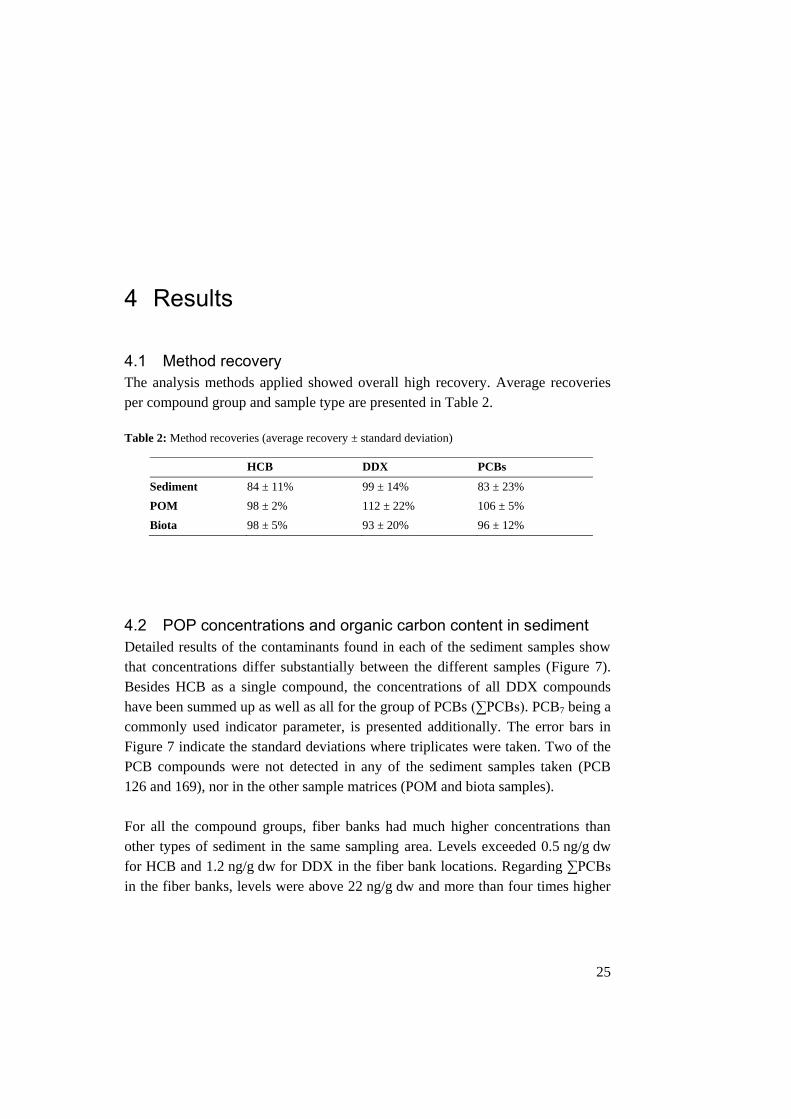
4.1 Method recovery The analysis methods applied showed overall high recovery. Average recoveries

per compound group and sample type are presented in Table 2.

Table 2: Method recoveries (average recovery ± standard deviation)

4.2 POP concentrations and organic carbon content in sediment Detailed results of the contaminants found in each of the sediment samples show

that concentrations differ substantially between the different samples (Figure 7).

Besides HCB as a single compound, the concentrations of all DDX compounds

have been summed up as well as all for the group of PCBs (∑PCBs). PCB7 being a

commonly used indicator parameter, is presented additionally. The error bars in

Figure 7 indicate the standard deviations where triplicates were taken. Two of the

PCB compounds were not detected in any of the sediment samples taken (PCB

126 and 169), nor in the other sample matrices (POM and biota samples).

For all the compound groups, fiber banks had much higher concentrations than

other types of sediment in the same sampling area. Levels exceeded 0.5 ng/g dw

for HCB and 1.2 ng/g dw for DDX in the fiber bank locations. Regarding ∑PCBs

in the fiber banks, levels were above 22 ng/g dw and more than four times higher

HCB DDX PCBs

Sediment 84 ± 11% 99 ± 14% 83 ± 23%

POM 98 ± 2% 112 ± 22% 106 ± 5%

Biota 98 ± 5% 93 ± 20% 96 ± 12%

26

than the highest value of the other types of sediment. However, P-FB1 forms

clearly an exception from the other fiber banks, in that concentrations are lower

and similar to concentrations in fiber rich sediment. In fact, the fiber rich sediment

in sampling site P-FRS3 had higher concentrations than P-FB1 for all three con-

taminant groups. Furthermore, it can be seen that even in the less affected sedi-

ments the targeted compounds can be found. Concentrations in fiber rich sedi-

ments and less affected sediments were not that different from each other. Differ-

ences in contaminant concentrations between the two sediment types were more

obvious in fiber bank R; all contaminant groups had higher concentrations in FRS

than SED. In fiber bank area Q, differences in concentrations for different sedi-

ment types were less obvious. Nevertheless, the fiber rich sediments seem to gen-

erally have slightly more elevated levels, especially for the PCBs.

Figure 7: Contamination levels [ng/g dw] of the different compound groups in sediment samples.

0

5

10

15

20

25

30

35

40

R-F

B1

R-F

B2

R-F

RS1

R-F

RS2

R-S

ED

Q-F

B

Q-F

RS1

Q-F

RS2

Q-S

ED1

Q-S

ED2

P-F

B1

P-F

B2

P-F

RS1

P-F

RS2

P-F

RS3

Co

nta

min

ant

con

cen

trat

ion

[n

g/g

dw

]

HCB

DDX

PCB7

∑PCBs

27

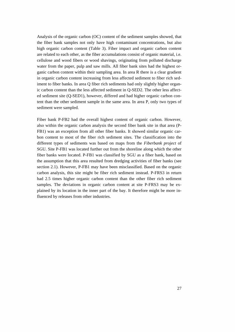
Analysis of the organic carbon (OC) content of the sediment samples showed, that

the fiber bank samples not only have high contaminant concentrations, but also

high organic carbon content (Table 3). Fiber impact and organic carbon content

are related to each other, as the fiber accumulations consist of organic material, i.e.

cellulose and wood fibers or wood shavings, originating from polluted discharge

water from the paper, pulp and saw mills. All fiber bank sites had the highest or-

ganic carbon content within their sampling area. In area R there is a clear gradient

in organic carbon content increasing from less affected sediment to fiber rich sed-

iment to fiber banks. In area Q fiber rich sediments had only slightly higher organ-

ic carbon content than the less affected sediment in Q-SED2. The other less affect-

ed sediment site (Q-SED1), however, differed and had higher organic carbon con-

tent than the other sediment sample in the same area. In area P, only two types of

sediment were sampled.

Fiber bank P-FB2 had the overall highest content of organic carbon. However,

also within the organic carbon analysis the second fiber bank site in that area (P-

FB1) was an exception from all other fiber banks. It showed similar organic car-

bon content to most of the fiber rich sediment sites. The classification into the

different types of sediments was based on maps from the Fiberbank project of

SGU. Site P-FB1 was located further out from the shoreline along which the other

fiber banks were located. P-FB1 was classified by SGU as a fiber bank, based on

the assumption that this area resulted from dredging activities of fiber banks (see

section 2.1). However, P-FB1 may have been misclassified. Based on the organic

carbon analysis, this site might be fiber rich sediment instead. P-FRS3 in return

had 2.5 times higher organic carbon content than the other fiber rich sediment

samples. The deviations in organic carbon content at site P-FRS3 may be ex-

plained by its location in the inner part of the bay. It therefore might be more in-

fluenced by releases from other industries.

28

Table 3: Percentage of total carbon content and the organic carbon content in each of the sediment

samples.

Tot-C % Org-C %

R-FB1 34.8 34.7

R-FB2 12.0 12.0

R-FRS1 4.8 4.7

R-FRS2 4.5 4.5

R-SED 2.9 2.9

Q-FB 8.6 8.6

Q-FRS1 2.1 2.0

Q-FRS2 2.0 2.0

Q-SED1 2.1 2.1

Q-SED2 2.0 2.0

P-FB1 2.6 2.5

P-FB2 36.6 36.6

P-FRS1 2.4 2.4

P-FRS2 2.6 2.6

P-FRS3 6.5 6.5

The highest values of organic carbon were found in P-FB2 (37%) and R-

FB1 (35%). These were the samples that showed the highest ∑PCBs concentra-

tions based on a dry weight basis, and HCB and DDX concentrations were also

high. Contaminant concentrations (ng/g dw) (Figure 7) were normalized with their

respective organic carbon content and are presented in Figure 8, where error bars

indicate the standard deviation for samples taken as triplicates. The results show

more even concentrations (ng/g OC) between sites. This is due to the fact that the

fiber bank sites are not only high in pollution, but also high in organic carbon con-

tent. Therefore these concentrations are preferable when comparing between dif-

ferent sites or for calculations of other indicators like for example BSAFs.

Figure 8 shows that, when normalized to OC, the sites Q-FB (380 ng/g OC) and

R-FB2 (250 ng/ OC) are the most polluted ones concerning ∑PCBs and differ

much in comparison to all other sites. In relation to their organic carbon content,

the fiber bank at R-FB1 had relatively low ∑PCBs contamination in comparison to

all other fiber banks and even compared to most other less fiber impacted sites.

Site P-FB1, that showed low POP concentrations on a dry weight basis, when

compared to other fiber banks, had the third highest ∑PCBs contamination on an

organic carbon basis. For ∑PCBs, a clear trend of increasing concentrations with

increasing fiber impact can only be seen in sampling area Q.

29

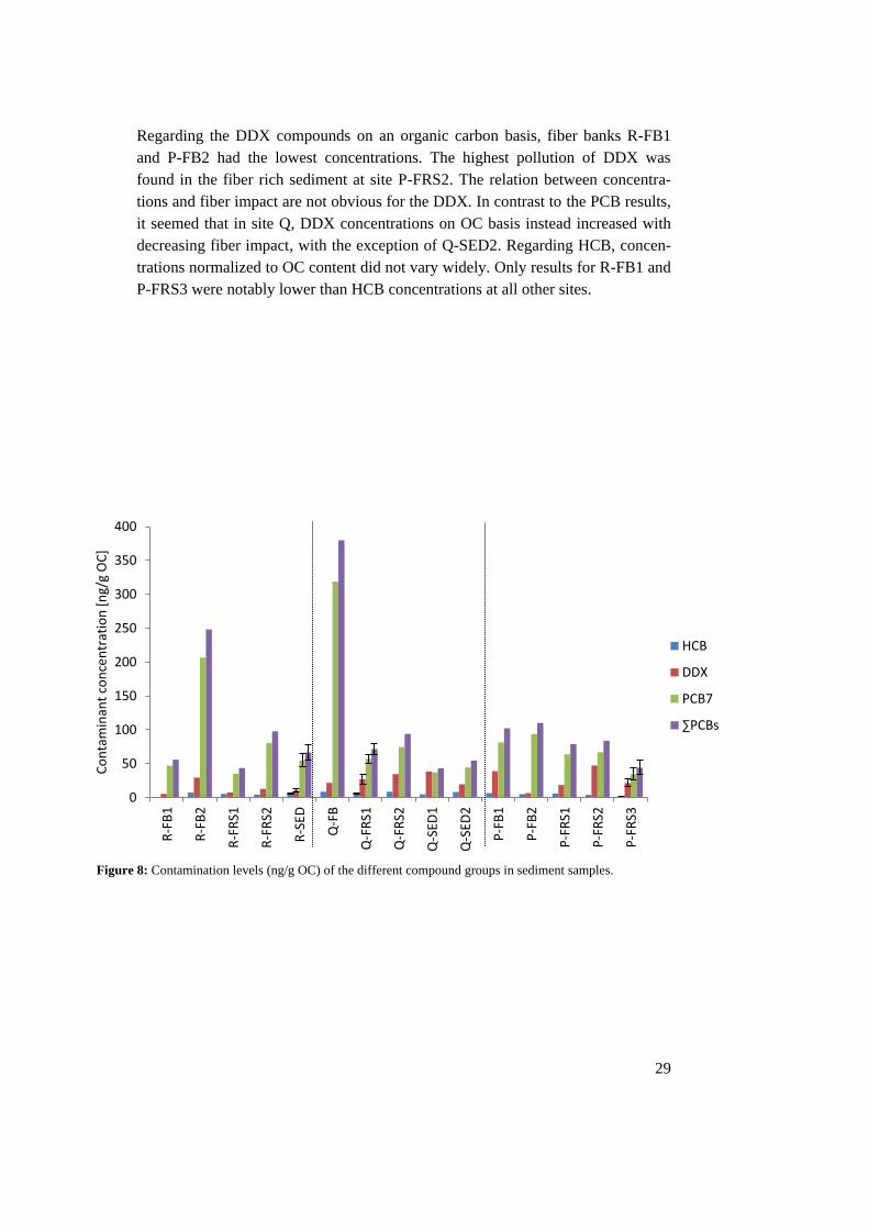
Regarding the DDX compounds on an organic carbon basis, fiber banks R-FB1

and P-FB2 had the lowest concentrations. The highest pollution of DDX was

found in the fiber rich sediment at site P-FRS2. The relation between concentra-

tions and fiber impact are not obvious for the DDX. In contrast to the PCB results,

it seemed that in site Q, DDX concentrations on OC basis instead increased with

decreasing fiber impact, with the exception of Q-SED2. Regarding HCB, concen-

trations normalized to OC content did not vary widely. Only results for R-FB1 and

P-FRS3 were notably lower than HCB concentrations at all other sites.

Figure 8: Contamination levels (ng/g OC) of the different compound groups in sediment samples.

0

50

100

150

200

250

300

350

400

R-F

B1

R-F

B2

R-F

RS1

R-F

RS2

R-S

ED

Q-F

B

Q-F

RS1

Q-F

RS2

Q-S

ED1

Q-S

ED2

P-F

B1

P-F

B2

P-F

RS1

P-F

RS2

P-F

RS3

Co

nta

min

ant

con

cen

trat

ion

[n

g/g

OC

]

HCB

DDX

PCB7

∑PCBs

30

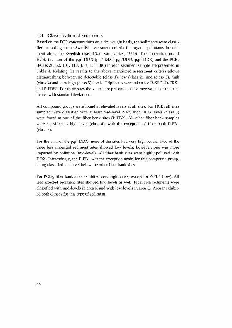
4.3 Classification of sediments Based on the POP concentrations on a dry weight basis, the sediments were classi-

fied according to the Swedish assessment criteria for organic pollutants in sedi-

ment along the Swedish coast (Naturvårdsverket, 1999). The concentrations of

HCB, the sum of the p,p’-DDX (p,p’-DDT, p,p’DDD, p,p’-DDE) and the PCB7

(PCBs 28, 52, 101, 118, 138, 153, 180) in each sediment sample are presented in

Table 4. Relating the results to the above mentioned assessment criteria allows

distinguishing between no detectable (class 1), low (class 2), mid (class 3), high

(class 4) and very high (class 5) levels. Triplicates were taken for R-SED, Q-FRS1

and P-FRS3. For these sites the values are presented as average values of the trip-

licates with standard deviations.

All compound groups were found at elevated levels at all sites. For HCB, all sites

sampled were classified with at least mid-level. Very high HCB levels (class 5)

were found at one of the fiber bank sites (P-FB2). All other fiber bank samples

were classified as high level (class 4), with the exception of fiber bank P-FB1

(class 3).

For the sum of the p,p’-DDX, none of the sites had very high levels. Two of the

three less impacted sediment sites showed low levels; however, one was more

impacted by pollution (mid-level). All fiber bank sites were highly polluted with

DDX. Interestingly, the P-FB1 was the exception again for this compound group,

being classified one level below the other fiber bank sites.

For PCB7, fiber bank sites exhibited very high levels, except for P-FB1 (low). All

less affected sediment sites showed low levels as well. Fiber rich sediments were

classified with mid-levels in area R and with low levels in area Q. Area P exhibit-

ed both classes for this type of sediment.

31

Table 4: Level of contamination in sediment samples in ng/g dw classified based on the Swedish

assessment criteria for organic pollutants in sediments along the Swedish coast (Naturvårdsverket,

1999).

Site HCB ∑ p,p'-DDX PCB7

R-FB1 0.63 1.6 28

R-FB2 0.96 1.5 26

R-FRS1 0.33 0.35 2.1

R-FRS2 0.17 0.36 3.0

R-SED * 0.11 ± 0.02 0.18 ± 0.03 1.0 ± 0.1

Q-FB 0.50 1.1 18

Q-FRS1 * 0.063 ± 0.015 0.26 ± 0.05 0.64 ± 0.05

Q-FRS2 0.089 0.30 0.75

Q-SED1 0.066 0.45 0.51

Q-SED2 0.084 0.17 0.45

P-FB1 0.096 0.44 1.2

P-FB2 1.6 1.7 30

P-FRS1 0.077 0.21 0.81

P-FRS2 0.058 0.53 0.97

P-FRS3 * 0.17 ± 0.05 1.0 ± 0.1 3.6 ± 1.1

* = Average value of the triplicate samples and standard deviation

4.4 POP relative distributions in sediments The relative distributions of the contaminants detected, calculated as the concen-

tration of that compound divided by the total concentration of all compounds, vary

between different sampling points (Figure 9). The variation in contaminant com-

position between the sites could indicate that usage and release of contaminants

differs at the local sources where the pollution comes from. However, as the com-

pounds investigated were applied as mixtures, the differences in sample composi-

tion could instead be due to different degradation rates.

Class 1 Class 2 Class 3 Class 4 Class 5

No level Low level Mid-level High level Very high

level

32

The three triplicates (R-SED-r1 – R-SED-r3; Q-FRS-r1 – Q-FRS-r3; P-FRS-r1 –

P-FRS-r3) were similar in their pollutant distribution patterns per site. However,

the triplicates in site P (P-FRS3-r1 – P-FRS3-r3) exhibited some deviations be-

tween the three samples. This is mostly due to different shares of o,p’-DDD and

PCB 156. While o,p’-DDD was found in a higher proportion at P-FRS3-r3,

PCB 156 was found in much higher proportion at P-FRS3-r1 than at any other site.

These deviations in the contaminant distribution of the triplicate may be due to

different degradation processes in the field at different spots or during the instru-

mental analysis (see 5.4), or be explained by how the triplicate sampling was done.

To not sample at exactly the same spot, the boat moved about 1 m between the

three replicates. Moreover, sediment concentrations on a dry weight basis at site

P-FRS3 were slightly higher than at the other fiber rich sediment sites in this fiber

bank area. This could indicate that the P-FRS3 may be located closer to the source

of pollution or may be influenced by several sources and consequently show a

patchier contaminant distribution than other samples more distant from the pollu-

tant source.

The highest PCB levels detected were the PCB7 congeners. Moreover, other PCBs

that were detected in relatively high amounts were PCB 105, 156, 170 and

167+128. Site Q-FB had the highest proportion of ∑PCBs followed by P-FB2.

Most of the differences in composition between different samples seem to occur

for DDX. For DDX, the most frequent detected compounds were o,p’-DDD and

all of the p,p’-configured DDX (i.e. DDT, DDD and DDE). The p,p’-DDT share

had a higher relative distribution in less affected sediment and in fiber rich sedi-

ment than in fiber bank samples. For o,p’-DDD the patterns in the graph suggested

the same assumption. However, at site R it was the opposite, and o,p’-DDD was

more common in fiber banks than in sediment with less fiber impact. The propor-

tion o,p’-DDD was highest at site P-FRS3, for triplicate P-FRS3-r3.

Finally, the results indicate that the fiber bank samples differ in their pollutant

distribution pattern from the less fiber impacted samples within the same fiber

bank area. However fiber bank P-FB1 was an exception and resembled more the

fiber rich sediment of that sampling area.

33

0%

10%

20%

30%

40%

50%

60%

70%

80%

90%

100%

R-F

B1

R-F

B2

R-F

RS1

R-F

RS2

R-S

ED-r

1

R-S

ED-r

2

R-S

ED-r

3

Q-F

B

Q-F

RS1

-r1

Q-F

RS1

-r2

Q-F

RS1

-r3

Q-F

RS2

Q-S

ED1

Q-S

ED2

P-F

B1

P-F

B2

P-F

RS1

P-F

RS2

P-F

RS3

-r1

P-F

RS3

-r2

P-F

RS3

-r3

PCB 209

PCB 189

PCB 180

PCB 170

PCB 167+128

PCB 157

PCB 156

PCB 153

PCB 138

PCB 123

PCB 118

PCB 114

PCB 105

PCB 101

PCB 81

PCB 77

PCB 52

PCB 28

p,p'-DDT

p,p-DDE

p,p'-DDD

o,p'-DDT

o,p'-DDE

o,p'-DDD

HCB

Figure 9: Distribution of analyzed compounds in each sediment sample.

34

4.5 POP concentrations in pore water The results of the pore water analysis based on the passive sampling are shown in

Appendix Figure A3. POM results were used to calculate sorption coefficients, Kd,

in order to provide answers to the hypotheses stated in the beginning. Non-

depletive conditions were not given for all compounds. In the calculation of the Kd

values, corrections for depletion are included. Regarding results of the POM anal-

ysis, it should also be noted that for the sites where triplicates were taken (R-SED

and Q-FRS1), results are presented as average values. For site P-FRS3, triplicates

were taken. However, P-FRS3r3 exhibited an extremely high concentration in the

POM for o,p’-DDD, which deviated substantially from the other replicates and

also exceeded the highest calibration standard by far (P-FRS3r1: 13 ng/g POM;

P-FRS3r2: 15 ng/g POM; P-FRS3r3: 1068 ng/g POM). Therefore, this POM repli-

cate (P-FRS3-r3) was excluded from calculations and results. However, in the

sediment sample taken at this site, o,p’-DDD was a common contaminant. In fact

P-FRS3 was the sample with the highest proportion of o,p’-DDD.

In all three fiber bank areas investigated, the highest ∑PCBs concentrations in the

pore water were found in the fiber bank sites. The only exception was for area P,

where one of the fiber rich sediment sites (P-FRS3) had higher ∑PCBs concentra-

tions than one of the fiber bank sites (P-FB1). That site, in turn, was more similar

in its levels to the other fiber rich sediment sites. This supports previous sugges-

tions (see section 4.2) that the classification of sediment type at site P-FB1, based

on previous mapping, may be incorrect, as shown by the organic carbon content.

The highest contamination levels in pore water were due to DDX contamination

(R-FB2: 160 pg/Lpw). In contrast to the pore water concentrations, the highest con-

centrations in biota and sediment samples were due to ∑PCB contamination. One

interesting finding about pore water concentration results was that in all but one

sampling site, DDX concentrations were higher than ∑PCB concentrations. The

exception was R-SED where the highest contaminant concentrations were in fact

HCB concentrations. HCB pore water concentrations were generally higher than

∑PCB concentrations. However, exceptions were all fiber bank sites and one fiber

rich sediment site (P-FRS2). At these sites, the highest contaminations were due to

DDX followed by ∑PCBs, PCB7 and HCB concentrations being lowest.

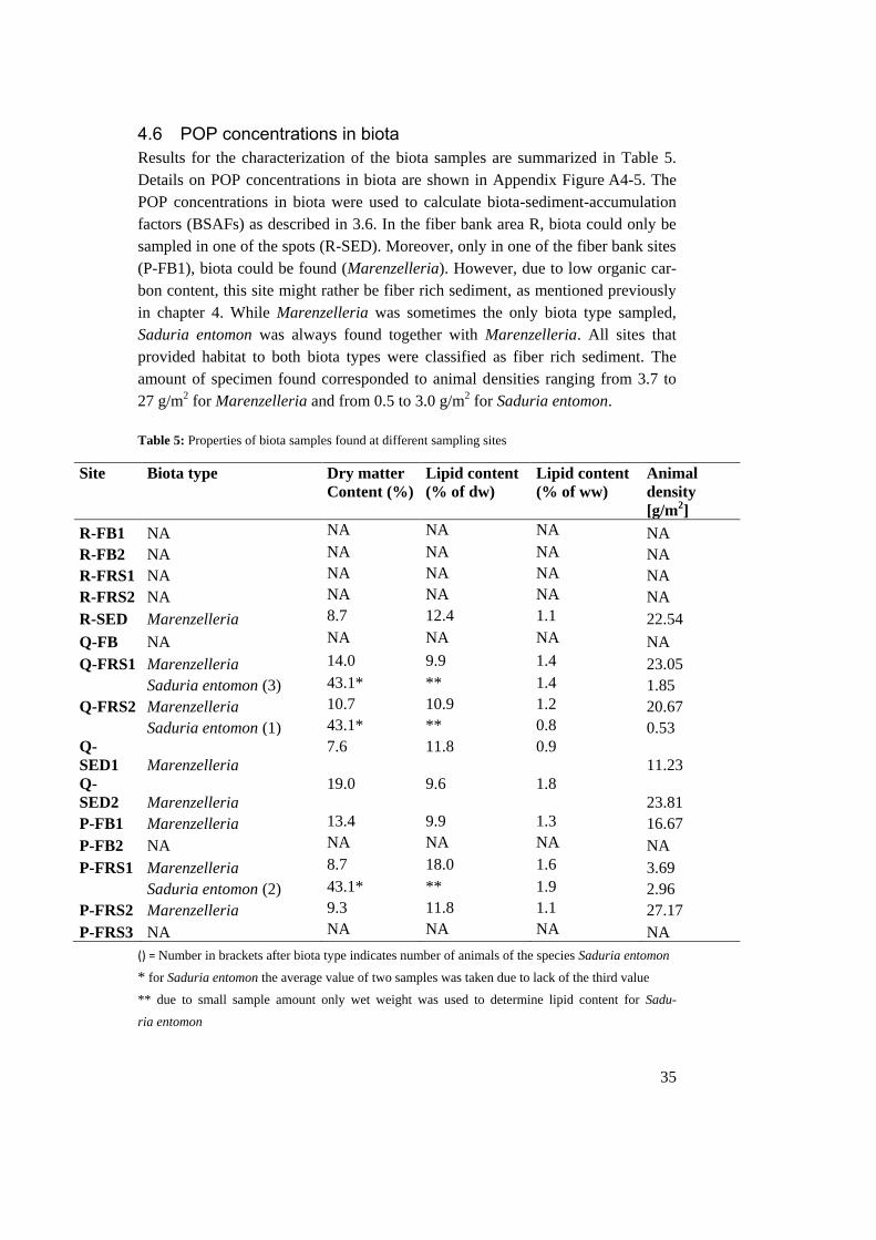
35

4.6 POP concentrations in biota Results for the characterization of the biota samples are summarized in Table 5.

Details on POP concentrations in biota are shown in Appendix Figure A4-5. The

POP concentrations in biota were used to calculate biota-sediment-accumulation

factors (BSAFs) as described in 3.6. In the fiber bank area R, biota could only be

sampled in one of the spots (R-SED). Moreover, only in one of the fiber bank sites

(P-FB1), biota could be found (Marenzelleria). However, due to low organic car-

bon content, this site might rather be fiber rich sediment, as mentioned previously

in chapter 4. While Marenzelleria was sometimes the only biota type sampled,

Saduria entomon was always found together with Marenzelleria. All sites that

provided habitat to both biota types were classified as fiber rich sediment. The

amount of specimen found corresponded to animal densities ranging from 3.7 to

27 g/m2 for Marenzelleria and from 0.5 to 3.0 g/m2 for Saduria entomon.

Table 5: Properties of biota samples found at different sampling sites

Site Biota type Dry matter

Content (%)

Lipid content

(% of dw)

Lipid content

(% of ww)

Animal

density

[g/m2]

R-FB1 NA NA NA NA NA

R-FB2 NA NA NA NA NA

R-FRS1 NA NA NA NA NA

R-FRS2 NA NA NA NA NA

R-SED Marenzelleria 8.7 12.4 1.1 22.54

Q-FB NA NA NA NA NA

Q-FRS1 Marenzelleria 14.0 9.9 1.4 23.05

Saduria entomon (3) 43.1* ** 1.4 1.85

Q-FRS2 Marenzelleria 10.7 10.9 1.2 20.67

Saduria entomon (1) 43.1* ** 0.8 0.53

Q-

SED1 Marenzelleria

7.6 11.8 0.9

11.23

Q-

SED2 Marenzelleria

19.0 9.6 1.8

23.81

P-FB1 Marenzelleria 13.4 9.9 1.3 16.67

P-FB2 NA NA NA NA NA

P-FRS1 Marenzelleria 8.7 18.0 1.6 3.69

Saduria entomon (2) 43.1* ** 1.9 2.96

P-FRS2 Marenzelleria 9.3 11.8 1.1 27.17

P-FRS3 NA NA NA NA NA

() = Number in brackets after biota type indicates number of animals of the species Saduria entomon

* for Saduria entomon the average value of two samples was taken due to lack of the third value

** due to small sample amount only wet weight was used to determine lipid content for Sadu-

ria entomon

36

In all biota samples, ∑PCBs concentrations on a dry weight basis were much

higher than concentrations of the other contaminant groups, and ranged between

8.8 and 31 ng/g dw (Appendix Figure A4a). On a dry weight basis, DDX, PCB7

and ∑PCBs concentrations in Marenzelleria were slighty higher than in the Sadu-

ria entomon samples found at the same site (Appendix Figure A5a). However, for

concentrations normalized to biota lipid weight, all Saduria entomon samples

showed noticeably higher values of PCB7, ∑PCBs and HCB than the Marenzeller-

ia samples found at the same site (Appendix Figure A5b). For DDX, the differ-

ences between the two biota types were not that clear.

4.7 Relation between sorption or bioaccumulation and hydrophobicity (hypothesis 1)

4.7.1 Sorption To provide answers to hypothesis 1, the sorption expressed as log Kd for each con-

taminant was investigated in relation to contaminant hydrophobicity. Figure 10

shows the sorption of each contaminant as an average for all sampling sites and

error bars indicate the standard deviation. Contaminant log Kow values, as an indi-

cator of their hydrophobicity, ranged from 5.5 to 7.7. Values of log Kd ranged be-

tween 3.7 (p,p’-DDD) and 7.0 (PCB 189). Sorption could not be calculated for

compounds PCB 81, 126, 169 and 209, as these contaminants were not detected in

one or both of the sample matrices (sediment or POM) the calculation is based on.

A linear trendline has been fitted through the data points to check for correlation.

The graph shows that sorption increases with increasing hydrophobicity. The sta-

tistical analysis showed that that the sorption of a certain compound could be ex-

plained significantly (p<0.001) by its log Kow value with 83%.

4.7.2 Bioaccumulation Furthermore, the bioaccumulation expressed as Marenzelleria BSAF values was

compared to the hydrophobicity of the contaminants. Average values (for all sites

with Marenzelleria) and their standard deviations are presented in Figure 11. Con-

taminant log Kow values ranged from 5.5 to 8.2. BSAF values ranged from 0.01

(o,p’-DDD) to 3.64 (PCB 180). BSAFs could not be calculated for o,p’-DDT,

PCB 81, 114, 126 and 169 because these contaminants were not detected in one or

both of the sample matrices (sediment or biota). A polynomial trendline was fitted

through the data points in order to check for the presumed relationship between

bioaccumulation and contaminant properties (see chapter 1.2). The R2 value indi-

cated that the variance in the Marenzelleria BSAFs of a certain contaminant could

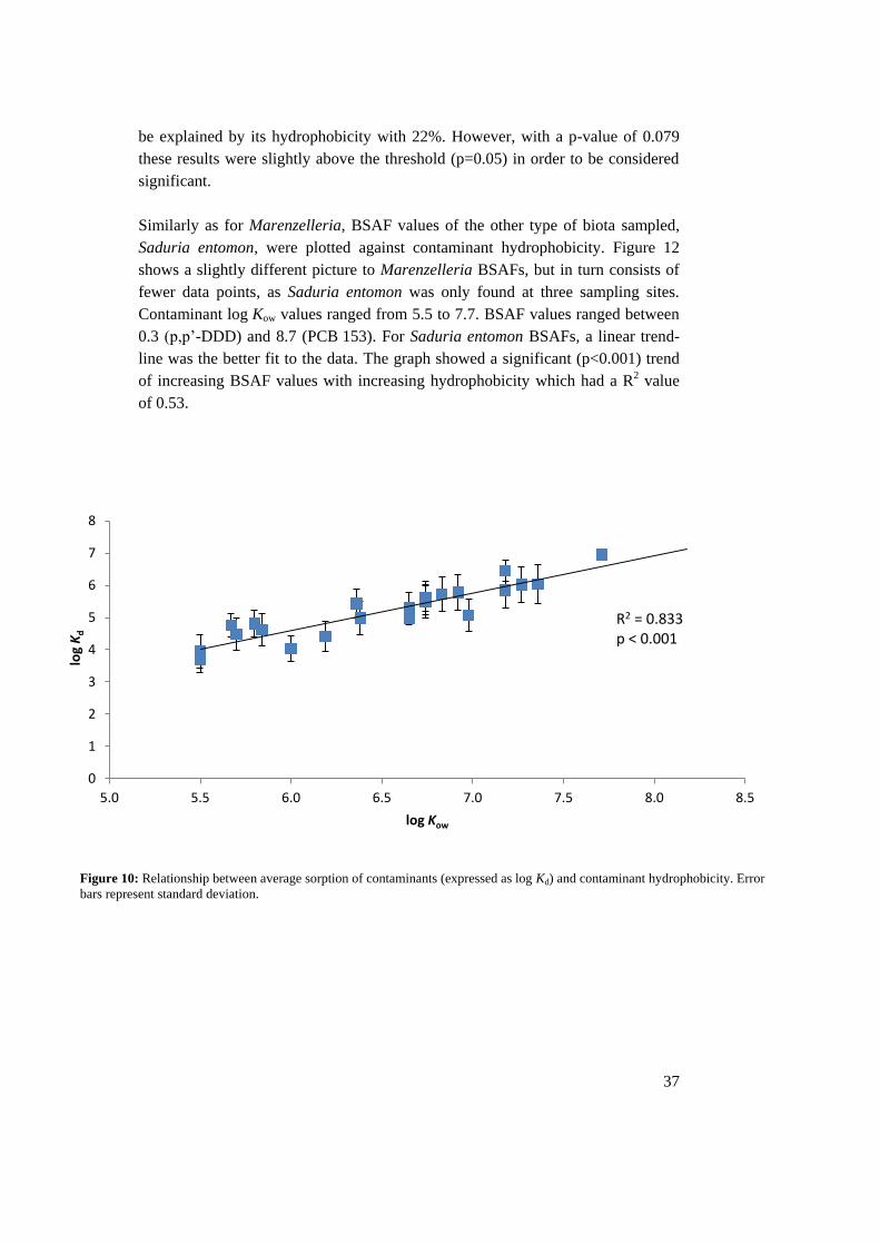
37

be explained by its hydrophobicity with 22%. However, with a p-value of 0.079

these results were slightly above the threshold (p=0.05) in order to be considered

significant.

Similarly as for Marenzelleria, BSAF values of the other type of biota sampled,

Saduria entomon, were plotted against contaminant hydrophobicity. Figure 12

shows a slightly different picture to Marenzelleria BSAFs, but in turn consists of

fewer data points, as Saduria entomon was only found at three sampling sites.

Contaminant log Kow values ranged from 5.5 to 7.7. BSAF values ranged between

0.3 (p,p’-DDD) and 8.7 (PCB 153). For Saduria entomon BSAFs, a linear trend-

line was the better fit to the data. The graph showed a significant (p<0.001) trend

of increasing BSAF values with increasing hydrophobicity which had a R2 value

of 0.53.

Figure 10: Relationship between average sorption of contaminants (expressed as log Kd) and contaminant hydrophobicity. Error

bars represent standard deviation.

0

1

2

3

4

5

6

7

8

5.0 5.5 6.0 6.5 7.0 7.5 8.0 8.5

log

Kd

log Kow

R2 = 0.833 p < 0.001

38

0

1

2

3

4

5

6

7

8

9

10

5.0 5.5 6.0 6.5 7.0 7.5 8.0

BSA

F (S

ad

uri

a e

nto

mo

n)

log Kow

R2 = 0.525 p < 0.001

Figure 12: Relationship between average Saduria entomon biota-sediment-accumulation factors of contaminants and contaminant

hydrophobicity. Error bars represent standard deviation.

-1

0

1

2

3

4

5

6

7

5.0 5.5 6.0 6.5 7.0 7.5 8.0 8.5

BSA

F (M

are

nze

lleri

a)

log Kow

R2 = 0.224 p = 0.079

Figure 11: Relationship between average Marenzelleria biota-sediment-accumulation factors of contaminants and contaminant

hydrophobicity. Error bars represent standard deviation.

39

4.8 Relation between sorption or bioaccumulation and sediment composition (hypothesis 2)

4.8.1 Sorption In order to find out if there was a correlation between the type of sediment and the

sorption of contaminants, the sites were grouped by their fiber impact. The aver-

age values of the sorption in each of the three groups of sediment type (FB = fiber

bank, FRS = fiber rich sediment, SED = less affected sediment) and their standard

deviations are presented in Figure 13. It needs to be noted that due to the sampling

set up, the sediment type groups did not exhibit the same amount of log Kd values,

because more samples were taken in fiber banks and fiber rich sediment than in

less affected sediment. The data included five sampling points of fiber bank sites,

seven of fiber rich sediment but only three of less affected sediment.

Sorption was lowest in the less affected sediment (log Kd=4.6) and highest in the

fiber banks (log Kd=5.5). The graph indicated an increase in sorption with increas-

ing fiber impact. Significant (p<0.001) differences in sorption between the three

sediment types with varying fiber impact were proved using single-factor ANO-

VA. Therefore, two-tailed z-tests were used as a post-hoc test to check for differ-

ences between the groups. The test was significant for the combinations fiber bank

and fiber rich sediment (p<0.001) as well as for fiber bank and sediment

(p<0.001). In conclusion, contaminants in fiber banks had significantly higher

average sorption than fiber rich sediment and less affected sediment. The experi-

ment however could not prove that average sorption is different between fiber rich

sediment and less affected sediment (p=0.068).

4.8.2 Bioaccumulation The same investigation was conducted for sediment type and BSAF values. Ma-

renzelleria was found at three less affected sediment sites and at four fiber rich

sediment sites and but only at one fiber bank sediment site (P-FB1). Considering

the organic carbon content, this site might not be a fiber bank but rather also fiber

rich sediment, as mentioned previously. The average BSAF values ranged between

1.6 and 2.4, and the fiber bank sediment appears to have the highest BSAF values

(Figure 14). However, there was no relationship observed for BSAF values along

the gradient of fiber impact. Likewise the single-factor ANOVA could not prove

significant differences between the means of Marenzelleria BSAFs in different

sediment types (p=0.994).

40

Specimen of the second biota type sampled (Saduria entomon) were only found at

three sampling sites. As all of them were in fiber rich sediment, the relation be-

tween Saduria entomon BSAF values and sediment composition could therefore

not be investigated.

Figure 13: Average sorption expressed in log Kd values in different sediment types. Error bard rep-

resent standard deviation.

0

1

2

3

4

5

6

7

FB FRS SED

log

Kd

ANOVA p < 0.001

0.0

0.5

1.0

1.5

2.0

2.5

3.0

3.5

4.0

FB FRS SED

BSA

F (M

are

nze

lleri

a)

ANOVA p = 0.994

Figure 14: Marenzelleria biota-sediment-accumulation factors in different sediment types, shown as

an average BSAF of all compounds at one (FB) or more sites (FRS and SED). Error bars represent

standard deviation.

41

4.9 Relations between POP concentration in biota and concentration in pore water or total concentration (hypothesis 3)

The POP concentrations in biota (based on lipid weight) were analyzed for corre-

lations with the concentrations found in pore water and in sediment (based on dry

weight as well as on organic carbon content). The data and trendlines are shown in

Figure 15 a-c - Figure 16 a-c. R2 values indicate how well the parameters in each

of the combination pairs correlate. For better overview these are summarized in

Table 6. The analysis was conducted for the two biota types separately. The only

statistically significant correlation between biota concentrations and sediment or

pore water concentrations was found between concentrations in Marenzelleria and

total sediment concentrations based on sediment dry weight for DDX, PCB7 and

∑PCBs.

For levels in Saduria entomon, the highest R2 was found for concentrations in the

sediment on an organic carbon basis for HCB and DDX, and for pore water con-

centrations for PCB7 and ∑PCBs. However, none of the correlations tested with

concentrations in Saduria entomon was significant. Closest to the significant

threshold was the correlation between biota concentrations and concentrations in

sediment based on organic carbon for DDX (p=0.069). Negative correlations were

observes for PCB7 and ∑PCBs concentrations between biota and sediment (on

organic carbon basis), as well as for all contaminant groups between biota (Sadu-

ria entomon) and pore water concentrations. These findings were unexpected, as

generally for high contamination in sediment or pore water, more elevated con-

taminant levels are to be expected in biota.

Table 6: Results of the correlations between the concentrations in the two biota types and the con-

centrations in sediment and pore water. Highest R2-values for each contaminant group and signifi-

cant p-values (below 0.05) are stressed in bold.

HCB DDX PCB7 ∑PCBs

Marenzelleria Sed dw R2

p-value 0.045 (0.649)

0.660 (0.026)

0.640 (0.031)

0.600 (0.041)

Sed OC R2

p-value 0.008 (0.847)

0.502 (0.075)

0.281 (0.221)

0.255 (0.247)

PW R2

p-value 0.022 (0.750)

0.279 (0.223)

0.413 (0.120)

0.382 (0.139)

Saduria entomon

Sed dw R2

p-value 0.558 (0.463)

0.969 (0.112)

0.429 (0.546)

0.242 (0.673)

Sed OC R2

p-value 0.919 (0.184)

0.988 (0.069)

0.090 (0.807)

0.225 (0.685)

PW R2

p-value 0.299 (0.632)

0.683 (0.381)

0.939 (0.159)

0.981 (0.088)

42

a)

b)

c)

0

50

100

150

200

250

300

350

0 20 40 60 80 100 120

Bio

ta c

on

cen

trat

ion

[n

g/gL

W]

Sediment concentration [ng/g OC]

Marenzelleria

HCB

DDX

PCB7

∑PCBs

∑PCBs R2 = 0.255

PCB7

R2 = 0.281

DDX R2 = 0.502

HCB R2 = 0.008

0

50

100

150

200

250

300

350

0.0 0.5 1.0 1.5 2.0

Bio

ta c

on

cen

trat

ion

[n

g/gL

W]

Sediment concentration [ng/g dw]

Marenzelleria

HCB

DDX

PCB7

∑PCBs

∑PCBs R2 = 0.600 PCB7

R2 = 0.640

DDX R2 = 0.660

HCB R2 = 0.045

0

50

100

150

200

250

300

350

0.00 0.02 0.04 0.06 0.08

Bio

ta c

on

cen

trat

ion

[n

g/gL

W]

Pore water concentration [ng/Lpw]

Marenzelleria

HCB

DDX

PCB7

∑PCBs

∑PCBs R2 = 0.382

PCB7

R2 = 0.241

DDX R2 = 0.279 HCB

R2 = 0.022

Figure 15: Correlation between contaminant concentrations in Marenzelleria and a) sediment

based on sediment dry weight, b) sediment based on organic carbon and c) pore water.

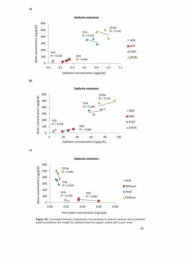
43

a)

b)

c)

0

100

200

300

400

500

600

0.0 0.2 0.4 0.6 0.8 1.0 1.2

Bio

ta c

on

cen

trat

ion

[n

g/gL

W]

Sediment concentration [ng/g dw]

Saduria entomon

HCB

DDX

PCB7

∑PCBs

∑PCBs R2 = 0.242

PCB7

R2 = 0.429

DDX R2 = 0.969

HCB R2 = 0.558

0

100

200

300

400

500

600

0 20 40 60 80 100

Bio

ta c

on

cen

trat

ion

[n

g/gL

W]

Sediment concentration [ng/g OC]

Saduria entomon

HCB

DDX

PCB7

∑PCBs

∑PCBs R2 = 0.225

PCB7

R2 = 0.090

DDX R2 = 0.988

HCB R2 = 0.919

0

100

200

300

400

500

600

0.00 0.02 0.04 0.06 0.08

Bio

ta c

on

cen

trat

ion

[n

g/gL

W]

Pore water concentration [ng/Lpw]

Saduria entomon

HCB

DDXsum

PCB7

PCBsum

∑PCBs R2 = 0.981

PCB7

R2 = 0.939

DDX R2 = 0.683

HCB R2 = 0.299

Figure 16: Correlation between contaminant concentrations in Saduria entomon and a) sediment

based on sediment dry weight, b) sediment based on organic carbon and c) pore water.

44

5 Discussion

5.1 General findings In general, method recoveries of all sample types were on average within a tolera-

ble range of 100±20%. In sediment samples 8 contaminants had average recover-

ies below 80%: PCB 52 (70±18%), PCB 114 (78±10%), PCB 126 (78±15%), PCB

157 (78±16%), PCB 169 (60±25%), PCB 170 (60±25%), PCB 189 (45±29%),

PCB 209 (62±25%). The lowest recoveries exhibited four out of the five latest

eluting compounds which could be related to their large molecular size and high

hydrophobicity. An evaluation of the method regarding these compounds could

improve future results.

Some contaminants could only be detected in low concentrations or in only a few

of the samples, and two of the target analytes (PCBs 126 and 169) were not de-

tected in any of the sediment, POM or biota samples. As these compounds are

non-ortho PCBs, their absence can be considered a positive result due to their co-

planar molecular structure and corresponding dioxin-like toxicity (see section

2.2.1). However, in sediment samples the recovery of PCB 126 and PCB 169 was

considerably lower. Instead of indicating absence of these contaminants this could

also point out that the method should be validated to ensure its suitability for these

compounds.

5.2 POP concentrations and organic carbon content in sediment Fiber banks exhibited the highest sediment contamination for all three contaminant

groups analyzed (Figure 7). This is only apparent when concentrations are based

on sediment dry weight. However, due to their hydrophobic properties the contam-

inants partition into the organic matter fraction in sediments. Consequently, for

sediments with high organic carbon content, higher contaminant concentrations

are expected. The organic carbon contents in the fiber banks are considerably

45

higher than in the other sediment types (Table 3), as a result of deposition of main-

ly cellulose (fiber bank area R & P) as well as wood fibers and wood shavings

(fiber bank area Q). Therefore, the results normalized to sediment organic carbon

content (Figure 8) allow an alternative way for comparison between sites. Concen-

trations normalized with organic carbon show less extreme differences between

the different sediment types. However, after normalization, two sites (Q-FB and

R-FB2) differed substantially from the other sites for PCB7 and ∑PCBs concentra-

tions (Figure 8). This clearly indicates influence of a nearby local source. For site

Q-FB, this is most likely the Sandviken sulfate pulp mill, judging by its location

just outside the factory (Appendix Figure A2). R-FB2 is one of the two fiber banks

in the proximity of the Väja sulfate pulp mill. The two fiber bank sites there are

separated by an erosion channel. The fiber bank site (R-FB1), which according to

the map seems to be located closer to the actual factory area (Appendix Figure

A1), had considerably lower PCB concentrations on an organic carbon basis than

R-FB2, but the organic carbon content is higher. The two fiber banks may both

have been part of the same fiber bank before. The formation of the erosion channel

might be the reason why they have been mapped as two independent fiber banks,

but in fact belong together with R-FB2 being the peripheral area of R-FB1. For

R-FB2, the larger distance from the mill could explain the lower organic carbon

content, as more of the fibers in the discharge water may have accumulated al-

ready close to the effluent inlet of the mill (forming R-FB1). The influence of the

nearby source together with comparably lower organic carbon content can explain

the high concentrations (on OC basis) at R-FB2 and the differences observed

(Figure 8) compared to the neighboring fiber bank site (R-FB1).

As mentioned in Chapter 4, the fiber bank site P-FB1 often showed exceptional

behavior compared to the other fiber bank sites. As suspected previously, the clas-

sification of sediment types made by SGU in the Fiberbank project may be incor-

rect for P-FB1. This can be explained by the fact that it differs in many site-

specific attributes from the other fiber bank sites. Compared with the other fiber

bank sediment samples, P-FB1 had low organic carbon content (2.55%) and was

the only site in this type of sediment where biota could be found. The sample

could be taken with the Gemax sampler unlike the others (OPB sampler). Also the

sampling depth was much deeper and the location differs: P-FB1 lies offshore,

while the remaining fiber banks are all located with connection to the shore. While

the other FB sites were formed around the discharge areas of the mills, P-FB1

most likely developed from dredging and depositing activities (Apler et al., 2014).

Due to these disparities one could argue that a further division into subcategories

would have been reasonable or rather, that the classification of fiber impacted

sediment types should be based on organic carbon contents. However, then the

question needs to be answered which specific organic carbon contents may be the

thresholds between the different fiber sediment types, i.e. FB, FRS, SED.

46

5.3 Classification of sediments The results showed that the sediments in the whole study area around Kramfors,

Sandviken and Väja are relatively high polluted with persistent organic pollutants.

At a few sites, low levels could be found for p,p’-DDX and PCB7. However, for

HCB, all of the sediment samples were classified with mid, high or even very high

(P-FB2) levels (Table 4). For PCB7 four sites were classified in the very high pol-

lution category (class 5). For ∑p,p’-DDX, however, none of the sites exhibited

class 5 contamination levels, nevertheless five sites were classified with high lev-

els (class 4). The highest classified level per compound group was always found at

fiber bank sites (with the exception of P-FB1). This suggests that the pollution is

connected with the fibers and consequently arouse from the sources of the fibers,

namely the pulp and saw mills in the area. Nevertheless, the existence of other

sources cannot be excluded.

The contaminants summed up as PCB7 are the seven most common PCBs, which

are also included in most studies. It is therefore applied as a standard indicator

parameter which facilitates comparison across different studies, which may not

target the same PCB congeners. Even though it is a helpful tool, it may lead to an

underestimation of the actual PCB burden by not taking into account the 14 other

PCB congeners analyzed in this master thesis study. Correspondingly, only the

p,p’-DDX were summed up as parameter leaving out the three o,p’-DDX. Never-

theless, it was found that for DDX, all sites were classified with the same level

when applying the same classification thresholds (Appendix Table A2) to the total

sum of DDX. However, for DDX this underestimation might not be as relevant as

for the PCBs, due to the fact that in nature, o,p’-DDX are generally present at sub-

stantially lower concentrations than p,p’-DDX.

5.4 POP relative distributions in sediments The compound distribution patterns in each of the sediment samples showed that

the samples had different contaminant compositions. The most apparent differ-

ences were noticeable in the proportion and composition of DDX. Differences in

the composition of DDX in sediments could indicate that usage and release of the

DDX compounds vary at the various local sources in different areas. However, as

these compounds are commonly applied as mixtures, the differences in the compo-

sition of DDX in different samples could also be due to problems during instru-

mental analysis. In the injector of the gas chromatograph, DDT can breakdown to

DDD and/or DDE (Foreman & Gates, 1997). This has been observed for

p,p’-DDT but o,p’-DDT is suspected to undergo similar breakdown. The break-

down of this thermolabile contaminant in the GC is often of relevance in sediment

47

samples (Foreman & Gates, 1997). Therefore, analysis of relationships between

the different DDX compounds should be interpreted with caution. Monitoring of a

performance evaluation standard (PES), after or several times during the field

samples injection in the GC would improve data quality and interpretations

(Foreman & Gates, 1997). Additionally, differences in the progress of the degrada-

tion process of DDT in the field could play a role as well.

5.5 POP concentrations in pore water In biota and sediment samples, PCB concentrations were generally the highest;

this was not the case for pore water concentrations. The highest concentrations in

pore water were due to DDX contamination (Appendix Figure A3). HCB and

∑PCBs concentrations were rather similar. But at some sites HCB concentrations

even exceeded the ∑PCBs concentration, even though HCB is only a single com-

pound. The reason might be that HCB and the DDX have lower log Kow values,

and are therefore less hydrophobic than the majority of the PCB contaminants

included in this master thesis study (Table 1). Less hydrophobic contaminants are

more likely to be found in the aqueous phase than the more hydrophobic ones.

5.6 POP concentrations in biota Site P FB1 was the only fiber bank sediment where biota could be sampled (Table

5). However, this site might be misclassified and instead be fiber rich sediment. In

that case, it was not possible to sample biota at any of the fiber bank sites. This

could indicate that fiber banks might not be suitable as habitat for biota, at least for

the two species investigated in this master thesis, due to the influences of the fi-

bers. A possible reason could be the anoxic conditions in the fiber bank, due to the

consumption of oxygen during microbial degradation of organic material. Fur-

thermore, the microbial degradation may lead to the presence of toxic products,

e.g. sulfide and ammonium, from microbial decomposition processes of organic

material (Forbes et al., 1998), which evidently is present in fiber banks in large

amounts. This will be discussed in more detail in 5.9.

48

5.7 Relation between sorption or bioaccumulation and hydrophobicity (hypothesis 1)

The results showed a significant relationship between the sorption of a contami-

nant and its hydrophobicity (Figure 10). The variation in the sorption could be

significantly explained by the log Kow value of the contaminant with 83%. This is

coherent with the general understanding of how organic compounds partition be-

tween different phases. The log Kd value gives insight on the sorption behavior of

contaminants. Sorption increases with increasing log Kd value. This means that

contaminants sorb stronger the more hydrophobic they are. At the same time, this

also gives insight about bioavailability. Contaminants with lower sorption will

have higher concentrations in the pore water. This explains why pore water con-

centrations of HCB and DDX exceed the concentration of the ∑PCBs (compare

4.5). Except for PCB 28 and 52, all other PCBs had higher log Kow values than the

HCB and DDX. In consequence, these less hydrophobic compounds will be more

readily available for uptake in biota. However, the real amount of the bioavailable

part that is actually taken up, depends on parameters such as feeding type of the

organisms (Kaag et al., 1997) and uptake paths (Forbes et al., 1998).

To what extent contaminants were taken up into biota is reflected by the BSAF

values. When related to corresponding log Kow values the polynomial trendline had

a rather poor (R2=0.224) and insignificant (p<0.079) fit for Marenzelleria. The

presumed bell-shaped distribution of the compounds implying low bioaccumula-

tion for compounds of both low and high hydrophobicity was observed for exam-

ple by Tracey and Hansen (1996). Their study compiled BSAF values of numerous

other studies and found a log Kow dependent bell shaped distribution for PCBs,

with lower bioaccumulation outside the log Kow range of 6.0-7.3. Reasons for this

behavior may be associated with lower accumulation efficiency, due to molecular

size for contaminants with high log Kow, and metabolization for compounds with

low log Kow (Tracey & Hansen, 1996). The data of this master thesis project could

not reliably confirm the observation by Tracey and Hansen (1996). In this master

thesis study, only two PCB compounds were analyzed that were below the log Kow

range identified by Tracey and Hansen (1996) as having high bioaccumulation,

and only 3 compounds had higher log Kow values. This might be too few data

points outside that range to be able to see a statistically significant bell-shaped

distribution. It needs to be mentioned that the study from 1996 observed the bell

shaped distribution for PCBs only and did not include DDX and HCB, unlike this

master thesis study. When only the PCBs were taken into account the R2 improved

(R2=0.327) but results were still not significant (p=0.077).

Regarding BSAF values of Saduria entomon, the results showed a significant line-

ar relationship (R2=0.525, p<0.001) between average BSAF values of a compound

49

and its hydrophobicity. As mentioned above, underrepresentation of compounds

outside the log Kow range may be a reason why a bell shaped distribution could not

be observed. Even though both biota species investigated are sediment-dwelling

organisms, they differ from each other regarding several characteristics, e.g. feed-

ing type and trophic level. These differences may possibly explain why for Sadu-

ria entomon and Marenzelleria not the same BSAF distributions were observed

with increasing contaminant hydrophobicity. However, Saduria entomon could

only be sampled at three spots, resulting in a generally low total number of data

points. Even though the statistical analysis resulted in a significant relationship,

the total amount of samples collected has influence on precision and uncertainty of

retrieved BSAF values (Burkhard, 2003). A higher amount of Saduria entomon

samples would be preferable for more representative results. Finally, the log Kow

range of contaminants detected in the two biota species differed. The high hydro-

phobic compounds that were related with the slight downward trend of the BSAF

distribution in Marenzelleria, were not detected in Saduria entomon samples. The

distributions of BSAF values between the two biota types may be more similar if

analyzed for the same log Kow range.

The average BSAF value per species showed that Saduria entomon (average of all

datapoints: 4.3) had a generally higher BSAF than Marenzelleria (average of all

datapoints: 1.9). While Marenzelleria is a surface deposit-feeder (Dauer et al.,

1981), Saduria entomon is a predator, feeding on other benthic fauna (Haahtela,

1990). Therefore, the higher average BSAF in Saduria entomon could be due to

biomagnification, as this species is on a higher trophic level in the food chain.

Other possible reasons might be differences in metabolism, lipid content or lipid

quality leading to different BSAF and BSAF distributions across different species.

To conclude, regarding sorption, hypothesis 1 could be accepted. Sorption proved

to be significantly correlated with contaminant properties showing low sorption

for compounds with low hydrophobicity (low log Kow). Regarding bioaccumula-

tion, hypothesis 1 had to be rejected. For Marenzelleria, the correlation between

bioaccumulation and hydrophobicity resembled the presumed bell-shaped distribu-

tion, but the relationship was not significant. For Saduria entomon the relationship

between the two parameters was significant, but with a linear relationship instead

of the expected bell-shaped distribution.

50

5.8 Relation between sorption or bioaccumulation and sediment composition (hypothesis 2)

Hypothesis 2 could partly be accepted. There is a relationship between sorption

and sediment composition regarding fiber banks and other sediment types. Sorp-

tion proved to be higher in fiber banks. Differences of sorption between fiber rich

sediments and less affected sediments, however, could not be confirmed. Regard-

ing bioaccumulation, no relationship between BSAFs and fiber impact on sedi-

ment could be found, so hypothesis 2 was rejected.

The suspended material in the discharged water, coming from pulp and paper

mills, led to the formation of the fiber banks. Sedimentation of cellulose fibers and

even wood fibers and wood shaving in the fiber banks introduced large amounts of

organic material. The increase of organic carbon enhances the opportunities for

pollutants to sorb and therefore increased sorption can be observed in the fiber

banks compared to other type of sediment. One could argue that the increased

sorption reduces availability of the contaminants. However, the organic material

may be degraded over time. In that case, the reduction of organic content could

lead to decreasing sorption. In consequence, contaminants could become even

more bioavailable in the future. Additionally, it needs to be considered that land-

slides or other movements arising from the land uplift (see section 2.1) can impact

the fiber banks and make large amounts of pollutants available in a short time.

Bioaccumulation did not differ in the different sediment types. This could indicate

that bioaccumulation is independent of the fiber impact on the sediment. However,

the organic carbon content, which is the major difference between the sediment

types, was already accounted for in the BSAF calculation (see section 3.6) unlike

in the Kd calculation. This could explain why along the fiber impact gradient dif-

ferences only could be observed for sorption. Nevertheless, it may be possible that

there actually exist differences for bioaccumulation as well, but the study and ex-

perimental setup could not manage to reveal these. If the differences between the

different sediment types only exist between fiber banks and other sediments, it

may be difficult to reveal these, when no biota could be found at any of the fiber

banks, except for P-FB1, which most likely was a fiber rich sediment site.

51

5.9 Relations between POP concentration in biota and concentration in pore water or total concentration (hypothesis 3)

Hypothesis 3 was formulated based on the assumption that contaminants are more

bioavailable if present in the pore water. It was presumed that the pollutants are

more readily available for uptake into biota when not being bound to the sediment

but occurring in the aqueous phase. Therefore, it was suspected that the pore water

concentrations reflect the concentrations found in biota best. However, results did

not prove the expected hypothesis. Only for PCB7 and ∑PCBs in Saduria entomon

contamination levels correlated best with pore water concentrations (Table 6;

Figure 16). Surprisingly, the direction of correlation opposed the expected one:

PCB levels in biota decreased with increasing pore water concentrations. Never-

theless, results were not significant and with only three sampling sites the results

should be interpreted with caution. HCB and DDX in Saduria entomon had best

correlations with levels in sediment normalized to organic carbon, but these were

also not significant.

For Marenzelleria significant correlations could be found. Increasing contaminant

concentrations were best reflected by increasing sediment concentrations normal-

ized to its dry weight. These findings were against expectations and therefore hy-

pothesis 3 had to be rejected.

For the calculation of the pore water concentration, data from the POM sampling

was used. As mentioned in 3.6, equilibrium and non-depletive conditions are re-

quired for the application of this method. Hawthorne et al. (2009) found the dura-

tion of 28 days sufficiently long in order to reach equilibrium. The check for de-

pletion, however, revealed that several POM samples exceeded the depletion

threshold of 5%. The sorption capacity of the passive sampling material should be

negligible (Lydy et al., 2014) in order to reflect pore water concentrations reliably.

The exceedance of the threshold indicates that inadvertently a higher amount of

the contaminant, originating from the sediment, is found in the POM sampler. Due

to depletion, the pore water concentrations might be distorted. This could in turn

influence which sample matrice reflects concentrations in biota best. In the present

study, the amount of sediment used for POM sampling may have been insufficient.

Its high water content could have played a role. In order to overcome this issue in

the future, the amount of sediment taken for POM analysis could be increased, or

the POM sampler size decreased. This in turn could, however, affect its ability for

reliable contaminant detection.

The contaminants investigated are characterized among others by differences in

their hydrophobicity. Uptake routes of contaminants into biota differ in their im-

52

portance depending on their hydrophobicity. With increasing log Kow the im-

portance shifts from uptake via pore water (for low log Kow compounds) to uptake

via ingested sediment particles (Josefsson et al., 2011). Most POPs in this master

thesis study have relatively high log Kow, therefore pore water as the source for

contaminant uptake may not be as important as the uptake by ingestion of contam-

inated sediment particles. Due to differences in the food sources, the uptake path-

way from sediment may not be as important to Saduria entomon, as it is feeding

on other biota (Haahtela, 1990). However, Marenzelleria can take up feed from

either pore water or sediment (Dauer et al., 1981). For highly hydrophobic con-

taminants, like the ones in this thesis project, the contaminant uptake via sediment

may be the dominant pathway in that case. This could therefore explain why biota

concentrations correlate better to sediment concentrations than to pore water con-

centrations. Additionally, some sediment-dwelling animals actively avoid contact

with pore water, as it is toxic to most of them (Forbes et al., 1998). This is due to

different products (e.g sulfide and ammonium) produced by microbes when de-

composing organic matter. Due to the fiber accumulation, sediments in the study

area have high organic matter contents. In combination with decomposition pro-

cesses taking place, it could be suspected, that the pore water in the contaminated

sediments might be toxic to biota as well as low in oxygen content. This could be

an additional explanation why pore water concentrations do not reflect biota con-

centrations best. In consequence, the presence of toxic metabolic products might

be higher and oxygen content lower in areas with more organic matter available

for composition. This could therefore additionally give an explanation why no

biota samples could be found at fiber bank sites.

53

6 Conclusions and outlook Besides determining contaminant burdens in sediment, pore water and biota,

this master thesis project gave insight into how physical-chemical properties of

contaminants, as well as sediment composition (regarding fiber impact) are re-

lated to the contaminant sorption and bioaccumulation. Increased organic car-

bon content, due to the fiber accumulation, played a major role in sorbing pollu-

tants. The presence of a wide range of POPs in high concentrations in fiber

banks shows that environmental impacts of paper and pulp mills should be fo-

cused on. This is especially true in an area like the High Coast, which is under-

going changes, due to the uplift of land and its consequences for the seabed.

More research is needed to fully understand processes and reasons for pollutant

behavior and pollutant transport in sediments on the one hand and in fiber im-

pacted sediments on the other hand. Moreover, an improved classification sys-

tem for differentiation between different fiber type sediment could improve fu-

ture research and the comparability between fiber bank areas in different loca-

tions. Additionally, it would be interesting for future studies to investigate the

contamination patterns, to see if significant differences in the contaminant com-

position between the different fiber bank areas exist and which congeners may

be more relevant. Multivariate statistics, e.g principal component analysis

(PCA), may be a suitable tool for this kind of investigations. In particular, dif-

ferences linked to the different type of pulp and paper production processes (e.g.

sulfate or sulfite factory) may be worthwhile analyzing and could help to track

pollution sources and consequently to counteract. The determination of fiber

bank impacts on the environment and assessing related risks for society and the

environment are important prospective steps. Subsequently, possibilities for re-

mediation of polluted sediments should be explored. Finally, once identified and

localized, pollutant sources can more easily be assigned to their polluter. This in

turn can facilitate the process of allocating responsibilities for potential reme-

diation activities and corresponding costs.

54

7 Acknowledgements

There are some people, who I would like to thank because they made it possible

for me to write this master thesis.

Thank you, Sarah Josefsson, for giving me the opportunity to work with this pro-

ject and providing answers to my countless questions during the whole duration of

the project. I appreciate a lot that you always took some time whenever I needed

your support. I would like to thank you for teaching me so much about the labora-

tory methods, instrumental analysis and this interesting research topic in general. I

am happy that I will be given the opportunity to follow the TREASURE project a

bit longer even after the end of this master thesis project.

Thank you, Andreas Loibner, the interest in my master thesis topic and for unhesi-

tatingly approving to be cross-border Co-supervisor.

Thank you, Karin Wiberg, for reading and assessing the final report as well as

presentation about what I have been working with over the last months. I am look-

ing forward to your comments as an examiner.

Thank you, Helene Puehringer, for your interest in my thesis and your offer to

read this work critically as an opponent. I am curious to find out about your com-

ments and ideas.

Thank you, Anna Apler, for providing me with maps, details about sampling as

well as with information about fiber banks in general and about the history of ac-

tivities related to paper and pulp industry in Västernorrland in particular.

Thank you, Joachim Audet, for motivational words and your kind support creating

a map with ArcGIS and for helping me gain an overview over my large amounts

of data using R.

55

And finally a special thanks to my friends and family:

Thank you for all the fun and entertaining moments and for making my studies in

Sweden to such an enjoyable and unforgettable experience.

Thank you for supporting me anytime, regardless of distances between countries

and in that way brightening up Swedish winter like times but also joyfully sharing

the walk on the bright side of life together.

56

References

Alexander, M. (2000). Aging, bioavailability, and overestimation of risk from environmental pollutants. Environmental Science & Technology, 34(20), pp. 4259-4265.

Apler, A., Nyberg, J., Jönsson, K., Hedlund, I., Heinemo, S.-Å. & Kjellin, B. (2014). Fiberbanksprojektet - Kartläggning av fiberhaltiga sediment längs Västernorrlands kust: SGU, Sveriges geologiska undersökning.

Bailey, R.E. (2001). Global hexachlorobenzene emissions. Chemosphere, 43(2), pp. 167-182.

Baird, C. & Cann, M. (2012). Environmental Chemistry5th Edition). New York: W.H. Freeman and Company.

Barber, J., Sweetman, A. & Jones, K. (2005a). Hexachlorobenzene - Sources, environmental fate and risk characterisation. Science Dossiers.

Barber, J.L., Sweetman, A.J., van Wijk, D. & Jones, K.C. (2005b). Hexachlorobenzene in the global environment: Emissions, levels, distribution, trends and processes. Science of the Total Environment, 349(1-3), pp. 1-44.

Birdwell, J., Cook, R.L. & Thibodeaux, L.J. (2007). Desorption kinetics of hydrophobic organic chemicals from sediment to water: A review of data and models. Environmental Toxicology and Chemistry, 26(3), pp. 424-434.

Boese, B.L., Lee Ii, H., Specht, D.T., Randall, R.C. & Winsor, M.H. (1990). Comparison of aqueous and solid‐phase uptake for hexachlorobenzene in the tellinid clam Macoma nasuta (conrad): A mass balance approach. Environmental Toxicology and Chemistry, 9(2), pp. 221-231.

Braune, B.M., Outridge, P.M., Fisk, A.T., Muir, D.C.G., Helm, P.A., Hobbs, K., Hoekstra, P.F., Kuzyk, Z.A., Kwan, M., Letcher, R.J., Lockhart, W.L., Norstrom, R.J., Stern, G.A. & Stirling, I. (2005). Persistent organic pollutants and mercury in marine biota of the Canadian Arctic: An overview of spatial and temporal trends. Science of the Total Environment, 351–352, pp. 4-56.

57

Burkhard, L.P. (2003). Factors influencing the design of bioaccumulation factor and biota‐sediment accumulation factor field studies. Environmental Toxicology and Chemistry, 22(2), pp. 351-360.

Dauer, D.M., Maybury, C.A. & Ewing, R.M. (1981). Feeding behavior and general ecology of several spionid polychaetes from the Chesapeake Bay. Journal of Experimental Marine Biology and Ecology, 54(1), pp. 21-38.

Dietz, R., Riget, F., Cleemann, M., Aarkrog, A., Johansen, P. & Hansen, J. (2000). Comparison of contaminants from different trophic levels and ecosystems. Science of the Total Environment, 245(1), pp. 221-231.

Endo, S., Hale, S.E., Goss, K.-U. & Arp, H.P.H. (2011). Equilibrium partition coefficients of diverse polar and nonpolar organic compounds to polyoxymethylene (POM) passive sampling devices. Environmental Science & Technology, 45(23), pp. 10124-10132.

Erickson, M.D. & Kaley, R.G. (2011). Applications of polychlorinated biphenyls. Environmental Science and Pollution Research, 18(2), pp. 135-151.

Forbes, T.L., Forbes, V.E., Giessing, A., Hansen, R. & Kure, L.K. (1998). Relative role of pore water versus ingested sediment in bioavailability of organic contaminants in marine sediments. Environmental Toxicology and Chemistry, 17(12), pp. 2453-2462.

Foreman, W.T. & Gates, P.M. (1997). Matrix-enhanced degradation of p, p'-DDT during gas chromatographic analysis: A consideration. Environmental Science & Technology, 31(3), pp. 905-910.

Haahtela, I. What do Baltic studies tell us about the isopod Saduria entomon (L.)? In: Proceedings of Annales Zoologici Fennici1990: JSTOR, pp. 269-278.

Hatzinger, P.B. & Alexander, M. (1995). Effect of Aging of Chemicals in Soil on Their Biodegradability and Extractability. Environmental Science & Technology, 29(2), pp. 537-545.

Hawker, D.W. & Connell, D.W. (1988). Octanol Water Partition-Coefficients of Polychlorinated Biphenyl Congeners. Environmental Science & Technology, 22(4), pp. 382-387.

Hawthorne, S.B., Miller, D.J. & Grabanski, C.B. (2009). Measuring Low Picogram Per Liter Concentrations of Freely Dissolved Polychlorinated Biphenyls in Sediment Pore Water Using Passive Sampling with Polyoxymethylene. Analytical Chemistry, 81(22), pp. 9472-9480.

Jaga, K. & Dharmani, C. (2003). Global surveillance of DDT and DDE levels in human tissues. Int J Occup Med Environ Health, 16(1), pp. 7-20.

Jones, K.d.V., P. (1999). Persistent organic pollutants (POPs): state of the science. Environmental Pollution, 100, pp. 209-221.

Josefsson, S., Leonardsson, K., Gunnarsson, J.S. & Wiberg, K. (2010). Bioturbation-Driven Release of Buried PCBs and PBDEs from Different Depths in Contaminated Sediments. Environmental Science & Technology, 44(19), pp. 7456-7464.

58

Josefsson, S., Leonardsson, K., Gunnarsson, J.S. & Wiberg, K. (2011). Influence of contaminant burial depth on the bioaccumulation of PCBs and PBDEs by two benthic invertebrates (Monoporeia affinis and Marenzelleria spp.). Chemosphere, 85(9), pp. 1444-1451.

Kaag, N.H., Foekema, E.M., Scholten, M.C.T. & van Straalen, N.M. (1997). Comparison of contaminant accumulation in three species of marine invertebrates with different feeding habits. Environmental Toxicology and Chemistry, 16(5), pp. 837-842.

Kelly, B.C., Ikonomou, M.G., Blair, J.D., Morin, A.E. & Gobas, F.A.P.C. (2007). Food Web–Specific Biomagnification of Persistent Organic Pollutants. Science, 317(5835), pp. 236-239.

Lake, J.L., Rubinstein, N.I., Lee, H., Lake, C.A., Heltshe, J. & Pavignano, S. (1990). Equilibrium partitioning and bioaccumulation of sediment‐associated contaminants by infaunal organisms. Environmental Toxicology and Chemistry, 9(8), pp. 1095-1106.

Lydy, M.J., Landrum, P.F., Oen, A.M.P., Allinson, M., Smedes, F., Harwood, A.D., Li, H., Maruya, K.A. & Liu, J. (2014). Passive sampling methods for contaminated sediments: State of the science for organic contaminants. Integrated Environmental Assessment and Management, 10(2), pp. 167-178.

Mackay, D., Shiu, W.-Y., Ma, K.-C. & Lee, S.C. (2006). Handbook of physical-chemical properties and environmental fate for organic chemicals: CRC press.

Meylan, W.M., Howard, P.H., Boethling, R.S., Aronson, D., Printup, H. & Gouchie, S. (1999). Improved method for estimating bioconcentration/bioaccumulation factor from octanol/water partition coefficient. Environmental Toxicology and Chemistry, 18(4), pp. 664-672.

National Research Council of the National Academies (2003). Bioavailability of Contaminants in Soils and Sediments: Processes, Tools, and Applications. Washington, DC: The National Academies Press. Available from: http://www.nap.edu/catalog/10523/bioavailability-of-contaminants-in-soils-and-sediments-processes-tools-and.

Naturvårdsverket (2015-01-22). Tabell 30 i Naturvårdsverkets rapport 4914 (1999) Bedömningsgrunder för miljökvalitet. http://www.naturvardsverket.se/Stod-i-miljoarbetet/Vagledningar/Miljoovervakning/Bedomningsgrunder/Sediment/ [2015-10-19].

Pokhrel, D. & Viraraghavan, T. (2004). Treatment of pulp and paper mill wastewater—a review. Science of the Total Environment, 333(1), pp. 37-58.

Reichenberg, F. & Mayer, P. (2006). Two complementary sides of bioavailability: Accessibility and chemical activity of organic contaminants in sediments and soils. Environmental Toxicology and Chemistry, 25(5), pp. 1239-1245.

59

Reid, B.J., Jones, K.C. & Semple, K.T. (2000). Bioavailability of persistent organic pollutants in soils and sediments - a perspective on mechanisms, consequences and assessment. Environmental Pollution, 108(1), pp. 103-112.

Schenker, U., MacLeod, M., Scheringer, M. & Hungerbühler, K. (2005). Improving data quality for environmental fate models: A least-squares adjustment procedure for harmonizing physicochemical properties of organic compounds. Environmental Science & Technology, 39(21), pp. 8434-8441.

Shiu, W.Y. & Mackay, D. (1986). A critical review of aqueous solubilities, vapor pressures, Henry’s law constants, and octanol–water partition coefficients of the polychlorinated biphenyls. Journal of Physical and Chemical Reference Data, 15(2), pp. 911-929.

Swedish Forest Industries Federation (2014). The Swedish Forest Industries Federation - Fact and Figures 2014 The Swedish Forest Industries Federation. Available from: http://www.forestindustries.se/documentation/facts_and_figures

Tehrani, R. & Van Aken, B. (2014). Hydroxylated polychlorinated biphenyls in the environment: sources, fate, and toxicities. Environmental Science and Pollution Research, 21(10), pp. 6334-6345.

Tracey, G. & Hansen, D. (1996). Use of biota-sediment accumulation factors to assess similarity of nonionic organic chemical exposure to benthically-coupled organisms of differing trophic mode. Archives of Environmental Contamination and Toxicology, 30(4), pp. 467-475.

Turusov, V., Rakitsky, V. & Tomatis, L. (2002). Dichlorodiphenyltrichloroethane (DDT): Ubiquity, persistence, and risks. Environmental Health Perspectives, 110(2), pp. 125-128.

United Nations Environment Programme The Stockholm Convention on Persitent Organic Pollutants. http://chm.pops.int/ [2015-11-04].

Van den Berg, M., Birnbaum, L.S., Denison, M., De Vito, M., Farland, W., Feeley, M., Fiedler, H., Hakansson, H., Hanberg, A., Haws, L., Rose, M., Safe, S., Schrenk, D., Tohyama, C., Tritscher, A., Tuomisto, J., Tysklind, M., Walker, N. & Peterson, R.E. (2006). The 2005 World Health Organization Reevaluation of Human and Mammalian Toxic Equivalency Factors for Dioxins and Dioxin-Like Compounds. Toxicological Sciences, 93(2), pp. 223-241.

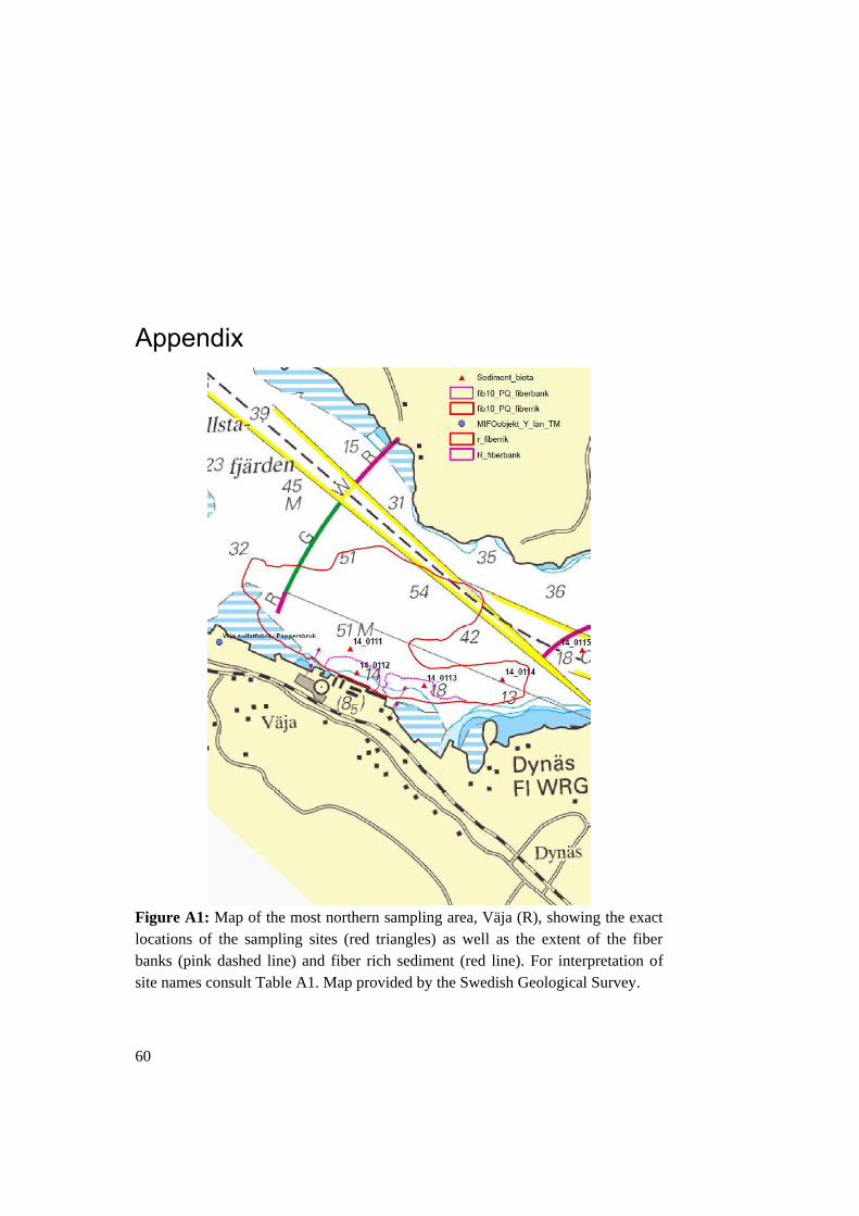
60

Appendix

Figure A1: Map of the most northern sampling area, Väja (R), showing the exact

locations of the sampling sites (red triangles) as well as the extent of the fiber

banks (pink dashed line) and fiber rich sediment (red line). For interpretation of

site names consult Table A1. Map provided by the Swedish Geological Survey.

61

Figure A2: Map of the two southern sampling areas, Sandviken (Q) and Kramfors

(P), showing the exact locations of the sampling sites (red triangles) as well as the

extent of the fiber banks (pink dashed line) and fiber rich sediment (red line). For

interpretation of site names consult Table A1. Map provided by the Swedish Geo-

logical Survey.

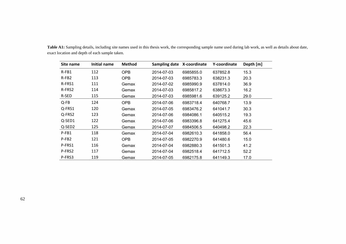
62

Table A1: Sampling details, including site names used in this thesis work, the corresponding sample name used during lab work, as well as details about date,

exact location and depth of each sample taken.

Site name Initial name Method Sampling date X-coordinate Y-coordinate Depth [m]

R-FB1 112 OPB 2014-07-03 6985855.0 637852.8 15.3 R-FB2 113 OPB 2014-07-03 6985783.3 638231.3 20.3 R-FRS1 111 Gemax 2014-07-02 6985990.9 637814.0 36.9 R-FRS2 114 Gemax 2014-07-03 6985817.2 638673.3 16.2 R-SED 115 Gemax 2014-07-03 6985981.6 639125.2 29.0 Q-FB 124 OPB 2014-07-06 6983718.4 640768.7 13.9 Q-FRS1 120 Gemax 2014-07-05 6983476.2 641041.7 30.3 Q-FRS2 123 Gemax 2014-07-06 6984086.1 640515.2 19.3 Q-SED1 122 Gemax 2014-07-06 6983396.8 641275.4 45.6 Q-SED2 125 Gemax 2014-07-07 6984506.5 640498.2 22.3 P-FB1 118 Gemax 2014-07-04 6982610.3 641858.0 56.4 P-FB2 121 OPB 2014-07-05 6982270.9 641480.6 15.0 P-FRS1 116 Gemax 2014-07-04 6982880.3 641501.3 41.2 P-FRS2 117 Gemax 2014-07-04 6982518.4 641712.5 52.2 P-FRS3 119 Gemax 2014-07-05 6982175.8 641149.3 17.0

63

Table A2: Assessment criteria for statistical classification of organic pollutants in sedi-

ment along the Swedish coast (ng/g dw) according to Naturvårdsverket (1999).

Class 1 Class 2 Class 3 Class 4 Class 5

No level

Low level

Mid level

High level

Very high level

HCB 0.00 0-0.04 0.04-0.2 0.2-1 >1

PCB7 0.00 0-1.3 1.3-4 4.0-15 >15

∑ p,p' DDX 0.00 0-0.2 0.2-1 1.0-6 >6

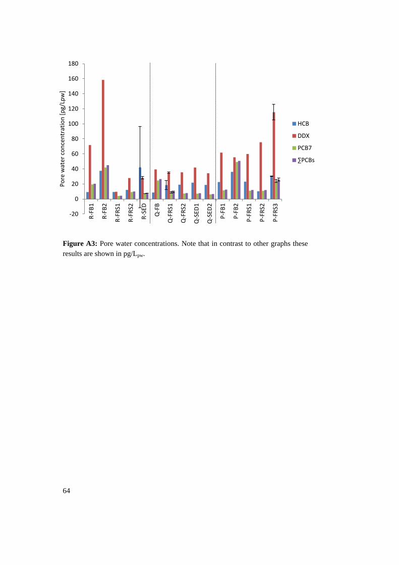
64

Figure A3: Pore water concentrations. Note that in contrast to other graphs these

results are shown in pg/Lpw.

-20

0

20

40

60

80

100

120

140

160

180

R-F

B1

R-F

B2

R-F

RS1

R-F

RS2

R-S

ED

Q-F

B

Q-F

RS1

Q-F

RS2

Q-S

ED1

Q-S

ED2

P-F

B1

P-F

B2

P-F

RS1

P-F

RS2

P-F

RS3

Po

re w

ater

co

nce

ntr

atio

n [

pg/

Lpw

]

HCB

DDX

PCB7

∑PCBs

65

a)

b)

Figure A4: Biota contaminant concentrations normalized to biota a) dry weight

and b) lipid weight. Biota types found were Marenzelleria (Mz) and Saduria en-

tomon (Sad).

0

5

10

15

20

25

30

35

R-S

ED-M

z

Q-F

RS1

-Mz

Q-F

RS1

-Sad

Q-F

RS2

-Mz

Q-F

RS2

-Sad

Q-S

ED1

-Mz

Q-S

ED2

-Mz

P-F

B1

-Mz

P-F

RS1

-Mz

P-F

RS1

-Sad

P-F

RS2

-Mz

Bio

ta c

on

cen

trat

ion

[n

g/g

dw

]

HCB

DDX

PCB7

∑PCBs

0

100

200

300

400

500

600

R-S

ED-M

z

Q-F

RS1

-Mz

Q-F

RS1

-Sad

Q-F

RS2

-Mz

Q-F

RS2

-Sad

Q-S

ED1

-Mz

Q-S

ED2

-Mz

P-F

B1

-Mz

P-F

RS1

-Mz

P-F

RS1

-Sad

P-F

RS2

-Mz

Bio

ta c

on

cen

trat

ion

[n

g/g

LW]

HCB

DDX

PCB7

∑PCBs

66

a)

b)

Figure A5: Biota contaminant concentrations normalized to biota a) dry weight

and b) lipid weight, for sites where both biota types were found.

0

5

10

15

20

25

Q-F

RS1

-Mz

Q-F

RS1

-Sad

Q-F

RS2

-Mz

Q-F

RS2

-Sad

P-F

RS1

-Mz

P-F

RS1

-Sad

Bio

ta c

on

cen

trat

ion

[n

g/gd

w]

HCB

DDX

PCB7

∑PCBs

0

100

200

300

400

500

600

Q-F

RS1

-Mz

Q-F

RS1

-Sad

Q-F

RS2

-Mz

Q-F

RS2

-Sad

P-F

RS1

-Mz

P-F

RS1

-Sad

Bio

ta c

on

cen

trat

ion

[n

g/gL

W]

HCB

DDX

PCB7

∑PCBs