
Patient-specific modelling of cortical spreading depression ...
284
T ESIS DOCTORAL /DOKTOREGO T ESIA Patient-specific modelling of cortical spreading depression applied to migraine studies Autora / Egilea: Julia M. Kroos Director / Zuzendaria: Dr. Luca Gerardo-Giorda Bilbao, 2019 (c)2019 JULIA M. KROOS
-
Upload
khangminh22 -
Category
Documents
-
view
0 -
download
0
Transcript of Patient-specific modelling of cortical spreading depression ...
TESIS DOCTORAL / DOKTOREGO TESIA
Patient-specific modelling of corticalspreading depression applied to migraine
studies
Autora / Egilea:Julia M. Kroos
Director / Zuzendaria:Dr. Luca Gerardo-Giorda
Bilbao, 2019
(c)2019 JULIA M. KROOS


DOCTORAL THESIS
Patient-specific modelling of corticalspreading depression applied to migraine
studies
Author:Julia M. Kroos
Supervisor:Dr. Luca Gerardo-Giorda
Bilbao, 2019


“If the human brain were so simple that we could understand it,we would be so simple that we couldn’t.”
Emerson M. Pugh, in The Biological Origin of Human Values (1978)


This research was carried out at the Basque Center for Applied Mathematics (BCAM)within the Mathematical Modelling in Biosciences (MMB) group. The research was sup-ported by the Basque Government through the BERC 2014-2017 program, and by theSpanish Ministry of Economics and Competitiveness MINECO through the BCAM SeveroOchoa excellence accreditation SEV-2013-0323 and SEV-2017-0718 and the Spanish "PlanEstatal de Investigación Desarrollo e Innovación Orientada a los Retos de la Sociedad"under Grant BELEMET - Brain ELEctro-METabolic modeling and numerical approxima-tion (MTM2015-69992-R).


i
Resumen corto
La migraña es un trastorno neurológico muy común. Un tercio de los pacientes quesufren migraña experimentan lo que se denomina aura, una serie de alteraciones sen-soriales que preceden al típico dolor de cabeza unilateral. Diversos estudios apuntana la existencia de una correlación entre el aura visual y la depresión cortical propa-gada (DCP), una onda de despolarización que tiene su origen en el córtex visual parapropagarse, a continuación, por todo el córtex hacia las zonas periféricas. La compleji-dad y la elevada especificidad de las características del córtex cerebral sugieren que lageometría podría tener un impacto significativo en la propagación de la DCP. En estatesis hemos combinado dos modelos existentes: un modelo neurológico pormenorizadopara el componente electrofisiológico de la DCP y un modelo de reacción-difusión quetiene en consideración la difusión del potasio, el impulsor de la propagación de la DCP.Durante el proceso, hemos integrado dos aspectos de la DCP que tienen lugar en dife-rentes escalas de tiempo: la dinámica electrofisiológica seguiría un patrón temporal delorden de milisegundos, mientras que la dinámica del potasio extracelular que accionalas funciones de propagación de la DCP se mediría en una escala de minutos. Como re-sultado, obtendremos un modelo multiescalar EDP-EDO. Asimismo, hemos incorporadolos datos específicos del paciente en el modelo DCP: (i) la geometría cerebral específicade un paciente obtenida a través de resonancia magnética, y (ii) los tensores de conduc-tividad personalizados obtenidos a través de diffusion tensor images. A fin de estudiar elpapel que desempeña la geometría en la propagación de la DCP, hemos definido las can-tidades de interés (CdI) relacionadas con la geometría y las que dependen de la DCP y lashemos evaluado en dos casos prácticos. Si bien la geometría no parece tener un impactosignificativo en la propagación de la DCP, algunas CdI han resultado ser unas candidatasmuy prometedoras para facilitar la clasificación de individuos sanos y pacientes con mi-graña. Finalmente, para justificar la carencia de datos experimentales para la validacióny selección de los parámetros del modelo, hemos aplicado diversas técnicas de cuantifi-cación de la incertidumbre al modelo DCP y hemos analizado el impacto de las diversaselecciones de parámetros en el resultado del modelo.

iii
Laburpena
Migraina ohiko gaixotasun neurologiko bat da, eta hiru pazientetik batek migraina-aura,hots, buruko minaren aurretik sortzen den ikusmenaren asaldura, jasaten du. Hain-bat ikerketaren arabera, aura korrelazioan egon liteke cortical spreading depression (CSD)delakoarekin, garun azal bisualean sortzen den eta gune periferikoetara zabaltzen dendespolarizazio uhinarekin alegia. Garun azalaren egitura konplexua eta pazientearenaraberakoak diren ezaugarriak direla eta, bere geometriak CSDaren hedapenean zeresanhandia izan lezakeela uste da. Tesi honetan ezagunak diren bi eredu bateratuko ditugu:bata, CSDaren elektrofisiologia zehazki deskribatzen duen eredua; bestea, CSDaren gara-penean eragina duen potasioaren hedapena aurreikusten duen erreakzio-difusio eredua.Biak konbinatzean, denbora-eskala desberdinetan gertatzen diren CSDaren bi ezaugarrihartuko ditugu kontuan; izan ere, dinamika elektrofisiologikoa milisegundoen eskalanneurtzen da; CSDa eragiten duen zelulaz kanpoko potasioaren dinamika, ordea, min-ututan. Ondorioz, eskala anitzeko eredu diferentziala lortuko dugu. Halaber, pazien-tearen araberako datuak kontuan hartuko ditugu ereduan. Alde batetik, pazientearenburmuinaren geometria behatuko dugu erresonantzia magnetikoaren bidez, eta bestetik,difusio-tentsoreen bidezko irudien bidez lortutako konduktibitate-tentsore pertsonalizat-uak erregistratuko ditugu. Geometriak CSDaren hedapenean duen eragina aztertzeko,ezaugarri geometrikoak dituzten eta CSDaren menpekoak diren zenbait kantitate defini-tuko ditugu quantities of interest (QoI) izenpean eta aurreko bi kasuetan neurtuko di-tugu. Dirudienez, geometriak ez du eragin handirik CSDaren hedapenean, baina halaere zenbait QoI erabilgarriak izan litezke banako osasuntsuak eta migrainadun banakoakbereizteko. Amaitzeko, ereduaren parametroak egoki aukeratzeko eta datu esperimen-talen falta konpontzeko, ziurgabetasun-kuantifikazio teknikak erabiliko ditugu ereduare-kin batera, eta parametroen aukera desberdinek ereduan duten eragina aztertuko dugu.


v
Abstract
Migraine is a common neurological disorder and one-third of migraine patients sufferfrom migraine aura, a perceptual disturbance preceding the typically unilateral headache.Cortical spreading depression (CSD), a depolarisation wave that originates in the visualcortex and propagates across the cortex to the peripheral areas, has been suggested as acorrelate of visual aura by several studies. The complex and highly individual-specificcharacteristics of the brain cortex suggest that the geometry might have a significant im-pact on CSD propagation. In this thesis, we combine two existing models, a detailed neu-rological model for the electrophysiological component of CSD and a reaction-diffusionmodel accounting for the potassium diffusion, the driving force of CSD propagation. Inthe process, we integrate two aspects of CSD that occur at different time scales: the elec-trophysiological dynamics features a temporal scale in the order of milliseconds, whilethe extracellular potassium dynamics that triggers CSD propagation features is on thescale of minutes. As a result we obtain a multi-scale PDE-ODE model. In addition, weincorporate patient-specific data in the CSD model: (i) a patient-specific brain geometryobtained from magnetic resonance imaging, and (ii) personalised conductivity tensorsderived from diffusion tensor imaging data. To study the role of the geometry in CSDpropagation, we define geometric and CSD-dependent quantities of interest (QoI) thatwe evaluate in two case studies. Even though the geometry does not seem to have amajor impact on the CSD propagation, some QoI are promising candidates to aid in theclassification of healthy individuals and migraine patients. Finally, to account for the lackof experimental data for validation and selection of the model parameters, we apply dif-ferent techniques of uncertainty quantification to the CSD model and analyse the impactof various parameter choices on the model outcome.


vii
Resumen
La migraña es una de las principales causas mundiales de incapacidad en la poblaciónactual. Un tercio de los pacientes que sufren migraña padecen también lo que se deno-mina aura de migraña, una serie de trastornos sensoriales que anteceden al típico dolorde cabeza. Diversos estudios apuntan a la existencia de una correlación entre el auravisual y la depresión cortical propagada (DCP), una onda de despolarización que tienesu origen en el córtex visual para propagarse a continuación por todo el córtex hacia laszonas periféricas (Hadjikhani et al., 2001; Richter y Lehmkühler, 2008). Tras más de 70años de investigación en el campo de la migraña y de la DCP, el origen y las causas deeste fenómeno siguen sin estar completamente claros.
El paso de una onda DCP desencadena diversos cambios en la respuesta vascular, enel flujo sanguíneo y en el metabolismo de la energía. Los cambios drásticos de las con-centraciones iónicas en el interior y el exterior de las neuronas corticales provocan unbreve periodo de una intensa actividad, seguido de una reducción abrupta del poten-cial de membrana que silencia la actividad neuronal durante un periodo corto de tiempo(Pietrobon y Moskowitz, 2014). La DCP se caracteriza por un aumento significativo delpotasio extracelular y la hipótesis más extendida apunta a la difusión del potasio ex-tracelular como su principal catalizador (Zandt, Haken, y Putten, 2013; Zandt et al., 2015).
Algunos estudios recientes han comenzado a considerar el efecto de las geometrías cor-ticales en la propagación de la DCP, con diverso nivel de detalle. Pocci et al., 2010 si-mularon la propagación de una onda en un conducto en 2D que presentaba una curva,demostrando que las curvas cerradas podrían bloquear la propagación de la onda. Si-guiendo un enfoque de modelización personalizado, Dahlem et al., 2015 emplearon lacurvatura de Gauss del córtex para identificar objetivos potenciales para la neuromodu-lación. Estos estudios ya aluden al hecho de que las dobleces y los pliegues en el córtexpodrían influir en la propagación de la onda de despolarización. En consecuencia, lacomplejidad y la elevada especificidad de las características del córtex cerebral podríandesempeñar un papel significativo en la propagación de la DCP.
Motivación y objetivos principales
Los avances en tecnología han permitido un acceso cada vez mayor a una enorme canti-dad de datos. Especialmente en el sector médico, en el que el análisis y la interpretaciónde los datos de los pacientes individuales podrían ayudarnos a entender las causas y ladinámica de una enfermedad en particular. Los modelos matemáticos pueden propor-cionarnos un conocimiento significativo y profundo sobre el origen de una enfermedady su progresión. Asimismo, estos modelos nos pueden ofrecer un análisis del contexto yuna evaluación de los riesgos de las estrategias de tratamiento posibles, que irán desdeun tratamiento personalizado y un diseño inteligente de los medicamentos, hasta un crib-ado de la población y una minería de datos electrónicos sobre la salud. Durante la inves-tigación de la migraña con aura, las resonancias magnéticas que incluyeron datos dediffusion-weighted imaging (DWI) o diffusion tensor imaging (DTI) ofrecieron informacióndetallada sobre el córtex y la estructura del tejido subyacente. En esta tesis proponemos
viii
un modelo matemático detallado para la propagación de la DCP en combinación coninformación específica de cada paciente sobre la geometría de su cerebro y las caracterís-ticas de su córtex cerebral.
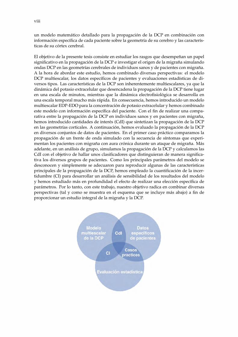
El objetivo de la presente tesis consiste en estudiar los rasgos que desempeñan un papelsignificativo en la propagación de la DCP e investigar el origen de la migraña simulandoondas DCP en las geometrías cerebrales de individuos sanos y de pacientes con migraña.A la hora de abordar este estudio, hemos combinado diversas perspectivas: el modeloDCP multiescalar, los datos específicos de pacientes y evaluaciones estadísticas de di-versos tipos. Las características de la DCP son inherentemente multiescalares, ya que ladinámica del potasio extracelular que desencadena la propagación de la DCP tiene lugaren una escala de minutos, mientras que la dinámica electrofisiológica se desarrolla enuna escala temporal mucho más rápida. En consecuencia, hemos introducido un modelomultiescalar EDP-EDO para la concentración de potasio extracelular y hemos combinadoeste modelo con información específica del paciente. Con el fin de realizar una compa-rativa entre la propagación de la DCP en individuos sanos y en pacientes con migraña,hemos introducido cantidades de interés (CdI) que sintetizan la propagación de la DCPen las geometrías corticales. A continuación, hemos evaluado la propagación de la DCPen diversos conjuntos de datos de pacientes. En el primer caso práctico comparamos lapropagación de un frente de onda simulado con la secuencia de síntomas que experi-mentan los pacientes con migraña con aura crónica durante un ataque de migraña. Másadelante, en un análisis de grupo, simulamos la propagación de la DCP y calculamos lasCdI con el objetivo de hallar unos clasificadores que distinguieran de manera significa-tiva los diversos grupos de pacientes. Como los principales parámetros del modelo sedesconocen y simplemente se adecuaron para reproducir algunas de las característicasprincipales de la propagación de la DCP, hemos empleado la cuantificación de la incer-tidumbre (CI) para desarrollar un análisis de sensibilidad de los resultados del modeloy hemos estudiado más en profundidad el efecto de realizar una elección específica deparámetros. Por lo tanto, con este trabajo, nuestro objetivo radica en combinar diversasperspectivas (tal y como se muestra en el esquema que se incluye más abajo) a fin deproporcionar un estudio integral de la migraña y la DCP.

ix
Principales logros
En esta tesis hemos identificado cuatro logros principales. En primer lugar, hemos com-binado dos modelos existentes para desarrollar un modelo multiescalar EDP-EDO queunifica las características de la DCP en distintas escalas de tiempo. Este modelo propor-ciona un conocimiento profundo sobre la conexión existente entre la dinámica electrofi-siológica y el carácter propagador de las ondas de la DCP. El segundo logro radica enla inclusión de información específica de cada paciente en el modelo arriba mencionadocon la geometría cortical obtenida a través de resonancia magnética y con los datos DWIo datos DTI. Con el fin de describir la geometría y la propagación de la onda de la DCP enel córtex, hemos introducido diversas CdI dirigidas a comparar la propagación de la DCPen pacientes con migraña y en individuos sanos. El último logro principal es la evalua-ción del modelo de la DCP en dos conjuntos de datos distintos y con diversas finalidades:comparar la propagación de la DCP simulada con los síntomas que experimentan los pa-cientes y calcular e investigar las CdI para poder hallar diferencias significativas entre losgrupos de pacientes.
Según nos consta, esta es la primera vez que las ondas de la DCP se han modelado enuna geometría completa del cerebro. El uso de datos específicos del córtex cerebral decada paciente, obtenidos a través de una resonancia magnética en combinación con laspropiedades de difusión de los datos DTI, mejora la precisión y la función predictiva deeste método. Se trata de un importante paso hacia la obtención de respuestas sobre pre-guntas vitales dentro del campo de la medicina personalizada.
Descripción del contenido de la tesis
Esta tesis se estructura en siete capítulos fundamentales. En el primer capítulo describire-mos de manera detallada la DCP. Nos centraremos en su fenomenología y en su carácterpropagador y destacaremos las redistribuciones iónicas implicadas en la generación yla propagación de la onda DCP. A escala microscópica, la DCP provoca una distorsióndrástica en la homeostasis cerebral, seguida por una onda de depresión de la actividadneuronal. A escala macroscópica, la onda de despolarización se propaga, casi con totalseguridad, debido a la difusión del potasio en el espacio extracelular (Kraio y Nicholson,1978; Enger et al., 2015; Zandt et al., 2015). La fuerte conexión existente entre la migrañacon aura visual y la DCP nos lleva a la hipótesis de que la DCP sería el desencadenantede los trastornos sensoriales observados (Lauritzen, 1994). También mencionamos demanera sucinta las subdivisiones del córtex cerebral humano en regiones, tanto por suestructura histológica (atlas Desikan-Killiany) como por sus roles funcionales en cuantoa sensación, conocimiento y comportamiento (áreas de Brodmann).
La dinámica de la DCP y su propagación están relacionadas con los flujos de iones a lolargo de la membrana de las neuronas y la difusión del potasio extracelular que puededescribirse a través de diversos modelos computacionales. El Capítulo 2 se centra enla presentación de los modelos fenomenológicos y aquellos electrofisiológicos más mi-nuciosos de la excitación neuronal que nos servirán como base para los modelos de laDCP que presentaremos en el siguiente capítulo. El primer apartado repasa los mode-los matemáticos que plasman la actividad eléctrica, empezando por el típico modelo deHodgkin-Huxley para continuar con los de Fitzhugh-Nagumo e Izhikevich. A lo largodel segundo apartado describiremos el modelo electrofisiológico, propuesto inicialmentepor Cressman et al., 2009 y por Barreto y Cressman, 2011, y posteriormente ampliadopor Wei, Ullah, y Schiff, 2014 al tener en consideración los metabolitos cerebrales. Este
x
modelo permite captar la actividad electrofisiológica del cerebro y los diversos patronesde activación, dependiendo de la concentración extracelular de potasio y de la disponi-bilidad de oxígeno, que actúa como un estimador de la energía disponible.
En el Capítulo 3 deducimos un modelo multiescalar EDP-EDO que no solo tiene en con-sideración los cambios iónicos y sus correspondientes circunstancias electrofisiológicas,sino también el carácter propagador de las ondas DCP. Este modelo se construye a par-tir de una combinación de dos modelos existentes: el modelo electrofisiológico propuestopor Wei, Ullah, y Schiff, 2014 y un modelo reacción-difusión presentado por Rogers y Mc-Culloch, 1994. Al acoplar ambos modelos, podemos aprovechar la reacción específica delmodelo electrofisiológico en diversas concentraciones de potasio con el fin de reproducirel comportamiento neuronal característico durante una DCP. Una concentración baja depotasio, de unos 5 mM provoca una frecuencia de 12 Hz que coincide con la actividadneuronal en descanso. Un aumento de la concentración de potasio hasta los 64 mM darácomo resultado un comportamiento parecido al de la DCP. El acople del sistema se realizade manera unidireccional: la electrofisiología se rige por la difusión de potasio, si bienel componente electrofisiológico no responde a la parte propagadora del modelo. Estemodelo se aproxima en el tiempo mediante diferencias finitas y en el espacio medianteelementos finitos. La última parte del capítulo está dedicada a ilustrar esta interacción ados niveles mediante diversos ejemplos de representaciones del tejido neuronal en una ydos dimensiones.
El cuarto capítulo muestra cómo enriquecer el modelo con información específica delpaciente sobre la geometría de su córtex cerebral con datos de difusión que muestren lamicroestructura del tejido subyacente. Como el modelo multiescalar previamente presen-tado resulta muy costoso a nivel computacional, en este caso hemos restringido nuestroscálculos a la simulación de la onda de potasio extracelular. Sin embargo, al estar ambaspartes del modelo acopladas de manera unidireccional, la electrofisiología podrá repro-ducirse fácilmente a través de los resultados de la onda de potasio que se propaga por elcórtex cerebral a costa de unos gastos computacionales más elevados. Debido a la defini-ción del tensor de difusión en cada elemento de la geometría de la malla en el ajuste delmétodo numérico de elementos finitos, los datos 3D de DTI tendrán que transformarse endatos de difusión 2D en la superficie cortical. También comentamos brevemente diversosmétodos numéricos dirigidos a reducir el coste computacional para resolver el sistemalineal resultante de la discretización de los elementos finitos del modelo distribuido en lamalla cortical. Por último, hemos simulado la propagación de la DCP en una geometríacerebral real obtenida a través de los datos de la resonancia magnética e incorporandolos datos DTI.
El Capítulo 5 aborda la presentación de una técnica de suavizado y de las CdI geométricasy dependientes de la DCP. Las CdI geométricas incluyen las mediciones de la curvaturay el índice de regularidad de la superficie, una proporción adimensional entre el volu-men determinado de la geometría y el volumen de una esfera con el mismo tamaño desuperficie. A fin de corregir los artefactos de la reconstrucción cerebral y hacer que la ge-ometría cortical resulte más realista y más adecuada para las valoraciones de la curvaturay las simulaciones de la propagación de la DCP, hemos aplicado la técnica de suavizadode Taubin antes de estimar la curvatura y el índice de regularidad de la superficie. Paralas aproximaciones de la curvatura media y de la curvatura de Gauss, hemos recurridoa los métodos presentados por Magid, Soldea, y Rivlin, 2007. Las CdI dependientes dela DCP pueden calcularse mediante el postprocesamiento de los datos obtenidos a travésde la simulación de la propagación de la DCP por todo el córtex para permitir establecer
xi
comparaciones (especialmente entre sujetos) y relacionar los resultados de la simulacióncon los síntomas observados a nivel experimental. El capítulo finaliza con un resumende las CdI resultantes para la geometría específica del paciente y para la propagación dela DCP basada en los datos DTI que se observaron en el Capítulo 4.
En el Capítulo 6 aplicamos el modelo DCP para estudiar dos conjuntos de datos distin-tos. El primer caso práctico de pacientes con migraña con aura crónica aspira a estableceruna correlación entre la propagación del frente de onda DCP simulado y los síntomasque experimentan los pacientes durante un ataque de migraña. El segundo caso prácticocompara diversos grupos de pacientes en cuanto a la propagación de la DCP y a los CdIque se presentaron el capítulo anterior. Con estas aplicaciones, buscamos investigar elimpacto de la geometría en la propagación de la DCP y su relación con la migraña (conaura). De este modo, podremos encontrar posibles clasificadores que puedan ayudarnosa distinguir entre cerebros sanos y cerebros con migraña identificando las regiones es-pecíficas que se hallan implicadas en la propagación de la DCP.
En los capítulos anteriores, los parámetros del modelo se ajustaron manualmente a finde que se correspondieran con las dos características principales de la DCP: el tiempototal de propagación a través del córtex y la duración de una elevada concentración depotasio. En el Capítulo 7 aplicamos la cuantificación de la incertidumbre para tener encuenta las incertidumbres en la elección de parámetro. Considerando los parámetrosindependientes en el espacio como variables aleatorias, aplicamos el método probabilís-tico de colocación, una técnica según la cual las incertidumbres en los cálculos puedencorresponderse con las incertidumbres en los parámetros empleando únicamente unacantidad reducida de simulaciones. Para poder investigar el impacto de algunas dis-tribuciones de parámetros, normalmente asumimos que los parámetros se distribuyen demanera uniforme, pero también comentamos el caso de una distribución beta. A travésde un análisis de sensibilidad basado en el enfoque del análisis de varianza (ANOVA),hemos estudiado la contribución de cada uno de los parámetros a la varianza de la solu-ción modelo y dos medidas específicas del problema: la concentración máxima de potasioy la duración de una elevada concentración de potasio tras el paso de una onda DCP. Elparámetro dependiente del espacio del término de difusión en el modelo puede, a suvez, observarse como un proceso aleatorio. Si bien abordar los procesos aleatorios en elespacio es más complejo que en el caso de otros parámetros previamente considerados,ofrecemos una breve idea de lo que podría hacerse siguiendo esta dirección y cómo po-dría emplearse la información deducida en la práctica.
Por último, el Apéndice A ofrece un listado de las contribuciones a diversas publica-ciones y el código desarrollado, y el Apéndice B proporciona información detallada sobrelos conceptos matemáticos que se emplearon en los capítulos anteriores. El Apéndice Cincluye una guía introductoria sobre cómo extraer la geometría cortical y los tensores dedifusión de los datos DTI, y el Apéndice D contiene resultados adicionales de las simula-ciones de la DCP para los diversos pacientes que incluídos en el Capítulo 6.

xiii
Summary
Migraine is a leading cause of disability worldwide in the present-day population. One-third of migraine patients suffers from migraine aura, perceptual disturbances precedinga typical headache. Several studies suggest cortical spreading depression (CSD), a depo-larisation wave that originates in the visual cortex and propagates across the cortex to theperipheral areas, to be a correlate of migraine aura (Hadjikhani et al., 2001; Richter andLehmenkühler, 2008). Despite more than 70 years of research in the field of migraine andCSD, the origin and causes of this phenomenon are not entirely understood yet.
The passage of a CSD wave triggers various changes in the vascular response, blood flowand energy metabolism. Massive changes in ionic concentrations inside and outside ofcortical neurons cause a brief period of intense activity followed by a drastic reduction ofthe membrane potential that silences the neuronal activity for a short period (Pietrobonand Moskowitz, 2014). A significant increase in extracellular potassium characterisesCSD and the most accepted hypothesis points to extracellular potassium diffusion as itsdriving force (Zandt, Haken, and Putten, 2013; Zandt et al., 2015).
Some recent studies started to consider the effects of cortical geometries on CSD propa-gation, at different levels of detail. Pocci et al., 2010 simulated a wave propagating in a2D duct containing a bend, showing that sharp bends can block the wave propagation. Ina personalised modelling approach, Dahlem et al., 2015 used the Gaussian curvature ofthe cortex to identify potential targets for neuromodulation. These studies already hintat the fact that folds and creases of the cortex could influence the propagation of the de-polarisation wave. Hence, the complex, highly individual-specific characteristics of thebrain cortex might play a significant role in CSD propagation.
Motivation and main objectives
Advancements in technology have created increasing access to vast amounts of data. Es-pecially in the medical sector, the analysis and interpretation of individual patient datacan help to understand the causes and dynamics of a particular disease. Mathematicalmodels can provide both significant insights into disease origin and progression as wellas scenario analysis and risk assessment of potential treatment strategies ranging frompersonalised therapy and intelligent drug design to population screening and electronichealth data-mining. In the investigation of migraine with aura, magnetic resonance imag-ing (MRI) scans including diffusion-weighted (DWI) or diffusion tensor imaging (DTI)data provide detailed information about the cortex and its underlying tissue structure. Inthis thesis we propose a detailed mathematical model for CSD propagation and combineit with patient-specific information on the brain geometry and diffusion characteristics ofthe cerebral cortex.
The objective of this thesis is to study features that play a significant role in CSD propaga-tion and investigate the origin of migraine by simulating CSD waves on brain geometriesof healthy individuals and migraine patients. To approach this study, we merge differentperspectives: a multi-scale CSD model, patient-specific data and statistical evaluations

xiv
of different kinds. The characteristics of CSD are inherently multi-scale as the extracel-lular potassium dynamics that triggers CSD propagation occurs on the scale of minutes,whereas the electrophysiological dynamics features a much faster temporal scale. Thus,we introduce a multi-scale PDE-ODE model for the extracellular potassium concentrationand combine this model with patient-specific information. In order to compare the CSDpropagation between healthy individuals and migraine patients, we introduce quanti-ties of interest (QoI) that summarise the CSD propagation on cortical geometries. Thenwe evaluate CSD propagation on different patient data sets. In the first case study wecompare the simulated wavefront propagation with the sequence of symptoms experi-enced by chronic migraine patients with aura during a migraine attack; later, in a groupanalysis, we simulate CSD propagation and compute QoI with the purpose of findingclassifiers that significantly distinguish the different patient groups. As the major modelparameters are unknown and were simply tuned to reproduce some main characteris-tics of CSD propagation, we use uncertainty quantification (UQ) to perform a sensitivityanalysis of the model outputs and study more in-depth the effect of making a particularparameter choice. Therefore, with this work, our aim was to merge different perspectives(as illustrated in the diagram below) to provide an integral study of migraine and CSD.
Main achievements
In this thesis we identify four main achievements. First, we combine two existing modelsto develop a multi-scale PDE-ODE model that unifies CSD characteristics on differenttemporal scales. This model provides a deeper understanding of the connection betweenthe electrophysiological dynamics and the propagative character of CSD waves. Thesecond accomplishment is the inclusion of patient-specific information in the aforemen-tioned model with the cortical geometry obtained from MRI and with the diffusion tensorfrom DWI or DTI data. In order to describe the geometry and CSD wave propagation onthe cortex, we introduce various QoI that aim at comparing CSD propagation betweenmigraine patients and healthy subjects. The last main achievement is the evaluation ofthe CSD model on two different data sets with different purposes: to compare the sim-ulated CSD propagation to the symptoms experienced by patients and to compute andinvestigate QoI to find significant differences between the patient groups.
xv
To the best of our knowledge, this is the first time that CSD waves were modelled on awhole brain geometry. Utilising patient-specific data of the brain cortex from MRI data incombination with the diffusion properties from DTI data further improves the accuracyand the predictive role of this approach. This is an important step towards addressingvital questions in the field of personalised medicine.
Description of the thesis content
This thesis is structured in seven main chapters. In the first chapter we discuss CSD indetail. We focus on its phenomenology and propagative behaviour and highlight theionic rearrangements involved in the generation and propagation of the CSD wave. Atthe microscopic scale, CSD causes a drastic distortion in brain homeostasis followed bya wave of depression of neuronal activity. At the macroscopic scale, the depolarisationwave propagates, most probably due to the diffusion of potassium in the extracellularspace (Enger et al., 2015; Kraio and Nicholson, 1978; Zandt et al., 2015). The strongconnection between migraine visual aura and CSD leads to the hypothesis that CSD istriggering the observed perceptual disturbances (Lauritzen, 1994). We briefly mentionsubdivisions of the human cerebral cortex into regions based either on the histologicalstructure (Desikan-Killiany atlas) or their functional roles in sensation, cognition, and be-haviour (Brodmann areas).
The dynamics of CSD and its propagation involve ion fluxes across the membrane ofneurons and the diffusion of extracellular potassium that can be described by differentcomputational models. Chapter 2 is dedicated to the introduction of phenomenologicaland more detailed electrophysiological models of neuronal excitation that will serve asthe basis for the CSD models we introduce in the next chapter. The first section reviewsmathematical models capturing electrical activity, starting from the classical Hodgkin–Huxley model and continuing with the Fitzhugh–Nagumo and the Izhikevich model. Inthe second section we describe the electrophysiological model, originally proposed byCressman et al., 2009 and Barreto and Cressman, 2011 that was extended in Wei, Ullah,and Schiff, 2014 taking into account brain metabolites. This model is able to capture brainelectrophysiological activity and different firing patterns depending on the extracellularpotassium concentration and the availability of oxygen that serves as an estimate for theavailable energy.
In Chapter 3 we derive a multi-scale PDE-ODE model which takes into account not onlythe ionic changes and their corresponding electrophysiological details but also the prop-agative character of CSD waves. The model is built upon a combination of two existingmodels: the electrophysiological model proposed by Wei, Ullah, and Schiff, 2014 anda reaction-diffusion model introduced by Rogers and McCulloch, 1994. Coupling thesetwo models, we exploit the specific reaction of the electrophysiological model to differ-ent potassium concentrations in order to reproduce the characteristic neuronal behaviourduring a CSD. A low potassium concentration of about 5 mM triggers a spiking frequencyof 12 Hz which coincides with the neuronal activity at rest. Increasing the potassiumconcentration up to 64 mM results in CSD-like behaviour. The coupling of the system isunidirectional: the electrophysiology is ruled by the potassium diffusion, but there is nofeedback from the electrophysiological component to the propagative part of the model.This model is approximated in time by finite differences and in space by finite elements.The last part of the chapter is devoted to examples in one- and two-dimensional repre-sentations of neuronal tissue to illustrate the interaction at these two levels.
xvi
The fourth chapter shows how to enrich the model with patient-specific information onthe cerebral cortex geometry with diffusion data representing the microstructure of theunderlying tissue. As the previously introduced multi-scale model is computationallyexpensive, here we restrict our computations to the simulation of the extracellular potas-sium wave. However, as the two parts of the model are coupled unidirectionally, theelectrophysiology could be easily reproduced from the results of the propagating potas-sium wave on the cerebral cortex at the expenses of higher computational costs. Due tothe definition of the diffusion tensor on each element of the mesh geometry in the finiteelements numerical approximation setting, the 3D DTI data has to be transformed to 2Ddiffusion data on the cortical surface. We briefly discuss different numerical methods toreduce the computational costs of solving the linear system resulting from the finite el-ement discretisation of the distributed model on the cortical mesh. Finally, we simulatethe CSD propagation on a real brain geometry derived from MRI data and incorporatediffusion data from DTI imaging.
Chapter 5 is devoted to the introduction of a smoothing technique and of geometric andCSD-dependent QoI. The geometric QoI include curvature measures and the surface reg-ularity index, a dimensionless ratio between the given volume of the geometry and thevolume of a sphere with the same surface size. To correct artefacts from the brain recon-struction and make the cortical geometry more realistic and more suited for curvatureestimations and simulations of CSD propagation, we apply Taubin smoothing before es-timating the curvature and the surface regularity index. For the discrete Gaussian andmean curvature approximations, we resort to methods introduced by Magid, Soldea, andRivlin, 2007. The CSD-dependent QoI can be computed by post-processing the resultsfrom the simulation of CSD propagation across the whole cortex to allow for compar-isons (especially between subjects) and relate simulation results to experimentally ob-served symptoms. We conclude the chapter with an overview of the resulting QoIs fora patient-specific brain geometry and CSD propagation based on the DTI-data discussedin Chapter 4.
In Chapter 6 we apply the CSD model to study two different data sets. The first casestudy of chronic migraine patients with aura aims to correlate the simulated CSD wave-front propagation to the symptoms experienced by the patients during a migraine attack.The second case study compares different patient groups in terms of CSD propagationand the QoI introduced in the previous chapter. With these applications, we want toinvestigate the impact of the geometry on the CSD propagation and its correlation to mi-graine (with aura) and find potential classifiers that could help to distinguish betweenmigraine brains and healthy brains by identifying specific regions involved in the CSDpropagation.
In the previous chapters the model parameters were tuned manually to match two ma-jor features of CSD, the total propagation time across the cortex and the duration of highpotassium concentration. In Chapter 7 we apply uncertainty quantification to account forthe uncertainties in the parameter choice. Considering the spatially independent param-eters as random variables, we apply the probabilistic collocation method, a technique bywhich uncertainties in the computations can be related to parameter uncertainties usingonly a small number of simulations. To investigate the impact of certain parameter dis-tributions, we typically assume the parameters to be uniformly distributed but also com-ment on the solution statistics in the case of an underlying beta-distribution. With a sensi-tivity analysis based on the analysis of variance (ANOVA) approach, we study the contri-bution of each parameter to the variance of the model solution and two problem-specific

xvii
measures: the maximum potassium concentration and the duration of high potassiumconcentration following the passage of the CSD wave. The space-dependent parameterof the diffusion term in the model can, in turn, be seen as a random process. Althoughcoping with random processes in space is more complex than for the other parameterspreviously considered, we provide a brief idea of what could be done in this directionand how the inferred information could be used in practice.
Finally, Appendix A provides a list of contributions to publications and developed code,and Appendix B gives detailed information on the mathematical concepts used in theprevious chapters. Appendix C provides an introductory guide on how to extract thecortical geometry and diffusion tensors from MRI and DTI data, and Appendix D con-tains additional results of CSD simulations for the different patients in Chapter 6.

xix
Contents
Resumen corto i
Laburpena iii
Abstract v
Resumen vii
Summary xiii
1 Biological introduction 11.1 Generation and propagation of action potentials . . . . . . . . . . . . . . . 2
1.1.1 Transmission of action potentials . . . . . . . . . . . . . . . . . . . . 41.1.2 Neurotransmitters in the central nervous system . . . . . . . . . . . 41.1.3 Energy metabolism . . . . . . . . . . . . . . . . . . . . . . . . . . . . 51.1.4 Astrocytes and glutamatergic synapses . . . . . . . . . . . . . . . . 5
1.2 Cerebral cortex and its compartments . . . . . . . . . . . . . . . . . . . . . 61.3 Cortical spreading depression . . . . . . . . . . . . . . . . . . . . . . . . . . 7
1.3.1 Phenomenology of CSD . . . . . . . . . . . . . . . . . . . . . . . . . 81.3.2 Mechanisms of CSD . . . . . . . . . . . . . . . . . . . . . . . . . . . 9
1.4 Migraine . . . . . . . . . . . . . . . . . . . . . . . . . . . . . . . . . . . . . . 101.4.1 Migraine with aura . . . . . . . . . . . . . . . . . . . . . . . . . . . . 111.4.2 Connection with CSD . . . . . . . . . . . . . . . . . . . . . . . . . . 111.4.3 Migraine and grey matter . . . . . . . . . . . . . . . . . . . . . . . . 12
1.5 Summary . . . . . . . . . . . . . . . . . . . . . . . . . . . . . . . . . . . . . . 12
2 Overview of models for neuronal dynamics 132.1 Phenomenological models . . . . . . . . . . . . . . . . . . . . . . . . . . . . 15
2.1.1 Hodgkin–Huxley model . . . . . . . . . . . . . . . . . . . . . . . . . 152.1.2 FitzHugh–Nagumo model . . . . . . . . . . . . . . . . . . . . . . . . 172.1.3 Izhikevich model . . . . . . . . . . . . . . . . . . . . . . . . . . . . . 19
2.2 Detailed electrophysiological models . . . . . . . . . . . . . . . . . . . . . . 202.2.1 Cressman model . . . . . . . . . . . . . . . . . . . . . . . . . . . . . 202.2.2 Wei model . . . . . . . . . . . . . . . . . . . . . . . . . . . . . . . . . 23
2.3 Summary . . . . . . . . . . . . . . . . . . . . . . . . . . . . . . . . . . . . . . 30
3 Distributed CSD model 333.1 Electrophysiological part of the model . . . . . . . . . . . . . . . . . . . . . 343.2 Propagative part of the model . . . . . . . . . . . . . . . . . . . . . . . . . . 363.3 The coupled system . . . . . . . . . . . . . . . . . . . . . . . . . . . . . . . . 373.4 Numerical approximation . . . . . . . . . . . . . . . . . . . . . . . . . . . . 38
3.4.1 Variational formulation . . . . . . . . . . . . . . . . . . . . . . . . . 383.4.2 Semi-discrete formulation . . . . . . . . . . . . . . . . . . . . . . . . 403.4.3 Multi-scale time steps . . . . . . . . . . . . . . . . . . . . . . . . . . 42
3.5 Simulation . . . . . . . . . . . . . . . . . . . . . . . . . . . . . . . . . . . . . 443.5.1 Measurable variables . . . . . . . . . . . . . . . . . . . . . . . . . . . 453.5.2 CSD simulation in 1D . . . . . . . . . . . . . . . . . . . . . . . . . . 473.5.3 CSD simulation on the unit square . . . . . . . . . . . . . . . . . . . 47
3.6 Summary . . . . . . . . . . . . . . . . . . . . . . . . . . . . . . . . . . . . . . 50
4 Model personalisation 514.1 MRI-T1 data . . . . . . . . . . . . . . . . . . . . . . . . . . . . . . . . . . . . 52
4.1.1 CSD propagation on a cortical geometry . . . . . . . . . . . . . . . 534.2 Diffusion tensor and diffusion-weighted imaging data . . . . . . . . . . . . 54
4.2.1 Description of the DTI data . . . . . . . . . . . . . . . . . . . . . . . 544.2.2 Quantifying the diffusion data . . . . . . . . . . . . . . . . . . . . . 574.2.3 Implementation in the model . . . . . . . . . . . . . . . . . . . . . . 604.2.4 Two-dimensional diffusion on the cortex . . . . . . . . . . . . . . . 66
4.3 Simulation of the CSD progression with DTI data . . . . . . . . . . . . . . 684.3.1 Numerical optimisation . . . . . . . . . . . . . . . . . . . . . . . . . 694.3.2 Impact of tensor anisotropies on the CSD . . . . . . . . . . . . . . . 73
4.4 Summary . . . . . . . . . . . . . . . . . . . . . . . . . . . . . . . . . . . . . . 76
5 Cortical assessment 795.1 Smoothing and curvature . . . . . . . . . . . . . . . . . . . . . . . . . . . . 80
5.1.1 Data smoothing techniques . . . . . . . . . . . . . . . . . . . . . . . 815.1.2 Discrete curvature approximation . . . . . . . . . . . . . . . . . . . 875.1.3 Numerical results on the brain . . . . . . . . . . . . . . . . . . . . . 89
5.2 Surface regularity index . . . . . . . . . . . . . . . . . . . . . . . . . . . . . 925.3 Quantities of interest in CSD propagation . . . . . . . . . . . . . . . . . . . 93
5.3.1 Centroids of the regions of interest . . . . . . . . . . . . . . . . . . . 935.3.2 Removal of corpus callosum . . . . . . . . . . . . . . . . . . . . . . 955.3.3 Quantities of interest . . . . . . . . . . . . . . . . . . . . . . . . . . . 96
5.4 Summary . . . . . . . . . . . . . . . . . . . . . . . . . . . . . . . . . . . . . . 105
6 Clinical applications 1076.1 Comparability of brain cortex reconstructions . . . . . . . . . . . . . . . . . 1086.2 Case study on single patients . . . . . . . . . . . . . . . . . . . . . . . . . . 108
6.2.1 MRI and DWI data . . . . . . . . . . . . . . . . . . . . . . . . . . . . 1096.2.2 Data processing . . . . . . . . . . . . . . . . . . . . . . . . . . . . . . 1106.2.3 Preprocessing and simulation set-up . . . . . . . . . . . . . . . . . . 1116.2.4 Results . . . . . . . . . . . . . . . . . . . . . . . . . . . . . . . . . . . 111
6.3 Patient group analysis . . . . . . . . . . . . . . . . . . . . . . . . . . . . . . 1176.3.1 MRI and DTI data . . . . . . . . . . . . . . . . . . . . . . . . . . . . 1176.3.2 Data processing . . . . . . . . . . . . . . . . . . . . . . . . . . . . . . 1176.3.3 Preprocessing and simulation set-up . . . . . . . . . . . . . . . . . . 1176.3.4 Results . . . . . . . . . . . . . . . . . . . . . . . . . . . . . . . . . . . 118
6.4 Summary . . . . . . . . . . . . . . . . . . . . . . . . . . . . . . . . . . . . . . 126
7 Uncertainty quantification 1277.1 Deterministic problem . . . . . . . . . . . . . . . . . . . . . . . . . . . . . . 1287.2 Uncertainties in spatially independent parameters . . . . . . . . . . . . . . 129
7.2.1 One-dimensional parameter space . . . . . . . . . . . . . . . . . . . 1307.2.2 Four-dimensional parameter space . . . . . . . . . . . . . . . . . . . 1367.2.3 Sparse grids . . . . . . . . . . . . . . . . . . . . . . . . . . . . . . . . 137
7.2.4 Beta distribution . . . . . . . . . . . . . . . . . . . . . . . . . . . . . 1407.3 Sensitivity analysis . . . . . . . . . . . . . . . . . . . . . . . . . . . . . . . . 141
7.3.1 Classical sensitivity indices . . . . . . . . . . . . . . . . . . . . . . . 1437.3.2 Sensitivity measure tailored to CSD wave characteristics . . . . . . 145
7.4 Uncertainties in spatially dependent parameters . . . . . . . . . . . . . . . 1467.4.1 Exponential covariance function . . . . . . . . . . . . . . . . . . . . 147
7.5 Summary . . . . . . . . . . . . . . . . . . . . . . . . . . . . . . . . . . . . . . 149
Conclusions 151
A Contributions and developed softwares 155A.1 Publications . . . . . . . . . . . . . . . . . . . . . . . . . . . . . . . . . . . . 155A.2 Presentations . . . . . . . . . . . . . . . . . . . . . . . . . . . . . . . . . . . . 156A.3 Developed software . . . . . . . . . . . . . . . . . . . . . . . . . . . . . . . . 157
B Mathematical compendium 159B.1 Preconditioned iterative solvers for sparse linear systems . . . . . . . . . . 159B.2 Differential geometry . . . . . . . . . . . . . . . . . . . . . . . . . . . . . . . 164B.3 Graph theory . . . . . . . . . . . . . . . . . . . . . . . . . . . . . . . . . . . 168B.4 Uncertainty quantification . . . . . . . . . . . . . . . . . . . . . . . . . . . . 169
C A hitchhiker’s guide to MRI and DTI brain imaging data 193C.1 Data . . . . . . . . . . . . . . . . . . . . . . . . . . . . . . . . . . . . . . . . . 194C.2 Processing T1 images before using FreeSurfer . . . . . . . . . . . . . . . . . 194C.3 Cortical reconstruction with FreeSurfer . . . . . . . . . . . . . . . . . . . . 195C.4 Processing the DTI or DWI data with FSL . . . . . . . . . . . . . . . . . . . 199
D Case study data 217
List of abbreviations 229
List of units 231
List of figures 233
List of tables 241
Bibliography 243
Acknowledgements 253

1
Chapter 1
Biological introduction
“In order to understand the universe, we need to connect observations into comprehensive theories.Earlier traditions usually formulated their theories in terms of stories. Modern science uses mathematics.”
Yuval Noah Harari, in Sapiens: A Brief History of Humankind (2015)
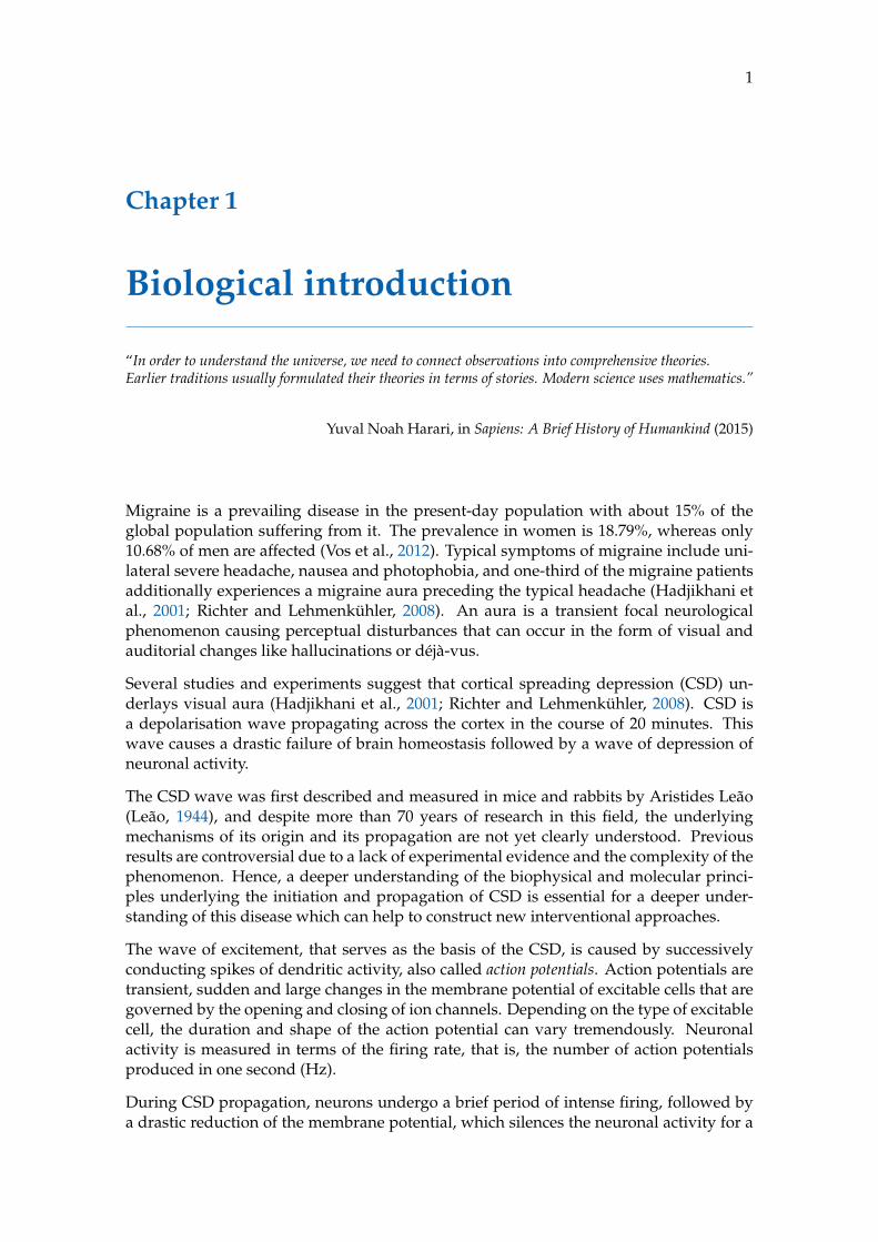
Migraine is a prevailing disease in the present-day population with about 15% of theglobal population suffering from it. The prevalence in women is 18.79%, whereas only10.68% of men are affected (Vos et al., 2012). Typical symptoms of migraine include uni-lateral severe headache, nausea and photophobia, and one-third of the migraine patientsadditionally experiences a migraine aura preceding the typical headache (Hadjikhani etal., 2001; Richter and Lehmenkühler, 2008). An aura is a transient focal neurologicalphenomenon causing perceptual disturbances that can occur in the form of visual andauditorial changes like hallucinations or déjà-vus.
Several studies and experiments suggest that cortical spreading depression (CSD) un-derlays visual aura (Hadjikhani et al., 2001; Richter and Lehmenkühler, 2008). CSD isa depolarisation wave propagating across the cortex in the course of 20 minutes. Thiswave causes a drastic failure of brain homeostasis followed by a wave of depression ofneuronal activity.
The CSD wave was first described and measured in mice and rabbits by Aristides Leão(Leão, 1944), and despite more than 70 years of research in this field, the underlyingmechanisms of its origin and its propagation are not yet clearly understood. Previousresults are controversial due to a lack of experimental evidence and the complexity of thephenomenon. Hence, a deeper understanding of the biophysical and molecular princi-ples underlying the initiation and propagation of CSD is essential for a deeper under-standing of this disease which can help to construct new interventional approaches.
The wave of excitement, that serves as the basis of the CSD, is caused by successivelyconducting spikes of dendritic activity, also called action potentials. Action potentials aretransient, sudden and large changes in the membrane potential of excitable cells that aregoverned by the opening and closing of ion channels. Depending on the type of excitablecell, the duration and shape of the action potential can vary tremendously. Neuronalactivity is measured in terms of the firing rate, that is, the number of action potentialsproduced in one second (Hz).
During CSD propagation, neurons undergo a brief period of intense firing, followed bya drastic reduction of the membrane potential, which silences the neuronal activity for a
2 Chapter 1. Biological introduction
short period (of 1 to 3 minutes), and then a slow recovery of the firing activity in whichneurons get back to their normal frequency (Sawat-Pokam et al., 2016). CSD is charac-terised by a significant increase in both extracellular potassium and glutamate, as wellas a rise in the intracellular sodium and calcium concentrations, and the two most ac-cepted hypotheses suggest that CSD propagation is due to diffusion of either potassiumor glutamate in the extracellular space (Zandt et al., 2015).
Some recent studies (Dahlem et al., 2015; Pocci et al., 2010) started to consider the effectsof cortical geometries on CSD propagation, at different levels of detail. Folds and creasesof the cortex influence the propagation of the depolarisation waves (and can stop themigraine in different positions depending on the patient).
This chapter is dedicated to the phenomenology of CSD, its characteristics and the cor-relation with migraine. We shortly describe in the following sections the biological com-partments and processes involved in neuronal excitation. For these descriptions, we fol-low mainly the work by Sadava et al., 2006. Subsequently, we explain the compartmentsof the cerebral cortex and the mechanisms of CSD in more detail, drawing their connec-tion to migraine and migraine with aura.
1.1 Generation and propagation of action potentials
The cell membrane of neurons acts as a capacitor separating different types of ions. Themain ions involved in the electrophysiology of action potentials are sodium (Na+), potas-sium (K+), calcium (Ca2+) and chloride (Cl−). At rest, the concentration of Na+ is higherin the extracellular fluid, while the concentration of K+ is higher inside the cell. Largeorganic anions inside the cell are responsible for the overall negative charge across themembrane. At rest, neurons exhibit a membrane potential between -60 mV and -70 mV.
Ion specific channels and ion pumps in the cell membrane govern the distribution andchanges of the ion concentration in the intracellular and extracellular space. The sodium-potassium pump actively exchanges K+ and Na+ ions in order to keep the concentrationof K+ inside the cell higher when the neuron is at rest. This pump uses adenosine triphos-phate (ATP) as an energy source to move the ions against the electrochemical gradient inthe cell. Ion channels are selective passive transporters – allowing only some types ofions to pass through – and the direction and magnitude of the movement of ions dependon the electrochemical gradient.
When an action potential is generated, a depolarising stimulus causes the voltage-gatedNa+ channels to open. Driven by the electrochemical gradient, this allows Na+ ions toenter the cell and thus depolarise the membrane potential. If the threshold of -50 mVis reached, more Na+ channels open causing a flush of Na+ ions inside the neuron andthe membrane potential to rise up to 50 mV. At the peak of the action potential, Na+
channels start to close and at the same time voltage-gated (but time-delayed) K+ channelsopen. This leads to an efflux of K+ to the extracellular space and the repolarisation of themembrane potential towards the resting potential of -60 mV. Many voltage-gated K+
channels do not close immediately when the membrane returns to its resting potential.This can lead to a hyperpolarisation of the membrane potential to values that are evenlower than the original resting potential. Subsequently, the sodium-potassium pumprestores the resting balance. After the excitation, the voltage-gated channels undergo arefractory period (of 1-2 milliseconds in which they do not react to any further incoming
1.1. Generation and propagation of action potentials 3
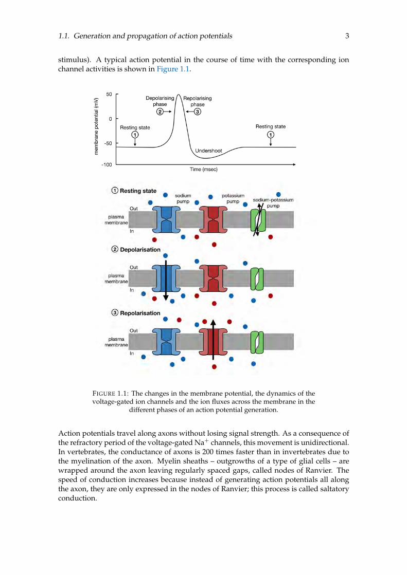
stimulus). A typical action potential in the course of time with the corresponding ionchannel activities is shown in Figure 1.1.
FIGURE 1.1: The changes in the membrane potential, the dynamics of thevoltage-gated ion channels and the ion fluxes across the membrane in the
different phases of an action potential generation.
Action potentials travel along axons without losing signal strength. As a consequence ofthe refractory period of the voltage-gated Na+ channels, this movement is unidirectional.In vertebrates, the conductance of axons is 200 times faster than in invertebrates due tothe myelination of the axon. Myelin sheaths – outgrowths of a type of glial cells – arewrapped around the axon leaving regularly spaced gaps, called nodes of Ranvier. Thespeed of conduction increases because instead of generating action potentials all alongthe axon, they are only expressed in the nodes of Ranvier; this process is called saltatoryconduction.

4 Chapter 1. Biological introduction
1.1.1 Transmission of action potentials
Neurons transmit action potentials to neighbouring cells via the space between the presy-naptic and the postsynaptic membrane, also called synapse. In electrical synapses, the ac-tion potential is directly passed from the presynaptic to the postsynaptic cell. Chemicalsynapses transmit action potentials with the help of neurotransmitters and allow morecomplex dynamics.
Action potentials arriving in the presynaptic axon terminal cause voltage-gated Ca2+
channels to open. As the concentration of Ca2+ is higher in the extracellular space, Ca2+
ions enter the axon terminal and trigger a release of vesicles containing neurotransmit-ters. These vesicles fuse with the membrane of the axon terminal releasing the neuro-transmitters into the synapse. The neurotransmitters diffuse across the synapse and bindto receptors on the postsynaptic membrane. These receptors activate chemically gatedchannels that allow Na+, K+ and Ca2+ to pass, but because of the electrochemical gra-dient, there is an influx of Na+ ions into the cell depolarising the membrane. Sufficientdepolarisation leads to an activation of the voltage-gated Na+ channels and a generationof an action potential in the postsynaptic cell. The neurotransmitters in the synapse arebroken down by specific enzymes, and the neurotransmitters and vesicles are recycledfor further use in the presynaptic axon terminal.
The synapses between neurons can be excitatory or inhibitory depending on the neuro-transmitters. Excitatory postsynaptic potentials depolarise the postsynaptic membrane,while inhibitory postsynaptic potentials cause hyperpolarisation. Every postsynapticneuron has a variety of different receptors for neurotransmitters, and each neurotrans-mitter has multiple receptor types. These receptors and channels are ion selective, andthe type of ions passing these channels determines if the presynaptic action potentialtriggers an excitatory or inhibitory action potential.
Neurons are connected to many axon terminals by branching fibres (dendrites) and thatway, a lot of incoming information arrives at the neurons’ cell body. Whether or not apostsynaptic neuron conducts the action potential does not only depend on the strengthof the input stimulus of the presynaptic neuron but rather on the sum of all input stimuli.The neuron integrates the information that arrives in the dendrites in the axon hillock,a specialised part of the cell body of a neuron that connects to the axon. Only if thecombination of the excitatory and inhibitory potentials reaches the threshold, an actionpotential is generated and passed on along the axon.
1.1.2 Neurotransmitters in the central nervous system
More than 50 different neurotransmitters have been discovered, varying from simpleamino acids to peptides and gasses. The main neurotransmitters in the central nervoussystem are glutamate (or glutamic acid) and γ-aminobutyric acid.
The excitatory neurotransmitter glutamate can bind to a variety of different receptors,and the activation of glutamate receptors always brings about an influx of Na+ ions anda depolarisation. Depending on the type of receptor, glutamate can trigger either a rapidinflow of Na+ ions into the postsynaptic cell or a slower and longer-lasting inflow thatis coupled to an influx of Ca2+ ions. Here, Ca2+ ions act as a second messenger and cancause different long-term effects. Free glutamate is rapidly removed from the synapse by
1.1. Generation and propagation of action potentials 5
transporters in the neuronal and glial membrane. In addition, glutamate acts as a precur-sor for the synthesis of γ-aminobutyric acid and this reaction is catalysed by glutamatedecarboxylase.
The primary inhibitory neurotransmitter in the central nervous system is γ-aminobutyricacid, whose binding to the various receptors can lead to either an influx of Cl− ions intothe cell or an efflux of K+ ions. For both receptor types, this results in a negative changein the membrane potential and thus a hyperpolarisation.
1.1.3 Energy metabolism
Most actions taking place in organisms require energy. For example, after the genera-tion of an action potential, the sodium-potassium pump requires energy in the form ofATP in order to transport the Na+ ions and K+ ions against the electrochemical gradi-ent across the membrane. Depending on the absence or presence of oxygen, differentmetabolic pathways transform glucose into energy. During this conversion the free en-ergy is stored in the form of ATP, nicotinamide adenine dinucleotide (NAD+) or flavinadenine dinucleotide (FAD). These coenzymes act as electron carriers and can releaseenergy for cellular work after oxidation.
There are three main processes involved in the energy generation from glucose: glycol-ysis, cellular respiration, and fermentation. Glycolysis takes place in the cell’s cytosoland each molecule of glucose is converted into two molecules of pyruvate. During theten enzyme-catalysed reactions of glycolysis, four molecules of ATP and two moleculesof NAD+ are gained. These reactions do not need any oxygen. Another way of energygeneration happens in the citric acid cycle. This is a pathway of eight reactions in themitochondrial matrix in which each pyruvate molecule is converted into three moleculesof CO2. The free energy released from these reactions is stored in the form of ATP and ofthe electron carriers NAD+ and FAD.
The citric acid cycle does not directly require oxygen but oxygen is necessary to oxidisethe electron carriers in order to provide a sufficient supply of excitable electron carriers.In the absence of oxygen, pyruvate is reduced in the cytosol. There are several differentfermentation ways but the most frequently occurring one is the lactic acid fermentation.This fermentation takes place especially in regions of high activity and energy consump-tion with a low oxygen supply. Pyruvate is reduced to lactate and the energy is storedin the form of NAD+. In total, the yield of cellular respiration is 32 molecules of ATPfor every molecule of glucose in the presence of oxygen. Under anaerobic conditions, theglycolysis via fermentation only produces two molecules of ATP per molecule of glucose.
1.1.4 Astrocytes and glutamatergic synapses
The energy metabolism of central nervous system cells is closely linked to their synapticactivity. Cell respiration and fermentation provide the neurons with the energy necessaryto trigger action potentials and restore the resting potential. Astrocytes are characteris-tic star-shaped glial cells in the brain and spinal cord, in which the glucose metabolismis coupled to the glutamate uptake from the synapse and to the transfer of lactate andglutamine to the neuron. Astrocytes in the central nervous system are predominatelypositioned between the synapse of neurons and capillaries. This makes them the ideal

6 Chapter 1. Biological introduction
connectors between synaptic activity and energy metabolism. Astrocytic end-feet arewrapped around the capillaries providing a constant supply with glucose and oxygen.
Astrocytes rapidly take up the glutamate from the synapse that was released by thepresynaptic neuron. This uptake is driven by the electrochemical gradient of Na+ ions,which acts as a co-transporter for glutamate. In astrocytes, the glutamate is converted toglutamine in a catalysed reaction that requires ATP. The glutamine is then released intothe extracellular space, taken up by the neurons and converted to glutamate to restockthe neurotransmitter pool. The co-transport of Na+ ions into the astrocyte increases theintracellular Na+ concentration, which leads to the activation of the sodium-potassiumpump. This stimulates the glucose uptake and triggers aerobic glycolysis. In aerobicglycolysis, glucose is transformed into lactate in the presence of sufficient oxygen. Thelactate is transferred to the neuron where it is converted to pyruvate. This pyruvate is– with the help of pyruvate dehydrogenase – converted to acetyl coenzyme A and en-ters the citric acid cycle converting energy. The main processes involved in the actionpotential transmission of a glutamatergic synapse are shown in Figure 1.2.
FIGURE 1.2: Schematic representation of a glutamatergic synapse and therecycling pathway of its neurotransmitters via a neighbouring astrocyte
(Rodrigues, Valette, and Bouzier-Sore, 2013).
Due to the reduced sodium permeability (compared to neurons) and due to a high den-sity of potassium channels, astrocytes clear the extracellular potassium that is releasedby active neurons. During an activity, there is a build up of potassium, which has beensuggested to be cleared by the astrocytes (Walz, 2000).
1.2 Cerebral cortex and its compartments
The nervous system allows us to experience our environment and react to it accordingly.More than 1011 neurons and glial cells process information in the form of electrical im-pulses and pass them on through more than 1014 synapses.
The cerebrum (lat. brain) is the principal part of the brain in mammals, located in thefront area of the skull and consisting of two hemispheres, left and right, separated by afissure. It makes up the largest part of the brain and is the centre of the nervous systemplaying a vital role in memory, language, attention, consciousness, and perception. Thecerebral cortex is a thin layer (2 - 4 mm) of grey matter that overlays the cerebrum and
1.3. Cortical spreading depression 7
is folded in larger mammals, thus allowing for an increased surface despite the limitingsize of the skull. The ridges of the folding are called gyri, and the fissures are termed sulci.The grey matter contains neuronal cell bodies, dendrites, axons, glial cells, synapses andcapillaries. In contrast to that, white matter is mainly composed of long myelinated axonsthat are responsible for the lighter colouring of this area.
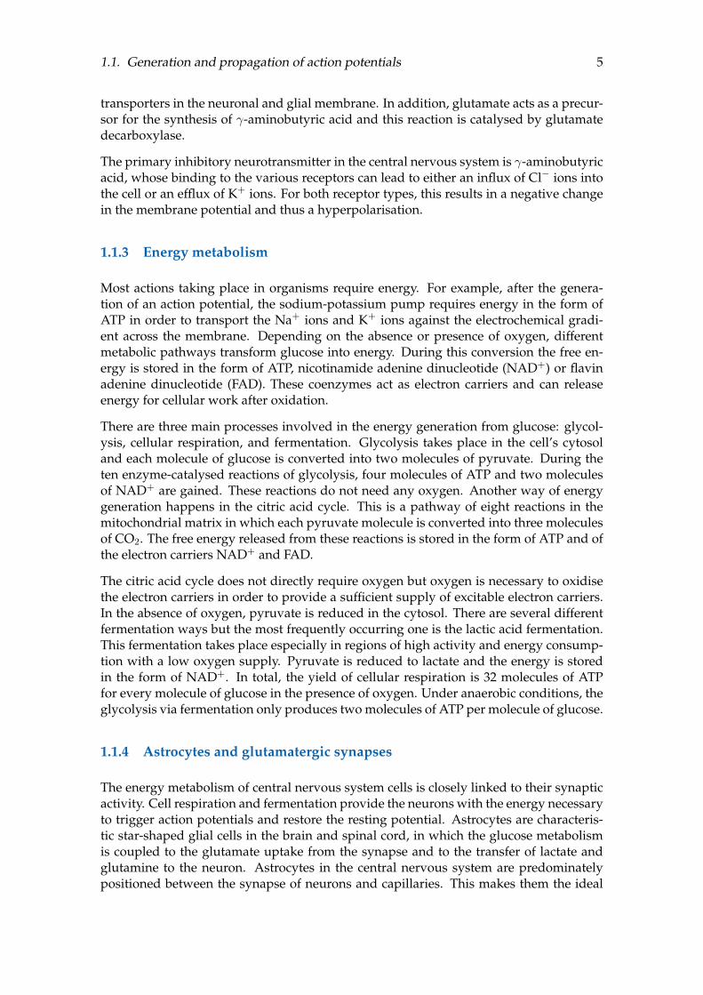
Different cortical regions can be described based on the histological structure and theirfunctional roles in sensation, cognition, and behaviour. A widely used parcellation inautomated labelling systems is the Desikan-Killiany atlas, dividing each hemisphere into34 cortical regions of interest (ROI) (Desikan et al., 2006). This subdivision of the cortexinto gyral-based neuroanatomical regions is reliable and serves for morphological as wellas functional studies and is shown in Figure 1.3. Brodmann introduced the first map tosubdivide the human cortex based on the neuronal organisation, and many of the areasidentified have been found to correlate to diverse cortical functions (Brodmann, 2006).For example, Brodmann area 17 is the primary visual cortex and the left Brodmann areas44 and 45 coincide with Broca’s speech and language areas (Broca, 1861).
(a) lateral view (b) medial view
FIGURE 1.3: The 34 regions of interest of the cerebral cortex, in the lateral(a) and medial (b) view of the left hemisphere.
A more general classification of the cerebral cortex is based on gross topographical con-ventions into six lobes: medial lobe, lateral temporal lobe, occipital lobe, parietal lobe,frontal lobe, and cingulate cortex. The lobes of the left hemisphere are shown in Fig-ure 1.4. Originally this classification was purely anatomical, but recent discoveries haveshown recently that the different lobes also correspond to different brain functions (Ribas,2010).
1.3 Cortical spreading depression
CSD is a propagating wave of depolarisation of neuronal and glial cells in the grey mat-ter originating in the visual cortex (located in the occipital lobe), spreading across thecortex, and followed by a wave of suppression of spontaneous activity. The outstandingduration of depolarisation during the CSD (lasting up to a minute or more) and its ex-tremely slow propagation (about 3 mm/min), are in stark contrast to the action potentialfeatures (depolarisation lasting milliseconds and propagation velocity of several m/sec)thus distinguishing the CSD from the normal neuronal activity.

8 Chapter 1. Biological introduction
(a) lateral view (b) medial view
FIGURE 1.4: The lobes of the brain, in the lateral (a) and medial (b) view ofthe left hemisphere.
The depolarisation wave of CSD causes various and tremendous changes in the vascularresponse, blood flow, and energy metabolism. During this excessive depolarisation, thereare drastic fluxes inside and outside the cell, and vast quantities of the neurotransmitterglutamate are released and can be observed in the extracellular space. Thus, CSD can beseen as a reaction-diffusion process, where the reaction includes processes like the releaseof K+ and glutamate, the pump activities and the tissue recovery, while the diffusion ofK+ and glutamate enable CSD propagation.
The first scientist to describe the CSD was Aristides Leão observing the basic phenomenonof the propagating depolarisation waves triggered in the cortex of rabbits, pigeons, andcats (Leão, 1944, 1947). His findings gave rise to the hypothesis that CSD is the underly-ing cause of migraine aura. In the past, CSD has been widely studied in animal models,but only lately the occurrence in the human brain started to be investigated. A lot of theserecent observations and investigations support this hypothesis, but the electrophysiolog-ical features of CSD have not been observed in a migraine patient yet. The main reasonfor this is that non-invasive electroencephalography techniques are not sensitive enoughto detect the weak signal of a CSD.
However, in injured brains CSD can be observed after strokes as peri-infarct depolari-sation or during global hypoxia, enlarging the damaged tissue area (Zandt, Haken, andPutten, 2013). Under normal metabolic conditions, CSD does not cause cell death orlong-term damage but increases the bioenergetic burden on the tissue (Pietrobon andMoskowitz, 2014).
1.3.1 Phenomenology of CSD
The complex phenomenon of CSD evolves in different stages and can be subdividedinto an early, main and late phase (Pietrobon and Moskowitz, 2014). These phases arecharacterised by massive rearrangements of ions across the plasma membrane and areassociated with changes in the pH-value as well as neuronal cell swelling in response toosmolarity changes.

1.3. Cortical spreading depression 9
The onset of the propagation wavefront triggers complex dynamics leading to abruptchanges in the neuronal behaviour. First neurons undergo a brief period of intense ac-tivity, featuring a firing rate that is 10-20 times higher than the one at rest, typically be-tween 8 and 12 Hz (Brötzner et al., 2014; Hyder et al., 2013). This period is followed by amembrane hyperpolarisation silencing the neuronal activity for a couple of minutes, afterwhich the neurons slowly recover their spiking activity and return to their normal spik-ing frequency at rest (Pietrobon and Moskowitz, 2014; Sawat-Pokam et al., 2016; Zandtet al., 2015).
In the early phase, the membrane potential is depolarised for a few seconds. This rapidchange in the membrane voltage is conjoined with a swift increase of extracellular K+
to 30-60 mM from a baseline value of 2.7-3.5 mM, a fast decrease in extracellular Na+
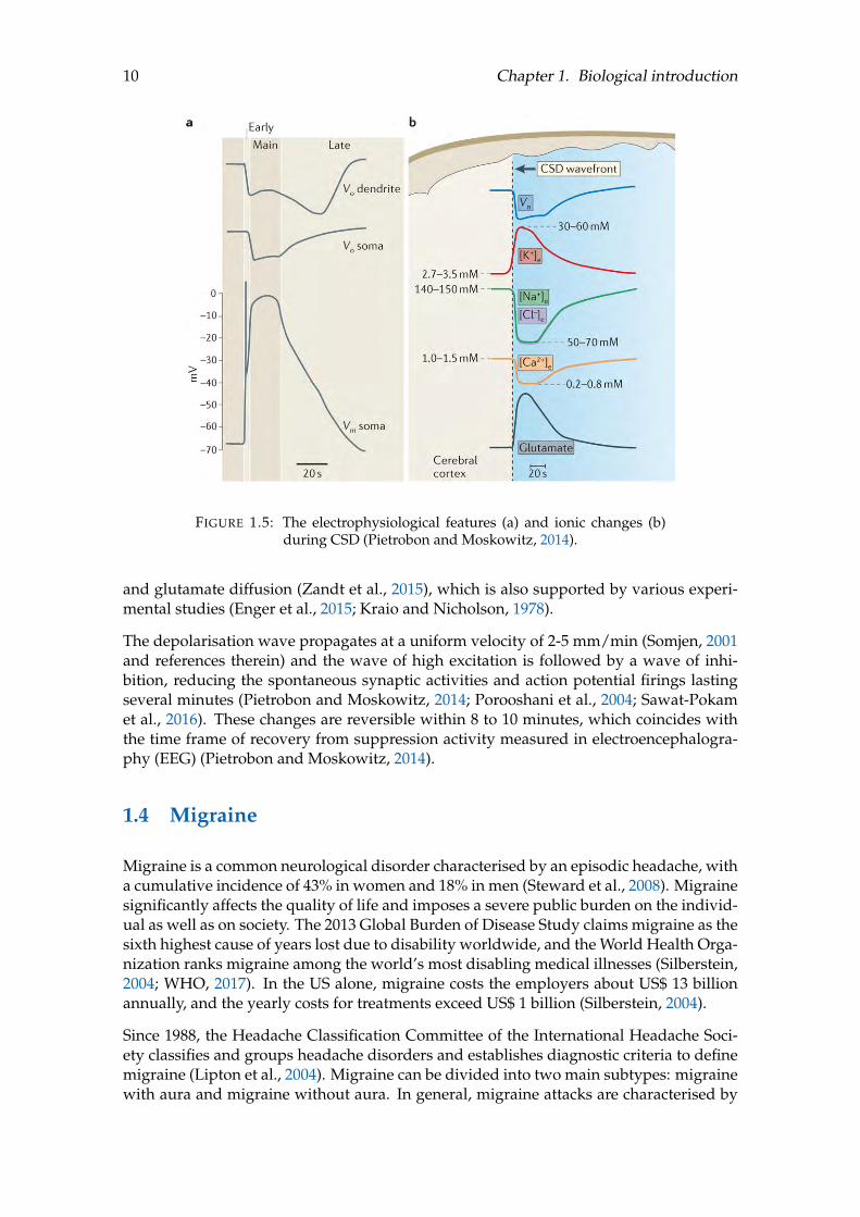
and Cl− to 50-70 mM from a baseline value of 140-150 mM and in Ca2+ to 0.2-0.8 mMfrom 1-1.5 mM (Pietrobon and Moskowitz, 2014). This is followed by the main phase,15-20 seconds in which the entire plasma membrane is completely depolarised. The de-crease in extracellular Na+ is greater than the one in extracellular K+, but the electroneu-trality is maintained by the efflux of organic anions, like glutamate and aspartate. Theelectrophysiological features and ionic changes during CSD are shown in Figure 1.5.
In both neuron and astrocyte, CSD causes a large increase in the intracellular Ca2+ con-centration. However, the rise in the neuronal Ca2+ precedes the one in the astrocyte andis not affected by the latter. During CSD, the astrocyte depolarisation is caused by theincrease in extracellular K+ and is mostly of passive nature.
The influx of Na+, Cl− and water ions cause neuronal swelling of about 40-70%, whileastrocytes only reveal passive swelling in response to a CSD-induced higher extracellularconcentration of K+ (Somjen, 2001).
The cerebral blood flow and brain metabolism are closely connected; the brain blood flowincreases with a rising demand for oxygen and glucose. As ATP is essential to restore theionic gradients and repolarise the membrane potential after an action potential, CSD isassociated with high energy metabolism and consequently a large transient rise in thecerebral blood flow. A potential source of ATP are the astrocytes that release ATP in cor-respondence to the intracellular Ca2+ signalling. In addition, CSD stimulates anaerobicglycolysis which results in a high production of lactate mainly generated in astrocytes.
1.3.2 Mechanisms of CSD
Experimentally, CSD can be triggered in healthy brain tissue of animals by the local re-lease of K+ or glutamate (Pietrobon and Moskowitz, 2014). Similar to the neuronal actionpotential, the CSD propagates in an all-or-nothing manner, once initiated and indepen-dent of the stimulus strength or type. Experimental data, as well as computational mod-els, support the concept that increasing the K+ concentration above a threshold is a keyevent triggering CSD, as originally proposed by Grafstein, 1956.
Four hypotheses explaining the CSD propagation on the cortex have been proposed andaccepted at different levels. The potassium and glutamate hypotheses state that CSDpropagates due to diffusion of potassium or glutamate in the extracellular space. Theneuronal gap junction hypothesis suggests that CSD propagates through the opening ofneuronal gap junctions. The glial hypothesis states that the CSD is transmitted throughglial gap junctions. The most accepted assumption is that of the extracellular potassium
10 Chapter 1. Biological introduction
FIGURE 1.5: The electrophysiological features (a) and ionic changes (b)during CSD (Pietrobon and Moskowitz, 2014).
and glutamate diffusion (Zandt et al., 2015), which is also supported by various experi-mental studies (Enger et al., 2015; Kraio and Nicholson, 1978).
The depolarisation wave propagates at a uniform velocity of 2-5 mm/min (Somjen, 2001and references therein) and the wave of high excitation is followed by a wave of inhi-bition, reducing the spontaneous synaptic activities and action potential firings lastingseveral minutes (Pietrobon and Moskowitz, 2014; Porooshani et al., 2004; Sawat-Pokamet al., 2016). These changes are reversible within 8 to 10 minutes, which coincides withthe time frame of recovery from suppression activity measured in electroencephalogra-phy (EEG) (Pietrobon and Moskowitz, 2014).
1.4 Migraine
Migraine is a common neurological disorder characterised by an episodic headache, witha cumulative incidence of 43% in women and 18% in men (Steward et al., 2008). Migrainesignificantly affects the quality of life and imposes a severe public burden on the individ-ual as well as on society. The 2013 Global Burden of Disease Study claims migraine as thesixth highest cause of years lost due to disability worldwide, and the World Health Orga-nization ranks migraine among the world’s most disabling medical illnesses (Silberstein,2004; WHO, 2017). In the US alone, migraine costs the employers about US$ 13 billionannually, and the yearly costs for treatments exceed US$ 1 billion (Silberstein, 2004).
Since 1988, the Headache Classification Committee of the International Headache Soci-ety classifies and groups headache disorders and establishes diagnostic criteria to definemigraine (Lipton et al., 2004). Migraine can be divided into two main subtypes: migrainewith aura and migraine without aura. In general, migraine attacks are characterised by

1.4. Migraine 11
typically unilateral and pulsating moderate to severe headache, lasting between 4 and 72hours, often accompanied by nausea, phonophobia, and photophobia (migraine withoutaura) (Pietrobon, 2005). In migraine with aura, the headache is preceded by neurologicalsymptoms, mostly visual but may also involve other senses or cause speech deficits.
In addition to that, migraine has a strong genetic component, with a likely multifactorialpolygenetic inheritance (Kors et al., 2004). Familial hemiplegic migraine (FHM), a rareautosomal dominantly inherited subtype of migraine with aura, is the only case in whichthe causative gene has been identified (Pietrobon, 2005). FHM is characterised by aurasymptoms consisting of motor weakness or paralysis, and thus, FHM attacks resembletypical migraine attacks with aura. In general, the genetic load can be seen as an inherentmigraine threshold that is influenced by external and internal factors.
Migraine is acutely treated by administering non-steroidal anti-inflammatory drugs, er-got derivatives, or triptans (Ayata et al., 2006). When patients experience more than threeor five attacks per month, prophylaxis is recommended in order to reduce the frequencyand the intensity of migraine headaches. However, migraine prophylaxis is only partiallyeffective in many patients, and a deeper understanding of molecular, cellular, genetic orphysiological drug targets is sought (Ayata et al., 2006).
1.4.1 Migraine with aura
For about 30% of the migraine patients, the migraine attack is preceded by an aura com-posed of transient focal neurological symptoms such as visual disturbances, paresthesias(abnormal sensations such as tingling or tickling of the skin for no apparent reasons) orlanguage disturbances (Tommaso et al., 2014). The visual disturbances during migraineaura are characterised by a serrated arc of shimmering shapes, the so-called scotoma. Thisscotoma usually appears in the form of a small blind or scintillating spot, increasing insize and drifting across the visual field to one side (Bolay and Moskowitz, 2005).
Analysing his own visual aura, the physiologist Karl S. Lashley published in 1941 hisobservations of the scotoma and was the first to postulate that the migraine aura resultsfrom depressed neuronal activity in the visual cerebral cortex (Lashley, 1941).
1.4.2 Connection with CSD
The considerable connection between migraine visual aura and CSD, lead to the hypoth-esis that CSD is underlaying migraine aura (Lauritzen, 1994). Recently, using blood oxy-genation level-dependent functional magnetic resonance imaging, Hadjikhani et al., 2001observed various cerebrovascular changes, typical for the CSD, in the cortex of migrainepatients while experiencing a visual aura. Another evidence that visual aura results fromCSD was obtained with magnetoencephalography (MEG). During a spontaneous visualaura, slow changes of the cortical field were measured that correspond to the poten-tial changes during neuronal depolarisation in CSD (Bowyer et al., 1999, 2001). Thisdemonstration of cerebrovascular and magnetic field correlates of CSD in migraine pa-tients strengthens the conclusion that CSD underlies visual aura.

12 Chapter 1. Biological introduction
However, some arguments are questioning the long-standing belief that CSD is under-lying migraine aura (Borgdorff, 2018) making the origin of migraine with aura and itsconnection to the CSD an up-to-date and still controversial topic to investigate.
1.4.3 Migraine and grey matter
Several whole-brain studies identified a common reduction in grey matter volume in mi-graine patients, in particular in the frontal cortex and the cingulate gyrus (Jia and Yu,2017). These changes in grey matter may indicate the location and mechanisms of painprocessing, but also pinpoint cortical areas that contribute to the propagation of the CSD.
1.5 Summary
Migraine is a common disease in the present-day population, with one-third of the mi-graine patients suffering from migraine aura, perceptual disturbances preceding the typ-ical headache. CSD, a depolarisation wave that originates in the visual cortex and prop-agates across the cortex to the peripheral areas, has been suggested as a correlate of thevisual aura by several studies.
On the microscopic scale, CSD causes a drastic distortion in the brain homeostasis fol-lowed by a wave of depression of neuronal activity. On the macroscopic scale, the depo-larisation wave propagates at a uniform velocity, most probably due to the diffusion ofpotassium or glutamate in the extracellular space.
Up to now, little is known about the origin of this phenomenon and possible curativetreatments. However, the complex and highly individual characteristics of the brain cor-tex suggest that the geometry might have a significant impact in supporting or contrast-ing the propagation of CSD. Accurate patient-specific computational models are thusfundamental to cope with the high variability in cortical geometries among individuals.
13
Chapter 2
Overview of models for neuronaldynamics
“Remember that all models are wrong;the practical question is how wrong do they have to be to not be useful.”
Box, G. E. P., and Draper, N. R., in Empirical Model Building and Response Surfaces, John Wiley &Sons, New York, NY (1987)
The slow propagative wave of CSD on the cerebral cortex is marked by neuronal depo-larisation and redistribution of ions, followed by a short period of suppressed neuronalactivity. This reaction-diffusion process consists of a variety of local mechanisms, likeactive or passive ionic movements and pump activities, and diffusion of potassium orglutamate, causing CSD and enabling it to propagate.
Several mathematical models for CSD, varying from reaction-diffusion models to mi-croscopic models accounting for the cells’ connectivity, have been proposed in the past.During spreading depression, the extracellular potassium concentration follows approx-imately the time-course of depolarised neurons and glial cells (Kraio and Nicholson,1978). Based on this fact, Tuckwell and Miura, 1978 proposed a model for CSD wavepropagation in 1D heterogenous space, including potassium and calcium fluxes, extra-cellular diffusion and active transport pumps in a Hodgkin–Huxley like system of equa-tions. The numerical results feature the basic qualitative properties of the spreadingdepression wave and account for the annihilation of two colliding waves. Reggia andMontgomery, 1996 coupled synaptic connectivity and extracellular potassium uptake ata single cell level in a simplified 2D array representation of the cortex. Using reaction-diffusion equations to describe the potassium changes, they projected the simulated cor-tical activity onto the visual field to mimic the corresponding visual pattern. The potas-sium wave features irregular patches of highly activated areas on the visual field, whichsupports the theory of CSD underlying migraine aura. These are just two examples ofmodelling CSD propagation, but both do not consider the 3D nature of physical space.Even though they feature the main characteristics of spreading depression and link itto the phenomenon of migraine with aura, they lack detailed microscopic and electro-physiological information that could help to understand the underlying mechanisms ofmigraine.

14 Chapter 2. Overview of models for neuronal dynamics
Computational models for CSD generally feature two major aspects. One is the mod-elling of microscopic processes, accounting for the electrical activity in the neuronal com-partment causing the homeostatic failure and excessive fluctuations in the ionic concen-trations. The other component describes the spread throughout the tissue, namely thediffusion leading to the propagation of the homeostatic disturbance (Zandt et al., 2015).The propagation is usually described in terms of simple expressions for diffusion, eitherthrough Brownian motion, or any other form of transport through the tissue. The varietyof mathematical models accounting for the microscopic interactions, i.e., the excitationand silencing of neurons, ranges from phenomenological models to detailed metabolicmodels considering a range of ionic concentrations and biological indicators, like cellswelling and energy supply. These models vary in their biological plausibility and com-putational efficiency, and some are restricted in their capacity to account for differentneuronal firing behaviours.
The Hodgkin–Huxley model was the first conductance-based model for excitable cells incomputational neuroscience (Hodgkin and Huxley, 1952, 1953). It consists of four differ-ential equations accounting for the membrane potential, the activation of Na+ and K+
currents and the inactivation of the Na+ current. This model exhibits the particular bio-logical properties of spiking neurons and is one of the fundamental models for neuronalexcitation. The FitzHugh–Nagumo model, a system of two ordinary differential equa-tions (ODEs), describes the membrane potential and one recovery variable, that acts asa negative feedback on the membrane potential (FitzHugh, 1955; Nagumo, 1962; Rogersand McCulloch, 1994). It describes the typical characteristics of spiking neurons but failsto account for tonic bursting, periods of rapid action potential spiking followed by a qui-escent period, and spike frequency adaptation, a reduction of the frequency of the actionpotential response to a stimulus. The Izhikevich model is a simplified model for neu-ronal spiking with an auxiliary after-spike resetting of the two variables representing themembrane potential and the recovery variable, respectively (Izhikevich, 2003, 2010). Thismodel exhibits firing patterns of all types of cortical neurons (Izhikevich, 2004). However,the big drawback of this model is the lack of autonomous behaviour. These phenomeno-logical models are able to reproduce the firing behaviour of highly activated cells andalso account for the following refractory period, but lack in providing detailed insightinto the ionic shifts in Na+, K+, Cl− and into the changes in oxygen concentration duringthe time course of a spreading depression. The oxygen concentration is often used as anindicator for the energy supply.
The model introduced by Cressman is an extension of the Hodgkin–Huxley formalismincorporating dynamic Na+ and K+ ionic concentrations (Barreto and Cressman, 2011;Cressman et al., 2009, 2011). It describes the sodium current, calcium-gated potassium,and the leak current, and it also takes into account the sodium-potassium pump current,glial current and potassium diffusion.
An extension of the previously mentioned model was proposed by Wei, Ullah, and Schiff,2014. This model supports various neuronal behaviours varying from seizure to spread-ing depression, tonic firing and a steady state, whose occurrence depends on the valuesof the potassium and oxygen bath concentrations, respectively.
Depending on the scale of the neuronal network, the required accuracy and the scopeof the biological description, each of these models could be most suited. In the follow-ing, we introduce these models in a detailed manner and discuss their relevance for theapplication of interest in this thesis.
2.1. Phenomenological models 15
2.1 Phenomenological models
2.1.1 Hodgkin–Huxley model
The first to develop a model describing the ionic mechanism underlying the action po-tential were Hodgkin and Huxley, 1952, 1953. They described the propagation of theelectrical current along giant axons of squids and received the Nobel Price in Physiologyor Medicine in 1963 for their work.
With the cell membrane acting as a capacitor, each component of the cell is treated asan electrical element, and the voltage-gated and leak channels are treated as electricalconductances. The temporal evolution of the membrane potential V can be expressed as
CdV
dt= I − Iion, (2.1)
where I is the applied current or the input stimulus, Iion is the total ionic current and Cis the membrane capacitance. The total ionic current is a combination of the sodium andpotassium current, plus a leak current combining the dynamics of the other ions, namely
Iion = INa + IK + Il. (2.2)
These ionic currents can be written in terms of the ionic conductances as
INa = gNa(V − VNa),
IK = gK(V − VK),
Il = gl(V − Vl),
(2.3)
where gNa, gK, gl are the sodium, potassium and leak conductances and VNa, VK, Vl arethe reversal potentials of the respective channels. The ionic conductances are defined interms of suitable gating variables (denoted by n, m, h) as
gNa = gNam3h,
gK = gKn4.
The gating variables n,m and h vary between 0 and 1 and describe the percentage of openchannels (1 indicates open channels, while 0 denotes closed ones). The temporal dynam-ics of n, m and h is governed by suitable ODEs, naturally depending on the membranepotential V , defined as follows
dw
dt= αw(V )(1− w)− βw(V )w, for w = n,m, h.
Note that, n, m and h are dimensionless variables, while the functions αw, βw (withw = n,m, h) depend on the membrane potential. Like in Hodgkin and Huxley, 1952,

16 Chapter 2. Overview of models for neuronal dynamics
we define
αn(V ) = 0.01
(10− V
exp(
10−V10
)− 1
), βn(V ) = 0.125 exp
(− V
80
),
αm(V ) = 0.1
(25− V
exp(
25−V10
)− 1
), βm(V ) = 4 exp
(− V
18
),
αh(V ) = 0.07 exp
(− V
20
), βh(V ) =
1
exp(
30−V10
)+ 1
.
The parameters provided by Hodgkin and Huxley correspond to a shifted membranepotential so that the resting potential is 0 mV instead of -65 mV. The choice of the remain-ing parameters is given in Table 2.1. As initial values we choose V (0) = 0, and the gatingvariables n(t),m(t) and h(t) have their steady-state value when t = 0 (Hodgkin and Hux-ley, 1952). This means n(0) = n∞ = 0.315, m(0) = m∞ = 0.042 and h(0) = h∞ = 0.608.For illustrative purposes, with 1[a,b](t) denoting the indicator function of an interval [a, b],we add a stimulus I = 2 · 1[2,8](t) µA/cm2. The resulting spiking dynamics generatedwith the Hodgkin–Huxley model are shown in Figure 2.1.
Parameter Description Value UnitVK reversal potential of the potassium current -12 mVVNa reversal potential of the sodium current 120 mVVl reversal potential of the leak current 10.6 mVgK potassium conductance 36 mS/cm2
gNa sodium conductance 120 mS/cm2
gl leak conductance 0.3 mS/cm2
C membrane capacitance 1 µF/cm2
TABLE 2.1: Model parameters for the simulation of the Hodgkin–Huxleymodel.
(a) membrane potential V (b) gating variables n, m and h
FIGURE 2.1: Neuronal spiking dynamics simulated with the Hodgkin–Huxley model.
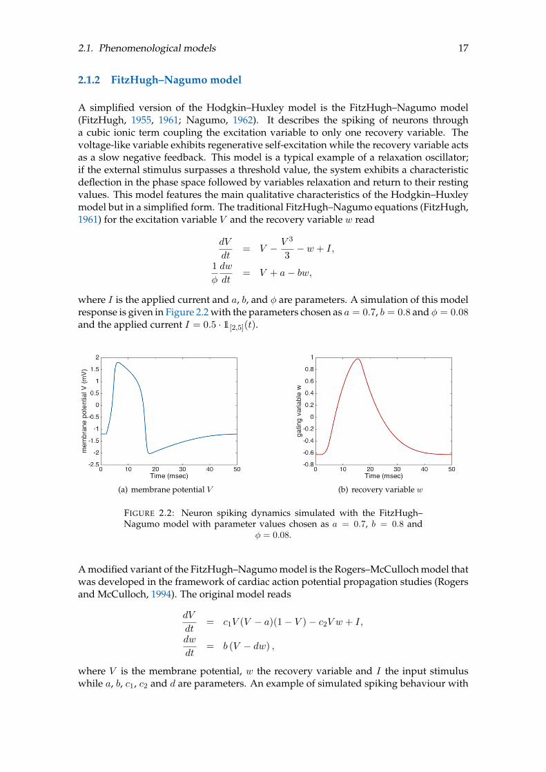
2.1. Phenomenological models 17
2.1.2 FitzHugh–Nagumo model
A simplified version of the Hodgkin–Huxley model is the FitzHugh–Nagumo model(FitzHugh, 1955, 1961; Nagumo, 1962). It describes the spiking of neurons througha cubic ionic term coupling the excitation variable to only one recovery variable. Thevoltage-like variable exhibits regenerative self-excitation while the recovery variable actsas a slow negative feedback. This model is a typical example of a relaxation oscillator;if the external stimulus surpasses a threshold value, the system exhibits a characteristicdeflection in the phase space followed by variables relaxation and return to their restingvalues. This model features the main qualitative characteristics of the Hodgkin–Huxleymodel but in a simplified form. The traditional FitzHugh–Nagumo equations (FitzHugh,1961) for the excitation variable V and the recovery variable w read
dV
dt= V − V 3
3− w + I,
1
φ
dw
dt= V + a− bw,
where I is the applied current and a, b, and φ are parameters. A simulation of this modelresponse is given in Figure 2.2 with the parameters chosen as a = 0.7, b = 0.8 and φ = 0.08and the applied current I = 0.5 · 1[2,5](t).
(a) membrane potential V (b) recovery variable w
FIGURE 2.2: Neuron spiking dynamics simulated with the FitzHugh–Nagumo model with parameter values chosen as a = 0.7, b = 0.8 and
φ = 0.08.
A modified variant of the FitzHugh–Nagumo model is the Rogers–McCulloch model thatwas developed in the framework of cardiac action potential propagation studies (Rogersand McCulloch, 1994). The original model reads
dV
dt= c1V (V − a)(1− V )− c2V w + I,
dw
dt= b (V − dw) ,
where V is the membrane potential, w the recovery variable and I the input stimuluswhile a, b, c1, c2 and d are parameters. An example of simulated spiking behaviour with

18 Chapter 2. Overview of models for neuronal dynamics
the parameters a = 0.13, b = 0.013, c1 = 0.26, c2 = 0.1 and d = 1 and the applied currentI = 0.05 · 1[100,110](t) is given in Figure 2.3.
(a) membrane potential V (b) recovery variable w
FIGURE 2.3: Neuronal spiking dynamics simulated with the Rogers–McCulloch variant of the FitzHugh–Nagumo model.
An alternative and more descriptive way to express these equations highlights the depen-dence of the dynamics on the initial, threshold and peak value. These values representthe baseline value, the value of excitation when an all-or-nothing response of an actionpotential is triggered and the maximum of the membrane potential, which indicates thebeginning of the recovery phase. This system can be written as
dV
dt= G(V − v0)
(1− V
vth
)(1− V
vp
)+ η1(V − v0)w + I,
dw
dt= η2 (V − v0 − η3w) ,
where V is the membrane potential, I the applied current, and w the recovery variable;G, η1, η2, η3 are positive parameters and v0, vth and vp are the initial value, the thresholdparameter, and peak potential, respectively. Through the above formulation of the model,the resulting spiking dynamics can be more easily tuned to the specific characteristics andtemporal behaviour of a certain type of neuronal response. A simulation of this model isshown in Figure 2.4 with the parameter choice given in Table 2.2.
Parameter Description Value UnitG 1.5 msec−1
v0 initial value 0 mVvth threshold value 13 mVvp peak value 100 mVη1 4.4 msec−1
η2 0.012 msec−1
η3 1 –
TABLE 2.2: Model parameters for the simulations of a variant of theRogers–McCulloch model.

2.1. Phenomenological models 19
(a) membrane potential V (b) recovery variable w
FIGURE 2.4: Neuronal spiking dynamics simulated with a variant of theRogers–McCulloch model.
2.1.3 Izhikevich model
Another simplified spiking model was introduced by Izhikevich (Izhikevich, 2003, 2010).This model is a system of two ODEs featuring the behaviour of a fast voltage variableand a slower recovery variable describing the activation of potassium or the inactivationof sodium (or both) and acting as a negative feedback on the fast variable. It is com-putationally less expensive but reproduces the spiking and bursting of cortical neuronswith the help of a non-autonomous system. The membrane potential V and the recoveryvariable w are described by the following system of ordinary differential equations
CdV
dt= k(V − vr)(V − vth)− w + I, (2.4)
dw
dt= a(b(V − vr)− w), (2.5)
where C is the membrane capacitance, vr is the resting membrane potential, vth is thethreshold, I an input stimulus and k, a and b are parameters. After exhibiting a spike(V ≥ 35 mV) the system is reset through the following condition:
if V ≥ vp, then
V ← c
w ← w + d, (2.6)
meaning that once V surpasses the peak value vp, then V and w are reassigned and giventhe values c and w + d, respectively, where c and d are given model parameters. Allthe parameters can be adjusted to obtain the characteristic spiking of any particular typeof neuron. The parameter a is a recovery time constant; the smaller a, the longer therecovery time. The parameter b describes the sensitivity of the recovery variable w to thebehaviour of the membrane potential V below the threshold vth. The after-spike resetvalue of the membrane potential is c, and the rest value of the recovery value is d. Theparameters k and b are closely related to the neurons’ spiking characteristics and inputresistance. An example of the spiking behaviour simulated with the Izhikevich model(2.4) - (2.6) and parameters listed in Table 2.3 is given in Figure 2.5.
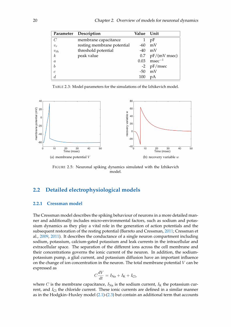
20 Chapter 2. Overview of models for neuronal dynamics
Parameter Description Value UnitC membrane capacitance 1 pFvr resting membrane potential -60 mVvth threshold potential -40 mVk peak value 0.7 pF/(mV msec)a 0.03 msec−1
b -2 pF/msecc -50 mVd 100 pA
TABLE 2.3: Model parameters for the simulations of the Izhikevich model.
(a) membrane potential V (b) recovery variable w
FIGURE 2.5: Neuronal spiking dynamics simulated with the Izhikevichmodel.
2.2 Detailed electrophysiological models
2.2.1 Cressman model
The Cressman model describes the spiking behaviour of neurons in a more detailed man-ner and additionally includes micro-environmental factors, such as sodium and potas-sium dynamics as they play a vital role in the generation of action potentials and thesubsequent restoration of the resting potential (Barreto and Cressman, 2011; Cressman etal., 2009, 2011). It describes the conductance of a single neuron compartment includingsodium, potassium, calcium-gated potassium and leak currents in the intracellular andextracellular space. The separation of the different ions across the cell membrane andtheir concentrations governs the ionic current of the neuron. In addition, the sodium-potassium pump, a glial current, and potassium diffusion have an important influenceon the change of ion concentration in the neuron. The total membrane potential V can beexpressed as
CdV
dt= INa + IK + ICl,
where C is the membrane capacitance, INa is the sodium current, IK the potassium cur-rent, and ICl the chloride current. These ionic currents are defined in a similar manneras in the Hodgkin–Huxley model (2.1)-(2.3) but contain an additional term that accounts

2.2. Detailed electrophysiological models 21
for the leak current of each ion involved:
INa = −gNam3∞(V )h(V − VNa)− gNaL(V − VNa),
IK =
(gKn
4 +gAHP[Ca]i1 + [Ca]i
)(V − VK)− gKL(V − VK),
ICl = −gClL(V − VCl).
Here, the parameters gNa, gK, and gAHP describe the conductance of the sodium, of thepotassium and of the after hyperpolarisation current, gNaL, gKL and gClL denote the con-ductances for the sodium, for the potassium and for the chloride leak currents. VNa, VKand VCl are the reversal potential of the sodium, of the potassium and of the chloridecurrent and [Ca]i denotes the intracellular calcium concentration. The different gatingvariables n, m and h correspond to the activating and inactivating sodium gate and theactivating potassium gate, respectively. The dynamics of the gating variables n and h isdefined as
dw
dt= ϕ (αw(V )(1− w)− βw(V )w) , for w = n, h,
with ϕ denoting the time constant of both gating variables. The model assumes that theactivating sodium gate m is fast compared to the voltage change. Thus, m is consideredto reach its equilibrium instantly which implies m = m∞, where
m∞(V ) =αm(V )
αm(V ) + βm(V ). (2.7)
The corresponding rate equations are
αn(V ) = 0.001V + 34
1− exp (0.1(V + 34)), βn(V ) = 0.125 exp
(−V + 44
80
),
αm(V ) =0.1(V + 30)
1− exp (−0.1(V + 30)), βm(V ) = 4 exp
(−V + 55
18
),
αh(V ) = 0.07 exp
(−V + 44
20
), βh(V ) =
1
(1 + exp (−0.1(V + 4))).
(2.8)
The intracellular calcium concentration, which influences the calcium gated potassiumcurrent, is defined as
d[Ca]idt
= −0.002 gCaV − VCa
1 + exp (−0.4 (V + 25))− [Ca]i
80,
where gCa describes the calcium conductance and VCa the calcium reversal potential. Theextracellular potassium concentration [K]o can be described in terms of the potassiumcurrent IK across the membrane, of the ionic current of the sodium-potassium pumpIpump, of the uptake of potassium by astrocytes Iglia and of the diffusion of potassium Idiffin the extracellular space to nearby reservoirs. In particular, the extracellular potassiumconcentration is given by
τd[K]odt
= γIK − 2βIpump − Iglia − Idiff, (2.9)
with the ratio of intracellular to extracellular volume of the cell β, the time conversionfactor τ = 1000 and the unit conversion factor γ that converts the membrane currentsinto millimolar per seconds. The intracellular sodium concentration [Na]i is governed bythe ionic sodium current INa and the ionic current of the sodium-potassium pump Ipump
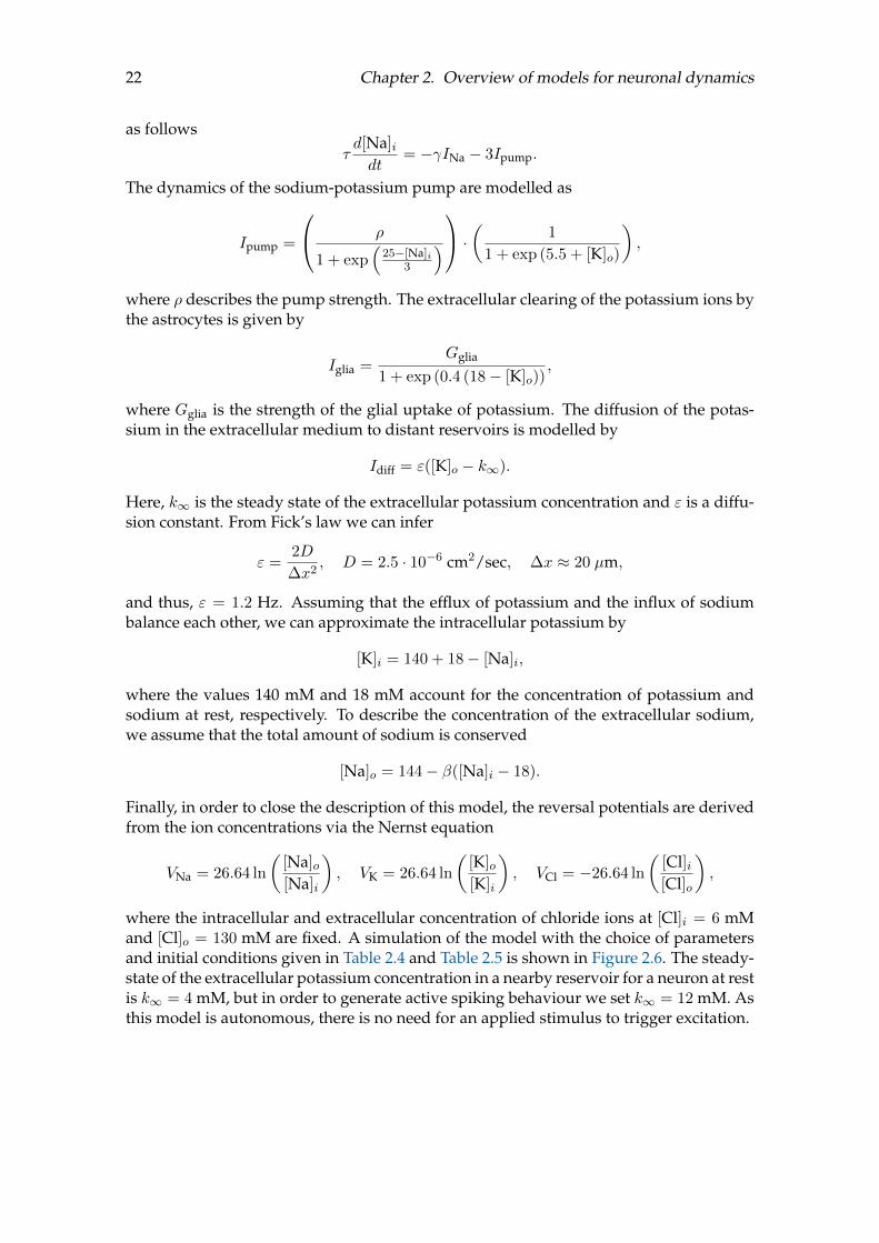
22 Chapter 2. Overview of models for neuronal dynamics
as follows
τd[Na]idt
= −γINa − 3Ipump.
The dynamics of the sodium-potassium pump are modelled as
Ipump =
ρ
1 + exp(
25−[Na]i3
) · ( 1
1 + exp (5.5 + [K]o)
),
where ρ describes the pump strength. The extracellular clearing of the potassium ions bythe astrocytes is given by
Iglia =Gglia
1 + exp (0.4 (18− [K]o)),
where Gglia is the strength of the glial uptake of potassium. The diffusion of the potas-sium in the extracellular medium to distant reservoirs is modelled by
Idiff = ε([K]o − k∞).
Here, k∞ is the steady state of the extracellular potassium concentration and ε is a diffu-sion constant. From Fick’s law we can infer
ε =2D
∆x2, D = 2.5 · 10−6 cm2/sec, ∆x ≈ 20 µm,
and thus, ε = 1.2 Hz. Assuming that the efflux of potassium and the influx of sodiumbalance each other, we can approximate the intracellular potassium by
[K]i = 140 + 18− [Na]i,
where the values 140 mM and 18 mM account for the concentration of potassium andsodium at rest, respectively. To describe the concentration of the extracellular sodium,we assume that the total amount of sodium is conserved
[Na]o = 144− β([Na]i − 18).
Finally, in order to close the description of this model, the reversal potentials are derivedfrom the ion concentrations via the Nernst equation
VNa = 26.64 ln
([Na]o[Na]i
), VK = 26.64 ln
([K]o[K]i
), VCl = −26.64 ln
([Cl]i[Cl]o
),
where the intracellular and extracellular concentration of chloride ions at [Cl]i = 6 mMand [Cl]o = 130 mM are fixed. A simulation of the model with the choice of parametersand initial conditions given in Table 2.4 and Table 2.5 is shown in Figure 2.6. The steady-state of the extracellular potassium concentration in a nearby reservoir for a neuron at restis k∞ = 4 mM, but in order to generate active spiking behaviour we set k∞ = 12 mM. Asthis model is autonomous, there is no need for an applied stimulus to trigger excitation.

2.2. Detailed electrophysiological models 23
Parameter Description Value UnitC membrane capacitance 1 µF/cm2
gNa conductance of the sodium current 100 mS/cm2
gK conductance of the potassium current 40 mS/cm2
gAHP conductance of the after hyperpolarisa-tion current
0.01 mS/cm2
gKL conductance of the sodium leak current 0.05 mS/cm2
gNaL conductance of the potassium leak cur-rent
0.0175 mS/cm2
gClL conductance of the chloride leak current 0.05 mS/cm2
gCa conductance of the calcium current 0.1 mS/cm2
VCa reversal potential of calcium 120 mVϕ time constant of the gating variables 30 msec−1
β ratio of intracellular to extracellular vol-ume of the cell
7 –
γ unit conversion factor 0.33 mM cm2/µCτ time conversion factor 1000 –ρ pump strength 1.25 mM/secε diffusion constant 1.2 HzGglia strength of the glial uptake of potassium 66 mM/sk∞ modified steady state of the extracellular
potassium concentration12 mM
[Cl]i intracellular chloride concentration 6 mM[Cl]o extracellular chloride concentration 130 mM
TABLE 2.4: Model parameters for the simulation of the Cressman model.
Parameter Description Value UnitV membrane potential -68.2102 mVn gating variable 20.1432 –h gating variable 0.9931 –[Ca]i intracellular calcium concentration 0.0008 mM[K]o extracellular potassium concentration 3.8155 mM[Na]i intracellular sodium concentration 20.1432 mM
TABLE 2.5: The initial conditions for the simulation of the Cressmanmodel.
2.2.2 Wei model
The model introduced by Wei, Ullah, and Schiff, 2014 is an extension of the neural modelproposed in Cressman et al., 2009 and accounts for a wider range of neuronal activitiesthan the original one. Wei’s model supports various neuronal behaviours varying fromseizure to spreading depression, tonic firing and a steady state, whose occurrence de-pend on the values of the potassium and oxygen bath concentrations, denoted by kbathand Obath, respectively. A detailed analysis of the bifurcation parameters can be found inWei, Ullah, and Schiff, 2014.

24 Chapter 2. Overview of models for neuronal dynamics
FIGURE 2.6: Neuronal spiking dynamics simulated with the electrophysi-ology model including sodium and potassium dynamics.
Membrane potential dynamics The membrane potential V is described by Hodgkin–Huxley type equations
CdV
dt= −INa − IK − ICl −
Ipump
γ,
INa = gNam3h(V − VNa) + gNaL(V − ENa),
IK = gKn4(V − VK) + gKL(V − EK), (2.10)
ICl = gClL(V − VCl),
dw
dt= αw(1− w)− βww, for w = n,m, h,
where C is the membrane capacitance, INa and IK are the sodium and potassium cur-rents, also including their respective leak currents, while ICl is the Cl− leak current; gNa
and gK are the maximal conductances of Na+ and K+, while gNaL, gKL and gClL are theleak Na+, K+ and Cl− conductances, respectively; Ipump is the pump current of the neu-ronal ATP-dependent sodium-potassium pump, that will be described in detail in thenext section. Finally, the conversion factor γ = S/(Fvi) · 10−2, where S is the cell surface,vi the intracellular volume and F = 96.485 C/mol the Faraday constant, transforms thecurrent units (µA/cm2) into concentration units (mM/s). The activation and inactiva-tion variables w = n,m, h represent the percentage of ion-selective channels in the open

2.2. Detailed electrophysiological models 25
and closed state and vary between 0 and 1, where 0 indicates closed channels, and 1 openones. The functions αw and βw forw = n,m, h are once again voltage-dependent openingand closing rates of the ion channels and for this model are defined as
αn = 0.032 V+521−exp(−V+52
5 ), βn = 0.5 exp
(−V + 57
40
),
αm = 0.32 V+541−exp(−V+54
4 ), βm = 0.28
V + 27
exp(V+27
5
)− 1
,
αh = 0.128 exp(−V+50
18
), βh =
4
1 + exp(−V+27
5
) .The reversal potentials of Na+, K+ and Cl− are linked to the ion concentrations via theNernst equation
VNa = 26.64 ln
([Na]o[Na]i
)VK = 26.64 ln
([K]o[K]i
)VCl = 26.64 ln
([Cl]i[Cl]o
)where [·]i and [·]o denote intracellular and extracellular concentrations, respectively.
Ion concentrations The dynamics of the ion concentrations is governed by the com-bined action of ionic currents and fluxes. The concentrations involved are computedthrough the number of ions per volume component, taking into account the possibleswelling of the cell during activity. The ion numbers are defined as
NXi = vi[X]i, NXo = vo[X]o, for X ∈ Na,K,Cl,
with vi and vo being the intracellular and extracellular volumes, respectively. In the in-tracellular space, the ion number dynamics read
d
dtNKi =
1
σ(−γIK + 2Ipump − Ikcc2 − Inkcc1)vi,
d
dtNNai =
1
σ(−γINa − 3Ipump − Inkcc1)vi, (2.11)
d
dtNCli =
1
σ(γIClL − Ikcc2 − 2Inkcc1)vi,
while in the extracellular space they read
d
dtNKo =
1
σ(γβIK − 2βIpump − Idiff − Iglia − 2Igliapump + βIkcc2 + βInkcc1)vo,
d
dtNNao =
1
σ(γβINa + 3βIpump + βInkcc1)vo, (2.12)
d
dtNClo =
1
σ(−γβIClL + βIkcc2 + 2βInkcc1)vo.
In the above equations, σ = 1000 is the time conversion factor from seconds to mil-liseconds, and β = vi/vo is the ratio between intracellular and extracellular volume. Bydefining
Ni(t) =
NKi(t)NNai(t)NCli(t)
, No(t) =
NKo(t)NNao(t)NClo(t)
,
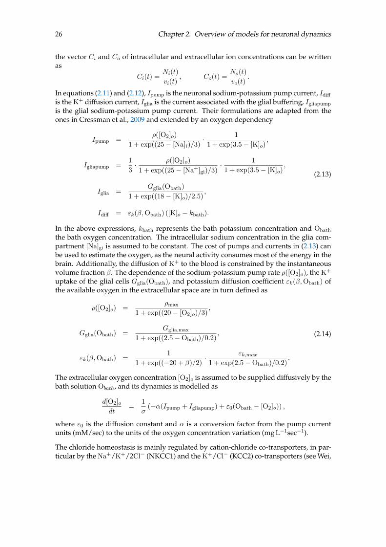
26 Chapter 2. Overview of models for neuronal dynamics
the vector Ci and Co of intracellular and extracellular ion concentrations can be writtenas
Ci(t) =Ni(t)
vi(t), Co(t) =
No(t)
vo(t).
In equations (2.11) and (2.12), Ipump is the neuronal sodium-potassium pump current, Idiff
is the K+ diffusion current, Iglia is the current associated with the glial buffering, Igliapump
is the glial sodium-potassium pump current. Their formulations are adapted from theones in Cressman et al., 2009 and extended by an oxygen dependency
Ipump =ρ([O2]o)
1 + exp((25− [Na]i)/3)· 1
1 + exp(3.5− [K]o),
Igliapump =1
3· ρ([O2]o)
1 + exp((25− [Na+]gi)/3)· 1
1 + exp(3.5− [K]o),
Iglia =Gglia(Obath)
1 + exp((18− [K]o)/2.5),
Idiff = εk(β,Obath) ([K]o − kbath).
(2.13)
In the above expressions, kbath represents the bath potassium concentration and Obath
the bath oxygen concentration. The intracellular sodium concentration in the glia com-partment [Na]gi is assumed to be constant. The cost of pumps and currents in (2.13) canbe used to estimate the oxygen, as the neural activity consumes most of the energy in thebrain. Additionally, the diffusion of K+ to the blood is constrained by the instantaneousvolume fraction β. The dependence of the sodium-potassium pump rate ρ([O2]o), the K+
uptake of the glial cells Gglia(Obath), and potassium diffusion coefficient εk(β,Obath) ofthe available oxygen in the extracellular space are in turn defined as
ρ([O2]o) =ρmax
1 + exp((20− [O2]o)/3),
Gglia(Obath) =Gglia,max
1 + exp((2.5−Obath)/0.2),
εk(β,Obath) =1
1 + exp((−20 + β)/2)·
εk,max1 + exp(2.5−Obath)/0.2)
.
(2.14)
The extracellular oxygen concentration [O2]o is assumed to be supplied diffusively by thebath solution Obath, and its dynamics is modelled as
d[O2]odt
=1
σ(−α(Ipump + Igliapump) + ε0(Obath − [O2]o)) ,
where ε0 is the diffusion constant and α is a conversion factor from the pump currentunits (mM/sec) to the units of the oxygen concentration variation (mg L−1sec−1).
The chloride homeostasis is mainly regulated by cation-chloride co-transporters, in par-ticular by the Na+/K+/2Cl− (NKCC1) and the K+/Cl− (KCC2) co-transporters (see Wei,

2.2. Detailed electrophysiological models 27
Ullah, and Schiff, 2014 for detailed physiological description). The co-transporter cur-rents Inkcc1 and Ikcc2 are modelled in a Nernst-like manner as
Ikcc2 = Ukcc2 ln
([K]i[Cl]i[K]o[Cl]o
),
Inkcc1 = Unkcc1f ([K]o)
(ln
([K]i[Cl]i[K]o[Cl]o
)+ ln
([Na]i[Cl]i[Na]o[Cl]o
)),
f([K]o) =1
1 + exp(16− [K]o),
where Ukcc2 and Unkcc1 are the co-transporter strengths.
Volume dynamics As the cell volume varies according to the level of activity (entailinghigh ion influx or efflux), the expected intracellular neuronal volume vi depends on thedifference between the extracellular and the intracellular osmotic pressures πo and πi.Both the extracellular and intracellular fluids consist of water, sodium, potassium andchloride ions. Negatively charged proteins (A−), also called anions and mainly presentin the intracellular space, cannot permeate the membrane and are one of the reasonsfor the overall negative charge of the membrane potential at rest. The intracellular andextracellular osmotic pressures can thus be written as
πo = [Na]o + [K]o + [Cl]o + [A]o,
πi = [Na]i + [K]i + [Cl]i + [A]i,
where [A]i = 132 mM and [A]o = 18 mM are the intra- and extracellular concentration ofanions.
The expected intracellular volume is given by
vi = v0i ·(
1.1029− 0.1029 exp
(πo − πi
20
)), (2.15)
where v0i is the initial intracellular volume of a cell with radius 7 µm, whereas the change
of cell volume is defined asdvidt
=vi − vi
250. (2.16)
Assuming a constant total volume, the extracellular volume is then computed as
vo =
(1 +
1
β0
)v0i − vi, (2.17)
where β0 is the initial ratio of intra- and extracellular volume. The instantaneous volumeratio β = vi/v0 is updated according to the temporal variations of vi and v0.
Vectorial representation To simplify the notation, we introduce a compact vector rep-resentation of the Wei model, and define
N(t) =
[Ni(t)No(t)
]∈ R6, w(t) = [n(t), m(t), h(t) ]T ∈ R3.

28 Chapter 2. Overview of models for neuronal dynamics
Furthermore, by setting
Λ(t) =
[vi(t) I3 0
0 vo(t) I3
]∈ R6×6,
where I3 ∈ R3×3 is the identity matrix, we have
C(t) =
[Ci(t)Co(t)
]= Λ(t)−1N(t) ∈ R6.
By introducing the vectors
U(t) =
V (t)w(t)N(t)
[O2]o(t)vi(t)
∈ R12, W (t) =
[C(t)vo(t)
]∈ R7, (2.18)
and by defining
ΦU (U,W ) =
ΦV
Φw1σ Λ ΦN1σ ΦO2
Φvi
∈ R12, ΦW (U) =
Λ−1N(1 +
1
β0
)v0i − vi
∈ R7,
with
ΦV = −INa − IK − ICl −Ipump
γ, Φw =
αn(1− n)− βnnαm(1−m)− βmmαh(1− h)− βhh
,
ΦN =
−γIK + 2Ipump − Ikcc2 − Inkcc1
−γINa − 3Ipump − Inkcc1
γIClL − Ikcc2 − 2Inkcc1
γβIK − 2βIpump − Idiff − Iglia − 2Igliapump + βIkcc2 + βInkcc1
γβINa + 3βIpump + βInkcc1
−γβIClL + βIkcc2 + 2βInkcc1
,
ΦO2 = −α(Ipump + Igliapump) + ε0([O2]bath − [O2]o), Φvi =vi − vi
250,
we can represent Wei’s differential-algebraic system in compact form asdU
dt= ΦU (U,W )
W = ΦW (U)
. (2.19)
A simulation of the model is given in Figure 2.7, with initial values given in Table 2.6 andthe parameters set as in Table 2.7.
Keeping all the other model parameters fixed, according to the bifurcation diagram inWei, Ullah, and Schiff, 2014, a resting state featuring a spiking frequency around 10-12 Hz is obtained for the parameter choices kbath = 5.5 mM and Obath = 30 mM, whilea spreading depression behaviour is triggered by a higher kbath concentration, in the
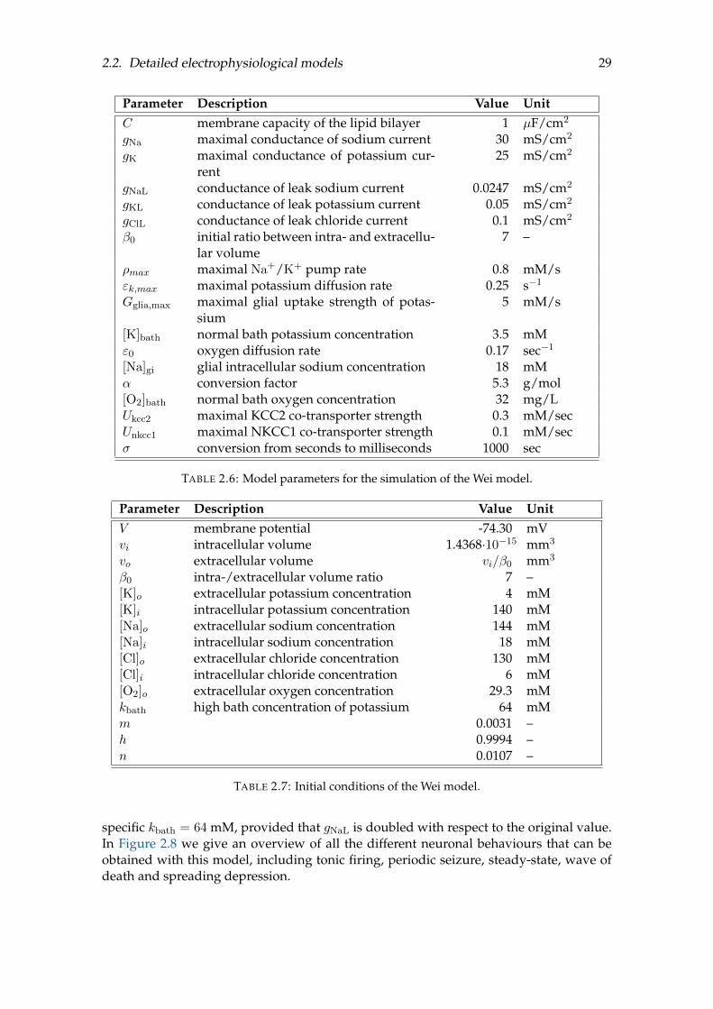
2.2. Detailed electrophysiological models 29
Parameter Description Value UnitC membrane capacity of the lipid bilayer 1 µF/cm2
gNa maximal conductance of sodium current 30 mS/cm2
gK maximal conductance of potassium cur-rent
25 mS/cm2
gNaL conductance of leak sodium current 0.0247 mS/cm2
gKL conductance of leak potassium current 0.05 mS/cm2
gClL conductance of leak chloride current 0.1 mS/cm2
β0 initial ratio between intra- and extracellu-lar volume
7 –
ρmax maximal Na+/K+ pump rate 0.8 mM/sεk,max maximal potassium diffusion rate 0.25 s−1
Gglia,max maximal glial uptake strength of potas-sium
5 mM/s
[K]bath normal bath potassium concentration 3.5 mMε0 oxygen diffusion rate 0.17 sec−1
[Na]gi glial intracellular sodium concentration 18 mMα conversion factor 5.3 g/mol[O2]bath normal bath oxygen concentration 32 mg/LUkcc2 maximal KCC2 co-transporter strength 0.3 mM/secUnkcc1 maximal NKCC1 co-transporter strength 0.1 mM/secσ conversion from seconds to milliseconds 1000 sec
TABLE 2.6: Model parameters for the simulation of the Wei model.
Parameter Description Value UnitV membrane potential -74.30 mVvi intracellular volume 1.4368·10−15 mm3
vo extracellular volume vi/β0 mm3
β0 intra-/extracellular volume ratio 7 –[K]o extracellular potassium concentration 4 mM[K]i intracellular potassium concentration 140 mM[Na]o extracellular sodium concentration 144 mM[Na]i intracellular sodium concentration 18 mM[Cl]o extracellular chloride concentration 130 mM[Cl]i intracellular chloride concentration 6 mM[O2]o extracellular oxygen concentration 29.3 mMkbath high bath concentration of potassium 64 mMm 0.0031 –h 0.9994 –n 0.0107 –
TABLE 2.7: Initial conditions of the Wei model.
specific kbath = 64 mM, provided that gNaL is doubled with respect to the original value.In Figure 2.8 we give an overview of all the different neuronal behaviours that can beobtained with this model, including tonic firing, periodic seizure, steady-state, wave ofdeath and spreading depression.
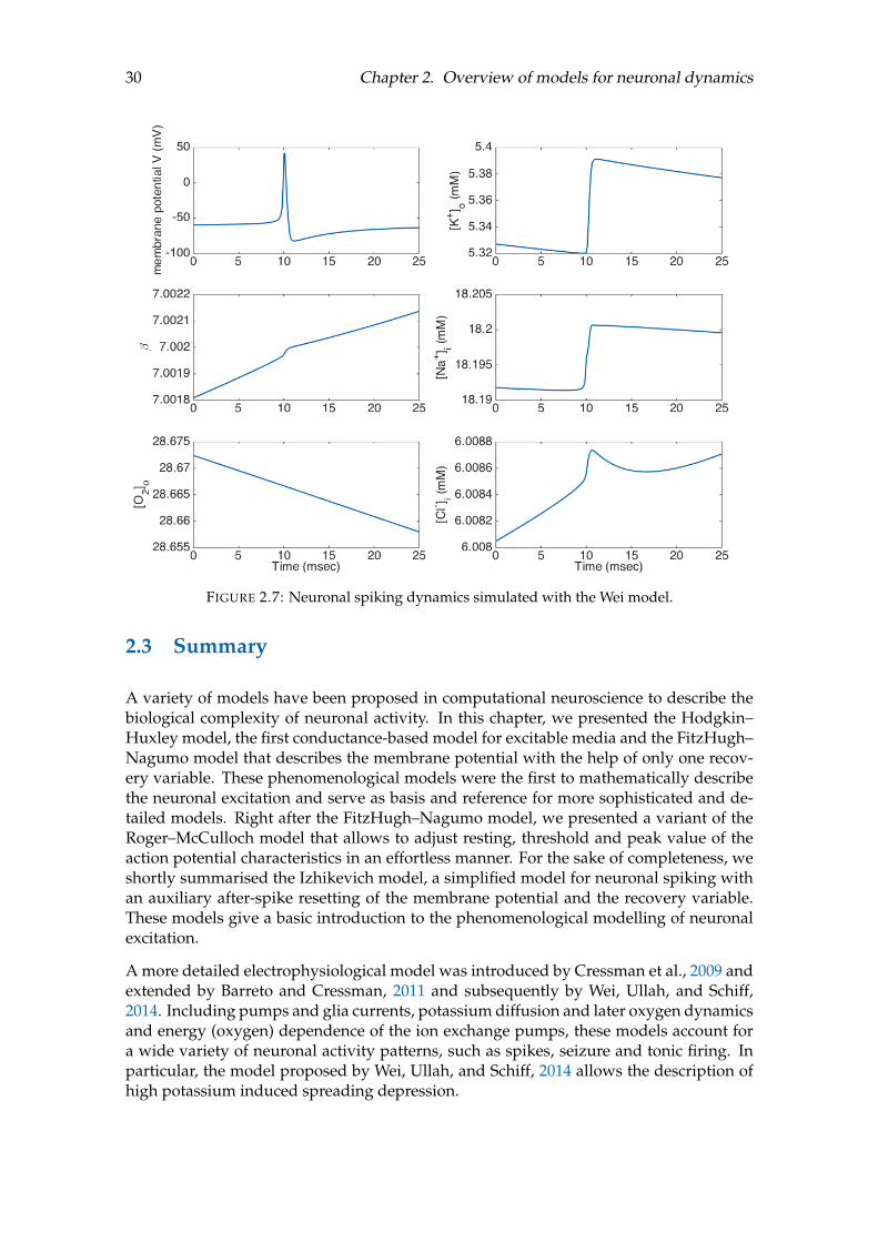
30 Chapter 2. Overview of models for neuronal dynamics
FIGURE 2.7: Neuronal spiking dynamics simulated with the Wei model.
2.3 Summary
A variety of models have been proposed in computational neuroscience to describe thebiological complexity of neuronal activity. In this chapter, we presented the Hodgkin–Huxley model, the first conductance-based model for excitable media and the FitzHugh–Nagumo model that describes the membrane potential with the help of only one recov-ery variable. These phenomenological models were the first to mathematically describethe neuronal excitation and serve as basis and reference for more sophisticated and de-tailed models. Right after the FitzHugh–Nagumo model, we presented a variant of theRoger–McCulloch model that allows to adjust resting, threshold and peak value of theaction potential characteristics in an effortless manner. For the sake of completeness, weshortly summarised the Izhikevich model, a simplified model for neuronal spiking withan auxiliary after-spike resetting of the membrane potential and the recovery variable.These models give a basic introduction to the phenomenological modelling of neuronalexcitation.
A more detailed electrophysiological model was introduced by Cressman et al., 2009 andextended by Barreto and Cressman, 2011 and subsequently by Wei, Ullah, and Schiff,2014. Including pumps and glia currents, potassium diffusion and later oxygen dynamicsand energy (oxygen) dependence of the ion exchange pumps, these models account fora wide variety of neuronal activity patterns, such as spikes, seizure and tonic firing. Inparticular, the model proposed by Wei, Ullah, and Schiff, 2014 allows the description ofhigh potassium induced spreading depression.
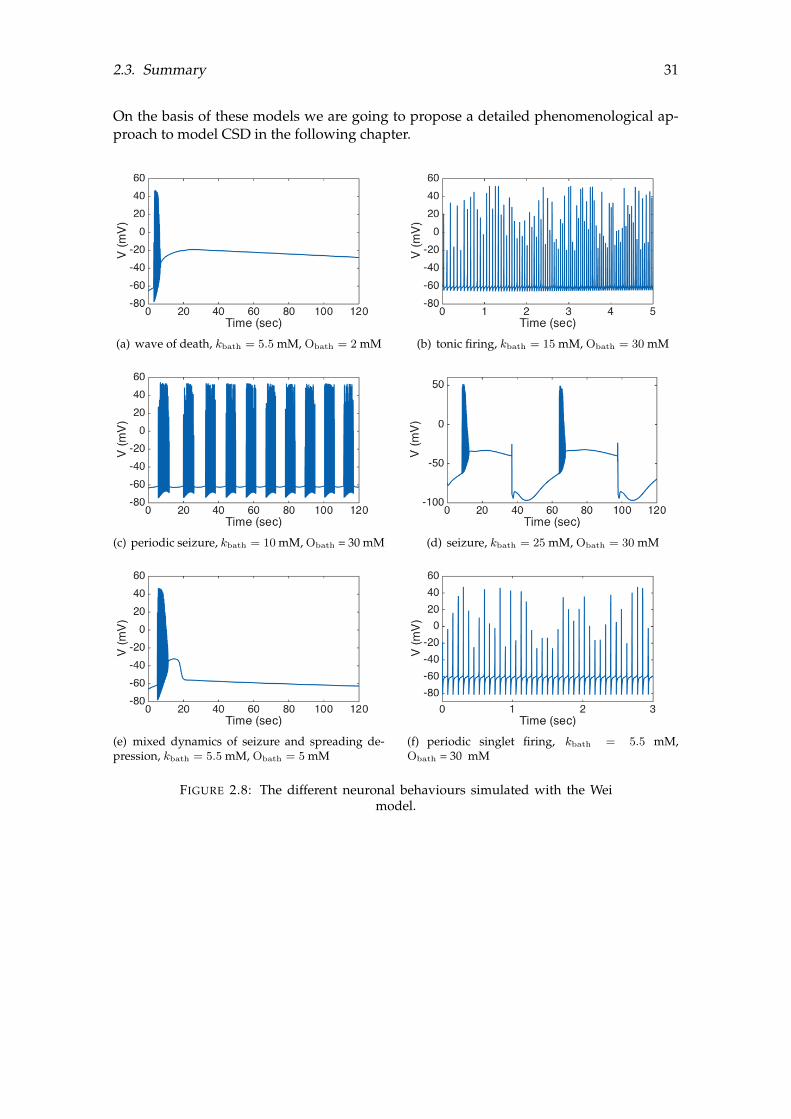
2.3. Summary 31
On the basis of these models we are going to propose a detailed phenomenological ap-proach to model CSD in the following chapter.
(a) wave of death, kbath = 5.5 mM, Obath = 2 mM (b) tonic firing, kbath = 15 mM, Obath = 30 mM
(c) periodic seizure, kbath = 10 mM, Obath = 30 mM (d) seizure, kbath = 25 mM, Obath = 30 mM
(e) mixed dynamics of seizure and spreading de-pression, kbath = 5.5 mM, Obath = 5 mM
(f) periodic singlet firing, kbath = 5.5 mM,Obath = 30 mM
FIGURE 2.8: The different neuronal behaviours simulated with the Weimodel.

33
Chapter 3
Distributed CSD model
“Science, my lad, is made up of mistakes,but they are mistakes which it is useful to make, because they lead little by little to the truth.”
Jules Verne, in A Journey to the Center of the Earth (1873)
Biophysical models aim at providing insight into interactions and dynamics at the micro-scopic (cellular or subcellular) level, whereas phenomenological models aim at providinginformation about the general propagation of the CSD on the macroscopic scale. In thischapter, we create a first bridge between the biophysical and phenomenological mod-elling approach, to provide a better understanding of the complex dynamics underlyingthe propagation of the depolarisation wave.
Following the potassium hypothesis for CSD propagation, we introduce a multi-scalecoupled PDE-ODE system accounting for the macroscopic propagation of the depolari-sation wave and the microscopic neuronal dynamics. The problem is inherently multi-scale in time: the propagation of the CSD wave is on the minute scale (taking about20 minutes to propagate from the visual cortex to the frontal cortex), whereas the elec-trophysiological dynamics features a much faster temporal scale (of the order of millisec-onds). We model the extracellular potassium bath concentration at the macroscopic levelwith a modified version of the FitzHugh–Nagumo model. Referring to the potassiumhypothesis, the propagation of the extracellular potassium is the driving force of CSDpropagation on the cerebral cortex (Zandt et al., 2015). The resulting dynamics of thepotassium bath concentration is then used as a driver for the activation of the detailedelectrophysiological model for the neurons. All models introduced in Chapter 2 are the-oretically suited to describe the microscopic neuronal response, especially the detailedelectrophysiological models introduced in Section 2.2. However, we chose to build ourmodel upon the one proposed by Wei, Ullah, and Schiff, 2014 (see also Section 2.2.2), asit supports various neuronal activity patterns depending on the extracellular potassiumand oxygen bath concentration. A constant potassium concentration around 5 mM trig-gers a spiking frequency of about 12 Hz which coincides with the neuronal activity atrest. Increasing the potassium concentration up to 64 mM results in CSD-like behaviour.In particular, constantly high extracellular potassium leads to periodic seizures in the mi-croscopic neuronal model dynamics with initial high intensity firing followed by a periodof neuronal silencing. We are going to take advantage of the model’s specific reaction tovarying potassium concentrations in order to reproduce the characteristic neuronal be-haviour during a CSD.
34 Chapter 3. Distributed CSD model
As the available literature describes the behaviour of a single cell, the behaviour of themicroscopic component of the coupled model can be considered a non-standard meanfield model (following the classical definition in Deco et al., 2008). The model variablesin a generic point x ∈ Ω represent the average value of the corresponding quantitiesfor the collection of neurons present at that particular spatial location. In addition tothat, it is advantageous to consider an ensemble of neurons in space, as it allows to usea computational grid with a characteristic size of the order of millimetres, based on thegeometry obtained from MRI imaging, rather than the characteristic size of individualneurons (typically of the order of µm).
In this chapter, we first describe the microscopic electrophysiological formulation of neu-ronal behaviour and then the macroscopic propagative model of the potassium bath con-centration for the depolarisation wave. Subsequently, the coupling and the numericalapproximation are discussed. The last part of the chapter is devoted to numerical evalu-ations in one and two space dimensions to demonstrate the model features and its corre-spondence to measurements and experiments on the CSD. In Chapter 4 we numericallysimulate CSD propagation on a brain geometry reconstructed from medical imaging us-ing the model described in the following.
3.1 Electrophysiological part of the model
For the description of the microscopic level we use the model proposed by Wei, Ullah,and Schiff, 2014, introduced in Section 2.2.2. This model features various neuronal be-haviours from seizure to spreading depression, tonic firing and a steady state. The modelbehaviour depends on the extracellular potassium (kbath) and oxygen bath concentration(Obath). We refer to the summary of the model in Section 2.2.2 and to Wei, Ullah, andSchiff, 2014 for a detailed bifurcation analysis. Here, we just repeat the outline and gen-eral formulation of the model and its variables in order to clarify the coupling with itspropagating driver kbath.
In contrast to the original model proposed by Wei, where kbath is a constant, we followthe potassium hypothesis and assume that the extracellular potassium varies in time andthus acts as a driver for the CSD propagation. This implies that the potassium diffusioncurrent Idiff in equation (2.13) explicitly depends on kbath, namely Idiff(kbath). This de-pendency is passed on to the functions depending on Idiff and the compact notation inthe vectorial representations of the model (see Section 2.2.2).
For the sake of presentation, we recall here the Wei model and, as in the previous chapter,we collect the number of intra- and extracellular ions in a vector variable N and groupthe activation and inactivation variables n, m, h in the vector w:
N(t) =
[Ni(t)No(t)
]∈ R6, w(t) = [n(t), m(t), h(t) ]T ∈ R3.
By setting
Λ(t) =
[vi(t) I3 0
0 vo(t) I3
]∈ R6×6,
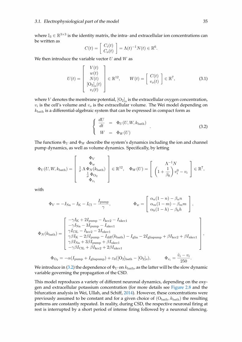
3.1. Electrophysiological part of the model 35
where I3 ∈ R3×3 is the identity matrix, the intra- and extracellular ion concentrations canbe written as
C(t) =
[Ci(t)Co(t)
]= Λ(t)−1N(t) ∈ R6.
We then introduce the variable vector U and W as
U(t) =
V (t)w(t)N(t)
[O2]o(t)vi(t)
∈ R12, W (t) =
[C(t)vo(t)
]∈ R7, (3.1)
where V denotes the membrane potential, [O2]o is the extracellular oxygen concentration,vi is the cell’s volume and vo is the extracellular volume. The Wei model depending onkbath is a differential-algebraic system that can be expressed in compact form as
dU
dt= ΦU (U,W, kbath)
W = ΦW (U)
. (3.2)
The functions ΦU and ΦW describe the system’s dynamics including the ion and channelpump dynamics, as well as volume dynamics. Specifically, by letting
ΦU (U,W, kbath) =
ΦV
Φw1σ Λ ΦN (kbath)
1σ ΦO2
Φvi
∈ R12, ΦW (U) =
Λ−1N(1 +
1
β0
)v0i − vi
∈ R7,
with
ΦV = −INa − IK − ICl −Ipump
γ, Φw =
αn(1− n)− βnnαm(1−m)− βmmαh(1− h)− βhh
,
ΦN (kbath) =
−γIK + 2Ipump − Ikcc2 − Inkcc1
−γINa − 3Ipump − Inkcc1
γIClL − Ikcc2 − 2Inkcc1
γβIK − 2βIpump − Idiff(kbath)− Iglia − 2Igliapump + βIkcc2 + βInkcc1
γβINa + 3βIpump + βInkcc1
−γβIClL + βIkcc2 + 2βInkcc1
,
ΦO2 = −α(Ipump + Igliapump) + ε0([O2]bath − [O2]o), Φvi =vi − vi
250.
We introduce in (3.2) the dependence of ΦU on kbath, as the latter will be the slow dynamicvariable governing the propagation of the CSD.
This model reproduces a variety of different neuronal dynamics, depending on the oxy-gen and extracellular potassium concentration (for more details see Figure 2.8 and thebifurcation analysis in Wei, Ullah, and Schiff, 2014). However, these concentrations werepreviously assumed to be constant and for a given choice of (Obath, kbath) the resultingpatterns are constantly repeated. In reality, during CSD, the respective neuronal firing atrest is interrupted by a short period of intense firing followed by a neuronal silencing.

36 Chapter 3. Distributed CSD model
These different dynamics can only be achieved by different parameter combinations ofthe pair (Obath, kbath).
Consequently, to reproduce realistic CSD dynamics, the pair (Obath, kbath) has to be afunction of time. To highlight this aspect, we show in Figure 3.1 the temporal dynamicsof the membrane potential obtained from Wei’s model under three different conditions:at rest kbath = 5.5 mM, high concentration kbath = 64 mM, and varying kbath in time,switching between the high and low concentration state. In particular, modelling kbath asa step function with a short period of high potassium
kbath(t) =
64 mM, if t ∈ [10, 30]
5.5 mM, else(3.3)
results in a CSD-like behaviour of the membrane potential. However, the choice of a stepfunction for an ion distribution is not a natural choice and does not represent naturaldynamics. We just use the step function to illustrate that a kbath varying in time triggersCSD-like reactions at the microscopic scale. In the following subsection, we introduce amore appropriate choice for the kbath concentration and its propagation.
(a) kbath = 5.5 mM (b) kbath = 64 mM (c) kbath varying in time
FIGURE 3.1: The different temporal dynamics of kbath and the membranepotential. The top row shows the extracellular potassium concentration:kbath = 5.5 mM (a), kbath = 64 mM (b) and kbath(t) depending on time(c), as defined in (3.3). The bottom row demonstrates the corresponding
dynamics of the membrane potential V .
3.2 Propagative part of the model
In accordance with the potassium hypothesis, we model the propagation of the extra-cellular potassium as the driving force of CSD propagation and its electrophysiologicaldynamics at the microscopic scale. We describe a dynamical system for the temporalevolution and propagation of kbath with a coupled reaction-diffusion PDE-ODE model as
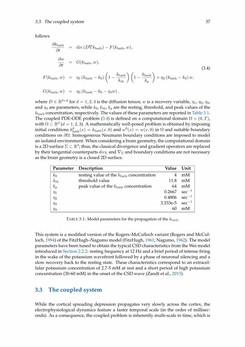
3.3. The coupled system 37
follows
∂kbath
∂t= div (D∇kbath)− F (kbath, w),
∂w
∂t= G(kbath, w),
F (kbath, w) = η1 (kbath − k0)
(1− kbath
kth
)(1− kbath
kp
)+ η2 (kbath − k0)w,
G(kbath, w) = η3 (kbath − k0 − η4w) ,
(3.4)
where D ∈ Rd×d for d = 1, 2, 3 is the diffusion tensor, w is a recovery variable, η1, η2, η3,and η4 are parameters, while k0, kth, kp are the resting, threshold, and peak values of thekbath concentration, respectively. The values of these parameters are reported in Table 3.1.The coupled PDE-ODE problem (3.4) is defined on a computational domain Ω × (0, T ),with Ω ⊂ Rd (d = 1, 2, 3). A mathematically well-posed problem is obtained by imposinginitial conditions k0
bath(x) = kbath(x, 0) and w0(x) = w(x, 0) in Ω and suitable boundaryconditions on ∂Ω: homogeneous Neumann boundary conditions are imposed to modelan isolated environment. When considering a brain geometry, the computational domainis a 2D surface Σ ⊂ R3; thus, the classical divergence and gradient operators are replacedby their tangential counterparts divΣ and∇Σ and boundary conditions are not necessaryas the brain geometry is a closed 2D surface.
Parameter Description Value Unitk0 resting value of the kbath concentration 4 mMkth threshold value 11.8 mMkp peak value of the kbath concentration 64 mMη1 0.2667 sec−1
η2 0.4806 sec−1
η3 3.333e-5 sec−1
η4 60 mM
TABLE 3.1: Model parameters for the propagation of the kbath.
This system is a modified version of the Rogers–McCulloch variant (Rogers and McCul-loch, 1994) of the FitzHugh–Nagumo model (FitzHugh, 1961; Nagumo, 1962). The modelparameters have been tuned to obtain the typical CSD characteristics from the Wei modelintroduced in Section 2.2.2: resting frequency at 12 Hz and a brief period of intense firingin the wake of the potassium wavefront followed by a phase of neuronal silencing and aslow recovery back to the resting state. These characteristics correspond to an extracel-lular potassium concentration of 2.7-5 mM at rest and a short period of high potassiumconcentration (30-60 mM) in the onset of the CSD wave (Zandt et al., 2015).
3.3 The coupled system
While the cortical spreading depression propagates very slowly across the cortex, theelectrophysiological dynamics feature a faster temporal scale (in the order of millisec-onds). As a consequence, the coupled problem is inherently multi-scale in time, which is

38 Chapter 3. Distributed CSD model
posing a non-negligible computational challenge. Given a region Ω ⊂ Rd, d = 1, 2, 3 thecomplete model for the CSD propagation in Ω× [0, T ], including the electrophysiologicaldynamics, is a differential-algebraic system, where the differential part consists of a cou-pled PDE-ODE system. With suitable initial conditions (k0
bath, w0, U0, W 0) this systemreads
∂kbath
∂t= div (D∇kbath)− F (kbath, w) in Ω× (0, T )
∂w
∂t= G(kbath, w) in Ω× (0, T )
1
σ
∂U
∂t= ΦU (U,W, kbath) in Ω× (0, T )
W = ΦW (U) in Ω× (0, T )
. (3.5)
In the above system, all variables depend on space, F (kbath, w) and G(kbath, w) are theones defined in equation (3.4), U and W are defined in equation (3.1), while σ = 1000is the conversion factor to the temporal scale of the electrophysiology, converting sec-onds to milliseconds. We obtain a well-posed problem by imposing initial conditionskbath(x, 0) = k0
bath, w(x, 0) = w0, U(x, 0) = U0 and W (x, 0) = W 0 in Ω and suitableboundary conditions on ∂Ω for the first equation in (3.5), as previously mentioned inSection 3.2.
With this coupled system we can now obtain the typical dynamics of CSD, at the macro-scopic scale as well as on the microscopic scale. To emphasise this and show the micro-scopic dynamics of the electrophysiology resulting from the temporal dynamics of theextracellular potassium, we visualise kbath and the membrane potential V in Figure 3.2as functions of time. In this example, we consider the dynamics without the diffusionpart of the potassium, that is, in one single point x ∈ Ω. A closer look at the V dynamicshighlights the key characteristics of CSD: a short period of intense firing at the onset ofthe CSD, followed by a silencing of the neurons and a slow recovery back to the normalspiking frequency of neurons at rest.
3.4 Numerical approximation
The final aim is to simulate and describe the propagation of a CSD wave on a real braingeometry without any simplifying assumptions. Brain geometries can be reconstructedfrom medical imaging and require the use of unstructured meshes. Consequently, wewill formulate the numerical discretisation of our problem in the broadest sense possibleto allow the application to real geometries.
We will first formulate the variational formulation of the coupled system, then we willdescribe the details of the semi-discrete formulation, and finally discuss the multi scaletime steps required to deal with the different time scales of the model.
3.4.1 Variational formulation
For the variational formulation of problem (3.5) let us denote by L2(Ω) and H1(Ω), theclassical space of square integrable functions over Ω, and the Sobolev space of L2(Ω)functions with weak first derivatives in L2(Ω), respectively. In addition, we will use the

3.4. Numerical approximation 39
(a) temporal dynamics of kbath and the membrane potential V
(b) detailed dynamics of the membrane potential V
FIGURE 3.2: The temporal dynamics of kbath and the membrane potentialV , solution to system (3.5) in (a) and three more detailed snapshots of themembrane potential dynamics to emphasise the key characteristics of the
CSD (b).
Sobolev spaceW 1,1(Ω) which is a subset of functions in L1(Ω) with weak first derivativesin L1(Ω). Then the variational formulation of system (3.5) can be stated as follows:
given k0bath, w
0, U0,W 0 ∈ L2(Ω), find kbath ∈ W 1,1(0, T ;H1(Ω)), w ∈ L2(0, T ;L2(Ω)),U ∈ L2(0, T ; [L2(Ω)]12), and W ∈ L2(0, T ; [L2(Ω)]7) such that for all t ∈ (0, T )
∂
∂t〈kbath(t), φ〉+ a(kbath(t), φ) + 〈F (kbath(t), w(t)), φ〉 = 0 ∀φ ∈ H1(Ω),
∂
∂t〈w(t), ψ〉 = 〈G(kbath(t), w(t)), ψ〉 ∀ψ ∈ L2(Ω),
∂
∂t〈U(t),ΨU 〉 = 〈ΦU (U(t),W (t), kbath(t)),ΨU 〉 ∀ΨU ∈ [L2(Ω)]12,
〈W (t),ΨW 〉 = 〈ΦW (U(t)),ΨW 〉 ∀ΨW ∈ [L2(Ω)]7,
(3.6)
with suitable initial conditions, as described in Section 3.2. In the above equation wedenote by 〈·, ·〉 the inner product in L2(Ω), namely
〈η, ζ〉 =
∫Ωηζ dx, ∀η, ζ ∈ L2(Ω)

40 Chapter 3. Distributed CSD model
and by a(·, ·) the bilinear form on H1(Ω)×H1(Ω)
a(ϕ, χ) =
∫Ω
(∇ϕ)TD(x)∇χdx, ∀ϕ, χ ∈ H1(Ω).
There are several theoretical results on reaction-diffusion equations that can be appliedto equation (3.6). As the bilinear form a(·, ·) is weakly coercive on H1(Ω) ×H1(Ω), a de-tailed well-posedness analysis of this problem would follow the one presented in ColliFranzone and Savare, 2002 for an analogous system.
3.4.2 Semi-discrete formulation
For the numerical approximation of the coupled system, we first start with the macro-scopic model for the kbath propagation. Then, in the following subsection, we add thediscretisation of the microscopic part, and we conclude the section with the multi-scalenumerical approximation of the coupled model.
Assuming that Ω is a triangulated surface (in R3), let Th be a regular triangulation ofΩ, namely Ω =
⋃K∈Th K, where each element K ∈ Th is the image of the reference
element E, a triangle with vertices (0, 0, 0), (1, 0, 0), and (0, 1, 0), through an invertibleaffine map TK (K = TK(E)). We define h as the maximum diameter of the elements ofthe triangulation. The corresponding finite element spaces Xk
h are defined as
Xkh = ϕh ∈ C0(Ω) |ϕh|K TK ∈ Pk(E),
where Pk(E) is the space of polynomials of degree less than or equal to k on E. In thefollowing, we use piecewise linear elements (k = 1). For a more detailed introduction tofinite element methods see Quarteroni and Valli, 1994.
For the semi-discrete approximation of our problem, we apply the Galerkin method se-lecting the finite dimensional space Vh = X1
h, the grid points xjNhj=1 and the finite el-ement basis ϕj(x) | j = 1, . . . , Nh associated to them; Nh is the dimension of Vh. Thesemi-discrete unknowns on the grid nodes are given by
k(t) =
k1(t)...
kNh(t)
, U(t) =
U1,1(t) . . . U12,1(t)...
...U1,Nh(t) . . . U12,Nh(t)
,
w(t) =
w1(t)...
wNh(t)
, W (t) =
W 1,1(t) . . . W 12,1(t)...
...W 1,Nh(t) . . . W 12,Nh(t)
,and by defining ϕ(x) = [ϕ1(x), . . . , ϕNh(x)]T , the semi-discrete solutions are given by
kh(x, t) = k(t)Tϕ(x), Uh(x, t) = U(t)Tϕ(x),
wh(x, t) = w(t)Tϕ(x), W h(x, t) = W (t)Tϕ(x).
For the sake of simplicity in notations, we simply denote by k the variable kbath, fromthis point forward.
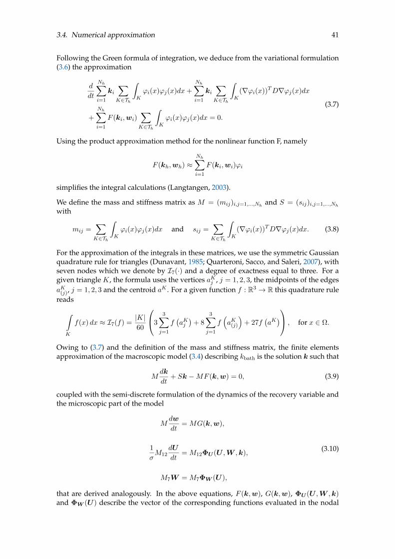
3.4. Numerical approximation 41
Following the Green formula of integration, we deduce from the variational formulation(3.6) the approximation
d
dt
Nh∑i=1
ki∑K∈Th
∫Kϕi(x)ϕj(x)dx+
Nh∑i=1
ki∑K∈Th
∫K
(∇ϕi(x))TD∇ϕj(x)dx
+
Nh∑i=1
F (ki,wi)∑K∈Th
∫Kϕi(x)ϕj(x)dx = 0.
(3.7)
Using the product approximation method for the nonlinear function F, namely
F (kh,wh) ≈Nh∑i=1
F (ki,wi)ϕi
simplifies the integral calculations (Langtangen, 2003).
We define the mass and stiffness matrix as M = (mij)i,j=1,...,Nh and S = (sij)i,j=1,...,Nh
with
mij =∑K∈Th
∫Kϕi(x)ϕj(x)dx and sij =
∑K∈Th
∫K
(∇ϕi(x))TD∇ϕj(x)dx. (3.8)
For the approximation of the integrals in these matrices, we use the symmetric Gaussianquadrature rule for triangles (Dunavant, 1985; Quarteroni, Sacco, and Saleri, 2007), withseven nodes which we denote by I7(·) and a degree of exactness equal to three. For agiven triangle K, the formula uses the vertices aKj , j = 1, 2, 3, the midpoints of the edgesaK(j), j = 1, 2, 3 and the centroid aK . For a given function f : R3 → R this quadrature rulereads∫
K
f(x) dx ≈ I7(f) =|K|60
3
3∑j=1
f(aKj)
+ 8
3∑j=1
f(aK(j)
)+ 27f
(aK) , for x ∈ Ω.
Owing to (3.7) and the definition of the mass and stiffness matrix, the finite elementsapproximation of the macroscopic model (3.4) describing kbath is the solution k such that
Mdk
dt+ Sk −MF (k,w) = 0, (3.9)
coupled with the semi-discrete formulation of the dynamics of the recovery variable andthe microscopic part of the model
Mdw
dt= MG(k,w),
1
σM12
dU
dt= M12ΦU (U ,W ,k),
M7W = M7ΦW (U),
(3.10)
that are derived analogously. In the above equations, F (k,w), G(k,w), ΦU (U ,W ,k)and ΦW (U) describe the vector of the corresponding functions evaluated in the nodal
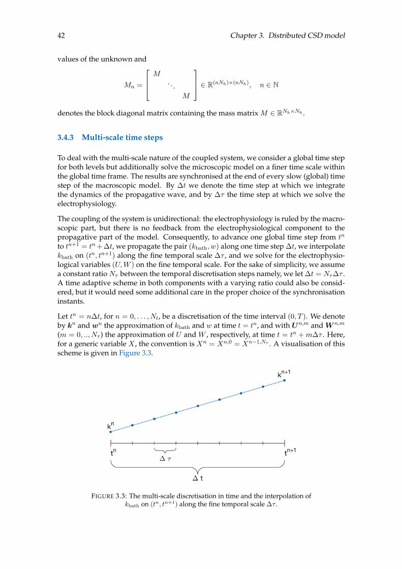
42 Chapter 3. Distributed CSD model
values of the unknown and
Mn =
M. . .
M
∈ R(nNh)×(nNh), n ∈ N
denotes the block diagonal matrix containing the mass matrix M ∈ RNh×Nh .
3.4.3 Multi-scale time steps
To deal with the multi-scale nature of the coupled system, we consider a global time stepfor both levels but additionally solve the microscopic model on a finer time scale withinthe global time frame. The results are synchronised at the end of every slow (global) timestep of the macroscopic model. By ∆t we denote the time step at which we integratethe dynamics of the propagative wave, and by ∆τ the time step at which we solve theelectrophysiology.
The coupling of the system is unidirectional: the electrophysiology is ruled by the macro-scopic part, but there is no feedback from the electrophysiological component to thepropagative part of the model. Consequently, to advance one global time step from tn
to tn+1 = tn+ ∆t, we propagate the pair (kbath, w) along one time step ∆t, we interpolatekbath on (tn, tn+1) along the fine temporal scale ∆τ , and we solve for the electrophysio-logical variables (U,W ) on the fine temporal scale. For the sake of simplicity, we assumea constant ratio Nτ between the temporal discretisation steps namely, we let ∆t = Nτ∆τ .A time adaptive scheme in both components with a varying ratio could also be consid-ered, but it would need some additional care in the proper choice of the synchronisationinstants.
Let tn = n∆t, for n = 0, . . . , Nt, be a discretisation of the time interval (0, T ). We denoteby kn andwn the approximation of kbath and w at time t = tn, and with Un,m andW n,m
(m = 0, .., Nτ ) the approximation of U and W , respectively, at time t = tn + m∆τ . Here,for a generic variable X , the convention is Xn = Xn,0 = Xn−1,Nτ . A visualisation of thisscheme is given in Figure 3.3.
FIGURE 3.3: The multi-scale discretisation in time and the interpolation ofkbath on (tn, tn+1) along the fine temporal scale ∆τ .

3.4. Numerical approximation 43
A fully discrete approximation of the problem is then obtained by integrating system(3.9) - (3.10) in time. Let us first focus on the propagative part of the coupled model. Wecan integrate this part between tn and tn+1 by means of a mixed implicit/explicit (IMEX)scheme: the linear diffusion term is discretised implicitly, while the nonlinear reactionterm F (k,w) is treated explicitly. Because of the particular form of the problem, the ODEfor the recovery variable w can be linearised around k at the previous time step, andintegrated exactly on the interval (tn, tn+1), in any spatial node independently:
w(t) =
w0 +
t∫t0
η3(k(t)− k0) exp
t∫t0
η3η4dξ
dθ
exp
− t∫t0
η3η4dθ
=
k − k0
η4+
(w0 − k − k
0
η4
)exp (−η3η4(t− t0)) .
This allows us to decouple the PDE-ODE system by solving it with respect to the re-covery variable wn+1. We approximate the first-order derivative by the backward finitedifference scheme
dkn+1
dt≈ kn+1 − kn
∆t.
Substituting this into the respective equation in (3.9) and plugging in the updated re-covery variable wn+1 into the nonlinear reaction term F (kn,wn+1), we are left with theproblem
(M + ∆tS)kn+1 = Mkn −∆tF (knh,wn+1). (3.11)
The full discretisation of the macroscopic model (3.4) for every time step tn to tn+1 isgiven in Algorithm 3.1.
Algorithm 3.1 Numerical approximation scheme for the macroscopic model
1: initialise: k0 ∈ RNh ,w0 ∈ RNh
2: for n = 0, . . . , Nt − 1 do
3: update: wn+1 =kn − k0
η4+
(wn − k
n − k0
η4
)exp (−η3η4∆t)
4: update: Fn+1 = F (kn,wn+1)
5: solve: (M + ∆tS)kn+1 = Mkn −∆tMFn+1
6: end for
After solving system (3.9) for the time step ∆t, we linearly interpolate the solution be-tween kn and kn+1 to obtain the values kn,m for m = 1, . . . , Nτ as input for the elec-trophysiological model. Let kn and kn+1 be the solution for the kbath concentration attime step tn and tn+1 and let tn,m = tn + m∆τ be the time steps at which we seek theinterpolation kn,m. In general, for every time t ∈ [tn, tn+1] a linear interpolant y satisfies
y − kn
t− tn=kn+1 − kn
tn+1 − tn,
which is equivalent to
y = kn +kn+1 − kn
∆t(t− tn).

44 Chapter 3. Distributed CSD model
For the interpolation at t = tn,m this expression can be rewritten as
kn,m =
(1− m∆τ
∆t
)kn +
m∆τ
∆tkn+1.
Approximating the time derivative of the variable U by a backward finite differencescheme, we obtain
dUn,m+1
dτ≈ U
n,m+1 −Un,m
∆τ,
and substituting this into the respective equation in (3.10), we are left with:
1
σ
Un,m+1 −Un,m
∆τ= ΦU (Un,m,W n,m,kn,m+1).
The full discretisation of the coupled model is given in Algorithm 3.2. The differential-algebraic system for the electrophysiology variables features stiff components and thushas to be integrated with a suitable ODE solver. For the sake of simplicity, the time in-tegrator for the ODE system of electrophysiology in Algorithm 3.2 is a Forward Eulermethod for Un,m+1 coupled with a linearisation around the previous state of the alge-braic unknowns W n,m, but other options (such as Backward Euler, Crank-Nicholson,Runge-Kutta, or Multistep) could be applied to this problem to improve the computa-tional efficiency and accuracy.
Algorithm 3.2 Numerical approximation scheme for the multi-scale coupled model
1: initialise: k0 ∈ RNh , w0 ∈ RNh , U0,0 ∈ RNh×12, W 0,0 ∈ RNh×7
2: for n = 0, . . . , Nt − 1 do
3: update: wn+1 =kn − k0
η4+
(wn − k
n − k0
η4
)exp (−η3η4∆t)
4: update: Fn+1 = F (kn,wn+1)
5: solve: (M + ∆t S) kn+1 = Mkn −∆tMFn+1
6: interpolate between kn and kn+1 on (tn, tn+1) at Nτ + 1 equally spaced nodes:
7: kn,m+1 =
(1− m∆τ
∆t
)kn +
m∆τ
∆tkn+1 for m = 0, ..Nτ
8: for m = 0, . . . , Nτ − 1 do
9: update: Un,m+1 = Un,m + ∆τσΦU (Un,m,W n,m,kn,m+1)
10: update: W n,m+1 = ΦW (Un,m+1)
11: end for
12: end for
3.5 Simulation
In this section, we present the numerical simulation of a CSD wave propagation in oneand two dimensional domains. With the final aim to simulate the CSD propagation, thepotassium propagation and the detailed electrophysiological characteristics, on the braincortex, we illustrate the model features in different domains increasing the dimensionstep by step.

3.5. Simulation 45
The numerical simulations of the multi-scale coupled model are performed with a self-developed code in Matlab (MathWorks Inc., Natick, MA), where we choose a constanttime step ∆t = 50 msec for the propagation and a constant time step ∆τ = 0.05 msecfor the electrophysiology, resulting in Nτ = 1000 electrophysiology steps within a prop-agative time step. The IMEX scheme described in Section 3.4.3 requires to solve a linearsystem associated with a linear parabolic system, for which a wide range of literature onpreconditioning is available (Saad, 2003).
Keeping in mind the final aim of applying this model to a brain geometry, we observethat a detailed discretisation of the cerebral cortex leads to a high number of grid pointsand thus a high dimensionality of the associated finite element matrix in the system(3.11). The matrix of this system is badly conditioned but symmetric. As of now, wesolve system (3.11) with a conjugate gradient (CG) method, preconditioned by incom-plete Cholesky factorisation, with pivoting and with drop tolerance set at 10−6. Thestopping criterion for the CG is set at a relative error of 10−6, and a maximum numberof iteration is set at 60. Combining the low drop tolerance in the incomplete Choleskyfactorisation and the propagative nature of the solution of system (3.4) entails that, bychoosing as initial guess at time tn+1 the solution at the previous time step kn, the pre-conditioned CG converges in very few iterations. The electrophysiology model is solvedby an explicit Euler scheme. A detailed description of the numerical optimisation of solv-ing system (3.11) on a brain geometry is discussed in the previous chapter.
3.5.1 Measurable variables
The dynamics of the microscopic and macroscopic part of the model takes place at dif-ferent timescales: the neuronal activity takes place at a millisecond timescale, whereasthe whole CSD propagation event occurs at the larger timescale of minutes. In order tobe able to grasp the overall dynamics on both timescales without resorting to the finetimescale of the electrophysiology, we introduce two auxiliary variables that describe thetypical characteristics of the electrophysiology but at the timescale of seconds.
The first quantity is the maximum membrane potential in a given point x ∈ Ω, defined, ateach second t, as
Vmax(x, t) = maxs∈[t−1,t]
V (x, s), (3.12)
which is also commonly measured by experimentalists (see e.g., Pietrobon, 2005; Sawat-Pokam et al., 2016).
Another common way to characterise the neuronal activity is through its spiking frequency(in Hz), which is naturally defined at the second timescale. We denote by φ(x, t) thespiking frequency in a given point x ∈ Ω, during the time interval [t−1, t]. The procedureto obtain the spiking frequency, that is, the number of spikes in a given interval, is notstraightforward and needs to be handled with care. Let V n,m be the membrane potentialV (x, t) in a generic point x ∈ Ω at the discrete time steps tn,m ∈ [tn, tn+1], with tn,m =tn +m∆τ for m = 1, . . . , Nτ . Then [tn, tn+1] is a time interval of the length ∆t like in theprevious section. We set ϑ as a threshold value above which we consider a rise in themembrane potential as a spike. The set of indices indicating a membrane potential abovethe threshold is then defined as
j := m ∈ 1, . . . , Nτ |V n,m > ϑ = m1, . . . ,mk.

46 Chapter 3. Distributed CSD model
We then shift this index set by inserting a zero and deleting the last entry of j
jshift = 0,m1, . . . ,mk−1
and take the difference between those two sets per entry, namely
jdiff = j − jshift = m1 − 0,m2 −m1, . . . ,mk −mk−1.
We then define the seta = l ∈ 1, . . . , k | jdiff(l) > 1,
where jdiff(l) refers to the l-th entry of the set jdiff. With these positions, the frequency isfinally defined as
φ(t) =|a|∆t
,
where |a| denotes the cardinality of the set a. Note that if the first point (m = 1) is al-ready above the threshold the procedure does not consider this as a spike. However, thisdoes not have a significant impact on the results, as we are interested in distinguishinghigh from low frequency spiking. In this case, one spike more or less does not signifi-cantly change the results. We illustrate this procedure with the help of a short example,visualised in Figure 3.4. For this example, the set j of the indices above the threshold ϑ is
j := m ∈ 1, . . . , 16 |V n,m > ϑ = 5, 6, 9, 12, 13,
then jshift, jdiff and a follow to be
jshift = 0, 5, 6, 9, 12, jdiff = 5, 1, 3, 3, 1, and a = 1, 3, 4.
As the cardinality of a is three, this number gives us the amount of spikes in the consid-ered time interval and thus a spiking frequency φ(t) = 3/∆t at time t.
FIGURE 3.4: An illustration of the computation of the spiking frequencyfrom the membrane potential.
In Figure 3.5 we plot the membrane potential V , computed at the millisecond scale,the comprehensive visualisation of the maximum membrane potential Vmax and the fre-quency φ, both computed at the seconds timescale. The maximum membrane potentialand the frequency simplify the membrane potential and characterise it in a comprehen-sive manner on the seconds scale without loss of information.
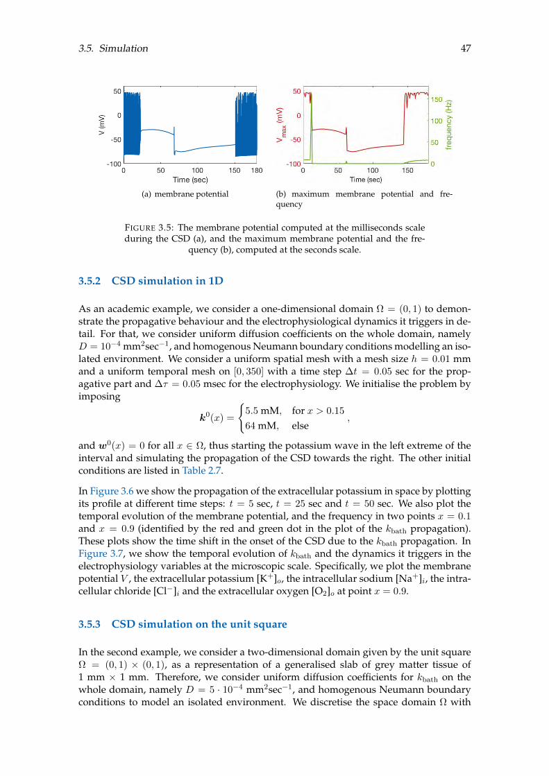
3.5. Simulation 47
(a) membrane potential (b) maximum membrane potential and fre-quency
FIGURE 3.5: The membrane potential computed at the milliseconds scaleduring the CSD (a), and the maximum membrane potential and the fre-
quency (b), computed at the seconds scale.
3.5.2 CSD simulation in 1D
As an academic example, we consider a one-dimensional domain Ω = (0, 1) to demon-strate the propagative behaviour and the electrophysiological dynamics it triggers in de-tail. For that, we consider uniform diffusion coefficients on the whole domain, namelyD = 10−4 mm2sec−1, and homogenous Neumann boundary conditions modelling an iso-lated environment. We consider a uniform spatial mesh with a mesh size h = 0.01 mmand a uniform temporal mesh on [0, 350] with a time step ∆t = 0.05 sec for the prop-agative part and ∆τ = 0.05 msec for the electrophysiology. We initialise the problem byimposing
k0(x) =
5.5 mM, for x > 0.15
64 mM, else,
and w0(x) = 0 for all x ∈ Ω, thus starting the potassium wave in the left extreme of theinterval and simulating the propagation of the CSD towards the right. The other initialconditions are listed in Table 2.7.
In Figure 3.6 we show the propagation of the extracellular potassium in space by plottingits profile at different time steps: t = 5 sec, t = 25 sec and t = 50 sec. We also plot thetemporal evolution of the membrane potential, and the frequency in two points x = 0.1and x = 0.9 (identified by the red and green dot in the plot of the kbath propagation).These plots show the time shift in the onset of the CSD due to the kbath propagation. InFigure 3.7, we show the temporal evolution of kbath and the dynamics it triggers in theelectrophysiology variables at the microscopic scale. Specifically, we plot the membranepotential V , the extracellular potassium [K+]o, the intracellular sodium [Na+]i, the intra-cellular chloride [Cl−]i and the extracellular oxygen [O2]o at point x = 0.9.
3.5.3 CSD simulation on the unit square
In the second example, we consider a two-dimensional domain given by the unit squareΩ = (0, 1) × (0, 1), as a representation of a generalised slab of grey matter tissue of1 mm × 1 mm. Therefore, we consider uniform diffusion coefficients for kbath on thewhole domain, namely D = 5 · 10−4 mm2sec−1, and homogenous Neumann boundaryconditions to model an isolated environment. We discretise the space domain Ω with

48 Chapter 3. Distributed CSD model
FIGURE 3.6: The extracellular potassium bath kbath dynamics in space attimes t = 5 sec, t = 25 sec and t = 50 sec and the membrane potential V ,
and the frequency φ at point x = 0.1 and x = 0.9.
an unstructured mesh with characteristic size h = 0.01 mm, and we choose uniformtime steps for both the macroscopic part, ∆t = 0.05 sec, and for the microscopic one,∆τ = 0.05 msec. We simulate a CSD wave starting the propagation from the centre of theslab, x ∈ Br(0) where Br(0) is the circle around the point (0, 0) with radius r. In Br(0)we initially impose kbath = 64 mM (in the rest of the domain kbath = 5.5 mM) and runthe simulation for 280 seconds. The initial conditions for the other variables are given inTable 2.7.
In Figure 3.8 we visualise the maximum membrane potential Vmax and the frequency φat four different time steps, t = 5, t = 50, t = 135 and t = 280 sec. In Figure 3.9 weplot the kbath distribution at t = 5 sec over the whole domain, and give the whole tem-poral dynamics on the microscopic scale in the points (0.5, 0.5) and (0.05, 0.05). Theseinclude the kbath, maximum membrane potential Vmax, the frequency φ, the membranepotential V , the extracellular potassium [K+]o, the intracellular sodium [Na+]i, the intra-cellular chloride [Cl−]i, the extracellular oxygen [O2]o and the ratio between the intra-and extracellular volume β.
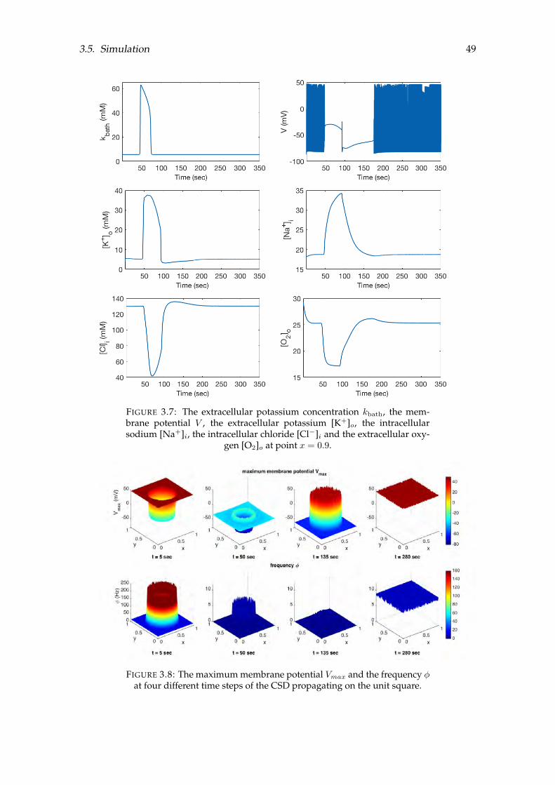
3.5. Simulation 49
FIGURE 3.7: The extracellular potassium concentration kbath, the mem-brane potential V , the extracellular potassium [K+]o, the intracellularsodium [Na+]i, the intracellular chloride [Cl−]i and the extracellular oxy-
gen [O2]o at point x = 0.9.
FIGURE 3.8: The maximum membrane potential Vmax and the frequency φat four different time steps of the CSD propagating on the unit square.
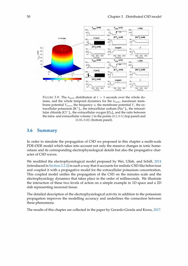
50 Chapter 3. Distributed CSD model
FIGURE 3.9: The kbath distribution at t = 5 seconds over the whole do-main, and the whole temporal dynamics for the kbath, maximum mem-brane potential Vmax, the frequency φ, the membrane potential V , the ex-tracellular potassium [K+]o, the intracellular sodium [Na+]i, the intracel-lular chloride [Cl−]i, the extracellular oxygen [O2]o and the ratio betweenthe intra- and extracellular volume β in the points (0.5, 0.5) (top panel) and
(0.05, 0.05) (bottom panel).
3.6 Summary
In order to simulate the propagation of CSD we proposed in this chapter a multi-scalePDE-ODE model which takes into account not only the massive changes in ionic home-ostasis and its corresponding electrophysiological details but also the propagative char-acter of CSD waves.
We modified the electrophysiological model proposed by Wei, Ullah, and Schiff, 2014(introduced in Section 2.2.2) in such a way that it accounts for realistic CSD-like behaviourand coupled it with a propagative model for the extracellular potassium concentration.This coupled model unifies the propagation of the CSD on the minutes scale and theelectrophysiology dynamics that takes place in the order of milliseconds. We illustratethe interaction of these two levels of action on a simple example in 1D space and a 2Dslab representing neuronal tissue.
The detailed description of the electrophysiological activity in addition to the potassiumpropagation improves the modelling accuracy and underlines the connection betweenthese phenomena.
The results of this chapter are collected in the paper by Gerardo-Giorda and Kroos, 2017.
51
Chapter 4
Model personalisation
“It is more important to know what sort of person has a disease,than to know what sort of disease a person has.”
Author unknown
Precision medicine (or personalised medicine) is the concept of customising healthcarewith medical decisions, treatments, practices or products tailored to the individual pa-tient. While patient-specific therapies go back to the time of Hippocrates, it is still apending topic in modern science and medicine as big data and fast genomic sequencingallow a deeper insight in the molecular basis of diseases (Engnew, 2009). Mathematicalmodels applied to medicine can help to understand diseases, develop drugs and hospitaltechnology. Especially including patient-specific information in a model can improve itsreliability and meaningfulness.
In the case of migraine with aura and the simulation of the underlying CSD, there aretwo levels at which individual patient data can be integrated into the model introducedin Chapter 3: the first step is to use a brain geometry obtained from an MRI scan; thesecond one is to incorporate patient-specific diffusion data collected either from diffusiontensor imaging (DTI) or diffusion-weighted imaging (DWI).
As the sulci and gyri of the human cortex provide a unique structure that is comparableto the friction ridges of the human fingerprint, their patterns are unique to every humanbeing. Thus, including the individual geometry of the cerebral cortex is a first step to per-sonalise the computational domain. Though measurements of diffusion anisotropy weretraditionally used as a white matter imaging technique, there is growing evidence thatDTI data can be useful to describe the grey matter microstructure (McNab et al., 2013).Consequently, the combination of the patient-specific geometry and the diffusion datarepresenting the microstructure of the cerebral cortex provide highly individual informa-tion on the patient’s brain for the model.
In the following sections we introduce the basics of MRI, DTI and DWI imaging, give adescription of the data at hand and a detailed explanation of how we incorporate themin the CSD model. Finally, we conclude the chapter by comparing the isotropic to theanisotropic case, stressing the improvement we make by adding patient-specific diffusiondata.

52 Chapter 4. Model personalisation
4.1 MRI-T1 data
The brain cortex is a thin layer of grey matter, characterised by a very large aspect ratiobetween its surface and its volume. At the spatial scale we are considering, such layercan be approximated by a two-dimensional surface obtained from MRI measurements.
The cortical geometry we use in this study is a closed surface Ω ⊂ R3 that has beenreconstructed from an MRI scan with FreeSurfer1 image analysis suite, see Fischl, 2012and references therein for further details. This data set was acquired and published inDiez et al., 2015 and used in Kroos et al., 2016, and its acquisition was approved bythe Ethics Committee at the Cruces University Hospital. The data set corresponds toone healthy subject, male, age 28, and was acquired with a Philips Achieva 1.5 T Novascanner. The cortical geometry was obtained from a high-resolution anatomical MRI, ac-quired using a T1-weighted 3D sequence with the following parameters: TR = 7.482 msec,TE = 3.425 msec; parallel imaging (SENSE) acceleration factor = 1.5; acquisition matrixsize = 256 x 256; FOV = 26 cm; slice thickness = 1.1 mm; and 170 contiguous sections.
The resulting computational mesh is a triangulation of the reconstructed cortex, consist-ing of 140,208 nodes and 280,412 triangles for the left hemisphere, and 139,953 nodes and279,902 triangles for the right hemisphere. We visualise the mesh triangulation of the lefthemisphere in Figure 4.1. This geometry already appeared previously in Section 1.2 inthe visualisation of the Desikan-Killiany atlas and the lobes (Figure 1.3 and Figure 1.4).
FIGURE 4.1: The triangular mesh of the reconstructed cortex in the lateraland medial view of the left hemisphere.
A priori the corpus callosum, an area made of white matter linking the two hemispheres,could be excluded from the computational domain, but in this case, boundary conditionsshould be imposed at the interface between corpus callosum and grey matter. Thus, at afirst stage, we keep the corpus callosum as part of the brain geometry. In Section 5.1 weimprove the mesh triangulation, remove noise by applying a smoothing technique andin this step also remove the corpus callosum from the computational domain.
1http://surfer.nmr.mgh.harvard.edu/

4.1. MRI-T1 data 53
4.1.1 CSD propagation on a cortical geometry
We apply the model introduced in the previous chapter to the real brain geometry ob-tained from MRI imaging and can observe the propagation of the depolarisation wavetriggering the microscopic dynamics. We consider an isotropic diffusion tensor, D = δIwith δ = 0.7174 mm2sec−1 and no boundary conditions, as the cortical geometry at handis a closed surface Ω ⊂ R3. We initialise the problem by imposing kbath = 64 mM in thelateral occipital region in the occipital lobe, to which the visual cortex belongs.
To show the behaviour of the model on the real brain geometry, we simulate the CSDon the left hemisphere. In Figure 4.2 we plot the kbath profile on the cerebral cortex attime t = 5 min in the lateral and medial view, as well as the detailed temporal dynam-ics for two different points on the cortex, one on the lateral and one on the medial side,highlighted by green circles. This example shows the propagation of the extracellularpotassium across the cortex triggering the characteristic CSD dynamics of the electro-physiology.
FIGURE 4.2: The kbath profile on the cerebral cortex at time t = 5 min in thelateral and medial view of the left hemisphere, and the detailed temporal
dynamics for two different points on the cortex.
The computation to simulate CSD propagation is complex and highly expensive. In par-ticular, the memory necessary to store the information at the small time step ∆τ , to eval-uate the functions involved at the bigger time steps ∆t and to compute the measurablevariables Vmax and φ at the seconds scale, quickly increases with the number of datapoints in the spatial dimension. Saving the values for all 12 variables, describing theelectrophysiology for 1000 small time steps to synchronise with the big time step (or even20000 small time steps to synchronise the measurable variables at the seconds scale) andevaluate them at the 140,208 discrete nodes of the brain geometry results in an array ofthe size 12×1000×140, 208. Taking into account that each number with double precisionrequires 8 bytes of memory, this array would easily need several GB of memory just tobe synchronised with one big time step. As this information is not the only one that hasto be stored in the course of the simulation, running out of memory becomes an issue assoon as we start considering real brain geometries with a high number of discrete datapoints.

54 Chapter 4. Model personalisation
To avoid this problem, we will only consider the propagation of the extracellular potas-sium in the following, keeping in mind that the potassium wave triggers the electrophys-iological characteristics of the CSD.
4.2 Diffusion tensor and diffusion-weighted imaging data
In neurology, brain pathologies can be detected by using DTI that provides a measure-ment for diffusion and anisotropy, the quality of exhibiting physical properties alongdifferent directional axis. DTI is mainly used to study the architecture of white matter inhuman brains in vivo. In white matter, diffusion tends to be more anisotropic than in greymatter, while in the cerebrospinal fluid the diffusion is equal in all directions (isotropic).
DTI imaging uses MRI techniques to measure the diffusion of water molecules in differ-ent directions in every voxel of an image. Its acquisition requires DWI measurementsin at least seven non-collinear directions which are necessary to describe the rate andpreferred direction of diffusion in each voxel (Huisman, 2010; Kingsely, 2006). Diffusion-weighted images are raw images where the signal has been sensitised to diffusion byusing a strong magnetic field (Le Bihan, 2013).
The underlying concept of DTI is that the random movement of water molecules is influ-enced by its surrounding tissue. Water molecules interact and collide with tissue compo-nents like cell membranes, fibres or macromolecules. In free water at 37 C, the diffusioncoefficient of water molecules is 3 ·10−9 m2sec−1 which can be interpreted as a movementof 17µm in 50 msec (Le Bihan, 2003). In a specific type of tissue, the movement of watergives an insight into the structure and geometric organisation of the tissue itself. To mea-sure the displacement of these molecules, a pair of magnetic field gradient pulses is usedto make the MR signal sensitive to diffusion. Along this gradient, the change of locationof the water nuclei is measured (Le Bihan, 2003). This change of position is proportionalto the displacement of water molecules in a given space. The conductivity tensor for thetissue can be approximated from the water diffusion tensor obtained through DTI (Tuchet al., 1999, 2001).
In addition, DTI measurements can be used to describe the directional flow of infor-mation between non-contiguous regions of the brain. The process of extracting this di-rectional information to obtain neural tracts throughout the brain is called tractography.Including the tractography to connect the two hemispheres and fast connections betweendistant regions could be further added to the modelling, but we leave this as a possiblefuture extension of the proposed work.
DTI data is given in the form of three eigenvalues and three normalised orthogonal eigen-vectors at each grid point and has to be processed in order to contribute to the model. Asthe cortex is a surface in 3D, we need to derive a 2D diffusion tensor from the 3D DTI dif-fusion data. In the following, we introduce a method to obtain these 2D diffusion tensors.
4.2.1 Description of the DTI data
The DTI data was acquired and published in Diez et al., 2015 and used in Kroos et al.,2017. Its acquisition was approved by the Ethics Committee at the Cruces UniversityHospital and all the methods employed were in accordance with approved guidelines.

4.2. Diffusion tensor and diffusion-weighted imaging data 55
The DTI data was processed with the FSL software2. First, an eddy current correction wasapplied to overcome the artefacts produced by head movement and to correct the changesproduced by the variations in gradient field directions during the acquisition. Then, thegradient directions were corrected using the head movement matrices obtained from theprevious step. Next, a local fitting of the diffusion tensor was then applied to computethe tensor model at each voxel. For each voxel, the tensor model provided the threeeigenvectors and the associated eigenvalues of the diffusion of water molecules withinbrain tissues. Then, to project the tensor data onto the points of the mesh triangulation,we first computed a nonlinear transformation between the T1 image and the fractionalanisotropy map. This transformation took as input a previous linear transformation us-ing 12 degrees of freedom and chose the mutual information as the cost function. Then,FreeSurfer was used to project the diffusion data onto the brain mesh. A more detaileddescription of the whole process can be found in Appendix C.
The data from the DTI is given in the form of three eigenvalues λ1, λ2, λ3 and three nor-malised and orthogonal eigenvectorsw1,w2,w3 at each grid point. The eigenvectors aresorted according to the size of the eigenvalue. Thus, w1 describes the principal directionof the movement. These eigenvalues and eigenvectors describe the principal directionand strength of the displacement of water molecules in the underlying tissue. The diffu-sion tensor in 3D space can be described as
D = λ1w1wT1 + λ2w2w
T2 + λ3w3w
T3 (4.1)
or equivalently as a 3× 3 matrix
D =
DxxDxyDxz
DyxDyyDyz
DzxDzyDzz
. (4.2)
The diffusion tensor D can be visualised as an ellipsoid that describes the average dis-placement and direction of the molecules in a particular spot. The eigenvectors determinethe principal directions of the ellipsoid’s axis and the eigenvalues their length. An exam-ple of diffusion tensors representing the conductivity of the brain cortex and visualisedas ellipsoids is given in Figure 4.3. Here, we plot the DTI data on the nodes of the lefthemisphere mesh. We provide a global view of the anisotropy by a lateral and medial vi-sualisation of the cortex, where the colour of the ellipsoids refers to the size of the largesteigenvalue. In addition, we plot different levels of zoom to make the anisotropy of thediffusion provided by the DTI data visible on the local scale. Both the orientation andsize of the ellipsoids exhibit huge variations across the cortex. In homogenous media, asthe diffusion is isotropic, the corresponding tensor is a multiple of the unit matrix, andthe corresponding ellipsoid is a sphere.
The data acquisition techniques for DTI and the low signal-to-noise ratio of this mea-surement can produce negative or vanishing eigenvalues (Soares et al., 2013). Anothersource for artefacts and missing data in the DTI datasets can originate from the gradientsystem hardware, the pulse sequence, and motion. The main problem is that DTI mea-surements are usually recorded with the aim to analyse diffusion in white matter. Thus,data acquisition is terminated as soon as it reaches border regions of the white matter. Asa consequence, some values in these border regions are missing and set to zero. The meshpoints of the geometry under consideration, featuring vanishing or negative eigenvalues
2http://fsl.fmrib.ox.ac.uk/

56 Chapter 4. Model personalisation
(a) lateral view (b) medial view
(c) different levels of zoom of the lateral surface
FIGURE 4.3: A visualisation of DTI data with ellipsoids coloured accordingto the size of the maximum eigenvalue on the left hemisphere in the lateral(a) and medial (b) view of the whole left cortex and two levels of zoom of
the lateral surface (c).
or eigenvectors are visualised in Figure 4.4. Here, the termination of data acquisition isone of the main reasons for missing data, as the majority is located at the border regionsat the very top and front of the brain geometry. Proper treatment of these artefacts isaddressed in the next sections.
FIGURE 4.4: A visualisation of the missing or noisy DTI data in red on thecerebral cortex in the superior and anterior view.

4.2. Diffusion tensor and diffusion-weighted imaging data 57
4.2.2 Quantifying the diffusion data
The degree of anisotropy in the diffusion ellipsoid gives information about the diffusiondata and provides information on the underlying tissue structure in each measuring unit(Le Bihan et al., 2001). There are three different ways to extract information from DWIdata: the mean diffusivity describes the mean-squared displacement of molecules in aspecific region or voxel, the main direction of diffusivity focuses on the orientation ofthe underlying structures, and the degree of anisotropy is a measure of how much thediffusion in the point deviates from the isotropic case.
The mean diffusivity (MD), giving a general evaluation of the diffusion, is defined as thetrace of the diffusion tensor D in (4.2) divided by three or equivalently the mean of itsdiagonal entries:
MD =Tr(D)
3=Dxx +Dyy +Dzz
3.
This quantity, as well as its mean values across the cortex, can give important informationabout the overall diffusion behaviour and speed. In a generic point in space, the MD canalso be represented as the mean of the eigenvalues of the diffusion tensor D, namely
MD =1
3
3∑i=1
λi = λ. (4.3)
In Figure 4.5 we plot the MD normalised with respect to its mean on the cortex of thebrain geometry for both hemispheres, and give the normalised histogram that describesthe probability density of the MD values. The normalisation highlights areas in whichthe MD is higher or lower than the average. In this figure, we visualise the values oneach triangle to make it comparable to the 2D case. For this, we average the MD valuesover all the vertices of the respective triangle.
For the degree of anisotropy a variety of measures have been proposed (Kingsley, 2006;Le Bihan et al., 2001). We will focus on the most common ones: the volume ratio (VR),the relative anisotropy (RA) and the fractional anisotropy (FA).
The volume ratio describes the ratio between the ellipsoid volume and a sphere volumewith radius λ (or equivalently, with radius MD), see (4.3). It is defined as
VR =λ1λ2λ3
λ3,
and ranges from 0 to 1, where 1 is the fully isotropic situation.
The relative anisotropy represents (like FA) the ratio of the anisotropic part of the diffu-sion tensor D to its isotropic part. It is a normalised standard deviation defined as
RA =
√(λ1 − λ
)2+(λ2 − λ
)2+(λ3 − λ
)23λ3
and varies between 0 and√
2, where 0 represents a fully isotropic condition.

58 Chapter 4. Model personalisation
(a) left hemisphere
(b) right hemisphere
FIGURE 4.5: The normalised mean diffusivity of the three-dimensional DTIdata of the cortex of the left (a) and right (b) hemisphere and a normalised
histogram displaying the probability density of the MD values.
Finally, the fractional anisotropy expresses the normalised variance of the eigenvalues,defined as
FA =
√3[(λ1 − λ)2 + (λ2 − λ)2 + (λ3 − λ)2]
2(λ21 + λ2
2 + λ23)
. (4.4)
The fractional anisotropy is positive and smaller than 1, where 0 represents a fully isotro-pic condition and is the most commonly used measurement for the degree of anisotropydue to its convenient domain of definition. In Figure 4.6 we plot the FA of the left andright hemisphere as well as a normalised histogram displaying the relative frequency ofthe FA values. Again, we plot on each triangle the average FA value over its three verticesto make it comparable to the 2D case later on. In the original 3D data set, the diffusion ismarginally anisotropic, with some areas of high anisotropy, like in the corpus callosum.
In Figure 4.7 we plot the joint distribution of 3D FA and the MD normalised by the meanover all triangles, for both left and right hemisphere. Again we consider the values inthe centroids of the triangles by averaging the values over the vertices of each triangle.The colours represent density, and the difference to an isotropic situation, where meandiffusivity and fractional anisotropy are 1 and 0, respectively, is evident. Thus, this figurestrongly supports the contribution of DTI-based diffusion coefficients.
In some cases, there are not enough DWI images to generate the diffusion tensor. Whenthis occurs, the apparent diffusion coefficient (ADC) can be computed by averaging overimages recorded with different diffusion weighting, giving the average diffusion of water

4.2. Diffusion tensor and diffusion-weighted imaging data 59
(a) left hemisphere
(b) right hemisphere
FIGURE 4.6: The fractional anisotropy of the three dimensional DTI dataof the cortex of the left (a) and right (b) hemisphere and a normalised his-
togram displaying the probability density of the FA values.
(a) left hemisphere (b) left hemisphere
FIGURE 4.7: The joint distribution of the fractional anisotropy and the nor-malised mean diffusivity of the 3D tensor for each triangle of the mesh,both for the left (a) and right (b) hemisphere. Colours represent the den-
sity.
molecules in each voxel. However, the ADC only provides information about the diffu-sion in a voxel, whereas the anisotropy maps go one step further and give informationabout the orientation of the underlying structure.
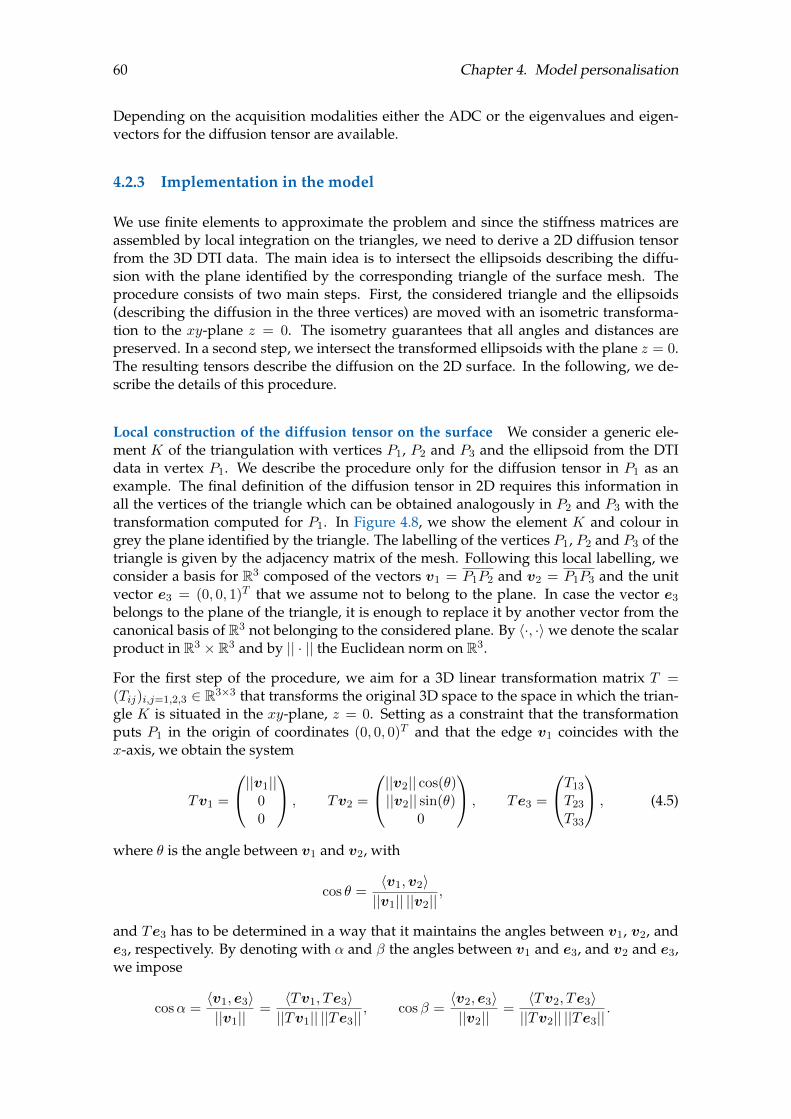
60 Chapter 4. Model personalisation
Depending on the acquisition modalities either the ADC or the eigenvalues and eigen-vectors for the diffusion tensor are available.
4.2.3 Implementation in the model
We use finite elements to approximate the problem and since the stiffness matrices areassembled by local integration on the triangles, we need to derive a 2D diffusion tensorfrom the 3D DTI data. The main idea is to intersect the ellipsoids describing the diffu-sion with the plane identified by the corresponding triangle of the surface mesh. Theprocedure consists of two main steps. First, the considered triangle and the ellipsoids(describing the diffusion in the three vertices) are moved with an isometric transforma-tion to the xy-plane z = 0. The isometry guarantees that all angles and distances arepreserved. In a second step, we intersect the transformed ellipsoids with the plane z = 0.The resulting tensors describe the diffusion on the 2D surface. In the following, we de-scribe the details of this procedure.
Local construction of the diffusion tensor on the surface We consider a generic ele-ment K of the triangulation with vertices P1, P2 and P3 and the ellipsoid from the DTIdata in vertex P1. We describe the procedure only for the diffusion tensor in P1 as anexample. The final definition of the diffusion tensor in 2D requires this information inall the vertices of the triangle which can be obtained analogously in P2 and P3 with thetransformation computed for P1. In Figure 4.8, we show the element K and colour ingrey the plane identified by the triangle. The labelling of the vertices P1, P2 and P3 of thetriangle is given by the adjacency matrix of the mesh. Following this local labelling, weconsider a basis for R3 composed of the vectors v1 = P1P2 and v2 = P1P3 and the unitvector e3 = (0, 0, 1)T that we assume not to belong to the plane. In case the vector e3
belongs to the plane of the triangle, it is enough to replace it by another vector from thecanonical basis of R3 not belonging to the considered plane. By 〈·, ·〉we denote the scalarproduct in R3 × R3 and by || · || the Euclidean norm on R3.
For the first step of the procedure, we aim for a 3D linear transformation matrix T =(Tij)i,j=1,2,3 ∈ R3×3 that transforms the original 3D space to the space in which the trian-gle K is situated in the xy-plane, z = 0. Setting as a constraint that the transformationputs P1 in the origin of coordinates (0, 0, 0)T and that the edge v1 coincides with thex-axis, we obtain the system
Tv1 =
||v1||00
, Tv2 =
||v2|| cos(θ)||v2|| sin(θ)
0
, Te3 =
T13
T23
T33
, (4.5)
where θ is the angle between v1 and v2, with
cos θ =〈v1,v2〉||v1|| ||v2||
,
and Te3 has to be determined in a way that it maintains the angles between v1, v2, ande3, respectively. By denoting with α and β the angles between v1 and e3, and v2 and e3,we impose
cosα =〈v1, e3〉||v1||
=〈Tv1, Te3〉||Tv1|| ||Te3||
, cosβ =〈v2, e3〉||v2||
=〈Tv2, Te3〉||Tv2|| ||Te3||
.
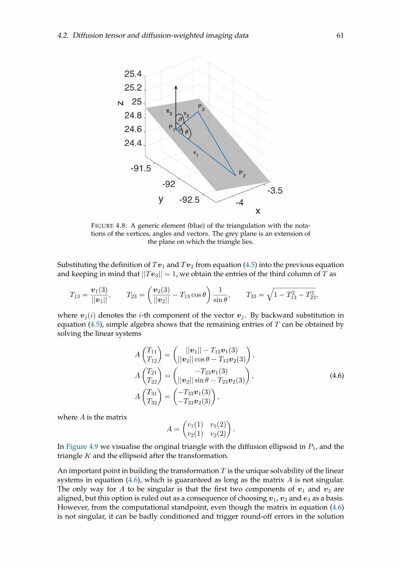
4.2. Diffusion tensor and diffusion-weighted imaging data 61
FIGURE 4.8: A generic element (blue) of the triangulation with the nota-tions of the vertices, angles and vectors. The grey plane is an extension of
the plane on which the triangle lies.
Substituting the definition of Tv1 and Tv2 from equation (4.5) into the previous equationand keeping in mind that ||Te3|| = 1, we obtain the entries of the third column of T as
T13 =v1(3)
||v1||, T23 =
(v2(3)
||v2||− T13 cos θ
)1
sin θ, T33 =
√1− T 2
13 − T 223,
where vj(i) denotes the i-th component of the vector vj . By backward substitution inequation (4.5), simple algebra shows that the remaining entries of T can be obtained bysolving the linear systems
A
(T11
T12
)=
(||v1|| − T13v1(3)
||v2|| cos θ − T13v2(3)
),
A
(T21
T22
)=
(−T23v1(3)
||v2|| sin θ − T23v2(3)
),
A
(T31
T32
)=
(−T33v1(3)−T33v2(3)
),
(4.6)
where A is the matrix
A =
(v1(1) v1(2)v2(1) v2(2)
).
In Figure 4.9 we visualise the original triangle with the diffusion ellipsoid in P1, and thetriangle K and the ellipsoid after the transformation.
An important point in building the transformation T is the unique solvability of the linearsystems in equation (4.6), which is guaranteed as long as the matrix A is not singular.The only way for A to be singular is that the first two components of v1 and v2 arealigned, but this option is ruled out as a consequence of choosing v1, v2 and e3 as a basis.However, from the computational standpoint, even though the matrix in equation (4.6)is not singular, it can be badly conditioned and trigger round-off errors in the solution

62 Chapter 4. Model personalisation
of the linear systems. To improve computational accuracy, we check the determinant ofmatrix A and, if it is less than 10−4, centre the transformation in one of the other twovertices of the triangle.
After the transformation, the second step to obtain the diffusion data in 2D on the surfaceis to intersect the ellipsoid with the plane identified by the triangle obtaining an ellipse.The ellipsoid representing the 3D DTI data in point Pj for j = 1, 2, 3 is given by
(X − Pj)T Wj Λ−2j W T
j (X − Pj) = 1, (4.7)
where Wj = [w1,w2,w3] is the matrix whose columns are the eigenvectors in point Pj ,while Λj = diag(λ1, λ2, λ3) is the diagonal matrix of the eigenvalues in point Pj andX = (x, y, z) ∈ R3. Letting T ∈ R3×3 denote the previously introduced isometric trans-formation, we indicate by Pj = TPj the transformed vertices of the triangle. By definitionwe have P1 = (0, 0, 0), while Pj = (xj , yj , 0) for suitable xj , yj when j = 2, 3. The equa-tion of the image of the ellipsoid in Pj under the transformation T is then given by(
X − Pj)T
(T Wj) Λ−2j (T Wj)
T(X − Pj
)= 1. (4.8)
LetBj = (T Wj) Λ−2j (T Wj)
T . By intersecting the ellipsoid (4.8) with the plane z = 0, weobtain the ellipse (
x− xjy − yj
)TBj,33
(x− xjy − yj
)= 1, (4.9)
where x, y ∈ R and we denote by Bj,33 ∈ R2×2 the principal submatrix of Bj of order 2,obtained by discarding the third row and the third column.
For each vertex of the triangle Pj , let (ξ1,j ,w1,j) and (ξ2,j ,w2,j) be the pair of eigen-value and eigenvector of Bj,33 (with normalised eigenvectors): the ellipse semi-axesare oriented along w1,j and w2,j , and their lengths are given by µ1,j = 1/
√ξ1,j , and
µ2,j = 1/√ξ2,j .
We sort them according to their size, namely
µ+j = max(µ1,j , µ2,j), µ−j = min(µ1,j , µ2,j),
and denote by pj and qj the eigenvectors associated with µ+j , and µ−j , respectively. By
construction, pj corresponds to the principal direction of diffusion in 2D, whereas qj isthe secondary direction of diffusion. Notice that for an isotropic point Pj , as the intersec-tion of a sphere with any plane through its centre is a circle, we are left with µ+
j = µ−j . InFigure 4.9 we plot the transformed ellipsoid in point P1 of the triangle and the resultingellipse with its principal axis from the intersection with the xy-plane.
Since the diffusion tensors are built at the triangular level, additional information fromDTI data can be obtained by considering the MD and FA values associated with eachtriangle. A natural choice is to consider such values in its centroid. In the numericalsimulation of CSD propagation on a cerebral cortex, we chose linear finite elements, andwe can assume that both the orientation and the size of the diffusion coefficients changelinearly across the triangle K. Thus, the diffusion coefficients in the centroid, that we
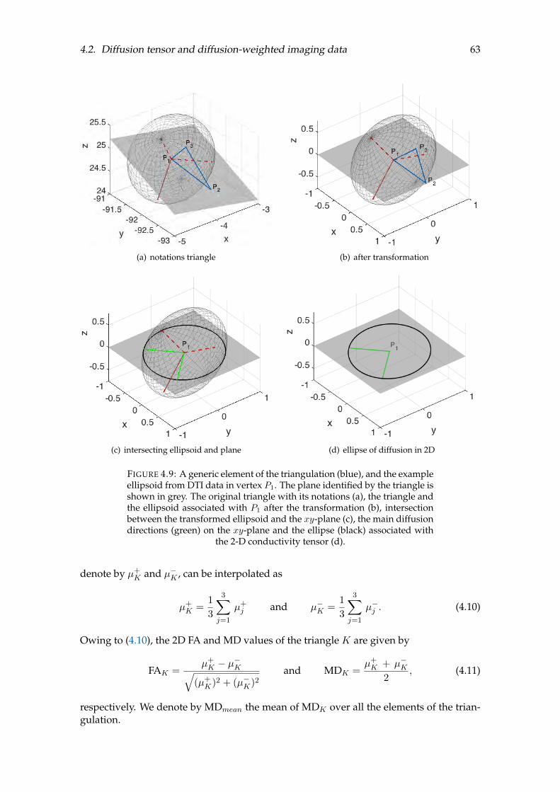
4.2. Diffusion tensor and diffusion-weighted imaging data 63
(a) notations triangle (b) after transformation
(c) intersecting ellipsoid and plane (d) ellipse of diffusion in 2D
FIGURE 4.9: A generic element of the triangulation (blue), and the exampleellipsoid from DTI data in vertex P1. The plane identified by the triangle isshown in grey. The original triangle with its notations (a), the triangle andthe ellipsoid associated with P1 after the transformation (b), intersectionbetween the transformed ellipsoid and the xy-plane (c), the main diffusiondirections (green) on the xy-plane and the ellipse (black) associated with
the 2-D conductivity tensor (d).
denote by µ+K and µ−K , can be interpolated as
µ+K =
1
3
3∑j=1
µ+j and µ−K =
1
3
3∑j=1
µ−j . (4.10)
Owing to (4.10), the 2D FA and MD values of the triangle K are given by
FAK =µ+K − µ
−K√
(µ+K)2 + (µ−K)2
and MDK =µ+K + µ−K
2, (4.11)
respectively. We denote by MDmean the mean of MDK over all the elements of the trian-gulation.
64 Chapter 4. Model personalisation
We can define the 2D diffusion tensor in the vertex Pj (j = 1, 2, 3) of triangle K as
Dj =δ
MDmean
(µ+j pj p
Tj + µ−j qj q
Tj
), (4.12)
where δ is a scaling factor normalised by MDmean.
The coefficient δ in (4.12) was tuned to adapt the velocity of the extracellular potassiumwave across the cortex to a propagation time that is comparable to the one of CSD. In thecase that real measurements were available, the parameter δ could be estimated througha data assimilation procedure (see, e.g., D’Elia et al., 2011; Delingette et al., 2012).
Treatment of artefacts and missing data In order to assign reasonable values for thediffusion at the points where the data is zero or incorrect, we assume isotropic conduc-tivity (D = d I2) and select a diffusivity d depending on the mean of the diffusion tensorintensity in the centroids of all vertices that belong to a specific region. Therefore, weconsider the anatomical subdivision of the brain cortex introduced in Section 1.2, whichdivides each hemisphere into 34 regions of interest (ROI) (Desikan et al., 2006). To assignreasonable values in these critical points, we average the mean diffusivity of all pointsthat do not feature missing or negative values and lie in the same ROI as the point itself.
In the specific, by denoting with R the ROI to which the critical point belongs, with PRthe set of points in R featuring data, and with |PR| the cardinality of PR, we assign aseigenvalues at the critical points the values
λi =∑P∈PR
MDR|PR|
, for i = 1, 2, 3 (4.13)
where MDR is the mean diffusivity of all points in the considered ROI computed onthe 3D data and we choose the eigenvectors wi, i = 1, 2, 3 as the standard basis for theEuclidean space.
Computational aspects In the previous section, we explained how we derive the 2Ddiffusion tensor in the vertices of a triangle. However, for the quadrature rule in thecomputation of the stiffness matrix in equation (3.8), we need to evaluate the diffusiontensor also in other points of the triangle. In the following, we show how to compute thediffusion tensor in the midpoints of the sides and the centroid of the triangle, as these arequadrature points required by the third-order Gaussian rule we use in our implementa-tion. The basic idea is to compute the conductivity tensor at the sides’ midpoints and atthe centroid by interpolating both orientation and length of the semi-axis of the conduc-tivity ellipses in the vertices. The following procedure can easily be extended to furtheradditional points whenever a higher quadrature rule is used.
Let Pi and Pj with i, j = 1, 2, 3, i 6= j be points with anisotropic diffusion and ϑ the anglebetween the major diffusion directions in the two points Pi and Pj , that is,
ϑ = arccos∣∣∣〈pi,pj〉∣∣∣,
where pi and pj are normalised vectors. The principal diffusion direction in the side’smidpoint between Pi andPj is obtained by rotating pi by half the angle ϑ between the twovectors pi and pj . This rotation can be performed either clockwise or counterclockwise,

4.2. Diffusion tensor and diffusion-weighted imaging data 65
but for the sake of consistency, we implement it in the direction of the shortest possiblerotation between pi and pj . We define the rotation matrix as
Rϑ/2 =
(cos (ϑ/2) − sin (ϑ/2)sin (ϑ/2) cos (ϑ/2)
)or R∗ϑ/2 =
(cos (ϑ/2) sin (ϑ/2)− sin (ϑ/2) cos (ϑ/2)
).
To select the rotation direction, we compute the vector corresponding to a full rotation ofϑ, namely Rϑpi, and consider the angle between Rϑpi and pj . If this angle is zero, therotation Rϑ/2 is along the shortest rotation path between pi and pj . In other words, weset
R =
Rϑ/2, if 〈Rϑpi,pj〉 = 1
R∗ϑ/2, else. (4.14)
Due to computational reasons, we also consider angles that are very close to zero as theshortest rotation path, that is, even when |〈Rϑpi,pj〉 − 1| < 10−6. Thus, the diffusiondirection vectors pij and qij of the midpoint are defined as
pij = Rpi and qij = R qj
The eigenvalues µ+ij and µ−ij are computed by linearly interpolating between µ+
i and µ+j
and µ−i and µ−j , respectively:
µ+ij =
µ+i + µ+
j
2and µ−ij =
µ−i + µ−j2
.
The case when Pi or Pj is isotropic requires some additional care. For example, let usassume that Pj is isotropic, then any direction is the principal one, and for simplicity wechoose the principal directions coinciding with the ones of Pi. Thus, ϑ = 0, and we onlyinterpolate the vector length.
For the diffusion tensor in the centroid, we already computed in equation (4.10) the cor-responding diffusion coefficients. To obtain the associated eigenvectors, we consider theprincipal diffusion directions in the midpoint Pij of a side of the triangle (pij and qij withi, j ∈ 1, 2, 3, i 6= j) and the ones on the opposite vertex Pl (pl and ql with l /∈ i, j).The choice of pij and pl does not affect the result by construction. Letting ψ be the anglebetween the major vectors pl and pij in the two points, given by
ψ = arccos∣∣∣〈pl,pij〉∣∣∣,
we rotate the principal diffusion directions pl and ql in the vertex by 2/3 of the angleψ. Again, the rotation is performed in the shortest possible path for consistency. Thediffusion directions in the centroid pK and pK are then given by
pK = Qpl and qK = Qql,
where Q is the rotation matrix defined either as
Q =
(cos (2ψ/3) − sin (2ψ/3)sin (2ψ/3) cos (2ψ/3)
)or Q =
(cos (2ψ/3) sin (2ψ/3)− sin (2ψ/3) cos (2ψ/3)
),
following the same idea previously used to determineR in (4.14). In the case when eitherPij or Pk is an isotropic point, the same procedure highlighted before is applied.

66 Chapter 4. Model personalisation
In Figure 4.10 we show the interpolation of the diffusion direction on a triangle, both foranisotropic points and the case in which one point features isotropic diffusion. We plotthe ellipses representing the 2D diffusion tensor and their major axis at the vertices, atthe midpoints and at the centroid.
(a) anisotropic diffusion in all vertices (b) isotropic diffusion in P3
FIGURE 4.10: Interpolation of diffusion direction and strength between thevertices of a triangle, with the axis of the diffusion ellipsoid at the vertices(red), at the midpoints (green) and at the centroid (blue). For anisotropic
diffusion in all vertices (a) and isotropic diffusion in vertex P3 (b).
4.2.4 Two-dimensional diffusion on the cortex
The DTI data preprocessing from 3D to 2D diffusion tensors, introduced in the previoussection, modifies the anisotropy characteristics of diffusion. Although some areas, likethe corpus callosum, feature a higher anisotropy level in the 3D data set, FA values arecentred around the value 0.2, showing that most areas feature mild anisotropy for theunderlying tissue (see Figure 4.6). In Figure 4.11 we plot the 2D FA values at the centroidof each triangle for both the left and right hemisphere and a normalised histogram thatdescribes the probability density of the FA values. This data maintains the overall struc-ture of a distributed mild anisotropy, but it exhibits a slightly larger amount of isotropicpoints compared to the original 3D data. This feature depends strongly on the orien-tation of the 3D eigenvectors of the diffusion with respect to the surface. Nevertheless,areas supporting higher FA in the 3D data set maintain these characteristics also after thetransformation of the diffusion tensor to 2D.
The reduction to 2D diffusion data on the surface does not only affect the FA but alsothe MD values. In Figure 4.12 we plot the MD values of the 2D transformed data at thecentroids of each triangle, for both hemispheres. To highlight their variability, the plotteddata is normalised with respect to the mean across the whole cortex. With this approach,we get insight into the behaviour of the parameter MDK/MDmean, which we use in thedefinition of the 2D diffusion tensor (see equation (4.11)). From Figure 4.12 we can inferthat larger MD values appear in the sulci and the corpus callosum. In the latter, the meshgeometry is much flatter and high anisotropy values of white matter tracts yield a much

4.2. Diffusion tensor and diffusion-weighted imaging data 67
(a) left hemisphere
(b) right hemisphere
FIGURE 4.11: The fractional anisotropy of the 2D diffusion data of the cor-tex on the left (a) and right (b) hemisphere and a normalised histogram
displaying the probability density of the FA values (right).
larger diffusion with respect to other cortical areas: as a consequence, the simulated CSDpropagation is expected to travel faster in this region.
In Figure 4.13 we plot the joint distribution of 2D FA and the normalised MD values inthe centroids of all triangles, for both left and right hemisphere. The colours representthe density, and one can observe the significant difference with respect to an isotropicsituation, whose MD and FA values are 1 and 0, respectively. Evidence from Figure 4.13 isa major advocate for the use of DTI-based diffusion coefficients. In general, the reductionto 2D diffusion data led to a minor reduction of the anisotropies as more FA values arecloser to 0 compared to the 3D case (see Figure 4.7). Comparing the MD values one canobserve that the values are slightly more spread out. However, all these changes areminor and result from the reduction by one dimension.
Finally, we plot in Figure 4.14 the principal diffusion direction, its strength on the medialside of the left hemisphere and a zoom of the lateral side. The direction of the linesindicates the diffusion direction, and the diffusion strength is given by the vector’s lengthand the colour. Here again, principal diffusion directions are considered in the centroidsof the triangles.

68 Chapter 4. Model personalisation
(a) left hemisphere
(b) right hemisphere
FIGURE 4.12: The normalised mean diffusivity of the 2D diffusion data ofthe cortex of the left (a) and right (b) hemisphere. Plotted data are nor-malised with respect to the average mean diffusivity across the whole cor-
tical hemispheres.
(a) left hemisphere (b) right hemisphere
FIGURE 4.13: The joint distribution of the fractional anisotropy and thenormalised mean diffusivity of the 2D diffusion tensors for each triangle ofthe mesh, both for the left (a) and right (b) hemisphere. Colours represent
the density.
4.3 Simulation of the CSD progression with DTI data
After describing the DTI data processing, we are now left with a 2D diffusion tensordescribing the diffusion direction and strength on the surface, the cerebral cortex. With
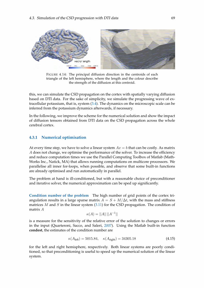
4.3. Simulation of the CSD progression with DTI data 69
FIGURE 4.14: The principal diffusion direction in the centroids of eachtriangle of the left hemisphere, where the length and the colour describe
the strength of the diffusion at this centroid.
this, we can simulate the CSD propagation on the cortex with spatially varying diffusionbased on DTI data. For the sake of simplicity, we simulate the progressing wave of ex-tracellular potassium, that is, system (3.4). The dynamics on the microscopic scale can beinferred from the potassium dynamics afterwards, if necessary.
In the following, we improve the scheme for the numerical solution and show the impactof diffusion tensors obtained from DTI data on the CSD propagation across the wholecerebral cortex.
4.3.1 Numerical optimisation
At every time step, we have to solve a linear system Ax = b that can be costly. As matrixA does not change, we optimise the performance of the solver. To increase the efficiencyand reduce computation times we use the Parallel Computing Toolbox of Matlab (Math-Works Inc., Natick, MA) that allows running computations on multicore processors. Weparallelise all inner for-loops, when possible, and observe that some built-in functionsare already optimised and run automatically in parallel.
The problem at hand is ill-conditioned, but with a reasonable choice of preconditionerand iterative solver, the numerical approximation can be sped up significantly.
Condition number of the problem The high number of grid points of the cortex tri-angulation results in a large sparse matrix A = S + M/∆t, with the mass and stiffnessmatrices M and S in the linear system (3.11) for the CSD propagation. The condition ofmatrix A
κ(A) = ||A|| ||A−1||
is a measure for the sensitivity of the relative error of the solution to changes or errorsin the input (Quarteroni, Sacco, and Saleri, 2007). Using the Matlab built-in functioncondest, the estimates of the condition number are
κ(Aleft) = 5015.84, κ(Aright) = 34305.18 (4.15)
for the left and right hemisphere, respectively. Both linear systems are poorly condi-tioned, so that preconditioning is useful to speed up the numerical solution of the linearsystem.

70 Chapter 4. Model personalisation
Preconditioning The IMEX scheme described in Section 3.4 requires to solve a linearsystem associated to a system of linear PDEs, for which a vast literature on precondition-ing is available (Saad, 2003). As potential preconditioners, we consider an incompleteLU factorisation without threshold and pivoting (ILU(0)), an incomplete LU factorisa-tion with both threshold and pivoting (ILUTP), and an incomplete Cholesky factorisationwith a drop tolerance (ICT). For a more detailed description of the preconditioners seeAppendix B.1.
To quantify the different possible preconditioners P for a problemAx = b, the most natu-ral way is to compare the condition number of the matrixA to the one of P−1A. However,such high dimensional matrices are difficult to invert. In the case of a symmetric positivedefinite matrix we have
κ2(A) =λmax
λmin,
where λmax and λmin are the maximum and minimum eigenvalues of A (Quarteroni,Sacco, and Saleri, 2007). Eigenvalues close to one (or in the complex case close to the unitcircle) indicate that the problem is well-conditioned. To avoid the inversion of the matrixP in the eigenvalue problem
P−1Ax = λx
we consider the generalised eigenvalue problem
Ax = λPx.
For the computation of the eigenvalues, we use the Matlab built-in function eigs whichapproximates the eigenvalues of large sparse matrices using the Lanczos algorithm (Lanc-zos, 1950).
In Figure 4.15 we plot an approximation of the eigenvalues of the generalised eigen-value problem with the different preconditioners for the left and right hemisphere. Weapproximate the smallest and biggest 500 eigenvalues and interpolate linearly betweenthem. The drop tolerance for the ILUTP and ICT is set to 10−6. In the top row, we plotthe eigenvalues (sorted by size) of the different preconditioned systems for the left andright hemisphere. The incomplete Cholesky factorisation with no fill-up of positive def-inite matrices does not necessarily always exist, and in our case, it does not exist neitherfor the left nor right hemisphere. ILU(0) preconditioning improves the condition of theproblem, but preconditioning with the ILUTP and the ICT perform the best.
Iterative solver The preconditioned gradient method (PCG) is an effective method thatis already parallelised as a built-in function in Matlab to solve symmetric linear systems.An alternative might have been the biconjugate gradient stabilised method (BiCGSTAB),but this method is not monotonously converging. To find the most efficient combinationof solver and preconditioners we compare PCG applied to the original system to thepreconditioned one. We use the solution from the previous time step as initial value forthe iterative solver and consider the relative residual norm at each iteration step, with andwithout preconditioning. For a detailed description of the PCG, we refer to Appendix B.1.
In Figure 4.16 we plot the relative residual at each iteration step of the PCG for the differ-ent preconditioners in the left and right hemisphere. Here, we solve system (3.11) at thevery first time step for a propagation wave starting in the lateraloccipital region.

4.3. Simulation of the CSD progression with DTI data 71
(a) left hemisphere (b) right hemisphere
(c) left hemisphere (d) right hemisphere
FIGURE 4.15: The smallest and biggest 500 eigenvalues of the originalmatrices, preconditioned with incomplete LU factorisation without fill-up (ILU(0)), with threshold and pivoting (ILUTP) and with incompleteCholesky factorisation with a drop tolerance of 10−6 (ICT), for the left(a) and right (b) hemisphere. A close up showing the difference between
ILUTP and ICT for the left (c) and right (d) hemisphere.
For a more detailed comparison we give the exact number of iterative steps and the rela-tive residual in Table 4.1. Again, different preconditioners for the system in the left andright hemisphere are considered.
left hemisphere right hemisphereiterations rel. residual iterations rel. residual
no preconditioner 156 9.403e-07 205 8.6915e-07ILU(0) 10 9.6725e-07 12 8.809e-07ILUTP 1 1.4769e-07 1 1.0432e-07ICT 1 1.2996e-07 1 1.2148e-07
TABLE 4.1: The iteration number and relative residual for the PCG withdifferent preconditioners in the left and right hemisphere.
Since the coefficients do not change in time during the simulation, neither does the fi-nite element matrix in (3.11). Thus, it is convenient to implement a low drop tolerance

72 Chapter 4. Model personalisation
(a) left hemishpere (b) right hemishpere
FIGURE 4.16: The relative residual norm at each iteration step of the PCGwith different preconditioning: ILU(0), ILUTP, and ICT for the left (a) and
right (b) hemisphere.
in the ICT factorisation, as the same preconditioner will be used for a large number oftime steps needed to simulate a whole CSD propagation. To investigate the impact of thedrop tolerance of the ICT, we consider as initial condition a fully depolarised lateraloc-cipital region, and we run the simulation until the whole cortex has been activated. InFigure 4.17 we give an overview of the iteration number and the relative residual for thedifferent drop tolerances of the ICT and consider the average number of iterations andthe average relative residual over time for the left and right hemisphere.
FIGURE 4.17: The average number of iterations (blue) and the relativeresidual (red) for the ICT with different drop tolerances, solved with PCGwith the initially activated lateraloccipital in the left (solid line) and right
(dashed line) hemisphere.
We also collect in Table 4.2 the average iteration number and average relative residual forboth hemispheres for different values of the drop tolerance in ICT. The combined effectof the low drop tolerance in the ICT factorisation, and the propagative nature of thesolution of system (3.4) entails that choosing as initial guess (at time tn+1) the solutionat the previous time step kn, PCG converges in very few iterations. Moreover, the singleiteration needed in most cases for the 10−6 drop tolerance advocates for the use of moreaccurate preconditioning for the CSD simulation.

4.3. Simulation of the CSD progression with DTI data 73
left hemisphere right hemispheredrop tol. iterations rel. residual iterations rel. residual10−6 1 2.1160e-8 1 2.1680e-810−5 1.0005 2.0239e-7 1.0005 2.0378e-710−4 2 3.0384e-9 1.9768 2.2775e-810−3 2.0266 1.6174e-7 2.4679 3.6689e-710−2 3.9924 5.8514e-7 3.9628 5.5549e-7
TABLE 4.2: Average number of iterations and average relative residual fordifferent drop tolerances in the preconditioner computation for the left and
right hemisphere.
To conclude, we solve system (3.11) with PCG, preconditioned by ICT, with pivoting anddrop tolerance set at 10−6. We consider as initial condition a fully depolarised lateraloc-cipital region, which corresponds to the area of the visual cortex where CSD typically isgenerated, and we run the simulation with the diffusion coefficients described in Section4.2.3 until every point of the cortical mesh has been reached by the potassium wave. Thescaling coefficient δ = 0.18 mm2 sec−1 for the diffusion (4.12) has been tuned to obtain apropagation time of around 20 minutes across the whole cortex, in agreement with thephysics of CSD. In Figure 4.18 we plot the potassium wavefronts on the left hemisphereat times t = 5 min, t = 10 min and t = 15 min.
FIGURE 4.18: Lateral and medial views of extracellular potassium propa-gation dynamics on the left hemisphere with DTI-based diffusion at time
t = 5 min, t = 10 min and t = 15 min.
4.3.2 Impact of tensor anisotropies on the CSD
In this series of tests, to assess the effect of the anisotropy in the coefficients on the pro-gression of CSD across the cortex, we compare the DTI-based diffusion tensors with theisotropic diffusion and a mixed isotropic diffusion tensor. The latter represents the casein which the diffusion imaging data only provides local diffusion coefficients, like theADC, and not a full diffusion tensor. We define the diffusion tensors in 2D locally oneach element K of the triangulation as:

74 Chapter 4. Model personalisation
1. Isotropic diffusion (Iso): For purely isotropic diffusion, FAK = 0. The diffusiontensor in a generic point Pj is given by
Dj = δI2.
2. DTI-based isotropic diffusion (i-DTI): We consider µ+j = µ−j in the diffusion ten-
sor definition (4.12). This means that MDj = µ+j and FAK = 0. Thus, the diffusion
coefficient is locally isotropic, but changes in space. In a generic point Pj the diffu-sion tensor reads
Dj = δµ+j
MDmeanI2.
3. DTI-based anisotropic diffusion (DTI): We consider the diffusion tensor intro-duced in equation (4.12). Thus, in the generic point Pj , it reads
Dj =δ
MDmean
(µ+j pjp
Tj + µ−j qjq
Tj
).
Using the same scaling coefficient δ = 0.18 mm2 sec−1 for all three simulations, we con-sider as initial condition a fully depolarised lateraloccipital region and run the simula-tions until every node of the computational grid, i.e., the whole cortex, has been reachedby the CSD wave. From Section 4.2.4 we expect differences in both propagation timesand wavefront patterns. In Table 4.3 we collect the different activation times, the mo-ment in time in which the last point is reached by the CSD wave, for the three differenttypes of diffusion tensors and both hemispheres. Compared to the isotropic diffusiontypes, the DTI-based anisotropic coefficients feature a slower wave propagation on thecortex, whereas the activation time with DTI-based isotropic diffusion is comparable tothe isotropic diffusion case.
Iso i-DTI DTIleft hemisphere 18.29 18.34 18.39right hemisphere 18.52 18.44 18.55
TABLE 4.3: The total activation times (in minutes) for a CSD wave origi-nating from the lateraloccipital region for the 3 diffusion tensors, and both
hemispheres.
Moreover, not only the final activation times are affected by the different diffusion types,but also the local propagation speed and direction are different when considering DTIdata, resulting in different depolarisation wavefronts. In Figure 4.19 we plot the depo-larisation wavefront on the left hemisphere originating from the lateraloccipital at timest = 10 min and t = 16 min for the different diffusion types. Even though the overallpropagation speed differs only slightly, up to 0.1 minutes in activation time delay, thewavefront propagation is different for the three cases of diffusion considered.
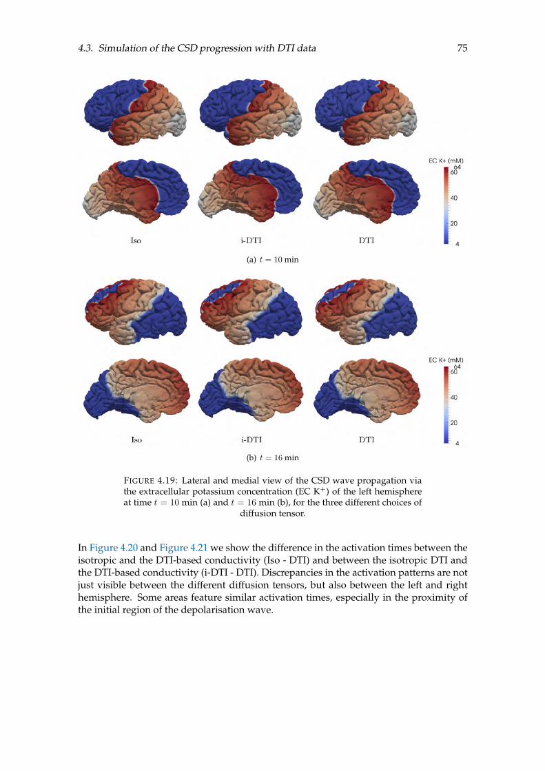
4.3. Simulation of the CSD progression with DTI data 75
(a) t = 10 min
(b) t = 16 min
FIGURE 4.19: Lateral and medial view of the CSD wave propagation viathe extracellular potassium concentration (EC K+) of the left hemisphereat time t = 10 min (a) and t = 16 min (b), for the three different choices of
diffusion tensor.
In Figure 4.20 and Figure 4.21 we show the difference in the activation times between theisotropic and the DTI-based conductivity (Iso - DTI) and between the isotropic DTI andthe DTI-based conductivity (i-DTI - DTI). Discrepancies in the activation patterns are notjust visible between the different diffusion tensors, but also between the left and righthemisphere. Some areas feature similar activation times, especially in the proximity ofthe initial region of the depolarisation wave.

76 Chapter 4. Model personalisation
FIGURE 4.20: The difference between the activation times (in minutes) forthe isotropic and the DTI-based diffusion tensor originating in the later-
aloccipital region for both hemispheres.
FIGURE 4.21: The difference between the activation times (in minutes) forthe isotropic DTI and the DTI-based diffusion tensor originating in the lat-
eraloccipital region for both hemispheres.
4.4 Summary
In this chapter we simulated a CSD wave on a real brain geometry obtained from MRIdata and were able to reproduce the propagation of the depolarisation wave triggeringthe microscopic dynamics of CSD that have been observed in experiments. After study-ing the coupled model and observing the CSD behaviour on the microscopic scale, weonly focused on the propagation of the extracellular potassium, that is, the macroscopicpart of the model, which already provides the essential information. From DTI data, wederived patient-specific conductivity tensors which provide detailed information aboutthe anisotropy and the electrical and ionic conductivity properties of the cortical tissue. Inaddition to the cortical geometry reconstructed from MRI imaging, diffusion coefficientsbased on DTI data bring the personalisation of the model to a higher level.

4.4. Summary 77
The algorithm to reduce the 3D DTI data to 2D diffusion data on the cortical surface wasdescribed in detail: the diffusion tensors were computed triangle by triangle in a finiteelements numerical approximation setting and the ellipsoids representing the diffusionin 3D were intersected with the plane identified by the considered triangle. Numericalresults showed differences in propagation time with respect to an isotropic diffusion thatwas assumed so far. The main contribution of the proposed model resides in the use ofa more detailed description of the tissue diffusivity: numerical simulations are expectedto be a closer match to CSD propagation, especially given Figure 4.13, Figure 4.20 andFigure 4.21, at a minimal additional computational effort.
The computational load of the proposed model is comparable with the one of the modelintroduced in Chapter 3. The only additional cost is associated with the pre-processingof the DTI data to compute the diffusion tensors in 2D, a procedure to be performed justonce for any given dataset, not affecting the actual computational time of the propaga-tion: the number of linear systems to be solved is the same as in the propagative part ofthe model in Chapter 3, with no additional computational issue. However, to reduce thecomputational load and speed up the numerical approximation we briefly elaborated onpossible preconditioners and the iterative solver.
Here, we just focused on the potassium dynamics, disregarding the electrophysiologicaldynamics at the microscopic scale. However, as these two parts of the model are coupledunidirectionally, the electrophysiology can be quickly reproduced from the results of thepropagating potassium wave on the cerebral cortex.
The results of this chapter have been published in two papers, in Kroos et al., 2016 andKroos et al., 2017.

79
Chapter 5
Cortical assessment
“Mathematics is biology’s next microscope, only better;biology is mathematics’ next physics, only better.”
J.R. Cohen, in PLoS Biology (2004)
After describing a way to personalise the CSD model, it is essential to assess the corti-cal geometry and the CSD propagation behaviour on the cortex from Chapter 3 for latergroup analysis. Our aim is to describe the unique structure of sulci and gyri of the hu-man cortex and CSD propagation in terms of quantities that can be compared betweensubjects.
Cortical curvature appears to be a specific and quantitative marker for white matter vol-ume irregularities. Fissures and sulci that consistently appear in all human brains showvariability in size and configuration (Thompson et al., 1996). Some studies support thehypothesis that cortical curvature abnormalities may indicate white matter atrophy, acharacteristic symptom in early multiple sclerosis (Deppe et al., 2014), or subtle malfor-mations of the cortex linked to seizure in temporal lobe epilepsy (Ronan et al., 2010).
To quantify the surface convolution of the cortex, we estimate the local curvature andcompute a surface regularity index. The curvature of a geometry is a differential invariantproperty that provides information about the direction of the bending of the surface andhow far the bending deviates from the plane, while the surface regularity index is theratio between the given volume and the volume of a sphere with the same surface size(Pérez-Beteta et al., 2018).
Some recent studies started to consider the effect of cortical geometries on CSD propaga-tion, at different levels of detail. Gyri and sulci affect the propagation of depolarisationwaves and can stop the CSD wave in different positions depending on the patient. Pocciet al., 2010 studied the effect of the cortical bending by simulating a wave propagationin a 2D duct containing a bend. They show how sharp bends naturally block the wavepropagation. Above a critical radius, blocking can be achieved by changing the systemparameters, assuming that adapted therapeutic agents can stop migraine aura. In a per-sonalised approach to migraine aura treatment, Dahlem et al., 2015 propose to use theGaussian curvature of the cortex to identify potential targets for neuromodulation. Ap-plying a generic reaction-diffusion model they highlight the local effects of the curvatureon a simple 2D geometry including a bump.
In this chapter the objective is to study the wave propagation on a whole 3D individualgeometry to identify symmetries and asymmetries in its behaviour and analyse regions
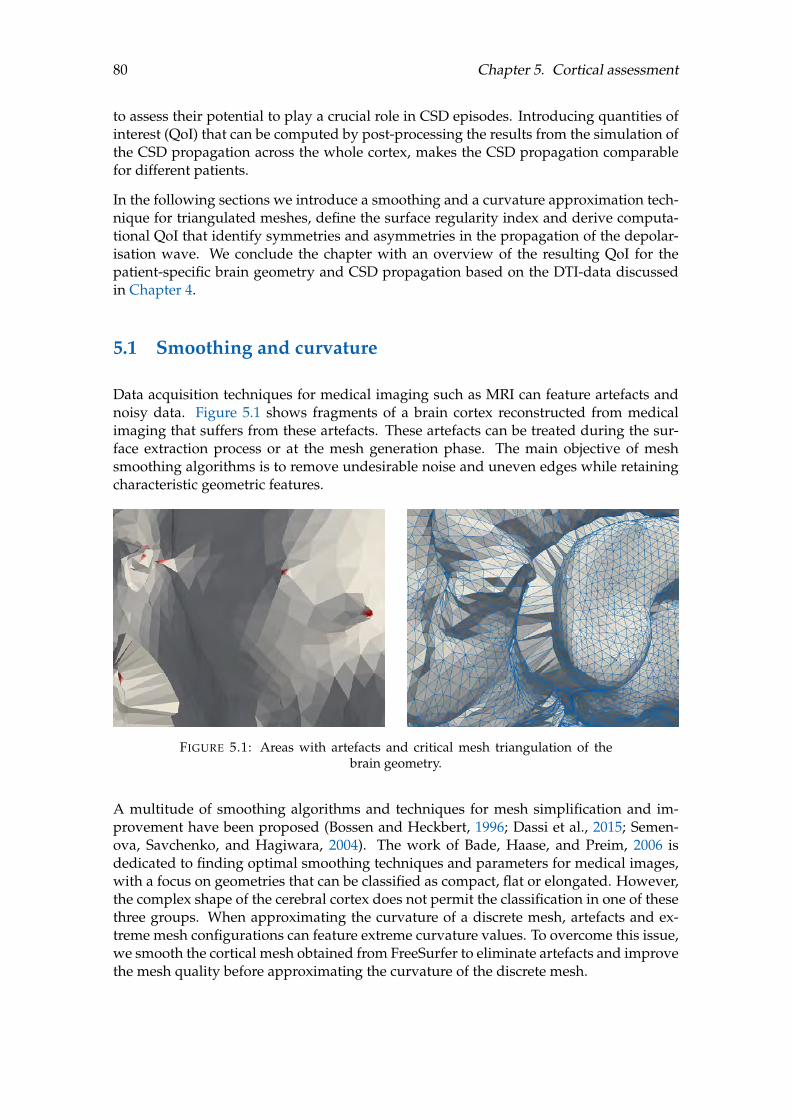
80 Chapter 5. Cortical assessment
to assess their potential to play a crucial role in CSD episodes. Introducing quantities ofinterest (QoI) that can be computed by post-processing the results from the simulation ofthe CSD propagation across the whole cortex, makes the CSD propagation comparablefor different patients.
In the following sections we introduce a smoothing and a curvature approximation tech-nique for triangulated meshes, define the surface regularity index and derive computa-tional QoI that identify symmetries and asymmetries in the propagation of the depolar-isation wave. We conclude the chapter with an overview of the resulting QoI for thepatient-specific brain geometry and CSD propagation based on the DTI-data discussedin Chapter 4.
5.1 Smoothing and curvature
Data acquisition techniques for medical imaging such as MRI can feature artefacts andnoisy data. Figure 5.1 shows fragments of a brain cortex reconstructed from medicalimaging that suffers from these artefacts. These artefacts can be treated during the sur-face extraction process or at the mesh generation phase. The main objective of meshsmoothing algorithms is to remove undesirable noise and uneven edges while retainingcharacteristic geometric features.
FIGURE 5.1: Areas with artefacts and critical mesh triangulation of thebrain geometry.
A multitude of smoothing algorithms and techniques for mesh simplification and im-provement have been proposed (Bossen and Heckbert, 1996; Dassi et al., 2015; Semen-ova, Savchenko, and Hagiwara, 2004). The work of Bade, Haase, and Preim, 2006 isdedicated to finding optimal smoothing techniques and parameters for medical images,with a focus on geometries that can be classified as compact, flat or elongated. However,the complex shape of the cerebral cortex does not permit the classification in one of thesethree groups. When approximating the curvature of a discrete mesh, artefacts and ex-treme mesh configurations can feature extreme curvature values. To overcome this issue,we smooth the cortical mesh obtained from FreeSurfer to eliminate artefacts and improvethe mesh quality before approximating the curvature of the discrete mesh.

5.1. Smoothing and curvature 81
The code for the smoothing and curvature approximation that we introduce in this sec-tion was developed in collaboration with Franco Dassi from the University of Milan-Biccoca in Italy.
5.1.1 Data smoothing techniques
One of the most popular techniques to smoothen curves and surfaces is Gaussian smooth-ing. In the continuous case, a convolution of the vector function parameterising the curveis performed with a Gauss kernel. For meshed surfaces, Gaussian smoothing has to beformulated in a discrete manner. In the following, we define this smoothing for discretesurfaces as well as the algorithm proposed by Gabriel Taubin to prevent shrinkage causedby the original Gaussian smoothing (Taubin, 1995).
Gaussian smoothing is an iterative algorithm in which at every step the smoothed posi-tion of a mesh point is defined by a weighted average of its current position and its directneighbours without changing the mesh topology. The direct neighbours of a mesh vertexare all vertices that share an edge of the mesh with the considered vertex. Let p ∈ P bea generic point in a set of points describing a mesh Γh, where h refers to the maximumdiameter of the elements of the triangulation. Then a vertex pi ∈ P is considered animmediate or direct neighbour of p if the edge ppi is part of the given mesh Γh. In theGaussian smoothing, the position of p is replaced in the smoothed mesh by
pnew = p+λ
c
∑pi∈P ∗
w(p, pi)(p− pi),
where λ ∈ (0, 1] is a scaling factor, P ∗ is the set of neighbouring vertices, w is a positiveweight function with
∑pi∈P ∗
w(p, pi) = 1 and c is a normalisation factor. The differentways to select the weight function w are discussed below.
Weight functions The weight functions can be chosen by taking into account the neigh-bourhood structure, the specific variations in the edge lengths and the face angles. Theequal weights proposed by Taubin provide good smoothing results for meshes with smallvariations in the edge length and face angles across the mesh. For more irregular meshes,like the ones obtained from medical imaging, other weights can be better suited to com-pensate for the irregular triangulation. Several choices of weight functions w have beenproposed in Taubin, 2000:
• equal weights: all edges connected to p are weighted with the same constant value,i.e.,
w(p, pi) :=1
|P ∗|, (5.1)
where | · | denotes the cardinality of the set.
• Fujiwara weights: the edges are weighted according to the inverse of the edge length,i.e.,
w(p, pi) :=1
||ppi||, (5.2)
where || · || is the Euclidean norm giving the length of the edge ppi.

82 Chapter 5. Cortical assessment
• Desbrun weights: the edges are weighed by the adjacent angles
w(p, pi) := cot(αi) + cot(βi) , (5.3)
where the angles αi and βi are the angle opposite to the edge ppi in the two adjacenttriangles sharing the edge ppi, as shown in Figure 5.2.
(a) angles opposite the edge ppi (b) angle at p
FIGURE 5.2: The notations for the angles opposite the edge ppi (a) and forthe angle at point p (b).
The resulting smoothed mesh depends on the choice of the weights. Applying the smooth-ing technique reduces the triangles’ stretch and transforms them into more equilateral tri-angles. To measure the performance of the smoothing algorithm, we introduce a qualitymeasure based on the triangles’ stretch.
Mesh quality measure To derive a global indicator for the mesh quality, we start byconsidering the aspect ratio defined for a generic triangle K as
q(K) := 2rKRK
,
where rK and RK are the radii of the inscribed and circumscribed circle, respectively(Shewchuk, 2002). For an equilateral triangle, this measure yields 1, while q(K) close tozero means that triangle K is highly stretched. We then compute the mean of q(K) overall the triangles to obtain a single quantity characterising the mesh quality, namely
qmean :=1
|Γh|∑K∈Γh
q(K) , (5.4)
where |Γh| is the number of triangles in the surface Γh. In the following, we use qmean asa proxy for mesh quality.
To illustrate the effect of smoothing in a particular example, we apply Gaussian smooth-ing with equal weights and λ = 0.33 to a cow geometry1 with 2903 nodes and 5804triangles. The original geometry, the results of N = 10 and N = 20 iterative steps of thesmoothing algorithm and the corresponding mesh qualities are shown in Figure 5.3. Thiscomparison highlights the significant loss of volume in the fine features of the geometry(like the legs) with an increasing number of iterations. This is known as the shrinkage
1from the INRIA Gamma mesh repository

5.1. Smoothing and curvature 83
effect associated to Gaussian smoothing. The mesh quality is not necessarily increasingwith the iteration number. After 10 smoothing iterations the mesh quality of the cowgeometry increases but after 10 more iterations the mesh quality is decreases. However,there is still an improvement in the mesh quality after 20 smoothing steps compared tothe initial mesh.
(a) original mesh, qmean = 0.7339 (b) N = 10, qmean = 0.8046 (c) N = 20, qmean = 0.7734
FIGURE 5.3: The Gaussian smoothing with equal weights applied to theoriginal geometry (a) with 2903 nodes and 5804 triangles with the scaling
factor λ = 0.33 and N = 10 (b) and N = 20 (c) iterations.
Taubin smoothing To prevent shrinkage, the Taubin algorithm consists of two consec-utive Gaussian smoothing steps with positive and negative scaling factors (Taubin, 1995).After a first Gaussian smoothing step with positive scaling λ is used, a second Gaussiansmoothing step is performed with negative scaling µ. These two values are chosen suchthat 0 < λ < −µ, and to produce a significant smoothing effect on the final mesh thesetwo steps have to be repeated iteratively. The precise scheme is given in Algorithm 5.1.
Algorithm 5.1 Taubin smoothing schemeΓh = SMOOTHING ( Γinith , λ, µ, w, N )
1: initialise: Γh = Γinith
2: for i = 1, . . . , N do
3: Γh = Gaussian smoothing with λ and w on Γh
4: Γh = Gaussian smoothing with µ and w on Γh
5: end for
To quantify the shrinkage caused by the smoothing algorithm, we consider a fast way tocompute the volume enclosed by a triangular mesh.
Volume computation for triangulated surfaces We start by redefining a generic vol-ume V ⊂ R3 as ∫
V1 dV.
Let V be a bounded open set (here in R3) with smooth or piecewise smooth enclosingsurface S (or, in general, boundary ∂V ) and F be a continuously differentiable vectorfield up to the boundary. Then the divergence theorem relates the flux of the vector field

84 Chapter 5. Cortical assessment
through a surface enclosing V to the behaviour of the vector field inside the volume,namely ∫
V∇ · F dV =
∫S
F · n dA. (5.5)
where ∇· is the divergence operator and n the outward pointing normal of the surfaceS (Kellogg, 1929). For volumes enclosed by a triangulated surface, the right hand sideof (5.5) can be split into a summation over triangular faces on which the normal n tothe surface remains constant. Choosing a vector field F = (x, 0, 0)T whose divergence isequal to 1, we can hence write∫
V1 dV =
∫V∇ · F dV =
∫S
F · n dA =∑K∈Γh
∫K
F · n dA (5.6)
for a set of triangles Γh describing the surface mesh and a normal vector n = (n1, n2, n3)T .Considering the triangle K with vertices Q = (q1, q2, q3)T , R = (r1, r2, r3)T and S =(s1, s2, s3)T , every point P in the triangle K can be expressed as
P = (1− u− v)Q+ uR+ vS, with u ∈ [0, 1], v ∈ [0, 1− u]
using barycentric coordinates. If F is linear, then
F (P ) = (1− u− v)F (Q) + uF (R) + vF (S)
and in our particular case with the definition of the vector field F, we have F (P ) =((1− u− v)q1 + ur1 + vs1, 0, 0)T . Using the triangle parametrisation, we can rewrite thesurface integral for the vector field F = (x, 0, 0)T as∫
KF · n dA = 2n1|K|
∫ 1
0
∫ 1−u
0(1− u− v)q1 + ur1 + vs1 dv du, (5.7)
where |K| is the area of the triangle with
|K| = ||n||2
and n = (R−Q)× (S −Q).
Using the fact that q1, r1 and s1 are constants and performing simple integration one canshow that ∫ 1
0
∫ 1−u
0(1− u− v)q1 + ur1 + vs1 dv du =
q1 + r1 + s1
6.
Hence, equation (5.7) simplifies to∫K
F · n dA =n1||n||
2
q1 + r1 + s1
3,
where the last fraction is the x-component of the barycentre Q+R+S3 of triangle K. Con-
sequently, the volume enclosed by a triangulated surface can be summarised as
1
2
∑K∈Γh
n1||n||q1 + r1 + s1
3.
Meshes with noise To evaluate the smoothing algorithm, the different weight functionsand the impact of the scaling factor, we consider again the example of the cow geometry.

5.1. Smoothing and curvature 85
As medical images usually include noise and artefacts, we artificially add noise to thecow geometry by moving some points along the normal to the surface, see Figure 5.4.We apply the smoothing procedure described in Algorithm 5.1 for the different weightfunctions and show the results for λ = 0.33 and µ = −0.34 in Figure 5.4.
(a) original (b) artificially added noise
(c) equal weights (d) Fujiwara weights (e) Desbrun weights
FIGURE 5.4: The original mesh of the cow geometry (a), with artificiallyadded noise (b) and the results of Taubin smoothing with equal (c), Fuji-wara (d) and Desbrun (e) weights afterN = 20 iterations and with λ = 0.33
and µ = −0.34.
To evaluate the impact of the smoothing weights and scaling factors on the mesh, we plotthe volume and the (mean) mesh quality (5.4) of the cow geometry at each iteration stepfor the different weight functions in Figure 5.5. Here, we choose different values for thescaling factors λ and µ but keep their ratio as proposed by Taubin, Zhang, and Golub,1996.
All the weight functions cause a similar loss of volume and the noise is removed (seeFigure 5.4). However, the equal weights perform better when considering the mesh qual-ity. In the beginning, both the equal and Fujiwara weights improve the mesh qualitysignificantly but this improvement levels off with the number of iterations. This is anumerical evidence that the smoothing at some point cannot improve the mesh qualityanymore. Consequently, other mesh operations such as edge flipping, edge contractionand point insertion have to be included to achieve further improvement (Frey, 2004; Freyand Borouchaki, 1998, 2003; Geuzaine and Remacle, 2009) but this goes beyond the scopeof this thesis.
Since the Taubin smoothing is based on the Gaussian one, there is always a shrinkage inthe triangular surface mesh. A standard stopping criterion for the iterative smoothingscheme is the maximum number of iterations. However, an appropriate choice of the

86 Chapter 5. Cortical assessment
(a) λ = 0.2, µ = −0.21 (b) λ = 0.33, µ = −0.34 (c) λ = 0.4, µ = −0.42
FIGURE 5.5: Volume and mesh quality of the cow geometry after applyingthe Taubin smoothing with equal, Fujiwara and Desbrun weights at eachiteration step for scaling parameters λ = 0.2 and µ = −0.21 (a), λ = 0.33
and µ = −0.34 (b) and λ = 0.4 and µ = −0.42 (c).
iteration number and the scaling factor is important for the quality of the final smoothingresult. To avoid choosing the number of iterations, we adopt an alternative stoppingcriterion in line 2 of Algorithm 5.1, and restrict it by the volume loss. Therefore, weassume that the discrete mesh Γh encloses a volume Vi after i iterations. We apply theTaubin smoothing until the percentage of volume loss exceeds the threshold Vtol, that is,we keep applying the smoothing as long as
|Vi − V0|V0
< Vtol,
where V0 is the volume enclosed by the initial surface mesh. This way the stoppingcriterion is a trade-off between the volume reduction and the smoothness. The Taubinsmoothing scheme with the new stopping criterion is given in Algorithm 5.2.
Algorithm 5.2 Taubin smoothing with volume restrictionΓh = SMOOTHING ( Γinith , λ, µ, w, Vtol )
1: V0 = volume of Γinith
2: initialise: Γh = Γinith , V = V0
3: while(|V−V0|V0
< Vtol
)do
4: Γh = Gaussian smoothing with λ and w on Γh
5: Γh = Gaussian smoothing with µ and w on Γh
6: V = volume of Γh
7: end while

5.1. Smoothing and curvature 87
Applying this smoothing algorithm to the example of the cow with a maximum volumeloss of 5% we present the number of iterations and the mesh quality of the final meshin Table 5.1. In this example the Taubin smoothing with equal weights results in a meshwith the best quality.
initial mesh Taubin smoothingweight function equal Fujiwara Desbruniterations 28 26 26mesh quality 0.7335 0.8107 0.7517 0.6873
TABLE 5.1: The iteration number and mesh quality of the noisy cow geom-etry after applying the Taubin smoothing with equal, Fujiwara and Des-
brun weights with λ = 0.33, µ = −0.34 and Vtol = 0.05.
5.1.2 Discrete curvature approximation
In 2D curvature can be defined in several equivalent ways: as the deviation of the curvefrom the tangent line, as the rate of change of the tangent direction, or as the reciprocalof the radius of the osculating circle. For surfaces in 3D the definition of curvature ismore complicated. In analogy to the 2D definition, the curvature should reproduce thedeviation of the surface from the tangent plane but in contrast to planar curves, there areseveral ways to measure this deviation. Gaussian curvature and mean curvature are twoapproaches to estimate this and to give precise information about the shape of the con-sidered surface. Gaussian curvature is defined as the product of the principal curvatures,while the mean curvature is defined as the average of the principal curvatures.
Differential geometry properties like Gaussian and mean curvature are well-known forparametrically defined curves and surfaces in the classical literature, and they provideessential and invariant information about a geometry (Do Carmo, 1976; Goldman, 2005;Kühnel, 2006). Considering a sufficiently regular surface Γ and the normal n in a genericpoint p ∈ Γ, we can construct a set of normal planes at the point p which contain thenormal vector n and the point p. All these planes cut the surface Γ in different planecurves that are characterised by a distinct curvature behaviour. We denote by k1 and k2
the principal curvatures, i.e., the maximum and minimum values of the curvature of allthese curves in p. Then, the Gaussian curvatureK and the mean curvatureH are definedas
K(p) := k1 k2, and H(p) := (k1 + k2)/2.
For a summary of the main definitions and results in differential geometry to clarify theconcept of Gaussian and mean curvature of surfaces in the framework of parametriccurves, we refer to Appendix B.2.
For an analytic evaluation of the curvature, a parametrisation of the surface Γ is neces-sary. In the case of discrete surfaces, like the brain geometry reconstructed from MRIimaging, we do not have such parametrisation, but a triangulated mesh instead. More-over, since we are dealing with a complex triangulated surface of a brain reconstruction,finding such parametrisation would require high computational effort and sophisticatedtechniques, see for instance Marchandise, Remacle, and Geuzaine, 2014.
Numerous approaches to estimate the curvature of 3D triangular meshes have been madeand a comprehensive overview of Gaussian and mean curvature estimation methods
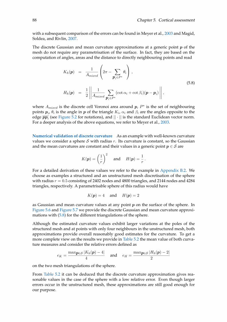
88 Chapter 5. Cortical assessment
with a subsequent comparison of the errors can be found in Meyer et al., 2003 and Magid,Soldea, and Rivlin, 2007.
The discrete Gaussian and mean curvature approximations at a generic point p of themesh do not require any parametrisation of the surface. In fact, they are based on thecomputation of angles, areas and the distance to directly neighbouring points and read
Kh(p) =1
Amixed
2π −∑pi∈P ∗
θi
,
(5.8)
Hh(p) =1
2
∣∣∣∣∣∣∣∣∣∣ 1
Amixed
∑pi∈P ∗
(cotαi + cotβi)(p− pi)
∣∣∣∣∣∣∣∣∣∣ ,
where Amixed is the discrete cell Voronoi area around p, P ∗ is the set of neighbouringpoints pi, θi is the angle in p of the triangle Ki, αi and βi are the angles opposite to theedge ppi (see Figure 5.2 for notations), and || · || is the standard Euclidean vector norm.For a deeper analysis of the above equations, we refer to Meyer et al., 2003.
Numerical validation of discrete curvature As an example with well-known curvaturevalues we consider a sphere S with radius r. Its curvature is constant, so the Gaussianand the mean curvatures are constant and their values in a generic point p ∈ S are
K(p) =
(1
r
)2
and H(p) =1
r.
For a detailed derivation of these values we refer to the example in Appendix B.2. Wechoose as examples a structured and an unstructured mesh discretisation of the spherewith radius r = 0.5 consisting of 2402 nodes and 4800 triangles, and 2144 nodes and 4284triangles, respectively. A parametrisable sphere of this radius would have
K(p) = 4 and H(p) = 2
as Gaussian and mean curvature values at any point p on the surface of the sphere. InFigure 5.6 and Figure 5.7 we provide the discrete Gaussian and mean curvature approxi-mations with (5.8) for the different triangulations of the sphere.
Although the estimated curvature values exhibit larger variations at the poles of thestructured mesh and at points with only four neighbours in the unstructured mesh, bothapproximations provide overall reasonably good estimates for the curvature. To get amore complete view on the results we provide in Table 5.2 the mean value of both curva-ture measures and consider the relative errors defined as
eK =maxp∈S |Kh(p)− 4|
4and eH =
maxp∈S |Hh(p)− 2|2
on the two mesh triangulations of the sphere.
From Table 5.2 it can be deduced that the discrete curvature approximation gives rea-sonable values in the case of the sphere with a low relative error. Even though largererrors occur in the unstructured mesh, these approximations are still good enough forour purpose.
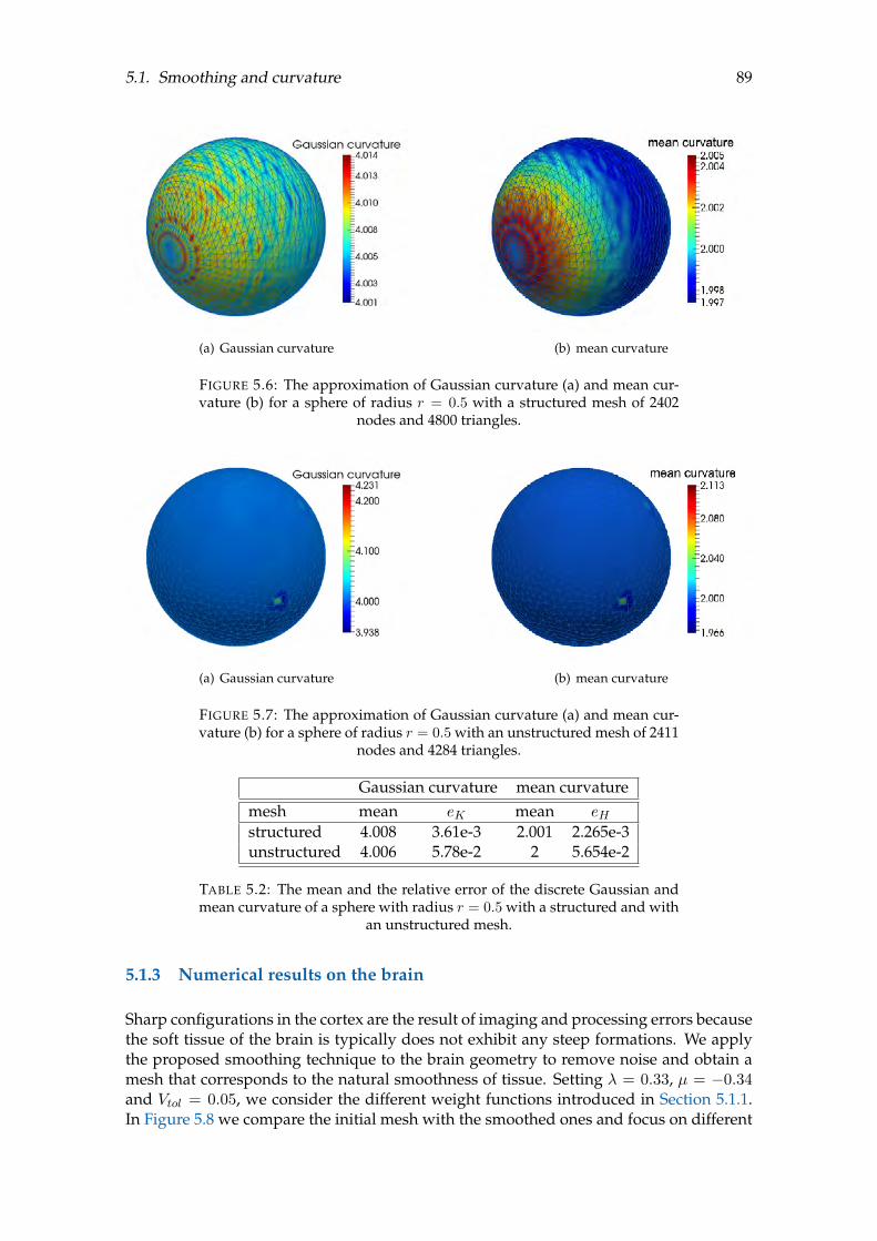
5.1. Smoothing and curvature 89
(a) Gaussian curvature (b) mean curvature
FIGURE 5.6: The approximation of Gaussian curvature (a) and mean cur-vature (b) for a sphere of radius r = 0.5 with a structured mesh of 2402
nodes and 4800 triangles.
(a) Gaussian curvature (b) mean curvature
FIGURE 5.7: The approximation of Gaussian curvature (a) and mean cur-vature (b) for a sphere of radius r = 0.5 with an unstructured mesh of 2411
nodes and 4284 triangles.
Gaussian curvature mean curvaturemesh mean eK mean eHstructured 4.008 3.61e-3 2.001 2.265e-3unstructured 4.006 5.78e-2 2 5.654e-2
TABLE 5.2: The mean and the relative error of the discrete Gaussian andmean curvature of a sphere with radius r = 0.5 with a structured and with
an unstructured mesh.
5.1.3 Numerical results on the brain
Sharp configurations in the cortex are the result of imaging and processing errors becausethe soft tissue of the brain is typically does not exhibit any steep formations. We applythe proposed smoothing technique to the brain geometry to remove noise and obtain amesh that corresponds to the natural smoothness of tissue. Setting λ = 0.33, µ = −0.34and Vtol = 0.05, we consider the different weight functions introduced in Section 5.1.1.In Figure 5.8 we compare the initial mesh with the smoothed ones and focus on different

90 Chapter 5. Cortical assessment
parts of the left hemisphere. These areas highlight the noise removal, maintaining thecomplexity of the geometry. In the case of equal weights, the triangulation is evidentlyimproved, converting stretched triangles of the initial mesh into more regular ones. Thisfact is numerically confirmed by the mesh quality, as it can be observed in Table 5.3.
initial mesh Taubin smoothingweight function equal Fujiwara Desbrunleft hemisphere 0.7187 0.7452 (43) 0.6819 (51) 0.6696 (78)right hemisphere 0.7241 0.7525 (44) 0.6867 (52) 0.6726 (81)
TABLE 5.3: Mesh quality and iteration number (in brackets) for Taubinsmoothing with λ = 0.33, µ = −0.34 and Vtol = 0.05 and equal, Fujiwara
and Desbrun weights for the left and right hemisphere.
From now on, we only consider equal weights as they perform best on the cortex geom-etry regarding the mesh quality. To elaborate a bit more on the choice of scaling parame-ters, we set the maximum volume loss to 5% and plot the volume loss and mesh qualityfor different parameters λ and µ in Figure 5.9. Choosing small parameters increases theiteration number to reach the maximum volume loss and obtain a specific mesh quality,significantly. For all considered choices of scaling parameters the smoothing algorithmconstantly improves the mesh quality and at the same time decreases the volume, forboth hemispheres. Thus, we choose the same scaling parameters as proposed in the liter-ature on Taubin smoothing. In what follows, we will smooth the brain mesh with equalweights and scaling parameters λ = 0.33 and µ = −0.34 up to a volume loss of 5%.
The results of applying the curvature approximation from Section 5.1.2 to the smoothedbrain geometry is shown in Figure 5.10. We present a close-up of the Gaussian curvatureand the mean curvature on the smoothed left hemisphere and in Table 5.4 we list themean and standard deviation of the Gaussian and mean curvature of the left and righthemisphere of the smoothed cortex geometry. Gaussian curvature values have a highstandard deviation which can be explained by a few very large curvature values that re-sult from extreme mesh formations even after applying Taubin smoothing, as illustratedin Figure 5.8.
Gaussian curvature mean curvaturehemisphere mean std mean stdleft 0.1893 12.6791 0.4278 1.2869right 0.3677 84.1972 0.4177 1.8088
TABLE 5.4: The mean and standard deviation of the Gaussian and meancurvature of the (smoothed) left and right hemisphere.

5.1. Smoothing and curvature 91
(a) original
(b) equal weights
(c) Fujiwara weights
(d) Desbrun weights
FIGURE 5.8: Results of the Taubin smoothing with scaling factors λ = 0.33and µ = −0.34, a maximum volume loss of Vtol = 0.05 and equal (b), Fu-jiwara (c) and Desbrun (d) weights for particular regions of the left hemi-
sphere.

92 Chapter 5. Cortical assessment
(a) left hemisphere (b) right hemisphere
FIGURE 5.9: Volume loss and mesh quality for different parameter choicesof λ and µ, for the left (a) and right (b) hemisphere.
(a) Gaussian curvature (b) mean curvature
FIGURE 5.10: Gaussian and mean curvature of the smoothed brain geom-etry of the left hemisphere.
5.2 Surface regularity index
For the computation of the surface regularity index (SRI) we refer to Pérez-Beteta et al.,2018. They introduce the surface regularity as a dimensionless ratio between the given
5.3. Quantities of interest in CSD propagation 93
volume of a geometry and the volume of a sphere with the same surface size, namely
SRI = 6V
√π
S3,
where V is the total volume and S is the total surface. The surface regularity variesbetween 0 (very irregular surface) and 1 (spherical geometry). To compute the volumeand the surface of a closed surface in 3D, we use the Python shell in Paraview (Ahrens,Geveci, and Law, 2005).
For the geometry at hand, the surface regularity index is 0.1799 for the left and 0.1807 forthe right hemisphere.
5.3 Quantities of interest in CSD propagation
CSD is known to originate from the visual cortex, but to gain deeper insight in the way thegeometry shapes the CSD propagation, we simulate the spread of depolarisation wavesbetween all the regions of the anatomical classification, in both hemispheres. In eachsimulation, we consider an area around the centroid of each region (out of the 34 ROI) asinitial condition. Each simulation is run until all remaining regions have been reached bythe depolarisation wave and the arrival times of this wave in the remaining 33 regions arerecorded. In previous works, the whole region was considered as initial conditions buthere we focus on the centroids to make the comparison between the propagation pathand speed more accurate (Kroos et al., 2016).
The corpus callosum is the only compartment that is not considered as initially activatedas it constitutes the intersection between the two hemispheres and obeys different rulesfor diffusion. For this reason, we eliminate the corpus callosum from the mesh and im-pose zero-flux boundary conditions on the boundary of the corpus callosum.
Using the data obtained from the 34 CSD simulations run per hemisphere, each one withCSD initiated in a different ROI, we can introduce different ways to assess symmetry andasymmetry in the propagation, with the aim of identifying regions featuring a peculiarpropagation behaviour.
In this section we start with some comments on the computation of the centroids and theremoval of the corpus callosum from the geometry. Then, we introduce the QoI describ-ing CSD propagation on the cortex and conclude with the results on the smoothed braingeometry at hand with CSD propagation with DTI-based diffusion coefficients.
5.3.1 Centroids of the regions of interest
For the centroid computation we consider all points PR in regionR and denote by TR alltriangles that have at least two vertices in that region.
The surface area of a generic triangle K with vertices P1, P2 and P3 is given by
SK =||(P2 − P1)× (P3 − P1)||
2,

94 Chapter 5. Cortical assessment
where || · || denotes the Euclidean norm, while the centroid of this triangle is CK = (P1 +P2 + P3)/3. Then, by defining the total mass of regionR as
SR =∑K∈TR
SK ,
we compute the weighted sum of all centroids of the respective triangles (weighted byeach triangle’s mass) divided by the total mass, that is,
C =1
SR
∑K∈TR
CKSK .
Finally, we consider as centroid of region R the point CR in region R that is closest to Cin the Euclidean distance, namely
CR = arg minp∈PR
||C − p||.
To obtain the initial condition for the CSD wave propagation, we consider a set of pointsin the proximity of the region’s centroid, namely
P ∗ = p ∈ PR | ||CR − p|| ≤ s,
where s is the maximum distance between the centroid and the points we consider asinitially excited (typically we set s = 10 mm). These initially excited points belong to thesame area and should not be located on opposite sides of a sharp bend, like in the examplein Figure 5.11. Here, all points in P ∗ are visualised with dots but some of them are notconnected (in the sense that will be described in detail below) to the centroid itself. Toavoid the problem of starting CSD propagation in several areas, we only consider pointsin the initial region that are connected to the centroid, that we identify by means of somedefinitions and results from the area of graph theory, see Appendix B.3.
FIGURE 5.11: A visualisation of all points considered within the radius ofs = 10 mm of the centroid (green). The non-connected points are coloured
in red.

5.3. Quantities of interest in CSD propagation 95
Connectivity centroids To verify that all points in the initially activated area aroundthe centroid CR are connected, we compute the adjacency matrix A ∈ Rl×l where l is thecardinality of P ∗. A well-known result in graph theory states that l vertices are connectedif and only if the matrix power (A+Il)l−1 has no zero entries. However, the size ofA andthe exponent l make this evaluation very expensive. Even using the diameter, that is, themaximum distance in a graph, as a lower boundary for the path length (see DefinitionB.3.3 and Lemma B.3.3) blows up the matrix. When calculations overflow the largestrepresentable floating point number in Matlab (which is 10309), big values are treated asinfinity and this leads to not defined values when multiplying infinity with zero.
Another approach is a modified version of the Dijkstra algorithm that finds the shortestpath between two nodes (Dijkstra, 1959). Most variations of this algorithm fix a singlenode as the source and find the shortest path from the source to any other node in thegraph. We are interested in the distance of all the points to the centroid. As the problemat hand is an undirected graph with constant edge weights, we use a modified version ofthis algorithm that is outlined in Algorithm 5.3 (Dijkstra, 1959; Peng et al., 2012).
Algorithm 5.3 Modified Dijkstra algorithmD = DIJKSTRA(A, P ∗, CR)
1: initialise: Q = P ∗ . all nodes initially in Q (unvisited nodes)
2: D(p) =∞ for all p ∈ Q with p 6= CR, D(CR) = 0 . initiating the distance matrix
3: while Q is not empty do
4: p = arg minp∈Q
D(p) . vertex in Q with minimum distance to CR
5: remove p from Q
6: for each neighbour u of p do . that is all u with A(p, u) = 1
7: a = D(p) + 1 . the distance between u and p is 1, as they are neighbours
8: if a < D(u) then . a shorter path to u has been found
9: D(u) = a
10: end if
11: end for
12: end while
Running the modified Dijkstra algorithm for the adjacency matrix A of all the pointsthat are considered excited and the centroid as the source point, the vector D gives thedistance of every vertex to the centroid. In the case of D(p) = ∞, this means that vertexp does not have any connection to the centroid and is thus dismissed from the initialcondition.
5.3.2 Removal of corpus callosum
Removing the corpus callosum from the cortical geometry is essential to prevent the CSDwave from propagating through an area of white matter that would not take place natu-rally. However, eliminating a set of points from a given mesh needs to be done carefullybecause of the triangulation, its node numbering and adjacencies.
96 Chapter 5. Cortical assessment
We start by creating a vector that gives the index number of all points belonging to regionR. These points and all triangles with a vertex in R are eliminated. An index exchangevector gives the new and old index number of all the points and has to be applied to thelist of triangles to account for the new vertex numbering after deleting region R. Theprecise scheme is given in Algorithm 5.4.
Algorithm 5.4 Removing regionR from the meshinput: set of points P , mesh Γh, point label label, regionR to eliminate
output: P new,Γnewh , labelnew
1: Set: N = |P | . number of points
2: ind := find(label = R) . vector with indices of points inR
3: M := 1, . . . , N\ind . row vector of remaining indices
4: m := |M | and swap := [(1 : m)T ;MT ] . matrix defining old and new labels
5: delete points ind from P and label
6: delete all triangles in Γh with vertex in ind and rename them according to swap
5.3.3 Quantities of interest
In each simulation, the centroid of one region is initially activated, and we record threevalues for each of the 33 remaining regions: the activation time of the centroid and theminimum and maximum activation times. The activation in the centroid is the momentin which the wave reaches the centroid of a region. The minimum activation time is themoment when the first point of the region considered is depolarised and reached by theCSD wave, while the maximum activation time is the moment at which the last point ofthe region is reached by the CSD wave. On the one hand, the minimum activation timefor a given arrival region does not depend on the region shape or size, but only on theinitially activated area and the area of the cortex previously traveled by the wave. Onthe other hand, the maximum activation time is related to the shape and area of thearrival region. These three recorded quantities allow assessing different aspects of thepropagation. Thus, the minimum activation time for a region provides information aboutthe propagation behaviour of its neighbouring regions, while the maximum activationtime is also accounting for the effect of the region’s geometry on the propagation. Theactivation in the centroid allows comparable measurements regarding the symmetry andrelating traveling distance to propagation speed.
These quantities are accumulated in six 34 × 34 matrices, that we denote by Lc, Lmin,Lmax, Rc, Rmin and Rmax where L and R refer to the left and right hemisphere, respec-tively. In all these matrices, rows represent the starting region of the wave propagation,while columns correspond to the arrival region. As an example, the (i, j)-th element ofLc represents the arrival time in the centroid of region j of a wave originated from theneighbourhood of the centroid in region i.
The ordering of the regions in building such matrices plays a crucial role in the clusteringof the results. Different sorting choices, as the clustering of all regions with respect totheir centroids distances or the ordering concerning the activation times, lead to differenttypes of ordering. To emphasise the spatial connection between the regions, we chose torearrange their ordering according to their affiliation to lobes as introduced in Section 1.2.

5.3. Quantities of interest in CSD propagation 97
Regions belonging to one lobe are then clustered according to the mutual distance of theircentroids in the Euclidean norm. The activation times in the centroids for both the leftand right hemispheres are given in Figure 5.12.
(a) left hemisphere (b) right hemisphere
FIGURE 5.12: The activation times in the centroids, Lc and Rc, for the left(a) and right (b) hemisphere.
Independently from the ordering of the regions, a lack of symmetry in the matrices Lcand Rc is a first clear indicator that the geometry plays a role in shaping the propaga-tion. A spherical cortex with isotropic conductivity coefficient would have resulted inthe matrices being symmetric.
Correlation between activation times and distances Despite the complex geometry ofthe cortex, a direct relation between the propagation time of wavefronts and the distancetraveled is expected. To further assess this association, we explicitly relate activationtimes to distances from the initially activated region. We consider the Euclidean distancebetween the centroids of two regions as a proxy of the distance traveled by the wavefront.From the off-diagonal entries of matrices Lc and Rc, we create two datasets. Diagonalelements of these matrices as well as the corresponding Euclidean distances vanish, sincethe starting and arrival points coincide. Thus, we can neglect diagonal entries in thedefinition of each dataset, obtaining a total of 1122 pairs in both Lc and Rc. In Figure 5.13we plot these two datasets for the left and right hemisphere.
Clearly, a correlation between the distance of the centroids and the activation times can beobserved. This correlation can be assessed by the Pearson product-moment correlationcoefficient, a measure of the linear correlation between two variables X and Y (Pearson,1895). The Pearson test returns values between +1 and -1 inclusive, where 1 is total posi-tive correlation, 0 is no correlation, and -1 is total negative correlation. For a given sampleof paired data (xi, yi)i=1,...,n the Pearson correlation coefficient is defined as
r =
∑ni=1 (xi − x) (yi − y)√∑n
i=1 (xi − x)2√∑n
i=1 (yi − y)2(5.9)
with x = 1n
∑ni=1 xi and y = 1
n
∑ni=1 yi.
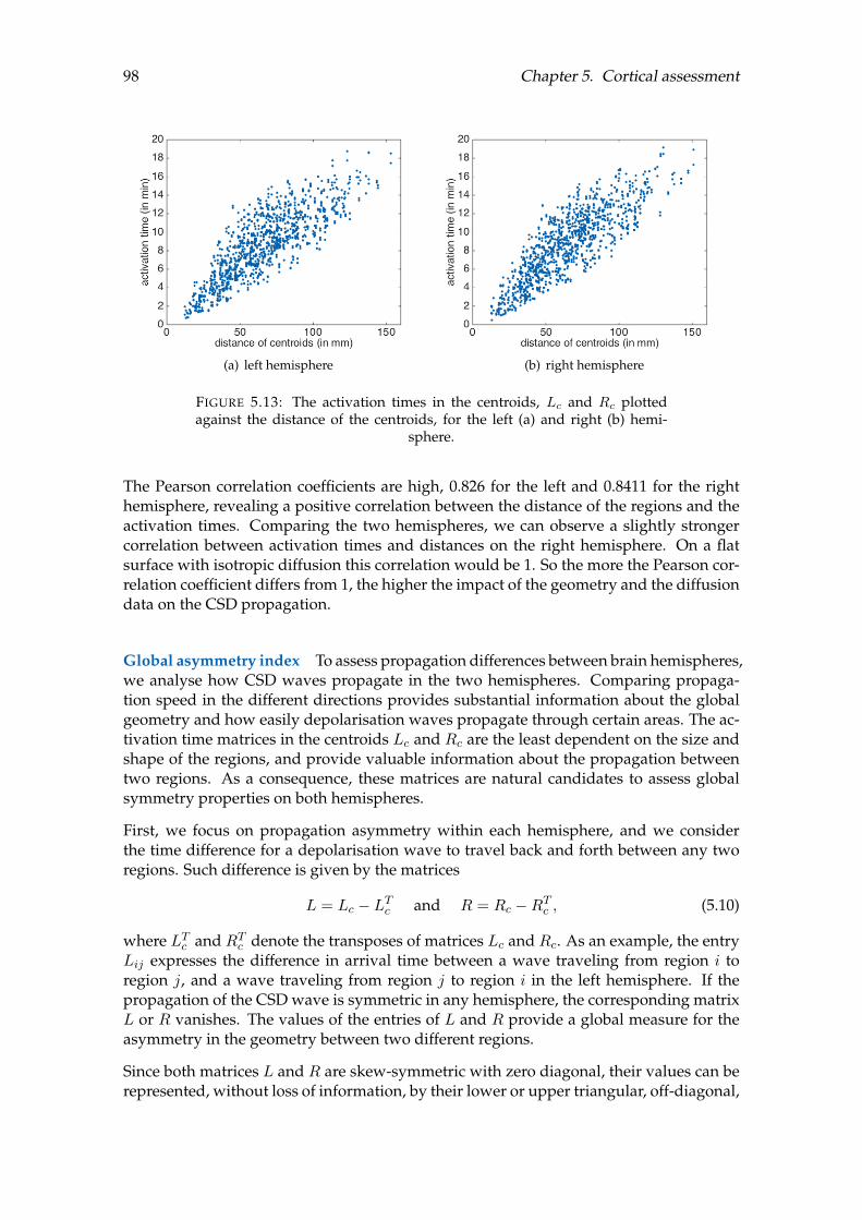
98 Chapter 5. Cortical assessment
(a) left hemisphere (b) right hemisphere
FIGURE 5.13: The activation times in the centroids, Lc and Rc plottedagainst the distance of the centroids, for the left (a) and right (b) hemi-
sphere.
The Pearson correlation coefficients are high, 0.826 for the left and 0.8411 for the righthemisphere, revealing a positive correlation between the distance of the regions and theactivation times. Comparing the two hemispheres, we can observe a slightly strongercorrelation between activation times and distances on the right hemisphere. On a flatsurface with isotropic diffusion this correlation would be 1. So the more the Pearson cor-relation coefficient differs from 1, the higher the impact of the geometry and the diffusiondata on the CSD propagation.
Global asymmetry index To assess propagation differences between brain hemispheres,we analyse how CSD waves propagate in the two hemispheres. Comparing propaga-tion speed in the different directions provides substantial information about the globalgeometry and how easily depolarisation waves propagate through certain areas. The ac-tivation time matrices in the centroids Lc and Rc are the least dependent on the size andshape of the regions, and provide valuable information about the propagation betweentwo regions. As a consequence, these matrices are natural candidates to assess globalsymmetry properties on both hemispheres.
First, we focus on propagation asymmetry within each hemisphere, and we considerthe time difference for a depolarisation wave to travel back and forth between any tworegions. Such difference is given by the matrices
L = Lc − LTc and R = Rc −RTc , (5.10)
where LTc and RTc denote the transposes of matrices Lc and Rc. As an example, the entryLij expresses the difference in arrival time between a wave traveling from region i toregion j, and a wave traveling from region j to region i in the left hemisphere. If thepropagation of the CSD wave is symmetric in any hemisphere, the corresponding matrixL or R vanishes. The values of the entries of L and R provide a global measure for theasymmetry in the geometry between two different regions.
Since both matrices L and R are skew-symmetric with zero diagonal, their values can berepresented, without loss of information, by their lower or upper triangular, off-diagonal,

5.3. Quantities of interest in CSD propagation 99
portion, combined in a single matrix G, whose entries are given by
Gij =
Lij for i > j0 for i = jRij for i < j
. (5.11)
MatrixG collects at once all the information on the lack of symmetry of both hemispheres,that can be compared in a single plot, see Figure 5.14. For the cortical geometry at hand,we can observe significant asymmetries in both hemispheres, in particular in the neigh-bourhood of the postcentral region in the left hemisphere and the superiortemporal re-gion in the right hemisphere.
FIGURE 5.14: The time difference of the depolarisation wave to propagatebetween two regions back and forth. The lower triangle gives the valuesof the left hemisphere and the upper triangle the values for the right hemi-
sphere.
To quantify the lack of symmetry in the propagation, we consider the normalised differ-ence matrices L and R, whose (i, j)-th entries are defined as
Lij =
0, for i = j
Lij(Lc)ij
, for i 6= j, Rij =
0, for i = j
Rij(Rc)ij
, for i 6= j. (5.12)
We denote by lj and rj the mean of the j-th column of matrix L and R, respectively. Foreach region j, positive values of lj (or rj) indicate that depolarisation waves moving awayfrom the region are faster than depolarisation waves approaching that region. A positivemean lj (respectively, rj) implies that the corresponding region is, in general, behaving asa source (or a facilitator) for the propagation of a depolarisation wave, while a negativemean implies that the region is behaving as a sink for the propagation. In Figure 5.15we summarise in the same plot the means lj and rj and identify regions that exhibit
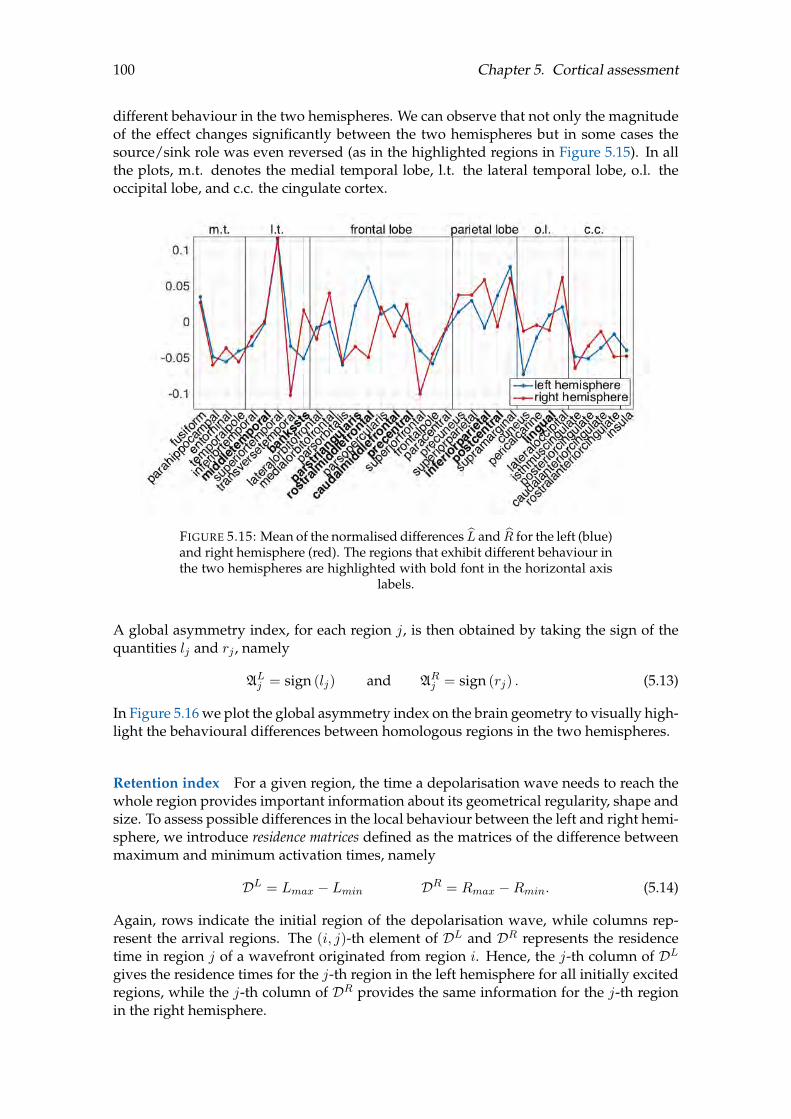
100 Chapter 5. Cortical assessment
different behaviour in the two hemispheres. We can observe that not only the magnitudeof the effect changes significantly between the two hemispheres but in some cases thesource/sink role was even reversed (as in the highlighted regions in Figure 5.15). In allthe plots, m.t. denotes the medial temporal lobe, l.t. the lateral temporal lobe, o.l. theoccipital lobe, and c.c. the cingulate cortex.
FIGURE 5.15: Mean of the normalised differences L and R for the left (blue)and right hemisphere (red). The regions that exhibit different behaviour inthe two hemispheres are highlighted with bold font in the horizontal axis
labels.
A global asymmetry index, for each region j, is then obtained by taking the sign of thequantities lj and rj , namely
ALj = sign (lj) and ARj = sign (rj) . (5.13)
In Figure 5.16 we plot the global asymmetry index on the brain geometry to visually high-light the behavioural differences between homologous regions in the two hemispheres.
Retention index For a given region, the time a depolarisation wave needs to reach thewhole region provides important information about its geometrical regularity, shape andsize. To assess possible differences in the local behaviour between the left and right hemi-sphere, we introduce residence matrices defined as the matrices of the difference betweenmaximum and minimum activation times, namely
DL = Lmax − Lmin DR = Rmax −Rmin. (5.14)
Again, rows indicate the initial region of the depolarisation wave, while columns rep-resent the arrival regions. The (i, j)-th element of DL and DR represents the residencetime in region j of a wavefront originated from region i. Hence, the j-th column of DLgives the residence times for the j-th region in the left hemisphere for all initially excitedregions, while the j-th column of DR provides the same information for the j-th regionin the right hemisphere.
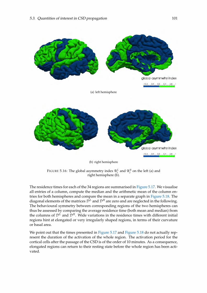
5.3. Quantities of interest in CSD propagation 101
(a) left hemisphere
(b) right hemisphere
FIGURE 5.16: The global asymmetry index ALj and AR
j on the left (a) andright hemisphere (b).
The residence times for each of the 34 regions are summarised in Figure 5.17. We visualiseall entries of a column, compute the median and the arithmetic mean of the column en-tries for both hemispheres and compare the mean in a separate graph in Figure 5.18. Thediagonal elements of the matricesDL andDR are zero and are neglected in the following.The behavioural symmetry between corresponding regions of the two hemispheres canthus be assessed by comparing the average residence time (both mean and median) fromthe columns of DL and DR. Wide variations in the residence times with different initialregions hint at elongated or very irregularly shaped regions, in terms of their curvatureor basal area.
We point out that the times presented in Figure 5.17 and Figure 5.18 do not actually rep-resent the duration of the activation of the whole region. The activation period for thecortical cells after the passage of the CSD is of the order of 10 minutes. As a consequence,elongated regions can return to their resting state before the whole region has been acti-vated.

102 Chapter 5. Cortical assessment
(a) left hemisphere
(b) right hemisphere
FIGURE 5.17: Duration of stay of the depolarisation wave for the regions ofthe left (a) and right (b) hemisphere. The red markers denote the median,
the green ones the arithmetic mean.
Comparing the average retention times (Figure 5.18), we can observe more similaritiesbetween the two hemispheres than in the previously observed back and forth propaga-tion. A few regions exhibit appreciably different behaviour, likely the consequence of thelack of anatomical symmetry between the two hemispheres. Looking at this differencevisually such regions are the middletemporal, the medialorbitofrontal, the parsopercu-laris, the frontalpole and the pericalcarine. From Figure 5.18 we can observe that, for thecortical geometry at hand, the major differences are localised in the frontal lobe and inthe cingulate cortex.
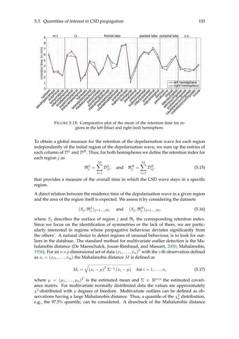
5.3. Quantities of interest in CSD propagation 103
FIGURE 5.18: Comparative plot of the mean of the retention time for re-gions in the left (blue) and right (red) hemisphere.
To obtain a global measure for the retention of the depolarisation wave for each regionindependently of the initial region of the depolarisation wave, we sum up the entries ofeach column ofDL andDR. Thus, for both hemispheres we define the retention index foreach region j as
RLj =
34∑i=1
DLij , and RRj =
34∑i=1
DRij , (5.15)
that provides a measure of the overall time in which the CSD wave stays in a specificregion.
A direct relation between the residence time of the depolarisation wave in a given regionand the area of the region itself is expected. We assess it by considering the datasets
(Sj ,RLj )j=1,...,34, and (Sj ,R
Rj )j=1,...,34, (5.16)
where Sj describes the surface of region j and Rj the corresponding retention index.Since we focus on the identification of symmetries or the lack of them, we are partic-ularly interested in regions whose propagative behaviour deviates significantly fromthe others’. A natural choice to detect regions of unusual behaviour, is to look for out-liers in the database. The standard method for multivariate outlier detection is the Ma-halanobis distance (De Maesschalck, Jouan-Rimbaud, and Massart, 2000; Mahalanobis,1936). For an n×p dimensional set of data (x1, . . . , xn)T with the i-th observation definedas xi = (xi1, . . . , xip) the Mahalanobis distance M is defined as
Mi =
√(xi − µ)T Σ−1 (xi − µ) for i = 1, . . . , n, (5.17)
where µ = (µ1, . . . , µn)T is the estimated mean and Σ ∈ Rp×p the estimated covari-ance matrix. For multivariate normally distributed data the values are approximatelyχ2-distributed with p degrees of freedom. Multivariate outliers can be defined as ob-servations having a large Mahalanobis distance. Thus, a quantile of the χ2
p distribution,e.g., the 97.5% quantile, can be considered. A drawback of the Mahalanobis distance

104 Chapter 5. Cortical assessment
is that it uses the classical estimators for mean and covariance, which can be highly af-fected by outlying values. In order to obtain more reliable results for the data analysis,more robust estimators are required. The minimum covariance determinant estimator ismost frequently used and can be computed with a fast algorithm (Rousseeuw and VanDriessen, 1999). Using robust estimators of location and scatter in equation (5.17) we ob-tain the so-called robust distance (Rousseeuw and Van Zomeren, 1990; Rousseeuw andVan Zomeren, 1991).
In Figure 5.19 we visualise the relationship between the surface of a region and its reten-tion index. We plot the size against the retention index and the robust tolerance ellipsedescribing the 97.5% quantile for the datasets of the left and right hemisphere. The Ma-halanobis distance and the robust distance can be compared in a distance - distance plot.In both graphs the 97.5% quantile of the χ2
2-distribution is drawn as a threshold valueand the numbers mark the six maximum distances and refer to the index of the datasetand thus the index of the regions. For a list of the indices and the corresponding regions,we refer to Table D.3.
(a) left hemisphere (b) right hemisphere
FIGURE 5.19: The tolerance ellipse (top row) of the 97.5% quantile for therobust distance and a distance - distance plot (bottom row) comparing Ma-halanobis distance and robust distance for the surface - retention indexdata of the left (a) and right (b) hemisphere. The numbers refer to the in-
dex of the datasets and the red lines mark the 97.5% quantile.
In Table 5.5 we list the detected outliers as well as the names corresponding to the in-dices of the regions. The rostalmiddlefrontal, the superiorfrontal, the superiorparietal,the interiorparietal and the lateraloccipital region in both hemispheres are identified as
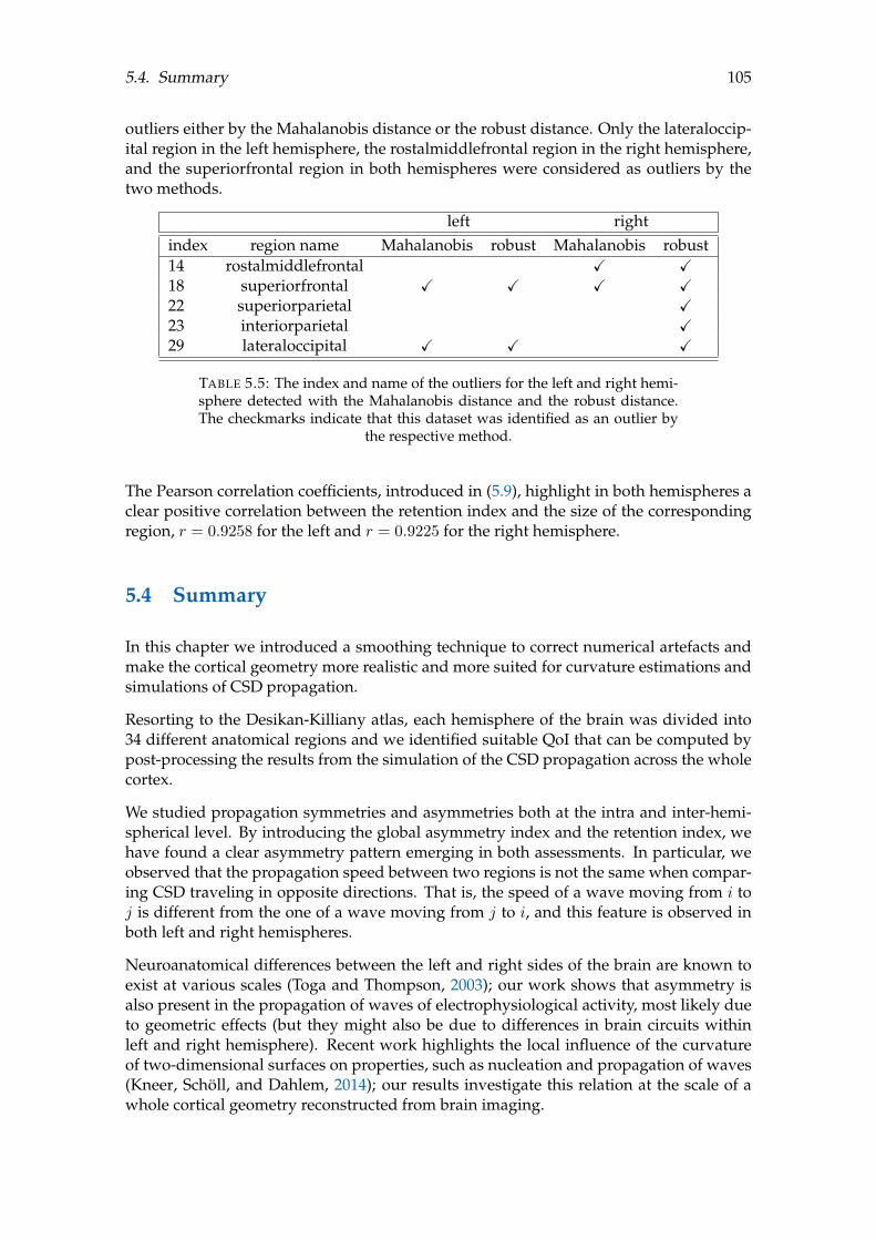
5.4. Summary 105
outliers either by the Mahalanobis distance or the robust distance. Only the lateraloccip-ital region in the left hemisphere, the rostalmiddlefrontal region in the right hemisphere,and the superiorfrontal region in both hemispheres were considered as outliers by thetwo methods.
left rightindex region name Mahalanobis robust Mahalanobis robust14 rostalmiddlefrontal X X18 superiorfrontal X X X X22 superiorparietal X23 interiorparietal X29 lateraloccipital X X X
TABLE 5.5: The index and name of the outliers for the left and right hemi-sphere detected with the Mahalanobis distance and the robust distance.The checkmarks indicate that this dataset was identified as an outlier by
the respective method.
The Pearson correlation coefficients, introduced in (5.9), highlight in both hemispheres aclear positive correlation between the retention index and the size of the correspondingregion, r = 0.9258 for the left and r = 0.9225 for the right hemisphere.
5.4 Summary
In this chapter we introduced a smoothing technique to correct numerical artefacts andmake the cortical geometry more realistic and more suited for curvature estimations andsimulations of CSD propagation.
Resorting to the Desikan-Killiany atlas, each hemisphere of the brain was divided into34 different anatomical regions and we identified suitable QoI that can be computed bypost-processing the results from the simulation of the CSD propagation across the wholecortex.
We studied propagation symmetries and asymmetries both at the intra and inter-hemi-spherical level. By introducing the global asymmetry index and the retention index, wehave found a clear asymmetry pattern emerging in both assessments. In particular, weobserved that the propagation speed between two regions is not the same when compar-ing CSD traveling in opposite directions. That is, the speed of a wave moving from i toj is different from the one of a wave moving from j to i, and this feature is observed inboth left and right hemispheres.
Neuroanatomical differences between the left and right sides of the brain are known toexist at various scales (Toga and Thompson, 2003); our work shows that asymmetry isalso present in the propagation of waves of electrophysiological activity, most likely dueto geometric effects (but they might also be due to differences in brain circuits withinleft and right hemisphere). Recent work highlights the local influence of the curvatureof two-dimensional surfaces on properties, such as nucleation and propagation of waves(Kneer, Schöll, and Dahlem, 2014); our results investigate this relation at the scale of awhole cortical geometry reconstructed from brain imaging.

106 Chapter 5. Cortical assessment
We have also identified brain regions whose behaviour significantly differs from the otherregions. In particular, some regions appear to trap the propagating depolarisation wavefor a longer time. The outliers in the relation between retention index and region sizesare strong candidates to identify areas that may play a vital role in CSD propagation.Such information would be relevant to design therapies using cortical neuromodulation,where target structures for modulation have to be carefully selected.
107
Chapter 6
Clinical applications
“It is important to understand what you can do before you learn to measure how well you seem to havedone it.”
John W. Tukey, in Exploratory Data Analysis (1977)
The simulation of CSD propagation on a personalised cortical geometry in Chapter 4 andthe introduction of QoI in Chapter 5 served as a proof of concept. As a next step, weapply these techniques to a set of patient data with the aim to find significant differencesbetween migraine patients and control groups. In a first case study, we simulate CSDpropagation on the cortices of chronic migraine patients with aura to assess the correla-tion of the symptoms they experience during a migraine attack with the CSD wavefrontpropagation. Then, in a group analysis, we compare different patient groups in terms ofCSD propagation and the QoI introduced in the previous chapter. With these applica-tions, we want to investigate the impact of the geometry on the CSD propagation and itscorrelation to migraine (with aura).
The data set for the initial case study and the ones for the group analysis were providedfrom different healthcare institutions and were acquired with different machines, at dif-ferent magnetic field strengths. Although we have access to various data sets, we haveto evaluate them independently of one another. In fact, we cannot set magnetic reso-nance imaging (MRI) and diffusion tensor imaging (DTI) data acquired from differentmachines or with different field strengths side by side because cortical reconstruction re-sults obtained with FreeSurfer corresponding to different machine brands and magneticfield strengths are not comparable.
In this chapter we will first comment on the consistency of brain reconstruction withFreeSurfer and the comparability of the results with different acquisition and processingmodes. Subsequently, we discuss the case study of the chronic migraine patients withaura and perform a group analysis for migraine patients without aura, abusive painkillerusers and a control group. The aim is to explore if the QoI provide a good indicator todistinguish between patient groups.
All the data used in this chapter was provided in MRI and DTI or diffusion-weightedimaging (DWI) raw format and had to be processed in order to extract the cortical geom-etry and the diffusion values at all mesh points of the triangulated cortical surface. Forthe first case study the conductivity tensors were provided in the form of DWI data, whilein the groups study DTI data was available. For the analysis carried out in this chapter,we use the FreeSurfer image analysis suit. In Appendix C, we give an introduction to
108 Chapter 6. Clinical applications
MRI, DWI and DTI data processing and provide detailed information on the programsand functions involved as well as the corresponding code.
6.1 Comparability of brain cortex reconstructions
Several studies have reported that FreeSurfer brain reconstructions from T1-weightedimages and diffusion data from DTI images depend on different factors that vary in theirimpact on the reconstruction results. For example, the acquisition platform and magneticfield strength, the FreeSurfer version, operating system and its version were found toaffect in different measure the cortical reconstruction and the corresponding diffusiondata. However, the latter two do not have such a significant impact on the reconstructionresults as the acquisition platform and the field strength. Despite these limitations, weuse FreeSurfer for the brain reconstruction as it is widely used in practice and an open-source software.
Jovicich et al., 2009 assessed the volume differences in specific regions as a measure tocompare brain reconstruction results on different platforms (Siemens, GE) and with dif-ferent field strengths and scanner upgrades. They concluded that automated segmenta-tion of T1 images is reliable within the same scanner platform, even after updates. How-ever, combining data across platforms and field strength introduces bias. Souza et al.,2018 consider the results of different skull stripping programs, i.e., advanced normal-ization tools1 (ANTs) and the brain extraction tool2 (BET) for MRI images recorded withmachines of different vendors and different field strength. Their findings support the factthat scanner vendors and magnetic field strength have a significant impact on the brainextraction results. In another study, Gronenschild et al., 2012 found that workstation andMacOS version only have a small impact on the anatomical volume and cortical thicknessin the FreeSurfer results. However, the FreeSurfer version has a more significant effecton the results.
The comparability of diffusion data obtained from DTI imaging with different acquisitionmodes seems controversial. Even though Brander and collaborators found only small dif-ferences in the mean fractional anisotropy (FA) and apparent diffusion coefficient (ADC)values when comparing data acquired with different field strengths, other studies provedthat ADC values were statistically significantly lower at 3 Tesla compared with 1.5 Teslaand FA values were statistically significantly higher at 3 Tesla compared with 1.5 Tesla(Brander et al., 2010; Huisman et al., 2006; Sasaki et al., 2008).
Consequently, we are going to treat separately the two data sets obtained with differentplatforms (Siemens Magnetom Aera, Phillips Achieva) and different field strengths (1.5T and 3 T, respectively) and only compare them with the corresponding control data setobtained with the same acquisition modalities.
6.2 Case study on single patients
For this study, performed in collaboration with Dr. Marina de Tommaso at the Policlinicodi Bari in Italy, the available data set consisted of five migraine patients with aura. For
1http://stnava.github.io/ANTs/2https://fsl.fmrib.ox.ac.uk/fsl/fslwiki/BET

6.2. Case study on single patients 109
the sake of anonymity, we refer to them as Subject 1 to Subject 5. Together with MRIand DWI imaging data of all the patients, a sequence of eloquent areas during a migraineattack marked on the brain cortex was provided as well as the corresponding symptoms.To avoid displaying the pictures for all five patients, we comment on the results of allof them but only provide a detailed description and illustrations for Subject 1. Informa-tion about the clinical symptoms and visualisations of results for all other patients arereported in Appendix D.
Subject 1 has been suffering from migraine with aura for nine years and experiences onaverage 5 migraine attacks with aura per month. In the course of a migraine attack, thispatient reports luminous scotoma in the central visual field followed by a scotoma in theright half of the visual field. These visual symptoms are proceeded by temporary rightand left paresthesia (abnormal dermal sensation like tingling, burning or numb sensa-tions in the extremities) and transitory aphasia and apraxia. Aphasia refers to the inabilityto comprehend and formulate language, while apraxia is a motor disorder in which thepatient has difficulties with the motor planning to perform tasks or movements. Theseaura symptoms can be related to specific cortical areas: the left visual cortex, bilateral so-matosensory cortex and left Broca’s area. These regions correspond to the Brodmann ar-eas (BA) 17/18, 1-4 and 44/45. In Figure 6.1 the eloquent areas are marked in orange andthe numbers indicate the sequence during a migraine attack for Subject 1. The areas thatare involved and correspond to the specific symptoms differ between the hemispheresand patients. The list of migraine symptoms, information about the clinical history andthe eloquent regions for all patients are summarised in Table D.1 and Table D.2.
FIGURE 6.1: The eloquent areas (orange) in a migraine attack of Subject 1.The numbers refer to the sequence of symptoms.
6.2.1 MRI and DWI data
The data set corresponds to four female and one male subject, with an age of 27.4 ± 9(range 21 - 43) years, suffering from chronic migraine with aura. The acquisition wasperformed at the Santissima Annunziata Hospital, Taranto, Italy and was approved bythe local ethics committee. Data was acquired with a Siemens Magnetom Aera 1.5 Tscanner using a T1-weighted 3D sequence with the following parameters: TR = 2650ms, TE = 106 ms; flip angle = 10; parallel imaging (mSENSE) acceleration factor = 1.5;

110 Chapter 6. Clinical applications
acquisition matrix size = 256 × 256; FoV = 260 × 260 mm, slice thickness = 1.1 mm, and176 contiguous sections. The DWI data was acquired with the same scanner using adiffusion-weighted 2D sequence with the following parameters: TR = 2650 msec, TE =106 msec; flip angle = 90; acquisition matrix size = 192 × 192 ; FoV = 229 × 229 mm, andslice thickness = 5 mm, and 23 contiguous sections.
The control data set consists of seven patients, corresponding to three female and fourmale subjects with an age of 36.7 ± 9.9 (range 23 - 54) years also acquired at the Santis-sima Annunziata Hospital, Taranto in Italy. The local ethics committee approved the ac-quisition and the data was obtained with the same machine and parameters listed abovefor the migraine patients.
6.2.2 Data processing
The cortical geometries were obtained from the high-resolution anatomical MRI withthe FreeSurfer image analysis suit. The brain reconstruction process was run with theFreeSurfer version 5.3.0 on BCAM’s in-house cluster Hipatia featuring at that time 18nodes (1 with Nvidia Tesla K40 GPU) for 624 cores with 4TB RAM and Infiniband net-work connectivity using CentOS 7, 64 bits. For the sake of comparability, all reconstruc-tions were run on the same node of the cluster with 32 cores (2xProcessor Intel(R) Xeon(R)CPU E5-2683 v4 @ 2.10 GHz with 16 cores) and 256 GB RAM. For further information onthe brain reconstruction procedure, we refer to Appendix C.3.
For the identification of the ROI, we use the lh.BA.annot and rh.BA.annot files gener-ated by the FreeSurfer reconstruction, which provide the labels for the essential Brod-mann areas (Brodmann, 2006). The BA listed in this annotation file include the primarysomatosensory cortex (BA 1-3), the primary motor cortex (BA 4), Broca’s area (BA 44, BA45) and the visual cortex (V1, V2 or BA 17, BA 18, respectively).
The DWI data was processed with the FSL software3. First, an eddy current correctionwas applied to correct the changes produced by the variations in gradient field directionsduring the acquisition and to overcome the artefacts produced by head motion. TheT1 and DWI brain data were extracted with BET using a fractional intensity thresholdof 0.3. Then, a local fitting of the DWI data was applied to compute the tensor modelat each voxel. For each voxel, the DWI data provided the mean diffusion strength ofwater molecules within brain tissues. To project this data onto the mesh obtained withFreeSurfer from the T1 image, a linear transformation between the T1 image and theADC map was computed using 6 degrees of freedom and taking the mutual informationas the cost function. Then, the transformation from T1 native space to the FreeSurferstructure space was computed with the FreeSurfer tkregister2 function. Combining thesetransformation matrices and applying them to the ADC data, the values in the FreeSurferspace were obtained. Finally, the FreeSurfer function mri_vol2surf was used to projectthe diffusion data onto the brain mesh with a projection fraction of 0.5 to sample in themiddle of the cortical surface and prevent bias from the white matter or the extracerebralfluid. For more details on the processing of DWI data with FSL, see Appendix C.4.
3http://fsl.fmrib.ox.ac.uk/
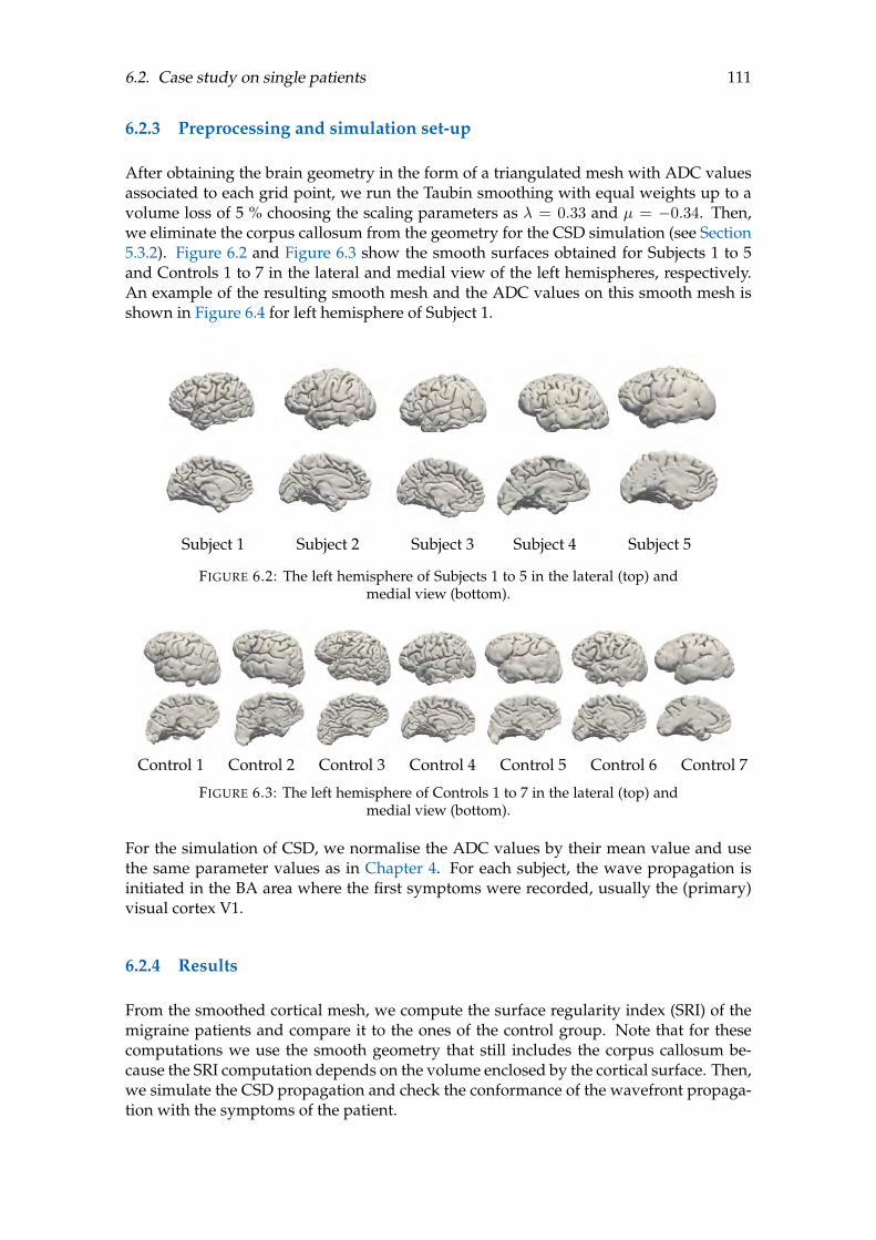
6.2. Case study on single patients 111
6.2.3 Preprocessing and simulation set-up
After obtaining the brain geometry in the form of a triangulated mesh with ADC valuesassociated to each grid point, we run the Taubin smoothing with equal weights up to avolume loss of 5 % choosing the scaling parameters as λ = 0.33 and µ = −0.34. Then,we eliminate the corpus callosum from the geometry for the CSD simulation (see Section5.3.2). Figure 6.2 and Figure 6.3 show the smooth surfaces obtained for Subjects 1 to 5and Controls 1 to 7 in the lateral and medial view of the left hemispheres, respectively.An example of the resulting smooth mesh and the ADC values on this smooth mesh isshown in Figure 6.4 for left hemisphere of Subject 1.
Subject 1 Subject 2 Subject 3 Subject 4 Subject 5
FIGURE 6.2: The left hemisphere of Subjects 1 to 5 in the lateral (top) andmedial view (bottom).
Control 1 Control 2 Control 3 Control 4 Control 5 Control 6 Control 7
FIGURE 6.3: The left hemisphere of Controls 1 to 7 in the lateral (top) andmedial view (bottom).
For the simulation of CSD, we normalise the ADC values by their mean value and usethe same parameter values as in Chapter 4. For each subject, the wave propagation isinitiated in the BA area where the first symptoms were recorded, usually the (primary)visual cortex V1.
6.2.4 Results
From the smoothed cortical mesh, we compute the surface regularity index (SRI) of themigraine patients and compare it to the ones of the control group. Note that for thesecomputations we use the smooth geometry that still includes the corpus callosum be-cause the SRI computation depends on the volume enclosed by the cortical surface. Then,we simulate the CSD propagation and check the conformance of the wavefront propaga-tion with the symptoms of the patient.

112 Chapter 6. Clinical applications
(a) mesh reconstructed from T1-weighted image
(b) ADC values on the surface mesh
FIGURE 6.4: The smoothed mesh reconstructed from T1-weighted image(a) and the ADC values on the surface mesh after taking out the corpus
callosum (b) for the left hemisphere of Subject 1.
Surface regularity index We compute the SRI, introduced in Section 5.2, for the mi-graine and control data and visualise it in the form of a box plot in Figure 6.5. The centralred mark indicates the median, the bottom and top edges of the blue box indicate the25th and 75th percentiles, respectively, and the whiskers extend to the most extreme datapoints that are not considered outliers.
From Figure 6.5 we cannot conclude directly that the SRI of migraine patients is signif-icantly different from the one of the control patients. The box plots already hint at dif-ferent means but the ranges of SRI values are similar. For further investigation, we testfor similar distribution of the two data sets. Because the data sets have different sizes, 5and 7 data points, respectively, and are samples from a bigger sample set whose meanand variance are unknown, we test the hypothesis that the two populations have equalmeans. For this purpose, we use an adaptation of Student’s t-test, called Welch’s t-test thatis more reliable when the two samples have unequal variances or unequal sample sizes(Welch, 1947). This is done in Matlab via the function ttest2 with the option Vartype =’unequal’. First, we consider left and right hemisphere for the two groups separately. The

6.2. Case study on single patients 113
(a) left and right hemisphere (b) whole brain
FIGURE 6.5: Box plots of the surface regularity index of the migraine andcontrol group differentiating between left and right hemisphere (a) and
considering the whole brain (b).
p-value of a test for equal means of the SRI of migraine patients and the control group inthe left hemispheres is 0.8483 and in the right hemisphere 0.8764. Then we distinguishsimply between patient groups by merging the SRI of left and right hemisphere in onedata set for migraine patients and control, respectively. Thus, the data sets consist of 10and 14 observations, respectively, and by applying the Welch’s t-test we obtain a p-valueof 0.7947. These high p-values indicate weak evidence against the hypothesis of equalmeans. Consequently, we cannot say that the data sets are significantly different.
Having a closer look at the reconstructed surfaces one could argue that the cortex of thelast patient of each group is not as well reconstructed as the rest, featuring less gyri andin general a smoother cortical surface, see Figure 6.2 and Figure 6.3. We can considerthose as outliers due to reconstruction error and visualise the data without the outliers ina box plot in Figure 6.6. Once more, we visualise the SRI of the left and right hemisphereseparately for the migraine patients (Subjects 1-4) and the control group (Controls 1-6) inthe first box plot and join the data of the two hemispheres in the second box plot.
Figure 6.6 shows slightly more different SRI values between the two groups and lessextreme data points compared to Figure 6.5. With this reduced data set we test the hy-pothesis that the two populations have equal means with the Welch’s t-test. The lowestp-value is obtained when considering left and right hemisphere together for the migraineand the control group, namely 0.3832. This p-value is still high and we cannot reject thehypothesis on a significant level. Hence, these tests confirm what could already be ex-pected from the box plots that we cannot make a reliable statement about the distributionof the data and cannot prove a significant difference between the SRI of migraine patientsand the control patient group.
CSD simulation Simulating the CSD propagation, we record the arrival time of thewavefront at every node as described in Section 5.3.
We visualise the arrival times of the wave on both the left and the right hemisphere forSubject 1 in Figure 6.7. Even though the CSD wave spreads across the whole cortex, onlythe BA involved in the migraine attack are coloured by the arrival time of the CSD wave.It can be observed that the temporal progression of the wave starting in the visual cortex

114 Chapter 6. Clinical applications
(a) left and right hemisphere (b) whole brain
FIGURE 6.6: Box plots of the surface regularity index of the migraine andcontrol group, just considering Subjects 1-4 and Controls 1-6. We differen-tiate between left and right hemisphere (a) and consider the whole brain
(b).
matches the sequence of the regions involved in the migraine attack, see Figure 6.1. Fromthe visual cortex the wave propagates to the somatosensory cortex (BA 1-3) and Broca’sarea (BA 44/45).
Considering the CSD propagation in Subjects 2 to 5 (see Appendix D) we can observethat for all patients the simulated CSD wave arrives in the eloquent areas in the sequencedescribed by the patients during a migraine attack with only some minor exceptions. Forexample, in the right hemisphere of Subject 4 and of Subject 5 we do not observe thefull sequence because only BA 17 and 18 are involved in the migraine attack. Moreover,in the left hemisphere of Subject 4, BA 1-4 and 44 are reached by the CSD wave nearlysimultaneously. Although, we lack data about the exact timing of the appearance ofdifferent symptoms, we can conclude that the simulated CSD wavefront propagationmatches the sequence of the affected areas during a migraine attack in all patients.
To sum up the CSD propagation behaviour and structure of the cortical geometry, welist the maximum time the wave takes to spread across the whole cortex (propagationtime), the surface area, the SRI and the propagation speed for all migraine patients inTable 6.1. The propagation speed describes the amount of space invaded in a certainamount of time. To demonstrate how these values relate to each other, we visualise thedata for Subjects 1 to 5 in the correlation plot of Figure 6.8. In this graph, we plot the5 observations for each pair of variables for the left hemisphere in the lower triangularpart of the plot and for the right hemisphere in the upper triangular part. The Pearsoncorrelation coefficients (see equation (5.9)) are given in each subplot and coefficients witha p-value below 0.05 are marked in red. The red lines show the linear regression for thegiven data points.
In Figure 6.8 we can observe a significant correlation between the surface area and thepropagation time, and between the propagation speed and the SRI in both hemispheres.Some correlations are more natural, like surface area, propagation speed, and SRI as thedefinitions of propagation speed and SRI both involve the surface area. The propagationspeed also relates by definition to the propagation time. Only in the right hemispherewe can observe a significant (negative) correlation between the propagation time and theSRI. The closer the SRI is to 1 the closer the geometry is a sphere. If the SRI is smaller,
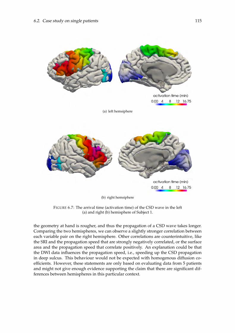
6.2. Case study on single patients 115
(a) left hemsiphere
(b) right hemsiphere
FIGURE 6.7: The arrival time (activation time) of the CSD wave in the left(a) and right (b) hemisphere of Subject 1.
the geometry at hand is rougher, and thus the propagation of a CSD wave takes longer.Comparing the two hemispheres, we can observe a slightly stronger correlation betweeneach variable pair on the right hemisphere. Other correlations are counterintuitive, likethe SRI and the propagation speed that are strongly negatively correlated, or the surfacearea and the propagation speed that correlate positively. An explanation could be thatthe DWI data influences the propagation speed, i.e., speeding up the CSD propagationin deep sulcus. This behaviour would not be expected with homogenous diffusion co-efficients. However, these statements are only based on evaluating data from 5 patientsand might not give enough evidence supporting the claim that there are significant dif-ferences between hemispheres in this particular context.
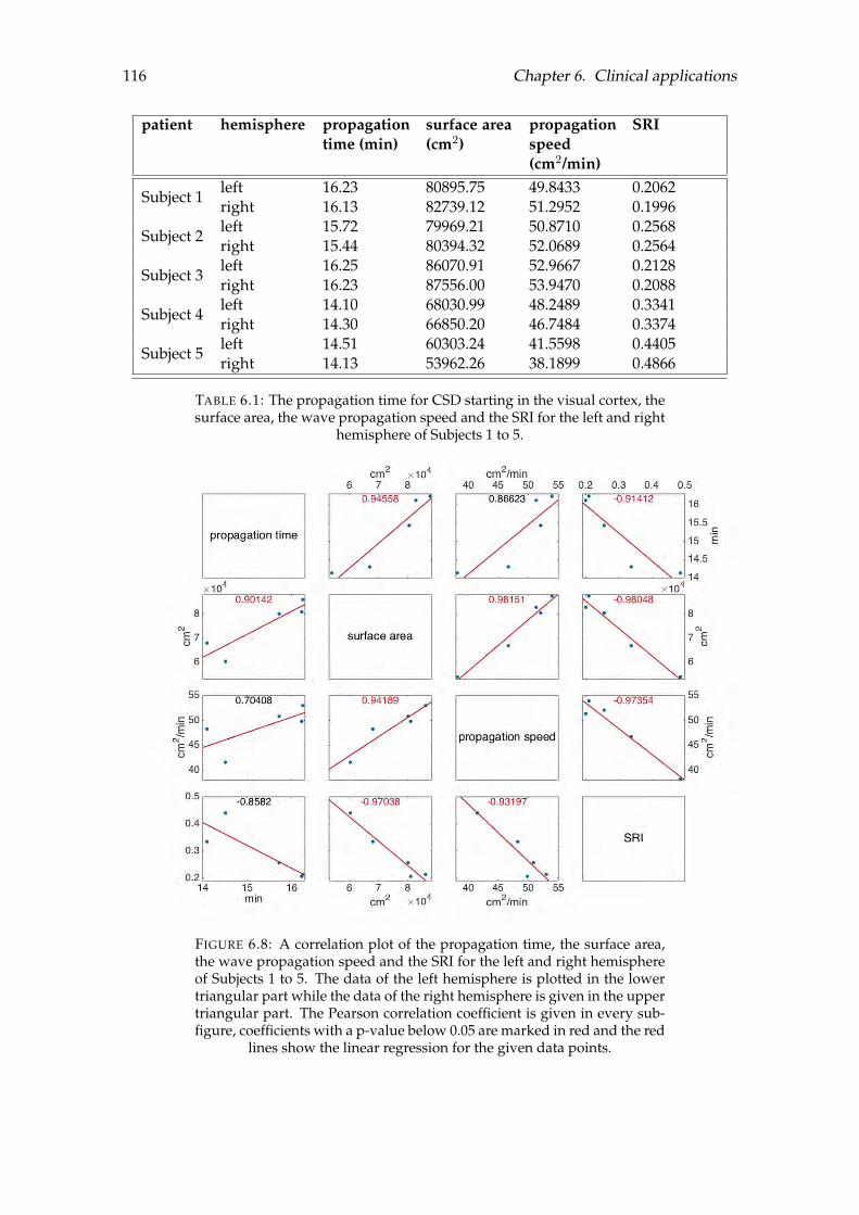
116 Chapter 6. Clinical applications
patient hemisphere propagationtime (min)
surface area(cm2)
propagationspeed(cm2/min)
SRI
Subject 1left 16.23 80895.75 49.8433 0.2062right 16.13 82739.12 51.2952 0.1996
Subject 2left 15.72 79969.21 50.8710 0.2568right 15.44 80394.32 52.0689 0.2564
Subject 3left 16.25 86070.91 52.9667 0.2128right 16.23 87556.00 53.9470 0.2088
Subject 4left 14.10 68030.99 48.2489 0.3341right 14.30 66850.20 46.7484 0.3374
Subject 5left 14.51 60303.24 41.5598 0.4405right 14.13 53962.26 38.1899 0.4866
TABLE 6.1: The propagation time for CSD starting in the visual cortex, thesurface area, the wave propagation speed and the SRI for the left and right
hemisphere of Subjects 1 to 5.
FIGURE 6.8: A correlation plot of the propagation time, the surface area,the wave propagation speed and the SRI for the left and right hemisphereof Subjects 1 to 5. The data of the left hemisphere is plotted in the lowertriangular part while the data of the right hemisphere is given in the uppertriangular part. The Pearson correlation coefficient is given in every sub-figure, coefficients with a p-value below 0.05 are marked in red and the red
lines show the linear regression for the given data points.
6.3. Patient group analysis 117
6.3 Patient group analysis
For the second study, performed in collaboration with Marian Gomez Beldarrain fromthe Department of Neurology at the Hospital Galdakao-Usansolo in Spain, the availabledata set consisted of 52 patients.
6.3.1 MRI and DTI data
The data set is anonymised and corresponds to 18 migraine patients without aura, 15control patients, and 19 patients with chronic headache that have been abusively usingpainkillers. These patients have been taking analgesics at least 15 times per month ina period of more than three months. The data was acquired at the Hospital Galdakao-Usansolo in Spain, and its acquisition was approved by the local ethics committee. Thedata was obtained from a Philips 3 T Achieva system with a 32-channel head coil (PhilipsMedical Systems, Best, the Netherlands), and underwent an anatomical acquisition, ahigh-resolution structural T1-weighted 3D volume, using a spoiled gradient recalled se-quence (SPGR-3D) with the following parameters: TR = 7.4 msec, TE = 3.4 msec; flipangle 8; matrix size = 228 × 227; FoV = 250 × 250 mm; number of slices = 301; in-planeresolution = 1 × 1 × 1 mm; NSA 1; total acquisition time = 4 min 58 sec.
6.3.2 Data processing
The cortical geometry was obtained from anatomical MRI data with the FreeSurfer imageanalysis suit in the same set-up as defined previously in Section 6.2.2.
Instead of the Brodmann areas, we use the region label for the Desikan-Killiany atlasdefined in the lh.aparc.annot and rh.aparc.annot files generated by the FreeSurfer recon-struction providing (Desikan et al., 2006).
The DTI data processing with the FSL software is very similar to the one for DWI data.After extracting the T1 and DTI brain data with BET, a local fitting of the diffusion tensorwas applied to compute the tensor model at each voxel with the function DTIFIT fromthe FSL toolbox. For each voxel, the DTI data provided the three eigenvectors and theassociated eigenvalues of the diffusion. The final steps to obtain the diffusion data on thebrain mesh is identical for DWI and DTI data. In the case of DTI data this procedure hasto be applied to all eigenvalues and eigenvectors, instead of just the ADC values like forthe DWI data.
6.3.3 Preprocessing and simulation set-up
After obtaining the brain geometry in the form of a triangulated mesh with diffusiontensors, FA and MD values associated to each grid point, we run the Taubin smoothingwith equal weights up to a volume loss of 5 % choosing the scaling parameters as λ = 0.33and µ = 0.34. Then, we eliminate the corpus callosum from the geometry for the CSDsimulation (see Section 5.3.2). An example of a smooth surface and FA values of the 3D

118 Chapter 6. Clinical applications
(a) mesh reconstructed from T1-weighted image
(b) FA values on the surface mesh
FIGURE 6.9: The smoothed mesh reconstructed from T1-weighted image(a) and FA values on the surface mesh (b) for the left hemisphere of a pa-
tient from the migraine group.
diffusion data for a patient from the migraine group is shown in Figure 6.9 in the lateraland medial view of the left hemisphere.
For the simulation of CSD, we use the technique to obtain 2D diffusion data introducedin Section 4.2.3 and use the same parameter values as proposed in Chapter 3 and Chapter4. We initiate the wave propagation in all the ROI and record the arrival in each regions’centroid together with the minimum and maximum arrival times as described in Chap-ter 5.
6.3.4 Results
From the smoothed cortical mesh, we compute the SRI of the migraine patients and com-pare it to the ones of the other two groups. Note that for these computations we usethe smooth geometry that still includes the corpus callosum since the SRI computationdepends on the volume enclosed by the cortical surface. Then, we simulate the CSD
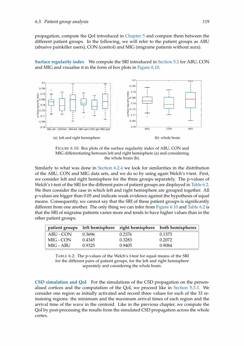
6.3. Patient group analysis 119
propagation, compute the QoI introduced in Chapter 5 and compare them between thedifferent patient groups. In the following, we will refer to the patient groups as ABU(abusive painkiller users), CON (control) and MIG (migraine patients without aura).
Surface regularity index We compute the SRI introduced in Section 5.2 for ABU, CONand MIG and visualise it in the form of box plots in Figure 6.10.
(a) left and right hemisphere (b) whole brain
FIGURE 6.10: Box plots of the surface regularity index of ABU, CON andMIG differentiating between left and right hemisphere (a) and considering
the whole brain (b).
Similarly to what was done in Section 6.2.4 we look for similarities in the distributionof the ABU, CON and MIG data sets, and we do so by using again Welch’s t-test. First,we consider left and right hemisphere for the three groups separately. The p-values ofWelch’s t-test of the SRI for the different pairs of patient groups are displayed in Table 6.2.We then consider the case in which left and right hemisphere are grouped together. Allp-values are bigger than 0.05 and indicate weak evidence against the hypothesis of equalmeans. Consequently, we cannot say that the SRI of these patient groups is significantlydifferent from one another. The only thing we can infer from Figure 6.10 and Table 6.2 isthat the SRI of migraine patients varies more and tends to have higher values than in theother patient groups.
patient groups left hemisphere right hemisphere both hemispheresABU - CON 0.3696 0.2376 0.1373MIG - CON 0.4345 0.3283 0.2072MIG - ABU 0.9325 0.9405 0.9084
TABLE 6.2: The p-values of the Welch’s t-test for equal means of the SRIfor the different pairs of patient groups, for the left and right hemisphere
separately and considering the whole brain.
CSD simulation and QoI For the simulations of the CSD propagation on the person-alised cortices and the computation of the QoI, we proceed like in Section 5.3.3. Weconsider one region as initially activated and record three values for each of the 33 re-maining regions: the minimum and the maximum arrival times of each region and thearrival time of the wave in the centroid. Like in the previous chapter, we compute theQoI by post-processing the results from the simulated CSD propagation across the wholecortex.
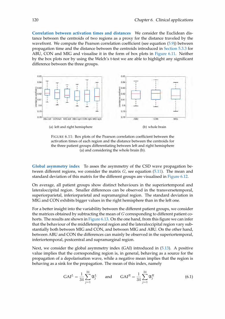
120 Chapter 6. Clinical applications
Correlation between activation times and distances We consider the Euclidean dis-tance between the centroids of two regions as a proxy for the distance traveled by thewavefront. We compute the Pearson correlation coefficient (see equation (5.9)) betweenpropagation time and the distance between the centroids introduced in Section 5.3.3 forABU, CON and MIG and visualise it in the form of box plots in Figure 6.11. Neitherby the box plots nor by using the Welch’s t-test we are able to highlight any significantdifference between the three groups.
(a) left and right hemisphere (b) whole brain
FIGURE 6.11: Box plots of the Pearson correlation coefficient between theactivation times of each region and the distance between the centroids forthe three patient groups differentiating between left and right hemisphere
(a) and considering the whole brain (b).
Global asymmetry index To asses the asymmetry of the CSD wave propagation be-tween different regions, we consider the matrix G, see equation (5.11). The mean andstandard deviation of this matrix for the different groups are visualised in Figure 6.12.
On average, all patient groups show distinct behaviours in the superiortemporal andlateraloccipital region. Smaller differences can be observed in the transversetemporal,superiorparietal, inferiorparietal and supramarginal region. The standard deviation inMIG and CON exhibits bigger values in the right hemisphere than in the left one.
For a better insight into the variability between the different patient groups, we considerthe matrices obtained by subtracting the mean ofG corresponding to different patient co-horts. The results are shown in Figure 6.13. On the one hand, from this figure we can inferthat the behaviour of the middletemporal region and the lateraloccipital region vary sub-stantially both between MIG and CON, and between MIG and ABU. On the other hand,between ABU and CON the differences can mainly be observed in the superiortemporal,inferiortemporal, postcentral and supramarginal region.
Next, we consider the global asymmetry index (GAI) introduced in (5.13). A positivevalue implies that the corresponding region is, in general, behaving as a source for thepropagation of a depolarisation wave, while a negative mean implies that the region isbehaving as a sink for the propagation. The mean of this index, namely
GAIL =1
34
34∑j=1
ALj and GAIR =1
34
34∑j=1
ARj (6.1)

6.3. Patient group analysis 121
(a) mean
(b) standard deviation
FIGURE 6.12: The mean (a) and standard deviation (b) of matrix G (5.11)for the different patient group: ABU, MIG and CON, respectively.
FIGURE 6.13: The difference in the mean of matrix G (5.11) between thedifferent patient groups: ABU, MIG and CON.
gives a way to summarise with only two values the source or sink nature of the consid-ered geometry in the CSD wave propagation for every patient. We visualise the GAI forthe three patient groups in box plots in Figure 6.14.
Again, from Figure 6.14 and using Welch’s t-test we cannot identify the GAI as a classifierto distinguish the patient groups.

122 Chapter 6. Clinical applications
(a) left and right hemisphere (b) whole brain
FIGURE 6.14: Box plots of the GAI for the three patient groups differentiat-ing between left and right hemisphere (a) and considering the whole brain
(b).
Retention index To assess possible differences in the local behaviour, we use the re-tention index (RI), introduced in (5.15). Because this index gives information about thespecific region, we take the mean over all the regions to obtain a value that describes thepropagation behaviour in each hemisphere of a patient, namely
RIL =1
34
34∑j=1
RLj , and RIR =
1
34
34∑j=1
RRj . (6.2)
We visualise the retention index for the different patient groups in the form of box plotsin Figure 6.15.
(a) left and right hemisphere (b) whole brain
FIGURE 6.15: Box plots of the RI for the three patient groups differentiatingbetween left and right hemisphere (a) and considering the whole brain (b).
Again, the box plots in Figure 6.15 and Welch’s t-test show that the retention times arenot significantly different between the patient cohorts.
Group classification using data mining So far we were unable to distinguish betweenthe patient groups but other techniques, i.e., in data mining might be able to do so. In-stead of considering every QoI independently, we consider the data of all QoI as a super-vised classification problem in machine learning. We can summarise all the QoI for the

6.3. Patient group analysis 123
different patient groups that we previously discussed in one data set with 52 observations(patients), the three (target) classes ABU, CON and MIG, and 414 numerical features: theaverage value and standard deviation (std) of the two curvature measures (introduced inSection 5.1), the global asymmetry index A, the GAI, the retention time R, the RI and theSRI. The GAI, RI and SRI are scalars describing each hemisphere of a patient, while theother features are values for each region of the left and right hemisphere, respectively.The number and the corresponding name of the ROI can be found in Table D.3 in Ap-pendix D. To analyse the data, we use the Orange data mining software4 (Demšar et al.,2013). For more details on the supervised classification techniques, we refer to Hastie,Tibshirani, and Friedman, 2009.
Based on all the features, we build a classification tree, that is, a series of binary splits of thedata set, in order to arrive to a set of criteria that separates the classes. As an example, wevisualise a decision tree with depth 5 in Figure 6.16. Nodes are coloured correspondingto the most likely class, and the edge width corresponds to the proportion of patients inthe corresponding node with respect to all the instances in the original data.
The decision tree in Figure 6.16 reveals the importance of the features related to the cur-vature and the retention time, mostly in regions of the left hemisphere. The first splitseparates the majority of ABU and CON, based on the retention time of the left ROI 31.In the subsequent split the average of the mean curvature in the left ROI 13 and the av-erage Gaussian curvature in the right ROI 34 are used to separate the migraine patients.Although the method fails to completely classify all patients in the correct group, theoverall rate to determine the correct group is high. Another way to display this decisiontree is to create a pythagorean tree which is shown in Figure 6.17. In the pythagorean tree,the sides of each triangle relate to the number of observations split by each decision andthe colour of the node denotes the most probable class.
Ranking the features in a classification problem can help to remove noise and focus onrelevant information that helps to identify the classes. Ranking methods score the fea-tures according to their correlation with the class. In the Orange software, several rank-ing algorithms are available, like the information gain that gives the expected amount ofinformation and the ANOVA approach that gives the difference between average valuesof the feature in different classes. The five features ranked highest by the two rankingmethods are:
Information gain ANOVA• std mean curvature left ROI 20 • average mean curvature left ROI 20• std Gaussian curvature left ROI 33 • std mean curvature left ROI 20• std Gaussian curvature right ROI 13 • std mean curvature left ROI 33• retention time left ROI 20 • average Gaussian curvature left ROI 15• average Gaussian curvature left ROI 7 • average mean curvature left ROI 18
The majority of the important features relate to the left hemisphere and the two curvaturemeasures and the retention time are identified as good classifiers for the three groups.Both ranking methods stress the role of the left ROI 20, with respect to both curvaturemeasures and the retention time. Previously, ROI 7 was already identified as a regiondisplaying significant differences between ABU and CON with respect to the mean ofthe matrix G, see Figure 6.13.
4https://orange.biolab.si
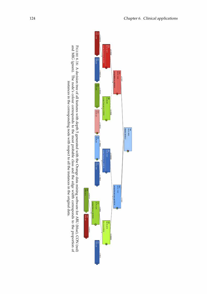
124 Chapter 6. Clinical applications
FI G
UR
E6.16:
Adecision
treeofallfeatures
with
depth5
generatedw
iththe
Orange
datam
iningsoftw
arefor
ABU
(blue),CO
N(red)
andM
IG(green).
Thenode’s
colourcorresponds
tothe
most
probableclass
andthe
edgew
idthcorresponds
tothe
proportionof
instancesin
thecorresponding
nodew
ithrespectto
alltheinstances
inthe
originaldata.
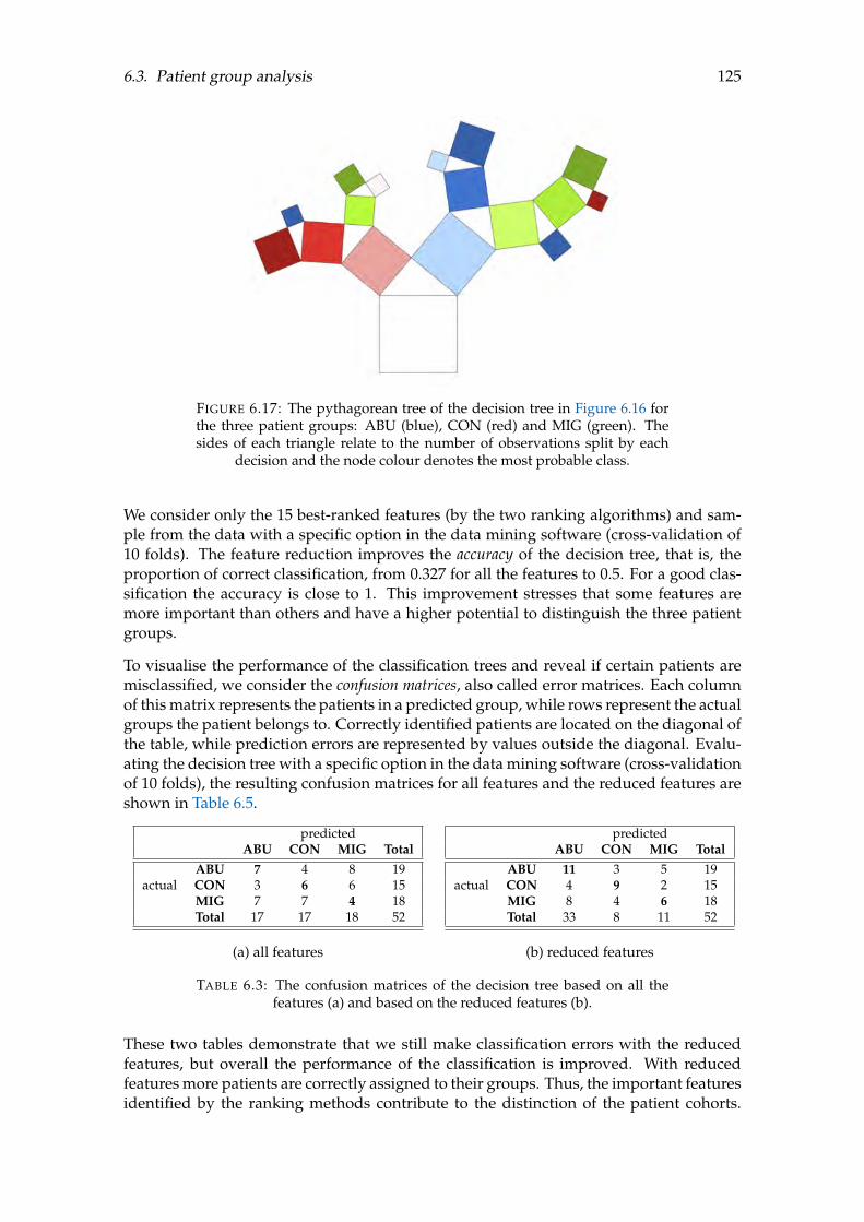
6.3. Patient group analysis 125
FIGURE 6.17: The pythagorean tree of the decision tree in Figure 6.16 forthe three patient groups: ABU (blue), CON (red) and MIG (green). Thesides of each triangle relate to the number of observations split by each
decision and the node colour denotes the most probable class.
We consider only the 15 best-ranked features (by the two ranking algorithms) and sam-ple from the data with a specific option in the data mining software (cross-validation of10 folds). The feature reduction improves the accuracy of the decision tree, that is, theproportion of correct classification, from 0.327 for all the features to 0.5. For a good clas-sification the accuracy is close to 1. This improvement stresses that some features aremore important than others and have a higher potential to distinguish the three patientgroups.
To visualise the performance of the classification trees and reveal if certain patients aremisclassified, we consider the confusion matrices, also called error matrices. Each columnof this matrix represents the patients in a predicted group, while rows represent the actualgroups the patient belongs to. Correctly identified patients are located on the diagonal ofthe table, while prediction errors are represented by values outside the diagonal. Evalu-ating the decision tree with a specific option in the data mining software (cross-validationof 10 folds), the resulting confusion matrices for all features and the reduced features areshown in Table 6.5.
predictedABU CON MIG Total
actualABU 7 4 8 19CON 3 6 6 15MIG 7 7 4 18Total 17 17 18 52
(a) all features
predictedABU CON MIG Total
actualABU 11 3 5 19CON 4 9 2 15MIG 8 4 6 18Total 33 8 11 52
(b) reduced features
TABLE 6.3: The confusion matrices of the decision tree based on all thefeatures (a) and based on the reduced features (b).
These two tables demonstrate that we still make classification errors with the reducedfeatures, but overall the performance of the classification is improved. With reducedfeatures more patients are correctly assigned to their groups. Thus, the important featuresidentified by the ranking methods contribute to the distinction of the patient cohorts.

126 Chapter 6. Clinical applications
Even though the accuracy is rather low for both classification approaches, we get a firstidea on how the QoI can help to distinguish between the different patient groups.
Obviously, there is a variety of other techniques and measures to evaluate the classifica-tion problem in supervised learning. However, this goes beyond the scope of this thesisand is left for future investigations.
6.4 Summary
In this chapter we simulated CSD propagation on different patient data sets. In a firstcase study of chronic migraine patients with aura, we confirmed that the simulated CSDwavefront propagates according to the sequence of symptoms experienced by the pa-tients during a migraine attack. This is adding computational evidence to the hypothesisof neural correlation between migraine with aura and CSD.
In the subsequent group analysis, we simulated CSD propagation on three different pa-tient groups: migraine patients (without aura), chronic headache patients that abusivelyuse painkillers and a control group. By simply looking at the mean and standard devia-tion in the QoI introduced in Chapter 5 we were unable to find any feature that signifi-cantly distinguishes the patient groups from each other. However, by using classificationtechniques from data mining, we showed that the two curvature measures and the re-tention time, especially in the left hemisphere, could be good indicators to differentiatebetween the considered patient groups. Different ranking methods indicate that thesethree QoI in the paracentral region (ROI 20) are important features to classify the threepatient groups.

127
Chapter 7
Uncertainty quantification
“We must think differently about our ideas – and how we test them.We must become more comfortable with probability and uncertainty.We must think more carefully about the assumptions and beliefs that we bring to a problem.”
Nate Silver, in The Signal and the Noise: The Art of Science and Prediction (2012)
In the previous chapters we simulated CSD propagation on the cerebral cortex using themodel for the extracellular potassium concentration introduced in Chapter 3. The modelparameters were tuned to match the characteristics of CSD, including the interval lengthof high potassium concentration and the overall propagation time across the cortex. Bychoosing such parameter values, we enforce strong assumptions on the model and its re-sults, but unfortunately, we are unable to validate more thoroughly the obtained resultsagainst experiments due to a lack of detailed experimental data. To address this limi-tation, we apply uncertainty quantification (UQ) to account for the uncertainties in thechoice of parameters and perform a sensitivity analysis to explore the parameter spacefor both a proper tuning of the model and for the improvement of its predictive role. Wedistinguish between the spatially independent and space-dependent parameters. Theformer can be considered random variables while the latter is considered a random pro-cess.
To estimate the impact of parameter uncertainties on the solution, we apply differenttechniques of UQ. By assigning certain parameter distributions rather than fixing pa-rameter values, UQ offers sophisticated and efficient methods to explore the parameterspace. Note that the selection of a specific parameter distribution still implies havingmade a particular modelling assumption. However, this guess is clearly less restrictivethan selecting a constant parameter value.
The basic idea in UQ is to draw samples from the parameter space according to theassumed distribution, evaluate the problem at hand with these parameter values andcompute some output statistics, e.g., by considering the mean and the variance of theobtained model outputs. Especially for a high number of parameters, exploring the pa-rameter space can be costly, but UQ techniques offer efficient strategies to pick samplesfrom this parameter space and reduce the computational effort.
In this chapter we first assume the parameters to be uniformly distributed and study theeffect on the solution in this context. Then we briefly comment on the solution statisticswhen an underlying beta-distribution is assumed. The choice of the two distributions ismotivated by the domain they are defined on, continuous finite intervals as opposed to
128 Chapter 7. Uncertainty quantification
distributions on discrete or continuous but infinite supports. This choice is a natural onefor parameters describing biological phenomena where experiments can narrow downthe parameter values to reasonable ranges.
The sensitivity analysis concerns the investigation of the sensitivity of simulation resultsto changes in the different parameters. We answer the question of how much the differ-ent parameters contribute to the solution and to other characteristics of the potassiumwave, such as the period of high potassium concentration and the maximum potassiumconcentration.
The diffusion direction and strength of the potassium wave are ruled by DTI measure-ments. Due to errors in the measurements and the pre-processing, there is noise in thedata. Thus, UQ offers a way to account for these uncertainties in the diffusion parameter.However, the diffusion data is spatially dependent and applying UQ is more complexthan for the other parameters that do not depend on space. We give a brief idea andintroduction to what could be done to address this problem.
In this chapter we first recapitulate the model for the extracellular potassium concentra-tion in the deterministic sense before exploring the parameter space with UQ (for bothspatially independent and dependent parameters) and before analysing the solution’ssensitivity to the different parameters. The results of this chapter were obtained dur-ing my visiting fellowship undertaken under the supervision of Prof. Dr. George EmKarniadakis at the Brown University in Providence, US.
For a basic introduction to UQ and sensitivity analysis, we refer to Appendix B.4. Thenotations in this chapter are mainly taken from Xiu, 2010.
7.1 Deterministic problem
The deterministic model for the temporal evolution and propagation of the extracellularpotassium kbath introduced in Chapter 3 (see system (3.4)) reads
∂kbath
∂t= div (D∇kbath)− F (kbath, w) + Ip,
∂w
∂t= G(kbath, w),
F (kbath, w) = η1 (kbath − k0)
(1− kbath
kth
)(1− kbath
kp
)+ η2 (kbath − k0)w,
G(kbath, w) = η3 (kbath − k0 − η4w) ,
(7.1)
where kbath and w are defined on W × (0, T ) with W ⊂ Rr for r = 1, 2, 3, D ∈ Rr×r isthe diffusion tensor, w is a recovery variable, η1, η2, η3, and η4 are parameters, while k0,kth, kp are the resting, threshold, and peak values of the kbath concentration, respectively.The parameters k0, kth and kp are chosen in a way that the resulting potassium wavetriggers the CSD-like behaviour in the coupling with the Wei model. The diffusion tensorD is space-dependent and based on DTI measurements while the remaining parametersη1, . . . , η4 have been tuned to match the characteristics of CSD. We start by considering
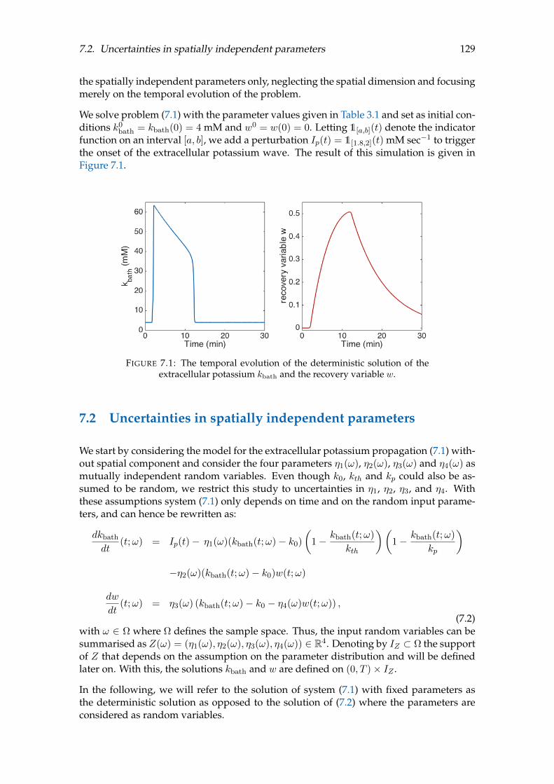
7.2. Uncertainties in spatially independent parameters 129
the spatially independent parameters only, neglecting the spatial dimension and focusingmerely on the temporal evolution of the problem.
We solve problem (7.1) with the parameter values given in Table 3.1 and set as initial con-ditions k0
bath = kbath(0) = 4 mM and w0 = w(0) = 0. Letting 1[a,b](t) denote the indicatorfunction on an interval [a, b], we add a perturbation Ip(t) = 1[1.8,2](t) mM sec−1 to triggerthe onset of the extracellular potassium wave. The result of this simulation is given inFigure 7.1.
FIGURE 7.1: The temporal evolution of the deterministic solution of theextracellular potassium kbath and the recovery variable w.
7.2 Uncertainties in spatially independent parameters
We start by considering the model for the extracellular potassium propagation (7.1) with-out spatial component and consider the four parameters η1(ω), η2(ω), η3(ω) and η4(ω) asmutually independent random variables. Even though k0, kth and kp could also be as-sumed to be random, we restrict this study to uncertainties in η1, η2, η3, and η4. Withthese assumptions system (7.1) only depends on time and on the random input parame-ters, and can hence be rewritten as:
dkbath
dt(t;ω) = Ip(t)− η1(ω)(kbath(t;ω)− k0)
(1− kbath(t;ω)
kth
)(1− kbath(t;ω)
kp
)−η2(ω)(kbath(t;ω)− k0)w(t;ω)
dw
dt(t;ω) = η3(ω) (kbath(t;ω)− k0 − η4(ω)w(t;ω)) ,
(7.2)with ω ∈ Ω where Ω defines the sample space. Thus, the input random variables can besummarised as Z(ω) = (η1(ω), η2(ω), η3(ω), η4(ω)) ∈ R4. Denoting by IZ ⊂ Ω the supportof Z that depends on the assumption on the parameter distribution and will be definedlater on. With this, the solutions kbath and w are defined on (0, T )× IZ .
In the following, we will refer to the solution of system (7.1) with fixed parameters asthe deterministic solution as opposed to the solution of (7.2) where the parameters areconsidered as random variables.
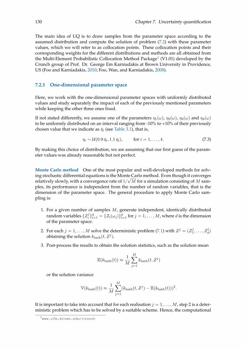
130 Chapter 7. Uncertainty quantification
The main idea of UQ is to draw samples from the parameter space according to theassumed distribution and compute the solution of problem (7.2) with these parametervalues, which we will refer to as collocation points. These collocation points and theircorresponding weights for the different distributions and methods are all obtained fromthe Multi-Element Probabilistic Collocation Method Package1 (V1.01) developed by theCrunch group of Prof. Dr. George Em Karniadakis at Brown University in Providence,US (Foo and Karniadakis, 2010; Foo, Wan, and Karniadakis, 2008).
7.2.1 One-dimensional parameter space
Here, we work with the one-dimensional parameter spaces with uniformly distributedvalues and study separately the impact of each of the previously mentioned parameterswhile keeping the other three ones fixed.
If not stated differently, we assume one of the parameters η1(ω), η2(ω), η3(ω) and η4(ω)to be uniformly distributed on an interval ranging from -10% to +10% of their previouslychosen value that we indicate as ηi (see Table 3.1), that is,
ηi ∼ U(0.9 ηi, 1.1 ηi), for i = 1, . . . , 4. (7.3)
By making this choice of distribution, we are assuming that our first guess of the param-eter values was already reasonable but not perfect.
Monte Carlo method One of the most popular and well-developed methods for solv-ing stochastic differential equations is the Monte Carlo method. Even though it convergesrelatively slowly, with a convergence rate of 1/
√M for a simulation consisting ofM sam-
ples, its performance is independent from the number of random variables, that is thedimension of the parameter space. The general procedure to apply Monte Carlo sam-pling is:
1. For a given number of samples M , generate independent, identically distributedrandom variables Zji di=1 = Zi(ωj)di=1 for j = 1, . . . ,M , where d is the dimensionof the parameter space.
2. For each j = 1, . . . ,M solve the deterministic problem (7.1) with Zj = (Zj1 , . . . , Zjd)
obtaining the solution kbath(t, Zj).
3. Post-process the results to obtain the solution statistics, such as the solution mean
E(kbath(t)) ≈ 1
M
M∑j=1
kbath(t, Zj)
or the solution variance
V(kbath(t)) ≈ 1
M
M∑j=1
(kbath(t, Zj)− E(kbath(t)))2.
It is important to take into account that for each realisation j = 1, . . . ,M , step 2 is a deter-ministic problem which has to be solved by a suitable scheme. Hence, the computational
1www.cfm.brown.edu/crunch

7.2. Uncertainties in spatially independent parameters 131
cost of the Monte Carlo method does not only depend on the number of samples Mbut also on the complexity of the solution of the deterministic problem. As the samplesare drawn randomly this requires M to be a large number in order to obtain significantstatistics. We plot the estimated mean and standard deviation computed with the MonteCarlo method forM = 10, 100, 104 samples of the variable η1(ω) ∼ U(0.9 η1, 1.1 η1) in Fig-ure 7.2. The black dotted line marks the solution corresponding to the original parameterset (see Table 3.1).
FIGURE 7.2: The solution statistics with the Monte Carlo method withM = 10, M = 100 and M = 104 realisations of the uniformly distributedparameter η1(ω) on [0.9 η1, 1.1 η1] with the other parameters (deterministic)
as listed in Table 3.1, and the original solution (dotted black).
In Figure 7.2 we can observe two things: the Monte Carlo method provides a smoothermean solution for a higher number of samples and the parameter η1 influences the extra-cellular potassium wave when values are returning to the resting state concentration.
Probabilistic collocation method Instead of drawing numerous samples from a ran-dom distribution with the Monte Carlo approach, other methods approximate the solu-tion on a small number of (well-chosen) points in the parameter space. The probabilisticcollocation method (PCM) is one of them and it relies on the basic concept of approximat-ing the response of the model by a polynomial. For PCM the model equations are solvedat a set of collocation points, also called nodes, in the parameter space.
Let (Z1, . . . , Zm) be a set of collocation points and Ljmj=1 the corresponding Wiener-Askey scheme polynomials on the support IZ . An example of polynomials of this schemeare the Legendre polynomials that are defined on [−1, 1]. We will see later on that thesepolynomials can be exploited when considering uniformly distributed parameters. We
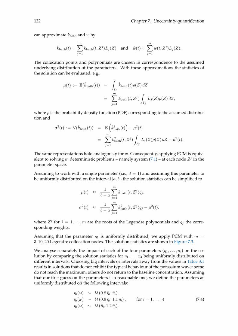
132 Chapter 7. Uncertainty quantification
can approximate kbath and w by
kbath(t) =m∑j=1
kbath(t, Zj)Lj(Z) and w(t) =m∑j=1
w(t, Zj)Lj(Z).
The collocation points and polynomials are chosen in correspondence to the assumedunderlying distribution of the parameters. With these approximations the statistics ofthe solution can be evaluated, e.g.,
µ(t) := E(kbath(t)) =
∫IZ
kbath(t)ρ(Z) dZ
=
m∑j=1
kbath(t, Zj)
∫IZ
Lj(Z)ρ(Z) dZ,
where ρ is the probability density function (PDF) corresponding to the assumed distribu-tion and
σ2(t) := V(kbath(t)) = E(k2
bath(t))− µ2(t)
=
m∑j=1
k2bath(t, Zj)
∫IZ
Lj(Z)ρ(Z) dZ − µ2(t).
The same representations hold analogously for w. Consequently, applying PCM is equiv-alent to solving m deterministic problems – namely system (7.1) – at each node Zj in theparameter space.
Assuming to work with a single parameter (i.e., d = 1) and assuming this parameter tobe uniformly distributed on the interval [a, b], the solution statistics can be simplified to
µ(t) ≈ 1
b− a
m∑j=1
kbath(t, Zj)qj ,
σ2(t) ≈ 1
b− a
m∑j=1
k2bath(t, Zj)qj − µ2(t).
where Zj for j = 1, . . . ,m are the roots of the Legendre polynomials and qj the corre-sponding weights.
Assuming that the parameter η1 is uniformly distributed, we apply PCM with m =3, 10, 20 Legendre collocation nodes. The solution statistics are shown in Figure 7.3.
We analyse separately the impact of each of the four parameters (η1, . . . , η4) on the so-lution by comparing the solution statistics for η1, . . . , η4 being uniformly distributed ondifferent intervals. Choosing big intervals or intervals away from the values in Table 3.1results in solutions that do not exhibit the typical behaviour of the potassium wave: somedo not reach the maximum, others do not return to the baseline concentration. Assumingthat our first guess on the parameters is a reasonable one, we define the parameters asuniformly distributed on the following intervals:
ηi(ω) ∼ U (0.8 ηi, ηi) ,
ηi(ω) ∼ U (0.9 ηi, 1.1 ηi) , for i = 1, . . . , 4
ηi(ω) ∼ U (ηi, 1.2 ηi) .
(7.4)

7.2. Uncertainties in spatially independent parameters 133
FIGURE 7.3: The solution statistics with PCM for m = 3, m = 10 andm = 20 Legendre collocation points with parameter as listed in Table 3.1and η1 uniformly distributed on [0.9 η1, 1.1 η1], and the original solution
(dotted black).
Figures 7.4 - 7.7 show the mean and standard deviation of the solution corresponding toPCM with m = 10 applied to the different parameters. In the case of η1 and η2 we can ob-serve that sampling in an interval of larger values can result in a mean solution that doesnot return to the low potassium concentration once the wave has passed. These figuresshow that all the parameters have an impact on the time period of the high potassiumconcentration.
In the following we choose the parameters as uniformly distributed on the intervals ηi ∼U (0.9 ηi, 1.1 ηi) for i = 1, . . . , 4 so that the parameter choice used in the previous chaptersis the average value of this distribution.
In Figures 7.4 - 7.7 the higher number of collocation points results in a smoother mean ofthe solution but requires a higher computational costs. Even though in the one-dimen-sional case the difference between computing 10 or 20 collocation points is not signifi-cant, considering all four parameters of interest simultaneously would mean refining bya factor 2 in each dimension of a 4-dimensional tensor grid. Increasing the number of col-location points by a factor 2 increases the computation time 10-fold and causes memoryissues due to big matrices that save the solution at every time step in all the collocationpoints.
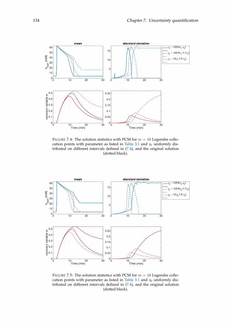
134 Chapter 7. Uncertainty quantification
FIGURE 7.4: The solution statistics with PCM for m = 10 Legendre collo-cation points with parameter as listed in Table 3.1 and η1 uniformly dis-tributed on different intervals defined in (7.4), and the original solution
(dotted black).
FIGURE 7.5: The solution statistics with PCM for m = 10 Legendre collo-cation points with parameter as listed in Table 3.1 and η2 uniformly dis-tributed on different intervals defined in (7.4), and the original solution
(dotted black).
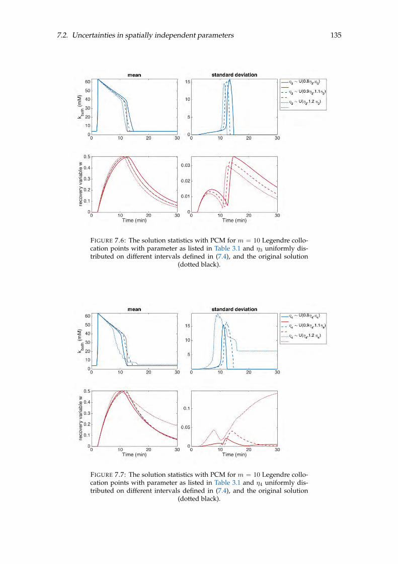
7.2. Uncertainties in spatially independent parameters 135
FIGURE 7.6: The solution statistics with PCM for m = 10 Legendre collo-cation points with parameter as listed in Table 3.1 and η3 uniformly dis-tributed on different intervals defined in (7.4), and the original solution
(dotted black).
FIGURE 7.7: The solution statistics with PCM for m = 10 Legendre collo-cation points with parameter as listed in Table 3.1 and η4 uniformly dis-tributed on different intervals defined in (7.4), and the original solution
(dotted black).
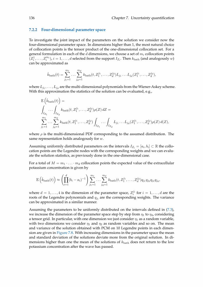
136 Chapter 7. Uncertainty quantification
7.2.2 Four-dimensional parameter space
To investigate the joint impact of the parameters on the solution we consider now thefour-dimensional parameter space. In dimensions higher than 1, the most natural choiceof collocation points is the tensor product of the one-dimensional collocation set. For ageneral formulation in each of the d dimensions, we choose a set of mi collocation points(Z1
i , . . . , Zmii ), i = 1, . . . , d selected from the support IZi . Then kbath (and analogously w)
can be approximated as
kbath(t) =
m1∑j1=1
. . .
md∑jd=1
kbath(t, Zj11 , . . . , Zjdd )Lj1 . . . Ljd(Z
j11 , . . . , Z
jdd ),
whereLj1 , . . . , Ljd are the multi-dimensional polynomials from the Wiener-Askey scheme.With this approximation the statistics of the solution can be evaluated, e.g.,
E(kbath(t)
)=∫
IZ1
. . .
∫IZd
kbath(t, Zj11 , . . . , Zjdd )ρ(Z) dZ =
m1∑j1=1
. . .
md∑jd=1
kbath(t, Zj11 , . . . , Zjdd )
∫IZ1
. . .
∫IZd
Lj1 . . . Ljd(Zj11 , . . . , Z
jdd )ρ(Z) d(Z),
where ρ is the multi-dimensional PDF corresponding to the assumed distribution. Thesame representation holds analogously for w.
Assuming uniformly distributed parameters on the intervals IZi = [ai, bi] ⊂ R the collo-cation points are the Legendre nodes with the corresponding weights and we can evalu-ate the solution statistics, as previously done in the one-dimensional case.
For a total of M = m1 · . . . ·md collocation points the expected value of the extracellularpotassium concentration is given by
E(kbath(t)
)≈
(d∏i=1
(bi − ai)−1
)m1∑j1=1
. . .
md∑jd=1
kbath(t, Zj11 , . . . , Zjdd )qj1qj2qj3qjd ,
where d = 1, . . . , 4 is the dimension of the parameter space, Zjii for i = 1, . . . , d are theroots of the Legendre polynomials and qji are the corresponding weights. The variancecan be approximated in a similar manner.
Assuming the parameters to be uniformly distributed on the intervals defined in (7.3),we increase the dimension of the parameter space step by step from η1 to η4, consideringa tensor grid. In particular, with one dimension we just consider η1 as a random variable,with two dimensions we consider η1 and η2 as random variables and so on. The meanand variance of the solution obtained with PCM on 10 Legendre points in each dimen-sion are given in Figure 7.8. With increasing dimensions in the parameter space the meanand standard deviation of the solutions deviate more from the original solution. In di-mensions higher than one the mean of the solutions of kbath does not return to the lowpotassium concentration after the wave has passed.

7.2. Uncertainties in spatially independent parameters 137
FIGURE 7.8: The solution statistics with PCM for m = 10 Legendre collo-cation points for different dimensions d = 1, . . . , 4. The dimension of theparameter space is increased step by step: one dimension considers onlyη1 as a random variable, two dimensions consider η1 and η2 as random
variables and so on. The original solution is plotted in dotted black.
With increasing dimensions, the number of collocation points and thus the number oftimes problem (7.2) has to be solved increases which is also known as the curse of dimen-sionality. A possible way to cope with this issue is to use sparse grids, which reduce thenumber of collocation points in higher dimensional parameter spaces.
7.2.3 Sparse grids
For the sparse grids, we use again Legendre polynomials and compute the collocationpoints with the Smolyak algorithm. Details on sparse grids can be found in Xiu and Hes-thaven, 2005 and in Appendix B.4. We visualise the full tensor grid and sparse grids atdifferent levels in Figure 7.9. The level of a sparse grid decreases as the sparsity increases.In Figure 7.10 we show collocation points and the corresponding weights on sparse gridsin 2D and 3D. The total number of points in the 2D case is 1578 whereas the numberof nodes in the 3D case is 6507. The collocation points are coloured according to theirweights. Note that some of the weights are negative.
In Figure 7.11 we show the solution statistics evaluated on sparse grids of different levels.Here, the solutions computed on a sparse grid exhibit an irregular behaviour rather thana smooth decrease in the potassium concentration. In contrast to the case of a full tensorgrid, the collocation points of the sparse grid can be associated with negative weights.When several solutions assigned to negative weight in the parameter space return to thelow potassium concentration, the impact of the solutions with positive weights increasesand leads to a sudden increase in the mean value. To visualise the effect of the negativeweights of the sparse grids on the solution statistics, we show in Figure 7.12 the meanand some solutions associated with negative weights on a four-dimensional sparse grid
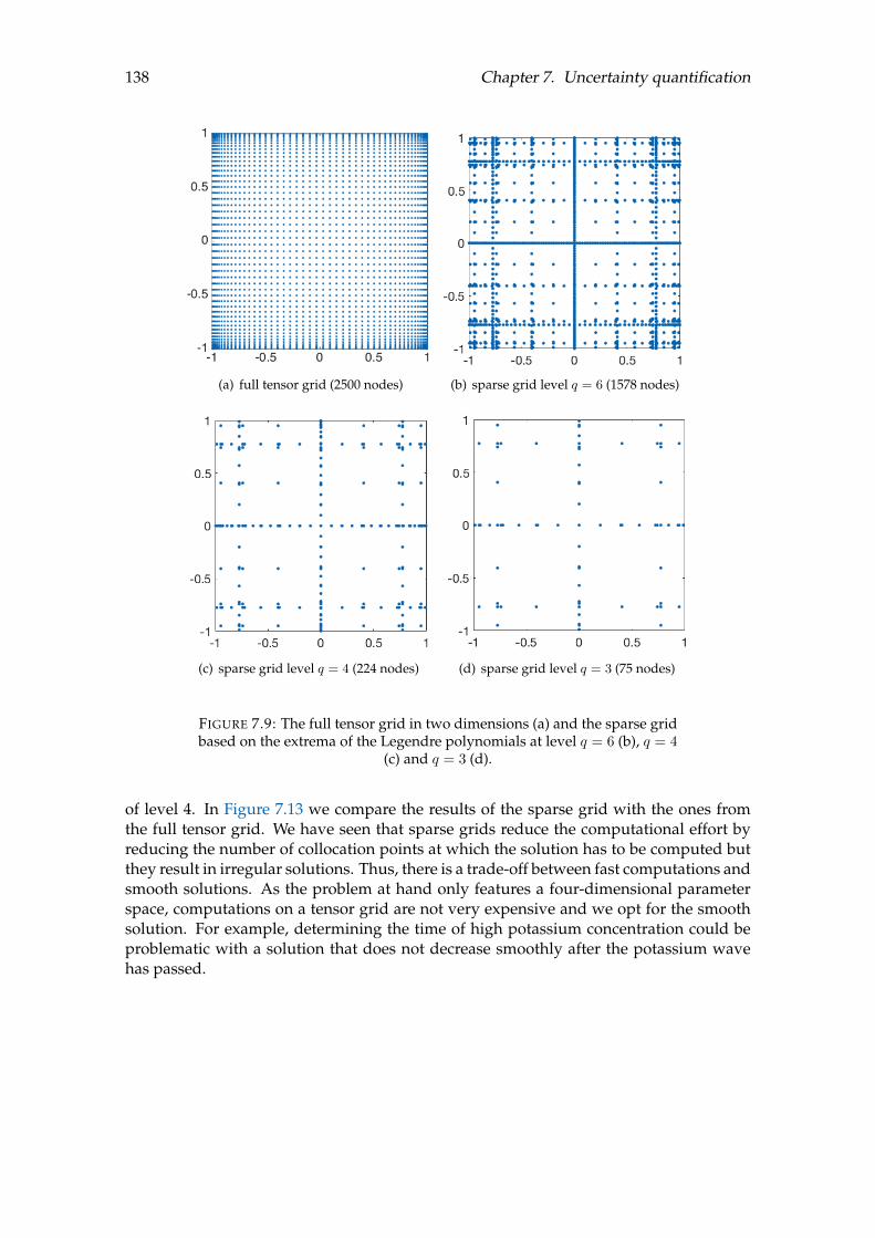
138 Chapter 7. Uncertainty quantification
(a) full tensor grid (2500 nodes) (b) sparse grid level q = 6 (1578 nodes)
(c) sparse grid level q = 4 (224 nodes) (d) sparse grid level q = 3 (75 nodes)
FIGURE 7.9: The full tensor grid in two dimensions (a) and the sparse gridbased on the extrema of the Legendre polynomials at level q = 6 (b), q = 4
(c) and q = 3 (d).
of level 4. In Figure 7.13 we compare the results of the sparse grid with the ones fromthe full tensor grid. We have seen that sparse grids reduce the computational effort byreducing the number of collocation points at which the solution has to be computed butthey result in irregular solutions. Thus, there is a trade-off between fast computations andsmooth solutions. As the problem at hand only features a four-dimensional parameterspace, computations on a tensor grid are not very expensive and we opt for the smoothsolution. For example, determining the time of high potassium concentration could beproblematic with a solution that does not decrease smoothly after the potassium wavehas passed.
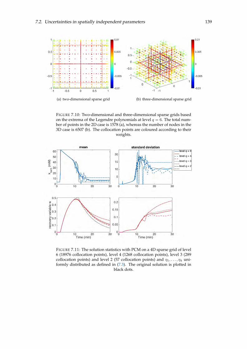
7.2. Uncertainties in spatially independent parameters 139
(a) two-dimensional sparse grid (b) three-dimensional sparse grid
FIGURE 7.10: Two-dimensional and three-dimensional sparse grids basedon the extrema of the Legendre polynomials at level q = 6. The total num-ber of points in the 2D case is 1578 (a), whereas the number of nodes in the3D case is 6507 (b). The collocation points are coloured according to their
weights.
FIGURE 7.11: The solution statistics with PCM on a 4D sparse grid of level6 (18976 collocation points), level 4 (1268 collocation points), level 3 (289collocation points) and level 2 (57 collocation points) and η1, . . . , η4 uni-formly distributed as defined in (7.3). The original solution is plotted in
black dots.
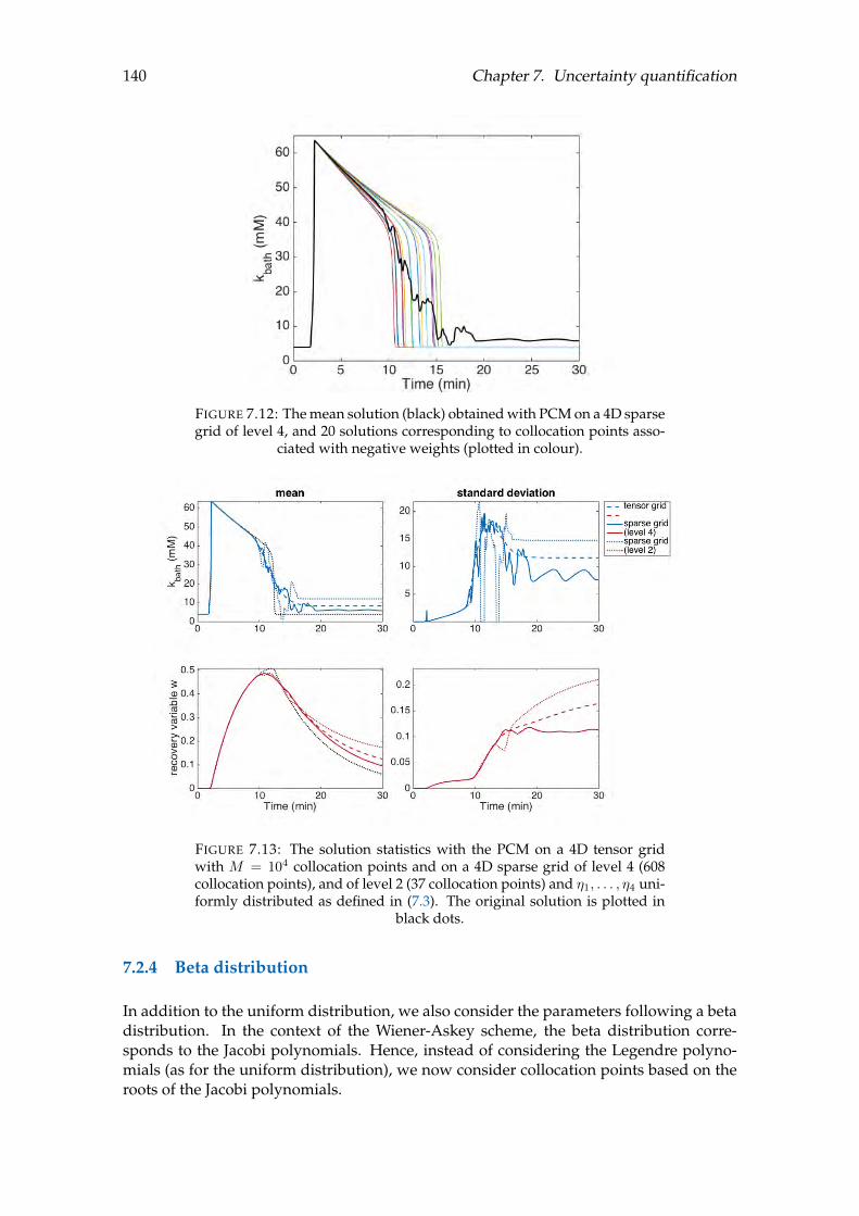
140 Chapter 7. Uncertainty quantification
FIGURE 7.12: The mean solution (black) obtained with PCM on a 4D sparsegrid of level 4, and 20 solutions corresponding to collocation points asso-
ciated with negative weights (plotted in colour).
FIGURE 7.13: The solution statistics with the PCM on a 4D tensor gridwith M = 104 collocation points and on a 4D sparse grid of level 4 (608collocation points), and of level 2 (37 collocation points) and η1, . . . , η4 uni-formly distributed as defined in (7.3). The original solution is plotted in
black dots.
7.2.4 Beta distribution
In addition to the uniform distribution, we also consider the parameters following a betadistribution. In the context of the Wiener-Askey scheme, the beta distribution corre-sponds to the Jacobi polynomials. Hence, instead of considering the Legendre polyno-mials (as for the uniform distribution), we now consider collocation points based on theroots of the Jacobi polynomials.

7.3. Sensitivity analysis 141
The beta distribution is (and thus also the Jacobi polynomials are) defined on [0, 1] anddepends on two positive shape parameters, denoted by α and β. For a better under-standing and to visually explain the next steps we plot the beta distribution for differentparameter combinations (α, β) in Figure 7.14. Specifically, we choose the parameter com-binations: (10, 10), (2, 10) and (10, 2). For α = β the beta distribution is very similar to atruncated Gauss distribution.
FIGURE 7.14: The probability density function of the beta distribution forthe parameter combinations (10, 10), (2, 10) and (10, 2).
We assume the parameters η1, . . . , η4 to be beta-distributed on the interval [0.9 ηi, 1.1 ηi]for i = 1, . . . , 4 so that the beta distribution with α = β is centred in ηi.
In Figure 7.15 we visually compare the solution statistics with PCM on a 4D tensor gridassuming an underlying beta distribution to the solution statistics assuming uniformlydistributed parameters. Depending on the choice of α and β the distribution is eithercentred around ηi or accumulates close to the endpoints of the interval. This reflects in thesolution statistics: with the centred beta distribution the solution resembles the originalsolution computed with ηi, while the beta distribution and α 6= β result in a solutionmean that returns earlier or later to the low potassium concentration, depending on thechoice of α and β.
7.3 Sensitivity analysis
Instead of computing and visually inspecting the solution statistics as seen in the previ-ous section, sensitivity analysis offers the possibility to quantify the impact of the inputparameters on the model output. Variance-based sensitivity analysis estimates the impactof input variability on the output variance, considered for either individual parametersor for combinations.
The computations of the classical sensitivity indices is a method for variance-based sensi-tivity analysis of the model outputs (Archer, Satelli, and Sobol’, 1997; Sobol’, 1993, 2001).This method is based on the decomposition of the variance of the model output intoterms of increasing dimensionality, as in the classical analysis of variance (ANOVA).
Together with the classical sensitivity indices we define some problem-specific measuresin Section 7.3.2. For more details on the classical indices, see Appendix B.4.6.
For the two sensitivity indices we use collocation points based on the ANOVA decom-position with 4 elements and 3 collocation points per element. This is just another wayof selecting collocation points, similar to the approach of tensor grids or sparse grids in

142 Chapter 7. Uncertainty quantification
FIGURE 7.15: The solution statistics with PCM on a 4D tensor grid withM = 104 (Jacobi) collocation points with η1, . . . , η4 being beta-distributedon the interval as defined in (7.3) with different combinations for the pa-rameter set (α, β), namely (10, 10), (2, 10) and (10, 2). The original solutionis visualised in black dots and the solution statistics with PCM assuming
uniformly distributed parameters is plotted in black.
the previous section. For more information on the multi-element collocation method, werefer to Appendix B.4.5.2 and the documentation of the Multi-Element Probabilistic Col-location Method Package (V1.01) developed by the Crunch group at Brown University.
Sensitivity analysis is based on the definition of collocation points and the computationof the solution with these parameter values. For the definition of the classical sensitivityindices, we need certain concepts that we introduce below.
Let Z11 , . . . , Z
m1 be collocation points. Then keeping kbath fixed at a reference point c =
(c1, . . . , c4), also known as the anchor point, and evaluating kbath only in the collocationpoints of the first dimension of the parameter space, its value at collocation point Zj1 forj = 1, . . . ,m is
k1bath(Z1
1 ) := kbath(Z11 , c2, c3, c4)− k0
bath,
with k0bath = kbath(c). The mean and variance of kbath can be approximated by
µ(k1bath) ≈
m∑j=1
k1bath(Zj1)qj1, σ2(k1
bath) ≈m∑j=1
(k1bath(Zj1))2qj1 −
(µ(k1
bath))2, (7.5)
where q11, . . . , q
m1 are the weights corresponding to the collocation pointsZ1
1 , . . . , Zm1 . This
definition applies analogously to all first-order terms k2bath, . . . , k
4bath with the general
notation kibath(Zji ) = kbath(c1, . . . , ci−1, Zji , ci+1, . . . , c4)− k0
bath.
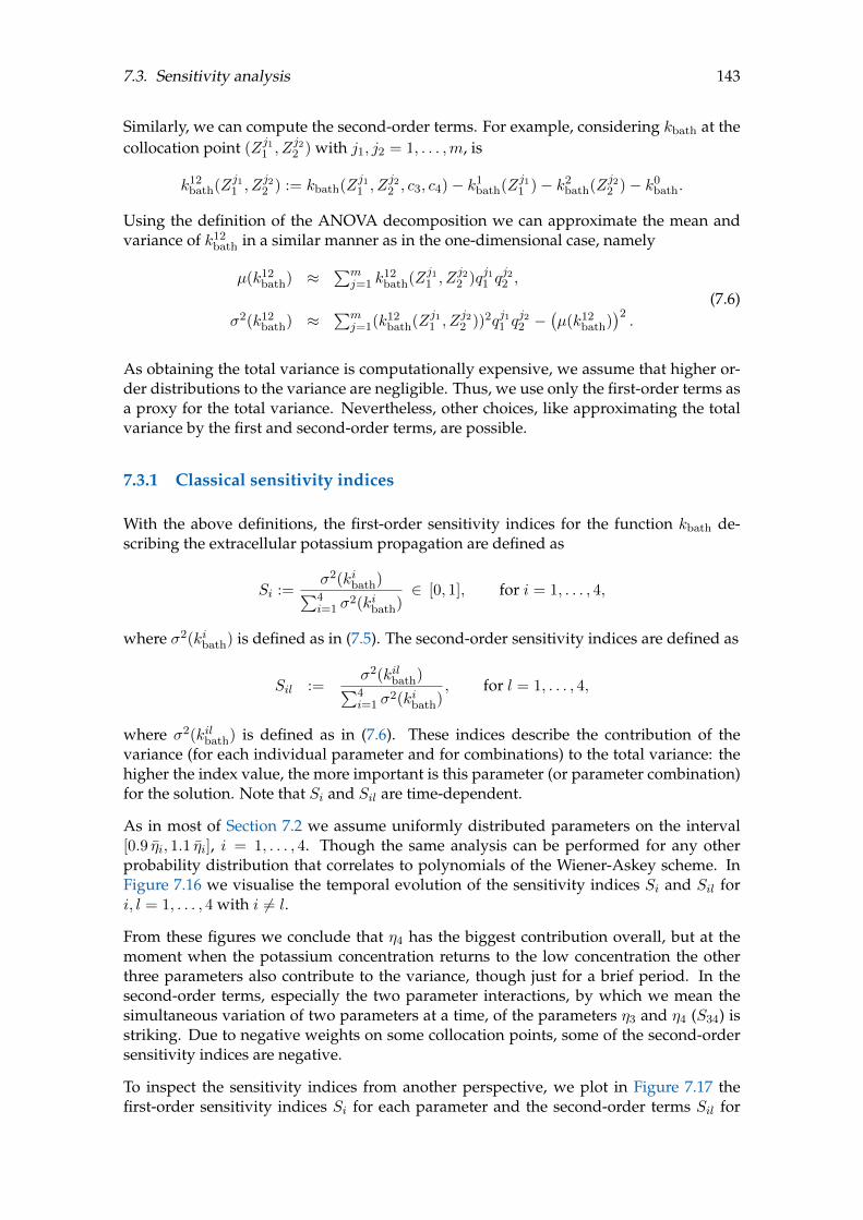
7.3. Sensitivity analysis 143
Similarly, we can compute the second-order terms. For example, considering kbath at thecollocation point (Zj11 , Z
j22 ) with j1, j2 = 1, . . . ,m, is
k12bath(Zj11 , Z
j22 ) := kbath(Zj11 , Z
j22 , c3, c4)− k1
bath(Zj11 )− k2bath(Zj22 )− k0
bath.
Using the definition of the ANOVA decomposition we can approximate the mean andvariance of k12
bath in a similar manner as in the one-dimensional case, namely
µ(k12bath) ≈
∑mj=1 k
12bath(Zj11 , Z
j22 )qj11 q
j22 ,
σ2(k12bath) ≈
∑mj=1(k12
bath(Zj11 , Zj22 ))2qj11 q
j22 −
(µ(k12
bath))2.
(7.6)
As obtaining the total variance is computationally expensive, we assume that higher or-der distributions to the variance are negligible. Thus, we use only the first-order terms asa proxy for the total variance. Nevertheless, other choices, like approximating the totalvariance by the first and second-order terms, are possible.
7.3.1 Classical sensitivity indices
With the above definitions, the first-order sensitivity indices for the function kbath de-scribing the extracellular potassium propagation are defined as
Si :=σ2(kibath)∑4i=1 σ
2(kibath)∈ [0, 1], for i = 1, . . . , 4,
where σ2(kibath) is defined as in (7.5). The second-order sensitivity indices are defined as
Sil :=σ2(kilbath)∑4i=1 σ
2(kibath), for l = 1, . . . , 4,
where σ2(kilbath) is defined as in (7.6). These indices describe the contribution of thevariance (for each individual parameter and for combinations) to the total variance: thehigher the index value, the more important is this parameter (or parameter combination)for the solution. Note that Si and Sil are time-dependent.
As in most of Section 7.2 we assume uniformly distributed parameters on the interval[0.9 ηi, 1.1 ηi], i = 1, . . . , 4. Though the same analysis can be performed for any otherprobability distribution that correlates to polynomials of the Wiener-Askey scheme. InFigure 7.16 we visualise the temporal evolution of the sensitivity indices Si and Sil fori, l = 1, . . . , 4 with i 6= l.
From these figures we conclude that η4 has the biggest contribution overall, but at themoment when the potassium concentration returns to the low concentration the otherthree parameters also contribute to the variance, though just for a brief period. In thesecond-order terms, especially the two parameter interactions, by which we mean thesimultaneous variation of two parameters at a time, of the parameters η3 and η4 (S34) isstriking. Due to negative weights on some collocation points, some of the second-ordersensitivity indices are negative.
To inspect the sensitivity indices from another perspective, we plot in Figure 7.17 thefirst-order sensitivity indices Si for each parameter and the second-order terms Sil for

144 Chapter 7. Uncertainty quantification
(a) sensitivity indices Si (b) sensitivity indices Sil
FIGURE 7.16: The sensitivity indices Si and Sil for i, l = 1, 2, 3, 4 and i 6= l.
the parameter interactions at different snapshots in time, namely t = 10, 11, 12, 13, 14, 15minutes. The circles indicate the single parameter sensitivity and the thickness of thelines indicates the sensitivity of two-parameter interactions, red lines indicate a negativesensitivity.
(a) t = 10 min (b) t = 11 min (c) t = 12 min
(d) t = 13 min (e) t = 14 min (f) t = 15 min
FIGURE 7.17: The sensitivity indices Si (circles) and Sil (lines) at the timesteps t = 10, 11, 12, 13, 14, 15 min. The size of the circles in each vertexof the diagrams indicates the sensitivity of the model solution to the par-ticular parameter considered and the thickness of the lines indicates thesensitivity of two-parameter interactions, red lines indicate a negative sen-
sitivity values.
Both Figure 7.16 and Figure 7.17 show that even though η4 contributes the most to thevariance of the solution, the other parameters have an impact on the variance, especiallywhen the potassium concentration decreases after the wave has passed.
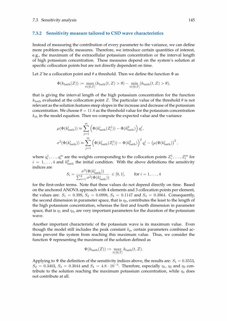
7.3. Sensitivity analysis 145
7.3.2 Sensitivity measure tailored to CSD wave characteristics
Instead of measuring the contribution of every parameter to the variance, we can definemore problem-specific measures. Therefore, we introduce certain quantities of interest,e.g., the maximum of the extracellular potassium concentration or the interval lengthof high potassium concentration. These measures depend on the system’s solution atspecific collocation points but are not directly dependent on time.
Let Z be a collocation point and θ a threshold. Then we define the function Φ as
Φ(kbath(Z)) := maxt∈[0,T ]
(kbath(t, Z) > θ)− mint∈[0,T ]
(kbath(t, Z) > θ),
that is giving the interval length of the high potassium concentration for the functionkbath evaluated at the collocation point Z. The particular value of the threshold θ is notrelevant as the solution features steep slopes in the increase and decrease of the potassiumconcentration. We choose θ = 11.8 as the threshold value for the potassium concentrationkth in the model equation. Then we compute the expected value and the variance
µ(Φ(kibath)) ≈m∑j=1
(Φ(kibath(Zji ))− Φ(k0
bath))qji ,
σ2(Φ(kibath)) ≈m∑j=1
(Φ(kibath(Zji ))− Φ(k0
bath))2qji −
(µ(Φ(kibath)
)2,
where q1i , . . . , q
mi are the weights corresponding to the collocation points Z1
i , . . . , Zmi for
i = 1, . . . , 4 and k0bath the initial condition. With the above definitions the sensitivity
indices are
Si =σ2(Φ(kibath))∑4i=1 σ
2(Φ(kibath))∈ [0, 1], for i = 1, . . . , 4
for the first-order terms. Note that these values do not depend directly on time. Basedon the anchored ANOVA approach with 4 elements and 3 collocation points per element,the values are: S1 = 0.399, S2 = 0.0998, S3 = 0.1147 and S4 = 0.3864. Consequently,the second dimension in parameter space, that is η2, contributes the least to the length ofthe high potassium concentration, whereas the first and fourth dimension in parameterspace, that is η1 and η4, are very important parameters for the duration of the potassiumwave.
Another important characteristic of the potassium wave is its maximum value. Eventhough the model still includes the peak constant kp, certain parameters combined ac-tions prevent the system from reaching this maximum value. Thus, we consider thefunction Ψ representing the maximum of the solution defined as
Ψ(kbath(Z)) := maxt∈[0,T ]
kbath(t, Z).
Applying to Ψ the definition of the sensitivity indices above, the results are: S1 = 0.3553,S2 = 0.3403, S3 = 0.3044 and S4 = 4.8 · 10−5. Therefore, especially η1, η2 and η3 con-tribute to the solution reaching the maximum potassium concentration, while η4 doesnot contribute at all.
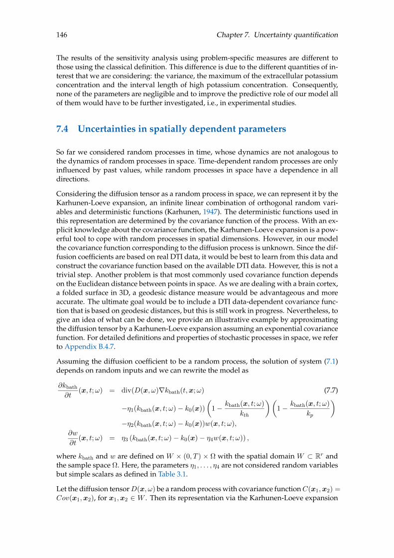
146 Chapter 7. Uncertainty quantification
The results of the sensitivity analysis using problem-specific measures are different tothose using the classical definition. This difference is due to the different quantities of in-terest that we are considering: the variance, the maximum of the extracellular potassiumconcentration and the interval length of high potassium concentration. Consequently,none of the parameters are negligible and to improve the predictive role of our model allof them would have to be further investigated, i.e., in experimental studies.
7.4 Uncertainties in spatially dependent parameters
So far we considered random processes in time, whose dynamics are not analogous tothe dynamics of random processes in space. Time-dependent random processes are onlyinfluenced by past values, while random processes in space have a dependence in alldirections.
Considering the diffusion tensor as a random process in space, we can represent it by theKarhunen-Loeve expansion, an infinite linear combination of orthogonal random vari-ables and deterministic functions (Karhunen, 1947). The deterministic functions used inthis representation are determined by the covariance function of the process. With an ex-plicit knowledge about the covariance function, the Karhunen-Loeve expansion is a pow-erful tool to cope with random processes in spatial dimensions. However, in our modelthe covariance function corresponding to the diffusion process is unknown. Since the dif-fusion coefficients are based on real DTI data, it would be best to learn from this data andconstruct the covariance function based on the available DTI data. However, this is not atrivial step. Another problem is that most commonly used covariance function dependson the Euclidean distance between points in space. As we are dealing with a brain cortex,a folded surface in 3D, a geodesic distance measure would be advantageous and moreaccurate. The ultimate goal would be to include a DTI data-dependent covariance func-tion that is based on geodesic distances, but this is still work in progress. Nevertheless, togive an idea of what can be done, we provide an illustrative example by approximatingthe diffusion tensor by a Karhunen-Loeve expansion assuming an exponential covariancefunction. For detailed definitions and properties of stochastic processes in space, we referto Appendix B.4.7.
Assuming the diffusion coefficient to be a random process, the solution of system (7.1)depends on random inputs and we can rewrite the model as
∂kbath
∂t(x, t;ω) = div(D(x, ω)∇kbath(t,x;ω) (7.7)
−η1(kbath(x, t;ω)− k0(x))
(1− kbath(x, t;ω)
kth
)(1− kbath(x, t;ω)
kp
)−η2(kbath(x, t;ω)− k0(x))w(x, t;ω),
∂w
∂t(x, t;ω) = η3 (kbath(x, t;ω)− k0(x)− η4w(x, t;ω)) ,
where kbath and w are defined on W × (0, T ) × Ω with the spatial domain W ⊂ Rr andthe sample space Ω. Here, the parameters η1, . . . , η4 are not considered random variablesbut simple scalars as defined in Table 3.1.
Let the diffusion tensorD(x, ω) be a random process with covariance functionC(x1,x2) =Cov(x1,x2), for x1,x2 ∈ W . Then its representation via the Karhunen-Loeve expansion
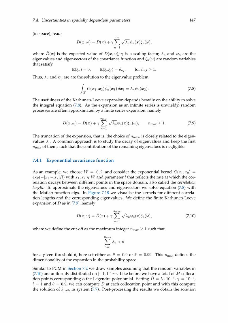
7.4. Uncertainties in spatially dependent parameters 147
(in space), reads
D(x, ω) = D(x) + γ∞∑n=1
√λnψn(x)ξn(ω),
where D(x) is the expected value of D(x, ω), γ is a scaling factor, λn and ψn are theeigenvalues and eigenvectors of the covariance function and ξn(ω) are random variablesthat satisfy
E(ξn) = 0, E(ξnξj) = δnj , for n, j ≥ 1.
Thus, λn and ψn are are the solution to the eigenvalue problem∫WC(x1,x2)ψn(x1) dx1 = λnψn(x2). (7.8)
The usefulness of the Karhunen-Loeve expansion depends heavily on the ability to solvethe integral equation (7.8). As the expansion as an infinite series is unwieldy, randomprocesses are often approximated by a finite series expansion, namely
D(x, ω) = D(x) + γ
nmax∑n=1
√λnψn(x)ξn(ω), nmax ≥ 1. (7.9)
The truncation of the expansion, that is, the choice of nmax, is closely related to the eigen-values λi. A common approach is to study the decay of eigenvalues and keep the firstnmax of them, such that the contribution of the remaining eigenvalues is negligible.
7.4.1 Exponential covariance function
As an example, we choose W = [0, 2] and consider the exponential kernel C(x1, x2) =exp(−|x1 − x2|/l) with x1, x2 ∈ W and parameter l that reflects the rate at which the cor-relation decays between different points in the space domain, also called the correlationlength. To approximate the eigenvalues and eigenvectors we solve equation (7.8) withthe Matlab function eigs. In Figure 7.18 we visualise the kernels for different correla-tion lengths and the corresponding eigenvalues. We define the finite Karhunen-Loeveexpansion of D as in (7.9), namely
D(x, ω) = D(x) + γ
nmax∑n=1
√λnψn(x)ξn(ω), (7.10)
where we define the cut-off as the maximum integer nmax ≥ 1 such that
nmax∑n=1
λn < θ
for a given threshold θ, here set either as θ = 0.9 or θ = 0.99. This nmax defines thedimensionality of the expansion in the probability space.
Similar to PCM in Section 7.2 we draw samples assuming that the random variables in(7.10) are uniformly distributed on [−1, 1]nmax . Like before we have a total of M colloca-tion points corresponding o the Legendre polynomial. Setting D = 5 · 10−4, γ = 10−4,l = 1 and θ = 0.9, we can compute D at each collocation point and with this computethe solution of kbath in system (7.7). Post-processing the results we obtain the solution
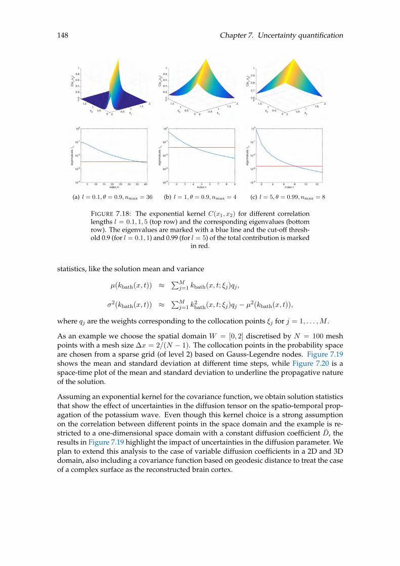
148 Chapter 7. Uncertainty quantification
(a) l = 0.1, θ = 0.9, nmax = 36 (b) l = 1, θ = 0.9, nmax = 4 (c) l = 5, θ = 0.99, nmax = 8
FIGURE 7.18: The exponential kernel C(x1, x2) for different correlationlengths l = 0.1, 1, 5 (top row) and the corresponding eigenvalues (bottomrow). The eigenvalues are marked with a blue line and the cut-off thresh-old 0.9 (for l = 0.1, 1) and 0.99 (for l = 5) of the total contribution is marked
in red.
statistics, like the solution mean and variance
µ(kbath(x, t)) ≈∑M
j=1 kbath(x, t; ξj)qj ,
σ2(kbath(x, t)) ≈∑M
j=1 k2bath(x, t; ξj)qj − µ2(kbath(x, t)),
where qj are the weights corresponding to the collocation points ξj for j = 1, . . . ,M .
As an example we choose the spatial domain W = [0, 2] discretised by N = 100 meshpoints with a mesh size ∆x = 2/(N − 1). The collocation points in the probability spaceare chosen from a sparse grid (of level 2) based on Gauss-Legendre nodes. Figure 7.19shows the mean and standard deviation at different time steps, while Figure 7.20 is aspace-time plot of the mean and standard deviation to underline the propagative natureof the solution.
Assuming an exponential kernel for the covariance function, we obtain solution statisticsthat show the effect of uncertainties in the diffusion tensor on the spatio-temporal prop-agation of the potassium wave. Even though this kernel choice is a strong assumptionon the correlation between different points in the space domain and the example is re-stricted to a one-dimensional space domain with a constant diffusion coefficient D, theresults in Figure 7.19 highlight the impact of uncertainties in the diffusion parameter. Weplan to extend this analysis to the case of variable diffusion coefficients in a 2D and 3Ddomain, also including a covariance function based on geodesic distance to treat the caseof a complex surface as the reconstructed brain cortex.

7.5. Summary 149
FIGURE 7.19: The mean and the standard deviation of the potassium wavekbath at different time steps, namely t = 0, 10, 20, 30, 40 sec.
(a) mean (b) standard deviation
FIGURE 7.20: The mean and the standard deviation of the potassium wavekbath in space and time.
7.5 Summary
In this chapter we treated the model parameters as random variables and processes (inspace) and analysed the impact of their uncertainties on the model solution. Since thereare different strategies to cope with uncertainties in the parameters that do not dependon space and in those that are spatially-dependent, we treated them separately.
Using PCM and other UQ techniques for uncertainties in the space-independent param-eters we observed the impact of individual parameters and of their combined effect onthe shape and characteristics of the potassium wave. We assumed either uniform or betadistributed parameters to ensure that their values are selected from finite intervals, asit is natural for biological parameters. With a sensitivity analysis based on the ANOVA

150 Chapter 7. Uncertainty quantification
approach we discovered the contribution of each parameter to the solution variance andto problem-specific measures, such as the time interval of high potassium concentrationor the maximum potassium concentration. Despite some of the parameters contributingmore than others to these characteristics, our results showed that none of them is negligi-ble. Consequently, to improve the predictive role of the model all the parameters wouldneed to be specified in experimental set-ups.
In principle all parameters could be space-dependent, but for this study we only consid-ered the diffusion coefficient (or diffusion tensor) to depend on space and approximatedit by the Karhunen-Loeve expansion. We considered the particular case of an exponentialkernel and presented the solution statistics in a one-dimensional space domain. These re-sults gave a first hint of what type of information could potentially be inferred from thistype of analysis. Nevertheless, assuming a specific kernel requires a strong knowledgeabout the correlation between different points of the mesh discretisation. Hence, the nextstep of some more grounded research in this direction would be to construct a kernelbased on the available DTI data and depending on geodesic distances.

151
Conclusions“All endings are also beginnings. We just don’t know it at that time.”
Mitch Albom, in The Five People you meet in Heaven (2003)
This thesis focused on patient-specific modelling and simulation of the cortical spreadingdepression (CSD), a correlate of migraine with aura. We developed and implemented amulti-scale PDE-ODE model that couples the propagation of the depolarisation wave as-sociated to CSD with a detailed electrophysiological model for neuronal activity in orderto capture both macroscopic and microscopic dynamics. The model was combined withpersonalised brain geometries, obtained from magnetic resonance imaging (MRI) andwith patient-specific conductivity tensors derived from diffusion tensor imaging (DTI)data. This DTI data provides detailed information about the anisotropy and the electricalconductivity properties of cortical tissue. To quantify the results and evaluate the prop-agation behaviour we identified various quantities of interest (QoI), such as the surfaceregularity index or asymmetry measures in the CSD propagation behaviour, for intra-patient statistics. This set-up was applied to a series of data sets of different patientgroups for statistical evaluations. As the system parameters are unknown and generallytuned to reproduce main features of the CSD, we concluded this work by applying differ-ent techniques of uncertainty quantification to the developed model and study the effectof uncertainties in the parameter choice.
In this final chapter we summarise and discuss the results and conclusions drawn inthis thesis, also highlighting some important limitations of the presented work. We thenpresent some possible future research to extend and improve the work presented in thisthesis.
Patient-specific CSD model
In Chapters 3 and Chapter 4 we introduced and described the implementation of a multi-scale model for the potassium diffusion that successfully reproduces the electrophysio-logical and propagative characteristics of CSD waves. We included patient-specific infor-mation about the cerebral cortex and diffusion data from DTI data representing the mi-crostructure of the cerebral tissue. For computational reasons in the context of full cortexsimulations, we only considered the propagative component of the model. However, asthe model is coupled unidirectionally, the electrophysiology could be easily reproducedfrom the results of the propagating potassium wave on the cerebral cortex. Finally, wesimulated the CSD propagation on a real brain geometry obtained from MRI data us-ing diffusion data from DTI imaging. However, this model has several limitations, i.e.,it is missing to account for inhibitory neurons, synaptic gaps, and large vessels. Espe-cially the latter can potentially stop the propagation of the depolarisation wave (Ayataand Lauritzen, 2015). CSD is not only triggering ionic changes but also a vascular re-sponse, including vasodilation, that is, the widening of blood vessels. Accounting fortheir presence and effect could add to the accuracy of the model and its predictions.

152
Quantities of interest and case studies of migraine patients
To correct artefacts from the brain reconstruction, in Chapter 5 we tested several smooth-ing techniques, weight functions and parameter choices to smoothen the surface meshof the cortex. Taubin smoothing with equal weights turned out to be the best optionfor cortical geometries and instead of limiting the iteration number we introduce a newstopping criterion, a threshold for the maximum volume loss, addressing a typical draw-back of Taubin smoothing. For this choice of weights, the mesh quality of the two brainhemispheres improved with every step of the iterative smoothing algorithm. Anotherapproach to improve the smoothing result could be to optimise the mesh quality, whilesatisfying the volume loss restriction. This is an approach we are currently working onwith Franco Dassi from the University of Milan-Biccoca in Italy.
In the sixth chapter we considered a set of chronic migraine patients with aura and con-firmed that the simulated CSD wavefront propagates according to the sequence of symp-toms experienced by these patients during a migraine attack. In the second case studywe computed and compared the QoI introduced in Chapter 5 for patients in three dif-ferent groups. One limitation of this study is the fact that CSD is a neuronal correlateof migraine aura, but the migraine patients in this study do not experience aura. Eventhough we could not find a QoI that classifies a certain patient type or significantly dis-tinguishes healthy individuals from migraineurs, we could show that some QoI, e.g., thetime the CSD wave remains in specific regions of the left hemisphere, have the potentialto differentiate between the patient groups to a certain extent. The main limitation of thischapter is the size of the data sets, especially in the first case study where considerationswere made only for five patients. Bigger data sets and more sophisticated techniques fordata mining could yield more informative results or drive the selection of appropriateQoI. In addition, the QoI we introduced (especially the geometric ones) could possiblybe efficient indicators for other neurological diseases and a study on patient groups ofdifferent clinical backgrounds could be envisioned.
Uncertainty quantification
In Chapter 7 we applied different techniques in uncertainty quantification to the param-eters of the CSD model. The impact of spatially independent parameters depends on theassumed underlying distribution and the choice of support for this distribution. By test-ing the effect on the model solution of different underlying distributions we showed thatdifferent aspects of the model outcome are sensitive to different parameters (consideredeither individually or jointly). We analysed the contribution of each parameter to the so-lution variance and to other problem-specific measures with a sensitivity analysis. Eventhough some of the parameters contribute more than others to the CSD characteristics,none of them is negligible and experimental studies would have to inform the selectionof parameter values or parameter distributions.
For the sensitivity analysis we limited ourselves to considering uniform distributionsonly, though different distributions can potentially be considered. Another restriction weimposed on the parameters was that all of them had the same distribution. However, inreality, different parameters might be governed by different distributions. In this thesis,we only considered parameters defined on finite intervals, but distributions defined onR could be considered as well.

153
To approximate space-dependent parameter by a random process, strong assumptions onthe correlation of points in the mesh discretisation and on the covariance kernel are nec-essary. We addressed this aspect only partially by showing the solution statistics in a one-dimensional space domain for a particular case of covariance kernel. A more groundedanalysis in this setting could include the three-dimensional space domain of the cerebralcortex and a kernel based on DTI-data and was left as a possible topic for further research.
Future work
Even though spreading depression has initially been described in the cerebral cortex, itcan also be induced in subcortical brain structures with sufficiently high neuronal andsynaptic density, and with limited extracellular space (Ayata, 2010; Bures, Buresova,and Krivanek, 1974). Besides, CSD can propagate into subcortical structures via con-tiguous matter (Ayata, 2010; Bures, Buresova, and Krivanek, 1974; Eikermann-Haerteret al., 2009). On the basis of these two arguments we are planning to extend the model tobrain volumes instead of limiting it to the cortical surface. The next step in this directionwould be to include fibre tracts (computed from DTI data) that connect different corticalregions through inter-brain highways. These connections could contribute to the accu-racy of CSD propagation and reveal features that could not be observed simply with asurface model.
In this thesis, we approximated the diffusion coefficients or diffusion tensors by theKarhunen-Loeve expansion in space when applying uncertainty quantification to themodel parameters. However, for this expansion we needed the eigenvalues and eigen-vectors of the corresponding covariance kernel. As an illustrative example of this strat-egy, we assumed an exponential kernel and presented the corresponding solution statis-tics in a one-dimensional spatial domain. However, assuming a specific kernel requires astrong knowledge about the correlation between different points of the mesh discretisa-tion. To obtain an improved representation of the diffusion coefficients via the Karhunen-Loeve expansion, a better option would be to construct a kernel based on real DTI data.Another problem is that most commonly used kernels depend on the Euclidean distancebetween the points in space. As we are dealing with a brain cortex, a folded surface in 3D,a geodesic distance measure would provide much more accurate information. Includinguncertainties of all parameters in the model and learning from the DTI measurements isan imperative step of future research for the improvement of the predictive role of thismodel.


155
Appendix A
Contributions and developedsoftwares
A.1 Publications
Kroos, J.M., Diez, I., Cortes, J.M., Stramaglia, S., Gerardo-Giorda, L. , Geometry shapespropagation: assessing the presence and absence of cortical symmetries through a com-putational model of cortical spreading depression, Front. Comput. Neurosci., 2016, vol.10. ISSN: 1662-5188, DOI: 10.3389/fncom.2016.00006
Abstract: Cortical spreading depression (CSD), a depolarization wave which originatesin the visual cortex and travels towards the frontal lobe, has been suggested to be oneneural correlate of aura migraine. To the date, little is known about the mechanismswhich can trigger or stop aura migraine. Here, to shed some light on this problem and,under the hypothesis that CSD might mediate aura migraine, we aim to study differentaspects favoring or disfavoring the propagation of CSD. In particular, by a using a com-putational neuronal model distributed throughout a realistic cortical mesh, we study therole that the geometry has in shaping CSD. Our results are two-fold: first, we foundimportant differences in the propagation traveling patterns of CSD, both intra and inter-hemispherically, revealing important asymmetries in the propagation profile. Second,we identified the brain regions which play a key role in the CSD propagation. Our studyreveals important dynamical aspects of CSD, which, if applied to subject-specific corticalgeometry, might help to differentiate between healthy subjects and those suffering mi-graine.
Kroos, J.M., Diez, I., Cortes, J.M., Stramaglia, S., Gerardo-Giorda, L. , Temporal exci-tation patterns on the cerebral cortex as a result of migraine modeling, In: Mantica G.,Stoop R., Stramaglia S. (eds) Emergent Complexity from Nonlinearity, in Physics, En-gineering and the Life Sciences, Springer Proceedings in Physics, vol 191. Springer,Cham March 2017, Doi: 10.1007/978-3-319-47810-4_13
Abstract: The complex, highly individual, geometry of the cerebral cortex in humanspresents a major challenge in studying the spreading of spontaneous neuronal activ-ity. Recent computational advances allow to simulate the propagation of depolariza-tion waves on the macroscale and for individual geometries, reconstructed from accuratemedical imaging as MRI, with high levels of detail. In this paper, we take advantage of

156 Appendix A. Contributions and developed softwares
such technique to study the temporal excitation patterns that follow the passage of a de-polarization wave on the cerebral cortex.
Kroos, J.M., Marinelli, I., Diez, I., Cortes, J.M., Stramaglia, S., Gerardo-Giorda, L. ,Patient-specific computational modeling of Cortical Spreading Depression via DiffusionTensor Imaging, Int. J. Numer. Method Biomed. Eng., 2017, vol. 33 (11), e2874, DOI:10.1002/cnm.2874
Abstract: Cortical spreading depression, a depolarization wave originating in the visualcortex and traveling towards the frontal lobe, is commonly accepted as a correlate of mi-graine visual aura. As of today, little is known about the mechanisms that can trigger orstop such phenomenon. However, the complex and highly individual characteristics ofthe brain cortex suggest that the geometry might have a significant impact in supportingor contrasting the propagation of cortical spreading depression. Accurate patient-specificcomputational models are fundamental to cope with the high variability in cortical ge-ometries among individuals, but also with the conduction anisotropy induced in a givencortex by the complex neuronal organisation in the grey matter. In this paper, we inte-grate a distributed model for extracellular potassium concentration with patient-specificdiffusivity tensors derived locally from diffusion tensor imaging data.
Gerardo-Giorda, L. , Kroos, J.M., Multiscale modeling and simulation of cortical spread-ing depression propagation, Computers and Mathematics with Applications, 2017, vol.74 (5), p. 1076-1090, DOI: 10.1016/j.camwa.2017.05.013
Abstract: Cortical Spreading Depression (CSD) is a disruption of the brain homeostasisthat, originating in the visual cortex and traveling towards the frontal lobe, temporarilyimpairs the normal functioning of neurons. Although, as of today, little is known aboutthe mechanisms that can trigger or stop such phenomenon, CSD is commonly acceptedas a correlate of migraine visual aura. In this paper, we introduce a multi-scale PDE-ODEmodel that couples the propagation of the depolarization wave associated to CSD with adetailed electrophysiological model for the neuronal activity to capture both macroscopicand microscopic dynamics.
Kroos, J.M., Dassi, F., Perotto, S. and Gerardo-Giorda, L., Curvature analysis of smoothedmeshes from medical brain images, in preparation 2019
Kroos, J.M., de Tommaso, M., Stramaglia, S., Gerardo-Giorda, L., Single case study of mi-graine with aura patients on the basis of mathematical modelling for cortical spreading depression,in preparation 2019
A.2 Presentations
eVita Winter School: Uncertainty Quatification, Geilo, Norway – poster presentationentitled "Numerical Simulation of Cortical Spreading Depression on a Real Brain Geom-etry", January 2015.

A.3. Developed software 157
Zaferna Colloquium, Institute for Applied Mathematics, Westfälische Wilhelms-UniversitätMünster, Münster, Germany – presentation entitled "Mathematical Models for ExcitableMedia: An Application to the Cerebral Cortex", March 2015.
BCAM Workshop on Quantitative Biomedicine for Health and Disease, BCAM, Bilbao,Spain – poster presentation entitled "Personalised Simulation of the Cortical SpreadingDepression", Februar 2016.
Stockholm Mathematics Centre, University of Stockholm, Sweden – presentation en-titled "Personalised Simulation of the Cortical Spreading Depression – ComputationalModelling via Diffusion Tensor Imaging", 10 June 2016.
SIAM Conference on the Life Sciences, Boston, Massachusetts, USA – presentation en-titled "Personalised Simulation of the Cortical Spreading Depression – ComputationalModelling via Diffusion Tensor Imaging", 14 July 2016.
International Conference on Systems Biology, Barcelona, Spain – poster presentationentitled "Patient-specific Modelling of Cortical Spreading Depression", September 2016.
2nd BCAM Workshop on Nonlinear Dynamics in Biological Systems, BCAM, Bilbao,Spain – poster presentation entitled "Patient-specific Modelling of Cortical Spreading De-pression", September 2016.
3rd BCAM Workshop on Quantitative Biomedicine for Health and Disease, BCAM,Bilbao, Spain – presentation entitled "Patient-specific Modelling of Cortical SpreadingDepression", 22 February 2017.
Crunch Group, The Division of Applied Mathematics, Brown University, Providence,Rhode Island, USA – presentation entitled "Patient-specific Modelling of Cortical Spread-ing Depression", 10 March 2017.
Stockholm Mathematics Centre, University of Stockholm, Sweden – presentation enti-tled "Patient-specific Modelling of Cortical Spreading Depression", 19 June 2017.
11th European Conference on Mathematical and Theoretical Biology, Lisbon, Portugal– presentation entitled "Patient-specific Modelling of Cortical Spreading Depression", 27July 2018.
2nd International Workshop on Neurodynamics, Castro-Urdiales, Spain – presenta-tion entitled "Patient-specific Modelling of Cortical Spreading Depression", 27 September2018.
A.3 Developed software
Cortical spreading depression simulation
Program Name: compute_csd_whole_brain.mAuthor: J.M. KroosLicense: N/AOperating System: MacOSProgramming Language: MatlabDescription: The package numerically solves the CSD progression on the meshes of realbrain geometries. It initiates the wave in each of the 34 regions of interest records the

158 Appendix A. Contributions and developed softwares
arrival times in the other regions, respectively. The electrophysiology part on the micro-scopic level is coupled with the macroscopic propagative part. After the CSD computa-tion, the QoI can be investigated by the user using a general user interface.
Diffusion data processing
Program Name: DTI_preprocessing.mAuthor: J.M. KroosLicense: N/AOperating System: MacOSProgramming Language: MatlabDescription: This package processes the DTI and DWI data and integrates it in the al-ready existing code for the CSD progression.
Brain smoothing and curvature approximation
Program Name: Mesh smoothing packageAuthors: F. Dassi, J.M. KroosLicense: N/AOperating System: MacOSProgramming Language: C++Description: This code was developed in C++ together with Franco Dassi. All in allwe provided simulations of the CSD on a real brain geometry with diffusion coefficientsobtained from DTI data.
159
Appendix B
Mathematical compendium
“If you can’t understand it without an explanation,you can’t understand it with an explanation.”
Haruki Murakami, in 1Q84 (2009)
In this appendix we gather some mathematical concepts that we just briefly referred to inthe previous chapters. First, we comment on preconditioned iterative solvers especiallyfor sparse linear systems. For a better understanding of the concepts of curvature usedin Chapter 5, we give a basic introduction and an example in Appendix B.2. In AppendixB.3 we summarise concepts of graph theory that we use in Chapter 5 to confirm the con-nectivity of points considered for the initial condition. Finally, Appendix B.4 gives a briefintroduction to the concepts, ideas and common techniques in uncertainty quantificationin Chapter 7.
B.1 Preconditioned iterative solvers for sparse linear systems
For the computation of CSD propagation, we need to solve a linear system Ax = b whereA is a large sparse matrix. We give a short introduction to iterative solvers and numericaltechniques for preconditioning to increase the efficiency and robustness of the solution.We mainly follow Saad, 2003 and Quarteroni, Sacco, and Saleri, 2007.
B.1.1 Iterative solvers for linear systems
Iterative methods yield the solution x of a linear system Ax = b after an infinite numberof steps. The basic idea is to construct a sequence of vectors xk that converges
x = limk→∞
xk.
In practice, the iterative process is stopped at a minimum value n, such that
||xn − x|| < ε,
where ε is a tolerance and || · || is any suitable vector norm.

160 Appendix B. Mathematical compendium
For a given linear system and a given initial datum x0, iterative methods are of the form
xk+1 = xk +M−1rk, for k ≥ 1,
where M is a non-singular matrix, also called preconditioner, and
rk = b−Axk
denotes the residual vector at step k.
There are two main classes of iterative methods, stationary iterative methods and Krylovsubspace methods. Here, we focus on Krylov subspace methods that approximate the so-lution by minimising the residual. Typical methods of this class are the conjugate gradi-ent method that assumes matrix A to be symmetric positive-definite and the biconjugategradient method for non-symmetric linear systems. We briefly present the preconditionedconjugate gradient method (PCG) and the biconjugate gradient stabilised method (BiCGSTAB),improvements of the afore mentioned methods.
B.1.1.1 Preconditioned conjugate gradient
PCG is one of the best known iterative techniques to solve linear systems with sparsesymmetric positive-definite matrices. Denoting with rk = b − Axk the original residualand with zk = M−1rk the residual for the preconditioned system, the algorithm of thePCG is given in Algorithm B.1.
Algorithm B.1 PCG
1: compute r0 = b−Ax0, z0 = M−1r0 and p0 = z0
2: for k = 0, 1, . . . until rk sufficiently small do
3: αk = (rk,zk)(Apk,pk)
4: xk+1 = xk + αkpk
5: rk+1 = rk − αkApk6: zk+1 = M−1rj+1
7: βk =(rk+1,zk+1)
(rk,zk)
8: pk+1 = zk+1 + βkpk
9: end for
B.1.1.2 Biconjugate gradient stabilised method
BiCGSTAB is a variant of the biconjugate gradient method and the conjugate gradientsquared method. The BiCGSTAB supports a faster but less stable convergence than theother two methods. For a preconditioning with the matrix M = M1M2 the BiCGSTABmethod is listed in detail in Algorithm B.2.

B.1. Preconditioned iterative solvers for sparse linear systems 161
Algorithm B.2 BiCGSTAB
1: compute r0 = b−Ax0
2: choose r0 s.t. (r0, r0) 6= 0
3: set p0 = r0
4: for k = 0, 1, . . . until convergence do
5: αk =rT0 rk
rTk AM−1pk
6: sk = rk + αkAM−1pk
7: t = AM−1sk
8: wk =(M−1
1 t,M−11 s)
(M−11 t,M−1
1 t)
9: xk+1 = xk + αkM−1pk + wkM
−1sk
10: rk+1 = sk − wkt
11: βk =(rk+1,r0)
(rj ,r0)αkwk
12: pk+1 = rk+1 + βk(pk − wkAM−1pk)
13: end for
B.1.2 Preconditioners for sparse matrices
Preconditioning is a technique to increase efficiency and robustness of linear solvers. Ittransforms the linear system into one that has the same solution but can be solved moreeasily and accurately. Considering the problem Ax = b, the preconditioner M is anapproximation of A for which the system M−1Ax = M−1b is easier to solve and M−1 ischeap to compute. Thus, we can solve the preconditioned system
M−1Ax = M−1b or AM−1u = b, x = M−1u.
In the next subsection, we introduce some of the most common preconditioners.
B.1.2.1 Incomplete LU factorisation
For a sparse matrix A = (aij)i,j=1,...,n, the incomplete LU factorisation (ILU) computes asparse lower triangular matrix L and a sparse upper triangular matrix U , so that theresidual R = A − LU satisfies certain constraints. The elements to drop at each step canbe chosen as some non-zero pattern in advance. For any zero pattern set P , such that
P ⊂ (i, j) | i 6= j, 1 ≤ i, j ≤ n,
the ILU factorisation can be computed as follows.
Zero fill-in ILU In the incomplete LU factorisation with no fill-in, denoted by ILU(0),the pattern of the matrixA is taken as a template for the sparsity patterns of the triangularmatrices. Thus the zero pattern P is defined as P = (i, j)|aij 6= 0. The matrix L hasthe sparsity pattern of the lower triangular part of A and the matrix U the one from theupper triangular part. An example of the sparsity pattern of a matrix A, the matrices Land U obtained with ILU(0) factorisation and their product are shown in Figure B.1.
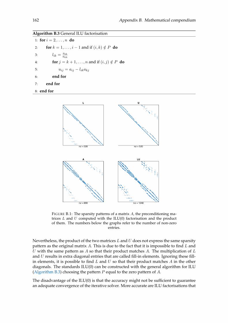
162 Appendix B. Mathematical compendium
Algorithm B.3 General ILU factorisation
1: for i = 2, . . . , n do
2: for k = 1, . . . , i− 1 and if (i, k) /∈ P do
3: lik = aikakk
4: for j = k + 1, . . . , n and if (i, j) /∈ P do
5: uij = aij − likakj6: end for
7: end for
8: end for
FIGURE B.1: The sparsity patterns of a matrix A, the preconditioning ma-trices L and U computed with the ILU(0) factorisation and the productof them. The numbers below the graphs refer to the number of non-zero
entries.
Nevertheless, the product of the two matrices L and U does not express the same sparsitypattern as the original matrix A. This is due to the fact that it is impossible to find L andU with the same pattern as A so that their product matches A. The multiplication of Land U results in extra diagonal entries that are called fill-in elements. Ignoring these fill-in elements, it is possible to find L and U so that their product matches A in the otherdiagonals. The standards ILU(0) can be constructed with the general algorithm for ILU(Algorithm B.3) choosing the pattern P equal to the zero pattern of A.
The disadvantage of the ILU(0) is that the accuracy might not be sufficient to guaranteean adequate convergence of the iterative solver. More accurate are ILU factorisations that

B.1. Preconditioned iterative solvers for sparse linear systems 163
allow some fill-in, also called ILU(p). However, in these techniques, the fill-in only de-pends on the structure of the original matrixA. A more sensible approach is to determinethe zero pattern P more dynamically and also depending on the values in A.
Threshold strategies and ILUT There are a few alternative methods to ILU(p) that basethe dropping of elements in the Gaussian elimination process according to their magni-tude instead of their location. With this, the zero pattern P is chosen more dynamically.The most common way to obtain an incomplete factorisation that ignores small entriesbelow a threshold is to take a sparse direct solver and add the dropping conditions forthe elements. An example is given in Algorithm B.4. Here v is a row vector collectingthe linear combinations of the rows in the elimination and vk is the k-th entry of v. Thenotation ai∗ describes the i-th row of matrix A.
Algorithm B.4 ILUT
1: for i = 1, . . . , n do
2: v := ai∗
3: for k = 1, . . . , i− 1 and if vk 6= 0 do
4: vk := vkakk
5: apply the dropping rule to vk
6: if vk 6= 0 then
7: v := v − vkuk∗8: end if
9: end for
10: apply the dropping rule to row v
11: lij := vj for j = 1, . . . , i− 1
12: uij := vj for j = i, . . . , n
13: v := 0
14: end for
The ILU(0) can be considered as a special case of this algorithm with the rule to dropelements that are in the position of zero entries in the original matrix. In the factorisationILUT(p,τ ) the dropping rules are:
(i) In line 5, the element vk is set to zero (e.g. by dropping it) if it is below the relativetolerance τi which is the product of τ and the norm of ai∗, the i-th row of the originalmatrix A.
(ii) In line 10, first all elements with values below the relative threshold τi are dropped.Then only the p largest elements in the L part and the p largest elements in the Upart are kept.
Here, the first dropping rule reduces the computational costs, whereas the second onehelps to control the memory usage.
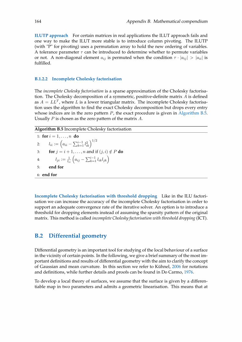
164 Appendix B. Mathematical compendium
ILUTP approach For certain matrices in real applications the ILUT approach fails andone way to make the ILUT more stable is to introduce column pivoting. The ILUTP(with "P" for pivoting) uses a permutation array to hold the new ordering of variables.A tolerance parameter τ can be introduced to determine whether to permute variablesor not. A non-diagonal element aij is permuted when the condition τ · |aij | > |aii| isfulfilled.
B.1.2.2 Incomplete Cholesky factorisation
The incomplete Cholesky factorisation is a sparse approximation of the Cholesky factorisa-tion. The Cholesky decomposition of a symmetric, positive-definite matrix A is definedas A = LLT , where L is a lower triangular matrix. The incomplete Cholesky factorisa-tion uses the algorithm to find the exact Cholesky decomposition but drops every entrywhose indices are in the zero pattern P , the exact procedure is given in Algorithm B.5.Usually P is chosen as the zero pattern of the matrix A.
Algorithm B.5 Incomplete Cholesky factorisation
1: for i = 1, . . . , n do
2: lii :=(aii −
∑i−1k=1 l
2ik
)1/2
3: for j = i+ 1, . . . , n and if (j, i) /∈ P do
4: lji := 1lii
(aij −
∑i−1k=1 likljk
)5: end for
6: end for
Incomplete Cholesky factorisation with threshold dropping Like in the ILU factori-sation we can increase the accuracy of the incomplete Cholesky factorisation in order tosupport an adequate convergence rate of the iterative solver. An option is to introduce athreshold for dropping elements instead of assuming the sparsity pattern of the originalmatrix. This method is called incomplete Cholesky factorisation with threshold dropping (ICT).
B.2 Differential geometry
Differential geometry is an important tool for studying of the local behaviour of a surfacein the vicinity of certain points. In the following, we give a brief summary of the most im-portant definitions and results of differential geometry with the aim to clarify the conceptof Gaussian and mean curvature. In this section we refer to Kühnel, 2006 for notationsand definitions, while further details and proofs can be found in Do Carmo, 1976.
To develop a local theory of surfaces, we assume that the surface is given by a differen-tiable map in two parameters and admits a geometric linearisation. This means that at

B.2. Differential geometry 165
every point there is a linear surface, i.e., a plane, that touches the surface at that pointonly. A map that satisfies this condition is called immersion.
Definition B.2.1. A map f : U → Rm defined on an open set U ⊂ Rn is differentiable at apoint x ∈ U , if there is a linear map Ax : Rn → Rm so that
f(x+ ξ) = f(x) +Axξ + o (||ξ||) ,
is true in a neighbourhood Uε(x). The symbol o (||ξ||) indicates, that the term convergesto zero for ξ → 0 after dividing it by ξ. The matrix Ax is the Jacobian of f , namely
Jxf =
(∂fi∂xj
∣∣∣x
)i,j
.
The rank of the map f in x is then defined as the rank of the Jacobian. If f is differen-tiable at every point x ∈ U and the rank is maximal everywhere, the map f is called animmersion (if n ≤ m) or a submersion (if n ≥ m).
In the following, let U ⊂ R2 be an open subset and f : U → R3, (u, v) 7→ f(u, v) animmersion. A parametrised surface is an immersion f and is also called parametrisation. Theclassical notation of a parametrisation is given by a triple of functions (x,y,z) in cartesiancoordinates
f(u, v) = (x(u, v), y(u, v), z(u, v)) ∈ R3,
where the parameter (u, v) is mapped to the point (x, y, z). A two-dimensional submani-fold of R3 can be locally described as a surface element. As an example, the upper cap ofthe unit sphere S = (x, y, z) ∈ R3 |x2 + y2 + z2 = 1 can be parametrised by
(u, v) 7→ (u, v,±√
1− u2 − v2), u2 + v2 < 1.
Being an immersion is equivalent to the fact, that the vectors ∂f∂u and ∂f
∂v are linearly in-dependent at every point and span the tangent plane. We will introduce the followingnotations for u ∈ U and p ∈ f(u):
TuU is the tangential space of U at u TuU = u × R2,TpR3 is the tangential space of R3 at p TpR3 = p × R3,Tuf is the tangential plane of f at p Tuf := Df |u(TuU) ⊂ Tf(u)R3
Definition B.2.2. We denote by 〈·, ·〉 the Euclidean scalar product in R3 and in all thetangent spaces TpR3. The first fundamental form I of a surface element is just the restrictionof 〈·, ·〉 to all the tangent planes TuU , i.e.,
I(X,Y ) := 〈X,Y 〉
for two tangent vectors X,Y ∈ Tuf .
In the coordinates f(u, v) = (x(u, v), y(u, v), z(u, v)), the first fundamental form is de-scribed by the symmetric and positive-definite matrix
G =
(I(∂f∂u ,
∂f∂u) I(∂f∂u ,
∂f∂v )
I(∂f∂v ,∂f∂u) I(∂f∂v ,
∂f∂v )
)=
(〈 ∂f∂u ,
∂f∂u〉 〈
∂f∂u ,
∂f∂v 〉
〈 ∂f∂v ,∂f∂u〉 〈
∂f∂v ,
∂f∂v 〉
).
In the two-dimensional case the curvature is characterised by the changes of the tangents.Analogously, we expect the curvature of a surface in three dimensions to be defined by

166 Appendix B. Mathematical compendium
the changes in the tangent planes. As every plane is uniquely determined by its normalvector, we can study the changes in those vectors instead. This is the major motivationfor the Gauss mapping.
Definition B.2.3. For a surface element f : U → R3 the Gauss map ν : U → S with theunit sphere S = (x, y, z) ∈ R3 |x2 + y2 + z2 = 1, is defined as
ν(u, v) :=∂f∂u ×
∂f∂v∥∥∥∂f∂u × ∂f∂v
∥∥∥ .Definition B.2.4. Let f : U → R3 be a surface element with Gauss map ν : U → S ⊂ R3.
(i) For every u ∈ U the image of the linear map
Dν|u : TuU → TνR3
is parallel to the tangent plane Tuf . By canonically identifying TνR3 with R3 andTf(u)R3, we can take Dν at every point as a map
Dν|u : TuU → Tuf.
Furthermore, we can view the map Df |u as a linear isomorphism
Df |u : TuU → Tuf,
by restricting the image. In this sense, the inverse map (Df |u)−1 is well-defined onthe tangential plane Tuf and is also an isomorphism.
(ii) The map L := −Dν (Df)−1 that is point-wise defined by
Lu := − (Dν|u) (Df |u)−1 : Tuf → Tuf,
is called Weingarten map or shape operator of f . Thus, for every parameter u this mapis a linear endomorphism of the tangent plane at the corresponding point f(u). Thismeans that L
(∂f∂ui
)= − ∂ν
∂uifor i = 1, 2 and the rank of L is equal to the rank of Dν.
(iii) L is independent of the parametrisation f and it is self-adjoint with respect to thefirst fundamental form I.
Definition B.2.5. Let f : U → R3, ν : U → S and L be the Weingarten map of f as inDefinition B.2.4. Then we define for the tangent vectors X and Y :
(i) the second fundamental form II of f by
II(X,Y ) := I(LX, Y ),
(ii) the third fundamental form III of f by
III(X,Y ) := I(L2X,Y ) = I(LX,LY ).
As L is self-adjoint with respect to I, II and III are symmetric bilinear forms on Tuf forevery u ∈ U .

B.2. Differential geometry 167
For the three fundamental forms, the following equation holds
III− Tr(L)II + Det(L)I = 0.
We consider an arbitrary curve c = cX on a surface through a fixed point p with unittangent vector c′(p) = X . The curvature κ of the curve c on the surface is defined as thelength of the vector c′′. We decompose c′′ into its tangential and normal parts:
c′′ = (c′′)Tang.︸ ︷︷ ︸tangential component
+ 〈c′′, ν〉ν︸ ︷︷ ︸normal component
.
The normal component in p is given by
〈c′′, ν〉ν =
⟨d2c
ds2, ν
⟩= −
⟨c′,∂ν
∂s
⟩= 〈X,LX〉ν = II(X,X)ν
and thus only depends on the tangent X at point p but not on the choice of the curve.Therefore, II(X,X) is called normal curvature κν of the curve cX . It always holds thatκ2 ≥ κ2
ν .
Definition B.2.6. LetX ∈ Tuf denote the unit tangent vector, i.e., I(X,X) = 1. X is calledprincipal curvature direction of f , if one of the following equivalent conditions is satisfied:
(i) II(X,X) (the normal curvature κν in the direction of X) has a stationary valueamong all X with I(X,X) = 1.
(ii) X is an eigenvector of the Weingarten map L.
The corresponding eigenvalue λ (for LX = λX) is called the principal curvature.
For a two-dimensional surface the two principal curvatures are simply the maximum andminimum of the normal curvature. In this case we denote the principal curvatures of fby κ1 and κ2.
Definition B.2.7. (i) The determinant K = Det(L) = κ1 · κ2 is called the Gaussian cur-vature of f .
(ii) The average value H = 12Tr(L) = 1
2(κ1 + κ2) is called the mean curvature of f .
Example: As an example for the Gaussian and mean curvature, we consider the sphereS ⊂ R3 with radius r. Therefore, let n be a normal vector pointing outwards. We fixa point p ∈ S , choose an arbitrary tangent vector X ∈ TpS and let σ : (−ε, ε) → S be acurve on the sphere S so that σ(0) = p, dσdt (0) = X . Then the Weingarten map L is definedby
L(X) = −∇Xn = − d
dtn σ(t)
∣∣∣∣t=0
.
But with n σ(t) = n(σ(t)) = σ(t)|σ(t)| = σ(t)
r it follows that
L(X) = − d
dt
σ(t)
r
∣∣∣∣t=0
= −1
r
dσ
dt
∣∣∣∣t=0
= −1
rX
for any X ∈ TpS. Thus, the Weingarten map for a sphere S is defined as L = −1r I, where
I is the identity matrix. With this and Definition B.2.7 we can determine the Gaussian

168 Appendix B. Mathematical compendium
curvature K and the mean curvature H of the sphere S as
K = Det(L) =1
r2, H =
1
2Tr(L) = −1
r.
B.3 Graph theory
Let P = p1, . . . , pn be a set of vertices and E = e1, . . . , em the set of edges connectingP , the resulting triangulation can also call graph Γ.
Definition B.3.1. If the edge pipj ∈ E, then we say pi and pj are adjacent. The adjacencymatrix A ∈ Rn×n with A = (aij)i,j=1,...,n is then defined as
aij =
1, if pi and pj are adjacent0, otherwise
.
The matrix A is a symmetric matrix with trace zero.
Definition B.3.2. A walk from vertex pi to pj of length k is defined as a finite sequence ofvertices such that
pi = u0, u1, . . . , uk = pj ,
where ut−1 and ut are adjacent for 1 ≤ t ≤ k. A graph is called connected if every pair ofvertices is joined by a walk.
Lemma B.3.1. A graph Γ with n vertices is connected if and only if (A+ I)n−1 has no zeroentries, where A is the adjacency matrix of Γ (Biggs, 1993).
Lemma B.3.2. The number of walks of length k from pi to pj is the entry in position (i, j)of the matrix Ak (Biggs, 1993).
Consequently, if an entry aij of the adjacency matrix Ak is zero, there is no walk of lengthk from pi to pj .
Definition B.3.3. The number of edges traversed in the shortest way joining p and p′ iscalled the distance between p and p′ and denoted by ∂(p, p′). The diameter of a connectedgraph Γ, denoted by diam(Γ) is the maximum distance between two vertices, namely
diam(Γ) := maxp∈P
minp′∈P
∂(p, p′).
The eccentricity of a vertex p is the maximum distance from this point to any other vertexp′, denoted by ecc(p). The radius, denoted by rad(Γ), is the minimum eccentricity amongall vertices of Γ, namely
rad(Γ) := minp∈P
maxp′∈P
∂(p, p′) = minp∈P
ecc(p).
Definition B.3.4. The degree of p ∈ P , denoted by deg(p), is the number of edges incidentto p. The maximum degree of a graph Γ is denoted by ∆(Γ) and defined as
∆(Γ) := maxp∈P
deg(p).
B.4. Uncertainty quantification 169
The maximum number of edges in an undirected graph without loop is n(n − 1)/2, butthe following lemma gives a tighter upper boundary.
Lemma B.3.3. For a graph Γ of order n it holds (Goddard and Oellermann, 2011):
1. diam(Γ) ≤ n−∆(Γ) + 1
2. rad(Γ) ≤ diam(Γ) ≤ 2rad(Γ)
3. rad(Γ) ≤ n−∆(Γ)2 + 1
B.4 Uncertainty quantification
B.4.1 Orthogonal polynomials
Let N = 0, 1, . . . or N = 0, 1, . . . , N be a (possibly finite) index set of non negativeintegers. A system of polynomials Qn(x) |n ∈ N with polynomials Qn(x) of exactdegree n, is an orthogonal system of polynomials with respect to a real positive measure υ, ifit satisfies the orthogonality condition∫
SQm(x)Qn(x) dυ(x) = γnδmn, m, n ∈ N , (B.1)
where S is the support of the measure υ, δmn is the Kronecker delta function with δmn = 1if m = n and δmn = 0 else, and γn is a positive constant, the so-called normalisationconstant. The system is orthonormal, if γn = 1.
The measure υ normally has a density w(x) or weights w(i) at point i in the discrete case.With this position, equation (B.1) becomes∫
SQm(x)Qn(x)w(x) dx = γnδmn, m, n ∈ N ,
or in the discrete case
N∑i=1
Qm(xi)Qn(xi)w(xi) dx = γnδmn, m, n ∈ N .
In the theory of orthogonal polynomials, the density w(x), or the weights w(i) in the dis-crete case, are often referred to as the weighting functions.
B.4.1.1 Hypergeometric series and the Askey scheme
An important class of orthogonal polynomials are the ones expressed in a unified way byusing hypergeometric series belonging to the Askey scheme (Askey and Willson, 1985). Thisscheme classifies the hypergeometric orthogonal polynomials that satisfy certain typesof differential (or difference) equations, and reveals their mutual relation. Each subsetof orthogonal polynomials of the Askey scheme has a different weighting function andit has been discovered that some of these weighting functions are identical to the prob-ability density functions (PDFs) of certain random distributions (Xiu and Karniadakis,

170 Appendix B. Mathematical compendium
2002). These findings allow to represent stochastic processes with different orthogonalpolynomials, according to the inherent properties of the process.
To start, we define the Pochammer symbol (a)n as
(a)n =
1, if n = 0,
a(a+ 1) · · · (a+ n− 1), if n = 1, 2, 3, . . ..
The hypergeometrical series rFs is then defined as
rFs(a1, . . . , ar; b1, . . . , bs; z) =∞∑k=0
(a1)k . . . (ar)k(b1)k . . . (bs)k
zk
k!,
with bi > 0 for i = 1, . . . , s and r, s ∈ N0. Orthogonal polynomials of this form that arelinked to probability functions of certain random distributions are the Hermite, Legen-dre, Laguerre, Jacobi, Charlier, Meixner, Krawtchouk and Hahn polynomials. A detaileddescription of these polynomials and their limit relations can be found in Koekoek andSwarrouw, 1998 and Schoutens, 2000.
B.4.1.2 Examples of orthogonal polynomials
In the following, we present several orthogonal polynomials that will be used later onin the context of the generalised polynomial chaos (see Appendix B.4.3). The main focushere is on continuous polynomials and we present and discuss Hermite polynomials de-fined on R, Legendre polynomials defined on [−1, 1] and Laguerre polynomials definedon [0,∞).
Hermite polynomials The sequence of Hermite polynomials
Hn(x) = (2x)n 2F0
(−n
2,−n− 1
2; ;− 2
x2
)(B.2)
satisfies the recursion
Hn+1(x) = 2xHn(x)− 2nHn−1(x), n > 0,
and the polynomials are orthogonal, that is,∫ ∞−∞
Hm(x)Hn(x)w(x) dx = n!δmn,
with respect to the weighting function
w(x) =1√2πe−x
2/2.
This weighting function is the same as the PDF of a standard Gaussian random variablewith zero mean and unit variance.

B.4. Uncertainty quantification 171
Legendre polynomials The sequence of Legendre polynomials
Pn(x) = 2F1
(−n, n+ 1; 1;
1− x2
)(B.3)
satisfies the recursion
Pn+1(x) =2n+ 1
n+ 1xPn(x)− n
n+ 1Pn−1(x), n > 0,
and the polynomials are orthogonal, that is,∫ 1
−1
1
2Pm(x)Pn(x) dx =
1
2n+ 1δmn.
Evidently, the weighting function in the orthogonality relation is constant, i.e., for theLegendre polynomials defined on [−1, 1] it is w(x) = 0.5. In general, this is the PDF of auniform distribution defined on a generic interval [a, b] with the PDF of f(x) = 1
b−a . InFigure B.2 we plot the Legendre polynomials on the interval [−1, 1] up to the order n = 5.
FIGURE B.2: Legendre polynomials on the interval [−1, 1] up to the ordern = 5.
Laguerre polynomials The sequence of Laguerre polynomials
L(α)n (x) =
(α+ 1)nn!
1F1 (−n;α+ 1;x) (B.4)
satisfies the recursion
(n+ 1)L(α)n+1(x) = (2x+ α+ 1− x)L(α)
n (x)− (n+ α)L(α)n−1(x), n > 0,
and the polynomials are orthogonal, that is,∫ ∞0
e−xxαL(α)m (x)L(α)
n (x) dx =Γ(n+ α+ 1)
n!δmn.

172 Appendix B. Mathematical compendium
Recalling that the PDF of the gamma distribution is defined as
f(x) =xαe−x/β
βα+1Γ(α+ 1), α > −1, β > 0, for x > 0 (B.5)
the weighting function of the Laguerre polynomial can be rescaled to the PDF of a gammadistribution.
B.4.2 Formulation of stochastic systems
We briefly describe the general aspects of formulating stochastic equations and how toproperly set up the stochastic model to study the effect of uncertainties in the input to thesystem. It is essential to properly characterise the random inputs, which usually means toreduce the infinite-dimensional probability space to a finite one (if necessary). In general,the critical step in formulating a stochastic system is to characterise the probability spacedefined by the random inputs by a finite set of mutually independent random variables.Such a characterisation usually involves an approximation error.
B.4.2.1 Input parametrisation: random parameters
In the case of uncertainties in the system parameters, the randomness is in the input andthe formulation of the stochastic system is straight forward. Under these circumstancesthe most important issue is to identify independent parameters in the set.
The problem can be formulated as follows: Let Y = (Y1, . . . , Ym), m > 1 be the systemparameters with given probability distribution function FY (y) = P (Y ≤ y), y ∈ Rm.Find a set of mutually independent random variables Z = (Z1, . . . , Zd) ∈ Rd, with 1 ≤d ≤ m, such that Y = R(Z) for a suitable transformation function R.
To illustrate the previous formulation, we consider the following example of an ordinarydifferential equation with two random variables:
du
dt(t, ω) = −α(ω)u, u(0, ω) = β(ω),
where the growth rate α and the initial condition β are assumed to be random. Thus, theinput random variables are Y (ω) = (α, β) ∈ R2 and the solution is u(t, ω) : [0, T ]×Ω→ R.
If α and β are mutually independent, we can simply set Z(ω) = Y (ω) and the solutionu(t, ω) can be expressed as
u(t, ω) : [0, T ]× R2 → R,
with one dimension in time and two random dimensions.
In the case that α and β are not mutually independent, there exists a function g such that
g(α, β) = 0.
Then we can find a random variable Z(ω) to parametrise the above relation so that
α(ω) = a(Z(ω)), β(ω) = b(Z(ω)),
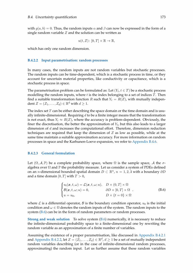
B.4. Uncertainty quantification 173
with g(a, b) = 0. Thus, the random inputs α and β can now be expressed in the form of asingle random variable Z and the solution can be written as
u(t, Z) : [0, T ]× R→ R,
which has only one random dimension.
B.4.2.2 Input parametrisation: random processes
In many cases, the random inputs are not random variables but stochastic processes.The random inputs can be time-dependent, which is a stochastic process in time, or theyaccount for uncertain material properties, like conductivity or capacitance, which is astochastic process in space.
The parametrisation problem can be formulated as: Let (Yt, t ∈ T ) be a stochastic processmodelling the random inputs, where t is the index belonging to a set of indices T . Thenfind a suitable transformation function R such that Yt = R(Z), with mutually indepen-dent Z = (Z1, . . . , Zd) ∈ Rd with d ≥ 1.
The index set T can be either describing the space domain or the time domain and is usu-ally infinite-dimensional. Requiring d to be a finite integer means that the transformationis not exact, thus Yt ≈ R(Z), where the accuracy is problem-dependent. Obviously, thefiner the discretisation, the better the approximation of Yt, but this also leads to a largerdimension of d and increases the computational effort. Therefore, dimension reductiontechniques are required that keep the dimension of Z as low as possible, while at thesame time maintain a suitable approximation accuracy. For more information on randomprocesses in space and the Karhunen-Loeve expansion, we refer to Appendix B.4.6.
B.4.2.3 General formulation
Let (Ω,A,P) be a complete probability space, where Ω is the sample space, A the σ-algebra over Ω and P the probability measure. Let us consider a system of PDEs definedon an n-dimensional bounded spatial domain D ⊂ Rn, n = 1, 2, 3 with a boundary ∂Dand a time domain [0, T ] with T > 0,
ut(x, t, ω) = L(x, t, ω;u), D × (0, T ]× Ω
B(x, t, ω;u) = 0, ∂D × [0, T ]× Ω
u = u0, D × t = 0 × Ω
, (B.6)
where L is a differential operator, B is the boundary condition operator, u0 is the initialcondition and ω ∈ Ω denotes the random inputs of the system. The random inputs to thesystem (B.6) can be in the form of random parameters or random processes.
Strong and weak solution To solve system (B.6) numerically, it is necessary to reducethe infinite-dimensional probability space to a finite-dimensional one by rewriting therandom variable as an approximation of a finite number of variables.
Assuming the existence of a proper parametrisation, like discussed in Appendix B.4.2.1and Appendix B.4.2.2, let Z = (Z1, . . . , Zd) ∈ Rd, d ≥ 1 be a set of mutually independentrandom variables describing (or in the case of infinite-dimensional random processes,approximating) the random input. Let us further assume that these random variables

174 Appendix B. Mathematical compendium
Zidi=1 have probability density functions ρi : IZi → R+ and the images IZi = Zi(Ω) arebounded intervals in R for i = 1, . . . , d. The joint PDF is
ρ(Z) =d∏i=1
ρi(Zi), for all Zi ∈ R,
with the support IZ =⊗d
i=1 IZi ⊂ Rd. Then we can rewrite the system (B.6) as a (d+ n)-dimensional differential equation in the strong form
ut(x, t, Z) = L(x, t, Z;u), D × (0, T ]× IZB(x, t, Z;u) = 0, ∂D × [0, T ]× IZu = u0, D × t = 0 × IZ
. (B.7)
Thus, the solution isu(x, t, Z) : D × [0, T ]× IZ → Rnu ,
where d is the dimensionality of the random space, n is the dimensionality of the physicalspace D and nu ≥ 1 is the dimension of u.
Similar to the weak formulation in deterministic problems, the system (B.7) is oftensolved in a weak form. For that reason, we define a finite-dimensional subspace VIZ ⊂L2p(IZ), the space of all square integrable functions in IZ with respect to the measure
ρ(Z)dZ. We are looking for a solution uV (x, t, Z) ∈ L2p(IZ), such that∫
IZ
ρ(Z)uVt (x, t, Z)φ(Z) dZ =
∫IZ
ρ(Z)L(x, t, Z;uV )φ(Z) dZ, for x ∈ D, (B.8)∫IZ
ρ(Z)B(x, t, Z;uV )φ(Z) dZ = 0, for x ∈ ∂D, (B.9)
for φ(Z) ∈ VIZ . The resulting problem is a deterministic one in the physical domain Dand can be solved with standard discretisation techniques, like finite elements or finitevolumes.
B.4.2.4 Traditional numerical methods
There are several numerical standard techniques that can be applied to the problem (B.7),or (B.9) - (B.9). Here, we shortly review the Monte Carlo method that has a relatively slowconvergence rate, but is independent of the dimensionality of the random space.
For further explanations on traditional numerical methods, including the moment equa-tion approach and the perturbation method, we refer to Xiu, 2010.
Monte Carlo method One of the most popular and well-developed methods for solv-ing stochastic differential equations is the Monte Carlo method. Even though it convergesrelatively slowly, with a convergence rate of 1/
√K for a simulation consisting of K sam-
ples, it is independent of the number of random variables Zi(ω)di=1 (Fishman, 1996).The general procedure to apply Monte Carlo sampling to problem (B.7) is:
1. For a given number of realisationsK, generate independent, identically distributedrandom variables Zji di=1 = Zi(ωj)di=1 for j = 1, . . . ,K.

B.4. Uncertainty quantification 175
2. For each j = 1, . . . ,K solve the deterministic problem (B.7) with Zj = (Zj1 , . . . , Zjd)
obtaining the solution uj(x, t, Zj).
3. Post-process the results to obtain the solution statistics, as the solution mean
u(x, t) =1
K
K∑j=1
uj ≈ E(u)
or the solution variance
V(u) ≈ 1
K
K∑j=1
(uj − u)2.
Note that for each realisation j = 1, . . . ,K step 2 is a deterministic problem which has tobe solved with a suitable scheme.
B.4.3 Generalised polynomial chaos
In this subsection we focus on the generalised polynomial chaos (gPC) expansion basedon globally smooth orthogonal polynomials, in particular the polynomials of the Askeyscheme introduced in Appendix B.4.1, as in contrast to for e.g. piecewise polynomials.
Let Z be a random variable with a distribution function FZ(z) = P (Z ≤ z) and letQn(x), n ∈ N be an orthogonal system of polynomials as defined in Appendix B.4.1,that fulfil the orthogonality condition (B.1). The generalised polynomial chaos basis func-tions are defined as these orthogonal polynomial functions, that additionally satisfy
γn = E(Q2m(Z)), n ∈ N
for the normalisation factor. If Z is continuous, the orthogonality can be rewritten interms of the corresponding PDF ρ, like in equation (B.1), namely
E(Qm(Z)Qn(Z)) =
∫Qm(z)Qn(z)ρ(z) dz = γnδmn, m, n ∈ N . (B.10)
We will now consider basis functions for different types of polynomials. Let Z be a stan-dard Gaussian random variable, namely Z ∼ N (0, 1) with PDF ρ(z) = (2π)−1/2e−z
2/2.Then the orthogonality condition (B.1), or rather (B.10), defines the Hermite orthogonalpolynomials Hn(Z) |n ≥ 0 like in (B.2). Employing the Hermite polynomials as thebasis function, we have
H0(Z) = 1, H1(Z) = Z, H2(Z) = Z2 − 1, H3(Z) = Z3 − 3Z, . . . . (B.11)
The basis in (B.11) is the classical Wiener-Hermite chaos.
Let Z be a random variable uniformly distributed on [−1, 1], namely Z ∼ U(−1, 1) withconstant PDF ρ(z) = 1/2. Then the orthogonality condition (B.1), or rather (B.10), definesthe Legendre orthogonal polynomials Pn(Z) |n ≥ 0 like in (B.3), with
P0(Z) = 1, P1(Z) = Z, P2(Z) =2
3Z2 − 1
2, . . . .

176 Appendix B. Mathematical compendium
Let Z be a random variable gamma-distributed on [0,∞) with shape parameter α andrate parameter β, namely Z ∼ Γ(α, β) with PDF as defined in (B.5). Then the orthog-onality condition (B.1), or rather (B.10), defines the Laguerre orthogonal polynomialsLn(Z) |n ≥ 0 like in (B.4), with
L0(Z) = 1, P1(Z) = −Z + 1, L2(Z) =1
2(Z2 − 4Z + 2), . . . . (B.12)
In Table B.1 we list the established correspondences between the probability distributionof Z and its gPC basis polynomials.
random variable Wiener-Askey chaos supportcontinuous Gaussian Hermite-chaos (−∞,∞)
gamma Laguerre-chaos [0,∞)beta Jacobi-chaos [a, b]
uniform Legendre-chaos [a, b]
discrete Poisson Charlier-chaos 0, 1, 2, . . . , Nbinomial Krawtchouk-chaos 0, 1, 2, . . . , N
negative binomial Meixner-chaos 0, 1, 2, . . .hypergeometric Hahn-chaos 0, 1, 2, . . . , N
TABLE B.1: The different types of Wiener-Askey scheme polynomials andtheir underlying random distribution.
In general, the homogenous chaos expansion employs orthogonal polynomials from theAskey scheme in terms of random variables. The resulting polynomial chaos providesa method for expanding second-order random processes in terms of orthogonal poly-nomials. The Wiener-Askey polynomial chaos is a generalisation of the original Wienerpolynomial chaos, using Hermite polynomials for the expansion to account for Gaussiandistributed random variables. Thus, the Wiener-Askey polynomial chaos allows account-ing for a wider range of distributions of random variables and processes.
We can represent the general random process Y (ω) by
Y (ω) = a0Q0
+∞∑i1=1
ci1Q1(ξi1(ω))
+∞∑i1=1
∞∑i2=1
ci1ci2Q2(ξi1(ω), ξi2(ω)) (B.13)
+∞∑i1=1
∞∑i2=1
∞∑i3=1
ci1ci2ci3Q3(ξi1(ω), ξi2(ω), ξi3(ω))
+ . . . ,
where Qn(ξi1 , . . . , ξin) denotes the Wiener-Askey polynomial chaos of order n in termsof the random vector ξ = (ξi1 , . . . , ξin). For notational convenience, we can summariseequation (B.13) as
Y (ω) =
∞∑j=1
cjQj(ξ). (B.14)

B.4. Uncertainty quantification 177
Then the orthogonality condition of the Wiener-Askey polynomial chaos can be writtenas
〈Qm,Qn〉 = 〈Qm,Qm〉 δmn, (B.15)
where δmn is the Kronecker delta and 〈·, ·〉 denotes the ensemble average, namely
〈f(ξ), g(ξ)〉 =
∫f(ξ)g(ξ)w(ξ) dξ,
where w(ξ) denotes the weighting function of the corresponding polynomial chaos basisQnn≥1. As previously mentioned, some of the polynomials from the Askey schemehave weighting functions corresponding to the distribution of certain types of randomvariables.
B.4.3.1 General procedure
Now, we introduce the general procedure of how to apply the Wiener-Askey polynomialchaos to solve stochastic differential equations. Let us consider the differential equation
L(x, t, ω;u) = f(x, t, ω). (B.16)
Then the solution u = u(x, t, ω) can be expanded by the Wiener-Askey polynomial chaosas
u(x, t, ω) =
P∑j=0
uj(x, t)Qj(ξ(ω)). (B.17)
The total number of expansion terms is depending on the dimension n of the randomvariable ξ and the highest order p of the polynomials Qnn≥1, i.e.,
P + 1 = (n!p!)−1(n+ 1)! .
Substituting (B.17) into equation (B.16) results in
L
x, t, ω;P∑j=0
uj(x, t)Qj(ξ (ω))
= f(x, t, ω). (B.18)
To ensure that the error is orthogonal to the functional space spanned by the finite dimen-sional basis Qnn≥1, a Galerkin projection of equation (B.18) is applied to each polyno-mial basis element.⟨L
x, t, ω;P∑j=0
uj(x, t)Qj(ξ (ω))
,Qk
⟩= 〈f(x, t, ω),Qk〉 , k = 0, 1, . . . , P. (B.19)
From (B.19) and the orthogonality of the polynomial basis, we obtain a set of P + 1 cou-pled equations for each random mode uj(x, t). The Wiener-Askey chaos expansion trans-fers the randomness into the polynomial basis, so that the equations for the expansioncoefficient uj from (B.19) are deterministic and can be solved with any conventional de-terministic technique.

178 Appendix B. Mathematical compendium
B.4.3.2 Stochastic ordinary differential equations
To exemplify the above, we consider the following ordinary differential equation
dy(t)
dt= −ky, y(0) = y0, (B.20)
where the coefficient k is assumed to be a random variable k(ω) with a specific distri-bution and mean value k. The PDF is defined as f(k) and the deterministic solution of(B.20) is y(t) = y0e
−kt, and
y(t) = y0
∫Se−ktf(k) dk
is the mean of the stochastic solution where S is the support of f . Applying the Wiener-Askey polynomial chaos expansion (B.14) to the solution y and the random input k, wecan rewrite these accordingly as
y(t) =
P∑i=0
yi(t)Qi, k =
P∑i=0
kiQi.
Substituting this into the governing equation (B.20), we obtain
P∑i=0
dyi(t)
dtQi = −
P∑i=0
P∑j=0
kiyj(t)QiQj .
Then we project the above equation onto the polynomial basis Qnn≥1, to ensure theorthogonality of the error to the space spanned by the orthogonal polynomials. Usingthe orthogonality condition (B.15), we obtain by applying 〈·,Ql〉 to the previous equation
dyl(t)
dt= − 1
〈Ql,Ql〉
P∑i=0
P∑j=0
kiyj(t)eijl, for l = 0, 1, . . . , P,
with eijl = E(QiQjQl). From this point on, a standard solver for ordinary differentialequations can be applied.
B.4.3.3 Definition in higher dimensions
In the case of more than one random variable, the multivariate gPC expansion is required.Therefore, let Z = (Z1, . . . , Zd) be a random vector with independent components withthe distribution FZ(z1, . . . , zd) = P (Z1 ≤ z1, . . . Zd ≤ zd) with z = (z1, . . . , zd). For everyi = 1, . . . , d, let FZi(zi) = P (Zi ≤ zi) be the marginal distribution of Zi on the supportIZi . The independence of the random variables Zi implies that FZ(z) =
∏di=1 FZi(zi) and
IZ =⊗d
i=1 IZi . Then, let Qk(Zi)Nk=0 ∈ PN (Zi) be the univariate gPC basis functions inZi of degree smaller or equal to N . These functions satisfy the orthogonality condition,that is,
E(Qj(Zi)Qk(Zi)) =
∫Qj(zi)Qk(zi)dFZi = γjδjk, 0 ≤ j, k ≤ N. (B.21)
Let i = (i1, . . . , id) ∈ Nd0 be a multi-index with |i| = i1 + . . .+ id. Then, the d-variate N -thdegree gPC basis functions are the product of gPC polynomials of the total degree less or

B.4. Uncertainty quantification 179
equal to N , that is,
Qi(Z) = Qi1(Z1) · · ·Qid(Zd), 0 ≤ |i| ≤ N.
With this, it follows directly
E(Qi(Z)Qj(Z)
)=
∫Qi(z)Qj(z)dFZ = γiδij ,
where γi = E(Q2i) = γi1 · · · γid are the normalisation factors and δij = δi1,j1 · · · δi1,jd the
d-variate Kronecker delta function. The span of these polynomials is PdN , the linear spaceof polynomials of degree at most N in d variables, namely
PdN (Z) =
p : IZ → R
∣∣∣∣∣ p(Z) =∑|i|≤N
ciQi(Z)
,
whose dimension is(N + d
N
).
B.4.4 Stochastic collocation method
In the probabilistic collocation method (PCM) system (B.6) is evaluated at a discrete set ofpoints, called nodes, in the random space. In this perspective, the classical samplingmethods, like the Monte Carlo method are collocation methods. In the following, wedescribe this approach using the polynomial approximation theory with Legendre poly-nomials.
Let ΘM = Z(i)Mi=1 ⊂ IZ be a set of nodes in the random space, whereM ≥ 1 is the num-ber of nodes and IZ the support of Z. Then in the collocation method we enforce (B.7)at the node Z(i), for all i = 1, . . . ,M . Thus, for every Z(i), the system is a deterministicproblem as the value of the random parameter is fixed and reads
ut(x, t, Z(i)) = L(x, t, Z(i);u), D × (0, T ]× IZ
B(x, t, Z(i);u) = 0, ∂D × [0, T ]× IZu = u0, D × t = 0 × Ω
.
Let u(i) = u(·, ·, Z(i)) be the solution of the above system for i = 1, . . . ,M . The result is aset of deterministic solutions u(i)Mi=1.
In the Legendre interpolation approach, the solution u is approximated by a polynomialv(Z) ∈ Π(Z) rewritten, such that v(Z(i)) = u(i) for all i = 1, . . . ,M , namely
v(Z) =
M∑i=1
u(Z(i))Pj(Z), (B.22)
where Pj(Z(i)) = δij for 1 ≤ i, j ≤ M are the Lagrangian polynomials and u(Z(i)) isthe solution at a given node Z(i). Consequently, the collocation method is equivalentto solving M deterministic problems, the deterministic counterpart of problem (B.6), ateach node Z(i), for i = 1, . . . ,M . With this, the statistics of the random solution can be

180 Appendix B. Mathematical compendium
evaluated, e.g.,
E(u) ≈ E(v) =
M∑i=1
u(Z(i))
∫ b
aLi(Z)ρ(Z) dZ
≈M∑i=1
u(Z(i))1
b− a
M∑k=1
Li(Zk)wk
=1
b− a
M∑i=1
u(Z(i))wi,
with the assumption of a uniform distribution with the PDF ρ on the interval [a, b]. Thewi are the weights of the collocation points depending on the choice of the quadraturerule.
B.4.4.1 Collocation points
The computational effort of the stochastic collocation method is M times that of the de-terministic problem, where M is the total number of nodes. In order to make the proce-dure more effective and faster, we choose a nodal set with as few points as possible butmaintaining a prescribed accuracy of the results. In the following, we present differentchoices of collocation points, with the main focus on multi-dimensional random spaces,that is IZ ⊂ Rd, d > 1. We assume that the bounded support of the random variable Ziis IZi = [−1, 1], for i = 1, . . . , d, so that the random space is a d-dimensional hypercube,namely IZ = [−1, 1]d. Random variables with a bounded support [a, b] can be mapped to[−1, 1].
Tensor product collocation The most natural way to choose the nodal set is the tensorproduct of the one-dimensional sets. For any smooth function f : [−1, 1]d → R, we canconstruct a good one-dimensional interpolation (for d = 1):
U i(f) =
mi∑k=1
f(Zki )wki , i = 1, . . . , d, (B.23)
for a nodal set Θ1i = (Z1
i , . . . , Zmii ) ⊂ [−1, 1] and interpolation weights wki = wk(Zi). In
the multivariate case, with d > 1, the tensor product formula reads
I(f) = (U i1 ⊗ · · · ⊗ U id)(f) =
mi1∑k1=1
. . .
mid∑kd=1
f(Zk1i1 , . . . , Zkdid
) · (wk1i1 ⊗ · · · ⊗ wkdid
).
In the above product formula, we need M = mi1 · · ·mid nodal points for the collocationmethod. Choosing the same interpolation function in all dimensions, i.e., mi1 = . . . =mid = m, the total number of points is md which quickly grows in high dimensionsd 1.
Consequently, the tensor product interpolation is easy to construct but the number ofinterpolation nodes grows rapidly with the dimension of the random space. So for higherdimensions it is reasonably to construct the interpolation grid more efficiently.

B.4. Uncertainty quantification 181
Sparse grids One way to reduce the total number of nodal points is to construct sparsegrids, for example with the Smolyak algorithm (Smolyak, 1963). Considering the one-dimensional interpolation formula (B.23), the Smolyak algorithm is given by
I(f) = A(q, d) =∑
q−d+1≤|i|≤q
(−1)q−|i|(d− 1
q − |i|
)(U i1 ⊗ · · · ⊗ U id), (B.24)
where i = (i1, . . . , id) ∈ Nd is a multi-index and q ≥ d is an integer denoting the levelof construction (Gerstner and Griebel, 1998; Xiu and Hesthaven, 2005). The result isa combination of subsets of the full tensor grid. To compute A(q, d), we only need toevaluate the function on the sparse grid
Θd =⋃
q−d+1≤|i|≤q
(Θ1i1 ⊗ · · · ⊗Θ1
id).
In Figure B.3 we visualise a comparison of the full tensor grid and a sparse grid in twodimensions (d = 2). The Smolyak formulas for this are based on one-dimensional poly-nomial interpolation at the extrema of the Legendre polynomials. The full grid is a tensorproduct of 50 nodes in each dimension, whereas the sparse grid has the level q = 4 ofconstruction. Table B.2 lists the number of nodes of the Smolyak sparse grid for differentdimensions d and levels q.
(a) full grid with 2500 points (b) sparse grid with 224 points
FIGURE B.3: Two-dimensional nodes (d = 2) based on the extrema of theLegendre polynomials at level q = 4. The total number of points is 2500
(a), whereas the number of nodes in the Smolyak sparse grid is 224 (b).
B.4.4.2 Multi-element probabilistic collocation method
The multi-element probabilistic collocation method (ME-PCM) is a generalised form ofthe PCM, where the parameter space is discretised and a collocation grid is prescribed oneach element. The ME-PCM offers the advantages of domain decomposition in the para-metric space and is especially useful to treat problems with discontinuous dependence
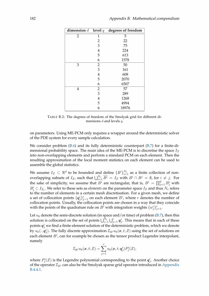
182 Appendix B. Mathematical compendium
dimension d level q degrees of freedom2 1 5
2 223 754 2245 6136 1578
3 2 503 1614 6085 20706 6507
4 2 573 2894 12685 49946 18976
TABLE B.2: The degrees of freedom of the Smolyak grid for different di-mensions d and levels q.
on parameters. Using ME-PCM only requires a wrapper around the deterministic solverof the PDE system for every sample calculation.
We consider problem (B.6) and its fully deterministic counterpart (B.7) for a finite-di-mensional probability space. The main idea of the ME-PCM is to discretise the space IZinto non-overlapping elements and perform a standard PCM on each element. Then theresulting approximation of the local moment statistics on each element can be used toassemble the global statistics.
We assume IZ ⊂ Rd to be bounded and define BiNei=1 as a finite collection of non-overlapping subsets of IZ , such that
⋃Nei=1B
i = IZ with Bi ∩ Bj = ∅, for i 6= j. Forthe sake of simplicity, we assume that Bi are rectangular, that is, Bi =
∏dj=1B
ij with
Bij ⊂ IZj . We refer to these sets as elements on the parameter space IZ and thus Ne refers
to the number of elements in a certain mesh discretisation. For a given mesh, we definea set of collocation points qijrj=1 on each element Bi, where r denotes the number ofcollocation points. Usually, the collocation points are chosen in a way that they coincidewith the points of the quadrature rule on Bi with integration weights wijrj=1.
Let uk denote the semi-discrete solution (in space and/or time) of problem (B.7), then thissolution is collocated on the set of points
⋃Nei=1
⋃rj=1 q
ij . This means that in each of these
points qij we find a finite element solution of the deterministic problem, which we denoteby uk(·, qij). The fully discrete approximation IBiuk(x, t;Z) using the set of solutions oneach element Bi, can for example be chosen as the tensor product Legendre interpolant,namely
IBiuk(x, t;Z) =r∑j=1
uk(x, t; qij)P
ij (Z),
where P ij (Z) is the Legendre polynomial corresponding to the point qij . Another choiceof the operator IBi can also be the Smolyak sparse grid operator introduced in AppendixB.4.4.1.
B.4. Uncertainty quantification 183
Then we can define the global approximation of the solution as
u(x, t;Z) =
Ne∑i=1
IBiuk(x, t;Z)1Bi ,
where 1Bi denotes the characteristic function of the set Bi.
For the statistics, i.e., the approximate global mean, we define the PDF on each elementas
ηi(Z) =ρ(Z)∫
Bi ρ(Z) dZ.
We assume the PDF ρ to be a tensor product form, namely ρ(Z) =∏dj=1 ρj(Zj), which
is inherited by the local density ηi(Z) =∏dj=1 ηj(Zj). Then the local mean of a function
v : D × [0, T ]×Bi → R on an element Bi is given by
Ei(v(x, t; ·)) = E(v(x, t; ·)|Z(ω) ∈ Bi) =
∫Biv(x, t;Z)ηi(Z) dZ.
Using a quadrature rule, we can approximate the local mean of u on each element Bi as
Ei(u) ≈r∑j=1
uk(x, t; qij)w
ij .
With this, we can approximate the global mean of u over all the elements, as
E(u) ≈Ne∑i=1
Ei(u)(x, t)P (Z(ω) ∈ Bi).
B.4.5 ANOVA approach and sensitivity measures
The analysis of variance (ANOVA) expansion offers a way to represent multivariate func-tions f(x) in high dimensions when estimating the sensitivity indices with a variance-based approach. In general, the standard ANOVA expansion consists of a unique orthog-onal decomposition of the function f(x) for independent random inputs. The drawbackof this expansion is the need for the computation of the high dimensional integrals whendealing with low-order component functions. The anchored ANOVA decomposition, onthe other hand offers a computationally more efficient way for numerical evaluations ofthe component functions in the ANOVA expansion (Tang, Congedo, and Abgrall, 2015).
B.4.5.1 Standard ANOVA expansion
Let y = f(x) be a function describing the model under investigation defined on the n-dimensional unit cube In = [0, 1]n with x = (x1, . . . , xn) ∈ In. Then we can representf(x) as
f(x) = f0 +
n∑s=1
n∑i1<...<is
fi1...is(xi1 , . . . , xis), (B.25)

184 Appendix B. Mathematical compendium
with 1 ≤ i1 < . . . < is ≤ n, or equivalently
f(x) = f0 +∑
1≤i≤nfi(xi) +
∑1≤i<j≤n
fij(xi, xj) + . . .+ f12...n(x1, . . . , xn).
The total number of summands in these formulas is 2n. Alternatively, using a more com-pact representation based on multi-indices sj , the ANOVA decomposition can be writtenas:
f(x) = fs0 +2n−1∑j=1
fsj (xsj ).
In the above expression, the multi-indices sj are defined as
s0 = (0, 0, 0, . . . , 0)
s1 = (1, 0, 0, . . . , 0)
s2 = (0, 1, 0, . . . , 0)
...sn = (0, 0, 0, . . . , 1)
sn+1 = (1, 1, 0, . . . , 1)
sn+2 = (1, 0, 1, . . . , 1)
...sN = (1, 1, 1, . . . , 1)
with N = 2n − 1.
The expression (B.25) is called ANOVA-representation of f(x) if f0 is constant and theintegral of every summand over any of its own variables is zero, namely∫ 1
0fi1...is(xi1 , . . . , xis)dxk = 0, for k = i1, . . . , is and s = 1, . . . , n. (B.26)
This equality can also be interpreted as an orthogonality condition under which everyadditional dimension considered in the function f is orthogonal to the preceding ones.From equations (B.25) and (B.26) it follows that
∫In f(x) dx = f0 and that the summands
in equation (B.25) are orthogonal and can be expressed as integrals of f(x), that is
f0 + fi(xi) =
∫ 1
0. . .
∫ 1
0f(x) dx−i, (B.27)
f0 + fi(xi) + fj(xj) + fij(xi, xj) =
∫ 1
0. . .
∫ 1
0f(x) dx−ij, . . . ,
where dx−i denotes the integration over all variables except for those within the sub-script parenthesis, namely x−i = (x1, . . . , xi−1, xi+1, . . . , xn).

B.4. Uncertainty quantification 185
Then the variance of f is the sum of the variances of all the decomposition terms:
σ2(f) =n∑s=1
n∑i1<...<is
σ2(fi1...is(xi1 , . . . , xis)),
σ2(fi1...is(xi1 , . . . , xis)) =
∫Isf2i1...is(xi1 , . . . , xis) dxi1 · · · dxis ,
or equivalently
σ2(f) =∑
1≤j1≤nσ2(fj1) +
∑1≤j1≤j2≤n
σ2(fj1j2) + . . .+ σ2(f12...n).
For the above equality, it is important that the measure used is the same as in the ANOVAdecomposition (B.27). The value of σ(f) is likely to be different from the exact value com-puted by the standard definition of the variance, that is, the integral with the Lebesguemeasure.
B.4.5.2 Anchored ANOVA expansion
The construction of the standard ANOVA expansion requires the evaluation of high-dimensional integration, which can be very expensive. An alternative formulation, theanchored (or Dirac) ANOVA expansion requires no integrals, but has an accuracy thatdepends heavily on the choice of the so-called anchor point.
Instead of the Lebesgue measure we can use the Dirac measure in the integrations, i.e.,dµ(x) = δ(x − c) dx, x ∈ In. The point c is called anchor point and this method is calledthe anchored ANOVA expansion. Consequently, we have
f0 = f(c) (B.28)
for the constant term. Different choices of the anchor point may lead to different approx-imations of the ANOVA decomposition of a function. For strategies on the selection ofthe anchor point, we refer for example to Gao and Hesthaven, 2010.
Applying the anchored ANOVA method to stochastic problems, we denote the highestdimension for the component function with ν and approximate f(x) with
f(x) ≈ f0 +∑j1≤n
fj1(xj1) +∑
j1<j2≤nfj1j2(xj1 , xj2) + . . . (B.29)
+∑
j1<j2<...<jν≤nfj1j2...jν (xj1 , xj2 , . . . , xjν ).
Here, n is called the nominal dimension, ν the truncation or effective dimension and we use µin the following to denote the number of collocation points in each dimension.
After obtaining the ANOVA decomposition of function f , we can approximate the inte-gration of the component functions with the values of these functions at the quadraturepoints with the corresponding weights. These quadrature points can also be used ascollocation points for PCM.

186 Appendix B. Mathematical compendium
B.4.5.3 Adaptive ANOVA expansion
Even though the ANOVA method reduces the computational effort, it still requires ahigh number of sampling to compute all the terms for high nominal dimensions n. Aneffective way to reduce the computational effort is the adaptive ANOVA decomposition,where the nominal dimension is replaced by an active dimension Di for each subgroup.In this approach, approximation (B.29) is modified to be
f(x) ≈ f0 +∑j1≤D1
fj1(xj1) +∑
j1<j2≤D2
fj1j2(xj1 , xj2) + . . .
+∑
j1<j2<...<jν≤Dν
fj1j2...jν .(xj1 , xj2 , . . . , xjν ).
In most cases, the decomposition is truncated with ν = 2 and D1 = n. Adaptive criteriato determine the active dimension were, i.e., developed in Yang et al., 2012.
B.4.5.4 Sensitivity analysis
Assuming that f(x) is square integrable, the total variance of f(x) can be written asD =
∫In f
2(x) dx − f20 and all the fi1...is are square integrable. Squaring equation (B.25)
and integrating over In, we obtain∫Inf2(x) dx− f2
0 =n∑s=1
n∑i1<...<is
∫Isf2i1...is(xi1 , . . . , xis) dxi1 · · · dxis ,
with Is = [0, 1]s. Defining the contribution to the total variance from the term fi1...is inthe expansion as
Di1...is =
∫Isf2i1...is(xi1 , . . . , xis) dxi1 · · · dxis ,
the total variance can also be written as
D =
n∑s=1
n∑i1<...<is
Di1...is . (B.30)
Then the global sensitivity indices are defined as the ratio
Si1...is =Di1...is
D, (B.31)
where s is often called the order or the dimension of the index Si1...is . From definition (B.31)and (B.30), it follows that all Si1...is are non-negative and
n∑s=1
n∑i1<...<is
Si1...is = 1.
Exemplarily, we present how to obtain the mean and varianceDi of the first- and second-order terms in the ANOVA decomposition. Therefore, let q1
1, . . . , qµ1 be the quadrature
points for the one-dimensional approximation. As we consider the Dirac measure whencomputing the component terms, this means that for example the value of f1 in the
B.4. Uncertainty quantification 187
quadrature point q11 is
f1(q11) = f(q1
1, c2, c3, . . . , cn)− f0,
where c = (c1, . . . , cn) is the anchor point and f0 = f(c), see equation (B.28). Then themean and variance of f1 can be approximated by
E(f1) ≈µ∑i=1
f1(qi1)wi1, σ2(f1) ≈µ∑i=1
f21 (qi1)wi1 − (E(f1))2 ,
where w11, . . . , w
µ1 are quadrature weights corresponding to collocation points q1
1, . . . , qµ1 .
This definition applies analogously to all first-order terms f2, . . . , fn with the generalnotation fk(qik) = f(c1, . . . , ck−1, q
ik, ck+1, . . . , cn)− f0.
Similarly, we can compute the second-order terms. For example, we consider f12 at thequadrature point (qi1, q
j2) with i, j = 1, . . . , µ. Using equation (B.27), we obtain
f12(qi1, qj2) = f(qi1, q
j2, c3, c4, . . . , cn)− f1(qi1)− f2(qj2)− f0,
and
E(f12) ≈µ∑i=1
µ∑j=1
f12(qi1, qj2)wij12
σ2(f12) ≈µ∑i=1
µ∑j=1
f212(qi1, q
j2)wij12 − (E(f12))2 ,
where wij12 with i, j = 1, . . . , µ are the quadrature weights corresponding to the tensorgrid of the collocation points (qi1, q
j2). Here, we use the tensor product rule to obtain the
quadrature rule in higher dimensions, but other methods such as sparse grids can beused.
Generally speaking, for the higher-order terms of the component functions, we have
fsi = f(c|xsi)−∑sj⊂si
fsi(xsi),
where f(c|xsi) describes the value of f(x) evaluated at the anchor point c except for thevariables involved in xsi .
As an illustrative example, we consider a function with separated variables that wasconsidered in Archer, Satelli, and Sobol’, 1997 and Sobol’, 2001, namely
g(x) =
n∏i=1
ϕi(xi), for xi ∈ [−2, 1], with ϕi(xi) =|4xi + 2|+ ai
1 + ai,
where ai ≥ 0 for i = 1, . . . , n are fixed deterministic coefficients. If ai = 0 this implies thatϕi varies between 0 and 6 and thus the variable xi is important, if ai is big, i.e., ai = 99,then ϕi varies between 0.99 and 1.77 and thus the variable xi is insignificant.

188 Appendix B. Mathematical compendium
The contribution to the total variance of the functions gi1 and gi1i2 for i1, i2 = 1, . . . , n canbe reformulated as
Di = V(∫
In−1
g(x) dx−i
)=
1
3(1 + ai)2,
Dij = V(∫
In−2
g(x) dx−ij
)−Di −Dj = DiDj
and the total variance can we written as a function of first-order terms only
D = −1 +
n∏i=1
(1 +Di).
Assuming that n = 8, and a1 = a2 = a6 = 0, a3 = 1 and ai = 3 for i = 4, 5, 7, 8. Thenthe first, second and sixth variable are the most important ones, variable x3 is not veryimportant, whereas the other remaining variables are insignificant. This can be verifiedby the Sobol’ indices: S1 = S2 = S6 = 0.333, S3 = 0.083 and Si = 0.021 for the remainingi = 4, 5, 7, 8. The second-order indices are: Sij = 0.0621 for i, j ∈ 1, 2, 3, Sij = 0.0155 ifone of the indices is 3 and the other one 1,2 or 6, Sij = 0.0039 for one index being fromthe set 1, 2, 6 and the other one from 4, 5, 7, 8. All other indices of second-order aresmaller than 9·10−4. We visualise these sensitivity indices of first-order and second-orderfor the variables x1, . . . , x8 in Figure B.4. The size of the blue spots indicates the magni-tude of the sensitivity index of first-order, whereas the connections between the spotsmark the strength of their connectivity or rather the sensitivity indices of order 2.
FIGURE B.4: The Sobol’ indices for the above example.

B.4. Uncertainty quantification 189
B.4.6 Stochastic processes in space
So far we considered stochastic processes in time. However, the dynamics of stochasticprocesses in space are not analogous to the dynamics of the ones in the time domain. Dueto the unilateral nature of the time series, the stochastic process is only influenced by pastvalues, whereas the spacial process has a dependence in all directions.
In general random fields are used to model spatial data, that is, observed in environmen-tal or biomedical sciences. These real life problems in 1, 2 or even 3 spatial dimensionscan be modelled by multi-dimensional stochastic processes. Realistic models of randomprocesses in space require autoregressive schemes with dependence in all directions, of-ten referred to as multi-dimensional second-order stochastic processes (Su and Lucor,2006).
In general, a continuous random process is formally defined as an indexed set of randomvariables, where the index belongs to a continuous uncountable set. Such process can beapproximated by restricting the index to a subset of the indexing set.
In the most general form, the spectral representation of a random process, can be ex-pressed as
Y (x, θ) =
∫g(x)dµ(θ),
where Y (x, θ) is a stochastic process with a covariance function C(x1, x2) = cov(x1, x2)that admits the decomposition
C(x1, x2) =
∫g(x1)g(x2)dµ1(θ)dµ2(θ),
where g(x) is a deterministic function, and dµ(θ) is an orthogonal set function, also calledorthogonal stochastic measure (Ghanem and Spanos, 1991).
An alternative formulation of the spectral representation is the Karhunen-Loeve expan-sion based on a Fourier-type series expansion. Let Y (x, θ) be a random process, namelya function of the position vector x defined over the space domain D, with θ belonging tothe space of random events Ω. Then the Karhunen-Loeve expansion reads
Y (x, θ) = Y (x) +∞∑n=0
√λnξn(θ)fn(x),
where Y (x) is the expected value of Y (x, θ), ξn(θ) is a set of random variables, and λnand fn(x) are the eigenvalue and eigenvector of the covariance kernel. That means theyare the solution to the integral equation∫
DC(x1, x2)fn(x) dx1 = λnfn(x2). (B.32)
Truncating the series at the m-th term gives
Y (x, θ) = Y (x) +m∑n=0
√λnξn(θ)fn(x).

190 Appendix B. Mathematical compendium
The Karhunen-Loeve expansion described above has some interesting and useful proper-ties that make it a good choice for some applications. Here, we briefly summarise them,but for a more detailed approach and proofs we refer to Ghanem and Spanos, 1991.
1. Error minimising propertyChoosing as an orthonormal set of functions the eigenfunctions of the covariancekernel is optimal to minimise the mean-square error resulting from the finite repre-sentation of the process.
2. Uniqueness of the expansionThe random variables in the expansion are orthonormal if and only if the orthonor-mal functions fn(x) and the constants λn are the eigenfunctions and eigenvalues ofthe covariance kernel as given in (B.32), respectively.
The usefulness of the Karhunen-Loeve expansion depends heavily on the ability to solvethe integral equation of the form∫
DC(x1, x2)f(x2) dx2 = λf(x1), (B.33)
where C(x1, x2) is the covariance function. This also implies that C(x1, x2) must bebounded, symmetric and positive-definite. These characteristics of the kernel ensure avariety of properties for the eigenvalues and eigenfunctions that are the solution to equa-tion (B.33):
1. The set fi(x) of eigenfunctions is orthogonal and complete.
2. To each eigenvalue λi corresponds a finite number of linearly independent eigen-functions.
3. There are at most a countable infinite set of eigenvalues.
4. The eigenvalues are all positive real numbers.
5. The kernel C(x1, x2) allows the following uniform convergent expansion
C(x1, x2) =
∞∑k=1
λkfk(x1)fk(x2).
All these properties are independent of the stochastic nature of the process and allow awide range of applications.
One important covariance kernel is the exponential kernel representing the first-order Marko-vian process. It is given by the equation
C(x1, x2) = e−|x1−x2|/b, (B.34)
where b is a parameter often termed the correlation length, as it reflects the rate at whichthe correlation decays between two points of the process. Assuming that the process isdefined on an interval [−a, a], the eigenvalues and eigenfunctions are the solutions of theintegral equation ∫ a
−ae−c|x1−x2|f(x2) dx2 = λf(x1),
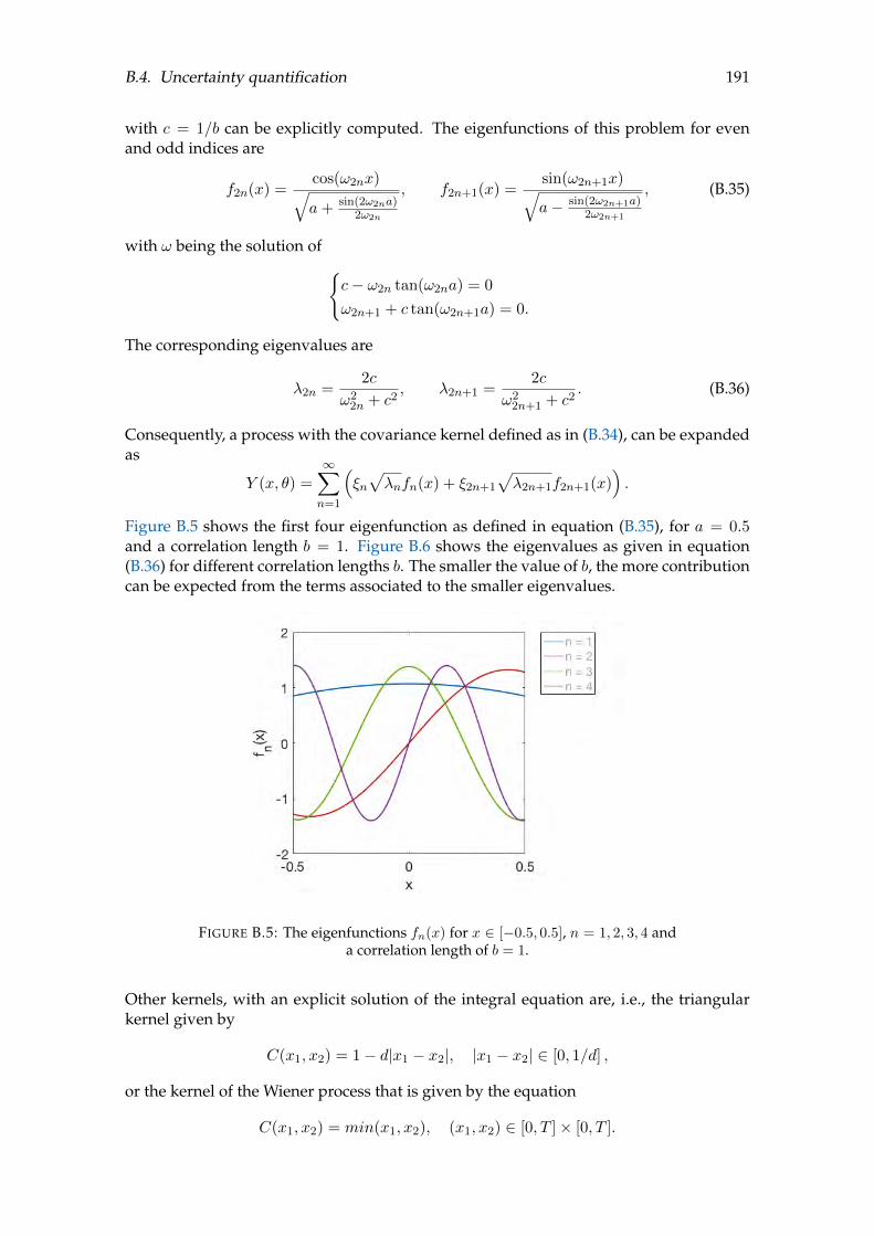
B.4. Uncertainty quantification 191
with c = 1/b can be explicitly computed. The eigenfunctions of this problem for evenand odd indices are
f2n(x) =cos(ω2nx)√a+ sin(2ω2na)
2ω2n
, f2n+1(x) =sin(ω2n+1x)√a− sin(2ω2n+1a)
2ω2n+1
, (B.35)
with ω being the solution of c− ω2n tan(ω2na) = 0
ω2n+1 + c tan(ω2n+1a) = 0.
The corresponding eigenvalues are
λ2n =2c
ω22n + c2
, λ2n+1 =2c
ω22n+1 + c2
. (B.36)
Consequently, a process with the covariance kernel defined as in (B.34), can be expandedas
Y (x, θ) =
∞∑n=1
(ξn√λnfn(x) + ξ2n+1
√λ2n+1f2n+1(x)
).
Figure B.5 shows the first four eigenfunction as defined in equation (B.35), for a = 0.5and a correlation length b = 1. Figure B.6 shows the eigenvalues as given in equation(B.36) for different correlation lengths b. The smaller the value of b, the more contributioncan be expected from the terms associated to the smaller eigenvalues.
FIGURE B.5: The eigenfunctions fn(x) for x ∈ [−0.5, 0.5], n = 1, 2, 3, 4 anda correlation length of b = 1.
Other kernels, with an explicit solution of the integral equation are, i.e., the triangularkernel given by
C(x1, x2) = 1− d|x1 − x2|, |x1 − x2| ∈ [0, 1/d] ,
or the kernel of the Wiener process that is given by the equation
C(x1, x2) = min(x1, x2), (x1, x2) ∈ [0, T ]× [0, T ].

192 Appendix B. Mathematical compendium
FIGURE B.6: The eigenvalues λn for various values of the correlationlength b for n = 1, 2, . . . , 10.
Consequently, the Karhunen-Loeve expansion requires the knowledge about the covari-ance function of the process, to compute the corresponding eigenfunctions and eigen-values. Without the knowledge of the covariance function this expansion cannot be im-plemented. An alternative expansion that circumvents this problem is the homogenouschaos expansion. For more details on the homogenous chaos expansion we refer Ghanemand Spanos, 1991.
193
Appendix C
A hitchhiker’s guide to MRI and DTIbrain imaging data
“Running in circles, coming up tails; Heads on a science apart, [...]No one ever said it would be this hard, oh take me back to the start.”
Coldplay, in The Scientist (2002)
This chapter is a brief guide to MRI and DTI or DWI data processing to extract the ge-ometry of the cerebral cortex and the corresponding diffusion parameters from brainimaging data. This appendix is meant as an introduction to the topic, providing the es-sential pieces of information and code, references and websites for in-depth studies ofthis topic and the available techniques and tools. We are commenting on the problemswe encountered and their solution.
We mention the different ways that MRI and DTI or DWI data is available and howto deal with these file formats. For the extraction of the cortical geometry, we use theFreeSurfer1 image analysis suit. FreeSurfer is an open-source software for processing andanalysing (human) brain MRI images developed by the Laboratory for ComputationalNeuroimaging in Charlestown, MA, for further details, see Fischl, 2012. For the extrac-tion and processing of the diffusion data, we use the FSL2 (FMRIB Software Library)toolkit developed by the FMRIB Group in Oxford, UK. FSL is a library of analysis toolsfor functional MRI (fMRI), MRI and DTI brain imaging data and offers different toolsto process DTI and DWI data (Jenkinson et al., 2012; Smith et al., 2004; Woolrich et al.,2009). Another commonly used tool for the automated processing of diffusion-weightedMRI images is the TRACULA3 (tracts constrained by underlying anatomy) toolbox thatis mainly used for the automatic reconstruction of major white matter pathways (Yendikiet al., 2011, 2013). However, this guide is focussing on the diffusion data processing withthe FSL toolkit.
1http://surfer.nmr.mgh.harvard.edu/2https://fsl.fmrib.ox.ac.uk/fsl/fslwiki3https://surfer.nmr.mgh.harvard.edu/fswiki/Tracula
194 Appendix C. A hitchhiker’s guide to MRI and DTI brain imaging data
C.1 Data
The MRI raw data can on one hand be provided in the form of NIfTI (neuroimaginginformatics technology initiative) files, as single files (.nii) or dual files including a headerand an image (.hdr and .img) file for the anatomical information, and gradient direction(.bvecs) and b-value (.bvals) files for the diffusion data. The NIfTI image format is asimple, compact and versatile standard format that was designed for scientific analysisof brain images. The .bvecs file is a text file containing the list of gradient directionsapplied during the acquisition of the diffusion-weighted image. The format is
x1 x2 x3 . . . xn
y1 y2 y3 . . . yn
z1 z2 z3 . . . zn.
The list of b-values applied during each volume acquisition is assumed to be in sec/mm2
and the order of entries in this file has to match the order of volumes in the input dataand the entries in the gradient directions text file. The format is
b1 b2 b3 . . . bn.
On the other hand, the same information can be provided in the form of DICOM (digitalimaging and communication in medicine) images compressing the information of MRIand DTI or DWI data.
C.2 Processing T1 images before using FreeSurfer
Before applying any structural imaging method (e.g., FreeSurfer, ANTs, etc.) it is impor-tant to follow a general pipeline4 of preprocessing to prepare the data in a standard fileformat. This mainly includes the conversion to the NIfTI image format, which can thenbe used as the input data format of the FreeSurfer software.
In order to convert DICOM images to NIfTI format, we use the dicom2nii5 software pack-age integrated in MATLAB. To open the GUI window, simply run
dicm2nii;
and introduce the source and result folder for the NIfTI files. In the case of dual files ofNIfTI images, we use the mri_convert6 command from FreeSurfer:
mri_convert T1.hdr T1.nii.gzmri_convert DTI.hdr DTI.nii.gz
Another important step in the pre-processing to obtain consistent results in the alignmentof MRI and DTI data is to check the orientation of the images and correct it if necessary.Information on the orientation can be obtained by opening the images with FSLeyes7, an
4https://biabl.github.io/tutorials/part-1-topics/preprocessing-t1-weighted-images/5https://es.mathworks.com/matlabcentral/fileexchange/42997-xiangruili-dicm2nii6https://surfer.nmr.mgh.harvard.edu/fswiki/mri_convert7https://fsl.fmrib.ox.ac.uk/fsl/fslwiki/FSLeyes

C.3. Cortical reconstruction with FreeSurfer 195
image viewer from the FSL toolbox, and by opening the image information window. Anexample of the orientation of T1 and DTI data is provided in Table C.1.
T1 DTIimage storage order radiological radiologicalX voxel orientation anterior - posterior right - leftY voxel orientation inferior - superior posterior - anteriorZ voxel orientation left - right inferior - superior
TABLE C.1: An example of the orientation of MRI and DTI data.
If the two images are not aligned it is important to fix their orientation before processingthe T1 images with the FreeSurfer suit. In the example of Table C.1 the two images are notaligned and the dimensions of the MRI images have to be rearranged in order to be in linewith the ones of the DTI image. For the change of dimensions, we use the fslswapdim8
command from the FSL toolbox, which reads for the above example:
fslswapdim T1.nii.gz -z -x y T1_reoriented.nii.gz
C.3 Cortical reconstruction with FreeSurfer
The input for the FreeSurfer software is a T1 contrast image of the whole brain, wherethe white matter is brighter than grey matter. Usually one acquisition with 1.5 Tesla or 3Tesla of patients above the age of 5 and without major brain problems, i.e., tumours ormissing parts is sufficient for the reconstruction.
To start the program and set the working directory and the directory of the FreeSurferapplication itself, we use the following code in the terminal:
setenv MY_DATA "path to data"setenv SUBJECTS_DIR $MY_DATAsetenv FREESURFER_HOME "/Applications/freesurfer"source $FREESURFER_HOME/SetUpFreeSurfer.csh
The variables SUBJECTS_DIR and FREESURFER_HOME are environment variables thathave to be defined in the beginning before running any commands in FreeSurfer. If theyare not defined FreeSurfer sets them as default values and hence, it will not find the data.
For a given patient with identification name CON01 and MRI data CON01_T1.nii, therecon-all command creates a folder "CON01" in the SUBJECTS_DIR and uses the spec-ified input path. The command -all runs the whole processing. Note that FreeSurferautomatically creates the folder with the patient ID and saves the results in this folder.
recon-all -s CON01 -i $SUBJECTS_DIR/T1data.nii -all
The individual steps of the acquisition are:
Volumetric processing stages (subjid/mri):
1. Motion cor, avg, conform (orig.mgz)
2. Non-uniform inorm (nu.mgz)
3. Talairach transform computation (ta-lairach.xfm)
8https://fsl.fmrib.ox.ac.uk/fsl/fslwiki/Fslutils

196 Appendix C. A hitchhiker’s guide to MRI and DTI brain imaging data
4. Intensity normalization 1 (T1.mgz)
5. Skull strip (brainmask.mgz)
6. EM register (linear volumetric registra-tion)
7. CA intensity normalization (norm.mgz)
8. CA nonlinear volumetric registration
9. CA label (volumetric labeling)(aseg.mgz)
10. Intensity normalization 2 (T1.mgz)
11. White matter segmentation (wm.mgz)
12. Edit WM with aseg
13. Fill and cut (filled.mgz)
Surface processing stages (subjid/surf):
14. Tessellate (?h.orig.nofix)
15. Smooth1
16. Inflate1
17. Sphere (?h.qsqhere)
18. Automatic topology fixer (?h.orig)
19. Final surfs (?h.white, ?h.pial, ?.thickness)
20. Smooth 2 (?h.smoothwm)
21. Inflate 2 (?h.inflated)
22. Aseg statistics (stats/aseg.stats)
23. Cortical ribbon mask (?h.ribbon.mgz)
24. Spherical morph
25. Spherical registration (?h.sphere.reg)
26. Map average curvature to subject
27. Cortical parcellation (labeling)
28. Cortical parcellation statistics
29. Cortical parcellation mapped to aseg
30. White matter parcellation (wmparc.mgz)
where ?h.orig denotes lh.orig or rh.orig relating to the left and right hemisphere. Theseresults are saved in the CON01 folder. The overall structure of the folders is shown inFigure C.1.
SUBJETCS_DIR
CON01
label
mriscripts
surftmp
touch
trashCON02
. . .
FIGURE C.1: The folder and subfolder structure created with the recon-allcommand of FreeSurfer.
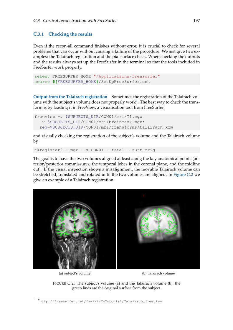
C.3. Cortical reconstruction with FreeSurfer 197
C.3.1 Checking the results
Even if the recon-all command finishes without error, it is crucial to check for severalproblems that can occur without causing a failure of the procedure. We just give two ex-amples: the Talairach registration and the pial surface check. When checking the outputsand the results always set up the FreeSurfer in the terminal so that the tools included inFreeSurfer work properly.
setenv FREESURFER_HOME "/Applications/freesurfer"source $FREESURFER_HOME/SetUpFreeSurfer.csh
Output from the Talairach registration Sometimes the registration of the Talairach vol-ume with the subject’s volume does not properly work9. The best way to check the trans-form is by loading it in FreeView, a visualisation tool from FreeSurfer,
freeview -v $SUBJECTS_DIR/CON01/mri/T1.mgz-v $SUBJECTS_DIR/CON01/mri/brainmask.mgz:reg=$SUBJECTS_DIR/CON01/mri/transforms/talairach.xfm
and visually checking the registration of the subject’s volume and the Talairach volumeby
tkregister2 --mgz --s CON01 --fstal --surf orig
The goal is to have the two volumes aligned at least along the key anatomical points (an-terior/posterior commissures, the temporal lobes in the coronal plane, and the midlinecut). If the visual inspection shows a misalignment, the movable Talairach volume canbe stretched, translated and rotated until the two volumes are aligned. In Figure C.2 wegive an example of a Talairach registration.
(a) subject’s volume (b) Talairach volume
FIGURE C.2: The subject’s volume (a) and the Talairach volume (b), thegreen lines are the original surface from the subject.
9http://freesurfer.net/fswiki/FsTutorial/Talairach_freeview
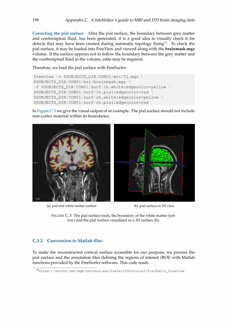
198 Appendix C. A hitchhiker’s guide to MRI and DTI brain imaging data
Correcting the pial surface After the pial surface, the boundary between grey matterand cerebrospinal fluid, has been generated, it is a good idea to visually check it fordefects that may have been created during automatic topology fixing10. To check thepial surface, it may be loaded into FreeView and viewed along with the brainmask.mgzvolume. If the surface appears not to follow the boundary between the grey matter andthe cerebrospinal fluid in the volume, edits may be required.
Therefore, we load the pial surface with FreeSurfer:
freeview -v $SUBJECTS_DIR/CON01/mri/T1.mgz \$SUBJECTS_DIR/CON01/mri/brainmask.mgz \-f $SUBJECTS_DIR/CON01/surf/lh.white:edgecolor=yellow \$SUBJECTS_DIR/CON01/surf/lh.pial:edgecolor=red \$SUBJECTS_DIR/CON01/surf/rh.white:edgecolor=yellow \$SUBJECTS_DIR/CON01/surf/rh.pial:edgecolor=red
In Figure C.3 we give the visual output of an example. The pial surface should not includenon-cortex material within its boundaries.
(a) pial and white matter surface (b) pial surface in 3D view
FIGURE C.3: The pial surface (red), the boundary of the white matter (yel-low) and the pial surface visualised as a 3D surface (b).
C.3.2 Conversion to Matlab files
To make the reconstructed cortical surface accessible for our purpose, we process thepial surface and the annotation files defining the regions of interest (ROI) with Matlabfunctions provided by the FreeSurfer software. This code reads
10https://surfer.nmr.mgh.harvard.edu/fswiki/FsTutorial/PialEdits_freeview

C.4. Processing the DTI or DWI data with FSL 199
% move to directory of matlab files in Freesurfercd ’/Applications/freesurfer/matlab’
% load data for points, vertices and curvature[data,vert]=read_surf(’$SUBJECTS_DIR/CON01/surf/lh.pial’);C = data’;
vert = vert+1;L = vert;
[vertices,label,colortable]=read_annotation...(’$SUBJECTS_DIR/CON01/label/lh.aparc.annot’);
for i = 1:36a = find(label == colortable.table(i,5));label(a) = i;
endlabel_names = colortable.struct_names;
save CON01_left_hemisphere.mat C L label label_names
The variable colourtable is a structure including the number of entries, the path to theoriginal Desikan-Killiany atlas, the structure names (label names) and a table includingcolour values and the ID for the different regions. For example, the label ’6553700’ canbe found in the colortable.table structure and its label name is the one with the sameindex in the colortable.struct_name structure, in this case the ’frontalpole’. However,after applying the above code the regions are associated with a number between 1 and 36(the regions of the Desikan-Killiany atlas including the corpus callosum plus a label forunknown regions - usually empty) and their name corresponds to the respective entry inlabel_names.
C.4 Processing the DTI or DWI data with FSL
In the following, we differentiate between DTI data that provides information about thediffusion strength and diffusion direction, and apparent diffusion coefficient (ADC) datathat provides an average diffusion coefficient but no diffusion directions.
In general, the processing of diffusion-weighted data needs a little bit more care thanthe processing of T1 images and involves results from the FreeSurfer recon-all functionapplied to the T1 image. The processing includes:
1. Correction of eddy current distortion and simple head motion
2. Brain extraction of the DTI or DWI and T1 data, respectively.
3. Application of the function DTIFIT in the case of DTI data.
4. Registration of the DTI or DWI data with T1 space.
5. Application of the inverse transformation to the DWI data and check for alignment.
6. Transformation from T1 space into FreeSurfer space.
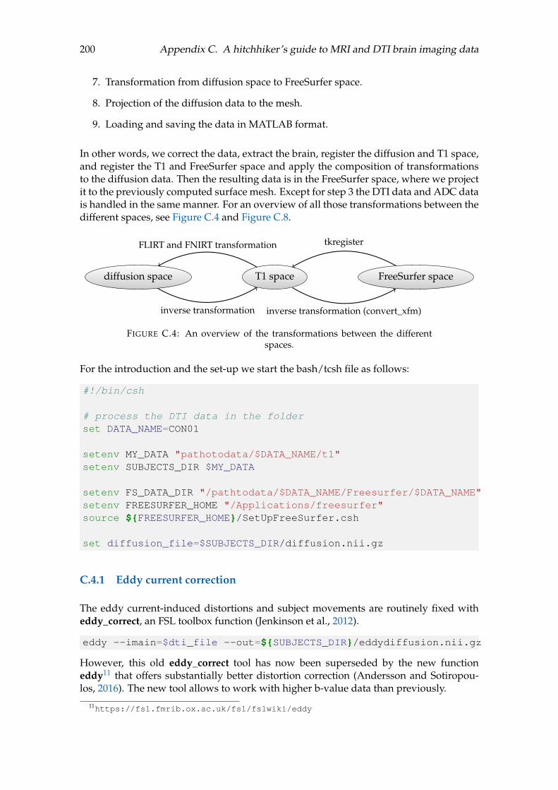
200 Appendix C. A hitchhiker’s guide to MRI and DTI brain imaging data
7. Transformation from diffusion space to FreeSurfer space.
8. Projection of the diffusion data to the mesh.
9. Loading and saving the data in MATLAB format.
In other words, we correct the data, extract the brain, register the diffusion and T1 space,and register the T1 and FreeSurfer space and apply the composition of transformationsto the diffusion data. Then the resulting data is in the FreeSurfer space, where we projectit to the previously computed surface mesh. Except for step 3 the DTI data and ADC datais handled in the same manner. For an overview of all those transformations between thedifferent spaces, see Figure C.4 and Figure C.8.
diffusion space T1 space FreeSurfer space
FLIRT and FNIRT transformation
inverse transformation
tkregister
inverse transformation (convert_xfm)
FIGURE C.4: An overview of the transformations between the differentspaces.
For the introduction and the set-up we start the bash/tcsh file as follows:
#!/bin/csh
# process the DTI data in the folderset DATA_NAME=CON01
setenv MY_DATA "pathotodata/$DATA_NAME/t1"setenv SUBJECTS_DIR $MY_DATA
setenv FS_DATA_DIR "/pathtodata/$DATA_NAME/Freesurfer/$DATA_NAME"setenv FREESURFER_HOME "/Applications/freesurfer"source $FREESURFER_HOME/SetUpFreeSurfer.csh
set diffusion_file=$SUBJECTS_DIR/diffusion.nii.gz
C.4.1 Eddy current correction
The eddy current-induced distortions and subject movements are routinely fixed witheddy_correct, an FSL toolbox function (Jenkinson et al., 2012).
eddy --imain=$dti_file --out=$SUBJECTS_DIR/eddydiffusion.nii.gz
However, this old eddy_correct tool has now been superseded by the new functioneddy11 that offers substantially better distortion correction (Andersson and Sotiropou-los, 2016). The new tool allows to work with higher b-value data than previously.
11https://fsl.fmrib.ox.ac.uk/fsl/fslwiki/eddy

C.4. Processing the DTI or DWI data with FSL 201
C.4.2 Brain extraction tool
FSL’s brain extraction tool12 (BET) is used to extract the brain tissue from the rest of theimage (Smith, 2002). For registration purposes, the brain extraction may contain somesmall errors without affecting the final result. Varying the fractional intensity thresholdparameter controls the threshold that distinguishes brain from non-brain. The fractionalintensity threshold varies between 0 and 1 with a default value of 0.5, smaller valuesgiving larger brain outline estimates. The brain extraction has to be executed for the DTIor DWI data as well as for the T1 structural image data.
bet $SUBJECTS_DIR/eddydiffusion.nii.gz$SUBJECTS_DIR/diffusion_data_brain.nii.gz -m -f 0.3
bet $SUBJECTS_DIR/T1.nii.gz$SUBJECTS_DIR/T1_brain.nii.gz -m -f 0.3
Here, the option -m generates a binary brain mask to be used later on for the DTIFIT (ofstep 3), while the option -f sets the fractional intensity threshold. An example of a brainextraction from T1 and DWI data is shown in Figure C.5.
(a) T1 image (b) DWI image
FIGURE C.5: The original image of an example dataset (grey scale) and theresult of the BET (heat colormap) for a T1 image (a) and a DWI image (b).
C.4.3 Fitting the diffusion tensor model
The FSL function DTIFIT13 assigns a diffusion tensor model to each voxel by fitting thetensors to the previously processed diffusion-weighted images. Typically DTIFIT is runon data that has been pre-processed and eddy current corrected. For DTIFIT the .bvecsand .bvals files have to be specified.
12https://fsl.fmrib.ox.ac.uk/fsl/fslwiki/BET/UserGuide13https://users.fmrib.ox.ac.uk/~behrens/fdt_docs/

202 Appendix C. A hitchhiker’s guide to MRI and DTI brain imaging data
set bvecs=$SUBJECTS_DIR/*bvecsset bvals=$SUBJECTS_DIR/*bvalsdtifit --data=$DTI_COMP_DIR/$DATA_NAME_eddy.nii.gz--out=$DTI_COMP_DIR/$DATA_NAME_dti--mask=$DTI_COMP_DIR/$DATA_NAME_dtidata_brain.nii.gz--bvecs=$bvecs --bvals=$bvals
The main output files of this procedure are:
• dtifit_FA.nii.gz - fractional anisotropy image
• dtifit_MD.nii.gz - mean diffusivity image
• dtifit_L1...L3 - primary, secondary, tertiary eigenvalues
• dtifit_V1...V3 - primary, secondary, tertiary eigenvectors
Some of the DTI image files (e.g., V1, the vector image showing the principal diffusiontensor direction) are multi-volume (4D) image files. To view such images in DTI Modeof the FslViewer, select the image in the Image List and press the Image Info button. Thiswill open the Image Info dialog. In the DTI Display options section, it is possible, forexample, to change the value from None to Lines or RGB. When Lines is set the DTIvectors are expressed by the direction of many small lines. Each layer set to display asLines is rendered in a different colour. When RGB is set the DTI vectors are expressed bycolours where red, green and blue represent the x, y and z diffusion directions, respec-tively. Colours such as purple are mixtures of red, green and blue and therefore expressvectors that have significant non-zero components in more than one of the x, y and z di-rections. An example of visualising DTI images including the fractional anisotropy (FA),V1, V1 intensity modulated by FA and the V1 direction visualised as lines is given inFigure C.6.
C.4.4 Registration of diffusion space with T1 space
To register the diffusion and T1 image, we perform a linear or non-linear transformation.FLIRT14 (FMRIB’s Linear Image Registration Tool) is a fully automated robust and accu-rate tool for linear (affine) intra- and inter-modal brain image registration (Jenkinson andSmith, 2001; Jenkinson et al., 2002). To run the FSL non-linear registration tool FNIRT15,it is required to perform an initial affine registration first using FLIRT (Greve and Fischl,2009; Jenkinson and Smith, 2001; Jenkinson et al., 2002).
One of the simplest applications of FLIRT is to register two single volumes together. Themain options are the input (-in) and the reference (-ref) volume; the output includes thecalculated affine transformation that registers the input to the reference and it is saved asa 4×4 affine matrix (-omat), and the final output volume (-out). Important features forthe registration are:
1. Degrees of freedom: For 3D to 3D mode the degrees of freedom (DOF) can be set to 12(affine), 9 (traditional), 7 (global rescale) or 6 (rigid body). In 2D to 2D mode only 3DOF can be set.
14https://fsl.fmrib.ox.ac.uk/fsl/fslwiki/FLIRT/UserGuide15https://fsl.fmrib.ox.ac.uk/fsl/fslwiki/FNIRT/UserGuide

C.4. Processing the DTI or DWI data with FSL 203
(a) fractional anisotropy (b) principal diffusion tensor direction V1
(c) V1 intensity modulated by FA (d) V1 direction visualised as lines
FIGURE C.6: Visualisation of DTI images: fractional anisotropy (FA) (a),the principal diffusion tensor direction V1 displayed in RGB colours (b),V1 intensity modulated by FA (c) and V1 direction visualised as lines (d).
2. Cost functions: The options include the within-modality functions least squares andnormalised correlation, as well as the between-modality functions correlation ratio(the default), mutual information and normalised mutual information.
Below we list the minimal example of the usage of the FLIRT16 toolbox, including a choiceof options and parameter choices.
16https://wiki.gacrc.uga.edu/wiki/Fsl

204 Appendix C. A hitchhiker’s guide to MRI and DTI brain imaging data
Syntax: flirt [options] -in <inputvol> -ref <refvol>Options are:
-init <matrix-filname> (input 4x4 affine matrix)-omat <matrix-filename> (output 4x4 ascii format)-out, -o <outputvol> (default is none)-cost (mutualinfo,corratio, (default is corratio)normcorr,normmi,leastsq,labeldiff)-dof <number of transform dofs> (default is 12)
The default and basic options of the non-linear transformation with FNIRT are not verylikely to give good results. Thus, FNIRT has a large set of parameters but we will justbriefly mention a few of them. Adding, for example, information about the affine trans-formation and the reference brain mask can improve the transformation.
Syntax: fnirt -in=<inputvol> -ref=<refvol>Options are:
-aff file containing affine transform-inwarp file containing initial non-linear warps-cout output file with field coefficients-refmask binary mask that determines interesting field of view
The function invwarp is used to reverse a nonlinear mapping. Even though there aresome optional arguments, we list only the basic command here.
Syntax: invwarp -w warpvol -o invwarpvol -r refvol
The overall registration process results in the following code for our example:
flirt -in $SUBJECTS_DIR/T1_brain.nii.gz-ref $SUBJECTS_DIR/diffusion_data_brain.nii.gz-cost mutualinfo -omat $SUBJECTS_DIR/struct2ADC.mat
fnirt --ref=$SUBJECTS_DIR/diffusion_data_brain.nii.gz--in=$SUBJECTS_DIR/T1_brain.nii.gz--aff=$SUBJECTS_DIR/struct2diffusion.mat--cout=$SUBJECTS_DIR/struct2diffusion_warp
invwarp --warp=$SUBJECTS_DIR/struct2diffusion_warp--ref=$SUBJECTS_DIR/T1_brain.nii.gz--out=$SUBJECTS_DIR/struct2diffusion_warp_inv
C.4.5 Transformation of DTI or DWI data to T1 space
The function applywarp is used to apply the transformations estimated by FNIRT (orsome other software) to the diffusion-weighted image to align it with the structural scan.
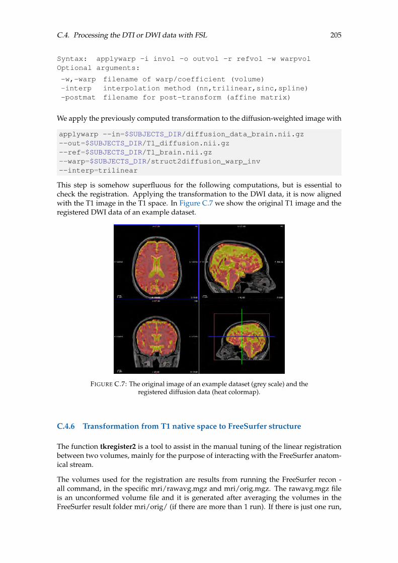
C.4. Processing the DTI or DWI data with FSL 205
Syntax: applywarp -i invol -o outvol -r refvol -w warpvolOptional arguments:
-w,-warp filename of warp/coefficient (volume)-interp interpolation method (nn,trilinear,sinc,spline)-postmat filename for post-transform (affine matrix)
We apply the previously computed transformation to the diffusion-weighted image with
applywarp --in=$SUBJECTS_DIR/diffusion_data_brain.nii.gz--out=$SUBJECTS_DIR/T1_diffusion.nii.gz--ref=$SUBJECTS_DIR/T1_brain.nii.gz--warp=$SUBJECTS_DIR/struct2diffusion_warp_inv--interp=trilinear
This step is somehow superfluous for the following computations, but is essential tocheck the registration. Applying the transformation to the DWI data, it is now alignedwith the T1 image in the T1 space. In Figure C.7 we show the original T1 image and theregistered DWI data of an example dataset.
FIGURE C.7: The original image of an example dataset (grey scale) and theregistered diffusion data (heat colormap).
C.4.6 Transformation from T1 native space to FreeSurfer structure
The function tkregister2 is a tool to assist in the manual tuning of the linear registrationbetween two volumes, mainly for the purpose of interacting with the FreeSurfer anatom-ical stream.
The volumes used for the registration are results from running the FreeSurfer recon -all command, in the specific mri/rawavg.mgz and mri/orig.mgz. The rawavg.mgz fileis an unconformed volume file and it is generated after averaging the volumes in theFreeSurfer result folder mri/orig/ (if there are more than 1 run). If there is just one run,
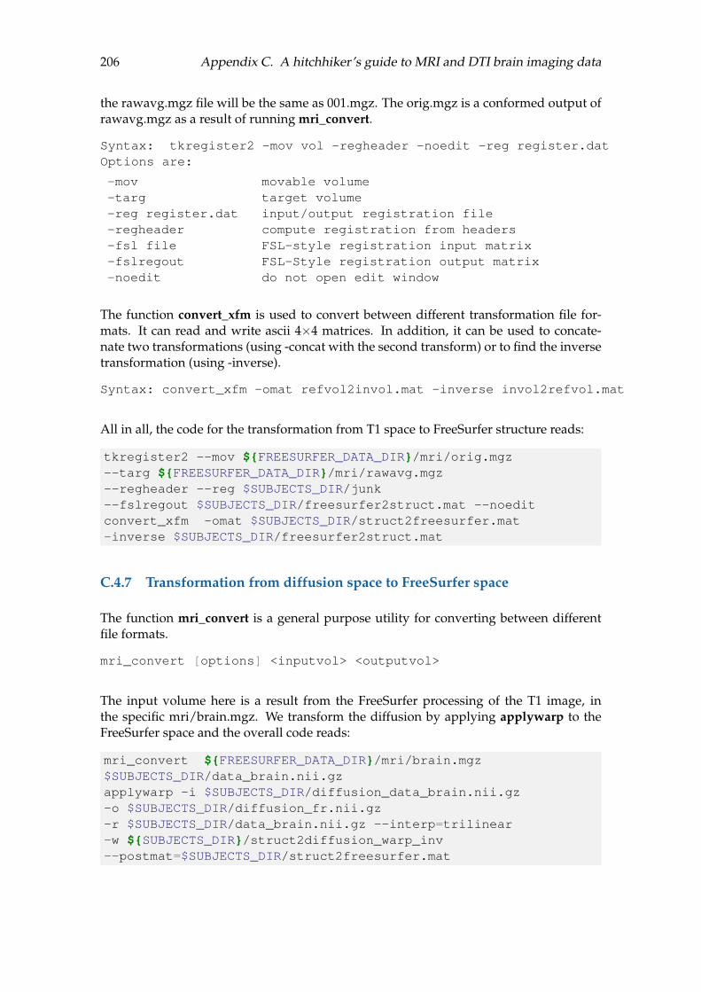
206 Appendix C. A hitchhiker’s guide to MRI and DTI brain imaging data
the rawavg.mgz file will be the same as 001.mgz. The orig.mgz is a conformed output ofrawavg.mgz as a result of running mri_convert.
Syntax: tkregister2 -mov vol -regheader -noedit -reg register.datOptions are:
-mov movable volume-targ target volume-reg register.dat input/output registration file-regheader compute registration from headers-fsl file FSL-style registration input matrix-fslregout FSL-Style registration output matrix-noedit do not open edit window
The function convert_xfm is used to convert between different transformation file for-mats. It can read and write ascii 4×4 matrices. In addition, it can be used to concate-nate two transformations (using -concat with the second transform) or to find the inversetransformation (using -inverse).
Syntax: convert_xfm -omat refvol2invol.mat -inverse invol2refvol.mat
All in all, the code for the transformation from T1 space to FreeSurfer structure reads:
tkregister2 --mov $FREESURFER_DATA_DIR/mri/orig.mgz--targ $FREESURFER_DATA_DIR/mri/rawavg.mgz--regheader --reg $SUBJECTS_DIR/junk--fslregout $SUBJECTS_DIR/freesurfer2struct.mat --noeditconvert_xfm -omat $SUBJECTS_DIR/struct2freesurfer.mat-inverse $SUBJECTS_DIR/freesurfer2struct.mat
C.4.7 Transformation from diffusion space to FreeSurfer space
The function mri_convert is a general purpose utility for converting between differentfile formats.
mri_convert [options] <inputvol> <outputvol>
The input volume here is a result from the FreeSurfer processing of the T1 image, inthe specific mri/brain.mgz. We transform the diffusion by applying applywarp to theFreeSurfer space and the overall code reads:
mri_convert $FREESURFER_DATA_DIR/mri/brain.mgz$SUBJECTS_DIR/data_brain.nii.gzapplywarp -i $SUBJECTS_DIR/diffusion_data_brain.nii.gz-o $SUBJECTS_DIR/diffusion_fr.nii.gz-r $SUBJECTS_DIR/data_brain.nii.gz --interp=trilinear-w $SUBJECTS_DIR/struct2diffusion_warp_inv--postmat=$SUBJECTS_DIR/struct2freesurfer.mat

C.4. Processing the DTI or DWI data with FSL 207
C.4.8 Projecting diffusion data to the mesh
The FreeSurfer function mri_vol2surf17 assigns values from a volume to each vertex of adiscretised surface.
Syntax: mri_vol2surf [options] -src inputfile -out outputfile-srcreg registrationfile -hemi hemisphereOptions are:
-mov input volume path (or -src)-ref reference volume name (default=orig.mgz)-reg source registration-hemi hemisphere (lh or rh)-projfrac fraction (0,1) of the cortical thickness at each
vertex to project along the surface normal.Default=0. When set at 0.5 with the whitesurface, this should sample in the middle of thecortical surface.
To project the diffusion data that has already been transformed to the FreeSurfer space tothe surface, we use the following code:
printf "$DATA_NAME\n1\n1\n1\n1 0 0 0\n0 1 0 0\n0 0 1 0\n0 0 0 1\n"> $SUBJECTS_DIR/reg.datsetenv SUBJECTS_DIR "pathtodata/$DATA_NAME/Freesurfer"setenv WORK_DIR "pathtodata/$DATA_NAME/t1"mri_vol2surf --src $WORK_DIR/diffusion_fr.nii.gz--reg $WORK_DIR/reg.dat --projfrac 0.5 --hemi lh--out $WORK_DIR/diffusion_Left.mghmri_vol2surf --src $WORK_DIR/diffusion_fr.nii.gz--reg $WORK_DIR/reg.dat --projfrac 0.5 --hemi rh--out $WORK_DIR/diffusion_Right.mgh
C.4.9 Load and save the DTI or DWI data in Matlab format
To save the diffusion data on the surface in an adequate format we process the datain Matlab using the .mgh files and Matlab functions provided by the FreeSurfer pack-age. This program reads the volume files and combines them with the data from theFreeSurfer processing.
17https://surfer.nmr.mgh.harvard.edu/fswiki/mri_vol2surf

208 Appendix C. A hitchhiker’s guide to MRI and DTI brain imaging data
function [] = createDWIparams(DWIpath,FSresultpath,dataname)% DWIpath: the path to the end results of the DWI processing,% namely adc_left.mgh and adc_Right.mgh% FSresultpath: the path to the end results of the Freesurfer% recon_all, namely% *_left_hemsiphere.mat and *_right_hemsiphere.mat
addpath(genpath(’/Applications/freesurfer/matlab’))
cd(DWIpath) % change to DWI path and load the .mgh filef = MRIread(’diffusion_Left.mgh’);Diffusion = f.vol;
cd(FSresultpath)s = strcat(dataname,’_left_hemisphere_sorted.mat’);load(s)
name = strcat(dataname,’_DWI_left_hemisphere.mat’);save(name,’L’, ’C’, ’label_names_sorted’, ’label_sorted’,’Diffusion’)end
In the case of DTI data, we apply the MRIread function to l1_left.mgh, l2_left.mgh,l3_left.mgh, v1_left.mgh, v2_left.mgh, v3_left.mgh, FA_left.mgh and MD_left.mgh. Anoverview of all the steps and files involved is given in Figure C.8.
The exact code for DTI and DWI processing with FSL is given in the next two sections.The procedures are very similar for the two different diffusion data types. The onlydifference is that DTI data requires the application of DTIFIT and the following stepshave to be applied to the results from DTIFIT instead of just to the ADC value, like inthe case of DWI data.

C.4. Processing the DTI or DWI data with FSL 209
DTI
/DW
Ifile
T1_b
rain
.nii.
gzT1
file
eddy
diff
usio
n.ni
i.gz
mri
/ori
g.m
gzm
ri/r
awav
g.m
gz
diff
usio
n_da
ta_b
rain
.nii.
gzT1
_diff
usio
n.ni
i.gz
free
surf
er2s
truc
t.mat
diff
usio
n_fr
.nii.
gzst
ruct
2fre
esur
fer.m
at
diff
usio
n_Le
ft.m
ghdi
ffus
ion_
Rig
ht.m
ghSu
bjec
t1_l
eft_
hem
isph
ere.
mat
Subj
ect1
_rig
ht_h
emis
pher
e.m
at
CO
N01
_DW
I_le
ft_h
emis
pher
e.m
atC
ON
01_D
WI_
righ
t_he
mis
pher
e.m
at
eddy
BET
BET
non-linea
rtransfo
rmatio
n
invwarp:str
uct2diffu
sion_warp
_inv
appl
ywar
p
-warp
Free
surf
erre
con_
all
tkre
gist
er2
appl
ywar
p
-warp
-pos
tmat
mri_
vol2
surf
mri_
vol2
surf
conv
ert_
xfm
-inv
erse
MR
Irea
dM
RIr
ead
FIG
UR
EC
.8:A
nov
ervi
ewof
the
who
leD
WIc
onve
rsio
npr
oced
ure.
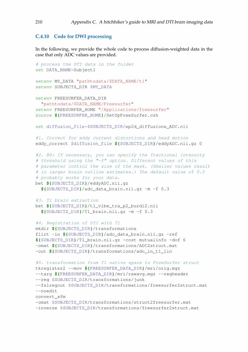
210 Appendix C. A hitchhiker’s guide to MRI and DTI brain imaging data
C.4.10 Code for DWI processing
In the following, we provide the whole code to process diffusion-weighted data in thecase that only ADC values are provided.
# process the DTI data in the folderset DATA_NAME=Subject1
setenv MY_DATA "pathtodata/$DATA_NAME/t1"setenv SUBJECTS_DIR $MY_DATA
setenv FREESURFER_DATA_DIR"pathtodata/$DATA_NAME/Freesurfer"
setenv FREESURFER_HOME "/Applications/freesurfer"source $FREESURFER_HOME/SetUpFreeSurfer.csh
set diffusion_file=$SUBJECTS_DIR/ep2d_diffusione_ADC.nii
#1. Correct for eddy current distortions and head motioneddy_correct $diffusion_file $SUBJECTS_DIR/eddyADC.nii.gz 0
#2. B0: If necessary, you can specify the fractional intensity# threshold using the "-f" option. Different values of this# parameter control the size of the mask. (Smaller values result# in larger brain outline estimates.) The default value of 0.5# probably works for your data.bet $SUBJECTS_DIR/eddyADC.nii.gz
$SUBJECTS_DIR/adc_data_brain.nii.gz -m -f 0.3
#3. T1 brain extractionbet $SUBJECTS_DIR/t1_vibe_tra_p2_burdi2.nii
$SUBJECTS_DIR/T1_brain.nii.gz -m -f 0.3
#4. Registration of DTI with T1mkdir $SUBJECTS_DIR/transformationsflirt -in $SUBJECTS_DIR/adc_data_brain.nii.gz -ref$SUBJECTS_DIR/T1_brain.nii.gz -cost mutualinfo -dof 6-omat $SUBJECTS_DIR/transformations/ADC2struct.mat-out $SUBJECTS_DIR/transformations/adc_in_t1_lin
#5. transformation from T1 native space to FreeSurfer structtkregister2 --mov $FREESURFER_DATA_DIR/mri/orig.mgz--targ $FREESURFER_DATA_DIR/mri/rawavg.mgz --regheader--reg $SUBJECTS_DIR/transformations/junk--fslregout $SUBJECTS_DIR/transformations/freesurfer2struct.mat--noeditconvert_xfm-omat $SUBJECTS_DIR/transformations/struct2freesurfer.mat-inverse $SUBJECTS_DIR/transformations/freesurfer2struct.mat
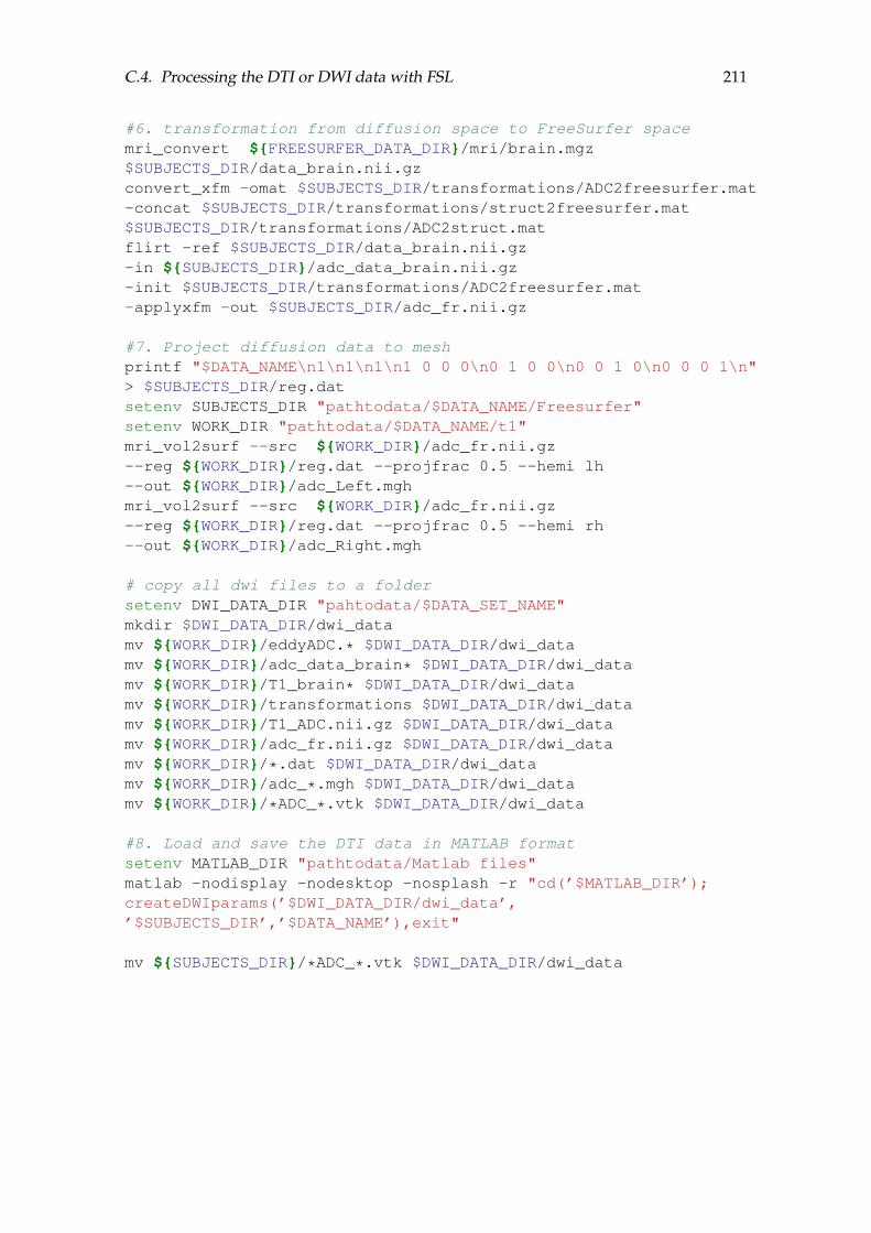
C.4. Processing the DTI or DWI data with FSL 211
#6. transformation from diffusion space to FreeSurfer spacemri_convert $FREESURFER_DATA_DIR/mri/brain.mgz$SUBJECTS_DIR/data_brain.nii.gzconvert_xfm -omat $SUBJECTS_DIR/transformations/ADC2freesurfer.mat-concat $SUBJECTS_DIR/transformations/struct2freesurfer.mat$SUBJECTS_DIR/transformations/ADC2struct.matflirt -ref $SUBJECTS_DIR/data_brain.nii.gz-in $SUBJECTS_DIR/adc_data_brain.nii.gz-init $SUBJECTS_DIR/transformations/ADC2freesurfer.mat-applyxfm -out $SUBJECTS_DIR/adc_fr.nii.gz
#7. Project diffusion data to meshprintf "$DATA_NAME\n1\n1\n1\n1 0 0 0\n0 1 0 0\n0 0 1 0\n0 0 0 1\n"> $SUBJECTS_DIR/reg.datsetenv SUBJECTS_DIR "pathtodata/$DATA_NAME/Freesurfer"setenv WORK_DIR "pathtodata/$DATA_NAME/t1"mri_vol2surf --src $WORK_DIR/adc_fr.nii.gz--reg $WORK_DIR/reg.dat --projfrac 0.5 --hemi lh--out $WORK_DIR/adc_Left.mghmri_vol2surf --src $WORK_DIR/adc_fr.nii.gz--reg $WORK_DIR/reg.dat --projfrac 0.5 --hemi rh--out $WORK_DIR/adc_Right.mgh
# copy all dwi files to a foldersetenv DWI_DATA_DIR "pahtodata/$DATA_SET_NAME"mkdir $DWI_DATA_DIR/dwi_datamv $WORK_DIR/eddyADC.* $DWI_DATA_DIR/dwi_datamv $WORK_DIR/adc_data_brain* $DWI_DATA_DIR/dwi_datamv $WORK_DIR/T1_brain* $DWI_DATA_DIR/dwi_datamv $WORK_DIR/transformations $DWI_DATA_DIR/dwi_datamv $WORK_DIR/T1_ADC.nii.gz $DWI_DATA_DIR/dwi_datamv $WORK_DIR/adc_fr.nii.gz $DWI_DATA_DIR/dwi_datamv $WORK_DIR/*.dat $DWI_DATA_DIR/dwi_datamv $WORK_DIR/adc_*.mgh $DWI_DATA_DIR/dwi_datamv $WORK_DIR/*ADC_*.vtk $DWI_DATA_DIR/dwi_data
#8. Load and save the DTI data in MATLAB formatsetenv MATLAB_DIR "pathtodata/Matlab files"matlab -nodisplay -nodesktop -nosplash -r "cd(’$MATLAB_DIR’);createDWIparams(’$DWI_DATA_DIR/dwi_data’,’$SUBJECTS_DIR’,’$DATA_NAME’),exit"
mv $SUBJECTS_DIR/*ADC_*.vtk $DWI_DATA_DIR/dwi_data

212 Appendix C. A hitchhiker’s guide to MRI and DTI brain imaging data
C.4.11 Code for DTI processing
In the following, we provide the code to process DTI diffusion data. This code is writtenin a more general form designed to be run for groups of data sets and saves a log file ofthe procedures and outputs. For DTI data we need to run DTIFIT in addition to the stepsfor the DWI data in Appendix C.4.10 and all transformations have to be applied to theresulting diffusion files.
set arr=(CON01 CON02 CON03 CON04)
foreach DATA_NAME ($arr)set logfile="pathtodata/$DATA_NAME/$DATA_NAME_dtilog.txt"date +"%T" | tee -a $logfilemkdir "pathtodata/$DATA_NAME"setenv MY_DATA "pathtodata/$DATA_NAME"setenv SUBJECTS_DIR $MY_DATAsetenv FREESURFER_DATA_DIR "pathtodata/$DATA_NAME/Freesurfer"setenv DTI_COMP_DIR "/pathtoDTIdata/$DATA_NAME"setenv FREESURFER_HOME "/Applications/freesurfer"source $FREESURFER_HOME/SetUpFreeSurfer.csh
set dti_file=$SUBJECTS_DIR/$DATA_NAME_dtidata.nii.gz
#1. Correct for eddy current distortions and head motioneddy_correct $dti_file $DTI_COMP_DIR/$DATA_NAME_eddy.nii.gz0 | tee -a $logfile
#2. B0: if necessary, you can also specify the fractional# intensity threshold using the "-f" option. Different values# of this parameter control the size of the mask. (Smaller# values result in larger brain outline estimates.) The default# value of 0.5 probably works for your data.bet $DTI_COMP_DIR/$DATA_NAME_eddy.nii.gz$DTI_COMP_DIR/$DATA_NAME_dtidata_brain.nii.gz-m -f 0.3 | tee -a $logfile
# 3. DTIFITset bvecs=$SUBJECTS_DIR/*bvecsset bvals=$SUBJECTS_DIR/*bvalsdtifit --data=$DTI_COMP_DIR/$DATA_NAME_eddy.nii.gz--out=$DTI_COMP_DIR/$DATA_NAME_dti--mask=$DTI_COMP_DIR/$DATA_NAME_dtidata_brain.nii.gz--bvecs=$bvecs --bvals=$bvals | tee -a $logfile
#4. T1 brain extractionbet $SUBJECTS_DIR/$DATA_NAME_T1.nii.gz$DTI_COMP_DIR/$DATA_NAME_T1_brain.nii.gz-m -f 0.3 | tee -a $logfile
#5. Registration of DTI with T1mkdir $DTI_COMP_DIR/transformations

C.4. Processing the DTI or DWI data with FSL 213
flirt -ref $DTI_COMP_DIR/$DATA_NAME_dti_FA.nii.gz-in $DTI_COMP_DIR/$DATA_NAME_T1_brain.nii.gz -dof 6-omat $DTI_COMP_DIR/transformations/struct2FA.mat-o $DTI_COMP_DIR/$DATA_NAME_dtiT1.nii.gz-cost mutualinfo | tee -a $logfilefnirt --ref=$DTI_COMP_DIR/$DATA_NAME_dti_FA.nii.gz--in=$DTI_COMP_DIR/$DATA_NAME_T1_brain.nii.gz--aff=$DTI_COMP_DIR/transformations/struct2FA.mat--cout=$DTI_COMP_DIR/transformations/struct2FA_warp--refmask=$DTI_COMP_DIR/$DATA_NAME_dtidata_brain_mask.nii.gz--inmask=$DTI_COMP_DIR/$DATA_NAME_T1_brain_mask.nii.gz |tee -a $logfileinvwarp --warp=$DTI_COMP_DIR/transformations/struct2FA_warp--ref=$DTI_COMP_DIR/$DATA_NAME_T1_brain.nii.gz--out=$DTI_COMP_DIR/transformations/struct2FA_warp_inv |tee -a $logfile
# Apply the transformation to the dataapplywarp -i $DTI_COMP_DIR/$DATA_NAME_dti_FA.nii.gz-o $DTI_COMP_DIR/$DATA_NAME_T1_FA.nii.gz-r $DTI_COMP_DIR/$DATA_NAME_T1_brain.nii.gz-w $DTI_COMP_DIR/transformations/struct2FA_warp_inv--interp=trilinear | tee -a $logfileapplywarp -i $DTI_COMP_DIR/$DATA_NAME_dti_MD.nii.gz-o $DTI_COMP_DIR/$DATA_NAME_T1_MD.nii.gz-r $DTI_COMP_DIR/$DATA_NAME_T1_brain.nii.gz-w $DTI_COMP_DIR/transformations/struct2FA_warp_inv--interp=trilinear | tee -a $logfileapplywarp -i $DTI_COMP_DIR/$DATA_NAME_dti_l1.nii.gz-o $DTI_COMP_DIR/$DATA_NAME_T1_l1.nii.gz-r $DTI_COMP_DIR/$DATA_NAME_T1_brain.nii.gz-w $DTI_COMP_DIR/transformations/struct2FA_warp_inv--interp=trilinear | tee -a $logfileapplywarp -i $DTI_COMP_DIR/$DATA_NAME_dti_l2.nii.gz-o $DTI_COMP_DIR/$DATA_NAME_T1_l2.nii.gz-r $DTI_COMP_DIR/$DATA_NAME_T1_brain.nii.gz-w $DTI_COMP_DIR/transformations/struct2FA_warp_inv--interp=trilinear | tee -a $logfileapplywarp -i $DTI_COMP_DIR/$DATA_NAME_dti_l3.nii.gz-o $DTI_COMP_DIR/$DATA_NAME_T1_l3.nii.gz-r $DTI_COMP_DIR/$DATA_NAME_T1_brain.nii.gz-w $DTI_COMP_DIR/transformations/struct2FA_warp_inv--interp=trilinear | tee -a $logfileapplywarp -i $DTI_COMP_DIR/$DATA_NAME_dti_v1.nii.gz-o $DTI_COMP_DIR/$DATA_NAME_T1_v1.nii.gz-r $DTI_COMP_DIR/$DATA_NAME_T1_brain.nii.gz-w $DTI_COMP_DIR/transformations/struct2FA_warp_inv--interp=nn | tee -a $logfileapplywarp -i $DTI_COMP_DIR/$DATA_NAME_dti_v2.nii.gz-o $DTI_COMP_DIR/$DATA_NAME_T1_v2.nii.gz-r $DTI_COMP_DIR/$DATA_NAME_T1_brain.nii.gz

214 Appendix C. A hitchhiker’s guide to MRI and DTI brain imaging data
-w $DTI_COMP_DIR/transformations/struct2FA_warp_inv--interp=nn | tee -a $logfileapplywarp -i $DTI_COMP_DIR/$DATA_NAME_dti_v3.nii.gz-o $DTI_COMP_DIR/$DATA_NAME_T1_v3.nii.gz-r $DTI_COMP_DIR/$DATA_NAME_T1_brain.nii.gz-w $DTI_COMP_DIR/transformations/struct2FA_warp_inv--interp=nn | tee -a $logfile
#6. transformation from T1 native space to FreeSurfer structtkregister2 --mov $FREESURFER_DATA_DIR/mri/orig.mgz--targ $FREESURFER_DATA_DIR/mri/rawavg.mgz--fslregout $DTI_COMP_DIR/transformations/freesurfer2struct.mat--reg $DTI_COMP_DIR/transformations/junk--regheader --noedit | tee -a $logfileconvert_xfm-omat $DTI_COMP_DIR/transformations/struct2freesurfer.mat-inverse $DTI_COMP_DIR/transformations/freesurfer2struct.mat |tee -a $logfile
#7. transformation from diffusion space to FreeSurfer spacemri_convert $FREESURFER_DATA_DIR/mri/brain.mgz$DTI_COMP_DIR/$DATA_NAME_data_brain.nii.gz | tee -a $logfileapplywarp -i $DTI_COMP_DIR/$DATA_NAME_dti_FA.nii.gz-o $DTI_COMP_DIR/$DATA_NAME_FA_fr.nii.gz-r $DTI_COMP_DIR/$DATA_NAME_data_brain.nii.gz-w $DTI_COMP_DIR/transformations/struct2FA_warp_inv--postmat=$DTI_COMP_DIR/transformations/struct2freesurfer.mat--interp=trilinear | tee -a $logfileapplywarp -i $DTI_COMP_DIR/$DATA_NAME_dti_MD.nii.gz-o $DTI_COMP_DIR/$DATA_NAME_MD_fr.nii.gz-r $DTI_COMP_DIR/$DATA_NAME_data_brain.nii.gz-w $DTI_COMP_DIR/transformations/struct2FA_warp_inv--postmat=$DTI_COMP_DIR/transformations/struct2freesurfer.mat--interp=trilinear | tee -a $logfileapplywarp -i $DTI_COMP_DIR/$DATA_NAME_dti_l1.nii.gz-o $DTI_COMP_DIR/$DATA_NAME_l1_fr.nii.gz-r $DTI_COMP_DIR/$DATA_NAME_data_brain.nii.gz-w $DTI_COMP_DIR/transformations/struct2FA_warp_inv--postmat=$DTI_COMP_DIR/transformations/struct2freesurfer.mat--interp=trilinear | tee -a $logfileapplywarp -i $DTI_COMP_DIR/$DATA_NAME_dti_l2.nii.gz-o $DTI_COMP_DIR/$DATA_NAME_l2_fr.nii.gz-r $DTI_COMP_DIR/$DATA_NAME_data_brain.nii.gz-w $DTI_COMP_DIR/transformations/struct2FA_warp_inv--postmat=$DTI_COMP_DIR/transformations/struct2freesurfer.mat--interp=trilinear | tee -a $logfileapplywarp -i $DTI_COMP_DIR/$DATA_NAME_dti_l3.nii.gz-o $DTI_COMP_DIR/$DATA_NAME_l3_fr.nii.gz-r $DTI_COMP_DIR/$DATA_NAME_data_brain.nii.gz-w $DTI_COMP_DIR/transformations/struct2FA_warp_inv--postmat=$DTI_COMP_DIR/transformations/struct2freesurfer.mat

C.4. Processing the DTI or DWI data with FSL 215
--interp=trilinear | tee -a $logfileapplywarp -i $DTI_COMP_DIR/$DATA_NAME_dti_v1.nii.gz-o $DTI_COMP_DIR/$DATA_NAME_v1_fr.nii.gz-r $DTI_COMP_DIR/$DATA_NAME_data_brain.nii.gz-w $DTI_COMP_DIR/transformations/struct2FA_warp_inv--postmat=$DTI_COMP_DIR/transformations/struct2freesurfer.mat--interp=nn | tee -a $logfileapplywarp -i $DTI_COMP_DIR/$DATA_NAME_dti_v2.nii.gz-o $DTI_COMP_DIR/$DATA_NAME_v2_fr.nii.gz-r $DTI_COMP_DIR/$DATA_NAME_data_brain.nii.gz-w $DTI_COMP_DIR/transformations/struct2FA_warp_inv--postmat=$DTI_COMP_DIR/transformations/struct2freesurfer.mat--interp=nn | tee -a $logfileapplywarp -i $DTI_COMP_DIR/$DATA_NAME_dti_v3.nii.gz-o $DTI_COMP_DIR/$DATA_NAME_v3_fr.nii.gz-r $DTI_COMP_DIR/$DATA_NAME_data_brain.nii.gz-w $DTI_COMP_DIR/transformations/struct2FA_warp_inv--postmat=$DTI_COMP_DIR/transformations/struct2freesurfer.mat--interp=nn | tee -a $logfile
#8. Project diffusion data to meshprintf "$DATA_NAME\n1\n1\n1\n1 0 0 0\n0 1 0 0\n0 0 1 0\n0 0 0 1\n"> $DTI_COMP_DIR/reg.datsetenv SUBJECTS_DIR "/pathtodata"
mri_vol2surf --src $DTI_COMP_DIR/$DATA_NAME_FA_fr.nii.gz--srcreg $DTI_COMP_DIR/reg.dat --projfrac 0.5 --hemi lh--out $DTI_COMP_DIR/$DATA_NAME_FA_left.mgh | tee -a $logfilemri_vol2surf --src $DTI_COMP_DIR/$DATA_NAME_MD_fr.nii.gz--srcreg $DTI_COMP_DIR/reg.dat --projfrac 0.5 --hemi lh--out $DTI_COMP_DIR/$DATA_NAME_MD_left.mgh | tee -a $logfilemri_vol2surf --src $DTI_COMP_DIR/$DATA_NAME_l1_fr.nii.gz--srcreg $DTI_COMP_DIR/reg.dat --projfrac 0.5 --hemi lh--out $DTI_COMP_DIR/$DATA_NAME_l1_left.mgh | tee -a $logfilemri_vol2surf --src $DTI_COMP_DIR/$DATA_NAME_l2_fr.nii.gz--srcreg $DTI_COMP_DIR/reg.dat --projfrac 0.5 --hemi lh--out $DTI_COMP_DIR/$DATA_NAME_l2_left.mgh | tee -a $logfilemri_vol2surf --src $DTI_COMP_DIR/$DATA_NAME_l3_fr.nii.gz--srcreg $DTI_COMP_DIR/reg.dat --projfrac 0.5 --hemi lh--out $DTI_COMP_DIR/$DATA_NAME_l3_left.mgh | tee -a $logfilemri_vol2surf --src $DTI_COMP_DIR/$DATA_NAME_v1_fr.nii.gz--srcreg $DTI_COMP_DIR/reg.dat --projfrac 0.5 --hemi lh--out $DTI_COMP_DIR/$DATA_NAME_v1_left.mgh | tee -a $logfilemri_vol2surf --src $DTI_COMP_DIR/$DATA_NAME_v2_fr.nii.gz--srcreg $DTI_COMP_DIR/reg.dat --projfrac 0.5 --hemi lh--out $DTI_COMP_DIR/$DATA_NAME_v2_left.mgh | tee -a $logfilemri_vol2surf --src $DTI_COMP_DIR/$DATA_NAME_v3_fr.nii.gz--srcreg $DTI_COMP_DIR/reg.dat --projfrac 0.5 --hemi lh--out $DTI_COMP_DIR/$DATA_NAME_v3_left.mgh | tee -a $logfile
mri_vol2surf --src $DTI_COMP_DIR/$DATA_NAME_FA_fr.nii.gz
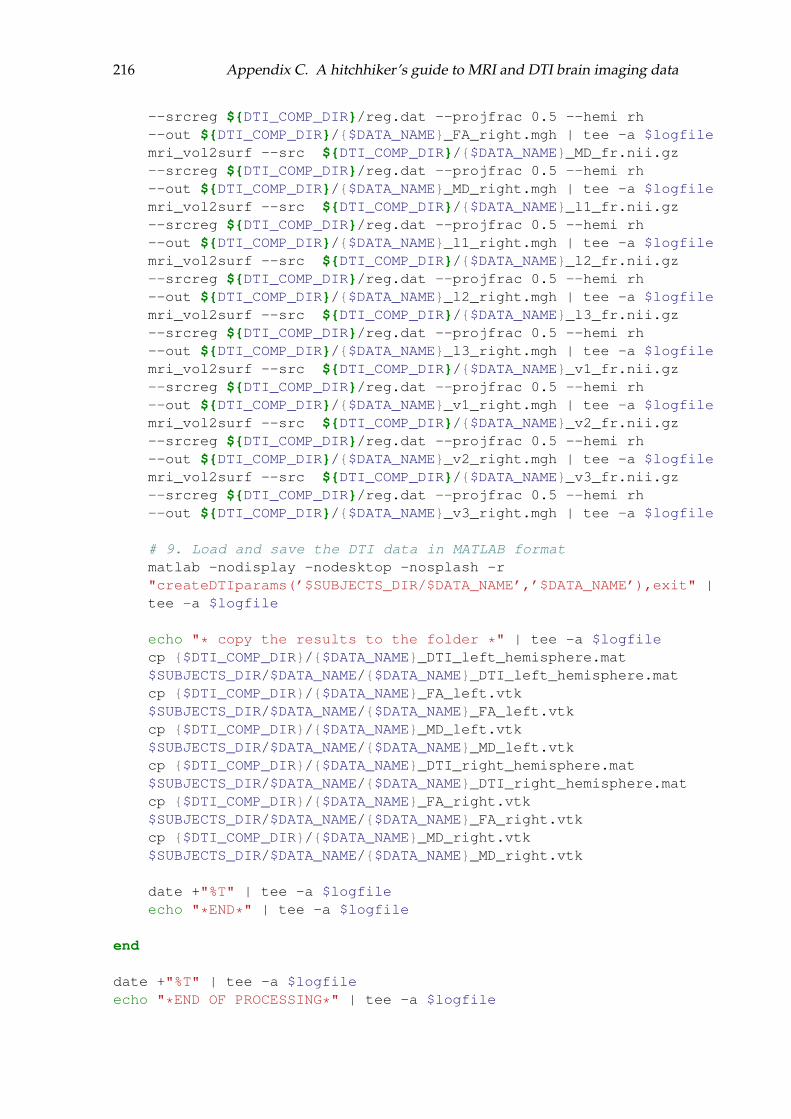
216 Appendix C. A hitchhiker’s guide to MRI and DTI brain imaging data
--srcreg $DTI_COMP_DIR/reg.dat --projfrac 0.5 --hemi rh--out $DTI_COMP_DIR/$DATA_NAME_FA_right.mgh | tee -a $logfilemri_vol2surf --src $DTI_COMP_DIR/$DATA_NAME_MD_fr.nii.gz--srcreg $DTI_COMP_DIR/reg.dat --projfrac 0.5 --hemi rh--out $DTI_COMP_DIR/$DATA_NAME_MD_right.mgh | tee -a $logfilemri_vol2surf --src $DTI_COMP_DIR/$DATA_NAME_l1_fr.nii.gz--srcreg $DTI_COMP_DIR/reg.dat --projfrac 0.5 --hemi rh--out $DTI_COMP_DIR/$DATA_NAME_l1_right.mgh | tee -a $logfilemri_vol2surf --src $DTI_COMP_DIR/$DATA_NAME_l2_fr.nii.gz--srcreg $DTI_COMP_DIR/reg.dat --projfrac 0.5 --hemi rh--out $DTI_COMP_DIR/$DATA_NAME_l2_right.mgh | tee -a $logfilemri_vol2surf --src $DTI_COMP_DIR/$DATA_NAME_l3_fr.nii.gz--srcreg $DTI_COMP_DIR/reg.dat --projfrac 0.5 --hemi rh--out $DTI_COMP_DIR/$DATA_NAME_l3_right.mgh | tee -a $logfilemri_vol2surf --src $DTI_COMP_DIR/$DATA_NAME_v1_fr.nii.gz--srcreg $DTI_COMP_DIR/reg.dat --projfrac 0.5 --hemi rh--out $DTI_COMP_DIR/$DATA_NAME_v1_right.mgh | tee -a $logfilemri_vol2surf --src $DTI_COMP_DIR/$DATA_NAME_v2_fr.nii.gz--srcreg $DTI_COMP_DIR/reg.dat --projfrac 0.5 --hemi rh--out $DTI_COMP_DIR/$DATA_NAME_v2_right.mgh | tee -a $logfilemri_vol2surf --src $DTI_COMP_DIR/$DATA_NAME_v3_fr.nii.gz--srcreg $DTI_COMP_DIR/reg.dat --projfrac 0.5 --hemi rh--out $DTI_COMP_DIR/$DATA_NAME_v3_right.mgh | tee -a $logfile
# 9. Load and save the DTI data in MATLAB formatmatlab -nodisplay -nodesktop -nosplash -r"createDTIparams(’$SUBJECTS_DIR/$DATA_NAME’,’$DATA_NAME’),exit" |tee -a $logfile
echo "* copy the results to the folder *" | tee -a $logfilecp $DTI_COMP_DIR/$DATA_NAME_DTI_left_hemisphere.mat$SUBJECTS_DIR/$DATA_NAME/$DATA_NAME_DTI_left_hemisphere.matcp $DTI_COMP_DIR/$DATA_NAME_FA_left.vtk$SUBJECTS_DIR/$DATA_NAME/$DATA_NAME_FA_left.vtkcp $DTI_COMP_DIR/$DATA_NAME_MD_left.vtk$SUBJECTS_DIR/$DATA_NAME/$DATA_NAME_MD_left.vtkcp $DTI_COMP_DIR/$DATA_NAME_DTI_right_hemisphere.mat$SUBJECTS_DIR/$DATA_NAME/$DATA_NAME_DTI_right_hemisphere.matcp $DTI_COMP_DIR/$DATA_NAME_FA_right.vtk$SUBJECTS_DIR/$DATA_NAME/$DATA_NAME_FA_right.vtkcp $DTI_COMP_DIR/$DATA_NAME_MD_right.vtk$SUBJECTS_DIR/$DATA_NAME/$DATA_NAME_MD_right.vtk
date +"%T" | tee -a $logfileecho "*END*" | tee -a $logfile
end
date +"%T" | tee -a $logfileecho "*END OF PROCESSING*" | tee -a $logfile

217
Appendix D
Case study data
“We are not going in circles, we are going upwards.The path is a spiral; we have already climbed many steps.”
Hermann Hesse, in Siddhartha (1951)
We give here detailed information about the data provided by Dr. Marina de Tommasofrom the Policlinico di Bari in Italy. We list the observed symptoms for each patient, showthe results of the cortical reconstruction and the ADC values mapped to the cortical mesh.Finally, we visualise the CSD propagation and just plot it on the hemispheres that showsymptoms during a migraine attack.
For each patient we have MRI and DWI data of the brain and the symptoms and theirorder of appearance during a migraine attack with aura. These symptoms can be re-lated to certain areas of the cerebral cortex, also called eloquent regions. For a completeoverview, we list the symptoms and information about the patient’s clinical history inTable D.1, while Table D.2 provides the list of eloquent areas for each patient.
In Figures D.1 to D.8 we show the ADC values on the smoothed reconstructed corticalmesh, the sequence of eloquent areas during a migraine attack and the activation timesof the CSD simulation for each patient.

218 Appendix D. Case study data
patientage
ofillness(years)
migraine
with
aurafrequency
(daysw
ithm
igraine/month)
migraine
without
aurafrequency
(daysw
ithm
igraine/month)
diagnosissym
ptoms
Subject19
5–
•m
igrainew
ithaura
•lum
inousscotom
ain
centralvisualfield•
right hemifield
scotoma
•right and
leftparesthesias•
aphasia, apraxiaSubject2
252
12•
migraine
with
aura(typical)
•visualsym
ptoms
•m
igrainew
ithoutaura•
1hour
Subject 310
0.5–
•m
igrainew
ithaura
(typical)•
usuallyvisualsym
ptoms
•m
igrainew
ithoutaura•
oneepisode
•1
singleepisode
with
•visualsym
ptoms,follow
edpr olonged
atypicalauraby
headache,sensorysym
ptoms
andaphasia
Subject 410
–1
•m
igraineaura
(typical)with
non-migraine
headache•
visualsymptom
s
•rightarm
motor
symptom
s•
rightarmsensory
symptom
s,aphasia
Subject 515
0.57
•m
igraineaura
•black
scotoma
infullvisual
field•
migraine
withoutaura
•lum
inousscotom
ain
peripheralleftvisualhemifield
TA
BL
ED
.1:Theclinicaldetails
ofthesym
ptoms
duringa
migraine
attackofSubjects
1-5.
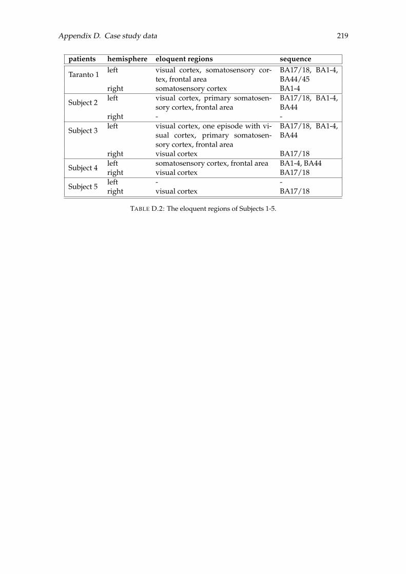
Appendix D. Case study data 219
patients hemisphere eloquent regions sequence
Taranto 1left visual cortex, somatosensory cor-
tex, frontal areaBA17/18, BA1-4,BA44/45
right somatosensory cortex BA1-4
Subject 2left visual cortex, primary somatosen-
sory cortex, frontal areaBA17/18, BA1-4,BA44
right - -
Subject 3left visual cortex, one episode with vi-
sual cortex, primary somatosen-sory cortex, frontal area
BA17/18, BA1-4,BA44
right visual cortex BA17/18
Subject 4left somatosensory cortex, frontal area BA1-4, BA44right visual cortex BA17/18
Subject 5left - -right visual cortex BA17/18
TABLE D.2: The eloquent regions of Subjects 1-5.

220 Appendix D. Case study data
(a) normalised ADC values on the smoothed cortical surface
(b) sequence of eloquent areas during a migraine attack
(c) activation times of the CSD simulation
FIGURE D.1: Left hemisphere of Subject 1: The ADC values on the smoothsurface mesh after taking out the corpus callosum (a), the sequence of elo-quent areas during a migraine attack (b) and the activation times of the
CSD simulation (c).

Appendix D. Case study data 221
(a) normalised ADC values on the smoothed cortical surface
(b) sequence of eloquent areas during a migraine attack
(c) activation times of the CSD simulation
FIGURE D.2: Right hemisphere of Subject 1: The ADC values on thesmooth surface mesh after taking out the corpus callosum (a), the sequenceof eloquent areas during a migraine attack (b) and the activation times of
the CSD simulation (c).
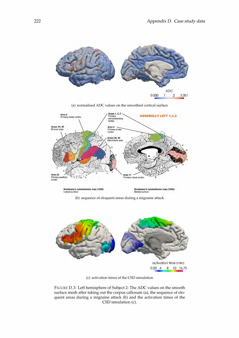
222 Appendix D. Case study data
(a) normalised ADC values on the smoothed cortical surface
(b) sequence of eloquent areas during a migraine attack
(c) activation times of the CSD simulation
FIGURE D.3: Left hemisphere of Subject 2: The ADC values on the smoothsurface mesh after taking out the corpus callosum (a), the sequence of elo-quent areas during a migraine attack (b) and the activation times of the
CSD simulation (c).
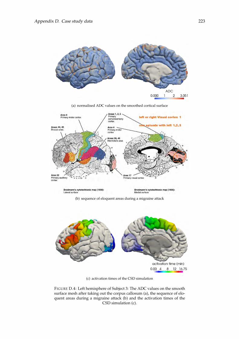
Appendix D. Case study data 223
(a) normalised ADC values on the smoothed cortical surface
(b) sequence of eloquent areas during a migraine attack
(c) activation times of the CSD simulation
FIGURE D.4: Left hemisphere of Subject 3: The ADC values on the smoothsurface mesh after taking out the corpus callosum (a), the sequence of elo-quent areas during a migraine attack (b) and the activation times of the
CSD simulation (c).
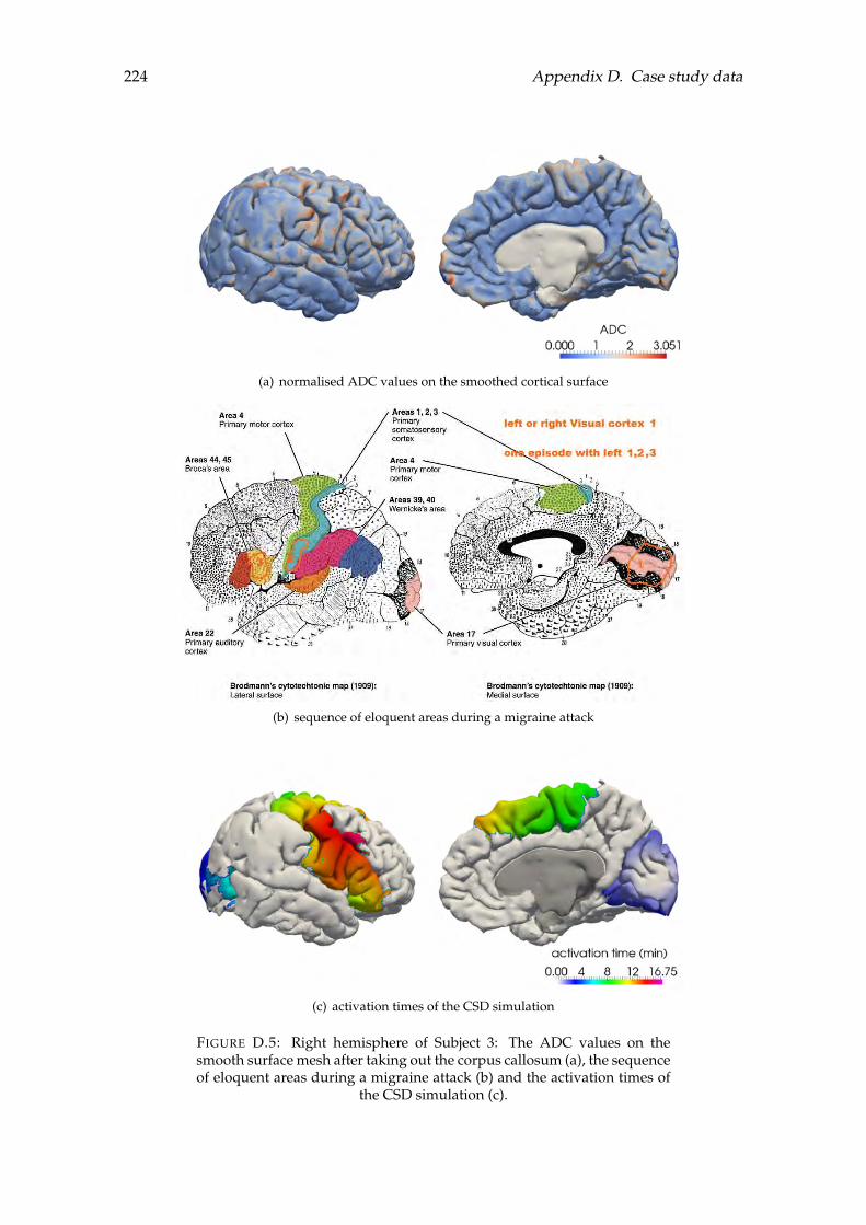
224 Appendix D. Case study data
(a) normalised ADC values on the smoothed cortical surface
(b) sequence of eloquent areas during a migraine attack
(c) activation times of the CSD simulation
FIGURE D.5: Right hemisphere of Subject 3: The ADC values on thesmooth surface mesh after taking out the corpus callosum (a), the sequenceof eloquent areas during a migraine attack (b) and the activation times of
the CSD simulation (c).
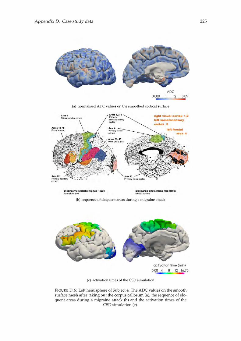
Appendix D. Case study data 225
(a) normalised ADC values on the smoothed cortical surface
(b) sequence of eloquent areas during a migraine attack
(c) activation times of the CSD simulation
FIGURE D.6: Left hemisphere of Subject 4: The ADC values on the smoothsurface mesh after taking out the corpus callosum (a), the sequence of elo-quent areas during a migraine attack (b) and the activation times of the
CSD simulation (c).
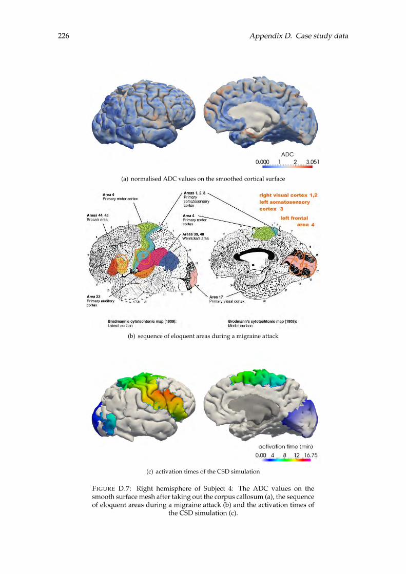
226 Appendix D. Case study data
(a) normalised ADC values on the smoothed cortical surface
(b) sequence of eloquent areas during a migraine attack
(c) activation times of the CSD simulation
FIGURE D.7: Right hemisphere of Subject 4: The ADC values on thesmooth surface mesh after taking out the corpus callosum (a), the sequenceof eloquent areas during a migraine attack (b) and the activation times of
the CSD simulation (c).

Appendix D. Case study data 227
(a) normalised ADC values on the smoothed cortical surface
(b) sequence of eloquent areas during a migraine attack
(c) activation times of the CSD simulation
FIGURE D.8: Right hemisphere of Subject 5: The ADC values on thesmooth surface mesh after taking out the corpus callosum (a), the sequenceof eloquent areas during a migraine attack (b) and the activation times of
the CSD simulation (c).

228 Appendix D. Case study data
ROI number ROI name ROI number ROI name1 fusiform 18 superiorfrontal2 parahippocampal 19 frontalpole3 entorhinal 20 paracentral4 temporalpole 21 precuneus5 inferiortemporal 22 superiorparietal6 middletemporal 23 inferiorparietal7 superiortemporal 24 postcentral8 transversetemporal 25 supramarginal9 bankssts 26 cuneus
10 lateralorbitofrontal 27 pericalcarine11 medialorbitofrontal 28 lingual12 parsorbitalis 29 lateraloccipital13 parstriangularis 30 isthmuscingulate14 rostralmiddlefrontal 31 posteriorcingulate15 parsopercularis 32 caudalanteriorcingulate16 caudalmiddlefrontal 33 rostralanteriorcingulate17 precentral 34 insula
TABLE D.3: The region of interest (ROI) number and the correspondingregion name for the 34 ROI defined by the Desikan-Killiany atlas.

229
List of abbreviations
ABU Abusive painkiller user groupADC Apparent diffusion coefficientANOVA Analysis of varianceANTs Advanced normalization toolsATP Adenosine triphosphateBA Brodmann areaBET Brain extraction toolBiCGSTAB Biconjugate gradient stabilised methodc.c. Cingulate cortexCG Conjugate gradient methodCON Control groupCSD Cortical spreading depressionDICOM Digital imaging and communication in medicineDTI Diffusion tensor imagingDOF Degrees of freedomDWI Diffusion-weighted imagingEEG ElectroencephalographyFA Fractional anisotropyFAD Flavin adenine dinucleotideFHM Familial hemiplegic migraineFLIRT FMRIB linear image registration toolfMRI Functional magnetic resonance imagingFNIRT FMRIB nonlinear image registration toolFSL FMRIB software libraryGAI Global asymmetry indexgPC Generalised polynomial chaosICT Incomplete Cholesky factorisation with drop toleranceILU Incomplete LU factorisationIMEX Implicit explicit schemel.t. Lateral temporal lobeMD Mean diffusivityMEG MagnetoencephalographyME-PCM Multi-element probabilistic collocation methodMIG Migraine patients without aura groupMRI Magnetic resonance imagingm.t. Medial temporal lobeNAD Nicotinamide adenine dinucleotideNIfTI Neuroimaging informatics technology initiativeODE Ordinary differential equationo.l. Occipital lobePCG Preconditioned conjugate gradient methodPCM Probabilistic collocation methodPDE Partial differential equation

PDF Probability density functionpH Potential of hydrogenQoI Quantity/quantities of interestRA Relative anisotropyRI Retention indexROI Region/regions of interestSRI Surface regularity indexstd Standard deviationTRACULA TRActs constrained by underlying anatomyUQ Uncertainty quantificationVR Volume ratio

231
List of units
A ampere electric currentkg kilogram massm metre lengthmol mole amount of substancesec second time
C coulomb electric chargeF farad capacitanceg gram massGB gigabyte digital informationHz hertz frequencyL liter volumeM molar molar concentrationmin minute timemm millimetres lengthmsec millisecond timemV millivolt electrical potentialS siemens electric conductanceT tesla magnetic flux densityV volt electric potential


233
List of figures
1.1 The changes in the membrane potential, the dynamics of the voltage-gatedion channels and the ion fluxes across the membrane in the different phasesof an action potential generation. . . . . . . . . . . . . . . . . . . . . . . . . 3
1.2 Schematic representation of a glutamatergic synapse and the recycling path-way of its neurotransmitters via a neighbouring astrocyte (Rodrigues, Valette,and Bouzier-Sore, 2013). . . . . . . . . . . . . . . . . . . . . . . . . . . . . . 6
1.3 The 34 ROI of the cerebral cortex, in the lateral and medial view of the lefthemisphere (Desikan et al., 2006). . . . . . . . . . . . . . . . . . . . . . . . . 7
1.4 The lobes of the brain, in the lateral and medial view of the left hemisphere. 8
1.5 The electrophysiological features and ionic changes during CSD (Pietrobonand Moskowitz, 2014). . . . . . . . . . . . . . . . . . . . . . . . . . . . . . . 10
2.1 Simulation of the Hodgkin–Huxley model. . . . . . . . . . . . . . . . . . . 16
2.2 Simulation of the FitzHugh–Nagumo model. . . . . . . . . . . . . . . . . . 17
2.3 Simulation of the Rogers–McCulloch variant of the FitzHugh–Nagumomodel. . . . . . . . . . . . . . . . . . . . . . . . . . . . . . . . . . . . . . . . 18
2.4 Simulation of a variant of the Rogers–McCulloch model. . . . . . . . . . . 19
2.5 Simulation of the Izhikevich model. . . . . . . . . . . . . . . . . . . . . . . 20
2.6 Simulation of the electrophysiology model. . . . . . . . . . . . . . . . . . . 24
2.7 Neuronal spiking dynamics simulated with the Wei model. . . . . . . . . . 30
2.8 Different neuronal behaviours of the Wei model. . . . . . . . . . . . . . . . 31
3.1 Temporal dynamics of kbath and the membrane potential for different con-stant values of kbath. . . . . . . . . . . . . . . . . . . . . . . . . . . . . . . . 36
3.2 Temporal dynamics of kbath and the membrane potential for the coupledsystem. . . . . . . . . . . . . . . . . . . . . . . . . . . . . . . . . . . . . . . . 39
3.3 Multi-scale discretisation in time and the interpolation of kbath on (tn, tn+1). 42
3.4 Illustration of the computation of the spiking frequency. . . . . . . . . . . . 46
3.5 Membrane potential, maximum membrane potential and frequency dur-ing CSD. . . . . . . . . . . . . . . . . . . . . . . . . . . . . . . . . . . . . . . 47

3.6 Extracellular potassium dynamics, membrane potential, and frequency inspace at different times steps. . . . . . . . . . . . . . . . . . . . . . . . . . . 48
3.7 Extracellular potassium concentration and other ion dynamics. . . . . . . 49
3.8 Maximum membrane potential and frequency at four time steps on theunit square. . . . . . . . . . . . . . . . . . . . . . . . . . . . . . . . . . . . . 49
3.9 kbath distribution at t = 5 seconds over the whole domain, and the wholetemporal dynamics for the kbath and other ions. . . . . . . . . . . . . . . . 50
4.1 Triangular mesh of reconstructed cortex, left hemisphere. . . . . . . . . . . 52
4.2 kbath profile and the detailed temporal dynamics for two different pointson the cortex. . . . . . . . . . . . . . . . . . . . . . . . . . . . . . . . . . . . 53
4.3 Visualisation of DTI data with ellipsoids. . . . . . . . . . . . . . . . . . . . 56
4.4 Visualisation of the missing or noisy DTI data on the cerebral cortex. . . . 56
4.5 Normalised mean diffusivity of the three-dimensional DTI data of the cortex. 58
4.6 Fractional anisotropy of the three-dimensional DTI data of the cortex. . . . 59
4.7 Joint distribution of the fractional anisotropy and the normalised meandiffusivity of the 3D tensor. . . . . . . . . . . . . . . . . . . . . . . . . . . . 59
4.8 A generic element of the triangulation with the notations of the vertices,angles and vectors. . . . . . . . . . . . . . . . . . . . . . . . . . . . . . . . . 61
4.9 A generic element of the triangulation, and the example ellipsoid fromdiffusion tensor imaging data, before and after the transformation, the in-tersection between the transformed ellipsoid and the plane and the ellipseassociated with the 2D conductivity tensor. . . . . . . . . . . . . . . . . . . 63
4.10 Interpolation of diffusion direction and strength between the vertices of atriangle. . . . . . . . . . . . . . . . . . . . . . . . . . . . . . . . . . . . . . . . 66
4.11 Fractional anisotropy of the 2D diffusion data of the cortex. . . . . . . . . . 67
4.12 Normalised mean diffusivity of the 2D diffusion data of the cortex. . . . . 68
4.13 Joint distribution of the fractional anisotropy and the normalised meandiffusivity of the 2D diffusion tensors. . . . . . . . . . . . . . . . . . . . . . 68
4.14 Principal diffusion direction in the centroids of each triangle of the lefthemisphere. . . . . . . . . . . . . . . . . . . . . . . . . . . . . . . . . . . . . 69
4.15 The smallest and biggest 500 eigenvalues of the original and the precondi-tioned problem. . . . . . . . . . . . . . . . . . . . . . . . . . . . . . . . . . . 71
4.16 Relative residual norm at each iteration step of PCG with different precon-ditioners. . . . . . . . . . . . . . . . . . . . . . . . . . . . . . . . . . . . . . . 72
4.17 Average number of iterations and the relative residual for the ICT withdifferent drop tolerances, solved with PCG. . . . . . . . . . . . . . . . . . . 72

4.18 Extracellular potassium propagation dynamics on the left hemisphere withDTI-based diffusion. . . . . . . . . . . . . . . . . . . . . . . . . . . . . . . . 73
4.19 Lateral and medial views of the CSD wave propagation via the extracellu-lar potassium concentration (EC K+) of the left hemisphere at time t = 10min and t = 16 min, for the three different choices of diffusion tensor. . . . 75
4.20 Difference between the activation times for the isotropic and the DTI-baseddiffusion tensor. . . . . . . . . . . . . . . . . . . . . . . . . . . . . . . . . . . 76
4.21 Difference between the activation times for the isotropic DTI and the DTI-based diffusion tensor. . . . . . . . . . . . . . . . . . . . . . . . . . . . . . . 76
5.1 Areas with artefacts and critical mesh triangulation of the brain geometry. 80
5.2 The notations for the angles opposite the edge ppi and for the angle atpoint p. . . . . . . . . . . . . . . . . . . . . . . . . . . . . . . . . . . . . . . . 82
5.3 The Gaussian smoothing with equal weights applied to the original cowgeometry for different iteration numbers. . . . . . . . . . . . . . . . . . . . 83
5.4 The original mesh of the cow geometry, with artificial noise and the resultsof Taubin smoothing with equal, Fujiwara and Desbrun weights. . . . . . 85
5.5 Volume and mesh quality of the cow geometry after applying the Taubinsmoothing with equal, Fujiwara and Desbrun weights at each iterationstep for different sets of scaling parameters. . . . . . . . . . . . . . . . . . . 86
5.6 The approximation of Gaussian curvature and mean curvature for a sphereof radius r = 0.5 with a structured mesh. . . . . . . . . . . . . . . . . . . . 89
5.7 The approximation of Gaussian curvature and mean curvature for a sphereof radius r = 0.5 with an unstructured mesh. . . . . . . . . . . . . . . . . . 89
5.8 Results of the Taubin smoothing with volume loss restriction with equal,Fujiwara and Desbrun weights for particular regions of the left hemisphere. 91
5.9 Volume loss and mesh quality for different parameter choices of λ and µ,for the left and right hemisphere. . . . . . . . . . . . . . . . . . . . . . . . . 92
5.10 Gaussian and mean curvature of the smoothed brain geometry of the lefthemisphere. . . . . . . . . . . . . . . . . . . . . . . . . . . . . . . . . . . . . 92
5.11 A visualisation of all points within a radius of s = 10 mm of the centroidand points that are not connected to the centroid. . . . . . . . . . . . . . . . 94
5.12 The activation times in the centroids, Lc andRc, for the left and right hemi-sphere. . . . . . . . . . . . . . . . . . . . . . . . . . . . . . . . . . . . . . . . 97
5.13 The activation times in the centroids, Lc and Rc plotted against the dis-tance of the centroids, for the left and right hemisphere. . . . . . . . . . . . 98
5.14 The time difference of the depolarisation wave to propagate between tworegions back and forth. . . . . . . . . . . . . . . . . . . . . . . . . . . . . . . 99
5.15 Mean of the normalised differences L and R for the left and right hemisphere.100

5.16 The global asymmetry index on the left and right hemisphere. . . . . . . . 101
5.17 Duration of stay of the depolarisation wave for the regions of the left andright hemisphere. . . . . . . . . . . . . . . . . . . . . . . . . . . . . . . . . . 102
5.18 Comparative plot of the mean of the duration of stay of the depolarisationwave for regions in the left and right hemisphere. . . . . . . . . . . . . . . 103
5.19 The tolerance ellipse of the 97.5% quantile for the robust distance and a dis-tance - distance plot comparing Mahalanobis distance and robust distancefor the surface - retention index data of the left and right hemisphere. . . . 104
6.1 The eloquent areas in a migraine attack of Subject 1. The numbers refer tothe sequence of symptoms. . . . . . . . . . . . . . . . . . . . . . . . . . . . 109
6.2 The left hemisphere of Subjects 1 to 5 in the lateral and medial view. . . . 111
6.3 The left hemisphere of Controls 1 to 7 in the lateral and medial view. . . . 111
6.4 The smoothed mesh reconstructed from T1-weighted image and the ADCvalues on the surface mesh after taking out the corpus callosum for the lefthemisphere of Subject 1. . . . . . . . . . . . . . . . . . . . . . . . . . . . . . 112
6.5 Box plots of the surface regularity index of the migraine and control group. 113
6.6 Box plots of the surface regularity index of the migraine and control group. 114
6.7 The arrival time of the CSD wave in both hemispheres of Subject 1. . . . . 115
6.8 Correlation plot with the Pearson correlation coefficient in the left andright hemisphere of Subjects 1 to 5. . . . . . . . . . . . . . . . . . . . . . . . 116
6.9 The smoothed mesh and the fractional anisotropy values on the surfacemesh for the left hemisphere of a patient from the migraine group. . . . . 118
6.10 Box plots of the surface regularity index of ABU, CON and MIG. . . . . . 119
6.11 Box plots of the Pearson correlation coefficient between the activation timesof each region and the distance between the centroids for the the three pa-tient groups. . . . . . . . . . . . . . . . . . . . . . . . . . . . . . . . . . . . . 120
6.12 The mean and standard deviation of matrix G (5.11) for the different pa-tient groups: ABU, MIG and CON, respectively. . . . . . . . . . . . . . . . 121
6.13 The difference in the mean of matrix G (5.11) between the different patientgroups: ABU, MIG and CON. . . . . . . . . . . . . . . . . . . . . . . . . . . 121
6.14 Box plots of the GAI for the the three patient groups. . . . . . . . . . . . . 122
6.15 Box plots of the RI for the the three patient groups. . . . . . . . . . . . . . . 122
6.16 A decision tree of all features with depth 5 for the ABU, CON and MIGpatient groups. . . . . . . . . . . . . . . . . . . . . . . . . . . . . . . . . . . 124
6.17 The pythagorean tree of the decision tree in Figure 6.16. . . . . . . . . . . . 125

7.1 The temporal evolution of the deterministic solution of the extracellularpotassium kbath and the recovery variable w. . . . . . . . . . . . . . . . . . 129
7.2 The solution statistics with the Monte Carlo method of the uniformly dis-tributed parameter η1 with different sample sizes. . . . . . . . . . . . . . . 131
7.3 The solution statistics with PCM for a uniformly distributed η1 on differentnumbers of Legendre collocation points. . . . . . . . . . . . . . . . . . . . . 133
7.4 The solution statistics with PCM for m = 10 Legendre collocation pointswith η1 uniformly distributed on different intervals. . . . . . . . . . . . . . 134
7.5 The solution statistics with PCM for m = 10 Legendre collocation pointswith η2 uniformly distributed on different intervals. . . . . . . . . . . . . . 134
7.6 The solution statistics with PCM for m = 10 Legendre collocation pointswith η3 uniformly distributed on different intervals. . . . . . . . . . . . . . 135
7.7 The solution statistics with PCM for m = 10 Legendre collocation pointswith η4 uniformly distributed on different intervals. . . . . . . . . . . . . . 135
7.8 The solution statistics with PCM for m = 10 Legendre collocation pointsfor different dimensions. . . . . . . . . . . . . . . . . . . . . . . . . . . . . . 137
7.9 The full tensor grid in two dimensions and the sparse grid based on theextrema of the Legendre polynomials at different levels. . . . . . . . . . . . 138
7.10 Two-dimensional and three-dimensional sparse grids based on the extremaof the Legendre polynomials at level q = 6. . . . . . . . . . . . . . . . . . . 139
7.11 The solution statistics with PCM on a 4D sparse grid with different levels. 139
7.12 The mean of the solutions with PCM on a 4D sparse grid level 4 and solu-tions at collocation points associated with negative weights. . . . . . . . . 140
7.13 The solution statistics with the PCM on a 4D tensor grid and sparse gridwith different levels. . . . . . . . . . . . . . . . . . . . . . . . . . . . . . . . 140
7.14 The probability density function of the beta distribution for the parametercombinations (10, 10), (2, 10) and (10, 2). . . . . . . . . . . . . . . . . . . . . 141
7.15 The solution statistics with PCM on a 4D tensor grid with η1, . . . , η4 beingbeta-distributed and different combinations for the parameter set (α, β). . 142
7.16 The sensitivity indices Si and Sil for i, l = 1, 2, 3, 4 and i 6= l. . . . . . . . . 144
7.17 The sensitivity indices Si and Sil at different time steps. . . . . . . . . . . . 144
7.18 The exponential kernel for different correlation lengths and the correspond-ing eigenvalues. . . . . . . . . . . . . . . . . . . . . . . . . . . . . . . . . . . 148
7.19 The mean and the standard deviation of the potassium wave kbath at dif-ferent time steps, namely t = 0, 10, 20, 30, 40 sec. . . . . . . . . . . . . . . . 149
7.20 The mean and the standard deviation of the potassium wave kbath in spaceand time. . . . . . . . . . . . . . . . . . . . . . . . . . . . . . . . . . . . . . . 149

B.1 The sparsity patterns of a matrix A, the preconditioning matrices L and Ucomputed with the ILU(0) factorisation and the product of them. . . . . . 162
B.2 Legendre polynomials on the interval [−1, 1] up to the order n = 5. . . . . 171
B.3 Two-dimensional nodes based on the extrema of the Legendre polynomi-als at level q = 4. . . . . . . . . . . . . . . . . . . . . . . . . . . . . . . . . . 181
B.4 The Sobol’ indices for the above example. . . . . . . . . . . . . . . . . . . . 188
B.5 The eigenfunctions fn(x) for x ∈ [−0.5, 0.5], n = 1, 2, 3, 4 and a correlationlength of b = 1. . . . . . . . . . . . . . . . . . . . . . . . . . . . . . . . . . . 191
B.6 The eigenvalues λn for various values of the correlation length b for n =1, 2, . . . , 10. . . . . . . . . . . . . . . . . . . . . . . . . . . . . . . . . . . . . . 192
C.1 The folder and subfolder structure created with the recon-all command ofFreeSurfer. . . . . . . . . . . . . . . . . . . . . . . . . . . . . . . . . . . . . . 196
C.2 The subject’s volume and the Talairach volume. . . . . . . . . . . . . . . . 197
C.3 The pial surface, the boundary of the white matter and the pial surfacevisualised as a 3D surface. . . . . . . . . . . . . . . . . . . . . . . . . . . . . 198
C.4 An overview of the transformations between the different spaces. . . . . . 200
C.5 The original image of an example dataset and the result of the BET. . . . . 201
C.6 Visualisation of DTI images: the fractional anisotropy, the principal dif-fusion tensor direction, V1 intensity of FA and V1 direction visualised aslines. . . . . . . . . . . . . . . . . . . . . . . . . . . . . . . . . . . . . . . . . 203
C.7 The original image of an example dataset and the registered diffusion data. 205
C.8 An overview of the whole DWI conversion procedure. . . . . . . . . . . . 209
D.1 Left hemisphere of Subject 1: The ADC values on the smooth surface mesh,the sequence of eloquent areas during a migraine attack and the activationtimes of the CSD simulation. . . . . . . . . . . . . . . . . . . . . . . . . . . . 220
D.2 Right hemisphere of Subject 1: The ADC values on the smooth surfacemesh, the sequence of eloquent areas during a migraine attack and theactivation times of the CSD simulation. . . . . . . . . . . . . . . . . . . . . 221
D.3 Left hemisphere of Subject 2: The ADC values on the smooth surface mesh,the sequence of eloquent areas during a migraine attack and the activationtimes of the CSD simulation. . . . . . . . . . . . . . . . . . . . . . . . . . . . 222
D.4 Left hemisphere of Subject 3: The ADC values on the smooth surface mesh,the sequence of eloquent areas during a migraine attack and the activationtimes of the CSD simulation. . . . . . . . . . . . . . . . . . . . . . . . . . . . 223
D.5 Right hemisphere of Subject 3: The ADC values on the smooth surfacemesh, the sequence of eloquent areas during a migraine attack and theactivation times of the CSD simulation. . . . . . . . . . . . . . . . . . . . . 224

D.6 Left hemisphere of Subject 4: The ADC values on the smooth surface mesh,the sequence of eloquent areas during a migraine attack and the activationtimes of the CSD simulation. . . . . . . . . . . . . . . . . . . . . . . . . . . . 225
D.7 Right hemisphere of Subject 4: The ADC values on the smooth surfacemesh, the sequence of eloquent areas during a migraine attack and theactivation times of the CSD simulation. . . . . . . . . . . . . . . . . . . . . 226
D.8 Right hemisphere of Subject 5: The ADC values on the smooth surfacemesh, the sequence of eloquent areas during a migraine attack and theactivation times of the CSD simulation. . . . . . . . . . . . . . . . . . . . . 227


241
List of tables
2.1 Model parameters for the simulation of the Hodgkin–Huxley model. . . . 16
2.2 Model parameters for the simulations of a variant of the Rogers–McCullochmodel. . . . . . . . . . . . . . . . . . . . . . . . . . . . . . . . . . . . . . . . 18
2.3 Model parameters for the simulations of the Izhikevich model. . . . . . . . 20
2.4 Model parameters for the simulation of the Cressman model. . . . . . . . 23
2.5 Initial conditions for the simulation of the Cressman model. . . . . . . . . 23
2.6 Model parameters for the simulation of the Wei model. . . . . . . . . . . . 29
2.7 Initial conditions of the Wei model. . . . . . . . . . . . . . . . . . . . . . . . 29
3.1 Model parameters for the propagation of the kbath. . . . . . . . . . . . . . . 37
4.1 Iteration number and relative residual for the PCG and different precondi-tioners in the left and right hemisphere. . . . . . . . . . . . . . . . . . . . . 71
4.2 Average number of iterations and average relative residual for differentdrop tolerances in the preconditioner computation. . . . . . . . . . . . . . 73
4.3 Total activation times for a CSD wave originating from the lateraloccipitalregion for the three diffusion tensors. . . . . . . . . . . . . . . . . . . . . . . 74
5.1 The iteration number and mesh quality of the noisy cow geometry afterapplying the Taubin smoothing with equal, Fujiwara and Desbrun weights. 87
5.2 Mean and relative error for the discrete Gaussian and mean curvature of asphere with different meshes. . . . . . . . . . . . . . . . . . . . . . . . . . . 89
5.3 Mesh quality and iteration number of Taubin smoothing with equal, Fuji-wara and Desbrun weights for the left and right hemisphere. . . . . . . . . 90
5.4 The mean and standard deviation of the Gaussian and mean curvature ofthe (smoothed) left and right hemisphere. . . . . . . . . . . . . . . . . . . . 90
5.5 The index and name of the outliers for the left and right hemisphere de-tected with the Mahalanobis distance and the robust distance. . . . . . . . 105
6.1 Propagation time for CSD starting in the visual cortex, surface area, wavepropagation speed and the SRI for both hemisphere of Subjects 1 to 5. . . . 116

6.2 The p-values of the Welch’s t-test for equal means of the SRI for the differ-ent pairs of patient groups. . . . . . . . . . . . . . . . . . . . . . . . . . . . . 119
6.3 The confusion matrices of the decision tree based on all the features andbased on the reduced number of features. . . . . . . . . . . . . . . . . . . . 125
B.1 The different types of Wiener-Askey scheme polynomials and their under-lying random distribution. . . . . . . . . . . . . . . . . . . . . . . . . . . . . 176
B.2 The degrees of freedom of the Smolyak grid for different dimensions d andlevels q. . . . . . . . . . . . . . . . . . . . . . . . . . . . . . . . . . . . . . . . 182
C.1 An example of the orientation of MRI and DTI data. . . . . . . . . . . . . . 195
D.1 The clinical details of the symptoms during a migraine attack of Subjects 1-5.218
D.2 The eloquent regions of Subjects 1-5. . . . . . . . . . . . . . . . . . . . . . . 219
D.3 The region of interest (ROI) number and the corresponding region namefor the 34 ROI defined by the Desikan-Killiany atlas. . . . . . . . . . . . . . 228
243
Bibliography
Ahrens, J., B. Geveci, and C. Law (2005). “ParaView: An end-user tool for large data vi-sualization”. In: Elsevier. DOI: 978-0123875822 (see p. 93).
Andersson, J.L.R. and S.N. Sotiropoulos (2016). “An integrated approach to correction foroff-resonance effects and subject movement in diffusion MR imaging”. In: NeuroImage125, pp. 1063–1078. DOI: 10.1016/j.neuroimage.2015.10.019 (see p. 200).
Archer, G.E.B., A. Satelli, and I.M. Sobol’ (1997). “Sensitivity measures, ANOVA-like tech-niques and the use of bootstrap”. In: J. of Statist. Comput. Simul. 58, pp. 99–120. DOI:10.1080/00949659708811825 (see pp. 141, 187).
Askey, R. and J. Willson (1985). Some Basic Hypergeometric Orthogonal Polynomials that Gen-eralize Jacobi Polynomials. 319. Mem. Amer. Math. Soc. DOI: 978-0-8218-2321-7(see p. 169).
Ayata, C. (2010). “Cortical spreading depression triggers migraine attack: pro”. In: Headache50.4, pp. 725–30. DOI: 10.1111/j.1526-4610.2010.01647.x (see p. 153).
Ayata, C. and M. Lauritzen (2015). “Spreading depression, spreading depolarizations,and the cerebral vasculature”. In: Physiol Rev. 95.3, pp. 953–993. DOI: 10 . 1152 /physrev.00027.2014 (see p. 151).
Ayata, C. et al. (2006). “Suppression of cortical spreading depression in migraine prophy-laxis”. In: Ann Neurol. 59.4, pp. 625–61. DOI: 10.1002/ana.20778 (see p. 11).
Bade, R., J. Haase, and B. Preim (2006). “Comparison of fundamental mesh smoothingalgorithms for medical surface models”. In: SimVis. Vol. 6, pp. 289–304 (see p. 80).
Barreto, E. and J.R. Cressman (2011). “Ion concentration dynamics as a mechnism forneuronal bursting”. In: J. Biol. Phys. 37.3, pp. 361–373. DOI: 10.1007/s10867-010-9212-6 (see pp. xv, 14, 20, 30).
Biggs, N. (1993). Algebraic Graph Theory. 2nd ed. Cambridge University Press. DOI: 10.1017/CBO9780511608704 (see p. 168).
Bolay, H. and M.A. Moskowitz (2005). “The emerging importance of cortical spreadingdepreassion in migraine headache”. In: Revue Neurologique 161.6-7, pp. 655–7. DOI:10.1016/s0035-3787(05)85108-2 (see p. 11).
Borgdorff, P. (2018). “Arguments against the role of cortical spreading depression in mi-graine”. In: Neurological Research 40.3, pp. 173–181. DOI: 10.1080/01616412.2018.1428406 (see p. 12).
Bossen, F.J. and P.S. Heckbert (1996). “A pliant method for anisotropic mesh generation”.In: 5th Intl. Meshing Roundtable, pp. 63–74 (see p. 80).
Bowyer, S.M. et al. (1999). “Analysis of MEG signals of spreading cortical depressionwith propagation constrained to a rectangular cortical strip: II. Gyrencephalic swinemodel”. In: Brain Res. 843.1-2, pp. 79–86. DOI: 10.1016/S0006-8993(99)01893-4(see p. 11).
Bowyer, S.M. et al. (2001). “Magnetoencephalographic fields from patients with sponta-neous and induced migraine aura”. In: Ann Neurol. 50.5, pp. 582–587. DOI: 10.1002/ana.1293 (see p. 11).
Brander, A. et al. (2010). “Diffusion tensor imaging of the brain in a healthy adult popu-lation: Normative values and measurement reproducibility at 3 T and 1.5 T”. In: ActaRadiologica 51.7, pp. 800–807. DOI: 10.3109/02841851.2010.495351 (see p. 108).
Broca, P. (1861). “L’aphasie de Broca”. In: Bulletin de la société française d’anthropologie (seep. 7).
Brodmann, K. (2006). Brodmann’s Localisation in the Cerebral Cortex - The Principles of Com-parative Localisation in the Cerebral Cortex Based on Cytoarchitectonics. Ed. by L.J. Garey.Springer. DOI: 10.1007/b138298 (see pp. 7, 110).
Brötzner, C.P. et al. (2014). “Resting state alpha frequency is associated with menstrualcycle phase, estradiol and use of oral contraceptives”. In: Brain Res. 1577, pp. 36–44.DOI: 10.1016/j.brainres.2014.06.034 (see p. 9).
Bures, J., O. Buresova, and J. Krivanek (1974). Mechanism and Applications of Leao’s Spread-ing Depression of Electroencephalographic Activity. Academic Press Inc.,U.S. DOI: 10.1002/neu.480060608 (see p. 153).
Colli Franzone, P. and G. Savare (2002). “Evolution Equations, Semigroups and Func-tional Analysis”. In: Progress in Nonlinear Differential Equations and Their Appli-cations. Birkäuser Basel. Chap. Degenerate Evolution Systems Modeling the CardiacElectric Field at Micro- and Macroscopic Level, pp. 49–78. DOI: 10.1007/978-3-0348-8221-7_4 (see p. 40).
Cressman, J.R. Jr. et al. (2009). “The influence of sodium and potassium dynamics onexcitability, seizures, and the stability of persistent states: I. Single neuron dynamics”.In: J. Comput. Neurosci. 26.2, pp. 159–170. DOI: 10.1007/s10827-008-0132-4 (seepp. ix, xv, 14, 20, 23, 26, 30).
— (2011). “Erratum to: The influence of sodium and potassium dynamics on excitability,seizures, and the stability of persistent states: I. Single neuron dynamics”. In: J ComputNeurosci 30.3, pp. 781–781. DOI: 10.1007/s10827-011-0333-0 (see pp. 14, 20).
Dahlem, M.A. et al. (2015). “Cortical hot spots and labyrinths: why cortical neuromod-ulation for episodic migraine with aura should be personalized”. In: Front. Comput.Neurosci. DOI: 10.3389/fncom.2015.00029 (see pp. vii, xiii, 2, 79).
Dassi, F. et al. (2015). “Anisotropic finite element mesh adaptation via higher dimensionalembedding”. In: Procedia Engineering 124, pp. 265–277. DOI: j.proeng.2015.10.138 (see p. 80).
De Maesschalck, R., D. Jouan-Rimbaud, and D.L. Massart (2000). “The Mahalanobis dis-tance”. In: Chemometrics and Intelligent Laboratory Systems 50.1, pp. 1–18. DOI: S0169-7439(99)00047-7 (see p. 103).
Deco, G. et al. (2008). “The dynamic brain: from spiking neurons to neural masses andcortical fields”. In: PLoS Comput Biol. 4.8, e1000092. DOI: 10.1371/journal.pcbi.1000092 (see p. 34).
D’Elia, M. et al. (2011). “Applications of variational data assimilation in computationalhemodynamics”. In: Modeling of Physiological Flows, pp. 363–394. DOI: 10.1007/978-88-470-1935-5_12 (see p. 64).
Delingette, H. et al. (2012). “Personalization of cardiac motion and contractility from im-ages using variational data assimilation”. In: IEEE Transactions on Biomedical Engineer-ing, Institute of Electrical and Electronics Engineers 59.1, pp. 20–24. DOI: 10.1109/TBME.2011.2160347 (see p. 64).
Demšar, J. et al. (2013). “Orange: Data mining toolbox in Python”. In: Journal of MachineLearning Research 14, pp. 2349–2353. URL: http : / / jmlr . org / papers / v14 /demsar13a.html (see p. 123).
Deppe, M. et al. (2014). “Increased cortical curvature reflects white matter atrophy in in-dividual patients with early multiple sclerosis”. In: NeuroImage: Clinical 6, pp. 475–487. ISSN: 2213-1582. DOI: https : / / doi . org / 10 . 1016 / j . nicl . 2014 .
02.012. URL: http://www.sciencedirect.com/science/article/pii/S2213158214000308 (see p. 79).
Desikan, R.S. et al. (2006). “An automated labeling system for subdividing the humancerebral cortex on MRI scans into gyral based regions of interest”. In: NeuroI 31,pp. 968–980. DOI: 10.1016/j.neuroimage.2006.01.021 (see pp. 7, 64, 117).
Diez, I. et al. (2015). “A novel brain partition highlights the modular skeleton shared bystructure and function”. In: Sci Rep 5.10532. DOI: 10.1038/srep10532 (see pp. 52,54).
Dijkstra, E. W. (1959). “A note on two problems in connexion with graphs”. In: Numer.Math. 1.1, pp. 269–271. DOI: 10.1007/BF01386390 (see p. 95).
Do Carmo, M.P. (1976). Differential Geometry of Curves and Surfaces. 1st ed. Prentice-HallEnglewood Cliffs. DOI: 9780132125895 (see pp. 87, 164).
Dunavant, D. A. (1985). “High degree efficient symmetrical Gaussian quadrature rulesfor the triangle”. In: Internat. J. Numer. Meth. Engrg 21.6, pp. 1129 –1148. DOI: 10.1002/nme.1620210612 (see p. 41).
Eikermann-Haerter, K. et al. (2009). “Genetic and hormonal factors modulate spreadingdepression and transient hemiparesis in mouse models of familial hemiplegic mi-graine type 1”. In: J Clin Invest 119.1, pp. 99–109. DOI: 10.1172/JCI36059 (seep. 153).
Enger, R. et al. (2015). “Dynamics of Ionic Shifts in Cortical Spreading Depression”. In:Cereb. Cortex 25.11, pp. 4469–76. DOI: 10.1093/cercor/bhv054 (see pp. xv, 10).
Engnew, T.R. (2009). “Suffering, meaning, and healing: Challenges of contemporary medicine”.In: Ann Fam Med 7.2, pp. 170–175. DOI: 10.1370/afm.943 (see p. 51).
Fischl, B. (2012). “FreeSurfer”. In: NeuroImage 62.2, pp. 774–781. DOI: 10 . 1016 / j .neuroimage.2012.01.021 (see pp. 52, 193).
Fishman, G.S. (1996). Monte Carlo: Concepts, Algorithms, and Applications. Springer NewYork. DOI: 10.1007/978-1-4757-2553-7 (see p. 174).
FitzHugh, R. (1955). “Mathematical models of threshold phenomena in the nerve mem-brane”. In: The Bulletin of Mathematical Biology 17.4, pp. 257–278. DOI: 10.1007/BF02477753 (see pp. 14, 17).
— (1961). “Impulses and physiological states in theoretical models of nerve membrane”.In: Biophysical Journal 1.6, pp. 445–466. DOI: 10.1007/s10867-010-9212-6 (seepp. 17, 37).
Foo, J. and G.E. Karniadakis (2010). “Multi-element probabilistic collocation method inhigh dimensions”. In: Journal of Computational Physics 229.5, pp. 1536–1557. DOI: 10.1016/j.jcp.2009.10.043 (see p. 130).
Foo, J., X. Wan, and G.E. Karniadakis (2008). “The multi-element probabilistic collocationmethod (ME-PCM): Error analysis and applicatio”. In: Journal of Computational Physics227.22, pp. 9572–9595. DOI: 10.1016/j.jcp.2008.07.009 (see p. 130).
Frey, P.J (2004). “Generation and adaptation of computational surface meshes from dis-crete anatomical data”. In: Int. J. Numer. Meth. Eng. 60.6, pp. 1049–1074. DOI: 10.1002/nme.992 (see p. 85).
Frey, P.J. and H. Borouchaki (1998). “Geometric surface mesh optimization”. In: Comput.Vis. Sci. 1.3, pp. 113–121. DOI: 10.1007/s007910050011 (see p. 85).
— (2003). “Surface meshing using a geometric error estimate”. In: Int. J. Numer. MethodsEngng. 58.2, pp. 227–245. DOI: 10.1002/nme.766 (see p. 85).
Gao, Z. and J.S. Hesthaven (2010). “On ANOVA expansion and strategies for choosingthe anchor point”. In: Applied Mathematica and Computations 217.7, pp. 3274–3285. DOI:10.1016/j.amc.2010.08.061 (see p. 185).
Gerardo-Giorda, L. and J.M. Kroos (2017). “Multiscale modeling and simulation of cor-tical spreading depression propagation”. In: Computers and Mathematics with Applica-tions 74.5, pp. 1076–1090. DOI: 10.1016/j.camwa.2017.05.013 (see p. 50).
Gerstner, T. and M. Griebel (1998). “Numerical integration using sparse grids”. In: Nu-merical Algorithms 18, pp. 209–232. DOI: 10.1023/A:1019129717644 (see p. 181).
Geuzaine, C. and J.F. Remacle (2009). “Gmsh: a three-dimensional finite element meshgenerator with built-in pre- and post-processing facilities”. In: Int. J. Numer. Meth.Engng. 79, pp. 1309–1331. DOI: 10.1002/nme.2579 (see p. 85).
Ghanem, R.G. and P.D. Spanos (1991). Stochastic Finite Elements: A Spectral Approach. SpringerNew York. DOI: 10.1007/978-1-4612-3094-6 (see pp. 189, 190, 192).
Goddard, W. and O.R. Oellermann (2011). “Distance in Graphs”. In: Structural Analysisof Complex Networks. Ed. by M. Dehmer. Boston: Birkhäuser Boston, pp. 49–72. ISBN:978-0-8176-4789-6. DOI: 10.1007/978-0-8176-4789-6_3 (see p. 169).
Goldman, R. (2005). “Curvature formulas for implicit curves and surfaces”. In: Comput.Aided Geom. Des. 22.7, pp. 632–658. DOI: 10.1016/j.cagd.2005.06.005 (seep. 87).
Grafstein, B. (1956). “Mechanism of spreading cortical depression”. In: J. Neurophysiol.19.2, pp. 154–71. DOI: 10.1152/jn.1956.19.2.154 (see p. 9).
Greve, D.N. and B. Fischl (2009). “Accurate and robust brain image alignment usingboundary-based registration”. In: NeuroImage 48.1, pp. 63–72. DOI: 10.1016/j.neuroimage.2009.06.060 (see p. 202).
Gronenschild, E.H.B.M. et al. (2012). “The effects of FreeSurfer version, workstation type,and Macintosh operating system version on anatomical volume and cortical thick-ness measurements”. In: PLOS ONE 7.6, e38234. DOI: 10.1371/journal.pone.0038234 (see p. 108).
Hadjikhani, N. et al. (2001). “Mechanisms of migraine aura revealed by functional MRIin human visual cortex”. In: Proceedings of the National Academy of Science of the USA98.8, pp. 4687–92. DOI: 10.1073/pnas.071582498 (see pp. xiii, 1, 11).
Hastie, T., R. Tibshirani, and J. Friedman (2009). The Elements of Statistical Learning. 2nd ed.Springer-Verlag New York. DOI: 10.1007/978-0-387-84858-7 (see p. 123).
Hodgkin, A.L. and A.F. Huxley (1952). “A quantitative description of membrane currentand its application to conduction and excitation in nerve”. In: J. Physiol. 117, pp. 500–544. DOI: 10.1113/jphysiol.1952.sp004764 (see pp. 14–16).
— (1953). “Propagation of electrical signals along giant nerve fibres”. In: Proceedings ofthe Royal Society of London. Series B, Biological Sciences 140.899, pp. 177–183. DOI: 10.1098/rspb.1952.0054 (see pp. 14, 15).
Huisman, T.A.G.M. (2010). “Diffusion-weighted and diffusion tensor imaging of the brain,made easy”. In: Cancer Imaging 10.1A, pp. 163–171. DOI: 10.1102/1470-7330.2010.9023 (see p. 54).
Huisman, T.A.G.M. et al. (2006). “Quantitative diffusion tensor MR imaging of the brain:field strength related variance of apparent diffusion coefficient (ADC) and fractionalanisotropy (FA) scalars”. In: European Radiology 16.8, p. 1651. DOI: 10.1007/s00330-006-0175-8 (see p. 108).
Hyder, F. et al. (2013). “Glutamatergic function in the resting awake human brain issupported by uniformly high oxidative energy”. In: J Cereb Blood Flow Metab. 33.3,pp. 339–347. DOI: 10.1038/jcbfm.2012.207 (see p. 9).
Izhikevich, E.M. (2003). “Simple model of spiking neurons”. In: IEEE Transaction on neuralnetworks 14.6, pp. 1569–1572. DOI: 10.1109/TNN.2003.820440 (see pp. 14, 19).
— (2004). “Which model to use for cortical spiking neurons?” In: IEEE Transactions onNeural Networks 15.5, pp. 1063–1070. DOI: 10.1109/TNN.2004.832719 (see p. 14).
— (2010). Dynamical Systems in Neuroscience: The Geometry of Excitability and Bursting. TheMIT Press. 528 pp. ISBN: 9780262514200. DOI: 10.7551/mitpress/2526.001.0001 (see pp. 14, 19).
Jenkinson, M. and S.M. Smith (2001). “A global optimisation method for robust affineregistration of brain images”. In: Medical Image Analysis 5.2, pp. 143–156. DOI: 10.1016/S1361-8415(01)00036-6 (see p. 202).
Jenkinson, M. et al. (2002). “Improved optimisation for the robust and accurate linearregistration and motion correction of brain images”. In: NeuroImage 17.2, pp. 825–841.DOI: 10.1006/nimg.2002.1132 (see p. 202).
Jenkinson, M. et al. (2012). “FSL”. In: NeuroImage 62.2, pp. 782–790. DOI: 10.1016/j.neuroimage.2011.09.015 (see pp. 193, 200).
Jia, Z. and S. Yu (2017). “Grey matter alterations in migraine: A systematic review andmeta-analysis.” In: Neuroimage Clin. 14, pp. 130–140. DOI: 10.1016/j.nicl.2017.01.019 (see p. 12).
Jovicich, J. et al. (2009). “MRI-derived measurements of human subcortical, ventricularand intracranial brain volumes: Reliability effects of scan sessions, acquisition se-quences, data analyses, scanner upgrade, scanner vendors and field strengths”. In:NeuroImage 46.1, pp. 177–192. DOI: 10.1016/j.neuroimage.2009.02.010 (seep. 108).
Karhunen, K. (1947). Über lineare Methoden in der Wahrscheinlichkeitsrechnung. AnnalesAcademiae scientiarum Fennicae. Series A. 1, Mathematica-physica 37, pp. 1–79 (seep. 146).
Kellogg, O.D. (1929). “Foundations of Potential Theory. Die Grundlehren der Mathema-tischen Wissenschaften (In Einzeldarstellungen mit Besonderer Berücksichtigung derAnwendungsgebiete)”. In: Springer, Berlin, Heidelberg. Chap. The Divergence Theo-rem, pp. 84–121. DOI: 10.1007/978-3-642-90850-7_4 (see p. 84).
Kingsely, P.B. (2006). “Introduction to diffusion tensor imaging mathematics: Part I. Ten-sor, rotation and eigenvectors”. In: Concepts in Magnetic Resonance Part A 28A.2, pp. 101–122. DOI: 10.1002/cmr.a.20048 (see p. 54).
Kingsley, P.B. (2006). “Introduction to diffusion tensor imaging mathematics: Part II. Anisotropy,diffusion-weighting factors, and gradient encoding schemes”. In: Concepts in MagneticResonance Part A 28 A.2, pp. 123–154. DOI: 10.1002/cmr.a.20049 (see p. 57).
Kneer, F., E. Schöll, and M.A. Dahlem (2014). “Nucleation of reaction-diffusion waveson curved surfaces”. In: New Journal of Physics 16, p. 053010. DOI: 10.1088/1367-2630/16/5/053010 (see p. 105).
Koekoek, R. and R. Swarrouw (1998). The Askey-scheme of hypergeometric orthogonal poly-nomials and its q-analogue. Tech. rep. 98-17. Faculty of Technical Mathematics and In-formatics, Delft University of Technology. URL: http://homepage.tudelft.nl/11r49/askey.html (see p. 170).
Kors, E.E. et al. (2004). “Recent findings on headache genetics”. In: Curr Opin Neurol 17.3,pp. 283–288. DOI: 10.1097/01.wco.0000130295.54572.be (see p. 11).
Kraio, R.P. and C. Nicholson (1978). “Extracellular ionic variations during spreading de-pression”. In: Neuroscience 3.11, pp. 1045–1059. DOI: 10.1016/0306- 4522(78)90122-7 (see pp. xv, 10, 13).
Kroos, J.M. et al. (2016). “Geometry shapes propagation: Assesssing the presence andabsence of cortical symmetries through a computational model of cortical spreadingdepression”. In: Front. Comput. Neurosci. 10.6. DOI: 10.3389/fncom.2016.00006(see pp. 52, 77, 93).
Kroos, J.M. et al. (2017). “Patient-specific computational modeling of cortical spreadingdepression via diffusion tensor imaging”. In: Int J Numer Meth Biomed Engng 33. DOI:10.1002/cnm.2874 (see pp. 54, 77).

Kühnel, W. (2006). Differential Geometry: Curves - Surfaces - Manifolds. 2nd ed. Vol. 16.American Mathematical Society. DOI: 10.1007/978-3-658-00615-0 (see pp. 87,164).
Lanczos, C. (1950). “An iteration method for the solution of the eigenvalue problem oflinear differential and integral operators”. In: J. Res. Natl. Bur. Stand. B 45.4, pp. 255–282. DOI: 10.6028/jres.045.026 (see p. 70).
Langtangen, H.P. (2003). Computational Partial Differential Equations. 2nd ed. Springer-Verlag Berlin Heidelberg. DOI: 10.1007/978-3-642-55769-9 (see p. 41).
Lashley, K.S. (1941). “Patterns of cerebral integration indicated by the scotomas”. In: ArchNeurPsych 46.2, pp. 331–339. DOI: 10.1001/archneurpsyc.1941.02280200137007(see p. 11).
Lauritzen, M. (1994). “Pathophysiology of the migraine aura: The spreading depressiontheory”. In: Brain 117.1, pp. 199–210. DOI: 10.1093/brain/117.1.199 (see pp. ix,xv, 11).
Leão, A.A.P. (1944). “Spreading depression of activity in the cerebral cortex”. In: J. Neuro-physiol. 7, pp. 391–396 (see pp. 1, 8).
— (1947). “Further observations on the spreading depression of activity in the cerebralcortex”. In: J. Neurophysiol. 10.6, pp. 409–14. DOI: 10.1152/jn.1947.10.6.409(see p. 8).
Le Bihan, D. (2003). “Looking into the functional architecture of the brain with diffusionMRI”. In: Nature Reviews Neuroscience 4.2, pp. 469–480. DOI: 10.1038/nrn1119 (seep. 54).
— (2013). “Apparent diffusion coefficient and beyond: What diffusion MR imaging cantell us about tissue structure”. In: Radiology 268.2, pp. 318–322. DOI: 10.1148/radiol.13130420 (see p. 54).
Le Bihan, D. et al. (2001). “Diffusion tensor imaging: Concepts and applications”. In: Jour-nal of Magnetic Resonance Imaging 13.4, pp. 534–546. DOI: 10.1002/jmri.1076 (seep. 57).
Lipton, R.B. et al. (2004). “Classification of primary headaches”. In: Neurology 63.3, pp. 427–35. DOI: 10.1212/WNL.0000133301.66364.9B (see p. 10).
Magid, E., O. Soldea, and E. Rivlin (2007). “A comparison of Gaussian and mean cur-vature estimation methods on triangular meshes of range image data”. In: ComputerVision and Image Understanding 107.3, pp. 139–159. DOI: 10.1016/j.cviu.2006.09.007 (see pp. xvi, 88).
Mahalanobis, P.C. (1936). “On the generalised distance in statistics”. In: Proceedings of theNational Institute of Science of India. URL: http://library.isical.ac.in:8080/jspui/bitstream/123456789/6765/1/Vol02_1936_1_Art05-pcm.pdf (seep. 103).
Marchandise, E., J.F. Remacle, and C. Geuzaine (2014). “Optimal parametrizations forsurface remeshing”. In: Engineering with Computers 30.3, pp. 383–402. DOI: 10.1007/s00366-012-0309-3 (see p. 87).
McNab, J.A. et al. (2013). “Surface based analysis of diffusion orientation for identifyingarchitectonic domains in the in vivo human cortex”. In: Neuroimage 69, pp. 87–100.DOI: 10.1016/j.neuroimage.2012.11.065 (see p. 51).
Meyer, M. et al. (2003). “Discrete differential-geometry operators for triangulated 2-manifolds”.In: Hege HC., Polthier K. (eds) Visualization and Mathematics III. Mathematics and Visual-ization, Springer, Berlin, Heidelberg, pp. 35–57. DOI: 10.1007/978-3-662-05105-4_2 (see p. 88).
Nagumo, J. (1962). “An active pulse transmission line simulating nerve acon”. In: Pro-ceedings of the IRE 50.10, pp. 2061–2070. DOI: 10.1109/JRPROC.1962.288235 (seepp. 14, 17, 37).
Pearson, K. (1895). “Notes on regression and inheritance in the case of two parents”. In:Proceedings of the Royal Society of London 58, pp. 240–242. DOI: 10.1098/rspl.1895.0041 (see p. 97).
Peng, W. et al. (2012). “A fast algorithm to find all-pairs shortest paths in complex net-works”. In: Preocedia Computer Science 9, pp. 557–566. DOI: 10.1016/j.procs.2012.04.060 (see p. 95).
Pérez-Beteta, J et al. (2018). “Tumor surface regularity at MR imaging predicts survivaland response to surgery in patients with glioblastoma”. In: Radiology 288.1, pp. 218–225. DOI: 10.1148/radiol.201171051 (see pp. 79, 92).
Pietrobon, D. (2005). “Migraine: New molecular mechanisms”. In: The Neuroscientist 11.4,pp. 373–386. DOI: 10.1177/1073858405275554 (see pp. 11, 45).
Pietrobon, D. and M.A. Moskowitz (2014). “Chaos and commotion in the wake of coti-cal spreading depression and spreading depolarization”. In: Nat. Rev. Neurosci. 15.6,pp. 379–393. DOI: 10.1038/nrn3770 (see pp. xiii, 8–10).
Pocci, C. et al. (2010). “Numerical study of the stopping of aura during migraine”. In:ESAIM: Proceedings 30, pp. 44–52. DOI: 10.1051/proc/2010005 (see pp. vii, xiii, 2,79).
Porooshani, H. et al. (2004). “Speed of progression of migrainous visual aura measuredby sequential field assessment”. In: Neuro-Ophthalmology 28.2, pp. 101–105. DOI: 10.1076/noph.28.2.101.23739 (see p. 10).
Quarteroni, A., R. Sacco, and F. Saleri (2007). Numerical Mathematics. 2nd ed. Vol. 37. Textsin Applied Mathematics. Springer-Verlag Berlin Heidelberg. DOI: 10.1007/b98885(see pp. 41, 69, 70, 159).
Quarteroni, A. and A. Valli (1994). Numerical Approximation of Partial Differential Equations.Springer-Verlag Berlin Heidelberg. DOI: 10.1007/978-3-540-85268-1 (see p. 40).
Reggia, J.A. and D. Montgomery (1996). “A computational model of visual hallucinationsin migraine”. In: Comput. Biol. Med. 26.2, pp. 133–41. DOI: 10.1016/0010-4825(95)00051-8 (see p. 13).
Ribas, G.C. (2010). “The cerebral sulci and gyri”. In: Neurosurgical Focus 28.2. DOI: 10.3171/2009.11.FOCUS09245 (see p. 7).
Richter, F. and A. Lehmenkühler (2008). “Cortical spreading depression (CSD): A neu-rophysiological correlate of migraine aura”. In: Der Schmerz 22.5, pp. 544–50. DOI:10.1007/s00482-008-0653-9 (see pp. xiii, 1).
Rodrigues, T.B., J. Valette, and A.K. Bouzier-Sore (2013). “13C NMR spectroscopy appli-cations to brain energy metabolism”. In: Front Neuroenergetics 5.9. DOI: 10.3389/fnene.2013.00009 (see p. 6).
Rogers, J.M. and A.D. McCulloch (1994). “A collocation-Galerkin finite element model ofcardiac action potential propagation”. In: IEEE Trans Biomed Eng. 41.8, pp. 743–757.DOI: 10.1109/10.310090 (see pp. xv, 14, 17, 37).
Ronan, L. et al. (2010). “Cortical curvature analysis in MRI-negative temporal lobe epilepsy:A surrogate marker for malformations of cortical development”. In: Epilepsia 52.1,pp. 28–34. DOI: j.1528-1167.2010.02895.x (see p. 79).
Rousseeuw, P. and B.C Van Zomeren (1990). “Unmasking multivariant outliers and lever-age points”. In: Journal of the American Statistical Association 85.411, pp. 633–639. DOI:10.1080/01621459.1990.10474920 (see p. 104).
Rousseeuw, P. and B.C. Van Zomeren (1991). “Robust distances: Simulations and cutoffvalues”. In: Springer-Verlag New York 34, pp. 195–203. DOI: 10.1007/978-1-4612-4444-8_11 (see p. 104).
Rousseeuw, P.J. and K. Van Driessen (1999). “A fast algorithm for the minimum covari-ance determinant estimator”. In: Technometrics 41.3, pp. 212–223. DOI: 10.1080/00401706.1999.10485670 (see p. 104).

Saad, Y. (2003). Iterative methods for sparse linear systems. 2nd ed. DOI: 10.1137/1.9780898718003 (see pp. 45, 70, 159).
Sadava, D. et al. (2006). Life: The Science of Biology. 8th ed. Sinauer Associates (see p. 2).Sasaki, M. et al. (2008). “Variability in absolute apparent diffusion coefficient values across
different platforms may be substantial: A multivendor, multi-institutional compari-son study”. In: Radiology 249.2, pp. 624–630. DOI: 10.1148/radiol.2492071681(see p. 108).
Sawat-Pokam, P.M. et al. (2016). “Mechanisms of neuronal silencing after cortical spred-ing depression”. In: Cereb. Cortex. DOI: 10.1093/cercor/bhv328 (see pp. 2, 9, 10,45).
Schoutens, W. (2000). Stochastic Processes and Orthogonal Polynomials. Springer New York.DOI: 10.1007/978-1-4612-1170-9 (see p. 170).
Semenova, I.B., V.V. Savchenko, and I. Hagiwara (2004). “Two techniques to improvemesh quality and preserve surface characteristics”. In: 13th International Meshing Roundtable,pp. 277–288 (see p. 80).
Shewchuk, J. R. (2002). “What is a good linear element? Interpolation, conditioning, andquality measures”. In: 11th International Meshing Roundtable, pp. 115–126 (see p. 82).
Silberstein, S.D. (2004). “Migraine”. In: The Lancet 363.9406, pp. 381–391. DOI: 10.1016/S0140-6736(04)15440-8 (see p. 10).
Smith, S.M. (2002). “Fast robust automated brain extraction”. In: Human Brain Mapping17.3, pp. 143–155. DOI: 10.1002/hbm.10062 (see p. 201).
Smith, S.M. et al. (2004). “Advances in functional and structural MR image analysisand implementation as FSL”. In: NeuroImage 23, pp. 208–219. DOI: 10.1016/j.neuroimage.2004.07.051 (see p. 193).
Smolyak, S.A. (1963). “Quadrature and interpolation formulas for tensor products of cer-tain classes of functions”. In: Soviet Mathematics Doklady 4, pp. 240–243 (see p. 181).
Soares, J.M. et al. (2013). “A hitchhiker’s guide to diffusion tensor imaging”. In: FrontNeurosci. 7.31. DOI: 10.3389/fnins.2013.00031 (see p. 55).
Sobol’, I.M. (1993). “Sensitivity estimates for nonlinear mathematical models”. In: Math.Model. Comput. Exp. 1, pp. 407–417. DOI: 1061-7590/93/04407-008 (see p. 141).
— (2001). “Global sensitivity indices for nonlinear mathematical models and their MonteCarlo estimates”. In: Mathematics and Computers in Simulation 55.1-3, pp. 271–280. DOI:10.1016/S0378-4754(00)00270-6 (see pp. 141, 187).
Somjen, G.G. (2001). “Mechanisms of spreading depression and hypxic spreading depression-like depolarisation”. In: Physiol. Rev. 81.3, pp. 1065–96. DOI: PMID:11427692 (seepp. 9, 10).
Souza, R. et al. (2018). “An open, multi-vendor, multi-field-strength brain MR dataset andanalysis of publicly available skull stripping methods agreement”. In: NeuroImage 170,pp. 482–494. DOI: 10.1016/j.neuroimage.2017.08.021 (see p. 108).
Steward, W.F. et al. (2008). “Cumulative lifetime migraine incidence in women and men”.In: Cephalalgia 28.11, pp. 1170–1178. DOI: 10.1111/j.1468-2982.2008.01666.x(see p. 10).
Su, C.H. and D. Lucor (2006). “Covariance kernel representations of multidimensionalsecond-order stochastic processes”. In: J. Comput. Phys. 217.1, pp. 82–99. DOI: 10.1016/j.jcp.2006.02.006 (see p. 189).
Tang, K., P.M. Congedo, and R. Abgrall (2015). “Sensitivity analysis using anchored ANOVAexpansion and high-order moments computation”. In: Int. J. Numer. Meth. Engng.102.9, pp. 1554–1584. DOI: 10.1002/nme.4856 (see p. 183).
Taubin, G. (1995). “Curve and surface smoothing without shrinkage”. In: Proceedings ofthe Fifth International Conference on Computer Vision. ICCV ’95, pp. 852–857. DOI: 10.1109/ICCV.1995.466848 (see pp. 81, 83).
— (2000). “Geometric signal processing on polygonal meshes”. In: Eurographics 2000 –STARs. ISSN: 1017-4656. DOI: 10.2312/egst.20001029 (see p. 81).
Taubin, G., T. Zhang, and G. Golub (1996). “Optimal surface smoothing as filter design”.In: Computer Vision – ECCV ’96 1064, pp. 283–292. DOI: 10.1007/BFb0015544 (seep. 85).
Thompson, P.M. et al. (1996). “Three-dimensional statistical analysis of sulcal variabilityin the human brain”. In: Journal of Neuroscience 16.13, pp. 4261–4274. DOI: 0.1523/JNEUROSCI.16-13-04261.1996 (see p. 79).
Toga, A.W. and P.M. Thompson (2003). “Mapping brain asymmetry”. In: Nat Rev Neurosci.4.1, pp. 37–48. DOI: 10.1038/nrn1009 (see p. 105).
Tommaso, M. de et al. (2014). “Altered processing of sensory stimuli in patients withmigraine”. In: Nat. Rev. Neurol. 10.3, pp. 144–55. DOI: 10.1038/nrneurol.2014.14(see p. 11).
Tuch, D.S. et al. (1999). “Conductivity mapping of biological tissue using diffusion MRI”.In: Annals New York Academy of Science 888, pp. 314–316. DOI: 10.1111/j.1749-6632.1999.tb07965.x (see p. 54).
— (2001). “Conductivity tensor mapping of the human brain using diffusion tensor MRI”.In: Proceedings of the National Academy of Sciences 98.20, pp. 11697–11701. DOI: 10.1073/pnas.171473898 (see p. 54).
Tuckwell, H.C. and R.M. Miura (1978). “A mathematical model for spreading corticaldepression”. In: Biophys. J. 23.2, pp. 257–276. DOI: 10.1016/S0006- 3495(78)85447-2 (see p. 13).
Vos, T. et al. (2012). “Years lived with disability (YLDs) for 1160 sequelae of 289 diseasesand injuries 1990-2010: a systematic analysis for the Global Burden of Disease Study2010”. In: The Lancet 380.9859, pp. 2163–2196. DOI: 10.1016/S0140- 6736(12)61729-2 (see p. 1).
Walz, W. (2000). “Role of astrocytes in the clearance of exess extracellular potassium”. In:Neurochemistry International 36.4-5, pp. 291–300. DOI: 10.1016/S0197-0186(99)00137-0 (see p. 6).
Wei, Y., G. Ullah, and S.J. Schiff (2014). “Unification of neuronal spikes, seizures, andspreading depression”. In: J. Neurosci. 34.35, pp. 11733–11743. DOI: 10.1523/JNEUROSCI.0516-14.2014 (see pp. xv, 14, 23, 26, 28, 30, 33–35, 50).
Welch, B.L. (1947). “The generalization of ’student’s’ problem when several differentpopulation variances are involved”. In: Biometrika 34.1-2, pp. 28–35. DOI: 10.1093/biomet/34.1-2.28 (see p. 112).
WHO (2017). “World Health Report”. In: URL: www.who.int/whr/index.htm (seep. 10).
Woolrich, M.W. et al. (2009). “Bayesian analysis of neuroimaging data in FSL”. In: Neu-roImage 45.1, pp. 173–186. DOI: 10.1016/j.neuroimage.2008.10.055 (seep. 193).
Xiu, D. (2010). Numerical Methods for Stochastic Computations: A Spectral Method Approach.Princeton University Press. DOI: 10.2307/j.ctv7h0skv (see pp. 128, 174).
Xiu, D. and G.E. Karniadakis (2002). “The Wiener–Askey polynomial chaos for stochasticdifferential equations”. In: SIAM J. Sci. Comput. 24.2, pp. 619–644. DOI: 10.1137/S1064827501387826 (see p. 169).
Xiu, D.B. and J.S. Hesthaven (2005). “High-order collocation methods for differentialequations with random inputs”. In: SIAM Journal on Scientific Computing 27.3, pp. 1118–1139. DOI: 10.1137/040615201 (see pp. 137, 181).
Yang, X. et al. (2012). “Adaptive ANOVA decomposition of stochastic incompressableand compressible flows”. In: J. Comput. Phys. 231.4, pp. 1587–1614. DOI: 10.1016/j.jcp.2011.10.028 (see p. 186).

252
Yendiki, A. et al. (2011). “Automated probabilistic reconstruction of white-matter path-ways in health and disease using an atlas of the underlying anatomy”. In: Front. Neu-roinform. 5.23. DOI: 10.3389/fninf.2011.00023 (see p. 193).
Yendiki, A. et al. (2013). “Spurious group differences due to head motion in a diffusionMRI study”. In: NeuroImage 88, pp. 79–90. DOI: 10.1016/j.neuroimage.2013.11.027 (see p. 193).
Zandt, B., B. ten Haken, and M.J.A.M van Putten (2013). “Diffusing substances duringspreading depolarisation: Analytic expression for the propagation speed, triggeringand concentration time courses”. In: Journal of Neuroscience 33.14, pp. 5915–5923. DOI:10.1523/JNEUROSCI.5115-12.2013 (see pp. xiii, 8).
Zandt, B. et al. (2015). “How does Spreading depression spread? - Physiology and model-ing”. In: Rev. Neurosci. 22.2, pp. 183–98. ISSN: 2191-0200. DOI: 10.1515/revneuro-2014-0069 (see pp. xiii, xv, 2, 9, 10, 14, 33, 37).
253
Acknowledgements
“Es gibt zwei Arten sein Leben zu leben: entweder so, als wäre nichts ein Wunder, oder so, als wäre alleseines. Ich glaube an Letzteres.”
Albert Einstein
I would like to express my gratitude to all those who have supported me during mygraduate years in making this work possible and these years unforgettable. My specialthanks goes to:
My supervisor Dr. Luca Gerado-Giorda for introducing me to the thrilling field of com-putational neuroscience, for your guidance, patience and support during the last years.
George Karniadakis for hosting me at the Brown University and introducing me to theexciting topic of uncertainty quantification.
Franco Dassi for interesting discussions on mesh improvements and curvature estima-tions, Ibai Diez and Iñigo Gabilondo for their support in the data processing with theFreeSurfer Analysis suit, and Ivi Tsantili for inspiring discussions on the ANOVA ap-proach and sensitivity analysis.
Silvia Daun, Gemma Huguet and Fabio Cavaliere for serving as members of my thesiscommittee.
Gabriela, Daniel, Martina and Ralf for their valuable comments on the thesis manuscript,and Daniel and Carmen-Ana for supporting me with the Basque and Spanish passages.I am especially grateful for Nicole supporting me in the final phase of my thesis not onlywith the manuscript revision but also with valuable scientific and academic advice.
The MMB group members, Ana, Argyrios, Gabriela, Isabella, Martina, and Nicole foralways being available for friendly chats, either technical or non-technical.
Dedicated staff of BCAM, especially Miguel Benítez, for being available and resolvingall the administrative issues appearing in my way, concerning the thesis and every otheradministrative aspect of living in a foreign country.
All present and former members of BCAM, especially Carmen-Ana, Marina, Inderpreet,Aitziber, Diana, Simone, Fabio, Mario, Ariel, Thomas, Biagio, Umberto, Antsa, Stefano,Daniel, Javi and David for many coffee breaks, lunches, and after work drinks, interestingdiscussions, and for creating such a pleasant team atmosphere, at work as well as in thebars and restaurants of Bilbao.
My office mates Mario, Simone, Tijana, Ander and Tamara for providing such a pleasantworking atmosphere.

254
My second little family in the Bowen Street apartment in Providence: Antoine, Cecilia,Esben, Olga and Seok. For all those nice dinners, after-work wines and my very firstscientific boat race.
Katie for being at my side through all those numerous Spanish classes, for the encour-agement, the support and for making me feel at home away from home. Andrew forbeing my gym, beach and party buddy through all those years. Raúl for being the besttandem partner, not only helping me patiently to learn Spanish but also introducing meto the Basque culture. Raúl for the excursions around Bilbao and the Basque country.Mila esker!
Kristina, Sarah and Theresa for always being there for me, numerous phone calls, andvisits all over Europe. Insbesondere für die Unterstützung, aufmunternden Worte undalternativen Sichtweisen in schwierigen Lebenslagen. Bis die Wolken wieder lila werden.
My brother Johannes, my mum Gerlinde and my dad Georg, for their unconditionallove, patience, and advice in every situation and supporting me in every way possiblenot matter what. Ohne euch hätte ich das niemals geschafft. Vielen Dank!
Julia M. KroosBilbao, May 2019