A multigrid for image deblurring with Tikhonov regularization
Upload
independentCategory
view
3download
0
Canales-Rodríguez et al – RUMBA-SD (ArXiv: physics.med-ph, Submission ID: 1092864)
1
Spherical deconvolution of multichannel diffusion MRI data with non-
Gaussian noise models and total variation spatial regularization
Erick J. Canales-Rodríguez1,2,§, Alessandro Daducci3,4*, Stamatios N. Sotiropoulos5*, Emmanuel Caruyer6, Santiago Aja-Fernández7, Joaquim Radua1,8, Yosu Yurramendi Mendizabal9, Yasser Iturria-Medina10, Lester Melie-García11, Yasser Alemán-Gómez2,12,13, Jean-Philippe Thiran3,4,
Salvador Sarró1,2, Edith Pomarol-Clotet1,2, Raymond Salvador1,2.
Erick Jorge Canales-Rodríguez (§Corresponding author, e-mail: [email protected])
* These authors contributed equally to this work
Canales-Rodríguez et al – RUMBA-SD (ArXiv: physics.med-ph, Submission ID: 1092864)
2
1 FIDMAG Germanes Hospitalàries, C/ Dr. Antoni Pujadas, 38, 08830, Sant Boi de Llobregat,
Barcelona, Spain. Tel: +34 93 6529999, Fax: +34 936400268.
2 Centro de Investigación Biomédica en Red de Salud Mental, CIBERSAM, C/Dr Esquerdo, 46, 28007,
Madrid, Spain.
3 Signal Processing Lab (LTS5), École polytechnique fédérale de Lausanne (EPFL), Switzerland. 4 University Hospital Center (CHUV) and University of Lausanne (UNIL), Switzerland. 5 Centre for Functional Magnetic Resonance Imaging of the Brain (FMRIB), University of Oxford, John Radcliffe Hospital, Oxford OX39DU, United Kingdom. 6 Section of Biomedical Image Analysis, Department of Radiology, University of Pennsylvania, USA. 7 Laboratorio de Procesado de Imagen (LPI), ETSI Telecomunicación, Universidad de Valladolid,
Valladolid, Spain.
8 Institute of Psychiatry, King’s College London, London, United Kingdom.
9 Departamento de Ciencias de la Computación e Inteligencial Artificial, Universidad del País Vasco - Euskal Herriko Unibertsitatea. 10 McConnell Brain Imaging Center, Montreal Neurological Institute, McGill University, Montreal, Quebec, Canada. 11 The Neuroimaging Research Laboratory (Laboratoire de Recherche en Neuroimagerie: LREN), Department of Clinical Neurosciences, University Hospital Center (CHUV), Lausanne, Switzerland.
12 Departamento de Bioingeniería e Ingeniería Aeroespacial. Universidad Carlos III de Madrid. 13 Instituto de Investigación Sanitaria Gregorio Marañón. Madrid.
Canales-Rodríguez et al – RUMBA-SD (ArXiv: physics.med-ph, Submission ID: 1092864)
3
ABSTRACT
Due to a higher capability in resolving white matter fiber crossings, Spherical Deconvolution
(SD) methods have become very popular in brain fiber-tracking applications. However, while
some of these estimation algorithms assume a central Gaussian distribution for the MRI noise, its
real distribution is known to be non-Gaussian and to depend on many factors such as the number
of coils and the methodology used to combine multichannel signals. Indeed, the two prevailing
methods for multichannel signal combination lead to noise patterns better described by Rician
and noncentral Chi distributions. Here we develop a Robust and Unbiased Model-BAsed
Spherical Deconvolution (RUMBA-SD) technique intended to deal with realistic MRI noise. The
algorithm relies on a maximum a posteriori formulation based on Rician and noncentral Chi
likelihood models and includes a total variation (TV) spatial regularization term. By means of a
synthetic phantom contaminated with noise mimicking patterns generated by data processing in
multichannel scanners, the performance of RUMBA-SD is compared to that of other well-
established SD methods (i.e., CSD and dRL-SD). The inclusion of proper likelihood models and
TV regularization in RUMBA-SD leads to an increased ability to resolve fiber crossings with
smaller inter-fiber angles and an increased robustness to noise. Finally, the proposed method is
also validated in human brain data, producing the most stable fiber reconstructions in front of
differing noise types and diffusion schemes based on a small number of gradient directions.
Keywords: diffusion weighted imaging; spherical deconvolution; Rician noise; noncentral Chi
noise; total variation.
Canales-Rodríguez et al – RUMBA-SD (ArXiv: physics.med-ph, Submission ID: 1092864)
4
1. INTRODUCTION
After decades of developments in diffusion Magnetic Resonance Imaging (MRI), the successful
implementation of a variety of advanced methods has shed light on the complex patterns of brain
organization present at micro (Salat et al., 2005) and macroscopic scales (Hagmann et al., 2008;
Iturria-Medina et al., 2011; Iturria-Medina et al., 2008). Among these methods, Diffusion Tensor
Imaging (DTI) (Basser et al., 1994) has become a classic in both clinical and research studies.
DTI can deliver quantitative results, it may be easily implemented in any clinical MRI system
and, thanks to its short acquisition time, it may be suitable for studying a wide range of brain
diseases. Unfortunately, it is now well recognized that due to its simplistic assumptions,
including Gaussian diffusion, the DTI model does not adequately describe diffusion processes in
areas of complex tissue organization (e.g. areas with kissing, branching or crossing fibers) (Tuch
et al., 2002).
Such limitations in the DTI approach have prompted the recent development of numerous
sampling protocols, diffusion models and reconstruction techniques (Assemlal et al., 2011;
Daducci et al., 2014a; Fillard et al., 2011). While some of these techniques have been based on
model-free methods, including q-ball imaging (Tuch, 2004) and its extensions (Aganj et al.,
2010; Anderson, 2005; Canales-Rodriguez et al., 2009; Descoteaux et al., 2007; Hess et al.,
2006; Tristan-Vega et al., 2009, 2010), diffusion orientation transforms (Canales-Rodriguez et
al., 2010b; Ozarslan et al., 2006), diffusion spectrum imaging (Wedeen et al., 2005) and related
q-space techniques (Canales-Rodriguez et al., 2010a; Descoteaux et al., 2011; Hosseinbor et al.,
2013; Wu and Alexander, 2007; Yeh et al., 2010), other approaches have relied on parametric
diffusion models using higher-order tensors (Jensen et al., 2005; Liu et al., 2004; Ozarslan and
Mareci, 2003) and multiple second-order diffusion tensors (Tuch et al., 2002). In the later group,
different numerical techniques involving gradient descent (Tuch et al., 2002), Bayesian inference
(Behrens et al., 2007; Jbabdi et al., 2012; Melie-Garcia et al., 2008) and algorithms inspired from
compressed sensing theory (Daducci et al., 2014c; Landman et al., 2012; Michailovich et al.,
2011) have been applied to obtain parameters of interest.
Canales-Rodríguez et al – RUMBA-SD (ArXiv: physics.med-ph, Submission ID: 1092864)
5
Spherical Deconvolution (SD) is a class of multi-compartment reconstruction technique that can
be implemented using both parametric and nonparametric signal models (Alexander, 2005;
Behrens et al., 2003; Dell'Acqua et al., 2007; Dell'acqua et al., 2010; Descoteaux et al., 2009;
Jian and Vemuri, 2007; Kaden et al., 2007; Kaden and Kruggel, 2012; Patel et al., 2010;
Ramirez-Manzanares et al., 2007; Sotiropoulos et al., 2012; Tournier et al., 2007; Tournier et al.,
2004). SD methods have become very popular owing to their ability to resolve fiber crossings
with small inter-fiber angles in datasets acquired within a clinically feasible scan time. This
resolving power is driven by the fact that, as opposed to model-free techniques which estimate
the diffusion Orientational Distribution Function (ODF), the output from SD is directly the fiber
ODF itself.
Among the different SD algorithms, Constrained Spherical Deconvolution (CSD) (Tournier et
al., 2007; Tournier et al., 2004) has been received with special interest due to its good
performance and short computational time. In CSD, the average signal profile from white-matter
regions of parallel fibers is first estimated, and afterwards, the fiber ODF is estimated by
deconvolving the measured diffusion data in each voxel with this signal profile (which is also
known as the single-fiber ‘response function’).
More recently and as an alternative to CSD, a new robust model-based SD method has been
proposed. This method is based on a damped Richardson-Lucy algorithm adapted to Gaussian
noise (dRL-SD) (Dell'Acqua et al., 2007; Dell'acqua et al., 2010). An extensive evaluation of
both CSD and dRL-SD algorithms has revealed a superior ability to resolve low anisotropy
crossing-fibers by CSD but a lower percentage of spurious fiber orientations and a lower over-all
sensitivity to the selection of the response function by the dRL-SD approach (Parker et al.,
2013). This later feature is of great relevance since the assumption of a common response
function for all brain tracts is a clear over-simplification of both methods, with the consequences
of it minimized by the dRL-SD.
From an algorithmic perspective dRL-SD inherits the benefits of the standard RL deconvolution
method applied with great success in diverse fields ranging from microscopy (Dey et al., 2006)
to astronomy (Starck et al., 2002). Remarkably, RL deconvolution is robust to the experimental
Canales-Rodríguez et al – RUMBA-SD (ArXiv: physics.med-ph, Submission ID: 1092864)
6
noise and the obtained solution can be constrained to be non-negative without the need for
including additional penalization functions in the estimation process. Moreover, from a modeling
point of view, dRL-SD is implemented using an extended multi-compartment model that allows
considering the partial volume effect in brain voxels with mixture of white matter (WM), gray
matter (GM) and cerebrospinal fluid (CSF), a strategy that has been shown to be effective in
reducing the occurrence of spurious fiber orientations (Dell'acqua et al., 2010).
However, in spite of the good properties of dRL-SD and other SD methods some methodological
issues remain. Both dRL-SD and CSD, to some extent, assume additivity and zero mean
Gaussianity for the underlying noise and are potentially vulnerable to significant departures from
such an assumption. Indeed, it is well known that the MRI noise is non-Gaussian and depends on
many factors, including the number of coils and the multichannel image combination method.
Real experiments have shown that noise follows Rician (Gudbjartsson and Patz, 1995) and
noncentral Chi (nc-χ) distributions (Dietrich et al., 2008) evidencing the inappropriateness of the
Gaussian model. This issue is especially relevant in diffusion MRI where high b-values required
to enhance the angular contrast lead to extremely low signal-to-noise (SNR) ratios. Also, a recent
study (Sotiropoulos et al., 2013) has shown that different multichannel image combination
methods can changes the properties of the signal and can have an effect on fiber orientation
estimation.
On the other hand, the standard reconstruction in SD, based on a voxel-by-voxel fiber ODF
estimation, although reasonable it may not be optimal in a global sense as it does not take into
account the underlying spatial continuity of the image. Recent research on the inclusion of
spatial continuity into SD methods via regularization has yielded promising results (Daducci et
al., 2014a; Reisert and Kiselev, 2011; Tournier et al., 2013). Among these, spatially regularized
SD methods based on Total Variation (TV) (Daducci et al., 2014a) are very appealing due to
their outstanding ability to simultaneously smooth away noise in flat regions whilst preserving
edges, and due to their robustness to high levels of noise (Rudin et al., 1992).
The main contribution of our study is the development of a unified SD estimation framework
which, following a more realistic view, deals with both Rician and nc-χ noise distributions. The
Canales-Rodríguez et al – RUMBA-SD (ArXiv: physics.med-ph, Submission ID: 1092864)
7
estimation algorithm proposed relies on a maximum a posteriori formulation based on Rician and
nc-χ likelihood models and includes a total variation (TV) spatial regularization term. As initial
hypotheses we expect: (1) that the adequate modelling of the noise distribution will improve the
characterization of the underlying signals, which in turn, will lead to robust and unbiased fiber
ODF estimates in fiber-crossing regions, and (2) that the inclusion of the TV spatial
regularization will be highly beneficial, especially in corrupted datasets with low signal-to-noise
(SNR) ratios.
To test these hypotheses and to compare the relative performance against the dRL-SD and CSD
methods, the different algorithms were applied to datasets generated from a synthetic phantom
which had been contaminated with noise patterns mimicking the Rician and nc-χ noise
distributions produced in multichannel scanners. To the best of our knowledge, this is the first
evaluation of such methods in a scenario where Rician and nc-χ noise are explicitly created as a
function of the number of coils, their spatial sensitivity maps, the correlation between coils, and
the reconstruction methodology used to combine the multichannel signals. As a final analysis,
the new method is also applied to real multichannel diffusion MRI data from a healthy subject.
Following this introduction there is a ‘Theory’ section providing an overview of the different
topics relevant to the study and the derivation of the new SD reconstruction algorithm.
Description about computer simulations, image acquisition strategies and metrics designed to
evaluate the performance of the reconstructions is provided in the Materials and Methods
section. Relevant findings are succinctly described in the Results section. Finally, main results,
contributions and limitations of this work are addressed in the Discussion and Conclusions
section.

Canales-Rodríguez et al – RUMBA-SD (ArXiv: physics.med-ph, Submission ID: 1092864)
8
2. THEORY
This section contains a description of the local forward/generative model used to relate the local
diffusion process with the measured diffusion MRI data. It also provides a brief review of MRI
noise models. Finally, the diffusion and MRI noise models are used to derive the new general SD
reconstruction algorithm.
2.1 Generative signal and fiber ODF model
The diffusion MRI signal measured for a given voxel can be expressed as the sum of the signals
from each intra-voxel compartment. The term ‘compartment’ is defined as a homogeneous
region in which the diffusion process possesses identical properties in magnitude and orientation
throughout, and which is different to the diffusion processes occurring in other compartments.
One example of this approach is the multi-tensor model that allows considering multiple WM
parallel-fiber populations within the voxel. In this model the diffusion process taking place inside
each compartment of parallel fibers is described by a second-order self-diffusion tensor (Tuch et
al., 2002).
In real brain data, in addition to the different WM compartments, voxels might also contain GM
and CSF components. This issue was considered by (Dell'acqua et al., 2010), who extended the
multi-tensor model by incorporating the possible contribution from these compartments. This is
the generative multi-tissue signal model that will be used in the present study. In the absence of
any source of noise, the resulting expression for the signal is:
( ) ( ) ( )( )0 1f exp f exp f exp
M T
i j i i j i GM i GM CSF i CSFjS S b b D b D
== − + − + −∑ v D v , (1)
where M is the total number of WM parallel fiber bundles; f j denotes the volume fraction of
the j th fiber-bundle compartment; fGM and fCSF are the volume fractions of the GM and CSF
Canales-Rodríguez et al – RUMBA-SD (ArXiv: physics.med-ph, Submission ID: 1092864)
9
compartments respectively, so that 1f f f 1
M
j GM CSFj=+ + =∑ ; ib is the diffusion-sensitization
factor (i.e., b-value) used in the acquisition scheme to measure the diffusion signal iS along the
diffusion-sensitizing gradient unit vector iv , 1,...,i N= ;
GMD and CSFD are respectively the
mean diffusivity coefficients in GM and CSF; 0S is the signal amplitude in the absence of
diffusion-sensitization gradients ( 0ib = ); T
j j j=D R AR denotes the anisotropic diffusion tensor
of the j th fiber-bundle, where jR is the rotation matrix that rotates a unit vector initially
oriented along the x-axis toward the j th fiber orientation ( ),j jθ φ and A is a diagonal matrix
containing information about the magnitude and anisotropy of the diffusion process inside that
compartment:
1
2
3
λ 0 0
0 λ 0
0 0 λ
=
A , (2)
where 1λ is the diffusivity along the j th fiber orientation, 2λ and 3λ are the diffusivities in the
plane perpendicular to it. It is assumed that 1 2 3λ λ λ> ≈ .
At each voxel, the measured diffusion signals iS for N different sampling parameters (i.e., iv
and ib , [ ]1,...,i N∈ ) can be recast in matrix form as:
=S Hf , (3)
where [ ]1
T
i NS S S=S … … and |WM ISO = H H H comprises two sub-matrices. WMH
is an N x M matrix where every column of length N contains the values of the signal generated
by the model given in Eq. (1) for a single fiber-bundle compartment oriented along one of the M-
Canales-Rodríguez et al – RUMBA-SD (ArXiv: physics.med-ph, Submission ID: 1092864)
10
directions, i.e., the ( , )i j th element of WMH is equal to ( )0 expWM T
ij i i j iS b= −H v D v . Likewise,
ISOH is an N x 2 matrix where each of the two columns of length N contains the values of the
signal for each isotropic compartment, i.e., ( )1 0 expISO
i i GMS b D= −H and ( )2 0 expISO
i i CSFS b D= −H .
Finally, the column-vector f of length M+2 includes the volume fractions of each compartment
of the voxel.
In the framework of model-based spherical deconvolution, H is created by specifying the
diffusivities, which are chosen according to prior information, and by providing a dense discrete
set of equidistant M-orientations ( ) [ ] , , 1,...,j j j Mθ φΩ = ∈ uniformly distributed on the unit
sphere. Previous studies have used different sets of orientations, ranging from M=129 (Ramirez-
Manzanares et al., 2007) to M=752 (Dell'Acqua et al., 2007). Then, the goal is to infer the
magnitude of each predefined oriented fiber, f , from the vector of measurements S and the
‘dictionary’ H of oriented basis signals. Under this reconstruction model, f can be interpreted
to as the fiber ODF evaluated on the set Ω . Matrix H is referred to in other contexts as the
‘diffusion basis functions’ (Ramirez-Manzanares et al., 2007), or the ‘point spread function’
(Dell'acqua et al., 2010; Kaden et al., 2007; Tournier et al., 2007) that blurs the fiber ODF to
produce the observed measurements.
It should be noticed that solving the deconvolution problem given by Eq. (3) is not simple
because the resulting system of linear equations is ill-conditioned and ill-posed (i.e., there are
more unknowns than measurements and some of the columns of H are highly correlated), which
can lead to numerical instabilities and physically meaningless results (e.g., volume fractions with
negative values). A common strategy to avoid such instabilities is to use robust algorithms that
search for solutions compatible with the observed data but which also satisfy some additional
constraints. Thus, in both CSD and dRL-SD the estimated fiber ODFs are constrained to be non-
negative and symmetric around the origin (i.e., antipodal symmetry). The stability of CSD is
further increased by assuming that the fiber ODF is a smooth function on the sphere. Compliance
with this assumption is achieved by representing the fiber ODF in terms of spherical harmonic
basis with a low number of terms, thus reducing the dimensionality of the problem. On the other

Canales-Rodríguez et al – RUMBA-SD (ArXiv: physics.med-ph, Submission ID: 1092864)
11
hand, in contrast to standard estimation algorithms, the dRL-SD implementation does not involve
any matrix inversion, which is crucial to avoid the instability that arises when inverting the
resulting dictionary H . As mentioned in the introduction, though, all these reconstruction
algorithms may not be necessarily optimal when dealing with non-Gaussian noise, as it is the
case for MRI noise.
2.2 MRI noise models
In conventional MRI systems, the data are measured using a single quadrature detector (i.e., coil
with two orthogonal elements) that gives two signals which, for convenience, are treated as the
real and imaginary parts of a complex number. The magnitude of this complex number (i.e. the
square root of the sum of their squares) is commonly used because it avoids different kinds of
MRI artifacts (Gudbjartsson and Patz, 1995). Given that the noise in the real and imaginary
components follows a Gaussian distribution, the magnitude signal iS will follow a Rician
distribution (Gudbjartsson and Patz, 1995) with a probability function given by
( )2 2 202 2 2
1( , ) exp
2i i i
i i i i i
S S SP S S S S I u Sσ
σ σ σ = − +
, (4)
where iS denotes the true magnitude signal intensity in the absence of noise, 2σ is the variance
of the Gaussian noise in the real and imaginary components, 0I is the modified Bessel function
of first kind of order zero and u is the Heaviside step function that is equal to 0 for negative
arguments and to 1 for non-negative arguments.
Modern clinical scanners are usually equipped with a set of 4 to 32 multiple phased-array coils,
the signals of which can be combined following different strategies that, in turn, will give rise to
different statistical properties for the noise (Dietrich et al., 2008). One frequent strategy uses the
spatial matched filter (SMF) approach linearly combining the complex signals of each coil and
producing voxelwise complex signals (Blaimer et al., 2004). Since the noise in the resulting real
Canales-Rodríguez et al – RUMBA-SD (ArXiv: physics.med-ph, Submission ID: 1092864)
12
and imaginary components remains Gaussian a Rician distribution is expected in the final
combined magnitude image. An alternative to the SMF is to create the composite magnitude
image as the root of the sum-of-squares (SoS) of the complex signals of each coil. Under this
approach the combined image follows a nc-χ distribution (Constantinides et al., 1997) given by,
( )2 2 212 2 2
1( , , ) exp
2
n
i i i ii i i i n i
i
S S S SP S S n S S I u S
Sσ
σ σ σ−
= − +
, (5)
where n is the number of coils and 1nI − is the modified Bessel function of first kind of order
1n − . This expression is strictly valid when the different coils have equal variance and
uncorrelated noise, and when noise correlation cannot be neglected it provides a good
approximation if effective effn and 2
effσ values are considered (Aja-Fernandez et al., 2011), with
effn being a non-integer number lower than the real number of coils and 2effσ is higher than the
real noise variance in each coil.
A related SoS image combination method that increases the validity of Eq. (5) is the covariance-
weighted SoS. This method is equivalent to pre-whitening (i.e., decorrelate) the measured signals
before applying the standard SoS image combination. The covariance-weighted SoS approach
requires the estimation of the noise covariance matrix of the system which, in practice, may be
carried out by digitizing noise from the coils in the absence of excitations (Keil and Wald, 2013).
It is important to note that there are additional factors that can change the noise characteristics
described above, including the use of accelerated techniques such as parallel MRI (pMRI) and
partial Fourier, certain reconstruction filters in k-space, and some of the preprocessing steps
conducted after image reconstruction.
Empirical data suggest that some of these factors do not substantially change the type of
distribution of the noise. On the one hand, (Dietrich et al., 2008) investigated the effects of the
type of filter in k-space, the number of receiving channels and the use of pMRI reconstruction
Canales-Rodríguez et al – RUMBA-SD (ArXiv: physics.med-ph, Submission ID: 1092864)
13
techniques, and found that noise distributions always followed Rician and nc-χ distributions with
a reasonable accuracy - although their standard deviations and effective number of receiver
channels were altered when fast pMRI and subsequent SoS reconstructions were used. On the
other hand, (Sotiropoulos et al., 2013) showed real diffusion MRI data noise to also follow
Rician and nc-χ noise distributions after a preprocessing that included motion and eddy currents
corrections. Unfortunately, the combined effect of all factors has not, to the best of our
knowledge, being studied. In this regard, a complete evaluation should include the study of the
effects of additional data manipulation processes routinely applied in many clinical research
studies, such as B0-unwarping due to magnetic field inhomogeneity and partial Fourier
reconstructions. Although the latter has been investigated in terms of signal-to-noise ratio, its
influence on the shape of the noise distribution remains unknown.
However, while it is impossible to ensure that Rician and nc-χ distributions are the optimal noise
models for all possible strategies used for sampling, reconstructing and preprocessing diffusion
MRI data, such models are flexible enough to adapt to deviations from the initial theoretical
assumptions via re-parameterization in terms of spatial-dependent effective parameters (i.e.,
( ) ( )2, , , , ,eff effn x y z x y zσ ), as in (Aja-Fernandez and Tristan-Vega, 2012; Aja-Fernandez et al.,
2011; Aja-Fernandez et al., 2014). Moreover, the use of effective parameters allows
characterizing the spatially varying nature of the noise in accelerated MRI reconstructed data, as
well as the additional spatial correlation introduced by reconstruction algorithms, whilst
preserving the good theoretical properties of the models with standard parameters (i.e. the null
probability to obtain negative signals as expected from magnitude MRI data, and the ability to
characterize the signal-dependent non-linear bias of the data).
2.3 Spherical deconvolution of diffusion MRI data
Equation (5) based on either conventional (i.e., n , 2σ ) or effective (i.e., effn , 2
effσ ) parameters
provides a very general MRI noise model, which includes the Rician distribution (given in Eq.
(4)) as a special case with 1n = . Consequently, if we derive the spherical deconvolution
Canales-Rodríguez et al – RUMBA-SD (ArXiv: physics.med-ph, Submission ID: 1092864)
14
reconstruction corresponding to Equation (6) any particular solution of interest will become
available.
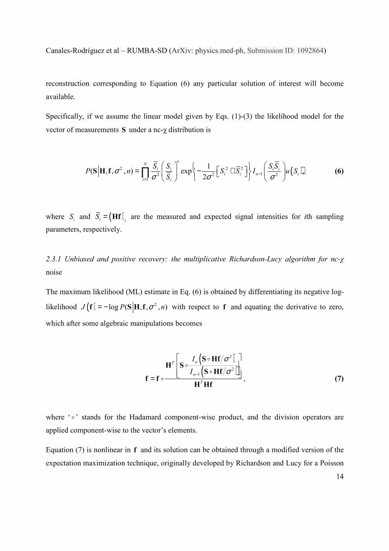
Specifically, if we assume the linear model given by Eqs. (1)-(3) the likelihood model for the
vector of measurements S under a nc-χ distribution is
( )2 2 212 2 2
1
1( , , , ) exp ,
2
nN
i i i ii i n i
i i
S S S SP n S S I u S
Sσ
σ σ σ−=
= − +
∏S H f (6)
where iS and ( )i iS = Hf are the measured and expected signal intensities for ith sampling
parameters, respectively.
2.3.1 Unbiased and positive recovery: the multiplicative Richardson-Lucy algorithm for nc-χ
noise
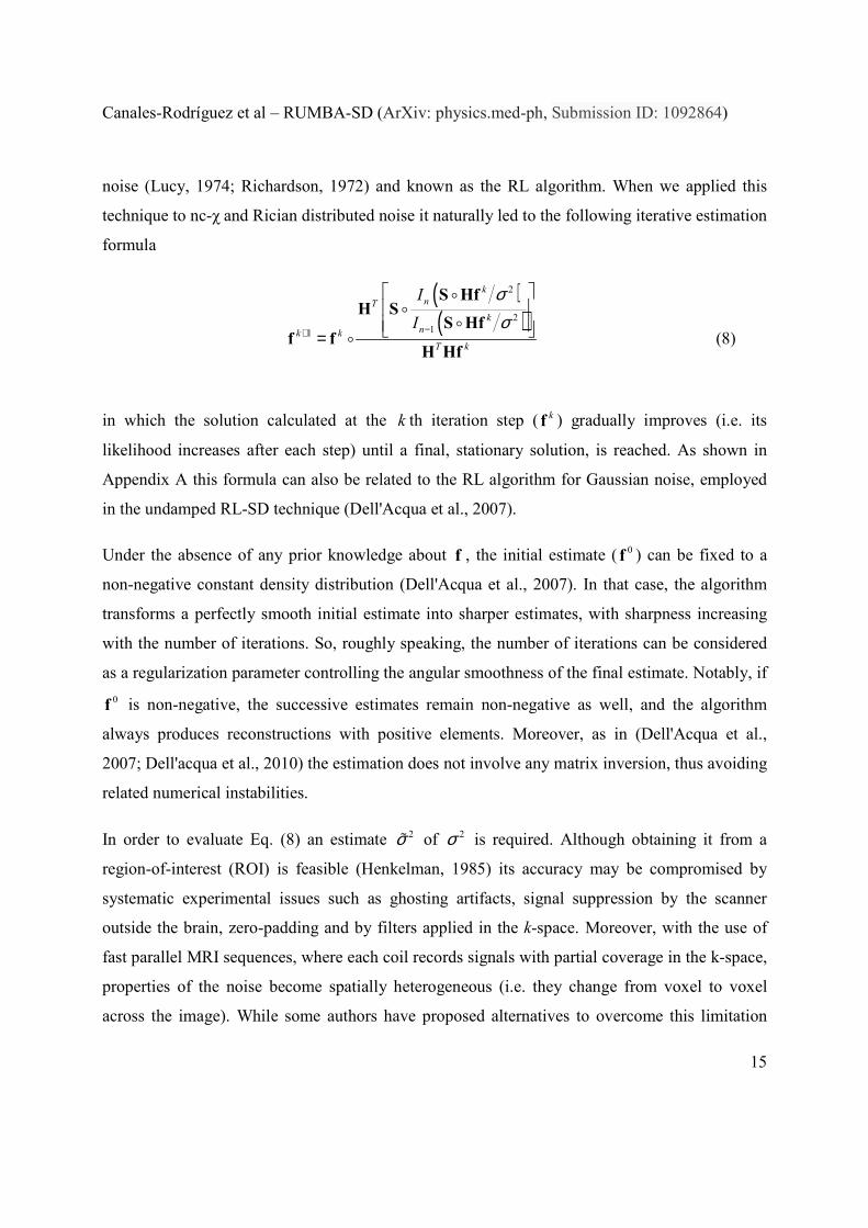
The maximum likelihood (ML) estimate in Eq. (6) is obtained by differentiating its negative log-
likelihood ( ) 2log ( , , , )J P nσ= −f S H f with respect to f and equating the derivative to zero,
which after some algebraic manipulations becomes
( )( )
2
21
nT
n
T
I
I
σσ−
=
S HfH S
S Hff f
H Hf
, (7)
where ‘ ’ stands for the Hadamard component-wise product, and the division operators are
applied component-wise to the vector’s elements.
Equation (7) is nonlinear in f and its solution can be obtained through a modified version of the
expectation maximization technique, originally developed by Richardson and Lucy for a Poisson
Canales-Rodríguez et al – RUMBA-SD (ArXiv: physics.med-ph, Submission ID: 1092864)
15
noise (Lucy, 1974; Richardson, 1972) and known as the RL algorithm. When we applied this
technique to nc-χ and Rician distributed noise it naturally led to the following iterative estimation
formula
( )( )
2
211
k
nT
k
nk k
T k
I
I
σσ−+
=
S HfH S
S Hff f
H Hf
(8)
in which the solution calculated at the k th iteration step ( kf ) gradually improves (i.e. its
likelihood increases after each step) until a final, stationary solution, is reached. As shown in
Appendix A this formula can also be related to the RL algorithm for Gaussian noise, employed
in the undamped RL-SD technique (Dell'Acqua et al., 2007).
Under the absence of any prior knowledge about f , the initial estimate ( 0f ) can be fixed to a
non-negative constant density distribution (Dell'Acqua et al., 2007). In that case, the algorithm
transforms a perfectly smooth initial estimate into sharper estimates, with sharpness increasing
with the number of iterations. So, roughly speaking, the number of iterations can be considered
as a regularization parameter controlling the angular smoothness of the final estimate. Notably, if
0f is non-negative, the successive estimates remain non-negative as well, and the algorithm
always produces reconstructions with positive elements. Moreover, as in (Dell'Acqua et al.,
2007; Dell'acqua et al., 2010) the estimation does not involve any matrix inversion, thus avoiding
related numerical instabilities.
In order to evaluate Eq. (8) an estimate 2σɶ of 2σ is required. Although obtaining it from a
region-of-interest (ROI) is feasible (Henkelman, 1985) its accuracy may be compromised by
systematic experimental issues such as ghosting artifacts, signal suppression by the scanner
outside the brain, zero-padding and by filters applied in the k-space. Moreover, with the use of
fast parallel MRI sequences, where each coil records signals with partial coverage in the k-space,
properties of the noise become spatially heterogeneous (i.e. they change from voxel to voxel
across the image). While some authors have proposed alternatives to overcome this limitation
Canales-Rodríguez et al – RUMBA-SD (ArXiv: physics.med-ph, Submission ID: 1092864)
16
(Aja-Fernandez et al., 2009) here we have estimated the noise variance at each voxel from the
same data used to infer the fiber ODF.
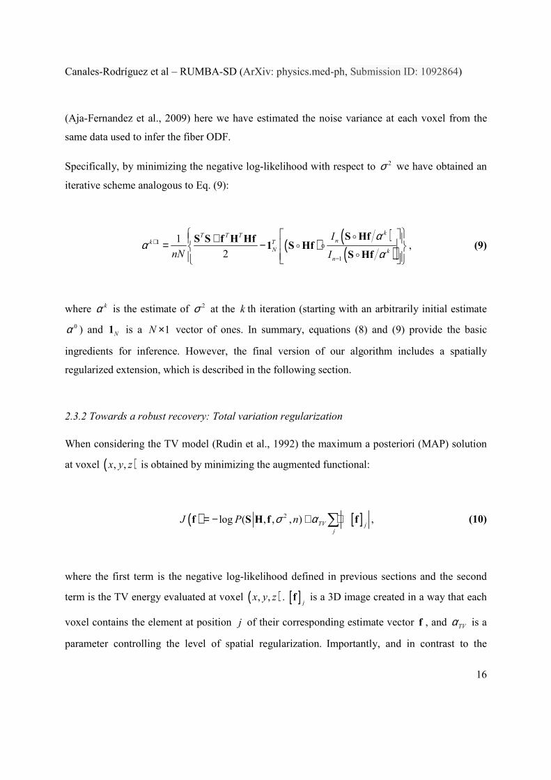
Specifically, by minimizing the negative log-likelihood with respect to 2σ we have obtained an
iterative scheme analogous to Eq. (9):
( ) ( )( )
1
1
1
2
kT T Tnk T
N k
n
I
nN I
αα
α+
−
+ = −
S HfS S f H Hf1 S Hf
S Hf
, (9)
where kα is the estimate of 2σ at the k th iteration (starting with an arbitrarily initial estimate
0α ) and N1 is a 1N × vector of ones. In summary, equations (8) and (9) provide the basic
ingredients for inference. However, the final version of our algorithm includes a spatially
regularized extension, which is described in the following section.
2.3.2 Towards a robust recovery: Total variation regularization
When considering the TV model (Rudin et al., 1992) the maximum a posteriori (MAP) solution
at voxel ( ), ,x y z is obtained by minimizing the augmented functional:
( ) [ ]2log ( , , , ) TV jj
J P nσ α= − + ∇∑f S H f f , (10)
where the first term is the negative log-likelihood defined in previous sections and the second
term is the TV energy evaluated at voxel ( ), ,x y z . [ ]j
f is a 3D image created in a way that each
voxel contains the element at position j of their corresponding estimate vector f , and TVα is a
parameter controlling the level of spatial regularization. Importantly, and in contrast to the

Canales-Rodríguez et al – RUMBA-SD (ArXiv: physics.med-ph, Submission ID: 1092864)
17
previous ML estimate, now the solution at a given voxel is not independent from the solutions in
other voxels. The spatial dependence introduced by the TV functional promote solutions that
minimize the sum of the absolute values of the first-order spatial derivative (i.e., gradient “ ∇ ”)
of the fiber ODF components over the entire brain image. This means that, although TV
regularization does penalize oscillations in homogeneous regions, it does not penalize
discontinuities (Rudin et al., 1992). This property is highly relevant for SD because, while it
promotes continuity and smoothness along individual tracts, it prevents partial volume
contamination from adjacent tracts.
MAP estimates are obtained by differentiating the functional in Eq.(10) with respect to f and
equating the derivative to zero. This yields the following iterative formula (see (Dey et al., 2006)
for a related derivation):
( )( )
2
211
k
nT
k
nk k k
T k
I
I
σσ−+
=
S HfH S
S Hff f R
H Hf
, (11)
with the TV regularization vector kR at voxel ( ), ,x y z , and at the k th iteration, computed
element-by-element as
( )
( ), ,
1
1
k
jk
j
TVk
jx y z
divα
= ∇ −
∇
R
f
f
, (12)
where ( )k
jR is the element j of vector kR and div is the divergence operator. In practice, to
correct for potential singularities at 0k
j ∇ = f , the term k
j ∇ f is replaced by its
Canales-Rodríguez et al – RUMBA-SD (ArXiv: physics.med-ph, Submission ID: 1092864)
18
approximated value 2
k
jε ∇ + f , whereε is a small positive constant. Notice that by setting
0TVα = the estimator in Eq. (11) becomes equal to the unregularized version of Eq. (8).
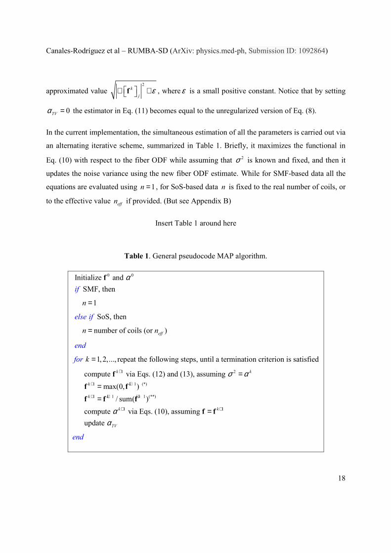
In the current implementation, the simultaneous estimation of all the parameters is carried out via
an alternating iterative scheme, summarized in Table 1. Briefly, it maximizes the functional in
Eq. (10) with respect to the fiber ODF while assuming that 2σ is known and fixed, and then it
updates the noise variance using the new fiber ODF estimate. While for SMF-based data all the
equations are evaluated using 1n = , for SoS-based data n is fixed to the real number of coils, or
to the effective value effn if provided. (But see Appendix B)
Insert Table 1 around here
Table 1. General pseudocode MAP algorithm.
0 0
1
Initialize and
SMF, then
1
SoS, then
number of coils (or )
1, 2,..., repeat the following steps, until a termination criterion is satisfied
compute
eff
k
if
else if
end
for
n
n n
k
α
+
=
=
=
f
f2
1 1 (*)
1 1 1 (**)
1 1
via Eqs. (12) and (13), assuming
max(0, )
/ sum( )
compute via Eqs. (10), assuming
update
k
k k
k k k
k k
TV
end
σ α
αα
+ +
+ + +
+ +
===
=
f f
f f f
f f
Canales-Rodríguez et al – RUMBA-SD (ArXiv: physics.med-ph, Submission ID: 1092864)
19
(*) Since small negative fibers may result from the introduction of the TV model, any spurious negative
component is set to zero at each step of the algorithm. This increases the sparsity of the estimator because,
once a component is set to zero, it remains zero at subsequent iterations.
(**) Optionally, the ODF vector may be normalized to unity, thus preserving the physical definition of the
j th element in f as the volume fraction of the j th compartment of the voxel (see Eqs. (1)-(3)).
Following the discrepancy principle, the regularization parameter TVα is adaptively adjusted at
each iteration. Specifically, it is selected to match the estimated variance (Chambolle, 2004)
using two alternative strategies: (i) assuming a constant mean parameter over the entire brain
image, 1k
TV Eα α += (see Table 1), potentially increasing the precision and robustness of the
estimator; or (ii) assuming a spatial dependent parameter, ( ) ( )1, , , ,k
TV x y z x y zα α += , which may
be more appropriate in situations where a differential variance across the image is expected, like
in accelerated pMRI based-data.
It should be remembered that the accuracy of the reconstruction for the SoS case depends on the
variant used to combine the images. In this work it is assumed that the data is combined using
the covariance-weighted SoS method. However, even if the available data were combined using
the conventional SoS approach (i.e., without taking into account the noise correlation matrix
among coil elements), the method could still provide a reasonable approximation (for more
details see Appendix B).
The evaluation of the ratio of modified Bessel functions of first kind involved in the updates of
Eqs. (11) and (9) is best computed by considering the ratio as a new composite function, and not
by means of the simple evaluation of the ratio of the individual functions. Specifically, this ratio
is computed here in terms of Perron continued fraction (Gautschi and Slavik, 1978). All the
details are provided in Appendix C.
Canales-Rodríguez et al – RUMBA-SD (ArXiv: physics.med-ph, Submission ID: 1092864)
20
3. MATERIAL AND METHODS
3.1 Synthetic phantom data
The reconstruction algorithm proposed here was tested on the synthetic diffusion MRI phantom
developed for the “HARDI Reconstruction Challenge 2013” Workshop, within the IEEE
International Symposium on Biomedical Imaging (ISBI 2013). This phantom comprises a set of
27 fiber bundles with fibers of varying radii and geometry which connect different areas of a 3D
image (matrix size: 50 x 50 x 50). It contains a wide range of configurations including branching,
crossing and kissing fibers, together with the presence of isotropic compartments mimicking the
CSF contamination effects occurring near ventricles in real brain images.
3.1.1 Signal generation
The intra-voxel diffusion MRI signal was generated using N = 64 sampling points on a sphere in
q-space with constant b=3000 s/mm2, plus one additional image with b=0 (i.e., 0 1S = was
assumed in all voxels). For pure GM and CSF voxels, signals were generated using two mono-
exponential models: exp( )GMD b− and exp( )CSFD b− withGMD = 0.2 10-3 mm2/s and
CSFD = 1.7
10-3 mm2/s. In voxels belonging to single-fiber WM bundles, the signal measured along the q-
space unit direction ˆ =q q q was generated by a mixture of signals from intra- and extra-axonal
compartments: ( ) ( )int int ext ext 1 2ˆf s , , , , f s , , , λ , λL R bτ +q v q v , where v denotes the local fiber
orientation. Signal from the intra-axonal compartment ints was created following the theoretical
model of a restricted diffusion process inside a cylinder of length 5 L mm= and radius
5 R mµ= at the diffusion time τ =20.8 s (Ozarslan et al., 2006; Söderman and Jönsson, 1995).
The extra-axonal signal exts was generated using a diffusion tensor model with cylindrical
symmetry (i.e., 1λ = 1.7 10-3 mm2/s, 2 3λ = λ = 0.2 10-3 mm2/s). Mixture fractions were fixed to
Canales-Rodríguez et al – RUMBA-SD (ArXiv: physics.med-ph, Submission ID: 1092864)
21
intf = 0.6 and extf = 0.4. The noiseless dataset can be freely downloaded from the Webpage of the
site1 as well as the ground-truth fiber orientations.
3.1.2 Multichannel noise generation
The synthetic diffusion image S was contaminated with noise mimicking the SoS and SMF
strategies used in scanners in order to combine multiple-coils signals. To that aim, the noisy
complex-valued image measured from the k th coil was assumed to be equal to
R I
k k k kS SC e ie= + + , (13)
where kC is the relative sensitivity map (Pruessmann et al., 1999) of k th coil, ( )0,R
ke N Σ∼ and
( )0,I
ke N Σ∼ are two different Gaussian noise realizations simulating the noise in the real and
imaginary components with zero-mean value and covariance matrix Σ . For simplicity Σ was
assumed to be given by
2
1
1
1
ρ ρρ ρ
σ
ρ ρ
Σ =
⋯
⋯
⋮ ⋮ ⋱ ⋮
⋯
, (14)
where 2σ is the noise variance of each coil and ρ indicates the correlation coefficient between
any two coils.
For the SoS reconstruction, magnitude images were generated as:
1 http://hardi.epfl.ch/static/events/2013_ISBI/

Canales-Rodríguez et al – RUMBA-SD (ArXiv: physics.med-ph, Submission ID: 1092864)
22
2
1
n
SoS kkS S
== ∑ , (15)
where kS stands for the magnitude of kS . Notice that Eq. (15) is the conventional SoS image
combination and not the covariance-weighted variant. We have followed this approach in order
to simulate the effect of any remaining residual correlation ρ present in real systems (we have
assumed a ρ = 0.05) (Aja-Fernandez and Tristan-Vega, 2012).
In the SMF reconstruction, magnitude images were generated as:
1
n
SMF k kkS S C
== ∑ , (16)
with simulated sensitivity maps depicted in Figure 1, satisfying the relationship 2
11
n
kkC
==∑ ,
which holds in practice when the relative sensitivity maps are calculated as /k k SoSC S S=
(Pruessmann et al., 1999). These maps have been previously used in (Aja-Fernandez et al., 2013)
Insert Figure 1 around here (1 column)
Canales-Rodríguez et al – RUMBA-SD (ArXiv: physics.med-ph, Submission ID: 1092864)
23
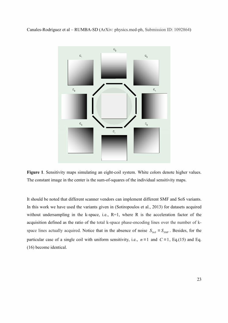
Figure 1. Sensitivity maps simulating an eight-coil system. White colors denote higher values.
The constant image in the center is the sum-of-squares of the individual sensitivity maps.
It should be noted that different scanner vendors can implement different SMF and SoS variants.
In this work we have used the variants given in (Sotiropoulos et al., 2013) for datasets acquired
without undersampling in the k-space, i.e., R=1, where R is the acceleration factor of the
acquisition defined as the ratio of the total k-space phase-encoding lines over the number of k-
space lines actually acquired. Notice that in the absence of noise SoS SMFS S= . Besides, for the
particular case of a single coil with uniform sensitivity, i.e., 1n = and 1C = , Eq.(15) and Eq.
(16) become identical.
Canales-Rodríguez et al – RUMBA-SD (ArXiv: physics.med-ph, Submission ID: 1092864)
24
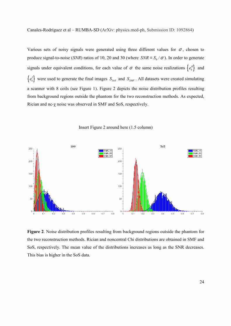
Various sets of noisy signals were generated using three different values for σ , chosen to
produce signal-to-noise (SNR) ratios of 10, 20 and 30 (where 0 /SNR S σ= ). In order to generate
signals under equivalent conditions, for each value of σ the same noise realizations R
ke and
I
ke were used to generate the final images SoSS and SMFS . All datasets were created simulating
a scanner with 8 coils (see Figure 1). Figure 2 depicts the noise distribution profiles resulting
from background regions outside the phantom for the two reconstruction methods. As expected,
Rician and nc-χ noise was observed in SMF and SoS, respectively.
Insert Figure 2 around here (1.5 column)
Figure 2. Noise distribution profiles resulting from background regions outside the phantom for
the two reconstruction methods. Rician and noncentral Chi distributions are obtained in SMF and
SoS, respectively. The mean value of the distributions increases as long as the SNR decreases.
This bias is higher in the SoS data.
Canales-Rodríguez et al – RUMBA-SD (ArXiv: physics.med-ph, Submission ID: 1092864)
25
3.1.3 Evaluation metrics
The performance of the reconstructions was quantified by comparing the obtained
reconstructions against the ground-truth via two main criteria: (i) angular error in the orientation
of the fiber populations and (ii) correct estimation of the number of fiber populations present in
every voxel.
For the analyses, the three main peaks from the reconstructed fiber ODFs were extracted,
retaining only those with magnitude exceeding one tenth of the amplitude of the highest peak (
max0.1 f⋅ ) (Parker et al., 2013), and local peaks were identified as those vertices in the grid with
higher fiber ODFs than their adjacent neighbors. Then, the angular error was defined as the
average minimum angle between the extracted peaks and the true fiber directions (Canales-
Rodriguez et al., 2008):
( ) trueM
1true
1θ min arccos
MT
m m kk == ∑ e v , (17)
where trueM is the true number of fiber populations, me is the unitary vector along with the m th
detected fiber peak and kv is the unitary vector along the k th true fiber direction. Notice that the
angular error between each pair of fibers is always measured between the true fiber and the
closest estimated fiber. Hence, although this metric implicitly depends on the correct detection of
the true number of fibers, it does not explicitly penalize the occurrence of spurious or undetected
fibers.
To quantify any incorrect fiber detection, the mean number of over-estimated n+ (i.e, false
positive) and underestimated n− (i.e., false negative) fiber populations over the whole image
were computed (Daducci et al., 2014a). To that aim, the following procedure was adopted.
Initially, all the estimated fibers forming an angle lower than 20 degrees with any of the true
fibers (i.e., ground-truth) were labeled. Next, not labeled fibers were considered as spurious

Canales-Rodríguez et al – RUMBA-SD (ArXiv: physics.med-ph, Submission ID: 1092864)
26
fibers ( n+ ) and true fibers without any associated labeled fiber were considered as undetected
fibers ( n− ). However, since a single labeled estimated fiber could be associated to different true
fibers, and differently labeled estimated fibers could be associated to a single true fiber, an
update of the +n and n− including such cases had to be made. In consequence, a ‘perfect’
estimation of the number of fiber populations (i.e., n n 0+ −= = ) was considered only when the
numbers of true and estimated fibers were equal and all estimated fibers were contained within
the tolerance cone of 20 degrees around the true fibers.
3.1.4 Settings for the evaluation algorithms
RUMBA-SD estimates were compared to those from dRL-SD and CSD. To investigate the
performance of the CSD as implemented in MRtrix software2, reconstructions for all the datasets
were independently computed via the csdeconv tool using spherical harmonic series of order
maxL = 6, 8 and 10, respectively. For each dataset, the response function was measured from the
images themselves in voxels known to comprise a single bundle of parallel fibers (Tournier et
al., 2008). Local peaks were obtained using the find_SH_peaks function, which identify the
orientation of the three largest peaks from the estimated spherical harmonic coefficients,
retaining only those exceeding the value max0.1 f⋅ (Parker et al., 2013).
Both RUMBA-SD and dRL-SD methods were implemented using in-house Matlab software and
the same dictionary H , created from the signal generative model given in Eqs.(1)-(3).
Specifically, M = 724 fiber orientations distributed on the unit sphere (mean angular separation
between adjacent neighbor vertices/standard deviation = 8.36/1.18 degrees) were assumed, with
diffusivities equal to 1λ = 1.4 10-3 mm2/s and 2 3λ = λ = 0.4 10-3 mm2/s. Two isotropic terms to
account for intra- (i.e., 0.2 10-3 mm2/s) and extra-axonal diffusion (i.e., 1.4 10-3 mm2/s) were also
included. The model diffusivities and the ‘true’ diffusivities in the phantom were deliberately set
to different values in order to consider the possibility of model misspecification.
2 http://www.brain.org.au/software/mrtrix/
Canales-Rodríguez et al – RUMBA-SD (ArXiv: physics.med-ph, Submission ID: 1092864)
27
The same dictionary was used in the estimation in both SMF- and SoS-based datasets. For SoS-
based data, n was fixed to the real number of coils. The starting condition for 0f was set as a
non-negative iso-probable spherical function (Dell'acqua et al., 2010). In order to investigate the
accuracy and convergence of RUMBA-SD as a function of the number of iterations, various
reconstructions were obtained using 200, 400, 600, 800 and 1000 iterations. In the case of dRL-
SD, 200 and 400 iterations were used, which is within the optimal range as suggested in
(Dell'acqua et al., 2010) and (Parker et al., 2013). The damping and threshold parameters for
dRL-SD method were set to 8 and 0.06 respectively (Dell'acqua et al., 2010).
Additionally, RUMBA-SD was computed without applying the TV spatial regularization (i.e.,
0TVα = ) denoted hereafter as ‘RUMBA-SD without TV’ (while keeping the name ‘RUMBA-
SD’ for the regularized version), and values of θ , n+ and n− for the standard DTI method
(using the dtifit tool from FSL) were also calculated assuming fiber orientation through the main
eigenvector. DTI results were used to evaluate the relative benefits of all other reconstruction
methods.
3.2 Real brain data
Diffusion MRI data were acquired from a healthy subject on a 3T Siemens scanner (Erlangen)
located at the University of Oxford (UK). The subject provided informed written consent before
participating in the study, which was approved by the Institutional Review Board of the
University of Oxford. Whole brain diffusion images were acquired with a 32-channel head coil
along 256 different gradient directions on the sphere in q-space with constant b = 2500 s/mm2.
Additionally, 36 b = 0 volumes were acquired with in-plane resolution = 2.0 x 2.0 mm2 and slice
thickness = 2 mm. The acquisition was carried out without undersampling in the k-space (i.e.,
R=1). Raw multichannel signals were combined using either the standard GRAPPA approach or
the GRAPPA approach with the adaptive combination of the SMF available in the scanner,
giving SoS and SMF-based datasets respectively. Then, the two resulting datasets were
Canales-Rodríguez et al – RUMBA-SD (ArXiv: physics.med-ph, Submission ID: 1092864)
28
separately corrected for eddy current distortions and head motion as implemented in FSL (Smith
et al., 2004).
In order to study the robustness of the methods under a lower number of measurements, subsets
of 64 and 35 directions were selected from the full set of 256 gradients directions, and
measurements for these subsets were used to ‘create’ two (under-sampled) versions of the data.
Specifically, a k-means clustering algorithm was employed to group the 256 directions into 64
and 35 non-overlapping clusters on the sphere by selecting the gradient direction closest to each
cluster centroid. This procedure allows identifying subsets of directions with nearly uniform
coverage on the sphere. Finally, from the 36 acquired b=0 volumes only the first 3 volumes were
included in the reduced datasets.
Canales-Rodríguez et al – RUMBA-SD (ArXiv: physics.med-ph, Submission ID: 1092864)
29
4. RESULTS
4.1 Synthetic phantom data
To differentiate the accuracy of all tested methods in regions with varying orientational
complexity, the quality metrics were independently computed in single-fiber regions of parallel
fibers (i.e., more than 12 000 voxels) and in multiple-fiber regions (i.e., more than 1 500 voxels
with inter-fiber angles ranging from 10 to 90 degrees; mean-value/standard deviation = 50/25
degrees).
Results corresponding to single-fiber regions are show in Figure 3. A set of patterns can be
drawn from these results. First, for both SMF- and SoS-based data, RUMBA-SD and dRL-SD
were the methods providing the overall best metrics. Second, the performance of RUMBA-SD
without TV was similar to CSD in terms of angular error and number of undetected fibers, but
CSD produced a higher number of spurious fibers. Finally, all the spherical deconvolution
methods produced lower angular errors than DTI.
Insert Figure 3 around here (1.5 columns)

Canales-Rodríguez et al – RUMBA-SD (ArXiv: physics.med-ph, Submission ID: 1092864)
30
Figure 3. Quantification of the reconstruction accuracy of RUMBA-SD, RUMBA-SD without
TV, dRL-SD, CSD and DTI in terms of θ (angular error), n+ (number of false positive) and n−
(number of false negative) in single-fiber regions of the phantom. Light colors correspond to
higher SNRs.

Canales-Rodríguez et al – RUMBA-SD (ArXiv: physics.med-ph, Submission ID: 1092864)
31
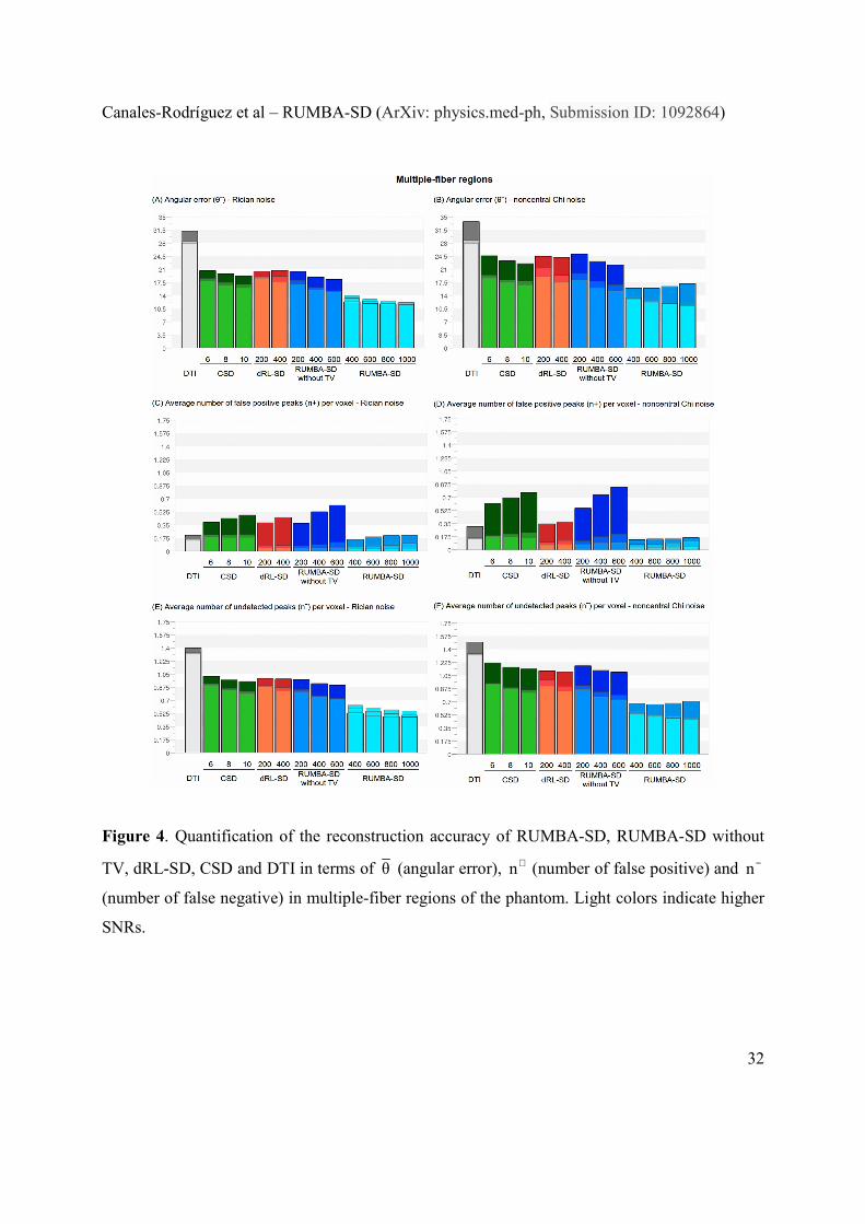
Results from multiple-fiber regions are show in Figure 4. For both SMF- and SoS-based data,
RUMBA-SD without TV and CSD performed quite similar. They performed better than dRL-SD
in terms of angular error and number of undetected fibers, and worse than it in terms of number
of spurious fibers. The superior ability of RUMBA-SD without TV to resolve fiber crossings, as
compared to dRL-SD under the same number of algorithm iterations (i.e., 200 and 400) and
dictionary of basis signals, suggest that it converges faster. RUMBA-SD was the method
providing the best results in terms of all metrics studied in all SNR levels. Notably, results from
RUMBA-SD at the lowest SNR (i.e., SNR = 10) were generally better than those from dRL-SD,
CSD and RUMBA-SD without TV at the highest SNRs (i.e., SNR = 20 and 30); demonstrating
the success of the TV regularization. The uniformity of RUMBA-SD metrics at different number
of iterations suggests that the regularization increases the stability and convergence of the
reconstruction. Finally, results from datasets based on SMF were better than those from SoS.
Results from DTI show a non-zero number of spurious fibers in multiple-fiber regions and
existing undetected fibers in single-fiber regions. These results may seem counterintuitive,
however, it should be noticed that these non-zero values are obtained due to the tolerance cone
used in the experiments to classify the fibers as true positives, false positives and false negatives.
Insert Figure 4 around here (1.5 columns)
Canales-Rodríguez et al – RUMBA-SD (ArXiv: physics.med-ph, Submission ID: 1092864)
32
Figure 4. Quantification of the reconstruction accuracy of RUMBA-SD, RUMBA-SD without
TV, dRL-SD, CSD and DTI in terms of θ (angular error), n+ (number of false positive) and n−
(number of false negative) in multiple-fiber regions of the phantom. Light colors indicate higher
SNRs.
Canales-Rodríguez et al – RUMBA-SD (ArXiv: physics.med-ph, Submission ID: 1092864)
33
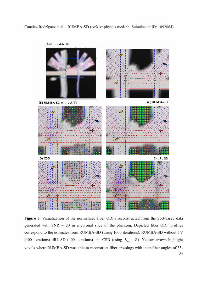
Figure 5 and Figure 6 depict normalized fiber ODF profiles estimated under different conditions.
Normalization was performed by dividing the fiber ODF amplitudes by its maximum value in
each voxel. In contrast to CSD, which does not allow estimating the volume fraction of the
isotropic compartments, the fiber ODFs computed from dRL-SD and RUMBA-SD contain such
volumes which, following (Dell'acqua et al., 2010), were added as constant terms along every
direction. Specifically, Figure 5 shows the estimates from the SoS-based data generated with
SNR = 20. Visual inspection shows that the RUMBA-SD higher performance could be related to
the improved reconstruction accuracy in some complex regions. In particular, yellow arrows
highlight voxels where RUMBA-SD was able to reconstruct fiber crossings with inter-fiber
angles of 35-40 degrees, which were not detected by the other deconvolution techniques. The
blue arrow highlights a region where RUMBA-SD was able to reconstruct fiber crossings with a
low inter-fiber angle of 25 degrees. The red arrow highlights a region where RUMBA-SD was
able to satisfactorily detect the non-dominant tract of a fiber crossing. It should be noted that
fiber ODF profiles in isotropic regions were well represented by both dRL-SD and RUMBA-SD
algorithms, whilst CSD produced a very noisy pattern in those regions. Moreover, the sharper
fiber ODF profiles depicted by RUMBA-SD without TV, as compared to dRL-SD, could explain
its superior ability to resolve fiber crossings.
Insert Figure 5 around here (1.5-2 columns)
Canales-Rodríguez et al – RUMBA-SD (ArXiv: physics.med-ph, Submission ID: 1092864)
34
Figure 5. Visualization of the normalized fiber ODFs reconstructed from the SoS-based data
generated with SNR = 20 in a coronal slice of the phantom. Depicted fiber ODF profiles
correspond to the estimates from RUMBA-SD (using 1000 iterations), RUMBA-SD without TV
(400 iterations) dRL-SD (400 iterations) and CSD (using max 8L = ). Yellow arrows highlight
voxels where RUMBA-SD was able to reconstruct fiber crossings with inter-fiber angles of 35-

Canales-Rodríguez et al – RUMBA-SD (ArXiv: physics.med-ph, Submission ID: 1092864)
35
40 degrees; blue arrow highlights a region where RUMBA-SD was able to reconstruct fiber
crossings with inter-fiber angles of 25 degrees. The red arrow highlights a region where
RUMBA-SD without TV, dRL-SD and CSD were not able to detect the non-dominant tract of a
fiber crossing.
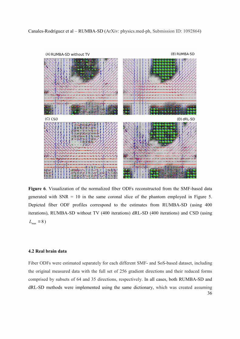
On the other hand, Figure 6 depicts the normalized fiber ODF estimates from the SMF-based
data generated with SNR = 10 at the same slice used in Figure 5. RUMBA-SD without TV
showed sharper fiber ODF profiles than those obtained from dRL-SD and CSD. At this low
SNR, the benefit of using the TV regularization in RUMBA-SD again is visually corroborated.
Insert Figure 6 around here (1.5-2 columns)
Canales-Rodríguez et al – RUMBA-SD (ArXiv: physics.med-ph, Submission ID: 1092864)
36
Figure 6. Visualization of the normalized fiber ODFs reconstructed from the SMF-based data
generated with SNR = 10 in the same coronal slice of the phantom employed in Figure 5.
Depicted fiber ODF profiles correspond to the estimates from RUMBA-SD (using 400
iterations), RUMBA-SD without TV (400 iterations) dRL-SD (400 iterations) and CSD (using
max 8L = )
4.2 Real brain data
Fiber ODFs were estimated separately for each different SMF- and SoS-based dataset, including
the original measured data with the full set of 256 gradient directions and their reduced forms
comprised by subsets of 64 and 35 directions, respectively. In all cases, both RUMBA-SD and
dRL-SD methods were implemented using the same dictionary, which was created assuming
Canales-Rodríguez et al – RUMBA-SD (ArXiv: physics.med-ph, Submission ID: 1092864)
37
diffusivities equal to 1λ = 1.0 10-3 mm2/s and 2 3λ = λ = 0.2 10-3 mm2/s, plus two isotropic terms
with diffusivities equal to 0.6 10-3 mm2/s and 1.4 10-3 mm2/s (see Eqs.(1)-(3)). These values were
selected to match the diffusivities obtained from a previous DTI fit in WM regions of parallel
fibers, GM and CSF respectively. In CSD, the response function was measured from the images
themselves in WM regions of parallel fibers (Tournier et al., 2008).
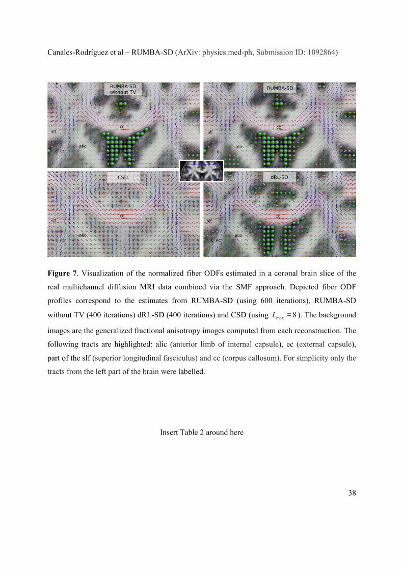
Figure 7 shows a coronal brain view with the normalized fiber ODFs and their maxima estimated
from the full SMF-based data (i.e., data containing the full set of 256 gradient directions and 36
b=0 volumes). The computation time for each method is also reported in Table 2. Visual
inspection of Fig. 7 reveals that all methods have produced quite similar reconstructions. Thus,
while no spurious fibers in regions comprised by parallel fibers, like the midbody of the corpus
callosum, was observed in any of the reconstructions, all approximations were able to resolve
complex fiber geometries, like the mixture of tracts in the coronal plane located bilaterally at the
intersection of the anterior limb of internal capsule, the external capsule and part of the superior
longitudinal fasciculus. Between two and three fibers per voxel were detected by the different
methods in this intersection, with RUMBA-SD being the method detecting three fibers in a
major number of cases. However, such conclusions derived from visual inspection are limited by
the fact that the underlying true anatomy is not known at the voxel level.
Insert Figure 7 around here (2 columns)
Canales-Rodríguez et al – RUMBA-SD (ArXiv: physics.med-ph, Submission ID: 1092864)
38
Figure 7. Visualization of the normalized fiber ODFs estimated in a coronal brain slice of the
real multichannel diffusion MRI data combined via the SMF approach. Depicted fiber ODF
profiles correspond to the estimates from RUMBA-SD (using 600 iterations), RUMBA-SD
without TV (400 iterations) dRL-SD (400 iterations) and CSD (using max 8L = ). The background
images are the generalized fractional anisotropy images computed from each reconstruction. The
following tracts are highlighted: alic (anterior limb of internal capsule), ec (external capsule),
part of the slf (superior longitudinal fasciculus) and cc (corpus callosum). For simplicity only the
tracts from the left part of the brain were labelled.
Insert Table 2 around here
Canales-Rodríguez et al – RUMBA-SD (ArXiv: physics.med-ph, Submission ID: 1092864)
39
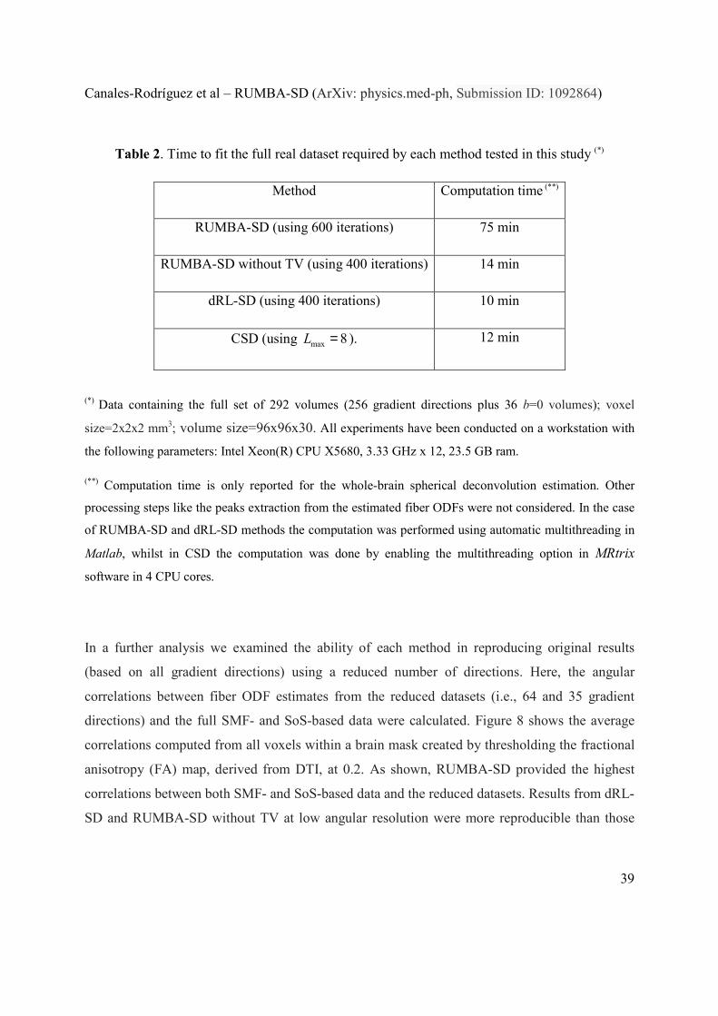
Table 2. Time to fit the full real dataset required by each method tested in this study (*)
Method Computation time (**)
RUMBA-SD (using 600 iterations) 75 min
RUMBA-SD without TV (using 400 iterations) 14 min
dRL-SD (using 400 iterations) 10 min
CSD (using max 8L = ). 12 min
(*) Data containing the full set of 292 volumes (256 gradient directions plus 36 b=0 volumes); voxel
size=2x2x2 mm3; volume size=96x96x30. All experiments have been conducted on a workstation with
the following parameters: Intel Xeon(R) CPU X5680, 3.33 GHz x 12, 23.5 GB ram.
(**) Computation time is only reported for the whole-brain spherical deconvolution estimation. Other
processing steps like the peaks extraction from the estimated fiber ODFs were not considered. In the case
of RUMBA-SD and dRL-SD methods the computation was performed using automatic multithreading in
Matlab, whilst in CSD the computation was done by enabling the multithreading option in MRtrix
software in 4 CPU cores.
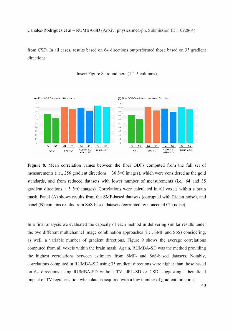
In a further analysis we examined the ability of each method in reproducing original results
(based on all gradient directions) using a reduced number of directions. Here, the angular
correlations between fiber ODF estimates from the reduced datasets (i.e., 64 and 35 gradient
directions) and the full SMF- and SoS-based data were calculated. Figure 8 shows the average
correlations computed from all voxels within a brain mask created by thresholding the fractional
anisotropy (FA) map, derived from DTI, at 0.2. As shown, RUMBA-SD provided the highest
correlations between both SMF- and SoS-based data and the reduced datasets. Results from dRL-
SD and RUMBA-SD without TV at low angular resolution were more reproducible than those
Canales-Rodríguez et al – RUMBA-SD (ArXiv: physics.med-ph, Submission ID: 1092864)
40
from CSD. In all cases, results based on 64 directions outperformed those based on 35 gradient
directions.
Insert Figure 8 around here (1-1.5 columns)
Figure 8. Mean correlation values between the fiber ODFs computed from the full set of
measurements (i.e., 256 gradient directions + 36 b=0 images), which were considered as the gold
standards, and from reduced datasets with lower number of measurements (i.e., 64 and 35
gradient directions + 3 b=0 images). Correlations were calculated in all voxels within a brain
mask. Panel (A) shows results from the SMF-based datasets (corrupted with Rician noise), and
panel (B) contains results from SoS-based datasets (corrupted by noncental Chi noise).
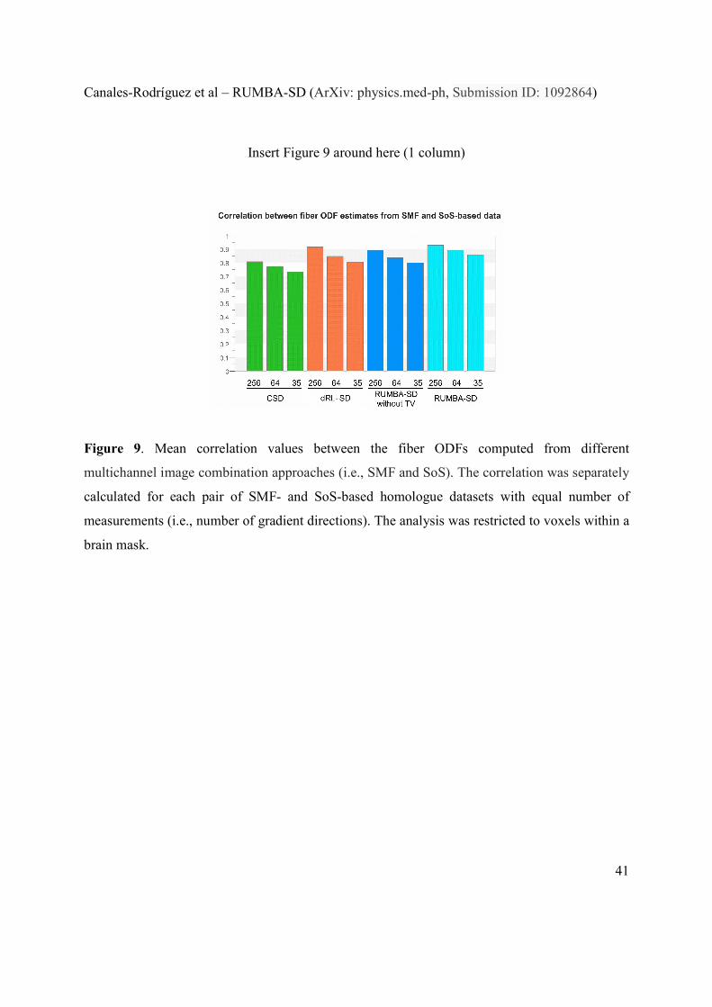
In a final analysis we evaluated the capacity of each method in delivering similar results under
the two different multichannel image combination approaches (i.e., SMF and SoS) considering,
as well, a variable number of gradient directions. Figure 9 shows the average correlations
computed from all voxels within the brain mask. Again, RUMBA-SD was the method providing
the highest correlations between estimates from SMF- and SoS-based datasets. Notably,
correlations computed in RUMBA-SD using 35 gradient directions were higher than those based
on 64 directions using RUMBA-SD without TV, dRL-SD or CSD, suggesting a beneficial
impact of TV regularization when data is acquired with a low number of gradient directions.
Canales-Rodríguez et al – RUMBA-SD (ArXiv: physics.med-ph, Submission ID: 1092864)
41
Insert Figure 9 around here (1 column)
Figure 9. Mean correlation values between the fiber ODFs computed from different
multichannel image combination approaches (i.e., SMF and SoS). The correlation was separately
calculated for each pair of SMF- and SoS-based homologue datasets with equal number of
measurements (i.e., number of gradient directions). The analysis was restricted to voxels within a
brain mask.
Canales-Rodríguez et al – RUMBA-SD (ArXiv: physics.med-ph, Submission ID: 1092864)
42
5. DISCUSSION AND CONCLUSIONS
In this study we propose a new model-based spherical deconvolution method, RUMBA-SD. In
contrast to previous diffusion reconstruction methods, usually based on Gaussian noise with zero
mean, we consider Rician and noncentral Chi noise models, more adequate for characterizing the
non-linear bias introduced in the images measured in current 1.5T and 3T multichannel MRI
scanners. Although recent progress has been made in new SD methods adapted to corrupted
Rician data, e.g., see (Clarke et al., 2008; Kaden and Kruggel, 2012) to the best of our
knowledge, our study provides the first SD extension to noncentral Chi noise, Furthermore,
RUMBA-SD offers a very general estimation framework applicable to different datasets. Its
flexibility emanates from the explicit dependence between the likelihood model used and the real
or effective number of coils in the scanner, and the methodology employed to combine
multichannel signals. Moreover, the voxel-wise estimation of the noise variance allows a better
adaptability to deviations in the shape of the noise distribution influenced, for instance, by use of
accelerated MRI techniques and preprocessing steps. We hope that the proposed technique will
help extending SD methods for a wide range of datasets taken from different scanners and using
different protocols.
This study adds to previous diffusion MRI studies trying to overcome the signal-dependent bias
introduced by the Rician and noncentral Chi noise. Among these studies, it has to be emphasized
the recent noise filtering techniques described in (Brion et al., 2013; Koay et al., 2009), which
may be applied in the pre-processing steps prior HARDI data estimation, as well as the robust
DTI estimation methods in (Tristan-Vega et al., 2012) and the earlier DTI study conducted by
(Salvador et al., 2005).
The relative performance of RUMBA-SD against two popular and powerful reconstruction
algorithms, i.e., CSD and dRL-SD, has been evaluated using one of the finest diffusion MRI
phantoms created to date. This phantom was particularly designed for the “HARDI
Reconstruction Challenge 2013” Workshop, organized within the IEEE International Symposium
on Biomedical Imaging. A previous version of RUMBA-SD took part in that challenge,
Canales-Rodríguez et al – RUMBA-SD (ArXiv: physics.med-ph, Submission ID: 1092864)
43
obtaining the first place in the ‘HARDI-like’ category (for more details see the website3; team
name: ‘Capablanca’). The first-place was shared with a reconstruction based on the CSD method
included in Dipy software4 (Garyfallidis et al., 2014). A manuscript on the ‘Challenge’ (currently
under preparation) provides additional information about the performance of RUMBA-SD in
relation to many other reconstruction methods not included in this work. In that sense, results
here, fully based on local intra-voxel metrics, may be complemented with results in that paper,
focused on global connectivity metrics derived from fiber tracking analyses.
In our work we have weighted the impact of Rician and noncentral Chi likelihood models
through comparisons of outcomes from dRL-SD and ‘RUMBA-SD without TV’. Such
comparisons, in contrast to those against CSD, were not biased by the use of different
dictionaries and estimation algorithms. Both dRL-SD and RUMBA-SD without TV were
implemented using the same dictionary of basis signals and similar reconstruction methods based
on Richardson-Lucy algorithms adapted to Gaussian, Rician and noncentral Chi noise,
respectively. Interestingly, dRL-SD had produced the lower number of spurious fiber
orientations in single-fiber regions (see Fig. 3), demonstrating the benefit of the novel damping
regularization procedure included in this algorithm (Dell'acqua et al., 2010). This performance is
in line with a previous study comparing dRL-SD and CSD (Parker et al., 2013). On the other
hand, RUMBA-SD without TV has showed a superior performance in multiple-fiber regions
with sharper fiber ODF profiles (see Figs. 4 and 5), demonstrating the benefit of using proper
likelihood models to speed the convergence of the algorithm and to increase our ability to
resolve fiber crossings, a result that is consistent with a previous work developing a noise
correction scheme for SD on Rician distributed data (Clarke et al., 2008).
CSD generated the highest number of spurious fibers in single-fiber regions, and had a
performance similar to RUMBA-SD without TV in multiple-fiber regions. These results may be
explained by the spherical harmonic basis used in CSD, effective at filtering noise and reducing
the problem dimensionality but at the expense of secondary side-lobes arising from truncation of
3 http://hardi.epfl.ch/static/events/2013_ISBI/workshop.html#results
4 http://nipy.org/dipy/
Canales-Rodríguez et al – RUMBA-SD (ArXiv: physics.med-ph, Submission ID: 1092864)
44
the harmonic series. Here, though, it should be acknowledged that CSD and RUMBA-SD
without TV used different approaches to create the signal dictionaries and, in consequence,
results shown here cannot be taken as a proof of superiority for any of the two methods. The
main purpose of including CSD in the evaluation was to obtain a practical estimation of the
performance of the proposed method in relation to this state-of-the-art technique that is being
extensively used in real applications.
Remarkably, when adequate likelihood models were combined with TV regularization (i.e. the
full RUMBA-SD approach) the most accurate results were obtained for all metrics employed.
TV regularization, apart from filtering noise has increased the ability to separate fiber bundles, as
revealed both numerically (Figs. 3 and 4) and visually (Figs. 5 and 6).
When applied to human brain data, RUMBA-SD has also achieved the best results, and its
reconstructions have shown the highest stability in front of differing noise types (characterized
by SMF and SoS based datasets) and a reduced number of gradient directions (see Figs. 8 and 9).
Interestingly, dRL-SD has also shown a performance superior to CSD, which may be explained
by two aspects. While dRL-SD estimates had the smoothest fiber ODF profiles, contributing to
obtain higher correlation values, results from CSD were probably affected by its worse
performance in voxels with mixtures of WM, GM and CSF (Roine et al., 2014) contributing to
the reduction in mean correlation values (see Fig. 7).
A recent study has demonstrated that the SoS approach produces a signal-dependent bias that
reduces the signal dynamic range and may subsequently lead to reduced precision and accuracy
in fiber orientation estimates (Sotiropoulos et al., 2013). Our study, however, suggests that the
noncentral Chi noise in SoS-based data is not a major concern for the SD methods considered.
For instance, heavier squashing of fiber ODFs when SoS reconstruction is used (Sotiropoulos et
al., 2013) is not that prominent with SD approaches, compared to diffusion ODF estimation
methods (Aganj et al., 2010). This result may have several possible explanations specific to each
technique. Thus, the robustness of CSD may be explained by the fact that the dictionary of basis
signals is directly created by averaging the measured signals and, in consequence, the noise bias
is already included in the dictionary. Although this would not allow cancelling the bias in brain
Canales-Rodríguez et al – RUMBA-SD (ArXiv: physics.med-ph, Submission ID: 1092864)
45
regions composed of multiple fibers, because the bias is non-linear and signal-dependent, the
final results are less sensitive to it. On the other hand, the robustness of dRL-SD may be
explained, in part, by its lower over-all sensitivity to selection of the response function (Parker et
al., 2013), which make it robust to the use of dictionaries estimated from either biased or
unbiased signals; behaviour that may be additionally boosted by the inclusion of the damping
factor in the RL algorithm. Finally, the robustness of RUMBA-SD can be explained by the use of
proper likelihood models that explicitly consider the bias as function of the noise corrupting the
data. However, it should be noted that the satisfactory performance of RUMBA-SD has been
significantly improved by the introduction of a total variation spatial regularization on the fiber
ODF field, adaptively incorporated into the estimation process.
At this point, it is important to highlight the differences between the ‘unified approach’ used in
this work for joint estimation and filtering, and previous strategies based on denoising the raw
diffusion MRI data prior to the actual SD reconstruction. The main advantage of the latter
approaches is that they may benefit from including state-of-art advanced denoising algorithms.
This was exemplified in the reconstruction ‘Challenge’ described above, where the other
winning SD technique in the ‘HARDI-like’ category, namely CSD, incorporated a sophisticated
adaptative non-local means denoising method (Manjon et al., 2010). Conversely, the main
advantage of the unified approach proposed here is that it provides a precise model to distinguish
real signals from noise throughout all the 4D diffusion MRI data. In contrast, many of the
advanced denoising algorithms that are currently being applied in isolation were developed to
filter volumetric (3D) data, and thus process each 3D image of the 4D series independently,
without considering the implicit orientation dependence of the measurements. In that sense, and
from a conceptual point of view, the unified approach described in this work provides a more
general estimation framework, which could be extended in future to include similarity measures
like those employed in advanced denoising algorithms (Manjon et al., 2010), thus allowing
merging the main benefits of both strategies.
To finish, some limitations and possible future extensions of the study should be acknowledged.
First, while our results were based on a single phantom, one would expect slightly different
results if methods were run on other datasets, requiring new data to derive definitive conclusions
Canales-Rodríguez et al – RUMBA-SD (ArXiv: physics.med-ph, Submission ID: 1092864)
46
about the behavior of each methodology under diverse situations. Second, we have not evaluated
the proposed method in synthetic data simulating partial Fourier k-space acquisitions and parallel
imaging methods with various acceleration factors (i.e., R>1), yet it may be interesting to
consider it in the future. Third, the estimation framework in RUMBA-SD is based on a discrete
approximation of the fiber ODF, and it may be potentially extended to continuous functions on
the sphere, like spherical harmonics and wavelets. Fourth, the TV regularization implemented in
this study is based on a channel-by-channel first order scheme. New studies may compare
different regularization techniques such as higher order TV, vectorial TV and the fiber continuity
function introduced in (Reisert and Kiselev, 2011), to mention only a few examples. Fifth,
different strategies for creating the signal dictionary could be explored, like using mixtures of
intra-compartment models to capture different diffusion profiles, or applying more appropriate
models to fit multi-shell data (Jbabdi et al., 2012; Jeurissen et al., 2014). Similarly, the recursive
calibration of the single-fiber response function (Tax et al., 2014) may be another possible
implementation. On the other hand, the linear inversion framework used in RUMBA-SD is not
limited to fiber ODF reconstructions, but it could be applied also to improve microstructure
imaging methods such as ActiveAx and NODDI. In fact, it was recently showed in that this class
of techniques can be reformulated as convenient linear systems (Daducci et al., 2014b). The
formulation in (Daducci et al., 2014b) is based, as most of the existing deconvolution
approaches, on the Gaussian assumption about the noise; likewise, the estimation is performed
on a voxel-by-voxel basis. Notably, the RUMBA-SD iterative scheme proposed in this work
addresses both limitations and could potentially lead to improved reconstructions also in the case
of microstructure imaging. Finally, a critical point of SD methods is their assumption of a
common response function for all brain tracts, and future studies should be oriented towards the
minimization of the impact of this approximation. In that direction, we envisage two different
estimation frameworks which may be adapted to the SD context. One of them is penalized total
least squares (TLS), which provides a more natural way to model the data when both measured
signal and assumed dictionary are contaminated by ‘errors’. Here, a TLS-based SD method may
be effective in reducing the sensitivity to the selection of the response function by adding
information about the range of variability expected for it. The other one is nonparametric blind
Canales-Rodríguez et al – RUMBA-SD (ArXiv: physics.med-ph, Submission ID: 1092864)
47
deconvolution, which offers the possibility of estimating different response functions at each
voxel without assuming predefined generative models.
6. ACKNOLEWGMENTS
This work was supported by the Catalonian Government (2009SGR211 to the Research Unit of
FIDMAG) and several grants from the Plan Nacional de I+D+i and co-funded by the Instituto de
Salud Carlos III-Subdirección General de Evaluación y Fomento de la Investigación and the
European Regional Development Fund (FEDER): Miguel Servet Research Contracts
(CP07/00048 to RS and CP10/00596 to EP-C) and Rio Hortega Research Contract (CM11/00024
to JR). The funding organizations played no role in the study design, data collection and analysis,
or manuscript approval. Also, we would like to thank Dr Karla Miller for assisting us with data
collection. The presented study is a tribute to composers who popularized Rumba music in the
1940s and 50s, including Dámaso Pérez Prado, Mongo Santamaría, Xavier Cugat, and Chano
Pozo.
Canales-Rodríguez et al – RUMBA-SD (ArXiv: physics.med-ph, Submission ID: 1092864)
48
APPENDICES
A – Relationship with the RL-SD method
In the limit of very high signal to noise ratio (i.e., 2k nσS Hf ≫ ) the modified Bessel
functions ratio in Eq. (8) tends to the unity (see Figure 10). In that limit, Eq. (8) becomes:
1T
k k
T k
+ = H Sf f
H Hf , (A-1)
which is just the undamped RL-SD method originally proposed in (Dell'Acqua et al., 2007)
under the assumption of zero-mean Gaussian noise .
B – Noncentral Chi noise model for SoS data - effective or standard values?
As previously discussed, for scanners with a high number of coils where the effect of noise
correlation cannot be easily decoupled, a best approximation for the noise model in SoS-based
images is obtained by using effective effn and 2effσ values (Aja-Fernandez and Tristan-Vega,
2012). This section is devoted to provide an initial insight on the implication of using a
noncentral Chi noise model in our estimation with standard parameters, instead of the effective
ones.
If considering the limit 1n≫ , the ratio provided by Eq. (C-1) in Appendix C can be
approximated as:
( )( ) 2 2
1
,n
n
I x x
I x n x n−
≈+ +
(B-1)
Canales-Rodríguez et al – RUMBA-SD (ArXiv: physics.med-ph, Submission ID: 1092864)
49
where we have used the identity relating the expansion of a square root in terms of continued
fraction. This expression can be regarded as a lower bound for the true ratio, which is more
accurate insofar as n increases.
Notably, based on this result we obtain
( )( ) ( ) ( )
2
2 222 21
n
n
I
I n n
σσ σ σ−
≈+ +
S Hf S Hf
S Hf S Hf
. (B-2)
Similarly,
( )( ) ( ) ( )
2
2 222 21
neff eff
neff effeff eff eff eff
I
I n n
σσ σ σ−
≈+ +
S Hf S Hf
S Hf S Hf
. (B-3)
The relevant feature of these relationships is that they do not depend on the individual
parameters of interest but just on their products 2nσ and 2eff effn σ . This implies that although in
general the functions ( )2nI σS Hf and ( )2
neff neffI σS Hf are different, if 2 2eff effn nσ σ= then
their ratios (which are the terms used in the computation) satisfy:
( )( )
( )( )
2 2
2 21 1
n neff eff
n neff eff
I I
I I
σ σσ σ− −
≈S Hf S Hf
S Hf S Hf
. (B-4)
The accuracy of this approximation is determined by the accuracy of Eq. (B-1) and the
assumption 2 2eff effn nσ σ= . Interestingly, in (Dietrich et al., 2008) was reported that for a system
with 32 receiver channels of non-accelerated SoS-based data, the mean effective number of
channels was effn =12. Theoretical calculations in (Aja-Fernandez and Tristan-Vega, 2012)
Canales-Rodríguez et al – RUMBA-SD (ArXiv: physics.med-ph, Submission ID: 1092864)
50
predict similar effn values for 32 and 16 coil systems with correlation coefficients between coil
of 0.3ρ ≈ and 0.2ρ ≈ , respectively. In a complementary analysis (result not shown) we have
verified that Eq. (B-1) provides a ‘reasonable’ approximation for that effective number of
channels. Moreover, in (Aja-Fernandez et al., 2013) was showed that for SoS reconstructions
without using fast pMRI techniques the product 2eff effn σ is constant across the image and equal to
2nσ . These results, taken together, indicate that for non-accelerated SoS-based data acquired in
multichannel scanners with a high number of coils and moderate correlation coefficients between
coils the SD estimation process may be approximately performed using the standard parameters.
That is, by working in terms of the real parameters n and 2σ , we can avoid the complex
estimation of the spatial-dependent effective parameters.
C – A note on the evaluation of the term ( ) ( )1n nI x I x−
The proposed SD algorithm involves the evaluation of the ratio of modified Bessel functions of
first kind. Such evaluation is best computed by considering the ratio as a new composite
function, and not by means of the simple evaluation of the ratio of the individual functions. The
main reason for this is related to the divergence towards infinity of the individual functions. For
instance, in Matlab software, numerical values for ( )nI x are only available for 700x ≤ ; for
higher values an infinity value is returned, and thus the ratio cannot be computed.
Interestingly, this ratio can be expressed in terms of Perron continued fraction (Gautschi and
Slavik, 1978):
( )( ) ( )
( )( )
12 1/ 2
22 3 / 2
2 1 22 5 / 2
2 2 22 3 2
n
n
I x x
x nI xn x
x nn x
x nn x
n x
−
=+
+ −+
+ + −+
+ + −+ + −⋱
(C-1)
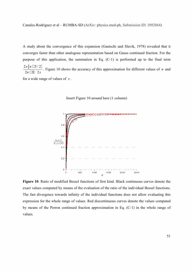
Canales-Rodríguez et al – RUMBA-SD (ArXiv: physics.med-ph, Submission ID: 1092864)
51
A study about the convergence of this expansion (Gautschi and Slavik, 1978) revealed that it
converges faster than other analogous representation based on Gauss continued fraction. For the
purpose of this application, the summation in Eq. (C-1) is performed up to the final term
( )2 5 / 2
2 3 2
x n
n x
++ +
. Figure 10 shows the accuracy of this approximation for different values of n and
for a wide range of values of x .
Insert Figure 10 around here (1 column)
Figure 10. Ratio of modified Bessel functions of first kind. Black continuous curves denote the
exact values computed by means of the evaluation of the ratio of the individual Bessel functions.
The fast divergence towards infinity of the individual functions does not allow evaluating this
expression for the whole range of values. Red discontinuous curves denote the values computed
by means of the Perron continued fraction approximation in Eq. (C-1) in the whole range of
values.
Canales-Rodríguez et al – RUMBA-SD (ArXiv: physics.med-ph, Submission ID: 1092864)
52
REFERENCES
Aganj, I., Lenglet, C., Sapiro, G., Yacoub, E., Ugurbil, K., Harel, N., 2010. Reconstruction
of the orientation distribution function in single- and multiple-shell q-ball imaging within
constant solid angle. Magn Reson Med 64, 554-566.
Aja-Fernandez, S., Brion, V., Tristan-Vega, A., 2013. Effective noise estimation and
filtering from correlated multiple-coil MR data. Magn Reson Imaging 31, 272-285.
Aja-Fernandez, S., Tristan-Vega, A., 2012. Influence of noise correlation in multiple-coil
statistical models with sum of squares reconstruction. Magn Reson Med 67, 580-585.
Aja-Fernandez, S., Tristan-Vega, A., Alberola-Lopez, C., 2009. Noise estimation in single-
and multiple-coil magnetic resonance data based on statistical models. Magn Reson
Imaging 27, 1397-1409.
Aja-Fernandez, S., Tristan-Vega, A., Hoge, W.S., 2011. Statistical noise analysis in
GRAPPA using a parametrized noncentral Chi approximation model. Magn Reson Med
65, 1195-1206.
Aja-Fernandez, S., Vegas-Sanchez-Ferrero, G., Tristan-Vega, A., 2014. Noise estimation in
parallel MRI: GRAPPA and SENSE. Magn Reson Imaging 32, 281-290.
Alexander, D.C., 2005. Maximum entropy spherical deconvolution for diffusion MRI. Inf
Process Med Imaging 19, 76-87.
Anderson, A.W., 2005. Measurement of fiber orientation distributions using high angular
resolution diffusion imaging. Magn Reson Med 54, 1194-1206.
Assemlal, H.E., Tschumperle, D., Brun, L., Siddiqi, K., 2011. Recent advances in diffusion
MRI modeling: Angular and radial reconstruction. Med Image Anal 15, 369-396.
Basser, P.J., Mattiello, J., LeBihan, D., 1994. Estimation of the effective self-diffusion
tensor from the NMR spin echo. J Magn Reson B 103, 247-254.
Behrens, T.E., Berg, H.J., Jbabdi, S., Rushworth, M.F., Woolrich, M.W., 2007.
Probabilistic diffusion tractography with multiple fibre orientations: What can we gain?
Neuroimage 34, 144-155.
Behrens, T.E., Woolrich, M.W., Jenkinson, M., Johansen-Berg, H., Nunes, R.G., Clare, S.,
Matthews, P.M., Brady, J.M., Smith, S.M., 2003. Characterization and propagation of
uncertainty in diffusion-weighted MR imaging. Magn Reson Med 50, 1077-1088.
Canales-Rodríguez et al – RUMBA-SD (ArXiv: physics.med-ph, Submission ID: 1092864)
53
Blaimer, M., Breuer, F., Mueller, M., Heidemann, R.M., Griswold, M.A., Jakob, P.M.,
2004. SMASH, SENSE, PILS, GRAPPA: how to choose the optimal method. Top Magn
Reson Imaging 15, 223-236.
Brion, V., Poupon, C., Riff, O., Aja-Fernandez, S., Tristan-Vega, A., Mangin, J.F., Le
Bihan, D., Poupon, F., 2013. Noise correction for HARDI and HYDI data obtained with
multi-channel coils and Sum of Squares reconstruction: An anisotropic extension of the
LMMSE. Magn Reson Imaging 31, 1360-1371.
Canales-Rodriguez, E.J., Iturria-Medina, Y., Aleman-Gomez, Y., Melie-Garcia, L., 2010a.
Deconvolution in diffusion spectrum imaging. Neuroimage 50, 136-149.
Canales-Rodriguez, E.J., Lin, C.P., Iturria-Medina, Y., Yeh, C.H., Cho, K.H., Melie-
Garcia, L., 2010b. Diffusion orientation transform revisited. Neuroimage 49, 1326-1339.
Canales-Rodriguez, E.J., Melie-Garcia, L., Iturria-Medina, Y., 2009. Mathematical
description of q-space in spherical coordinates: exact q-ball imaging. Magn Reson Med 61,
1350-1367.
Canales-Rodriguez, E.J., Melie-Garcia, L., Iturria-Medina, Y., Martinez-Montes, E.,
Aleman-Gomez, Y., Lin, C.P., 2008. Inferring multiple maxima in intravoxel white matter
fiber distribution. Magn Reson Med 60, 616-630.
Chambolle, A., 2004. An algorithm for total variation minimization and applications.
Journal of Mathematical Imaging and Vision 20, 89–97.
Clarke, R.A., Scifo, P., Rizzo, G., Dell'Acqua, F., Scotti, G., Fazio, F., 2008. Noise
correction on Rician distributed data for fibre orientation estimators. IEEE Trans Med
Imaging 27, 1242-1251.
Constantinides, C.D., Atalar, E., McVeigh, E.R., 1997. Signal-to-noise measurements in
magnitude images from NMR phased arrays. Magn Reson Med 38, 852-857.
Daducci, A., Canales-Rodriguez, E.J., Descoteaux, M., Garyfallidis, E., Gur, Y., Ying-Chia,
L., Mani, M., Merlet, S., Paquette, M., Ramirez-Manzanares, A., Reisert, M., Reis
Rodrigues, P., Sepehrband, F., Caruyer, E., Choupan, J., Deriche, R., Jacob, M., Menegaz,
G., Prckovska, V., Rivera, M., Wiaux, Y., Thiran, J.P., 2014a. Quantitative Comparison of
Reconstruction Methods for Intra-Voxel Fiber Recovery From Diffusion MRI. Medical
Imaging, IEEE Transactions on 33, 384-399.
Daducci, A., Canales-Rodríguez, E.J., Zhang, H., Dyrby, T.B., Alexander, D.C., Thiran, J.-
P., 2014b. Accelerated Microstructure Imaging via Convex Optimization (AMICO) from
diffusion MRI data. Neuroimage (In press).
Canales-Rodríguez et al – RUMBA-SD (ArXiv: physics.med-ph, Submission ID: 1092864)
54
Daducci, A., Van De Ville, D., Thiran, J.P., Wiaux, Y., 2014c. Sparse regularization for
fiber ODF reconstruction: from the suboptimality of l2 and l1 priors to l0. Med Image Anal
18, 820-833.
Dell'Acqua, F., Rizzo, G., Scifo, P., Clarke, R.A., Scotti, G., Fazio, F., 2007. A model-based
deconvolution approach to solve fiber crossing in diffusion-weighted MR imaging. IEEE
Trans Biomed Eng 54, 462-472.
Dell'acqua, F., Scifo, P., Rizzo, G., Catani, M., Simmons, A., Scotti, G., Fazio, F., 2010. A
modified damped Richardson-Lucy algorithm to reduce isotropic background effects in
spherical deconvolution. Neuroimage 49, 1446-1458.
Descoteaux, M., Angelino, E., Fitzgibbons, S., Deriche, R., 2007. Regularized, fast, and
robust analytical Q-ball imaging. Magn Reson Med 58, 497-510.
Descoteaux, M., Deriche, R., Knosche, T.R., Anwander, A., 2009. Deterministic and
probabilistic tractography based on complex fibre orientation distributions. IEEE Trans
Med Imaging 28, 269-286.
Descoteaux, M., Deriche, R., Le Bihan, D., Mangin, J.F., Poupon, C., 2011. Multiple q-shell
diffusion propagator imaging. Med Image Anal 15, 603-621.
Dey, N., Blanc-Feraud, L., Zimmer, C., Roux, P., Kam, Z., Olivo-Marin, J.C., Zerubia, J.,
2006. Richardson-Lucy algorithm with total variation regularization for 3D confocal
microscope deconvolution. Microsc Res Tech 69, 260-266.
Dietrich, O., Raya, J.G., Reeder, S.B., Ingrisch, M., Reiser, M.F., Schoenberg, S.O., 2008.
Influence of multichannel combination, parallel imaging and other reconstruction
techniques on MRI noise characteristics. Magn Reson Imaging 26, 754-762.
Fillard, P., Descoteaux, M., Goh, A., Gouttard, S., Jeurissen, B., Malcolm, J., Ramirez-
Manzanares, A., Reisert, M., Sakaie, K., Tensaouti, F., Yo, T., Mangin, J.F., Poupon, C.,
2011. Quantitative evaluation of 10 tractography algorithms on a realistic diffusion MR
phantom. Neuroimage 56, 220-234.
Garyfallidis, E., Brett, M., Amirbekian, B., Rokem, A., Van Der Walt, S., Descoteaux, M.,
Nimmo-Smith, I., 2014. Dipy, a library for the analysis of diffusion MRI data. Front.
Neuroinform. 8:8.
Gautschi, W., Slavik, J., 1978. On the Computation of Modified Bessel Function Ratios.
MATHEMATICS OF COMPUTATION 32, 865-875.
Gudbjartsson, H., Patz, S., 1995. The Rician distribution of noisy MRI data. Magn Reson
Med 34, 910-914.
Canales-Rodríguez et al – RUMBA-SD (ArXiv: physics.med-ph, Submission ID: 1092864)
55
Hagmann, P., Cammoun, L., Gigandet, X., Meuli, R., Honey, C.J., Wedeen, V.J., Sporns,
O., 2008. Mapping the structural core of human cerebral cortex. PLoS Biol 6, e159.
Henkelman, R.M., 1985. Measurement of signal intensities in the presence of noise in MR
images. Med Phys 12, 232-233.
Hess, C.P., Mukherjee, P., Han, E.T., Xu, D., Vigneron, D.B., 2006. Q-ball reconstruction of
multimodal fiber orientations using the spherical harmonic basis. Magn Reson Med 56,
104-117.
Hosseinbor, A.P., Chung, M.K., Wu, Y.C., Alexander, A.L., 2013. Bessel Fourier
Orientation Reconstruction (BFOR): an analytical diffusion propagator reconstruction for
hybrid diffusion imaging and computation of q-space indices. Neuroimage 64, 650-670.
Iturria-Medina, Y., Perez Fernandez, A., Morris, D.M., Canales-Rodriguez, E.J., Haroon,
H.A., Garcia Penton, L., Augath, M., Galan Garcia, L., Logothetis, N., Parker, G.J., Melie-
Garcia, L., 2011. Brain hemispheric structural efficiency and interconnectivity rightward
asymmetry in human and nonhuman primates. Cereb Cortex 21, 56-67.
Iturria-Medina, Y., Sotero, R.C., Canales-Rodriguez, E.J., Aleman-Gomez, Y., Melie-
Garcia, L., 2008. Studying the human brain anatomical network via diffusion-weighted
MRI and Graph Theory. Neuroimage 40, 1064-1076.
Jbabdi, S., Sotiropoulos, S.N., Savio, A.M., Grana, M., Behrens, T.E., 2012. Model-based
analysis of multishell diffusion MR data for tractography: how to get over fitting problems.
Magn Reson Med 68, 1846-1855.
Jensen, J.H., Helpern, J.A., Ramani, A., Lu, H., Kaczynski, K., 2005. Diffusional kurtosis
imaging: the quantification of non-gaussian water diffusion by means of magnetic
resonance imaging. Magn Reson Med 53, 1432-1440.
Jeurissen, B., Tournier, J.D., Dhollander, T., Connelly, A., Sijbers, J., 2014. Multi-tissue
constrained spherical deconvolution for improved analysis of multi-shell diffusion MRI
data. Neuroimage.
Jian, B., Vemuri, B.C., 2007. A unified computational framework for deconvolution to
reconstruct multiple fibers from diffusion weighted MRI. IEEE Trans Med Imaging 26,
1464-1471.
Kaden, E., Knosche, T.R., Anwander, A., 2007. Parametric spherical deconvolution:
inferring anatomical connectivity using diffusion MR imaging. Neuroimage 37, 474-488.
Kaden, E., Kruggel, F., 2012. Nonparametric Bayesian inference of the fiber orientation
distribution from diffusion-weighted MR images. Med Image Anal 16, 876-888.
Canales-Rodríguez et al – RUMBA-SD (ArXiv: physics.med-ph, Submission ID: 1092864)
56
Keil, B., Wald, L.L., 2013. Massively parallel MRI detector arrays. J Magn Reson 229, 75-
89.
Koay, C.G., Ozarslan, E., Basser, P.J., 2009. A signal transformational framework for
breaking the noise floor and its applications in MRI. J Magn Reson 197, 108-119.
Landman, B.A., Bogovic, J.A., Wan, H., El Zahraa ElShahaby, F., Bazin, P.L., Prince, J.L.,
2012. Resolution of crossing fibers with constrained compressed sensing using diffusion
tensor MRI. Neuroimage 59, 2175-2186.
Liu, C., Bammer, R., Acar, B., Moseley, M.E., 2004. Characterizing non-Gaussian diffusion
by using generalized diffusion tensors. Magn Reson Med 51, 924-937.
Lucy, L.B., 1974. An iterative technique for the rectification of observed distributions.
Astron. J. 79, 745–754.
Manjon, J.V., Coupe, P., Marti-Bonmati, L., Collins, D.L., Robles, M., 2010. Adaptive non-
local means denoising of MR images with spatially varying noise levels. J Magn Reson
Imaging 31, 192-203.
Melie-Garcia, L., Canales-Rodriguez, E.J., Aleman-Gomez, Y., Lin, C.P., Iturria-Medina,
Y., Valdes-Hernandez, P.A., 2008. A Bayesian framework to identify principal intravoxel
diffusion profiles based on diffusion-weighted MR imaging. Neuroimage 42, 750-770.
Michailovich, O., Rathi, Y., Dolui, S., 2011. Spatially regularized compressed sensing for
high angular resolution diffusion imaging. IEEE Trans Med Imaging 30, 1100-1115.
Ozarslan, E., Mareci, T.H., 2003. Generalized diffusion tensor imaging and analytical
relationships between diffusion tensor imaging and high angular resolution diffusion
imaging. Magn Reson Med 50, 955-965.
Ozarslan, E., Shepherd, T.M., Vemuri, B.C., Blackband, S.J., Mareci, T.H., 2006.
Resolution of complex tissue microarchitecture using the diffusion orientation transform
(DOT). Neuroimage 31, 1086-1103.
Parker, G.D., Marshall, D., Rosin, P.L., Drage, N., Richmond, S., Jones, D.K., 2013. A
pitfall in the reconstruction of fibre ODFs using spherical deconvolution of diffusion MRI
data. Neuroimage 65, 433-448.
Patel, V., Shi, Y., Thompson, P.M., Toga, A.W., 2010. Mesh-based spherical deconvolution:
a flexible approach to reconstruction of non-negative fiber orientation distributions.
Neuroimage 51, 1071-1081.
Canales-Rodríguez et al – RUMBA-SD (ArXiv: physics.med-ph, Submission ID: 1092864)
57
Pruessmann, K.P., Weiger, M., Scheidegger, M.B., Boesiger, P., 1999. SENSE: sensitivity
encoding for fast MRI. Magn Reson Med 42, 952-962.
Ramirez-Manzanares, A., Rivera, M., Vemuri, B.C., Carney, P., Mareci, T., 2007. Diffusion
basis functions decomposition for estimating white matter intravoxel fiber geometry. IEEE
Trans Med Imaging 26, 1091-1102.
Reisert, M., Kiselev, V.G., 2011. Fiber continuity: an anisotropic prior for ODF estimation.
IEEE Trans Med Imaging 30, 1274-1283.
Richardson, W.H., 1972. Bayesian-based iterative method of image restoration. J Opt. Soc.
Am. 62, 55–59.
Roine, T., Jeurissen, B., Perrone, D., Aelterman, J., Leemans, A., Philips, W., Sijbers, J.,
2014. Isotropic non-white matter partial volume effects in constrained spherical
deconvolution. Front Neuroinform 8, 28.
Rudin, L.I., Osher, S., Fatemi, E., 1992. Nonlinear total variation based noise removal
algorithms. Physica D 60, 259–268.
Salat, D.H., Tuch, D.S., Greve, D.N., van der Kouwe, A.J., Hevelone, N.D., Zaleta, A.K.,
Rosen, B.R., Fischl, B., Corkin, S., Rosas, H.D., Dale, A.M., 2005. Age-related alterations in
white matter microstructure measured by diffusion tensor imaging. Neurobiol Aging 26,
1215-1227.
Salvador, R., Pena, A., Menon, D.K., Carpenter, T.A., Pickard, J.D., Bullmore, E.T., 2005.
Formal characterization and extension of the linearized diffusion tensor model. Hum Brain
Mapp 24, 144-155.
Smith, S.M., Jenkinson, M., Woolrich, M.W., Beckmann, C.F., Behrens, T.E., Johansen-
Berg, H., Bannister, P.R., De Luca, M., Drobnjak, I., Flitney, D.E., Niazy, R.K., Saunders,
J., Vickers, J., Zhang, Y., De Stefano, N., Brady, J.M., Matthews, P.M., 2004. Advances in
functional and structural MR image analysis and implementation as FSL. Neuroimage 23
Suppl 1, S208-219.
Söderman, O., Jönsson, B., 1995. Restricted diffusion in cylindrical geometry. Journal of
Magnetic Resonance Series A, 117, 94-97.
Sotiropoulos, S.N., Behrens, T.E., Jbabdi, S., 2012. Ball and rackets: Inferring fiber
fanning from diffusion-weighted MRI. Neuroimage 60, 1412-1425.
Sotiropoulos, S.N., Moeller, S., Jbabdi, S., Xu, J., Andersson, J.L., Auerbach, E.J., Yacoub,
E., Feinberg, D., Setsompop, K., Wald, L.L., Behrens, T.E., Ugurbil, K., Lenglet, C., 2013.

Canales-Rodríguez et al – RUMBA-SD (ArXiv: physics.med-ph, Submission ID: 1092864)
58
Effects of image reconstruction on fibre orientation mapping from multichannel diffusion
MRI: Reducing the noise floor using SENSE. Magn Reson Med.
Starck, J.L., Pantin, E., Murtagh, F., 2002. Deconvolution in Astronomy: A Review.
Publications of the Astronomical Society of the Pacific 114, 1051–1069.
Tax, C.M., Jeurissen, B., Vos, S.B., Viergever, M.A., Leemans, A., 2014. Recursive
calibration of the fiber response function for spherical deconvolution of diffusion MRI
data. Neuroimage 86, 67-80.
Tournier, J.-D., Calamante, F., Connelly, A., 2013. A Robust Spherical Deconvolution
Method for the Analysis of Low SNR or Low Angular Resolution Diffusion Data, ISMRM
21st Annual Meeting, Salt Lake City, Utah, USA.
Tournier, J.D., Calamante, F., Connelly, A., 2007. Robust determination of the fibre
orientation distribution in diffusion MRI: non-negativity constrained super-resolved
spherical deconvolution. Neuroimage 35, 1459-1472.
Tournier, J.D., Calamante, F., Gadian, D.G., Connelly, A., 2004. Direct estimation of the
fiber orientation density function from diffusion-weighted MRI data using spherical
deconvolution. Neuroimage 23, 1176-1185.
Tournier, J.D., Yeh, C.H., Calamante, F., Cho, K.H., Connelly, A., Lin, C.P., 2008.
Resolving crossing fibres using constrained spherical deconvolution: validation using
diffusion-weighted imaging phantom data. Neuroimage 42, 617-625.
Tristan-Vega, A., Aja-Fernandez, S., Westin, C.F., 2012. Least squares for diffusion tensor
estimation revisited: propagation of uncertainty with Rician and non-Rician signals.
Neuroimage 59, 4032-4043.
Tristan-Vega, A., Westin, C.F., Aja-Fernandez, S., 2009. Estimation of fiber orientation
probability density functions in high angular resolution diffusion imaging. Neuroimage 47,
638-650.
Tristan-Vega, A., Westin, C.F., Aja-Fernandez, S., 2010. A new methodology for the
estimation of fiber populations in the white matter of the brain with the Funk-Radon
transform. Neuroimage 49, 1301-1315.
Tuch, D.S., 2004. Q-ball imaging. Magn Reson Med 52, 1358-1372.
Tuch, D.S., Reese, T.G., Wiegell, M.R., Makris, N., Belliveau, J.W., Wedeen, V.J., 2002.
High angular resolution diffusion imaging reveals intravoxel white matter fiber
heterogeneity. Magn Reson Med 48, 577-582.
Canales-Rodríguez et al – RUMBA-SD (ArXiv: physics.med-ph, Submission ID: 1092864)
59
Wedeen, V.J., Hagmann, P., Tseng, W.Y., Reese, T.G., Weisskoff, R.M., 2005. Mapping
complex tissue architecture with diffusion spectrum magnetic resonance imaging. Magn
Reson Med 54, 1377-1386.
Wu, Y.C., Alexander, A.L., 2007. Hybrid diffusion imaging. Neuroimage 36, 617-629.
Yeh, F.C., Wedeen, V.J., Tseng, W.Y., 2010. Generalized q-sampling imaging. IEEE Trans
Med Imaging 29, 1626-1635.
Copyright © 2022 FDOKUMEN