
Spatial/spectral endmember extraction by multidimensional morphological operations
17
IEEE TRANSACTIONS ON GEOSCIENCE AND REMOTE SENSING, VOL. 40, NO. 9, SEPTEMBER 2002 2025 Spatial/Spectral Endmember Extraction by Multidimensional Morphological Operations Antonio Plaza, Pablo Martínez, Rosa Pérez, and Javier Plaza Abstract—Spectral mixture analysis provides an efficient mechanism for the interpretation and classification of remotely sensed multidimensional imagery. It aims to identify a set of reference signatures (also known as endmembers) that can be used to model the reflectance spectrum at each pixel of the original image. Thus, the modeling is carried out as a linear combination of a finite number of ground components. Although spectral mixture models have proved to be appropriate for the purpose of large hyperspectral dataset subpixel analysis, few methods are available in the literature for the extraction of appropriate endmembers in spectral unmixing. Most approaches have been designed from a spectroscopic viewpoint and, thus, tend to neglect the existing spatial correlation between pixels. This paper presents a new automated method that performs unsupervised pixel purity determination and endmember extraction from multidimensional datasets; this is achieved by using both spatial and spectral information in a combined manner. The method is based on mathematical morphology, a classic image processing technique that can be applied to the spectral domain while being able to keep its spatial characteristics. The proposed methodology is evaluated through a specifically designed framework that uses both simulated and real hyperspectral data. Index Terms—Automated endmember extraction, mathematical morphology, morphological eccentricity index, multidimensional analysis, spatial/spectral integration, spectral mixture model. I. INTRODUCTION I MAGING spectroscopy, also known as hyperspectral remote sensing, allows a sensor on a moving platform to gather re- flected radiation from a ground target so that a detector system consisting of CCD devices can record a great deal (typically tens) of spectral channels simultaneously. With such detail, the ability to detect and identify individual materials or classes is expected to be greatly improved [1]. During the last several years, a great deal of new airborne and spaceborne sensors have been improved for hyperspectral remote sensing applications. A chief hyperspectral sensor is the NASA/JPL Airborne Visible and Infra-Red Imaging Spectrom- eter (AVIRIS) system, which currently covers the wavelength region from 0.38–2.50 m [2]. Other sensors that offer hyper- spectral capabilities have been available as research instruments for the last ten years, including DAIS/ROSIS [3], CASI-2 [4], AISA [5], MIVIS [6], HyMap [7], or HYPERION [8]. In the Manuscript received January 11, 2002; revised May 22, 2002. This work was supported in part by the Spanish Government under Grant TIC-2000-0739-C04-03 and by Junta de Extremadura (local Government) Grant 2PR01A085. The authors are with the Neural Networks and Signal Processing Group (GRNPS), Computer Science Department, University of Extremadura, Escuela Politécnica, 10.071 Cáceres, Spain (e-mail: [email protected]; [email protected]; [email protected]). Digital Object Identifier 10.1109/TGRS.2002.802494 near future, the use of these types of sensors on satellite plat- forms will produce a nearly continual stream of high-dimen- sional data, and this expected high data volume will require fast and efficient means for storage, transmission, and analysis [9], [10]. Linear spectral unmixing [11]–[13] is one of the most impor- tant approaches for the analysis and classification of multi/hy- perspectral datasets. This approach involves two steps: to find spectrally unique signatures of pure ground components (usu- ally referred to as endmembers [14]) and to express individual pixels as a linear combination of endmembers [15]. Let be a spectrum of values obtained at the sensor for a certain pixel with spatial coordinates in a multispectral image. This spectrum can be considered as an -dimensional ( -D) vector (where is the number of spectral bands) and may be modeled in terms of a linear combination of several endmember vectors , according to the equations and constraints [16] (1) (2) where is the number of endmembers needed to accurately model the original spectrum, and is a scalar value representing the fractional coverage of endmember vector in pixel . The ideal case is that the coefficients in the linear combination are nonnegative and sum to 1, being, therefore, interpretable as cover fractions or abundances [13]. A set of endmembers and cover fractions is called a mix- ture model [16]. One of the new perspectives opened by this approach, together with the improved spectral resolution of sen- sors, is the possibility of subpixel analysis of scenes, which aims to quantify the abundance of different materials in a single pixel. Like principal components, endmembers provide a basis set in whose terms the rest of the data can be described [17], [18]. However, unlike principal components, the endmembers are ex- pected to provide a more “physical” description of the data with no orthogonalization restrictions. For instance, a simple mixture model based on three endmembers has the geometrical interpre- tation of a triangle whose vertices are the endmembers. Cover fractions are determined by the position of spectra within the triangle and can be considered relative coordinates in a new ref- erence system given by the endmembers, as Fig. 1 shows. Although the development of effective devices with new and improved technical capabilities stands out, the evolution in the design of algorithms for data processing is not as positive. Many of the techniques currently under way for hyperspectral data 0196-2892/02$17.00 © 2002 IEEE
-
Upload
independent -
Category
Documents
-
view
0 -
download
0
Transcript of Spatial/spectral endmember extraction by multidimensional morphological operations
IEEE TRANSACTIONS ON GEOSCIENCE AND REMOTE SENSING, VOL. 40, NO. 9, SEPTEMBER 2002 2025
Spatial/Spectral Endmember Extraction byMultidimensional Morphological Operations
Antonio Plaza, Pablo Martínez, Rosa Pérez, and Javier Plaza
Abstract—Spectral mixture analysis provides an efficientmechanism for the interpretation and classification of remotelysensed multidimensional imagery. It aims to identify a set ofreference signatures (also known as endmembers) that can be usedto model the reflectance spectrum at each pixel of the originalimage. Thus, the modeling is carried out as a linear combinationof a finite number of ground components. Although spectralmixture models have proved to be appropriate for the purposeof large hyperspectral dataset subpixel analysis, few methodsare available in the literature for the extraction of appropriateendmembers in spectral unmixing. Most approaches have beendesigned from a spectroscopic viewpoint and, thus, tend to neglectthe existing spatial correlation between pixels. This paper presentsa new automated method that performs unsupervised pixel puritydetermination and endmember extraction from multidimensionaldatasets; this is achieved by using both spatial and spectralinformation in a combined manner. The method is based onmathematical morphology, a classic image processing techniquethat can be applied to the spectral domain while being able tokeep its spatial characteristics. The proposed methodology isevaluated through a specifically designed framework that usesboth simulated and real hyperspectral data.
Index Terms—Automated endmember extraction, mathematicalmorphology, morphological eccentricity index, multidimensionalanalysis, spatial/spectral integration, spectral mixture model.
I. INTRODUCTION
I MAGING spectroscopy, also known as hyperspectral remotesensing, allows a sensor on a moving platform to gather re-
flected radiation from a ground target so that a detector systemconsisting of CCD devices can record a great deal (typicallytens) of spectral channels simultaneously. With such detail, theability to detect and identify individual materials or classes isexpected to be greatly improved [1].
During the last several years, a great deal of new airborneand spaceborne sensors have been improved for hyperspectralremote sensing applications. A chief hyperspectral sensor is theNASA/JPL Airborne Visible and Infra-Red Imaging Spectrom-eter (AVIRIS) system, which currently covers the wavelengthregion from 0.38–2.50 m [2]. Other sensors that offer hyper-spectral capabilities have been available as research instrumentsfor the last ten years, including DAIS/ROSIS [3], CASI-2 [4],AISA [5], MIVIS [6], HyMap [7], or HYPERION [8]. In the
Manuscript received January 11, 2002; revised May 22, 2002. Thiswork was supported in part by the Spanish Government under GrantTIC-2000-0739-C04-03 and by Junta de Extremadura (local Government)Grant 2PR01A085.
The authors are with the Neural Networks and Signal Processing Group(GRNPS), Computer Science Department, University of Extremadura,Escuela Politécnica, 10.071 Cáceres, Spain (e-mail: [email protected];[email protected]; [email protected]).
Digital Object Identifier 10.1109/TGRS.2002.802494
near future, the use of these types of sensors on satellite plat-forms will produce a nearly continual stream of high-dimen-sional data, and this expected high data volume will require fastand efficient means for storage, transmission, and analysis [9],[10].
Linear spectral unmixing [11]–[13] is one of the most impor-tant approaches for the analysis and classification of multi/hy-perspectral datasets. This approach involves two steps: to findspectrally unique signatures of pure ground components (usu-ally referred to as endmembers [14]) and to express individualpixels as a linear combination of endmembers [15]. Letbe a spectrum of values obtained at the sensor for a certain pixelwith spatial coordinates in a multispectral image. Thisspectrum can be considered as an-dimensional ( -D) vector(where is the number of spectral bands) and may be modeledin terms of a linear combination of several endmember vectors
, according to the equations and constraints [16]
(1)
(2)
where is the number of endmembers needed to accuratelymodel the original spectrum, andis a scalar value representingthe fractional coverage of endmember vectorin pixel .The ideal case is that the coefficients in the linear combinationare nonnegative and sum to 1, being, therefore, interpretable ascover fractions or abundances [13].
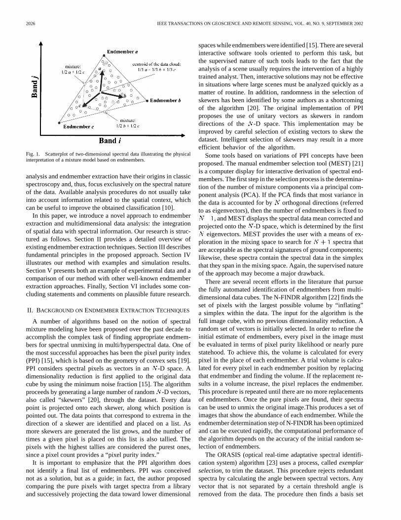
A set of endmembers and cover fractions is called a mix-ture model [16]. One of the new perspectives opened by thisapproach, together with the improved spectral resolution of sen-sors, is the possibility of subpixel analysis of scenes, which aimsto quantify the abundance of different materials in a single pixel.Like principal components, endmembers provide a basis set inwhose terms the rest of the data can be described [17], [18].However, unlike principal components, the endmembers are ex-pected to provide a more “physical” description of the data withno orthogonalization restrictions. For instance, a simple mixturemodel based on three endmembers has the geometrical interpre-tation of a triangle whose vertices are the endmembers. Coverfractions are determined by the position of spectra within thetriangle and can be considered relative coordinates in a new ref-erence system given by the endmembers, as Fig. 1 shows.
Although the development of effective devices with new andimproved technical capabilities stands out, the evolution in thedesign of algorithms for data processing is not as positive. Manyof the techniques currently under way for hyperspectral data
0196-2892/02$17.00 © 2002 IEEE
2026 IEEE TRANSACTIONS ON GEOSCIENCE AND REMOTE SENSING, VOL. 40, NO. 9, SEPTEMBER 2002
Fig. 1. Scatterplot of two-dimensional spectral data illustrating the physicalinterpretation of a mixture model based on endmembers.
analysis and endmember extraction have their origins in classicspectroscopy and, thus, focus exclusively on the spectral natureof the data. Available analysis procedures do not usually takeinto account information related to the spatial context, whichcan be useful to improve the obtained classification [10].
In this paper, we introduce a novel approach to endmemberextraction and multidimensional data analysis: the integrationof spatial data with spectral information. Our research is struc-tured as follows. Section II provides a detailed overview ofexisting endmember extraction techniques. Section III describesfundamental principles in the proposed approach. Section IVillustrates our method with examples and simulation results.Section V presents both an example of experimental data and acomparison of our method with other well-known endmemberextraction approaches. Finally, Section VI includes some con-cluding statements and comments on plausible future research.
II. BACKGROUND ONENDMEMBER EXTRACTION TECHNIQUES
A number of algorithms based on the notion of spectralmixture modeling have been proposed over the past decade toaccomplish the complex task of finding appropriate endmem-bers for spectral unmixing in multi/hyperspectral data. One ofthe most successful approaches has been the pixel purity index(PPI) [15], which is based on the geometry of convex sets [19].PPI considers spectral pixels as vectors in an-D space. Adimensionality reduction is first applied to the original datacube by using the minimum noise fraction [15]. The algorithmproceeds by generating a large number of random-D vectors,also called “skewers” [20], through the dataset. Every datapoint is projected onto each skewer, along which position ispointed out. The data points that correspond to extrema in thedirection of a skewer are identified and placed on a list. Asmore skewers are generated the list grows, and the number oftimes a given pixel is placed on this list is also tallied. Thepixels with the highest tallies are considered the purest ones,since a pixel count provides a “pixel purity index.”
It is important to emphasize that the PPI algorithm doesnot identify a final list of endmembers. PPI was conceivednot as a solution, but as a guide; in fact, the author proposedcomparing the pure pixels with target spectra from a libraryand successively projecting the data toward lower dimensional
spaces while endmembers were identified [15]. There are severalinteractive software tools oriented to perform this task, butthe supervised nature of such tools leads to the fact that theanalysis of a scene usually requires the intervention of a highlytrained analyst. Then, interactive solutions may not be effectivein situations where large scenes must be analyzed quickly as amatter of routine. In addition, randomness in the selection ofskewers has been identified by some authors as a shortcomingof the algorithm [20]. The original implementation of PPIproposes the use of unitary vectors as skewers in randomdirections of the -D space. This implementation may beimproved by careful selection of existing vectors to skew thedataset. Intelligent selection of skewers may result in a moreefficient behavior of the algorithm.
Some tools based on variations of PPI concepts have beenproposed. The manual endmember selection tool (MEST) [21]is a computer display for interactive derivation of spectral end-members. The first step in the selection process is the determina-tion of the number of mixture components via a principal com-ponent analysis (PCA). If the PCA finds that most variance inthe data is accounted for by orthogonal directions (referredto as eigenvectors), then the number of endmembers is fixed to
, and MEST displays the spectral data mean corrected andprojected onto the -D space, which is determined by the first
eigenvectors. MEST provides the user with a means of ex-ploration in the mixing space to search for spectra thatare acceptable as the spectral signatures of ground components;likewise, these spectra contain the spectral data in the simplexthat they span in the mixing space. Again, the supervised natureof the approach may become a major drawback.
There are several recent efforts in the literature that pursuethe fully automated identification of endmembers from multi-dimensional data cubes. The N-FINDR algorithm [22] finds theset of pixels with the largest possible volume by “inflating”a simplex within the data. The input for the algorithm is thefull image cube, with no previous dimensionality reduction. Arandom set of vectors is initially selected. In order to refine theinitial estimate of endmembers, every pixel in the image mustbe evaluated in terms of pixel purity likelihood or nearly purestatehood. To achieve this, the volume is calculated for everypixel in the place of each endmember. A trial volume is calcu-lated for every pixel in each endmember position by replacingthat endmember and finding the volume. If the replacement re-sults in a volume increase, the pixel replaces the endmember.This procedure is repeated until there are no more replacementsof endmembers. Once the pure pixels are found, their spectracan be used to unmix the original image.This produces a set ofimages that show the abundance of each endmember. While theendmember determination step of N-FINDR has been optimizedand can be executed rapidly, the computational performance ofthe algorithm depends on the accuracy of the initial random se-lection of endmembers.
The ORASIS (optical real-time adaptative spectral identifi-cation system) algorithm [23] uses a process, calledexemplarselection, to trim the dataset. This procedure rejects redundantspectra by calculating the angle between spectral vectors. Anyvector that is not separated by a certain threshold angle isremoved from the data. The procedure then finds a basis set
PLAZA et al.: SPATIAL/SPECTRAL ENDMEMBER EXTRACTION 2027
of much lower dimension than the original data by a modifiedGram–Schmidt process. The exemplar spectra are then pro-jected onto this basis subspace, and a simplex is found througha minimum volume transform. Even though ORASIS is tunedfor rapid execution, there is no dimensionality reduction aspart of this algorithm. The whole process is very sensitive tothe threshold angle parameter, related to sensor noise. Thisparameter must be selected cautiously in order to avoid the lossof important endmembers.
The iterative error analysis (IEA) algorithm [24] is alsoexecuted directly on the data with neither the dimensionalityreduction nor the data thinning. An initial vector (usually themean spectrum of the data) is chosen to start the process. Aconstrained unmixing is then performed, and an error image isformed. The average score of vectors with higher degrees oferror (distance from the initial vector) is assumed to be the firstendmember. Another constrained unmixing is then performed,and the error image is formed. The average score of vectors withgreater errors (distance from the first endmember) is assumedto be the second endmember. This process is continued until apredetermined number of endmembers is found, and fractionalabundance maps are found by the final constrained unmixing.There are no published computer time estimates for the IEAalgorithm, but the repeated constrained unmixings involvedshould take significant time.
The use of multiple endmembers at a pixel level has also beena main topic of interest to account for endmember variability.Multiple endmember spectral mixture analysis (MESMA) [25]is a spectral unmixing approach in which many possible mix-ture models are analyzed simultaneously in order to produce thebest fit. The weighting coefficients (fractions) for each modeland each pixel are determined so that the linear combinationof the endmember spectra produces the lowest margin of RMSerror when compared to the apparent surface reflectance for thepixel. Weighting coefficients are constrained to lie between zeroand one, and a valid fit is restricted to a maximum preset RMSerror. This approach requires an extensive library of field, lab-oratory, and image spectra, where each plausible component isrepresented at least once. Since the need for spectral librariesturns out to be a demanding constraint (intensive ground workis required in their development), this fact may be the majorlimitation of this approach.
Another attempt to incorporate endmember variability intospectral mixture analysis [16] is based on the representation ofa landscape component type, not with one endmember spectrumbut with a set or bundle of spectra, where each spectrum is fea-sible as an instance of the component (e.g., in the case of a treecomponent, each spectrum could be the spectral reflectance ofa tree canopy). A pixel may have an infinite number of mixturemodels with endmembers selected from the bundles. Authors inthis approach [16] use a simulated annealing algorithm to de-rive bundles of endmembers. This task is carried out by con-structing a simplex from a partition of facets in a convex hullof a point data cloud. Bundle unmixing finds the maximum andminimum endmember fractions in those models, i.e., the rangeof endmember fraction values possible for a pixel.
Finally, self-organizing neural network algorithms have beenapplied also to the unsupervised classification of multi/hy-
TABLE IA COMPARISON OFSEVERAL ENDMEMBER EXTRACTION APPROACHES
perspectral datasets through endmember extraction [26].Kohonen’s self-organizing maps are suitable to perform com-petitive endmember learning. Hence, clusters are formed in thespectral space. The topology of the network and the trainingalgorithm are key parameters that must be fixed with caution inorder to obtain satisfactory results.
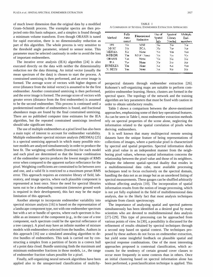
Table I shows a comparison between the above-mentionedapproaches, emphasizing some of their key operational features.As can be seen in Table I, most endmember extraction methodsrely on spectral properties of the scene alone, neglecting theinformation related to the spatial correlation of pixels whenderiving endmembers.
It is well known that many multispectral remote sensingdatasets have the unique feature of being representations ofcollections of images, where a particular pixel is characterizedby spectral and spatial properties. Spectral information dealswith pixel value in an independent manner from the neigh-boring pixel values, whereas spatial information concerns therelationship between the pixel value and those of its neighbors.Despite the inherent spatial–spectral duality that resides ina multidimensional data cube, most available processingtechniques tend to focus exclusively on the spectral domain,handling the data not as an image but as an unordered listing ofspectral measurements. These gauges can be shuffled arbitrarilywithout affecting analysis [10]. The incorporation of spatialinformation results from the notion of image processing, whichis not yet fully exploited in the field of multidimensional dataanalysis, due to the likely fact that most analysis techniquesoriginate from classic spectroscopy.
The importance of analyzing spatial and spectral patternssimultaneously has been identified as a desired goal by manyscientists who are devoted to multidimensional data analysis[27]–[29]. This type of processing can be approached fromvarious points of view. In [30], a possibility is discussed for therefinement of results obtained by spectral techniques througha second step based on spatial context. The techniques pro-posed by these authors do not focus on endmember extraction,but yield some insightful feedback on plausible spatial andspectral response combinations. One of the most interestingapproaches proposed is contextual classification, which ac-counts for the tendency of certain ground cover classes tooccur more frequently in some contexts than in others. Oncean initial clustering based on spectral information alone hasbeen performed, a postclassification technique is applied. This
2028 IEEE TRANSACTIONS ON GEOSCIENCE AND REMOTE SENSING, VOL. 40, NO. 9, SEPTEMBER 2002
method consists of two main parts: the definition of a pixelneighborhood (surrounding each pixel of the scene) and theperformance of a local operation so that the pixel may bechanged into the label mostly represented in the window thatdefines the neighborhood. This simple operation entirely sep-arates spatial information from spectral information, and thusthe two types of information are not treated simultaneously;quite the opposite, spectral information is first extracted, anda spatial context is then imposed.
In this paper, we present the possibility of obtaining a methodthat integrates both spatial and spectral responses in a simulta-neous manner. Mathematical morphology [31], [32] is a classicnonlinear spatial processing technique that provides a remark-able framework to achieve the desired integration. Morphologywas originally defined for binary images and has been extendedto the grayscale [33] and color [34] image cases, but it hasbeen seldom used to process multi/hyperspectral imagery [35].We propose a new application of mathematical morphologyfocused on the automated extraction of endmembers from mul-tidimensional data. In addition, we list key advantages in theuse of morphology to perform this task.
A first major point is that endmember extraction is basicallya nonlinear task. Furthermore, morphology allows for the in-troduction of a local-to-global approach in the search for end-members by using spatial kernels (structuring elements in themorphology jargon). These items define local neighborhoodsaround each pixel. This type of processing can be applied tothe search of convexities or extremities within a data cloud ofspectral points and to the use of the spatial correlation betweenthe data. Endmembers can be identified by following an itera-tive process where pixels in close proximity in the spatial do-main compete against each other in terms of their convexity orspectral purity. As a result, they allow for the determination ofa local representative in a neighborhood that will be comparedto other locally selected pixels. The adoption of this approachleads to the incorporation of spatial information into the end-member determination procedure. As a final main step, morpho-logical operations are implemented by replacing a pixel with aneighbor that satisfies a certain condition. In binary/grayscalemorphology, the condition is usually related to the digital valueof the pixel, and the two basic morphological operations (dila-tion and erosion) are, respectively, based on the replacement ofa pixel by the neighbor with the maximum and minimum value.Since an endmember is defined as a spectrally pure pixel thatdescribes several mixed pixels in the scene, extended morpho-logical operations can obviously contribute to locating suitablepixels that replace others in the scene according to some desiredparticularity of the pixel, e.g., its spectral purity.
Therefore, we propose a mathematical framework to extendmathematical morphology to the multidimensional domain,which results in the definition of a set of spatial/spectral opera-tions that can be used to extract reference spectral signatures.Our objective in this research is to analyze the viability ofextended morphological operations to analyze multidimen-sional remote sensing data. It is important to emphasize thatthe combination of spatial and spectral information leads to anew interpretation of the endmember concept, related to thecapacity of a particular signature in order to describe variousmixed pixels coherently in both spectral and spatial terms.
III. M ETHODS
This section is organized as follows. Section III-A providesan overview of classic mathematical morphology. Section III-Bfocuses on the proposed framework to extend classic mor-phological operations to a multidimensional domain. Somesimple examples that illustrate the behavior of basic extendedmorphological operations are included. Finally, Section III-Cdescribes the proposed approach for endmember extraction:the general algorithm, parameters, and implementation optionsare also discussed.
A. Classic Mathematical Morphology
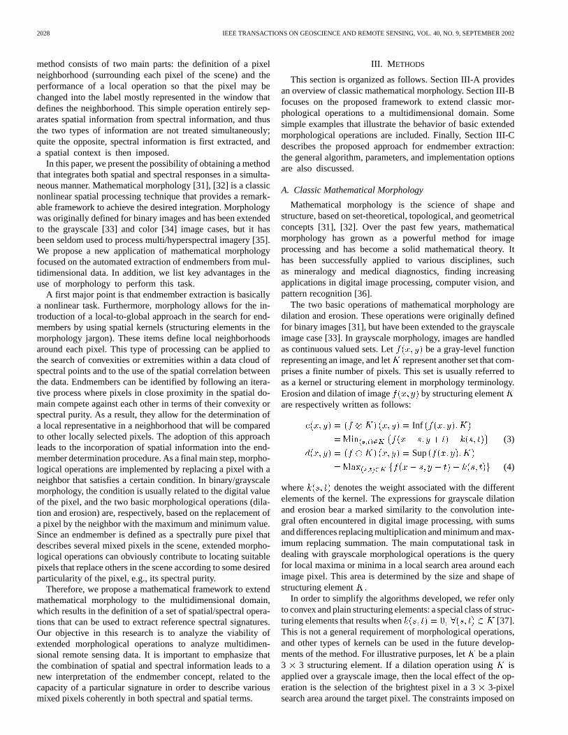
Mathematical morphology is the science of shape andstructure, based on set-theoretical, topological, and geometricalconcepts [31], [32]. Over the past few years, mathematicalmorphology has grown as a powerful method for imageprocessing and has become a solid mathematical theory. Ithas been successfully applied to various disciplines, suchas mineralogy and medical diagnostics, finding increasingapplications in digital image processing, computer vision, andpattern recognition [36].
The two basic operations of mathematical morphology aredilation and erosion. These operations were originally definedfor binary images [31], but have been extended to the grayscaleimage case [33]. In grayscale morphology, images are handledas continuous valued sets. Let be a gray-level functionrepresenting an image, and letrepresent another set that com-prises a finite number of pixels. This set is usually referred toas a kernel or structuring element in morphology terminology.Erosion and dilation of image by structuring elementare respectively written as follows:
Inf
(3)
Sup
(4)
where denotes the weight associated with the differentelements of the kernel. The expressions for grayscale dilationand erosion bear a marked similarity to the convolution inte-gral often encountered in digital image processing, with sumsand differences replacing multiplication and minimum and max-imum replacing summation. The main computational task indealing with grayscale morphological operations is the queryfor local maxima or minima in a local search area around eachimage pixel. This area is determined by the size and shape ofstructuring element .
In order to simplify the algorithms developed, we refer onlyto convex and plain structuring elements: a special class of struc-turing elements that results when [37].This is not a general requirement of morphological operations,and other types of kernels can be used in the future develop-ments of the method. For illustrative purposes, letbe a plain3 3 structuring element. If a dilation operation using isapplied over a grayscale image, then the local effect of the op-eration is the selection of the brightest pixel in a 33-pixelsearch area around the target pixel. The constraints imposed on
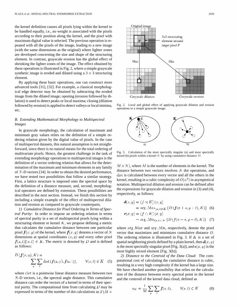
PLAZA et al.: SPATIAL/SPECTRAL ENDMEMBER EXTRACTION 2029
the kernel definition causes all pixels lying within the kernel tobe handled equally, i.e., no weight is associated with the pixelsaccording to their position along the kernel, and the pixel withmaximum digital value is selected. The previous operation is re-peated with all the pixels of the image, leading to a new image(with the same dimensions as the original) where lighter zonesare developed concerning the size and shape of the structuringelement. In contrast, grayscale erosion has the global effect ofshrinking the lighter zones of the image. The effect obtained bythese operations is illustrated in Fig. 2, where a simple grayscalesynthetic image is eroded and dilated using a 33 structuringelement.
By applying these basic operations, one can construct moreadvanced tools [31], [32]. For example, a classical morpholog-ical edge detector may be obtained by subtracting the erodedimage from the dilated image; opening (erosion followed by di-lation) is used to detect peaks or local maxima; closing (dilationfollowed by erosion) is applied to detect valleys or local minima,etc.
B. Extending Mathematical Morphology to MultispectralImages
In grayscale morphology, the calculation of maximum andminimum gray values relies on the definition of a simple or-dering relation given by the digital value of pixels. In the caseof multispectral datasets, this natural assumption is not straight-forward, since there is no natural means for the total ordering ofmultivariate pixels. Hence, the greatest challenge in the task ofextending morphology operations to multispectral images is thedefinition of a vector ordering relation that allows for the deter-mination of the maximum and minimum elements in any familyof -D vectors [34]. In order to obtain the desired performance,we have tested two possibilities that follow a similar strategy.First, a lattice structure is imposed onto the spectral space bythe definition of a distance measure, and, second, morpholog-ical operators are defined by extension. These possibilities aredescribed in the next section. Instead, we finish this section byincluding a simple example of the effect of multispectral dila-tion and erosion as compared to grayscale counterparts.
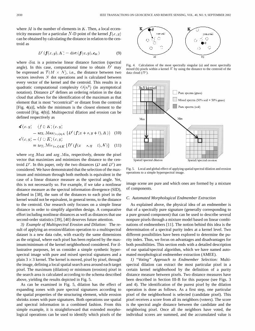
1) Cumulative Distance for Pixel Ordering in Terms of Spec-tral Purity: In order to impose an ordering relation in termsof spectral purity in a set of multispectral pixels lying within astructuring element or kernel , we propose defining a metricthat calculates the cumulative distance between one particularpixel of the kernel, where denotes a vector ofdimensions at spatial coordinates and every other pixel
. The metric is denoted by and is definedas follows:
(5)
where is a pointwise linear distance measure between two-D vectors, i.e., the spectral angle distance. This cumulative
distance can order the vectors of a kernel in terms of their spec-tral purity. The computational time from calculatingmay beexpressed in terms of the number of dot calculations as
Fig. 2. Local and global effect of applying grayscale dilation and erosionoperations to a simple grayscale image.
Fig. 3. Calculation of the most spectrally singular (a) and most spectrallymixed (b) pixels within a kernelK by using cumulative distanceD.
, where is the number of elements in the kernel. Thedistance between two vectors involvesdot operations, and
is calculated between every vector and all the others in thekernel, resulting in a cubic complexity of in asymptoticalnotation. Multispectral dilation and erosion can be defined afterthe expressions for grayscale dilation and erosion in (3) and (4),respectively, as follows:
(6)
(7)
where and , respectively, denote the pixelvector that maximizes and minimizes cumulative distance.The ordering relation is illustrated in Fig. 3. If is a set ofspatial neighboring pixels defined by a plain kernel, thenis the most spectrally singular pixel [Fig. 3(a)], and is themost highly mixed element [Fig. 3(b)].
2) Distance to the Centroid of the Data Cloud:The com-putational cost of calculating the cumulative distance is cubic,resulting in a very high complexity if the kernel has a large size.We have checked another possibility that relies on the calcula-tion of the distance between every spectral point in the kerneland the centroid of the kernel data cloud, defined as
(8)
2030 IEEE TRANSACTIONS ON GEOSCIENCE AND REMOTE SENSING, VOL. 40, NO. 9, SEPTEMBER 2002
where is the number of elements in . Then, a local eccen-tricity measure for a particular -D point of the kernelcan be obtained by calculating the distance in relation to the cen-troid as
(9)
where is a pointwise linear distance function (spectralangle). In this case, computational time to obtain maybe expressed as , i.e., the distance between twovectors involves dot operations and is calculated betweenevery vector of the kernel and the centroid. This results in aquadratic computational complexity (in asymptoticalnotation). Distance defines an ordering relation in the datacloud that allows for the identification of the maximum as thatelement that is most “eccentrical” or distant from the centroid[Fig. 4(a)], while the minimum is the closest element to thecentroid [Fig. 4(b)]. Multispectral dilation and erosion can bedefined respectively as
(10)
(11)
where and , respectively, denote the pixelvector that maximizes and minimizes the distance to the cen-troid . In this paper, only the two distances (and ) areconsidered. We have demonstrated that the selection of the max-imum and minimum through both methods is equivalent in thecase of a linear distance measure as the spectral angle. Yet,this is not necessarily so. For example, if we take a nonlineardistance measure as the spectral information divergence (SID),defined in [38], the sum of the distances to each pixel in thekernel would not be equivalent, in general terms, to the distanceto the centroid. Our research only focuses on a simple lineardistance in order to simplify algorithm design. A comparativeeffort including nonlinear distances as well as distances that usesecond-order statistics [39], [40] deserves future attention.
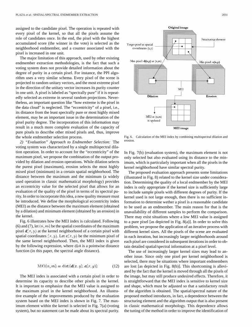
3) Example of Multispectral Erosion and Dilation:The re-sult of applying an erosion/dilation operation to a multispectraldataset is a new data cube, with exactly the same dimensionsas the original, where each pixel has been replaced by the max-imum/minimum of the kernel neighborhood considered. For il-lustrative purposes, let us consider a simple synthetic hyper-spectral image with pure and mixed spectral signatures and aplain 3 3 kernel. The kernel is moved, pixel by pixel, throughthe image, defining a local spatial search area around each targetpixel. The maximum (dilation) or minimum (erosion) pixel inthe search area is calculated according to the schema describedabove, yielding the results depicted in Fig. 5.
As can be examined in Fig. 5, dilation has the effect ofexpanding zones with pure spectral signatures according tothe spatial properties of the structuring element, while erosionshrinks zones with pure signatures. Both operations use spatialand spectral information in a combined fashion. From thissimple example, it is straightforward that extended morpho-logical operations can be used to identify which pixels of the
Fig. 4. Calculation of the most spectrally singular (a) and most spectrallymixed (b) pixels within a kernelK by using the distance to the centroid of thedata cloud (D ).
Fig. 5. Local and global effect of applying spatial/spectral dilation and erosionoperations to a simple hyperspectral image.
image scene are pure and which ones are formed by a mixtureof components.
C. Automated Morphological Endmember Extraction
As explained above, the physical idea of an endmember isthat of a spectrally pure signature (generally corresponding toa pure ground component) that can be used to describe severalnonpure pixels through a mixture model based on linear combi-nations of endmembers [11]. The notion behind this idea is thedetermination of a spectral purity index at a kernel level. Twodifferent possibilities have been explored to determine the pu-rity index. Thus, we focus on advantages and disadvantages forboth possibilities. This section ends with a detailed descriptionof our spatial/spectral algorithm, which we have named auto-mated morphological endmember extraction (AMEE).
1) “Voting” Approach to Endmember Selection:Multi-spectral dilation can extract the most particular pixel in acertain kernel neighborhood by the definition of a puritydistance measure between pixels. Two distance measures havebeen described in Section III-B for this purpose (see Figs. 3and 4). The identification of the purest pixel by the dilationoperation is done as follows. As a first step, one particularpixel of the neighborhood is selected (candidate pixel). Thispixel receives a score from all its neighbors (voters). The scoreis the spectral angle distance between the candidate and theneighboring pixel. Once all the neighbors have voted, theindividual scores are summed, and the accumulated value is
PLAZA et al.: SPATIAL/SPECTRAL ENDMEMBER EXTRACTION 2031
assigned to the candidate pixel. The operation is repeated withevery pixel of the kernel, so that all the pixels assume therole of candidates once. In the end, the pixel with the highestaccumulated score (the winner in the vote) is selected as theneighborhood endmember, and a counter associated with thepixel is increased in one unit.
The major limitation of this approach, used by other existingendmember extraction methodologies, is the fact that such avoting system does not provide detailed information about thedegree of purity in a certain pixel. For instance, the PPI algo-rithm uses a very similar schema. Every pixel of the scene isprojected to random unitary vectors, and the most extreme pixelin the direction of the unitary vector increases its purity counterin one unit. A pixel is labeled as “spectrally pure” if it is repeat-edly selected as extreme in several random projections. Never-theless, an important question like “how extreme is the pixel inthe data cloud” is neglected. The “eccentricity” of a pixel, i.e.,its distance from the least spectrally pure or most highly mixedelement, may be an important issue in the determination of thepixel purity degree. The incorporation of this information mayresult in a much more complete evaluation of the capacity ofpure pixels to describe other mixed pixels and, thus, improvethe whole endmember selection process.
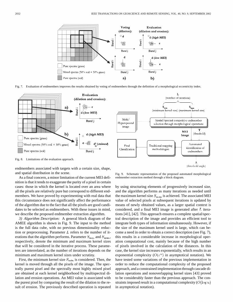
2) “Evaluation” Approach to Endmember Selection:Thevoting system was characterized by a single multispectral dila-tion operation. In order to account for the “eccentricity” of themaximum pixel, we propose the combination of the output pro-vided by dilation and erosion operations. While dilation selectsthe purest pixel (maximum), erosion selects the most highlymixed pixel (minimum) in a certain spatial neighborhood. Thedistance between the maximum and the minimum (a widelyused operation in classic mathematical morphology) providesan eccentricity value for the selected pixel that allows for anevaluation of the quality of the pixel in terms of its spectral pu-rity. In order to incorporate this idea, a new quality measure mustbe introduced. We define the morphological eccentricity index(MEI) as the distance between the maximum element (obtainedby a dilation) and minimum element (obtained by an erosion) inthe kernel.
Fig. 6 illustrates how the MEI index is calculated. Following(6) and (7), let be the spatial coordinates of the maximumpixel at the kernel neighborhood of a certain pixel withspatial coordinates . Let be the minimum pixel ofthe same kernel neighborhood. Then, the MEI index is givenby the following expression, where is a pointwise distancefunction (in this paper, the spectral angle distance).
(12)
The MEI index is associated with a certain pixel in order todetermine its capacity to describe other pixels in the kernel.It is important to emphasize that the MEI value is assigned tothe maximum pixel in the kernel neighborhood. An illustra-tive example of the improvements produced by the evaluationsystem based on the MEI index is shown in Fig. 7. The max-imum element within the kernel is selected in Fig. 7(a) (votingsystem), but no statement can be made about its spectral purity.
Fig. 6. Calculation of the MEI index by combining multispectral dilation anderosion.
In Fig. 7(b) (evaluation system), the maximum element is notonly selected but also evaluated using its distance to the min-imum, which is particularly important when all the pixels in thekernel neighborhood have similar spectral purity.
The proposed evaluation approach presents some limitations(illustrated in Fig. 8) related to the kernel size under considera-tion. Determining the quality of a local endmember by the MEIindex is only appropriate if the kernel size is sufficiently largeto include sample pixels with different degrees of purity. If thekernel used is not large enough, then there is no sufficient in-formation to determine wether a pixel is a reasonable candidateto be used as an endmember. The main reason for that is theunavailability of different samples to perform the comparison.There may exist situations where a low MEI value is assignedto a pure pixel [as depicted in Fig. 8(a)]. In order to solve thisproblem, we propose the application of an iterative process withdifferent kernel sizes. All the pixels of the scene are evaluatedin each iteration, but increasingly larger neighborhoods aroundeach pixel are considered in subsequent iterations in order to ob-tain detailed spatial/spectral information at a pixel level.
The use of increasingly larger kernel sizes may lead to an-other issue. Since only one pixel per kernel neighborhood isselected, there may be situations where important endmembersare lost [as depicted in Fig. 8(b)]. This shortcoming is allevi-ated by the fact that the kernel is moved through all the pixels ofthe image, but may still produce undesired effects. Therefore, itis straightforward that the MEI index is sensitive to kernel sizeand shape, which must be adjusted so that a satisfactory resultof the algorithm is obtained. The spatial/spectral nature of theproposed method introduces, in fact, a dependence between thestructuring element and the algorithm output that is also presentin classic mathematical morphology. This dependence allowsthe tuning of the method in order to improve the identification of
2032 IEEE TRANSACTIONS ON GEOSCIENCE AND REMOTE SENSING, VOL. 40, NO. 9, SEPTEMBER 2002
Fig. 7. Evaluation of endmembers improves the results obtained by voting of endmembers through the definition of a morphological eccentricity index.
Fig. 8. Limitations of the evaluation approach.
endmembers associated with targets with a certain size, shape,and spatial distribution in the scene.
As a final concern, a minor limitation of the current MEI defi-nition is that it tends to exaggerate the purity of a pixel in certaincases: those in which the kernel is located over an area whereall the pixels are relatively pure but correspond to different end-members. We have proved by experimenting with real data thatthis circumstance does not significantly affect the performanceof the algorithm due to the fact that all the pixels are good candi-dates to be selected as endmembers. With these issues in mind,we describe the proposed endmember extraction algorithm.
3) Algorithm Description: A general block diagram of theAMEE algorithm is shown in Fig. 9. The input to the methodis the full data cube, with no previous dimensionality reduc-tion or preprocessing. Parameterrefers to the number of it-erations that the algorithm performs. Parameter and ,respectively, denote the minimum and maximum kernel sizesthat will be considered in the iterative process. These parame-ters are interrelated, as the number of iterations depends on theminimum and maximum kernel sizes under scrutiny.
First, the minimum kernel size is considered. Then, thekernel is moved through all the pixels of the image. The spec-trally purest pixel and the spectrally most highly mixed pixelare obtained at each kernel neighborhood by multispectral di-lation and erosion operations. An MEI value is associated withthe purest pixel by comparing the result of the dilation to the re-sult of erosion. The previously described operation is repeated
Fig. 9. Schematic representation of the proposed automated morphologicalendmember extraction method through a block diagram.
by using structuring elements of progressively increased size,and the algorithm performs as many iterations as needed untilthe maximum kernel size is achieved. The associated MEIvalue of selected pixels at subsequent iterations is updated bymeans of newly obtained values, as a larger spatial context isconsidered, and a final MEI image is generated afteritera-tions [41], [42]. This approach ensures a complete spatial/spec-tral description of the image and provides an efficient tool tointegrate both types of information simultaneously. However, ifthe size of the maximum kernel used is large, which can be-come a need in order to obtain a correct description (see Fig. 7),this results in a considerable increase in morphological oper-ation computational cost, mainly because of the high numberof pixels involved in the calculation of the distances. In thiscase, the kernel size increases exponentially, which results in anexponential complexity ( in asymptotical notation). Wehave tested some variations of the previous implementation inorder to reduce the computational complexity of the proposedapproach, and a constrained implementation through cascade di-lation operations and nonoverlapping kernel sizes [43] provedto be considerably faster than the previous approach. The con-straints imposed result in a computational complexity (in asymptotical notation).
PLAZA et al.: SPATIAL/SPECTRAL ENDMEMBER EXTRACTION 2033
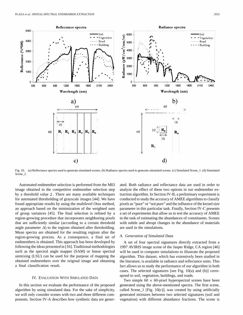
Fig. 10. (a) Reflectance spectra used to generate simulated scenes. (b) Radiance spectra used to generate simulated scenes. (c) Simulated Scene_1. (d) SimulatedScene_2.
Automated endmember selection is performed from the MEIimage obtained in the competitive endmember selection stepby a threshold value . There are many available techniquesfor automated thresholding of grayscale images [44]. We havefound appropriate results by using the multilevel Otsu method,an approach based on the minimization of the weighted sumof group variances [45]. The final selection is refined by aregion-growing procedure that incorporates neighboring pixelsthat are sufficiently similar (according to a certain thresholdangle parameter ) to the regions obtained after thresholding.Mean spectra are obtained for the resulting regions after theregion-growing process. As a consequence, a final set ofendmembers is obtained. This approach has been developed byfollowing the ideas presented in [16]. Traditional methodologiessuch as the spectral angle mapper (SAM) or linear spectralunmixing (LSU) can be used for the purpose of mapping theobtained endmembers over the original image and obtaininga final classification result.
IV. EVALUATION WITH SIMULATED DATA
In this section we evaluate the performance of the proposedalgorithm by using simulated data. For the sake of simplicity,we will only consider scenes with two and three different com-ponents. Section IV-A describes how synthetic data are gener-
ated. Both radiance and reflectance data are used in order toanalyze the effect of these two options in our endmember ex-traction algorithm. In Section IV-B, a preliminary experiment isconducted to study the accuracy of AMEE algorithms to classifypixels as “pure” or “not pure” and the influence of the kernel sizeparameter in this particular task. Finally, Section IV-C presentsa set of experiments that allow us to test the accuracy of AMEEin the task of estimating the abundances of constituents. Sceneswith subtle and abrupt changes in the abundance of materialsare used in the simulations.
A. Generation of Simulated Data
A set of four spectral signatures directly extracted from a1997 AVIRIS image scene of the Jasper Ridge, CA region [46]will be used in computer simulations to illustrate the proposedalgorithm. This dataset, which has extensively been studied inthe literature, is available in radiance and reflectance units. Thisfact allows us to study the performance of our algorithm in bothcases. The selected signatures [see Fig. 10(a) and (b)] corre-spond to soil, vegetation, buildings, and roads.
Two simple 60 60-pixel hyperspectral scenes have beengenerated using the above-mentioned spectra. The first scene,called Scene_1 [Fig. 10(c)], was created by using artificiallygenerated mixtures between two selected signatures (soil andvegetation) with different abundance fractions. The scene is
2034 IEEE TRANSACTIONS ON GEOSCIENCE AND REMOTE SENSING, VOL. 40, NO. 9, SEPTEMBER 2002
TABLE IIABUNDANCE ASSIGNMENT FORREGIONS IN SIMULATED
SCENESSCENE_1 AND SCENE_2
formed by six regions of ten-pixels width, and the abundanceshave been assigned to the regions so that the linear mixturebetween the two components is progressive and adds to one (asshown in Table II).
The synthetic hyperspectral scene in Fig. 10(d) (calledScene_2) simulates homogeneous targets (a road and abuilding) in a soil background. The simple simulated “objects”are a 10 10-pixel building and a road ten pixels wide. Thisimage is characterized by abrupt changes in the abundances ofmaterials. There is no linear mixture among components in thescene. Instead, there is a situation where 1) three different pureconstituents are present and 2) each pixel is characterized byhaving an abundance of one for one particular endmember andzero for the others (see Table II).
Both Scene_1 and Scene_2 have been generated by using ra-diance and reflectance spectra. We will refer to them from nowon as Scene_1_radiance, Scene_1_reflectance, Scene_2_ra-diance, and Scene_2_reflectance. Random noise was used tosimulate contributions from ambient (clutter) and instrumentalsources. Noise was created by using numbers with a standardnormal distribution obtained from a pseudorandom numbergenerator and added to each pixel to generate a signal-to-noiseratio (SNR) of 30:1. For the simulations, we will define theSNR for each band as the ratio of the 50% signal level to thestandard deviation of the noise [47]. Thus, the simulated dataare created, based on a simple linear model, by the followingexpression [19]:
(13)
where is a vector containing the simulated discretespectrum,; is the number of endmembers used;is a scalarvalue representing the fractional abundance of endmemberat pixel (Table II contains a description of the abundanceof endmembers in each region); and is the noise factor.The signal is scaled by 50% of the SNR, which is equivalentto reducing the noise standard deviation by the inverse factor( ), so that the simulated data meet the SNR definition[19]. The vector terms in the parentheses are multiplied elementby element.
B. Identification of Pure Pixels
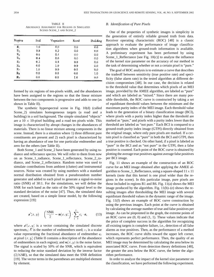
One of the properties of synthetic images is simplicity inthe generation of entirely reliable ground truth from data.Receiver operating characteristic (ROC) [48] is a classicapproach to evaluate the performance of image classifica-tion algorithms when ground-truth information is available.A preliminary experiment has been performed by usingScene_1_Reflectance [see Fig. 10(c)] to analyze the influenceof the kernel size parameter on the accuracy of our method inthe task of determining whether or not a certain pixel is “pure.”
The goal of ROC analysis is to estimate a curve that describesthe tradeoff between sensitivity (true positive rate) and speci-ficity (false alarm rate) in the tested algorithm at different de-cision compromises [48]. In our case, the decision is relatedto the threshold value that determines which pixels of an MEIimage, provided by the AMEE algorithm, are labeled as “pure”and which are labeled as “mixed.” Since there are many pos-sible thresholds, the ROC curve is constructed by taking a setof equidistant threshold values between the minimum and themaximum purity index of the MEI image. Each threshold valueleads to the generation of a binary classification image (BCI),where pixels with a purity index higher than the threshold aremarked as “pure,” and pixels with a purity index lower than thethreshold are labeled as “not pure.” Each BCI is compared to aground-truth purity index image (GTPI) directly obtained fromthe original image, where only pure pixels are marked. If a cer-tain pixel is classified as “pure” in both the BCI and GTPI, thena true positive is checked. On other hand, if a pixel is labeled as“pure” in the BCI and as “not pure” in the GTPI, then a falsepositive is counted. Each point of the ROC curve is obtained byplotting the average true positives against average false positivesper BCI image.
Fig. 11 shows an example of the construction of an ROCcurve for an MEI image obtained after applying the AMEE al-gorithm to Scene_1_Reflectance, using a square-shaped 1111kernels (note that this kernel is one pixel wider than the re-gions in the scene). In this particular image, pure pixels arethose included in regions R1 and R6. Fig. 11(a) shows the MEIimage produced by the algorithm. Fig. 11(b)–(e) shows the re-sulting images after thresholding the MEI image with severalequidistant threshold values in the dynamic range of the image.Fig. 11(f) shows an example of ROC curve construction byusing the previous images. Each point at the curve is obtainedby calculating the average number of true and false positives perimage. As can be pinpointed in the graph, the extreme points ofan ROC curve are (0, 0) and (1, 1). These values indicate thatthe price of complete success in the algorithm for recognizingall existing targets is complete failure, i.e., detection of all falsealarms as true positives. Then, as the performance of a methodincreases, the ROC curve shifts toward the upper left corner,which represents perfect performance. Then, the quality of anMEI image may be determined by calculating the area below itsassociated ROC curve. From detection theory definitions [48],the greater the area below the ROC curve, the better the algo-rithm performance.
In order to analyze the impact of the kernel size parameter onthe classification, we have performed the following experiment.
PLAZA et al.: SPATIAL/SPECTRAL ENDMEMBER EXTRACTION 2035
Fig. 11. (a) MEI image obtained after applying the AMEE algorithm to Scene_1_Reflectance by using a square-shaped 11�11 kernel. (b)–(e) Resulting imagesafter thresholding the MEI image with four equidistant threshold values. (f) Construction of an ROC curve for the MEI image (the area under the curve isalsoaddressed). (g) Area under ROC curves associated with classification images obtained by using voting and evaluation of endmembers with different kernel sizes.
The kernel size parameter is initially set to 33 pixels and isprogressively increased to a maximum value of 2121 pixels.For each considered size, an MEI image is obtained. An ROCcurve is then constructed for each MEI image, and the area underthe curve is estimated. The resulting area estimations are plottedagainst the correspondent values of the parameter, obtaininga curve that indicates which values of the parameter providebetter results. Fig. 11(g) shows the results of this experimentafter applying the AMEE algorithm to Scene_1_Reflectance.For comparative purposes, we have considered the voting andevaluation systems for endmember selection (refer to Section IIIfor a detailed description of each approach). The results shownin Fig. 11(g) reveal that the purity determination process issensitive to the kernel size parameter, which must be largeenough to contain samples with different spectral purity. Inboth cases (voting and evaluation), performance is high whenthe kernel size is 11 11 or larger (the width of spatialpatterns in Scene_1 is ten pixels). In contrast, this experimentreveals that voting is much more dependent on kernel sizethan evaluation, which provides acceptable results for smallkernel sizes.
C. Estimation of Abundances
In order to perform abundance estimation simulations, wehave applied our algorithm to the simulated scenes describedin Fig. 10. A set of endmembers is extracted for each image,and the abundance of each endmember is estimated by usingfully constrained linear spectral unmixing [49]. In order to deter-mine the accuracy of our method in this particular task, we com-pare the estimated abundances to the true abundances, shown inTable II. Both reflectance and radiance spectra are used in thesimulations.
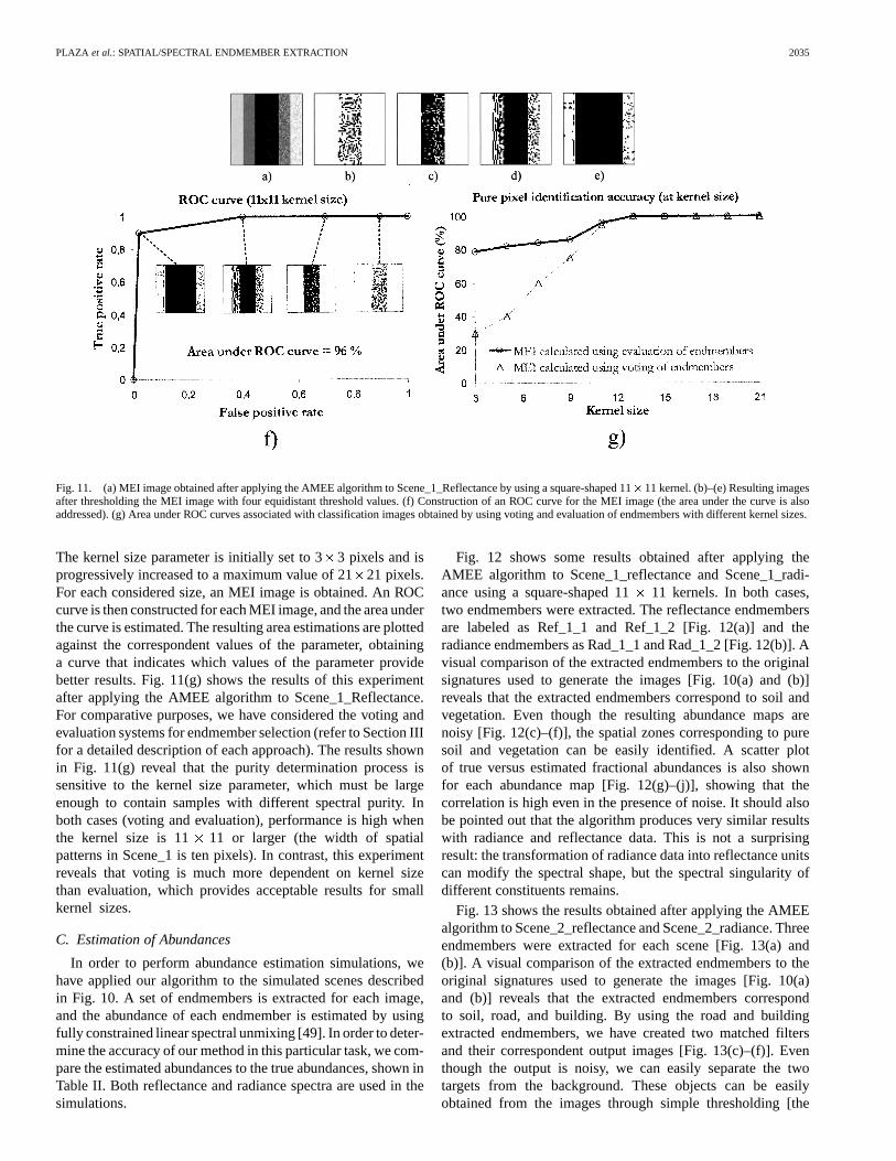
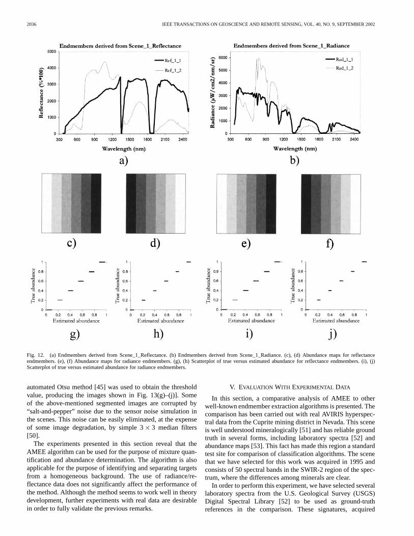
Fig. 12 shows some results obtained after applying theAMEE algorithm to Scene_1_reflectance and Scene_1_radi-ance using a square-shaped 1111 kernels. In both cases,two endmembers were extracted. The reflectance endmembersare labeled as Ref_1_1 and Ref_1_2 [Fig. 12(a)] and theradiance endmembers as Rad_1_1 and Rad_1_2 [Fig. 12(b)]. Avisual comparison of the extracted endmembers to the originalsignatures used to generate the images [Fig. 10(a) and (b)]reveals that the extracted endmembers correspond to soil andvegetation. Even though the resulting abundance maps arenoisy [Fig. 12(c)–(f)], the spatial zones corresponding to puresoil and vegetation can be easily identified. A scatter plotof true versus estimated fractional abundances is also shownfor each abundance map [Fig. 12(g)–(j)], showing that thecorrelation is high even in the presence of noise. It should alsobe pointed out that the algorithm produces very similar resultswith radiance and reflectance data. This is not a surprisingresult: the transformation of radiance data into reflectance unitscan modify the spectral shape, but the spectral singularity ofdifferent constituents remains.
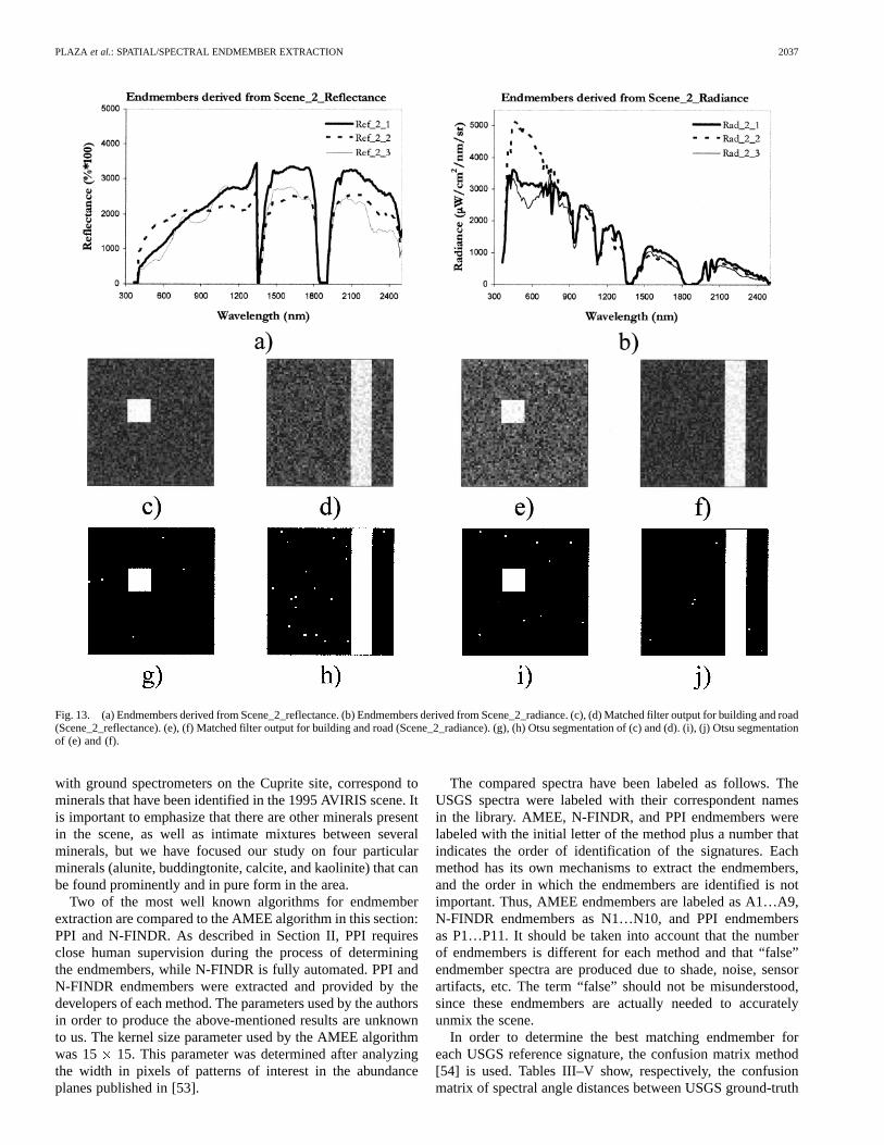
Fig. 13 shows the results obtained after applying the AMEEalgorithm to Scene_2_reflectance and Scene_2_radiance. Threeendmembers were extracted for each scene [Fig. 13(a) and(b)]. A visual comparison of the extracted endmembers to theoriginal signatures used to generate the images [Fig. 10(a)and (b)] reveals that the extracted endmembers correspondto soil, road, and building. By using the road and buildingextracted endmembers, we have created two matched filtersand their correspondent output images [Fig. 13(c)–(f)]. Eventhough the output is noisy, we can easily separate the twotargets from the background. These objects can be easilyobtained from the images through simple thresholding [the
2036 IEEE TRANSACTIONS ON GEOSCIENCE AND REMOTE SENSING, VOL. 40, NO. 9, SEPTEMBER 2002
Fig. 12. (a) Endmembers derived from Scene_1_Reflectance. (b) Endmembers derived from Scene_1_Radiance. (c), (d) Abundance maps for reflectanceendmembers. (e), (f) Abundance maps for radiance endmembers. (g), (h) Scatterplot of true versus estimated abundance for reflectance endmembers. (i), (j)Scatterplot of true versus estimated abundance for radiance endmembers.
automated Otsu method [45] was used to obtain the thresholdvalue, producing the images shown in Fig. 13(g)–(j)]. Someof the above-mentioned segmented images are corrupted by“salt-and-pepper” noise due to the sensor noise simulation inthe scenes. This noise can be easily eliminated, at the expenseof some image degradation, by simple 33 median filters[50].
The experiments presented in this section reveal that theAMEE algorithm can be used for the purpose of mixture quan-tification and abundance determination. The algorithm is alsoapplicable for the purpose of identifying and separating targetsfrom a homogeneous background. The use of radiance/re-flectance data does not significantly affect the performance ofthe method. Although the method seems to work well in theorydevelopment, further experiments with real data are desirablein order to fully validate the previous remarks.
V. EVALUATION WITH EXPERIMENTAL DATA
In this section, a comparative analysis of AMEE to otherwell-known endmember extraction algorithms is presented. Thecomparison has been carried out with real AVIRIS hyperspec-tral data from the Cuprite mining district in Nevada. This sceneis well understood mineralogically [51] and has reliable groundtruth in several forms, including laboratory spectra [52] andabundance maps [53]. This fact has made this region a standardtest site for comparison of classification algorithms. The scenethat we have selected for this work was acquired in 1995 andconsists of 50 spectral bands in the SWIR-2 region of the spec-trum, where the differences among minerals are clear.
In order to perform this experiment, we have selected severallaboratory spectra from the U.S. Geological Survey (USGS)Digital Spectral Library [52] to be used as ground-truthreferences in the comparison. These signatures, acquired
PLAZA et al.: SPATIAL/SPECTRAL ENDMEMBER EXTRACTION 2037
Fig. 13. (a) Endmembers derived from Scene_2_reflectance. (b) Endmembers derived from Scene_2_radiance. (c), (d) Matched filter output for building and road(Scene_2_reflectance). (e), (f) Matched filter output for building and road (Scene_2_radiance). (g), (h) Otsu segmentation of (c) and (d). (i), (j)Otsu segmentationof (e) and (f).
with ground spectrometers on the Cuprite site, correspond tominerals that have been identified in the 1995 AVIRIS scene. Itis important to emphasize that there are other minerals presentin the scene, as well as intimate mixtures between severalminerals, but we have focused our study on four particularminerals (alunite, buddingtonite, calcite, and kaolinite) that canbe found prominently and in pure form in the area.
Two of the most well known algorithms for endmemberextraction are compared to the AMEE algorithm in this section:PPI and N-FINDR. As described in Section II, PPI requiresclose human supervision during the process of determiningthe endmembers, while N-FINDR is fully automated. PPI andN-FINDR endmembers were extracted and provided by thedevelopers of each method. The parameters used by the authorsin order to produce the above-mentioned results are unknownto us. The kernel size parameter used by the AMEE algorithmwas 15 15. This parameter was determined after analyzingthe width in pixels of patterns of interest in the abundanceplanes published in [53].
The compared spectra have been labeled as follows. TheUSGS spectra were labeled with their correspondent namesin the library. AMEE, N-FINDR, and PPI endmembers werelabeled with the initial letter of the method plus a number thatindicates the order of identification of the signatures. Eachmethod has its own mechanisms to extract the endmembers,and the order in which the endmembers are identified is notimportant. Thus, AMEE endmembers are labeled as A1…A9,N-FINDR endmembers as N1…N10, and PPI endmembersas P1…P11. It should be taken into account that the numberof endmembers is different for each method and that “false”endmember spectra are produced due to shade, noise, sensorartifacts, etc. The term “false” should not be misunderstood,since these endmembers are actually needed to accuratelyunmix the scene.
In order to determine the best matching endmember foreach USGS reference signature, the confusion matrix method[54] is used. Tables III–V show, respectively, the confusionmatrix of spectral angle distances between USGS ground-truth
2038 IEEE TRANSACTIONS ON GEOSCIENCE AND REMOTE SENSING, VOL. 40, NO. 9, SEPTEMBER 2002
TABLE IIICONFUSIONMATRIX OF SPECTRAL ANGLE DISTANCESBETWEENAMEE ENDMEMBERS AND USGS REFERENCESPECTRA
TABLE IVCONFUSIONMATRIX OF SPECTRAL ANGLE DISTANCESBETWEEN N-FINDR ENDMEMBERS AND USGS REFERENCESPECTRA
TABLE VCONFUSIONMATRIX OF SPECTRAL ANGLE DISTANCESBETWEEN PPI ENDMEMBERS AND USGS REFERENCESPECTRA
signatures and AMEE, N-FINDR, and PPI endmembers. Wehave selected the spectral angle distance for the comparison dueto existing scale and ilumination variations between referenceand extracted endmembers, which are mainly due to atmospherictransmission effects that are not present in spectra acquiredby ground spectrometers.
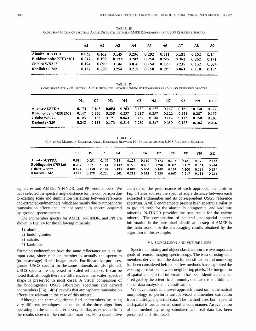
The endmember spectra for AMEE, N-FINDR, and PPI areshown in Fig. 14 for the following minerals:
1) alunite;2) buddingtonite;3) calcite;4) kaolinite.
Extracted endmembers have the same reflectance units as theinput data, since each endmember is actually the spectrum(or an average) of real image pixels. For illustrative purposes,ground USGS spectra for the same minerals are also plotted.USGS spectra are expressed in scaled reflectance. It can benoted that, although there are differences in the scales, spectralshape is preserved in most cases. A visual comparison ofthe buddingtonite USGS laboratory spectrum and derivedendmembers [Fig. 14(b)] reveals that atmospheric transmissioneffects are relevant in the case of this mineral.
Although the three algorithms find endmembers by usingvery different techniques, the output of the three algorithmsoperating on the same dataset is very similar, as expected fromthe results shown in the confusion matrices. For a quantitative
analysis of the performance of each approach, the plots inFig. 14 also address the spectral angle distance between eachextracted endmember and its correspondent USGS referencespectrum. AMEE endmembers present high spectral similarityto ground truth for the alunite, buddingtonite, and kaoliniteminerals. N-FINDR provides the best result for the calcitemineral. The combination of spectral and spatial contextinformation in the pure pixel identification step of AMEE isthe main reason for the encouraging results obtained by thealgorithm in this example.
VI. CONCLUSION AND FUTURE LINES
Spectral unmixing and object classification are two importantgoals of remote imaging spectroscopy. The idea of using end-members derived from the data for classification and unmixinghas been considered before, but few methods have exploited theexisting correlation between neighboring pixels. The integrationof spatial and spectral information has been identified as a de-sired goal by the scientific community dedicated to multidimen-sional data analysis and classification.
We have described a novel approach based on mathematicalmorphology to perform unsupervised endmember extractionfrom multi/hyperspectral data. The method uses both spectraland spatial information in a simultaneous manner. An evaluationof the method by using simulated and real data has beenpresented and discussed.
PLAZA et al.: SPATIAL/SPECTRAL ENDMEMBER EXTRACTION 2039
Fig. 14. Algorithm scene derived and USGS laboratory reflectance spectra for (a) alunite, (b) buddingtonite, (c) calcite, and (d) kaolinite. Extracted endmembershave the same reflectance units as the input data, while USGS spectra are expressed in scaled reflectance. The spectral angle distance between each extractedendmember and the correspondent USGS reference spectrum is addressed.
Results with simulated data reveal that the method can accu-rately model the spatial distribution of spectral patterns in thescene by extended morphological operations that apply plainspatial kernels. The spatial properties (size and shape) of thekernel have a strong influence on the final result, a fact that isconsistent with classic mathematical morphology theory. Thebehavior of the algorithm also depends on the relationship be-tween the spatial properties of the kernels used and the distribu-tion of spectral patterns in the scene. This fact allows for thetuning of our method for a wide range of applications, fromtarget detection to global classification and spectral unmixingof scenes. The use of reflectance/radiance data does not have asignificant impact on the output of the algorithm.
Results with experimental data show that the proposedmethod produces results that are comparable to those foundby working with other widely accepted methodologies. Theproposed method is accurate in the task of identifying end-members from complicated scenes as the famous AVIRISCuprite dataset, which has become a standard test site for thecomparison of algorithms due to the availability of qualityground-truth measurements.
As with any new approach, there are some unresolved issuesthat may present challenges over time. In this sense, future lines
will cover some relevant developments that were not included inthe present study. An evaluation of different distance measures(both linear and nonlinear) to be used in the extension of mor-phological operations is a key topic, deserving future research.In addition, the structuring elements developed in this paperare limited to plain square-shaped kernels. The use of kernelswith no such limitations is of great interest in order to explore,in greater detail, the existing spatial/spectral interrelation be-tween the kernel used and patterns in the scene. The numberof endmembers extracted per kernel neighborhood is also aninteresting issue. In the present research, some limitations ofthe proposed method have been identified as a consequence ofthe fact that only one pixel per kernel neighborhood is selected.Alternative definitions of the local MEI index may overcome ex-isting limitations. Finally, efficient hardware implementationsbased on field-programmable logic arrays and systolic arraysare being currently tested at our laboratory in order to providethe methodology with real-time capabilities.
ACKNOWLEDGMENT
The authors acknowledge the suggestions and comments ofJ. Pinzón, R. O. Green, and J. A. Gualtieri that helped to improve

2040 IEEE TRANSACTIONS ON GEOSCIENCE AND REMOTE SENSING, VOL. 40, NO. 9, SEPTEMBER 2002
the quality of this paper. Indications made by P. Gomez-Vildaabout efficient implementation in the proposed method are alsogratefully acknowledged. In addition, the authors would liketo express their gratitude to M. Winter and E. Winter for pro-viding results of the N-FINDR algorithm for the Cuprite dataset.Finally, we also wish to state our appreciation to A. CuradoFuentes, from the Department of English at University of Ex-tremadura, who reviewed the submitted version of this paper.
REFERENCES
[1] N. M. Shortet al.. The remote sensing tutorial. NASA/GSFC. [Online].Available: http://rst.gsfc.nasa.gov.
[2] R. O. Greenet al., “Imaging spectroscopy and the airborne visible/in-frared imaging spectrometer (AVIRIS),”Remote Sens. Environ., vol. 65,pp. 227–248, 1998.
[3] A. Müller, A. Hausold, and P. Strobl, “HySens—DAIS/ROSIS imagingspectrometers at DLR,” inProc. SPIE Image and Signal Processing forRemote Sensing VII, Toulouse, France, 2001.
[4] I. Keller and J. Fischer, “Details and improvements of the calibration ofthe compact airborne spectrographic imager (CASI),” inFirst EARSELWorkshop on Imaging Spectroscopy, Paris, France, 1998, pp. 81–88.
[5] C. Mao, M. Seal, and G. Heitschmidt, “Airborne hyperspectral imageaquisition with digital CCD video camera,” in16th Biennial Workshopon Videography and Color Photography in Resource Assessment, Wes-laco, TX, 1997, pp. 129–140.
[6] R. Bianchi, R. M. Cavalli, L. Fiumi, C. M. Marino, and S. Pignatti, “CNRLARA project, Italy: Airborne laboratory for environmental research,”in Summaries of the V JPL Airborne Earth Science Workshop, Pasadena,CA, 2001.
[7] P. Launeau, J. Girardeau, D. Despan, C. Sotin, J. M. Tubia, B. Diez-Gar-retas, and A. Asensi, “Study of serpentine and specific vegetation in theRonda Peridotite (Spain) from 1991 AVIRIS to 2001 hymap images,” inSummaries of the XI JPL Airborne Earth Science Workshop, Pasadena,CA, 2001.
[8] F. A. Kruse, J. W. Boardman, and J. F. Huntington, “Progress report:Geologic validation of E0-1 hyperion using AVIRIS,” inSummaries ofthe XI JPL Airborne Earth Science Workshop, Pasadena, CA, 2001.
[9] S. Tadjudin and D. Landgrebe, “Classification of high dimensional datawith limited training samples,” Ph.D. dissertation, School of Elect. Eng.Comput. Sci., Purdue Univ., Lafayette, IN, 1998.
[10] V. Madhok and D. Landgrebe, “Spectral–spatial analysis of remotesensing data: An image model and a procedural design,” Ph.D. disser-tation, School of Elect. Eng. Comput. Sci., Purdue Univ., Lafayette, IN,1998.
[11] J. J. Settle, “On the relationship between spectral unmixing and sub-space projection,”IEEE Trans. Geosci. Remote Sensing, vol. 34, pp.1045–1046, July 1996.
[12] Y. H. Hu, H. B. Lee, and F. L. Scarpace, “Optimal linear spectral un-mixing,” IEEE Trans. Geosci. Remote Sensing, vol. 37, pp. 639–644,Jan. 1999.
[13] M. Petrou and P. G. Foschi, “Confidence in linear spectral unmixingof single pixels,” IEEE Trans. Geosci. Remote Sensing, vol. 37, pp.624–626, Jan. 1999.
[14] F. A. Kruse, “Spectral identification of image endmembers determinedfrom AVIRIS data,” inSummaries of the VII JPL Airborne Earth ScienceWorkshop, Pasadena, CA, 1998.
[15] J. W. Boardman, F. A. Kruse, and R. O. Green, “Mapping target signa-tures via partial unmixing of AVIRIS data,” inSummaries of the V JPLAirborne Earth Science Workshop, Pasadena, CA, 1995.
[16] C. A. Bateson, G. P. Asner, and C. A. Wessman, “Endmember bundles:A new approach to incorporating endmember variability into spectralmixture analysis,”IEEE Trans. Geosci. Remote Sensing, vol. 38, pp.1083–1094, Mar. 2000.
[17] J. W. Boardman and F. A. Kruse, “Automated spectral analysis: A ge-ological example using AVIRIS data, Northern Grapevine Mountains,Nevada,” inProc. 10th Thematic Conference, Geologic Remote Sensing,San Antonio, TX, 1994.
[18] F. A. Kruse, J. F. Huntington, and R. O. Green, “Results from the 1995AVIRIS geology group shoot,” inProc. 2nd Int. Airborne RemoteSensing Conf. Exhib., 1996.
[19] A. Ifarraguerri and C.-I. Chang, “Multispectral and hyperspectral imageanalysis with convex cones,”IEEE Trans. Geosci. Remote Sensing, vol.37, pp. 756–770, Mar. 1999.
[20] J. Theiler, D. Lavenier, N. Harvey, S. Perkins, and J. Szymanski, “Usingblocks of skewers for faster computation of pixel purity index,” inSPIEInt. Conf. Optical Science and Technology, San Diego, CA, 2000.
[21] C. A. Bateson and B. Curtiss, “A tool for manual endmember selectionand spectral unmixing,” inSummaries of the V JPL Airborne Earth Sci-ence Workshop, Pasadena, CA, 1993.
[22] M. E. Winter, “N-FINDR: An algorithm for fast autonomous spectralend-member determination in hyperspectral data,” inProc. SPIEImaging Spectrometry V, 1999, pp. 266–275.
[23] J. Bowles, P. J. Palmadesso, J. A. Antoniades, M. M. Baumback, and L.J. Rickard, “Use of filter vectors in hyperspectral data analysis,”Proc.SPIE Infrared Spaceborne Remote Sensing III, pp. 148–157, 1995.
[24] K. Staenz, T. Szeredi, and J. Schwarz, “ISDAS—A system for pro-cessing/analyzing hyperspectral data,”Can. J. Remote Sens., vol. 24,pp. 99–113, 1998.
[25] D. Roberts, M. Gardener, J. Regelbrugge, D. Pedreros, and S. Ustin,“Mapping the distribution of wildfire fuels using AVIRIS in the SantaMonica Mountains,” inSummaries of the VIII JPL Airborne Earth Sci-ence Workshop, Pasadena, CA, 1998.
[26] P. Martínez, J. A. Gualtieri, P. L. Aguilar, R. M. Pérez, M. Linaje, J. C.Preciado, and A. Plaza, “Hyperspectral image classification using a self-organizing map,” inSummaries of the XI JPL Airborne Earth ScienceWorkshop, Pasadena, CA, 2001.
[27] J. Pinzón, S. Ustin, and J. F. Pierce, “Robust feature extraction for hy-perspectral imagery using both spatial and spectral redundancies,” inSummaries of the VII JPL Airborne Earth Science Workshop, Pasadena,CA, 1998.
[28] L. Hudgins and C. Hines, “Spatial–spectral morphological operators forhyperspectral region-growing,” inInt. Symp. Spectral Sensing Research(ISSSR), Quebec City, Canada, 2001.
[29] B. Peppin, P. L. Hauff, D. C. Peters, E. C. Prosh, and G. Borstad, “Dif-ferent correction-to-reflectance methods and their impacts on mineralclassification using SFSI and low- and high-altitude AVIRIS,” inSum-maries of the XI JPL Airborne Earth Science Workshop, Pasadena, CA,2001.
[30] L. O. Jimenez-Rodriguez and J. Rivera-Medina, “Integration of spatialand spectral information in unsupervised classification for multispectraland hyperspectral data,”Proc. SPIE Image and Signal Processing forRemote Sensing V, pp. 24–33, 1999.
[31] J. Serra,Image Analysis and Mathematical Morphology. London:Academic Press, 1982.
[32] , Image Analysis and Mathematical Morphology. London: Aca-demic Press, 1993, vol. 1.
[33] S. R. Sternberg, “Greyscale morphology,”Comput. Vision, GraphicsImage Processing, vol. 35, pp. 283–305, 1999.
[34] P. Lambert and J. Chanussot, “Extending mathematical morphology tocolor image processing,” inProc. CGIP 2000, Saint-Etienne, France,2000.
[35] P. Soille, “Morphological partitioning of multispectral images,”J. Elec-tron. Imaging, vol. 5, pp. 252–265, July 1996.
[36] R. M. Haralick and L. G. Shapiro,Computer and Robot Vi-sion. Reading, MA: Addison-Wesley, 1993.
[37] M. Comer and E. Delp, “Morphological operations for color image pro-cessing,”J. Electron. Imaging, vol. 8, pp. 279–289, July 1999.
[38] C.-I. Chang, “An information theoretic-based approach to spectral vari-ability, similarity and discriminability for hyperspectral image analysis,”IEEE Trans. Inform. Theory, vol. 46, Aug. 2000.
[39] L. O. Jimenez-Rodriguez and D. Landgrebe, “Hyperspectral dataanalysis and supervised feature reduction via projection pursuit,”IEEETrans. Geosci. Remote Sensing, vol. 37, pp. 2653–2667, Nov. 1999.
[40] , “Supervised classification in high-dimensional space: Geomet-rical, statistical and asymptotical properties of multivariate data,”IEEETrans. Syst., Man, Cybern. A, vol. 28, Feb. 1998.
[41] A. Plaza, P. Martínez, J. A. Gualtieri, and R. M. Pérez, “Spatial/spec-tral endmember extraction from AVIRIS hyperspectral data using math-ematical morphology,” inSummaries of the XI JPL Airborne Earth Sci-ence Workshop, Pasadena, CA, 2001.
[42] P. L. Aguilar, A. Plaza, R. M. Pérez, and P. Martinez, “Morpholog-ical endmember identification and its systolic array design,” inNeuralNetworks and Systolic Array Design, Singapore: World Scientific Pub-lishers, 2002, ch. 3.
[43] A. Plaza, P. Martinez, J. A. Gualtieri, and R. M. Perez, “Automated iden-tification of endmembers from hyperspectral data using mathematicalmorphology,” inProc. SPIE Image and Signal Processing for RemoteSensing VII, Toulouse, France, 2001.
[44] P. K. Sahoo, S. Soltani, and A. K. C. Wong, “A survey of thresholdingtechniques,”Comput. Vision, Graphics Image Processing, vol. 41, pp.233–260, 1988.
PLAZA et al.: SPATIAL/SPECTRAL ENDMEMBER EXTRACTION 2041
[45] N. Otsu, “A threshold selection method from gray-level histograms,”IEEE Trans. Syst., Man, Cybern., vol. SMC-9, Jan. 1979.
[46] California Institute of Technology. AVIRIS (Airborne Visible/In-frared Imaging Spectrometer) homepage. [Online]. Available:http://aviris.jpl.nasa.gov.
[47] J. C. Harsanyi and C.-I. Chang, “Hyperspectral image classificationand dimensionality reduction: An orthogonal subspace projectionapproach,”IEEE Trans. Geosci. Remote Sensing, vol. 32, pp. 779–785,July 1994.
[48] N. A. Macmillan and C. D. Creelman,Detection Theory: A User’sGuide. Cambridge, U.K.: Cambridge University Press, 1991.
[49] D. Heinz and C. I Chang, “Fully constrained least squares linear mix-ture analysis for material quantification in hyperspectral imagery,”IEEETrans. Geosci. Remote Sensing, vol. 39, pp. 529–545, Mar. 2001.
[50] R. C. Gonzalez and R. E. Woods,Digital Image Processing. Reading,MA: Addison-Wesley, 1992.
[51] G. Swayze, “The hydrothermal and structural history of the cupritemining district, Southwestern Nevada: An integrated geological andgeophysical approach,” Ph.D. dissertation, Univ. Colorado, Boulder,CO, 1997.
[52] R. N. Clark, G. A. Swayze, A. Gallagher, T. V. V. King, and W. M.Calvin, “The U.S. Geological Survey Digital Spectral Library: Version1: 0.2 to 3.0 m,”, U.S. Geological Survey Open File Rep. 93–592, 1993.
[53] R. N. Clark and G. A. Swayze, “Evolution in imaging spectroscopy anal-ysis and sensor signal-to-noise: An examination of how far we havecome,” inSummaries of the VI JPL Airborne Earth Science Workshop,Pasadena, CA, 2001.
[54] R. G. Congalton, “Considerations and techniques for assessing the ac-curacy of remotely sensed data,” inProc. IGARSS, vol. 3, 1989, pp.1847–1850.
Antonio Plaza received the M.S. degree in computerscience from the University of Extremadura, Caceres,Spain, in 1997, where he is currently pursuing thePh.D. degree.
He is currently an Assistant Professor at theComputer Science Department, University ofExtremadura, since 1999, where he was a ResearchAssociate, 1997 to 1999. He was also a VisitingResearcher at Applied Information Sciences Branch,Goddard Space Flight Center, Greenbelt, MD, andthe AVIRIS Data Facility, Jet Propulsion Laboratory,
Pasadena, CA. His main research interests include computer vision, image pro-cessing, pattern recognition, and the development and efficient implementationof algorithms for multi/hyperspectral image analysis.
Pablo Martínez received the M.S. and Ph.D.degrees in physics from the University of Granada,Andalucia, Spain, in 1980 and 1992 respectively.
He is currently the Head Scientist of the NeuralNetworks and Signal Processing Group (GRNPS)at the University of Extremadura, Caceres, Spain,where he has also been a Professor of computerscience at University of Extremadura since 1985. Hewas Visiting Researcher at the Applied InformationSciences Branch, Goddard Space Flight Center,Greenbelt MD in 2000. His main research interests
include remote sensing, digital image analysis, and neural networks.
Rosa Pérezreceived the M.S. degree in mathematicsfrom the University of Extremadura, Caceres, Spain,in 1985, and the Ph.D. degree in computer sciencefrom the Polytechnic University of Madrid, Madrid,Spain, in 1995.
Since 1985, she has been a Professor of computerscience at University of Extremadura, Caceres,Spain. Her main research interests include neuralnetworks, systolic arrays, field-programmable logicarray design, and signal processing.
Javier Plaza is currently pursuing the M.S. de-gree in computer science from the University ofExtremadura, Caceres, Spain.
His current research work is focused on imagingspectrometry. He is mainly involved in quantitativeapplications using real and simulated remote sensingdata. Other major research interests include telecom-munications and image processing.