SPACE ALLOCATION AND STOCK REPLENISHMENT SYNCHRONIZATION IN A DISTRIBUTION CENTER

JEAN-PHILIPPE GAGLIARDI1 ANGEL RUIZ1,2

JACQUES RENAUD1,2,*

Emails: Jacques.renaud@fsa.ulaval.ca; Angel.Ruiz@centor.ulaval.ca; 1Interuniversity Research Centre on Enterprise Networks, Logistics and Transportation (CIRRELT)

2Faculté des Sciences de l’administration, Laval University, Canada G1K 7P4 *Corresponding author, Tel : 418-656-7029 ; Fax : 418-656-2624

Abstract Distribution centers are one of the most important components in a supply chain. In the

context of a new global economy in which filling orders within a 24-hour period is the

industry standard, product locating, replenishing and picking activities must be managed

efficiently. This article proposes and analyzes different product location and

replenishment strategies for a distribution center that uses a pick-to-belt system for order

fulfillment. Based on real data, the study shows that selecting the right location and

replenishment methods can significantly reduce the number of stockouts in the picking

area (up to 77%), thus improving the distribution center's productivity.

Key words : Product location, Order picking, Replenishment, Distribution, Warehousing.

April 2008

1

1. Introduction

The new global economy has increased the pressure on distributors to rapidly supply

products to customers. In such a competitive market, filling customer orders within a

24-hour period is becoming the new standard in many industries, including the

pharmaceutical, food & beverage, office supply, and furniture industries. Meanwhile,

the number of different stock keeping units (SKU) that must be delivered is

exploding, which means that low volumes of more and more numerous SKUs have to

be delivered more frequently and more quickly (van den Berg & Zijm, 1999).

Needless to say, distribution centers (DC) have no choice but to improve their order

fulfillment operations through better storage, picking and routing strategies (Petersen

and Aase, 2005).

When a large number of SKUs need to be picked in small quantities (case picking),

DCs often divide the storage area into two parts: the reserve area, where products are

stored on pallets, and the forward area (or fast pick area), where products are stored

in cases for easy retrieval by order pickers (Rouwenhorst et al. 2000). Given this

context, the job of DC managers is to decide where to locate the different SKUs, how

to collect them, and how much space should be allocated to each one in the fast pick

area in order to optimize customer order fulfillment. In addition, these managers have

to determine replenishment strategies that will guarantee product availability in the

fast pick area. Making the right decisions is challenging, both due to the level of

complexity and the impact that these decisions can have on the DC performance in

terms of throughput and operational costs.

This paper studies the case of a real high-throughput distribution center that handles

more than 12 million cases annually. The company considered in this paper is the

largest snack food supplier in the United States. This company adopted a “2%

improvement” program, calling for each department to increase its productivity by

2% annually. The warehousing department’s budget for the coming year is calculated

by linking the current budget to the warehouse's productivity, measured as the annual

2

warehouse outflow in kilograms. If productivity doesn't increase, the annual budget is

reduced by 2%. If productivity does increase, the budget for the coming year is also

increased by the difference between the productivity reached and the 2% goal; for

example, a 3% increase in productivity would result in a 1% budget increase.

However, as the years go by, it becomes harder and harder to find improvement

opportunities. For this reason, the company is now looking at its order picking system

to see if there is room for improvement.

The company’s fast pick area is organized around a conveyor belt. Customer orders

are assembled one by one by an order picker, who walks along the aisle, gathering the

required quantities of each SKU from the various locations and putting them on the

conveyor belt. Since there are 1 012 storage locations, or slots, around the belt and

only 253 active SKUs, managers must decide how many slots to allocate to each

SKU. Obviously, as customer orders are filled by the picker, the inventory level of

each SKU in the fast pick area decreases; these levels are replenished by a

replenishment technician (RT) who refills the slots from the pallets stored in the

reserve area. Clearly, product availability in the fast pick area is directly related to an

appropriate RT work schedule. If a product in the fast pick area is missing, the

conveyor belt must stop while the picker calls for an emergency replenishment. While

waiting for a replenished supply, the order picker is unproductive. This local

unproductivity has a global impact: while the picker waits, no products are sent to the

trucks, which must wait longer to be loaded, which in turn increases the freight

terminal costs. Delaying the truck departure may even trigger substantial financial

penalties if the driver can’t respect the delivery time windows imposed by certain

large retail customers.

Given this context, we chose to focus on two questions: how much space should be

allocated to each SKU in the fast pick area and which replenishment strategy should

the RT use in order to improve the productivity of the order picking activity. To

answer these questions, we developed space allocation and stock replenishment

methods and tested them using a simulation model of the conveyor. Using real data,

3

we examined the effect that these allocation and replenishment decisions had on the

distribution center's productivity and discovered that synchronizing these decisions

correctly can greatly improve the distribution center's performance.

The remainder of this paper is organized as follows. Section 2 reviews some of the

most important research works related to the problem addressed in this paper. Section

3 describes how the studied order picking system works. Section 4 presents the space

allocation and stock replenishment methods that were evaluated using the simulation

approach described in Section 5. Detailed computational results are given in Section

6, and our conclusions are offered in the last section.

2. Literature review

As shown in the recent review by de Koster et al. (2007), warehouse design and

control is a growing field of research. (See the reviews by Rouwenhorst et al. (2000),

Cormier and Gunn (1992), van den Berg (1999) and van den Berg and Zijm (1999)

for more information.) From an operational point of view, decisions about storage,

order picking and routing have an impact on order fulfillment (Petersen and Aase,

2004).

Storage strategies mainly concern how SKUs are assigned to the available slots.

Classic storage strategies include dedicated storage, in which products are allocated

to fixed locations; random storage, in which products are allocated to various

locations according to the available storage space; and class-based storage, in which

products are allocated to specific zones or areas in the warehouse. In addition to these

classic storage strategies, the warehouse or DC design can help to increase the

efficiency of the picking process by using a reserve area for bulk stock and a fast pick

area for order picking. The size of the fast pick area is an important consideration

since the smaller the area, the lower the picker's average travel time. However, as the

fast pick area shrinks, so does the space is available for the SKUs. Thus, it is a

question of trade-offs to determine the best possible size. Van den Berg et al. (1998)

4

and Bartholdi & Hackman (2007) have addressed the problem of which SKUs should

be placed in the fast pick area and in which quantities.

Order picking strategies determine how the ordered SKUs are retrieved from their

storage locations. Product-to-picker systems are used in automated warehousing

systems, such as automated storage/retrieval systems (AS/RS) and carousels (see Van

den Berg et al. 1999). Manual warehousing systems use picker-to-product systems, in

which the order picker visits the slot where the SKU is stocked. There are four basic

procedures for picking orders manually: discrete, zone, batch and wave. In discrete

picking, one person picks one order, one line at a time. This strategy is often preferred

because it is easily implemented and maintains the integrity of the order. In zone

picking, the warehouse is divided into distinct zones, with one picker assigned to each

zone. This means that the items in an order are divided into several picking lists. In

batch picking, one person may pick many orders at the same time, with the order

picker either sorting the orders while moving through the warehouse (sort-while-pick)

or retrieving all items together and sorting them afterwards (pick-and-sort). In wave

picking, orders are picked to satisfy the required shipping schedule. All other picking

practices are usually a combination of these basic procedures. For a more detailed

description of these basic procedures, please consult Tompkins et al. (1996),

Tompkins and Smith (1998), and Petersen (2000). One picking system, called pick-to-

belt, effectively combines the manual and automatic systems, with the order picker

depositing the picked items directly on a conveyor to be transported to a specific

destination point.

Routing strategies determine the sequence in which the SKUs on a given picking list

are collected, the objective being to minimize the distance travelled by the picker. For

a general warehouse configuration, this problem corresponds to the classic Traveling

Salesman Problem, which is NP-hard (see Laporte 1992 and Lawler et al. 1985).

However, for some special warehouse configurations, the corresponding routing

problem can be solved easily, as Ratliff and Rosenthal (1983) and Goetschalckx and

Ratliff (1988) have shown. Many studies have demonstrated the impact of order

5

picker routing on warehouse efficiency (De Koster and Van der Poort 1998, Petersen

and Aase, 2004, Petersen 1997, 1999, 2000, Petersen and Schmenner, 1999).

Accordingly to the terminology defined above, the problem addressed in this paper

corresponds to a pick-to-belt system with a discrete picking of the orders. Products

are assigned to slots around the conveyor belt, according to a dedicated storage

policy. The problem is dynamic since it seeks to optimize system performance over a

certain time horizon, organizing the replenishment of the SKUs in the fast pick area

in order to minimize the number of stockouts. To the best of our knowledge, this kind

of problem has never been addressed in the literature before. The next section

provides a detailed presentation of the order picking system of our industrial partner.

3. Order picking system

Our industrial partner's order picking system comprises three different elements: the

orders themselves, the conveyor belt that moves the picked orders, and the stock

replenishment activities. In addition to describing these elements, this section

provides statistical data about the elements; these data were taken from previous

measurement and time studies about the warehouse operations, done in collaboration

with our industrial partner.

In the industrial partner's distribution center, picking activities are linked to the

shipping schedule. Each individual order comes from a specific customer and is

composed of a given number of lines – generally around a hundred. Each line

corresponds to a request for a given quantity of a specific SKU. In general, each truck

in the shipping fleet is loaded with 4 to 8 orders, the average load containing 6.58

orders. Since an average order includes 239 cases, the average truck load is 1 572

cases, with an estimated 2.44 trucks being loaded during a shift.

Based on a dedicated storage policy, products are assigned to slots in a mezzanine

shelving system situated on both sides of a conveyor belt. There are 1 012 slots

6

available for the 253 SKUs. Under the current space allocation rule, each product

receives exactly four slots. For each order, the picker walks along the shelves, gathers

the required cases of the products from the various slots, and puts them on the

conveyor belt, which automatically moves them to the right truck in the shipping

area. The total handling time for one case, tc, is estimated at 4 seconds: 2 seconds for

handling the specific case and another 2 seconds for other associated activities, such

as unwrapping new pallets, moving empty pallets, and validating the orders. Since the

picking list is printed out at the beginning of the conveyor belt, the picker must

almost always walk through the entire shelving system to complete each order, which

makes decisions about routing and product positioning irrelevant. Strictly for

practical proposes, all products with a given SKU are positioned in contiguous slots.

The walking time, tw, to complete the circuit is 388 seconds per order.

In the current system, individual cases are not scanned, and the products in an order

must be picked as they appear on the picking list that will be given to the client. This

constraint simplifies truck loading at the distribution center and unloading at

customer sites. The downside of this constraint is that if a product is "out of stock" in

the picking area, picking activities must stop until the product is replenished by the

replenishment technician (RT). Clearly, such disruptions must be minimized because

they waste the pickers' time, reduce the system throughput, and increase the freight

terminal costs since trucks must wait longer to be loaded. Typically, this system

operates in three shifts, 24 hours a day, 5 days a week. In general, no order picking is

done on weekends unless overtime hours are required due to a surplus workload or

too many system breakdowns. Only the RT works a regular shift on Saturdays in

order to completely replenish the stock in the fast pick area. For a given shift, a picker

is paid for 8h05 (485 minutes), with the extra 5 minutes being given to insure the

smooth change over from one shift to the next. Of the 485 minutes, 84 minutes must

be deducted—60 minutes for two coffee breaks and a lunch break and the 24 minutes

needed to walk from the conveyor to the break area (a round trip takes 4 minutes

multiplied by 3 break periods per shift). Another 21 minutes are dedicated to opening

7

and closing shift operations, which leaves only 380 minutes per shift for real picking

work. Thus, a total of 95 operational hours are worked per week.

The replenishment of the fast pick area is performed by a single technician (RT). The

RT’s mission is to avoid product stockouts in the fast pick area. To this end, the RT

brings new pallets of products by forklift to the empty slots along the belt. The

average time needed to perform a replenishment cycle, tr, is 240 seconds. The

replenishment cycle includes the total time for traveling to the reserve area in the

warehouse (45 seconds on average), selecting the pallet from one of the three levels

in the reserve (60 seconds on average), returning to the fast pick area (45 seconds on

average), and placing the new pallet in one of the empty slots (90 seconds).

Clearly, the manner in which the RT schedules the replenishments has a direct impact

on the probability of product stockouts. The Warehouse Management System (WMS)

currently in use at the company does not synchronize the RT's work with product

consumption on the belt. Instead, the technician inspects the slots visually and brings

a new pallet of the SKU that seems to need replenishing. The RT activity continues

24 hours a day, 5 days a week for a total of 95 work hours per week. However, since

the replenishment capacity is a little bit less than the product consumption on the

conveyor, the global product inventory level gets lower as the week winds down,

which is why an extra RT shift is needed on Saturday to bring all the product

inventories back to their maximum levels.

In light of these observations, it appears that order picking efficiency could be

improved by determining more carefully how much space should be allocated to each

SKU in the fast pick area and which replenishment strategy should be used by the RT

to minimize product stockouts on the belt. The next section presents the allocation

and replenishment procedures whose efficiency was assessed through simulation.

8

4. Space allocation and stock replenishment procedures

This section proposes six procedures for improving warehouse management

efficiency: two space allocation heuristics–one with four different ratios–and four

replenishment heuristics. These heuristics can all be used without modifying the

current warehouse management system.

4.1 Space allocation heuristics

In this section, two space allocation heuristics are described. The first one is a list

allocation heuristic, with four different criteria or ratios that can be used to sort the

list, each producing different results. The second heuristic is an iterative improvement

algorithm.

List allocation heuristic

The four criteria, or ratios, used with the list allocation heuristic are described below:

Ratio fα : This ratio is based on the product demand frequency. Let fi be the

number of times that SKU i is ordered over a given reference time

period and ai be the number of slots currently allocated to SKU i.

Thus, the demand frequency ratio of product i is obtained using

i

ifi a

f=α .

Ratio qα : This ratio is based on the product demand quantity. Let qi be the total

demand of SKU i over a given reference time period. The demand

quantity ratio of product i is i

iqi a

q=α .

Ratio pα : This ratio is based on the average SKU quantity picked pi, defined as

i

ii f

qp = . The average picked quantity ratio of product i is

i

ipi a

p=α .

9

Ratio cα : This ratio is based on the number of cases of product i per pallet, ci,

and on the demand quantity qi. Thus, the average number of pallets to

be replenished is i

ic

q . The average case ratio of product i is

( )i

iici a

cq=α .

The list allocation heuristic, LH(α ) works as follows:

1. Initialization : Assign two slots to each product in order to ensure that all the

SKUs will be present in the picking zone, iai ∀= ,2 .

2. Allocation : Assign a new slot to product i, such that i = Argmax( iα ) where

α corresponds to fiα , q

iα , piα and cα depending on the ratio

used. Set ai = ai + 1 and repeat this step until a product is assigned

to each slot.

Please note that ratio fα corresponds to the famous cube-per-order index (Heskett

1963, Malmborg and Bhaskaran 1990), which minimizes the routing distance when

only one product is picked on each route (pallet picking). In our preliminary

computations, we found that assigning only one slot to some products leads to too

many stockouts. For example, if a SKU has only one pallet and the demand is higher

than the number of cases on this pallet, a stockout can’t be avoided since the new

pallet can only be set in place after the empty one has been removed. For this reason,

the minimum number of slots per product was set to 2; our computational results

show that this decision always produces better results.

Iterative improvement heuristic (IIH)

The iterative improvement heuristic begins with a given product allocation,

{ }1 2, , , iA a a a= K , which can be obtained, for example, from any variant of the

previously defined list allocation heuristic. Then a simulation is executed using A, and

10

the number of times that each SKU i has experienced a stockout si as well as the total

number of stockouts ∑= isZ are recorded. Next, the following steps are repeated

until the best solution is not improved for β consecutive iterations:

1. Initialization : Define Z* as the lowest number of stockouts found so far, and

t as the number of iterations (simulations) without improving

Z*. Initially, Z* = Z , A* = A and t = 0.

2. SKU identification : Find { })(sArgiiS imax 1 == and

{ })(sArgjjS jmin 2 == . If both 11 =S and 12 =S , one

slot of product j is assigned to product i, aj = aj – 1 and ai = ai

+ 1. If a set has more than one element, a SKU is picked

randomly. Note that no SKU can ever be assigned less than

two slots ( iai ∀≥ ,2 ).

3. Iteration : Perform a complete simulation using the new allocation A.

Let t = t +1 and Z be the resulting number of stockouts. If

Z < Z*, record the incumbent allocation, A* = A, set Z* = Z

and t = 0, and then go to step 2 with A. Otherwise, proceed to

step 4.

4. Termination test: If t < β, go back to step 2 using the current allocation A;

otherwise, the search is terminated. The final allocation is A*,

and the resulting number of stockouts is Z*.

It is worth mentioning that the reduction in the number of stockouts obtained by this

iterative improvement heuristic is not monotonic, since the algorithm always works

with the current allocation A, which may sometimes produce worse results. In fact,

sometimes promising exchanges lead to small increases in the number of stockouts;

however, some of these exchanges are needed to eventually reach a better allocation.

Restricting the search to improving exchanges only tends make the algorithm stop too

early.

11

4.2 Replenishment heuristics

The replenishment heuristics are designed to minimize the number of product

stockouts. We assumed the availability of a list of the SKUs with at least one empty

pallet, since only those SKUs can be considered for replenishment. This list is called

the replenishment list. Based on a given selection criterion, the RT must choose the

next product to be replenished from the list. Four heuristics that can facilitate this

choice are proposed below.

The first replenishment heuristic, RHf, selects the SKU with the highest order

frequency fi to be replenished first. The objective of this heuristic is to maintain the

inventory level of highly requested SKUs at their maximum levels.

The second replenishment heuristic, RHw, selects the SKU with the highest weekly

demand to be replenished first (in this case, qi corresponds to the average weekly

demand of product i). The rationale behind this heuristic is that, since all the SKUs

are replenished on Saturday, the RT needs to replenish only the quantities required for

the week.

The third heuristic, RHp, uses the information from the incoming picking lists. The

heuristic starts by looking at the next picking list to be filled by the picker. Each line

of this picking list is scanned separately, and when a line corresponds to a SKU on

the replenishment list, this SKU is selected. The heuristic will scan as many lines as

necessary to find the next SKU that must be replenished. In practice, very few picking

lists need to be considered.

The fourth replenishment heuristic, RHs, seeks to identify the next SKU that will

experience a stockout. For this reason, this heuristic requires more calculations. It

first evaluates the inventory level of each SKU in the replenishment list. Then, by

scanning each line of the incoming picking lists, it reduces the inventory of each SKU

12

by the quantity on the order picking list until the inventory level of a SKU becomes

smaller than or equal to zero. This SKU is then selected to be replenished next.

All these methods can easily be implemented within the actual warehouse

management system, since each fork lift is equipped with a wireless computer

terminal as well as a barcode scanning device, making it easy to transmit the

replenishment decision to the technician.

5. Simulation model

Computer simulation has proved to be a very attractive tool for systems design and

reengineering, particularly when system inputs are uncontrollable, dynamic, and

random or non-deterministic. This is the case for our industrial partner's system

(described in section 3), in which product demands are clearly dynamic and unknown.

Section 4 proposed several space allocation and stock replenishment procedures that,

based on historical data, produce different system configurations. However, the

performance of these configurations in terms of the future, unknown demand can not

be stated deterministically, but only estimated based on the statistical results produced

through simulation experiments. The next few paragraphs present the simulation

model for the studied distribution center.

Any computer-based simulator seeks to truthfully reproduce the behavior of real

systems. To achieve this goal, the different system elements (i.e., order arrival,

conveyor belt behavior, SKU inventory levels and stock replenishment) must be

accurately modeled. With this in mind, the simulator presented here is built around a

discrete event simulator engine (DES), using the three-phase approach introduced by

Pidd (1995). Discrete event simulation is used to model a system as it evolves over

time, representing system variables as changing instantaneously at separate points in

time – the ones at which an event occurs (Law and Kelton 2000). The implementation

of this simulation was done using Visual Basic.

13

The simulator has three main components: a database, a list of events, and a clock

that manages the simulated time. The database contains the list of orders to be

processed and stores the system parameters. Let oi, where i = 1, …, n, be the order

set, with each order corresponding to a picking list; li , the number of lines in order

oi; ijp , the product on the jth line, where j=1, …, li, of order I; and i

jq , the requested

quantity. We assume that the products are listed in the order in the same sequence in

which they appear on the conveyor.

The simulation engine contains a list of events and a simulation clock that manages

the simulated time. The events list is organized chronologically and includes the time

at which each event will occur. This events list is examined sequentially, and each

time an event is processed, future events are created and added to the list. After an

event has been executed, it is deleted from the list and the clock is advanced to the

next event starting time.

The warehousing activities studied here are modeled using three different events. At

the beginning of the simulation, the events list contains only two events: an event

triggering the picking of the order o1, and an event associated with the beginning of

the first replenishment activity. The simulation clock – set to zero at the beginning of

the simulation – is advanced to the time of the first of these events, and the event is

executed. For example, let us assume that the first two events on the list are SPO1

(start picking o1) and RP1 (start replenishment activity RP1) at time t1=0. The

replenishment activity takes a constant time tr, and thus is completed at t1+tr. The

completion of RP1 will create a new event RP2. Executing SPO1 involves gathering li

lines of products. The exact arrival time at the slot of product ip1 is then evaluated. If

the requested quantity iq1 is available, the picking time is tciq1 . If all the products of

order oi are available in sufficient quantity, the order is terminated at time t1 + tw +

∑ =

il

jijc qt

1, and SPO1 is removed from the events list and a new event SPO2 is

inserted.

14

If a stockout is detected while picking a line, an emergency replenishment demand

(ER) is created. This event is inserted in the first position on the work list of the RT,

who finishes his/her current replenishment task and then performs the ER.

Meanwhile, the order-picker has to wait at the slot with the stockout until the SKU

has been replenished; the wait time varies between tr (if the technician happens to be

idle at the exact moment when the ER demand is received) and 2tr (if the technician

has just begun a new replenishment task). Once the stock is replenished, the order

picker can continue on his/her route. When an emergency replenishment is added to

the RT's work list, this event is prioritized and performed next. Otherwise, the RT

applies one of the replenishment heuristic proposed in Section 4.

The database stores all event executions, making it possible to further analyze results

and performance or even to review the entire simulation of the different decisions

made along the simulated period. The parameters used for the simulation are also

stored in the database.

6. Computational results

This section first presents the data and then provides a detailed analysis of the

simulation results, in order to help to understand the changes in system behavior

under the different product location and stock replenishment rules.

The data and the system parameters

All our simulations and tests are based on real data provided by our industrial partner.

Specifically, we used orders (i.e., products, requested quantities, vehicle assignments

and routes) from eight consecutives weeks spanning the months from March to May.

During this period, 372 customers ordered 253 different products, resulting in 2 708

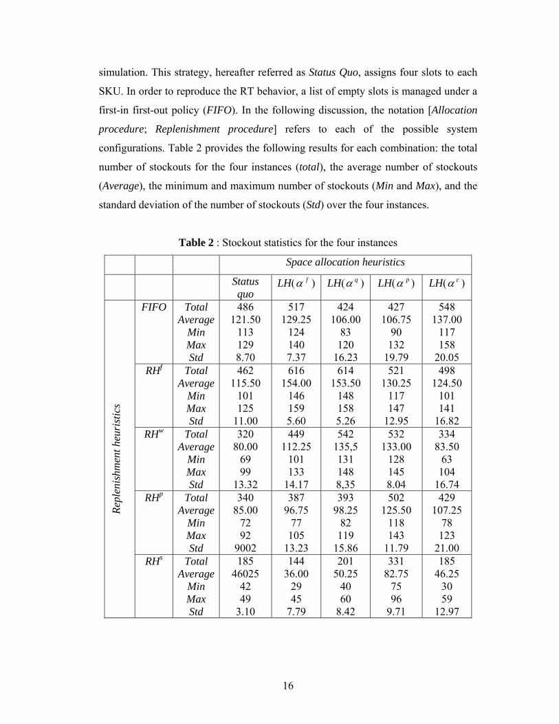
different picking lists, 145 344 lines and a total of 687 554 individual cases. Table 1

provides the figures for the eight weeks that were studied. Since inventory levels are

completely restored to their maximums each weekend, each week's simulation is

independent from the others. As shown in Table 1, the demand during this period of

15

the year was fairly stable, so we decided to split our data set into two subsets: the

design set and the test set. The design set, which contains the first four weeks of data,

was used as “historical data” to design the system (i.e., run the space allocation

heuristics and determine the best number of slots for each SKU). The test set,

containing the data for weeks five to eight, was used to evaluate the performance of

the space allocations through simulation. Each week was considered as an

independent instance of the problem, which allowed us to reproduce the real

decisional context of a warehouse manager looking at the sales history to decide how

many slots to allocate to each SKU for the coming week.

Table 1 : Numbers of picking lists, lines and cases per week

Week

1 2 3 4 5 6 7 8

Picking lists 349 341 336 304 340 340 343 355

Lines 18643 18548 17904 16281 18603 18331 18400 18634

Cases 89793 84622 81039 73189 81431 96124 93920 87436

The system parameters were set to the values provided by recent measurement and

time studies: case handling time, tc = 4 seconds; walking time to complete the

conveyor circuit, tw = 388 seconds per order; and replenishment time, tr = 240

seconds. The order pickers were considered to work 95 hours per week. All

computations were done on a P4 3.2Ghz, running under Windows XP, with 1GB

RAM.

Simulation results

As explained above, the data from weeks 1 to 4 were used as input for the space

allocation heuristic H(α ) and IIH in order to allocate space. Each of the five resulting

allocations were then combined with each of the replenishment methods (RHf, RHw,

RHp and RHs) and tested using the four remaining instances (i.e., weeks). The space

allocation strategy currently used in the distribution center was also included in our

16

simulation. This strategy, hereafter referred as Status Quo, assigns four slots to each

SKU. In order to reproduce the RT behavior, a list of empty slots is managed under a

first-in first-out policy (FIFO). In the following discussion, the notation [Allocation

procedure; Replenishment procedure] refers to each of the possible system

configurations. Table 2 provides the following results for each combination: the total

number of stockouts for the four instances (total), the average number of stockouts

(Average), the minimum and maximum number of stockouts (Min and Max), and the

standard deviation of the number of stockouts (Std) over the four instances.

Table 2 : Stockout statistics for the four instances

Space allocation heuristics

Status quo

LH( fα ) LH( qα ) LH( pα ) LH( cα )

FIFO Total Average

Min Max Std

486 121.50

113 129 8.70

517 129.25

124 140 7.37

424 106.00

83 120

16.23

427 106.75

90 132

19.79

548 137.00

117 158

20.05 RHf Total

Average Min Max Std

462 115.50

101 125

11.00

616 154.00

146 159 5.60

614 153.50

148 158 5.26

521 130.25

117 147

12.95

498 124.50

101 141

16.82 RHw Total

Average Min Max Std

320 80.00

69 99

13.32

449 112.25

101 133

14.17

542 135,5 131 148 8,35

532 133.00

128 145 8.04

334 83.50

63 104

16.74 RHp Total

Average Min Max Std

340 85.00

72 92

9002

387 96.75

77 105

13.23

393 98.25

82 119

15.86

502 125.50

118 143

11.79

429 107.25

78 123

21.00

Repl

enis

hmen

t heu

rist

ics

RHs Total Average

Min Max Std

185 46025

42 49

3.10

144 36.00

29 45

7.79

201 50.25

40 60

8.42

331 82.75

75 96

9.71

185 46.25

30 59

12.97

17

Let us first analyze the behavior of the replenishment methods. If the space allocation

method remains unchanged (i.e., Status quo is maintained), the RHs method, which

replenishes the next SKU that will experience a stockout, outperforms the others, with

a total of only 185 stockouts. Compared to the current replenishment method (FIFO)

with its 486 stockouts, implementing RHs would mean a reduction of 301 stockouts

and a time savings of 30.1 hours, assuming that every time a stockout occurs, it takes

an average of 6 minutes for the stock to be replenished. In fact, used in combination

with any of the space allocation heuristics, the RHs replenishment method produces

the lowest number of stockouts, which clearly demonstrates its dominance. Both RHp

and RHw obtained the second best results twice, while the current method, FIFO,

obtained the second best results only once. In light of these results, it appears that the

actual replenishment method is clearly inefficient.

Let us now analyze the space allocation methods. Although RHs is clearly the best

replenishment method, there is no one dominant space allocation heuristic. Line by

line, the Status quo, which allocates four positions to each SKU, surprisingly

produces the best results three times—in combination with RHf, RHw and RHp. The

other most advantageous combinations are [LH( qα ) ; FIFO] and [LH( fα ) ; RHs].

Based on these results, we can conclude that the performance of the space allocation

methods is correlated to the replenishment method used. For example, when the RHf

replenishment method is used, no space allocation heuristic is able to produce good

results: the number of stockouts is never lower than 462. In addition, although the

space allocation heuristic LH( fα ) generates only 144 stockouts when used in

combination with RHs, it generates 517 stockouts when associated with the

replenishment method currently in use. These results indicate the existence of a

strong and complex relationship between space allocation and the work of the

replenishment technician.

Table 3 presents the same data for the case in which each space allocation heuristic is

followed by the IIH improvement heuristic. The IIH heuristic stops after β = 15

18

consecutives iterations without reducing the number of stockouts. The additional line

∆ in each table row gives the total reduction in the number of stockouts with respect

to the results produced without IIH.

Table 3 : Stockout statistics for the four instances with IIH

Space allocation heuristics

Status quo + IIH

LH( fα ) + IIH

LH( qα ) + IIH

LH( pα ) + IIH

LH( cα ) + IIH

FIFO Total ∆

Average Min Max Std

176 310

44.00 23 69

21.31

211 306

52.75 31 76

19.26

230 194

57.50 33 85

21.44

198 229

49.50 33 75

20.04

500 48

50.00 33 79

21.32 RHf Total

∆ Average

Min Max Std

329 133

82.25 52 115

25.97

605 11

151.25 147 155 4.35

558 56

139.50 130 144 6.61

308 213

77.00 53 110

25.34

429 69

107.25 77 132

23.20 RHw Total

∆ Average

Min Max Std

217 103

54.25 33 81

19.96

233 216

58.25 40 88

20.79

509 33

127.25 121 136 7.50

309 223

77.25 65 100

15.52

241 93

60.25 42 88

19.60 RHp Total

∆ Average

Min Max Std

167 137

41.75 31 56

10.90

175 212

43.75 31 58

12.45

249 144

62.25 50 79

12.15

329 173

82.25 59 108

20.21

184 245

46.00 36 61

11.86

Repl

enis

hmen

tt he

uris

tics

RHs Total ∆

Average Min Max Std

182 3

45.50 40 52

5.51

107 37

26.75 21 32

4.50

197 4

49.25 34 61

11.32

328 3

82.00 73 96

10.23

185 0

46.25 30 59

12.97

In almost all cases, the extra calculations required by IIH produce better solutions.

The best improvement (310 stockouts) is obtained with the combination [Status Quo

19

+ IIH ; FIFO]. The overall best combination is [LH( fα ) + IIH ; RHs], which

produces 107 stockouts, or an average of 26.75 per week. This is a reduction of 342

stockouts over the company’s current solution, and represents a time savings of about

34.2 hours. Judging by the standard deviation of only 4.5 stockouts per week, the

robustness of the combination [LH( fα ) + IIH ; RHs] is also quite good.

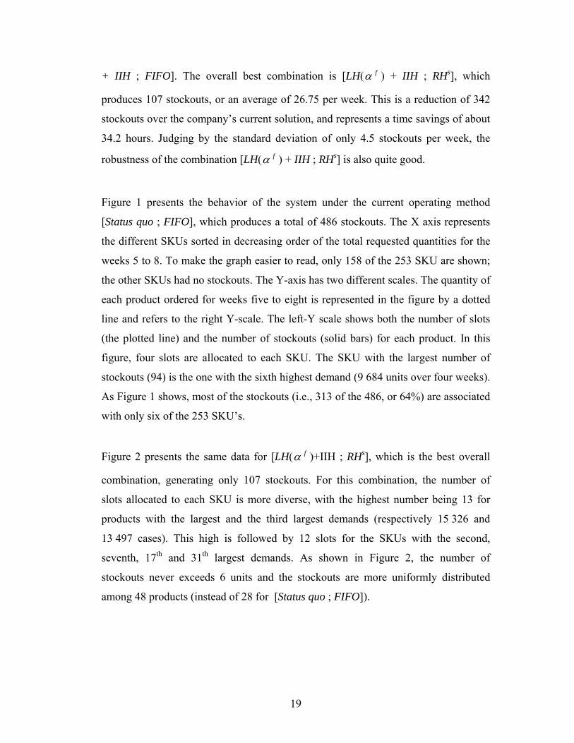
Figure 1 presents the behavior of the system under the current operating method

[Status quo ; FIFO], which produces a total of 486 stockouts. The X axis represents

the different SKUs sorted in decreasing order of the total requested quantities for the

weeks 5 to 8. To make the graph easier to read, only 158 of the 253 SKU are shown;

the other SKUs had no stockouts. The Y-axis has two different scales. The quantity of

each product ordered for weeks five to eight is represented in the figure by a dotted

line and refers to the right Y-scale. The left-Y scale shows both the number of slots

(the plotted line) and the number of stockouts (solid bars) for each product. In this

figure, four slots are allocated to each SKU. The SKU with the largest number of

stockouts (94) is the one with the sixth highest demand (9 684 units over four weeks).

As Figure 1 shows, most of the stockouts (i.e., 313 of the 486, or 64%) are associated

with only six of the 253 SKU’s.

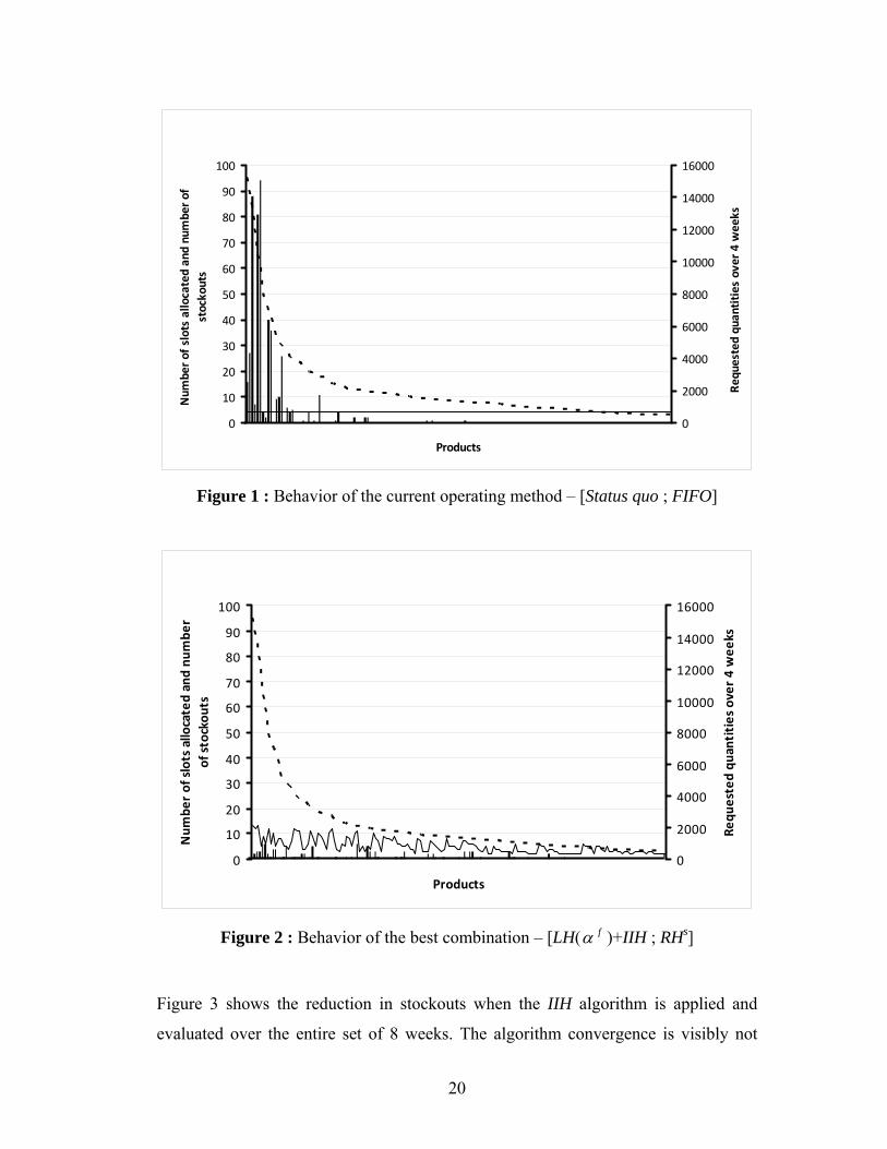
Figure 2 presents the same data for [LH( fα )+IIH ; RHs], which is the best overall

combination, generating only 107 stockouts. For this combination, the number of

slots allocated to each SKU is more diverse, with the highest number being 13 for

products with the largest and the third largest demands (respectively 15 326 and

13 497 cases). This high is followed by 12 slots for the SKUs with the second,

seventh, 17th and 31th largest demands. As shown in Figure 2, the number of

stockouts never exceeds 6 units and the stockouts are more uniformly distributed

among 48 products (instead of 28 for [Status quo ; FIFO]).

20

0

10

20

30

40

50

60

70

80

90

100

Products

Num

ber of slots allocated and number of 

stockouts

0

2000

4000

6000

8000

10000

12000

14000

16000

Requested

 quantities over 4 weeks

Figure 1 : Behavior of the current operating method – [Status quo ; FIFO]

0

10

20

30

40

50

60

70

80

90

100

Products

Num

ber of slots allocated and nu

mbe

r of stockou

ts

0

2000

4000

6000

8000

10000

12000

14000

16000

Requ

ested qu

antities over 4 wee

ks

Figure 2 : Behavior of the best combination – [LH( fα )+IIH ; RHs]

Figure 3 shows the reduction in stockouts when the IIH algorithm is applied and

evaluated over the entire set of 8 weeks. The algorithm convergence is visibly not

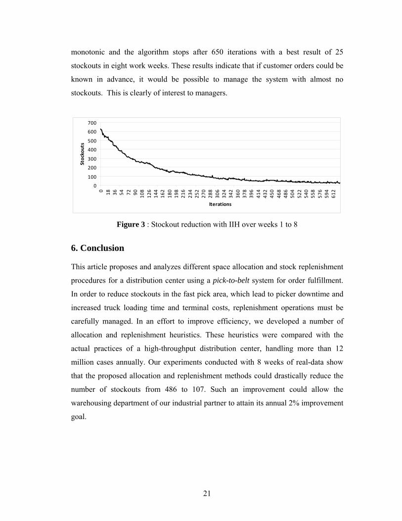
21

monotonic and the algorithm stops after 650 iterations with a best result of 25

stockouts in eight work weeks. These results indicate that if customer orders could be

known in advance, it would be possible to manage the system with almost no

stockouts. This is clearly of interest to managers.

0

100

200

300

400

500

600

700

0 18 36 54 72 90 108

126

144

162

180

198

216

234

252

270

288

306

324

342

360

378

396

414

432

450

468

486

504

522

540

558

576

594

612

Iterations

Stockouts

Figure 3 : Stockout reduction with IIH over weeks 1 to 8

6. Conclusion This article proposes and analyzes different space allocation and stock replenishment

procedures for a distribution center using a pick-to-belt system for order fulfillment.

In order to reduce stockouts in the fast pick area, which lead to picker downtime and

increased truck loading time and terminal costs, replenishment operations must be

carefully managed. In an effort to improve efficiency, we developed a number of

allocation and replenishment heuristics. These heuristics were compared with the

actual practices of a high-throughput distribution center, handling more than 12

million cases annually. Our experiments conducted with 8 weeks of real-data show

that the proposed allocation and replenishment methods could drastically reduce the

number of stockouts from 486 to 107. Such an improvement could allow the

warehousing department of our industrial partner to attain its annual 2% improvement

goal.

22

Acknowledgement

This work was partially supported by grants [OPG 0293307 and OPG 0172633]

from the Canadian Natural Sciences and Engineering Research Council (NSERC).

This support is gratefully acknowledged. We would also like to thank the logistics

manager of our industrial partner for providing us with the relevant data.

References Bartholdi J. J. & Hackman S. T., Warehouse & Distribution Science, Release 0.85,

Revised January 20, 2007. Available on line at :

http://www2.isye.gatech.edu/~jjb/

wh/book/editions/history.html (accessed June 2007).

Cormier G. & Gunn E. A., A review of warehouse models. European Journal of

Operational Research, 58, 3-13, 1992.

De Koster R., Le-Duc T. & Roodbergen K. J., Design and control of warehouse order

picking: A literature review. European Journal of Operational Research, 182,

481-501, 2007.

De Koster R. & Van Der Poort E., Routing orderpickers in a warehouse : a comparison

between optimal and heuristic solutions. IIE Transactions, 1998, 30, 469-480

Goetschalckx M. and Ratliff H. D., Order picking in an aisle. IIE Transactions, 20,

1988, 53-62.

Hwang H. S. & Cho G. S., A performance evaluation model for order picking

warehouse design. Computers & Industrial Engineering, 51, 335-342, 2006.

Laporte G., The traveling salesman problem: An overview of exact and approximate

algorithms. European Journal of Operational Research, 59, 1992, 231-247.

Lawler E. L., Lenstra J. K., Rinnooy Kan A. H. G. & Shmoys D. B., The traveling

salesman problem. A guided tour of combinatorial optimisation. John Wiley &

Sons, 1985.

Malmborg C. J. & Bhaskaran K., A revised proof of optimality for the cube-per-order

index rule for stored item location. Applied Mathelatical Modelling, 1990, 14, 87-

95.

23

Petersen II C. G., An evaluation of order picking routeing policies. International

Journal of Operations & Production Management, 17, 11, 1997, 1098-1111.

Petersen II C. G., The impact of routing and storage policies on warehouse efficiency.

International Journal of Operations & Production Management. 19, 1053-1064,

1999.

Petersen II C. G., An evaluation of order picking policies for mail order companies.

Production and Operations Management, 9, 4, 2000, 319-335.

Petersen C. G. & Aase G., A comparison of picking, storage, and routing policies in

manual order picking. International Journal of Production Economics, 92, 2004,

11-19.

Petersen II C. G. & Schmenner R. W., An evaluation of routing and volume-based

storage policies in an order picking operation. Decision Science, 30, 2, 1999, 481-

501.

Ratliff H. D. and Rosenthal A. S., Order-picking in a rectangular warehouse : A

solvable case of the traveling salesman problem. Operations Research, 31, 1983,

507-521.

Rouwenhorst B., Reuter B., Stockrahm V., van Houtum G. J., Mantel R. J. & Zijm W.

H. M., Warehouse design and control : Framework and literature review.

European Journal of Operational Research, 122, 2000, 515-533.

Tompkins J. A. & Smith J. D., The warehouse management handbook.Tompkins Press,

second edition, 1998, Ann Arbor, MI.

Tompkins J. A., White J. A., Bozer Y. A., Frazelle E. H., Tanchoco J. M. A. &

Trevino J., Facilities Planning, Wiley & Sons, New York, Second edition 1996.

van der Berg J. P., A literature survey on planning and control of warehousing systems.

IIE Transactions, 1999, 31, 751-762.

van den Berg J. P., Sharp G. P., Gademann A. J. R. M. (Noud) and Pochet Y., Forward-

reserve allocation in a warehouse with unit-load replenishments.

European Journal of Operational Research, 111, 1998, 98-113

van den Berg J. P. & Zijm W. H. M., Models for warehouse management :

Classification and examples. International Journal of Production Economics, 59,

519-528, 1999.