Sonic Crystal Noise Barriers - Open Research Online oro ...
353
Open Research Online The Open University’s repository of research publications and other research outputs Sonic Crystal Noise Barriers Thesis How to cite: Chong, Yung Boon (2012). Sonic Crystal Noise Barriers. PhD thesis The Open University. For guidance on citations see FAQs . c 2012 The Author https://creativecommons.org/licenses/by-nc-nd/4.0/ Version: Version of Record Link(s) to article on publisher’s website: http://dx.doi.org/doi:10.21954/ou.ro.0000add6 Copyright and Moral Rights for the articles on this site are retained by the individual authors and/or other copyright owners. For more information on Open Research Online’s data policy on reuse of materials please consult the policies page. oro.open.ac.uk
-
Upload
khangminh22 -
Category
Documents
-
view
0 -
download
0
Transcript of Sonic Crystal Noise Barriers - Open Research Online oro ...

Open Research OnlineThe Open University’s repository of research publicationsand other research outputs
Sonic Crystal Noise BarriersThesisHow to cite:
Chong, Yung Boon (2012). Sonic Crystal Noise Barriers. PhD thesis The Open University.
For guidance on citations see FAQs.
c© 2012 The Author
https://creativecommons.org/licenses/by-nc-nd/4.0/
Version: Version of Record
Link(s) to article on publisher’s website:http://dx.doi.org/doi:10.21954/ou.ro.0000add6
Copyright and Moral Rights for the articles on this site are retained by the individual authors and/or other copyrightowners. For more information on Open Research Online’s data policy on reuse of materials please consult the policiespage.
oro.open.ac.uk

The Open University
Sonic Crystal Noise Barriers
by
Yung Boon Chong, BEng
A doctoral thesis submitted in partial fulfilment for the degree of
Doctor of Philosophy
in the
Department of Design, Development, Environment and Materials
Faculty of Mathematics, Computing and Technology
The Open University Milton Keynes
United Kingdom
November 2012
© 2012 Y.B. Chong

Certificate of Originality This is to certify that I am responsible for the work submitted in this thesis, that the original work is my own except as specified in acknowledgements, in text or in bibliography, and that neither the thesis nor the original work contained therein has been submitted to this or any other institution for a degree.
_____________________________ (Signature)
(Y.B. Chong)
_____________________________ (Date)
Faculty of Mathematics, Computing and Technology
Department of Design, Development,
Environment and Materials
The Open University
Walton Hall
Milton Keynes
MK7 6AA
United Kingdom
Tel +44 (0) 1908 653686
Fax +44 (0) 1908 652192
www.open.ac.uk

I
Acknowledgements This dissertation would not have been possible without the guidance and the help of several individuals who in one way or another contributed and extended their valuable assistance in the preparation and completion of this study. First of all, I would like to express my deepest gratitude to my supervisors Prof. Keith Attenborough and Dr. Shahram Taherzadeh for their unfailing guidance, support and patience during the years I worked on this research and dissertation at The Open University, United Kingdom. Also, through their meticulous reviews and keen observations, the quality of my research is enhanced. Working with them has not only opened my eyes to the multiple facets of acoustics, but also they played a shaping role in my personal development. It has been great pleasure and inspiration to work with them. Thanks are also due to Dr. David Brian Sharp who has shared his valuable and helpful comments. This research has been undertaken with the support of Engineering and Physical Science Research Council, United Kingdom (Grant number EP/E062806/1) which is gratefully acknowledged. I should also mention with gratitude that my graduate studies were supported by the University as part of the employee subsidy scheme. I could not fulfil my dream to pursue this higher degree without these sponsors. Sincere appreciations are given to our project collaborators Dr. Olga Umnova and Dr. Anton Krynkin from the University of Salford for providing their expertise and the many productive and challenging discussions. I also wish to acknowledge the help from Dr. Anton Krynkin for providing and guiding the use of the MST algorithms. Special thanks are due to Dr. Juan V. Sanchez-Perez and Dr. Vincent Romero Garcia from the Polytechnic University of Valencia for collaboration in several aspects of the work related to this Thesis, notably in respect of the influence of ground effect on sonic crystal performance. The assistance given by the staff and fellow research student in the Acoustic Research Group throughout the research periods are acknowledged and appreciated. I am indebted to Dr. Roland Kruse, Dr. Toby Hill, Dr. Ho-chul Shin and Dr. Adrien Mamou-mani for their constructive advice on my research. Special thanks to Peter Seabrook (Project Officer) who contributed much time and effort to source and fabricated specimens to be used for the sonic crystal both in laboratory and outdoor measurements. I should mention with gratitude to Roger Frith and Mikki Thomas (Project Officers) for their help rendered during the laboratory measurements. Credit also goes to Stan Hiller (Project Officer) from the Material’s Department for his expertise in performing tensile strength testing for the latex specimen used in our design. I would also like to thank Imran Bashir (PhD student) for his insightful suggestions, discussions and help rendered. Last, but not least, I am truly grateful to my family whose care and support have been the important factors which let me seek this higher degree without worries. This dissertation is dedicated to them.

II
Preface This PhD Thesis entitled “Sonic Crystal Noise Barriers” contains the results of
research undertaken at the Department of Design, Development, Environment
and Materials of the Open University, United Kingdom. The Supervisors
involved in this research are Prof. Keith Attenborough, Dr. Shahram
Taherzadeh and Dr. David Brian Sharp who are all members of academic
staff at the Open University. This research was funded by the Engineering
and Physical Science Research Council (EPSRC), United Kingdom (Grant
number EP/E062806/1). Under an EPSRC joint research scheme, this
research closely collaborated with the School of Computing Science and
Engineering, University of Salford, United Kingdom (Grant number
EP/E063136/1). During the course of research, there was a close
collaboration with Dr. Olga Umnova and Dr. Anton Krynkin from University of
Salford. Their works on the development of the Multiple Scattering Theory
(MST) and computational model (rigid, elastic shell, composite scatterers and
sonic crystal above a ground surface) have been used extensively in this
Thesis (Chapter 3, 6, 7 and 8). An alternative modelling using Finite Element
Method (FEM) and experimental works are developed and performed at the
Open University and Diglis Weir, Worcester. The sonic crystals work on Diglis
Weir arose from an opportunity due to the “Organ of Corti” project, (see
details in Section 5.6). Based on the outcome of the research findings, there
has been a total of 3 peer reviewed journal papers and 7 conference
proceedings published. The list of publications is provided on the next page.

III
List of Publications
International journals
1) A. Kyrnkin, O. Umnova, J.V. Sanchez-Perez, A.Y.B. Chong, S. Taherzadeh, K. Attenborough, “Acoustic insertion loss due to two dimensional periodic arrays of circular cylinders parallel to a nearby surface”, J. Acoust. Soc. Am., 130, (6) (2011).
2) A. Kyrnkin, O. Umnova, A.Y.B. Chong, S. Taherzadeh, K. Attenborough, “Scattering by coupled resonating elements in air”, J. Phys. D: Applied Physics, 44, (12), 125501 (2011).
3) A. Kyrnkin, O. Umnova, Y.B. Chong, S. Taherzadeh, K. Attenborough, “Predictions and measurements of sound transmission through a periodic array of elastic shells in air”, J. Acoust. Soc. Am., 128, (6)
(2010).
Conference proceedings
1) Y.B. Chong, S. Taherzadeh, K. Attenborough, “Numerical and experimental studies of sonic crystal noise barriers”, Universities Transport Studies Group conference 2011, Milton Keynes, United Kingdom.
2) J.V. Sanchez-Perez, V. Romero-Garcia, K. Attenborough, S. Taherzadeh, Y.B. Chong, “The influence of the ground on the attenuation properties of sonic crystal barriers”, 2nd Pan-American/Iberian Meeting on Acoustics 2010, Cancun, Mexico.
3) K. Attenborough, Y.B. Chong, S. Taherzadeh, “Resonant elements for sonic crystal barriers”, 2nd Pan-American/Iberian Meeting on Acoustics 2010, Cancun, Mexico.
4) A. Kyrnkin, O. Umnova, Y.B. Chong, S. Taherzadeh, K. Attenborough, “Sonic crystal noise barriers made of resonant elements”, International Congress of Acoustic 2010, Sydney, Australia.
5) Y.B. Chong, S. Taherzadeh, K. Attenborough, “The performance of vertical and horizontal sonic crystal noise barriers above a ground plane”, InterNoise 2010 conference, Lisbon, Portugal.
6) Y.B. Chong, S. Taherzadeh, K. Attenborough, “laboratory studies on sonic crystal noise barrier”, EuroNoise 2009 conference, Edinburgh, United Kingdom.
7) Y.B. Chong, S. Taherzadeh, K. Attenborough, “laboratory studies on sonic crystal noise barrier”, InterNoise 2009 conference, Ottawa, Canada.

IV
Contents Acknowledgments ------------------------------------------------ I
Preface ------------------------------------------------------------------ II
List of Publications ------------------------------------------------ III
Contents ---------------------------------------------------------------- IV
List of Figures ------------------------------------------------------- IX
List of Tables ------------------------------------------------------- XXII
List of Symbols ------------------------------------------------------- XXIII
Abstracts ---------------------------------------------------------------- XXVIII
Chapter 1: Introduction
1.1) Fundamentals of acoustics ------------------------------- 1 1.2) Complex number notation ------------------------------- 6 1.3) The conventional road traffic noise barrier ---------- 7 1.4) Sonic Crystals ----------------------------------------------- 9
1.4.1) History ----------------------------------------------- 9 1.4.2) Crystallography -------------------------------------- 13
1.5) Aims and thesis organisation ----------------------------- 23
Chapter 2: The Plane Wave Expansion (PWE) Method
2.1) Introduction --------------------------------------------------- 26 2.1.1) Two-dimensional periodicity ------------------- 27
2.2) Plane Wave Expansion Results ------------------------ 32 2.2.1) Band structure of Sonic Crystal -------------- 32 2.2.2) Predicted influence of the lattice ------------- 35 constant 2.2.3) Predicted influence of filling fraction ------- 37 2.2.4) Predicted influence of material ---------------- 40
parameters
V
Chapter 3: Multiple Scattering Theory (MST)
3.1) Introduction ---------------------------------------------------- 43 3.2) Multipole method for circular scatterers in 2- ---------- 47
dimensional system 3.3) Plane wave scattering model ----------------------------- 51 3.4) Cylindrical wave scattering model ----------------------- 56 3.5) Simulation and results -------------------------------------- 58
Chapter 4: The Finite Element Method (FEM)
4.1) Introduction --------------------------------------------------- 63 4.2) Acoustic modelling in COMSOL® Multiphysics ------ 65 4.3) FEM computed results -------------------------------------- 70 4.4) Investigation of accuracy of FEM ----------------------- 73 4.5) Investigation of sonic crystal performance ----------- 77
using scatterers with different shapes 4.5.1) Triangular scatterers ---------------------------- 77 4.5.2) Square scatterers -------------------------------- 80 4.5.3) Elliptical shape scatterers --------------------- 81
4.6) Investigation of arrays with different lattice ---------- 85 arrangements
4.7) Perfectly Matched Layers (PML) ------------------------ 87
Chapter 5: Measurement Techniques
5.1) Introduction ---------------------------------------------------- 90 5.2) Laboratory measurements using Maximum- --------- 92
Length Sequence System Analyzer (MLSSA) 5.2.1) Introduction to MLSSA --------------------------- 92 5.2.2) MLSSA setup, data acquisition and ---------- 95
analysis in laboratory 5.2.3) Influence on the different of windowing ----- 101
size for signal post processing 5.2.4) Influence on the effects of different ----------- 103
window functions for signal post processing 5.2.5) Influence of the floor grille in the --------------- 104
anechoic chamber 5.2.6) Influence of microphone size ------------------ 105
5.3) Excess Attenuation (EA) measurements in the ------ 106 laboratory
5.4) Outdoor Measurements (Open University -------------- 107 barrier test site)
5.4.1) Data acquisition and data analysis ----------- 111 for the outdoor measurements
5.4.2) Microphone calibration --------------------------- 115 5.4.3) Measuring meteorological conditions -------- 118
using a sonic anemometer 5.5) Swept sine signal --------------------------------------------- 121

VI
5.6) Outdoor in situ measurements of a sonic -------------- 123 crystal at Diglis Weir, Worcester
5.6.1) Measurement arrangement --------------------- 125 5.6.2) Measurement results ------------------------------ 127 5.6.3) Modelling with Multiple Scattering Theory -- 128
(MST) assuming a single point source 5.6.4) Modelling with multiple point sources -------- 132
on a line
Chapter 6: Improving the performance of sonic crystal noise
barriers by using resonant elastic shell elements 6.1) Introduction --------------------------------------------------- 136 6.2) Acoustics of single elastic shells ------------------------ 139 6.3) Proof of breathing mode concept using modal ------ 153
analysis through FEM single elastic shell in vacuum (undamped)
6.4) Proof of breathing mode concept using modal ------ 156 analysis through FEM - single elastic shell in air (damped)
6.5) Influence of shell diameter -------------------------------- 158 6.6) Influence of wall thickness -------------------------------- 160 6.7) Influence of material stiffness ---------------------------- 162 6.8) Influence of tensioning -------------------------------------- 163 6.9) Arrays of elastic shells -------------------------------------- 164 6.10) Influence of angle between source-receiver -------- 168
and array axes 6.11) Calculation of transmission for a single latex ------ 171
cylinder using FEM 6.12) Fabrication of specimen and effect of ---------------- 173
non-uniformity in latex scatterers 6.13) Effect of gluing on the resonances of the shell ----- 176 6.14) Effect of disc attachment on the latex scatterer ---- 180 6.15) Industrial latex array results ------------------------------ 183
Chapter 7: Enhancing the performance of sonic crystal noise
barriers by using Split Ring Resonator (SRR) and composite cylinders
7.1) Introduction --------------------------------------------------- 185 7.2) Working principles of a conventional Helmholtz ---- 186
resonator 7.3) SRR array design ------------------------------------------- 190 7.4) Numerical model ------------------------------------------- 191 7.5) SRR results --------------------------------------------------- 192
7.5.1) Single SRR ---------------------------------------- 192 7.5.2) Single SRR – influence of slit orientation -- 194 7.5.3) The influence of the size of slit opening ---- 196
in a single SRR 7.5.4) Arrays of SRRs ------------------------------------ 196 7.5.5) Outdoor measurements (SRR array) ------ 198

VII
7.6) Coupled resonating elements ----------------------------- 202 7.6.1) Semi-analytical formulation of single -------- 204
composite scatterer 7.6.2) FEM modelling of single composite ---------- 212
scatterer 7.6.3) Results for single composite scatterer ------ 213 7.6.4) Semi-analytical formulation of an array ----- 220
of composite cylinders 7.6.5) Results for array of composite scatterers -- 222
7.7) Influence of adjustable parameters on the ------------- 229 acoustical performance of composite scatterer arrays outdoors
7.7.1) The predicted influence of the elastic ------- 230 shell outer diameter
7.7.2) The predicted influence of elastic shell ----- 231 wall thickness
7.7.3) Predicted influence of the slit widths --------- 232 in the outer PVC cylinder
Chapter 8: Performance of sonic crystal noise barriers above a
ground surface 8.1) Introduction ----------------------------------------------------- 234 8.2) Ground impedance models -------------------------------- 236 8.3) Ground impedance measurement ------------------------ 239
8.3.1) Single microphone method --------------------- 239 8.3.2) Transfer function method --------------------- 239
8.4) Excess Attenuation (EA) and Level Difference ------- 243 (LD) results
8.4.1) EA spectra over MDF 1 board ------------------ 243 8.4.2) EA spectra over MDF 2 board ------------------ 245 8.4.3) EA spectra over glass board -------------------- 247 8.4.4) EA spectra over polyurethane foam layer --- 249 8.4.5) Level Difference (LD) spectra over ------------ 250
MDF 2 board 8.4.6) LD spectra over asphalt (Outdoor in situ ---- 251
measurement) 8.4.7) LD spectra over grass covered ground ------ 252
in situ 8.5) Analytical formulation for array of sonic crystals ------ 253
with their axes parallel to a rigid ground 8.5.1) Rigid scatterers -------------------------------------- 254 8.5.2) Elastic shell scatterers ---------------------------- 259 8.5.3) Laboratory measurements ------------------------ 260 8.5.4) Comparisons of data and predictions ---------- 263
for rigid cylinders array with their axes parallel to a rigid ground
8.5.5) Comparisons of data and predictions ---------- 267 for elastic shells array with their axes parallel to a rigid ground
VIII
8.6) Laboratories studies on rigid and elastic cylinder --------- 271
arrays with their axes parallel to a finite impedance ground and normal to a rigid ground
8.6.1) IL spectra for horizontal rigid cylinders ------- 271 array over a finite impedance ground
8.6.2) IL spectra for horizontal elastic shell ---------- 273 cylinders array over a finite impedance ground
8.6.3) Laboratories studies on a vertical axis -------- 274 cylinder array over a horizontal acoustically rigid ground (MDF 1)
8.7) Laboratories studies on vertical axis array over ------ 276 acoustically rigid ground (glass plate)
Chapter 9: Summary and concluding remarks
9.1) Summary of contents ------------------------------------ 278 9.2) Concluding remarks ------------------------------------ 289 9.3) Suggestions for future work ----------------------------- 291
Appendix A (Matlab® coding for PWE) --------------------- XXIX
Appendix B (Graf’s Additional Theorem) ----------------- XXXII
Appendix C
i) Experimental study of the use of Polyethylene ------ XXXV
scatterers in a sonic crystal noise barrier
ii) Experimental study of the use of periodic ------------- XXXVII
stiffening along the scatterer length
Appendix D (Tensile test) --------------------------------------- XXXIX
Appendix E (Meteorological conditions)
i) Compass plots on 12/5/11 ------------------------------ XLIII
ii) Compass plots on 27/5/11 ------------------------------ XLIV
References --------------------------------------------------------- XLV

IX
List of Figures
Fig. Descriptions Page
1.1 Air molecule patterns during propagation of plane acoustic wave through infinite space: (a) the arrangement of air molecules at equilibrium positions without any external force excitation, (b) during plane acoustic waves propagating through the air medium and (c) during transverse wave propagation through a homogeneous solid material.
------- 3
1.2 Simple harmonic waves illustrated in polar form. ------- 6 1.3 Normalised traffic noise spectrum. ------- 8 1.4 Minimalistic sculpture by Eusebio Sempere. ------- 10 1.5 Sound attenuation as a function of frequency, also
known as Insertion Loss. ------- 11
1.6 An ideal crystal structure. ------- 13 1.7 Schematic illustrations of crystal structure (a) one-
dimensional, (b) two-dimensional and (c) three-dimensional.
------- 14
1.8 The five fundamental 2-Dimensionals Bravais lattices (a) square, (b) oblique, (c) rectangular, (d) centered rectangular and (e) hexagonal.
------- 15
1.9 Illustration of direct lattice points (black dot), reciprocal lattice points (white dots) and a shaded region indicating the reciprocal space.
------- 16
1.10 Bragg diffraction. ------- 18 1.11 2D schematic of square lattice array showing the
Brillouin zone (triangle depicted by points , X and M ). mM VZ , and ss VZ , denote the acoustic
impedance and velocity for the medium and scatterer respectively).
------- 22
2.1 Plane wave expansion computed band structure for a homogeneous medium with equivalent material properties of air. Inset: Brillouin zone. refers to
[1,0] direction, M refers to [1,1] direction and refers to the wave vector varying from [1,0] to [1,1] on the extreme side of the Brillouin zone.
------- 33

X
2.2 The left hand panel shows the plane wave expansion computed band structure for a SC consisting of cylindrical PVC scatterers embedded in air in a square array with lattice constant L of 0.069 m and filling fraction of 50%. The right hand panel shows the laboratory measured IL spectrum for 7x3 array
for the [1, 0] direction. Inset: schematic of a Brillouin zone. refers to [1,0] direction, refers
to [1,1] direction and refers to the wave vector varying from [1,0] to [1,1]. The (red) dotted box indicates a full bandgap and the (blue) shaded regions indicate partial bandgap.
------- 34
2.3 Plane wave expansion predictions of the effect of varying the lattice constant in a SC comprising of 0.055 m diameter PVC cylinders embedded in air. Lattice constant L of (a) 0.08 m and (b) 0.135 m. Left hand panels show the band structure of the corresponding SC and right hand panels show the measured IL for the different lattice parameters.
------- 35
2.4 Plane Wave Expansion predictions of the band structure with Lattice constant fixed at 0.135 m and varying scatterer diameters (a) 0.055, (b) 0.09, (c) 0.11 and (d) 0.13 m.
------- 38
2.5 Plane Wave Expansion predictions of the influence of material parameters on the band structure. The lattice constant is fixed at 0.069 m and scatterers are made from different materials (a) PVC, (b) silicone rubber, (c) steel (d) PMMA and (e) wood. (f) PVC scatterers embedded in water.
------- 41
3.1 Plan view of two identical cylinders and corresponding cartesian and polar coordinates.
------- 48
3.2 Example scenario including an array of rigid scatterers.
------- 59
3.3 MST predictions and measured Insertion Loss spectra for square lattice arrays of rigid circular scatterers of 0.055 m diameter with lattice constants of (a) 0.069, (b) 0.08 and (c) 0.135 m respectively. Both plane and cylindrical waves are compared for all three cases.
------- 60
3.4 MST predictions and measured Insertion Loss spectra for square lattice arrays of rigid circular scatterers of 0.055 m diameter with lattice constants
of 0.069. Different truncation number of 5 , ... 2, ,1M
is used for the MST predictions for (a) plane wave and (b) cylindrical wave.
------- 61
4.1 Definition of domain discretized using triangular shape finite elements.
------- 66
4.2 Definition of geometry for a rectangular domain modelled as air and an incoming cylindrical wave source.
------- 69

XI
4.3 COMSOL® computed pressure map for a rectangular domain modelled as air and an incoming plane (a) or cylindrical wave (b) source.
------- 70
4.4 COMSOL® computed pressure maps for 7x3 array of sonic crystal (acoustically hard scatterer) modelled in rectangular air domain. Cylindrical waves is performed and pressure maps at 200 Hz, 1.2, 3, 4, 4.5 and 5 kHz are shown for figure (a), (b), (c), (d) and (e) respectively.
------- 71
4.5 FEM predictions and laboratory measured Insertion Loss spectra for 7x3 square lattice arrays of rigid scatterers of radius 0.0275 m with lattice constant 0.135 m. FEM predictions are performed with plane and cylindrical wave sources for a rectangular domain modelled as air.
------- 72
4.6 FEM predicted pressure plots for cylindrical waves with different mesh element sizes.
------- 75
4.7 Sound pressure level spectra at single point position for FEM computations of the field due to a cylindrical wave computed using different mesh element sizes.
------- 76
4.8 FEM (COMSOL®) predicted pressure maps comparing three different arrangements (top to bottom) and 2 frequencies pressure maps for each arrangement (left 1.3 kHz and right 2.3 kHz) of 7x3 triangular rigid scatterer arrays (square lattice) with lattice constant of 0.135 m.
------- 78
4.9 FEM predictions of Insertion Loss spectra for 7x3 square lattice arrays of triangular rigid scatterers with lattice constant 0.135 m. A cylindrical wave source is assumed and a rectangular domain is modelled as air.
------- 79
4.10 FEM (COMSOL®) predicted pressure maps comparing two 7x3 square scatterer arrangements (square lattice with lattice constant of 0.135 m) at 4.3 kHz.
------- 80
4.11 FEM predictions of Insertion Loss spectra for two arrangements of 7x3 square lattice arrays of square rigid scatterers and a reference array of cylindrical rigid scatterers with lattice constant 0.135 m. A cylindrical wave source is assumed and a rectangular domain is modelled as air.
------- 80
4.12 FEM (COMSOL®) predicted pressure maps for three 7x3 arrangements of elliptical rigid scatterers (square lattice) with lattice constant of 0.135 m at 1.5 kHz.
------- 82
4.13 FEM predicted Insertion Loss spectra for 7x3 square lattice arrays of elliptical rigid scatterers with lattice constant 0.135 m compared with that predicted for an equivalent cylindrical scatterer array. For the FEM predictions a cylindrical wave source is assumed and the rectangular domain is modelled as air.
------- 82
XII
4.14 FEM predictions of Insertion Loss spectra for 7x3 square lattice arrays of the best performing triangular, square and elliptical rigid scatterer arrays compared to that predicted for the reference cylindrical scatterer array.
------- 83
4.15
FEM (COMSOL®) predicted pressure maps at 1.5 kHz for 7x3 arrays of cylindrical rigid scatterers with lattice constant of 0.135 m (a) hexagonal lattice and (b) square lattice.
------- 84
4.16 FEM predictions of Insertion Loss spectra for 7x3 hexagonal and square arrays of cylindrical rigid scatterers with lattice constant 0.135 m. FEM prediction are performed with cylindrical wave source and a rectangular domain modelled as air. The cylindrical wave source is located at 1.5 m away from the front face of the array and the receiver is positioned 0.05 m from the nearest face of the array but on the opposite side of the source.
------- 85
4.17 Implementation of PMLs around a 7x3 square lattice array of circular scatterers (a) location of PMLs and (b) FEM-computed pressure map at 1.2 kHz.
------- 87
4.18 FEM predictions (with and without PML) compared to laboratory measurements of Insertion Loss spectra for a 7x3 square lattice array of circular rigid scatterers with a lattice constant 0.135 m.
------- 87
5.1 Flow diagram for a typical impulse response measurement.
------- 93
5.2 Linear feedback shift register for generation of a MLS (of length 24 - 1= 15) signal.
------- 94
5.3 MLSSA system with audio patch cable connecting analogue output to input.
------- 95
5.4 System loopback test - MLS time signal. ------- 96 5.5 Transfer function for system loopback test - MLS
power spectrum. ------- 96
5.6 Laboratory measuring system incorporating MLSSA. ------- 99 5.7 (a) Supporting base plate for 7x3 arrays of PVC or
elastic cylinders. 55 mm diameter holes for PVC cylinders. 5 mm diameter holes for elastic shell using bolt and nut securing system. (b) Lower end of an elastic shell showing plastic pipe for air inlet and mounting bolt.
------- 100
5.8 (a) Plan view of the source, receiver and array in the laboratory measurements at normal incidence (b) the corresponding side view. Refer to chapters 2, 3, 4, 6 and 7 for the outer diameters and lattice constants used.
------- 101
5.9 MLSSA time signals for direct and total transmitted fields.
------- 102
5.10 MLSSA Frequency spectra for direct and total transmitted fields.
------- 103
XIII
5.11 Insertion Loss (IL) spectrum using MLSSA of 7x3 square lattice arrays of rigid PVC scatterers of outer diameter 0.055 m and lattice constant 0.069 m. Frequency resolution at 48 Hz.
------- 103
5.12 Power spectra for different window size taken in calculating the FFT for total transmitted fields.
------- 104
5.13 Insertion loss spectra for 7x3 array of PVC scatterers of outer diameter 0.055 m and lattice constant of 0.069 m using different FFT filters.
------- 106
5.14 Insertion loss spectra for single latex scatterer. ------- 107 5.15 Insertion loss spectra for single PVC scatterer of
outer diameter 0.11 m, wall thickness of 0.003 m with 4 symmetrical slits size of 0.012 m.
------- 108
5.16 Arrangement for measuring Excess attenuation spectra above a Medium Density Fibreboard (MDF) in the laboratory.
------- 109
5.17 Drilled Metal panels used for securing the scatterers. ------- 111 5.18 The outdoor noise barrier site, (a) source side of
barrier showing SC and conventional noise barrier sections and (b) rear side of barrier.
------- 112
5.19 Plan view of the outdoor measurement arrangement using simultaneous multiple channels.
------- 112
5.20 Graphical User Interface (GUI) Traffic Noise Analyzer implemented in Matlab®.
------- 113
5.21 Example time domain signals measured outdoors (a) during SC barrier measurements using B&K microphones and (b) during fence measurements using ACO microphones.
------- 115
5.22 Example power spectra measured outdoors (a) during SC barrier measurements using B&K microphones and (b) during fence measurements using ACO microphones.
------- 116
5.23 Example background noise power spectra measured at the barrier test site (a) during SC barrier measurements using B&K microphones and (b) during fence measurements using ACO microphones.
------- 117
5.24 Setup for B&K microphone calibration. ------- 118 5.25 Calibration results for B&K microphones. ------- 119 5.26 Sonic anemometer mounted above the
instrumentation cabin. ------- 121
5.27 Data from sonic anemometer. ------- 121 5.28 Example of a deduced wind vector diagram. ------- 122 5.29 Swept sine signal generated electrically. ------- 123 5.30 Direct and total transmitted fields measured using the
swept sine method in the laboratory. ------- 123
5.31 Comparison of IL spectra due to a single PVC scatterer of OD 0.11 m, WT 0.003 m with 4 symmetrical slits of 0.012 m measured using the MLS and swept sine methods.
------- 124

XIV
5.32 (a) Plan view schematic of the sonic crystal arrangement and microphone locations at Diglis weir, Worcester. (b) Aerial map of the site showing where the sonic crystal was situated (picture taken from Google map).
------- 126
5.33 Mean IL spectrum (average of 3 measurements) with error bars for receiver position Pt 1.
------- 127
5.34 The original receiver position Pt 1 and 4 other perturbed positions made for MST modelling.
------- 128
5.35 Predicted IL spectra of all the 5 individual positions (Pt 1 original and 4 perturbed positions) and the averaged IL spectrum. Source is located at coordinates (0, 0).
------- 129
5.36 Measured (averaged of 3 measurements) and predicted (averaged of 5 receiver points) IL spectra for receiver position Pt 1 with source located at coordinates (0, 0).
------- 130
5.37 Predicted IL spectra at all the 5 individual positions (Pt 1 original and 4 perturbed positions) and the averaged predicted IL spectrum. The point source is assumed to be located at coordinates (0, 10).
------- 131
5.38 Measured (averaged of 3 measurements) and predicted (averaged of 5 points) IL spectra for receiver position Pt 1 with source located at coordinates (0, 10).
------- 132
5.39 Picture illustration for the location of the 10 sources (S1 to S10) and the position of sonic crystal.
------- 134
5.40 Measured (average of 3 measurements) and MST predicted with multiple point sources IL spectra for receiver position Pt 1 (averaged over 5 receiver points for each individual source).
------- 135
6.1 Example predictions of the two basic mode shapes of a freely supported cylinder – (a) radial (b) beam modes up to fourth order (c) the combination of the first radial mode (mode 0) and up to the fourth order of bending modes (d) the combination of the first radial mode (mode 0) and up to the third order of axial modes [103].
------- 141
6.2 Cross-section of an elastic shell in the primary cell of doubly periodic array.
------- 142
6.3 Measured (solid black line) and MST predicted (broken blue line) IL spectra for single latex scatterer of outer diameter (OD) 0.055 m, wall thickness (WT) 0.00025 m and length of 2 m. For comparison the IL spectrum measured for an acoustically “rigid” Poly Vinyl Chloride (PVC) pipe with similar diameter and length is shown also (broken red line).
------- 154
6.4 2-Dimensional modal analysis showing static deformation plots in sequence (a-f) on the “Breathing mode” shape of elastic element in vacuum.
------- 157
XV
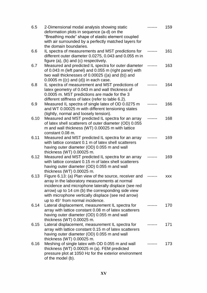
6.5 2-Dimensional modal analysis showing static deformation plots in sequence (a-d) on the “Breathing mode” shape of elastic element coupled with air surrounded by a perfectly matched layers for the domain boundaries.
------- 159
6.6 IL spectra of measurements and MST predictions for different outer diameter 0.0275, 0.043 and 0.055 m in figure (a), (b) and (c) respectively.
------- 161
6.7 Measured and predicted IL spectra for outer diameter of 0.043 m (left panel) and 0.055 m (right panel) with two wall thicknesses of 0.00025 ((a) and (b)) and 0.0005 m ((c) and (d)) in each case.
------- 163
6.8 IL spectra of measurement and MST predictions of latex geometry of 0.043 m and wall thickness of 0.0005 m. MST predictions are made for the 3 different stiffness of latex (refer to table 6.2).
------- 164
6.9 Measured IL spectra of single latex of OD 0.0275 m and WT 0.00025 m with different tensioning states (tightly, normal and loosely tension).
------- 166
6.10 Measured and MST predicted IL spectra for an array of latex shell scatterers of outer diameter (OD) 0.055 m and wall thickness (WT) 0.00025 m with lattice constant 0.08 m.
------- 168
6.11 Measured and MST predicted IL spectra for an array with lattice constant 0.1 m of latex shell scatterers having outer diameter (OD) 0.055 m and wall thickness (WT) 0.00025 m.
------- 169
6.12 Measured and MST predicted IL spectra for an array with lattice constant 0.15 m of latex shell scatterers having outer diameter (OD) 0.055 m and wall thickness (WT) 0.00025 m.
------- 169
6.13 Figure 6.13: (a) Plan view of the source, receiver and array in the laboratory measurements at normal incidence and microphone laterally displace (see red arrow) up to 14 cm (b) the corresponding side view with microphone vertically displace (see red arrow)
up to 45 from normal incidence.
------- xxx
6.14 Lateral displacement, measurement IL spectra for array with lattice constant 0.08 m of latex scatterers having outer diameter (OD) 0.055 m and wall thickness (WT) 0.00025 m.
------- 170
6.15 Lateral displacement, measurement IL spectra for array with lattice constant 0.15 m of latex scatterers having outer diameter (OD) 0.055 m and wall thickness (WT) 0.00025 m.
------- 171
6.16 Meshing of single latex with OD 0.055 m and wall thickness (WT) 0.00025 m (a). FEM predicted pressure plot at 1050 Hz for the exterior environment of the model (b).
------- 173
XVI
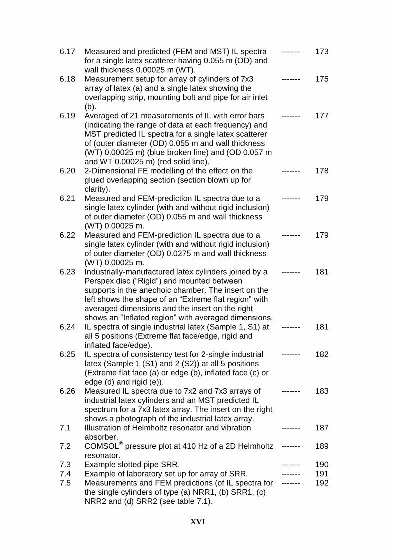
6.17 Measured and predicted (FEM and MST) IL spectra for a single latex scatterer having 0.055 m (OD) and wall thickness 0.00025 m (WT).
------- 173
6.18 Measurement setup for array of cylinders of 7x3 array of latex (a) and a single latex showing the overlapping strip, mounting bolt and pipe for air inlet (b).
------- 175
6.19 Averaged of 21 measurements of IL with error bars (indicating the range of data at each frequency) and MST predicted IL spectra for a single latex scatterer of (outer diameter (OD) 0.055 m and wall thickness (WT) 0.00025 m) (blue broken line) and (OD 0.057 m and WT 0.00025 m) (red solid line).
------- 177
6.20 2-Dimensional FE modelling of the effect on the glued overlapping section (section blown up for clarity).
------- 178
6.21 Measured and FEM-prediction IL spectra due to a single latex cylinder (with and without rigid inclusion) of outer diameter (OD) 0.055 m and wall thickness (WT) 0.00025 m.
------- 179
6.22 Measured and FEM-prediction IL spectra due to a single latex cylinder (with and without rigid inclusion) of outer diameter (OD) 0.0275 m and wall thickness (WT) 0.00025 m.
------- 179
6.23 Industrially-manufactured latex cylinders joined by a Perspex disc (“Rigid”) and mounted between supports in the anechoic chamber. The insert on the left shows the shape of an “Extreme flat region” with averaged dimensions and the insert on the right shows an “Inflated region” with averaged dimensions.
------- 181
6.24 IL spectra of single industrial latex (Sample 1, S1) at all 5 positions (Extreme flat face/edge, rigid and inflated face/edge).
------- 181
6.25 IL spectra of consistency test for 2-single industrial latex (Sample 1 (S1) and 2 (S2)) at all 5 positions (Extreme flat face (a) or edge (b), inflated face (c) or edge (d) and rigid (e)).
------- 182
6.26 Measured IL spectra due to 7x2 and 7x3 arrays of industrial latex cylinders and an MST predicted IL spectrum for a 7x3 latex array. The insert on the right shows a photograph of the industrial latex array.
------- 183
7.1 Illustration of Helmholtz resonator and vibration absorber.
------- 187
7.2 COMSOL® pressure plot at 410 Hz of a 2D Helmholtz resonator.
------- 189
7.3 Example slotted pipe SRR. ------- 190 7.4 Example of laboratory set up for array of SRR. ------- 191 7.5 Measurements and FEM predictions (of IL spectra for
the single cylinders of type (a) NRR1, (b) SRR1, (c) NRR2 and (d) SRR2 (see table 7.1).
------- 192

XVII
7.6 Pressure maps predicted using COMSOL® for incident cylindrical waves on (a) a single scatterer SRR1 at 700 Hz and (b) a single scatterer SRR2 at 300 Hz.
------- 193
7.7 Single SRR orientation. ------- 194 7.8 Measured Insertion Loss spectra of the radiation
pattern of single SRR (refer to figure 7.7 for the definition of the orientated angle).
------- 195
7.9 FEM predictions of IL spectra for the single SRR1 with increasing slit width.
------- 195
7.10 Predicted and measured Insertion Loss spectra due to square arrays of SRR1 (refer to table 7.1) with lattice constants of (a) 135, (b) 80 and (c) 70 mm. Also shown in the left hand panels are pressure maps at the first Bragg diffraction frequency for the corresponding array geometry.
------- 197
7.11 Example outdoor measurement arrangement (a) lateral displacements of the microphone along the length of barrier. (b) Vertical displacement of the microphone along the height of barrier.
------- 199
7.12 Predicted and measured Insertion Loss spectra at outdoor for square arrays of reference no slit cylinders (NRR2) and SRR scatterers (SRR2) with lattice constants, L, of 160 mm (refer to table 7.1). (a) 54x3 square lattice array of scatterer NRR2. (b) 54x3 square array of scatterer SRR2. Corresponding pressure maps at 500 Hz are shown in the left-hand panels.
------- 199
7.13 Measured Insertion Loss spectra of various lateral angles at outdoor for square lattice arrays of SRR2 (see table 7.1) with lattice constant of 0.16 m.
------- 200
7.14 Measured Insertion Loss spectra due to outdoor square arrays of split ring resonators, SRR2 (see table 7.1) with lattice constant of 0.16 m at various inclinations of the source-receiver axis.
------- 201
7.15 (a) Cross section of composite element consisting of a concentric arrangement of an outer 4-slit rigid cylinder and an inner elastic cylindrical shell. (b) Geometry of the slit.
------- 204
7.16 (a) Measured and FEM predicted IL spectra due to a single PVC cylinder with 4 symmetrical slits (component of SRR3, see table 7.2). (b) FEM (COMSOL®) predictions of pressure maps at 2 kHz for a similar scatterer showing the interior and exterior environments.
------- 213
7.17 Measured and predicted (MST and FEM) IL spectra for a single composite scatterer, SRR3 (refer to table 7.2).
------- 213

XVIII
7.18 FEM (COMSOL®) predicted pressure maps at 1 kHz for SRR3 showing the exterior and annular cavity environments (a), interior environment of the latex cavity (b) and static deformation plot on the “Breathing mode” shape of elastic element in air.
------- 215
7.19 Measured and predicted (MST and FEM) IL spectra for a single composite scatterer, SRR4 (refer to table 7.2).
------- 216
7.20 Measured IL spectra for a single composite scatterer, SRR3 and it’s own component (refer to table 7.2).
------- 216
7.21 Measured (in laboratory) IL spectra for a single concentric cylinder (SRR4) and its components (i.e. single 4 slit PVC and latex, see table 7.2).
------- 217
7.22 (a) Measured and MST predicted IL spectra for 7x3 PVC array of lattice constant 0.08 m (PVC with 4 symmetrical slits, component of SRR3, see table 7.2). (b) FEM (COMSOL®) predicted pressure maps at 2 kHz for a similar scatterer array showing the interior and exterior environments.
------- 220
7.23 Measured and FEM predicted IL spectra for 7x3 array of composite scatterers SRR3 (see table 7.2) arranged in square lattice of lattice constant 0.08 m.
------- 221
7.24 Measured IL spectra due to 7x3 arrays of composite scatterer, SRR3 and the two components separately (refer to table 7.2).
------- 222
7.25 Average of 8-day measurements (outdoor) and MST IL spectra for 54x3 arrays of composite scatterers SRR4 (see table 7.2) arranged in square lattice of lattice constant 0.16 m. Error bars are plotted for the measured spectrum.
------- 223
7.26 Measured IL spectral of 36x4 and 54x3 arrays of concentric cylinders (averaged of all 8 measurements).
------- 224
7.27 Measured IL spectral of 54x3 arrays of concentric cylinders (averaged of 8 measurements) and rigid no slit cylinders (average of 3 measurements).
------- 224
7.28 Measured IL spectral of 54x3 arrays of concentric cylinders (averaged of 8 measurements) and fence (average of 8 measurements).
------- 225
7.29 IL spectra for the MST predicted effect on changing latex outer diameter for 54x3 square lattice array of SRR4 scatterer with lattice constant of 0.16 m.
------- 226
7.30 IL spectra for the MST predicted effect on changing latex wall thickness for 54x3 square lattice array of SRR4 scatterer with lattice constant of 0.16 m.
------- 227
7.31 MST predicted IL spectra for 54x3 square lattice array with lattice constant of 0.16 m as the slit widths in the outer PVC cylinders are varied from 3 to 12 mm.
------- 228
XIX
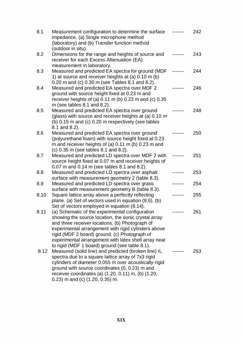
8.1 Measurement configuration to determine the surface impedance. (a) Single microphone method (laboratory) and (b) Transfer function method (outdoor in situ).
------- 242
8.2 Dimensions for the range and heights of source and receiver for each Excess Attenuation (EA) measurement in laboratory.
------- 243
8.3 Measured and predicted EA spectra for ground (MDF 1) at source and receiver heights at (a) 0.10 m (b) 0.20 m and (c) 0.30 m (see Tables 8.1 and 8.2).
------- 244
8.4 Measured and predicted EA spectra over MDF 2 ground with source height fixed at 0.23 m and receiver heights of (a) 0.11 m (b) 0.23 m and (c) 0.35 m (see tables 8.1 and 8.2).
------- 246
8.5 Measured and predicted EA spectra over ground (glass) with source and receiver heights at (a) 0.10 m (b) 0.15 m and (c) 0.20 m respectively (see tables 8.1 and 8.2).
------- 248
8.6 Measured and predicted EA spectra over ground (polyurethane foam) with source height fixed at 0.23 m and receiver heights of (a) 0.11 m (b) 0.23 m and (c) 0.35 m (see tables 8.1 and 8.2).
------- 250
8.7 Measured and predicted LD spectra over MDF 2 with source height fixed at 0.07 m and receiver heights of 0.07 m and 0.14 m (see tables 8.1 and 8.2).
------- 251
8.8 Measured and predicted LD spectra over asphalt surface with measurement geometry 2 (table 8.3).
------- 253
8.9 Measured and predicted LD spectra over grass surface with measurement geometry B (table 8.3).
------- 254
8.10 Square lattice array above a perfectly reflecting plane. (a) Set of vectors used in equation (8.6). (b) Set of vectors employed in equation (8.14).
------- 255
8.11 (a) Schematic of the experimental configuration showing the source location, the sonic crystal array and three receiver locations. (b) Photograph of experimental arrangement with rigid cylinders above rigid (MDF 2 board) ground. (c) Photograph of experimental arrangement with latex shell array near to rigid (MDF 1 board) ground (see table 8.1).
------- 261
8.12 Measured (solid line) and predicted (broken line) IL spectra due to a square lattice array of 7x3 rigid cylinders of diameter 0.055 m over acoustically-rigid ground with source coordinates (0, 0.23) m and receiver coordinates (a) (1.20, 0.11) m, (b) (1.20, 0.23) m and (c) (1.20, 0.35) m.
------- 263

XX
8.13 Measured insertion loss spectra due to a 7x3 rigid cylinder array over acoustically rigid ground (solid line) compared with that of an identical array measured in free field (broken line) as well as measured inverted excess attenuation (dash dot line) The source is at coordinates (0.0.235) m and the receiver coordinates are (a) (1.20, 0.11) m, and (c) (1.20, 0.35) m.
------- 265
8.14 Measured (solid line) and predicted (broken line) IL spectra due to a square lattice array of 7x3 latex shell cylinders of diameter 0.055 m over acoustically-rigid ground with source coordinates (0, 0.23) m and receiver coordinates (a) (0.8, 0.11) m, and (c) (0.8, 0.35) m.
------- 267
8.15 Measured insertion loss spectra due to a 7x3 latex shell cylinders array over acoustically rigid ground (solid line) compared with that of an identical array measured in free field (broken line) as well as measured inverted excess attenuation (dash dot line) The source is at coordinates (0.0.235) m and the receiver coordinates are (a) (1.20, 0.11) m, and (c) (1.20, 0.35) m.
------- 269
8.16 Measured insertion loss spectra due to a 7x3 rigid cylinders array over finite impedance (Polyurethane foam) ground (solid line) compared with that due to an identical array measured in free field (broken line) as well as measured inverted excess attenuation spectra of the ground (dash dot line) taken at same source-receiver distances. The source is at coordinates (0.0.235) m and the receiver coordinates are (a) (1.20, 0.11) m, and (c) (1.20, 0.35) m.
------- 271
8.17 Measured insertion loss spectra due to a 7x3 latex shell cylinder array over finite impedance (Polyurethane foam) ground (solid line) compared with that due to an identical array measured in free field (broken line) as well as measured inverted excess attenuation spectra due to the ground alone (dash dot line) The source is at coordinates (0.0.235) m and the receiver coordinates are (a) (1.20, 0.11) m, (b) (1.20, 0.23) m and (c) (1.20, 0.35) m.
------- 273
8.18 7x3 PVC cylinders in vertical array orientation above a MDF ground (MDF 1).
------- 274
8.19 Measured insertion loss spectra of vertical array with source and receiver at 0.3m height with and without the MDF 1 ground plane. Measured inverted excess attenuation spectra of the ground (dash dot line).
------- 275
XXI
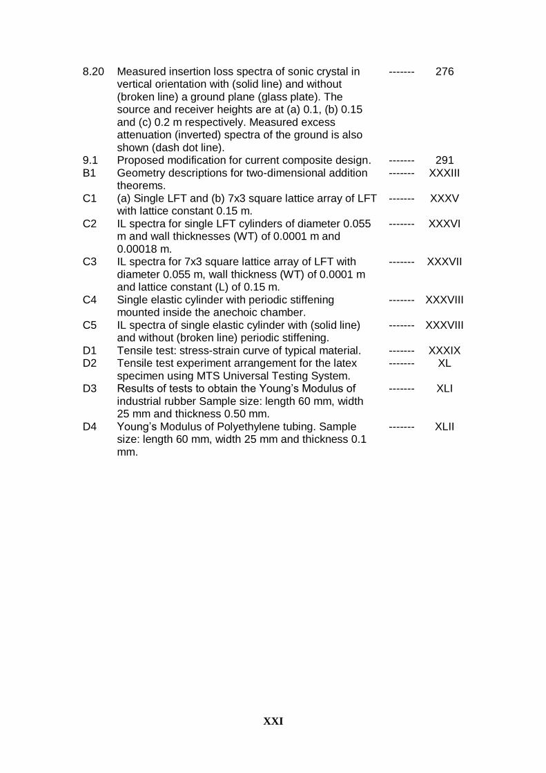
8.20 Measured insertion loss spectra of sonic crystal in vertical orientation with (solid line) and without (broken line) a ground plane (glass plate). The source and receiver heights are at (a) 0.1, (b) 0.15 and (c) 0.2 m respectively. Measured excess attenuation (inverted) spectra of the ground is also shown (dash dot line).
------- 276
9.1 Proposed modification for current composite design. ------- 291 B1 Geometry descriptions for two-dimensional addition
theorems. ------- XXXIII
C1 (a) Single LFT and (b) 7x3 square lattice array of LFT with lattice constant 0.15 m.
------- XXXV
C2 IL spectra for single LFT cylinders of diameter 0.055 m and wall thicknesses (WT) of 0.0001 m and 0.00018 m.
------- XXXVI
C3 IL spectra for 7x3 square lattice array of LFT with diameter 0.055 m, wall thickness (WT) of 0.0001 m and lattice constant (L) of 0.15 m.
------- XXXVII
C4 Single elastic cylinder with periodic stiffening mounted inside the anechoic chamber.
------- XXXVIII
C5 IL spectra of single elastic cylinder with (solid line) and without (broken line) periodic stiffening.
------- XXXVIII
D1 Tensile test: stress-strain curve of typical material. ------- XXXIX D2 Tensile test experiment arrangement for the latex
specimen using MTS Universal Testing System. ------- XL
D3 Results of tests to obtain the Young’s Modulus of industrial rubber Sample size: length 60 mm, width 25 mm and thickness 0.50 mm.
------- XLI
D4 Young’s Modulus of Polyethylene tubing. Sample size: length 60 mm, width 25 mm and thickness 0.1 mm.
------- XLII
XXII
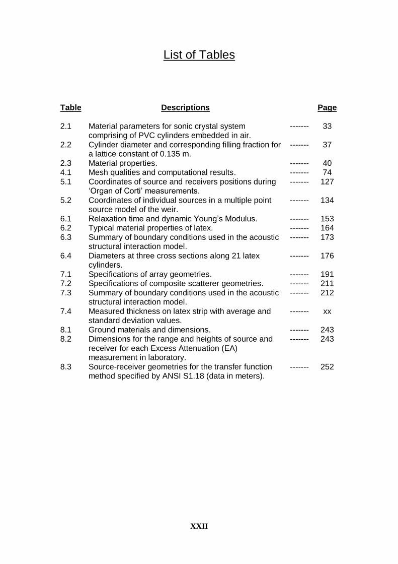
List of Tables Table Descriptions Page
2.1 Material parameters for sonic crystal system comprising of PVC cylinders embedded in air.
------- 33
2.2 Cylinder diameter and corresponding filling fraction for a lattice constant of 0.135 m.
------- 37
2.3 Material properties. ------- 40 4.1 Mesh qualities and computational results. ------- 74 5.1 Coordinates of source and receivers positions during
‘Organ of Corti’ measurements. ------- 127
5.2 Coordinates of individual sources in a multiple point source model of the weir.
------- 134
6.1 Relaxation time and dynamic Young’s Modulus. ------- 153 6.2 Typical material properties of latex. ------- 164 6.3 Summary of boundary conditions used in the acoustic
structural interaction model. ------- 173
6.4 Diameters at three cross sections along 21 latex cylinders.
------- 176
7.1 Specifications of array geometries. ------- 191 7.2 Specifications of composite scatterer geometries. ------- 211 7.3 Summary of boundary conditions used in the acoustic
structural interaction model. ------- 212
7.4 Measured thickness on latex strip with average and standard deviation values.
------- xx
8.1 Ground materials and dimensions. ------- 243 8.2 Dimensions for the range and heights of source and
receiver for each Excess Attenuation (EA) measurement in laboratory.
------- 243
8.3 Source-receiver geometries for the transfer function method specified by ANSI S1.18 (data in meters).
------- 252
XXIII
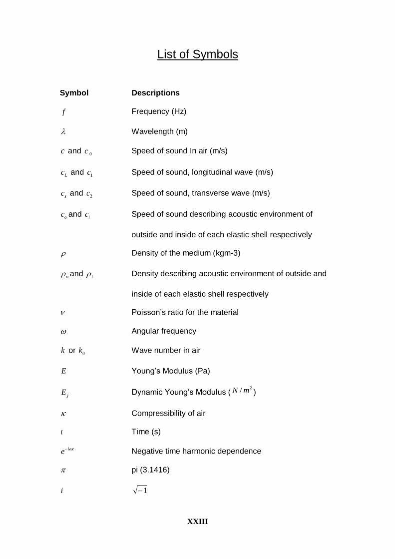
List of Symbols
Symbol Descriptions
f Frequency (Hz)
Wavelength (m)
c and 0c Speed of sound In air (m/s)
Lc and 1c Speed of sound, longitudinal wave (m/s)
sc and 2c Speed of sound, transverse wave (m/s)
oc and ic Speed of sound describing acoustic environment of
outside and inside of each elastic shell respectively
Density of the medium (kgm-3)
o and i Density describing acoustic environment of outside and
inside of each elastic shell respectively
Poisson’s ratio for the material
Angular frequency
k or 0k Wave number in air
E Young’s Modulus (Pa)
jE Dynamic Young’s Modulus (2/ mN )
Compressibility of air t Time (s)
tie
Negative time harmonic dependence
pi (3.1416)
i 1

XXIV
p Pressure (Pa)
IL Insertion Loss (dB)
DCIL Insertion Loss (dB) with source distance correction
directp Pressure (direct field, Pa)
dtransmittetotalp _ Pressure (total transmitted field, Pa)
)(r Vector for space r
ucA Area of the unit cell
cylA Area of the considered cylinder
G Reciprocal lattice of periodic structure
)(GF Structure factor
1J Bessel function of the first kind
'Gk
and eigen Eigenvector
)( and eigenf Eigenfrequencies
).(k Band structures
ff Filling fraction
Bragg Lowest Bragg band gap central frequency (square lattice
array)
HexBraggf _ Lowest Bragg band gap central frequency (Hexagonal
lattice array)
L Lattice constant
incp Incident wave (pressure, Pa)
j
scp Scattered wave by the j-th scatterer (superscript to
change for other scatterer eg. k )

XXV
zyx ,, Cartesian coordinates
jjr , Polar coordinates centred at the j-th cylinder
ja Radius of cylindrical j-th scatterer
2
2
2
2
1
22
xx
Laplacian
eB Unbounded exterior
n Incident wavefunction (outgoing cylindrical wavefunction
of n-order)
)1(
n Hankel function of n-order of the first kind
n Regular cylindrical wavefunctions of the first kind
(outgoing wave radiating from each cylinder)
nJ Bessel function of n-order of the first kind
nY Bessel function of n-order of the second kind
yxp , Pressure at position defined by Cartesian coordinates
qqrp , and ,rpo Pressure at position defined by polar coordinates
j
nZ and
m
nZ Impedance factor of j-th and m-th scatterer respectively
cZ Relative characteristic impedance
m
nA Unknown coefficient to be solved in Multiple Scattering
Theory model
jI Phase factor associated with the j-th cylinder
M Truncation number for Multiple Scattering Theory model
pinp _ Plane wave source (pressure, Pa)
cinp _ Cylindrical wave source (pressure, Pa)
XXVI
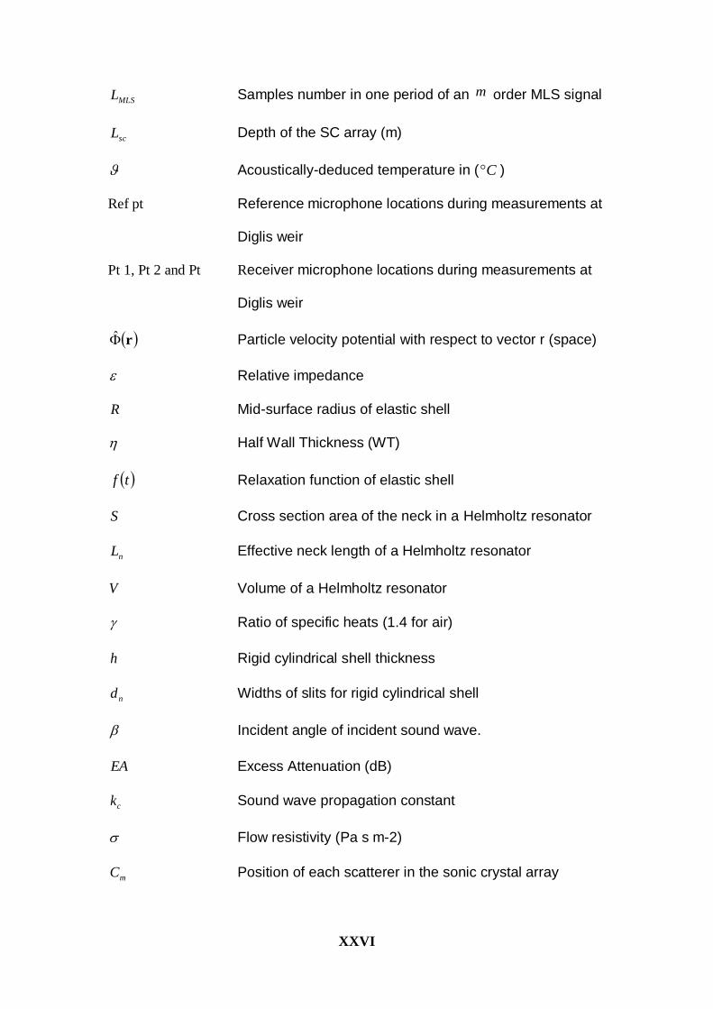
MLSL Samples number in one period of an m order MLS signal
scL Depth of the SC array (m)
Acoustically-deduced temperature in ( C )
Ref pt Reference microphone locations during measurements at
Diglis weir
Pt 1, Pt 2 and Pt Receiver microphone locations during measurements at
Diglis weir
r Particle velocity potential with respect to vector r (space)
Relative impedance
R Mid-surface radius of elastic shell
Half Wall Thickness (WT)
tf Relaxation function of elastic shell
S Cross section area of the neck in a Helmholtz resonator
nL Effective neck length of a Helmholtz resonator
V Volume of a Helmholtz resonator
Ratio of specific heats (1.4 for air)
h Rigid cylindrical shell thickness
nd Widths of slits for rigid cylindrical shell
Incident angle of incident sound wave.
EA Excess Attenuation (dB)
ck Sound wave propagation constant
Flow resistivity (Pa s m-2)
mC Position of each scatterer in the sonic crystal array
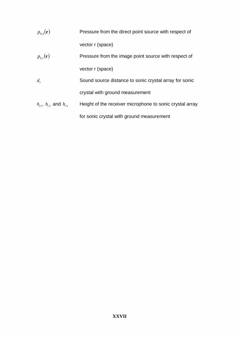
XXVII
rdp ,0 Pressure from the direct point source with respect of
vector r (space)
rrp ,0 Pressure from the image point source with respect of
vector r (space)
1d Sound source distance to sonic crystal array for sonic
crystal with ground measurement
1rh , 2rh and 3rh Height of the receiver microphone to sonic crystal array
for sonic crystal with ground measurement
XXVIII
Abstract An alternative road traffic noise barrier using an array of periodically arranged
vertical cylinders known as a Sonic Crystal (SC) is investigated. As a result of
multiple (Bragg) scattering, SCs exhibit a selective sound attenuation in
frequency bands called band gaps or stop bands related to the spacing and
size of the cylinders. Theoretical studies using Plane Wave Expansion (PWE),
Multiple Scattering Theory (MST) and Finite Element Method (FEM) have
enabled study of the performance of SC barriers. Strategies for improving the
band gaps by employing the intrinsic acoustic properties of the scatterer are
considered. The use of the tube cavity (Helmholtz type) resonances in Split
Ring Resonator (SRR) or the breathing mode resonances observed in thin
elastic shells is shown to increase Insertion loss (IL) in the low-frequency
range below the first Bragg stop band. Subsequently, a novel design of
composite scatterer uses these 2 types of cylindrical scatterer in a concentric
configuration with multiple symmetrical slits on the outer rigid shell. An array
of composite scatterers forms a system of coupled resonators and gives rise
to multiple low-frequency resonances. Measurements have been made in an
anechoic chamber and also on a full-scale prototypes outdoors under various
meteorological conditions. The experimental results are found to confirm the
existence of the Bragg band gaps for SC barriers and the predicted significant
improvements when locally resonant scatterers are used. The resonant arrays
are found to give rise to relatively angle-independent stop bands in a useful
range of frequencies. Good agreement between computational modelling and
experimental work is obtained. Studies have been made also of the acoustical
performances of regular arrays of cylindrical elements, with their axes aligned
and parallel to a ground plane including predictions and laboratory experiment

Chapter 1 Page 1
Chapter 1
Introduction 1.1) Fundamentals of acoustics
Sound is produced by movement of particles from a vibrating body in a
given medium. Sound can be described as the variations in pressure, particle
displacement or particle velocity that propagate through any medium. The
frequency of mechanical vibration associated with the sound wave can be
expressed by,
where,
f = frequency, reciprocal of a time period (Hz),
c = speed of sound in the medium (m/s),
= wavelength in which the distance of sound travels to complete one cycle
(m).
There are various types of wave motions studied in the science of
acoustics and the first mode pertaining to the propagation of wave in a
compressible fluid (i.e. air) will be introduced. Such acoustic waves produce
the aural sensation of sound we encounter in our everyday life. There are also
ultrasonic and infrasonic waves whose frequencies are beyond the audible
cf , (1.1)
Chapter 1 Page 2
limits of human which span from 20 Hz to 20 kHz. The molecules in the
undisturbed air can be assumed to be located at their equilibrium positions
(figure 1.1(a)). Acoustic waves propagating in air are described as longitudinal
(also known as compressional) waves, where the motion of the air molecules
transmitting the wave is parallel to the direction of propagation of the wave
creating a series of compressions and rarefactions as shown in figure 1.1(b).
At any instance, some of the particles move closer together and some are
further apart from their equilibrium positions. This type of wave mode can
travel through solid, liquid and gases. Another type of wave mode to consider
is the transverse (also known as shear) wave which is observed in solid
material. Without any disturbance, the atoms in a homogeneous solid material
are periodically arranged in space and for simplicity the atoms of the solid
material at equilibrium can be shown similarly as in figure 1.1(a). Contrary to
longitudinal wave, for transverse wave the particle move perpendicular to the
direction of propagation of the wave (see figure 1.1(c)).

Chapter 1 Page 3
Figure 1.1: Air molecule patterns during propagation of plane acoustic wave through
infinite space: (a) the arrangement of air molecules at equilibrium positions without
any external force excitation, (b) during plane acoustic waves propagating through the
air medium and (c) during transverse wave propagation through a homogeneous solid
material.
Using the equation of motion for elastic wave as described by Ewing
[1], the speed of sound for the longitudinal signal, Lc , can be determined from
the elastic constants of the underlying solid material by,
Particle at equilibrium (air/solid) (a)
Movement of air particle Direction of sound propagation
Region of compression
(Higher sound pressure)
Region of rarefaction
(Lower sound pressure)
(b)
Movement of particle in
solid material Direction of sound propagation
(c)
Higher pressure Lower pressure

Chapter 1 Page 4
211
1
EcL , (1.2)
where,
E Young’s Modulus,
density of the medium,
Poisson’s Ratio for the material.
whereas the speed of sound for the transverse wave can be calculated by,
21
Ecs
, (1.3)
In general, sound waves have non-planar waveforms and propagate in
a complex three dimensional manner. Consequently their motion can be
difficult to model. However, there are conditions under which a simplified
model is sufficient to describe acoustic wave propagation. This is the plane
wave model, in which sound waves are assumed to have the same direction
of propagation everywhere in space and their wavefronts are in planes
perpendicular to that direction of propagation.
For one-dimensional acoustic wave propagation (in air) in the x-
direction, the wave equation in terms of the pressure can be expressed as [2],
2
2
22
2 1
t
p
cx
p
, (1.4)
where c is the acoustic wave and t is the time. Note that 2
1
c where
and are the equilibrium density and the compressibility of air respectively. It
Movement of air molecules Direction of sound propagation (b)

Chapter 1 Page 5
is worth to note that equation 1.4 is restricted to homogeneous, isotropic fluid
and that small wave amplitude is assumed. For this reason, equation 1.4 is
often referred to as the linear, lossless wave equation.
Also Equation 1.4 can be modified with the assumption of time-harmonic
waves to give, the Helmholtz equation [3].
02
0
2 pkp , (1.5)
where p is the complex valued function and c
fk
2 is the wave number in
air.
A solution of the equation 1.4 has the following form
ctxGctxFtxp , , (1.6)
where F and G can be any function.
The first part of equation 1.6 refers to wave travelling in the x direction and
the second part of the equation refers to wave travelling in the x direction
respectively.

Chapter 1 Page 6
1.2) Complex number notation
It is convenient to use complex number notation when working with the
wave equation and its solution (see equation 1.5) due to the frequent interest
in simple harmonic waves. If the wave is not simple harmonic, the waveform
may be expanded by means of a Fourier series, which involves a series of
sinusoidal terms. In addition, a complex notation provides information for both
magnitude of a quantity and its phase angle. A complex number may be
written in Cartesian form,
),()( pipiyxp Im Re (1.7)
Where )( px Re = real and )( py Im = imaginary part of the complex
quantity. The complex quantity may also be written in polar form as,
,iepp (1.8)
And p is the magnitude and is the phase.
Figure 1.2: Simple harmonic waves illustrated in polar form.

Chapter 1 Page 7
1.3) The conventional road traffic noise barrier
Noise, defined as ‘unwanted sound’, is perceived as an environmental
stressor and nuisance. Road traffic noise is a prolific source of environmental
noise especially during the night time in urban areas and has been identified
as a major source of sleep disorder. Considering the continuing growth of
vehicular traffic and the large number of people exposed to it, disturbance of
sleep by road traffic noise has become an increasing important cause of
concern. Many studies have shown that exposure to road traffic noise may
induce further adverse health effects, including cardiovascular effects [4, 5
and 6]. Road traffic noise control can be achieved through better engineering
design of vehicles for example through quieter power plants, improvement of
road or tyre surfaces and controlling the flow of the vehicles in a particular
area. When these at-source strategies are insufficient to reduce noise, the
implementation of noise barriers is often necessary to further reduce noise
level at the receiver. Usually these noise barriers are airtight and sufficiently
dense to shield the noise from the source to the receiver. Most of the sound
energy reaches the receiver only as a result of diffraction around the barrier
edges [7]. In the UK, £5 million are spent annually on highway noise barrier
schemes with the intention to provide between 5 and 10 decibels (dB)
reduction within the protected areas [8]. The drawbacks of using such barrier
are the aesthetic impact such as restriction of view and natural lighting caused
by the barrier. One consequences of the adverse visual impact of opaque
barriers has been the design of transparent (Perspex) barriers. Anecdotally,
there are cases where an architect wishes to incorporate acoustic barriers
within a new construction but is unable to do so because of planning
Chapter 1 Page 8
constraints. The presence of barriers alters the wind profile and turbulence in
their vicinity and this can act to reduce the barrier effect in outdoors.
Fluctuations of ±2 m/s in the wind velocity can result in between 5 and 7 dB
degradation in the spectral values of insertion loss for frequencies above 800
– 1000 Hz [9].
The performance of barrier used along highways is affected by
temporal effects from moving traffic and by vehicle composition and speed.
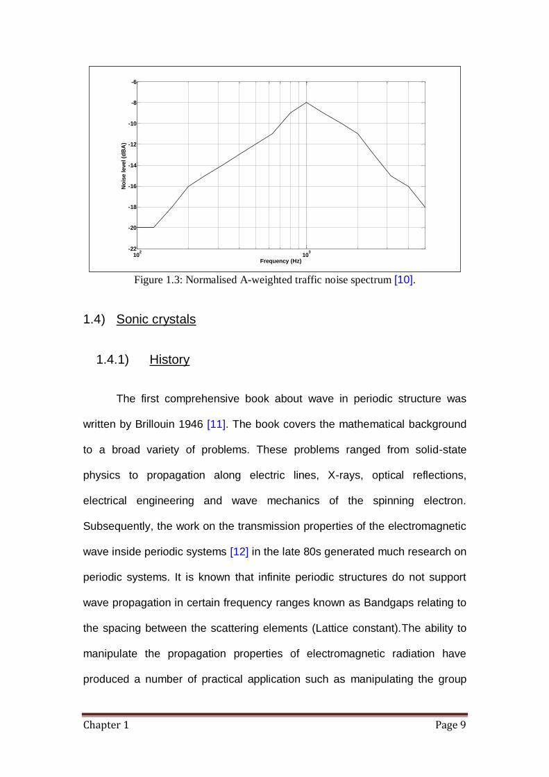
According to the British Standards (see figure 1.3), the normalised traffic
noise spectrum expressed in A-weighted decibel (dBA) lies between 100 Hz
to 5 KHz, with the main noise energy centred at 1 kHz [10]. It should be noted
that this normalised traffic noise spectrum does not take accounts into the
temporal effects. Although a more comprehensive traffic noise model
(European Commision project “Harmonoise”) [134] is available but for
simplicity the British Standards is used. Usually the effectiveness of a road
traffic noise barrier is measured by the Insertion Loss (IL) expressed in
Decibel (dB) shown in equation 1.9. directp and dtransmittetotalp _ denote the
pressure obtain without and with the barrier respectively.
dtransmittetotal
direct
p
pIL
_
10log20 , (1.9)
Chapter 1 Page 9
Figure 1.3: Normalised A-weighted traffic noise spectrum [10].
1.4) Sonic crystals
1.4.1) History
The first comprehensive book about wave in periodic structure was
written by Brillouin 1946 [11]. The book covers the mathematical background
to a broad variety of problems. These problems ranged from solid-state
physics to propagation along electric lines, X-rays, optical reflections,
electrical engineering and wave mechanics of the spinning electron.
Subsequently, the work on the transmission properties of the electromagnetic
wave inside periodic systems [12] in the late 80s generated much research on
periodic systems. It is known that infinite periodic structures do not support
wave propagation in certain frequency ranges known as Bandgaps relating to
the spacing between the scattering elements (Lattice constant).The ability to
manipulate the propagation properties of electromagnetic radiation have
produced a number of practical application such as manipulating the group
102
103
-22
-20
-18
-16
-14
-12
-10
-8
-6
Frequency (Hz)
No
ise level (d
BA
)
Chapter 1 Page 10
velocity of light [13], superlensing effect [14], designing highly efficient
nanoscale lasers [15], sharp bend radius waveguides [16], microwave
cloaking devices [17], optical computer chips [18] and enhancing surface
mounted microwave antennas [19].
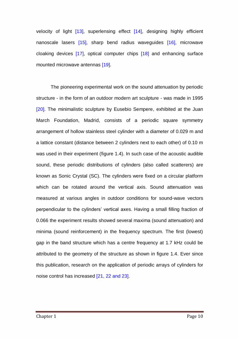
The pioneering experimental work on the sound attenuation by periodic
structure - in the form of an outdoor modern art sculpture - was made in 1995
[20]. The minimalistic sculpture by Eusebio Sempere, exhibited at the Juan
March Foundation, Madrid, consists of a periodic square symmetry
arrangement of hollow stainless steel cylinder with a diameter of 0.029 m and
a lattice constant (distance between 2 cylinders next to each other) of 0.10 m
was used in their experiment (figure 1.4). In such case of the acoustic audible
sound, these periodic distributions of cylinders (also called scatterers) are
known as Sonic Crystal (SC). The cylinders were fixed on a circular platform
which can be rotated around the vertical axis. Sound attenuation was
measured at various angles in outdoor conditions for sound-wave vectors
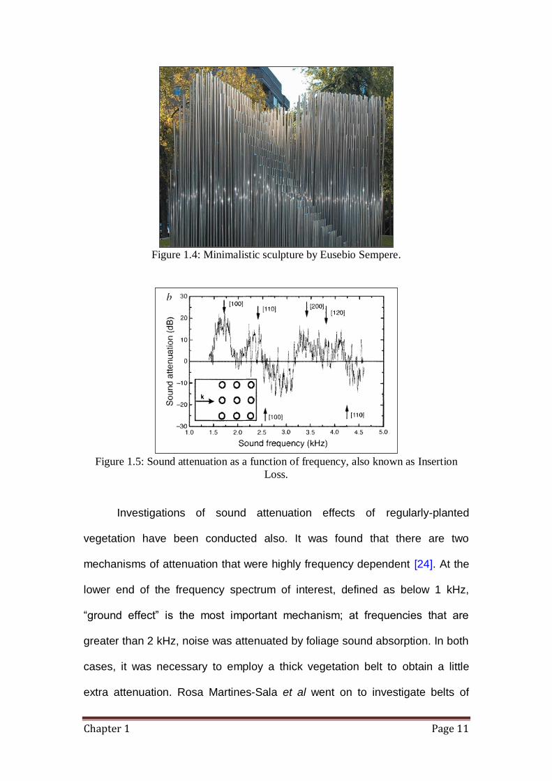
perpendicular to the cylinders’ vertical axes. Having a small filling fraction of
0.066 the experiment results showed several maxima (sound attenuation) and
minima (sound reinforcement) in the frequency spectrum. The first (lowest)
gap in the band structure which has a centre frequency at 1.7 kHz could be
attributed to the geometry of the structure as shown in figure 1.4. Ever since
this publication, research on the application of periodic arrays of cylinders for
noise control has increased [21, 22 and 23].
Chapter 1 Page 11
Figure 1.4: Minimalistic sculpture by Eusebio Sempere.
Figure 1.5: Sound attenuation as a function of frequency, also known as Insertion
Loss.
Investigations of sound attenuation effects of regularly-planted
vegetation have been conducted also. It was found that there are two
mechanisms of attenuation that were highly frequency dependent [24]. At the
lower end of the frequency spectrum of interest, defined as below 1 kHz,
“ground effect” is the most important mechanism; at frequencies that are
greater than 2 kHz, noise was attenuated by foliage sound absorption. In both
cases, it was necessary to employ a thick vegetation belt to obtain a little
extra attenuation. Rosa Martines-Sala et al went on to investigate belts of

Chapter 1 Page 12
trees arranged in periodic array in bid to achieve attenuation at low
frequencies. Peaks of attenuation at low frequencies ( <500 Hz) were
obtained which can be considered to be results of destructive interferences of
scattered wave, not results of “ground effect”. Furthermore, using periodic
arrangements of trees belts, greater attenuation effect was observed using
less width, making them more effective noise screen than typically more
randomly spaced tree belts. More recent work on sonic crystal noise barriers
exploits the use of localised sound absorption properties (i.e. rigid perforated
cylindrical shells filled with recycled rubber crumb material). Both numerical
and experimental studies have been made of the reflectance and
transmittance spectra of such a sonic crystal [25]. Such design offers the
additional mechanism of absorption, apart from the multiple scattering
phenomenon in periodic structure, to further attenuate noise (as did Umnova
et al [59]). It is also shown in this work that having three rows of scatterers are
sufficient to achieve well defined bandgaps which would be an important
factor with respect to economics and land take. The subject of wind generated
noise affecting SC performance is considered also. It is concluded that there
should not be such adverse influence up to wind speeds of 30 m/s.
Another type of optimisation of SC noise barrier which has been studied
numerically is the use of concentrically placed Helmholtz resonators (i.e. in a
Matryoshka configuration) [26]. It was found that the intrinsic resonance
properties of the six shell Matryoshka SC give rise to multiple independent
resonance bandgaps below the first Bragg bandgap (i.e. due to the periodicity
of the SC) between 400 and 1600 Hz which is important for traffic noise
Chapter 1 Page 13
reduction. Essentially this design is based on the use of concentric split ring
resonators (SRR). The basis for split ring resonator designs is investigated in
Chapter 7.
1.4.2) Crystallography
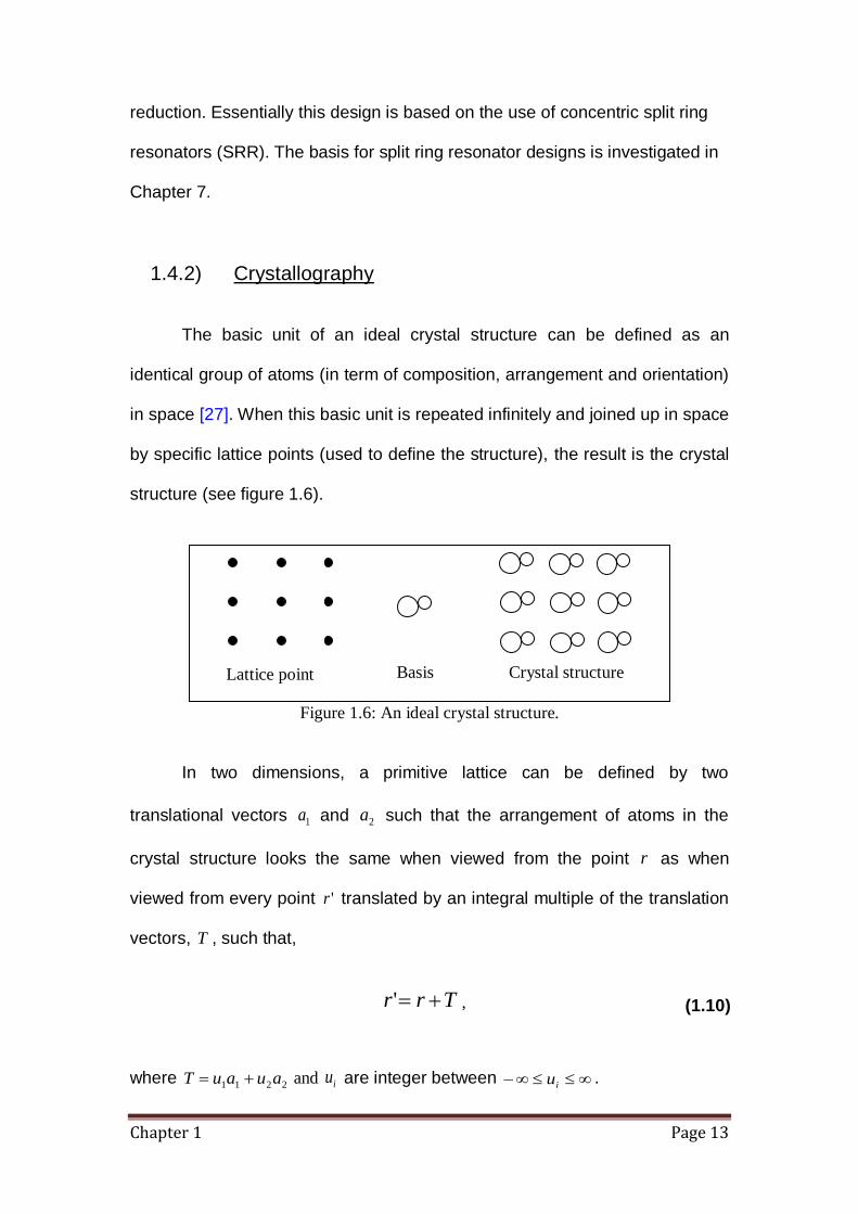
The basic unit of an ideal crystal structure can be defined as an
identical group of atoms (in term of composition, arrangement and orientation)
in space [27]. When this basic unit is repeated infinitely and joined up in space
by specific lattice points (used to define the structure), the result is the crystal
structure (see figure 1.6).
Figure 1.6: An ideal crystal structure.
In two dimensions, a primitive lattice can be defined by two
translational vectors 1a and 2a such that the arrangement of atoms in the
crystal structure looks the same when viewed from the point r as when
viewed from every point 'r translated by an integral multiple of the translation
vectors, T , such that,
Trr ' , (1.10)
where 2211 auauT and iu are integer between iu .
Lattice point Basis Crystal structure
Chapter 1 Page 14
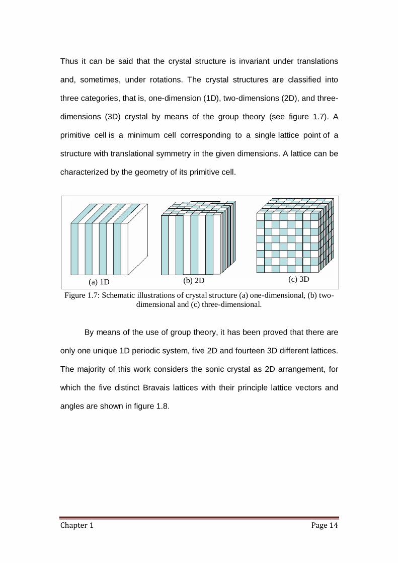
Thus it can be said that the crystal structure is invariant under translations
and, sometimes, under rotations. The crystal structures are classified into
three categories, that is, one-dimension (1D), two-dimensions (2D), and three-
dimensions (3D) crystal by means of the group theory (see figure 1.7). A
primitive cell is a minimum cell corresponding to a single lattice point of a
structure with translational symmetry in the given dimensions. A lattice can be
characterized by the geometry of its primitive cell.
Figure 1.7: Schematic illustrations of crystal structure (a) one-dimensional, (b) two-
dimensional and (c) three-dimensional.
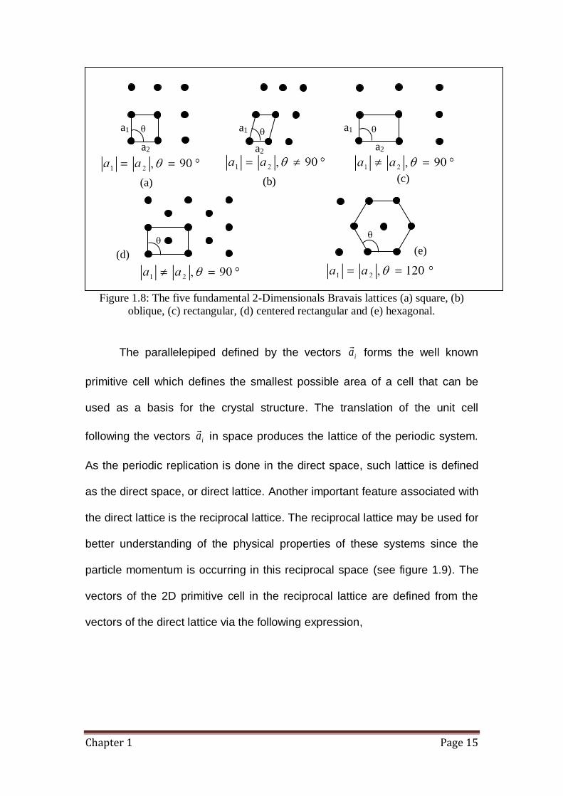
By means of the use of group theory, it has been proved that there are
only one unique 1D periodic system, five 2D and fourteen 3D different lattices.
The majority of this work considers the sonic crystal as 2D arrangement, for
which the five distinct Bravais lattices with their principle lattice vectors and
angles are shown in figure 1.8.
(a) 1D (b) 2D (c) 3D
Chapter 1 Page 15
Figure 1.8: The five fundamental 2-Dimensionals Bravais lattices (a) square, (b)
oblique, (c) rectangular, (d) centered rectangular and (e) hexagonal.
The parallelepiped defined by the vectors ia
forms the well known
primitive cell which defines the smallest possible area of a cell that can be
used as a basis for the crystal structure. The translation of the unit cell
following the vectors ia
in space produces the lattice of the periodic system.
As the periodic replication is done in the direct space, such lattice is defined
as the direct space, or direct lattice. Another important feature associated with
the direct lattice is the reciprocal lattice. The reciprocal lattice may be used for
better understanding of the physical properties of these systems since the
particle momentum is occurring in this reciprocal space (see figure 1.9). The
vectors of the 2D primitive cell in the reciprocal lattice are defined from the
vectors of the direct lattice via the following expression,
a1
a2 a2
a1 a1
a2
(b) (c)
(d) (e)
(a)

Chapter 1 Page 16
21
21 2
aa
ab
, (1.11)
21
12 2
aa
ab
, (1.12)
Where both the vectors of the direct ( 1a and 2a ) and the reciprocal ( 1b and 2b
) arrays satisfy an orthogonality relationship which can be expressed as,
ijij ab 2 , (1.13)
where 1ij if ji and 0ij if ji .
Figure 1.9: Illustration of direct lattice points (black dot), reciprocal lattice points (red
dots) and a shade region indicate the reciprocal space.
Another physical property of the periodic system is known as the filling
fraction, ff , and can be determined once the lattice constant and the size of
the scatterers are known. The filling fraction is defined as the ratio between
the volume occupied by the scatterers and the total volume occupied by the
unit cell. If we consider cylindrical scatterers with radius, 0r , the ff for both the
square and hexagonal lattices can be expressed as,

Chapter 1 Page 17
2
2
0
a
rff square
, (1.14)
2
2
0
3
2
a
rff hexagonal
, (1.15)
It should be noted that the concept of a periodic system is a mathematical
abstraction that implies the existence of an infinite structure. In practice such
an infinite system may not be attainable but under certain assumptions a finite
structure may mimic an infinite periodic system. For example, crystalline
structures can be studied as periodic media using periodic boundary
conditions if the size of the crystal is much smaller than the wavelength of the
wave used to examine the crystal.
The performance of sonic crystals can be interpreted in a similar way to
that used for the analysis of semiconductor bandgap materials. In a
semiconductor, electrons are confined in certain energy bands and forbidden
from others. The energy span between the valence band and the conduction
band is called an energy bandgap. The properties of this energy bandgap are
determined by the size, periodicity and arrangement of atoms in the crystal
lattice of the semiconductor which cause the diffraction of electrons based on
Bloch’s Theorem [28]. The same concept of wave reflection in Bragg’s Law
which refers mainly to light diffraction can be analogously used for sound
waves. It was found that artificial crystals can produce strong peaks over a
range of frequencies that depends on the lattice constant of the array as given
by Bragg’s Law (see equation 1.16). When a wave passes through a crystal,
part of it will be reflected by the first layer while the rest of it will continue to

Chapter 1 Page 18
move to the second layer, some portion of it will again be reflected and the
remaining part will be reflected once more, hence the process continues.
Figure 1.10: Bragg diffraction.
Consider two parallel planes of cylinders A-A1 and B-B1 (figure 1.10) having
an inter-planar spacing, L. Now assume that a plane wave of wavelength, ,
is incident on the two planes at an angle, . Two waves labelled 1W and
2W
are scattered by cylinders 1S and
2S . Constructive interference of scattered
sound waves 11W and
22W occurs at an angle, and ' to the planes if the
path difference between 1W → 1S → 11W and 2W → 2S → 22W , i.e. 21 LL is
equal to the whole number n , of wavelengths. Therefore condition for
diffraction is 21 LLn . The interference is constructive when the phase
shift is a multiple of 2 .
Bragg’s law is given by:
nL sin2 , (1.16)
A A1
B1
B
L θ θ'
Incident

Chapter 1 Page 19
where, L is the spacing between planes (lattice constant), is the
wavelength, is the angle between incident ray and scattering planes
n is an integer.
In a similar way, an SC can be described as a finite-size periodic array
composed of scatterers embedded in a homogeneous host (sometime called
the matrix) material. The geometry of the SC takes the form of a single unit
cell made of Bravais Lattice (basic geometries in solid-state) as illustrated in
figure 1.8. In these periodic structures (when we consider having rigid
scatterers), coherence interference phenomena such as aforementioned
Bragg diffraction (this term and the equivalent term Bragg resonance are used
interchangeably in this Thesis) based scattering are responsible for a total
reflection regime in certain frequency ranges creating full or complete band
gaps. At these frequencies, the amplitude of the transmitted wave decreases
as it passes through the crystal. Sound waves are therefore forbidden to pass
through in such band gaps which physically can be well described by the
classical wave theory for the multiple scattering of waves within the periodic
structure. The 2D schematic diagram (figure 1.11) illustrates a square lattice
of cylindrical scatterers with acoustic impedance, sZ , and acoustic velocity,
sV , arranged in a homogeneous host material with acoustic impedance, mZ ,
and acoustic velocity, mV . The distinct X and M directions of acoustic
wave propagation are also depicted in the figure. This denotes the first
irreducible Brillouin Zone (BZ). For example X refers to the [100] direction
and M refers to the [110] direction, while XM refers to the wave vector
varying from [100] and [110] on the side of the first BZ. The geometrical
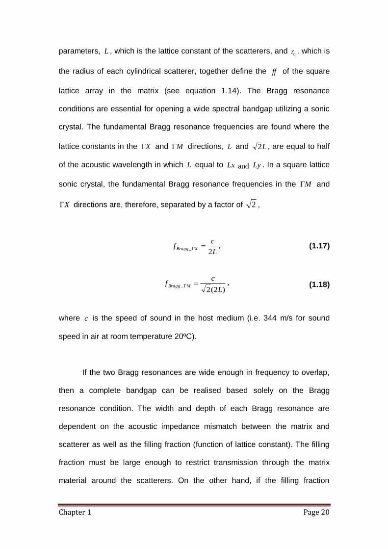
Chapter 1 Page 20
parameters, L , which is the lattice constant of the scatterers, and 0r , which is
the radius of each cylindrical scatterer, together define the ff of the square
lattice array in the matrix (see equation 1.14). The Bragg resonance
conditions are essential for opening a wide spectral bandgap utilizing a sonic
crystal. The fundamental Bragg resonance frequencies are found where the
lattice constants in the X and M directions, L and L2 , are equal to half
of the acoustic wavelength in which L equal to Lx and Ly . In a square lattice
sonic crystal, the fundamental Bragg resonance frequencies in the M and
X directions are, therefore, separated by a factor of 2 ,
L
cf XBragg
2_
, (1.17)
)2(2_
L
cf MBragg
, (1.18)
where c is the speed of sound in the host medium (i.e. 344 m/s for sound
speed in air at room temperature 20ºC).
If the two Bragg resonances are wide enough in frequency to overlap,
then a complete bandgap can be realised based solely on the Bragg
resonance condition. The width and depth of each Bragg resonance are
dependent on the acoustic impedance mismatch between the matrix and
scatterer as well as the filling fraction (function of lattice constant). The filling
fraction must be large enough to restrict transmission through the matrix
material around the scatterers. On the other hand, if the filling fraction
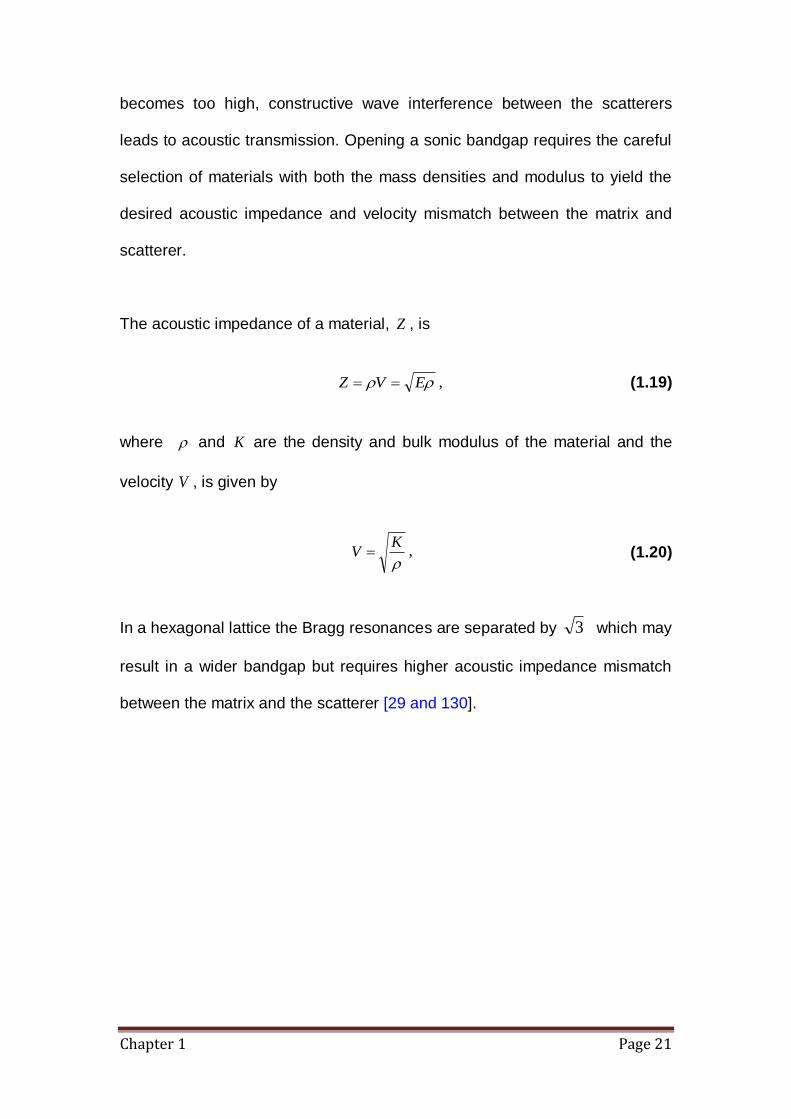
Chapter 1 Page 21
becomes too high, constructive wave interference between the scatterers
leads to acoustic transmission. Opening a sonic bandgap requires the careful
selection of materials with both the mass densities and modulus to yield the
desired acoustic impedance and velocity mismatch between the matrix and
scatterer.
The acoustic impedance of a material, Z , is
EVZ , (1.19)
where and K are the density and bulk modulus of the material and the
velocity V , is given by
KV , (1.20)
In a hexagonal lattice the Bragg resonances are separated by 3 which may
result in a wider bandgap but requires higher acoustic impedance mismatch
between the matrix and the scatterer [29 and 130].

Chapter 1 Page 22
Figure 1.11: 2D schematic of square lattice array showing the Brillouin zone (triangle
depicted by points , X and M ). mM VZ , and ss VZ , denote the acoustic
impedance and velocity for the medium and scatterer respectively.
Such bandgap phenomena require a large contrast in physical
properties such as density and speed of sound between the scatterer and the
matrix material. Sonic crystals seem therefore very attractive as acoustic
passband filters. The nature of the host materials can be used to differentiate
between sonic and phononic crystals. If the host material (matrix material) is
solid then the term ‘Phononic Crystal’ is used for the artificial crystal. In a
phononic crystal, both longitudinal and transverse shear waves (elastic
waves) may exist and couple with one another which will add to the
complexity of the nature of eigenmodes. In contrast, sonic crystals are
considered to be independent of the transverse waves. The scatterers are
typically made of solid materials and the host matrix is air/fluid to give high
acoustic impedance contrast between them.
(Zs, Vs) r
(ZM, VM)
α = /2 (ГX Bragg)
Г X
M

Chapter 1 Page 23
1.5) Aims and thesis organisation This Thesis offers a study of the interaction of sound with periodic structures.
The objective and scopes of the study are as follows:
(i) To review the various numerical techniques for modelling an SC.
(ii) To find ways of improving the size and magnitude of the band gaps
in an SC through both computational modelling and experiment.
(iii) To develop a multi-channel measurement system suitable for
performing measurements at outdoors.
(iv) Test and evaluate a full scale SC traffic noise barrier (in-situ).
(v) To gain an understanding on the influence on the effects of wind and
ground in the vicinity of an SC noise barrier.
Among these studies, the most important contributions in this thesis are:
• novel designs of SC noise barriers based on multiple resonances to
enhance the noise shielding performance at frequencies below the
first Bragg band gap.
• pioneering investigations of the influence of ground effects on SC
noise barriers.
The introduction presented in the previous sections of this first chapter
indicated that accurate predictions of the interactions of acoustic waves with
periodic structures can be applied in various ways. It has served also to
describe the general context of road traffic noise control. The basic theories
Chapter 1 Page 24
on acoustic wave propagation and concepts of crystallography were reviewed
to facilitate the derivations of the formulations in the subsequent work. A brief
summary of the aim and content of the other chapters is as follows.
Chapter 2 reviews the Plane Wave Expansion (PWE) prediction method and
is intended to serve as a starting point for the creation of acoustic band gaps
in 2D infinite periodic structures.
Chapter 3 describes an alternative prediction model viz. Multiple Scattering
Theory (MST) on which the subsequent research work has been largely
based. Contrary to the PWE described in Chapter 2, MST allows computation
for 2D finite sonic crystals and the results obtained can be directly compared
with experimental data.
Chapter 4 provides another means of predicting the performance of 2D finite
sonic crystal using the Finite Element Method (FEM). Such a numerical
modelling technique is suitable for considering different shapes of scatterer in
sonic crystal design. It is used also for analysis of elastic shells and concentric
cylinders in chapters 6 and 7 respectively. Preliminary attempts at transient
analysis for SC using FEM are also made.
Chapter 5 is devoted to the development and implementation of the acoustic
measuring systems (single and multiple channels) as well as the fabrication of
the different types of scatterers. Some issues arising from experimental
methods and signal are broadly discussed.
Chapter 1 Page 25
Chapter 6 studies numerically and experimentally the feasibility of replacing
the conventional rigid scatterer with thin elastic shell whereby a local
resonance (i.e. breathing mode) effect is exploited to enhance the band gap
frequency below the first Bragg band gap. It provides an understanding of
how some parameters could be optimised in a sonic crystal noise barrier
design.
Chapter 7 first re-visits of the widely known Split Ring Resonator (SRR) based
on Helmholtz resonance to enhance the Band gap in sonic crystal. Both
numerical and experimental attempts to improve the latex shell design
(chapter 6) are made. A novel design combines the elastic shell with an outer
protective rigid shell (with symmetrical slits).
Chapter 8 presents a study of the effects of ground in the vicinity of a sonic
crystal. A method is described of characterising the ground by fitting
measured Excess Attenuation (EA) spectra with a widely known ground
impedance deduction model (Delany and Bazley). Comparison of the
performance of the sonic crystal with and without acoustically “hard” or “soft”
grounds are made.
Chapter 9 states conclusions for each chapter and offers some ideas for
future work.

Chapter 2 Page 26
Chapter 2
The Plane Wave Expansion (PWE) Method
2.1) Introduction
The periodicity of any system structure plays a crucial role in
understanding the physical properties of both micro and macro crystalline
structures. To design sonic crystals and determine how sound will propagate
through a particular crystal structure it is possible to use numerical
techniques. The pioneering work on band theory describing electromagnetic
wave transmission inside a periodic system was introduced by Yablonovitch
[12], and the study of wave dispersion bands for electronic waves in solids
[30, 31, 32 and 33] provides the basis of understanding the properties of
conductors, semiconductors and insulators. Following the principles of Bloch
waves, the concepts of dispersion relations and Brillouin Zones (BZ) can be
extended to all kinds of periodic structures. One special characteristic is the
prospect of achieving a complete band gap; this is defined to be the stop band
in which, sound waves are prohibited for all values of the wave-vector (or
Bloch vector). There has been considerable subsequent research into the
analogous phononic or sonic crystal band gaps [34, 35 and 36]. There are
several techniques, but one of the most studied method is the Plane Wave
Expansion (PWE) method [37 and 38] as it can be applied to an infinite arrays
of any scatterer shape. It was used in some of the earliest studies of photonic
crystals and can be readily applied in acoustics. The PWE method uses the
periodicity of the given structure and the Bloch theorem to solve the wave

Chapter 2 Page 27
equation. This allows the computation of the allowable frequencies also
known as eigenfrequencies for sound propagation in all directions of the
crystal and can be used also to determine the field distributions in the crystal
over a broad range of frequencies. The accuracy in calculating the
eigenfrequencies from this method depends on the computational time. This
section presents the theory of acoustic band structures for periodic composite
structures.
2.1.1) Two-dimensional periodicity
Consider a sonic crystal array composed of circular cylinders made of
an isotropic solid A, embedded periodically using a square lattice in an air
background B. Such a system is assumed to have a translational symmetry in
one direction (i.e. the z axis). This means that the material parameters of
mass density and velocity of sound in this case depend on the coordinates x
and y . The propagation of the incidental wave is also limited to the xy plane
(2D) – an assumption which is used in other studies, both theoretical and
experimental, on the photonic band structure of dielectric cylinders. Thus, the
field parameter, pressure ( p ) is also independent of the z coordinate.
The wave equation describing the propagation of sound is
0)()(
)()(
)(
1.
2
2
rcr
rprp
r l
,
(2.1)
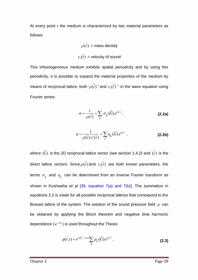
Chapter 2 Page 28
At every point r the medium is characterized by two material parameters as
follows:
)(r = mass density
)(rcl = velocity of sound
This inhomogeneous medium exhibits spatial periodicity and by using this
periodicity, it is possible to expand the material properties of the medium by
means of reciprocal lattice, both 1)( r and 1)( rcl in the wave equation using
Fourier series:
G
rGieGr
)( )(
1
, (2.2a)
G
rGi
l
eGrcr
)()( )(
12
, (2.2b)
where )(G is the 2D reciprocal-lattice vector (see section 1.4.2) and )(r is the
direct lattice vectors. Since )(r and )(rcl are both known parameters, the
terms
and
can be determined from an inverse Fourier transform as
shown in Kushwaha et al [39, equation 7(a) and 7(b)]. The summation in
equations 2.2 is made for all possible reciprocal lattices that correspond to the
Bravais lattice of the system. The solution of the sound pressure field p can
be obtained by applying the Bloch theorem and negative time harmonic
dependence ( tie ) is used throughout the Thesis:
G
rGitri eGpetrp )(),( )( , (2.3)

Chapter 2 Page 29
where is called the 2D Bloch wave vector and f 2 is the angular
frequency of the wave.
For a 2D sonic crystal system with square lattice geometry we have to define
some variable in the PWE method. For such a system the cylinder material
has density a and it occupies the filling fraction ff of the background
material with density b . It can be shown that:
0),(
0,1)(
22
22
GGF
GffG
bbaa
bbaa
, (2.4)
where )(GF is the structure factor, subscripts a and b denotes the host and
scatterer media respectively. Since the system has circular scatterers, the
structure factor will be defined in the PWE method as:
001
2 /21
)( rGrGfJerdA
GFcylA
rGi
uc
, (2.5)
such that ucA is defined as the area of the unit cell, cylA
is the area of the
considered cylinder and 1J is the Bessel function of the first kind of order 1.
After substituting the expanded wave equations (2.2) and the Bloch form
equation (2.3) into the initial wave equation we obtain:
0'''''
2 GGGGGGGk
G
k . (2.6)

Chapter 2 Page 30
Equation 2.6 is based on a simple modification which excludes the transverse
term in reference [39, equation 9]. For G taking all the possible values,
equation (2.6) constitutes an infinite set of linear, homogeneous equations for
the eigenvector 'Gk
and the eigenfrequencies )( . The ( ) is introduced
to differentiate summation over spatial position relative to the acoustic field
from those relative to the static distributions of material properties [40].
In numerical computations, truncation of the Fourier series has to include a
number of spatial harmonics large enough to ensure convergence. Assuming
N terms in the Fourier expansion, an appropriate NN matrix equation can
be solved for equation 2.6. The following vector notations are considered for
the generalised displacement fields [40],
)
)
NNGp
Gp
p
(
( 1
. (2.7)
The same explicit matrix formulation can be applied to matrices and
(generalised displacement fields) as follows:
) )
) )
NNNNNN
NN
GGGG
GGGG
((
((
1
111
, (2.8)
)( )(
)( )(
1
111
NNNNNN
NN
GGGG
GGGG
. (2.9)

Chapter 2 Page 31
Having i as the diagonal matrix whose terms are generated by first-order
spatial derivatives:
ii
ii
ii
i
G
G
G
0
0 0
0 0
, (2.10)
where i is equal to 1, 2, 3.
Thus, equation 2.6 can be expressed by a compact formulation:
pp
i
ii
23
1
. (2.11)
The specific Bravais lattice to be considered is the square lattice. Its
reciprocal lattice is also square, with the reciprocal-lattice vectors given by
yx NNaG /2 . (2.12)
Where a is defined as the lattice constant, xN and yN assume all the integer
values. With the substitutions of equations (2.5) and (2.12) into equation (2.6)
and then by solving the system equation given in (2.11) for each Bloch
vectors in the irreducible area of the first BZ for NN ,, , 2 , are obtained
and they can be used to represent the band structures, ).(k .

Chapter 2 Page 32
2.2) Plane Wave Expansion Results
2.2.1) Band structure of Sonic Crystal
We consider a solid-fluid composite structure. The sonic crystal system
studied consists of solid circular cylinders embedded in air. A square lattice
array with lattice constant L of 0.069 m and scatterer diameter of 0.055 m is
used for the initial case. This geometry gives a filling fraction ( ff ) of 50%.
These parameters will describe the contrast parameter and shape function for
the composite structure in the PWE method. Table 2.1 shows the material
parameters based on hollow PVC cylinders used in the PWE calculations. We
compute the band structure in the three principal symmetry directions, letting
k scan the periphery of the irreducible triangle of the first BZ. The dispersion
relation is obtained by plotting frequency against the Bloch wave vector in the
first BZ related to the incident direction of the wave. This is also known as the
reduced wave vector as it is the vector confined to only the first BZ. The PWE
method tends to have a large convergence problem due to the large number
of plane waves needed to calculate the band structure [41]. For reasonable
accuracy (less than 5% discrepancy) and computational time, we allow the
integer xN and yN to take values in the interval defined by 10,10 yx NN ,
thus giving 2)12( N = 441 planes waves. This results in very good
convergence in our numerical results. Figure 2.1 show the first 10 bands for
PVC cylinders in an air background predicted using the PWE method in
MATLAB® (see Appendix A) This indicates any regions where the band gaps
exist (see figure 2.1).

Chapter 2 Page 33
Material Density kgm-3 Speed of sound ms-1
Air 1.2 344
PVC 1380 2400
Table 2.1: Material parameters for sonic crystal system comprising of PVC cylinders
embedded in air.
Assuming linear dispersion, the lowest Bragg band gap central frequency is
approximately given by
L
cl
Bragg2
. (2.13)
As a test case, the band structure has been computed for a
homogeneous material. The PWE method solved for the first ten bands with
material parameters equal to that of air, ba = 1.2 kg/m3 and lbla cc = 344
m/s (see figure 2.1).
Figure 2.1: Plane wave expansion computed band structure for a homogeneous
medium with equivalent material properties of air. Inset: Brillouin zone. refers to
[1,0] direction, M refers to [1,1] direction and refers to the wave vector
varying from [1,0] to [1,1] on the extreme side of the Brillouin zone.
0
1000
2000
3000
4000
5000
6000
Fre
qu
en
cy (
kH
z)
M X M
Reduced Wave Vector
Reduced Wave Vector
Г X
M
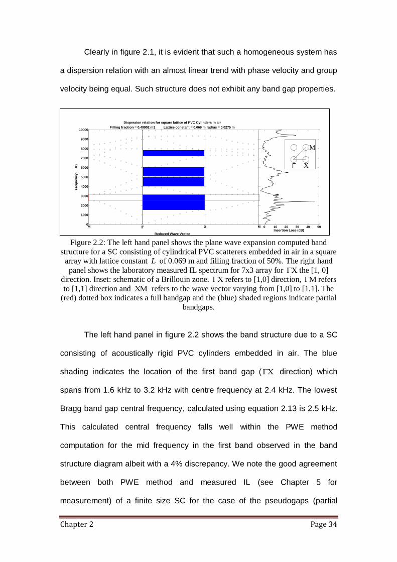
Chapter 2 Page 34
Clearly in figure 2.1, it is evident that such a homogeneous system has
a dispersion relation with an almost linear trend with phase velocity and group
velocity being equal. Such structure does not exhibit any band gap properties.
Figure 2.2: The left hand panel shows the plane wave expansion computed band
structure for a SC consisting of cylindrical PVC scatterers embedded in air in a square
array with lattice constant L of 0.069 m and filling fraction of 50%. The right hand
panel shows the laboratory measured IL spectrum for 7x3 array for the [1, 0]
direction. Inset: schematic of a Brillouin zone. refers to [1,0] direction, refers
to [1,1] direction and refers to the wave vector varying from [1,0] to [1,1]. The
(red) dotted box indicates a full bandgap and the (blue) shaded regions indicate partial
bandgaps.
The left hand panel in figure 2.2 shows the band structure due to a SC
consisting of acoustically rigid PVC cylinders embedded in air. The blue
shading indicates the location of the first band gap ( direction) which
spans from 1.6 kHz to 3.2 kHz with centre frequency at 2.4 kHz. The lowest
Bragg band gap central frequency, calculated using equation 2.13 is 2.5 kHz.
This calculated central frequency falls well within the PWE method
computation for the mid frequency in the first band observed in the band
structure diagram albeit with a 4% discrepancy. We note the good agreement
between both PWE method and measured IL (see Chapter 5 for
measurement) of a finite size SC for the case of the pseudogaps (partial
0
1000
2000
3000
4000
5000
6000
7000
8000
9000
10000
Fre
qu
en
cy (
kH
z)
M X M
Reduced Wave Vector
Disperaion relation for square lattice of PVC Cylinders in air
Filling fraction = 0.49902 m2 Lattice constant = 0.069 m radius = 0.0275 m
0 10 20 30 40 50Insertion Loss (dB)
Г X
M
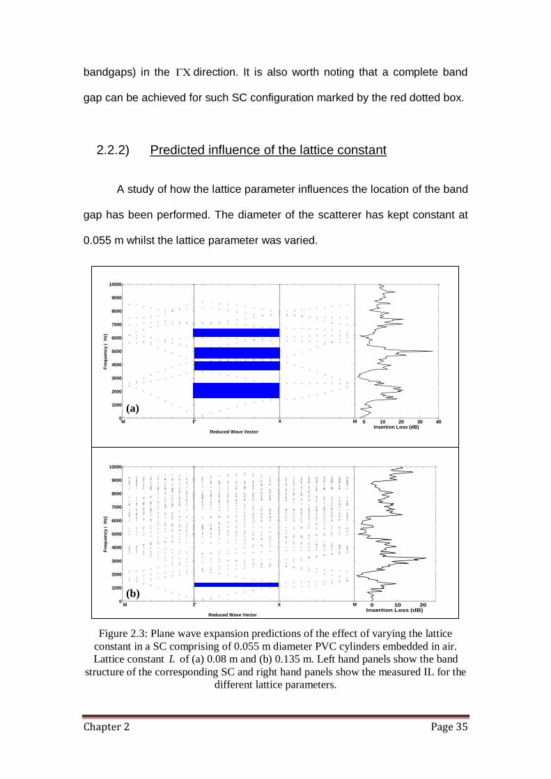
Chapter 2 Page 35
bandgaps) in the direction. It is also worth noting that a complete band
gap can be achieved for such SC configuration marked by the red dotted box.
2.2.2) Predicted influence of the lattice constant
A study of how the lattice parameter influences the location of the band
gap has been performed. The diameter of the scatterer has kept constant at
0.055 m whilst the lattice parameter was varied.
Figure 2.3: Plane wave expansion predictions of the effect of varying the lattice
constant in a SC comprising of 0.055 m diameter PVC cylinders embedded in air.
Lattice constant L of (a) 0.08 m and (b) 0.135 m. Left hand panels show the band
structure of the corresponding SC and right hand panels show the measured IL for the
different lattice parameters.
0
1000
2000
3000
4000
5000
6000
7000
8000
9000
10000
Fre
qu
en
cy (
kH
z)
M X M
Reduced Wave Vector
0 10 20 30 40Insertion Loss (dB)
0
1000
2000
3000
4000
5000
6000
7000
8000
9000
10000
Fre
qu
en
cy (
kH
z)
M X M
Reduced Wave Vector
0 10 20Insertion Loss (dB)
(a)
(b)
Chapter 2 Page 36
For a lattice constant of 0.08 m, the plane wave expansion method is
solved for the first 10 bands whereas the first 40 bands would be required to
extend the range of frequencies to 9 kHz. Focusing on the lowest band gap at
direction for SC with lattice constant of 0.08 m (see figure 2.3a – area
marked blue), the band gap lies between 1.4 kHz to 2.6 kHz, centred at 2
kHz. These band gaps are shifted to lower frequency as compared with the
original lattice constant of 0.069 m (see figure 2.2). We observed a further
shift of the first Bragg band gap to an even lower frequency when the lattice
constant is further increased to 0.135 m (see figure 2.3b). The first band gap (
direction) predicted by PWE method spans from 1 kHz to 1.4 kHz, and is
centred at 1.2 kHz (area marked blue). The lowest Bragg band gap central
frequencies calculated using equation 2.13 are found to be exactly matched
with the PWE method for lattice constants of 0.08 and 0.135 m. The
corresponding measured IL spectral for both lattice constant are also found to
agree well on the first Bragg band gap. From this investigation it is clear that
lower frequencies are attenuated as the lattice parameter is increased. On the
other hand, for the same number of array elements this increasing the lattice
constant increases the size of the sonic crystal.

Chapter 2 Page 37
2.2.3) Predicted influence of filling fraction
Plane Wave Expansion predictions of the influence of the filling fraction
have been studied. It should be noted that in the previous section 2.2.2, the
filling fraction is inherently changed by varying the lattice constant. In the
current study the lattice constant is kept constant but the scatterer size is
varied as shown in table 2.2.
Cylinder diameter (m) Filling fraction (%)
0.055 13
0.09 35
0.11 52
0.13 73 Table 2.2: Cylinder diameter and corresponding filling fraction for a lattice constant
of 0.135 m.

Chapter 2 Page 38
Figure 2.4: Plane Wave Expansion predictions of the band structure with Lattice constant fixed at 0.135 m and varying scatterer diameters (a)
0.055, (b) 0.09, (c) 0.11 and (d) 0.13 m.
0
1000
2000
3000
4000
5000
6000
7000
8000
9000
10000
Fre
qu
en
cy (
kH
z)
M X M
Reduced Wave Vector
0
1000
2000
3000
4000
5000
6000
7000
8000
9000
10000
Fre
qu
en
cy (
kH
z)
M X M
Reduced Wave Vector
0
1,000
2,000
3,000
4,000
5,000
6,000
7,000
8,000
9,000
10,000
Fre
qu
en
cy (kH
z)
M X M
Reduced Wave Vector
0
1000
2000
3000
4000
5000
6000
7000
8000
9000
10000
Fre
qu
en
cy (
kH
z)
M X M
Reduced Wave Vector
(c)
(b) (a)
(d)

Chapter 2 Page 39
According to the PWE predictions, the wave propagation in different
directions is inhibited within different frequency regimes for different filling
fractions. An indication of the complete band gap can be observed when the
filling fraction exceeds certain value. For systems with low filling fractions of
13% and 35%, narrow pseudogaps are observed for the direction in the
band structure (see figure 2.4a and 2.4b). Although there have the same
number of band gaps predicted for these two filling fractions at similar
frequencies, careful examination reveals that they are not identical. The
lowest band gap extends from 1030 to 1390 Hz for the case of 13% filling
fraction whereas the lowest band gap for 35% filling fraction extends from 850
to 1530 Hz. Also the mid frequency for the first band in both filling fractions
occurs at about 1.2 kHz. It is evident that as the filling fraction increases
further to 52% and 73%, the band gaps are widened and additional band gaps
are formed. Complete acoustic band gaps are allowed to form for such filling
fraction as the frequency bands in different directions of periodicity
overlapped. Two complete band gaps are observed for the range of
frequencies calculated. Clearly, for a given lattice constant, increasing the
filling fraction results in enlargement of Bragg band gaps and the
enhancement of the IL performance of the SC in the direction.
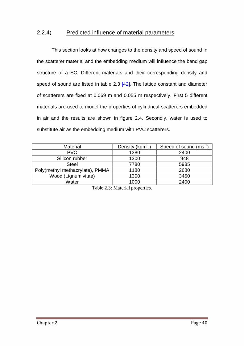
Chapter 2 Page 40
2.2.4) Predicted influence of material parameters
This section looks at how changes to the density and speed of sound in
the scatterer material and the embedding medium will influence the band gap
structure of a SC. Different materials and their corresponding density and
speed of sound are listed in table 2.3 [42]. The lattice constant and diameter
of scatterers are fixed at 0.069 m and 0.055 m respectively. First 5 different
materials are used to model the properties of cylindrical scatterers embedded
in air and the results are shown in figure 2.4. Secondly, water is used to
substitute air as the embedding medium with PVC scatterers.
Material Density (kgm-3) Speed of sound (ms-1)
PVC 1380 2400
Silicon rubber 1300 948
Steel 7780 5985
Poly(methyl methacrylate), PMMA 1180 2680
Wood (Lignum vitae) 1300 3450
Water 1000 2400
Table 2.3: Material properties.

Chapter 2 Page 41
Figure 2.5: Plane Wave Expansion predictions of the influence of material parameters on the band structure. The lattice constant is fixed at 0.069
m and scatterers are made from different materials (a) PVC, (b) silicone rubber, (c) steel (d) PMMA, (e) wood and (f) PVC scatterers embedded
in water
0
1000
2000
3000
4000
5000
6000
7000
8000
9000
10000
Fre
qu
en
cy (
kH
z)
M X M
Reduced Wave Vector
0
1000
2000
3000
4000
5000
6000
7000
8000
9000
10000
Fre
qu
en
cy (
kH
z)
M X M
Reduced Wave Vector
0
1000
2000
3000
4000
5000
6000
7000
8000
9000
10000
Fre
qu
en
cy (
kH
z)
M X M
Reduced Wave Vector
0
1000
2000
3000
4000
5000
6000
7000
8000
9000
10000
Fre
qu
en
cy (
kH
z)
M X M
Reduced Wave Vector
0
1000
2000
3000
4000
5000
6000
7000
8000
9000
10000
Fre
qu
en
cy (
kH
z)
M X M
Reduced Wave Vector
0
1000
2000
3000
4000
5000
6000
7000
8000
9000
10000
Fre
qu
en
cy (
kH
z)
X: 0.5
Y: 2815
M X M
Reduced Wave Vector
(a) (b) (c)
(d) (f) (e)

Chapter 2 Page 42
Figures 2.5(a), (b), (c), (d) and (e) show the predicted band structures
for scatterers made from PVC, silicon rubber, steel, PMMA and wood
respectively. The width of the first Bragg band gaps are identical for all of
these scatterers and the first Bragg band gaps lie between 1490 to 3170 Hz.
This demonstrates that so long as the scatterers are acoustically hard they
have no effect on the band structure of the SC. On the other hand, when PVC
scatterers are embedded in water, a different band structure is observed (see
2.5(f)). In such system, fewer band gaps are predicted for the direction
since the impedance contrast between PVC and water is smaller than that
between PVC and air.
Chapter 3 Page 43
Chapter 3
Multiple Scattering Theory (MST)
3.1) Introduction
When waves travelling in a homogeneous medium such as air
encounter an obstacle (sometimes called a scatterer), parts of the waves
remain undisturbed while others are scattered and spread out from the
scatterer in all directions distorting and interfering with the incident wave. If
the scatterer is large in comparison to the wavelength some of an incident
wave spreads uniformly in all directions from the scatterer and the rest is
more or less concentrated behind the scatterer such that it interferes
destructively with the unchanged incident wave. On the other hand, if the
scatterer is small compared to the wavelength (which is often the case with
sound wave) then, the entire scattered wave is propagated in all directions
and there is no interference behind the scatterer [2]. For a single obstacle,
calculation of the total field includes the sum of the scattered field and the
incident field. This assumption is valid only if the scatterer placed far enough
from other scatterers and the incident wavelength is small compared to the
distance between the scatterers. Some authors have suggested that the
centre to centre distance of two identical wavelength-sized spheres has to be
four times the radius of the scatterer for independent scattering to be valid
[44]. Clearly a single scattering approximation will not be valid if multiple
scatterers are placed within close proximity to each other: a situation often
encountered in many areas of physics. Research on multiple scattering of
Chapter 3 Page 44
waves dates back to 1913 [45] when a method for predicting scattering of
acoustic waves by two dimensional finite arrays was described. Ever since,
there has been a growing interest in wave propagation in periodic or randomly
arranged composites. The underlying theory is also applicable to other types
of waves. A few examples of various fields in which relevant research is
known to have taken place are electromagnetic waves [46 and 47],
condensed matter physics [48], water waves [49], optics [50 and 51] and
acoustics [52].
In general multiple scattering can be defined as the interaction of the
fields due to two or more scatterers [53]. As explained previously for single
scattering where an incident field impinges on the individual scatterer, the
total scattered field is just the sum of the incident field and the field scattered
by that individual scatterer. However, multiple scattering (due to several
scatterers within close proximity) takes account of the field scattered from one
scatterer which will induce further scattered fields from all the other scatterers,
which will again induce further scattered fields from all the other obstacles and
so on until the energy in the field has decayed. In multiple scattering, it is
possible to have constructive or destructive interference between waves.
Multiple Scattering Theory can be classified as a self-consistent method which
is valid for both periodically and randomly placed scatterers. In this section,
we follow a previously published multiple scattering approach first published
by Lord Rayleigh in 1892 when he worked on the potential flow through a
periodic rectangular array of identical cylinders [54]. Subsequently,
investigations on multiple scattering have been made for a variety of 2D or 3D
Chapter 3 Page 45
problems e.g. Mal and Bose [55] in 1974 and Linton and Evans in 1990 [49].
Martin’s book [53] explains each technique developed during these periods of
time in great detail. In this section, periodically arranged rigid cylinders will be
considered.
Suppose we have N disjoint scatterers and an incident wave impinging
on them, the problem is to calculate the scattered waves [53],
N
j
j
scinc pp1
, (3.1)
where incp is the incident wave and j
scp is the wave field scattered by the j-th
scatterer.
Then the effective field over the k-th scatterer which is the radiation incident
on the k-th scatterer in the presence of all other scatterers (N-1) can be
defined as,
N
kjj
j
scinck ppp1
. (3.2)
Since this is a linear problem, it is possible to write,
j
incj
j
sc pp , (3.3)
where j is an operator relating the field incident on the j-th scatterer, j
incp , to
the field scattered by the j-th scatterer, j
scp . Thus substituting equation 3.3
into equation 3.2 gives,
Chapter 3 Page 46
N
kjj
j
incjinck ppp1
, (3.4)
or equivalently,
N
kjj
j
scinck
k
sc ppp1
, (3.5)
by solving equation 3.4 for kp or equation 3.5 for k
scp where k = 1, 2…, N, the
total field would then be given by,
N
j
jjinc ppp1
, (3.6)
This over simplified equation hides the complexity through the operator
j which has not been clearly defined at this stage and also where equation
3.5 and 3.6 is required to hold in space. The next section will show how the
separations of variables is done for the acoustic scattering problem involving
two or more cylindrical scatterers. For system made up of circular or spherical
scatterers, a self-consistent method can be easily realised using the
multipoles method.
Chapter 3 Page 47
3.2) Multipole method for circular scatterers in 2-dimensional system
There are several methods for defining j in equation 3.6 such as T-
matrix [56], iterative technique [57] and the multipole methods [45]. The
multipole method is preferred for treating simple geometries, such as circular
and spherical scatterers. This method was developed by Zaviska, 1913 for
two-dimensional scattering by circular scatterers. This method combines
separated solutions of the Helmholtz equation using an important concept of
addition theorem for expanding multipoles centred at one origin in terms of
similar multipoles centred on a different origin. Such a scattering problem can
be conveniently formulated using polar coordinates. This chapter will consider
the multipole method using both plane and cylindrical incident waves
developed by our collaborators in University of Salford.
Assuming the sonic crystal is formed from N infinitely long cylinders of
radius ja , with j = 1, 2,…, N in either a regular lattice or a random array. The
various parameters relating to the relative positions and sizes of the N = 2
cylinders are shown in figure 3.1. The acoustic source transmitting
monochromatic waves is positioned at the origin 0,0 of the Cartesian
coordinate system, some distance away from the array. We will introduce N+1
coordinate systems in the x-y plane normal to the cylinder axes ,r centred
at the origin and jjr , centred at the j-th cylinder. The vertical circular
cylinders are fixed along the z-axis and it is assumed that waves propagate in
the plane perpendicular to the main axis of the cylinders. Since the boundary
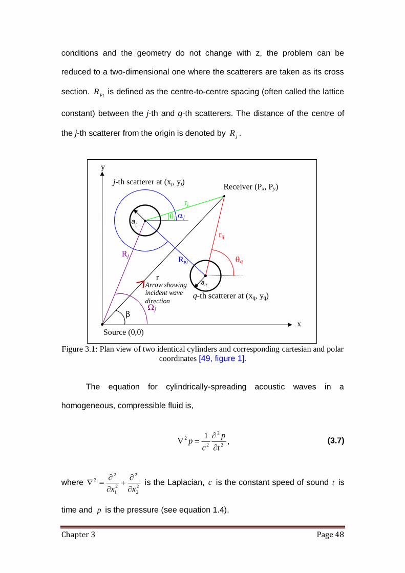
Chapter 3 Page 48
conditions and the geometry do not change with z, the problem can be
reduced to a two-dimensional one where the scatterers are taken as its cross
section. jqR is defined as the centre-to-centre spacing (often called the lattice
constant) between the j-th and q-th scatterers. The distance of the centre of
the j-th scatterer from the origin is denoted by jR .
Figure 3.1: Plan view of two identical cylinders and corresponding cartesian and polar
coordinates [49, figure 1].
The equation for cylindrically-spreading acoustic waves in a
homogeneous, compressible fluid is,
2
2
2
2 1
t
p
cp
, (3.7)
where 2
2
2
2
1
22
xx
is the Laplacian, c is the constant speed of sound t is
time and p is the pressure (see equation 1.4).
r
j-th scatterer at (xj, yj)
q-th scatterer at (xq, yq)
Source (0,0) x
β
Rjq
Receiver (Px, Py)
rq
rj
j
Rj
j
q
j
y
Arrow showing
incident wave
direction
Chapter 3 Page 49
Assuming that an external wave incp with temporal dependence tie
impinges the array of scatterers where is the angular frequency f2 , we
can write,
ti
inc epp Re . (3.8)
Hence, the complex-valued function p satisfies the well known Helmholtz
equation as shown,
02
0
2 pkp in eB , (3.9)
Where 0
0
2
c
fk
, is the wave number in air and eB is the unbounded exterior
to the cylinders region occupied by the air medium. Thus, solution can be
obtained by solving for equation 3.9 satisfying some boundary conditions on
the exterior of the scatterers and a radiation condition at infinity.
Each individual cylinder scatters the waves which are incident upon it
and the total field around the j-th cylinder is a superposition of the external
field and the radiation scattered by the rest of cylinders. Solutions of the
Helmholtz equation are called wavefunctions and two essential wavefunctions
[53] which can be expressed in term for the scattering of waves by cylindrical
scatterers will be discussed. Firstly, the incident wavefunction n is
represented by an outgoing cylindrical wavefunction of n-order and this
ensures that the Sommerfeld radiation condition (in two dimensions) at infinity
Chapter 3 Page 50
is satisfied. Such a condition implies that there are no incoming scattered
waves at infinity (i.e. no reflection from the boundaries).
in
nn ekrr )1()( , ... ,2 ,1 ,0 n (3.10)
Assuming plane polar coordinates, r the radius vector is equal to
sin,cos rr .
Secondly, a regular cylindrical wavefunctions of the first kind represent a
general outgoing wave radiating from each cylinder is given by,
in
nn ekrJr )(ˆ , ... ,2 ,1 ,0 n (3.11)
The general solution for solving the total wave field at any point exterior to the
cylinders (position that is within the host medium which is air in this case) will
be introduced here for later convenience,
N
j n
in
jn
j
n
j
nincjerkHZApyxp
1
0
)1(,
, (3.12)
where incp is the incidence wave over a two dimensions system of scatterers
in the form of either a plane wave from infinity or a cylindrical wave from a
point. It is also worth noting that incp can also be modelled with a spherical
wave which will extends the problem to three dimensions but will necessarily
require higher computing resource. We restrict further consideration to two
dimensional systems so plane and cylindrical incident waves. The formulation
of this equation will be discussed further in the next section where incident
wave incp , coefficient j
nA , and impedance factor j
nZ will be defined. We
Chapter 3 Page 51
will assume in our model that all motion is time harmonic with angular
frequency which uses positive time dependence xkie where the wave is
propagating from the negative values of x axis. k and r are defined as the
wave vector (with fk 2 as the angular frequency) and location respectively.
3.3) Plane wave scattering model
As previously explained, the scattering problem of N scatterers can be
conveniently formulated using polar coordinates. Suppose an incident plane
wave with angle propagating to the j-th cylinder as shown in figure 3.1
(brown arrow), such plane wave can be written as an expansion of Bessel
functions of the first kind centred at the origin of coordinates [49],
sincos yxik
inc ep . (3.13)
Cartesian x and y coordinates can then be easily defined,
cosrx and sinry . (3.14)
Substitute equation 3.14 into equation 3.13 gives,
sinsincoscos rrik
inc ep
sinsincoscos ikre .
(3.15)
Using rules of trigonometric transforms (compound angle formulae), equation
3.15 can be written as,
Chapter 3 Page 52
cosikr
inc ep. (3.16)
The plane wave impinging the j-th scatterer is then scattered to other
positions (e.g. the receiver position) thus, the scalar product krj is now
replaced with krR jj . Following a similar approach in equation 3.14 gives,
jjjjx rR coscos p and
jjjjy rR sinsin p , (3.17)
where,
jjj Rx cos and jjj Ry sin . (3.18)
Therefore,
jjikr
jinc eIpcos
, (3.19)
where sincos jj yxik
j eI
is a phase factor associated with the j-th cylinder. As
sincos jj yxike
can be written as series of Bessel function [58], equation 3.19
can be written as,
n
n
in
jn
n
incjekRJip , (3.20)
where c
fk
2 , and nJ is the Bessel function of n-th order of the first kind.
Thus, equation 3.20 becomes [49],
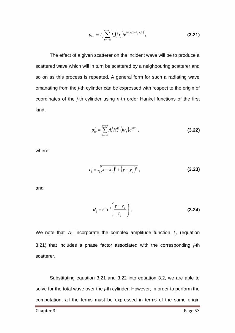
Chapter 3 Page 53
n
n
in
jnjincjekrJIp
2 , (3.21)
The effect of a given scatterer on the incident wave will be to produce a
scattered wave which will in turn be scattered by a neighbouring scatterer and
so on as this process is repeated. A general form for such a radiating wave
emanating from the j-th cylinder can be expressed with respect to the origin of
coordinates of the j-th cylinder using n-th order Hankel functions of the first
kind,
n
n
in
jn
j
n
j
scjekrHAp
1 , (3.22)
where
22
jjj yyxxr , (3.23)
and
j
j
jr
yy1sin
, (3.24)
We note that j
nA incorporate the complex amplitude function jI (equation
3.21) that includes a phase factor associated with the corresponding j-th
scatterer.
Substituting equation 3.21 and 3.22 into equation 3.2, we are able to
solve for the total wave over the j-th cylinder. However, in order to perform the
computation, all the terms must be expressed in terms of the same origin

Chapter 3 Page 54
coordinates qqr , . This can be done using Graf’s addition theorem (See
Appendix B). When using the addition theorem for Bessel functions it is
important to note that in order to write functions of jjr , in terms of the
coordinates qqr , , we have to ensure that jqq Rr for all qj . This
geometry restriction implies that the expression obtained is only valid if the
point qqr , is closer to the centre of cylinder q rather than to the centre of
any other cylinders or the source and thus we can write the expression
obtained for qqr , as,
N
qjj
n
n
m
m
ee
jqmnqm
j
n
j
n
n
n
in
qn
k
n
k
n
in
qnqr
jmniqim
qpq
RkHrkJZA
erkHZAerkJIp
1
0
1
0
0
12
0,
, (3.25)
for some set of unknown complex numbers j
nA . Both j
nA and j
nZ are related by
the boundary conditions of the scatterers surface. Definition of the term j
nZ
which is the impedance factor [49] of the scatterers will follow.
We apply boundary conditions of continuity of both pressure and
particle velocity between the scatterer and the surrounding air medium. Thus,
for the case of the q-th scatterer, the boundary condition can be expressed
by,
qqqq ararext int , (3.26)
Chapter 3 Page 55
Leading to,
qqqq ar
ar
q
ext
rr
int11
, (3.27)
where is the density of the surrounding medium (air) and q is the density
of the q-th scatterer. If the scatterers are acoustically-rigid, the condition of
zero velocity is applied. This is widely known as the Neumann boundary
condition which specifies the values that the derivative of a solution is to take
on the boundary of the domain,
0
qqqq ar
q
j
sc
q
incar
qp
ext
r
pp
r
, (3.28)
where incp the total incident pressure over the q-th scatterer (refer to equation
3.21 and j
scp is the scattered wave by the j-th scatterer (refer to equation
3.22).
This boundary condition leads to the definition of impedance for the rigid
scatterers as follow,
qn
qnj
nakH
akJZ
0
'1
0
'
, (3.29)
Applying this boundary conditions for pressure and velocity on the outer
surface of q-th scatterer and after using the orthogonality of the functions qime
taking ,...,2,1,0 m make it possible to derive an infinite system of
equations which can lead to solve for coefficientsq
mA .

Chapter 3 Page 56
2
1
0
12 im
q
N
qjj
M
M
jqMn
mnij
n
j
n
q
m eIRkHeZAA j . (3.30)
The obtained algebraic system can then be truncated to the finite number
12 MN of equations. Where Mn ...,2,1,0 and Nq .., ,3 ,2 ,1 . In [49],
it was found that taking M = 6 gave results accurate to four significant figures,
except when the scatterers were positioned very close together.
3.4) Cylindrical wave scattering model
The previous scattering model was for incident plane waves. The
source may not be placed sufficiently far enough from the scatterers for such
approximation to be valid so it is necessary to consider cylindrical wave
incidence. For simplicity without compromising generality, we approximate the
acoustic source as a line source located at origin 0r . The wave in free field
is governed by the following equation,
rrpk 22
0
2 4
in eB , (3.31)
where c
fk
20 , 2 is the 2-dimension delta-function and eB is the
unbounded exterior to the cylinders region occupied by the air medium. In
cylindrical polar coordinates, the solution can be expressed as,
rkHpinc 0
1
0 , (3.32)
where 1
0H is the zero-th order of Hankel function and of the first kind.
Chapter 3 Page 57
Following similar procedure in equation 3.21 where we considered the
scattering in the presence of N cylinders (repeated for convenience). The
radiating wave emanating from the j-th cylinder can be expressed with respect
to the origin of coordinates of the j-th cylinder using n-th order Hankel
functions of the first kind,
n
n
in
jn
j
n
j
scjekrHAp
1 . (3.33)
Similarly by applying Graf’s addition theorems to solve for the total wave
N
qj
n
n
m
m
ee
jqmnqm
j
n
j
n
n
n
in
qn
k
n
k
n
in
qnqr
jmniqim
qpq
RkHrkJZA
erkHZAerkJIp
1
0
1
0
0
12
0,
2
.
(3.34)
Applying the boundary condition for acoustically-rigid cylinders as shown in
equation 3.25 and 3.29 leads to the definition of impedance as follow,
qn
qnj
nakH
akJZ
0
'1
0
'
, (3.35)
Using the same approach as for equation 3.30, i.e. applying boundary
conditions for pressure and velocity on the outer surface on the q-th scatterer
and using the orthogonality of the functions qime taking ,...,2 ,1 ,0 m it is
possible to derive an infinite system of equations which can be solved for
coefficientsq
mA with cylindrical incident waves [59]. The obtained algebraic
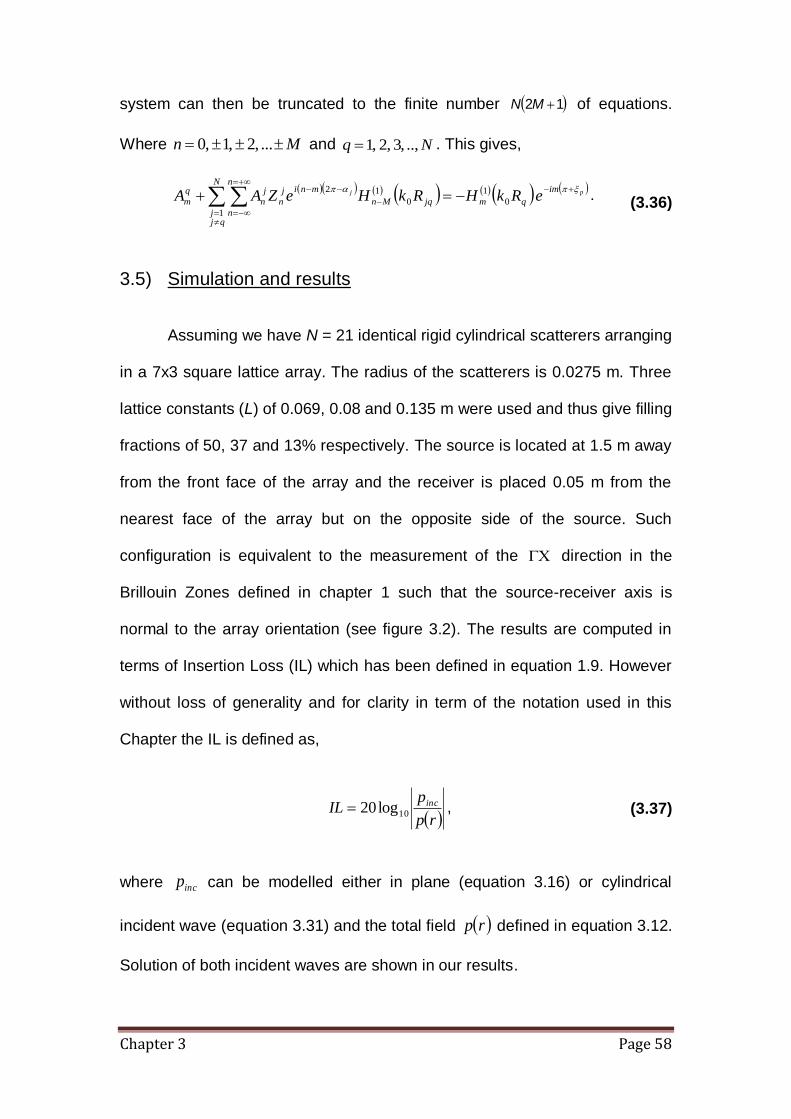
Chapter 3 Page 58
system can then be truncated to the finite number 12 MN of equations.
Where Mn ... ,2 ,1 ,0 and Nq .., ,3 ,2 ,1 . This gives,
pj im
qm
N
qjj
n
n
jqMn
mnij
n
j
n
q
m eRkHRkHeZAA
0
1
1
0
12.
(3.36)
3.5) Simulation and results
Assuming we have N = 21 identical rigid cylindrical scatterers arranging
in a 7x3 square lattice array. The radius of the scatterers is 0.0275 m. Three
lattice constants (L) of 0.069, 0.08 and 0.135 m were used and thus give filling
fractions of 50, 37 and 13% respectively. The source is located at 1.5 m away
from the front face of the array and the receiver is placed 0.05 m from the
nearest face of the array but on the opposite side of the source. Such
configuration is equivalent to the measurement of the direction in the
Brillouin Zones defined in chapter 1 such that the source-receiver axis is
normal to the array orientation (see figure 3.2). The results are computed in
terms of Insertion Loss (IL) which has been defined in equation 1.9. However
without loss of generality and for clarity in term of the notation used in this
Chapter the IL is defined as,
rp
pIL inc
10log20 , (3.37)
where incp can be modelled either in plane (equation 3.16) or cylindrical
incident wave (equation 3.31) and the total field rp defined in equation 3.12.
Solution of both incident waves are shown in our results.
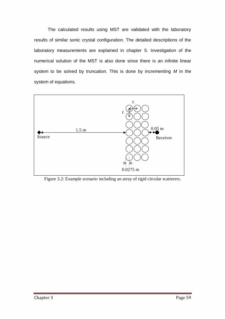
Chapter 3 Page 59
The calculated results using MST are validated with the laboratory
results of similar sonic crystal configuration. The detailed descriptions of the
laboratory measurements are explained in chapter 5. Investigation of the
numerical solution of the MST is also done since there is an infinite linear
system to be solved by truncation. This is done by incrementing M in the
system of equations.
Figure 3.2: Example scenario including an array of rigid circular scatterers.
1.5 m 0.05 m
Receiver Source
L
L
0.0275 m

Chapter 3 Page 60
Figure 3.3: MST predictions and measured Insertion Loss spectra for square lattice
arrays of rigid circular scatterers of 0.055 m diameter with lattice constants of (a)
0.069, (b) 0.08 and (c) 0.135 m respectively. Both plane and cylindrical waves are
compared for all three cases.
102
103
-10
0
10
20
30
40
50
Frequency (Hz)
Insert
ion
Lo
ss (
dB
)
Measurement
MST prediction, cylindrical wave
MST prediction, plane wave
7x3 array, scatterer radius 0.0275 m and lattice constant 0.069 m
102
103
-10
0
10
20
30
40
50
Frequency (Hz)
Insert
ion
Lo
ss (
dB
)
Measurement
MST prediction, cylindrical wave
MST prediction, plane wave
7x3 array, scatterer radius 0.0275 m and lattice constant 0.08 m
102
103
-10
0
10
20
30
40
50
Frequency (Hz)
Insert
ion
Lo
ss (
dB
)
Measurement
MST prediction, cylindrical wave
MST prediction, plane wave
7x3 array, scatterer radius 0.0275 m and lattice constant 0.135 m
(b)
(a)
(c)
Chapter 3 Page 61
According to figure 3.3, the theoretical (MST) predictions for both plane
and cylindrical incident waves show relatively good agreement with the
laboratory measurement data for 7x3 square lattice array of rigid circular
scatterers. The shifting of the band gaps due to the effect of changing the
periodicity by varying the lattice constant for the structure can be observed.
The first Bragg diffraction frequency can be predicted by using the formulation
given in equation 2.13.
Measurements and predictions demonstrate that the first Bragg
diffraction frequency can be controlled by altering the lattice constant in a
finite sonic crystal array. The peaks near 2.5, 2 and 1.3 kHz for 50, 37 and 13
% filling fractions respectively correspond to the first Bragg frequencies for the
corresponding lattice constants of 0.069, 0.08 and 0.135 m respectively. The
relatively minor peaks occurring before the first Bragg frequencies can be
attributed to the finite length and depth of the array.

Chapter 3 Page 62
Figure 3.4: MST predictions and measured Insertion Loss spectra for square lattice
arrays of rigid circular scatterers of 0.055 m diameter with lattice constants of 0.069.
Different truncation number of 5 , ... 2, ,1M is used for the MST predictions for (a)
plane wave and (b) cylindrical wave.
Figure 3.4 shows IL spectra with different number of truncation number
M, for both plane and cylindrical incident waves. This test is to determine the
accuracy of the numerical MST solution. We assume a lattice constant of
0.069 m for both types of incident wave and increment M from 1 to 5. It can be
observed that for our geometry, the accuracy of the numerical results
converge as long as 4M for the case of plane waves and 3M in the case
102
103
-10
0
10
20
30
40
50
Frequency (Hz)
Insert
ion
Lo
ss (
dB
)
Measurement
MST prediction, M = 1
MST prediction, M = 2
MST prediction, M = 3
MST prediction, M = 4
MST prediction, M = 5
7x3 array, scatterer radius 0.0275 m and lattice constant 0.069 m, plane wave
102
103
-10
0
10
20
30
40
50
Frequency (Hz)
Insert
ion
Lo
ss (
dB
)
Measurement
MST prediction, M = 1
MST prediction, M = 2
MST prediction, M = 3
MST prediction, M = 4
MST prediction, M = 5
7x3 array, scatterer radius 0.0275 m and lattice constant 0.069 m, cylindrical wave
(a)
(b)

Chapter 3 Page 63
of cylindrical waves. Using 4M and 3M for plane and cylindrical incident
wave respectively requires less than 3 minutes computation time on a
standard office PC (Intel core 2 Dual CPU 2.4 GHz, 2GB RAM with 32 bit
Operating System).

Chapter 4 Page 63
Chapter 4
Numerical method using Finite Element Method (FEM)
4.1) Introduction
It is not always feasible to solve for scatterers with non-geometrical
shapes or resonant constructions by means of an exact analytical solution.
The Finite Element Method (FEM), also known as Finite Element Analysis
(FEA), based on numerical solutions of Partial Differential Equations (PDEs)
offers a method for finding approximate numerical solutions of the scattered
and total fields in a wide range of physical and engineering problems. The
solution approach involves either eliminating the differential equations
completely (steady state problems) or rendering the PDEs into an
approximating system of ordinary differential equations, which are then solved
numerically by integration using standard techniques such as Euler’s method.
The history of FEM dates back to 1943 when Courant determined the
torsional rigidity of a hollow shaft by dividing the cross section into triangles
and interpolating values of the stress function at each intersecting point [60].
Subsequently, the first publication using FEM for determining the frequencies
and mode shapes of acoustic cavities was published by Gladwell [61]. Beside
of having the capability to solve for a structure with an irregular shape, the
common advantages of using FEM include a reduction of development time
due to elimination or reduction of the need for testing, optimising product
performance, cost saving and improved information for making engineering
Chapter 4 Page 64
decisions. In the early 70’s, the use of FEM was limited to the expensive
mainframe computers available in the defence, automobile and aeronautical
industries. With the increased availability of powerful computers, this
technique has become much more widely available. Driven by research and
industry demands, FEM codes have developed rapidly and become
increasingly popular. The advent of FEM commercial software such as
COMSOL® or ANSYS® has greatly helped to promote the wide acceptance of
FEM. Its impact on the advancement of modern technology is well
demonstrated by its implementation in various fields such as acoustics [62
and 63], optics [64 and 65], biomechanics [66], thermodynamics [67],
materials [68] and telecommunications [69]. By 1995, it is estimated that
about 3800 papers on FEM were being published annually and that the
cumulative total of FEM publications amounted to some 380 books, 400
conference proceedings and 56000 papers [70].
Given an acoustic space with specified conditions on the boundaries
generally yields five standard problems. Firstly, the radiation problem where
we have a source (i.e. speaker) radiating sound into the surrounding space.
For such a problem, a far-field boundary condition is necessary to model an
unbounded domain. Secondly, the scattering problem where the incident
wave impinges on an acoustically hard structure which in turn creates a
scattered wave. Thirdly, the transmission problem where the incident sound
wave propagates into a structure which can have different acoustical
properties (i.e. absorbing). Fourthly, the sound field in an enclosed space
such as a room (bounded domain). Lastly, the coupled fluid-elastic structure

Chapter 4 Page 65
interactions (also known as structural acoustics) where the scattering
structure consists of an elastic material in which the interaction between the
structure and the surrounding fluid must be considered. Such modelling is
done in chapter 6 and 7 for cases where an elastic scatterer is used as an
element in sonic crystal design.
Finite element method computations for sonic crystals have been
reported using different finite element method software packages such as
COMSOL® Multiphysics [71] and the Local Interaction Simulation Approach
(LISA) [72]. In this chapter, COMSOL® Multiphysics (version 3.5a) has been
used to simulate the scattering of acoustic waves in two-dimensional sonic
crystals. This software is relatively easy to use due to its user friendly
graphical user interface simulation environment for all of the steps of the
modelling process: definition of geometry, specification of physics, meshing,
solving and post-processing of results. In addition, the user is able to
customise PDEs to allow complex analyses such as acoustic and structural
interactions (see chapter 6 and 7).
4.2) Acoustic modelling in COMSOL® Multiphysics
The fundamental concept of the finite element method is that a
complicated domain can be divided into a series of small interconnected
subregions in which the PDEs are approximately solved. Each subregion of
the domain is referred to as an element and the process of subdividing a
domain into a finite number of elements is referred to as discretization (see
figure 4.1). The particular arrangement of elements is called a mesh. The set
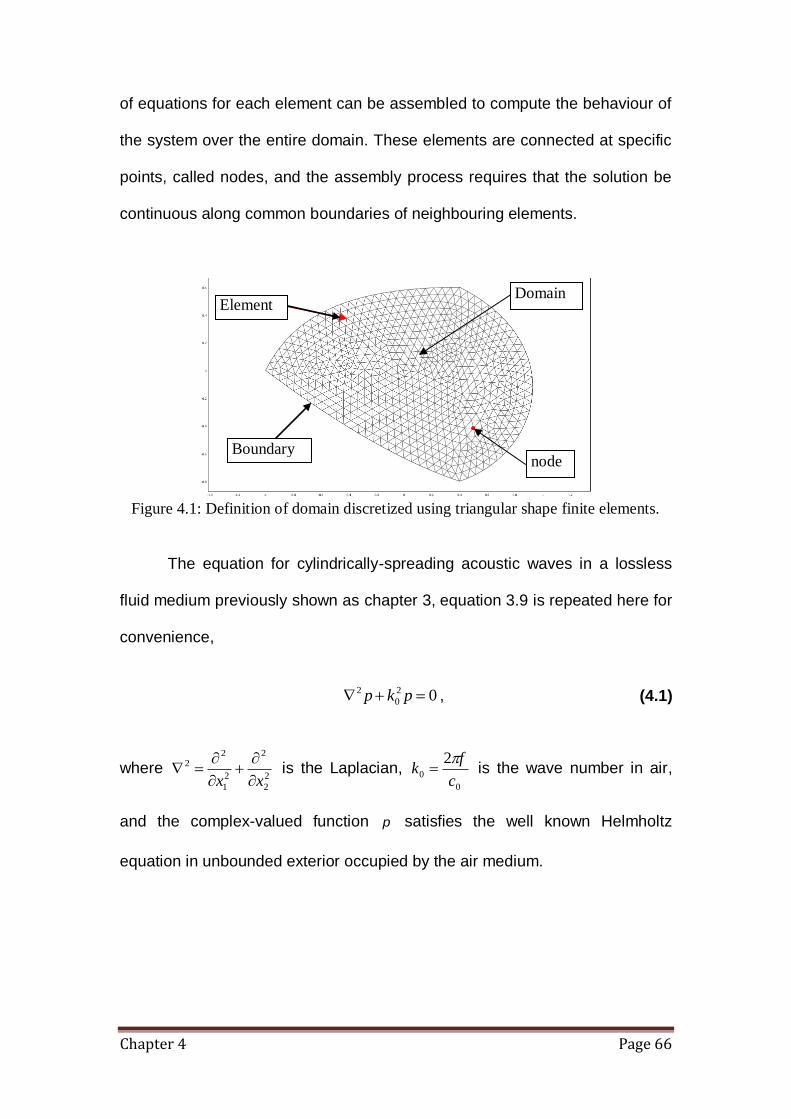
Chapter 4 Page 66
of equations for each element can be assembled to compute the behaviour of
the system over the entire domain. These elements are connected at specific
points, called nodes, and the assembly process requires that the solution be
continuous along common boundaries of neighbouring elements.
Figure 4.1: Definition of domain discretized using triangular shape finite elements.
The equation for cylindrically-spreading acoustic waves in a lossless
fluid medium previously shown as chapter 3, equation 3.9 is repeated here for
convenience,
02
0
2 pkp , (4.1)
where 2
2
2
2
1
22
xx
is the Laplacian,
0
0
2
c
fk
is the wave number in air,
and the complex-valued function p satisfies the well known Helmholtz
equation in unbounded exterior occupied by the air medium.
Boundary
Domain Element
node

Chapter 4 Page 67
The expressions for the pressure emitted by:
either a plane wave source or a cylindrical source are
xik
pin ep 0
_ , (4.2)
cccin rkiYrkJ
ip 0000_
4 , (4.3)
respectively, where 22
ccc yxr is the distance defined by the source
location to the travelling wave position. There have been more advanced
studies allowing for oblique incidence of the waves [73] but, in our model, we
consider that the direction of waves is normal to the symmetry axis of the
scatterer.
We define an acoustically-hard boundary condition (widely known as
the Neumann boundary condition) to model the rigid surface of the scatterers
whereby the normal acceleration of particle velocity is equal to zero,
01
.0
pn
, (4.4)
where 0 represents the density of the scatterer.
To compute two dimensional scattering problems in an unbounded domain
involves a domain decomposition by introducing an artificial boundary around
the obstacles. The radiation boundary conditions are applied to the
surrounding boundaries of the modelling domain (see figure 4.2). For the

Chapter 4 Page 68
outward travelling wave, this boundary condition ensures minimal or no
reflections from the model boundary. The radiation boundary conditions can
be expressed as [74],
riep
nirikp
rikpn
0
00
0
0
0
1
, (4.5)
where r is a function whose form depends on the type of wave as
described in the following,
plane wave: 0r , or
cylindrical wave: r
r2
1 ,
in which r is define as the shortest distance from the point on the boundary to
the source.
The term on the right hand side represents an incoming pressure wave with
amplitude, 0p and direction of propagation given by wave vector, and
normal vector, n .
A triangular mesh is used and the number of elements per wavelength is at
least 6 to obtain the desired accuracy. The accuracy of FEM will be discussed
in section 4.4. Equation 4.1 can now be solved using a parametric solver to
obtain the pressure field for the rectangular domain modelled as air. This is
done by performing a frequency sweep over 100 Hz to 8 kHz with frequency
step of 100 Hz to produce a frequency spectrum for both direct field and total
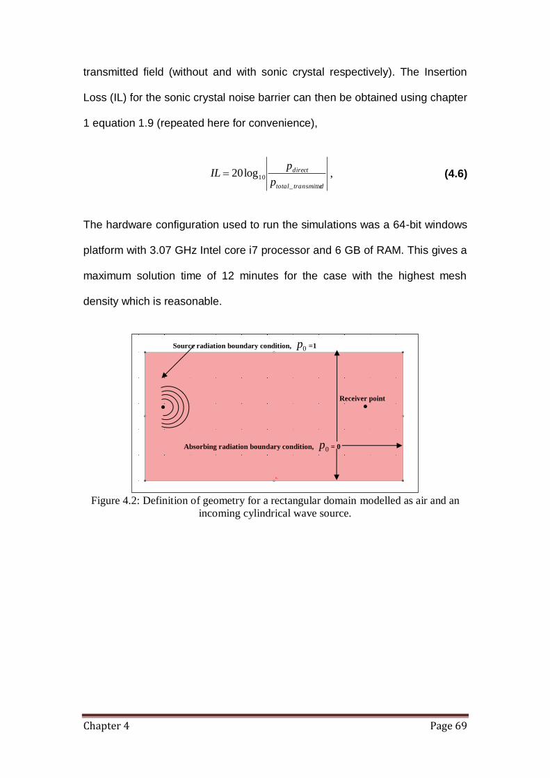
Chapter 4 Page 69
transmitted field (without and with sonic crystal respectively). The Insertion
Loss (IL) for the sonic crystal noise barrier can then be obtained using chapter
1 equation 1.9 (repeated here for convenience),
dtransmittetotal
direct
p
pIL
_
10log20 , (4.6)
The hardware configuration used to run the simulations was a 64-bit windows
platform with 3.07 GHz Intel core i7 processor and 6 GB of RAM. This gives a
maximum solution time of 12 minutes for the case with the highest mesh
density which is reasonable.
Figure 4.2: Definition of geometry for a rectangular domain modelled as air and an
incoming cylindrical wave source.
Receiver point
Absorbing radiation boundary condition, 0p = 0
Source radiation boundary condition, 0p =1
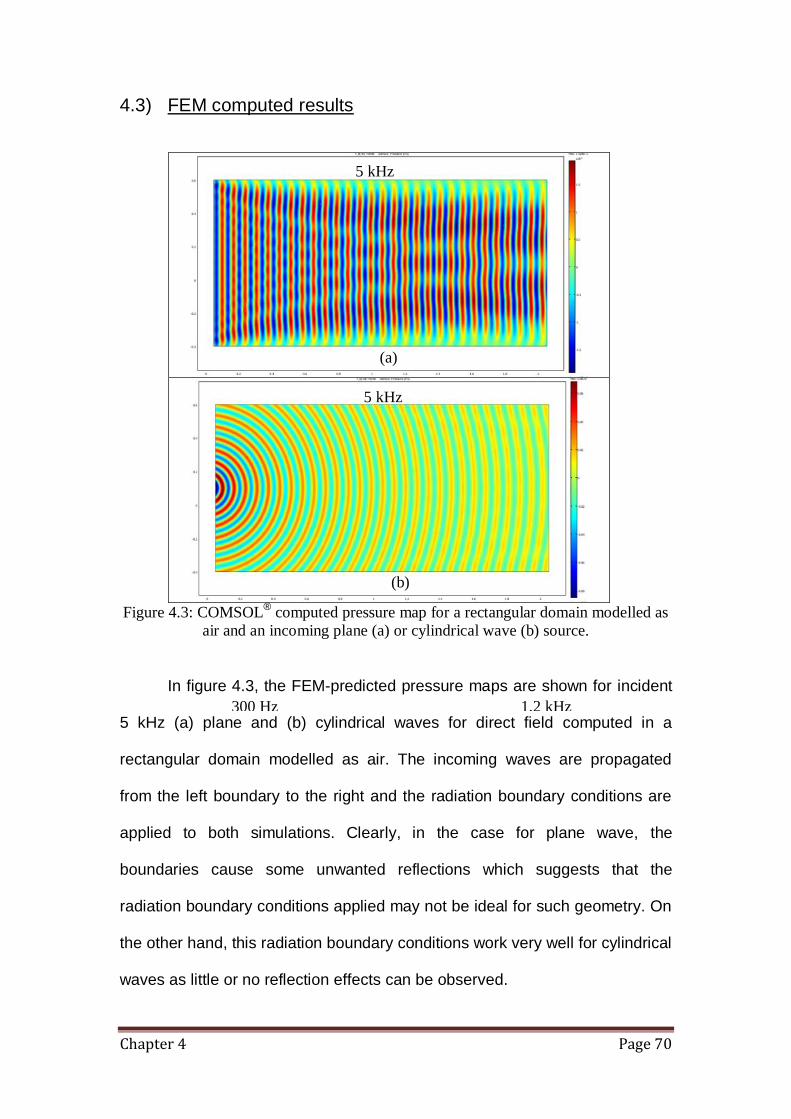
Chapter 4 Page 70
4.3) FEM computed results
Figure 4.3: COMSOL
® computed pressure map for a rectangular domain modelled as
air and an incoming plane (a) or cylindrical wave (b) source.
In figure 4.3, the FEM-predicted pressure maps are shown for incident
5 kHz (a) plane and (b) cylindrical waves for direct field computed in a
rectangular domain modelled as air. The incoming waves are propagated
from the left boundary to the right and the radiation boundary conditions are
applied to both simulations. Clearly, in the case for plane wave, the
boundaries cause some unwanted reflections which suggests that the
radiation boundary conditions applied may not be ideal for such geometry. On
the other hand, this radiation boundary conditions work very well for cylindrical
waves as little or no reflection effects can be observed.
5 kHz
5 kHz
300 Hz 1.2 kHz
(a)
(b)

Chapter 4 Page 71
Figure 4.4: COMSOL computed pressure maps for 7x3 array of sonic crystal
(acoustically hard scatterer) modelled in rectangular air domain. Cylindrical waves is
performed and pressure maps at 200 Hz, 1.2, 3, 4, 4.5 and 5 kHz are shown for figure
(a), (b), (c), (d) and (e) respectively.
Figure 4.4 shows the FEM-predicted pressure maps for a square lattice
array of 7x3 rigid circular scatterers with lattice constant of 0.135 m modelled
with similar boundary conditions to those used for the direct field
computations shown in figure 4.3. The radius of the scatterers is 0.0275 m.
The cylindrical wave source is located at 1.5 m away from the front face of the
array and the receiver is positioned 0.05 m from the nearest face of the array
but on the opposite side of the source. The number of triangular elements for
this model is 157392. The pressure maps are shown for various frequencies
ranging from 300 Hz to 5 kHz. Clearly, these results support the introductory
section on scattering (MST chapter 3, section 3.1), whereby incident waves
(a) (b)
3 kHz
(c) (d)
4 kHz
4.5 kHz
(e)
5 kHz
(f)
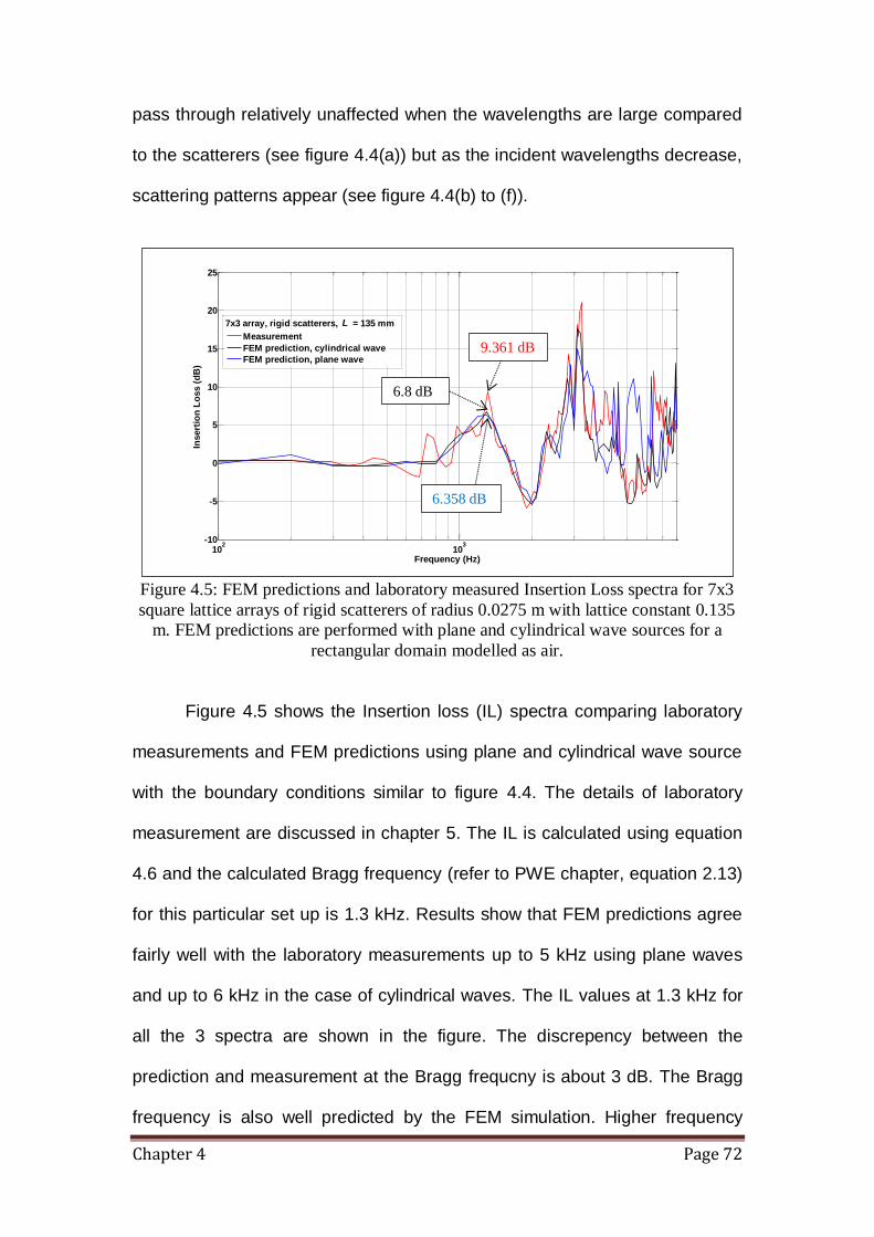
Chapter 4 Page 72
pass through relatively unaffected when the wavelengths are large compared
to the scatterers (see figure 4.4(a)) but as the incident wavelengths decrease,
scattering patterns appear (see figure 4.4(b) to (f)).
Figure 4.5: FEM predictions and laboratory measured Insertion Loss spectra for 7x3
square lattice arrays of rigid scatterers of radius 0.0275 m with lattice constant 0.135
m. FEM predictions are performed with plane and cylindrical wave sources for a
rectangular domain modelled as air.
Figure 4.5 shows the Insertion loss (IL) spectra comparing laboratory
measurements and FEM predictions using plane and cylindrical wave source
with the boundary conditions similar to figure 4.4. The details of laboratory
measurement are discussed in chapter 5. The IL is calculated using equation
4.6 and the calculated Bragg frequency (refer to PWE chapter, equation 2.13)
for this particular set up is 1.3 kHz. Results show that FEM predictions agree
fairly well with the laboratory measurements up to 5 kHz using plane waves
and up to 6 kHz in the case of cylindrical waves. The IL values at 1.3 kHz for
all the 3 spectra are shown in the figure. The discrepency between the
prediction and measurement at the Bragg frequcny is about 3 dB. The Bragg
frequency is also well predicted by the FEM simulation. Higher frequency
102
103
-10
-5
0
5
10
15
20
25
Frequency (Hz)
Insert
ion
Lo
ss (
dB
)
Measurement
FEM prediction, cylindrical wave
FEM prediction, plane wave
L7x3 array, rigid scatterers, = 135 mm
9.361 dB
6.8 dB
6.358 dB
Chapter 4 Page 73
agreement could be improved using higher mesh densities which inevitably
require a higher computational resource (explained in next section) or by
improvement of the boundary conditions to further minimise reflection as in
the case for plane wave. Peaks occurring in the measurements before the first
Bragg frequencies could be due to the finite height of the array (finite length of
the cylinders).
4.4) Investigation of accuracy of FEM
FEM is renowned for its versatility, being applicable to a wide range of
problems with complex geometries. But also the method lends itself easily to
a rigorous error analysis. Acoustics is a wave phenomenon in which the
waves are characterized by its wavelength in space, whose value depends
on the frequency and the speed of sound in the medium c relating to
equation 1.1. To solve wave problems governed by the Helmholtz equation
using FEM, the mesh must offer sufficient resolution. Generally for FEM, this
requires mesh grids with around ten nodal points per wavelength [75]. The
Mesh elements have to be increased even more when curvature or sharp
edges are present in the geometry. This section will discuss how frequency
convergence can be used to establish a high level of accuracy based on the
quality of mesh. In this study, an identical rectangular domain (direct field) to
that described in section 4.2 is modelled with cylindrical waves. Similar
radiation boundary conditions are applied to the edges of the rectangular
domain. The FEM computation is solved for the different mesh densities listed
in table 4.1 using a parametric solver (frequency sweep over 100 Hz to 8 kHz
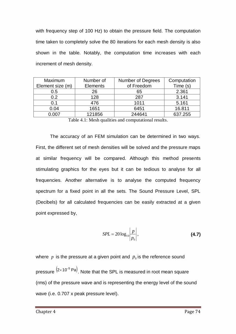
Chapter 4 Page 74
with frequency step of 100 Hz) to obtain the pressure field. The computation
time taken to completely solve the 80 iterations for each mesh density is also
shown in the table. Notably, the computation time increases with each
increment of mesh density.
Maximum Element size (m)
Number of Elements
Number of Degrees of Freedom
Computation Time (s)
0.5 26 65 2.361
0.2 128 287 3.141
0.1 476 1011 5.161
0.04 1651 6451 16.811
0.007 121856 244641 637.255
Table 4.1: Mesh qualities and computational results.
The accuracy of an FEM simulation can be determined in two ways.
First, the different set of mesh densities will be solved and the pressure maps
at similar frequency will be compared. Although this method presents
stimulating graphics for the eyes but it can be tedious to analyse for all
frequencies. Another alternative is to analyse the computed frequency
spectrum for a fixed point in all the sets. The Sound Pressure Level, SPL
(Decibels) for all calculated frequencies can be easily extracted at a given
point expressed by,
0
10log20p
pSPL , (4.7)
where p is the pressure at a given point and 0p is the reference sound
pressure Pa 102 5 . Note that the SPL is measured in root mean square
(rms) of the pressure wave and is representing the energy level of the sound
wave (i.e. 0.707 x peak pressure level).

Chapter 4 Page 75
Figure 4.6: FEM predicted pressure plots for cylindrical waves with different mesh element sizes.
200 Hz 500 Hz 1 kHz 3 kHz 5 kHz 8 kHz Mesh element size
0.5 m
0.2 m
0.1 m
0.04 m
0.007 m

Chapter 4 Page 76
Inaccuracy of the results will arise when there are an insufficient
number of elements. This is due to the inability to capture high-frequency
(short wavelength) solutions when using a mesh with large element size
which leads to the non-convergence of the solution and so the pressure map
will have poor resolution at these high frequencies. This is clearly
demonstrated in the FEM computed pressure maps (figure 4.6), which
illustrate that solutions are unresolved at high frequencies ranges for low
mesh density and that the resolution of the computed pressure map at higher
frequencies improves as the mesh density increases.
Figure 4.7: Sound pressure level spectra at single point position for FEM
computations of the field due to a cylindrical wave computed using different mesh
element sizes.
Figure 4.7 shows the SPL in dB for the range of frequencies. Evidently
convergence problems can be observed in the high frequency range for an
insufficient mesh density (i.e. Roll off from the nominal SPL value of near 60
dB. The frequency spectrum for the highest mesh density demonstrates that
the cylindrical wave source has a flat frequency content.
300 1000 8000-60
-40
-20
0
20
40
60
80
Frequency (Hz)
So
un
d P
ressu
re L
evel (d
B)
0.5 m
0.2 m
0.1 m
0.04 m
0.007 m
Mesh element size

Chapter 4 Page 77
Bearing this convergence study in mind, the maximum element size of
0.007 m will be chosen for all subsequent computational modelling in FEM.
This set the convergence criterion to about 3%. This allows good
convergence up to 8 kHz which is sufficient for the study of barriers subject to
a traffic noise spectrum. For FEM simulations at higher frequencies, the
maximum element size must be at least 6 times smaller than the shortest
wavelength.
4.5) Investigation of sonic crystal performance using scatterers with different shapes
The relative ease of modelling different shapes in FEM allows the study
of sonic crystals in two-dimension with different geometrical shapes of the
scatterers and different lattice configurations. The first part of this section
looks at predictions of the insertion loss spectra due to 7x3 arrays with a filling
fraction of about 13% containing different (rigid) scatterer shapes including
triangular, square and elliptical shapes, and compares them with predictions
for cylindrical scatterers in an array of similar size. These studies are also
performed with the similar source and receiver distances mentioned in section
4.3. A source of cylindrical waves propagating parallel to the scatterer axis
and radiation boundary conditions are assumed in the FE models.
4.5.1) Triangular scatterers
Each triangular scatterer has a surface area of 0.0024 m2 (base 0.074
m and height 0.064 m) that is similar to the surface area of a cylindrical
scatterer considered previously. The array size and lattice constant are

Chapter 4 Page 78
identical with the reference sonic crystal with cylindrical scatterers. Three
different orientations are studied and the pressure maps at 1.3 and 2.3 kHz
are compared (see figure 4.8). Comparisons are made also with an equivalent
cylindrical scatterer design (see figure 4.9).
Figure 4.8: FEM (COMSOL
®) predicted pressure maps comparing three different
arrangements (top to bottom) and 2 frequencies pressure maps for each arrangement
(left 1.3 kHz and right 2.3 kHz) of 7x3 triangular rigid scatterer arrays (square lattice)
with lattice constant of 0.135 m.
Figure 4.8 shows the FEM computed pressure maps for the 3 different
arrangements of 7x3 triangular shape arrays in a square lattice configuration.
For all the 3 arrangements, similar scattering patterns are observed at 1.3 kHz
which is the first (Bragg) band gap frequency due to the periodicity. At the
higher frequency of 2.3 kHz, the scattering patterns vary from one
Arrangement 1 (1.3 kHz)
(a)
Arrangement 2 (1.3 kHz)
(e)
Arrangement 3 (1.3 kHz)
(b)
Arrangement 1 (2.3 kHz)
Arrangement 2 (2.3 kHz)
Arrangement 3 (2.3 kHz)
(d)
(f)
(c)
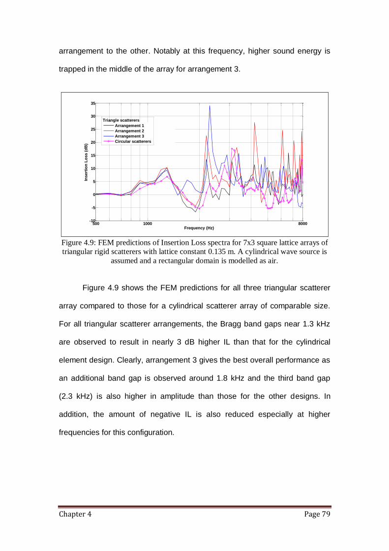
Chapter 4 Page 79
arrangement to the other. Notably at this frequency, higher sound energy is
trapped in the middle of the array for arrangement 3.
Figure 4.9: FEM predictions of Insertion Loss spectra for 7x3 square lattice arrays of
triangular rigid scatterers with lattice constant 0.135 m. A cylindrical wave source is
assumed and a rectangular domain is modelled as air.
Figure 4.9 shows the FEM predictions for all three triangular scatterer
array compared to those for a cylindrical scatterer array of comparable size.
For all triangular scatterer arrangements, the Bragg band gaps near 1.3 kHz
are observed to result in nearly 3 dB higher IL than that for the cylindrical
element design. Clearly, arrangement 3 gives the best overall performance as
an additional band gap is observed around 1.8 kHz and the third band gap
(2.3 kHz) is also higher in amplitude than those for the other designs. In
addition, the amount of negative IL is also reduced especially at higher
frequencies for this configuration.
500 1000 8000-10
-5
0
5
10
15
20
25
30
35
Frequency (Hz)
Insert
ion
Lo
ss (
dB
)
Arrangement 1
Arrangement 2
Arrangement 3
Circular scatterers
Triangle scatterers
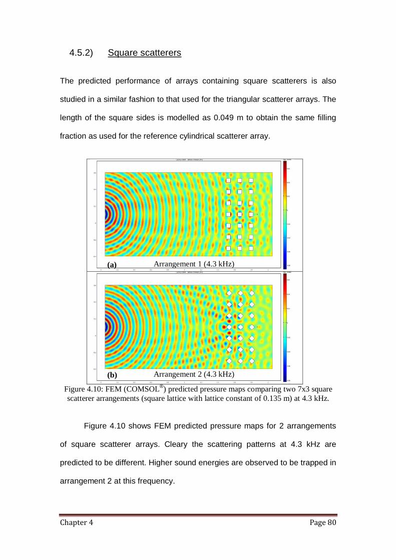
Chapter 4 Page 80
4.5.2) Square scatterers The predicted performance of arrays containing square scatterers is also
studied in a similar fashion to that used for the triangular scatterer arrays. The
length of the square sides is modelled as 0.049 m to obtain the same filling
fraction as used for the reference cylindrical scatterer array.
Figure 4.10: FEM (COMSOL
®) predicted pressure maps comparing two 7x3 square
scatterer arrangements (square lattice with lattice constant of 0.135 m) at 4.3 kHz.
Figure 4.10 shows FEM predicted pressure maps for 2 arrangements
of square scatterer arrays. Cleary the scattering patterns at 4.3 kHz are
predicted to be different. Higher sound energies are observed to be trapped in
arrangement 2 at this frequency.
(a) Arrangement 1 (4.3 kHz)
(b) Arrangement 2 (4.3 kHz)

Chapter 4 Page 81
Figure 4.11: FEM predictions of Insertion Loss spectra for two arrangements of 7x3
square lattice arrays of square rigid scatterers and a reference array of cylindrical rigid
scatterers with lattice constant 0.135 m. A cylindrical wave source is assumed and a
rectangular domain is modelled as air.
Figure 4.11 shows the FEM predicted IL spectra for the 2 square
scatterer arrangements and the reference cylindrical scatterer array. The
Bragg band gaps (1.3 kHz) are predicted to be of similar size and amplitude
for all the designs. The results show no significant advantage in using square
scatterers.
4.5.3) Elliptical shape scatterer
Previous research on sonic crystals with elliptical shape scatterers has
reported that certain configurations can vary the direction of propagation due
to the geometry anisotropy of the elliptical scatterer [76]. In our model, the
elliptical scatterers have a semi-major axis of 0.035 m and semi-minor axis of
0.0218 m. This geometry provides the same filling fraction as that assumed
500 1000 8000-10
-5
0
5
10
15
20
25
30
35
Frequency (Hz)
Insert
ion
Lo
ss (
dB
)
Arrangement 1
Arrangement 2
Circular scatterers
Square scatterers

Chapter 4 Page 82
for different scatterer shapes previously. The elliptical scatterer arrays are
modelled with 3 different arrangements (see figure 4.12).
Figure 4.12: FEM (COMSOL
®) predicted pressure maps for three 7x3 arrangements
of elliptical rigid scatterers (square lattice) with lattice constant of 0.135 m at 1.5 kHz
(a)
(b)
Arrangement 1 (1.5 kHz)
(c)
Arrangement 2 (1.5 kHz)
Arrangement 3 (1.5 kHz)

Chapter 4 Page 83
Figure 4.12 shows FEM predicted pressure maps for 3 arrangements
of elliptical scatterer arrays. The scattering patterns for all arrangements are
predicted to be different at 1.5 kHz.
Figure 4.13: FEM predicted Insertion Loss spectra for 7x3 square lattice arrays of
elliptical rigid scatterers with lattice constant 0.135 m compared with that predicted
for an equivalent cylindrical scatterer array. For the FEM predictions a cylindrical
wave source is assumed and the rectangular domain is modelled as air.
In figure 4.13, IL spectra for the elliptical scatterer arrays at a similar
receiver position are compared with that measured for the equivalent
cylindrical scatterer array. Arrangement 1 which the elliptical scatterer has its
semi-major axis perpendicular to the direction of wave propagation is
predicted to produce the highest amplitude Bragg band gap at 1.3 kHz. This
suggests that much of the incoming wave front is blocked by the larger
surface of the scatterer. Also the Bragg band gap is predicted to contain two
peaks instead of one for this particular arrangement. The lowest amplitude
Bragg band gap is predicted for arrangement 2 where the semi-minor axis is
parallel to the incoming wave. Thus, allowing the largest transmission of
500 1000 8000-10
-5
0
5
10
15
20
25
Frequency (Hz)
Insert
ion
Lo
ss (
dB
)
Arrangement 1
Arrangement 2
Arrangement 3
Circular scatterers
Elliptical scatterers

Chapter 4 Page 84
incident waves. Arrangement 3 with scatterers having 45° orientation is
predicted to give comparable IL to the equivalent cylindrical array near the
Bragg band gap but is predicted to offer better performance at higher
frequencies.
Figure 4.14: FEM predictions of Insertion Loss spectra for 7x3 square lattice arrays of
the best performing triangular, square and elliptical rigid scatterer arrays compared to
that predicted for the reference cylindrical scatterer array.
Figure 4.14 compares the predicted IL spectra for the best performing
scatterer shape examples (circular, triangular, square and elliptical) discussed
in this section. The array with triangular scatterers in arrangement 3 is
predicted to reduce the focusing effect (negative IL) and that with elliptical
scatterers in arrangement 1 offers the highest amplitude first Bragg band gap.
Although predicted to give significant advantages in comparison with
equivalent cylindrical arrays, the manufacturing cost for elliptical shapes will
be much higher. For example, it costs more than £1000 for 21 3 m long
elliptical scatterers made of stainless steel.
500 1000 8000-10
-5
0
5
10
15
20
25
30
35
Frequency (Hz)
Insert
ion
Lo
ss (
dB
)
Triangle scatterers, arrangement 3
Elliptical scatterers, arrangement 1
Square scatterers, arrangement 1
Circular scatterers
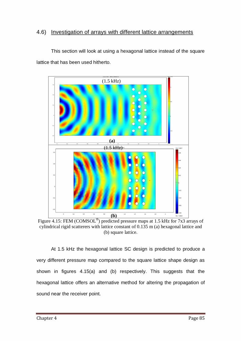
Chapter 4 Page 85
4.6) Investigation of arrays with different lattice arrangements
This section will look at using a hexagonal lattice instead of the square
lattice that has been used hitherto.
Figure 4.15: FEM (COMSOL
®) predicted pressure maps at 1.5 kHz for 7x3 arrays of
cylindrical rigid scatterers with lattice constant of 0.135 m (a) hexagonal lattice and
(b) square lattice.
At 1.5 kHz the hexagonal lattice SC design is predicted to produce a
very different pressure map compared to the square lattice shape design as
shown in figures 4.15(a) and (b) respectively. This suggests that the
hexagonal lattice offers an alternative method for altering the propagation of
sound near the receiver point.
(1.5 kHz)
(a)
(b)
(1.5 kHz)
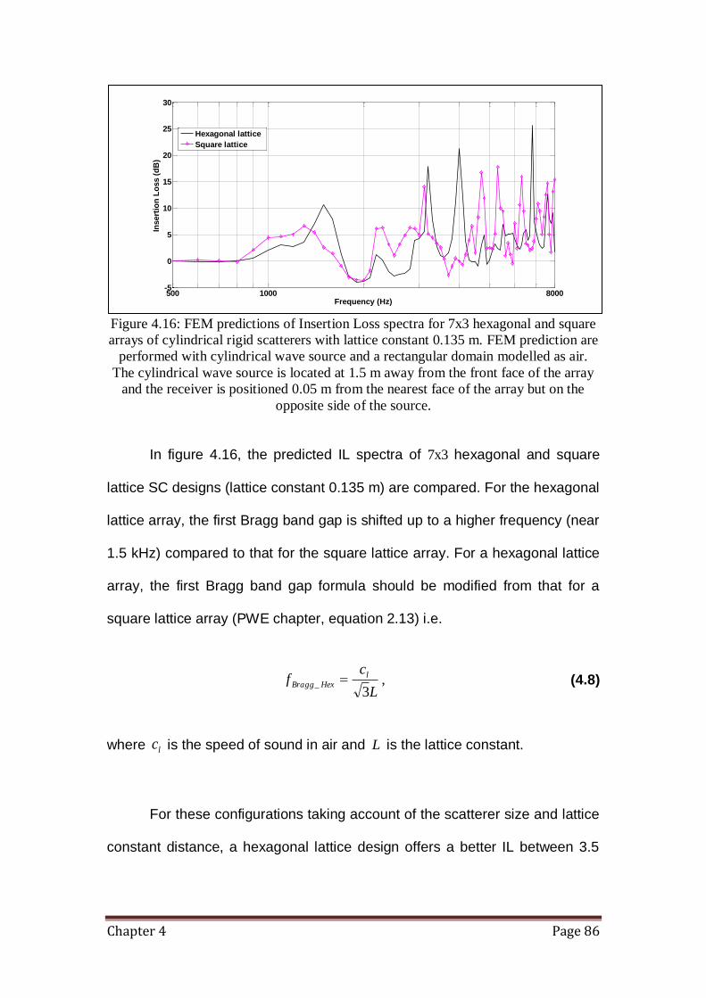
Chapter 4 Page 86
Figure 4.16: FEM predictions of Insertion Loss spectra for 7x3 hexagonal and square
arrays of cylindrical rigid scatterers with lattice constant 0.135 m. FEM prediction are
performed with cylindrical wave source and a rectangular domain modelled as air.
The cylindrical wave source is located at 1.5 m away from the front face of the array
and the receiver is positioned 0.05 m from the nearest face of the array but on the
opposite side of the source.
In figure 4.16, the predicted IL spectra of 7x3 hexagonal and square
lattice SC designs (lattice constant 0.135 m) are compared. For the hexagonal
lattice array, the first Bragg band gap is shifted up to a higher frequency (near
1.5 kHz) compared to that for the square lattice array. For a hexagonal lattice
array, the first Bragg band gap formula should be modified from that for a
square lattice array (PWE chapter, equation 2.13) i.e.
L
cf l
HexBragg3
_ , (4.8)
where lc is the speed of sound in air and L is the lattice constant.
For these configurations taking account of the scatterer size and lattice
constant distance, a hexagonal lattice design offers a better IL between 3.5
500 1000 8000-5
0
5
10
15
20
25
30
Frequency (Hz)
Insert
ion
Lo
ss (
dB
)
Hexagonal lattice
Square lattice

Chapter 4 Page 87
and 7 kHz (based on a single receiver position). However as a traffic noise
barrier the square lattice design could possibly be better.
4.7) Perfectly Matched Layers (PML)
The capability of emulating the Sommerfeld radiation condition, which
requires that outgoing wave propagate out towards infinity and therefore the
absence of reflection from the boundaries (i.e. creating an unbounded
modelling enviroment), is critical for any numerical code concerned with the
solution of wave problems. Normally, in FEM computations, the outer
boundaries of the computational region are subjected to a radiation boundary
condition and this has been used to treat these boundaries in the earlier
sections. An alternative method is to implement Perfectly Matched Layers
(PML) at these boundaries. This approach was first introduced by Bérenger
[146] in 1994 for electromagnetic waves. It is commonly used for simulating
wave problems with open boundaries. A PML is an artificial (non-physical)
absorbing layer in which the wave equation has been modified with an
anisotropic damping, which increases with distance in the direction
perpendicular to the interface with the physical domain (see figure 4.17). The
result is that waves entering the PML are absorbed only in the outgoing
direction, while the wave components tangential to the interface between the
PML and physical domain remain unaffected. The key property of a PML that
distinguishes it from an ordinary absorbing material is that it is designed so
that waves incident upon the PML from a non-PML medium do not reflect at
the interface. The main advantages of the PML over radiation boundary

Chapter 4 Page 88
conditions are the relative ease of implementation using a complex
coordinates scaling [77]. Thus making it possible to minimise the size of the
computational domain and this in turn reduces the computational demands.
The implementation of a PML for computing the pressure field due to a
7x3 array of circular scatterers with similar setup to that investigated in section
5.3 has been studied. The incident waves are modelled as plane waves due
to the reduced size of the domain.
Figure 4.17: Implementation of PMLs around a 7x3 square lattice array of circular
scatterers (a) location of PMLs and (b) FEM-computed pressure map at 1.2 kHz.
1.2 kHz
(PML)
(PML)
(PM
L)
(PM
L)
(a)
(b)

Chapter 4 Page 89
Figure 4.18: FEM predictions (with and without PML) compared to laboratory
measurements of Insertion Loss spectra for a 7x3 square lattice array of circular rigid
scatterers with a lattice constant 0.135 m.
As shown in figure 4.18, the FEM predicted IL spectra with and without PML
implementation are in fair agreement with the laboratory data. The time taken
to solve the problem using PML is 402.41 s which is 0.37 times faster than
that taken when using radiation boundary conditions with the maximum
element size (see table 4.1).
500 1000 8000-10
-5
0
5
10
15
20
25
Frequency (Hz)
Insert
ion
Lo
ss (
dB
)
Measurement
FEM prediction, PML
FEM prediction, without PML

Chapter 5 Page 90
Chapter 5
Measurement Techniques
5.1) Introduction
It is important to validate any hypothesis and/or prediction by performing a
relevant experiment. The first experimental evidence of the acoustical
properties of a sonic crystal in air was performed in 1995 by Martinez-Sala et
al [20]. The authors measured the transmission properties of a finite periodic
minimalist sculpture in outdoor by Eusebio Sempere in Spain (see figure 1.4).
It was observed that such periodic structures have similar acoustical
characteristics to electromagnetic properties of solid crystalline structures.
Subsequently, research has resulted in the development of improved
experimental methods for checking theoretical results. The experiments
reported in this Chapter were carried out either in an anechoic laboratory or
outdoors at the Open University’s noise barrier test site and at Diglis weir near
Worcester.
To measure or analyse an acoustic waveform which consists of a
variation in pressure as time passes, it is usual to generate an electrical
analogue of the pressure variation by means of an input transducer (i.e.
microphone). Likewise to generate a sound, we also start with an electrical
waveform and use an output transducer (i.e. loudspeaker) to convert it into a
pressure change. Under the assumption of source and receiver immobility,
the acoustic space in which they are placed can be considered as linear and
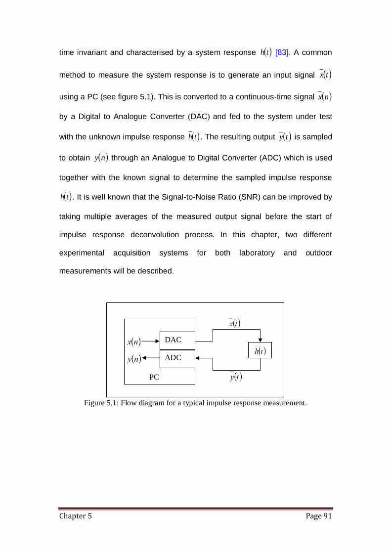
Chapter 5 Page 91
time invariant and characterised by a system response th [83]. A common
method to measure the system response is to generate an input signal tx
using a PC (see figure 5.1). This is converted to a continuous-time signal nx
by a Digital to Analogue Converter (DAC) and fed to the system under test
with the unknown impulse response th . The resulting output ty is sampled
to obtain ny through an Analogue to Digital Converter (ADC) which is used
together with the known signal to determine the sampled impulse response
th . It is well known that the Signal-to-Noise Ratio (SNR) can be improved by
taking multiple averages of the measured output signal before the start of
impulse response deconvolution process. In this chapter, two different
experimental acquisition systems for both laboratory and outdoor
measurements will be described.
Figure 5.1: Flow diagram for a typical impulse response measurement.
DAC
ADC
PC

Chapter 5 Page 92
5.2) Laboratory measurments using Maximum-Length Sequence System Analyzer (MLSSA).
5.2.1) Introduction to MLSSA
Acoustical impulse response measurements using the Maximum-
Length Sequence (MLS) technique were first proposed by Schroeder in 1973
[84]. MLSSA can measure and analyze many types of linear systems and is
widely used for audio and acoustics measurements [85, 86 and 87]. A MLS
signal is a type of pseudorandom binary sequence which, unlike white noise,
is deterministic and periodic yet still retains most of the desirable
characteristics of white noise (i.e. broadband and flat response). MLS may be
generated computationally by employing linear feedback shift registers as
illustrated in figure 5.2. In contrast with a conventional dual channel analyzer,
MLSSA is single channel but, given the periodic nature of the MLS, a single
time domain circular cross-correlation calculation can recover the complete
system impulse response. Thus, effectively it can do the work of a dual
channel analyzer with the advantage of doubling the useful bandwidth and
significant reduction in cost [88].
Figure 5.2: Linear feedback shift register for generation of a MLS (of length 2
4 - 1=
15) signal.
XOR
z-1
z-1
z-1
z-1
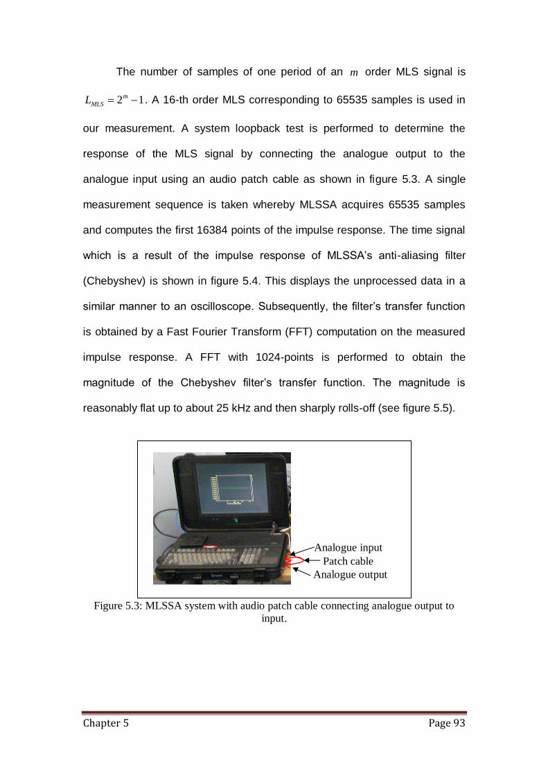
Chapter 5 Page 93
The number of samples of one period of an m order MLS signal is
12 m
MLSL . A 16-th order MLS corresponding to 65535 samples is used in
our measurement. A system loopback test is performed to determine the
response of the MLS signal by connecting the analogue output to the
analogue input using an audio patch cable as shown in figure 5.3. A single
measurement sequence is taken whereby MLSSA acquires 65535 samples
and computes the first 16384 points of the impulse response. The time signal
which is a result of the impulse response of MLSSA’s anti-aliasing filter
(Chebyshev) is shown in figure 5.4. This displays the unprocessed data in a
similar manner to an oscilloscope. Subsequently, the filter’s transfer function
is obtained by a Fast Fourier Transform (FFT) computation on the measured
impulse response. A FFT with 1024-points is performed to obtain the
magnitude of the Chebyshev filter’s transfer function. The magnitude is
reasonably flat up to about 25 kHz and then sharply rolls-off (see figure 5.5).
Figure 5.3: MLSSA system with audio patch cable connecting analogue output to
input.
Patch cable
Analogue input
Analogue output
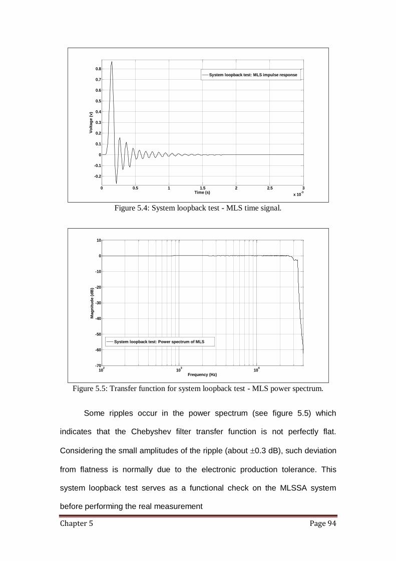
Chapter 5 Page 94
Figure 5.4: System loopback test - MLS time signal.
Figure 5.5: Transfer function for system loopback test - MLS power spectrum.
Some ripples occur in the power spectrum (see figure 5.5) which
indicates that the Chebyshev filter transfer function is not perfectly flat.
Considering the small amplitudes of the ripple (about 0.3 dB), such deviation
from flatness is normally due to the electronic production tolerance. This
system loopback test serves as a functional check on the MLSSA system
before performing the real measurement
0 0.5 1 1.5 2 2.5 3
x 10-3
-0.2
-0.1
0
0.1
0.2
0.3
0.4
0.5
0.6
0.7
0.8
Time (s)
Vo
ltag
e (
v)
System loopback test: MLS impulse response
102
103
104
-70
-60
-50
-40
-30
-20
-10
0
10
Frequency (Hz)
Mag
nit
ud
e (
dB
)
System loopback test: Power spectrum of MLS
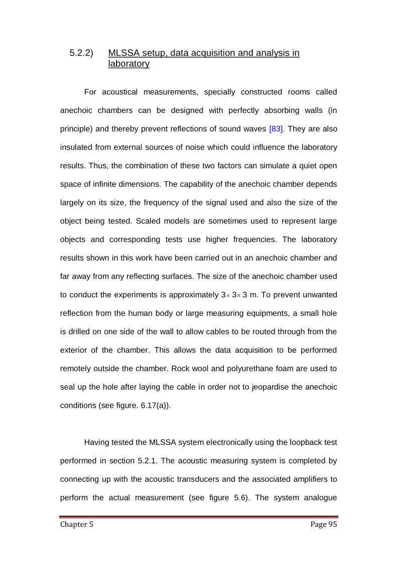
Chapter 5 Page 95
5.2.2) MLSSA setup, data acquisition and analysis in laboratory
For acoustical measurements, specially constructed rooms called
anechoic chambers can be designed with perfectly absorbing walls (in
principle) and thereby prevent reflections of sound waves [83]. They are also
insulated from external sources of noise which could influence the laboratory
results. Thus, the combination of these two factors can simulate a quiet open
space of infinite dimensions. The capability of the anechoic chamber depends
largely on its size, the frequency of the signal used and also the size of the
object being tested. Scaled models are sometimes used to represent large
objects and corresponding tests use higher frequencies. The laboratory
results shown in this work have been carried out in an anechoic chamber and
far away from any reflecting surfaces. The size of the anechoic chamber used
to conduct the experiments is approximately 3 3 3 m. To prevent unwanted
reflection from the human body or large measuring equipments, a small hole
is drilled on one side of the wall to allow cables to be routed through from the
exterior of the chamber. This allows the data acquisition to be performed
remotely outside the chamber. Rock wool and polyurethane foam are used to
seal up the hole after laying the cable in order not to jeopardise the anechoic
conditions (see figure. 6.17(a)).
Having tested the MLSSA system electronically using the loopback test
performed in section 5.2.1. The acoustic measuring system is completed by
connecting up with the acoustic transducers and the associated amplifiers to
perform the actual measurement (see figure 5.6). The system analogue
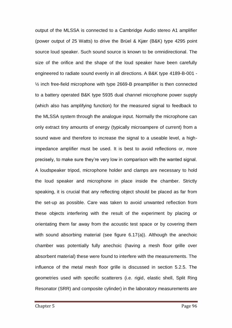
Chapter 5 Page 96
output of the MLSSA is connected to a Cambridge Audio stereo A1 amplifier
(power output of 25 Watts) to drive the Brüel & Kjær (B&K) type 4295 point
source loud speaker. Such sound source is known to be omnidirectional. The
size of the orifice and the shape of the loud speaker have been carefully
engineered to radiate sound evenly in all directions. A B&K type 4189-B-001 -
½ inch free-field microphone with type 2669-B preamplifier is then connected
to a battery operated B&K type 5935 dual channel microphone power supply
(which also has amplifying function) for the measured signal to feedback to
the MLSSA system through the analogue input. Normally the microphone can
only extract tiny amounts of energy (typically microampere of current) from a
sound wave and therefore to increase the signal to a useable level, a high-
impedance amplifier must be used. It is best to avoid reflections or, more
precisely, to make sure they’re very low in comparison with the wanted signal.
A loudspeaker tripod, microphone holder and clamps are necessary to hold
the loud speaker and microphone in place inside the chamber. Strictly
speaking, it is crucial that any reflecting object should be placed as far from
the set-up as possible. Care was taken to avoid unwanted reflection from
these objects interfering with the result of the experiment by placing or
orientating them far away from the acoustic test space or by covering them
with sound absorbing material (see figure 6.17(a)). Although the anechoic
chamber was potentially fully anechoic (having a mesh floor grille over
absorbent material) these were found to interfere with the measurements. The
influence of the metal mesh floor grille is discussed in section 5.2.5. The
geometries used with specific scatterers (i.e. rigid, elastic shell, Split Ring
Resonator (SRR) and composite cylinder) in the laboratory measurements are
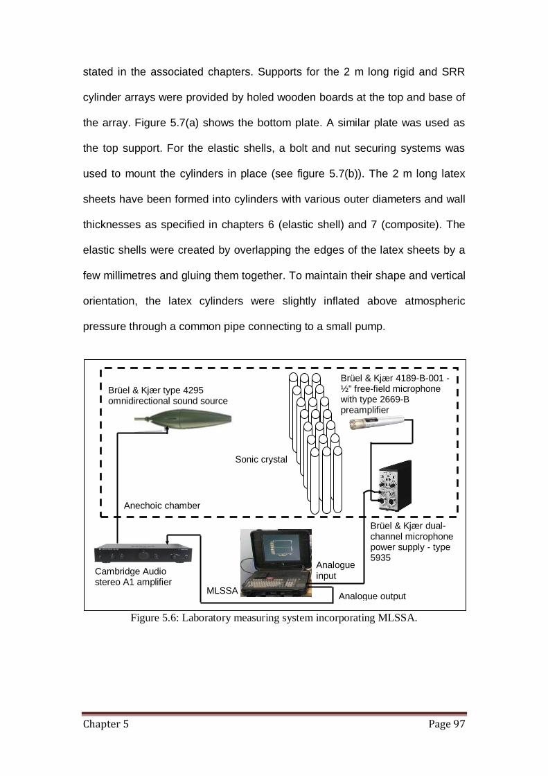
Chapter 5 Page 97
stated in the associated chapters. Supports for the 2 m long rigid and SRR
cylinder arrays were provided by holed wooden boards at the top and base of
the array. Figure 5.7(a) shows the bottom plate. A similar plate was used as
the top support. For the elastic shells, a bolt and nut securing systems was
used to mount the cylinders in place (see figure 5.7(b)). The 2 m long latex
sheets have been formed into cylinders with various outer diameters and wall
thicknesses as specified in chapters 6 (elastic shell) and 7 (composite). The
elastic shells were created by overlapping the edges of the latex sheets by a
few millimetres and gluing them together. To maintain their shape and vertical
orientation, the latex cylinders were slightly inflated above atmospheric
pressure through a common pipe connecting to a small pump.
Figure 5.6: Laboratory measuring system incorporating MLSSA.
Brüel & Kjær type 4295 omnidirectional sound source
Anechoic chamber
Cambridge Audio stereo A1 amplifier
Brüel & Kjær dual-channel microphone power supply - type 5935 Analogue
input
Analogue output
Brüel & Kjær 4189-B-001 - ½" free-field microphone with type 2669-B preamplifier
Sonic crystal
MLSSA

Chapter 5 Page 98
Figure 5.7: (a) Supporting base plate for 7x3 arrays of PVC or elastic cylinders. 55
mm diameter holes for PVC cylinders. 5 mm diameter holes for elastic shell using
bolt and nut securing system. (b) Lower end of an elastic shell showing plastic pipe
for air inlet and mounting bolt.
The direct sound field measurement method that has been used is
closely related with that described in BS EN 1793-6 [89]. During the array
measurements, the receiver microphone was positioned 50 mm from the
nearest face of the array but on the opposite side of the source. Both source
and receiver were 1.2 m above the floor of the chamber. The loud speaker
was placed between 1.5 m and 1.63 m away from the array, such that the
source-receiver axis was normal to the array orientation (see figure 5.8).
55 mm diameter holes for PVC
cylinders
5 mm thick MDF
5 mm diameter holes for elastic shells
(a) (b)
Elastic shell
Bolt
Perspex
disc pipe
overlapped

Chapter 5 Page 99
Figure 5.8: (a) Plan view of the source, receiver and array in the laboratory
measurements at normal incidence (b) the corresponding side view. Refer to chapters
2, 3, 4, 6 and 7 for the outer diameters and lattice constants used.
The input signals are first passed through the fixed analogue
Chebyshev filter implanted in MLSSA system to remove any signals with
frequency component beyond the selected range which is 10 kHz in our case.
The sampling rate was chosen to be greater than twice the maximum
frequency contained in the signal to be measured. This Nyquist frequency is
crucial to accurately reconstruct the measured signal. To improve the SNR
using the MLSSA system, 16 time averages were carried out for each
measurement. The time required for each measurement was very short, only
a few seconds were necessary to obtain the impulse response for the
acoustic test space (see figure 5.8). Example plots of the time signals
corresponding to the direct field and total transmitted field through a sonic
crystal are shown in figure 5.9. In contrast with figure 5.4, the direct field
signal looks different to that in figure 5.4 since the complete system response
is influenced by factors such as the physical setup, responses of loudspeaker
and microphone. For the post-processing operation, a half Blackman Harris
filter was used to frame the time signal and window out the unwanted
reflections. An FFT was applied to decompose the time domain signal to yield
(Refer to relevant chapters for d and L values).
L
L
d
1.5 m
50 mm
x
y
x
z
Ground
1.5 m
50 mm
1.2 m
1.2 m
(a) (b)
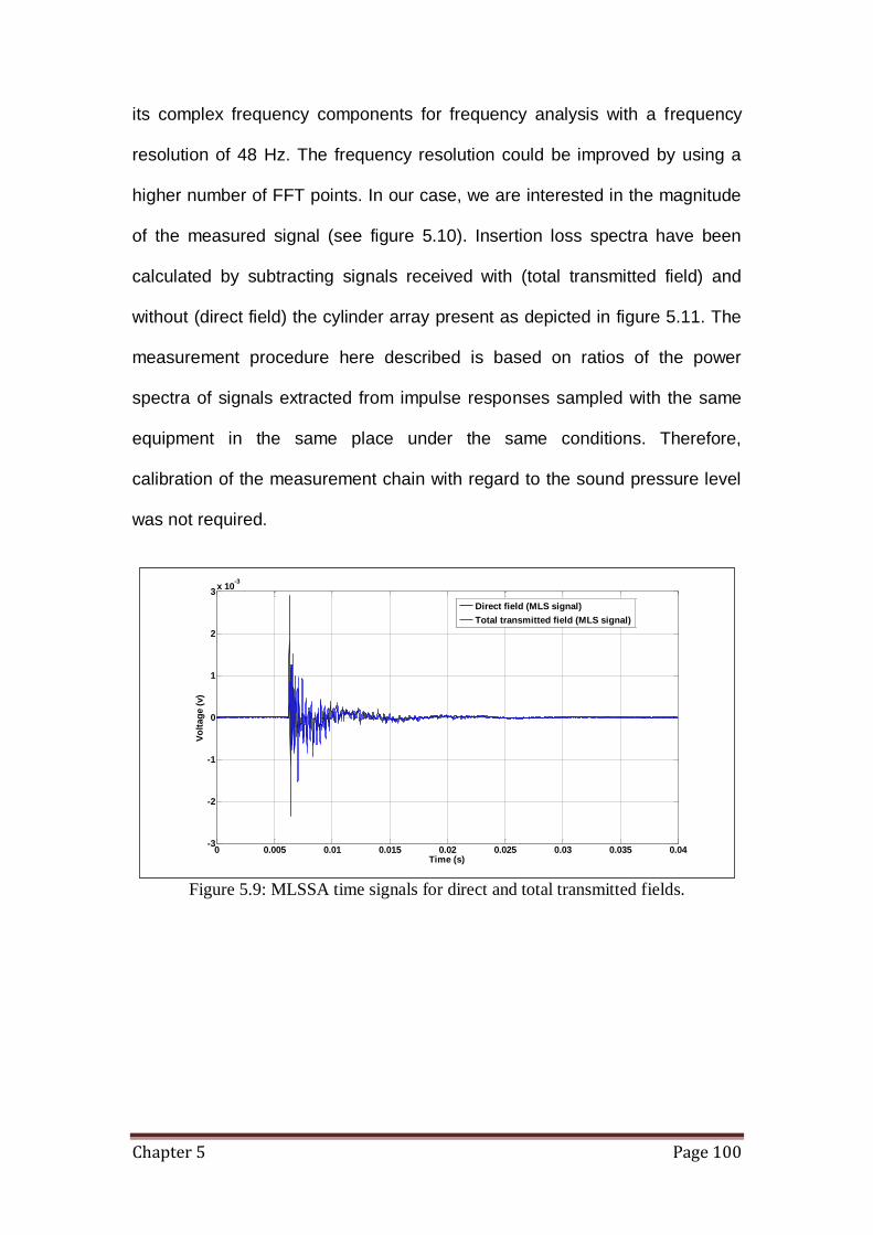
Chapter 5 Page 100
its complex frequency components for frequency analysis with a frequency
resolution of 48 Hz. The frequency resolution could be improved by using a
higher number of FFT points. In our case, we are interested in the magnitude
of the measured signal (see figure 5.10). Insertion loss spectra have been
calculated by subtracting signals received with (total transmitted field) and
without (direct field) the cylinder array present as depicted in figure 5.11. The
measurement procedure here described is based on ratios of the power
spectra of signals extracted from impulse responses sampled with the same
equipment in the same place under the same conditions. Therefore,
calibration of the measurement chain with regard to the sound pressure level
was not required.
Figure 5.9: MLSSA time signals for direct and total transmitted fields.
0 0.005 0.01 0.015 0.02 0.025 0.03 0.035 0.04-3
-2
-1
0
1
2
3x 10
-3
Time (s)
Vo
ltag
e (
v)
Direct field (MLS signal)
Total transmitted field (MLS signal)

Chapter 5 Page 101
Figure 5.10: MLSSA Frequency spectra for direct and total transmitted fields.
Figure 5.11: Insertion Loss (IL) spectrum using MLSSA of 7x3 square lattice arrays
of rigid PVC scatterers of outer diameter 0.055 m and lattice constant 0.069 m.
Frequency resolution at 48 Hz.
5.2.3) Influence on the difference of windowing size for signal post processing.
As discussed in section 5.2.2, a finite length of the input signal was
chosen during the post-processing. A test was carried out to determine how
truncation of the time domain signal by the size of the window could affect the
power spectrum. The time domain signal of the total transmitted signal (see
102
103
104
-120
-110
-100
-90
-80
-70
-60
Frequency (Hz)
Mag
nit
ud
e (
dB
)
Direct field
Total transmitted field
102
103
-10
0
10
20
30
40
50
Frequency (Hz)
Insert
ion
Lo
ss (
dB
)
Measurement, 7x3 array of rigid PVC with L = 0.069 m

Chapter 5 Page 102
figure 5.9) was used for this test. The starting of the signal is fixed at 6.2 ms
and the end signal was varied from 10, 15, 20 and 30 ms corresponding to
window sizes of 3.8, 8.8, 13.8, and 23.8 ms respectively. The resulting power
spectra look different for each signal (see figure 5.12) in the low frequency
region, this is especially so for the smallest window size in which a dip
appears at 1.7 kHz. Such a phenomenon could be due to spectral leakage
resulting from sampling discontinuities (i.e. integer number of periods are not
sampled by the FFT. This causes the energy contained in the signal to ‘leak’
from the signal frequency points into adjacent frequency points [90] (see
figure 5.12). This indicates that spectral leakage can occur if the length is not
properly chosen. Also worth noting is that the true frequency resolution or
lowest accurate frequency of a measurement is at best equal to 1/T where T
is the duration of the measured signal used in the FFT calculation. This gives
lowest accurate frequencies of 263, 113, 72 and 42 Hz respectively for the
window sizes of 3.8, 8.8, 13.8 and 23.8 ms. For the laboratory measurements
reported in this thesis, window sizes of at least 20 ms have been used.
Figure 5.12: Power spectra for different window size taken in calculating the FFT for
total transmitted fields.
102
103
104
-120
-110
-100
-90
-80
-70
-60
Frequency (Hz)
Mag
nit
ud
e (
dB
)
Window size (3.8 ms)
Window size (8.8 ms)
Window size (13.8 ms)
Window size (23.8 ms)
Total transmitted power spectra

Chapter 5 Page 103
5.2.4) Influence on the effect of different window functions for signal post processing.
The FFT computes the frequency spectrum from a block of sample of
the input to which is an integral extending over time. The implicit assumption
is made that the measured signal contained in the sampled block is repeated
throughout time without any discontinuity. This is difficult to achieve in practice
and window function is commonly implemented to reduce the effects of
spectral leakage due to such discontinuity. The basis of a window function is
to assign a weighting coefficient to each of the input signal and thus reducing
those samples that cause spectral leakage. In this section, two types of
window functions, namely the rectangular and half Blackman Harris were
tested. Half Blackman Harris is known to exhibit less spectral leakage than
rectangle window function [88]. A 4 term half Blackman Harris give excellent
side band rejection [83]. The comparison is made with both the windows
having the same size of 20 ms. In figure 5.13, the IL spectra shown are
calculated from the same direct field and total transmitted field signal (see
figure 5.9) for the two different window functions. The IL spectra for both
windows function does not differ much except for the spike at 2.5 kHz for the
windowing method with half Blackman Harris. This peak coincides with the
Bragg centre frequency for such lattice constant and since the spectrum does
not differ much for other frequency components, half Blackman Harris window
function is chosen for all the data processing in MLSSA.

Chapter 5 Page 104
Figure 5.13: Insertion loss spectra for 7x3 array of PVC scatterers of outer diameter
0.055 m and lattice constant of 0.069 m using different FFT filters.
5.2.5) Influence of the floor grille in the anechoic chamber.
As explained in section 5.2.2, the presence of the floor grille made from
steel in the anechoic chamber could affect the laboratory measurements. The
insertion loss of a single latex scatterer of diameter 0.055 m and wall
thickness of 0.25 mm has been measured with and without sections of the
floor grille. During the measurement with the floor sections removed, the
remaining grille edges and the steel beam (a permanent fixture to support the
mesh floor grille) were covered with sound absorbing materials as shown in
figure 6.17(a). The measured insertion loss spectra for the single latex
scatterer are shown in figure 5.14. Clearly the presence of the grille floor
sections interfere with the measurements.
102
103
104
-10
0
10
20
30
40
50
Frequency (Hz)
Insert
ion
Lo
ss (
dB
)
Half Blackman Harris window
Rectangular window
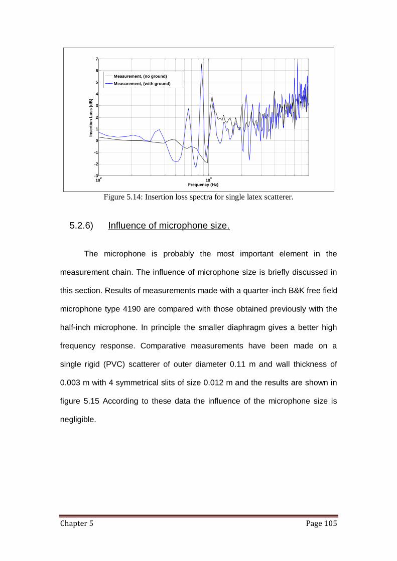
Chapter 5 Page 105
Figure 5.14: Insertion loss spectra for single latex scatterer.
5.2.6) Influence of microphone size.
The microphone is probably the most important element in the
measurement chain. The influence of microphone size is briefly discussed in
this section. Results of measurements made with a quarter-inch B&K free field
microphone type 4190 are compared with those obtained previously with the
half-inch microphone. In principle the smaller diaphragm gives a better high
frequency response. Comparative measurements have been made on a
single rigid (PVC) scatterer of outer diameter 0.11 m and wall thickness of
0.003 m with 4 symmetrical slits of size 0.012 m and the results are shown in
figure 5.15 According to these data the influence of the microphone size is
negligible.
102
103
-3
-2
-1
0
1
2
3
4
5
6
7
Insert
ion
Lo
ss (
dB
)
Frequency (Hz)
Measurement, (no ground)
Measurement, (with ground)
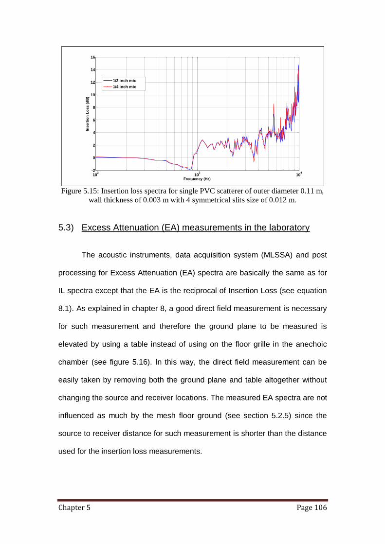
Chapter 5 Page 106
Figure 5.15: Insertion loss spectra for single PVC scatterer of outer diameter 0.11 m,
wall thickness of 0.003 m with 4 symmetrical slits size of 0.012 m.
5.3) Excess Attenuation (EA) measurements in the laboratory
The acoustic instruments, data acquisition system (MLSSA) and post
processing for Excess Attenuation (EA) spectra are basically the same as for
IL spectra except that the EA is the reciprocal of Insertion Loss (see equation
8.1). As explained in chapter 8, a good direct field measurement is necessary
for such measurement and therefore the ground plane to be measured is
elevated by using a table instead of using on the floor grille in the anechoic
chamber (see figure 5.16). In this way, the direct field measurement can be
easily taken by removing both the ground plane and table altogether without
changing the source and receiver locations. The measured EA spectra are not
influenced as much by the mesh floor ground (see section 5.2.5) since the
source to receiver distance for such measurement is shorter than the distance
used for the insertion loss measurements.
102
103
104
-2
0
2
4
6
8
10
12
14
16
Frequency (Hz)
Insert
ion
Lo
ss (
dB
)
1/2 inch mic
1/4 inch mic

Chapter 5 Page 107
Figure 5.16: Arrangement for measuring Excess attenuation spectra above a Medium
Density Fibreboard (MDF) in the laboratory.
5.4) Outdoor Measurements (Open University barrier test site)
Outdoor measurements have been made at the noise barrier test site
situated at the Open University Milton Keynes campus. This section will give
detailed descriptions of how the measurements (in situ) were performed using
a multi-channel (2 outputs and 8 inputs) data acquisition system. Some of the
outdoor measurements were on an array consisting of 3 rows of 54 3 m long
composite scatterers (SRR4) as specified in table 7.2. The bottom ends of the
PVC pipes were capped and bolted to a metal panel which was flush with the
ground surface (see figure 5.17). The latex scatterers were inserted into the
PVC pipes from the other end and bolted to the top cover. Perspex clips for
each individual pipe were attached to the adjacent pipes at a height of around
2 m (see figures 5.18(a) and (b)). This reinforcement acted to maintain the
uniformity of the periodicity and structural integrity of the array. Pieces of
Medium-density fibreboard (MDF) were used to prevent the sound from
passing underneath the barrier. Conventional road side noise barriers panels

Chapter 5 Page 108
(sometime referred to as fences) of comparable length (9 m) were erected on
both sides of the SC. The measurement method used is closely related to the
indirect prediction method described in ANSI S12.8 [91]. Insertion loss
measurements were made simultaneously on the SC and neighbouring
conventional barrier panel using different sources and receivers (see figure.
5.19). Both the speakers and receiving microphones were placed 5 m away
from each face of the respective barriers (see figure 5.19) at a height of 1.6 m
above the ground. Another pair of microphones was used for reference sound
level measurements and they were placed at 1 m away from each source.
The speakers were located above non-porous asphalt (a car park) and the
receivers were located over grass.
MLSSA is based on the assumption of perfect linearity and time-
invariance. Although this works well in laboratory (see section 5.2), the
assumptions do not apply for outdoors as a result of variation in temperature,
wind speed and humidity [92]. Consequently a more robust modified white
noise measurement technique was used for the outdoor measurements. This
applies a traffic filter (represented by the road traffic noise spectrum specific in
EN 1793-3 [10]) to a white noise spectrum. For simplicity, this is termed as a
Traffic Noise (TN) signal. The measurements were controlled remotely
(approximately 10 m away from the test site) from the noise barrier to reduce
any unwanted reflections due to equipment or people. A TN signal of 50 Hz to
10 kHz for duration of 7 seconds was produced by the DAC of a National
Instruments NI USB-6259 board controlled by a PC built in with MATLAB®
data acquisition toolbox. The TN signal was fed into a high powered Mordaunt
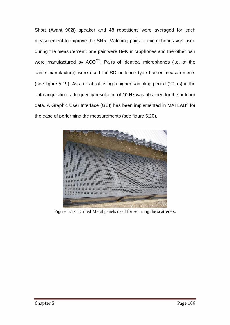
Chapter 5 Page 109
Short (Avant 902i) speaker and 48 repetitions were averaged for each
measurement to improve the SNR. Matching pairs of microphones was used
during the measurement: one pair were B&K microphones and the other pair
were manufactured by ACOTM. Pairs of identical microphones (i.e. of the
same manufacture) were used for SC or fence type barrier measurements
(see figure 5.19). As a result of using a higher sampling period (20 s) in the
data acquisition, a frequency resolution of 10 Hz was obtained for the outdoor
data. A Graphic User Interface (GUI) has been implemented in MATLAB® for
the ease of performing the measurements (see figure 5.20).
Figure 5.17: Drilled Metal panels used for securing the scatterers.
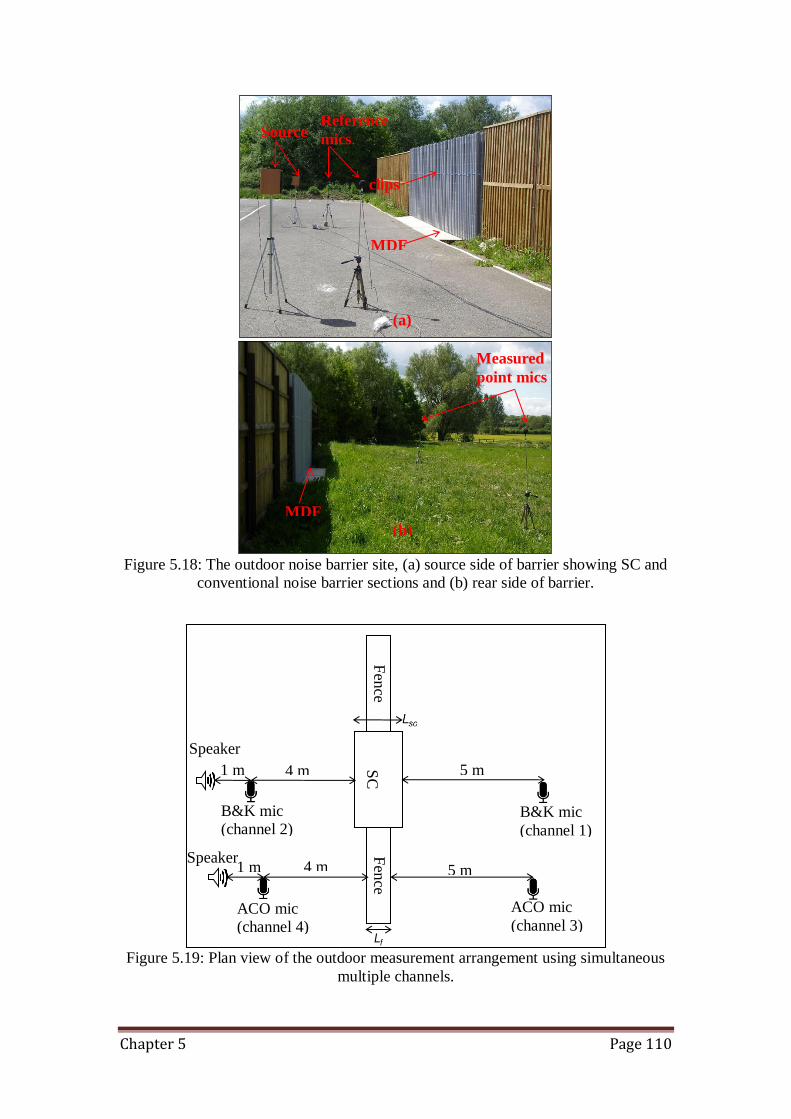
Chapter 5 Page 110
Figure 5.18: The outdoor noise barrier site, (a) source side of barrier showing SC and
conventional noise barrier sections and (b) rear side of barrier.
Figure 5.19: Plan view of the outdoor measurement arrangement using simultaneous
multiple channels.
Fen
ce F
ence
SC
5 m
5 m
4 m
4 m 1 m
1 m
B&K mic
(channel 2) B&K mic
(channel 1)
ACO mic
(channel 4)
ACO mic
(channel 3)
Source
s
Reference
mics.
MDF
clips
MDF
Measured
point mics
(b)
(a)
Speaker
Speaker
fL
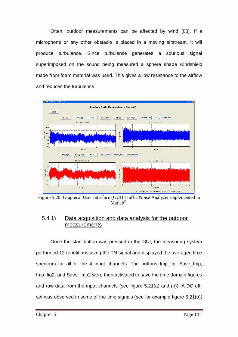
Chapter 5 Page 111
Often, outdoor measurements can be affected by wind [83]. If a
microphone or any other obstacle is placed in a moving airstream, it will
produce turbulence. Since turbulence generates a spurious signal
superimposed on the sound being measured a sphere shape windshield
made from foam material was used. This gives a low resistance to the airflow
and reduces the turbulence.
Figure 5.20: Graphical User Interface (GUI) Traffic Noise Analyzer implemented in
Matlab®.
5.4.1) Data acquisition and data analysis for the outdoor measurements
Once the start button was pressed in the GUI, the measuring system
performed 12 repetitions using the TN signal and displayed the averaged time
spectrum for all of the 4 input channels. The buttons Imp_fig, Save_Imp,
Imp_fig2, and Save_Imp2 were then activated to save the time domain figures
and raw data from the input channels (see figure 5.21(a) and (b)). A DC off-
set was observed in some of the time signals (see for example figure 5.21(b))
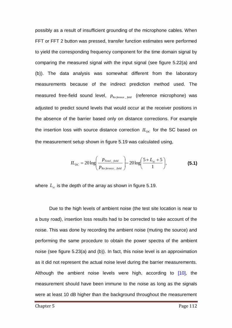
Chapter 5 Page 112
possibly as a result of insufficient grounding of the microphone cables. When
FFT or FFT 2 button was pressed, transfer function estimates were performed
to yield the corresponding frequency component for the time domain signal by
comparing the measured signal with the input signal (see figure 5.22(a) and
(b)). The data analysis was somewhat different from the laboratory
measurements because of the indirect prediction method used. The
measured free-field sound level, fieldferencep _Re (reference microphone) was
adjusted to predict sound levels that would occur at the receiver positions in
the absence of the barrier based only on distance corrections. For example
the insertion loss with source distance correction DCIL for the SC based on
the measurement setup shown in figure 5.19 was calculated using,
1
55log20log20
_Re
_ sc
fieldference
fieldTotal
DC
L
p
pIL , (5.1)
where scL is the depth of the array as shown in figure 5.19.
Due to the high levels of ambient noise (the test site location is near to
a busy road), insertion loss results had to be corrected to take account of the
noise. This was done by recording the ambient noise (muting the source) and
performing the same procedure to obtain the power spectra of the ambient
noise (see figure 5.23(a) and (b)). In fact, this noise level is an approximation
as it did not represent the actual noise level during the barrier measurements.
Although the ambient noise levels were high, according to [10], the
measurement should have been immune to the noise as long as the signals
were at least 10 dB higher than the background throughout the measurement
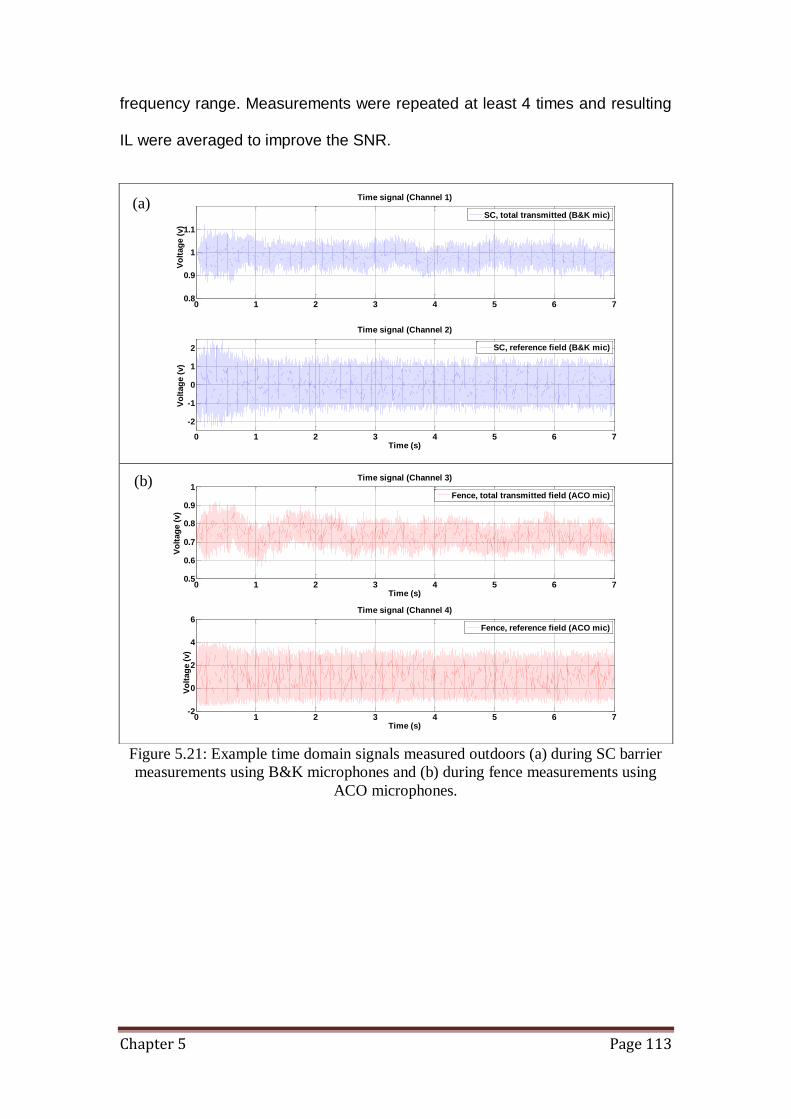
Chapter 5 Page 113
frequency range. Measurements were repeated at least 4 times and resulting
IL were averaged to improve the SNR.
Figure 5.21: Example time domain signals measured outdoors (a) during SC barrier
measurements using B&K microphones and (b) during fence measurements using
ACO microphones.
0 1 2 3 4 5 6 70.8
0.9
1
1.1
Time (s)
Vo
ltag
e (
v)
Time signal (Channel 1)
0 1 2 3 4 5 6 7
-2
-1
0
1
2
Time (s)
Vo
ltag
e (
v)
Time signal (Channel 2)
SC, total transmitted (B&K mic)
SC, reference field (B&K mic)
0 1 2 3 4 5 6 70.5
0.6
0.7
0.8
0.9
1
Time (s)
Vo
ltag
e (
v)
Time signal (Channel 3)
0 1 2 3 4 5 6 7-2
0
2
4
6
Time (s)
Vo
ltag
e (
v)
Time signal (Channel 4)
Fence, reference field (ACO mic)
Fence, total transmitted field (ACO mic)
(a)
(b)

Chapter 5 Page 114
Figure 5.22 Example power spectra measured outdoors (a) during SC barrier
measurements using B&K microphones and (b) during fence measurements using
ACO microphones.
102
103
20
40
60
80
100
120
140FFT (Channel 1)
Frequency (Hz)
Mag
nit
ud
e (
dB
)
102
103
20
40
60
80
100
120
140FFT (Channel 2)
Frequency (Hz)
Mag
nit
ud
e (
dB
)
SC, total transmitted (B&K mic)
SC, reference field (B&K mic)
102
103
20
40
60
80
100
120
140FFT (Channel 3)
Frequency (Hz)
Mag
nit
ud
e (
dB
)
102
103
20
40
60
80
100
120
140FFT (Channel 4)
Frequency (Hz)
Mag
nit
ud
e (
dB
)
Fence, total transmitted (B&K mic)
Fence, reference field (B&K mic)
(b)
(a)
Chapter 5 Page 115
Figure 5.23: Example background noise power spectra measured at the barrier test site
(a) during SC barrier measurements using B&K microphones and (b) during fence
measurements using ACO microphones.
5.4.2) Microphone calibration
Given that the required precision is high and that outdoor conditions
involve varying environmental temperature and humidity compared with
laboratory conditions, the question of long term stability of the microphones
arises. One approach that has been used for measuring ground impedance is
to use more than two microphones. In that case, since more than one transfer
function is measured it is possible that errors in the transfer function and
102
103
0
20
40
60
80
100FFT (Channel 1)
Frequency (Hz)
Mag
nit
ud
e (
dB
)
102
103
0
20
40
60
80
100FFT (Channel 2)
Frequency (Hz)
Mag
nit
ud
e (
dB
)
Background noise at channel 1
Background noise at channel 2
102
103
0
20
40
60
80
100FFT (Channel 3)
Frequency (Hz)
Mag
nit
ud
e (
dB
)
102
103
0
20
40
60
80
100
FFT (Channel 4)
Frequency (Hz)
Mag
nit
ud
e (
dB
)
Background noise at channel 3
Background noise at channel 4
(a)
(b)

Chapter 5 Page 116
geometry partially average out. This procedure is similar to the phase gradient
method [93].
The reliability of the indirect prediction method shown in section 5.4.1
relies on another important factor which is extent to which pair of microphones
have identical responses. It is possible that by using a phase matched pair of
microphones (an expensive method), the error in the measurement could be
reduced. Another possibility is to determine the difference between two
conventional microphones in the laboratory and use the results to
subsequently correct the field data. This is a cheaper option but the question
of long term stability arises (i.e. whether the laboratory data is still valid under
outdoor conditions with different humidity and temperature). In this section, an
example of how the calibration is done for the B&K microphones is briefly
discussed. To perform the calibration, the source was isolated and replaced
by a B&K sound calibrator type 4231 using the same NI acquisition system.
The microphones (mic reference no. 306 and 307) were individually tested by
inserting them into the calibrator as shown in figure 5.24. The calibrator emits
a known sound pressure level at single frequency of 1 kHz with amplitude of
94 dB. Since the B&K dual-channel microphone power supply - type 5935
comes with selector switch to vary the gain, the calibration test was performed
with the gain at zero and 30 dB to test for linearity.

Chapter 5 Page 117
Figure 5.24: Setup for B&K microphone calibration.
The calibration results for both B&K microphones at different amplifier
gain levels are shown in figure 5.25. All the frequency spectra show the peak
at 1 kHz and for the corresponding gains level, the amplitudes of the sound
pressure are also within a reasonable range of the desired values of 94 dB
and 124 dB. Undesirable features in these spectra are the spikes that occur at
various frequencies. Since the spikes for both microphones occur at similar
frequencies, the likely cause is electrical noise in the measuring system.
However these spikes will cancel out after performing the correction
procedure. From these calibration results and assuming linearity for all other
frequencies, the differences between the microphones can be known and will
be taken into account in our outdoor measurement. Hence the final calculated
Insertion Loss (IL) spectra take account of the distance correction on
reference microphone signal, the background noise and the system response.
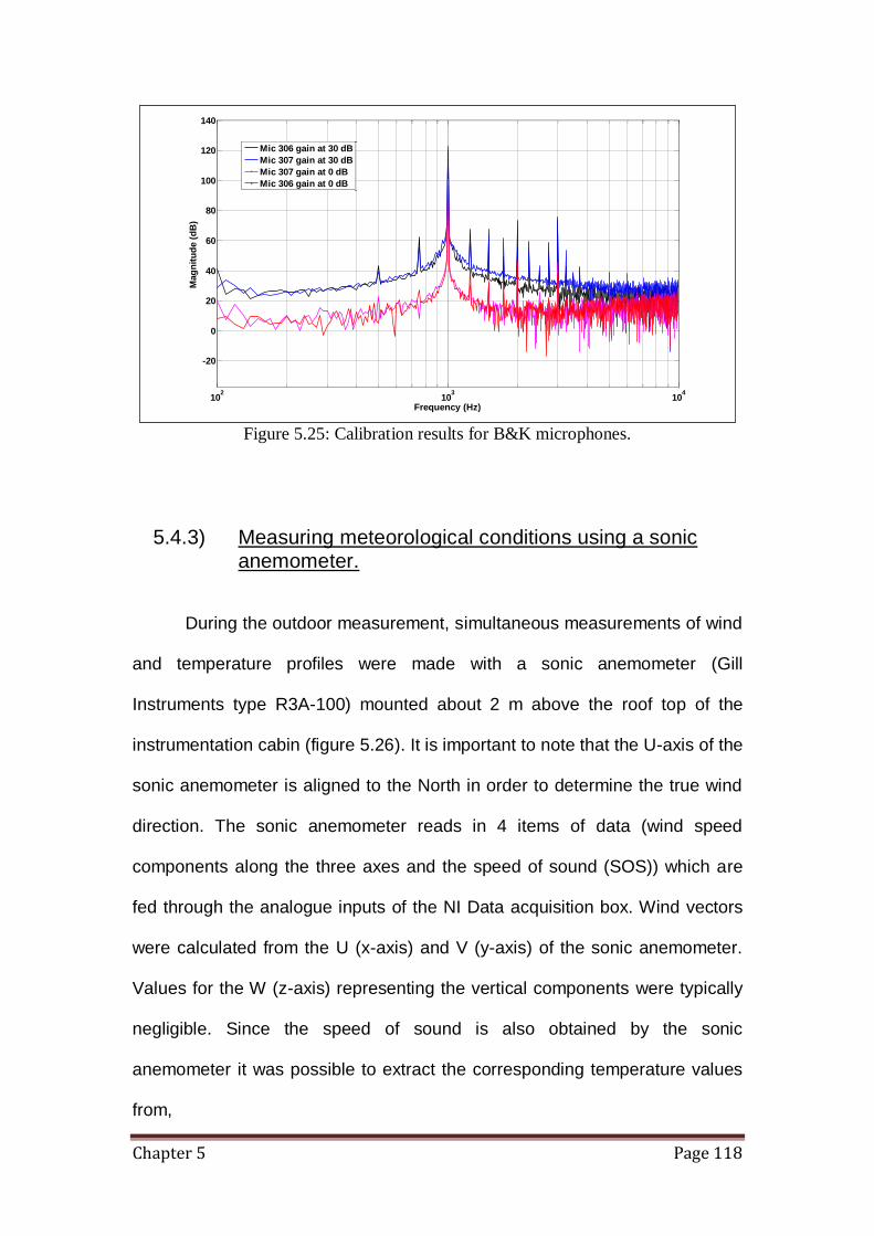
Chapter 5 Page 118
Figure 5.25: Calibration results for B&K microphones.
5.4.3) Measuring meteorological conditions using a sonic anemometer.
During the outdoor measurement, simultaneous measurements of wind
and temperature profiles were made with a sonic anemometer (Gill
Instruments type R3A-100) mounted about 2 m above the roof top of the
instrumentation cabin (figure 5.26). It is important to note that the U-axis of the
sonic anemometer is aligned to the North in order to determine the true wind
direction. The sonic anemometer reads in 4 items of data (wind speed
components along the three axes and the speed of sound (SOS)) which are
fed through the analogue inputs of the NI Data acquisition box. Wind vectors
were calculated from the U (x-axis) and V (y-axis) of the sonic anemometer.
Values for the W (z-axis) representing the vertical components were typically
negligible. Since the speed of sound is also obtained by the sonic
anemometer it was possible to extract the corresponding temperature values
from,
102
103
104
-20
0
20
40
60
80
100
120
140
Frequency (Hz)
Mag
nit
ud
e (
dB
)
Mic 306 gain at 30 dB
Mic 307 gain at 30 dB
Mic 307 gain at 0 dB
Mic 306 gain at 0 dB

Chapter 5 Page 119
Csmc
15.2731.3.331 1
0
, (5.2)
where 0c
= speed of sound in air and is the acoustically-deduced
temperature in Degree Celsius.
When the anemometer button on the GUI was pressed (see figure
5.20), the reading from the sonic anemometer was displayed as in figure 5.27.
These data were saved for further analysis.
Figure 5.26: Sonic anemometer mounted above the instrumentation cabin.
Sonic
anemometer

Chapter 5 Page 120
Figure 5.27: Data from sonic anemometer.
Figure 5.28 shows an example of the wind vector plot (north is at 0°),
the black line indicates the barrier position and the red dotted line denotes the
direction of sound propagation. Blue solid lines calculated from vector U and
V show the wind speed according to this set of measurements which is about
0.8 m/s. The average speeds of sound and temperature for the entire 7
seconds (multiply by 4 repetitions) are also shown at the bottom of the wind
vector diagram.
Figure 5.28: Example of a deduced wind vector diagram.
0 1 2 3 4 5 6 7-0.5
0
0.5
Vecto
r U
0 1 2 3 4 5 6 7-1
-0.5
0V
ecto
r V
0 1 2 3 4 5 6 7-0.2
0
0.2
Vecto
r W
0 1 2 3 4 5 6 7340
340.5
341
Sp
eed
(m
/s)
0 1 2 3 4 5 6 714
15
16
Tem
p. (
C)
Time (s)
Vector U
Vector V
Vector W
Speed of sound (m/s)
Temperature (C)
0.2 0.4
0.6 0.8 1
30
210
60
240
90
120
300
150
330
270
180
0
Average speed of sound = 339.1 m/s
Average temperature
= 13.1 C
Direction of sound propagation
Barrier
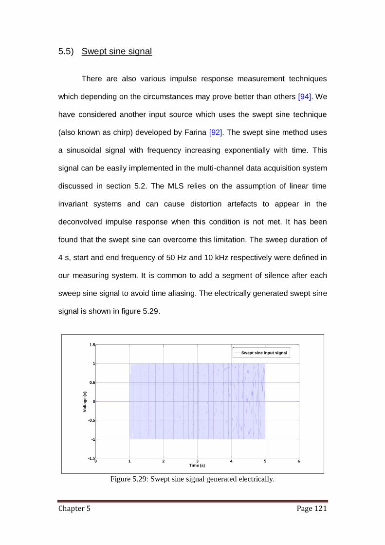
Chapter 5 Page 121
5.5) Swept sine signal
There are also various impulse response measurement techniques
which depending on the circumstances may prove better than others [94]. We
have considered another input source which uses the swept sine technique
(also known as chirp) developed by Farina [92]. The swept sine method uses
a sinusoidal signal with frequency increasing exponentially with time. This
signal can be easily implemented in the multi-channel data acquisition system
discussed in section 5.2. The MLS relies on the assumption of linear time
invariant systems and can cause distortion artefacts to appear in the
deconvolved impulse response when this condition is not met. It has been
found that the swept sine can overcome this limitation. The sweep duration of
4 s, start and end frequency of 50 Hz and 10 kHz respectively were defined in
our measuring system. It is common to add a segment of silence after each
sweep sine signal to avoid time aliasing. The electrically generated swept sine
signal is shown in figure 5.29.
Figure 5.29: Swept sine signal generated electrically.
0 1 2 3 4 5 6-1.5
-1
-0.5
0
0.5
1
1.5
Time (s)
Vo
ltag
e (
v)
Swept sine input signal

Chapter 5 Page 122
The swept sine signal was tested in the anechoic chamber using a
loudspeaker and a single microphone. The direct sound field method
described in section 5.2.2 was used to measure the IL spectrum due to a
single PVC scatterer of outer diameter 0.11 m and wall thickness of 0.003 m
with 4 symmetrical slits of 0.012 m. To make a fair comparison with MLSSA
measurements, 16 repetitions were made for the direct field and total
transmitted field measurements. The time domain signals for both
measurements are shown in figure 5.30.
Figure 5.30: Direct and total transmitted fields measured using the swept sine method
in the laboratory.
The transfer function estimate is used to deconvolve the time signal
into its frequency component and the Insertion Loss (IL) is calculated. The IL
spectra obtained using MLS and Swept sine methods are compared in figure
5.31 and show little difference. This swept sine method has also been
implemented for the level difference measurements described in section
8.4.5.
0 1 2 3 4 5 6-0.06
-0.05
-0.04
-0.03
-0.02
-0.01
0
0.01
0.02
Time (s)
Vo
ltag
e (
v)
Direct field, swept-sine signal
Total transmitted field, swept sine signal

Chapter 5 Page 123
Figure 5.31: Comparison of IL spectra due to a single PVC scatterer of OD 0.11 m,
WT 0.003 m with 4 symmetrical slits of 0.012 m measured using the MLS and swept
sine methods.
5.6) Outdoor in situ measurement of a sonic crystal at Diglis Weir, Worcester.
During the course of research, the opportunity arose for investigating
the creation of ‘acoustical gimmicks’ based on sonic crystals. This opportunity
involved collaboration with Liminal – winners of PRS for Music Foundation’s
New Music Award 2010 [78]. The project entitled “Organ of Corti” involved
creation of an experimental instrument that employs sonic crystal technology
to accentuate and attenuate frequencies within the broad range of sounds
present in road traffic or falling water.
The measurements on the “Organ of Corti” i.e. a sonic crystal
composed of transparent acrylic cylinders mounted on a platform, which was
used to accentuate and attenuate frequencies within the broad range of
sounds present in road traffic and falling water (i.e. weir). This device was
intended to draw attention to the sounds already present in the environment
by re-harvesting them in a new way. One way of manipulating sound waves in
102
103
104
-2
0
2
4
6
8
10
12
14
Frequency
Insert
ion
Lo
ss (
dB
)
MLS
Swept sine

Chapter 5 Page 124
periodic arrays is to introduce defects (vacancies) in their structure [79, 80,
95, 96 and 97]. There has been increasing interest in application structures
with a low number of defects with respect to the total number of scatterers in
the structure, so that the periodicity is locally broken, to high precision wave
filters [81] or waveguides [82].
The particular design studied in this section consists of eighty one 4 m
long 0.22 m diameter vertical acrylic cylinders arranged in a hexagonal lattice
with lattice constant, L = 0.3 m (see figure 5.32(a)). This structure was placed
at Diglis Weir, river Severn, Worcester as part of the Worcester Music Festival
in August 2011 (see figure 5.32(b)). The cylinders were arranged in a quasi-
ordered lattice arrangement and some cylinders were intentionally removed to
form a passageway. This allowed people to walk through the structure and
listen to the different characteristics of sound at different locations within the
structure as well as while walking around it. For an SC with regular hexagonal
lattice arrangement of lattice constant 0.3 m, the calculated Bragg band gap
(centre frequency) is:
Hz
Lf HexBragg 660
3.03
344
3
344_ , (5.3)
This section will also provide some modelling results using Multiple Scattering
Theory (MST) explained in chapter 3 to compare with our experimental data.

Chapter 5 Page 125
5.6.1) Measurement arrangement
During these measurements, the sound generated by the weir was
acting as the source. Time signal was recorded for 7 seconds with data
sampling rate of 20 μs for each set of measurement using the multi-channel
data acquisition system discussed in section 5.2. Three sets of measurements
were made and for each set of measurement there were 16 repetitions (thus a
total of 48 measurements) to improve the SNR. Transfer function estimation
was used to obtain the frequency spectrum from the recorded time signal. The
positioning of the receivers and approximated source location are given in
figure 5.32(a) and table 5.1. During the experiment, there were some errors
made in the data acquisition system (due to crosstalk of signal) and thus, only
2 points (Ref pt and Pt 1) were correctly measured. This error resulted in an
investigation of possible ways to prevent such mistakes from happening in
future measurements. The insertion loss (IL) was deduced by using the
indirect prediction method discussed in section 5.2 which takes accounts of
the distance correction for the reference microphone, ambient noise and
system response. The meteorological conditions were measured with
handheld anemometer and thermometer. The meteorological conditions taken
during the measurement were as follows:
i) Average temperature: 23°C.
ii) Average wind speed: 1m/s.
iii) Wind direction: West (cross wind).

Chapter 5 Page 126
Figure 5.32: (a) Plan view schematic of the sonic crystal arrangement and microphone
locations at Diglis weir Worcester. (b) Aerial map of the site showing where the sonic
crystal was situated (picture taken from Google map).
Microphone locations
(coordinates)
x y
Reference point (Ref pt) 9.7 1.69
Point 1 (Pt 1) 10.9 -1
Point 2 (Pt 2) 10.7 1.09
Point 3 (Pt 3) 11.6 1.69
Table 5.1: Coordinates of source and receivers positions during ‘Organ of Corti’
measurements.
0 2 4 6 8 10 12-3
-2
-1
0
1
2
3
Cylinders
Position of microphonesRef pt
Pt 2
Pt 1
Pt 3
Note: Cylinders are not to scale.
Sonic crystal weir
(a)
(b)
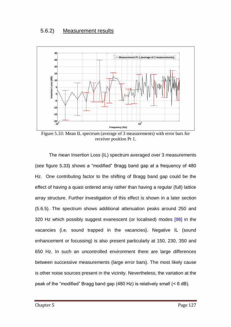
Chapter 5 Page 127
5.6.2) Measurement results
Figure 5.33: Mean IL spectrum (average of 3 measurements) with error bars for
receiver position Pt 1.
The mean Insertion Loss (IL) spectrum averaged over 3 measurements
(see figure 5.33) shows a “modified” Bragg band gap at a frequency of 480
Hz. One contributing factor to the shifting of Bragg band gap could be the
effect of having a quasi ordered array rather than having a regular (full) lattice
array structure. Further investigation of this effect is shown in a later section
(5.6.5). The spectrum shows additional attenuation peaks around 250 and
320 Hz which possibly suggest evanescent (or localised) modes [98] in the
vacancies (i.e. sound trapped in the vacancies). Negative IL (sound
enhancement or focussing) is also present particularly at 150, 230, 350 and
650 Hz. In such an uncontrolled environment there are large differences
between successive measurements (large error bars). The most likely cause
is other noise sources present in the vicinity. Nevertheless, the variation at the
peak of the “modified” Bragg band gap (480 Hz) is relatively small (< 6 dB).
102
103
-20
-15
-10
-5
0
5
10
15
20
25
30
Frequency (Hz)
Insert
ion
Lo
ss (
dB
)
Measurement Pt 1 (average of 3 measurements)

Chapter 5 Page 128
5.6.3) Modelling with Multiple Scattering Theory (MST) assuming a single point source
Multiple Scattering Theory (MST) has been used to predict the IL
spectrum at Pt 1 receiver position. Two predictions are made with the
(assumed line) source located at coordinate (0, 0) and (0, 10), see figure
5.32(a). The receiver positions Pt 1 are averaged over 4 other positions
(±0.05 m perturbation in both axes) from the original position (see figure 5.34).
This is to give a more realistic prediction of the IL spectrum in the region of Pt
1.
Figure 5.34: The original receiver position Pt 1 and 4 other perturbed positions
made for MST modelling.
10.8 10.82 10.84 10.86 10.88 10.9 10.92 10.94 10.96 10.98
-1.08
-1.06
-1.04
-1.02
-1
-0.98
-0.96
-0.94
Original position,Pt 1 at (10.9, -1)
Perturbed position,(10.95, -1)
Perturbed position,(10.85, -1)
Perturbed position,(10.9, -0.95)
Perturbed position,(10.9, -1.05)

Chapter 5 Page 129
Figure 5.35: Predicted IL spectra of all the 5 individual positions (Pt 1 original and 4
perturbed positions) and the averaged IL spectrum. Source is located at coordinates
(0, 0).
Figure 5.35 shows the predicted IL results for all the 5 positions (Pt 1
original and 4 perturbed positions) and the averaged IL spectrum. The source
is modelled to be positioned at coordinates (0, 0). Some variations are
noticeable when there is a slight change in the receiver position but the
overall trend seems to be agreeing. An exception is at coordinates (10.9, -
0.95) where almost 20 dB difference is observed near 450 Hz. This narrow
band spike could be due to a numerical artefact as it occurs at only a single
frequency point.
102
103
-20
-10
0
10
20
30
40
50
Frequency (Hz)
Insert
ion
Lo
ss (
dB
)
MST prediction, (10.9, -1)
MST prediction, (10.95, -1)
MST prediction, (10.85, -1)
MST prediction, (10.9, -0.95)
MST prediction, (10.9, -1.05)
Average of MST predictions
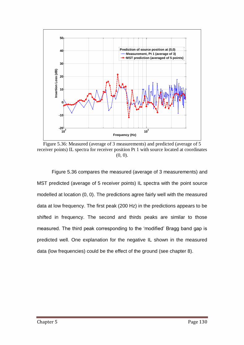
Chapter 5 Page 130
Figure 5.36: Measured (average of 3 measurements) and predicted (average of 5
receiver points) IL spectra for receiver position Pt 1 with source located at coordinates
(0, 0).
Figure 5.36 compares the measured (average of 3 measurements) and
MST predicted (average of 5 receiver points) IL spectra with the point source
modelled at location (0, 0). The predictions agree fairly well with the measured
data at low frequency. The first peak (200 Hz) in the predictions appears to be
shifted in frequency. The second and thirds peaks are similar to those
measured. The third peak corresponding to the ‘modified’ Bragg band gap is
predicted well. One explanation for the negative IL shown in the measured
data (low frequencies) could be the effect of the ground (see chapter 8).
102
103
-20
-10
0
10
20
30
40
50
Frequency (Hz)
Insert
ion
Lo
ss (
dB
)
Measurement, Pt 1 (average of 3)
MST prediction (averaged of 5 points)
Prediction of source position at (0,0)

Chapter 5 Page 131
Figure 5.37: Predicted IL spectra at all the 5 individual positions (Pt 1 original and 4
perturbed positions) and the averaged predicted IL spectrum. The point source is
assumed to be located at coordinates (0, 10).
Figure 5.37 shows the predicted IL results for all the 5 positions (Pt 1
original and 4 perturbed positions) and the averaged IL spectrum. The source
is modelled to be positioned at coordinates (0, 10). Again, variations in the IL
spectra are observed when there is a slight change in the receiver position as
in figure 5.35.
102
103
-20
-10
0
10
20
30
40
50
Frequency (Hz)
Insert
ion
Lo
ss (
dB
)
MST prediction, (10.9, -1)
MST prediction, (10.95, -1)
MST prediction, (10.85, -1)
MST prediction, (10.9, -0.95)
MST prediction, (10.9, -1.05)
Average of MST predictions

Chapter 5 Page 132
Figure 5.38: Measured (average of 3 measurements) and predicted (average of 5
points) IL spectra for receiver position Pt 1 with source located at coordinates (0, 10).
Figure 5.38 compares the measured (average of 3 measurements) and
MST predicted (average of 5 points) IL spectra with the source modelled as a
point at location (0, 10). The prediction agrees slightly better at high
frequencies with the source modelled at an oblique angle rather than at
coordinates (0, 0) see figure 5.32(a). Three peaks are again predicted at 290,
380 and 500 Hz. The Bragg band gap is well predicted in terms of the centre
frequency (near 500 Hz) but with smaller amplitude.
5.6.4) Modelling with multiple point sources on a line
The fact that predictions using a single fixed point source at (0,0) are in
better agreement with the measured data than those assuming a source at
(0,10 suggests that using a line of point sources could improve the accuracy
of the prediction. Consequently the weir was modelled by 10 point sources
102
103
-20
-10
0
10
20
30
40
50
Frequency (Hz)
Insert
ion
Lo
ss (
dB
)
Measurement, Pt 1 (average of 3)
MST predictions (average of 5 points)
Prediction of source position at (0,10)
Chapter 5 Page 133
spaced along the whole span of the weir (approximately 200 m). The positions
of the sources are shown in figure 5.39 and the corresponding coordinates
are shown in table 5.2. The MST prediction was run for each source location
and receiver position, Pt 1 (see table 5.1). Similarly, averaging of all the 5
points (receiver Pt 1 and 4 perturbed positions) was carried out (see figure
5.34). It is reasonable to assume that all the point sources are coherent since
the weir noise is caused by more or less the same flow and drop over the
length of the weir. The direct pressure (without SC) in Decibel, )(dBDirectp was
then summed over all sources at each frequency point, n ,
n p
dBtotalDirect
dBDirect
p0
1010)(_
)(
10log10 . (5.4)
Likewise for the total transmitted pressure (with SC) in Decibel, )(_ dBtranmittedtotalP
was summed over all sources at each frequency point, n ,
n P
dBtranmittedtotal
dBtranmittedtotal
p0
1010)(_
)(_
10log10.
(5.5)
The IL in dB could then be expressed by,
)(__)(_ dBtotaldtransmitteTotaldBtotalDirect ppIL . (5.6)
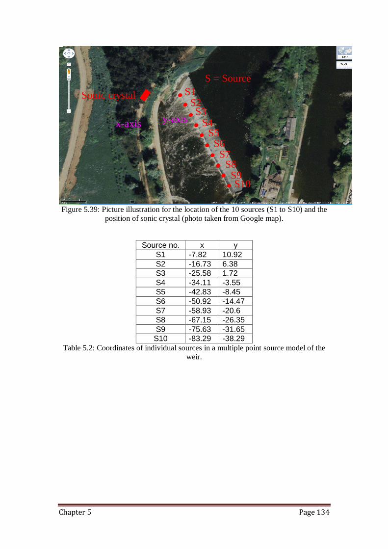
Chapter 5 Page 134
Figure 5.39: Picture illustration for the location of the 10 sources (S1 to S10) and the
position of sonic crystal (photo taken from Google map).
Source no. x y
S1 -7.82 10.92
S2 -16.73 6.38
S3 -25.58 1.72
S4 -34.11 -3.55
S5 -42.83 -8.45
S6 -50.92 -14.47
S7 -58.93 -20.6
S8 -67.15 -26.35
S9 -75.63 -31.65
S10 -83.29 -38.29
Table 5.2: Coordinates of individual sources in a multiple point source model of the
weir.
Sonic crystal S1
S10
S2 S3
S4 S5
S6 S7
S8 S9
x-axis y-axis
S = Source

Chapter 5 Page 135
Figure 5.40: Measured (average of 3 measurements) and MST predicted with multiple
point sources IL spectra for receiver position Pt 1 (averaged over 5 receiver points for
each individual source).
Figure 5.40 shows the measured and MST predicted IL spectra at
receiver position 1. The predictions resulting from the 10 source model of the
weir show better agreement with measurements than those assuming a single
point source at either location (0,0) or (0,10) (see figures 5.36 and figure
5.38). The first IL peak around 250 - 350 Hz is well predicted and this could
be due to the evanescent mode suggested in figure 5.33. Also, the prediction
for the modified Bragg band gap (possibly shifted due to the quasi periodic
ordered array effect) near 450 Hz agrees fairly well with the measured data.
102
103
-20
-10
0
10
20
30
40
50
Frequency (Hz)
Insert
ion
Lo
ss (
dB
)
Measurement, average of 3 measurements, point 1
MST Prediction, worcester original design, 10 sources

Chapter 6 Page 136
Chapter 6
Improving the performance of sonic crystal noise barriers by using resonant elastic shell elements
6.1) Introduction
A conventional technique for reducing low frequency noise
transmission is to increase the thickness or the mass per unit area of the
sound insulation material. A drawback of this technique is that usually it
results in large size and mass of the insulator. On the other hand the stop and
pass bands of a Sonic Crystal (SC) composed of solid rigid elements and their
angle dependence makes an SC unsuitable for use as a barrier for broadband
noise such as road traffic. To make a SC noise barrier appealing, methods
must be found of reducing the angle-dependence of the stop bands and
targeting the frequencies of interest without increasing the size. One
possibility for achieving these objectives is to use resonant scatterers. There
has been previous numerical and theoretical work in respect to periodic arrays
of elastic scatterers in a gas involving hollow spheres and cylinders [99].
There have also been numerical studies of acoustical performance of a
periodic array of resonant silicone rubber scatterers embedded in an epoxy
resin matrix [100]. Previous experimental work in respect of periodic array of
scatterers in air has investigated the use of pressurized gas-filled cylindrical
balloons [101 and 102]. In Kushwaha et al, the authors examined
(theoretically) a square lattice SC in 3 dimensions made up of hydrogen filled
cylindrical balloons in air. In these systems, the authors analysed the band

Chapter 6 Page 137
gap creation for three different configurations relating to parameters such as
the latex wall thickness, the filling fraction and the pressure inside the
balloons. It’s reported that the pressure inside the balloon is kept at 1.1 atm
which is slightly above the ambient pressure and the latex wall thickness is
made very thin to obtain high-velocity, low-density scatterer in a low-velocity
and high-density host conditions thus giving high impedance mismatch in
such matrix. It has been found that resonance attenuation peaks can be
obtained at frequencies which do not depend on the periodicity of the SC but
on the resonance frequency of the resonators. However it was found difficult
to predict the measured effects due to the pre-stress condition i.e. to take
account of any static external load and thereby model scattering by elastic
materials under tension.
It is also known that for thin-walled elastic cylinder, the lowest
resonance is corresponds to a radial or “breathing” mode of vibration which
results in a significant change in volume of the cylinder on account of the
variation of the radius through each cycle. Vibration analysis for the natural
frequencies and mode shapes of an elastic shell is generally much more
complex than that for a beam or plate because the generality of the shell
equation permits a wide variety of mode shapes with vastly different
characters. The modal shapes of the cylinder model are basically composed
of two kinds of mode patterns: the breathing mode and the freely supported
beam mode [103]. The combination of the two basic mode patterns support
three modal shapes – axial, bending and torsional modes (see figure 6.1). It is
possible to realise such a mode provided that the thickness of the cylinder
Chapter 6 Page 138
wall is less than 1/50th of the cylinder diameter and that the wall stiffness
(Young’s Modulus) is of the order of 1 MPa [104]. In this chapter, the theory of
wave propagation through doubly periodic arrays of elastic shells based on
the Multiple Scattering Theory (MST) covered in Chapter 3 will be discussed.
It is a semi-analytical method and in this work the terms ‘MST’ and ‘semi-
analytical prediction’ are used interchangeably. In addition, the breathing
mode resonance is also verified by performing modal analysis with the Finite
Element Method (FEM) using COMSOL® Multiphysics software. FEM is also
used to predict the transmission problem for a single elastic shell. These
predictions are compared with data from experiments using commercially
available non-vulcanized rubber (latex) and data confirm the presence and
identity of the resonances for the chosen material and geometry of the elastic
shell. Some failed attempts to use different materials such as polyethylene
and periodically stiffened latex are also reported in Appendix C.
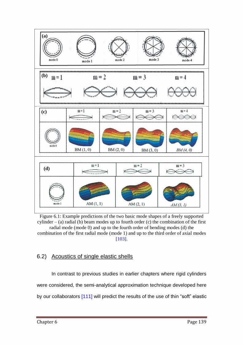
Chapter 6 Page 139
Figure 6.1: Example predictions of the two basic mode shapes of a freely supported
cylinder – (a) radial (b) beam modes up to fourth order (c) the combination of the first
radial mode (mode 0) and up to the fourth order of bending modes (d) the
combination of the first radial mode (mode 1) and up to the third order of axial modes
[103].
6.2) Acoustics of single elastic shells
In contrast to previous studies in earlier chapters where rigid cylinders
were considered, the semi-analytical approximation technique developed here
by our collaborators [111] will predict the results of the use of thin “soft” elastic
(c)
(b)
(a)
(d)
Chapter 6 Page 140
shells. For the elastic material to be classified as soft, 11
2 c
c, where 1c and 2c
are the compressional and shear wave speeds of the elastic material
respectively. The properties of this material allow several relatively low-
frequency resonances that generate stop bands by multiple scattering in an
array. These stop bands are independent from those related to the periodic
arrangement of the rigid scatterers. Using the semi-analytical approximation
results, the scattering problem is solved for a single scatterer in this section
and for a finite array of scatterers in section 6.9.
The problem of acoustic wave propagation through a doubly periodic
array of identical elastic shells is considered. The time-harmonic dependence
is taken as tie throughout the chapter. Assuming that waves propagate in
the plane perpendicular to the normal axis of infinite cylindrical shells jC ,
where j takes positive integer values, each shell can be replaced by its cross-
section (i.e. an elastic ring), see figure 6.2. The acoustic environment
outside/inside of each shell is described by density i
o
and sound speed
i
o
c
c,
whereas the elastic linear isotropic material of the shell is represented by
density , compressional velocity 1c and shear velocity 2c .

Chapter 6 Page 141
Figure 6.2: Cross-section of an elastic shell in the primary cell of doubly periodic
array.
Without loss of generality, the origins of the Cartesian yx , and polar
coordinates ,r used in this section coincide with the centre of the scatterer
0C in the primary cell of size L, also known as the lattice constant. Centre jO
of each scatterer in the infinite periodic array is defined by the position vector
2211 ananR j ; where 1n and 2n take integer values and 1a and 2a are the
fundamental translation vectors [105] (see chapter 1.4.2).
The equation for cylindrically-spreading acoustic waves in a lossless
fluid medium previously shown in chapter 4, equation 4.1 is repeated here for
convenience. The displacement potential rp in the acoustic medium
satisfies the two-dimensional Helmholtz equation,
022 pkp , (6.1)
Primary cell
Chapter 6 Page 142
and the quasi-periodicity conditions which follow from Bloch theorem,
rRr jR
pepTi
j
. (6.2)
Where 2
2
2
2
1
22
xx
is the Laplacian,
c
fk
2 is the wave number in air
defined as the ratio between angular frequency and sound speed of the
outer acoustic environment c , is a given wave vector. Index relates
density to one of the acoustic media (i.e., it equals to either “o” or “i” for
outside and inside environment respectively). rp is related to the acoustic
pressure r and particle velocity potential r by:
p2 , (6.3)
pi
, (6.4)
The wave field in the elastic ring is represented by two displacement
potentials describing the longitudinal wave r and the shear wave r ,
which are solutions of the following equations [106]:
02
1
2 k , (6.5)
02
2
2 k , (6.6)
where 1
1c
k
and 2
2c
k
.
Chapter 6 Page 143
The solutions to equation (6.1), (6.5) and (6.6) are subject to continuity
conditions at the elastic–acoustic interface of scatterer jC . This gives at
oar and iar :
prr
2 , (6.7)
0 r , (no rotational), (6.8)
rrr
p 1. (6.9)
Where stresses rr and r are defined by:
2
2
2
2
2
22
rr
rr
r
crr
, (6.10)
2
2
2
2
2
22
rr
rr
r
cr
, (6.11)
The solutions to the problems in equations (6.1) – (6.9) can be described by
orthogonal series of Bessel and trigonometric functions. In the outer and inner
acoustic media the potentials take the following forms:
in
n
onnonno erkYBrkJArp
, , oar , (6.12)
in
n
inni erkJErp
, , iar , (6.13)
whereas the solutions of the elastic shell are expanded as:

Chapter 6 Page 144
in
n
nnnn erkYCrkJCr
1,21,1, , oi ara , (6.14)
in
n
nnnn erkYDrkJDr
2,22,1, , oi ara . (6.15)
The set of unknown coefficients nnnnnn EDDCCA ,,,,, ,2,1,2,1 can be
identified in terms of coefficient nB by using boundary conditions at the
surface of the elastic shell. Thus, substituting solutions of equations (6.12) -
(6.15) into equations (6.7) - (6.9) and taking inner product
de im
2
0
will
result in an algebraic system of equations:
n
oon
oon
oono
noonoonooonoonon B
akJ
akY
akJa
akinYakYaakinJakJaA
'
'
'
'' ,,,
, (6.16)
n
T
oono
ooonn B
akJa
kC
0,
2,0,0
'
2
, (6.17)
where oa outer boundary of the shell, '
nJ = Bessel function of n-th order of the
first kind, '
nY = Bessel function of n-th order of the second kind, n ,
c
fko
2 (the wave number in air),
2c
c ,
2c
c
,
dr
rkdZrkZ n
n
' is the
derivative of cylindrical function, n is the vector Tnnnn DCDC ,2,2,1,1 ,,, of
unknown coefficients, and nC is the matrix of 44 elements in the following
form,
Chapter 6 Page 145
YoYoJoJo
YoYoJoJo
YiYiJiJi
YiYiJiJi
n
gggg
ffff
gggg
ffff
C
,,2,,1,,2,,1
,,2,,1,,2,,1
,,2,,1,,2,,1
,,2,,1,,2,,1
, (6.18)
where the coefficients are defined as:
akZ
a
aknakZ
akZ
akZk
af nn
n
nZ 12
22
2
2
1
'
'
2
,,1
22
, (6.19)
akZ
akZ
akZk
aakZ
a
inf n
n
nnZ 2'
2
2
'
,,2
22 , (6.20)
a
akZakZ
a
ing n
nZ1
1
'
,,1
2, (6.21)
akZa
aknakZ
ag nnZ 2
22
2
2
2
'
,,2
22
1. (6.22)
In the case of the rigid scatterer equation 6.16 is reduced to the well-known
relation between coefficients nA and nB by setting n to the zero vector and
o to the zero value (Neumann boundary condition).
The contrast between elastic material of the shell and air medium considered
here is relatively large. This can be described in term of the relative
impedance,
12
c
coo
. (6.23)
Chapter 6 Page 146
If the thickness of the elastic shell is much smaller than its mid-surface
radius
2
io aaR
, then 1
R
h , where h is half Wall Thickness (WT) of the
shell.
In order to have better interaction between elastic and acoustic media, the
contrast has to be reduced. This can be achieved by assuming that the
relative impedance is of the same order as the ratio between half-thickness
and mid-surface radius of the elastic shell. This assumption can be written as
.
Acoustic waves are generated by a cylindrical source, which is
positioned in the outer region of the shell. For convenience, but without loss of
generality, the origin of the Cartesian yx, and polar coordinates ,r
coincides with the source location. Potential rop in the outer acoustic
medium satisfies the Helmholtz equation (6.1) and Sommerfeld’s radiation
conditions (refer to chapter 3 equation 3.10),
2/10
rikp
r
po
o , as r , (6.24)
where 22 yxr . The solution representing the scattered field is given by,
n
in
onnnso erkHZArp ˆ1
,ˆ, , oar ˆ , (6.25)
so that the total field in the outer acoustic medium takes the following form,
Chapter 6 Page 147
,, ,
1 rprkHrp soooo , (6.26)
where ,ˆ rr and ,ˆ r are the polar coordinates of receiver with origin
placed at the centre of scatterer, nA are unknown coefficients and factors nZ
are found from,
non
onn
UiRkH
RkJZ
,1
1
'
ˆ . (6.27)
Note that when 0ˆ,1 nU factors nZ transform to those for the case of a rigid
cylinder.
Solution for the field in the inner acoustic medium can be described by the
formulation in equation 6.7. The following will describe the formulation of the
thin shell medium.
Using a technique described in detail by [107], a long-wave low-frequency
approximation for the wave equations of the thin-walled elastic shell based on
the previous assumption regarding the thickness and relative impedance can
be formulated.
The problem stated by equation 5.5 and 5.6 and boundary conditions in
equation 5.7 to 5.9 can be reduced to the asymptotic equations given by:

Chapter 6 Page 148
h
RRk
kuku
u
R
io
o 2
,,12
31
2
312
2
, (6.28)
01
2
2
31
2
2
2
2
uk
uu
R , (6.29)
where 1u and 2u are the approximations of the in-plane displacement
components in the elastic shell, 3
3c
k
and 2c
ck o
o . The p-wave speed 3c for
a thin elastic plate can be defined as,
231
E
c , (6.30)
The right-hand side of equation 6.28 describes the types of surface
loading applied to the walls of the shell which in our case is a membrane
compression type of loading.
Equation 6.28 and 6.29 are solved in conjunction with the conditions imposed
on the displacements at the shell mid-surface that are:
Rr
i
Rr
o
r
rp
r
rp
,, , (6.31)
1
,u
r
rp
Rr
o
. (6.32)
The displacements of the elastic shell can be expanded into the Fourier
series:
Chapter 6 Page 149
in
neuu ,11 , (6.33)
in
neuu ,22 , (6.34)
To perform the computation, the cylindrical source function in equation
6.26 has to be expanded into series using Graf’s additional theorem
(Appendix B) so that all the terms can be expressed in terms of the same
origin coordinates as explained in chapter 3. This gives,
0
ˆ11 ˆ,ˆˆˆ,ˆ arerkHZAeQkHrkJrp in
n
onnn
in
onono
, (6.35)
within which vector sin,cosQQ is the radius vector to the centre of the
shell.
The unknown coefficients can be derived by using asymptotic equations 6.28
and 6.29, boundary conditions 6.31 and 6.32, and the modified solution 6.35.
After solving the appropriate algebraic system, coefficients nA are derived as,
neQkHA in
onn ,1 . (6.36)
The formulation outlined here describes wave scattering from a thin
shell made of a perfectly elastic material. Relevant viscoelasticity has to be
taken into account. For rubber-like solids, viscoelasticity can be described by
a linear model. The dynamic Young’s modulus is,
tfEtE 1ˆ , (6.37)
Chapter 6 Page 150
within which we introduce dynamic Young’s modulus E and relaxation
function of the following well-known form,
j
t
jjeEtf
1ˆ , (6.38)
where the sum of measured extensional moduli jE is taking over the
relaxation time j .
Applying the Laplace transform
0
dte st , one can derived the Young’s
modulus in term of the transform parameter s as:
ssFEsE 1ˆ , (6.39)
j j
j
ss
EsF
1
ˆ. (6.40)
This can be represented in the frequency domain by using is , so that,
j
j
i
EEE
1
ˆ1ˆ , (6.41)
Equation 6.41 may also be obtained from the general stress-strain
relationship by taking the Fourier transform
0
dte ti .
We use viscoelasticity data measured for the material with properties similar
to latex used in our experiment [108]. Instead of equation 6.41, this requires
use of:

Chapter 6 Page 151
N
j j
jj
i
EiEE
1 1
, (6.42)
j
N
j
j EEEandEEE ˆˆˆˆ
1
. (6.43)
where the Young’s modulus corresponds to the equilibrium state and values
of and are taken for an elastomer with properties similar to latex [108] (see
table 6.1).
Relaxation time j (s) Dynamic Young’s Moduli, 2/ mNE j
0 1.745361577x10⁶
0 2.13x10⁶
4.32x10⁻⁹ 9.00x10⁶
5.84x10⁻⁸ 4.20x10⁶
3.51x10⁻⁷ 2.94x10⁶
2.28x10⁻⁶ 2.41x10⁶
1.68x10⁻⁵ 1.87x10⁶
2.82x10⁻⁴ 1.31x10⁶
7.96x10⁻³ 7.02x10⁵
9.50x10⁻³ 4.45x10⁵
Table 6.1: Relaxation time and dynamic Young’s Modulus.
Since the surrounding acoustic environment is assumed to be always
the same ( o = i = 1.25 kg/m3 and oc = ic = 344 m/s). Also the latex
material properties used for prediction are kept constant (except in section
6.7) with = 1100 kg/m3, 1c = 954m/s, 2c = 23m/s, E = 1.75 MPa and =
0.4997. Tensile testing to yield the E of latex was performed with the kind
assistance of the Materials Department. The test procedure and results are
provided in Appendix D and data confirmed that the E value is consistent with
the approximation used. Initially, the prediction is made for a latex cylinder

Chapter 6 Page 152
with an Outer Diameter (OD) = 0.055 m and Wall Thickness (WT) = 0.00025
m but in later sections, this semi-analytical method is applied to other
cylinders as well. The results shown in figure 6.3 are computed in terms of
insertion loss (IL) defined as,
0
1
10log20p
rkHIL oo . (6.44)
Figure 6.3: Measured (solid black line) and MST predicted (broken blue line) IL
spectra for single latex scatterer of outer diameter (OD) 0.055 m, wall thickness (WT)
0.00025 m and length of 2 m. For comparison the IL spectrum measured for an
acoustically “rigid” Poly Vinyl Chloride (PVC) pipe with similar diameter and length
is shown also (broken red line).
In figure 6.3, the measured and MST predicted IL spectra for a single
latex scatterer of Outer Diameter (OD) 0.055 m and Wall Thickness (WT)
0.00025 m are shown. A non-resonating reference spectrum (measured data)
for a single Poly Vinyl Chloride (PVC) pipe of similar length (2 m), outer
diameter (0.055 m) and WT (0.002 m) is shown for comparison with the latex
scatterer. Clearly, the latex scatterer produces a resonance peak around 1.1
kHz which is not observed in the data for the PVC scatterer. The MST
102
103
-3
-2
-1
0
1
2
3
4
5
6
Insert
ion
Lo
ss (
dB
)
Frequency (Hz)
Measurement latex 0.055 m (OD) and 0.00025 m (WT)
MST Prediction latex
Measurement PVC 0.055 m (OD) and 0.002 m (WT)

Chapter 6 Page 153
prediction for latex agrees well with the measured latex data showing
resonance peaks at around 1.1, 4 and 6.1 kHz. A negative IL peak between
500 Hz and 1 kHz is observed just below the latex resonance. The narrow
band higher order resonance mode that appears in the predicted IL spectrum
at around 6 kHz is not visible in the data. This might suggest that such narrow
band resonance mode is difficult to excite in practice.
6.3) Proof of breathing mode concept using modal analysis through FEM - single elastic shell in vacuum (undamped)
To better understand the structural vibration problem and support the
existence of a breathing mode in thin walled latex cylinder, the resonant
frequencies of a structure need to be identified and quantified, this can be
done using FEM. Eigenfrequencies and modes of deformation of a
component can be determined using the structural mechanics module in
COMSOL® Multiphysics. The modes are inherent properties of a structure and
are determined by the material properties (i.e. mass, damping and stiffness)
sometimes referred to as the free vibration of a structure. Firstly,
eigenfrequency analysis is to find the undamped eigenfrequencies and mode
shapes of an elastic shell. In COMSOL®, there is an option to choose between
working with eigenfrequencies, eigenf and working with eigenvalues, eigen . The
relationship for the eigenfrequencies in the structural mechanics field is
related to the eigenvalue returned by the solver through,
2
eigen
eigen
mf
. (6.45)

Chapter 6 Page 154
The eigenvalue solver extracts the Jacobian, the damping matrix and the
mass matrix through Taylor expansion of the problem with respect to the
eigenvalue variable around a specified eigenvalue linearlisation point. This
involves finding the eigensolutions u with their associated eigenvalues, eigen ,
in a Partial Differential Equation (PDE) problem of the following form,
ueuduuuuc aeigenaeigen
2.. . (6.46)
The 2-dimensional simulation is first performed for an elastic shell with similar
geometry and material properties stated in section 6.2 (figure 6.3). This is
performed under vacuum for the inside and outside environments of the
cylinder. Although not practical in our application the comparative study
between vacuum and air environments (see section 6.4) serves as an
underlying understanding of how the eigenfrequencies can be shifted due to
damping. Eigenfrequency analysis istiffness chosen for this simulation and
therefore solution is presented directly under the COMSOL® defined variable
eigfreq_smps. Note 3-dimensional simulation for such modal analysis is not
performed as it involves much higher computational resource.

Chapter 6 Page 155
Figure 6.4: 2-Dimensional modal analysis showing static deformation plots in
sequence (a-f) on the “Breathing mode” shape of elastic element in vacuum.
Figures 6.4 (a - f) shows the 2-dimensional static deformation plots in
sequence of the latex breathing mode in vacuum predicted by modal analysis
using FEM. Clearly, the characteristic of the mode shapes (mode of
deformation) looks similar to mode 0 in figure 6.1 (a). The breathing mode
(mode 0) frequency is predicted to be 232 Hz with displacement of +0.0075 m
and 0.0025 m for the volumetric expansion and contraction respectively. This
result differs from semi-analytical and measurement results (figure 6.3) as no
damping is introduced in this simulation.
(a) (b)
(c) (d)
(e) (f)
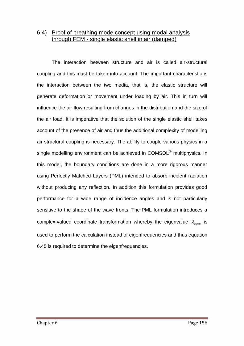
Chapter 6 Page 156
6.4) Proof of breathing mode concept using modal analysis through FEM - single elastic shell in air (damped)
The interaction between structure and air is called air-structural
coupling and this must be taken into account. The important characteristic is
the interaction between the two media, that is, the elastic structure will
generate deformation or movement under loading by air. This in turn will
influence the air flow resulting from changes in the distribution and the size of
the air load. It is imperative that the solution of the single elastic shell takes
account of the presence of air and thus the additional complexity of modelling
air-structural coupling is necessary. The ability to couple various physics in a
single modelling environment can be achieved in COMSOL® multiphysics. In
this model, the boundary conditions are done in a more rigorous manner
using Perfectly Matched Layers (PML) intended to absorb incident radiation
without producing any reflection. In addition this formulation provides good
performance for a wide range of incidence angles and is not particularly
sensitive to the shape of the wave fronts. The PML formulation introduces a
complex-valued coordinate transformation whereby the eigenvalue eigen is
used to perform the calculation instead of eigenfrequencies and thus equation
6.45 is required to determine the eigenfrequencies.

Chapter 6 Page 157
Figure 6.5: 2-Dimensional modal analysis showing static deformation plots in
sequence (a-d) on the “Breathing mode” shape of elastic element coupled with air
surrounded by a perfectly matched layers for the domain boundaries.
Figures 6.5 (a-d) show in sequence 2-dimensional static deformation
plots of the latex breathing mode results after using perfectly matched layers
for the domain boundaries. The eigenvalues have to be converted to
eigenfrequencies using equation 6.45. For example
2
5924 gives an
eigenfrequency of 942 Hz. Clearly with the introduction of air damping, the
breathing mode (mode 0) frequency is predicted to shift to a much higher
frequency with the volumetric expansion and contraction displacement of
+0.0075 m and 0.0025 m respectively. The FEM predicted breathing mode
resonance frequency also agrees fairly well with the semi-analytical and
measurement results of about 1 kHz (figure 6.3). These modal analysis
results show that the resonance is indeed a breathing mode type resonance
and that there is a possibility of tuning the resonance frequency by using a
(a) (b)
(c) (d)

Chapter 6 Page 158
different damping ratio between the latex scatterer and surrounding
environments (inside and outside).
6.5) Influence of shell diameter
In this section, the influence of the size of the elastic scatterer is
studied both in laboratory and using MST. Three different types of diameter
(0.0275, 0.043 and 0.055 m) with similar wall thickness of 0.00025 m are
investigated.
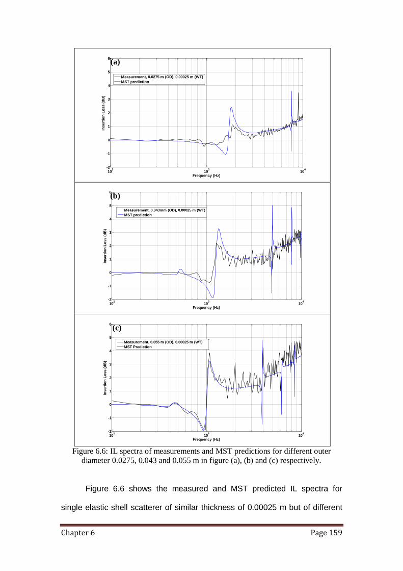
Chapter 6 Page 159
Figure 6.6: IL spectra of measurements and MST predictions for different outer
diameter 0.0275, 0.043 and 0.055 m in figure (a), (b) and (c) respectively.
Figure 6.6 shows the measured and MST predicted IL spectra for
single elastic shell scatterer of similar thickness of 0.00025 m but of different
102
103
104
-2
-1
0
1
2
3
4
5
6
Frequency (Hz)
Insert
ion
Lo
ss (
dB
)
Measurement, 0.0275 m (OD), 0.00025 m (WT)
MST prediction
102
103
104
-2
-1
0
1
2
3
4
5
6
Frequency (Hz)
Insert
ion
Lo
ss (
dB
)
Measurement, 0.043mm (OD), 0.00025 m (WT)
MST prediction
102
103
104
-2
-1
0
1
2
3
4
5
6
Insert
ion
Lo
ss (
dB
)
Frequency (Hz)
Measurement, 0.055 m (OD), 0.00025 m (WT)
MST Prediction
(a)
(b)
(c)
Chapter 6 Page 160
diameter 0.0275, 0.043 and 0.055 m in figure (a), (b) and (c) respectively. The
breathing mode resonance frequencies for diameters of 0.0275, 0.043 and
0.055 m are observed to be near 1.8, 1.5 and 1.1 kHz respectively. This
clearly shows that the “breathing mode” resonance can be tuned to lower
frequency by increasing the diameter of the elastic shell scatterer. For all
three cases, the MST predictions agree well with the experimental results. It is
also noted that the accuracy of the MST prediction for the IL amplitude
improves as the diameter of the scatterer is increased. Again, the predicted
narrow-band higher order modes are not observed in the data.
6.6) Influence of wall thickness
Another physical parameter of which we are keen to investigate is wall
thickness of the elastic shell. Experiments and semi-analytical predictions
using MST are performed for 2 different diameter sizes of elastic shell 0.043
and 0.055 m. For each of the different diameters, wall thicknesses of 0.00025
(figure 6.7(a) and (c)) and 0.0005 m (figure 6.7(b) and (d)) are used.
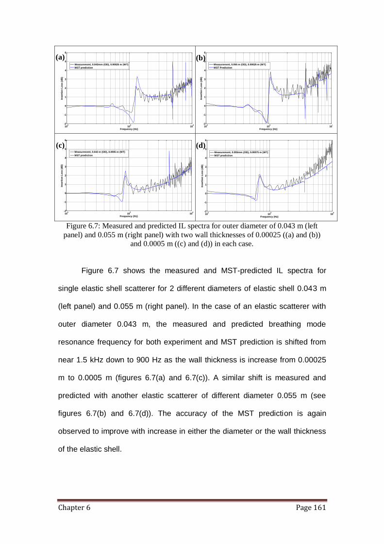
Chapter 6 Page 161
Figure 6.7: Measured and predicted IL spectra for outer diameter of 0.043 m (left
panel) and 0.055 m (right panel) with two wall thicknesses of 0.00025 ((a) and (b))
and 0.0005 m ((c) and (d)) in each case.
Figure 6.7 shows the measured and MST-predicted IL spectra for
single elastic shell scatterer for 2 different diameters of elastic shell 0.043 m
(left panel) and 0.055 m (right panel). In the case of an elastic scatterer with
outer diameter 0.043 m, the measured and predicted breathing mode
resonance frequency for both experiment and MST prediction is shifted from
near 1.5 kHz down to 900 Hz as the wall thickness is increase from 0.00025
m to 0.0005 m (figures 6.7(a) and 6.7(c)). A similar shift is measured and
predicted with another elastic scatterer of different diameter 0.055 m (see
figures 6.7(b) and 6.7(d)). The accuracy of the MST prediction is again
observed to improve with increase in either the diameter or the wall thickness
of the elastic shell.
102
103
104
-2
-1
0
1
2
3
4
5
6
Frequency (Hz)
Insert
ion
Lo
ss (
dB
)
Measurement, 0.043mm (OD), 0.00025 m (WT)
MST prediction
102
103
104
-2
-1
0
1
2
3
4
5
6
Insert
ion
Lo
ss (
dB
)
Frequency (Hz)
Measurement, 0.055 m (OD), 0.00025 m (WT)
MST Prediction
102
103
104
-2
-1
0
1
2
3
4
5
6
Insert
ion
Lo
ss (
dB
)
Frequency (Hz)
Measurement, 0.043 m (OD), 0.0005 m (WT)
MST prediction
102
103
104
-2
-1
0
1
2
3
4
5
6
Frequency (Hz)
Insert
ion
Lo
ss (
dB
)
Measurement, 0.055mm (OD), 0.00075 m (WT)
MST prediction
(c) (d)
(a) (b)
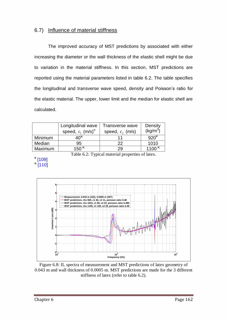
Chapter 6 Page 162
6.7) Influence of material stiffness
The improved accuracy of MST predictions by associated with either
increasing the diameter or the wall thickness of the elastic shell might be due
to variation in the material stiffness. In this section, MST predictions are
reported using the material parameters listed in table 6.2. The table specifies
the longitudinal and transverse wave speed, density and Poisson’s ratio for
the elastic material. The upper, lower limit and the median for elastic shell are
calculated.
Longitudinal wave
speed, 1c (m/s)¤
Transverse wave
speed, 2c (m/s)
Density (kg/m3)
Minimum 40җ 11 920¥
Median 95 22 1010
Maximum 150 җ 29 1100 җ
Table 6.2: Typical material properties of latex. ¥ [109] җ [110]
Figure 6.8: IL spectra of measurement and MST predictions of latex geometry of
0.043 m and wall thickness of 0.0005 m. MST predictions are made for the 3 different
stiffness of latex (refer to table 6.2).
102
103
104
-2
-1
0
1
2
3
4
5
6
Insert
ion
Lo
ss (
dB
)
Frequency (Hz)
Measurement, 0.043 m (OD), 0.0005 m (WT)
MST prediction, rho 920, c1 40, c2 11, poisson ratio 0.48
MST prediction, rho 1010, c1 95, c2 22, poisson ratio 0.485
MST prediction, rho 1100, c1 150, c2 29, poisson ratio 0.49

Chapter 6 Page 163
Figure 6.8 compares the MST predicted IL spectra using the latex
material parameters provided in table 2 with measurement data for diameter
0.043 and wall thickness of 0.0005 m. The predicted resonance peak
frequencies for minimum, median and maximum stiffness values for latex are
near 930, 880 and 840 Hz respectively. Increasing the material density is
predicted to shift the breathing mode resonance to lower frequency. This
result indicates the robustness of the breathing mode resonance for such
material where only a small deviation (about 100 Hz) of the resonance
frequency results from the change in latex density between lowest and
highest typical values.
6.8) Influence of tensioning
The complexity and computational resource that would be required for
both semi-analytical and FEM calculations do not allow consideration of the
influence of the 3 dimensional aspect of the latex cylinder (i.e. the finite height
of the cylinder). The robustness of the breathing modes of latex cylinders to
the method of end support has been investigated empirically by varying the
tension at the ends of the latex cylinders between ‘loose’ and ‘tight’. To
quantify the tension, the numbers of turns on the securing nuts are recorded.
First, the single latex cylinder is mounted with ‘normal’ tension. Then a further
15 turns of the securing nuts (top and bottom of supporting plate) has been
used to give ‘tight’ tensions and 15 less turns than required for ‘normal’
tension has been used as ‘loose’ tension.

Chapter 6 Page 164
Figure 6.9: Measured IL spectra of single latex of OD 0.0275 m and WT 0.00025 m
with different tensioning states (tightly, normal and loosely tension).
Figure 6.9 shows measured IL spectra obtained with a single latex
cylinder of OD 0.0275 m and WT 0.00025 m with different tensioning states
(‘tight’, ‘normal’ and ‘loose’). The tension is controlled by the 2 mounting nuts
at both top and bottom of the latex cylinder. The breathing mode resonance at
around 1.7 kHz is clear for the ‘tight’ and ‘normal’ tensioning states. However
for ‘loose’ the IL is reduced especially at low frequency.
6.9) Arrays of elastic shells
We next consider a finite array of thin elastic shells distributed in a
lattice with square cells of size L (figure 6.2). Assuming that a cylindrical
source generates sound waves and using a multiple scattering technique
developed by our collaborators [111], the solution in the outer acoustic
environment can be derived in the following form,
103
104
-2
-1.5
-1
-0.5
0
0.5
1
1.5
2
2.5
3
Frequency (Hz)
Insert
ion
Lo
ss (
dB
)
Tightly tension
Normal tension
Loosely tension
Measurements, 0.0275 m (OD), 0.00025 m (WT)

Chapter 6 Page 165
minM
m n
mon
m
n
m
nooo erkHZArkHrpˆ
1
11 ˆ,
, (6.47)
where M is the number of scatterers in the array, the first sum is taken over all
numbers of shells in the array, the factors m
nZ take the previously derived
from equation 6.27 specified to the scatterer with index m , and variables
,ˆ rrm and ,ˆ rm are the polar coordinates with origin in the center of shell
of index m . Note that the solutions for the shells and the inner acoustic
medium are identical to those in section 6.2.
To compute the unknown coefficients m
nA in equation 6.47, we again need to
express solution in equation 6.47 in terms of one set of polar coordinates
mmr ,ˆ using Graff’s Additional theorem that results in,
m
mp
m
in
n
M
mpp
nqi
mponqmo
q
n
p
q
p
q
mon
m
n
m
n
in
monmon
mmo eeQkHrkJZA
rkHZAeQkHrkJ
rp
ˆ
,1
1
11
ˆ
ˆˆ
ˆ,ˆ
, ,,...,1 Mm
(6.48)
where vector mmmm QQ sin,cos is the radius vector to the centre of
scatterer mC and vector mpmpmpm QQ sin,cos defines the position of
scatterer pC with respect to scatterer mC .
Use of the modified solution 6.48 in equations 6.28, 6.29, 6.31 and 6.32
together with the solutions of inner acoustic medium and elastic shell makes it

Chapter 6 Page 166
possible to derive the system of algebraic equations, which is similar to the
equation 3.36 (chapter 3). This gives,
mmp in
mon
M
mpp
nqi
mponq
N
Nq
p
q
p
q
m
n eQkHeQkHZAA
1
,1
1 ,
,,...,1 Mm
(6.49)
The obtained algebraic system must be truncated to the finite number
M(2N+1) of equations, and then can be used to obtain the coefficients m
nA ,
1n , …, N , 1m ,…, M numerically. Again the results are plotted in terms of
Insertion Loss (IL) as in equation 6.27.
To compare the semi-analytical results with data for arrays, viscoelasticity
defined by a Young’s modulus of complex form (equation 6.42 and 6.43) is
again introduced and this leads to redefining unknown coefficient in equation
6.48 by solving system equation 6.49 with modified elastic parameters.
Figure 6.10: Measured and MST predicted IL spectra for an array of latex shell
scatterers of outer diameter (OD) 0.055 m and wall thickness (WT) 0.00025 m with
lattice constant 0.08 m.
100 1000 5000-5
0
5
10
15
20
25
30
35
Frequency (Hz)
Insert
ion
Lo
ss (
dB
)
Measurement, 7x3 elastic shell and L = 0.08 m
MST prediction

Chapter 6 Page 167
Figure 6.11: Measured and MST predicted IL spectra for an array with lattice constant
0.1 m of latex shell scatterers having outer diameter (OD) 0.055 m and wall thickness
(WT) 0.00025 m.
Figure 6.12: Measured and MST predicted IL spectra for an array with lattice constant
0.15 m of latex shell scatterers having outer diameter (OD) 0.055 m and wall
thickness (WT) 0.00025 m.
In figure 6.10 – 6.12 show the measured and MST predicted IL spectra
for a 7x3 square lattice array with lattice constants of 0.08 m, 0.1 m and 0.15
m respectively. Each latex shell used in all three array configurations has OD
0.055 m and WT 0.00025 m (similar to the single scatterer use in figure 6.3).
100 1000 5000-5
0
5
10
15
20
25
30
35
Frequency (Hz)
Insert
ion
Lo
ss (
dB
)
Measurement, 7x3 elastic shell and L = 0.1 m
MST prediction
100 1000 3000-10
-5
0
5
10
15
20
25
30
Frequency (Hz)
Insert
ion
Lo
ss (
dB
)
Measurement, 7x3 elastic shell and L = 0.15 m
MST prediction

Chapter 6 Page 168
The calculated Bragg band gap central frequencies defined by equation 2.13
(chapter 2) for lattice constants of 0.08 m, 0.1 m and 0.15 m are 2.1 kHz, 1.7
kHz and 1.1 kHz respectively. The predictions show relatively good
agreement with measured data. The peaks near 1 kHz in figures 6.10 and
6.11 can be identified as the result of the resonant behaviour of the elastic
shells which is independent of the effect due to periodicity. The discrepancy in
amplitude between theoretical and experiment results for the resonant peak
may be explained by the differences between assumed and actual source and
receiver positions during the experiments. Also in the low-frequency regime,
the assumed values of the viscoelasticity parameters influence the agreement
between data and predictions. The peak at about 750 Hz could be due to the
finite height of the array as discussed in chapter 4.
6.10) Influence of angle between source-receiver and array axes
Figure 6.13: (a) Plan view of the source, receiver and array in the laboratory
measurements at normal incidence and microphone laterally displace (see red arrow)
up to 14 cm (b) the corresponding side view with microphone vertically displace (see
red arrow) up to 45 from normal incidence.
(Lateral displacement up to 14 cm)
L
L
d
1.5 m
50 mm
x
y
x
z
Ground
1.5 m
50 mm
1.2 m
(a) (b)
(Vertical displacement up to 45)

Chapter 6 Page 169
Figure 6.14: Lateral displacement, measurement IL spectra for array with lattice
constant 0.08 m of latex scatterers having outer diameter (OD) 0.055 m and wall
thickness (WT) 0.00025 m.
Figure 6.14 shows the IL spectra measured for 7x3 square lattice array
of latex scatterer of OD 0.055 m and WT 0.00025 m with lattice constant of
0.08 m. The microphone position is laterally displaced up to 14 cm from the
normal incidence position (corresponding to an angle of less than 10), see
figure 6.13(a). The constancy of the low frequency peaks around 1 kHz
supports the contention that these IL peaks correspond to resonance of the
latex cylinders and should therefore be relatively independent of the source-
receiver angle. The Bragg band gap central frequency for this lattice
configuration is around 2 kHz, similar to that for a rigid scatterer array with the
same dimensions. It seems that the classical band gap is not angle
dependent either. However further displacement of the receiving microphone
was not possible without introducing diffraction from the array edges. The
peak at around 700 Hz attributed to the finite height of the array (refer to FEM
chapter 4) is fairly constant except for the largest displacement.
300 1000 5000-5
0
5
10
15
20
25
30
35
Frequency (Hz)
Insert
ion
Lo
ss (
dB
)
Lat. displ = 0
1 cm
2 cm
3 cm
5 cm
14 cm
Measurement, 7x3 array,elastic shell, L = 0.08 m

Chapter 6 Page 170
Figure 6.15: Lateral displacement, measurement IL spectra for array with lattice
constant 0.15 m of latex scatterers having outer diameter (OD) 0.055 m and wall
thickness (WT) 0.00025 m.
Figure 6.15 shows the measured IL spectra due to a 7x3 square lattice
array with lattice constant of 0.1 m of latex scatterers having OD 0.055 m and
WT 0.00025 m as the microphone position is vertically displaced up to 45
from the normal incidence source-receiver axis, see figure 6.13(b). On
average there is a decrease of about 15 dB in the band gap magnitude
between 1 and 2 kHz as the elevation angle is changed from 0 to 45. One
possible explanation is that the breathing mode for the latex shell is supported
only by waves incident in the plane normal to the cylinders. A second possible
reason could be the influence of reflections from the end plates of the
supporting structure (see 6.17). Further displacement of the receiving
microphone was not possible to avoid diffraction from the base of the
supporting structure. These results also support the argument that the peak at
around 700 Hz could be attributed to the finite height of the array.
300 1000 5000-10
-5
0
5
10
15
20
25
30
35
40
Frequency (Hz)
Insert
ion
Lo
ss (
dB
)
Vert. Displ = 0
13
27
45
Measurement, 7x3 array,elastic shell, L = 0.1 m
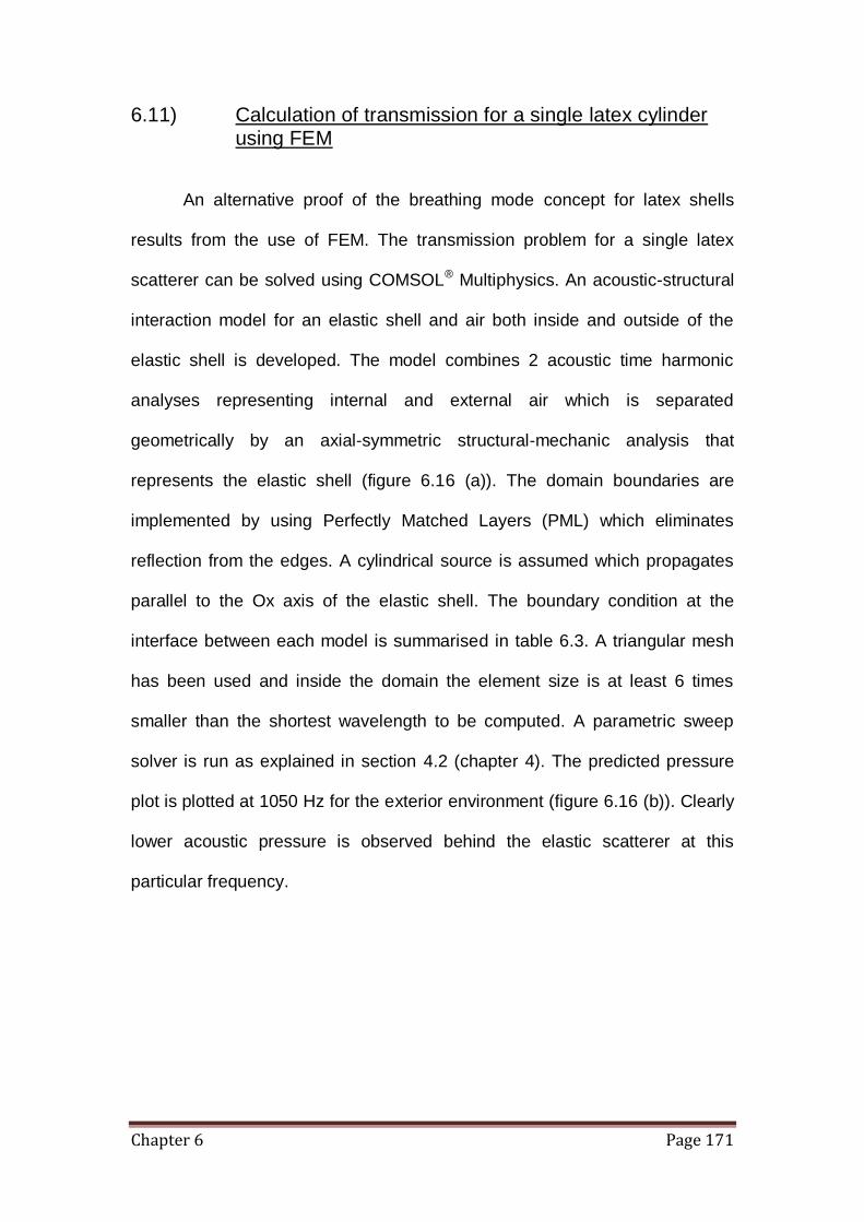
Chapter 6 Page 171
6.11) Calculation of transmission for a single latex cylinder using FEM
An alternative proof of the breathing mode concept for latex shells
results from the use of FEM. The transmission problem for a single latex
scatterer can be solved using COMSOL® Multiphysics. An acoustic-structural
interaction model for an elastic shell and air both inside and outside of the
elastic shell is developed. The model combines 2 acoustic time harmonic
analyses representing internal and external air which is separated
geometrically by an axial-symmetric structural-mechanic analysis that
represents the elastic shell (figure 6.16 (a)). The domain boundaries are
implemented by using Perfectly Matched Layers (PML) which eliminates
reflection from the edges. A cylindrical source is assumed which propagates
parallel to the Ox axis of the elastic shell. The boundary condition at the
interface between each model is summarised in table 6.3. A triangular mesh
has been used and inside the domain the element size is at least 6 times
smaller than the shortest wavelength to be computed. A parametric sweep
solver is run as explained in section 4.2 (chapter 4). The predicted pressure
plot is plotted at 1050 Hz for the exterior environment (figure 6.16 (b)). Clearly
lower acoustic pressure is observed behind the elastic scatterer at this
particular frequency.

Chapter 6 Page 172
Figure 6.16: Meshing of single latex with OD 0.055 m and wall thickness (WT
0.00025 m (a). FEM predicted pressure plot at 1050 Hz for the exterior environment
of the model (b).
Air outside cylinder Elastic cylinder Air inside cylinder
Model suffix Acpr (Acoustic) smps (Structural Mech.) acpr2 (Acoustic)
Inner wall Continuity Load (N/m2)
-p2*nx_smps (x-direction)
-p2*ny_smps (y-direction)
Normal acceleration
(m/s2)
u3_tt_smps*nx_smps+
v3_tt_smps*ny_smps
Outer wall Normal acceleration
(m/s2)
u3_tt_smps*nx_smps+
v3_tt_smps*ny_smps
Load (N/m2)
-(p+p_i_acpr)*nx_smps
(x-direction)
-(p+p_i_acpr)*ny_smps
(y-direction)
Continuity
Table 6.3: Summary of boundary conditions used in the acoustic structural interaction
model.
Figure 6.17: Measured and predicted (FEM and MST) IL spectra for a single latex
scatterer having 0.055 m (OD) and wall thickness 0.00025 m (WT).
102
103
-3
-2
-1
0
1
2
3
4
5
6
Insert
ion
Lo
ss (
dB
)
Frequency (Hz)
Measurement 0.055 m (OD) and 0.00025 m (WT)
MST Prediction
FEM prediction
(a) (b)
3.8 dB
3.6 dB
3.2 dB

Chapter 6 Page 173
According to figure 6.17, the IL spectrum predicted by FEM agrees with both
MST predictions and the measurement data for the single latex scatterer
(0.055 m (OD) and wall thickness 0.00025 m (WT)). For all measurements
and predictions, the receiver is positioned 0.05 m away from the scatterer.
The IL values at 1 kHz (breathing mode resonance frequency) for all the 3
spectra are shown in the figure. The discrepency between the prediction and
measurement at the Bragg frequency is about 0.6 dB. Higher order modes
are observed by FEM as well as MST but due to the narrow band
characteristics, these modes are not observed in the measurements.
6.12) Fabrication of specimen and effect of non-uniformity in latex scatterer
To make the 2 m long elastic shells, latex sheets (2 m long and
0.00025 m thick) have been formed into cylinders with outer diameter of
0.0275 and 0.055 m, respectively. This has been achieved by folding each
latex sheet into a cylindrical shape, overlapping the edges by a few
millimetres (< 0.01 m) and gluing them together using cyanoacrylate. Perspex
circular end caps with metal bolts were made for both ends of the latex
cylinder and used to attach them to holed wooden boards at the top and base
of the cylinders. To maintain their shape and vertical orientation, the latex
cylinders were slightly inflated above atmospheric pressure through a
common pipe driven by a small pump. Nevertheless some deviations from the
cylindrical shape could not be avoided.

Chapter 6 Page 174
Figure 6.18: Measurement setup for array of cylinders of 7x3 arrays of latex (a) and a
single latex showing the overlapping strip, mounting bolt and pipe for air inlet (b).
To quantify the variation in the shapes of the latex scatterers, 21 latex
cylinders of OD 0.055 m, WT 0.00025 m and length of 2 m were tested
individually. The diameters were measured at 3 positions with a calliper (see
table 6.4). The resulting mean diameter and standard deviation are 0.05732 m
and 0.00126 m respectively.
(a) (b)
overlapped
pipe
bolt
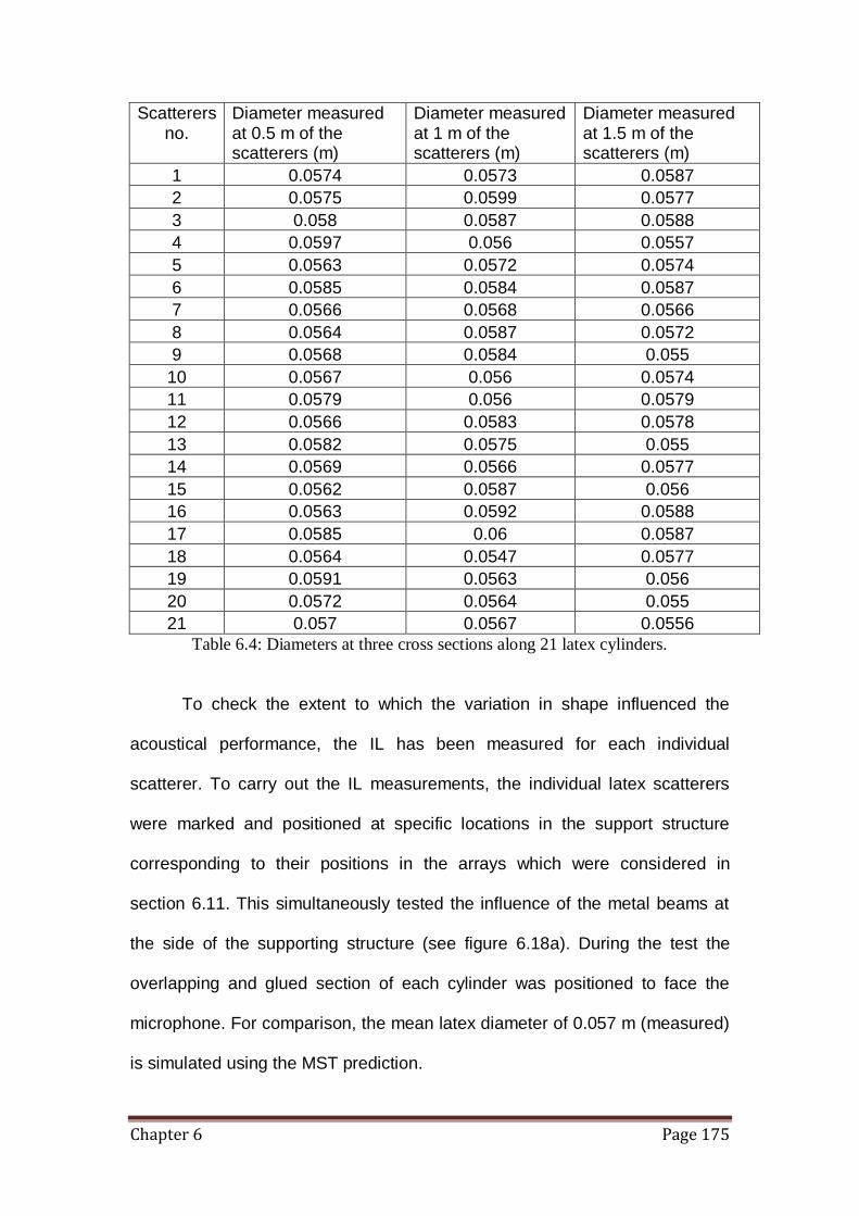
Chapter 6 Page 175
Scatterers no.
Diameter measured at 0.5 m of the scatterers (m)
Diameter measured at 1 m of the scatterers (m)
Diameter measured at 1.5 m of the scatterers (m)
1 0.0574 0.0573 0.0587
2 0.0575 0.0599 0.0577
3 0.058 0.0587 0.0588
4 0.0597 0.056 0.0557
5 0.0563 0.0572 0.0574
6 0.0585 0.0584 0.0587
7 0.0566 0.0568 0.0566
8 0.0564 0.0587 0.0572
9 0.0568 0.0584 0.055
10 0.0567 0.056 0.0574
11 0.0579 0.056 0.0579
12 0.0566 0.0583 0.0578
13 0.0582 0.0575 0.055
14 0.0569 0.0566 0.0577
15 0.0562 0.0587 0.056
16 0.0563 0.0592 0.0588
17 0.0585 0.06 0.0587
18 0.0564 0.0547 0.0577
19 0.0591 0.0563 0.056
20 0.0572 0.0564 0.055
21 0.057 0.0567 0.0556
Table 6.4: Diameters at three cross sections along 21 latex cylinders.
To check the extent to which the variation in shape influenced the
acoustical performance, the IL has been measured for each individual
scatterer. To carry out the IL measurements, the individual latex scatterers
were marked and positioned at specific locations in the support structure
corresponding to their positions in the arrays which were considered in
section 6.11. This simultaneously tested the influence of the metal beams at
the side of the supporting structure (see figure 6.18a). During the test the
overlapping and glued section of each cylinder was positioned to face the
microphone. For comparison, the mean latex diameter of 0.057 m (measured)
is simulated using the MST prediction.
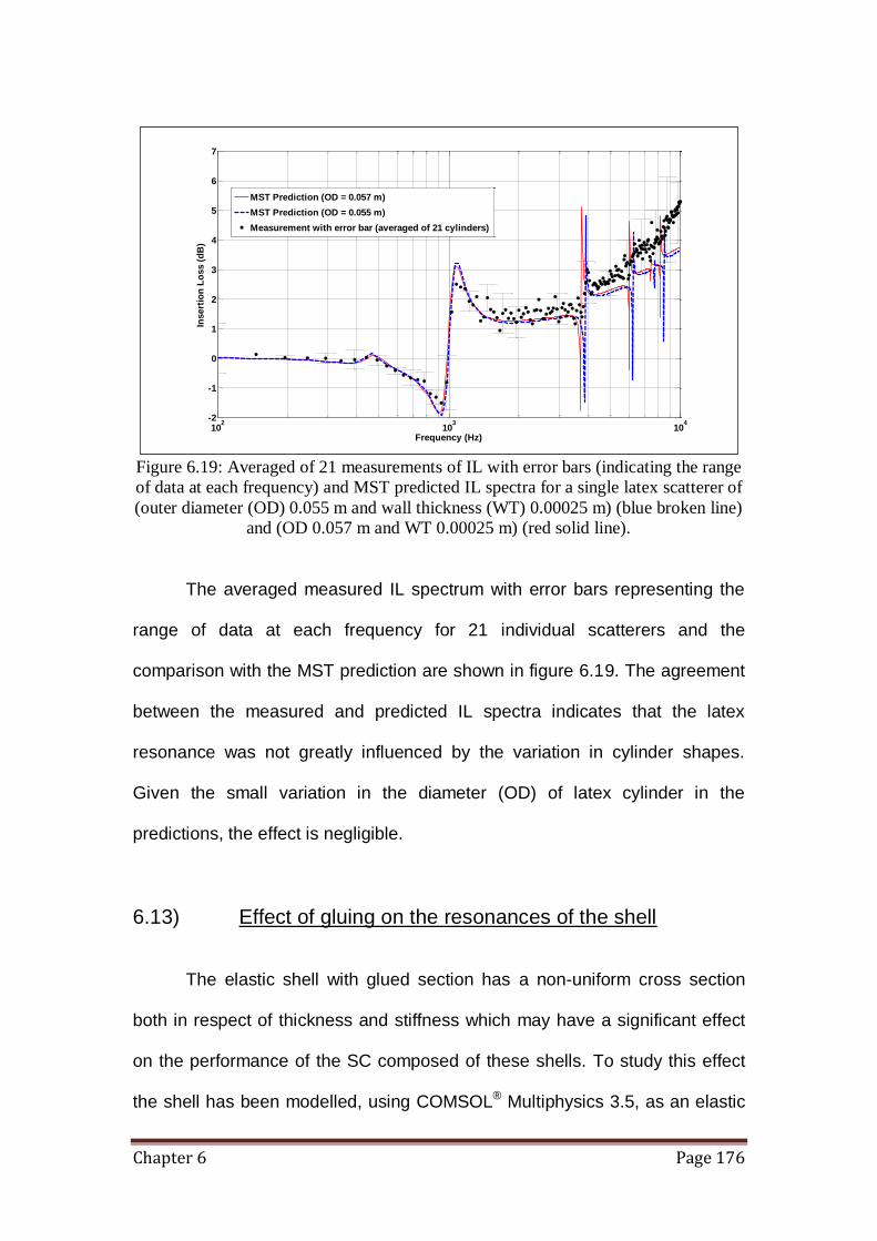
Chapter 6 Page 176
Figure 6.19: Averaged of 21 measurements of IL with error bars (indicating the range
of data at each frequency) and MST predicted IL spectra for a single latex scatterer of
(outer diameter (OD) 0.055 m and wall thickness (WT) 0.00025 m) (blue broken line)
and (OD 0.057 m and WT 0.00025 m) (red solid line).
The averaged measured IL spectrum with error bars representing the
range of data at each frequency for 21 individual scatterers and the
comparison with the MST prediction are shown in figure 6.19. The agreement
between the measured and predicted IL spectra indicates that the latex
resonance was not greatly influenced by the variation in cylinder shapes.
Given the small variation in the diameter (OD) of latex cylinder in the
predictions, the effect is negligible.
6.13) Effect of gluing on the resonances of the shell
The elastic shell with glued section has a non-uniform cross section
both in respect of thickness and stiffness which may have a significant effect
on the performance of the SC composed of these shells. To study this effect
the shell has been modelled, using COMSOL® Multiphysics 3.5, as an elastic
102
103
104
-2
-1
0
1
2
3
4
5
6
7
Frequency (Hz)
Insert
ion
Lo
ss (
dB
)
MST Prediction (OD = 0.057 m)
MST Prediction (OD = 0.055 m)
Measurement with error bar (averaged of 21 cylinders)

Chapter 6 Page 177
material containing a rigid strip. Figure 6.20 illustrates the geometry used in
the 2D numerical simulation. A rigid inclusion of width 0.01 m has Neumann
boundary conditions imposed at the acoustic interface and fixed faces (zero
displacement) at the elastic interface. The source is a cylindrical wave
propagating parallel to the Ox axis. In the formulation of the FE model, the
outer environment is surrounded by perfectly matched layers (PML) which
replaces the radiation condition and as such the domain size can be reduced.
The 2-Dimensional Finite Elements (FE) simulation is defined by the triangular
elements and the active domain is meshed by at least six elements per
wavelength. The hardware configuration used to run the simulations was a
64-bits windows platform with 3.07 GHz Intel core i7 processor and 6 GB of
RAM. The estimated computational time for solving the full problem in the
frequency interval (0, 8000) Hz is 15 mins. Constrained by the computational
resources, only a single latex scatterer is simulated. However a full array
simulation has been performed by our collaborators [111]. Also note that in
contrast with their simulation, the simulation done here is performed with a
cylindrical wave rather than a plane wave. The results are found to have
similar characteristics despite the differences in the source and number of
scatterers,
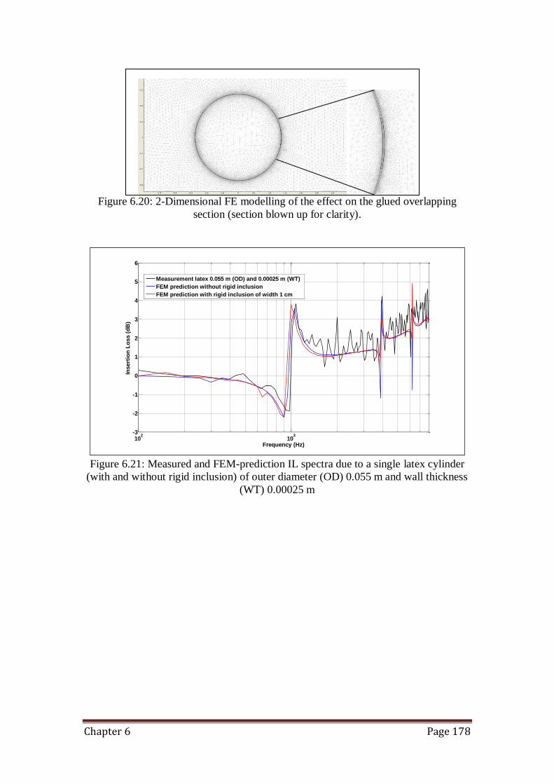
Chapter 6 Page 178
Figure 6.20: 2-Dimensional FE modelling of the effect on the glued overlapping
section (section blown up for clarity).
Figure 6.21: Measured and FEM-prediction IL spectra due to a single latex cylinder
(with and without rigid inclusion) of outer diameter (OD) 0.055 m and wall thickness
(WT) 0.00025 m
102
103
-3
-2
-1
0
1
2
3
4
5
6
Insert
ion
Lo
ss (
dB
)
Frequency (Hz)
Measurement latex 0.055 m (OD) and 0.00025 m (WT)
FEM prediction without rigid inclusion
FEM prediction with rigid inclusion of width 1 cm
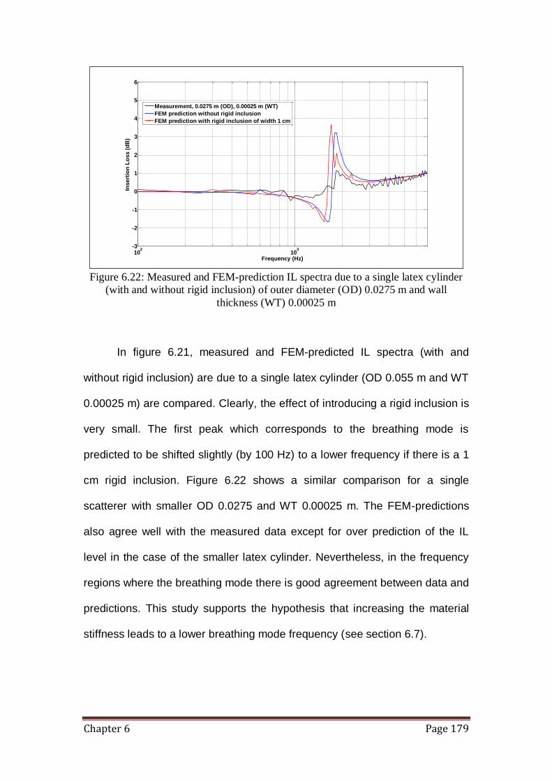
Chapter 6 Page 179
Figure 6.22: Measured and FEM-prediction IL spectra due to a single latex cylinder
(with and without rigid inclusion) of outer diameter (OD) 0.0275 m and wall
thickness (WT) 0.00025 m
In figure 6.21, measured and FEM-predicted IL spectra (with and
without rigid inclusion) are due to a single latex cylinder (OD 0.055 m and WT
0.00025 m) are compared. Clearly, the effect of introducing a rigid inclusion is
very small. The first peak which corresponds to the breathing mode is
predicted to be shifted slightly (by 100 Hz) to a lower frequency if there is a 1
cm rigid inclusion. Figure 6.22 shows a similar comparison for a single
scatterer with smaller OD 0.0275 and WT 0.00025 m. The FEM-predictions
also agree well with the measured data except for over prediction of the IL
level in the case of the smaller latex cylinder. Nevertheless, in the frequency
regions where the breathing mode there is good agreement between data and
predictions. This study supports the hypothesis that increasing the material
stiffness leads to a lower breathing mode frequency (see section 6.7).
102
103
-3
-2
-1
0
1
2
3
4
5
6
Frequency (Hz)
Insert
ion
Lo
ss (
dB
)
Measurement, 0.0275 m (OD), 0.00025 m (WT)
FEM prediction without rigid inclusion
FEM prediction with rigid inclusion of width 1 cm

Chapter 6 Page 180
6.14) Effect of disc attachment on the latex scatterer
The industrially-manufactured latex cylinders used for some of the
experiments were delivered in 0.7 m lengths due to the limitating size of the
standard mould used during the manufacturing process. To lengthen the
cylinder, a Perspex disc of slightly larger diameter was used to join the
individual latex cylinders together (see figure 6.23). This improvised approach
also served to restore and maintain their cylindrical shape as the latex
cylinders were flattened when they are delivered. Nevertheless segments
along the scatterers were observed to be more elliptical than cylindrical. The
difference is more prominent at the “extreme flat region” which has the largest
semi-major axis. Another anomalous region is the “inflated region”, about 0.05
m deviation from the joining disc, where the cylinder starts to deviate from the
cylindrical shape maintained by the disc. The average dimensions taken from
5 cylinders for these two regions are shown in the insert in figure 6.23.
Laboratory measurements have been carried out to check on the influence on
the breathing mode of the introduction of rigid disc and the changes in shape
along each latex scatterer. For convenience, measurements performed at the
semi-major axis are denoted as “face” measurements and those made at
“extreme flat and inflated” regions are denoted as ‘edge’ (see figure 6.23).

Chapter 6 Page 181
Figure 6.23: Industrially-manufactured latex cylinders joined by a Perspex disc
(“Rigid”) and mounted between supports in the anechoic chamber. The insert on the
left shows the shape of an “Extreme flat region” with averaged dimensions and the
insert on the right shows an “Inflated region” with averaged dimensions.
Figure 6.24: IL spectra of single industrial latex (Sample 1, S1) at all 5 positions
(Extreme flat face/edge, rigid and inflated face/edge).
Figure 6.24 shows the IL spectra of a single industrially-manufactured
latex cylinder at all 5 positions illustrated in figure 6.23. Clearly, the breathing
mode resonance near 900 Hz is preserved in all the positions despite the non-
uniformity of the scatterer. This indicates that the breathing mode resonance
is little influenced by the method of joining the latex cylinders.
102
103
-1
0
1
2
3
4
5
Frequency (Hz)
Insert
ion
Lo
ss (
dB
)
Extreme flat face
Extreme flat edge
Rigid (joint)
Inflated flat edge
Inflated flat face
S1
“Extreme flat region”, average
dimensions.
“Inflated region”, average
dimensions.
Perspex
disc,
“Rigid”

Chapter 6 Page 182
Figure 6.25: IL spectra of consistency test for 2-single industrial latex (Sample 1 (S1)
and 2 (S2)) at all 5 positions (Extreme flat face (a) or edge (b), inflated face (c) or
edge (d) and rigid (e)).
Laboratory measurements have been made on another single
industrial latex cylinder constructed in a similar way using Perspex disc.
Figure 6.25 shows the IL spectra comparing two single industrial latex
cylinders at 5 different receiver locations opposite portions with (a) an
extremely flat face (b), an extremely flat edge (c) an inflated face (d) an
inflated edge and (e) rigid. The results show that the breathing mode
resonance frequency (near 1 kHz) is fairly consistent between both cylinders.
The deviation between the IL spectra at higher frequency could be due to the
102
103
104
-2
-1
0
1
2
3
4
5
6
Frequency (Hz)
Insert
ion
Lo
ss (
dB
)
S1
S2
Extreme flat face
102
103
104
-1
-0.5
0
0.5
1
1.5
2
2.5
3
3.5
Frequency (Hz)
Insert
ion
Lo
ss (
dB
)
S1
S2
Extreme flat edge
102
103
104
-1
0
1
2
3
4
5
6
Frequency (Hz)
Insert
ion
Lo
ss (
dB
)
S1
S2
Inflated face
102
103
104
-0.5
0
0.5
1
1.5
2
2.5
3
3.5
Frequency (Hz)
Insert
ion
Lo
ss (
dB
)
S1
S2
Inflated edge
102
103
104
-1
-0.5
0
0.5
1
1.5
2
2.5
3
3.5
4
Frequency (Hz)
Insert
ion
Lo
ss (
dB
)
S1
S2
Rigid
(a) (b)
(c) (d)
(e)

Chapter 6 Page 183
precise location of receiver with respect to the cylinder. These single elastic
cylinders results confirm the robustness of the breathing mode resonance.
6.15) Industrial latex array results
Based on the successful prototype test on the single latex cylinder,
arrays of elastic cylinders have been constructed and their performance has
been determined by laboratory measurements.
Figure 6.26: Measured IL spectra due to 7x2 and 7x3 arrays of industrial latex
cylinders and an MST predicted IL spectrum for a 7x3 latex array. The insert on the
right shows a photograph of the industrial latex array.
Figure 6.26 shows measured IL spectra due to 7x2 and 7x3 arrays of
industrial latex cylinders at normal incidence. The receiver was located at 0.05
m from the centre of the nearest row of the array. The lattice constant for this
set up is 0.069 m and the calculated Bragg band gap central frequency is 2.5
kHz (refer to PWE chapter equation 2.13). Indeed the peak due to the Bragg
band gap is near 2.5 kHz in both measured IL spectra and this band gap is
enhanced by the breathing mode resonance of the latex which is at 900 Hz.
102
103
-5
0
5
10
15
20
25
30
35
Frequency (Hz)
Insert
ion
Lo
ss (
dB
)
Measurement, 7x2 array
Measurement, 7x3 array
MST prediction, 7x3 array
Extreme flat face

Chapter 6 Page 184
The MST predicted IL spectrum for the 7x3 latex arrays also shows the 2
distinct band gap peaks and the other features in the predicted IL spectrum
agrees with those in the measured spectrum. These results indicate that
significant improvement in band gap widths can be achieved by adding a row
to the array but one has to consider the larger array area and costs that would
be incurred.

Chapter 7 Page 185
Chapter 7
Enhancing the performance of sonic crystal noise barriers by using Split Ring Resonator (SRR) and
composite cylinders
7.1) Introduction
In the previous chapter, it was shown that the insertion loss spectra
produced by periodic arrays of resonant scatterers using thin elastic shells
benefit from both Bragg scattering and individual scatterer resonance.
However, an array of elastic shells exposed to the environment would not be
practical as an outdoor noise barrier. Moreover there are types of resonant
elements other than thin elastic shells. So in this chapter, the possibilities for
using alternative local resonance methods will be explored. One such
possibility is the use of the Split Ring Resonator (SRR). The concept of SRR
was initially introduced by Pendry et al in 1999 [112] in the context of the
electromagnetism. There have been theoretical and experimental studies on
SRR which introduce ranges of frequencies related to the resonant frequency
in which waves cannot propagate through the system [113 and 114]. This
potentially allows increasing insertion loss in the low-frequency regime if the
resonant frequencies of the scatterer lie below the first stop band associated
with the Bragg-scattering-type mechanism. In recent years the application of
such scatterers in the design of negative index metamaterials has been
studied intensively [115 and 116]. It has also been shown numerically that
good sound focusing can be achieved by an array of SRRs arranged in a

Chapter 7 Page 186
lens-like configuration [117]. A particular type of resonator (known as a
Helmholtz resonator) consists of a bottle almost entirely enclosing a volume of
air, with a small opening, or neck, resulting in a coupling between the air in
the neck and the external air in the room [118]. There are also similar air
cavity-type resonators such as half- and quarter-wave tubes used commonly
on air intake systems to attenuate noise at specific frequencies [119]. The
dimensions of the resonator are small compared with the wavelength of sound
at which it will resonate.
7.2) Working principles of a conventional Helmholtz resonator
Helmholtz resonators are often used as components in acoustic filters,
the acoustic analog of electric wave filters. Helmholtz resonator consists of a
rigid cavity with a protruding neck that connects to the cavity (see figure 7.1).
The behaviour of a Helmholtz resonator is analogous to that of a vibration
absorber in that the volume of air in the neck of the Helmholtz resonator
behaves much like a vibration absorber mass and the volume of air acts like a
compliance (reciprocal of stiffness). The excitation is provided by pressure
fluctuation acting over the opening of the neck, resulting in oscillations of the
volume of air in the neck. Damping is the result of radiation losses at the neck
ends and viscous losses due to friction of the oscillating air in the neck. When
air is forced into a cavity, the pressure inside increases. When the external
force pushing the air into the cavity is removed, the higher-pressure air inside
will flow out. The cavity will be left at a pressure slightly lower than the

Chapter 7 Page 187
outside, causing air to be drawn back in. This process repeats with the
magnitude of the pressure changes decreasing with time.
Figure 7.1: Illustration of Helmholtz resonator and vibration absorber.
It can be shown that the effective mass of a Helmholtz resonator is
approximately,
nLSm , (7.1)
where is the density of the air, S is the cross section area of the neck and
nL is the effective neck length which includes a correction factor for mass-
loading due to air entrainment near the neck extremities [120]. If this “plug” of
air descends a small distance x into the bottle, it compresses the air in the
container so that the air that previously occupied volume V now has SxV .
Consequently the pressure of the air rises from atmospheric pressure Ap to a
higher value ppA .
Air at atmospheric
pressure, .
Inside air
compressed
Air in neck
of bottle
Helmholtz resonator Vibration absorber
R

Chapter 7 Page 188
For such vibrations that give rise to sound, changes to the increasing
pressure in respect of the decreasing volume are fast and temperature rises
on compression, giving a large change in pressure. This is an adiabatic
process and the resulting equation involves a constant , the ratio of specific
heats, which is about 1.4 for air. The pressure change p produced by a small
volume change V can be expressed by,
V
Sx
V
V
p
p
A
. (7.2)
The mass m is moved by the difference in pressure between the top
and bottom of the neck, i.e. a net force pS , so acceleration a can be
determine using Newton’s law (second law of motion):
maF ,
or m
F
dt
xd
2
2
, (7.3)
substituting for F and m gives:
n
A
n VL
Spx
SL
pS
dt
xd
2
2
, (7.4)
so that the restoring force is proportional to the displacement. This is an
equation for Simple Harmonic Motion (SHM) at a frequency which is 2
1
times the square root of the constant of proportionality i.e.,

Chapter 7 Page 189
n
A
VL
Spf
2
1 , (7.5)
The speed c of sound in air is determined by the density, the pressure and
ratio of specific heat so equation 7.5 can be written as,
nVL
Scf
2 , (7.6)
An example calculation of the pressure inside a 2D Helmholtz
resonator at its resonant frequency has been performed by the Finite Element
Method (FEM) using COMSOL® and is shown in figure 7.2. The parameters
are nL = 0.01 m, outer radius = 0.0275 m, inner radius = 0.0255 m and the
opening = 0.004 m. The pressure map at 410 Hz indicates that the maximum
values of the acoustic pressure occur inside the cavity. This result agrees with
the calculated resonance frequency of 415 Hz using equation 7.6.
Figure 7.2: COMSOL® pressure plot at 410 Hz of a 2D Helmholtz resonator.
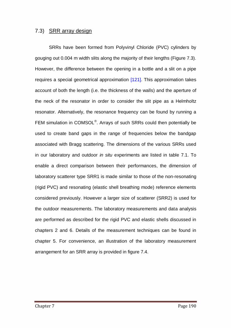
Chapter 7 Page 190
7.3) SRR array design
SRRs have been formed from Polyvinyl Chloride (PVC) cylinders by
gouging out 0.004 m width slits along the majority of their lengths (Figure 7.3).
However, the difference between the opening in a bottle and a slit on a pipe
requires a special geometrical approximation [121]. This approximation takes
account of both the length (i.e. the thickness of the walls) and the aperture of
the neck of the resonator in order to consider the slit pipe as a Helmholtz
resonator. Alternatively, the resonance frequency can be found by running a
FEM simulation in COMSOL®. Arrays of such SRRs could then potentially be
used to create band gaps in the range of frequencies below the bandgap
associated with Bragg scattering. The dimensions of the various SRRs used
in our laboratory and outdoor in situ experiments are listed in table 7.1. To
enable a direct comparison between their performances, the dimension of
laboratory scatterer type SRR1 is made similar to those of the non-resonating
(rigid PVC) and resonating (elastic shell breathing mode) reference elements
considered previously. However a larger size of scatterer (SRR2) is used for
the outdoor measurements. The laboratory measurements and data analysis
are performed as described for the rigid PVC and elastic shells discussed in
chapters 2 and 6. Details of the measurement techniques can be found in
chapter 5. For convenience, an illustration of the laboratory measurement
arrangement for an SRR array is provided in figure 7.4.
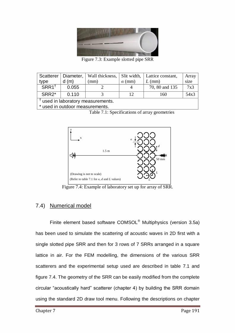
Chapter 7 Page 191
Figure 7.3: Example slotted pipe SRR
Scatterer type
Diameter, d (m)
Wall thickness,
(mm)
Slit width,
α (mm)
Lattice constant,
L (mm)
Array
size
SRR1† 0.055 2 4 70, 80 and 135 7x3
SRR2* 0.110 3 12 160 54x3 † used in laboratory measurements. * used in outdoor measurements.
Table 7.1: Specifications of array geometries
Figure 7.4: Example of laboratory set up for array of SRR.
7.4) Numerical model
Finite element based software COMSOL® Multiphysics (version 3.5a)
has been used to simulate the scattering of acoustic waves in 2D first with a
single slotted pipe SRR and then for 3 rows of 7 SRRs arranged in a square
lattice in air. For the FEM modelling, the dimensions of the various SRR
scatterers and the experimental setup used are described in table 7.1 and
figure 7.4. The geometry of the SRR can be easily modified from the complete
circular “acoustically hard” scatterer (chapter 4) by building the SRR domain
using the standard 2D draw tool menu. Following the descriptions on chapter
(Refer to table 7.1 for α, d and L values)
L
L
α
d
1.5 m
50 mm
x
(Drawing is not to scale)
y
Chapter 7 Page 192
4, the source is implemented with cylindrical waves and Perfectly Matched
Layers (PML) is used for the domain boundaries. To obtain the level of
accuracy, triangular element meshing is done with the number of elements
per wavelength chosen to be at least 6.
7.5) SRR results
Insertion Loss (IL) spectra have been calculated using chapter 3
equation 3.37 to determine the performance of the SRR scatterer. It should be
noted that the slits are all facing the source at the Ox plane as illustrated in
figure 7.4. The FEM results are then compared with data.
7.5.1) Single SRR
For single SRR, the result is compared with non-resonating reference
(i.e. cylinder made from PVC without any slit) of the same geometry. For
convenience, the non-resonating references for type SRR1 and SRR2 will be
referred to as NRR1 and NRR2 respectively.

Chapter 7 Page 193
Figure 7.5: Measurements and FEM predictions (of IL spectra for the single cylinders
of type (a) NRR1, (b) SRR1, (c) NRR2 and (d) SRR2 (see table 7.1)
In figure 7.5, IL spectra resulting from measurements on single
cylinders of types NRR1, SRR1, NRR2 and SRR2 are plotted against FEM
predictions. The IL spectra for single SRR scatterers have low frequency
peaks near 700 Hz for SRR1 and 450 Hz for SRR2 (see figures 7.5(b) and
7.5(d) respectively). These can be assumed to be the result of resonances
since they are not present in the IL spectra for identical PVC cylinders (i.e.
with the same diameter and wall thickness) without slits (see figures 7.5(a)
and 7.5(c)). Notably, the measured resonance peak amplitudes are smaller
than predicted for both types of SRR scatterers which could be the result of
damping that is not taken into account in the FEM model. Narrow band gaps
are predicted at higher frequencies for both SRR1 and SRR2. However these
higher order band gaps are predicted to have small amplitudes and are not
distinguishable in the measured spectra.
102
103
-2
-1
0
1
2
3
4
5
6
Frequency (Hz)
Ins
ert
ion
lo
ss
(d
B)
Measurement (SRR1)
FEM prediction
102
103
-2
-1
0
1
2
3
4
5
6
Frequency (Hz)
Ins
ert
ion
Lo
ss
(d
B)
Measurement (NRR1)
FEM prediction
102
103
-2
0
2
4
6
8
10
12
Ins
ert
ion
Lo
ss
(d
B)
Frequency (Hz)
Measurement (NRR2)
FEM prediction
102
103
-2
0
2
4
6
8
10
12
Frequency (Hz)
Ins
ert
ion
L
os
s (
dB
)
Measurement (SRR2)
FEM prediction
(a) (c)
(b) (d)

Chapter 7 Page 194
Figure 7.6: Pressure maps predicted using COMSOL® for incident cylindrical waves
on (a) a single scatterer SRR1 at 700 Hz and (b) a single scatterer SRR2 at 300 Hz.
Figure 7.6(a) shows an FEM-predicted pressure map at 700 Hz for a
cylindrical wave incident on a single scatterer SRR1. The maximum values of
the acoustic pressure are inside the cavity. Similar effects are observed
during the scattering of a 300 Hz wave by slit cylinder SRR2. These
predictions correspond to the low frequency IL peaks shown in figure 7.5(b)
and 7.5(d) for SRR scatterers SRR1 and SRR2 respectively.
7.5.2) Single SRR – influence of slit orientation
Intuitively, the configuration will work best for the SRR when the slit
opens towards the source since this will trap the majority of the incoming
waves. This hypothesis has been tested empirically by measuring the
Insertion Loss (IL) of the single SRR in laboratory while rotating the slit to
different angles (see figure 7.7). For this experiment, SRR1 is used (refer to
table 7.1).
(a)
(b)

Chapter 7 Page 195
Figure 7.7: Single SRR orientation.
Figure 7.8: Measured Insertion Loss spectra of the radiation pattern of single SRR
(refer to figure 7.7 for the definition of the orientated angle).
Figure 7.8 shows the IL spectra measured with different orientations of
the slit in a single SRR. As expected, the resonance amplitude is at least
twice as much for the slit facing the source (i.e. at 180°) than any other
angles. This will lay the foundation of future sonic crystal designs using SRR.
103
-0.5
0
0.5
1
1.5
2
2.5
3
3.5
4
Frequency (Hz)
Insert
ion
Lo
ss (
dB
)
0
45
90
135
180
Microphone
180° 135° 90° 45° 0°
Source
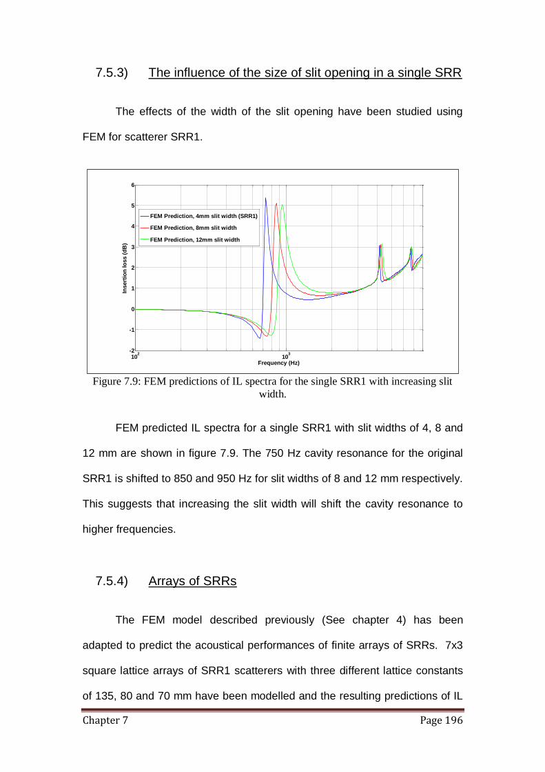
Chapter 7 Page 196
7.5.3) The influence of the size of slit opening in a single SRR
The effects of the width of the slit opening have been studied using
FEM for scatterer SRR1.
Figure 7.9: FEM predictions of IL spectra for the single SRR1 with increasing slit
width.
FEM predicted IL spectra for a single SRR1 with slit widths of 4, 8 and
12 mm are shown in figure 7.9. The 750 Hz cavity resonance for the original
SRR1 is shifted to 850 and 950 Hz for slit widths of 8 and 12 mm respectively.
This suggests that increasing the slit width will shift the cavity resonance to
higher frequencies.
7.5.4) Arrays of SRRs
The FEM model described previously (See chapter 4) has been
adapted to predict the acoustical performances of finite arrays of SRRs. 7x3
square lattice arrays of SRR1 scatterers with three different lattice constants
of 135, 80 and 70 mm have been modelled and the resulting predictions of IL
102
103
-2
-1
0
1
2
3
4
5
6
Frequency (Hz)
Insert
ion
lo
ss (
dB
)
FEM Prediction, 4mm slit width (SRR1)
FEM Prediction, 8mm slit width
FEM Prediction, 12mm slit width
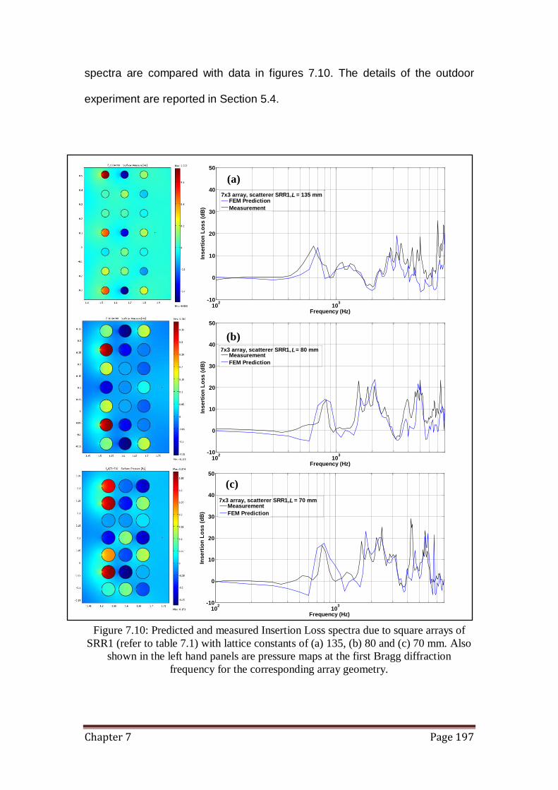
Chapter 7 Page 197
spectra are compared with data in figures 7.10. The details of the outdoor
experiment are reported in Section 5.4.
Figure 7.10: Predicted and measured Insertion Loss spectra due to square arrays of
SRR1 (refer to table 7.1) with lattice constants of (a) 135, (b) 80 and (c) 70 mm. Also
shown in the left hand panels are pressure maps at the first Bragg diffraction
frequency for the corresponding array geometry.
102
103
-10
0
10
20
30
40
50
Frequency (Hz)
Ins
ert
ion
Lo
ss
(d
B)
FEM Prediction
Measurement
7x3 array, scatterer SRR1, = 135 mmL
102
103
-10
0
10
20
30
40
50
Frequency (Hz)
Ins
ert
ion
Lo
ss
(d
B)
Measurement
FEM Prediction
L7x3 array, scatterer SRR1, = 80 mm
(a)
(b)
102
103
-10
0
10
20
30
40
50
Frequency (Hz)
Ins
ert
ion
Lo
ss
(d
B)
Measurement
FEM Prediction
L7x3 array, scatterer SRR1, = 70 mm
(c)
Chapter 7 Page 198
The IL spectra shown in figure 7.10 for arrays of split ring resonators
reveal considerable enhancement between 700 Hz and 1 kHz corresponding
to the resonance frequency observed with a single SRR1 (refer to figure
7.6(b)). These additional peaks are not observed for reference arrays of pipes
of the same size but no slits (FEM chapter, figure 4.5). The band gaps due to
the periodicity of the arrays are preserved in these IL spectra for SRR1
arrays. A possible cause of discrepancies between predictions and
measurements is the non-continuous slit construction. The pressure maps
suggest that the maximum values of the acoustic pressure are localised in the
cavities of some of the pipes with lengthwise slits. This is consistent with
resonance of the slit cylinders.
7.5.5) Outdoor measurements (SRR array)
The encouraging laboratory results observed for SRR encouraged
making larger scale outdoor trials at the OU test barrier site. The outdoor
measurements used 3 rows of 54 by 3 m long SRR2 scatterers (refer to table
7.1). The SRR2 scatterers were arranged in square lattice arrays with a lattice
constant of 160 mm. Detailed descriptions of the outdoor measurements are
covered in chapter 5 but for the reader’s convenience, the geometry used for
the outdoor experiments is briefly discussed here. The plan view of the array
is shown in figure 7.11(a). The source and receiver are placed 5 m apart from
the array with the source positioned at the asphalt ground and the receiver
positioned at the grass area to simulate a realistic road traffic environment. To
test the angle dependency of the SRR barrier performance, the source was

Chapter 7 Page 199
displaced laterally and vertically. (i.e. angles subtended from Ox plane in
figure 7.11(a)) and from the Oz plane in figure 7.11(b)).
Figure 7.11: Example outdoor measurement arrangement (a) lateral displacements of
the microphone along the length of barrier. (b) Vertical displacement of the
microphone along the height of barrier.
5 m
5 m
y
x
3 x 54
array
= 0°
= -11°
= -22°
= 11°
= 22°
5 m
5 m
z
x 3 x 53
array
= 0°
= 6°
= 8°
Asphalt ground
Grass area
1.6 m
1.6 m
Panel
(b)
(a)
(Drawing is not to scale)
(Drawing is not to scale)

Chapter 7 Page 200
Figure 7.12: Predicted and measured Insertion Loss spectra at outdoor for square
arrays of reference no slit cylinders (NRR2) and SRR scatterers (SRR2) with lattice
constants, L, of 160 mm (refer to table 7.1). (a) 54x3 square lattice array of scatterer
NRR2. (b) 54x3 square array of scatterer SRR2. Corresponding pressure maps at 500
Hz are shown in the left-hand panels.
The IL spectra measured outdoors are compared with FEM predictions
in figure 7.12(a). Both data and FEM predictions show a Bragg band gap
centred around 1 kHz and higher order modes. In this case it has been found
possible to obtain a close approximation of the IL spectra using a reduced
size model in COMSOL®. This is necessary to limit the computational
demands in making predictions for the exact outdoor geometry (array size as
well as distances for source and receiver). The IL peaks below the Bragg
band gap could be due to scattering from ground or other objects near the
vicinity of the less controlled environment or due to finite array effects. In
102
103
-10
-5
0
5
10
15
20
25
30
35
Frequency (Hz)
Ins
ert
ion
Lo
ss
(d
B)
Measurement
FEM Prediction
L3x54 array, scatterer SRR2, = 160 mm
102
103
-10
-5
0
5
10
15
20
25
30
35
Frequency (Hz)
Ins
ert
ion
Lo
ss
(d
B)
Measurement
FEM prediction
54x3 array, scatterer NRR2, = 160 mmL
(b)
(a)

Chapter 7 Page 201
addition to the first Bragg band gap around 1 kHz, a strong insertion peak
occurs at around 450 Hz corresponding to the cavity resonance for the SRR2
scatterer (see figure 7.5(d)). This effect is predicted also. The measured data
also show higher order modes in comparison with arrays of cylinders with no
slits for the same geometry (figure 7.12(a)). We also note the anomalous
noise created by such a barrier with the presence of high downwind (source to
receiver) speeds.
Figure 7.13: Measured Insertion Loss spectra of various lateral angles at outdoor for
square lattice arrays of SRR2 (see table 7.1) with lattice constant of 0.16 m.
Figure 7.13 shows the IL spectra measured for the 54x3 array of SRR2
(refer to table 7.1) when the microphone position is laterally displaced up to
±22 degree from normal incidence (see figure 7.11(a)). The constancy of the
low frequency peaks near 450 Hz offers experimental support for the
hypothesis that the IL peaks corresponding to resonances of the SRRs are
relatively independent of the source-receiver angle. Further displacement of
102
103
-5
0
5
10
15
20
25
30
35
40
Frequency (Hz)
Insert
ion
Lo
ss (
dB
)
0 deg
-11.2 deg
-21.6 deg
+11.2 deg
+21.6 deg
L
54x3 array, scatterer SRR2,
= 160 mm
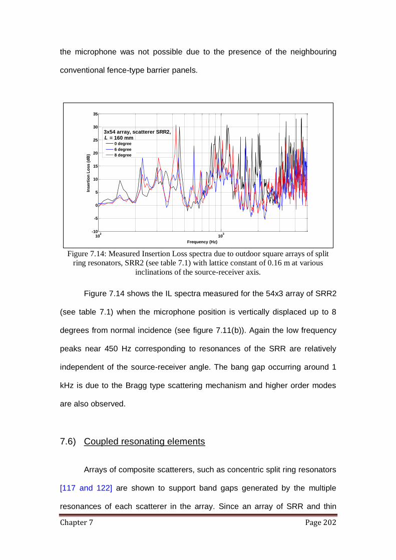
Chapter 7 Page 202
the microphone was not possible due to the presence of the neighbouring
conventional fence-type barrier panels.
Figure 7.14: Measured Insertion Loss spectra due to outdoor square arrays of split
ring resonators, SRR2 (see table 7.1) with lattice constant of 0.16 m at various
inclinations of the source-receiver axis.
Figure 7.14 shows the IL spectra measured for the 54x3 array of SRR2
(see table 7.1) when the microphone position is vertically displaced up to 8
degrees from normal incidence (see figure 7.11(b)). Again the low frequency
peaks near 450 Hz corresponding to resonances of the SRR are relatively
independent of the source-receiver angle. The bang gap occurring around 1
kHz is due to the Bragg type scattering mechanism and higher order modes
are also observed.
7.6) Coupled resonating elements
Arrays of composite scatterers, such as concentric split ring resonators
[117 and 122] are shown to support band gaps generated by the multiple
resonances of each scatterer in the array. Since an array of SRR and thin
102
103
-10
-5
0
5
10
15
20
25
30
35
Frequency (Hz)
Insert
ion
Lo
ss (
dB
)
0 degree
6 degree
8 degree
L3x54 array, scatterer SRR2, = 160 mm

Chapter 7 Page 203
walled elastic shell in air have been shown to possess strong resonance in
the low-frequency range, improvement of the sonic crystal design could be
achieved by combining both types of resonator. These composite scatterers,
referred to as composites serve a double purpose. First, they support multiple
resonances including Helmholtz and annular cavity resonances and also the
breathing mode resonance of the elastic shell. Secondly, since an array of
elastic shells exposed to the environment would not be practical for an
outdoor noise barrier, protecting the shells using concentric outer PVC
cylinders containing slits offers a simple solution. Recent experimental studies
by Cui et al suggest the possibility of using hollow tubes with multiple narrow
slits [123], such that all the slits occupy the quadrants facing the source, to
create a broader band gap. In contrast with the slit locations used by Cui et al,
multiple symmetrical slits (referred to as N-slit cylinders) have been used in
our experiment. To solve the scattering problem for N-slit cylinders we use
boundary conditions dependent on polar angle [124]. In the present model the
finite thickness of the wall of the N-slit cylinder is taken into consideration.
This avoids the use of adjustable parameters introduced for numerical stability
[124 and 125] and provides a more accurate description of the real structure
used in the experiments. The solution inside slits is replaced by jump
conditions [126] that describe the slit interface as a moving piston. It should
be noted that use of jump conditions to replace the slits make it possible to
accurately predict the total wave field in the low- and mid-frequency range.
The resulting approximations are of particular interest for studying the low-
frequency resonant behaviour of a single composite arrangement and a finite
periodic array of them.

Chapter 7 Page 204
7.6.1) Semi-analytical formulation of single composite scatterer
The description of the theory follows from the development work
carried out by our collaborators [128]. Consider the two-dimensional problem
of acoustic wave scattering by a single N-slit acoustically rigid cylindrical shell
of thickness h and external radius or . The sound is generated by the
cylindrical source placed at the origin of the coordinate system which is
defined by either the Cartesian yx, or polar ,r coordinates. The widths of
consecutive slits in the xyO plane are denoted by nd , Nn ,...,1 and they are
infinitely long in the direction of the cylinder main axis zO . The external length
of the rigid arc is referred to as mD (see figure 7.15(a)). It is also assumed that
the thickness of the rigid shell is much smaller than its radius so that the
following geometric simplifications can be applied:
(i) Internal and external arc lengths of the rigid strip have the same
length.
(ii) Internal and external arcs subtend the same angle.
(iii) The angle n subtended by the arc of n-th slit and its width nd are
related by Nnrd onn ,...,1, .
(iv) The angle m subtended by the arc between slit 1n and slit n
and its width mD are related by NmrD omm ,...,1, .
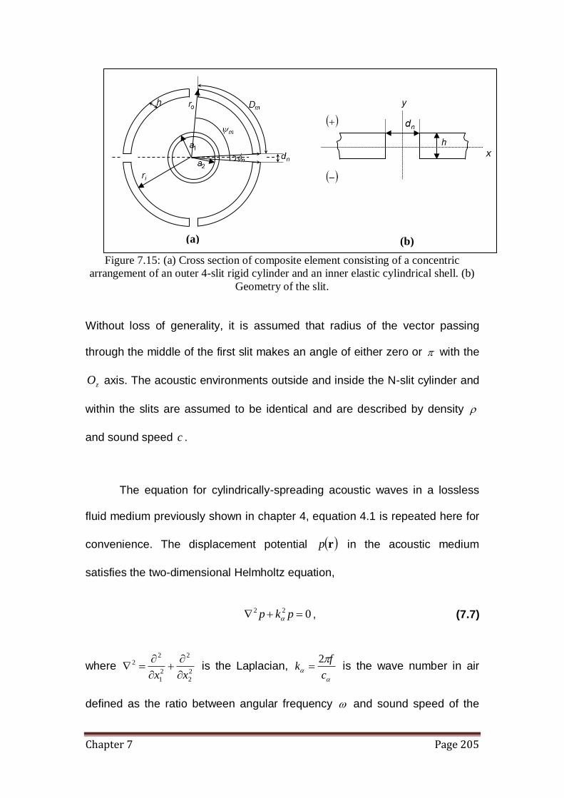
Chapter 7 Page 205
Figure 7.15: (a) Cross section of composite element consisting of a concentric
arrangement of an outer 4-slit rigid cylinder and an inner elastic cylindrical shell. (b)
Geometry of the slit.
Without loss of generality, it is assumed that radius of the vector passing
through the middle of the first slit makes an angle of either zero or with the
zO axis. The acoustic environments outside and inside the N-slit cylinder and
within the slits are assumed to be identical and are described by density
and sound speed c .
The equation for cylindrically-spreading acoustic waves in a lossless
fluid medium previously shown in chapter 4, equation 4.1 is repeated here for
convenience. The displacement potential rp in the acoustic medium
satisfies the two-dimensional Helmholtz equation,
022 pkp , (7.7)
where 2
2
2
2
1
22
xx
is the Laplacian,
c
fk
2 is the wave number in air
defined as the ratio between angular frequency and sound speed of the
(b) (a)
x
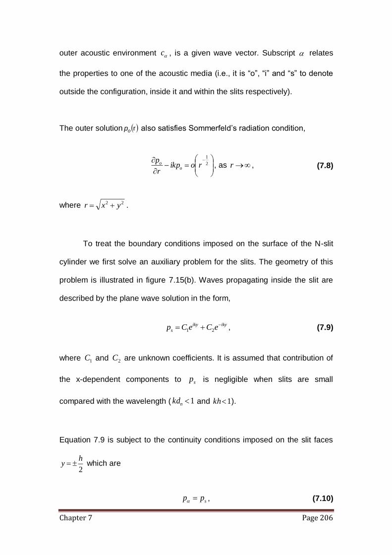
Chapter 7 Page 206
outer acoustic environment c , is a given wave vector. Subscript relates
the properties to one of the acoustic media (i.e., it is “o”, “i” and “s” to denote
outside the configuration, inside it and within the slits respectively).
The outer solution rop also satisfies Sommerfeld’s radiation condition,
2
1
roikpr
po
o , as r , (7.8)
where 22 yxr .
To treat the boundary conditions imposed on the surface of the N-slit
cylinder we first solve an auxiliary problem for the slits. The geometry of this
problem is illustrated in figure 7.15(b). Waves propagating inside the slit are
described by the plane wave solution in the form,
ikyiky
s eCeCp 21 , (7.9)
where 1C and 2C are unknown coefficients. It is assumed that contribution of
the x-dependent components to sp is negligible when slits are small
compared with the wavelength ( 1nkd and 1kh ).
Equation 7.9 is subject to the continuity conditions imposed on the slit faces
2
hy which are
spp , (7.10)
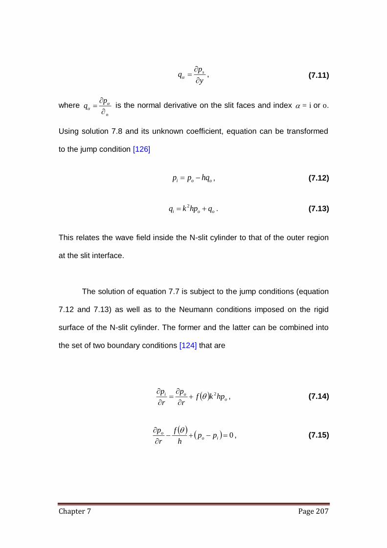
Chapter 7 Page 207
y
pq s
, (7.11)
where n
pq
is the normal derivative on the slit faces and index = i or o.
Using solution 7.8 and its unknown coefficient, equation can be transformed
to the jump condition [126]
ooi hqpp , (7.12)
ooi qhpkq 2 . (7.13)
This relates the wave field inside the N-slit cylinder to that of the outer region
at the slit interface.
The solution of equation 7.7 is subject to the jump conditions (equation
7.12 and 7.13) as well as to the Neumann conditions imposed on the rigid
surface of the N-slit cylinder. The former and the latter can be combined into
the set of two boundary conditions [124] that are
o
oi hpkfr
p
r
p 2
, (7.14)
0
io
o pph
f
r
p , (7.15)

Chapter 7 Page 208
where the stepwise function f of the polar angle introduces the
distribution of slits along the N-slit cylinder surface over the interval 2,00
so that
otherwise
if
0
22,
22
2,
21 1111
NNNf
, (7.16)
For the non-zero value of this function equations 7.14 and 7.15 are
transformed to the jump conditions 7.12 and 7.13 whereas the Neumann
conditions can be obtained from equation 7.14 and 7.15 by setting f to
zero.
The periodic angle distribution of N slits can be introduced through the
alternative form of f ,
N
n
nn
N
nH
N
nHf
2 2
12
2
12
,
1
0
11
22
22
j
jHjH
(7.17)
where H is the Heaviside function.
The total wave field outside the slit cylinder is given by
in
n
nno erkHAkrHp
ˆ11
0 , (7.18)

Chapter 7 Page 209
where ,ˆ rr and ,ˆ r are the polar coordinates of receiver with origin
placed at the centre of the scatterer and nA are unknown coefficients. The
solution inside the slit cylinder is given by
ˆˆ in
n
nnnni erkYCrkJBp
, (7.19)
where coefficients nB and nC have to be found. The coefficient nC can be
derived in terms of nB or set to zero according to the type of the core so that:
nnn CBC , n , (7.20)
where
0nC , N-slit cylinder alone, (7.21)
1
'
1
'
kaY
kaJC
n
nn , rigid core, (7.22)
12222''
222'
1
1
RhRknnRkkRYkRJ
nRkkRJC
sssnn
snn
, (7.23)
where primes ' denote the derivative with respect to polar coordinate r . In
equation 7.23, the elastic shell is described by wave number s
sc
k
, density
s , dilatational wave speed sc , radius of the elastic shell mid-surface
2
21 aaR
and its half thickness
2
21 aahs
. The dilatational wave speed sc
for a thin elastic plate is given by
Elastic shell core

Chapter 7 Page 210
21
s
s
Ec , (7.24)
with Young’s modulus E and Poison’s ratio . We consider the thin
viscoelastic shells made of latex discussed in chapter 6. For the numerical
predictions the size of each elastic shell is always defined by the outer radius
1a = 0.0215m and thickness sh2 = 0.00025 m.
To find the unknown coefficients nA we apply Graf’s addition theorem
(see Appendix B) to the outer solution (equation 7.18). This enables us to
express ,r in terms of ,r . Then, substituting (equation 7.18) and (7.19)
into the boundary conditions (equations 7.14 and 7.15) and taking the inner
product we arrive at infinite algebraic system of equations in nA , n ,
variables as follows:
j
jjnmj
n
onnononmnonnmn FFkrHhk
krHkrHFkrhHA 12
'11'1
,2
2
n
nononmnonnm
in
n krJkrJFkrhJekQH ''
,
1 2
j
j
jnmjon FFkrJhk
2
2
, m ,
(7.25)
where nm, is Kronecker delta, vector sin,cosQQ is the radius vector to
the centre of the slit cylinder,

Chapter 7 Page 211
innin
inninn
krYCkrJ
krYCkrJ''
, (7.26)
and nF is the Fourier transform of function f given by
1
0
/2
1
02
sin2
0
NNinl
N
n
nen
n
n
F
for
for
, (7.27)
Note that factor nC and the geometrical parameters of the slits only appear in
n and nF , respectively. This makes the form of system (equation 7.25)
invariant with respect to scatterer core type and the arrangement and size of
the slits.
Taking ,0 , the solutions of system (equation 7.25) is reduced to the
case of scattering by rigid cylinder that is
im
m
om
omm ekQH
krH
krJA
1
'1
'
, m , (7.28)
To find the numerical solution the infinite system (7.25) has to be truncated at
some number MMjnm ,,,, . In general, the convergence of the
numerical solution is dependent on the radius or of the N-slit cylinder, number
of slits and their angles (i.e. their length) as well as on the frequency.
Reducing the angle n of the slit results in faster convergence so that
numerical solution approaches the value defined in (equation 7.28).
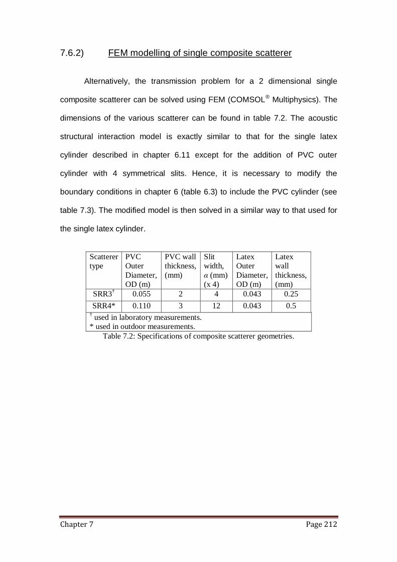
Chapter 7 Page 212
7.6.2) FEM modelling of single composite scatterer
Alternatively, the transmission problem for a 2 dimensional single
composite scatterer can be solved using FEM (COMSOL® Multiphysics). The
dimensions of the various scatterer can be found in table 7.2. The acoustic
structural interaction model is exactly similar to that for the single latex
cylinder described in chapter 6.11 except for the addition of PVC outer
cylinder with 4 symmetrical slits. Hence, it is necessary to modify the
boundary conditions in chapter 6 (table 6.3) to include the PVC cylinder (see
table 7.3). The modified model is then solved in a similar way to that used for
the single latex cylinder.
Scatterer
type
PVC
Outer
Diameter,
OD (m)
PVC wall
thickness,
(mm)
Slit
width,
α (mm)
(x 4)
Latex
Outer
Diameter,
OD (m)
Latex
wall
thickness,
(mm)
SRR3† 0.055 2 4 0.043 0.25
SRR4* 0.110 3 12 0.043 0.5 † used in laboratory measurements.
* used in outdoor measurements.
Table 7.2: Specifications of composite scatterer geometries.

Chapter 7 Page 213
Domain Air outside latex
cylinder
Elastic cylinder Air inside latex
cylinder
Model suffix Acpr (Acoustic) smps (Structural Mech.) acpr2 (Acoustic)
Inner wall of
latex
Continuity Load (N/m2)
-p2*nx_smps (x-direction)
-p2*ny_smps (y-direction)
Normal acceleration
(m/s2)
u3_tt_smps*nx_smps+
v3_tt_smps*ny_smps
Outer wall of
latex
Normal acceleration
(m/s2)
u3_tt_smps*nx_smps+
v3_tt_smps*ny_smps
Load (N/m2)
-(p+p_i_acpr)*nx_smps
(x-direction)
-(p+p_i_acpr)*ny_smps
(y-direction)
Continuity
Additional boundary conditions for outer shell PVC with 4 symmetrical slits
Domain Air outside PVC
cylinder
PVC cylinder Air inside PVC
cylinder
Model suffix Acpr (Acoustic) smps (Structural Mech.) acpr2 (Acoustic)
Inner wall of
PVC
Sound hard boundary
Load (N/m2)=0
(inactive domain)
Sound hard boundary
Outer wall of
PVC
Sound hard boundary
Load (N/m2)=0
(inactive domain)
Sound hard boundary
Slit region Sound hard boundary
Load (N/m2)=0
(inactive domain)
Sound hard boundary
Table 7.3: Summary of boundary conditions used in the acoustic structural interaction
model.
7.6.3) Results for single composite scatterer
The semi-analytical MST and FEM models enable us to compute the
insertion loss spectra for composite scatterers and the results are compared
with data from measurements (see chapter 5 for detailed descriptions). First,
the acoustical performance of a single PVC with 4-symmetrical slits is
considered. The geometry of the study of 4-slits PVC will use the component
specification of SRR3. A simple modification of the FEM model discussed in
section 7.4, to include the additional 3 slits can be achieved in a
straightforward manner. The FEM predictions are compared with data from
laboratory experiments.

Chapter 7 Page 214
Figure 7.16: (a) Measured and FEM predicted IL spectra due to a single PVC
cylinder with 4 symmetrical slits (component of SRR3, see table 7.2). (b) FEM
(COMSOL®) predictions of pressure maps at 2 kHz for a similar scatterer showing
the interior and exterior environments.
In figure 7.16, the IL spectrum predicted by FEM agrees with the
measurement data for the PVC cylinder with 4 symmetrical slits. The same
size of scatterer but with only one slit was found to have a resonance at 700
Hz (figure 7.5(b)). So increasing the number of slits results in a significant shift
of this Helmholtz type resonance towards higher frequencies, in this case to
near 2 kHz.
Figure 7.17: Measured and predicted (MST and FEM) IL spectra for a single
composite scatterer, SRR3 (refer to table 7.2)
103
104
-2
-1
0
1
2
3
4
5
6
7
8
Frequency (Hz)
Insert
ion
Lo
ss (
dB
)
Measurement
FEM Prediction
103
-4
-3
-2
-1
0
1
2
3
4
Frequency (Hz)
Insert
ion
Lo
ss (
dB
)
Measurement
FEM Prediction
MST Prediction
(a) (b)

Chapter 7 Page 215
According to figure 7.17, the IL spectra (measured and predicted by
MST and FEM) shows a strong resonance at around 1 to 2 kHz for composite
scatterer SRR3 (refer to table 7.2). Higher order resonances at higher
frequencies are also observed. For all measurements and predictions, the
receiver is positioned 0.05 m away from the scatterer. Contrary to the
predictions obtained by our collaborators from Salford [128], our MST
predictions disagree with measurements after 2.5 kHz. This could be the
result of a lower truncation number M in our computations which were limited
by our computational resource to 6 rather than 35 which was used in the
paper.

Chapter 7 Page 216
Figure 7.18: FEM (COMSOL®) predicted pressure maps at 1 kHz for SRR3 showing
the exterior and annular cavity environments (a), interior environment of the latex
cavity (b) and static deformation plot on the “Breathing mode” shape of elastic
element in air.
In figure 7.18, FEM predicted pressure maps at 1 kHz for SRR3 (refer
to table 7.2) are shown. According to these pressure maps, higher energies
are observed to be trapped inside annular cavity (see a) and interior of the
(a)
(b)
(c)
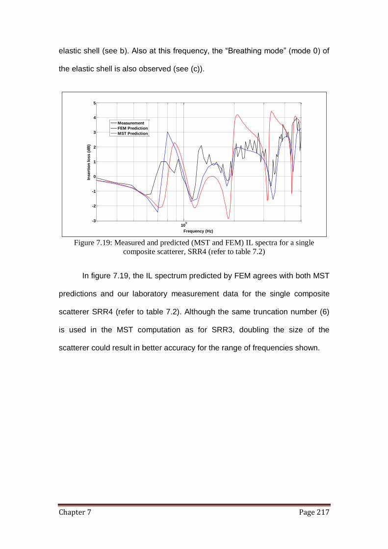
Chapter 7 Page 217
elastic shell (see b). Also at this frequency, the “Breathing mode” (mode 0) of
the elastic shell is also observed (see (c)).
Figure 7.19: Measured and predicted (MST and FEM) IL spectra for a single
composite scatterer, SRR4 (refer to table 7.2)
In figure 7.19, the IL spectrum predicted by FEM agrees with both MST
predictions and our laboratory measurement data for the single composite
scatterer SRR4 (refer to table 7.2). Although the same truncation number (6)
is used in the MST computation as for SRR3, doubling the size of the
scatterer could result in better accuracy for the range of frequencies shown.
103
-3
-2
-1
0
1
2
3
4
5
Frequency (Hz)
Insert
ion
lo
ss (
dB
)
Measurement
FEM Prediction
MST Prediction

Chapter 7 Page 218
Figure 7.20: Measured IL spectra for a single composite scatterer, SRR3 and it’s own
component (refer to table 7.2).
The measured IL spectrum for the latex cylinder in Fig. 7.20 shows the
breathing mode resonance near 1.5 kHz. The resonance for the 4 slits PVC
cylinder is near 1.8 kHz. When combined to form a concentric composite
cylinder, the resulting IL spectrum shows a modified resonance at about 1
kHz. This indicates that the coupling between two resonators leads to the shift
of the shell’s resonance to a lower frequency. This is confirmed also by the
FEM static deformation plot in figure 7.18(c).
103
104
-2
-1
0
1
2
3
4
5
6
Frequency (Hz)
Insert
ion
Lo
ss (
dB
)
SRR3
PVC component
Elastic shell component
Measurements
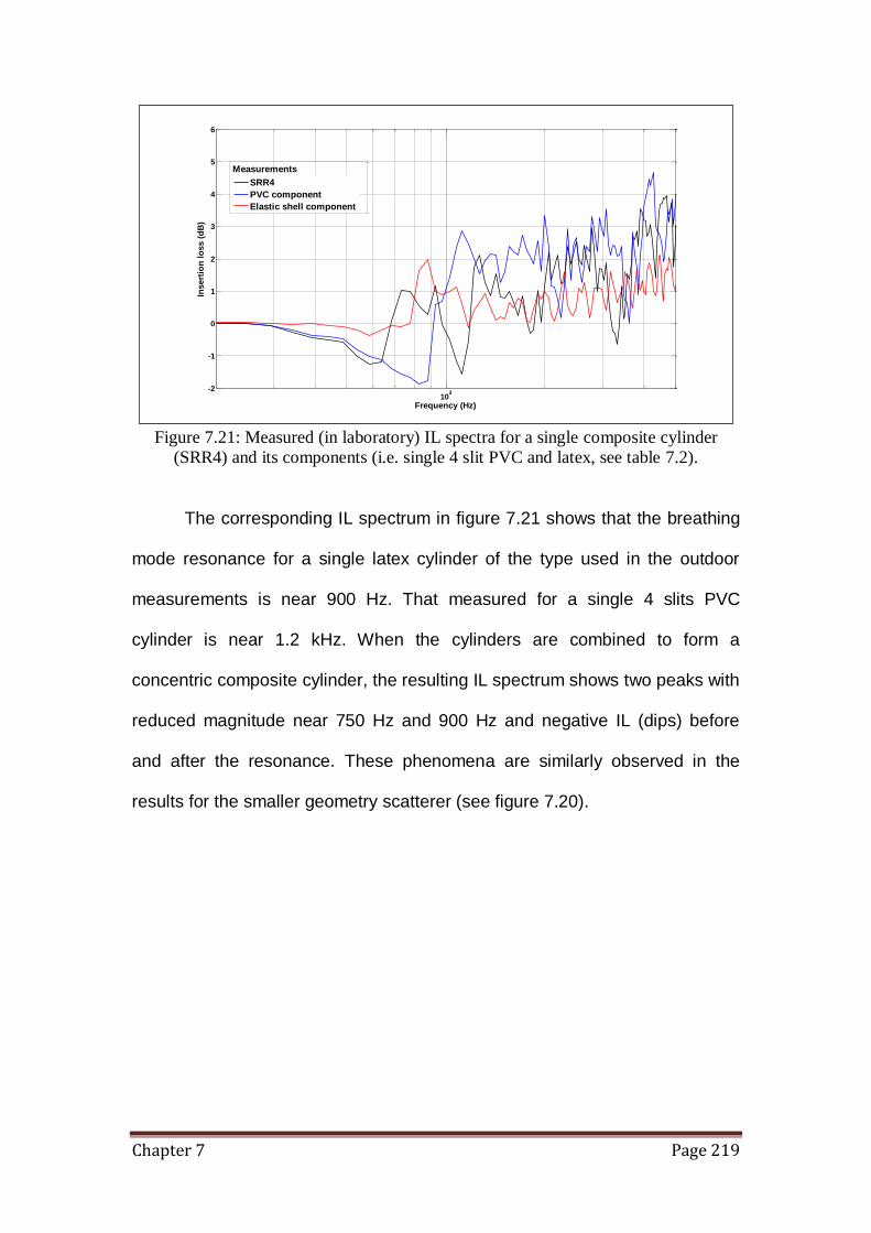
Chapter 7 Page 219
Figure 7.21: Measured (in laboratory) IL spectra for a single composite cylinder
(SRR4) and its components (i.e. single 4 slit PVC and latex, see table 7.2).
The corresponding IL spectrum in figure 7.21 shows that the breathing
mode resonance for a single latex cylinder of the type used in the outdoor
measurements is near 900 Hz. That measured for a single 4 slits PVC
cylinder is near 1.2 kHz. When the cylinders are combined to form a
concentric composite cylinder, the resulting IL spectrum shows two peaks with
reduced magnitude near 750 Hz and 900 Hz and negative IL (dips) before
and after the resonance. These phenomena are similarly observed in the
results for the smaller geometry scatterer (see figure 7.20).
103
-2
-1
0
1
2
3
4
5
6
Frequency (Hz)
Insert
ion
lo
ss (
dB
)
SRR4
PVC component
Elastic shell component
Measurements
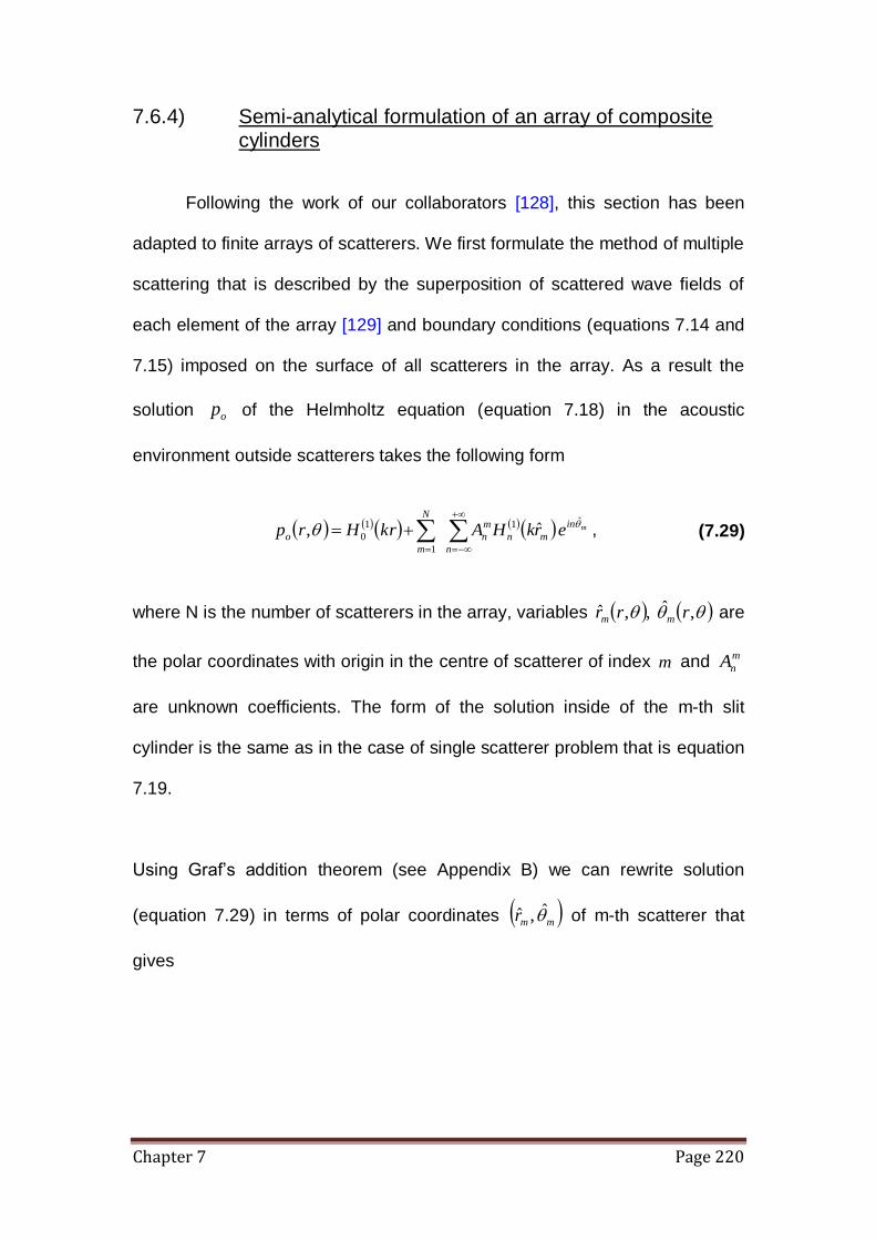
Chapter 7 Page 220
7.6.4) Semi-analytical formulation of an array of composite cylinders
Following the work of our collaborators [128], this section has been
adapted to finite arrays of scatterers. We first formulate the method of multiple
scattering that is described by the superposition of scattered wave fields of
each element of the array [129] and boundary conditions (equations 7.14 and
7.15) imposed on the surface of all scatterers in the array. As a result the
solution op of the Helmholtz equation (equation 7.18) in the acoustic
environment outside scatterers takes the following form
min
n
mn
m
n
N
m
o erkHAkrHrpˆ1
1
1
0ˆ,
, (7.29)
where N is the number of scatterers in the array, variables ,ˆ,,ˆ rrr mm are
the polar coordinates with origin in the centre of scatterer of index m and m
nA
are unknown coefficients. The form of the solution inside of the m-th slit
cylinder is the same as in the case of single scatterer problem that is equation
7.19.
Using Graf’s addition theorem (see Appendix B) we can rewrite solution
(equation 7.29) in terms of polar coordinates mmr ,ˆ of m-th scatterer that
gives

Chapter 7 Page 221
minnqi
q
mpnqmn
p
q
N
mpp
mn
m
n
in
n
mmnno
eekQHrkJA
rkHAkrHekQrkHJrp
mp
m
ˆ1
,1
11
0
1
ˆ
ˆ,ˆˆ,ˆ
,
Nm ,,1
(7.30)
where vector mmmm QQ sin,cos is the radius vector to the centre of m-th
scatterer, vector mpmpmpmp QQ sin,cos defines the position of p-th
scatterer with respect to m-th scatterer and mmp rQ ˆ that is the requirement of
the addition theorem. The expansion (equation 7.30), along with the inner
solution (equation 7.19), is subject to the boundary conditions (equations 7.14
and 7.15). This results in an infinite algebraic system of equations in m
nA ,
Nm ,,1 , n , variables given by
n
p
nponpon
p
mnponnm
p
n IkrHkrHFkrhHA ,
'1
,
1
,
'1
, 2
p
j
p
jn
j
p
mjpon IFFkrHhk
,
12
2
N
pss n,1
psni
psvn
s
n ekQHA
1
p
nponpon
p
mponm IkrJkrJFkrhJ ,
'
,,
'
, 2
p
j
p
jv
j
p
mjpo IFFkrJhk
,
2
2
n
ponnm
in
pn krhJekQH p ,
'
,
1 2
p
nponponmn IkrJkrJF ,
'
,
,,,1,,2
,
2
NpmIFFkrJhk p
j
p
jn
j
p
mjpon
(7.31)
where factors p
mI and p
mF are given by equations 7.26 and 7.27 respectively.
The superscript p relates these factors to p-th scatterer. To find the unknown
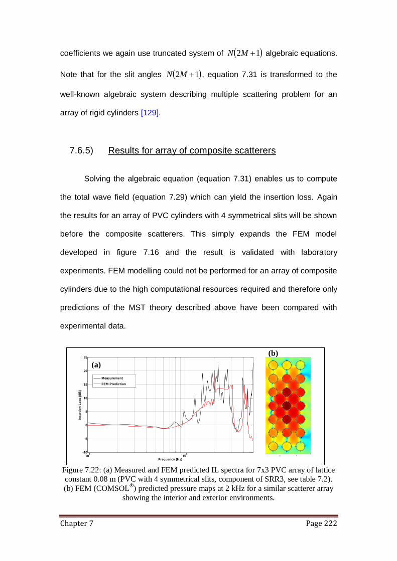
Chapter 7 Page 222
coefficients we again use truncated system of 12 MN algebraic equations.
Note that for the slit angles 12 MN , equation 7.31 is transformed to the
well-known algebraic system describing multiple scattering problem for an
array of rigid cylinders [129].
7.6.5) Results for array of composite scatterers
Solving the algebraic equation (equation 7.31) enables us to compute
the total wave field (equation 7.29) which can yield the insertion loss. Again
the results for an array of PVC cylinders with 4 symmetrical slits will be shown
before the composite scatterers. This simply expands the FEM model
developed in figure 7.16 and the result is validated with laboratory
experiments. FEM modelling could not be performed for an array of composite
cylinders due to the high computational resources required and therefore only
predictions of the MST theory described above have been compared with
experimental data.
Figure 7.22: (a) Measured and FEM predicted IL spectra for 7x3 PVC array of lattice
constant 0.08 m (PVC with 4 symmetrical slits, component of SRR3, see table 7.2).
(b) FEM (COMSOL®) predicted pressure maps at 2 kHz for a similar scatterer array
showing the interior and exterior environments.
102
103
-10
-5
0
5
10
15
20
25
Insert
ion
Lo
ss (
dB
)
Frequency (Hz)
Measurement
FEM Prediction
(b)
(a)
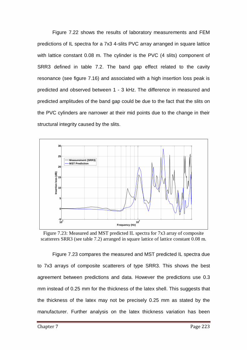
Chapter 7 Page 223
Figure 7.22 shows the results of laboratory measurements and FEM
predictions of IL spectra for a 7x3 4-slits PVC array arranged in square lattice
with lattice constant 0.08 m. The cylinder is the PVC (4 slits) component of
SRR3 defined in table 7.2. The band gap effect related to the cavity
resonance (see figure 7.16) and associated with a high insertion loss peak is
predicted and observed between 1 - 3 kHz. The difference in measured and
predicted amplitudes of the band gap could be due to the fact that the slits on
the PVC cylinders are narrower at their mid points due to the change in their
structural integrity caused by the slits.
Figure 7.23: Measured and MST predicted IL spectra for 7x3 array of composite
scatterers SRR3 (see table 7.2) arranged in square lattice of lattice constant 0.08 m.
Figure 7.23 compares the measured and MST predicted IL spectra due
to 7x3 arrays of composite scatterers of type SRR3. This shows the best
agreement between predictions and data. However the predictions use 0.3
mm instead of 0.25 mm for the thickness of the latex shell. This suggests that
the thickness of the latex may not be precisely 0.25 mm as stated by the
manufacturer. Further analysis on the latex thickness variation has been
102
103
-5
0
5
10
15
20
25
30
Frequency (Hz)
Insert
ion
lo
ss (
dB
)
Measurement (SRR3)
MST Prediction

Chapter 7 Page 224
performed in table 7.4 which justify the thickness parameter used in the
prediction. The MST predictions agree fairly well with measurements except
at high frequencies. The coupled resonances of the composite cylinders
generate several band gaps that result in high insertion loss peaks. One of
these peaks is observed around 1 kHz and is related to the shifted breathing
mode resonance of latex elastic shell. The insertion loss peak associated with
the shifted Helmholtz resonance in the slit cylinder is observed around 2.6
kHz and it follows the first Bragg band gap peak observed and expected
around 2 kHz for the given lattice constant.
Position
number
Measured
thickness (mm)
1 0.32
2 0.28
3 0.31
4 0.33
5 0.29
6 0.3
7 0.34
8 0.29
9 0.31
10 0.28
Average thickness: 0.305 mm
Standard deviation: 0.02 mm
Table 7.4: Measured thickness on latex strip with average and standard deviation
values.
Measurement has been carried out to determine the average thickness
of the latex shell using a micrometer. To be statistically sufficient, this is done
with thickness measurement on 10 different positions on a strip of latex (see
table 7.4). According to the results, this yields an average thickness of 0.3 mm
and a standard deviation of 0.02 mm. In view of this, all MST predictions
involving latex of 0.25 mm (as stated by the manufacturer) reported in this
Thesis are calculated using the average thickness of 0.3 mm.
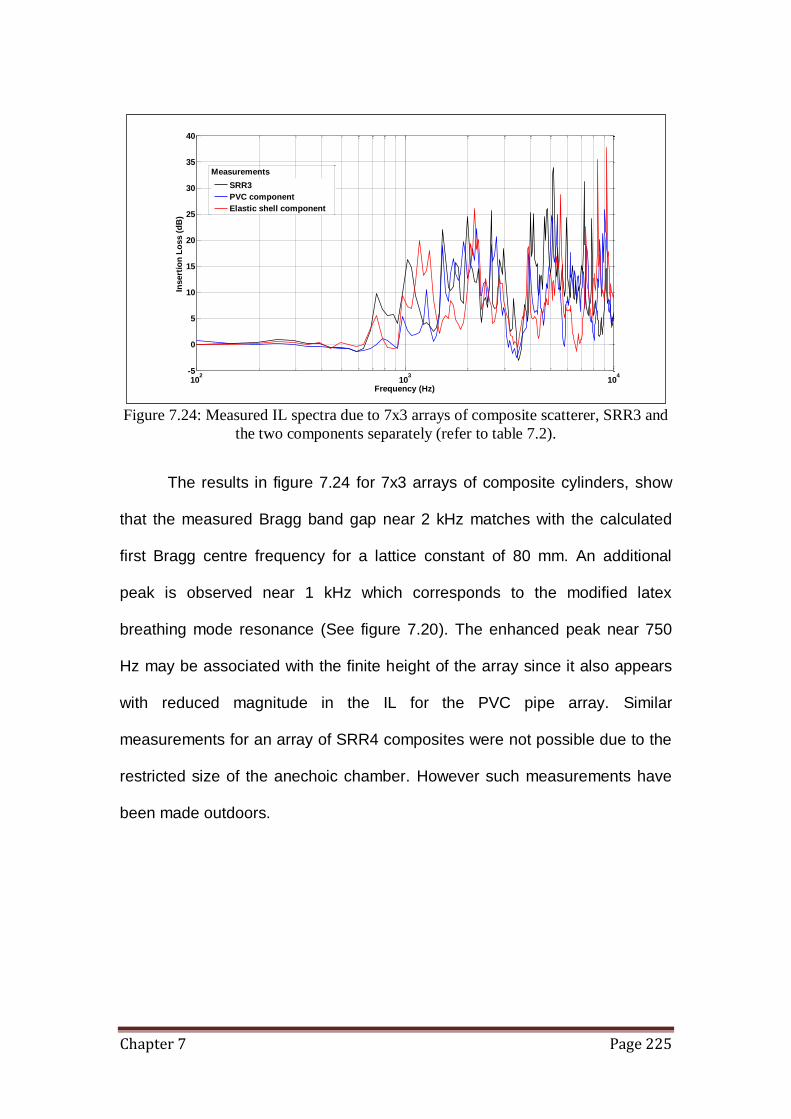
Chapter 7 Page 225
Figure 7.24: Measured IL spectra due to 7x3 arrays of composite scatterer, SRR3 and
the two components separately (refer to table 7.2).
The results in figure 7.24 for 7x3 arrays of composite cylinders, show
that the measured Bragg band gap near 2 kHz matches with the calculated
first Bragg centre frequency for a lattice constant of 80 mm. An additional
peak is observed near 1 kHz which corresponds to the modified latex
breathing mode resonance (See figure 7.20). The enhanced peak near 750
Hz may be associated with the finite height of the array since it also appears
with reduced magnitude in the IL for the PVC pipe array. Similar
measurements for an array of SRR4 composites were not possible due to the
restricted size of the anechoic chamber. However such measurements have
been made outdoors.
102
103
104
-5
0
5
10
15
20
25
30
35
40
Insert
ion
Lo
ss (
dB
)
Frequency (Hz)
SRR3
PVC component
Elastic shell component
Measurements
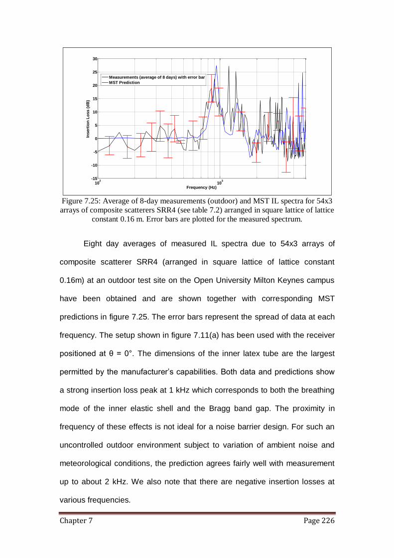
Chapter 7 Page 226
Figure 7.25: Average of 8-day measurements (outdoor) and MST IL spectra for 54x3
arrays of composite scatterers SRR4 (see table 7.2) arranged in square lattice of lattice
constant 0.16 m. Error bars are plotted for the measured spectrum.
Eight day averages of measured IL spectra due to 54x3 arrays of
composite scatterer SRR4 (arranged in square lattice of lattice constant
0.16m) at an outdoor test site on the Open University Milton Keynes campus
have been obtained and are shown together with corresponding MST
predictions in figure 7.25. The error bars represent the spread of data at each
frequency. The setup shown in figure 7.11(a) has been used with the receiver
positioned at θ = 0°. The dimensions of the inner latex tube are the largest
permitted by the manufacturer’s capabilities. Both data and predictions show
a strong insertion loss peak at 1 kHz which corresponds to both the breathing
mode of the inner elastic shell and the Bragg band gap. The proximity in
frequency of these effects is not ideal for a noise barrier design. For such an
uncontrolled outdoor environment subject to variation of ambient noise and
meteorological conditions, the prediction agrees fairly well with measurement
up to about 2 kHz. We also note that there are negative insertion losses at
various frequencies.
102
103
-15
-10
-5
0
5
10
15
20
25
30
Frequency (Hz)
Insert
ion
Lo
ss (
dB
)
Measurements (average of 8 days) with error bar
MST Prediction
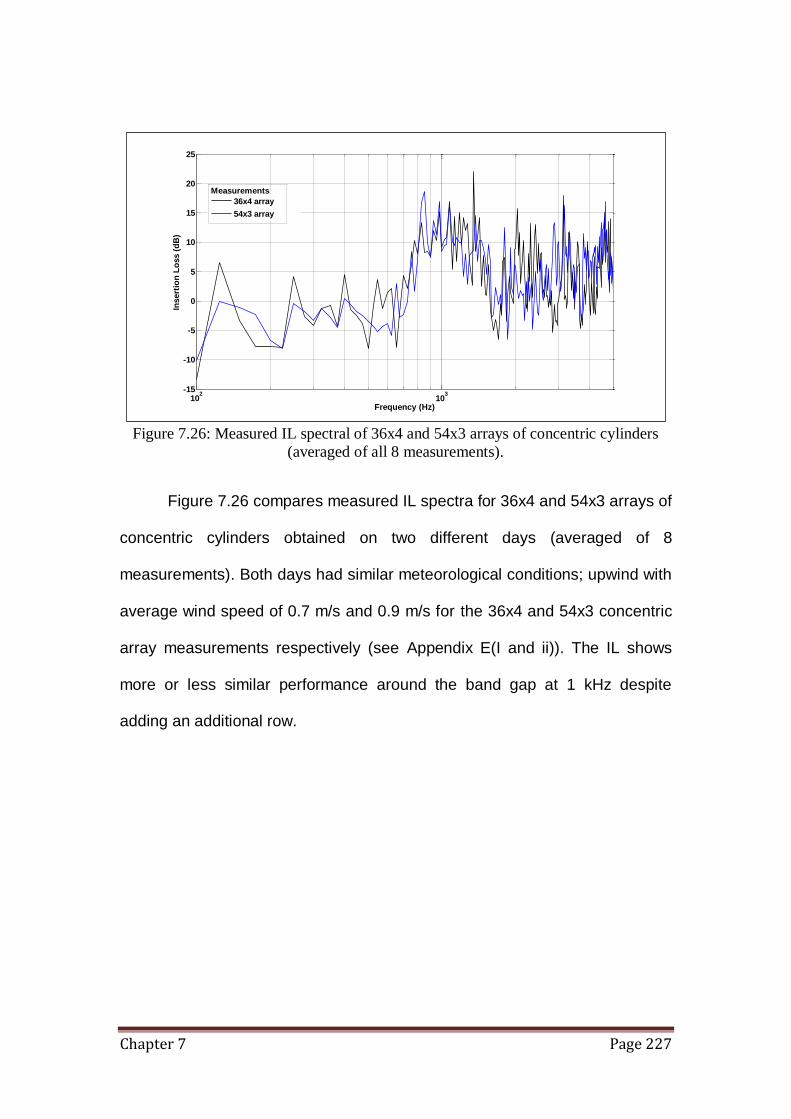
Chapter 7 Page 227
Figure 7.26: Measured IL spectral of 36x4 and 54x3 arrays of concentric cylinders
(averaged of all 8 measurements).
Figure 7.26 compares measured IL spectra for 36x4 and 54x3 arrays of
concentric cylinders obtained on two different days (averaged of 8
measurements). Both days had similar meteorological conditions; upwind with
average wind speed of 0.7 m/s and 0.9 m/s for the 36x4 and 54x3 concentric
array measurements respectively (see Appendix E(I and ii)). The IL shows
more or less similar performance around the band gap at 1 kHz despite
adding an additional row.
102
103
-15
-10
-5
0
5
10
15
20
25
Frequency (Hz)
Insert
ion
Lo
ss (
dB
)
36x4 array
54x3 array
Measurements

Chapter 7 Page 228
Figure 7.27: Measured IL spectral of 54x3 arrays of concentric cylinders (average of 8
measurements) and rigid no slit cylinders (average of 3 measurements).
Figure 7.27 compares the measured IL spectra for 54x3 arrays of
concentric cylinders and rigid no slit cylinders. Although for the concentric
cylinders configuration there is some improvement in the frequency range
near 1.2 – 2 kHz, there is a worse performance between 500 Hz and 800 Hz.
Thus, some modifications are necessary to improve the performance of
barriers based on arrays of the composite cylinders. The proposed
modifications to the current design for the concentric scattereres are
elaborated in suggestion 5 of section 9.3 (see Chapter 9).
102
103
-10
-5
0
5
10
15
20
25
30
Frequency (Hz)
Insert
ion
Lo
ss (
dB
)
54x3 concentric array
54x3 rigid array
Measurements

Chapter 7 Page 229
Figure 7.28: Measured IL spectral of 54x3 arrays of concentric cylinders (averaged of
8 measurements) and fence (average of 8 measurements).
Figure 7.28 compares the measured IL spectra for 54x3 arrays of
concentric cylinders and a typical fence at normal incidence. It can be
observed that generally the performance of a typical fence is superior to sonic
crystal except for the distinctive improvement at 1.2 kHz. The IL dip for the
fence at this frequency could be attributed by factor such as holes along the
uneven ground where the fence is placed.
7.7) Influence of adjustable parameters on the acoustical performance of composite scatterer arrays outdoors
The elastic shell outer diameter, elastic shell thickness and the slit
widths in the PVC cylinders can be varied to improve the performance of
composite cylinder arrays as outdoor noise barriers. MST predictions have
been used to investigate the effects of varying these parameters and
therefore the possibilities for better designs.
102
103
-20
-10
0
10
20
30
40
Frequency (Hz)
Insert
ion
Lo
ss (
dB
)
54x3 concentric array
Fence

Chapter 7 Page 230
7.7.1) The predicted influence of the elastic shell outer diameter
The influence of the outer diameter of the inner elastic shell has been
studied using MST computations. The composite cylinder arrays considered
for this study are 54x3 arrays of SRR4 scatterers arranged in a square lattice
with a lattice constant of 0.16 m. The shell outer diameter has been increased
up to 83 mm in increments of 10 mm. The latex material properties used for
the predictions have been assumed to be density = 1100 kg/m3, longitudinal
velocity = 954 m/s, Transverse velocity = 23 m/s, Poisson ratio = 0.4997 as in
chapter 6. Source and receiver have been considered to be 5 m away from
front and back faces of the array with the source to receiver line of sight
centred at the gap between the 2 central scatterers (see figure 7.11).
Frequency steps of around 50 Hz have been used in all predictions.
Figure 7.29: IL spectra for the MST predicted effect on changing latex outer diameter
for 54x3 square lattice array of SRR4 scatterer with lattice constant of 0.16 m.
102
103
-10
-5
0
5
10
15
20
25
30
35
Frequency (Hz)
Insert
ion
Lo
ss (
dB
)
43 mm
53 mm
63 mm
83 mm
MST Prediction (latex OD)

Chapter 7 Page 231
Figure 7.29 shows that the first IL peak is predicted to be moved to
lower frequencies as the latex tube diameter is increases and leads to
increasing separation of the modified latex resonance from the 1 kHz Bragg
band gap. Also there is a relationship between the predicted amplitude of the
modified latex resonance and that of the IL peak associated with the Bragg
band gap as they are separated. As the predicted IL peak amplitude
corresponding to the modified latex resonance increases there is a decrease
in the predicted Bragg band gap amplitude and vice-versa. However again
enhancement of sound (i.e. negative IL) is predicted at high frequencies.
7.7.2) The predicted influence of elastic shell wall thickness
Another parameter that has been investigated is the wall thickness of
the inner elastic shell. Following the predictions in figure 7.29 which show that
an elastic shell outer diameter of 83 mm will result in a separate low
frequency band gap. The wall thickness for such scatterer has been varied
from 0.5 to 2 mm.

Chapter 7 Page 232
Figure 7.30: IL spectra for the MST predicted effect on changing latex wall thickness
for 54x3 square lattice array of SRR4 scatterer with lattice constant of 0.16 m.
The resulting predictions are shown in figure 7.30. The IL peak is
shifted to lower frequency and decreased in amplitude (except for 2 mm
thickness) as the latex wall thickness is increased. The Bragg band gap
remains fairly constant at about 920 Hz. However again enhancement of
sound is observed at high frequencies.
7.7.3) Predicted influence of the slit widths in the outer PVC cylinder
The effects of varying the slit widths in the outer 4-slits PVC cylinder
have been predicted. The assumed slit width has been varied from 3 to 12
mm.
102
103
-10
-5
0
5
10
15
20
25
30
Frequency (Hz)
Insert
ion
Lo
ss (
dB
)
0.5 mm
1 mm
1.5 mm
2 mm
MST Predictions(latex thickness)

Chapter 7 Page 233
Figure 7.31: MST predicted IL spectra for 54x3 square lattice array with lattice
constant of 0.16 m as the slit widths in the outer PVC cylinders are varied from 3 to
12 mm.
The resulting IL spectra predictions are shown in Figure 7.31 for 54x3
4-slits PVC arrays with lattice constant 0.16 m and different slit widths. The IL
peak associated with the Bragg band gap slowly broadens near 1 kHz as the
slits width decreases. This may explain the modification of the 1st Bragg band
gap in data for our current outdoor setup (see figure 7.25). The predicted
effects of varying the parameters of the composite elements can lead to better
array design for outdoor noise reduction. This will be pursued in chapter 9.
102
103
-5
0
5
10
15
20
25
30
35
40
45
Frequency (Hz)
Insert
ion
lo
ss (
dB
)
12 mm
6 mm
3 mm
MST Prediction (slit width)

Chapter 8 Page 234
Chapter 8
Performance of sonic crystal noise barriers above a ground surface
8.1) Introduction
Outdoor sound propagation is subject to a combination of influences
along the propagation path including geometrical spreading, atmospheric
absorption and extra attenuation (i.e. barrier and ground effect) [131].
Geometrical spreading of the wave fronts leads to a declining source pressure
at a rate that depends on the type of source (point source or line source).
Atmospheric absorption is the results of shear velocity, heat conduction and
molecular relaxation losses. Natural or artificial obstacles impede the sound
propagation. The wind profile can also have pronounced effect. For example a
down wind condition (wind blowing towards the receiver from the source) will
refract sound waves downwards, resulting in increased noise levels behind
the barrier. At distances less than 100 m, meteorological effects play a minor
role and the acoustical properties of the ground – typically given by the
surface impedance are most important [132].
Regular arrays of cylindrical scatterers embedded in a medium with
different physical properties are known to produce acoustic band gaps, also
called stop bands, which prevent sound transmission at selective frequencies.
If the scatterers are solid and the host medium is air then these are called
Sonic Crystals (SC). At these frequencies, the amplitudes of the transmitted

Chapter 8 Page 235
waves decrease as they pass through the crystal. Conversely there are pass
bands within which the amplitudes of transmitted waves are relatively high.
Pass bands and band gaps are a consequence of multiple scattering of waves
in a periodic structure and also due to the effect of local resonance
mechanism in certain type of scatterer as discussed in chapters 6 and 7.
Given an interest in the potential use of sonic crystals as environmental noise
barriers, recent research into sonic crystal barriers for highway noise has
focused on methods to achieve a broader band gap and promising results
have been obtained using locally-resonant cylinders such as thin-walled
elastic shells [101], slit cylinders (Helmholtz resonance) [117] or a
combination of both as shown in chapter 7. However, much of the literature on
sonic crystals considers their acoustical performance in the absence of a
ground plane. Clearly this will be unrealistic if SCs are to be used as noise
barriers since a ground will always be present. On the other hand, the
problem of sound scattering by a single cylinder over a plane boundary has
been investigated [132 and 133] and the sound diffraction effect of a
Quadratic Residual Diffuser (QRD) profile, a type of Edge-Modified Barrier
(see chapter 9.2), for a single noise barrier has been studied using a 2
dimensional Boundary Element Method [145]. The prime objective of this
chapter is to study the total effect of SC and a reflecting ground. First there is
an overview on acoustical characterisation of the ground which requires a
method to determine the ground impedance. Laboratory and outdoor in-situ
measurements of various types of plane surfaces are performed and data is
fitted with a ground impedance model. Subsequently, a semi-analytical
approach for predicting the transmission properties of sonic crystals in 2-
Chapter 8 Page 236
Dimensional (2D) has been developed for circular scatterers and it is based
on the superposition of the solution for a single scatterer. Although the most
interesting situation is likely to involve periodic vertical finite cylinder arrays,
this would inevitably require solution of a 3-Dimensional problem where high
computation resource is necessary. Hence the more feasible 2D problem is
considered involving a periodic array of cylinders (rigid or elastic) with their
axes parallel to the ground. The semi-analytical method is used to analyse the
performance of rigid or elastic cylindrical scatterers suspended with their axes
parallel to a rigid ground. In this chapter, square lattice arrays of 7x3
scatterers are considered. The predicted performance of the sonic crystal
arrays in the presence of rigid ground is compared with that of the same
arrays in the free field. Insertion Loss (IL) data from laboratory experiments
are compared with predictions. Laboratory studies have been performed for
rigid or elastic arrays over a finite impedance ground. Some preliminary
laboratory measurements on vertical cylinder arrays on hard ground are also
described.
8.2) Ground impedance models for propagation modelling
The prime objective of this chapter is to study the total effect of sonic
crystals over a reflecting plane but first an understanding of acoustic
characterisation of the ground is necessary. In many predictions schemes
[135] ground surfaces are considered as either ‘acoustically hard’, which
means they are perfectly reflecting, or ‘acoustically soft’, which implies that
they are perfectly absorbing. According to ISO 9613-2, any ground surface of

Chapter 8 Page 237
low porosity maybe considered acoustically hard and any vegetation-covered
ground is to be considered acoustically soft. Although this might be an
adequate representation in some circumstances, it is an over simplification of
a considerable range of properties and resulting effects. Even different
versions of the category of ground known as ‘grassland’ can result in a
significant variation in ground effect [136]. Characterizing the sound field
above a surface can be done through measuring the sound pressure (easiest
parameter than can be measured for sound field) at one or more locations. A
convenient indicator of the acoustical characteristics of the ground can be
determined from the spectrum of the ratio of the direct source to receiver total
sound level without fieldFreep _ and with
fieldTotalp _ a ground surface (equation
8.1), keeping the distance between source to receiver and the source strength
constant. This is called the Excess Attenuation (EA) due to the ground surface
and it depends on the source-ground-receiver geometry and the ground
properties. If expressed in decibels, a positive value will imply that the sound
pressure is lower than the sound pressure in free field. We note that this
formula is only true as long as the ground is considered as locally reacting,
that is the surface impedance is independent of the angle of incident sound
[136].
fieldFree
fieldTotal
p
pEA
_
_log20 . (8.1)
Frequently ground properties are represented by a semi-empirical
single parameter model developed by Delany and Bazley [137] in 1970. They
published empirical relationships for determining the propagation constant, ck ,

Chapter 8 Page 238
and relative characteristic impedance, cZ (equation 8.2 and 8.3). The
variables in these relationships were frequency and flow resistivity, , of the
material where the flow resistivity represents the ratio of the applied pressure
gradient to the induced volume flow rate per unit thickness of material due to
the porosity. This single parameter model has been widely used in deducing
the acoustical properties of several types of porous materials [137].
595.0700.0
0
189.00978.01
XiX
ckc
. (8.2)
732.0754.0 087.00571.01 XiXZc , (8.3)
where
0X , 0 , is the density of air, , is an effective flow resistivity
and the frequency.
These equations are based on best fits to a large number of impedance
tube measurements on fibrous materials having porosities close to 1. It is
semi-empirical since X is related to the dimensionless ratio of the pore
dimension to the thickness of the viscous boundary layer and this ratio is
crucial in the acoustical characteristic of rigid-porous material. Nevertheless,
the model has been used with tolerable success to characterize outdoor
surface impedance. Other impedance models are available such as variable
porosity, Hamet, and Wilson relaxation models which require more
parameters (i.e. porosity rate of change with depth, porosity, tortuosity,
structure factor viscous and thermal relaxation times etc…) [139].

Chapter 8 Page 239
8.3) Ground impedance measurement
8.3.1) Single microphone method
A straight forward method uses a point source of broadband sound
located above the surface and a receiver point also located above the surface
as shown in figure 8.1(a). This allows the total field pressure fieldTotalp _ to be
measured. The free field spectrum level is obtained either by removing the
ground plane or by raising the source and receiver sufficiently far above the
surface that ground effect may be ignored. The latter method proved to be
more prone to error due to the required precision for the source-receiver
distance (see equation 8.1). Thus in our laboratory measurement, a flat table
elevated to a height of about 1 m from the floor of the anechoic chamber
(figure 5.16) is used as the ground plane support so that to establish the free
field spectrum, both the ground plane and the supporting table were removed
without altering the positions of the source and receiver.
8.3.2) Transfer function method
The above measuring technique serves well for deducing the excess
attenuation when conditions allow an accurate free field spectrum level to be
measured. However, this technique is difficult to use in outdoor in-situ
measurements where the ground to be measured is fixed. It is more
convenient to use the difference in spectra between two separate receiver
locations. The locations maybe separated horizontally or vertically. This
Chapter 8 Page 240
transfer function method (sometime known as the template method) is
standardised in ANSI S1.18 [140]. It allows for a very convenient
determination of the surface impedance with only basic knowledge of
acoustical measurements and without complicated mathematical routines. A
typical measurement setup for the transfer function method is shown in figure
8.1(b). The sound pressure emitting from the loudspeaker is measured
simultaneously with two microphones at different locations. If rotational
symmetry is assumed the transfer function between the two locations will
characterize the sound field which depends on the surface impedance and
geometry. The user has to measure the Level Difference (LD) using only
magnitude between the two microphone locations and swop around both
microphones to cancel out any errors introduced by the measuring system.
The level difference spectrum is then calculated as the difference between the
excess attenuation spectra at the two receivers. Since this method eliminates
the need of reference measurement, temporal changes in the propagation
conditions have relatively little influence.

Chapter 8 Page 241
Figure 8.1: Measurement configuration to determine the surface impedance. (a) Single
microphone method (laboratory) and (b) Transfer function method (outdoor in situ).
Two Medium Density Fibre (MDF) boards and a glass plate have been
used to provide ‘acoustically hard’ ground surfaces in the laboratory. A layer
of polyurethane form layer has been used as ‘acoustically soft’ ground. The
surfaces and their dimensions are listed in table 8.1. Various ranges (source
to receiver distance) and heights of source and receiver have been used
according to the different types of surface materials (see table 8.2). During
measurements, care was taken to ensure that the ground planes were
horizontal by testing with a tubular sprit level gauge (see figure 8.2).
Non-removable ground (i.e. in-situ measurement)
hs
Rdirect
Rreflected hru
Source Receivers
hrl θ
Removable ground (i.e measurement in laboratory)
hs
Rdirect
Rreflected hr
Source Receiver
θ
Lower mic.
Upper mic.
(a)
(b)

Chapter 8 Page 242
Table 8.1: Ground materials and dimensions.
Table 8.2: Dimensions for the range and heights of source and receiver for each
Excess Attenuation (EA) measurement in laboratory.
Figure 8.2: Levelling test for MDF board using tubular spirit level gauge.
Ground (Material
measured in laboratory)
Length (m) Width (m) Thickness (m)
MDF 1 2 1.3 0.006
MDF 2 1.2 0.94 0.018
Glass 1.2 1.2 0.005
Polyurethane form 2 1.2 0.03
Ground (Material) Range (m) Source height (m) Receiver height (m)
MDF 1 1 0.10 0.10
1 0.20 0.20
1 0.30 0.30
MDF 2 0.8 and 1.2 0.23 0.11
0.8 and 1.2 0.23 0.23
0.8 and 1.2 0.23 0.35
Glass 1 0.10 0.10
1 0.15 0.15
1 0.20 0.20
Polyurethane foam 0.8 and 1.2 0.23 0.11
0.8 and 1.2 0.23 0.23
0.8 and 1.2 0.23 0.35
MDF

Chapter 8 Page 243
8.4) Excess Attenuation (EA) and Level Difference (LD) results
8.4.1) EA spectra over MDF 1 board
Figure 8.3 – Measured and predicted EA spectra for ground (MDF 1) at source and
receiver heights at (a) 0.10 m (b) 0.20 m and (c) 0.30 m (see Tables 8.1 and 8.2)
Figure 8.3 shows the excess attenuation spectra obtained over the
surface of MDF 1 with various source and receiver heights (see tables 8.1 and
103
104
-30
-25
-20
-15
-10
-5
0
5
10
Frequency (Hz)
Excess A
tten
uati
on
(d
B)
Measurement, Rdirect
= 1 m, hs = 10 cm, h
r = 10 cm
Prediction, = 10 GPa s m-2
103
104
-30
-25
-20
-15
-10
-5
0
5
10
Frequency (Hz)
Excess A
tten
uati
on
(d
B)
Measurement, Rdirect
= 1 m, hs = 20 cm, h
r = 20 cm
Prediction, = 10 GPa s m-2
103
104
-30
-25
-20
-15
-10
-5
0
5
10
Frequency (Hz)
Excess A
tten
uati
on
(d
B)
Measurement, Rdirect
= 1 m, hs = 30 cm, h
r = 30 cm
Prediction, = 10 GPa s m-2
(c)
(b)
(a)
Chapter 8 Page 244
8.2). For source and receiver heights of 0.10 m, the minima for the ground
effect are at 8.2 kHz (figure 8.3(a)). Higher order dips are observed for source
and receiver heights of 0.20 and 0.30 m (figures 8.3(b) and 8.3(c)) when the
source and receiver are elevated. The excess attenuation predicted using the
Delany and Bazley one parameter model with an effective flow resistivity of 10
GPa s m-2 gives reasonable agreement with the data in the frequency range
of interest except in respect of dip amplitudes (figure 8.3(c)). Such ground is
considered as locally reacting, that is the surface impedance is independent of
the angle of incident sound [138]. The formula used in the EA prediction is
only valid when this condition is met for the ground.
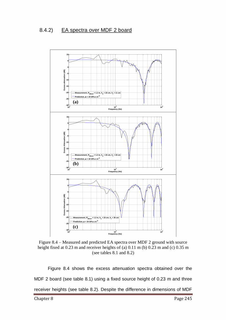
Chapter 8 Page 245
8.4.2) EA spectra over MDF 2 board
Figure 8.4 – Measured and predicted EA spectra over MDF 2 ground with source
height fixed at 0.23 m and receiver heights of (a) 0.11 m (b) 0.23 m and (c) 0.35 m
(see tables 8.1 and 8.2)
Figure 8.4 shows the excess attenuation spectra obtained over the
MDF 2 board (see table 8.1) using a fixed source height of 0.23 m and three
receiver heights (see table 8.2). Despite the difference in dimensions of MDF
102
103
104
-30
-25
-20
-15
-10
-5
0
5
10
Frequency (Hz)
Excess a
tten
uati
on
(d
B)
Measurement, Rdirect
= 1.2 m, hs = 23 cm, h
r = 11 cm
Prediction, = 10 GPa s m-2
102
103
104
-30
-25
-20
-15
-10
-5
0
5
10
Frequency (Hz)
Excess A
tten
uati
on
(d
B)
Measurement, Rdirect
= 1.2 m, hs = 23 cm, h
r = 23 cm
Prediction, = 10 GPa s m-2
102
103
104
-30
-25
-20
-15
-10
-5
0
5
10
Frequency (Hz)
Excess A
tten
uati
on
(d
B)
Measurement, Rdirect
= 1.2 m, hs = 23 cm, h
r = 35 cm
Prediction, = 10 GPa s m-2
(c)
(a)
(b)

Chapter 8 Page 246
2 from MDF 1, the ground effect minima agree reasonably well with
predictions using the one parameter model for ground impedance with an
effective flow resistivity of 10 GPa s m-2. The enhancements around 400 Hz
could be due to the effect of diffraction by the edges of the board as the
dimensions of the MDF2 board are smaller.
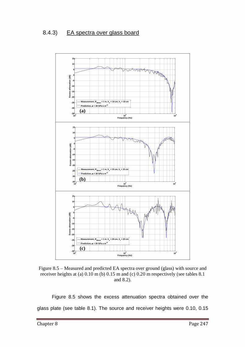
Chapter 8 Page 247
8.4.3) EA spectra over glass board
Figure 8.5 – Measured and predicted EA spectra over ground (glass) with source and
receiver heights at (a) 0.10 m (b) 0.15 m and (c) 0.20 m respectively (see tables 8.1
and 8.2).
Figure 8.5 shows the excess attenuation spectra obtained over the
glass plate (see table 8.1). The source and receiver heights were 0.10, 0.15
102
103
104
-35
-30
-25
-20
-15
-10
-5
0
5
10
15
Frequency (Hz)
Excess a
tten
uati
on
(d
B)
Measurement, Rdirect
= 1 m, hs = 10 cm, h
r = 10 cm
Prediction, = 30 GPa s m-2
102
103
104
-35
-30
-25
-20
-15
-10
-5
0
5
10
15
Frequency (Hz)
Excess a
tten
uati
on
(d
B)
Measurement, Rdirect
= 1 m, hs = 15 cm, h
r = 15 cm
Prediction, = 30 GPa s m-2
102
103
104
-35
-30
-25
-20
-15
-10
-5
0
5
10
15
Frequency (Hz)
Excess a
tten
uati
on
(d
B)
Measurement, Rdirect
= 1 m, hs = 20 cm, h
r = 20 cm
Prediction, = 30 GPa s m-2
(a)
(c)
(b)
Chapter 8 Page 248
and 0.20 m show in figure (a), (b) and (c) respectively. The measured ground
effect minima agree with predictions using the one parameter model for
ground surface impedance with an effective flow resistivity of 30 GPa s m-2.
This higher fitted flow resistivity value suggests that the glass plate is
acoustically harder than either MDF board.
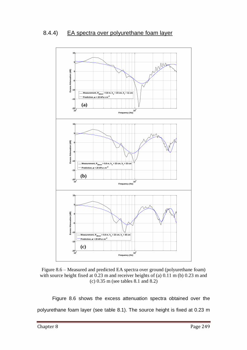
Chapter 8 Page 249
8.4.4) EA spectra over polyurethane foam layer
Figure 8.6 – Measured and predicted EA spectra over ground (polyurethane foam)
with source height fixed at 0.23 m and receiver heights of (a) 0.11 m (b) 0.23 m and
(c) 0.35 m (see tables 8.1 and 8.2)
Figure 8.6 shows the excess attenuation spectra obtained over the
polyurethane foam layer (see table 8.1). The source height is fixed at 0.23 m
102
103
-20
-15
-10
-5
0
5
10
Frequency (Hz)
Excess A
tten
uati
on
(d
B)
Measurement, Rdirect
= 0.8 m, hs = 23 cm, h
r = 11 cm
Prediction, = 20 kPa s m-2
102
103
-20
-15
-10
-5
0
5
10
Frequency (Hz)
Excess A
tten
uati
on
(d
B)
Measurement, Rdirect
= 0.8 m, hs = 23 cm, h
r = 23 cm
Prediction, = 20 kPa s m-2
102
103
-20
-15
-10
-5
0
5
10
Frequency (Hz)
Excess A
tten
uati
on
(d
B)
Measurement, Rdirect
= 0.8 m, hs = 23 cm, h
r = 35 cm
Prediction, = 20 kPa s m-2
(a)
(b)
(c)
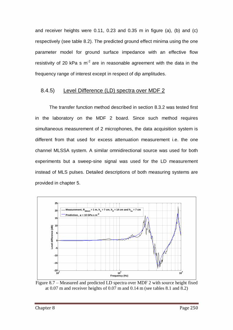
Chapter 8 Page 250
and receiver heights were 0.11, 0.23 and 0.35 m in figure (a), (b) and (c)
respectively (see table 8.2). The predicted ground effect minima using the one
parameter model for ground surface impedance with an effective flow
resistivity of 20 kPa s m-2 are in reasonable agreement with the data in the
frequency range of interest except in respect of dip amplitudes.
8.4.5) Level Difference (LD) spectra over MDF 2
The transfer function method described in section 8.3.2 was tested first
in the laboratory on the MDF 2 board. Since such method requires
simultaneous measurement of 2 microphones, the data acquisition system is
different from that used for excess attenuation measurement i.e. the one
channel MLSSA system. A similar omnidirectional source was used for both
experiments but a sweep-sine signal was used for the LD measurement
instead of MLS pulses. Detailed descriptions of both measuring systems are
provided in chapter 5.
Figure 8.7 – Measured and predicted LD spectra over MDF 2 with source height fixed
at 0.07 m and receiver heights of 0.07 m and 0.14 m (see tables 8.1 and 8.2)
102
103
104
-20
-15
-10
-5
0
5
10
15
20
25
Frequency (Hz)
Level d
iffe
ren
ce (
dB
)
Measurement, Rdirect
= 1 m, hs = 7 cm, h
rl = 14 cm and h
ru = 7 cm
Prediction, = 10 GPa s m-2

Chapter 8 Page 251
Figure 8.7 shows predicted and measured level difference spectra
obtained over the MDF 2 board (see table 8.1) using a source height of 0.07
m and receiver heights of 0.07 and 0.14 m (see table 8.2). The measured
ground effects agree reasonably well with predictions using the one parameter
model for ground impedance with an effective flow resistivity of 10 GPa s m-2
as was the case for the data obtained with the one microphone method (see
figure 8.4). This confirms the reliability of the transfer function method for
ground impedance characterisation.
8.4.6) LD spectra over asphalt (Outdoor in situ measurement)
Given the consistency of the flow resistivity deduced for MDF 2 board
by both methods in the laboratory (section 8.3.1 and 8.3.2); the transfer
function method has been adopted for measurement of outdoor ground
properties in situ. Geometry B suggested by ANSI S1.18 has been considered
for the outdoor measurement (see table 8.3).
Geometry Source
height (hs)
Distance source-
receiver (Rdirect)
Height of lower
microphone (hrl)
Height of upper
microphone (hru)
A 0.325 1.75 0.23 0.46
B 0.2 1 0.05 0.20
C 0.4 1 0.05 0.40
Table 8.3: Source-receiver geometries for the transfer function method specified by
ANSI S1.18 (data in meters).

Chapter 8 Page 252
Figure 8.8 – Measured and predicted LD spectra over asphalt surface with
measurement geometry 2 (table 8.3).
Figure 8.8 shows the level difference spectra obtained over the asphalt
surface at the vicinity of the outdoor barrier test site. The measurement
follows the geometry (B) suggested by ANSI (see table 8.3) with a source
height of 0.2 m and receiver heights of 0.05 and 0.2 m. The measured ground
effects agree reasonably well with predictions using the one parameter model
for ground impedance with an effective flow resistivity of 50 GPa s m-2, except
for the maxima and minima where the amplitudes are over predicted. This
suggests that asphalt ground is acoustically harder than glass plate and MDF
board.
8.4.7) LD spectra over grass covered ground in situ
The ground impedance for grass covered ground has been deduced
following the same procedure as for asphalt (section 8.4.6).
102
103
104
-40
-30
-20
-10
0
10
20
30
40
Frequency (Hz)
Level d
iffe
ren
ce (
dB
)
Measurement, Rdirect
= 1 m, hs = 20 cm, h
rl = 20 cm and h
ru = 5 cm
Prediction, = 50 GPa s m-2

Chapter 8 Page 253
Figure 8.9 – Measured and predicted LD spectra over grass surface with measurement
geometry B (table 8.3).
Figure 8.9 shows the level difference spectra obtained over the grass
surface at the vicinity of the outdoor barrier test site. Predictions (using the
Delany and Bazley model give a better fit with the grass ground than obtained
with asphalt. The effective flow resistivity is predicted to be 200 kPa s m-2
which is in good agreement with typical flow resistivity values (150 – 300 kPa
s m-2) for outdoor grass surfaces [136].
8.5) Analytical formulation for array of sonic crystals with their axes parallel to a rigid ground
Following the development work by our collaborators [147], assuming
the ground to be considered ‘acoustically hard’, then the multiple scattering
method (see chapter 3) can be modified using the method of images to
construct the reflected acoustic field [141]. This semi-analytical method is
used to analyse the performance of arrays of rigid or elastic cylindrical
scatterers suspended with their axes parallel to a rigid ground. In this section,
102
103
104
-10
-5
0
5
10
15
Frequency (Hz)
Level d
iffe
ren
ce (
dB
)
Measurement, Rdirect
= 1 m, hs = 20 cm, h
rl = 20 cm and h
ru = 5 cm
Prediction, = 200 kPa s m-2

Chapter 8 Page 254
square lattice arrays of 7x3 scatterers are considered. The predicted
performance of the sonic crystals in the presence of rigid ground is compared
with that of the crystals placed in the free field. Insertion Loss (IL) spectra
measured in an anechoic chamber are compared with predictions.
8.5.1) Rigid scatterers
We consider an array of M circular scatterers placed in a (positive) half-
space characterised by the sound speed in air c = 344 m/s and density = 1.2
kg/m3. The source is assumed to be a point source. Figure 8.10 illustrates the
geometry of the array and its image. The position of each scatterer mC ,
Mm 1 , is given by the vector mR . The position of the scatterer mC is
defined by the radius vector '
mR . The scatterers are considered to be
arranged in a square lattice which is defined by the lattice constant L .
However the method described subsequently can be applied to any other
lattice configuration.
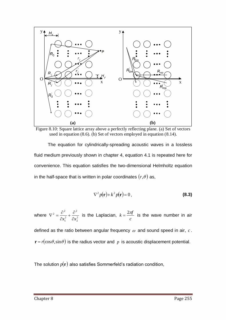
Chapter 8 Page 255
Figure 8.10: Square lattice array above a perfectly reflecting plane. (a) Set of vectors
used in equation (8.6). (b) Set of vectors employed in equation (8.14).
The equation for cylindrically-spreading acoustic waves in a lossless
fluid medium previously shown in chapter 4, equation 4.1 is repeated here for
convenience. This equation satisfies the two-dimensional Helmholtz equation
in the half-space that is written in polar coordinates ,r as,
022 rr pkp , (8.3)
where 2
2
2
2
1
22
xx
is the Laplacian,
c
fk
2 is the wave number in air
defined as the ratio between angular frequency and sound speed in air, c .
sin,cosrr is the radius vector and p is acoustic displacement potential.
The solution rp also satisfies Sommerfeld’s radiation condition,
O
y
x
O
y
x
(b) (a)

Chapter 8 Page 256
2
1
roikpr
p, as r . (8.4)
We imposed Neumann condition on the boundary of acoustic half-space (i.e.
rigid ground) and on the surface of the scatterers (this condition has to be
replaced by continuity conditions if scatterer is an elastic shell described in
chapter 6) that is
0
n
p. (8.5)
Following the multiple scattering described in chapter 3 and the method of
images [141] the general solution of the formulated problem can be written as
[142]
rrr sppp 0 . (8.6)
whereby contributions from the point source and its image are collected in 0p
which can be expressed by
rrr rd ppp ,0,00 , (8.7)
0
1
0,0 krHp d r , (8.8)
'01
0,0 krHp r r , (8.9)
whereas the scattered field components are described by
rrr rsds ppp ,,0 , (8.10)

Chapter 8 Page 257
min
mn
M
m n
m
n
m
nds ekrHZAp
r1
1
,
, (8.11)
''1
1
,min
mn
M
m n
m
n
m
nrs ekrHZAp
r . (8.12)
The vector 0000 sin,cos rr connects the point source and the receiver
point (i.e. point P in figure 8.11(a)). The vector mmmm r sin,cosr connects
the centre of scatterer mC and the receiver. The prime ' is used to indicate
the geometrical parameters for the image source and the image scatterers
placed in the negative half-space. m
nA , Zn , Mm 1 , are unknown
coefficients. The solution for the unbounded acoustic space can be retrieved
from equation 8.6 by putting to zero in equations (8.7) and (8.10) all terms
related to the constructed images that are rp ,0 and rsp , respectively. One can
also deduce from equation (8.6) and vector definitions in figure 8.10(a) that for
the source and receiver both on the ground, the acoustic pressure in a half-
space is double the pressure in the unbounded acoustic space.
The factors m
nZ describe the type of conditions imposed on the surface of the
scatterers and in case of rigid cylinders they can be expressed as
mnr
mnrm
nkaH
kaJZ
1
, (8.13)
where ma is the radius of scatter mC and r is the derivative with respect to
polar coordinate r.
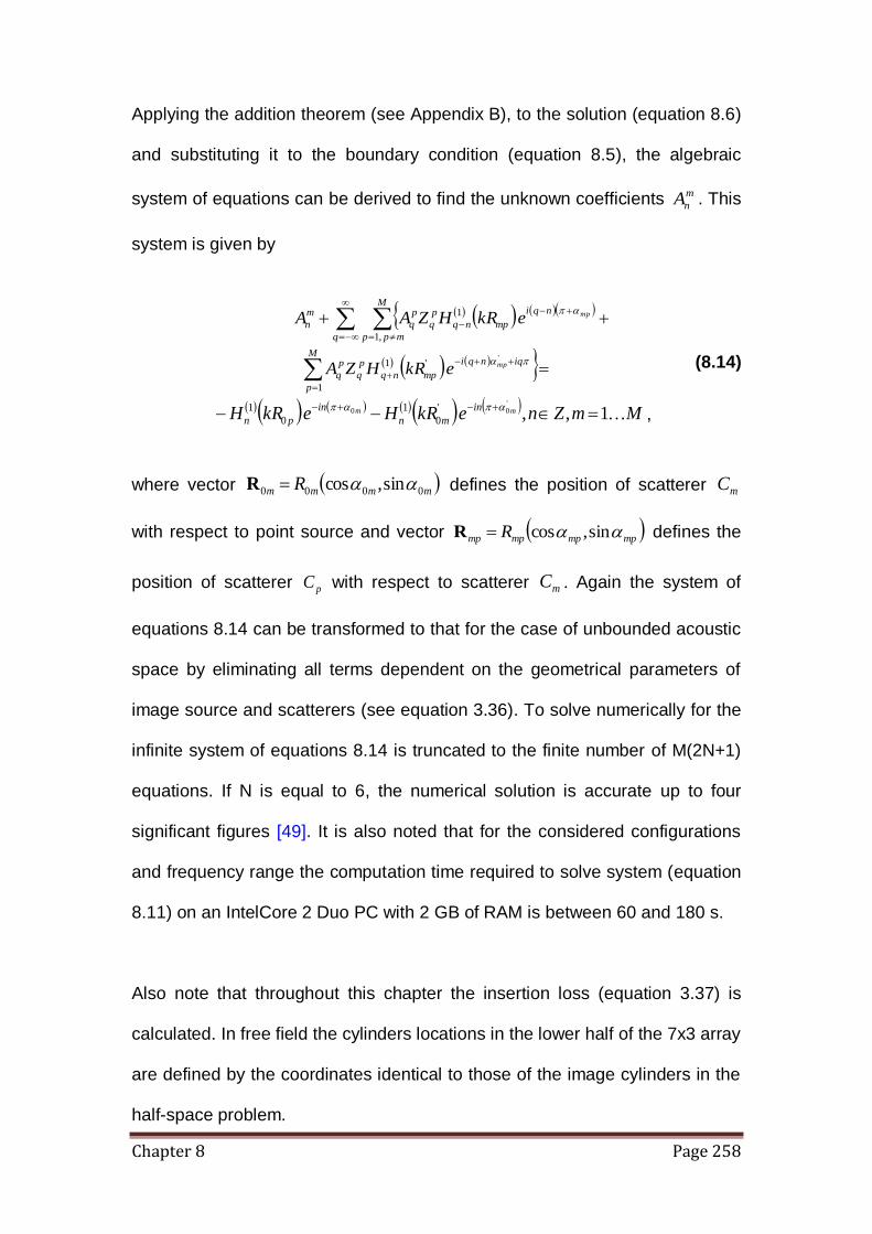
Chapter 8 Page 258
Applying the addition theorem (see Appendix B), to the solution (equation 8.6)
and substituting it to the boundary condition (equation 8.5), the algebraic
system of equations can be derived to find the unknown coefficients m
nA . This
system is given by
q
M
mpp
nqi
mpnq
p
q
p
q
m
nmpekRHZAA
,1
1
M
p
iqnqi
mpnq
p
q
p
qmpekRHZA
1
'1'
MmZnekRHekRH mm in
mn
in
pn 1,,'00 '
0
1
0
1
,
(8.14)
where vector mmmm R 0000 sin,cos R defines the position of scatterer mC
with respect to point source and vector mpmpmpmp R sin,cosR defines the
position of scatterer pC with respect to scatterer mC . Again the system of
equations 8.14 can be transformed to that for the case of unbounded acoustic
space by eliminating all terms dependent on the geometrical parameters of
image source and scatterers (see equation 3.36). To solve numerically for the
infinite system of equations 8.14 is truncated to the finite number of M(2N+1)
equations. If N is equal to 6, the numerical solution is accurate up to four
significant figures [49]. It is also noted that for the considered configurations
and frequency range the computation time required to solve system (equation
8.11) on an IntelCore 2 Duo PC with 2 GB of RAM is between 60 and 180 s.
Also note that throughout this chapter the insertion loss (equation 3.37) is
calculated. In free field the cylinders locations in the lower half of the 7x3 array
are defined by the coordinates identical to those of the image cylinders in the
half-space problem.
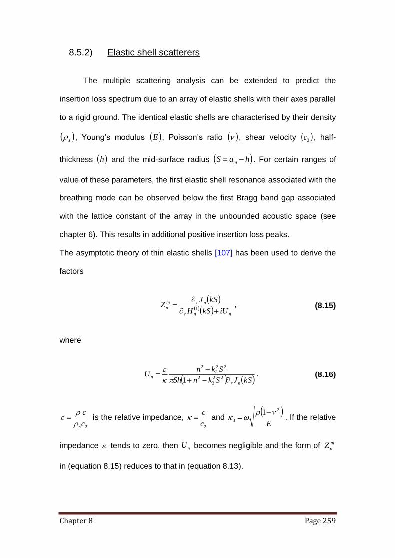
Chapter 8 Page 259
8.5.2) Elastic shell scatterers
The multiple scattering analysis can be extended to predict the
insertion loss spectrum due to an array of elastic shells with their axes parallel
to a rigid ground. The identical elastic shells are characterised by their density
s , Young’s modulus E , Poisson’s ratio , shear velocity 2c , half-
thickness h and the mid-surface radius haS m . For certain ranges of
value of these parameters, the first elastic shell resonance associated with the
breathing mode can be observed below the first Bragg band gap associated
with the lattice constant of the array in the unbounded acoustic space (see
chapter 6). This results in additional positive insertion loss peaks.
The asymptotic theory of thin elastic shells [107] has been used to derive the
factors
nnr
nrm
niUkSH
kSJZ
1, (8.15)
where
kSJSknSh
SknU
nr
n
22
3
2
22
3
2
1
. (8.16)
2c
c
s
is the relative impedance,
2c
c and
E
2
3
1
. If the relative
impedance tends to zero, then nU becomes negligible and the form of m
nZ
in (equation 8.15) reduces to that in (equation 8.13).
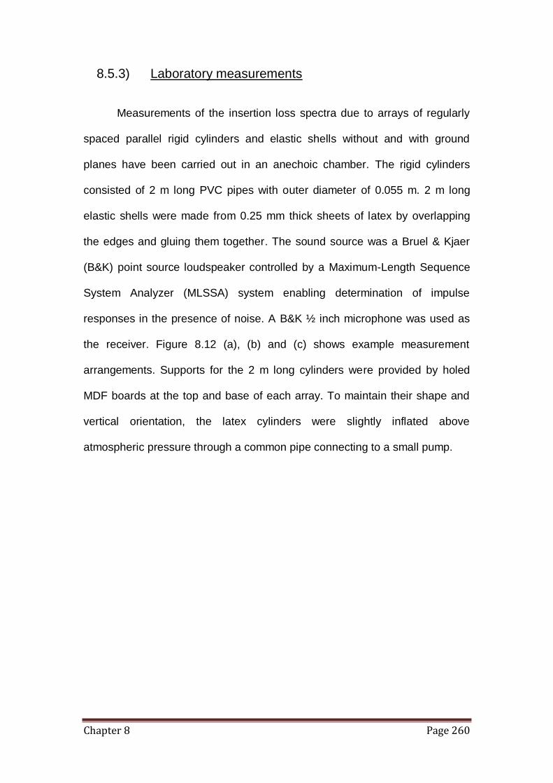
Chapter 8 Page 260
8.5.3) Laboratory measurements
Measurements of the insertion loss spectra due to arrays of regularly
spaced parallel rigid cylinders and elastic shells without and with ground
planes have been carried out in an anechoic chamber. The rigid cylinders
consisted of 2 m long PVC pipes with outer diameter of 0.055 m. 2 m long
elastic shells were made from 0.25 mm thick sheets of latex by overlapping
the edges and gluing them together. The sound source was a Bruel & Kjaer
(B&K) point source loudspeaker controlled by a Maximum-Length Sequence
System Analyzer (MLSSA) system enabling determination of impulse
responses in the presence of noise. A B&K ½ inch microphone was used as
the receiver. Figure 8.12 (a), (b) and (c) shows example measurement
arrangements. Supports for the 2 m long cylinders were provided by holed
MDF boards at the top and base of each array. To maintain their shape and
vertical orientation, the latex cylinders were slightly inflated above
atmospheric pressure through a common pipe connecting to a small pump.

Chapter 8 Page 261
Figure 8.11: (a) Schematic of the experimental configuration showing the source
location, the sonic crystal array and three receiver locations. (b) Photograph of
experimental arrangement with rigid cylinder above rigid (MDF 2 board) ground. (c)
Photograph of experimental arrangement with latex shell array near to rigid (MDF 1
board) ground (see table 8.1).
An MDF board large enough to avoid the diffraction at the edges was
used as a rigid surface. The rigid cylinders could be arranged horizontally
above a horizontal MDF board (figure 8.11 (b)). However since the latex
cylinders had to be arranged vertically to preserve their shape, the MDF board
was also supported vertically (figure 8.11 (c)). In both cases the cylinder axes
were parallel to the board. For simplicity all distances to the MDF board in
both setups are referred to as heights. As shown in figure 8.11(a), the loud
speaker point source was positioned 1d = 0.75 m from the array of rigid
cylinders and 1d = 0.35 m from the array of latex shells at the height of the
horizontal mid-plane of the array ( sh = 0.23 m above the ground). The height
of the receiver microphone was 1rh = 0.11 m, 2rh = 0.23 m and 3rh = 0.35 m
and it was placed in a vertical plane 3d = 0.25 m from the back of the array.
The receiver heights were chosen to be below, at and above, the horizontal
mid-plane of the array. In all cases, the distance between the microphone and
hr3
d
Ground
hs hr1
Source
Receivers
hr2
d1 d2 d3
(a) (b) (c)

Chapter 8 Page 262
the cylinder array has been considered the same. The difference between the
sound levels recorded in the x direction (0°) at the same point behind the
array and without the ground was measured.

Chapter 8 Page 263
8.5.4) Comparisons of data and predictions for rigid cylinders array with their axes parallel to a rigid ground.
Figure 8.12 – Measured (solid line) and predicted (broken line) IL spectra due to a
square lattice array of 7x3 rigid cylinders of diameter 0.055 m over acoustically-rigid
ground with source coordinates (0, 0.23) m and receiver coordinates (a) (1.20, 0.11)
m, (b) (1.20, 0.23) m and (c) (1.20, 0.35) m.
102
103
104
-40
-30
-20
-10
0
10
20
30
40
50
Frequency (Hz)
Excess A
tten
uati
on
/In
sert
ion
Lo
ss (
dB
)
Measurement, 7x3 array over rigid ground, Rdirect
= 1.2 m, hs = 23 cm, h
r1 = 11 cm
Prediction, sigma = 10 GPa s m-2
102
103
104
-40
-30
-20
-10
0
10
20
30
40
50
Frequency (Hz)
Excess A
tten
uati
on
//In
sert
ion
Lo
ss (
dB
)
Measurement, 7x3 array over rigid ground, Rdirect
= 1.2 m, hs = 23 cm, h
r2 = 23 cm
Prediction, = 10 GPa s m-2
102
103
104
-40
-30
-20
-10
0
10
20
30
40
50
Frequency (Hz)
Insert
ion
Lo
ss (
dB
)
Measurement, 7x3 array over rigid ground, Rdirect
= 1.2 m, hs = 23 cm, h
r3 = 35 cm
Prediction, = 10 GPa s m-2
(a)
(b)
(c)

Chapter 8 Page 264
Figure 8.12 compares measured and predicted insertion loss spectra
for a 7x3 rigid cylinder array over rigid ground for three receiver heights. The
predictions assume the source-array-receiver geometries used in the
experiments described in section 8.5.3. Up to 1.5 kHz the predictions and data
are in close agreement. Above 1.5 kHz there are some discrepancies which
may be due to unwanted reflections and departures from the assumed ideal
geometry. Both data and predictions in figures 8.12(a) and 8.12(b) show IL
maxima near 2.5 kHz which are associated with the Bragg band gaps
expected in the unbounded domain. Both data and predictions for the
elevated receiver height (0.23 m and 0.35 m) show the adverse influence of
the rigid ground effect on the IL spectra near 2 kHz and 1.25 kHz. This point
will be further elaborated in figure 8.13 with the IL spectra plotted against the
excess attenuation spectra. Indeed in figure 8.12(b), for the receiver at 0.235
m height, it is clear that the destructive interference in the ground effect near
2.5 kHz is rather dominant.
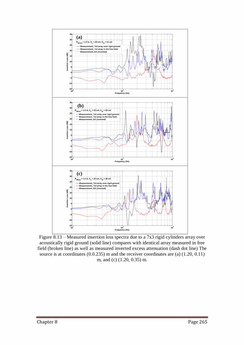
Chapter 8 Page 265
Figure 8.13 – Measured insertion loss spectra due to a 7x3 rigid cylinders array over
acoustically rigid ground (solid line) compares with identical array measured in free
field (broken line) as well as measured inverted excess attenuation (dash dot line) The
source is at coordinates (0.0.235) m and the receiver coordinates are (a) (1.20, 0.11)
m, and (c) (1.20, 0.35) m.
102
103
104
-15
-10
-5
0
5
10
15
20
25
30
35
Frequency (Hz)
Insert
ion
Lo
ss (
dB
)
Measurement, 7x3 array over rigid ground
Measurement, 7x3 array in the free field
Measurement, EA (inverted)
Rdirect
= 1.2 m, hs = 23 cm, h
r1 = 11 cm
102
103
104
-15
-10
-5
0
5
10
15
20
25
30
35
Frequency (Hz)
Insert
ion
Lo
ss (
dB
)
Measurement, 7x3 array over rigid ground
Measurement, 7x3 array in the free field
Measurement, EA (inverted)
Rdirect
= 1.2 m, hs = 23 cm, h
r2 = 23 cm
102
103
104
-15
-10
-5
0
5
10
15
20
25
30
35
Frequency (Hz)
Insert
ion
Lo
ss (
dB
)
Measurement, 7x3 array over rigid ground
Measurement, 7x3 array in the free field
Measurement, EA (inverted)
Rdirect
= 1.2 m, hs = 23 cm, h
r3 = 35 cm
(c)
(b)
(a)

Chapter 8 Page 266
Figure 8.13 compares the measured IL spectra for a horizontal PVC
pipe array with and without a rigid (MDF 2) ground at source height of 0.23 m
and three receiver heights of 0.11, 0.23 and 0.35 m as shown in (a), (b) and
(c) respectively. The measured excess attenuation spectrum due to rigid
(MDF 2) ground for a similar source-receiver geometry to that used for the IL
measurements is superimposed into the IL plot but inverted (see figure 8.4).
The Bragg band gap in this particular arrangement (lattice constant of 0.69 m)
is near 2.5 kHz. The array band gaps are impaired, resulting in negative
insertion loss, where they coincide with the minima in the ground.

Chapter 8 Page 267
8.5.5) Comparisons of data and predictions for elastic shells array with their axes parallel to a rigid ground.
Figure 8.14 – Measured (solid line) and predicted (broken line) IL spectra due to a
square lattice array of 7x3 latex shell cylinders of diameter 0.055 m over acoustically-
rigid ground with source coordinates (0, 0.23) m and receiver coordinates (a) (0.8,
0.11) m, and (c) (0.8, 0.35) m.
.
102
103
104
-30
-20
-10
0
10
20
30
40
50
Frequency (Hz)
Insert
ion
Lo
ss (
dB
)
Measurement, 7x3 array over rigid ground, Rdirect
= 0.8 m, hs = 23 cm, h
r1 = 11 cm
Prediction, = 10 GPa s m-2
102
103
104
-30
-20
-10
0
10
20
30
40
50
Frequency (Hz)
Insert
ion
Lo
ss (
dB
)
Measurement, 7x3 array over rigid ground, Rdirect
= 0.8 m, hs = 23 cm, h
r2 = 23 cm
Prediction, = 10 GPa s m-2
102
103
104
-30
-20
-10
0
10
20
30
40
50
Frequency (Hz)
Insert
ion
Lo
ss (
dB
)
Measurement, 7x3 array over rigid ground, Rdirect
= 0.8 m, hs = 23 cm, h
r2 = 23 cm
Prediction, = 10 GPa s m-2
(a)
(b)
(c)
Chapter 8 Page 268
The measured and predicted performance of 7x3 array of latex shells
over the rigid ground shown in figure 8.14 are similar to that described in
section 8.5.2. In particular, figure 8.14(c) shows that when the first ground
effect dip is in the vicinity of the breathing mode resonance of the shell (near
900 Hz) the corresponding positive IL peak is no longer present. Again, this
point will be further elaborated in figure 8.15 with the excess attenuation
spectra plotted against the insertion loss spectra.

Chapter 8 Page 269
Figure 8.15 – Measured insertion loss spectra due to a 7x3 latex shell cylinders array
over acoustically rigid ground (solid line) compares with identical array measured in
free field (broken line) as well as measured inverted excess attenuation (dash dot line)
The source is at coordinates (0.0.235) m and the receiver coordinates are (a) (1.20,
0.11) m, and (c) (1.20, 0.35) m.
Figure 8.15 compares the measured IL spectra (see equation 1.9) for a
horizontal elastic shell cylinders array with and without a rigid (MDF 2) ground
at source height of 0.23 m and three receiver heights of 0.11, 0.23 and 0.35 m
as shown in (a), (b) and (c) respectively. The measured excess attenuation
102
103
104
-30
-20
-10
0
10
20
30
40
Frequency (Hz)
Insert
ion
Lo
ss (
dB
)
Measurement, 7x3 array over rigid ground
Measurement, 7x3 array in the free field
Measurement, EA (inverted)
Rdirect
= 0.8 m, hs = 23 cm, h
r1 = 11 cm
102
103
104
-30
-20
-10
0
10
20
30
40
Frequency (Hz)
Insert
ion
Lo
ss (
dB
)
Measurement, 7x3 array over rigid ground
Measurement, 7x3 array in the free field
Measurement, EA (inverted)
Rdirect
= 0.8 m, hs = 23 cm, h
r2 = 23 cm
102
103
104
-30
-20
-10
0
10
20
30
40
Frequency (Hz)
Insert
ion
Lo
ss (
dB
)
Measurement, 7x3 array over rigid ground
Measurement, 7x3 array in the free field
Measurement, EA (inverted)
Rdirect
= 0.8 m, hs = 23 cm, h
r3 = 35 cm
(b)
(c)
(a)
Chapter 8 Page 270
spectrum due to rigid ground for a similar source-receiver geometry to that
used for the IL measurements is superimposed into the IL plot but inverted.
The Bragg band gap in this particular arrangement (lattice constant of 0.069
m) is near 2.5 kHz. The array band gaps are impaired, resulting in negative
insertion loss, where they coincide with the minima in the ground.
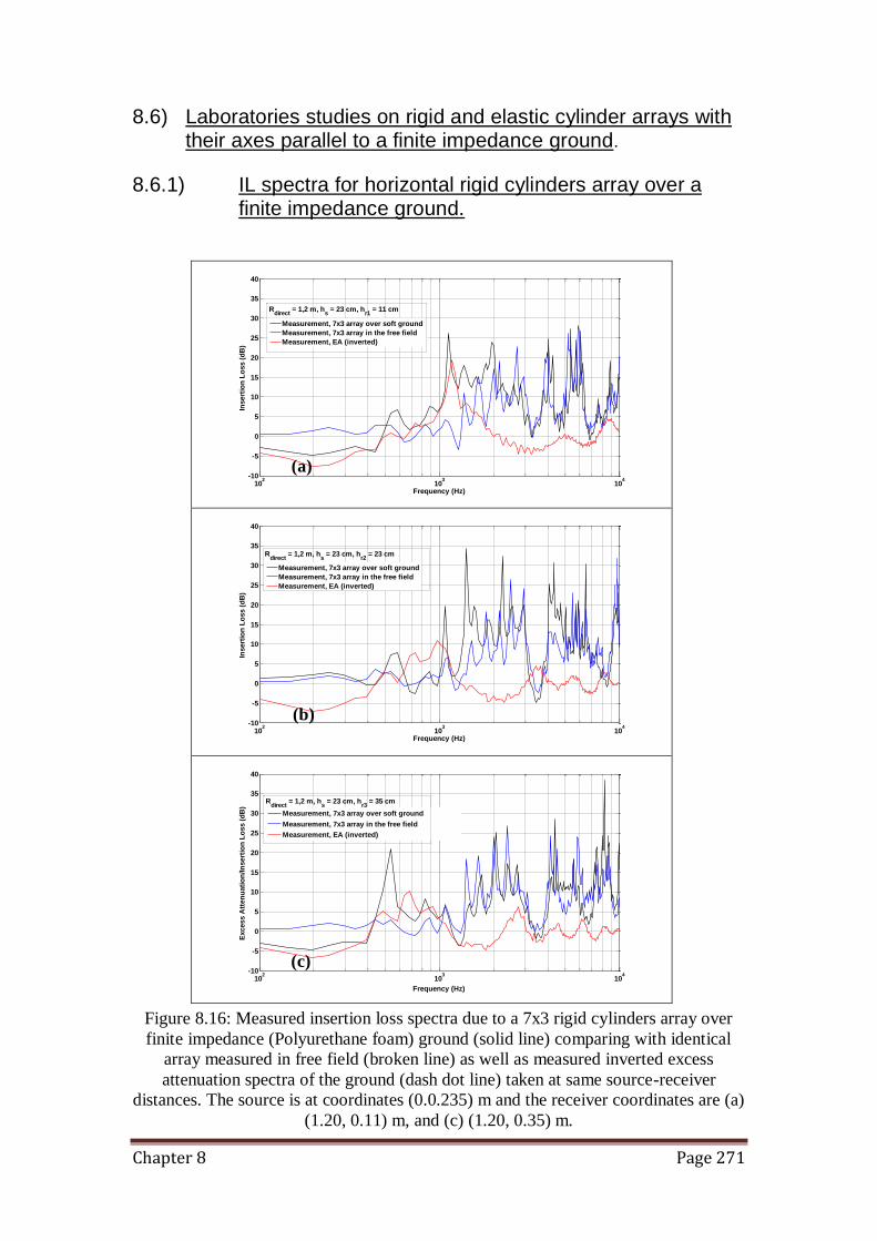
Chapter 8 Page 271
8.6) Laboratories studies on rigid and elastic cylinder arrays with their axes parallel to a finite impedance ground.
8.6.1) IL spectra for horizontal rigid cylinders array over a finite impedance ground.
Figure 8.16: Measured insertion loss spectra due to a 7x3 rigid cylinders array over
finite impedance (Polyurethane foam) ground (solid line) comparing with identical
array measured in free field (broken line) as well as measured inverted excess
attenuation spectra of the ground (dash dot line) taken at same source-receiver
distances. The source is at coordinates (0.0.235) m and the receiver coordinates are (a)
(1.20, 0.11) m, and (c) (1.20, 0.35) m.
102
103
104
-10
-5
0
5
10
15
20
25
30
35
40
Frequency (Hz)
Insert
ion
Lo
ss (
dB
)
Measurement, 7x3 array over soft ground
Measurement, 7x3 array in the free field
Measurement, EA (inverted)
Rdirect
= 1,2 m, hs = 23 cm, h
r1 = 11 cm
102
103
104
-10
-5
0
5
10
15
20
25
30
35
40
Frequency (Hz)
Insert
ion
Lo
ss (
dB
)
Measurement, 7x3 array over soft ground
Measurement, 7x3 array in the free field
Measurement, EA (inverted)
Rdirect
= 1,2 m, hs = 23 cm, h
r2 = 23 cm
102
103
104
-10
-5
0
5
10
15
20
25
30
35
40
Frequency (Hz)
Excess A
tten
uati
on
/In
sert
ion
Lo
ss (
dB
)
Measurement, 7x3 array over soft ground
Measurement, 7x3 array in the free field
Measurement, EA (inverted)
Rdirect
= 1,2 m, hs = 23 cm, h
r3 = 35 cm
(b)
(a)
(c)
Chapter 8 Page 272
Figure 8.16 compares the measured insertion loss spectra due to 7x3
rigid cylinder arrays over finite impedance ground (Polyurethane foam) for
three receiver heights using the source location described in section 8.5.3.
The measure IL spectra due to identical arrays without the presence of the
ground and excess attenuation (inverted) due to the Polyurethane foam layer
with the same source-receiver geometry are superimposed to the plots.
Compared to the results for the rigid ground plotted in figure 8.13, the minima
associated with the finite impedance ground effect seem to enhance the IL
peaks and also we note that the ground effects are also shifted towards lower
frequency. This effect could be exploitable in the design of SC-based noise
barriers.

Chapter 8 Page 273
8.6.2) IL spectra for horizontal elastic shell cylinders array over a finite impedance ground.
Figure 8.17 – Measured insertion loss spectra due to a 7x3 latex shell cylinders array
over finite impedance (Polyurethane foam) ground (solid line) compared with that due
to an identical array measured in free field (broken line) as well as measured inverted
excess attenuation spectra due to the ground alone (dash dot line) The source is at
coordinates (0.0.235) m and the receiver coordinates are (a) (1.20, 0.11) m, (b) (1.20,
0.23) m and (c) (1.20, 0.35) m.
102
103
104
-10
0
10
20
30
40
50
Frequency (Hz)
Insert
ion
Lo
ss (
dB
)
Measurement, 7x3 array over soft ground
Measurement, 7x3 array in the free field
Measurement, EA (inverted)
Rdirect
= 0.8 m, hs = 23 cm, h
r1 = 11 cm
102
103
104
-20
-10
0
10
20
30
40
50
Frequency (Hz)
Insert
ion
Lo
ss (
dB
)
Measurement, 7x3 array over soft ground
Measurement, 7x3 array in the free field
Measurement, EA (inverted)
Rdirect
= 0.8 m, hs = 23 cm, h
r2 = 23 cm
102
103
104
-20
-10
0
10
20
30
40
50
Frequency (Hz)
Insert
ion
Lo
ss (
dB
)
Measurement, 7x3 array over soft ground
Measurement, 7x3 array in the free field
Measurement, EA (inverted)
Rdirect
= 0.8 m, hs = 23 cm, h
r3 = 35 cm
(a)
(c)
(b)
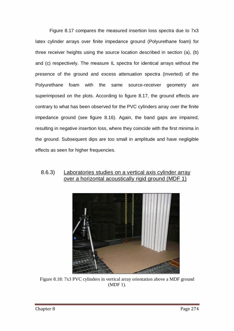
Chapter 8 Page 274
Figure 8.17 compares the measured insertion loss spectra due to 7x3
latex cylinder arrays over finite impedance ground (Polyurethane foam) for
three receiver heights using the source location described in section (a), (b)
and (c) respectively. The measure IL spectra for identical arrays without the
presence of the ground and excess attenuation spectra (inverted) of the
Polyurethane foam with the same source-receiver geometry are
superimposed on the plots. According to figure 8.17, the ground effects are
contrary to what has been observed for the PVC cylinders array over the finite
impedance ground (see figure 8.16). Again, the band gaps are impaired,
resulting in negative insertion loss, where they coincide with the first minima in
the ground. Subsequent dips are too small in amplitude and have negligible
effects as seen for higher frequencies.
8.6.3) Laboratories studies on a vertical axis cylinder array over a horizontal acoustically rigid ground (MDF 1)
Figure 8.18: 7x3 PVC cylinders in vertical array orientation above a MDF ground
(MDF 1).

Chapter 8 Page 275
Figure 8.19: Measured insertion loss spectra of vertical array with source and receiver
at 0.3m height with (solid line) and without (broken line) the MDF 1 ground plane.
Measured inverted excess attenuation (inverted) spectra of the ground (dash dot line).
Figure 8.19 compares IL spectra due a vertical axis array without and
with the MDF 1 surface and source and receiver at 0.3 m height. Without the
ground surface, there is a band gap centred at about 2.5 kHz, due to multiple
scattering by the (acoustically hard) cylinders. This corresponds with the first
Bragg diffraction frequency (see equation 2.14). However, in the presence of
the reflecting surface, the first and higher order band gaps are impaired when
they coincide with minima in the EA spectra. On the other hand, for this
geometry, the first ground attenuation maximum due to the MDF 1 board is
shifted in frequency by the presence of the vertical array.
102
103
104
-20
-10
0
10
20
30
40
50
Frequency (Hz)
Insert
ion
Lo
ss (
dB
)
Measurement, 7x3 vertical array over rigid ground
Measurement, 7x3 array in the free field
Measurement, EA (inverted)
Rdirect
= 1.3 m, hs = 30 cm, h
r = 30 cm
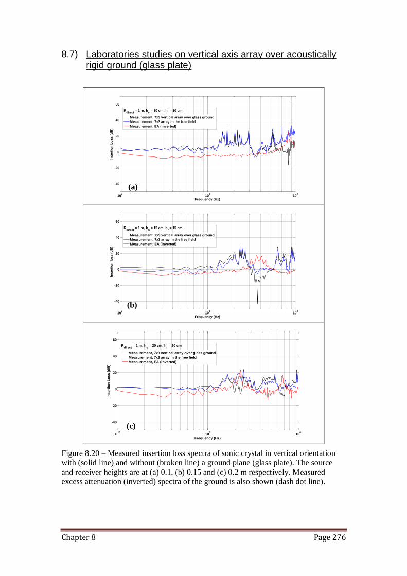
Chapter 8 Page 276
8.7) Laboratories studies on vertical axis array over acoustically rigid ground (glass plate)
Figure 8.20 – Measured insertion loss spectra of sonic crystal in vertical orientation
with (solid line) and without (broken line) a ground plane (glass plate). The source
and receiver heights are at (a) 0.1, (b) 0.15 and (c) 0.2 m respectively. Measured
excess attenuation (inverted) spectra of the ground is also shown (dash dot line).
102
103
104
-40
-20
0
20
40
60
Frequency (Hz)
Insert
ion
Lo
ss (
dB
)
Measurement, 7x3 vertical array over glass ground
Measurement, 7x3 array in the free field
Measurement, EA (inverted)
Rdirect
= 1 m, hs = 10 cm, h
r = 10 cm
102
103
104
-40
-20
0
20
40
60
Frequency (Hz)
Insert
ion
lo
ss (
dB
)
Measurement, 7x3 vertical array over glass ground
Measurement, 7x3 array in the free field
Measurement, EA (inverted)
Rdirect
= 1 m, hs = 15 cm, h
r = 15 cm
102
103
104
-40
-20
0
20
40
60
Frequency (Hz)
Insert
ion
Lo
ss (
dB
)
Measurement, 7x3 vertical array over glass ground
Measurement, 7x3 array in the free field
Measurement, EA (inverted)
Rdirect
= 1 m, hs = 20 cm, h
r = 20 cm
(a)
(c)
(b)

Chapter 8 Page 277
Figure 8.20 compares the measured insertion loss spectra for 7x3 rigid
cylinder arrays over acoustically solid ground (glass plate) for three receiver
heights using the source and receiver location described in table 8.2. The
destruction of the band gap at around 2.3 kHz due to its coincidence with a
ground effect minimum for this geometry can be observed again (see figure
8.20 (c)).
Chapter 9 Page 278
Chapter 9
Summary and concluding remarks
9.1) Summary of contents
Chapter 1 provided an introduction to acoustic wave theories and
derivations of some formulations for both fluid and elastic waves. Only linear
wave phenomena were considered. The issue of road traffic noise impact was
outlined together with the mitigation method using a conventional noise
barrier. A review of past work on the use of sonic crystals as noise barrier was
performed along with describing the underlying basis of crystallography.
Chapter 2 reviewed the Plane Wave Expansion (PWE) Method as a
semi-analytical technique for analysing the performance of a sonic crystal,
employing aspects of the wave and crystallography theories discussed in
Chapter 1. The PWE technique describes the acoustic wave transmission
inside an infinite two-dimensional periodic composite (solid-fluid) structure.
PWE allows the computation of eigenfrequencies (using MATLAB®) in the first
irreducible Brillouin zone specified by the three principal symmetry directions (
, and ) of a square lattice crystal. The dispersion relationship was
represented using a band structure diagram (figure 2.2). It was demonstrated
that a periodic square array of rigid cylinders in air can give rise to complete
and partial stopbands in which sound cannot propagate through at all or only
at certain angles respectively. It was seen also that by tuning the lattice
constant, the Bragg band gap frequency could be shifted to a region of

Chapter 9 Page 279
interest. A simple formula given in equation 2.13 was found to be able to
predict the centre frequency of the Bragg band gap for a specific square
lattice array. This formula must be modified if the configuration of the array is
changed to another Bravais lattice (i.e. hexagonal, see equation 4.8). The
comparison between the theoretical results (presented as band structure) and
the laboratory results (finite size and presented as Insertion Loss (IL)) for a
similar periodic structure yielded favourable agreement in determining the
Bragg band gap. An investigation of the effect of varying the size of the
scatterer (which inherently varies the filling fraction) was performed using the
PWE method. It was predicted that, for a higher filling fraction, ff ,
enlargement of Bragg band gaps and the enhancement of the IL performance
of the SC in the direction could be achieved. The last section of this
chapter, enabled us to infer that it is, in fact, the density contrast that strongly
influences the occurrence of the band gaps. The ability to determine the band
structure through PWE could be a cost effective way for making the proper
design choice for a sonic crystal noise barrier.
Chapter 3 studied another theoretical method to determine the acoustic
transmission loss for a two dimensional (2D) periodic array of identical rigid
circular cylinders based on Multiple Scattering Theory (MST). This method
demonstrated how a general 2D acoustic wave diffraction problem concerning
a structure consisting of a number of separate circular scatterers can be
solved exactly in terms of the diffraction characteristics of each individual
scatterer. The basis of this theory uses the multipole methods to combine
separated solutions of the Helmholtz equation using an addition theorem (See

Chapter 9 Page 280
Appendix B) for expanding multipoles centred at one origin in terms of similar
multipoles centred on a different origin. Two essential wavefunctions to
describe the scattering of waves by circular scatterers were involved. The first
used a Hankel function to express the incident wave which satisfies
Sommerfeld radiation condition and the second employed a Bessel function of
the first kind to express an outgoing wave radiating from each cylinder.
Contrary to the PWE method described in Chapter 2 which is restricted to
infinite arrays, MST calculates the total wave field (pressure) for a finite size
array at any point exterior to the cylinders. This method thereby offers a
means of direct comparison with laboratory results. The incident wave can be
modelled using a plane or cylindrical waves where the latter can take account
of the near field effects (i.e. when source is placed close to the array). The
MST method has proved to be powerful, and self-consistent with the ability to
solve in principle all multiple-body (i.e. the configuration of the scatterers can
be periodic or random) diffraction problems of which the solutions for an
individual scatterer are already known. This method was used to calculate the
insertion loss for a 7x3 square lattice arrays consisting of rigid circular
scatterers. The perfectly-reflecting Neumann boundary condition was used to
define the acoustically-hard boundary to model the rigid surface of the
scatterers. Insertion losses for three different configurations were computed
and the results were compared with laboratory data. The MST predicted
results (both plane and cylindrical incident waves) were found to agree well
with the laboratory data and these results complimented the hypothesis that
the Bragg band gap could be tuned to the desired frequency by varying the
lattice constant of the rigid scatterers. The data indicated minor peaks at

Chapter 9 Page 281
frequencies below the first Bragg band gap is observed for the case of lattice
constant equal to 0.069 and 0.08 m that could be the effect of finite width or
height of the sonic crystal array. This extra low frequency band gap could be
exploited in SC noise barrier design. The accuracy of the MST has been
investigated and for a 7x3 square lattice array of rigid circular scatterers with
radius of 0.0275 m and lattice constant of 0.135 m, truncation numbers 4M
and 3M respectively are necessary to obtain reliable results for plane and
cylindrical incident waves. The main drawback of this iterative technique is
that the time for computation rapidly increases as the number of scatterers
increases.
Chapter 4 concerned FEM modelling of the acoustic transmission
through 2D sonic crystal using the commercial software COMSOL®
Multiphysics (version 3.5a). FEM provides a good technique to solve
scattering problem of acoustic waves which involve complicated geometries
and when several physical problems are coupled (see chapter 6). Both plane
and cylindrical incident waves were simulated and the Insertion Loss (IL)
calculated for each incident wave was compared with data for an equivalent
SC configuration taken in the laboratory. The FEM predicted results were
found to agree well with the laboratory data in term of predicting the bandgaps
(see figure 4.5). The computation time for FEM is much longer than that for
MST for the same SC configuration. Nevertheless, the computation time has
been found to be reasonable period even for the case with the largest number
of elements (mesh density). Comparisons with theoretical and experimental
results have shown that increasing the number of elements in the FEM model

Chapter 9 Page 282
leads to better convergence results for higher frequencies. Three different
shapes scatterer (triangle, square and elliptical) with similar cross section area
as the circular scatterer (arranged in square lattice) were considered. Their
performances were compared with that of the circular shape scatterers and,
according to the FEM results, the triangular shape scatterer with arrangement
3 (see figure 4.8) offers a better IL performance than the other shapes.
Comparisons made for hexagonal and square lattice arrangement for circular
scatterers, have shown that the square lattice is more suitable as for road
traffic noise barrier design. An efficient FEM for calculating the acoustical
properties of 2D sonic crystals was solved by the use of Perfectly-Matched
Layer (PML). Preliminary work using FEM on transient analysis was
performed also for SC with vacancies which potentially could be used to guide
the incoming waves.
Chapter 5 detailed the measurement arrangements, data acquisition
systems and signal processing. A robust indoor measuring system has been
set up to measure the insertion loss of the sonic crystal in the anechoic
chamber using the one channel Maximum-Length Sequence System Analyzer
(MLSSA). Studies on the effect of transducer size and post processing of the
measured signal (i.e. different window sizes and functions) were reported. To
perform accurate measurements, the acoustical environment in the chamber
was improved. The method of construction of scatterer (i.e. elastic scatterer
and Split Ring Resonator) and the supporting structure in the chamber were
also described. The chapter continued to describe the outdoor measurement
taken at the Open University barrier test site. For these outdoor
Chapter 9 Page 283
measurements, a multiple channels data acquisition system was used instead
of MLSSA. Two contributing factors for this change are; the question of the
reliability using MLSSA at outdoor conditions and second, the means of
obtaining multiple data simultaneously (following ANSI S12.8 standards) for
both the microphones and sonic anemometer. Pertaining to the reliability of
the source, a modified white noise (termed as Traffic Noise signal in this
Thesis) was used instead of an MLS signal. A Graphical User Interface (GUI)
was developed using MATLAB® for enabling the user to control the data
acquisition system. The control is through clicking of buttons on the display
screen and the associate time or frequency domain signal spectrum taken
during the measurement will then be plotted on the display. Saving the data is
subsequently done with a click on the save button to allow post-processing of
data. The outdoor barriers IL performance testing takes account of various
degrading effects such as the estimated background noise (measured
separately) and the difference in microphones responses based on a
calibration process. Microphone distance corrections were also necessary for
barrier measurements. A wind vector diagram was plotted for every
measurement based on the outputs from the sonic anemometer and has
enabled analysis of the meteorological effects on SC performance. In this
chapter, an alternative swept sine source was also considered. The outdoor
measuring system (except that the source is replaced with a natural made
sound) was used to perform measurements on a SC arranged in quasi-
ordered lattice arrangement near a weir at Worcester (‘Organ of Corti’
project). The measured IL was compared with MST predictions and an
Chapter 9 Page 284
investigation of the influence of the quasi periodicity in the array was carried
out.
SCs composed of elastic shells have been considered in chapter 6.
Additional low-frequency bandgaps are predicted in an infinite periodic
structure formed by the thin elastic shells made of suitable non-vulcanised
rubber (latex). The additional bandgap due to the breathing mode resonance
of the shell is predicted to be the widest among those generated by the shell
resonances. Proof of concept for the breathing mode was performed using
modal analysis with FEM. A semi-analytical method (based on MST) was
found to offer a fast and reliable approach to solving the problem of scattering
by an array of cylindrical elastic shells. It provided a tool for choosing the
material as well as radius and thickness of the shell so that the first resonance
frequencies could be positioned below the first Bragg bandgap of the array.
The computational time required by using the MST is less than one tenth of
that needed for traditional numerical methods such as FEM for modelling a
transmission problem for a single elastic shell. The predicted performance of
single and arrays of elastic shells in the low-frequency range was verified by
laboratory experiments. The combination of the resonance and classical band
gaps (first Bragg diffraction frequency) could be used to yield designs of
barriers suitable for traffic noise. Laboratory experiments using periodic arrays
of elastic thin-walled and hollow rigid split cylinders demonstrated relatively
angle-independent insertion loss at frequencies below the first classical band

Chapter 9 Page 285
gap. Attempts at an alternative design using polyethylene scatterers (See
Appendix C) were unsuccessful.
Use of an alternative local resonance scatterer termed Split Ring
Resonator (SRR) which is made from single slit cylindrical cylinder was
explored in chapter 7. Initial activities confirmed a result already known from
the literature that arrays of single slit cylindrical ‘Helmholtz’ resonators
produce an additional angle-independent band gap at frequencies below the
first Bragg band gap. The re-visiting of this work also served to provide a
better understanding of the possible influences (i.e. slit width, area of cavity
and slit orientation) on the performance of the SRR which were studied both
numerically and experimentally in laboratory. Outdoor measurements were
performed on the full scale SC barriers made with SRR and their performance
was compared with that of a non-resonating SC barrier. The additional and
fairly angle independent bandgap corresponding to the cavity resonance of
such SRR array provides another means of enhancing the barrier
performance. Subsequent sections of Chapter 7 tackled the question of
practicality of using latex cylinders (studied in chapter 6) in outdoor
environments since without some form of protection, arrays of latex cylinders
would be impractical in outdoor environments. Therefore the acoustical effects
of providing suitable protection were investigated. It was found theoretically
and experimentally that increasing the number of slits in an empty pipe
causes an increase in the frequency of the Helmholtz-type resonance. A low-
frequency approximation which models the slit cylinder by an equivalent fluid

Chapter 9 Page 286
layer predicted that the frequency increase is proportional to the square root
of the number of slits and this was confirmed experimentally. Subsequent
work investigated novel configurations of concentric cylinders (having the
elastic shells arrange inside the rigid 4-slit pipes) and suggested that it is
possible both to protect the elastic cylinders and, effectively, to broaden the
band gaps. The IL of a 7x3 array of 55 mm outer diameter PVC cylinders with
4 mm wide slits and an inner latex cylinder with 43 mm outer diameter and
0.25 mm thick walls was measured and demonstrated the efficacy of this
arrangement. The concentric arrangements resulted in resonances associated
with both circular and annular cavities. With an inner elastic shell, an
additional breathing mode resonance of the shell is preserved but modified by
the presence of the outer 4-slit pipe. This is due to the coupling between the
components of the concentric arrangement results in shifts in the resonant
frequencies corresponding to each element of the composite configuration.
This is similar to the effect that is observed in mass-spring systems with
multiple degrees of freedom. A theoretical formulation used boundary
conditions dependent on polar angle to represent arbitrary positioned slits. For
simplicity, in the studied geometries the slits are positioned symmetrically.
Jump boundary conditions imposed on the slit interface were used to
represent the solution inside the slits. The method can be applied to various
types of 2D resonators with concentric multiple layered/ solid cylinder inner. A
low-frequency approximation for the acoustical properties of the concentric
arrangement with an elastic shell inner correctly predicted the observed
frequency shift in the breathing mode resonance. When used in periodic
arrays the concentric arrangements with inner elastic shells and outer 4-slit

Chapter 9 Page 287
cylinders resulted in additional sound attenuation in the low-frequency range
below the first Bragg band gap while still preserving the Bragg band gaps.
This concentric arrangement is more practical than the use of unprotected
elastic shells, hence is a potentially useful basis for a sonic crystal barrier
design. Full scale field trials of such a sonic crystal barrier (using 3 rows each
containing 54 110 mm outer diameter slit PVC cylinders and commercially-
produced latex cylinders) and comparisons of its performance with that of a
conventional noise fence were performed on a test site that has been
constructed on the OU campus. The parameters used for the outdoor
concentric cylinder array did not result in as good an acoustical performance
as might be possible (see figure 7.28). An alternative manufacturer would be
required to make latex cylinders with the desired dimensions. Nevertheless,
the numerical modelling results (see figure 9.1) indicated that the outdoor
array performance would be improved significantly with the use of narrower
slits and larger latex cylinders.
The influence of the presence of a reflecting or absorbing ground on
sonic crystal band gaps produced by the effect of multiple scattering from
acoustically-hard and -soft cylinders was studied in Chapter 8. Two ground
impedance measurement methods (i.e. single microphone and transfer
function method) were used to yield the Excess Attenuation (EA) spectra for
different experimental conditions (i.e. in the laboratory and outdoor in-situ). In
the laboratory, acoustical properties of 2 Medium Density Fibreboard (MDF) of
different dimensions, a glass plate and a polyurethane foam were measured,
Those of asphalt and grass covered ground were measured in-situ. Fits to
Chapter 9 Page 288
these spectra using a one parameter empirical impedance model confirm that
the ground planes used were either acoustically-hard (MDF and glass) or –
soft (polyurethane foam and grass covered ground). A semi-analytical method
has been derived for predicting multiple scattering effects of a finite arrays of
cylinders with axes parallel to either rigid or impedance ground. Results of the
semi-analytical method have been compared with laboratory data. 7x3 square
lattice arrays consisting of both rigid and elastic scatterers have been placed
with their axes parallel to the grounds and the insertion losses at various
source and receiver heights have been measured. Laboratory experiments
have shown also that it is possible to augment the barrier effect of a sonic
crystal array by means of the ground effect i.e. the interference between
sound travelling directly from source to receiver and that reflected from the
ground beneath the barrier. The data show that sonic crystal band gaps are
much reduced when their frequency coincides with excess attenuation minima
associated with the acoustically ‘hard’ ground. Depending on the source-
array-receiver geometry the presence of a rigid ground can result in
destruction of the positive IL peak associated with the first Bragg band gap if
the first destructive interference minimum in the ground effect is coincident.
However, introduction of the impedance ground results in the shift of ground
effect minima to lower frequencies so that the Bragg band gap is maintained.
This work revealed that it should be possible for ground effect and SC stop
and pass bands to be used synergistically. Preliminary studies of a vertical
axis SC arrays over an acoustically ‘hard’ ground were found to show the
same phenomena as observed with the horizontal axis SC.

Chapter 9 Page 289
9.2) Concluding remarks In this work, an alternative road traffic noise barrier using an array of
periodically arranged vertical cylinders known as a Sonic Crystal (SC) is
investigated. Such SCs exhibit a selective sound attenuation in particular
frequency bands, called band gaps related to the spacing and size of the
cylinders. This Thesis considers the propagation of acoustic waves through
SCs and explores means of enhancing the stop bands notably in the low
frequency regime. Theoretical studies using Plane Wave Expansion (PWE),
Multiple Scattering Theory (MST) and Finite Element Method (FEM) have
enabled study of the performance of SC barriers. In addition to multiple
scattering that can lead to band gaps, strategies for improving the band gaps
by employing the intrinsic acoustic properties of the scatterer are considered:
for example (i) making each cylinder in the form of a Split Ring Resonator
(SRR) and (ii) substituting the acoustically rigid scatterer with thin elastic shell.
Such designs are shown to increase Insertion loss (IL) in the low-frequency
range if the tube cavity (similar to Helmholtz) resonances in SRR or the
breathing mode resonance observed in elastic shells occur at frequencies
below the Bragg resonance stop band. With the better knowledge of the
factors affecting the frequency response for both the SRR and thin elastic
shells, a novel design of composite scatterer uses these 2 types of scatterers
arranged in a concentric configuration with multiple symmetrical slits on the
outer rigid shell. An array of such composite scatterers forms a system
of coupled resonators and gives rise to multiple low-frequency resonances.
Measurements have been made in an anechoic chamber and also on a full-
scale prototype of an outdoor SC noise barrier taking account of

Chapter 9 Page 290
meteorological conditions (i.e. wind profiles and temperature gradients).
Theoretical and experimental results confirmed the existence of the Bragg
band gaps for SC barriers and the significant improvements when locally
resonant scatterers are used. Such resonant arrays are found to give rise to
relatively angle-independent stop bands in a useful range of frequencies.
Good agreement between computational modelling and experimental work is
obtained. Further studies of the acoustical performances of regular arrays of
cylindrical elements, with their axes aligned and parallel to either an
acoustically “hard” or “soft” ground plane, have been made using predictions
and laboratory experiments. Some data have also been obtained also for
scatterers with their axes perpendicular to the ground plane.
The most important contributions in this Thesis are:
• novel designs of SC noise barriers based on multiple resonances to
enhance the noise shielding performance at frequencies below the
first Bragg band gap.
• pioneering investigations of the influence of ground effects on SC noise
barriers.
Chapter 9 Page 291
9.3) Suggestions for future studies
Possible areas of research and further research along the lines of the
present investigation pursued here are recommended as follows.
1) The formulation developed for interaction of acoustic waves and SC
structure in the present study are for a either a plane or a fixed single
point source. According to Section 5.6.4, multiple point sources could
potentially improve the prediction results. Extensions of the prediction
methods to allow for multiple fixed or transient sources should be
explored.
2) In the present study, the predictions are modelled in a 2D system
where the scatterers are infinitely long in the z-axis. It would be
interesting to know how the diffraction at the ends of the finite cylinders
influences the scattering. An extended study could look into the
combination of an SC barrier with an Edge-Modified Barrier (EMB)
which has been widely researched recently [143 and 144] to increase
the noise shielding efficiency.
3) Although the breathing mode resonance from the elastic scatterers
(which are protected from the rigid cylinder) work in principle they are
still subject to harsh outdoor environments including (UV, temperature,
humidity etc…). Degradation of material is inevitable under these
circumstances and so properties of the elastic shell may change.
Therefore some form of climatic cycling tests on the elastic scatterers
Chapter 9 Page 292
will be necessary to address this non-acoustic engineering practicality.
More outdoor data taken with the monitored meteorological conditions
will also aid in such studies.
4) The SC barrier studied is suitable only for straight road. It would be
interesting to study the performance along bends which will cause the
SC barrier periodicity to vary due to the curvature.
5) The parameter values chosen for the full scale prototype are far from
the optimum values as a consequence of unavailability of the numerical
modelling routines (now developed) at the time of their design.
According to subsequent MST predictions (see figure 9.1), the slits in
the outer cylinders (grouted by hand in the prototype) are too wide and
the 0.043 m diameter of the latex cylinders, although the largest that
could be obtained at the time of the prototype construction, is too small.
These problems should be overcome by using larger latex cylinders
(0.08 m diameter of the same thickness) with a different method of
support and by precision manufacture of narrower slits (0.004 m) in the
outer cylinders. This would potentially offer a significantly better
performance than the current configuration.
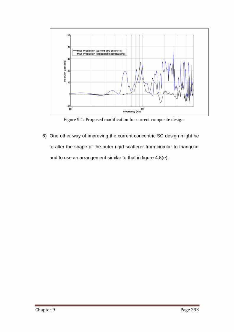
Chapter 9 Page 293
Figure 9.1: Proposed modification for current composite design.
6) One other way of improving the current concentric SC design might be
to alter the shape of the outer rigid scatterer from circular to triangular
and to use an arrangement similar to that in figure 4.8(e).
102
103
-10
0
10
20
30
40
50
Frequency (Hz)
Insert
ion
Lo
ss (
dB
)
MST Prediction (current design SRR4)
MST Prediction (proposed modifications)

XXIX
Appendix A MATLAB® Coding for Plane Wave Expansion (PWE) method
Plane Wave Expansion MATLAB® script modified from codes obtained from
Daniel Peter Elford PhD thesis [43].
tic; num_Eigenvals = 10; nmax = 10; n1=(-nmax:nmax); n2=(-floor((2*nmax+1)^2/2):floor((2*nmax+1)^2/2)); lat_a=0.135; ro=0.0275; f=pi*ro^2/lat_a^2; pa=1380; pb=1.2; delp=(pb/pa-1)/(f*pb/pa+1-f); va=2400; vb=344; pcla=(va^2)*pa; pclb=(vb^2)*pb; delt=(pclb/pcla-1)/(f*pclb/pcla+1-f); nx_arr=repmat(n1,1,2*nmax+1); ny_arr=round(n2/(2*nmax+1)); [nx,nxp]=meshgrid(nx_arr, nx_arr); [ny,nyp]=meshgrid(ny_arr, ny_arr); fill =ones(1,length(nx_arr)); fillt =diag(fill); G_Gp=sqrt(4*pi*f*((nx-nxp).^2+(ny-nyp).^2))+fillt; fG_Gp=2*f*besselj(1,G_Gp)./G_Gp; mode=1; if mode==1 for kyind=1:3 onoff=1;
for kx=.05:.05:.5 XXIX if kyind == 1 kxt=kx; kx=.55-kx; ky=kx;

XXX
elseif kyind==2 kxt=kx; ky=0; elseif kyind==3 kxt=kx; ky=.5; end mag_k_p_g=((kx+nx).^2+(ky+ny).^2); k_p_g_dot_kp_p_g=(kx+nx).*(kx+nxp)+(ky+ny).*(ky+nyp); kro_del_ggp=(nxp==nx)&(nyp==ny); M=mag_k_p_g.*kro_del_ggp+delp.*fG_Gp.*k_p_g_dot_kp_p_g.*(1-kro_del_ggp); N=kro_del_ggp+fG_Gp.*delt.*(1-kro_del_ggp); A=N^-1*M; [a,b]=eig(A); g=find(b~=0); eigs=(sort(b(g))); eigs(1:num_Eigenvals); k=repmat(kxt,1,num_Eigenvals); min(b(g)); if onoff == 1 omega=[((340)/lat_a)*real(sqrt(eigs(1:num_Eigenvals)))']; karr=[k]; if kyind == 1 omegafull=[((340)/lat_a)*real(sqrt(eigs(1:num_Eigenvals)))']; karrfull=[k]; end onoff = 0; else omega=[omega,((340)/lat_a)*real(sqrt(eigs(1:num_Eigenvals)))']; karr=[karr,k]; omegafull=cat(1,omegafull,((340)/lat_a)*real(sqrt(eigs(1:num_Eigenvals)))'); karrfull=cat(1,karrfull,k); end end if kyind==1 myfig = figure; ymax=10000; subplot(1,3,1) b1=plot(karr,omega,'*'); ax1=gca; po=get(gca, 'position'); set(gca, 'YLim', [0,ymax]); set(gca, 'XLim', [0,.5]); set(gca, 'nextplot', 'add'); left_side=po(1); set(gca, 'xtick', []); width=po(3); right_side=left_side+width; set(gca, 'xticklabel', {}); ylabel('Frequency (kHz)') elseif kyind==2 subplot(1,3,2) b2=plot(karr,omega,'*'); po=get(gca, 'position'); po(1)=right_side;

XXXI
ax2=gca; set(gca, 'nextplot', 'add'); set(gca, 'YLim', [0,ymax]); set(gca, 'XLim', [0,.5]); set(gca, 'ytick', []); left_side=po(1); width=po(3); right_side=left_side+width; set(gca, 'xticklabel', {}); elseif kyind==3 subplot(1,3,3) b3=plot(karr,omega,'*'); po=get(gca, 'position'); po(1)=right_side; ax3=gca; set(gca, 'nextplot', 'add'); set(gca, 'ytick', []); set(gca, 'YLim', [0,ymax]); set(gca, 'XLim', [0,.5]); left_side=po(1); width=po(3); right_side=left_side+width; set(gca, 'xticklabel', {}); text(-1,-.05*ymax,'M'); text(-.5,-.05*ymax,'\Gamma'); text(0,-.05*ymax,'X'); text(.5,-.05*ymax,'M'); text(-.3,-.1*ymax,'Reduced Wave Vector', 'HorizontalAlignment','Center'); text(-.3,1.075*ymax,['Disperaion Relation for Square Lattice of PVC Cylinder in Air'],'HorizontalAlignment', 'Center'); text(-.3,1.025*ymax,['f=',num2str(f),' a=',num2str(lat_a),'mr_{o}=',num2str(ro)],'HorizontalAlignment', 'Center'); end end end to
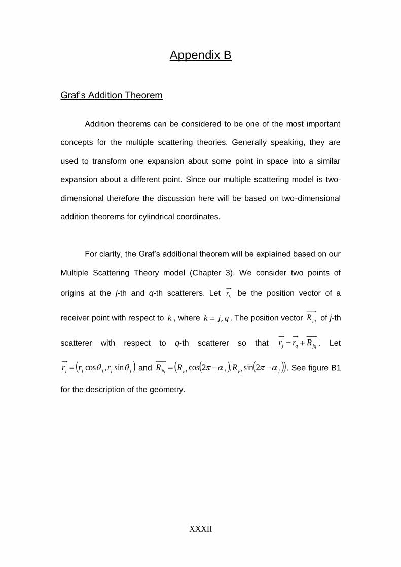
XXXII
Appendix B
Graf’s Addition Theorem
Addition theorems can be considered to be one of the most important
concepts for the multiple scattering theories. Generally speaking, they are
used to transform one expansion about some point in space into a similar
expansion about a different point. Since our multiple scattering model is two-
dimensional therefore the discussion here will be based on two-dimensional
addition theorems for cylindrical coordinates.
For clarity, the Graf’s additional theorem will be explained based on our
Multiple Scattering Theory model (Chapter 3). We consider two points of
origins at the j-th and q-th scatterers. Let kr be the position vector of a
receiver point with respect to k , where qjk , . The position vector jqR of j-th
scatterer with respect to q-th scatterer so that jqqj Rrr . Let
jjjjj rrr sin,cos and
jjqjjqjq RRR 2sin,2cos . See figure B1
for the description of the geometry.
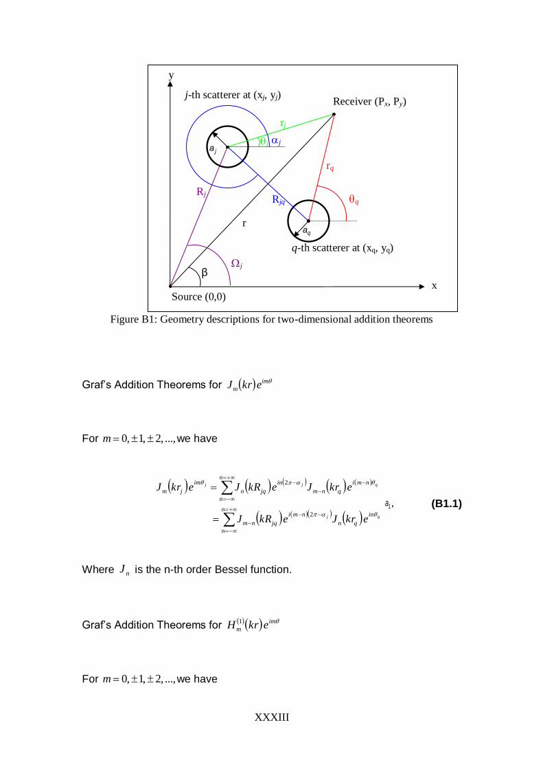
XXXIII
Figure B1: Geometry descriptions for two-dimensional addition theorems
Graf’s Addition Theorems for im
m ekrJ
For ...,,2,1,0 m we have
n
n
in
qn
nmi
jqnm
n
n
nmi
qnm
in
jqn
im
jm
qj
qjj
ekrJekRJ
ekrJekRJekrJ
2
2
1a , (B1.1)
Where nJ is the n-th order Bessel function.
Graf’s Addition Theorems for im
m ekrH 1
For ...,,2,1,0 m we have
r
j-th scatterer at (xj, yj)
q-th scatterer at (xq, yq)
Source (0,0) x
β
Rjq
Receiver (Px, Py)
rq
rj
j
Rj
j
q
j
y

XXXIV
n
n
in
qn
nmi
jqnm
im
jmqjj ekrJekRHekrH
2111a , (B1.2)
For jqq Rr , and
n
n
in
qn
nmi
jqnm
im
jmqjj ekrHekRJekrH
1211a , (B1.3)
For jqq rr .
Where 1
nH is the n-th order Hankel function of the first kind.
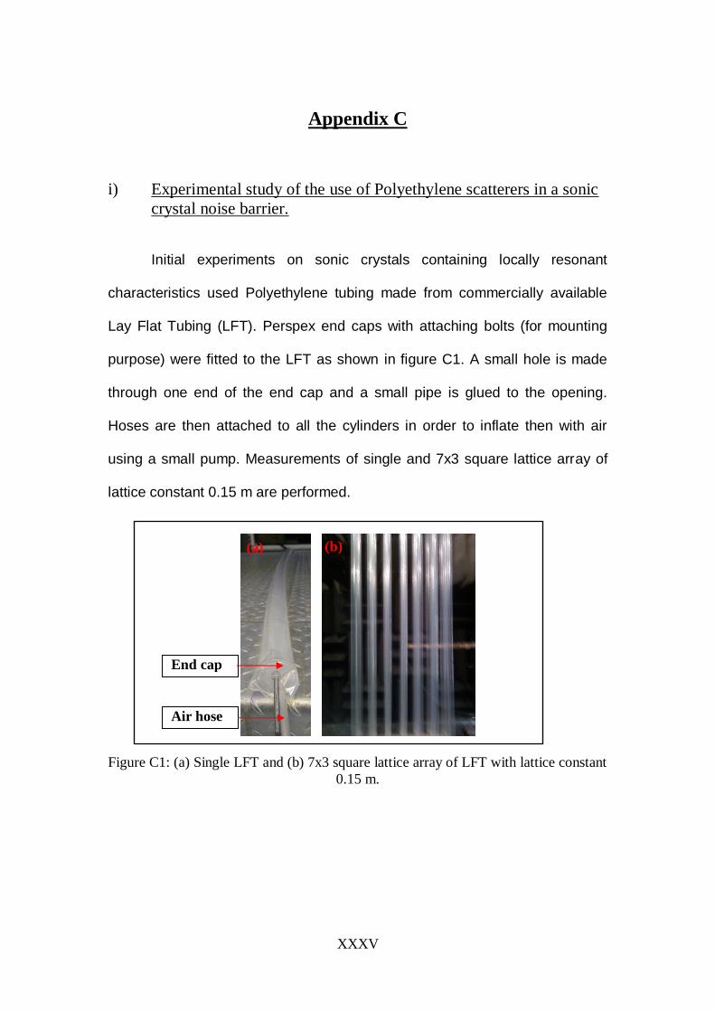
XXXV
Appendix C
i) Experimental study of the use of Polyethylene scatterers in a sonic
crystal noise barrier.
Initial experiments on sonic crystals containing locally resonant
characteristics used Polyethylene tubing made from commercially available
Lay Flat Tubing (LFT). Perspex end caps with attaching bolts (for mounting
purpose) were fitted to the LFT as shown in figure C1. A small hole is made
through one end of the end cap and a small pipe is glued to the opening.
Hoses are then attached to all the cylinders in order to inflate then with air
using a small pump. Measurements of single and 7x3 square lattice array of
lattice constant 0.15 m are performed.
Figure C1: (a) Single LFT and (b) 7x3 square lattice array of LFT with lattice constant
0.15 m.
(a) (b)
Air hose
End cap
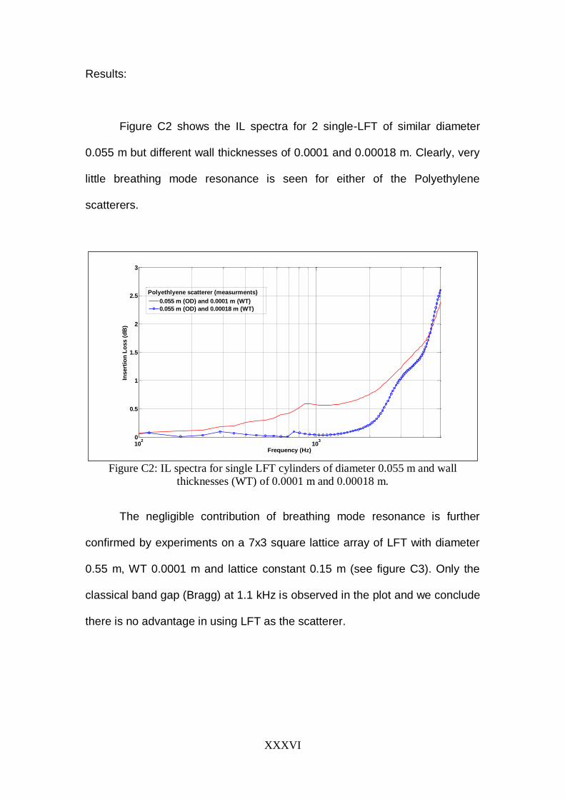
XXXVI
Results:
Figure C2 shows the IL spectra for 2 single-LFT of similar diameter
0.055 m but different wall thicknesses of 0.0001 and 0.00018 m. Clearly, very
little breathing mode resonance is seen for either of the Polyethylene
scatterers.
Figure C2: IL spectra for single LFT cylinders of diameter 0.055 m and wall
thicknesses (WT) of 0.0001 m and 0.00018 m.
The negligible contribution of breathing mode resonance is further
confirmed by experiments on a 7x3 square lattice array of LFT with diameter
0.55 m, WT 0.0001 m and lattice constant 0.15 m (see figure C3). Only the
classical band gap (Bragg) at 1.1 kHz is observed in the plot and we conclude
there is no advantage in using LFT as the scatterer.
102
103
0
0.5
1
1.5
2
2.5
3
Frequency (Hz)
Insert
ion
Lo
ss (
dB
)
0.055 m (OD) and 0.0001 m (WT)
0.055 m (OD) and 0.00018 m (WT)
Polyethlyene scatterer (measurments)

XXXVII
Figure C3: IL spectra for 7x3 square lattice array of LFT with diameter 0.055 m, wall
thickness (WT) of 0.0001 m and lattice constant (L) of 0.15 m.
ii) Experimental study on the use on periodic stiffening along the
scatterer length.
The possibility of enhancing resonance-related band gaps due to
elastic thin-walled cylinders by periodic stiffening along their lengths has been
investigated experimentally. Such structures were achieved by overlapping
and gluing together multiple vertical sections using “gaffer” tape. The width of
the tape sections is 0.05 m and they are periodically spaced at 0.05 m
throughout the length of the elastic cylinder as shown in figure C4. The IL
spectrum for a single elastic cylinder with periodic stiffening has been
measured in the laboratory.
102
103
0
2
4
6
8
10
12
Frequency (Hz)
Insert
ion
Lo
ss (
dB
)
Measurement, 7x3 LFT, WT=0.0001 m, L=0.15 m
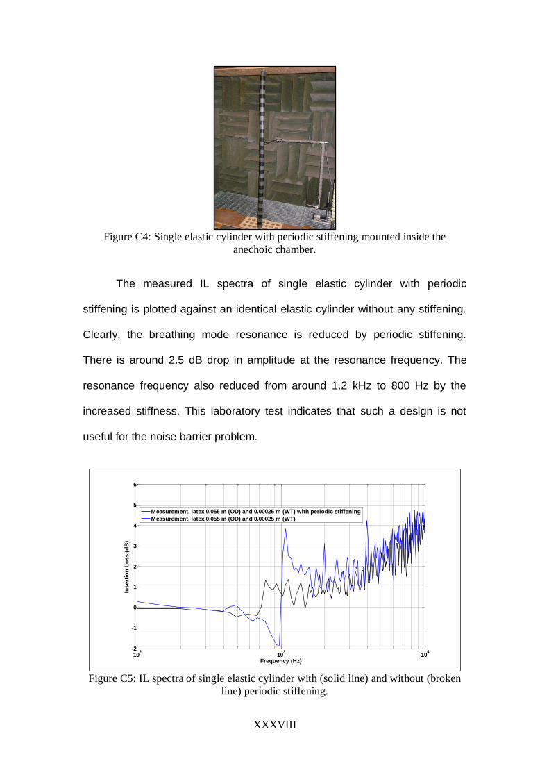
XXXVIII
Figure C4: Single elastic cylinder with periodic stiffening mounted inside the
anechoic chamber.
The measured IL spectra of single elastic cylinder with periodic
stiffening is plotted against an identical elastic cylinder without any stiffening.
Clearly, the breathing mode resonance is reduced by periodic stiffening.
There is around 2.5 dB drop in amplitude at the resonance frequency. The
resonance frequency also reduced from around 1.2 kHz to 800 Hz by the
increased stiffness. This laboratory test indicates that such a design is not
useful for the noise barrier problem.
Figure C5: IL spectra of single elastic cylinder with (solid line) and without (broken
line) periodic stiffening.
102
103
104
-2
-1
0
1
2
3
4
5
6
Frequency (Hz)
Insert
ion
Lo
ss (
dB
)
Measurement, latex 0.055 m (OD) and 0.00025 m (WT) with periodic stiffening
Measurement, latex 0.055 m (OD) and 0.00025 m (WT)
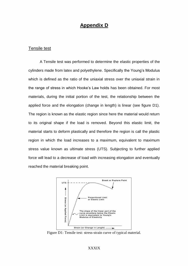
XXXIX
Appendix D
Tensile test
A Tensile test was performed to determine the elastic properties of the
cylinders made from latex and polyethylene. Specifically the Young’s Modulus
which is defined as the ratio of the uniaxial stress over the uniaxial strain in
the range of stress in which Hooke’s Law holds has been obtained. For most
materials, during the initial portion of the test, the relationship between the
applied force and the elongation (change in length) is linear (see figure D1).
The region is known as the elastic region since here the material would return
to its original shape if the load is removed. Beyond this elastic limit, the
material starts to deform plastically and therefore the region is call the plastic
region in which the load increases to a maximum, equivalent to maximum
stress value known as ultimate stress (UTS). Subjecting to further applied
force will lead to a decrease of load with increasing elongation and eventually
reached the material breaking point.
Figure D1: Tensile test: stress-strain curve of typical material.
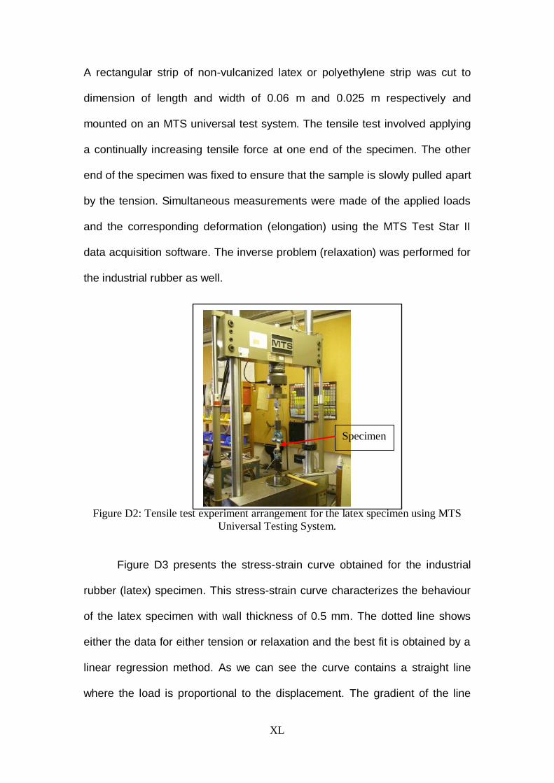
XL
A rectangular strip of non-vulcanized latex or polyethylene strip was cut to
dimension of length and width of 0.06 m and 0.025 m respectively and
mounted on an MTS universal test system. The tensile test involved applying
a continually increasing tensile force at one end of the specimen. The other
end of the specimen was fixed to ensure that the sample is slowly pulled apart
by the tension. Simultaneous measurements were made of the applied loads
and the corresponding deformation (elongation) using the MTS Test Star II
data acquisition software. The inverse problem (relaxation) was performed for
the industrial rubber as well.
Figure D2: Tensile test experiment arrangement for the latex specimen using MTS
Universal Testing System.
Figure D3 presents the stress-strain curve obtained for the industrial
rubber (latex) specimen. This stress-strain curve characterizes the behaviour
of the latex specimen with wall thickness of 0.5 mm. The dotted line shows
either the data for either tension or relaxation and the best fit is obtained by a
linear regression method. As we can see the curve contains a straight line
where the load is proportional to the displacement. The gradient of the line
Specimen
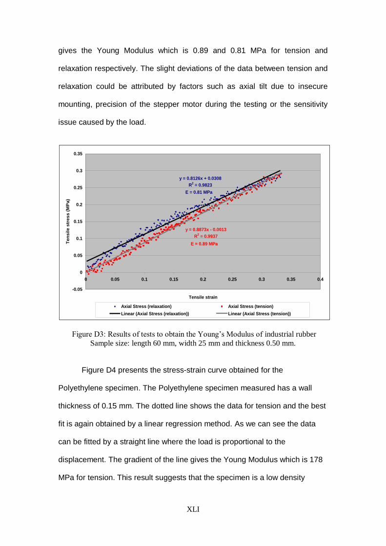
XLI
gives the Young Modulus which is 0.89 and 0.81 MPa for tension and
relaxation respectively. The slight deviations of the data between tension and
relaxation could be attributed by factors such as axial tilt due to insecure
mounting, precision of the stepper motor during the testing or the sensitivity
issue caused by the load.
Figure D3: Results of tests to obtain the Young’s Modulus of industrial rubber
Sample size: length 60 mm, width 25 mm and thickness 0.50 mm.
Figure D4 presents the stress-strain curve obtained for the
Polyethylene specimen. The Polyethylene specimen measured has a wall
thickness of 0.15 mm. The dotted line shows the data for tension and the best
fit is again obtained by a linear regression method. As we can see the data
can be fitted by a straight line where the load is proportional to the
displacement. The gradient of the line gives the Young Modulus which is 178
MPa for tension. This result suggests that the specimen is a low density
y = 0.8126x + 0.0308
R2 = 0.9823
y = 0.8873x - 0.0013
R2 = 0.9937
-0.05
0
0.05
0.1
0.15
0.2
0.25
0.3
0.35
0 0.05 0.1 0.15 0.2 0.25 0.3 0.35 0.4
Tensile strain
Te
ns
ile
str
es
s (
MP
a)
Axial Stress (relaxation) Axial Stress (tension)
Linear (Axial Stress (relaxation)) Linear (Axial Stress (tension))
E = 0.81 MPa
E = 0.89 MPa
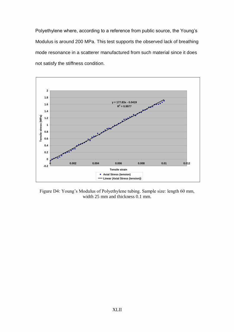
XLII
Polyethylene where, according to a reference from public source, the Young’s
Modulus is around 200 MPa. This test supports the observed lack of breathing
mode resonance in a scatterer manufactured from such material since it does
not satisfy the stiffness condition.
Figure D4: Young’s Modulus of Polyethylene tubing. Sample size: length 60 mm,
width 25 mm and thickness 0.1 mm.
y = 177.83x - 0.0419
R2 = 0.9977
-0.2
0
0.2
0.4
0.6
0.8
1
1.2
1.4
1.6
1.8
2
0 0.002 0.004 0.006 0.008 0.01 0.012
Tensile strain
Ten
sil
e s
tres
s (
MP
a)
Axial Stress (tension)
Linear (Axial Stress (tension))
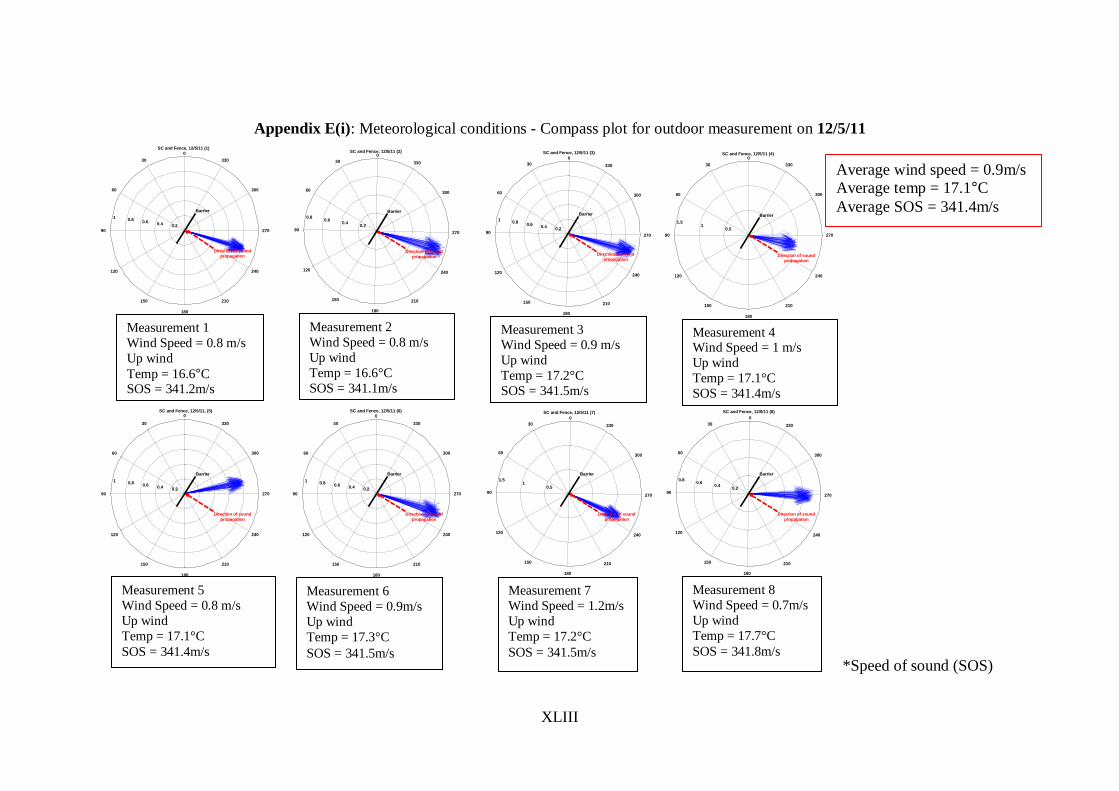
XLIII
Appendix E(i): Meteorological conditions - Compass plot for outdoor measurement on 12/5/11
0.2 0.4 0.6 0.8 1
30
210
60
240
90 270
120
300
150
330
180
0
SC and Fence, 12/5/11 (1)
Speed of sound = 341.2 m/s Temperature = 16.6 C
Barrier
Direction of sound
propagation
Measurement 1
Wind Speed = 0.8 m/s
Up wind
Temp = 16.6°C SOS = 341.2m/s
0.2 0.4
0.6 0.8
30
210
60
240
90270
120
300
150
330
180Speed of sound = 341.1 m/s Temperature = 16.6 C
0SC and Fence, 12/5/11 (2)
Direction of sound
propagation
Barrier
Measurement 2
Wind Speed = 0.8 m/s
Up wind
Temp = 16.6°C
SOS = 341.1m/s
0.2 0.4
0.6 0.8
1
30
210
60
240
90270
120
300
150
330
180
0
SC and Fence, 12/5/11 (3)
Speed of sound = 341.5 m/s Temperature = 17.2 C
Barrier
Direction of sound
propagation
0.5 1
1.5
30
210
60
240
90 270
120
300
150
330
180
0SC and Fence, 12/5/11 (4)
Speed of sound = 341.4 m/s Temperature = 17.1 C
Direction of sound
propagation
Barrier
0.2 0.4 0.6 0.8 1
30
210
60
240
90 270
120
300
150
330
180
0SC and Fence, 12/5/11, (5)
Speed of sound = 341.4 m/s Temperature = 17.1 C
Direction of sound
propagation
Barrier
Measurement 5
Wind Speed = 0.8 m/s
Up wind
Temp = 17.1°C
SOS = 341.4m/s
0.2 0.4 0.6 0.8 1
30
210
60
240
90 270
120
300
150
330
180
0
SC and Fence, 12/5/11 (6)
Speed of sound = 341.5 m/sTemperature = 17.3 C
Barrier
Direction of sound
propagation
Measurement 6
Wind Speed = 0.9m/s
Up wind
Temp = 17.3°C
SOS = 341.5m/s
0.5 1
1.5
30
210
60
240
90270
120
300
150
330
180
0
SC and Fence, 12/5/11 (7)
Speed of sound = 341.5 m/s Temperature = 17.2 C
Direction of sound
propagation
Barrier
Measurement 7
Wind Speed = 1.2m/s
Up wind
Temp = 17.2°C
SOS = 341.5m/s
0.2 0.4
0.6 0.8
30
210
60
240
90270
120
300
150
330
180Speed of sound = 341.8 m/s Temperature = 17.7 C
0
SC and Fence, 12/5/11 (8)
Direction of sound
propagation
Barrier
Measurement 8
Wind Speed = 0.7m/s
Up wind
Temp = 17.7°C
SOS = 341.8m/s
Average wind speed = 0.9m/s
Average temp = 17.1°C
Average SOS = 341.4m/s
Measurement 3
Wind Speed = 0.9 m/s
Up wind
Temp = 17.2°C
SOS = 341.5m/s
Measurement 4 Wind Speed = 1 m/s
Up wind
Temp = 17.1°C
SOS = 341.4m/s
*Speed of sound (SOS)
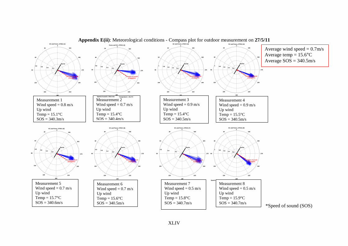
XLIV
Appendix E(ii): Meteorological conditions - Compass plot for outdoor measurement on 27/5/11
0.2 0.4
0.6 0.8
30
210
60
240
90 270
120
300
150
330
180
0
SC and Fence, 270511 (1)
Speed of sound = 340.3 m/s Temperature = 15.1 C
Barrier
Direction of sound
propagation
Measurement 1
Wind speed = 0.8 m/s
Up wind
Temp = 15.1°C
SOS = 340.3m/s
Measurement 2
Wind speed = 0.7 m/s
Up wind
Temp = 15.4°C
SOS = 340.4m/s
0.2 0.4
0.6 0.8
30
210
60
240
90270
120
300
150
330
180
0
Fence and SC, 27/5/11 (2)
Speed of sound = 340.4 m/s Temperature = 15.4 C
Barrier
Direction of sound
propagation
0.2 0.4 0.6 0.8 1
30
210
60
240
90 270
120
300
150
330
180
0
SC and Fence, 27/5/11 (3)
Speed of sound = 340.5 m/s Temperature = 15.4 C
Direction of sound
propagation
Barrier
Measurement 3
Wind speed = 0.9 m/s
Up wind
Temp = 15.4°C
SOS = 340.5m/s
0.2 0.4 0.6 0.8 1
30
210
60
240
90 270
120
300
150
330
180
0SC and Fence, 27/5/11 (4)
Speed of sound = 340.5 m/s Temperature = 15.5 C
Barrier
Direction of sound
propagation
Measurement 4
Wind speed = 0.9 m/s
Up wind
Temp = 15.5°C
SOS = 340.5m/s
0.2 0.4
0.6 0.8
30
210
60
240
90270
120
300
150
330
180
0SC and Fence, 27/5/11 (5)
Speed of sound = 340.6 m/s Temperature = 15.7 C
Direction of sound
propagation
Barrier
Measurement 5
Wind speed = 0.7 m/s
Up wind
Temp = 15.7°C
SOS = 340.6m/s
0.2 0.4
0.6 0.8
30
210
60
240
90 270
120
300
150
330
180
0SC and Fence, 27/5/11 (6)
Speed of sound = 340.5 m/s Temperature = 15.6 C
Direction of sound
propagation
Barrier
Measurement 6
Wind speed = 0.7 m/s
Up wind
Temp = 15.6°C
SOS = 340.5m/s
0.2 0.4
0.6
30
210
60
240
90 270
120
300
150
330
180
0SC and Fence, 27/5/11 (7)
Speed of sound = 340.7 m/s Temperature = 15.8 C
Direction of sound
propagation
Barrier
Measurement 7
Wind speed = 0.5 m/s
Up wind
Temp = 15.8°C
SOS = 340.7m/s
0.2 0.4 0.6 0.8 1
30
210
60
240
90 270
120
300
150
330
180
0
SC and Fence, 27/5/11 (8)
Speed of sound = 340.7 m/s Temperature = 15.9 C
Barrier
Direction of sound
propagation
Measurement 8
Wind speed = 0.5 m/s
Up wind
Temp = 15.9°C
SOS = 340.7m/s
Average wind speed = 0.7m/s
Average temp = 15.6°C
Average SOS = 340.5m/s
*Speed of sound (SOS)
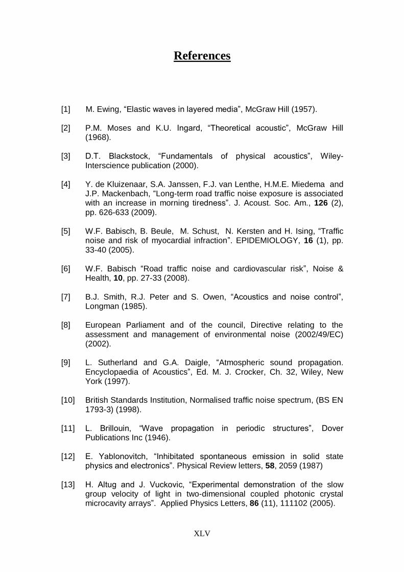
XLV
References
[1] M. Ewing, “Elastic waves in layered media”, McGraw Hill (1957). [2] P.M. Moses and K.U. Ingard, “Theoretical acoustic”, McGraw Hill
(1968). [3] D.T. Blackstock, “Fundamentals of physical acoustics”, Wiley-
Interscience publication (2000). [4] Y. de Kluizenaar, S.A. Janssen, F.J. van Lenthe, H.M.E. Miedema and
J.P. Mackenbach, “Long-term road traffic noise exposure is associated with an increase in morning tiredness”. J. Acoust. Soc. Am., 126 (2), pp. 626-633 (2009).
[5] W.F. Babisch, B. Beule, M. Schust, N. Kersten and H. Ising, “Traffic
noise and risk of myocardial infraction”. EPIDEMIOLOGY, 16 (1), pp. 33-40 (2005).
[6] W.F. Babisch “Road traffic noise and cardiovascular risk”, Noise &
Health, 10, pp. 27-33 (2008). [7] B.J. Smith, R.J. Peter and S. Owen, “Acoustics and noise control”,
Longman (1985). [8] European Parliament and of the council, Directive relating to the
assessment and management of environmental noise (2002/49/EC) (2002).
[9] L. Sutherland and G.A. Daigle, “Atmospheric sound propagation.
Encyclopaedia of Acoustics”, Ed. M. J. Crocker, Ch. 32, Wiley, New York (1997).
[10] British Standards Institution, Normalised traffic noise spectrum, (BS EN
1793-3) (1998). [11] L. Brillouin, “Wave propagation in periodic structures”, Dover
Publications Inc (1946). [12] E. Yablonovitch, “Inhibitated spontaneous emission in solid state
physics and electronics”. Physical Review letters, 58, 2059 (1987) [13] H. Altug and J. Vuckovic, “Experimental demonstration of the slow
group velocity of light in two-dimensional coupled photonic crystal microcavity arrays”. Applied Physics Letters, 86 (11), 111102 (2005).
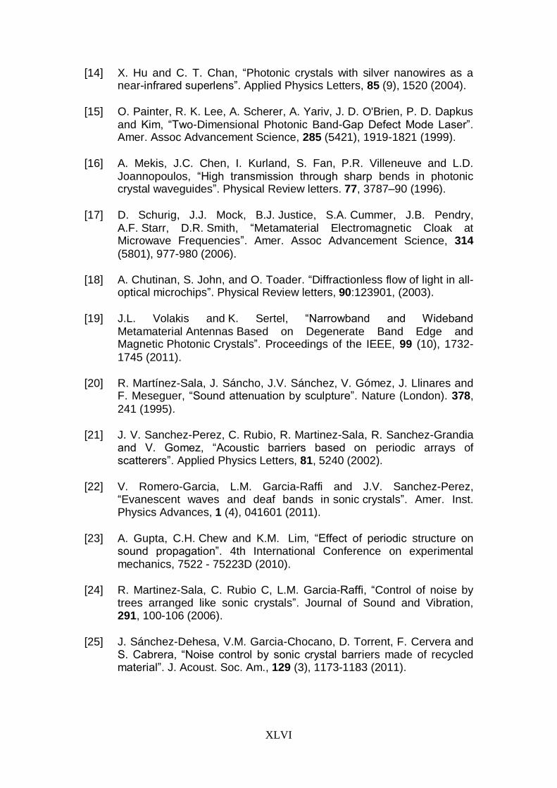
XLVI
[14] X. Hu and C. T. Chan, “Photonic crystals with silver nanowires as a near-infrared superlens”. Applied Physics Letters, 85 (9), 1520 (2004).
[15] O. Painter, R. K. Lee, A. Scherer, A. Yariv, J. D. O'Brien, P. D. Dapkus
and Kim, “Two-Dimensional Photonic Band-Gap Defect Mode Laser”. Amer. Assoc Advancement Science, 285 (5421), 1919-1821 (1999).
[16] A. Mekis, J.C. Chen, I. Kurland, S. Fan, P.R. Villeneuve and L.D.
Joannopoulos, “High transmission through sharp bends in photonic crystal waveguides”. Physical Review letters. 77, 3787–90 (1996).
[17] D. Schurig, J.J. Mock, B.J. Justice, S.A. Cummer, J.B. Pendry,
A.F. Starr, D.R. Smith, “Metamaterial Electromagnetic Cloak at Microwave Frequencies”. Amer. Assoc Advancement Science, 314
(5801), 977-980 (2006). [18] A. Chutinan, S. John, and O. Toader. “Diffractionless flow of light in all-
optical microchips”. Physical Review letters, 90:123901, (2003).
[19] J.L. Volakis and K. Sertel, “Narrowband and Wideband
Metamaterial Antennas Based on Degenerate Band Edge and Magnetic Photonic Crystals”. Proceedings of the IEEE, 99 (10), 1732-
1745 (2011). [20] R. Martínez-Sala, J. Sáncho, J.V. Sánchez, V. Gómez, J. Llinares and
F. Meseguer, “Sound attenuation by sculpture”. Nature (London). 378,
241 (1995). [21] J. V. Sanchez-Perez, C. Rubio, R. Martinez-Sala, R. Sanchez-Grandia
and V. Gomez, “Acoustic barriers based on periodic arrays of scatterers”. Applied Physics Letters, 81, 5240 (2002).
[22] V. Romero-Garcia, L.M. Garcia-Raffi and J.V. Sanchez-Perez,
“Evanescent waves and deaf bands in sonic crystals”. Amer. Inst. Physics Advances, 1 (4), 041601 (2011).
[23] A. Gupta, C.H. Chew and K.M. Lim, “Effect of periodic structure on
sound propagation”. 4th International Conference on experimental mechanics, 7522 - 75223D (2010).
[24] R. Martinez-Sala, C. Rubio C, L.M. Garcia-Raffi, “Control of noise by
trees arranged like sonic crystals”. Journal of Sound and Vibration, 291, 100-106 (2006).
[25] J. Sánchez-Dehesa, V.M. Garcia-Chocano, D. Torrent, F. Cervera and
S. Cabrera, “Noise control by sonic crystal barriers made of recycled material”. J. Acoust. Soc. Am., 129 (3), 1173-1183 (2011).
XLVII
[26] D.P. Elford, L. Chalmers, F.V. Kusmartsev and G.M. Swallowe, “Matryoshka locally resonant sonic crystal”. J. Acoust. Soc. Am., 130
(5), 2746-2755 (2011). [27] C. Kittel, “Introduction to solid state physic”, John Wiley & Sons Inc, 8
editions (2005). [28] R.H.III. Olssen and I. EL-Kady, “Microfabricated Phononic Crystal
devices and applications”. Meas. Sci. Technol., 20 012002 (2009). [29] T. Miyashita, “Sonic crystals and sonic wave-guides”. Meas. Sci.
Technol., 16, 47-63 (2005).
[30] M. Plihal and A.A. Maradudin, “Photonic band structure of two-
dimensional systems: The triangular lattice”. Physical Review B, 44, 8565-8571 (1991).
[31] P.R. Villeneuve and M. Piché, “Photonic band gaps in two-dimensional
square and hexagonal lattices”. Physical Review B, 46, 4969-4972 (1992).
[32] R.D. Meade, K.D. Brommer, A.M. Rappe, and J.D. Joannopoulos,
“Existence of a photonic band gap in two dimensions”, Applied Physics Letters, 61, 495-497 (1992).
[33] K.M. Ho, C.T. Chan, and C.M. Soukoulis, “Existence of a photonic gap
in periodic dielectric structures”. Physical Review Letters, 65, 3152-3155 (1990).
[34] Y.M. Soliman, M.F. Su, Z.C. Leseman, C.M. Reinke, I. El-kady and
R.H.III Olsson, “Phononic crystals operating in the gigahertz range with extremely wide band gaps”. Applied Physics Letters, 97, 193502
(2010). [35] J.V. Sánchez-Pérez, D. Caballero, R. Martínez-Sala, J. Sánchez-
Dehesa, F. Meseguer, J. Llinares and F. Gálvez, “Sound Attenuation by a Two-Dimensional Array of Rigid Cylinders”. Physical Review Letters, 80, 5325 (1998).
[36] M.S. Kushwaha and B. Djafari-Rouhani, “Complete acoustic stop
bands for cubic arrays of spherical liquid balloons”. Applied Physics, 80, 3191-3195 (1996).
[37] Y. Chen and Z. Ye, “Theoretical analysis of acoustic bands in two-
dimensional periodic arrays”. Physical Review E, 64, 036616 (2001). [38] J.O. Vasseur, P.A. Deymier, B. Djafari-Rouhani, Y. Pennec, A-C.
Hladky-Hennion, “Absolute forbidden bands and waveguiding in two-dimensional phononic crystal plates”. Physical Review B, 77, 085415 (2008).
XLVIII
[39] M.S. Kushwaha, P. Halevi , G. Martínez, L. Dobrzynski and B. Djafari-Rouhani, “Theory of acoustic band structure of periodic elastic composites”. Physical Review B, 49, 2313-2322 (1994).
[40] M. Wilm, S. Ballandras, V. Laude and T. Pastureaud, “A full 3D plane-
wave-expansion model for 1-3 piezoelectric composite structures”. J. Acoust. Soc. Am., 112, 943-952 (2002).
[41] Y. Cao, Z. Hou and Y. Liu, “Convergence problem of plane-wave
expansion method for phononic crystals”. Physics Letter A, 327, 247-
253 (2004). [42] www.engineeringtoolbox.com/wood-density-d_40.html, last accessed
on 15/2/11. [43] D. P. Elford, “Band gap formation in acoustically resonant phononic
crystals”, PhD thesis (2010). [44] M.I. Mishchenko, D.W. Mackowski and L.D. Travis, “Scattering of light
by bispheres with touching and separated components”. Applied Optics, 34, 21, 4589 (1995).
[45] F. Zaviska, “Uber die beugung elektromagnetischer wellen an
parallelen, unendlich langen kreisylindern”. Ann. Phys., 40, 1023
(1913). [46] D.W. Mackowski and M.I. Mishchenko, “Direct simulation of multiple
scattering by discrete random media illuminated by Gaussian beams”. Physical Review A, 83, 013804 (2011).
[47] V. Twersky, “Multiple scattering of radiation by an arbitrary
configuration of parallel cylinders”. J. Acoust. Soc. Am., 24, 1, 42-46
(1952). [48] L.L. Araujo, G.F. Foran and M.C. Ridgway, “Multiple scattering effects
on the EXAFS of Ge nanocrystal”. Journal of Physics: Condense Matter, 20, 165210 (2008).
[49] C.M. Linton and D.V. Evans, “The interaction of waves with arrays of
vertical circular cylinders”. J. Fluid Mech., 215, pp549-569 (1990).
[50] S. Boscolo and M. Midrio, “Three-Dimensional Multiple-Scattering
Technique for the Analysis of Photonic-Crystal Slabs”. J. of Lightwave Technology, 22 (12), 2778-2786 (2004).
[51] J.M. Elson, “Infrared light scattering from surfaces covered with
multiple dielectric overlayers”. Applied Optics 16 (11), 2872–2881 (1977).
XLIX
[52] A. Aubry, A. Derode, “Multiple scattering of ultrasound in weakly inhomogeneous media: Application to human soft tissues”. J. Acoust. Soc. Am., 129 (1), 225-233 (2011).
[53] P.A. Martin, “MULTIPLE SCATTERING – Interaction of Time-Harmonic
Waves with N Obstacles”, Cambridge University Press (2006). [54] L. Rayleigh, “On the influence of obstacles arranged in rectangular
order upon the properties of a medium”. Phil. Mag., Series 5, 34, 481-502 (1892).
[55] A.K. Mal and S.K. Bose, “Dynamic elastic moduli of a suspension of
imperfectly bonded spheres”. Proceeding of the Cambridge Philosophical Society, 76, 587-600 (1974).
[56] P.C. Waterman, “Symmetry unitarity and geometry in electromagnetic
scattering”. Physical Review D, 3, 825-839 (1971). [57] V. Twersky, Multiple scattering of radiation by an arbitrary configuration
of parallel cylinders”, J. Acoust. Soc. Am., 24, 42-46, (1952).
[58] I.S. Gradshteyn and I.M. Ryzhik, “Table of integrals, series and
products”, 6 editions, 8.51-8.52, MO 27, 926 (2000). [59] O. Umnova, K. Attenborough and C.M. Linton, “Effects of porous
covering on sound attenuation by periodic arrays of cylinders”. J. Acoust. Soc. Am., 119, 278-284 (2006).
[60] R.D. Cook, D.S. Malkus, M.E. Plesha and R.J. Witt, “Concepts and
applications of finite element analysis”. John Wiley & Sons, 4 editions, Chapter 1, pp 10 (2002).
[61] G.M.L. Gladwell, “A finite element method for acoustics”. Proceedings
of the 5th International Congress on Acoustics, Leigh, Belgium (1965). [62] B.R. Mace, D. Duhamel and M.J. Brennan, “Finite element prediction of
wave motion in structural waveguides”. J. Acoust. Soc. Am., 117(5), 2835-2843 (2005).
[63] M. Hofer, N. Finger and G. Kovacs, “Finite-element simulation of wave
propagation in periodic piezoelectric SAW structures”, IEEE Transcactions on ultrasonics ferroelectrics and frequency control, 53
(6), 1192-1201 (2006). [64] T. Delort, “Finite-element method for gratings”. J. Opt. Soc. Am., A, 10,
12, 2592-2601 (1993). [65] X. Wei, A.J. Wachters and H.P. Urbach, “Finite-element model for
three-dimensional optical scattering problems”, J. Opt. Soc. Am., A, 24, 3, 866-881 (2007).

L
[66] C. Lally, F. Dolan and P.J. Prendergast, “Cardiovascular stent design and vessel stresses: a finite element analysis”. Journal of Biomechanics, 38 (8), 1574-1581 (2005).
[67] P. Majumdar, R. Jayaramachandran and S. Ganesan, “Finite element
analysis of temperature rise in metal cutting process”. Applied thermal engineering, 25 (4), 591-601 (2005).
[68] E. Ferrie, J.Y. Buffiere and W. Ludwig, “Fatigue crack propagation: In
situ visualisation using X-ray microtomography and 3D simulation using the extended finite element method”. ACTA Materialia, 54 (4), 1111-1122 (2006).
[69] O. Ozgun and M. Kuzuoglu, “Non-Maxwellian locally-conformal PML
absorbers for finite element mesh truncation”. IEEE Transactions on Antennas and propagation, 55(3), 931-937 (2007).
[70] J. Mackerle, “Some remarks on progress with finite elements”.
Computers & structures, 55 (6), 1101-1106 (1995). [71] O.A. Kaya, A. Cicek and B. Ulug, “Forcusing with two-dimensional
angular-symmetric circular acoustic lenses”. Acoustical Physics, 57 (3),
292-300 (2011). [72] M. Hirsekorn and P.P. Delsanto, “Design and optimization of locally
resonating sonic crystals”, 2003 IEEE Ultrasonics Symposium Proceedings, 1, 1491-1494 (2003).
[73] S. Guenneau and A.B. Movchan. “Analysis of elastic band structures
for oblique incidence”. Archieve for Rational Mechanics and Analysisl, 171, 129-150 (2004).
[74] COMSOL® Multiphysics Modelling Guide, version 3.5a, chapter 3, 26
(2008). [75] M.S. Mohamed, O. Laghrouche and A. El-kacimi, “Some numerical
aspects of the PUFEM for efficient solution of 2D Helmholtz problem”. Computers & Structures, 88 (23), 1484-1491 (2010).
[76] L. Wu and L. Chen, “The dispersion characteristics of sonic crystals
consisting of elliptic cylinders”. Journal of Physical D: Applied Physic, 40, 7579-7583 (2007).
[77] M. Zampolli, A. Tesei, F.B. Jensen, N. Malm, J.B. Blottman, “A
computationally efficient finite element model with perfectly matched layers applied to scattering from acially symmetric objects”. J. Acoust. Soc. Am., 122, 1472-1485 (2007).
[78] http://www.liminal.org.uk/organ-of-corti/, last accessed on 25/7/11.

LI
[79] T. Miyashita, W. Sato and Y. Nakaso, “Experimental studies on two-dimensional defect-mode waveguides in a sonic/phononic crystal”, Japanese Journal of Applied Physic Part 1-Regular papers brief communications & review papers, 46 (7B), 4684-4687 (2007).
[80] Y. Pennec, B. Djafari-Rouhani, H. Larabi, J. Vasseur, A.C. Hladky-
Hennion, “Phononic crystals and manipulation of sound”, Physica status solidi C – current topics in solid state physics, 6 (9), 2080-2085
(2009). [81] V. Romero-Garcia, J.V. Sanchez-Perez, L.M. Garcia-Raffi, J.M.
Herrero, S. Garcia-Nieto, X. Blasco, “Hole distribution in phononic crystals: Design and optimization”. J. Acoust. Soc. Am., 125 (6), 3774-3783 (2009).
[82] T. Miyashita, “Acoustic defect-mode waveguides fabricated in sonic
crystal: Numerical analyses by elastic finite-difference time-domain method”, Japanese Journal of Applied Physic Part 1 - Regular papers brief communications & review papers, 45 (5B), 4440-4447 (2006).
[83] J.D. Turner and A.J. Pretlove, “Acoustic for engineers”, Macmillan
(1991). [84] M.R. Schroeder, “Integrated-impulse method for measuring sound
decay without using impulses”. 66, no. 2, pp. 497–500 (1979). [85] M. Vorländer and M. Kob, “Practical aspects of MLS measurements in
building acoustics”. APPLIED ACOUSTICS, 52 (3-4), 239-258 (1997).
[86] K Heutschi and A. Rosenheck, “Outdoor sound propagation
measurements using an MLS technique”. Applied Acoustics, 51 (1), 13-32 (1997).
[87] D.G. Ciric and M.A. Milosevic, “Transient noise influence
in MLS measurement of room impulse response”. ACTA Acustica United with Acustica, 91 (1), 110-120 (2005).
[88] D.D. Rife, “Maximum-Length-Sequence-Analyzer (Reference Manual)”,
DRA Laboratories, Ver. 10WI, Rev. 8 (1987). [89] BS EN 1793-6, “Road traffic noise reducing devices. Test method for
determining the acoustic performance. Part 6. Intrinsic characteristics. In situ values of airborne sound insulation under direct sound field conditions” (2010).
[90] F.J. Harris, “On the use of windows for Harmonic Analysis with the
Discrete Fourier Transform”. Proceeding of the IEEE, 66, 1 (1987). [91] ANSI S12.8 - 1998, “Methods for Determination of Insertion Loss of
Outdoor Noise Barriers” (2008).

LII
[92] A. Farina, “Simultaneous measurement of impulse response and distortion with a Swept-sine technique”. 108th Audio Engineering Society Convention, 5093 (D-4) (2000).
[93] T. Legouis and J. Nicolas, “Phase gradient method of measuring the
acoustic impedance of materials”, J. Acoust. Soc. Am., 81 (1), 33-50
(1987). [94] S. Guy-Bart and E. Jean-Jacques, A. Dominique, Comparison of
different impulse response measurement techniques”, Journal of Audio Engineering Society, 50 (4), 249-262 (2002).
[95] K. Suzuki, “X-ray studies on precipitation of metastable centers in
mixed crystals nacl-cdcl2”, J.Phys. Soc. Jpn., 16:67 (1961).
[96] D. Caballero, J. Sánchez-Dehesa, R. Martínez-Sala, C. Rubio, J.V.
Sánchez-Pérez, L. Sanchis, and F. Meseguer. “Suzuki phase in two-dimensional sonic crystals”. Physical Review B, 64:064303 (2001).
[97] F.G. Wu, Z.L. Hou, Z.Y. Liu, and Y.Y. Liu. “Point defect states in two-
dimensional phononic crystals”. Physics Letter A, 292:198 (2001). [98] M. Sigalas, “Eastic wave band gaps and defect states in two-
dimensional composites”. J. Acoust. Soc. Am., 101, 1257 (1997).
[99] R. Sainidou, B. Djafari-Rouhani, Y. Pennec and J.O. Vasseur, “Locally
resonant phononic crystals made of hollow spheres or cylinders”. J. Acoust. Soc. Am., 119, 278-284 (2006).
[100] M. Hirsekorn, P.P. Delsanto, N.K. Batra and P. Matic, “Modelling and
simulation of acoustic wave propagation in locally resonant sonic materials”. Ultrasonics, 42, 231-235 (2004).
[101] M.S. Kushwaha and P. Halevi, “Stop bands for cubic arrays of
spherical balloons”. J. Acoust. Soc. Am., 101, 619-622 (1997). [102] E. Fuster-Garcia, V. Romero-Garcia, J. V. Sánchez-Pérez, and L. M.
Garcia-Raffi, “Targeted band gap creation using mixed sonic crystal arrays including resonators and rigid scatterers,” Applied Physics Letter 90, 244104 (2007).
[103] F. Wang, C.K. Mechefske, “Modal Analysis and testing of a thin-walled
gradient coil cylinder model”. Concepts in Magnetic resonance part B – Magnetic resonance engineering, 27B, 34-50 (2005).
[104] A. Krynkin and O. Umnova, “Characteristics of wave propagation
through doubly-periodic array of elastic shells”. paper presented at EuroNoise (2009).

LIII
[105] N.A. Nicorovici, R.C. Mcphedran, “Photonic band gaps for arrays of perfectly conducting cylinders”. Physical Review E, 52, 1135-1145
(1995). [106] G.C. Gaunaurd, “Sonar cross section of a coated hollow cylinder in
water”. J. Acoust. Soc. Am., 61, 360–368 (1977).
[107] J.D. Kaplunov, L. Yu. Kossovich and E.V. Nolde, “Dynamic of thin
walled elastic bodies”. Academic Press London, 110 (1998). [108] B. Merheb, P.A. Deymier, M. Jain, M. Aloshyna-Lesuffleur, S. Mohanty,
A. Barker and R.W. Greger, “Elastic and viscoelastic effects in rubber-air acoustics band gap structure: A theoretical and experimental study”. J. Applied Physics, 104, 064913 (2008).
[109] http://www.makeitfrom.com/data/?material=Natural_Rubber, last
accessed on 11 Aug 2011. [110] http://www.engineeringtoolbox.com/density-solids-d_1265.html, last
accessed on 11 Aug 2011. [111] A. Krynkin, O. Umnova, A.Y.B. Chong, S. Taherzadeh and K.
Attenborough, “Predictions and measurements of sound transmission through a periodic array of elastic shells in air”. J. Acoust. Soc. Am., 128, 3496-3506 (2010).
[112] J.B. Pendry, A.J. Holden, W.J. Stewart, and I. Youngs, “Magnetism
from conductors, and enhanced non-linear phenomena.” IEEE Trans. Microw. Theory Tech., 47, 2975 (1999).
[113] A.B. Movchan and S. Guenneau, “Split-ring resonators and localized
modes”. Physical Review B, 70, 125116 (2004).
[114] L.Y. Wu, L.W. Chen, M.L. Wu, “The nondiffractive wave propagation in
the sonic crystal consisting of rectangular rods with a slit”, Journal of physics – Condensed Matter, 20, 295229 (2008).
[115] R. Marques, F. Mesa, J, Martel and F Medina, “Comparitive analysis of
edge- and broadside- coupled split ring resonators for metamaterial design, theory and experiments”. IEEE Transactions on Antennas and Propagation, 51, 2572 (2003).
[116] K. Aydin and E. Ozbay, “Capacitor-loaded split ring resonators as
tunable metamaterial components”. Journal of Applied Physics, 101,
024911 (2007). [117] X. Hu and C.T. Chan, “Two-dimensional sonic crystals with Helmholtz
resonators”. Physical Review E, 71, 055601 (2005).

LIV
[118] W. Elmore and M. Heald, “Physics of Waves”, New York: McGraw-Hill, p. 148 (1969).
[119] C.H. Sohn and J.H. Park, “A comparative study on acoustic damping
induced by half-wave, quarter-wave and Helmholtz resonators”. Aerospace Science and Technology, 15, 606 (2011).
[120] L. Kinsler, A. Frey, A. Coppens and J. Sanders, “Fundamentals of
Acoustic”. John Wiley and Sons, New York, third edition (1982). [121] F.P. Mechel, “Formulas of acoustics”, Springer Verlag, New York Inc
(2008). [122] S.G.L. Smith and A.M.J. Davis, "The split ring resonator". Proceedings
of the Royal Society A, 466, 3117-3134 (2010). [123] Z.Y. Cui, T.N. Chen and Y.P. Su, “Experimental and calculated
research on a large band gap constituting of tubes with periodic narrow slits”. Applied Acoustics 70, 1087 (2009).
[124] F. Montiel and M. Neviere, “Perfectly conducting gratings: a new
approach using infinitely thin strips”. Optics Communications, 144, 82
(1997). [125] B. Guizal and D Felbacq, “Numerical computation of the scattering
matrix of an electromagnetic resonator”. Physical Review E, 66,
026602 (2002). [126] A.D. Rawlins, “Approximate boundary conditions for diffraction by thin
transmissive media”. ZAMM - Journal of Applied Mathematics and Mechanics 87, 711 (2007).
[127] M. Abramowitz and I.A. Stegun, “Handbook of Mathematical Functions,
National Bureau of Standards, New York: Dover, 363 (1972). [128] A. Krynkin, O. Umnova, A.Y.B. Chong, S. Taherzadeh and K.
Attenborough, “Scattering by coupled resonating elements in air”. Journal of Physics D: Applied Physics, 44, 125501 (2011).
[129] A. Kyrnkin, O. Umnova, J.V. Sanchez-Perez, A.Y.B. Chong, S.
Taherzadeh, K. Attenborough, “Acoustic insertion loss due to two dimensional periodic arrays of circular cylinders parallel to a nearby surface”, J. Acoust. Soc. Am., 130, (6) (2011).
[130] R. H. Olsson III , I. EI-Kady, M. F. Su, M. R. Tuck, F. B. McCormick and
J. G. Fleming, “Research on micro-size acoustic bandgap structure”, SANDIA Report, SAND2010-0044, page 15 (2010).
[131] R. Kruse, “In-situ measurement of ground impedances”, PhD Thesis,
(2008).
LV
[132] W. K. Lui and K.M. Li, “The scattering of sound by a long cylinder
above an impedance boundary”. J. Acoust. Soc. Am., 127 (2), 664-674 (2010).
[133] J. C. Bertrand and J. W. Young, “Multiple scattering between a cylinder
and a plane”. J. Acoust. Soc. Am., 60 (6), 1265-1269 (1976). [134] G. Watts, “Harmonise prediction model for road traffic noise”, Transport
Research Laboratory report, PPP034 (2005). [135] D. van Maercke and J. Defrance, “Development of an analytical model
for outdoor sound propagation within the Harmonoise project”, ACTA Acustica United with Acustica, 93, 201 (2007).
[136] K. Attenborough, K.M. Li, K. Horoshenkov, “Predicting Outdoor Sound”,
Taylor & Francis, (2007). [137] M.E. Delany and E.N. Bazley, “Acoustic properties of fibrous absorbent
materials”. Applied Acoustics, 3, pp 105-116 (1970).
[138] K. Attenborough and I. Ver, “Noise and vibration control engineering”.
Beranek and Ver ed, New York (USA), 3rd Edition (2008). [139] K. Attenborough, I. Bashir and S. Taherzadeh, “Outdoor ground
impedance models”. J. Acoust. Soc. Am., 129 (5) 2806 – 2819 (2011)).
[140] American National Standard method for determining the acoustic
impedance of ground surfaces (2010). [141] P. Boulanger, K. Attenborough, Q. Qin and C.M. Linton, “Reflection of
sound from random distributions of semi-cylinders on a hard plane: models and data”. Journal of Physics D: Applied Physics, 38, 3480-3490 (2005).
[142] A. Krynkin and O. Umnova, “On performance of sonic crystals in
presence of ground plane”. Proceedings of Inter-noise, Lisbon (2010). [143] D.C. Hothershall, D.H. Crombie, S.N. Chandler-Wilde, “The
performance of T-profile and associated noise barriers,” Applied Acoustics, 32, 269-287 (1991).
[144] G.R. Watts, “Acoustic performance of a multiple edge noise barrier
profile at motorway sites.” Applied Acoustics, 47, 47-66 (1996).
[145] M.R. Monazzam and Y.W. Lam, “Performance of Profiled Single Noise
Barriers Covered with Quadratic Residue Diffusers”, Applied Acoustics 66, pp.709-730 (2005)

LVI
[146] J. Berenger "A perfectly matched layer for the absorption of electromagnetic waves". Journal of Computational Physics 114 (2),
185–200 (1994). [147] A. Kyrnkin, O. Umnova, J.V. Sanchez-Perez, A.Y.B. Chong, S.
Taherzadeh, K. Attenborough, “Acoustic insertion loss due to two dimensional periodic arrays of circular cylinders parallel to a nearby surface”, J. Acoust. Soc. Am., 130, (6) (2011).