Some theoretical aspects in computational analysis of adhesive lap joints

INTERNATIONAL JOURNAL FOR NUMERICAL METHODS IN ENGINEERING, VOL. 35, 1237-1262 (1992)

SOME THEORETICAL ASPECTS IN COMPUTATIONAL ANALYSIS OF ADHESIVE LAP JOINTS

P. DESTUYNDER

Institut ACrotechnique de Saint-Cyr, C N A M , 78210 Saint-Cyr-I'Ecole, France

F. MICHAVILA AND A. SANTOS

Departamento de Matematica Aplicada y Mktodos Informaticos, E TSI de Minas, 28003 Madrid, Spain

AND

Y . OUSSET

Ofice National d'Etudes et de Recherches ACrospatiales, 92320 Chatillon, France

SUMMARY This paper is devoted to the numerical analysis of bidimensional bonded lap joints. For this purpose, the stress singularities occurring at the intersections of the adherend-adhesive interfaces with the free edges are first investigated and a method for computing both the order and the intensity factor of these singularities is described briefly. After that, a simplified model, in which the adhesive domain is reduced to a line, is derived by using an asymptotic expansion method. Then, assuming that the assembly debonding is produced by a macro-crack propagation in the adhesive, the associated energy release rate is computed. Finally, a homogenization technique is used in order to take into account a preliminary adhesive damage consisting of periodic micro-cracks. Some numerical results are presented.

INTRODUCTION

The wide spread use, in industry, of bonding as an assembly technique depends on capabilities of knowing precisely the mechanical behaviour of such assemblies under loading. To this end, a combination of two kinds of approaches, local and global ones, is proposed here. The purpose of the former is to study the stress singularities occurring at the intersection points of an adherend-adhesive interface with a free edge, on the one hand, and at the intersection points of two interfaces, on the other. In the latter, a simplified model of bonded joint is derived that allows the study of both the assembly debonding and the adhesive damage caused by micro-cracks development.

Now, it is well-known' that, near a singular point, the displacement field u can be written, in polar coordinates (see Figure l), as

N.

u = uR + K,rang"(B) (1) n = 1

where uR is the regular part of u, N , is the number of singularities, a, is the singularity order satisfying 0 < Re(&,) < 1 (Re stands for the real part) and K , is the intensity factor.

0029-598 1/92/191237-26S18.00 0 1992 by John Wiley & Sons, Ltd.

Received 9 October 1990 Revised 17 December 1991

1238 P. DESTUYNDER, F. MICHAVILA, A. SANTOS AND Y. OUSSET

" I r

Figure 1. Adhesive laps joint-notations

The next section is devoted to the determination of both singularity orders and intensity factors. Let us begin by determining the singularity orders. The methods used at this time are of two kinds:

(i) numerical methods in which a,, and g" are the eigenvalues and the eigenfunctions, respect-

(ii) analytical methods using, following Lekhnit~kii ,~ formulations in terms of the Airy stress ively, of an eigenvalue problem depending only on t9,2,

functions. -

Here, a method of this latter kind is described. The computation of intensity factors is conducted extending to the elasticity problem for

multimaterials, the concept of dual singular functions first introduced for the Laplacian. 2,

These dual singular fields can be viewed as the right extraction functions in the sense of Babuska and Miller14 for intensity factors. Applications to the study of a single lap joint are presented.

In most situations encountered, the ratios between adhesive thickness and overlap length, on the one hand, and between Young's modulus of the adhesive and the adherend, on the other, are small parameters. Under the assumption that these parameters are of the same order, a simplified model is derived in the third section using an asymptotic expansion method. The limit model so obtained is similar to the model proposed by Goodman et al.' The associated adhesive element has the same shear stiffness as both Barker and Hatt's element16 and Johnson's element17 but the normal stiffness is somewhat different.

At last, it is pointed out that the models presented here are derived making a plane-strain assumption. Nevertheless, similar models can be obtained under plane-stress assumption by using the same methodology.

ADHESIVE LAP JOINTS 1239

STRESS SINGULARITIES INVESTIGATIONS

The problem to be solved

It is assumed in the sequel that the materials are isotropic and that the assembly is under a plane-strain state. So, the problem to be solved is bidimensional and is governed by the equations

CT,~,~(U) = 0 in R u = O on To

a(u)+n = 0 on r; a, fi = 1 , 2 a(u).n = t on T,

[u] = [a(u)*n] = 0 on C,

where [u] is the jump of u through Za (see Figure 1). The stress a is related to the strain y by the Hooke’s law

with Y ~ S = $(ua,fi + up,,) (4)

Here R is the stiffness tensor, E is the Young’s modulus and v is the Poisson’s ratio.

Singularity-order determination

homogeneous problem, The asymptotic behaviour of u near a singular point A is given by the non-zero solutions of the

v . ~ , ~ ( S ) = 0 in R, a(S).n=O on r:

IS] = [a(S).n] = 0 on C, +conditions at infinity

set in an unbounded domain (see Figure 1). The determination of S is performed I complementary energy formulation of problem (5)

ai ing from the

for any self-equilibrated stress field t (satisfying equations (5)) . Here, S = R-’ is the plane-strain compliance tensor. Then, introducing the Airy stress function Y such that

6 1 1 = y ’ . 2 2 ; 6 1 2 = - y.12; 6 2 2 = Y,l l (7) the free-edge condition on T: becomes


whereas equation (6) gives rise to the following relations. lo, 11318

(i) Compatibility equation in Q,:

A2Y = O (ii) Jump conditions through Z,

1 "yn = vx = 0

(9)

The solutions of problem (9) are ~el l -known.~ In Q:, Y can be written as

Y = a:(xl + ix2)d + a$(xl - ix2)(x1 + ix2)"-'

+ a:(xl - ix2)' + a,'(xl + ix2)(xl - ix2)'-' (1 1)

with i = n. On substituting expression (11) into equations (8) and (lo), one obtains: (iii) Boundary conditions on I-2

u:eid8+ + a;ei(d-2)B+ + a3+e-i18+ + a q + e i ( A - 2 ) B + -

- ( 2 - 2)aq+ei(A--2)f-J+ =

+ u3-e-iM- + aqe - i (A-2 )8 - = 0 (12)

Aa;e-ide- - ( 2 - 2)a;ei(d--2)8- = -: 0 I lal-ei"- + (A - 2)a;ei(d-2)8- -

+ M e - ' " + Aa;eid8+ + (A - 2)a;ei(A--2"3+

,l-eiA9- + a;ei(d-2)8-

where 8' and 8- are the polar angles of r: and r,, respectively, measured from the interface.

(iv) Jump conditions through Em

1 + a2 + a3 + a o j = o [ l a l + ( A - 2)a2 - La3 - (A - 2)a4] = .O

[i {Aal + [A - 4(1 - v)]a2 + l a 3 + [A - 4(1 - v)]a4}

[${AU1 + [A + 2(1 - 2v)laz + Au3 - [A + 2(1 - 2v)]a4}

Thus, the unknown coefficients a' are the solutions of a homogeneous linear system of eighth order given by equations (12) and (13) and written in condensed form as

K(A).a = 0 (14)

(15) These values are either real or complex conjugate. When A is real, one has a3 = iil and a4 = ii2, where 2 is the complex conjugate of a. Then, equations (12) and (13) reduce to those given by Rao' (Table 2c, column 1 and Table 2b, column B, respectively).

The desired values of A are the roots of the determinant of K satisfying the inequalities

1 < Re(A) < 2


In order to compute I , the strip (1 < Re(I) < 2; 0 d Im(I ) d A,!,ax} of the complex plane is squared (see Figure 2). The determinant A(K) of K is evaluated at each node using a Gauss method. The roots of A(K) are located in squares at the nodes of which both Re(A(I)) and Im (A(I)) do not maintain the same sign. When such a square is found, it is subdivided into four squares and the process is repeated until the convergence is reached. The value of I,!,,ax is taken of order unity. All the numerical experiments we have conducted have shown that the roots were located near the real axis. Once the I's are known, system (14) is solved in order to determine their associated ai.

Intensity factors determination

We have just seen that the displacement field could have singularities. The same is true for its dual, the field of loadings. This is why the singular parts of the loadings are called dual singular fields and denoted here as S*. These dual singularities are the tools which are going to allow us the computation of intensity factors.

The theory of dual singular fields is based on the mathematical properties of the elasticity ~ p e r a t o r ' ~ . ' ~ and seems to us too complex to be developed in this paper. Therefore, we are satisfied with just giving the main results which shall be accepted.

(i) At any singular point, there is the same number of dual singular fields as singular

(ii) S* belong to (L2(R))' and are solutions of the following elasticity problem: displacements.

(16)

(17)

r O , ~ , ~ ( S * ) = 0 in R S * = O on To

o(S*). n = 0 on dR - To Is*] = [e(S*).n] = 0 on c,

In spite of the boundary condition on To, this problem possesses non-zero solutions due to the weak-regularity required for S*.

(iii) At a singular point, S* can be written as

S* = S*(S*") = S*Rn + S*"; n = 1, . . . , N ,

1 2

Figure 2. Two-dimensional dichotomy to compute 1


where - S*" is the singular part of S*. It is locally a solution of problem ( 5 ) so that it is computed as S"

using the method described in the previous section. Due to the Lz (0) regularity requirement, the order A * of its associated Airy function (see relation (11)) must satisfy

0 < Re(A*) < 1

in place of condition (15). In fact, the A * values are directly deduced from the A values by the relations (see hereafter)

A,* +A, = 2; n = 1 , . . . , N , (18)

The coefficients a: are then computed by solving the linear system (14). - S*Rn is the regular part of S*. It is computed in order to satisfy equations (16). Introducing

the decomposition (17) into equations (16), one obtains that S*Rn is a solution of the following problems:

c ~ ~ , ~ ( S * ~ ~ ) = - C , ~ , ~ ( S * " ) in R

a(S*R").n= -a(S*").n (19)

On 1 S * R n = - s * n

on 30 - ro on c,

[a(S*Rn).n]= on Za

[s*"q = - [s*"]l = o

(iv) Once the singular fields are known, the intensity factors K, can be computed. If A,, is a single root of A ( K ) and if the neighbourhood of the singular point is unloaded, one has

where

and I.

Comments

(i) The A, values depend on the local geometry of the domain and on the material characteristics near the singular point only.

(ii) The integrals appearing in the definitions of both a, and b, are path-independent. As a consequence, these coefficients can be computed using different integration paths. The choice of a circular arc allows to determine a, analytically and to prove relation (18).

(iii) There are two ways to compute b,. If the domain bounded by the integration path and the free edges of the assembly contains only the singular point of interest (Figure 3(a)), relation (22) is used and only S*" is needed. In the opposite case (several singular points in the


Adherend 8 Adhesive

Adherend Adherend

Adhesive

(a) (b)

Figure 3. Integration paths surrounding (a) a single singular point; (b) several singular points

domain, Figure 3(b)), relation (23) is used and problem (19) must be solved. This latter way seems to be very attractive for the free-edge singularities computation in laminated plates because all the singular points can be investigated simultaneously.

(iv) The present method can be extended to various cases, such as anisotropic materials,’ - l 1

clamped edges,’ intersection of two interface^''^^ (or more). Of course, if the edges adjacent to the singular point are loaded, a logarithmic singularity’ can be added.

Numerical computation

The determination of b, involves finite element computations. We have programmed formula (22) uniquely, so that only the knowledge of the solution u (and also (a(u)) of problem (2) is needed. For this purpose, the domain is discretized using six-noded triangular and eight-noded serendipity quadratic elements. The integration path C in formula (22) is constituted by element edges Ci (see Figure 4(a)). Both the displacement u and the stress vector ( o ( u ) ) . n are known by their nodal values. As the dual singularities S*” are given in a local reference frame having the singular point as origin and the interface as x,-axis, u, ( a ( u ) ) . n and the nodal co-ordinates are expressed in this reference frame. For quadratic elements, the co-ordinates of any point of Ci are given by (see Figure 4(b)):

3

x ( l ) = c N/r(Ox(k) k = 1

where x ( k ) are the co-ordinates of node k, and N k are the following shape functions:

N I ( 0 = (1 - 5)(1 - 25); N 2 ( 5 ) = - 8 1 - 25); N 3 ( 0 = 4 a 1 - 0 Then, for any functionf one has .

r r i

with


Figure 4. Finite element approximation of the integration path

Finally, the integral along the edge Ci is computed with the aid of the Simpson's formula:

Numerical example

of edge shapes of the adhesive layer are considered (Figure 5): Here, a single lap joint submitted to a tensile stress of 1 MPa is analysed. Three different types

type I: Square edge type 11: 45" chamfered edge type 111: spew fillet

The materials have the following characteristics:

adhesive E 3 = Eb = 3400 MPa adherends El = E 2 = E , = 200000 MPa

Young's modulus

adhesive vg = vb = 035 adherends v1 = v2 = v, = 0.3

Poisson's ratio

All the computations were made for an overlap length lo = 50 mm and an adhesive thickness eb = 0 2 mm. The intensity factors were computed using an integration path located at a distance of eb/2 from the singular points and with four layers of elements between the singular point and the integration path.

The stress singularity order values are summarized in Table I. It can be seen that for type I1 and type-111 adhesive edges, there are two singularities at A2 (see Figure 5 for A2 location). The singular stresses along the adhesive-adherend interface are plotted in Figures 6 and 7 as functions of the distance to the singular point of interest. These figures show that the singularities effect is confined to a very small domain surrounding the singular point.

For both type-I1 and type-111 adhesive edges, the strongest singularity is located at point A2 as it can be seen in Table I. Accordingly, one can expect that the crack initiation takes place at this


I IT lII

Figure 5. Geometrical characteristics of the single lap joint

Table I. Stress singularity order values for the three types of adhesive edges

Type I I1 111

Point A1 A2 A1 A2 A, A2

Order -0.3273 -03015 -0.0219 -0142 -0.219 -0.2191 -04147 -0,3696

point. Figures 8 and 9 illustrate the dependence of singular stresses on polar angle. A possible crack propagation direction is given by ure = 0 and Uee maximum. Figure 10 shows that the angle value is nearly independent of the distance to the singular point. These directions are illustrated in Figure 11. For the type-I11 case, one obtains a crack propagation pattern pointed out by Groth and Jangblad.21

THE SIMPLIFIED MODEL

In the present section, we shall introduce a simplified model based on the assumption that both the ratios E , / E , and eb/lo are small parameters of the same order, say E. The derivation of the results stated here is tedious and somewhat technical; so, we shall be satisfied with giving the leading lines of the steps followed.

1246

0

7.5

5

2.5

0

- 2.5

P. DESTUYNDER, F. MICHAVILA, A. SANTOS AND Y. OUSSET

mm x 10-2 I I i -

0.1 0.5 1 x1

Figure 6. Type I: Stresses along the interface XI versus the distance from A,

The undamaged case

Starting from the variational problem associated with problem (2),

aa(u, v) + a3(u, v) = taua Vv k.a.; a = 1,2 .lrt

(k.a stands for kinematically admissible), where

ADHESIVE LAP JOINTS

o

7.5 -

5

2.5-

1 -

0 - 1 -

1247

4 (MPa)

i i -.i I I*\ 1. '=,. '\ -\ '*-*---. 022 ---.

-*-.-. 0 1 1 mm x 10-3

I I I 1 I t x1

012 0.1 0.25 0.5 0.75 *-.-.-*-*-*

f I

- 2.5J

Figure 7. Type 11: stresses along the interface Z2 versus the distance from A,

Figure 8. Type 11: stresses around A, as functions of the polar angle


Figure 9. Type 111: stresses around A2 as functions of the polar angle

40 'f I 1 I I I t

0 0.01 0.025 0.05 0.075 0.1 r (mm)

Figure 10. Type 11: polar angle for which ud = 0 and is maximum as a function of the distance from A,

one proceeds as follows:

(i) By setting XZ

Y z = - &

a scale change is performed in fi3 in order to make apparent the &-dependence of a3. It involves the following rules of integration and derivation:


Figure 11. Expected crack propagation angles for both type I1 and type I11 adhesive edges

Thus, a3 becomes

U3(U, v) = ai(u&, v) + Ea:(U&, v) + E2a;(UL, v)

where

and UE(X1, Y 2 ) = u(x1, x2) = “1, EY2)

ue = uo + E i i + 0 ( E )

(ii) uc is expanded in a power series of E:

(28) Introducing equations (26) and (28) into equation (24) and identifying the terms of the same order in E, one obtains that uo is a solution of the problem

ua(uo, v) + a2(uo, v) = t.u, Vvk.a. Lt The following results can be deduced from problem (29):

- The displacement uo in the adhesive depends linearly on x2 and takes the form

where = u o ~ z a ; 1.1 = - u2

- The stresses in the adhesive are independent of x2. They are directly related to the jump of displacements through the adhesive by

c


Ql

I A2 Q2

c1

I c2 c 2 I

initial model Simplified model

Figure 12. The retained crack propagation model

-Using expressions (30) and (31) in relation (27) and integrating in x2, one has

where C is the medium line off&.

The debonding analysis

Let us first describe the retained crack propagation model. It is assumed that the crack is developing on the whole thickness of the adhesive and that the crack front rf remains parallel to the x2-axis during the propagation (Figure 12). This assumption is consistent with the simplified model developed before, in which the adhesive domain is reduced to a straight line. Hence, the crack propagation is well-described by a virtual displacement field 8 = (0, (xl, x2), 0) such that (Figure 12)

(i) The support of 8 is confined to a small neighbourhood of Tf. (ii) el is independent of x2 in the adhesive domain Q3.

It is associated to 8 a mapping FT : L? -+ Q4 defined by

Then, the energy release rate g associated to a displacement of the crack front is related to the Lagrangian derivative of the mechanical energy J by22


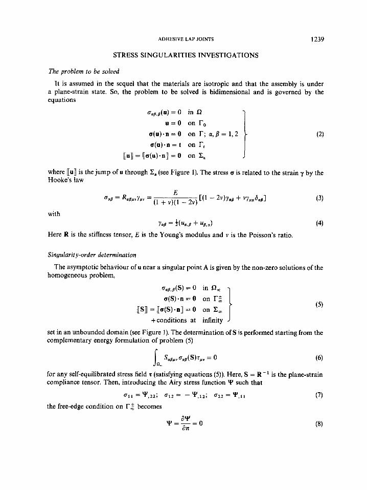
where 1

4 1 ) = 5 4 p Y a p ( U ? - t u u ! L? Jrt ((@, u") is a solution of problem (2) set in Rq). Following the same steps as in Reference 22, one obtains that

9 = jn"o.Bus,lel.a + ~ ~ 3 0 1 g u a , l ~ l , l - j~*au"B(u)el , l 1

(33)

One can give a simpler expression of g. For this purpose, let us define first a parametric partition of R into Q and D (Figure 12). Then g is written as

with

n n (34) gD = J ~ a p u g . 1 e l . a + J o l a u u , 1 e 1 , 1

g D = -1. ~ a , ~ u ~ . ~ ~ , ~ ~ ~ - 6, c ~ ~ ~ ~ ~ , ~ I . ~ ~ ~ +

D" D3

can be transformed into a line integral in both cases of initial and simplified models as it will be

- Initial model. The displacement and stress fields are regular in D. Accordingly, integrations

seen.

by parts can be performed in relation (34). This gives:

Then, using both equilibrium and constitutive equations, it can be shown that reduces to

90 = J ~ a v p u p , 1 n v - t o v p ~ v p ( ~ ) n 1 1 e 1 - 6 1 J Ca1aua,1 - f a u p ~ a s ( u ) l C U Ca

Of course, g is independent of the R partitioning, so, we can take the limit as R tends to zero. We have seen in the previous section that u has an asymptotic behaviour:

us = Kr"g(0); Re(a) > 0.5

(Table 1 gives CI - 1). This involves that gQ and the integrals along C, in Consequently, g reduces to

vanish with R.

1 r

- Simplijied model. gQ and 91, are written using the displacements (30) and the stresses (31). Only the terms of order unity, g$ and g;, respectively, are retained. One has

1 1 ~ u s Y u p ( ~ ) e l , l - - oa2iuIln s,. J x n Q


As before, integrating by parts and using both equilibrium and constitutive equations of the simplified model, g: can be expressed in terms of a line integral

gg = - ~ ~ u p ~ u p ~ ~ ~ ~ l i ~ l + 4 ccz.~uaneli(~) 1. go is still partitioning-independent. The numerical results reported before show that the simplified model solution exhibits a singular behaviour near the point A. It can be verified easily that this singularity is not of power type as for the initial model. In fact, it is of logarithmic type as it is the case for the antiplane problem.23 Consequently, g i and the integrals along Cv in g i vanish with R, so that go reduces to

(36) go = 4 ca2,(rU,n el I (A)

The damaged case

Sometimes, it happens that, prior to debonding propagation, quasi-periodically distributed oblique micro-cracks take place in the adhesive, with a period of the same order as the adhesive thickness (Figure 13). Consequently, we shall derive here a simplified model including damage by using the classical technique of periodic homogenization. 243 2 J

To this end, let us define the mapping F' in S13

X I = X I + Eyl

x2 = EY2 F': {

t x2 L

eb-wil +/- rf

Figure 13. The periodic micro-cracks adhesive damage-notations


where x1 and y play the role of macroscopic and microscopic variables, respectively. This involves the following derivation and integration rules:

a - - & - I __ a a a a __-- - + & - I - - . - ax, ax, aY1' 8x2 ayz

I-

Introducing these rules into equation (24), one obtains that uE is a solution of the variational problem

UO(UE, v ) + & U , ( U E , v ) + &2UZ(UE, v ) = tau, It for any y,-periodic displacement field v such that v = 0 on To. Here

I- I-

(37)

1 au; ao, au; avz ax , ax, ax, a x , + R ! 2 1 2 -a-

and Rb is the adhesive stiffness tensor

z stands for x or y

U~ is then expanded in a power series of E:

U E = uo + E i i + E Z Q + O(&)

Introducing this expansion in equation (37) and identifying the terms of the same order in E, one obtains that uo, ii, 6 are solutions of the following sequence of problems:

r

1 Vv k.a.

i uo(ii, v ) = -u,(uO, v )

uo($ v ) = -ul(ii, v) - uz(uo, v)

Vv k.a.

Vv k.a.

Equations (38) are exploited in a classical wayz4*z5 in order to obtain the homogenized model. For the sake of brevity, we give only the result.

- In the adhesive, uo is of the form


where !4 = 4 IZi

is the trace of the component u," of uo on interface XI.

stated on the elementary cell Y (Figure 13): - The vectors w", called local correctors, are solutions of bidimensional elastostatic problems

d

J Y a - [ R ~ s , v y ~ y ( w A 7 ) ] = 0 in Y

R ~ s p v y ~ v ( w " ) n s = 0 on Tr w IT y,-periodic

on C: on X2y

1 on C: J bar: Kronecker symbol on C:

t (40)

- The adhesive homogenized stiffness tensor RbH associated to the simplified model is connec- ted to the undamaged stiffness tensor by the relations

with n: = 1 and nz= - 1, - Finally, uo is a solution of the variational problem

r r r

J aas(uO)yas(v) + R:fi,g;'$ dxl = taua Vv k.a. n" J f J rt

or, equivalently,

aa(uo, v ) + ai(uo, v ) = taua Vv k.a. Lt with

Numerical approximation: adhesive elements

elements with four d.0.f. per node: Adhesive elements used to approximate the bilinear forms a; and a i are one-dimensional

(.>' = { d , u:, u : , 4 ) (44) Their degree of interpolation must be compatible with the degree of two-dimensional adjacent elements used to discretize the adherends. The way to derive the elementary stiffness matrix for linear element is well-described in Goodman et a1.l' and can be easily extended to elements of degree greater than one. Accordingly, it does not seem necessary for us to develop this point. On the other hand, we shall discuss the stiffness matrix involved in the constitutive equations of the


simplified adhesive model. We recall here that the general form of an elementary stiffness matrix is

K e g B ~ . D . B element

(i) Undamaged case. Definition (27) of a: shows that, with the d.0.f. ordering of relation (44), the stiffness matrix D has the form

r k, - k, 0 O 1 k n - k n

0 - k, k , 0

where

( 4 4 )

If the displacement jumps are taken as d.o.f., D reduces to the matrix given by Goodman et al.," Barker and Hatt16 and J o h n ~ o n . ' ~ In Reference 15, both the shear stiffness k , and the normal stiffness k , are deduced from experimental curves, whereas References 16 and 17 give

without any justification. This value underestimates the normal stiffness of the adhesive. Let us notice that, with plane-stress, instead of plane-strain assumption, one should obtain

Eb

( l - vb2)eb k, =

Values given by equation (45) were also used in a recent paper by Edlund and Klarbring.26 (ii) Damaged case. Definitions (41) of RbH and (43) of a i show that the constitutive equations of

the simplified adhesive model with damage are more complicated. Here, D has the form:

(46) 1 RE11 RK21 R?12 RE22 RZ11 RE21 RZ12 R E 2 2

R E i i RE21 RK12 RK22 R,b%1 R2bL RE12 RE22

D = [ In spite of appearances, D is symmetric as it is shown in the Appendix. Generally, it is

impossible to reduce the d.0.f to the displacements jumps only as for the undamaged case. As a consequence, the cracked adhesive exhibits an anisotropic behaviour.

Numerical results

The first course of computations is devoted to the comparison of both initial and simplified models applied to the study of a double lap joint. The assembly characteristics are those used in the previous section (Figure 5) with I,, = 30 mm and eb = 0.1 mm. Here, conditions of symmetry are prescribed at the bottom and at the right edges of the lower adherend domain. The used


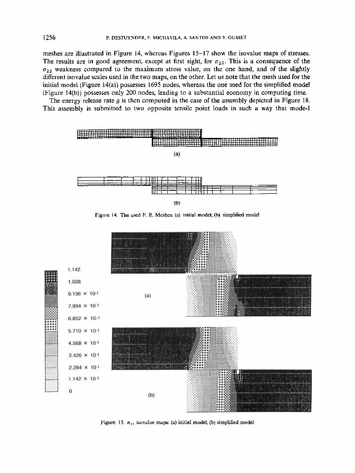
meshes are illustrated in Figure 14, whereas Figures 15-17 show the isovalue maps of stresses. The results are in good agreement, except at first sight, for ~ 7 ~ ~ . This is a consequence of the a22 weakness compared to the maximum stress value, on the one hand, and of the slightly different isovalue scales used in the two maps, on the other. Let us note that the mesh used for the initial model (Figure 14(a)) possesses 1695 nodes, whereas the one used for the simplified model (Figure 14(b)) possesses only 200 nodes, leading to a substantial economy in computing time.

The energy release rate g is then computed in the case of the assembly depicted in Figure 18. This assembly is submitted to two opposite tensile point loads in such a way that mode-I

(b)

Figure 14. The used F. E. Meshes: (a) initial model; (b) simplified model

Figure 15. oI1 isovalue maps: (a) initial model; (b) simplified model

Figure 17. uZ2 isovalue maps: (a) initial model; (b) simplified model


2 mm

Figure 18. The specimen used for the energy release rate computation

- 3' I I I -I

0.5 1 1.5 2 0

Figure 19. Crack front displacement as a function of the crack length; component u1

debonding occurs. The most crucial point for the comparison of the two models is the crack front. Figures 19 and 20 show the displacements of the intersection point of the crack front with the upper interface as a function of the crack length; good concordance is obtained. Finally, Figure 21 shows the accuracy of the simplified model to evaluate the energy release rate of the adhesive


u2 (rn X 10-5)

1.6

0.44 -+- Simplified model \L

0.24

ec ~

0 I I I

0.5 1 1.5 2

Figure 20. Crack front displacement as a function of the crack length; component u2

25-

20 -

15-

10-

5-

I ec (m) * 0 I I I I

0.5 1 1.5 2

Figure 21. Energy release rate as a function of crack length

crack. Let us note that the present debonding model produces a non-zero energy release rate when there is no crack in the adhesive.

CONCLUSION

A methodology for the numerical analysis of adhesive lap joints that combines a local and a global approaches has been presented. It involves essentially the post-processor developments in F.E. codes and permits one to provide some answer to the problem of bonded assembly design by implementing inexpensive computing models. Of particular interest is the obtained result regarding the simplified model energy release rate go. It can be proved that the initial model


energy release rate g tends to g o when E tends to zero. This result is noteworthy because, on the one hand, these two models do not exhibit the same type of stress singularities (and then, no convergence result is obtained for the intensity factors) and, on the other hand, the stresses given by the simplified model are incorrect near the crack front (they do not satisfy the free-stress boundary condition on rf). This is not surprising because convergence results are obtained in energy norm, whereas things as singularities and boundary layer, describe a local behaviour of the solution, and convergence in energy does not involve generally pointwise convergence. Further- more, go is very easy to compute.

Nevertheless, several questions remain unanswered at this time.

(i) How to connect the singular stresses to micro-crack initiation? (ii) What is the effect of micro-cracks adhesive damage on the energy release rate?

(iii) How to connect micro-cracks damage to debonding? (iv) Is the simplified model able to solve the adhesive as well as the cohesive failure problems?

There is no doubt that we shall not be able to answer these questions without taking into account the theormodynamical aspects of micro-cracks growth.

ACKNOWLEDGEMENTS

This work was jointly carried out by the Laboratoire de Mtcanique de 1'Ecole Centrale de Paris (France), the Centre Technique des Industries MCcaniques (France), and the Matematica Aplicada y Metodos Informaticos of the E.T.S.I. de Minas de Madrid (Spain), under grant no 86E0262 of the Ministere de la Recherche et de la Technologie (France) and grant no 078/01 of the Ministere des Affaires Etrangeres (France) and the Ministerio de Education y Ciencia (Spain).

APPENDIX

In view of expression (46), symmetry of the damaged adhesive stiffness matrix does not seem obvious. We are going to show here the equality

RZ21 = RE11

Let us recall that, from definition (41), we have for an isotropic adhesive 1 r

where w l l and w21 are solutions of problems (40) which are made explicit below.

(i) Problem for w l l . Problem (40) is written as

a - [ R $ B Y y ; Y ( ~ l l ) ] = 0 in J Y ,

R~opvy;u(wll)nor = 0 on Tf w l ' y , - periodic

w i l = 1 and w i l = O on Zf w i l = w i ' = o on E:


Then, for any yl-periodic displacement field v such that

v1 = v 2 = O on Z: v2 = 0 on Z;

w l l satisfies I- ,-

fii) Problemfor w Z 1 . Problem (40) is written as

7 a - [ R $ , , ~ ; , ( W ~ ~ ) ] = o in Y aY=

i R2ppvy;v (~21)n , = 0 on rf w Z 1 y l - periodic

w f l = 1 and w:' = 0 on Z i

w f l = w;' = O on Z:

Then, for any yl-periodic displacement field v such that

v2 = 0 on Z{ v 1 = v 2 = O on Z:

w satisfies : r r

Now, taking w Z 1 and w l l as test displacement fields in equations (47) and (48), respectively, we obtain:

r r I-

The desired equality is deduced from it directly.

analytically. The local correctors W" have the following expressions in the initial variables: Furthermore, let us note that, if the adhesive is uncracked, problems (40) can be solved

x 1 l w ? 1 = - 2 + -

W - - x2 1 + - _ -

, eb

Using expressions (41), it is easy to show that the stiffness matrix (46) degenerates to the stiffness matrix (44) of the undamaged adhesive.


REFERENCES

1. P. Grisvard, EHiptic Problems in Nonsmooth Domains, Monographs and Studies in Mathematics 24, Pitman, London, 1985.

2. J. R. Yeh and 1. G. Tadibakhsh, ‘Stress singularity in composite laminates by finite element method’, J . Compos. Mater., 20, 347-364 (1986).

3. D. Leguillon and E. Sanchez-Palencia, Computation of Singular Solutions in Elliptic Problems and Elasticity, Collection Recherches en Mathematiques Appliquees, Masson, Paris, 1987.

4. S . G. Lekhnitskii, Anisotropic Plates, Gordon and Breach, New York, 1968. 5. A. K. Rao, ‘Stress concentrations and singularities at interface corners’, Z A M M , 51, 395-406 (1971). 6. G. B. Sinclair, ‘On the singular eigenfunctions for plane harmonic problems in composite regions’, J . Appl. Mech.

7. S. S. Wang and I. ChoT, ‘Boundary layer effects in composite laminates, part 1-Free-edge stress singularities, part 2-Free-edge stress solutions and basic characteristics’, J . Appl. Mech. ASME, 49, 541-560 (1982).

8. R. I. Zwiers, T. C. T. Ting and R. L. Spilker, ‘On the logarithmic singularity of laminated composites under uniform extension’, J . Appl. Mech. ASME, 49, 561-569 (1982).

9. N. Somaratna and T. C. T. Ting, ‘Three-dimensional stress singularities at conical notches and inclusions in transversaly isotropic materials, J . Appl. Mech. ASME, 53, 89-96 (1986).

10. Ph. Destuynder, ‘Calcul des singularites dans les effets de bord d’une plaque composite multicouche’, C . R . Acad. Sci. Paris, 302/II, 257-262 (1986).

11. Y. Ousset, ‘Singularites de contraintes dans les joints colles-1: determination de I’ordre des singularites’, CETIM report 107060-8713, Senlis (France), (1987).

12. M. A. Moussaoui, ‘Sur I‘approximation des solutions du probleme de Dirichlet dans un ouvert avec coin’, in A. Dold and B. Eckmann (eds.), Singularities and Constructive Methods for their Treatment, Lecture Notes in Mathematics 1121, Springer, Berlin, 1985, pp. 199-206.

13. M. Dobrowolski, ‘On finite element method for nonlinear elliptic problems on domains with corners’, in A. Dold and B. Eckmann (eds.), Singularities and Constructive Methodsfor their Treatment, Lecture Notes in Mathematics 1121, Springer, Berlin, 1985, pp. 85-103.

14. I. Babuska and A. Miller, ‘The post-processing approach in the finite element method. Part 11: The calculation of stress intensity factors’, Int. j . numer. methods eng., 20, 11 11-1 129 (1984).

15. R. E. Goodman, R. L. Taylor and T. L. Brekke, ‘A model for the mechanics of jointed rock’, J . Soil Mech. Found. Din

16. R. M. Barker and R. B. Hatt, ‘Analysis of bonded joints in vehicular structures’, AIAA J., 11, 1650-1654 (.1973). 17. C. L. Johnson, ‘Effect of ply stacking sequence on stress in a scarf joint’, AIAA J . , 27, 79-86 (1989). 18. P. Destuynder, Y. Ousset and C. Stackler, ‘Sur les singularitts de contraintes dans les joints collts’, Journal de

Micanique Thkorique et Appliquee 7, 899-925 (1986). 19. P. Destuynder and Y. Ousset, ‘Singularites de contraintes dans les joints collts-2: methode de calcul des facteurs

d’jntensitl: CETIM report 107060-87/12, Senlis, France, 1987. 20. Y. Ousset, ‘Singularites de contraintes dans les joints colles-3: application a I’etude d’assemblages a double et simple

recouvrement’, CETIM report 107950-88/31, Senlis, France, 1988. 21. H. L. Groth and D. Jangblad, ‘Fracture initiation at interface corners in bonded joints’, G. Verchery and A. H.

Chardon (eds.), Mechanical Behaviour of Adhesive Joints, Editions Pluralis, Paris, 1987 pp. 257-270. 22. P. Destuynder and M. Djaoua, ‘Sur une interpretation mathematique de I’integrale de Rice en mecaniqde de la

rupture fragile’, Math. Meth. in Appl. Sci., 3, 70-87 (1981). 23. P. Destuynder, F. Michavila, Y. Ousset and A. Santos, ‘Utilisation du taux de restitution de I’energie dans I’analyse

a deux echelles de I’endommagement d’unt joint collc”, C. R. Acad. Sci. Paris, t. 310, Serie I, 161-165 (1990). 24. A. Bensoussan, J. L. Lions and G. Papanicolaou Asymptotic Analysisfor Periodic Structures, Studies in Mathematics

and its Applications, 5 , North-Holland, Amsterdam, 1978. 25. E. Sanchez-Palencia, Non-Homogeneous Media and Vibration Theory, Lecture Notes in Physics, 127, Springer, Berlin,

1980. 26. U. Edlund and A. Klarbring, ‘Analysis of elastic and elastic-plastic adhesive joints using a mathematical program-

ming approach’, Comp. Methods Appl. Mech. Eng., 78, 19-47 (1990).

ASME, 47, 87-92 (1980).

ASCE, 3, 637-659 (1968).

Some theoretical aspects in computational analysis of adhesive lap joints

Documents

Transcript of Some theoretical aspects in computational analysis of adhesive lap joints