Georgia State University Georgia State University

ScholarWorks @ Georgia State University ScholarWorks @ Georgia State University

Mathematics Theses Department of Mathematics and Statistics

8-3-2008

Some Conclusions of Statistical Analysis of the Spectropscopic Some Conclusions of Statistical Analysis of the Spectropscopic

Evaluation of Cervical Cancer Evaluation of Cervical Cancer

Hailun Wang

Follow this and additional works at: https://scholarworks.gsu.edu/math_theses

Part of the Mathematics Commons

Recommended Citation Recommended Citation Wang, Hailun, "Some Conclusions of Statistical Analysis of the Spectropscopic Evaluation of Cervical Cancer." Thesis, Georgia State University, 2008. https://scholarworks.gsu.edu/math_theses/58

This Thesis is brought to you for free and open access by the Department of Mathematics and Statistics at ScholarWorks @ Georgia State University. It has been accepted for inclusion in Mathematics Theses by an authorized administrator of ScholarWorks @ Georgia State University. For more information, please contact scholarworks@gsu.edu.

SOME CONCLUSIONS OF STATISTICAL ANALYSIS OF THE

SPECTROPSCOPIC EVALUATION OF CERVICAL CANCER

by

Hailun Wang

Under direction of Yu-sheng Hsu

ABSTRACT

To significantly improve the early detection of cervical precancers and cancers,

LightTouch™ is under development by SpectRx Inc.. LightTouch™ identifies cancers

and precancers quickly by using a spectrometer to analyze light reflected from the

cervix. Data from the spectrometer is then used to create an image of the cervix that

highlights the location and severity of disease.

Our research is conducted to find the appropriate models that can be used to

generate map-like image showing disease tissue from normal and further diagnose the

cervical cancerous conditions. Through large work of explanatory variable search and

reduction, logistic regression and Partial Least Square Regression successfully applied to

our modeling process. These models were validated by 60/40 cross validation and 10

folder cross validation. Further examination of model performance, such as AUC,

sensitivity and specificity, threshold had been conducted.

INDEX WORDS: Cervical cancer, Logistic Regression, Partial Least Square Regression, AUC, Sensitivity, Specificity, Threshold

SOME CONCLUSIONS OF STATISTICAL ANALYSIS OF THE

SPECTROPSCOPIC EVALUATION OF CERVICAL CANCER

by

Hailun Wang

A Thesis Submitted in Partial Fulfillment of Requirements for the Degree of

Master of Science

in the College of Art and Sciences

Georgia State University

2007

Copyright by Hailun Wang

2007

SOME CONCLUSION OF STATISTICAL ANALYSIS OF THE

SPECTROPSCOPIC EVALUATION OF CERVICAL CANCER

by

Hailun Wang

Electronic Version Approved:

Office of Graduate Studies College of Art and Sciences Georgia State University August 2007

Major Professor: Yu-sheng Hsu Committee: Mark Faupel Xu Zhang

iv

ACKOWLEGEMENTS

First of all, I sincerely and gratefully acknowledge my advisor, Dr. Yu-sheng

Hsu, for his guidance, patience and gracious support. I greatly benefit from his

invaluable suggestion.

I owe special appreciation for Dr. Mark Faupel, President and Chief

Executive Officer and Dr. Shabbir Bambot, Senior director of SpectRx, who

provided me this great opportunity to experience the real world and supervised me

throughout my internship. I thank David Mongin and Rick Fowler in SpectRx for

helping me developing my skill as a team member. I also thank Chenghong Shen

and Yi Li for their help during the project.

Special thanks go to my husband and my parents. They helped me through

the frustrating and difficult times with support and love.

v

Table of Content

Acknowledgements…………………………………………………………. iv

List of Tables………………………………………………………………… vi

List of Graphs……………………………………………………………….. viii

List of Abbreviations………………………………………………………… ix

Chapter one: Introduction……………………………………………………. 1

Chapter two: Point Level Algorithm…………………………………………. 4

2.1 Data Manipulation and Variable Selection……………………. 4

2.2 Methodologies………………………………………………… 7

2.3 Results and Conclusion……………………………………….. 12

Chapter three: Diagnostic Methods…………………………………………. 19

3.1 Data Manipulation and Variable Selection…………………… 19

3.2 Methodologies……………………………………………….. 26

3.3 Results and Conclusion………………………………………. 28

Chapter Four: Future Study…………………………………………………. 36

Reference……………………………………………………………………. 38

Appendix I: SAS Code for Initial Data Manipulation, Variable

Reduction in Point Analysis…………………………………… 41

Appendix II: SAS Code for Creating New Variables in Point Analysis

Using Tissue Type……………………………………………. 46

Appendix III: SAS Code for Creating New Variables in Point

vi

Analysis Using Percentiles in Peripheral Group………………………… 50

APPENDIX IV: SAS Code for Calculating AUC on Training

and 10-floder cross-validation datasets………………………………….. 52

APPENDIX V: SAS Code for Data Manipulation and

Percentile Variable Creation in Whole Cervix Diagnosis………………… 57

APPENDIX VI: SAS Code for Read Pilot Data into

Alpha Pick and Beta Pick Sets…………………………………………… 63

APPENDIX VII: SAS Code for T-test and Wilcoxon Test……………….. 70

APPENDIX VIII: SAS Code for Generating Coefficients

of All Whole Cervix Model ……………………………………………... 73

APPENDIX IX: SAS Code for Sensitivity and Specificity

Calculation ……………………..………………………………………… 79

vii

List of Tables

Table 2.1: Lookup table for excluding points…………………………………… 5

Table 2.2: Spectrum data structure in database …………………………………. 5

Table 2.3: Pathology variable index ……………………………………………. 6

Table 2.4: 2x2 classification table ………………………………………………. 10

Table 2.5: earlier study results of point level diagnosis…………………………. 12

Table 2.6: Normalized data structure (e.g. Patient 1001) ………………………. 13

Table 2.7: Effectiveness of Normalization process --- Tissue Type …………… 13

Table 2.8: Effectiveness of Normalization process --- Percentile ……………… 15

Table 2.9: Model performance comparison --- RGB image information ………. 16

Table 3.1: Variable flip index …………………………………………………… 2 2

Table 3.2: Pap variable index …………………………………………………… 25

Table 3.3: Pathology variable index …………………………………………….. 26

Table 3.4: Variable Reduction Performance …………………………………….. 28

Table 3.5: Wilcoxon Rank for Ratio Variables …………………………………. 29

Table 3.6: Model performance comparison chart I ……………………………... 30

Table 3.7: Model performance comparison chart II …………………………….. 32

Table 3.8: Model performance comparison chart III ……………………………. 32

Table 3.9: Model performance comparison chart IV ……………………………. 33

Table 3.10: Model performance comparison chart V ……………………………. 34

Table 3.11: Ratio Variables List ………………………………………………….. 34

viii

Table 3.12: Model performance comparison chart VI ………………………… 35

ix

List of Graph

Graph 2.1: Data manipulation process …………………………………….. 7

Graph 2.2: Cervix surface divided by peripheral vs central ……………….. 14

Graph 2.3: Cervix surface color map ……………………………………… 16

Graph 3.1: Mean of P25 spectra for 522 Training subjects ……………….. 20

Graph 3.2: Mean of P75 spectra for 522 Training subjects ……………….. 21

Graph 3.3: Ratio variable specificity performances under 95% sensitivity... 23

x

List of Abbreviations

ASC-US Atypical Squamous Cells of Undetermined Significance

AGUS Atypical glandular cells of undetermined significance

CIN Cervical Intraepithelial Lesion

CN Columnar Normal

FDA Food and Drug Administration

LSIL Low Grade Squamous Intraepithelial Lesion

Pap Papanicolaou test

PLS Partial Least Square

SN Squamous Normal

TZ Transformation Zone

1

Chapter One: Introduction

According to published reports, cervical cancer is the second most common

cancer among women worldwide. Globally, there are approximately 371,000 cases of

cervical cancer diagnosed annually and approximately 190,000 deaths per year [1]. The

incidence of cervical cancer is on the decline in more developed countries, largely due to

implementation of the Pap test.

The most common findings on a Pap test are ASC-US and LSIL which provoke

millions of follow-up Pap tests, colposcopies and biopsies. However, only about 5% of

ASC-US and 10% of LSIL Paps actually reflect an immediate cancer precursor. Even

with colposcopy, diagnosis is imperfect, with 50% - 80% sensitivity and around 50%

specificity [3], [4]. All of these mean that a significant number of women were

misclassified through diagnosis of colposcopies and biopsies.

LightTouch™, under development by SpectRx Inc., is being designed as a new

non-invasive test. LightTouch™ identifies cancers and precancers quickly by using a

spectrometer to analyze light reflected from the cervix. Data from the spectrometer is

then used to create an image of the cervix that highlights the location and severity of

disease.

Florescence and reflectance spectroscopy have been shown to be valuable in

cancer diagnosis by some investigators [4]. A number of studies show the performance of

either spectroscopy in discriminating between normal tissue and different epithelial

2

cancer grades use point measurements of area that are either suspect or normal. As an

example, studies from the Richard Kortum’s Lab indicate that variability between

normal tissues in different patients is higher than variability between tissues with disease

grades [5], [6]. In addition, reflectance spectra of cervical pre-cancer show consistent

differences from that of normal tissue at multiple distances between the light source and

detector. Spectral patterns in diffuse reflectance spectra can be used for the

discrimination of normal cervical tissue from low grade and high grade intraepithelial

lesions.

From 1999 to 2000, SpectRx’s Fiber Optical System and Camera System were

introduced into a feasibility studies. In 2001, a hybrid System of these was developed.

Data collected from this device were used for algorithm development and a validation

study. As equivalence to hybrid system, Alpha and Beta prototype systems were

developed during 2002-2006. The pivotal trial data from this device were also used for

algorithm validation.

Spectrx, Inc collected 648 patients’ data in multicenter clinical trial. The device

collected data from 56 spatial points on the surface of the cervix for each patient. For

each point, reflectance spectrum wavelength ranging from 410nm-700nm and

florescence spectrum wavelength ranging from 400nm-700nm was gathered. The

point level algorithms were developed based on approximately 30,000 observations and

10,000 initial variables. The whole cervix models were built from 648 observations and

10,000 initial variables. It should be noticed that we only use many fewer inputs to the

3

algorithm. With the process of SpectRx pilot study, another 100 patients’ data are

available for model prediction examination.

At Georgia State University, three graduate students in statistics department have

previously worked on the statistical analysis of the spectroscopic evaluation of cervical

cancer. Wei Xu was first to compare the logistic regression models and CART models.

In 2004, Kai Qu use cluster analysis to divide data into two parts then use partial least

squares to classify both parts [7]. These results were compared with the one without using

cluster analysis. Two years later, Chenghong Shen reconsidered variables which were

not used before, and adding more newly created variables to built models [8].

This thesis is organized in the following order. In chapter two, the data

manipulation and variable selection procedure for point level analysis are first

introduced, followed by logistic regression, cross-validation. Then the results from

different approaches are compared and a conclusion is presented. Chapter three is

organized in the same way as previous chapter. The future studies are discussed in

chapter four.

4

Chapter Two: Point Level Diagnosis

One objective of the medical device is to create an image of the cervix that

highlights the location and severity of disease. Since the device collects data from 56

spatial points on the surface of cervix, point level analysis of disease would help us to

find the location of the disease and the patient diagnosis could be also conducted by

combining all of the spatial information. Furthermore, we would like to using point

level diagnosis to render a cervix map that uses colors to represent the model output for

each point. Then a “weather map”- like image can be generated for each patient with the

brighter areas corresponding to increased likelihood of disease.

2.1 Data Manipulation and Variable Selection

1. Observations

The training dataset contains 510 evaluable subjects. For each subject, there are 56

records corresponding to 56 spatial points’ data. Since some of the data points are

excluded from the training dataset for various reasons, the total number of observations

is around 20000. However, these observations are not independent. The approaches we

used to create independent observations are discussed in the methodology section.

(Table 2.1 provides the lookup table for excluding points)

5

Table 2.1 Lookup table for excluding points

Artifact code Description 0 No artifact 1 Specular Reflection

1.1 Possible Specular Reflection 2 Mucus

2.1 Possible Mucus 3 Blood

3.1 Possible Blood 4 Non-Cervical Tissue

4.1 Possibly Non-Cervical Tissue 5 White Marking Dot

5.1 Possibly White Marking Dot 6 Bad Interrogation Point

6.1 Possibly Bad Interrogation Point 999 Other artifact

2. Explanatory Variables

The spectra data which contains all important explanatory variables are stored in

an ASCII file for each patient. It was composed of four spectrums: Reflectance

spectrum; 340nm Fluorescence spectrum; 400nm Fluorescence spectrum; 460

Fluorescence spectrum. The spectrum data format is described as following table:

Table 2.2 Spectrum data structure in database

Columns Description No. of wavelength elements1 Point Number NA

2-63 Reflectance Spectrum 62 69-126 340nm Fluorescence Spectrum 58 132-184 400nm Fluorescence Spectrum 53 189-228 460nm Fluorescence Spectrum 40

The initial number of explanatory variables is the sum of number of all

wavelengths. These 213 initial variables was selected and reduced to 80 variables by

6

applying following rules which was established by Previous research from Spectrx:

1) Eliminate 400nm Fluorescence variables due to its little discriminating capability.

2) Average 2 neighboring spectra variables. (also called 10nm binning)

3) Divide the spectral variable by group mean. (also called self-normalization)

3. Response Variable

Biopsy conducted by pathologist and its result, histo-pathology, is considered as

the gold standard. SpectRx uses the pathology as the response variable for all models.

Table 2.3 Pathology variable index 0 Squamous Normal

0.5 Transformation Zone 1 Columnar Normal 2 CIN 1

2.5 CIN 1/2 3 CIN 2

3.2 CIN 2/3 3.5 CIN 3+ 9 Os -1 Unknown Classification

999 Other Classification

The points with pathology values equal to -1, 9, and 999 are not useful for our

point diagnosis, so they need to be excluded first. FDA stated that patient with

pathology diagnosis as CIN1 or CIN1/2 can be classified as either disease or non-disease.

So, in our model building process, CIN1 and CIN 1/2 are also excluded. In order to

create two distinct classes of disease, the cases were as positive for disease if the cases

had pathology values greater than or equal to 3, while the non-disease were defined as a

7

pathology value less than 3.

4. Data manipulation process

The data manipulation process of importing external file and variable creation are

illustrated by the table below:

Graph 2.1 Data manipulation process

↓

↓

2.2 Methodology

1. Observation independence

As described in 2.1, since each patient has multiple spectral records which are

correlated, treating each spectrum record as single observation is not practical.

Independent observation could be created by reducing the variability between patients.

Several approaches have been applied to reduce the correlation among the records

within patient.

It has been shown that the spectral intensity of a disease point is lower than non-

Import three spectrum data file from external ASCII data file into SAS

Column positions in external file are 2-63, 69-126, 189-226

Self Normalization 1) Average every two neighboring column

in each group of spectrum 2) Divide each of the above average value

by its group mean

8

disease point at a low wavelengths. For each patient, if we can subtract non-disease part

from each record, then the newly-created record will not involve disease (or non-disease)

variability between patients. This problem therefore becomes to how to find the non-

disease part for each patient.

From a biological perspective, squamous normal (SN), transformation zone (TZ)

and columnar normal (CN) tissues can be treated as non-disease tissue. We tried several

combinations of normalization by looking at difference between SN, TZ and CN.

However, this approach needs pre-knowledge of the position of these three types of

normal tissues.

As an alternative, using the assumption of normal tissues’ position is more

practical. It has been proved that cancer usually does not start on the peripheral region

of the cervix. Thus, each patient’s normal tissue can be found in the peripheral region.

2. Model building

Because our response variable is binary, which is either 1(disease) or 0(non-

disease), the multiple linear regression model is not appropriate for our data. Partial

Least Squares and Logistic Regression [9], [10] can be used to accommodate binary data.

Logistic regression analyzes binomially distributed data of the form Yi ~ B (pi, ni),

for i=1, ... , m, where the numbers of Bernoulli trials ni are known and the probabilities

of success pi are unknown. For each i, there is a k-vector Xi of known explanatory

variables (independent variables or covariates). Thus

9

|ii i

i

Yp E Xn

=

The logits of the unknown binomial probabilities (i.e., the logarithms of the odds)

are modelled as a linear function of the Xi.

1 1, ,log ( ) ln ...1

ii i k k i

i

pit p x xp

β β

= = + + −

Note that a particular element of Xi can be set to 1 for all i to yield an intercept in

the model. The unknown parameters βj are usually estimated by maximum likelihood.

The interpretation of the βj parameter estimates is the additive effect on the log odds

ratio for a unit change in the jth explanatory variable. In the case of a dichotomous

explanatory variable, for instance gender, eβ is the estimate of the odds ratio of having

the outcome for, say, males compared with females. The model has an equivalent

formulation of:

Extensions of the model exist to cope with multi-category dependent variables and

ordinal dependent variables, such as polytomous regression. Multi-class classification by

logistic regression is also known as multinomial logit modeling. An extension of the

logistic model to sets of interdependent variables is the conditional random field.

1 1, ,( ... )1

1 i k k ii x xpe β β− + +=

+

10

We use Proc Logistic and Proc PLS procedures in SAS package (Cary, NC) to

build logistic and PLS models respectively and discovered the logistic models performed

better than the PLS model for most criterion in our point level analysis. The PLS

approach is introduced in next chapter.

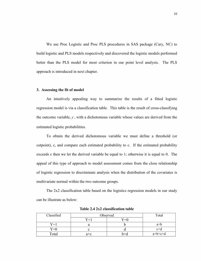
3. Assessing the fit of model

An intuitively appealing way to summarize the results of a fitted logistic

regression model is via a classification table. This table is the result of cross-classifying

the outcome variable, y , with a dichotomous variable whose values are derived from the

estimated logistic probabilities.

To obtain the derived dichotomous variable we must define a threshold (or

cutpoint), c, and compare each estimated probability to c. If the estimated probability

exceeds c then we let the derived variable be equal to 1; otherwise it is equal to 0. The

appeal of this type of approach to model assessment comes from the close relationship

of logistic regression to discriminate analysis when the distribution of the covariates is

multivariate normal within the two outcome groups.

The 2x2 classification table based on the logistics regression models in our study

can be illustrate as below:

Table 2.4 2x2 classification table Observed Classified

Y=1 Y=0 Total

Y=1 a b a+b Y=0 c d c+d Total a+c b+d a+b+c+d

11

asensitivitya c

=+

dspecificityb d

=+

Sensitivity and specificity rely on a single cutpoint to classify a test result as

positive. A more complete description of classification accuracy is given by the area

under the ROC (Receiver Operating Characteristic) curve. This curve plots the

probability of detecting true positive (sensitivity) and false negative (1-specificity) for an

entire range of possible cutpoints.

The area under the ROC curve, which ranges from zero to one, provides a

measure of the model’s ability to discriminate between those subjects who experience

the outcome of interest versus those who do not.

As a general rule, If ROC=0.5, a test shows no discrimination; If 0.7<ROC<0.8:

this is considered acceptable discrimination; If 0.8<ROC<0.9: this is considered

excellent discrimination; If ROC>0.9: this is considered outstanding discrimination.

4. Model Validation

Model validation is used to evaluate how well a model can be applied to any new data.

We employed conventional cross-validation as well as K-folder cross-validation in the

research. The conventional cross-validation is to randomly split the data into two parts.

We use 60/40, the larger part for training and the smaller for validation. K-folder cross-

validation is a technique to train and validate data on the same dataset. In our study, we

divided the training dataset into 10 approximately equal sized subsets. Moreover, we

ensure that patients with a certain Pap value are evenly allocated to each subset,

12

Therefore the 10 subsets are equivalent in size and content. The cross-validation process

is then repeated 10 times, with each of the 10 sub samples used exactly once as the

validation data. The 10 results from the folds then can be averaged (or otherwise

combined) to produce a single estimation.

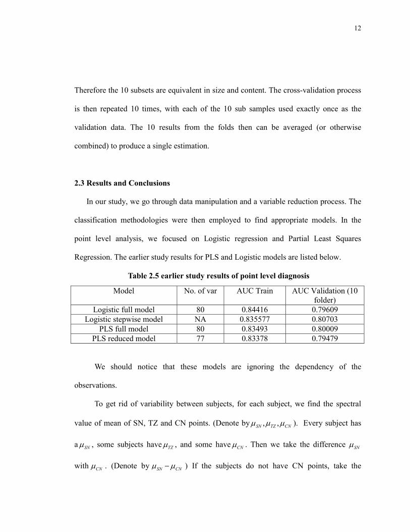
2.3 Results and Conclusions

In our study, we go through data manipulation and a variable reduction process. The

classification methodologies were then employed to find appropriate models. In the

point level analysis, we focused on Logistic regression and Partial Least Squares

Regression. The earlier study results for PLS and Logistic models are listed below.

Table 2.5 earlier study results of point level diagnosis

We should notice that these models are ignoring the dependency of the

observations.

To get rid of variability between subjects, for each subject, we find the spectral

value of mean of SN, TZ and CN points. (Denote by , ,SN TZ CNµ µ µ ). Every subject has

a SNµ , some subjects have TZµ , and some have CNµ . Then we take the difference SNµ

with CNµ . (Denote by SN CNµ µ− ) If the subjects do not have CN points, take the

Model No. of var AUC Train AUC Validation (10 folder)

Logistic full model 80 0.84416 0.79609 Logistic stepwise model NA 0.835577 0.80703

PLS full model 80 0.83493 0.80009 PLS reduced model 77 0.83378 0.79479

13

difference of SNµ with. TZµ . (Denote by SN TZµ µ− ). Then, we subtract spectra values of

each point from its SN CNµ µ− or SN TZµ µ− .

Table 2.5 illustrates the one patient’s spectral data structure after the normalization

process.

Table 2.6 Normalized data structure (e.g. Patient 1001)

We later discovered that patients trend to have much more SN tissue than TZ or

CN tissue. When the mean of SN, TZ and CN were taken respectively and followed by

taking the difference of (CN-SN) or (TZ-SN), the weight of CN and TZ increase.

Therefore, we treat CN, TZ as normal part is a solution.

Table 2.7 Effectiveness of Normalization process --- Tissue Type

Before Normalization

Normal part for patient 1001 After Normalization Point

Var1 … Var80

Tissues type

Var1 … Var80 Var1 Var80 1 X1,1 … X1,80 SN X1,1- N1 X1,80- N80

2 X2,1 … X2,80 SN X2,1- N1 X2,80- N80

3 X3,1 … X3,80 TZ X3,1- N1 X3,80- N80

4 X4,1 … X4,80 SN X4,1- N1 X4,80- N80

5 X5,1 … X5,80 CN2 X5,1- N1 X5,80- N80

….. …… … …… …… …… …… 56 X56,1 … X56,80 TZ

N1=( X1,1+

X2,1+ X4,1)/3 – ( X3,1+ X56,1)/2

…

N80=( X1,

80+X2,80+X4,80)/3 – (X3,80+ X56,80)/2

X56,1- N1 X56,80-N80

Model Normalization AUC Train AUC Validation Logistic full model (CN-SN) or (TZ-SN) 0.90288 0.82423

PLS full model (CN-SN) or (TZ-SN) 0.88376 0.85027 PLS reduced model (CN-SN) or (TZ-SN) 0.88377 0.85041 Logistic full model TZ or CN 0.90683 0.85522

14

Comparing table 2.6 with 2.4, both training and validation AUC are improved.

This provides evidence that normalization process is useful for our point level diagnosis.

The major drawback of this approach is it has limit application for a new

population, because it requires pre-knowledge of tissue type and the information about

where these zones begin and end for new population, which is impractible.

Graph 2.2 Cervix surface divided by peripheral vs central

As mentioned previously, cancer almost never starts on the peripheral region of

the cervix and its spectral value are usually small, we tried to find the normal part by

taking the low percentiles combination (e.g. 5th, 10th, 25th, 50th) of the 20 peripheral

locations’ spectral data. Then we subtract these percentiles with spectrum data to get rid

of the variability between subjects.

15

Table 2.8 Effectiveness of Normalization process --- Percentile

Finding the “real” normal part can further improve above models. The fixed

twenty positions may not reflect the real peripheral locations, which depend on how the

cervix images are taken.

It was known that by identifying os location in cervix, the “true” central and

peripheral group can be found. It is also known that areas close to the os have a higher

likelihood of disease than those that are distant. Using the RGB image to identify those

points that are peripheral vs. those that are central may help. This because contrition in

not always assured. As a first step toward this approach we will use Os locations already

identified in the point level data set to see if this helps. Use points neighboring the one

marked 'Os' in the database as the central points and the remaining as peripheral.

Percentile AUC Train AUC Validation P5 0.83281 0.72989 P10 0.81333 0.72322 P25 0.82765 0.75890 p50 0.80079 0.73381

p75-p5 0.87156 0.76555 p75-p10 0.87171 0.77955 p75-p25 0.86258 0.77270 p90-p5 0.87534 0.76521 p90-p10 0.87891 0.78125 p90-p25 0.85947 0.75531 p95-p5 0.86837 0.74421 p95-p10 0.87099 0.75372 p95-p25 0.86444 0.75104

16

Table 2.9 Model performance comparison --- RGB image information

Based on output indices from model (p90-p10), SpectRx engineers developed

color maps. The indices from logistic models range from 0 to 1, which represents

probability of having cervical cancer or precancer. Given a disease threshold, for model

(p90-p10), 0.41, any index below 0.41 will be colored as dark, as number getting close

to threshold, the color appears to be light. Above the threshold point are colored as white.

Graph 2.3 Cervix surface color map

Percentile AUC Train AUC Validation P5 0.85410 0.74893 P10 0.83922 0.71755 P25 0.86288 0.76410 p50 0.84781 0.76926

p75-p5 0.87086 0.76861 p75-p10 0.87857 0.77113 p75-p25 0.87725 0.77385 p90-p5 0.87787 0.77522 p90-p10 0.88121 0.76224 p90-p25 0.88210 0.77600 p95-p5 0.87983 0.78031 p95-p10 0.88276 0.76594 p95-p25 0.88447 0.76647

17

The problem has to do with the approach of considering all points put together

from all the subjects and then determining performance by the number of false negatives,

false positives and so on. This compared to whole cervix performance where a true

18

positive occurs when, for example, only one point on the cervix of a person with disease

needs to show up as positive. In other words, there can be many false negative points on

the cervix but as long as we have one true positive we will be correct with this subject.

This puts a very high performance demand on any point level algorithm.

To illustrate this problem using Model (90-10), we have been able to get a

performance of 95/60 sensitivity/specificity. The algorithm result was about 8,000 False

Positives and 12,000 True Negatives. Thus specificity is 60% (TN/(TN+FP)). However

those 8,000 False Positives are distributed over almost all the subjects making it seem as

if every subject has disease. Thus our whole cervix specificity is 0% and sensitivity

100%. It is clear that we must raise the threshold. This will make the performance on

the "all points put together" population abysmal and obviate any "mapping for disease

location" strategy.

19

Chapter Three: Diagnostic Methods

The color map is one approach for cervical cancer diagnosis. However, it requires

the model having extremely high discrimination of disease point from non-disease point

for all 56 locations. From subject level diagnosis perspective, it is not necessary to have

all point level results. Past researchers [8] have shown that the 25th percentile of the 56

locations’ spectral data can best discriminate patients with CIN2 or higher. In this

chapter, we further examine the 25th percentile model and other previous models by

applying to our current clinical trail data. Since all pervious models [8] might use too

many variables, which can cause overfit of the model and low prediction powers. We

conducted a thorough variable reduction process and the useful variable searching

process is detailed in following sections.

3.1 Data Manipulation and Variable Selection

1. Observations

As we described in the previous chapter, for each subject, there are 56 records

corresponding to 56 spatial points’ data. In our subject level diagnosis, only one of the

56 observations could be chosen to represent a patient’s disease status. The early study

showed that the 25th percentile is most useful data for discrimination. Besides the 510

subject’s data in SpectRx early clinical trail, we add more clinical trial data (e.g. dallas

dataset, pilot alpha dataset, pilot beta dataset) to test model prediction.

20

2. Explanatory Variables

In SpectRx’s early study, for all 78 spectral wavelengths, the 25th percentile was

chosen to create 78 explanatory variables. Our recent research indicates that lower

percentiles, such as 10th, 25th, are useful for discrimination for lower wavelengths of

spectrum data; while the higher percentiles, such as 75th, 90th, contains discrimination

information in the higher wavelengths of spectral data. Thus we extend 78 explanatory

variables to 312 variables. This trend can be illustrated by the graphs which were

produced by a SpectRx engineer.

Graph 3.1 Mean of P25 spectra for 522 Training subjects

Reflectance Spectrum

340 nm Fluorescence Spectrum

21

460nm Fluorescence Spectrum

Graph 3.2 Mean of P75 spectra for 522 Training subjects

Reflectance Spectrum

340 nm Fluorescence Spectrum

460nm Fluorescence Spectrum

22

Following observations and conclusions may be made:

We notice that at wavelengths below 590 nm spectra (blue wavelengths) diseased

tissue has a lower intensity than normal tissue

On the other hand, for wavelengths above 590 nm spectra (red wavelengths)

diseased tissue has higher intensity than normal tissue

At a lower percentile, 25th percentile for example, we would select spectra from

diseased tissue (when present)

The higher percentiles are better discriminator for red wavelengths.

The higher percentiles are not as good as lower percentiles for selecting disease

tissue

Table 3.1 summarizes these trends.

Table 3.1 Variable flip index Blue Flip Red Reflectance (wavelength in nm) 410 590 690 Reflectance (wavelength variable) 1 19 29 Fluorescence 340 ex (wavelength in nm) 410 490 690 Fluorescence 340 ex (wavelength variable) 30 38 58 Fluorescence 460 ex (wavelength in nm) 500 590 690 Fluorescence 460 ex (wavelength variable) 59 68 78

To verify these findings in quantitative way, we conducted several mean

comparison tests, including Wilcoxon test and t test. These tests were conducted as

23

follows: within certain variables, observations are grouped by their pathology test results.

Two groups are formed: cancer vs non-cancer. Calculate a score (t-statistic / wilcoxon

rank statistic) for each variable. We ranked the 312 scores to find 312 variables’

discrimination power. We finally reduced the simple explanatory variable number to 15

in the variable pre-selection.

We also discovered that taking the ratio between two simple variables increases

discrimination. For the 510 subject training data set, using the 78 spectral variables, we

created 78x78=6084 variables where each variable was divided by itself and the

remaining 77 variables and so on. Then we generated ROC curves and from these pick

the highest specificity obtained at 95% sensitivity or above.

Graph 3.3 showed color plots where the color coded specificities are shown for each

of p10, p25, p50 and p75 aggregate vectors.

Graph 3.3 ratio variable specificity performances under 95% sensitivity

1. P10

24

2. P25

3. P50

25

4. P75

In addition to spectral data, other test results, such as the Pap smear result

(cytology), are collected. The pap test is microscopic examination of cells from the

cervix. It is primarily designed to detect changes that may be cancerous or may lead to

cancer. It may also detect infections and abnormalities. Because this information is

available and may add information independent from the spectral variables, we can

include it in the model.

Table 3.2 Pap variable index 0 Normal 1 Benign Changes 2 ASCUS, not favoring neoplasia

2.8 ASCUS, favor neoplasia 3 LSIL

3.2 AGUS

2. Response Variable

The biopsy conducted by pathologist and its result, pathology, is considered as the

26

gold standard. SpectRx uses the pathology as the response variable for all models.

Table 3.3 Pathology variable index 0 Normal 1 Non-dysplastic change 2 CIN 1

2.5 CIN 1/2 3 CIN 2

3.2 CIN 2/3 3.5 CIN 3+

Patients with a pathology diagnosis as CIN1 or CIN1/2 can be regarded as either

disease or non-disease. So, in our model building process, CIN1 and CIN 1/2 are

excluded. The disease cases are defined as pathology value greater than or equal to 3,

while the non-disease are pathology value less or equal to 1.

3.2 Methodology

Partial Least Squares (PLS) is a method for constructing predictive models when

factors are many and highly collinear [11], [12]. PLS balances objectives of explaining

response variation and explaining predictor variation. A PLS model can be shown as

1 1 2 2 3 3 ... ,n n nY t q t q t q t q E= + + + + +

Where t are the latent variables or scores; q are the loading vectors.

Note that the scores are chosen so that the relationship between successive pairs of

scores is as strong as possible. In general, PLS is finding a linear combination of

variables [13]. It can be shown that PLS seeks directions that have high variance and high

27

correlation with the response in contrast to principal components. In particular, the mth

principal component direction mv solves:

10, 1,.., 1

var( )maxTlv s l m

Xα

α

α== = −

,

Where S is the sample covariance matrix of xj. The conditions 0Tlv sα = ensures

that mz Xα= is uncorrelated with all the previous linear combinations l lz Xv= . The

mth PLS direction mϑ∧

solves:

2

1

0, 1,.., 1

( , ) ( )maxT

l s l m

Corr y X Var Xα

ϑ α

α α∧

=

= = −

We calculated Area Under Curve (AUC), sensitivity and specificity to evaluate

model performance. It is observed that model performance in terms of AUC is closely

related to the number of variables and the variables chosen. Model can be built based on

AUC criterion [14], but it was found to be asymptotically equivalent to stepwise

regression. Therefore, we have to adopt both statistical methods and non-statistical

(manual) methods in variable selection.

We evaluate our models by following criteria described as below:

a Best specificity at 99/95/90 sensitivity levels will be evaluated.

b Models should give sensitivity that does not vary more than +/- 5 percentage points

when the same threshold is applied to all data sets.

c The same PAP test scaling must be used in conjunction with criterion (b) above

28

when determining performance with PAP.

d The model should meet a minimum performance benchmark for each Pap category

across all data sets.

e The candidate model will have the least shrinkage upon 10 folder cross validation

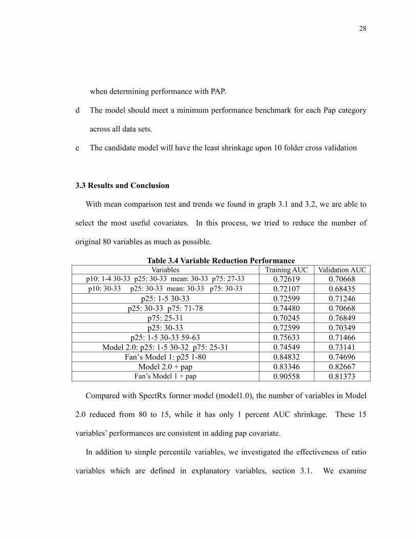
3.3 Results and Conclusion

With mean comparison test and trends we found in graph 3.1 and 3.2, we are able to

select the most useful covariates. In this process, we tried to reduce the number of

original 80 variables as much as possible.

Table 3.4 Variable Reduction Performance Variables Training AUC Validation AUC

p10: 1-4 30-33 p25: 30-33 mean: 30-33 p75: 27-33 0.72619 0.70668 p10: 30-33 p25: 30-33 mean: 30-33 p75: 30-33 0.72107 0.68435

p25: 1-5 30-33 0.72599 0.71246 p25: 30-33 p75: 71-78 0.74480 0.70668

p75: 25-31 0.70245 0.76849 p25: 30-33 0.72599 0.70349

p25: 1-5 30-33 59-63 0.75633 0.71466 Model 2.0: p25: 1-5 30-32 p75: 25-31 0.74549 0.73141

Fan’s Model 1: p25 1-80 0.84832 0.74696 Model 2.0 + pap 0.83346 0.82667

Fan’s Model 1 + pap 0.90558 0.81373 Compared with SpectRx former model (model1.0), the number of variables in Model

2.0 reduced from 80 to 15, while it has only 1 percent AUC shrinkage. These 15

variables’ performances are consistent in adding pap covariate.

In addition to simple percentile variables, we investigated the effectiveness of ratio

variables which are defined in explanatory variables, section 3.1. We examine

29

individual ratio variables performance which provided in graph 3.3. In the graph,

variables falls in the lightest color area are most potentially useful. Their discriminative

ability is ranked by Wilcoxon statistics.

Table 3.5 Wilcoxon Rank for Ratio Variables variable Wilcoxon Statistics

f125r30v45 6.91 f125r30v48 6.84 f125r30v46 6.79 f125r30v49 6.77 f125r31v45 6.76 f125r30v50 6.75 f125r30v47 6.75 f175r30v50 6.75 f110r30v45 6.70 f175r30v49 6.69 f125r30v51 6.67 f150r30v48 6.66 f175r31v50 6.65 f150r30v45 6.63 f150r30v50 6.63 f175r31v49 6.62 f110r30v46 6.61 f150r30v49 6.61 f110r31v45 6.60 f175r30v48 6.60 f110r30v47 6.59 f110r30v48 6.58 f125r31v48 6.58 f175r31v48 6.58

Note: f125r30v45 ratio variable represents variable 30 at 25th percentile (of 56 locations)

divided by variable 45 at 25th percentile.

By combining simple variables with ratio variables, we were able to form several

variable combinations to place into PLS regression. These models, with SpectRx

previous models (model 1.0, 2, Mixed 1.5, Mixed 1.9) were evaluated for their

specificities under 99/95/90 present sensitivity levels. Dallas dataset and pilot datasets

30

are used to validate model prediction on new populations.

Table 3.6 Model performance comparison chart I Specificity at 90% Sensitivity 510

training

62 case

s

Dallas

Dallas

2

Pilot Beta1/Beta2

EquivAlpha

Model 1.0 50 4 22 55 24 13 8 Model 1.1 50 42 28 61 27 17 12 Hailun 15 Coeff Model 47 0 13 23 28 25 16 Chenghong Mixed Model 1.5

58 50 20 29 12 9 12

Chenghong Mixed Model 1.9

58 42 15 52 16 9 8

Model 2.3: 15 simple+11 ratio

47 13 23 23 24 29 40

Mixed percentile (p25+p75) 58 25 28 52 20 4 4 Mixed percentile (p25+p90) 55 67 33 52 20 25 12 New ratio 1+15 coeff model 52 36 28 New ratio 2+15 coeff model 52 23 28 New ratio 3+15 coeff model 48 36 44 New ratio 4+15 coeff model 48 29 40 Mark F+ 15 + mix model 61 22 36 9 56 Mark F+ 15 + reduce mix model

40 30 32 26 48

New1 MarkF(p25/p75)+15 52 12 40 13 28 New2 Mark F (p25/p90)+ 15

55 15 36 17 36

Specificity at 95% Sensitivity 510

training

62 cases

Dallas Dallas 2

Pilot Beta1/Beta2

Equiv Alpha

Model 1.0 37 N/A 21 N/A N/A N/A N/A Model 1.1 41 N/A 28 N/A N/A N/A N/A Hailun 15 Coeff Model 36 N/A 11 N/A N/A N/A N/A Chenghong Mixed Model 1.5

38 N/A 17 N/A N/A N/A N/A

Chenghong Mixed Model 1.9

38 N/A 13 N/A N/A N/A N/A

Model 2.3: 15 simple+11 41 N/A 17 N/A N/A N/A N/A

31

ratio Mixed percentile (p25+p75) 44 N/A 27 N/A N/A N/A N/A Mixed percentile (p25+p90) 45 N/A 23 N/A N/A N/A N/A New ratio 1+15 coeff model 32 N/A N/A New ratio 2+15 coeff model 34 N/A N/A New ratio 3+15 coeff model 29 N/A N/A New ratio 4+15 coeff model 27 N/A N/A Mark F+ 15 + mix model 45 22 N/A N/A N/A Mark F+ 15 + reduce mix model

29 18 N/A N/A N/A

New Mark F (p25/p75) + 15

40 10 N/A N/A N/A

New2 Mark F (p25/p90) + 15

46 10 N/A N/A N/A

Specificity at 99% Sensitivity 510

training

62 cases

Dallas Dallas 2

Pilot Beta1/Beta2

Equiv Alpha

Model 1.0 20 4 20 32 4 13 8 Model 1.1 15 42 28 29 12 13 8 Hailun 15 Coeff Model 16 0 2 3 28 0 8 Chenghong Mixed Model 1.5

17 21 15 26 0 9 4

Chenghong Mixed Model 1.9

27 25 12 19 8 9 8

Model 2.3: 15 simple+11 ratio

24 8 5 10 23 8 32

Mixed percentile (p25+p75) 18 8 17 32 4 0 4 Mixed percentile (p25+p90) 9 4 8 16 4 0 12 New ratio 1+15 coeff model 16 13 20 New ratio 2+15 coeff model 20 13 28 New ratio 3+15 coeff model 16 6 16 New ratio 4+15 coeff model 17 19 32 Mark F+ 15 + mix model 20 12 0 4 0 Mark F+ 15 + reduce mix model

22 5 28 9 4

New Mark F (p25/p75) + 15

7 2 20 0 16

New2 Mark F (p25/p90) + 15

17 5 32 0 24

32

From this performance chart, we find model 2.3 is the best candidate model, not only

because of its reasonable performance on our training dataset, but also its high

specificity for new datasets, especially for pilot data.

To complete the classification analysis, we include CIN1, CIN1/2 cases to our study.

Model 2.31 has same covariates as 2.3, but with CIN1 and CIN1/2 cased in. The Model

has little shrinkage under 10 folder cross validation.

Table 3.7 Model performance comparison chart II Specificity at 90% Sensitivity 510

training62

cases

Dallas

Dallas 2

Pilot Beta1/Beta2

Equiv Alpha

Model 2.3 38/48 11/8 23/23 20/23 24/24 29/29 36/40 Model 2.31 37/48 21/21 27/27 32/39 31/28 27/33 33/44 Model 2.31 (validation) 37/48 21/21 27/27 38/39 31/28 27/33 33/44 Specificity at 95% Sensitivity 510

training62

cases

Dallas

Dallas 2

Pilot Beta1/Beta2

Equiv Alpha

Model 2.3 16/21 9/8 3/5 8/10 20/23 6/8 30/32 Model 2.31 22/31 9/4 4/10 5/0 19/24 6/8 28/36 Model 2.31 (validation) 22/31 9/4 4/10 5/0 19/24 6/8 28/36

Adding pap categories to model 2.3 using a decision tree method, we obtained a

common threshold at -0.05 across all data sets. For model 2.3 itself, the common

threshold for all datasets is also obtained at 0.08.

Table 3.8 Model performance comparison chart III Model 2.3

Data Set Sensitivity Specificity 510 99% 18%

Dallas all 94% 26% Equivalence alpha 100% 32% Equivalence beta1 100% 24% Equivalence beta2 92% 21%

33

Model 2.3 + pap Data Set Sensitivity Specificity

510 132/133 (99%) 64/226 (29%) Dallas2 9/10 (90%) 16/31 (52%)

Dallas all 16/17 (94%) 20/60 (33%) Equivalence alpha 12/12 (100%) 8/25 (32%) Equivalence beta1 12/12 (100%) 6/25 (24%) Equivalence beta2 11/12 (92%) 5/23 (22%)

Total 192/195 (98.5%) 119/392 (30%) In order to further reduce the variables in model 2.3, we did variable selection based

on significance and correlation tests. The results are listed in table 3.9.

Table 3.9 Model performance comparison chart IV 90% 95% 99%

510 Alpha Beta 510 Alpha Beta 510 Alpha BetaModel 2.3 (26 var) 47 46 28 41 46 NA 21 4 24

Model 2.37 (20 var) 50 48 28 37 41 NA 23 2 24 Model 2.38 (20var) 49 46 32 40 43 NA 25 2 28

Model 2.39 (20 var) 48 32 28 29 30 NA 20 2 28

Model 2.40(21 var) 50 39 24 45 29 NA 24 NA 24

Model 2.41(13 var) 42 11 16 35 7 NA 23 7 0

Model 2.42(18 var) 45 11 16 37 7 NA 23 7 0

Model 2.43(25 var) 42 11 20 29 7 NA 16 0 12

Note that Model 2.37 has 6 less variables than 2.3, but its performance is quite

competitive. We compared them at common thresholds across all datasets.

Table 3.10 Model performance comparison chart V

Model 2.3 at threshold 0.105 Model 2.37 at threshold 0.115 510 98.5 / 19 98.5 / 21

Alpha pick 95.5 / 46.4 95.5 / 41 Beta pick 100 / 24 91.7 / 28 Inspired by the color graph 3.3, we explored the ratio variable by this rule: the

numerators (minimum) were always chosen from blue wavelengths and denominators

34

(maximum) from red (see table 3.1). To be consistent with biological theory, when

mixed ratios are used the numerators are from the lower percentile and denominator

from the higher percentile. The threshold for choosing variables was a minimum of 25%

specificity at 95% sensitivity. When this threshold was raised to 30% the ratio groups

highlighted in yellow survived although not all individual variables in that group. The

ratios highlighted in red are unstable because they are too close to the flip point (from

red to blue) wavelengths.

Table 3.11 Ratio Variables List P10 (31,32)/(41-43) (33,34)/(37,38) P25 (30,31)/(21,22) (30,31)/(50-56) P50 (30,31)/(50-56) P75 (30-32)/(47-58) (30-32)/(75-78) P90 (30-32)/(47-58) P10_75 (30-32)/(49-57) (30,31)/(75-78) (33,34)/(37,38) (61-66)/(41-43) (62-64)/(46-48) P10_90 (30-32)/(21-29) (30,31)/(49-51) (30-32)/(70-78) (33,34)/(37,38) P25_75 (30-32)/(21-29) (30,31)/(46-57) (30,31)/(71-78) (64-66)/(42,43) (61-64)/(46-48) P25_90 (30-32)/(21-29) (30-32)/(49-57) (30-32)/(69-78)

There are a total of 22 cells, excluding 3 red cells. Each ratio variable can be created

by applying a min/max rule which is effective in reducing the correlation among

adjacent variables. For example, ratio var1 = min of (31, 32) / max of (41-43).

Applying this rule, we built four new models with new ratio variables. Notice that

Model 2.45: 22 min/max variables; Model 2.46: 15 single variables + 22 min/max;

Model 2.47: reduced 2.45 to 11 vars; Model 2.48: 15 single var + 11 min/max. Table

3.10 shows that model 2.46 has best performance at 99% sensitivity levels for both 510

and pilot data.

35

Table 3.12 Model performance comparison chart VI 90% 95% 99%

510 Alpha Beta 510 Alpha Beta 510 Alpha BetaModel 2.45 51 30 20 37 21 NA 20 21 4 Model 2.46 50 23 24 38 23 NA 25 20 20 Model 2.47 44 25 16 24 16 NA 18 13 16 Model 2.48 53 23 32 27 18 NA 18 11 32

36

Chapter Four: Future Study

One purpose of our point level analysis was to combine all diagnostic results of all 56

cervical surface locations to provide index for each subject. Thus, we have more

information for patient level diagnosis. For each individual, once we have the 56 point

indices which represent probabilities of having disease, the combination of these points

may provide information for patient level diagnosis. Logistic algorithm and PLS

algorithm could be adopted to find out relationship between point diagnosis and patient

level diagnosis. Some work has been done by using point level models (p90-p10).

1. Point output indices from the point level model (AUC: 0.88(T) 0.78(V)) with Os

location, totally are 273 subjects (no CIN1) and 56 variables(points), apply PLS

algorithm:

10-folder AUC performance:

Train Validation

56 variables 0.725 0.714

56 variables + pap 0.888 0.834

2. Point output indices from the point level model (AUC: 0.88(T) 0.78(V)) with fixed

20 peripheral location, totally are 347 subjects (no CIN1) and 56 variables(points),

apply PLS algorithm:

10-folder AUC performance:

37

Train Validation

56 variables 0.633 0.624

56 variables + pap 0.865 0.801

Compared with the models in chapter three, this approach did not improve AUC.

One of the reasons might be that 28% points are missing which results in insufficient

information for running PLS regression. To improve this, a simulation might be

involved to solve the missing data problem. Since we have the point position

information, once we have some point indices, their adjacent point having missing

values might be simulated by some approximation methods.

38

Reference

[1] J. Ferlay, F. Bray, P. Pisani and D.M. Parkin., GLOBOCAN 2000: Cancer Incidence,

Mortality and Prevalence Worldwide, Version 1.0, IARC CancerBase No. 5. Lyon,

IARC Press, 2001.

[2] Sherman et al, Effects of age and human Papilloma viral load on colposcopy triage:

data from the randomized Atypical Squamous Cells of Undetermined Significance/

Low-Grade Squamous Intraepithelial lesion Triage Study (ALTS), J. Natl. Can. Inst.,

2002. 94(2):102-7.

[3] Wright T, Cox T, Massad L, Twiggs L, Wilkinson E 2001 Consensus Guidelines for

the Management of Women with Cervical Cytological Abnormalities, JAMA, April 2002,

Vol 287, No. 16, 2120-2129.

[4] Richards-Kortum R. & Sevick-Muraca E. Quantitative optical spectroscopy for

tissue diagnosis. Annu. Rev. Phys. Chem. 47. 1996. P. 555-606.

[5] Ramanujam N. et. al., In vivo diagnosis of cervical intraepithelial neoplasia using

337 nm excited laser-induced fluorescence. PNAS, 91, 1994, p. 10193-10197.

[6] Ramanujam N. et. al., Development of a multivariate statistical algorithm to analyze

human cervical tissue fluorescence spectra acquired in vivo. Lasers in Surgery and

39

Medicine. 19, 1996, p. 46-62.

[7] Kai Qu, Some Contribution in the Classification Analysis of the

SpectroscopicEvaluation of Cervical Cancer, Graduate Thesis, 2004

[8] Chenghong Shen, Some Significant Results in the Classification Analysis of the

Spectroscopic Evaluation of Cervical Cancer, Graduate Thesis, 2006

[9] Hosmer,D.W, Lemeshow,S., 2000, Applied Logistic Regression (2nd edition), John

Wiley & Sons, Inc.

[10] Paul D. Allison, Logistic Regression Using the SAS System: Theory and Application,

SAS Institute., Cary, NC

[11] Randall D. Tobias, An Introduction to Partial Least Squares Regression, SAS

Institute., Cary, NC

[12] Herve Abdi. Partial Least Squares (PLS) Regression, 2003, The University of

Texas at Dallas

[13] Geoff Der, Brian S. Everitt, Handbook of Statistical Analyses Using SAS, Second

40

Edition, Chapman&Hall/CRC

[14] Yong Zhang, A Logistic Regression Model Selection Problem Through Maximizing

the Area under the ROC Curve, Graduate Thesis, 2005

41

APPENDIX I: SAS CODE FOR INITIAL DATA MANIPULATION, VARIABLE

REDUCTION IN POINT ANALYSIS

/* This is a program to manipulate data for point analysis file: point_analysis_mani.sas created by: Chenghong Shen modified by: Hailun Wang last update: 06/22/2006 */ %include 'K:\intern\spectrx\fan\missing_mac.sas'; libname After 'K:\intern\spectrx\PointAnalysis\'; options nonotes; options nonumber nodate; data After.R; set _null_; run; %macro getpointdata(path1 = , path2 = , path3 = , path4 = , path5 = , file = , spacing = 10, dataout =, subselect = 1, pointselect = 0, disq = no, extype = manual, spectype = orig, /*sub_id=, point_start=, point_end=, reflec=, fluore1=, fluore2=, fluore3=*/); data demo; infile "&path1&file" expandtabs lrecl = 10000 missover; input sub_id$ available unclean datec$ whole1 sitepath qa1 PriorPap PriorPaptype DayofPap DayofPaptype PreferredPap PreferredPaptype scjvisible colpoadequacy Age Race menstrual Menopause Gravida Para Abort Birthcontrol Priorsurgery1 DaysPriorsurgery1 Priorsurgery2 DaysPriorsurgery2 Priorsurgery3 DaysPriorsurgery3 Priorsurgery4 DaysPriorsurgery4 Priorsurgery5 DaysPriorsurgery5 height weight smoking Cigarettesperday; d_id = substr(sub_id, 1, 1);

42

year = substr(datec, 1, 4); month = substr(datec, 5, 2); day = substr(datec, 7, 2); date = mdy(month, day, year); %nmissing(varlist = available unclean whole1 sitepath qa1 PriorPap PriorPaptype DayofPap DayofPaptype PreferredPap PreferredPaptype scjvisible colpoadequacy Age Race menstrual Menopause Gravida Para Abort Birthcontrol Priorsurgery1 DaysPriorsurgery1 Priorsurgery2 DaysPriorsurgery2 Priorsurgery3 DaysPriorsurgery3 Priorsurgery4 DaysPriorsurgery4 Priorsurgery5 DaysPriorsurgery5 height weight smoking Cigarettesperday, missing = -1 -2); if available and &subselect; run; proc sort data = demo; by sub_id; run; data _null_; set demo end = last; call symput('sub'||left(_n_), trim(left(sub_id))); if last then call symput('nsub', _n_); run; proc sort data = demo; by sub_id; run; data coordinates; infile 'k:\intern\spectrx\fan\nci\hybrid\data3\HybridInterrogationPointCoordsmm.txt' expandtabs; input point x y; run; %do i = 1 %to &nsub; %put Read Data File For Subject #&i out of %left(&nsub) &&sub&i; /* Read the point analysis data */ %if %sysfunc(fileexist("&path4.&&sub&i.._pointgold.txt")) %then %do; data pointgold; infile "&path4.&&sub&i.._pointgold.txt" expandtabs lrecl = 100000; input point pathology1 pathology2;

43

if pathology1>pathology2 then pathology=pathology1; else pathology=pathology2; if pathology=0.5 then pathology=0; drop pathology1 pathology2; run; data pointcat; infile "&path3.&&sub&i.._excl_&extype..txt" expandtabs; input point reject; run; Data org; INFILE "&path2.&&sub&i.._spectra_autopeakrowdetect_notiszero2.txt" expandtabs lrecl = 100000; input point rf_1-rf_63 b1-b4 f1_1-f1_59 b5-b8 f2_1-f2_53 b9-b12 f3_1-f3_41; array rf rf_1-rf_63; array f1 f1_1-f1_59; array f2 f2_1-f2_53; array f3 f3_1-f3_41; %spacingselfnorm; sub_id = "&&sub&i"; run; data org_merge; merge org pointgold pointcat; *if reject in (&pointselect); by point; run; data After.R; set After.R org_merge; run; %end;

44

%end; %mend; %macro spacingselfnorm; %let t1 = 31; %let t2 = 29; %let t3 = 26; %let t4 = 20; array nrf nrf_1-nrf_&t1; array nf1 nf1_1-nf1_&t2; array nf2 nf2_1-nf2_&t3; array nf3 nf3_1-nf3_&t4; array rnrf rnrf_1-rnrf_&t1; array rnf1 rnf1_1-rnf1_&t2; array rnf2 rnf2_1-rnf2_&t3; array rnf3 rnf3_1-rnf3_&t4; %if &spacing = 5 %then %do; do i = 1 to &t1; nrf(i) = rf(i); end; do i = 1 to &t2; nf1(i) = f1(i); end; do i = 1 to &t3; nf2(i) = f2(i); end; do i = 1 to &t4; nf3(i) = f3(i); end; %end; %else %if &spacing = 10 %then %do; do i = 1 to &t1; nrf(i) = (rf(2 * i - 1) + rf(2 * i)) / 2; end; do i = 1 to &t2; nf1(i) = (f1(2 * i - 1) + f1(2 * i)) / 2; end; do i = 1 to &t3; nf2(i) = (f2(2 * i - 1) + f2(2 * i)) / 2; end; do i = 1 to &t4; nf3(i) = (f3(2 * i - 1) + f3(2 * i)) / 2; end; %end; %else %do; do i = 1 to &t1; nrf(i) = (rf(4 * i - 3) + rf(4 * i - 2) + rf(4 * i - 1) + rf(4 * i)) / 4; end; do i = 1 to &t2; nf1(i) = (f1(4 * i - 3) + f1(4 * i - 2) + f1(4 * i - 1) + f1(4 * i)) / 4; end; do i = 1 to &t3; nf2(i) = (f2(4 * i - 3) + f2(4 * i - 2) + f2(4 * i - 1) + f2(4 * i)) / 4; end; do i = 1 to &t4; nf3(i) = (f3(4 * i - 3) + f3(4 * i - 2) + f3(4 * i - 1) + f3(4 * i)) / 4; end; %end; avgnrf = mean(of nrf_1-nrf_&t1); stdnrf = std(of nrf_1-nrf_&t1); avgnf1 = mean(of nf1_1-nf1_&t2); stdnf1 = std(of nf1_1-nf1_&t4); avgnf2 = mean(of nf2_1-nf2_&t3); stdnf2 = std(of nf2_1-nf2_&t4); avgnf3 = mean(of nf3_1-nf3_&t4); stdnf3 = std(of nf3_1-nf3_&t4);

45

do i = 1 to &t1; rnrf(i) = (nrf(i) / avgnrf); end; do i = 1 to &t2; rnf1(i) = (nf1(i) / avgnf1); end; do i = 1 to &t3; rnf2(i) = (nf2(i) / avgnf2); end; do i = 1 to &t4; rnf3(i) = (nf3(i) / avgnf3); end; %mend; %getpointdata(path1 = k:\intern\spectrx\fan\Aftertrain\, /* Data for training */ path2 = k:\intern\spectrx\workdir\DATA\, path3 = k:\intern\spectrx\workdir\manual\, path4 = k:\intern\spectrx\workdir\point_analysis\, path5 = k:\intern\spectrx\workdir\graph\, /*sub_id =4124, point_start =29, point_end =33, reflec =1, fluore1 =1, fluore2 =1, fluore3 =1, */ file = HybridFINAL_ClinicalData_dm_2.txt, spacing = 10, dataout = All, disq = yes, subselect = (unclean = 0 and whole1~= .));

46

APPENDIX II: SAS CODE FOR CREATING NEW VARIABLES IN POINT ANALYSIS USING TISSUE TYPE

/* This is the point data manipulation, treating the range of values between normal types of tissue in each subject as index to get rid of variability between subjects file: test_point_model2.1_new_mani Created by: Hailun Wang Last update: 06/22/06*/ libname After 'k:\intern\spectrx\pointAnalysis'; option nodate nonotes; data SN; set After.M; if pathology in (0); run; data CN; set After.M; if pathology in (1); run; data TZ; set After.M; if pathology in (0.5); run; proc means data=SN noprint; var nrf_1-nrf_31 nf1_1-nf1_29 nf3_1-nf3_20; by sub_id; output out=SN_mean mean=x1-x31 y1-y29 z1-z20; run; proc means data=CN noprint; var nrf_1-nrf_31 nf1_1-nf1_29 nf3_1-nf3_20; by sub_id; output out=CN_mean mean=m1-m31 n1-n29 k1-k20; run; proc means data=TZ noprint;

47

var nrf_1-nrf_31 nf1_1-nf1_29 nf3_1-nf3_20; by sub_id; output out=TZ_mean mean=a1-a31 b1-b29 c1-c20; run; data SNandCN; merge SN_mean CN_mean; by sub_id; if m1=. or x1=. then delete; run; data SNremain; merge SN_mean CN_mean; by sub_id; if m1 not in(.) then delete; drop m1-m31 n1-n29 k1-k20; run; data SNandTZ; merge SNremain TZ_mean; by sub_id; if x1=. or a1=. then delete; run; data normalization1; set SNandCN; %macro norm; %do i=1 %to 31; norm1_&i=m&i-x&i; %end; %do j=1 %to 29; norm2_&j=n&j-y&j; %end; %do h=1 %to 20; norm3_&h=k&h-z&h; %end; %mend; %norm; run;

48

data normalization2; set SNandTZ; %macro norm; %do i=1 %to 31; norm1_&i=a&i-x&i; %end; %do j=1 %to 29; norm2_&j=b&j-y&j; %end; %do h=1 %to 20; norm3_&h=c&h-z&h; %end; %mend; %norm; run; data normalization; set normalization1 normalization2; run; proc sort data=After.M; by sub_id point; run; proc sort data=normalization; by sub_id; run; data mix; merge After.M normalization; by sub_id; if x1=. then delete; run; data point_train; set mix; %macro group; %do i=1 %to 31; diff1_&i=nrf_&i-norm1_&i; %end; %do j=1 %to 29; diff2_&j=nf1_&j-norm1_&j; %end; %do k=1 %to 20;

49

diff3_&k=nf3_&k-norm1_&k; %end; %mend; %group; run; data After.point_diff4; set point_train (keep=sub_id point pathology reject diff1_1-diff1_31 diff2_1-diff2_29 diff3_1-diff3_20); run;

50

APPENDIX III: SAS CODE FOR CREATING NEW VARIABLES IN POINT

ANALYSIS USING PERCENTILES IN PERIPHERAL GROUP

/* this is the point data manipulation, treating the difference between different percentiles in peripheral area in each subject as index to get rid of variability between subjects file: test_point_model1.3(2)_new_mani Created by: Hailun Wang Last update: 06/25/06*/

libname After 'k:\intern\spectrx\pointAnalysis'; data Peripheral; set After.M; where point in (1 2 3 4 5 11 12 19 20 28 29 37 38 45 46 52 53 54 55 56); run; proc means data=Peripheral noprint; var rnrf_1-rnrf_31 rnf1_1-rnf1_29 rnf3_1-rnf3_20; by sub_id; output out=peripheral_mean p10=a1-a31 b1-b29 c1-c20 p90=d1-d31 e1-e29 f1-f20; run; data peripheral_mean; set peripheral_mean; %macro normal; %do i=1 %to 31; x&i=d&i-a&i; %end; %do j=1 %to 29; y&j=e&j-b&j; %end; %do k=1 %to 20; z&k=f&k-c&k; %end; %mend;

51

%normal; run; proc sort data=After.M; by sub_id point; run; proc sort data=peripheral_mean; by sub_id; run; data mix; merge After.M peripheral_mean; by sub_id; run; data point_train; set mix; %macro group; %do i=1 %to 31; diff1_&i=rnrf_&i-x&i; %end; %do j=1 %to 29; diff2_&j=rnf1_&j-y&j; %end; %do k=1 %to 20; diff3_&k=rnf3_&k-z&k; %end; %mend; %group; run;

52

APPENDIX IV: SAS CODE FOR CALCULATING AUC ON TRAINING AND 10-

FLODER CROSS-VALIDATION DATASETS

/* This is a macro to carry out the n-folder cross validation. It is modified from nfolder_mac.sas. It takes 3 sets of variables. file name: nfolder_mac.sas last updated: May 22, 2002 by: Fan Xu Modified by: Hailun Wang */ %include 'k:\intern\spectrx\fan\macros\rocest_mac.sas'; %macro nfolder(datain = model, folder = n, response = whole, var1 =, var2 = , var3 = , n = , select = stepwise, print = no, sig = 0.01, pap = no); option nonotes; %foldermark(datain = &datain, folder = &folder); /*proc princomp data = mark noprint out = prin prefix; var &var1; run;*/ %do i = 1 %to &folder; %put &i out of &folder running...; data oneout; set mark; if group = &i then &response = .; run; proc logistic data = oneout descending noprint; %if %upcase(&pap) = YES %then %do; model &response = &var1 /*pm1-pm&n ps1-ps&n pt1-pt&n*/ preferredPap

53

%end; %if %upcase(&pap) = NO %then %do; model &response = &var1 /*pm1-pm&n ps1-ps&n pt1-pt&n*/ %end; %if %upcase(&select) = STEPWISE %then %do; / fast selection = stepwise sle = &sig sls = &sig; %end; %else %do; ; %end; output out = lout pred = pred; run; data pred1; set lout; if group = &i ; keep pred; run; data pred2; set mark; if group = &i ; keep &response; run; data pred; merge pred1 pred2; run; %if &i = 1 %then %do; data valid; set _null_; run; %end; data valid; set valid pred; run; %end; proc logistic data = mark noprint descending ; %if %upcase(&pap) = YES %then %do; model &response = &var1 /* pm1-pm&n ps1-ps&n pt1-pt&n */ preferredPap %end; %if %upcase(&pap) = NO %then %do; model &response = &var1 /*pm1-pm&n ps1-ps&n pt1-pt&n */ %end; %if %upcase(&select) = STEPWISE %then %do; / selection = stepwise sle = &sig sls = &sig; %end; %else %do; ; %end; output out = lout pred = pred; run;

54

%if %upcase(&print) = YES %then %do; %rocest(datain = lout, tests = pred, gold = &response); title 'Training Performance'; proc print data = roc; run; %rocest(datain = valid, tests = pred, gold = &response); title 'Cross-Validation Performance'; proc print data = roc; run; %end; %mend; %macro foldermark(datain = , folder = ); proc sort data = &datain; by whole1; run; data mark; set &datain; by whole1; if first.whole1 then obs = 0; else obs + 1; if last.whole1 then do; if whole1=3.2 then do; call symput('groupobs3_2', round(obs / &folder)); end; if whole1=3.5 then do; call symput('groupobs3_5', round(obs / &folder)); end; if whole1=3 then do; call symput('groupobs3', round(obs / &folder)); end; if whole1=2.5 then do; call symput('groupobs2_5', round(obs / &folder)); end; if whole1=2 then do; call symput('groupobs2', round(obs / &folder)); end; if whole1=1 then do;

55

call symput('groupobs1', round(obs / &folder)); end; if whole1=0 then do; call symput('groupobs0', round(obs / &folder)); end; end; run; data mark; set mark; if whole1 = 0 then group = int(obs / &groupobs0) + 1; if whole1 = 1 then group = int(obs / &groupobs1) + 1; if whole1 = 3 then group = int(obs / &groupobs3) + 1; if whole1 = 3.2 then group = int(obs / &groupobs3_2) + 1; if whole1 = 3.5 then group = int(obs / &groupobs3_5) + 1; if group > &folder then group = &folder; run; %mend; %include 'K:\intern\spectrx\workdir\programs\nfolder3_mac.sas'; data train; set Point_diff; whole1=pathology; if whole1 not in (2 2.5); if pathology not in (-1 -2 9 999); whole = (whole1 > 2); high = (whole1 >= 3); highlow = (whole1 >= 2); low = whole1 in (2 2.5); run; proc logistic data=train descending noprint; model whole= diff1_1-diff1_31 diff2_1-diff2_29 diff3_1-diff3_20/ scale=none clparm=wald clodds=pl rsquare outroc=roc1; output out=lout pred=pred p=prob XBETA=beta; run;

56

data indice1; set lout(keep=sub_id point pred); if _n_<16000; run; data indice2; set lout(keep=sub_id point pred); if _n_>=16000; run; /*logistic 1.1(full)*/ %nfolder(datain = Train, folder = 10, response = whole, var1 = diff1_1-diff1_31 diff2_1-diff2_29 diff3_1-diff3_20, var2 = , var3 = , n =3 , select = forward, print = yes, sig = 0.01, pap = no);

57

APPENDIX V: SAS CODE FOR DATA MANIPULATION AND PERCENTILE

VARIABLE CREATION IN WHOLE CERVIX DIAGNOSIS

/* This is data manipulation to read 522 subjects with spectrum 410+ into sas data set . Hailun Wang last update: 02/28/2007 */ %include 'G:\intern\spectrx\fan\missing_mac.sas'; libname After 'G:\intern\whole cervix model\sas data'; option nonotes; options nonumber nodate; %macro readdata(path1 = , path2 = , path3 = , file = , spacing = 10, dataout =, subselect = 1, pointselect = 0, disq = yes, extype = manual); data demo; infile "&path1&file" expandtabs lrecl = 10000 missover; input sub_id$ available unclean datec$ whole1 sitepath qa1 PriorPap PriorPaptype DayofPap DayofPaptype PreferredPap PreferredPaptype scjvisible colpoadequacy Age Race menstrual Menopause Gravida Para Abort Birthcontrol Priorsurgery1 DaysPriorsurgery1 Priorsurgery2 DaysPriorsurgery2 Priorsurgery3 DaysPriorsurgery3 Priorsurgery4 DaysPriorsurgery4 Priorsurgery5 DaysPriorsurgery5 height weight smoking Cigarettesperday; d_id = substr(sub_id, 1, 1); year = substr(datec, 1, 4); month = substr(datec, 5, 2); day = substr(datec, 7, 2); date = mdy(month, day, year); %nmissing(varlist = available unclean whole1 sitepath qa1 PriorPap PriorPaptype DayofPap DayofPaptype PreferredPap PreferredPaptype scjvisible colpoadequacy Age Race menstrual Menopause Gravida Para Abort Birthcontrol Priorsurgery1 DaysPriorsurgery1

58

Priorsurgery2 DaysPriorsurgery2 Priorsurgery3 DaysPriorsurgery3 Priorsurgery4 DaysPriorsurgery4 Priorsurgery5 DaysPriorsurgery5 height weight smoking Cigarettesperday, missing = -1 -2); if available and &subselect; run; proc sort data = demo; by sub_id; run; data _null_; set demo end = last; call symput('sub'||left(_n_), trim(left(sub_id))); if last then call symput('nsub', _n_); run; proc sort data = demo; by sub_id; run; data coordinates; infile 'G:\intern\spectrx\fan\nci\hybrid\data3\HybridInterrogationPointCoordsmm.txt' expandtabs; input point x y; run; %do i = 1 %to &nsub; %put Read Data File For Subject #&i out of %left(&nsub) &&sub&i; Data org; /*infile "&path2.&&sub&i.._spectra_&spectype..txt" expandtabs lrecl = 100000;*/ INFILE "&path2.&&sub&i.._spectra_autopeakrowdetect_notiszero2.txt" EXPANDTABS LRECL=100000; %if %upcase(&disq) = NO %then %do; input point rf_1-rf_63 f1_1-f1_63 f2_1-f2_57 f3_1-f3_45; array rf rf_1-rf_63; array f1 f1_1-f1_63; array f2 f2_1-f2_57; array f3 f3_1-f3_45; %if &spacing = 5 %then %do; %let t1 = 63; %let t2 = 63; %let t3 = 57; %let t4 = 45; %end; %else %if &spacing = 10 %then %do; %let t1 = 31; %let t2 = 31; %let t3 = 28; %let t4 = 22; %end;

59

%else %if &spacing = 20 %then %do; %let t1 = 15; %let t2 = 15; %let t3 = 14; %let t4 = 11; %end; %end; %else %do; input point b1-b4 rf_1-rf_59 b5-b8 f1_1-f1_59 b9-b12 f2_1-f2_53 b13-b16 f3_1-f3_41; array rf rf_1-rf_59; array f1 f1_1-f1_59; array f2 f2_1-f2_53; array f3 f3_1-f3_41; %if &spacing = 5 %then %do; %let t1 = 59; %let t2 = 59; %let t3 = 53; %let t4 = 41; %end; %else %if &spacing = 10 %then %do; %let t1 = 29; %let t2 = 29; %let t3 = 26; %let t4 = 20; %end; %else %if &spacing = 20 %then %do; %let t1 = 15; %let t2 = 14; %let t3 = 13; %let t4 = 10; %end; %end; %let t = %eval(&t1 + &t2 + &t3 + &t4); %spacingselfnorm; sub_id = "&&sub&i"; run; data pointcat; infile "&path3.&&sub&i.._excl_&extype..txt" expandtabs; input point reject; run; data org; merge org pointcat coordinates; by point; run; %meanpro(datain = org, dataout = m&i); %end; data model; merge demo %mf; by sub_id; run;

60

data &dataout; set model; CIN31 = (whole1 = 3.5); CIN32 = (whole1 >= 3.2); high = (whole1 >= 3); highlow = (whole1 >= 2); low = whole1 in (2 2.5); nandb = whole1 in (0 1); nc = whole1 = 1; normal = whole1 = 0; run; %mend; %macro mf; %do j = 1 %to &nsub; m&j %end; %mend; %macro spacingselfnorm; array nrf nrf_1-nrf_&t1; array nf1 nf1_1-nf1_&t2; array nf2 nf2_1-nf2_&t3; array nf3 nf3_1-nf3_&t4; array rnrf rnrf_1-rnrf_&t1; array rnf1 rnf1_1-rnf1_&t2; array rnf2 rnf2_1-rnf2_&t3; array rnf3 rnf3_1-rnf3_&t4; %if &spacing = 5 %then %do; do i = 1 to &t1; nrf(i) = rf(i); end; do i = 1 to &t2; nf1(i) = f1(i); end; do i = 1 to &t3; nf2(i) = f2(i); end; do i = 1 to &t4; nf3(i) = f3(i); end; %end; %else %if &spacing = 10 %then %do; do i = 1 to &t1; nrf(i) = (rf(2 * i - 1) + rf(2 * i)) / 2; end; do i = 1 to &t2; nf1(i) = (f1(2 * i - 1) + f1(2 * i)) / 2; end; do i = 1 to &t3; nf2(i) = (f2(2 * i - 1) + f2(2 * i)) / 2; end; do i = 1 to &t4; nf3(i) = (f3(2 * i - 1) + f3(2 * i)) / 2; end; %end; %else %do; do i = 1 to &t1; nrf(i) = (rf(4 * i - 3) + rf(4 * i - 2) + rf(4 * i - 1) + rf(4 * i)) / 4; end; do i = 1 to &t2; nf1(i) = (f1(4 * i - 3) + f1(4 * i - 2) + f1(4 * i - 1) + f1(4 *

61

i)) / 4; end; do i = 1 to &t3; nf2(i) = (f2(4 * i - 3) + f2(4 * i - 2) + f2(4 * i - 1) + f2(4 * i)) / 4; end; do i = 1 to &t4; nf3(i) = (f3(4 * i - 3) + f3(4 * i - 2) + f3(4 * i - 1) + f3(4 * i)) / 4; end; %end; avgnrf = mean(of nrf_1-nrf_&t1); stdnrf = std(of nrf_1-nrf_&t1); avgnf1 = mean(of nf1_1-nf1_&t2); stdnf1 = std(of nf1_1-nf1_&t4); avgnf2 = mean(of nf2_1-nf2_&t3); stdnf2 = std(of nf2_1-nf2_&t4); avgnf3 = mean(of nf3_1-nf3_&t4); stdnf3 = std(of nf3_1-nf3_&t4); do i = 1 to &t1; rnrf(i) = nrf(i) / avgnrf; end; do i = 1 to &t2; rnf1(i) = nf1(i) / avgnf1; end; do i = 1 to &t3; rnf2(i) = nf2(i) / avgnf2; end; do i = 1 to &t4; rnf3(i) = nf3(i) / avgnf3; end; %mend; %macro meanpro(datain = , dataout = ); proc means data = &datain noprint; var rnrf_1-rnrf_&t1 rnf1_1-rnf1_&t2 rnf2_1-rnf2_&t3 rnf3_1-rnf3_&t4 ; output out = &dataout p10 = p10ra1-p10ra&t p25 = p25ra1-p25ra&t p50 = p50ra1-p50ra&t p75 = p75ra1-p75ra&t p90 = p90ra1-p90ra&t; where reject in (&pointselect); by sub_id; run; %mend; %readdata(path1 = \\SPRXDEV1\Can1\CCDataAnalysis\PreProcessedData\export\HybridFINAL\ClinicalD

62

ata\, path2 = \\SPRXDEV1\Can1\CCDataAnalysis\PreProcessedData\export\HybridFINAL\Spectra\autopeakrowdetect_notiszero2\, path3 = \\SPRXDEV1\Can1\CCDataAnalysis\PreProcessedData\export\HybridFINAL\ExcludedPoints\manual\, file = HybridFINAL_ClinicalData_dm_2.txt, spacing = 10, dataout = After.clean522, disq = yes, subselect = (unclean = 0 and whole1~= .));

63

APPENDIX VI: SAS CODE FOR READ PILOT DATA INTO ALPHA PICK AND

BETA PICK SETS

/**************************************************** This is a program to read alpha polit data and generate p10-p90 var and ratio var *****************************************************/ libname After 'G:\intern\whole cervix model\sas data'; option nonotes; options nonumber nodate; %macro readdata (pointselect=, extype = , dataout=); proc import datafile="G:\intern\whole cervix model\pilot\clinicaldata_epa.xls" out=demo dbms=excel; data demo; set demo; if whole1=. then delete; sub_id=substr(subject,6,4); run; proc sort data = demo; by sub_id; run; data _null_; set demo end = last; call symput('sub'||left(_n_), trim(left(sub_id))); if last then call symput('nsub', _n_); run; %do i = 1 %to &nsub; %put Read Data File For Subject #&i out of %left(&nsub) &&sub&i; %macro spacingselfnorm; array nrf nrf_1-nrf_&t1; array nf1 nf1_1-nf1_&t2; array nf3 nf3_1-nf3_&t4; array rnrf rnrf_1-rnrf_&t1; array rnf1 rnf1_1-rnf1_&t2; array rnf3 rnf3_1-rnf3_&t4;

64

do i = 1 to &t1; nrf(i) = (rf(2 * i - 1) + rf(2 * i)) / 2; end; do i = 1 to &t2; nf1(i) = (f1(2 * i - 1) + f1(2 * i)) / 2; end; do i = 1 to &t4; nf3(i) = (f3(2 * i - 1) + f3(2 * i)) / 2; end; avgnrf = mean(of nrf_1-nrf_&t1); avgnf1 = mean(of nf1_1-nf1_&t2); avgnf3 = mean(of nf3_1-nf3_&t4); do i = 1 to &t1; rnrf(i) = nrf(i) / avgnrf; end; do i = 1 to &t2; rnf1(i) = nf1(i) / avgnf1; end; do i = 1 to &t4; rnf3(i) = nf3(i) / avgnf3; end; %mend; Data org; infile "G:\intern\whole cervix model\pilot\Spectra_alpha\11EPA&&sub&i.._spectra.txt" expandtabs lrecl = 100000; input point b1-b4 rf_1-rf_58 b5-b9 f1_1-f1_58 b10-b14 f3_1-f3_41; array rf rf_1-rf_59; array f1 f1_1-f1_59; array f3 f3_1-f3_40; %let t1 = 29; %let t2 = 29; %let t4 = 20; %let t = %eval(&t1 + &t2 + &t4); %spacingselfnorm; sub_id = "&&sub&i"; run; data pointcat; infile "G:\intern\whole cervix model\pilot\2filtercombo_alpha\11EPA&&sub&i.._excl_&extype..txt" expandtabs; input point reject; run; data org; merge org pointcat; by point; run; %meanpro(datain = org, dataout = m&i); %end;

65

data model; merge demo %mf; by sub_id; run; data &dataout; set model; CIN31 = (whole1 = 3.5); CIN32 = (whole1 >= 3.2); high = (whole1 >= 3); highlow = (whole1 >= 2); low = whole1 in (2 2.5); nandb = whole1 in (0 1); nc = whole1 = 1; normal = whole1 = 0; run; %mend; %macro mf; %do j = 1 %to &nsub; m&j %end; %mend; %macro meanpro(datain = , dataout = ); proc means data = &datain noprint; var rnrf_1-rnrf_&t1 rnf1_1-rnf1_&t2 rnf3_1-rnf3_&t4 ; output out = &dataout p10 = p10ra1-p10ra&t p25 = p25ra1-p25ra&t p50 = p50ra1-p50ra&t p75 = p75ra1-p75ra&t p90 = p90ra1-p90ra&t; where reject in (&pointselect); by sub_id; run; %mend;

66

%readdata( pointselect = 0, extype = 2filtercombo, dataout = polit_alpha);

/**************************************************** This is a program to read beta1 polit data and generate p10-p90 var and ratio var *****************************************************/ libname After 'G:\intern\whole cervix model\sas data'; option nonotes; options nonumber nodate; %macro readdata (pointselect=, extype = , dataout=); proc import datafile="G:\intern\whole cervix model\pilot\clinicaldata_epb.xls" out=demo dbms=excel; data demo; set demo; if whole1=. then delete; sub_id=substr(subject,6,4); run; proc sort data = demo; by sub_id; run; data _null_; set demo end = last; call symput('sub'||left(_n_), trim(left(sub_id))); if last then call symput('nsub', _n_); run; %do i = 1 %to &nsub; %put Read Data File For Subject #&i out of %left(&nsub) &&sub&i; %macro spacingselfnorm; array nrf nrf_1-nrf_&t1; array nf1 nf1_1-nf1_&t2; array nf3 nf3_1-nf3_&t4; array rnrf rnrf_1-rnrf_&t1; array rnf1 rnf1_1-rnf1_&t2; array rnf3 rnf3_1-rnf3_&t4; do i = 1 to &t1; nrf(i) = (rf(2 * i - 1) + rf(2 * i)) / 2; end;

67

do i = 1 to &t2; nf1(i) = (f1(2 * i - 1) + f1(2 * i)) / 2; end; do i = 1 to &t4; nf3(i) = (f3(2 * i - 1) + f3(2 * i)) / 2; end; avgnrf = mean(of nrf_1-nrf_&t1); avgnf1 = mean(of nf1_1-nf1_&t2); avgnf3 = mean(of nf3_1-nf3_&t4); do i = 1 to &t1; rnrf(i) = nrf(i) / avgnrf; end; do i = 1 to &t2; rnf1(i) = nf1(i) / avgnf1; end; do i = 1 to &t4; rnf3(i) = nf3(i) / avgnf3; end; %mend; Data org; infile "G:\intern\whole cervix model\pilot\Spectra_beta\11EPB&&sub&i.._spectra_orig_iscorr_Sequence_1.txt" expandtabs lrecl = 100000; input point b1-b4 rf_1-rf_58 b5-b72 f1_1-f1_58 b73-b77 f3_1-f3_40; array rf rf_1-rf_58; array f1 f1_1-f1_58; array f3 f3_1-f3_40; %let t1 = 29; %let t2 = 29; %let t4 = 20; %let t = %eval(&t1 + &t2 + &t4); %spacingselfnorm; sub_id = "&&sub&i"; run; data pointcat; infile "G:\intern\whole cervix model\pilot\2filtercombo_beta\11EPB&&sub&i.._excl_&extype._sequence_1.txt" expandtabs; input point reject; run; data org; merge org pointcat; by point; run; %meanpro(datain = org, dataout = m&i); %end;

68

data model; merge demo %mf; by sub_id; run; data &dataout; set model; CIN31 = (whole1 = 3.5); CIN32 = (whole1 >= 3.2); high = (whole1 >= 3); highlow = (whole1 >= 2); low = whole1 in (2 2.5); nandb = whole1 in (0 1); nc = whole1 = 1; normal = whole1 = 0; run; %mend; %macro mf; %do j = 1 %to &nsub; m&j %end; %mend; %macro meanpro(datain = , dataout = ); proc means data = &datain noprint; var rnrf_1-rnrf_&t1 rnf1_1-rnf1_&t2 rnf3_1-rnf3_&t4 ; output out = &dataout p10 = p10ra1-p10ra&t p25 = p25ra1-p25ra&t p50 = p50ra1-p50ra&t p75 = p75ra1-p75ra&t p90 = p90ra1-p90ra&t; where reject in (&pointselect); by sub_id; run; %mend;

69

%readdata( pointselect = 0, extype = 2filtercombo, dataout = polit_beta1);

libname After 'G:\intern\whole cervix model\sas data'; libname Dallas 'G:\intern\whole cervix model\sas data\dallas'; libname comb 'G:\intern\whole cervix model\sas data\comb'; option nonotes; options nonumber nodate; data pilotalpha; set after.politalpha_mixratio; keep subject preferredpap whole1 p10ra1-p10ra78 p25ra1-p25ra78 p50ra1-p50ra78 p75ra1-p75ra78 p90ra1-p90ra78 r1-r11 m1-m78; run; data pilotbeta1; set after.politbeta1_mixratio; length sub_id $10; machine='B1'; sub_id=machine||subject; keep sub_id preferredpap whole1 p10ra1-p10ra78 p25ra1-p25ra78 p50ra1-p50ra78 p75ra1-p75ra78 p90ra1-p90ra78 r1-r11 m1-m78; run; data dallas2; set dallas.dallas2_10remove_mixratio; keep sub_id subject priorpap whole1 p10ra1-p10ra78 p25ra1-p25ra78 p50ra1-p50ra78 p75ra1-p75ra78 p90ra1-p90ra78 m1-m78 r1-r11; rename priorpap=preferredpap sub_id=subject; run ; data comb.comb1; length subject $10.; merge dallas2 pilotalpha; by subject; run; data comb.comb2; merge pilotbeta1; by sub_id; run;

70

APPENDIX VII: SAS CODE FOR T-TEST, WILCOXON TEST

/*****This is program to conduct ttest for 15 single variables and 78 mixed varialbes****/ libname After 'G:\intern\whole cervix model\sas data'; data ttest; set after.diffpt; if whole1 not in (2 2.5); if whole1>=3 then group=1; else group=2; run; %macro ttest1; %do i=1 %to 78; ods listing close; ods trace on; ods output Stat.TTest.TTests=m&i; proc ttest data=ttest; class group; var m&i; run; %end; %mend; %ttest1; data result; set %mj1; if method='Satterthwaite'; run; %macro mj1; %do j=1 %to 78; m&j %end;

71

%mend; data result; length variable $6.0; set %mj1; if method='Satterthwaite'; run; proc sort data=result; by probt; run; /*****This is program to conduct ttest for model2.3 and 78 mixed varialbes****/ data ttest; set after.clean510_ratio; if whole1 not in (2 2.5); if whole1>=3 then group=1; else group=2; run; ods listing close; ods trace on; ods output Stat.TTest.TTests=allvar; proc ttest data=ttest; class group; var p25ra1-p25ra5 p25ra30-p25ra32 p75ra25-p75ra29 p75ra57-p75ra58 r1-r11; run; data result2; length variable $8.0; set allvar result; if method='Satterthwaite'; run; proc sort data=result2; by probt; run;

/********wilcoxon test*****************/

72

options nonotes nodate; libname after 'G:\intern\whole cervix model\sas data'; data cin1out; set after.clean510_dmratio; if whole1 not in (2 2.5); whole = (whole1 > 2); run; proc npar1way wilcoxon data=cin1out noprint; class whole; var p25ra1-p25ra5 p25ra30-p25ra32 p75ra25-p75ra29 p75ra57 p75ra58 r1-r11 dmr1-dmr18 d1-d8; output out=all wilcoxon; run;

73

APPENDIX VIII: SAS CODE FOR GENERATING COEFFICIENTS OF ALL

WHOLE CERVIX MODEL

/*This is a program to generate coefficients for all models*/ libname after 'G:\intern\whole cervix model\sas data'; /*model 1.0*/ data cin1out; set after.p25_80var;if whole1 not in (2 2.5); whole = (whole1 >=3); run; proc pls data = cin1out ; model high = p25ra1-p25ra80/solution; run; /*model1.01*/ data all; set After.p25_80var; whole=int(whole1); run; proc pls data = all ; model whole = p25ra1-p25ra80/solution; run; /*model1.02 */ data cin1out; set After.clean510; if whole1 not in (2 2.5); whole = (whole1 >=3); run; proc pls data = cin1out noprint; model high = p25ra1-p25ra58 p25ra85-p25ra104/solution; run; /*model1.03*/ data all; set After.clean522; whole=int(whole1); run; proc pls data = all ; model whole = p25ra1-p25ra58 p25ra85-p25ra104/solution; output out = fan2 predicted=fan2; run; /*helen's 15 var model*/ data cin1out; set After.clean510; if whole1 not in (2 2.5); whole = (whole1 >=3); run;

74

proc pls data = cin1out noprint; model whole = p25ra1-p25ra5 p25ra30-p25ra32 p75ra25-p75ra29 p75ra57-p75ra58/solution; output out = var15 predicted = var15; run; /*helen's 15+ratio var model*****************Model 2.3*********/ data cin1out; set After.clean510_ratio; if whole1 not in (2 2.5); whole = (whole1 >=3); run; proc pls data = cin1out noprint; model whole = p25ra1-p25ra5 p25ra30-p25ra32 p75ra25-p75ra29 p75ra57-p75ra58 r1-r11/solution; run; /*mixed percentile model*/ data cin1out; set After.clean510; if whole1 not in (2 2.5); whole = (whole1 >=3); run; proc pls data = cin1out noprint; model high = p25ra1-p25ra19 p25ra30-p25ra38 p25ra85-p25ra94 p75ra20-p75ra29 p75ra39-p75ra58 p75ra95-p75ra104/solution; output out=mix1 predicted = mix1; run; /*mixed percentile mode2*/ data cin1out; set After.clean510; if whole1 not in (2 2.5); whole = (whole1 >=3); run; proc pls data = cin1out noprint; model high = p25ra1-p25ra19 p25ra30-p25ra38 p25ra85-p25ra94 p90ra20-p90ra29 p90ra39-p90ra58 p90ra95-p90ra104/solution; output out=mix2 predicted = mix2; run; /*chenghong's 1.5*/ data cin1out; set after.diffpt; if whole1 not in (2 2.5); whole = (whole1 >=3); run; proc pls data = cin1out noprint; model whole = p25ra1-p25ra17 p25ra22-p25ra35 p25ra39-p25ra58 p25ra85-p25ra92 p25ra95-p25ra104/solution; output out = ch1_5 predicted = ch1_5; run;

75

/*chenghong's 1.9*/ data cin1out; set after.diffpt; if whole1 not in (2 2.5); whole = (whole1 >=3); run; proc pls data = cin1out; model whole = p25ra8-p25ra19 p25ra22-p25ra35 p25ra39-p25ra58 p25ra85-p25ra104 m1-m12 m18-m28 m31 m32/solution; output out = ch1_9 predicted = ch1_9; run; /*510 no cin1 model output*/ data fan2; set fan2; if whole1 not in (2 2.5); run; data total; merge fan2 var15 ch1_5 ch1_9 mix1 mix2; by sub_id; keep sub_id preferredpap whole1 fan2 var15 ch1_5 ch1_9 mix1 mix2; if fan2=. then delete; run; /*****************Model 2.3 with CIN1 cases in********************/ data all; set After.clean510_ratio; select (whole1); when (0) high=0; when (1) high=1; when (2) high=2; when (2.5) high=3; when (3,3.2,3.5) high=4; end; run; proc pls data = all; model high = p25ra1-p25ra5 p25ra30-p25ra32 p75ra25-p75ra29 p75ra57-p75ra58 r1-r11/solution; output out = model2_3_all predicted = pred; run; data output; set model2_3_all;

76

keep sub_id whole1 preferredpap pred; run; /*******************10 folder cv on Model 2.3**************/ data cin1out; set After.clean510_ratio; if whole1 not in (2 2.5); whole = (whole1 >=3); run; proc pls data = cin1out cv=split(10) noprint; model whole = p25ra1-p25ra5 p25ra30-p25ra32 p75ra25-p75ra29 p75ra57-p75ra58 r1-r11/solution; run; /*****************Model 2.3 + pap +Mars***********/ data cin1out; set After.clean510_ratio; if whole1 not in (2 2.5); whole = (whole1 >=3); if preferredpap eq 3 or preferredpap eq 4 then BF1 = 1; else BF1 = 0; if (preferredpap eq 0 or preferredpap eq 1 or preferredpap eq 3) then BF3 = 1; else BF3 = 0; run; proc pls data = cin1out; model whole = p25ra1-p25ra5 p25ra30-p25ra32 p75ra25-p75ra29 p75ra57-p75ra58 r1-r11 preferredpap BF1 BF3/solution; run; /*******************model 2.43 new: model 2.3 train by 451 data (apply 15-exclude rule to 510 data)**********/ data cin1out; set After.retrain510_ratio; if whole1 not in (2 2.5); whole = (whole1 >=3); run; proc pls data = cin1out noprint; model whole = p25ra1-p25ra5 p25ra30-p25ra32 p75ra25-p75ra29 p75ra57-

77

p75ra58 r1-r11/solution; run; /***************model 2.44: 15 single var + david 18 ratio + 8 difference var***********/ data cin1out; set after.clean510_dmratio; if whole1 not in (2 2.5); whole = (whole1 >=3); run; proc pls data = cin1out; model whole =p25ra1-p25ra4 p25ra30-p25ra32 p75ra25-p75ra29 dmr1-dmr3 dmr5-dmr6 dmr9 dmr11 dmr14-dmr15 d1 d3 d4 d7 / solution; run; /***************model 2.45: min/max ratio variables**********/ data cin1out; set after.clean510_ratio; if whole1 not in (2 2.5); whole = (whole1 >=3); run; proc pls data = cin1out; model whole = p10m1 p25m1 p25m2 p50m1 p75m1 p75m2 p90m1 p10_75m1 p10_75m2 p10_75m3 p10_75m4 p10_90m1 p10_90m2 p10_90m3 p25_75m1 p25_75m2 p25_75m3 p25_75m4 p25_75m5 p25_90m1 p25_90m2 p25_90m3/solution; run; /*************model 2.46: 15 single var + 22 min/max ratio variables********/ data cin1out; set after.clean510_ratio; if whole1 not in (2 2.5); whole = (whole1 >=3); run; proc pls data = cin1out; model whole = p25ra1-p25ra5 p25ra30-p25ra32 p75ra25-p75ra29 p75ra57-p75ra58 p10m1 p25m1 p25m2 p50m1 p75m1 p75m2 p90m1 p10_75m1 p10_75m2 p10_75m3 p10_75m4 p10_90m1 p10_90m2 p10_90m3 p25_75m1 p25_75m2 p25_75m3 p25_75m4 p25_75m5 p25_90m1 p25_90m2 p25_90m3/solution; run; /**************model 2.47: reduce 2.45 to 11 vars***********/ data cin1out; set after.clean510_ratio; if whole1 not in (2 2.5); whole = (whole1 >=3); run; proc pls data = cin1out; model whole = p10m1 p25m1 p25m2 p75m2 p90m1 p10_75m2 p10_90m1 p25_75m2 p25_75m4 p25_75m5 p25_90m3/solution; run;

78

/*************model 2.48: 15 single var + 11 min/max********/ data cin1out; set after.clean510_ratio; if whole1 not in (2 2.5); whole = (whole1 >=3); run; proc pls data = cin1out; model whole = p25ra1-p25ra5 p25ra30-p25ra32 p75ra25-p75ra29 p75ra57-p75ra58 p10m1 p25m1 p25m2 p75m2 p90m1 p10_75m2 p10_90m1 p25_75m2 p25_75m4 p25_75m5 p25_90m3/solution; run; /*************model 2.46+pap: 15 single var + 22 min/max ratio+pap variables********/ data cin1out; set after.clean510_ratio; if whole1 not in (2 2.5); whole = (whole1 >=3); run; proc pls data = cin1out; model whole = p25ra1-p25ra5 p25ra30-p25ra32 p75ra25-p75ra29 p75ra57-p75ra58 p10m1 p25m1 p25m2 p50m1 p75m1 p75m2 p90m1 p10_75m1 p10_75m2 p10_75m3 p10_75m4 p10_90m1 p10_90m2 p10_90m3 p25_75m1 p25_75m2 p25_75m3 p25_75m4 p25_75m5 p25_90m1 p25_90m2 p25_90m3 preferredpap/solution; run;

79

APPENDIX IX: SAS CODE FOR SENSITIVITY AND SPECIFICITY

CALCULATION

libname After 'G:\intern\whole cervix model\sas data'; libname Dallas 'G:\intern\whole cervix model\sas data\dallas'; %macro sspec(datain=, applydata=, var1=, var2=, scale=); data cin1out; set &datain; if whole1 not in (2 2.5); whole = (whole1 > 2); run; data apply_cin1out; set &applydata; if whole1 not in (2 2.5); whole = (whole1 > 2); run; ods listing close; ods html close; ods trace off; ods output ParameterEstimates=solution; proc pls data = cin1out; model high = &var1/solution; run; data solution(keep=high rename=(high=coeff)); set solution; run; data response (KEEP= whole); set apply_cin1out; run; DATA INPUTS (KEEP= &var2); set apply_cin1out; RUN; option notes; ods listing; PROC IML; START Sens_Spec; USE INPUTS;

80

READ ALL VAR _ALL_ into X; CLOSE INPUTS; USE response; READ ALL VAR _ALL_ into whole; CLOSE response; USE SOLUTION; READ ALL VAR _ALL_ into coefficients; CLOSE SOLUTION; Z=NROW(coefficients); M2= coefficients[2:Z,1:1]; /* Calculate all the response variables */ Y2= coefficients[1,1] + X* M2; N = NROW(Y2); O=J(1000,4,0); DO J=1 TO 1000 by 1; CUTOFF= &scale + J * 0.001; R = J(N, 1, CUTOFF); Diff = Y2 - R; ALL = WHOLE[LOC(WHOLE=1),]; COUNT_ALL = NROW(ALL); DIF = DIFF[LOC(WHOLE=1),]; indices = LOC(DIF>0); if nrow(indices) > 0 then do; TEST_P = DIF[LOC(DIF>0),];

81

COUNT_P = NROW(TEST_P); SENS = COUNT_P/COUNT_ALL; end; else SENS = 0; /* FIND SPECIFICITIES */ ALL = WHOLE[LOC(WHOLE=0),]; COUNT_ALL = NROW(ALL); DIF = DIFF[LOC(WHOLE=0),]; indices = LOC(DIF<=0); if nrow(indices) > 0 then do; TEST_N = DIF[LOC(DIF<=0),]; COUNT_N = NROW(TEST_N); SPEC = COUNT_N/COUNT_ALL; end; else SPEC = 0; /* PUT CUTOFF SENS SPEC INTO MATRIX O FOR OUTPUT */ O[J,1]=CUTOFF; O[J,2]=SENS; O[J,3]=1-SPEC; O[J,4]=SPEC; end; CREATE SSPEC FROM O; APPEND FROM O; FINISH; RUN Sens_Spec; quit iml; run; data mark (drop=col3 rename=(col1=cutoff col2=sens col4=specs));

82

set SSPEC; run; %mend; /*Fan's model1*/ %sspec(datain=After.clean522, applydata=After.clean522, var=p25ra1-p25ra58 p25ra85-p25ra104, scale=0); /*15var+ratio*/ %sspec(datain=After.clean522_ratio, applydata=After.clean522_ratio,var1=p25ra1-p25ra5 p25ra30-p25ra32 p75ra25-p75ra29 p75ra57-p75ra58 r1-r11, var2=p25ra1-p25ra5 p25ra30-p25ra32 p75ra25-p75ra31 r1-r11, scale=-0.5); /*chenghong's 1.5*/ %sspec(datain=After.diffpt, applydata=After.diffpt, var= p25ra1-p25ra17 p25ra22-p25ra35 p25ra39-p25ra58 p25ra85-p25ra92 p25ra95-p25ra104 m1-m13 m26-m29, scale=-0.5); /*chenghong's 1.9*/ %sspec(datain=After.diffpt,applydata=After.diffpt, var=p25ra8-p25ra19 p25ra22-p25ra35 p25ra39-p25ra58 p25ra85-p25ra104 m1-m12 m18-m28 m31 m32, scale=0.02); /*helen's 15var on pilot alpha*/ %sspec(datain=After.clean510, applydata=After.politalpha, var1=p25ra1-p25ra5 p25ra30-p25ra32 p75ra25-p75ra29 p75ra57-p75ra58, var2=p25ra1-p25ra5 p25ra30-p25ra32 p75ra25-p75ra29 p75ra57-p75ra58, scale=-0.5); /*helen's 15var+ratio on pilot alpha*/ %sspec(datain=After.clean510_ratio, applydata=After.politalpha, var1=p25ra1-p25ra5 p25ra30-p25ra32 p75ra25-p75ra29 p75ra57-p75ra58 r1-r11, var2=p25ra1-p25ra5 p25ra30-p25ra32 p75ra25-p75ra29 p75ra57-p75ra58 r1-r11, scale=-0.5);