Solving Consumption and Portfolio Choice Problems: The State Variable Decomposition Method
55
Solving Consumption and Portfolio Choice Problems: The State Variable Decomposition Method Lorenzo Garlappi Finance Department, Sauder School of Business, University of British Columbia Georgios Skoulakis Finance Department, Robert H. Smith School of Business, University of Maryland We develop a new solution method for a broad class of discrete-time dynamic portfo- lio choice problems. The method efficiently approximates conditional expectations of the value function by using (i) a decomposition of the state variables into a component observ- able by the investor and a stochastic deviation; and (ii) a Taylor expansion of the value function. We illustrate the accuracy of the method in handling several realistic features of portfolio choice problems such as intermediate consumption, multiple assets, multiple state variables, portfolio constraints, non-time-separable preferences, and nonredundant endoge- nous state variables. We finally use the method to solve a realistic large-scale life-cycle portfolio choice and consumption problem with predictable expected returns and recursive preferences. (JEL G11, G12) Since the seminal work of Merton (1969, 1971) and Samuelson (1969), the study of portfolio formation and management for long-lived investors has enjoyed a rich and celebrated history in the financial economics literature. With a few notable exceptions, 1 the vast majority of realistic dynamic port- folio choice problems are analytically intractable, and their solution typically relies on complex numerical procedures. The computationally intensive na- ture of existing numerical methods restricts the range of potential applications An earlier version of this article circulated under the title “A State Variable Decomposition Methodology for Solving Portfolio Choice Problems.” We are grateful to Gurdip Bakshi, Ravi Jagannathan, Raymond Kan, Pete Kyle, Mark Loewenstein, Dmitry Makarov (EFA discussant), Oleg Rytchkov, Jacob Sagi, Costis Skiadas, Stathis Tompaidis, Raman Uppal, Alex Ziegler (WFA discussant), and seminar participants at the 2007 Interna- tional Conference on Computing in Economics and Finance, Montr´ eal, the 2008 Western Finance Association meetings, Hawaii, the 2008 European Finance Association meetings, Athens, the 2009 INFORMS meetings, San Diego, the 2009 Pacific Northwest Finance Conference, Seattle, and the University of Texas at Austin for help- ful discussions and comments. Any errors are our sole responsibility. Send correspondence to Lorenzo Garlappi ([email protected]) or Georgios Skoulakis ([email protected]). 1 Obtaining a fully closed-form solution to a portfolio choice/consumption problem typically requires particular assumptions about preferences, market completeness, and absence of frictions and constraints. Examples of papers that derive closed-form solutions include Kim and Omberg (1996), Wachter (2002), Chacko and Viceira (2005), Cvitani´ c, Lazrak, Martellini, and Zapatero (2006), Liu (2007), and A¨ ıt-Sahalia, Cacho-Diaz, and Hurd (2009). c The Author 2010. Published by Oxford University Press on behalf of The Society for Financial Studies. All rights reserved. For Permissions, please e-mail: [email protected]. doi:10.1093/rfs/hhq045 Advance Access publication August 3, 2010 at University of British Columbia on October 7, 2010 rfs.oxfordjournals.org Downloaded from
Transcript of Solving Consumption and Portfolio Choice Problems: The State Variable Decomposition Method
Solving Consumption and Portfolio ChoiceProblems: The State Variable DecompositionMethod
Lorenzo GarlappiFinance Department, Sauder School of Business, University of BritishColumbia
Georgios SkoulakisFinance Department, Robert H. Smith School of Business, Universityof Maryland
We develop a new solution method for a broad class of discrete-time dynamic portfo-lio choice problems. The method efficiently approximates conditional expectations of thevalue function by using (i) a decomposition of the state variables into a component observ-able by the investor and a stochastic deviation; and (ii) a Taylor expansion of the valuefunction. We illustrate the accuracy of the method in handling several realistic features ofportfolio choice problems such as intermediate consumption, multiple assets, multiple statevariables, portfolio constraints, non-time-separable preferences, and nonredundant endoge-nous state variables. We finally use the method to solve a realistic large-scale life-cycleportfolio choice and consumption problem with predictable expected returns and recursivepreferences. (JEL G11, G12)
Since the seminal work of Merton (1969, 1971) and Samuelson (1969), thestudy of portfolio formation and management for long-lived investors hasenjoyed a rich and celebrated history in the financial economics literature.With a few notable exceptions,1 the vast majority of realistic dynamic port-folio choice problems are analytically intractable, and their solution typicallyrelies on complex numerical procedures. The computationally intensive na-ture of existing numerical methods restricts the range of potential applications
An earlier version of this article circulated under the title “A State Variable Decomposition Methodology forSolving Portfolio Choice Problems.” We are grateful to Gurdip Bakshi, Ravi Jagannathan, Raymond Kan,Pete Kyle, Mark Loewenstein, Dmitry Makarov (EFA discussant), Oleg Rytchkov, Jacob Sagi, Costis Skiadas,Stathis Tompaidis, Raman Uppal, Alex Ziegler (WFA discussant), and seminar participants at the 2007 Interna-tional Conference on Computing in Economics and Finance, Montreal, the 2008 Western Finance Associationmeetings, Hawaii, the 2008 European Finance Association meetings, Athens, the 2009 INFORMS meetings, SanDiego, the 2009 Pacific Northwest Finance Conference, Seattle, and the University of Texas at Austin for help-ful discussions and comments. Any errors are our sole responsibility. Send correspondence to Lorenzo Garlappi([email protected]) or Georgios Skoulakis ([email protected]).
1 Obtaining a fully closed-form solution to a portfolio choice/consumption problem typically requires particularassumptions about preferences, market completeness, and absence of frictions and constraints. Examples ofpapers that derive closed-form solutions include Kim and Omberg (1996), Wachter (2002), Chacko and Viceira(2005), Cvitanic, Lazrak, Martellini, and Zapatero (2006), Liu (2007), and Aıt-Sahalia, Cacho-Diaz, and Hurd(2009).
c© The Author 2010. Published by Oxford University Press on behalf of The Society for Financial Studies.All rights reserved. For Permissions, please e-mail: [email protected]:10.1093/rfs/hhq045 Advance Access publication August 3, 2010
at University of B
ritish Colum
bia on October 7, 2010
rfs.oxfordjournals.orgD
ownloaded from

The State Variable Decomposition Method
3347
The Review of Financial Studies / v 00 n 0 2010
to problems with a small number of assets and/or state variables. Moreover,numerical complexity limits the empirical relevance of optimal portfoliochoice models as it renders realistic calibrations practically infeasible.
The objective of this article is to develop a simple, precise, and efficientnumerical methodology for the solution of a large class of discrete-timedynamic portfolio choice problems. The method we propose relies on accu-rately approximating conditional expectations, which are crucial quantities inevery stochastic dynamic programming problem. In our methodology, theseconditional expectations are efficiently computed and, under standard distribu-tional assumptions, even available analytically. While our focus is on portfoliochoice problems, the ideas developed in this article can be applied to a host ofdynamic problems in economics and finance that are characterized by a similarrecursive structure.
Our approximation scheme rests on two simple building blocks. The first is adecomposition of each state variable characterizing the problem into (i) a com-ponent that belongs to the information set of the investor; and (ii) the associatedstochastic deviation. The second is the use of a Taylor expansion for approx-imating the value function of the problem by a polynomial in the stochasticdeviations. These two simple steps allow us to approximate the next-periodvalue function by a sum of products of two separate functions: one dependingonly on stochastic shocks and one depending only on choice variables. Thisseparation between shocks and choice variables is computationally efficientbecause it reduces the complex task of computing conditional expectations ofthe value function to the much simpler task of computing the moments of theshocks driving the state variables. Since the above decomposition of the statevariables is key for achieving this separation, we use the term State VariableDecomposition (SVD hereafter) to refer to our approach.
To assess the usefulness of an approximation scheme, it is important to iden-tify the possible sources of the error incurred in its implementation. There aretwo main sources of error that can arise from applying the SVD method. Thefirst is the projection error due to the fact that the value function is usually notknown analytically and therefore has to be approximated over the state space.In practice, the value function used in the numerical solution of a dynamicprogramming problem is a projection of the true, unknown value function ona space generated by a set of basis functions. The projection error is commonto various numerical methods used to solve dynamic programming problems.The second source of error, unique to the SVD method, is the Taylor error,which is incurred by using Taylor expansions to approximate the (projectionof the) value function by a polynomial in the stochastic shocks to the statevariables.
In implementing the SVD approach, we strive to minimize both sources ofapproximation error. To minimize the projection error, we find it convenient towork with the certainty equivalent function instead of the original value func-tion. The certainty equivalent function is a strictly monotonic transformation
2
at University of B
ritish Colum
bia on October 7, 2010
rfs.oxfordjournals.orgD
ownloaded from

The Review of Financial Studies / v 23 n 9 2010
3348
The State Variable Decomposition Method
of the value function. In our analysis, the certainty equivalent function turnsout to be much less nonlinear than the value function and facilitates a moreefficient and accurate approximation through projection methods. To minimizethe Taylor error, we carefully select the center of the Taylor expansion in orderto guarantee the convergence of the method, as the number of Taylor termsincreases.
As stated above, the essence of the SVD method is to reduce the originalproblem into an approximate one that involves conditional expectations thatdo not depend on the choice variables. In several cases, e.g., when assetreturns and state variables follow normal or lognormal distributions, suchexpectations can be obtained analytically in closed form. Alternatively, theseexpectations can be computed using either quadrature methods (as in Judd1998) or simulation/regression methods (as in Longstaff and Schwartz 2001,Tsitsiklis and Van Roy 2001, and Brandt et al. 2005). The crucial advantage ofour decomposition, however, is that, regardless of the method used to computeconditional expectations in the approximate problem, this computation neednot be repeated each time a candidate solution is considered in the numericaloptimization process. This repetition is responsible for the loss of efficiencyof traditional quadrature methods applied to the original problem, especiallywhen the number of state variables is large.
There exists a large literature on numerical methods for solving portfo-lio choice problems. We contribute to this literature by proposing a methodthat can handle a broad array of challenging and economically relevant fea-tures, such as a large number of assets and state variables, general returndistributions, portfolio constraints, time-separable (including nonhomothetic)as well as recursive preferences, and does not require market complete-ness. We provide a brief discussion of alternative methods in Subsection 1.3.A paper closely related to ours is Brandt et al. (2005) (BGSS hereafter),who rely on simulation and regression methods for the computation of con-ditional expectations of the value function. Like SVD, the BGSS method usesTaylor approximations of the value function to simplify the computation ofthese expectations. Our approach, however, differs from BGSS in severalimportant aspects.
First, the SVD method is based on value function iteration, while BGSS isbased on policy function iteration. van Binsbergen and Brandt (2007), usingthe BGSS method in the context of a portfolio choice problem with CRRApreferences and one risky asset with predictable expected returns, argue thatvalue function iteration can be inferior to policy function iteration, whenTaylor approximation is used. This conclusion is challenged by Garlappi andSkoulakis (2009a), who, using the SVD method developed in this article, showthat, once implemented properly, value function iteration is very accurate forthe problem studied by van Binsbergen and Brandt (2007). In this article, wemake a stronger case for the value function iteration approach in the con-text of Taylor approximation. Specifically, in Section 4, we show that the
3
at University of B
ritish Colum
bia on October 7, 2010
rfs.oxfordjournals.orgD
ownloaded from

The Review of Financial Studies / v 23 n 9 2010
3348
The State Variable Decomposition Method
3349
The Review of Financial Studies / v 00 n 0 2010
BGSS method, which relies on policy function iteration combined with Taylorapproximation, cannot handle problems in which the choice variable dependsin a nontrivial fashion on endogenous state variables such as wealth, e.g., prob-lems with nonhomothetic preferences. In contrast, the SVD method does notsuffer from this limitation and can easily handle nonredundant endogenousstate variables.2 Another important shortcoming of the policy function itera-tion approach proposed by BGSS is that, unlike the SVD method, it cannothandle consumption-portfolio choice problems with recursive preferences.Second, under standard distributional assumptions for the primitive shocks(e.g., normal and log-normal distributions), the SVD method allows the com-putation of conditional expectations analytically, without the need to rely onsimulation and regression methods. When analytical moments are not avail-able, the separation between choice variables and stochastic shocks facilitatesefficient computation of these quantities through alternative methods, such asquadrature or simulation. Third, the SVD method allows total flexibility in theconstruction of the Taylor expansion used to approximate the value function.This aspect of the method is crucial for guaranteeing the convergence of theTaylor series approximation, as the number of Taylor terms increases. In ourapplications, we document that the choice of the center of expansion can havea substantial effect on computational accuracy, especially when solving prob-lems with multiple risky assets.
To assess the performance of the SVD method, we apply it to several staticand dynamic portfolio choice problems. We compare the SVD solution tothe exact analytical solution, whenever available. Alternatively, we use as abenchmark for comparison the approximate numerical solution obtained viatraditional quadrature-based methods. It is important to note, however, thatquadrature-based solutions are computationally inefficient and practically fea-sible only for small-scale problems. In all the applications we consider, theSVD method proves to be extremely accurate, producing solutions that arevirtually indistinguishable from the benchmark used for comparison. Fromthese applications, we deduce two important methodological points that arerelevant for understanding the potential errors of a numerical approximationscheme that relies on Taylor expansions, like the SVD and BGSS methods.
The first point is that the choice of the center of expansion is extremelyimportant, especially when solving problems with multiple assets. An ill-chosen center of expansion can lead to severe losses in terms of certaintyequivalent return. The SVD method, by appropriately choosing the centerof expansion, does not suffer from this shortcoming and guarantees conver-gence and minimal losses in accuracy. The second point, specific to the case ofdynamic portfolio choice problems, is that the use of Taylor approximationfor solving problems in which wealth is not a redundant state variable cannot
2 It is beyond the scope of this article to provide a comprehensive comparison between the value function iterationand policy function iteration methods. Our goal is to provide an assessment of the use of Taylor approximationin conjunction with either of these approaches in the solution of portfolio choice problems.
4
at University of B
ritish Colum
bia on October 7, 2010
rfs.oxfordjournals.orgD
ownloaded from

The Review of Financial Studies / v 23 n 9 2010
3350
The State Variable Decomposition Method
abstract away from the knowledge of the value function and its properly com-puted derivatives. While the SVD approach is accurate and always convergesas the number of Taylor terms increases, methods that rely on Taylor expansionand policy function iteration, like BGSS, are bound to ignore the dependenceof the portfolio weights on wealth. The consequences of ignoring this depen-dence can be detrimental to the accuracy of the approximation. In fact, in thecontext of a simple multiperiod problem with CARA utility and normally dis-tributed asset returns, we show that overlooking the dependence of portfolioweights on wealth can lead to inaccurate solutions.
To illustrate the full potential of the SVD method, we use it to solve arealistic lifetime multi-asset portfolio choice problem of an investor who hasrecursive preferences and faces a time-varying investment opportunity set.Following Campbell, Chan, and Viceira (2003), we consider a menu of threerisky assets (T-bill, T-bond, and equity) whose risk premia are assumed to bepredictable by the dividend-yield, the term spread, the short nominal inter-est, as well as by lagged values of the asset returns themselves. Our approachallows us to impose realistic no-short-selling constraints, yielding a chal-lenging dynamic problem with six state variables and three choice variables.Despite the complexity of this problem, the SVD approach produces resultsthat are indistinguishable from those obtained from the more traditional, butalso much less efficient, quadrature-based method.3 More importantly, theSVD method can be employed to solve problems with recursive utility evenwhen the elasticity of intertemporal substitution (EIS) is not close to 1, with-out any additional computational effort. In contrast, analytical approxima-tion methods, such as the log-linearization approach of Campbell and Viceira(1999), deliver accurate results only for short time intervals and values of EISclose to unity.
In summary, the main advantages of the method we propose are: (i) concep-tual simplicity: we rely on a state variable decomposition and simple Taylorseries approximations; (ii) computational convenience: the particular ap-proximation used allows efficient computation of the required conditionalexpectations, either analytically or numerically; (iii) generality: the methodis applicable to a variety of portfolio choice problems with realistic features;and (iv) precision: the flexibility in the construction of the Taylor series andthe use of the certainty equivalent function help to minimize and control theapproximation error.
The rest of the article proceeds as follows. In Section 1, we develop theSVD methodology and discuss implementation issues and alternative solu-tion methods. Section 2 illustrates the precision of the approach by applyingit to a standard static portfolio choice problem with CRRA preferences. InSection 3, we apply the SVD method to a dynamic portfolio choice prob-
3 In the solution of a life-cycle portfolio choice and consumption problem with recursive preferences, the SVDmethod was found to be 35 times faster than the quadrature method. See Section 5 for further details.
5
at University of B
ritish Colum
bia on October 7, 2010
rfs.oxfordjournals.orgD
ownloaded from

The Review of Financial Studies / v 23 n 9 2010
3350
The State Variable Decomposition Method
3351
The Review of Financial Studies / v 00 n 0 2010
lem with CARA preferences and a constant investment opportunity set. InSection 4, we present a detailed comparison between the SVD and BGSSmethods. In Section 5, we apply the SVD method to solve a life-cycle port-folio choice and consumption problem with predictable returns and recursivepreferences. Section 6 concludes. Proofs are in Appendix A. Appendix B con-tains details on the implementation of the SVD method in the context of theproblems analyzed in Sections 3 and 5. In Appendix C, we discuss conver-gence properties of the SVD methodology, and Appendix D contains auxiliaryresults from multivariate analysis that are useful for the efficient implementa-tion of the SVD method.
1. The State Variable Decomposition (SVD) Method
1.1 An illustrative exampleConsider an investor with investment horizon T and CRRA utility u(WT ) =W 1−γ
T1−γ
, over terminal wealth WT , where γ is the coefficient of relative riskaversion. The investment opportunity set consists of one risky and one risk-free asset.4 The investor’s problem can be described as
max{xt }T −1
t=0
E0 [u(WT )] , (1)
where xt is the portfolio weight on the risky asset at time t . The wealth evolvesaccording to the budget equation:
Wt+1 = Wt (R f + xt Rt+1), (2)
where R f denotes the gross rate on the risk-free asset and Rt+1 denotes thereturn on the risky asset in excess of the risk-free rate. We assume that theinvestment opportunity set is constant and that there are no frictions such astransaction costs or taxes. This assumption implies that wealth Wt is the onlystate variable. As we demonstrate in the sequel, the essence and applicabilityof the SVD methodology are not affected by this assumption.
The investor’s problem is characterized by the sequence of problems:
Jt (Wt ) = max{xs }T −1
s=t
Et [u(WT )] , t = 0, . . . , T − 1, (3)
subject to the budget constraint (2), where Jt (·) is the value function at timet . By the Bellman principle of optimality, (3) is equivalent to the followingrecursion:
Jt (Wt ) = maxxt
Et[Jt+1
(Wt (R f + xt Rt+1)
)], (4)
with terminal condition given by JT (WT ) = u (WT ) = W 1−γT
1−γ.
4 The example can easily be generalized to multiple risky assets, but we focus on a single risky asset to keep theexposition as simple as possible.
6
at University of B
ritish Colum
bia on October 7, 2010
rfs.oxfordjournals.orgD
ownloaded from

The Review of Financial Studies / v 23 n 9 2010
3352
The State Variable Decomposition Method
Note that, without loss of information, one can restate problem (4) in termsof a strictly monotonic transformation Vt (·) of Jt (·), instead of Jt (·) itself. Anatural choice for such transformation is, for example, the inverse of the util-ity function u−1, i.e., V (·) = u−1(J (·)), in which case the transformed valuefunction Vt (·), implicitly determined by the relationship
Jt (Wt ) = u (Vt (Wt )), (5)
is simply the certainty equivalent of Jt (·). As a result, the certainty equiva-lent Vt (·) is typically less nonlinear than the value function Jt (·) itself and,therefore, easier to approximate.
Using the transformation (5), we can express the original problem (4) asfollows:
u (Vt (Wt )) = maxxt
Et[u (Vt+1(Wt+1))
], (6)
subject to the wealth evolution equation (2) and the terminal conditionVT (WT ) = 1. The solution of (6) is obtained by traditional backward recur-sion on the function Vt (·). Typically, in each step of the backward recursion,the value function cannot be characterized analytically and has to be approx-imated using either interpolation or projection methods.5 For example, if weuse a polynomial of order K for such an approximation, then Vt+1(Wt+1) ≈∑K
k=0 ϑk W kt+1, where ϑk are constant polynomial coefficients. Hence, the
actual quantity we maximize in (6) involves an approximation of Vt+1(Wt+1),instead of the true, unknown value function. However, to keep the notation sim-ple in the sequel, we also use Vt+1(Wt+1) to refer to such an approximation.
To apply the SVD methodology for the solution of (6), we start by decom-posing the excess return vector Rt+1 into a component cR,t that belongs to theinformation set of the investor at time t and the associated stochastic deviationεR,t+1, i.e.,
Rt+1 = cR,t + εR,t+1. (7)
The stochastic deviation εR,t+1 represents the primitive shocks to wealth,unobservable at time t . If, for example, we specify the component cR,t to bethe conditional mean of the excess return at time t , then εR,t+1 is a conditionalzero-mean random variable. The decomposition in (7) implies an equivalentdecomposition for the law of motion of wealth (2) as
Wt+1 = cw,t (xt ) + εw,t+1(xt ), (8)
where:
cw,t (xt ) = Wt (R f + xt cR,t ) and εw,t+1(xt ) = Wt xtεR,t+1. (9)
5 See Judd (1998) for a treatment of value function approximations in the context of dynamic programmingproblems.
7
at University of B
ritish Colum
bia on October 7, 2010
rfs.oxfordjournals.orgD
ownloaded from
The Review of Financial Studies / v 23 n 9 2010
3352
The State Variable Decomposition Method
3353
The Review of Financial Studies / v 00 n 0 2010
Using the law of motion (8), we then take the Taylor expansion of thefunction Jt+1(Wt+1) = u (Vt+1 (Wt+1)) in (4) with respect to the stochasticdeviation εR,t+1 around zero. Note that such an expansion is equivalent to theexpansion with respect to the shock εw,t+1(xt ) to next-period Wt+1 around0. For example, the second-order Taylor expansion of the composite functionJt+1(Wt+1) = u (Vt+1(Wt+1)) centered at cw,t (xt ) is
Jt+1(Wt+1) ≈ Jt+1(cw,t (xt )) + J �t+1(cw,t (xt )) · (Wt xt ) · εR,t+1
+1
2J ��
t+1(cw,t (xt )) · (Wt xt )2 · ε2
R,t+1, (10)
where
J �t+1(W ) = u� (Vt+1 (W )) · V �
t+1 (W ) , (11)
J ��t+1(W ) = u�� (Vt+1 (W )) · [
V �t+1 (W )
]2 + u� (Vt+1 (W ))
·V ��t+1 (W ) . (12)
As a consequence of the decomposition (7) and the Taylor series expansion,in equation (10) the choice variable xt is separated from the shock εR,t+1.This separation property is crucial for enhancing the efficiency of the com-putation of the conditional expectations required for solving the optimizationproblem (6).
A key step in the implementation of the SVD method is the computationof the derivatives of the composite function Jt+1(W ) = u (Vt+1(W )) in (10).These derivatives depend on the derivatives of the functions u(·) and V (·). Forstandard utility functions, the derivatives of u(·) are readily available. For in-
stance, for the CRRA utility function u(W ) = W 1−γ
1−γ, we have u� (W ) = W −γ
and u��(W ) = (−γ )W −γ−1.6 Given a functional form for Vt+1(·), the deriva-tives of V (·) are also easily obtained. For example, if Vt+1(·) is a polyno-mial of second degree, e.g., Vt+1(W ) = ϑ0 + ϑ1W + ϑ2W 2, then we haveV �
t+1(W ) = ϑ1 + 2ϑ2W and V ��t+1(W ) = 2ϑ2.7 As can be inferred from equa-
tions (11) and (12), the number of terms involved in each derivative ofJt+1(W ) = u (Vt+1(W )) increases rapidly with the derivative order. However,these derivatives follow an underlying pattern that can be exploited to sim-plify their computation. In fact, it turns out that the derivatives of Jt+1(W ) =u (Vt+1(W )) are linear combinations of the derivatives of u(·) evaluated at
6 The general expression for the r-th derivative in the CRRA case is u(r)(W ) = (1−γ )r1−γ
W 1−γ−r , for r = 1, 2, . . .,
where (a)r = a(a − 1) · · · (a − r + 1) is the falling factorial of a of order r .
7 For a generic polynomial V (W ) = ∑Kk=0 ϑk W k , the r-th derivative of V (·) is given by V (r)(W ) =∑K
k=r (k)r ϑk W k−r for r = 1, . . . , K and V (r)(W ) = 0 for r > K .
8
at University of B
ritish Colum
bia on October 7, 2010
rfs.oxfordjournals.orgD
ownloaded from

The Review of Financial Studies / v 23 n 9 2010
3354
The State Variable Decomposition Method
Vt+1(W ) with coefficients given by functions that depend on the derivatives ofVt+1(·). These coefficients can be efficiently computed in a recursive fashionusing existing results from mathematical analysis.8
The solution of the optimization problem (6) requires the computation ofthe expectation Et [u(Vt+1(Wt+1))]. Using the Taylor expansion in (10), weapproximate this conditional expectation as
Et [Jt+1(Wt+1)] ≈ Jt+1(cw,t (xt )) + J �t+1(cw,t (xt )) · (Wt xt ) · Et [εR,t+1]
+1
2J ��
t+1(cw,t (xt )) · (Wt xt )2 · Et [ε2
R,t+1]. (13)
Notice that in (13), the expectation on the right-hand side, Et
[εm
R,t+1
], m =
1, 2, is simply the m-th moment of the shock εR,t+1 and does not depend onthe portfolio weight xt . Because the investment opportunity set is constant in
this example, the expectations Et
[εm
R,t+1
]do not depend on time t and need
to be computed only once at the outset, providing a significant improvement inefficiency.
Employing the approximation (13), we solve the optimization problem (6)on a discrete grid of wealth levels and obtain the function u(Vt (·)), and hencethe function Vt (·), on the grid. Then, using this information and a projectionmethod, we construct an approximation to the function Vt (·) over the entirewealth space. This approximation provides the starting point of the next stepin the backward recursion at time t − 1. The same procedure is continued untilwe reach time 0.
In the rest of this section, we describe how the idea developed in the aboveexample can be generalized to dynamic portfolio choice problems with mul-tiple assets, time-varying investment opportunity sets, and general preferencespecifications.
1.2 General frameworkLet us consider a general dynamic portfolio choice problem characterized bythe following recursive structure:
Jt (st ) = maxxt ∈Xt
{H (u(F(st , xt )), Et [Jt+1(st+1)])}, where
st+1 = �(st , xt , δδδt+1).(14)
In the above expression, Jt (·) is the value function at time t ; st denotes a vectorof state variables taking values on the state space St ; and xt is a vector of choice
8 More specifically, according to Corollary 3.2 in Savits (2006), the m-th derivative of the function J (W ) =u (V (W )) with respect to W is given by the so-called Faa di Bruno (1855, 1857) formula J (m)(W ) =∑m
r=1 u(r) (V (W )) · αm,r (W ), where the functions αm,r (W ), r = 1, . . . , m, m = 1, 2, . . ., satisfy the recursion
αm+1,r (W ) = ∑m�=r−1
(m�
) · V (m+1−�) (W ) · α�,r−1 (W ), subject to the initial conditions α0,0 (W ) = 1 andαm,0 (W ) = 0, m ≥ 1.
9
at University of B
ritish Colum
bia on October 7, 2010
rfs.oxfordjournals.orgD
ownloaded from

The Review of Financial Studies / v 23 n 9 2010
3354
The State Variable Decomposition Method
3355
The Review of Financial Studies / v 00 n 0 2010
variables taking values on the set Xt . The function u(·) is a smooth utilityfunction (i.e., it possesses derivatives of all orders) and u(F(st , xt )) representsthe utility of the immediate reward F(st , xt ) from taking action xt when thestate variable is st . The function H(·, ·) is an “aggregator” of the immediateutility, u(F(st , xt )), and the expected value of future utility, Et [Jt+1(st+1)].Finite horizon problems with final date T are characterized by a known ter-minal condition satisfied by the value function JT (sT ). Infinite horizon prob-lems are also accommodated by the general recursion in (14) by removing theexplicit dependence of the value function from time, i.e., Jt (·) = J (·) for all t .
The evolution through time of the state variable is described by the law ofmotion st+1 = �(st , xt , δδδt+1), in which δδδt+1 is a vector of innovations. Theinnovation term is a function of the state variable st and a vector of primi-tive shocks εεεt+1, i.e., δδδt+1 = δδδt+1(st , εεεt+1).9 We assume that, for every t , theinnovation vector δδδt+1 possesses finite conditional cross moments of all or-ders, given the information set at time t . The state variable vector st consists ofboth endogenous and exogenous state variables. By definition, the value of anendogenous variable at time t depends on the choice variable at time t − 1. Inthe example of the previous subsection, the choice variable xt is represented bythe portfolio allocation xt to the risky asset, the state variable st is representedby the wealth Wt , and the innovation δδδt+1 is represented by the excess returnRt+1.
The setup described in (14) is quite general. In fact, by taking an aggregatorfunction H(·, ·) of the form H(u, v) = u + βv, 0 < β < 1, the problem (14)simplifies to the familiar Bellman equation for the case of time separableutility, i.e.,
Jt (st ) = maxxt ∈Xt
{u(F(st , xt )) + βEt [Jt+1(st+1)]}. (15)
Alternatively, if we take H(u, v) =[(1 − β)u
1θ + βv
1θ
]θ
, θ �= 0, we obtain
the recursion
Jt (st ) = maxxt ∈Xt
[(1 − β)u(F(st , xt ))
1θ + βEt [Jt+1(st+1)] 1
θ
]θ
, (16)
which is the Bellman equation characterizing the optimization problem of anagent with recursive preferences, as in Epstein and Zin (1989, 1991). 10
As discussed in the illustrative example above, before applying the SVDmethod, it is convenient to restate the problem in terms of a strictly monotonic
9 We use the term innovation in a generic sense and, for flexibility purposes, do not require δδδt+1 to have zeromean.
10 To see the equivalence between the formulation (16) and the original formulation in Epstein and Zin (1991),define J ≡ V 1−γ , γ > 0, and take θ = (1 − γ )/ρ, ρ < 1, ρ �= 0. Substituting in (16) delivers the Bellmanequation (8) in Epstein and Zin (1991) with α = 1 − γ , where γ is the constant of relative risk aversion, ρ
the intertemporal substitution parameter, and β a time preference parameter. Notice that when γ = 1 − ρ, wehave θ = 1 and (16) simplifies to the time-separable case (15).
10
at University of B
ritish Colum
bia on October 7, 2010
rfs.oxfordjournals.orgD
ownloaded from

The Review of Financial Studies / v 23 n 9 2010
3356
The State Variable Decomposition Method
transformation Vt (·) of Jt (·), instead of Jt (·) itself. The transformation Vt (·) isimplicitly defined through the relationship
Jt (st ) = U(Vt (st )), (17)
where U(·) is a strictly monotonic smooth function. Using as a transforma-tion the utility function itself, i.e., U(·) = u(·), the transformed value functionVt (·) = U−1(Jt (·)) is simply the certainty equivalent of Jt (·). It is worth em-phasizing that the certainty equivalent function Vt (·) is measured in units ofwealth. In principle, there might be multiple suitable choices for the transfor-mation U(·) as long as they are strictly monotonic and smooth, and make thetransformed value function less nonlinear and easier to approximate than theoriginal value function. We suggest the certainty equivalent transformation as anatural candidate for portfolio choice problems because of its sound economicmotivation and its intuitive interpretation.
Using the transformation (17), we can express the recursive equation (14) interms of the function Vt (·) as follows:
U(Vt (st )) = maxxt ∈Xt
{H (u(F(st , xt )), Et [U(Vt+1(st+1))])}, where
st+1 = �(st , xt , δδδt+1).(18)
The recursion (18) is the starting point of the SVD methodology.The solution to the problem (18) is obtained by traditional backward recur-
sion on the function Vt (·). In each step of the backward recursion, we constructa grid on the state space and compute the value function at the grid points. Thisinformation is then used to provide an approximation to the value function overthe entire state space. In our applications, we obtain these approximations byusing a projection method in which we choose as basis functions either poly-nomials, radial basis functions, or feedforward neural networks.11 The last twoclasses of basis functions are flexible structures based on nonlinear functions,such as the exponential and logistic functions, that facilitate accurate approx-imation in high-dimensional spaces.12 Furthermore, to evenly and efficientlycover the state space, we construct the state space grid using quasi-random (or
11 Comprehensive reviews of radial basis functions and feedforward neural networks and their application can befound in White (1992), Bishop (1995), Hassoun (1995), Haykin (1998), and Reed and Marks (1999). An excel-lent treatment of applications of neural networks in the context of dynamic programming is given in Bertsekasand Tsitsiklis (1996).
12 A radial basis function (RBF) is a linear combination of a number of Gaussian kernels. Specifically, the
functional form of an RBF defined on Rd is given by f (s) = a + ∑Kk=1 bk · e
−θ2k ||s−ck ||2
, s ∈ Rd , wherea, b1, . . . , bK , θ1, . . . , θK are real numbers and c1, . . . , cK (centers) are d-dimensional vectors. A feed-forward neural network (FFNN) (with one hidden layer) is a function of the form f (s) = a + ∑K
k=1 bk ·g
(c�
k s + θk
), s ∈ Rd , where a, b1, . . . , bK , θ1, . . . , θK are real numbers and c1, . . . , cK are d-dimensional
vectors. Common choices for the function g are the hyperbolic tangent function g(x) = tanh(x) = ex −e−x
ex +e−x and
the logistic function g(x) = 11+e−x . Numerical methods for approximating functions using RBFs and FFNNs
are readily available. In our implementations, we use the MATLAB Neural Network toolbox.
11
at University of B
ritish Colum
bia on October 7, 2010
rfs.oxfordjournals.orgD
ownloaded from

The Review of Financial Studies / v 23 n 9 2010
3356
The State Variable Decomposition Method
3357
The Review of Financial Studies / v 00 n 0 2010
low-discrepancy) sequences.13 These sequences are multidimensional exten-sions of standard one-dimensional uniform grids and substantially enhance thecomputational efficiency of the SVD method.
At each time t , our solution procedure involves the following two steps:
A. Projection step. Given the values of the function Vt+1(st+1) on a discretegrid of points Gt+1 on the state space St+1, we obtain an approximation ofVt+1(st+1) over the entire state space St+1 by using a projection method.The accuracy of this approximation depends on the degree of nonlinearityof Vt+1(st+1). It is in this step that the transformation U(·) proves to beuseful.
B. SVD step. We perform the optimization and obtain U(Vt (st )) in (18) on adiscrete grid of points Gt on the state space St .14 This step involves thefollowing three substeps:B-1. Decomposition of state variables.B-2. Separation of choice variables from shocks.B-3. Computation of conditional expectations.
The SVD step delivers the quantity U(Vt (st )), from which, using the transfor-mation U−1(·), we can obtain the function Vt (st ) on the grid Gt . We can thenproceed to Step A and continue until we reach time zero.
We next describe in detail the above three substeps required for the imple-mentation of the SVD methodology. The basic idea of the SVD methodologyis to separate the choice variables from the shocks to the state variables in amultiplicative fashion. This separation reduces the original problem to an ap-proximate one that involves conditional expectations of quantities that do notdepend on choice variables.
Step B-1. Decomposition of state variables The first step consists ofdecomposing the innovation vector δδδt+1 = δδδt+1(st , εεεt+1) in the Bellmanequation (18) into an adapted component and the corresponding stochasticdeviation:
δδδt+1 = cδ,t + εεεδ,t+1, (19)
where the adapted component cδ,t ≡ cδ,t (st ) is, by definition, a function of thestate variable st and hence observable at time t . The stochastic deviation εεεδ,t+1is a function of the state variable st and the primitive shock εεεt+1. Using thisdecomposition, we can rewrite the law of motion of the state variables as
st+1 = �(st , xt , cδ,t + εεεδ,t+1
). (20)
13 See Niederreiter (1992) for a comprehensive treatment of quasi-random sequences.
14 The optimization can be performed using standard constrained optimization algorithms. In our implementa-tion, we use the medium-scale optimization version of the fmincon routine from the MATLAB optimizationtoolbox.
12
at University of B
ritish Colum
bia on October 7, 2010
rfs.oxfordjournals.orgD
ownloaded from

The Review of Financial Studies / v 23 n 9 2010
3358
The State Variable Decomposition Method
Step B-2. Separation of choice variables from shocks The goal of the sec-ond step is to separate the choice variables xt from the primitive shocks εεεt+1.This separation is achieved by using the law of motion (20) and taking theTaylor expansion of the function U(Vt+1(st+1)) with respect to the stochasticdeviation εεεδ,t+1 around zero. As a result, we obtain an approximation that canbe expressed as a sum of products of functions that are separable in the choicevariable xt and the stochastic deviation εεεδ,t+1 as follows:
U(Vt+1(st+1)) ≈L∑
�=1
At+1,�(st , xt ) · Bt+1,�(εεεδ,t+1), (21)
where the terms At+1,�(st , xt ) involve partial derivatives ofU
(Vt+1
(�
(st , xt , cδ,t + εεεδ,t+1
)))with respect to εεεδ,t+1 evaluated at zero,
and the terms Bt+1,�(εεεδ,t+1) are products of powers of elements of εεεδ,t+1.Equation (21) is the analogue of equation (10) in the illustrative example ofSubsection 1.1. Note that the terms At+1,�(st , xt ) depend on the state andchoice variables, st and xt , respectively, but do not depend on the primitiveshock εεεt+1. In contrast, the terms Bt+1,�(εεεδ,t+1) depend on the primitiveshock εεεt+1 through εεεδ,t+1 but do not depend on the choice variable xt .The derivatives of the composite function U
(Vt+1
(�
(st , xt , cδ,t + εεεδ,t+1
)))contained in the terms At+1,�(st , xt ) can be efficiently computed using therecursive version of the multivariate version of the Faa di Bruno formula,developed by Savits (2006) (see Appendix D.1 for details).
Note that the Taylor expansion of U(Vt+1(st+1)) with respect to εεεδ,t+1around zero is simply one particular way to obtain the desired separation. In-deed, there are alternative ways to achieve the same goal. For example, onecan approximate U(Vt+1(st+1)) by Chebyshev or Legendre orthogonal poly-nomials in Vt+1(st+1) to obtain an approximation of the form U(Vt+1(st+1)) ≈∑M
m=0 bm[Vt+1(st+1)
]m . In an additional step, one can then use a Taylorseries expansion of each term
[Vt+1(st+1)
]m with respect to εεεδ,t+1 aroundzero to obtain the desired separation between xt and εεεδ,t+1.
Step B-3. Computation of conditional expectations In the third andlast step of the SVD method, we compute the conditional expectationEt [U(Vt+1(st+1))] in (18). Using the approximation (21) in the previous step,the conditional expectation can be expressed as
Et [U(Vt+1(st+1))] ≈M∑
m=1
At+1,m(st , xt ) · Et[Bt+1,m(εεεδ,t+1)
]. (22)
By assumption, the innovation δδδt+1 has finite conditional cross moments ofevery order, given the information set at time t , and the terms Bt+1,m(εεεδ,t+1)
are products of powers of elements of εεεδ,t+1. It then follows that the expecta-tions Et
[Bt+1,m(εεεδ,t+1)
]are finite. Since the quantities Bt+1,m(εεεδ,t+1) in (22)
do not depend on the choice variable xt , one does not need to recompute theconditional expectations Et
[Bt+1,m(εεεδ,t+1)
]every time a candidate xt is con-
sidered by the optimization algorithm. These conditional expectations need
13
at University of B
ritish Colum
bia on October 7, 2010
rfs.oxfordjournals.orgD
ownloaded from

The Review of Financial Studies / v 23 n 9 2010
3358
The State Variable Decomposition Method
3359
The Review of Financial Studies / v 00 n 0 2010
only be computed once for each grid point in the state space and can be treatedas parameters in the optimization. More importantly, when the shocks to thestate variables are homoscedastic, which is the case in all the applicationswe consider, the required expectations do not depend on the state variableand, therefore, are unconditional. As a result, they are computed only onceat the outset and are used repeatedly throughout the backward recursion. Thisaspect of the SVD method results in a significant improvement in computa-tional efficiency.
The actual computation of the conditional expectation Et[Bt+1,m(εεεδ,t+1)
]can be carried out either analytically, if shocks are normally or lognormally dis-tributed, or numerically, via either quadrature (e.g., Judd 1998) or simulationmethods (e.g., Tsitsiklis and Van Roy 2001; Longstaff and Schwartz 2001).As a consequence of the separation between choice variables and shocks, theuse of quadrature methods to compute conditional expectation within the SVDmethodology does not suffer from the curse of dimensionality that affectsthe traditional quadrature-based approach. In fact, if one were to follow thetraditional quadrature approach in solving (18), the conditional expectationEt [U(Vt+1(st+1))] would have to be computed every time a candidate solutionxt is considered in the optimization routine. As we illustrate in Section 5, thegain in efficiency provided by the SVD method over the traditional quadraturemethod can be substantial, especially for large-scale problems.
1.3 Discussion of alternative solution methodsThere is an extensive literature on analytical and numerical approximationmethods for the solution of portfolio choice problems. The early work fo-cuses mainly on polynomial approximation to the investor’s utility function(e.g., Samuelson 1970; Hakansson 1971; Loistl 1976; Pulley 1981, 1983;Kroll, Levy, and Markowitz 1984; Markowitz 1991; Hlawitschka 1994). Morerecently, considerable effort has been devoted to the development of nu-merical methods. This literature can be roughly classified into the followingfive broad areas: (1) numerical solution of partial differential equations (e.g.,Brennan, Schwartz, and Lagnado 1997); (2) analytical approximations, suchas log-linearization of the budget constraint (e.g., Campbell and Viceira 1999;Campbell, Chan, and Viceira 2003) or perturbation methods (e.g., Das andSundaram 2002; Kogan and Uppal 2003); (3) state-space discretization andlinear interpolation of the value function with expectations computed viaquadrature integration (e.g., Balduzzi and Lynch 1999; Lynch and Bal-duzzi 2000), simulations (e.g., Barberis 2000), binomial discretization (e.g.,Dammon, Spatt, and Zhang 2001), or non-parametric regressions (e.g., Brandt1999); (4) Malliavin calculus and Monte Carlo methods (e.g., Detemple, Gar-cia, and Rindisbacher 2003); and (5) dynamic stochastic programming (e.g.,Consigli and Dempster 1998).
Typically, these methods have limited applicability to large-scale problemsdue to the well-known “curse of dimensionality” that can manifest itself in two
14
at University of B
ritish Colum
bia on October 7, 2010
rfs.oxfordjournals.orgD
ownloaded from
The Review of Financial Studies / v 23 n 9 2010
3360
The State Variable Decomposition Method
important ways: when the number of the state variables is large and/or when thevector of primitive shocks is high-dimensional. This issue is particularly severefor methods that rely on the numerical solution of partial differential equationsand discretization of the state space in which expectations are computed viaeither quadrature or binomial approximations. In general, methods that rely onanalytical approximations or Malliavin calculus suffer less from the curse ofdimensionality. However, the trade-off is that additional assumptions or param-eter restrictions are needed for a successful implementation of such methods.For example, perturbation methods require homotheticity; Malliavin calculusmethods require completeness of financial markets; and log-linearization ofthe budget constraint cannot handle portfolio constraints and is accurate onlywhen the time period is small and the elasticity of intertemporal substitution isclose to one. Finally, dynamic stochastic programming methods are designedto solve large-scale problems, but, in order to take full advantage of techniquesfrom linear and quadratic programming, their applicability is restricted toobjective functions that are either linear or quadratic.
To put the SVD method in perspective, we note that it shares several fea-tures with the above methods, while, at the same time, avoids some of thedrawbacks that can impede its efficient implementation. First, SVD is a valuefunction iteration method. As we demonstrate in Section 4, only value func-tion iteration methods are suitable in the context of Taylor approximations.Like discretized state space methods, the SVD uses a grid on the state space,solves the optimization problem on the grid points, and then uses a projectionstep to approximate the value function over the entire state space. Like the log-linearization approach, the SVD method uses Taylor expansion as an analyticalapproximation tool. When expectations cannot be computed analytically, onecan use quadrature or simulation methods.
The SVD method, however, is designed to deal with the curse of dimension-ality related to both the state variable and the primitive shock. It deals withthe state variable dimensionality issue in three ways. First, it employs quasi-random sequences to efficiently construct the grid for large-scale problems andadequately cover the state space. Second, instead of using the original valuefunction, the SVD method uses backward recursion on the certainty equiva-lent function, which is less nonlinear and easier to approximate. The resultingtrade-off for the SVD method is the more involved computation of deriva-tives of composite functions. This complexity, however, is handled through theuse of the efficient recursive Faa di Bruno formula. Third, the SVD methoduses flexible sets of basis functions, such as radial basis functions and feedfor-ward neural networks, in the projection step. It is worth emphasizing that theabove elements of the SVD method, i.e., quasi-random sequences, the certaintyequivalent function, and radial basis functions, have broader applicability andcan be exploited by other methods that are grid-based and use value func-tion approximation via projection methods. Moreover, the SVD approach han-dles the shock dimensionality issue by using the state variable decomposition
15
at University of B
ritish Colum
bia on October 7, 2010
rfs.oxfordjournals.orgD
ownloaded from

The Review of Financial Studies / v 23 n 9 2010
3360
The State Variable Decomposition Method
3361
The Review of Financial Studies / v 00 n 0 2010
and Taylor expansion to obtain an approximate optimization problem in whichexpectations do not depend on the choice variables. This is a distinct feature ofthe method and the main reason behind its computational efficiency.
We close this subsection with a few remarks on issues related to the practicalimplementation of the SVD method. First, while this is not a concern in mostrelevant applications, the SVD method does require smoothness of the valuefunction. Second, we should point out that the SVD method has an advantageover other approximation methods when the dimension of the primitive shockvector is large and/or when the shock distributions are outside the normaland lognormal classes. If, for example, the problem involves a normallydistributed shock vector of dimension up to two, then a standard quadratureapproach would be equally efficient. In more complex problems, the SVDmethod offers a better alternative as it can deal more efficiently with the curseof dimensionality. The third issue relates to the speed of convergence of theTaylor approximation. All else being equal, the convergence will be slowerwhen the curvature of the utility function is higher and/or when the support ofthe shock distribution is wider. Hence, in such cases, one is advised to increasethe order of the Taylor approximation until stable results obtain. The finalissue relates to the dimension of the state variable vector and the set of basisfunctions used in the projection step. In our experience, for problems withlow-dimensional state variables, e.g., up to dimension two, using polynomialsis sufficient. However, if the dimension of the state space is larger, then it isadvisable to use more flexible structures, such as radial basis functions andfeedforward neural networks. In Appendix C, we discuss further technicaldetails pertaining to the convergence properties of the SVD approach.
In the remainder of the article, we assess the accuracy of the proposedmethodology by solving a variety of static and dynamic portfolio choiceproblems.
2. A Static Portfolio Choice Problem
We begin the analysis of the SVD method by solving a simple static portfoliochoice problem with multiple risky assets for an investor with CRRA prefer-ences. We present two versions of the SVD method: one based on a decomposi-tion of excess returns and one based on a decomposition of log excess returns.We demonstrate the accuracy of the SVD approximation using a numericalexample based on an international equity index data calibration.
2.1 FrameworkConsider an investor with CRRA preferences represented by the utilityfunction:
u(W ) = W 1−γ
1 − γ, γ > 1. (23)
16
at University of B
ritish Colum
bia on October 7, 2010
rfs.oxfordjournals.orgD
ownloaded from

The Review of Financial Studies / v 23 n 9 2010
3362
The State Variable Decomposition Method
The investment opportunity set consists of N risky assets and one risk-freeasset. The portfolio choice problem is
maxωωω
E [u(W1)] , W1 = W0(R f + ωωω�R), (24)
where W0 > 0 denotes the initial level of wealth, ωωω = (ω1, . . . , ωN )� is theN -dimensional vector of portfolio weights, and R = Rg − R f 1N is the N -dimensional vector of excess returns on the risky assets, defined as the dif-ference between the gross return vector Rg and the gross risk-free rate R f .Since the problem is homogeneous in wealth, we can assume, with no loss ofgenerality, that W0 = 1. We impose no short-selling and no borrowing con-straints, i.e., we restrict the portfolio weights on all assets to be between 0 and1. For illustration purposes, we assume that the vector of log excess returns,r = log(Rg) − log(R f )1N , is normally distributed, with mean μμμr and covari-ance matrix ���r , i.e., r ∼ N (μμμr ,���r ).
2.2 Applying the SVD methodologyThe SVD method can be applied in two alternative ways. The first employs adecomposition of the excess return R, while the second employs a decomposi-tion of the log excess return r. As we illustrate below, the latter is more efficientas it converges faster when log excess returns are normally distributed.
2.2.1 SVD with decomposition of excess returns. To apply the SVDmethod using the excess return decomposition, we write
R = cR + εεεR (25)
and approximate the utility of terminal wealth u(W1) by the M-th orderTaylor expansion of u(W1) = u(R f + ωωω�(cR + εεεR)) with respect to εεεR =(εR,1, . . . , εR,N )� centered at 0N . This yields the following approximateoptimization problem:
maxωωω
⎧⎨⎩
1
1 − γ
M�m=0
(1 − γ )m (R f + ωωω�cR)1−γ−m�
{m:|m|=m}
1
m!
·N�
n=1
ωmnn · E
�N�
n=1
εmnR,n
��, (26)
where (1 − γ )m = (1 − γ )(−γ ) · · · (1 − γ − m + 1) is the m-th order fallingfactorial, |m| = �N
n=1 mn , and m! = �Nn=1(mn !) for any vector m =
(m1, . . . , m N )� of nonnegative integers.We choose cR = �
cR,1, . . . , cR,N�� by setting cR,n equal to the midpoint of
the support of Rn truncated at its 0.5 and 99.5 percentiles, for n = 1, . . . , N .15
15 More precisely, we consider the approximate portfolio choice problem in which the excess returns follow atruncated normal distribution. We choose as a center of expansion the midpoint of the truncated support, assuggested by Garlappi and Skoulakis (2009b).
17
at University of B
ritish Colum
bia on October 7, 2010
rfs.oxfordjournals.orgD
ownloaded from

The Review of Financial Studies / v 23 n 9 2010
3362
The State Variable Decomposition Method
3363
The Review of Financial Studies / v 00 n 0 2010
Solving for the optimal portfolio weight vector ωωω requires computing the cross
moments E��N
n=1 εmnR,n
�in (26). For normally distributed log excess returns,
this computation can be performed efficiently by using the recursive schemeof Skoulakis (2008). Under alternative distributional assumptions, the crossmoments can be computed via quadrature or Monte Carlo simulation methods.
2.2.2 SVD with decomposition of log excess returns. To apply the SVDmethod using the log excess return decomposition, we write
r = cr + εεεr . (27)
Since R = R f (er − 1N ), the portfolio return is given by R f (1 + ωωω�(er − 1N ))
and the utility of terminal wealth is u(W1) = R1−γ
f h(εεεr ;ωωω), where h(εεεr ;ωωω) =1
1−γ
�1 + ωωω�(ecr +εεεr − 1N )
�1−γ . The function h(εεεr ;ωωω) can be expressed as the
composite function h(εεεr ;ωωω) = f (g(εεεr ;ωωω)), where f (y) = y1−γ
1−γ, y ∈ R, and
g(εεεr ;ωωω) = 1 + ωωω�(ecr +εεεr − 1N ), εεεr ∈ RN . We approximate the utility of ter-minal wealth u(W1) using a Taylor expansion of h(εεεr ;ωωω) with respect to εεεr
around 0N and obtain the following approximate optimization problem:
maxωωω
⎧⎨⎩
�|m|≤M
hm(ωωω)E
�N�
n=1
εmnr,n
�⎫⎬⎭, (28)
where hm(ωωω) denotes the m-th order partial derivative of h(εεεr ;ωωω) withrespect to εεεr evaluated at 0N . To efficiently compute the partial derivativesof the composite function h(·) = f (g(·)), we use the recursive version of themultidimensional Faa di Bruno formula developed by Savits (2006) and pre-sented in Appendix D.1. Since the distribution of εεεr is normal and hence sym-metric, we select the cr to be the expected value of r, i.e., cr = μμμr . This choiceof the center of expansion reduces the likelihood of large deviations in the Tay-lor series expansion and, as we illustrate, yields very accurate approximations.Under this choice, εεεr follows a N (0N ,���r ) distribution, and its cross momentsare easily computed using the efficient recursive scheme of Savits (2006), aswe explain in Appendix D.2.
2.3 A numerical illustrationTo demonstrate the accuracy of the SVD method, we solve the portfolio choiceproblem of a CRRA investor with three risky assets. The three assets consid-ered are the gross indices for the United States, Europe, and Asia-Pacific, ob-tained from Morgan Stanley Capital International (MSCI)-Barra. We use a timeseries from December 1969 to July 2006 to obtain parameter estimates and as-sume an annual risk-free rate of 5%. As the investment horizon increases, thedistribution of return shocks becomes wider, rendering the approximation less
18
at University of B
ritish Colum
bia on October 7, 2010
rfs.oxfordjournals.orgD
ownloaded from

The Review of Financial Studies / v 23 n 9 2010
3364
The State Variable Decomposition Method
Table 1Optimal portfolios under CRRA preferences
Quadrature State Variable DecompositionExcess Return Log Excess Return
M=4 M=5 M=6 M=4 M=5 M=6
γ = 2 ω1 28.96 26.33 27.45 28.62 28.96 28.96 28.96ω2 47.49 48.13 48.15 47.57 47.50 47.50 47.49ω3 23.55 25.54 24.40 23.82 23.54 23.54 23.55
CEL 0.31 0.07 0.01 0.00 0.00 0.00
γ = 5 ω1 23.91 26.40 24.84 24.14 23.88 23.88 23.91ω2 22.82 24.27 23.61 22.93 22.81 22.81 22.82ω3 10.70 12.65 11.32 10.86 10.69 10.69 10.70
CEL 2.59 0.39 0.02 0.00 0.00 0.00
γ = 10 ω1 11.94 12.74 12.20 11.99 11.93 11.93 11.94ω2 11.34 11.79 11.57 11.36 11.35 11.35 11.34ω3 5.30 5.94 5.48 5.34 5.30 5.30 5.30
CEL 0.51 0.06 0.00 0.00 0.00 0.00
γ = 15 ω1 7.95 29.56 8.09 7.97 7.94 7.94 7.95ω2 7.54 20.15 7.66 7.55 7.55 7.55 7.54ω3 3.52 50.29 3.62 3.54 3.52 3.52 3.52
CEL 1743.40 0.03 0.00 0.00 0.00 0.00
The table reports solutions to the portfolio choice problem (24) with CRRA utility and three risky assets. In thetable, ωi , i = 1, 2, 3 are the optimal portfolio weights in percent, γ is the coefficient of relative risk aversion,and M is the order of Taylor approximation used by the SVD method. The three risky assets we consider arethe MSCI gross indices for the U.S., Europe, and Pacific obtained from MSCI-Barra. Under the assumptionof normally distributed log excess returns, we estimate parameters using a time series from December 1969 toJuly 2006, as given in (29). The annual risk-free rate is assumed to be 5%. We report three sets of results. Thefirst column reports the solution obtained by using quadrature to approximate expectations in the optimizationproblem. Moreover, we report results for two versions of the SVD method: the first uses a decomposition ofexcess returns, while the second uses a decomposition of log excess returns. CEL is the certainty equivalent lossin annualized basis points.
accurate. To check the validity of the approximation, we conservatively choosea horizon of one year. The estimated annual mean and covariance matrix of thelog excess returns on the U.S., Europe, and Pacific MSCI-Barra gross indicesare
μμμr =⎡⎣
0.05300.06200.0570
⎤⎦, ���r =
⎡⎣
0.02630.0219 0.03240.0183 0.0282 0.0714
⎤⎦. (29)
We solve the optimization problem in (24) using both the SVD and a quadra-ture method, as in Judd (1998), and we compare the two solutions. Specifically,we use Gauss-Hermite quadrature with 10 nodes in each dimension. Since theproblem does not admit a closed-form solution, we use the quadrature solutionas a benchmark for comparison purposes.
Table 1 shows that, for CRRA preferences, the SVD method is extremelyaccurate, especially the version based on the log excess return decompositiondescribed in Subsection 2.2.2. The SVD portfolio weights are indistinguish-able from their quadrature counterparts. Moreover, the associated certaintyequivalent loss (CEL) with respect to the benchmark quadrature solution,
19
at University of B
ritish Colum
bia on October 7, 2010
rfs.oxfordjournals.orgD
ownloaded from

The Review of Financial Studies / v 23 n 9 2010
3364
The State Variable Decomposition Method
3365
The Review of Financial Studies / v 00 n 0 2010
stated in annualized basis points, is zero when the order of Taylor expan-sion, M , is as small as 4. While the SVD solution based on the excess returndecomposition—described in Subsection 2.2.1—does converge and eventuallygives accurate results, it does so more slowly than the SVD solution based onthe log excess return decomposition.
The intuition behind this result is simple. The quality of an approximationscheme based on Taylor series expansions improves as the associated devi-ations from the center of the expansion become smaller. As a result of thenonlinear transformation involved in the definition of log excess returns, thedeviations in the case of the log excess return decomposition are of smallermagnitude compared to the corresponding deviations in the case of the excessreturn decomposition. Garlappi and Skoulakis (2009b) provide a more detaileddiscussion of the importance of using appropriate nonlinear transformations inorder to improve the quality of Taylor approximations.
In the rest of the article, we consider dynamic portfolio choice problemswith both constant and time-varying investment opportunity sets.
3. A Dynamic Portfolio Choice Problem with Constant InvestmentOpportunity Set
It is well known that a large number of dynamic portfolio choice problemsdo not admit analytical solutions. In the absence of a closed-form solution, itis hard to assess the accuracy of a numerical approximation scheme. In thissection, we focus on a dynamic portfolio choice problem that does admit ananalytical solution, i.e., the portfolio choice problem of an investor with CARApreferences when risky asset returns are serially independent and normally dis-tributed. This relatively simple setting allows us to achieve two goals. First, theavailability of a closed-form solution allows us to assess the accuracy of theSVD method against an exact benchmark. Second, this setup also facilitatesthe comparison between the approximations provided by the SVD and BGSSmethods in a dynamic setting, undertaken in Subsection 4.2.
3.1 FrameworkConsider an investor with CARA preferences who seeks to maximize the ex-pected utility of terminal wealth, E0 [u(WT )], where u(WT ) = − exp(−αWT )
and α is the coefficient of absolute risk aversion. Let R f denote the risk-freerate and Rt the N -dimensional vector of excess returns on the risky assets attime t . The investment opportunity set is constant, and the excess returns Rt
are assumed to be serially independent and normally distributed with meanμμμR and covariance matrix ���R , i.e., Rt = μμμR + εεεR,t with εεεR,t ∼ N (0N ,���R),for all t . Since returns are i.i.d., the investor’s wealth, Wt , is the only statevariable. In terms of the notation introduced in Section 1, the state variableis st = Wt , the innovation term is δδδt+1 = Rt+1, and the primitive shock vec-
20
at University of B
ritish Colum
bia on October 7, 2010
rfs.oxfordjournals.orgD
ownloaded from

The Review of Financial Studies / v 23 n 9 2010
3366
The State Variable Decomposition Method
tor is εεεR,t+1 = (εR1,t+1, . . . , εRN ,t+1)�. The law of motion of wealth, i.e., the
intertemporal budget equation, is
Wt+1 = Wt (R f + ωωω�t Rt+1), t = 0, . . . , T − 1, (30)
where ωωωt denotes the vector of portfolio weights in the risky assets.Let Jt (Wt ) be the value function that satisfies the usual Bellman equa-tion, Jt (Wt ) = maxωωωt Et
[Jt+1
(Wt (R f + ωωω�
t Rt+1))]
, with terminal conditionJT (WT ) = u(WT ) = − exp(−αWT ). Proposition 1 provides the analyticalsolution to the portfolio choice problem.16
Proposition 1. Assume that the investment opportunity set is characterizedby risky assets whose returns Rt in excess of the risk-free rate R f are seriallyindependent and normally distributed with mean μμμR and covariance matrix���R , i.e., Rt ∼ N (μμμR,���R). Then, the value function Jt (Wt ) and the optimalportfolio allocation ωωω∗
t (Wt ) of an investor with CARA utility u(W ) = −e−αW ,α > 0, and investment horizon T , are given by
Jt (Wt ) = − exp
(−αWt RT −t
f − T −t
2μμμ�
R���−1R μμμR
), t =0, . . . , T, (31)
ωωω∗t (Wt ) = 1
αWt R(T −1)−tf
���−1R μμμR, t = 0, . . . , T − 1. (32)
The closed-form solution in the above proposition is a useful benchmark forassessing the accuracy of the SVD approach. Note finally that, despite the sim-plicity of the problem under consideration, wealth is not a redundant state vari-able because CARA preferences are nonhomothetic. This aspect of the prob-lem is important because it allows us to assess the ability of the SVD methodto handle cases with endogenous state variables that cannot be factored out ofthe problem.
3.2 Applying the SVD methodologyAs discussed in Section 1, instead of directly using the value function Jt (·), itis computationally more efficient to perform the backward recursion on thecertainty equivalent function Vt (Wt ), defined by the relationship Jt (Wt ) =u (Vt (Wt )), or
Vt (Wt ) = − 1
αlog (−Jt (Wt )). (33)
Using this transformation, the dynamic program becomes u(Vt (Wt )) =maxωωωt Et [u(Vt+1(Wt+1))] or, from the definition of u(·),
−e−αVt (Wt ) = maxωωωt
Et
[−e−αVt+1(Wt+1)
], (34)
16 The proof of the proposition is a standard application of backward recursion and is available upon request.
21
at University of B
ritish Colum
bia on October 7, 2010
rfs.oxfordjournals.orgD
ownloaded from

The Review of Financial Studies / v 23 n 9 2010
3366
The State Variable Decomposition Method
3367
The Review of Financial Studies / v 00 n 0 2010
with terminal condition VT (WT ) = WT . We solve the problem using backwardrecursion as outlined in Section 1. Appendix B.1 contains a detailed descriptionof the implementation of the SVD method in the context of this example.
3.3 Comparing the SVD to the exact closed-form solutionIn this subsection, we compare the approximate solution obtained from theSVD method to the exact closed-form solution provided by Proposition 1. Ourcalibration is based on the international data used in Subsection 2.1. The es-timated annual mean and covariance matrix of the excess returns on the U.S.,Europe, and Pacific MSCI-Barra gross indices are17
μμμR =⎡⎣
0.07120.08540.1023
⎤⎦, ���R =
⎡⎣
0.02920.0251 0.04270.0190 0.0347 0.0999
⎤⎦. (35)
The annual risk-free rate is set equal to 5%. We consider three levels of ab-solute risk aversion, α = 2, 4, and 6, and three choices for the investmenthorizon, T = 10, 20, and 30 years. We approximate the certainty equiva-lent function Vt (·) by a quadratic function of wealth, i.e., we set K = 2in (B.1), and use a Taylor approximation of order M = 4. Table 2 presentsthe certainty equivalent returns (CER) that correspond to the exact solutiongiven in Proposition 1 and the SVD solution for five levels of initial wealth:W0 = 1, 1.25, 1.5, 1.75, and 2. The CER represents the annualized risk-freereturn that the investor is willing to accept in exchange for the opportunity toinvest optimally in the existing risky assets over the next T years. To defineCER formally, consider a portfolio policy denoted by ωωωt (·), t = 0, . . . , T − 1.The associated terminal wealth �WT is obtained by the wealth evolution equa-tion �Wt+1 = �Wt
�1 + ωωωt ( �Wt )
�Rt+1�, t = 0, . . . , T − 1, with �W0 = W0. The
annualized CER is then defined through the equation u�W0(1 + C E R)T
� =E0
�u( �WT )
�. For the exact solution ωωω∗
t (·) described in Proposition 1, we haveE0
�u(W ∗
T )� = J0(W0) and, therefore, we can use equation (31) to explicitly
express the CER associated with the exact solution as
C E REX =�
1
W0u−1 (J0(W0))
� 1T − 1 =
�RT
f + T
2αW0μμμR���−1
R μμμR
� 1T − 1.
(36)
Since the value function associated with the approximate SVD solution is notavailable analytically, we compute the CER through Monte Carlo simulation.Specifically, we simulate I risky asset return paths
�Ri
t+1 : t = 0, . . . , T − 1�,
for i = 1, . . . , I , according to the i.i.d. data-generating process Rt+1 ∼N (μμμR,���R). For each simulated path i , we obtain the associated terminal
17 Note that the parameter estimates in (35) refer to excess returns, while the parameter estimates in (29), used inSubsection 2.1, refer to log excess returns.
22
at University of B
ritish Colum
bia on October 7, 2010
rfs.oxfordjournals.orgD
ownloaded from

The Review of Financial Studies / v 23 n 9 2010
3368
The State Variable Decomposition Method
Table 2Certainty equivalent under CARA preferences and normal IID returns
W0 = 1 W0 = 1.25 W0 = 1.5 W0 = 1.75 W0 = 2
Exact
α = 2 T = 10 8.078 7.523 7.138 6.856 6.639T = 20 6.825 6.504 6.280 6.114 5.987T = 30 6.130 5.931 5.791 5.688 5.609
α = 4 T = 10 6.639 6.329 6.118 5.964 5.848T = 20 5.987 5.803 5.677 5.585 5.515T = 30 5.609 5.495 5.417 5.360 5.317
α = 6 T = 10 6.118 5.902 5.757 5.652 5.572T = 20 5.677 5.548 5.460 5.397 5.349T = 30 5.417 5.337 5.283 5.244 5.215
SVD
α = 2 T = 10 8.080 7.510 7.140 6.853 6.642T = 20 6.824 6.507 6.279 6.123 5.988T = 30 6.135 5.938 5.793 5.696 5.605
α = 4 T = 10 6.638 6.334 6.118 5.964 5.850T = 20 5.981 5.800 5.677 5.583 5.513T = 30 5.614 5.497 5.421 5.361 5.321
α = 6 T = 10 6.116 5.905 5.756 5.653 5.572T = 20 5.679 5.547 5.461 5.397 5.350T = 30 5.420 5.332 5.283 5.245 5.215
The table reports the certainty equivalent returns, in annualized percentages, obtained by the exact and theSVD approximate solutions for the dynamic portfolio choice problem with CARA preferences discussed inSubsection 3.1. There are three risky assets with serially independent and normally distributed excess returns.The mean vector and the covariance matrix of the risky asset excess returns are provided in (35), the annualizedrisk-free rate is set equal to 5%, α is the coefficient of absolute risk aversion, W0 is initial wealth, and T ismeasured in years. The label “Exact” refers to the exact closed-form solution obtained in Proposition 1. Thelabel “SVD” refers to the SVD solution in which we approximate the value function Vt by a second-orderpolynomial and use a Taylor expansion of order M = 4.
wealth WT,i and utility u(WT,i
), and then estimate the expected utility of ter-
minal wealth by the sample mean of realized utility across the I simulatedpaths:
EUSVD = 1
I
I∑i=1
u(WT,i
). (37)
The estimated CER associated with the SVD solution is then obtained by
C E RSVD =(
1
W0u−1 (EUSVD)
) 1T − 1. (38)
In our implementation, we use one million return paths with antithetic randomnumbers in order to reduce the Monte Carlo error.18
From Table 2, which reports the CER in annualized percentages, it is clearthat the SVD approximation is extremely accurate. The difference in CER is
18 See Glasserman (2004) for details on variance reduction using antithetic random numbers.
23
at University of B
ritish Colum
bia on October 7, 2010
rfs.oxfordjournals.orgD
ownloaded from

The Review of Financial Studies / v 23 n 9 2010
3368
The State Variable Decomposition Method
3369
The Review of Financial Studies / v 00 n 0 2010
less than one basis point across the various risk aversion levels, investmenthorizons, and initial wealth levels that we consider.19
4. Comparison of the BGSS and SVD methods
In this section, we rely on the examples analyzed in the previous two subsec-tions to present a comparison between the BGSS and the SVD methods. InSubsection 4.1, we rely on the solution of the static portfolio choice problemdeveloped in Section 2 to study how the choice of the center of the Taylorexpansion impacts the accuracy of the solution. In Subsection 4.2, we buildon the analysis of the dynamic portfolio choice problem with CARA prefer-ences in Section 3 to investigate the implication of a key structural differencebetween the SVD and BGSS methods. While BGSS is based on a policy func-tion iteration algorithm, SVD relies on a value function iteration algorithm.We show that, when used in conjunction with Taylor approximations, meth-ods that rely on policy function iteration, such as the BGSS approach, cannothandle problems with endogenous state variables. In contrast, this limitationdoes not apply to methods that rely on value function iteration, such as theSVD approach. Finally, in Subsection 4.3 we illustrate that the BGSS methodcannot be used to solve consumption-portfolio choice problems with recursivepreferences.
4.1 A static portfolio choice problemIn the context of static portfolio choice problems, the BGSS method is a spe-cial case of the version of the SVD method presented in Subsection 2.2.1. Tosee this, it suffices to note that the BGSS method uses a Taylor expansion ofthe portfolio return R f + ωωω�R around the risk-free rate R f . This is equivalentto applying the SVD version of Subsection 2.2.1 with cR = 0. From equa-tion (26), the resulting approximate optimization problem in BGSS is
maxωωω
⎧⎨⎩
1
1 − γ
M�m=0
(1 − γ )m R1−γ−mf
�{m:|m|=m}
1
m! ·N�
n=1
ωmnn · E
�N�
n=1
Rmnn
�⎫⎬⎭.
(39)
According to the BGSS method, the expectations E��N
n=1 Rmnn
�in the above
expression are computed via Monte Carlo simulation. However, in the partic-ular example of Section 2 with normally distributed log excess return r, theseexpectations can be easily computed analytically using the efficient recursivescheme developed by Skoulakis (2008).
19 Note that frequently the CER obtained by the SVD solution is higher (by a fraction of a basis point) than theCER obtained by the exact solution. This discrepancy is purely due to Monte Carlo error, since, by construction,the CER obtained by the approximate solution cannot be larger than the CER obtained by the exact solution.
24
at University of B
ritish Colum
bia on October 7, 2010
rfs.oxfordjournals.orgD
ownloaded from

The Review of Financial Studies / v 23 n 9 2010
3370
The State Variable Decomposition Method
Table 3Comparison of BGSS and SVD methods
Correlation −0.5 −0.25 0 0.25 0.5
BGSS CEL
M = 4 151.59 124.80 68.53 39.78 24.87M = 5 1505.24 1332.87 1181.77 1086.91 1023.68M = 6 81.99 81.86 40.25 20.29 10.99M = 7 1505.24 1332.87 1181.77 1086.91 1023.68M = 8 39.71 57.87 25.82 11.29 5.24
SVD (excess return decomposition) CEL
M = 4 1.61 3.87 24.09 96.53 194.27M = 5 0.45 1.36 19.29 47.79 9.41M = 6 0.07 0.25 13.23 1.86 0.39M = 7 0.02 0.11 2.95 0.61 0.19M = 8 0.00 0.02 0.36 0.04 0.00
SVD (log excess return decomposition) CEL
M = 4 0.00 0.00 0.77 0.10 0.01M = 5 0.00 0.00 0.77 0.10 0.01M = 6 0.00 0.00 0.00 0.00 0.00M = 7 0.00 0.00 0.00 0.00 0.00M = 8 0.00 0.00 0.00 0.00 0.00
The table reports the certainty equivalent loss (CEL) associated with the BGSS and SVD solutions to the CRRAportfolio choice problem (24) with two risky assets. The benchmark used to compute the CEL is the solutionobtained by computing expectations through Gauss-Hermite quadrature with 10 nodes in each dimension. Thelog excess returns on the two risky assets are assumed to be jointly normally distributed with means equal to 8%and 11%, and standard deviations equal to 13% and 20%, respectively. The correlation between the log excessreturns on the two assets takes values −0.5, −0.25, 0, 0.25, and 0.5. The annualized risk-free rate is set equalto 5%, the coefficient of relative risk aversion is set equal to γ = 10, and M is the order of Taylor expansionranging from 4 to 8. We impose no short-selling and no borrowing constraints. We report results for the BGSSmethod and two variants of the SVD method: one that uses a decomposition of excess returns and another thatuses a decomposition of log excess returns. CEL is stated in annualized basis points.
In Table 3, we compare the BGSS and the SVD solutions to the problemwith CRRA preferences in Section 2 for the case of two risky assets. The an-nual log excess returns on the two risky assets are assumed to be jointly nor-mally distributed with means equal to 8% and 11%, and standard deviationsequal to 13% and 20%, respectively. The correlation between the log excessreturns on the two assets takes five values: −0.5, −0.25, 0, 0.25, and 0.5. Theannualized risk-free rate is set equal to 5%, and the coefficient of relative riskaversion is set equal to γ = 10. We impose no short-selling and no borrowingconstraints and consider Taylor expansion orders from 4 to 8. The table reportsthe certainty equivalent loss (CEL) in annualized basis points with respect tothe benchmark solution obtained using Gauss-Hermite quadrature integrationwith 10 nodes in each dimension.
Our analysis reveals that the particular form of Taylor expansion is criticalfor the accuracy of the approximation. The CEL associated with the BGSSsolution can take extremely large values, as high as 1,500 basis points whenan odd number of Taylor terms is used in the expansion. Moreover, the BGSSsolutions oscillate wildly as the order M of the Taylor expansion alternatesfrom even to odd. These results are striking and highlight the fact that the
25
at University of B
ritish Colum
bia on October 7, 2010
rfs.oxfordjournals.orgD
ownloaded from

The Review of Financial Studies / v 23 n 9 2010
3370
The State Variable Decomposition Method
3371
The Review of Financial Studies / v 00 n 0 2010
Taylor approximation used in BGSS may diverge. The reason behind this poorperformance is that the Taylor expansions in BGSS are expressed in terms ofthe quantity ωωω�R, which can potentially take large values and, hence, resultin poor approximations. In contrast, both variants of the SVD methods—i.e.,the one based on the excess return decomposition (Subsection 2.2.1) and theone based on the log excess return decomposition (Subsection 2.2.2)—exhibitextremely low values of CEL and a stable convergence pattern, as the numberof Taylor terms increases.
4.2 A dynamic portfolio choice problemIn the context of dynamic portfolio choice problems, the BGSS and SVD meth-ods differ in another important dimension, besides the center of the Taylor ex-pansion. While SVD is a value function iteration method, BGSS is a policyfunction iteration method. Specifically, for each time t , the SVD method usesthe next-period value function Vt+1(·) to solve the portfolio choice problemand determine the current-period value function Vt (·), as it moves backwardfrom time T to time 0. In contrast, to solve the portfolio choice problem at timet , the BGSS method uses the optimal portfolio weightsωωω∗
s (·), s = t + 1, . . . , Tat the future times t + 1 through T , which are quantities that are availablefrom the previous steps of the backward recursion. The conditional expecta-tions involved in the approximate Bellman equation are then computed throughcross-sectional regressions based on simulated paths of asset returns and statevariables.
The simulation-based policy function iteration procedure in BGSS avoidsthe need of recursively approximating the value function, as is required by avalue function iteration approach like the SVD. However, there are two impor-tant difficulties associated with such an approach. First, simulating state vari-ables forward is practically feasible only when the variables to be simulatedare exogenous. If a state variable is endogenous, e.g., wealth in the CARAproblem of Section 3, one needs to know the choice variable before simulatingthe endogenous state variable. But the choice variable is also the ultimate ob-jective of the optimization. This circularity makes the problem of simulatingan endogenous state variable cumbersome and practically not feasible. Second,when approximating the expected utility of terminal wealth using a Taylor ex-pansion, as the BGSS method does, one needs to make sure to explicitly takeinto account the potential dependence of optimal portfolio weights on wealth.As we explain below, by the very nature of the policy function iteration ap-proach, the BGSS method is forced to ignore the dependence of future optimalportfolio weights on current wealth. Such a property holds for portfolio choiceproblems with homothetic preferences and no frictions, but is generally vio-lated in all other cases, as in the CARA example considered in this section.
The analytically tractable framework of the dynamic portfolio choice prob-lem with CARA preferences and normal returns that we solve in Section 3
26
at University of B
ritish Colum
bia on October 7, 2010
rfs.oxfordjournals.orgD
ownloaded from

The Review of Financial Studies / v 23 n 9 2010
3372
The State Variable Decomposition Method
allows us to investigate in depth the differences between the SVD and BGSSmethods in solving dynamic portfolio problems. To highlight the consequencesof ignoring the dependence of portfolio weights on wealth, we compare theBGSS and SVD approximations to the exact solution in the context of a sim-pler version of the problem considered in Section 3 in which we limit the in-vestment horizon to two periods. This simple setting provides a transparentway of investigating the convergence properties of both methods, as the orderof the Taylor expansion increases.
Consider the two-period version of the portfolio choice problem, studiedin Section 3, with CARA preferences and serially independent and normallydistributed returns. We assume that the optimal portfolio at time 1, ωωω∗
1(W1),has been determined, and the only task left is to find the portfolio at time 0.Both SVD and BGSS methods rely on an approximate Bellman equation ofthe following form:
J0(W0) = maxωωω0
E0[J1(W1)]
≈ maxωωω0
E0
[M∑
m=0
1
m! Dm J1(W1)
∣∣W1=W 1
(W1 − W 1)m
], (40)
where Dm J1(W1) = dm J1(W1)dW m
1, m = 0, 1, . . . , M . The approximate Bellman
equation is obtained by the M-th order Taylor expansion of J1(W1) centeredat W 1.
In order to provide a fair comparison between SVD and BGSS, we assumethat at time zero, both methods make use of the exact optimal portfolio weightωωω∗
1(W1), or equivalently the exact value function J1(W1), at time 1. FromProposition 1, these quantities are given by
ωωω∗1(W1) = 1
αW1���−1
R μμμR (41)
and
J1(W1) = − exp
(−αW1 R f − 1
2μμμ�
R���−1R μμμR
). (42)
We next characterize the approximate Bellman equations used by the SVDand BGSS methods in the context of this two-period problem with CARApreferences. Proposition 2 will be useful in the subsequent analysis.
27
at University of B
ritish Colum
bia on October 7, 2010
rfs.oxfordjournals.orgD
ownloaded from

The Review of Financial Studies / v 23 n 9 2010
3372
The State Variable Decomposition Method
3373
The Review of Financial Studies / v 00 n 0 2010
Proposition 2. Let W1 be any level of wealth at time 1, define W2 = W1 R f +1αμμμ�
R���−1R R2, and let u(m)(·) denote the m-th order derivative of the CARA
utility u(W ) = −e−αW . Then,
E1
[u(m)
(W2
) (R f + 1
αW1μμμ�
R���−1R R2
)m]
= (−1)m+1αme−αW1 R f − S22
m∑k=0
(m
k
)(1
αW1
)k
Rm−kf Skφk, (43)
where S2 = μμμ�R���−1
R μμμR denotes the squared Sharpe ratio, and φk denotes thek-th order central moment of the standard normal distribution given by
φk ={
0, if k is odd,k!
(k/2)!2k/2 , if k is even. (44)
4.2.1 BGSS approximate Bellman equation. There are two important dif-ferences between the SVD and BGSS methods. The first difference con-cerns the center of Taylor expansion W 1. As discussed in Subsection 3.2,SVD chooses W 1 = μW,1 = W0(R f + ωωω�
0μμμR) and, hence, W1 − W 1 =W0(ωωω
�0εεεR,1) = εW,1, where εεεR,1 = R1 − μμμR . In contrast, BGSS chooses
W 1 = W0 R f , which implies W1 − W 1 = W0(ωωω�0R1). The second difference
concerns the computation of the derivatives of the value function Dm J1(W1) =dm J1(W1)
dW m1
. The SVD method, which is based on value function iteration, ex-
plicitly uses the value function J1(W1) when computing these derivatives. Incontrast, the BGSS method, which does not use value function iteration, relieson the law of motion:
W2 = W1(R f + ωωω∗1(W1)
�R2) (45)
to express the value function J1(W1) as
J1(W1) = E1 [u(W2)] = E1[u(W1(R f + ωωω∗
1(W1)�R2))
]. (46)
However, when computing the derivatives Dm J1(W1), the BGSS method ig-nores the dependence of ωωω∗
1(W1) on W1 [see equations (16) and (17) on p. 843in BGSS]. Therefore, the m-th order derivative in (40), for m = 0, 1, . . . , M ,evaluated at W1 = W0 R f , is computed by the BGSS method as
DmBGSS J1(W1)
∣∣W1=W0 R f
= E1
[u(m)
(W
BGSS
2
) (R f + ωωω∗
1(W0 R f )�R2
)m],
(47)where
WBGSS
2 = W0 R f (R f + ωωω∗1(W0 R f )
�R2). (48)
28
at University of B
ritish Colum
bia on October 7, 2010
rfs.oxfordjournals.orgD
ownloaded from

The Review of Financial Studies / v 23 n 9 2010
3374
The State Variable Decomposition Method
It is worth pointing out that ignoring the dependence of the portfolio weightωωω∗
1(W1) on W1 is an inherent limitation of the BGSS method. In a multiperiodproblem, all future portfolio weights depend on current wealth and, as equation(45) suggests, they do so in a complex fashion. Properly taking into accountthe dependence of all future portfolio weights on current wealth does not seemfeasible in the BGSS method. Using the expression for the optimal portfolioweight ωωω∗
1(W1) given in (41), we obtain
WBGSS
2 = W0 R2f + 1
αμμμ�
R���−1R R2, (49)
and therefore
DmBGSS J1(W1)
��W1=W0 R f
= E1
�u(m)
�W
BGSS
2
��R f + 1
αW0 R fμμμ�
R���−1R R2
�m�.
(50)Applying Proposition 2 with �W1 = W0 R f , we obtain
DmBGSS ≡ Dm
BGSS J1(W1)��W1=W0 R f
= (−1)m+1αme−αW0 R2f − S2
2
×m�
k=0
�m
k
� �1
αW0 R f
�k
Sk Rm−kf φk . (51)
Therefore, by (i) assuming a Taylor expansion centered at W 1 = W0 R f and (ii)ignoring the dependence of the optimal portfolio weight ωωω∗
1(W1) on wealthW1 when computing derivatives, the BGSS method arrives at the followingapproximate Bellman equation:
J0(W0) ≈ maxωωω0
E0
�M�
m=0
1
m! DmBGSS(W0ωωω
�0R1)
m
�
= maxωωω0
⎧⎨⎩
M�m=0
DmBGSSW m
0
�{q:|q|=m}
1
q!N�
n=1
ωqnn,0 E0
�N�
n=1
Rqnn,1
�⎫⎬⎭, (52)
where DmBGSS, m = 0, 1, . . . , M , are given by (51).
4.2.2 SVD approximate Bellman equation. To explicitly obtain the ap-proximate Bellman equation used by the SVD method, we need an expres-sion for the derivatives of the value function J1(W1) evaluated at μW,1 =W0(R f + ωωω�
0μμμR). It follows from (42) that, for m = 0, 1, . . . , M ,
dm J1(W1)
dW m1
= (−1)m+1αm Rmf e−αW1 R f − S2
2 . (53)
29
at University of B
ritish Colum
bia on October 7, 2010
rfs.oxfordjournals.orgD
ownloaded from

The Review of Financial Studies / v 23 n 9 2010
3374
The State Variable Decomposition Method
3375
The Review of Financial Studies / v 00 n 0 2010
Hence, the derivatives of J1(W1) evaluated at μW,1, as used by the SVDmethod, are
DmSVD(ωωω0) ≡ Dm
SVD J1(W1)��W1=μW,1
= dm J1(μW,1)
dW m1
= (−1)m+1αm Rmf e−αW0(R f +ωωω�
0μμμR)R f − S22 . (54)
Therefore, by (i) assuming a Taylor expansion centered at W 1 = μW,1 ≡W0(R f + ωωω�
0μμμR) and (ii) explicitly using the value function J1(W1), the SVDmethod arrives at the following approximate Bellman equation:
J0(W0) ≈ maxωωω0
E0
�M�
m=0
1
m! DmSVD(ωωω0)ε
mW,1
�
=maxωωω0
⎧⎨⎩
M�m=0
DmSVD(ωωω0)W m
0
�{q:|q|=m}
1
q!N�
n=1
ωqnn,0 E0
�N�
n=1
εqnRn ,1
�⎫⎬⎭, (55)
where we make use of equation (B.7), and the coefficients DmSVD(ωωω0), m =
0, 1, . . . , M , are given by (54).
The expectations E0
��Nn=1 Rqn
n,1
�and E0
��Nn=1 ε
qnRn ,1
�for all q =
(q1, . . . , qN )� with |q| ≤ M , which appear in the approximate Bellman equa-tions (52) and (55), can be efficiently computed using the recursive scheme ofSavits (2006), as illustrated in Appendix D.2.
4.2.3 Approximate Bellman equations of two “hybrid” methods. To bet-ter understand the two dimensions along which SVD and BGSS differ, wedevelop two modifications that can be thought of as “hybrids” of the BGSSand SVD approaches. In the first modification, referred to as M1, we (i) useW 1 = μW,1 = W0(R f + ωωω�
0μμμR) as the center of expansion (as in the SVD ap-proach); and (ii) ignore the dependence of ωωω∗
1(W1) on W1 when computing thederivatives with respect to W1 (as in the BGSS approach). In the second mod-ification, referred to as M2, we (i) use W0 R f as the center of expansion (asin the BGSS approach); and (ii) account for the dependence of ωωω∗
1(W1) on W1by explicitly using the value function J1(W1) in the computation of derivatives(as in the SVD approach).
It follows that the approximate Bellman equation used by modification M1 isidentical to the SVD approximate Bellman equation (55) except that the deriva-tives of J1(W1) are computed differently. Specifically, since the M1 method ig-nores the dependence of ωωω∗
1(W1) on W1, the m-th order derivative in (40), form = 0, 1, . . . , M , evaluated at W1 = μW,1, is computed by the M1 method as
DmM1 J1(W1)
��W1=μW,1
= E1
�u(m)
�W
M1
2
� �R f + ωωω∗
1(μW,1)�R2
�m�, (56)
30
at University of B
ritish Colum
bia on October 7, 2010
rfs.oxfordjournals.orgD
ownloaded from

The Review of Financial Studies / v 23 n 9 2010
3376
The State Variable Decomposition Method
where
WM1
2 = μW,1(R f + ωωω∗1(μW,1)
�R2). (57)
Using the expression for the optimal portfolio weight ωωω∗1(W1) given in (41)
yields
WM1
2 = μW,1 R f + 1
αμμμ�
R���−1R R2, (58)
and therefore,
DmM1 J1(W1)
��W1=μW,1
= E1
�u(m)
�W
M1
2
� �R f + 1
αμW,1μμμ�
R���−1R R2
�m�.
(59)Applying Proposition 2 with �W1 = μW,1, we obtain
DmM1(ωωω0) ≡ Dm
M1 J1(W1)��W1=μW,1
= (−1)m+1αme−αμW,1 R f − S22
×m�
k=0
�m
k
� �1
αμW,1
�k
Sk Rm−kf φk . (60)
Hence, the approximate Bellman equation solved by the M1 method is
J0(W0) ≈ maxωωω0
E0
�M�
m=0
1
m! DmM1(ωωω0)ε
mW,1
�
=maxωωω0
⎧⎨⎩
M�m=0
DmM1(ωωω0)W m
0
�{q:|q|=m}
1
q!N�
n=1
ωqnn,0 E0
�N�
n=1
εqnRn ,1
�⎫⎬⎭, (61)
where we make use of equation (B.7), and the coefficients DmM1(ωωω0), m =
0, 1, . . . , M , are given by (60). Note that DmM1(ωωω0) explicitly depends on the
portfolio weight ωωω0.Similarly, the approximate Bellman equation used by modification M2 has
the same structure as the BGSS approximate Bellman equation (52) except thatthe derivatives of J1(W1) are computed differently. Specifically, since the M2method explicitly uses the value function J1(W1), the derivatives of J1(W1)
evaluated at W0 R f are given by
DmM2 ≡ Dm
M2 J1(W1)��W1=W0 R f
= dm J1(W0 R f )
dW m1
= (−1)m+1αm Rmf e−αW0 R2
f − S22 ,
(62)
31
at University of B
ritish Colum
bia on October 7, 2010
rfs.oxfordjournals.orgD
ownloaded from

The Review of Financial Studies / v 23 n 9 2010
3376
The State Variable Decomposition Method
3377
The Review of Financial Studies / v 00 n 0 2010
where the last equality follows from (53). Formally, this leads to the followingapproximate Bellman equation solved by the M2 method:
J0(W0) ≈ maxωωω0
E0
�M�
m=0
1
m! DmM2(W0ωωω
�0R1)
m
�
= maxωωω0
⎧⎨⎩
M�m=0
DmM2W
m0
�{q:|q|=m}
1
q!N�
n=1
ωqnn,0 E0
�N�
n=1
Rqnn,1
�⎫⎬⎭, (63)
where the coefficients DmM2, that do not depend on the portfolio weights ωωω0, are
given by (62).It is important to stress that accurate computation of derivatives is possible
only in methods that rely on the information contained in the value function,such as the SVD and M2 methods. In contrast, methods that rely on policyfunction iteration and subsequently ignore dependence of portfolio weights onwealth, such as the BGSS and M1 methods, result in erroneous computationof derivatives and, therefore, in inaccurate solutions to the portfolio choiceproblem. As we show next, the SVD method is the dominant method amongthe ones considered here.
4.2.4 Performance of the four alternative approximation methods. Weuse each of the aforementioned four methods (BGSS, M1, M2, and SVD) toderive approximate optimal portfolio allocations ωωω0 and compare the varioussolutions on the basis of their certainty equivalent return (CER). Note that allfour methods use the exact optimal portfolio allocation ωωω∗
1(W1) and, hence, theterminal wealth can be explicitly expressed as a function of the initial wealthW0, the initial allocation ωωω0, and the returns R1 and R2. Specifically, usingthe expression for ωωω∗
1(W1) in (41) and the wealth evolution equation W1 =W0
�R f + ωωω�
0R1�, we obtain
W2 = W1�R f + ωωω∗
1(W1)�R2
� = W0�R f + ωωω�
0R1�
R f + 1
αμμμ�
R���−1R R2. (64)
Hence, the expected utility of terminal wealth for initial wealth W0 and port-folio allocation ωωω0 can be computed as follows:
J (W0,ωωω0) = E0
�−e−αW2
�
= E0
�−e
−α�
W0(R f +ωωω�0R1)R f + 1
αμμμ�
R���−1R R2
��
= −e−αW0(R f +ωωω�0μμμR)R f + 1
2 α2W 20 R2
f (ωωω�0���Rωωω0)− 1
2μμμ�R���−1
R μμμR . (65)
The last equality uses the independence of R1 and R2 and the expression forthe moment-generating function of the normal distribution.
32
at University of B
ritish Colum
bia on October 7, 2010
rfs.oxfordjournals.orgD
ownloaded from
The Review of Financial Studies / v 23 n 9 2010
3378
The State Variable Decomposition Method
Since we focus on a two-period problem, the per-period CER associatedwith the allocation ωωω0 for initial wealth W0, denoted by C E R(W0,ωωω0), is im-plicitly defined by
J0(W0,ωωω0) = u(
W0(1 + C E R(W0,ωωω0))2)
= −e−αW0(1+C E R(W0,ωωω0))2,
(66)or, explicitly, through (65), by
C E R(W0,ωωω0) =[
1
W0
(W0(R f + ωωω�
0μμμR)R f − 1
2αW 2
0 R2f (ωωω
�0���Rωωω0)
+ 1
2αμμμ�
R���−1R μμμR
)] 12 − 1. (67)
The CER associated with the exact optimal solution is obtained from (36) forT = 2:
C E REX(W0) =[
R2f + 1
αW0μμμ�
R���−1R μμμR
] 12 − 1. (68)
We assess the quality of each approximation by computing the certaintyequivalent loss (CEL) of each method, defined as the difference betweenthe CER obtained from the exact optimal solution, given by equation (68),and the CER associated with each approximate optimal solution ωωω0, given byequation (67).
Table 4 reports the CEL (in annual basis points) for the four methods de-scribed above. The numbers in the table refer to a problem with two risky assetsand a risk-free asset. The return on the risk-free asset is set to 5% per annum,the annual expected excess returns of the risky assets are 10% and 15%, andtheir annual volatilities are 15% and 25%, respectively. Returns are assumedto be normally distributed and i.i.d. over time. The coefficient of absolute riskaversion is set equal to α = 4, and the initial wealth level, W0, takes three val-ues: 0.5, 1, and 1.5. The table reports the CEL of the four solution methods fordifferent values of (i) the correlation ρ between the two risky assets and (ii) theorder of expansion M in the Taylor approximation.
The CEL results reported in Table 4 reveal that the SVD method is clearlysuperior to the other three methods, for all levels of asset return correlationand initial wealth considered. In particular, using a Taylor expansion of orderM = 6 or higher, the SVD method produces a solution that is virtually indis-tinguishable from the exact solution. In contrast, with a Taylor expansion oforder M = 8, the BGSS method accumulates losses between 0.16 (W0 = 1.5,ρ = 0.25) and 107.67 basis points (W0 = 0.5, ρ = −0.25). The choice of cen-ter of expansion seems to be important also for dynamic problems, reinforcingour findings in the solution of the static CRRA problem in Section 2. For ex-ample, for the BGSS and M2 methods, which choose W0 R f as the expan-sion point, the CEL is 239.48 and 105.22 basis points, respectively, when
33
at University of B
ritish Colum
bia on October 7, 2010
rfs.oxfordjournals.orgD
ownloaded from

The Review of Financial Studies / v 23 n 9 2010
3378
The State Variable Decomposition Method
3379
The Review of Financial Studies / v 00 n 0 2010
Table 4Comparison of the BGSS, M1, M2, and SVD methods
W0 = 0.5 W0 = 1.0 W0 = 1.5
ρ −0.25 0 0.25 −0.25 0 0.25 −0.25 0 0.25
BGSS M = 4 239.48 114.42 59.84 78.74 33.47 15.84 46.33 19.11 8.81M = 6 157.05 61.02 26.45 34.45 9.76 3.19 16.57 4.18 1.22M = 8 107.67 35.39 14.36 13.86 2.63 0.76 4.68 0.67 0.16M = 10 77.12 23.77 10.61 5.44 1.04 0.42 1.12 0.17 0.06
M1 M = 4 2.57 4.44 3.83 1.69 0.07 0.00 3.41 0.50 0.12M = 6 30.59 16.92 10.13 2.55 1.26 0.69 0.35 0.19 0.10M = 8 37.81 19.41 11.16 3.95 1.68 0.84 0.81 0.32 0.15M = 10 39.35 19.83 11.30 4.20 1.73 0.85 0.90 0.34 0.15
M2 M = 4 105.22 43.65 20.10 57.43 23.43 10.67 39.57 16.03 7.27M = 6 28.78 6.59 1.70 15.72 3.54 0.90 10.84 2.42 0.62M = 8 4.38 0.38 0.04 2.39 0.20 0.02 1.65 0.14 0.02M = 10 0.26 0.01 0.00 0.14 0.00 0.00 0.10 0.00 0.00
SVD M = 4 21.96 4.41 1.43 12.00 2.37 0.76 8.27 1.62 0.52M = 6 0.29 0.05 0.01 0.16 0.03 0.01 0.11 0.02 0.00M = 8 0.00 0.00 0.00 0.00 0.00 0.00 0.00 0.00 0.00M = 10 0.00 0.00 0.00 0.00 0.00 0.00 0.00 0.00 0.00
The table reports the certainty equivalent loss in annual basis points for the four methods considered in Sub-section 4.2. The CEL of a method i = BGSS, M1, M2, SVD is the difference between the certainty equivalentreturn associated with method i , computed according to (67), and the certainty equivalent return associated withthe exact closed-form solution given by (68). The initial wealth level W0 takes values 0.5, 1, and 1.5, and riskaversion is set to α = 4. The return on the risk-free asset is 5% per annum; the annual expected returns of therisky assets, in excess of the risk-free rate, are 10% and 15% and their annual volatilities are 15% and 25%,respectively. The correlation between the excess returns on the two assets takes three values: −0.25, 0, and 0.25.The order of expansion in the Taylor approximation, M , takes values 4, 6, 8, and 10.
ρ = −0.25 and the order of expansion is M = 4. For the M2 and SVD ap-proaches, which choose the expected next-period wealth μW,1 as the expansionpoint, the corresponding CEL is 2.57 and 21.96 basis points, respectively.
All methods, with the exception of M1, improve as the order of expansion Mincreases. The M1 method exhibits the rather undesirable property that its per-formance deteriorates, as more terms are used in the Taylor expansion. Thisis not surprising since this method does not properly account for the depen-dence of portfolio weights on wealth, and the problem becomes more severeas higher-order derivatives are used (i.e., higher M). The good performance ofthe M1 method for M = 4 appears to be attributable to the good choice of theexpansion point. However, the overall evidence suggests that the M1 methodshould not be relied upon in the solution of larger-scale problems.
In summary, the analysis in this subsection illustrates that methods that cor-rectly account for the dependence of portfolio weights on wealth (SVD andM2) are much more accurate than methods that ignore such dependence (BGSSand M1). We deduce that the use of Taylor expansion for solving approximateportfolio choice problems in which wealth is not a redundant state variablecannot ignore the value function and its properly computed derivatives. Bychoosing the expected wealth μW,1 as the center of expansion and properly
34
at University of B
ritish Colum
bia on October 7, 2010
rfs.oxfordjournals.orgD
ownloaded from

The Review of Financial Studies / v 23 n 9 2010
3380
The State Variable Decomposition Method
computing derivatives of the value function, the SVD method emerges as thedominant method for addressing this class of problems.
4.3 BGSS and recursive preferencesAnother important dimension in which BGSS and SVD differ is their abilityto handle problems with recursive preferences. In this subsection, through asimple example, we illustrate that the BGSS method cannot be used to solvesuch problems.
Consider the consumption-portfolio choice problem of an investor withEpstein and Zin (1989) recursive preferences. The investment opportunity setconsists of a risk-free asset with gross rate of return R f and a risky asset withtime-t excess return Rt . Assume that the investment opportunity set is time-varying and there is a single-state variable st capturing this time variation. Letct be the consumption-to-wealth ratio and ωt be the portfolio allocation to therisky asset. The Bellman equation for this problem is then stated as
Vt (Wt , st ) = maxct ,ωt
{(1 − β)(ct Wt )
ρ + β(
Et
[Vt+1(Wt+1, st+1)
1−γ]) ρ
1−γ
} 1ρ
,
(69)with terminal condition VT (WT , sT ) = (1 − β)
1ρ WT , where γ is the coef-
ficient of relative risk aversion and 1/(1 − ρ) is the elasticity of intertem-poral substitution. Wealth evolves according to the budget equation Wt+1 =Wt (1 − ct )(R f + ωt Rt+1). Due to homotheticity, there is a function Vt (st )
such that
Vt (Wt , st ) = (1 − β)1ρ WtVt (st ) (70)
(see, e.g., equation (13) in Bhamra and Uppal 2006). The reduced Bellmanequation for Vt (·) then is
Vt (st ) = maxct ,ωt
{(1 − β)cρ
t + β(
Et
[[(1 − ct )(R f + ωt Rt+1)
]1−γ
× Vt+1(st+1)1−γ
]) ρ1−γ
} 1ρ
, (71)
with terminal condition VT (sT ) = 1. For simplicity, let us focus on atwo-period problem, i.e., T = 2. Suppose that, at time t = 1, the optimalconsumption-to-wealth ratio c∗
1(·) and portfolio allocation ω∗1(·) have been ob-
tained. It then follows from (71) that V1(s1) can be expressed as
V1(s1)1−γ =
{(1 − β)(c∗
1(s1))ρ + β(1 − c∗
1(s1))ρ
×(
E1
[(R f + ω∗
1(s1)R2)1−γ
]) ρ1−γ
} 1−γρ
. (72)
35
at University of B
ritish Colum
bia on October 7, 2010
rfs.oxfordjournals.orgD
ownloaded from

The Review of Financial Studies / v 23 n 9 2010
3380
The State Variable Decomposition Method
3381
The Review of Financial Studies / v 00 n 0 2010
At time t = 0, the problem to be solved is
V0(s0) = maxc0,ω0
{(1 − β)cρ
0 + β(
E0
[[(1 − c0)(R f + ω0 R1)
]1−γ
× V1(s1)1−γ
]) ρ1−γ
} 1ρ
. (73)
We follow BGSS and use a second-order Taylor expansion of[(1 − c0)(R f + ω0 R1)
]1−γ around (1 − c)R f , where c is the optimalconsumption-to-wealth ratio when ω0 = 0. This gives the following approxi-mate first-order condition for ω0:
ω0 = [(1 − c) + γ (c0 − c)] R f E0[R1V1 (s1)
1−γ]
γ (1 − c0) E0[R2
1 V1 (s1)1−γ
] . (74)
Similarly, one can obtain the approximate first-order condition with respectto c0. This equation should be jointly solved with (74) to determine theoptimal consumption-to-wealth ratio c∗
0(·) and portfolio allocation ω∗0(·).
It follows from (74) that doing so requires computing the expectationsE0[Rm
1 V1(s1)1−γ ], m = 1, 2.
In the time-separable case, we have γ = 1 − ρ, and so (72) simplifies to
V1(s1)1−γ = (1 − β)(c∗
1(s1))1−γ + β(1 − c∗
1(s1))1−γ
× E1
[(R f + ω∗
1(s1)R2)1−γ
]. (75)
Using the Law of Iterated Expectations, we obtain
E0[Rm1 V1(s1)
1−γ ] = (1 − β)E0[Rm1 (c∗
1(s1))1−γ ]
+βE0
[Rm
1 (1 − c∗1(s1))
1−γ(R f + ω∗
1(s1)R2)1−γ
]. (76)
The time-0 conditional expectations in the right-hand side of the above equa-tion are evaluated, according to the BGSS method, via simulations and cross-sectional regressions. It is important to emphasize that the Law of IteratedExpectations allows expressing every quantity required for solving the first-order conditions at time 0 as a time-0 conditional expectation of future pathsof returns and state variables through the future optimal policy functions.20
Inspection of equation (72), however, reveals that when preferences are non-time-separable, i.e., γ �= 1 − ρ, the Law of Iterated Expectations cannot be ap-plied and hence the quantities needed to solve the first-order conditions at time0 cannot be collapsed into time-0 conditional expectations. The inapplicabilityof the Law of Iterated Expectations makes the BGSS method unsuitable forsolving consumption-portfolio choice problems with recursive preferences. In
20 The Law of Iterated Expectations is explicitly invoked by BGSS in the derivation of the optimal portfolio of aninvestor who maximizes utility of terminal wealth (see equation (18) in BGSS).
36
at University of B
ritish Colum
bia on October 7, 2010
rfs.oxfordjournals.orgD
ownloaded from

The Review of Financial Studies / v 23 n 9 2010
3382
The State Variable Decomposition Method
contrast, the SVD method, which relies on value function iteration, does notsuffer from this shortcoming, as we illustrate in the next section.
5. A Dynamic Portfolio Choice Problem with a Stochastic InvestmentOpportunity Set and Recursive Preferences
We study the intertemporal consumption and portfolio choice problem of afinitely lived investor with recursive preferences (Epstein and Zin 1989, 1991),who can invest in multiple assets and faces a time-varying investment oppor-tunity set characterized by predictable risk premia of asset returns. It is wellknown that time variation in the investment opportunity set introduces hedg-ing motives in the formation of optimal portfolios. Our setup is similar to thatof Campbell, Chan, and Viceira (2003) (CCV hereafter), with three importantdifferences: (1) the investor has a finite instead of an infinite horizon; (2) theinvestor faces realistic no-short-selling constraints; and (3) our approximationscheme relies on a decomposition of the state variables and a Taylor expansioninstead of log-linearization of the budget equation.
The finite horizon and the presence of portfolio constraints make the prob-lem more realistic but, at the same time, considerably more challenging,because the log-linearization methodology of CCV cannot be used for thesolution of a constrained problem. Campbell, Cocco, Gomes, Maenhout, andViceira (2001) use standard quadrature techniques to numerically solve theconstrained version of the problem solved previously by Campbell and Vi-ceira (1999), with one risky asset and one state variable. In our applicationwe consider, as in CCV, three assets and six state variables. The presence ofconstraints is dictated also by the necessity to avoid bankruptcy in the port-folio problem. In the unconstrained problem solved by CCV, bankruptcy canoccur with positive probability, in which case the utility function is not welldefined. Finally, our methodology allows us to consider a wider array of pa-rameter specifications than CCV. This is particularly important for parameterslike the elasticity of intertemporal substitution (EIS). It is well known that esti-mates of the elasticity of intertemporal substitution vary substantially, depend-ing on whether one uses aggregate consumption data or household data and onthe class of investors chosen (stockholders or bondholders). Vissing-Jørgensen(2002), for example, estimate EIS values of 0.3–0.4 for stockholders and 0.8–1 for bondholders. While the log-linear approximation relies on values of theEIS close to unity, the SVD method is accurate for any value of this parameter,as we illustrate below.
In the rest of this section, we describe the ingredients of the intertemporalportfolio problem, show how to apply the SVD methodology in this setting,and assess the precision of the SVD method by comparing it to traditionalquadrature methods.
37
at University of B
ritish Colum
bia on October 7, 2010
rfs.oxfordjournals.orgD
ownloaded from
The Review of Financial Studies / v 23 n 9 2010
3382
The State Variable Decomposition Method
3383
The Review of Financial Studies / v 00 n 0 2010
5.1 FrameworkWe consider an investor who allocates resources across three risky assets: nom-inal Treasury bills (the short-term asset), stocks, and long-term nominal Trea-sury bonds.21 The predictability of expected returns is captured by a vectorautoregressive (VAR) system that includes six state variables: the returns onthe three assets (i.e., the short-term ex post real interest rate, the excess stockreturn, and the excess bond return), plus three other exogenous variables thatempirical research has identified as useful risk premium predictors (i.e., theshort-term nominal interest rate, the dividend-price ratio, and the yield spreadbetween long-term and short-term bonds).
We denote by RN
f the gross nominal return on the T-bill rate, by RN
b the grossnominal return on the bond, by RN
s the gross nominal stock return, and by �
the gross rate of inflation. The corresponding real gross returns on the threeassets are R f = RN
f /�, Rb = RN
b/�, and Rs = RNs /�, and the continuously
compounded real returns are
r f = log(R f
), rb = log (Rb) , rs = log (Rs). (77)
Let r1 ≡ r f , r2 ≡ rb − r f , r3 ≡ rs − r f , and denote by r the three-dimensional vector composed of r f and the log excess returns on the bond andthe stock, i.e., r = (r1, r2, r3)
�. The real return Rp(ωωω) on a given portfolio withweights ωωω = (ω f , ωb, ωs)
� in the T-bill, T-bond, and stock, respectively, is
Rp(ωωω) = R f + ωb(Rb − R f ) + ωs(Rs − R f )
= er1[1 + ωb(e
r2 − 1) + ωs(er3 − 1)
], (78)
where the last equality follows from equation (77). Because the investor is notallowed to short any of the assets, each of the portfolio weights has to lie inthe unit interval, i.e., 0 ≤ ωi ≤ 1, i = f, s, b.
We collect the three exogenous expected return predictors in the vector z =(z1, z2, z3)
�, where z1 is the yield on the 90-day T-bill, z2 is the dividend-priceratio, and z3 is the spread between the 5-year zero-coupon bond yield and theT-bill rate. The six-dimensional state variable yt = (r�
t , z�t )
� follows the VARsystem:
yt+1 = a + Byt + εεεy,t+1, (79)
where a is a 6 × 1 vector of intercepts, B is a 6 × 6 matrix of slope coefficients,and εεεy,t+1 is a 6 × 1 vector of shocks to the state variable. The shocks εεεy,t+1are serially independent and satisfy the following distributional assumption:
εεεy,t+1 ∼ N (06,���ε), ���ε ≡ Var(εεεy,t+1) =[���rr ����
r z���r z ���zz
]. (80)
21 Note that, because of inflation risk, the real return on the nominal bill is risky and hence the short-term asset isnot a “risk-free” asset.
38
at University of B
ritish Colum
bia on October 7, 2010
rfs.oxfordjournals.orgD
ownloaded from

The Review of Financial Studies / v 23 n 9 2010
3384
The State Variable Decomposition Method
The VAR specification (79) summarizes the dependence of asset returns ontheir lagged realizations, as well as the other exogenous predictive variables.The distributional assumption in (80) implies that the shocks are correlatedcross-sectionally. Note that if the covariance matrix ���ε has full rank, thenshocks to the variables governing the evolution of the investment opportunityset are imperfectly correlated with shocks to asset returns, and therefore cannotbe hedged completely by trading in these assets. In other words, in this setting,markets are incomplete.
The finitely lived investor has recursive preferences of the form describedby Epstein and Zin (1989). Specifically, the utility Ut at time t is defined re-cursively by
Ut ={(1 − β)Cρ
t + β(
Et
[U 1−γ
t+1
]) ρ1−γ
} 1ρ
, ρ ≤ 1, ρ �= 0, β > 0,
(81)
where Ct is consumption at time t , and the utility at the terminal date T is givenby UT = (1 − β)1/ρWT , with WT denoting terminal wealth. The investor fi-nances consumption entirely from financial wealth and does not receive laborincome. Defining by Wt the wealth at time t , the intertemporal budget con-straint hence is
Wt+1 = (Wt − Ct )Rp,t+1(ωωωt ), (82)
where ωωωt is the vector of portfolio weights selected at time t . Under these con-ditions, Epstein and Zin (1989) show that the Bellman equation of the portfoliochoice problem takes the form
Vt (Wt , yt ) = maxCt ,ωωωt
{(1 − β)Cρ
t + β(
Et
[V 1−γ
t+1 (Wt+1, yt+1)]) ρ
1−γ
} 1ρ
, (83)
where yt+1 = (r�t+1, z�
t+1)� is the vector of exogenous state variables defined
above, γ is the coefficient of relative risk aversion, and 1/(1 − ρ) is the elas-ticity of intertemporal substitution. In the case of time-separable preferences,risk aversion equals the inverse of the elasticity of intertemporal substitution,i.e., γ = 1 − ρ. In this case, equation (83) reduces to the familiar Bellmanequation for the consumption-portfolio choice problem in Merton (1973). Notefinally that, by construction, the function Vt (·, ·) in the Bellman equation (83)can be interpreted as the certainty equivalent function discussed in Section 1.We next discuss how to apply the SVD method to solve the problem underconsideration.
5.2 Applying the SVD methodologyIn terms of the notation introduced in Section 1, the vector of state variablesconsists of the wealth Wt and the vector of predictors yt , i.e., st = (
Wt , y�t
)�.
39
at University of B
ritish Colum
bia on October 7, 2010
rfs.oxfordjournals.orgD
ownloaded from

The Review of Financial Studies / v 23 n 9 2010
3384
The State Variable Decomposition Method
3385
The Review of Financial Studies / v 00 n 0 2010
The innovation vector δδδt coincides with the predictor vector yt , and the vec-tor of primitive shocks εεεt coincides with εεεy,t . Note that δδδt+1 is determinedby st = (
Wt , y�t
)� and εεεt+1 = εεεy,t+1 through the VAR equation (79), which isreexpressed as δδδt+1 = a + Byt + εεεt+1. The SVD method proceeds by decom-posing the innovation vector δδδt+1 ≡ yt+1, as we explain below. In principle,one could apply the SVD method directly to the Bellman equation (83). How-ever, the homotheticity of preferences allows us to simplify the problem byremoving wealth as a state variable according to Proposition 3, which restatesProposition 1 in Bhamra and Uppal (2006).
Proposition 3. Under the homothetic recursive preferences described by (81),the value function that solves (83) is given by
Vt (Wt , yt ) = (1 − β)1/ρVt (yt )Wt , (84)
where
Vt (yt ) ={
1 +[β
(minωωωt
Et
[(Rp,t+1(ωωωt )
)1−γ
× Vt+1(yt+1)1−γ
]) ρ1−γ
] 11−ρ
} 1−ρρ
, (85)
with terminal condition VT (yT ) = 1. The optimal consumption-to-wealth ratiois given by
c∗t (yt ) = Vt (yt )
− ρ1−ρ . (86)
The above proposition shows that the portfolio and consumption problems areseparable. For a given value of the state variable yt , the optimal portfolio allo-cation can be found by solving the optimization problem:
minωωωt
Et
[(Rp,t+1(ωωωt )
)1−γ Vt+1(yt+1)1−γ
]. (87)
The conditional expectations involved in the transformed Bellman equation(85) have the same form as the ones encountered in the previous sections.Therefore, the SVD methodology can be easily applied to the case of recursivepreferences as well.
We solve the problem by backward recursion starting from the terminal dateT . As a preliminary step, we first construct a sequence of T successive grids,denoted by G0, . . . , GT −1, in the six-dimensional state space. The initial gridG0 is based on the stationary distribution of the state variable vector impliedby the VAR specification, and is constructed ensuring that 99% of the sup-port of this distribution is covered by G0. Given the grid Gt , we construct thegrid Gt+1 ensuring that, starting from the grid points in Gt and using the VARspecification, the realizations of the state variable yt+1 are covered by the grid
40
at University of B
ritish Colum
bia on October 7, 2010
rfs.oxfordjournals.orgD
ownloaded from

The Review of Financial Studies / v 23 n 9 2010
3386
The State Variable Decomposition Method
Gt+1 with a probability of 99%. Each grid consists of 1,000 evenly distributedpoints.22 Following the general procedure outlined in Section 1, we next dis-cuss the details of the projection and SVD steps required for the solution of thereduced Bellman equation (85). Appendix B.2 contains a detailed descriptionof the implementation of the SVD method to this problem.
5.3 ResultsWe assess the accuracy of the SVD method by comparing its solution to thebenchmark solution obtained via the Gauss-Hermite quadrature method withfour nodes in each of the six dimensions of the state space. It is important toemphasize that quadrature methods are extremely inefficient for problems ofthis scale.23
The data, at the annual frequency, and the estimation of the VAR system (79)are taken directly from CCV.24 The data span a period from 1890 to 1998. Thechoice of the annual frequency is made to create a more challenging environ-ment for assessing the quality of the SVD approximation. In our benchmarkcalibration of the recursive utility specification (83), we set the coefficient ofrisk aversion γ equal to 5, the elasticity of intertemporal substitution 1/(1 − ρ)
equal to 0.5, and the time preference parameter β equal to 0.94.Table 5 displays the optimal portfolio allocations for a planning horizon
of 15 years (Panel A) and 30 years (Panel B). The SVD and the benchmarkquadrature solutions are reported in the columns labeled “SVD” and “Q,” re-spectively. Each of the six subpanels in the table reports the optimal portfolioallocations to T-bonds (ωb) and stocks (ωs), and the optimal consumption-to-wealth ratio (c).25 To assess the accuracy of the solution, for each of the sixpredictor variables, we record the optimal portfolio weights and consumptionat the first (p25), second (p50), and third (p75) quartiles of the stationary distri-bution of that predictor, conditional on keeping all the remaining five predic-tors at their median level. For example, the first subpanel reports the optimalportfolio allocation and consumption policy at the 25th , 50th , and 75th per-centiles of the distribution of the log return on the nominal T-bill, assumingthat the other five predictors (excess nominal T-bond log return, excess stocklog return, short-term rate, dividend yield, and yield spread) are set at theirmedian values. Because the quartiles are computed according to the station-ary distributions, the portfolio weights at different time horizons in each tableare directly comparable since they refer to the same point in the state space.
22 We select the grid points using quasi-random (or low-discrepancy) sequences, which are multidimensional ex-tensions of standard one-dimensional uniform grids. Niederreiter (1992) provides a thorough treatment of suchsequences.
23 For example, in our MATLAB implementation, the SVD method took 3.46 hours, while the quadrature methodtook 126.59 hours, which translates into a huge improvement in terms of efficiency by a factor of at least 35.
24 We thank John Campbell for making the data available. Sample statistics and parameter estimates can be foundin Tables 1 and 2 of CCV.
25 The portfolio holdings ω f of T-bills are ω f = 1 − ωb − ωs .
41
at University of B
ritish Colum
bia on October 7, 2010
rfs.oxfordjournals.orgD
ownloaded from

The Review of Financial Studies / v 23 n 9 2010
3386
The State Variable Decomposition Method
3387
The Review of Financial Studies / v 00 n 0 2010
Table 5Life-cycle portfolio choice and consumption with predictable returns: SVD versus quadrature
Panel A: Investment horizon 15 years Panel B: Investment horizon 30 years
Q SVD Q SVD Q SVD Q SVD Q SVD Q SVDp25 p50 p75 p25 p50 p75
Log real T-bill return (r1)
ωb 21.38 21.31 48.03 48.29 51.69 51.94 32.01 31.80 46.48 46.92 50.25 50.70ωs 53.52 53.24 51.97 51.71 48.31 48.06 56.29 55.83 53.52 53.08 49.75 49.30c 8.68 8.68 8.76 8.75 8.84 8.84 6.13 6.12 6.17 6.17 6.22 6.21
Log excess real T-bond return (r2)
ωb 50.54 50.79 48.03 48.29 45.51 45.78 49.01 49.45 46.48 46.92 43.95 44.39ωs 49.46 49.21 51.97 51.71 54.49 54.22 50.99 50.55 53.52 53.08 56.05 55.61c 8.74 8.73 8.76 8.75 8.78 8.78 6.15 6.15 6.17 6.17 6.19 6.19
Log excess real stock return (r3)
ωb 11.29 11.16 48.03 48.29 49.90 50.15 21.99 21.78 46.48 46.92 48.36 48.81ωs 50.69 50.40 51.97 51.71 50.10 49.85 53.35 52.88 53.52 53.08 51.64 51.19c 8.77 8.77 8.76 8.75 8.75 8.74 6.19 6.18 6.17 6.17 6.16 6.45
Short-term nominal interest rate (z1)
ωb 48.05 48.32 48.03 48.29 48.06 48.29 46.03 46.50 46.48 46.92 47.00 47.41ωs 51.95 51.68 51.97 51.71 51.94 51.71 53.97 53.50 53.52 53.08 53.00 52.59c 8.52 8.51 8.76 8.75 9.01 9.01 5.95 5.95 6.17 6.17 6.42 6.41
Divident yield (z2)
ωb 66.33 66.56 48.03 48.29 29.74 30.02 65.43 65.85 46.48 46.92 27.61 28.11ωs 33.67 33.44 51.97 51.71 70.26 69.98 34.57 34.15 53.52 53.08 72.39 71.89c 8.63 8.63 8.76 8.75 8.95 8.95 6.07 6.07 6.17 6.17 6.33 6.33
Yield yield (z3)
ωb 0.00 0.00 48.03 48.29 54.84 55.04 0.00 0.00 46.48 46.92 53.54 53.91ωs 50.19 49.90 51.97 51.71 45.17 44.96 52.99 52.51 53.52 53.08 46.46 46.09c 8.72 8.71 8.76 8.75 8.83 8.83 6.13 6.12 6.17 6.17 6.24 6.23
The table reports the portfolio weights in the nominal T-bond (ωb) and stock (ωs ), and the consumption-to-wealth ratio (c) for the life-cycle portfolio choice and consumption problem discussed in Section 5. Panel Aconsiders a 15-year horizon problem, while Panel B presents a 30-year problem. Each subpanel reports theportfolio allocation at different quartiles in the distribution of the variable mentioned in the heading of thesubpanel, assuming that all the remaining five variables are kept at their median. The columns labeled “Q”contain the solution obtained by the quadrature method, while the columns labeled “SVD” contain the solutionobtained by the SVD method.
A comparison between the entries in the SVD and Q columns reveals that theSVD method is extremely accurate, producing asset allocation weights andconsumption policies that are never more than 1% apart (and in the vast major-ity of cases less than 0.5% apart) from the corresponding quantities obtainedusing the quadrature method.
Since stocks have a large and positive Sharpe ratio (CCV estimate it to be0.374 in their Table 1), the optimal portfolio is usually long in equity. More-over, because positive shocks to the dividend yield are positively correlatedwith stock expected returns and tend to be associated with lower realized stockreturns, equity represents a natural hedge against changes in the investment op-portunity set driven by the dividend yield. As a consequence, the optimal allo-cation to stocks increases with the dividend yield for both investment horizons(15 and 30 years), as illustrated in the “Dividend yield” subpanel of Table 5.
42
at University of B
ritish Colum
bia on October 7, 2010
rfs.oxfordjournals.orgD
ownloaded from
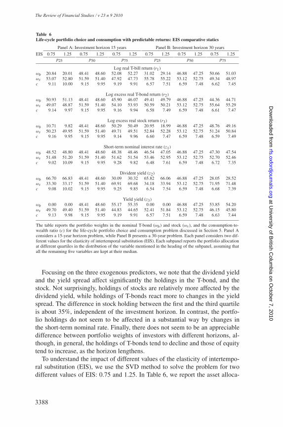
The Review of Financial Studies / v 23 n 9 2010
3388
The State Variable Decomposition Method
Table 6Life-cycle portfolio choice and consumption with predictable returns: EIS comparative statics
Panel A: Investment horizon 15 years Panel B: Investment horizon 30 years
EIS 0.75 1.25 0.75 1.25 0.75 1.25 0.75 1.25 0.75 1.25 0.75 1.25p25 p50 p75 p25 p50 p75
Log real T-bill return (r1)
ωb 20.84 20.01 48.41 48.60 52.08 52.27 31.02 29.14 46.88 47.25 50.66 51.03ωs 53.07 52.80 51.59 51.40 47.92 47.73 55.78 55.22 53.12 52.75 49.34 48.97c 9.11 10.00 9.15 9.95 9.19 9.91 6.57 7.51 6.59 7.48 6.62 7.45
Log excess real T-bond return (r2)
ωb 50.93 51.13 48.41 48.60 45.90 46.07 49.41 49.79 46.88 47.25 44.36 44.71ωs 49.07 48.87 51.59 51.40 54.10 53.93 50.59 50.21 53.12 52.75 55.64 55.29c 9.14 9.97 9.15 9.95 9.16 9.94 6.58 7.49 6.59 7.48 6.61 7.47
Log excess real stock return (r3)
ωb 10.71 9.82 48.41 48.60 50.29 50.49 20.95 18.99 46.88 47.25 48.76 49.16ωs 50.23 49.95 51.59 51.40 49.71 49.51 52.84 52.28 53.12 52.75 51.24 50.84c 9.16 9.95 9.15 9.95 9.14 9.96 6.60 7.47 6.59 7.48 6.59 7.49
Short-term nominal interest rate (z1)
ωb 48.52 48.80 48.41 48.60 48.38 48.46 46.54 47.05 46.88 47.25 47.30 47.54ωs 51.48 51.20 51.59 51.40 51.62 51.54 53.46 52.95 53.12 52.75 52.70 52.46c 9.02 10.09 9.15 9.95 9.28 9.82 6.48 7.61 6.59 7.48 6.72 7.35
Divident yield (z2)
ωb 66.70 66.83 48.41 48.60 30.09 30.32 65.82 66.06 46.88 47.25 28.05 28.52ωs 33.30 33.17 51.59 51.40 69.91 69.68 34.18 33.94 53.12 52.75 71.95 71.48c 9.08 10.02 9.15 9.95 9.25 9.85 6.54 7.54 6.59 7.48 6.68 7.39
Yield yield (z3)
ωb 0.00 0.00 48.41 48.60 55.17 55.35 0.00 0.00 46.88 47.25 53.85 54.20ωs 49.70 49.40 51.59 51.40 44.83 44.65 52.41 51.84 53.12 52.75 46.15 45.80c 9.13 9.98 9.15 9.95 9.19 9.91 6.57 7.51 6.59 7.48 6.63 7.44
The table reports the portfolio weights in the nominal T-bond (ωb) and stock (ωs ), and the consumption-to-wealth ratio (c) for the life-cycle portfolio choice and consumption problem discussed in Section 5. Panel Aconsiders a 15-year horizon problem, while Panel B presents a 30-year problem. Each panel considers two dif-ferent values for the elasticity of intertemporal substitution (EIS). Each subpanel reports the portfolio allocationat different quartiles in the distribution of the variable mentioned in the heading of the subpanel, assuming thatall the remaining five variables are kept at their median.
Focusing on the three exogenous predictors, we note that the dividend yieldand the yield spread affect significantly the holdings in the T-bond, and thestock. Not surprisingly, holdings of stocks are relatively more affected by thedividend yield, while holdings of T-bonds react more to changes in the yieldspread. The difference in stock holding between the first and the third quartileis about 35%, independent of the investment horizon. In contrast, the portfo-lio holdings do not seem to be affected in a substantial way by changes inthe short-term nominal rate. Finally, there does not seem to be an appreciabledifference between portfolio weights of investors with different horizons, al-though, in general, the holdings of T-bonds tend to decline and those of equitytend to increase, as the horizon lengthens.
To understand the impact of different values of the elasticity of intertempo-ral substitution (EIS), we use the SVD method to solve the problem for twodifferent values of EIS: 0.75 and 1.25. In Table 6, we report the asset alloca-
43
at University of B
ritish Colum
bia on October 7, 2010
rfs.oxfordjournals.orgD
ownloaded from

The Review of Financial Studies / v 23 n 9 2010
3388
The State Variable Decomposition Method
3389
The Review of Financial Studies / v 00 n 0 2010
tions to the T-bond and the stock as well as the consumption-to-wealth ratio.Because EIS captures the willingness of the investor to substitute consump-tion intertemporally, the quantity that is most affected by changes in EIS is theconsumption-to-wealth ratio. To understand the pattern of consumption overthe state space, it is useful to recall that changes in expected asset returns carryboth income and substitution effects. If a shock to one or more state variablescauses the expected portfolio return to increase, then the investor will tradeoff the incentive to consume more out of his wealth (income effect) with theincentive to save and take advantage of the favorable investment opportunities(substitution effect). For EIS less than one, the income effect dominates, whilefor EIS greater than one, the substitution effect dominates. We can see this inTable 6 by looking, for example, at the behavior of the consumption-to-wealthratio at different levels of the dividend yield. As the dividend yield increases,for low EIS the consumption-to-wealth ratio increases, while for high EIS theratio decreases. All else being equal, the effect of a change in EIS is morepronounced for longer investment horizons.
Finally, in Table 7 we decompose the total demand in the three assets intomyopic (M) and hedging (H) demand. We define the myopic demand as theportfolio choice of an investor who solves a static problem, i.e., ignoring theevolution of the state variables describing the investment opportunity set. Asthe magnitude of the hedging demands illustrates, ignoring the evolution ofthe investment opportunity set leads to significantly different portfolios. Themagnitudes of the hedging demands are smaller than those reported in CCVbecause we are imposing no short-selling constraints. The hedging demand forstock is always positive and increasing with the investment horizon. A positivehedging demand in a particular asset emerges when the shock to the returnon that asset is negatively correlated with the shock to the state variable thatmostly affects the holding in that asset. For stocks this variable is the dividendyield, and positive holdings of stocks are a way to hedge against changes inthe evolution of the opportunity set brought forth by such a variable. However,with six state variables as in this case, there are multiple cross-effects thatrender the interpretation of each hedging demand less straightforward. Theno-short-selling constraint appears to be more severe in the T-bill. This is con-sistent with the results in CCV, who find that at the annual level, the hedgingdemand for bond and stock is positive, thus causing a large short position incash. Because our investor cannot sell short, he optimally holds a zero positionin the T-bill over a large portion of the state space, as confirmed by the valuesof ω f in Table 7.
In summary, the results of this section demonstrate that the SVD methodyields efficient and accurate solutions to a realistic portfolio choice and con-sumption problem with a large number of state variables and assets, portfolioconstraints, and non-time-separable preferences. These findings suggest thatthe SVD method is suitable for handling other interesting problems of similarscale and complexity.
44
at University of B
ritish Colum
bia on October 7, 2010
rfs.oxfordjournals.orgD
ownloaded from

The Review of Financial Studies / v 23 n 9 2010
3390
The State Variable Decomposition Method
Table 7Life-cycle portfolio choice and consumption with predictable returns: Hedging demands
Panel A: Investment horizon 15 years Panel B: Investment horizon 30 years
M H M H M H M H M H M Hp25 p50 p75 p25 p50 p75
Log real T-bill return (r1)
ω f 63.46 −38.01 0.00 0.00 0.00 0.00 63.46 −51.09 0.00 0.00 0.00 0.00ωb 0.00 21.31 60.56 −12.28 63.51 −11.57 0.00 31.80 60.56 −13.65 63.51 −12.81ωs 36.54 16.70 39.44 12.28 36.49 11.57 36.54 19.29 39.44 13.65 36.49 12.81
Log excess real T-bond return (r2)
ω f 0.00 −0.00 0.00 0.00 37.13 −37.13 0.00 −0.00 0.00 0.00 37.13 −37.13ωb 62.97 −12.18 60.56 −12.28 24.08 21.69 62.97 −13.53 60.56 −13.65 24.08 20.31ωs 37.03 12.18 39.44 12.28 38.78 15.44 37.03 13.53 39.44 13.65 38.78 16.82
Log excess real stock return (r3)
ω f 65.53 −27.09 0.00 −0.00 0.00 0.00 65.53 −40.20 0.00 −0.00 0.00 0.00ωb 0.00 11.16 60.56 −12.28 62.40 −12.25 0.00 21.78 60.56 −13.65 62.40 −13.60ωs 34.47 15.94 39.44 12.28 37.60 12.25 34.47 18.41 39.44 13.65 37.60 13.60
Short-term nominal interest rate (z1)
ω f 0.00 0.00 0.00 −0.00 0.00 0.00 0.00 0.00 0.00 −0.00 0.00 0.00ωb 61.39 −13.08 60.56 −12.28 59.73 −11.44 61.39 −14.89 60.56 −13.65 59.73 −12.33ωs 38.61 13.08 39.44 12.28 40.27 11.44 38.61 14.89 39.44 13.65 40.27 12.33
Divident yield (z2)
ω f 21.19 −21.19 0.00 0.00 0.00 0.00 21.19 −21.19 0.00 0.00 0.00 0.00ωb 56.68 9.88 60.56 −12.28 44.96 −14.94 56.68 9.17 60.56 −13.65 44.96 −16.84ωs 22.13 11.31 39.44 12.28 55.04 14.94 22.13 12.02 39.44 13.65 55.04 16.84
Yield yield (z3)
ω f 66.57 −16.47 0.00 −0.00 0.00 0.00 66.57 −19.09 0.00 0.00 0.00 0.00ωb 0.00 0.00 60.56 −12.28 66.52 −11.48 0.00 0.00 60.56 −13.65 66.52 −12.60ωs 33.43 16.47 39.44 12.28 33.48 11.48 33.43 19.09 39.44 13.65 33.48 12.60
The table reports the portfolio weights in the nominal T-bill (ω f ), nominal T-bond (ωb), and stock (ωs ) forthe life-cycle portfolio choice and consumption problem discussed in Section 5. Panel A considers a 15-yearhorizon, and Panel B is the solution to a 30-year problem. Each subpanel reports the portfolio allocation atdifferent quartiles in the distribution of the variable mentioned in the heading of the subpanel, assuming that allthe remaining five variables are kept at their median. The columns labeled “M” represents the myopic demand,while the columns labeled “H” are the hedging demands.
6. Conclusion
We propose a new, precise, and efficient numerical method for the solution ofdynamic portfolio choice problems and, more generally, for a broad class ofconsumption-portfolio choice problems. The key feature of the State VariableDecomposition (SVD) method we develop is that it approximates the originalproblem by one in which the required conditional expectations do not dependon the choice variables and can be computed efficiently. We achieve this goalvia (i) a decomposition of each state variable into an adapted component andthe associated stochastic deviation; and (ii) the use of Taylor approximation.This allows us to factor out the choice variables and reduce the task of com-puting conditional expectations that involve the value function to that of com-puting conditional moments of the shocks to the state variables. Since thesemoments do not depend on the choice variables, this computation does not
45
at University of B
ritish Colum
bia on October 7, 2010
rfs.oxfordjournals.orgD
ownloaded from

The Review of Financial Studies / v 23 n 9 2010
3390
The State Variable Decomposition Method
3391
The Review of Financial Studies / v 00 n 0 2010
have to be repeated for each candidate solution in the optimization procedure,improving the computational efficiency of the SVD method.
An additional advantage of the SVD method is its ability to handle (i) prob-lems in which endogenous state variables are not redundant, such as wealthwhen preferences are nonhomothetic; and (ii) problems with recursive prefer-ences. This is due to the fact that the SVD method relies on value functioniteration. In contrast, as our analysis shows, methods that rely on policy func-tion iteration in conjunction with Taylor approximations, such as the methoddeveloped by Brandt et al. (2005), cannot handle these two important classesof problems.
We apply the SVD method to a broad array of static and dynamic problemsand verify its accuracy under several realistic features, such as the presenceof intermediate consumption, multiple risky assets and state variables, non-additive preferences, time-varying investment opportunity sets, and nonredun-dant endogenous state variables. In all of the applications we consider, the SVDmethod emerges as a fast, accurate, and reliable procedure. The conceptualsimplicity, precision, and computational efficiency of the SVD method makeit an important new tool for solving realistic consumption-portfolio choiceproblems.
A. Appendix: Proofs
A.1 Proof of Proposition 2For the CARA utility function, u(W ) = − exp(−αW ), we have
u(m)(W ) = (−1)m+1αme−αW . (A.1)
Therefore, for W2 = W1 R f + 1αμμμ�
R���−1R R2, we have
u(m)(W2
) = (−1)m+1αme−αW1 R f e−Y2 , (A.2)
where Y2 = μμμ�R���−1
R R2 ∼ N (S2, S2) and S2 = μμμ�R���−1
R μμμR is the squared Sharpe ratio. Hence,using the binomial formula, we obtain
E1
[u(m)
(W2
) (R f + 1
αW1μμμ�
R���−1R R2
)m]
= (−1)m+1αme−αW1 R f E1
[e−Y2
(R f + 1
αW1Y2
)m]
= (−1)m+1αme−αW1 R fm∑
k=0
(m
k
)(1
αW1
)kRm−k
f E1
[Y k
2 e−Y2]. (A.3)
46
at University of B
ritish Colum
bia on October 7, 2010
rfs.oxfordjournals.orgD
ownloaded from

The Review of Financial Studies / v 23 n 9 2010
3392
The State Variable Decomposition Method
Using the fact that Y2 ∼ N (S2, S2), we obtain
E1
[Y k
2 e−Y2]
=∫ ∞
−∞1√
2π S2yke−ye
− (y−S2)2
2S2 dy
= e− S22
∫ ∞
−∞1√
2π S2yke
− y2
2S2 dy
= e− S22 Sk
∫ ∞
−∞1√2π
zke− z22 dz
= e− S22 Skφk , (A.4)
where φk is the k-th central moment of the standard normal distribution. Substituting
E1
[Y k
2 e−Y2]
= e− S22 Skφk in (A.3) yields the result and completes the proof.
B. Appendix: Implementation Details
In this Appendix we describe in detail how the SVD method is implemented to solve the problemsconsidered in Sections 3 and 5.
B.1 CARA-Normal Example of Section 3A. Projection step. At each time t , we know the values of the function Vt+1
(Wt+1
)(see equa-
tion (33)) on a grid of points on the wealth space.26 Given these values, we approximateVt+1
(Wt+1
)over the entire wealth space by a polynomial of order K in Wt+1:27
Vt+1(Wt+1) ≈K∑
k=0
ϑt+1,k W kt+1. (B.1)
Given the terminal condition VT (WT ) = WT , the above approximation is exact at time T withϑT,0 = 0, ϑT,1 = 1, and ϑT,k = 0 for k = 2, . . . , K .
B. SVD step. In this step we use the SVD method to find the optimal portfolio in (34) and obtainthe value of Vt (Wt ) on a grid of points for Wt . This step involves three separate substeps.
B-1. Decomposition of state variables. We first decompose the innovation, i.e., the riskyasset excess return Rt+1, into its mean μμμR and the associated deviation εεεR,t+1:28
Rt+1 = μμμR + εεεR,t+1. (B.2)
This decomposition induces the following decomposition on the state variable, i.e.,wealth:
Wt+1 = Wt(R f + ωωω�
t Rt+1) = μW,t + εW,t+1, (B.3)
26 We construct a sequence of expanding grids as follows. We start at time 0 with an equally spaced grid G0over the interval
[W0,L , W0,U
]. Then, for t = 0, 1, . . . , T − 1, we successively define Wt+1,L = Wt,L − QL
and Wt+1,U = Wt,U + QU and construct an equally spaced grid Gt+1 over the interval[Wt+1,L , Wt+1,U
].
In practice, we increase QL and QU gradually until we obtain a stable solution. In our implementation, theresults of which are reported in Subsection 3.3, we use W0,L = 1, W0,U = 2, QL = 0.2, QU = 0.5, and eachgrid consists of 100 points.
27 While one can use alternative functional approximations in this projection step, using polynomials is sufficientin the context of this problem since the state space is one-dimensional.
28 As discussed in the previous section, since the distribution of asset returns is symmetric, the choice of the meanas center of expansion is desirable as it minimizes the likelihood of large deviations in the Taylor approximation.
47
at University of B
ritish Colum
bia on October 7, 2010
rfs.oxfordjournals.orgD
ownloaded from

The Review of Financial Studies / v 23 n 9 2010
3392
The State Variable Decomposition Method
3393
The Review of Financial Studies / v 00 n 0 2010
where μW,t = Wt (R f + ωωω�tμμμR) and εW,t+1 = Wt (ωωω
�tεεεR,t+1). Note that although the
center of expansion for the decomposition of return in (B.2) is exogenous, the impliedcenter of expansion for the state variable in (B.3) is endogenous because it dependson the choice variable ωωωt . Combining the wealth decomposition (B.3) with the projec-tion (B.1), we obtain the following approximation:
Vt+1(Wt+1) ≈K�
k=0
ϑt+1,k (μW,t + εW,t+1)k . (B.4)
Using (B.4), we approximate the conditional expectation in the Bellman equation (34)as follows:
Et
�−e−αVt+1(Wt+1)
�≈ Et
�−e−α
�Kk=0 ϑt+1,k
�μW,t +εW,t+1
�k�
≡ Et�gt+1(εW,t+1)
�. (B.5)
B-2. Separation of choice variables from shocks. To separate choice variables from shocks,we first approximate gt+1(εW,t+1) in equation (B.5) by a Taylor expansion of orderM centered at εW,t+1 = 0:
gt+1(εW,t+1) ≈M�
m=0
1
m! g(m)t+1(0)εm
W,t+1, (B.6)
where g(m)t+1(0) denotes the m-th derivative of gt+1(εW,t+1) evaluated at εW,t+1 =
0, for m = 0, . . . , M . We then use the fact that εW,t+1 = Wt�ωωω�
tεεεR,t+1�
and fullyseparate the choice variable ωωωt from εεεR,t+1 by applying the multinomial formula tothe expression
�ωωω�
tεεεR,t+1�m . This yields
εmW,t+1 = W m
t (ωωω�tεεεR,t+1)m = W m
t
�{q:|q|=m}
m!q!
N�
n=1
ωqnn,t
N�
n=1
εqnRn ,t+1, (B.7)
where q = (q1, . . . , qN )� is a vector of nonnegative integers, |q| = q1 + · · · + qN ,and q! = q1! · · · qN !
B-3. Computation of conditional expectations. Combining (34), (B.5), (B.6), and (B.7), wecan compute an approximation to the certainty equivalent function Vt (Wt ) as follows:
−e−αVt (Wt ) ≈ maxωωωt
⎧⎨⎩
M�
m=0
W mt g(m)
t+1(0)�
{q:|q|=m}
1
q!N�
n=1
ωqnn,t Et
⎡⎣
N�
n=1
εqnRn ,t+1
⎤⎦
⎫⎬⎭.
(B.8)Solving the optimization problem in (B.8) involves computing the moments
Et
��Nn=1 ε
qnRn ,t+1
�. This calculation is performed in an efficient fashion using the
recursive scheme developed by Savits (2006) and discussed in Appendix D.2.
The solution of (B.8) delivers the values Vt (Wt ) on a grid of points for Wt , and the algorithmproceeds to step A above until we reach time zero.
B.2 Life-cycle Problem of Section 5A. Projection step. At time t , we know the values of the function Vt+1(yt+1) (see equation (85))
on the set Gt+1 of grid points in the state space. Using this information, we approximate the
48
at University of B
ritish Colum
bia on October 7, 2010
rfs.oxfordjournals.orgD
ownloaded from
The Review of Financial Studies / v 23 n 9 2010
3394
The State Variable Decomposition Method
value function Vt+1(yt+1) over the entire yt+1 space by a projection based on a radial basisfunction with 500 Gaussian kernels.29
B. SVD step. In this step, we perform the optimization in (87) and use (85) to obtain the valuefunction Vt (yt ) on the grid Gt . This step consists of three separate substeps.
B-1. Decomposition of state variables. We decompose each element yi,t+1 of the vector yt+1 =(r�
t+1, z�t+1)� into its conditional mean μi,t and the associated zero-mean stochastic devia-
tion εi,t+1 as follows:yi,t+1 = μi,t + εi,t+1, i = 1, . . . , 6, (B.9)
where�μ1,t , . . . , μ6,t
�� ≡ μμμt = a + Byt . Substituting the decomposition (B.9) in equation
(87), we can express the quantities Rp,t+1(ωωωt )1−γ and Vt+1(yt+1)1−γ as functions of
the primitive shocks εεεy,t+1. We do so by introducing two functions h1 and h2 defined asfollows:
h1(ωωωt , ε1,t+1, ε2,t+1, ε3,t+1) = �eμ1,t +ε1,t+1
�1 + ωb,t (e
μ2,t +ε2,t+1 − 1)
+ωs,t (eμ3,t +ε3,t+1 − 1)
��1−γ, (B.10)
h2(εεεy,t+1) = �Vt+1(μt + εεεy,t+1)
�1−γ, (B.11)
where the base of the power on the right-hand side of (B.10) follows directly from thedefinition of Rp,t+1(ωωωt ) in (78) and the decomposition (B.9). Having defined these twofunctions, we can express the expectation in (87) as
Et
�Rp,t+1(ωωωt )
1−γ · Vt+1(yt+1)1−γ�= Et
�h1(ωωωt , ε1,t+1, ε2,t+1, ε3,t+1) · h2(εεεy,t+1)
�.
(B.12)B-2. Separation of choice variables from shocks. We use a Taylor expansion of the functions
h1 and h2 in equation (B.12) with respect to (ε1,t+1, ε2,t+1, ε3,t+1)� and εεεy,t+1 around03 and 06, respectively. Because h1 is a function of three state variables only (three assetreturns) while h2 is a function of all six state variables (three asset returns and three ex-ogenous predictors), to simplify notation, we denote by n the vector of indices of the firstthree variables, i.e., n = (n1, n2, n3)�, and by k the vector of indices for all six variables,i.e., k = (k1, . . . , k6)�. These indices represent the orders of partial derivative in each of thecorresponding variables. We further denote by h1,n the partial derivative of order n of thefunction h1, i.e.,
h1,n(ωωωt ) = ∂ |n|h1
∂εn11 ∂ε
n22 ∂ε
n33
(ωωωt , 03), (B.13)
and by h2,k the partial derivative of order k of the function h2, i.e.,
h2,k = ∂ |k|h2
∂εk11 ∂ε
k22 ∂ε
k33 ∂ε
k44 ∂ε
k55 ∂ε
k66
(06), (B.14)
where |n| = �3i=1 ni and |k| = �6
i=1 ki . The expectation (B.12) is then approximated by
Et
⎡⎣
⎛⎝ �
|n|≤M1
1
n! h1,n(ωωωt )
3�
i=1
εnii,t+1
⎞⎠ ·
⎛⎝ �
|k|≤M2
1
k! h2,k
6�
j=1
εk jj,t+1
⎞⎠
⎤⎦, (B.15)
29 Given the high dimensionality and the complexity of the value function approximation problem, we opted forthe more powerful class of radial basis functions instead of using more traditional basis functions, such aspolynomials. See footnote 12 for the definition of radial basis functions. The use of radial basis functions allowsus to keep the mean square error in the approximation of Vt (·) in each step of the backward recursion in theorder of 10−6.
49
at University of B
ritish Colum
bia on October 7, 2010
rfs.oxfordjournals.orgD
ownloaded from
The Review of Financial Studies / v 23 n 9 2010
3394
The State Variable Decomposition Method
3395
The Review of Financial Studies / v 00 n 0 2010
where M1 and M2 are the chosen orders of Taylor expansion for h1 and h2, respectively.Note that in equation (B.15), the choice variables ωωωt are separated from the primitive shocksεi,t+1. The derivatives h1,n(ωωωt ) and h2,k can be computed efficiently by using the recursivescheme in Savits (2006) (see Appendix D.1). In our implementation of the SVD method, weuse Taylor expansions of order 4 for the functions h1 and h2 (i.e., M1 = M2 = 4 in (B.15)).
B-3. Computation of conditional expectations. Given the separation between choice variablesand shocks achieved in the previous step, the computation of conditional expectationsin (B.15) reduces to the computation of cross moments of the form
Et
⎡⎣
3�
i=1
εnii,t+1
6�
j=1
εk jj,t+1
⎤⎦ = Et
⎡⎣
3�
i=1
εni +kii,t+1
6�
j=4
εk jj,t+1
⎤⎦. (B.16)
Under the VAR dynamics (79), this amounts to computing the central moments of a mul-tivariate normal distribution for which the efficient recursive scheme of Savits (2006) canbe used (see Appendix D.2). Note that the computation of these moments needs to be doneonly once and does not have to be repeated at each step of the backward recursion. It turnsout that for high-dimensional problems like the one considered in this section, this providesa tremendous improvement in computational efficiency.
Once the optimization in (87) is performed, we use (85) to recover the value function Vt (yt ) onthe set Gt of grid points in the state space. The algorithm then proceeds to Step A and continuesuntil we reach time zero.
C. Appendix: Convergence Issues
An important issue underlying the applicability of the SVD method relates to the convergence ofthe Taylor series approximation. In the context of a static portfolio choice problem with HARApreferences, Garlappi and Skoulakis (2009b) show that convergence obtains provided that thedistribution of the stochastic shocks has compact support, and the center of the Taylor expansionis chosen to be the midpoint of the support of the risky asset excess return distribution.
The same idea can be used in the context of dynamic portfolio choice problems when the utilityfunction belongs to the HARA class. To see this, consider the problem stated in (14) and the taskof approximating the conditional expectation Et
�Jt+1(st+1)
� = Et�U
�Vt+1(st+1)
��. Using the
law of motion st+1 = �(st , xt , δδδt+1) and defining Qt+1�δδδt+1; st , xt
� ≡ Vt+1��(st , xt , δδδt+1)
�,
the objective is to approximate Et�U
�Qt+1
�δδδt+1; st , xt
���. This can be accomplished by first us-
ing the decomposition δδδt+1 = cδ,t + εεεδ,t+1 and then taking the Taylor expansion with respect to
εεεδ,t+1 around zero. If the utility function is in the HARA class, i.e., u(W ) = 11−γ
�W + γ
ζ
�1−γ,
where ζ �= 0, γ �= 1, γ > 0, W + γζ > 0, and we use U(·) = u(·), then, adapting the analysis in
Garlappi and Skoulakis (2009b), one can show that the Taylor series converges if the center cδ,t isselected so that, for all δδδt+1, |Qt+1
�δδδt+1; st , xt
� − Qt+1�cδ,t ; st , xt
� | < Qt+1�cδ,t ; st , xt
� +γζ .30 A sufficient condition for this is Qt+1
�cδ,t ; st , xt
�> 1
2 Qt+1�δδδt+1; st , xt
�, for all δδδt+1.
For a similar argument, see Corollary 2.3 in Garlappi and Skoulakis (2009b).More generally, convergence of the Taylor expansion can also be established for the wider
class of mixed risk aversion (MRA) utility functions (e.g., Brockett and Golden 1987; Caballeand Pomansky 1996). This is a very general class that contains all utility functions that possessderivatives of every order that alternate in sign. According to Theorem 1 in Brockett and Golden(1987), for every MRA utility function u(·), there exists a measure μ on [0,∞) such that
u(W ) = u(W0) +� ∞
0
1 − exp (−α(W − W0))
αμ(dα), (C.1)
30 To see this, note that the function f (x) = (1 + x)1−γ has a Taylor series expansion around x = 0 that convergeswhen |x | < 1. It then follows that the function g(x) = (x + θ)1−γ has a Taylor series expansion around κ , with
κ + θ > 0, that converges when |x − κ| < κ + θ , since g(x) = (κ + θ)1−γ�
1 + x−κκ+θ
�1−γ.
50
at University of B
ritish Colum
bia on October 7, 2010
rfs.oxfordjournals.orgD
ownloaded from
The Review of Financial Studies / v 23 n 9 2010
3396
The State Variable Decomposition Method
where W0 satisfies −∞ < u(W0) < ∞. In other words, u(·) is equivalent to a mixture of CARAutility functions with absolute risk aversion α distributed over [0,∞) according to measure μ.The MRA class contains, as special cases, the HARA class, the power risk aversion class, and thepower risk tolerance class. Of particular importance for our purposes is the procedure, developedby Brockett and Golden (1987), for approximating any MRA utility function by a finite mixture ofexponential (CARA) utility functions through interpolation.31 This is a convenient result since afinite mixture of CARA utility functions has a Taylor series representation that converges globally,i.e., for any shock realization. This means that we can approximate u(·), or equivalently U(·), overthe range of Vt (·) by a function u(·), which is a finite mixture of CARA utility functions and hasglobally convergent Taylor series expansion. Since in the projection step we approximate Vt (·) byeither a polynomial or a radial basis function, i.e., functional forms that have a globally convergentseries representation, it follows that the Taylor series approximation to u(Vt (·)) converges for anycenter of expansion (see Theorem 9.25 in Apostol 1974).
A final technical point relates to the assumption of compactness of the distribution of shocksthat is required for establishing formal convergence results. This assumption is not as restrictive asit might appear, for the following reasons. First, given the finite amount of data that we observe inreality, it is impossible to statistically reject the assumption that a distribution of an economic vari-able has bounded support. Second, from a purely theoretical point of view, compactness appearsto be an indispensable technical requirement for rigorously establishing convergence results in thecontext of dynamic programming problems. It is worth noting that a similar issue arises in provingconvergence of the quadrature approximation method in Tauchen and Hussey (1991), which canonly be shown under the assumption of shocks with compact support. In justifying this assump-tion, Tauchen and Hussey (1991, p. 380) make the following statement: “. . . we follow the traditionin this area of research of applying results deduced for the case of bounded support to models withunbounded support.” We are not aware of theoretical results that establish convergence without thecompactness assumption.
D. Appendix: Useful Recursive Schemes from Multivariate Analysis
In this Appendix, we summarize two useful recursive schemes that facilitate the efficient numericalimplementation of the SVD approach. D.1 introduces a recursive scheme for the computation ofderivatives of a composite function of multiple variables, and D.2 describes a recursive scheme forthe efficient computation of central moments of a multivariate normal distribution. The results arebased on Savits (2006).
D.1 Efficient Computation of Derivatives of Composite FunctionsThe application of the SVD approach relies on Taylor expansion and this, in turn, creates the needfor efficient computation of the derivatives of composite functions of the form h(εεε) = f (g(εεε)),where f : R → R, g : RN → R, and εεε denotes the N -dimensional vector of fundamental shocks.The generic M-th order Taylor expansion of h centered at 0N is
h(ε) ≈∑
{q:|q|≤M}
1
q! hq(0N )
N∏
n=1
εqnn , (D.1)
31 Specifically, consider a utility function u(·) in the MRA class. Then, given an equally spaced grid{Vi = a + bi : i = 0, 1, . . . , 2N
}of 2N points, where b > 0, one can determine a real ξ0, and positive ξn and
αn , n = 1, . . . , N , so that u(Vi ) = u(Vi ), i = 0, 1, . . . , 2N , where u(V ) = ξ0 − ∑Nn=1 ξne−αn V .
51
at University of B
ritish Colum
bia on October 7, 2010
rfs.oxfordjournals.orgD
ownloaded from

The Review of Financial Studies / v 23 n 9 2010
3396
The State Variable Decomposition Method
3397
The Review of Financial Studies / v 00 n 0 2010
where q = (q1, . . . , qN )� is a vector of nonnegative integers, |q| = ∑Nn=1 qn , q! = ∏N
n=1(qn !),and hq(0N ) denotes the partial derivative of order q of the function h(εεε) evaluated at 0N , i.e.,
hq(0N ) = ∂q1+···+qN h
∂εq11 · · · εqN
N
(0N ). (D.2)
To compute such derivatives, we rely on the recursive version of the multidimensional Faa diBruno (1855, 1857) formula derived in Savits (2006). To present the formula, we need to introducesome notation. Let N0 denote the set of nonnegative integers. Let q = (q1, . . . , qN )� ∈ NN
0 and
��� = (�1, . . . , �N )� ∈ NN0 . We write ��� ≤ q if �n ≤ qn , for n = 1, . . . , N , and denote
(q���
)= q!
���!(q − ���)! . (D.3)
Let gq(εεε) denote the partial derivative of order q of the function g(εεε), and fn(x) denote then-th derivative of the function f (x) with respect to the one-dimensional variable x . According tothe multivariate Faa di Bruno formula, the partial derivative of order q of the composite functionh(εεε) = f (g(εεε)), i.e., hq(εεε), can be expressed as
hq(εεε) =|q|∑
n=1
fn(g(εεε)) αq,n(εεε), (D.4)
where αq,n(εεε) are homogeneous polynomials of degree n in the partial derivatives g���(εεε), ��� ≤ q.To compute the generic derivative of h, it is, therefore, sufficient to determine the polynomialsαq,n(εεε). These can be computed efficiently by relying on the recursive relationship proved inTheorem 3.1 of Savits (2006), which we reproduce here.
Theorem 1. For q ≥ 0N , 1 ≤ j ≤ N , and 1 ≤ n ≤ |q| + 1, we have
αq+e j ,n(εεε) =∑
{���∈NN0 : 0N ≤���≤q, |���|≥n−1}
(q���
)gq+e j −���(εεε)α���, n−1(εεε), (D.5)
where e j is the N -dimensional unit vector with j-th component equal to 1, and we set
α���,0(εεε) ={
1, if ��� = 0N ,
0, if ��� �= 0N .(D.6)
If the set {��� ∈ NN0 : 0N ≤ ��� ≤ q, |���| ≥ n − 1} is empty, the polynomial αq+e j , n(εεε) vanishes.
D.2 Efficient Computation of Multivariate Moments of a NormalRandom Variable
Let εεε = (ε1, . . . , εN )� be a zero-mean N -dimensional normal random variable with covariancematrix ���, with (i, j) element equal to σi j . Let λ(ν1,...,νN ) be its (ν1, . . . , νN )-moment, where
ν1, . . . , νN are nonnegative integers, i.e., λ(ν1,...,νN ) ≡ E[εν11 . . . ε
νNN
]. Then, from Theorem 5.1
in Savits (2006), we have the following recursive characterization of the multivariate momentsof εεε.
Theorem 2. Set λ(0,...,0) = 1. Then, for all (ν1, . . . , νN ) ≥ 0N and 1 ≤ j ≤ N , we have
λ(ν1,...,νN )+e j ≡ E
[εν11 · · · εν j +1
j · · · ενNN
]=
N∑
k=1
σ jk νk λ(ν1,...,νN )−ek , (D.7)
where e j is the N -dimensional unit vector with j-th component equal to 1.
52
at University of B
ritish Colum
bia on October 7, 2010
rfs.oxfordjournals.orgD
ownloaded from

The Review of Financial Studies / v 23 n 9 2010
3398
The State Variable Decomposition Method
ReferencesAıt-Sahalia, Y., J. Cacho-Diaz, and T. R. Hurd. 2009. Portfolio Choice with Jumps: A Closed-Form Solution.Annals of Applied Probability 19:556–84.
Apostol, T. M. 1974. Mathematical Analysis. Reading, MA: Addison-Wesley.
Balduzzi, P., and A. Lynch. 1999. Transaction Costs and Predictability: Some Utility Cost Calculations. Journalof Financial Economics 52:47–78.
Barberis, N. 2000. Investing for the Long Run When Returns Are Predictable. Journal of Finance 55:225–64.
Bertsekas, D., and J. Tsitsiklis. 1996. Neuro-Dynamic Programming. Nashua, NH: Athena Scientific.
Bhamra, H., and R. Uppal. 2006. The Role of Risk Aversion and Intertemporal Substitution in DynamicConsumption-Portfolio Choice with Recursive Utility. Journal of Economic Dynamics and Control 30:967–91.
Bishop, C. 1995. Neural Networks for Pattern Recognition. Oxford: Oxford University Press.
Brandt, M. W. 1999. Estimating Portfolio and Consumption Choice: A Conditional Euler Equation Approach.Journal of Finance 54:1609–46.
Brandt, M. W., A. Goyal, P. Santa-Clara, and J. R. Stroud. 2005. A Simulation Approach to Dynamic PortfolioChoice with an Application to Learning about Return Predictability. Review of Financial Studies 18:831–73.
Brennan, M. J., E. S. Schwartz, and R. Lagnado. 1997. Strategic Asset Allocation. Journal of Economic Dynam-ics and Control 21:1377–403.
Brockett, P. L., and L. L. Golden. 1987. A Class of Utility Functions Containing All the Common Utility Func-tions. Management Science 133:955–64.
Caballe, J., and A. Pomansky. 1996. Mixed Risk Aversion. Journal of Economic Theory 71:485–513.
Campbell, J. Y., Y. L. Chan, and L. M. Viceira. 2003. A Multivariate Model of Strategic Asset Allocation.Journal of Financial Economics 67:41–80.
Campbell, J. Y., J. Cocco, F. Gomes, P. J. Maenhout, and L. M. Viceira. 2001. Stock Market Mean Reversionand the Optimal Equity Allocation of a Long-Lived Investor. European Finance Review 5:269–92.
Campbell, J. Y., and L. M. Viceira. 1999. Consumption and Portfolio Decisions When Expected Returns AreTime Varying. Quarterly Journal of Economics 114:433–95.
Chacko, G., and L. M. Viceira. 2005. Dynamic Consumption and Portfolio Choice with Stochastic Volatility inIncomplete Markets. Review of Financial Studies 18:1369–402.
Consigli, G., and M. Dempster. 1998. Dynamic Stochastic Programming for Asset-Liability Management.Annals of Operations Research 81:131–62.
Cvitanic, J., A. Lazrak, L. Martellini, and F. Zapatero. 2006. Dynamic Portfolio Choice with Uncertainty andthe Economic Value of Analysts’ Recommendations. Review of Financial Studies 19:1113–56.
Dammon, R. M., C. S. Spatt, and H. H. Zhang. 2001. Optimal Consumption and Investment with Capital GainsTaxes. Review of Financial Studies 14:583–616.
Das, S. R., and R. K. Sundaram. 2002. A Numerical Algorithm for Consumption-Investment Problems. Interna-tional Journal of Intelligent Systems in Accounting, Finance and Management 11:55–69.
Detemple, J. B., R. Garcia, and M. Rindisbacher. 2003. A Monte Carlo Method for Optimal Portfolios. Journalof Finance 58:410–46.
Epstein, L. G., and S. Zin. 1989. Substitution, Risk Aversion and the Temporal Behavior of Consumption andAsset Returns: A Theoretical Framework. Econometrica 57:937–69.
53
at University of B
ritish Colum
bia on October 7, 2010
rfs.oxfordjournals.orgD
ownloaded from

The Review of Financial Studies / v 23 n 9 2010
3398
The State Variable Decomposition Method
3399
The Review of Financial Studies / v 00 n 0 2010
———. 1991. Substitution, Risk Aversion and the Temporal Behavior of Consumption and Asset Returns: AnEmpirical Analysis. Journal of Political Economy 99:263–86.
Faa di Bruno, F. 1855. Sullo Sviluppo delle Funzioni. Annali di Scienze Matematiche e Fisiche 6:479–80.
———. 1857. Note Sur une Nouvelle Formule de Calcul Differentiel. Quarterly Journal of Pure and AppliedMathematics 1:359–60.
Garlappi, L., and G. Skoulakis. 2009a. Numerical Solutions to Dynamic Portfolio Problems: The Case for ValueFunction Iteration Using Taylor Expansion. Computational Economics 33:193–207.
———. 2009b. Taylor Series Approximations to Expected Utility and Portfolio Choice. Working Paper, Uni-versity of British Columbia and University of Maryland.
Glasserman, P. 2004. Monte Carlo Methods in Financial Engineering. New York: Springer-Verlag.
Hakansson, N. H. 1971. Capital Growth and the Mean-Variance Approach to Portfolio Selection. Journal ofFinancial and Quantitative Analysis 6:517–57.
Hassoun, M. 1995. Fundamentals of Artificial Neural Networks. Cambridge, MA: MIT Press.
Haykin, S. 1998. Neural Networks: A Comprehensive Foundation, 2nd ed. Upper Saddle River, NJ: PrenticeHall.
Hlawitschka, W. 1994. The Empirical Nature of Taylor-Series Approximations to Expected Utility. AmericanEconomic Review 84:713–19.
Judd, K. 1998. Numerical Methods in Economics. Cambridge, MA: MIT Press.
Kim, T. S., and E. Omberg. 1996. Dynamic Nonmyopic Portfolio Behavior. Review of Financial Studies9:141–61.
Kogan, L., and R. Uppal. 2003. Risk Aversion and Optimal Portfolio Policies in Partial and General EquilibriumEconomies. CEPR Discussion Paper 3306 and NBER Working Paper 8609.
Kroll, Y., H. Levy, and H. M. Markowitz. 1984. Mean-Variance Versus Direct Utility Maximization. Journal ofFinance 39:47–75.
Liu, J. 2007. Portfolio Selection in Stochastic Environments. Review of Financial Studies 20:1–39.
Loistl, O. 1976. The Erroneous Approximation of Expected Utility by Means of a Taylor’s Series Expansion:Analytic and Computational Results. American Economic Review 66:904–10.
Longstaff, F. A., and E. S. Schwartz. 2001. Valuing American Options by Simulation: A Simple Least-SquaresApproach. Review of Financial Studies 14:113–47.
Lynch, A. W., and P. Balduzzi. 2000. Predictability and Transaction Costs: The Impact on Rebalancing Rulesand Behavior. Journal of Finance 55:2285–309.
Markowitz, H. M. 1991. Foundations of Portfolio Theory. Journal of Finance 46:469–77.
Merton, R. C. 1969. Lifetime Portfolio Choice: The Continuous-Time Case. Review of Economics and Statistics51:247–57.
Merton, R. C. 1971. Optimum Consumption and Portfolio Rules in a Continuous-Time Model. Journal of Eco-nomic Theory 3:373–413.
———. 1973. An Intertemporal Asset Pricing Model. Econometrica 41:867–88.
Niederreiter, H. 1992. Random Number Generation and Quasi-Monte Carlo Methods. Society for Industrial andApplied Mathematics.
Pulley, L. B. 1981. A General Mean-Variance Approximation to Expected Utility for Short Holding Periods.Journal of Financial and Quantitative Analysis 16:361–73.
54
at University of B
ritish Colum
bia on October 7, 2010
rfs.oxfordjournals.orgD
ownloaded from

The Review of Financial Studies / v 23 n 9 2010
3400
The State Variable Decomposition Method
———. 1983. Mean-Variance Approximations to Expected Logarithmic Utility. Operations Research31:685–96.
Reed, R., and R. Marks. 1999. Neural Smithing: Supervised Learning in Feedforward Artificial Neural Networks.MIT Press.
Samuelson, P. A. 1969. Lifetime Portfolio Selection by Dynamic Stochastic Programming. Review of Economicsand Statistics 51:239–46.
———. 1970. The Fundamental Approximation Theorem of Portfolio Analysis in Terms of Means, Variancesand Moments. Review of Economic Studies 37:537–42.
Savits, T. H. 2006. Some Statistical Applications of Faa di Bruno. Journal of Multivariate Analysis97:2131–40.
Skoulakis, G. 2008. A Recursive Formula for Computing Central Moments of a Multivariate Lognormal Distri-bution. American Statistician 62:147–50.
Tauchen, G., and R. Hussey. 1991. Quadrature-Based Methods for Obtaining Approximate Solutions to Nonlin-ear Asset Pricing Models. Econometrica 59:371–96.
Tsitsiklis, J. N., and B. Van Roy. 2001. Regression Methods for Pricing Complex American-Style Options. IEEETransactions on Neural Networks 12:694–703.
van Binsbergen, J. H., and M. W. Brandt. 2007. Solving Dynamic Portfolio Choice Problems by Recursing onOptimized Portfolio Weights or on the Value Function? Computational Economics 29:355–67.
Vissing-Jørgensen, A. 2002. Limited Asset Market Participation and the Elasticity of Intertemporal Substitution.Journal of Political Economy 110:825–53.
Wachter, J. A. 2002. Portfolio and Consumption Decisions under Mean-Reverting Returns: An Exact Solutionfor Complete Markets. Journal of Financial and Quantitative Analysis 37:63–91.
White, H. 1992. Artificial Neural Networks: Approximation and Learning Theory. Cambridge, MA: Blackwell.
55
at University of B
ritish Colum
bia on October 7, 2010
rfs.oxfordjournals.orgD
ownloaded from