Solutions for modelling moving heat sources

in a semi-infinite medium and applications to

laser material processing

M. Van Elsen a,∗, M. Baelmans a, P. Mercelis a and J.-P. Kruth a

aDepartement of Mechanical Engineering, Catholic University of Leuven,Celestijnenlaan 300b, B-3001 Heverlee, Belgium

Abstract

This study describes the analytical and numerical solution of the heat conductionequation for a localised moving heat source of any type for use in laser materialprocessing, as welding, layered manufacturing and laser alloying. In this paper, theanalytical solution for a uniform heat source is derived from the solution of an in-stantaneous point heat source. The result is evaluated numerically and is comparedto existing solutions for the moving point source and a semi-ellipsoidal source. Next,the result is used to demonstrate how such model can be used to study the effectof the heat source geometry. Besides, this solution reveals that a melting efficiencyhigher than 0.37 (= 1/e, a maximum value stated by Rykalin [1]) can be obtained.To investigate the effect of the temperature dependence of the material parameters,in particular the latent heat of fusion, a finite difference model is implemented. Itis shown that the enthalpy method is most suited to implement the latent heat offusion. A numerical evaluation for TiAl6V4, reveals that the effect of the latent heatis rather small, except for the case when the conductivity is very low, e.g. whenscanning in a loose powder bed. The results demonstrate that analytical and nu-merical solutions can be effectively used to calculate the temperature distributionin a semi-infinite medium for finite 3D heat sources. In this way, a tool to inves-tigate the importance of different processing parameters in laser manufacturing isobtained.

Key words: Moving heat source, Semi-infinite body, Temperature distribution,Laser manufacturing

∗ Corresponding author. Tel.: +32-16-32-25-52; Fax: +32-16-32-29-87Email address: Maarten.VanElsen@mech.kuleuven.be (M. Van Elsen).

Preprint submitted to Int. Journal on Heat and Mass Transfer 20 February 2006

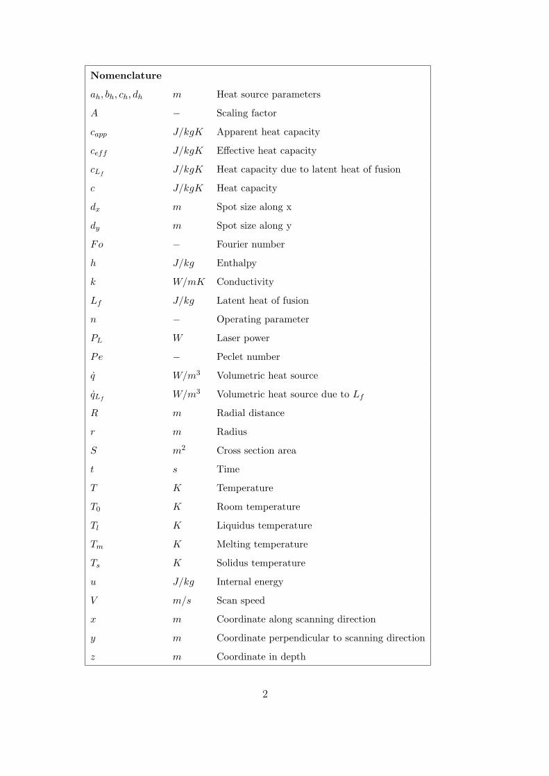
Nomenclature

ah, bh, ch, dh m Heat source parameters

A − Scaling factor

capp J/kgK Apparent heat capacity

ceff J/kgK Effective heat capacity

cLfJ/kgK Heat capacity due to latent heat of fusion

c J/kgK Heat capacity

dx m Spot size along x

dy m Spot size along y

Fo − Fourier number

h J/kg Enthalpy

k W/mK Conductivity

Lf J/kg Latent heat of fusion

n − Operating parameter

PL W Laser power

Pe − Peclet number

q̇ W/m3 Volumetric heat source

q̇LfW/m3 Volumetric heat source due to Lf

R m Radial distance

r m Radius

S m2 Cross section area

t s Time

T K Temperature

T0 K Room temperature

Tl K Liquidus temperature

Tm K Melting temperature

Ts K Solidus temperature

u J/kg Internal energy

V m/s Scan speed

x m Coordinate along scanning direction

y m Coordinate perpendicular to scanning direction

z m Coordinate in depth

2

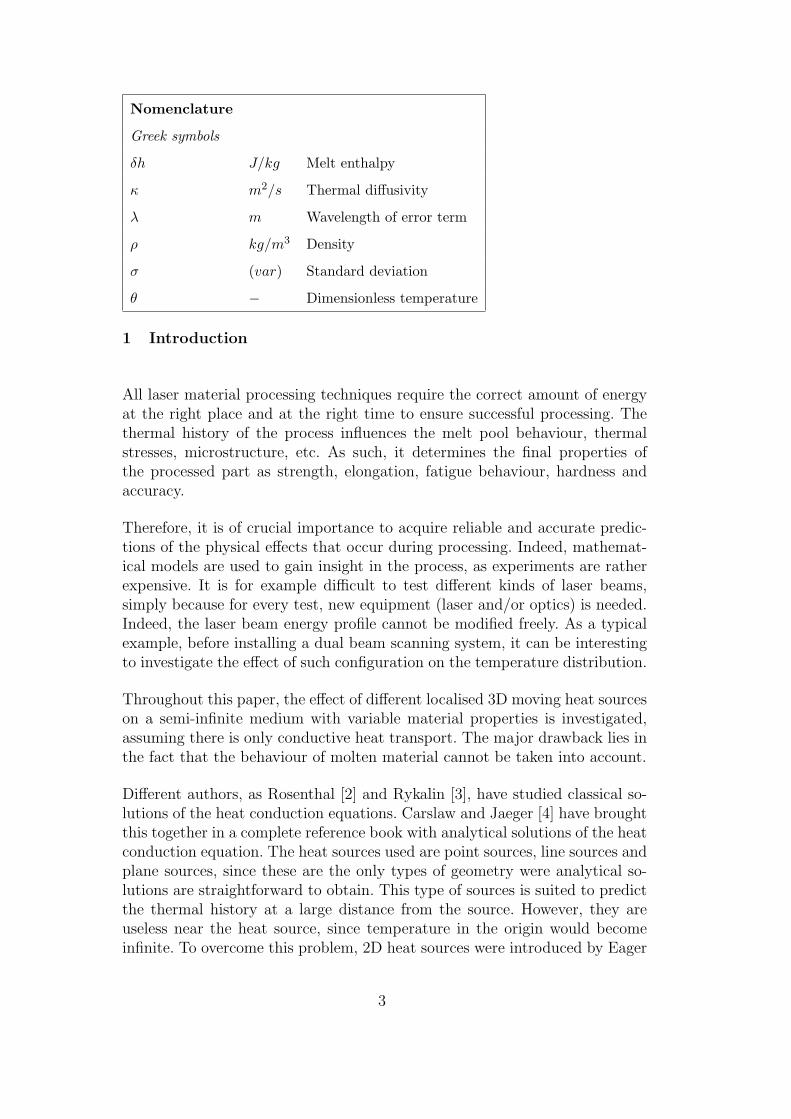
Nomenclature

Greek symbols

δh J/kg Melt enthalpy

κ m2/s Thermal diffusivity

λ m Wavelength of error term

ρ kg/m3 Density

σ (var) Standard deviation

θ − Dimensionless temperature

1 Introduction

All laser material processing techniques require the correct amount of energyat the right place and at the right time to ensure successful processing. Thethermal history of the process influences the melt pool behaviour, thermalstresses, microstructure, etc. As such, it determines the final properties ofthe processed part as strength, elongation, fatigue behaviour, hardness andaccuracy.

Therefore, it is of crucial importance to acquire reliable and accurate predic-tions of the physical effects that occur during processing. Indeed, mathemat-ical models are used to gain insight in the process, as experiments are ratherexpensive. It is for example difficult to test different kinds of laser beams,simply because for every test, new equipment (laser and/or optics) is needed.Indeed, the laser beam energy profile cannot be modified freely. As a typicalexample, before installing a dual beam scanning system, it can be interestingto investigate the effect of such configuration on the temperature distribution.

Throughout this paper, the effect of different localised 3D moving heat sourceson a semi-infinite medium with variable material properties is investigated,assuming there is only conductive heat transport. The major drawback lies inthe fact that the behaviour of molten material cannot be taken into account.

Different authors, as Rosenthal [2] and Rykalin [3], have studied classical so-lutions of the heat conduction equations. Carslaw and Jaeger [4] have broughtthis together in a complete reference book with analytical solutions of the heatconduction equation. The heat sources used are point sources, line sources andplane sources, since these are the only types of geometry were analytical so-lutions are straightforward to obtain. This type of sources is suited to predictthe thermal history at a large distance from the source. However, they areuseless near the heat source, since temperature in the origin would becomeinfinite. To overcome this problem, 2D heat sources were introduced by Eager

3

and Tsai [5]. The first to introduce a 3D heat source, was Goldak et al. [6]. Heused a double ellipsoidal moving heat source to calculate the temperature fieldwith finite element modelling. Especially for the prediction of deeper welds,this was an improvement compared to 2D heat sources. More recently Nguyenet. al. [7,8] developed a closed form analytical solution for this kind of 3D heatsources in a semi-infinite body or in a thick plate. This enabled them to pre-dict the melt pool geometry. Further, many more authors have used numericaltechniques to evaluate particular problems in heat transfer. A review is givenby Hu and Argyropoulos [9].

In the field of Rapid Manufacturing, many authors describe the modelling ofa specific process, with specific boundary conditions, by use of FEM software( [10,11], a.o.). Amongst them, Chen and Zhang [12] have written an interest-ing contribution on the modelling of the shrinkage during processing of powdermixtures. Besides, some authors have described models for very specific sub-processes that occur during SLM. Gusarov and Kruth [13] have described theabsorptivity of lasers used on powder beds. Determination of the contact an-gle of a fluid on a solid is described by Gould [14]. Roy and Schwartz havedescribed the stability of liquid ridges [15]. Modelling of marangoni convectionis less straightforward.

The aim of the present study is to investigate the relative importance of dif-ferent parameters for laser manufacturing. If the effect of the heat source isto be studied, an analytical solution can be effective. If the effect of mate-rial properties is to be studied, the use of a finite difference model (FDM) isobvious. This paper contains the mathematical exposition, needed for theseinvestigations. The paper is organised as follows: section 2 contains the math-ematical relations that describe the general process of heat transfer. In section3, these equations, are solved analytically for different heat source geometriesand constant material parameters. In section 4, a FDM for a 3D semi-infinitemedium is derived. Different techniques to implement the latent heat of fusionare discussed.

2 Heat conduction equation for moving heat sources

The general convection-diffusion equation can be written as

∂ρu

∂t+∂ρhV

∂x= ∇ · (k∇T ) + q̇ (1)

where u is the internal energy, h the enthalpy, ρ the density, k the conductivity,q̇ a volumetric heat source, T the temperature and V the speed of either theheat source or the medium. In most applications, the origin of the coordinatesystem is fixed to the centre of the heat source on top of the processed surface.

4

The x direction corresponds to the constant speed of a moving heat source.y is the direction perpendicular to x, in the plane of the processed materialsurface, and z is directed inside the processed material. The first term in eq.(1) on the left hand side represents the change of internal energy and thesecond is a convective term. On the right hand side, there is the conductiveterm and a heat source or sink. For V = 0, this equation becomes the heatconduction equation, given that du = cdT , with c the heat capacity:

c∂ρT

∂t= ∇ · (k∇T ) + q̇ (2)

The steady state equation with constant velocity V , can be simplified usingthe continuity equation

∂ρ

∂t+∂ρV

∂x= 0 (3)

resulting in

ρc(T )V∂T

∂x= ∇ · (k(T )∇T ) + q̇ (4)

given that du = dh = cdT .

3 Analytical solution of the heat conduction equation

In this section, the analytical solution of a uniform heat source, irradiating asemi-infinite 3D medium is derived. The temperature field will be comparedto existing analytical solutions.

Firstly, the well known solution of a point heat source is given as a reference.Secondly, the solution of a semi-ellipsoidal moving heat source is given (Goldaket al. [6]). And thirdly, the solution for a uniform finite heat source is deduced.Subsequently, these results are used to study the effect of the heat sourcegeometry on the temperature field. First, it is shown for a numerical examplethat near the heat source, the temperature field is different for different heatsources. Next, the consequences of this for the melting efficiency of a processare discussed. Further, it is shown that one can predict the temperature fieldof very complex heat sources. Finally, the results are used to get some insightin what happens if the Peclet number is changed. This is important whenstudying the effect of the latent heat, a topic that will be discussed in moredetails in section 4.

5

3.1 Moving point heat source

The derivation and the analytical solution of the temperature field inducedby a moving point heat source in a 3D semi-infinite body is a.o. described byCarslaw and Jaeger [4]:

θ =PL

4πkR(Tm − T0)exp (−V (R + x)/2κ) (5)

with the dimensionless temperature θ = (T − T0)/(Tm − T0), κ the thermaldiffusivity, defined as κ = k

ρc, PL the applied laser power and R the distance

from the heat source location (R2 = x2 + y2 + z2).

From this equation, it is clear that the temperature at the heat source locationis infinite. Although this equation cannot accurately predict the temperaturefield in the neighbourhood of a finite heat source, it can serve well for validationpurposes. Indeed, far from the source, the isotherms should tend to coincide.It should be noted here that calculating the temperature field of a heat sourcescanning a line in a loose powder bed, as is done in Selective Laser Sinteringand Selective Laser Melting [16,17], is not possible analytically. The reasonis that part of the material will remain powder, and part of the material willbe converted to liquid material and, after solidification, to solid material. Thisgives rise to huge differences in the temperature field, due to large differencesin thermal conductivity.

3.2 Semi-ellipsoidal moving heat source

Goldak et al. [6] were the first to introduce a 3D heat source, more in particulara semi-ellipsoidal heat source, with heat flux q̇:

q̇(x, y, z) =6√

3PL

ahbhchπ√π

exp

(−3x2

c2h− 3y2

a2h

− 3z2

b2h

)(6)

with ah, bh and ch heat source geometry parameters.

The solution for the temperature field in a semi-infinite body was derived byNGuyen et al. [7]. The result in dimensionless form is given as

θ

n=

1√2π

V 2t2κ∫0

dτ√τ + u2

a

√τ + u2

b

A1√τ + u2

c

(7)

6

where

A1 = exp

(− (ξ + τ)2

2(τ + u2c)− ψ2

2 (τ + u2a)− ζ2

2 (τ + u2b)

)The dimensionless parameters are defined as recommended by Christensen’smethod [18]: ξ = V x/2κ, ψ = V y/2κ, ζ = V z/2κ, τ = V 2(t − t′)/2κ, ua =V ah2

√6κ, ub = V bh2

√6κ, uc = V ch2

√6κ and n = PLV/(4πκ

2ρc(Tm − T0)).

This solution approximates the temperature field near the laser spot fairlywell in most cases, since normally, the beam profile resembles quite good thistype of source, except that a real heat source does not spread to infinity, as isthe case for a Gaussian profile.

Goldak et al. experienced that this type of heat source predicted the tem-perature gradients in front of the source to be less steep than experimentallyobserved. Therefore, they created the double ellipsoidal heat source, which isa mathematical deformation of the semi-ellipsoidal or ellipsoidal heat source.However, in practice, most heat sources are symmetrical. In this paper, arti-ficial heat sources will not be used, because for the purpose of this research,this seems of little value.

On the other hand, the fact that a small change of the source intensity profileresults in a noticeable change in temperature field, is an indication that theheat source geometry is significant for the temperature field.

In order to study the effect of source shapes, the solution of the ellipsoidalheat source is not very useful, because it is not straightforward to create othergeometries by adding multiple ellipsoidal heat sources. As a basis for complexheat source geometries, a heat source that is completely uniform is optimal.Therefore, the solution for a uniform moving heat source will be deduced inthe next section.

3.3 Uniform moving heat source

The heat flux q̇(x, y, z) at a point (x, y, z) within a uniform source is given by:

q̇(x, y, z) =PL

4ahbhch

−ch < x < ch

−ah < y < ah

0 < z < bh

(8)

As for the other types of heat sources, the solution is based on the solutionfor an instantaneous point source in fixed coordinates [4]:

7

dTt′ =q̇dt′

ρc[4πκ(t− t′)]3/2(9)

exp

(−(x− x′)2 + (y − y′)2 + (z − z′)2

4κ(t− t′)

)

where (x′, y′, z′) is the location of the instant point source and dTt′ is thetransient temperature increase at the observation time t due to the point heatsource q̇ at time t′.

Integration over the volume of the heat source and substitution of eq. (8)gives:

dTt′ =

ch∫−ch

dx′ah∫

−ah

dy′bh∫

−bh

dz′dt′

ρc[4πκ(t− t′)]3/2·

PL

4ahbhchexp

(−(x− x′)2 + (y − y′)2 + (z − z′)2

4κ(t− t′)

)(10)

The integrals can be calculated as follows:

I =

ch∫−ch

exp

(− (x− x′)2

4κ(t− t′)

)dx′

=−√

4κ(t− t′)

ch∫−ch

exp

(− (x− x′)2

4κ(t− t′)

)d

x− x′√4κ(t− t′)

=−

√4κπ(t− t′)

2

Erf

x− ch√4κ(t− t′)

− Erf

x+ ch√4κ(t− t′)

(11)

With Fos the Fourier number based on s and t− t′ as length and time respec-tively, Erfh(x, s, t′) is defined as

Erfh(x, s, t′)4= Erf

x− s√4κ(t− t′)

− Erf

x+ s√4κ(t− t′)

= Erf

(√Fos

2

(x

s− 1

))− Erf

(√Fos

2

(x

s+ 1

))4= Erfh

(x

s, Fos

)(12)

and substituting eqs. (11) and (12) in eq. (10) results in:

8

dTt′ =−PLdt

′

25ρcahbhchErfh(x, ch, t

′)Erfh(y, ah, t′)Erfh(z, bh, t

′) (13)

Integration over time gives

T − T0 =− PL

25ρcahbhch

t∫0

Erfh(x+ V (t− t′), ch, t′)

Erfh(y, ah, t′)Erfh(z, bh, t

′)dt′ (14)

for a uniform heat source moving with velocity V along the x direction.

The heating efficiency is defined as η = ρcahbhch(Tm−T0)PLt

. The latter is closelyrelated to the melting efficiency which will be used later. The equation cannow be formulated dimensionless:

θ=− 1

25η

t∫0

Erfh

(x+ V (t− t′)

ch, Foch

)

Erfh(y

ah

, Foah

)(z

bh, Fobh

)dt′

t(15)

θ(x, y, z, t) can be evaluated by numerical integration. For t → ∞ or Fo →∞, we obtain a steady state situation. Practically, for most cases in laserprocessing, already after 1 s, the steady state situation has settled.

Another important dimensionless parameter in heat transfer is the Peclet num-ber Pe, which measures the proportion of convection to conduction. Pe isdefined in this paper as:

Pe =V chκ

(16)

For a given heat source, the steady state temperature field can now be writtenin function of Pe and η, where the latter one only results in a scaling of thetemperature field, as can be seen from eq. (15). Because Pe is often used as areference, it will be mentioned for each example. The shape of the temperaturefield will also depend on the type of heat source, as will be shown in the nextsection.

3.4 Numerical evaluation

All equations are implemented in Matlab r©, using a trapezium rule for thenumerical integration over time. The material parameters used in this study

9

correspond to that of TiAl6V4: Tm = 1933 K, T0 = 293 K, ρ = 4450 kg,c = 564 J/kgK, k = 6 W/mK (resulting in a diffusivity κ = 2.4 · 10−6 m2/s).The time to obtain steady state was chosen to be t = 1.5 s. A conductivity of6 W/mK, slightly lower than normal bulk TiAl6V4, was used because partsproduced by selective laser melting often have still some amount of porosity,which lowers the conductivity [19–22].

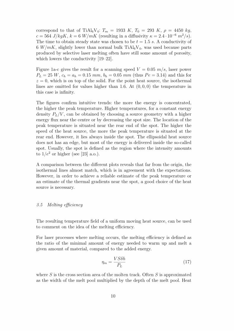
Figure 1a-c gives the result for a scanning speed V = 0.05 m/s, laser powerPL = 25 W , ch = ah = 0.15 mm, bh = 0.05 mm (thus Pe = 3.14) and this forz = 0, which is on top of the solid. For the point heat source, the isothermallines are omitted for values higher than 1.6. At (0, 0, 0) the temperature inthis case is infinity.

The figures confirm intuitive trends: the more the energy is concentrated,the higher the peak temperature. Higher temperatures, for a constant energydensity PL/V , can be obtained by choosing a source geometry with a higherenergy flux near the centre or by decreasing the spot size. The location of thepeak temperature is situated near the rear end of the spot. The higher thespeed of the heat source, the more the peak temperature is situated at therear end. However, it lies always inside the spot. The ellipsoidal heat sourcedoes not has an edge, but most of the energy is delivered inside the so-calledspot. Usually, the spot is defined as the region where the intensity amountsto 1/e2 or higher (see [23] a.o.).

A comparison between the different plots reveals that far from the origin, theisothermal lines almost match, which is in agreement with the expectations.However, in order to achieve a reliable estimate of the peak temperature oran estimate of the thermal gradients near the spot, a good choice of the heatsource is necessary.

3.5 Melting efficiency

The resulting temperature field of a uniform moving heat source, can be usedto comment on the idea of the melting efficiency.

For laser processes where melting occurs, the melting efficiency is defined asthe ratio of the minimal amount of energy needed to warm up and melt agiven amount of material, compared to the added energy.

ηm =V Sδh

PL

(17)

where S is the cross section area of the molten track. Often S is approximatedas the width of the melt pool multiplied by the depth of the melt pool. Heat

10

a) Point heat source

b) Ellipsoidal heat source

c) Uniform heat source

Fig. 1. Temperature field for various heat sources

11

that is not used for melting, is used for overheating of the melt pool or is lostby conduction. The latter results in the heating of the material next to themolten track 1 . It should be noted that different heat source geometries willresult in different values of ηm.

Rykalin [3] derived that the maximum melting efficiency for a point heat sourceis about 0.37 for the 3D case. However, does this mean that in practice nohigher efficiencies can be achieved? There are at least two ways to get a higherefficiency, in theory.

In general, high efficiencies can be obtained for high scanning speeds, sincethen, the conduction can be neglected. In the limit, no energy is lost by con-duction, since conduction needs time. A simulation of a stationary point heatsource, reveals that in the very beginning, all the excess of energy is found inthe overheating of the melt. Indeed, for a point heat source, there will alwaysbe overheating of the melt since the peak temperature is infinite. The simula-tion suggests that overheating is the reason for the limited melting energy.

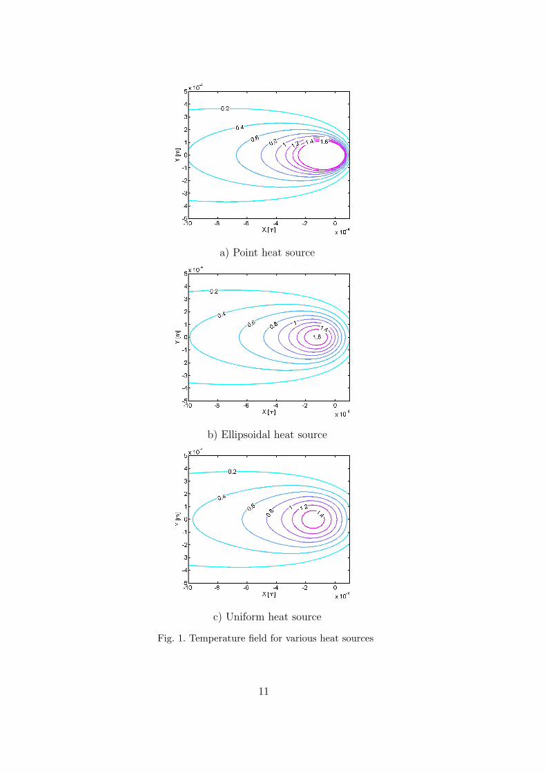
On the other hand, suppose now that a uniform source is used, that has justenough energy to melt part of the material, with hardly any overheating. Sup-pose, the conductivity is low and the scanning speed is very high. Intuitively,it is expected that the melting efficiency is 1. From a mathematical point ofview, however, it is not easy to prove this. Therefore, the integration is per-formed numerically. Parameters are V = 2 m/s, PL = 125 W , k = 0.1 W/mK,t = 0.1 s, ah = ch = 0.15 mm, bh = 0.05 mm, resulting in Pe = 7529. Theresulting temperature field is given in figure 2. The depth of the melt pool isabout 0.042 mm and the efficiency is about 0.67. Going faster or decreasingthe conductivity, will increase the efficiency. In fact, the higher Pe, the higherthe efficiency.

Another possibility to increase the efficiency is the fact that part of the energycan be recycled. This idea is only significant for rapid prototyping techniques,where large surfaces are scanned. Suppose one wants to scan a circular surfaceand starts from the outer edge. The first scan is a fast circle with high efficiency.The second scan, a smaller circle is made some seconds later, and so on.Some heat will be conducted to the inner part of the circle. For the last scan,the part will have been preheated significantly and therefore, the laser powercan be decreased, increasing the efficiency. The same is seen when scanninggeometries with sharp edges in a loose power bed. The scanning parametersshould be adapted to compensate for the heat accumulation, which is in facta recuperation of already used heat.

1 In addition, energy is lost by radiation, by convection with the surrounding at-mosphere and by expulsion of material. These effects are not taken into account inthis simple model. However, in a lot of relevant cases, these losses are negligible [24].

12

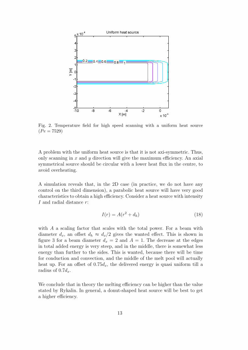
Fig. 2. Temperature field for high speed scanning with a uniform heat source(Pe = 7529)

A problem with the uniform heat source is that it is not axi-symmetric. Thus,only scanning in x and y direction will give the maximum efficiency. An axialsymmetrical source should be circular with a lower heat flux in the centre, toavoid overheating.

A simulation reveals that, in the 2D case (in practice, we do not have anycontrol on the third dimension), a parabolic heat source will have very goodcharacteristics to obtain a high efficiency. Consider a heat source with intensityI and radial distance r:

I(r) = A(r2 + dh) (18)

with A a scaling factor that scales with the total power. For a beam withdiameter dx, an offset dh ≈ dx/2 gives the wanted effect. This is shown infigure 3 for a beam diameter dx = 2 and A = 1. The decrease at the edgesin total added energy is very steep, and in the middle, there is somewhat lessenergy than further to the sides. This is wanted, because there will be timefor conduction and convection, and the middle of the melt pool will actuallyheat up. For an offset of 0.75dx, the delivered energy is quasi uniform till aradius of 0.7dx.

We conclude that in theory the melting efficiency can be higher than the valuestated by Rykalin. In general, a donut-shaped heat source will be best to geta higher efficiency.

13

Fig. 3. Energy distribution through the cross section of a parabolic heat source

3.6 Other source geometries

The heat conduction equation is linear. Therefore, the solution of this equationfor two heat sources is the same as the sum of the solutions of the separate heatsources. Thus, whatever geometry that is wanted, can be obtained by a linearcombination of elementary heat sources. As an example, this was implementedfor a ‘smiley’ (figure 4, left), consisting of 2 semi-ellipsoidal heat sources withah = ch = 0.15 mm, and PL = 20 W (the eyes) and 6 uniform heat sourceswith parameters ah = ch = 0.075 mm and PL = 10 W (the mouth). bh = 0.05for all sources. The other parameters are k = 6 W/mK and V = 0.05 m/s.The result is given in figure 4 on the right 2 .

3.7 Latent heat of fusion

Analytically, it is impossible to take into account the effect of the latent heat.Nevertheless, the latent heat has a significant effect on the melt pool sizeand the melt pool shape. As explained by De Lange [25], in the zone werethe solidification occurs, the Peclet number becomes very high because of Lf ,reducing the importance of the conduction, thus making the rear end of themelt isotherm much sharper than the other isothermal lines. This effect can beseen by simulating the temperature field for different samples of homogenous

2 The reason why this irrelevant source geometry is chosen, lies in the fact that thevisual effect for such a source, shows the difference more clearly. The isotherms fora round source, always have the same shape.

14

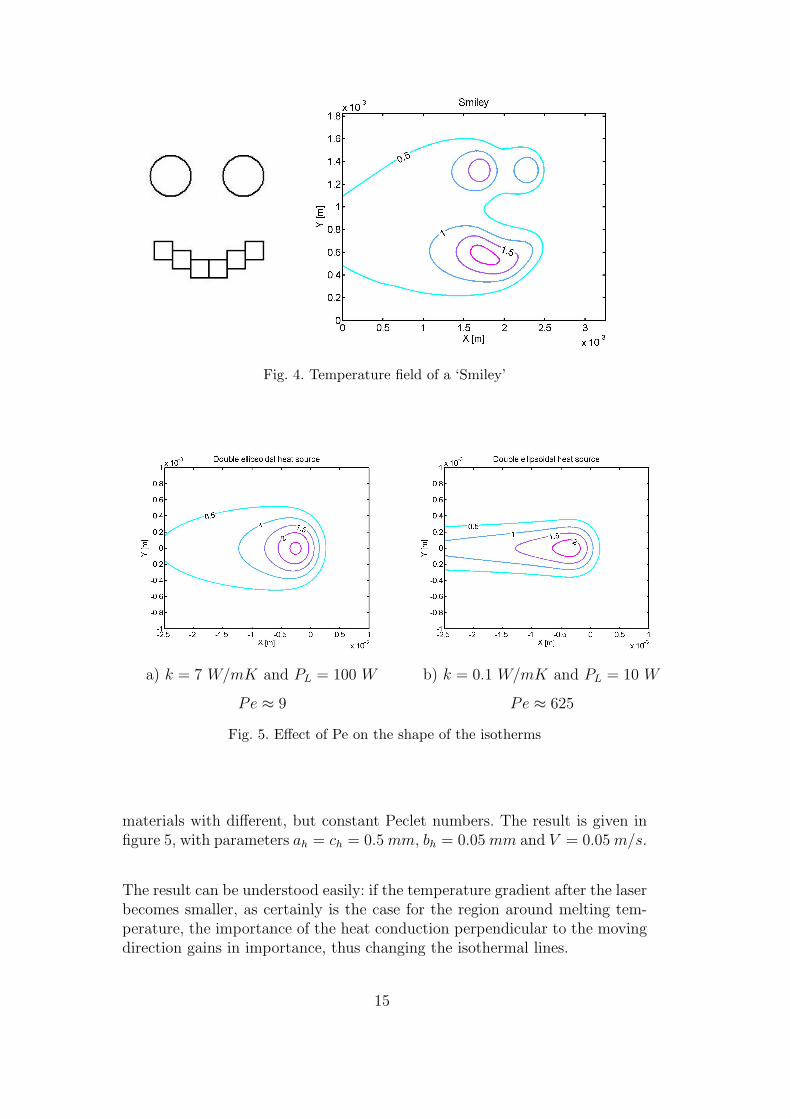
Fig. 4. Temperature field of a ‘Smiley’

a) k = 7 W/mK and PL = 100 W b) k = 0.1 W/mK and PL = 10 W

Pe ≈ 9 Pe ≈ 625

Fig. 5. Effect of Pe on the shape of the isotherms

materials with different, but constant Peclet numbers. The result is given infigure 5, with parameters ah = ch = 0.5mm, bh = 0.05mm and V = 0.05m/s.

The result can be understood easily: if the temperature gradient after the laserbecomes smaller, as certainly is the case for the region around melting tem-perature, the importance of the heat conduction perpendicular to the movingdirection gains in importance, thus changing the isothermal lines.

15

4 Finite difference model

A finite difference model (FDM) was implemented in Matlab r© to investigatethe effect of the material parameters temperature dependence and in particularthe effect of the latent heat, since simulations have shown that the effect issignificant.

4.1 Derivation of the model

Time-marching or false time stepping is used to make the convection-diffusionequation easier to solve. We are only interested in the steady state solution.The equation now becomes

ρc(T ?)∂T

∂t+ ρc(T )V

∂T

∂x= ∇ · (k(T )∇T ) + q̇ (19)

for a heat source moving to the left. T ? is a fixed temperature, that can bechosen freely at the beginning. The exact value will not influence the steadystate solution. It should be noted here, that for a transient temperature field,modelled with a fixed grid, ρ should be constant in order to conserve mass.However, for a steady state solution in a semi-infinite medium, this require-ment should not be fulfilled.

Implicit Euler is used for the time integration:

Φn+1 − Φn = f(tn+1,Φn+1)∆t (20)

where Φ = T in our case.

For the convective term, a first order upwind difference scheme is used. ForV > 0, this becomes:

ρc(T )V∂T

∂x→ V ρi

c(Ti) + c(Ti−1)

2

(Ti − Ti−1

xi − xi−1

)(21)

For the diffusive term, a central difference scheme is used

∇ · (k(T )∇T )→ (kijh + ki+1)

(Ti+1 − Tijh

(xi+1 − xijh)(xi+1 − xi−1)

)−

(kijh + ki−1)

(Tijh − Ti−1

(xijh − xi−1)(xi+1 − xi−1)

)+ . . . (22)

16

The material parameters are evaluated at moment t. For each time step, theequation can be written as

AT t+1 = BT t + q̇ (23)

4.2 Boundary conditions

There are 2 different kinds of boundary conditions that can be used. The firstone is a known temperature on the boundary. The second one is a known heatflux. The latter is used to incorporate the symmetry boundary conditions,where the heat flux is zero perpendicular on that face.

The advantage of the analytical solution is that one can calculate the tem-perature at a particular point, without calculating the complete temperaturefield. Therefore, using the analytical solution as boundary condition, is fastand easy to implement. In this study, the Goldak heat source is used. Thisway, the size of the grid can be limited, because room temperature is onlyfound far from the origin.

4.3 Stability and convergence

Define d as the inverse of a Peclet number and ν as a dimensionless speed sothat

d =k∆t

ρc(T ?)∆x2(24)

and

ν =V∆t

∆x

ρc

ρc(T ?)(25)

Then the footprint becomes, as described by Hirsch [26],

f(λ)∆t= (−2d− ν) + (d)eIλ∆x + (d+ ν)e−Iλ∆x

= (−2d− ν) + d[cos (λ∆x) + I sin (λ∆x)] + (d+ ν)[cos (λ∆x)− I sin (λ∆x)]

= (2d+ ν)[cos (λ∆x)− 1]− νI sin (λ∆x) (26)

If d >= 0 and ν >= 0, the footprints are situated in the left half plane and themethod is always stable. Thus, for constant material properties, the solutionis found immediately, by taking a very large time step.

However, the region around the melting and solidification fronts have highlynon-linear material properties. In this case, some instabilities can occur, de-

17

pending on the method that is used to implement the latent heat of fusion.This will be discussed below.

4.4 Latent heat of fusion

There are different ways to take into account the effect of latent heat. Huand Argyropoulos give an overview of different methods that can be used [9].They state that solving the strong numerical solution, i.e. locating the exactmoving boundary, is very difficult to apply for 3D cases. The alternative is toreformulate the problem in such a way that the Stefan condition 3 is implicitlyincorporated in a new form of equations, which applies over the entire regionof a fixed domain. These methods are referred to as weak numerical solutions,in which explicit attention to the nature of the moving boundary is avoided.As such, eq. (4) can be solved for a temperature dependent c′ (capp or ceff ) oran extra heat sink q̇Lf

. There are five main weak numerical solutions, whichwill be discussed here.

To evaluate different solutions, it is necessary to have a look at the stabilityand the convergence in such situation. This is discussed first.

4.4.1 Stability and convergence

For linear problems, there is a method to evaluate stability and convergencefor a numerical method. However, for non-linear problems such a method isnot available. The behaviour of a solution is validated by practical calcula-tions. Convergence to the correct solution cannot be proved. Fortunately, aqualitative picture of the temperature field is known a priori. This enables usto comment on the stability of different implementations.

Consider for example the 1D problem, without heat source. The formulationof the problem can be written as

ρc′V∂T

∂x= k

∂2T

∂x2(27)

or

ρcV∂T

∂x= k

∂2T

∂x2+ q̇Lf

(28)

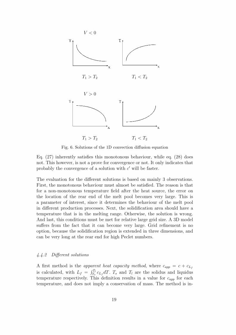
From a physical point of view, latent heat can never cause the temperaturefield to have a local maximum or minimum. For a region where c′ can beconsidered to be constant, only 4 solutions exist (see figure 6).

3 ks∂Ts∂x −kl

∂Tl∂x = LfρdX

dt , where X is the position of the moving boundary betweenmelt l and solid s.

18

V < 0

T1 > T2 T1 < T2

V > 0

T1 > T2 T1 < T2

Fig. 6. Solutions of the 1D convection diffusion equation

Eq. (27) inherently satisfies this monotonous behaviour, while eq. (28) doesnot. This however, is not a prove for convergence or not. It only indicates thatprobably the convergence of a solution with c′ will be faster.

The evaluation for the different solutions is based on mainly 3 observations.First, the monotonous behaviour must almost be satisfied. The reason is thatfor a non-monotonous temperature field after the heat source, the error onthe location of the rear end of the melt pool becomes very large. This isa parameter of interest, since it determines the behaviour of the melt poolin different production processes. Next, the solidification area should have atemperature that is in the melting range. Otherwise, the solution is wrong.And last, this conditions must be met for relative large grid size. A 3D modelsuffers from the fact that it can become very large. Grid refinement is nooption, because the solidification region is extended in three dimensions, andcan be very long at the rear end for high Peclet numbers.

4.4.2 Different solutions

A first method is the apparent heat capacity method, where capp = c + cLf

is calculated, with Lf =∫ TlTscLf

dT . Ts and Tl are the solidus and liquidustemperature respectively. This definition results in a value for capp for eachtemperature, and does not imply a conservation of mass. The method is in-

19

herent instable. A complete proof is out of the scope of this work. However,it can be shown that multiple solutions exist. Consider for example the onedimensional equation, without heat source 4 :

θi+1 − θi

(2 +

capp(θi)ρV∆x

k(θi)

)+ θi−1

(1 +

capp(θi−1)ρV∆x

k(θi−1)

)= 0 (29)

Suppose that the boundary condition is θ = 0.95. The correct solution is auniform temperature at this value. For θi+1 = θi−1 = 0.95, two numericalsolutions for the equation can be found: θi,1 = 0.95, which is what is expected,but also θi,2 slightly higher than 1. The exact value depends on the temperaturedependence of capp, being a function of Lf , Ts and Tl. Practically, there is nopossibility to obtain a resulting temperature field that meets the criterion ofmonoticity.

The effective capacity method is a more stable (i.e. the resulting temperaturefield is closer to the correct temperature field) variant of the apparent heatcapacity method. Here, the apparent heat capacity is averaged over the vol-ume of a unite cell, supposing that the temperature profile between two cellsis linear. However, there still is no conservation of energy, and practically,the resulting temperature field is not monotonous for grid sizes, that can behandled with Matlab r©.

A third method is the heat integration method. The idea is that the tempera-ture of the molten material will be lower by an amount of:

∆T = Lf/c (30)

which corresponds to the extra energy for the phase transition itself. Thisenergy cannot be used for overheating of the melt. For TiAl6V4, ∆T is morethan 500 K.

However, for a 3D moving heat source, this method seems incorrect, The othermethods indicate that the peak temperature is independent of Lf for normalvalues of Lf . This can be understood by the fact that the net heat source, dueto the latent heat of fusion, is zero, because both melting and solidificationoccur. This is only the case for a steady state solution, since the energy input isinfinite. The energy consumed during melting is released during solidification.

Brockmann et al. [27] have described a similar problem for thin foils, with asurrounding gas. In this case the peak temperature will be much lower withlatent heat, compared to the case without. In such case, the heat integrationmethod could result in a better mathematical prediction of the temperature

4 This is a special case of the general problem. If the solution of this problem isunstable, the solution of the more general problem will also be unstable. This isexactly what is observed.

20

profile, compared to an analytical solution. However, the shape is not predictedin an appropriate way.

A fourth method is the source based method. Here a new source term is con-structed:

q̇Lf= −ρ

∂hLf

∂t= −ρV

∂∫cLf

dT

∂x(31)

Closely related to the source based method is the last method, the enthalpymethod. Both are conservative ways to introduce the latent heat. The heatconduction equation can be written as

ρV∂h

∂x= ∇ · (k(T )∇T ) + q̇ (32)

This is implemented like the heat capacity method, with

cLf= (

T2∫T1

cLfdT )/(T2 − T1) (33)

The effective heat capacity becomes

ceff = c+ cLf(34)

The difference with the apparent heat capacity method is that here a changebetween xi−1 and xi is observed, which guarantees the conservation of energy.Furthermore, for pure materials, the heat capacity becomes infinite in the heatcapacity method. For the enthalpy method, this does not pose any numericalproblem.

Mathematically, the enthalpy method and the source based method are equiv-alent:

q̇Lf= −ρV

∂∫cLf

dT

∂x↔ −ρV

∂∫cLf

dT

∂x

(T t+12 − T t+1

1 )

(T t2 − T t

1)(35)

However, the stability is different. The enthalpy method is more stable as wasshown in the section on stability and convergence. This results in an easierand faster convergence for the enthalpy method. The source based methodcan be made more stable, by implementing it implicitly, but this is some-what less straightforward. As a result, the enthalpy method is selected for theimplementation, and will be used in the remaining of the paper.

For the ease of calculation, we assume that heat capacity due to the latentheat is Gaussian. This assures a smooth transition. Hence we have

cLf=

Lf

σ ·√

2πexp

(−(T − Tm)2

2σ2

)(36)

21

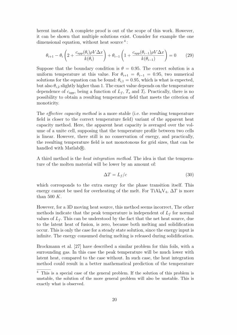
a. Latent heat modelled as cLf b. Without latent heat

Fig. 7. Temperature profile on the surface of a semi-infinite medium

Here, σ is the standard deviation and is a measure of the melting region. It iscalculated as σ = a ·∆Tm where a is a fixed, but in fact unknown, parameter.

Figure 7a a gives the result for a spot with ah = ch = 0.3 mm, V = 0.05 m/s,PL = 40 W , rho = 4450 kg/m3, k = 7 W/mK, c = 564 J/kgK and ahigh Lf = 2920000 J/kg (∆T = 5 K). This high value of Lf was chosen fordemonstration. For TiAl6V4, Lf = 292000 J/kg. The effect for a smaller valueof Lf is rather small for a low Peclet number. All parameters are constant andthe same for the liquid and the solid. In Figure 7b, Lf = 0. One can verifythat the temperature distribution only changes significantly at the rear endof the melt pool. The peak temperature is the same in both cases! The lengthof the melt pool can change significantly due to the latent heat of fusion forhigh Peclet numbers. A factor 2 or more is possible if scanning on a materialwith a low conductivity, like a powder bed.

If we want to determine the enthalpy hLf, we obtain

hLf=

T∫0

cLfdT =

Lf

σ ·√

2π

T∫0

e−(T−Tm)2

2σ2 dT

=Lf√π

T−Tmσ√

2∫− Tm

σ√

2

e−x2

dx

=Lf

2

[erf

(T − Tm

σ√

2

)− erf

(−Tm

σ√

2

)]

≈ Lf

2

[erf

(T − Tm

σ√

2

)+ 1

](37)

22

Hence we have

∆21h =

Lf

2

[erf

(T2 − Tm

σ√

2

)− erf

(T1 − Tm

σ√

2

)](38)

The average power that is stored or released because of melting is

PLf=π

4bdV Lfρ (39)

where π4bd is the frontal area of the melt (b is the width and d is the depth,

and the surface is supposed to be elliptical).

For a Ti-6Al-4V alloy with Lf = 292000 J/kg and ρ = 4450 kg/m3, a spotof 0.3 mm travelling at a speed of 50 mm/s, we obtain, for PL = 40 W , acalculated width of the melt pool b ≈ 0.3 mm and a calculated depth of themelt pool d ≈ 0.2 mm, so that PLf

≈ 3.06 W . This is a small value comparedto a normal power that is PL = 50 . . . 200 W . The effect of the latent heatis therefore rather small. This is in agreement with the previous solution forthe temperature field. The variation of the power of the heat source, or thechange in absorptivity of the material might have the same size.

The same conclusion can be found when observing typical values for the melt-ing efficiency. For Ti-6Al-4V, the relative importance of Lf = 292000 J/kgis rather small, compared to the heating of the material, which is c∆T ≈564 J/kgK ∗ 1600K = 902400 J/kg. This means that only 25 % of the usefulenergy is needed for the melting. If the melting efficiency is ηm ≈ 10 %, thanproportion of the melting energy is only 2.5 %. This value compared to a laserpower PL = 100 W , gives 2.5 W .

5 Conclusions

For constant material properties, it is possible to solve the 3D heat conductionequation with a moving heat source analytically. This is elaborated for the caseof a uniform heat source. The result is compared to existing solutions for themoving point source and a semi-ellipsoidal source. This analytical model hasseveral advantages over FDM. First, it is very useful to study different heatsource geometries. Moreover, with this analytical model, it is shown that theefficiency can be higher than 0.37, a value stated by Rykalin. Last but notleast, analytical solution can serve very well as boundary condition for FDM.If the material parameters depend upon the temperature, as is especially thecase when the effect of latent heat is to be studied, the problem can be solvedwith FDM. To implement the latent heat of fusion, the enthalpy method ismost stable, converges fastest and incorporates the conservation of energy.

23

For TiAl6V4, the effect of the latent heat is rather small, except for the casewhen the conductivity is very low, like scanning in a loose powder bed. Theimplementation of the presented models results in a useful tool to investigatethe effect of different processing parameters.

Acknowledgement

This research is supported by the K.U.Leuven Research Fund ‘GeconcerteerdeOnderzoeksActie’ (GOA/2002/06), and the Belgian Science Policy throughthe projects ‘Interuniversity Attraction Poles’ (IAP P5/08) and ‘TechnologicalAttraction Poles’ (TAP-32) for Rapid Manufacturing for Space Applications.

References

[1] P. W. Fuerschbach, G. R. Eisler, Determination of material properties forwelding models by means of arc weld experiments, in: Sixth International Trendsin Welding Research, Pine Mountain, Georgia, 2002, pp. 1 – 5.

[2] D. Rosenthal, Mathematical theory of heat distribution during welding andcutting, Welding Journal 20(5) (1941) 220 – 234.

[3] N. Rykalin, A. Uglov, A. Kokora, O. Glebov, Laser machining and welding,Moscow: Mir, 1978.

[4] H. Carslaw, J. Jaeger, Conduction of heat in solids, Oxford, 1990.

[5] T. Eager, N. Eager, Temperature fields produced by traveling distributed heatsources, Welding Journal 62(12) (1983) 346 – 355.

[6] J. Goldak, A. Chakravarti, M. Bibby, A double ellipsoid finite element modelfor welding heat sources (1985).

[7] N. T. Nguyen, A. Otha, K. Matsuoka, N. Suzuki, Y. Maeda, Analytic solutionsfor transient temperature of semi-infinite body subjected to 3-D moving heatsources, Welding Research Supplement (August 1999) 265 – 274.

[8] N. T. Nguyen, Y.-W. Mai, S. Simpson, A. Otha, Analytical approximatesolution for double ellipsoidal heat source in finite thick plate, Welding Research(March 2004) 82 – 93.

[9] H. Hu, S. A. Argyropoulos, Mathematical modelling of solidification andmelting: a review, Modelling Simul. Mater. Sci. Eng. 4 (1996) 371 – 396.

[10] M. Matsumoto, M. Shiomi, K. Osakada, F. Abe, Finite element analysis ofsingle layer forming on metallic powder bed in rapid prototyping by selectivelaser processing, International Journal of Machine Tools & Manufacture 42(2002) 61 – 67.

24

[11] S. H. Choi, S. Samavedam, Modelling and optimisation of rapid prototyping,Computers in industry 47 (2002) 39 – 53.

[12] T. Chen, Y. Zhang, Thermal modeling of metal powder-based selective lasersintering, in: Proc. Solid Freeform Fabrication, August 2005, pp. 356 – 369.

[13] A. V. Gusarov, J. P. Kruth, Mathematical simulation of radiation transfer inthe powder bed: application to selective laser sintering, in: VRP Internationalconference on advanced research in virtual and rapid prototyping, 2003, pp. 241– 248.

[14] R. F. Gould, Contact angle: wettability and adhesion, American ChemicalSociety, 1964.

[15] R. V. Roy, L. W. Schwartz, On the stability of liquid ridges, Journal on FluidMechanics 391 (1999) 293 – 318.

[16] G. N. Levy, R. Schindel, J. P. Kruth, Rapid manufacturing and rapid toolingwith layer manufacturing (lm) technologies, state of the art and futureperspectives, CIRP Annals 52/2 (2003) 589.

[17] J. P. Kruth, P. Mercelis, J. Van Vaerenbergh, L. Froyen, M. Rombouts, Bindingmechanisms in selective laser sintering and selective laser melting, RapidPrototyping Journal 11 (1) (January 2005) 26 – 36.

[18] N. Christensen, V. Davies, K. Gjermundsen, The distribution of temperaturein arc welding, British Welding Journal 12(2) (1965) 54 – 75.

[19] J. K. Carson, S. J. Lovatt, D. J. Tanner, A. C. Cleland, Thermal conductivitybounds for isotropic, porous materials, Int. Journal of Heat and Mass Transfer48 (2005) 2150 – 2158.

[20] W. Meiners, Direktes selektives laser sintern einkomponentiger metallischerwerkstoffe, Ph.D. thesis, Aachen (1999).

[21] J. C. Y. Koh, A. Fortini, Prediction of thermal conductivity and electricalresistivity of porous metallic materials, Int. Journal of Heat and Mass Transfer16 (1973) 2013 – 2021.

[22] A. V. Gusarov, T. Laoui, L. Froyen, V. I. Titov, Contact thermal conductivityof a powder bed in selective laser sintering, Int. Journal of Heat and MassTransfer 46 (2003) 1103 – 1109.

[23] J. F. Ready, D. F. Farson (Eds.), Handbook of laser materials processing, LaserInstitute of America, 2001.

[24] M. Pietro, C. Rivela, B. Marco, Mathematical modelling of laser treatmentprocesses, Laser Materials Processing: industrial and microelectronicsapplications SPIE 2207 (1994) 256 – 268.

[25] D. F. De Lange, S. Postma, J. Meijer, Modelling and observation of laserwelding: The effect of latent heat, in: Proceedings of ICALEO 2003, Vol. SectionC, Jacksonville FL, 2003, pp. 154 – 162.

25

[26] C. Hirsch, Numerical computation of internal and external flows, Vol. 1, JohnWiley & Sons, 1995.

[27] R. Brockmann, K. Dickmann, P. Geshev, K.-J. Matthes, Calculation of laser-induced temperature field on moving thin metal foils in consideration of stefanproblem, Optics & Laser Technology 35 (2003) 115 – 122.

26