SOCIAL DEVELOPMENT – A MULTIDIMENSIONAL APPROACH TO SOCIAL DEVELOPMENT ANALYSIS. COUNTRY LEVEL...

SOCIAL DEVELOPMENT –

A MULTIDIMENSIONAL APPROACH

TO SOCIAL DEVELOPMENT

ANALYSIS. COUNTRY LEVEL

EVIDENCE

Ewa Lechman*

GUT Faculty of Management and Economics

Working Paper Series A (Economics, Management, Statistics)

No.2/2013 (2)

March 2013

* Gdansk University of Technology, Faculty of Management and Economics, [email protected] (corresponding author)

2

SOCIAL DEVELOPMENT –

A MULTIDIMENSIONAL APPROACH TO

SOCIAL DEVELOPMENT ANALYSIS.

COUNTRY LEVEL EVIDENCE.

Ewa Lechman1

Abstract

The study investigates disparities in social development in 144 countries worldwide. In the paper

we aim to investigate cross-country differences in social development level in year 2011, as well

as to estimate inequalities on the field. Secondly, we assess relative social development level

differences – gaps (divides) among countries. For the analysis purposes, we apply: descriptive

statistics analysis, Kernel Epanechnikov density (to check for world distribution of social

welfare), inequality measure – Gini coefficient and square Euclidean distance (full linkages)

method. The analysis sample encompasses 144 countries, and we mainly collect statistical data for

the year 2011 (if available). The data applied in the study are derived from databases like: United

Nations Millennium Development Goals Database; United Nations Department of Economic

and Social Affairs, Population Division; United Nations Educational, Scientific and Cultural

Organization; World Health Organization; International Human Development Indicators.

JEL codes: I0, I2, I3, O15, O50

Keywords: social development, living standards, inequalities, Kernel distribution

1 Gdansk University of Technology, Faculty of Management and Economics,

[email protected] (corresponding author)

3

1. Social development – theoretical outline

The problem of social development remains of critical importance. There exists huge set of

literature and empirical studies identifying problems of definition, measurement methods on the

field of social development. The discussion on the problem, its determinants, and/or

measurement proposals can be found in the work of i.e Streeten and ul Haq (1981), Lucas (1988),

Sen (1985, 1992), Behrman (1990), Birdsall and Nancy (1993), Bozer, Ranis and Stewart (2000,

2004). Also the issues on social development are in the centre of interests of international

agencies like i.e. United Nations Development Programme, UNESCO, WHO and many others.

Social development is broadly associated with the large thing called general societal welfare

(wellbeing). It is broad and multidimensional in nature. The multitude of ways to define it is

mainly a consequence of wide array of factors that constitute the issue. The concept of social

development encompasses a variety of aspects of human life, which are often non-material ones,

and can refer to different dimensions of education, healthcare, social and political freedom, or

race. It is widely thought that social development goes far beyond pure economic development,

however it can enhance entering dynamic and sustainable economic development (and growth)

pattern. The phenomenon of social development is also associated with human capabilities (see

Sen 1985, 1992), possibilities to educate, self-develop and lead healthy life. Social development

encompasses all kinds of “functionings” (see again Sen 1992), which enable any individual to get

personal achievements and that reflect his life-style. Social development also refers to all kinds of

freedom, freedom perceived as opportunities to take active part in social, economic, political and

cultural life. Any kind of exclusion is always treated as the denial of social welfare. The freedom

to develop reflects directly living-conditions of any individual, and in that sense it is a prerequisite

for dynamic economic growth and development. Rahman and Wandschneider (2003) stress the

importance of factors like social relationship, security of workplace or environmental quality.

4

Despite those, there is no widely accepted consensus on crucial factors determining the level of

social development as well as we still seek for the best measure it. In recent years there have been

elaborated many composite measures (indexes) which try to capture the multidimensionality of

social development, i.e. Human Development Index (developed by United Nations), Physical

Quality of Life (developed by Morris), or many others.

In the paper, we strongly support the idea of purely non-income (non-monetary) approach to

social development. However, the notion of social development is broad and can cover a wide

array of aspects of social, cultural or political life, we prose a reductionist approach and we aim to

concentrate exclusively on arbitrary selected variables. The social development variables are

presumed to be quality-of-life attributes, and are to measure the well-being directly.

2. Cross-country disparities in social development level

For the analysis purposes, we have completed the dataset composed of 144 world economies,

and statistics are derived for year 2011. The statistical data sources are following: United Nations

Millennium Development Goals Database; United Nations Department of Economic and Social

Affairs, Population Division 2011; UNESCO; World Health Organization; International Human

Development Indicators datasets. Using the cited databases, we have chosen 8 different variables

(indicators), which are broadly treated as proxies of social development level. These are: Life

Expectancy2 (LE3), Drinking Water Access (DWA), Improved Sanitation Coverage (ISC), Total

Fertility Rate (TFR), Maternal Mortality Rate (MMR), Infant Mortality Rate (IMR), Combined

Gross Enrolment (CGE) and Mean Years of Schooling (MYS). We have classified the indicators

into two groups:

a) Indicators positively influencing human development (P-HD, Positive-Human

Development) – these are: LE, DWA, ISC, CGE and MYS.

2 Detailed explanation of selected variables is put in Appendix 2. 3 In the following parts of the paper, we use systematically the abbreviations.

5

b) Indicators negatively influencing human development (N-HD, Negative-Human

Development) – these are: TFR, MMR and IMR.

The empirical part of the paper encompasses of three sections. In the first step we aim to check

for descriptive statistics and estimate the Gini coefficients for given variables in the sample.

Secondly, we estimate densities lines for each variable separately to learn about the world

distribution of social welfare approximated by the P-HD, and world distribution of exclusion

from such – approximated by N-HD. To complete the analysis of the world differences in social

development, we calculate square Euclidean distances4 (metrics) to know about the relative

backwardness of economies analyzed in relation to reference country (best performing country in

the sample).

2.1. World distribution of social welfare.

As stated in previous section we have selected statistical data for 8 different variables – assumed

to be proxies of social development level, for 144 economies. In the following Table 1 (see

below), we report on descriptive characteristics of chosen variables in year 2011. In addition the

Gini coefficients values are calculated. The variables are expressed in different units, which imply

some difficulties with direct comparisons among countries. LE, TFR and MYR are expressed in

absolute numbers, while the rest of them are expressed as relative ones.

4 Full linkages

6

Table 1. Basic descriptive statistics for social indicators. Year 2011. 144 countries.

Variable Obs Mean Std. Dev. Min Max Gini

coefficient

LE (years) 144 69,68 9,72 48,82 83,61 0,077 DWA (%) 144 86,11 16,42 38 100 0,09 ISC (%) 144 71,26 30,18 9 100 0,23 TFR (no of children) 144 2,77 1,38 1,13 6,92 0,266 MMR (per 100 000 live births) 144 203,67 265,16 2 1200 0,64 IMR (per 1000 live births before age of 1 year)

144 31,94 29,73 2,05 123,94 0,499

CGE (% of total no of 3 school groups)

144 72,02 17,57 29,6 112,1 0,138

MYS (for people at 25 years and older)

144 7,46 3,08 1,2 12,6 0,236

Source: own calculations using STATA 12.00. Data drawn from United Nations Millennium Development Goals Database, United Nations Department of Economic and Social Affairs, Population Division, UNESCO, World Health Organization, International Human Development Indicators databases. Accessed: Sept 2012.

The variability of social indicators values is presented in Table 1. Analyzed jointly with smooth

densities charts give a general idea about worldwide differences in social welfare distribution (see

charts 1,2,3,4,5,6,7 and 8).

Chart 1. Life Expectancy world distribution line (Kernel density). Year 2011, 144 countries.

0.0

1.0

2.0

3.0

4.0

5D

ensi

ty

40 50 60 70 80 90LE

kernel = epanechnikov, bandwidth = 3.2320

Life expectancy. Kernel density estimate. 144 countries, year 2011

Source: own estimates using STATA 12.0. Data applied drawn from United Nations Department of Economic and Social Affairs, Population Division datasets. Accessed: Sept 2012.

In case of life expectancy we observe relatively low differentiation among countries. The Gini

coefficient is 0,077, which results to be low, and indicates no huge differences life expectancy

7

(expressed in years) – the variable value is fairly distributed among countries. Chart 1 (see above)

reports on density in the variable distribution. We see the twin-peak line, which suggests existing

two different groups of countries. In such case, the polarization is evident. One group (in right

part of the plot), constitutes economies that enjoy relatively high life expectancy – these are

highly developed countries. The group consists of 84 economies, where LE varies from about 70

(i.e. Belarus, Trinidad and Tobago, Azerbaijan and Belarus) to 83 years in Japan. Note, that from

the densities values we can conclude that probability of achieving the LE value at 70-80 years is

relatively high and varies from 0,3 – 0,5. While the left one peak suggest existence of different

group of countries where the LE varies from 48 years (in Guinea-Bissau and Lesotho), to about

70 years (i.e. in Iraq, Indonesia, Guyana) – there are 60 countries in the group. However, despite

the clear emergence of the two peaks, we can conclude than in general the achievement is terms

of LE are high in the world sample.

Chart 2. Drinking Water Access world distribution line (Kernel density). Year 2011, 144

countries.

0.0

1.0

2.0

3.0

4D

ensi

ty

40 60 80 100 120DWA


Drinking Water Access. Kernel density estimate. 144 countries, year 2011.

Source: own estimates using STATA 12.0. Data applied drawn from United Nations Millennium Development Goals Database. Accessed: Sept 2012.

8

Chart 3. Improved Sanitation Coverage world distribution line (Kernel density). Year 2011, 144 countries.

0.0

05.0

1.0

15.0

2D

ens

ity

0 50 100ISC


Improved Sanitation Coverage. Kernel density estimate. 144 countries, year 2011.

Source: own estimates using STATA 12.0. Data applied drawn from United Nations Millennium Development Goals Database. Accessed: Sept 2012.

Secondly, we aim to analyze the statistics on drinking water access and improved sanitation

coverage. We suggest analyzing them jointly as the two variables reflect level of development of

basic sanitation infrastructure. From descriptive statistics (Table 1) we conclude that average

levels of DWA are slightly better than in case of ISC. Also the Gini value for DWA – (0,09)

suggest almost even distribution in the country sample. The mean access for improved sanitation

results to be a bit lower (71,26% of population), and at the same higher Gini is reported – (0,23).

However, the data seem to be optimistic, they shall be interpreted carefully. If we see chart 2 and

3, where densities line are drawn for each variable, the picture of performance of countries in

terms of DWA and ISC differs slightly. In two cases we observe emergence of one-peak line

accompanied by long left tail. Such construction of density line suggests existing one relatively

homogenous group of countries, where drinking water access (counted as % of total population

having access) and improved sanitation coverage (counted as % of population having access) is at

high level – about 90-100% of total population enjoying access to both kinds of facilities.

However, in case of DWA the probability of having access to drinking water by almost 100% of

population is close to 0,2-0,4 (90 countries in the sample), if we go to chart 3, we see that the

analogues value is at about 0,15-0,2 of probability (60 countries). The left tail in chart 2, stands

9

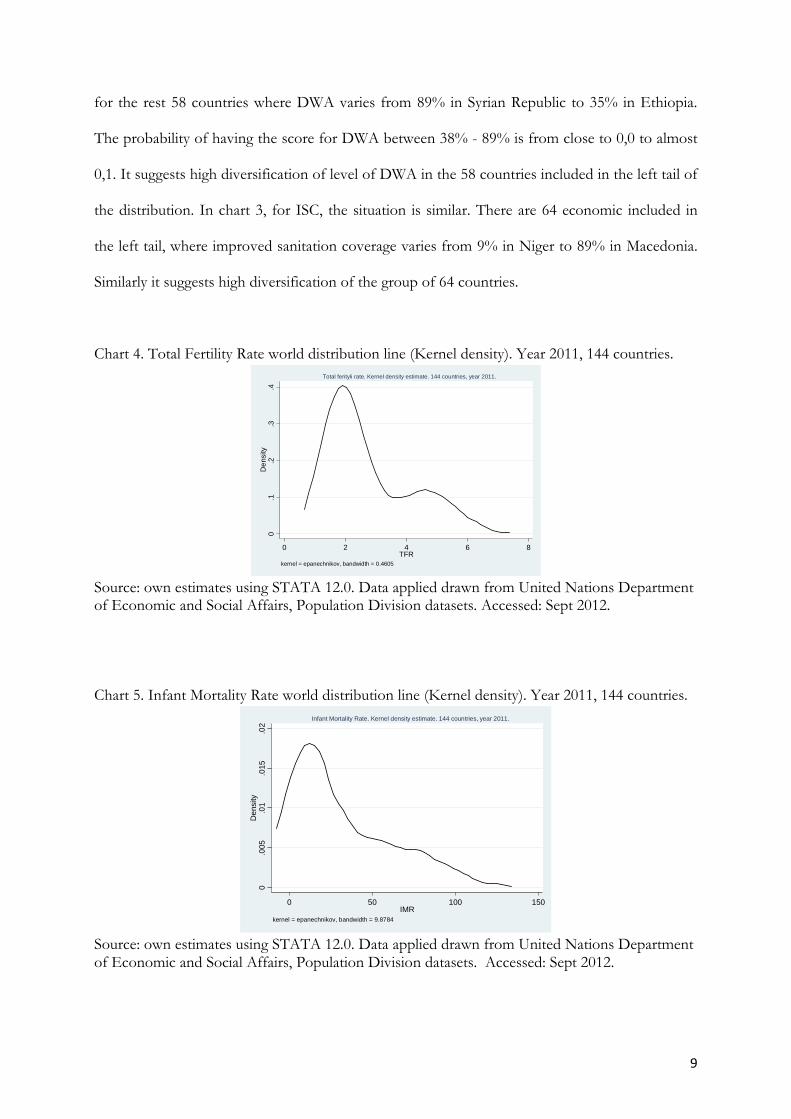
for the rest 58 countries where DWA varies from 89% in Syrian Republic to 35% in Ethiopia.

The probability of having the score for DWA between 38% - 89% is from close to 0,0 to almost

0,1. It suggests high diversification of level of DWA in the 58 countries included in the left tail of

the distribution. In chart 3, for ISC, the situation is similar. There are 64 economic included in

the left tail, where improved sanitation coverage varies from 9% in Niger to 89% in Macedonia.

Similarly it suggests high diversification of the group of 64 countries.

Chart 4. Total Fertility Rate world distribution line (Kernel density). Year 2011, 144 countries.

0.1

.2.3

.4D

ens

ity

0 2 4 6 8TFR


Total ferityli rate. Kernel density estimate. 144 countries, year 2011.


Chart 5. Infant Mortality Rate world distribution line (Kernel density). Year 2011, 144 countries.

0.0

05.0

1.0

15.0

2D

ensi

ty

0 50 100 150IMR


Infant Mortality Rate. Kernel density estimate. 144 countries, year 2011.


10

Chart 6. Maternal Mortality Rates world distribution line (Kernel density). Year 2011, 144 countries.

0.0

005

.001

.001

5.0

02.0

025

Den

sity

0 500 1000 1500MMR


Maternal Mortality Rate. Kernel density estimate. 144 countries, year 2011.


In the next step we investigate the following 3 social factors – total fertility rate (TFR), infant

mortality rate (IMR) and maternal mortality rate (MMR). The varibales factors reflect basic access

to medical care and healthcare system. High values of each variable suggest high deprivation of

general access to medical care, and a time usually go along with very low overall socio-economic

performance of countries. As we see from the descriptive statistics in Table 1, the average total

fertility rate is 2,77 children per woman, the Min value reported is 1,13 children per woman (the

value of 1,13 refers to Bosnia, but note that in many sequent countries like Malta, Austria,

Portugal the value is not much higher), while the Max value is 6,92 children per woman (in

Niger). We also need to stress that Niger is not the outside on the field. When analyzing raw data

(see Appendix 1), we see that in the next 34 economies, the variable is above 4. Considering the

fact, that such high fertility rates are common for low-income countries, this can constitute a

great obstacle for entering economic development path, especially if GDP per capita annual

growth rates result to be lower than crude birth rate. If we look at the following two variables

statistics – MMR and IMR, the picture is even more alarming. In the analyzed set of countries the

average maternal mortality rate is 203,67 woman per 100 000 live births. At the same time the

best performing country on the field is Greece (MMR=2), while the worst country in the group is

11

Chad and Guinea-Bissau, with the values MMR=1200 and MMR=1000 respectively. In addition,

we need to note that in the next 49 economies the maternal mortality rate is still above the mean.

The Gini coefficient reported in the case of MMR is 0,64 (the highest score of all variables),

which suggests relatively highest inequalities (disparities) in the variables in the 144 economies. In

case of infant mortality rate variable, the statistics are evenly alarming. On average almost 32 (per

1000 live births) children die before age of 1. In the worst performing countries the IMR are 443

and 371, which again refers to Chad and Guinea-Bissau respectively. We also need to stress that

in case of 71 economies (out of the 144 included in the sample), the IMR values is higher than

the mean. This again shows quite a disadvantageous situation in the countries and assigns for low

level of social development. In addition, we analyze the densities plots in charts 4,5 and 6. The

density line in chart 4 gives us clear idea about the variable (TFR) distribution worldwide.

Actually, we observe again an emergence of twin-peak line, which indicates formation of two

distinct groups of countries that differ significantly. The left peak identifies the group of better

off economies, where the probability of achieving the TFR=2 is about 0,3 – 0,4. The probabilities

of a country to obtain a score of TFR below 2, is clearly lower – at about 0,1 – 0,2. The right

peak, reversely show the group of countries which are evidently worse off in terms of TFR.

Going to maternal mortality rate and infant mortality rate, we see that densities functions are

similar in shape. In both cases, we observe an emergence of one-peak line (on the left side of

coordinate system). This proofs existence of relatively homogenous groups of countries, where

values of both variables are low. However if we see the densities values (probability), we see that

these are rather low. In case of maternal mortality rate, the probability of achieving the MMR

value a bit above “0” is at about 0,025 (2,5%). The probability of higher MMR are consequently

lower, but the long right tail indicates high diversification of countries on the field. Similar

situation is reported in chart 5 which refers to infant mortality rate. Again there emergence one-

peak line (left located peak), which indicates rather a homogenous group of relatively wealthier

countries, where the variable values are low. However, the long right tail shows that in middle

12

and low-income economies the diversification in terms of IMR is high. Actually similar

conclusions were drawn according to Gini coefficient for MMR and IMR.

Chart 7. Combined Gross Enrolment world distribution line (Kernel density). Year 2011, 144 countries.

0.0

05.0

1.0

15.0

2D

ensi

ty

20 40 60 80 100 120CGE


Combined Gross Enrolment. Kernel density estimate. 144 countries, year 2011.

Source: own estimates using STATA 12.0. Data applied drawn from UNESCO datasets. Accessed: Sept 2012.

Chart 8. Mean Years of Schooling world distribution line (Kernel density). Year 2011, 144 countries.

0.0

5.1

Den

sity

0 5 10 15MYS


Mean years of schooling. Kernel density estimate. 144 countries, year 2011.

Source: own estimates using STATA 12.0. Data applied drawn from UNESCO datasets. Accessed: Sept 2012.

Finally, we investigate the variables of combined gross enrolment (CGE) and mean years of

schooling (MYS). The preliminary data analysis shows that average country diversification on the

13

field of schooling achievement is relatively low. The Gini coefficients are 0,138 – for CGE, and

0,236 for MYS, and indicate low inequalities. However, as can be read from data in Table 1, the

differences between Minimum and Maximum values for both variables seem to be significant. In

Djibouti, Eritrea, Kuwait, Niger and Nigeria the average CGE is slightly above 30% CGE, while

in 51 countries the CGE is above 80%. In the group of 51 cited economies, there also countries

like i.e. Bolivia, Peru, Colombia or Venezuela, which are mainly classified as medium developed

countries. If to look at MYS statistics, the average is almost 7,5 years. Again, there are 69

countries where are level of MYS is below the average. This suggests very poor developed

educational system and basic education infrastructure like school access etc. Looking at charts 7

and 8, we conclude on world distribution of the variables values. In both cases the distributions

are close to normal distribution (see chart 9 below).

Chart 9. Normal probability plots. CGE and MYS variables. Year 2011, 144 countries.

0.00

0.25

0.50

0.75

1.00

Nor

mal

F[(

CG

E-m

)/s]

0.00 0.25 0.50 0.75 1.00Empirical P[i] = i/(N+1)

Normal probability plot. CGE variable. Year 2011. 144 countries.

0.00

0.25

0.50

0.75

1.00

Nor

mal

F[(

MY

S-m

)/s]

0.00 0.25 0.50 0.75 1.00Empirical P[i] = i/(N+1)

Normal probability plot. MYS variable. Year 2011. 144 countries.

Source: own elaboration using STATA 11.2.

This suggests no significant disparities in the variables values across countries, which of course

does not mean that in all countries the achievements are equal. The differences still exist.

14

2.2. On relative social development backwardness.

In the following part of section 2, we aim to learn about relative backwardness of countries in

terms of social development. We run a study, applying square Euclidean distance approach,

which allows estimating distances between pair of countries on the assumed field of interest. The

methodology let us to know about relative distance (metric) between two points in n-dimension

space and the value of distance shows how far the objects are located from each other. This is the

pair-wise analysis, and it shows inter-country relations. In our case we divide the distances

estimates into two sets. As it was pointed in begging of section 2, we have classified chosen

variables into two groups. We have created P-HD (Positive-Human Development) indicators

group – these are: LE, DWA, ISC, CGE and MYS; and N-HD (Negative-Human Development)

indicators group – these are: TFR, MMR and IMR. Consequently, the analysis is two-pattern.

Simultaneously we estimate metrics for countries applying P-HD variables and – separately –

applying N-HD variables. In each case, we have chosen the reference object – the best

performing country in the sample if taking into account chosen variables. For P-HD indicators

this is Australia (Australia achieved highest average variables` values of LE, DWA, ISC, CGE and

MYS), while for N-HD indicators – Greece (Greece achieved lowest average variables` values of

TFR, MMR and IMR). In the following table 2, we present estimates results. The numbers

indicate the metric value (distance value) for each country in relation to Australia (for P-HD) and

to Greece (for N-HD). The higher the metric`s value the greatest distance is reported between

the given country and reference one. As can be concluded from general estimates, the countries

closest to Australia are: Ireland, Republic of Korea, Denmark, Netherlands, Spain, Norway,

Finland, Greece. It can be interpreted as the lowest average differences between Australia and

listed countries in terms of the 5 social variables. At the bottom on the table 2, reversely, we find

countries, which are relatively most backward in relation to Australia. If we consider the N-HD

indicator, we find 27 countries where the metric is close “0”, which suggest that in terms of TFR,

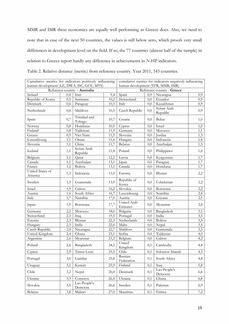
15

MMR and IMR these economies are equally well performing as Greece does. Also, we need to

note that in case of the next 50 countries, the values is still below zero, which proofs very small

differences in development level on the field. If so, the 77 countries (almost half of the sample) in

relation to Greece report hardly any difference in achievements in N-HP indicators.

Table 2. Relative distance (metric) from reference country. Year 2011, 143 countries.

Cumulative metrics for indicators positively influencing human development (LE, DWA, ISC, GCE, MYS)

cumulative metrics for indicators negatively influencing human development (TFR, MMR, IMR)

Reference country – Australia Reference country - Greece Ireland 0,4 Iran 9,4 Spain 0,0 Nicaragua 0,9 Republic of Korea 0,5 Suriname 10,2 Switzerland 0,0 Ecuador 0,9 Denmark 0,6 Paraguay 10,3 Italy 0,0 Kazakhstan 0,9

Netherlands 0,6 Maldives 10,5 Czech Republic 0,0 Syrian Arab Republic

0,9

Spain 0,7 Trinidad and Tobago

10,7 Croatia 0,0 Belize 1,0

Norway 0,8 Honduras 10,9 Cyprus 0,0 Israel 1,0 Finland 0,8 Tajikistan 11,5 Germany 0,0 Morocco 1,1 Greece 0,9 Viet Nam 11,5 Slovenia 0,0 Jordan 1,3 Luxembourg 1,1 Oman 11,6 Hungary 0,0 Indonesia 1,4 Slovenia 1,1 China 11,7 Belarus 0,0 Azerbaijan 1,5

Iceland 1,1 Syrian Arab Republic

11,8 Poland 0,0 Philippines 1,6

Belgium 1,1 Qatar 12,2 Latvia 0,0 Kyrgyzstan 1,7 Canada 1,1 Azerbaijan 13,1 Japan 0,0 Paraguay 1,7 France 1,2 Bolivia 13,1 Canada 0,0 Honduras 1,7 United States of America

1,3 Indonesia 13,5 Estonia 0,0 Bhutan 2,2

Sweden 1,3 Guatemala 13,9 Republic of Korea

0,0 Uzbekistan 2,2

Israel 1,5 Gabon 16,2 Slovakia 0,0 Botswana 2,2 Austria 1,6 South Africa 16,7 Luxembourg 0,0 Namibia 2,4 Italy 1,7 Namibia 17,0 Austria 0,0 Guyana 2,5

Japan 1,9 Botswana 17,7 United Arab Emirates

0,0 Myanmar 2,8

Germany 2,2 Morocco 18,0 Bulgaria 0,0 Bangladesh 3,5 Switzerland 2,3 Iraq 19,5 Portugal 0,0 India 3,5 Estonia 2,3 Bhutan 22,3 Netherlands 0,0 Bolivia 3,5 Hungary 2,3 India 22,6 Malta 0,0 Nepal 3,5 Czech Republic 2,4 Nicaragua 22,7 Maldives 0,0 Guatemala 3,5 United Kingdom 2,4 Ghana 23,1 Serbia 0,0 Tajikistan 4,0 Argentina 2,6 Myanmar 23,2 Belgium 0,0 Gabon 4,2

Poland 2,6 Bangladesh 24,2 United Kingdom

0,1 Cambodia 4,4

Cyprus 2,9 Timor-Leste 25,5 Chile 0,1 Solomon Islands 4,5

Portugal 3,0 Gambia 25,8 Russian Federation

0,1 South Africa 4,8

Uruguay 3,1 Kuwait 25,9 Finland 0,1 Iraq 5,8

Chile 3,2 Nepal 26,0 Denmark 0,1 Lao People's Democra

6,6

Ukraine 3,3 Comoros 26,4 Ukraine 0,1 Ghana 6,8

Slovakia 3,5 Lao People's Democra

26,6 Sweden 0,1 Pakistan 6,9

Belarus 3,8 Malawi 27,0 Mauritius 0,1 Eritrea 7,2

16

Latvia 3,8 Kenya 27,3 Thailand 0,1 Swaziland 8,2 Jamaica 4,0 Solomon Islands 27,4 Australia 0,1 Yemen 8,6 Malta 4,1 Uganda 27,5 Costa Rica 0,1 Madagascar 9,0 Croatia 4,1 Cameroon 27,8 Norway 0,1 Lesotho 9,2

Kazakhstan 4,2 Swaziland 27,8 TFYR Macedonia

0,1 Togo 9,3

Serbia 4,6 Pakistan 27,8 France 0,1 Djibouti 9,4

Venezuela 4,7 Cambodia 28,6 Republic of Moldova

0,1 Senegal 9,8

Bulgaria 4,7 Rwanda 28,8 United States of America

0,2 Ethiopia 10,0

Mexico 4,8 Yemen 31,1 Ireland 0,2 Comoros 11,1 United Arab Emirates

4,8 Congo 31,3 Bosnia and Herzegovi

0,2 Côte d'Ivoire 11,9

Russian Federation 5,1 Lesotho 31,4 Iceland 0,2 Gambia 12,1 Armenia 5,2 Senegal 31,9 Albania 0,2 Kenya 12,5 Ecuador 5,6 Liberia 32,0 Bahamas 0,2 Mauritania 13,6 Jordan 5,8 Burundi 34,7 Uruguay 0,2 Congo 13,9 Lebanon 5,9 Tanzania 35,1 Oman 0,2 Sudan 15,2 Panama 5,9 Madagascar 35,4 Qatar 0,3 Benin 15,2 Georgia 9 5,9 Togo 35,7 Kuwait 0,3 Timor-Leste 15,3 Bosnia and Herzegovi

5,9 Benin 35,8 Viet Nam 0,3 Mozambique 16,0

Brazil 6,0 Djibouti 37,2 China 0,3 Equatorial Guinea 16,7 Colombia 6,4 Angola 37,2 Lebanon 0,3 Cameroon 16,8

Bahamas 6,5 Equatorial Guinea

40,2 Brazil 0,3 Uganda 18,2

Costa Rica 6,5 Côte d'Ivoire 40,9 Tunisia 0,3 Burkina Faso 19,1 Belize 6,6 Mauritania 41,3 Argentina 0,4 Tanzania 20,1 Albania 6,9 Guinea-Bissau 41,8 Turkey 0,4 Guinea 20,6 Malaysia 7,0 Guinea 42,0 Iran 0,4 Rwanda 20,8 Philippines 7,1 Sudan 42,4 Mexico 0,5 Malawi 22,0 Peru 7,2 Mali 43,6 Armenia 0,5 Angola 22,1

Guyana 7,4 Central African Rep

45,1 Trinidad and Tobago

0,5 Central African Rep 24,6

Kyrgyzstan 7,4 Burkina Faso 47,6 Georgia 9 0,6 Nigeria 26,3 Mauritius 7,5 Nigeria 47,7 Colombia 0,6 Burundi 26,3 TFYR Macedonia 7,5 Eritrea 48,2 Malaysia 0,6 Liberia 26,7 Tunisia 7,9 Mozambique 50,3 Venezuela 0,6 Mali 30,1 Algeria 8,3 Ethiopia 50,6 El Salvador 0,6 Niger 32,8 Uzbekistan 8,5 Chad 55,7 Panama 0,6 Guinea-Bissau 33,4 Turkey 8,6 Niger 60,2 Suriname 0,7 Chad 46,9 El Salvador 8,8 Algeria 0,7 Republic of Moldova

9,0

Jamaica 0,7

Thailand 9,1 Peru 0,8

Source: own calculations using STATISTICA 10.0.

17

Chart 10. Tree diagram. N-HD and P-HD variables. Square Euclidean metrics, full linkages. Year 2011, 143 countries (for N-HD – Greece excluded; for P-HD – Australia excluded).

N-HD variables. Square Euclidean metrics. Full linkages.

0

10

20

30

40

50

Met

ric

valu

e

P-HD. Square Euclidean metrics. Full linkages.

0

10

20

30

40

50

60

70

Met

ric v

alue

.

Source: own elaboration using STATISTICA 10.0.

The tree diagrams (see chart 10 above), shows that in both cases there exists quite numerous

groups of countries, which are relatively similar to one another as well as to the reference

country. Again, in both cases we identify many countries, which are far behind Australia and

Greece. The differences in metrics values – especially for N-HD – astonish, however in case of

P-HD the distance values seem to be more diversified and averagely higher (see chart 11 below).

The densities estimates clearly show the differences in the two sets of metrics. The metrics for P-

HD result to vary significantly across countries, achieving values from 0,4 till 60,2 (the average

for all is 15,7, and we investigated 57 countries to be above the average). For N-HD they are

much less diversified – the emerged one-peak line suggest existence of rather homogenous group

of countries that in relation to Greece present only slight differences in achievement in TFR,

MMR and IMR. Anyway, the average metric for N-HP variables is just 5,3, and 40 economies still

remain above the mean.

18

Chart 11. Distributions of metrics values for P-HD and N-HD. Year 2011, 143 countries (for N-HD – Greece excluded; for P-HD – Australia excluded).

0.0

5.1

.15

0 20 40 60x

kdensity PHD kdensity NHD

Densities for P-HD and N-HD indicators. Year 2011, 143 countries.

Source: own elaboration using STATA 12.00.

3. Concluding remarks

The main objective of the paper was to investigate the cross-national difference in social

development level that existed in the year 2011. We have based the analysis on eight dimensions

of social development, collecting statistical data for 144 countries worldwide. Despite presenting

quite a reductionist approach, we strongly support the idea that selected variables draw a clear

picture of overall social welfare in a country. From the analysis results, we can conclude that in

year 2011, the inequalities (according to Gini coefficients) in values of social factors were rather

low in most of cases. The lowest Gini coefficient was reported for life expectancy (only 0,07),

while for maternal mortality ratio it was 0,64. We see that differences are enormous. However,

the Gini coefficients report on relatively low inequalities, if we complete the picture adding by the

distributions line for each variable, we see that among countries still exist quite a disparities. In

most of cases we deal with the one-peak density line that indicates existence of just one

homogenous group of counties (mainly high-income economies), where social variables achieve

comparable high levels. The rest of countries (middle and low-income ones), still stays

significantly diversified where huge disparities are revealed. Secondly, our analysis has shown

relative backwardness of countries in terms of social development. By dividing the variables into

19

two groups, we have identified relative backwardness taking into account factors positively

correlated to human development, and separately – the ones correlated negatively. In case of P-

HD the best performing country was Australia, and for N-HD it was Greece. We can conclude

that for P-HD the relative distances (expressed as metrics values) among countries are more

uneven distributed, which indicates high diversification of countries when P-HD factors are

taken into account. While, in case of N-HD the high diversification disappears, and we observe

that for 50 countries the metric value is 0, which is to say that among these economies exist

hardly any differences in N-HD are taken into account.

In general, the low Gini coefficients give an illusion of low disparities among countries in level of

social development. However, we do need to have in mind that in the world map, huge

disparities exist on the field. Many countries, starting from 60`s have made a great advance in the

ladder of social development and improved social factors values significantly. But still we need to

note, that a bit less than half of world countries perform poorly on the field and shall improve

living conditions in the most of dimensions of social life.

References

Barro, J.R., Sala-i-Martin, X. (1997). Economic Growth, The MIT Press.

Berenger, V., Verdier-Chouchane, A. (2007). Multidementional measures of well-being: standard

of living and quality of life across countries, World Development Vol. 35.

Cohen, E.H. (2000). Multi-dimensional analysis of international social indicators – education,

economy, media and demography, Social Indicators Research 50, pp.83-106, Kluwer Academic

Publishers, Netherlands.

Comin, A.D., Eastely, W. (2008). Was the wealth of nations determined in 1000 B.C.?.Harvard

Business School Working Paper 09-052.

Baumol, W.J. (1986). Productivity growth, convergence and welfare: what the long run data

show. American Economic Review 76(5), pp.1072-1085.

20

Behrman, J.R. (1990). The action of human recourse and poverty on one another: what we have

yet to learn. Living Standards Measurement Study Working Paper No. 74, World Bank.

Birdsall, N.(1993). Social development is economic development. Policy Research Working Paper No.

1123 World Bank.

Boozer, M., Ranis, G., Stewart, F., Suri, T. (2004). Paths to success: the relationship between

human development and economic growth. Economic Growth Centre Discussion Paper, Yale

University.

Davis, L., Owen, A., Videras J. (2008). Do all countries follow the same growth process?, see:

http://ideas.repec.org/p/pra/mprapa/11589.html.

Dowrick, S., Dunlop, Y., Quiggin, J. (2003). Social indicators and comparisons of living

standards. Journal of Development Economics 70 (2003), pp.501-529.

Fei, J.C.H., Ranis, G. (1999). Growth and development from evolutionary perspective. Blackwell Publishers.

Fielding, D. (2002). Health and Wealth: a structural model of social and economic development.

Review of Development Economics 6(3), pp.393-414.

Grandville, de la O. (2009). Economic growth. A unified approach. Cambridge University Press.

Grasso, M., Canova, L. (2007). An assessment of the Quality of Life in the European Union

Based on the Social Indicators Approach. Social Indicators Research 87, pp.1-25, Springer .

Goldfarb, A., Prince, J. (2008). Internet adoption and usage patterns are different: implications

for the digital divide. Information Economics and Policy 20, pp.2-15.

Haslam, P.A., Schafer, J., Beaudet, P., (2008). Introduction to International Development, Oxford

Univeristy Press.

Howard, P.N. (2007). Testing the leap-frog hypothesis. The impact of existing infrastructure and

telecommunications policy on the global digital divide. Information, Communication & Society,

Vol. 10, No.2, pp. 133-157.

James, J. (2003). Bridging the global digital divide. Edward Elgar.

21

Kalimo, E. (2005). OECD Social Indicators for 2001: a critical appraisal. Social Indicators Research

(2005) 70, pp. 185-229.

Kang, S.J. (2002). Relative backwardness and technology catching up with scale effects. Journal of

Evolutionary Economics, 12, pp.425-441.

Kauffman, R.J., Techatassanasoontorn, A.A. (2005). Is there a global digital divide for wireless

phone technologies?. Journal of the Association for Information Systems Vol.6, No. 12, pp.338-382.

Koop, G. (2009). Analysis of economic data. Wiley.

Lucas, R.E. (1988). On the mechanics of economic development. Journal of Monetary Economics 22

(1), pp.3-42.

Maurseth, P.B. (2001). Convergence, geography and technology. Structural Change and Economic

Dynamics 12.

Meier, G.M., Rauch, J.E. (2005). Leading issues in economic development. Oxford University Press

Mookherjee, D., Ray D. (2001). Readings in the theory of economic development, Blackwell Publishers.

Neumayer, E. (2003). Beyond income: convergence in living standards, big time. Structural changes

and Economic Dynamics 14(2003).

Ocampo, J.A. (2007). Growth Divergences. Explaining differences in economic performance. Zed Books.

Ranis, G., Stewart, F., Ramirez, A. (2000). Economic growth and human development. World

Development 28(2), pp.197-219.

Ranis, G., Stewart, G. (2005). Dynamic links between the economy and human development.

DESA Working Paper No.8.

Ray, D. (1998). Development economics. Princeton University Press.

Redding, S., Schott, P.K. (2003). Distance, skill deepening and development: will peripheral

countries ever get rich?. Journal of Development Economics 72 (2003), pp.515-541.

Rostow, W.W. (1980). Why the poor get richer and rich slow down?. Austin University of Texas

Press 1980.

Seligson, M.A. (2008). Development and underdevelopment. Lynn Rienner Publishers.

22

Sen, A. (1999). Development as freedom. Oxford University Press.

Steeten, P., Burki, S.J., ul Haq, M., Hicks, N., Stewart, F. (1981). First things first: meeting basic

needs in the developing countries. Oxford University Press, New York.

Thirlwall, A.P. (2006). Growth and Development with special reference to developing economies. Palgrave.

Todaro, M.P., Smith, S.C. (2009). Economic Development. Pearson Education

Where is the wealth of nations? Measuring capital do 21st century. The World Bank, Washington

D.C., 2006.

Wolff, E.N. (2009). Poverty and income distribution. Wiley-Blackwell.

Verbeek, M. (2012). A guide to modern econometrics. Wiley

Yusufm S., Deatonm A., Dervism K,. Easterly, W., Ito, T., Stiglitz, J., (2009). Development economics

through decades. A critical look at 30 years of world development report. The World Bank.

Zhu, K., Kraemer, K.L. (2005). Post-adoption variations in usage and value of e-business by

organizations: cross-country evidence from the retail industry. Information Systems Research 16,

pp.61-84

23

Appendix 1. Social indicators statistical database. Year 20115. 144 countries.

Life Expectancy

at birth (years)

Drinking water access

(%)

Improved Sanitation Coverage

(%)

Total Fertility Rate (no

of children)

Maternal Mortality Ratio (per 100 000 live

births)

Infant Mortality

Rate (total,

per 1000 live

births before

age of 1 year)

Combined Gross

Enrollment Ratio (% of total no of 3 school groups)

Mean years of

schooling (for people at 25 years and older)

Albania 77,315 97 98 1,53 31 17 68 10,4 Algeria 73,445 83 95 2,14 120 21 78 7 Angola 51,685 50 57 5,14 610 96 57,8 4,4 Argentina 76,125 97 90 2,17 70 12 92 9,3 Armenia 74,16 96 90 1,74 29 24 76,3 10,8 Australia 82,07 100 100 1,95 8 4 112,1 12 Austria 80,975 100 100 1,35 5 4 90,9 10,8 Azerbaijan 70,83 80 45 2,15 38 38 70,6 8,6 Bahamas 75,785 96 100 1,88 49 14 74,1 8,5 Bangladesh 69,38 80 53 2,16 340 42 48,7 4,8 Belarus 70,765 100 93 1,48 15 6 90,2 9,3 Belgium 79,985 100 100 1,84 5 4 94,9 10,9 Belize 76,35 99 90 2,68 94 16 75,1 8 Benin 56,75 75 12 5,08 410 77 56,7 3,3 Bhutan 67,865 92 65 2,26 200 38 60,5 2,3 Bolivia 67,09 86 25 3,23 180 41 82,4 9,2 Bosnia and Herzegovina 75,85 99 95 1,13 9 13 75,6 8,7 Botswana 52,51 95 60 2,62 190 35 71,6 8,9 Brazil 74,03 97 80 1,80 58 19 85,1 7,2 Bulgaria 73,7 100 100 1,55 13 9 78,1 10,6 Burkina Faso 55,995 76 11 5,75 560 71 39,1 1,3 Burundi 51,075 72 46 4,05 970 94 59,4 2,7 Cambodia 63,63 61 29 2,42 290 53 58,1 5,8 Cameroon 52,47 74 47 4,29 600 85 60,4 5,9 Canada 81,17 100 100 1,69 12 5 93,4 12,1 Central African Republic 49,515 67 34 4,42 850 96 39,6 3,5 Chad 50,125 50 9 5,74 1200 124 45,6 1,5 Chile 79,29 96 96 1,83 26 7 84,7 9,7 China 73,84 89 55 1,56 38 20 68,7 7,5 Colombia 74,035 92 74 2,29 85 17 85,1 7,3 Comoros 61,75 95 36 4,74 340 63 61 2,8 Congo 57,985 71 30 4,44 580 67 50,1 5,9 Costa Rica 79,555 97 95 1,81 44 9 73 8,3 Côte d'Ivoire 56,485 80 23 4,22 470 69 38,1 3,3 Croatia 76,845 99 99 1,50 14 6 80,3 9,8 Cyprus 79,905 100 100 1,46 10 4 85 9,8 Czech Republic 77,87 100 98 1,50 8 3 86,4 12,3 Denmark 79,045 100 100 1,89 5 4 100,3 11,4 Djibouti 58,5 92 56 3,59 300 75 30,4 3,8 Ecuador 75,96 94 92 2,39 140 19 82,1 7,6 El Salvador 72,38 87 87 2,17 110 19 73,4 7,5 Equatorial Guinea 51,615 43 51 4,98 280 93 55,3 5,4 Eritrea 62,075 61 14 4,24 280 48 29,6 3,4 Estonia 74,855 98 95 1,70 12 4 89,3 12

5 Or the last relevant year of data collection.

24

Ethiopia 59,965 38 12 3,85 470 63 55,2 1,5 Finland 80,215 100 100 1,88 8 3 99,7 10,3 France 81,68 100 100 1,99 8 3 94,5 10,6 Gabon 63,29 87 33 3,20 260 44 74,1 7,5 Gambia 59,015 92 67 4,69 400 66 57,3 2,8 Georgia 73,915 98 95 1,53 48 26 72,3 12,1 Germany 80,59 100 100 1,46 7 3 86 12,2 Ghana 64,725 82 13 3,99 350 44 63,3 7,1 Greece 80,1 100 98 1,54 2 4 99,9 10,1 Guatemala 71,53 94 81 3,84 110 26 70,5 4,1 Guinea 54,78 71 19 5,03 680 84 51 1,6 Guinea-Bissau 48,825 61 21 4,88 1000 110 64,6 2,3 Guyana 70,32 94 81 2,19 270 37 78,6 8 Honduras 73,605 86 71 3,00 110 24 71,8 6,5 Hungary 74,65 100 100 1,43 13 5 89,6 11,1 Iceland 82,015 100 100 2,10 5 2 96 10,4 India 66,03 88 31 2,54 230 48 62,6 4,4 Indonesia 70,04 80 52 2,06 240 25 77,6 5,8 Iran 73,39 93 83 1,59 30 23 69,9 7,3 Iraq 70,115 79 73 4,54 75 33 53,5 5,6 Ireland 80,805 100 99 2,10 3 4 101,2 11,6 Israel 81,91 100 100 2,91 7 3 91 11,9 Italy 81,93 100 100 1,48 5 3 91,8 10,1 Jamaica 73,455 94 83 2,26 89 22 86,7 9,6 Japan 83,61 100 100 1,42 6 3 88,1 11,6 Jordan 73,68 96 98 2,89 59 19 78,3 8,6 Kazakhstan 67,565 95 97 2,48 45 24 90 10,4 Kenya 57,93 59 31 4,62 530 58 66,7 7 Kuwait 74,95 99 100 2,25 9 8 30,5 6,1 Kyrgyzstan 68,34 90 93 2,62 81 33 76,4 9,3 Lao People's Democratic Republic 67,92 57 53 2,54 580 37 59 4,6 Latvia 73,65 99 78 1,51 20 7 84,5 11,5 Lebanon 72,905 100 98 1,76 26 20 80,8 7,9 Lesotho 48,895 85 29 3,05 530 62 59,2 5,9 Liberia 57,5 68 17 5,04 990 77 65,3 3,9 Luxembourg 80,14 100 100 1,68 17 2 98 10,1 Madagascar 66,915 41 11 4,49 440 41 69,1 5,2 Malawi 55,02 80 56 5,97 510 86 59,3 4,2 Malaysia 74,685 100 96 2,57 31 7 70,3 9,5 Maldives 77,34 91 98 1,67 37 8 69,3 5,8 Mali 52,035 56 36 6,12 830 92 52,7 2 Malta 79,95 100 100 1,28 8 5 79 9,9 Mauritania 59,165 49 26 4,36 550 70 50,3 3,7 Mauritius 73,645 99 91 1,59 36 12 76,2 7,2 Mexico 77,235 94 85 2,23 85 14 82,6 8,5 Morocco 72,57 81 69 2,18 110 29 61 4,4 Mozambique 50,905 47 17 4,71 550 78 58,8 1,2 Myanmar 66 71 81 1,94 240 45 56,5 4 Namibia 62,555 92 33 3,06 180 30 71,2 7,4 Nepal 69,095 88 31 2,59 380 32 56 3,2 Netherlands 80,82 100 100 1,79 9 4 98,7 11,6 Nicaragua 74,415 85 52 2,50 100 18 45 5,8 Niger 55,28 48 9 6,93 820 86 31,3 1,4 Nigeria 52,535 58 32 5,43 840 88 31,3 5 Norway 81,295 100 100 1,95 7 3 96,9 12,6 Oman 73,905 88 87 2,15 20 8 70,1 5,5 Pakistan 65,865 90 45 3,20 260 66 42 4,9 Panama 76,47 93 69 2,41 71 16 78,9 9,4 Paraguay 72,845 86 70 2,86 95 27 70,4 7,7 Peru 74,32 82 68 2,41 98 18 81,4 8,7 Philippines 69,285 91 76 3,05 94 21 80 8,9 Poland 76,355 100 90 1,42 6 6 88,9 10

25

Portugal 79,785 99 100 1,31 7 4 94,1 7,7 Qatar 78,46 100 100 2,20 8 8 57,4 7,3 Republic of Korea 80,605 98 100 1,39 18 4 100,3 11,6 Republic of Moldova 69,815 90 79 1,45 32 14 69,5 9,7 Russian Federation 69,165 96 87 1,53 39 11 84,3 9,8 Rwanda 55,8 65 54 5,28 540 93 67,6 3,3 Senegal 59,775 69 51 4,61 410 50 45,7 4,5 Serbia 74,75 99 92 1,56 8 11 79 10,2 Slovakia 75,71 100 100 1,37 6 6 81,7 11,6 Slovenia 79,465 99 100 1,48 18 3 94,5 11,6 Solomon Islands 68,49 70 32 4,04 100 35 54 4,5 South Africa 53,61 91 77 2,38 410 46 70 8,5 Spain 81,79 100 100 1,50 6 4 100,7 10,4 Sudan 62,01 57 34 4,23 750 57 38 3,1 Suriname 70,995 93 84 2,27 100 20 69,3 7,2 Swaziland 49,115 69 55 3,17 420 65 63,7 7,1 Sweden 81,65 100 100 1,93 5 3 92,1 11,7 Switzerland 82,44 100 100 1,54 10 4 86,2 11 Syrian Arab Republic 76,085 89 96 2,77 46 14 66,4 5,7 Tajikistan 67,99 70 94 3,16 64 51 71,6 9,8 Macedonia 75,09 100 89 1,40 9 13 71,6 8,2 Thailand 74,43 98 96 1,53 48 11 71,4 6,6 Timor-Leste 63,16 69 50 5,92 370 56 67,8 2,8 Togo 57,82 60 12 3,86 350 67 56,7 5,3 Trinidad and Tobago 70,35 94 92 1,63 55 24 62 9,2 Tunisia 74,835 94 85 1,91 60 18 77,8 6,5 Turkey 74,325 99 90 2,02 23 20 74,1 6,5 Uganda 54,635 67 48 5,90 430 72 66,8 4,7 Ukraine 69,05 98 95 1,48 26 12 91,6 11,3 United Arab Emirates 77,01 100 97 1,71 10 7 78,1 9,3 United Kingdom 80,335 100 100 1,87 12 5 90 9,3 Tanzania 59,27 54 24 5,50 790 54 56,6 5,1 United States of America 78,74 99 100 2,08 24 6 93,5 12,4 Uruguay 77,17 100 100 2,04 27 12 90,4 8,5 Uzbekistan 68,8 87 100 2,26 30 44 70,8 10 Venezuela 74,755 93 91 2,39 68 15 88,7 7,6 Viet Nam 75,43 94 75 1,75 56 18 70 5,5 Yemen 66,08 62 52 4,94 210 44 54,4 2,5

Source: own compilation based on data from United Nations Millennium Development Goals Database, United Nations Department of Economic and Social Affairs, Population Division, UNESCO, World Health Organization, International Human Development Indicators databases. Accessed: Sept 2012.

26

Appendix 2. Variables definitions.

Variable Definition Source of data

Life Expectancy

Life expectancy at birth is an estimate of the number of years to be lived by a female or male newborn, based on current age-specific mortality rates. Life expectancy at birth by sex gives a statistical summary of current differences in male and female mortality across all ages. In areas with high infant and child mortality rates, the indicator is strongly influenced by trends and differentials in infant and child mortality (UN).

United Nations, Department of Economic and Social Affairs, Population Division (2011), World Population Prospects: The 2010 Revision.

Drinking Water Access Coverage estimates are expressed as the percentage of the population using improved drinking water sources (UN).

United Nations, MDG Database

Improved Sanitation Coverage

Coverage estimates are expressed as the percentage of the population using improved sanitation facilities (UN).

United Nations, MDG Database

Total Fertility Rate

The adolescent fertility rate is defined as the annual number of live births born to women aged 15 to 19 years per 1,000 women in the same age group. The indicator is used to monitor adolescent reproductive behavior and to assess the relative contribution of adolescent fertility to the total fertility rate (UN)


Maternal Mortality Rate

The maternal mortality ratio is the annual number of female deaths from any cause related to or aggravated by pregnancy or its management (excluding accidental or incidental causes) during pregnancy and childbirth or within 42 days of termination of pregnancy, irrespective of the duration and site of the pregnancy, per 100,000 live births, for a specified year (UN).


Infant Mortality Rate

Infant mortality rate is the total number of infants dying before reaching the age of one year per 1,000 live births in a given year. It is an approximation of the number of deaths per 1,000 children born alive who die within one year of birth (UN).


Combined Gross Enrollment

Designates a nation's total enrollment "in a specific level of education, regardless of age, expressed as a percentage of the population in the official age group corresponding to this level of education. (UNESCO). Combined enrollment refers to 3 levels of education.

UNESCO

Mean Years of Schooling

Average number of years of education received by people ages 25 and older, converted from education attainment levels using official durations of each level (UNDP)

International Human Development Indicators

Source: own compilation based on information from United Nations Millennium Development Goals Database, United Nations Department of Economic and Social Affairs, Population Division, UNESCO, World Health Organization, International Human Development Indicators databases. Accessed: Sept 2012.

28

Original citation: Lechman, E. (2013). Social development – a multidimensional approach to social development analysis. Country level evidence.. GUT FME Working Paper Series A, No. 2/2013(2). Gdansk (Poland): Gdansk University of Technology, Faculty of Management and Economics. All GUT Working Papers are downloadable at:

http://www.zie.pg.gda.pl/web/english/working-papers

GUT Working Papers are listed in Repec/Ideas

GUT FME Working Paper Series A jest objęty licencją Creative Commons Uznanie autorstwa-UŜycie

niekomercyjne-Bez utworów zaleŜnych 3.0 Unported.

GUT FME Working Paper Series A is licensed under a Creative Commons Attribution-NonCommercial-NoDerivs

3.0 Unported License.

Gdańsk University of Technology, Faculty of Management and Economics

Narutowicza 11/12, (premises at ul. Traugutta 79)

80-233 Gdańsk, phone: 58 347-18-99 Fax 58 347-18-61

www.zie.pg.gda.pl

SOCIAL DEVELOPMENT – A MULTIDIMENSIONAL APPROACH TO SOCIAL DEVELOPMENT ANALYSIS. COUNTRY LEVEL...

Documents

Transcript of SOCIAL DEVELOPMENT – A MULTIDIMENSIONAL APPROACH TO SOCIAL DEVELOPMENT ANALYSIS. COUNTRY LEVEL...