SNP Discovery and Genotyping for Evolutionary Genetics Using RAD Sequencing

Virginie Orgogozo and Matthew V. Rockman (eds.), Molecular Methods for Evolutionary Genetics, Methods in Molecular Biology, vol. 772, DOI 10.1007/978-1-61779-228-1_9, © Springer Science+Business Media, LLC 2011

Chapter 9

SNP Discovery and Genotyping for Evolutionary Genetics Using RAD Sequencing

Paul D. Etter, Susan Bassham, Paul A. Hohenlohe, Eric Johnson, and William A. Cresko

Abstract

Next-generation sequencing technologies are revolutionizing the field of evolutionary biology, opening the possibility for genetic analysis at scales not previously possible. Research in population genetics, quan-titative trait mapping, comparative genomics, and phylogeography that was unthinkable even a few years ago is now possible. More importantly, these next-generation sequencing studies can be performed in organisms for which few genomic resources presently exist. To speed this revolution in evolutionary genet-ics, we have developed Restriction site Associated DNA (RAD) genotyping, a method that uses Illumina next-generation sequencing to simultaneously discover and score tens to hundreds of thousands of single-nucleotide polymorphism (SNP) markers in hundreds of individuals for minimal investment of resources. In this chapter, we describe the core RAD-seq protocol, which can be modified to suit a diversity of evo-lutionary genetic questions. In addition, we discuss bioinformatic considerations that arise from unique aspects of next-generation sequencing data as compared to traditional marker-based approaches, and we outline some general analytical approaches for RAD-seq and similar data. Despite considerable progress, the development of analytical tools remains in its infancy, and further work is needed to fully quantify sampling variance and biases in these data types.

Key words: Genetic mapping, Population genetics, Genomics, Evolution, Genotyping, Single-Nucleotide Polymorphisms, Next-generation sequencing, RAD-seq

Next-generation sequencing (NGS) technologies open the possibility of gathering genomic information across multiple individuals at a genome-wide scale, both in mapping crosses and natural populations (1, 2]. This breakthrough technology is revo-lutionizing the biomedical sciences (3–5) and is becoming increas-ingly important for evolutionary genetics (6). The rapidly decreasing

1. Introduction

1

2

3

4

5

6

7

8

9

10

11

12

13

14

15

16

17

18

19

20

21

22

23

24

25

26

27

28

29

P.D. Etter et al.

cost of NGS makes it feasible for most laboratories to address genome-wide evolutionary questions using hundreds of individu-als, even in organisms for which few genomic resources presently exist (7, 8). This innovation has already led to studies in QTL map-ping (9), population genomics (10), and phylogeography (11, 12) that were not possible even a few years ago.

Current NGS technology theoretically allows perfect genetic information – the entire genome sequence of an individual – to be collected (2). With rapidly decreasing sequencing costs, it may soon be feasible to completely sequence genomes from the large sample of individuals necessary for many population genomic or genome-wide association studies in organisms other than humans (6). However, genome resequencing is still prohibitively expensive for most evolutionary studies. Fortunately, for many purposes, gathering complete genomic sequence data is an unnecessary waste of resources. For example, because linkage blocks are often quite large in a quantitative trait locus (QTL) mapping cross, progeny can be adequately typed with genetic markers of sufficient density (9). Similarly, many other evolutionary genetic studies require large numbers of genetics markers, but not necessarily complete coverage of the genome (6, 10, 11).

An alternative approach to whole genome resequencing is to use NGS to gather data on dense panels of genomic markers spread evenly throughout the genome. A large number of short reads, provided by platforms such as Illumina, are ideal for this applica-tion (7). A methodological difficulty is focusing these large num-bers of repeated reads on the same genomic regions to maximize the probability that most individuals in a study will be assayed at orthologous regions. We developed a procedure called restriction site associated DNA sequencing (RAD-seq) that accomplishes this goal of genome subsampling (9). By focusing the sequencing on the same subset of genomic regions across multiple individuals, RAD-seq technology allows single-nucleotide polymorphisms (SNPs) to be identified and typed for tens or hundreds of thou-sands of markers spread evenly throughout the genome, even in organisms for which few genomic resources presently exist. Therefore, RAD-seq provides a flexible, inexpensive platform for the simultaneous discovery of tens of thousands of genetic markers in model and nonmodel organisms alike.

In this chapter, we describe the basic protocols for generating RAD markers specifically for sequencing using the Illumina plat-form. Although we provide details for Illumina sequencing, these protocols can be modified for other sequencing platforms. We also provide a general framework for the analysis of RAD-seq data and discuss several primary bioinformatic considerations that arise from unique aspects of next-generation sequencing data as compared to traditional marker-based approaches. These include inferring marker loci and genotypes de novo from RAD tag sequences for an

30

31

32

33

34

35

36

37

38

39

40

41

42

43

44

45

46

47

48

49

50

51

52

53

54

55

56

57

58

59

60

61

62

63

64

65

66

67

68

69

70

71

72

73

74

75

76

77

9 SNP Discovery and Genotyping for Evolutionary Genetics Using RAD Sequencing

organism with no sequenced genome, distinguishing SNPs from error, inferring heterozygosity in the face of sampling variance, and carrying these sources of uncertainty through further analyses. New bioinformatic advances will certainly be made in this area. We, therefore, present these analytical approaches less as a set of concrete protocols, and more as a conceptual framework with a focus on potential sources of error and bias in next-generation genotyping data produced via protocols such as RAD-seq.

1. DNeasy Blood & Tissue Kit (Qiagen) (see Note 1). 2. RNaseA (Qiagen). 3. High-quality genomic DNA from 2.1: 25 ng/ l (see Note 2). 4. Restriction enzyme (NEB; see Note 3).

1. NEB Buffer 2. 2. rATP (Promega): 100 mM. 3. P1 Adapter: 100 nM stocks in 1! Annealing Buffer (AB).

Prepare 100 M stocks for each single-stranded oligonucle-otide in 1! Elution Buffer (EB: 10 mM Tris–Cl, pH 8.5). Combine complementary adapter oligos at 10 M each in 1! AB (10! AB: 500 mM NaCl, 100 mM Tris–Cl, pH 7.5–8.0). Place in a beaker of water just off boil and cool slowly to room temperature to anneal. Alternatively, use a boil and gradual cool program in a PCR machine. Dilute to desired concentra-tion in 1! AB (see Notes 4 and 5).

4. Concentrated T4 DNA Ligase (NEB): 2,000,000 U/ml. 5. QIAquick or MinElute PCR Purification Kit (Qiagen). 6. Bioruptor, nebulizer, or Branson sonicator 450.

1. Agarose. 2. 5! TBE: 0.45 M Tris–Borate, 0.01 M EDTA, pH 8.3. 3. 6! Orange Loading Dye Solution (Fermentas). 4. GeneRuler 100 bp DNA Ladder Plus (Fermentas). 5. Razor blades. 6. MinElute Gel Purification Kit (Qiagen).

1. Quick Blunting Kit (NEB). 2. NEB Buffer 2. 3. dATP (Fermentas): 10 mM. 4. Klenow Fragment (3 –5 exo-, NEB): 5,000 U/ml.

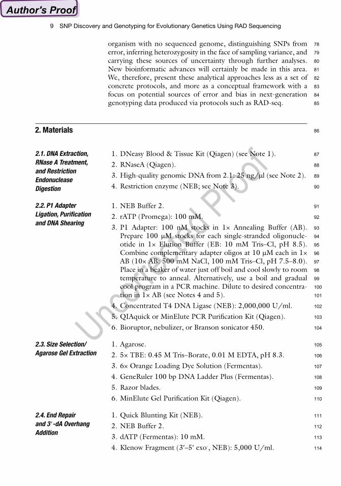
2. Materials

2.1. DNA Extraction, RNase A Treatment, and Restriction Endonuclease Digestion

2.2. P1 Adapter Ligation, Purification and DNA Shearing

2.3. Size Selection/Agarose Gel Extraction

2.4. End Repair and 3 -dA Overhang Addition

78

79

80

81

82

83

84

85

86

87

88

89

90

91

92

93

94

95

96

97

98

99

100

101

102

103

104

105

106

107

108

109

110

111

112

113

114

P.D. Etter et al.

1. NEB Buffer 2. 2. rATP: 100 mM. 3. P2 Adapter: 10 M stock in 1! AB prepared as P1 adapter

described above (see Notes 4 and 5). 4. Concentrated T4 DNA Ligase. 5. Phusion High-Fidelity PCR Master Mix with HF Buffer

(NEB). 6. RAD amplification primer mix: 10 M. Prepare 100 M stocks

for each oligonucleotide in 1! EB. Mix together at 10 M in buffer EB (see Note 6).

The protocol described below, outlined in Fig. 1, prepares RAD tag libraries for high-throughput Illumina sequencing (see Note 7). In short, genomic DNA is digested with a restriction enzyme and an adapter (P1) is ligated to the fragments’ compatible ends (Fig. 1a). This adapter contains forward amplification and Illumina sequenc-ing primer sites, as well as a nucleotide bar code 4 or 5 bp long for sample identification. To reduce erroneous sample assignment due to sequencing error, all bar codes differ by at least three nucleotides (see Note 8). The adapter-ligated fragments are subsequently pooled, randomly sheared, and a specific size fraction is selected fol-lowing electrophoresis (Fig. 1b). DNA is then ligated to a second adapter (P2), a Y adapter (13) that has divergent ends whose two strands are complementary for only part of their length (Fig. 1c). The reverse amplification primer is unable to bind to P2 unless the complementary sequence is filled in during the first round of for-ward elongation originating from the P1 amplification primer. The structure of this adapter ensures that only P1 adapter-ligated RAD tags will be amplified during the final PCR amplification step (Fig. 1d). The protocol for mapping of the lateral plate locus in three-spined stickleback using EcoRI RAD markers reported in Baird et al. (9) is described here in detail as an example of the

2.5. P2 Adapter Ligation and RAD Tag Amplification/Enrichment

3. Methods

Fig. 1. RAD tag library generation. (a) Genomic DNA is digested with a restriction enzyme and a bar-coded P1 adapter is ligated to the fragments. The P1 adapter contains a forward amplification primer site, an Illumina sequencing primer site, and a bar code (shaded boxes represent P1 adapters with different bar codes). (b) Adapter-ligated fragments are combined (if multiplexing), sheared, and (c) ligated to a second adapter (P2, white boxes). The P2 adapter is a divergent “Y” adapter, containing the reverse complement of the P2 reverse amplification primer site, preventing amplification of genomic fragments lacking a P1 adapter. (d) RAD tags, which have a P1 adapter, are selectively and robustly enriched by PCR amplification (reproduced from ref. 9).

115

116

117

118

119

120

121

122

123

124

125

126

127

128

129

130

131

132

133

134

135

136

137

138

139

140

141

142

143

144

145

146


IlluminaSequencingPrimer Site

Barcode

P1 Adapter

P2 Adapter

CTCAGGCATCACTCGATTCCTCCGAGAACAATGAGTCCGTAGTGAGCTAAGGAGGCAGCATACGGCAGAAGACGAAC

Complement of Reverse Amplification Primer Site

Illumina sequenceread length

Ligate P1 Adapter to digested genomic DNA

Pool barcoded samples and shear

Ligate P2 Adapter to sheared fragments

Selectively amplify RAD tags

Genomic DNA

Restrictionsite

ForwardAmplificationPrimer Site

a

b

c

d

P.D. Etter et al.

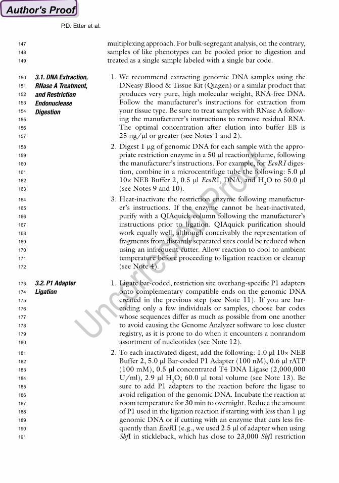
multiplexing approach. For bulk-segregant analysis, on the contrary, samples of like phenotypes can be pooled prior to digestion and treated as a single sample labeled with a single bar code.

1. We recommend extracting genomic DNA samples using the DNeasy Blood & Tissue Kit (Qiagen) or a similar product that produces very pure, high molecular weight, RNA-free DNA. Follow the manufacturer’s instructions for extraction from your tissue type. Be sure to treat samples with RNase A follow-ing the manufacturer’s instructions to remove residual RNA. The optimal concentration after elution into buffer EB is 25 ng/ l or greater (see Notes 1 and 2).

2. Digest 1 g of genomic DNA for each sample with the appro-priate restriction enzyme in a 50 l reaction volume, following the manufacturer’s instructions. For example, for EcoRI diges-tion, combine in a microcentrifuge tube the following: 5.0 l 10! NEB Buffer 2, 0.5 l EcoRI, DNA, and H2O to 50.0 l (see Notes 9 and 10).

3. Heat-inactivate the restriction enzyme following manufactur-er’s instructions. If the enzyme cannot be heat-inactivated, purify with a QIAquick column following the manufacturer’s instructions prior to ligation. QIAquick purification should work equally well, although conceivably the representation of fragments from distantly separated sites could be reduced when using an infrequent cutter. Allow reaction to cool to ambient temperature before proceeding to ligation reaction or cleanup (see Note 4).

1. Ligate bar-coded, restriction site overhang-specific P1 adapters onto complementary compatible ends on the genomic DNA created in the previous step (see Note 11). If you are bar- coding only a few individuals or samples, choose bar codes whose sequences differ as much as possible from one another to avoid causing the Genome Analyzer software to lose cluster registry, as it is prone to do when it encounters a nonrandom assortment of nucleotides (see Note 12).

2. To each inactivated digest, add the following: 1.0 l 10! NEB Buffer 2, 5.0 l Bar-coded P1 Adapter (100 nM), 0.6 l rATP (100 mM), 0.5 l concentrated T4 DNA Ligase (2,000,000 U/ml), 2.9 l H2O; 60.0 l total volume (see Note 13). Be sure to add P1 adapters to the reaction before the ligase to avoid religation of the genomic DNA. Incubate the reaction at room temperature for 30 min to overnight. Reduce the amount of P1 used in the ligation reaction if starting with less than 1 g genomic DNA or if cutting with an enzyme that cuts less fre-quently than EcoRI (e.g., we used 2.5 l of adapter when using SbfI in stickleback, which has close to 23,000 SbfI restriction

3.1. DNA Extraction, RNase A Treatment, and Restriction Endonuclease Digestion

3.2. P1 Adapter Ligation

147

148

149

150

151

152

153

154

155

156

157

158

159

160

161

162

163

164

165

166

167

168

169

170

171

172

173

174

175

176

177

178

179

180

181

182

183

184

185

186

187

188

189

190

191


sites in its 460 Mb genome). It is critical to optimize the amount of P1 adapter added when a given restriction enzyme is used for the first time in an organism (see Note 14).

3. Heat-inactivate T4 DNA Ligase for 10 min at 65°C. Allow reac-tion to cool slowly to ambient temperature before shearing.

1. Combine bar-coded samples at an equal or otherwise desired ratio. Use a 100–300 l aliquot containing 1–2 g DNA total to complete the protocol and freeze the rest at "20°C in case you need to optimize shearing in the next step. In Baird et al. (9), DNA from F2 stickleback progeny that shared a phenotype was pooled and each pool was uniquely bar-coded for SbfI bulk-segregant analysis. These samples were then combined at equal volumes with bar-coded samples from each parent to create one library. In a second experiment, EcoRI-based librar-ies were made by pooling DNA samples from F2 fish after they were bar-coded individually by P1 ligation (see Note 12).

2. Shear DNA samples to an average size of 500 bp to create a pool of P1-ligated molecules with random, variable ends. This step requires some optimization for different DNA concentra-tions and for each type of restriction endonuclease. The fol-lowing protocol has been optimized to shear stickleback DNA digested with either EcoRI or SbfI using the Bioruptor and is a good starting point for any study (see Note 16). The goal is to create sheared product that is predominantly smaller than 1 kb in size (see Fig. 1).

3. Dilute ligation reaction to 100 l in water (or take 100–300 l aliquot from multiplexed samples) and shear in the Bioruptor 10 times for 30 s on high following manufacturer’s instruc-tions. Make sure that the tank water in the Bioruptor is cold (4°C) before starting. All other positions in the Bioruptor holder not filled by your sample/s should be filled with bal-ance tubes containing an equal volume of water.

4. Clean up the sheared DNA using a MinElute column follow-ing manufacturer’s instructions. This purification is performed to remove the ligase and restriction enzyme, and to concen-trate the DNA so that the entire sample can be loaded in a single lane on an agarose gel. Elute in 20 l EB.

1. This step in the protocol removes free unligated or concate-merized P1 adapters and restricts the size range of tags to those that can be sequenced efficiently on an Illumina Genome Analyzer flow cell. Run the entire sheared sample in 1! Orange Loading Dye on a 1.25% agarose, 0.5! TBE gel for 45 min at 100 V, next to 2.0 l GeneRuler 100 bp DNA Ladder Plus for size reference; run the ladder in lanes flanking the samples until the 300 and 500 bp ladder bands are sufficiently resolved from 200 to 600 bp bands (see Fig. 2; Note 17).

3.3. Sample Multiplexing (see Note 15) and DNA Shearing

3.4. Size Selection/Agarose Gel Extraction and End Repair

192

193

194

195

196

197

198

199

200

201

202

203

204

205

206

207

208

209

210

211

212

213

214

215

216

217

218

219

220

221

222

223

224

225

226

227

228

229

230

231

232

233

234

235

236

237

P.D. Etter et al.

2. Being careful to exclude any free P1 adapters and P1 dimers running at ~130 bp and below, use a fresh razor blade to cut a slice of the gel spanning 300–500 bp (see Note 18). Extract DNA using MinElute Gel Purification Kit following manufac-turer’s instructions with the following modification: to improve representation of AT-rich sequences, melt agarose gel slices in the supplied buffer at room temperature (18–22°C) with agi-tation until dissolved (usually less than 30 min) (14). Elute in 20 l EB into a microcentrifuge tube containing 2.5 l 10! Blunting Buffer from the Quick Blunting Kit used in the following step (see Note 19).

3. The Quick Blunting Kit protocol converts 5 or 3 overhangs, created by shearing, into phosphorylated blunt ends using T4 DNA Polymerase and T4 Polynucleotide Kinase.

4. To the eluate from the previous step, add 2.5 l dNTP mix (1 mM) and 1.0 l Blunt Enzyme Mix. Incubate at RT for 30 min.

5. Purify with a QIAquick column. Elute in 43 l EB into a microcentrifuge tube containing 5.0 l 10! NEB Buffer 2.

1. This step in the protocol adds an “A” base to the 3 ends of the blunt phosphorylated DNA fragments, using the polymerase activity of Klenow Fragment (3 –5 exo-). This prepares the DNA fragments for ligation to the P2 adapter, which possesses a single “T” base overhang at the 3 end of its bottom strand.

2. To the eluate from the previous step, add: 1.0 l dATP (10 mM), 3.0 l Klenow (exo-). Incubate at 37°C for 30 min. Allow the reaction to cool to ambient temperature.

3. Purify with a QIAquick column. Elute in 45 l EB into a microcentrifuge tube containing 5.0 l 10! NEB Buffer 2.

4. This step in the protocol ligates the P2 adapter, a “Y” adapter with divergent ends that contains a 3 dT overhang, onto the ends of DNA fragments with 3 dA overhangs to create RAD-seq library template ready for amplification.

3.5. 3 -dA Overhang Addition and P2 Adapter Ligation

Fig. 2. Three bar-coded and multiplexed RAD tag libraries. Lanes 2, 3, and 5 each contain two DNA samples that were restriction digested, ligated to bar-coded P1 adapters, com-bined, sheared, purified, and then loaded on an agarose gel. 2 – parental DNA samples cut with SbfI. 3 – F2 pools cut with SbfI. 4 – blank. 5 – parental DNA samples cut with EcoR I. Libraries contain 2 g total combined genomic DNA each. 1 and 6 – 2.0 l GeneRuler 100-bp DNA Ladder Plus.

238

239

240

241

242

243

244

245

246

247

248

249

250

251

252

253

254

255

256

257

258

259

260

261

262

263

264

265

266

267

268

269

270


5. To the eluate from previous step, add: 1.0 l P2 Adapter (10 M), 0.5 l rATP (100 mM), 0.5 l concentrated T4 DNA Ligase. Incubate the reaction at room temperature for 30 min to overnight.

6. Purify with a QIAquick column. Elute in 50 l EB and quan-tify (see Note 18).

1. In this step high-fidelity PCR amplification is performed on P1 and P2 adapter-ligated DNA fragments, enriching for RAD tags that contain both adaptors and preparing them to be hybridized to an Illumina Genome Analyzer flow cell (see Fig. 1).

2. Perform a test amplification to determine library quality. In a thin-walled PCR tube, combine: 10.5 l H2O, 12.5 l Phusion High-Fidelity Master Mix, 1.0 l RAD amplification primer mix (10 M), 1.0 l RAD library template (or a quantified amount; see Note 20). Perform 18 cycles of amplification in a thermal cycler: 30 s 98°C, 18! (10 s 98°C, 30 s 65°C, 30 s 72°C), 5 min 72°C, hold 4°C. Run 5.0 l PCR product in 1! Orange Loading Dye out on 1.0% agarose gel next to 1.0 l RAD library template and 2.0 l GeneRuler 100 bp DNA Ladder Plus (Fig. 3).

3. If the amplified product is at least twice as bright as the tem-plate, perform a larger volume amplification (typically 50–100 l) but with fewer cycles (12–14, to minimize bias), to create enough to retrieve a large amount of the RAD tag library from a final gel extraction (see Note 21). If amplification looks poor, use more library template in a second test PCR reaction. Figure 3 shows three libraries used in Baird et al. (9) that amplified well, which is apparent when comparing the amplified product to the amount of template loaded in the lane to the right of each sample. Template should appear dim, yet visible on the gel. Purify the large volume reaction with a MinElute column. Elute in 20 l EB.

3.6. RAD Tag Amplification/Enrichment

Fig. 3. Test amplification PCR product from the three libraries shown in Fig. 2. Lanes 2, 4, and 6 contain 5.0 l amplified PCR product. 2 – parental SbfI library. 4 – F2 Sbf I library. 6 – parental EcoR I library. Lanes 3, 5, and 7 contain 1.0 l template used for amplification in the lane to the left. Template was loaded at 5! the amount used in the equivalent volume loaded for amplified reactions. 1 and 8 – 2.0 l GeneRuler 100-bp DNA Ladder Plus. Libraries are 300–600 bp in size.

271

272

273

274

275

276

277

278

279

280

281

282

283

284

285

286

287

288

289

290

291

292

293

294

295

296

297

298

299

300

301

302

P.D. Etter et al.

4. The following purification step is performed to eliminate any artifactual bands that may appear due to an improper ratio of P1 adapter to restriction-site compatible ends (see Note 14). Load the entire sample in 1! Orange Loading Dye on a 1.25% agarose, 0.5! TBE gel and run for 45 min at 100 V, next to 2.0 l GeneRuler 100 bp DNA Ladder Plus for size reference (Fig. 4). Being careful to exclude any free adapters or P1 dim-ers running at ~130 bp and below, use a fresh razor blade to cut a slice of the gel spanning ~350–550 bp. Extract DNA using MinElute Gel Purification Kit following manufacturer’s instructions, but melt agarose gel slices in the supplied buffer at room temperature. Elute in 20 l EB (see Note 22).

5. Quantify the DNA using a fluorometer to accurately measure the concentration. Concentrations will range from 1 to 20 ng/ l. Determine the molar concentration of the library by examining the gel image and estimating the median size of the library smear, which should be around 450 bp. Multiply this size by 650 (the average molecular mass of a base-pair) to get the molecular weight of the library. Use this number to calcu-late the molar concentration of the library (see Note 23).

6. Sequence libraries on Illumina Genome Analyzer following manufacturer’s instructions (see Note 24).

Fig. 4. PCR product from the three libraries shown in Figs. 2 and 3 after the final large volume amplification and purification. Lanes 2, 4, and 6 each contain 20 l purified PCR product from 100 l amplifications. 2 – parental SbfI library. 4 – F2 Sbf I library. 6 – parental EcoR I library. 1 – 2.0 l GeneRuler 100-bp DNA Ladder Plus. Lanes 3, 5, and 7 are blank. Libraries are 300–600 bp in size.

Fig. 5. Schematic diagram of population genomic data analysis using RAD sequencing. (a) Following Illumina sequencing of bar-coded fragments, sequence reads (thin lines) are aligned to a reference genome sequence (thick line). Depth of coverage varies across tags. Reads that do not align to the genome, or align in multiple locations, are discarded. (b) Sample of reads at a single RAD site. The recognition site for the enzyme Sbf1 is indicated along the reference genome sequence (top), and sequence reads typically proceed in both directions from this point, at which they overlap. At each nucleotide site, reads showing each of the four possible nucleotides can be tallied (solid box). (c) Nucleotide counts at each site for each individual are used in a maximum likelihood framework to assign the diploid genotype at the site. In this example, G/T heterozygote is the most likely genotype; the method provides the log-likelihood for this genotype, a maximum-likelihood estimate for the sequencing error rate , and a likelihood ratio test statistic comparing G/T to the second-most-likely geno-type, G/G homozygote. (d) Each individual now has a diploid genotype at each nucleotide site sequenced, and single-nucleotide polymorphisms (SNPs) can be identified across populations. Note, however, that haplotype phase is still unknown across RAD tags. (e) SNPs (ovals) are distributed across the genome (thick line), and population genetic measures (e.g., FST) are calculated for each SNP. (f) A kernel smoothing average across multiple nucleotide positions is used to produce genome-wide distributions of population genetic measures.

303

304

305

306

307

308

309

310

311

312

313

314

315

316

317

318

319

320

321

322

323

324


A significant consideration for the analysis of RAD sequencing data is whether the organism of interest has a reference genome. If it does, then RAD sequences can be aligned against the genome directly, and SNPs can be called as depicted in Fig. 5 and described below.

3.7. Alignment Against a Reference Genome and De Novo Assembly

325

326

327

328

P.D. Etter et al.

However, because the length of reads is still relatively short on most NGS platforms, at least some of the reads will fall in repetitive regions that are similar across several parts of the genome, which will be evidenced by potential assignment with equal probability to these locations. These reads can be removed from the analysis. Alternatively, paired-end sequencing can be performed to help infer the correct location of each read in the genome.

When a reference genome does not exist RAD genotyping can still be performed by assembling reads with respect to one another. For genomic regions that are unique, this assembly works as well as aligning against the genome. The aligned stack of reads can be analyzed to determine SNPs and genotypes that can be used in a genetic map or population genomic analysis. Repetitive regions are problematic as above, but the additional information provided by aligning to multiple genomic regions in the reference genome is absent, making the identification of these repetitive regions even more difficult. Stacks of reads may be abnormally deep because the focal RAD site was by chance sampled significantly more than average, or because paralogous regions with similar sequences were erroneously assembled together. For stacks that fall outside the range of the expected number of reads, the data can simply be expunged from the analysis. More problematic is a situation where two or a small number of paralogous regions are assembled, and the total number of reads is large, but not significantly so, because of sampling variation across all RAD loci.

In situations where paralogous regions are mistakenly assem-bled, one of several things can be done. First, the length of the reads can be increased, or fragments can be paired-end sequenced, with the hope of obtaining unique information that can be used to tell paralagous regions apart. These solutions increase the cost of the sequencing to an extent that may not be justified by the increase in information. If data are being collected from individuals in a population or mapping cross, tests of Hardy Weinberg Equilibrium (HWE) may allow identification of problematic, incorrectly identi-fied “genotypes” that are really paralogous regions. For example when two monomorphic, paralogous regions are fixed for alterna-tive nucleotides and then mistakenly assembled as a single locus, a SNP will be inferred but no homozygotes will be identified. Lastly, a network-based approach can be employed with the expectation that true SNPs should be at significant frequency and surrounded in sequence space by a constellation of low frequency sequencing errors. In most populations SNPs will be binary, and therefore, the network will consist of two high frequency alleles at the center of the constellation. In situations where paralogous regions are incor-rectly assembled, the network will have the easily identifiable topol-ogy of three or more high frequency alleles each surrounding by low frequency errors. All of these solutions are imperfect, and

329

330

331

332

333

334

335

336

337

338

339

340

341

342

343

344

345

346

347

348

349

350

351

352

353

354

355

356

357

358

359

360

361

362

363

364

365

366

367

368

369

370

371

372

373

374

375


extracting information from de novo RAD tags and other NGS data will be a significant area of research in the near future.

Another challenge of next-generation sequencing data for bioinformatic analyses is the introduction of sequencing error into many of the reads. Although the sequencing error rate is quite low, in the order of 0.1–1.0% per nucleotide, it still becomes a signifi-cant source of inferential confusion when millions of reads are con-sidered simultaneously. Unfortunately, sequencing error compounds the problems of assembling similar paralogous regions, outlined in the previous section, by increasing the probability of misassembly. Error rates can vary across samples, RAD sites, and positions in the reads for each site. In addition, the sampling pro-cess of a heterogeneous library inherent in NGS introduces sam-pling variation in the number of reads observed across RAD sites as well as between alleles at a single site. These issues could be overcome by greatly increasing total sequencing depth, but of course this approach will also increase the cost of a study. A better approach to differentiating true SNPs from sequencing error is a statistical framework that accounts for the uncertainty in genotyp-ing. Undoubtedly significant progress will be made in this area in the near future; here we present one approach as an example of a straightforward, flexible statistical model.

The following maximum-likelihood framework is based upon Hohenlohe et al. (10), designed for genotyping diploid individuals sampled from a population. The expectation is that errors should be differentiated from heterozygous SNPs by the frequency of nucleotides, with errors being represented at low frequency while alleles at heterozygous sites in an individual will be present in near equal frequencies in the total number of reads. Modifications to this approach would be required in other cases, such as haploid organisms, recombinant inbred lines, backcross mapping crosses, or single bar codes representing pools of individuals.

For a given site in an individual, let n be the total number of reads at that site, where n = n1 + n2 + n3 + n4, and ni is the read count for each possible nucleotide at the site (disregarding ambiguous reads). For a diploid individual, there are ten possible genotypes (four homozygous and six (unordered) heterozygous genotypes). A multinomial sampling distribution gives the probability of observing a set of read counts (n1,n2,n3,n4) given a particular geno-type, which translates into the likelihood for that genotype. For example, the likelihoods of a homozygote (genotype 1,1) or a heterozygote (1,2) are, respectively:

1 2 3 4

1 2 3 41 2 3 4

! 3(1,1) ( , , , |1,1) 1

! ! ! ! 4 4

n n n nnL P n n n n

n n n ne e (1a)

3.8. Inferring Genotypes in the Face of Sequencing Error and Sampling Variance

376

377

378

379

380

381

382

383

384

385

386

387

388

389

390

391

392

393

394

395

396

397

398

399

400

401

402

403

404

405

406

407

408

409

410

411

412

413

414

415

416

417

418

P.D. Etter et al.

and

1 2 3 4

1 2 3 41 2 3 4

!(1,2) ( , , , |1,2)

! ! ! !

0.5 ,4 4

n n n n

nL P n n n n

n n n n

e e (1b)

where is the sequencing error rate. If we let n1 be the count of the most observed nucleotide, and n2 be the count of the second-most observed nucleotide, then the two equations in (1) give the likeli-hood of the two most likely hypotheses out of the ten possible gen-otypes. From here, one approach is to assign a diploid genotype to each site based on a likelihood ratio test between these two most likely hypotheses with one degree of freedom. For example, if this test is significant at the = 0.05 level, the most likely genotype at the site is assigned; otherwise the genotype is left unassigned for that individual. In effect this criterion removes data for which there are too few sequence reads to determine a genotype, instead of establishing a constant threshold for sequencing coverage (10). An alternative approach is to carry the uncertainty in genotyping through all subsequent analyses. This can be done by incorporating the likelihoods of each genotype in a Bayesian framework in subse-quent calculation of population genetic measures, such as allele fre-quency, or by using genotype likelihoods in systematic resampling of the data. In either case, information on linkage disequilibrium and genotypes at neighboring loci could also be used to update the posterior probabilities of genotypes at each site.

A central parameter in the model above is the sequencing error rate e. One option for this parameter is to assume that it is constant across all sites (15), and either estimate it from the data by maxi-mum likelihood or calculate it from sequencing of a control sample in the sequencing run. However, there is empirical evidence that sequencing error varies among sites, and alternatively e can be esti-mated independently from the data at each site. Maximum likeli-hood estimates of e are calculated directly at each site by differentiation of equations (9.1). This technique has been applied successfully to RAD-seq data (10). More sophisticated models could be applied here as well, for instance assuming a probability distribution from which e is drawn independently for each site. This probability distribution could be iteratively updated by the data, and it could also be allowed to vary by nucleotide position along each sequence read or even by cluster position on the Illumina flow cell. Further empirical work is needed to assess alternative models of sequencing error.

419

420

421

422

423

424

425

426

427

428

429

430

431

432

433

434

435

436

437

438

439

440

441

442

443

444

445

446

447

448

449

450

451

452

453

454

455

456

457


The analytical method described in the previous section accounts for sequencing error and the random sampling variance inherent in NGS data. However, it does not account for any systematic biases in, for instance, the frequency of sequence reads for alternative alleles at a heterozygous site. For example, biased representation could occur because PCR amplification occurs more readily on one allele or bar code. Bar coding and calling genotypes separately in each individual alleviates some of this bias. In addition, sampling variation among sites and alleles that occurs early in the process can be propagated and amplified in the RAD-seq protocol. Optimizing the protocol to minimize the number of PCR cycles required is an important component of dealing with this issue. However, to date no analytical theory or tools have been developed to handle these sources of variation, and numerical simulations and empirical studies are needed to quantify them. Most simply, individuals of known sequence could be repeatedly genotyped by RAD-seq, using replicate libraries and bar codes, to estimate and partition the resulting variance in observed read frequencies.

Some evolutionary genetic applications will dictate alternative experimental designs, including sequencing of pools of individuals to produce point estimates (with error) of allele frequencies (15). Two examples are pools of individuals from natural populations for phylogeography (11), or groups of individuals of different pheno-typic classes in a quantitative trait locus (QTL) mapping cross (9). These approaches lose information about individual genotypes, but because of the volume of data produced by NGS, techniques or analyses that lose some information remain highly effective. For instance, Emerson et al. (11) estimated the fine-scale phylogeo-graphic relationships among populations of the pitcher plant mosquito Wyeomia smithii that originated postglacially along the eastern seaboard of USA. Because of the small amount of DNA in each mosquito, six individuals from each population were pooled and genotyped with bar-coded adaptors. Rather than directly esti-mating allele frequencies, which could not be done with high con-fidence, the analysis focused only on those SNPs for which a statistical model indicated that allele frequency differed signifi-cantly between populations. This produced a set of nucleotides that were variable among, and fixed (or nearly so) within, popula-tions. These data were used in subsequent standard phylogenetic analyses. The majority of the potentially informative SNPs were removed from the study, but because such a large number of RAD sites were identified and typed, the remaining 3,741 sites resulted in a beautifully resolved phylogeny, with high branch support and congruity to previous biogeographic hypotheses for this species.

Ever since the integration of Mendel’s laws with evolutionary theory during the Modern Synthesis of the 1930s, biologists have dreamed of a day when perfect genetic knowledge would be available for

3.9. Future Directions and Alternative Strategies

3.10. Summary

458

459

460

461

462

463

464

465

466

467

468

469

470

471

472

473

474

475

476

477

478

479

480

481

482

483

484

485

486

487

488

489

490

491

492

493

494

495

496

497

498

499

500

501

502

503

504

P.D. Etter et al.

almost any organism. Nearly a century later, NGS technologies are fulfilling that promise and opening the possibility for genetic analyses that have heretofore been impossible. Perhaps the most critical aspect of these breakthroughs is the unshackling of genetic analyses from traditional model organisms, allowing genomic studies to be performed in organisms for which few genomic resources presently exist. We presented one application of NGS, RAD geno-typing, a focused reduced-representation methodology that uses Illumina next-generation sequencing to simultaneously discover and score tens to hundreds of thousands markers in a very cost-efficient manner. The core RAD-seq protocol can be performed in nearly any evolutionary genetic laboratory. Undoubtedly numerous modifications of the core RAD molecular protocols can be made to suit a variety of additional research problems. Despite the ease of use of RAD and other NGS protocols, a significant challenge facing biologists is developing the appropriate analytical and bioinformatic tools for these data. Although we outline some general analytical approaches for RAD-seq, we fully anticipate that the development of bioinformatic tools for RAD and similar data will be a rich area of research for many years.

1. Clean, intact, high-quality DNA is required for optimal restric-tion endonuclease digestion and is important for the overall success of the protocol. We have found that lower quality DNA can be used, but the starting amount will likely need to be increased because a large number of DNA fragments that have a correctly ligated P1 adapter may not end up in the proper size range when the starting DNA is partially degraded. When working with heavily degraded DNA samples is the only option, we have found that parameters of the protocol can be optimized (such as using more input DNA to start with and shearing less) to create usable libraries. These libraries often do not amplify as well as ones made with intact, high molecular weight genomic DNA. The “Best Practices” sections of the most recent Illumina Sample Prep Guides are a good resource for quantification, handling, and temperature considerations.

2. We recommend using a fluorescence-based method for DNA quantification to get the most accurate concentration readings. Since they bind specifically to double-stranded DNA, the dyes used in fluorometric assays are not as affected by RNA, free nucleotides, or other contaminants commonly found in DNA preparations (which can lead to inaccurate concentration pre-dictions when using absorbance). If using another form of DNA quantification, such as UV spectrometer 260/280

4. Notes

505

506

507

508

509

510

511

512

513

514

515

516

517

518

519

520

521

522

523

524

525

526

527

528

529

530

531

532

533

534

535

536

537

538

539

540

541

542

543

544

545

546

547

548


absorbance readings, be sure to confirm the concentration by comparing a known calibration sample or running the sample on an agarose gel and comparing to a known quantity of DNA or ladder. We recommend checking the integrity of samples on a gel prior to embarking on this protocol regardless of the quantification method. Genomic DNA should consist of a fairly tight high-molecular-weight band without any visible degradation products or smears.

3. The choice of the particular restriction enzyme to use for a study is based upon several parameters such as the desired frequency of RAD sites throughout the genome, GC content, the depth of coverage necessary, and size of the genome. For example, an average restriction endonuclease with an 8-bp recognition sequence will produce 1 tag every 64 kb in an organism with equal and random frequency of cut sites. Of course, the latter part of the previous sentence is hardly ever true, so the predicted and actual number of restriction sites in a genome can be quite different. For example, the predicted number of SbfI sites (CCTGCAGG) in the stickleback genome is 7,069, whereas we have identified 22,829 sites found at an average distance of 20.2 kb between sites. Yet SgrDI (CGTCGACG), with the same nucleotides as SbfI, but in a different order, has 2892 sites found at an average distance of 160.2 kb between sites, nearly an eight-fold difference. In addition, the depth of coverage for calling a genotype in an outbred sample is quite a bit higher than what is necessary for an isogenic, recombinant inbred line. In general, RAD-seq experimental design is a challenge of optimizing the number of individuals, markers, and coverage given a fixed sequencing effort due to budgetary constraints.

4. The P1 and P2 adapters are modified Solexa© adapters (2006 Illumina, Inc., all rights reserved). The presence of some salt is necessary for the double-stranded adapters used in this protocol to hybridize and remain stable at ambient temperatures and above. At a 1 mM salt concentration, the P1 adapter, which has 64 bases of complementary double-stranded sequence (assuming a 5-bp bar code), has a Tm of approximately 41ºC (depending on bar-code composition). P2, which has only 24 complementary bases, has a Tm of only 27ºC at the same salt concentration. At 50 mM salt the Tms increase significantly to ~69º and 56º, respectively. Care should be taken to allow reagents to cool to ambient tem-perature before double-stranded adapters are ligated to digested fragments so as not to denature them. In addition, heating short AT rich RAD fragments may result in their denaturation. Since single-stranded RAD fragments will not ligate to the double-stranded adapter overhangs, these RAD tags may be underrepre-sented in the final library. The P2 adapter described here, and used in Hohenlohe et al. (10), is longer than the adapter we used for our first forays into RAD sequencing. The new, longer P2

549

550

551

552

553

554

555

556

557

558

559

560

561

562

563

564

565

566

567

568

569

570

571

572

573

574

575

576

577

578

579

580

581

582

583

584

585

586

587

588

589

590

591

592

593

594

595

596

P.D. Etter et al.

adapter has a higher Tm closer to that of the P1 adapters and the added benefit of being paired-end compatible. Thus, the salt con-centration in the P2 ligation becomes less important. However, the longer P2 doesn’t get effectively eliminated with a column cleanup, necessitating a gel extraction after amplification no mat-ter how well P1 adapter titration has gone (see Note 14).

5. Below are example bar-coded EcoRI P1 and P2 adapter sequences. “P” denotes a phosphate group, “x” refers to bar-code nucleotides, and an asterisk denotes a phosphorothioate bond in the P2 adapter that is introduced to confer nuclease resistance to the double-stranded oligo (14). Phosphorothioate bonds should be added to any 3 overhangs on P1 adapters (e.g., SbfI adapters).P1 top: 5 -AATGATACGGCGACCACCGAGATCTACACTC

TTTCCCTACACGACGCTCTTCCGATCTxxxxx-3AATTxxxxxAGATCGGAAGAGCGTCGTGTAGGG

A A A G A G T G TA G AT C T C G G T G G T C G C C G T ATCATT-3

P2 top: 5 -P-CTCAGGCATCACTCGATTCCTCCGAGAACAA-3P2 bot: 5 -CAAGCAGAAGACGGCATACGACGGAGGAAT

CGAGTGATGCCTGAG*T-3 6. RAD amplification primers are Modified Solexa Amplification

primers (2006 Illumina, Inc., all rights reserved).P1-forward primer: 5 -AATGATACGGCGACCACCG*A-3P2-reverse primer: 5 -CAAGCAGAAGACGGCATACG*A-3

7. This protocol has been modified from that used in Baird et al. (9) and now incorporates critical improvements made since publication, including ones adopted from Quail et al. (14) and Illumina library preparation protocols. Although we recom-mend following the protocol as described, other companies may offer superior (or cheaper) versions of reagents that come at different enzyme concentrations or activities, which should work just as well. Using them may require additional optimiza-tion, including different incubation times or reaction volumes for efficient RAD-seq library preparation. Many other brands of DNA cleanup and gel extraction columns could instead be used also, but an important consideration is the minimum required elution volume. We have successfully substituted Zymo’s DNA Clean and Concentrator for Qiagen’s MinElute kit and 10 Weiss units/ l Epicentre T4 ligase instead of NEB’s 2000 cohesive end units/ l ligase.

8. Three-mismatch bar codes are optimal because although a sig-nificant number of reads will have a sequencing error in the bar code, it is very unlikely that a single read will have two errors in the same 5-bp sequence. Therefore, most of the reads that have an error in the bar code can still be assigned to the correct

597

598

599

600

601

602

603

604

605

606

607

608

609

610

611

612

613

614

615

616

617

618

619

620

621

622

623

624

625

626

627

628

629

630

631

632

633

634

635

636

637

638

639

640

641

642


sample when the adapters are designed to have three mismatches, whereas with only two mismatches a read with a sequencing error in the bar code may have come from one of two samples.

9. “H2O” in this text refers to water that has a resistivity of 18.2 M -cm and total organic content of less than five parts per billion.

10. Set up larger reactions if necessitated by dilute DNA and then concentrate the samples with a column before proceeding to ligation. This will cut down on throughput of the protocol, of course.

11. In general, when making master mixes, using multichannel pipettes and working with samples in 96- or 384-well plates will speed up the restriction digest and P1 ligation steps when multiplexing multiple bar-coded individuals.

12. In Baird et al. (9) DNA samples from 96 recombinant F2 indi-viduals were uniquely bar-coded, which allowed us to track RAD markers and associate them with differing phenotypes. For example, F2 individuals used in the mapping analysis included 60 possessing a complete compliment of lateral plate armor and 31 with a reduced number of plates. Up to 60 uniquely bar-coded samples were pooled in a single library, and all samples were sequenced in two sequencing lanes. Sequences from each individual fish were sorted out in silico by bar code, allowing the genetic mapping of variation in the lat-eral plates as well as variation in another skeletal trait, the pelvic structure. For the bulk-segregant analysis, DNA from F2 indi-viduals was pooled by phenotype prior to digestion with SbfI. Each digested pool was labeled with a unique bar code and then combined into a single library. In both cases, the parental samples were uniquely bar-coded and combined into single libraries that were sequenced along with the F2 libraries.

13. NEB Buffer 2 is used in the ligation reactions instead of ligase buffer because the salt it contains (50 mM NaCl) ensures the double-stranded adapters remain annealed during the reactions (see Note 4). T4 DNA Ligase is active in all 4 NEB Buffers if supplemented with 1 mM rATP, but doesn’t work at maximum efficiency in NEB 3 because of the high levels of salt in that buf-fer. The presence of some salt is necessary for the double-stranded adapters to remain stable at ambient temperature during the ligation, but too much may cause a problem. Be aware of the amount of salt put into the ligation reactions and adjust the concentration of the adapters accordingly (for instance, if working with a frequent cutter, use lower volumes of P1 at 1 M instead of higher volumes at 100 nM to cut down on salt added to the reaction). If the restriction buffer used for diges-tion does not contain 50 mM potassium or sodium ions, or if the restriction endonuclease cannot be heat-inactivated, purify

643

644

645

646

647

648

649

650

651

652

653

654

655

656

657

658

659

660

661

662

663

664

665

666

667

668

669

670

671

672

673

674

675

676

677

678

679

680

681

682

683

684

685

686

687

688

689

P.D. Etter et al.

the reaction in a column prior to P1 ligation and add 6.0 l NEB Buffer 2. This will negate the benefits of multiplexing somewhat but may be useful in certain RAD library applications involving one or only a few individuals.

14. EcoRI has been shown to work robustly in multiple organisms in our labs. Restriction enzymes that cut less frequently create fewer RAD tags and, thus, require more input DNA and less P1 adapter to keep the molar ratio approximately equal. Libraries produced with less frequent cutters are more difficult to amplify in general and protocol parameters may take some optimization for favorable results. It is critical to perform preliminary studies to optimize the appropriate amount of P1 adapter for a given restriction enzyme that is used for the first time in an organism, unless the actual number of sites is known (i.e., if a genome sequence is available). A range of P1 adapter to DNA ratios can be used in a preliminary study, and the efficiency of ligation can then assayed via gel visualization. Alternatively, a more precise estimate of the quantity of correctly adapted fragments in each P1-DNA ratio can be determined via a qPCR reaction using primers designed to the P1 and P2 adapters. Over the correct range of adapter-DNA ratios, the amount of ligated DNA should increase and then asymptote. The inflexion point of this rela-tionship is the ideal ratio of P1 adapter to DNA. If the ratio of P1 adapter overhangs to available genomic compatible ends is too low, you can get insufficient amplification and/or biased representation of some RAD tags. However, if the ratio of P1 to genomic overhangs is too high, a contaminant band that runs around 130 bp will appear after the final PCR reaction. If this contaminant overwhelms the amplification reaction it can lead to significant adapter sequence reads in the final sequencing out-put (even after gel extraction following the final PCR). This phenomenon is completely dependent upon the number of actual cut sites present in that genome and the corresponding amount of P1 adapter used. Our SbfI study in stickleback used 2.5 l P1 per microgram starting material and performed very well for library construction (see Figs. 3 and 4; lanes 2 and 4); however, this is likely due to the fact that there are actually more SbfI sites than expected by chance (see Note 3). Therefore, it may be preferable to start with less P1 when working on genomes with closer to the expected number of sites. In addition, the prescribed amounts of P1 adapters used in this protocol were optimized for the studies published in Baird et al. (9), using adapters lacking phosphorothioate bonds. In our hands, RAD-seq libraries created using adapters that have the phosphorothioate modifications amplify better and appear much less prone to adapter contamination. Though we have not optimized the maximum amount to use for these new adapters , P1 concentra-tions in the ligation reactions can be increased.

690

691

692

693

694

695

696

697

698

699

700

701

702

703

704

705

706

707

708

709

710

711

712

713

714

715

716

717

718

719

720

721

722

723

724

725

726

727

728

729

730

731

732

733

734

735

736

737


15. This step allows multiple individually bar-coded samples to be combined and processed as well as to cut down on cost, work time, and differences in amplification efficiency that may arise between different library preparations when processing many samples at once.

16. Although we have optimized our protocol for shearing via son-ication, other forms of shearing should work (the “Alternate Fragmentation Methods” sections of the Illumina Sample Prep Guides are a good resource for important considerations when choosing a shearing method).

17. We have found that it is unwise to run more than one library sample on the same agarose gel, as is shown in the figures, unless they will be combined and sequenced in the same lane on the flow cell, since it can lead to contamination between samples. This is especially important when dealing with sam-ples following PCR amplification. We also recommend using aerosol-resistant filter tips for all amplification and downstream steps in the protocol to avoid library contamination.

18. A wider size range can be isolated (Subheading 3.6, step 2) to have more RAD fragments to carry through the protocol if low template amounts are evident after the P2 ligation (see Note 22).

19. Use MinElute columns and not QIAquick columns, which require a larger elution volume.

20. The optimal amount of template is dependent on the restric-tion enzyme used and its occurrence throughout the particular genome; however, a good starting point is 5–10 ng per 25 l reaction. Lower template input concentrations are preferable, as you can be more confident of the true concentration of amplified RAD tag molecules in your final sample, which have both P1 and P2 sequences, and are, therefore, able to bind the adapter oligonucleotides present on the Illumina flow cell. Poorly amplified libraries will contain a greater number of background sheared genomic DNA fragments with only P2 adapters attached, which cannot bind to the flow cell.

21. Libraries that amplify robustly, such as those shown in Fig. 3, can be amplified with only 14 or fewer cycles of amplification to avoid skewing the representation of the library (14]. The goal is to use as few PCR cycles as possible to obtain robustly amplified libraries with as little amplification bias as possible.

22. For long-term storage of DNA samples, Illumina recommends a concentration of 10 nM and adding Tween-20 to the sample to a final concentration of 0.1%. This helps to prevent adsorp-tion of the template to plastic tubes upon repeated freeze–thaw cycles, which would decrease the effective DNA concentration and, therefore, the number of sequencing clusters the library will produce.

738

739

740

741

742

743

744

745

746

747

748

749

750

751

752

753

754

755

756

757

758

759

760

761

762

763

764

765

766

767

768

769

770

771

772

773

774

775

776

777

778

779

780

781

782

783

784

P.D. Etter et al.

23. For example, a measured DNA concentration of 10 ng/ l expressed in grams per liter is 0.01 g/l. 650 g/mol/bp ! 400 bp = 292,500 g/mol = 0.0002925 g/nmol. To calcu-late the nanomolarity, divide 0.01 g/l by 0.0002925 g/nmol to get 34.2 nmol/l or 34.2 nM.

24. We recommend that you validate your first one or two RAD-seq libraries by cloning 1.0 l of the gel-purified library into a blunt-end compatible sequencing vector. Sequence individual clones by conventional Sanger sequencing. Confirm that insert sequences contain the correct bar codes and restriction cut site overhang and are from the genomic source DNA.

Acknowledgments

The authors thank the University of Oregon researchers who, over the past 2 years, have helped troubleshoot many preliminary versions of this protocol. This work was funded by grants from the National Institutes of Health (1R24GM079486-01A1 and Ruth L. Kirschstein National Research Service Award F32 GM078949) and the National Science Foundation (IOS-0642264 and DEB-0919090).

References

1. Mardis ER (2008) The impact of next- generation sequencing technology on genetics. Trends Genet 24:133–141.

2. Shendure J, Ji H (2008) Next-generation DNA sequencing. Nat Biotech 26:1135–1145.

3. Asmann YW, Wallace MB, Thompson EA (2008) Transcriptome profiling using next-generation sequencing. Gastroenterology 135:1466–1468.

4. Marguerat S, Wilhelm BT, Bahler J (2008) Next-generation sequencing: applications beyond genomes. Biochem Soc Trans 36:1091–1096.

5. Mortazavi A, Williams BA, McCue K et al (2008) Mapping and quantifying mammalian transcrip-tomes by RNA-Seq. Nat Methods 5:621–628.

6. Rokas A, Abbot P (2009) Harnessing genomics for evolutionary insights. Trends Ecol Evol 24:192–200.

7. Mardis ER (2008) Next-generation DNA sequencing methods. Annu Rev Genomics Hum Genet 9:387–402.

8. Van Tassell CP, Smith TP, Matukumalli LK et al (2008) SNP discovery and allele frequency esti-mation by deep sequencing of reduced repre-sentation libraries. Nat Methods 5:247–252.

9. Baird NA, Etter PD, Atwood TS et al (2008) Rapid SNP discovery and genetic mapping

using sequenced RAD markers. PLoS ONE 3:e3376.

10. Hohenlohe P, Bassham S, Stiffler N et al (2010) Population genomics of parallel adaptation in threespine stickleback using sequenced RAD tags. PLoS Genet 6:e1000862.

11. Emerson KJ, Merz CR, Catchen JM et al (2010) Resolving post-glacial phylogeography using high throughput sequencing. Proc Natl Acad Sci USA 107:16196–200.

12. Gompert Z, Lucas LK, Fordyce JA et al (2010) Secondary contact between Lycaeides idas and L. melissa in the Rocky Mountains: extensive admixture and a patchy hybrid zone. Mol Ecol 19:3171–3192.

13. Coyne KJ, Burkholder JM, Feldman RA et al (2004) Modified serial analysis of gene expres-sion method for construction of gene expres-sion profiles of microbial eukaryotic species. Appl Environ Microbiol 70:5298–5304.

14. Quail MA, Kozarewa I, Smith F et al (2008) A large genome center’s improvements to the Illumina sequencing system. Nat Methods 5:1005–1010.

15. Lynch M (2009) Estimation of allele frequen-cies from high-coverage genome-sequencing projects. Genetics 18:295–301.

785

786

787

788

789

790

791

792

793

794

795

796

797

798

799

800

801

802

803

804

805

806

807

808

809

810

811

812

813

814

815

816

817

818

819

820

821

822

823

824

825

826

827

828

829

830

831

832

833

834

835

836

837

838

839

840

841

842

843

844

845

846

847

848

849

850

851

852

853

854

855

856

857

SNP Discovery and Genotyping for Evolutionary Genetics Using RAD Sequencing

Documents

Transcript of SNP Discovery and Genotyping for Evolutionary Genetics Using RAD Sequencing