MNRAS 479, 570–587 (2018) doi:10.1093/mnras/sty1455Advance Access publication 2018 June 5

SMHASH: anatomy of the Orphan Stream using RR Lyrae stars

David Hendel,1‹ Victoria Scowcroft,2,3 Kathryn V. Johnston,1 Mark A. Fardal,4

Roeland P. van der Marel,4,5 Sangmo T. Sohn,4 Adrian M. Price-Whelan,6

Rachael L. Beaton,6† Gurtina Besla,7 Giuseppe Bono,8,9 Maria-Rosa L. Cioni,10

Giselle Clementini,11 Judith G. Cohen,12 Michele Fabrizio,9,13 Wendy L. Freedman,14

Alessia Garofalo,11,15 Carl J. Grillmair,16 Nitya Kallivayalil,17 Juna A. Kollmeier,3

David R. Law,4 Barry F. Madore,3 Steven R. Majewski,17 Massimo Marengo,18

Andrew J. Monson,3 Jillian R. Neeley,18 David L. Nidever,19 Grzegorz Pietrzynski,20

Mark Seibert,3 Branimir Sesar,21 Horace A. Smith,22 Igor Soszynski23 andAndrzej Udalski23

Affiliations are listed at the end of the paper

Accepted 2018 May 25. Received 2018 May 23; in original form 2017 November 10

ABSTRACTStellar tidal streams provide an opportunity to study the motion and structure of the disruptinggalaxy as well as the gravitational potential of its host. Streams around the Milky Way areespecially promising as phase space positions of individual stars will be measured by ongoingor upcoming surveys. Nevertheless, it remains a challenge to accurately assess distances tostars farther than 10 kpc from the Sun, where we have the poorest knowledge of the Galaxy’smass distribution. To address this, we present observations of 32 candidate RR Lyrae stars inthe Orphan tidal stream taken as part of the Spitzer Merger History and Shape of the GalacticHalo (SMHASH) program. The extremely tight correlation between the periods, luminosities,and metallicities of RR Lyrae variable stars in the Spitzer IRAC 3.6μm band allows thedetermination of precise distances to individual stars; the median statistical relative distanceuncertainty to each RR Lyrae star is 2.5 per cent. By fitting orbits in an example potential, weobtain an upper limit on the mass of the Milky Way interior to 60 kpc of 5.6+1.2

−1.1 × 1011 M�,bringing estimates based on the Orphan Stream in line with those using other tracers. TheSMHASH data also resolve the stream in line-of-sight depth, allowing a new perspective onthe internal structure of the disrupted dwarf galaxy. Comparing with N–body models, we findthat the progenitor had an initial dark halo mass of approximately 3.2 × 109 M�, placing theOrphan Stream’s progenitor amongst the classical dwarf spheroidals.

Key words: stars: variables: RR Lyrae – Galaxy: halo – Galaxy: kinematics and dynamics –Galaxy: structure.

1 IN T RO D U C T I O N

Tidal debris structures are striking evidence of hierarchical assem-bly – the premise that the Milky Way and systems like it have beenbuilt over cosmic time through the coalescence of many smallerobjects (White & Rees 1978; Johnston, Hernquist & Bolte 1996;Bullock, Kravtsov & Weinberg 2001; Freeman & Bland-Hawthorn

� E-mail: hendel@astro.columbia.edu†Hubble Fellow.

2002). Some of this construction is in the form of major mergers,where two near-equal mass galaxies collide and their stars are re-distributed wholesale as the new galaxy violently relaxes. However,in the prevailing �-cold dark matter (�CDM) model, the vast ma-jority of mergers (by number) are minor (Fakhouri, Ma & Boylan-Kolchin 2010), where one halo, the host, dominates the interactionand a smaller object, the satellite, is dragged inward by dynamicalfriction and eventually stripped of mass by tidal forces. When theluminous component is disrupted the stars may form a stellar tidalstream or shell, depending on the parameters of the interaction (e.g.

C© 2018 The Author(s)Published by Oxford University Press on behalf of the Royal Astronomical Society

Dow

nloaded from https://academ

ic.oup.com/m

nras/article/479/1/570/5033412 by guest on 11 January 2022

Anatomy of the Orphan Stream 571

Johnston et al. 2008; Amorisco 2015; Hendel & Johnston 2015).The study of tidal features therefore probes the accretion historiesof galaxies.

Stellar tidal streams are also key tools for our current under-standing of the Milky Way’s gravitational potential. The techniquesapplied to measure the potential are wide-ranging but commonly afew-parameter potential model is varied in an attempt to match sim-ulations to the available data. Historically, the streams used mostoften for this purpose are the Sagittarius dwarf galaxy’s stream(Majewski et al. 2003; Law & Majewski 2010; Gibbons, Belokurov& Evans 2014) and various globular cluster streams such as Palo-mar 5 and GD-1 (Koposov, Rix & Hogg 2010;Fritz & Kallivay-alil 2015; Kupper et al. 2015; Pearson et al. 2015; Bovy et al.2016).

The Orphan tidal stream (Belokurov et al. 2006; Grillmair 2006)has several advantages over the other streams mentioned above. Itforms a smooth arc that is significantly longer (detected length of≈108◦; Grillmair et al. 2015), wider (∼2◦; Belokurov et al. 2006),and farther from the Galactic centre (>50 kpc; Newberg et al.2010; Sesar et al. 2013) than any of the commonly studied glob-ular cluster streams. Along with its total luminosity (Mr < −7.5,Belokurov et al. 2007) and metallicity spread of 0.56 dex (Caseyet al. 2013), these characteristics suggest a dwarf spheroidal galaxyas the likely origin, but the progenitor is elusive and possibly nearlycompletely disrupted by the Galaxy’s tidal field (Grillmair et al.2015). In contrast to the Sagittarius stream, the Orphan Streamhas a uniform appearance and cold velocity structure; the Sagittar-ius stream is notoriously complex, featuring multiple wraps, bifur-cated tails, and several stellar populations with different kinematics(Belokurov et al. 2006; Koposov et al. 2012; Gibbons, Belokurov& Evans 2017). The orbital planes of the Orphan and Sagittariusstreams are misaligned by ∼67◦ (Pawlowski, Pflamm-Altenburg &Kroupa 2012), making the combination of the two an attractive tar-get for multistream potential measuring methods (Sanderson, Helmi& Hogg 2015; Bovy et al. 2016).

The Orphan Stream also has the advantage of a well-filled hor-izontal branch resulting in numerous classes of stars that may beused as standard candles for distance estimation, for example theBlue Horizontal Branch (BHB) stars studied by Newberg et al.(2010). Of particular relevance to this work, the Orphan Streamcontains a significant population of RR Lyrae stars (RRL), whichhave been the focus of several recent efforts to improve distancemeasurement into the Galactic halo (e.g. Hernitschek et al. 2017;Sesar et al. 2017). These stars make excellent standard candlesusing period–luminosity (PL) relations with their near- or mid-infrared magnitudes (Longmore, Fernley & Jameson 1986; Bonoet al. 2001, 2003; Catelan, Pritzl & Smith 2004; Braga et al.2015). In addition to the advantage of decreased extinction at theselonger wavelengths compared to the V band (AV /A[3.6μm] ∼ 15,Cardelli, Clayton & Mathis 1989; Indebetouw et al. 2005), thePL relation has also been shown to have a small intrinsic scat-ter in the infrared (Madore et al. 2013; Neeley et al. 2015; Mu-raveva et al. 2018). Recently these relations have been extendedto include a metallicity component (Neeley et al. 2017) with theeffect of further decreasing the uncertainty on individual stars’ ab-solute magnitudes and thus removing scatter in measured distancesfor systems with a large range in metallicity, such as the OrphanStream.

The Spitzer Merger History And Shape of the Galactic Halo(SMHASH) program builds upon the previous Carnegie RR LyraeProgram (CRRP; Freedman et al. 2012) to leverage these excellentdistance indicators and explore a variety of Local Group substruc-

tures including five dwarf galaxies [Sagittarius, Sculptor (Garofaloet al. 2018), Ursa Minor, Carina, and Bootes] along with the Sagit-tarius and Orphan tidal streams. As we will show, the precision issuch that we are able to resolve the three-dimensional structure ofthe stream, granting special access to a system that is in many waysthe archetypal minor merger event.

In this work, we present Spitzer Space Telescope (Werner et al.2004) Infrared Array Camera (IRAC; Fazio et al. 2004) 3.6μmmagnitudes and inferred distances to 32 candidate Orphan StreamRR Lyrae stars with the principal goal of informing future studies ofthe Galactic potential and Orphan Stream progenitor. In Section 2,we describe our Spitzer photometry and the calculation of apparentmagnitudes. Section 3 describes how we derive distances to indi-vidual Orphan Stream stars. In Section 4, we define a procedureto fit orbits to the RRL and measure bulk properties of the stream;in Section 5, we investigate the extent to which the orbit fits placeconstraints on the mass of the Milky Way. Section 6 studies theOrphan progenitor and Section 7 concludes.

2 O B S E RVAT I O N S A N D DATA R E D U C T I O N

2.1 Data selection

The RR Lyrae stars selected for observation in the SMHASH Or-phan program are the 31 ‘high probability’ candidate stream mem-bers of Sesar et al. (2013); these stars are all fundamental-mode pul-sators (RRab). Also included is one ‘medium probability’ candidate,RR5, because it was measured at a large distance despite having aline-of-sight velocity somewhat discrepant with expectations for theOrphan Stream given its position. The stars were identified from acompilation of three synoptic sky surveys: the Catalina Real-TimeSky Survey (CRTS; Drake et al. 2009), the Lincoln Near EarthAsteroid Research (LINEAR; Stokes et al. 2000) survey, and thePalomar Transient Factory (PTF; Law et al. 2009; Rau et al. 2009).Sesar et al. (2013) obtained low-resolution follow-up spectroscopicobservations in order to implement a Galactic standard of rest veloc-ity cut as part of their stream membership criteria. All of our targetstherefore have uniformly determined metallicity (on the Layden1994 system, which is calibrated to the globular cluster metallicityscale of Zinn & West 1984) and line-of-sight velocity measurementswith uncertainties of 0.15 dex and ∼15 km s−1, respectively. Theircatalogue number in Table 1 is in order of decreasing declination,which approximately corresponds to a sequence of increasing ap-parent magnitude and decreasing Heliocentric distance (see fig. 2in Sesar et al. 2013).

2.2 Spitzer observations

The mid-infrared observations presented here were collected usingthe Infrared Array Camera (IRAC) on the Spitzer Space Telescopeas part of the Warm Spitzer Cycle 10 between 2014 June 19 and2015 August 31 (Johnston et al. 2013). Each star was observed in12 epochs at 3.6 μm only.

The targets selected in the Orphan Stream span a wide range indistance and therefore cover a significant range in apparent infraredmagnitude. In order to achieve a sufficient signal-to-noise ratio onthe individual epochs for both the nearest and most distant targets,the stars were divided into two groups based on their distances fromSesar et al. (2013) and their anticipated apparent magnitude fromthe K-band PL relation. The closer, brighter targets (with estimateddistances less than ∼40 kpc) were observed at each epoch withfive dithered 100 s exposures, with all 12 epochs approximately

MNRAS 479, 570–587 (2018)

Dow

nloaded from https://academ

ic.oup.com/m

nras/article/479/1/570/5033412 by guest on 11 January 2022

572 D. Hendel et al.

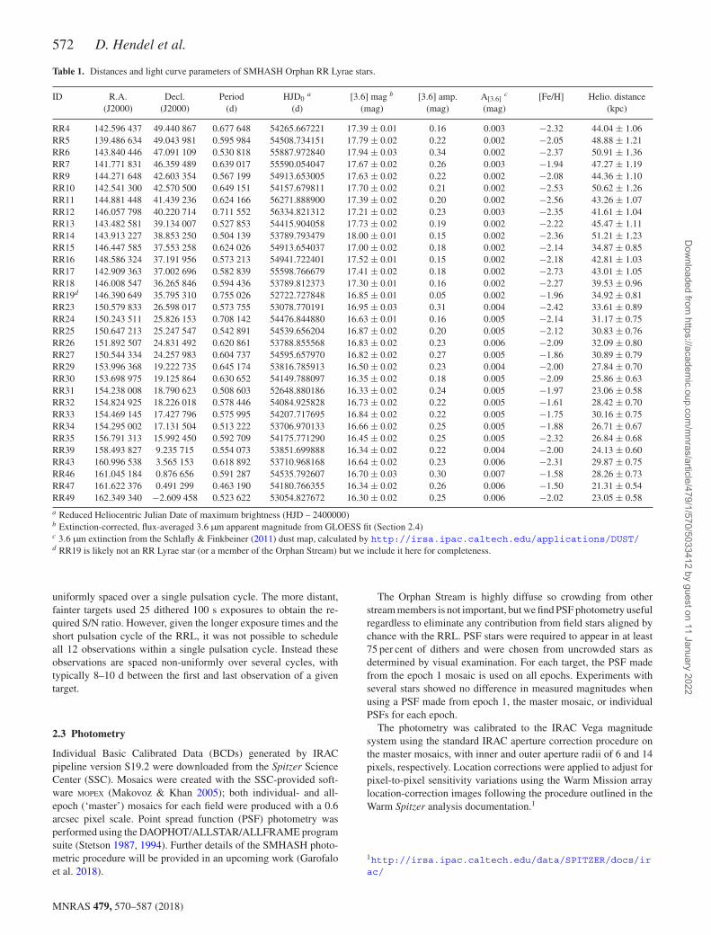
Table 1. Distances and light curve parameters of SMHASH Orphan RR Lyrae stars.

ID R.A. Decl. Period HJD0a [3.6] mag b [3.6] amp. A[3.6]

c [Fe/H] Helio. distance(J2000) (J2000) (d) (d) (mag) (mag) (mag) (kpc)

RR4 142.596 437 49.440 867 0.677 648 54265.667221 17.39 ± 0.01 0.16 0.003 −2.32 44.04 ± 1.06RR5 139.486 634 49.043 981 0.595 984 54508.734151 17.79 ± 0.02 0.22 0.002 −2.05 48.88 ± 1.21RR6 143.840 446 47.091 109 0.530 818 55887.972840 17.94 ± 0.03 0.34 0.002 −2.37 50.91 ± 1.36RR7 141.771 831 46.359 489 0.639 017 55590.054047 17.67 ± 0.02 0.26 0.003 −1.94 47.27 ± 1.19RR9 144.271 648 42.603 354 0.567 199 54913.653005 17.63 ± 0.02 0.22 0.002 −2.08 44.36 ± 1.10RR10 142.541 300 42.570 500 0.649 151 54157.679811 17.70 ± 0.02 0.21 0.002 −2.53 50.62 ± 1.26RR11 144.881 448 41.439 236 0.624 166 56271.888900 17.39 ± 0.02 0.20 0.002 −2.56 43.26 ± 1.07RR12 146.057 798 40.220 714 0.711 552 56334.821312 17.21 ± 0.02 0.23 0.003 −2.35 41.61 ± 1.04RR13 143.482 581 39.134 007 0.527 853 54415.904058 17.73 ± 0.02 0.19 0.002 −2.22 45.47 ± 1.11RR14 143.913 227 38.853 250 0.504 139 53789.793479 18.00 ± 0.01 0.15 0.002 −2.36 51.21 ± 1.23RR15 146.447 585 37.553 258 0.624 026 54913.654037 17.00 ± 0.02 0.18 0.002 −2.14 34.87 ± 0.85RR16 148.586 324 37.191 956 0.573 213 54941.722401 17.52 ± 0.01 0.15 0.002 −2.18 42.81 ± 1.03RR17 142.909 363 37.002 696 0.582 839 55598.766679 17.41 ± 0.02 0.18 0.002 −2.73 43.01 ± 1.05RR18 146.008 547 36.265 846 0.594 436 53789.812373 17.30 ± 0.01 0.16 0.002 −2.27 39.53 ± 0.96RR19d 146.390 649 35.795 310 0.755 026 52722.727848 16.85 ± 0.01 0.05 0.002 −1.96 34.92 ± 0.81RR23 150.579 833 26.598 017 0.573 755 53078.770191 16.95 ± 0.03 0.31 0.004 −2.42 33.61 ± 0.89RR24 150.243 511 25.826 153 0.708 142 54476.844880 16.63 ± 0.01 0.16 0.005 −2.14 31.17 ± 0.75RR25 150.647 213 25.247 547 0.542 891 54539.656204 16.87 ± 0.02 0.20 0.005 −2.12 30.83 ± 0.76RR26 151.892 507 24.831 492 0.620 861 53788.855568 16.83 ± 0.02 0.23 0.006 −2.09 32.09 ± 0.80RR27 150.544 334 24.257 983 0.604 737 54595.657970 16.82 ± 0.02 0.27 0.005 −1.86 30.89 ± 0.79RR29 153.996 368 19.222 735 0.645 174 53816.785913 16.50 ± 0.02 0.23 0.004 −2.00 27.84 ± 0.70RR30 153.698 975 19.125 864 0.630 652 54149.788097 16.35 ± 0.02 0.18 0.005 −2.09 25.86 ± 0.63RR31 154.238 008 18.790 623 0.508 603 52648.880186 16.33 ± 0.02 0.24 0.005 −1.97 23.06 ± 0.58RR32 154.824 925 18.226 018 0.578 446 54084.925828 16.73 ± 0.02 0.22 0.005 −1.61 28.42 ± 0.70RR33 154.469 145 17.427 796 0.575 995 54207.717695 16.84 ± 0.02 0.22 0.005 −1.75 30.16 ± 0.75RR34 154.295 002 17.131 504 0.513 222 53706.970133 16.66 ± 0.02 0.25 0.005 −1.88 26.71 ± 0.67RR35 156.791 313 15.992 450 0.592 709 54175.771290 16.45 ± 0.02 0.25 0.005 −2.32 26.84 ± 0.68RR39 158.493 827 9.235 715 0.554 073 53851.699888 16.34 ± 0.02 0.22 0.004 −2.00 24.13 ± 0.60RR43 160.996 538 3.565 153 0.618 892 53710.968168 16.64 ± 0.02 0.23 0.006 −2.31 29.87 ± 0.75RR46 161.045 184 0.876 656 0.591 287 54535.792607 16.70 ± 0.03 0.30 0.007 −1.58 28.26 ± 0.73RR47 161.622 376 0.491 299 0.463 190 54180.766355 16.34 ± 0.02 0.26 0.006 −1.50 21.31 ± 0.54RR49 162.349 340 −2.609 458 0.523 622 53054.827672 16.30 ± 0.02 0.25 0.006 −2.02 23.05 ± 0.58

a Reduced Heliocentric Julian Date of maximum brightness (HJD – 2400000)b Extinction-corrected, flux-averaged 3.6μm apparent magnitude from GLOESS fit (Section 2.4)c 3.6μm extinction from the Schlafly & Finkbeiner (2011) dust map, calculated by http://irsa.ipac.caltech.edu/applications/DUST/d RR19 is likely not an RR Lyrae star (or a member of the Orphan Stream) but we include it here for completeness.

uniformly spaced over a single pulsation cycle. The more distant,fainter targets used 25 dithered 100 s exposures to obtain the re-quired S/N ratio. However, given the longer exposure times and theshort pulsation cycle of the RRL, it was not possible to scheduleall 12 observations within a single pulsation cycle. Instead theseobservations are spaced non-uniformly over several cycles, withtypically 8–10 d between the first and last observation of a giventarget.

2.3 Photometry

Individual Basic Calibrated Data (BCDs) generated by IRACpipeline version S19.2 were downloaded from the Spitzer ScienceCenter (SSC). Mosaics were created with the SSC-provided soft-ware MOPEX (Makovoz & Khan 2005); both individual- and all-epoch (‘master’) mosaics for each field were produced with a 0.6arcsec pixel scale. Point spread function (PSF) photometry wasperformed using the DAOPHOT/ALLSTAR/ALLFRAME programsuite (Stetson 1987, 1994). Further details of the SMHASH photo-metric procedure will be provided in an upcoming work (Garofaloet al. 2018).

The Orphan Stream is highly diffuse so crowding from otherstream members is not important, but we find PSF photometry usefulregardless to eliminate any contribution from field stars aligned bychance with the RRL. PSF stars were required to appear in at least75 per cent of dithers and were chosen from uncrowded stars asdetermined by visual examination. For each target, the PSF madefrom the epoch 1 mosaic is used on all epochs. Experiments withseveral stars showed no difference in measured magnitudes whenusing a PSF made from epoch 1, the master mosaic, or individualPSFs for each epoch.

The photometry was calibrated to the IRAC Vega magnitudesystem using the standard IRAC aperture correction procedure onthe master mosaics, with inner and outer aperture radii of 6 and 14pixels, respectively. Location corrections were applied to adjust forpixel-to-pixel sensitivity variations using the Warm Mission arraylocation-correction images following the procedure outlined in theWarm Spitzer analysis documentation.1

1http://irsa.ipac.caltech.edu/data/SPITZER/docs/irac/

MNRAS 479, 570–587 (2018)

Dow

nloaded from https://academ

ic.oup.com/m

nras/article/479/1/570/5033412 by guest on 11 January 2022

Anatomy of the Orphan Stream 573

2.4 Light curves and average magnitudes

The phase-folded light curves for each of our observed stars, usingthe period and time of maximum brightness determined from theoptical data (Table 1), are presented in Fig. A1; a subset is shown inFig. 1. Each light curve is repeated for 3 phase cycles to highlightthe variability. Stars where the telescope’s scheduling resulted inmultiple samples of the same point in phase (e.g. RR9, RR18) un-derscore Spitzer’s precision photometric capabilities; the measuredmagnitudes of field stars have typical root-mean-squared variationsof 0.03 mag between epochs, somewhat less than their mean single-epoch photometric uncertainty. The single-epoch magnitudes mea-sured for each RRL are provided as an electronic supplement to thisarticle. These have magnitude uncertainties of approximately 0.03mag for the nearby subset and 0.02 mag for the farther subset which,while fainter, received an effective integration that was five timeslonger. Combined with the fact that (in each subset) the uncertaintydecreases approximately with the square root of the flux, we con-clude that photon count statistics are likely the dominant source ofphotometric uncertainty.

A smooth light curve is obtained from the observations using theGaussian Local Estimation (GLOESS; Persson et al. 2004) algo-rithm. This technique evaluates the magnitude at a point in phaseby fitting a second-order polynomial to the data, whose contribu-tions to the fit are inversely weighted by the combination of boththeir statistical uncertainties and Gaussian distance from the pointof interest. We use a Gaussian window of width 0.25 (in phase); theflux-averaged magnitude obtained from the fitted curve is not at allsensitive (�m = 1–3 × 10−4 mag) to this smoothing length for anyreasonable choice. The GLOESS light curve is used to determinethe time-averaged, intensity-weighted mean magnitude. We com-pute the uncertainty on this quantity by adding in quadrature theper-star average photometric error and the uncertainty on the meanmagnitude of the fitted light curve,

σ[3.6] =√

�σ 2i

N2+ σ 2

fit, (1)

where N is the number of observations, σ i is an individual epoch’sphotometric uncertainty, and σ fit is the uncertainty on the averagemagnitude calculated from the GLOESS fit. The latter is dependenton the observing scheme; one can show that the uncertainty on meanmagnitude decreases as 1/N if the light curve is sampled uniformly,in contrast to the slower 1/

√N drop for data that has been randomly

sampled (Freedman et al. 2012). Following the method of Scowcroftet al. (2011), we take advantage of this property where appropriateand compute σfit = A/(N

√12) for the brighter, uniformly sampled

stars and σfit = A/(√

12N ) for the fainter, non-uniformly observedsubset, where A is the amplitude of the GLOESS light curve. Table1 compiles the SMHASH mean magnitudes calculated in this wayalong with the archival data.

2.5 Membership and contamination

One of the principal difficulties in the study of halo substructure isseparating tracers belonging to the object of interest from the back-ground of halo objects of the same type. While the surveys contribut-ing to the Orphan RRL catalogue are expected to be >95 per centcomplete (Sesar et al. 2013), partitioning the objects into membersand contaminants is key to drawing any conclusions from them. Forthis study of the Orphan Stream in particular, the issue is furthercomplicated by one of Sagittarius’ tails crossing the survey areaaround Galactic longitude l ∼ 200◦; fortunately the Sagittarius de-

bris is offset from the Orphan Stream in heliocentric radial velocityby ∼200 km s−1 in this part of the sky (e.g. Law, Johnston & Ma-jewski 2005). This section discusses several heuristics that may beused to differentiate individual populations.

A typical way of separating stellar systems is identifying char-acteristic patterns in their chemical abundances left by their starformation histories. Unfortunately, the SMHASH Orphan Streamsample has a mean [Fe/H] of −2.1 dex and a dispersion of about0.25 dex, which is not distinguishable from either the sample ofstars in Sesar et al. (2013) whose kinematics are inconsistent withstream membership or RR Lyrae stars more generally in the smoothhalo (mean [Fe/H] ∼ −1.6, σ ∼ 0.3, Drake et al. 2013). The meanmetallicity can be used, however, to estimate how many OrphanStream stars we should expect in the survey area. Using the uni-versal dwarf galaxy luminosity–metallicity (LZ) relation obtainedby Kirby et al. (2013) and the Orphan Stream K-giant metallic-ity of −1.63 ± 0.19 from Casey et al. (2013) (which should bemore representative than the metal-poor RRL), we calculate thatthe progenitor should have had a luminosity LV ∼ 1.6 × 106 L�.Sanderson (2016) found that the quantity log10NRRLy/L� is linearin metallicity with a scatter of 0.64 dex, which, when combinedwith the luminosity estimate, implies that the Orphan debris systemhas of order 100 RRL – with an uncertainty of ∼0.7 dex. Given thatour precursor catalogues likely only cover one tail of the stream andthat there are approximately 20 stars without spectra that Sesar et al.(2013) find are consistent with the stream’s distance, we concludethat the observed RRL population is appropriate given the probableprogenitor.

Next we consider the contribution of a principal contaminantpopulation – the smooth stellar halo. For some time, it has beenknown that the number density of halo RR Lyrae stars sharply de-creases at a Galactocentric distance of approximately 25 kpc (Saha1985). More recent studies have shown that the power law indexof this decline is n = −4.5 or greater (Keller et al. 2008; Watkinset al. 2009; Sesar et al. 2010; Cohen et al. 2017a). This is a signifi-cant advantage for studies of substructures beyond about 30 kpc ascontaminants from the smooth component become almost negligi-ble. For the case of the SMHASH Orphan footprint in particular,using the latest density normalization from Sesar et al. (2010), weexpect only about 4 halo interlopers between 30 and 40 kpc andonly 2 between 40 and 50 kpc. It is unlikely that a smooth halo starwould also match the large radial velocity of the stream; a varietyof halo tracers including RRL have measured velocity dispersionsof ∼100 km s−1 (Wilhelm et al. 1999; Xue et al. 2008; Brown et al.2010; Cohen et al. 2017b), comparable to the mean Galactic stan-dard of rest velocities of our sample, which suppresses the expectednumber of contaminants by an additional factor of approximatelyfour. The catalogue star RR5 was marked as a medium-probabilitymember for precisely this reason – distant at 49 kpc but discrepantin radial velocity by 100 km s−1.

There is also a subset of RRL that we do not expect to find aspart of the Orphan Stream: high amplitude short period (HASP)RRab stars. These are fundamental mode pulsators that have largeamplitudes, AV ≥ 0.75 mag, and periods less than approximately0.48 d. RR Lyrae variables in dwarf spheroidal galaxies do not pop-ulate this part of the period–amplitude plane, possibly because theirmetallicity evolution is too slow to produce a component both oldenough and metal rich enough to pulsate in this range (Bersier &Wood 2002; Fiorentino et al. 2015). The smooth halo does, however,contain stars in the HASP parameter space at the several percentlevel and therefore such stars are likely contaminants. Amongst theSMHASH Orphan sample only RR47 meets the HASP criteria; it

MNRAS 479, 570–587 (2018)

Dow

nloaded from https://academ

ic.oup.com/m

nras/article/479/1/570/5033412 by guest on 11 January 2022

574 D. Hendel et al.

Figure 1. Four example 3.6μm SMHASH RRL light curves. Each is repeated for three phase cycles to highlight their periodic behaviour. The remainder aredisplayed in Fig. A1. The infrared light curves display a more sinusoidal shape than the sharply peaked and skewed optical light curves, as expected. Thissubset demonstrates the difference in phase coverage between the near and far subsamples; the more distant stars (RR5, RR17) may have substantial gapsresulting from the telescope’s scheduling but often also smaller uncertainties in individual measurements due to the larger number of BCDs per epoch.

is also at the smallest distance from the Galactic centre, where thesmooth halo is more dominant as described above. Since it has notyet been proven that the Orphan Stream’s progenitor was a dwarfspheroidal galaxy we do not exclude RR47 from the following dy-namical analysis but note that the conclusions are not substantivelychanged if it is omitted.

We can, of course, use our 3.6μm data to identify non-RRLcontaminants. Examination of the light curve for RR19 leads us tobelieve that it is not, in fact, an RRL. This star was observed overa single presumed period (as determined from the optical data) butthere is no evidence of coherent variability. The optical light curvefrom LINEAR, folded at the catalogue period, shows what mightbest be described as ‘bursty’ variability, which is also inconsistentwith being an RRL. Investigating this further, we performed ourown period search on the LINEAR data and found no significantperiods consistent with being an RRab for this star. We posit that thismay simply be a false positive in the database. RR19 is thereforeexcluded from the rest of our analysis, however we include it inTable 1 and Fig. A1 for completeness.

Finally, the recent Gaia Data Release 2 (Gaia Collaborationet al. 2016, 2018) source catalogue contains entries for each ofthe SMHASH Orphan Stream stars. As expected from pre-releaseestimates, the RRL considered here are too distant to have well-constrained parallaxes and too faint to have radial velocities mea-sured in DR2. Most have measured proper motions that are broadlyconsistent with expectations for the Orphan Stream (see Section 4)with the clear exception of RR19; given the recorded (μα , μδ) = (− 3.5 ± 0.3, −8.8 ± 0.2) mas yr−1, its transverse motion would bemore than an order of magnitude larger than the others if it wereat the same distance, validating its rejection as an interloper. Theremaining RRL have typical relative proper motion uncertainties of90 per cent (and even these may be systematically underestimated,c.f. Arenou et al. 2018; Lindegren et al. 2018). The most suspectof these are RR31, RR43, RR46, RR47, and RR49, which are alsoamong the closest to the Galactic centre. However, to further cleanthe sample of contamination using the proper motions would requirea highly model-dependent and iterative process. We defer this to fu-ture work to allow an equitable comparison with previous studiesof the Orphan Stream and maintain focus on the precise distancesprovided by Spitzer.

3 D I S TA N C E S TO TH E O R P H A N R R LY R A ESTARS

Distances to each of the Orphan RRL are determined using the(RRab-only) theoretical period–luminosity–metallicity (PLZ) rela-tion of Neeley et al. (2017). They derived the PLZ using non-linear,time-dependent convective hydrodynamical models of RR Lyraevariables with a range of metal abundances. They found that fittingthose models with a simple PL relation results in an ‘intrinsic’ scat-ter of ∼0.13 mag, whereas including a metallicity term reduces thescatter to ∼0.035 mag. The absolute magnitude in IRAC 3.6μm isgiven by

M[3.6] = − 2.276(±0.021) log(P )

+ 0.184(±0.004)[Fe/H] − 0.786(±0.007).(2)

We fully propagate all sources of uncertainty, including thosefrom the photometry, the light curve fit, the constants in the PLZrelation including its intrinsic scatter, the measured metallicities,and the extinction in this band, A[3.6]. The latter is calculated fromthe Schlafly & Finkbeiner (2011) dust map.2 Because the extinctionis very low, ∼0.005 mag, the entire value is adopted as the uncer-tainty on extinction. This conservative choice negligibly affects theresultant uncertainty on M[3.6].

The SMHASH Orphan Stream sample’s relative distance uncer-tainty distribution is shown in Fig. 2. The median relative distanceuncertainty is a mere 2.5 per cent. It is interesting to consider which,if any, of the observational uncertainties most strongly limit the pre-cision of SMHASH distances. An elementary analysis of the errorbudget suggest that the metallicity uncertainty and Z-term slopecontribute 0.5 per cent, the photometric and fit uncertainties con-tribute 0.9 per cent, and the intrinsic scatter, period slope and zeropoint are responsible for 1.1 per cent of the 2.5 per cent relative un-certainty. The heliocentric distances derived for each RRL using theNeeley et al. (2017) PLZ relation are given in Table 1.

Fig. 3 shows the RRLs’ heliocentric distances as a function ofGalactic longitude. We trace the stream to approximately 51 kpc.This figure makes it apparent that the Orphan Stream is not ‘thin’ at

2Evaluated usinghttp://irsa.ipac.caltech.edu/applications/DUST/

MNRAS 479, 570–587 (2018)

Dow

nloaded from https://academ

ic.oup.com/m

nras/article/479/1/570/5033412 by guest on 11 January 2022

Anatomy of the Orphan Stream 575

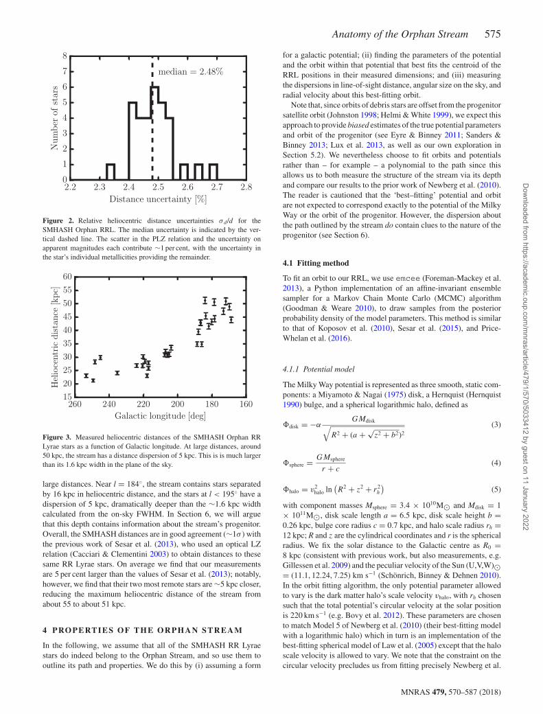
Figure 2. Relative heliocentric distance uncertainties σ d/d for theSMHASH Orphan RRL. The median uncertainty is indicated by the ver-tical dashed line. The scatter in the PLZ relation and the uncertainty onapparent magnitudes each contribute ∼1 per cent, with the uncertainty inthe star’s individual metallicities providing the remainder.

Figure 3. Measured heliocentric distances of the SMHASH Orphan RRLyrae stars as a function of Galactic longitude. At large distances, around50 kpc, the stream has a distance dispersion of 5 kpc. This is is much largerthan its 1.6 kpc width in the plane of the sky.

large distances. Near l = 184◦, the stream contains stars separatedby 16 kpc in heliocentric distance, and the stars at l < 195◦ have adispersion of 5 kpc, dramatically deeper than the ∼1.6 kpc widthcalculated from the on-sky FWHM. In Section 6, we will arguethat this depth contains information about the stream’s progenitor.Overall, the SMHASH distances are in good agreement (∼1σ ) withthe previous work of Sesar et al. (2013), who used an optical LZrelation (Cacciari & Clementini 2003) to obtain distances to thesesame RR Lyrae stars. On average we find that our measurementsare 5 per cent larger than the values of Sesar et al. (2013); notably,however, we find that their two most remote stars are ∼5 kpc closer,reducing the maximum heliocentric distance of the stream fromabout 55 to about 51 kpc.

4 PRO P E RT I E S O F T H E O R P H A N ST R E A M

In the following, we assume that all of the SMHASH RR Lyraestars do indeed belong to the Orphan Stream, and so use them tooutline its path and properties. We do this by (i) assuming a form

for a galactic potential; (ii) finding the parameters of the potentialand the orbit within that potential that best fits the centroid of theRRL positions in their measured dimensions; and (iii) measuringthe dispersions in line-of-sight distance, angular size on the sky, andradial velocity about this best-fitting orbit.

Note that, since orbits of debris stars are offset from the progenitorsatellite orbit (Johnston 1998; Helmi & White 1999), we expect thisapproach to provide biased estimates of the true potential parametersand orbit of the progenitor (see Eyre & Binney 2011; Sanders &Binney 2013; Lux et al. 2013, as well as our own exploration inSection 5.2). We nevertheless choose to fit orbits and potentialsrather than – for example – a polynomial to the path since thisallows us to both measure the structure of the stream via its depthand compare our results to the prior work of Newberg et al. (2010).The reader is cautioned that the ‘best–fitting’ potential and orbitare not expected to correspond exactly to the potential of the MilkyWay or the orbit of the progenitor. However, the dispersion aboutthe path outlined by the stream do contain clues to the nature of theprogenitor (see Section 6).

4.1 Fitting method

To fit an orbit to our RRL, we use emcee (Foreman-Mackey et al.2013), a Python implementation of an affine-invariant ensemblesampler for a Markov Chain Monte Carlo (MCMC) algorithm(Goodman & Weare 2010), to draw samples from the posteriorprobability density of the model parameters. This method is similarto that of Koposov et al. (2010), Sesar et al. (2015), and Price-Whelan et al. (2016).

4.1.1 Potential model

The Milky Way potential is represented as three smooth, static com-ponents: a Miyamoto & Nagai (1975) disk, a Hernquist (Hernquist1990) bulge, and a spherical logarithmic halo, defined as

disk = −αGMdisk√

R2 + (a + √z2 + b2)2

(3)

sphere = GMsphere

r + c(4)

halo = v2halo ln

(R2 + z2 + r2

h

)(5)

with component masses Msphere = 3.4 × 1010M� and Mdisk = 1× 1011M�, disk scale length a = 6.5 kpc, disk scale height b =0.26 kpc, bulge core radius c = 0.7 kpc, and halo scale radius rh =12 kpc; R and z are the cylindrical coordinates and r is the sphericalradius. We fix the solar distance to the Galactic centre as R0 =8 kpc (consistent with previous work, but also measurements, e.g.Gillessen et al. 2009) and the peculiar velocity of the Sun (U,V,W)�= (11.1, 12.24, 7.25) km s−1 (Schonrich, Binney & Dehnen 2010).In the orbit fitting algorithm, the only potential parameter allowedto vary is the dark matter halo’s scale velocity vhalo, with rh chosensuch that the total potential’s circular velocity at the solar positionis 220 km s−1 (e.g. Bovy et al. 2012). These parameters are chosento match Model 5 of Newberg et al. (2010) (their best-fitting modelwith a logarithmic halo) which in turn is an implementation of thebest-fitting spherical model of Law et al. (2005) except that the haloscale velocity is allowed to vary. We note that the constraint on thecircular velocity precludes us from fitting precisely Newberg et al.

MNRAS 479, 570–587 (2018)

Dow

nloaded from https://academ

ic.oup.com/m

nras/article/479/1/570/5033412 by guest on 11 January 2022

576 D. Hendel et al.

(2010)’s Model 5 since that potential’s circular velocity at the solarposition is only 207 km s−1.

4.2 Model parameters

We wish to find the phase space coordinates of the initial conditionx0 = (l, b, DM, μl, μb, vr)0 for the orbit that best reproducesthe observed sky positions li, bi, heliocentric radial velocities vr, i

and distance modulii DMi of the RRL given their uncertaintiesσvr,i

, σDMi. The sky coordinates are assumed perfectly known and

are transformed to the Orphan frame �, B defined in Newberget al. (2010), a heliocentric spherical coordinate system in whichthe Orphan Stream lies approximately on the equator. The rotationbetween Galactic coordinates and the Orphan coordinates is definedby the Euler angles (φ, θ , ψ) = (128.79◦, 54.39◦, 90.70◦). We setl0 = 200◦ without interesting loss of generality.

Because tidal streams are generated with orbital parameterssomewhat offset from the progenitor galaxy and with some intrin-sic scatter (cf. Hendel & Johnston 2015, and references therein)we also include additional model parameters δ = (δB, δvr

, δDM )to account for the average dispersions in the observational coor-dinates. We neglect the fact that each of these dispersions willvary along the stream. Besides representing the physical width,velocity dispersion, and depth of the stream, they serve to deteroverfitting in coordinates where δ/σ is large. The last parame-ter is the halo scale velocity vhalo. The full parameter set is thenθ = ((b, DM,μl, μb, vr )0, (δB, δvr

, δDM ), vhalo). Orbits were inte-grated using a symplectic leapfrog integrator as implemented in theGala package (Price-Whelan 2017).

The MCMC algorithm uses 144 walkers to explore this nine-dimensional parameter space. After running for a burn-in periodof 1 000 steps, the sampler is restarted and run for an additional10 000 steps. Since the autocorrelation time for each walker is ∼50steps in all dimensions, only every 100th sample is taken from thechains to be included in the posterior. This ensures that each isa nearly independent sample from the posterior distribution. Theautocorrelation time does not change substantially after the burn-inperiod, indicating that the sampling has converged.

4.2.1 Likelihood

We assume that our data are independent and that the uncertainties ineach coordinate are normally distributed. Thus, the joint likelihoodis the product of the likelihoods in each coordinate, which are

p(Bi |�i, θ ) = N(Bi |Bmodel(�i), δ2B ) (6)

p(vri |�i, θ ) = N(vri |vmodelr (�i), σ

2vr

+ δ2vr

) (7)

p(DMi |�i, θ ) = N(DMi |DMmodel(�i), σ2DM + δ2

DM ), (8)

where Bmodel, vmodelr , and DMmodel are interpolated from the model

orbit integrated using the initial conditions in θ and N is the normaldistribution

N(x|μ, σ 2) = 1√2πσ 2

exp − (x − μ)2

2σ 2(9)

with μ as its mean and σ its standard deviation.

4.2.2 Priors

We implement priors on Galactic latitude and distance modulusthat are uniform in Cartesian space; for the former this is uniform

in cos (b), while the latter is

p(DM) ∝ 1025 DM+2. (10)

Using the notation U(f , g) for the uniform distribution with end-points f and g, we place an uninformative prior on Heliocentricradial velocity as

p(vr ) = U(50, 300) km s−1. (11)

The dispersions δi are required to be positive to prevent a phys-ically equivalent but bimodal posterior that hampers the walkers’convergence. We use logarithmic (scale-invariant) priors for theseparameters,

p(δi) ∝ δ−1i . (12)

The halo scale velocity vhalo must be greater than about 68 km s−1

to maintain a circular speed at the solar radius of 220 km s−1 givenour choices for the other parameters. It is therefore constrained by

p(vhalo) = U(68, 200) km s−1. (13)

Finally, we consider the two phase space dimensions that are unob-served for individual RRL: their proper motions. Since we cannotcompare them to a prior on a star-by-star basis, we instead use thevalue for the model orbit where it crosses l = 199.779 6◦. This po-sition is specifically chosen to correspond to the location of HubbleSpace Telescope – based proper motions of Orphan Stream stars(Sohn et al. 2016). We consider two cases: first wide, uninformativepriors

p(μl cos b) = U(−5, 5) mas yr−1 (14)

p(μb) = U(−5, 5) mas yr−1, (15)

and then those based on the Hubble observations

p(μl cos b) = N(0.211, 0.052) mas yr−1 (16)

p(μb) = N(−0.774, 0.052) mas yr−1. (17)

In the following, we will refer to the former as ‘without’ a propermotion prior for conciseness.

4.3 Centroid of the Orphan Stream

Fig. 4 shows a corner plot displaying projections of the orbit fit-ting’s posterior distribution, in the case of the uniform proper mo-tion priors. The median value of the samples in each parameter,along with uncertainties computed as the 16th and 84th percentiles(the 68 per cent credible interval), are summarized in Table 2. Weconfirm that the orbit is prograde with respect to the Milky Way’srotation. Even if the walkers are restricted to only exploring thespace of retrograde orbits, there are no local maxima to compareto the prograde fit shown here. If the overdensity detected by Grill-mair et al. (2015) is indeed the nearly disrupted progenitor then thisdirection of motion makes the SMHASH RR Lyrae stars part of theleading tidal tail. The median distance modulus of 17.68 mag corre-sponds to a heliocentric distance of 34.2 kpc; this is approximately150 pc more distant than Newberg et al. (2010)’s Model 5 orbitat the same longitude, which is compatible within their respectiveuncertainties.

Focusing on each of the two-dimensional histograms in Fig. 4 inturn, one sees that the fit parameters have minimal covariance withfew exceptions: the proper motions μlcos (b) with μb, vhalo withμlcos (b), and to a lesser extent vhalo with μb and with vr. Note that

MNRAS 479, 570–587 (2018)

Dow

nloaded from https://academ

ic.oup.com/m

nras/article/479/1/570/5033412 by guest on 11 January 2022

Anatomy of the Orphan Stream 577

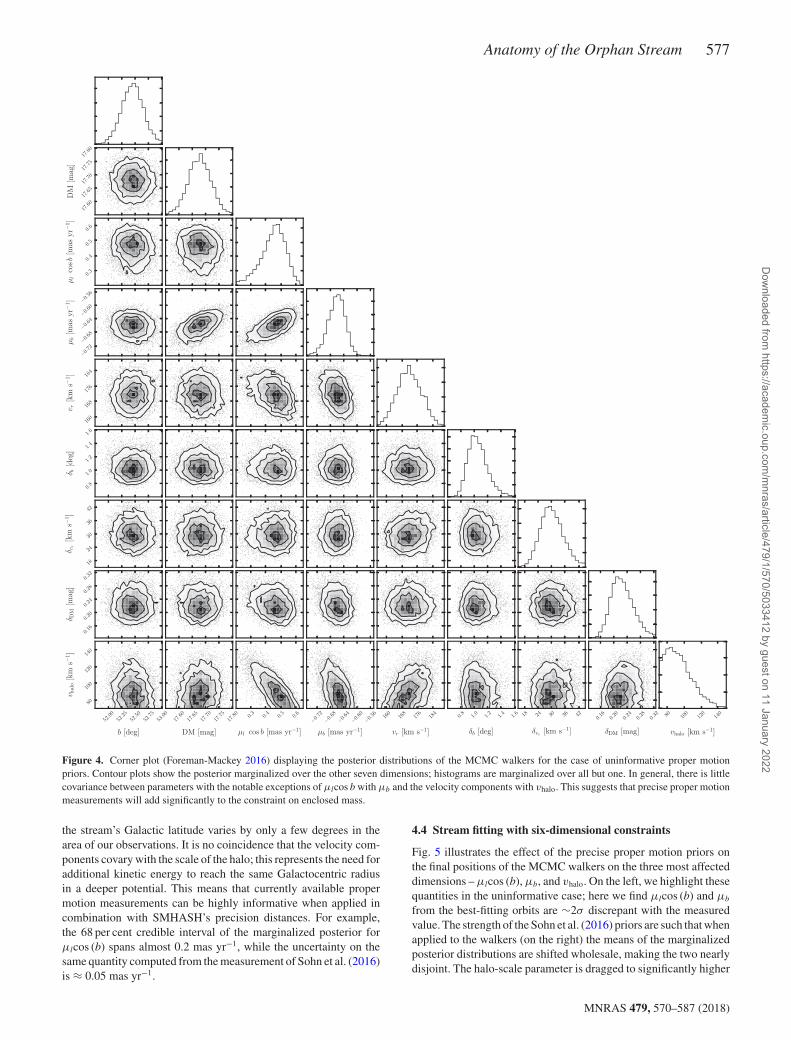
Figure 4. Corner plot (Foreman-Mackey 2016) displaying the posterior distributions of the MCMC walkers for the case of uninformative proper motionpriors. Contour plots show the posterior marginalized over the other seven dimensions; histograms are marginalized over all but one. In general, there is littlecovariance between parameters with the notable exceptions of μlcos b with μb and the velocity components with vhalo. This suggests that precise proper motionmeasurements will add significantly to the constraint on enclosed mass.

the stream’s Galactic latitude varies by only a few degrees in thearea of our observations. It is no coincidence that the velocity com-ponents covary with the scale of the halo; this represents the need foradditional kinetic energy to reach the same Galactocentric radiusin a deeper potential. This means that currently available propermotion measurements can be highly informative when applied incombination with SMHASH’s precision distances. For example,the 68 per cent credible interval of the marginalized posterior forμlcos (b) spans almost 0.2 mas yr−1, while the uncertainty on thesame quantity computed from the measurement of Sohn et al. (2016)is ≈ 0.05 mas yr−1.

4.4 Stream fitting with six-dimensional constraints

Fig. 5 illustrates the effect of the precise proper motion priors onthe final positions of the MCMC walkers on the three most affecteddimensions – μlcos (b), μb, and vhalo. On the left, we highlight thesequantities in the uninformative case; here we find μlcos (b) and μb

from the best-fitting orbits are ∼2σ discrepant with the measuredvalue. The strength of the Sohn et al. (2016) priors are such that whenapplied to the walkers (on the right) the means of the marginalizedposterior distributions are shifted wholesale, making the two nearlydisjoint. The halo-scale parameter is dragged to significantly higher

MNRAS 479, 570–587 (2018)

Dow

nloaded from https://academ

ic.oup.com/m

nras/article/479/1/570/5033412 by guest on 11 January 2022

578 D. Hendel et al.

Table 2. Median and 68% credible intervals of parameters in the poste-rior distribution resulting from orbit fitting to the SMHASH data, with andwithout including the observational proper motion constraints. The fixedGalactic longitude value used for the initial condition is included for com-pleteness, along with the mass enclosed at 60 kpc and circular velocities at25, 40, and 60 kpc implied by the vhalo distribution.

Parameter Without PM prior With PM prior

l (deg) 199.779 6 199.779 6b (deg) 52.45+0.21

−0.21 52.46+0.23−0.21

DM(mag) 17.68+0.04−0.04 17.66+0.05

−0.05μl cos(b) (mas yr−1) 0.456+0.071

−0.096 0.244+0.049−0.051

μb (mas yr−1) −0.660+0.023−0.028 −0.715+0.022

−0.024vr (km s−1) 171.7+6.9

−6.3 176.2+6.5−6.8

δB (deg) 1.042+0.168−0.129 1.039+0.175

−0.129δvr (km s−1) 29.86+5.72

−4.82 29.61+5.81−4.94

δDM (mag) 0.224+0.040−0.030 0.258+0.046

−0.036vhalo (km s−1) 92+19

−14 128+16−17

M(60 kpc) (1011 M�) 3.4+1.1−0.65 5.6+1.2

−1.1vcirc(25 kpc) (km s−1) 191+14

−10 216+10−11

vcirc(40 kpc) (km s−1) 173+19−13 208+15

−16vcirc(60 kpc) (km s−1) 161+21

−15 202+18−19

values, as one would naively expect based on the covariance withμlcos (b).

The marginalized posterior of vhalo can be directly converted intoa distribution of enclosed masses at any given radius; we choose60 kpc for convenient comparison with literature values. The re-sults of this transformation are shown in Fig. 6, both without (inblue hatch) and with (in red) the HST proper motions as a prior.3 Thedifference between them is substantial: the latter’s median value is64 per cent larger than the former; however, due to the large confi-dence intervals they are consistent at the ∼1.4σ level. The apparentnarrowness of the blue posterior distribution is driven by the as-sumption that the circular speed at the Solar radius is 220 km s−1.Given our model, this requires a minimum total mass of ∼2.4 ×1011 M� at 60 kpc. To facilitate comparison with observations andother methods that use different potential shapes, we have also tabu-lated circular velocities at 25, 40, and 60 kpc in Table 2. For example,Watkins et al. (2018) recently used Gaia and HST proper motionsof halo globular clusters to obtain vcirc(39.5 kpc) = 220+17

−16 km s−1,which agrees well with our results when applying the the HST propermotion prior.

A selection of orbits generated from randomly chosen samplesof the posteriors are shown in Fig. 7. The left-hand (right-hand)panels show the results without (with) including informative propermotion priors. Plotted from top to bottom are projections in thethree observational coordinates (Galactic latitude, radial velocity,and distance) as a function of Galactic longitude. Both sets of sam-ples capture the path of the stream over most of the survey area.Individual orbits diverge somewhat around l � 170◦, where thedepth in line-of-sight distance is large. Both sets of orbits seem tosystematically overestimate the Heliocentric radial velocity of starsabove l ≈ 250◦, however individual stars are only offset by ∼1 δi.Including the Sohn et al. (2016) measurement slightly improves thematch to the data in b and vr but causes the distance to the far end

3The Sohn et al. (2016) measurement is error-weighted; using the averagemotion instead both increases the uncertainty and shifts the mean towards thevalues found using the uniform prior, resulting in a posterior with intermedi-ate values of vhalo = 112+18

−17 km s−1 and M(60 kpc) = 4.6+1.0−1.2 × 1011 M�.

of the stream to be underestimated. This is problematic because theleading arm of the stream is made up of stars with lower specificenergy than the progenitor and are expected to be interior to itsorbit. We interpret this mismatch as evidence that the 1-parameterpotential model used here is not flexible enough to recover the fullphase space structure of the stream. In the N–body models describedbelow, there is no offset between fitted orbits and selected particlesat the 0.05 mas yr−1 level.

4.5 The solar circular velocity as measured from the OrphanStream

To the extent that a stream follows an orbit, the proper motionof member stars perpendicular to the stream should be zero. Anyobserved perpendicular proper motion is therefore a measure ofthe solar reflex (c.f. Carlin et al. 2012). The Hubble proper motionmeasurement and the SMHASH distance distribution posterior canbe combined at the longitude of the Sohn et al. (2016) Orphan F1field to estimate the solar motion.

We define a new coordinates system relative to the Orphan coor-dinates of Newberg et al. (2010) with axes that point into the planeof the sky, parallel to the stream, and perpendicular to the stream.The unit vector perpendicular to the stream points in the direc-tion (in Orphan coordinates) n = (0.62619, 0.50664, 0.59261). Inthis direction, the marginalized posterior derived using the Hubbleproper motion priors approximates a Gaussian with mean 136.5 kms−1 and dispersion 9.1 km s−1. If we assume that the solar peculiarvelocity relative to the local standard of rest (LSR) is known fromSchonrich et al. (2010), then this implies that the azimuthal velocityof the LSR (which equals the circular velocity if the disk is circular)is vy = 235 ± 16 km s−1. This result is consistent with both thetraditional IAU value of 220 km s−1 as well as more recent stud-ies that give somewhat larger results (e.g. McMillan 2011; Bovyet al. 2012). While this new measurement does not help to resolvethe controversy surrounding the exact value of the solar motion, itdoes provide an independent consistency check on the SMHASHdistances.

5 IMPLI CATI ONS FOR THE MI LKY WAY ’SMASS

Orbit fitting is known to introduce systematic biases in potentialmeasures (Eyre & Binney 2011; Lux et al. 2013; Sanders & Binney2013). To investigate what effect this might have for the specificcase of the Orphan Stream, we have created N–body models ofthe stream and ‘observed’ them in such a way as to recreate theSMHASH dataset. We then apply an identical orbit fitting techniqueand compare with the simulation inputs. This method allows us tocontextualize the results of our RRL observations in terms of thedirection and size of systematic biases as well as compare themwith earlier results.

Previous measurements of the Milky Way’s mass using the Or-phan Stream found that the best-fitting halo was a factor of ∼2 lessmassive inside 60 kpc (2.74 × 1011 M�; Newberg et al. 2010) thancontemporary models using other techniques, such as fitting Sagit-tarius Stream data (4.7 × 1011 M�; Law et al. 2005) or the velocitydistribution of field BHB stars (4.0 × 1011 M�; Xue et al. 2008).A complete summary of mass estimates is outside the scope of thiswork; the review of Bland-Hawthorn & Gerhard (2016) providesan overview. However, the Newberg et al. (2010) measurementremains below all other published estimates, with recent results

MNRAS 479, 570–587 (2018)

Dow

nloaded from https://academ

ic.oup.com/m

nras/article/479/1/570/5033412 by guest on 11 January 2022

Anatomy of the Orphan Stream 579

Figure 5. Corner plot displaying the marginalized posterior distributions for the model parameters μlcos (b), μb, and vhalo along with their covariances.Left: uniform prior on μlcos (b) and μb. Right: result when otherwise identical chains are run with the additional priors p(μl cos(b)) = N(0.211, 0.052),p(μb) = N(−0.774, 0.052). Due to the covariance between the proper motions and the halo-scale velocity, these priors result in a median vhalo that correspondsto a halo 64 per cent more massive than the uniform case.

Figure 6. Milky Way mass enclosed at 60 kpc, calculated from the scalevelocities vhalo of the samples. Including the proper motion prior noticeablyincreases the median value, from 3.4 × 1011 M� (in blue hatch) to 5.6 ×1011M� (in red), but the confidence intervals are consistent at ∼1.4σ .

reaching masses only as low as about 3.2 × 1011 M� (Gibbonset al. 2014).

5.1 Creating and observing mock data sets

We use the self-consistent field method (SCF; Hernquist & Ostriker1992), which represents the gravitational potential of the disrupting

satellite as a basis function expansion, to create a series of N-bodysimulations designed to reasonably mimic the observed OrphanStream. The single-component, dark matter only Orphan progenitoris implemented as a Navarro–Frenk–White (NFW; Navarro, Frenk& White 1997) distribution with 105 particles. The particles areinstantiated out to 35 scale radii and so the model’s total mass differsfrom the virial mass; in the following we report the correspondingvirial mass to avoid confusion. All simulations have the same meandensity inside the scale radius, which results in tides unbindingthem at approximately the same time. This allows the separationof effects due to the time of disruption and passive evolution. Thedensity scaling is set such that the halo with a virial mass of 109 M�has a scale radius of 0.75 kpc although the results are not particularlysensitive to this choice.

We chose the orbit and potential model to be precisely that ofNewberg et al. (2010)’s Model 5: that is, an orbit initialized fromthe phase space coordinate with Heliocentric position (l, b, R) =(218◦, 53.5◦, 28.6 kpc) and Galactocentric velocity (vx, vy, vz) =( −156, 79, 107) km s−1 moving in a logarithmic potential model(equations 3–5) with the one unspecified parameter vhalo set to73 km s−1. The orbit is integrated backwards in time to find thephase space coordinate of the third apocenter, 4.8 Gyr ago. Whenthe satellite is near apocenter the hosts’ tidal field is at its weakest,so beginning the simulation here minimizes artificial gravitationalshocking. After relaxing in isolation the host potential is turned onover 10 internal dynamical times, the particle distribution is inserted,and the satellite is evolved to the present day. We assume that thecurrent position of the progenitor is at the overdensity identified byGrillmair et al. (2015), l ≈ 268.7◦, so the simulation ends at thatpoint.

To produce synthetic observations that approximate those of theSMHASH RRL, we first select the particles below the tenth per-centile in initial internal binding energy. These are tagged as stars.This simple strategy has been shown to reproduce the observedproperties of Local Group dwarf galaxies in semianalytic models

MNRAS 479, 570–587 (2018)

Dow

nloaded from https://academ

ic.oup.com/m

nras/article/479/1/570/5033412 by guest on 11 January 2022

580 D. Hendel et al.

Figure 7. Left: a selection of orbit fits (blue lines) generated from randomly selected samples of the posterior distribution shown in Fig. 4, where the propermotion prior is uninformative. Right: the same (red lines), but with samples from the walkers constrained by the observed μlcos b and μb. The former betterreproduces the trend of distance with longitude, while the latter slightly improves the match in radial velocity and sky position, especially at l > 240◦.

(Bullock & Johnston 2005) and create stellar haloes with realisticproperties in simulations of Milky Way-like galaxies with cosmo-logical infall (De Lucia & Helmi 2008; Cooper et al. 2010). Fromthis subset, we choose at random 30 particles that match the selec-tion criteria used in Sesar et al. (2013), namely Galactic longitude260◦ > l > 160◦, Orphan latitude 4◦ > B > −4◦, and Galactic stan-dard of rest velocity vgsr > 40 km s−1. Since the particle positionsand velocities are precisely known, we introduce ‘observational’uncertainties by adding a random velocity drawn from a Gaussianof width 15 km s−1 to each particle’s heliocentric velocity. Similarly,the selected particles are scattered in heliocentric distance accord-ing to the 2.5 per cent relative uncertainty demonstrated in Fig. 2.These same values are retained as uncertainties to be fed into theorbit fitting algorithm as well.

5.2 Biases in orbit fitting

The problems associated with assuming stars in a tidal stream fol-low a single orbit are conceptually simplified when considering theOrphan Stream since we observe only the leading tail. In this case,stars farther from the satellite – towards apocenter – have lower total

energy than the progenitor, with the difference tending to increasewith distance; their individual orbits turn around at smaller Galac-tocentric radii than the progenitor’s does. Thus, orbits matched tothe stream’s path are tracing both the loss of kinetic energy to thegravitational potential as well as an additional loss determined bythe total energy gradient of stars along the stream. Since the latteris not modelled in orbit fitting, the potential needs to be deeper atfixed radius to compensate for this ‘extra’ loss, leading to an inflatedmass estimate.

Fig. 8 illustrates the typical systematic errors in inferred massintroduced by this effect. Despite the fact that each simulation wasrun in a potential with Mencl(60 kpc) = 2.7 × 1011 M�, the medianvalue of the marginalized posterior distributions of vhalo generate anestimate ∼ 20–50 per cent more massive. There is also an additionalrealization-dependent scatter of order 20 per cent, not depicted here.The bias is nearly independent of satellite mass, which matches the-oretical expectations (Sanders & Binney 2013). To our knowledgethis is the first time that the bias in mass enclosed due to orbit fittinghas been quantified in a scenario that replicates an observed system.The magnitude of the effect presumably depends on the details of

MNRAS 479, 570–587 (2018)

Dow

nloaded from https://academ

ic.oup.com/m

nras/article/479/1/570/5033412 by guest on 11 January 2022

Anatomy of the Orphan Stream 581

Figure 8. Bias in the best-fitting host halo’s enclosed mass, calculated fromvhalo, as a function of the initial halo mass of the progenitor satellite. Theblack horizontal line represents the true value in the model potential, whilethe points illustrate the transformed posterior distribution. The median valueexceeds expectations by typically 20–50 per cent.

the potential model but the direction should not – the fitting al-gorithm will tend to prefer haloes that are more massive than arecorrect. In fact, the synthetic data that produce the correct answerseem to be less representative of the underlying simulation, in termsof their on-sky and distance distributions, than those that producebiased results. For this reason, we report the mass value measuredfor the Milky Way only as an upper limit.

We also note that the already low enclosed mass measurementof Newberg et al. (2010)’s Model 5 should also be affected by thissystematic error since the approximation is the same despite theirdifferent fitting technique. If the magnitude of the bias is identicalthen the corrected mass enclosed is approximately 1.8 × 1011 M�,slightly more than half that found by Gibbons et al. (2014). Modelswith such small enclosed masses may have difficulty matching otherobservables such as the circular velocity of the Sun.

6 TH E O R P H A N P RO G E N I TO R

In the previous section, we were concerned primarily with the modelparameters that describe the phase space position of the orbits andthe shape of the potential. Now, we focus on the internal structureof the stream, characterized by the dispersions δB, δvr

, and δDM.For a particular progenitor orbit, the spatial and velocity scalesof the stream stars vary with the satellite-to-host mass ratio as(m/M)1/3 (Johnston 1998; Helmi & White 1999; Johnston, Sackett& Bullock 2001); therefore the δi contain information about theprogenitor system. To first order, this is the mass when the starsare unbound; however, it may be possible to recover the satellite’scentral density distribution which also imprints itself on the stream(Errani, Penarrubia & Tormen 2015).

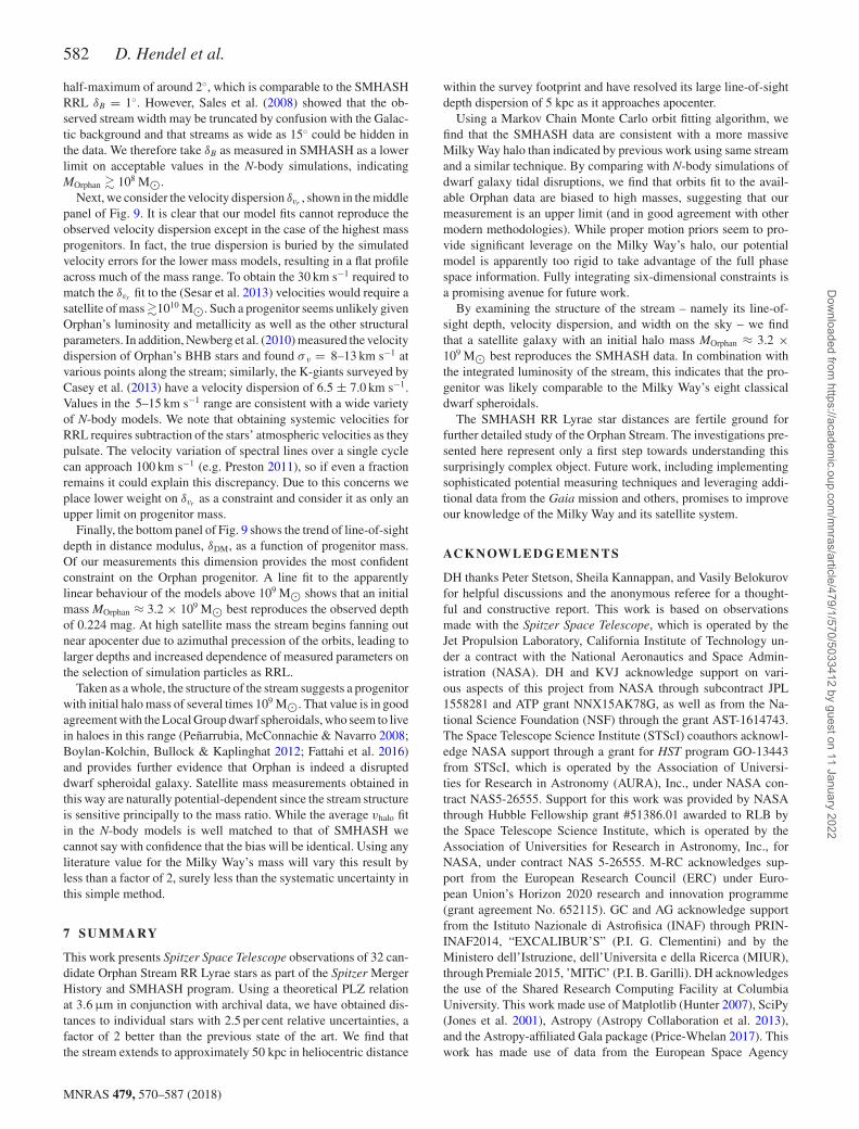
Fig. 9 shows the effect of satellite mass on the simulated streams’structural parameters. In each panel, the horizontal blue lines illus-trate the values measured from the SMHASH data while the blackpoints show the same quantities found after applying the same orbitfitting algorithm to N-body simulations of varying initial satellite

Figure 9. Fitted values of width on the sky (top), velocity dispersion (cen-ter), and line-of-sight depth (bottom) for a set of N-body models of theOrphan Stream (black points) as a function of model satellite mass, com-pared to the same quantities as measured for the SMHASH Orphan data(blue region).

halo masses. The mass range shown, from 3.8 × 107 to 1.2 ×1010 M�, captures dwarf galaxies from the ultrafaints to a fewtimes less massive than the Small Magellanic Cloud (Guo et al.2010).

First, we consider the stream’s width on the sky, δB, plotted inthe upper panel. The measured value δB = 1◦ appears at a glanceto be most consistent with the lowest mass simulations, indicatingthat MOrphan ≈ 108 M�. However, the selection of RR Lyrae starsfor spectroscopic follow-up in the SMHASH precursor cataloguesis non-uniform and appears to be weighted significantly towardsstars that are nearer the stream centre (e.g. of the stars with 2◦ < B< 4◦, 3 have spectra and 11 do not). The observed δB is thereforeunlikely to be representative of the true distribution. An alternativeapproach is to look at studies of Orphan’s main sequence popu-lation; since our synthetic RRL are selected at random from the‘star’ particles, they represent any other stellar population just aswell under the assumption that Orphan was originally well mixed.Belokurov et al. (2007) found that the stream has a full-width at

MNRAS 479, 570–587 (2018)

Dow

nloaded from https://academ

ic.oup.com/m

nras/article/479/1/570/5033412 by guest on 11 January 2022

582 D. Hendel et al.

half-maximum of around 2◦, which is comparable to the SMHASHRRL δB = 1◦. However, Sales et al. (2008) showed that the ob-served stream width may be truncated by confusion with the Galac-tic background and that streams as wide as 15◦ could be hidden inthe data. We therefore take δB as measured in SMHASH as a lowerlimit on acceptable values in the N-body simulations, indicatingMOrphan � 108 M�.

Next, we consider the velocity dispersion δvr, shown in the middle

panel of Fig. 9. It is clear that our model fits cannot reproduce theobserved velocity dispersion except in the case of the highest massprogenitors. In fact, the true dispersion is buried by the simulatedvelocity errors for the lower mass models, resulting in a flat profileacross much of the mass range. To obtain the 30 km s−1 required tomatch the δvr

fit to the (Sesar et al. 2013) velocities would require asatellite of mass�1010 M�. Such a progenitor seems unlikely givenOrphan’s luminosity and metallicity as well as the other structuralparameters. In addition, Newberg et al. (2010) measured the velocitydispersion of Orphan’s BHB stars and found σ v = 8–13 km s−1 atvarious points along the stream; similarly, the K-giants surveyed byCasey et al. (2013) have a velocity dispersion of 6.5 ± 7.0 km s−1.Values in the 5–15 km s−1 range are consistent with a wide varietyof N-body models. We note that obtaining systemic velocities forRRL requires subtraction of the stars’ atmospheric velocities as theypulsate. The velocity variation of spectral lines over a single cyclecan approach 100 km s−1 (e.g. Preston 2011), so if even a fractionremains it could explain this discrepancy. Due to this concerns weplace lower weight on δvr

as a constraint and consider it as only anupper limit on progenitor mass.

Finally, the bottom panel of Fig. 9 shows the trend of line-of-sightdepth in distance modulus, δDM, as a function of progenitor mass.Of our measurements this dimension provides the most confidentconstraint on the Orphan progenitor. A line fit to the apparentlylinear behaviour of the models above 109 M� shows that an initialmass MOrphan ≈ 3.2 × 109 M� best reproduces the observed depthof 0.224 mag. At high satellite mass the stream begins fanning outnear apocenter due to azimuthal precession of the orbits, leading tolarger depths and increased dependence of measured parameters onthe selection of simulation particles as RRL.

Taken as a whole, the structure of the stream suggests a progenitorwith initial halo mass of several times 109 M�. That value is in goodagreement with the Local Group dwarf spheroidals, who seem to livein haloes in this range (Penarrubia, McConnachie & Navarro 2008;Boylan-Kolchin, Bullock & Kaplinghat 2012; Fattahi et al. 2016)and provides further evidence that Orphan is indeed a disrupteddwarf spheroidal galaxy. Satellite mass measurements obtained inthis way are naturally potential-dependent since the stream structureis sensitive principally to the mass ratio. While the average vhalo fitin the N-body models is well matched to that of SMHASH wecannot say with confidence that the bias will be identical. Using anyliterature value for the Milky Way’s mass will vary this result byless than a factor of 2, surely less than the systematic uncertainty inthis simple method.

7 SU M M A RY

This work presents Spitzer Space Telescope observations of 32 can-didate Orphan Stream RR Lyrae stars as part of the Spitzer MergerHistory and SMHASH program. Using a theoretical PLZ relationat 3.6μm in conjunction with archival data, we have obtained dis-tances to individual stars with 2.5 per cent relative uncertainties, afactor of 2 better than the previous state of the art. We find thatthe stream extends to approximately 50 kpc in heliocentric distance

within the survey footprint and have resolved its large line-of-sightdepth dispersion of 5 kpc as it approaches apocenter.

Using a Markov Chain Monte Carlo orbit fitting algorithm, wefind that the SMHASH data are consistent with a more massiveMilky Way halo than indicated by previous work using same streamand a similar technique. By comparing with N-body simulations ofdwarf galaxy tidal disruptions, we find that orbits fit to the avail-able Orphan data are biased to high masses, suggesting that ourmeasurement is an upper limit (and in good agreement with othermodern methodologies). While proper motion priors seem to pro-vide significant leverage on the Milky Way’s halo, our potentialmodel is apparently too rigid to take advantage of the full phasespace information. Fully integrating six-dimensional constraints isa promising avenue for future work.

By examining the structure of the stream – namely its line-of-sight depth, velocity dispersion, and width on the sky – we findthat a satellite galaxy with an initial halo mass MOrphan ≈ 3.2 ×109 M� best reproduces the SMHASH data. In combination withthe integrated luminosity of the stream, this indicates that the pro-genitor was likely comparable to the Milky Way’s eight classicaldwarf spheroidals.

The SMHASH RR Lyrae star distances are fertile ground forfurther detailed study of the Orphan Stream. The investigations pre-sented here represent only a first step towards understanding thissurprisingly complex object. Future work, including implementingsophisticated potential measuring techniques and leveraging addi-tional data from the Gaia mission and others, promises to improveour knowledge of the Milky Way and its satellite system.

AC K N OW L E D G E M E N T S

DH thanks Peter Stetson, Sheila Kannappan, and Vasily Belokurovfor helpful discussions and the anonymous referee for a thought-ful and constructive report. This work is based on observationsmade with the Spitzer Space Telescope, which is operated by theJet Propulsion Laboratory, California Institute of Technology un-der a contract with the National Aeronautics and Space Admin-istration (NASA). DH and KVJ acknowledge support on vari-ous aspects of this project from NASA through subcontract JPL1558281 and ATP grant NNX15AK78G, as well as from the Na-tional Science Foundation (NSF) through the grant AST-1614743.The Space Telescope Science Institute (STScI) coauthors acknowl-edge NASA support through a grant for HST program GO-13443from STScI, which is operated by the Association of Universi-ties for Research in Astronomy (AURA), Inc., under NASA con-tract NAS5-26555. Support for this work was provided by NASAthrough Hubble Fellowship grant #51386.01 awarded to RLB bythe Space Telescope Science Institute, which is operated by theAssociation of Universities for Research in Astronomy, Inc., forNASA, under contract NAS 5-26555. M-RC acknowledges sup-port from the European Research Council (ERC) under Euro-pean Union’s Horizon 2020 research and innovation programme(grant agreement No. 652115). GC and AG acknowledge supportfrom the Istituto Nazionale di Astrofisica (INAF) through PRIN-INAF2014, “EXCALIBUR’S” (P.I. G. Clementini) and by theMinistero dell’Istruzione, dell’Universita e della Ricerca (MIUR),through Premiale 2015, ’MITiC’ (P.I. B. Garilli). DH acknowledgesthe use of the Shared Research Computing Facility at ColumbiaUniversity. This work made use of Matplotlib (Hunter 2007), SciPy(Jones et al. 2001), Astropy (Astropy Collaboration et al. 2013),and the Astropy-affiliated Gala package (Price-Whelan 2017). Thiswork has made use of data from the European Space Agency

MNRAS 479, 570–587 (2018)

Dow

nloaded from https://academ

ic.oup.com/m

nras/article/479/1/570/5033412 by guest on 11 January 2022

Anatomy of the Orphan Stream 583

(ESA) mission Gaia (https://www.cosmos.esa.int/gaia), processedby the Gaia Data Processing and Analysis Consortium (DPAC, https://www.cosmos.esa.int/web/gaia/dpac/consortium). Funding forthe DPAC has been provided by national institutions, in par-ticular the institutions participating in the Gaia MultilateralAgreement.

RE FERENCES

Amorisco N. C., 2015, MNRAS, 450, 575Arenou F. et al., 2018, A&A, preprint (arXiv:1804.09375)Astropy Collaboration et al., 2013, A&A, 558, A33Belokurov V. et al., 2006, ApJ, 642, L137Belokurov V. et al., 2007, ApJ, 658, 337Bersier D., Wood P. R., 2002, AJ, 123, 840Bland-Hawthorn J., Gerhard O., 2016, ARA&A, 54, 529Bono G., Caputo F., Castellani V., Marconi M., Storm J., 2001, MNRAS,

326, 1183Bono G., Caputo F., Castellani V., Marconi M., Storm J., Degl’Innocenti S.,

2003, MNRAS, 344, 1097Bovy J. et al., 2012, ApJ, 759, 131Bovy J., Bahmanyar A., Fritz T. K., Kallivayalil N., 2016, ApJ, 833, 31Boylan-Kolchin M., Bullock J. S., Kaplinghat M., 2012, MNRAS, 422,

1203Braga V. F. et al., 2015, ApJ, 799, 165Brown W. R., Geller M. J., Kenyon S. J., Diaferio A., 2010, AJ, 139,

59Bullock J. S., Johnston K. V., 2005, ApJ, 635, 931Bullock J. S., Kravtsov A. V., Weinberg D. H., 2001, ApJ, 548, 33Cacciari C., Clementini G., 2003, in Alloin D., Gieren W., eds, Lecture Notes

in Physics, Vol. 635, Stellar Candles for the Extragalactic Distance Scale.Springer-Verlag, Berlin, p. 105

Cardelli J. A., Clayton G. C., Mathis J. S., 1989, ApJ, 345, 245Carlin J. L., Majewski S. R., Casetti-Dinescu D. I., Law D. R., Girard T. M.,

Patterson R. J., 2012, ApJ, 744, 25Casey A. R., Da Costa G., Keller S. C., Maunder E., 2013, ApJ, 764,

39Catelan M., Pritzl B. J., Smith H. A., 2004, ApJS, 154, 633Cohen J., Sesar B., Bahnolzer S., He K., Kulkarni S. R., Prince T. A., Bellm

E., Laher R. R., 2017a, AJ, 849, 18Cohen J. G., Sesar B., Bahnolzer S., He K., Kulkarni S. R., Prince T. A.,

Bellm E., Laher R. R., 2017b, ApJ, 849, 150Cooper A. P. et al., 2010, MNRAS, 406, 744De Lucia G., Helmi A., 2008, MNRAS, 391, 14Drake A. J. et al., 2009, ApJ, 696, 870Drake A. J. et al., 2013, ApJ, 763, 32Errani R., Penarrubia J., Tormen G., 2015, MNRAS, 449, L46Eyre A., Binney J., 2011, MNRAS, 413, 1852Fakhouri O., Ma C.-P., Boylan-Kolchin M., 2010, MNRAS, 406, 2267Fattahi A., Navarro J. F., Sawala T., Frenk C. S., Sales L. V., Oman K.,

Schaller M., Wang J., 2016, MNRAS, preprint (arXiv:1607.06479)Fazio G. G. et al., 2004, ApJS, 154, 10Fiorentino G. et al., 2015, ApJ, 798, L12Foreman-Mackey D., 2016, J. Open Source Soft., 24Foreman-Mackey D., Hogg D. W., Lang D., Goodman J., 2013, PASP, 125,

306Freedman W. L., Madore B. F., Scowcroft V., Burns C., Monson A., Persson

S. E., Seibert M., Rigby J., 2012, ApJ, 758, 24Freeman K., Bland-Hawthorn J., 2002, ARA&A, 40, 487Fritz T. K., Kallivayalil N., 2015, ApJ, 811, 123Gaia Collaboration Brown A. G. A., Vallenari A., Prusti T., de Bruijne

J. H. J., Babusiaux C., Bailer-Jones C. A. L., 2018, A&A, preprint(arXiv:1804.09365)

Gaia Collaboration et al., 2016, A&A, 595, A1Garofalo A., et al., 2018, MNRAS, submittedGibbons S. L. J., Belokurov V., Evans N. W., 2014, MNRAS, 445, 3788Gibbons S. L. J., Belokurov V., Evans N. W., 2017, MNRAS, 464, 794

Gillessen S., Eisenhauer F., Fritz T. K., Bartko H., Dodds-Eden K., PfuhlO., Ott T., Genzel R., 2009, ApJ, 707, L114

Goodman J., Weare J., 2010, Comm. App. Math. Comp. Sci., 5, 65Grillmair C. J., 2006, ApJ, 645, L37Grillmair C. J., Hetherington L., Carlberg R. G., Willman B., 2015, ApJ,

812, L26Guo Q., White S., Li C., Boylan-Kolchin M., 2010, MNRAS, 404,

1111Helmi A., White S. D. M., 1999, MNRAS, 307, 495Hendel D., Johnston K. V., 2015, MNRAS, 454, 2472Hernitschek N. et al., 2017, ApJ, 850, 96Hernquist L., 1990, ApJ, 356, 359Hernquist L., Ostriker J. P., 1992, ApJ, 386, 375Hunter J. D., 2007, Comput. Sci. Eng., 9, 90Indebetouw R. et al., 2005, ApJ, 619, 931Johnston K. et al., 2013, SMASH: Spitzer Merger History and Shape of the

Galactic Halo, Spitzer ProposalJohnston K. V., 1998, ApJ, 495, 297Johnston K. V., Hernquist L., Bolte M., 1996, ApJ, 465, 278Johnston K. V., Sackett P. D., Bullock J. S., 2001, ApJ, 557, 137Johnston K. V., Bullock J. S., Sharma S., Font A., Robertson B. E., Leitner

S. N., 2008, ApJ, 689, 936Jones E., et al., 2001, SciPy: Open source scientific tools for Python,

available at: http://www.scipy.org/Keller S. C., Murphy S., Prior S., DaCosta G., Schmidt B., 2008, ApJ, 678,

851Kirby E. N., Cohen J. G., Guhathakurta P., Cheng L., Bullock J. S., Gallazzi

A., 2013, ApJ, 779, 102Koposov S. E. et al., 2012, ApJ, 750, 80Koposov S. E., Rix H.-W., Hogg D. W., 2010, ApJ, 712, 260Kupper A. H. W., Balbinot E., Bonaca A., Johnston K. V., Hogg D. W.,

Kroupa P., Santiago B. X., 2015, ApJ, 803, 80Law N. M. et al., 2009, PASP, 121, 1395Law D. R., Majewski S. R., 2010, ApJ, 714, 229Law D. R., Johnston K. V., Majewski S. R., 2005, ApJ, 619, 807Layden A. C., 1994, AJ, 108, 1016Lindegren L. et al., 2018, A&A, preprint (arXiv:1804.09366)Longmore A. J., Fernley J. A., Jameson R. F., 1986, MNRAS, 220, 279Lux H., Read J. I., Lake G., Johnston K. V., 2013, MNRAS, 436, 2386Madore B. F. et al., 2013, ApJ, 776, 135Majewski S. R., Skrutskie M. F., Weinberg M. D., Ostheimer J. C., 2003,

ApJ, 599, 1082Makovoz D., Khan I., 2005, in Shopbell P., Britton M., Ebert R., eds, ASP

Conf. Ser. Vol. 347: Astronomical Data Analysis Software and SystemsXIV. Astron. Soc. Pac., San Francisco, p. 81

McMillan P. J., 2011, MNRAS, 414, 2446Miyamoto M., Nagai R., 1975, PASJ, 27, 533Muraveva T. et al., 2018, MNRAS, 473, 3131Navarro J. F., Frenk C. S., White S. D. M., 1997, ApJ, 490, 493Neeley J. R. et al., 2015, ApJ, 808, 11Neeley J. R. et al., 2017, ApJ, 841, 84Newberg H. J., Willett B. A., Yanny B., Xu Y., 2010, ApJ, 711, 32Pawlowski M. S., Pflamm-Altenburg J., Kroupa P., 2012, MNRAS, 423,

1109Pearson S., Kupper A. H. W., Johnston K. V., Price-Whelan A. M., 2015,

ApJ, 799, 28Penarrubia J., McConnachie A. W., Navarro J. F., 2008, ApJ, 672, 904Persson S. E., Madore B. F., Krzeminski W., Freedman W. L., Roth M.,

Murphy D. C., 2004, AJ, 128, 2239Preston G. W., 2011, AJ, 141, 6Price-Whelan A. M., 2017, J. Open Source Softw., 1, 24Price-Whelan A. M., Sesar B., Johnston K. V., Rix H.-W., 2016, ApJ, 824,

104Rau A. et al., 2009, PASP, 121, 1334Saha A., 1985, ApJ, 289, 310Sales L. V. et al., 2008, MNRAS, 389, 1391Sanders J. L., Binney J., 2013, MNRAS, 433, 1813Sanderson R. E., 2016, ApJ, 818, 41

MNRAS 479, 570–587 (2018)

Dow

nloaded from https://academ

ic.oup.com/m

nras/article/479/1/570/5033412 by guest on 11 January 2022

584 D. Hendel et al.

Sanderson R. E., Helmi A., Hogg D. W., 2015, ApJ, 801, 98Schlafly E. F., Finkbeiner D. P., 2011, ApJ, 737, 103Schonrich R., Binney J., Dehnen W., 2010, MNRAS, 403, 1829Scowcroft V., Freedman W. L., Madore B. F., Monson A. J., Persson S. E.,

Seibert M., Rigby J. R., Sturch L., 2011, ApJ, 743, 76Sesar B. et al., 2010, ApJ, 708, 717Sesar B. et al., 2013, ApJ, 776, 26Sesar B. et al., 2015, ApJ, 809, 59Sesar B., Hernitschek N., Dierickx M. I. P., Fardal M. A., Rix H.-W., 2017,

ApJ, 844, L4Sohn S. T. et al., 2016, ApJ, 833, 235Stetson P. B., 1987, PASP, 99, 191Stetson P. B., 1994, PASP, 106, 250Stokes G. H., Evans J. B., Viggh H. E. M., Shelly F. C., Pearce E. C., 2000,

Icarus, 148, 21Watkins L. L. et al., 2009, MNRAS, 398, 1757Watkins L. L., van der Marel R. P., Sohn S. T., Evans N. W., 2018, AAS,

preprint (arXiv:1804.11348)

Werner M. W. et al., 2004, ApJS, 154, 1White S. D. M., Rees M. J., 1978, MNRAS, 183, 341Wilhelm R., Beers T. C., Sommer-Larsen J., Pier J. R., Layden A. C., Flynn

C., Rossi S., Christensen P. R., 1999, AJ, 117, 2329Xue X. X. et al., 2008, ApJ, 684, 1143Zinn R., West M. J., 1984, ApJS, 55, 45

SUPPORTI NG INFORMATI ON

Supplementary data are available at MNRAS online.smhash orphan epochs.txtsmhash orphan rrly.txt

Please note: Oxford University Press is not responsible for thecontent or functionality of any supporting materials supplied bythe authors. Any queries (other than missing material) should bedirected to the corresponding author for the article.

MNRAS 479, 570–587 (2018)

Dow

nloaded from https://academ

ic.oup.com/m

nras/article/479/1/570/5033412 by guest on 11 January 2022

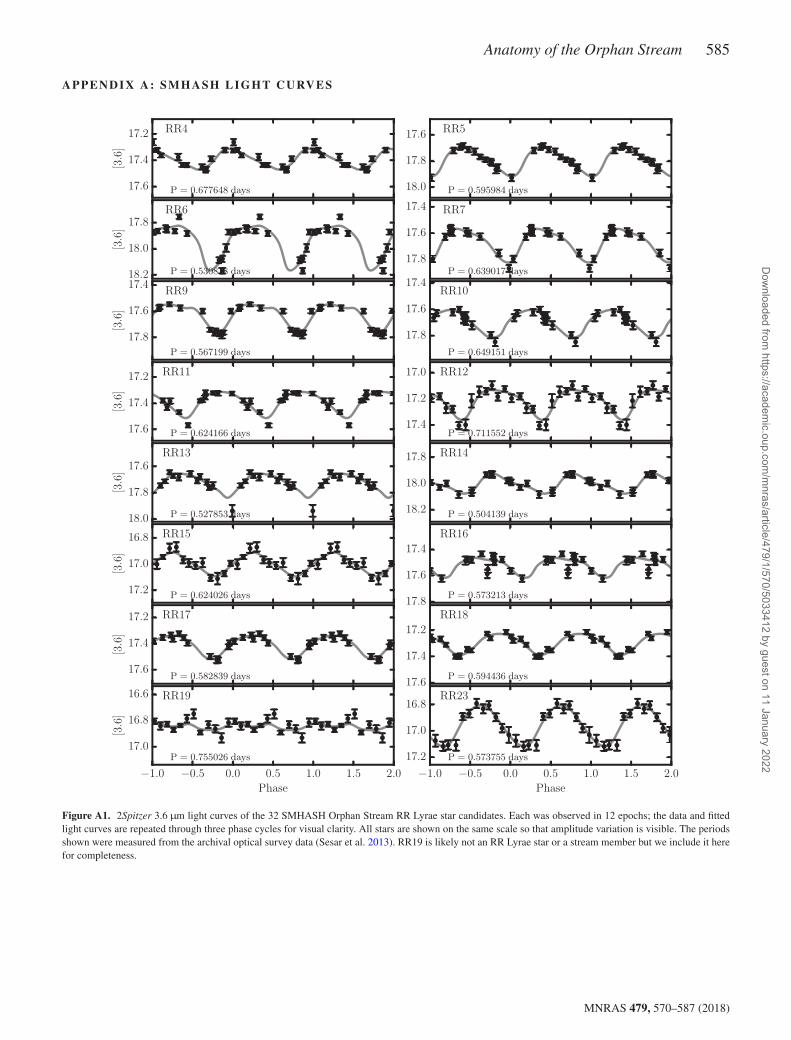
Anatomy of the Orphan Stream 585

A P P E N D I X A : SM H A S H L I G H T C U RV E S

Figure A1. 2Spitzer 3.6μm light curves of the 32 SMHASH Orphan Stream RR Lyrae star candidates. Each was observed in 12 epochs; the data and fittedlight curves are repeated through three phase cycles for visual clarity. All stars are shown on the same scale so that amplitude variation is visible. The periodsshown were measured from the archival optical survey data (Sesar et al. 2013). RR19 is likely not an RR Lyrae star or a stream member but we include it herefor completeness.

MNRAS 479, 570–587 (2018)

Dow

nloaded from https://academ

ic.oup.com/m

nras/article/479/1/570/5033412 by guest on 11 January 2022

586 D. Hendel et al.

Figure A1. continued

1Department of Astronomy, Columbia University, 550 West 120th Street,New York, NY 10027, USA2Department of Physics, University of Bath, Claverton Down, Bath, BA27AY, UK3Observatories of the Carnegie Institution of Washington, 813 Santa Bar-bara St., Pasadena, CA 91101, USA4Space Telescope Science Institute, 3700 San Martin Drive, Baltimore, MD21218, USA5Center for Astrophysical Sciences, Department of Physics & Astronomy,Johns Hopkins University, Baltimore, MD 21218, USA6Department of Astrophysical Sciences, Princeton University, 4 Ivy Lane,Princeton, NJ 08544, USA

7Steward Observatory, University of Arizona, 933 North Cherry Avenue,Tucson, AZ 85721, USA8Dipartimento di Fisica, Universita di Roma Tor Vergata, via Della RicercaScientifica 1, I-00133, Roma, Italy9INAF, Rome Astronomical Observatory, via Frascati 33, I-00040, MontePorzio Catone, Italy10Leibniz-Institut fur Astrophysik Potsdam, An der Sternwarte 16, D-14482,Potsdam, Germany11INAF-Osservatorio di Astrofisica e Scienza dello Spazio di Bologna, ViaGobetti 93/3, I - 40129, Bologna, Italy12Division of Physics, Mathematics and Astronomy, California Institute ofTechnology, Pasadena, Ca., 91125

MNRAS 479, 570–587 (2018)

Dow

nloaded from https://academ

ic.oup.com/m

nras/article/479/1/570/5033412 by guest on 11 January 2022

Anatomy of the Orphan Stream 587

13Space Science Data Center - ASI, via del Politecnico, s.n.c., I-00133,Roma, Italy14Department of Astronomy & Astrophysics, University of Chicago, 5640South Ellis Avenue, Chicago, IL 60637, USA15Dipartimento di Fisica e Astronomia, Universita di Bologna, Via Gobetti93/2, I - 40129, Bologna, Italy16IPAC, Mail Code 314-6, Caltech, 1200 E. California Blvd., Pasadena, CA91125, USA17Department of Astronomy, University of Virginia, 530 McCormick Road,Charlottesville, VA 22904, USA18Department of Physics and Astronomy, Iowa State University, A313EZaffarano, Ames, IA 50010, USA19National Optical Astronomy Observatory, 950 North Cherry Avenue, Tuc-son, AZ 85719, USA

20Nicolaus Copernicus Astronomical Center, Polish Academy of Sciences,Bartycka 18, 00-716 Warsaw, Poland21Max Planck Institute for Astronomy, Konigstuhl 17, D-69117, Heidelberg,Germany22Department of Physics and Astronomy, Michigan State University, EastLansing, MI 48824-2320, USA23Warsaw University Observatory, Al. Ujazdowskie 4, 00-478 Warszawa,Poland

This paper has been typeset from a TEX/LATEX file prepared by the author.

MNRAS 479, 570–587 (2018)

Dow

nloaded from https://academ

ic.oup.com/m

nras/article/479/1/570/5033412 by guest on 11 January 2022