Working Paper 09-15 Statistics and Econometrics Series 05 March 2009

Departamento de Estadística Universidad Carlos III de Madrid

Calle Madrid, 12628903 Getafe (Spain)

Fax (34) 91 624-98-49

SMALL AREA ESTIMATION OF POVERTY INDICATORS

Molina, Isabel1 and Rao, J. N. K.2 Abstract We propose to estimate non-linear small area population quantities by using Empirical Best (EB) estimators based on a nested error model. EB estimators are obtained by Monte Carlo approximation. We focus on poverty indicators as particular non-linear quantities of interest, but the proposed methodology is applicable to general non-linear quantities. Small sample properties of EB estimators are analyzed by model-based and design-based simulation studies. Results show large reductions in mean squared error relative to direct estimators and estimators obtained by simulated censuses. An application is also given to estimate poverty incidences and poverty gaps in Spanish provinces by sex with mean squared errors estimated by parametric bootstrap. In the Spanish data, results show a significant reduction in coefficient of variation of the proposed EB estimators over direct estimators for most domains.

Keywords: Empirical best estimator; Parametric bootstrap; Poverty mapping; Small area estimation.

1 Departamento de Estadística, Universidad Carlos III de Madrid, C/ Madrid 126, 28903 Getafe (Madrid), Spain. E-mail: isabel.molina@uc3m.es 2 School of Mathematics and Statistics, Carleton University, 125 Colonel By Drive, Ottawa, ON CANADA K1S 5B6. E-mail: jrao@math.carleton.ca

Small Area Estimation of Poverty Indicators∗

Isabel Molina†and J. N. K. Rao‡

Abstract

We propose to estimate non-linear small area population quantitiesby using Empirical Best (EB) estimators based on a nested error model.EB estimators are obtained by Monte Carlo approximation. We focuson poverty indicators as particular non-linear quantities of interest, butthe proposed methodology is applicable to general non-linear quantities.Small sample properties of EB estimators are analyzed by model-basedand design-based simulation studies. Results show large reductions inmean squared error relative to direct estimators and estimators obtainedby simulated censuses. An application is also given to estimate povertyincidences and poverty gaps in Spanish provinces by sex with mean squarederrors estimated by parametric bootstrap. In the Spanish data, resultsshow a significant reduction in coefficient of variation of the proposed EBestimators over direct estimators for most domains.

Key words: Empirical best estimator; Parametric bootstrap; Povertymapping; Small area estimation.

1 Introduction

The first of the Millennium Development Goals established by the United Na-tions is the eradication of extreme poverty and hunger. The availability of themost possible accurate information concerning the living conditions of people isa basic instrument for targeting policies and programs aiming at the reductionof poverty. Thus, there are no doubts about the importance of the estimation ofpoverty measures. In many cases the information collected from national surveysis limited and allows estimation only for larger regions or larger population sub-groups. Therefore, small area estimation techniques are required that “borrowstrength” across areas through linking models and auxiliary information such as

∗Supported by the Spanish grants MTM2006-05693 and SEJ2007-64500, and by the Euro-pean project num. 217565-FP7-SSH-2007-1.

†Department of Statistics, Universidad Carlos III de Madrid. Address: C/Madrid 126,28903 Getafe (Madrid), Spain, Tf: +34 916249887, Fax: +34 916249849, E-mail: is-abel.molina@uc3m.es

‡School of Mathematics and Statistics, Carleton University. E-mail: jrao@math.carleton.ca

1

censuses and administrative data; see Rao (2003) for a comprehensive accountof these techniques.

Many measures of poverty and inequality are non-linear functions of a welfarevariable for the population units. This makes many of the current small areaestimation methods, typically developed for the estimation of linear characteris-tics, such as means, not applicable. Here we propose the use of empirical bestpredictors (EBPs) obtained through Monte Carlo approximation. This methodprovides estimators that are “best” in the sense of minimizing the mean squarederror (MSE) under assumed small area models. It is useful for the estimationof any function of a welfare variable, when this variable or some transforma-tion of it follows a linear model. We show by simulations that empirical bestpredictors behave good in terms of bias and mean squared error. We also pro-pose a parametric bootstrap method for MSE estimation and study its bias insimulations.

In the U.S. the need for small area poverty estimates has given rise to theSAIPE program (Small Area Income & Poverty Estimates) of the U.S. CensusBureau; for further details see http://www.census.gov/hhes/www/saipe. Themain objective of this program is to provide updated estimates of income andpoverty statistics for the administration of federal programs and the allocation offederal funds to local jurisdictions. The county level methodology, summarizedby Bell (1997), basically uses a Fay-Herriot area level model (Fay & Herriot, 1979)to produce model-based county estimates of school-age children under poverty.

The World Bank (WB) has been releasing small area poverty and incomeinequality estimates for some countries, using the methodology of Elbers et al.(2003). This methodology is currently widely used, see e.g. Neri et al. (2005),Ballini et al. (2006), Tarozzi and Deaton (2007) and Haslett and Jones (2005).Elbers et al. (2003) assumed a unit level model that combines both census andsurvey data. Using that model, they produce disaggregated maps that describethe spatial distribution of poverty and inequality. Section 7 shows that thismethod, when used to estimate small area means, is basically equal to a syntheticregression estimator.

Measures of inequality include the Gini coefficient, the Sen index, the generalentropy and the Theil index (see e.g. Neri et al., 2005). Although the methoddeveloped in this paper allows the estimation of these inequality measures aswell, for the sake of brevity we will focus on the estimation of a class of povertymeasures called FGT poverty measures due to Foster et al (1984), see Section 2,and used in the WB method.

A common definition of poverty classifies a person as “under poverty” whenthe selected welfare variable for this person is below a threshold called povertyline, which is usually a given percentage of the median welfare for the population.For instance, the Spanish National Statistical Institute (INE) established thepoverty line at 60% of the median per capita income. Here we assume that thepoverty line is fixed at some quantity established by the corresponding authorityand we avoid discussions concerning the definition of this threshold.

2

The paper is organized as follows. Section 2 defines the family of FGT povertymeasures and Section 3 introduces two basic types of direct estimators, whichmake use only of the sample data from the target area. Section 4 describes thebest prediction methodology for finite populations and Section 5 applies thismethodology to the estimation of FGT poverty measures through the use of anested error linear regression model. Section 6 describes a parametric bootstrapmethod for MSE estimation. Section 7 makes a theoretical comparison of thedifferent methods in the context of estimating small area means. Sections 8 and9 present the results of simulation studies on the performance of the proposedmethod relative to the WB method and direct estimation, in terms of bias andMSE. Performance of bootstrap MSE estimator is also studied. Finally, in Sec-tion 10, the proposed method is applied to Spanish data to estimate povertyincidences and poverty gaps in Spanish provinces by gender.

2 FGT poverty measures for small areas

Consider a finite population of size N that is partitioned into D small areasof sizes N1, . . . , ND. Let Edj be a suitable quantitative measure of welfare forindividual j in small area d, such as income or expenditure, and let z be the givenpoverty line; that is, the threshold for Edj under which a person is consideredas “under poverty”. The family of poverty measures introduced by Foster et al.(1984) and called throughout the paper as FGT poverty measures, for each smallarea d, is defined as

Fαd =1

Nd

Nd∑

j=1

(

z − Edj

z

)α

I(Edj < z), α = 0, 1, 2, d = 1, . . . , D,

where I(Edj < z) = 1 if Edj < z (person under poverty) and I(Edj < z) = 0if Edj ≥ z (person not under poverty). For α = 0 we get the proportion ofindividuals under poverty in small area d, also called poverty incidence or headcount ratio. The FGT measure for α = 1 is called poverty gap, and measuresthe area mean of the relative distance to non-poverty (the poverty gap) of eachindividual. For α = 2 the measure is called poverty severity. This measuresquares the poverty gaps, and thus emphasizes extreme poverty.

3 Direct estimators of poverty measures

In the inference process, a random sample of size n < N is drawn from thepopulation according to a specified sampling design. Let Ω denote the set ofindexes of the population units. Let s be the set of units selected in the sampleand r the set of indexes of the units that are not selected (with size N − n).The restrictions of Ω, s, N and n to area d are denoted by Ωd, sd, Nd and nd

respectively, where n = n1 + · · · + nD. The unweighted sample FGT poverty

3

measures are given by

fαd =1

nd

∑

j∈sd

(

z − Edj

z

)α

I(Edj < z), α = 0, 1, 2, d = 1, . . . , D. (1)

A direct estimator for a small area, as a sample estimator, uses only thesample data from the target small area and it is usually design-based. Let wdj

be the sampling weight (inverse of the probability of inclusion) of individual jfrom area d. Direct estimators of the FGT measures are given by

fwαd =

1

Nd

∑

j∈sd

wdj

(

z − Edj

z

)α

I(Edj < z), α = 0, 1, 2, d = 1, . . . , D, (2)

where Nd =∑

j∈sdwdj is the direct estimator of the population size of small area

d, Nd. If the sampling weights wdj do not depend on the unit j, for examplewdj = nd/Nd under simple random sampling within areas, then (2) reduces tothe unweighted mean (1).

The limited sample sizes nd within some of the areas prevent the use of es-timators such as (1) or (2). Indeed, a common definition of poverty classifiesa person as “under poverty” when the selected welfare variable for this personis below 60% of the median. Under this definition the outcome of being un-der poverty is likely to have low frequency. Then, to obtain reliable estimatorsfor small domains or geographical areas it is necessary to appeal to small areatechniques (Rao, 2003). These techniques improve the estimation procedures byusing models that establish some relationships between the areas, based on aux-iliary information (census and/or administrative variables) related to the welfarevariables of interest. These models provide “indirect” estimators that make useof related data from other areas, and which might reduce drastically the esti-mation errors as long as model assumptions hold. Model checking should be anintegral part of indirect estimation methods.

4 Best prediction under a finite population

Section 4 introduces the best predictor (BP) of a function of a random vectorin a finite population. Application of the BP methodology for estimating FGTpoverty measures in small areas is described in Section 5.

Consider a random vector y = (Y1, . . . , YN)′ containing the values of a randomvariable associated with N units of a finite population. Let ys be the sub-vectorof y corresponding to sample elements and yr the sub-vector of out-of-sampleelements; that is, y = (y′

s,y′r)

′. The target is to predict the value of a real-valued function δ = h(y) of the random vector y using the sample data ys. Fora particular predictor δ, the mean squared error is defined as

MSE(δ) = Ey(δ − δ)2, (3)

4

where Ey denotes expectation with respect to the joint distribution of the pop-ulation vector y. The BP of δ is the function of ys that minimizes (3). Considerthe conditional expectation δ0 = Eyr

(δ|ys), where the expectation is taken withrespect to the conditional distribution of yr given ys and the result is a functionof sample data ys. Subtracting and adding δ0 in the mean squared error, weobtain

MSE(δ) = Ey(δ − δ0)2 + 2 Ey(δ − δ0)(δ0 − δ) + Eyδ0 − δ)2.

In this expression, the last term does not depend on δ. For the second term,observe that

Ey(δ − δ0)(δ0 − δ) = Eys

[

Eyr

(δ − δ0)(δ0 − δ)|ys

]

= Eys

[

(δ − δ0)

δ0 − Eyr(δ|ys)

]

= 0.

Thus, the BP is the value δ that minimizes Ey(δ − δ0)2. Since this quantity isnon-negative and its minimum value is zero, the BP is

δB = δ0 = Eyr(δ|ys). (4)

Typically, the joint distribution of y depends on some unknown model pa-rameters. Then an empirical BP (EBP) of δ can be obtained by replacing allunknown parameters by suitable estimators and then evaluating the expectation(4) from the estimated distribution.

Remark 1. Suppose that y follows a Normal distribution with mean vector µ =Xβ, for a known matrix X, and positive definite covariance matrix V. Let thetarget quantity δ be a linear function of y, δ = a′y. In this case, the best linearunbiased predictor (BLUP) of δ, obtained by Royall (1976), is equal to the BPwhen the true β is replaced by the generalized least squares estimator.

5 Empirical best prediction of FGT poverty mea-

sures

In this section we describe how to obtain BPs of FGT poverty measures for smallareas. For a given α ∈ 0, 1, 2, let us define the random variables

Fαdj =

(

z − Edj

z

)α

I(Edj < z), j = 1, . . . , Nd, d = 1, . . . , D.

Then the FGT poverty measure for area d is the mean

Fαd =1

Nd

Nd∑

j=1

Fαdj, d = 1, . . . , D. (5)

5

Suppose that there is a one-to-one transformation Ydj = T (Edj) of the welfarevariables, Edj, such that the vector y containing the values of the transformedvariables Ydj for all the population units satisfies y ∼ N(µ,V). Then we canexpress the random variables Fαdj in terms of Ydj as

Fαdj =

(

z − T−1(Ydj)

z

)α

IT−1(Ydj) < z = hα(Ydj), j = 1, . . . , Nd.

Thus, the FGT poverty measure (5) is a non-linear function of the vector y. Bythe results of Section 4, taking δ = Fαd the BP of Fαd is

FBαd = Eyr

(Fαd|ys). (6)

Using the decomposition of the mean (5) in terms of sample and out-of-sampleelements, we have

Fαd =1

Nd

∑

j∈sd

Fαdj +∑

j∈rd

Fαdj

, (7)

where rd denotes the set of out-of-sample elements belonging to area d. Nowtaking conditional expectation of (7) and introducing the conditional expectationinside the sum, the BP becomes

FBαd =

1

Nd

∑

j∈sd

Fαdj +∑

j∈rd

FBαdj

, (8)

where FBαdj = Eyr

(Fαdj|ys) is the BP of the out-of-sample variable Fαdj = hα(Ydj),which is defined as

FBαdj = Eyr

[hα(Ydj)|ys] =

∫

IR

hα(Ydj)f(Ydj|ys) dYdj, j ∈ rd, (9)

where f(Ydj|ys) is the conditional density of Ydj given the data vector ys. Theexpectation in (9) cannot be calculated explicitly due to the complexity of hα.However, since y = (y′

s,y′r)

′ is Normally distributed with mean vector µ =(µ′

s,µ′r)

′ and covariance matrix partitioned conformably as

V =

(

Vs Vsr

Vrs Vr

)

,

the conditional distribution of yr given ys is

yr|ys ∼ N(µr|s,Vr|s), (10)

whereµr|s = µr + VrsV

−1s (ys − µs), Vr|s = Vr − VrsV

−1s Vsr. (11)

Then, we propose to use an empirical approximation by Monte Carlo simulationof a large number L of vectors yr generated from (10). Let Y

(ℓ)dj be the value

6

of the out-of-sample observation Ydj, j ∈ rd, obtained in the ℓ-th simulation,ℓ = 1, . . . , L. A Monte Carlo approximation to the best predictor of Ydj is thengiven by

FBαdj = Eyr

[hα(Ydj)|ys] ≈1

L

L∑

ℓ=1

hα(Y(ℓ)dj ), j ∈ rd. (12)

In practice, the mean vector µ and the covariance matrix V usually dependon an unknown vector of parameters θ. Thus the conditional density f(Ydj|ys)depends on θ and we make this explicit in the notation using f(Ydj|ys,θ). We

can take an estimator θ of θ such as the maximum likelihood (ML) estimator orthe residual ML (REML) estimator. Then the expectation can be approximated

by generating values Y(ℓ)dj from the estimated density f(Ydj|ys, θ). The resulting

predictor, denoted FEBαdj , is called the empirical best predictor (EBP). Finally,

the EBP of the poverty measure Fαd is given by

FEBαd =

1

Nd

[

∑

j∈sd

Fαdj +∑

j∈rd

FEBαdj

]

.

In this paper, we consider the nested error linear regression model for theYdj (Battese et al., 1988). This model relates the transformed variables Ydj (e.g.,log-earnings) to a vector of p explanatory variables xdj for all areas, and includesa random area-specific effect ud along with the usual residual errors edj:

Ydj = x′djβ + ud + edj, ud ∼ iid N(0, σ2

u),

edj ∼ iid N(0, σ2e), j = 1, . . . , Nd, d = 1, . . . , D, (13)

where the area effects ud and the errors edj are independent. Defining vectorsand matrices obtained by stacking the elements for area d as

yd = col1≤j≤Nd

(Ydj), ed = col1≤j≤Nd

(edj), Xd = col1≤j≤Nd

(x′dj),

the vectors yd, d = 1, . . . , D, under model (13), are independent with

yd ∼ N(µd,Vd),

whereµd = Xdβ and Vd = σ2

u1Nd1′

Nd+ σ2

eINd.

We assume that the population model (13) holds for the sample, i.e., sampleselection bias is absent (Pfeffermann et al. 1998).

Consider the decomposition of yd into sample and out-of-sample elementsyd = (y′

dr,y′ds)

′, and the corresponding decomposition of µd = E(yd) and Vd =Var(yd). Then the distribution of the out-of-sample vector ydr given the sampledata yds is

ydr|yds ∼ N(µdr|s,Vdr|s), (14)

7

where the conditional mean vector and covariance matrix are given by

µdr|s = Xdrβ + σ2u1Nd−nd

1′nd

V−1ds (ys − Xsβ) (15)

Vdr|s = σ2u(1 − γd)1Nd−nd

1′Nd−nd

+ σ2eINd−nd

. (16)

Note that ydr|yds and ydr|ys have the same distribution (14) due to the inde-pendence of the vectors yd.

Observe that the application of the Monte Carlo approximation (12) involvessimulation of D multivariate Normal vectors of sizes Nd −nd, d = 1, . . . , D, from(14). Then this process has to be repeated L times, something computationallyvery intensive. This can be avoided in the following way. Observe that thematrix Vdr|s corresponds to the covariance matrix of a vector ydr generated bythe model

ydr = µdr|s + vd1Nd−nd+ ǫdr, (17)

with new random effects vd and errors ǫdr that are independent and satisfy

vd ∼ N(0, σ2u(1 − γd)) and ǫdr ∼ N(0Nd−nd

, σ2eINd−nd

).

Using these relations, instead of generating a multivariate normal vector of sizeNd−nd, we just need to generate univariate normal variables vd ∼ N(0, σ2

u(1−γd))and ǫdj ∼ N(0, σ2

e) independently, for j ∈ rd, and then obtain the responses Ydj

from (17) using the known value of µdr|s. As mentioned before, in practice all theunknown model parameters β, σ2

u and σ2e are replaced by suitable estimators, and

then the variables Ydj are generated from the corresponding estimated normaldistributions.

Summarizing, the proposed EBP method to estimate poverty measures worksin the following way:

(a) Fit model (13) to the initial (transformed) data ys.

(b) Draw L out-of-sample vectors y(ℓ)r , ℓ = 1, . . . , L from (14), or equivalently

from (17), but with the unknown parameters replaced by the estimatorsobtained in (a).

(c) With the L generated vectors y(ℓ)r , ℓ = 1, . . . , L, and using the sample data

ys, compute EBPs of the poverty measures from (8) using the Monte Carloapproximation (12).

Instead of introducing the expectation inside the sum as in (8), we can approx-imate by Monte Carlo directly the expectation of the poverty measure (6). Inthis way, the proposed procedure can be used to predict any other function h(y)and it requires only the assumption of a model for some transformation of thewelfare variable Edj.

8

6 Parametric bootstrap for MSE estimation

Here we propose to use an extension of the parametric bootstrap method forfinite populations (Gonzalez-Manteiga et al., 2008) to estimate the MSE of theempirical best predictors FEB

αd , d = 1, . . . , D. For a given α, this method worksas follows:

1. Fit model (13) to sample data ys and obtain model parameter estimatesβ, σ2

u and σ2e .

2. Generate bootstrap random area effects as u∗d ∼ iid N(0, σ2

u), d = 1, . . . , D.

3. Generate, independently of the random effects u∗d, bootstrap random errors

e∗dj ∼ iid N(0, σ2e), j = 1, . . . , Nd, d = 1, . . . , D.

4. Construct a bootstrap population using the estimated model,

Y ∗dj = x′

djβ + u∗d + e∗dj, j = 1, . . . , Nd, d = 1, . . . , D, (18)

and calculate the FGT measures for this population, that is, calculate firstF ∗

αdj = hα(Y ∗dj), j = 1, . . . , Nd, and then take the small area means as

F ∗αd =

1

Nd

Nd∑

j=1

F ∗αdj, d = 1, . . . , D.

5. Take the elements Y ∗dj with indices contained in the sample s, denoted y∗

s .

Fit the model again to y∗s obtaining new model parameter estimates β∗,

σ2∗u and σ2∗

e .

6. Using the bootstrap sample data y∗s and the known matrix X, apply the EB

method as described in Section 5 and calculate bootstrap EBPs, FEBP∗αd ,

d = 1, . . . , D.

Observe that the bootstrap elements, given the original sample data, preserveproperties of the original population model. Random effects and errors are iidwith

E∗(u∗d) = 0, V ar∗(u

∗d) = σ2

u, E∗(e∗dj) = 0, V ar∗(e

∗dj) = σ2

e , (19)

where E∗ and V ar∗ denote expectation and variance with respect to the distri-bution defined by the bootstrap model (18) given sample data ys. Consider thevector y∗ with all the population bootstrap elements defined analogously to y

for the original population. Then the mean vector and covariance matrix of thisbootstrap vector are

E∗(y∗) = Xβ, V ar∗(y

∗) = σ2uZZ′ + σ2

eIN .

9

Thus, the distribution of the bootstrap population y∗ (given sample data ys)imitates that of the original population y. Then an estimator of MSE(FEB

αd ) isthe bootstrap MSE of the bootstrap EBP, defined as

MSE∗(FEBP∗αd ) = E∗(F

EBP∗αd − F ∗

αd)2.

In practice, this quantity can be approximated through a Monte Carlo procedure,by repeating steps 2–6 a large number of times, B, and then taking the mean overthe B replicates. More specifically, let F

∗(b)αd and F

EB∗(b)αd be the poverty measure

and its corresponding EBP for the bootstrap replicate b, for b = 1, . . . , B. Then,the estimator of the MSE is calculated as

mse(FEBαd ) =

1

B

B∑

b=1

(FEB∗(b)αd − F

∗(b)αd )2. (20)

It is possible to obtain a better MSE estimator, in terms of relative bias, byusing a double bootstrap method (Hall and Maiti, 2006) applied to the trans-formed sample data.

7 Estimation of small area means

In this section we restrict ourselves to the estimation of the small area means

Yd =1

Nd

Nd∑

j=1

Ydj, d = 1, . . . , D,

since means are common target quantities which also deserve attention; more-over, means allow for the study of some theoretical properties of estimators.

Consider first the case of population elements Ydj following a linear modelwithout area effects,

Ydj = x′djβ + edj, edj ∼ iid N(0, σ2

e), j = 1, . . . , Nd, d = 1, . . . , D. (21)

Let us assume for simplicity of exposition that all model parameters are known.Taking the average of (21) over the elements in area d, we can express the truemean as

Yd = x′dβ + ed,

where xd = N−1d

∑Nd

j=1 x′dj and ed = N−1

d

∑Nd

j=1 edj. Common small area es-timators derived under model (21) are the synthetic estimators, obtained bypredicting all the Ydj and then taking the area mean, that is, taking

ˆY SY Nd =

1

Nd

Nd∑

j=1

Ydj,

10

as the synthetic estimator, where Ydj = x′djβ is the predictor of Ydj for j =

1, . . . , Nd. However, under model (21), the BP of Yd is obtained by predictingonly the out-of-sample observations and keeping the sample data, i.e.,

ˆY Bd =

1

Nd

∑

j∈sd

Ydj +∑

j∈rd

Ydj

.

Let us compare the MSEs of the synthetic and the BP estimators. Writing

the synthetic estimator as ˆY SY Nd = x′

dβ, we obtain

ˆY SY Nd − Yd = x′

dβ − (x′dβ + ed) = ed,

and then the MSE becomes

MSE( ˆY SY Nd ) = E( ˆY SY N

d − Yd)2 = E(e2

d) =V ar(edj)

Nd

=σ2

e

Nd

.

However, observe that the difference between the BP and the true mean is equalto

ˆY Bd − Yd =

1

Nd

∑

j∈rd

edj,

which implies that the MSE of ˆY Bd is given by

MSE( ˆY Bd ) = E( ˆY B

d − Yd)2 =

σ2e

Nd

(

1 −nd

Nd

)

<σ2

e

Nd

= MSE( ˆY SY Nd ).

Thus, under model (21) with known parameters, the BP has always smaller MSEdue to the more efficient use of available information, namely the sample data.When the sampling fraction nd/Nd is negligible both estimators have a similarMSE.

Now consider the case of extra area variation not explained by the auxiliaryvariables; that is, the true model is (13), but we fit the model (21). The truemean for area d is then given by

Yd = x′dβ + ud + ed.

Then the MSE of the synthetic estimator under the true model is

MSE( ˆY SY Nd ) = E[(ud + ed)

2] = σ2u +

σ2e

Nd

. (22)

For the BP, the MSE under the true model is

MSE( ˆY Bd ) = σ2

u +σ2

e

Nd

(

1 −nd

Nd

)

,

which is again smaller than MSE( ˆY SY Nd ).

11

The method of Elbers et al. (2003), henceforth called the ELL method,assumes a linear model with random cluster effects, where clusters may be dif-ferent from the areas. They computed small area estimators by (a) fitting alinear model with cluster random effects, (b) generating bootstrap random clus-ter effects, (c) generating bootstrap random errors, (d) constructing a populationfrom the bootstrap model

Y ∗dj = x′

djβ + u∗c + e∗dj, j = 1, . . . , Nd, d = 1, . . . , D, (23)

where u∗c is the bootstrap random effect of cluster c and (e) calculating the

average of the bootstrap elements from area d:

Y ∗d = N−1

d

Nd∑

j=1

Y ∗dj. (24)

The ELL estimator of the small area mean Yd is then the bootstrap mean

ˆY ELLd = E∗(Y

∗d ),

which, in practice, is obtained from a Monte Carlo approximation by generatinga large number, L, of populations, calculating the area means (24) for eachpopulation and later averaging over the L populations. The bootstrap varianceis used as the mean squared error of the ELL estimator; that is, the ELL methoduses

MSE( ˆY ELLd ) = V ar∗(Y

∗d ),

which again is approximated by Monte Carlo simulations.In the case of no clusters (as in some establishment surveys), the ELL method

fits the linear model (21) and uses this model to construct bootstrap populations.Then the bootstrap mean for area d becomes

Y ∗d = N−1

d

Nd∑

j=1

Y ∗dj =

1

Nd

Nd∑

j=1

(x′djβ + e∗dj) = ˆY SY N

d + e∗d,

and the ELL estimator is given by

ˆY ELLd = E∗(Y

∗d ) = E∗(

ˆY SY Nd + e∗d) = ˆY SY N

d + E∗(e∗d) = ˆY SY N

d ,

due to property (19) of the bootstrap method and the fact that the expectationE∗ is conditional on the sample. The ELL estimator of the MSE is

MSE( ˆY ELLd ) = V ar∗(Y

∗d ) = E∗[(Y

∗d − E∗(Y

∗d ))2] = E∗[(e

∗d)

2] =V ar∗(e

∗dj)

Nd

=σ2

e

Nd

.

Thus, when fitting a model without cluster effects, the ELL estimator of a smallarea mean is essentially the synthetic estimator, which is a good estimator whenthe true model is (21). When the true model is (13), the ELL method is not

12

accounting for the area effects and the MSE estimator has a bias equal to σ2u,

see (22). Thus, the ELL estimator of MSE can lead to serious underestimationof MSE when the area effects have a substantial variance σ2

u.Now consider the ideal case for ELL, in which clusters are the same as the

small areas. In this case we use the ELL method by fitting the correct model(13). Then the ELL estimator is again

ˆY ELLd = E∗(

ˆY SY Nd + u∗

d + e∗d) = ˆY SY Nd ,

and the ELL estimator of the MSE becomes

MSE( ˆY ELLd ) = V ar∗(Y

∗d ) = E∗[(Y

∗d − E∗(Y

∗d ))2] = E∗[(u

∗d + e∗d)

2] = σ2u +

σ2e

Nd

,

which is the MSE of the synthetic estimator under model (13). Thus, whenthe clusters are equal to the small areas, the ELL estimator remains essentiallyequal to the synthetic estimator, but in this case the ELL variance estimatoris unbiased. Actually, under model (13), the difference between the ELL andEB methods is that the target quantities are not the same. EB method tries toestimate (or better predict) the actual area means Yd, while the ELL method isestimating instead the marginal expectations E(Yd).

8 Model-based simulation experiment

A model-based simulation study has been carried out to study the performanceof the proposed EB predictors of small area FGT poverty measures with α = 0(proportion of people under poverty) and α = 1 (poverty gap). For this, we sim-ulated populations of size N = 20000, composed of D = 80 areas with Nd = 250elements in each area d = 1, . . . , D. The response variables for the populationunits Ydj were generated from model (13) taking as auxiliary variables two dum-mies X1 ∈ 0, 1 and X2 ∈ 0, 1 plus an intercept. The values of these twodummies for the population units were generated from Bernouilli distributionswith success probabilities increasing with the area index for X1 and constant forX2; that is,

p1d = 0.3 + 0.5 d/20; p2d = 0.2, d = 1, . . . , D,

respectively. Here the welfare variables Edj are the exponential of the responsesYdj; that is, the transformation T (·) defined in Section 5 is T (x) = log(x). A set ofsample indices s was drawn from the population indices 1, . . . , N, by a stratifieddesign with areas as strata and simple random sampling without replacementwithin each area. The values of the auxiliary variables for the population unitsand the sample indices were kept fixed over all Monte Carlo simulations.

The intercept and the regression coefficients associated with the two auxiliaryvariables used to generate populations were β = (3, 0.03,−0.04)′. In this way,

13

the mean welfare increases when moving from the case (X1 = 0, X2 = 0) to(X1 = 1, X2 = 0), but decreases when moving from (X1 = 0, X2 = 0) to (X1 =0, X2 = 1). This implies that the “richest” individuals are those with valuesX1 = 1 and X2 = 0. Since the probability p1d of X1 = 1 increases with thearea index but that of X2 = 1 is constant, then the last areas will have moreindividuals with larger Ydj and then the FGT poverty measures will decreasewith the area index. The random area effects variance was taken as σ2

u = (0.15)2

and the error variance as σ2e = (0.5)2. The poverty line z was fixed as z = 12,

which is roughly equal to 0.6 times the median of the welfare variables Edj for apopulation generated as mentioned above. In this way, the poverty incidence forthe simulated populations is approximately 16%.

Under this setup, I = 1000 populations y(i) were generated from the truemodel. For each population i, we carried out the following tasks:

(a) The true area poverty incidences and gaps (FGT measures for α = 0 andα = 1 respectively) were obtained for each population as

F(i)αd =

1

Nd

Nd∑

j=1

(

z − E(i)dj

z

)α

I(E(i)dj < z), α = 0, 1, d = 1, . . . , D,

where E(i)dj = exp(Y

(i)dj ) , j = 1, . . . , Nd.

(b) Sample estimators of the same quantities were also calculated as

f(i)αd =

1

nd

∑

j∈sd

(

z − E(i)dj

z

)α

I(E(i)dj < z), α = 0, 1, d = 1, . . . , D.

In this simulation study sample estimators are equal to direct estimators.

(c) Model (13) was fitted to the sample data. Then, substituting the estimated

model parameters in (15) and (16), L = 50 out-of-sample vectors y(iℓ)r ,

ℓ = 1, . . . , L were generated from the conditional distribution (14) using

(17). Then using the sample data y(i)s and the generated out-of-sample data

y(iℓ)r , EB predictors of the area poverty incidences and gaps were calculated.

For this, first, for each sample unit j we considered the sample values

F(i)αdj =

(

z − E(i)dj

z

)α

I(E(i)dj < z), j ∈ sd, d = 1, . . . , D,

while for each out-of-sample unit j, we computed the EB predictors of F(i)αdj

using the L simulated vectors,

FEB(i)αdj =

1

L

L∑

ℓ=1

(

z − E(iℓ)dj

z

)α

I(E(iℓ)dj < z), j ∈ rd, d = 1, . . . , D,

14

for α = 0, 1. Then the EB predictor of the FGT measure of order α = 0, 1was obtained as

FEB(i)αd =

1

Nd

[

∑

j∈sd

F(i)αdj +

∑

j∈rd

FEB(i)αdj

]

, d = 1, . . . , D.

(d) The ELL estimators of the poverty measures were calculated. Forthis, first the model (13) was fitted to the sample data and then L = 50populations were generated using the parametric bootstrap described inSection 6. For each population, the poverty measures were obtained andfinally, the results were averaged over the L = 50 populations.

Means over Monte Carlo populations i = 1, . . . , I of the true values of theFGT measures of order α = 0, 1 were computed as

E(Fαd) =1

I

I∑

i=1

F(i)αd , d = 1, . . . , D.

These means are the reference values for comparison. Finally, for all estimators,namely, EBP, sample and ELL, the mean, variance and mean squared error overMonte Carlo populations i = 1, . . . , I were obtained for each area d = 1, . . . , D.

Figure 1 a) plots the means of the true poverty incidences F(i)0d , EB esti-

mates FEB(i)0d , direct estimates f

(i)0d and ELL estimates F

ELL(i)0d for each area

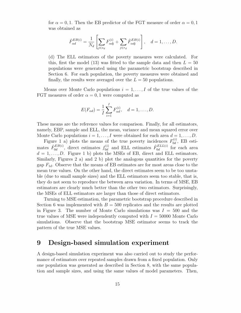
d = 1, . . . , D. Figure 1 b) plots the MSEs of EB, direct and ELL estimators.Similarly, Figures 2 a) and 2 b) plot the analogous quantities for the povertygap F1d. Observe that the means of EB estimates are for most areas close to themean true values. On the other hand, the direct estimates seem to be too unsta-ble (due to small sample sizes) and the ELL estimators seem too stable, that is,they do not seem to reproduce the between area variation. In terms of MSE, EBestimators are clearly much better than the other two estimators. Surprisingly,the MSEs of ELL estimators are larger than those of direct estimators.

Turning to MSE estimation, the parametric bootstrap procedure described inSection 6 was implemented with B = 500 replicates and the results are plottedin Figure 3. The number of Monte Carlo simulations was I = 500 and thetrue values of MSE were independently computed with I = 50000 Monte Carlosimulations. Observe that the bootstrap MSE estimator seems to track thepattern of the true MSE values.

9 Design-based simulation experiment

A design-based simulation experiment was also carried out to study the perfor-mance of estimators over repeated samples drawn from a fixed population. Onlyone population was generated as described in Section 8, with the same popula-tion and sample sizes, and using the same values of model parameters. Then,

15

a)

0 20 40 60 80

15.0

15.5

16.0

16.5

Area

Pov

erty

inci

denc

e (x

100)

TrueEBSampleELL

b)

0 20 40 60 80

1020

3040

5060

70

Area

MS

E p

over

ty in

cide

nce

(x10

000)

EB Sample ELL

Figure 1: a) Means (×100) and b) MSEs (×104) over simulated populations oftrue values, EB, sample and ELL estimators of the poverty incidence F0d for eacharea d.

in each replication out of I = 1000, a new sample was drawn from this fixedpopulation according to SRS without replacement within each area. From eachsample, the three types of estimators of poverty measures, namely EBP, directand ELL were obtained.

Results for the poverty incidence are displayed in Figures 4 and 5. Figure 4shows the true values and the means over the Monte Carlo samples of the EB,direct and ELL estimators. Observe that the ELL estimators remain practicallyconstant across the areas. On the other hand, EB estimators track the truevalues well, even though these estimators are supposed to have good theoreticalproperties with respect to the model. Of course, direct estimators perform betterbecause they are design-unbiased. In terms of MSE, Figure 5 shows that ELLestimators have small MSEs for some of the areas and large for the other areas,while the MSE of EB and direct estimators remain small for all areas. For mostareas, the MSE of EB estimators is smaller than that of the direct estimators.

10 Application

The EB method was applied to compute poverty incidences and poverty gapsin Spanish provinces crossed with gender. For this, data from the EuropeanSurvey on Income and Living Conditions (EUSILC) from the year 2006 has beenused. The welfare variable for the individuals is the normalized annual incomecalculated following the standard procedure of the Spanish Statistical Institute(INE). This variable has been transformed by adding a fixed quantity to makeit always positive and then taking logarithm. This transformed variable acts asthe response in the nested-error regression model. As auxiliary variables we haveconsidered the indicators of the 5 quinquennial groupings of the variable age,

16

a)

0 20 40 60 80

3.2

3.3

3.4

3.5

3.6

3.7

3.8

Area

Pov

erty

gap

(x10

0)

TrueEBSampleELL

b)

0 20 40 60 80

12

34

56

Area

MS

E p

over

ty g

ap (x

1000

0)

EB Sample ELL

Figure 2: a) Means (×100) and b) MSEs (×104) over simulated populations oftrue values, EB, sample and ELL estimators of the poverty gaps FE

1d for eacharea d.

the indicator of having Spanish nationality, the indicators of the 3 levels of thevariable education level, and the indicators of the 3 categories of the variableemployment, with categories “unemployed”, “employed” and “inactive”. Fromeach variable, one of the categories was considered as base reference, omittingthe corresponding indicator and then including an intercept in the model.

The values of the dummy indicators are not known for the out-of-sampleunits, but the EB method requires only the knowledge of the total number ofpeople with the same x-values. These totals were estimated using the samplingweights attached to the sample units in the EUSILC.

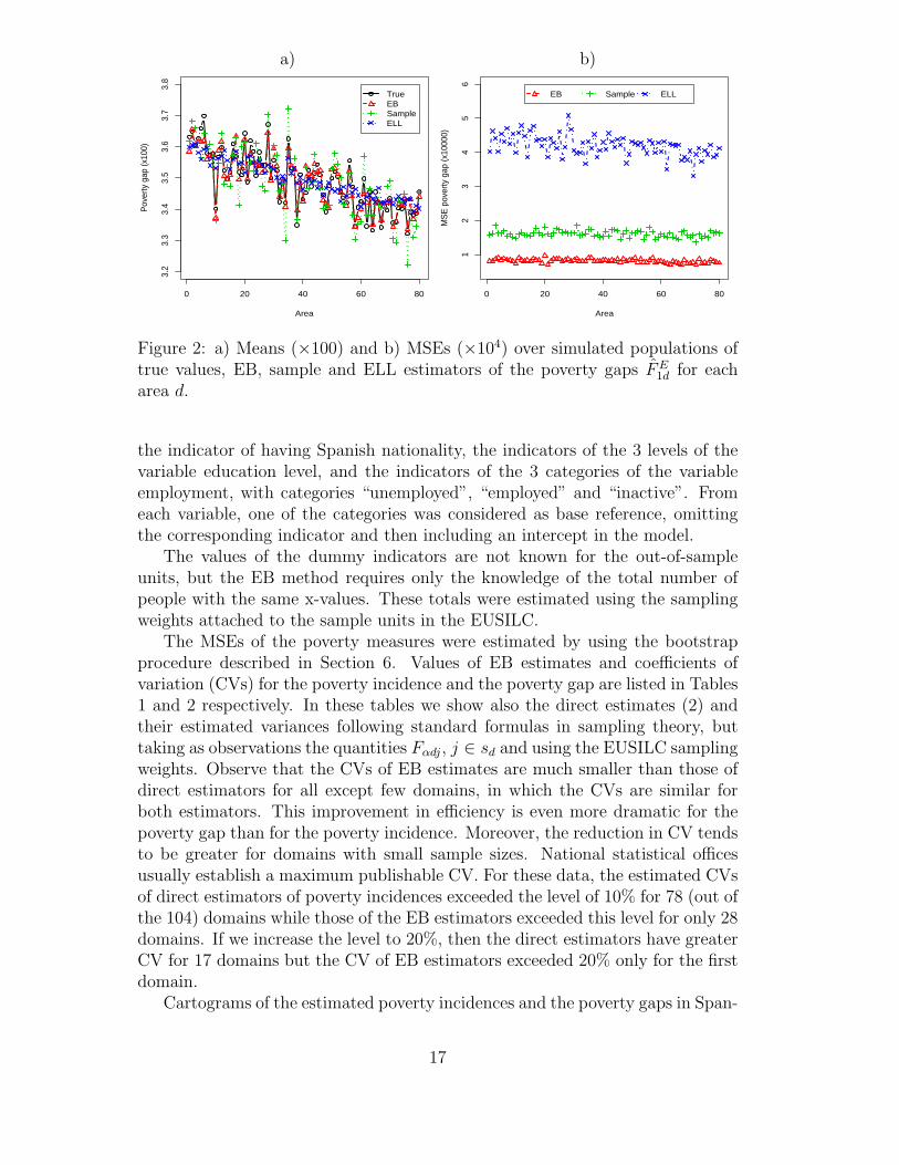
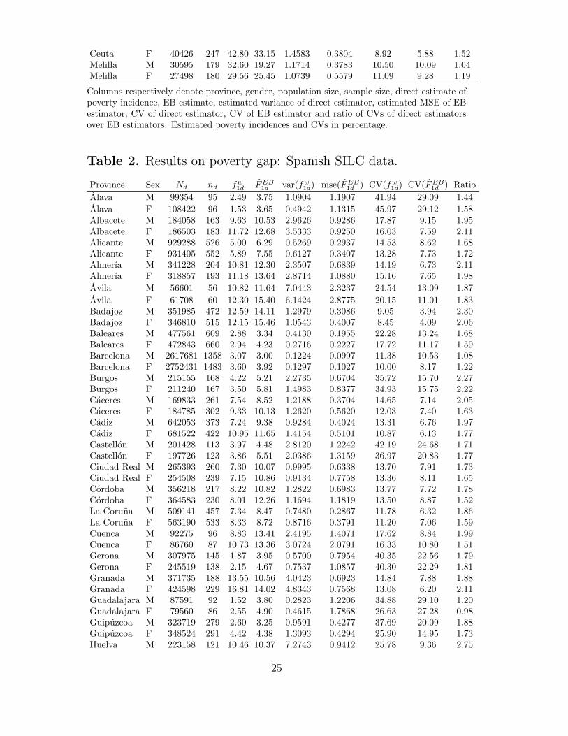
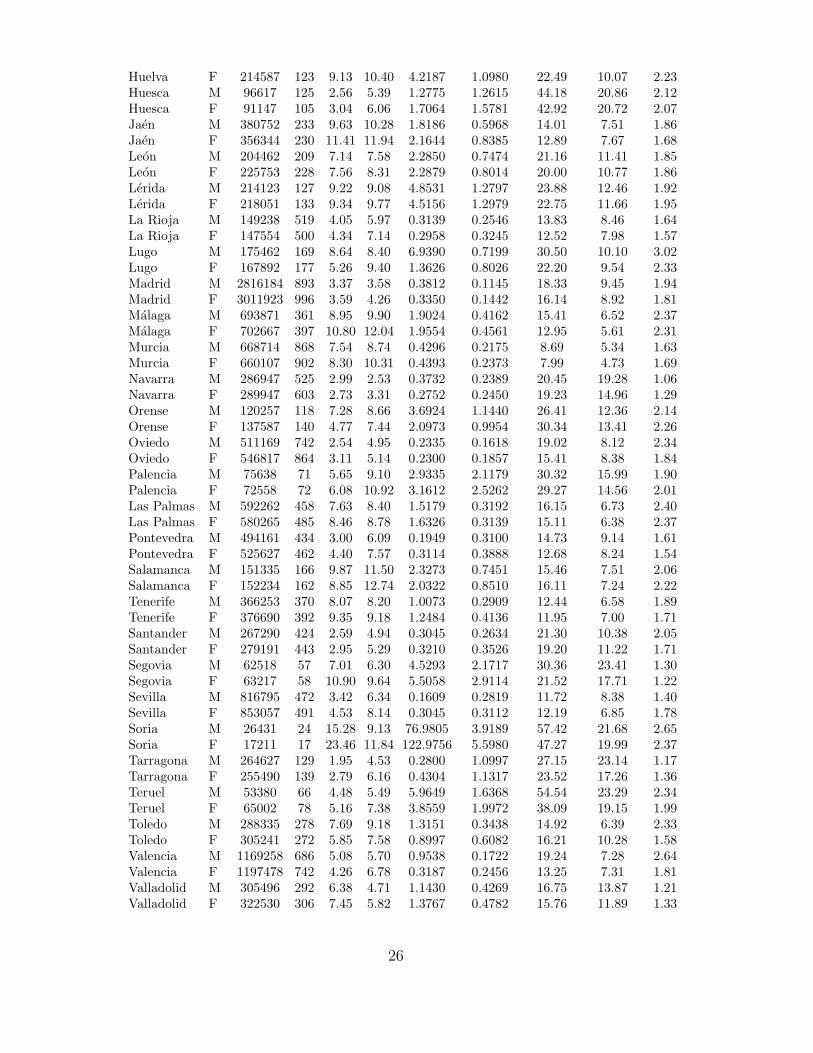
The MSEs of the poverty measures were estimated by using the bootstrapprocedure described in Section 6. Values of EB estimates and coefficients ofvariation (CVs) for the poverty incidence and the poverty gap are listed in Tables1 and 2 respectively. In these tables we show also the direct estimates (2) andtheir estimated variances following standard formulas in sampling theory, buttaking as observations the quantities Fαdj, j ∈ sd and using the EUSILC samplingweights. Observe that the CVs of EB estimates are much smaller than those ofdirect estimators for all except few domains, in which the CVs are similar forboth estimators. This improvement in efficiency is even more dramatic for thepoverty gap than for the poverty incidence. Moreover, the reduction in CV tendsto be greater for domains with small sample sizes. National statistical officesusually establish a maximum publishable CV. For these data, the estimated CVsof direct estimators of poverty incidences exceeded the level of 10% for 78 (out ofthe 104) domains while those of the EB estimators exceeded this level for only 28domains. If we increase the level to 20%, then the direct estimators have greaterCV for 17 domains but the CV of EB estimators exceeded 20% only for the firstdomain.

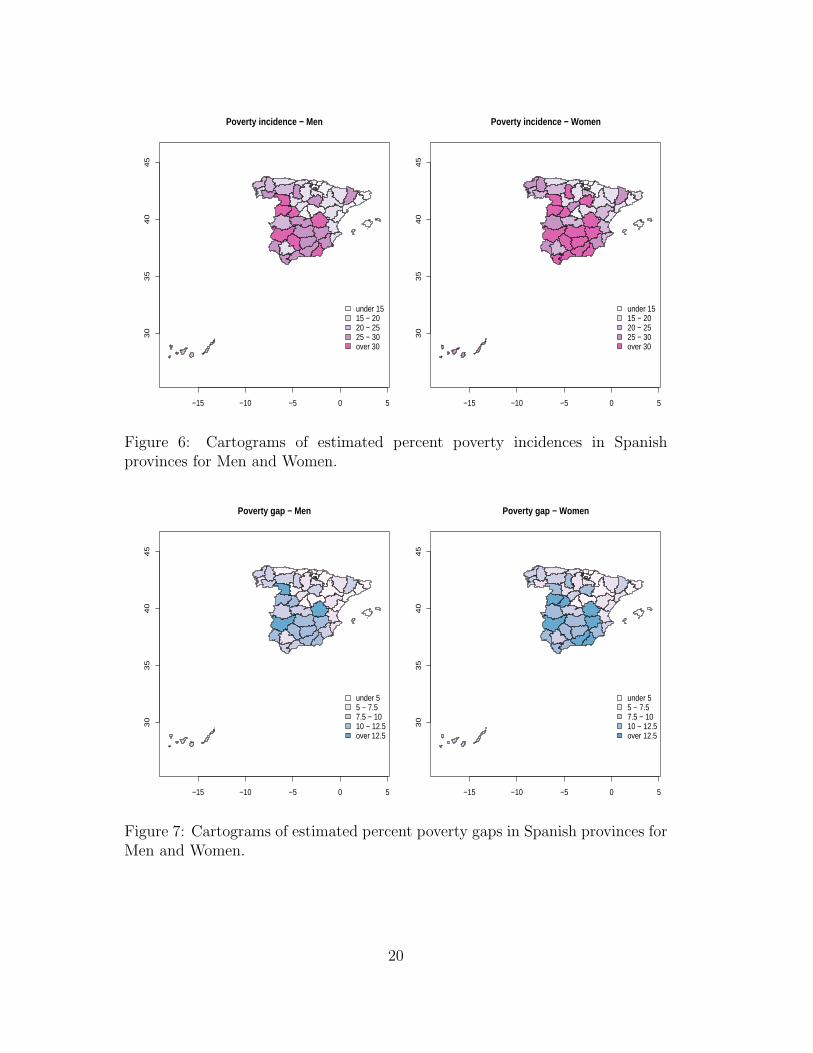
Cartograms of the estimated poverty incidences and the poverty gaps in Span-

17

a)

0 20 40 60 80

10.0

10.2

10.4

10.6

10.8

Area

MS

E P

over

ty in

cide

nce

(x10

000)

True MSEBootstrap MSE

b)

0 20 40 60 80

0.78

0.80

0.82

0.84

0.86

Area

MS

E P

over

ty g

ap (x

1000

0)

True MSEBootstrap MSE

Figure 3: True MSEs (×104) of EB predictors and bootstrap MSE estimateswith B = 500 for each area d: a) Poverty incidence, b) Poverty gap.

ish provinces for males and females have been constructed using the EB esti-mates, see Figures 6 and 7. In these maps we can see that the poorer provincesconcentrate mainly in the south and west parts of Spain. Provinces with criticalpoverty incidences (over 30%) for men are, in the south: Almerıa and Cordoba;west: Badajoz, Avila, Salamanza and Zamora and then Cuenca, situated east ofMadrid. For women the poverty incidences increase in most provinces, becomingcritical also, in the south: Granada, Jaen, Albacete and Ciudad Real, and inthe north: Palencia and Soria. The poverty level for Lerida (north-east) seemsunexpected considering that this province belongs to the region of Catalonia,which is commonly considered as a rich region.

The poverty gap measures the degree of poverty instead of the quantity ofpeople under poverty. For a region with many people whose income is under thepoverty line but very close to it, the poverty gap will be close to zero. Observethat the provinces with an income of over 12.5% under the poverty line arealso among those provinces with critical values of poverty incidence, except forthe northern provinces such as Lerida, which do not have significant gaps incomparison with the rest of the provinces.

11 Conclusions

In this paper Empirical Best (EB) methodology to estimate poverty measuresis proposed. Parametric bootstrap is used for mean squared error (MSE) es-timation. Simulation results show the good performance of EB estimators incomparison with the direct and the ELL estimators. Simulation results confirmthe discussion that the ELL estimator is basically a synthetic-type estimatorderived from a linear regression model.

Model (17) illustrates a parallelism between ELL and EB methods. When

18

0 20 40 60 80

510

1520

2530

35

Area

Pove

rty in

ciden

ce (x

100)

TrueEBSampleELL

Figure 4: Means (×100) over Monte Carlo samples of true values, EB, sampleand ELL estimators of the poverty incidence F0d for each area d.

0 20 40 60 80

050

100

150

200

250

300

Area

MSE

pove

rty in

ciden

ce (x

1000

0)

EBSampleELL

Figure 5: MSEs (×104) over Monte Carlo samples of EB, sample and ELL esti-mators of the poverty incidence F0d for each area d.

19

−15 −10 −5 0 5

30

35

40

45

Poverty incidence − Men

under 1515 − 2020 − 2525 − 30over 30

−15 −10 −5 0 5

30

35

40

45

Poverty incidence − Women

under 1515 − 2020 − 2525 − 30over 30

Figure 6: Cartograms of estimated percent poverty incidences in Spanishprovinces for Men and Women.

−15 −10 −5 0 5

30

35

40

45

Poverty gap − Men

under 55 − 7.57.5 − 1010 − 12.5over 12.5

−15 −10 −5 0 5

30

35

40

45

Poverty gap − Women

under 55 − 7.57.5 − 1010 − 12.5over 12.5

Figure 7: Cartograms of estimated percent poverty gaps in Spanish provinces forMen and Women.

20

the clusters in the ELL method are taken to be equal to the small areas, theELL method generates a full population or census file of responses Ydj from thebootstrap model (23) with v∗

c = v∗d. Then the poverty measure is calculated from

this census file. The procedure is repeated a large number of times and finally thecomputed poverty measures are averaged over bootstrap replications. The EBmethod also creates a new census file, but first plugging in the observed sampleelements Ydj in their corresponding place, and then generating only the non-sample values from the conditional model (17). The main difference betweenmodel (17) and bootstrap model (23) used for the ELL method is the termσ2

u1Nd−nd1′

ndV−1

ds (ys−Xsβ) appearing in the conditional mean given in (16). Therest of the procedure is the same as in the ELL method. Thus, this term makesan improvement for areas that are not fully explained by auxiliary variables andtherefore reduces the MSE of estimators significantly.

We remark that EB is a model-based method that relies on the validity ofthe model. Thus, model selection procedures and model diagnostics are essentialin the practical application of this methodology.

References

Ballini, F., Betti, G. and Neri, L. (2006). Poverty and inequality mapping inthe Commonwealth of Dominica. Preprint.

Battese, G. E., Harter, R. M. and Fuller, W. A. (1988). An Error-ComponentsModel for Prediction of County Crop Areas Using Survey and SatelliteData. Journal of the American Statistical Association, 83, 28–36.

Bell, W. (1997). Models for county and state poverty estimates. Preprint,Census Statistical Research Division.

Elbers, C., Lanjouw, J. O. and Lanjouw, P. (2003). Micro-level estimation ofpoverty and inequality. Econometrica, 71, 355–364.

Fay, R. E. and Herriot, R. A. (1979). Estimation of income from small places:An application of James-Stein procedures to census data. Journal of theAmerican Statistical Association, 74, 269–277.

Foster, J., Greer, J. and Thorbecke, E. (1984). A class of decomposable povertymeasures, Econometrica, 52, 761–766.

Gonzalez-Manteiga, W., Lombardıa, M. J., Molina, I., Morales, D. and Santa-marıa, L. (2008). Journal of Statistical Computation and Simulation, 75,443–462.

Hall, P. and Maiti, T. (2006). On Parametric Bootstrap Methods for SmallArea Prediction. Journal Royal Statistical Society, Series B, 68, 221–238.

21

Haslett, S. and Jones, G. (2005). Small area estimation using surveys and somepractical and statistical issues. Statistics in Transition, 7, 541–555.

Neri, L., Ballini, F. and Betti, G. (2005). Poverty and inequality in transitioncountries. Statistics in Transition, 7, 135–157.

Pfeffermann, D., Skinner, C. J., Holmes, D. J., Goldstein, H. and Rasbash, J.(1998). Weighting in Unequal Probabilities in Multilevel Models. Journalof the Royal Statistical Society B, 60, 23–40.

Rao, J. N. K. (2003). Small Area Estimation. London: Wiley.

Royall, R. M. (1976). The Linear Least Squares Prediction Approach to Two-Stage Sampling, Journal of the American Statistical Association, 71, 657–664.

Tarozzi, A. and Deaton, A. (2007). Using census and survey data to estimatepoverty and inequality for small areas. Preprint.

22

Application results

Table 1. Results on poverty incidence: Spanish SILC data.

Province Sex Nd nd fw

0dFEB

0dvar(fw

0d) mse(FEB

0d) CV(fw

0d) CV(FEB

0d) Ratio

Alava M 99354 95 7.10 12.84 0.6751 0.6805 36.60 20.32 1.80

Alava F 108422 96 14.60 12.50 1.5637 0.6000 27.08 19.60 1.38Albacete M 184058 163 30.11 29.22 1.0801 0.4617 10.92 7.35 1.48Albacete F 186503 183 30.58 33.74 1.1558 0.4618 11.12 6.37 1.75Alicante M 929288 526 17.96 19.45 0.2793 0.1466 9.31 6.23 1.49Alicante F 931405 552 17.95 22.59 0.2482 0.1601 8.78 5.60 1.57Almerıa M 341228 204 35.34 32.88 1.3701 0.3642 10.47 5.80 1.80Almerıa F 318857 193 33.54 35.72 1.1329 0.5020 10.04 6.27 1.60

Avila M 56601 56 20.85 31.48 2.5112 1.2061 24.03 11.03 2.18

Avila F 61708 60 20.42 38.51 2.4398 1.3285 24.19 9.46 2.56Badajoz M 351985 472 31.97 36.56 0.5177 0.1703 7.12 3.57 1.99Badajoz F 346810 515 34.90 39.13 0.4958 0.1947 6.38 3.57 1.79Baleares M 477561 609 12.76 11.55 0.2297 0.1042 11.88 8.84 1.34Baleares F 472843 660 15.57 14.05 0.2228 0.1130 9.59 7.57 1.27Barcelona M 2617681 1358 9.82 10.49 0.0569 0.0524 7.68 6.90 1.11Barcelona F 2752431 1483 11.80 13.10 0.0619 0.0494 6.67 5.37 1.24Burgos M 215155 168 15.35 16.72 0.7776 0.3736 18.16 11.56 1.57Burgos F 211240 167 17.82 18.33 0.8419 0.4097 16.28 11.04 1.47Caceres M 169833 261 33.20 24.69 0.8999 0.2099 9.04 5.87 1.54Caceres F 184785 302 41.91 28.24 0.9402 0.2689 7.32 5.81 1.26Cadiz M 642053 373 34.75 26.88 0.5629 0.2013 6.83 5.28 1.29Cadiz F 681522 422 35.92 31.63 0.5660 0.2316 6.62 4.81 1.38Castellon M 201428 113 18.03 14.79 1.1401 0.6489 18.73 17.22 1.09Castellon F 197726 123 17.71 17.35 1.2807 0.6008 20.21 14.13 1.43Ciudad Real M 265393 260 27.97 28.39 0.8795 0.3060 10.60 6.16 1.72Ciudad Real F 254508 239 33.82 30.18 0.9979 0.3598 9.34 6.29 1.49Cordoba M 356218 217 37.15 30.16 1.0097 0.3636 8.55 6.32 1.35Cordoba F 364583 230 41.55 33.32 0.9769 0.5025 7.52 6.73 1.12La Coruna M 509141 457 22.89 24.66 0.3935 0.1549 8.67 5.05 1.72La Coruna F 563190 533 19.36 25.36 0.2888 0.1789 8.78 5.27 1.66Cuenca M 92275 96 35.91 35.26 3.2294 0.6676 15.82 7.33 2.16Cuenca F 86760 87 43.95 35.35 3.0522 0.9183 12.57 8.57 1.47Gerona M 307975 145 11.23 13.29 0.6006 0.4512 21.83 15.98 1.37Gerona F 245519 138 11.38 15.38 0.5847 0.5672 21.25 15.48 1.37Granada M 371735 188 31.53 29.16 0.8038 0.3423 8.99 6.35 1.42Granada F 424598 229 35.74 36.34 0.8358 0.3340 8.09 5.03 1.61Guadalajara M 87591 92 13.53 12.74 0.9309 0.6339 22.55 19.76 1.14Guadalajara F 79560 86 16.77 15.83 1.1738 0.9055 20.43 19.01 1.08Guipuzcoa M 323719 279 10.10 11.30 0.3226 0.2488 17.79 13.96 1.27Guipuzcoa F 348524 291 11.70 14.56 0.3297 0.2250 15.52 10.30 1.51Huelva M 223158 121 34.24 29.06 1.6956 0.4976 12.03 7.68 1.57Huelva F 214587 123 30.95 29.13 1.5825 0.5606 12.85 8.13 1.58Huesca M 96617 125 11.67 17.11 0.8957 0.6126 25.64 14.47 1.77Huesca F 91147 105 14.44 18.99 1.1769 0.8048 23.76 14.94 1.59Jaen M 380752 233 24.11 28.60 0.8679 0.2878 12.22 5.93 2.06Jaen F 356344 230 24.76 32.31 0.8523 0.4010 11.79 6.20 1.90Leon M 204462 209 18.96 22.60 0.7566 0.3772 14.51 8.59 1.69Leon F 225753 228 20.69 24.17 0.7933 0.3639 13.62 7.89 1.72

23

Lerida M 214123 127 16.82 25.74 1.2317 0.6116 20.87 9.61 2.17Lerida F 218051 133 15.57 27.36 1.0677 0.5777 20.98 8.79 2.39La Rioja M 149238 519 16.75 18.57 0.3618 0.1383 11.36 6.33 1.79La Rioja F 147554 500 18.50 21.45 0.3613 0.1557 10.27 5.82 1.77Lugo M 175462 169 32.68 24.51 1.4726 0.3914 11.74 8.07 1.45Lugo F 167892 177 30.17 26.87 1.3821 0.4034 12.32 7.47 1.65Madrid M 2816184 893 7.95 12.06 0.0513 0.0619 9.01 6.52 1.38Madrid F 3011923 996 9.36 13.91 0.0527 0.0704 7.76 6.04 1.29Malaga M 693871 361 18.96 27.95 0.5823 0.2031 12.73 5.10 2.50Malaga F 702667 397 22.88 32.45 0.5375 0.2190 10.13 4.56 2.22Murcia M 668714 868 23.83 25.35 0.2471 0.1027 6.60 4.00 1.65Murcia F 660107 902 23.67 28.70 0.2371 0.1087 6.50 3.63 1.79Navarra M 286947 525 11.03 9.13 0.1812 0.1405 12.21 12.98 0.94Navarra F 289947 603 12.98 11.40 0.2185 0.1211 11.39 9.66 1.18Orense M 120257 118 24.94 25.07 1.3845 0.5993 14.92 9.77 1.53Orense F 137587 140 21.27 22.12 1.0968 0.4809 15.57 9.92 1.57Oviedo M 511169 742 12.26 16.01 0.1823 0.0824 11.01 5.67 1.94Oviedo F 546817 864 12.56 16.59 0.1464 0.0893 9.63 5.70 1.69Palencia M 75638 71 27.29 26.16 2.3375 1.0455 17.72 12.36 1.43Palencia F 72558 72 30.63 30.13 2.5426 1.0907 16.46 10.96 1.50Las Palmas M 592262 458 24.45 24.65 0.5337 0.1615 9.45 5.16 1.83Las Palmas F 580265 485 29.76 25.40 0.5325 0.1520 7.75 4.85 1.60Pontevedra M 494161 434 13.03 19.15 0.2430 0.1620 11.97 6.64 1.80Pontevedra F 525627 462 15.69 22.66 0.2803 0.1865 10.67 6.03 1.77Salamanca M 151335 166 26.92 31.46 1.2025 0.3862 12.88 6.25 2.06Salamanca F 152234 162 31.58 33.56 1.3392 0.4030 11.59 5.98 1.94Tenerife M 366253 370 17.63 24.14 0.3997 0.1590 11.34 5.22 2.17Tenerife F 376690 392 17.07 26.36 0.3078 0.2006 10.28 5.37 1.91Santander M 267290 424 8.79 16.00 0.1586 0.1398 14.33 7.39 1.94Santander F 279191 443 12.65 16.93 0.2339 0.1678 12.09 7.65 1.58Segovia M 62518 57 39.16 19.24 3.7441 1.0910 15.63 17.17 0.91Segovia F 63217 58 47.03 26.74 3.7211 1.2032 12.97 12.97 1.00Sevilla M 816795 472 22.06 19.61 0.2737 0.1575 7.50 6.40 1.17Sevilla F 853057 491 28.07 24.04 0.3173 0.1493 6.35 5.08 1.25Soria M 26431 24 23.68 26.33 8.0523 2.0666 37.89 17.26 2.19Soria F 17211 17 26.73 31.48 11.6416 2.7052 40.37 16.52 2.44Tarragona M 264627 129 12.96 14.86 0.6612 0.5761 19.85 16.15 1.23Tarragona F 255490 139 16.19 19.28 0.6499 0.5197 15.75 11.82 1.33Teruel M 53380 66 12.43 17.13 1.0073 0.8420 25.53 16.94 1.51Teruel F 65002 78 16.22 22.26 1.3288 1.0112 22.48 14.29 1.57Toledo M 288335 278 23.86 26.22 0.6157 0.1871 10.40 5.22 1.99Toledo F 305241 272 20.56 22.50 0.5188 0.2784 11.08 7.42 1.49Valencia M 1169258 686 17.53 17.89 0.1995 0.0940 8.06 5.42 1.49Valencia F 1197478 742 19.64 20.78 0.1978 0.1162 7.16 5.19 1.38Valladolid M 305496 292 14.98 15.34 0.4731 0.2216 14.52 9.70 1.50Valladolid F 322530 306 18.59 18.29 0.4771 0.2352 11.75 8.38 1.40Vizcaya M 576042 515 9.08 10.01 0.1458 0.1267 13.30 11.24 1.18Vizcaya F 590094 532 10.26 11.57 0.1753 0.1175 12.91 9.37 1.38Zamora M 101433 109 36.14 34.67 2.6728 0.7388 14.30 7.84 1.82Zamora F 98337 100 36.53 32.84 2.3562 0.7964 13.29 8.59 1.55Zaragoza M 466651 555 10.64 15.42 0.2081 0.1232 13.55 7.20 1.88Zaragoza F 462937 574 10.22 15.34 0.1435 0.0989 11.72 6.48 1.81Ceuta M 35705 223 40.87 30.26 1.5506 0.3482 9.63 6.17 1.56

24

Ceuta F 40426 247 42.80 33.15 1.4583 0.3804 8.92 5.88 1.52Melilla M 30595 179 32.60 19.27 1.1714 0.3783 10.50 10.09 1.04Melilla F 27498 180 29.56 25.45 1.0739 0.5579 11.09 9.28 1.19

Columns respectively denote province, gender, population size, sample size, direct estimate ofpoverty incidence, EB estimate, estimated variance of direct estimator, estimated MSE of EBestimator, CV of direct estimator, CV of EB estimator and ratio of CVs of direct estimatorsover EB estimators. Estimated poverty incidences and CVs in percentage.

Table 2. Results on poverty gap: Spanish SILC data.

Province Sex Nd nd fw

1dFEB

1dvar(fw

1d) mse(FEB

1d) CV(fw

1d) CV(FEB

1d) Ratio

Alava M 99354 95 2.49 3.75 1.0904 1.1907 41.94 29.09 1.44

Alava F 108422 96 1.53 3.65 0.4942 1.1315 45.97 29.12 1.58Albacete M 184058 163 9.63 10.53 2.9626 0.9286 17.87 9.15 1.95Albacete F 186503 183 11.72 12.68 3.5333 0.9250 16.03 7.59 2.11Alicante M 929288 526 5.00 6.29 0.5269 0.2937 14.53 8.62 1.68Alicante F 931405 552 5.89 7.55 0.6127 0.3407 13.28 7.73 1.72Almerıa M 341228 204 10.81 12.30 2.3507 0.6839 14.19 6.73 2.11Almerıa F 318857 193 11.18 13.64 2.8714 1.0880 15.16 7.65 1.98

Avila M 56601 56 10.82 11.64 7.0443 2.3237 24.54 13.09 1.87

Avila F 61708 60 12.30 15.40 6.1424 2.8775 20.15 11.01 1.83Badajoz M 351985 472 12.59 14.11 1.2979 0.3086 9.05 3.94 2.30Badajoz F 346810 515 12.15 15.46 1.0543 0.4007 8.45 4.09 2.06Baleares M 477561 609 2.88 3.34 0.4130 0.1955 22.28 13.24 1.68Baleares F 472843 660 2.94 4.23 0.2716 0.2227 17.72 11.17 1.59Barcelona M 2617681 1358 3.07 3.00 0.1224 0.0997 11.38 10.53 1.08Barcelona F 2752431 1483 3.60 3.92 0.1297 0.1027 10.00 8.17 1.22Burgos M 215155 168 4.22 5.21 2.2735 0.6704 35.72 15.70 2.27Burgos F 211240 167 3.50 5.81 1.4983 0.8377 34.93 15.75 2.22Caceres M 169833 261 7.54 8.52 1.2188 0.3704 14.65 7.14 2.05Caceres F 184785 302 9.33 10.13 1.2620 0.5620 12.03 7.40 1.63Cadiz M 642053 373 7.24 9.38 0.9284 0.4024 13.31 6.76 1.97Cadiz F 681522 422 10.95 11.65 1.4154 0.5101 10.87 6.13 1.77Castellon M 201428 113 3.97 4.48 2.8120 1.2242 42.19 24.68 1.71Castellon F 197726 123 3.86 5.51 2.0386 1.3159 36.97 20.83 1.77Ciudad Real M 265393 260 7.30 10.07 0.9995 0.6338 13.70 7.91 1.73Ciudad Real F 254508 239 7.15 10.86 0.9134 0.7758 13.36 8.11 1.65Cordoba M 356218 217 8.22 10.82 1.2822 0.6983 13.77 7.72 1.78Cordoba F 364583 230 8.01 12.26 1.1694 1.1819 13.50 8.87 1.52La Coruna M 509141 457 7.34 8.47 0.7480 0.2867 11.78 6.32 1.86La Coruna F 563190 533 8.33 8.72 0.8716 0.3791 11.20 7.06 1.59Cuenca M 92275 96 8.83 13.41 2.4195 1.4071 17.62 8.84 1.99Cuenca F 86760 87 10.73 13.36 3.0724 2.0791 16.33 10.80 1.51Gerona M 307975 145 1.87 3.95 0.5700 0.7954 40.35 22.56 1.79Gerona F 245519 138 2.15 4.67 0.7537 1.0857 40.30 22.29 1.81Granada M 371735 188 13.55 10.56 4.0423 0.6923 14.84 7.88 1.88Granada F 424598 229 16.81 14.02 4.8343 0.7568 13.08 6.20 2.11Guadalajara M 87591 92 1.52 3.80 0.2823 1.2206 34.88 29.10 1.20Guadalajara F 79560 86 2.55 4.90 0.4615 1.7868 26.63 27.28 0.98Guipuzcoa M 323719 279 2.60 3.25 0.9591 0.4277 37.69 20.09 1.88Guipuzcoa F 348524 291 4.42 4.38 1.3093 0.4294 25.90 14.95 1.73Huelva M 223158 121 10.46 10.37 7.2743 0.9412 25.78 9.36 2.75

25

Huelva F 214587 123 9.13 10.40 4.2187 1.0980 22.49 10.07 2.23Huesca M 96617 125 2.56 5.39 1.2775 1.2615 44.18 20.86 2.12Huesca F 91147 105 3.04 6.06 1.7064 1.5781 42.92 20.72 2.07Jaen M 380752 233 9.63 10.28 1.8186 0.5968 14.01 7.51 1.86Jaen F 356344 230 11.41 11.94 2.1644 0.8385 12.89 7.67 1.68Leon M 204462 209 7.14 7.58 2.2850 0.7474 21.16 11.41 1.85Leon F 225753 228 7.56 8.31 2.2879 0.8014 20.00 10.77 1.86Lerida M 214123 127 9.22 9.08 4.8531 1.2797 23.88 12.46 1.92Lerida F 218051 133 9.34 9.77 4.5156 1.2979 22.75 11.66 1.95La Rioja M 149238 519 4.05 5.97 0.3139 0.2546 13.83 8.46 1.64La Rioja F 147554 500 4.34 7.14 0.2958 0.3245 12.52 7.98 1.57Lugo M 175462 169 8.64 8.40 6.9390 0.7199 30.50 10.10 3.02Lugo F 167892 177 5.26 9.40 1.3626 0.8026 22.20 9.54 2.33Madrid M 2816184 893 3.37 3.58 0.3812 0.1145 18.33 9.45 1.94Madrid F 3011923 996 3.59 4.26 0.3350 0.1442 16.14 8.92 1.81Malaga M 693871 361 8.95 9.90 1.9024 0.4162 15.41 6.52 2.37Malaga F 702667 397 10.80 12.04 1.9554 0.4561 12.95 5.61 2.31Murcia M 668714 868 7.54 8.74 0.4296 0.2175 8.69 5.34 1.63Murcia F 660107 902 8.30 10.31 0.4393 0.2373 7.99 4.73 1.69Navarra M 286947 525 2.99 2.53 0.3732 0.2389 20.45 19.28 1.06Navarra F 289947 603 2.73 3.31 0.2752 0.2450 19.23 14.96 1.29Orense M 120257 118 7.28 8.66 3.6924 1.1440 26.41 12.36 2.14Orense F 137587 140 4.77 7.44 2.0973 0.9954 30.34 13.41 2.26Oviedo M 511169 742 2.54 4.95 0.2335 0.1618 19.02 8.12 2.34Oviedo F 546817 864 3.11 5.14 0.2300 0.1857 15.41 8.38 1.84Palencia M 75638 71 5.65 9.10 2.9335 2.1179 30.32 15.99 1.90Palencia F 72558 72 6.08 10.92 3.1612 2.5262 29.27 14.56 2.01Las Palmas M 592262 458 7.63 8.40 1.5179 0.3192 16.15 6.73 2.40Las Palmas F 580265 485 8.46 8.78 1.6326 0.3139 15.11 6.38 2.37Pontevedra M 494161 434 3.00 6.09 0.1949 0.3100 14.73 9.14 1.61Pontevedra F 525627 462 4.40 7.57 0.3114 0.3888 12.68 8.24 1.54Salamanca M 151335 166 9.87 11.50 2.3273 0.7451 15.46 7.51 2.06Salamanca F 152234 162 8.85 12.74 2.0322 0.8510 16.11 7.24 2.22Tenerife M 366253 370 8.07 8.20 1.0073 0.2909 12.44 6.58 1.89Tenerife F 376690 392 9.35 9.18 1.2484 0.4136 11.95 7.00 1.71Santander M 267290 424 2.59 4.94 0.3045 0.2634 21.30 10.38 2.05Santander F 279191 443 2.95 5.29 0.3210 0.3526 19.20 11.22 1.71Segovia M 62518 57 7.01 6.30 4.5293 2.1717 30.36 23.41 1.30Segovia F 63217 58 10.90 9.64 5.5058 2.9114 21.52 17.71 1.22Sevilla M 816795 472 3.42 6.34 0.1609 0.2819 11.72 8.38 1.40Sevilla F 853057 491 4.53 8.14 0.3045 0.3112 12.19 6.85 1.78Soria M 26431 24 15.28 9.13 76.9805 3.9189 57.42 21.68 2.65Soria F 17211 17 23.46 11.84 122.9756 5.5980 47.27 19.99 2.37Tarragona M 264627 129 1.95 4.53 0.2800 1.0997 27.15 23.14 1.17Tarragona F 255490 139 2.79 6.16 0.4304 1.1317 23.52 17.26 1.36Teruel M 53380 66 4.48 5.49 5.9649 1.6368 54.54 23.29 2.34Teruel F 65002 78 5.16 7.38 3.8559 1.9972 38.09 19.15 1.99Toledo M 288335 278 7.69 9.18 1.3151 0.3438 14.92 6.39 2.33Toledo F 305241 272 5.85 7.58 0.8997 0.6082 16.21 10.28 1.58Valencia M 1169258 686 5.08 5.70 0.9538 0.1722 19.24 7.28 2.64Valencia F 1197478 742 4.26 6.78 0.3187 0.2456 13.25 7.31 1.81Valladolid M 305496 292 6.38 4.71 1.1430 0.4269 16.75 13.87 1.21Valladolid F 322530 306 7.45 5.82 1.3767 0.4782 15.76 11.89 1.33

26

Vizcaya M 576042 515 2.57 2.80 0.2783 0.2338 20.49 17.27 1.19Vizcaya F 590094 532 2.26 3.35 0.1756 0.2177 18.56 13.92 1.33Zamora M 101433 109 12.58 13.10 5.5333 1.5147 18.71 9.40 1.99Zamora F 98337 100 9.86 12.18 4.7252 1.7185 22.04 10.76 2.05Zaragoza M 466651 555 4.29 4.77 0.7891 0.2377 20.69 10.23 2.02Zaragoza F 462937 574 5.08 4.72 0.9837 0.1956 19.53 9.38 2.08Ceuta M 35705 223 14.79 11.09 3.3694 0.7296 12.41 7.70 1.61Ceuta F 40426 247 20.68 12.52 5.5107 0.8832 11.35 7.50 1.51Melilla M 30595 179 11.87 6.22 7.3207 0.7442 22.80 13.86 1.64Melilla F 27498 180 12.47 8.82 3.5770 1.1392 15.16 12.10 1.25

Columns respectively denote province, gender, population size, sample size, direct estimateof poverty gap, EB estimate, estimated variance of direct estimator, estimated MSE of EBestimator, CV of direct estimator, CV of EB estimator and ratio of CVs of direct estimatorsover EB estimators. Estimated poverty gaps and CVs in percentage.

27