arX

iv:h

ep-p

h/95

1234

4v2

25

Jun

1996

Small–Angle Electron–Positron Scattering

with a Per Mille Accuracy1

A.B. Arbuzov a, V.S. Fadin b, E.A. Kuraev a, L.N. Lipatov c, N.P. Merenkov d

and

L. Trentadue e23

a Joint Institute for Nuclear Research

Dubna, Moscow region, 141980, Russia

b Budker Institute for Nuclear Physics

Novosibirsk State University, 630090, Novosibirsk, Russia

c St.-Petersburg Institute of Nuclear Physics

Gatchina, Leningrad region, 188350, Russia

d Institute of Physics and Technology, Kharkov, 310108, Ukraine

e Theoretical Physics Division, CERN,

CH–1211 Geneva 23, Switzerland

Abstract

The elastic and inelastic high–energy small–angle electron–positron scattering is con-sidered. All radiative corrections to the cross–section with the relative accuracy δσ/σ =0.1% are explicitly taken into account. According to the generalized eikonal representa-tion for the elastic amplitude, in higher orders only diagrams with one exchanged photonmay be considered. Single photon emission with radiative corrections and next–to–leading two–photon and pair production diagrams are evaluated, together with leadingthree–loop corrections. All contributions have been calculated analytically. We integratethe calculated distributions over typical for LEP 1 experiments intervals of angles andenergies. To the leading approximation, the results are shown to be described in termsof kernels of electron structure functions. Some numerical results are presented.

PACS numbers 12.15.Lk, 12.20.-m, 12.20.Ds, 13.40.-f

1Work supported by the Istituto Nazionale di Fisica Nucleare (INFN). INTAS Grant 1867–93.2On leave from Dipartimento di Fisica, Universita di Parma, Parma, Italy.3INFN, Gruppo Collegato di Parma, Parma, Italy.

1 Introduction

An accurate verification of the Standard Model is one of the primary aims of LEP [1]. Whileelectroweak radiative corrections to the s-channel annihilation process and to large–angleBhabha scattering allow a direct extraction of the Standard Model parameters, small an-gle Bhabha cross–section affects, as an overall normalization condition, all observable cross–sections and represents an equally unavoidable condition toward a precise determination ofthe Standard Model parameters. The small–angle Bhabha scattering process is used to mea-sure the luminosity of electron–positron colliders. At LEP an experimental accuracy on theluminosity of

|δσσ| < 0.001 (1)

has been reached [2]. However, to obtain the total accuracy, a systematic theoretical errormust also be added. This precision calls for an equally accurate theoretical expression for theBhabha scattering cross–section in order to extract the Standard Model parameters from theobserved distributions. An accurate determination of the small–angle Bhabha cross–sectionand of the luminosity directly affects the determination of absolute cross–sections such as,for example, the determination of the invisible width and of the number of massless neutrinospecies Nν [3].

In recent years a considerable attention has been devoted to the Bhabha process [4, 5, 6].The reached accuracy is however still inadequate [2]. According to these evaluations thetheoretical estimates are still incomplete; moreover, they are somewhat larger (∼ a factor2) than the projected theoretical and experimental precision [2] and are comparable to thecurrently published experimental precision.

The process that will be considered in this work is that of Bhabha scattering when electronsand positrons are emitted at small angles with respect to the initial electron and positrondirections. We have examined the radiative processes inclusively accompanying the maine+e−→ e+e− reaction at high energies, when both the scattered electron and positron aretagged within the counter aperture.

We assume that the center-of-mass energies are within the range of the LEP collider 2ǫ =√s = 90 – 200 GeV and the scattering angles are within the range θ ≃ 10 – 150 mrad. We

assume that the charged-particle detectors have the following polar angle cuts:

θ1 < θ− = p1q1 ≡ θ < θ3, θ2 < θ+ = p2q2 < θ4, 0.01 <∼ θi <∼ 0.1 rad , (2)

where p1, q1 (p2, q2 ) are the momenta of the initial and of the scattered electron (positron)in the center-of-mass frame.

In this paper we present the results of our calculations of the electron–positron scatteringcross–section with an accuracy of O(0.1%). The squared matrix elements of the variousexclusive processes inclusively contributing to the e+e− → e+e− reaction are integrated inorder to define an experimentally measurable cross–section according to suitable restrictionson the angles and energies of the detected particles. The different contributions to the electronand positron distributions, needed for the required accuracy, are presented using analyticalexpressions.

In order to define the angular range of interest and the implications on the required ac-curacy, let us first briefly discuss, in a general way, the angle-dependent corrections to thecross–section.

We consider e+e− scattering at angles as defined in Eq. (2). Within this region, if oneexpresses the cross–section by means of a series expansion in terms of angles, the main con-tribution to the cross–section dσ/dθ2 comes from the diagrams for the scattering amplitudescontaining one exchanged photon in the t-channel. These diagrams, as well known, show asingularity of the type θ−4 for θ → 0, e.g.

dσ

dθ2∼ θ−4 .

Let us now estimate the correction of order θ2 to this contribution. If

dσ

dθ2∼ θ−4(1 + c1θ

2) , (3)

then, after integration over θ2 in the angular range of Eq. (2), we obtain:

θ2max∫

θ2min

dσ

dθ2dθ2 ∼ θ−2

min(1 + c1θ

2min

lnθ2

max

θ2min

). (4)

We see that, for θmin = 50 mrad and θmax = 150 mrad (we have taken the case where theθ2 corrections are maximal), the relative contribution of the θ2 terms is about 5 × 10−3c1.Therefore, the terms of relative order θ2 must be kept only in the Born cross–section wherethe coefficient c1 is not small. In higher orders of the perturbative expansion the coefficientc1 contains at least one factor α/π and therefore these terms can be safely omitted. Thisimplies that, within our accuracy, only radiative corrections from the scattering-type diagramscontribute [7]. Furthermore only diagrams with one photon exchanged in the t-channel shouldbe taken into account according to the generalized eikonal representation see Eq.(16) below.

Having as a final goal for the experimental cross–section the relative accuracy of Eq. (1),and taking into account that the minimal value of the squared momentum transfer Q2 =2ǫ2(1 − cos θ) in the region defined in Eq. (2) is of the order of 1 GeV2, we may omit in thefollowing also the terms appearing in the radiative corrections of the type m2/Q2, with mequal to the electron mass.

The contents of this paper can be outlined as follows. In Section 2 we discuss the Borncross–section dσB by taking the Z0-boson exchange into account and we compute the correc-tions to it due to the virtual and real soft-photon emission. We define also an experimentally

measurable cross–section σexp with the experimental cuts on angles and energies taken intoaccount and we discuss how to obtain it from the differential distributions. We present theresults, as discussed above, in the form of an expansion in terms of the scattering angle θ.The ratio Σ = σexp/σ0 is introduced by normalizing σexp with respect to the cross–sectionσ0 = 4πα2/ǫ2θ2

1. In Section 3, by using a simplified, but still suitable to obtain the requiredaccuracy, version of the differential cross–section for the small–angle scattering, we discussthe contribution to σexp from the single bremsstrahlung process. The details of the Sudakov

2

technique which we use to calculate the hard-photon emission are given in Appendix A. InSection 4 we find all corrections of O(α2) to σexp caused by virtual and real photons emissionas well as pair production. In Section 5 we consider the virtual and soft-photon emission ac-companying the single photon bremsstrahlung process. The details of this derivation are givenin Appendices B and C. In Section 6 we consider the double hard-photon emission process inboth the same-side and opposite-side cases. Details are given in Appendix D. In Section 7 weconsider the hard pair production process in both the collinear and semi–collinear kinematicalregion. The details of this calculation are given in Appendix F. In Appendix D the expres-sions for the leading logarithmic approximation in terms of structure functions factorizationare given. The details of the cancellation of the ∆-dependence are presented in Appendix E,∆ is a small auxiliary parameter (∆ ≪ 1) which separate the processes of soft and hard realphoton emission (see eq. (15)). In Section 8 the expressions to leading logarithmic O(α3) forthe e+e− and e+e−γ radiative processes are obtained. In Section 9, finally, estimates of theneglected terms together with numerical results are presented.

A less detailed derivation of these results has been reported elsewhere [8].

2 Born cross–section and one-loop virtual and soft cor-

rections

The Born cross–section for Bhabha scattering within the Standard Model is well known [6]:

dσB

dΩ=

α2

8s4B1 + (1 − c)2B2 + (1 + c)2B3, (5)

where

B1 = (s

t)2∣∣∣1 + (g2

v − g2a)ξ∣∣∣2, B2 =

∣∣∣1 + (g2v − g2

a)χ∣∣∣2,

B3 =1

2

∣∣∣∣1 +s

t+ (gv + ga)

2(s

tξ + χ)

∣∣∣∣2

+1

2

∣∣∣∣1 +s

t+ (gv − ga)

2(s

tξ + χ)

∣∣∣∣2

,

χ =Λs

s − m2z + iMZΓZ

, ξ =Λt

t − M2Z

,

Λ =GFM2

Z

2√

2πα= (sin 2θw)−2, ga = −1

2, gv = −1

2(1 − 4 sin2 θw),

s = (p1 + p2)2 = 4ε2, t = −Q2 = (p1 − q1)

2 = −1

2s (1 − c),

c = cos θ, θ = p1q1.

Here θw is the Weinberg angle. In the small–angle limit (c = 1−θ2/2+θ4/24+ . . .), expandingformula (5) leads to

dσB

θdθ=

8πα2

ε2θ4(1 − θ2

2+

9

40θ4 + δweak), (6)

3

where ε =√

s/2 is the electron or positron initial energy and the weak correction term δweak,connected with diagrams with Z0-boson exchange, is given by the expression:

δweak = 2g2vξ −

θ2

4(g2

v + g2a)Re χ +

θ4

32(g4

v + g4a + 6g2

vg2a)|χ|2. (7)

One can see from Eq. (7) that the contribution cw1 of the weak correction δweak into the

coefficient c1 introduced in Eq. (3)

cw1

<∼ 2g2v +

(g2v + g2

a)

4

MZ

ΓZ+ θ2

max

(g4v + g4

a + 6g2vg

2a)

32

M2Z

Γ2Z

≃ 1. (8)

The contribution connected with Z0-boson exchange diagrams does not exceed 0.3% for typicalenergy and angle ranges. Radiative corrections to Z0 − γ interference contributions wereconsidered in detail in papers by W. Beenakker and B. Pietrzyk [4]. They are not small andshould be taken into account in an analysis of experimental data. We will not touch thesubject in this publication.

In the pure QED case one-loop radiative corrections to Bhabha cross–section were calcu-lated a long time ago [9]. Taking into account a contribution from soft-photon emission with

energy less than a given finite threshold ∆ε, we have here for the cross–section dσ(1)QED, in the

one-loop approximation:

dσ(1)QED

dc=

dσBQED

dc(1 + δvirt + δsoft), (9)

where dσBQED is the Born cross–section in the pure QED case (it is equal to dσB with

ga = gv = 0) and

δvirt + δsoft = 2α

π

[2(1 − ln

4ε2

m2+ 2 ln(cot

θ

2))

lnε

∆ε+

sin2(θ/2)∫

cos2(θ/2)

dx

xln(1 − x)

− 23

9+

11

6ln

4ε2

m2

]+

α

π

1

(3 + c2)2

[π2

3(2c4 − 3c3 − 15c)

+ 2 (2c4 − 3c3 + 9c2 + 3c + 21) ln2(sinθ

2)

− 4 (c4 + c2 − 2c) ln2 cosθ

2− 4 (c3 + 4c2 + 5c + 6) ln2(tan

θ

2)

+2

3(11c3 + 33c2 + 21c + 111) ln(sin

θ

2) + 2 (c3 − 3c2 + 7c − 5) ln(cos

θ

2)

+ 2 (c3 + 3c2 + 3c + 9) δt − 2 (c3 + 3c)(1 − c) δs

].

The value δt (δs) is defined by contributions to the photon vacuum polarization function Π(t)(Π(s)) as follows:

Π(t) =α

π

(δt +

1

3L − 5

9

)+

1

4(α

π)2L, (10)

4

where

L = lnQ2

m2, Q2 = −t = 2ε2(1 − c), (11)

and we took into account the leading part of the two–loop contribution in the polarizationoperator. In the Standard Model, δt contains contributions of muons, tau-leptons, W -bosonsand hadrons:

δt = δµt + δτ

t + δWt + δH

t , δs = δt (Q2 → −s), (12)

the first three contributions are theoretically calculable and can be given as:

δµt =

1

3ln

Q2

m2µ

− 5

9,

δτt =

1

2vτ (1 − 1

3v2

τ ) lnvτ + 1

vτ − 1+

1

3v2

τ −8

9, vτ =

√1 +

4m2τ

Q2, (13)

δWt =

1

4vW (v2

W − 4) lnvW + 1

vW − 1− 1

2v2

W +11

6, vW =

√√√√1 +4M2

W

Q2.

The contribution of hadrons cannot be calculated theoretically; instead, it can be given asintegration of the experimentally measurable cross–section:

δHt =

Q2

4πα2

+∞∫

4m2π

σe+e−→h (x)

x + Q2dx. (14)

For numerical calculations we will use for Π(t) the results of Ref. [10].In the small scattering angle limit we can present (9) in the following form:

dσ(1)QED

dc=

dσBQED

dc(1 − Π(t))−2 (1 + δ), (15)

δ = 2α

π

[2(1 − L) ln

1

∆+

3

2L − 2

]+

α

πθ2 ∆θ +

α

πθ2 ln ∆,

∆θ =3

16l2 +

7

12l − 19

18+

1

4(δt − δs),

∆ =∆ε

ε, l = ln

Q2

s≃ ln

θ2

4.

This representation gives us a possibility to verify explicitly that the terms of relative orderθ2 in the radiative corrections are small. Taking into account that the large contributionproportional to ln ∆ disappears when we add the cross–section for the hard emission, wecan verify again that such terms can be neglected. Therefore we will omit in higher orders

5

the annihilation diagrams and multiple-photon exchange diagrams in the scattering channel.The second simplification is justified by the generalized eikonal representation for small–anglescattering amplitudes. In particular, for the case of elastic processes we have [11]:

A(s, t) = A0(s, t) F 21 (t) (1 − Π(t))−1 eiϕ(t)

[1 + O

(α

π

Q2

s

)], s ≫ Q2 ≫ m2, (16)

where A0(s, t) is the Born amplitude, F1(t) is the Dirac form factor and ϕ(t) = −α ln(Q2/λ2)is the Coulomb phase, λ is the photon mass auxiliary parameter. The eikonal representation isviolated at a three–loop level, but, fortunately, the corresponding contribution to the Bhabhacross–section is small enough (∼ α5) and can be neglected for our purposes. We may considerthe eikonal representation as correct within the required accuracy4.

Let us now introduce the dimensionless quantity Σ = Q21 σexp/(4πα2), with Q2

1 = ε2θ21,

where σexp is the Bhabha–process cross–section integrated over the typical experimental energyand angular ranges5:

Σ =Q2

1

4πα2

∫dx1

∫dx2 Θ(x1x2 − xc)

∫d2q⊥

1 Θc1

∫d2q⊥

2 Θc2

dσe+e−→e+(q⊥

2,x2) e−(q⊥

1,x1)+X

dx1d2q⊥

1 dx2d2q⊥

2

, (17)

where x1,2, q⊥1,2 are the energy fractions and the transverse components of the momenta of the

electron and positron in the final state, sxc is the experimental cut–off on their invariant masssquared and the functions Θc

i do take into account the angular cuts (2):

Θc1 = Θ(θ3 −

|q⊥1 |

x1ε) Θ(

|q⊥1 |

x1ε− θ1), Θc

2 = Θ(θ4 −|q⊥

2 |x2ε

) Θ(|q⊥

2 |x2ε

− θ2). (18)

In the case of a symmetrical angular acceptance (we restrict ourselves further to this caseonly) we have:

θ2 = θ1, θ4 = θ3, ρ =θ3

θ1

> 1. (19)

We will present Σ as the sum of various contributions:

Σ = Σ0 + Σγ + Σ2γ + Σe+e− + Σ3γ + Σe+e−γ (20)

= Σ00(1 + δ0 + δγ + δ2γ + δe+e− + δ3γ + δe+e−γ),

Σ00 = 1 − ρ−2,

4 Result obtained in paper [12], we believe, is incorrect. It contradicts to the well established result ofD. Yennie et al. [13] about cancelation of infrared singularities.

5Really this quantity corresponds to some ideal detectors. It is intended for comparisons with the resultsof Monte Carlo event generators.

6

where Σ0 stands for a modified Born contribution, Σγ for a contribution of one-photon emission(real and virtual) and so on. The values of the δi as function of xc are given in Table 1 (seein Section 9). Being stimulated by the representation in Eq. (16), we shall slightly modifythe perturbation theory, using the full propagator for the t-channel photon, which takes intoaccount the growth of the electric charge at small distances. By integrating Eq. (6) with thisconvention, we obtain:

Σ0 = θ21

θ22∫

θ21

dθ2

θ4(1 − Π(t))−2 + ΣW + Σθ, (21)

where ΣW is the correction due to the weak interaction:

ΣW = θ21

θ22∫

θ21

dθ2

θ4δweak , (22)

and the term Σθ comes from the expansion of the Born cross–section in powers of θ2,

Σθ = θ21

ρ2∫

1

dz

z(1 − Π(−zQ2

1))−2(−1

2+ zθ2

1

9

40

). (23)

The remaining contributions to Σ in (20) are considered below.

3 Single hard-photon emission

In order to calculate the contribution to Σ due to the hard-photon emission we start from thecorresponding differential cross–section written in terms of energy fractions x1,2 and transversecomponents q⊥

1,2 of the final particle momenta [14]:

dσe+e−→e+e−γB

dx1d2q⊥

1 dx2d2q⊥

2

=2α3

π2

R(x1; q

⊥1 , q⊥

2) δ(1 − x2)

(q⊥2 )4 (1 − Π(−(q⊥

2 )2))2(24)

+R(x2; q

⊥2 , q⊥

1 ) δ(1 − x1)

(q⊥1 )4 (1 − Π(−(q⊥

1 )2))2

(1 + O(θ2)),

where

R(x; q⊥1 , q⊥

2 ) =1 + x2

1 − x

[(q⊥

2 )2(1 − x)2

d1d2

− 2m2(1 − x)2x

1 + x2

(d1 − d2)2

d21d

22

], (25)

d1 = m2(1 − x)2 + (q⊥1 − q⊥

2 )2, d2 = m2(1 − x)2 + (q⊥1 − xq⊥

2 )2,

7

and we use the full photon propagator for the t-channel photon. Performing a simple azimuthalangle integration of Eq. (24) we obtain for the hard-photon emission the contribution ΣH :

ΣH =α

π

1−∆∫

xc

dx1 + x2

1 − xF (x, D1, D3; D2, D4), (26)

with

F =

D3∫

D1

dz1

D4∫

D2

dz2

z2

(1 − Π(−z2Q21))

−2

1 − x

z1 − xz2

(a− 1

21 − xa

− 12

2 ) − 4xσ2

1 + x2[a

− 32

1 + x2a− 3

22 ]

, (27)

where

a1 = (z1 − z2)2 + 4z2σ

2, a2 = (z1 − x2z2)2 + 4x2z2σ

2, σ2 =m2

Q21

(1 − x)2, (28)

and the integration limits in (27) in the symmetrical case are:

D1 = x2, D2 = 1, D3 = x2ρ2, D4 = ρ2. (29)

From Eqs. (26)–(29) we have that:

ΣH =α

π

1−∆∫

xc

dx1 + x2

1 − x

ρ2∫

1

dz

z2(1 − Π(−zQ2

1))−2

×[1 + Θ(x2ρ2 − z)] (L − 1) + k(x, z)

, (30)

k(x, z) =(1 − x)2

1 + x2[1 + Θ(x2ρ2 − z)] + L1 + Θ(x2ρ2 − z) L2 + Θ(z − x2ρ2)L3 ,

where L = ln(zQ21/m

2) and

L1 = ln

∣∣∣∣∣x2(z − 1)(ρ2 − z)

(x − z)(xρ2 − z)

∣∣∣∣∣ , L2 = ln

∣∣∣∣∣(z − x2)(x2ρ2 − z)

x2(x − z)(xρ2 − z)

∣∣∣∣∣ , (31)

L3 = ln

∣∣∣∣∣(z − x2)(xρ2 − z)

(x − z)(x2ρ2 − z)

∣∣∣∣∣ .

It is seen from Eq. (30) that ΣH contains the auxiliary parameter ∆. This parameter disap-pears, as it should, in the sum Σγ = ΣH + ΣV +S, where ΣV +S is the contribution of virtualand soft real photons which can be obtained using Eq. (15):

Σγ =α

π

ρ2∫

1

dz

z2

1∫

xc

dx(1 − Π(−zQ21))

−2(L − 1)P (x) (32)

× [1 + Θ(x2ρ2 − z)] +1 + x2

1 − xk(x, z) − δ(1 − x)

,

8

where

P (x) =(

1 + x2

1 − x

)

+= lim

∆→0

1 + x2

1 − xθ(1 − x − ∆) + (

3

2+ 2 ln∆) δ(1 − x)

(33)

is the non–singlet splitting kernel (see Appendix A for details).

4 Radiative corrections to O(α2)

A systematic treatment of all O(α2) contributions is absent up to now. This is mainly dueto the extreme complexity of the analysis (more then 100 Feynman diagrams are to be takeninto account considering elastic and inelastic processes). Nevertheless in the case of smallscattering angles we may restrict ourselves by considering only diagrams of the scatteringtype. It is enough to make some rough estimates of other contributions. Contributions of pureannihilation–type diagrams, describing some O(α2) RC, have so-called double–logarithmicalenhancement [15] but, fortunately, it is proportional to the 4th power of the small scatteringangle:

(Σγγ)annih ∼ (Σe+e−)annih ∼ θ4(α

π)2L4. (34)

The contribution of interference of the scattering–type and the annihilation–type amplitudescan be estimated as

(Σγγ)interf ∼ (Σe+e−)interf ∼ θ2(α

π)2 ln4(

Q2

s). (35)

The absence of large lograrithms here has a similar origin as in (15). The uncertainties comesfrom the discussed contributions are considered in sect. 9.

We consider first virtual two–loop corrections dσ(2)V V to the elastic scattering cross–section.

Using the representation (16) and the loop expansion for the Dirac form factor F1

F1 = 1 +α

πF

(1)1 + (

α

π)2F

(2)1 (36)

one obtains

dσ(2)V V

dc=

dσ0

dc(α

π)2(1 − Π(t))−2[ 6(F

(1)1 )2 + 4F

(2)1 ]. (37)

The one-loop contribution to the form factor is well known:

F(1)1 = (L − 1) ln

λ

m+

3

4L − 1

4L2 − 1 +

1

2ζ2. (38)

9

The two–loop correction can be obtained from the results of Ref. [16]. Let us present it in theform

F(2)1 = F γγ

1 + F e+e−

1 , (39)

where the contribution F e+e−

1 is related to the vacuum polarization by e+e− pairs:

F e+e−

1 = − 1

36L3 +

19

72L2 −

(265

216+

1

6ζ2

)L + O(1), (40)

F γγ1 =

1

32L4 − 3

16L3 +

(17

32− 1

8ζ2

)L2 +

(−21

32− 3

8ζ2 +

3

2ζ3

)L (41)

+1

2(L − 1)2 ln2 m

λ+ (L − 1)

[−1

4L2 +

3

4L − 1 +

1

2ζ2

]ln

λ

m+ O(1),

ζ2 =∞∑

1

1

n2=

π2

6, ζ3 =

∞∑

1

1

n3≈ 1.202 .

The photon mass λ entering Eqs. (38)–(41) is cancelled in the expression dσ(2)/dc for the

sum of the virtual and soft-photon corrections of the second order dσ(2)V V /dc (see Eq. (37)),

dσ(2)SS/dc and dσ

(2)SV /dc.

The cross–section dσ(2)SS/dc for the emission of two soft photons, each of energy smaller

than ∆ε = ε∆, is (∆ ≪ 1):

dσ(2)SS = dσ0 (

α

π)2(1 − Π(t))−2 8

[(L − 1) ln

m∆

λ+

1

4L2 − 1

2ζ2

]2, (42)

and the virtual correction dσ(2)SV /dc to the cross–section of the single soft-photon emission is:

dσ(2)SV = dσ0 (

α

π)2(1 − Π(t))−216F

(1)1

[(L − 1) ln

m∆

λ+

1

4L2 − 1

2ζ2

]. (43)

The contribution to Σ of this sum, except the part coming from F e+e−

1 connected with thevacuum polarization, contains no more than a second power of L. It has the following form:

ΣγγS+V = ΣV V + ΣV S + ΣSS = (

α

π)2

ρ2∫

1

dz

z2(1 − Π(−zQ2

1))−2Rγγ

S+V . (44)

It is convenient to separate the RγγS+V in the following way:

RγγS+V = rγγ

S+V + rS+V γγ + rγS+V γ , (45)

rγγS+V = rS+V γγ = L2

(2 ln2 ∆ + 3 ln ∆ +

9

8

)

+ L(−4 ln2 ∆ − 7 ln∆ + 3ζ3 −

3

2ζ2 −

45

16

),

rγS+V γ = 4[(L − 1) ln∆ +

3

4L − 1]2.

10

The contribution to Σ coming from F e+e−

1 contains an L3 term, which is also cancelledwhen we take into account the soft pair production contribution

dσe+e−

S = (α

π)2dσ0 (1 − Π(t))−2Re+e−

S = (α

π)2dσ0 (1 − Π(t))−2

[1

9(L + 2 ln∆)3 (46)

− 5

9(L + 2 ln∆)2 +

(56

27− 2

3ζ2

)(L + 2 ln∆) + O(1)

].

Thus for the contribution of the virtual and soft e+ e− pairs to Σ we have

Σe+e−

S+V = (α

π)2

ρ2∫

1

dz

z2(1 − Π(−zQ2

1))−2Re+e−

S+V , (47)

Re+e−

S+V = Re+e−

S + 4F e+e−

1 = L2(

2

3ln ∆ +

1

2

)+ L

(−17

6+

4

3ln2 ∆

− 20

9ln ∆ − 4

3ζ2

)+ O(1).

In expressions (45)–(47), ∆ = δε/ε is the energy fraction carried by the soft pair, and it isassumed that 2m ≪ δε ≪ ε. Here we have taken into account only e+ e− pair production. Theorder of magnitude of the radiative correction due to pair production is less than 0.5%. A roughestimate of the muon pair contribution gives less than 0.05% since ln(Q2/m2) ∼ 3 ln(Q2/m2

µ).Contributions of pion and tau lepton pairs give corrections that are still smaller. Therefore,within the 0.1% accuracy, we may omit any pair production contribution except the e+ e−

one.

5 Virtual and soft corrections to the hard-photon emis-

sion

By evaluating the corrections arising from the emission of virtual and real soft photons whichaccompany a single hard-photon we will consider two cases. The first case corresponds to theemission of the photons by the same fermion. The second one occurs when the hard-photonis emitted by another fermion:

dσ

∣∣∣∣H(S+V )

= dσH(S+V ) + dσH(S+V ) + dσH(S+V ) + dσ

(S+V )H . (48)

In the case when both fermions emit, one finds that:

ΣH(S+V ) + Σ

(S+V )H = 2ΣH(

α

π)[(L − 1) ln∆ +

3

4L − 1

], (49)

11

where ΣH is given in Eq. (30). A more complex expression arises when the radiative correctionsare applied to the same fermion line. Here the cross–section may be expressed in terms of theCompton tensor with an off–shell photon [17], which describes the process

γ∗(q) + e−(p1) → e−(q1) + γ(k) + (γsoft). (50)

In the limit of small–angle photon emission we have:

dσH(S+V ) =α4dxd2q⊥

1 d2q⊥2

4x(1 − x)(q⊥2 )4π3

[(B11(s1, t1) + x2B11(t1, s1))h + T ], (51)

T = T11(s1, t1) + x2T11(t1, s1) + x(T12(s1, t1) + T12(t1, s1)),

h = 2(L − ln

(q⊥2 )2

−u1

− 1)(2 ln ∆ − ln x) + 3L − ln2 x − 9

2,

where ∆ = (∆ε/ε) ≪ 1, ∆ε is the maximal energy of the soft photon, escaping the detectors,B11(s1, t1) = (−4(q⊥

2 )2)/(s1t1) − 8m2/s21 is the Born Compton tensor component, and the

invariants are: s1 = 2q1k, t1 = −2p1k, u1 = (p1 − q1)2, s1 + t1 + u1 = q2.

The final result (see Appendix C for details) has the form:

ΣH(S+V ) = ΣH(S+V ) =1

2(α

π)2

ρ2∫

1

dz

z2

1−∆∫

xc

dx(1 + x2)

1 − xL(

2 ln∆ − ln x +3

2

)(52)

× [(L − 1)(1 + Θ) + k(x, z)] +1

2ln2 x + (1 + Θ)[−2 + ln x − 2 ln∆]

+ (1 − Θ)[1

2L ln x + 2 ln∆ ln x − ln x ln(1 − x)

− ln2 x − Li2(1 − x) − x(1 − x) + 4x lnx

2(1 + x2)

]− (1 − x)2

2(1 + x2)

,

Li2(x) ≡ −x∫

0

dt

tln(1 − t),

where k(x, z) is given in Eq. (30) and Θ ≡ Θ(x2ρ2 − z).

6 Double hard-photon bremsstrahlung

We now consider the contribution given by the process of emission of two hard photons. Wewill distinguish two cases: a) the double simultaneous bremsstrahlung in opposite directionsalong electron and positron momenta, and b) the double bremsstrahlung in the same directionalong electron or positron momentum. The differential cross–section in the first case can beobtained by using the factorization property of cross–sections within the impact parameter

12

representation [18]. It takes the following form [14] (see Appendix A):

dσe+e−→(e+γ)(e−γ)

dx1d2q⊥

1 dx2d2q⊥

2

=α4

π3

∫ d2k⊥

π(k⊥)4(1 − Π(−(k⊥)2))−2R(x1; q

⊥1 , k⊥)R(x2; q

⊥2 ,−k⊥), (53)

where R(x; q⊥, k⊥) is given by Eq. (25). The calculation of the corresponding contributionΣH

H to Σ is analogous to the case of the single hard-photon emission and the result has theform:

ΣHH =

1

4(α

π)2

∞∫

0

dz

z2(1 − Π(−zQ2

1))−2

1−∆∫

xc

dx1

1−∆∫

xc/x1

dx21 + x2

1

1 − x1

1 + x22

1 − x2

Φ(x1, z)Φ(x2, z), (54)

where (see Eq. (31)):

Φ(x, z) = (L − 1)[Θ(z − 1)Θ(ρ2 − z) + Θ(z − x2)Θ(ρ2x2 − z)] (55)

+ L3[−Θ(x2 − z) + Θ(z − x2ρ2)] +(L2 +

(1 − x)2

1 + x2

)Θ(z − x2)Θ(x2ρ2 − z)

+(L1 +

(1 − x)2

1 + x2

)Θ(z − 1)Θ(ρ2 − z)

+ (Θ(1 − z) − Θ(z − ρ2)) ln

∣∣∣∣∣(z − x)(ρ2 − z)

(xρ2 − z)(z − 1)

∣∣∣∣∣ .

Let us now turn to the double hard-photon emission in the same direction and the harde+ e− pair production. Here we use the method developed by one of us [19, 20]. We willdistinguish the collinear and semi–collinear kinematics of final particles. In the first case allproduced particles move in the cones within the polar angles θi < θ0 ≪ 1 centered along thecharged-particle momenta (final or initial). In the semi–collinear region only one producedparticle moves inside those cones, while the other moves outside them. For the totally inclusivecross–section, such a distinction no longer has physical meaning and the dependence on theauxiliary parameter θ0 disappears. We underline that in this way all double and single–logarithmical contributions may be extracted rigorously. The contribution of the region whenboth the photons move outside the small cones does not contain any large logarithm L. Thesystematic omission of those contributions in the double bremsstrahlung and pair productionprocesses is the source of uncertainties of order (α/π)2 ≤ 0.6 · 10−5.

The contribution of both collinear and semi–collinear regions (we consider for definitenessthe emission of both hard photons along the electron, since the contribution of the emissionalong the positron is the same) has the form (see Appendix B for details):

ΣHH = ΣHH =1

4(α

π)2

ρ2∫

1

dz

z2(1 − Π(−zQ2

1))−2 (56)

13

×1−2∆∫

xc

dx

1−x−∆∫

∆

dx1IHHL

x1(1 − x − x1)(1 − x1)2,

IHH = A Θ(x2ρ2 − z) + B + C Θ((1 − x1)2ρ2 − z),

where

A = γβ(

L

2+ ln

(ρ2x2 − z)2

x2(ρ2x(1 − x1) − z)2

)+ (x2 + (1 − x1)

4) ln(1 − x1)

2(1 − x − x1)

xx1+ γA,

B = γβ

(L

2+ ln

∣∣∣∣∣x2(z − 1)(ρ2 − z)(z − x2)(z − (1 − x1)

2)2(ρ2x(1 − x1) − z)2

(ρ2x2 − z)(z − (1 − x1))2(ρ2(1 − x1)2 − z)2(z − x(1 − x1))2

∣∣∣∣∣

)

+ (x2 + (1 − x1)4) ln

(1 − x1)2x1

x(1 − x − x1)+ δB,

C = γβ

(L + 2 ln

∣∣∣∣∣x(ρ2(1 − x1)

2 − z)2

(1 − x1)2(ρ2x(1 − x1) − z)(ρ2(1 − x1) − z)

∣∣∣∣∣

)

− 2(1 − x1)β − 2x(1 − x1)γ,

where

γ = 1 + (1 − x1)2, β = x2 + (1 − x1)

2,

γA = xx1(1 − x − x1) − x21(1 − x − x1)

2 − 2(1 − x1)β,

δB = xx1(1 − x − x1) − x21(1 − x − x1)

2 − 2x(1 − x1)γ.

One may see that the combinations

rγγ + ΣH(S+V ) + ΣHH , rγγ + ΣH

S+V + ΣS+VH + ΣH

H (57)

with rγγ and rγγ normalized (see Eqs. (42,43)) to

rγγ → (α

π)2

ρ2∫

1

dz

z2(1 − Π(−zQ2

1))−2rγγ

S+V ,

and

rγγ → (

α

π)2

ρ2∫

1

dz

z2(1 − Π(−zQ2

1))−2rγ

S+V γ,

respectively, do not depend on ∆ for ∆ → 0 (see Appendix E).The total expression Σ2γ , which describes the contribution to (20) from the two–photon

(real and virtual) emission processes is determined by expressions (43), (47), (49), (51) , (53)

14

and (55). Furthermore it does not depend on the auxiliary parameter ∆ and has the form:

Σ2γ = ΣγγS+V + 2ΣH(V +S) + 2ΣH

S+V + ΣHH + 2ΣHH (58)

= Σγγ + Σγγ + (

α

π)2L(φγγ + φγ

γ), L = lnε2θ2

1

m2.

The leading contributions Σγγ , Σγγ have the following forms (see Appendix D):

Σγγ =1

2(α

π)2

ρ2∫

1

dz

z2L2(1 − Π(−Q2

1z))−2

1∫

xc

dx

1

2P (2)(x) [ Θ(x2ρ2 − z) + 1]

+

1∫

x

dt

tP (t) P (

x

t) Θ(t2ρ2 − z)

, (59)

P (2)(x) =

1∫

x

dt

tP (t) P (

x

t) = lim

∆→0

[(2 ln ∆ +

3

2

)2

− 4ζ2

]δ(1 − x) (60)

+ 2[1 + x2

1 − x

(2 ln(1 − x) − lnx +

3

2

)+

1

2(1 + x) lnx − 1 + x

]Θ(1 − x − ∆)

,

Σγγ =

1

4(α

π)2

∞∫

0

dz

z2L2(1 − Π(−Q2

1z))−2

1∫

xc

dx1

1∫

xc/x1

dx2P (x1)P (x2) (61)

× [Θ(z − 1)Θ(ρ2 − z) + Θ(z − x21)Θ(x2

1ρ2 − z)]

× [Θ(z − 1)Θ(ρ2 − z) + Θ(z − x22)Θ(x2

2ρ2 − z)].

We see that the leading contributions to Σ2γ may be expressed in terms of kernels for theevolution equation for structure functions.

The functions φγγ and φγγ in expression Eq. (58) collect the next-to-leading contributions

which cannot be obtained by the structure functions method [21]. They have a form thatcan be obtained by comparing the results in the leading logarithmic approximation with thelogarithmic ones given above.

7 Pair production

Pair production process in high–energy e+ e− collisions was considered about 60 years ago (see[14] and references therein). In particular it was found that the total cross–section containscubic terms in large logarithm L. These terms come from the kinematics when the scatteredelectron and positron move in narrow (with opening angles ∼ m/ǫ) cones and the createdpair have the invariant mass of the order of m and moves preferably along either the electronbeam direction or the positron one. According to the conditions of the LEP detectors, such akinematics can be excluded. In the relevant kinematical region a parton-like description couldbe used giving L2 and L-enhanced terms.

15

We accept the LEP 1 conventions whereby an event of the Bhabha process is defined asone in which the angles of the simultaneously registered particles hitting opposite detectors(see Eq. (94)).

The method, developed by one of us (N.P.M.) [19, 20], of calculating the real hard pairproduction cross–section within logarithmic accuracy (see the discussion in sect. 6) consistsin separating the contributions of the collinear and semi–collinear kinematical regions. In thefirst one (CK) we suggest that both electron and positron from the created pair go in thenarrow cone around the direction of one charged particle [the projectile (scattered) electronp1 (q1) or the projectile (scattered) positron p2 (q2)]:

p+p− ∼ p−pi ∼ p+pi < θ0 ≪ 1, εθ0/m ≫ 1, pi = p1, p2, q1, q2 . (62)

The contribution of the CK contains terms of order (αL/π)2, (α/π)2L ln(θ0/θ) and (α/π)2L,where θ = p−q1 is the scattering angle. In the semi–collinear region only one of conditions(62) on the angles is fulfilled:

p+p− < θ0, p±pi > θ0 ; or p−pi < θ0, p+pi > θ0 ; (63)

or p−pi > θ0, p+pi < θ0 .

The contribution of the SCK contains terms of the form:(

α

π

)2

L lnθ0

θ,

(α

π

)2

L. (64)

The auxiliary parameter θ0 drops out in the total sum of the CK and SCK contributions.All possible mechanisms for pair creation (singlet and non–singlet) and the identity of the

particles in the final state are taken into account [24]. In the case of small–angle Bhabhascattering only a part of the total 36 tree-type Feynman diagrams are relevant, i.e. thescattering diagrams6.

The sum of the contributions due to virtual pair emission (due to the vacuum polarizationinsertions in the virtual photon Green’s function) and of those due to the real soft pair emissiondoes not contain cubic (∼ L3) terms but depends on the auxiliary parameter ∆ = δε/ε(me ≪ δε ≪ ε, where δε is the sum of the energies of the soft pair components). The ∆-dependence disappears in the total sum after the contributions due to real hard pair productionare added. Before summing one has to integrate the hard pair contributions over the energyfractions of the pair components, as well as over those of the scattered electron and positron:

∆ =∆ε

ε< x1 + x2, xc < x = 1 − x1 − x2 < 1 − ∆, (65)

x1 =ε+

ε, x2 =

ε−ε

, x =q01

ε,

6We have verified that the interference between the amplitudes describing the production of pairs movingin the electron direction and the positron one cancels. This is known as up–down (interference) cancellation[24].

16

where ε± are the energies of the positron and electron from the created pair. We consider fordefiniteness the case when the created hard pair moves close to the direction of the initial (orscattered) electron.

Consider first the collinear kinematics. There are four different CK regions, when thecreated pair goes in the direction of the incident (scattered) electron or positron. We willconsider only two of them, corresponding to the initial and the final electron directions. Forthe case of pair emission parallel to the initial electron, it is useful to decompose the particlemomenta into longitudinal and transverse components:

p+ = x1p1 + p⊥+, p− = x2p1 + p⊥−, q1 = xp1 + q⊥1 , (66)

x = 1 − x1 − x2, q2 ≈ p2, p⊥+ + p⊥− + q⊥1 = 0,

where p⊥i are the two–dimensional momenta of the final particles, which are transverse withrespect to the initial electron beam direction. It is convenient to introduce dimensionlessquantities for the relevant kinematical invariants:

zi =

(εθi

m

)2

, 0 < zi <

(εθ0

m

)2

≫ 1, (67)

A =(p+ + p−)2

m2= (x1x2)

−1[(1 − x)2 + x21x

22(z1 + z2 − 2

√z1z2 cos φ)],

A1 =2p1p−m2

= x−12 [1 + x2

2 + x22z2], A2 =

2p1p+

m2= x−1

1 [1 + x21 + x2

1z1],

C =(p1 − p−)2

m2= 2 − A1, D =

(p1 − q1)2

m2− 1 = A − A1 − A2,

where φ is the azimuthal angle between the (p1p⊥+) and (p1p

⊥−) planes.

Keeping only the terms from the sum over spin states of the square of the absolute value ofthe matrix element, which give non–zero contributions to the cross–section in the limit θ0 → 0,we find that only 8 from the total 36 Feynman diagrams are essential [24].

The result has the factorized form:∑

spins

|M |2∣∣∣p+,p−‖p1

=∑

spins

|M0|2 27π2α2 I

m4, (68)

where one of the multipliers corresponds to the matrix element in the Born approximation(without pair production):

∑

spins

|M0|2 = 27π2α2

(s4 + t4 + u4

s2t2

), (69)

s = 2p1p2, t = −Q2x, u = −s − t,

and the quantity I, which stands for the collinear factor, coincides with the expression for Ia

obtained in [20]. We write it here in terms of our kinematical variables:

I = (1 − x2)−2

(A(1 − x2) + Dx2

DC

)2

+ (1 − x)−2

(C(1 − x) − Dx2

AD

)2

(70)

17

+1

2xAD

[2(1 − x2)

2 − (1 − x)2

1 − x+

x1x − x2

1 − x2+ 3(x2 − x)

]

+1

2xCD

[(1 − x2)

2 − 2(1 − x)2

1 − x2+

x − x1x2

1 − x+ 3(x2 − x)

]

+x2(x

2 + x22)

2x(1 − x2)(1 − x)AC+

3x

D2+

2C

AD2+

2A

CD2+

2(1 − x2)

xA2D

− 4C

xA2D2− 4A

D2C2+

1

DC2

[(x1 − x)(1 + x2)

x(1 − x2)− 2

1 − x

x

].

We rewrite the phase volume of the final particles as

dΓ =d3q1d

3q2

(2π)62q012q

02

(2π)4δ(4)(p1x + p2 − q1 − q2) (71)

× m42−8π−4x1x2dx1dx2dz1dz2dφ

2π.

Using the table of integrals given in Appendix F we further integrate over the variables of thecreated pair. Following a similar procedure in the case when the pair moves in the directionof the scattered electron, integrating the resulting sum over the energy fractions of the paircomponents, and finally adding the contribution of the two remaining CK regions (when thepair goes in the positron directions), we obtain7:

dσcoll =α4dx

πQ21

ρ2∫

1

dz

z2LR0(x)

(L + 2 ln

λ2

z

)(1 + Θ) (72)

+ 4R0(x) ln x + 2Θf(x) + 2f1(x)

, λ =θ0

θmin

,

Θ ≡ Θ(x2ρ2 − z) =

1, x2ρ2 > z,0, x2ρ2 ≤ z,

R0(x) =2

3

1 + x2

1 − x+

(1 − x)

3x(4 + 7x + 4x2) + 2(1 + x) ln x,

f(x) = −107

9+

136

9x − 2

3x2 − 4

3x− 20

9(1 − x)+

2

3[−4x2 − 5x + 1

+4

x(1 − x)] ln(1 − x) +

1

3[8x2 + 5x − 7 − 13

1 − x] ln x − 2

1 − xln2 x

+ 4(1 + x) ln x ln(1 − x) − 2(3x2 − 1)

1 − xLi2(1 − x),

f1(x) = −x Re f(1

x) = −116

9+

127

9x +

4

3x2 +

2

3x− 20

9(1 − x)+

2

3[−4x2

7 Some misprints, which occur in the expressions for f(x) and f1(x) in [20, 24], are corrected here.

18

− 5x + 1 +4

x(1 − x)] ln(1 − x) +

1

3[8x2 − 10x − 10 +

5

1 − x] lnx

− (1 + x) ln2 x + 4(1 + x) ln x ln(1 − x) − 2(x2 − 3)

1 − xLi2(1 − x),

Q1 = εθmin, L = lnzQ2

1

m2.

Consider now semi–collinear kinematical regions. We will restrict ourselves again to thecase in which the created pair goes close to the electron momentum (initial or final). Asimilar treatment applies in the CM system in the case in which the pair follows the positronmomentum. There are three different semi–collinear regions, which contribute to the cross–section within the required accuracy. The first region includes the events for which the createdpair has very small invariant mass:

4m2 ≪ (p+ + p−)2 ≪ |q2|,and the pair escapes the narrow cones (defined by θ0) in both the incident and scatteredelectron momentum directions. We will refer to this SCK region as p+ ‖ p−. The reasonis the smallness (in comparison with s) of the square of the four–momentum of the virtualphoton converting to the pair [24].

The second SCK region includes the events for which the invariant mass of the createdpositron and the scattered electron is small, 4m2 ≪ (p+ + q1)

2 ≪ |q2|, with the restrictionthat the positron should escape the narrow cone in the initial electron momentum direction.We refer to it as p+ ‖ q1 [24].

The third SCK region includes the events in which the created electron goes inside thenarrow cone in the initial electron momentum direction, but the created positron does not.We refer to it as p− ‖ p1 [24].

The differential cross–section takes the following form:

dσ =α4

8π4s2

|M |2q4

dx1dx2dx

x1x2xd2p⊥

+d2p⊥−d2q⊥

1 d2q⊥2 δ(1 − x1 − x2 − x) (73)

× δ(2)(p⊥+ + p⊥

− + q⊥1 + q⊥

2 ) ,

where x1 (x2), x and p⊥+ (p⊥

−), q⊥1 are the energy fractions and the perpendicular momenta of

the created positron (electron) and the scattered electron (positron) respectively; s = (p1+p2)2

and q2 = −Q2 = (p2−q2)2 = −ε2θ2 are the center-of-mass energy squared and the momentum

transferred squared; the matrix element squared |M |2 takes different forms according to thedifferent SCK regions.

For the differential cross–section in the p+ ‖ p− region we have (see, for details, [23]):

dσp+‖p

−=

α4

πL dx dx2

d(q⊥2 )2

(q⊥2 )2

d(q⊥1 )2

(q⊥1 + q⊥

2 )2(74)

× dφ

2π

1

(q⊥1 + xq⊥

2 )2

[(1 − x1)

2 + (1 − x2)2 − 4xx1x2

(1 − x)2

],

19

where φ is the angle between the two–dimensional vectors q⊥1 and q⊥

2 , q⊥1,2 are the transverse

momentum components of the final electrons, x1,2 are their energy fractions (x = 1−x1 −x2).At this stage it is necessary to use the restrictions on the two–dimensional momenta q⊥

1 and q⊥2 .

They appear when the contribution of the CK region (which here represents the narrow coneswith opening angle θ0 in the momentum directions of both incident and scattered electrons)is excluded: ∣∣∣∣∣

p⊥+

ε+

∣∣∣∣∣ > θ0,∣∣∣r⊥

∣∣∣ =∣∣∣∣∣p⊥

+

ε+− q⊥

1

ε2

∣∣∣∣∣ > θ0 , (75)

where ε+ and ε2 are the energies of the created positron and the scattered electron respectively.In order to exclude p⊥+ from the above equation we use the conservation of the perpendicularmomentum, in this case:

q⊥1 + q⊥

2 +1 − x

x1

p⊥+ = 0.

In the semi–collinear region p+ ‖ q1 we obtain:

dσp+‖q

1=

α4

πL dx dx2

d(q⊥2 )2

(q⊥2 )2

d(q⊥1 )2

(q⊥1 )2

(76)

× dφ

2π

1

(q⊥1 + xq⊥

2 )2

x2

(1 − x2)2

[(1 − x)2 + (1 − x1)

2 − 4xx1x2

(1 − x2)2

],

with the restrictions∣∣∣∣∣p⊥−

ε−− q⊥

1

ε2

∣∣∣∣∣ > θ0, p⊥− + q⊥

2 +1 − x2

xq⊥

1 = 0. (77)

Finally for the p− ‖ p1 semi–collinear region we get:

dσp−‖p

1=

α4

πL dx dx2

d(q⊥2 )2

(q⊥2 )2

d(q⊥1 )2

(q⊥1 )2

(78)

× dφ

2π

1

(q⊥1 + q⊥

2 )2

[(1 − x)2 + (1 − x1)

2

(1 − x2)2− 4xx1x2

(1 − x2)4

].

The restriction due to the exclusion of the collinear region when the created pair movesinside a narrow cone in the direction of the initial electron has the form

|p⊥+|

ε1> θ0, p⊥

+ + q⊥1 + q⊥

2 = 0. (79)

In order to obtain the finite expression for the cross–section we have to add dσp+‖p

−+

dσp+‖q

1+dσp

−‖p

1to the contribution of the collinear kinematics region (72) and those due to

the production of virtual and soft pairs. Taking into account the leading and next-to-leading

20

terms we can write the full hard pair contribution including also the pair emission along thepositron direction, after the integration over x2 as

σhard = 2α4

πQ21

ρ2∫

1

dz

z2

1−∆∫

xc

dxL2(1 + Θ)R(x) + L[ΘF1(x) + F2(x)]

, (80)

F1(x) = d(x) + C1(x), F2(x) = d(x) + C2(x),

d(x) =1

1 − x

(8

3ln(1 − x) − 20

9

),

C1(x) = −113

9+

142

9x − 2

3x2 − 4

3x− 4

3(1 + x) ln(1 − x)

+2

3

1 + x2

1 − x

[ln

(x2ρ2 − z)2

(xρ2 − z)2− 3Li2(1 − x)

]+ (8x2 + 3x − 9 − 8

x

− 7

1 − x) ln x +

2(5x2 − 6)

1 − xln2 x + β(x) ln

(x2ρ2 − z)2

ρ4,

C2(x) = −122

9+

133

9x +

4

3x2 +

2

3x− 4

3(1 + x) ln(1 − x)

+2

3

1 + x2

1 − x

[ln

∣∣∣∣∣(z − x2)(ρ2 − z)(z − 1)

(x2ρ2 − z)(z − x)2

∣∣∣∣∣+ 3Li2(1 − x)]

+1

3(−8x2 − 32x − 20 +

13

1 − x+

8

x) ln x + 3(1 + x) ln2 x

+ β(x) ln

∣∣∣∣∣(z − x2)(ρ2 − z)(z − 1)

x2ρ2 − z

∣∣∣∣∣ , β = 2R(x) − 2

3

1 + x2

1 − x,

R(x) =1

3

1 + x2

1 − x+

1 − x

6x(4 + 7x + 4x2) + (1 + x) lnx. (81)

Eq. (80) describes the small–angle high–energy cross–section for the pair production pro-cess, provided that the created hard pair can move along both electron and positron beamdirections.

The contribution to the cross–section of the small–angle Bhabha scattering connected withthe real soft (with energy lower than ∆ε) and virtual pair production can be defined [24] bythe formula:

σsoft+virt =4α4

πQ21

ρ2∫

1

dz

z2

L2(

2

3ln ∆ +

1

2

)+ L

(−17

6+

4

3ln2 ∆ (82)

− 20

9ln ∆ − 4

3ζ2

).

Using Eqs. (80) and (82) it is easy to verify that the auxiliary parameter ∆ is cancelled in the

21

sum σpair = σhard + σsoft+virt. We can, therefore, write the total contribution σpair as

σpair =2α4

πQ21

ρ2∫

1

dz

z2

L2(1 +

4

3ln(1 − xc) −

2

3

1∫

xc

dx

1 − xΘ) + L

[−17

3(83)

−8

3ζ2 −

40

9ln(1 − xc) +

8

3ln2(1 − xc) +

1∫

xc

dx

1 − xΘ · (20

9− 8

3ln(1 − x))

]

+

1∫

xc

dx[L2(1 + Θ)R(x) + L(ΘC1(x) + C2(x))], R(x) = R(x) − 2

3(1 − x),

Θ = 1 − Θ.

The right-hand side of Eq. (83) gives the contribution to the small–angle Bhabha scatteringcross–section for pair production. It is finite and can be used for numerical estimations. Theleading term can be described by the electron structure function De

e(x) [22].

8 Terms of O(αL)3

In order to evaluate the leading logarithmic contribution represented by terms of the type(αL)3, we use the iteration up to β3 of the master equation [21] obtained in Ref. [22]. Tosimplify the analytical expressions we adopt here a realistic assumption about the smallnessof the threshold for the detection of the hard subprocess energy and neglect terms of the orderof:

xnc (

α

πL)3 ≤ 3 · 10−5, n = 1, 2, 3 . (84)

We may, therefore, limit ourselves to consider the emission by the initial electron and positron.Three photons (virtual and real) contribution to Σ have the form:

Σ3γ =1

4(α

πL)3

ρ2∫

1

dz

z2

1∫

xc

dx1

1∫

xc

dx2 Θ(x1x2 − xc)[1

6δ(1 − x2) P (3)(x1) (85)

× Θ(x21ρ

2 − z) +1

2x21

P (2)(x1)P (x2)Θ1Θ2

](1 + O(x3

c)),

where P (x) and P (2)(x) are given by Eqs. (33) and (59) correspondingly:

Θ1Θ2 = Θ(z − x22

x21

) Θ(ρ2 x22

x21

− z),

P (3)(x) = δ(1 − x) ∆t + Θ(1 − x − ∆) Θt,

22

∆t = 48[1

3ζ3 −

1

2ζ2

(ln ∆ +

3

4

)+

1

6

(ln ∆ +

3

4

)3], (86)

Θt = 48

1

2

1 + x2

1 − x

[9

32− 1

2ζ2 +

3

4ln(1 − x) − 3

8ln x +

1

2ln2(1 − x)

+1

12ln2 x − 1

2ln x ln(1 − x)

]+

1

8(1 + x) ln x ln(1 − x) − 1

4(1 − x) ln(1 − x)

+1

32(5 − 3x) ln x − 1

16(1 − x) − 1

32(1 + x) ln2 x +

1

8(1 + x)Li2(1 − x)

.

The contribution to Σ of the process of pair production accompanied by photon emissionwhen both, pair and photons, may be real and virtual has the form (with respect to paper byM. Skrzypek [22] we include also the non–singlet mechanism of pair production):

Σe+e−γ =1

4(α

πL)3

ρ2∫

1

dz z−2

1∫

xc

dx1

1∫

xc

dx2 Θ(x1x2 − xc)

×1

3[RP (x1) −

1

3Rs(x1)] δ(1 − x2)Θ(x2

1ρ2 − z) +

1

2x21

P (x2)R(x1) Θ1Θ2,

where

R(x) = Rs(x) +2

3P (x), Rs(x) =

1 − x

3x(4 + 7x + 4x2) + 2(1 + x) ln x, (87)

RP (x) = Rs(x)(3

2+ 2 ln(1 − x)) + (1 + x)(− ln2 x + 4Li2(1 − x)

+1

3(−9 − 3x + 8x2) lnx +

2

3(−3

x− 8 + 8x + 3x2) +

2

3P (2)(x).

The total expression for Σ in Eq. (20) is the sum of the contributions in Eqs. (21), (32), (56),(60), (66) and (68). The quantity Σ depends on the parameters xc, ρ and Q2

1.

9 Estimates of neglected terms and numerical results

The uncertainty of our calculations is defined by neglected terms. Let us list them.a) Terms of the first order RC coming from annihilation–type diagrams (15):

α

πθ21

θ22∫

θ21

dθ

θ2∆θ ≤ 0.10 · 10−4. (88)

b) Similar terms in the second order do not exceed (see sect. 4)

(α

π)2θ2

1

θ22∫

θ21

dθ

θ2l4 ≤ 0.23 · 10−4, (89)

(α

π)2(θ4

2 − θ41)L4 ≤ 0.5 · 10−5.

23

c) We neglect terms which violate the eikonal approximation:

α

π

Q2

s≤ 0.3 · 10−6. (90)

d) We omit term of the second order which are not enhanced by large logarithms:

(α

π)2 = 0.5 · 10−5. (91)

e) Creation of heavy pairs (µµ, ττ , ππ, . . .) gives in sum at least one order of magnitudesmaller than the corresponding contribution due to light particle production [25]:

Σππ + Σµµ + Σττ ≤ 0.1 Σe+e− ≤ 0.5 · 10−4. (92)

f) Higher–order corrections, including soft and collinear multi-photon contributions, canbe neglected since they only give contributions of the type (αL/π)4 ≤ 0.2 · 10−5 or less.

g) The terms in the third order associated with the emission off the final particles8:

xc(αLπ

)3 ≤ 0.3 · 10−4 (for xc = 0.5). (93)

Regarding all the uncertainties a)–g) and (82) as independent ones we conclude the totaltheoretical uncertainty of our results to be ±0.006%. ”

Let us define Σ00 to be equal to Σ0|Π=0 (see Eq. (21)), which corresponds to the Born

cross–section obtained by switching off the vacuum polarization contribution Π(t). For theexperimentally observable cross–section we obtain:

σ =4πα2

Q21

Σ00 (1 + δ0 + δγ + δ2γ + δe+e− + δ3γ + δe+e−γ), (94)

where

Σ00 = Σ0|Π=0 = 1 − ρ−2 + ΣW + Σθ|Π=0 (95)

and

δ0 =Σ0 − Σ0

0

Σ00

; δγ =Σγ

Σ00

; δ2γ =Σ2γ

Σ00

; · · · . (96)

The numerical results are presented below in Table 1.

Table 1: The values of δi in per cent for√

s = 91.161 GeV, θ1 = 1.61, θ2 = 2.8,sin2 θW = 0.2283, ΓZ = 2.4857 GeV.

8Usually, in a calorimetric experimental set–up such terms do not contribute.

24

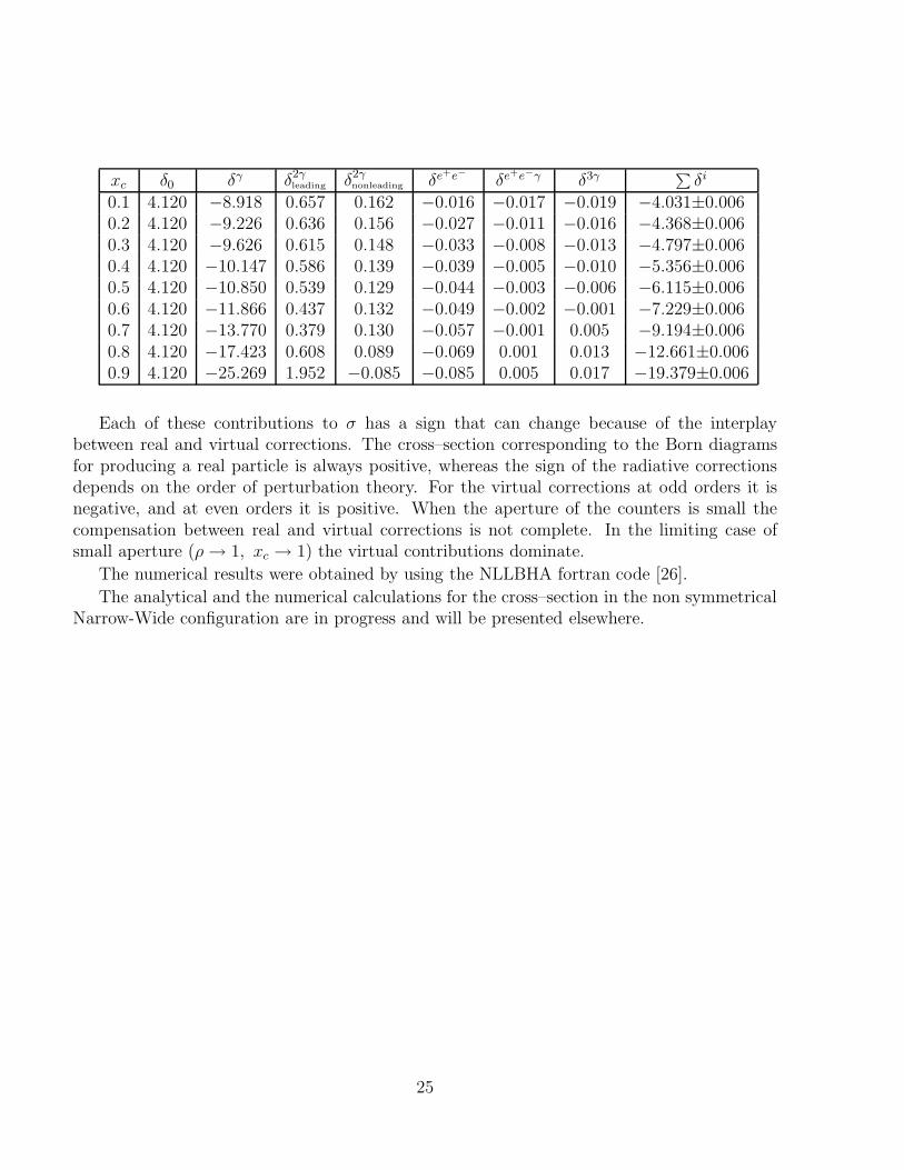
xc δ0 δγ δ2γleading δ2γ

nonleading δe+e− δe+e−γ δ3γ ∑δi

0.1 4.120 −8.918 0.657 0.162 −0.016 −0.017 −0.019 −4.031±0.0060.2 4.120 −9.226 0.636 0.156 −0.027 −0.011 −0.016 −4.368±0.0060.3 4.120 −9.626 0.615 0.148 −0.033 −0.008 −0.013 −4.797±0.0060.4 4.120 −10.147 0.586 0.139 −0.039 −0.005 −0.010 −5.356±0.0060.5 4.120 −10.850 0.539 0.129 −0.044 −0.003 −0.006 −6.115±0.0060.6 4.120 −11.866 0.437 0.132 −0.049 −0.002 −0.001 −7.229±0.0060.7 4.120 −13.770 0.379 0.130 −0.057 −0.001 0.005 −9.194±0.0060.8 4.120 −17.423 0.608 0.089 −0.069 0.001 0.013 −12.661±0.0060.9 4.120 −25.269 1.952 −0.085 −0.085 0.005 0.017 −19.379±0.006

Each of these contributions to σ has a sign that can change because of the interplaybetween real and virtual corrections. The cross–section corresponding to the Born diagramsfor producing a real particle is always positive, whereas the sign of the radiative correctionsdepends on the order of perturbation theory. For the virtual corrections at odd orders it isnegative, and at even orders it is positive. When the aperture of the counters is small thecompensation between real and virtual corrections is not complete. In the limiting case ofsmall aperture (ρ → 1, xc → 1) the virtual contributions dominate.

The numerical results were obtained by using the NLLBHA fortran code [26].

The analytical and the numerical calculations for the cross–section in the non symmetricalNarrow-Wide configuration are in progress and will be presented elsewhere.

25

Acknowledgements

We are grateful for support to the Istituto Nazionale di Fisica Nucleare (INFN), to theInternational Association (INTAS) for the grant 93-1867 and to the Russian Foundation forFundamental Investigations (RFFI) for the grant 96-02-17512. One of us (L.T.) would like tothank H. Czyz, M. Dallavalle, B. Pietrzyk and T. Pullia for several useful discussions at variousstages of the work and the CERN theory group for the hospitality. Three of us (A.A., E.K.and N.M.) would like to thank the INFN Laboratori Nazionali di Frascati, the Dipartimento diFisica dell’Universita di Roma ”Tor Vergata” and the Dipartimento di Fisica dell’Universita diParma for their hospitality during the preparation of this work. One of us (A.A.) is thankfulto the Royal Swedish Academy of Sciences for an ICFPM grant.

26

References

[1] G. Altarelli, Lectures given at the E. Majorana Summer Scool, Erice, Italy, July 1993,CERN-TH.7072/93.

[2] LEP Electroweak Working Group, A Combination of Preliminary LEP Electroweak Re-sults from the 1995 Summer Conferences, 1995, CERN report LEPEWWG/95–02.B. Pietrzyk, High Precision Measurements of the Luminosity at LEP, Proceedings of the”Tennessee International Symposium on Radiative Corrections: Status and Outlook”,Gatlinburg, Tennessee, 27 June– 1 July, 1994, Ed. B.F.L. Ward (World Scientific, Singa-pore 1995).

[3] Neutrino Counting in Z Physics at LEP , G. Barbiellini et al., L. Trentadue (conv.),G. Altarelli, R. Kleiss and C. Verzegnassi eds., CERN Report 89-08 (1989).

[4] W. Beenakker, F.A. Berends and S.C. van der Marck, Nucl. Phys. B355 (1991) 281;M. Cacciari, A. Deandrea, G. Montagna, O. Nicrosini and L. Trentadue, Phys. Lett. B271(1991) 431;M. Caffo, H. Czyz and E. Remiddi, Nuovo Cim. 105A (1992) 277;K.S. Bjorkenvoll, G. Faldt and P. Osland, Nucl. Phys. B386 (1992) 280, 303;W. Beenakker and B. Pietrzyk, Phys. Lett. B296 (1992) 241; and B304 (1993) 366.M. Cacciari, G. Montagna, O. Nicrosini and F. Piccinini, Comput. Phys. Commun. 90(1995) 301.

[5] S. Jadach et al., Phys. Rev. D47 (1993) 3733;S. Jadach, E. Richter-Was, B.F.L. Ward and Z. Was, Phys. Lett. B260 (1991) 438, and268 (1991) 253;S. Jadach, M. Skrzypek and B.F.L. Ward, Phys. Lett. B257 (1991) 173.S. Jadach et al., Phys. Lett. B353 (1995) 362.

[6] R. Budny, Phys. Lett. 55B (1975) 227;D. Bardin, W. Hollik and T. Riemann, Z. Phys. C49 (1991) 485;M. Boehm, A. Denner and W. Hollik, Nucl. Phys. B304 (1988) 687.

[7] V.S. Fadin, E.A. Kuraev, L.N. Lipatov, N.P. Merenkov and L. Trentadue, Yad. Fiz. 56(1993) 145;S. Jadach et al., Phys. Lett. B253 (1991) 469.

[8] V.S. Fadin, E.A. Kuraev, L.N. Lipatov, N.P. Merenkov and L. Trentadue, Yad. Fiz. 56(1993) 145.V.S. Fadin, E.A. Kuraev, L.N. Lipatov, N.P. Merenkov and L. Trentadue, Proceedings ofthe XXIX Rencontres de Moriond, Meribel, March 1994.

27

V.S. Fadin, E.A. Kuraev, L.N. Lipatov, N.P. Merenkov and L. Trentadue, same Proceed-ings as in Ref. [2] p.168.

[9] R.V. Polovin, JEPT 31 (1956) 449 ;F.A. Redhead, Proc. Roy. Soc. 220 (1953) 219;F.A. Berends et al., Nucl. Phys. B68 (1974) 541.

[10] S. Eidelman, F. Egerlehner, Z. Phys. C67 (1995) 585.

[11] E.A. Kuraev, L.N. Lipatov and N.P. Merenkov, Phys Lett. 47B (1973) 33; preprint 46LNPI, 1973;H. Cheng, T. T. Wu, Phys. Rev. 187 (1969) 1868;V.S. Fadin, E.A. Kuraev, L.N. Lipatov, N.P. Merenkov and L. Trentadue, Yad. Fiz. 56(1993) 145.

[12] G. Faldt and P. Osland, Nucl. Phys. B413 (1994) 16; Erratum ibidem B419 (1994) 404.

[13] D.R. Yennie, S.C. Frautchi, H. Suura, Ann. Phys. 13 (1961) 379.

[14] V.N. Baier, V.S. Fadin, V. Khoze and E.A. Kuraev, Phys. Rep. 78 (1981) 294;V.M. Budnev, I.F. Ginzburg, G.V. Meledin and V.G. Serbo, Phys. Rep. C15 (1975) 183.

[15] V.G. Gorshkov, Uspekhi Fiz. Nauk 110 (1973) 45.

[16] R. Barbieri, J.A. Mignaco and E. Remiddi, Il Nuovo Cimento 11A (1972) 824.

[17] E.A. Kuraev, N.P. Merenkov, V.S. Fadin, Sov. J. Nucl. Phys. 45 (1987) 486.

[18] H. Cheng and T.T. Wu, Expanding Protons: Scattering at High Energies, London, Eng-land, 1986.

[19] N.P. Merenkov, Sov. J. Nucl. Phys. 48 (1988) 1073.

[20] N.P. Merenkov, Sov. J. Nucl. Phys. 50 (1989) 469.

[21] L.N. Lipatov, Sov. J. Nucl. Phys. 20 (1974) 94;G. Altarelli and G. Parisi, Nucl. Phys. B126 (1977) 298;E. A. Kuraev and V. S. Fadin, Sov. J. of Nucl. Phys. 41 (1985) 466; Preprint INP 84-44,Novosibirsk, 1984;O. Nicrosini and L. Trentadue, Phys. Lett. 196B (1987) 551.

[22] M. Skrzypek, Acta Phys. Pol. B23 (1993), 135;E.A. Kuraev, N.P. Merenkov and V.S. Fadin, Sov. J. Nucl. Phys. 47 (1988) 1009.S. Jadach, M. Skrzypek, B.F.L. Ward, Phys. Lett. B257 (1991) p.173.

28

[23] A.B. Arbuzov, E.A. Kuraev, N.P. Merenkov and L. Trentadue, JETP 108 (1995) 1164;preprint CERN–TH/95–241, JINR E2–95–110, Dubna, 1995.

[24] A.B. Arbuzov, V.S. Fadin, E.A. Kuraev, L.N. Lipatov, N.P. Merenkov and L. Trentadue,Report CERN 95-03 (1995) p. 369.

[25] V.N. Baier, V.S. Fadin, V.M. Katkov, Emission of relativistic electrons, Moscow, Atom-izdat, 1973.

[26] A short write-up of the NLLBHA code can be found in the CERN Yellow Report CERN-96-01, vol.2. A copy of the program is available, upon request, from the authors.

29

Appendix A

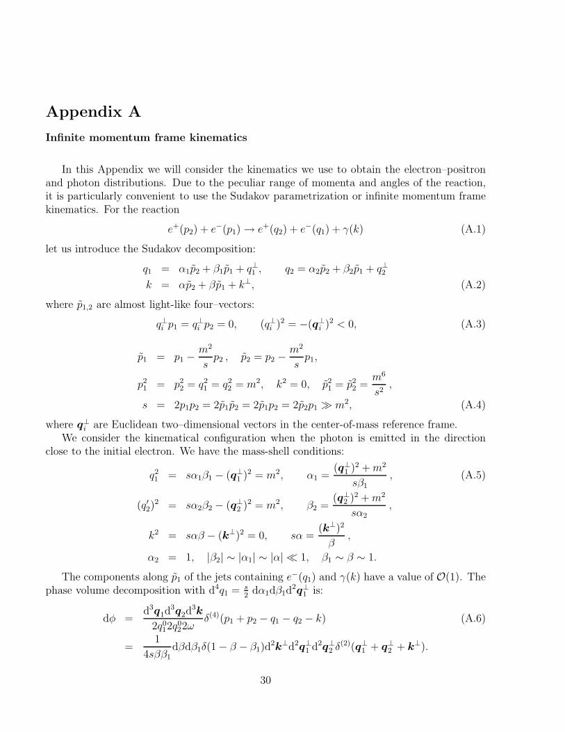
Infinite momentum frame kinematics

In this Appendix we will consider the kinematics we use to obtain the electron–positronand photon distributions. Due to the peculiar range of momenta and angles of the reaction,it is particularly convenient to use the Sudakov parametrization or infinite momentum framekinematics. For the reaction

e+(p2) + e−(p1) → e+(q2) + e−(q1) + γ(k) (A.1)

let us introduce the Sudakov decomposition:

q1 = α1p2 + β1p1 + q⊥1 , q2 = α2p2 + β2p1 + q⊥2k = αp2 + βp1 + k⊥, (A.2)

where p1,2 are almost light-like four–vectors:

q⊥i p1 = q⊥i p2 = 0, (q⊥i )2 = −(q⊥i )2 < 0, (A.3)

p1 = p1 −m2

sp2 , p2 = p2 −

m2

sp1,

p21 = p2

2 = q21 = q2

2 = m2, k2 = 0, p21 = p2

2 =m6

s2,

s = 2p1p2 = 2p1p2 = 2p1p2 = 2p2p1 ≫ m2, (A.4)

where q⊥i are Euclidean two–dimensional vectors in the center-of-mass reference frame.

We consider the kinematical configuration when the photon is emitted in the directionclose to the initial electron. We have the mass-shell conditions:

q21 = sα1β1 − (q⊥

1 )2 = m2, α1 =(q⊥

1 )2 + m2

sβ1

, (A.5)

(q′2)2 = sα2β2 − (q⊥

2 )2 = m2, β2 =(q⊥

2 )2 + m2

sα2,

k2 = sαβ − (k⊥)2 = 0, sα =(k⊥)2

β,

α2 = 1, |β2| ∼ |α1| ∼ |α| ≪ 1, β1 ∼ β ∼ 1.

The components along p1 of the jets containing e−(q1) and γ(k) have a value of O(1). Thephase volume decomposition with d4q1 = s

2dα1dβ1d

2q⊥1 is:

dφ =d3q1d

3q2d3k

2q012q

022ω

δ(4)(p1 + p2 − q1 − q2 − k) (A.6)

=1

4sββ1dβdβ1δ(1 − β − β1)d

2k⊥d2q⊥1 d2q⊥

2 δ(2)(q⊥1 + q⊥

2 + k⊥).

30

The conservation law reads (we introduce a new four–momentum q of the exchanged pho-ton):

p1 + q = q1 + k, p2 = q2 + q. (A.7)

The inverse propagators are (here and further we use β1 = x):

(p1 − k)2 − m2 =−1

1 − xd1 , (p1 + q)2 − m2 =

1

x(1 − x)d, (A.8)

q2 = −(q⊥2 )2, d = m2(1 − x)2 + (q⊥

1 + q⊥x)2, d1 = m2(1 − x)2 + (q⊥1 + q⊥)2.

The matrix element reads

M =gµν

q2v(p2)γµv(q2)u(q1)Oνu(p1)

Oν = γν p1 − k + m

(p1 − k)2 − m2e + e

p1 + q + m

(p1 + q)2 − m2γν . (A.9)

The following decomposition of the metric tensor gµν is used:

gµν = g⊥µν +

pµ1p

ν2 + pν

1pµ2

p1p2≃ 2pµ

1pν2

s

(1 + O(

q⊥2

s)). (A.10)

We use also the identity

pν2u(q1)Oνu(p1) ≡ u(q1)vρu(p1)eρ(k). (A.11)

The generalized vertex vρ has the form [14]:

vρ = sγρx(1 − x)(

1

d− 1

d1

)− γρkp2

dx(1 − x) − p2kγρ

d1

(1 − x). (A.12)

The evaluation of the spin sum of the squared matrix element gives

∑

spin

|v(q2)p1v(p2)|2 = Tr p2p1p2p1 = 2s2, (A.13)

The squared matrix element for the single photon radiation is given by

R = − 1

4s2Tr (p1 + m)vµ(p1 + k − q + m)vµ (A.14)

= x[−2xm2(d − d1)2 + (q⊥

2 )2(1 + x2)dd1]1

d2d21

.

31

Finally we obtain that

dσe+e−→e+(e−γ) = 2α3d2q⊥1 dq⊥

2 dx(1 − x)

π2((q⊥2 )2)2(dd1)2

[−2xm2(d − d1)2 + (q⊥

2 )2(1 + x2)dd1]. (A.15)

In the same way we may obtain the cross–section for the process of the double bremsstrahlungin the opposite directions:

dσe+e−→e+γe−γ

d2q⊥1 d2q⊥

2 dx1dx2

=α4(1 + x2

1)(1 + x22)

π4(1 − x1)(1 − x2)

∫d2q⊥

((q⊥)2)2(A.16)

×[(q⊥)2(1 − x1)

2

d1d2

− 2x1

1 + x21

m2(1 − x1)2(d1 − d2)

2

d21d

22

]

×[(q⊥)2(1 − x2)

2

d1d2

− 2x2

1 + x22

m2(1 − x2)2(d2 − d1)

2

d21d

22

],

where x1, q⊥1 and x2, q⊥

2 are the energy fractions and the components transverse to the beamaxis of the scattered electron and positron, respectively; q⊥ is the transverse two–dimensionalmomentum of the exchanged photon;

d1 = (1 − x1)2m2 + (q⊥

1 − q⊥x1)2, d2 = (1 − x1)

2m2 + (q⊥1 − q⊥)2, (A.17)

d1 = (1 − x2)2m2 + (q⊥

2 + q⊥x2)2, d2 = (1 − x2)

2m2 + (q⊥2 + q⊥)2.

Let us now discuss the restrictions on the d2q⊥1 , d2q⊥

2 integration imposed by experimentalconditions of the electron and positron tagging. We consider the emission of a hard photonalong the electron direction. We will consider the symmetric case:

θ1 < θe =|q⊥

1 |xε

< θ2 , θe = ˆp1q1, (A.18)

θ1 < θe =|q⊥

2 |ε

< θ2 , θe = ˆp2q2.

Here θ1 and θ2 are the minimal and maximal angles of aperture for the counters. It isconvenient to introduce dimensionless quantities ρ = θ2/θ1, z1,2 = (q1,2)

2/Q21 (Q1 = εθ1).

The region in the z1, z2 plane that gives the largest contribution to Σ is made by twonarrow strips along the lines z1 = z2 and z1 = x2z2. Therefore the leading logarithmiccontribution will appear only in the cases where these lines cross the rectangle defined byx2 < z1 < ρ2x2 , 1 < z2 < ρ2. Note that the line z1 = x2z2, which corresponds to theemission of one hard photon along the momentum of the scattered electron, is the diagonal ofthe rectangle defined above. As for the line z1 = z2, which corresponds to the emission alongthe initial electron momentum, it crosses the rectangle only if x2ρ2 > z2 , xρ > 1. This lastcondition defines the appearance of leading contributions to ΣH .

32

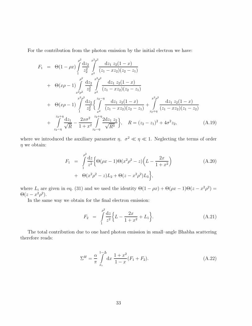
For the contribution from the photon emission by the initial electron we have:

F1 = Θ(1 − ρx)

ρ2∫

1

dz2

z22

x2ρ2∫

x2

dz1 z2(1 − x)

(z1 − xz2)(z2 − z1)

+ Θ(xρ − 1)

ρ2∫

x2ρ2

dz2

z22

x2ρ2∫

x2

dz1 z2(1 − x)

(z1 − xz2)(z2 − z1)

+ Θ(xρ − 1)

x2ρ2∫

1

dz2

z22

z2−η∫

x2

dz1 z2(1 − x)

(z1 − xz2)(z2 − z1)+

x2ρ2∫

z2+η

dz1 z2(1 − x)

(z1 − xz2)(z1 − z2)

+

z2+η∫

z2−η

dz1√R

− 2xσ2

1 + x2

z2+η∫

z2−η

2dz1 z2√R3

, R = (z2 − z1)

2 + 4σ2z2, (A.19)

where we introduced the auxiliary parameter η, σ2 ≪ η ≪ 1. Neglecting the terms of orderη we obtain:

F1 =

ρ2∫

1

dz

z2

Θ(ρx − 1)Θ(x2ρ2 − z)

(L − 2x

1 + x2

)(A.20)

+ Θ(x2ρ2 − z)L2 + Θ(z − x2ρ2)L3

,

where Li are given in eq. (31) and we used the identity Θ(1 − ρx) + Θ(ρx − 1)Θ(z − x2ρ2) =Θ(z − x2ρ2).

In the same way we obtain for the final electron emission:

F2 =

ρ2∫

1

dz

z2

L − 2x

1 + x2+ L1

. (A.21)

The total contribution due to one hard photon emission in small–angle Bhabha scatteringtherefore reads:

ΣH =α

π

1−∆∫

xc

dx1 + x2

1 − x(F1 + F2). (A.22)

33

Appendix B

The contribution to Σ from the semi–collinear region of emission

of two hard photons in the same direction

An alternative way to use the quasi-real electron approximation is to compute the cross–section directly. To logarithmic accuracy we may restrict ourselves to considering only tworegions i) the one with photon with momentum k1 emitted along the momentum direction ofthe initial electron inside a narrow cone with opening angle θ0 ≪ 1, and ii) the region withthe photon emitted along the scattered electron. Taking into account the identity of photonswith the statistical factor 1

2!we obtain the cross–section:

dσHHSC =

α4

2π

∫d2q⊥

2

π((q⊥2 )2)2

∫d2q⊥

1

π

1−2∆∫

xc

dx (B.1)

×1−x−∆∫

∆

dx1dx2

x1x2xδ(1 − x1 − x2 − x)

∫R

d2k⊥1

π,

where

∫R

d2k⊥1

π= 2(q⊥

2 )2Q41

∫d2k⊥

1

π

[1 + (1 − x1)

2][x2 + (1 − x1)2]

x1(1 − x1)2(2p1k1)(2p1k2)(2q1k2)

∣∣∣∣k1‖p1

(B.2)

+x[1 + (1 − x2)

2][x2 + (1 − x2)2]

x1(1 − x2)2(2q1k1)(2p1k2)(2q1k2)

∣∣∣∣k1‖q1

.

It is convenient to specify the kinematics: in the case of the emission of the collinear photonwith momentum k1 parallel to p1 we have

2p1k1 =Q2

1

x1[(k⊥

1 )2 + σ2x21], 2p1k2 =

Q21

x2(k⊥

2 )2, (B.3)

2q1k2 =Q2

1

x2x[xq⊥

2 − (1 − x1)q⊥1 ]2, k⊥

2 = −q⊥2 − q⊥

1 ;

in the case when the photon is emitted along q1 we have

2k1q1 =Q2

1

x1x[σ2x2

1 + (xk⊥1 − q⊥

1 )2], 2p1k2 =Q2

1

x2

(k⊥2 )2, (B.4)

2q1k2 =Q2

1

x2x(q⊥

1 − xq⊥2 )2, k⊥

2 = −q⊥2 − q⊥

1

1 − x2

x,

where Q21 = ǫ2θ2

1, σ2 = m2/Q21, and we introduced two–dimensional vectors k⊥

2 , q⊥1 and q⊥

2 so

that (q⊥1 )2 = z1, (q⊥

2 )2 = z2 and q⊥

1 q⊥2 = φ.

34

The integration over d2k⊥1 can be done with single logarithmic accuracy:

Q21

∫d2k⊥

1

π(2p1k1)

∣∣∣∣k1‖p1

= x1L, Q21

∫d2k⊥

1

π(2q1k1)

∣∣∣∣k1‖q1

=x1

xL. (B.5)

It is also necessary, here, to consider the kinematical restrictions on the integration variablesφ and z1. When the photon is emitted within an angle θ0 along the direction of the momentumof the initial electron, θ0 represents the angular range to be filled by collinear kinematics events.We assign to the semi–collinear kinematics the events characterized by

i)

∣∣∣∣∣k⊥

2

x2

∣∣∣∣∣ > θ0 , ii)

∣∣∣∣q⊥

1

x− k⊥

2

x2

∣∣∣∣ > θ0, (B.6)

where the region i) the photon with four–momentum k2 escapes the narrow cone with openingangle θ0 along the momentum direction of the initial electron. In the region ii) the samehappens for the final electron.

We can rewrite the conditions above in terms of the variables z1 and φ as follows:

i) 1 > cos φ > −1 +λ2 − (

√z1 −

√z2)

2

2√

z1z2

, |√z1 −√

z2| < λ,

ii) 1 > cos φ > −1, |z1 − z2| > 2√

z2λ,

iii) 1 > cos φ > −1 +

x2

(1−x1)2λ2 − (

√z1 − x

1−x1

√z2)

2

2√

z1z2x

1−x1

,

|√z1 −x√

z2

1 − x1| < λ

x

1 − x1,

iv) 1 > cos φ > −1, |z1 −x2

(1 − x1)2z2| > 2λ

√z2

x2

(1 − x1)2,

where λ = x2θ0/θ1. In our calculation we take the parameter λ ≪ 1. Indeed, the restrictionson θ0 for collinear kinematics calculations are εθ0 ≫ m or θ0 ≫ 10−5 at LEP energies. On theother hand the experimental conditions on θ1 are θ1 > 10−2. Therefore we can take λ ≪ 1within our accuracy.

Analogous considerations can be made for the case when a photon with momentum k1

is emitted along the direction of the final electron. In regions ii) and iv) we may do theintegration over the azimuthal angle:

2π∫

0

dφ

2π(2p1k2)(2q1k2)

∣∣∣∣k1‖p1

=x2xQ−4

1

(1 − x1)z1 − xz2

[1

|z2 − z1|− x(1 − x1)

|x2z2 − (1 − x1)2z1|

],(B.7)

∫ 2π

0

dφ

2π(2p1k2)(2q1k2)

∣∣∣∣k1‖q1

=x2x

3(1 − x2)−2Q−4

1

z1 − z2x2/(1 − x2)

[1

|z1 − z2x2

(1−x2)2|− 1 − x2

|z1 − x2z2|

].(B.8)

35

The integration of regions i), iii) has the form

I =∫

dz1

∫ dφ

2π(z1 + z2 + 2√

z1z2 cos φ)

∣∣∣∣|√z1−

√z2|<λ

(B.9)

=2

π

∫dz

|z1 − z2|arctan

(√

z1 −√

z2)2

|z1 − z2|tan

φ0

2

,

where

φ0 = arccos(−1 +

λ2 − (√

z1 −√

z2)2

2√

z1z2

). (B.10)

The result reads

I = 2 ln 2. (B.11)

We give here the complete contribution of the semi–collinear region:

dσHHs-coll

=α2L4π2

1−2∆∫

xc

dx

1−x−∆∫

∆

dx1dx2δ(1 − x − x1 − x2)

x1x2(1 − x1)2[1 + (1 − x1)

2][x2 + (1 − x1)2]

×ρ2∫

1

dz

z2

ln

zθ21

θ20

[1 + Θ(ρ2x2 − z) + 2Θ(ρ2(1 − x1)2 − z)]

+ Θ(ρ2x2 − z) ln(z − x2)(ρ2x2 − z)

x2(z − x(1 − x1))(ρ2x(1 − x1) − z)

+ Θ(z − ρ2(1 − x1)2)[ln

(z − ρ2(1 − x1)x)(z − (1 − x1)2)

(ρ2(1 − x1)2 − z)(z − x(1 − x1))

+ ln(ρ2(1 − x1) − z)(z − (1 − x1)

2)

(ρ2(1 − x1)2 − z)(z − (1 − x1))

]+ Θ(z − ρ2x2) ln

z − ρ2x(1 − x1)(z − x2)

(ρ2x2 − z)(z − x(1 − x1))

+ Θ(ρ2(1 − x1)2 − z)

[ln

(z − (1 − x1)2)(ρ2(1 − x1)

2 − z)

(ρ2x(1 − x1) − z)(z − x(1 − x1))(1 − x1)2

+ ln(z − (1 − x1)

2)(ρ2(1 − x1)2 − z)

(ρ2(1 − x1) − z)(z − (1 − x1))(1 − x1)2

]+ ln

(z − 1)(ρ2 − z)

(z − (1 − x1))(ρ2(1 − x1) − z)

.

To see the cancellation of the auxiliary parameter θ0/θ1 we give here the relevant part of thecontribution for the collinear region :

ΣHHcoll

=α2

4π2

1−2∆∫

xc

dx

1−x−∆∫

∆

dx1 dx2δ(1 − x − x1 − x2)

x1x2(1 − x1)2[1 + (1 − x1)

2][x2 + (1 − x1)2]

×ρ2∫

1

dz

z2

(L2 + 2L ln

θ20

zθ21

)[1

2+

1

2Θ(ρ2x2 − z) + Θ(ρ2(1 − x1)

2 − z)]

+ . . . .

36

We see from the above expression that the dependence on θ0/θ1 disappears in the sum of thecontributions for the collinear and semi–collinear regions. The total sum is given by Eq. (56).

37

Appendix C

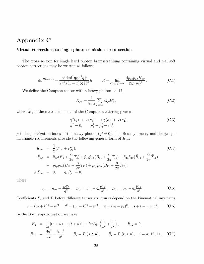
Virtual corrections to single photon emission cross–section

The cross–section for single hard photon bremsstrahlung containing virtual and real softphoton corrections may be written as follows:

dσH(S+V ) =α3dxd2q⊥

2 d2q⊥1

2π2x(1 − x)(q⊥2 )4

R, R = lim(2p1p2)→∞

4p2ρp2σKρσ

(2p1p2)2. (C.1)

We define the Compton tensor with a heavy photon as [17]:

Kρσ =1

8πα

∑

spins

MρM∗σ , (C.2)

where Mρ is the matrix elements of the Compton scattering process

γ∗(q) + e(p1) −→ γ(k) + e(p2), (C.3)

k2 = 0, p21 = p2

2 = m2,

ρ is the polarization index of the heavy photon (q2 6= 0). The Bose symmetry and the gauge-invariance requirements provide the following general form of Kρσ:

Kρσ =1

2(Pρσ + P ∗

σρ), (C.4)

Pρσ = gρσ(Bg +α

2πTg) + p1ρp1σ(B11 +

α

2πT11) + p2ρp2σ(B11 +

α

2πT11)

+ p1ρp2σ(B12 +α

2πT12) + p2ρp1σ(B12 +

α

2πT12),

qρPρσ = 0, qσPρσ = 0,

where

gρσ = gρσ − qρqσ

q2, p1ρ = p1ρ − qρ

p1q

q2, p2ρ = p2ρ − qρ

p2q

q2. (C.5)

Coefficients Bi and Ti before different tensor structures depend on the kinematical invariants

s = (p2 + k)2 − m2, t2 = (p1 − k)2 − m2, u = (p1 − p2)2, s + t + u = q2. (C.6)

In the Born approximation we have

Bg =1

st[(s + u)2 + (t + u)2] − 2m2q2

(1

s2+

1

t2

), B12 = 0,

B11 =4q2

st− 8m2

s2Bi = Bi(s, t, u), Bi = Bi(t, s, u), i = g, 12 , 11. (C.7)

38

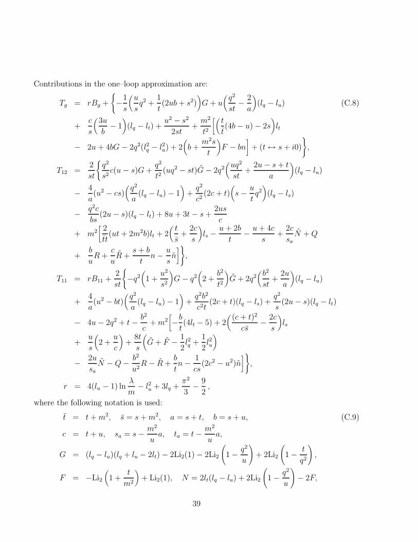
Contributions in the one–loop approximation are:

Tg = rBg +

−1

s

(u

sq2 +

1

t(2ub + s2)

)G + u

(q2

st− 2

a

)(lq − lu) (C.8)

+c

s

(3u

b− 1

)(lq − lt) +

u2 − s2

2st+

m2

t2

[(t

t(4b − u) − 2s

)lt

− 2u + 4bG − 2q2(l2q − l2u) + 2(b +

m2s

t

)F − bn

]+ (t ↔ s + i0)

,

T12 =2

st

q2

s2c(u − s)G +

q2

t2(uq2 − st)G − 2q2

(uq2

st+

2u − s + t

a

)(lq − lu)

− 4

a(u2 − cs)

(q2

a(lq − lu) − 1

)+

q2

c2(2c + t)

(s − u

tq2)(lq − ls)

− q2c

bs(2u − s)(lq − lt) + 8u + 3t − s +

2us

c

+ m2[

2

tt(ut + 2m2b)lt + 2

(t

s+

2c

s

)ls −

u + 2b

t− u + 4c

s+

2c

saN + Q

+b

uR +

c

uR +

s + b

tn − u

sn]

,

T11 = rB11 +2

st

−q2

(1 +

u2

s2

)G − q2

(2 +

b2

t2

)G + 2q2

(b2

st+

2u

a

)(lq − lu)

+4

a(u2 − bt)

(q2

a(lq − lu) − 1

)+

q2b2

c2t(2c + t)(lq − ls) +

q2

s(2u − s)(lq − lt)

− 4u − 2q2 + t − b2

c+ m2

[−b

t(4lt − 5) + 2

((c + t)2

cs− 2c

s

)ls

+u

s

(2 +

u

c

)+

8t

s

(G + F − 1

2l2q +

1

2l2u

)

− 2u

sa

N − Q − b2

u2R − R +

b

tn − 1

cs(2c2 − u2)n

],

r = 4(lu − 1) lnλ

m− l2u + 3lq +

π2

3− 9

2,

where the following notation is used:

t = t + m2, s = s + m2, a = s + t, b = s + u, (C.9)

c = t + u, sa = s − m2

ua, ta = t − m2

ua,

G = (lq − lu)(lq + lu − 2lt) − 2Li2(1) − 2Li2

(1 − q2

u

)+ 2Li2

(1 − t

q2

),

F = −Li2

(1 +

t

m2

)+ Li2(1), N = 2lt(lq − lu) + 2Li2

(1 − q2

u

)− 2F,

39

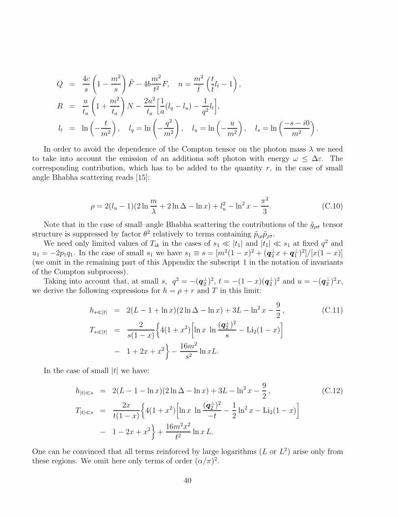
Q =4c

s

(1 − m2

s

)F − 4b

m2

t2F, n =

m2

t

(t

tlt − 1

),

R =u

ta

(1 +

m2

ta

)N − 2u2

ta

[1

a(lq − lu) −

1

q2lt

],

lt = ln(− t

m2

), lq = ln

(− q2

m2

), lu = ln

(− u

m2

), ls = ln

(−s − i0

m2

).

In order to avoid the dependence of the Compton tensor on the photon mass λ we needto take into account the emission of an additiona soft photon with energy ω ≤ ∆ε. Thecorresponding contribution, which has to be added to the quantity r, in the case of smallangle Bhabha scattering reads [15]:

ρ = 2(lu − 1)(2 lnm

λ+ 2 ln∆ − lnx) + l2u − ln2 x − π2

3. (C.10)

Note that in the case of small–angle Bhabha scattering the contributions of the gρσ tensorstructure is suppressed by factor θ2 relatively to terms containing piρpjσ.

We need only limited values of Tik in the cases of s1 ≪ |t1| and |t1| ≪ s1 at fixed q2 andu1 = −2p1q1. In the case of small s1 we have s1 ≡ s = [m2(1 − x)2 + (q⊥

2 x + q⊥1 )2]/[x(1 − x)]

(we omit in the remaining part of this Appendix the subscript 1 in the notation of invariantsof the Compton subprocess).

Taking into account that, at small s, q2 = −(q⊥2 )2, t = −(1 − x)(q⊥

2 )2 and u = −(q⊥2 )2x,

we derive the following expressions for h = ρ + r and T in this limit:

hs≪|t| = 2(L − 1 + ln x)(2 ln∆ − ln x) + 3L − ln2 x − 9

2, (C.11)

Ts≪|t| =2

s(1 − x)

4(1 + x2)

[ln x ln

(q⊥2 )2

s− Li2(1 − x)

]

− 1 + 2x + x2− 16m2

s2ln xL.

In the case of small |t| we have:

h|t|≪s = 2(L − 1 − ln x)(2 ln ∆ − ln x) + 3L − ln2 x − 9

2, (C.12)

T|t|≪s =2x

t(1 − x)

4(1 + x2)

[ln x ln

(q⊥2 )2

−t− 1

2ln2 x − Li2(1 − x)

]

− 1 − 2x + x2

+16m2x2

t2ln xL.

One can be convinced that all terms reinforced by large logarithms (L or L2) arise only fromthese regions. We omit here only terms of order (α/π)2.

40

The further integration is straightforward. We show here the most important moments.The contribution of the h containing terms gives (in close analogy with the Born contribution):

ΣH(S+V )h =

1

2(α

π)2

ρ2∫

1

dz

z2L

1−∆∫

xc

dx1 + x2

1 − x

(1 + Θ(ρ2x2 − z)) (C.13)

×[L(2 ln∆ − ln x +

3

2) + (2 ln∆ − ln x)(ln x − 2) − 1

2ln2 x − 15

4

]

+ (2 ln∆ − ln x +3

2) k(x, z) − 2 lnx(2 ln ∆ − ln x)Θ(ρ2x2 − z)

.

To obtain the contributions from T we consider at first new types of integrals:

Ist = Q21

∫d2q⊥

2

π(q⊥2 )4

∫d2q⊥

1

πst ln(q⊥

2 )2

s−t , (C.14)

ist = Q21

∫ d2q⊥2

π(q⊥2 )4

∫ d2q⊥1

πst , mst = Q21

∫ d2q⊥2

π(q⊥2 )4

∫ d2q⊥1 m2

πs2t2 .

Denoting σ2(1 − x)2 + (q⊥2 x − q⊥

1 )2/Q21 as a + b cos φ and using the expressions

1

2π

2π∫

0

dφ

a + b cos φ=

1√a2 − b2

, (C.15)

1

2π

2π∫

0

dφln(a + b cos φ)

a + b cos φ=

1√a2 − b2

ln2(a2 − b2)

a +√

a2 − b2

with a2 − b2 = (z1 − x2z2)2 + 4σ2(1 − x)2x2z2 , σ2 = m2/Q2

1 and z1,2 = (q⊥1,2)

2/Q21 we derive

that

Is = (1 − x)x

ρ2∫

1

dz2

z22

x2ρ2∫

x2

dz1 (C.16)

× ln(z22(1 − x)x3) − ln[(z1 − z2x

2)2 + 4σ2x2(1 − x)2z2]√(z1 − x2z2)2 + 4σ2x2(1 − x)2z2

.

Since we are evaluating with logarithmic accuracy, we may consider the contribution of theregion |z1 − x2z2| < η, σ2 ≪ η ≪ 1 when integrating over z1. The result reads

Is = x(1 − x)

ρ2∫

1

dz2

z22

L[1

2L + ln

x

1 − x

]. (C.17)

41

The rest of the integrals can be calculated in the same way, and we have:

It = −(1 − x)

ρ2x2∫

1

dz2

z22

L[1

2L + ln

1

1 − x

], it = −(1 − x)

ρ2x2∫

1

dz2

z22

L, (C.18)

is = x(1 − x)

ρ2∫

1

dz2

z22

L, mt =

ρ2x2∫

1

dz2

z22

, ms = x2

ρ2x2∫

1

dz2

z22

.

Using (C.17) and (C.18) we may represent the final result for the contribution to ΣH(S+V ) dueto the T term as

ΣH(S+V )T =

1

2(α

π)2

ρ2∫

1

dz

z2L

1−∆∫

xc

dx1 + x2

1 − x

(1

2L + ln

x

1 − x

)ln x (C.19)

+ ζ2 − Li2(x) +x2 + 2x − 1

4(1 + x2)− 2x ln x

1 + x2− Θ(x2ρ2 − z)

[(1

2L + ln

1

1 − x

)ln x

− 1

2ln2 x − Li2(1 − x) − 1 + 2x − x2

4(1 + x2)− 2x ln x

1 + x2

].

The total contribution to ΣH(S+V ) (one-side hard photon emission with virtual and softphoton corrections) is the sum of (C.13) and (C.19):

ΣH(S+V ) = ΣH(S+V )ρ + Σ

H(S+V )T . (C.20)

This quantity is given in Eq. (52).

42

Appendix D

Leading logarithmic contribution to Σγγ

Here we show that the main logarithmic terms can be summed according to the renormal-ization group. The sum, as given in the text, may be written as:

S = 2(α

π)2

ρ2∫

1

dz

z2L2 1∫

xc

dx δ(1 − x)(ln2 ∆ +

3

2ln ∆ +

9

16

)(D.1)

× (1 + Θ(x2ρ2 − z)) +1

2

∫ 1−∆

xc

1 + x2

1 − x(2 ln ∆ − ln x +

3

2)(1 + Θ(x2ρ2 − z))

+1

4

1−2∆∫

xc

dx[21 + x2

1 − xln

1 − x − ∆

∆+

1

2(1 + x) ln x − 1 + x

][1 + 3Θ(x2ρ2 − z)]

+1

4

1∫

xc

dx[21 + x2

1 − xln

((1 − x − ∆)(ρ −√

z)

∆(√

z − ρx)

√x

)+ x − 1

− 1

2(1 + x) ln

ρ2

z+

√z

ρ− xρ√

z

]Θ(z − x2ρ2)

.

One can see that the dependence on the parameter ∆ disappears in the expression above.We will now show that eq. (D.1) is equivalent to eq. (59). Let us transform eq. (59) using

the substitution

Θ(t2ρ2 − z) =1

2(1 + Θ(x2ρ2 − z)) +

1

2Θ(z − x2ρ2) − Θ(z − t2ρ2), (D.2)

and changing the order of integration in the last term:

1∫

x

dt

ρ2∫

ρ2t2

dz =

ρ2∫

ρ2x2

dz

√z/ρ∫

x

dt =

ρ2∫

1

dzΘ(z − ρ2x2)

√z/ρ∫

x

dt. (D.3)

By evaluating the integral over t, and using the explicit expressions for the splitting func-tions one can verify the coincidence of Eqs. (D.1) and (59). In an analogous way one can provethe validity of the representation (61) for Σγ

γ .

Using the representation in Eq. (60) for the function P (2) one can see that the aboveexpression is equivalent to Eq. (D.1). In an analogous way one can prove the validity ofrepresentation in Eq. (61) for Σγ

γ.

43

Appendix E

Cancellation of the ∆ dependence in the nonleading contributions to Σ2γ

Let us consider the singular nonleading terms in Σ2γ in the limiting case ∆ → 0. Droppingthe common factor (α/π)2L ∫ dz/z2, we give below the various contributions separately.

Let us consider first Σγγ . The contributions from the soft photon radiation and virtualcorrections are:

(ΣV V +V S+SS)∆ = ln ∆(−7 − 4 ln ∆)(1, ρ2), (E.1)

where we denote by (a, b) the limits of the integration over z: (a, b) = Θ(z − a)Θ(b − z).The contribution due to the virtual corrections to the single hard photon emission gives9

(ΣH(S+V ))∆ =1

2ln ∆

(1, ρ2)(16 ln∆ + 14) + 4

1∫

xc

dx1 + x2

1 − x[(1, ρ2) − (1, ρ2x2)] (E.2)

+ 4[−2 ln(1 − xc) − 2 ln(1 − xc) +

1∫

xc

dx (1 + x) +

1∫

xc

dx (1 + x)]

+ 2

1∫

xc

dx1 + x2

1 − x[(1, ρ2) − (1, ρ2x2)] lnx + 2

1∫

xc

dx1 + x2

1 − xk(x, z)

,

where xc = max(xc, 1/ρ) and the quantity k(x, z) is defined in Eq. (30). The singular part inthe contribution in Eq. (56) due to double hard photon bremsstrahlung reads:

(ΣHH)∆ = ln∆ 1∫

xc

dx1 + x2

1 − x[−(1, ρ2)L1 − (1, ρ2x2)L2 − ((1, ρ2) − (1, ρ2x2))L3] (E.3)

−1∫

xc

dx (3 + x) −1∫

xc

dx (3 + x) − 4 ln ∆ + 4 ln(1 − xc) + 4 ln(1 − xc)

−1∫

xc

dx1 + x2

1 − x[(1, ρ2) − (1, ρ2x2)]

.

It is possible to verify the cancellation:

(ΣV V +V S+SS)∆ + (ΣH(S+V ))∆ + (ΣHH)∆ = 0. (E.4)9In our contribution to the Tenessee–94 workshop (see [2]) there are some misprints, which are corrected

here

44

The corresponding contributions to Σγγ are:

(ΣS+VS+V )∆ = ln ∆(−14 − 8 ln∆)(1, ρ2), (E.5)

(ΣHS+V + ΣS+V

H )∆ = ln ∆2

1∫

xc

dx1 + x2

1 − xk(x, z) + (1, ρ2)[16 ln∆ + 14 − 8 ln(1 − xc)

− 8 ln(1 − xc) + 4

1∫

xc

dx (1 + x) + 4

1∫

xc

dx (1 + x)]

+ 4

1∫

xc

dx1 + x2

1 − x[(1, ρ2) − (1, ρ2x2)]

,

(ΣHH)∆ = ln ∆

−8(1, ρ2)[ln ∆ − ln(1 − xc) − ln(1 − xc)]

− 8

1∫

xc

dx(1, ρ2) − (1, ρ2x2)

1 − x− 2

1∫

xc

dx k(x, z)1 + x2

1 − x

− 4

1∫

xc

dx (1 + x)[(1, ρ2) + (1, ρ2x2)].

Rearranging the last term in (ΣHH)∆ as

−4

1∫

xc

dx (1 + x)[(1, ρ2) + (1, ρ2x2)] = −4

1∫

xc

dx (1 + x)(1, ρ2) (E.6)

−4

1∫

xc

dx (1 + x)(1, ρ2) + 4

1∫

xc

dx (1 + x)[(1, ρ2) − (1, ρ2x2)],

we can see again the cancellation of the ∆-dependence in the sum:

(ΣS+VS+V )∆ + (ΣH

S+V + ΣS+VH )∆ + (ΣH

H)∆ = 0. (E.7)

45

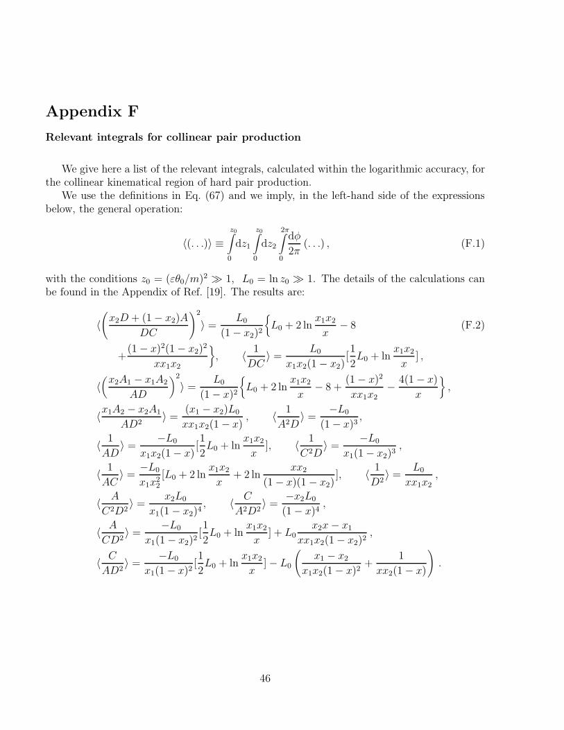
Appendix F

Relevant integrals for collinear pair production

We give here a list of the relevant integrals, calculated within the logarithmic accuracy, forthe collinear kinematical region of hard pair production.

We use the definitions in Eq. (67) and we imply, in the left-hand side of the expressionsbelow, the general operation:

〈(. . .)〉 ≡z0∫

0

dz1

z0∫

0

dz2

2π∫

0

dφ

2π(. . .) , (F.1)

with the conditions z0 = (εθ0/m)2 ≫ 1, L0 = ln z0 ≫ 1. The details of the calculations canbe found in the Appendix of Ref. [19]. The results are:

〈(

x2D + (1 − x2)A

DC

)2

〉 =L0

(1 − x2)2

L0 + 2 ln

x1x2

x− 8 (F.2)

+(1 − x)2(1 − x2)

2

xx1x2

, 〈 1

DC〉 =

L0

x1x2(1 − x2)[1

2L0 + ln

x1x2

x] ,

〈(

x2A1 − x1A2

AD

)2

〉 =L0

(1 − x)2

L0 + 2 ln

x1x2

x− 8 +

(1 − x)2

xx1x2− 4(1 − x)

x

,

〈x1A2 − x2A1

AD2〉 =

(x1 − x2)L0

xx1x2(1 − x), 〈 1

A2D〉 =

−L0

(1 − x)3,

〈 1

AD〉 =

−L0

x1x2(1 − x)[1

2L0 + ln

x1x2

x], 〈 1

C2D〉 =

−L0

x1(1 − x2)3,

〈 1

AC〉 =

−L0

x1x22

[L0 + 2 lnx1x2

x+ 2 ln

xx2

(1 − x)(1 − x2)], 〈 1

D2〉 =

L0

xx1x2

,

〈 A

C2D2〉 =

x2L0

x1(1 − x2)4, 〈 C

A2D2〉 =

−x2L0

(1 − x)4,

〈 A

CD2〉 =

−L0

x1(1 − x2)2[1

2L0 + ln

x1x2

x] + L0

x2x − x1

xx1x2(1 − x2)2,

〈 C

AD2〉 =

−L0

x1(1 − x)2[1

2L0 + ln

x1x2

x] − L0

(x1 − x2

x1x2(1 − x)2+

1

xx2(1 − x)

).

46