INTERNATIONAL JOURNAL FOR NUMERICAL METHODS IN FLUIDSInt. J. Numer. Meth. Fluids 2009; 59:443–458Published online 2 June 2008 in Wiley InterScience (www.interscience.wiley.com). DOI: 10.1002/fld.1825

Slip effects and heat transfer analysis in a viscous fluid overan oscillatory stretching surface

Z. Abbas1,2,∗,†, Y. Wang1,3, T. Hayat4 and M. Oberlack1

1Chair of Fluid Dynamics, Department of Mechanical Engineering, Darmstadt University of Technology,Darmstadt 64289, Germany

2Department of Mathematics, Faculty of Basic and Applied Sciences, IIU, Islamabad 44000, Pakistan3Institute of Geotechnical Engineering, University of Natural Resources and Applied Life Sciences,

Feistmantelstrasse 4, 1180 Vienna, Austria4Department of Mathematics, Quaid-I-Azam University 45320, Islamabad 44000, Pakistan

SUMMARY

In this study, we investigate the heat transfer problem in a viscous fluid over an oscillatory infinite sheetwith slip condition. The sheet is moved back and forth in its own plane. The derived problem involves adimensionless parameter indicating the relative magnitude of frequency to sheet stretching rate. A systemof non-linear partial differential equations is solved numerically using the finite-difference scheme, inwhich a coordinate transformation is employed to transform the semi-infinite physical space to a boundedcomputational domain. The physical features of interesting parameters on the velocity and temperaturedistributions are shown graphically and discussed. The values of the skin-friction coefficient and the localNusselt number are given in tabular form. Copyright q 2008 John Wiley & Sons, Ltd.

Received 7 December 2007; Revised 10 March 2008; Accepted 24 March 2008

KEY WORDS: viscous fluid; heat transfer; slip flow; stretching sheet; numerical solution

1. INTRODUCTION

As evidenced by the recent literature [1–10], tremendous progress has been made in various waysfor the steady flow of a stretching sheet. The work on this problem has been initiated by Sakiadis[11]. In fact, such investigations are motivated by their relevance in engineering and technology;for instance, in the aerodynamic extrusion of plastic sheets, in the boundary layer along a materialhandling conveyers, in the cooling of an infinite metallic plate in a cooling bath, the cooling and/or

∗Correspondence to: Z. Abbas, Department of Mathematics, Faculty of Basic and Applied Sciences, IIU, Islamabad44000, Pakistan.

†E-mail: za qau@yahoo.com

Contract/grant sponsor: Higher Education Commission (HEC) Pakistan

Copyright q 2008 John Wiley & Sons, Ltd.

444 Z. ABBAS ET AL.

drying of paper and in textile and glass fiber production. Despite such potential importance, verylittle work has been done on the unsteady flow induced by a stretching sheet. For a list of the basicattempts concerning with this subject, we refer the readers to the articles [12–17]. Furthermore,Wang [18] analyzed the viscous flow caused by the oscillatory stretching of a sheet.

Flow and heat transfer characteristics over a stretching sheet have important industrial applica-tions, for instance, in the extrusion of a polymer sheet from a die. In the manufacture of such sheets,the melt issues from a slit and is subsequently stretched. The rates of stretching and cooling have asignificant influence on the quality of the final product with desired characteristics. Moreover, thepolymer melts often exhibit macroscopic wall slip, which in general is governed by a non-linearand monotone relationship between the slip velocity and traction. In the light of this, the purposeof this article is to study the heat transfer of a viscous fluid over an oscillatory stretching sheet withslip condition. The slip condition is taken into account in terms of the shear stress. The resultingnon-linear problem is solved numerically and the influences of the various pertinent parametersare discussed.

2. FLOW ANALYSIS

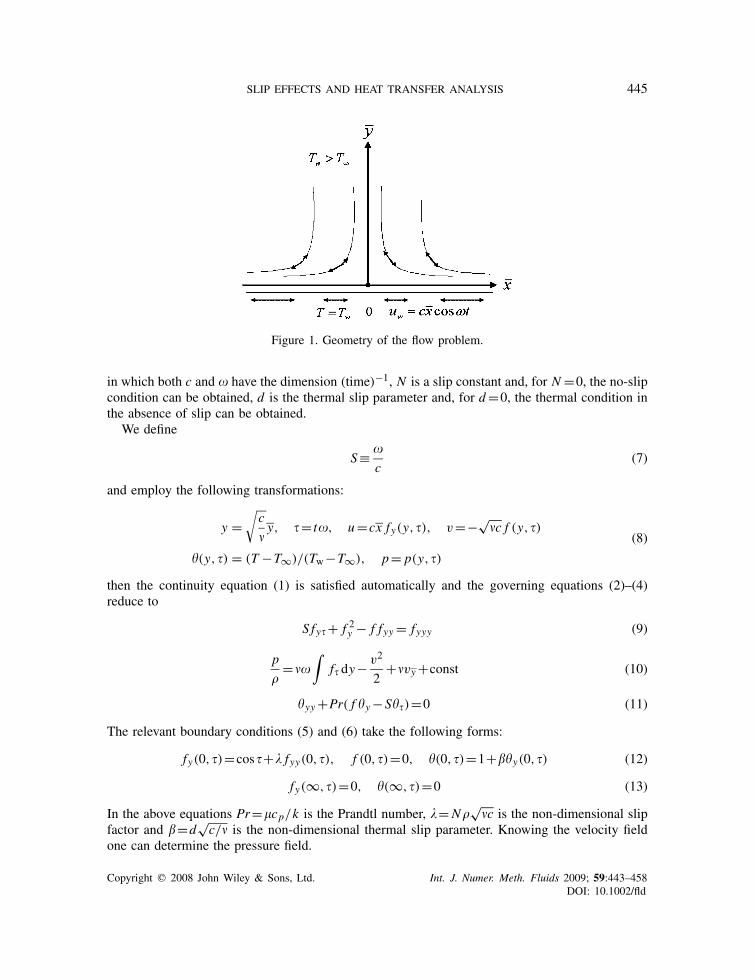
Consider a two-dimensional flow of an incompressible viscous fluid over an oscillatory stretchingsurface at y=0. Here, the x-axis is taken along the stretching surface and the y-axis normal toit (Figure 1). The elastic sheet is stretched back and forth with velocity uw=cx cos�t (c is themaximum stretching rate and � is the frequency). The fluid occupies the region y>0. The surfaceand ambient temperatures are Tw and T∞, respectively, and Tw>T∞. In the absence of viscousdissipation, the continuity, Navier–Stokes equations and energy equations are

�u�x

+ �v

�y=0 (1)

�u�t

+u�u�x

+v�u�y

=−1

�

�p�x

+�∇2u (2)

�v

�t+u

�v

�x+v

�v

�y=−1

�

�p�y

+�∇2v (3)

�cp

(�T�t

+u�T�x

+v�T�y

)=k∇2T (4)

where (u,v) are the velocity components in the (x, y) directions, respectively, t is the time, � isthe kinematic viscosity of fluid, � is the density of the fluid, p is the pressure, cp is the specificheat at constant pressure, k is the thermal diffusivity and T is the temperature.

The corresponding slip conditions for the velocity and temperature are

u=uw=cx cos�t+N��u�y

, v=0, T =Tw+d�T�y

at y=0 (5)

u→0, T →T∞ as y→∞ (6)

Copyright q 2008 John Wiley & Sons, Ltd. Int. J. Numer. Meth. Fluids 2009; 59:443–458DOI: 10.1002/fld

SLIP EFFECTS AND HEAT TRANSFER ANALYSIS 445

Figure 1. Geometry of the flow problem.

in which both c and � have the dimension (time)−1, N is a slip constant and, for N =0, the no-slipcondition can be obtained, d is the thermal slip parameter and, for d=0, the thermal condition inthe absence of slip can be obtained.

We define

S≡ �

c(7)

and employ the following transformations:

y =√c

�y, �= t�, u=cx fy(y,�), v=−√

�c f (y,�)

�(y,�) = (T −T∞)/(Tw−T∞), p= p(y,�)

(8)

then the continuity equation (1) is satisfied automatically and the governing equations (2)–(4)reduce to

S fy�+ f 2y − f fyy = fyyy (9)

p

�=��

∫f� dy− v2

2+�vy+const (10)

�yy+Pr( f �y−S��)=0 (11)

The relevant boundary conditions (5) and (6) take the following forms:

fy(0,�)=cos�+� fyy(0,�), f (0,�)=0, �(0,�)=1+�y(0,�) (12)

fy(∞,�)=0, �(∞,�)=0 (13)

In the above equations Pr=�cp/k is the Prandtl number, �=N�√

�c is the non-dimensional slipfactor and =d

√c/� is the non-dimensional thermal slip parameter. Knowing the velocity field

one can determine the pressure field.

Copyright q 2008 John Wiley & Sons, Ltd. Int. J. Numer. Meth. Fluids 2009; 59:443–458DOI: 10.1002/fld

446 Z. ABBAS ET AL.

The physical quantities of interest are also the skin-friction coefficient Cf and the local Nusseltnumber Nux , which are defined as

Cf= �w�u2w

, Nux = xqwk(Tw−T∞)

(14)

where �w and qw are the wall skin friction and the heat transfer from the sheet, respectively. Theseare given by

�w=�

(�u�y

)y=0

, qw=−k

(�T�y

)y=0

(15)

Through the transformations (8) one obtains

Re1/2x Cf= fyy(0,�), Re−1/2x Nux =−�y(0,�) (16)

where Rex =uwx/� is the local Reynolds number.

3. SOLUTION OF THE PROBLEM

The coordinate transformation =1/(y+1) is applied for transforming the semi-infinite physicaldomain y∈[0,∞) to a finite calculation domain ∈[0,1], i.e.

y= 1

−1,

��y

=−2��

,�2

�y2=4

�2

�2+23

��

�2

�y��=−2

�2

���,

�3

�y3=−6

�3

�3−65

�2

�2−64

��

With these transformations, the differential equations (9) and (11) can be rewritten in terms of as

S�2 f���

=2(

� f

�

)2

+(62−2 f )� f

�+(63− f )

�2 f�2

+4�3 f�3

(17)

4�2��2

+23��

�−Pr

(f 2

��

�+S

��

��

)=0 (18)

The boundary conditions (12) and (13) can be rewritten in terms of as

f =0, �=0 at =0 (19)

f =0, −2 f =cos�+�(4 f+23 f), �=1−2� at =1 (20)

We can discretize them for M uniformly distributed discrete points in g=(1,2,3, . . . ,{M})∈(0,1) with a space grid size of �=1/(M+1) and the time levels t=(t1, t2, . . .). Hence, thediscrete values ( f n1 , f n2 , . . . , f nM ) and (�n1,�

n2, . . . ,�

nM ) at these grid points for the time levels

tn =n�t (�t is the time step size) can be numerically solved together with the boundary conditions

Copyright q 2008 John Wiley & Sons, Ltd. Int. J. Numer. Meth. Fluids 2009; 59:443–458DOI: 10.1002/fld

SLIP EFFECTS AND HEAT TRANSFER ANALYSIS 447

at =0=0 and ={M+1} =1, (19) and (20), as the initial conditions are given. We start oursimulations from a motionless velocity field and a uniform temperature distribution equal to thetemperature at infinity

f (,�=0)=0 and �(,�=0)=0

The oscillatory motion of the sheet with a temperature Tw (�=1) is suddenly set from �=0 at=1 (y=0). We will see that the periodic motion will be reached after 2–4 periods. Since there aretwo boundary conditions for f at =1 and only one at =0, we cannot use central differences toapproximate the third-order spatial derivative f emerging in Equation (17). For the third-orderderivative, the following finite-difference scheme is used, which is not central differences, andonly of first-order accuracy:

�3 f�3

∣∣∣∣∣{=i }= fi+2−3 fi+1+3 fi − fi−1

(�)3+O(�2) (21)

where fi is the numerical value of f at the point =i . We construct a semi-implicit time differencefor f and �, respectively, and make sure that only linear equations for the new time step (n+1)need to be solved:

S1

�t

(� f (n+1)

�− � f (n)

�

)= 2

(� f (n)

�

)2

+62� f (n+1)

�−2 f (n)

� f (n)

�+63

�2 f (n+1)

�2

− f (n)2�2 f (n)

�2+4

�3 f (n+1)

�3(22)

SPr(�(n+1)−�(n))

�t=4

�2�(n+1)

�2+23

��(n+1)

�−Pr f (n)2

��(n+1)

�(23)

It should be noted that other different choices of time differences are also possible. By meansof the finite-difference method we can obtain two linear equation systems for f (n+1)

i and �(n+1)i

(i=1,2, . . . ,M) at the time step (n+1), which can be solved, e.g. by the Gaussian elimination.

4. NUMERICAL RESULTS AND DISCUSSION

We obtain the velocity and temperature fields by solving Equations (17) and (18) with boundaryconditions (19) and (20) numerically for the -coordinate. Then the numerical solutions are trans-formed to the physical space with y-coordinate. The velocity f ′ (= fy) and the temperature profile� and the time series of the first five periods �∈[0,10�] are illustrated for various values ofnon-dimensional relative amplitude of frequency to the stretching rate S, the slip parameter �, thePrandtl number Pr and the thermal slip parameter in the case of no-slip (�=0,=0) and withslip (� =0, =0). Furthermore, we compute and compare the values of skin-friction coefficientRe1/2x Cf and the local Nusselt number Re−1/2

x Nux for various parameters both graphically andthey are tabulated.

Copyright q 2008 John Wiley & Sons, Ltd. Int. J. Numer. Meth. Fluids 2009; 59:443–458DOI: 10.1002/fld

448 Z. ABBAS ET AL.

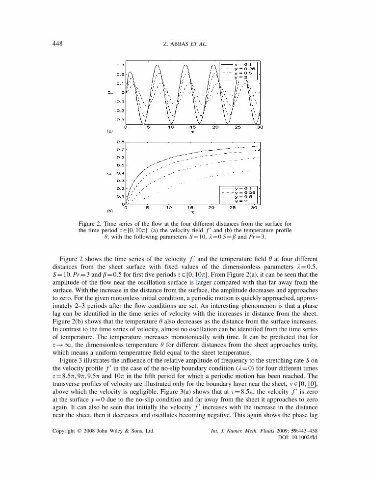
Figure 2. Time series of the flow at the four different distances from the surface forthe time period �∈[0,10�]: (a) the velocity field f ′ and (b) the temperature profile

�, with the following parameters S=10, �=0.5= and Pr=3.

Figure 2 shows the time series of the velocity f ′ and the temperature field � at four differentdistances from the sheet surface with fixed values of the dimensionless parameters �=0.5,S=10,Pr=3 and =0.5 for first five periods �∈[0,10�]. From Figure 2(a), it can be seen that theamplitude of the flow near the oscillation surface is larger compared with that far away from thesurface. With the increase in the distance from the surface, the amplitude decreases and approachesto zero. For the given motionless initial condition, a periodic motion is quickly approached, approx-imately 2–3 periods after the flow conditions are set. An interesting phenomenon is that a phaselag can be identified in the time series of velocity with the increases in distance from the sheet.Figure 2(b) shows that the temperature � also decreases as the distance from the surface increases.In contrast to the time series of velocity, almost no oscillation can be identified from the time seriesof temperature. The temperature increases monotonically with time. It can be predicted that for�→∞, the dimensionless temperature � for different distances from the sheet approaches unity,which means a uniform temperature field equal to the sheet temperature.

Figure 3 illustrates the influence of the relative amplitude of frequency to the stretching rate S onthe velocity profile f ′ in the case of the no-slip boundary condition (�=0) for four different times�=8.5�,9�,9.5� and 10� in the fifth period for which a periodic motion has been reached. Thetransverse profiles of velocity are illustrated only for the boundary layer near the sheet, y∈[0,10],above which the velocity is negligible. Figure 3(a) shows that at �=8.5�, the velocity f ′ is zeroat the surface y=0 due to the no-slip condition and far away from the sheet it approaches to zeroagain. It can also be seen that initially the velocity f ′ increases with the increase in the distancenear the sheet, then it decreases and oscillates becoming negative. This again shows the phase lag

Copyright q 2008 John Wiley & Sons, Ltd. Int. J. Numer. Meth. Fluids 2009; 59:443–458DOI: 10.1002/fld

SLIP EFFECTS AND HEAT TRANSFER ANALYSIS 449

Figure 3. Transverse profiles of the velocity field f ′ at the four different values of S for the fifthperiod �∈[8�,10�] for which a periodic velocity field has been reached: (a) �=8.5�; (b) �=9�;

(c) �=9.5�; and (d) �=10� in the case of no-slip �=0.

between the flow and the oscillation of the sheet. It indicates that along the transverse direction aphase difference larger than � may occur. The velocity profiles for several other time points withinthe fifth period are displayed in Figures 3(b)–(d). It can also be seen that the velocity field is notin phase with the sheet oscillation. With the increase in the distance from the sheet, the phasedisplacement increases. Furthermore, when S increases, the oscillation amplitude of the velocitydecreases.

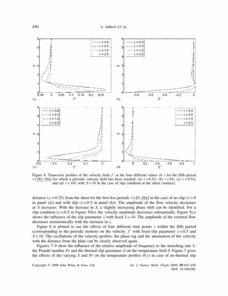
Figure 4 is plotted for the variations of the slip parameter � on the velocity profile f ′ by keepingS=10 fixed for the different times of �∈[8.5�,9�,9.5�,10�] in the fifth period, respectively.When slip occurs (� =0), the flow velocity near the sheet is no longer equal to the sheet oscillationvelocity, i.e. a velocity slip exists. With the increase in �, such a slip velocity increases. Furthermore,increasing the value of � will decrease the flow velocity amplitude, because under the slip conditionthe propulsion of the oscillatory sheet can be only partly transmitted to the fluid.

Figure 5 elucidates the effects of the relative amplitude of frequency to the stretching rate S(panels a and b) and the slip parameter � (panel c) on the time series of velocity at a fixed

Copyright q 2008 John Wiley & Sons, Ltd. Int. J. Numer. Meth. Fluids 2009; 59:443–458DOI: 10.1002/fld

450 Z. ABBAS ET AL.

Figure 4. Transverse profiles of the velocity field f ′ at the four different values of � for the fifth period�∈[8�,10�] for which a periodic velocity field has been reached: (a) �=8.5�; (b) �=9�; (c) �=9.5�;

and (d) �=10� with S=10 in the case of slip condition at the sheet (surface).

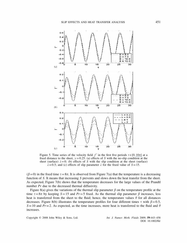
distance (y=0.25) from the sheet for the first five periods �∈[0,10�] in the case of no-slip (�=0in panel (a)) and with slip (�=0.5 in panel (b)). The amplitude of the flow velocity decreasesas S increases. With the increase in S, a slightly increasing phase shift can be identified. For aslip condition (�=0.5 in Figure 5(b)), the velocity amplitude decreases substantially. Figure 5(c)shows the influence of the slip parameter � with fixed S=10. The amplitude of the external flowdecreases monotonically with the increase in �.

Figure 6 is plotted to see the effects of four different time points � within the fifth period(corresponding to the periodic motion) on the velocity f ′ with fixed slip parameter �=0.5 andS=10. The oscillations of the velocity profiles, the phase lag and the attenuation of the velocitywith the distance from the plate can be clearly observed again.

Figures 7–9 show the influence of the relative amplitude of frequency to the stretching rate S,the Prandtl number Pr and the thermal slip parameter on the temperature field �. Figure 7 givesthe effects of the varying S and Pr on the temperature profiles �(y) in case of no-thermal slip

Copyright q 2008 John Wiley & Sons, Ltd. Int. J. Numer. Meth. Fluids 2009; 59:443–458DOI: 10.1002/fld

SLIP EFFECTS AND HEAT TRANSFER ANALYSIS 451

Figure 5. Time series of the velocity field f ′ in the first five periods �∈[0,10�] at afixed distance to the sheet, y=0.25: (a) effects of S with the no-slip condition at thesheet (surface) �=0; (b) effects of S with the slip condition at the sheet (surface)

�=0.5; and (c) effects of slip parameter � for the fixed value of S=15.

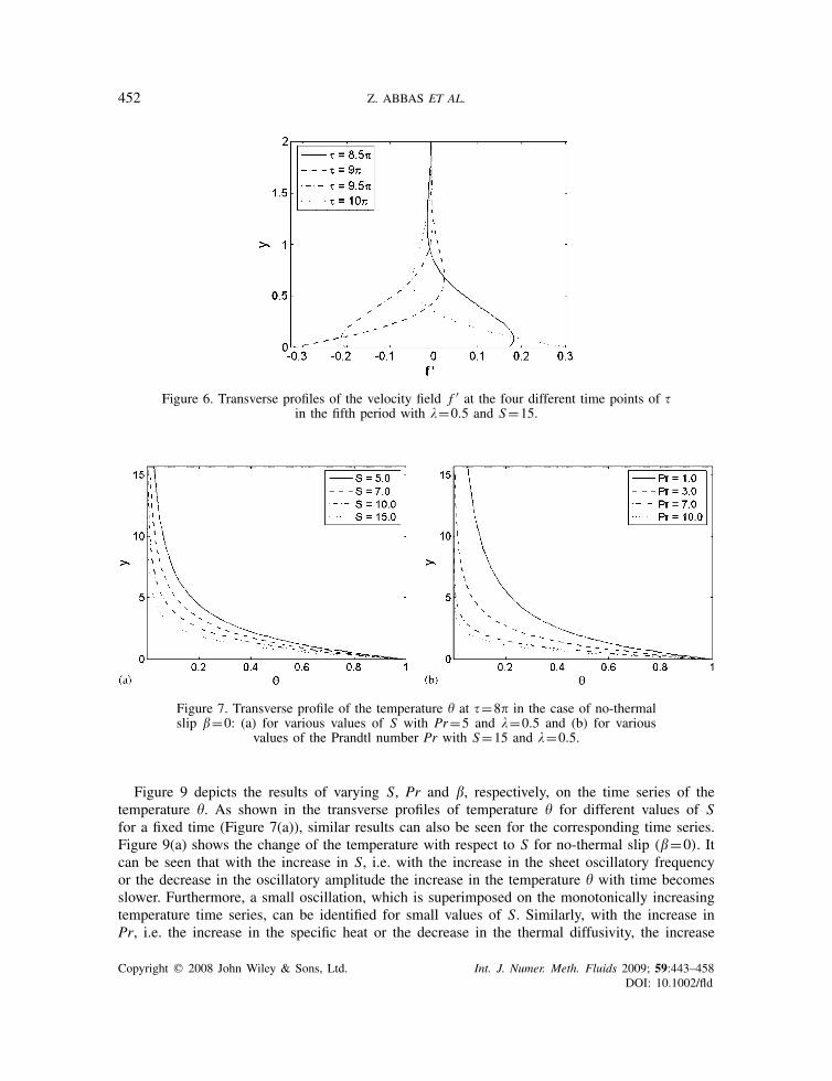
(=0) in the fixed time �=8�. It is observed from Figure 7(a) that the temperature is a decreasingfunction of S. It means that increasing S prevents and slows down the heat transfer from the sheet.As expected, Figure 7(b) shows that the temperature decreases for the large values of the Prandtlnumber Pr due to the decreased thermal diffusivity.

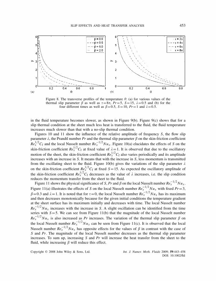
Figure 8(a) gives the variations of the thermal slip parameter on the temperature profile at thetime �=8� by keeping S=15 and Pr=5 fixed. As the thermal slip parameter increases, lessheat is transferred from the sheet to the fluid; hence, the temperature values � for all distancesdecreases. Figure 8(b) illustrates the temperature profiles for four different times � with =0.5,S=10 and Pr=2. As expected, as the time increases, more heat is transferred to the fluid and �increases.

Copyright q 2008 John Wiley & Sons, Ltd. Int. J. Numer. Meth. Fluids 2009; 59:443–458DOI: 10.1002/fld

452 Z. ABBAS ET AL.

Figure 6. Transverse profiles of the velocity field f ′ at the four different time points of �in the fifth period with �=0.5 and S=15.

Figure 7. Transverse profile of the temperature � at �=8� in the case of no-thermalslip =0: (a) for various values of S with Pr=5 and �=0.5 and (b) for various

values of the Prandtl number Pr with S=15 and �=0.5.

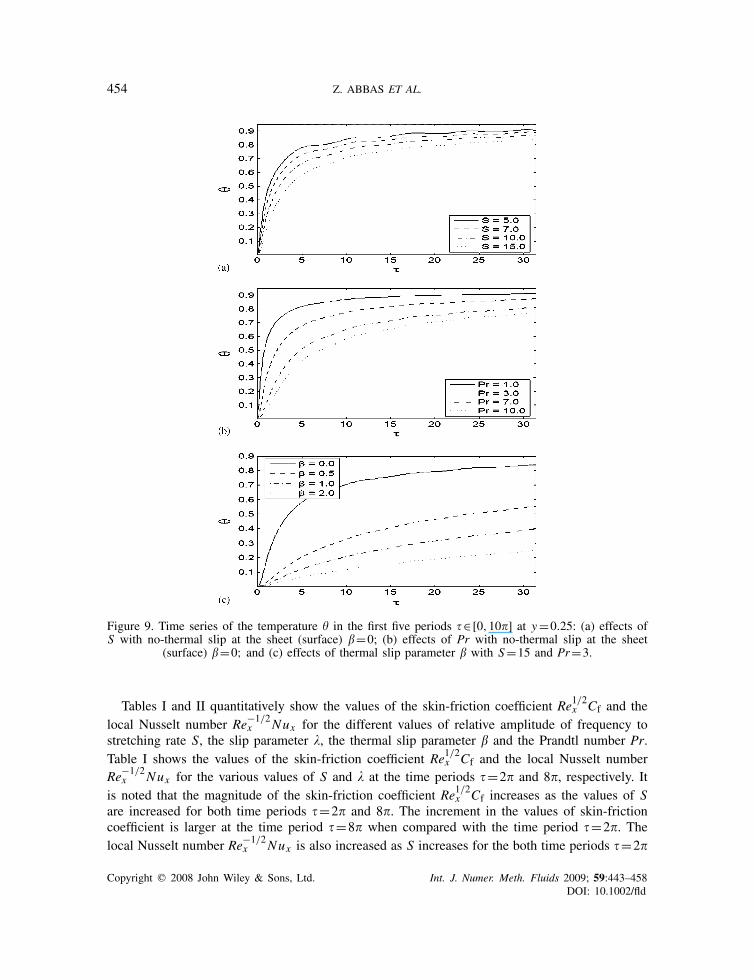
Figure 9 depicts the results of varying S, Pr and , respectively, on the time series of thetemperature �. As shown in the transverse profiles of temperature � for different values of Sfor a fixed time (Figure 7(a)), similar results can also be seen for the corresponding time series.Figure 9(a) shows the change of the temperature with respect to S for no-thermal slip (=0). Itcan be seen that with the increase in S, i.e. with the increase in the sheet oscillatory frequencyor the decrease in the oscillatory amplitude the increase in the temperature � with time becomesslower. Furthermore, a small oscillation, which is superimposed on the monotonically increasingtemperature time series, can be identified for small values of S. Similarly, with the increase inPr, i.e. the increase in the specific heat or the decrease in the thermal diffusivity, the increase

Copyright q 2008 John Wiley & Sons, Ltd. Int. J. Numer. Meth. Fluids 2009; 59:443–458DOI: 10.1002/fld

SLIP EFFECTS AND HEAT TRANSFER ANALYSIS 453

Figure 8. The transverse profiles of the temperature �: (a) for various values of thethermal slip parameter as well as �=8�, Pr=5, S=15, �=0.5 and (b) for the

four different times as well as =0.5, S=10, Pr=1 and �=0.5.

in the fluid temperature becomes slower, as shown in Figure 9(b). Figure 9(c) shows that for aslip thermal condition at the sheet much less heat is transferred to the fluid, the fluid temperatureincreases much slower than that with a no-slip thermal condition.

Figures 10 and 11 show the influence of the relative amplitude of frequency S, the flow slipparameter �, the Prandtl number Pr and the thermal slip parameter on the skin-friction coefficientRe1/2x Cf and the local Nusselt number Re−1/2

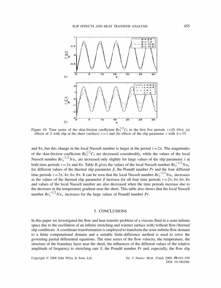
x Nux . Figure 10(a) elucidates the effects of S on theskin-friction coefficient Re1/2x Cf at fixed value of �=1. It is observed that due to the oscillatorymotion of the sheet, the skin-friction coefficient Re1/2x Cf also varies periodically and its amplitudeincreases with an increase in S. It means that with the increase in S, less momentum is transmittedfrom the oscillating sheet to the fluid. Figure 10(b) gives the variations of the slip parameter �on the skin-friction coefficient Re1/2x Cf at fixed S=15. As expected the oscillatory amplitude ofthe skin-friction coefficient Re1/2x Cf decreases as the value of � increases, i.e. the slip conditionreduces the momentum transfer from the sheet to the fluid.

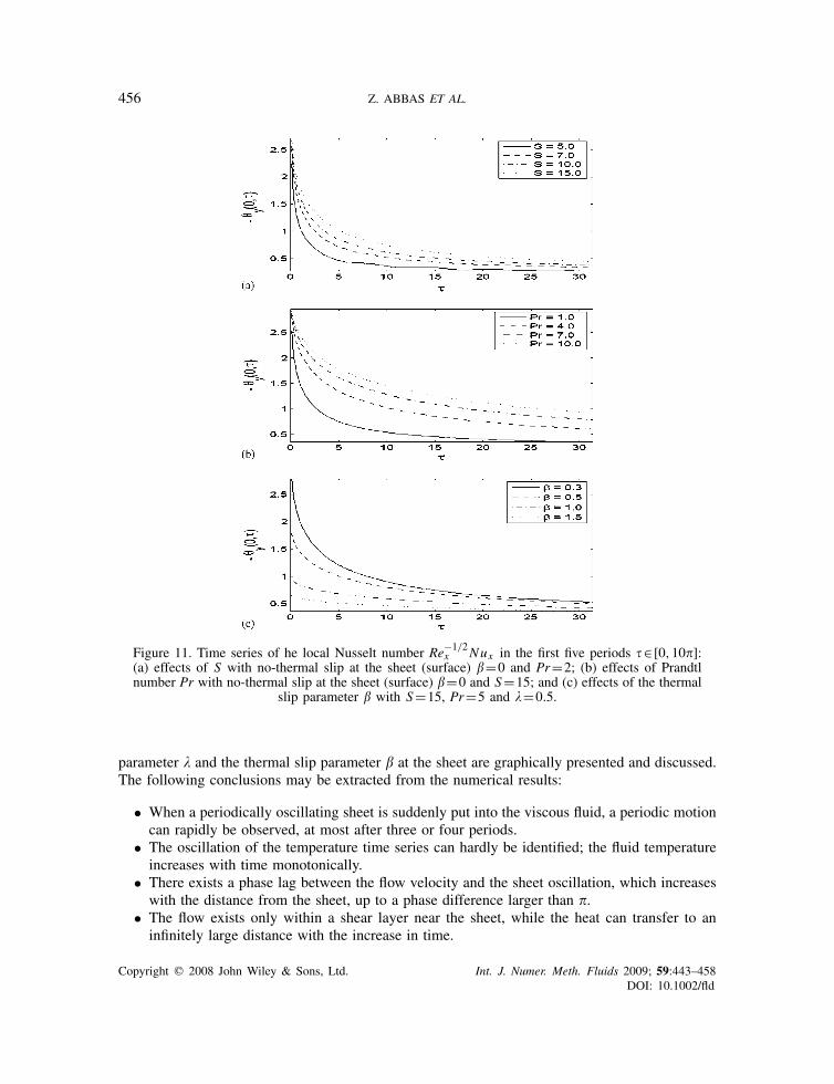
Figure 11 shows the physical significance of S, Pr and on the local Nusselt number Re−1/2x Nux .

Figure 11(a) illustrates the effects of S on the local Nusselt number Re−1/2x Nux with fixed Pr=3,

=0.3 and �=1. It is noted that for �=0, the local Nusselt number Re−1/2x Nux has its maximum

and then decreases monotonically because for the given initial conditions the temperature gradientat the sheet surface has its maximum initially and decreases with time. The local Nusselt numberRe−1/2

x Nux increases with the increase in S. A slight oscillation can be identified from the timeseries with S=5. We can see from Figure 11(b) that the magnitude of the local Nusselt numberRe−1/2

x Nux is also increased as Pr increases. The variation of the thermal slip parameter onthe local Nusselt number Re−1/2

x Nux can be seen from Figure 11(c). It is observed that the localNusselt number Re−1/2

x Nux has opposite effects for the values of in contrast with the case ofS and Pr. The magnitude of the local Nusselt number decreases as the thermal slip parameterincreases. To sum up, increasing S and Pr will increase the heat transfer from the sheet to thefluid, while increasing will reduce this effect.

Copyright q 2008 John Wiley & Sons, Ltd. Int. J. Numer. Meth. Fluids 2009; 59:443–458DOI: 10.1002/fld

454 Z. ABBAS ET AL.

Figure 9. Time series of the temperature � in the first five periods �∈[0,10�] at y=0.25: (a) effects ofS with no-thermal slip at the sheet (surface) =0; (b) effects of Pr with no-thermal slip at the sheet

(surface) =0; and (c) effects of thermal slip parameter with S=15 and Pr=3.

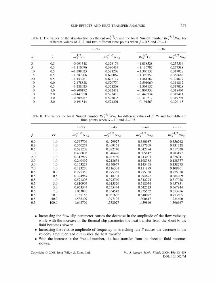
Tables I and II quantitatively show the values of the skin-friction coefficient Re1/2x Cf and thelocal Nusselt number Re−1/2

x Nux for the different values of relative amplitude of frequency tostretching rate S, the slip parameter �, the thermal slip parameter and the Prandtl number Pr.Table I shows the values of the skin-friction coefficient Re1/2x Cf and the local Nusselt numberRe−1/2

x Nux for the various values of S and � at the time periods �=2� and 8�, respectively. Itis noted that the magnitude of the skin-friction coefficient Re1/2x Cf increases as the values of Sare increased for both time periods �=2� and 8�. The increment in the values of skin-frictioncoefficient is larger at the time period �=8� when compared with the time period �=2�. Thelocal Nusselt number Re−1/2

x Nux is also increased as S increases for the both time periods �=2�

Copyright q 2008 John Wiley & Sons, Ltd. Int. J. Numer. Meth. Fluids 2009; 59:443–458DOI: 10.1002/fld

SLIP EFFECTS AND HEAT TRANSFER ANALYSIS 455

Figure 10. Time series of the skin-friction coefficient Re1/2x Cf in the first five periods �∈[0,10�]: (a)effects of S with slip at the sheet (surface) �=1 and (b) effects of the slip parameter � with S=15.

and 8�, but this change in the local Nusselt number is larger at the period �=2�. The magnitudesof the skin-friction coefficient Re1/2x Cf are decreased considerably, while the values of the localNusselt number Re−1/2

x Nux are increased only slightly for large values of the slip parameter � atboth time periods �=2� and 8�. Table II gives the values of the local Nusselt number Re−1/2

x Nuxfor different values of the thermal slip parameter , the Prandtl number Pr and the four differenttime periods �=2�,4�,6�,8�. It can be seen that the local Nusselt number Re−1/2

x Nux decreasesas the values of the thermal slip parameter increase for all four time periods �=2�,4�,6�,8�and values of the local Nusselt number are also decreased when the time periods increase due tothe decrease in the temperature gradient near the sheet. This table also shows that the local Nusseltnumber Re−1/2

x Nux increases for the large values of Prandtl number Pr.

5. CONCLUSIONS

In this paper we investigated the flow and heat transfer problem of a viscous fluid in a semi-infinitespace due to the oscillation of an infinite stretching and warmer surface with/without flow/thermalslip conditions. A coordinate transformation is employed to transform the semi-infinite flow domainto a finite computational domain and a suitable finite-difference method is used to solve thegoverning partial differential equations. The time series of the flow velocity, the temperature, thestructure of the boundary layer near the sheet, the influences of the different values of the relativeamplitude of frequency to stretching rate S, the Prandtl number Pr and, especially, the flow slip

Copyright q 2008 John Wiley & Sons, Ltd. Int. J. Numer. Meth. Fluids 2009; 59:443–458DOI: 10.1002/fld

456 Z. ABBAS ET AL.

Figure 11. Time series of he local Nusselt number Re−1/2x Nux in the first five periods �∈[0,10�]:

(a) effects of S with no-thermal slip at the sheet (surface) =0 and Pr=2; (b) effects of Prandtlnumber Pr with no-thermal slip at the sheet (surface) =0 and S=15; and (c) effects of the thermal

slip parameter with S=15, Pr=5 and �=0.5.

parameter � and the thermal slip parameter at the sheet are graphically presented and discussed.The following conclusions may be extracted from the numerical results:

• When a periodically oscillating sheet is suddenly put into the viscous fluid, a periodic motioncan rapidly be observed, at most after three or four periods.

• The oscillation of the temperature time series can hardly be identified; the fluid temperatureincreases with time monotonically.

• There exists a phase lag between the flow velocity and the sheet oscillation, which increaseswith the distance from the sheet, up to a phase difference larger than �.

• The flow exists only within a shear layer near the sheet, while the heat can transfer to aninfinitely large distance with the increase in time.

Copyright q 2008 John Wiley & Sons, Ltd. Int. J. Numer. Meth. Fluids 2009; 59:443–458DOI: 10.1002/fld

SLIP EFFECTS AND HEAT TRANSFER ANALYSIS 457

Table I. The values of the skin-friction coefficient Re1/2x Cf and the local Nusselt number Re−1/2x Nux for

different values of S, � and two different time points when =0.5 and Pr=1.

�=2� �=8�

S � Re1/2x Cf Re−1/2x Nux Re1/2x Cf Re−1/2

x Nux

3 0.5 −0.991348 0.326176 −1.038528 0.2575345 0.5 −1.110076 0.390433 −1.136707 0.27738810 0.5 −1.288023 0.521208 −1.303137 0.31702815 0.5 −1.387906 0.620067 −1.398357 0.35668820 0.5 −1.453961 0.698117 −1.461767 0.39467710 0.0 −2.478828 0.520770 −2.591060 0.31481210 0.5 −1.288023 0.521208 −1.303137 0.31702810 1.0 −0.800192 0.522412 −0.804338 0.31840410 2.0 −0.447958 0.523418 −0.448734 0.31941110 3.0 −0.309987 0.523835 −0.310217 0.31979410 5.0 −0.191544 0.524201 −0.191563 0.320115

Table II. The values the local Nusselt number Re−1/2x Nux for different values of , Pr and four different

time points when S=10 and �=0.5.

�=2� �=4� �=6� �=8�

Pr Re−1/2x Nux Re−1/2

x Nux Re−1/2x Nux Re−1/2

x Nux

0.0 1.0 0.567704 0.429927 0.380987 0.3567620.3 1.0 0.550257 0.409161 0.357609 0.3317280.5 1.0 0.521208 0.392740 0.342794 0.3170281.0 1.0 0.436805 0.346426 0.305842 0.2831972.0 1.0 0.312979 0.267130 0.243003 0.2280413.0 1.0 0.240492 0.213634 0.198383 0.1883775.0 1.0 0.163227 0.150957 0.143468 0.1382737.0 1.0 0.123270 0.116301 0.111899 0.1087610.5 0.0 0.275358 0.275358 0.275358 0.2753580.5 0.5 0.394987 0.318701 0.294697 0.2842090.5 1.0 0.521208 0.392740 0.342794 0.3170280.5 3.0 0.810907 0.615329 0.518054 0.4578510.5 5.0 0.963344 0.755444 0.642523 0.5679440.5 7.0 1.063076 0.854542 0.735532 0.6539560.5 10.0 1.165156 0.961632 0.840072 0.7538050.5 50.0 1.538309 1.397107 1.300617 1.2246000.5 100.0 1.648709 1.538027 1.459846 1.396667

• Increasing the flow slip parameter causes the decrease in the amplitude of the flow velocity,while with the increase in the thermal slip parameter the heat transfer from the sheet to thefluid becomes slower.

• Increasing the relative amplitude of frequency to stretching rate S causes the decrease in thevelocity amplitude and diminishes the heat transfer.

• With the increase in the Prandtl number, the heat transfer from the sheet to fluid becomesslower.

Copyright q 2008 John Wiley & Sons, Ltd. Int. J. Numer. Meth. Fluids 2009; 59:443–458DOI: 10.1002/fld

458 Z. ABBAS ET AL.

ACKNOWLEDGEMENTS

We are grateful to the reviewers for the useful suggestions. One of the authors Z. Abbas gratefullyacknowledges the support provided for this study by the Higher Education Commission (HEC) Pakistanunder the International Research Support Initiative Program (IRSIP).

REFERENCES

1. Sajid M, Hayat T. Non-similar series solution for boundary layer flow of a third order fluid over a stretchingsheet. Applied Mathematics and Computation 2007; 189:1576–1585.

2. Ariel PD, Hayat T, Asghar S. Homotopy perturbation method and axisymmetric flow over a stretching sheet.International Journal of Nonlinear Science and Numerical Simulation 2006; 7:399–406.

3. Hayat T, Sajid M. Analytic solution for axisymmetric flow and heat transfer of a second grade fluid past astretching sheet. International Journal of Heat and Mass Transfer 2007; 50:75–84.

4. Sajid M, Hayat T, Asghar S. Non-similar solution for the axisymmetric flow of a third grade fluid over a radiallystretching sheet. Acta Mechanica 2007; 189:193–205.

5. Wang CY. Flow due to a stretching boundary with partial slip-an exact solution of the Navier–Stokes equations.Chemical Engineering Science 2002; 57:3745–3747.

6. Cortell R. A note on magnetohydrodynamic flow of a power-law fluid over a stretching sheet. Applied Mathematicsand Computation 2005; 168:557–566.

7. Cortell R. A note on flow and heat transfer of a viscoelastic fluid over a stretching sheet. International Journalof Non-linear Mechanics 2006; 41:78–85.

8. Vajravelu K, Rollins D. Hydromagnetic flow of second grade fluid over a stretching sheet. Applied Mathematicsand Computation 2004; 148:783–791.

9. Liu IC. Flow and heat transverse of an electrically conducting fluid of second grade over a stretching sheetsubject to a transverse magnetic field. International Journal of Heat and Mass Transfer 2004; 47:4427–4437.

10. Hayat T, Abbas Z, Sajid M. Series solution for the upper convected Maxwell fluid over a porous stretching plate.Physics Letters A 2006; 358:396–403.

11. Sakiadis BC. Boundary-layer behavior on continuous solid surfaces: II. The boundary layer on a continuous flatsurface. AIChE Journal 1961; 7:221–227.

12. Pop I, Na TY. Unsteady flow past a stretching sheet. Mechanics Research Communications 1996; 23:413–422.13. Nazar R, Amin N, Pop I. Unsteady boundary layer flow due to a stretching surface in a rotating fluid. Mechanics

Research Communications 2004; 31:121–128.14. Liao SJ. An analytic solution of unsteady boundary layer flows caused by an impulsively stretching plate.

Communications in Nonlinear Science and Numerical Simulation 2006; 11:326–339.15. Wang C, Pop I. Analysis of the flow of a power-law fluid film on an unsteady stretching surface by means of

homotopy analysis method. Journal of Non-Newtonian Fluid Mechanics 2006; 138:161–172.16. Xu H, Liao SJ. Series solution of unsteady magnetohydrodynamic flows of non-Newtonian fluids caused by an

impulsively stretching plate. Journal of Non-Newtonian Fluid Mechanics 2005; 129:46–55.17. Sajid M, Ahmad I, Hayat T, Ayub M. Series solution for unsteady axisymmetric flow and heat transfer over a

radially stretching sheet. Communications in Nonlinear Science and Numerical Simulation, in press.18. Wang CY. Nonlinear streaming due to the oscillatory stretching of a sheet in a viscous fluid. Acta Mechanica

1988; 72:261–268.

Copyright q 2008 John Wiley & Sons, Ltd. Int. J. Numer. Meth. Fluids 2009; 59:443–458DOI: 10.1002/fld