NOLTA, IEICE

Invited Paper

Size frequency distribution of Japaneseplace-names

Kouki Hirosawa 1 and Tsuyoshi Mizuguchi 2a)

1 Department of Accelerator Science, SOKENDAI (The Graduate University for

Advanced Studies), Shonan Village, Hayama, Kanagawa 240-0193, Japan

2 Department of Mathematical Sciences, Osaka Prefecture University, 1-1,

Gakuencho, Nakaku, Sakai 599-8531, Japan

a) gutchi@ms.osakafu-u.ac.jp

Received April 9, 2016; Revised June 6, 2016; Published October 1, 2016

Abstract: The size frequency distribution of Japanese place-name is analyzed. The list ofmunicipalities and town-area names are extracted from the zip code table and their size fre-quency distributions are measured. The distribution of town-area names obeys a power lawbehavior while the distribution of municipality names is well fitted by a lognormal distribution.A simple mathematical model of the municipality and town-area evolution and their namingprocess is suggested.

Key Words: toponym, place-name, size distribution, power law, lognormal distribution

1. IntroductionEvery person has a name. In many cultures, he or she has a personal name composed of a familyname and a given name (and middle name(s)). There are many kind of family names from verycommon names to rare ones. Miyajima reported that the size frequency distribution of Japanesefamily names obeys a power law [1, 2]. Several studies follow these works, such as better fittings,a calculation of the extinction probability, researches in different countries or areas and stochasticmodels as an inheritance [3–8]. This power law behavior is a kind of Zipf’s law which is observed invarious fields. Several scenario are suggested as their underling mechanism such as a random walk,the phase transitions, the Yule process, the self-organized criticality, and a successive total of randommultiplicative process [9–12].

Similar analysis has been done for the size distribution of given names [13–18]. Hayakawa et al.reported that the size frequency distribution of Japanese given names also shows a power law behavior.The exponent is quite similar to that of the family name distribution. Although the naming processesof the family names and the given names differ each other, it is interesting that they show commonstatistical properties. This power law behavior of given name distribution is also reported in othercountries. Hayakawa et al. suggested a mathematical model based on the Yule process, i.e., (I) newname creation events with some probability and (II) the size-dependent selection mechanism. Theyalso adopt an exclusion principle of the given name which ensures the uniqueness in each family [17].

Not only human names, the distribution of names is considered to be a result of numerously

499

Nonlinear Theory and Its Applications, IEICE, vol. 7, no. 4, pp. 499–508 c©IEICE 2016 DOI: 10.1587/nolta.7.499

iterated naming process in the history. And if the two mechanisms, (I) and (II), exist of a certainnaming process, a power law distribution will be observed. Under these background, we analyze thedistribution of place-names, a.k.a, toponym, the designation of the local place.

There are several differences between place-names and human names. Human names are assignedfor each person, basically. The family name and the given name can be considered as an expressionof small but definite hierarchical structure of a family and individuals in it. On the other hand, theobject of place-names is widely distributed in scales, i.e., from the name of a continent to a tiny squarein a town. The fact that an inclusion relation between the objects suggests that there should be acomplex hierarchical structure between place-names. The name assigned to specific objects, such asmountains, rivers, and streets can be considered as place-names in a broad sense. There are manykinds of place-names for various objects, it is not easy to obtain comprehensive list of them.

In this article, we analyze the list of postal addresses based on the zip code table. Each of thepostal address is composed of definite hierarchical class, i.e., prefecture, municipality, and town-area.Based on this list, we measure the size frequency distribution of the municipality names and thetown-area names. Two definite features are observed: the lognormality of the municipality name sizedistribution and the power law behavior of the town-area name size distribution.

In the following section, the dataset is introduced and the size frequency distribution of the munici-pality names and the town-area names are analyzed. Distributions for several categories are comparedeach other. In section 3, a simple mathematical model of municipality and town-area evolution andtheir naming process is suggested. The final section is devoted to the discussions and comments. InAppendix, the correlation function between the population size and the municipality name size forall the municipalities are exhibited.

2. Data analysis

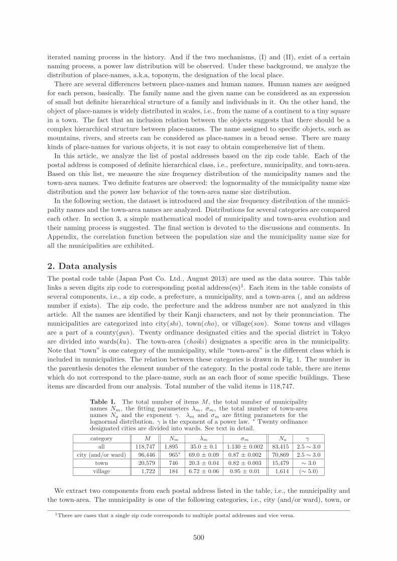
The postal code table (Japan Post Co. Ltd., August 2013) are used as the data source. This tablelinks a seven digits zip code to corresponding postal address(es)1. Each item in the table consists ofseveral components, i.e., a zip code, a prefecture, a municipality, and a town-area (, and an addressnumber if exists). The zip code, the prefecture and the address number are not analyzed in thisarticle. All the names are identified by their Kanji characters, and not by their pronunciation. Themunicipalities are categorized into city(shi), town(cho), or village(son). Some towns and villagesare a part of a county(gun). Twenty ordinance designated cities and the special district in Tokyoare divided into wards(ku). The town-area (choiki) designates a specific area in the municipality.Note that “town” is one category of the municipality, while “town-area” is the different class which isincluded in municipalities. The relation between these categories is drawn in Fig. 1. The number inthe parenthesis denotes the element number of the category. In the postal code table, there are itemswhich do not correspond to the place-name, such as an each floor of some specific buildings. Theseitems are discarded from our analysis. Total number of the valid items is 118,747.

Table I. The total number of items M , the total number of municipalitynames Nm, the fitting parameters λm, σm, the total number of town-areanames Na and the exponent γ. λm and σm are fitting parameters for thelognormal distribution. γ is the exponent of a power law. ∗ Twenty ordinancedesignated cities are divided into wards. See text in detail.

category M Nm λm σm Na γ

all 118,747 1,895 35.0 ± 0.1 1.130 ± 0.002 83,415 2.5 ∼ 3.0city (and/or ward) 96,446 965∗ 69.0 ± 0.09 0.87 ± 0.002 70,869 2.5 ∼ 3.0

town 20,579 746 20.3 ± 0.04 0.82 ± 0.003 15,479 ∼ 3.0village 1,722 184 6.72 ± 0.06 0.95 ± 0.01 1,614 (∼ 5.0)

We extract two components from each postal address listed in the table, i.e., the municipality andthe town-area. The municipality is one of the following categories, i.e., city (and/or ward), town, or

1There are cases that a single zip code corresponds to multiple postal addresses and vice versa.

500

Fig. 1. The relation between the components of postal address. The (part of)lower class is included in the upper class(es) connected by the line. The numberin the parenthesis denotes the element number of the categories. #There aretwenty three wards without city in the special district in Tokyo. ## There aretwenty ordinance designated cities which have wards. ∗,∗∗ There are two townsand seven villages independent of a county.

village. And the town-area is the following component after the municipality2. For example, if weconsider the postal address “Osakafu Sakaishi Nakaku Gakuencho 1-1” the municipality name of thispostal address is “Sakaishi Nakaku”, and the town-area name is “Gakuencho”. Both the prefecture“Osakafu” and the address numbers “1-1” are discarded.

Here we introduce several variables to characterize the dataset, i.e., the total number of items M ,the total number of municipality names Nm and the total number of town-area names Na, respectively.For example, the number of all the valid data in the postal code table is 118,747, and there are 1,895kinds of municipality names and 83,415 kinds of town-area names as in the first row in Table I.

First we focus on the size distribution of the town-area names. Some town-areas are composed oftwo or more elements, such as multiple sub-areas, local section called “aza”, etc. Especially, manyaddresses are made of two crossing streets name like the Cartesian coordinates in the middle part ofKyoto city. Or some items include address number information. All of them are considered to becomposite town-area names. It is, however, not easy to decompose them into elemental place-names.Therefore we treat them as a single place-name in this analysis. Almost all of such composite namesare unique, and they contribute to their size frequency distribution as a size of unity.

Among 83,415 kinds of town-area names, the most common town-area name is Honmachi, Honchoor Motomachi, all of which share the same Kanji characters. The size is 309, which means that309 different municipalities have a town-area of this name. Sakaemachi, Sakaecho or Eimachi, is thesecond common name shared by 221 town-areas. And Shinmachi, Shincho or Aramachi follows themby 169 town-areas, and so on.

Now we introduce the size distribution and its cumulative form. Let sj is the size of a certainplace-name j. And the cumulative form of size distribution is defined

P (> s) ≡∫ ∞

s

f(s′)ds′, (1)

where f(s) is the name size distribution of s. (Generalized) Zipf’s law means f(s) ∝ s−γ , which leadsP (> s) ∝ s−γ+1 if γ > 1. Hereafter, we use a suffix ‘a’ and ‘m’ to denote the town-area and themunicipality, respectively. For example, fa(s) denotes the size distribution of town-area names, whilePm(> s) is the cumulative size distribution of municipality names.

Figure 2(a) shows the cumulative distribution Pa(> s) of the town-area names in log-log plot.Pa(> s) is fairly straight with a slope slightly less than 2.0 in a certain range, i.e., Pa(> s) ∼ s−γ+1

or the size distribution obeys fa(s) ∼ s−γ with 2.5 < γ < 3.0. Note that the power law exponentof place-name is larger than that of human names because the exponent of the size distribution of

2This is Japanese address writing style. In European style, the town-area is written before the municipality.

501

Fig. 2. The cumulative distribution function of size of place-names in log-logplot. (a) The town-area names and (b) the municipality names. The solid linein (a) is drawn as a visual guide with slope −2.0 while the solid line in (b)denotes the fitting function by the lognormal distribution. See text.

human names ranges in 1 < γ < 2.2 [5, 17]. The distribution deviates from the power law at the sizeof unity. This is due to the many “unique” composite town-names described above.

Next we show the size distribution of the municipality names. Here we note two points: if towns orvillages belong to a county, the combined name are used as their name. And the wards are also treatedas individual municipalities with its city name if it exists. Namely, twenty ordinance designated citiesand the special district in Tokyo are separated into wards. As in the previous example, the totalnumber of municipality names Nm = 1, 895. The largest municipality name is Toyama city whosesize is 1,146, i.e., there are 1,146 town-areas in it. The second largest municipality name is Gifu cityhaving 833 town-areas, and Joetsu city follows them with 751 town-areas.

The cumulative distribution Pm(> s) of the municipality names is shown in Fig. 2(b). The solidline is the fitted line of the cumulative distribution function form of the lognormal distribution:

Pm(> s) =Mm

2

{1 − erf

(log s − log λm√

2σm

)}, (2)

where erf( ) is the Gaussian error function, i.e., erf(x) = 2π−1∫ x

0exp(−t2)dt. The coefficient Mm is

the total number of municipality names and the value of two fitting parameters λm and σm are listedin Table I. Data at the large size seem to deviate from the fitting line. Nevertheless, if we take as thenull hypothesis that the cumulative distribution of the municipality names size obeys Eq. (2) withparameters λm and σm, it is confirmed that the hypothesis is not rejected under the significance levelof 0.05 in terms of the χ2 test.

We also analyze the size distribution of the municipality names and the town-area names in eachcategory, i.e., city (and/or ward), town and village. The size distributions of the town-area namesexhibit power law behavior in all categories as shown in Fig. 3. Note that the exponent may dependon the categories. Similarly, all the size distribution of the municipality names are well fitted by alognormal distribution (see Fig. 4). The fitting parameters are listed in Table I. If we again take asthe null hypothesis that the cumulative distribution of municipality names for each category obeysEq. (2) with parameters λm and σm, it is confirmed that the hypothesis is not rejected under thesignificance level of 0.05.

We comment about the homonym of the municipalities. There exist two names shared by differentcities: One is Fuchu city used both in Tokyo and in Hiroshima prefecture. The other is Date city inHokkaido and Fukushima. Except these two pairs, all the city names are different each other. Thereare several homonym for town and village names. All the degeneracy of the names are resolved byincluding the name of the county to which they belong. Therefore the size of the municipality namesrepresents the number of town-area in the municipality approximately. In other words, the size ofthe municipality name expresses a kind of dimension of the municipality. In Appendix we introducethe previous studies on the size distribution of the population in Japanese municipalities. And thecorrelation between the population and the size of municipality names of Japanese municipalities are

502

Fig. 3. Log-log plot of the cumulative distribution function of size of town-area names. (a) City (and/or ward), (b) town, and (c) village. The solid linesare drawn as a visual guide with the slope value.

Fig. 4. Log-log plot of the cumulative distribution function of size of munici-pality names. (a) City (and/or ward), (b) town, and (c) village. The solid linesrepresent the fitting function by cumulative form of the lognormal distribution.

exhibited.

3. Model and simulationIn this section, we introduce a simple mathematical model of municipalities and town-areas evolutionand their naming process. From the real data analysis, two features are obtained, i.e., the lognormalityof the municipality name size distribution and the power law behavior of the town-area name sizedistribution. As described in the last part of the previous section, the size of the municipality namesin the postal code table corresponds to the number of town-area in each municipality, approximately.And the creation or merger process of town-areas may results from the population dynamics inand between the municipalities. The positive correlation between the population and the size ofmunicipality names in Appendix is consistent with this assumption.

On the contrary, the distribution of town-area names is considered to result from an iterated namingprocess of the newly constructed town-areas in the history. Some town-areas are named with wellused name like Honmachi or Sakaecho, and others are named with a completely new name never usedbefore. How the new town-area is named? This is a similar question for the case of the human namingprocess. Considering that there is no inheritance process between town-area names as observed in thehuman family names, we assume that the naming process of the town-area is close to that of humangiven names.

Our model consists of municipalities and town-area included in each municipality. A discretizedrandom multiplicative process is assumed to express the evolution of town-area number while theYule process with an exclusion principle is adopted for the name assignment process [17, 20]. Forthe simplicity, the total number of the municipality Nm is set to be constant. Let a generationg = 0, 1, 2, · · · and the i-th municipality Mi which consists of ni(g) town-areas. We assume thefollowing dynamics:

ni(g) = Round(ξ × ni(g − 1)), i = 1, · · · , Nm (3)

where Round( ) is the round off function introduced to keep ni(g) an integer, and ξ is a randomgrowth rate whose value is taken from a uniform random number in the range [λ′ − σ′, λ′ + σ′]. Eachtown-area has its own name. The newly constructed town-area is named using the following rule R:Assume that a new town-area is created in the municipality Mi at the generation g. Assign a new

503

Fig. 5. Typical time evolutions of the size of town-area names and munici-pality names in the simulation. (a) Five town-area names (j = 9224, 15673,48003, 38767, and 16110) are chosen as representatives and their sizes at gener-ation g are drawn in a semi-log plot. (b) Five municipality names (i = 262, 4,36, 11, and 230) are chosen as representatives and their sizes, ni(g), are drawnin a semi-log plot.

name never used before with a probability α. Otherwise, i.e., with a probability 1 − α, we choose aname from a list, Li, consisting of all existed town-area names in all municipalities in the generationsfrom 0 to g except the town-area names in the Mi at g. The exception is introduced to ensure theuniqueness of the town-area name in the municipality. This is a kind of exclusion principle of thehomonym. The probability of choosing name j in the list Li is given as

Πj = sβj /

∑k∈Li

sβk , (4)

where sj is the size of town-area having name j in the all municipalities in the generation from 0 tog. β is a parameter, and the denominator is the normalization constant. If β = 0, all the town-areanames in the Li is randomly chosen. A positive β means that the more the size of the name is, themore it tends to be chosen as a name of the new town-area, like so-called preferential attachmentprocess. Especially, it corresponds to the Yule process if β = 1. We call the parameter β popularity.

We summarize the simulation procedure of our model:

(i) As an initial condition, all the municipalities have the same number of town-area, ni(0) = n0.And different names are assigned to these initial town-areas.

(ii) As the generation g is incremented, the number of town-area in each municipality is changed byEq. (3). If new town-areas are created, their names are assigned by the rule R. If the numberof town-area decreases to zero, the number of town-area of the municipality is reset to n0 andthe name of each town-area is assigned by R. If the number of town-area decreases to a positivenumber, randomly chosen town-area(s) in the municipality is removed.

(iii) The procedure (ii) is iterated until g = gmax.

Typical parameter values are as follows: Nm = 1, 895, n0 = 20, gmax = 50, λ′ = 1.025, σ′ = 0.15,α = 0.16 and β = 1.4. Nm is the same value of the municipality number of all categories of thepostal code table. We assume that the number of town-area gradually increases in average with somefluctuation due to creation or merger events. Therefore we set λ′ slightly above the unity, whileλ′ − σ′ slightly below the unity. Other parameters are chosen by trial and error. Simulations areperformed with several initial conditions and random seeds, and the results reported below do notchange qualitatively.

Figure 5 shows typical time evolutions of the size of town-area names and municipality names. Fivetown-areas are chosen as representatives and their sizes at generation g are drawn in a semi-log plot(Fig. 5(a)). The size of each town-area name fluctuates with g due to the newly assigned process orthe removal process. The town-area j = 9224 is the most common town-area name at g = 50 whilej = 16110 is one of the rarest town-area names (actually it is a singleton) at g = 50. Some town-area names such as j = 48003 are created during the time evolution, and others such as j = 16110

504

Fig. 6. Typical simulation results of the model. (a) The cumulative sizedistribution function of the town-area names and (b) the municipality namesin log-log plots. The solid line in (a) is a visual guide with slope −2 while thesolid line in (b) is the fitted by the lognormal distribution.

Fig. 7. Parameter dependency of the town-area names distribution. Log-log plot of the cumulative distribution functions of the town-area names aresuperimposed. (a) The iteration number gmax is increased from 30 to 70. (b)The new name probability α is changed from 0.04 to 0.64. (c) The popularityβ is changed from 1.2 to 1.6. A power law behavior is observed in a certainrange of the name size. Its exponent, however, depends on the parameters.

vanish and are reused again. Similarly, five municipalities are chosen as representatives and the timeevolution of their sizes, ni(g), is drawn in a semi-log plot in Fig. 5(b). Their sizes also fluctuate withg. This is, however, due to the random multiplicative process in Eq. (3). In other words, this is akind of biased random walk on the log n line (with an wall at n < 0.5 where the particle jumps ton = n0). The municipality i = 262 is the largest municipality at g = 50 while i = 230 is one of thesmallest municipalities at g = 50.

Figure 6 show a typical result of this model. The cumulative size distribution of town-area namesat gmax exhibits a power law behavior with an exponent slightly less than 2.0 as shown in Fig. 6(a).The cumulative size distribution of municipality names is well fitted by a lognormal distribution(Fig. 6(b)). It is known that a random multiplicative process produces a lognormal distribution [9,19]. Therefore it is a quite natural result.

The distribution function form depends on some parameters. If we increase the iteration numbergmax with keeping the other parameters as in the values listed above, the exponent of the powerlaw γ tends to decrease as shown in Fig. 7(a). The exclusion principle is the rule to avoid the sametown-area name in one municipality. Therefore, its effect depends on the number of town-area ni(g).And ni(g) increases with g because λ is grater than unity in this case. This is an interpretation whythe distribution function Pa(> s) depends on g. If λ becomes unity by a kind of saturation effect,Pa(> s) is expected to converge to a stationary form.

Figure 7(b) indicates that the exponent γ increases with an increase of the new name probabilityα. This is because an increase of α means the increase of new town-area names and the ratio betweennew rare names to old common names increases. With respect to the popularity β, it seems to affectthe convexity at the middle range of Pa(> s) (Fig. 7(c)).

505

4. Conclusion and discussionIn this article, we study the size distribution of place-names. The data based on the zip code tableare used. The municipality component and the town-area component are extracted from the tableand their size distributions are analyzed. For whole dataset, the size distribution of the town-areanames shows a power law behavior with the exponent 2.5 < γ < 3.0. On the other hand, the sizedistribution of municipality names is well fitted by the lognormal distribution. We decompose thedata into three municipality categories, i.e., city (and/or ward), town, and village. Similar featuresare obtained for each dataset.

The number of municipality names in the zip code table is considered to correspond to the numberof town-areas in the municipality. Therefore it express a kind of dimension of the municipality. Thelognormality of their size distribution suggests that it obeys a random multiplicative process. On theother hand, the size distribution of town-area names exhibits a power law. This statistical featureresembles that of human name distributions. Considering that there is no inheritance process betweentown-area names as observed in the human family names, it is conjectured that the naming process ofthe town-area is close to that of human given names. We suggest a simple mathematical model of themunicipalities and town-areas evolution and their naming process. The town-area number evolutionis modeled by a discretized random multiplicative process, while their naming process is modeled bythe Yule process with the exclusion principle. The statistical feature of the distribution functions ofthe real data are reproduced by the model quantitatively in a certain parameter range.

We point out a few important differences between place-names and human names. One is the scaleof lifetime of individuals. The typical generation length of human beings is around 30 years, i.e.,babies are born every these years. Each of them inherits its family name and obtains its given name.Then, what is the typical time scale of the place-names? Some place-area names have been used fromor before the Edo period, while some have been assigned just at the Heisei period. Therefore thelifetime of the place-names is widely distributed in comparison with that of human. A systematicresearch of the place-name history is required.

Another definite difference is the merger process. The merger is the reconstruction of municipalitiesaccompanied with union and/or incorporation of them. There have been several great mergers, i.e.,Meiji, Showa and Heisei. At each great merger, many municipalities changes their internal structure.For the human names, a marriage may correspond to this kind of reconstruction process. It is,however, a process of a single person, and the scale of the event is quite different. Anyway, our modeldoes not take account of the merger process of the municipalities. The effect of this process remainsopen.

Next, we comment on the limitation of the decomposition of the place-names. In our analysis, wedecompose the postal addresses into several components, i.e., prefecture, municipality and town-area,to extract the place-names. Some town-areas, however, are still composed of more elemental place-names. For example, there are several town-areas whose names share a common word “Ohara” inKyoto city, like “Oharaidecho”, “Oharanomuracho”, “Oharamomoicho”, and so on. These town-areanames are considered to be decomposed into more elemental word such as “Ohara” and “idecho”,“nomuracho”, and “momoicho”, etc. Probably, it reflects a kind of hierarchical structure of theseplaces, i.e., “idecho”, “nomuracho”, and “momoicho” express the local area and they are includedin the larger area “Ohara”. From the viewpoint of place-names study, these hierarchical structureshould also be analyzed. It is, however, not easy to decompose these composite names into elementalwords systematically. An adequate decomposition method is necessary.

Finally, we comment about the place-names in other countries. The power law behavior of sizedistribution of human names (both family names and given names) is widely observed in manycountries [5, 17]. Therefore it is expected that the place-names also exhibit similar statistical featuresin other countries or objects.

Acknowledgments

The authors thank Professor Daido, Professor Horita, and Professor Kuninaka for fruitful discussions.

506

Fig. A-1. The correlation between the population x and size of municipalitynames s of each municipality in log-log plot.

Appendix

A. Relation between population of municipalities

As described in the main text, the size of the municipality names represents the number of town-areain the municipality approximately. Therefore the size of the municipality name expresses a kind ofdimension of the municipality. The population, the number of people living, in the area is anotherindex which represents the dimension of the municipality.

It is reported that the population distribution in Japanese municipalities obeys a specific functionform. Namely, a lognormal distribution in the small size range while a power law in the larger sizerange [21, 22]. In the previous studies, the population distribution of municipalities are analyzedin three categories, i.e., city, town, and village. And population distribution of each categories hasa characteristic form which reflects their properties. Namely, the population distribution of villagesobeys a lognormal distribution, while that of town has a cut off at large population regime. Populationdistribution of cities shows a power law tail. This is in contrast to the fact that all the size distributionof municipality names in different categories obeys a lognormal distribution as show in Fig. 4.

Figure A-1 shows a correlation between the size of municipality names and the population in log-log plot. The population data are taken from 2010 population census, Statistics Bureau, Ministryof Internal Affairs and Communications, Japan [23]. It is rather distributed but shows a positivecorrelation. Therefore there is a weak tendency that the more people live in the municipality, themore town-areas exist in it.

We think that the discrepancy between the population distribution and the municipality namesdistribution may result from the internal structure of town-areas such as the address numbers in thepostal address. Or there are many differences between the population dynamics and the town-areaevolution. For example, time scale of human movement seems to be shorter than the lifetime of town-areas. And it may require longer time for the town-area evolution to reflect the result the populationdynamics.

References[1] S. Miyazima, Y. Lee, T. Nagamine, and H. Miyajima, “Family name distribution in Japanese

societies,” J. Phys. Soc. Jpn., vol. 68, pp. 3244–3247, 1999.[2] S. Miyazima, Y. Lee, T. Nagamine, and H. Miyajima, “Power-law distribution of family names

in Japanese societies,” Physica, vol. A278, pp. 282–288, 2000.[3] D.H. Zanette and S.C. Manrubia, “Vertical transmission of culture and the distribution of family

names,” Physica, vol. A295, pp. 1–8. 2001.[4] S.C. Manrubia and D.H. Zanette, “At the boundary between biological and cultural evolution:

The origin of surname distributions,” J. theor. Biol., vol. 216, pp. 461–477, 2002.

507

[5] S.K. Baek, H.A.T. Kiet, and B.J. Kim, “Family name distributions: Master equation approach,”Phys. Rev. E., vol. 76, 046113, 2007.

[6] H.S. Yamada and K. Iguchi, “q-exponential fitting for distributions of family names,” Physica,vol. A387, pp. 1628–1636, 2008.

[7] A. Luca and P. Rossi, “Renormalization group evaluation of exponents in family name distri-butions,” Physca, vol. A388, pp. 3609–3614, 2009.

[8] Y.E. Maruvka, N.M. Shnerb, and D.A. Kessler, “Universal features of surname distribution ina subsample of a growing population,” J. theor. Biol., vol. 262, pp. 245–256, 2010.

[9] M. Mitzenmacher, “A brief history of generative models for power law and lognormal distribu-tions,” Internet Mathe., vol. 1, pp. 226–251, 2004.

[10] M.E.J. Newman, “Power laws, Pareto distributions and Zipf’s law,” Contemporary Physics,vol. 46, pp. 323–351, 2005.

[11] S.K. Baek, S. Bernhardsson, and P. Minnhagen, “Zipf’s law unzipped,” New J. of Phys., vol. 13,043004, 2011.

[12] K. Yamamoto, “Stochastic model of Zipf’s law and the universality of the power-law exponent,”Phys. Rev. E, vol. 89, 042115, 2014.

[13] B.M. Savage and F.L. Wells, “A note on singularity in given names,” J. Social Psychology,vol. 27, pp. 271–272, 1948.

[14] M.W. Hahn and R.A. Bentley, “Drift as a mechanism for cultural change: an example frombaby names,” Proc. R. Soc. Lond. B (Suppl.), vol. 270, pp. S120–S123, 2003.

[15] T.M. Gureckis and R.L. Goldstone, “How you named your child: Understanding the relationshipbetween individual decision making and collective outcomes,” Topics in Cognitive Science, vol. 1,pp. 651–674, 2009.

[16] G. Jin-Zhong, C. Qing-Hua, and W. You-Gui, “Statistical distribution of Chinese names,” Chin.Phys. B, vol. 20, 118901, 2011.

[17] R. Hayakawa, Y. Fukuoka, and T. Mizuguchi, “Size frequency distributions of Japanese GivenNames,” J. Phys. Soc. Jpn., vol. 81, 094001, 2012.

[18] M.J. Lee, W.S. Jo, and I.G. Yi, et al., “Evolution of popularity in given names,” Physica,vol, A443, pp. 415–422, 2016.

[19] R. Gibrat, “Une loi des repartitions economiques: l’effet proportionnel,” Bull. Statis. Gen. Fr.,vol. 19, pp. 469–513, 1930. (in French)

[20] J.C. Willis and G.U. Yule, “Some statistics of evolution and geographical distribution in plantsand animals, and their significance,” Nature, vol. 109, pp. 177–179, 1922.

[21] Y. Sasaki, H. Kuninaka, N. Kobayashi, and M. Matsushita, “Characteristics of PopulationDistributions in Municipalities,” J. Phys. Soc. Jpn., vol. 76, 074801, 2007.

[22] H. Kuninaka and M. Matsushita, “Why does Zipf’s law break down in rank-size distribution ofcities?” J. Phys. Soc. Jpn., vol. 77, 114801, 2008.

[23] www.stat.go.jp/index.htm

508