SIPro and PIPro - Keysight

SIPro and PIPro

ADS 2016.01

Notice© Keysight Technologies, Inc. 1983-2016

1400 Fountaingrove Pkwy., Santa Rosa, CA 95403-1738, United States

All rights reserved.

No part of this documentation may be reproduced in any form or by any means (including electronic storage

and retrieval or translation into a foreign language) without prior agreement and written consent from

Keysight Technologies, Inc. as governed by United States and international copyright laws.

Restricted Rights Legend

If software is for use in the performance of a U.S. Government prime contract or subcontract, Software is

delivered and licensed as "Commercial computer software" as defined in DFAR 252.227-7014 (June 1995),

or as a "commercial item" as defined in FAR 2.101(a) or as "Restricted computer software" as defined in FAR

52.227-19 (June 1987) or any equivalent agency regulation or contract clause.

Use, duplication or disclosure of Software is subject to Keysight Technologies' standard commercial license

terms, and non-DOD Departments and Agencies of the U.S. Government will receive no greater than

Restricted Rights as defined in FAR 52.227-19(c)(1-2) (June 1987). U.S. Government users will receive no

greater than Limited Rights as defined in FAR 52.227-14 (June 1987) or DFAR 252.227-7015 (b)(2)

(November 1995), as applicable in any technical data.

Acknowledgments

Layout Boolean Engine by Klaas Holwerda, v1.7 http://boolean.klaasholwerda.nl/bool.html

FreeType Project, Copyright (c) 1996-1999 by David Turner, Robert Wilhelm, and Werner Lemberg.

QuestAgent search engine (c) 2000-2002, JObjects.

Portions of the code Copyright (c) 1990-1996

The Regents of the University of California. All rights reserved. Permission is hereby granted, without written

agreement and without license or royalty fees, to use, modify and distribute the Ptolemy software and its

documentation for any purpose, provided that the above copyright notice and the following two paragraphs

appear in all copies of the software and documentation.

In no event shall the University of California be liable to any party for direct, indirect, special, incidental, or

consequential damages arising out of the use of this software and its documentation, even if the University

of California has been advised of the possibility of such damage.

The University of California specifically disclaims any warranties, including, but not limited to, the implied

warranties of merchantability and fitness for a particular purpose. The software provided hereunder is on an

"as is" basis and the University of California has no obligation to provide maintenance, support, updates,

enhancements, or modifications.

Portions of this product include the SystemC software licensed under Open Source terms, which are

available for download at . This software is redistributed by Keysight. The Contributors of http://systemc.org/

http://boolean.klaasholwerda.nl/bool.html

http://systemc.org/

the SystemC software provide this software "as is" and offer no warranty of any kind, express or implied,

including without limitation warranties or conditions or title and non-infringement, and implied warranties or

conditions merchantability and fitness for a particular purpose. Contributors shall not be liable for any

damages of any kind including without limitation direct, indirect, special, incidental and consequential

damages, such as lost profits. Any provisions that differ from this disclaimer are offered by Keysight only.

Motif is a trademark of the Open Software Foundation.

Netscape is a trademark of Netscape Communications Corporation.

UNIX is a registered trademark of the Open Group.

Microsoft, Windows, Windows NT, Windows 2000, and Windows Internet Explorer are registered trademarks

of Microsoft Corporation in the United States and other countries.

Pentium is a registered trademark of Intel Corporation.

Acrobat, PDF, and PostScript are registered trademarks of Adobe Systems Incorporated.

FLEXlm and FLEXnet are registered trademarks of Flexera Software LLC Terms of Use for Flexera Software

information can be found at http://www.flexerasoftware.com/company/about/terms.htm

Netscape Portable Runtime (NSPR), Copyright (c) 1998-2003 The Mozilla Organization. A copy of the Mozilla

Public License is at http://www.mozilla.org/MPL/

FFTW, The Fastest Fourier Transform in the West, Copyright (c) 1997-1999 Massachusetts Institute of

Technology. All rights reserved.

Oracle and Java are registered trademarks of Oracle and/or its affiliates. Other names may be trademarks of

their respective owners.

Cadence, Allegro, Assura, Dracula, SKILL, Spectre, and Virtuoso are registered trademarks of Cadence

Design Systems, Inc. in the United States and/or other jurisdictions.

Mentor, Mentor Graphics, Board Station, Calibre, and Expedition are registered trademarks of Mentor

Graphics Corporation in the United States and other countries.

SystemC is a registered trademark of Open SystemC Initiative, Inc. in the United States and other countries

and is used with permission.

Gradient, HeatWave and FireBolt are trademarks of Gradient Design Automation Inc.

The following third-party libraries are used by the NlogN Momentum solver:

Metis 4.0, Copyright © 1998, Regents of the University of Minnesota", , http://www.cs.umn.edu/~metis

METIS was written by George Karypis ([email protected]).

Intel@ Math Kernel Library, http://www.intel.com/software/products/mkl

HSPICE is a registered trademark of Synopsys, Inc. in the United States and/or other countries.

DWG and DXF are registered trademarks of Autodesk, Inc. in the United States and/or other countries.

http://www.flexerasoftware.com/company/about/terms.htm

http://www.mozilla.org/MPL/

http://www.cs.umn.edu/~metis

http://www.intel.com/software/products/mkl

1.

2.

MATLAB is a registered trademark of The MathWorks, Inc. in the United States and/or other countries.

SuperLU_MT version 2.0

SuperLU Copyright: Copyright © 2003, The Regents of the University of California, through Lawrence

Berkeley National Laboratory (subject to receipt of any required approvals from U.S. Dept. of Energy). All

rights reserved.

SuperLU Disclaimer: THIS SOFTWARE IS PROVIDED BY THE COPYRIGHT HOLDERS AND CONTRIBUTORS

"AS IS" AND ANY EXPRESS OR IMPLIED WARRANTIES, INCLUDING, BUT NOT LIMITED TO, THE IMPLIED

WARRANTIES OF MERCHANTABILITY AND FITNESS FOR A PARTICULAR PURPOSE ARE DISCLAIMED. IN NO

EVENT SHALL THE COPYRIGHT OWNER OR CONTRIBUTORS BE LIABLE FOR ANY DIRECT, INDIRECT,

INCIDENTAL, SPECIAL, EXEMPLARY, OR CONSEQUENTIAL DAMAGES (INCLUDING, BUT NOT LIMITED TO,

PROCUREMENT OF SUBSTITUTE GOODS OR SERVICES; LOSS OF USE, DATA, OR PROFITS; OR BUSINESS

INTERRUPTION) HOWEVER CAUSED AND ON ANY THEORY OF LIABILITY, WHETHER IN CONTRACT, STRICT

LIABILITY, OR TORT (INCLUDING NEGLIGENCE OR OTHERWISE) ARISING IN ANY WAY OUT OF THE USE OF

THIS SOFTWARE, EVEN IF ADVISED OF THE POSSIBILITY OF SUCH DAMAGE.

7-zip

7-Zip Copyright: Copyright (C) 1999-2009 Igor Pavlov.

Licenses for files are:

7z.dll: GNU LGPL + unRAR restriction.

All other files: GNU LGPL.

7-zip License: This library is free software; you can redistribute it and/or modify it under the terms of the

GNU Lesser General Public License as published by the Free Software Foundation; either version 2.1 of the

License, or (at your option) any later version. This library is distributed in the hope that it will be useful,but

WITHOUT ANY WARRANTY; without even the implied warranty of MERCHANTABILITY or FITNESS FOR A

PARTICULAR PURPOSE. See the GNU Lesser General Public License for more details. You should have

received a copy of the GNU Lesser General Public License along with this library; if not, write to the Free

Software Foundation, Inc., 59 Temple Place, Suite 330, Boston, MA 02111-1307 USA.

unRAR copyright: The decompression engine for RAR archives was developed using source code of unRAR

program.All copyrights to original unRAR code are owned by Alexander Roshal.

unRAR License: The unRAR sources cannot be used to re-create the RAR compression algorithm, which is

proprietary. Distribution of modified unRAR sources in separate form or as a part of other software is

permitted, provided that it is clearly stated in the documentation and source comments that the code may

not be used to develop a RAR (WinRAR) compatible archiver.

7-zip Availability: http://www.7-zip.org/

AMD Version 2.2

AMD Notice: The AMD code was modified. Used by permission.

AMD copyright: AMD Version 2.2, Copyright © 2007 by Timothy A. Davis, Patrick R. Amestoy, and Iain S.

Duff. All Rights Reserved.

http://www.7-zip.org/

AMD License: Your use or distribution of AMD or any modified version of AMD implies that you agree to this

License. This library is free software; you can redistribute it and/or modify it under the terms of the GNU

Lesser General Public License as published by the Free Software Foundation; either version 2.1 of the

License, or (at your option) any later version. This library is distributed in the hope that it will be useful, but

WITHOUT ANY WARRANTY; without even the implied warranty of MERCHANTABILITY or FITNESS FOR A

PARTICULAR PURPOSE. See the GNU Lesser General Public License for more details. You should have


Software Foundation, Inc., 51 Franklin St, Fifth Floor, Boston, MA 02110-1301 USA Permission is hereby

granted to use or copy this program under the terms of the GNU LGPL, provided that the Copyright, this

License, and the Availability of the original version is retained on all copies.User documentation of any code

that uses this code or any modified version of this code must cite the Copyright, this License, the Availability

note, and "Used by permission." Permission to modify the code and to distribute modified code is granted,

provided the Copyright, this License, and the Availability note are retained, and a notice that the code was

modified is included.

AMD Availability: http://www.cise.ufl.edu/research/sparse/amd

UMFPACK 5.0.2

UMFPACK Notice: The UMFPACK code was modified. Used by permission.

UMFPACK Copyright: UMFPACK Copyright © 1995-2006 by Timothy A. Davis. All Rights Reserved.

UMFPACK License: Your use or distribution of UMFPACK or any modified version of UMFPACK implies that

you agree to this License. This library is free software; you can redistribute it and/or modify it under the

terms of the GNU Lesser General Public License as published by the Free Software Foundation; either version

2.1 of the License, or (at your option) any later version. This library is distributed in the hope that it will be

useful, but WITHOUT ANY WARRANTY; without even the implied warranty of MERCHANTABILITY or FITNESS

FOR A PARTICULAR PURPOSE. See the GNU Lesser General Public License for more details. You should have


Software Foundation, Inc., 51 Franklin St, Fifth Floor, Boston, MA 02110-1301 USA Permission is hereby

granted to use or copy this program under the terms of the GNU LGPL, provided that the Copyright, this

License, and the Availability of the original version is retained on all copies. User documentation of any code

that uses this code or any modified version of this code must cite the Copyright, this License, the Availability

note, and "Used by permission." Permission to modify the code and to distribute modified code is granted,

provided the Copyright, this License, and the Availability note are retained, and a notice that the code was

modified is included.

UMFPACK Availability: UMFPACK (including versions http://www.cise.ufl.edu/research/sparse/umfpack

2.2.1 and earlier, in FORTRAN) is available at . MA38 is available in http://www.cise.ufl.edu/research/sparse

the Harwell Subroutine Library. This version of UMFPACK includes a modified form of COLAMD Version 2.0,

originally released on Jan. 31, 2000, also available at . COLAMD V2.http://www.cise.ufl.edu/research/sparse

0 is also incorporated as a built-in function in MATLAB version 6.1, by The MathWorks, Inc. http://www.

. COLAMD V1.0 appears as a column-preordering in SuperLU (SuperLU is available at mathworks.com

). UMFPACK v4.0 is a built-in routine in MATLAB 6.5. UMFPACK v4.3 is a built-in http://www.netlib.org

routine in MATLAB 7.1.

Errata

http://www.cise.ufl.edu/research/sparse/amd

http://www.cise.ufl.edu/research/sparse/umfpack

http://www.cise.ufl.edu/research/sparse

http://www.cise.ufl.edu/research/sparse

http://www.mathworks.com

http://www.mathworks.com

http://www.netlib.org

The ADS product may contain references to "HP" or "HPEESOF" such as in file names and directory names.

The business entity formerly known as "HP EEsof" is now part of Keysight Technologies and is known as

"Keysight EEsof". To avoid broken functionality and to maintain backward compatibility for our customers,

we did not change all the names and labels that contain "HP" or "HPEESOF" references.

Qt Version 4.8.4

Qt Notice: The Qt code was modified. Used by permission.

Qt Version 4.8.4, Copyright (C) 2014 Digia Plc and/or its subsidiary(-ies). All Rights Reserved. Contact:

http://www.qt-project.org/legal

Qt License: . Your use or distribution of Qt or any modified version http://qt-project.org/doc/qt-4.8/lgpl.html

of Qt implies that you agree to this License. This library is free software; you can redistribute it and/or modify

it under the terms of the GNU Lesser General Public License as published by the Free Software Foundation;

either version 2.1 of the License, or (at your option) any later version. This library is distributed in the hope

that it will be useful, but WITHOUT ANY WARRANTY; without even the implied warranty of

MERCHANTABILITY or FITNESS FOR A PARTICULAR PURPOSE. See the GNU Lesser General Public License

for more details. You should have received a copy of the GNU Lesser General Public License along with this

library; if not, write to the Free Software Foundation, Inc., 51 Franklin St, Fifth Floor, Boston, MA 02110-

1301 USA Permission is hereby granted to use or copy this program under the terms of the GNU LGPL,

provided that the Copyright, this License, and the Availability of the original version is retained on all copies.

User documentation of any code that uses this code or any modified version of this code must cite the

Copyright, this License, the Availability note, and "Used by permission." Permission to modify the code and to

distribute modified code is granted, provided the Copyright, this License, and the Availability note are

retained, and a notice that the code was modified is included.

Qt Availability: http://www.qtsoftware.com/downloads

Patches Applied to Qt can be found in the installation at: $HPEESOF_DIR/prod/licenses/thirdparty/qt

/patches.

You may also contact Brian Buchanan at Keysight Inc. at [email protected] for more

information.

The HiSIM_HV source code, and all copyrights, trade secrets or other intellectual property rights in and to

the source code, is owned by Hiroshima University and/or STARC.

HDF5

HDF5 Notice: The HDF5 code was modified. Used by permission.

HDF5 Copyright: Copyright 2006-2013 by The HDF Group.

HDF5 License:

Copyright Notice and License Terms for HDF5 (Hierarchical Data Format 5) Software Library and Utilities

------------------------------------------------------------------------------------------------------------------------------------------------------

HDF5 (Hierarchical Data Format 5) Software Library and Utilities

Copyright 2006-2013 by The HDF Group.

http://www.qt-project.org/legal

http://qt-project.org/doc/qt-4.8/lgpl.html

http://www.qtsoftware.com/downloads

1.

2.

3.

4.

5.

NCSA HDF5 (Hierarchical Data Format 5) Software Library and Utilities

Copyright 1998-2006 by the Board of Trustees of the University of Illinois.


Redistribution and use in source and binary forms, with or without modification, are permitted for any

purpose (including commercial purposes) provided that the following conditions are met:

Redistributions of source code must retain the above copyright notice, this list of conditions, and the

following disclaimer.

Redistributions in binary form must reproduce the above copyright notice, this list of conditions, and

the following disclaimer in the documentation and/or materials provided with the distribution.

In addition, redistributions of modified forms of the source or binary code must carry prominent

notices stating that the original code was changed and the date of the change.

All publications or advertising materials mentioning features or use of this software are asked, but not

required, to acknowledge that it was developed by The HDF Group and by the National Center for

Supercomputing Applications at the University of Illinois at Urbana-Champaign and credit the

contributors.

Neither the name of The HDF Group, the name of the University, nor the name of any Contributor may

be used to endorse or promote products derived from this software without specific prior written

permission from The HDF Group, the University, or the Contributor, respectively.

libpng

libpng Copyright: libpng versions 1.2.6, August 15, 2004, through 1.6.3, July 18, 2013, are Copyright (c)

2004, 2006-2013.

libpng License: This copy of the libpng notices is provided for your convenience. In case of any discrepancy

between this copy and the notices in the file png.h that is included in the libpng distribution, the latter shall

prevail.

COPYRIGHT NOTICE, DISCLAIMER, and LICENSE:

If you modify libpng you may insert additional notices immediately following this sentence.

This code is released under the libpng license.

libpng versions 1.2.6, August 15, 2004, through 1.6.3, July 18, 2013, are Copyright (c) 2004, 2006-2013

Glenn Randers-Pehrson, and are distributed according to the same disclaimer and license as libpng-1.2.5

with the following individual added to the list of Contributing Authors, Cosmin Truta

libpng versions 1.0.7, July 1, 2000, through 1.2.5 - October 3, 2002, are Copyright (c) 2000-2002 Glenn

Randers-Pehrson, and are distributed according to the same disclaimer and license as libpng-1.0.6 with the

following individuals added to the list of Contributing Authors

Simon-Pierre Cadieux, Eric S. Raymond, Gilles Vollant and with the following additions to the disclaimer:

There is no warranty against interference with your enjoyment of the library or against infringement. There is

no warranty that our efforts or the library will fulfill any of your particular purposes or needs. This library is

provided with all faults, and the entire risk of satisfactory quality, performance, accuracy, and effort is with

the user.

1.

2.

3.

1.

2.

libpng versions 0.97, January 1998, through 1.0.6, March 20, 2000, are Copyright (c) 1998, 1999 Glenn

Randers-Pehrson, and are distributed according to the same disclaimer and license as libpng-0.96, with the

following individuals added to the list of Contributing Authors: Tom Lane, Glenn Randers-Pehrson, Willem

van Schaik

libpng versions 0.89, June 1996, through 0.96, May 1997, are Copyright (c) 1996, 1997 Andreas Dilger

Distributed according to the same disclaimer and license as libpng-0.88, with the following individuals added

to the list of Contributing Authors: John Bowler, Kevin Bracey, Sam Bushell, Magnus Holmgren, Greg

Roelofs, Tom Tanner

libpng versions 0.5, May 1995, through 0.88, January 1996, are Copyright (c) 1995, 1996 Guy Eric Schalnat,

Group 42, Inc.

For the purposes of this copyright and license, "Contributing Authors" is defined as the following set of

individuals: Andreas Dilger, Dave Martindale, Guy Eric Schalnat, Paul Schmidt, Tim Wegner

The PNG Reference Library is supplied "AS IS". The Contributing Authors and Group 42, Inc. disclaim all

warranties, expressed or implied, including, without limitation, the warranties of merchantability and of

fitness for any purpose. The Contributing Authors and Group 42, Inc. assume no liability for direct, indirect,

incidental, special, exemplary, or consequential damages, which may result from the use of the PNG

Reference Library, even if advised of the possibility of such damage.

Permission is hereby granted to use, copy, modify, and distribute this source code, or portions hereof, for any

purpose, without fee, subject to the following restrictions:

The origin of this source code must not be misrepresented.

Altered versions must be plainly marked as such and must not be misrepresented as being the original

source.

This Copyright notice may not be removed or altered from any source or altered source distribution.

The Contributing Authors and Group 42, Inc. specifically permit, without fee, and encourage the use of this

source code as a component to supporting the PNG file format in commercial products. If you use this

source code in a product, acknowledgment is not required but would be appreciated.

OpenSSL

The OpenSSL toolkit stays under a dual license, i.e. both the conditions of the OpenSSL License and the

original SSLeay license apply to the toolkit. See below for the actual license texts. Actually both licenses are

BSD-style Open Source licenses. In case of any license issues related to OpenSSL please contact openssl-

[email protected]

OpenSSL License

---------------

====================================================================

Copyright (c) 1998-2011 The OpenSSL Project. All rights reserved.

Redistribution and use in source and binary forms, with or without modification, are permitted provided that

the following conditions are met:

Redistributions of source code must retain the above copyright notice, this list of conditions and the


Redistributions in binary form must reproduce the above copyright notice, this list of conditions and

the following disclaimer in the documentation and/or other materials provided with the distribution.

3.

4.

5.

6.

1.

2.

All advertising materials mentioning features or use of this software must display the following

acknowledgment: "This product includes software developed by the OpenSSL Project for use in the

OpenSSL Toolkit. ( )"http://www.openssl.org/

The names "OpenSSL Toolkit" and "OpenSSL Project" must not be used to endorse or promote

products derived from this software without prior written permission. For written permission, please

contact [email protected]

Products derived from this software may not be called "OpenSSL" nor may "OpenSSL" appear in their

names without prior written permission of the OpenSSL Project.

Redistributions of any form whatsoever must retain the following acknowledgment: "This product

includes software developed by the OpenSSL Project for use in the OpenSSL Toolkit (http://www.

)"openssl.org/

THIS SOFTWARE IS PROVIDED BY THE OpenSSL PROJECT "AS IS" AND ANY EXPRESSED OR IMPLIED

WARRANTIES, INCLUDING, BUT NOT LIMITED TO, THE IMPLIED WARRANTIES OF MERCHANTABILITY AND

FITNESS FOR A PARTICULAR PURPOSE ARE DISCLAIMED. IN NO EVENT SHALL THE OpenSSL PROJECT OR

ITS CONTRIBUTORS BE LIABLE FOR ANY DIRECT, INDIRECT, INCIDENTAL, SPECIAL, EXEMPLARY, OR

CONSEQUENTIAL DAMAGES (INCLUDING, BUT NOT LIMITED TO, PROCUREMENT OF SUBSTITUTE GOODS

OR SERVICES; LOSS OF USE, DATA, OR PROFITS; OR BUSINESS INTERRUPTION) HOWEVER CAUSED AND

ON ANY THEORY OF LIABILITY, WHETHER IN CONTRACT, STRICT LIABILITY, OR TORT (INCLUDING

NEGLIGENCE OR OTHERWISE) ARISING IN ANY WAY OUT OF THE USE OF THIS SOFTWARE, EVEN IF

ADVISED OF THE POSSIBILITY OF SUCH DAMAGE.

====================================================================

This product includes cryptographic software written by Eric Young ( ). This product [email protected]

includes software written by Tim Hudson ( )[email protected]

Original SSLeay License

-----------------------

Copyright (C) 1995-1998 Eric Young ( )[email protected]


This package is an SSL implementation written by Eric Young ( )[email protected]

The implementation was written so as to conform with Netscapes SSL. This library is free for commercial and

non-commercial use as long as the following conditions are aheared to. The following conditions apply to all

code found in this distribution, be it the RC4, RSA, lhash, DES, etc., code; not just the SSL code. The SSL

documentation included with this distribution is covered by the same copyright terms except that the holder

is Tim Hudson ( )[email protected]

Copyright remains Eric Young's, and as such any Copyright notices in the code are not to be removed. If this

package is used in a product, Eric Young should be given attribution as the author of the parts of the library

used. This can be in the form of a textual message at program startup or in documentation (online or textual)

provided with the package.



Redistributions of source code must retain the copyright notice, this list of conditions and the




http://www.openssl.org/



3.

4.

1.

2.

3.

All advertising materials mentioning features or use of this software must display the following

acknowledgement: "This product includes cryptographic software written by Eric Young (

)" The word 'cryptographic' can be left out if the rouines from the library being [email protected]

used are not cryptographic related.

If you include any Windows specific code (or a derivative thereof) from the apps directory (application

code) you must include an acknowledgement: "This product includes software written by Tim Hudson (

)"[email protected]

THIS SOFTWARE IS PROVIDED BY ERIC YOUNG ``AS IS'' AND ANY EXPRESS OR IMPLIED WARRANTIES,

INCLUDING, BUT NOT LIMITED TO, THE IMPLIED WARRANTIES OF MERCHANTABILITY AND FITNESS FOR A

PARTICULAR PURPOSE ARE DISCLAIMED. IN NO EVENT SHALL THE AUTHOR OR CONTRIBUTORS BE LIABLE

FOR ANY DIRECT, INDIRECT, INCIDENTAL, SPECIAL, EXEMPLARY, OR CONSEQUENTIAL DAMAGES

(INCLUDING, BUT NOT LIMITED TO, PROCUREMENT OF SUBSTITUTE GOODS OR SERVICES; LOSS OF USE,

DATA, OR PROFITS; OR BUSINESS INTERRUPTION) HOWEVER CAUSED AND ON ANY THEORY OF LIABILITY,

WHETHER IN CONTRACT, STRICT LIABILITY, OR TORT (INCLUDING NEGLIGENCE OR OTHERWISE) ARISING

IN ANY WAY OUT OF THE USE OF THIS SOFTWARE, EVEN IF ADVISED OF THE POSSIBILITY OF SUCH

DAMAGE.

The licence and distribution terms for any publically available version or derivative of this code cannot be

changed. i.e. this code cannot simply be copied and put under another distribution license \[including the

GNU Public Licence.]

Growl GNTP support:

[The "BSD licence"] Copyright (c) 2009-2010 Yasuhiro Matsumoto




Redistributions of source code must retain the above copyright notice, this list of conditions and the




The name of the author may not be used to endorse or promote products derived from this software

without specific prior written permission.

THIS SOFTWARE IS PROVIDED BY THE AUTHOR "AS IS'' AND ANY EXPRESS OR IMPLIED WARRANTIES,

INCLUDING, BUT NOT LIMITED TO, THE IMPLIED WARRANTIES OF MERCHANTABILITY AND FITNESS FOR A

PARTICULAR PURPOSE ARE DISCLAIMED. IN NO EVENT SHALL THE AUTHOR BE LIABLE FOR ANY DIRECT,

INDIRECT, INCIDENTAL, SPECIAL, EXEMPLARY, OR CONSEQUENTIAL DAMAGES (INCLUDING, BUT NOT

LIMITED TO, PROCUREMENT OF SUBSTITUTE GOODS OR SERVICES; LOSS OF USE, DATA, OR PROFITS; OR

BUSINESS INTERRUPTION) HOWEVER CAUSED AND ON ANY THEORY OF LIABILITY, WHETHER IN

CONTRACT, STRICT LIABILITY, OR TORT (INCLUDING NEGLIGENCE OR OTHERWISE) ARISING IN ANY WAY

OUT OF THE USE OF THIS SOFTWARE, EVEN IF ADVISED OF THE POSSIBILITY OF SUCH DAMAGE.

Cuda

Cuda Redistributable Software - 1.8. Attachment A

---------------------------------

In connection with Section 1.2.1.1 of this Agreement, the following files may be redistributed with software

applications developed by Licensee, including certain variations of these files that have version number or

architecture specific information embedded in the file name - as an example only, for release version 6.0 of

the 64-bit Windows software, the file cudart64_60.dll is redistributable.

Component : CUDA Runtime

Windows : cudart.dll, cudart_static.lib

MacOS : libcudart.dylib, libcudart_static.a

Linux : libcudart.so, libcudart_static.a

Android : libcudart.so, libcudart_static.a

Component : CUDA FFT Library

Windows : cufft.dll

MacOS : libcufft.dylib

Linux : libcufft.so

Android : libcufft.so

Component : CUDA BLAS Library

Windows : cublas.dll

MacOS : libcublas.dylib

Linux : libcublas.so

Android : libcublas.so

Component : CUDA Sparse Matrix Library

Windows : cusparse.dll

MacOs : libcusparse.dylib

Linux : libcusparse.so

Android : libcusparse.so

Component : CUDA Random Number Generation Library

Windows : curand.dll

MacOs : libcurand.dylib

Linux : libcurand.so

Android : libcurand.so

Component : NVIDIA Performance Primitives Library

Windows : nppc.dll, nppi.dll, npps.dll

MacOs : libnppc.dylib, libnppi.dylib, libnpps.dylib

Linux : libnppc.so, libnppi.so, libnpps.so

Android : libnppc.so, libnppi.so, libnpps.so

Component : NVIDIA Optimizing Compiler Library

Windows : nvvm.dll

MacOs : libnvvm.dylib

Linux : libnvvm.so

Component : NVIDIA Common Device Math Functions Library

Windows : libdevice.compute_20.bc, libdevice.compute_30.bc, libdevice.compute_35.bc

MacOs : libdevice.compute_20.bc, libdevice.compute_30.bc, libdevice.compute_35.bc

Linux : libdevice.compute_20.bc, libdevice.compute_30.bc, libdevice.compute_35.bc

Component : CUDA Occupancy Calculation Header Library

All : cuda_occupancy.h

Read more at: http://docs.nvidia.com/cuda/eula/index.html#ixzz30CrknWfU

Warranty The material contained in this document is provided "as is", and is subject to being changed,

without notice, in future editions. Further, to the maximum extent permitted by applicable law, Keysight

disclaims all warranties, either express or implied, with regard to this documentation and any information

contained herein, including but not limited to the implied warranties of merchantability and fitness for a

particular purpose. Keysight shall not be liable for errors or for incidental or consequential damages in

connection with the furnishing, use, or performance of this document or of any information contained herein.

Should Keysight and the user have a separate written agreement with warranty terms covering the material

in this document that conflict with these terms, the warranty terms in the separate agreement shall control.

http://docs.nvidia.com/cuda/eula/index.html#ixzz30CrknWfU

Table of Contents

SIPro/PIPro . . . . . . . . . . . . . . . . . . . . . . . . . . . . . . . . . . . . . . . . . . . . . . . . . . . . . . . . 20

Contents . . . . . . . . . . . . . . . . . . . . . . . . . . . . . . . . . . . . . . . . . . . . . . . . . . . . . . . . . . . . . . . . . . . . . . 20

Getting Started with SIPro/PIPro . . . . . . . . . . . . . . . . . . . . . . . . . . . . . . . . . . . . . . . 22

SIPro/PIPro Workflow . . . . . . . . . . . . . . . . . . . . . . . . . . . . . . . . . . . . . . . . . . . . . . . . . . . . . . . . . . . 22

Analysis Capabilities . . . . . . . . . . . . . . . . . . . . . . . . . . . . . . . . . . . . . . . . . . . . . . . . . . . . . . . . . . . . 23

PI-DC Analysis . . . . . . . . . . . . . . . . . . . . . . . . . . . . . . . . . . . . . . . . . . . . . . . . . . . . . . . . . . . . . . . . . 23

PI-AC Analysis . . . . . . . . . . . . . . . . . . . . . . . . . . . . . . . . . . . . . . . . . . . . . . . . . . . . . . . . . . . . . . . . . 23

Power Plane Resonance Analysis . . . . . . . . . . . . . . . . . . . . . . . . . . . . . . . . . . . . . . . . . . . . . . . . . . 24

Power-Aware Signal Integrity Analysis . . . . . . . . . . . . . . . . . . . . . . . . . . . . . . . . . . . . . . . . . . . . . . 24

Design Assumptions . . . . . . . . . . . . . . . . . . . . . . . . . . . . . . . . . . . . . . . . . . . . . . . . . . . . . . . . . . . . 24

Example Workspace . . . . . . . . . . . . . . . . . . . . . . . . . . . . . . . . . . . . . . . . . . . . . . . . . . . . . . . . . . . . 25

Creating an SIPro and PIPro Setup . . . . . . . . . . . . . . . . . . . . . . . . . . . . . . . . . . . . . . 26

Creating a New SIPro/PIPro Setup . . . . . . . . . . . . . . . . . . . . . . . . . . . . . . . . . . . . . . . . . . . . . . . . . 26

Opening an Existing SIPro/PIPro Setup . . . . . . . . . . . . . . . . . . . . . . . . . . . . . . . . . . . . . . . . . . . . . 27

SIPro/PIPro Setup Window Elements . . . . . . . . . . . . . . . . . . . . . . . . . . . . . . . . . . . . . . . . . . . . . . . 27

SIPro and PIPro Setup Window Overview . . . . . . . . . . . . . . . . . . . . . . . . . . . . . . . . 29

SIPro/PIPro Setup Window Overview . . . . . . . . . . . . . . . . . . . . . . . . . . . . . . . . . . . . . . . . . . . . . . . 29

Contents . . . . . . . . . . . . . . . . . . . . . . . . . . . . . . . . . . . . . . . . . . . . . . . . . . . . . . . . . . . . . . . . . . . . . . 29

SIPro and PIPro Project Panel . . . . . . . . . . . . . . . . . . . . . . . . . . . . . . . . . . . . . . . . . . . . . . . . . . . . . 29

Design . . . . . . . . . . . . . . . . . . . . . . . . . . . . . . . . . . . . . . . . . . . . . . . . . . . . . . . . . . . . . . . . . . . . . . . 31Nets . . . . . . . . . . . . . . . . . . . . . . . . . . . . . . . . . . . . . . . . . . . . . . . . . . . . . . . . . . . . . . . . . . . . . . . . . . . . 31

Changing Net Type . . . . . . . . . . . . . . . . . . . . . . . . . . . . . . . . . . . . . . . . . . . . . . . . . . . . . . . . . . . . 31

How to Find a Net . . . . . . . . . . . . . . . . . . . . . . . . . . . . . . . . . . . . . . . . . . . . . . . . . . . . . . . . . . . . . 32

How SIPro/PIPro Identifies the Net Type . . . . . . . . . . . . . . . . . . . . . . . . . . . . . . . . . . . . . . . . . . . 33

Setting the Net Type Manually . . . . . . . . . . . . . . . . . . . . . . . . . . . . . . . . . . . . . . . . . . . . . . . . . . 33

Components . . . . . . . . . . . . . . . . . . . . . . . . . . . . . . . . . . . . . . . . . . . . . . . . . . . . . . . . . . . . . . . . . . . . . . 33

How to Find a Component Instance . . . . . . . . . . . . . . . . . . . . . . . . . . . . . . . . . . . . . . . . . . . . . . . 33

Substrate . . . . . . . . . . . . . . . . . . . . . . . . . . . . . . . . . . . . . . . . . . . . . . . . . . . . . . . . . . . . . . . . . . . . . . . . 34

How to View the Geometry by Layer . . . . . . . . . . . . . . . . . . . . . . . . . . . . . . . . . . . . . . . . . . . . . . 34

Pins . . . . . . . . . . . . . . . . . . . . . . . . . . . . . . . . . . . . . . . . . . . . . . . . . . . . . . . . . . . . . . . . . . . . . . . . . . . . . 34

Definitions . . . . . . . . . . . . . . . . . . . . . . . . . . . . . . . . . . . . . . . . . . . . . . . . . . . . . . . . . . . . . . . . . . . . 34Materials . . . . . . . . . . . . . . . . . . . . . . . . . . . . . . . . . . . . . . . . . . . . . . . . . . . . . . . . . . . . . . . . . . . . . . . . . 34

Scripts . . . . . . . . . . . . . . . . . . . . . . . . . . . . . . . . . . . . . . . . . . . . . . . . . . . . . . . . . . . . . . . . . . . . . . . 34

Analyses . . . . . . . . . . . . . . . . . . . . . . . . . . . . . . . . . . . . . . . . . . . . . . . . . . . . . . . . . . . . . . . . . . . . . . 35

Viewing and Hiding Project Tree Components . . . . . . . . . . . . . . . . . . . . . . . . . . . . . . . . . . . . . . . . 35Customizing View . . . . . . . . . . . . . . . . . . . . . . . . . . . . . . . . . . . . . . . . . . . . . . . . . . . . . . . . . . . . . . . . . . 36

Workspace Windows . . . . . . . . . . . . . . . . . . . . . . . . . . . . . . . . . . . . . . . . . . . . . . . . . . . . . . . . . . . . 36

Layout Window . . . . . . . . . . . . . . . . . . . . . . . . . . . . . . . . . . . . . . . . . . . . . . . . . . . . . . . . . . . . . . . . 36

Simulation Window . . . . . . . . . . . . . . . . . . . . . . . . . . . . . . . . . . . . . . . . . . . . . . . . . . . . . . . . . . . . . 39

Scripting Window . . . . . . . . . . . . . . . . . . . . . . . . . . . . . . . . . . . . . . . . . . . . . . . . . . . . . . . . . . . . . . 41Scripting Options . . . . . . . . . . . . . . . . . . . . . . . . . . . . . . . . . . . . . . . . . . . . . . . . . . . . . . . . . . . . . . . . . . 41

Parameter Window . . . . . . . . . . . . . . . . . . . . . . . . . . . . . . . . . . . . . . . . . . . . . . . . . . . . . . . . . . . . . 42Parameter Options . . . . . . . . . . . . . . . . . . . . . . . . . . . . . . . . . . . . . . . . . . . . . . . . . . . . . . . . . . . . . . . . . 43

Configuring SIPro and PIPro . . . . . . . . . . . . . . . . . . . . . . . . . . . . . . . . . . . . . . . . . . . . . . . . . . . . . . 43

General . . . . . . . . . . . . . . . . . . . . . . . . . . . . . . . . . . . . . . . . . . . . . . . . . . . . . . . . . . . . . . . . . . . . . . . 44

Interface Tab . . . . . . . . . . . . . . . . . . . . . . . . . . . . . . . . . . . . . . . . . . . . . . . . . . . . . . . . . . . . . . . . . . 45

Modeling Tab . . . . . . . . . . . . . . . . . . . . . . . . . . . . . . . . . . . . . . . . . . . . . . . . . . . . . . . . . . . . . . . . . . 46

Nets . . . . . . . . . . . . . . . . . . . . . . . . . . . . . . . . . . . . . . . . . . . . . . . . . . . . . . . . . . . . . . . . . . . . . . . . . 47

Add-on Manager . . . . . . . . . . . . . . . . . . . . . . . . . . . . . . . . . . . . . . . . . . . . . . . . . . . . . . . . . . . . . . . 48

Add-on Manager . . . . . . . . . . . . . . . . . . . . . . . . . . . . . . . . . . . . . . . . . . . . . . . . . . . . . . . . . . . . . . . 48Add-on Search Path . . . . . . . . . . . . . . . . . . . . . . . . . . . . . . . . . . . . . . . . . . . . . . . . . . . . . . . . . . . . . . . . 49

Installing Additional Add-ons . . . . . . . . . . . . . . . . . . . . . . . . . . . . . . . . . . . . . . . . . . . . . . . . . . . . . 49

Setup Options for Customizing Results . . . . . . . . . . . . . . . . . . . . . . . . . . . . . . . . . . . . . . . . . . . . . 50

Range . . . . . . . . . . . . . . . . . . . . . . . . . . . . . . . . . . . . . . . . . . . . . . . . . . . . . . . . . . . . . . . . . . . . . . . . 50

Size Factor . . . . . . . . . . . . . . . . . . . . . . . . . . . . . . . . . . . . . . . . . . . . . . . . . . . . . . . . . . . . . . . . . . . . 52

Hiding and Unloading Results . . . . . . . . . . . . . . . . . . . . . . . . . . . . . . . . . . . . . . . . . . . . . . . . . . . . . 53See Also . . . . . . . . . . . . . . . . . . . . . . . . . . . . . . . . . . . . . . . . . . . . . . . . . . . . . . . . . . . . . . . . . . . . . . . . . 53

Using Component Models . . . . . . . . . . . . . . . . . . . . . . . . . . . . . . . . . . . . . . . . . . . . . 54

Using Component Models . . . . . . . . . . . . . . . . . . . . . . . . . . . . . . . . . . . . . . . . . . . . . . . . . . . . . . . . 54

Contents . . . . . . . . . . . . . . . . . . . . . . . . . . . . . . . . . . . . . . . . . . . . . . . . . . . . . . . . . . . . . . . . . . . . . . 54

Creating and Editing Component Models for Analysis . . . . . . . . . . . . . . . . . . . . . . . . . . . . . . . . . . 54

Creating Component Models for Analysis . . . . . . . . . . . . . . . . . . . . . . . . . . . . . . . . . . . . . . . . . . . . 54

Editing a Component Model for Analysis . . . . . . . . . . . . . . . . . . . . . . . . . . . . . . . . . . . . . . . . . . . . 55

Adding a Lumped Model . . . . . . . . . . . . . . . . . . . . . . . . . . . . . . . . . . . . . . . . . . . . . . . . . . . . . . . . . 55

Adding an SnP Model . . . . . . . . . . . . . . . . . . . . . . . . . . . . . . . . . . . . . . . . . . . . . . . . . . . . . . . . . . . 56

Selecting an Existing Model DB . . . . . . . . . . . . . . . . . . . . . . . . . . . . . . . . . . . . . . . . . . . . . . . . . . . 57

Selecting Multiple Model DBs . . . . . . . . . . . . . . . . . . . . . . . . . . . . . . . . . . . . . . . . . . . . . . . . . . . . . 58

Specifying a Default Model . . . . . . . . . . . . . . . . . . . . . . . . . . . . . . . . . . . . . . . . . . . . . . . . . . . . . . . 59

Specifying a Model with more than 2 pins . . . . . . . . . . . . . . . . . . . . . . . . . . . . . . . . . . . . . . . . . . . 60

Specifying a Arrayed Component . . . . . . . . . . . . . . . . . . . . . . . . . . . . . . . . . . . . . . . . . . . . . . . . . . 61

Using Vendor Parts DB Browser . . . . . . . . . . . . . . . . . . . . . . . . . . . . . . . . . . . . . . . . . . . . . . . . . . . 62

Using Vendor Parts DB Browser . . . . . . . . . . . . . . . . . . . . . . . . . . . . . . . . . . . . . . . . . . . . . . . . . . . 62

Adding Components to the Vendor Parts DB . . . . . . . . . . . . . . . . . . . . . . . . . . . . . . . . . . . . . . . . . 63Adding Custom Component . . . . . . . . . . . . . . . . . . . . . . . . . . . . . . . . . . . . . . . . . . . . . . . . . . . . . . . . . 64

Adding a Lumped Model . . . . . . . . . . . . . . . . . . . . . . . . . . . . . . . . . . . . . . . . . . . . . . . . . . . . . . . 64

Adding an SnP Model . . . . . . . . . . . . . . . . . . . . . . . . . . . . . . . . . . . . . . . . . . . . . . . . . . . . . . . . . . 64

PIPro Analysis . . . . . . . . . . . . . . . . . . . . . . . . . . . . . . . . . . . . . . . . . . . . . . . . . . . . . . 66

PIPro Analysis . . . . . . . . . . . . . . . . . . . . . . . . . . . . . . . . . . . . . . . . . . . . . . . . . . . . . . . . . . . . . . . . . . 66

Contents . . . . . . . . . . . . . . . . . . . . . . . . . . . . . . . . . . . . . . . . . . . . . . . . . . . . . . . . . . . . . . . . . . . . . . 66

Tutorial-Performing a PI-DC and PI-AC Analysis . . . . . . . . . . . . . . . . . . . . . . . . . . . . . . . . . . . . . . 66

Performing a PI-DC Analysis . . . . . . . . . . . . . . . . . . . . . . . . . . . . . . . . . . . . . . . . . . . . . . . . . . . . . . 67Creating a PI-DC Analysis Setup . . . . . . . . . . . . . . . . . . . . . . . . . . . . . . . . . . . . . . . . . . . . . . . . . . . . . . 67

Defining a VRM . . . . . . . . . . . . . . . . . . . . . . . . . . . . . . . . . . . . . . . . . . . . . . . . . . . . . . . . . . . . . . . 67

Defining a Sink . . . . . . . . . . . . . . . . . . . . . . . . . . . . . . . . . . . . . . . . . . . . . . . . . . . . . . . . . . . . . . . 68

Defining Options . . . . . . . . . . . . . . . . . . . . . . . . . . . . . . . . . . . . . . . . . . . . . . . . . . . . . . . . . . . . . . 70

Saving the Analysis Setup . . . . . . . . . . . . . . . . . . . . . . . . . . . . . . . . . . . . . . . . . . . . . . . . . . . . . . 71

Running the Analysis . . . . . . . . . . . . . . . . . . . . . . . . . . . . . . . . . . . . . . . . . . . . . . . . . . . . . . . . . . . . . . . 71

Viewing Results . . . . . . . . . . . . . . . . . . . . . . . . . . . . . . . . . . . . . . . . . . . . . . . . . . . . . . . . . . . . . . . . . . . 71

Overview . . . . . . . . . . . . . . . . . . . . . . . . . . . . . . . . . . . . . . . . . . . . . . . . . . . . . . . . . . . . . . . . . . . . 72

Voltage . . . . . . . . . . . . . . . . . . . . . . . . . . . . . . . . . . . . . . . . . . . . . . . . . . . . . . . . . . . . . . . . . . . . . 72

Current Density . . . . . . . . . . . . . . . . . . . . . . . . . . . . . . . . . . . . . . . . . . . . . . . . . . . . . . . . . . . . . . . 72

Power Loss Density . . . . . . . . . . . . . . . . . . . . . . . . . . . . . . . . . . . . . . . . . . . . . . . . . . . . . . . . . . . 73

Generate Schematic . . . . . . . . . . . . . . . . . . . . . . . . . . . . . . . . . . . . . . . . . . . . . . . . . . . . . . . . . . . 73

Performing a PI-AC Analysis . . . . . . . . . . . . . . . . . . . . . . . . . . . . . . . . . . . . . . . . . . . . . . . . . . . . . . 73Enable MuRata Library . . . . . . . . . . . . . . . . . . . . . . . . . . . . . . . . . . . . . . . . . . . . . . . . . . . . . . . . . . . . . . 73

Opening the Example Design . . . . . . . . . . . . . . . . . . . . . . . . . . . . . . . . . . . . . . . . . . . . . . . . . . . . . . . . . 74

Creating a PI-AC Analysis Setup . . . . . . . . . . . . . . . . . . . . . . . . . . . . . . . . . . . . . . . . . . . . . . . . . . . . . . 74

Defining a Component Model . . . . . . . . . . . . . . . . . . . . . . . . . . . . . . . . . . . . . . . . . . . . . . . . . . . 75


Running the Analysis . . . . . . . . . . . . . . . . . . . . . . . . . . . . . . . . . . . . . . . . . . . . . . . . . . . . . . . . . . . . . . . 77

Viewing PDN Impedance . . . . . . . . . . . . . . . . . . . . . . . . . . . . . . . . . . . . . . . . . . . . . . . . . . . . . . . . . . . . 77

PIPro Analysis Setup Overview . . . . . . . . . . . . . . . . . . . . . . . . . . . . . . . . . . . . . . . . . . . . . . . . . . . . 77

Prerequisites . . . . . . . . . . . . . . . . . . . . . . . . . . . . . . . . . . . . . . . . . . . . . . . . . . . . . . . . . . . . . . . . . . 77

Setup . . . . . . . . . . . . . . . . . . . . . . . . . . . . . . . . . . . . . . . . . . . . . . . . . . . . . . . . . . . . . . . . . . . . . . . . 77

VRMs . . . . . . . . . . . . . . . . . . . . . . . . . . . . . . . . . . . . . . . . . . . . . . . . . . . . . . . . . . . . . . . . . . . . . . . . 78

Sinks . . . . . . . . . . . . . . . . . . . . . . . . . . . . . . . . . . . . . . . . . . . . . . . . . . . . . . . . . . . . . . . . . . . . . . . . . 78

Options . . . . . . . . . . . . . . . . . . . . . . . . . . . . . . . . . . . . . . . . . . . . . . . . . . . . . . . . . . . . . . . . . . . . . . . 78

PI-DC Static IR Drop Analysis . . . . . . . . . . . . . . . . . . . . . . . . . . . . . . . . . . . . . . . . . . . . . . . . . . . . . 79

PI-DC Static IR Drop Analysis . . . . . . . . . . . . . . . . . . . . . . . . . . . . . . . . . . . . . . . . . . . . . . . . . . . . . 79

Creating a PI-DC Analysis Set up . . . . . . . . . . . . . . . . . . . . . . . . . . . . . . . . . . . . . . . . . . . . . . . . . . 79Defining a VRM . . . . . . . . . . . . . . . . . . . . . . . . . . . . . . . . . . . . . . . . . . . . . . . . . . . . . . . . . . . . . . . . . . . 80

Defining a Sink . . . . . . . . . . . . . . . . . . . . . . . . . . . . . . . . . . . . . . . . . . . . . . . . . . . . . . . . . . . . . . . . . . . . 80

Defining Options . . . . . . . . . . . . . . . . . . . . . . . . . . . . . . . . . . . . . . . . . . . . . . . . . . . . . . . . . . . . . . . . . . . 81

Running the PI-DC Analysis . . . . . . . . . . . . . . . . . . . . . . . . . . . . . . . . . . . . . . . . . . . . . . . . . . . . . . . . . . 81

Show Me How Do I Perform a PI-DC Analysis . . . . . . . . . . . . . . . . . . . . . . . . . . . . . . . . . . . . . . . 81

Viewing PI-DC Analysis Results . . . . . . . . . . . . . . . . . . . . . . . . . . . . . . . . . . . . . . . . . . . . . . . . . . . 81Running a PI-DC Analysis . . . . . . . . . . . . . . . . . . . . . . . . . . . . . . . . . . . . . . . . . . . . . . . . . . . . . . . . . . . 81

Overview . . . . . . . . . . . . . . . . . . . . . . . . . . . . . . . . . . . . . . . . . . . . . . . . . . . . . . . . . . . . . . . . . . . . . . . . . 82

Pins . . . . . . . . . . . . . . . . . . . . . . . . . . . . . . . . . . . . . . . . . . . . . . . . . . . . . . . . . . . . . . . . . . . . . . . . 82

VRMs . . . . . . . . . . . . . . . . . . . . . . . . . . . . . . . . . . . . . . . . . . . . . . . . . . . . . . . . . . . . . . . . . . . . . . . 83

Vias . . . . . . . . . . . . . . . . . . . . . . . . . . . . . . . . . . . . . . . . . . . . . . . . . . . . . . . . . . . . . . . . . . . . . . . . 83

Reports . . . . . . . . . . . . . . . . . . . . . . . . . . . . . . . . . . . . . . . . . . . . . . . . . . . . . . . . . . . . . . . . . . . . . 83

Setting Template . . . . . . . . . . . . . . . . . . . . . . . . . . . . . . . . . . . . . . . . . . . . . . . . . . . . . . . . . 83

Voltage . . . . . . . . . . . . . . . . . . . . . . . . . . . . . . . . . . . . . . . . . . . . . . . . . . . . . . . . . . . . . . . . . . . . . . . . . . 83

Current Density . . . . . . . . . . . . . . . . . . . . . . . . . . . . . . . . . . . . . . . . . . . . . . . . . . . . . . . . . . . . . . . 84

Power Loss Density . . . . . . . . . . . . . . . . . . . . . . . . . . . . . . . . . . . . . . . . . . . . . . . . . . . . . . . . . . . . . . . . 85

Generate Schematic . . . . . . . . . . . . . . . . . . . . . . . . . . . . . . . . . . . . . . . . . . . . . . . . . . . . . . . . . . . . . . . 86

PI-AC Dynamic IR Drop Analysis . . . . . . . . . . . . . . . . . . . . . . . . . . . . . . . . . . . . . . . . . . . . . . . . . . . 87

PI-AC Dynamic IR Drop Analysis . . . . . . . . . . . . . . . . . . . . . . . . . . . . . . . . . . . . . . . . . . . . . . . . . . . 87

Creating a PI-AC Analysis Setup . . . . . . . . . . . . . . . . . . . . . . . . . . . . . . . . . . . . . . . . . . . . . . . . . . . 87Defining a PI-AC Analysis Setup . . . . . . . . . . . . . . . . . . . . . . . . . . . . . . . . . . . . . . . . . . . . . . . . . . . . . . 87

Copying the PI-DC Analysis Setup . . . . . . . . . . . . . . . . . . . . . . . . . . . . . . . . . . . . . . . . . . . . . . . . 87

Creating a New PI-AC Analysis Setup . . . . . . . . . . . . . . . . . . . . . . . . . . . . . . . . . . . . . . . . . . . . . 87

Defining VRMs . . . . . . . . . . . . . . . . . . . . . . . . . . . . . . . . . . . . . . . . . . . . . . . . . . . . . . . . . . . 88

Defining Sinks . . . . . . . . . . . . . . . . . . . . . . . . . . . . . . . . . . . . . . . . . . . . . . . . . . . . . . . . . . . 89

Defining Component Models . . . . . . . . . . . . . . . . . . . . . . . . . . . . . . . . . . . . . . . . . . . . . . . . . . . . . . . . . 89


Defining Frequency Plans . . . . . . . . . . . . . . . . . . . . . . . . . . . . . . . . . . . . . . . . . . . . . . . . . . 90

Saving fields for field plots . . . . . . . . . . . . . . . . . . . . . . . . . . . . . . . . . . . . . . . . . . . . . . . . . 90

Saving the Setup . . . . . . . . . . . . . . . . . . . . . . . . . . . . . . . . . . . . . . . . . . . . . . . . . . . . . . . . . . . . . . . . . . 91

Show Me How Do I Perform a PI-AC Analysis . . . . . . . . . . . . . . . . . . . . . . . . . . . . . . . . . . . . . . . 91

Viewing PI-AC Analysis Results . . . . . . . . . . . . . . . . . . . . . . . . . . . . . . . . . . . . . . . . . . . . . . . . . . . . 91Running a PI-AC Analysis . . . . . . . . . . . . . . . . . . . . . . . . . . . . . . . . . . . . . . . . . . . . . . . . . . . . . . . . . . . 91

PDN Impedance . . . . . . . . . . . . . . . . . . . . . . . . . . . . . . . . . . . . . . . . . . . . . . . . . . . . . . . . . . . . . . . . . . . 92

Viewing PDN Impedance . . . . . . . . . . . . . . . . . . . . . . . . . . . . . . . . . . . . . . . . . . . . . . . . . . . . . . . 92

Removing PDN Impedance Plots . . . . . . . . . . . . . . . . . . . . . . . . . . . . . . . . . . . . . . . . . . . . 93

Importing a Target Impedance File . . . . . . . . . . . . . . . . . . . . . . . . . . . . . . . . . . . . . . . . . . . . . . . 93

Result Type Options . . . . . . . . . . . . . . . . . . . . . . . . . . . . . . . . . . . . . . . . . . . . . . . . . . . . . . 94

VRM Options . . . . . . . . . . . . . . . . . . . . . . . . . . . . . . . . . . . . . . . . . . . . . . . . . . . . . . . . . . . . 94

Viewing Electric Field . . . . . . . . . . . . . . . . . . . . . . . . . . . . . . . . . . . . . . . . . . . . . . . . . . . . . . . . . . . . . . . 95

Viewing Magnetic Field . . . . . . . . . . . . . . . . . . . . . . . . . . . . . . . . . . . . . . . . . . . . . . . . . . . . . . . . . . . . . 95

Current Density . . . . . . . . . . . . . . . . . . . . . . . . . . . . . . . . . . . . . . . . . . . . . . . . . . . . . . . . . . . . . . . . . . . 96

Generating a Schematic . . . . . . . . . . . . . . . . . . . . . . . . . . . . . . . . . . . . . . . . . . . . . . . . . . . . . . . . . . . . 97

Enable the decoupling capacitors . . . . . . . . . . . . . . . . . . . . . . . . . . . . . . . . . . . . . . . . . . . . . . . . 98

Tuning Parameters . . . . . . . . . . . . . . . . . . . . . . . . . . . . . . . . . . . . . . . . . . . . . . . . . . . . . . . . . . . . 98

PI-PPR Analysis . . . . . . . . . . . . . . . . . . . . . . . . . . . . . . . . . . . . . . . . . . . . . . . . . . . . . . . . . . . . . . . . 99

PI-PPR Analysis . . . . . . . . . . . . . . . . . . . . . . . . . . . . . . . . . . . . . . . . . . . . . . . . . . . . . . . . . . . . . . . . 99

Creating a PI-PPR Analysis Setup . . . . . . . . . . . . . . . . . . . . . . . . . . . . . . . . . . . . . . . . . . . . . . . . . . 99Defining a PI-PPR Analysis Setup . . . . . . . . . . . . . . . . . . . . . . . . . . . . . . . . . . . . . . . . . . . . . . . . . . . . . 99

Copying the PI DC/AC Analysis Setup . . . . . . . . . . . . . . . . . . . . . . . . . . . . . . . . . . . . . . . . . . . . . 99

Creating a New PI-PPR Analysis Setup . . . . . . . . . . . . . . . . . . . . . . . . . . . . . . . . . . . . . . . . . . . . 99

Defining VRMs . . . . . . . . . . . . . . . . . . . . . . . . . . . . . . . . . . . . . . . . . . . . . . . . . . . . . . . . . . . 99

Defining Sinks . . . . . . . . . . . . . . . . . . . . . . . . . . . . . . . . . . . . . . . . . . . . . . . . . . . . . . . . . . 100

Defining Component Models . . . . . . . . . . . . . . . . . . . . . . . . . . . . . . . . . . . . . . . . . . . . . . . . . . . . . . . . 100

Defining Options . . . . . . . . . . . . . . . . . . . . . . . . . . . . . . . . . . . . . . . . . . . . . . . . . . . . . . . . . . . . . . . . . 100

Defining Frequency Plan . . . . . . . . . . . . . . . . . . . . . . . . . . . . . . . . . . . . . . . . . . . . . . . . . . . . . . 101

Saving the Setup . . . . . . . . . . . . . . . . . . . . . . . . . . . . . . . . . . . . . . . . . . . . . . . . . . . . . . . . . . . . . . . . . 101

Viewing PI-PPR Analysis Results . . . . . . . . . . . . . . . . . . . . . . . . . . . . . . . . . . . . . . . . . . . . . . . . . . 101Running a PI-PPR Analysis . . . . . . . . . . . . . . . . . . . . . . . . . . . . . . . . . . . . . . . . . . . . . . . . . . . . . . . . . 101

Electric Field . . . . . . . . . . . . . . . . . . . . . . . . . . . . . . . . . . . . . . . . . . . . . . . . . . . . . . . . . . . . . . . . . . . . . 101

Magnetic Field . . . . . . . . . . . . . . . . . . . . . . . . . . . . . . . . . . . . . . . . . . . . . . . . . . . . . . . . . . . . . . . . . . . 102

Current Density . . . . . . . . . . . . . . . . . . . . . . . . . . . . . . . . . . . . . . . . . . . . . . . . . . . . . . . . . . . . . . . . . . 103

SIPro Analysis . . . . . . . . . . . . . . . . . . . . . . . . . . . . . . . . . . . . . . . . . . . . . . . . . . . . . 105

SIPro Analysis . . . . . . . . . . . . . . . . . . . . . . . . . . . . . . . . . . . . . . . . . . . . . . . . . . . . . . . . . . . . . . . . 105

Contents . . . . . . . . . . . . . . . . . . . . . . . . . . . . . . . . . . . . . . . . . . . . . . . . . . . . . . . . . . . . . . . . . . . . . 105

Tutorial-Performing Power Aware SI Analysis . . . . . . . . . . . . . . . . . . . . . . . . . . . . . . . . . . . . . . . 105

Opening the Example Design . . . . . . . . . . . . . . . . . . . . . . . . . . . . . . . . . . . . . . . . . . . . . . . . . . . . 105

Creating a Power Aware SI Setup . . . . . . . . . . . . . . . . . . . . . . . . . . . . . . . . . . . . . . . . . . . . . . . . . 106Defining Ports . . . . . . . . . . . . . . . . . . . . . . . . . . . . . . . . . . . . . . . . . . . . . . . . . . . . . . . . . . . . . . . . . . . . 106

Defining Options . . . . . . . . . . . . . . . . . . . . . . . . . . . . . . . . . . . . . . . . . . . . . . . . . . . . . . . . . . . . . . . . . 107

Running the Analysis . . . . . . . . . . . . . . . . . . . . . . . . . . . . . . . . . . . . . . . . . . . . . . . . . . . . . . . . . . . 108

Viewing Results . . . . . . . . . . . . . . . . . . . . . . . . . . . . . . . . . . . . . . . . . . . . . . . . . . . . . . . . . . . . . . . 108View TDR/TDT Results . . . . . . . . . . . . . . . . . . . . . . . . . . . . . . . . . . . . . . . . . . . . . . . . . . . . . . . . . . . . . 108

Show Me How Do I Perform a Power Aware SI Analysis . . . . . . . . . . . . . . . . . . . . . . . . . . . . . . . . . . 109

Creating a Power Aware SI Analysis Setup . . . . . . . . . . . . . . . . . . . . . . . . . . . . . . . . . . . . . . . . . . 109

Creating a New Power Aware SI Analysis Setup . . . . . . . . . . . . . . . . . . . . . . . . . . . . . . . . . . . . . 109

Selecting Nets . . . . . . . . . . . . . . . . . . . . . . . . . . . . . . . . . . . . . . . . . . . . . . . . . . . . . . . . . . . . . . . . 109

Defining I/O Ports . . . . . . . . . . . . . . . . . . . . . . . . . . . . . . . . . . . . . . . . . . . . . . . . . . . . . . . . . . . . . 110

Defining Component Models . . . . . . . . . . . . . . . . . . . . . . . . . . . . . . . . . . . . . . . . . . . . . . . . . . . . . 111

Defining Options . . . . . . . . . . . . . . . . . . . . . . . . . . . . . . . . . . . . . . . . . . . . . . . . . . . . . . . . . . . . . . 111Defining Frequency Plans . . . . . . . . . . . . . . . . . . . . . . . . . . . . . . . . . . . . . . . . . . . . . . . . . . . . . . . . . . 112

Saving the Setup . . . . . . . . . . . . . . . . . . . . . . . . . . . . . . . . . . . . . . . . . . . . . . . . . . . . . . . . . . . . . . 112

Viewing Power Aware SI Analysis Results . . . . . . . . . . . . . . . . . . . . . . . . . . . . . . . . . . . . . . . . . . 113

Running a Power Aware SI Analysis . . . . . . . . . . . . . . . . . . . . . . . . . . . . . . . . . . . . . . . . . . . . . . . 113

S-Parameters . . . . . . . . . . . . . . . . . . . . . . . . . . . . . . . . . . . . . . . . . . . . . . . . . . . . . . . . . . . . . . . . . 113

Using the S-Parameters Results Window . . . . . . . . . . . . . . . . . . . . . . . . . . . . . . . . . . . . . . . . . . . 114Data . . . . . . . . . . . . . . . . . . . . . . . . . . . . . . . . . . . . . . . . . . . . . . . . . . . . . . . . . . . . . . . . . . . . . . . . . . . 114

Insert . . . . . . . . . . . . . . . . . . . . . . . . . . . . . . . . . . . . . . . . . . . . . . . . . . . . . . . . . . . . . . . . . . . . . . . . . . . 114

View . . . . . . . . . . . . . . . . . . . . . . . . . . . . . . . . . . . . . . . . . . . . . . . . . . . . . . . . . . . . . . . . . . . . . . . . . . . 115

Toolbar Options . . . . . . . . . . . . . . . . . . . . . . . . . . . . . . . . . . . . . . . . . . . . . . . . . . . . . . . . . . . . . . . . . . 115

Graph Type Selector . . . . . . . . . . . . . . . . . . . . . . . . . . . . . . . . . . . . . . . . . . . . . . . . . . . . . . . . . . . . . . 116

Single Ended Tab . . . . . . . . . . . . . . . . . . . . . . . . . . . . . . . . . . . . . . . . . . . . . . . . . . . . . . . . . . . . . . . . . 116

Port Property Table . . . . . . . . . . . . . . . . . . . . . . . . . . . . . . . . . . . . . . . . . . . . . . . . . . . . . . . . . . 116

Mixed Mode Tab . . . . . . . . . . . . . . . . . . . . . . . . . . . . . . . . . . . . . . . . . . . . . . . . . . . . . . . . . . . . . . . . . . 119


Context menus . . . . . . . . . . . . . . . . . . . . . . . . . . . . . . . . . . . . . . . . . . . . . . . . . . . . . . . . . . . . . . 120

Context menus only for Mixed Mode tab . . . . . . . . . . . . . . . . . . . . . . . . . . . . . . . . . . . . . 120

Context menus not available for Mixed Mode tab . . . . . . . . . . . . . . . . . . . . . . . . . . . . . . 120

View Mixed Mode S-parameters . . . . . . . . . . . . . . . . . . . . . . . . . . . . . . . . . . . . . . . . . . . 120

View TDR/TDT Results . . . . . . . . . . . . . . . . . . . . . . . . . . . . . . . . . . . . . . . . . . . . . . . . . . . . . . . . . . 121

Using the TDR/TDT Results Window . . . . . . . . . . . . . . . . . . . . . . . . . . . . . . . . . . . . . . . . . . . . . . 121Export . . . . . . . . . . . . . . . . . . . . . . . . . . . . . . . . . . . . . . . . . . . . . . . . . . . . . . . . . . . . . . . . . . . . . . . . . . 121

Toolbar Options . . . . . . . . . . . . . . . . . . . . . . . . . . . . . . . . . . . . . . . . . . . . . . . . . . . . . . . . . . . . . . . . . . 122

TDR/TDT Setup Options . . . . . . . . . . . . . . . . . . . . . . . . . . . . . . . . . . . . . . . . . . . . . . . . . . . . . . . . . . . . 122

Single Ended Tab . . . . . . . . . . . . . . . . . . . . . . . . . . . . . . . . . . . . . . . . . . . . . . . . . . . . . . . . . . . . . . . . . 122


Mixed Mode Tab . . . . . . . . . . . . . . . . . . . . . . . . . . . . . . . . . . . . . . . . . . . . . . . . . . . . . . . . . . . . . . . . . . 123


Matrix Selector . . . . . . . . . . . . . . . . . . . . . . . . . . . . . . . . . . . . . . . . . . . . . . . . . . . . . . . . . . . . . . . . . . . 123

Generate Sub Circuit . . . . . . . . . . . . . . . . . . . . . . . . . . . . . . . . . . . . . . . . . . . . . . . . . . . . . . . . . . . 124

Installing the Deprecated SI and PI Analysis Addon . . . . . . . . . . . . . . . . . . . . . . . 125

Installing the Deprecated SI and PI Analysis Addon . . . . . . . . . . . . . . . . . . . . . . . . . . . . . . . . . . . 125

SIPro/PIPro Videos . . . . . . . . . . . . . . . . . . . . . . . . . . . . . . . . . . . . . . . . . . . . . . . . . 127

SIPro and PIPro

20

SIPro/PIProSIPro/PIPro is a simulation and analysis tool that enables you to evaluate the signal integrity (SI) performance of signal

nets and the power integrity (PI) performance of power distribution networks (PDNs). This tool provides several

capabilities to perform pre-layout analyses and post-layout verifications. The following figure illustrates the analysis

setup and results visualization environment of SIPro/PIPro:

ContentsGetting Started with SIPro and PIPro

Creating an SIPro and PIPro Setup

SIPro and PIPro Setup Window Overview

Using Component Models

PIPro Analysis

PIPro Analysis Setup Overview

Tutorial-Performing a PI-DC and PI-AC Analysis

PI-DC Static IR Drop Analysis

Creating a PI-DC Analysis Setup

Viewing PI-DC Analysis Results

PI-AC Dynamic IR Drop Analysis

Creating a PI-AC Analysis Setup

Viewing PI-AC Analysis Results

PI-PPR Analysis

Creating a PI-PPR Analysis Setup

Viewing PI-PPR Analysis Results

SIPro and PIPro

21

SIPro Analysis

Tutorial-Performing Power Aware SI Analysis

Creating a Power Aware SI Analysis Setup

Viewing Power Aware SI Analysis Results

SIPro and PIPro Videos

SIPro and PIPro

22

Getting Started with SIPro/PIProUsing the SIPro/PIPro simulation and analysis tool, you can evaluate the signal integrity (SI) performance of signal nets

and the power integrity (PI) performance of power distribution networks (PDNs). It enables you to perform pre-layout

analysis and post-layout verifications. SIPro/PIPro provides the following analysis capabilities:

PI-DC Analysis

PI-AC Analysis

Power Plane Resonance Analysis

Power-Aware Signal Integrity Analysis

The following figure illustrates the analysis setup and results visualization environment of SIPro/PIPro:

SIPro/PIPro WorkflowThe workflow for evaluating the SI or PI performance of a layout design is displayed in the following figure:

SIPro and PIPro

23

Analysis Capabilities

PI-DC AnalysisA PI-DC analysis computes the voltage, IR drop (voltage drop), current, and power loss density in the power supply nets.

It helps you to identify the IC and connector pins or stitching vias drawing large amounts of current at DC operating

conditions. Due to excessive voltage drop, the power supply voltage at the IC might fall below the recommended

minimum voltage. This can cause malfunctioning of the IC. Excessive current density in the perforated power supply rails

can generate excessive heat, which might lead to board failures due to delamination or fusing. Also, excessive current in

the stitching vias can lead to via failures losing connection. Any number of power supply nets with source and sink

models can be simulated together.

PI-AC AnalysisA PI-AC analysis computes the impedance for the IC current loads over a broad frequency range. It helps you to identify

whether the power distribution network (PDN) provides a low impedance path from the Voltage Regulator Module (VRM)

to the IC. An excessive impedance in a certain frequency range can generate excessive voltage noise, also called dynamic

IR drop, when the IC power supply pins draw large amounts of transient current, required for I/O or core logic switching,

at rates that fall into that frequency range.

SIPro and PIPro

24

Power Plane Resonance AnalysisA power plane resonance (PPR) analysis computes the self-resonant frequencies and corresponding Q-factors of the

power distribution network (PDN). It helps you to identify optimal placement of ICs, decoupling capacitors and stitching

vias. A power plane resonance can disturb sensitive analog circuitry and generate excessive radiation. This can cause

that EMC specifications cannot be met.

Power-Aware Signal Integrity AnalysisA power-aware signal integrity analysis computes a model characterizing the behavior of signal and power networks. The

model can be assesed from within the SIPro window and can be used as input for further analysis in circuit simulation, e.

g. channel or transient simulations.

For PI-AC, Power Plane Resonance Analysis and Power-Aware Signal Integrity Analysis, the

minimal recommended memory requirement is 4 GB, preferrably higher. There is a fixed

overhead cost even for small designs of 1.5-2GB. The memory growth as the simulated designs

get larger is close to linear. The memory requirement is not dependend on the requested

frequency range.

Design AssumptionsThe recommended starting point for using SIPro and PIPro is . A flat layout with a layout with instantiated components

top level pins can be used, but an analysis setup is much easier when the component instances are available. Net names

play a key role in the analysis setup. The file import in ADS for following design transfer formats preserves the net names

when that information is provided by the third party tool. Verify the file export options in the third part tool to pass as

much design information as possible.

Vendor Tool Recommended

Design Transfer Format

Altium®

Designer ODB++

Cadence®

Allegro PCB BRD or ODB++

APD ADFI

SiP ADFI

OrCAD ODB++

http://edadocs.software.keysight.com/display/adsss/ODB+Translator#ODBTranslator-ImportingODB++FilestoADS

http://edadocs.software.keysight.com/display/adsss/Cadence+Allegro+BRD+Translator

http://edadocs.software.keysight.com/display/adsss/ADS+Design+Flow+Integration+%28ADFI%29+Overview

SIPro and PIPro

25

Mentor Graphics®

Expedition ODB++

PADS ODB++

BoardStation ODB++

Zuken™

CR5000 ODB++

CR8000 ODB++

CADSTAR ODB++

Other Formats

ABL

The (layer stackup) defines the arrangement and materials of the signal and power plane layers in a multi-layer substrate

board or package design. Always verify the substrate definition in case of a design transfer from a third party tool. The

third party tool often does not export the full substrate specification. Once you have the layout with components, net

names and substrate, you are ready to open the SIPro/PIPro Setup window.

Example WorkspaceAn example workspace to get started with SIPro and PIPro is provided with ADS, see examples/HSD

. The workspace contains a Samsung DDR3 UDIMM memory card. The /SIPro_PIPro_Getting_Started_Example_wrk.7zads

design files are from the JEDEC ( ). The design consists of a 6 layer board with single power rail for core www.jedec.com

and I/O buffers.

http://edadocs.software.keysight.com/display/adsss/ADS+Board+Link+%28ABL%29+Overview

http://www.jedec.com/

SIPro and PIPro

26

1.

2.

3.

4.

5.

Creating an SIPro and PIPro SetupTo analyze the SI and PI performance, you can create an SIPro/PIPro setup in the following ways:

Create a new setup

Open an existing setup

Creating a New SIPro/PIPro SetupTo create a new SIPro/PIPro setup:

Open a Layout window in ADS.

Select from a Layout window to create a new setup. The New SIPro/PIPro Setup Tools > SIPro/PIPro > New Setup

window is displayed, as shown in the following figure:

Specify the name.Cellview

Select the required substrate.

click . A new SIPro/PIPro Setup window is displayed, where you can set up and run an analysis.OK

SIPro and PIPro

27

1.

2.

3.

4.

The SIPro/PIPro window cannot be used for ADS layout designs that contain the following

features:

Derived layers

3D EMPro components

Slot layers

Multi-technology setup

In addition, the SIPro/PIPro setup assumes meaningful and consistent net definitions in the

design.

Opening an Existing SIPro/PIPro Setup

The SI and/or PI analysis setup data for a specific design is stored in a cell view of the “SIPro/PIPro Setup” type .

The default view name is “sipiSetup”. These views are registered with OA and behave like “Schematic” and “Layout”

views. You can perform various tasks such as, renaming, copying, moving, and archiving. A single view can contain

multiple analysis setups, such as PI-DC and PI-AC analysis setup.

To open an existing setup:


Select from a Layout window to open an existing setup. The Select one view Tools > SIPro/PIPro > Open Setup

window is displayed, as shown in the following figure:

Select the required view.

Click . The SIPro/PIPro Setup window is displayed.OK

Alternatively, you can open an existing setup by clicking the sipiSetup view in the Main window.

SIPro/PIPro Setup Window ElementsThe SIPro/PIPro Setup window consists of the following elements:

SIPro and PIPro

28

GUI Element Description

Project Panel Consists of a panel that provides a tree-structured

representation of the design Parts, Definitions, Graphs,

and Analyses.

Geometry Window Comprises the main viewing area. It enables you to

perform various viewing operations.

Simulation Window Allows you to monitor analyses sent the calculation

engine.

Parameters Window Enables you to create, edit, and delete parameters that

can be referenced in an analysis setup

Scripting Window Allows you to view, edit, and execute scripts.

Menus Provides File, Edit, View, Tools, and Help menus.

Workspace Tabs Provides Geometry, Simulation, Parameters, and Scripting

tabs to control the associated windows

For more information about SIPro/PIPro windows, see .Workspace Windows

SIPro and PIPro

29

SIPro and PIPro Setup Window Overview

SIPro/PIPro Setup Window Overview

ContentsSIPro and PIPro Project Panel

Workspace Windows

Configuring SIPro and PIPro

Add-on Manager

Setup Options for Customizing Results

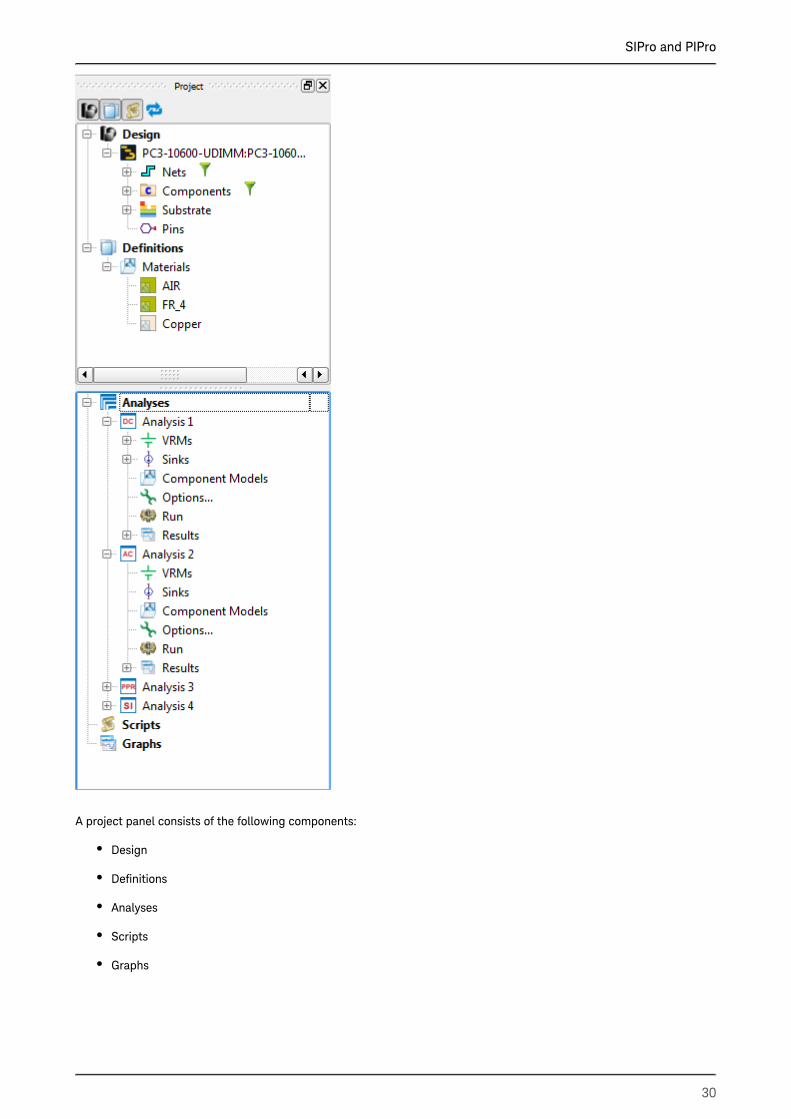
SIPro and PIPro Project PanelIn the SIPro/PIPro Setup window, the Project panel provides a tree-structured representation of a design. You can use

the Project panel to define a specific PI or SI analysis setup, to run the analysis and to review results. The Project panel

toolbar enables you to show or hide specific items of a design. The following figure displays a project panel:

SIPro and PIPro

30

A project panel consists of the following components:

Design

Definitions

Analyses

Scripts

Graphs

SIPro and PIPro

31

1.

2.

DesignThe list displays the physical parts of the design-under-test. Currently, this is the layout view from which the SIProDesign

/PIPro Setup was opened, no other parts can be added. The layout tree contains four items: , , Nets Components Substrate

and .Pins

NetsAll nets in the layout view are listed. Each net gets a type, ‘Power’, ‘Ground’, ‘Signal’ or ‘Undefined’ assigned. The nets are

sorted by type.

Type Icon

Power

Ground

Signal

Undefined

Verify that the nets that you plan to simulate have been typed correctly. Even though SIPro

/PIPro attempts to automatically identify the net type, the algorithm can miss nets with arbitrary

names.

Changing Net TypeTo change a net type:

Select the required net.

Right-click the selected net and select the required type.

SIPro and PIPro

32

2.

1.

2.

3.

4.

How to Find a NetTo find a specific net:

Click the icon ( ) next to in the tree.Filter Nets Parts

Type the required net name.

Click to display a list of matching algorithms, as shown in the following figure:

Simple: Display tree nodes that contains specified text

Regular Expression: Display tree nodes that contains specified regular expression.

Hierarchical: Display tree nodes that contains specified regular expression per hierarchy level separated by

slash.

Regular Expression is very powerful tool but it requires certain knowledge to use. Below is some

convenient example for typical use cases.

Example Match Note

U(1|2|5|11) Matches U1, U2, U5 and U11 "|" means "OR"

U[5-8] Matches U5, U6, U7 and U8 "-" can be used for "range"

U1[1-3] Matches U11, U12 and U13 U[11-13] doesn't work as

expected

DQ[1-8]N? Matches DQ1, DQ1N, DQ2,

DQ2N,...,DQ8 and DQ8N

"?" can be used as optional

string

Select the string matching algorithm: Simple, Regular Expression, or Hierarchical.

The Hierarchical option is relevant when tree nodes are hierarchical

SIPro and PIPro

33

1.

2.

3.

How SIPro/PIPro Identifies the Net TypeSIPro/PIPro attempts to identify the net type by case-insensitive name matching. In case no match is found, the net type

is ‘Undefinded’. The algorithm uses following rules by default:

Type Regular Expression Examples

Power pwr|power|vdd|vcc|vref|vtt|bat

^[\+\-]?\d+[p_]\d+v

^[\+\-]?\d+v

^[\+\-]?\d+

AVDD, DVDD, VREF, VTT, VBAT

+1p2v, -1p2v, 1p2v, +1_2v, -1_2v,

1_2v

+12v -12v 12v

+12, -12, 12

Ground gnd|ground|grnd|vss AGND, AVSS

Signal

Memory

Clock

Diff pair

HS Serial

dq

a\d+

ba\d+

clock|clk

_[pn]$

[\+\-]$

sig|tx|rx

DQ0, DQ1

A01, A02

BA01, BA02

CLK

DQS0_P, DQS0_N

DQS0+, DQS0-

SIG01

This rule can be modified by user. See for more detail.here

Setting the Net Type ManuallyTo override the automatic net type, you can select one or more nets, right-click and choose the appropriate net type.

ComponentsAll component instances in the layout view are listed and grouped per component.

How to Find a Component InstanceTo find a specific component instance:

Click the icon ( ) next to in the tree.Filter Components Parts

Type the component instance name.

Click to display a list of matching algorithms, as shown in the following figure:

SIPro and PIPro

34

3.

4.

1.

2.

Select the string matching algorithm: Simple, Regular Expression, or Hierarchical.

SubstrateThe Substrate tree item presents the objects in the layer grouped by Conductor layer, Via layer or Dielectric layer.

How to View the Geometry by LayerFirst, switch off the Parts Visibility toggle. This toggle can be found on the Geometry Window’s View toolbar. Then, select

the appropriate layer in the Substrate tree. The view displays the objects on the selected layer only.

PinsAll top level pins in the layout are listed.

DefinitionsThe branch stores definitions that can be applied to or shared with other objects within the project. You can Definitions

apply a definition to other objects in the Project panel by clicking and dragging the definition object on the required

object.

MaterialsTo view a material definition object, select a material from the list.Materials

ScriptsThe branch stores user-defined scripts. Right-click to add a new script or import an existing macro or Scripts Scripts

function script to the project.

You can execute or edit the script in the Scripting workspace window.

To add a new scripts:

Right-click in the Project panel:Scripts

Select to create a new script or click to use an existing script.New Python Script Import Scripts

SIPro and PIPro

35

1.

2.

AnalysesThe Analyses branch enables you to run a PI DC analysis, PI AC analysis, PPR analysis, and SI analysis. By default, it

provides an empty template for creating an analysis, as shown in the following figure:

Instead of using the default templates, if you want to add a new analysis:

Right-click in the Project panel:Analyses

Select the required analysis. A new analysis is added at the end of the Analysis branch.

Viewing and Hiding Project Tree ComponentsYou can view or hide options present in the Project panel by using toggle buttons. The following figure displays these

toggle buttons:

The following table describes each toggle button:

Option Icon Description

View Parts Enables you to view or hide in Parts

the project panel.

View Definitions Enables you to view or hide

in the project panel.Definitions

SIPro and PIPro

36


View Scripts Enables you to view or hide in Scripts

the project panel.

Toggle All Enables you to view or hide all the

components of the project panel.

Customizing ViewTo set a specific view for your design in the layout window, you can right-click the required component and select one of

the following options:


Set Visible Enables you to view the selected

component in the Layout window.

Set Invisible Enables you to hide the selected

component in the Layout window.

Solid Enables you to display components in

a solid view in the Layout window.

Wireframe Enables you to view or hide all the

components of the project panel.

Delete Enables you to delete a component.

Expand Enables you to display all the

subparts of a component in the

project panel.

Workspace WindowsThe SIPro/PIPro Setup window consists of the following windows:

Layout

Simulation

Parameters

Scripting

Layout Window

SIPro and PIPro

37

Layout WindowThe Layout window provides a layout view of your design. In this window, you can use various tools for customizing the

view of a simulation space. This window comprises the main design viewing area.

The following table describes options available in the View menu and View Tools toolbar:


Toolbars View Tools

View Manipulation Select: The Select tool is used to

select objects as well as

manipulate the view of the

simulation space.

Orbit: The Orbit tool is selected to

perform rotation of the simulation

space through left-clicking-and-

dragging.

Pan: The Pan tool is selected to

perform translation of the

simulation space through right-

clicking-and-dragging.

Zoom: Zoom-in or zoom-out of

simulation space by scrolling up or

down the mouse wheel,

respectively.

Zoom to Window: Zoom into a

rectangular shaped area of the

geometry as specified by the user.

To use, select the tool, then left-

click and drag the mouse to

designate the rectangular zoom

area.

Zoom to Extents Enable you to zoom automatically as

can view the entire geometry.

Zoom to Selection Enables you to automatically zoom

selected object only.

Standard Views The Standard View button function is

to automatically change the

perspective of the objects in the

workspace window.

SIPro and PIPro

38


Front (-Y)

Back (+Y)

Top (-Z)

Bottom (+Z)

Right (-X)

Left (+X)

Isometric Views The Isometric Views button function

is to automatically change the

perspective of the objects in the

workspace window.

Front/Right/Top

Front/Left/Top

Front/Right/Bottom

Front/Left/Bottom

Back/Right/Top

Back/Left/Top

Back/Right/Bottom

Back/Left/Bottom

Custom Views Enable you to define any perspective

than the Standard Views and

Isometric Views, and display at that

perspective.

Add View

Cutting Planes Cutting Planes button feature allows

you to define an arbitrary cross-

section of the object and display it.

Toggle Cutting Plane

Edit Cutting Plane

Save Cutting Plane

Field Reader The Field Reader tool measures field

values at the location where the

mouse hovers over the geometry.

SIPro and PIPro

39


Export Image The Export Image tool takes a screen

shot of the geometry as it is currently

shown in the workspace window, and

saves it to a specified location.

Toggle Parts Visibility Toggles the design parts on and off.

Clicking the button located Opacity

to the right of this button, opens a

slider to customize the translucency

of its objects. The sliders change the

alpha of the design objects, making

them more or less translucent as the

slider is dragged right or left,

respectively.

Toggle Output Visibility Toggles the output results on and off.

Clicking the button located Opacity

to the right of this button, opens a

slider to customize the translucency

of its objects. The sliders change the

alpha of the design objects, making

them more or less translucent as the

slider is dragged right or left,

respectively.

Toggle Bounding Box Visibility Ttoggles the visibility of the bounding

box of a design when the design is

selected.

Toggle Output Viewing Controls Toggles the visibility of the output

viewing controls for sensor results.

Simulation WindowThe Simulations workspace provides an interface to define simulations to send to the calculation engine. Simulations can

be easily created, defined, and stored in the Simulations workspace window. Each time a project is modified and saved,

you must define a new simulation to register the change. This workspace window stores definitions such as source types,

parameter sweeps, S-Parameters, frequencies of interest, scattered/total field interfaces and termination criteria that are

specific to a calculation. EMPro supports the following solver EM simulation technologies:

The following table lists the icons present in the Simulations window:

SIPro and PIPro

40


Simulation Starts a simulation.

Add To Queue Selects the required simulation from

the upper panel of the Simulations

window and add to the queue.

Remove From Queue Selects the required simulation from

the upper panel of the Simulations

window and remove from the queue.

Delete From Queue Deletes the selected simulation from

the disk.

To start the next phase To interrupt the current phase of the

simulation and start the next phase.

Kill the Queue Kills the currently executed

simulation.

The following information is available in the upper pane of the Simulations window:

Option Description

Id Displays a project ID, which references the location of the

loaded project in the file directory.

Name Displays the project name specified by a user.

Date Created Specifies the date when a simulation was created.

Engine The simulator used for performing simulation.

Status Displays whether a result is complete or still being

calculated while the simulation is running. This status can

be refreshed manually by pressing the Update button or

automatically by selecting Auto-scroll.

The following tabs are available in the lower pane of the Simulations window:

SIPro and PIPro

41

1.

2.

Option Description

Summary Provides a summary of the simulation such as simulation

path, status, boundary conditions, ports, feed, and

waveforms.

Notes Displays any notes that you might have added while

setting up a simulation.

Log Displays a log of tasks performed during the simulation.

Scripting WindowThe Scripting workspace allows you to view, edit, and execute scripts.

To create a new python script;

Select > , as shown in the following figures:Script New Python Script

Type commands in the scripting window:

Scripting OptionsThe following table describes options available in the Scripting window toolbar:

SIPro and PIPro

421.

Option Description

Script New Python Script

Commit

Revert

Clear Output

Edit Enables you to copy, cut, or select text in a script.

Execute Execute Script

Cancel Execution

View Script Tools

Editing Tools

Execution Tools

Editor View

Indentation

ConvertEOL

PsychicPy

Parameter WindowThe window enables you to create, edit, and delete parameters that are referenced. By default, three Parameters

parameters are provided , , and .minFreq maxFreq timestep

To modify the frequency range of the default minimum and maximum frequency parameters:

SIPro and PIPro

43

1.

2.

3.

4.

Click . The Parameters window is displayed.Parameters

Double-click the or value in the field.minFreq maxFreq Formula

Specify the required value.

Click .Apply

Parameter OptionsThe following table describes the Parameters options:

Name Description

Name Enables you to define a parameter, which can be

referenced later.

Formula Allows you to provide a mathematical formula or a simple

numeric value that will define the value of a given

parameter. This formula can reference other parameters

that have already been defined.

Value This column is a read-only column that displays the

evaluated value of the parameter. If an invalid formula is

entered, an error message will appear within this field

with a description of the invalidity. Simply hold the mouse

over the error message to view this description. Similarly,

a parameter is deleted by selecting the unwanted

parameter and clicking the button above the table. If a

parameter is deleted that is referenced within another

parameter's definition, an error message will appear since

the parameter that is referenced is no longer defined.

Description Allows you to describe a parameter.

Configuring SIPro and PIProBefore setting up an SIPro/PIPro project, you can configure the project settings by using the Options window. This

window consists of various tabs such as General, Interface, Modeling, and Nets. Using these tabs, you can specify the

global settings for your project.

Select > to open the Options window. In this window, you can use the following tabs:Tools Options

General

Interface

Modeling

SIPro and PIPro

44

Nets

GeneralThe General tab enables you to set the following options:

Templates: Enables you to specify the default folder location for storing SIPro/PIPro project templates.

Rendering Options: Allows you to control several display options in the SIPro/PIPro GUI:

Graphics Drivers: Specifies the display driver to be used for rendering graphics in SIPro/PIPro. The list of available

drivers depends on the operating system, graphics card, and on the usage of remote desktop. Using an

unsupported display driver may result in a blank Geometry Window. Any change to this setting will take effect

until you restart SIPro/PIPro. The display driver can also be changed using the --driver command line option when

starting SIPro/PIPro. Available graphics drivers are: OpenGL, OpenGL 2, DirectX 9, X11, MSW.

Transparency Algorithm: Determines the way SIPro/PIPro renders the parts opacity of an object. You can select

the values:

Z-sort Only Fast: This is the most efficient rendering option, but may contain artifacts

(small areas of inaccurate rendering).

Z-sort Only Nice: This is a more accurate rendering option than Z-sort Only Fast, but runs slower. It will

have less artifacts.

Depth Peeling: This option is more accurate than both Z-Sort algorithms. It's performance is dependent on

the graphics card, and may be significantly slower if the card does not support it.

Painters Algorithm: This is the most accurate rendering option, but runs the slowest. On modern graphics

cards, this option works very well.

Transparency Algorithm: This setting affects only the way an object is displayed in

the SIPro/PIPro interface, and does not affect calculation results.

SIPro and PIPro

45

Interface TabThe Interface tab enables you to set the following options:

Object Editing: Controls the editing of objects, when a new object is added to the project tree by right-clicking the

project tree. You can select one of the following values from the New Item Action drop-down list:

None: Adds a new object to the project tree.

Edit Name: Adds an object to the tree and provides a blinking cursor to add the object name in the project

tree.

Edit Properties: Adds an object and displays the appropriate window to edit the new object properties. The

Material Editor dialog box is displayed to specify settings.

Layout: Enables you to set preferences for saving or restoring the GUI layout.

Information: Enables you to to set their preference for decimal precision in tooltips.

Gridding: Enables or disables the use of the simplified grid.

Project Tree: The scroll adjusts the size of the items in the project tree.Icon/Text Size

Workspace:

Show All Tabs shows all workspace windows in tabbed workspace regardless of whether they are active or

not.

Show Only Active Tabs stores only the active tabs that are stored in the project workspace.

Don't Show Tabs removes the tabbed workspace. Windows can still be accessed from the View menu.

SIPro and PIPro

46

Appearance: The Appearance pane allows you to change the appearance of the SIPro/PIPro GUI and buttons

within.

Modeling TabThe Modeling tab provides several options for adjusting the color and appearance of faces, edges, vertices, components,

and the background. You can set the default colors used to display faces, edges, and/or vertices for parts when they are

first created. You can also set the color of the components (like voltage sources) and Geometry window background

color.

Components: Specifies the color used to render circuit components.

Background: Specifies the background color of the View.

Construction Grid: Specifies the color for the lines of the construction grid of the Sketcher and Orientation tools.

Mesh Slice: The color for mesh edges that are Free Space.

Invert Mouse Wheel: Switches the zoom direction when rolling the mouse wheel.

Separate View Tools: Toggles between showing all View tools in a drop-down list or as individual items.

Smooth View Transitions: Specifies SIPro/PIPro to perform smooth rotations between different view orientations. If

you do not select this option, SIPro/PIPro snaps to the selected view orientation.

SIPro and PIPro

47

NetsUsing the Nets tab, you can specify the net type recognition rules for ground, power, and signal by using Regular

Expression options.

SIPro and PIPro

48

Also, you can specify differential pair recognition by using pairs of Regular Expression for plus net and minus net.

Differential Pair recognition is currently used only for mixed mode of S-parameter plots and TDT/TDR plot window.

Specify regular expression for Plus Net and Minus Net respectively. If given any of two Net names are matched with given

regular expressions and rest string that are matched pieces are stripped off are the same, they are recognized as

differential pair.

For example, regular expression P$ for Plus and N$ detect Sig1P and Sig1N as differential pair.

Either one of Plus or Minus can be empty. This can be used to recognize a case such as pair name is like AAA and AAA#. (

empty regular expression for Plus Net and #$ for Minus Net).

Add-on ManagerYou can extend the SIPro/PIPro user interface with additional functions, which are customized for your design needs.

These tools are python scripts that you can customize for your workflow. You can access the following add-on tools:

Component Models Add-on: Enables you to Export their Components and ComponetModels to a file and also

allows to Import them.

Introspection Add-on: Enables you to generate the recipie of the setup and the elements of the setup like Sinks,

Vrms, Component Models and Results.

Layers Display Setting: Enables you to change the Display Settings of the Conductive layers and the via layers in

the Active Project.

ScaleViewZ Add-on: Enables you to add a toolbar to the main window to scale the view in the Z direction.

Add-on ManagerThe Add-on Manager allows you to enable or disable add-ons, inspect their status and possible load errors, and modify

the search path. It can be accessed from > .Tools Add-on Manager

The Add-on Manager displays a separate panel with the following elements:

A check box with the file name of the add-on: Select the check box to enable a add-on. Hovering over the file

name will show the full path of the add-on.

The load status on the left of the check box: A green icon is shown when an add-on is successfully loaded, a

yellow exclamation mark when it failed to load. Hover over the icon to see the full error message. No icon will be

shown for a disabled add-on that is not loaded.

If available, a short description of the add-on: Click in the Add-on Manager to display more information

about an add-on.

If available, two labels with the author and version information of the add-on.

SIPro and PIPro

49

1.

2.

3.

Add-on Search PathYou can download additional add-ons, which are saved on the following search path:

Additional search path: A user specified location where downloaded or custom add-ons can be saved. This path

can be modified in the Add-on manager and multiple locations can be specified using the platform specific path

separator (colon on Linux, semicolon on Windows). By default, a location in the user home directory is set. Add-

ons discovered on the additional search path are disabled by default, and must explicitly be enabled in the Add-on

manager.

If multiple add-ons with the same filename are found, only the first one on the path will be loaded. This way, a default

add-on can be overridden by a custom version placed in the additional search path.

Installing Additional Add-onsYou can download more add-ons and updates from the . To install an add-on, perform the add-on download page

following steps:

Save the downloaded Python script to one of the locations configured in the additional search path.

Open the Add-on Manager.

Find the new add-on and select its check box to enable it.

http://www.keysight.com/find/eesof-empro-addons

SIPro and PIPro

50

If the downloaded add-on is an update of the existing add-on, save the the update on the additional search path. Restart

ADS and the updated version should be found and loaded instead of the original.

Once an add-on is added, it cannot be unloaded until the program is exited. While managing add-ons during a session,

consider the following factors:

When a loaded add-on is disabled, the status icon will still be shown in the Add-on Manager. Only the next time

that ADS is started, the add-on will no longer be loaded.

When an add-on fails to load because of a Python exception or other error, it will remain in this state even if the

error is fixed. Restart ADS to load the add-on.

When add-ons with the same file name are found on the search path, only the first to be found is loaded.

However, if the first add-on was added only to the path while ADS is already running, it does not overrule an add-

on by the same name that is already loaded, even if the latter one is found further on the search path.

Setup Options for Customizing ResultsWhile viewing the results of an analysis, you can specify the setup options displayed in the following figure:

RangeThe following table describes the Range options:

Range Description

Min Minimum value of the scale bar

Max Maximum value of the scale bar

Layer Layer name to show the values

Net Type Net type to show the values (Not available in some type

of filed plots)

Automatic Automatically set the Min/Max values. Turn this option off

if you want to specify your preferred Min/Max.

For complex/multi-layered board, it might be difficult to display the Field plots for all layers. In such a scenario, using

Layer Display Settings add-on to limit the displaying layers as well as Layer selector and/or Net Type selector in the Field

plot setup provides a better view.

SIPro and PIPro

51

Select the following options for a better view:

From the drop-down list, select , from the , and in the Layer Show All drop-down list, select Net Type Power Layer

select Display Settings panel, , All Layers Visible

SIPro and PIPro

52

Layer: ETCH_SPLIT3, ETCH_SPLIT3, PowerLayer Display Settings: Net Type:

Size FactorSpecify the size factor of the arrows in the window. ( Below left is Size Factor = 1, Below right is Size Factor = 2 )

Excitation: Specify a excitation source from either VRMs or Sinks you defined in the setup.(Not available in some type of

filed plots)

SIPro and PIPro

53

Frequency: Specify a frequency to display values.(Not available in some type of filed plots)

Hiding and Unloading ResultsWhile viewing results in the Layout window, you can hide and unload other results.

To hide other results, click the button.Hide Others

To unload other results, click the button.Unload

See AlsoViewing PI-DC Analysis Results




SIPro and PIPro

54

1.

2.

3.



ContentsCreating and Editing Component Models for Analysis

Using Vendor Parts DB Browser

Creating and Editing Component Models for AnalysisFor an SIPro/PIPro analysis, you need to calculate the impact of decoupling capacitors. Identify the component models

and define electrical models for the selected components by defining component models.

In this section, you will learn how to create component models and then add a lumped, SnP, or model DB for analysis.

Creating Component Models for AnalysisTo create a component model for analysis:

Select a component group in the list.Components

Right-click the selected component group and select . The SIPro/PIPro Create Component Model for Analysis

Setup window is displayed.

Select the target analysis where you want to create the component model:

SIPro and PIPro

55

3.

4.

1.

2.

3.

4.

Click .OK

You can also drag and drop the selected components on in the SIPro/PIPro Component Models

Setup. The instances will be grouped by component name.

Editing a Component Model for AnalysisAfter creating a component model in the SIPro/PIPro Setup panel, you can define the electrical model parameters. The

following types of models can be added:

Lumped

SnP

Model DB

Multiple Model DBs

Adding a Lumped ModelTo define a lumped component model:

Double-click the component group in the SIPro/PIPro Setup panel. The is displayed.Component Model Editor

Select from the drop-down list.Lumped Add

Specify the , , and value.Resistance Inductance Capacitance

Select an option.RLC arrangement

SIPro and PIPro

56

4.

5.

6.

1.

2.

3.

Click .Apply

Click .Done

Adding an SnP ModelYou can add an SnP model for multi-port components, such as 4-pack resistors and 7-pack resistors. To define an SnP

component model:


Select from the drop-down list.SnP Add

Specify the S parameter file in the File Name text box. You can also click to browse to the required

file.

SIPro and PIPro

57

3.

4.

5.

1.

2.

3.

4.

5.

Click .Apply

Click .Done

Selecting an Existing Model DBTo use an existing model:


Select from the drop-down list.Model DB Add

Click in the section.Model

The window is displayed.Model DB

Select the required model.

SIPro and PIPro

58

5.

6.

7.

8.

1.

2.

3.

4.

5.

6.

Click . All the fields are filled with the details of the selected model.OK

Click .Apply

Click .Done

Selecting Multiple Model DBsTo use an existing model:


Select from the drop-down list.Multiple Model DB Add

Click in the section.Model

The window is displayed.Model DB

Select the required models.

Click . All the fields are filled with the details of the selected model.OK

SIPro and PIPro

59

6.

7.

8.

1.

2.

3.

Click .Apply

Click .Done

Specifying a Default ModelIf you have added multiple models, you can select a default model that will be considered during an analysis. After you

have completed a simulation, you can change the default model and view results immediately. You do not need to re-

simulate your design.

To specify a default model:


Select a model in the section.Model List

Click . For example, in the following figure, is selected:Set Default model_4

SIPro and PIPro

60

3.

4.

5.

1.

2.

Click .Apply

Click .Done

Specifying a Model with more than 2 pinsIf you have a component that has more than 2 pins, you can specify port numbers for each pins to define how the model

is connected when simulated.

If number of pins of component is more than 2 Ports pane appears in the left of the dialog.

To specify ports and models

Modify column so each pin connection matches the actual model's port numbers. "0" means Port Number

common reference ground. In below example, 3 ports are defined where P1( + ) and P4 ( - ) as Port1, P2( + ) and

P4( - ) as Port2, P3( + ) and P4( - ) as Port3. You can make Port Number column blank if you don't want to

connect model to that pin.

Specify model(s) that matches the number of ports you defined in Ports pane.

SIPro and PIPro

61

1.

2.

3.

Specifying a Arrayed ComponentIf you have an arrayed component contains multiple 2-pin components, you can define it by using "Arrayed Component"

checkbox.

To specify a Arrayed Component

Check checkbox. Note that the checkbox only appears when the component has more than 2 Arrayed Component

pins.

Specify Port Numbers for each pins. Use "-" sign to make pin connects to minus terminal of the port. In below

example, P1 connects to plus terminal of port1 and P5 connects to minus terminal of the port1.

Specify 2-pin model(s). The same model will be applied to each ports.

SIPro and PIPro

62

1.

2.

Using Vendor Parts DB Browser

Using Vendor Parts DB BrowserSIPro/PIPro provides a database of vendor part electrical models. It provides a complete set of MuRata, Samsung, and

TDK components. You can select an electrical model for the required capacitor in the Vendor Parts DB Browser window.

To display the Vendor Parts DB Browser:

Select > . The Vendor Parts DB Browser window is displayed.Tools Vendor Parts DB

Select the required electrical model. You can also use the text field to search the required model. Type a Filter

value in the required column. You can use multiple filter values. For example, the following figure displays results

of the capacitors search.2.2uF

SIPro and PIPro

63

2.

In the Vendor Parts DB Browser window, you can also view the impedance of various capacitors. You can select multiple

capacitors in the window and compare the impedance value, as shown in the following figure:

The properties that are the same for all selected components appear grayed out in the Part Details panel.

Adding Components to the Vendor Parts DBSIPro/PIPro allows you to extend the existing vendor parts database. The following types of models are supported:

SIPro and PIPro

64

1.

2.

3.

4.

5.

1.

2.

3.

Component from ADS

Lumped

SnP

Adding Custom Component

Adding a Lumped ModelTo add a custom lumped model type to the Vendor Parts DB:

Click the button in the window to open the Component Add Custom Component Vendor Components Browser

Model Creator dialog box.

Select the model type from the drop-down list.Lumped Select Model Type

Specify the Lumped Model properties:

Click .Apply

Click .Done

Adding an SnP ModelTo add a custom SnP model type to the Vendor Parts DB:

Click the " " button in the window to open the Component Add Custom Component... Vendor Components Browser

Model Creator dialog.

Select the model type from the drop-down list.SnP Select Model Type

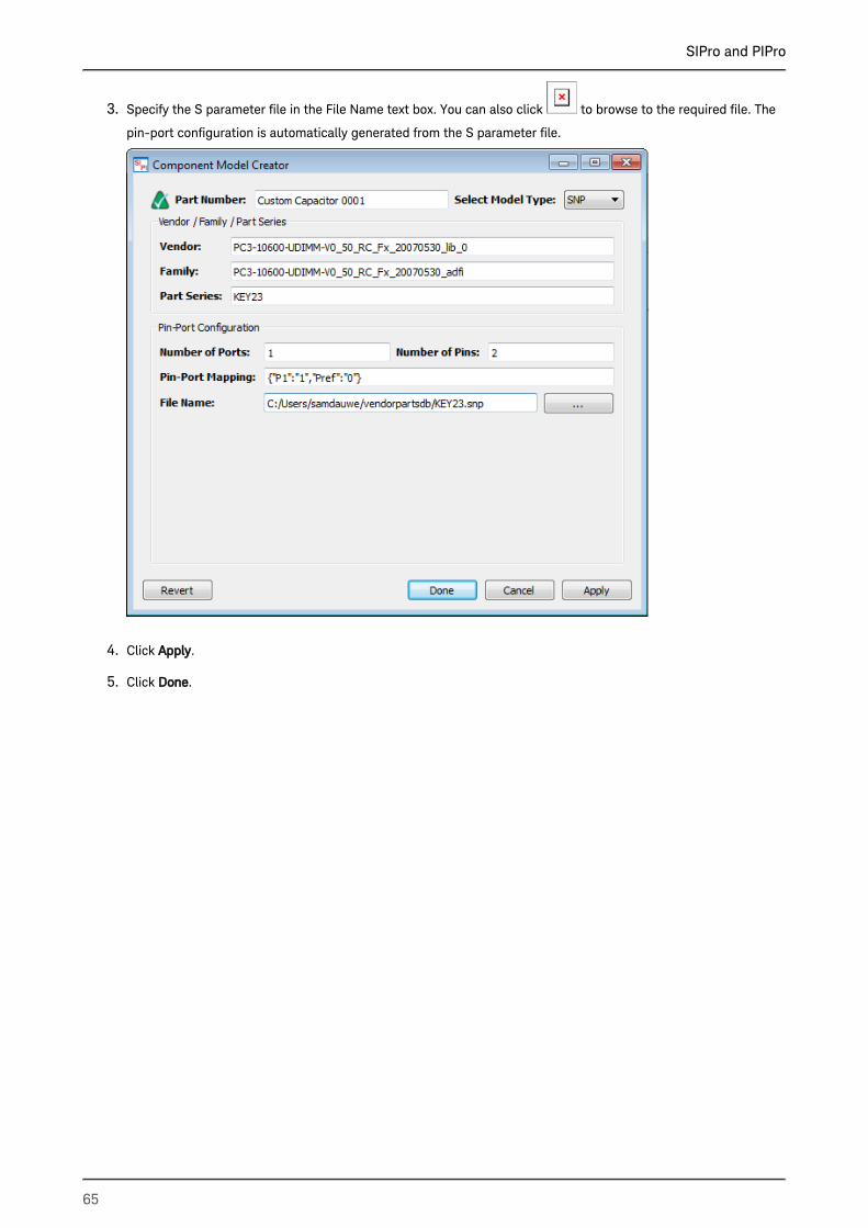
SIPro and PIPro

65

3.

4.

5.

Specify the S parameter file in the File Name text box. You can also click to browse to the required file. The

pin-port configuration is automatically generated from the S parameter file.

Click .Apply

Click .Done

SIPro and PIPro

66

PIPro Analysis

PIPro Analysis

ContentsTutorial-Performing a PI-DC and PI-AC Analysis

PIPro Analysis Setup Overview



PI-PPR Analysis

Tutorial-Performing a PI-DC and PI-AC AnalysisIn this tutorial, you will learn how to create a PI-DC and PI-AC analysis setup, run the analysis, and view results. The

example workspace contains a Samsung DDR4 UDIMM memory card. The design files are downloaded from JEDEC (www.

) and used for demonstration purposes. The example design consists of a 6 layer board with a single power rail jedec.com

for core and I/O buffers, as shown in the following figure:

You can view the nets, components instances, and individual nets in the navigator window. The main power net passes

from the conductor at the bottom of the design to the devices at the top. GND nets are present on the design. The

substrate pack consists of routing on the top and bottom layer. The power and GND nets are on layer 3 and 4. Before

performing the PIPro analysis, you need to know the names of the power and GND nets.

In this example design, the VRM is connector J1, which is the source of power supply. It is the connector device at the

bottom of DDR4 board. There are eight sinks, which are the ICs distributed over the board. The power supply is

consumed by sinks. You will analyze the impact of decoupling capacitors.

You can access the example workspace from the following location:

examples/HSD/SIPro_PIPro_Getting_Started_Example_wrk.7zadsfcv

In this tutorial, you will perform the following tasks:

Perform a PI-DC analysis

Perform a PI-AC analysis



SIPro and PIPro

67

1.

2.

1.

2.

Performing a PI-DC AnalysisYou can analyze the voltage drop in the VDD-GND power distribution network. The supply power comes in through

connector 'J1', the ICs that consume current are the 'DDR4...' component instances. There are no series components.

To perform an analysis, open the SIPro/PIPro Setup window:


Select from a Layout window to create a new or open an existing setup. The Tools > SIPro/PIPro > Open Setup

SIPro/PIPro Setup window is displayed.

Creating a PI-DC Analysis SetupTo create a PIPro Static IR Drop (PI-DC) analysis, use the default empty template available in the project panel. Expand

in the SIPro/PIPro panel, as shown in the following figure:DC Analysis 1

To create a setup, you need to define the following:

VRM

Sink

Options

Defining a VRMTo setup a VRM:

Select the connector component instance in the list, as shown in the following figure:J1 Components

Drag and drop the selected instance on the part in the SIPro/PIPro Setup panel. The Select Net for J1 VRMs

window is displayed.

SIPro and PIPro

68

2.

3.

4.

5.

6.

1.

Select .VDD

Click . A new VRM definition is added in the SIPro/PIPro Setup panel.OK

Double click the VRM definition to open the dialog box.VRM Editor

Specify the , , and .DC Voltage Voltage Tolerance Resistance Inductance

Defining a SinkSinks are devices that consume current. To define a sink:

Select at component level in the list, as shown in the following figure:u_ddr4_x4_fbga78-10x13 Components

SIPro and PIPro

69

1.

2.

3.

4.

5.

Drag and drop the component on . Since the component connects to multiple power nets, the Sinks Select Net for

dialog box is displayed.U7

Select as the power net you want to analyze.VDD

Select the option.Use same selection for All Sinks/VRMs

Click . A Sinks definition is added having a list of 8 sinks, as shown in the following figure:OK

SIPro and PIPro

70

5.

6.

7.

8.

1.

2.

3.

Double click in the list to open the Sink Editor dialog box.sink_U4 Sinks

Type in the field.30 DC Current

Click .Done

Defining OptionsA PI-DC analysis provides the following options:

Use Ideal Ground Approximation. When enabled, this option will treat all Ground nets as ideal shorts. The power

rail is often the dominant contributor to the voltage drop. This option provides you the capability to analyze this

dominant factor in less simulation time.

To specify options:

Double-click in the Analyses list. The Setup PI-DC Simulation window is displayed.Options

Select .Use Ideal Ground Approximation

SIPro and PIPro

71

3.

4.

Select and specify the required value.Custom target mesh size

Click .Done

Saving the Analysis SetupAfter defining your analysis setup, select > . Now, you are ready to perform the analysis.File Save

Running the AnalysisDouble-click to start the PI-DC analysis. The window is displayed and the PI-DC analysis is initiated.Run Simulations

Viewing ResultsAfter the simulation is complete, the results are listed in the project panel. You can view the results by double-clicking

the required Results option:

SIPro and PIPro

72

OverviewClicking the option opens a window with a table based overview of voltages and currents at Sinks, Pins, VRMs, Overview

and Vias.

VoltageClicking the option in the Results list loads the voltage plot in the Geometry window. This is a scalar plot. The Voltage

voltage is forced at 0 at the negative pins of the VRMs.

Current DensityClicking the option in the Results list loads the current density plot in the Geometry window. This is a Current Density

vector plot. The color indicates the current density amplitude. The white arrow indicates the direction of the current. The

arrow size is not an indication for the current density amplitude.

SIPro and PIPro

73

Power Loss DensityClicking the option in the Results list loads the power loss density. This is a scalar plot. This plot Power Loss Density

shows the power loss per unit area.

Generate SchematicClicking the option opens a Schematic window with the VRMs, Sinks, Component Models and an Generate Schematic

SNP that points to the DC S-parameter model.

Performing a PI-AC AnalysisAfter running a PI-DC analysis, you can perform the PI-AC analysis. A PI-AC analysis enables you to calculate the

impedance of the power distribution networks from different sinks. It helps you to determine and minimize the

impedance between power and ground pins at various IC locations on the board. A PDN should have the lowest

impedance for achieving good power integrity. Therefore, you need to minimize the impedance between power and

ground pins, which will vary based on the location of capacitors and the type and value of capacitor. The goal of PI-AC

analysis is to provide low impedance to all sinks.

In this example, the impact of components placed between the capacitors is calculated. You will use component models

of the MuRata library.

Enable MuRata Library

SIPro and PIPro

74

1.

2.

3.

4.

5.

Enable MuRata LibraryIn this example, you will run simulations with MuRata library components. Download the MuRata library from the Web:

http://www.murata.com/en-global/tool/library/keysight3

Include the MuRata library in the current ADS workspace and enable this library in ADS.

Opening the Example DesignOpen the design. The PI analysis setup data for a specific design is SIPro_PIPro_Getting_Started_Example_wrk.7zadsfcv

stored in a cell view of the “SIPro/PIPro Setup”.

Double-click the view in the ADS Main window. sipiSetup

The SIPro/PIPro Setup window is displayed.

Creating a PI-AC Analysis SetupIn this example, you will copy the PI-DC analysis setup. Therefore, you do not need to redefine the VRMs, which are the

connectors for supplying power, and sinks that consume the current.

Right-click the PI-DC analysis setup in the project panel:

Select > :Copy To PI-AC Analysis

The PI-DC analysis setup is copied to create a new PI-AC Analysis.

Right-click the copied analysis and select .Rename

Type , as shown in the following figure:VDD_GND_AC

http://www.murata.com/en-global/tool/library/keysight3

SIPro and PIPro

75

5.

1.

2.

3.

4.

5.

Defining a Component ModelFor a PI-AC analysis, you need to calculate the impact of decoupling capacitors. Identify the component models and

define electrical models for the selected components.

To define a component model:

Select the component group in the list. This group of c_capacitors_0603-511-500044_4.7a Components

components will be analyzed.

Drag and drop the selected component on in the SIPro/PIPro Setup window. A new list is Component Models

created, as shown in the following figure:

After adding a component model in in the SIPro/PIPro setup panel, you may need to

delete the nets that are not connected to GND and VDD.

Double-click in the Component Models branch to specify the electrical c_capacitors_0603-511-500044_4.7a

models to be used for analysis.

Select from the drop-down list.Lumped Add

Type 4.7 uF in the field.Capacitance

SIPro and PIPro

76

5.

6.

1.

2.

3.

4.

Click Done

You can also search an electrical model in the database provided by the vendor. For more

information, see and Using Vendor Parts DB Browser Creating and Editing Component Models

.for Analysis

Defining OptionsTo define options:

Double-click in the PI-AC Analysis list in the SIPro/PIPro Setup panel.Options

Accept the default and value.Resolution Arc Resolution

Click the tab.Frequency Plans

Click .Done

SIPro and PIPro

77

1.

2.

3.

Running the AnalysisSave your PI-AC analysis setup and double-click to start the PI-AC analysis. The window is displayed Run Simulations

and the PI-AC analysis is initiated.

Viewing PDN ImpedanceTo view PDN impedance results:

In the list, double-click . The PDN impedance window is displayed.Results PDN Impedance

Select the required sinks.

Right-click the selected sinks and choose . The PDN Impedance plot is displayed.Add PDN Impedance

PIPro Analysis Setup OverviewTo perform a power integrity (PIPro) simulation, you require detailed information about the power distribution network

(PDN) in a design. This information includes identifying the voltage regulator module (VRM), the IC that consumes power,

the components and component models, and stimulus for the analysis.

PrerequisitesBefore performing a PIPro analysis, you need to gather the following Information about a PDN:

Identify the power and ground rail net name(s) that you want to analyze and obtain the DC voltage. A power rail

can consist of multiple nets that are connected through series components.

Identify the instance name (or reference designator) of the Voltage Regulator Module (VRM). In case the VRM is

not mounted on the Printed Circuit Board (PCB) and the supply power comes in through one (or more) connectors,

identify these instances name(s). Also, the power rail and ground rail might come in through a separate connector.

For such designs, you need to identify both connector instance names.

Identify the instance name(s) of the ICs that consume power. Obtain the DC current consumption properties of

each IC. This is the total current that will be distributed among the set of individual pins of the IC. Obtain the

allowed DC voltage drop for each power rail. This is the recommended minimum DC supply voltage that is needed

by the IC to guarantee proper operation. You might consult the datasheet, ask the vendor, run the power

calculator provided by FPGA vendors, or ask the IC designers.

Identify the instance name(s) of all series components on the power rail. These are typically resistors, inductors, or

fuses. Obtain the electrical model parameters for them (RLC values and topology).

SetupIn a new SIPro/PIPro setup, you can use the empty templates for PI-DC, PI-AC, and PPR analysis in the Project panel. You

can also create a new analysis. To create a new analysis, right-click and choose the required analysis. The Analyses

following figure displays the PI-DC and PI-AC setup:

SIPro and PIPro

78

VRMsA voltage regulator module (VRM) allows processors with different supply voltage to be mounted on the same

motherboard. A VRM regulates the voltage fed to a microprocessor. While creating an analysis setup, you can define

various properties of a VRM, such as the DC voltage, voltage tolerance, and resistance.

SinksA sink is a component, such as ICs, that consumes electricity in a design. While creating a setup, you can define the

amount of current the ICs will consume by defining the properties of a sink, such as the DC current, resistance, and

voltage tolerance.

OptionsThe following table describes various options available for a PIPro analysis:

Option Description

Resolution This option specifies that points closer than the

Resolution distance will be considered as equal during

simulation

Arc Resolution Arc resolution is used to discretize arcs and circles during

simulation

Custom Target Mesh Size Specifies the mesh size for generating the global 3D

mesh during simulation

Use Ideal Ground Approximation Ground net metalization is modeled as a perfect

conductor during simulation

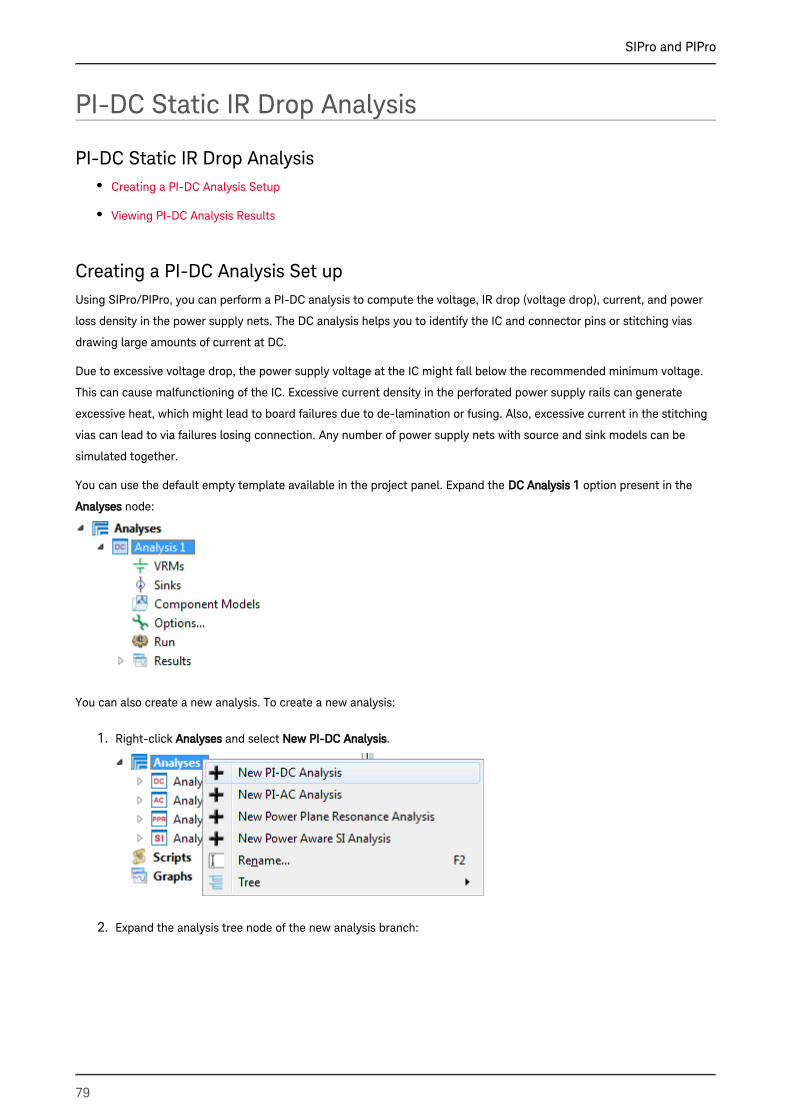
SIPro and PIPro

79

1.

2.


PI-DC Static IR Drop AnalysisCreating a PI-DC Analysis Setup

Viewing PI-DC Analysis Results

Creating a PI-DC Analysis Set upUsing SIPro/PIPro, you can perform a PI-DC analysis to compute the voltage, IR drop (voltage drop), current, and power

loss density in the power supply nets. The DC analysis helps you to identify the IC and connector pins or stitching vias

drawing large amounts of current at DC.

Due to excessive voltage drop, the power supply voltage at the IC might fall below the recommended minimum voltage.

This can cause malfunctioning of the IC. Excessive current density in the perforated power supply rails can generate

excessive heat, which might lead to board failures due to de-lamination or fusing. Also, excessive current in the stitching

vias can lead to via failures losing connection. Any number of power supply nets with source and sink models can be

simulated together.

You can use the default empty template available in the project panel. Expand the option present in the DC Analysis 1

node:Analyses

You can also create a new analysis. To create a new analysis:

Right-click and select .Analyses New PI-DC Analysis

Expand the analysis tree node of the new analysis branch:

SIPro and PIPro

80

2.

1.

2.

3.

4.

5.

6.

1.

2.

Defining a VRMA VRM regulates the voltage provided to a microprocessor.

To define a VRM:

Select a VRM (or connector) component instance in the Parts tree. You can also search the required component.

For more information about, see .How to Find a Component Instance

Drag and drop the selected instance on the part in the project panel. A new VRM definition is added in the VRMs

project panel.

If the VRM connects to multiple power nets, the dialog box is displayed, where you have Select Net for Instance

to select the required net. The same applies for ground nets.

Double click the VRM definition to open the VRM Editor dialog box.

Specify the , , and . The will not play a role for a DC analysis. DC Voltage Voltage Tolerance Resistance Inductance

The Voltage Tolerance (absolute or in percent) is the voltage drop that is allowed at the output pins of the VRM.

There will be no voltage drop in the VRM in case the series resistance and inductance values are 0.

Click .Done

Defining a SinkA sink is a component that reduces the temperature of an electronic device by dissipating heat into the surrounding air.

You can define the following options for a sink:

To define a sink:

Find the IC component instance(s) in the Components list.

Select the instance(s) and drag and drop them onto . New Sink definitions will be added in the tree.Sinks

SIPro and PIPro

81

3.

4.

5.

6.

1.

2.

3.

In case the IC connects to multiple power nets, the dialog box is displayed, where you can Select Net for Instance

select the required net.

In case multiple instances were dropped, the dialog box provides a check box to Select Net for Multiple Instances

. The same applies for ground nets.Use same Selection for All Sinks/VRMs

Double-click the Sink definition to open the Sink Editor dialog box.

Specify the , and . The Voltage Tolerance (absolute or in percent) is DC Current Resistance Voltage Tolerance

maximum voltage drop that is allowed at the input pins of the IC.

Defining OptionsA PI-DC analysis provides following options:

Option Description

Use Ideal Ground Approximation When enabled, this option will treat all Ground nets as

ideal shorts. The power rail is often the dominant

contributor to the voltage drop. This option provides you

the capability to analyze this dominant factor in less

simulation time.

Running the PI-DC AnalysisAfter saving your analysis setup, double click to start the PI-DC analysis. The Simulations window is displayed and Run

the PI-DC analysis will start. The Simulations window allows you to monitor and manage simulations.

Show Me How Do I Perform a PI-DC Analysis

Video: How to Perform a PI-DC Analysis

Viewing PI-DC Analysis ResultsAfter completing a PI-DC analysis setup, you can run the analysis in SIPro/PIPro. You can view the overview, voltage,

current density, and power loss density. You can also generate a schematic.

Running a PI-DC AnalysisTo run a PI-DC analysis and view results:

Save your PI-DC analysis setup.

Double-click to start the PI-DC analysis. The Simulations window is displayed, which allows you to monitor Run

and manage simulations. The results are listed in the project panel.

Expand in the Analysis list of the project panel:Results

https://youtu.be/LLZ_1C9subE

https://youtu.be/LLZ_1C9subE

SIPro and PIPro

82

3.

4.

1.

2.

Double-click the required analysis result.

OverviewClicking the option in the Results list opens the DC Results Overview window. This window provides a table-Overview

based overview of voltages and currents at Sinks, Pins, VRMs, and Vias.

Sinks

In the Sinks tab, you can view the source current, VRM voltage, input voltage, resistance, tolerance, and margin values.

PinsTo view pins:

Click the tab in the DC Results Overview window.Pins

Choose the required pin from the drop-down list. The table is updated with the selected pin results.Select Pins

SIPro and PIPro

83

2.

1.

2.

VRMsTo view VRMs, click the tab in the DC Results Overview window.VRMs

ViasTo view ID and current of vias, click the tab.Vias

ReportsTo generate a PI-DC analysis report:

Click the tab.Reports

Click .Save Report

Setting TemplateTo set a template for your report, click the button. Browse to the DocX, ODT, and HTML location for Set Templates

selecting a template for your report.

Voltage

SIPro and PIPro

84

VoltageClicking the option in the Results list loads the voltage plot. This is a scalar plot. The voltage is forced at 0 at the Voltage

negative pins of the VRMs.

Current DensityClicking the option in the Results list loads the current density plot. This is a vector plot. The color Current Density

indicates the current density amplitude. The white arrow indicates the direction of the current. The arrow size is not an

indication for the current density amplitude.

SIPro and PIPro

85

Power Loss DensityClicking the option in the Results list loads the power loss density. This is a scalar plot. This plot Power Loss Density

shows the power loss per unit area.

SIPro and PIPro

86

Generate SchematicClicking the option opens a Schematic window with the VRMs, Sinks, Component Models and an Generate Schematic

SNP that points to the DC S-parameter model.

SIPro and PIPro

87

1.

2.

See Also



PI-AC Dynamic IR Drop AnalysisCreating a PI-AC Analysis Setup


Creating a PI-AC Analysis SetupA PI-AC analysis computes the impedance for the IC current loads over a broad frequency range. It helps you to identify

whether the power distribution network (PDN) provides a low impedance path from the Voltage Regulator Module (VRM)

to the IC. An excessive impedance in a certain frequency range can generate excessive voltage noise, also called dynamic

IR drop, when the IC power supply pins draw large amounts of transient current, required for I/O or core logic switching,

at rates that fall into that frequency range.

Defining a PI-AC Analysis SetupYou can create a PI-AC analysis setup in the following ways:

Copying an existing PI-DC analysis setup.

Creating a new PI-AC analysis setup.

Copying the PI-DC Analysis SetupIf you have already performed a PI-DC analysis, you can copy its setup for creating a PI-AC analysis setup. To copy an

existing setup:

Right-click the PI-DC analysis setup in the project panel.

Select > .Copy To PI-AC Analysis

Creating a New PI-AC Analysis Setup

SIPro and PIPro

88

1.

2.

3.

4.

Creating a New PI-AC Analysis SetupIf you want to create a new setup, right-click and then select . After creating a new setup, Analyses New PI-AC Analysis

you need to define VRMs and sinks. For more information, see .PIPro Analysis Setup Overview

Defining VRMsTo define a VRM:

Select a VRM (or connector) component instance in the list. You can also search the required Components

component. For more information about, see .How to Find a Component Instance

Drag and drop the selected instance on in the AC Analysis list. A new VRM definition is added.VRMs

If the VRM connects to multiple power nets, the Select Net for Instance dialog box is displayed. Select a net.

Similarly, you can select ground nets.

Double-click the VRM definition to open the VRM Editor dialog box.

SIPro and PIPro

89

4.

5.

1.

2.

3.

4.

5.

1.

2.

3.

Specify the , , and . The will not play a role for a DC analysis. DC Voltage Voltage Tolerance Resistance Inductance



Defining SinksTo define a sink:

Find the IC component instance(s) in the list.Components

Select the instance(s) and drag and drop them onto . New Sink definitions will be added in the tree.Sinks

In case the IC connects to multiple power nets, the Select Net for Instance dialog pops up where you will have to

select one.

In case multiple instances were dropped, the Select Net for Multiple Instances dialog provides a check box to Use

. The same applies for ground nets.same Selection for All Sinks/VRMs

Double click the Sink definition to open the Sink Editor dialog. Specify the , and DC Current Resistance Voltage

. The Voltage Tolerance (absolute or in percent) is maximum voltage drop that is allowed at the input Tolerance

pins of the IC.

Defining Component ModelsFor a PI-AC analysis, you need to consider the decoupling capacitors because they are not an open circuit at AC.


Select the component group, which you want to analyze, in the list.Components

Drag and drop the component group on . The instances will be grouped by component name.Component Models

Define the electrical model parameters by using one of the following ways:

SIPro and PIPro

90

Double-click the component instance to display the Component Model Editor window. For more

information, see .Creating and Editing Component Models for Analysis

Alternatively, you can open the Vendor Parts database by selecting . Drag and drop Tools > Vendor Parts DB

the appropriate vendor part onto the component instance node (single model assignment) or onto the

component model group node (group model assignment). For more information, see Using Vendor Parts DB

.Browser

Defining OptionsTo define options, double-click in the PI-AC Analysis list in the project panel. provides It provides the following Options

options:

Option Description

Resolution Points closer than the specified resolution will be

considered equal during the simulation

Arc Resolution Value used to discretize circles and arcs during the

simulation

Custom Target Mesh Size Mesh size used to generate the global 3D mesh during

simulation

Use Ideal Ground Approximation When enabled, this option specifies that all Ground nets

are considered as ideal shorts. The power rail is often the

dominant contributor to the voltage drop. This option

provides you the capability to analyze this dominant

factor in less simulation time.

Defining Frequency PlansBy default, you can use the Automatic, Logarithmic and Adaptive frequency plan. The Automatic will provide the optimal

frequency sampling using a combination of Adaptive and Logarithmic sweeps.

Click the tab to specify a plan.Frequency Plans

Saving fields for field plotsBy default, the fields valued needed for visualization are not stored. You can enable this using the Field Storage dialog.

SIPro and PIPro

91

1.

2.

Note that this will save big files to disc. Depending on the example this can result in multiple GB of saved data.

Saving the SetupSave your PI-AC analysis setup and double-click to start the PI-AC analysis.Run

Show Me How Do I Perform a PI-AC Analysis

Video: How to Perform a PI-AC Analysis

Viewing PI-AC Analysis ResultsAfter creating a PI-AC analysis setup, you can run the analysis in the SIPro/PIPro Setup window. For a PI-AC analysis, the

following results are displayed:

PDN Impedance

S-parameters

Electric Field

Magnetic Field

Current Density

Generate Test Bench

Generate Sub Circuit

Running a PI-AC AnalysisTo run a PI-AC analysis and view results:

Save your PI-AC analysis setup.

Double-click to start the PI-AC analysis. The Simulations window is displayed, which allows you to monitor Run

and manage simulations:

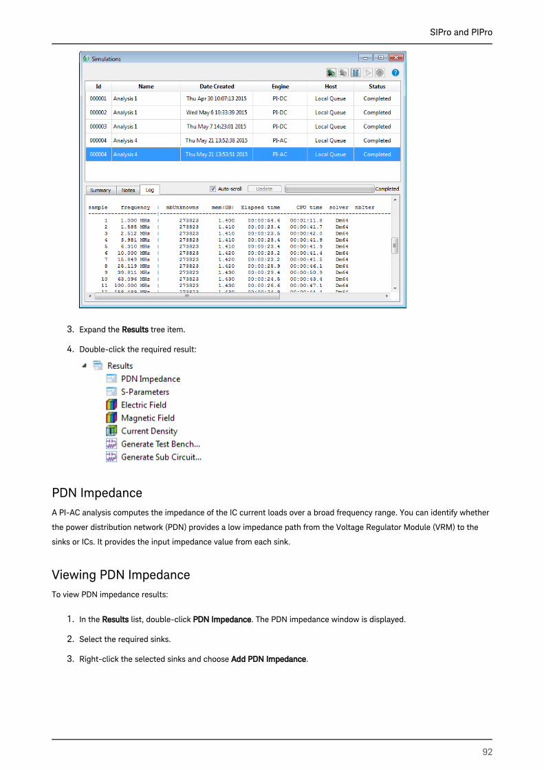
https://www.youtube.com/watch?v=x7IygjN_xDU&feature=youtu.be

https://youtu.be/QtYhs-H2oZU

SIPro and PIPro

92

2.

3.

4.

1.

2.

3.

Expand the tree item.Results

Double-click the required result:

PDN ImpedanceA PI-AC analysis computes the impedance of the IC current loads over a broad frequency range. You can identify whether

the power distribution network (PDN) provides a low impedance path from the Voltage Regulator Module (VRM) to the

sinks or ICs. It provides the input impedance value from each sink.

Viewing PDN ImpedanceTo view PDN impedance results:

In the list, double-click . The PDN impedance window is displayed.Results PDN Impedance

Select the required sinks.

Right-click the selected sinks and choose .Add PDN Impedance

SIPro and PIPro

93

3.

1.

2.

3.

Removing PDN Impedance PlotsTo remove PDN Impedance plots:

Click the tab.Plot

Select the plots to be removed.

Click . The selected plots are deleted from the PDN Impedance window.

Importing a Target Impedance FileThe PDN impedance window supports the import and visualization of target impedances. The following table lists the

contents of a sample CSV file:

Frequency[Hz] Impedance[Ohm]

100000 0.01

1000000 0.01

1000000 0.1

10000000 0.1

10000000 1.5

1E+08 1.5

1E+08 2

1E+09 2

SIPro and PIPro

94

1.

2.

3.

Frequency[Hz] Impedance[Ohm]

1E+09 2

To import a series of target impedances:

Select > . The Import Custom Target Impedance File dialog box is displayed.File Import Target Impedance

Select a file containing values. This file should contain comma separated frequency and impedance values.CSV

The importer does not perform a validity check on the actual data.

Once imported, the values are added as a new plot on the impedance graph, as shown in the following figure:

Result Type OptionsIn the Result Type section, you can select the following options:

Impedance: Displays the PDN impedance values.

S-Parameters: Displays the s parameter results.

The impedance plots show the PDN impedance values including the default component models specified in the setup.

After changing the default model specified in the Component Model Editor dialog (see Creating and Editing Component

), you can update the impedance plots without recalculation. This allows a quick way to vary e.g. Models for Analysis

decap component models and inspect the effect on the PDN plots.

VRM OptionsIf you are viewing Impedance results, you can also select the following VRMs options:

Open

SIPro and PIPro

95

Closed

Viewing Electric FieldDouble-click in the list of PI AC analysis. The electric field plot is displayed:Electric Field Results

Viewing Magnetic FieldDouble-click in the Results list of PI AC analysis. The magnetic field plot is displayed:Magnetic Field

SIPro and PIPro

96

If you want to view only the recent results and hide previous analysis, click .Hide Others

Current DensityDouble-click in the Results list of PI AC analysis.Current Density

SIPro and PIPro

97

Generating a SchematicDouble-click in the Results list of PI-AC analysis. A Schematic window is displayed, which includes Generate Schematic

the VRMs, Sinks, Component Models and an SNP that points to the S-parameter model.

You can run a simulation from the schematic. The results display the input impedance for sinks, which is similar to the

SIPro/PIPro results.

SIPro and PIPro

98

1.

2.

3.

4.

5.

6.

Enable the decoupling capacitorsThe key parameter is the index, which determines the location of the switch. If the index is 0, the switch is open. If the

value of index is set to 1, the connection is made to the first part. Similarly, if the index is 2, then connection is made to

the second part. The following figure displays the results when the index value is set to 1:

Tuning ParametersTo tune parameters:

Click the icon. The dialog box is displayed.Tuning TuneParameters

Select the decoupling capacitor in Schematic.

Set the Minimum value to .0

Set the maximum value to .5

Specify the Step value as .1

Click the up and down arrows.

See Also


SIPro and PIPro

99

1.

2.

1.

2.

3.

PI-PPR Analysis

PI-PPR AnalysisCreating a PI-PPR Analysis Setup


Creating a PI-PPR Analysis SetupA PI-PPR (Power Plane Resonance) analysis computes the resonances of the design over a broad frequency range. It

helps you to identify the resonance frequencies and fields of the design, with and without components. It provides a

global view on natural modes (eigenmodes) between the power and ground planes. Some of the modes may cause

excessive impedance from VRM to IC. Some modes resonating around the signal frequencies may affect the signal

quality.

Defining a PI-PPR Analysis SetupYou can create a PI-PPR analysis setup in the following ways:

Copying an existingPI-DC/AC analysis setup.

Creating a new PI-PPR analysis setup.

Copying the PI DC/AC Analysis SetupIf you have already performed a PI-DC or PI-AC analysis, you can copy its setup for creating a PI-PPR analysis setup. To

copy an existing setup:

Right-click the existing or analysis setup in the project panel.PI-DC PI-AC

Select > . The entire setup is copied to create a new PI-PPR analysis setup.Copy To PI-PPR Analysis

Creating a New PI-PPR Analysis SetupIf you want to create a new setup, right-click and then select .Analyses New PI-PPR Analysis

Definition of VRMs and sinks are optional in PI-PPR. At least one VRM, or one sink or one

component is suggested to be defined to indicate the power and ground nets be put in PPR

simulation. For more information, see .PIPro Analysis Setup Overview

Defining VRMsTo define a VRM:

Select a VRM (or connector) component instance in the Parts tree. You can also search the required component.

For more information about, see How to Find a Component Instance.

Drag and drop the selected instance on the VRMs part in the project panel. A new VRM definition is added in the

project panel.

SIPro and PIPro

100

3.

4.

5.

1.

2.

3.

4.

5.

1.

2.

3.

a.

b.

If the VRM connects to multiple power nets, the Select Net for Instance dialog pops up where you will have to

select one. The same applies for ground nets.

Double-click the VRM definition to open the VRM Editor dialog box.

Specify the DC Voltage, Voltage Tolerance, and Resistance. The Inductance will not play a role for a DC analysis.



Defining SinksTo define a sink:

Find the IC component instance(s) in the Parts tree.

Select the instance(s) and drag and drop them onto Sinks. New Sink definitions will be added in the tree.

In case the IC connects to multiple power nets, the Select Net for Instance dialog pops up where you will have to

select one.

In case multiple instances were dropped, the Select Net for Multiple Instances dialog provides a check box to Use

same Selection for All Sinks/VRMs. The same applies for ground nets.

Double click the Sink definition to open the Sink Editor dialog. Specify the DC Current, Resistance and Voltage

Tolerance. The Voltage Tolerance (absolute or in percent) is maximum voltage drop that is allowed at the input

pins of the IC.

Defining Component ModelsFor a PI- analysis, you need to consider the decoupling capacitors because the R, L and C parameters associated PPR

with that component may affect the resonances.


Select the component group, which you want to analyze, in the list.Components



Double-click the component instance to specify the electrical model parameters for that instance.

Alternatively, you can open the Vendor Parts database by selecting Tools > Vendor Parts DB. Drag and

drop the appropriate vendor part onto the component instance node (single model assignment) or onto

the component model group node (group model assignment). For more information, see Using Vendor

Parts DB Browser.

Defining OptionsThe same options can be set as for an PI-AC simulation.

SIPro and PIPro

101

1.

2.

3.

4.

Defining Frequency PlanThere are three parameters in PPR frequency plan: , , and Start frequency (Fstart) Stop frequency (Fstop) Number of

. The first N modes with resonant frequencies between Fstart and Fstop would be provided. By default, eigenmodes (N)

the Start and Stop frequencies are defined as minFreq and maxFreq. You can change the minFreq, maxFreq, by using the

Parameters window. For more information, see .Parameters window

Saving the SetupSave your PI-PPR analysis setup and double-click to start the PI-PPR analysis.Run

Viewing PI-PPR Analysis ResultsAfter creating a PI-PPR analysis setup, you can run the analysis in the SIPro/PIPro Setup window. For a PI-PPR analysis,

the following results are displayed:

Electric Field

Magnetic Field

Current Density

Running a PI-PPR AnalysisTo run a PI-PPR analysis and view results:

Save your PI-PPR analysis setup.

Double-click to start the PI-PPR analysis. The Simulations window is displayed, which allows you to monitor Run

and manage simulations.

Expand the tree item.Results

Double-click the required result:

Electric FieldDouble-click in the list of PI-PPR analysis. The electric field plot is displayed:Electric Field Results

SIPro and PIPro

102

Magnetic FieldDouble-click in the Results list of PI -PPR analysis. The magnetic field plot is displayed:Magnetic Field

SIPro and PIPro

103

Current DensityDouble-click in the Results list of PI-PPR analysis.Current Density

SIPro and PIPro

104

See Also


SIPro and PIPro

105

SIPro Analysis

SIPro Analysis

ContentsTutorial-Performing Power Aware SI Analysis

Creating a Power Aware SI Analysis Setup


Tutorial-Performing Power Aware SI AnalysisIn this tutorial, you will learn how to create a Power Aware SI analysis setup, run the analysis, and view results. The

example workspace contains a Samsung DDR4 UDIMM memory card. The design files are downloaded from JEDEC (www.

) and used for demonstration purposes. The example design consists of a 6 layer board with a single power rail jedec.com

for core and I/O buffers, as shown in the following figure:

You can view the nets, components instances, and individual nets in the navigator window. The main power net passes

from the conductor at the bottom of the design to the devices at the top. GND nets are present on the design. The

substrate pack consists of routing on the top and bottom layer. The power and GND nets are on layer 3 and 4. Before

performing the PIPro analysis, you need to know the names of the power and GND nets.

In this example design, the goal is to analyze the signal behavior of the critical line, including the effect of the GND

metallization.

The goal of SI analysis is to provide an S-parameter model for the DQR15 line.

Example Workspace

examples/HSD/SIPro_PIPro_Getting_Started_Example_wrk.7zads

Objective

Set up a Power Aware SI analysis

Run the Power Aware SI analysis

View Power Aware SI results (S-parameter and Generate Schematic)

Opening the Example DesignOpen the design. The SI analysis setup data for a specific design is SIPro_PIPro_Getting_Started_Example_wrk.7zads

stored in a cell view of the “SIPro/PIPro Setup”.

http://www.jedec.com

http://www.jedec.com

SIPro and PIPro

106

1.

2.

To create a view, open the layout and select > > .sipiSetup Tools SIPro/PIPro Open Setup

If the view already exists, you can open it with a double-click in the ADS Main window.sipiSetup

The SIPro/PIPro Setup window is displayed.

Creating a Power Aware SI SetupIn this example, you will create a new SI analysis setup. To create a new setup, right-click and then select Analyses New

.SI Analysis

Defining PortsFor an SI analysis, you need to define ports that will be the ports of the S-parameters calculated by the tool. In this

example, you will define two ports, one on each side of the single DQR15 line.

To define a port:

Select the line in the Nets tree.DQ15

In this example, you will use pins 6 and C2 to define the ports.

Drag and drop pin on the ports part of the tree.RN20

By hovering over the exclamation mark, you will see that the GND reference for the port is not

defined. You can either manually select a GND pin and drag it to the port. Alternatively, you can

automatically find the closest GND pin by right-clicking and then selecting 1: port Add Nearby Pins To

, which will add as the minus reference to the port:Minus Terminal J1.P24

SIPro and PIPro

107

2.

3.

4.

1.

2.

3.

4.

5.

6.

Two nets were automatically added to the list of nets: GND and DQ15. The metallization

associated with these nets will be included in the Power Aware SI simulation.

Drag and drop pin to the I/O Ports part of the tree.J1

Right-click and select , which will add as the minus 2: DQ15_J1 Add Nearby Pins To Minus Terminal J1.P_165

reference to the port:

Defining OptionsTo define options:

Double-click in the SI Analysis list.Options

Double-click in the field of the frequency plan and type .Points Adaptive 150

Click the tab.Options

Accept the default and value.Resolution Arc Resolution

Optionally, you can model the GND metallization as ideal PEC by selecting the ‘Use Ideal Ground Approximation’

option, which will result in a faster overall simulation.

Click .Done

SIPro and PIPro

108

1.

2.

3.

1.

2.

3.

Running the AnalysisSave your SI analysis setup and double-click to start the SI analysis. The window is displayed and the SI Run Simulations

analysis is initiated.

Viewing ResultsAfter the analysis is complete, you can view results in the Results list. You can open the results during a simulation to

viewing the intermediate results.

To view the S-parameters results:

Double-click the option in the Results list.S-Parameters

Select the required nets in the section.Single-Ended

Right-click the selected nets and select .Add Return Loss

View TDR/TDT ResultsTo View TDR/TDT results:

Double-click the option in the Results list.TDR/TDT

Select the required nets in the tab.Single-Ended

Right-click the selected nets and select .Add TDR

SIPro and PIPro

109

3.

1.

2.

3.

Show Me How Do I Perform a Power Aware SI Analysis

Video: How to Perform a Power Aware SI Analysis

Creating a Power Aware SI Analysis SetupA Power Aware SI analysis enables you to compute the S-parameters over a broad frequency range for one or more

critical lines defined via I/O ports in the setup.

Creating a New Power Aware SI Analysis SetupIf you want to create a new setup, right-click and then select .Analyses New SI Analysis

Alternatively, you can copy an existing analysis setup to create a new one.

Selecting NetsTo add nets to the SI analysis node in the SIPro/PIPro setup:

Select the required nets in the Project panel:

Right-click the nets and select .Add to Analysis

Select as the target analysis.PA-SI Analysis

https://youtu.be/dBylcH2N614

https://youtu.be/YYAGqfhJd_c

SIPro and PIPro

110

3.

4.

1.

2.

3.

4.

1.

2.

Click . The selected nets are added to the SI Analysis list.OK

Defining I/O PortsThe I/O ports define the + and – terminals for the S-parameter ports in the Power Aware SI simulation.

To define an I/O Port:

Select the required nets in the list of the SI Analysis node.Nets

Right-click the selected nets and select .Create Ports or Component Model Groups

To create a port, accept the default selection, .Create Ports

Click .OK

Alternatively, you can drag and drop pins. To define ports:

Drag a pin connected to the net that you want to model to the I/O Ports in the project panel. This will create a

new I/O port with only the + connection defined.

SIPro and PIPro

111

2.

1.

2.

3.

a.

b.

To complete the definition of this I/O Port, drag a nearby pin connected to a GND or PWR net to the I/O Port

definition, or alternatively automatically connect the closest GND pin to the – terminal of the port by right-

clicking the Port and selecting .Add Nearby Pins To Minus Terminal

This operation will automatically populate the Nets list with the nets connected to the + and –

terminal.

Defining Component ModelsOptionally, you can add components (series components such as resistors or decoupling capacitors) in the SI analysis.


Select the component group, which you want to analyze, in the Components list.



Double-click the component instance to specify the electrical model parameters for that instance.

Alternatively, you can open the Vendor Parts database by selecting > . Drag and Tools Vendor Parts DB

drop the appropriate vendor part onto the component instance node (single model assignment) or onto

the component model group node (group model assignment). For more information, see Using Vendor

.Parts DB Browser

Defining OptionsTo define options, double-click Options in the SI Analysis list in the project panel. It provides the following options:

Option Description

Resolution Points closer than the specified resolution will be

considered equal during the simulation

SIPro and PIPro

112

Option Description

Arc Resolution Value used to discretize circles and arcs during the

simulation

Custom Target Mesh Size Mesh size used to generate the global 3D mesh during

simulation

Use Ideal Ground Approximation When enabled, this option specifies that all Ground nets

are considered as ideal shorts. The power rail is often the

dominant contributor to the voltage drop. This option

provides you the capability to analyze this dominant

factor in less simulation time.

Use Optimized Via Modeling Use via modeling settings optimized for simulation

performance.

Model Signal Return Currents in Coplanar Ground Ground metallization close to signal metallization is

included in the signal modeling during simulation

Defining Frequency PlansClick the tab to specify a plan.You can use the Automatic, Linear, Logarithmic and Adaptive frequency Frequency Plans

plan. The Automatic uses a optimal combination of Adpative and Linear sweeps to cover the frequency range. The Start

frequency can be 0 Hz, the simulator will assume 1 kHz when 0 Hz is specified.

When using an Adaptive sweep for electrically long lines on a complex board, a large number of frequency points may be

required to reach convergence, specifically when a large number of signal lines is being analyzed. A linear frequency plan

setup is advised in this case.

To capture the dynamic behavior of a signal line when using a Linear sweep, you will need 10 frequency points per

wavelength, so in case the length of the signal line is 5 wavelengths, you will need 50 frequency points. This is typically

sufficient when using the SiPro generated S-parameter model in e.g. a transient or channel simulation.

Saving the SetupSave your SI analysis setup and double-click to start the SI analysis.Run

SIPro and PIPro

113

1.

2.

3.

1.

2.

3.

Viewing Power Aware SI Analysis ResultsAfter creating an SI analysis setup, you can run the analysis in the SIPro/PIPro Setup window. For an SI analysis, the

following results are displayed:

S-Parameters

TDR/TDT

Generate Sub Circuit

Running a Power Aware SI AnalysisTo run an SI analysis and view results:

Save your SI analysis setup.

Double-click to start the SI analysis. The Simulations window is displayed, which allows you to monitor and Run

manage simulations.

Expand the Results list:

You can view S-parameters and generate a Schematic.

S-ParametersTo view the S-parameters results:

Double-click the option in the Results list. The S-Parameters window is displayed.S-Parameters


Right-click the selected nets and select the required option such as, .Add transmission

SIPro and PIPro

114

3.

Using the S-Parameters Results WindowThe S-Parameters window consists of the following menus:

Data

Insert

View

DataThe Data menu provides the following options:

Export : Exports the currently displayed plot to a text file.

Save Plots as New Graph: Copies the current graph including plots and markers. It is saved in the node in Graphs

the project tree.

InsertThe Insert menu provides the following options:

Point Marker: Insert a point marker in the graph.

Crosshair Marker: Insert a crosshair marker.

SIPro and PIPro

115

Horizontal Marker: Insert a horizontal marker.

Vertical Marker: Insert a vertical marker.

ViewThe View menu provides the following options:

Pan: Left-click on the graph and move mouse pointer to pan.

Zoom: Left click on the graph and move mouse pointer to create a rectangle to zoom.

Zoom to Extents: Zoom in or out to current plots so that they can fit into the graph.

Export Image: Export plot image to a file.

Toolbar OptionsThe S-Parameters window provides several toolbar options for customizing the graph.

Icon Description

The Export Data icon enables you to export the currently

displayed plot to a text file.

The Export Image icon enables you to export the plot

image to a file.

The Zoom to Extents icon enables you to zoom in or out

to current plots so that they can fit into the graph.

The Pan icon enables you to move mouse pointer to pan.

The Zoom Tool icon enables you to move mouse pointer

to create a rectangle to zoom.

SIPro and PIPro

116

Icon Description

The Legend Visible icon enables you to show or hide the

legends of the plots.

The Selection tool icon enables you to select items in a

plot.

The Point Marker Tool insert a point marker in the graph.

The Crosshair Marker icon inserts a crosshair marker.

The Horizontal Marker icon inserts a horizontal marker.

The Graph Properties icon displays the graph properties

pane. You can change graph appearance, and axis

controls.

Graph Type Selector

You can set the following options to select a graph type:Graph Type Selector

XY Graph Magnitude: Displays magnitude of the plots in the XY rectangular graph.

XY Graph Phase: Displays phase of the plots in the XY rectangular graph.

Smith Chart: Displays plots in the Smith chart.

Single Ended TabIn the Single Ended tab, you can view the port properties, change the port impedance, and manipulate plots by right-

clicking on each row in the table.

Port Property TableThe Port Property Table shows various port properties in a table.

SIPro and PIPro

117

Number: Specifies to the S-parameter index.

Net Type: Specifies whether the port's plus terminal connects to Signal nets or Power nets

Port: Port name that you define in the analysis tree

+Net: Specifies the net name(s) that is connected to the plus terminal of the port.

-Net: Specifies the net name(s) that is connected to the minus terminal of the port.

Instance: Specifies the instance name(s) with which a port connected. For top level pins, this property becomes

blank.

Z: Specifies the port impedance. This property is editable. To edit, double-click the cell or select Specify Reference

Impedance context menu.

You can perform the following tasks by right-clicking a port and selecting the required option:

Viewing the Transmission : Right-click the selected port and then select to display the plot Add transmission

transmission characteristic(s) of selected port(s) to the graph. This feature will automatically find the other end of

connected link of the selected ports. This feature is convenient to check transmission characteristics for the

multiple lines.

SIPro and PIPro

118

Viewing the Return Loss: Right-click the selected port(s) and select to display the return plot(s) of Add return loss

selected port(s) to the graph.

View the Insertion Loss: Right-click a net and then select to display the insertion loss between Add Insertion Loss

the selected two ports to the graph.

Insertion loss here does not necessarily mean "transmission". It means loss between any

of two ports.

View Near End Crosstalk: Right-click a port and then select to view the near end crosstalkAdd Near End Crosstalk

(s)of selected port(s) in the graph. This feature will automatically find all near end cross talk of the selected ports

with using information.Instance

SIPro and PIPro

119

Add Far End Crosstalk : Add far end crosstalk(s) of selected port(s) to the graph. This feature will automatically

find all far end cross talk of the selected ports with using information.Instance

Specify Reference Impedance : Set preferred reference impedance to the selected ports.

Remove All Plots : Remove all plots from the graph.

Mixed Mode TabIn the Mixed Mode tab, you can define differential pair of ports and add mixed mode plots in the graph in addition to most

of what you can do in the Single Ended tab.

Port Property TableIn the Mixed Mode tab, column is added to the ones for Single Ended table.Signal

Signal: Shows the type of the port.

SE stands for Single Ended

D stands for Differential

C stands for Common.

SIPro and PIPro

120

Context menusIn mixed mode tab, some context menus are added and some context menus are removed comparing to the one for

Single Ended tab.

Context menus only for Mixed Mode tabMake Differential Pairs: Make differential pairs for selected ports. This context menu works in two different ways

depending on how many ports you select in the table.

If you select two ports in the table it means to create an differential pair for the selected two ports

explicitly. If selected ports are already a part of other differential pair that differential pair will be broken

before creating new differential pair.

If you select more than two ports in the table it means to create multiple differential pairs for selected

ports. In this case differential pairs will be recognized and created automatically based on net names and

instance name with using predefined Differential Pair Recognition Rule. (See more detail ).here

In below example picture, selecting 4 ports and using Make Differential Pair for them will create two pairs

as follows.

Port1 and 3 as a differential pair because these plus nets are DQ1 and DQ1# which are recognized as

differential pair by the recognition rule and also these are on the same instance Rx.

Port2 and 4 as a differential pair because these plus nets are DQ1 and DQ1# which are recognized as

differential pair by the recognition rule and also these are on the same instance Tx.

Break Differential Pairs : Break existing pairs for selected ports.

Context menus not available for Mixed Mode tabAdd Near End Crosstalk

Add Far End Crosstalk

View Mixed Mode S-parametersView Return Loss : Use context menu on desired ports. Add Return Loss

View Insertion Loss : Use context menu on desired two ports that you want to view insertion Add Insertion Loss

loss in between. ( Note: term of "Insertion Loss" doesn't necessarily mean insertion loss of physically connected

link. )

SIPro and PIPro

121

1.

2.

3.

Matrix Selector

Matrix Selector allows you to select add/remove plots based on S-parameter index.

View TDR/TDT ResultsTo view TDR/TDT results:

Double-click the option in the Results list.TDR/TDT


Right-click the selected nets and select the required option such as, .Add TDR

Using the TDR/TDT Results WindowThe TDR/TDT window consists of the following menus:

Export

ExportThe Export menu provides the following options:

SIPro and PIPro

122

Save Plots as New Graph: Copies the current graph including plots and markers. It is saved in the node in Graphs

the project tree.

Toolbar OptionsThe TDR/TDT window provides several toolbar options for customizing the graph. See section in the Toolbar Options

Using the for more detail.S-Parameters Results Window

TDR/TDT Setup Options

Start Time : Specify start time.

Stop Time : Specify stop time.

Delay : Specify delay value.

Samples : Specify number of data samples in time domain.

Result Type : Specify Y-axis unit in either Impedance or Voltage.

Response Type : Specify response type either Step or Pulse.

Pulse Width : Specify pulse width for Pulse Response Type. This value is ignored in Step Response Type.

Window : Specify window type

Single Ended TabIn the Single Ended tab, you can view the port properties, change the port impedance, and manipulate plots by right-

clicking on each row in the table.

Port Property TableThe Port Property Table shows various port properties in a table. See section in the Using the Port Property Table S-

for more detail of table contents.Parameters Results Window

You can perform the following tasks by right-clicking a port and selecting the required option:

SIPro and PIPro

123

Viewing the TDT : Right-click the selected port and then select to display the TDT characteristic(s) of plot Add TDT

selected port(s) to the graph. This feature will automatically find the other end of connected link of the selected

ports. This feature is convenient to check transmission characteristics for the multiple lines.

Viewing the TDR : Right-click the selected port and then select to display the TDR characteristic(s) plot Add TDR

of selected port(s) to the graph.

Specify Reference Impedance : Set preferred reference impedance to the selected ports.

Remove All Plots : Remove all plots from the graph.

Mixed Mode TabIn the Mixed Mode tab, you can define differential pair of ports and add mixed mode plots in the graph in addition to most

of what you can do in the Single Ended tab.

Port Property TableIn the Mixed Mode tab, column is added to the ones for Single Ended table.Signal

Signal: Shows the type of the port.

SE stands for Single Ended

D stands for Differential

C stands for Common.

In mixed mode tab, following context menus are added comparing to the one for Single Ended tab.

Make Differential Pairs: Make differential pairs for selected ports. See the same section in the Using the S-

Parameters Results Window.

Break Differential Pairs : Break existing pairs for selected ports. See the same section in the Using the S-

Parameters Results Window.

Matrix SelectorMatrix Selector allows you to select add/remove plots based on S-parameter index.

SIPro and PIPro

124

Generate Sub CircuitDouble-click in the Results list. A Schematic window is displayed, as shown in the following figure:Generate Sub Circuit

SIPro and PIPro

125

1.

2.

3.

4.

5.

6.

7.

Installing the Deprecated SI and PI Analysis Addon

The legacy SI/PI analyzer is still available, but is a deprecated solution. Please use SIPro or

PIPro instead, see . This addon will no longer be available in Getting Started with SIPro and PIPro

the future major releases of ADS.

Installing the Deprecated SI and PI Analysis AddonThe legacy SI/PI analyzer is available as an addon. The SI/PI Analyzer addon assists in setting up SI or PI EM and circuit

simulations. This addon consists of two parts:

Setup wizard: The setup wizard guides you through the process of creating a new cell that contains only selected

nets (physical interconnects) to be analyzed. The output of the setup wizard is a cell that is ready for EM analysis.

Analysis guide: The analysis guide assists in setting up typical SI or PI circuit simulation testbench. The output of

the analysis guide is a circuit schematic, ready to be simulated, a data display template that captures relevant

output figures. In addition, the analysis guide supports Momentum current visualization based on the results.

To install the SI and PI Analyzer addon:

Select > in the ADS Main window.Tools App Manager

Click . The Add User Addon dialog box is displayed.Add User ADS Addon

Click .Browse

Access the folder.$HPEESOF_DIR/ael_addons/sipi_deprecated/ael

Select the file and click .PhysSipi_boot.atf Open

Click . The PhysSipi_boot option is displayed in the User Addons list.OK

Select the check box for , as shown in the following figure:Enabled PhysSipi_boot

SIPro and PIPro

126

7.

8.

9.

10.

11.

Click in the message box.Yes

Click in the message box.OK

Click in the App Manager window.Close

Open a Layout window. The SI/PI Analyzer addon is displayed in the menu bar, as shown in the following figure:

SIPro and PIPro

127

SIPro/PIPro Videos

Perform a PI-DC Analysis

This video talks about how to perform a PI-DC analysis.

Perform a Power Aware SI Analysis

This video talks about how to perform a Power Aware SI analysis.

Perform a PI-AC Analysis

This video talks about how to perform a PI-AC analysis.

SIPro and PIPro - Keysight

Documents

Transcript of SIPro and PIPro - Keysight