A time-dependent dusty gas dynamic model of axisymmetric cometary jets
Upload
khangminh22Category
view
3download
0
Simulations of chemistry in star-formingregions and cometary ices
Draft: July 28, 2020
Eric R. WillisFalls, PA
B.S. Chemistry, University of Scranton, 2014
A Dissertation Presented to theGraduate Faculty of the
University of Virginia
in Candidacy for the Degree of
Doctor of Philosophy
Department of Chemistry
University of VirginiaAug. 2020
Committee Members:Robin T. Garrod
Eric HerbstBrooks H. Pate
Remy IndebetouwRobert E. Johnson

c© Copyright by
Eric R. Willis
All rights reserved
August 7, 2020
iii
Abstract
Astrochemical models have long been used in the study of the chemistry of interstellar
space (Herbst & Klemperer 1973). Over the past decades, several advancements have been
made to these models, including the incorporation of grain-surface chemistry (Hasegawa
et al. 1992), the incorporation of warm-ups to simulate nascent star formation (Garrod
et al. 2008), and more recently adaption of these models to study cometary ice chem-
istry (Garrod 2019). Here we present several studies which utilize state-of-the-art as-
trochemical models (MAGICKAL; Garrod 2013a, MIMICK; Garrod 2013b). First, we
use MIMICK to study the effect of grain-surface back-diffusion on reaction rates for the
H + H H2 reaction system (Willis & Garrod 2017). Then we incorporate this
correction into MAGICKAL to study several organic molecules in star-forming regions.
These include methoxymethanol (CH3OCH2OH), cyanamide (NH2CN), methyl isocyanide
(CH3NC), and propyne (CH3CCH). We then develop a new chemical network for the study
of isocyano species in the star-forming region Sagittarius B2(N2) (Willis et al. 2020). In
this study, we also present a new method of modeling the chemistry of the star-formation
process, transitioning from the simple two-stage methods of past models to a simultaneous
collapse/warm-up model. Finally, we present ongoing work that builds on the cometary
ice simulations of Garrod (2019). Here we include heat-transfer simulations to model the
effects of solar radiation on the temperature of the cometary ice, as well as a new back-
diffusion treatment for the movement of particles between layers in the cometary ice.

v
Acknowledgements
It is very difficult to condense 6 years of experiences into a couple pages. There are so
many people I’d like to thank in this section. First, thanks to Rob for mentoring me on
this journey. I’d like to think I’ve grown a lot as a scientist over these few years, and it’s
thanks in no small part to your guidance. Thanks also to Eric Herbst, for taking me into
your group when I first arrived at UVa, and for being a consistent mentor throughout my
time here.
My heartfelt thanks go to Ruth-Ann for being a constant source of support over the past
couple years, especially lately. I have not been the easiest housemate to live with during
this pandemic, especially with my crazy work hours. But you’ve been patient with me, and
I’ll be eternally grateful for that.
Thanks to Matt, Chris, and Andrew for making my years in Charlottesville more bear-
able than they would have otherwise been. I’ll never forget those nights spent making beer,
and talking about the meaning of existence, and how to best live our lives. It was therapy
for me, and you are all lifelong friends. Thanks to Mary and everyone at Grit for providing
an escape from coding all day, and serving excellent coffee. Thanks to Ilse for organizing
trivia the past few months during this insanity, and for also being an impromptu mentor to
me whenever I needed it. Thanks to Dustin for pretty much the same reason. Thanks also to
everyone in the Garrod group, for providing a welcoming environment, and for listening to
me complain about back-diffusion. I can’t forget Ryan and Brett either, for being excellent

vi
scientific mentors and friends.
To my dad, Grandma, and the rest of the family, thanks for being supportive. I know
you guys never really understood what I was doing, but you still asked questions about it
and showed interest. Thanks for always being there for me. Thanks also to Dr. Daniel
Ciudin, for helping me through some of the darkest times of my life, and for helping me
find the strength within myself to finish this endeavor.

To everyone who has helped me reach this point

ix
Table of Contents
Abstract iii
Acknowledgements v
List of Figures xviii
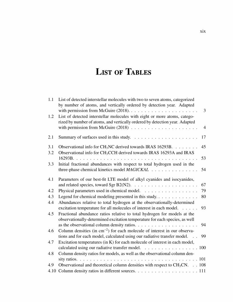
List of Tables xx
1 Introduction and Background 11.1 A Brief History of Molecular Detections in Space . . . . . . . . . . . . . . 11.2 Astrochemical Modelling . . . . . . . . . . . . . . . . . . . . . . . . . . . 2
1.2.1 Rate-equation models . . . . . . . . . . . . . . . . . . . . . . . . . 21.2.2 Microscopic Monte Carlo methods . . . . . . . . . . . . . . . . . . 6
1.3 Dissertation Scope . . . . . . . . . . . . . . . . . . . . . . . . . . . . . . 6
2 Kinetic Monte Carlo Simulations of the Grain-Surface Back-Diffusion Effect 92.1 Introduction . . . . . . . . . . . . . . . . . . . . . . . . . . . . . . . . . . 92.2 Methods . . . . . . . . . . . . . . . . . . . . . . . . . . . . . . . . . . . . 14
2.2.1 Simple flat-surface model . . . . . . . . . . . . . . . . . . . . . . 142.2.2 MIMICK . . . . . . . . . . . . . . . . . . . . . . . . . . . . . . . 152.2.3 Grains . . . . . . . . . . . . . . . . . . . . . . . . . . . . . . . . . 152.2.4 MIMICK, one mobile particle . . . . . . . . . . . . . . . . . . . . 172.2.5 MIMICK, all particles diffusing . . . . . . . . . . . . . . . . . . . 17
2.3 Results . . . . . . . . . . . . . . . . . . . . . . . . . . . . . . . . . . . . . 192.3.1 Flat-surface model . . . . . . . . . . . . . . . . . . . . . . . . . . 192.3.2 MIMICK results, one mobile particle . . . . . . . . . . . . . . . . 212.3.3 MIMICK results, all particles mobile . . . . . . . . . . . . . . . . 222.3.4 MIMICK, two-particle models . . . . . . . . . . . . . . . . . . . . 242.3.5 Comparison of fits to rate-equation results . . . . . . . . . . . . . . 26
2.4 Discussion . . . . . . . . . . . . . . . . . . . . . . . . . . . . . . . . . . . 282.5 Conclusions . . . . . . . . . . . . . . . . . . . . . . . . . . . . . . . . . . 31
3 Studies of several organic molecules using MAGICKAL 35
x Table of Contents
3.1 Introduction . . . . . . . . . . . . . . . . . . . . . . . . . . . . . . . . . . 353.2 Methoxymethanol (CH3OCH2OH) . . . . . . . . . . . . . . . . . . . . . . 36
3.2.1 Overview of NGC 6334I and Observations . . . . . . . . . . . . . 363.2.2 Chemical Modeling . . . . . . . . . . . . . . . . . . . . . . . . . . 37
3.3 IRAS 16293-2422 & The Protostellar Interferometric Line Survey (PILS) . 383.3.1 Cyanamide (NH2CN) . . . . . . . . . . . . . . . . . . . . . . . . . 40
3.3.1.1 Chemical modelling of NH2CN . . . . . . . . . . . . . . 413.3.2 Methyl isocyanide (CH3NC) . . . . . . . . . . . . . . . . . . . . . 43
3.3.2.1 Chemical modelling . . . . . . . . . . . . . . . . . . . . 453.3.3 Propyne (CH3CCH) . . . . . . . . . . . . . . . . . . . . . . . . . 49
3.3.3.1 Chemical modelling . . . . . . . . . . . . . . . . . . . . 52
4 Exploring Molecular Complexity with ALMA (EMoCA): Complex Isocyanidesin Sgr B2(N) 594.1 Preface . . . . . . . . . . . . . . . . . . . . . . . . . . . . . . . . . . . . 594.2 Introduction . . . . . . . . . . . . . . . . . . . . . . . . . . . . . . . . . . 594.3 Observations* . . . . . . . . . . . . . . . . . . . . . . . . . . . . . . . . . 634.4 Laboratory spectroscopy background* . . . . . . . . . . . . . . . . . . . . 644.5 Observational results* . . . . . . . . . . . . . . . . . . . . . . . . . . . . . 65
4.5.1 Detection of CH3NC and HCCNC* . . . . . . . . . . . . . . . . . 664.5.2 Upper limits for C2H5NC, C2H3NC, HNC3, and HC3NH+* . . . . . 69
4.6 Chemical modeling . . . . . . . . . . . . . . . . . . . . . . . . . . . . . . 694.6.1 Chemical network . . . . . . . . . . . . . . . . . . . . . . . . . . 70
4.6.1.1 CH3NC . . . . . . . . . . . . . . . . . . . . . . . . . . 714.6.1.2 C2H5NC . . . . . . . . . . . . . . . . . . . . . . . . . . 724.6.1.3 C2H3NC . . . . . . . . . . . . . . . . . . . . . . . . . . 744.6.1.4 HC3N, HCCNC . . . . . . . . . . . . . . . . . . . . . . 75
4.6.2 Physical model . . . . . . . . . . . . . . . . . . . . . . . . . . . . 764.6.3 Cosmic-ray ionization . . . . . . . . . . . . . . . . . . . . . . . . 79
4.7 Modeling results . . . . . . . . . . . . . . . . . . . . . . . . . . . . . . . 804.7.1 Standard model and H + CH3NC barrier . . . . . . . . . . . . . . . 804.7.2 Comparison to old physical model . . . . . . . . . . . . . . . . . . 834.7.3 Cosmic-ray ionization rate . . . . . . . . . . . . . . . . . . . . . . 854.7.4 Comparison of chemical modeling to observations and spectral mod-
eling . . . . . . . . . . . . . . . . . . . . . . . . . . . . . . . . . 914.8 Discussion . . . . . . . . . . . . . . . . . . . . . . . . . . . . . . . . . . . 103
4.8.1 H + CH3NC reaction . . . . . . . . . . . . . . . . . . . . . . . . . 1034.8.2 Effects of changing ζ . . . . . . . . . . . . . . . . . . . . . . . . . 1034.8.3 Comparison of observations to models . . . . . . . . . . . . . . . . 1064.8.4 Comparison of Sgr B2(N2) to other sources* . . . . . . . . . . . . 110
4.9 Conclusion . . . . . . . . . . . . . . . . . . . . . . . . . . . . . . . . . . 1134.10 Complementary observational figures and tables* . . . . . . . . . . . . . . 119
Table of Contents xi
4.11 Additional tables . . . . . . . . . . . . . . . . . . . . . . . . . . . . . . . 122
5 Simulations of cometary ice chemistry during solar approach 1255.1 Introduction . . . . . . . . . . . . . . . . . . . . . . . . . . . . . . . . . . 1255.2 Methods . . . . . . . . . . . . . . . . . . . . . . . . . . . . . . . . . . . . 128
5.2.1 Non-thermal chemical mechanisms . . . . . . . . . . . . . . . . . 1285.2.2 Heat transfer and solar approach . . . . . . . . . . . . . . . . . . . 1315.2.3 Layer back-diffusion . . . . . . . . . . . . . . . . . . . . . . . . . 135
5.3 Results . . . . . . . . . . . . . . . . . . . . . . . . . . . . . . . . . . . . . 1385.3.1 Heat transfer simulations . . . . . . . . . . . . . . . . . . . . . . . 1385.3.2 Layer back-diffusion . . . . . . . . . . . . . . . . . . . . . . . . . 1395.3.3 Updated chemical model results . . . . . . . . . . . . . . . . . . . 146
5.4 Future Work . . . . . . . . . . . . . . . . . . . . . . . . . . . . . . . . . . 148
6 Concluding Remarks 1576.1 Chapter 2 . . . . . . . . . . . . . . . . . . . . . . . . . . . . . . . . . . . 1576.2 Chapter 3 . . . . . . . . . . . . . . . . . . . . . . . . . . . . . . . . . . . 1586.3 Chapter 4 . . . . . . . . . . . . . . . . . . . . . . . . . . . . . . . . . . . 1596.4 Chapter 5 . . . . . . . . . . . . . . . . . . . . . . . . . . . . . . . . . . . 160
References 161
Biographical Sketch 175

xiii
List of Figures
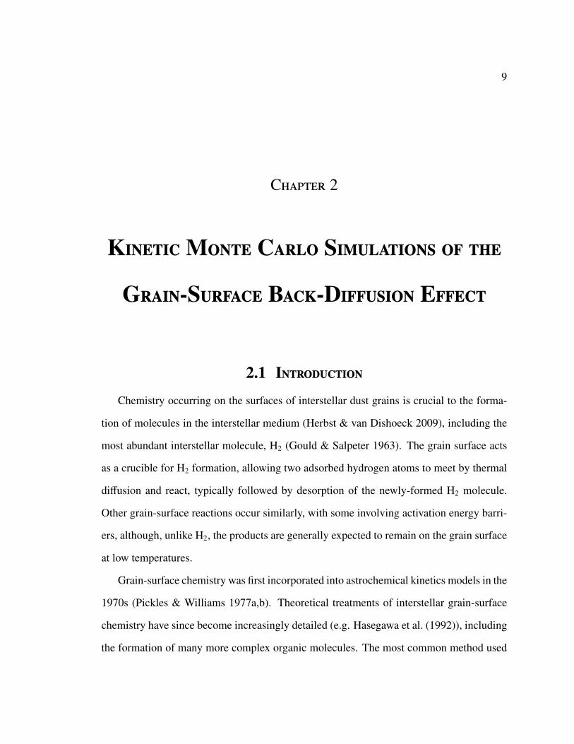
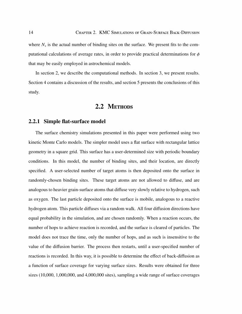
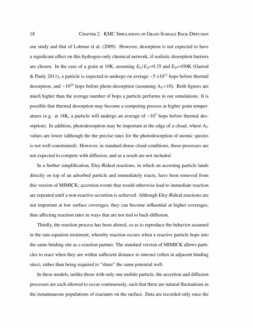
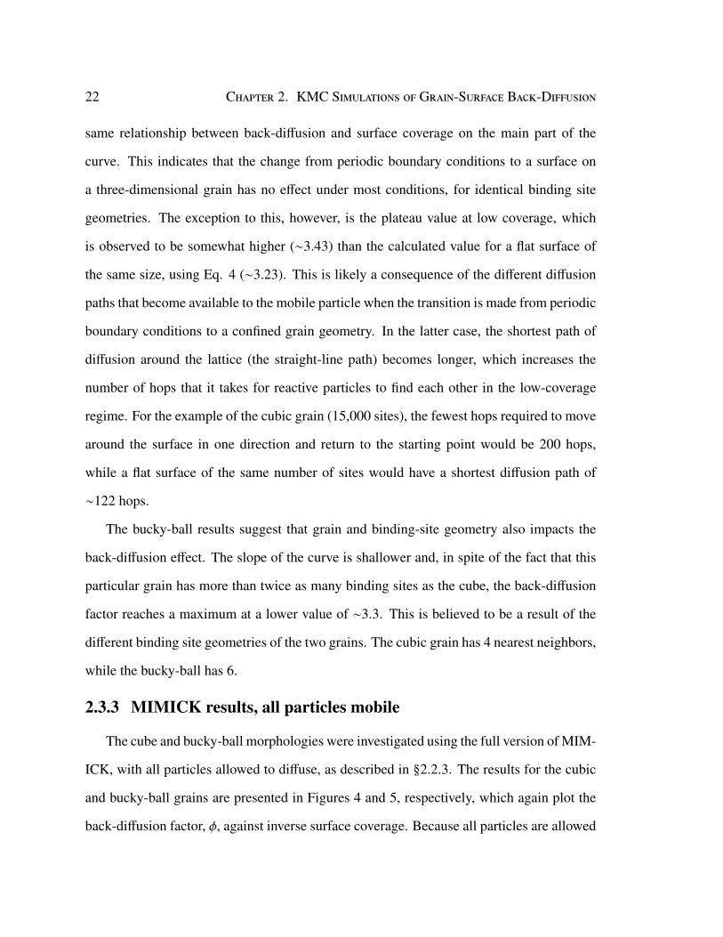
2.1 The two grain morphologies used in this study. The grain on the left is thecubic grain with 15,000 sites (side length of 40 Å), while the grain on theright is the bucky-ball grain with 6,757 sites (radius of 95 Å). The grainsare not to scale with each other. . . . . . . . . . . . . . . . . . . . . . . . . 16
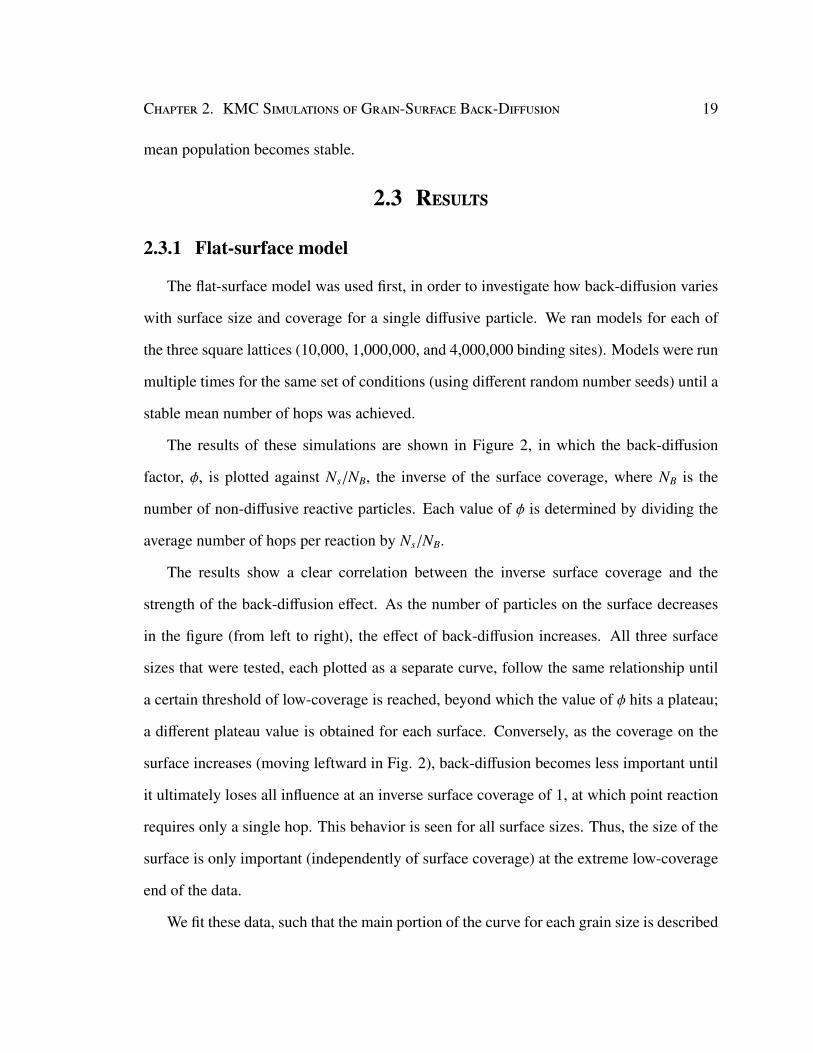
2.2 Data from the flat-surface models, showing the back-diffusion factor ver-sus the inverse surface coverage. Data from three different surface sizesare plotted: 10,000 sites (crosses), 1,000,000 sites (squares) and 4,000,000sites (diamonds). The values of the plateaus for each size are also shown. . 20
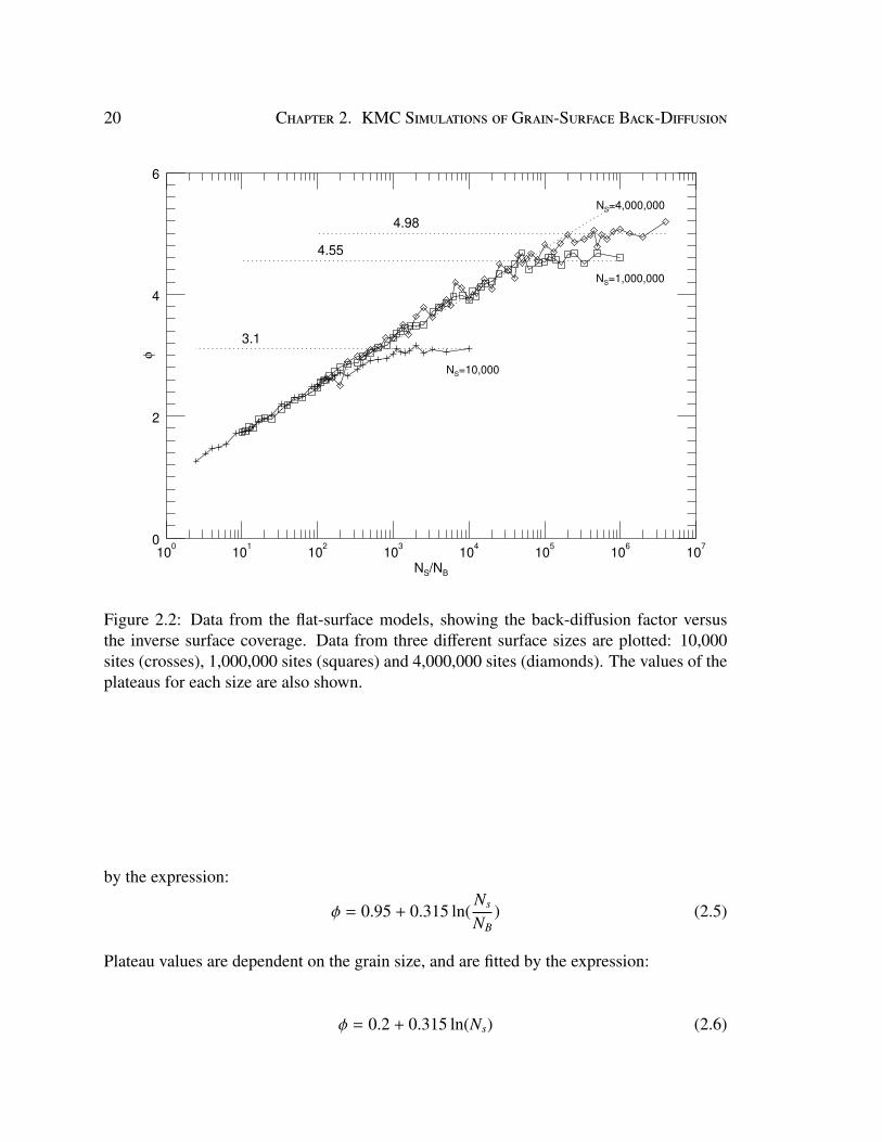
2.3 Data from MIMICK with one mobile particle overlaid with flat-surface data(shown in black); cube-grain data are shown as red squares, bucky-ball dataas blue circles. Plateau values for each grain are marked. The cubic grainused here has 15,000 surface binding sites, while the bucky-ball grain has32,710. . . . . . . . . . . . . . . . . . . . . . . . . . . . . . . . . . . . . 21
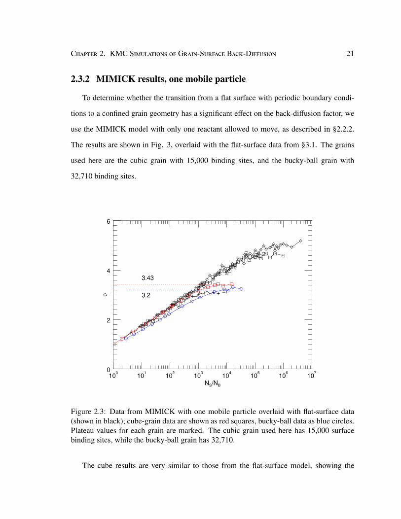
2.4 Results for cubic grains, obtained using the full reaction treatment in MIM-ICK, allowing all particles to diffuse. The arrows are color-coded to corre-spond to the data points for the same grain size, and indicate the points onthe line corresponding to an average of two particles on each grain. . . . . . 23
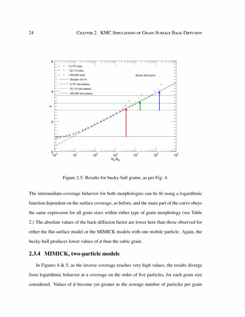
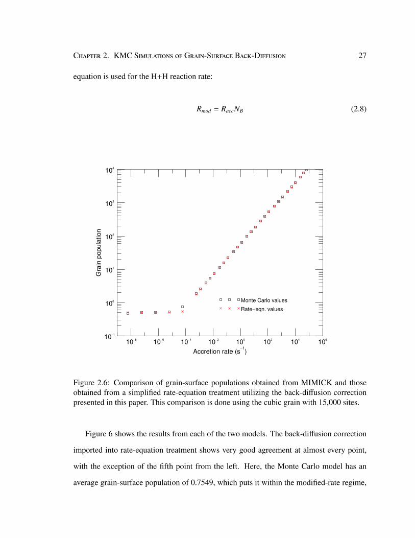
2.5 Results for bucky-ball grains, as per Fig. 4. . . . . . . . . . . . . . . . . . 242.6 Comparison of grain-surface populations obtained from MIMICK and those
obtained from a simplified rate-equation treatment utilizing the back-diffusioncorrection presented in this paper. This comparison is done using the cubicgrain with 15,000 sites. . . . . . . . . . . . . . . . . . . . . . . . . . . . . 27
3.1 Abundance profiles of CH3OCH2OH for three warm-up timescales. Gas-phase abundance is displayed as a solid curve, while grain-surface abun-dance is shown as a dotted curve. Panel (a) shows the abundance profilefor the longest warm-up timescale; (b) and (c) show the abundance profilefor the intermediate and fast warm-up timescales, respectively. . . . . . . . 38
3.2 Continuum images of IRAS 16293 from the PILS survey. The contourscorrespond to 20 logarithmically-divided levels between 0.5% and 100%of peak flux. These images clearly reveal the A (southern) and B (northern)sources. Figure taken from Jørgensen et al. (2016). . . . . . . . . . . . . . 39
xiv List of Figures
3.3 Unblended lines of NH2CN detected towards IRAS 16293B with ALMA.The red line depicts the best-fit spectral model with TEx=300 K, whilethe blue line shows a similar model with TEx=100 K. Figure taken fromCoutens et al. (2018) . . . . . . . . . . . . . . . . . . . . . . . . . . . . . 41
3.4 Chemical model abundances for the warm-up stage of a hot-core type modelwith a final collapse density of nH = 6 × 1010 cm−3. Solid lines denote gas-phase molecules; dotted lines indicate the same species on the grains. Thered dashed line corresponds to the abundance profile of gas-phase NH2CNfor a separate model, with a final collapse density of nH = 1.6 × 107 cm−3 . 44
3.5 Spectral lines of CH3NC detected towards IRAS 16293B. Black denotesthe ALMA data, while blue denotes the spectral model used to fit the data.Figure taken from Calcutt et al. (2018). . . . . . . . . . . . . . . . . . . . 45
3.6 Chemical model abundances for the warm-up stage of a hot-core type model.Panel (a) is for a model with a final collapse density of nH = 1.6×107 cm−3,and panel (b) is for a model with a final collapse density of nH = 6 × 10¹⁰
cm−3. Solid lines denote gas-phase abundances, while dashed lines indicategrain-surface abundances. Panel (c): CH3CN/CH3NC ratio (blue) for thenH = 1.6 × 107 cm−3 model; panel (d): CH3CN/CH3NC ratio (blue) for thenH = 6 × 1010 cm−3 model. . . . . . . . . . . . . . . . . . . . . . . . . . . 50
3.7 Chemical model abundances of CH3CN (black) and CH3NC (green) forthe warm-up stage of a hot core type model where the main destructionpathway for CH3NC (H + CH3NC) has been disabled. Solid lines de-note gas-phase abundances, while dashed lines indicate grain-surface abun-dances. The top panel shows the model with a final collapse density ofnH = 1.6 × 107 cm−3 and the bottom panel shows the model with a finalcollapse density of nH = 6 × 1010 cm−3. . . . . . . . . . . . . . . . . . . . 51
3.8 Spectral lines of CH3CCH detected towards IRAS 16293A and IRAS 16293B.Black denotes the ALMA data, while blue denotes the spectral model usedto fit the data. The red dashed line indicates the systemic velocity of thesource. Figure taken from Calcutt et al. (2019). . . . . . . . . . . . . . . . 52
3.9 Abundances of CH3CCH derived from chemcial modelling for the warm-up stage of a hot-core model. Each panel represents a model with a differentfinal collapse density, shown in the upper left. Solid lines denote gas-phaseabundances, while dotted lines indicate grain-surface abundances. The redand blue dashed lines show the observational abundances in IRAS 16293Aand B, respectively. Figure taken from Calcutt et al. (2019). . . . . . . . . 56
List of Figures xv
4.1 Transitions of CH3NC, 3 = 0 covered by our ALMA survey. The best-fitLTE synthetic spectrum of CH3NC, 3 = 0 is displayed in red and overlaidon the observed spectrum of Sgr B2(N2) shown in black. The green syn-thetic spectrum contains the contributions of all molecules identified in oursurvey so far, including the species shown in red. The central frequencyand width are indicated in MHz below each panel. The y-axis is labeledin effective radiation temperature scale. The dotted line indicates the 3σnoise level. The lines counted as detected in Table 4.1 are marked with ablue star. . . . . . . . . . . . . . . . . . . . . . . . . . . . . . . . . . . . 68
4.2 Same as Fig. 4.1 but for HCCNC, 3 = 0. . . . . . . . . . . . . . . . . . . . 68
4.3 Integrated intensity maps of CH3CN, CH3NC, HC3N, and HCCNC. In eachpanel, the name of the molecule followed by the vibrational state of theline is written in the top left corner, the line frequency in MHz is givenin the top right corner, the rms noise level σ in mJy beam−1 km s−1 iswritten in the bottom right corner, and the beam (HPBW) is shown in thebottom left corner. The black contour levels start at 3σ and then increasegeometrically by a factor of two at each step. The blue, dashed contoursshow the −3σ level. The large and small crosses indicate the positions ofthe hot molecular cores Sgr B2(N2) and Sgr B2(N1), respectively. Becauseof the variation in systemic velocity across the field, the assignment ofthe detected emission to each molecule is valid only for the region aroundSgr B2(N2), highlighted with the red box. . . . . . . . . . . . . . . . . . . 70
4.4 Abundances of cyanides and isocyanides in the standard model presented inthis paper (Model 1). Dashed lines correspond to grain abundances, whilesolid lines correspond to gas-phase abundances. Left panel: HCN, CH3CN,CH3NC, C2H5CN, C2H5NC. Right panel: HNC, C2H3CN, C2H3NC, HC3N,HC2NC. . . . . . . . . . . . . . . . . . . . . . . . . . . . . . . . . . . . . 81
4.5 Abundances of cyanides and isocyanides in the model with a barrier of3000 K for the reaction of H + CH3NC (Model 2). . . . . . . . . . . . . . . 82
4.6 Abundances of cyanides and isocyanides in the model with a barrier of2000 K for the reaction of H + CH3NC. . . . . . . . . . . . . . . . . . . . 83
4.7 Abundances of cyanides and isocyanides in the standard two-phase hot-core chemical model. Dashed lines correspond to grain abundances, whilesolid lines correspond to gas-phase abundances. Left panel: HCN, CH3CN,CH3NC, C2H5CN, C2H5NC. Right panel: HNC, C2H3CN, C2H3NC, HC3N,HC2NC. . . . . . . . . . . . . . . . . . . . . . . . . . . . . . . . . . . . . 86
4.8 Abundances of cyanides and isocyanides in the old physical model with H+
HCCNC HCN + C2H (Eq. 4.20) added. Left panel: HCN, CH3CN,CH3NC, C2H5CN, C2H5NC. Right panel: HNC, C2H3CN, C2H3NC, HC3N,HC2NC. . . . . . . . . . . . . . . . . . . . . . . . . . . . . . . . . . . . . 87
xvi List of Figures
4.9 Abundances of cyanides and isocyanides in the standard model presentedin this paper (Model 1), with H + HCCNC HCN + C2H (Eq. 4.20)added. Left panel: HCN, CH3CN, CH3NC, C2H5CN, C2H5NC. Rightpanel: HNC, C2H3CN, C2H3NC, HC3N, HC2NC. . . . . . . . . . . . . . . 88
4.10 ζ profiles for each model as a function of AV . The dashed line shows thereference value that is typically assumed in hot-core models (1.3 × 10⁻¹⁷
s−1). Recent observational constraints have placed ζ for the diffuse mediumaround Sgr B2 at 10−15-10−14 s−1. The panel on the right shows the AV
profile as a function of radius. . . . . . . . . . . . . . . . . . . . . . . . . 894.11 Abundances of cyanides and isocyanides in Model 3, which has an AV-
dependent ζ shown in Figure 4.10. Left panel: HCN, CH3CN, CH3NC,C2H5CN, C2H5NC. Right panel: HNC, C2H3CN, C2H3NC, HC3N, HC2NC. 90
4.12 Abundances of cyanides and isocyanides in Model 4, which has an AV-dependent ζ shown in Figure 4.10. Left panel: HCN, CH3CN, CH3NC,C2H5CN, C2H5NC. Right panel: HNC, C2H3CN, C2H3NC, HC3N, HC2NC. 91
4.13 Abundances of cyanides and isocyanides in Model 5, which has an AV-dependent ζ shown in Figure 4.10. Left panel: HCN, CH3CN, CH3NC,C2H5CN, C2H5NC. Right panel: HNC, C2H3CN, C2H3NC, HC3N, HC2NC. 92
4.14 Abundances of cyanides and isocyanides in Model 6, with a constant ζof 1 × 10⁻¹⁶ s−1. Left panel: HCN, CH3CN, CH3NC, C2H5CN, C2H5NC.Right panel: HNC, C2H3CN, C2H3NC, HC3N, HC2NC. . . . . . . . . . . . 95
4.15 Abundances of cyanides and isocyanides in Model 7, with a constant ζof 3 × 10⁻¹⁴ s−1. Left panel: HCN, CH3CN, CH3NC, C2H5CN, C2H5NC.Right panel: HNC, C2H3CN, C2H3NC, HC3N, HC2NC. . . . . . . . . . . . 96
4.16 Density and temperature profiles used in the radiative transfer calculationsfor the modeling data. The density is that of total hydrogen. . . . . . . . . . 98
4.17 Rotational diagrams for cyanides and isocyanides. We note that Model 4was used to produce these diagrams. . . . . . . . . . . . . . . . . . . . . . 116
4.18 Comparison of column density ratios between observations and models. . . 1174.19 Comparison of excitation temperatures between observations and models. . 1184.20 Same as Fig. 4.1 for CH3NC, 38 = 1. . . . . . . . . . . . . . . . . . . . . 1194.21 Selection of transitions of C2H5NC, 3 = 0 covered by our ALMA survey.
The LTE synthetic spectrum of C2H5NC, 3 = 0 used to derive the upperlimit on its column density is displayed in red and overlaid on the observedspectrum of Sgr B2(N2) shown in black. The green synthetic spectrumcontains the contributions of all molecules identified in our survey so far,but does not include the species shown in red. The central frequency andwidth are indicated in MHz below each panel. The y-axis is labeled ineffective radiation temperature scale. The dotted line indicates the 3σ noiselevel. . . . . . . . . . . . . . . . . . . . . . . . . . . . . . . . . . . . . . 119
4.22 Same as Fig. 4.21 but for C2H3NC, 3 = 0. . . . . . . . . . . . . . . . . . . 1204.23 Same as Fig. 4.21 but for HNC3, 3 = 0. . . . . . . . . . . . . . . . . . . . 120
List of Figures xvii
4.24 Same as Fig. 4.21 but for HC3NH+, 3 = 0. . . . . . . . . . . . . . . . . . . 120
5.1 Temperature through the first ∼20 m of ice for the first orbital evolution ofHale-Bopp. The plots are color-coded for each orbital position. . . . . . . . 139
5.2 Temperatures throughout the cometary ice for subsequent orbits after Fig-ure 5.1. Upper-left: orbit 2, upper-right: orbit 3, lower-left: orbit 4, lower-right: orbit 5. . . . . . . . . . . . . . . . . . . . . . . . . . . . . . . . . . 140
5.3 Raw data from 3-D back-diffusion Monte Carlo code. Data are color-codedaccording to thickness. The x-axis displays the base-10 logarithm of thenumber of diffusers, while the y-axis displays the number of hops per par-ticle before a single particle exits out of the top or bottom of the ice. . . . . 141
5.4 Monte Carlo data for single diffusers, fit to Eq. 5.17. . . . . . . . . . . . . 1425.5 Data for back-diffusion simulation with Nth = 1. . . . . . . . . . . . . . . . 1425.6 Data for back-diffusion simulations with Nth = 20. The green and orange
lines correspond to the values of Eq. 5.17 and Eq. 5.16, respectively. . . . . 1435.7 Data for back-diffusion simulations with Nth = 30. The red line is θtot, with
a given by Eq. 5.20. . . . . . . . . . . . . . . . . . . . . . . . . . . . . . . 1445.8 Data for back-diffusion simulations with Nth = 100. . . . . . . . . . . . . . 1455.9 Abundances of molecules throughout the cometary nucleus at t = 106 yr.
The top panel displays the initial ice components along with a few othersimple molecules, while the bottom panel displays more complex molecules.149
5.10 Abundances of molecules throughout the cometary nucleus at t = 5 × 10⁹
yr. The top panel displays the initial ice components along with a few othersimple molecules, while the bottom panel displays more complex molecules.150
5.11 Abundances of molecules throughout the cometary nucleus at first aphe-lion. The top panel displays the initial ice components along with a fewother simple molecules, while the bottom panel displays more complexmolecules. . . . . . . . . . . . . . . . . . . . . . . . . . . . . . . . . . . . 151
5.12 Abundances of molecules throughout the cometary nucleus at first perihe-lion. The top panel displays the initial ice components along with a fewother simple molecules, while the bottom panel displays more complexmolecules. . . . . . . . . . . . . . . . . . . . . . . . . . . . . . . . . . . . 152
5.13 Abundances of molecules throughout the cometary nucleus at third aphe-lion. The top panel displays the initial ice components along with a fewother simple molecules, while the bottom panel displays more complexmolecules. . . . . . . . . . . . . . . . . . . . . . . . . . . . . . . . . . . . 153
5.14 Abundances of molecules throughout the cometary nucleus at third perihe-lion. The top panel displays the initial ice components along with a fewother simple molecules, while the bottom panel displays more complexmolecules. . . . . . . . . . . . . . . . . . . . . . . . . . . . . . . . . . . . 154
xviii List of Figures
5.15 Abundances of molecules throughout the cometary nucleus at fifth aphe-lion. The top panel displays the initial ice components along with a fewother simple molecules, while the bottom panel displays more complexmolecules. . . . . . . . . . . . . . . . . . . . . . . . . . . . . . . . . . . . 155
5.16 Abundances of molecules throughout the cometary nucleus at fifth perihe-lion. The top panel displays the initial ice components along with a fewother simple molecules, while the bottom panel displays more complexmolecules. . . . . . . . . . . . . . . . . . . . . . . . . . . . . . . . . . . . 156
xix
List of Tables
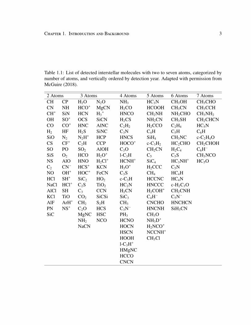
1.1 List of detected interstellar molecules with two to seven atoms, categorizedby number of atoms, and vertically ordered by detection year. Adaptedwith permission from McGuire (2018). . . . . . . . . . . . . . . . . . . . . 3
1.2 List of detected interstellar molecules with eight or more atoms, catego-rized by number of atoms, and vertically ordered by detection year. Adaptedwith permission from McGuire (2018) . . . . . . . . . . . . . . . . . . . . 4
2.1 Summary of surfaces used in this study. . . . . . . . . . . . . . . . . . . . 17
3.1 Observational info for CH3NC derived towards IRAS 16293B. . . . . . . . 453.2 Observational info for CH3CCH derived towards IRAS 16293A and IRAS
16293B. . . . . . . . . . . . . . . . . . . . . . . . . . . . . . . . . . . . . 533.3 Initial fractional abundances with respect to total hydrogen used in the
three-phase chemical kinetics model MAGICKAL . . . . . . . . . . . . . . 54
4.1 Parameters of our best-fit LTE model of alkyl cyanides and isocyanides,and related species, toward Sgr B2(N2). . . . . . . . . . . . . . . . . . . . 67
4.2 Physical parameters used in chemical model. . . . . . . . . . . . . . . . . 794.3 Legend for chemical modeling presented in this study. . . . . . . . . . . . . 804.4 Abundances relative to total hydrogen at the observationally-determined
excitation temperature for all molecules of interest in each model. . . . . . 934.5 Fractional abundance ratios relative to total hydrogen for models at the
observationally-determined excitation temperature for each species, as wellas the observational column density ratios. . . . . . . . . . . . . . . . . . . 94
4.6 Column densities (in cm−2) for each molecule of interest in our observa-tions and for each model, calculated using our radiative transfer model. . . 99
4.7 Excitation temperatures (in K) for each molecule of interest in each model,calculated using our radiative transfer model. . . . . . . . . . . . . . . . . 100
4.8 Column density ratios for models, as well as the observational column den-sity ratios. . . . . . . . . . . . . . . . . . . . . . . . . . . . . . . . . . . . 101
4.9 Observational and theoretical column densities with respect to CH3CN. . . 1084.10 Column density ratios in different sources. . . . . . . . . . . . . . . . . . . 111

xx List of Tables
4.11 Lines of CH3NC and HCCNC detected in the EMoCA spectrum of SgrB2(N2). . . . . . . . . . . . . . . . . . . . . . . . . . . . . . . . . . . . . 121
4.12 Physical quantities of new and related chemical species. . . . . . . . . . . . 1224.13 New grain-surface/ice-mantle reactions involved in formation and destruc-
tion of new and related species. . . . . . . . . . . . . . . . . . . . . . . . . 1234.14 New gas-phase reactions involved in formation and destruction of new and
related species. . . . . . . . . . . . . . . . . . . . . . . . . . . . . . . . . 124
5.1 Physical parameters used in the heat diffusion model. . . . . . . . . . . . . 132
1
Chapter 1
Introduction and Background
1.1 A Brief History ofMolecular Detections in SpaceAstrochemistry, broadly, is the study of the formation and destruction of molecules in
space. The first molecule to be detected in interstellar space was methylidine (CH; Swings
& Rosenfeld (1937); Dunham (1937); McKellar (1940)). This first molecular detection, as
well as subsequent detections of the cyano radical (CN: McKellar (1940); Adams (1941))
and the methylidine cation (CH+; Douglas & Herzberg (1941)) were made using optical
telescopes. These three molecules retained their status as the only molecular detections in
space until the advent of radio telescope technology in the 1960s.
The first molecule to be detected using radio astronomy was the now-ubiquitous hy-
droxyl radical (OH; Weinreb et al. (1963)), using the Millstone Hill Observatory at MIT.
This discovery catalyzed an exciting era of radio observations, with the next ten years in-
cluding detections of several terrestrially-important molecules including water (H2O; Che-
ung et al. (1969)), carbon monoxide (CO; Wilson et al. (1970)), and methanol (CH3OH;
Ball et al. (1970)).
Since these early detections, radio telescopes have become increasingly sensitive, both
2 Chapter 1. Introduction and Background
in terms of spatial and spectral resolution. The improvement in receiver technology, as
well as the construction of large radio interferometers such as the Atacama Large Millime-
ter/submillimeter Array in the Atacama Desert in Chile, has allowed astronomers to detect
more complex molecules in more distant objects than previously possible. As a result, there
are currently over 200 molecules known in space. For example, the recent detection of rug-
byballene (C70; Cami et al. (2010)), as well as the first polycyclic aromatic hydrocarbon in
space, benzonitrile (c-C6H5CN; McGuire et al. (2018a)) have revealed a great deal about
the depth of chemical complexity in space. Tables 1.1 and 1.2 lists the known detections at
the time of this writing.
1.2 AstrochemicalModellingOnce it became apparent that molecules were ubiquitous in interstellar environments,
astrochemists endeavored to explain their chemistry with astrochemical models. The ma-
jority of this thesis will focus on this topic, so it will be covered in some depth here. The
first models to be constructed to explain interstellar chemistry were those that used chem-
ical kinetics rate-equations. They are generally referred to as “rate-equation models,” and
are still the most common form of astrochemical model in use today, though with several
improvements since their inception.
1.2.1 Rate-equation models
The first astrochemical model based on rate-equations to be published was that of
Herbst & Klemperer (1973). Their model contained 37 chemical species, the most complex
of which contained five atoms. From these species, they constructed a system of ordinary
differential equations (ODEs), one for each species, and solved these equations numerically
through iteration to get the abundances of molecules as a function of time.
Chapter 1. Introduction and Background 3
Table 1.1: List of detected interstellar molecules with two to seven atoms, categorized bynumber of atoms, and vertically ordered by detection year. Adapted with permission fromMcGuire (2018).
2 Atoms 3 Atoms 4 Atoms 5 Atoms 6 Atoms 7 AtomsCH CP H2O N2O NH3 HC3N CH3OH CH3CHOCN NH HCO+ MgCN H2CO HCOOH CH3CN CH3CCHCH+ SiN HCN H3
+ HNCO CH2NH NH2CHO CH3NH2
OH SO+ OCS SiCN H2CS NH2CN CH3SH CH2CHCNCO CO+ HNC AlNC C2H2 H2CCO C2H4 HC5NH2 HF H2S SiNC C3N C4H C5H C6HSiO N2 N2H+ HCP HNCS SiH4 CH3NC c-C2H4OCS CF+ C2H CCP HOCO+ c-C3H2 HC2CHO CH2CHOHSO PO SO2 AlOH C3O CH2CN H2C4 C6H–
SiS O2 HCO H2O+ l-C3H C5 C5S CH3NCONS AlO HNO H2Cl+ HCNH+ SiC4 HC3NH+ HC5OC2 CN– HCS+ KCN H3O+ H2CCC C5NNO OH+ HOC+ FeCN C3S CH4 HC4HHCl SH+ SiC2 HO2 c-C3H HCCNC HC4NNaCl HCl+ C2S TiO2 HC2N HNCCC c-H2C3OAlCl SH C3 CCN H2CN H2COH+ CH2CNHKCl TiO CO2 SiCSi SiC3 C4H– C5N–
AlF ArH+ CH2 S2H CH3 CNCHO HNCHCNPN NS+ C2O HCS C3N– HNCNH SiH3CNSiC MgNC HSC PH3 CH3O
NH2 NCO HCNO NH3D+
NaCN HOCN H2NCO+
HSCN NCCNH+
HOOH CH3Cll-C3H+
HMgNCHCCOCNCN
4 Chapter 1. Introduction and Background
Table 1.2: List of detected interstellar molecules with eight or more atoms, categorized bynumber of atoms, and vertically ordered by detection year. Adapted with permission fromMcGuire (2018)
8 Atoms 9 Atoms 10 Atoms 11 Atoms 12 Atoms 13 Atoms FullerenesHCOOCH3 CH3OCH3 (CH3)2CO HC9N C6H6 c-C6H5CN C60
CH3C3N CH3CH2OH HO(CH2)2OH CH3C6H n-C3H7CN C60+
C7H CH3CH2CN CH2CH2CHO CH3CH2OCHO i-C3H7CN C70
CH3COOH HC7N CH3C5N CH3COOCH3
H2C6 CH3C4H CH3CHCH2OCH2OHCHO C8H CH3OCH2OHHC6H CH3CONH2
CH2CHCHO C8H–
CH2CCHCN CH2CHCH3
NH2CH2CN CH3CH2SHCH3CHNH HC7OCH3SiH3
The general form of one of the ODEs is a rate-equation model is as follows:
dn(i)dt
=∑mn
km+nn(m)n(n) −∑
i j
ki+ jn(i)n( j) +∑
j
k j→in( j) −∑all
kin(i) (1.1)
Here, n(i) corresponds to the number density of species i in the chemical model, usually ex-
pressed in units of cm−3. Often, these densities will be expressed as fractional abundances
with respect to the amount of total hydrogen. The quantities denoted by k correspond to the
rate constants of each reaction. The units and typical values of these constants vary from
one reaction mechanism to another. The first term on the right-hand side signifies two-body
formation of species i, through any number of reaction mechanisms, including radiative as-
sociation and ion-molecule collisions. The second term corresponds to two-body destruc-
tion mechanisms, through generally the same mechanisms. The third and fourth terms are
for one-body formation and destruction of species i, respectively. Chemical processes that
contribute to these terms include dissociation of molecules from UV photons and cosmic
rays.
Chapter 1. Introduction and Background 5
Thus each chemical model contains N ODEs, where N denotes the number of chemical
species considered in the model. This system of equations is heavily non-linear, as the
abundance of each species depends in different ways on the abundances of many other
species in the chemical network. Through the use of modern ODE solvers such as the Gear
algorithm, computers can solve these systems with relative ease.
As in Herbst & Klemperer (1973), inital astrochemical models considered only chem-
istry occurring in the gas-phase. However, the importance of chemistry occurring on the
surfaces of interstellar dust particles was realized, and efforts were made to include this
chemistry into standard rate-equation models. Hasegawa et al. (1992) is a seminal exam-
ple of such a model. These models incorporate interactions between the gas phase and
the surfaces of dust particles through processes such as accretion and thermal desorption.
Reactions on the grain surfaces are treated much the same as those in the gas phase, with
rate constants being calculated from the rate of diffusion of reactants on the surface, itself
a quantity dependent on the molecule.
These models have evolved over the years to incorporate a three-phase structure, which
includes reactions in the gas phase, on the grain surface, and in the bulk ice mantle between
the grain surface and core (Garrod 2013a). The physical conditions of these models have
evolved over time as well, from the quiescent cold interstellar clouds of Herbst & Klem-
perer (1973), to attempts to simulate the warm-up that occurs in regions of nascent star
formation (Garrod et al. 2008).
Despite the proliferation and success of rate-equation models in astrochemistry, they
do have some shortcomings, particularly when treating grain chemistry. For example, the
rate-equation method can overestimate reaction rates for grain reactions in which the av-
erage abundance of one or more reactants is less than 1. This problem has been remedied
by the introduction of modified rate equations (MREs; Garrod (2008)). However, due to
the fact that rate equations use average abunbances of species to calculate reaction rates,
6 Chapter 1. Introduction and Background
microscopic information about chemistry occurring on surfaces is generally lost.
1.2.2 Microscopic Monte Carlo methods
Partly in an effort to remedy the shortcomings of rate equations, microscopic Monte
Carlo methods were developed to study astrochemical systems. These methods explictly
account for the position of molecules on grains, and thus precise microscopic information
about the chemistry is retained. However, these models are much more computationally
expensive than rate-equation models, and thus cannot be used to solve the chemistry of
large astronomical systems. Instead, as in the case of Garrod (2013b), chemistry is usually
simulated on a single dust particle and insights are applied to dust chemistry as a whole.
These models have been used to gain valuable insights about chemistry occurring on
interstellar dust particles, as well as in astrochemical laboratory simulations. For exam-
ple, using the model of Garrod (2013b), Willis & Garrod (2017) were able to determine a
method to incorporate surface back-diffusion of reactive species into rate-equation models.
This work will be discussed in further detail in Chapter 2 of this thesis. Using the same
model, Clements et al. (2018) investigated the porosity of water ice deposited at labora-
tory conditions and compared that to those in interstellar space and protoplanetary disks.
Additionally, Shingledecker et al. (2017) developed a Monte Carlo model of cosmic-ray
chemistry in solids, which has since been incorporated into rate-equation models (Shin-
gledecker & Herbst 2018). These insights would not be possible without the interplay of
Monte Carlo kinetics and rate-equation models, and as such this dissertation will devote
much discussion to that interplay.
1.3 Dissertation ScopeThis dissertation will be focused primarily on the development of new computational
methods in both rate-equation models as well as microscopic Monte Carlo models to more
Chapter 1. Introduction and Background 7
accurately simulate astrochemical sources. The chapters will be broken down as follows.
Chapter 2 will be focused on adapting the microscopic Monte Carlo model of Garrod
(2013b) to study the back-diffusion effect of reactive particles on interstellar dust surfaces.
The chapter will be focused on the simple reaction system of H + H H2, but its results
are applicable to any reaction system that involves surface diffusion. The discussion will
include methods for inclusion into general astrochemical rate-equation models.
Chapter 3 will concern the study of several molecules of astrochemical interest using
rate-equation models. These models have been updated to include the back-diffusion cor-
rection presented in Chapter 2. The molecules that will be covered vary in complexity, but
all are of fundamental interest to the study of interstellar chemistry. The molecules include
methoxymethanol (CH3OCH2OH; McGuire et al. (2017)), cyanamide (NH2CN; Coutens
et al. (2018)), methyl isocyanide (CH3NC; Calcutt et al. (2018)), and propyne (CH3CCH;
Calcutt et al. (2019)). The inclusion of CH3NC into chemical networks marks the first time
that this molecule has been studied in astrochemical models.
Chapter 4 will concern further study of the class of molecules known as isocyanides,
CH3NC being among them. In particular, it will focus on the study of these molecules’
abundances in the Galactic Center star-forming region Sgr B2(N2). Several new molecules
were incorporated into the chemical model, and spectral modelling was performed to model
their line emission for comparison with radio astronomy observations. In addition, a new
physical model for Sgr B2(N2) is presented, along with a general way of more accurately
incorporating observational physical conditions into astrochemical models.
Chapter 5 will focus on the chemistry of cometary surfaces in the solar system. Several
new numerical methods will be applied to the cometary model first presented by Garrod
(2019), including expanded discussion of the back-diffusion effect of molecules in an ice
matrix. We will also present orbital calculations that allow the model to simulate any
known cometary orbit, or generic orbits calculated from chosen orbital elements. Several

8 Chapter 1. Introduction and Background
new non-diffusive reaction mechanisms in ice matrices will also be studied.
9
Chapter 2
KineticMonte Carlo Simulations of the
Grain-Surface Back-Diffusion Effect
2.1 IntroductionChemistry occurring on the surfaces of interstellar dust grains is crucial to the forma-
tion of molecules in the interstellar medium (Herbst & van Dishoeck 2009), including the
most abundant interstellar molecule, H2 (Gould & Salpeter 1963). The grain surface acts
as a crucible for H2 formation, allowing two adsorbed hydrogen atoms to meet by thermal
diffusion and react, typically followed by desorption of the newly-formed H2 molecule.
Other grain-surface reactions occur similarly, with some involving activation energy barri-
ers, although, unlike H2, the products are generally expected to remain on the grain surface
at low temperatures.
Grain-surface chemistry was first incorporated into astrochemical kinetics models in the
1970s (Pickles & Williams 1977a,b). Theoretical treatments of interstellar grain-surface
chemistry have since become increasingly detailed (e.g. Hasegawa et al. (1992)), including
the formation of many more complex organic molecules. The most common method used
10 Chapter 2. KMC Simulations of Grain-Surface Back-Diffusion
to simulate the time-dependent evolution of interstellar chemistry is the so-called rate-
equation (RE) method, whereby a system of ordinary differential equations (one for the
abundance of each chemical species in the network) is solved using publicly-available
solver routines. Construction of the differential equations requires the evaluation of av-
erage rates of reaction (and other processes); the calculated abundances thus correspond to
average values, often interpreted as a time-average over a period in which the macroscopic
conditions of the system remain constant.
Rate-equation treatments are very accurate when applied to pure gas-phase chemistry,
but can fail in certain regimes when the method is used to simulate grain-surface chemistry,
due to the discrete nature of the grains. When the average population of reactive species
on grain surfaces falls below order unity, stochastic effects can become important. This
particular problem can be remedied reasonably well using modified rate equations, MRE
(Garrod 2008).
The RE and MRE methods provide a fast and efficient means to simulate coupled gas
and grain chemistry, but the application specifically to grain-surface reactions still retains
certain inaccuracies related to the use of average reaction rates, which are determined by
the rates of diffusion of surface species. The typical approach (Hasegawa et al. 1992) is to
calculate the absolute reaction rate between diffusive species, i and j, using the expression:
Ri j = κi jkreacNiN j (2.1)
where κi j is a reaction efficiency related to the activation energy, Ni and N j are the popula-
tions of species i and j on the grain surface, and kreac is defined as follows:
kreac =khop,i + khop, j
Ns(2.2)

Chapter 2. KMC Simulations of Grain-Surface Back-Diffusion 11
where khop,i and khop, j are the diffusion rates of species i and j, respectively, from one site to
an adjacent site, and Ns is the number of binding sites on the surface. A similar expression
is used in the case that j=i, such as that of the reaction H + H→ H2:
kreac =khop,i
Ns(2.3)
The quantity khop/Ns is sometimes referred to as the scanning rate, and is interpreted as the
rate at which a diffusing particle succeeds in visiting all surface sites, which, in the case
of only two particles on the grain surface, would be equal to the average number of hops
required for two reactants to meet. However, this implicitly assumes that the particle visits
each site only once. A more rigorous derivation for Eqs. (1) – (3) considers the absolute
reaction rate, Ri j, to be determined by the rate of hopping of species i into an adjacent site,
khop,i, multiplied by the probability that the new site contains a reaction partner j. The latter
probability is given by Ni, j/Ns, the fractional coverage of the surface by species j. A similar
term may be constructed for diffusion by species j into a site containing reaction partner i.
By basing the overall reaction rate on the individual rate associated with a single hop,
rather than the full chain of diffusion events leading to reaction, the above treatment ignores
the possibility that the random walk of the diffusing species may include hops that return
it to previously-visited binding sites. This effect, known as back diffusion, will act to slow
down grain-surface reactions compared to the standard treatment used in astrochemical
models.
There has been extensive research conducted on the theory of random walks in statis-
tical physics and other fields, of which we cite a small fraction; Hatlee & Kozak (1980)
investigated the problem of random walks on finite lattices using a Monte Carlo approach,
in an attempt to investigate the effect of boundaries on processes related to chemical dy-
namics. Botar & Vidóczy (1984) used Monte Carlo models to study reaction kinetics at
12 Chapter 2. KMC Simulations of Grain-Surface Back-Diffusion
different solute concentrations, while Allen & Seebauer (1996) used a combination of an-
alytical and Monte Carlo techniques to study the relationship between the diffusion coeffi-
cient and rate constant on square lattices. More recently, Paster et al. (2014) investigated a
similar problem to that presented in this work, investigating the effect of stochastic initial
conditions on the diffusion-reaction equation on grids in 1-3 dimensions.
The problem of random walks on interstellar dust grains in particular has been ap-
proached by various authors. Charnley (2005) investigated the diffusion on grain surfaces
in order to challenge the so-called ‘two-coreactant restriction.’ Charnley used results al-
ready known for random walks, showing that for a surface with 106 binding sites, reaction
would be slowed by a factor of ∼4.9 when including back-diffusion, indicating that the
scanning rate should be adjusted accordingly. This derivation considered a single particle
diffusing over the grain, so surface-coverage effects were not included.
Lohmar & Krug (2006) also investigated a modification to the scanning rate in models
of grain-surface chemistry. They considered a spherical grain with two surface particles
adsorbed. One particle was forced to be stationary, while the other was allowed to dif-
fuse, but in the case where all surface sites are identical, this arrangement is equivalent to
having two mobile (identical) particles. They then calculated the exact scanning rate for
this situation, defined in terms of an encounter probability for the two particles (see also
Lohmar et al. (2009)). This encounter probability was found to depend upon both the dif-
fusion and desorption rates of the mobile atom. The new scanning rate was broken into
two regimes of interest: small grains and large grains. The true scanning rate was found
to be reduced in comparison to the conventional approximation, with this reduction being
greatest for large grains, but still significant on smaller grains. Overall, the factor by which
this exact scanning rate slowed down reactions was between ∼2-5, depending on grain size.
The follow-up paper by Lohmar et al. (2009) presented a more approximate solution to the
problem for ease of inclusion into astrochemical models, conducting kinetic Monte Carlo
Chapter 2. KMC Simulations of Grain-Surface Back-Diffusion 13
simulations that showed that the approximation accurately reproduced the behavior seen
in the exact solution. Despite the promise of this work, it has not yet been tested in an
astrochemical model. However, the derivation of the encounter probability undertaken by
Lohmar & Krug (2006) considers just two particles on the grain surface, while interstellar
dust particles can accumulate larger numbers of reactive atoms and molecules.
In this paper, we explore the dependence of the back-diffusion effect not only on the
number of surface binding sites on the grain, but on the surface coverage of reactants, using
kinetic Monte Carlo methods that can simulate a range of astrophysically-relevant condi-
tions and surfaces. We use both a 2-D model of a square surface with periodic boundary
conditions, and a fully three-dimensional model of a grain, in which the surface binding
sites and the associated directions of diffusion are determined by the arrangement of the
atoms that make up the grain surface (see Garrod 2013). Such methods are useful in solv-
ing this problem, as they allow the positions of particles on a grain surface to be traced
explicitly, allowing averaged path lengths (in terms of the number of hops) to be calculated
over large numbers of diffusion/reaction events. The resultant averaged scanning rates may
then be incorporated directly into standard rate-equation models. The use of numerical
simulations such as these also lay the groundwork for their use in characterizing the kinetic
properties of rough, amorphous surfaces.
In the simulations and analysis presented here, we define the back-diffusion factor, φ, as
the factor by which reactions are slowed by the back-diffusion effect, as compared with the
standard rate-equation formulation of Eqs. (1) – (3). With this definition in mind, it is also
convenient to define an effective number of surface sites on the grain, NE f f , which may,
as with Eq. (3) in the case of two particles on the surface, be identified with the average
number of hops required for reaction to occur. These quantities are related thus:
NE f f = φNs (2.4)
14 Chapter 2. KMC Simulations of Grain-Surface Back-Diffusion
where Ns is the actual number of binding sites on the surface. We present fits to the com-
putational calculations of average rates, in order to provide practical determinations for φ
that may be easily employed in astrochemical models.
In section 2, we describe the computational methods. In section 3, we present results.
Section 4 contains a discussion of the results, and section 5 presents the conclusions of this
study.
2.2 Methods
2.2.1 Simple flat-surface model
The surface chemistry simulations presented in this paper were performed using two
kinetic Monte Carlo models. The simpler model uses a flat surface with rectangular lattice
geometry in a square grid. This surface has a user-determined size with periodic boundary
conditions. In this model, the number of binding sites, and their location, are directly
specified. A user-selected number of target atoms is then deposited onto the surface in
randomly-chosen binding sites. These target atoms are not allowed to diffuse, and are
analogous to heavier grain-surface atoms that diffuse very slowly relative to hydrogen, such
as oxygen. The last particle deposited onto the surface is mobile, analogous to a reactive
hydrogen atom. This particle diffuses via a random walk. All four diffusion directions have
equal probability in the simulation, and are chosen randomly. When a reaction occurs, the
number of hops to achieve reaction is recorded, and the surface is cleared of particles. The
model does not trace the time, only the number of hops, and as such is insensitive to the
value of the diffusion barrier. The process then restarts, until a user-specified number of
reactions is recorded. In this way, it is possible to determine the effect of back-diffusion as
a function of surface coverage for varying surface sizes. Results were obtained for three
sizes (10,000, 1,000,000, and 4,000,000 sites), sampling a wide range of surface coverages
Chapter 2. KMC Simulations of Grain-Surface Back-Diffusion 15
by altering the number of deposited stationary particles.
2.2.2 MIMICK
The two-dimensional model has shortcomings; firstly that only one particle is allowed
to diffuse on the surface, and secondly that the surface is flat and periodic, rather than being
the bounding surface of a three-dimensional dust grain. In order to overcome both these
deficiencies at once, the off-lattice Monte Carlo kinetics model MIMICK (Model for Inter-
stellar Monte-Carlo Ice Chemical Kinetics) was used (Garrod (2013b)). MIMICK allows
for the simulation of chemistry on grains of user-defined size and morphology. The posi-
tions of all particles are determined explicitly based upon the local potential minima on the
surface, so there are no pre-defined lattice sites, thus making it a true off-lattice model. In
this paper, the chemical network has been vastly simplified, with atomic hydrogen being
the only species allowed to accrete onto the grain surface from the gas phase. This model
explicitly traces the passage of time, and uses an explicit diffusion barrier. However, while
exact pairwise potentials are used to determine the positions of the surface potential min-
ima, all diffusion barriers are set to ∼510.6 K (the value for amorphous carbon determined
by Katz et al. (1999)), to replicate the conditions assumed by Lohmar et al. (2009)
2.2.3 Grains
Two grain morphologies were used with MIMICK to investigate the effect that grain-
surface morphology has on the back-diffusion factor. The first was a cubic grain, created
using a simple cubic lattice. Each binding site (i.e. potential well) on the grain has four
diffusion paths leading out of it, which is identical to the flat surface used in the simple two-
dimensional model. It was not possible to create a simple flat surface for use in MIMICK,
due to the difficulty of incorporating periodic boundary conditions into this more complex
model. Thus the cube was chosen as a reliable comparison to the flat surface, to determine
if the transition from the flat surface to a confined grain geometry had an effect on the
16 Chapter 2. KMC Simulations of Grain-Surface Back-Diffusion
back-diffusion factor.
The second grain used in this study assumed the shape of a bucky-ball, created with the
aid of the DOME program.1 Coordinates for each bucky-ball were generated using DOME,
and these coordinates were then transformed into input compatible with MIMICK. Some
error may be introduced as a result of the coordinate transformation, causing the spacing
between atoms to vary on small scales throughout the grain. However, this does not impact
the results presented here, due to the adoption of a fixed diffusion barrier for all sites and
directions. The bucky-ball was chosen because it is spherical, with all binding sites being
essentially equivalent, and as such is analogous to the spherical grain geometry assumed by
rate-equation codes. Each binding site on the bucky-ball grain has a hexagonal geometry.
An image of both grains is shown in Figure 1, created using POV-Ray.2
Figure 2.1: The two grain morphologies used in this study. The grain on the left is the cubicgrain with 15,000 sites (side length of 40 Å), while the grain on the right is the bucky-ballgrain with 6,757 sites (radius of 95 Å). The grains are not to scale with each other.
For the cube morphology, grains of 15,000, 135,000 and 301,056 surface binding sites
were created. For the bucky-ball morphology, grains of 6,757, 32,710 and 300,665 surface1www.antiprism.com/other/dome2www.povray.org
Chapter 2. KMC Simulations of Grain-Surface Back-Diffusion 17
Table 2.1: Summary of surfaces used in this study.
Morphology NS Radius/side length (Å) Nearest-neighbor distance (Å) CodeFlat surface 10,000, 1,000,000, 4,000,000 N/A N/A Flat-surface model
Cubic 15,000, 135,000, 301,056 40, 120, 179.2 3.2 MIMICKBucky-ball 6,757, 32,710, 300,665 95, 215, 650 ∼4-5 MIMICK
binding sites were used. Table 1 contains a short summary of all surfaces used in this study.
The number of binding sites on each grain was determined computationally, by allowing a
test particle to sample all positions on the surface. All MIMICK simulations were under-
taken with a grain temperature of 18 K and a gas temperature of 100 K, following Lohmar
et al. (2009)
2.2.4 MIMICK, one mobile particle
A vastly simplified version of MIMICK was first used in order to test the effect of using
a confined three-dimensional grain geometry instead of a flat surface. In this model, a
specified number of particles was accreted onto the grain surface. The last particle was
allowed to diffuse, while the others were held static, following the conditions of the flat,
two-dimensional model. The number of hops by the lone mobile particle was counted
before reaction occurred. All particles were then removed from the grain surface. This
process was repeated a sufficient number of times to account for fluctuations in particle
position, and an average number of hops was taken. This was done for the cubic grain with
15,000 binding sites, and the bucky-ball grain with 32,710 binding sites.
2.2.5 MIMICK, all particles diffusing
To investigate the behavior of a system in which all surface reactants are allowed to
move, simulations were run using the standard MIMICK code with a few small modifica-
tions. Firstly, desorption from the grain surface was prohibited, in order to isolate back-
diffusion from the effects of competing processes. This is one point of deviation between
18 Chapter 2. KMC Simulations of Grain-Surface Back-Diffusion
our study and that of Lohmar et al. (2009). However, desorption is not expected to have
a significant effect on this hydrogen-only chemical network, if realistic desorption barriers
are chosen. In the case of a grain at 10K, assuming Eb/ED=0.35 and ED=450K (Garrod
& Pauly 2011), a particle is expected to undergo on average ∼5 x10¹² hops before thermal
desorption, and ∼1020 hops before photo-desorption (assuming AV=10). Both figures are
much higher than the average number of hops a particle performs in our simulations. It is
possible that thermal desorption may become a competing process at higher grain temper-
atures (e.g. at 18K, a particle will undergo an average of ∼107 hops before thermal des-
orption). In addition, photodesorption may be important at the edge of a cloud, where AV
values are lower (although the the precise rates for the photodesorption of atomic species
is not well-constrained). However, in standard dense cloud conditions, these processes are
not expected to compete with diffusion, and as a result are not included.
In a further simplification, Eley-Rideal reactions, in which an accreting particle lands
directly on top of an adsorbed particle and immediately reacts, have been removed from
this version of MIMICK; accretion events that would otherwise lead to immediate reaction
are repeated until a non-reactive accretion is achieved. Although Eley-Rideal reactions are
not important at low surface coverages, they can become influential at higher coverages,
thus affecting reaction rates in ways that are not tied to back-diffusion.
Thirdly, the reaction process has been altered, so as to reproduce the behavior assumed
in the rate-equation treatment, whereby reaction occurs when a reactive particle hops into
the same binding site as a reaction partner. The standard version of MIMICK allows parti-
cles to react when they are within sufficient distance to interact (often in adjacent binding
sites), rather than being required to “share” the same potential well.
In these models, unlike those with only one mobile particle, the accretion and diffusion
processes are each allowed to occur continuously, such that there are natural fluctuations in
the instantaneous populations of reactants on the surface. Data are recorded only once the
Chapter 2. KMC Simulations of Grain-Surface Back-Diffusion 19
mean population becomes stable.
2.3 Results
2.3.1 Flat-surface model
The flat-surface model was used first, in order to investigate how back-diffusion varies
with surface size and coverage for a single diffusive particle. We ran models for each of
the three square lattices (10,000, 1,000,000, and 4,000,000 binding sites). Models were run
multiple times for the same set of conditions (using different random number seeds) until a
stable mean number of hops was achieved.
The results of these simulations are shown in Figure 2, in which the back-diffusion
factor, φ, is plotted against Ns/NB, the inverse of the surface coverage, where NB is the
number of non-diffusive reactive particles. Each value of φ is determined by dividing the
average number of hops per reaction by Ns/NB.
The results show a clear correlation between the inverse surface coverage and the
strength of the back-diffusion effect. As the number of particles on the surface decreases
in the figure (from left to right), the effect of back-diffusion increases. All three surface
sizes that were tested, each plotted as a separate curve, follow the same relationship until
a certain threshold of low-coverage is reached, beyond which the value of φ hits a plateau;
a different plateau value is obtained for each surface. Conversely, as the coverage on the
surface increases (moving leftward in Fig. 2), back-diffusion becomes less important until
it ultimately loses all influence at an inverse surface coverage of 1, at which point reaction
requires only a single hop. This behavior is seen for all surface sizes. Thus, the size of the
surface is only important (independently of surface coverage) at the extreme low-coverage
end of the data.
We fit these data, such that the main portion of the curve for each grain size is described
20 Chapter 2. KMC Simulations of Grain-Surface Back-Diffusion
3.1
4.55
4.98
NS=10,000
NS=1,000,000
NS=4,000,000
100
101
102
103
104
105
106
107
NS/NB
0
2
4
6
φ
Figure 2.2: Data from the flat-surface models, showing the back-diffusion factor versusthe inverse surface coverage. Data from three different surface sizes are plotted: 10,000sites (crosses), 1,000,000 sites (squares) and 4,000,000 sites (diamonds). The values of theplateaus for each size are also shown.
by the expression:
φ = 0.95 + 0.315 ln(Ns
NB) (2.5)
Plateau values are dependent on the grain size, and are fitted by the expression:
φ = 0.2 + 0.315 ln(Ns) (2.6)
Chapter 2. KMC Simulations of Grain-Surface Back-Diffusion 21
2.3.2 MIMICK results, one mobile particle
To determine whether the transition from a flat surface with periodic boundary condi-
tions to a confined grain geometry has a significant effect on the back-diffusion factor, we
use the MIMICK model with only one reactant allowed to move, as described in §2.2.2.
The results are shown in Fig. 3, overlaid with the flat-surface data from §3.1. The grains
used here are the cubic grain with 15,000 binding sites, and the bucky-ball grain with
32,710 binding sites.
3.43
3.2
100
101
102
103
104
105
106
107
NS/N
B
0
2
4
6
φ
Figure 2.3: Data from MIMICK with one mobile particle overlaid with flat-surface data(shown in black); cube-grain data are shown as red squares, bucky-ball data as blue circles.Plateau values for each grain are marked. The cubic grain used here has 15,000 surfacebinding sites, while the bucky-ball grain has 32,710.
The cube results are very similar to those from the flat-surface model, showing the
22 Chapter 2. KMC Simulations of Grain-Surface Back-Diffusion
same relationship between back-diffusion and surface coverage on the main part of the
curve. This indicates that the change from periodic boundary conditions to a surface on
a three-dimensional grain has no effect under most conditions, for identical binding site
geometries. The exception to this, however, is the plateau value at low coverage, which
is observed to be somewhat higher (∼3.43) than the calculated value for a flat surface of
the same size, using Eq. 4 (∼3.23). This is likely a consequence of the different diffusion
paths that become available to the mobile particle when the transition is made from periodic
boundary conditions to a confined grain geometry. In the latter case, the shortest path of
diffusion around the lattice (the straight-line path) becomes longer, which increases the
number of hops that it takes for reactive particles to find each other in the low-coverage
regime. For the example of the cubic grain (15,000 sites), the fewest hops required to move
around the surface in one direction and return to the starting point would be 200 hops,
while a flat surface of the same number of sites would have a shortest diffusion path of
∼122 hops.
The bucky-ball results suggest that grain and binding-site geometry also impacts the
back-diffusion effect. The slope of the curve is shallower and, in spite of the fact that this
particular grain has more than twice as many binding sites as the cube, the back-diffusion
factor reaches a maximum at a lower value of ∼3.3. This is believed to be a result of the
different binding site geometries of the two grains. The cubic grain has 4 nearest neighbors,
while the bucky-ball has 6.
2.3.3 MIMICK results, all particles mobile
The cube and bucky-ball morphologies were investigated using the full version of MIM-
ICK, with all particles allowed to diffuse, as described in §2.2.3. The results for the cubic
and bucky-ball grains are presented in Figures 4 and 5, respectively, which again plot the
back-diffusion factor, φ, against inverse surface coverage. Because all particles are allowed
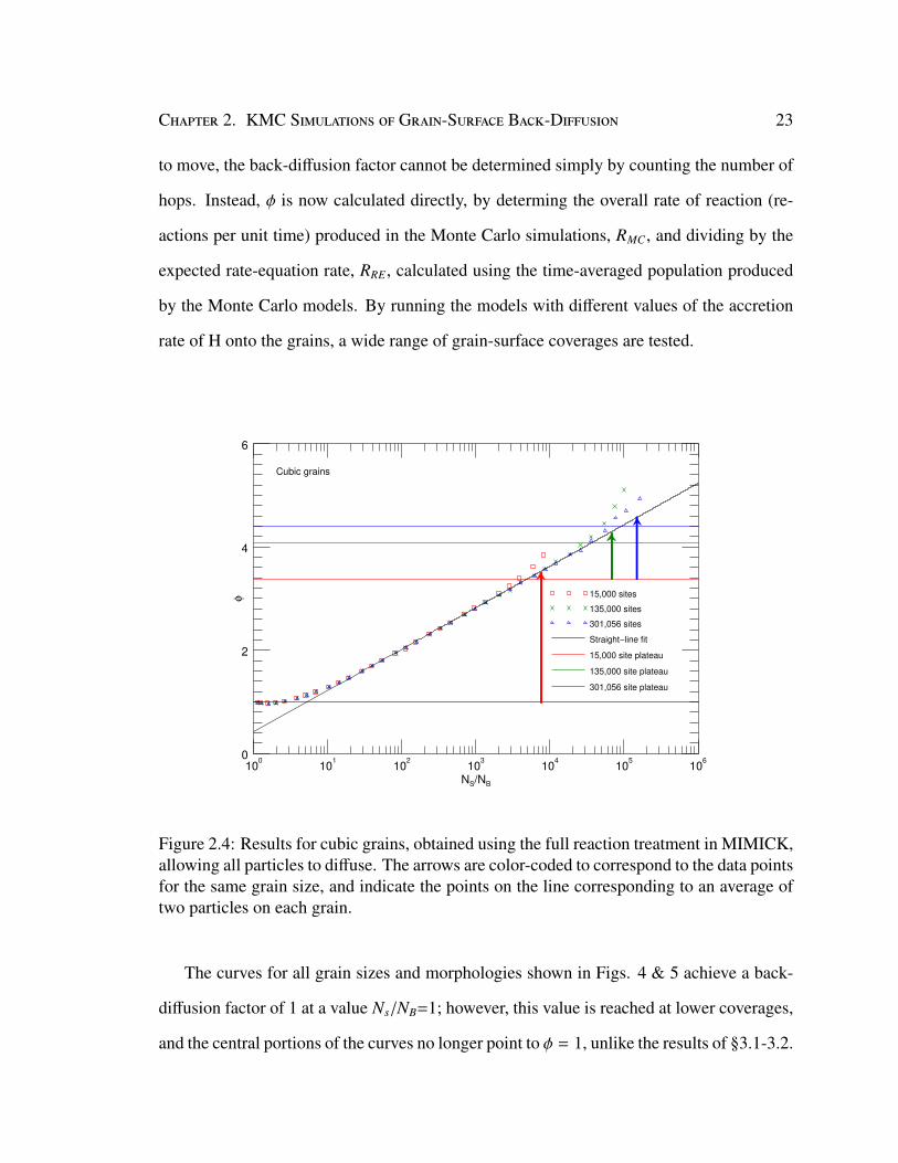
Chapter 2. KMC Simulations of Grain-Surface Back-Diffusion 23
to move, the back-diffusion factor cannot be determined simply by counting the number of
hops. Instead, φ is now calculated directly, by determing the overall rate of reaction (re-
actions per unit time) produced in the Monte Carlo simulations, RMC, and dividing by the
expected rate-equation rate, RRE, calculated using the time-averaged population produced
by the Monte Carlo models. By running the models with different values of the accretion
rate of H onto the grains, a wide range of grain-surface coverages are tested.
Cubic grains
100
101
102
103
104
105
106
NS/NB
0
2
4
6
φ 15,000 sites
135,000 sites
301,056 sites
Straight−line fit
15,000 site plateau
135,000 site plateau
301,056 site plateau
Figure 2.4: Results for cubic grains, obtained using the full reaction treatment in MIMICK,allowing all particles to diffuse. The arrows are color-coded to correspond to the data pointsfor the same grain size, and indicate the points on the line corresponding to an average oftwo particles on each grain.
The curves for all grain sizes and morphologies shown in Figs. 4 & 5 achieve a back-
diffusion factor of 1 at a value Ns/NB=1; however, this value is reached at lower coverages,
and the central portions of the curves no longer point to φ = 1, unlike the results of §3.1-3.2.
24 Chapter 2. KMC Simulations of Grain-Surface Back-Diffusion
Bucky−ball grains
100
101
102
103
104
105
106
NS/NB
0
2
4
6
φ
6,757 sites
32,710 sites
300,665 sites
Straight−line fit
6,757 site plateau
32,710 site plateau
300,665 site plateau
Figure 2.5: Results for bucky-ball grains, as per Fig. 4.
The intermediate-coverage behavior for both morphologies can be fit using a logarithmic
function dependent on the surface coverage, as before, and the main part of the curve obeys
the same expression for all grain sizes within either type of grain morphology (see Table
2.) The absolute values of the back-diffusion factor are lower here than those observed for
either the flat-surface model or the MIMICK models with one mobile particle. Again, the
bucky-ball produces lower values of φ than the cubic grain.
2.3.4 MIMICK, two-particle models
In Figures 4 & 5, as the inverse coverage reaches very high values, the results diverge
from logarithmic behavior at a coverage on the order of five particles, for each grain size
considered. Values of φ become yet greater as the average number of particles per grain
Chapter 2. KMC Simulations of Grain-Surface Back-Diffusion 25
decreases below this value, and the plateaus seen previously are not apparent in any of the
results.
This divergence from the behavior seen in the other models is actually an artifact of the
method used post hoc to determine the total rate of reaction produced by the Monte Carlo
models, RMC, which is used to calculate φ. Because RMC is evaluated by dividing the total
number of reactions by the amount of time passed, this means that, for very low coverages,
much of this time corresponds to occasions when the population of reactants on the grain
is either 0 or 1, meaning that no reaction can occur. This “dead-time” would correspond
to many hopping events that do not contribute to the reaction process, and should therefore
not be included in the determination of the back-diffusion effect. Note that low coverages
in these models correspond to low mean populations, which may be less than two, while
reactions can only occur when the instantaneous population state is greater than or equal to
2.
A separate model was used in order to study the behavior on the grains when only
2 particles were present. In these two-particle simulations, accretion was always halted as
soon as two particles were present on the surface, and was allowed to resume following each
reaction. The number of hops between reactions was counted, thus eliminating any time
dependence. These two-particle values may be considered as cutoffs, or plateau values,
for the back-diffusion factor for each grain size and type. Straight lines at these values
are overlaid on the data in Figs. 4 and 5, color-coded for each data set. If a calculated
back-diffusion factor is found to be above these values, it should be corrected down to the
two-particle value for that grain size. Generalized fits are again presented in Table 2, for
both the main part of the curves and the plateaus.
26 Chapter 2. KMC Simulations of Grain-Surface Back-Diffusion
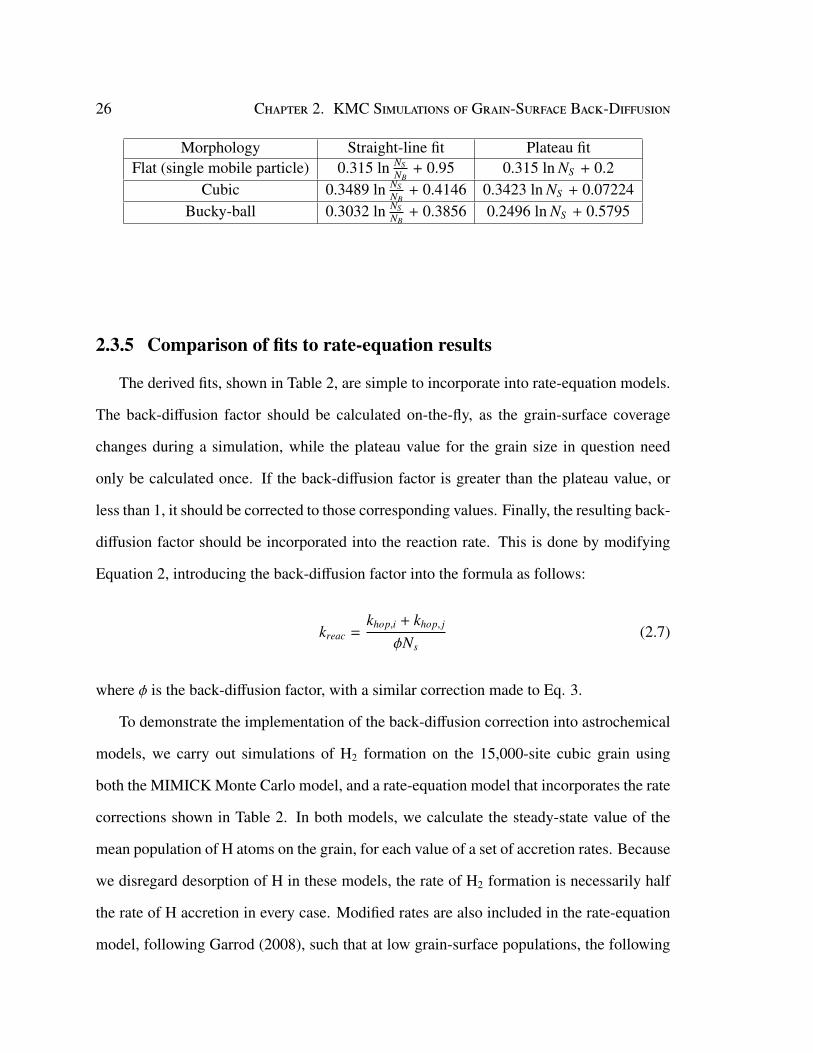
Morphology Straight-line fit Plateau fitFlat (single mobile particle) 0.315 ln NS
NB+ 0.95 0.315 ln NS + 0.2
Cubic 0.3489 ln NSNB
+ 0.4146 0.3423 ln NS + 0.07224Bucky-ball 0.3032 ln NS
NB+ 0.3856 0.2496 ln NS + 0.5795
2.3.5 Comparison of fits to rate-equation results
The derived fits, shown in Table 2, are simple to incorporate into rate-equation models.
The back-diffusion factor should be calculated on-the-fly, as the grain-surface coverage
changes during a simulation, while the plateau value for the grain size in question need
only be calculated once. If the back-diffusion factor is greater than the plateau value, or
less than 1, it should be corrected to those corresponding values. Finally, the resulting back-
diffusion factor should be incorporated into the reaction rate. This is done by modifying
Equation 2, introducing the back-diffusion factor into the formula as follows:
kreac =khop,i + khop, j
φNs(2.7)
where φ is the back-diffusion factor, with a similar correction made to Eq. 3.
To demonstrate the implementation of the back-diffusion correction into astrochemical
models, we carry out simulations of H2 formation on the 15,000-site cubic grain using
both the MIMICK Monte Carlo model, and a rate-equation model that incorporates the rate
corrections shown in Table 2. In both models, we calculate the steady-state value of the
mean population of H atoms on the grain, for each value of a set of accretion rates. Because
we disregard desorption of H in these models, the rate of H2 formation is necessarily half
the rate of H accretion in every case. Modified rates are also included in the rate-equation
model, following Garrod (2008), such that at low grain-surface populations, the following
Chapter 2. KMC Simulations of Grain-Surface Back-Diffusion 27
equation is used for the H+H reaction rate:
Rmod = RaccNB (2.8)
10−8
10−6
10−4
10−2
100
102
104
106
Accretion rate (s−1
)
10−1
100
101
102
103
104
Gra
in p
op
ula
tio
n
Monte Carlo values
Rate−eqn. values
Figure 2.6: Comparison of grain-surface populations obtained from MIMICK and thoseobtained from a simplified rate-equation treatment utilizing the back-diffusion correctionpresented in this paper. This comparison is done using the cubic grain with 15,000 sites.
Figure 6 shows the results from each of the two models. The back-diffusion correction
imported into rate-equation treatment shows very good agreement at almost every point,
with the exception of the fifth point from the left. Here, the Monte Carlo model has an
average grain-surface population of 0.7549, which puts it within the modified-rate regime,
28 Chapter 2. KMC Simulations of Grain-Surface Back-Diffusion
but close to the threshold between rate-equation and modified-rate behavior used by Gar-
rod (2008). Its proximity to this threshold appears to be the source of the disagreement
between the two methods, rather than the back-diffusion correction. At all other points,
disagreement between the two methods rarely exceeds 5%, with the majority of points be-
ing within 1% of each other. Similar levels of agreement are seen for all grains tested in
this paper, showing that this method is valid and will produce the appropriate results in real
astrochemical models. Note that the production rates, which are not shown, are an exact
match between models in all cases, due to the imposed steady-state condition.
2.4 DiscussionIt is instructive to compare the low-coverage results obtained here with the back-diffusion
factors determined by Lohmar et al. (2009) for the two-particle case. The plateau values
displayed in Figs. 4 & 5 are seen to be in reasonable agreement with the results of Krug et
al. (as seen in Fig. 1 of that paper, specifically their values with Rdes:Rdi f f of 10−6). For
example, the cubic grain with 15,000 sites shown in Fig. 4 has a plateau value of φ'3.37,
while a spherical grain with square-lattice geometry and a similar number of sites is found
by Lohmar et al. (2009) to have a back-diffusion factor of ∼3.33, suggesting that both treat-
ments are similar in the low-coverage regime, in spite of the morphological differences be-
tween the grains in either model. Using the fit (Table 2) to the results for our spherical grain
with hexagonal-lattice structure (Fig. 5), and assuming 15,000 sites, a back-diffusion factor
of ∼2.98 is obtained. Clearly, at low coverage, it is the local surface structure (i.e. num-
ber of diffusion pathways available) that is the primary influence on back-diffusion, rather
than the choice of overall grain morphology (cube vs. sphere). This effect has been previ-
ously studied and observed to have a similar impact on hydrogen recombination efficiency
Chapter 2. KMC Simulations of Grain-Surface Back-Diffusion 29
by Chang et al. (2005). In that paper, the authors investigated hydrogen recombination
on lattices with rectangular and hexagonal binding site geometry using a continuous-time
random-walk model. They found that, for homogeneous surfaces like those we are inter-
ested in, the hexagonal lattice shows a greater hydrogen recombination efficiency. This
indicates a lesser impact from back-diffusion, similar to our results.
It may also be seen that the value of φ at the plateau (i.e. very low coverage) is ex-
clusively determined by the size of the grain, assuming the same surface structure and
morphology. However, the transition from a flat, periodic surface to a surface that bounds a
three-dimensional grain produces a somewhat larger degree of back-diffusion. This transi-
tion does not, however, appear to have any significant effect other than at the plateau. The
differences seen at all coverages between the flat-surface treatment and the bucky-ball grain
appear to be entirely caused by the alternative local structure, as do the differences between
the bucky-ball and the cubic grain. It is possible that a more extreme grain morphology
could show a greater deviation; for example, one may consider a hypothetical grain com-
posed of two contiguous spheres, with just a small number of binding sites connecting the
two parts. Such would be an interesting case for future study.
At the higher coverages that are examined only in our models, in the case where just
one surface particle is mobile (Fig. 3), it is also apparent that the plateau value of φ (i.e.
the extreme two-particle value) is no longer applicable beyond some threshold, and that
the back-diffusion factor then begins to fall with increasing numbers of particles on the
surface, reaching a value of 1 at full surface coverage. A similar trend is seen for the case
where all particles are mobile, but in this case φ reaches unity (i.e. no back-diffusion effect)
at a surface coverage less than one (i.e. Ns/NB > 1). This effect may be understood by
considering that at high coverages, there is a very large probability that multiple particles
may be within just a single hop of a reaction partner at any particular moment. In the one-
mobile-particle case, the back-diffusion effect manifests itself entirely through the diffusion
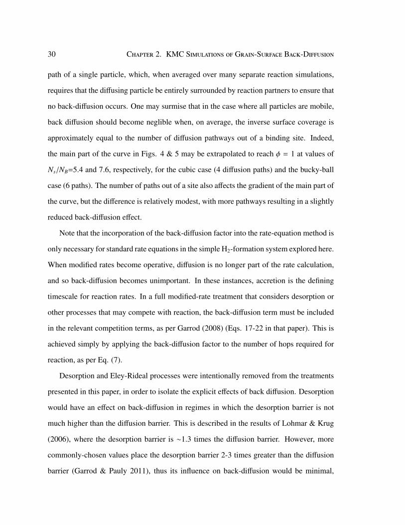
30 Chapter 2. KMC Simulations of Grain-Surface Back-Diffusion
path of a single particle, which, when averaged over many separate reaction simulations,
requires that the diffusing particle be entirely surrounded by reaction partners to ensure that
no back-diffusion occurs. One may surmise that in the case where all particles are mobile,
back diffusion should become neglible when, on average, the inverse surface coverage is
approximately equal to the number of diffusion pathways out of a binding site. Indeed,
the main part of the curve in Figs. 4 & 5 may be extrapolated to reach φ = 1 at values of
Ns/NB=5.4 and 7.6, respectively, for the cubic case (4 diffusion paths) and the bucky-ball
case (6 paths). The number of paths out of a site also affects the gradient of the main part of
the curve, but the difference is relatively modest, with more pathways resulting in a slightly
reduced back-diffusion effect.
Note that the incorporation of the back-diffusion factor into the rate-equation method is
only necessary for standard rate equations in the simple H2-formation system explored here.
When modified rates become operative, diffusion is no longer part of the rate calculation,
and so back-diffusion becomes unimportant. In these instances, accretion is the defining
timescale for reaction rates. In a full modified-rate treatment that considers desorption or
other processes that may compete with reaction, the back-diffusion term must be included
in the relevant competition terms, as per Garrod (2008) (Eqs. 17-22 in that paper). This is
achieved simply by applying the back-diffusion factor to the number of hops required for
reaction, as per Eq. (7).
Desorption and Eley-Rideal processes were intentionally removed from the treatments
presented in this paper, in order to isolate the explicit effects of back diffusion. Desorption
would have an effect on back-diffusion in regimes in which the desorption barrier is not
much higher than the diffusion barrier. This is described in the results of Lohmar & Krug
(2006), where the desorption barrier is ∼1.3 times the diffusion barrier. However, more
commonly-chosen values place the desorption barrier 2-3 times greater than the diffusion
barrier (Garrod & Pauly 2011), thus its influence on back-diffusion would be minimal,
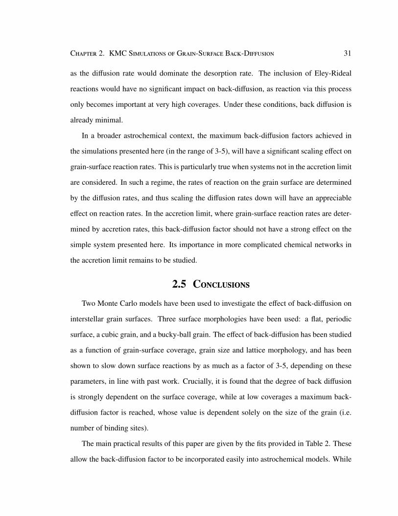
Chapter 2. KMC Simulations of Grain-Surface Back-Diffusion 31
as the diffusion rate would dominate the desorption rate. The inclusion of Eley-Rideal
reactions would have no significant impact on back-diffusion, as reaction via this process
only becomes important at very high coverages. Under these conditions, back diffusion is
already minimal.
In a broader astrochemical context, the maximum back-diffusion factors achieved in
the simulations presented here (in the range of 3-5), will have a significant scaling effect on
grain-surface reaction rates. This is particularly true when systems not in the accretion limit
are considered. In such a regime, the rates of reaction on the grain surface are determined
by the diffusion rates, and thus scaling the diffusion rates down will have an appreciable
effect on reaction rates. In the accretion limit, where grain-surface reaction rates are deter-
mined by accretion rates, this back-diffusion factor should not have a strong effect on the
simple system presented here. Its importance in more complicated chemical networks in
the accretion limit remains to be studied.
2.5 ConclusionsTwo Monte Carlo models have been used to investigate the effect of back-diffusion on
interstellar grain surfaces. Three surface morphologies have been used: a flat, periodic
surface, a cubic grain, and a bucky-ball grain. The effect of back-diffusion has been studied
as a function of grain-surface coverage, grain size and lattice morphology, and has been
shown to slow down surface reactions by as much as a factor of 3-5, depending on these
parameters, in line with past work. Crucially, it is found that the degree of back diffusion
is strongly dependent on the surface coverage, while at low coverages a maximum back-
diffusion factor is reached, whose value is dependent solely on the size of the grain (i.e.
number of binding sites).
The main practical results of this paper are given by the fits provided in Table 2. These
allow the back-diffusion factor to be incorporated easily into astrochemical models. While
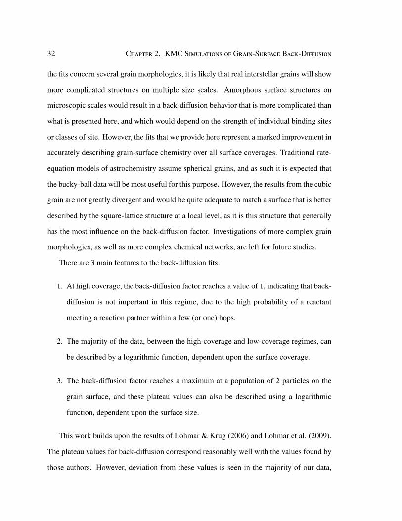
32 Chapter 2. KMC Simulations of Grain-Surface Back-Diffusion
the fits concern several grain morphologies, it is likely that real interstellar grains will show
more complicated structures on multiple size scales. Amorphous surface structures on
microscopic scales would result in a back-diffusion behavior that is more complicated than
what is presented here, and which would depend on the strength of individual binding sites
or classes of site. However, the fits that we provide here represent a marked improvement in
accurately describing grain-surface chemistry over all surface coverages. Traditional rate-
equation models of astrochemistry assume spherical grains, and as such it is expected that
the bucky-ball data will be most useful for this purpose. However, the results from the cubic
grain are not greatly divergent and would be quite adequate to match a surface that is better
described by the square-lattice structure at a local level, as it is this structure that generally
has the most influence on the back-diffusion factor. Investigations of more complex grain
morphologies, as well as more complex chemical networks, are left for future studies.
There are 3 main features to the back-diffusion fits:
1. At high coverage, the back-diffusion factor reaches a value of 1, indicating that back-
diffusion is not important in this regime, due to the high probability of a reactant
meeting a reaction partner within a few (or one) hops.
2. The majority of the data, between the high-coverage and low-coverage regimes, can
be described by a logarithmic function, dependent upon the surface coverage.
3. The back-diffusion factor reaches a maximum at a population of 2 particles on the
grain surface, and these plateau values can also be described using a logarithmic
function, dependent upon the surface size.
This work builds upon the results of Lohmar & Krug (2006) and Lohmar et al. (2009).
The plateau values for back-diffusion correspond reasonably well with the values found by
those authors. However, deviation from these values is seen in the majority of our data,
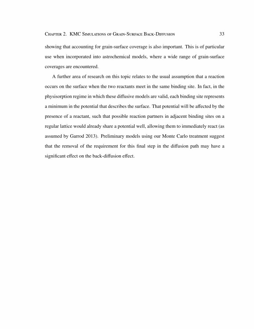
Chapter 2. KMC Simulations of Grain-Surface Back-Diffusion 33
showing that accounting for grain-surface coverage is also important. This is of particular
use when incorporated into astrochemical models, where a wide range of grain-surface
coverages are encountered.
A further area of research on this topic relates to the usual assumption that a reaction
occurs on the surface when the two reactants meet in the same binding site. In fact, in the
physisorption regime in which these diffusive models are valid, each binding site represents
a minimum in the potential that describes the surface. That potential will be affected by the
presence of a reactant, such that possible reaction partners in adjacent binding sites on a
regular lattice would already share a potential well, allowing them to immediately react (as
assumed by Garrod 2013). Preliminary models using our Monte Carlo treatment suggest
that the removal of the requirement for this final step in the diffusion path may have a
significant effect on the back-diffusion effect.

35
Chapter 3
Studies of several organic molecules
usingMAGICKAL
3.1 IntroductionThe following chapter is comprised of several studies that have been undertaken over
the past few years, using the chemical code MAGICKAL to model the chemistry of molecules
of interest in star-forming regions. It is divided into sections, where each section corre-
sponds to a different molecule. The sections are ordered chronologically based on publica-
tion date of the respective study.
Section 3.2 focuses on simple chemical models of the molecule methoxymethanol
(CH3OCH2OH) following the first detection of this molecule in the interstellar medium
towards the star-forming region NGC6334I (McGuire et al. 2017). Section 3.3.1 presents
updated chemical models of the molecule cyanamide (NH2CN), and compares those mod-
els to observations towards the solar-type protostar IRAS 16293-2422B (hereafter IRAS
16293B) (Coutens et al. 2018). This section also discusses the shortcomings of two-
stage chemical models of hot-core chemistry. Section 3.3.2 discusses the incorporation of
36 Chapter 3. Studies of several organic molecules using MAGICKAL
methyl isocyanide (CH3NC) into astrochemical networks for the first time, and once again
compares those models to observations of IRAS 16293B (Calcutt et al. (2018)). Section
3.3.3 discusses the use of the same observations for the simple organic molecule propyne
(CH3CCH), and examination of the fit of those observations to current chemical models of
propyne (Calcutt et al. 2019).
Note that these papers were large collaborations, and as such, I have not reproduced the
entire text of each. I have summarized, in my own words, the key observational components
at the start of each section. I did not conduct these observations, and the figures that detail
the detected spectral lines of each molecule are not mine, but are used to illustrate the
molecular detections. The chemical modelling is what I contributed to each paper, and I
have reproduced the text and figures from each paper’s chemical modelling section here.
3.2 Methoxymethanol (CH3OCH2OH)
3.2.1 Overview of NGC 6334I and Observations
NGC 6334I is a massive protocluster located 1.3 kpc from Earth (Reid et al. 2014). It is
a site of active massive star formation and contains two well-known hot core regions (MM1
and MM2; Brogan et al. (2016)). The detection of CH3OCH2OH presented in McGuire
et al. (2017) was made towards this source in four separate ALMA datasets. Following
detailed analysis of the convolved spectra assuming a single-excitation model (Hollis et al.
2004), the column density of CH3OCH2OH was determined to be 4 ± 2 × 1018 cm−2,
assuming an excitation temperature of 200 K. The uncertainty in the column density is due
to the uncertainty in the assumed excitation temperature, as well as the difficulty in fitting
the molecule’s unblended transitions.
Chapter 3. Studies of several organic molecules using MAGICKAL 37
3.2.2 Chemical Modeling
CH3OCH2OH was included in the three-phase chemical kinetics model MAGICKAL of
Garrod (2013a). In an initial effort to explore the ability of the model to reproduce the
observed abundance, we modified the model with the back-diffusion correction of Willis
& Garrod (2017), and used a network based on that of Belloche et al. (2017), in which
CH3OCH2OH is produced via the following reaction:
CH3O + CH2OH CH3OCH2OH (3.1)
The network also contains likely gas-phase and grain-surface destruction mechanisms
for CH3OCH2OH.
The chemical modeling was performed using the two-stage approach described in Gar-
rod (2013a). Phase 1 is a cold collapse to a maximum density of 2 × 108 cm−3 and a dust
grain temperature of 8 K. This is followed by a warm-up from 8 K to 400 K, simulating the
‘ignition’ of a hot core. Three different warm-up timescales have been used, as the choice
of timescale has been previously shown to have significant effects on the chemistry (Garrod
2013a). The fastest timescale reaches a temperature of 200 K at 5 × 10⁴ yr, and 400 K at
7.12 × 10⁴ yr. The slowest timescale reaches these milestones at 106 yr and 1.43 × 10⁶ yr;
the intermediate timescale takes 2 × 10⁵ yr and 2.85 × 10⁵ yr.
The results of the model are shown graphically in Figure 3.1. The fast warm-up timescale
produces the highest abundance of CH3OCH2OH, with a maximum fractional abundance
of ∼10−12 with respect to total hydrogen, which is well-maintained to a temperature of
400 K. The abundance of CH3OH in the same model approaches 10−5, corresponding
to CH3OCH2OH:CH3OH of ∼10−7. The observed ratio of CH3OCH2OH:CH3OH is esti-
mated to be 1:34. The intermediate timescale shows very similar results, while the slowest
timescale produces a very low gas-phase abundance of CH3OCH2OH, peaking at ∼10−17.
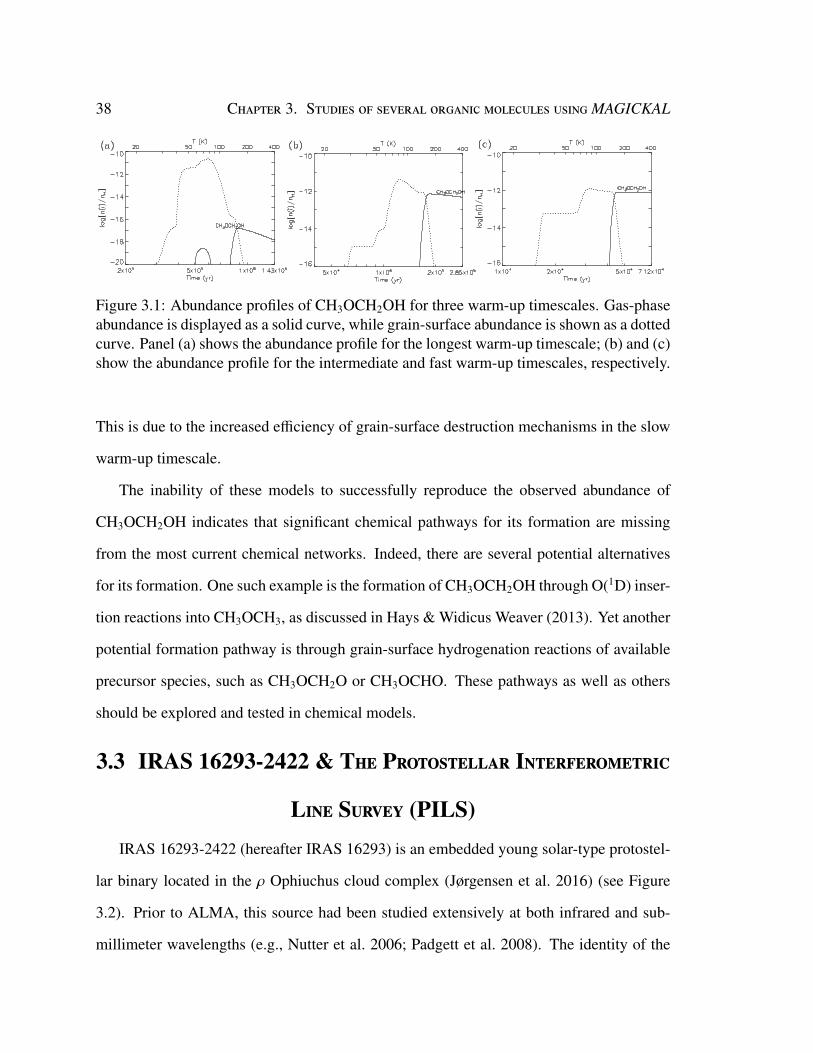
38 Chapter 3. Studies of several organic molecules using MAGICKAL
Figure 3.1: Abundance profiles of CH3OCH2OH for three warm-up timescales. Gas-phaseabundance is displayed as a solid curve, while grain-surface abundance is shown as a dottedcurve. Panel (a) shows the abundance profile for the longest warm-up timescale; (b) and (c)show the abundance profile for the intermediate and fast warm-up timescales, respectively.
This is due to the increased efficiency of grain-surface destruction mechanisms in the slow
warm-up timescale.
The inability of these models to successfully reproduce the observed abundance of
CH3OCH2OH indicates that significant chemical pathways for its formation are missing
from the most current chemical networks. Indeed, there are several potential alternatives
for its formation. One such example is the formation of CH3OCH2OH through O(1D) inser-
tion reactions into CH3OCH3, as discussed in Hays & Widicus Weaver (2013). Yet another
potential formation pathway is through grain-surface hydrogenation reactions of available
precursor species, such as CH3OCH2O or CH3OCHO. These pathways as well as others
should be explored and tested in chemical models.
3.3 IRAS 16293-2422& The Protostellar Interferometric
Line Survey (PILS)IRAS 16293-2422 (hereafter IRAS 16293) is an embedded young solar-type protostel-
lar binary located in the ρ Ophiuchus cloud complex (Jørgensen et al. 2016) (see Figure
3.2). Prior to ALMA, this source had been studied extensively at both infrared and sub-
millimeter wavelengths (e.g., Nutter et al. 2006; Padgett et al. 2008). The identity of the
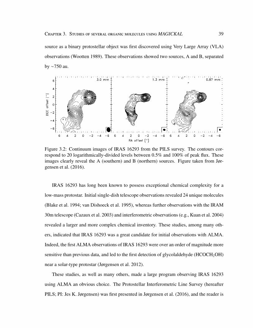
Chapter 3. Studies of several organic molecules using MAGICKAL 39
source as a binary protostellar object was first discovered using Very Large Array (VLA)
observations (Wootten 1989). These observations showed two sources, A and B, separated
by ∼750 au.
Figure 3.2: Continuum images of IRAS 16293 from the PILS survey. The contours cor-respond to 20 logarithmically-divided levels between 0.5% and 100% of peak flux. Theseimages clearly reveal the A (southern) and B (northern) sources. Figure taken from Jør-gensen et al. (2016).
IRAS 16293 has long been known to possess exceptional chemical complexity for a
low-mass protostar. Initial single-dish telescope observations revealed 24 unique molecules
(Blake et al. 1994; van Dishoeck et al. 1995), whereas further observations with the IRAM
30m telescope (Cazaux et al. 2003) and interferometric observations (e.g., Kuan et al. 2004)
revealed a larger and more complex chemical inventory. These studies, among many oth-
ers, indicated that IRAS 16293 was a great candidate for initial observations with ALMA.
Indeed, the first ALMA observations of IRAS 16293 were over an order of magnitude more
sensitive than previous data, and led to the first detection of glycolaldehyde (HCOCH2OH)
near a solar-type protostar (Jørgensen et al. 2012).
These studies, as well as many others, made a large program observing IRAS 16293
using ALMA an obvious choice. The Protostellar Interferometric Line Survey (hereafter
PILS; PI: Jes K. Jørgensen) was first presented in Jørgensen et al. (2016), and the reader is
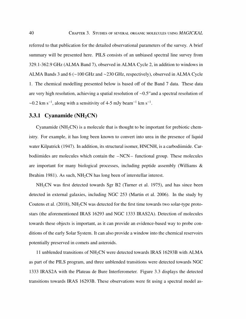
40 Chapter 3. Studies of several organic molecules using MAGICKAL
referred to that publication for the detailed observational parameters of the survey. A brief
summary will be presented here. PILS consists of an unbiased spectral line survey from
329.1-362.9 GHz (ALMA Band 7), observed in ALMA Cycle 2, in addition to windows in
ALMA Bands 3 and 6 (∼100 GHz and ∼230 GHz, respectively), observed in ALMA Cycle
1. The chemical modelling presented below is based off of the Band 7 data. These data
are very high resolution, achieving a spatial resolution of ∼0.5′′and a spectral resolution of
∼0.2 km s−1, along with a sensitivity of 4-5 mJy beam−1 km s−1.
3.3.1 Cyanamide (NH2CN)
Cyanamide (NH2CN) is a molecule that is thought to be important for prebiotic chem-
istry. For example, it has long been known to convert into urea in the presence of liquid
water Kilpatrick (1947). In addition, its structural isomer, HNCNH, is a carbodiimide. Car-
bodiimides are molecules which contain the – NCN – functional group. These molecules
are important for many biological processes, including peptide assembly (Williams &
Ibrahim 1981). As such, NH2CN has long been of interstellar interest.
NH2CN was first detected towards Sgr B2 (Turner et al. 1975), and has since been
detected in external galaxies, including NGC 253 (Martin et al. 2006). In the study by
Coutens et al. (2018), NH2CN was detected for the first time towards two solar-type proto-
stars (the aforementioned IRAS 16293 and NGC 1333 IRAS2A). Detection of molecules
towards these objects is important, as it can provide an evidence-based way to probe con-
ditions of the early Solar System. It can also provide a window into the chemical reservoirs
potentially preserved in comets and asteroids.
11 unblended transitions of NH2CN were detected towards IRAS 16293B with ALMA
as part of the PILS program, and three unblended transitions were detected towards NGC
1333 IRAS2A with the Plateau de Bure Interferometer. Figure 3.3 displays the detected
transitions towards IRAS 16293B. These observations were fit using a spectral model as-
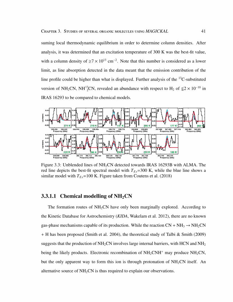
Chapter 3. Studies of several organic molecules using MAGICKAL 41
suming local thermodynamic equilibrium in order to determine column densities. After
analysis, it was determined that an excitation temperature of 300 K was the best-fit value,
with a column density of ≥7 × 1013 cm−2. Note that this number is considered as a lower
limit, as line absorption detected in the data meant that the emission contribution of the
line profile could be higher than what is displayed. Further analysis of the 13C-substituted
version of NH2CN, NH132CN, revealed an abundance with respect to H2 of /2 × 10−10 in
IRAS 16293 to be compared to chemical models.
Figure 3.3: Unblended lines of NH2CN detected towards IRAS 16293B with ALMA. Thered line depicts the best-fit spectral model with TEx=300 K, while the blue line shows asimilar model with TEx=100 K. Figure taken from Coutens et al. (2018)
3.3.1.1 Chemical modelling of NH2CN
The formation routes of NH2CN have only been marginally explored. According to
the Kinetic Database for Astrochemistry (KIDA, Wakelam et al. 2012), there are no known
gas-phase mechanisms capable of its production. While the reaction CN + NH3→ NH2CN
+ H has been proposed (Smith et al. 2004), the theoretical study of Talbi & Smith (2009)
suggests that the production of NH2CN involves large internal barriers, with HCN and NH2
being the likely products. Electronic recombination of NH2CNH+ may produce NH2CN,
but the only apparent way to form this ion is through protonation of NH2CN itself. An
alternative source of NH2CN is thus required to explain our observations.
42 Chapter 3. Studies of several organic molecules using MAGICKAL
Cyanamide could be formed on grain surfaces through the addition of NH2 and CN
radicals. The possible formation of formamide from the same precursor NH2 (Fedoseev et
al. 2016; Coutens et al. 2016) could explain the similarity of these two species in terms of
deep absorption against the strong continuum and the similar deuteration of the two species
towards IRAS16293 B.
To test this hypothesis, we ran a three-phase chemical kinetics model MAGICKAL (Gar-
rod 2013), modified with the grain-surface back-diffusion correction of Willis & Garrod
(2017). The model uses a network based on that of Belloche et al. (2017), in which dis-
sociative recombination of NH2CNH+ was assumed to produce NH2CN in 5% of cases.
The reaction NH2 + CN→ NH2CN was added to the grain/ice chemical network, and the
gas-phase reaction between HCN and NH2 was adjusted per Talbi & Smith. The physical
model used here is very similar to that described by Belloche et al. (2017), in which a
cold collapse to high density is followed by warm up to 400 K; here, a final density of
nH=6 × 1010 cm−3 was assumed to better represent the density structure of IRAS 16293.
The results from the chemical model (for an intermediate warm-up timescale) are shown
in Figure 3.4 for the two primary molecules of interest, NH2CN and NH2CHO. NH2CN is
seen to be produced at a temperature of ∼30 K on the grain surfaces, desorbing into the gas
at higher temperatures. The model underproduces the gas-phase abundance of NH2CN,
showing a peak abundance of ∼6.7 × 10⁻¹² that is well maintained to a temperature of
300 K and beyond. The low NH2CN abundance in the gas-phase is caused primarily by un-
derproduction on the dust grains; at the high density used in the model, the rapid accretion
of H and H2 onto grain surfaces makes hydrogenation of the NH2 and CN radicals much
more competitive with the reaction that produces NH2CN. This competition becomes im-
portant for gas densities greater than ∼109 cm−3. We therefore also present a model with a
lower final density of nH = 1.6 × 107 cm−3 (corresponding to the density of the envelope
between the two protostars in IRAS16293; Jacobsen et al. 2018). This model produces an
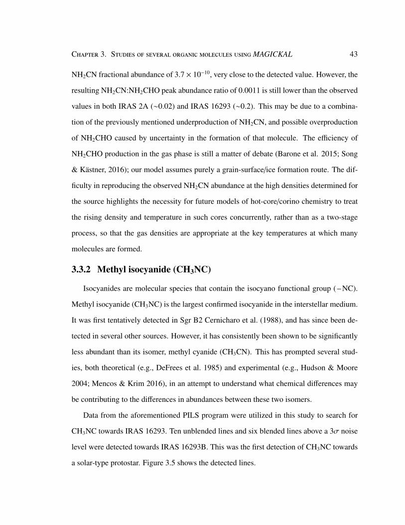
Chapter 3. Studies of several organic molecules using MAGICKAL 43
NH2CN fractional abundance of 3.7 × 10⁻¹⁰, very close to the detected value. However, the
resulting NH2CN:NH2CHO peak abundance ratio of 0.0011 is still lower than the observed
values in both IRAS 2A (∼0.02) and IRAS 16293 (∼0.2). This may be due to a combina-
tion of the previously mentioned underproduction of NH2CN, and possible overproduction
of NH2CHO caused by uncertainty in the formation of that molecule. The efficiency of
NH2CHO production in the gas phase is still a matter of debate (Barone et al. 2015; Song
& Kästner, 2016); our model assumes purely a grain-surface/ice formation route. The dif-
ficulty in reproducing the observed NH2CN abundance at the high densities determined for
the source highlights the necessity for future models of hot-core/corino chemistry to treat
the rising density and temperature in such cores concurrently, rather than as a two-stage
process, so that the gas densities are appropriate at the key temperatures at which many
molecules are formed.
3.3.2 Methyl isocyanide (CH3NC)
Isocyanides are molecular species that contain the isocyano functional group ( – NC).
Methyl isocyanide (CH3NC) is the largest confirmed isocyanide in the interstellar medium.
It was first tentatively detected in Sgr B2 Cernicharo et al. (1988), and has since been de-
tected in several other sources. However, it has consistently been shown to be significantly
less abundant than its isomer, methyl cyanide (CH3CN). This has prompted several stud-
ies, both theoretical (e.g., DeFrees et al. 1985) and experimental (e.g., Hudson & Moore
2004; Mencos & Krim 2016), in an attempt to understand what chemical differences may
be contributing to the differences in abundances between these two isomers.
Data from the aforementioned PILS program were utilized in this study to search for
CH3NC towards IRAS 16293. Ten unblended lines and six blended lines above a 3σ noise
level were detected towards IRAS 16293B. This was the first detection of CH3NC towards
a solar-type protostar. Figure 3.5 shows the detected lines.
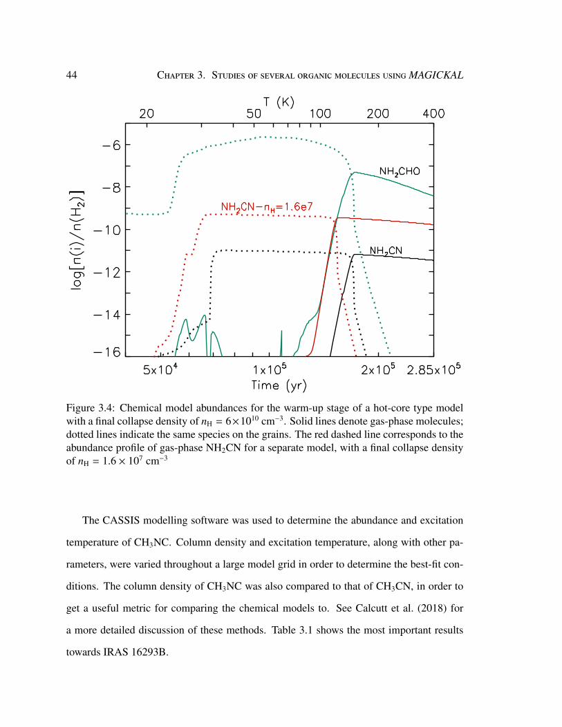
44 Chapter 3. Studies of several organic molecules using MAGICKAL
Figure 3.4: Chemical model abundances for the warm-up stage of a hot-core type modelwith a final collapse density of nH = 6×1010 cm−3. Solid lines denote gas-phase molecules;dotted lines indicate the same species on the grains. The red dashed line corresponds to theabundance profile of gas-phase NH2CN for a separate model, with a final collapse densityof nH = 1.6 × 107 cm−3
The CASSIS modelling software was used to determine the abundance and excitation
temperature of CH3NC. Column density and excitation temperature, along with other pa-
rameters, were varied throughout a large model grid in order to determine the best-fit con-
ditions. The column density of CH3NC was also compared to that of CH3CN, in order to
get a useful metric for comparing the chemical models to. See Calcutt et al. (2018) for
a more detailed discussion of these methods. Table 3.1 shows the most important results
towards IRAS 16293B.
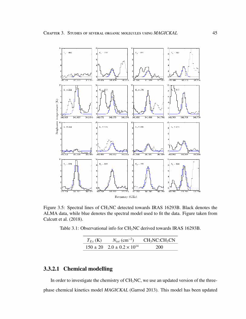
Chapter 3. Studies of several organic molecules using MAGICKAL 45
Figure 3.5: Spectral lines of CH3NC detected towards IRAS 16293B. Black denotes theALMA data, while blue denotes the spectral model used to fit the data. Figure taken fromCalcutt et al. (2018).
Table 3.1: Observational info for CH3NC derived towards IRAS 16293B.
TEx (K) Ntot (cm−2) CH3NC:CH3CN150 ± 20 2.0 ± 0.2 × 10¹⁴ 200
3.3.2.1 Chemical modelling
In order to investigate the chemistry of CH3NC, we use an updated version of the three-
phase chemical kinetics model MAGICKAL (Garrod 2013). This model has been updated
46 Chapter 3. Studies of several organic molecules using MAGICKAL
with the back-diffusion correction of Willis and Garrod (2017). The chemical network is
based on that of Belloche et al. (2017), with formation and destruction mechanisms for
CH3NC added. This is, to the authors’ knowlege, the first time that CH3NC has been
incorporated into an astrochemical kinetics model. This network is a preface to a more
complete chemical treatment for isocyanides (Willis et al. 2020). The two-stage physical
model used is also similar to that of Belloche et al. (2017), in which a cold collapse is
followed by a static warm up to 400 K. The cold collapse in the model has an isothermal
gas temperature (10 K), and the dust temperature cools from an initial value of 16 K to a
final value of 8 K. Following Coutens et al. (2018), we run two models, using two different
final densities for the collapse phase: nH = 6 × 1010 cm−3, corresponding to the continuum
peak of IRAS 16293B and nH = 1.6 × 107 cm−3, corresponding to the density of the filament
between IRAS 16293A and IRAS 16293B (Jacobsen et al. 2018). The subsequent warm-
up phase starts at a dust temperature of 8 K, and reaches a final temperature of 400 K
at 2.8 × 10⁵ years. This timescale is used to represent an intermediate warm-up, where
2 × 10⁵ yr is the time spent to reach a dust temperature of 200 K. This is taken from Garrod
& Herbst (2006). The model presented here follows Garrod (2013a) in using a warm-up
to 400 K instead of 200 K, by extending the “intermediate” temperature function beyond
200 K.
The primary formation mechanism of CH3NC in our model follows DeFrees et al.
(1985). First, the radiative association of CH3+ and HCN forms CH3CNH+. This inter-
mediate is formed with enough energy that a certain percentage of these molecules can
isomerize to CH3NCH+; we use the suggestion by DeFrees et al. (1985) of 15%. The
CH3NCH+ then recombines with free electrons, forming CH3NC and H as the primary
channel (∼65% of recombinations), with the remainder of CH3NCH+ molecules recombin-
ing to HCN and CH3. The binding energies on water ice for methyl cyanide and methyl
isocyanide were updated in the network using new values from Bertin et al. (2017; 6150
Chapter 3. Studies of several organic molecules using MAGICKAL 47
K and 5686 K, respectively). The primary destruction mechanism for CH3NC on the grain
surface is reaction with H, forming HCN and the radical CH3. This reaction is assumed to
have a barrier of 1200 K, based on recent calculations of the barrier for H+HNC (Graninger
et al. 2014). The same reaction is also allowed to occur in the gas phase, assuming the same
barrier.
Since we are comparing CH3NC abundances to values for CH3CN, it is important to
review how CH3CN is formed in our network as well. CH3CN is formed primarily via the
hydrogenation of the CH2CN radical on the grain surface and in the ice mantle, with a small
contribution from reaction of CH2CN with HCO. There is also a viable, less efficient gas-
phase pathway to production of CH3CN, previously discussed in regards to CH3NC. The
CH3CNH+ molecules that do not isomerize to CH3NCH+ can recombine with electrons to
form CH3CN and H as the primary products, with some instances of this channel leading
to HNC and CH3.
The basic chemical network we construct here for CH3NC chemistry is intended to
incorporate the most obvious formation and destruction mechanisms, in keeping with the
larger network. It is nevertheless possible that alternative mechanisms exist, while the
efficiencies of those included here cannot be reliably known without careful experimental
studies. In particular, the reaction of H with CH3NC, which is included in both the gas-
phase and grain-surface networks, is quite speculative. The mechanics of the reaction with
H and HNC are fundamentally different from this process, but the lack of experimental
work makes it difficult to produce a better prediction. We have refined this network for
CH3NC and other isocyanides (Willis et al. 2020), but this result highlights the need for
more experimental work on these molecules.
The results of the models are shown in Figure 3.6, with panel (a) corresponding to nH
= 1.6 × 107 cm−3, and panel (b) to nH = 6 × 1010 cm−3, and panels (c) and (d) showing
the CH3CN:CH3NC ratio for each of the models. The different densities exhibit different
48 Chapter 3. Studies of several organic molecules using MAGICKAL
behavior, particularly with regards to CH3NC. The peak abundance of CH3NC in the low-
density model is ∼4 × 10⁻¹⁰, while the high-density model produces a much lower peak
abundance, ∼44 × 10−15. This is due to the increased efficiency of grain-surface destruction
of CH3NC via reaction with H in the high-density model. As a result of this, as well as a
higher peak abundance of CH3CN in the high-density model, the CH3CN:CH3NC ratios at
150 K (the approximate excitation temperature of CH3NC) vary greatly between the two
models. In the low-density case, the ratio at 150 K is ∼450, which is the same order as the
observed ratio in IRAS 16293B. The ratio at the same point in the high-density model is
∼2.5 × 10⁶, which is consistent with the upper limits for IRAS 16293A.
We also ran several models incorporating the radiative association of CH3+ and HNC
to test the effect that this proposed reaction has on the abundances of CH3CN and CH3NC.
This process was given the same rate as the equivalent association of HCN with CH3+, and
results in CH3NCH+. This ion is then assumed to have enough internal energy to isomerize
as in the HCN reaction. Several different branching ratios were tested, including those that
lead predominantly to CH3CN and CH3NC. However, it was observed that the inclusion of
this process did not affect the abundance of CH3CN in any significant way, and had only
a small effect on the abundance of CH3NC in the low-density model, increasing the peak
abundance to a maximum of ∼9 × 10⁻¹⁰ when the reaction favors CH3NC production.
Additionally, we have explored disabling the H + CH3NC grain surface reaction and
gas-phase reaction to understand how important this speculative reaction is on the CH3CN:CH3NC
ratio. Disabling the grain surface reaction had practically no effect, however, disabling the
gas-phase reaction had a significant impact at higher temperatures (Figure 3.7). CH3NC
is not destroyed efficiently in the gas-phase and this keeps the CH3CN:CH3NC ratio much
closer to unity. It is in fact quite close to the 85%:15% split seen in the formation path-
ways. This result shows that there needs to be some efficient mechanism for the destruction
of CH3NC in the gas-phase that does not operate on CH3CN.
Chapter 3. Studies of several organic molecules using MAGICKAL 49
The CH3CN:CH3NC ratio varies greatly in the temperature range of 130-170 K. This
is due to multiple factors. First, both species come off of the grain surface in this window,
with CH3CN coming off slightly later due to its somewhat higher binding energy. Once
both species are off the grain, CH3NC can be destroyed in the gas phase by reaction with
H, which is not the case for CH3CN. This leads to a dip in CH3NC abundance relative to
CH3CN and a change in the abundance ratio of these molecules. This may be the reason for
the difference in CH3CN:CH3NC between sources A and B. Also, although the low-density
model fits the observations better than the high-density model, it may not be a represen-
tative density for the regions being probed by these observations. Nevertheless, a density
somewhat less than the maximum value used here may be most appropriate to reproduce
observed molecular ratios. This and recent results from our other models (Coutens et al.
2018) highlight the need for chemical models in which the collapse and warm-up phases
occur simultaneously, and which are tailored for specific objects. Models in which the max-
imum density is reached prior to any warm-up seem to provide a poor representation of the
chemistry in cases where densities reach extreme values. This density threshold appears to
be around 109 cm−3, based on results from Coutens et al. (2018) for NH2CN.
3.3.3 Propyne (CH3CCH)
Propyne (CH3CCH), also known as methyl acetylene, was first detected in the interstel-
lar medium in Sgr B2 (Buhl & Snyder 1973). Since then, it has been detected in numerous
star-forming regions in the Milky Way (e.g. Bøgelund et al. 2019), as well as in external
galaxies (e.g. Martin et al. 2006). Due to its high abundance in star-forming regions and its
complex rotational spectrum, propyne is an ideal molecule for probing temperature condi-
tions near protostars. In Calcutt et al. (2019), the aforementioned PILS data were used to
investigate the emission of CH3CCH in IRAS 16293A and IRAS 16293B.
From analyzing the PILS data, 18 lines of propyne were detected towards IRAS 16293A
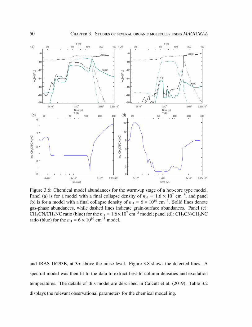
50 Chapter 3. Studies of several organic molecules using MAGICKAL
Figure 3.6: Chemical model abundances for the warm-up stage of a hot-core type model.Panel (a) is for a model with a final collapse density of nH = 1.6 × 107 cm−3, and panel(b) is for a model with a final collapse density of nH = 6 × 1010 cm−3. Solid lines denotegas-phase abundances, while dashed lines indicate grain-surface abundances. Panel (c):CH3CN/CH3NC ratio (blue) for the nH = 1.6×107 cm−3 model; panel (d): CH3CN/CH3NCratio (blue) for the nH = 6 × 1010 cm−3 model.
and IRAS 16293B, at 3σ above the noise level. Figure 3.8 shows the detected lines. A
spectral model was then fit to the data to extract best-fit column densities and excitation
temperatures. The details of this model are described in Calcutt et al. (2019). Table 3.2
displays the relevant observational parameters for the chemical modelling.
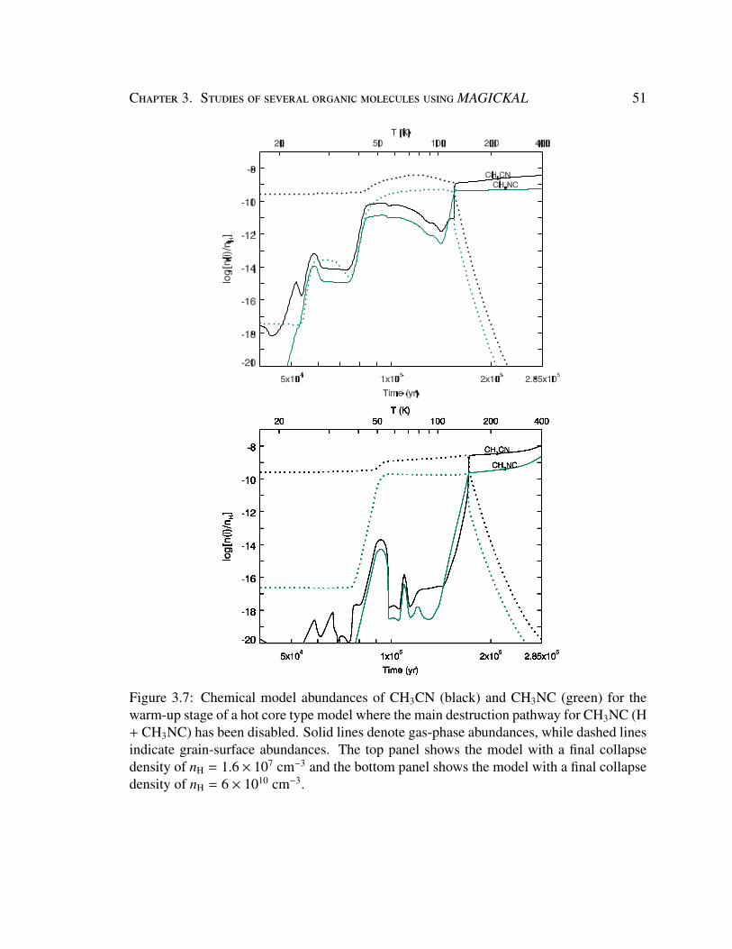
Chapter 3. Studies of several organic molecules using MAGICKAL 51
Figure 3.7: Chemical model abundances of CH3CN (black) and CH3NC (green) for thewarm-up stage of a hot core type model where the main destruction pathway for CH3NC (H+ CH3NC) has been disabled. Solid lines denote gas-phase abundances, while dashed linesindicate grain-surface abundances. The top panel shows the model with a final collapsedensity of nH = 1.6 × 107 cm−3 and the bottom panel shows the model with a final collapsedensity of nH = 6 × 1010 cm−3.
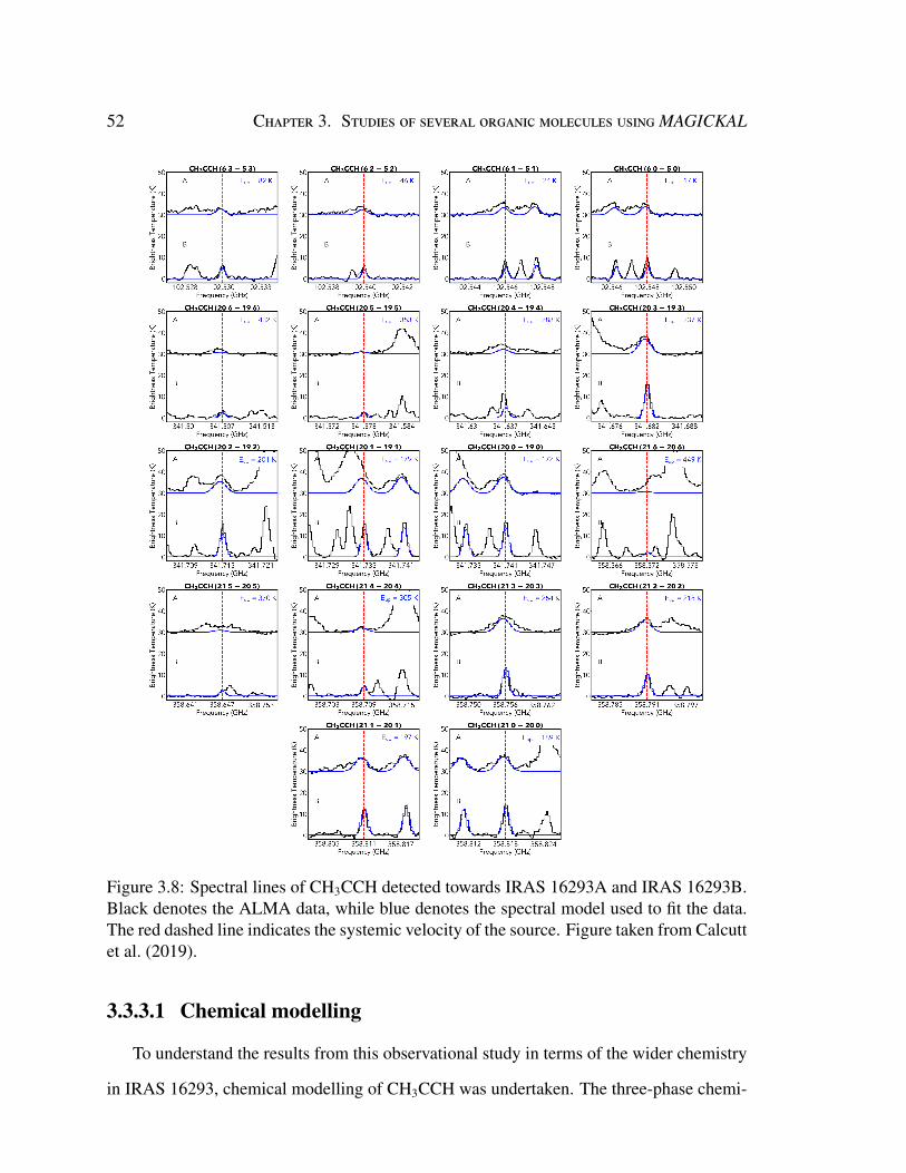
52 Chapter 3. Studies of several organic molecules using MAGICKAL
Figure 3.8: Spectral lines of CH3CCH detected towards IRAS 16293A and IRAS 16293B.Black denotes the ALMA data, while blue denotes the spectral model used to fit the data.The red dashed line indicates the systemic velocity of the source. Figure taken from Calcuttet al. (2019).
3.3.3.1 Chemical modelling
To understand the results from this observational study in terms of the wider chemistry
in IRAS 16293, chemical modelling of CH3CCH was undertaken. The three-phase chemi-
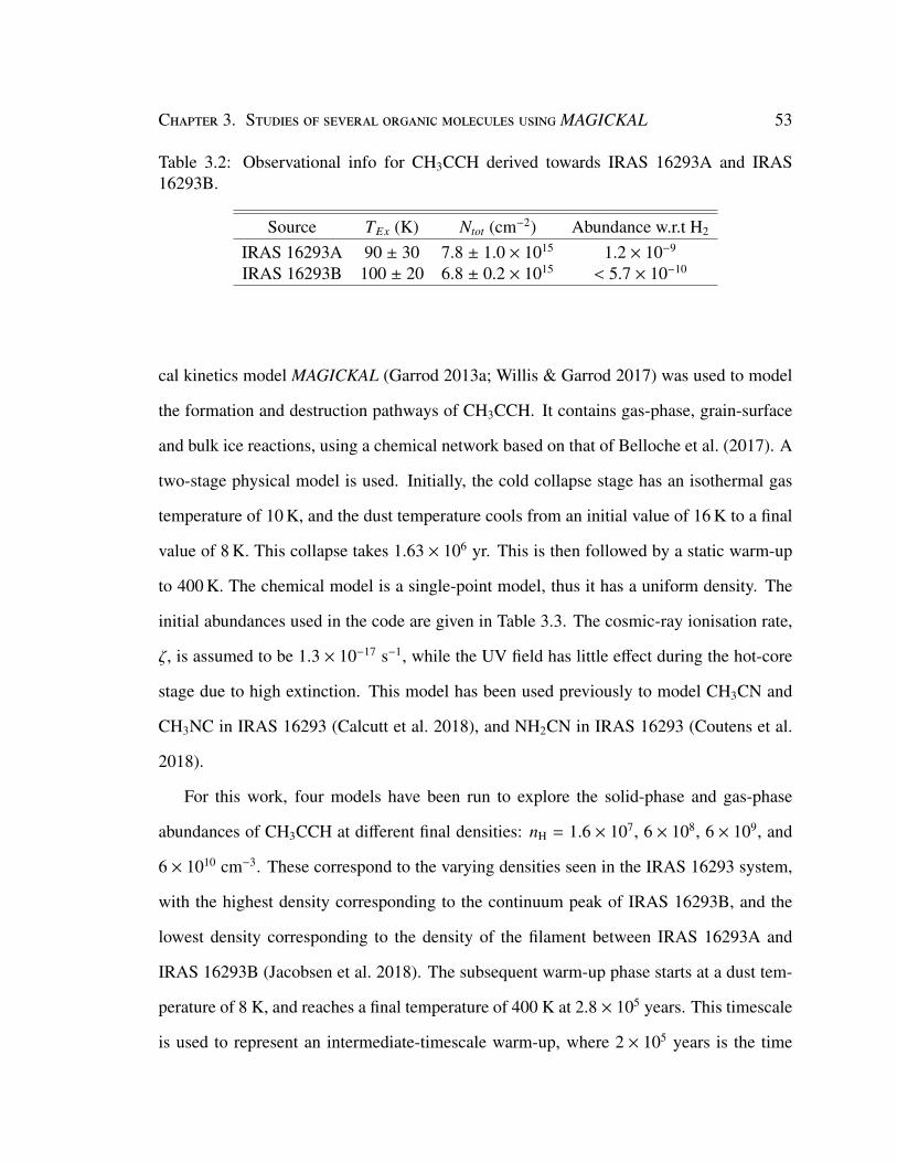
Chapter 3. Studies of several organic molecules using MAGICKAL 53
Table 3.2: Observational info for CH3CCH derived towards IRAS 16293A and IRAS16293B.
Source TEx (K) Ntot (cm−2) Abundance w.r.t H2
IRAS 16293A 90 ± 30 7.8 ± 1.0 × 10¹⁵ 1.2 × 10⁻⁹
IRAS 16293B 100 ± 20 6.8 ± 0.2 × 10¹⁵ < 5.7 × 10⁻¹⁰
cal kinetics model MAGICKAL (Garrod 2013a; Willis & Garrod 2017) was used to model
the formation and destruction pathways of CH3CCH. It contains gas-phase, grain-surface
and bulk ice reactions, using a chemical network based on that of Belloche et al. (2017). A
two-stage physical model is used. Initially, the cold collapse stage has an isothermal gas
temperature of 10 K, and the dust temperature cools from an initial value of 16 K to a final
value of 8 K. This collapse takes 1.63 × 10⁶ yr. This is then followed by a static warm-up
to 400 K. The chemical model is a single-point model, thus it has a uniform density. The
initial abundances used in the code are given in Table 3.3. The cosmic-ray ionisation rate,
ζ, is assumed to be 1.3 × 10⁻¹⁷ s−1, while the UV field has little effect during the hot-core
stage due to high extinction. This model has been used previously to model CH3CN and
CH3NC in IRAS 16293 (Calcutt et al. 2018), and NH2CN in IRAS 16293 (Coutens et al.
2018).
For this work, four models have been run to explore the solid-phase and gas-phase
abundances of CH3CCH at different final densities: nH = 1.6 × 10⁷, 6 × 10⁸, 6 × 10⁹, and
6 × 1010 cm−3. These correspond to the varying densities seen in the IRAS 16293 system,
with the highest density corresponding to the continuum peak of IRAS 16293B, and the
lowest density corresponding to the density of the filament between IRAS 16293A and
IRAS 16293B (Jacobsen et al. 2018). The subsequent warm-up phase starts at a dust tem-
perature of 8 K, and reaches a final temperature of 400 K at 2.8 × 10⁵ years. This timescale
is used to represent an intermediate-timescale warm-up, where 2 × 10⁵ years is the time
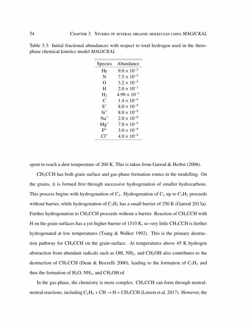
54 Chapter 3. Studies of several organic molecules using MAGICKAL
Table 3.3: Initial fractional abundances with respect to total hydrogen used in the three-phase chemical kinetics model MAGICKAL
Species AbundanceHe 9.0 × 10⁻²
N 7.5 × 10⁻⁵
O 3.2 × 10⁻⁴
H 2.0 × 10⁻³
H2 4.99 × 10⁻¹
C 1.4 × 10⁻⁴
S+ 8.0 × 10⁻⁸
Si+ 8.0 × 10⁻⁹
Na+ 2.0 × 10⁻⁸
Mg+ 7.0 × 10⁻⁹
P+ 3.0 × 10⁻⁹
Cl+ 4.0 × 10⁻⁹
spent to reach a dust temperature of 200 K. This is taken from Garrod & Herbst (2006).
CH3CCH has both grain surface and gas-phase formation routes in the modelling. On
the grains, it is formed first through successive hydrogenation of smaller hydrocarbons.
This process begins with hydrogenation of C3. Hydrogenation of C3 up to C3H2 proceeds
without barrier, while hydrogenation of C3H2 has a small barrier of 250 K (Garrod 2013a).
Further hydrogenation to CH3CCH proceeds without a barrier. Reaction of CH3CCH with
H on the grain surfaces has a yet-higher barrier of 1510 K, so very little CH3CCH is further
hydrogenated at low temperatures (Tsang & Walker 1992). This is the primary destruc-
tion pathway for CH3CCH on the grain-surface. At temperatures above 45 K hydrogen
abstraction from abundant radicals such as OH, NH2, and CH2OH also contributes to the
destruction of CH3CCH (Dean & Bozzelli 2000), leading to the formation of C3H3 and
thus the formation of H2O, NH3, and CH3OH.rd
In the gas-phase, the chemistry is more complex. CH3CCH can form through neutral-
neutral reactions, including C2H4 + CH→H + CH3CCH (Loison et al. 2017). However, the
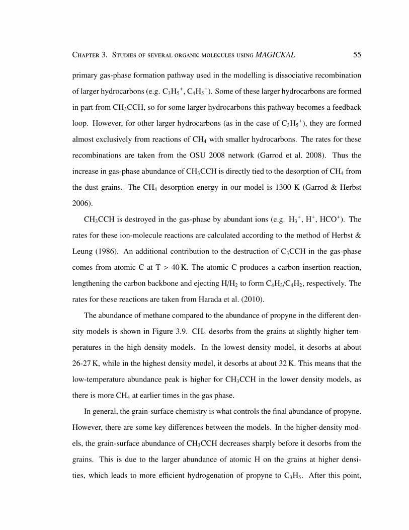
Chapter 3. Studies of several organic molecules using MAGICKAL 55
primary gas-phase formation pathway used in the modelling is dissociative recombination
of larger hydrocarbons (e.g. C3H5+, C4H5
+). Some of these larger hydrocarbons are formed
in part from CH3CCH, so for some larger hydrocarbons this pathway becomes a feedback
loop. However, for other larger hydrocarbons (as in the case of C3H5+), they are formed
almost exclusively from reactions of CH4 with smaller hydrocarbons. The rates for these
recombinations are taken from the OSU 2008 network (Garrod et al. 2008). Thus the
increase in gas-phase abundance of CH3CCH is directly tied to the desorption of CH4 from
the dust grains. The CH4 desorption energy in our model is 1300 K (Garrod & Herbst
2006).
CH3CCH is destroyed in the gas-phase by abundant ions (e.g. H3+, H+, HCO+). The
rates for these ion-molecule reactions are calculated according to the method of Herbst &
Leung (1986). An additional contribution to the destruction of C3CCH in the gas-phase
comes from atomic C at T > 40 K. The atomic C produces a carbon insertion reaction,
lengthening the carbon backbone and ejecting H/H2 to form C4H3/C4H2, respectively. The
rates for these reactions are taken from Harada et al. (2010).
The abundance of methane compared to the abundance of propyne in the different den-
sity models is shown in Figure 3.9. CH4 desorbs from the grains at slightly higher tem-
peratures in the high density models. In the lowest density model, it desorbs at about
26-27 K, while in the highest density model, it desorbs at about 32 K. This means that the
low-temperature abundance peak is higher for CH3CCH in the lower density models, as
there is more CH4 at earlier times in the gas phase.
In general, the grain-surface chemistry is what controls the final abundance of propyne.
However, there are some key differences between the models. In the higher-density mod-
els, the grain-surface abundance of CH3CCH decreases sharply before it desorbs from the
grains. This is due to the larger abundance of atomic H on the grains at higher densi-
ties, which leads to more efficient hydrogenation of propyne to C3H5. After this point,
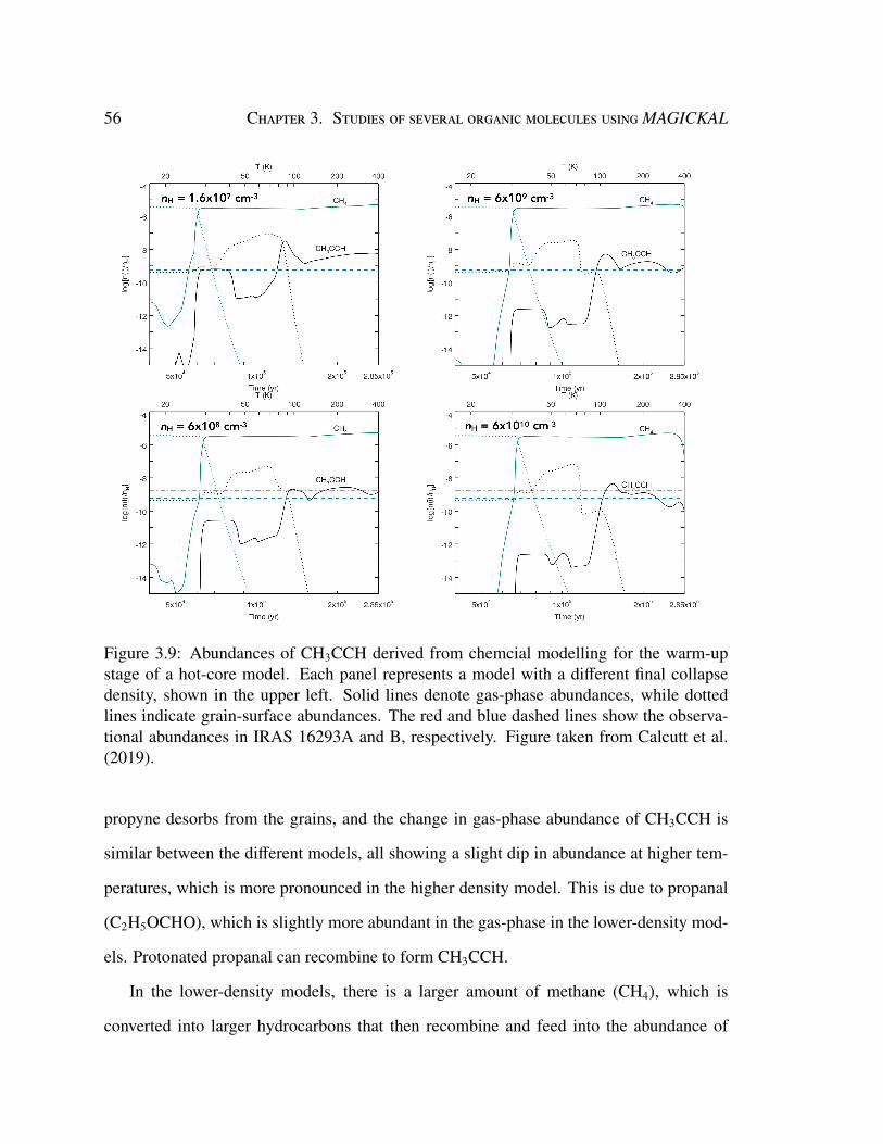
56 Chapter 3. Studies of several organic molecules using MAGICKAL
Figure 3.9: Abundances of CH3CCH derived from chemcial modelling for the warm-upstage of a hot-core model. Each panel represents a model with a different final collapsedensity, shown in the upper left. Solid lines denote gas-phase abundances, while dottedlines indicate grain-surface abundances. The red and blue dashed lines show the observa-tional abundances in IRAS 16293A and B, respectively. Figure taken from Calcutt et al.(2019).
propyne desorbs from the grains, and the change in gas-phase abundance of CH3CCH is
similar between the different models, all showing a slight dip in abundance at higher tem-
peratures, which is more pronounced in the higher density model. This is due to propanal
(C2H5OCHO), which is slightly more abundant in the gas-phase in the lower-density mod-
els. Protonated propanal can recombine to form CH3CCH.
In the lower-density models, there is a larger amount of methane (CH4), which is
converted into larger hydrocarbons that then recombine and feed into the abundance of
Chapter 3. Studies of several organic molecules using MAGICKAL 57
propyne. This is responsible for the difference in the level of abundance at ∼30 K in the
models, and that heavily influences the later behavior as well. This primarily has an impact
on the gas-phase abundances in the models, whereas the peak grain-surface abundances do
not vary significantly between the different models. Methane is predominantly formed on
grains, through the hydrogenation of C. At higher temperatures, methane is also produced
as a product of the CH3 radical abstracting H atoms from species such as H2 and H2CO
(Baulch et al. 1992). The CH3 radical is formed primarily from dissociation of CH3OH
by cosmic rays. The rate of dissociation is computed in the model to be 4.6 × 10⁻¹⁵ s−1,
assuming a canonical cosmic-ray ionization rate of 1.3 × 10⁻¹⁷ s−1 in our network. Overall,
the models do a reasonable job of reproducing the observational abundance of CH3CCH in
both sources.


59
Chapter 4
ExploringMolecular Complexity with
ALMA (EMoCA): Complex Isocyanides
in Sgr B2(N)
4.1 PrefaceThe following chapter of this dissertation is taken from published work that was done
in collaboration with others (Willis et al. 2020). In order to preserve context for the work,
and to maintain consistency with the published version, sections that were contributed by
co-authors are included here. Those sections are marked clearly with an asterisk (*), both
in this chapter and in the table of contents. Note that figures and tables introduced in these
sections were also contributed by co-authors. Sections for which there is no asterisk are
my work.
4.2 IntroductionIn chemistry, a cyanide is any organic molecule that contains the cyano functional
group ( – C ––– N). Cyanide species have been observed astronomically for some time, be-
60Chapter 4. ExploringMolecular Complexity with ALMA (EMoCA): Complex
Isocyanides in Sgr B2(N)
ginning with the first detection of the CN radical toward visually bright stars in the optical
regime (McKellar 1940). Radio telescopes did not detect the CN radical until 30 years
later (Jefferts et al. 1970). More complex cyanides have since been detected in the inter-
stellar medium (ISM), with the identification of hydrogen cyanide (HCN; Snyder & Buhl
1971) and methyl cyanide (CH3CN; Solomon & Jefferts 1971) the following year. Since
then, many cyanide species have been found, including vinyl cyanide (C2H3CN; Gardner
& Winnewisser 1975), ethyl cyanide (C2H5CN; Johnson et al. 1977), n-propyl cyanide
(n-C3H7CN; Belloche et al. 2009) and i-propyl cyanide (i-C3H7CN, a branched species;
Belloche et al. 2014). Most recently, benzonitrile (c-C6H5CN; McGuire et al. 2018b), the
first benzene-derived aromatic molecule detected in the ISM through radio astronomy was
seen towards the dark cloud TMC-1.
Although these detections are interesting in that they help to reveal the chemical com-
plexity achieved in the ISM, observations of these molecules have also proven useful from
a practical standpoint. For example, the HCN(J=1−0) rotational line has been used exten-
sively as a dense gas tracer in external galaxies (e.g., Schirm et al. 2016; Sliwa & Downes
2017; Johnson et al. 2018). HCN is also very abundant in the atmosphere of Titan, and has
been used to measure nitrogen fractionation there (e.g., Molter et al. 2016). CH3CN is reg-
ularly used to determine kinetic temperature in star-forming regions (Bell et al. 2014), and
HC3N has been shown to be important in observations of ultraluminous infrared galaxies
(Costagliola et al. 2015).
Despite the extent to which cyanides have been studied in the ISM, the isocyanides
(molecules that contain the isocyano functional group, – N ––– C) have been comparatively
sparsely studied. The first isocyanide detected in the ISM was HNC, along with the related
molecule HNCO, toward Sgr B2 (Snyder & Buhl 1972). Since these first detections, to
the authors’ knowledge, only seven other isocyanides have been unambiguously detected
in astronomical sources, most of them (only) in the circumstellar envelope of the carbon-
Chapter 4. ExploringMolecular Complexity with ALMA (EMoCA): ComplexIsocyanides in Sgr B2(N) 61
rich asymptotic giant branch star IRC+10216: CH3NC (Cernicharo et al. 1988), HCCNC
(Kawaguchi et al. 1992a), MgNC (Kawaguchi et al. 1993), AlNC (Ziurys et al. 2002),
SiNC (Guélin et al. 2004), HMgNC (Cabezas et al. 2013), and CaNC (Cernicharo et al.
2019). HCCNC was detected toward TMC-1 (Kawaguchi et al. 1992a), and Belloche et al.
(2013) reported a tentative detection of this species towards Sgr B2(N) with the IRAM
30 m telescope, with only one uncontaminated line and one blended line. Remijan et al.
(2005) reported the detection of one transition of CH3NC with the GBT toward Sgr B2(N),
with two velocity components seen in absorption and emission, respectively. This detection
added an additional piece of evidence for the presence of CH3NC in Sgr B2, complement-
ing the initial tentative detection of three higher-energy transitions obtained with the IRAM
30 m toward Sgr B2(OH) by Cernicharo et al. (1988). Remijan et al. failed to detect any
compact emission of CH3NC with BIMA, suggesting that the GBT detection traces a large-
scale distribution of CH3NC in Sgr B2.
Even more sparse than the observational efforts for isocyanides have been the modeling
efforts, with the exception of HNC. Of the six most complex isocyanides detected, only
HMgNC has been included in a chemical network, in the aforementioned detection paper
(Cabezas et al. 2013). The interstellar chemistry of CH3NC has been investigated before
(DeFrees et al. 1985). These latter authors investigated the formation rate of the protonated
ions CH3NCH+ and CH3CNH+ from the radiative association reaction of CH3+ and HCN.
They found, using ab initio quantum theory as well as equilibrium calculations, that the
ratio of formation of CH3NCH+/CH3CNH+ after relaxation of the complex should be be-
tween 0.1 and 0.4. However, this mechanism, as well as any others involving CH3NC, does
not appear to have been incorporated into a large chemical network until recent work by
some of the present authors (Calcutt et al. 2018).
It is important to confront new modeling efforts with state-of-the-art observational data.
To this end, we make use of the Exploring Molecular Complexity with ALMA (EMoCA)
62Chapter 4. ExploringMolecular Complexity with ALMA (EMoCA): Complex
Isocyanides in Sgr B2(N)
survey. EMoCA is an imaging spectral line survey conducted towards Sagittarius B2(N).
Sgr B2(N) is a protocluster located in the Galactic center region, at a projected distance
of about 100 pc from Sgr A?. It contains a number of HII regions, some compact and
ultracompact (e.g., Gaume et al. 1995), and Class II methanol masers (Caswell 1996), both
signposts of ongoing high mass star formation. Sgr B2(N) also harbors several hot molec-
ular cores at the early stage of high mass star formation which present a high density of
spectral lines revealing the presence of numerous complex organic molecules. Many com-
plex organic molecules were first detected toward Sgr B2(N), which motivated its selection
as a target for the EMoCA survey. Analysis of the data from EMoCA has led to several
important results, including the aforementioned detection of i-propyl cyanide (Belloche
et al. 2014), as well as important insights into deuteration levels in Sgr B2(N) (Belloche
et al. 2016). More recently, three new hot cores have been detected and characterized in
Sgr B2(N), signifying further sources to study complex organic molecules (Bonfand et al.
2017, see also Sánchez-Monge et al. 2017). This work focuses on using the EMoCA data
to search for various nitrogen-containing organic molecules toward Sgr B2(N). We include
alkyl cyanides and isocyanides in our search, which are chemical species in which the -CN
or -NC group is attached to an alkyl substituent. Alkyl substituents are acyclic saturated hy-
drocarbons that are missing one hydrogen atom. We also search for simple cyanopolyynes
and isocyanopolyynes (e.g., HC3N and HCCNC).
This paper aims to be the most comprehensive modeling and observational study of
isocyanide chemistry in the ISM to date. We expand on the chemical network for CH3NC
first introduced in Calcutt et al. (2018). Several new molecules have been introduced in the
chemical network as well. These include vinyl isocyanide (C2H3NC) and ethyl isocyanide
(C2H5NC), as well as associated radicals (e.g., CH2NC). This marks the first time that these
molecules have been incorporated into an astrochemical network.
The paper is organized as follows. Section 2 outlines the observational methods. Sec-
Chapter 4. ExploringMolecular Complexity with ALMA (EMoCA): ComplexIsocyanides in Sgr B2(N) 63
tion 3 provides information about the spectroscopic predictions used to analyze the ob-
served spectra. Section 4 outlines the observational results. Section 5 discusses the addi-
tions made to the chemical modeling. Modeling results are presented in Sect. 6. Section 7
contains the discussion, while Sect. 8 is the conclusion.
4.3 Observations*We use data from the the EMoCA spectral line survey performed with the Atacama
Large Millimeter/submillimeter Array (ALMA) in its cycles 0 and 1 to search for vari-
ous nitrogen-containing organic molecules toward the high-mass star-forming region Sgr
B2(N). We used the main array with baselines ranging from ∼17 m to ∼400 m, which
imply a maximum recoverable scale of ∼ 20′′. This scale translates into ∼0.8 pc at the
adopted distance of 8.3 kpc (Reid et al. 2014). The survey covers the frequency range be-
tween 84.1 and 114.4 GHz in five setups. It has a spectral resolution of 488.3 kHz (1.7 to
1.3 km s−1) and a median angular resolution of 1.6′′(∼0.06 pc or ∼13000 au). The achieved
rms sensitivity is on the order of 3 mJy beam−1, which translates into an rms sensitivity of
0.1-0.2 K in effective radiation temperature scale depending on the setup. The field was
centered at (α, δ)J2000= (17h47m19.87s,−28◦22′16′′), half way between the two main hot
cores Sgr B2(N1) and (N2) that are separated by 4.9′′(∼0.2 pc) in the north–south direc-
tion. Sgr B2(N1) and (N2) have systemic velocities of ∼64 and ∼74 km s−1, respectively
(e.g., Belloche et al. 2008, 2016). The size of the primary beam varies between 69′′at
84 GHz and 51′′at 114 GHz. A detailed description of the observations, the data reduction
process, and the method used to identify the detected lines and derive column densities was
presented in Belloche et al. (2016).
64Chapter 4. ExploringMolecular Complexity with ALMA (EMoCA): Complex
Isocyanides in Sgr B2(N)
4.4 Laboratory spectroscopy background*Transition frequencies were taken from the catalog of the Cologne Database for Molec-
ular Spectroscopy, CDMS, (Müller et al. 2001; Endres et al. 2016) for the most part. Other
sources of data are mentioned in specific cases.
The CH3CN 38 = 1 laboratory data are based on Müller et al. (2015) with additional
data, especially in the range of our survey, coming from BAUER & MAES (1969). The
partition function includes energy levels from vibrational states up to ∼1700 K (Müller
et al. 2015), and as such the vibrational contributions are complete at 170 K. The CH3NC
3 = 0 data are based on Pracna et al. (2011b). Additional data, also in the range of our
survey, were taken from BAUER & BOGEY (1970). The values of the spectroscopic pa-
rameters A and DK , along with vibrational information, were taken from Pliva et al. (1995).
Preliminary CH3NC 38 = 1 data were calculated from Pracna et al. (2011a).
The C2H5CN data are based on Brauer et al. (2009) with additional important informa-
tion especially in the range of our survey from Fukuyama et al. (1996) and from Pearson
et al. (1994). Vibrational correction factors to the rotational partition function are avail-
able via the CDMS documentation. They are based on Heise et al. (1981). The C2H5NC
data are based on Margulès et al. (2018) with additional low-frequency data (Anderson &
Gwinn 1968; Fliege & Dreizler 1985; Krüger & Dreizler 1992). Vibrational energies of the
three lowest vibrational fundamentals were estimated from quantum chemical calculations
(H. S. P. Müller, 2017, unpublished) in comparison to higher lying fundamentals (Bolton
et al. 1969).
The C2H3CN data are based on Müller et al. (2008) with particularly noteworthy data
in the range of our survey from Baskakov et al. (1996). The partition function includes
numerous low-lying vibrational states (H. S. P. Müller, 2008, unpublished) and is converged
up to ∼200 K. The vibrational energies were based on Khlifi et al. (1999) and on quantum
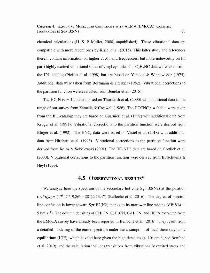
Chapter 4. ExploringMolecular Complexity with ALMA (EMoCA): ComplexIsocyanides in Sgr B2(N) 65
chemical calculations (H. S. P. Müller, 2008, unpublished). These vibrational data are
compatible with more recent ones by Kisiel et al. (2015). This latter study and references
therein contain information on higher J, Ka, and frequencies, but more noteworthy on (in
part) highly excited vibrational states of vinyl cyanide. The C2H3NC data were taken from
the JPL catalog (Pickett et al. 1998) but are based on Yamada & Winnewisser (1975).
Additional data were taken from Bestmann & Dreizier (1982). Vibrational corrections to
the partition function were evaluated from Benidar et al. (2015).
The HC3N 37 = 1 data are based on Thorwirth et al. (2000) with additional data in the
range of our survey from Yamada & Creswell (1986). The HCCNC 3 = 0 data were taken
from the JPL catalog; they are based on Guarnieri et al. (1992) with additional data from
Krüger et al. (1991). Vibrational corrections to the partition function were derived from
Bürger et al. (1992). The HNC3 data were based on Vastel et al. (2018) with additional
data from Hirahara et al. (1993). Vibrational corrections to the partition function were
derived from Kolos & Sobolewski (2001). The HC3NH+ data are based on Gottlieb et al.
(2000). Vibrational corrections to the partition function were derived from Botschwina &
Heyl (1999).
4.5 Observational results*We analyze here the spectrum of the secondary hot core Sgr B2(N2) at the position
(α, δ)J2000= (17h47m19.86s,−28◦22′13.4′′) (Belloche et al. 2016). The degree of spectral
line confusion is lower toward Sgr B2(N2) thanks to its narrower line widths (FWHM ∼
5 km s−1). The column densities of CH3CN, C2H5CN, C2H3CN, and HC3N extracted from
the EMoCA survey have already been reported in Belloche et al. (2016). They result from
a detailed modeling of the entire spectrum under the assumption of local thermodynamic
equilibrium (LTE), which is valid here given the high densities (> 107 cm−3, see Bonfand
et al. 2019), and the calculation includes transitions from vibrationally excited states and
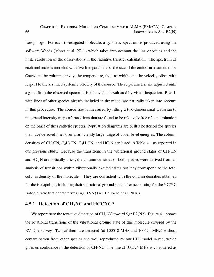
66Chapter 4. ExploringMolecular Complexity with ALMA (EMoCA): Complex
Isocyanides in Sgr B2(N)
isotopologs. For each investigated molecule, a synthetic spectrum is produced using the
software Weeds (Maret et al. 2011) which takes into account the line opacities and the
finite resolution of the observations in the radiative transfer calculation. The spectrum of
each molecule is modeled with five free parameters: the size of the emission assumed to be
Gaussian, the column density, the temperature, the line width, and the velocity offset with
respect to the assumed systemic velocity of the source. These parameters are adjusted until
a good fit to the observed spectrum is achieved, as evaluated by visual inspection. Blends
with lines of other species already included in the model are naturally taken into account
in this procedure. The source size is measured by fitting a two-dimensional Gaussian to
integrated intensity maps of transitions that are found to be relatively free of contamination
on the basis of the synthetic spectra. Population diagrams are built a posteriori for species
that have detected lines over a sufficiently large range of upper-level energies. The column
densities of CH3CN, C2H5CN, C2H3CN, and HC3N are listed in Table 4.1 as reported in
our previous study. Because the transitions in the vibrational ground states of CH3CN
and HC3N are optically thick, the column densities of both species were derived from an
analysis of transitions within vibrationally excited states but they correspond to the total
column density of the molecules. They are consistent with the column densities obtained
for the isotopologs, including their vibrational ground state, after accounting for the 12C/13C
isotopic ratio that characterizes Sgr B2(N) (see Belloche et al. 2016).
4.5.1 Detection of CH3NC and HCCNC*
We report here the tentative detection of CH3NC toward Sgr B2(N2). Figure 4.1 shows
the rotational transitions of the vibrational ground state of this molecule covered by the
EMoCA survey. Two of them are detected (at 100518 MHz and 100524 MHz) without
contamination from other species and well reproduced by our LTE model in red, which
gives us confidence in the detection of CH3NC. The line at 100524 MHz is considered as
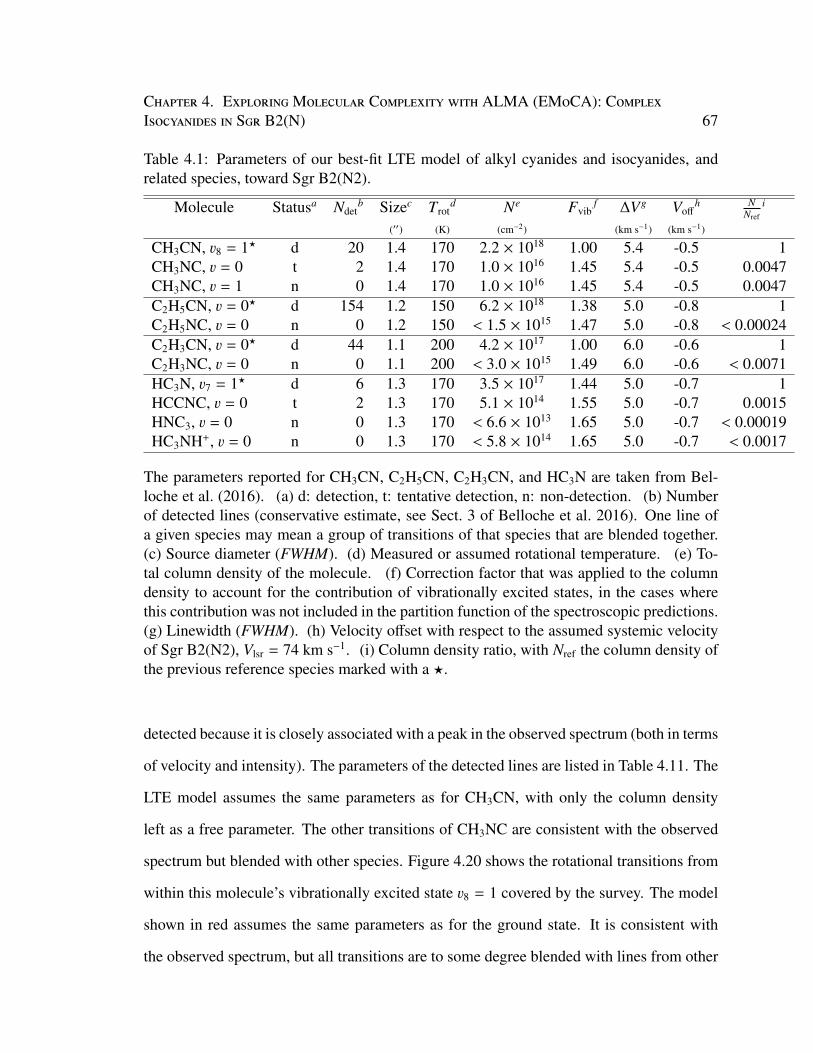
Chapter 4. ExploringMolecular Complexity with ALMA (EMoCA): ComplexIsocyanides in Sgr B2(N) 67
Table 4.1: Parameters of our best-fit LTE model of alkyl cyanides and isocyanides, andrelated species, toward Sgr B2(N2).
Molecule Statusa Ndetb Sizec Trot
d Ne Fvibf ∆Vg Voff
h NNref
i
(′′) (K) (cm−2) (km s−1) (km s−1)
CH3CN, 38 = 1? d 20 1.4 170 2.2 × 10¹⁸ 1.00 5.4 -0.5 1CH3NC, 3 = 0 t 2 1.4 170 1.0 × 10¹⁶ 1.45 5.4 -0.5 0.0047CH3NC, 3 = 1 n 0 1.4 170 1.0 × 10¹⁶ 1.45 5.4 -0.5 0.0047C2H5CN, 3 = 0? d 154 1.2 150 6.2 × 10¹⁸ 1.38 5.0 -0.8 1C2H5NC, 3 = 0 n 0 1.2 150 < 1.5 × 10¹⁵ 1.47 5.0 -0.8 < 0.00024C2H3CN, 3 = 0? d 44 1.1 200 4.2 × 10¹⁷ 1.00 6.0 -0.6 1C2H3NC, 3 = 0 n 0 1.1 200 < 3.0 × 10¹⁵ 1.49 6.0 -0.6 < 0.0071HC3N, 37 = 1? d 6 1.3 170 3.5 × 10¹⁷ 1.44 5.0 -0.7 1HCCNC, 3 = 0 t 2 1.3 170 5.1 × 10¹⁴ 1.55 5.0 -0.7 0.0015HNC3, 3 = 0 n 0 1.3 170 < 6.6 × 10¹³ 1.65 5.0 -0.7 < 0.00019HC3NH+, 3 = 0 n 0 1.3 170 < 5.8 × 10¹⁴ 1.65 5.0 -0.7 < 0.0017
The parameters reported for CH3CN, C2H5CN, C2H3CN, and HC3N are taken from Bel-loche et al. (2016). (a) d: detection, t: tentative detection, n: non-detection. (b) Numberof detected lines (conservative estimate, see Sect. 3 of Belloche et al. 2016). One line ofa given species may mean a group of transitions of that species that are blended together.(c) Source diameter (FWHM). (d) Measured or assumed rotational temperature. (e) To-tal column density of the molecule. (f) Correction factor that was applied to the columndensity to account for the contribution of vibrationally excited states, in the cases wherethis contribution was not included in the partition function of the spectroscopic predictions.(g) Linewidth (FWHM). (h) Velocity offset with respect to the assumed systemic velocityof Sgr B2(N2), Vlsr = 74 km s−1. (i) Column density ratio, with Nref the column density ofthe previous reference species marked with a ?.
detected because it is closely associated with a peak in the observed spectrum (both in terms
of velocity and intensity). The parameters of the detected lines are listed in Table 4.11. The
LTE model assumes the same parameters as for CH3CN, with only the column density
left as a free parameter. The other transitions of CH3NC are consistent with the observed
spectrum but blended with other species. Figure 4.20 shows the rotational transitions from
within this molecule’s vibrationally excited state 38 = 1 covered by the survey. The model
shown in red assumes the same parameters as for the ground state. It is consistent with
the observed spectrum, but all transitions are to some degree blended with lines from other
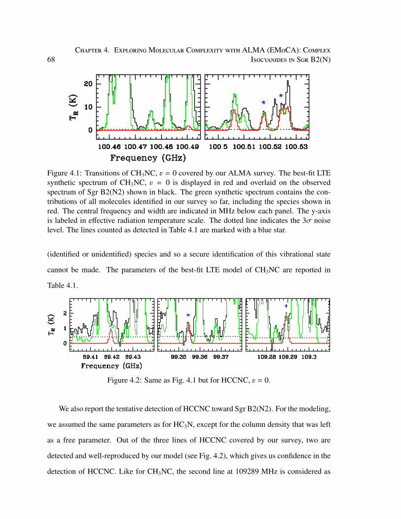
68Chapter 4. ExploringMolecular Complexity with ALMA (EMoCA): Complex
Isocyanides in Sgr B2(N)
Figure 4.1: Transitions of CH3NC, 3 = 0 covered by our ALMA survey. The best-fit LTEsynthetic spectrum of CH3NC, 3 = 0 is displayed in red and overlaid on the observedspectrum of Sgr B2(N2) shown in black. The green synthetic spectrum contains the con-tributions of all molecules identified in our survey so far, including the species shown inred. The central frequency and width are indicated in MHz below each panel. The y-axisis labeled in effective radiation temperature scale. The dotted line indicates the 3σ noiselevel. The lines counted as detected in Table 4.1 are marked with a blue star.
(identified or unidentified) species and so a secure identification of this vibrational state
cannot be made. The parameters of the best-fit LTE model of CH3NC are reported in
Table 4.1.
Figure 4.2: Same as Fig. 4.1 but for HCCNC, 3 = 0.
We also report the tentative detection of HCCNC toward Sgr B2(N2). For the modeling,
we assumed the same parameters as for HC3N, except for the column density that was left
as a free parameter. Out of the three lines of HCCNC covered by our survey, two are
detected and well-reproduced by our model (see Fig. 4.2), which gives us confidence in the
detection of HCCNC. Like for CH3NC, the second line at 109289 MHz is considered as

Chapter 4. ExploringMolecular Complexity with ALMA (EMoCA): ComplexIsocyanides in Sgr B2(N) 69
detected because it is closely associated with a peak in the observed spectrum (both in terms
of velocity and intensity). The third transition is consistent with the observed spectrum but
blended with emission from other species. The parameters of the detected lines are listed in
Table 4.11. The parameters of the best-fit LTE model of HCCNC are reported in Table 4.1.
We also searched for transitions from within the vibrationally excited states 35 = 1, 36 = 1,
and 37 = 1 assuming the same parameters as for the ground state, but none are detected.
Their predicted peak intensities are below the sensitivity limit of the EMoCA survey.
Examples of integrated intensity maps of rotational lines of CH3CN, CH3NC, HC3N,
and HCCNC are displayed in Fig. 4.3. The integration was performed around the systemic
velocity of Sgr B2(N2). In all cases, the emission is centrally peaked on the hot core.
4.5.2 Upper limits for C2H5NC, C2H3NC, HNC3, and HC3NH+*
We searched for C2H5NC, C2H3NC, HNC3, and HC3NH+ toward Sgr B2(N2) but did
not detect these species. For a spectral line survey with thousands of lines detected, it is
standard practice to model the emission and to use this model to derive upper limits. For the
modeling, we assumed the same parameters as for C2H5CN, C2H3CN, HC3N, and HC3N,
respectively, except for the column densities that were left as free parameters. The models
used to obtain upper limits to their column densities are displayed in red in Figs. 4.21–4.24
and the upper limits are listed in Table 4.1.
4.6 Chemical modelingIn this paper, we use the chemical kinetics code MAGICKAL (Garrod 2013a). The
basis of the chemical network is taken from Garrod et al. (2017), with the above-mentioned
inclusion of CH3NC chemistry first presented by Calcutt et al. (2018). The model also uses
the grain-surface back-diffusion correction of Willis & Garrod (2017). The model simulates
a fully coupled gas-phase-, grain-surface-, and ice-mantle chemistry under time-dependent
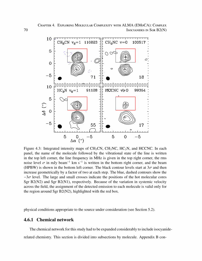
70Chapter 4. ExploringMolecular Complexity with ALMA (EMoCA): Complex
Isocyanides in Sgr B2(N)
Figure 4.3: Integrated intensity maps of CH3CN, CH3NC, HC3N, and HCCNC. In eachpanel, the name of the molecule followed by the vibrational state of the line is writtenin the top left corner, the line frequency in MHz is given in the top right corner, the rmsnoise level σ in mJy beam−1 km s−1 is written in the bottom right corner, and the beam(HPBW) is shown in the bottom left corner. The black contour levels start at 3σ and thenincrease geometrically by a factor of two at each step. The blue, dashed contours show the−3σ level. The large and small crosses indicate the positions of the hot molecular coresSgr B2(N2) and Sgr B2(N1), respectively. Because of the variation in systemic velocityacross the field, the assignment of the detected emission to each molecule is valid only forthe region around Sgr B2(N2), highlighted with the red box.
physical conditions appropriate to the source under consideration (see Section 5.2).
4.6.1 Chemical network
The chemical network for this study had to be expanded considerably to include isocyanide-
related chemistry. This section is divided into subsections by molecule. Appendix B con-

Chapter 4. ExploringMolecular Complexity with ALMA (EMoCA): ComplexIsocyanides in Sgr B2(N) 71
tains a more comprehensive list of reactions included in this updated model, as well as
binding energies and enthalpies of formation for grain-surface species of note. Here we
only focus on the most important reactions.
4.6.1.1 CH3NC
The incorporation of CH3NC into our chemical network was discussed in some detail
by Calcutt et al. (2018), but it is summarized here. CH3NC is formed primarily through
the radiative association of CH3+ and HCN, which produces two isomers, CH3CNH+ and
CH3NCH+, in a ratio of 85:15 (DeFrees et al. 1985) due to unimolecular isomerization.
These isomers can then recombine with electrons to produce CH3CN and CH3NC , respec-
tively. We note that the protonated form of both the cyanide and isocyanide can be formed
from proton transfer reactions with species such as H3O+, but they are not assumed to be
formed with enough internal energy to isomerize in that case. No isomerization is assumed
to occur as a result of recombination. This schematic is shown below:
CH3+ + HCN CH3CNH+/CH3NCH+ + hν (4.1)
CH3CNH+/CH3NCH+ + e− CH3CN/CH3NC + H (4.2)
For both isomers, ∼40% of recombinations produce CH3CN and CH3NC, respectively. The
remaining ∼60% produce more fragmented species. These branching ratios are taken from
Loison et al. (2014), based on laboratory work from Plessis et al. (2012). There is currently
no known efficient grain-surface formation path for CH3NC. Due to the lack of efficient
pathways for interconversion between the isomers, the point of divergence in the chemical
networks for CH3CN and CH3NC therefore occurs with Reaction 4.1.
Reaction with abundant positive ions (e.g., C+, H3+, H+) is the primary destruction path-
72Chapter 4. ExploringMolecular Complexity with ALMA (EMoCA): Complex
Isocyanides in Sgr B2(N)
way for CH3NC at T < 100 K. At higher temperatures, ion-molecule reactions are still im-
portant, but reaction with atomic hydrogen becomes the dominant destruction pathway for
CH3NC following:
CH3NC + H CH3 + HCN (4.3)
The activation energy barrier of this reaction is not known experimentally. The standard
models presented in this paper use a barrier of 1200 K, which is assumed from the reaction
of H and HNC (Graninger et al. 2014). This barrier was varied in several model tests to see
what effect it would have on the chemistry of the isocyanides, and CH3NC in particular.
Recent theoretical work by Nguyen et al. (2019) shows that CH3NC does react with H
on surfaces with barriers similar to the standard value used here of 1200 K, though it is
important to note that without experimental measurements, this value is still uncertain.
Binding energies for CH3CN and CH3NC on amorphous water ice are used, and are
taken from Bertin et al. (2017). The values are 6150 K for CH3CN and 5686 K for CH3NC.
4.6.1.2 C2H5NC
Ethyl isocyanide has, to our knowledge, not been incorporated into any astrochemical
networks until now. As such, the chemical network for this species had to be constructed
from the ground up. In most cases, reactions were implemented based on analogous pro-
cesses for C2H5CN.
In the models presented here, C2H5NC is formed primarily through hydrogenation reac-
tions on the surfaces and in the ice mantles of dust particles, specifically via the following:
H + CH2CH2NC C2H5NC (4.4)
H + CH3CHNC C2H5NC (4.5)
Chapter 4. ExploringMolecular Complexity with ALMA (EMoCA): ComplexIsocyanides in Sgr B2(N) 73
These large isocyanide radicals also had to be added to our chemical network, as they were
not involved in any reactions before the introduction of ethyl isocyanide. CH2CH2NC is
formed through the following two reactions on grain surfaces and in grain ice mantles:
CH2 + CH2NC CH2CH2NC (4.6)
H + C2H3NC CH2CH2NC (4.7)
The first reaction (Reaction 4.6) is the primary means by which the CH2CH2NC radi-
cal is formed, and has no barrier. The second reaction is a secondary channel by which
CH2CH2NC can be formed, though it has an activation energy barrier of 1320 K, which
we assume based on the analogous reaction with C2H3CN. CH3CHNC is formed solely
through hydrogen addition to vinyl isocyanide:
H + C2H3NC CH3CHNC. (4.8)
This reaction has a barrier of 619 K, also taken from the analogous cyanide process.
Another minor formation path for C2H5NC that occurs on grains is the following reac-
tion:
CH3 + CH2NC C2H5NC. (4.9)
Reaction 4.9 is significantly less efficient than Reactions 4.4 and 4.5 because of the need
for mobility of the heavier CH3 radical. We note that CH2NC is formed primarily in the
gas phase from reactions of CH3CN+ with electrons and CO molecules, as well as by
recombination of CH3NCH+.
Standard destruction mechanisms for C2H5NC were also included. These include photo-
74Chapter 4. ExploringMolecular Complexity with ALMA (EMoCA): Complex
Isocyanides in Sgr B2(N)
dissociation and cosmic-ray-induced (photo-)dissociation. However, the most efficient de-
struction mechanism for C2H5NC is ion-molecule reactions with abundant gas-phase ions.
Grain-surface binding energies for C2H5NC and related radicals were chosen to mimic
those of the corresponding cyanides, considering the lack of experimental data on these
species. These values can be found in Table 4.12. We note that there is no reaction of
C2H5NC with H, which would be analogous to Reaction 4.3. Since there has been, to
the authors’ knowledge, no experimental or theoretical work done on this reaction, it was
decided not to extrapolate the barrier used in Reaction 4.3 to the larger C2H5NC.
4.6.1.3 C2H3NC
Vinyl isocyanide was incorporated into our chemical network. This is the first time
this species has been included in an astrochemical network, to the authors’ knowledge. A
similar strategy was followed with vinyl isocyanide as is explained for ethyl isocyanide, in
that reactions were selected as analogs to the cyanide isomer, vinyl cyanide.
There are important formation reactions for C2H3NC in both the gas phase and on
grains in our network. On grains, it is formed through hydrogenation of the C2H2NC
radical, through the following reaction:
H + C2H2NC C2H3NC. (4.10)
C2H2NC is formed on grains from hydrogenation of HCCNC. The formation of HCCNC
at low temperatures is dominated by the dissociative recombination of C3H2N+ (via a rear-
rangement of the heavy atoms of the carbon backbone -CCCN to -CCNC), while at higher
temperatures (greater than ∼26K in the models presented below), production is dominated
by the reaction:
H + HCNCC HCCNC + H. (4.11)
Chapter 4. ExploringMolecular Complexity with ALMA (EMoCA): ComplexIsocyanides in Sgr B2(N) 75
HCNCC is primarily formed from dissociative recombination of C3H2N+. We note that
C3H2N+ is formed from the reaction of C3NH+ with H2 in the gas phase. C3NH+ is formed
from the reaction of H2 with C3N+. These reactions were already present in previous net-
works.
In the gas phase, C2H3NC is formed in one of the primary recombination channels of
protonated ethyl isocyanide (C2H6NC+):
C2H6NC+ + e− C2H3NC + H2 + H. (4.12)
Thus the chemistry of ethyl and vinyl isocyanide is linked. Approximately 40% of recom-
binations are assumed to go through this channel, which is consistent with the experiments
of Vigren et al. (2012).
Similar to methyl and ethyl isocyanide discussed previously, standard destruction mech-
anisms for vinyl isocyanide are included as well. These include photo-dissociation, cosmic
ray-photon induced dissociation, and ion-molecule reactions. Binding energies are chosen
to be equivalent to vinyl cyanide, in the absence of experimental data, and are shown in
Table 4.12.
4.6.1.4 HC3N, HCCNC
Although both cyanoacetylene and isocyanoacetylene have been studied in detail pre-
viously (e.g., Hébrard et al. 2009; Woon & Herbst 2009), a review of their basic chemistry
is presented here. HC3N has a few primary gas-phase formation pathways. At lower tem-
peratures, it is formed primarily through the following reaction:
C + CH2CN HC3N + H, (4.13)
76Chapter 4. ExploringMolecular Complexity with ALMA (EMoCA): Complex
Isocyanides in Sgr B2(N)
while at higher temperatures (&27K in the models presented below) the following reaction
takes over:
N + C3H3 HC3N + H2. (4.14)
C2H + HCN is also a viable formation path, though it is secondarily important. There are
minor grain-surface formation pathways as well, namely hydrogenation of C3N and the
reaction of atomic N with C3H3. Moreover, HC3N is destroyed on the grains by further
hydrogenation to C2H2CN, which has an activation energy barrier of 1710 K, and in the
gas via standard ion-molecule destruction routes.
The chemistry of HCCNC is less complex. It has two primary gas-phase formation
pathways. It is formed from Reaction 4.11 and the following reaction:
C3H2N+ + e− HCCNC + H. (4.15)
Standard ion-molecule destruction routes are also included. Grain-surface chemistry for
HCCNC is minimal, as there are no known formation routes, and, similarly to HC3N, it is
destroyed by hydrogenation to C2H2NC, with the same barrier.
4.6.2 Physical model
For the chemical modeling in this paper, we introduce a new way of incorporating the
physical profile of astronomical sources. Traditional astrochemical models of hot cores
consist of two stages of physical evolution; these are described in detail by Garrod et al.
(2017). First, the molecular cloud undergoes a cold collapse to some specified gas density.
This is followed by a static warm-up to a dust and gas temperature of 400 K. This warm-up
can be tuned to occur at different rates depending on the source, with the warm-up rate
believed to be roughly correlated with the mass of the source (Garrod & Herbst 2006).
However, there are some issues with a modeling approach like this, as discussed by
Chapter 4. ExploringMolecular Complexity with ALMA (EMoCA): ComplexIsocyanides in Sgr B2(N) 77
Coutens et al. (2018), who applied it to a low-mass source. In two-stage chemical models,
the maximum gas density in the simulation is reached before any warm-up has occurred.
This provides an inaccurate physical picture of star formation, particularly in cases where
extreme densities are reached in the central core (∼109 cm−3, based on the results from
Coutens et al. 2018). A more accurate physical depiction of these sources includes a density
gradient coupled with a temperature gradient, whereby colder regions at the outer edge of
the cloud are less dense than the warm regions in the interior of the source. Treating the
physics more accurately will lead to a more accurate chemical treatment of the source.
In this paper, we have incorporated a new method of physical modeling into MAG-
ICKAL. Instead of following the canonical two-stage approach to modeling hot cores, we
have introduced a single-stage modeling approach. This method can be thought of as fol-
lowing an infalling parcel of gas through a physical profile, which dictates the physical
conditions of the chemical model.
First, a spatial density and temperature profile is obtained from observations of a source,
in this case Sgr B2(N2). The profiles have the form shown in equations 16 and 17, where n0
and T0 are the density and temperature at radius r0, and α and q correspond to indices for the
power law for density and temperature, respectively. The physical profile culminates in a
final density, n f . Here, T0, n0, and r0 are determined from observations of Sgr B2(N2) taken
as part of the EMoCA survey (Bonfand et al. 2017, 2019), while α and q are assumptions
for hot-core sources (α: Shu 1977, q: Terebey et al. 1993). To determine T0, we assume
the rotational temperature measured for COMs at r0 to be equal to the dust temperature at
that radius and this dust temperature to result from the radiative heating by the protostar.
n = n0(r0
r)α, (4.16)
78Chapter 4. ExploringMolecular Complexity with ALMA (EMoCA): Complex
Isocyanides in Sgr B2(N)
T = T0(r0
r)q. (4.17)
For the chemical modeling, we have made some changes to these profiles. We have chosen
to give the density profile a minimum gas-phase density of 104 cm−3. This is to represent the
background density of the Sgr B2(N2) region, since it is unlikely that lower densities would
be reached. Moreover, implementing this density floor gives us a good fit (within a factor
of two) to the observational H2 column density. The density profile is otherwise unchanged
from the assumed power-law shape as discussed earlier. In other words, Equation 16 is
assumed until a radius at which the density falls to 104 cm−3, at which point the density is
assumed to remain constant at this value at larger radii. The visual extinction is then re-
computed from this new density profile with the following standard relation (Bohlin et al.
1978):
Av =3.1
5.8 × 10²¹ NH. (4.18)
This density minimum leads to a higher extinction at lower temperatures than in the unal-
tered profile. We note that in the chemical model, the dust temperature in the outer envelope
of the source is calculated from the visual extinction, as in Garrod & Pauly (2011; Equation
17), until that temperature and the temperature given by the observational profile cross. At
this point, the temperature is determined by Equation 4.17. The collapse is stopped once a
temperature of 400 K is reached, as that is the highest temperature at which our chemical
network is reliable. Relevant parameters for the chemical modeling are shown in Table 4.2.
These physical parameters are then used to compute a full physical profile of the source
using a simple free-fall collapse model. This profile is assumed to remain static through
time, while a parcel of gas freefalls inward, experiencing physical conditions dictated by
the profile. This approach has the advantage of monitoring the observed profiles throughout
in the absence of any historical information about the profiles, while still allowing a more
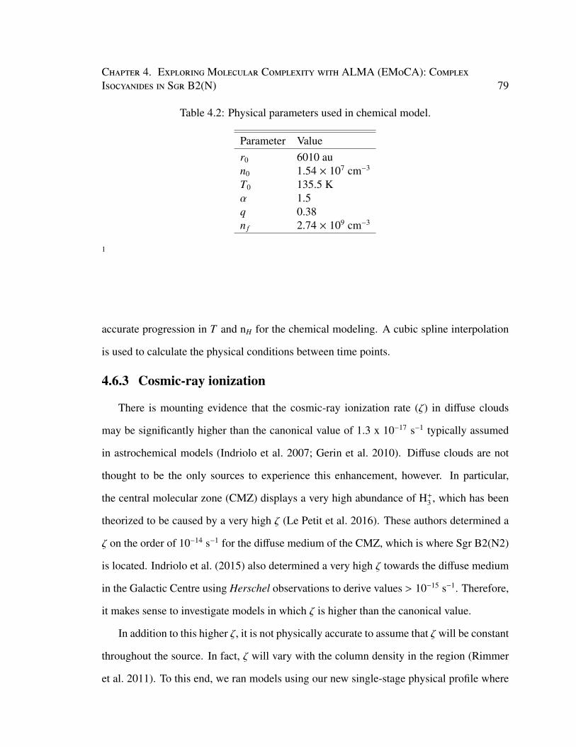
Chapter 4. ExploringMolecular Complexity with ALMA (EMoCA): ComplexIsocyanides in Sgr B2(N) 79
Table 4.2: Physical parameters used in chemical model.
Parameter Valuer0 6010 aun0 1.54 × 107 cm−3
T0 135.5 Kα 1.5q 0.38n f 2.74 × 109 cm−3
1
accurate progression in T and nH for the chemical modeling. A cubic spline interpolation
is used to calculate the physical conditions between time points.
4.6.3 Cosmic-ray ionization
There is mounting evidence that the cosmic-ray ionization rate (ζ) in diffuse clouds
may be significantly higher than the canonical value of 1.3 x 10⁻¹⁷ s−1 typically assumed
in astrochemical models (Indriolo et al. 2007; Gerin et al. 2010). Diffuse clouds are not
thought to be the only sources to experience this enhancement, however. In particular,
the central molecular zone (CMZ) displays a very high abundance of H+3 , which has been
theorized to be caused by a very high ζ (Le Petit et al. 2016). These authors determined a
ζ on the order of 10−14 s−1 for the diffuse medium of the CMZ, which is where Sgr B2(N2)
is located. Indriolo et al. (2015) also determined a very high ζ towards the diffuse medium
in the Galactic Centre using Herschel observations to derive values > 10−15 s−1. Therefore,
it makes sense to investigate models in which ζ is higher than the canonical value.
In addition to this higher ζ, it is not physically accurate to assume that ζ will be constant
throughout the source. In fact, ζ will vary with the column density in the region (Rimmer
et al. 2011). To this end, we ran models using our new single-stage physical profile where
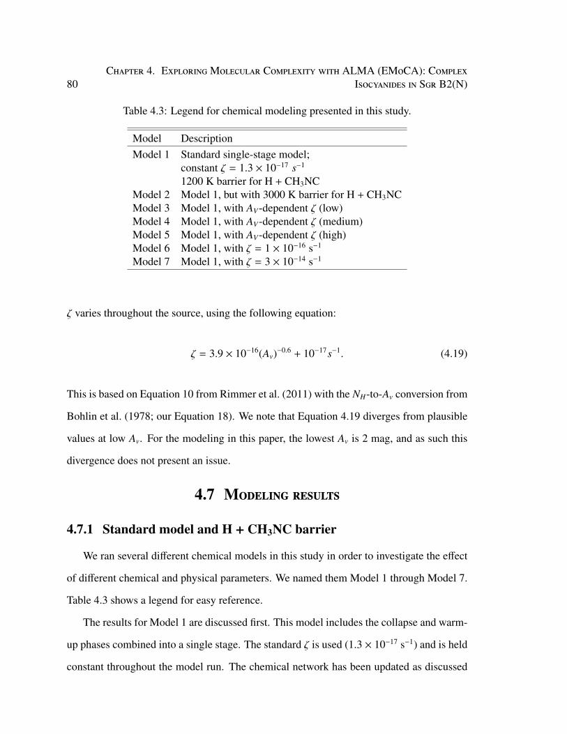
80Chapter 4. ExploringMolecular Complexity with ALMA (EMoCA): Complex
Isocyanides in Sgr B2(N)
Table 4.3: Legend for chemical modeling presented in this study.
Model DescriptionModel 1 Standard single-stage model;
constant ζ = 1.3 × 10⁻¹⁷ s−1
1200 K barrier for H + CH3NCModel 2 Model 1, but with 3000 K barrier for H + CH3NCModel 3 Model 1, with AV-dependent ζ (low)Model 4 Model 1, with AV-dependent ζ (medium)Model 5 Model 1, with AV-dependent ζ (high)Model 6 Model 1, with ζ = 1 × 10⁻¹⁶ s−1
Model 7 Model 1, with ζ = 3 × 10⁻¹⁴ s−1
ζ varies throughout the source, using the following equation:
ζ = 3.9 × 10⁻¹⁶(Av)−0.6 + 10−17s−1. (4.19)
This is based on Equation 10 from Rimmer et al. (2011) with the NH-to-Av conversion from
Bohlin et al. (1978; our Equation 18). We note that Equation 4.19 diverges from plausible
values at low Av. For the modeling in this paper, the lowest Av is 2 mag, and as such this
divergence does not present an issue.
4.7 Modeling results
4.7.1 Standard model and H + CH3NC barrier
We ran several different chemical models in this study in order to investigate the effect
of different chemical and physical parameters. We named them Model 1 through Model 7.
Table 4.3 shows a legend for easy reference.
The results for Model 1 are discussed first. This model includes the collapse and warm-
up phases combined into a single stage. The standard ζ is used (1.3 × 10⁻¹⁷ s−1) and is held
constant throughout the model run. The chemical network has been updated as discussed
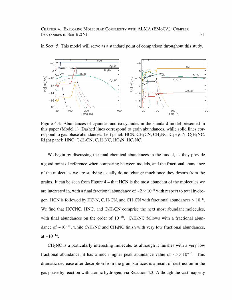
Chapter 4. ExploringMolecular Complexity with ALMA (EMoCA): ComplexIsocyanides in Sgr B2(N) 81
in Sect. 5. This model will serve as a standard point of comparison throughout this study.
Figure 4.4: Abundances of cyanides and isocyanides in the standard model presented inthis paper (Model 1). Dashed lines correspond to grain abundances, while solid lines cor-respond to gas-phase abundances. Left panel: HCN, CH3CN, CH3NC, C2H5CN, C2H5NC.Right panel: HNC, C2H3CN, C2H3NC, HC3N, HC2NC.
We begin by discussing the final chemical abundances in the model, as they provide
a good point of reference when comparing between models, and the fractional abundance
of the molecules we are studying usually do not change much once they desorb from the
grains. It can be seen from Figure 4.4 that HCN is the most abundant of the molecules we
are interested in, with a final fractional abundance of ∼2 × 10⁻⁶ with respect to total hydro-
gen. HCN is followed by HC3N, C2H5CN, and CH3CN with fractional abundances > 10−8.
We find that HCCNC, HNC, and C2H3CN comprise the next most abundant molecules,
with final abundances on the order of 10−10. C2H5NC follows with a fractional abun-
dance of ∼10−11, while C2H3NC and CH3NC finish with very low fractional abundances,
at ∼10−14.
CH3NC is a particularly interesting molecule, as although it finishes with a very low
fractional abundance, it has a much higher peak abundance value of ∼5 × 10⁻¹⁰. This
dramatic decrease after desorption from the grain surfaces is a result of destruction in the
gas phase by reaction with atomic hydrogen, via Reaction 4.3. Although the vast majority
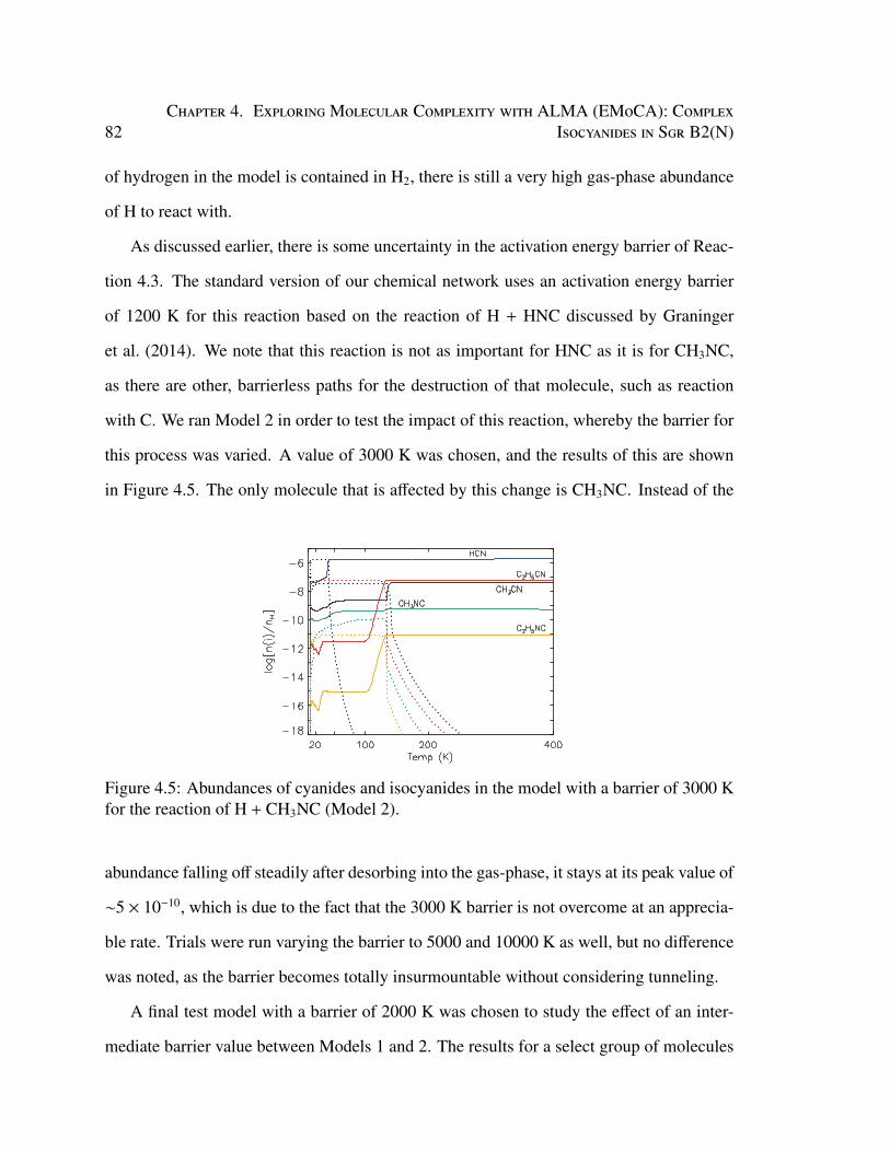
82Chapter 4. ExploringMolecular Complexity with ALMA (EMoCA): Complex
Isocyanides in Sgr B2(N)
of hydrogen in the model is contained in H2, there is still a very high gas-phase abundance
of H to react with.
As discussed earlier, there is some uncertainty in the activation energy barrier of Reac-
tion 4.3. The standard version of our chemical network uses an activation energy barrier
of 1200 K for this reaction based on the reaction of H + HNC discussed by Graninger
et al. (2014). We note that this reaction is not as important for HNC as it is for CH3NC,
as there are other, barrierless paths for the destruction of that molecule, such as reaction
with C. We ran Model 2 in order to test the impact of this reaction, whereby the barrier for
this process was varied. A value of 3000 K was chosen, and the results of this are shown
in Figure 4.5. The only molecule that is affected by this change is CH3NC. Instead of the
Figure 4.5: Abundances of cyanides and isocyanides in the model with a barrier of 3000 Kfor the reaction of H + CH3NC (Model 2).
abundance falling off steadily after desorbing into the gas-phase, it stays at its peak value of
∼5 × 10⁻¹⁰, which is due to the fact that the 3000 K barrier is not overcome at an apprecia-
ble rate. Trials were run varying the barrier to 5000 and 10000 K as well, but no difference
was noted, as the barrier becomes totally insurmountable without considering tunneling.
A final test model with a barrier of 2000 K was chosen to study the effect of an inter-
mediate barrier value between Models 1 and 2. The results for a select group of molecules
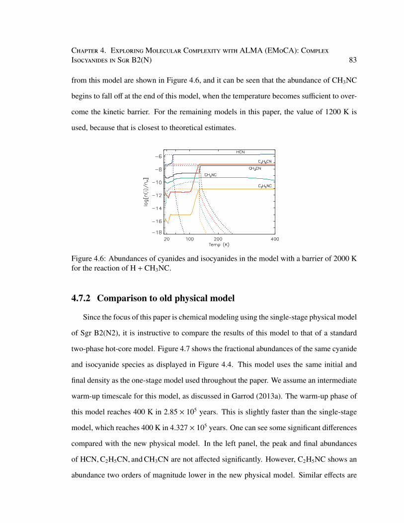
Chapter 4. ExploringMolecular Complexity with ALMA (EMoCA): ComplexIsocyanides in Sgr B2(N) 83
from this model are shown in Figure 4.6, and it can be seen that the abundance of CH3NC
begins to fall off at the end of this model, when the temperature becomes sufficient to over-
come the kinetic barrier. For the remaining models in this paper, the value of 1200 K is
used, because that is closest to theoretical estimates.
Figure 4.6: Abundances of cyanides and isocyanides in the model with a barrier of 2000 Kfor the reaction of H + CH3NC.
4.7.2 Comparison to old physical model
Since the focus of this paper is chemical modeling using the single-stage physical model
of Sgr B2(N2), it is instructive to compare the results of this model to that of a standard
two-phase hot-core model. Figure 4.7 shows the fractional abundances of the same cyanide
and isocyanide species as displayed in Figure 4.4. This model uses the same initial and
final density as the one-stage model used throughout the paper. We assume an intermediate
warm-up timescale for this model, as discussed in Garrod (2013a). The warm-up phase of
this model reaches 400 K in 2.85 × 10⁵ years. This is slightly faster than the single-stage
model, which reaches 400 K in 4.327 × 10⁵ years. One can see some significant differences
compared with the new physical model. In the left panel, the peak and final abundances
of HCN, C2H5CN, and CH3CN are not affected significantly. However, C2H5NC shows an
abundance two orders of magnitude lower in the new physical model. Similar effects are
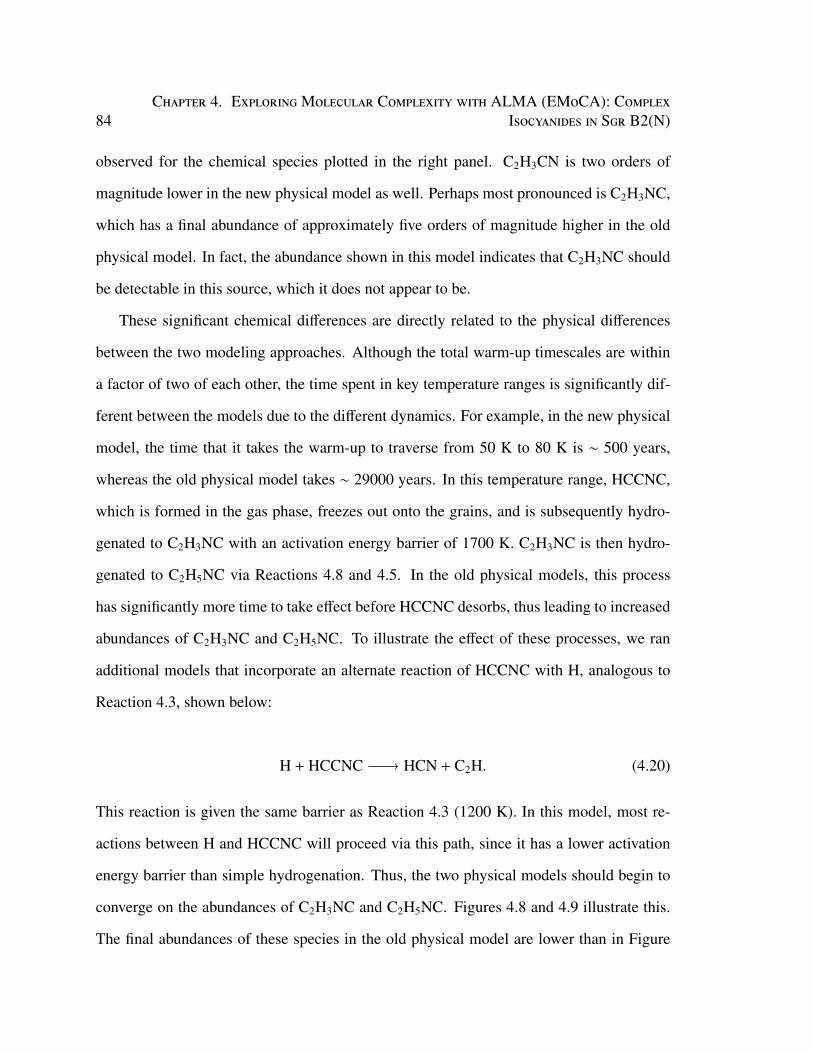
84Chapter 4. ExploringMolecular Complexity with ALMA (EMoCA): Complex
Isocyanides in Sgr B2(N)
observed for the chemical species plotted in the right panel. C2H3CN is two orders of
magnitude lower in the new physical model as well. Perhaps most pronounced is C2H3NC,
which has a final abundance of approximately five orders of magnitude higher in the old
physical model. In fact, the abundance shown in this model indicates that C2H3NC should
be detectable in this source, which it does not appear to be.
These significant chemical differences are directly related to the physical differences
between the two modeling approaches. Although the total warm-up timescales are within
a factor of two of each other, the time spent in key temperature ranges is significantly dif-
ferent between the models due to the different dynamics. For example, in the new physical
model, the time that it takes the warm-up to traverse from 50 K to 80 K is ∼ 500 years,
whereas the old physical model takes ∼ 29000 years. In this temperature range, HCCNC,
which is formed in the gas phase, freezes out onto the grains, and is subsequently hydro-
genated to C2H3NC with an activation energy barrier of 1700 K. C2H3NC is then hydro-
genated to C2H5NC via Reactions 4.8 and 4.5. In the old physical models, this process
has significantly more time to take effect before HCCNC desorbs, thus leading to increased
abundances of C2H3NC and C2H5NC. To illustrate the effect of these processes, we ran
additional models that incorporate an alternate reaction of HCCNC with H, analogous to
Reaction 4.3, shown below:
H + HCCNC HCN + C2H. (4.20)
This reaction is given the same barrier as Reaction 4.3 (1200 K). In this model, most re-
actions between H and HCCNC will proceed via this path, since it has a lower activation
energy barrier than simple hydrogenation. Thus, the two physical models should begin to
converge on the abundances of C2H3NC and C2H5NC. Figures 4.8 and 4.9 illustrate this.
The final abundances of these species in the old physical model are lower than in Figure
Chapter 4. ExploringMolecular Complexity with ALMA (EMoCA): ComplexIsocyanides in Sgr B2(N) 85
4.7, and the abundances in the new physical model are virtually unchanged from Figure
4.4. The reason the models do not converge perfectly is that there is still a small fraction
of HCCNC that is getting converted to C2H3NC in the old physical models, and there is
significantly more time for this process to occur. A very similar process is responsible for
the decreased abundance of C2H3CN in the new physical model, as this molecule is pre-
dominantly formed through hydrogenation of HC3N which is subject to the same timescale
effects as hydrogenation of HCCNC.
Other differences are noted as well. In general, the cold-phase chemistry of the cyanides
and isocyanides also appears to be much more efficient in the new physical model. In Figure
4.4 the ice-phase abundances of all of the molecules reach a peak at very low temperature
(∼20 K), whereas in the old models (Figure 4.7), the peak values for these same molecules
are not reached until much later (∼50 K). This seems to be a result of the amount of time
spent at low temperatures in the models. The new physical model takes significantly longer
to go from 15 K to 20 K (∼6.3 × 10⁴ years), whereas the old physical model spends only
∼ 1.2 × 10⁴ years in this temperature range. This longer timescale for collapse leads to
peak ice abundances being reached at lower temperatures, which has complex effects on
the chemistry. The new physical model used throughout this paper is more directly rele-
vant to the source structure of Sgr B2(N2), and a more accurate representation of hot-core
dynamics in general.
4.7.3 Cosmic-ray ionization rate
To test the effect of varying ζ on the fractional abundances of cyanides and isocyanides,
we ran three chemical models using Equation 4.19 to vary ζ throughout the source. The
magnitude of the AV multiplier was changed in each run. The chosen values of the mul-
tiplier were 3.9 × 10⁻¹⁶ (Model 3), 3.9 × 10⁻¹⁵ (Model 4), and 3.9 × 10⁻¹⁴ (Model 5). As
a further test of the effect of ζ on hot-core chemistry, we also ran two additional models
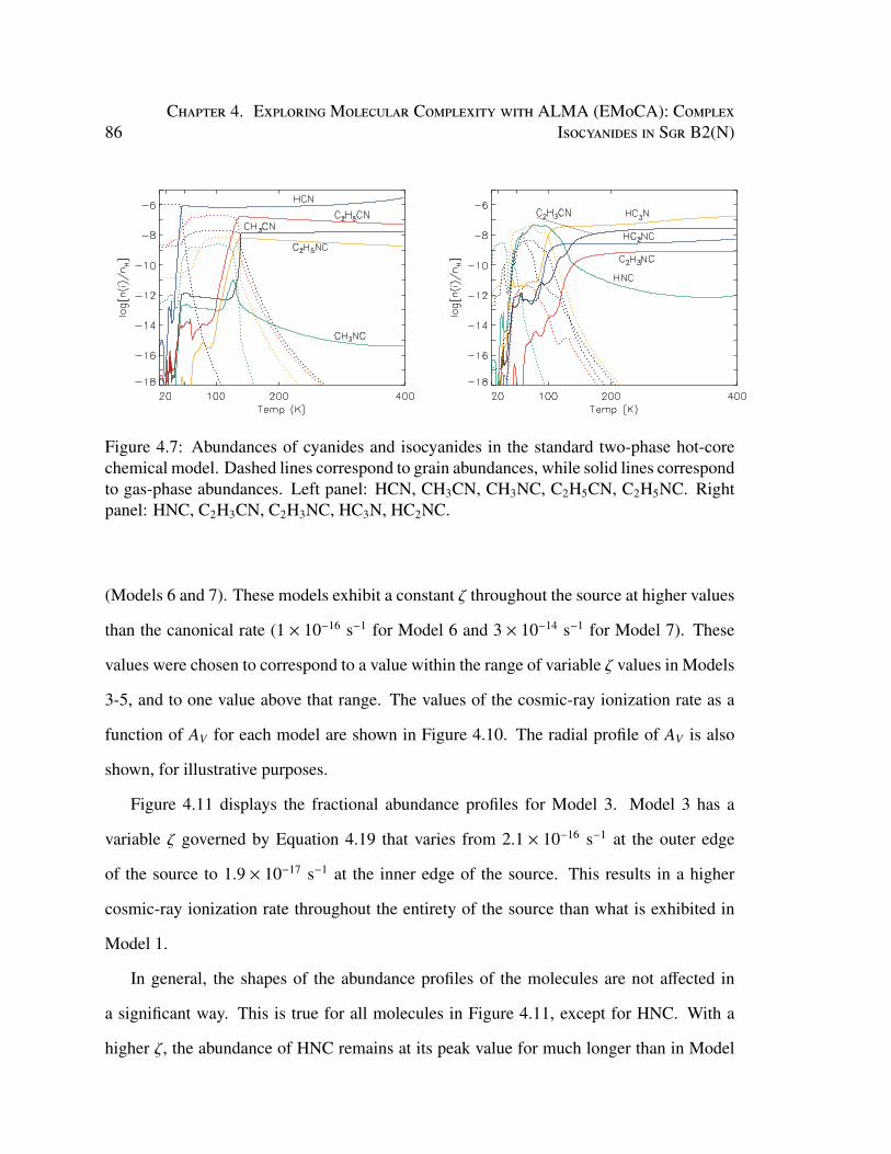
86Chapter 4. ExploringMolecular Complexity with ALMA (EMoCA): Complex
Isocyanides in Sgr B2(N)
Figure 4.7: Abundances of cyanides and isocyanides in the standard two-phase hot-corechemical model. Dashed lines correspond to grain abundances, while solid lines correspondto gas-phase abundances. Left panel: HCN, CH3CN, CH3NC, C2H5CN, C2H5NC. Rightpanel: HNC, C2H3CN, C2H3NC, HC3N, HC2NC.
(Models 6 and 7). These models exhibit a constant ζ throughout the source at higher values
than the canonical rate (1 × 10⁻¹⁶ s−1 for Model 6 and 3 × 10⁻¹⁴ s−1 for Model 7). These
values were chosen to correspond to a value within the range of variable ζ values in Models
3-5, and to one value above that range. The values of the cosmic-ray ionization rate as a
function of AV for each model are shown in Figure 4.10. The radial profile of AV is also
shown, for illustrative purposes.
Figure 4.11 displays the fractional abundance profiles for Model 3. Model 3 has a
variable ζ governed by Equation 4.19 that varies from 2.1 × 10⁻¹⁶ s−1 at the outer edge
of the source to 1.9 × 10⁻¹⁷ s−1 at the inner edge of the source. This results in a higher
cosmic-ray ionization rate throughout the entirety of the source than what is exhibited in
Model 1.
In general, the shapes of the abundance profiles of the molecules are not affected in
a significant way. This is true for all molecules in Figure 4.11, except for HNC. With a
higher ζ, the abundance of HNC remains at its peak value for much longer than in Model
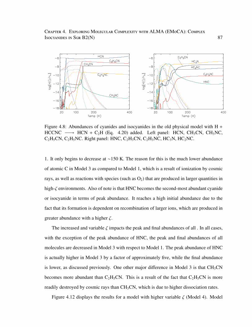
Chapter 4. ExploringMolecular Complexity with ALMA (EMoCA): ComplexIsocyanides in Sgr B2(N) 87
Figure 4.8: Abundances of cyanides and isocyanides in the old physical model with H +
HCCNC HCN + C2H (Eq. 4.20) added. Left panel: HCN, CH3CN, CH3NC,C2H5CN, C2H5NC. Right panel: HNC, C2H3CN, C2H3NC, HC3N, HC2NC.
1. It only begins to decrease at ∼150 K. The reason for this is the much lower abundance
of atomic C in Model 3 as compared to Model 1, which is a result of ionization by cosmic
rays, as well as reactions with species (such as O2) that are produced in larger quantities in
high-ζ environments. Also of note is that HNC becomes the second-most abundant cyanide
or isocyanide in terms of peak abundance. It reaches a high initial abundance due to the
fact that its formation is dependent on recombination of larger ions, which are produced in
greater abundance with a higher ζ.
The increased and variable ζ impacts the peak and final abundances of all . In all cases,
with the exception of the peak abundance of HNC, the peak and final abundances of all
molecules are decreased in Model 3 with respect to Model 1. The peak abundance of HNC
is actually higher in Model 3 by a factor of approximately five, while the final abundance
is lower, as discussed previously. One other major difference in Model 3 is that CH3CN
becomes more abundant than C2H5CN. This is a result of the fact that C2H5CN is more
readily destroyed by cosmic rays than CH3CN, which is due to higher dissociation rates.
Figure 4.12 displays the results for a model with higher variable ζ (Model 4). Model
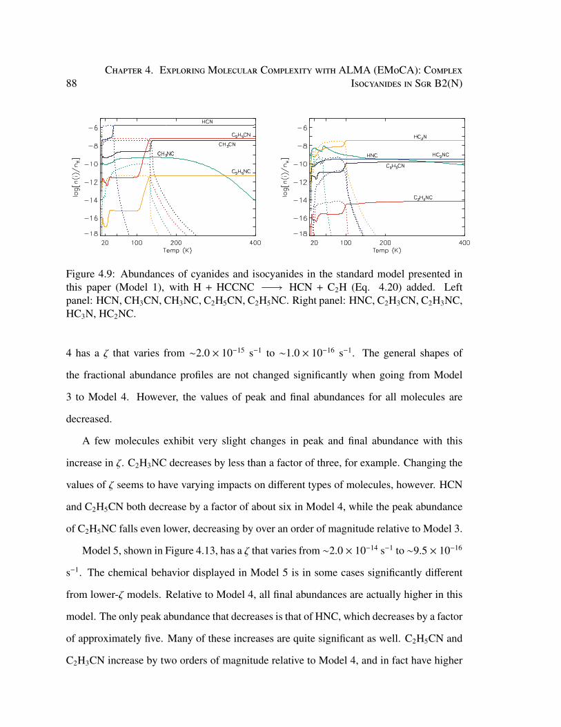
88Chapter 4. ExploringMolecular Complexity with ALMA (EMoCA): Complex
Isocyanides in Sgr B2(N)
Figure 4.9: Abundances of cyanides and isocyanides in the standard model presented inthis paper (Model 1), with H + HCCNC HCN + C2H (Eq. 4.20) added. Leftpanel: HCN, CH3CN, CH3NC, C2H5CN, C2H5NC. Right panel: HNC, C2H3CN, C2H3NC,HC3N, HC2NC.
4 has a ζ that varies from ∼2.0 × 10⁻¹⁵ s−1 to ∼1.0 × 10⁻¹⁶ s−1. The general shapes of
the fractional abundance profiles are not changed significantly when going from Model
3 to Model 4. However, the values of peak and final abundances for all molecules are
decreased.
A few molecules exhibit very slight changes in peak and final abundance with this
increase in ζ. C2H3NC decreases by less than a factor of three, for example. Changing the
values of ζ seems to have varying impacts on different types of molecules, however. HCN
and C2H5CN both decrease by a factor of about six in Model 4, while the peak abundance
of C2H5NC falls even lower, decreasing by over an order of magnitude relative to Model 3.
Model 5, shown in Figure 4.13, has a ζ that varies from ∼2.0 × 10⁻¹⁴ s−1 to ∼9.5 × 10⁻¹⁶
s−1. The chemical behavior displayed in Model 5 is in some cases significantly different
from lower-ζ models. Relative to Model 4, all final abundances are actually higher in this
model. The only peak abundance that decreases is that of HNC, which decreases by a factor
of approximately five. Many of these increases are quite significant as well. C2H5CN and
C2H3CN increase by two orders of magnitude relative to Model 4, and in fact have higher
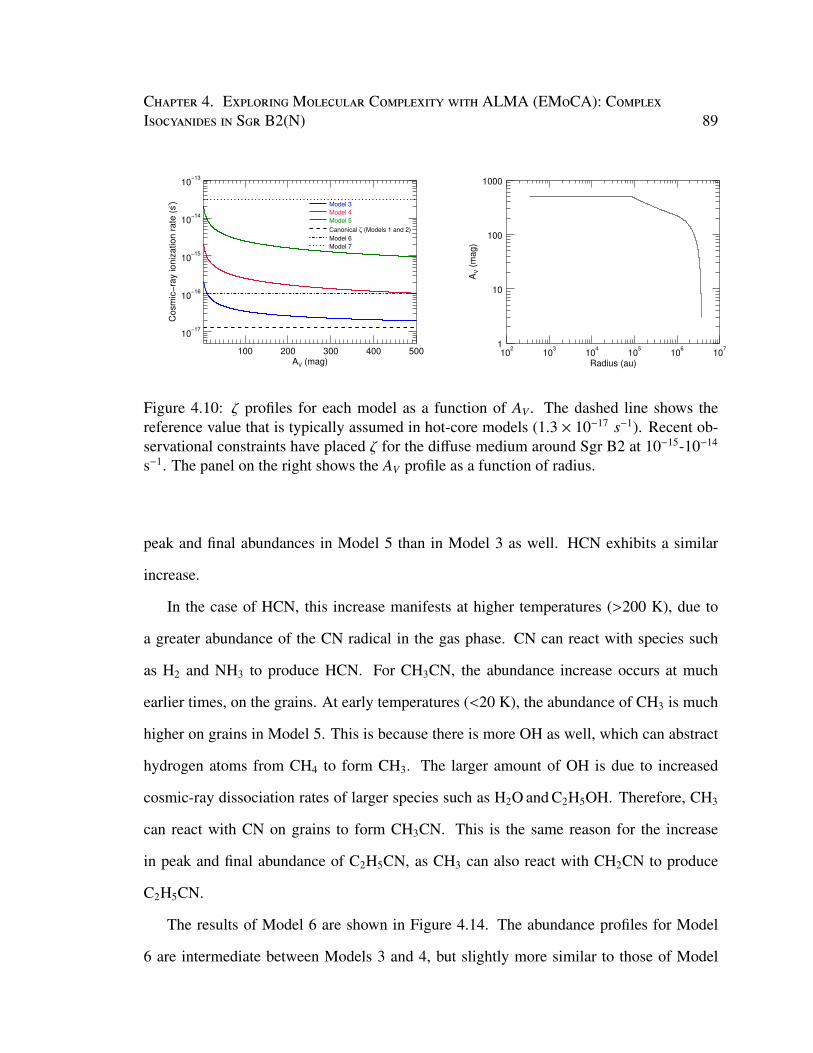
Chapter 4. ExploringMolecular Complexity with ALMA (EMoCA): ComplexIsocyanides in Sgr B2(N) 89
100 200 300 400 500AV (mag)
10−17
10−16
10−15
10−14
10−13
Cosm
ic−
ray io
niz
ation
rate
(s−
1 ) Model 3
Model 4
Model 5
Canonical ζ (Models 1 and 2)
Model 6
Model 7
102
103
104
105
106
107
Radius (au)
1
10
100
1000
AV (
mag)
Figure 4.10: ζ profiles for each model as a function of AV . The dashed line shows thereference value that is typically assumed in hot-core models (1.3 × 10⁻¹⁷ s−1). Recent ob-servational constraints have placed ζ for the diffuse medium around Sgr B2 at 10−15-10−14
s−1. The panel on the right shows the AV profile as a function of radius.
peak and final abundances in Model 5 than in Model 3 as well. HCN exhibits a similar
increase.
In the case of HCN, this increase manifests at higher temperatures (>200 K), due to
a greater abundance of the CN radical in the gas phase. CN can react with species such
as H2 and NH3 to produce HCN. For CH3CN, the abundance increase occurs at much
earlier times, on the grains. At early temperatures (<20 K), the abundance of CH3 is much
higher on grains in Model 5. This is because there is more OH as well, which can abstract
hydrogen atoms from CH4 to form CH3. The larger amount of OH is due to increased
cosmic-ray dissociation rates of larger species such as H2O and C2H5OH. Therefore, CH3
can react with CN on grains to form CH3CN. This is the same reason for the increase
in peak and final abundance of C2H5CN, as CH3 can also react with CH2CN to produce
C2H5CN.
The results of Model 6 are shown in Figure 4.14. The abundance profiles for Model
6 are intermediate between Models 3 and 4, but slightly more similar to those of Model
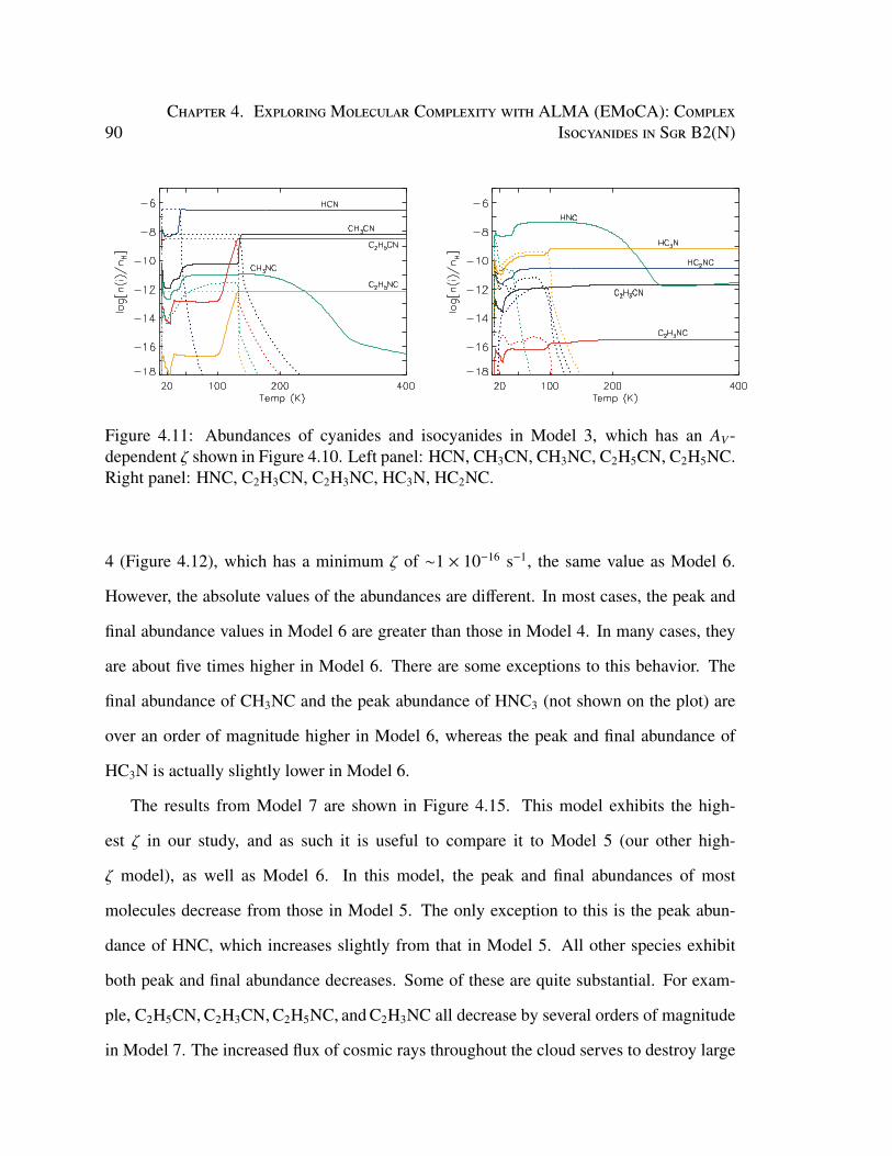
90Chapter 4. ExploringMolecular Complexity with ALMA (EMoCA): Complex
Isocyanides in Sgr B2(N)
Figure 4.11: Abundances of cyanides and isocyanides in Model 3, which has an AV-dependent ζ shown in Figure 4.10. Left panel: HCN, CH3CN, CH3NC, C2H5CN, C2H5NC.Right panel: HNC, C2H3CN, C2H3NC, HC3N, HC2NC.
4 (Figure 4.12), which has a minimum ζ of ∼1 × 10⁻¹⁶ s−1, the same value as Model 6.
However, the absolute values of the abundances are different. In most cases, the peak and
final abundance values in Model 6 are greater than those in Model 4. In many cases, they
are about five times higher in Model 6. There are some exceptions to this behavior. The
final abundance of CH3NC and the peak abundance of HNC3 (not shown on the plot) are
over an order of magnitude higher in Model 6, whereas the peak and final abundance of
HC3N is actually slightly lower in Model 6.
The results from Model 7 are shown in Figure 4.15. This model exhibits the high-
est ζ in our study, and as such it is useful to compare it to Model 5 (our other high-
ζ model), as well as Model 6. In this model, the peak and final abundances of most
molecules decrease from those in Model 5. The only exception to this is the peak abun-
dance of HNC, which increases slightly from that in Model 5. All other species exhibit
both peak and final abundance decreases. Some of these are quite substantial. For exam-
ple, C2H5CN, C2H3CN, C2H5NC, and C2H3NC all decrease by several orders of magnitude
in Model 7. The increased flux of cosmic rays throughout the cloud serves to destroy large
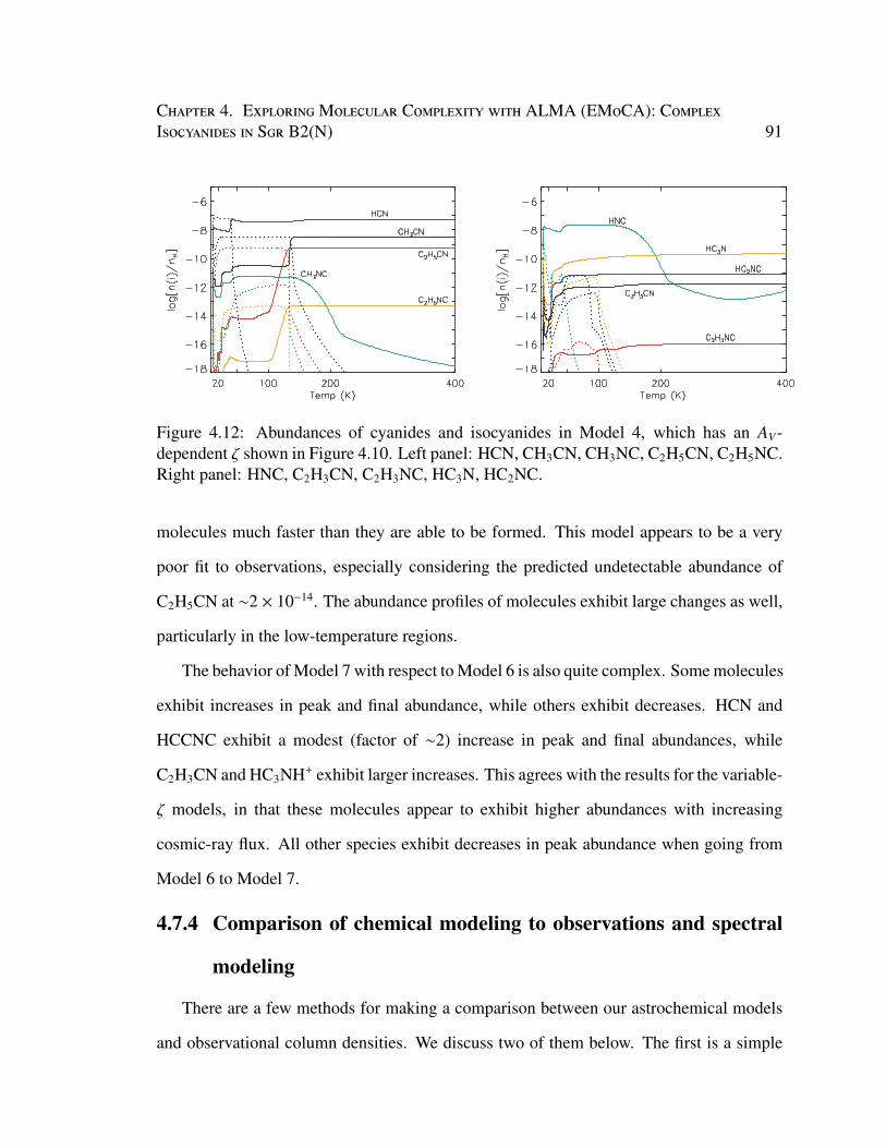
Chapter 4. ExploringMolecular Complexity with ALMA (EMoCA): ComplexIsocyanides in Sgr B2(N) 91
Figure 4.12: Abundances of cyanides and isocyanides in Model 4, which has an AV-dependent ζ shown in Figure 4.10. Left panel: HCN, CH3CN, CH3NC, C2H5CN, C2H5NC.Right panel: HNC, C2H3CN, C2H3NC, HC3N, HC2NC.
molecules much faster than they are able to be formed. This model appears to be a very
poor fit to observations, especially considering the predicted undetectable abundance of
C2H5CN at ∼2 × 10⁻¹⁴. The abundance profiles of molecules exhibit large changes as well,
particularly in the low-temperature regions.
The behavior of Model 7 with respect to Model 6 is also quite complex. Some molecules
exhibit increases in peak and final abundance, while others exhibit decreases. HCN and
HCCNC exhibit a modest (factor of ∼2) increase in peak and final abundances, while
C2H3CN and HC3NH+ exhibit larger increases. This agrees with the results for the variable-
ζ models, in that these molecules appear to exhibit higher abundances with increasing
cosmic-ray flux. All other species exhibit decreases in peak abundance when going from
Model 6 to Model 7.
4.7.4 Comparison of chemical modeling to observations and spectral
modeling
There are a few methods for making a comparison between our astrochemical models
and observational column densities. We discuss two of them below. The first is a simple
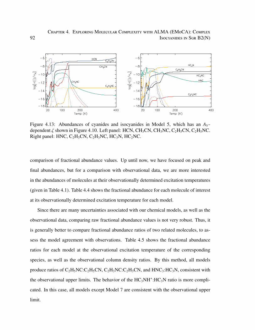
92Chapter 4. ExploringMolecular Complexity with ALMA (EMoCA): Complex
Isocyanides in Sgr B2(N)
Figure 4.13: Abundances of cyanides and isocyanides in Model 5, which has an AV-dependent ζ shown in Figure 4.10. Left panel: HCN, CH3CN, CH3NC, C2H5CN, C2H5NC.Right panel: HNC, C2H3CN, C2H3NC, HC3N, HC2NC.
comparison of fractional abundance values. Up until now, we have focused on peak and
final abundances, but for a comparison with observational data, we are more interested
in the abundances of molecules at their observationally determined excitation temperatures
(given in Table 4.1). Table 4.4 shows the fractional abundance for each molecule of interest
at its observationally determined excitation temperature for each model.
Since there are many uncertainties associated with our chemical models, as well as the
observational data, comparing raw fractional abundance values is not very robust. Thus, it
is generally better to compare fractional abundance ratios of two related molecules, to as-
sess the model agreement with observations. Table 4.5 shows the fractional abundance
ratios for each model at the observational excitation temperature of the corresponding
species, as well as the observational column density ratios. By this method, all models
produce ratios of C2H5NC:C2H5CN, C2H3NC:C2H3CN, and HNC3:HC3N, consistent with
the observational upper limits. The behavior of the HC3NH+:HC3N ratio is more compli-
cated. In this case, all models except Model 7 are consistent with the observational upper
limit.
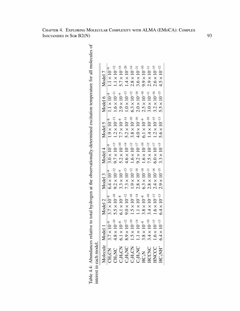
Chapter 4. ExploringMolecular Complexity with ALMA (EMoCA): ComplexIsocyanides in Sgr B2(N) 93
Tabl
e4.
4:A
bund
ance
sre
lativ
eto
tota
lhyd
roge
nat
the
obse
rvat
iona
lly-d
eter
min
edex
cita
tion
tem
pera
ture
for
allm
olec
ules
ofin
tere
stin
each
mod
el.
Mol
ecul
eM
odel
1M
odel
2M
odel
3M
odel
4M
odel
5M
odel
6M
odel
7C
H3C
N3.
7×
10−
83.
7×
10−
86.
4×
10−
93.
0×
10−
91.
9×
10−
81.
1×
10−
81.
1×
10−
9
CH
3NC
4.8×
10−
105.
5×
10−
109.
2×
10−
129.
7×
10−
131.
2×
10−
131.
6×
10−
111.
1×
10−
12
C2H
5CN
6.1×
10−
86.
1×
10−
83.
3×
10−
95.
2×
10−
107.
7×
10−
82.
9×
10−
95.
7×
10−
14
C2H
5NC
8.9×
10−
129.
0×
10−
127.
3×
10−
134.
6×
10−
145.
2×
10−
141.
0×
10−
131.
4×
10−
20
C2H
3CN
1.5×
10−
101.
5×
10−
101.
9×
10−
121.
6×
10−
123.
8×
10−
106.
3×
10−
122.
8×
10−
14
C2H
3NC
1.1×
10−
141.
1×
10−
142.
8×
10−
169.
2×
10−
174.
0×
10−
162.
0×
10−
163.
6×
10−
21
HC
3N3.
8×
10−
83.
8×
10−
86.
3×
10−
101.
6×
10−
106.
1×
10−
92.
5×
10−
109.
9×
10−
10
HC
CN
C3.
4×
10−
103.
4×
10−
102.
8×
10−
117.
5×
10−
121.
4×
10−
103.
0×
10−
112.
9×
10−
11
HN
CC
C1.
6×
10−
131.
6×
10−
132.
4×
10−
166.
0×
10−
171.
2×
10−
153.
2×
10−
162.
6×
10−
15
HC
3NH
+6.
4×
10−
136.
4×
10−
132.
9×
10−
153.
3×
10−
155.
6×
10−
135.
5×
10−
154.
5×
10−
12
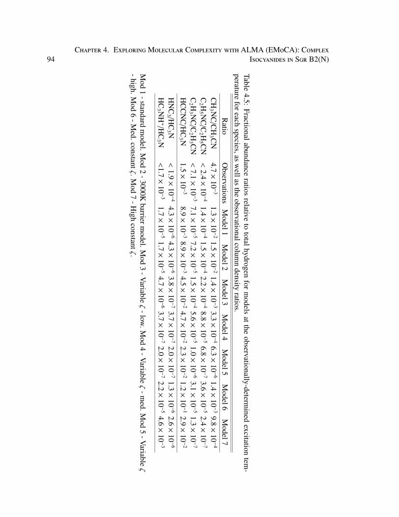
94Chapter 4. ExploringMolecular Complexity with ALMA (EMoCA): Complex
Isocyanides in Sgr B2(N)
Table4.5:
Fractionalabundanceratios
relativeto
totalhydrogenfor
models
attheobservationally-determ
inedexcitation
tem-
peratureforeach
species,asw
ellasthe
observationalcolumn
densityratios.
Ratio
Observations
Model1
Model2
Model3
Model4
Model5
Model6
Model7
CH
3 NC
/CH
3 CN
4.7×
10−
31.3×
10−
21.5×
10−
21.4×
10−
33.3×
10−
46.3×
10−
61.4×
10−
39.8×
10−
4
C2 H
5 NC
/C2 H
5 CN
<2.4×
10−
41.4×
10−
41.5×
10−
42.2×
10−
48.8×
10−
56.8×
10−
73.6×
10−
52.4×
10−
7
C2 H
3 NC
/C2 H
3 CN
<7.1×
10−
37.1×
10−
57.2×
10−
51.5×
10−
45.6×
10−
51.0×
10−
63.1×
10−
51.3×
10−
7
HC
CN
C/H
C3 N
1.5×
10−
38.9×
10−
38.9×
10−
34.5×
10−
24.7×
10−
22.3×
10−
21.2×
10−
12.9×
10−
2
HN
C3 /H
C3 N
<1.9×
10−
44.3×
10−
64.3×
10−
63.8×
10−
73.7×
10−
72.0×
10−
71.3×
10−
62.6×
10−
6
HC
3 NH
+/H
C3 N
<1.7×
10−
31.7×
10−
51.7×
10−
54.7×
10−
63.7×
10−
72.0×
10−
72.2×
10−
54.6×
10−
3
Mod
1-standard
model.M
od2
-3000Kbarrierm
odel.Mod
3-V
ariableζ
-low.M
od4
-Variable
ζ-m
ed.Mod
5-V
ariableζ
-high.Mod
6-M
ed.constantζ.M
od7
-High
constantζ.
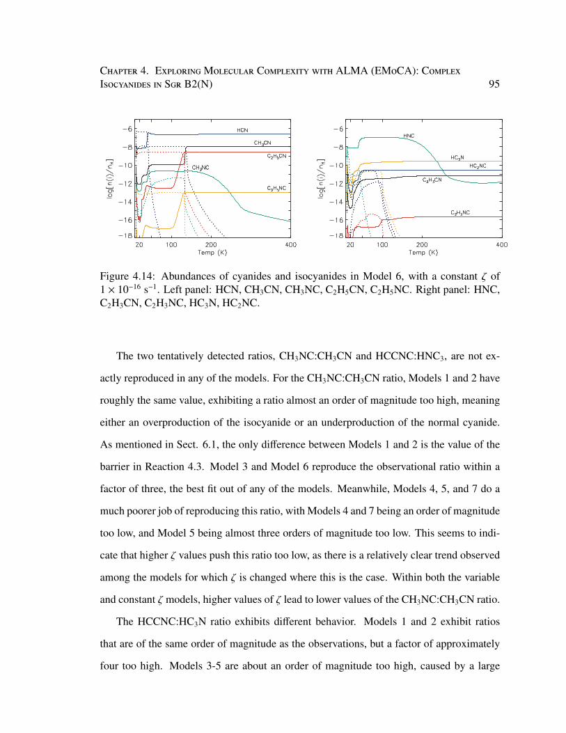
Chapter 4. ExploringMolecular Complexity with ALMA (EMoCA): ComplexIsocyanides in Sgr B2(N) 95
Figure 4.14: Abundances of cyanides and isocyanides in Model 6, with a constant ζ of1 × 10−16 s−1. Left panel: HCN, CH3CN, CH3NC, C2H5CN, C2H5NC. Right panel: HNC,C2H3CN, C2H3NC, HC3N, HC2NC.
The two tentatively detected ratios, CH3NC:CH3CN and HCCNC:HNC3, are not ex-
actly reproduced in any of the models. For the CH3NC:CH3CN ratio, Models 1 and 2 have
roughly the same value, exhibiting a ratio almost an order of magnitude too high, meaning
either an overproduction of the isocyanide or an underproduction of the normal cyanide.
As mentioned in Sect. 6.1, the only difference between Models 1 and 2 is the value of the
barrier in Reaction 4.3. Model 3 and Model 6 reproduce the observational ratio within a
factor of three, the best fit out of any of the models. Meanwhile, Models 4, 5, and 7 do a
much poorer job of reproducing this ratio, with Models 4 and 7 being an order of magnitude
too low, and Model 5 being almost three orders of magnitude too low. This seems to indi-
cate that higher ζ values push this ratio too low, as there is a relatively clear trend observed
among the models for which ζ is changed where this is the case. Within both the variable
and constant ζ models, higher values of ζ lead to lower values of the CH3NC:CH3CN ratio.
The HCCNC:HC3N ratio exhibits different behavior. Models 1 and 2 exhibit ratios
that are of the same order of magnitude as the observations, but a factor of approximately
four too high. Models 3-5 are about an order of magnitude too high, caused by a large
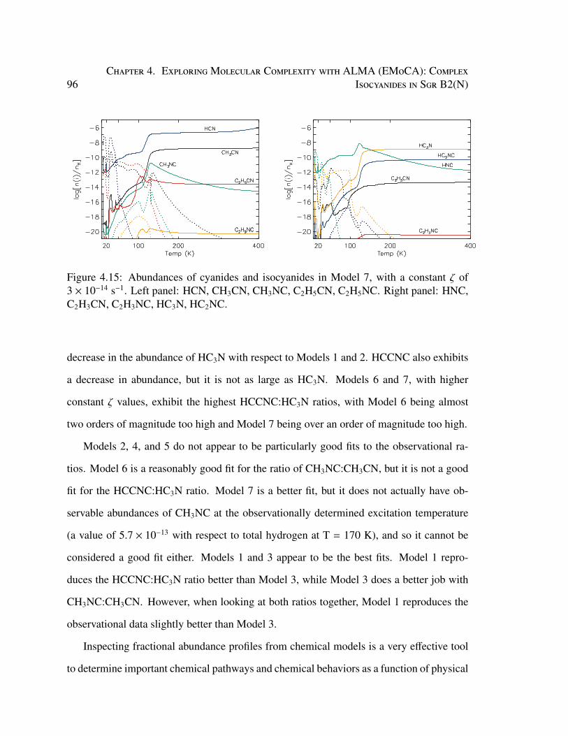
96Chapter 4. ExploringMolecular Complexity with ALMA (EMoCA): Complex
Isocyanides in Sgr B2(N)
Figure 4.15: Abundances of cyanides and isocyanides in Model 7, with a constant ζ of3 × 10−14 s−1. Left panel: HCN, CH3CN, CH3NC, C2H5CN, C2H5NC. Right panel: HNC,C2H3CN, C2H3NC, HC3N, HC2NC.
decrease in the abundance of HC3N with respect to Models 1 and 2. HCCNC also exhibits
a decrease in abundance, but it is not as large as HC3N. Models 6 and 7, with higher
constant ζ values, exhibit the highest HCCNC:HC3N ratios, with Model 6 being almost
two orders of magnitude too high and Model 7 being over an order of magnitude too high.
Models 2, 4, and 5 do not appear to be particularly good fits to the observational ra-
tios. Model 6 is a reasonably good fit for the ratio of CH3NC:CH3CN, but it is not a good
fit for the HCCNC:HC3N ratio. Model 7 is a better fit, but it does not actually have ob-
servable abundances of CH3NC at the observationally determined excitation temperature
(a value of 5.7 × 10⁻¹³ with respect to total hydrogen at T = 170 K), and so it cannot be
considered a good fit either. Models 1 and 3 appear to be the best fits. Model 1 repro-
duces the HCCNC:HC3N ratio better than Model 3, while Model 3 does a better job with
CH3NC:CH3CN. However, when looking at both ratios together, Model 1 reproduces the
observational data slightly better than Model 3.
Inspecting fractional abundance profiles from chemical models is a very effective tool
to determine important chemical pathways and chemical behaviors as a function of physical
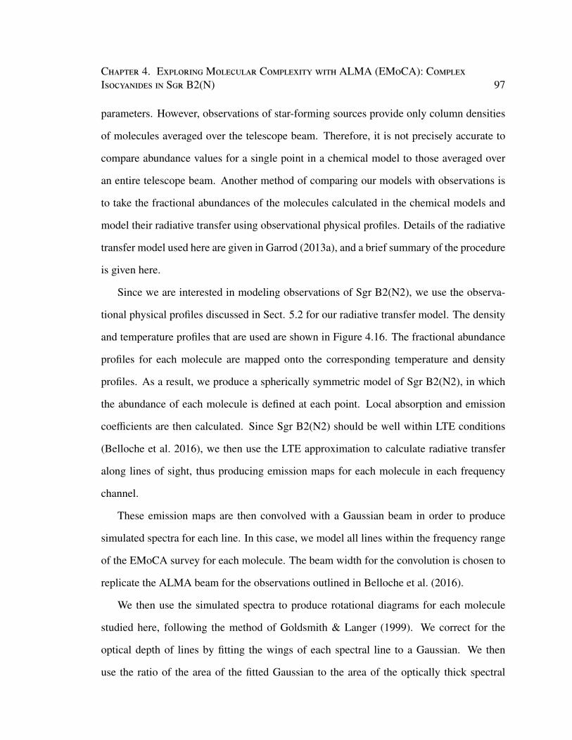
Chapter 4. ExploringMolecular Complexity with ALMA (EMoCA): ComplexIsocyanides in Sgr B2(N) 97
parameters. However, observations of star-forming sources provide only column densities
of molecules averaged over the telescope beam. Therefore, it is not precisely accurate to
compare abundance values for a single point in a chemical model to those averaged over
an entire telescope beam. Another method of comparing our models with observations is
to take the fractional abundances of the molecules calculated in the chemical models and
model their radiative transfer using observational physical profiles. Details of the radiative
transfer model used here are given in Garrod (2013a), and a brief summary of the procedure
is given here.
Since we are interested in modeling observations of Sgr B2(N2), we use the observa-
tional physical profiles discussed in Sect. 5.2 for our radiative transfer model. The density
and temperature profiles that are used are shown in Figure 4.16. The fractional abundance
profiles for each molecule are mapped onto the corresponding temperature and density
profiles. As a result, we produce a spherically symmetric model of Sgr B2(N2), in which
the abundance of each molecule is defined at each point. Local absorption and emission
coefficients are then calculated. Since Sgr B2(N2) should be well within LTE conditions
(Belloche et al. 2016), we then use the LTE approximation to calculate radiative transfer
along lines of sight, thus producing emission maps for each molecule in each frequency
channel.
These emission maps are then convolved with a Gaussian beam in order to produce
simulated spectra for each line. In this case, we model all lines within the frequency range
of the EMoCA survey for each molecule. The beam width for the convolution is chosen to
replicate the ALMA beam for the observations outlined in Belloche et al. (2016).
We then use the simulated spectra to produce rotational diagrams for each molecule
studied here, following the method of Goldsmith & Langer (1999). We correct for the
optical depth of lines by fitting the wings of each spectral line to a Gaussian. We then
use the ratio of the area of the fitted Gaussian to the area of the optically thick spectral
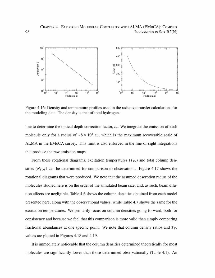
98Chapter 4. ExploringMolecular Complexity with ALMA (EMoCA): Complex
Isocyanides in Sgr B2(N)
102
103
104
105
106
107
Radius (au)
102
104
106
108
1010
Density (
cm
−3 )
102
103
104
105
106
107
Radius (au)
0
100
200
300
400
500
Tem
p (
K)
Figure 4.16: Density and temperature profiles used in the radiative transfer calculations forthe modeling data. The density is that of total hydrogen.
line to determine the optical depth correction factor, cτ. We integrate the emission of each
molecule only for a radius of ∼8 × 10⁴ au, which is the maximum recoverable scale of
ALMA in the EMoCA survey. This limit is also enforced in the line-of-sight integrations
that produce the raw emission maps.
From these rotational diagrams, excitation temperatures (TEx) and total column den-
sities (NTOT ) can be determined for comparison to observations. Figure 4.17 shows the
rotational diagrams that were produced. We note that the assumed desorption radius of the
molecules studied here is on the order of the simulated beam size, and, as such, beam dilu-
tion effects are negligible. Table 4.6 shows the column densities obtained from each model
presented here, along with the observational values, while Table 4.7 shows the same for the
excitation temperatures. We primarily focus on column densities going forward, both for
consistency and because we feel that this comparison is more valid than simply comparing
fractional abundances at one specific point. We note that column density ratios and TEx
values are plotted in Figures 4.18 and 4.19.
It is immediately noticeable that the column densities determined theoretically for most
molecules are significantly lower than those determined observationally (Table 4.1). An
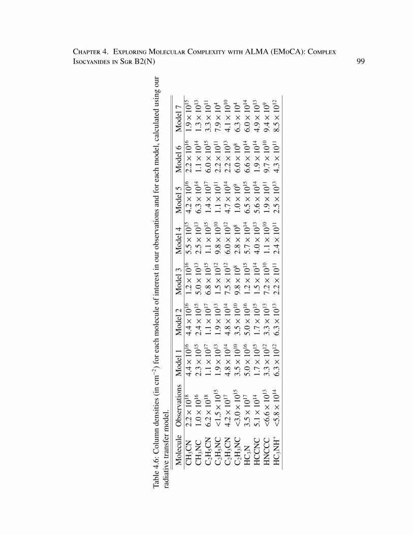
Chapter 4. ExploringMolecular Complexity with ALMA (EMoCA): ComplexIsocyanides in Sgr B2(N) 99
Tabl
e4.
6:C
olum
nde
nsiti
es(i
ncm−
2 )for
each
mol
ecul
eof
inte
rest
inou
robs
erva
tions
and
fore
ach
mod
el,c
alcu
late
dus
ing
our
radi
ativ
etr
ansf
erm
odel
.
Mol
ecul
eO
bser
vatio
nsM
odel
1M
odel
2M
odel
3M
odel
4M
odel
5M
odel
6M
odel
7C
H3C
N2.
2×
1018
4.4×
1016
4.4×
1016
1.2×
1016
5.5×
1015
4.2×
1016
2.2×
1016
1.9×
1015
CH
3NC
1.0×
1016
2.3×
1015
2.4×
1015
5.0×
1013
2.5×
1013
6.3×
1014
1.1×
1014
1.3×
1013
C2H
5CN
6.2×
1018
1.1×
1017
1.1×
1017
6.8×
1015
1.1×
1015
1.4×
1017
6.0×
1015
3.3×
1011
C2H
5NC
<1.
5×
1015
1.9×
1013
1.9×
1013
1.5×
1012
9.8×
1010
1.1×
1011
2.2×
1011
7.9×
104
C2H
3CN
4.2×
1017
4.8×
1014
4.8×
1014
7.5×
1012
6.0×
1012
4.7×
1014
2.2×
1013
4.1×
1010
C2H
3NC
<3.
0×
1015
3.5×
1010
3.5×
1010
9.8×
108
2.8×
108
1.0×
109
6.0×
108
6.3×
104
HC
3N3.
5×
1017
5.0×
1016
5.0×
1016
1.2×
1015
5.7×
1014
6.5×
1015
6.6×
1014
6.0×
1014
HC
CN
C5.
1×
1014
1.7×
1015
1.7×
1015
1.5×
1014
4.0×
1013
5.6×
1014
1.9×
1014
4.9×
1013
HN
CC
C<
6.6×
1013
3.3×
1012
3.3×
1013
7.2×
1010
1.1×
1010
1.9×
1011
9.7×
1010
9.4×
109
HC
3NH
+<
5.8×
1014
6.3×
1012
6.3×
1013
2.2×
1011
2.4×
1011
2.5×
1013
4.3×
1011
8.5×
1012
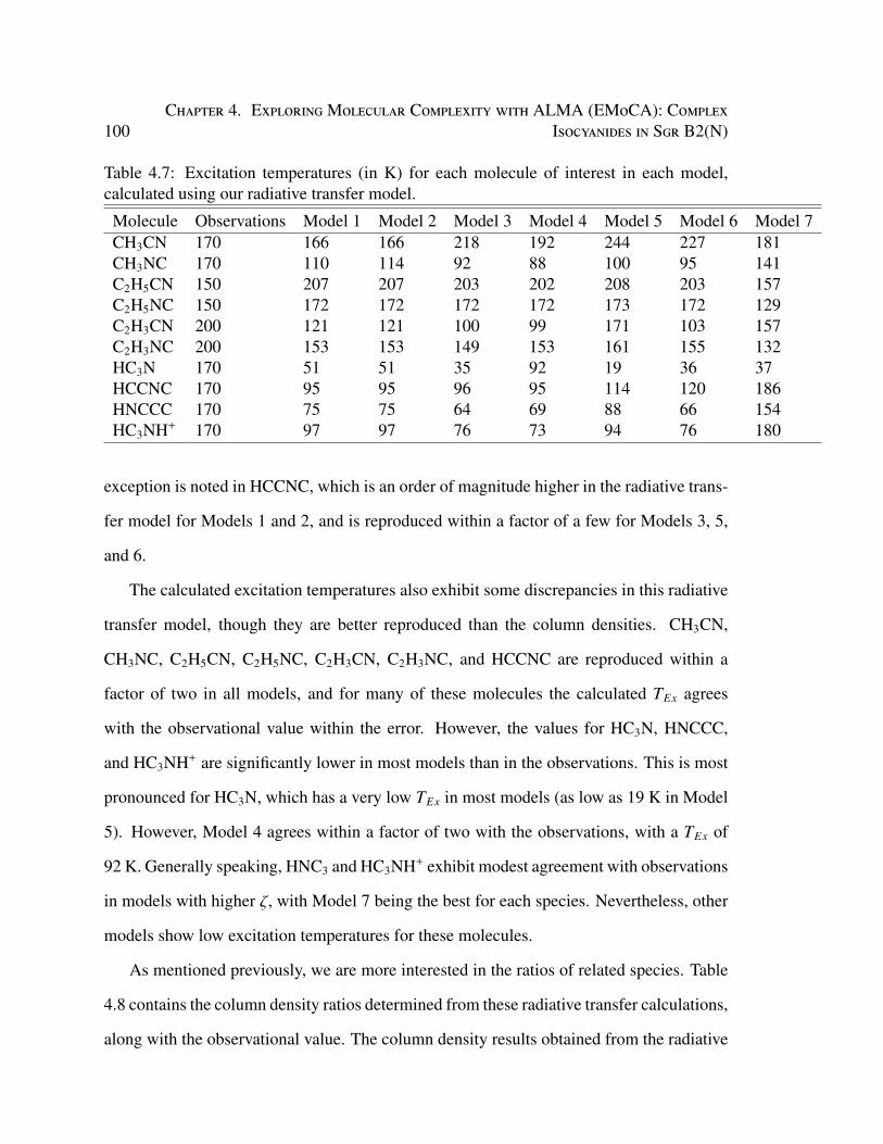
100Chapter 4. ExploringMolecular Complexity with ALMA (EMoCA): Complex
Isocyanides in Sgr B2(N)
Table 4.7: Excitation temperatures (in K) for each molecule of interest in each model,calculated using our radiative transfer model.
Molecule Observations Model 1 Model 2 Model 3 Model 4 Model 5 Model 6 Model 7CH3CN 170 166 166 218 192 244 227 181CH3NC 170 110 114 92 88 100 95 141C2H5CN 150 207 207 203 202 208 203 157C2H5NC 150 172 172 172 172 173 172 129C2H3CN 200 121 121 100 99 171 103 157C2H3NC 200 153 153 149 153 161 155 132HC3N 170 51 51 35 92 19 36 37HCCNC 170 95 95 96 95 114 120 186HNCCC 170 75 75 64 69 88 66 154HC3NH+ 170 97 97 76 73 94 76 180
exception is noted in HCCNC, which is an order of magnitude higher in the radiative trans-
fer model for Models 1 and 2, and is reproduced within a factor of a few for Models 3, 5,
and 6.
The calculated excitation temperatures also exhibit some discrepancies in this radiative
transfer model, though they are better reproduced than the column densities. CH3CN,
CH3NC, C2H5CN, C2H5NC, C2H3CN, C2H3NC, and HCCNC are reproduced within a
factor of two in all models, and for many of these molecules the calculated TEx agrees
with the observational value within the error. However, the values for HC3N, HNCCC,
and HC3NH+ are significantly lower in most models than in the observations. This is most
pronounced for HC3N, which has a very low TEx in most models (as low as 19 K in Model
5). However, Model 4 agrees within a factor of two with the observations, with a TEx of
92 K. Generally speaking, HNC3 and HC3NH+ exhibit modest agreement with observations
in models with higher ζ, with Model 7 being the best for each species. Nevertheless, other
models show low excitation temperatures for these molecules.
As mentioned previously, we are more interested in the ratios of related species. Table
4.8 contains the column density ratios determined from these radiative transfer calculations,
along with the observational value. The column density results obtained from the radiative
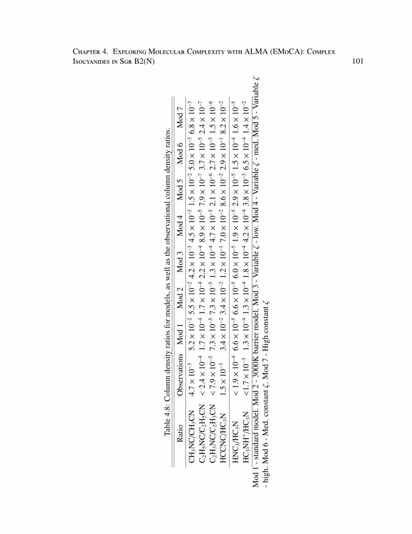
Chapter 4. ExploringMolecular Complexity with ALMA (EMoCA): ComplexIsocyanides in Sgr B2(N) 101
Tabl
e4.
8:C
olum
nde
nsity
ratio
sfo
rmod
els,
asw
ella
sth
eob
serv
atio
nalc
olum
nde
nsity
ratio
s.
Rat
ioO
bser
vatio
nsM
od1
Mod
2M
od3
Mod
4M
od5
Mod
6M
od7
CH
3NC
/CH
3CN
4.7×
10−
35.
2×
10−
25.
5×
10−
24.
2×
10−
34.
5×
10−
31.
5×
10−
25.
0×
10−
36.
8×
10−
3
C2H
5NC
/C2H
5CN
<2.
4×
10−
41.
7×
10−
41.
7×
10−
42.
2×
10−
48.
9×
10−
57.
9×
10−
73.
7×
10−
52.
4×
10−
7
C2H
3NC
/C2H
3CN
<7.
9×
10−
57.
3×
10−
57.
3×
10−
51.
3×
10−
44.
7×
10−
52.
1×
10−
62.
7×
10−
51.
5×
10−
6
HC
CN
C/H
C3N
1.5×
10−
33.
4×
10−
23.
4×
10−
21.
2×
10−
17.
0×
10−
28.
6×
10−
22.
9×
10−
18.
2×
10−
2
HN
C3/
HC
3N<
1.9×
10−
46.
6×
10−
56.
6×
10−
56.
0×
10−
51.
9×
10−
52.
9×
10−
51.
5×
10−
41.
6×
10−
5
HC
3NH
+/H
C3N
<1.
7×
10−
31.
3×
10−
41.
3×
10−
41.
8×
10−
44.
2×
10−
43.
8×
10−
36.
5×
10−
41.
4×
10−
2
Mod
1-s
tand
ard
mod
el.M
od2
-300
0Kba
rrie
rmod
el.M
od3
-Var
iabl
eζ
-low
.Mod
4-V
aria
bleζ
-med
.Mod
5-V
aria
bleζ
-hig
h.M
od6
-Med
.con
stan
tζ.M
od7
-Hig
hco
nsta
ntζ
102Chapter 4. ExploringMolecular Complexity with ALMA (EMoCA): Complex
Isocyanides in Sgr B2(N)
transfer modeling vary from model to model in most cases. For those column density
ratios for which we only have an upper limit, there is generally good agreement with obser-
vations. For C2H5NC:C2H5CN, Models 1-7 all agree with the observationally determined
upper limit of 2.4 × 10⁻⁴. All models also agree with the upper limit of 1.9 × 10⁻⁴ for
HNC3:HC3N. For C2H3NC:C2H3CN, Model 3 exhibits a column density ratio greater than
the observational upper limit, while all other models are in agreement with the upper limit.
For HC3NH+:HC3N, only Models 5 and 7 (those with very high ζ) do not agree with the
observational upper limit.
It is perhaps more useful to compare the column density ratios of CH3NC:CH3CN and
HCCNC:HC3N, since these pairs have observationally defined values of 4.7 × 10⁻³ and
1.5 × 10⁻³ respectively. CH3NC:CH3CN is remarkably well-produced by some of the ra-
diative transfer models presented here. For example, Models 3, 4, 6, and 7 are all within a
factor of two of the observational value, with Model 4 being almost an exact match. These
results provide evidence that a ζ higher than the canonical value of 1.3 × 10⁻¹⁷ s−1 is needed
to re-produce the CH3NC:CH3CN ratio for Sgr B2(N2).
The agreement for HCCNC:HC3N is generally much poorer across the models than for
CH3NC:CH3CN. All radiative transfer models overproduce this ratio by at least an order
of magnitude, with Models 1 and 2 showing the best-fit value of 3.4 × 10⁻², still a factor of
approximately 23 too high. This systematic over-production of HCCNC relative to HC3N
for all models, which was also seen in the fractional abundance values from Table 4.4, likely
means that there is something missing from our network in regards to the chemistry of these
molecules. Since Model 4 provides such a good fit to CH3NC:CH3CN, and is consistent
with all upper limits, we show the rotational diagrams for that model as a sample of the
output from our radiative transfer modeling in Figure 4.17.
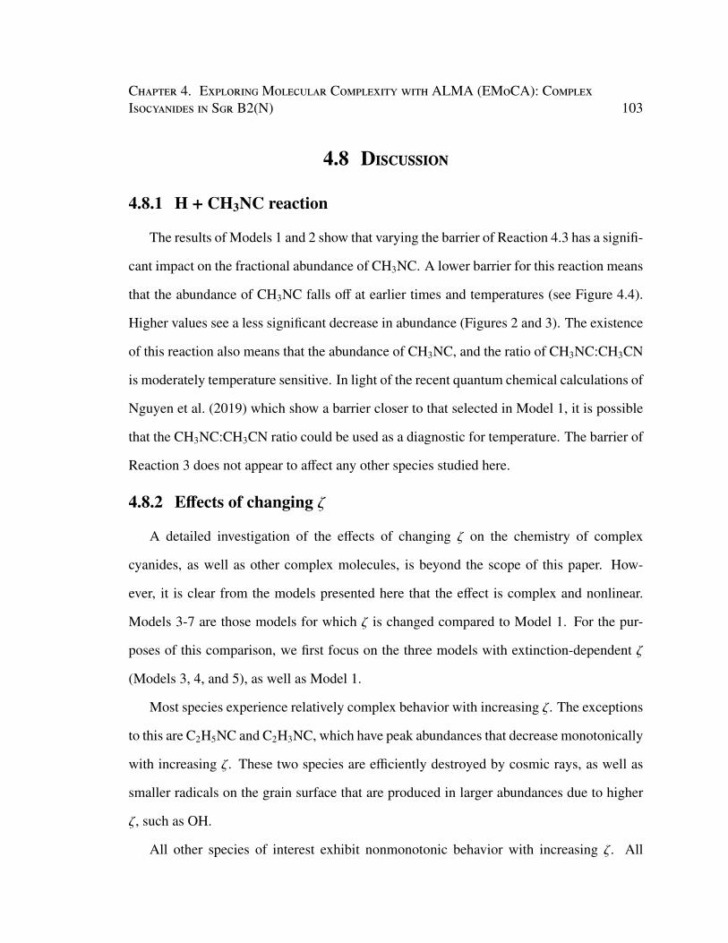
Chapter 4. ExploringMolecular Complexity with ALMA (EMoCA): ComplexIsocyanides in Sgr B2(N) 103
4.8 Discussion
4.8.1 H + CH3NC reaction
The results of Models 1 and 2 show that varying the barrier of Reaction 4.3 has a signifi-
cant impact on the fractional abundance of CH3NC. A lower barrier for this reaction means
that the abundance of CH3NC falls off at earlier times and temperatures (see Figure 4.4).
Higher values see a less significant decrease in abundance (Figures 2 and 3). The existence
of this reaction also means that the abundance of CH3NC, and the ratio of CH3NC:CH3CN
is moderately temperature sensitive. In light of the recent quantum chemical calculations of
Nguyen et al. (2019) which show a barrier closer to that selected in Model 1, it is possible
that the CH3NC:CH3CN ratio could be used as a diagnostic for temperature. The barrier of
Reaction 3 does not appear to affect any other species studied here.
4.8.2 Effects of changing ζ
A detailed investigation of the effects of changing ζ on the chemistry of complex
cyanides, as well as other complex molecules, is beyond the scope of this paper. How-
ever, it is clear from the models presented here that the effect is complex and nonlinear.
Models 3-7 are those models for which ζ is changed compared to Model 1. For the pur-
poses of this comparison, we first focus on the three models with extinction-dependent ζ
(Models 3, 4, and 5), as well as Model 1.
Most species experience relatively complex behavior with increasing ζ. The exceptions
to this are C2H5NC and C2H3NC, which have peak abundances that decrease monotonically
with increasing ζ. These two species are efficiently destroyed by cosmic rays, as well as
smaller radicals on the grain surface that are produced in larger abundances due to higher
ζ, such as OH.
All other species of interest exhibit nonmonotonic behavior with increasing ζ. All
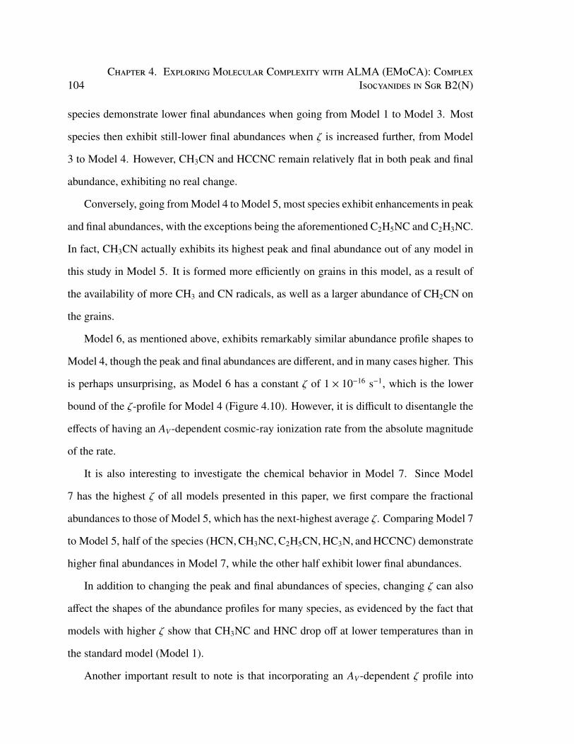
104Chapter 4. ExploringMolecular Complexity with ALMA (EMoCA): Complex
Isocyanides in Sgr B2(N)
species demonstrate lower final abundances when going from Model 1 to Model 3. Most
species then exhibit still-lower final abundances when ζ is increased further, from Model
3 to Model 4. However, CH3CN and HCCNC remain relatively flat in both peak and final
abundance, exhibiting no real change.
Conversely, going from Model 4 to Model 5, most species exhibit enhancements in peak
and final abundances, with the exceptions being the aforementioned C2H5NC and C2H3NC.
In fact, CH3CN actually exhibits its highest peak and final abundance out of any model in
this study in Model 5. It is formed more efficiently on grains in this model, as a result of
the availability of more CH3 and CN radicals, as well as a larger abundance of CH2CN on
the grains.
Model 6, as mentioned above, exhibits remarkably similar abundance profile shapes to
Model 4, though the peak and final abundances are different, and in many cases higher. This
is perhaps unsurprising, as Model 6 has a constant ζ of 1 × 10⁻¹⁶ s−1, which is the lower
bound of the ζ-profile for Model 4 (Figure 4.10). However, it is difficult to disentangle the
effects of having an AV-dependent cosmic-ray ionization rate from the absolute magnitude
of the rate.
It is also interesting to investigate the chemical behavior in Model 7. Since Model
7 has the highest ζ of all models presented in this paper, we first compare the fractional
abundances to those of Model 5, which has the next-highest average ζ. Comparing Model 7
to Model 5, half of the species (HCN, CH3NC, C2H5CN, HC3N, and HCCNC) demonstrate
higher final abundances in Model 7, while the other half exhibit lower final abundances.
In addition to changing the peak and final abundances of species, changing ζ can also
affect the shapes of the abundance profiles for many species, as evidenced by the fact that
models with higher ζ show that CH3NC and HNC drop off at lower temperatures than in
the standard model (Model 1).
Another important result to note is that incorporating an AV-dependent ζ profile into
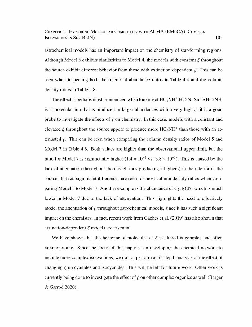
Chapter 4. ExploringMolecular Complexity with ALMA (EMoCA): ComplexIsocyanides in Sgr B2(N) 105
astrochemical models has an important impact on the chemistry of star-forming regions.
Although Model 6 exhibits similarities to Model 4, the models with constant ζ throughout
the source exhibit different behavior from those with extinction-dependent ζ. This can be
seen when inspecting both the fractional abundance ratios in Table 4.4 and the column
density ratios in Table 4.8.
The effect is perhaps most pronounced when looking at HC3NH+:HC3N. Since HC3NH+
is a molecular ion that is produced in larger abundances with a very high ζ, it is a good
probe to investigate the effects of ζ on chemistry. In this case, models with a constant and
elevated ζ throughout the source appear to produce more HC3NH+ than those with an at-
tenuated ζ. This can be seen when comparing the column density ratios of Model 5 and
Model 7 in Table 4.8. Both values are higher than the observational upper limit, but the
ratio for Model 7 is significantly higher (1.4 × 10⁻² vs. 3.8 × 10⁻³). This is caused by the
lack of attenuation throughout the model, thus producing a higher ζ in the interior of the
source. In fact, significant differences are seen for most column density ratios when com-
paring Model 5 to Model 7. Another example is the abundance of C2H5CN, which is much
lower in Model 7 due to the lack of attenuation. This highlights the need to effectively
model the attenuation of ζ throughout astrochemical models, since it has such a significant
impact on the chemistry. In fact, recent work from Gaches et al. (2019) has also shown that
extinction-dependent ζ models are essential.
We have shown that the behavior of molecules as ζ is altered is complex and often
nonmonotonic. Since the focus of this paper is on developing the chemical network to
include more complex isocyanides, we do not perform an in-depth analysis of the effect of
changing ζ on cyanides and isocyanides. This will be left for future work. Other work is
currently being done to investigate the effect of ζ on other complex organics as well (Barger
& Garrod 2020).
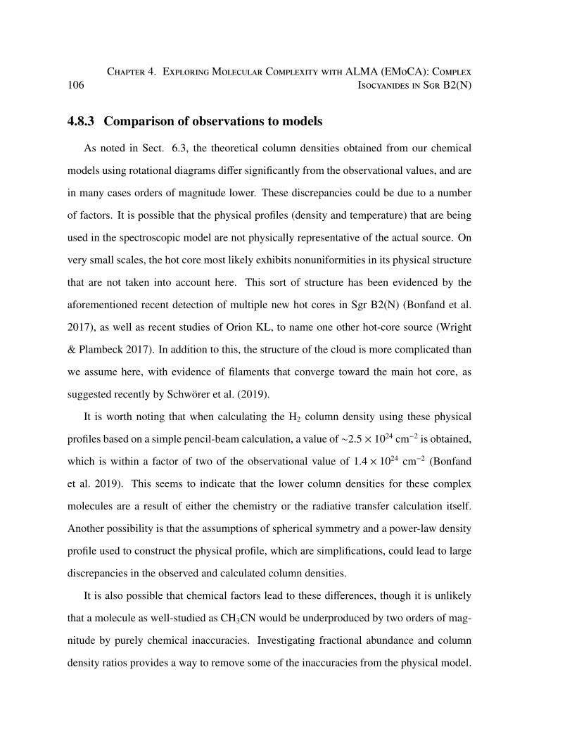
106Chapter 4. ExploringMolecular Complexity with ALMA (EMoCA): Complex
Isocyanides in Sgr B2(N)
4.8.3 Comparison of observations to models
As noted in Sect. 6.3, the theoretical column densities obtained from our chemical
models using rotational diagrams differ significantly from the observational values, and are
in many cases orders of magnitude lower. These discrepancies could be due to a number
of factors. It is possible that the physical profiles (density and temperature) that are being
used in the spectroscopic model are not physically representative of the actual source. On
very small scales, the hot core most likely exhibits nonuniformities in its physical structure
that are not taken into account here. This sort of structure has been evidenced by the
aforementioned recent detection of multiple new hot cores in Sgr B2(N) (Bonfand et al.
2017), as well as recent studies of Orion KL, to name one other hot-core source (Wright
& Plambeck 2017). In addition to this, the structure of the cloud is more complicated than
we assume here, with evidence of filaments that converge toward the main hot core, as
suggested recently by Schwörer et al. (2019).
It is worth noting that when calculating the H2 column density using these physical
profiles based on a simple pencil-beam calculation, a value of ∼2.5 × 1024 cm−2 is obtained,
which is within a factor of two of the observational value of 1.4 × 1024 cm−2 (Bonfand
et al. 2019). This seems to indicate that the lower column densities for these complex
molecules are a result of either the chemistry or the radiative transfer calculation itself.
Another possibility is that the assumptions of spherical symmetry and a power-law density
profile used to construct the physical profile, which are simplifications, could lead to large
discrepancies in the observed and calculated column densities.
It is also possible that chemical factors lead to these differences, though it is unlikely
that a molecule as well-studied as CH3CN would be underproduced by two orders of mag-
nitude by purely chemical inaccuracies. Investigating fractional abundance and column
density ratios provides a way to remove some of the inaccuracies from the physical model.
Chapter 4. ExploringMolecular Complexity with ALMA (EMoCA): ComplexIsocyanides in Sgr B2(N) 107
It is interesting to note the change that occurs in the R-NC:R-CN ratio when going
from the fractional abundance ratios to the column density ratios derived from the radiative
transfer model. For example, the CH3NC:CH3CN and HCCNC:HC3N ratios both increase
significantly in the rotational diagrams. This is because the rotational diagram method
includes a range of the abundance profiles of the species in the calculation. As mentioned
previously, we integrate out to a radius of ∼8 × 10⁴ au, or a temperature of ∼50 K, in our
chemical model. In both of these cases, at lower temperatures, the ratios between the NC
and CN molecules are higher, and thus the convolved ratios are higher than the values at a
specific temperature. The temperature dependence of these ratios is something that could
potentially be very useful as an observational probe in the future.
In general, it is useful to use both methods of observational comparison. Since ALMA
is not sensitive to the large-scale emission included in our radiative transfer models, the
column densities we obtain from our models are not directly comparable to those obtained
with ALMA, though we have attempted to minimize this issue by only integrating out to
ALMA’s maximum recoverable scale in our calculations. However, simply comparing a
fractional abundance ratio at a specific temperature is not robust on its own either, par-
ticularly for species that experience large abundance variations with temperature, such as
CH3NC. Therefore, using both methods allows us to a get a better idea for where our
models agree with observations and where improvement is needed.
Since the chemistry of CH3CN is the best-understood of the complex molecules studied
here, it is useful also to look at the column densities of species with respect to CH3CN, as
this can provide a clue as to which are least-well reproduced in our models. This of course
assumes that the chemistry that we have for CH3CN is correct in our network. Table 4.9
shows observational and theoretical column densities with respect to CH3CN for all models.
From looking at Table 4.9, it can be seen that we produce column densities with respect
to CH3CN that are consistent with the upper limits for most species that were not detected.
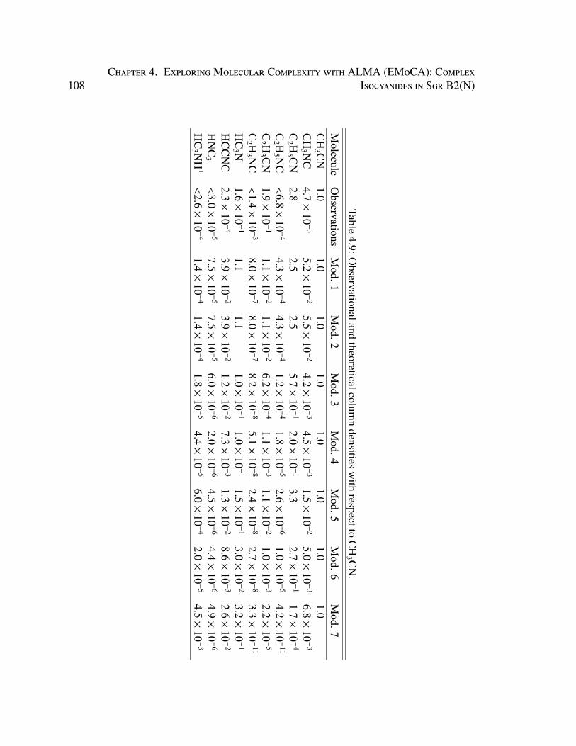
108Chapter 4. ExploringMolecular Complexity with ALMA (EMoCA): Complex
Isocyanides in Sgr B2(N)
Table4.9:O
bservationalandtheoreticalcolum
ndensities
with
respecttoC
H3 C
N.
Molecule
Observations
Mod.1
Mod.2
Mod.3
Mod.4
Mod.5
Mod.6
Mod.7
CH
3 CN
1.01.0
1.01.0
1.01.0
1.01.0
CH
3 NC
4.7×
10−
35.2×
10−
25.5×
10−
24.2×
10−
34.5×
10−
31.5×
10−
25.0×
10−
36.8×
10−
3
C2 H
5 CN
2.82.5
2.55.7×
10−
12.0×
10−
13.3
2.7×
10−
11.7×
10−
4
C2 H
5 NC
<6.8×
10−
44.3×
10−
44.3×
10−
41.2×
10−
41.8×
10−
52.6×
10−
61.0×
10−
54.2×
10−
11
C2 H
3 CN
1.9×
10−
11.1×
10−
21.1×
10−
26.2×
10−
41.1×
10−
31.1×
10−
21.0×
10−
32.2×
10−
5
C2 H
3 NC
<1.4×
10−
38.0×
10−
78.0×
10−
78.2×
10−
85.1×
10−
82.4×
10−
82.7×
10−
83.3×
10−
11
HC
3 N1.6×
10−
11.1
1.11.0×
10−
11.0×
10−
11.5×
10−
13.0×
10−
23.2×
10−
1
HC
CN
C2.3×
10−
43.9×
10−
23.9×
10−
21.2×
10−
27.3×
10−
31.3×
10−
28.6×
10−
32.6×
10−
2
HN
C3
<3.0×
10−
57.5×
10−
57.5×
10−
56.0×
10−
62.0×
10−
64.5×
10−
64.4×
10−
64.9×
10−
6
HC
3 NH
+<
2.6×
10−
41.4×
10−
41.4×
10−
41.8×
10−
54.4×
10−
56.0×
10−
42.0×
10−
54.5×
10−
3
Chapter 4. ExploringMolecular Complexity with ALMA (EMoCA): ComplexIsocyanides in Sgr B2(N) 109
Exceptions are seen for HNC3 in Models 1 and 2, and once again for HC3NH+, which is
overproduced in models with very high ζ. Although it is good that we are consistent with
these upper limits, no significant further information on the chemistry can be determined
from these ratios; detections of these species would allow us to make further constraints.
Regarding those species that are firmly detected, Models 1, 2, and 5 do a reasonably
good job of reproducing the ratio of C2H5CN:CH3CN, and Models 3-5 do the best job at
reproducing HC3N. The ratio of HCCNC to CH3CN is consistently higher in our models,
once again indicating that we are systematically overproducing HCCNC. This is something
that will be investigated in future studies. The opposite problem exists for C2H3CN, which
appears to be systematically underproduced relative to CH3CN in our models. Overall,
there appears to be a significant amount of work remaining on constraining the chemistry
of the cyanides and isocyanides in hot-core models.
Based on all of the results presented here, it appears that an enhanced cosmic-ray ioniza-
tion rate does the best job at reproducing the observational results towards Sgr B2(N2), par-
ticularly when investigating the column density ratios obtained from our chemical models.
Model 4 is a very good match to the observational column density ratio of CH3NC:CH3CN,
and is also consistent with all upper limits for ratios we do not have definitive values for.
However, it does a poor job of reproducing the HCCNC:HC3N ratio. Nevertheless, this
can be said of all the models, and is likely a result of some systematic inaccuracy in the
chemical network for these species, most likely for HCCNC. Model 4 has an AV-dependent
ζ which varies from ∼2.0 × 10⁻¹⁵ s−1 to ∼1.0 × 10⁻¹⁶ s−1. This result qualitatively agrees
with the result of Bonfand et al. (2019), which showed that chemical models with en-
hanced ζ more accurately reproduced the observations for several of the hot cores in Sgr
B2(N). Therefore, we believe that enhanced, extinction-dependent cosmic-ray ionization
rates should be considered in all models of the chemistry of Sgr B2(N) in the future.
Figures 4.18 and 4.19 summarize the results of the modeling efforts presented here,
110Chapter 4. ExploringMolecular Complexity with ALMA (EMoCA): Complex
Isocyanides in Sgr B2(N)
showing a comparison between the observational and theoretical column density ratios and
excitation temperatures. Regarding the excitation temperatures, many chemical species
are reproduced within a factor of approximately two or better for most of the molecules,
particularly those molecules traditionally associated with hot cores. However, many of
the smaller molecules (HC3N, HCCNC, and HC3NH+) have much poorer agreement, with
theoretical excitation temperatures much lower or higher than the observational values.
These discrepancies in TEx could be related to an inaccurate physical profile, similarly to
the inaccuracies in column densities. However, there are also potential contributions from
inaccurate binding energies for many of these molecules, particularly the isocyanides, as
there are not many data in the literature for these species. Yet another potential explanation
for this is the assumption of LTE in our radiative transfer model. The density at the radius
for which we truncate our radiative transfer calculations (∼8 × 10⁴ au) is ∼3 × 105 cm−3,
which may not be high enough to thermalize some transitions we are simulating. This
would preferentially weigh low-temperature material in the model integration, leading to
lower TEx values. However, this would also tend to overestimate our calculated column
densities, which are already too low. The discrepancies between theoretical and observa-
tional values also appear to be related to having too few lines available for some species in
the wavelength range of ALMA Band 3. Therefore, it is difficult to tell at this point what is
causing the disagreement between observations and our models, but it is likely a combined
effect.
4.8.4 Comparison of Sgr B2(N2) to other sources*
The observational column density ratios obtained for the pairs of cyanides/isocyanides
or their upper limits toward Sgr B2(N2) are compared to the ratios reported in the liter-
ature for a separate study of Sgr B2(N) sensitive to larger scales, as well as for the hot
core Orion KL, the low-mass protostellar binary IRAS 16293-2422(A and B), the low-
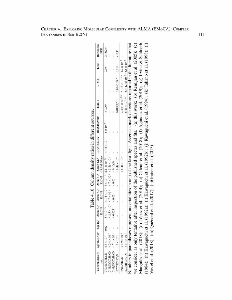
Chapter 4. ExploringMolecular Complexity with ALMA (EMoCA): ComplexIsocyanides in Sgr B2(N) 111
Tabl
e4.
10:C
olum
nde
nsity
ratio
sin
diff
eren
tsou
rces
.C
olum
nde
nsity
SgrB
2(N
2)a
SgrB
2bO
rion
KL
cO
rion
KL
cO
rion
KL
cO
rion
KL
dIR
AS1
6293
Ae
IRA
S162
93B
eT
MC
-1L
1544
L48
3fH
orse
head
ratio
EtC
N3
EtC
N1
EtC
N2
(IR
AM
30m
)PD
RC
H3N
C/C
H3C
N4.
7×
10−
30.
023×
10−
3?<
1.4×
10−
36×
10−
4?2(
1)×
10−
3?<
1.8×
10−
45×
10−
3<
0.09
g–
0.09
0.15
(2)n
C2H
5NC
/C2H
5CN
<2.
4×
10−
4–
<2.
5×
10−
3<
7×
10−
3<
7×
10−
3<
3(2)×
10−
3–
––
––
–C
2H3N
C/C
2H3C
N<
7.1×
10−
3–
<0.
025
<0.
02<
0.05
<0.
10(5
)–
––
––
–H
CC
NC
/HC
3N1.
5×
10−
3–
––
–<
8(4)×
10−
4–
–0.
018(
2)h,
k0.
05–0
.09l,m
0.01
4<
0.1n
HN
C3/
HC
3N<
1.9×
10−
4–
––
–<
8(4)×
10−
4–
–2.
4(4)×
10−
3i,k
5−
8×
10−
3l,m
1.2×
10−
3–
HC
3NH
+/H
C3N
<1.
7×
10−
3–
––
––
––
6(1)×
10−
3j,k
8.4(
42)×
10−
3m5.
5×
10−
3–
Num
bers
inpa
rent
hese
sre
pres
entu
ncer
tain
ties
inun
itof
the
last
digi
t.A
ster
isks
mar
kde
tect
ions
repo
rted
inth
elit
erat
ure
that
we
cons
ider
ason
lyte
ntat
ive
afte
rin
spec
tion
ofth
epu
blis
hed
spec
tra
and
fits.
(a)
this
wor
k;(b
)R
emija
net
al.(
2005
);(c
)M
argu
lès
etal
.(20
18);
(d)
Lóp
ezet
al.(
2014
);(e
)C
alcu
ttet
al.(
2018
);(f
)A
gúnd
ezet
al.(
2019
);(g
)Ir
vine
&Sc
hloe
rb(1
984)
;(h
)Kaw
aguc
hiet
al.(
1992
a);
(i)K
awag
uchi
etal
.(19
92b)
;(j
)Kaw
aguc
hiet
al.(
1994
);(k
)Tak
ano
etal
.(19
98);
(l)
Vas
tele
tal.
(201
8);
(m)Q
uéna
rdet
al.(
2017
);(n
)Gra
tiere
tal.
(201
3).
112Chapter 4. ExploringMolecular Complexity with ALMA (EMoCA): Complex
Isocyanides in Sgr B2(N)
mass protostar L483, the dark cloud TMC-1, the prestellar core L1544, and the Horsehead
photodissociation region (PDR) in Table 4.10. The column density ratios reported for Sgr
B2(N2) in this table account for the contribution of vibrationally excited states to the total
partition function of the molecules, as in Table 4.1. This is also the case for the data for
IRAS 16293A and IRAS16293B, but may not be true for the other values reported in the
literature.
It is interesting to note that the observed ratio of CH3NC:CH3CN varies significantly
from source to source. Table 4.10 shows a significant range of values, from 0.15 for the
Horsehead PDR, to an upper limit of 1.8 × 10⁻⁴ for IRAS16293A. There are many factors
that could contribute to this difference. For example, these differences may be due to
differing kinetic temperatures, differing UV fields, or differing cosmic-ray ionization rates.
We note that the chemical models presented here (with the exception of Model 2) also
predict a significant change in CH3NC:CH3CN ratio with temperature. It is likely that
it is a combination of all parameters. The observations of Remijan et al. (2005) toward
Sgr B2 is a factor of approximately four higher than what we determine for Sgr B2(N2).
This is qualitatively consistent with the models we present here. Remijan et al. (2005)
did not detect compact emission of CH3NC from the hot core with BIMA. They instead
detected extended emission in the cloud with the GBT. Our chemical models show a higher
CH3NC:CH3CN ratio in the low-temperature regions of the cloud, which is what their GBT
observations probe.
Gratier et al. (2013) determined a high abundance ratio in the Horsehead PDR, but
the excitation temperatures derived for CH3CN in their work were ∼30-40 K, which is
much lower than what we have derived here. In addition, the Horsehead PDR also has a
significantly greater UV flux. So it is likely that both effects combine in this case. In the
case of UV, these results appear to highlight the fact that UV and cosmic-ray chemistry
behave differently, as it is shown that high UV flux appears to increase the CH3NC:CH3CN
Chapter 4. ExploringMolecular Complexity with ALMA (EMoCA): ComplexIsocyanides in Sgr B2(N) 113
ratio, whereas higher ζ appears to decrease it. Differences in UV and cosmic-ray chemistry
have been noted before. An example of this is the case of ArH+, which has been shown to be
formed from cosmic-ray-induced processes, but not from UV processes, albeit in diffuse
atomic hydrogen environments that are quite different from the denser regions discussed
here (Schilke et al. 2014).
It is also instructive to compare the HCCNC:HC3N and HNC3:HC3N ratios between
sources. Observations of the cold regions TMC-1, L1544, and L483 reveal a HCCNC:HC3N
ratio that is about an order of magnitude higher than Sgr B2(N2). This is in better agree-
ment with our chemical model predictions for these species, albeit in a much colder en-
vironment than what we are modeling. This could indicate that we are missing some im-
portant temperature-sensitive reactions for the formation and destruction of these species.
The same can be shown when looking at the HNC3:HC3N ratio, which is also about an
order of magnitude higher in TMC-1, L1544, and L483 than in Sgr B2(N2). However,
this higher ratio is in worse agreement with our models, contrary to the behavior shown in
HCCNC:HC3N. It is clear that there are key ingredients missing from the chemical network
in regards to these smaller cyanides and isocyanides.
4.9 ConclusionHere, we present a joint observational and modeling effort aimed at studying the chem-
istry of complex isocyanides in Sgr B2(N2). This is, to our knowledge, the most com-
prehensive effort aimed at understanding the chemistry of these species in the literature to
date. We introduce a new, single-stage chemical model that combines the traditional two
stages of a hot-core chemical model (collapse and warm-up) into a single concerted phase.
We also introduce a visual extinction-dependent cosmic-ray ionization rate into hot-core
chemical models. Several new species and reactions were added to our chemical network,
including C2H5NC, C2H3NC, and related radicals, and our models were compared with
114Chapter 4. ExploringMolecular Complexity with ALMA (EMoCA): Complex
Isocyanides in Sgr B2(N)
observations from the EMoCA survey. Our main conclusions are summarized below.
1. We report tentative detections of CH3NC and HCCNC toward Sgr B2(N2) for the
first time, with abundance ratios of CH3NC:CH3CN ∼ 5 × 10⁻³ and HCCNC:HC3N
∼ 1.5 × 10⁻³. In addition, we calculate upper limits for C2H5NC, C2H3NC, HNC3,
and HC3NH+.
2. Using a variable and higher cosmic-ray ionization rate has a complex effect on the
chemistry of the cyanides and isocyanides. Incorporating this into our chemical net-
work increases agreement for some molecular ratios (CH3NC:CH3CN) to a point, but
models with very high ζ do not show as good an agreement. The impact of changing
ζ must be studied in greater detail.
3. The best agreement with observations is reached using an enhanced, extinction-
dependent cosmic-ray ionization rate, which is in line with other observational and
modeling studies of Sgr B2(N2). Model 4 reproduces the ratio of CH3NC:CH3CN
almost exactly when considering the theoretical column density ratios, and is also
consistent with all upper limits. Models with high, constant ζ do not reproduce obser-
vations particularly well. This highlights the need for extinction-dependent ζ profiles
in chemical models.
4. The HCCNC:HC3N ratio is too high across all models presented here. This appears
to be due to a systematic overproduction of HCCNC, as the ratio of HCCNC:CH3CN
is also too high. This overproduction will be a topic of further study.
5. Molecular radiative transfer calculations that take account of source structure show
that the column densities produced are multiple orders of magnitude too low in some
cases. This implies that we are not producing enough complex molecules in our mod-
els, or that the physical profile we are using is inaccurate. Excitation temperatures
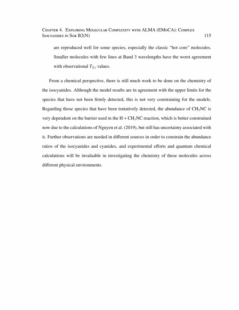
Chapter 4. ExploringMolecular Complexity with ALMA (EMoCA): ComplexIsocyanides in Sgr B2(N) 115
are reproduced well for some species, especially the classic “hot core” molecules.
Smaller molecules with few lines at Band 3 wavelengths have the worst agreement
with observational TEx values.
From a chemical perspective, there is still much work to be done on the chemistry of
the isocyanides. Although the model results are in agreement with the upper limits for the
species that have not been firmly detected, this is not very constraining for the models.
Regarding those species that have been tentatively detected, the abundance of CH3NC is
very dependent on the barrier used in the H + CH3NC reaction, which is better constrained
now due to the calculations of Nguyen et al. (2019), but still has uncertainty associated with
it. Further observations are needed in different sources in order to constrain the abundance
ratios of the isocyanides and cyanides, and experimental efforts and quantum chemical
calculations will be invaluable in investigating the chemistry of these molecules across
different physical environments.
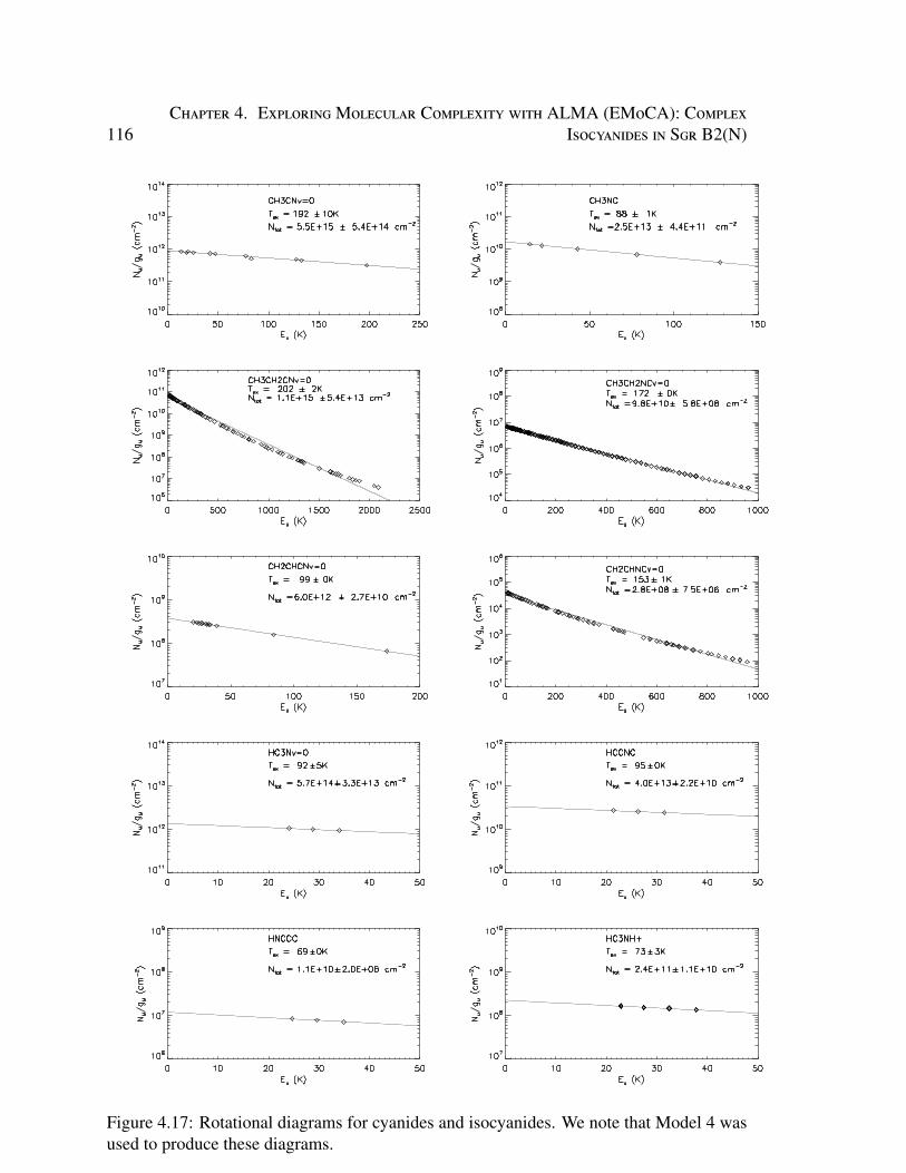
116Chapter 4. ExploringMolecular Complexity with ALMA (EMoCA): Complex
Isocyanides in Sgr B2(N)
Figure 4.17: Rotational diagrams for cyanides and isocyanides. We note that Model 4 wasused to produce these diagrams.
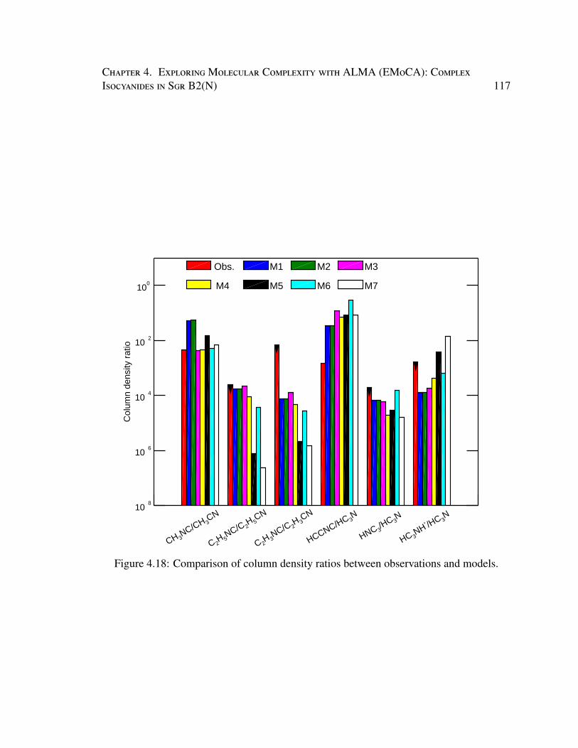
Chapter 4. ExploringMolecular Complexity with ALMA (EMoCA): ComplexIsocyanides in Sgr B2(N) 117
108
106
104
102
100
Colu
mn d
ensity r
atio
CH 3NC/C
H 3CN
C 2H 5
NC/C 2H 5
CN
C 2H 3
NC/C 2H 3
CN
HCCNC/HC 3
N
HNC 3/H
C 3N
HC 3NH
+ /HC 3
N
Obs. M1 M2 M3
M4 M5 M6 M7
Figure 4.18: Comparison of column density ratios between observations and models.
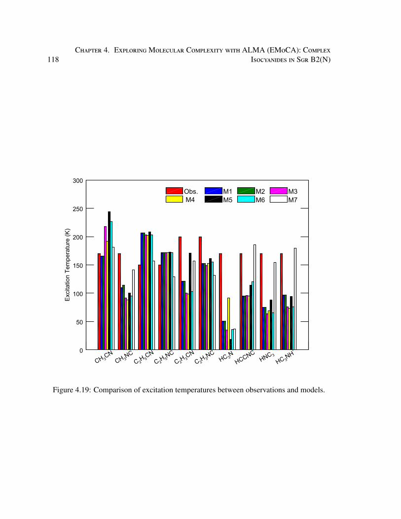
118Chapter 4. ExploringMolecular Complexity with ALMA (EMoCA): Complex
Isocyanides in Sgr B2(N)
0
50
100
150
200
250
300
Excita
tio
n T
em
pe
ratu
re (
K)
CH 3CN
CH 3NC
C 2H 5
CN
C 2H 5
NC
C 2H 3
CN
C 2H 3
NCHC 3
N
HCCNCHNC 3
HC 3NH
+
Obs. M1 M2 M3
M4 M5 M6 M7
Figure 4.19: Comparison of excitation temperatures between observations and models.
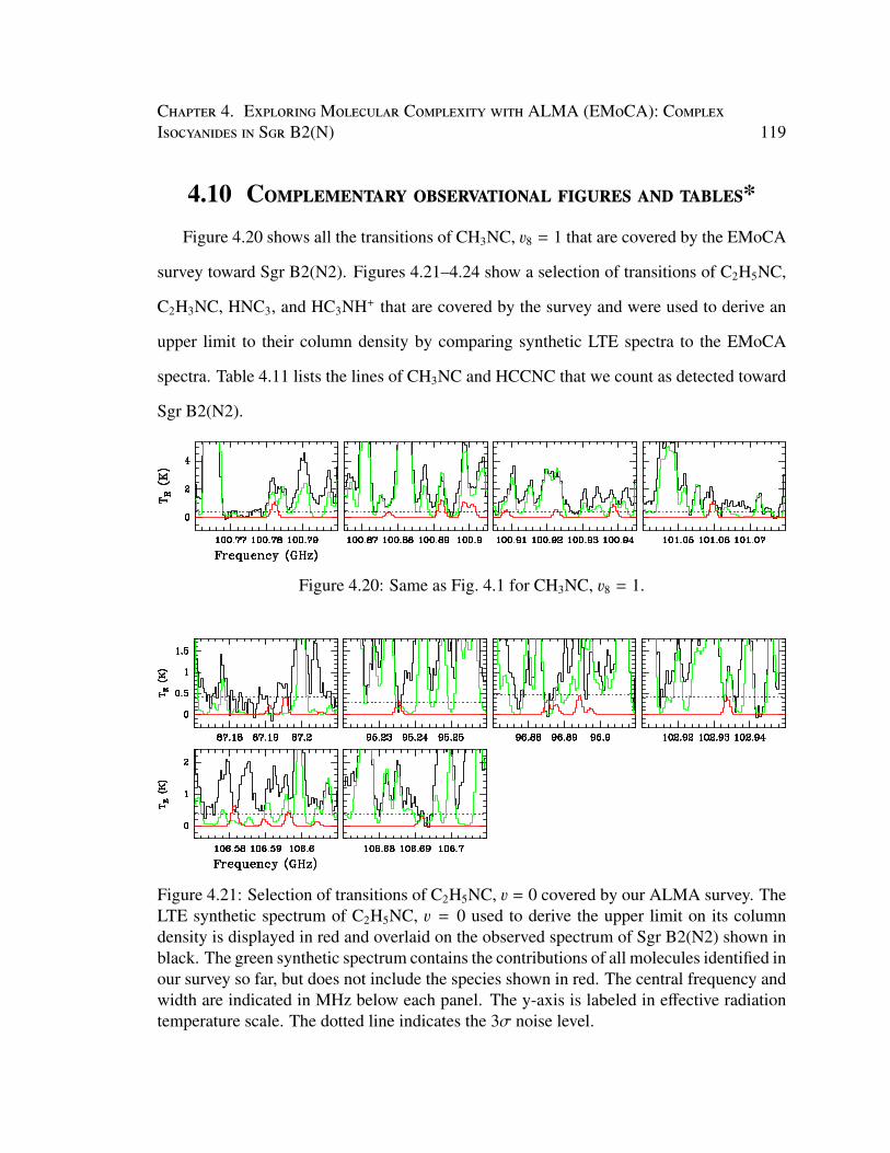
Chapter 4. ExploringMolecular Complexity with ALMA (EMoCA): ComplexIsocyanides in Sgr B2(N) 119
4.10 Complementary observational figures and tables*Figure 4.20 shows all the transitions of CH3NC, 38 = 1 that are covered by the EMoCA
survey toward Sgr B2(N2). Figures 4.21–4.24 show a selection of transitions of C2H5NC,
C2H3NC, HNC3, and HC3NH+ that are covered by the survey and were used to derive an
upper limit to their column density by comparing synthetic LTE spectra to the EMoCA
spectra. Table 4.11 lists the lines of CH3NC and HCCNC that we count as detected toward
Sgr B2(N2).
Figure 4.20: Same as Fig. 4.1 for CH3NC, 38 = 1.
Figure 4.21: Selection of transitions of C2H5NC, 3 = 0 covered by our ALMA survey. TheLTE synthetic spectrum of C2H5NC, 3 = 0 used to derive the upper limit on its columndensity is displayed in red and overlaid on the observed spectrum of Sgr B2(N2) shown inblack. The green synthetic spectrum contains the contributions of all molecules identified inour survey so far, but does not include the species shown in red. The central frequency andwidth are indicated in MHz below each panel. The y-axis is labeled in effective radiationtemperature scale. The dotted line indicates the 3σ noise level.
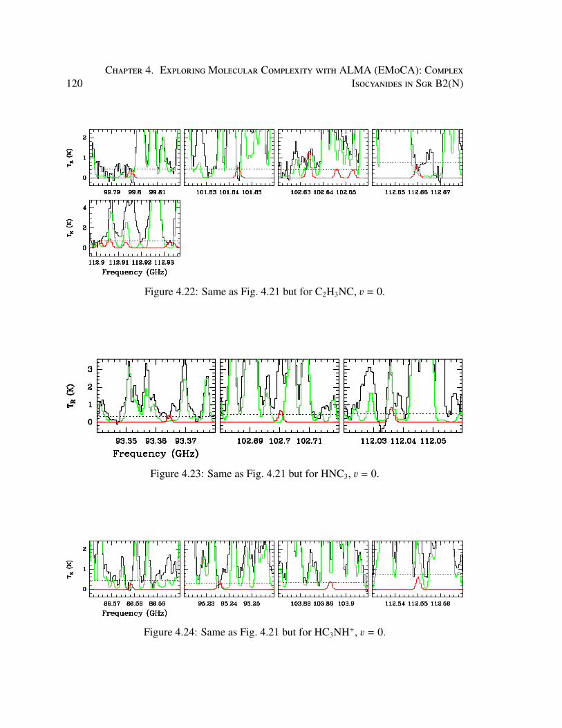
120Chapter 4. ExploringMolecular Complexity with ALMA (EMoCA): Complex
Isocyanides in Sgr B2(N)
Figure 4.22: Same as Fig. 4.21 but for C2H3NC, 3 = 0.
Figure 4.23: Same as Fig. 4.21 but for HNC3, 3 = 0.
Figure 4.24: Same as Fig. 4.21 but for HC3NH+, 3 = 0.
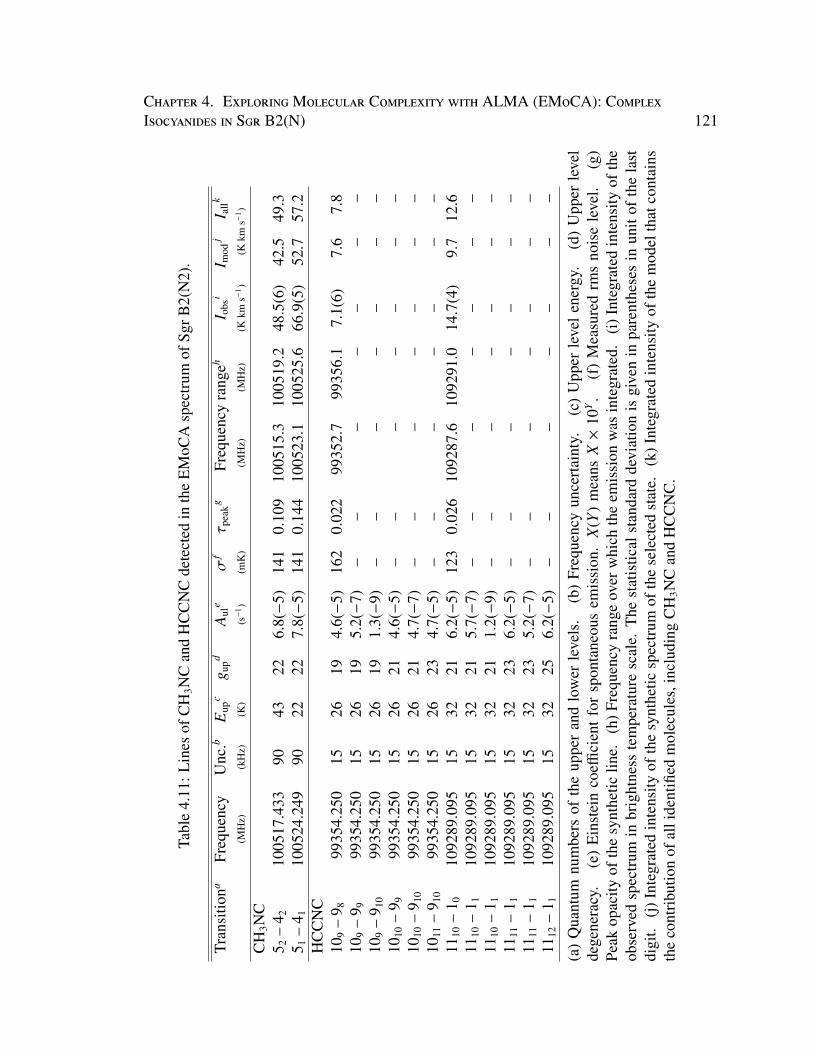
Chapter 4. ExploringMolecular Complexity with ALMA (EMoCA): ComplexIsocyanides in Sgr B2(N) 121
Tabl
e4.
11:L
ines
ofC
H3N
Can
dH
CC
NC
dete
cted
inth
eE
MoC
Asp
ectr
umof
SgrB
2(N
2).
Tran
sitio
naFr
eque
ncy
Unc
.bE
upc
g upd
Aul
eσ
fτ p
eakg
Freq
uenc
yra
ngeh
I obs
iI m
odj
I all
k
(MH
z)(k
Hz)
(K)
(s−
1 )(m
K)
(MH
z)(M
Hz)
(Kkm
s−1 )
(Kkm
s−1 )
CH
3NC
5 2–
4 210
0517
.433
9043
226.
8(−
5)14
10.
109
1005
15.3
1005
19.2
48.5
(6)
42.5
49.3
5 1–
4 110
0524
.249
9022
227.
8(−
5)14
10.
144
1005
23.1
1005
25.6
66.9
(5)
52.7
57.2
HC
CN
C10
9–
9 899
354.
250
1526
194.
6(−
5)16
20.
022
9935
2.7
9935
6.1
7.1(
6)7.
67.
810
9–
9 999
354.
250
1526
195.
2(−
7)–
––
––
––
109
–9 1
099
354.
250
1526
191.
3(−
9)–
––
––
––
1010
–9 9
9935
4.25
015
2621
4.6(−
5)–
––
––
––
1010
–9 1
099
354.
250
1526
214.
7(−
7)–
––
––
––
1011
–9 1
099
354.
250
1526
234.
7(−
5)–
––
––
––
1110
–1 0
1092
89.0
9515
3221
6.2(−
5)12
30.
026
1092
87.6
1092
91.0
14.7
(4)
9.7
12.6
1110
–1 1
1092
89.0
9515
3221
5.7(−
7)–
––
––
––
1110
–1 1
1092
89.0
9515
3221
1.2(−
9)–
––
––
––
1111
–1 1
1092
89.0
9515
3223
6.2(−
5)–
––
––
––
1111
–1 1
1092
89.0
9515
3223
5.2(−
7)–
––
––
––
1112
–1 1
1092
89.0
9515
3225
6.2(−
5)–
––
––
––
(a)
Qua
ntum
num
bers
ofth
eup
per
and
low
erle
vels
.(b
)Fr
eque
ncy
unce
rtai
nty.
(c)
Upp
erle
vel
ener
gy.
(d)
Upp
erle
vel
dege
nera
cy.
(e)
Ein
stei
nco
effici
ent
for
spon
tane
ous
emis
sion
.X
(Y)
mea
nsX×
10Y.
(f)
Mea
sure
drm
sno
ise
leve
l.(g
)Pe
akop
acity
ofth
esy
nthe
ticlin
e.(h
)Fre
quen
cyra
nge
over
whi
chth
eem
issi
onw
asin
tegr
ated
.(i
)Int
egra
ted
inte
nsity
ofth
eob
serv
edsp
ectr
umin
brig
htne
sste
mpe
ratu
resc
ale.
The
stat
istic
alst
anda
rdde
viat
ion
isgi
ven
inpa
rent
hese
sin
unit
ofth
ela
stdi
git.
(j)I
nteg
rate
din
tens
ityof
the
synt
hetic
spec
trum
ofth
ese
lect
edst
ate.
(k)I
nteg
rate
din
tens
ityof
the
mod
elth
atco
ntai
nsth
eco
ntri
butio
nof
alli
dent
ified
mol
ecul
es,i
nclu
ding
CH
3NC
and
HC
CN
C.
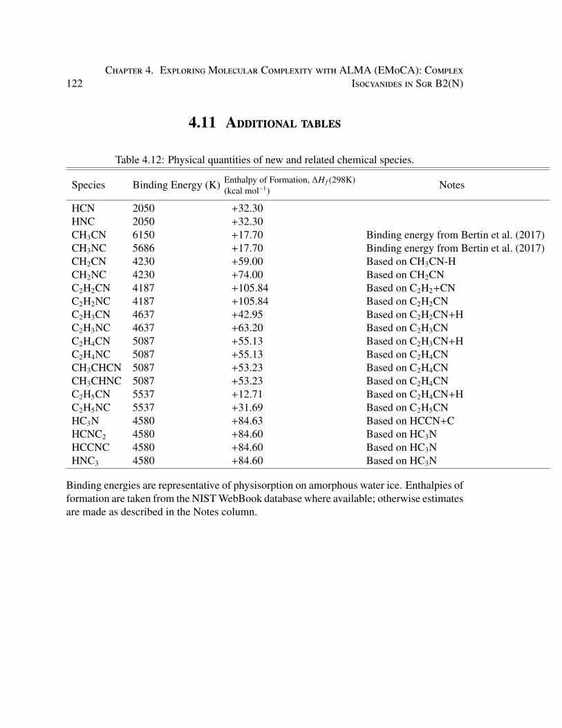
122Chapter 4. ExploringMolecular Complexity with ALMA (EMoCA): Complex
Isocyanides in Sgr B2(N)
4.11 Additional tables
Table 4.12: Physical quantities of new and related chemical species.
Species Binding Energy (K) Enthalpy of Formation, ∆H f (298K)(kcal mol−1) Notes
HCN 2050 +32.30HNC 2050 +32.30CH3CN 6150 +17.70 Binding energy from Bertin et al. (2017)CH3NC 5686 +17.70 Binding energy from Bertin et al. (2017)CH2CN 4230 +59.00 Based on CH3CN-HCH2NC 4230 +74.00 Based on CH2CNC2H2CN 4187 +105.84 Based on C2H2+CNC2H2NC 4187 +105.84 Based on C2H2CNC2H3CN 4637 +42.95 Based on C2H2CN+HC2H3NC 4637 +63.20 Based on C2H3CNC2H4CN 5087 +55.13 Based on C2H3CN+HC2H4NC 5087 +55.13 Based on C2H4CNCH3CHCN 5087 +53.23 Based on C2H4CNCH3CHNC 5087 +53.23 Based on C2H4CNC2H5CN 5537 +12.71 Based on C2H4CN+HC2H5NC 5537 +31.69 Based on C2H5CNHC3N 4580 +84.63 Based on HCCN+CHCNC2 4580 +84.60 Based on HC3NHCCNC 4580 +84.60 Based on HC3NHNC3 4580 +84.60 Based on HC3N
Binding energies are representative of physisorption on amorphous water ice. Enthalpies offormation are taken from the NIST WebBook database where available; otherwise estimatesare made as described in the Notes column.
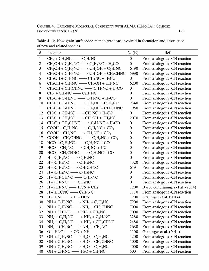
Chapter 4. ExploringMolecular Complexity with ALMA (EMoCA): ComplexIsocyanides in Sgr B2(N) 123
Table 4.13: New grain-surface/ice-mantle reactions involved in formation and destructionof new and related species.
# Reaction EA (K) Ref.1 CH2 + CH2NC C2H4NC 0 From analogous -CN reaction2 CH2OH + C2H4NC C2H5NC + H2CO 0 From analogous -CN reaction3 CH2OH + C2H5NC CH3OH + C2H4NC 6490 From analogous -CN reaction4 CH2OH + C2H5NC CH3OH + CH3CHNC 5990 From analogous -CN reaction5 CH2OH + CH2NC CH3NC + H2CO 0 From analogous -CN reaction6 CH2OH + CH3NC CH3OH + CH2NC 6200 From analogous -CN reaction7 CH2OH + CH3CHNC C2H5NC + H2CO 0 From analogous -CN reaction8 CH3 + CH2NC C2H5NC 0 From analogous -CN reaction9 CH3O + C2H4NC C2H5NC + H2CO 0 From analogous -CN reaction10 CH3O + C2H5NC CH3OH + C2H4NC 2340 From analogous -CN reaction11 CH3O + C2H5NC CH3OH + CH3CHNC 1950 From analogous -CN reaction12 CH3O + CH2NC CH3NC + H2CO 0 From analogous -CN reaction13 CH3O + CH3NC CH3OH + CH2NC 2070 From analogous -CN reaction14 CH3O + CH3CHNC C2H5NC + H2CO 0 From analogous -CN reaction15 COOH + C2H4NC C2H5NC + CO2 0 From analogous -CN reaction16 COOH + CH2NC CH3NC + CO2 0 From analogous -CN reaction17 COOH + CH3CHNC C2H5NC + CO2 0 From analogous -CN reaction18 HCO + C2H4NC C2H5NC + CO 0 From analogous -CN reaction19 HCO + CH2NC CH3NC + CO 0 From analogous -CN reaction20 HCO + CH3CHNC C2H5NC + CO 0 From analogous -CN reaction21 H + C2H2NC C2H3NC 0 From analogous -CN reaction22 H + C2H3NC C2H4NC 1320 From analogous -CN reaction23 H + C2H3NC CH3CHNC 619 From analogous -CN reaction24 H + C2H4NC C2H5NC 0 From analogous -CN reaction25 H + CH3CHNC C2H5NC 0 From analogous -CN reaction26 H + CH2NC CH3NC 0 From analogous -CN reaction27 H + CH3NC HCN + CH3 1200 Based on Graninger et al. (2014)28 H + HCCNC C2H2NC 1710 From analogous -CN reaction29 H + HNC H + HCN 1200 Graninger et al. (2014)30 NH + C2H5NC NH2 + C2H4NC 7200 From analogous -CN reaction31 NH + C2H5NC NH2 + CH3CHNC 7000 From analogous -CN reaction32 NH + CH3NC NH2 + CH2NC 7000 From analogous -CN reaction33 NH2 + C2H5NC NH3 + C2H4NC 3280 From analogous -CN reaction34 NH2 + C2H5NC NH3 + CH3CHNC 2480 From analogous -CN reaction35 NH2 + CH3NC NH3 + CH2NC 2680 From analogous -CN reaction36 O + HNC CO + NH 1100 Graninger et al. (2014)37 OH + C2H5NC H2O + C2H4NC 1200 From analogous -CN reaction38 OH + C2H5NC H2O + CH3CHNC 1000 From analogous -CN reaction39 OH + C2H3NC H2O + C2H2NC 4000 From analogous -CN reaction40 OH + CH3NC H2O + CH2NC 500 From analogous -CN reaction
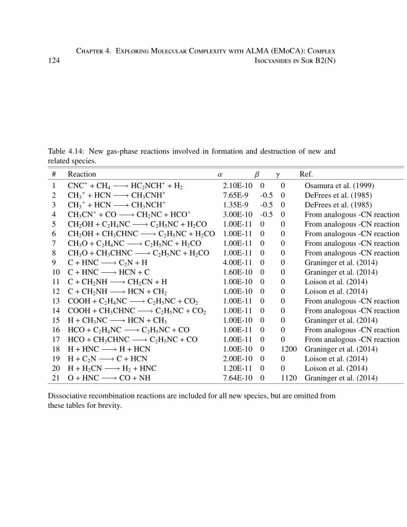
124Chapter 4. ExploringMolecular Complexity with ALMA (EMoCA): Complex
Isocyanides in Sgr B2(N)
Table 4.14: New gas-phase reactions involved in formation and destruction of new andrelated species.
# Reaction α β γ Ref.1 CNC+ + CH4 HC2NCH+ + H2 2.10E-10 0 0 Osamura et al. (1999)2 CH3
+ + HCN CH3CNH+ 7.65E-9 -0.5 0 DeFrees et al. (1985)3 CH3
+ + HCN CH3NCH+ 1.35E-9 -0.5 0 DeFrees et al. (1985)4 CH3CN+ + CO CH2NC + HCO+ 3.00E-10 -0.5 0 From analogous -CN reaction5 CH2OH + C2H4NC C2H5NC + H2CO 1.00E-11 0 0 From analogous -CN reaction6 CH2OH + CH3CHNC C2H5NC + H2CO 1.00E-11 0 0 From analogous -CN reaction7 CH3O + C2H4NC C2H5NC + H2CO 1.00E-11 0 0 From analogous -CN reaction8 CH3O + CH3CHNC C2H5NC + H2CO 1.00E-11 0 0 From analogous -CN reaction9 C + HNC C2N + H 4.00E-11 0 0 Graninger et al. (2014)10 C + HNC HCN + C 1.60E-10 0 0 Graninger et al. (2014)11 C + CH2NH CH2CN + H 1.00E-10 0 0 Loison et al. (2014)12 C + CH2NH HCN + CH2 1.00E-10 0 0 Loison et al. (2014)13 COOH + C2H4NC C2H5NC + CO2 1.00E-11 0 0 From analogous -CN reaction14 COOH + CH3CHNC C2H5NC + CO2 1.00E-11 0 0 From analogous -CN reaction15 H + CH3NC HCN + CH3 1.00E-10 0 0 Graninger et al. (2014)16 HCO + C2H4NC C2H5NC + CO 1.00E-11 0 0 From analogous -CN reaction17 HCO + CH3CHNC C2H5NC + CO 1.00E-11 0 0 From analogous -CN reaction18 H + HNC H + HCN 1.00E-10 0 1200 Graninger et al. (2014)19 H + C2N C + HCN 2.00E-10 0 0 Loison et al. (2014)20 H + H2CN H2 + HNC 1.20E-11 0 0 Loison et al. (2014)21 O + HNC CO + NH 7.64E-10 0 1120 Graninger et al. (2014)
Dissociative recombination reactions are included for all new species, but are omitted fromthese tables for brevity.
125
Chapter 5
Simulations of cometary ice chemistry
during solar approach
5.1 IntroductionCometary nuclei are believed to contain some of the most primitive and well-preserved
material from the formation of the Solar System (Weissman et al. 2020). Generally, comets
are stored in one of two regions of the Solar System before they are perturbed and begin
their solar approach. These regions are known as the Kuiper Belt (Kuiper 1951) and the
Oort cloud (Oort 1950). The Kuiper Belt extends from the orbit of Neptune (∼30 au) to ∼50
au, and has a mean temperature of ∼40 K. The Oort cloud is significantly larger and colder,
with a radius that extends up to 200,000 au (Duncan et al. 1987), and a mean temperature
of ∼10 K.
Cometary ice is known to be dominated by H2O (Mumma & Charnley 2011), yet com-
plex organic molecules (COMs) have been detected in comets from remote observations
as well as from returned samples. For example, Bockelée-Morvan et al. (2000) detected
formamide (NH2CHO) and methyl formate (HCOOCH3) in the coma of comet C1/1995
126 Chapter 5. Simulations of cometary ice chemistry during solar approach
(Hale-Bopp) using ground-based telescopes. In the same comet, Crovisier et al. (2004)
detected ethylene glycol ((CH2OH)2) at ∼0.25% of the production rate of H2O from the
cometary nucleus.
Samples returned from the Stardust mission to comet 81P/Wild 2 (Brownlee et al. 2006)
have also revealed significant chemical complexity. Glavin et al. (2008) utilized a combi-
nation of liquid chromatography and UV fluorescence to make detections of methylamine
(CH3NH2) and ethylamine (CH3CH2NH2) in the returned samples. Following on from
that study, Elsila et al. (2009) studied the 13C content of amino acids in the solid sam-
ples returned from Wild 2, reporting the first detection of a cometary amino acid, glycine
(NH2CH2COOH). More recently, Altwegg et al. (2016) used the ROSINA mass spectrom-
eter (Balsiger et al. 2007) to detect glycine, methylamine, and ethylamine in the coma of
Comet 67P/Churyumov-Gerasimenko. These detections, along with the simultaneous iden-
tifications of phosphorus and other organics, have confirmed the discoveries made by the
Stardust team, and highlighted the role that comets could have played in seeding the early
Earth with organic building blocks.
Understanding the origin of COMs in cometary ices is of fundamental importance.
Models of gas-phase chemistry in cometary comae have existed for some time (e.g. Irvine
et al. 1998). These models have only included gas-phase processes in active comets, and
have been adapted from models constructed to simulate interstellar chemistry. One of the
key questions motivating their use has been in distinguising between those species formed
in the cometary ice (“parent” species) and those formed via energetic processing in the
coma (“daughter” species). However, in order to properly determine which species are
produced in the coma, and which are inherited directly from the cometary nucleus, detailed
models of the solid-phase chemistry in comets are needed.
Garrod (2019) published the first such model of solid-state chemistry in cometary ices.
This model was adapted from the Model for Astrophysical Gas and Ice Chemical Kinetics
Chapter 5. Simulations of cometary ice chemistry during solar approach 127
and Layering (MAGICKAL; Garrod (2013a)). In the model of Garrod (2019), the comet
nucleus was constructed by extending the grain-surface and ice-mantle chemistry already
included in MAGICKAL. The comet was divided into 25 layers, each layer increasing in
thickness with depth, going down to a maximum depth of ∼136 m. Chemistry was studied
for the “cold storage” phase of the comet’s lifecycle, before any activity caused by solar
approach. Significant COM formation was observed to a depth of ∼10 m, due to processing
of cometary ice by UV photons and cosmic-ray bombardment.
Although comets spend the majority of their time in cold storage, either in the Kuiper
Belt or the Oort Cloud, the solar approach of cometary bodies is very interesting from
a chemical perspective. As previously mentioned, cometary bodies eject material from
their surfaces when approaching the Sun, and COMs have been detected in these ejecta.
However, there have been no models of solid-phase cometary chemistry that consider solar
approach.
In this paper, we present an updated version of the cometary ice chemistry model of
Garrod (2019). Here, we consider both the “cold-storage” phase, as well as a solar ap-
proach, following the orbit of Comet C1/1995 (Hale-Bopp). We solve the heat diffusion
equation in one dimension in order to model the temperature evolution of the cometary ice,
and then incorporate this evolution into our chemical model. We also include a new treat-
ment for thermal back-diffusion in calculating the rates of material transfer between layers
in the ice, as well as non-thermal chemical mechanisms initiated by photo-chemistry (Jin
& Garrod, in revision).
§5.2 describes the new mechanisms incorporated into the chemical model, as well as the
heat transfer and back-diffusion simulations. §5.3 presents the results of the heat-transfer
and back-diffusion simulations, as well as our chemical model results.
128 Chapter 5. Simulations of cometary ice chemistry during solar approach
5.2 MethodsHere we build upon the model of ice chemistry in cometary nuclei introduced by Garrod
(2019). The initial model was adapted from the hot-core chemical kinetics model, MAG-
ICKAL (Garrod 2013a). The reader is referred to Garrod (2019) for a full description of
the chemical model. Here, we aim to outline the major updates that have been made to this
new version.
The new comet model moves beyond the cold-storage phase studied by Garrod (2019),
and presents several improvements. Firstly, we have incorporated several new non-diffusive
chemistry mechanisms, as discussed in Jin & Garrod (in revision). §5.2.1 provides a brief
outline of these mechanisms, but the reader is referred to the reference for a detailed ex-
planation. In the models presented here, the cold-storage phase is followed by the solar
approach of the comet. In §5.2.2, this method is outlined. We have also more accurately
incorporated thermal back-diffusion between ice layers within the comet, building on the
work of Willis & Garrod (2017). §5.2.3 outlines these methods.
5.2.1 Non-thermal chemical mechanisms
Historically, production of complex organic molecules (COMs) in astrochemical mod-
els has relied on diffusive chemistry on the surfaces, and in the bulk ice of, interstellar dust
particles (e.g., Hasegawa et al. 1992; Garrod 2013b). These mechanisms generally require
dust grains to reach temperatures at which larger radical species become mobile, which
are reached easily in hot-core environments. However, recent detections of COMs in cold
environments (e.g., Bacmann et al. 2012; Cernicharo et al. 2012; Bergner et al. 2017) have
raised the need for mechanisms to form these molecules at temperatures below which large
radicals become mobile. This work is also relevant to cometary ice chemistry, as comets
in the Oort cloud exist at very low temperatures (∼10 K) for very long time periods. The
Chapter 5. Simulations of cometary ice chemistry during solar approach 129
discovery of COMs (such as glycine) in cometary ice samples (e.g., Elsila et al. 2009; Al-
twegg et al. 2016) indicates that it is possible these species form at low temperatures in the
cometary ice.
In the model presented by Garrod (2019), chemistry was assumed to occur diffusively
and through a photodissociation-induced mechanism, whereby reactive radicals produced
by photolysis could spontaneously react with nearby reaction partners. In this work, we
make significant changes and additions to the mechanisms by which reactions occur within
the cometary ice.
First, diffusion within the bulk ice is prohibited for species other than H and H2. This
is in line with experimental and modeling evidence (e.g. Ghesquière et al. 2018; Shin-
gledecker et al. 2019) that indicates that heavier radicals do not diffuse rapidly, and as such
that bulk diffusion may not be the main mechanism by which bulk-ice chemistry is driven.
We also add in new chemical mechanisms. The details of these mechanisms are de-
scribed in Jin & Garrod (in revision), but they are summarized here. The main addition to
the chemistry is in the form of what we call “three-body reactions.” These are reactions
in which a reactive species is formed in close proximity to another reactive species, thus
initiating a spontaneous reaction.
We also consider the possibility that molecules formed from a three-body reaction may
go on to initiate other three-body reactions themselves. In this way, a “chain-reaction” of
sorts may be initiated. These appearance rates are defined in the same way as Eq. 5.3.
We limit the number of cycles of this method that can occur following a single reaction to
three. Finally, we also consider that the species formed via an initiating reaction may be
formed with enough energy to overcome an activation energy barrier to react with a stable
species, such as H2O or CO.
The generic form for calculating rates of such processes, between two species A and B,
130 Chapter 5. Simulations of cometary ice chemistry during solar approach
is given by
RAB = fact(AB)Rcomp(A)N(B)NM
+ fact(AB)Rcomp(B)N(A)NM
,
(5.1)
where fact is an efficiency related to the activation energy barrier (between 0 and 1), Rcomp
is the “completion” rate of species A and B, N(A, B) is the abundance of species A and B
in the ice layer, and NM is the abundance of all species in the ice layer.
The “completion” rate of a species is further defined (with species A being the example)
as
Rcomp(A) =1
1/Rapp(A) + tAB, (5.2)
where Rapp is the “appearance” rate of species A, which varies depending on the reaction
mechanism being considered. The definition of Rapp(A) is given by
Rapp(A) =∑
R j(A), (5.3)
where R j(A) is the production rate of species i from each individual formation pro-
cess. In the case of photodissociation-induced reactions, this would be all of the individual
photodissociation processes that produce species A. Finally, tAB is defined as
tAB = 1/(νABκAB + khop(A) + khop(B)), (5.4)
which is the lifetime against the reaction of A and B. In this expression, νAB is the faster
characteristic frequency of either species A or B, κAB is a Boltzmann factor or tunneling
efficiency for the reaction, and khop(A, B) are the individual hopping rates for species A and
B. Note that, in the mantle, these rates will be 0 unless A or B are H/H2. Similar expressions
Chapter 5. Simulations of cometary ice chemistry during solar approach 131
exist for reaction on the cometary surface.
5.2.2 Heat transfer and solar approach
Garrod (2019) presented detailed models of the cold-storage phase of inactive comets.
In this work, we aim to go beyond this, including several solar orbits after this cold-storage
model. In order to do this, we must first calculate the orbits of a comet of interest, which
requires knowledge of its orbital elements. The PyEphem package (Rhodes 2011) was used
to load these orbital elements from the IAU Minor Planet Center. The orbital positions of
the comet of interest were then calculated for one solar orbit, using the most recently-
known orbital elements. These orbital elements were then assumed to be unchanged for
subsequent orbits of the comet in this model.
Once the orbits of the comet have been calculated, we must then calculate heat transfer
throughout the cometary ice, such that we have temperatures at each layer in the comet
model for each time point. This is done following the method of Herman & Podolak
(1985), in which the heat diffusion equation is solved in a one-dimensional fashion. The
heat diffusion equation is given by
ρc(T )∂T∂t
= ∇[κ∇T ], (5.5)
where ρ is the material density, c(T ) is the specific heat, κ is the thermal conductivity,
and T is the temperature. In the heat diffusion simulations presented here, we assume that
the comet is spherical and uniformly illuminated by the Sun. We must define boundary
conditions at the surface and the interior edge of the comet nucleus. At the surface, the
boundary condition is defined by conservation of energy:
∂T∂r|r=R = εσT 4 −
(1 − A)Sd2
H
〈cosξ〉 − FIS RF . (5.6)
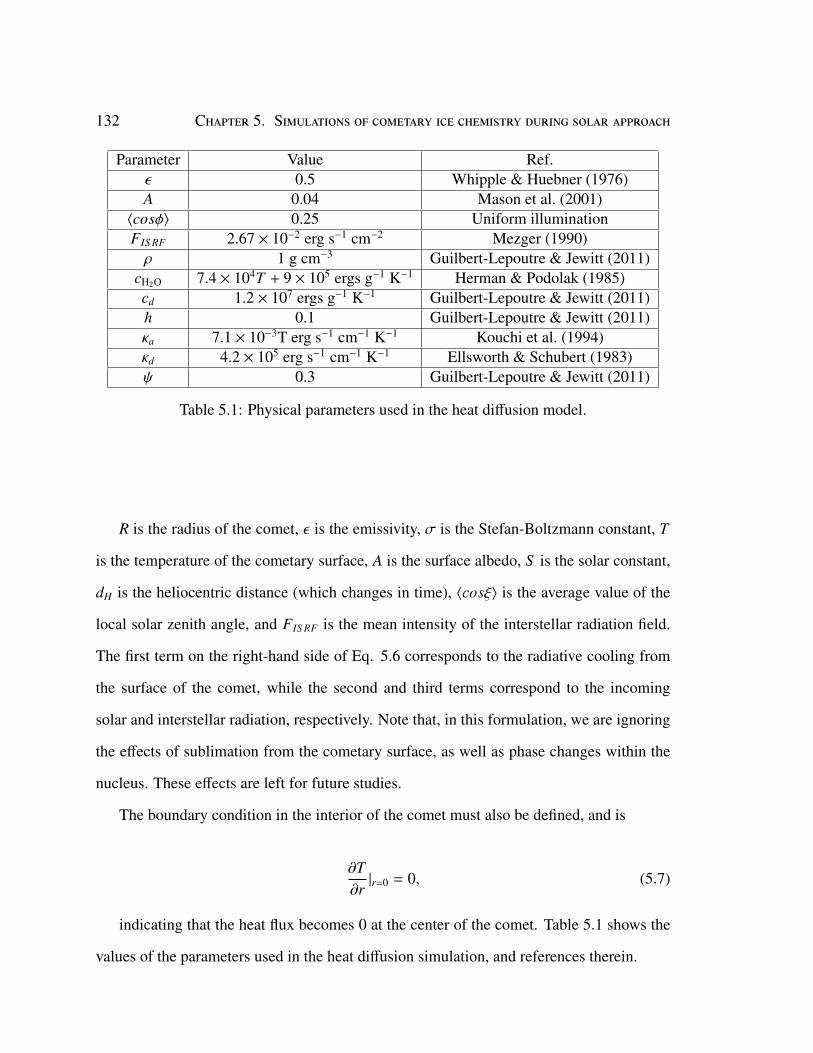
132 Chapter 5. Simulations of cometary ice chemistry during solar approach
Parameter Value Ref.ε 0.5 Whipple & Huebner (1976)A 0.04 Mason et al. (2001)
〈cosφ〉 0.25 Uniform illuminationFIS RF 2.67 × 10⁻² erg s−1 cm−2 Mezger (1990)ρ 1 g cm−3 Guilbert-Lepoutre & Jewitt (2011)
cH2O 7.4 × 10⁴T + 9 × 10⁵ ergs g−1 K−1 Herman & Podolak (1985)cd 1.2 × 10⁷ ergs g−1 K−1 Guilbert-Lepoutre & Jewitt (2011)h 0.1 Guilbert-Lepoutre & Jewitt (2011)κa 7.1 × 10⁻³T erg s−1 cm−1 K−1 Kouchi et al. (1994)κd 4.2 × 10⁵ erg s−1 cm−1 K−1 Ellsworth & Schubert (1983)ψ 0.3 Guilbert-Lepoutre & Jewitt (2011)
Table 5.1: Physical parameters used in the heat diffusion model.
R is the radius of the comet, ε is the emissivity, σ is the Stefan-Boltzmann constant, T
is the temperature of the cometary surface, A is the surface albedo, S is the solar constant,
dH is the heliocentric distance (which changes in time), 〈cosξ〉 is the average value of the
local solar zenith angle, and FIS RF is the mean intensity of the interstellar radiation field.
The first term on the right-hand side of Eq. 5.6 corresponds to the radiative cooling from
the surface of the comet, while the second and third terms correspond to the incoming
solar and interstellar radiation, respectively. Note that, in this formulation, we are ignoring
the effects of sublimation from the cometary surface, as well as phase changes within the
nucleus. These effects are left for future studies.
The boundary condition in the interior of the comet must also be defined, and is
∂T∂r|r=0 = 0, (5.7)
indicating that the heat flux becomes 0 at the center of the comet. Table 5.1 shows the
values of the parameters used in the heat diffusion simulation, and references therein.
Chapter 5. Simulations of cometary ice chemistry during solar approach 133
As noted in Eq. 5.5, c(T ) is a function of temperature. The specific heat is defined as
c(T ) = XH2OcH2O + Xdcd, (5.8)
where X is the mass fraction of water (as a proxy for the total ice) and dust, respec-
tively, and c is the specific heat of each component. For these simulations, we assume
that XH2O = Xd = 0.5, following Guilbert-Lepoutre & Jewitt (2011). The expressions for
cH2O and cd are given in Table 5.1.
Similarly, κ is also a function of temperature. In the simulations presented here, it is
defined as
κ = φhκs, (5.9)
following Guilbert-Lepoutre & Jewitt (2011). In Eq. 5.9, h is the Hertz factor, which scales
the conductivity to account for reduced contact area between grains within the solid matrix.
We set h to 0.1. κs is the conductivity of the cometary ice matrix, which is calculated as
κs = xH2Oκa + xdκd, (5.10)
where xH2O,d are the volume fractions of water and dust, and κa,d are the conductivities of
amorphous water and dust, respectively. Table 5.1 shows their values. Note that, in this
formulation, we assume that all ice in the comet is amorphous in nature. This is likely to
be the case when the comet is in cold storage, but there will be phase changes when solar
approach begins. However, our chemical model does not currently have the functionality
to account for these phase changes, so we save their study for future work.
Finally, φ is a correction factor, first developed by Russell (1935), which accounts for
134 Chapter 5. Simulations of cometary ice chemistry during solar approach
the effect of pores on the thermal conductivity of a solid matrix. Its formula is given by
φ =ψ2/3 f + (1 − ψ2/3)
ψ − ψ2/3 + 1 − ψ2/3(ψ1/3 − 1) f, (5.11)
where ψ is the porosity (assumed to be 0.3, following Guilbert-Lepoutre & Jewitt (2011)),
and f is the ratio of the conductivity of pores to the solid matrix, κp/κs. The conductivity
of the pores is calculated by
κp = 4rpεσT 3, (5.12)
where rp = 10−4 cm (the mean radius of a pore) and ε = 0.9 (Guilbert-Lepoutre & Jewitt
2011).
Once the boundary conditions and parameters are defined, the heat diffusion equation
can be solved through time. First, the space over which we wish to solve Eq. 5.5 must
be defined. We chose R = 30 km (Hale-Bopp, Fernández (2000)), and integrated over this
whole space. First, depths must be defined, as well as the initial temperatures at those
depths. The ice is divided into 250 depth points, such that the final depth point ends at 30
km. The surface is considered its own layer, and the layers after that increase in thickness
as the depth increases. The first layer beneath the surface comprises the first cm of ice,
while the final layer contains 140 m of ice. Once the depths are set, the initial temperature
is defined at each point. For this model, we simply assume a uniform temperature of 10 K
throughout the ice at the initial time point of the simulation, corresponding to Oort cloud
conditions.
Once the initial conditions have been defined, the orbital position is allowed to evolve
according to the specified cometary orbit. The impinging flux at the surface changes ac-
cording to the heliocentric distance dH, and the change in temperature is first calculated at
the surface. Derivatives ∂T/∂r are then calculated throughout the ice. Once these deriva-
Chapter 5. Simulations of cometary ice chemistry during solar approach 135
tives have been calculated, the second derivatives are computed, and the temperatures are
calculated at each depth in the ice using Gear’s method. Finally, the orbit is allowed to
evolve, and the calculations are done again. For our purposes, we calculate 5 orbits using
Hale-Bopp’s orbital parameters. §5.3.1 presents the results from these simulations, and
discusses their inclusion into the cometary ice chemistry model.
5.2.3 Layer back-diffusion
Back-diffusion is the phenomenon by which particles diffusing in a lattice may re-visit
lattice sites that they have already diffused away from. This effect has been shown to
impact reaction rates on the surface of interstellar dust grains of various morphologies
(Willis & Garrod 2017). In that study, the authors used two kinetic Monte Carlo models
to demonstrate that the reaction rates for the simple chemical system of H + H H2
were decreased compared to the typical rate-equation chemical kinetics approach when
back-diffusion was included. The magnitude of this effect was observed to be inversely
proportional to the surface coverage of the diffusing particle. In other words, when the
surface was mostly covered with diffusers, the effect was negligible, whereas with just two
diffusers, a maximum back-diffusion factor of ∼5 was observed.
Back-diffusion may also have a significant impact on diffusion between layers in the
model of cometary nuclei chemistry. As discussed earlier, in the model presented here,
we are limiting diffusion within the bulk ice to H/H2. Garrod (2019) describes in detail
the process by which molecules thermally diffuse within the bulk ice. To summarize, the
swapping rate at which species i diffuses into the surface from the mantle layer below is
given by
Rswap,m(i) = Nm(i)NS
NM
kswap(i)6
. (5.13)
In this expression, Nm(i) corresponds to the population of species i within the mantle
136 Chapter 5. Simulations of cometary ice chemistry during solar approach
layer, NS and NM are the total surface and mantle populations of all species, and kswap is
the swapping rate coefficient, given by
kswap(i) = ν0(i)exp[−Eswap(i)/T ], (5.14)
where ν0(i) is the characteristic frequency of species i, Eswap(i) is the barrier to bulk
diffusion of species i, and T is the temperature of the ice layer. Note that the 6 in Eq. 5.13
comes from the six diffusion directions available to a particle at the interface between the
surface and the mantle ice layer. Similar expressions exist at the interfaces for all 25 layers
in the comet model.
These expressions do not include a term for back-diffusion. Since this model contains
very large layers of ice, and the abundances of diffusing particles are expected to be low,
back-diffusion could have a significant impact on the rates of material transfer between
layers.
Garrod et al. (2017) incorporated a simple method for modeling the effect of back-
diffusion from the mantle to the surface in a hot-core chemistry model. In this formulation,
a simple three-dimensional kinetic Monte Carlo model was used to model the number of
diffusion events (denoted by Nmove) required for a diffuser to reach the top layer of an ice
of finite thickness. This process was found to follow the relationship
Nmove = 2(Nth + 1/2)2, (5.15)
where Nth is the thickness of the ice. This expression indicates that, with increasing
thickness, the number of diffusion events needed to reach the interface between the surface
and the mantle also increases. However, as was shown in Willis & Garrod (2017), the
abundance of the diffuser is also an important quantity, so further simulations were needed
before incorporation of a similar expression into this model of cometary ice chemistry.
Chapter 5. Simulations of cometary ice chemistry during solar approach 137
In this work, we present the results of a new three-dimensional Monte Carlo model that
investigates the back-diffusion effect across a wide range of conditions relevant to comets.
This model is functionally similar to that described in Garrod et al. (2017), except it has
now been extended to many diffusers. In this model, a maximum ice thickness is defined,
along with its lateral size. In the case of most of the simulations here, we have limited the
maximum thickness to 30 monolayers (ML), for computational efficiency. We have also
tested various lateral sizes (Nlat), including 8, 10, and 15 sites wide. The model has periodic
boundary conditions, except at the top and bottom of the ice.
Once these quantities have been defined, the model begins by creating an ice with a
thickness of 1 ML, and depositing one diffuser in a randomly-chosen site. This diffuser is
then allowed to hop, with an equal probability of choosing any of the six directions available
to it. The number of hops are recorded until that diffuser leaves the ice, by hopping either
out of the top or bottom. The diffuser is then replaced in another randomly-chosen site,
and the process is repeated 500,000 times for a proper statistical sample. Then, a second
diffuser is added, and so on. For simulations with multiple diffusers, the total number of
hops of all diffusers is recorded, and all diffusers are replaced on the ice once a single
diffuser leaves. If a diffuser attempts to hop into a site that is already occupied, a swapping
event occurs, where the two particles exchange places. This is counted as two hops, one
for each particle.
Once the maximum number of diffusers has been reached in a given thickness, the
model adds another layer onto the ice, and starts over again at one diffuser. This way, the
maximum amount of coverage space is properly sampled, and a relationship detailing the
magnitude of the back-diffusion effect as a result of both thickness (Nth) and diffusers (Nd)
can be derived. In order to derive expressions to describe this phenomenon, we make use
of the Eureqa modeling engine (Schmidt & Lipson 2009, 2014). §3.2 details the results of
these simulations, and their incorporation into the cometary ice model.
138 Chapter 5. Simulations of cometary ice chemistry during solar approach
5.3 ResultsThis is the results section.
5.3.1 Heat transfer simulations
The method outlined in §5.2.2 was used to solve the temperature evolution of Hale-
Bopp (R = 30 km) for 5 orbits. Figure 5.1 shows the results for the first orbit, at five
positions from the sun. It can be seen that, as expected, the temperatures are highest at
points closest to the sun. The maximum temperature achieved at perihelion is ∼338 K at the
surface for this orbit. Then, as the comet recedes from the sun, it cools from the surface first,
leading to peak temperatures at a few m into the ice. By the time the orbit has completed,
the temperature is mostly uniform throughout the first 20 m, slightly elevated from the
initial value at a temperature of ∼18 K. Temperatures greater than 15 K are maintained
to a depth of ∼88 m, but they are not shown here in order to emphasize the heating at
the surface. The shapes of these temperature profiles are qualitatively similar to the one-
dimensional calculations of Herman & Weissman (1987) (see their Fig. 2), though their
methods were slightly more complicated as they included a crystalline component to their
ice, as well as sublimation in Eq. 5.6.
The remaining four orbits look qualitatively similar to Figure 5.1. The results for these
are shown in Figure 5.2. The maximum temperature achieved at perihelion is ∼338 K for
each orbit. One difference between orbits is that the temperature evolves slightly further
down into the cometary ice for each evolution, though this effect is small. For example, at
the end of the fifth orbit, the temperature at a depth of 20 m is ∼21 K, whereas it is 18 K at
the end of the first orbit. Thus there is some small hysteresis in the ice temperature.
Once these simulations are completed, their results must be incorporated into our model
of cometary ice chemistry. This incorporation is very simple. First, the temperatures and
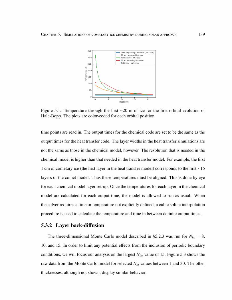
Chapter 5. Simulations of cometary ice chemistry during solar approach 139
0 5 10 15 20Depth (m)
0
50
100
150
200
250
300
350
Tem
pera
ture
(K)
Orbit beginning - aphelion (360.5 au)10 au - approaching sunPerihelion (~0.92 au)10 au, receding from sunOrbit end - aphelion
Figure 5.1: Temperature through the first ∼20 m of ice for the first orbital evolution ofHale-Bopp. The plots are color-coded for each orbital position.
time points are read in. The output times for the chemical code are set to be the same as the
output times for the heat transfer code. The layer widths in the heat transfer simulations are
not the same as those in the chemical model, however. The resolution that is needed in the
chemical model is higher than that needed in the heat transfer model. For example, the first
1 cm of cometary ice (the first layer in the heat transfer model) corresponds to the first ∼15
layers of the comet model. Thus these temperatures must be aligned. This is done by eye
for each chemical model layer set-up. Once the temperatures for each layer in the chemical
model are calculated for each output time, the model is allowed to run as usual. When
the solver requires a time or temperature not explicitly defined, a cubic spline interpolation
procedure is used to calculate the temperature and time in between definite output times.
5.3.2 Layer back-diffusion
The three-dimensional Monte Carlo model described in §5.2.3 was run for Nlat = 8,
10, and 15. In order to limit any potential effects from the inclusion of periodic boundary
conditions, we will focus our analysis on the largest Nlat value of 15. Figure 5.3 shows the
raw data from the Monte Carlo model for selected Nth values between 1 and 30. The other
thicknesses, although not shown, display similar behavior.
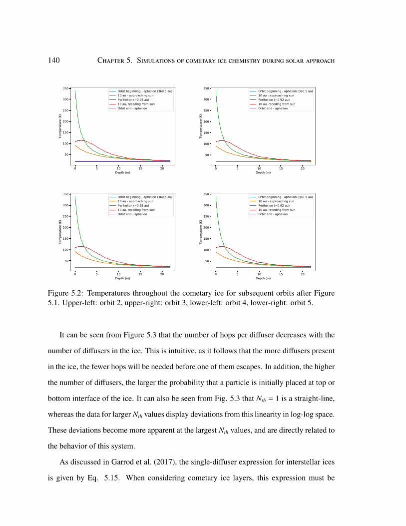
140 Chapter 5. Simulations of cometary ice chemistry during solar approach
0 5 10 15 20Depth (m)
50
100
150
200
250
300
350
Tem
pera
ture
(K)
Orbit beginning - aphelion (360.5 au)10 au - approaching sunPerihelion (~0.92 au)10 au, receding from sunOrbit end - aphelion
0 5 10 15 20Depth (m)
50
100
150
200
250
300
350
Tem
pera
ture
(K)
Orbit beginning - aphelion (360.5 au)10 au - approaching sunPerihelion (~0.92 au)10 au, receding from sunOrbit end - aphelion
0 5 10 15 20Depth (m)
50
100
150
200
250
300
350
Tem
pera
ture
(K)
Orbit beginning - aphelion (360.5 au)10 au - approaching sunPerihelion (~0.92 au)10 au, receding from sunOrbit end - aphelion
0 5 10 15 20Depth (m)
50
100
150
200
250
300
350
Tem
pera
ture
(K)
Orbit beginning - aphelion (360.5 au)10 au - approaching sunPerihelion (~0.92 au)10 au, receding from sunOrbit end - aphelion
Figure 5.2: Temperatures throughout the cometary ice for subsequent orbits after Figure5.1. Upper-left: orbit 2, upper-right: orbit 3, lower-left: orbit 4, lower-right: orbit 5.
It can be seen from Figure 5.3 that the number of hops per diffuser decreases with the
number of diffusers in the ice. This is intuitive, as it follows that the more diffusers present
in the ice, the fewer hops will be needed before one of them escapes. In addition, the higher
the number of diffusers, the larger the probability that a particle is initially placed at top or
bottom interface of the ice. It can also be seen from Fig. 5.3 that Nth = 1 is a straight-line,
whereas the data for larger Nth values display deviations from this linearity in log-log space.
These deviations become more apparent at the largest Nth values, and are directly related to
the behavior of this system.
As discussed in Garrod et al. (2017), the single-diffuser expression for interstellar ices
is given by Eq. 5.15. When considering cometary ice layers, this expression must be
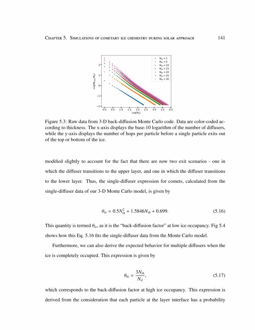
Chapter 5. Simulations of cometary ice chemistry during solar approach 141
0.0 0.5 1.0 1.5 2.0 2.5 3.0 3.5 4.0Log(Nd)
2
1
0
1
2
Log(
N hop
s/Nd)
Nth = 1Nth = 5Nth = 10Nth = 15Nth = 20Nth = 25Nth = 30
Figure 5.3: Raw data from 3-D back-diffusion Monte Carlo code. Data are color-coded ac-cording to thickness. The x-axis displays the base-10 logarithm of the number of diffusers,while the y-axis displays the number of hops per particle before a single particle exits outof the top or bottom of the ice.
modified slightly to account for the fact that there are now two exit scenarios - one in
which the diffuser transitions to the upper layer, and one in which the diffuser transitions
to the lower layer. Thus, the single-diffuser expression for comets, calculated from the
single-diffuser data of our 3-D Monte Carlo model, is given by
θlo = 0.5N2th + 1.5846Nth + 0.699. (5.16)
This quantity is termed θlo, as it is the “back-diffusion factor” at low ice occupancy. Fig 5.4
shows how this Eq. 5.16 fits the single-diffuser data from the Monte Carlo model.
Furthermore, we can also derive the expected behavior for multiple diffusers when the
ice is completely occupied. This expression is given by
θhi =3Nth
Nd, (5.17)
which corresponds to the back-diffusion factor at high ice occupancy. This expression is
derived from the consideration that each particle at the layer interface has a probability
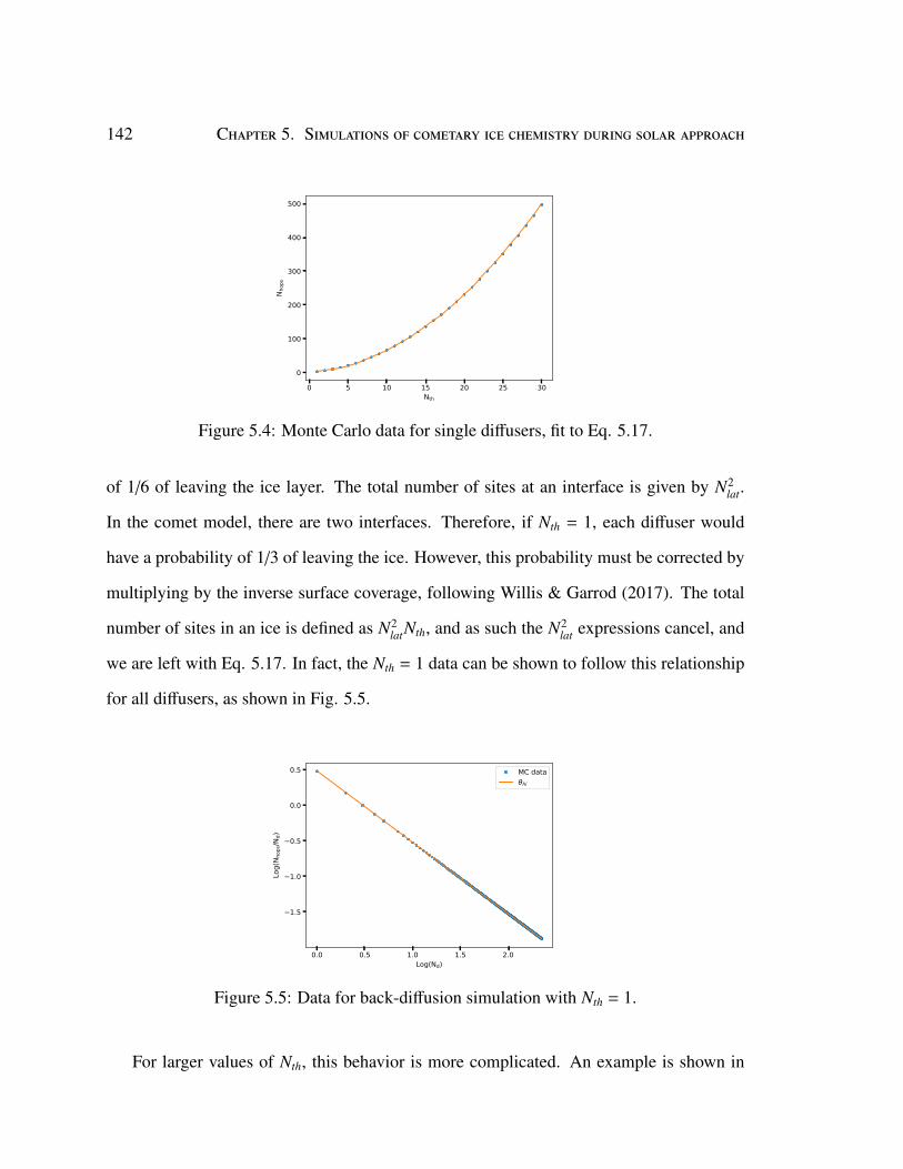
142 Chapter 5. Simulations of cometary ice chemistry during solar approach
0 5 10 15 20 25 30Nth
0
100
200
300
400
500
N hop
s
Figure 5.4: Monte Carlo data for single diffusers, fit to Eq. 5.17.
of 1/6 of leaving the ice layer. The total number of sites at an interface is given by N2lat.
In the comet model, there are two interfaces. Therefore, if Nth = 1, each diffuser would
have a probability of 1/3 of leaving the ice. However, this probability must be corrected by
multiplying by the inverse surface coverage, following Willis & Garrod (2017). The total
number of sites in an ice is defined as N2latNth, and as such the N2
lat expressions cancel, and
we are left with Eq. 5.17. In fact, the Nth = 1 data can be shown to follow this relationship
for all diffusers, as shown in Fig. 5.5.
0.0 0.5 1.0 1.5 2.0Log(Nd)
1.5
1.0
0.5
0.0
0.5
Log(
N hop
s/Nd)
MC datahi
Figure 5.5: Data for back-diffusion simulation with Nth = 1.
For larger values of Nth, this behavior is more complicated. An example is shown in
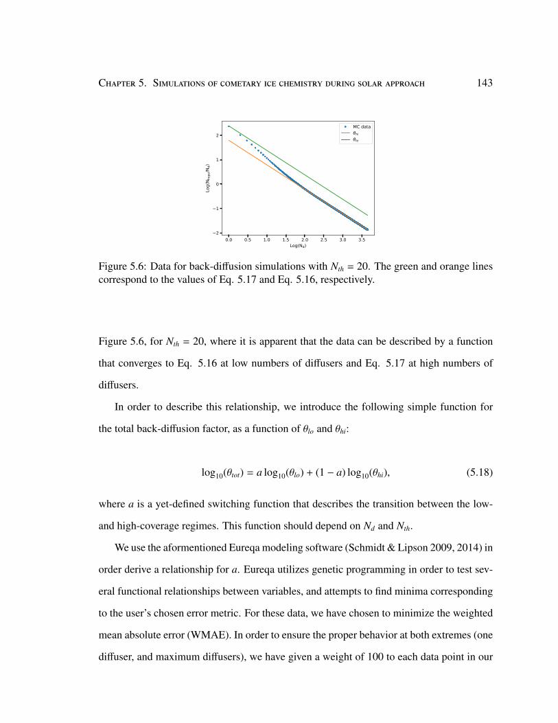
Chapter 5. Simulations of cometary ice chemistry during solar approach 143
0.0 0.5 1.0 1.5 2.0 2.5 3.0 3.5Log(Nd)
2
1
0
1
2
Log(
N hop
s/Nd)
MC datahi
lo
Figure 5.6: Data for back-diffusion simulations with Nth = 20. The green and orange linescorrespond to the values of Eq. 5.17 and Eq. 5.16, respectively.
Figure 5.6, for Nth = 20, where it is apparent that the data can be described by a function
that converges to Eq. 5.16 at low numbers of diffusers and Eq. 5.17 at high numbers of
diffusers.
In order to describe this relationship, we introduce the following simple function for
the total back-diffusion factor, as a function of θlo and θhi:
log10(θtot) = a log10(θlo) + (1 − a) log10(θhi), (5.18)
where a is a yet-defined switching function that describes the transition between the low-
and high-coverage regimes. This function should depend on Nd and Nth.
We use the aformentioned Eureqa modeling software (Schmidt & Lipson 2009, 2014) in
order derive a relationship for a. Eureqa utilizes genetic programming in order to test sev-
eral functional relationships between variables, and attempts to find minima corresponding
to the user’s chosen error metric. For these data, we have chosen to minimize the weighted
mean absolute error (WMAE). In order to ensure the proper behavior at both extremes (one
diffuser, and maximum diffusers), we have given a weight of 100 to each data point in our
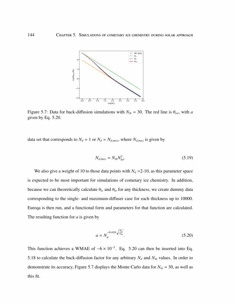
144 Chapter 5. Simulations of cometary ice chemistry during solar approach
0.0 0.5 1.0 1.5 2.0 2.5 3.0 3.5 4.0Log(Nd)
2
1
0
1
2
Log(
N hop
s/Nd)
MC datahi
lo
tot
Figure 5.7: Data for back-diffusion simulations with Nth = 30. The red line is θtot, with agiven by Eq. 5.20.
data set that corresponds to Nd = 1 or Nd = Nd,max, where Nd,max is given by
Nd,max = NthN2lat. (5.19)
We also give a weight of 10 to those data points with Nd =2-10, as this parameter space
is expected to be most important for simulations of cometary ice chemistry. In addition,
because we can theoretically calculate θlo and θhi for any thickness, we create dummy data
corresponding to the single- and maximum-diffuser case for each thickness up to 10000.
Eureqa is then run, and a functional form and parameters for that function are calculated.
The resulting function for a is given by
a = N−0.418
√NdNth
d . (5.20)
This function achieves a WMAE of ∼6 × 10⁻⁵. Eq. 5.20 can then be inserted into Eq.
5.18 to calculate the back-diffusion factor for any arbitrary Nd and Nth values. In order to
demonstrate its accuracy, Figure 5.7 displays the Monte Carlo data for Nth = 30, as well as
this fit.
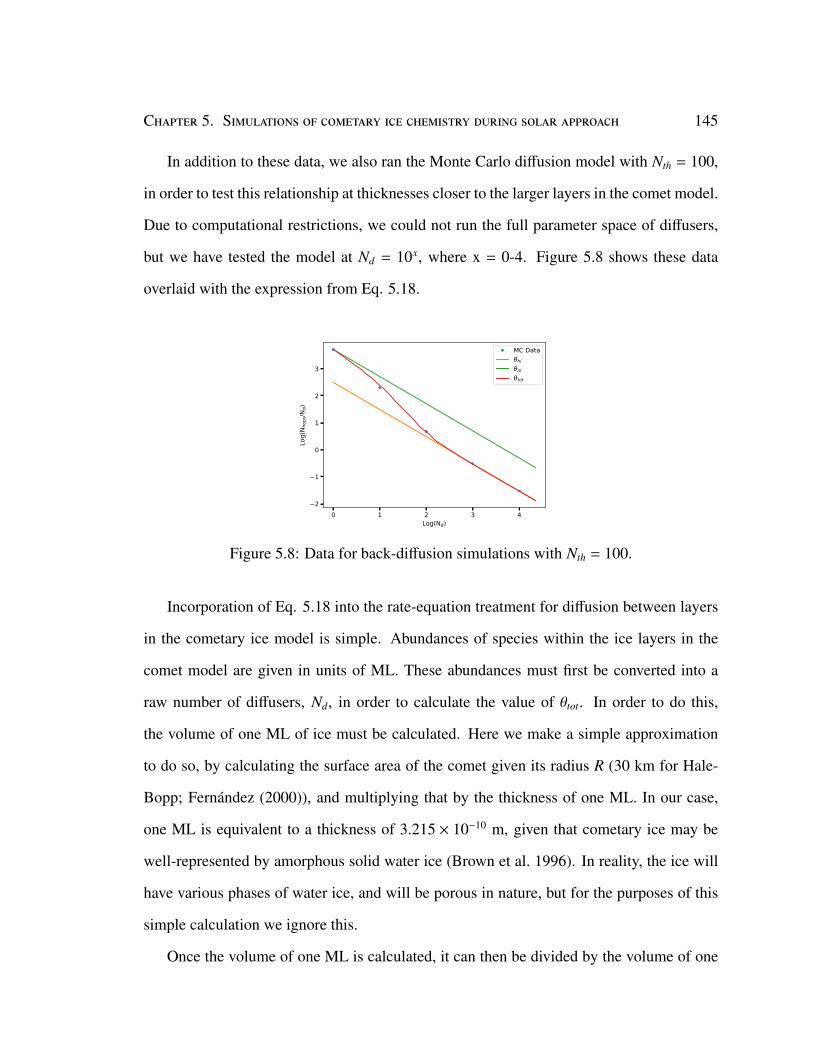
Chapter 5. Simulations of cometary ice chemistry during solar approach 145
In addition to these data, we also ran the Monte Carlo diffusion model with Nth = 100,
in order to test this relationship at thicknesses closer to the larger layers in the comet model.
Due to computational restrictions, we could not run the full parameter space of diffusers,
but we have tested the model at Nd = 10x, where x = 0-4. Figure 5.8 shows these data
overlaid with the expression from Eq. 5.18.
0 1 2 3 4Log(Nd)
2
1
0
1
2
3
Log(
N hop
s/Nd)
MC Datahi
lo
tot
Figure 5.8: Data for back-diffusion simulations with Nth = 100.
Incorporation of Eq. 5.18 into the rate-equation treatment for diffusion between layers
in the cometary ice model is simple. Abundances of species within the ice layers in the
comet model are given in units of ML. These abundances must first be converted into a
raw number of diffusers, Nd, in order to calculate the value of θtot. In order to do this,
the volume of one ML of ice must be calculated. Here we make a simple approximation
to do so, by calculating the surface area of the comet given its radius R (30 km for Hale-
Bopp; Fernández (2000)), and multiplying that by the thickness of one ML. In our case,
one ML is equivalent to a thickness of 3.215 × 10⁻¹⁰ m, given that cometary ice may be
well-represented by amorphous solid water ice (Brown et al. 1996). In reality, the ice will
have various phases of water ice, and will be porous in nature, but for the purposes of this
simple calculation we ignore this.
Once the volume of one ML is calculated, it can then be divided by the volume of one
146 Chapter 5. Simulations of cometary ice chemistry during solar approach
H2O molecule in order to get the number of molecules in one ML of ice. Note that, for
each consecutive layer in the comet, we simply multiply this volume by the number of ML
in the layer to get the total volume of that layer. This does not account for the changing
radius as depth increases in the comet, but the radius of the comet is much larger than the
depth to which we are studying. As such, the effect on the volume is negliglible.
Once we have the total number of molecules in one layer, we can easily calculate Nd
for the diffuser of interest. Then, the value of Eq. 5.20 is calculated, followed by the value
of θtot using Eq. 5.18. Eq. 5.13 is then modified using the new back-diffusion factor as
follows:
Rswap,m(i) = Nm(i)NS
NM
kswap(i)θtot
. (5.21)
The same modification is made for the calculations of the diffusion rates between all lay-
ers in the cometary ice. Finally, the surface back-diffusion correction of Willis & Garrod
(2017) is implemented for surface reactions, using the flat-surface formulation from those
authors.
5.3.3 Updated chemical model results
The back-diffusion results described in Section 5.3.2, as well as the heat transfer re-
sults from Section 5.3.1, were incorporated into the chemical model of Garrod (2019). The
model was then run in two stages. First, a cold-storage model was run, simulating the
physical conditions in the Oort cloud. The temperature was held at 10 K for 5 × 10⁹ yr,
following Garrod (2019). The medium interstellar radiation field (G = G0) from that paper
was also used. Following the cold-storage model, the orbit of Comet C1/1995 (Hale-Bopp)
was simulated. In total, five orbits were calculated, starting at aphelion. The orbital ele-
ments were assumed to remain unchanged for each orbit, and the chemistry was simulated
as the temperature structure of the cometary nucleus evolved over time. The five orbits
Chapter 5. Simulations of cometary ice chemistry during solar approach 147
took ∼12,000 yrs.
The chemical network that is used is based on that of Willis et al. (2020). However, for
computational efficiency, the network is limited to only species containing three or fewer
carbon atoms. In addition, molecules containing rare heavy atoms, such as P, S, and Si, are
removed from the network. The ice is separated into 18 layers, with increasing thickness
with depth. This is one deviation from the study of Garrod (2019), where 25 layers were
used, and a greater depth was achieved. This was changed for computational efficiency.
Figures 5.9 and 5.10 show outputs for the chemical model during the cold-storage
phase, at 1 × 10⁶ yr and 5 × 10⁹ yr. These plots display the fractional composition in the
ice as a function of depth. The top x-axis displays depth in meters, while the bottom x-axis
shows depth in monolayers.
In general, the initial ice constituents do not change much in fractional composition
throughout the ice from the initiation of the model to the end of the cold-storage phase. The
more complex molecules exhibit much more drastic changes in composition throughout the
ice. At earlier times, they are concentrated primarily in the first cm of ice. At the final time
of the cold-storage phase, however, their abundances are elevated all throughout the ice.
This is a key difference of this model as compared to that of Garrod (2019). This is likely
due to the addition of more non-thermal chemical reaction mechanisms.
Figures 5.11-5.16 display chemical model results from the solar approach model at the
first, third, and fifth aphelion and perihelion. Overall, there is not much chemical change
from one orbit to another. In fact, the fractional composition of the ice is not substantially
different from the cold-storage model, even after five orbits.
One key feature of interest in the solar approach model occurs at the surface of the
cometary ice. It is apparent that many species are depleted near the surface at perihelion,
caused by sublimation from due to the elevated temperatures. One exception is glycine,
which appears elevated at perihelion. This change is then reversed as the comet recedes
148 Chapter 5. Simulations of cometary ice chemistry during solar approach
from the sun, and by the time aphelion is achieved, most of the fractional composition
returns to how it was before perihelion. Further analysis of these data will investigate the
sublimation rates of species from the surface.
5.4 FutureWorkThe models presented here will be further analyzed, paying special attention to subli-
mation rates and the chemical mechanisms contributing to the chemistry observed here.
In addition, other chemical models will also be run. A full cold-storage/solar approach
model with an expanded chemical network, and an identical layer set-up to that described
in Garrod (2019). A chemical model with the same mechanisms as those in Garrod (2019)
will be also run, with both the smaller and expanded chemical networks, in order to isolate
the effects of the new mechanisms presented here.

Chapter 5. Simulations of cometary ice chemistry during solar approach 149
Figure 5.9: Abundances of molecules throughout the cometary nucleus at t = 106 yr. Thetop panel displays the initial ice components along with a few other simple molecules,while the bottom panel displays more complex molecules.
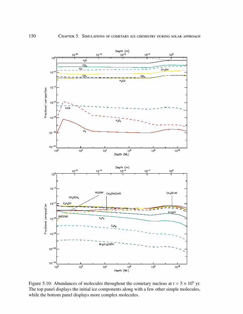
150 Chapter 5. Simulations of cometary ice chemistry during solar approach
Figure 5.10: Abundances of molecules throughout the cometary nucleus at t = 5 × 10⁹ yr.The top panel displays the initial ice components along with a few other simple molecules,while the bottom panel displays more complex molecules.
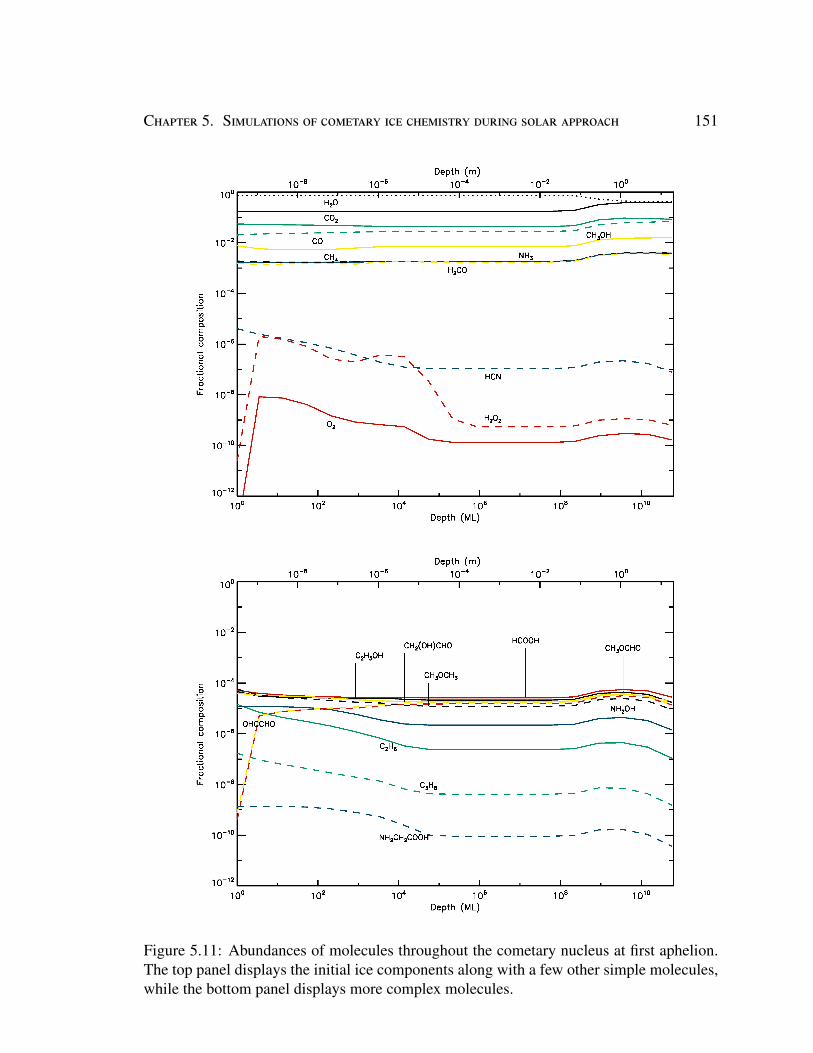
Chapter 5. Simulations of cometary ice chemistry during solar approach 151
Figure 5.11: Abundances of molecules throughout the cometary nucleus at first aphelion.The top panel displays the initial ice components along with a few other simple molecules,while the bottom panel displays more complex molecules.
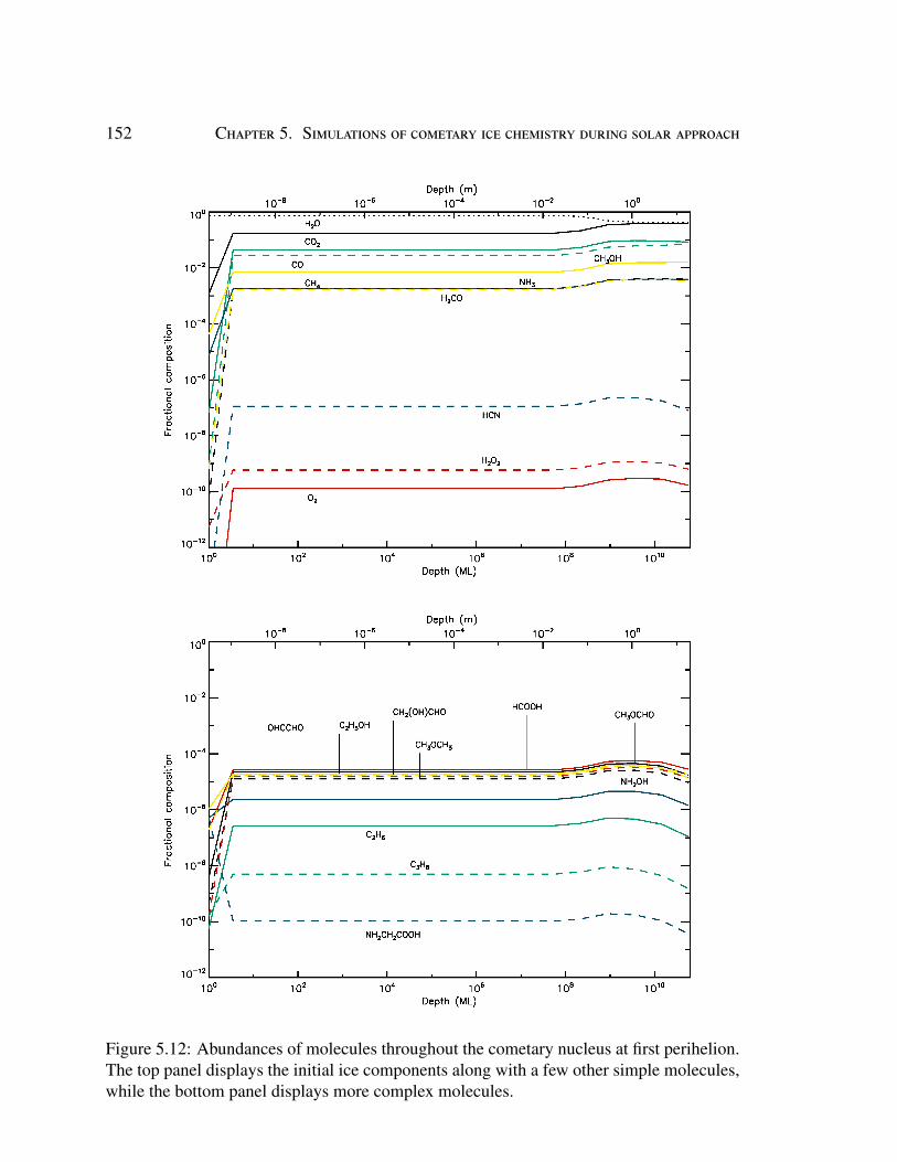
152 Chapter 5. Simulations of cometary ice chemistry during solar approach
Figure 5.12: Abundances of molecules throughout the cometary nucleus at first perihelion.The top panel displays the initial ice components along with a few other simple molecules,while the bottom panel displays more complex molecules.
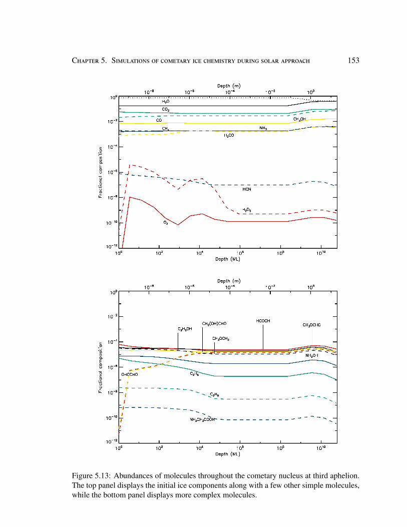
Chapter 5. Simulations of cometary ice chemistry during solar approach 153
Figure 5.13: Abundances of molecules throughout the cometary nucleus at third aphelion.The top panel displays the initial ice components along with a few other simple molecules,while the bottom panel displays more complex molecules.
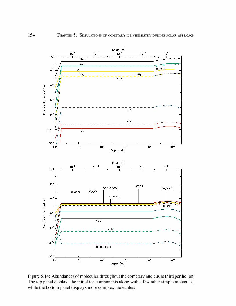
154 Chapter 5. Simulations of cometary ice chemistry during solar approach
Figure 5.14: Abundances of molecules throughout the cometary nucleus at third perihelion.The top panel displays the initial ice components along with a few other simple molecules,while the bottom panel displays more complex molecules.
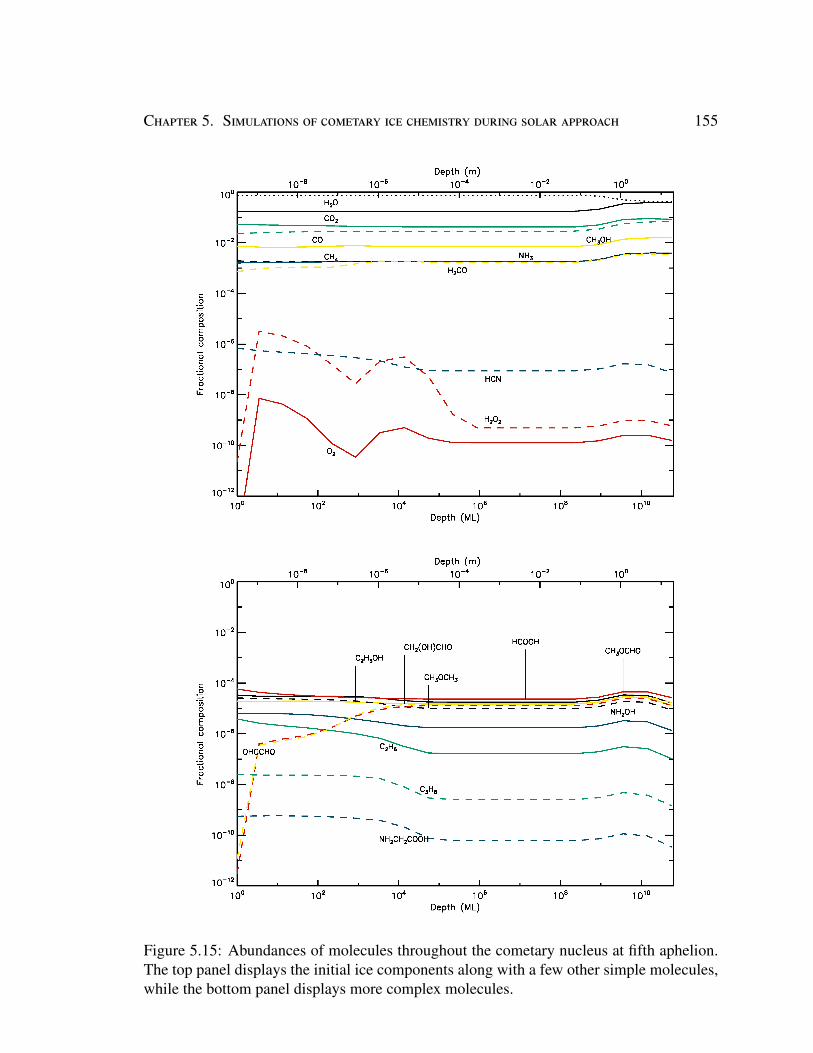
Chapter 5. Simulations of cometary ice chemistry during solar approach 155
Figure 5.15: Abundances of molecules throughout the cometary nucleus at fifth aphelion.The top panel displays the initial ice components along with a few other simple molecules,while the bottom panel displays more complex molecules.
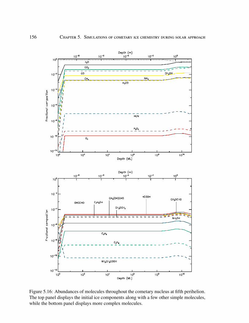
156 Chapter 5. Simulations of cometary ice chemistry during solar approach
Figure 5.16: Abundances of molecules throughout the cometary nucleus at fifth perihelion.The top panel displays the initial ice components along with a few other simple molecules,while the bottom panel displays more complex molecules.
157
Chapter 6
Concluding Remarks
In this work, we have made several advancements in the modelling of the chemistry of
star-forming regions and cometary nuclei. To do this, we have made use of various compu-
tational techniques, including kinetic Monte Carlo simulations and rate-equation models.
The main conclusions of each chapter are summarized below.
6.1 Chapter 2In Chapter 2, we utilized two kinetic Monte Carlo models to investigate the phenomenon
of back-diffusion and its application to interstellar grain-surface chemistry. The magnitude
of the back-diffusion effect, φ, was studied and found to vary with factors including the
grain-surface coverage, grain size, and lattice morphology. The largest effect is seen for
grains with low surface coverage, where back-diffusion can slow surface reactions by as
much as a factor of ∼5. Simple expressions are fit to these Monte Carlo data for incorpora-
tion of the grain-surface back-diffusion effect into astrochemical rate-equation models. A
simple rate-equation model is constructed and found to be in excellent agreement with the
Monte Carlo results using this method.
158 Chapter 6. Concluding Remarks
6.2 Chapter 3In Chapter 3, several astrochemical modelling studies of organic molecules in star-
forming regions were presented. The main conclusions are below:
1. Methoxymethanol (CH3OCH2OH) was detected for the first in the interstellar medium,
towards the star-forming region NGC 6334I. The chemical kinetics model MAG-
ICKAL was used to simulate the chemistry of methoxymethanol using different warm-
up timescales for the hot core. All models significantly underproduced methoxymethanol,
indicating that significant chemical pathways were missing from the chemical net-
work used.
2. Cyanamide (NH2CN) was detected towards the protostar IRAS 16293 as part of the
PILS program. MAGICKAL was used to simulate the chemistry of this molecule,
after making changes to the chemical network for cyanamide based on recent experi-
mental and theoretical work. It was found that, when using physical conditions repre-
sentative of IRAS 16293, the abundance of cyanamide was severely under-predicted.
It was determined that this was due to a fault in the two-stage approach typically used
to simulate the chemistry of hot-core regions, where high gas densities are reached
at very low temperatures. This highlighted the need for simultaneous collapse and
warm-up models of hot cores.
3. Methyl isocyanide (CH3NC) was detected towards IRAS 16293, also as part of the
PILS program. To compare to observational values, we used MAGICKAL to sim-
ulate the chemistry of CH3NC. This was the first modelling study conducted for
this molecule, and so its reaction network was built from scratch. A similar result
was found as for NH2CN, where lower gas densities were needed to reproduce ob-
servational column densities. The CH3NC:CH3CN ratio was also discovered to be
Chapter 6. Concluding Remarks 159
sensitive to temperature.
4. Propyne (CH3CCH) was also detected towards IRAS 16293. Using MAGICKAL,
the chemistry of propyne was studied, varying the final gas-phase density for the
collapse phase of the chemical model. Grain-surface chemistry was found to be
the predominant means by which propyne was formed. Observational values were
generally found to be well-reproduced by most of the models.
6.3 Chapter 4In Chapter 4, we have expanded on the study of CH3NC presented in Chapter 3. The
chemistry of complex cyanides and isocyanides is modelled in the context of the EMoCA
observational survey of Sagittarius B2(N2).
Tentative detections of CH3NC and HCCNC are reported towards Sgr B2(N2) for the
first time. The chemistry of these molecules, along with much more complex cyanides and
isocyanides (including C2H3NC and C2H5NC) were studied using MAGICKAL, with many
of these species being incorporated into astrochemical models for the first time.
A new method of modelling star-formation in astrochemical models was also intro-
duced, where the collapse and warm-up phases of traditional hot-core models occur con-
currently. Using this new model, it was found that an elevated, extinction-dependent,
cosmic-ray ionization rate produced the best agreement with observational values. This
is particularly true for the ratio of CH3NC:CH3CN, which was reproduced almost exactly
in such models. However, the ratio of HCCNC:HC3N was significantly higher than obser-
vational values in all models presented. Thus, this systematic overproduction of HCCNC
should be a topic of further study.

160 Chapter 6. Concluding Remarks
6.4 Chapter 5In Chapter 5, we have presented the first chemical models of cometary nuclei undergo-
ing solar approach. The incorporation of the orbital mechanics of Hale-Bopp, as well as
the calculations of heat transfer throughout the ice, are presented and their incorporation
into chemical kinetics models is discussed.
A new Monte Carlo model for the simulation of back-diffusion in ice layers is also
discussed, and its results are presented. Fits are calculated for the inclusion of this effect
into chemical kinetics models.
Finally, the first results of the complete chemical model of cometary cold storage and
solar approach are presented, along with a discussion of key features of the outputs. Av-
enues for future work are also discussed.
161
References
Adams, W. S. 1941, The Astrophysical Journal, 93, 11
Agúndez, M., Marcelino, N., Cernicharo, J., Roueff, E., & Tafalla, M. 2019, Astronomy &Astrophysics, 625, A147
Allen, C. E., & Seebauer, E. G. 1996, Journal of Chemical Physics, 104, 2557
Altwegg, K., Balsiger, H., Bar-Nun, A., et al. 2016, Science Advances, 2, 1
Anderson, R. J., & Gwinn, W. D. 1968, The Journal of Chemical Physics, 49, 3988
Bacmann, A., Taquet, V., Faure, A., Kahane, C., & Ceccarelli, C. 2012, Astronomy andAstrophysics, doi:10.1051/0004-6361/201219207
Ball, J. A., Gottlieb, C. A., Lilley, A. E., & Radford, H. E. 1970, The Astrophysical Journal,162, L203
Balsiger, H., Altwegg, K., Bochsler, P., et al. 2007, Space Science Reviews,doi:10.1007/s11214-006-8335-3
Barger, C. J., & Garrod, R. T. 2020, The Astrophysical Journal, 888, 38
Baskakov, O. I., Dyubko, S. F., Ilyushin, V. V., et al. 1996, Journal of Molecular Spec-troscopy, 179, 94
BAUER, A., & BOGEY, M. 1970, COMPTES RENDUS HEBDOMADAIRES DESSEANCES DE L ACADEMIE DES SCIENCES SERIE B, 271, 892
BAUER, A., & MAES, S. 1969, JOURNAL DE PHYSIQUE, 30, 169
Baulch, D. L., Cobos, C. J., Cox, R. A., et al. 1992, Journal of Physical and ChemicalReference Data, 21, 411
162 References
Bell, T. A., Cernicharo, J., Viti, S., et al. 2014, Astronomy and Astrophysics, 564,doi:10.1051/0004-6361/201321872
Belloche, A., Garrod, R. T., Müller, H. S., et al. 2009, Astronomy and Astrophysics, 499,215
Belloche, A., Garrod, R. T., Müller, H. S., & Meuten, K. M. 2014, Science, 345, 1584
Belloche, A., Menten, K. M., Comito, C., et al. 2008, Astronomy and Astrophysics, 482,179
Belloche, A., Müller, H. S., Garrod, R. T., & Menten, K. M. 2016, Astronomy and Astro-physics, 587, arXiv:1511.05721
Belloche, A., Müller, H. S., Menten, K. M., Schilke, P., & Comito, C. 2013, Complexorganic molecules in the interstellar medium: IRAM 30 m line survey of SagittariusB2(N) and (M), EDP Sciences for European Southern Observatory, arXiv:1308.5062
Belloche, A., Meshcheryakov, A. A., Garrod, R. T., et al. 2017, Astronomy and Astro-physics, 601, arXiv:1701.04640
Benidar, A., Bégué, D., Richter, F., et al. 2015, ChemPhysChem, 16, 848
Bergner, J. B., Öberg, K. I., Garrod, R. T., & Graninger, D. M. 2017, The AstrophysicalJournal, arXiv:1705.05338
Bertin, M., Doronin, M., Fillion, J. H., et al. 2017, Astronomy and Astrophysics, 598,arXiv:1610.05010
Bestmann, G., & Dreizier, H. 1982, Zeitschrift fur Naturforschung - Section A Journal ofPhysical Sciences, 37, 58
Blake, G. A., van Dishoek, E. F., Jansen, D. J., Groesbeck, T. D., & Mundy, L. G. 1994,The Astrophysical Journal, 428, 680
Bockelée-Morvan, D., Lis, D. C., Wink, J. E., et al. 2000, Astronomy and Astrophysics,353, 1101
Bøgelund, E. G., Barr, A. G., Taquet, V., et al. 2019, Astronomy and Astrophysics, 628,arXiv:1906.06156
References 163
Bohlin, R. C., Savage, B. D., & Drake, J. F. 1978, The Astrophysical Journal, 224, 132
Bolton, K., Owen, N. L., & Sheridan, J. 1969, Spectrochimica Acta Part A: MolecularSpectroscopy, 25, 1
Bonfand, M., Belloche, A., Garrod, R. T., et al. 2019, Astronomy and Astrophysics, 628,arXiv:1906.04695
Bonfand, M., Belloche, A., Menten, K. M., Garrod, R. T., & Müller, H. S. 2017, Astronomyand Astrophysics, 604, arXiv:1703.09544
Botar, L., & Vidóczy, T. 1984, Chemical Physics Letters, 104, 16
Botschwina, P., & Heyl. 1999, Molecular Physics, 97, 209
Brauer, C. S., Pearson, J. C., Drouin, B. J., & Yu, S. 2009, Astrophysical Journal, Supple-ment Series, 184, 133
Brogan, C. L., Hunter, T. R., Cyganowski, C. J., et al. 2016, The Astrophysical Journal,832, 187
Brown, D. E., George, S. M., Huang, C., et al. 1996, Journal of Physical Chemistry,doi:10.1021/jp952547j
Brownlee, D., Tsou, P., Aléon, J., et al. 2006, Science, doi:10.1126/science.1135840
Buhl, D., & Snyder, L. E. 1973, in Molecules in the Galactic Environment, ed. M. A.Gordon & L. E. Snyder, 187
Bürger, H., Sommer, S., Lentz, D., & Preugschat, D. 1992, Journal of Molecular Spec-troscopy, 156, 360
Cabezas, C., Cernicharo, J., Alonso, J. L., et al. 2013, Astrophysical Journal, 775, 10
Calcutt, H., Fiechter, M., Willis, E., et al. 2018, Astronomy and Astrophysics, 617,doi:10.1051/0004-6361/201833140
Calcutt, H., Willis, E. R., Jørgensen, J. K., et al. 2019, Astronomy & Astrophysics, 631,A137
Cami, J., Bernard-Salas, J., Peeters, E., & Malek, S. E. 2010, Science, 329, 1180
164 References
Caswell, J. L. 1996, Monthly Notices of the Royal Astronomical Society, 283, 606
Cazaux, S., Tielens, A. G. G. M., Ceccarelli, C., et al. 2003, The Astrophysical Journal,593, L51
Cernicharo, J., Kahane, C., Guelin, M., & Gomez-Gonzalez, J. 1988, Astronomy and As-trophysics, 189, L1
Cernicharo, J., Marcelino, N., Roueff, E., et al. 2012, Astrophysical Journal Letters,doi:10.1088/2041-8205/759/2/L43
Cernicharo, J., Velilla-Prieto, L., Agúndez, M., et al. 2019, Astronomy and Astrophysics,627, arXiv:1906.09352
Chang, Q., Cuppen, H. M., & Herbst, E. 2005, Astronomy and Astrophysics, 434, 599
Charnley, S. B. 2005, in Advances in Space Research, Vol. 36, 132–136
Cheung, A. C., Rank, D. M., Townes, C. H., Thornton, D. D., & Welch, W. J. 1969, Nature,221, 626
Clements, A. R., Berk, B., Cooke, I. R., & Garrod, R. T. 2018, Physical Chemistry Chemi-cal Physics, 20, 5553
Costagliola, F., Sakamoto, K., Muller, S., et al. 2015, Astronomy and Astrophysics, 582,doi:10.1051/0004-6361/201526256
Coutens, A., Willis, E., Garrod, R., et al. 2018, Astronomy and Astrophysics, 612,doi:10.1051/0004-6361/201732346
Crovisier, J., Bockelée-Morvan, D., Biver, N., et al. 2004, Astronomy and Astrophysics,doi:10.1051/0004-6361:20040116
Dean, A. M., & Bozzelli, J. W. 2000, in Gas-Phase Combustion Chemistry (N/A), 125–341
DeFrees, D., McLean, A., & Herbst, E. 1985, The Astrophysical Journal, 293, 236
Douglas, A. E., & Herzberg, G. 1941, The Astrophysical Journal, 94, 381
Duncan, M., Quinn, T., & Tremaine, S. 1987, The Astronomical Journal,doi:10.1086/114571
References 165
Dunham, T., J. 1937, Publications of the Astronomical Society of the Pacific, 49, 26
Ellsworth, K., & Schubert, G. 1983, Icarus, doi:10.1016/0019-1035(83)90242-7
Elsila, J. E., Glavin, D. P., & Dworkin, J. P. 2009, Meteoritics and Planetary Science,doi:10.1111/j.1945-5100.2009.tb01224.x
Endres, C. P., Schlemmer, S., Schilke, P., Stutzki, J., & Müller, H. S. 2016, Journal ofMolecular Spectroscopy, 327, 95
Fernández, Y. R. 2000, Earth, Moon, and Planets, 89, 3
Fliege, E., & Dreizler, H. 1985, Zeitschrift fur Naturforschung - Section A Journal of Phys-ical Sciences, 40, 43
Fukuyama, Y., Odashima, H., Takagi, K., & Tsunekawa, S. 1996, The Astrophysical Jour-nal Supplement Series, 104, 329
Gaches, B. A. L., Offner, S. S. R., & Bisbas, T. G. 2019, The Astrophysical Journal, 878,105
Gardner, F. F., & Winnewisser, G. 1975, The Astrophysical Journal, 195, L127
Garrod, R. T. 2008, Astronomy and Astrophysics, 491, 239
—. 2013a, The Astrophysical Journal, 765, 60
—. 2013b, The Astrophysical Journal, 778, 158
—. 2019, The Astrophysical Journal, arXiv:1909.03366
Garrod, R. T., Belloche, A., Müller, H. S., & Menten, K. M. 2017, Astronomy and Astro-physics, doi:10.1051/0004-6361/201630254
Garrod, R. T., & Herbst, E. 2006, Astronomy & Astrophysics, doi:10.1051/0004-6361:20065560
Garrod, R. T., & Pauly, T. 2011, The Astrophysical Journal, 735, 15
Garrod, R. T., Weaver, S. L. W., & Herbst, E. 2008, The Astrophysical Journal, 682, 283
166 References
Gaume, R. A., Claussen, M. J., de Pree, C. G., Goss, W. M., & Mehringer, D. M. 1995,The Astrophysical Journal, 449, 663
Gerin, M., De Luca, M., Black, J., et al. 2010, Astronomy and Astrophysics, 518, L110
Ghesquière, P., Ivlev, A., Noble, J. A., & Theulé, P. 2018, Astronomy and Astrophysics,doi:10.1051/0004-6361/201732288
Glavin, D. P., Dworkin, J. P., & Sandford, S. A. 2008, Meteoritics and Planetary Science,doi:10.1111/j.1945-5100.2008.tb00629.x
Goldsmith, P. F., & Langer, W. D. 1999, The Astrophysical Journal, 517, 209
Gottlieb, C. A., Apponi, A. J., McCarthy, M. C., Thaddeus, P., & Linnartz, H. 2000, Journalof Chemical Physics, 113, 1910
Gould, R. J., & Salpeter, E. E. 1963, The Astrophysical Journal, 138, 393
Graninger, D. M., Herbst, E., Öberg, K. I., & Vasyunin, A. I. 2014, The AstrophysicalJournal, 787, 74
Gratier, P., Pety, J., Guzmán, V., et al. 2013, Astronomy and Astrophysics, 557,doi:10.1051/0004-6361/201321031
Guarnieri, A., Hinze, R., Krüger, M., et al. 1992, Journal of Molecular Spectroscopy, 156,39
Guélin, M., Muller, S., Cernicharo, J., McCarthy, M. C., & Thaddeus, P. 2004, Astronomyand Astrophysics, 426, doi:10.1051/0004-6361:200400074
Guilbert-Lepoutre, A., & Jewitt, D. 2011, Astrophysical Journal, doi:10.1088/0004-637X/743/1/31
Harada, N., Herbst, E., & Wakelam, V. 2010, Astrophysical Journal, 721, 1570
Hasegawa, T. I., Herbst, E., & Leung, C. M. 1992, The Astrophysical Journal SupplementSeries, 82, 167
Hatlee, M. D., & Kozak, J. J. 1980, Physical Review B, 21, 1400
Hays, B. M., & Widicus Weaver, S. L. 2013, Journal of Physical Chemistry A, 117, 7142
References 167
Hébrard, E., Dobrijevic, M., Pernot, P., et al. 2009, Journal of Physical Chemistry A, 113,11227
Heise, H. M., Winther, F., & Lutz, H. 1981, Journal of Molecular Spectroscopy, 90, 531
Herbst, E., & Klemperer, W. 1973, The Astrophysical Journal, 185, 505
Herbst, E., & Leung, C. M. 1986, The Astrophysical Journal, 310, 378
Herbst, E., & van Dishoeck, E. F. 2009, Annual Review of Astronomy and Astrophysics,47, 427
Herman, G., & Podolak, M. 1985, Icarus, doi:10.1016/0019-1035(85)90107-1
Herman, G., & Weissman, P. R. 1987, Icarus, doi:10.1016/0019-1035(87)90108-4
Hirahara, Y., Ohshima, Y., & Endo, Y. 1993, The Astrophysical Journal, 403, L83
Hollis, J. M., Jewell, P. R., Lovas, F. J., & Remijan, A. 2004, The Astrophysical Journal,613, L45
Hudson, R. L., & Moore, M. H. 2004, Icarus, 172, 466
Indriolo, N., Geballe, T. R., Oka, T., & McCall, B. J. 2007, The Astrophysical Journal, 671,1736
Indriolo, N., Neufeld, D. A., Gerin, M., et al. 2015, Astrophysical Journal, 800,arXiv:1412.1106
Irvine, W. M., Bergin, E. A., Dickens, J. E., et al. 1998, Nature, 393, 547
Irvine, W. M., & Schloerb, F. P. 1984, The Astrophysical Journal, 282, 516
Jacobsen, S. K., Jørgensen, J. K., Van Der Wiel, M. H., et al. 2018, Astronomy and Astro-physics, 612, arXiv:1712.06984
Jefferts, K. B., Penzias, A. A., & Wilson, R. W. 1970, The Astrophysical Journal, 161, L87
Johnson, D. R., Lovas, F. J., Gottlieb, C. A., et al. 1977, The Astrophysical Journal, 218,370
168 References
Johnson, K. E., Brogan, C. L., Indebetouw, R., et al. 2018, The Astrophysical Journal, 853,125
Jørgensen, J. K., Favre, C., Bisschop, S. E., et al. 2012, Astrophysical Journal Letters, 757,arXiv:1208.5498
Jørgensen, J. K., Van Der Wiel, M. H., Coutens, A., et al. 2016, Astronomy and Astro-physics, arXiv:1607.08733
Katz, N., Furman, I., Biham, O., Pirronello, V., & Vidali, G. 1999, The AstrophysicalJournal, 522, 305
Kawaguchi, K., Kagi, E., Hirano, T., Takano, S., & Saito, S. 1993, The AstrophysicalJournal, 406, L39
Kawaguchi, K., Kasai, Y., Ishikawa, S.-I., et al. 1994, The Astrophysical Journal, 420, L95
Kawaguchi, K., Ohishi, M., Ishikawa, S.-I., & Kaifu, N. 1992a, The Astrophysical Journal,386, L51
Kawaguchi, K., Takano, S., Ohishi, M., et al. 1992b, The Astrophysical Journal, 396, L49
Khlifi, M., Nollet, M., Paillous, P., et al. 1999, Journal of Molecular Spectroscopy, 194,206
Kilpatrick, M. L. 1947, Journal of the American Chemical Society, 69, 40
Kisiel, Z., Martin-Drumel, M. A., & Pirali, O. 2015, Journal of Molecular Spectroscopy,315, 83
Kolos, R., & Sobolewski, A. L. 2001, Chemical Physics Letters, 344, 625
Kouchi, A., Yamamoto, T., Kozasa, T., & Kuroda, T. 1994, ASTRONOMY AND ASTRO-PHYSICS -BERLIN-
Krüger, M., & Dreizler, H. 1992, Zeitschrift fur Naturforschung - Section A Journal ofPhysical Sciences, 47, 1067
Krüger, M., Dreizler, H., Preugschat, D., & Lentz, D. 1991, Angewandte Chemie, 103,1674
References 169
Kuan, Y.-J., Huang, H.-C., Charnley, S. B., et al. 2004, The Astrophysical Journal, 616,L27
Kuiper, G. P. 1951, Proceedings of the National Academy of Science, 37, 1
Le Petit, F., Ruaud, M., Bron, E., et al. 2016, Astronomy and Astrophysics, 585,arXiv:1510.02221
Lohmar, I., & Krug, J. 2006, Monthly Notices of the Royal Astronomical Society, 370,1025
Lohmar, I., Krug, J., & Biham, O. 2009, Astronomy and Astrophysics, 504,doi:10.1051/0004-6361/200912746
Loison, J. C., Wakelam, V., & Hickson, K. M. 2014, Monthly Notices of the Royal Astro-nomical Society, 443, 398
Loison, J. C., Agúndez, M., Wakelam, V., et al. 2017, Monthly Notices of the Royal Astro-nomical Society, 470, 4075
López, A., Tercero, B., Kisiel, Z., et al. 2014, Astronomy and Astrophysics, 572,doi:10.1051/0004-6361/201423622
Maret, S., Hily-Blant, P., Pety, J., Bardeau, S., & Reynier, E. 2011, Astronomy and Astro-physics, 526, arXiv:1012.1747
Margulès, L., Tercero, B., Guillemin, J. C., Motiyenko, R. A., & Cernicharo, J. 2018,Astronomy and Astrophysics, 610, doi:10.1051/0004-6361/201731515
Martin, S., Mauersberger, R., Martin-Pintado, J., Henkel, C., & Garcia-Burillo, S. 2006,The Astrophysical Journal Supplement Series, 164, 450
Mason, C. G., Gehrz, R. D., Jones, T. J., et al. 2001, The Astrophysical Journal,doi:10.1086/319039
McGuire, B., Shingledecker, C., Willis, E., et al. 2017, Astrophysical Journal Letters, 851,doi:10.3847/2041-8213/aaa0c3
McGuire, B., Brogan, C., Hunter, T., et al. 2018a, Astrophysical Journal Letters, 863,doi:10.3847/2041-8213/aad7bb
170 References
McGuire, B. A. 2018, The Astrophysical Journal Supplement Series, 239, 17
McGuire, B. A., Burkhardt, A. M., Kalenskii, S., et al. 2018b, Science, 359, 202
McKellar, A. 1940, Publications of the Astronomical Society of the Pacific, 52, 187
Mencos, A., & Krim, L. 2016, Monthly Notices of the Royal Astronomical Society, 460,1990
Mezger, P. G. 1990, in IAU Symposium, Vol. 139, The Galactic and Extragalactic Back-ground Radiation, ed. S. Bowyer & C. Leinert, 63
Molter, E. M., Nixon, C. A., Cordiner, M. A., et al. 2016, The Astronomical Journal, 152,42
Müller, H. S., Belloche, A., Menten, K. M., Comito, C., & Schilke, P. 2008, Journal ofMolecular Spectroscopy, 251, 319
Müller, H. S., Thorwirth, S., Roth, D. A., & Winneswisser, G. 2001, The Cologne Databasefor Molecular Spectroscopy, CDMS, EDP Sciences for European Southern Observatory,doi:10.1051/0004-6361:20010367
Müller, H. S., Brown, L. R., Drouin, B. J., et al. 2015, Journal of Molecular Spectroscopy,arXiv:1502.06867
Mumma, M. J., & Charnley, S. B. 2011, Annual Review of Astronomy and Astrophysics,49, 471
Nguyen, T., Fourré, I., Favre, C., et al. 2019, Astronomy and Astrophysics, 628,doi:10.1051/0004-6361/201935127
Nutter, D., Ward-Thompson, D., & André, P. 2006, Monthly Notices of the Royal Astro-nomical Society, 368, 1833
Oort, J. H. 1950, Bulletin of the Astronomical Institutes of the Netherlands, 11, 91
Osamura, Y., Fukuzawa, K., Terzieva, R., & Herbst, E. 1999, The Astrophysical Journal,519, 697
Padgett, D. L., Rebull, L. M., Stapelfeldt, K. R., et al. 2008, The Astrophysical Journal,672, 1013
References 171
Paster, A., Bolster, D., & Benson, D. A. 2014, Journal of Computational Physics, 263, 91
Pearson, J. C., Sastry, K. V. L. N., Herbst, E., & de Lucia, F. C. 1994, The AstrophysicalJournal Supplement Series, 93, 589
Pickett, H. M., Poynter, R. L., Cohen, E. A., et al. 1998, Journal of Quantitative Spec-troscopy and Radiative Transfer, 60, 883
Pickles, J. B., & Williams, D. A. 1977a, Astrophysics and Space Science, 52, 443
—. 1977b, Astrophysics and Space Science, 52, 453
Plessis, S., Carrasco, N., Dobrijevic, M., & Pernot, P. 2012, Icarus, 219, 254
Pliva, J., Le, L. D., Johns, J. W., Lu, Z., & Bernheim, R. A. 1995, Journal of MolecularSpectroscopy, 173, 423
Pracna, P., Urban, J., Votava, O., et al. 2011ain , 2237–2243
Pracna, P., Urban, J., Votava, O., et al. 2011b, Journal of Physical Chemistry A, 115, 1063
Quénard, D., Vastel, C., Ceccarelli, C., et al. 2017, Monthly Notices of the Royal Astro-nomical Society, 470, 3194
Reid, M. J., Menten, K. M., Brunthaler, A., et al. 2014, Astrophysical Journal, 783,doi:10.1088/0004-637X/783/2/130
Remijan, A. J., Hollis, J. M., Lovas, F. J., Plusquellic, D. F., & Jewell, P. R. 2005, TheAstrophysical Journal, 632, 333
Rhodes, B. C. 2011, PyEphem: Astronomical Ephemeris for Python, , , ascl:1112.014
Rimmer, P. B., Herbst, E., Morata, O., & Roueff, E. 2011, Astronomy & Astrophysics, 537,A7
Russell, H. W. 1935, Journal of the American Ceramic Society, doi:10.1111/j.1151-2916.1935.tb19340.x
Sánchez-Monge, Schilke, P., Schmiedeke, A., et al. 2017, Astronomy and Astrophysics,604, arXiv:1704.01805

172 References
Schilke, P., Neufeld, D. A., Müller, H. S., et al. 2014, Astronomy and Astrophysics, 566,arXiv:1403.7902
Schirm, M. R. P., Wilson, C. D., Madden, S. C., & Clements, D. L. 2016, The AstrophysicalJournal, 823, 87
Schmidt, M., & Lipson, H. 2009, Science, doi:10.1126/science.1165893
—. 2014, Eureqa (Version 0.98 beta), ,
Schwörer, A., Sánchez-Monge, A., Schilke, P., et al. 2019, Astronomy and Astrophysics,628, arXiv:1906.10979
Shingledecker, C. N., & Herbst, E. 2018, Phys. Chem. Chem. Phys, 20, 5359
Shingledecker, C. N., Le Gal, R., & Herbst, E. 2017, Physical Chemistry Chemical Physics,19, 11043
Shingledecker, C. N., Vasyunin, A., Herbst, E., & Caselli, P. 2019, The AstrophysicalJournal, arXiv:1904.04143
Shu, F. H. 1977, The Astrophysical Journal, 214, 488
Sliwa, K., & Downes, D. 2017, Astronomy and Astrophysics, 604, arXiv:1704.03766
Snyder, L. E., & Buhl, D. 1971, The Astrophysical Journal, 163, L47
—. 1972, Annals of the New York Academy of Sciences, 194, 17
Solomon, P., & Jefferts, K. 1971, The Astrophysical Journal, 168, 107
Swings, P., & Rosenfeld, L. 1937, The Astrophysical Journal, 86, 483
Takano, S., Masuda, A., Hirahara, Y., et al. 1998, Astronomy and Astrophysics, 329, 1156
Terebey, S., Chandler, C. J., & Andre, P. 1993, The Astrophysical Journal, 414, 759
Thorwirth, S., Müller, H. S., & Winnewisser, G. 2000, Journal of molecular spectroscopy,204, 133
Tsang, W., & Walker, J. A. 1992, Journal of Physical Chemistry, 96, 8378
References 173
Turner, B. E., Liszt, H. S., Kaifu, N., & Kisliakov, A. G. 1975, The Astrophysical Journal,201, L149
van Dishoeck, E. F., Blake, G. A., Jansen, D. J., & Groesbeck, T. D. 1995, The Astrophys-ical Journal, 447, 760
Vastel, C., Kawaguchi, K., Quénard, D., et al. 2018, Monthly Notices of the Royal Astro-nomical Society: Letters, 474, L76
Vigren, E., Semaniak, J., Hamberg, M., et al. 2012in , 102–106
Weinreb, S., Barrett, A. H., Meeks, M. L., & Henry, J. C. 1963, Nature, 200, 829
Weissman, P., Morbidelli, A., Davidsson, B., & Blum, J. 2020, Origin and Evolution ofCometary Nuclei, , , doi:10.1007/s11214-019-0625-7
Whipple, F. L., & Huebner, W. F. 1976, Annual Review of Astronomy and Astrophysics,doi:10.1146/annurev.aa.14.090176.001043
Williams, A., & Ibrahim, I. T. 1981, Chemical Reviews, 81, 589
Willis, E. R., & Garrod, R. T. 2017, The Astrophysical Journal, 840, 61
Willis, E. R., Garrod, R. T., Belloche, A., et al. 2020, Astronomy and Astrophysics, 636,doi:10.1051/0004-6361/201936489
Wilson, R. W., Jefferts, K. B., & Penzias, A. A. 1970, The Astrophysical Journal, 161, L43
Woon, D. E., & Herbst, E. 2009, The Astrophysical Journal Supplement Series, 185, 273
Wootten, A. 1989, The Astrophysical Journal, 337, 858
Wright, M. C. H., & Plambeck, R. L. 2017, The Astrophysical Journal, 843, 83
Yamada, K., & Winnewisser, M. 1975, Zeitschrift fur Naturforschung - Section A Journalof Physical Sciences, 30, 672
Yamada, K. M., & Creswell, R. A. 1986, Journal of Molecular Spectroscopy, 116, 384
Ziurys, L. M., Savage, C., Highberger, J. L., et al. 2002, The Astrophysical Journal, 564,L45


175
Biographical Sketch
I was born on April 15, 1992 in the (very) small town of Tunkhannock, Pennsylvania to
Linda Marlatt and Robert Willis, Jr. I spent probably about half of my childhood in the
(even smaller) town of Falls. That may not have been where I was born, but it is my home.
I attended the University of Scranton in Scranton, PA from 2010-2014 where I received
my B.S. in Chemistry with a minor in Physics. I conducted undergraduate research under
Dr. Christopher Baumann, investigating the structure and infrared spectra of dimers and
trimers of γ-butyrolactone using quantum chemical calculations.
From there, I attempted to combine my interest in physics and chemistry by studying
astrochemistry here at UVa. I initially joined Dr. Eric Herbst’s group, but was not there
for long. I switched to Rob’s group when he arrived as a faculty on grounds and have been
there since. The vast majority of my research is contained within this document, so I will
not belabor the point here. Just look at the pictures if you don’t want to read it.
Although I will be leaving academia after the completion of this requirement, I am glad
to have had the opportunity to take part in this very interesting institution. I do not know
where this life will lead, but I have a definite feeling it will be a place both wonderful and
strange.
ERIC R. WILLISCharlottesville, VA 22911
(+1)570-328-5694 � [email protected]
Education
• University of Virginia Charlottesville, VAPh.D, Chemistry Aug 2014 - Aug 2020 (expected)
• University of Scranton Scranton, PAB.S., Chemistry Aug 2010 - Jun 2014
Summary
• Aspire to harness analytical, communication and computation skills to solve challenging, open-ended prob-lems
• Trained astrochemist leveraging computational techniques and data analysis to answer complex questions
• Skilled in presenting complex concepts to diverse audiences
Research/Work Experience
• Data Science Intern Jan 2020- presentElder Research, Inc.
• Graduate Research Assistant Aug 2014 - presentUniversity of Virginia Advisor: Robin T. Garrod
• NSF REU Fellow May 2013 - Aug 2013Georgetown University Advisor: YuYe J. Tong
• Undergraduate Research Assistant Apr 2013 - Jul 2014University of Scranton Advisor: Christopher A. Baumann
Technical Expertise
• Astrochemical Modeling: Used computational techniques to model the chemistry of interstellar sources, witha particular focus on hot-core chemistry during graduate research work. Used and contributed to bothtraditional, three-phase chemical kinetics models, as well as microscopic Monte Carlo kinetics models. Madevarious technical improvements to current astrochemical kinetics models, and have expanded current chemicalnetworks. Applied these methods to many individual sources, including Sgr B2(N) and IRAS 16293-2422.
• Data Analysis for Astrochemistry: Skilled at using both Python and IDL to manipulate and visualize largesets of data output from astrochemical models. Used Python packages such as scipy and matplotlib to fitcomplex data sets and solve key problems in astrochemistry. Experienced with data visualization techniquesusing Python packages such as seaborn.
• Deep Learning Networks for Computer Vision: Skilled at developing and evaluating convolutional neuralnetworks for the analysis of satellite imagery.
• Quantum Chemistry: Used quantum chemistry packages such as GAUSSIAN and NWChem to calculate theproperties of small organic molecules, as well as metal clusters as part of undergraduate research and NSFREU fellowship. Determined the fundamental properties of chemical species, and analyzed the resultantdata.
Honors and Awards
• 2020, PhD Plus Fellowship, University of Virginia
• 2018, Travel Grant, 42nd COSPAR Assembly
• 2017, Young Researcher Travel Grant, IAU Symposium 332
• 2014, Departmental Fellowship, University of Virginia
• 2010-2014, Vincent A. Sedlak Scholarship, University of Scranton
• 2010-2014, Dean’s Scholarship, University of Scranton
• 2013, NSF REU Fellowship, Georgetown University
• 2013, ACS Undergraduate Award in Analytical Chemistry
Teaching Experience
• Graduate Teaching Assistant Aug 2014 - Jun 2015University of Virginia General Chemistry Lab I/II
• Substitute Lecturer Oct 2018 - presentUniversity of Virginia Graduate-level Astrochemistry
Mentoring Experience
• Undergraduate Students MentoredMr. Dylan Jones
• Graduate Students MentoredMs. Jherian Mitchell-Jones, Mr. Drew Christianson
Service and Outreach
• Organizer, Astronomy on Tap, 2019 - present
• Session Chair, 74th International Symposium on Molecular Spectroscopy
• Main Organizer, University of Virginia/National Radio Astronomy Observatory Astrochemistry DiscussionGroup, 2018 - present
• Organizing Committee, 2017 Astrobiology Graduate Conference
• Organizer, Ruckersville Elementary School Science Expo, March 2017
• Organizer, Dark Skies, Bright Kids Star Party, October 2016
Refereed Publications
15. McGuire, B. A., Burkhardt, A. M., Loomis, R. A., Lee, K. L. K., Charnley, S. B., Cordiner, M. A., Herbst,E., Kalenskii, S., Momijan, E., Shingledecker, C. N., Willis, E. R., Xue, C., Remijan, A. J., & McCarthy,M. C., “Early science from GOTHAM: project overview, methods and the detection of interstellar propargylcyanide (HCCCH2CN) in TMC-1,” Astrophysical Journal Letters, submitted
14. Xue, C., Willis, E. R., Loomis, R. A., Burkhardt, A. M., Charnley, S. B., Cordiner, M. A., Herbst, E.,Kalenskii, S., Lee, K. L. K., McCarthy, M. C., Remijan, A. J., Shingledecker, C. N., & McGuire, B. A.,“Early science from GOTHAM: detection of interstellar HC4NC and an investigation of CN/NC formationchemistry in TMC-1,” Astrophysical Journal Letters, submitted
13. McCarthy, M. C., Lee, K. L. K., Loomis, R. A., Burkhardt, A. M., Shingledecker, C. N., Charnley, S. B.,Cordiner, M. A., Herbst, E., Kalenskii, S., Willis, E. R., Xue, C., Remijan, A. J., & McGuire, B. A.,“Detection of interstellar cyanocyclopentadiene, c-C5H5CN, a highly polar five-membered ring,” ScienceAdvances, submitted
12. Loomis, R. A., Burkhardt, A. M., Charnley, S. B., Cordiner, M. A., Herbst, E., Kalenskii, S., Lee, K. L. K.,McCarthy, M. C., Remijan, A. J., Shingledecker, C. N., Willis, E. R., Xue, C., & McGuire, B. A., “ARigorous Investigation of spectral line stacking techniques and application to the detection of HC11N,”Nature Astronomy, submitted
11. McGuire, B. A., Loomis, R. A., Burkhardt, A. M., Lee, K. L. K., Shingledecker, C. N., Charnley, S. B.,Cordiner, M. A., Herbst, E., Kalenskii, S., Willis, E. R., Xue, C., Remijan, A. J., & McCarthy, M. C., “Dis-covery of the interstellar polycyclic aromatic hydrocarbons 1- and 2-cyanonaphthalene,” Science, submitted
10. Willis, E. R., Garrod, R. T., Belloche, A., Muller, H. S. P, Barger, C. J., Bonfand, M., & Menten, K. M.,“Exploring molecular complexity with ALMA(EMoCA): Complex isocyanides in Sgr B2(N),” Astronomyand Astrophysics, 636, A29
9. Calcutt, H., Willis, E. R., Jørgensen, J. K., Bjerkeli, P., Ligterink, N. F. W., Coutens, A., Muller, H. S. P,Garrod, R. T., Wampfler, S. F., & Drozdovskaya, M. N., “The ALMA-PILS survey: propyne (CH3CCH) inIRAS 16293-2422,” Astronomy & Astrophysics, 631, A137
8. McGuire, B. A., Shingledecker, C. N., Willis, E. R., Lee, K. L. K., Martin-Drumel, M.-A., Blake, G. A.,Brogan, C. L., Burkhardt, A. M., Caselli, P., Chuang, K.-J., El-Abd, S., Hunter, T. R., Ioppolo, S., Linnartz,H., Remijan, A. J., Xue, C., & McCarthy, M. C., “Searches for Interstellar HCCSH and H2CCS,” 2019,Astrophys. J., 883, 201
7. El-Abd, S. J., Brogan, C. L., Hunter, T. R., Willis, E. R., Garrod, R. T., & McGuire, B. A., “Interstel-lar Glycolaldehyde, Methyl Formate, and Acetic Acid I: A Bi-modal Abundance Pattern in Star FormingRegions,” 2019, Astrophys. J., 883, 129
6. Bonfand, M., Belloche, A., Garrod, R. T., Menten, K. M., Willis, E. R., Stephan, G., & Muller, H. S. P,“The complex chemistry of hot cores in Sgr B2(N): influence of cosmic-ray ionization and thermal history,”2019 Astronomy & Astrophysics, 628, A27
5. Calcutt, H., Fiechter, M. R., Willis, E. R., Muller, H. S. P, Garrod, R. T., Jørgensen, J. K., Wampfler, S. F.,Bourke, T. L., Coutens, A., Drozdovskaya, M. N., Ligterink, N. F. W., & Kristensen, L. E., “The ALMA-PILS survey: first detection of methyl isocyanide (CH3NC) in a solar-type protostar.” 2018 Astronomy &Astrophysics, 617, A95
4. McGuire, B. A., Brogan, C. L., Hunter, T. R., Remijan, A. J., Blake, G. A., Burkhardt, A. M., Carroll,P. B., van Dishoeck, E. F., Garrod, R. T., Linnartz, H., Shingledecker, C. N., & Willis, E. R., “First Resultsof an ALMA Band 10 Spectral Line Survey of NGC 6334I: Detections of Glycolaldehyde (HC(O)CH2OH)and a New Compact Bipolar Outflow in HDO and CS,” 2018 Astrophys. J. Lett., 863, L35
3. Coutens, A., Willis, E. R., Garrod, R. T., Muller, H. S. P., Bourke, T. L., Calcutt, H., Drozdovskaya, M. N.,Jørgensen, J. K., Ligterink, N. F. W., Persson, M. V., Stephan, G., van der Wiel, M. H. D., van Dishoeck,E. F., Wampfler, & S. F., “First detection of cyanamide (NH2CN) towards solar-type protostars,” 2018Astronomy & Astrophysics, 612, A107
2. McGuire, B. A., Shingledecker, C. N., Willis, E. R., Burkhardt, A. M., El-Abd, S., Motiyenko, R. A., Brogan,C. L., Hunter, T. R., Margules, L., Guillemin, J.-C., Garrod, R. T., Herbst, E., & Remijan, A. J., “ALMADetection of Interstellar Methoxymethanol (CH3OCH2OH),” 2017 Astrophys. J. Lett., 851, L46
1. Willis, E. R. & Garrod, R. T., “Kinetic Monte Carlo Simulations of the Grain-surface Back-diffusion Effect,”2017 Astrophys. J., 840, 61
Other Publications
1. McGuire, B. A., Bergin, E., Blake, G. A., Burkhardt, A. M., Cleeves, L. I., Loomis, R. A., Remijan,A. J., Shingledecker, C. N., & Willis, E. R., “Observing the Effects of Chemistry on Exoplanets and PlanetFormation,” 2018, Science with a Next Generation Very Large Array, ASP Conference Series, 7, 217
Conference Talks and Posters
8. Willis, E. R., Garrod, R. T., Belloche, A., Muller, H. S. P, Barger, C. J., Bonfand, M., & Menten, K. M.,
“Exploring molecular complexity with ALMA (EMoCA): complex isocyanides in Sgr B2,” 74th InternationalSymposium on Molecular Spectroscopy, Urbana-Champaign, IL, June 17, 2019; Contributed Talk
7. Willis, E. R., “Nitrogen-bearing molecules in the interstellar medium,” University of Scranton RecruitmentSeminar, Scranton, PA, November 2, 2018; Invited Talk
6. Willis, E. R., “Investigations of N-bearing molecules in the interstellar medium,” University of VirginiaChemistry Department Retreat, Charlottesville, VA, October 5, 2018; Invited Talk
5. Willis, E. R., Coutens, A., Garrod, R. T., Muller, H. S. P, Bourke, T. L., Calcutt, H., Drozdovskaya, M. N.,Jørgensen, J. K., Ligterink, N. F. W., Persson, M. V., Stephan, G., van der Wiel, M. H. D., van Disoeck,E. F., & Wampfler, S. F., “First detection of cyanamide (NH2CN) towards solar-type protostars,” 42nd
COSPAR Scientific Assembly, Pasadena, CA, July 16, 2018; Contributed Talk
4. Willis, E. R., Coutens, A., Garrod, R. T., Muller, H. S. P, Bourke, T. L., Calcutt, H., Drozdovskaya, M. N.,Jørgensen, J. K., Ligterink, N. F. W., Persson, M. V., Stephan, G., van der Wiel, M. H. D., van Disoeck, E. F.,& Wampfler, S. F., “First detection of cyanamide (NH2CN) towards solar-type protostars,” Astrochemistry:Past, Present, and Future, Pasadena, CA, July 12, 2018; Contributed Poster
3. Willis, E. R. & Garrod, R. T., “Kinetic Monte Carlo simulations of the grain-surface back-diffusion effect,”IAU Symposium 332: Astrochemistry VII - Through the Cosmos from Galaxies to Planets, Puerto Varas,Chile, March 2017; Contributed Poster
2. Willis, E. R. & Garrod, R. T., “Monte Carlo kinetics simulations of the grain-surface back-diffusion effect,”European Conference on Laboratory Astrophysics, Madrid, Spain, November 2016; Contributed Poster
1. Willis, E. R. & Baumann, C. A., “Infrared Spectra and Calculated Binding Energies of γ-butyrolactone
Dimers and Trimers,” 69th International Symposium on Molecular Spectroscopy, Urbana-Champaign, IL,June 19, 2014; Contributed Talk
Copyright © 2022 FDOKUMEN