Simulation of Water-Table Response to Sea-Level Rise and ...

U.S. Department of the InteriorU.S. Geological Survey

Scientific Investigations Report 2020–5080

Prepared in cooperation with the National Park Service

Simulation of Water-Table Response to Sea-Level Rise and Change in Recharge, Sandy Hook Unit, Gateway National Recreation Area, New Jersey

Cover. North Pond at the tip of Sandy Hook, New Jersey. Photograph by U.S. National Park Service.


By Glen B. Carleton, Emmanuel G. Charles, Alex R. Fiore, and Richard B. Winston

Prepared in cooperation with the National Park Service

Scientific Investigations Report 2020–5080

U.S. Department of the InteriorU.S. Geological Survey

U.S. Geological Survey, Reston, Virginia: 2021

For more information on the USGS—the Federal source for science about the Earth, its natural and living resources, natural hazards, and the environment—visit https://www.usgs.gov or call 1–888–ASK–USGS.

For an overview of USGS information products, including maps, imagery, and publications, visit https://store.usgs.gov/.

Any use of trade, firm, or product names is for descriptive purposes only and does not imply endorsement by the U.S. Government.

Although this information product, for the most part, is in the public domain, it also may contain copyrighted materials as noted in the text. Permission to reproduce copyrighted items must be secured from the copyright owner.

Suggested citation:Carleton, G.B., Charles, E.G., Fiore, A.R., and Winston, R.B., 2021, Simulation of water-table response to sea-level rise and change in recharge, Sandy Hook unit, Gateway National Recreation Area, New Jersey: U.S. Geological Survey Scientific Investigations Report 2020–5080, 91 p., https://doi.org/ 10.3133/ sir20205080.

Associated data release:Carleton, G.B., Charles, E.G, Fiore, A.R., and Winston, R.B., 2021, MODFLOW-2005 with SWI2 used to evaluate the water-table response to sea-level rise and change in recharge, Sandy Hook Unit, Gateway National Recreation Area, New Jersey: U.S. Geological Survey data release, https://doi.org/ 10.5066/ F7BP 018M.

ISSN 2328-0328 (online)

https://doi.org/10.3133/sir20205080

https://doi.org/10.5066/F7BP018M

iii

Acknowledgments

The authors thank the National Park Service (NPS) personnel who provided data and techni-cal insights, including Jean Heuser, Mark Ringenary, Robert Galante, and Jordan Raphael. Assistance in the field from NPS personnel, including Jean Heuser, Mark Ringenary, Carol Thompson, and members of the facilities and grounds department was critical to the success of the field-data collection effort. Kenneth Miller (Rutgers University) and Scott Stanford (New Jersey Geological and Water Survey) provided important insights and draft interpretations of their ongoing geologic studies of the area. U.S. Geological Survey (USGS) personnel working in Sandy Hook, New Jersey, and USGS personnel working on related studies in Fire Island, New York, and Assateague Island, Maryland/Virginia, provided suggestions and technical assistance over many hours of meetings and conference calls, including Mary Chepiga, Lois Voronin, Susan Colarullo, Robert Nicholson, Paul Misut, Chris Schubert, Brandon Fleming, Jeff Raffensperger, and Mat Pajerowski. Technical reviews by USGS hydrologists Jason Bellino and Sigfredo Torres-Gonzalez improved the quality and technical accuracy of the report.

v

ContentsAcknowledgments ........................................................................................................................................iiiAbstract ...........................................................................................................................................................1Introduction.....................................................................................................................................................1

Purpose and Scope ..............................................................................................................................5Related Studies and Previous Investigations ..................................................................................5Well-Numbering System ......................................................................................................................6

Hydrogeologic Framework ...........................................................................................................................8Hydrogeologic Setting .........................................................................................................................8

Unit A—Beach Sands .................................................................................................................8Unit B—Estuarine-Tidal Complex .............................................................................................8Unit C—Estuarine Mud ...............................................................................................................8Unit D—Glaciofluvial/Fluviodeltaic Sands and Gravels ......................................................10

Hydrologic Setting ..............................................................................................................................10Simulated Effects of Sea-Level Rise and Changes in Recharge on Groundwater Flow on

Sandy Hook......................................................................................................................................11Baseline Scenario...............................................................................................................................11

Depth to Water Table ................................................................................................................11Recharge and Discharge Areas ..............................................................................................15Freshwater/Saltwater Interface ..............................................................................................15

Steady-State Simulation with Higher Sea Levels and Varying Recharge .................................15Change in Depth to Water Table .............................................................................................16Recharge and Discharge ..........................................................................................................16Freshwater/Saltwater Interface ..............................................................................................26Effects of Sea-Level Rise ..........................................................................................................26

Limitations of the Study .....................................................................................................................27Use of Long-Term Monitoring to Assess Water Resources ........................................................30

Groundwater Levels ..................................................................................................................30Water-Quality Samples .............................................................................................................30

Summary and Conclusions .........................................................................................................................32References Cited..........................................................................................................................................33Appendix 1. Wells, Coreholes, and Geophysical Logs .......................................................................36Appendix 2. Specific Conductance and Water-Level Data ...............................................................43Appendix 3. Groundwater-Flow Model Design and Calibration .......................................................53Appendix 4. SWI Observation Extractor ...............................................................................................86

vi

Figures

1. Map showing locations of Sandy Hook, New Jersey, Fire Island, New York, and Assateague Island, Maryland, National Seashore study areas ...........................................2

2. Map showing surface features on and near Sandy Hook, New Jersey .............................3 3. Graph showing the 10 highest water levels at the Sandy Hook tide gauge,

Sandy Hook, New Jersey, 1932–2016 ........................................................................................4 4. Map showing location of observation wells, core holes and line of

hydrogeologic section A—A', Sandy Hook, New Jersey ......................................................7 5. Hydrogeologic section A—A’, Sandy Hook, New Jersey ......................................................9 6. Schematic cross section showing the shallow groundwater-flow system,

Sandy Hook, New Jersey ..........................................................................................................10 7. Map showing Baseline scenario simulated water-table altitude, Sandy Hook,

New Jersey ..................................................................................................................................12 8. Map showing Baseline scenario simulated depth to the water table, Sandy

Hook, New Jersey ......................................................................................................................13 9. Map showing Baseline scenario simulated altitude of the freshwater/saltwater

interface, Sandy Hook, New Jersey ........................................................................................14 10. Maps showing simulated inundated areas and A, areas of groundwater

newly above land surface and simulated change in depth to groundwater, B simulated increase in evapotranspiration, and C, altitude of freshwater/saltwater interface and change in simulated depth to the freshwater/saltwater interface with 0.2-meter sea-level rise above baseline conditions, Sandy Hook, New Jersey ..................................................................................................................................17

11. Maps showing simulated inundated areas and A, areas of groundwater newly above land surface and simulated change in depth to water, B, simulated change in evapotranspiration, and C, simulated altitude of freshwater/saltwater interface and simulated change in depth to the freshwater/saltwater interface with 0.4-meter sea-level rise above baseline conditions, Sandy Hook, New Jersey ..................................................................................................................................20

12. Maps showing simulated inundated areas and A, areas of groundwater newly above land surface and simulated change in depth to water, B, simulated change in evapotranspiration, and C, altitude of freshwater/saltwater interface and simulated change in depth to the freshwater/saltwater interface with 0.6-meter sea-level rise above baseline conditions, Sandy Hook, New Jersey ..............23

13. Cross sections showing the simulated freshwater/saltwater interface from the Baseline scenario and the 0.6-meter Sea-Level Rise scenario for A, line of section B-B’ with depth of estimated freshwater/saltwater interface, B, line of section C-C’ with depth of estimated freshwater/saltwater interface, and C, line of section D-D’, Sandy Hook, New Jersey .............................................................................28

14. Map showing areas in and near the Bayside Holly Forest where the simulated half-seawater surface is within 9 meters of the water table from the 0.6-meter Sea-Level Rise scenario, and simulated inundated areas, Sandy Hook, New Jersey ..................................................................................................................................29

15. Map showing locations of areas with Baseline scenario simulated depth to water less than 1 meter, areas with simulated depth to water less than 0.5 meter, locations of previously installed wells, and suggested well locations in or near the holly forest or cultural resources suitable for long-term water-level and water-quality monitoring, Sandy Hook, New Jersey ....................................................31

vii

Tables

1. The 10 highest water levels at the National Oceanic and Atmospheric Administration tide gauge at Sandy Hook, New Jersey, 1932–2016 ....................................4

2. Simulated area of land inundated by saltwater from sea-level rise and simulated increase or decrease in area of wetlands, Sandy Hook, New Jersey ............16

3. Simulated flow rates to model boundaries for the Baseline scenario, 0.2-meter, 0.4-meter, and 0.6-meter Sea-Level Rise scenarios, Increased and Decreased Recharge scenarios, and 0.6-meter plus Increased Recharge scenario, Sandy Hook, New Jersey ......................................................................................................................26

viii

Conversion FactorsInternational System of Units to Inch/Pound

Multiply By To obtain

Length

centimeter (cm) 0.3937 inch (in.)millimeter (mm) 0.03937 inch (in.)meter (m) 3.281 foot (ft)kilometer (km) 0.6214 mile (mi)

Area

square meter (m2) 10.76 square foot (ft2)square kilometer (km2) 0.3861 square mile (mi2)hectare (ha) 2.471 acre (ac)

Volume

liter (L) 0.2642 gallon (gal)cubic meter (m3) 264.2 gallon (gal)

Flow rate

cubic meter per day (m3/d) 35.31 cubic foot per day (ft3/d)cubic meter per day (m3/d) 264.2 gallon per day (gal/d)millimeter per year (mm/yr) 0.03937 inch per year (in/yr)

Mass

kilogram (kg) 2.205 pound avoirdupois (lb)Density

kilogram per cubic meter (kg/m3) 0.06242 pound per cubic foot (lb/ft3)Hydraulic conductivity

meter per day (m/d) 3.281 foot per day (ft/d)Hydraulic gradient

meter per kilometer (m/km) 5.27983 foot per mile (ft/mi)

Temperature in degrees Celsius (°C) may be converted to degrees Fahrenheit (°F) as °F = (1.8 × °C) + 32.

DatumVertical coordinate information is referenced to the North American Vertical Datum of 1988 (NAVD 88)].

Horizontal coordinate information is referenced to the North American Datum of 1983 (NAD 83)].

Altitude, as used in this report, refers to distance above the vertical datum.

ix

Supplemental InformationSpecific conductance is given in microsiemens per centimeter at 18 degrees Celsius (µS/cm at 18 °C).

Concentrations of chemical constituents in water are given in milligrams per liter (mg/L).

AbbreviationsAMOC Atlantic Meridional Overturning Circulation

ASIS Assateague Island National Seashore, Maryland, Virginia (U.S. National Park Service)

bls Below Land Surface

CoNED NJDE TBDEM USGS Coastal National Elevation Dataset, New Jersey-Delaware Topographic-Bathymetric Digital Elevation Model

ET Evapotranspiration

FIIS Fire Island National Seashore, New York (U.S. National Park Service)

GATE Gateway National Recreation Area, New York, New Jersey (U.S. National Park Service)

GNSS Global Navigation Satellite System

MSL Mean sea level

NPS National Park Service

ppt parts per thousand

SC Specific conductance

SHU Sandy Hook Unit of Gateway National Recreation Area, New Jersey

SLR Sea-level rise

TDS Total dissolved solids

USACE U.S. Army Corps of Engineers

USCG U.S. Coast Guard

USGS U.S. Geological Survey


By Glen B. Carleton, Emmanuel G. Charles, Alex R. Fiore, and Richard B. Winston

AbstractThe Sandy Hook Unit, Gateway National Recreation

Area (hereafter Sandy Hook) in New Jersey is a 10-kilometer-long spit visited by thousands of people each year who take advantage of the historical and natural resources and recre-ational opportunities. The historical and natural resources are threatened by global climate change, including sea-level rise (SLR), changes in precipitation and groundwater recharge, and changes in the frequency and severity of coastal storms. Fresh groundwater resources are important to the ecosystems of Sandy Hook. The Bayside Holly Forest, one of only two known old-growth American holly (Ilex opaca) maritime forests, is particularly vulnerable to global climate change because of the proximity of the water table to land surface in low-lying areas and the potential for saltwater intrusion and inundation.

The shallow groundwater-flow system on Sandy Hook is dominated by recharge from precipitation, fresh groundwater discharge to evapotranspiration (ET), discharge to surface seeps, and submarine groundwater discharge (groundwa-ter discharging directly to the ocean). A three-dimensional groundwater-flow model that simulates the shallow groundwater-flow system and interaction with surrounding saltwater boundaries was constructed to simulate multi-density groundwater flow, treating the freshwater/saltwater transition zone as a sharp interface that represents the half-seawater surface.

Groundwater-flow simulations completed for this study include a Baseline scenario, three SLR scenarios (0.2, 0.4, and 0.6 meter [m]), two Recharge scenarios—a 10-percent Increased Recharge scenario and a 10-percent Decreased Recharge scenario—and a scenario with 0.6 m of SLR and 10-percent increase in recharge. The Recharge scenarios indicate the system is not sensitive to a 10-percent increase or decrease in recharge from the Baseline scenario. In the SLR scenarios, SLR causes the water table to rise, resulting in increased fresh groundwater discharge to ET and seeps, and reduced submarine discharge compared to the Baseline scenario. The increased discharge to ET and seeps causes the magnitude of water-table rise to be less than that of SLR,

which in turn causes the thickness of the freshwater lens to thin, reducing the depth to the half-seawater surface. Water-table rise associated with SLR diminishes the thickness of the unsaturated zone; comparing the Baseline and the 0.6-m SLR scenarios, the area where the simulated water table is above land surface increases by 50.6 hectares, from about 0.9 to 7.4 percent of the land area of Sandy Hook. Areas where the simulated water table is above land surface are likely to be emergent wetlands and contain freshwater if they are tens of meters or more from the shoreline. The steady-state simulations indicate that the percentage of land where the half-seawater surface is less than 9 m below the water table increases from about 2.5 percent (20 hectares) to about 9 per-cent (74 hectares) with 0.6 m of SLR. In low-lying areas close to the Sandy Hook Bay shoreline, the half-seawater surface is simulated to be as much as 20 m closer to the water table with SLR of 0.6 m. Transient salinization, if any, of shallow groundwater from increased frequency or severity of storm-driven inundation is not included in the analysis.

Natural resources on Sandy Hook, particularly the Bayside Holly Forest, may be adversely affected by the ris-ing water table associated with SLR. Freshwater emergent wetlands may increase in area at the expense of other eco-system assemblages occurring in or on the edges of low-lying enclosed depressions. Cultural resources close to the water table, such as existing basements of structures, may be adversely affected.

IntroductionGlobal climate change is expected to contribute to a sea-

level rise (SLR) of 0.2–2 meters (m) by 2100 and to changes in precipitation that could result in reduced or increased groundwater recharge (U.S. Global Change Research Program, 2014). The National Park Service (NPS), among other agen-cies, has a mandate to evaluate the effects of global climate change on NPS parks and promote resiliency and sustain-ability of park resources to the extent possible (National Park Service, 2017).

2 Simulation of Water-Table Response, Sandy Hook Unit, Gateway National Recreation Area, New Jersey

This study of the Sandy Hook Unit, Gateway National Recreation Area (hereafter Sandy Hook), is one of three studies done by the U.S. Geological Survey (USGS), in cooperation with the National Park Service, on the response of groundwater resources to expected SLR and changes in groundwater recharge associated with global climate change. The three mid-Atlantic National Seashores study areas are (fig. 1) Fire Island, New York (FIIS), Sandy Hook, New Jersey (GATE-SHU), and Assateague Island, Maryland/Virginia (ASIS). These three studies build on previous studies of Fire Island by Schubert (2010) and Assateague Island by Masterson and others (2013a, 2013b).

Sandy Hook, one of three geographic units of Gateway National Recreation Area (National Park Service, 2016a), is a 10,900 hectare (27,000-acre) urban national park; it hosts

historic, education, nature, and recreation activities for about 9.5 million visitors per year (National Park Service, 2016b). Prior to administration by the National Park Service, which began in 1974, Sandy Hook was the site of national mari-time and defense facilities, including the oldest surviving lighthouse in the United States (first lit in 1764), U.S. Life Saving Service (beginning 1849), U.S. Army Proving Ground (1874–1919), and Fort Hancock (1895–1974). Currently (2021), an active U.S. Coast Guard base is at the northwestern end of Sandy Hook.

Sandy Hook is a 10-kilometer (km) -long spit that extends from the bridge across the Navesink River at the southern end to New York Harbor at the northern tip (fig. 2). Sandy Hook is the continuation of the narrow spit (essen-tially a barrier island) between the Shrewsbury and Navesink

VIRGINIA

PENNSYLVANIA

MARYLAND

NEW JERSEY

CONNECTICUT

DC

Sandy Hook Gateway National Recreation Area

Fire Island National Seashore

Assateague Island National Seashore

Chesapeake Bay

Delaware Bay

Base from U.S. Geological Survey digital data, 1:2,000,000, 2017 Albers Equal-Area Conic projection North American Datum of 1983

NEW YORK

DELAWARE

ATLA

NTIC

O

CEAN

Long Island Sound

70°

72°

74°

76°

78°

42°

40°

38°0 20 40 60 80 100 KILOMETERS

0 20 40 60 MILES

NO

RT H

E RN

A

T L AN

T I C

CO

AS

TAL

PL A

I N

Figure 1. Locations of Sandy Hook, New Jersey, Fire Island, New York, and Assateague Island, Maryland, National Seashore study areas.

Introduction 3

SANDY HOOKBAY

ATLANTIC OCEAN

Spermaceti Cove

Horseshoe Cove

Atlantic Highlands

Highlands

Fort Hancock

FISHERMANS

ROAD

NikePond

RoundPond

NorthPond

Coast GuardPond

73°58'74°74°2'

40°28'

40°26'

40°24'

Base from New Jersey Department of Environmental Protection, 20121:24,000-scale digital data, Universal Transverse Mercator projection, Zone 18, North American Datum of 1983

0 0.5 1 MILE

0 1 2 KILOMETERS

NOAA Sandy Hook tide gauge

Lighthouse

Parade ground

Guardian Park

Gunnison Beach

Mills Battery

Kingman Battery

Lot C

Ferry landingLot G

North maintenance yard

South maintenance yard

Nine-Gun Battery

PlumIsland

Entrance, Sandy Hook Unit

Gateway NationalRecreation Area

Sandy Hook Visitor Center(former U.S. Life Saving

Service Station)

Lot E

Lot D

Lot J

Lot K

Lot I

Lot B

NEW YORK

NEW JERSEY

0 10 KILOMETERS

0 5 MILES

74°20'

74°

40°40'

40°20'Map image is the intellectual property of Esri and is used herein under license. Copyright © 2020 Esri and its licensors. All rights reserved.

Shrewsbury R.

NewYork

Harbor

Naves

ink R.

Raritan River SandyHookBay

Raritan Bay

Long Branch

Figure 2. Surface features on and near Sandy Hook, New Jersey.


Rivers and the Atlantic Ocean that extends another 10 km to the south before it merges with the mainland in Long Branch, New Jersey.

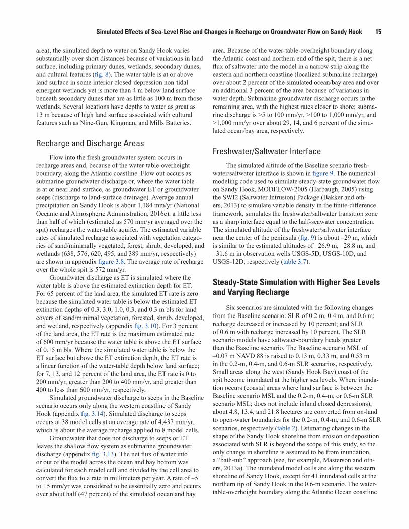
Sandy Hook geomorphology is similar to that of barrier islands such as Fire Island and Assateague Island National Seashores. Sandy Hook has experienced long-term erosion at the southern, narrow end of the spit and deposition at the northern end. The lighthouse was about 150 m from the northern end of Sandy Hook when it was built in 1764 but is now about 1,800 m inland because of long-term deposition. As is typical of barrier-island environments, Sandy Hook experiences overwash events during which areas that are normally above tide level are flooded. The 10 highest water levels at Sandy Hook since 1932 (table 1, fig. 3) range from

1.091 to 2.440 m above mean higher high water (MHHW), including record high water for the period of record during Hurricane Sandy in 2012 (National Oceanic and Atmospheric Administration, 2017). Of the 10 highest water levels in the 85-year period of record, 4 are associated with tropical storms, 4 with late fall/early winter nor’easters, and 2 with spring nor’easters.

Hurricane Sandy (also known as Superstorm Sandy because the storm transitioned to an extra-tropical storm just before landfall) is the storm of record for Sandy Hook, with a high water level nearly a meter higher than the previous highest storm in the 85-year period of record. In addition to the unique magnitude and track of Hurricane Sandy, SLR contributed to the height of the water levels because of the

Table 1. The 10 highest water levels at the National Oceanic and Atmospheric Administration tide gauge at Sandy Hook, New Jersey, 1932–2016.

[MHHW, Mean higher high water; NAVD 88, North American Vertical Datum of 1988. Data from National Oceanic and Atmospheric Administration, 2017]

Date of observationHigh water level

(meters above MHHW)High water level (meters NAVD 88) Commonly used name

10/29/2012 2.440 3.175 Hurricane Sandy9/12/1960 1.481 2.216 Hurricane Donna12/11/1992 1.478 2.213 Great Nor’easter of 1992; Downslope Nor’easter8/28/2011 1.383 2.118 Hurricane Irene11/7/1953 1.360 2.095 Nor’easter of 19539/14/1944 1.268 2.003 Great Atlantic Hurricane3/6/1962 1.268 2.003 Ash Wednesday Storm; Five-High Storm3/13/2010 1.158 1.893 Nor’easter of 201011/25/1950 1.146 1.881 Great Appalachian Storm11/12/1968 1.091 1.826 Nor’easter of 1968

0

1

2

3

4

1930 1940 1950 1960 1970 1980 1990 2000 2010 2020

Wat

er le

vel,

in m

eter

s ab

ove

NAV

D 88

Year

Figure 3. The 10 highest water levels at the Sandy Hook tide gauge, Sandy Hook, New Jersey, 1932–2016. [NAVD 88, North American Vertical Datum of 1988]

Introduction 5

4.05-millimeter per year (mm/yr) average rate of SLR at the Sandy Hook tide gauge (about 0.405 m per century; National Oceanic and Atmospheric Administration, 2016a); for example, the high water level would have been about 0.20 m lower if the same storm had occurred at the same tidal height 50 years earlier.

There are three federally listed endangered species on Sandy Hook: Charadrius melodus (piping plover), Cicindela dorsalis dorsalis (Northeastern beach tiger beetle), and Amaranthus pumilus (seabeach amaranth) (National Park Service, 2016c). Sandy Hook also has one of only two old-growth holly maritime forests known worldwide, the other is the Sunken Forest on Fire Island National Seashore, New York (Forrester and others, 2007). Sandy Hook habitats include beach and dune, tidal wetland, freshwater emergent wetland, forested wetland, deciduous and evergreen successional forest, and other northeastern maritime habitats.

Although Sandy Hook receives an average of 1,184 mm/yr of precipitation, the spit lacks an incised surface-water drainage network, except near the coast where seeps occur, so groundwater flow is the predominant pathway for freshwater movement on Sandy Hook, affecting both forested and wetland ecosystems. Understanding effects on the ground-water flow system of SLR and changes in recharge will allow the NPS to allocate scarce resources to best prepare for and manage climate-change-driven changes in the groundwater system and the subsequent effects on park ecosystems. This study, done by the USGS in cooperation with the NPS, evalu-ated the effects of SLR and increased or decreased recharge on the groundwater resources of Sandy Hook, including simulat-ing the change in depth to water below land surface and move-ment of the freshwater/saltwater interface.

Purpose and Scope

The purpose of this report is to present results of analy-ses of the effects of possible SLR and changes in recharge on the groundwater-flow system of Sandy Hook, New Jersey. This report documents the hydrogeology of Sandy Hook, the design and calibration of a groundwater-flow model to baseline conditions, and simulation of six scenarios: SLR of 0.20 m, 0.40 m, and 0.60 m, groundwater recharge increased or decreased by 10 percent, and SLR of 0.60 m and recharge increased by 10 percent from baseline conditions. Results of the simulations are presented. The report also presents a framework and considerations for long-term monitoring of groundwater resources. Data used for analyses in this report are stored in publicly available databases: geophysical logs are available in the U.S. Geological Survey GeoLog Locator data-base (U.S. Geological Survey, 2020a); water-level and specific conductance data are available in the U.S. Geological Survey National Water Information System database (U.S. Geological Survey, 2020b). Groundwater-flow model input and output

files for all of the simulations described in the report are avail-able in a U.S. Geological Survey data release (Carleton and others, 2020).

Related Studies and Previous Investigations

The Sandy Hook study was completed concurrently with studies of Fire Island, New York, (Misut, 2021) and Assateague Island, Maryland and Virginia (Fleming and oth-ers, 2021). Previous studies of Fire Island (Schubert, 2010) and Assateague Island (Masterson and others, 2013a,b) included the use of the variable-density groundwater-flow model SEAWAT (Langevin and others, 2007). Both previous studies incorporated hydrogeologic information into multi-layer models that were calibrated to water-level data and that simulated the shallow groundwater-flow system on the islands. The Fire Island study (Schubert, 2010) included groundwater-quality sampling to estimate nutrient loading from septic-system discharge and calculated nitrogen loads in simulated groundwater discharge to back-barrier estuaries and the ocean but did not evaluate the aquifer response to SLR. Masterson and others (2013a,b) evaluated the response of the fresh groundwater system at Assateague Island to SLR magnitudes of 20, 40, and 60 centimeters (cm). Their results indicate that the depth to water below land surface would be reduced and, in locations where evapotranspiration (ET) or discharge to groundwater seeps increased, the depth to the freshwater/salt-water interface would also be reduced.

The surficial geology of the Sandy Hook quadrangle is described by Minard (1969), including data collected in nine coreholes located on the Sandy Hook peninsula. Environmental investigations have been completed on behalf of the U.S. Army Corps of Engineers (USACE) by, for example, Metcalf and Eddy, Inc. (1989); these investigations have generally focused on determining whether hazardous materials, unexploded ordnance, or contaminated groundwa-ter remain from military activities on Sandy Hook. Zapecza (1989) describes the hydrogeologic framework of the New Jersey Coastal Plain, including the presence and depths of confined aquifers on Sandy Hook determined in part from a geophysical log of a Fort Hancock potable-supply well.

Raphael (2014) investigated mortality of vegetation in the Sunken Forest on Fire Island, which is similar to the holly maritime forest on Sandy Hook. Raphael cites examples of coastal habitats experiencing unsaturated zone thinning caused by SLR (Ross and others, 1994; Hayden and others, 1995; Kirwan and others, 2007; Saha and others, 2011; Masterson and others, 2013b). Thinning of the unsaturated zone can lead to increased salinity and accompanying mortality of vegetation (Saha and others, 2011). Thinning can also cause mortality by freshwater drowning of the roots of plants that require a thicker unsaturated zone (Werner and Simmons, 2009; Terry and Chui, 2012; Holding and Allen, 2014; Masterson and


others, 2013b). Thinning has changed the structure of the habitat and resulted in patterns of vegetation die off (Hayden and others, 1995). Thinning of the unsaturated zone has also resulted in mortality of Pinus ellioti (slash pine) on Sugarloaf Key, Florida, and coastal hardwood hemlocks-buttonwood for-ests of Everglades National Park (Ross and others, 1994; Saha and others, 2011) and has affected vegetation in coastal areas of Virginia (Hayden and others, 1995). Freshwater wetland herbaceous species (for example, Polygonum hydropiperoides or swamp smartweed) are colonizing depression sites in the Sunken Forest, perhaps because their tolerance of a thinner unsaturated zone caused by SLR is allowing them to out-compete the extant vegetation (Jordan Raphael, National Park Service, written commun., 2016). In locations where SLR has caused the freshwater/saltwater interface to move closer to the surface, shallow-rooted species may be unaffected, but deeper-rooted trees could be reaching brackish water causing the observed mortality. Erosion also could play a role by moving the shoreline closer to depressions in the Sunken Forest and, therefore, bringing the saltwater/freshwater interface closer to the surface (Raphael, 2014; Ataie-Ashtiani and others, 1999; Werner and Simmons, 2009).

Well-Numbering System

Observation wells included in this study (fig. 4; table 1.1 in appendix 1) have local identifiers established by the NPS, the USACE or the USGS. Wells with local identifiers of GWW followed by a 2-digit integer (for example, GWW02) are observation wells that were installed prior to this study, typi-cally for USACE environmental studies; the 2-digit number is a sequential number assigned by NPS, generally going from north to south on Sandy Hook (Mark Ringenary, National Park Service, written commun., 2015). Other USACE wells have a local identifier assigned by USACE (for example, USACE-MW-6). Monitoring wells installed by the USGS in 2014 and 2015 have local identifiers beginning with USGS, a sequential number, and “S” or “D,” indicating whether the wells are shal-low (less than 6 m deep) or deep (between 24 and 36 m deep), respectively, for example USGS-10S. Temporary drivepoints installed by the USGS in 2014 have local identifiers begin-ning with GP and a 1-digit sequential number, for example GP-8 and are at the same location as the USGS well with the same number, for example USGS-8DS. Boreholes and wells installed for, or used by, previous investigations have local identifiers assigned by those investigations (for example, M-1 for borehole 1 installed by Minard (1969), FH-5A for Fort Hancock production well 5A, and SH-1 for USGS observation well Sandy Hook 1).

Introduction 7

SANDY HOOKBAY

ATLANTIC OCEAN

Spermaceti Cove

Horseshoe Cove

Atlantic Highlands

Highlands

FISHERMANS

ROAD

NikePond

RoundPond

NorthPond

Coast GuardPond

73°58'73°59'74°74°1'74°2'

40°29'

40°28'

40°27'

40°26'

40°25'

40°24'


0 0.5 1 MILE

0 1 2 KILOMETERS

EXPLANATION

A

A'

Line of hydrogeologic section

Location of well and identifer from this study

Location of borehole and identifier from Minard (1969)

Location of core site and identifer from Johnson (2015)

Location of other well or borehole and identifier

GWW-24

M-2

SS

SH-1

A'A

GWW-24

GWW-23

GWW-22

GWW-19

GWW-18GWW-17

GWW-16GWW-15GWW-14GWW-13GWW-10

GWW-08

GWW-07

GWW-02GWW-01

USGS-5S

USGS-9D

USGS-3D

USGS-5D

USGS-8D

USGS-7S

USGS-9S

USGS-10D

USGS-11S

GWW-BG

GWW-12GWW-11

GWW-05

GWW-03

USGS-1S

USGS-2S

USGS-4S

USGS-6S

USGS-3SUSGS-8S

USGS-12D

USGS-10S

USACE-MW-6

M-9

M-8

M-7

M-6

M-5

M-4

M-2

M-1

M-3

SS

NMY

SMY

SH-1

SH-2

NF-3

FH-5A

Figure 4. Location of observation wells, core holes and line of hydrogeologic section A–A', Sandy Hook, New Jersey.


Hydrogeologic FrameworkThe hydrogeologic framework of Sandy Hook was devel-

oped using borehole geophysical logs collected for this study (U.S. Geological Survey, 2020a), descriptions of geologic logs of cores (Miller and others, 2018; Johnson and others, 2018), data on boreholes and wells in the USGS National Water Information System (NWIS) database (U.S. Geological Survey, 2020b), and geologic interpretations by Minard (1969) and Stanford and others, 2015. The “Hydrogeologic Setting” section below contains descriptions of the hydrogeologic lay-ers of the shallow groundwater-flow system on Sandy Hook. Additional information on the coreholes and wells from which data were obtained and the borehole geophysics data collected for this study can be found in appendix 1.

Hydrogeologic Setting

Sandy Hook is a barrier spit at the northern edge of the New Jersey Coastal Plain and consists of unconsoli-dated Quaternary sediments in active deposition since the Pleistocene epoch over an unconformable contact with Cretaceous formations from the Magothy Formation to the Navesink Formation (fig. 5) (Minard, 1969). Although the production wells providing potable water on Sandy Hook are screened in the confined upper and middle Potomac-Raritan-Magothy aquifer (known locally as the Old Bridge and Farrington aquifers, respectively), the Cretaceous formations are not included in the hydrogeologic framework for this study because the flux of groundwater between the Quaternary sedi-ments and Cretaceous formations are likely negligible. The altitude of the unconformable contact between the Quaternary and Cretaceous sediments ranges from about –8 m, referenced to the North American Vertical Datum of 1988 (NAVD 88), at the southernmost end of Sandy Hook to about –85 m at the northern end. The framework of the Quaternary sediments has been divided into the four hydrostratigraphic units described below that generally correspond to the four layers of the groundwater-flow model described further on in the report. Virtually no data were available for areas east or west of the line of section shown in figure 4, and the areal extent/thickness of the units was hypothesized on the basis of the depositional environments.

Unit A—Beach SandsHydrogeologic unit A is the shallowest layer and repre-

sents modern barrier beach and shore face sands. This unit is equivalent to the upper portion of the “beach sands” (“Qbs”) mapped by Minard (1969), which forms the surficial layer across the entire peninsula. Unit A is in a constant state of flux near the shorelines and in overwash areas, given the high degree of present-day depositional and erosional activity at Sandy Hook. All of the ecosystem interactions with soils,

sediments, and groundwater on Sandy Hook occur in unit A. Unit A thickness ranges from about 10 m in the south to about 20 m in the center and north of Sandy Hook (fig. 5).

Unit B—Estuarine-Tidal ComplexHydrogeologic unit B underlies unit A and contains thin

zones of interbedded estuarine and tidal channel clays, silts, sands, and gravels resulting from lateral movement of adjacent high-energy and low-energy environments (Bratton, 2007). The variety of sedimentary facies results in heterogeneous aquifer properties. Limited data are available to differentiate between specific thin beds, so unit B represents the consoli-dation of numerous thin beds into one heterogeneous hydro-logic layer. Unit B is within the deeper part of the “Qbs” unit mapped by Minard (1969) that occurs north of well USGS-5D and is thicker toward the northern end of Sandy Hook (figs. 4, 5). The southern extent of unit B and its contacts with units C-South and D (represented by dashed lines in fig. 5) is unclear owing to limited available data. Descriptions of modern off-shore bay bottom sediments (Gaswirth and others, 2002) indicate these sediments are hydraulically similar to unit B sediments despite being of the same geologic age as unit A; thus, bay bottom sediments are included in unit B west of Sandy Hook. Unit B thickness ranges from about 10 m in the south to about 20 m in the north (fig. 5).

Unit C—Estuarine MudUnit C consists of lower estuarine mud, clay, and silt and

is divided into two subunits, unit C-North and unit C-South. Unit C-North is generally equivalent to the “foraminiferal clay” (“Qfc”) of Minard (1969) north of well USGS-5D. Minard (1969) estimates the northern pinch-out of the north-ern lens of “Qfc” occurs south of FH-5A (fig. 5) about 1 km north of USGS-5D (fig. 5). However, the North Maintenance Yard (NMY) and Salt Shed (SS) cores (Stanford and others, 2015; Miller and others, 2018; Johnson and others, 2018) and the gamma log of FH-5A, which was collected in 1970 and unavailable to Minard (1969), indicate this unit thickens towards the north on Sandy Hook. The southern pinch-out of unit C-North occurs between USGS-5D and borehole NF-3 (fig. 5), where sediments coarsen and are labeled unit C-South. Gaswirth and others (2002) describe an estuarine mud lithofa-cies below Raritan Bay and Sandy Hook Bay and considered those sediments correlative with Minard’s (1969) “Qfc,” indicating unit C extends west. Unit C-North thickness ranges from 10 m at the southern extent to about 30 m in the north (fig. 5).

Unit C-South is depositionally similar to unit C-North, but the larger grain sizes yield different hydrologic proper-ties that require distinction. Fine sediments were deposited in a paleo-estuary centered in the northern part of proto-Sandy Hook during a sea-level transgression (Stanford and others,

Hydrogeologic Framework 9

2015), so a coarsening of sediments southward away from the center of the paleo-estuary (shallower) is to be expected. A 1978 driller’s log of NF-3, about 500 m south of USGS-5D (figs. 4 and 5), identifies a 0.6-m-thick clay interval from 24.4 to 25.0 m below land surface (bls), which is the same interval described at borehole M-4 at the northern extent of the south-ern “Qfc” lens of Minard (1969). However, no substantial clay intervals were present in the South Maintenance Yard (SMY, figs. 4 and 5) core acquired about 60 m from NF-3 (Miller and

others, 2018; Johnson and others, 2018), and the gamma log of well SH-1, about 500 m south of M-4, recorded lower gamma intensities than the intensities from similarly described fine sediments north of USGS-5D, which indicates the fine beds used to characterize “Qfc” of Minard (1969) and the driller’s log of NF-3 are likely coarser than similarly described beds to the north and subsequently more permeable. Unit C-South thickness ranges from about 5 m near the northern end of its extent to about 10 m in the south (fig. 5).

EXPLANATION

Hydrogeologic contact—Dashed where inferred

Location of well, borehole, or core site

Site identifier

Gamma log

USGS

10-D

0 0.5 1 MILE

0 1 2 KILOMETERSVERICAL SCALE GREATLY EXAGGERATED

Land surface

Unit A

Unit B

Unit C (north)

Unit C (south)

NavesinkFormation

Mount Laurel / Wenonah /Marshalltown Formations

Englishtown Formation

Woodbury / MerchantvilleFormations

Magothy Formation

Unit D

A A’

NM

Y

USGS

-10D

FH-5

A

SS USGS

-5D

M-3

NF-

3SM

Y

M-4

SH-1

M-5

M-6

M-7

M-8

M-9

SH-2

C r e t a c

eo

u

s

U n c o n f o r m i t y

20

NAVD 88

-20

-40

-60

-80

-100

METERS

Figure 5. Hydrogeologic section A–A’, Sandy Hook, New Jersey. Line of section shown in fig. 4; NAVD 88, North Atlantic Vertical Datum of 1988.


Few additional data are available in the south, so the boundaries of units B, C-South, and D are uncertain (fig. 5). Unit C-South could potentially be incorporated into unit B or unit D, but no hydrologic data are available to evaluate its properties. Given the high degree of uncertainty that stems from lack of data, unit C-South is assumed for this study to have the same hydraulic conductivity as unit C-North but may have hydraulic conductivities more similar to those of unit B or unit D.

Unit D—Glaciofluvial/Fluviodeltaic Sands and Gravels

Unit D is the deepest layer included in this study and consists of glaciofluvial, postglacial fluvial, deltaic, and upper estuarine gravels and sands. This unit underlies unit C and overlies the Cretaceous unconformity. Unit D fines upward from gravels at the base to fine sand at the top of the unit. Minard (1969) does not distinguish between the sands above and below the “Qfc,” calling both “Qbs.” Sand and gravel have been found to overlie the Cretaceous boundary in Raritan Bay (Gaswirth and others, 2002) and are included in unit D. As stated above, the boundaries with units B, C-South, and D are ambiguous south of well USGS-5D. Unit D thickness ranges from about 5 m at the southern end of Fort Hancock to about 20 m south of the South Maintenance Yard.

Hydrologic Setting

Freshwater on Sandy Hook is dominated by precipitation and the recharge and discharge of the shallow groundwater-flow system. Precipitation recharges the aquifer; the aqui-fer discharges (1) to the atmosphere as groundwater ET, (2) directly to saltwater bodies as submarine groundwater discharge, and (3) indirectly via seeps where groundwater reaches and flows along the land surface (fig 6). Some of the precipitation on Sandy Hook does not recharge the aquifer; some is removed from land surface and the unsaturated zone by direct evaporation and plant transpiration (ET). Shallow groundwater recharge flows towards the coastlines and dis-charges as groundwater ET in locations where the water table is close to land surface (or above land surface in enclosed depressions holding emergent wetlands), discharges as seeps where groundwater reaching land surface can flow across land surface to the bay or ocean, and as direct submarine fresh groundwater discharge to the bay and ocean bottoms. There is no incised stream network on Sandy Hook; discharge from groundwater seeps reaches saltwater bodies as dispersed flow without first concentrating in a freshwater stream. The shallow flow described above occurs in the upper 100 m or less of Quaternary sediments; the underlying Cretaceous sediments and bedrock have little to no effect on the localized flow system on Sandy Hook. The shallow aquifer is divided into four layers that generally correspond to the four hydrogeologic units described in the preceding section of this report.

Submarine groundwater discharge

Groundwater discharge to seeps

Groundwater discharge to evapotranspiration

PrecipitationEvapotranspiration from unsaturated zone

Groundwater recharge

Water-table overheight boundaryEmergent freshwater

wetland

F r e s h g r o u n d w a t e r

S a l t y g r o u n d w a t e r

Estimated sharp freshwater-saltwater interface

Ocean sideBay side

Tran

sitio

nzo

ne

NOT TO SCALE

Figure 6. The shallow groundwater-flow system, Sandy Hook, New Jersey.

Simulated Effects of Sea-Level Rise and Changes in Recharge on Groundwater Flow on Sandy Hook 11

Freshwater is less dense than saltwater, and the transition zone from freshwater to saltwater creates a flow boundary: recharge on the center of the spit flows down to, and later-ally along, the transition zone until it discharges to surface water. Borehole geophysical logs indicate the transition zone from freshwater to seawater in the water-table aquifer is about 5–20 m thick (fig. 6, appendix figs. 1.1, 1.2). The thickness of the transition zone results from complex mixing processes, including diffusion, density-driven flow, daily tidal fluctua-tions, approximately weekly freshwater recharge events, monthly tidal-range changes, periodic storm-driven salt spray and overwash, and long-term response to SLR. Simulation of all of these complex processes is beyond the scope of this study, and the freshwater/saltwater transition zone is delin-eated as a sharp interface at a total dissolved solids (TDS) concentration of 17.5 parts per thousand (ppt), about one-half that of seawater. Discussion of data and analysis used to delin-eate the freshwater/saltwater interface and discussion of the ecosystem freshwater/saltwater transition at about 3 ppt TDS are included in appendix 2.

Simulated Effects of Sea-Level Rise and Changes in Recharge on Groundwater Flow on Sandy Hook

Groundwater flow on Sandy Hook was simulated to eval-uate the effects of SLR and changes in recharge on the depth to water below land surface (unsaturated-zone thickness), changes in recharge and discharge areas, and the depth of the freshwater/saltwater interface. The design and calibration of the steady-state model is described briefly below and in detail in appendix 3. The simulations use the USGS finite-difference groundwater-modeling code MODFLOW-2005 (Harbaugh, 2005) with the Seawater Intrusion (SWI2) Package (Bakker and others, 2013) to simulate multi-density flow. The simu-lated depth to the freshwater/saltwater interface at observa-tion points was extracted for parameter estimation using the SWI Observation Extractor software utility documented in appendix 4. The model has four layers that correspond closely with the four hydrogeologic units described in the preceding “Hydrogeologic Setting” section. Freshwater recharge is simu-lated in all on-land model cells at five different rates associ-ated with different land covers: sand/minimally vegetated, forest, shrub, developed, and non-tidal wetland at rates of 638, 576, 620, 495, and 389 mm/yr, respectively. Freshwater recharge via the treated effluent infiltration basins is included. Groundwater discharge is simulated as groundwater ET (at a maximum rate of 600 mm/yr), surface seeps, and submarine discharge. A water-table-overheight boundary, which repre-sents mounding of groundwater near the shoreline caused by wave run-up and tidal pumping, is included along the Atlantic Ocean coastline and is set to 0.50 m NAVD 88 (0.57 m above

mean sea level [MSL]). All of the model input and output files for the simulations described in this report are available in a USGS data release (Carleton and others, 2020).

The Baseline scenario model was calibrated to aver-age 2015 groundwater levels and the 1983–2001 MSL at the Sandy Hook tide gage. Water-level altitude, depth to water below land surface (bls), and depth to the freshwater/saltwater interface associated with SLR of 0.2 m, 0.4 m, and 0.6 m, with recharge increases or decreases of 10 percent, and with SLR of 0.6 m and 10-percent increase in recharge were compared to those from the Baseline scenario to calculate changes associ-ated with each scenario.

The effects of SLR and changes in recharge were evalu-ated by calculating changes in depth to water below land sur-face and depth to the freshwater/saltwater interface between the Baseline scenario and each of the six alternative scenarios. Also, changes in proportions of groundwater discharge to ET, land-surface seeps, and submarine discharge were evaluated.

Baseline Scenario

The Baseline scenario uses a sea-level boundary equal to the 1981–2001 MSL at Sandy Hook (–0.07 m NAVD 88; National Oceanic and Atmospheric Administration, 2016b) with calibrated recharge rates and other parameters as described in appendix 3. The simulated water-table altitude, depth to water below land surface, and freshwater/saltwa-ter interface altitude are shown in figures 7–9, respectively. The simulated water-level altitude on Sandy Hook ranges from MSL to a maximum of 0.66 m (fig. 7). The asymmetry of the water-table surface caused by the higher water-table-overheight boundary along the Atlantic coastline and lower MSL boundary along Sandy Hook Bay is evident but is less pronounced than on Fire Island and Assateague Island; the northern half of Sandy Hook is wider than Fire Island and Assateague Island, ranging in width from 800 to 1,400 m, whereas the widths of Fire Island and Assateague Island generally range from 400 to 800 m. The simulated water table does not exhibit substantial local variations in response to local differences in recharge or groundwater ET rates associ-ated with different land covers (sand/minimally vegetated, for-ested, shrub, developed, or wetland), although in the northern half of the spit some minor deflections in the contours occur where ET is highest or parking lots redistribute recharge. Also, the saltwater boundaries surrounding the spit and lack of incised stream channels result in a water table aligned with the axis of the spit, varying primarily with the width rather than local features.

Depth to Water TableAlthough the simulated water-table altitude (fig. 7) does

not show small-scale variations and has modest horizontal gradients (1 meter per kilometer or less over most of the land


SANDY HOOKBAY

ATLANTIC OCEAN

Spermaceti Cove

Horseshoe Cove

Atlantic Highlands

Highlands

Fort Hancock

FISHERMANS

ROAD

NikePond

RoundPond

NorthPond

Coast GuardPond

73°58'74°74°2'

40°28'

40°26'

40°24'


0 0.5 1 MILE

0 1 2 KILOMETERS

Extent of holly maritime forest

Water-table altitude, in meters relative to NAVD 88 (>, greater than)

−0.05 to 0

>0 to 0.10

>0.10 to 0.20

>0.20 to 0.30

>0.30 to 0.40

>0.40 to 0.50

>0.50 to 0.60

>0.60 to 0.66

EXPLANATION


LighthouseParade groundGuardian Park

Gunnison Beach

Mills Battery

Kingman Battery

Ferry landingNorth maintenance yard


Nine-Gun Battery

PlumIsland




Service Station)

Figure 7. Baseline scenario simulated water-table altitude, Sandy Hook, New Jersey.


SANDY HOOKBAY

ATLANTIC OCEAN

Spermaceti Cove

Horseshoe Cove

Atlantic Highlands

Highlands

Fort Hancock

FISHERMANS

ROAD

NikePond

RoundPond

NorthPond

Coast GuardPond

73°58'74°74°2'

40°28'

40°26'

40°24'


0 0.5 1 MILE

0 1 2 KILOMETERS


Depth to water, in meters below land surface (>, greater than)

−0.22 to 0

>0 to 0.30

>0.30 to 0.50

>0.50 to 1.0

>1.0 to 2.0

>2.0 to 3.0

>3.0 to 4.0

>4.0 to 13.4

EXPLANATION



Gunnison Beach

Mills Battery

Kingman Battery



Nine-Gun Battery

PlumIsland




Service Station)

Figure 8. Baseline scenario simulated depth to the water table, Sandy Hook, New Jersey.


SANDY HOOKBAY

ATLANTIC OCEAN

Spermaceti Cove

Horseshoe Cove

Atlantic Highlands

Highlands

Fort Hancock

FISHERMANS

ROAD

NikePond

RoundPond

NorthPond

Coast GuardPond

73°58'74°74°2'

40°28'

40°26'

40°24'


0 0.5 1 MILE

0 1 2 KILOMETERS


Altitude of freshwater/saltwater interface in meters relative to NAVD 88 (>, greater than)

−29.3 to −25

>−25 to −20

>−20 to −15

>−15 to −10

>−10 to −5

>−5 to −2

>−2 to −0.97

EXPLANATION



Gunnison Beach

Mills Battery

Kingman Battery



Nine-Gun Battery

PlumIsland




Service Station)

Figure 9. Baseline scenario simulated altitude of the freshwater/saltwater interface, Sandy Hook, New Jersey.


area), the simulated depth to water on Sandy Hook varies substantially over short distances because of variations in land surface, including primary dunes, wetlands, secondary dunes, and cultural features (fig. 8). The water table is at or above land surface in some interior closed-depression non-tidal emergent wetlands yet is more than 4 m below land surface beneath secondary dunes that are as little as 100 m from those wetlands. Several locations have depths to water as great as 13 m because of high land surface associated with cultural features such as Nine-Gun, Kingman, and Mills Batteries.

Recharge and Discharge AreasFlow into the fresh groundwater system occurs in

recharge areas and, because of the water-table-overheight boundary, along the Atlantic coastline. Flow out occurs as submarine groundwater discharge or, where the water table is at or near land surface, as groundwater ET or groundwater seeps (discharge to land-surface drainage). Average annual precipitation on Sandy Hook is about 1,184 mm/yr (National Oceanic and Atmospheric Administration, 2016c), a little less than half of which (estimated as 570 mm/yr averaged over the spit) recharges the water-table aquifer. The estimated variable rates of simulated recharge associated with vegetation catego-ries of sand/minimally vegetated, forest, shrub, developed, and wetlands (638, 576, 620, 495, and 389 mm/yr, respectively) are shown in appendix figure 3.8. The average rate of recharge over the whole spit is 572 mm/yr.

Groundwater discharge as ET is simulated where the water table is above the estimated extinction depth for ET. For 65 percent of the land area, the simulated ET rate is zero because the simulated water table is below the estimated ET extinction depths of 0.3, 3.0, 1.0, 0.3, and 0.3 m bls for land covers of sand/minimal vegetation, forested, shrub, developed, and wetland, respectively (appendix fig. 3.10). For 3 percent of the land area, the ET rate is the maximum estimated rate of 600 mm/yr because the water table is above the ET surface of 0.15 m bls. Where the simulated water table is below the ET surface but above the ET extinction depth, the ET rate is a linear function of the water-table depth below land surface; for 7, 13, and 12 percent of the land area, the ET rate is 0 to 200 mm/yr, greater than 200 to 400 mm/yr, and greater than 400 to less than 600 mm/yr, respectively.

Simulated groundwater discharge to seeps in the Baseline scenario occurs only along the western coastline of Sandy Hook (appendix fig. 3.14). Simulated discharge to seeps occurs at 38 model cells at an average rate of 4,437 mm/yr, which is about the average recharge applied to 8 model cells.

Groundwater that does not discharge to seeps or ET leaves the shallow flow system as submarine groundwater discharge (appendix fig. 3.13). The net flux of water into or out of the model across the ocean and bay bottom was calculated for each model cell and divided by the cell area to convert the flux to a rate in millimeters per year. A rate of –5 to +5 mm/yr was considered to be essentially zero and occurs over about half (47 percent) of the simulated ocean and bay

area. Because of the water-table-overheight boundary along the Atlantic coast and northern end of the spit, there is a net flux of saltwater into the model in a narrow strip along the eastern and northern coastline (localized submarine recharge) over about 2 percent of the simulated ocean/bay area and over an additional 3 percent of the area because of variations in water depth. Submarine groundwater discharge occurs in the remaining area, with the highest rates closer to shore; subma-rine discharge is >5 to 100 mm/yr, >100 to 1,000 mm/yr, and >1,000 mm/yr over about 29, 14, and 6 percent of the simu-lated ocean/bay area, respectively.

Freshwater/Saltwater InterfaceThe simulated altitude of the Baseline scenario fresh-

water/saltwater interface is shown in figure 9. The numerical modeling code used to simulate steady-state groundwater flow on Sandy Hook, MODFLOW-2005 (Harbaugh, 2005) using the SWI2 (Saltwater Intrusion) Package (Bakker and oth-ers, 2013) to simulate variable density in the finite-difference framework, simulates the freshwater/saltwater transition zone as a sharp interface equal to the half-seawater concentration. The simulated altitude of the freshwater/saltwater interface near the center of the peninsula (fig. 9) is about –29 m, which is similar to the estimated altitudes of –26.9 m, –28.8 m, and –31.6 m in observation wells USGS-5D, USGS-10D, and USGS-12D, respectively (table 3.7).

Steady-State Simulation with Higher Sea Levels and Varying Recharge

Six scenarios are simulated with the following changes from the Baseline scenario: SLR of 0.2 m, 0.4 m, and 0.6 m; recharge decreased or increased by 10 percent; and SLR of 0.6 m with recharge increased by 10 percent. The SLR scenario models have saltwater-boundary heads greater than the Baseline scenario. The Baseline scenario MSL of –0.07 m NAVD 88 is raised to 0.13 m, 0.33 m, and 0.53 m in the 0.2-m, 0.4-m, and 0.6-m SLR scenarios, respectively. Small areas along the west (Sandy Hook Bay) coast of the spit become inundated at the higher sea levels. Where inunda-tion occurs (coastal areas where land surface is between the Baseline scenario MSL and the 0.2-m, 0.4-m, or 0.6-m SLR scenario MSL; does not include inland closed depressions), about 4.8, 13.4, and 21.8 hectares are converted from on-land to open-water boundaries for the 0.2-m, 0.4-m, and 0.6-m SLR scenarios, respectively (table 2). Estimating changes in the shape of the Sandy Hook shoreline from erosion or deposition associated with SLR is beyond the scope of this study, so the only change in shoreline is assumed to be from inundation, a “bath-tub” approach (see, for example, Masterson and oth-ers, 2013a). The inundated model cells are along the western shoreline of Sandy Hook, except for 41 inundated cells at the northern tip of Sandy Hook in the 0.6-m scenario. The water-table-overheight boundary along the Atlantic Ocean coastline


of Sandy Hook is the same relative height above the SLR sce-nario MSL as it is in the Baseline scenario. For the Increased and Decreased Recharge scenarios, the only difference from the Baseline scenario is the uniform 10-percent increase or decrease in the recharge rates applied to the five land-cover types (sand/minimally vegetated, forest, shrub, developed, and wetland).

Change in Depth to Water TableThe simulated changes in the depth to the water table

of the three SLR scenarios are shown in figures 10A, 11A, and 12A. Sea-level rise causes the simulated water table to rise and, therefore, decreases the depth to water. The increas-ing magnitude of SLR results in a water-table rise that is a decreasing percentage of the SLR. In the 0.2-m, 0.4-m, and 0.6-m SLR scenarios, the water-table rise is within 0.05 m of the SLR over 94, 63, and 38 percent of the land area, respectively. A substantial difference occurs in the flow-system response to 0.6 m of SLR compared to the response to 0.2-m and 0.4-m SLR, which is discussed in more detail in the “Effects of Sea-Level Rise” section. The depth to water changes very little in the Increased and Decreased Recharge scenarios; the water table rises less than 0.04 m in the Increased Recharge scenario and declines less than 0.04 m in the Decreased Recharge scenario.

Simulated on-land areas on Sandy Hook where the water table is above land surface typically represent non-tidal, fresh-water emergent wetlands (although some areas close to the coast may represent beach faces or tidally affected saltwater wetlands). Areas of land where the simulated water table is above land surface increase about 13.9, 33.3, and 58.1 hectares in the 0.2-m, 0.4-m, and 0.6-m SLR scenarios, respectively (table 2). Areas where the simulated water table is above land surface decrease or increase about 1 hectare in the Increased and Decreased Recharge scenarios, respectively (table 2).

Recharge and DischargeThe SLR and Increased Recharge scenarios result in

a water-table rise and, therefore, an increase in the rate of groundwater discharge to ET and seeps; the Decreased Recharge scenario results in decreased groundwater discharge to ET and surface seeps (table 3). Simulated groundwater ET occurs only when the water table is within 3.0 m and 1.0 m of land surface in forested and shrub areas, respectively, and within 0.30 m in sand/minimally vegetated, developed, and wetland areas. The ET rate decreases linearly from a depth of 0.15 m down to the extinction depths that are the esti-mated depths where direct uptake of groundwater by roots or evaporation occurs. Compared to the Baseline scenario, simulated groundwater discharge to ET (appendix fig. 3.10) increases from 21 percent of net simulated freshwater recharge (recharge from precipitation plus infiltrated effluent) to 25, 29, and 33 percent in the 0.2-m, 0.4-m, and 0.6-m SLR scenarios, respectively (table 3, figs. 10B, 11B, and 12B). Evapotranspiration increases 2 percent (as a percentage of net recharge) or decreases 1 percent in the Decreased and Increased Recharge scenarios, respectively, compared to the Baseline scenario. Simulated groundwater discharge to seeps increases from 2 percent of net discharge in the Baseline scenario to 10, 10, and 14 percent in the 0.2-m, 0.4-m, and 0.6-m SLR scenarios, respectively. The higher percentage of discharge to seeps in the 0.6-m SLR scenario (compared to the 0.2 m and 0.4 m SLR scenarios) is likely related to the number of model cells identified as closed depressions with an outlet altitude of 0.5 m. Estimates of closed-depression outlet altitudes are discussed in the “Groundwater Discharge to Land-Surface Seeps” section in appendix 3. Outlet altitudes of closed depressions were determined using land-surface-altitude contours with a 0.5-m contour interval. Groundwater discharge to seeps decreases and increases between 0.5 and 1 percent of net recharge in the Decreased and Increased Recharge scenarios, respectively, compared to the Baseline

Table 2. Simulated area of land inundated by saltwater from sea-level rise and simulated increase or decrease in area of wetlands, Sandy Hook, New Jersey.

[MSL, mean sea level; m, meters; NAVD 88, North American Vertical Datum of 1988; SLR, sea-level rise; --, no data]

ScenarioMSL

(m NAVD 88)

Number of model cells inundated

by SLR

Simulated area of land inundated by

saltwater from SLR (hectare)

Number of new (compared to Baseline scenario) on-land model cells with simulated

emergent wetlands1

Simulated increase or decrease from Baseline

scenario in area of wetlands1 (hectare)

0.20-m SLR 0.13 77 4.8 223 13.90.40-m SLR 0.33 214 13.4 533 33.30.60-m SLR 0.53 349 21.8 929 58.1Recharge decreased 10 percent –0.07 -- -- 107 –0.8Recharge increased 10 percent –0.07 -- -- 136 1.0

1Model cells in which the water table is above land surface.


74°74°2'

40°28'

40°26'

0 0.50.25 MILE

0 10.5 KILOMETER



Lighthouse

Parade ground

Guardian Park

Gunnison Beach

Mills Battery

Kingman Battery

Ferry landing


Southmaintenance

yard

Nine-Gun Battery

Sandy HookVisitor Center(former U.S.Life Saving

Service Station)

SANDY HOOKBAY

ATLANTIC OCEAN

Spermaceti Cove

Horseshoe Cove

F or t H

an

co

ck

FISHERMANS

ROAD

NikePond

RoundPond

NorthPond

Coast GuardPond

EXPLANATIONExtent of holly maritime forest

Change in depth to water, in meters (>, greater than)

−0.21 to −0.19

>−0.19 to −0.17

>−0.17 to −0.15

>−0.15 to −0.07

>−0.07 to 0

Area with groundwater newly above land surface due to sea-level rise of 0.2 meter

Area inundated by 0.2-meter sea-level rise

A. Depth to water

Figure 10. Simulated inundated areas and A, areas of groundwater newly above land surface and simulated change in depth to groundwater, B simulated increase in evapotranspiration, and C, altitude of freshwater/saltwater interface and change in simulated depth to the freshwater/saltwater interface with 0.2-meter sea-level rise above baseline conditions, Sandy Hook, New Jersey. [NAVD88, North American Vertical Datum of 1988]



Lighthouse

Parade ground

Guardian Park

Gunnison Beach

Mills Battery

Kingman Battery

Ferry landing


Southmaintenance

yard

Nine-Gun Battery


Service Station)

SANDY HOOKBAY

ATLANTIC OCEAN

Spermaceti Cove

Horseshoe Cove

F or t H

an

co

ck

FISHERMANS

ROAD

NikePond

RoundPond

NorthPond

Coast GuardPond

0 0.50.25 MILE

0 10.5 KILOMETER


74°74°2'

40°28'

40°26'


Increase in evapotranspiration, in millimeters per year (>, greater than)

0 to 100

>100 to 200

>200 to 300

>300 to 400

>400 to 500

>500 to 600


B. Evapotranspiration

Figure 10.—Continued



Lighthouse

Parade ground

Guardian Park

Gunnison Beach

Mills Battery

Kingman Battery

Ferry landing


Southmaintenance

yard

Nine-Gun Battery


Service Station)

SANDY HOOKBAY

ATLANTIC OCEAN

Spermaceti Cove

Horseshoe Cove

F or t H

an

co

ck

FISHERMANS

ROAD

NikePond

RoundPond

NorthPond

Coast GuardPond

74°74°2'

40°28'

40°26'

0 0.50.25 MILE

0 10.5 KILOMETER



Area with freshwater/saltwater interface newly shallower than −9 meters relative to NAVD 88 due to sea-level rise of 0.2 meter* (>, greater than)

−9 to −4

>−4 to −1

Change in depth to freshwater/saltwater interface, in meters

−13.5 to −8.6

>−8.6 to −4.1

>−4.1 to 1.5


C. Depth of saltwater/freshwater interface

* Areas where the baseline saltwater interface is below −9 meters and the scenario saltwater interface is above −9 meters.




Lighthouse

Parade ground

Guardian Park

Gunnison Beach

Mills Battery

Kingman Battery

Ferry landing


Southmaintenance

yard

Nine-Gun Battery


Service Station)

SANDY HOOKBAY

ATLANTIC OCEAN

Spermaceti Cove

Horseshoe Cove

F or t H

an

co

ck

FISHERMANS

ROAD

NikePond

RoundPond

NorthPond

Coast GuardPond

74°74°2'

40°28'

40°26'

0 0.50.25 MILE

0 10.5 KILOMETER




−0.42 to −0.36

>−0.36 to −0.30

>−0.30 to −0.22

>−0.22 to −0.09

>−0.09 to 0



A. Depth to water

Figure 11. Simulated inundated areas and A, areas of groundwater newly above land surface and simulated change in depth to water, B, simulated change in evapotranspiration, and C, simulated altitude of freshwater/saltwater interface and simulated change in depth to the freshwater/saltwater interface with 0.4-meter sea-level rise above baseline conditions, Sandy Hook, New Jersey. [NAVD88, North American Vertical Datum of 1988]



Lighthouse

Parade ground

Guardian Park

Gunnison Beach

Mills Battery

Kingman Battery

Ferry landing


Southmaintenance

yard

Nine-Gun Battery


Service Station)

SANDY HOOKBAY

ATLANTIC OCEAN

Spermaceti Cove

Horseshoe Cove

F or t H

an

co

ck

FISHERMANS

ROAD

NikePond

RoundPond

NorthPond

Coast GuardPond

74°74°2'

40°28'

40°26'

0 0.50.25 MILE

0 10.5 KILOMETER




0 to 100

>100 to 200

>200 to 300

>300 to 400

>400 to 500

>500 to 600






Lighthouse

Parade ground

Guardian Park

Gunnison Beach

Mills Battery

Kingman Battery

Ferry landing


Southmaintenance

yard

Nine-Gun Battery


Service Station)

SANDY HOOKBAY

ATLANTIC OCEAN

Spermaceti Cove

Horseshoe Cove

F or t H

an

co

ck

FISHERMANS

ROAD

NikePond

RoundPond

NorthPond

Coast GuardPond

74°74°2'

40°28'

40°26'

0 0.50.25 MILE

0 10.5 KILOMETER




−9 to −4

>−4 to −0.2


−13.5 to −10.2

>−10.2 to −7.6

>−7.6 to −5.3

>−5.3 to −3.1

>−3.1 to 1.1


C. Depth of saltwater/freshwaterinterface





Lighthouse

Parade ground

Guardian Park

Gunnison Beach

Mills Battery

Kingman Battery

Ferry landing


Southmaintenance

yard

Nine-Gun Battery


Service Station)

SANDY HOOKBAY

ATLANTIC OCEAN

Spermaceti Cove

Horseshoe Cove

F or t H

an

co

ck

FISHERMANS

ROAD

NikePond

RoundPond

NorthPond

Coast GuardPond

74°74°2'

40°28'

40°26'

0 0.50.25 MILE

0 10.5 KILOMETER




−0.62 to −0.55

>−0.55 to −0.45

>−0.45 to −0.30

>−0.30 to −0.11

>−0.11 to 0



A. Depth to water

Figure 12. Simulated inundated areas and A, areas of groundwater newly above land surface and simulated change in depth to water, B, simulated change in evapotranspiration, and C, altitude of freshwater/saltwater interface and simulated change in depth to the freshwater/saltwater interface with 0.6-meter sea-level rise above baseline conditions, Sandy Hook, New Jersey. [NAVD88, North American Vertical Datum of 1988]



Lighthouse

Parade ground

Guardian Park

Gunnison Beach

Mills Battery

Kingman Battery

Ferry landing


Southmaintenance

yard

Nine-Gun Battery


Service Station)

SANDY HOOKBAY

ATLANTIC OCEAN

Spermaceti Cove

Horseshoe Cove

F or t H

an

co

ck

FISHERMANS

ROAD

NikePond

RoundPond

NorthPond

Coast GuardPond

74°74°2'

40°28'

40°26'

0 0.50.25 MILE

0 10.5 KILOMETER




0 to 100

>100 to 200

>200 to 300

>300 to 400

>400 to 500

>500 to 600






LighthouseParade ground

Guardian Park

Gunnison Beach

Mills Battery

Kingman Battery

Ferry landing


Southmaintenance

yard

Nine-Gun Battery


Service Station)

SANDY HOOKBAY

ATLANTIC OCEAN

Spermaceti Cove

Horseshoe Cove

F or t H

an

co

ck

FISHERMANS

ROAD

NikePond

RoundPond

NorthPond

Coast GuardPond

B B'

C C'

D D'

USGS-9D

USGS-3DUSGS-5D

USGS-8D

USGS-12D

USGS-10D

USGS-9D

USGS-3DUSGS-5D

USGS-8D

USGS-12D

USGS-10D

74° 73°58'

40°28'

40°26'

0 0.50.25 MILE

0 10.5 KILOMETER




−9 to −4

>−4 to −0.2


−13.5 to −10.2

>−10.2 to −7.6

>−7.6 to −5.3



Deep observation well and identifier

B B'USGS-8DUSGS-8D

C. Depth of saltwater/freshwater interface


>−5.3 to −3.1

>−3.1 to 1.1



scenario. The increase in the percentage of groundwater discharges to ET and seeps in the 0.2, 0.4, and 0.6 m SLR scenarios are offset by decreases in net submarine discharge; submarine discharge decreases from 77 percent of net recharge in the Baseline scenario to 65, 61, and 53 percent in the 0.2-m, 0.4-m, and 0.6-m SLR scenarios, respectively. Submarine groundwater discharge decreases and increases about 1 per-cent (as a percentage of net recharge) in the Decreased and Increased Recharge scenarios, respectively, compared to the Baseline scenario. For the 0.6-m SLR with 10-percent Increase in Recharge scenario, the rates of groundwater discharge to seeps, ET, and net submarine discharge are higher than those from the 0.6-m SLR scenario, but as a percentage of net recharge, the percent discharge to seeps is unchanged and the percent discharge to ET and submarine discharge decrease and increase, respectively (table 3).

Freshwater/Saltwater InterfaceCompared to the Baseline scenario, the depth to the fresh-

water/saltwater interface decreased with SLR. For the SLR scenarios, the changes in depth to the freshwater/saltwater interface (figs. 10C, 11C, and 12C) have patterns similar to the change in depth to water (figs. 10A, 11A, and 12A), reaching a maximum change of about 8 m, 13 m, and 22 m for the 0.2-m, 0.4-m, and 0.6-m SLR scenarios, respectively. Changes in the depth to the freshwater/saltwater interface are related to the

changes in the water table; where the water table does not rise as much as SLR, the comparatively lower freshwater elevation above MSL results in a shallower saltwater interface (Ghyben, 1889; Herzberg, 1901; Masterson and others, 2013b). The depth to the freshwater/saltwater interface changes less than 2 m in the two Recharge scenarios.

Effects of Sea-Level RiseSLR causes the water table to rise closer to land surface,

thereby increasing groundwater discharge to ET and seeps and reducing submarine groundwater discharge compared to the Baseline scenario (table 3). SLR is likely to affect ecosystems wherever the rise in the water table reduces the depth to water (that is, makes the unsaturated zone thinner) across thresh-olds particular to those ecosystems. For example, Raphael (2014) identified a rising water table as a possible cause of tree mortality in low-lying areas of the Sunken Forest on Fire Island, New York. Results of the simulations for this study can be used to estimate where SLR will potentially affect specific ecosystems, such as the Bayside Holly Forest on Sandy Hook. Areas where the simulated SLR-altered water table is newly above land surface that are not currently emergent wetlands are likely to experience ecosystem changes; 58.1 additional hectares (about 6.4 percent of the land area) on Sandy Hook have groundwater above land surface in the 0.6-m SLR sce-nario compared to the Baseline scenario (table 2).

Table 3. Simulated flow rates to model boundaries for the Baseline scenario, 0.2-meter, 0.4-meter, and 0.6-meter Sea-Level Rise scenarios, Increased and Decreased Recharge scenarios, and 0.6-meter plus Increased Recharge scenario, Sandy Hook, New Jersey.

[m, meter; SLR, sea-level rise; m3/d, cubic meters per day; GW, groundwater; ET, evapotranspiration]

Boundary condition name

Scenario

Baseline 0.2-m SLR 0.4-m SLR 0.6-m SLR

Recharge decreased 10 percent

Recharge increased 10 percent

0.6-m SLR and recharge

increased 10 percent

1Flow into model from boundary, in m3/d

Net Recharge2 12,872 12,788 12,639 12,509 11,598 14,141 13,743GW discharge to seeps –288 –1,255 –1,320 –1,795 –187 –417 –2,108GW discharge to evapotranspiration –2,701 –3,191 –3,632 –4,072 –2,630 –2,766 –4,149Net GW submarine discharge –9,883 –8,342 –7,687 –6,642 –8,783 –10,958 –7,486

Percentage of net recharge discharging to seeps, ET, and net submarine discharge boundaries3

Seeps 2 10 10 14 2 3 15Evapotranspiration 21 25 29 33 23 20 30Net submarine discharge4 77 65 61 53 76 78 55

1Negative value indicates flow out of groundwater system.2Net Recharge is groundwater recharge plus a constant 168 m3/d of infiltrated effluent from a sewage treatment plant.3Total may not equal 100 percent because of rounding.4Net submarine discharge is the sum of flow out of, and into, the groundwater model as submarine discharge and submarine recharge, respectively.


SLR is likely to reduce the thickness of the freshwater lens on low-lying barrier islands and similar environments, potentially causing saltwater intrusion; the magnitude of the simulated water-table-altitude rise is less than the simulated SLR, reducing the depth to the freshwater/saltwater interface because discharge to ET and surface seeps is proportionally increased and submarine groundwater discharge decreased (figs. 10C, 11C, 12C, 13A–C; Ghyben, 1889; Herzberg, 1901; Masterson and others, 2013b). However, at most locations on Sandy Hook, SLR is unlikely to substantially increase the salinity of shallow groundwater; the simulated freshwater/salt-water interface (representing the 17.5-ppt TDS isochlor) in the 0.6-m SLR scenario remains more than 9 m below the water table over 92 percent of the land area. The estimated thickness of the transition zone of 3 ppt to 17.5 ppt TDS in six wells on Sandy Hook is an average of 9.2 m and ranges from 2.1 m to 17 m (table 2.4), indicating that shallow groundwater likely will remain fresh (salinity less than 3 ppt) over 92 percent of Sandy Hook with a 0.6-m SLR. However, low-lying land areas near the Sandy Hook Bay coastline, including part of the holly forest, may experience SLR-driven increases in the long-term average salinity of shallow groundwater (figs. 12C, 13C, 14).

Numerous cultural resources exist on Sandy Hook, most of them associated with Fort Hancock military infrastructure built and operated during 1890–1974. Any cultural resources with important infrastructure near the water table (such as basements and utility lines) are vulnerable to groundwater inundation with SLR. Altitude data for subsurface cultural resources were not available for this study, but the simulated water-table altitude and depth-to-water surfaces generated can be used to evaluate the risk to specific structures.

Limitations of the Study

Groundwater-flow models are simplifications of natu-ral flow systems and cannot capture their true complexity (Anderson and Woessner, 1992). The simulations completed for this study are steady state and do not attempt to simulate gradual SLR or any delay in the response that might occur in the deeper part of the flow system. Because the steady-state simulations use average annual rates of recharge and ET, the simulations do not capture any seasonal or yearly changes to recharge or ET that might occur with changing climate. Steady-state simulations are considered sufficient for this study because of the expected slow rate of changes in the hydrologic system driven by climate change.

The representation of the freshwater/saltwater interface as a sharp interface (representing a TDS concentration halfway between freshwater and seawater) rather than a transition zone does not provide direct simulation of changes to the location of the 3-ppt TDS surface, which is of more importance to the ecosystem than the half-seawater interface. The only data available to characterize the transition zone from 3 ppt to the half-seawater (about 17.5 ppt) sharp interface were those from

the six observation wells drilled for this study; additional data could allow more complete characterization of the transition zone, including better estimates of the distance between the half-seawater and 3-ppt surfaces. Variations in the thickness of the transition zone could also be evaluated with a modeling code that explicitly simulates the transition rather than using a sharp interface.

The only data available for calibrating recharge, ET, and hydraulic conductivity parameters were water-level altitudes and estimates of the altitude of the freshwater/saltwater interface. Water-level data include (1) water levels from two rounds of site-wide data collection (synoptics) that provided good areal coverage but were single points in time and (2) short-term (1–6 months) continuous data collected in selected wells. Additional continuous water-level data col-lected in different recharge and ET zones could improve the simulation estimates of recharge and ET. The lack of streams prevents the collection of stream base-flow data that would improve model-derived recharge estimates; methods to detect groundwater discharge to surface water, such as bed seep-age meters or fiber-optic distributed temperature sensing (for example, Rosenberry and others, 2016) could possibly be used to provide estimates of submarine discharge rates. Without discharge data, water-level data alone are not sufficient to resolve the model correlation between hydraulic conductivity and recharge. The six freshwater/saltwater interface altitude data points did not provide substantial additional information for calibration. Additional borehole data could provide better resolution of the horizontal and vertical extents of hydrogeo-logic layers and altitude of the freshwater/saltwater interface. Restrictions to flow in the vertical direction can substantially affect the movement of saltwater and possibly lengthen the time required for the shallow flow system to respond to SLR. Additional water-level and hydrogeologic data could provide better resolution and calibration in areas of particular concern, such as the holly maritime forest.

The magnitude of the combined effect of wave run-up and tidal pumping is not well constrained with the avail-able data, and the value determined via parameter estimation is affected by uncertainties in other parameters. Additional continuous water-level data from several closely spaced wells near the Atlantic beachline could improve the confidence in the water-table-overheight boundary and, therefore, improve estimates of depth to water because the simulated water levels are sensitive to this parameter (described in the “Sensitivity and Parameter Correlation” section of appendix 3).

For this study, it is assumed that as sea level rises and the regime of deposition and erosion changes, the resulting morphological changes of nearshore submarine, and border-ing shoreline and dune areas, will not substantially affect the results of the scenarios. Although morphological changes to Sandy Hook could be substantial, estimation of those changes is beyond the scope of this study. Although such morphologi-cal changes could substantially affect various ecosystems on Sandy Hook, assumption of static morphology allows


ATLANTIC OCEANSandy Hook Bay

LAYER 1

LAYER 2

LAYER 3

LAYER 4

Water table

USG

S-9D

USG

S-10D

USG

S-12D

F R E S H W A T E R

S A L T W A T E R

NAVD 88

10

−10

−20

−30

−40

−50

−60

−70

−80

−90

−100

B'METERS

B

VERTICAL EXAGGERATION ×20

A

B

C



LAYER 1

LAYER 2

LAYER 3

LAYER 4

LAYER 1LAYER 2LAYER 3

LAYER 4

Water table

Water table

USG

S-8D

USG

S-5D

USG

S-3D

F R E S H W A T E R

S A L T W A T E R

F R E S H W A T E R

S A L T W A T E R

0 0.50.25 MILE

0 10.5 KILOMETER

NAVD 88

10METERS

−10

−20

−30

−40

−50

−60

NAVD 88

10

−10

−20

−30

−40

−50

C'

D D'

METERSC



EXPLANATIONSimulated freshwater/saltwater

interface

Baseline scenario

0.6-m sea-level rise scenario

Observation well identifier and depth of estimated freshwater/saltwater interface

USG

S-9D

Figure 13. The simulated freshwater/saltwater interface from the Baseline scenario and the 0.6-meter Sea-Level Rise scenario for A, line of section B-B’ (model row 121) with depth of estimated freshwater/saltwater interface, B, line of section C-C’ (model row 211) with depth of estimated freshwater/saltwater interface, and C, line of section D-D’ (model row 239), Sandy Hook, New Jersey. Lines of section and locations of observation wells shown on figure 12C. Vertical exaggeration 20:1.



LighthouseParade ground

Guardian Park

Gunnison Beach

Mills Battery

Kingman Battery

Ferry landing


Southmaintenance

yard

Nine-Gun Battery


Service Station)

SANDY HOOKBAY

ATLANTIC OCEAN

Spermaceti Cove

Horseshoe Cove

F or t H

an

co

ck

FISHERMANS

ROAD

NikePond

RoundPond

NorthPond

Coast GuardPond

B B'

C C'

D D'

USGS-9D

USGS-3DUSGS-5D

USGS-8D

USGS-12D

USGS-10D

USGS-9D

USGS-3DUSGS-5D

USGS-8D

USGS-12D

USGS-10D

74° 73°58'

40°28'

40°26'

0 0.50.25 MILE

0 10.5 KILOMETER


EXPLANATION


Half-seawater surface within 9 meters of water table



Deep observation well and identifier

B B'

USGS-8DUSGS-8D

Figure 14. Areas in and near the Bayside Holly Forest where the simulated half-seawater surface is within 9 meters of the water table from the 0.6-meter Sea-Level Rise scenario, and simulated inundated areas, Sandy Hook, New Jersey.


simulation of changes in the freshwater-flow system that can be used to evaluate the effects of SLR-associated changes to the freshwater-flow system on existing ecosystems.

The model created for this study simulates only the shallow groundwater-flow system on Sandy Hook, specify-ing no-flow boundaries on the sides and bottom of the model. Although some flow from the mainland in the shallow system may affect flow on Sandy Hook, the limited extent of simu-lated submarine discharge in Sandy Hook Bay indicates that the mainland flow system does not have a major effect. This hypothesis could be tested by expanding the lateral extent of the model. Similarly, the connection between the shallow aqui-fer and the underlying Cretaceous sediments is thought to be minimal, but this hypothesis could be tested by including the deeper aquifers and confining units in the model.

Use of Long-Term Monitoring to Assess Water Resources

Long-term monitoring can be used in conjunction with the simulation results of this study to assess changes in the freshwater system that may occur with climate change. Water-level and water-quality (especially salinity) monitoring can be used to document long-term changes in freshwater resources. Comparison of observed and simulated water levels and monitoring of salinity can be used to evaluate possible causes of observed changes, and if the observed changes are con-trary to simulated results, the observed changes can be used to improve the groundwater-flow model. The scenarios from this study can provide information for the design of a moni-toring plan including the use of sentinel-point monitoring for issues of concern, such as sentinel wells located in areas where water-table flooding of tree roots or cultural features is of con-cern. Long-term monitoring may help determine ecosystem threshold values, such as minimum depth to water or maxi-mum salinity at which holly-tree mortality begins to occur.

Groundwater LevelsThe SLR scenario results indicate that a rise in the water

table (and accompanying thinning of the unsaturated zone) is a near certainty with rising sea level. Of particular concern is the Bayside Holly Forest, in which trees in some low-lying, enclosed areas died as a result of Hurricane Sandy (Stalter and Heuser, 2015). Parts of the Sunken Forest on Fire Island are dying, which is attributed to a thinning unsaturated zone, and areas in the Bayside Holly Forest on Sandy Hook may simi-larly be threatened (Jordan Raphael, National Park Service, written commun., 2016). The ranges of unsaturated-zone thickness and groundwater salinity that cause tree mortality in American holly maritime forests are not currently (2021) well documented, but water-table and land-surface altitudes determined for this study could be used to identify areas where the depth to water is near thresholds later found to be impor-tant. Existing or new wells in or near the holly forest could be

used to monitor the water-table altitude in or near low-lying areas (fig. 15). Similarly, wells could be located near (or even inside) structures threatened with groundwater inundation.

SLR and the water-table response are slow processes, and occasional (for example, monthly or quarterly) water-level observations are likely sufficient to evaluate long-term threats. However, a sufficient number of observations and (or) limited continuous monitoring are required to separate short-term tidal, recharge (precipitation), or seasonal effects from long-term changes associated with SLR. Water levels can be measured with pressure transducer/data logger probes installed in observation wells. Probes are especially useful because they provide a continuous record, but they require regular (every 8–10 weeks) maintenance and calibration. Alternatively, water levels can be measured manually at a lower cost and on a routine and (or) event-driven schedule. For a semi-annual, manual-measurement schedule, measurements during the sea-sonal high water-level period (March or April) and during the seasonal low water-level period (September or October) would have the most value. The combined use of limited continuous monitoring and periodic synoptic measurements is a cost-efficient data-collection strategy.

Water-Quality SamplesSome areas of the Bayside Holly Forest are likely to

experience increased salinity in shallow groundwater associ-ated with SLR because of thinning of the freshwater lens and (or) increasingly frequent storm-driven inundation events [for example, low-lying holly forest areas near the north end of Spermaceti Cove] (Raphael, 2014; Stalter and Heuser, 2015). The SLR scenarios indicate that increased freshwater dis-charge to ET and groundwater seeps will cause the freshwater/saltwater interface to move closer to land surface. Effects of salinity increases from SLR could be further exacerbated by an increasing frequency of storm-driven inundation caused by SLR. Possible effects of global climate change include the potential for increasing frequency and (or) intensity of coastal storms that cause more frequent and (or) severe inundation of low-lying areas (Werner and Simmons, 2009). Few exist-ing wells on Sandy Hook are suitably located for monitoring the changes in groundwater salinity associated with storm-inundation events with a return period of about 1–5 years; suggested suitable well locations are shown in figure 15.

In general, specific conductance is a good surrogate for salinity and chloride concentration, and monitoring can be done with specific conductance/data logger probes installed in observation wells. Probes are especially useful because they provide a continuous record, but they do require regular (every 4 to 6 weeks) maintenance and recalibration. Alternatively, analysis of chloride concentrations in well water is inexpen-sive, but the quality control of well sampling requires purging (pumping) about three well volumes before sampling in order to ensure the sample is representative of the aquifer water in the vicinity of the well.



Lighthouse

Parade ground

Guardian Park

Gunnison Beach

Mills Battery

Kingman Battery

Ferry landing


Southmaintenance

yard

Nine-Gun Battery


Service Station)

SANDY HOOKBAY

ATLANTIC OCEAN

Spermaceti Cove

Horseshoe Cove

F or t H

an

co

ck

FISHERMANS

ROAD

NikePond

RoundPond

NorthPond

Coast GuardPond

WW25

WW24

WW23

WW22

WW19WW18

WW16

WW10

WW08

WW02

GP7S

GP6S

ACOEGW6

ACOEGWBG

74°74°2'

40°28'

40°26'

0 0.50.25 MILE

0 10.5 KILOMETER



Depth to water

Less than 1 meter

Less than 0.5 meter

Existing well and identifier

Proposed well location

WW08

Figure 15. Locations of areas with Baseline scenario simulated depth to water less than 1 meter, areas with simulated depth to water less than 0.5 meter, locations of previously installed wells, and suggested well locations in or near the holly forest or cultural resources suitable for long-term water-level and water-quality monitoring, Sandy Hook, New Jersey.


Summary and ConclusionsThe National Park Service’s Sandy Hook Unit of the

Gateway National Recreation Area (hereafter Sandy Hook) is a 10-kilometer-long spit; it is visited by thousands of people every year who take advantage of the historical and natural resources and recreational opportunities. The historical and natural resources are threatened by global climate change, including sea-level rise (SLR), changes in precipitation and groundwater recharge, and changes in the frequency and severity of coastal storms. Fresh groundwater resources play a crucial role in the ecosystems of Sandy Hook. The lack of streams means that spring-fed ponds and wetlands are the only sources of fresh surface water, and the proximity of the water table to land surface can determine which ecosystem regimes are supported in any given location. The Bayside Holly Forest, one of only two known old-growth American holly mari-time forests (the other is the Sunken Forest in the Fire Island National Seashore) is particularly vulnerable to SLR because of the proximity of the water table to land surface in low-lying areas and the potential for saltwater intrusion and inundation. About 70 percent of the Bayside Holly Forest was inundated during Hurricane Sandy in 2012.

The shallow groundwater-flow system on Sandy Hook occurs in Quaternary sediments overlying Cretaceous for-mations of the New Jersey Coastal Plain. The Quaternary sediments range in thickness from about 10 meters (m) at the southern end of the spit to about 100 m at the northern end and are divided into four hydrogeologic layers that include (1) homogeneous modern barrier beach sands; (2) heteroge-neous estuarine and tidal channel deposits ranging from clay to gravel; (3) estuarine mud, silt, and clay; and (4) glacioflu-vial/fluviodeltaic sand and gravel overlying the Cretaceous unconformity.

A three-dimensional groundwater-flow model simulat-ing the shallow groundwater-flow system and interaction with surrounding saltwater boundaries was constructed using MODFLOW with the Saltwater Intrusion Package (SWI2) that explicitly simulates multi-density groundwater flow, treating the freshwater/saltwater transition zone as a sharp interface representing the half-seawater surface (17.5 parts per thousand of total dissolved solids). The model was calibrated to water-level data from 25 shallow wells and estimated half-seawater altitudes in 6 deep wells.

The simulated shallow groundwater-flow system is domi-nated by recharge from precipitation, fresh groundwater dis-charge to evapotranspiration (ET), discharge to surface seeps that then flows across land surface to saltwater, and submarine groundwater discharge. Saltwater in Sandy Hook Bay and the Atlantic Ocean form the dominant hydrologic boundary surrounding Sandy Hook. Recharge occurs at variable rates

depending on the land-use/land-cover categories of sand/mini-mally vegetated, forest, shrub, developed, and wetland. In the flow model, ET attributes are assigned to the same five land-use/land-cover categories as recharge, but the same maximum ET rate is assigned to all categories. Only the extinction depth of ET is varied.

Groundwater-flow simulations completed for this study include a Baseline scenario, three SLR scenarios (0.2 m, 0.4 m, and 0.6 m), two Recharge scenarios (10-percent increase and 10-percent decrease in recharge), and a 0.6 m SLR plus 10-percent increase in recharge scenario. The Recharge scenarios indicate the system is not sensitive to a 10-percent increase or decrease in recharge. Only minor changes occur to the simulated percentage of freshwater discharge to ET, seeps, and submarine discharge; to the water-table elevation (and therefore depth to water below land surface); and to the depth to the half-seawater surface of less than 2 m. In the SLR scenarios, SLR causes the water table to rise, resulting in increased fresh groundwater discharge to ET and seeps and reduced submarine discharge. The increased discharge to ET and seeps causes the magnitude of the water-table rise to be less than that of SLR, which in turn causes the thickness of the freshwater lens to thin, reducing the depth to the half-seawater surface below the water table. Although the magnitude of the water-table rise is less than SLR, in the 0.6-m SLR scenario, the simulated water table is above land surface over 58.1 more hectares of land area (about 6.4 percent of Sandy Hook) than in the Baseline scenario. Areas where the simulated water table is above land surface are likely to be emergent wetlands, possibly freshwater emergent wetlands if more than tens of meters from the coastline. Where the water table rises to near or above land surface, changes in the domi-nant ecosystem are likely to occur. The steady-state simula-tions indicate that the half-seawater surface will remain more than 9 m below the water table under average conditions over most (92 percent) of the land area even with 0.6 m of SLR. Low-lying areas close to the Sandy Hook Bay shoreline may experience a rise in the half-seawater surface, bringing the half-seawater surface as much as 8, 13, or 22 m closer to the water table with SLR of 0.2 m, 0.4 m, or 0.6 m, respectively. Transient salinization, if any, of shallow groundwater from increased frequency or severity of storm-driven inundation is not included in the above analysis.

Natural resources on Sandy Hook, particularly the Bayside Holly Forest, may be adversely affected by the rising water table associated with SLR. Freshwater emer-gent wetlands may increase in area at the expense of other ecosystem assemblages occurring in or on the edges of low-lying enclosed depressions. Cultural resources close to the water table, such as basements of structures, may be adversely affected.

References Cited 33

References Cited

Anderson, M.P., and Woessner, W.M., 1992, Applied ground-water modeling: San Diego, California, Academic Press, Inc., 381 p.

Ataie-Ashtiani, B., Volker, R.E., and Lockington, D.A., 1999, Tidal effects on sea water intrusion in unconfined aqui-fers: Journal of Hydrology (Amsterdam), v. 216, no. 1-2, p. 17–31.

Bakker, M., and Schaars, F., Hughes, J.D., Langevin, C.D., and Dausman, A.M., 2013, Documentation of the Seawater Intrusion (SWI2) Package for MODFLOW: U.S. Geological Survey Techniques and Methods, book 6, chap. A46, 47 p., accessed December 15, 2017, at ht tps://pubs .usgs.gov/ tm/ 6a46/ .

Bratton, J.F., 2007, The importance of shallow confining units to submarine groundwater flow, in Sanford, W., Langevin, C., Polemio, M., and Povinec, P., eds., A new focus on groundwater-seawater interactions: Oxfordshire, UK, IAHS Publication 312, p. 28–36.

Carleton, G.B., Charles, E.G, Fiore, A.R., and Winston, R.B., 2021, MODFLOW-2005 with SWI2 used to evalu-ate the water-table response to sea-level rise and change in recharge, Sandy Hook Unit, Gateway National Recreation Area, New Jersey: U.S. Geological Survey data release, https://doi.org/ 10.5066/ F7BP 018M.

Fleming, B.J., Raffensperger, J.P., Masterson, J.P., and Pajerowski, M., 2021, Effects of sea-level rise on the fresh groundwater system of Assateague Island, Maryland and Virginia: U.S. Geological Survey Scientific Investigations Report 2020–5104, 62 p., https://doi.org/10.3133/ sir20205104.

Forrester, J.A., Leopold, D.J., and Art, H.W., 2007, Disturbance history and mortality patterns in a rare Atlantic barrier island maritime holly forest: Natural Areas Journal, v. 27, no. 2, p. 169–182.

Gaswirth, S.B., Ashley, G.M., and Sheridan, R.E., 2002, Use of seismic stratigraphy to identify conduits for saltwa-ter intrusion in the vicinity of Raritan Bay, New Jersey: Environmental & Engineering Geoscience, v. 8, no. 3, p. 209–218. https://doi.org/ 10.2113/ 8.3.209.

Ghyben, W.B., 1889, Nota in verband met de voorgenomen putboring nabij Amsterdam—The Hague, Netherlands: Tijdschrift van het Koninklijk Instituut van Ingenieurs, v. 9, p. 8–22.

Harbaugh, A.W., 2005, MODFLOW-2005, The U.S. Geological Survey modular ground-water model—The Ground-Water Flow Process: U.S. Geological Survey Techniques and Methods 6-A16. [variously paged]. [Also available at https://doi.org/ 10.3133/ tm6A16.]

Hayden, B.P., Santos, M.C., Shao, G., and Kochel, R.C., 1995, Geomorphological controls on coastal vegetation at the Virginia Coast Reserve: Geomorphology, v. 13, no. 1-4, p. 283–300. [Also available at https://doi.org/ 10.1016/ 0169- 555X(95)00032- Z.]

Herzberg, A., 1901, Die Wasserversorgung eini-ger Nordseebäder: Journal für Gasbeleuchtung und Wasserversorgung, v. 44, p. 815–819.

Holding, S., and Allen, D.M., 2014, From days to decades—Numerical modeling of freshwater lens response to climate change stressors on small islands: Hydrology and Earth System Sciences Discussions, v. 11, no. 10, p. 11439–11487.

Jacob, C.E., 1950, Flow of ground-water, chap. 5 of Rouse, H., ed., Engineering Hydraulics: Hoboken, N.J., John Wiley, p. 321–386.

Johnson, C.S., Miller, K.G., Browning, J.V., Kopp, R.E., Khan, N.S., Fan, Y., Stanford, S.D., and Horton, B.P., 2018, The role of sediment compaction and groundwater with-drawal in local sea-level rise, Sandy Hook, New Jersey, USA: Quaternary Science Reviews, v. 181, p. 30–42, accessed December 15, 2017, at https://doi.org/ 10.1016/ j.quascir ev.2017.11 .031.

Kirwan, M.L., Kirwan, J.L., and Copenheaver, C.A., 2007, Dynamics of an estuarine forest and its response to ris-ing sea level: Journal of Coastal Research, v. 23, no. 2, p. 457–463, accessed December 15, 2017, at ht tps://www. jstor.org/ stable/ 4494214? seq= 1#page_ scan_ tab_ contents.

Langevin, C.D., Thorne, D.T., Jr., Dausman, A.M., Sukop, M.C., and Guo, Weixing, 2007, SEAWAT version 4—A computer program for simulation of multi-species solute and heat transport: U.S. Geological Survey Techniques and Methods, book 6, chap. A22, 39 p.

Masterson, J.P., Fienen, M.N., Gesch, D.B., and Carlson, C.S., 2013a, Development of a numerical model to simu-late groundwater flow in the shallow aquifer system of Assateague Island, Maryland and Virginia: U.S. Geological Survey Open-File Report 2013–1111, 34 p., accessed December 15, 2017, at ht tps://pubs .usgs.gov/ of/ 2013/ 1111/ .

Masterson, J.P., Fienen, M.N., Thieler, E.R., Gesch, D.B., Gutierrez, B.T., and Plant, N.G., 2013b, Effects of sea-level rise on barrier island groundwater system dynamics–ecohydrological implications: Ecohydrology, v. 7, no. 3, p. 1064–1071, accessed December 15, 2017, at h ttp://onli nelibrary. wiley.com/ doi/ 10.1002/ eco.1442/ full.

https://pubs.usgs.gov/tm/6a46/





https://doi.org/10.2113/8.3.209

https://doi.org/10.3133/tm6A16

https://doi.org/10.1016/0169-555X(95)00032-Z

https://doi.org/10.1016/0169-555X(95)00032-Z

https://doi.org/10.1016/j.quascirev.2017.11.031

https://doi.org/10.1016/j.quascirev.2017.11.031

https://www.jstor.org/stable/4494214?seq=1#page_scan_tab_contents

https://www.jstor.org/stable/4494214?seq=1#page_scan_tab_contents

https://pubs.usgs.gov/of/2013/1111/

http://onlinelibrary.wiley.com/doi/10.1002/eco.1442/full

http://onlinelibrary.wiley.com/doi/10.1002/eco.1442/full


Metcalf and Eddy, Inc., 1989, Contamination evaluation at the former Fort Hancock: Submitted to the Department of the Army, Kansa City District, Corps of Engineers: Project Number CO2NJ006300, 69 p.

Miller, K.G., Sugarman, P.J., Stanford, S.D., Browning, J.V., Baldwin, K., Buttari, B., Dunham, B., Farazaneh, M., Filo, R., Gagliano, M.P., Horton, B., Gallegos, G., Graham, S., Johnson, C.S., Khan, N., Kulhanek, D.K., Lombardi, C.J., Malerba, N., McKoy, K., McLaughlin, P.P., Jr., Monteverde, D.H., Stanley, J.N., and Woodard, S., 2018, Sandy Hook sites, in Miller, K.G., Sugarman, P.J., Browning, J.V., et al., eds., Proceedings of the Ocean Drilling Program, initial reports: Ocean Drilling Program, College Station, Texas, v. 174AX, 59 p., accessed December 15, 2017, at https://doi.org/ 10.2973/ odp.proc.1 74AXS.112. 2018.

Miller, R.L., Bradford, W.L., and Peters, N.E., 1988, Specific conductance: theoretical considerations and application to analytical quality control: U.S. Geological Survey Water-Supply Paper 2311, 16 p., accessed December 15, 2017, at ht tps://pubs .usgs.gov/ wsp/ 2311/ report.pdf.

Minard, J.P., 1969, Geology of the Sandy Hook quadrangle in Monmouth County, New Jersey: U.S. Geological Survey Bulletin 1276, 43 p.

Misut, P.E., 2021, Simulation of water-table response to climate-change-driven sea-level rise and changes in recharge, Fire Island National Seashore, New York: U.S. Geological Survey Scientific Investigations Report 2020–5117, 47 p., https://doi.org/ 10.3133/ sir2020 5117.

National Oceanic and Atmospheric Administration, 2016a, Mean sea level trend at tide gauge 8531680, Sandy Hook, New Jersey: National Oceanic and Atmospheric Administration web page, accessed December 15, 2017, at htt p://tidesa ndcurrents .noaa.gov/ sltrends/ sltrends_ station.shtml? stnid= 8531680.

National Oceanic and Atmospheric Administration, 2016b, Datums at tide gauge 8531680, Sandy Hook, New Jersey: National Oceanic and Atmospheric Administration web page, accessed December 15, 2017, at http s://tidesa ndcurrents .noaa.gov/ datums.html? units= 1&epoch= 0&id= 8531680&name= Sandy+Hook&state= NJ.

National Oceanic and Atmospheric Administration, 2016c, Data tools—1981–2010 Climate Normals: National Centers for Environmental Information web page, accessed December 15, 2017, at https: //www.ncdc .noaa.gov/ cdo- web/ datatools/ normals.

National Oceanic and Atmospheric Administration, 2017, Top ten highest water levels for long term stations in meters above MHHW (as of 4/2017): National Oceanic and Atmospheric Administration web page, accessed November 10, 2017, at http s://tidesa ndcurrents .noaa.gov/ est/ Top10_ form.pdf.

National Park Service, 2016a, Gateway National Recreation Area—Many places, one park: National Park Service web page, accessed December 15, 2017, at https://www.nps.gov/ gate/ index.htm.

National Park Service, 2016b, Fort Hancock National Historic Landmark District: National Park Service web page, accessed December 15, 2017, at https://www.nps.gov/ gate/ learn/ historyculture/ hancock.htm.

National Park Service, 2016c, Endangered species man-agement plan, Sandy Hook Unit of Gateway National Recreation Area: National Park Service web page, accessed December 15, 2017, at https://p arkplannin g.nps.gov/ projectHome.cfm? projectID= 16178.

National Park Service, 2017, Climate change action plan 2012–2014: National Park Service web page, accessed December 5, 2017 at https:/ /www.natur e.nps.gov/ climatechange/ docs/ NPS_ CCActionPlan.pdf.

Raphael, J., 2014, 50 years of vegetation change in a Holly Maritime Forest: Long Island, N.Y., Hofstra University, M.S. thesis, ProQuest UMI number 1573792, 92 p., accessed December 15, 2017, at https://pq dtopen.pro quest.com/ doc/ 1654262477.html? FMT= ABS.

Rosenberry, D.O., Briggs, M.A., Delin, G., and Hare, D.K., 2016, Combined use of thermal methods and seepage meters to efficiently locate, quantify, and monitor focused groundwater discharge to a sand-bed stream: Water Resources Research, v. 52, no. 6, p. 4486–4503. [Also avail-able at https://doi.org/ 10.1002/ 2016WR018808.]

Ross, M.S., O’Brien, J.J., and Sternberg, L.D.S.L., 1994, Sea-level rise and the reduction in pine forests in the Florida Keys: Ecological Applications, v. 4, no. 1, p. 144–156, accessed December 17, 2017, at https ://researc h.fit.edu/ sealevelriselibrary/ documents/ doc_ mgr/ 448/ Florida_ Keys_ Forest_ SLR_ Impacts_ - _ Ross_ et_ al_ 1994.pdf.

Saha, A.K., Saha, S., Sadle, J., Jiang, J., Ross, M.S., Price, R.M., Sternberg, L.S.L.O., and Wendelberger, K.S., 2011, Sea level rise and South Florida coastal forests: Climatic Change, v. 107, no. 1, p. 81–108, accessed December 15, 2017, at https: //link.spr inger.com/ article/ 10.1007/ s10584- 011- 0082- 0.

Schubert, C.E., 2010, Analysis of the shallow groundwa-ter flow system at Fire Island National Seashore, Suffolk County, New York: U.S. Geological Survey Scientific Investigations Report 2009–5259, 106 p. [Also available at ht tps://pubs .usgs.gov/ sir/ 2009/ 5259.]

Stalter, R., and Heuser, J., 2015, Survival and growth of Ilex Opaca following Superstorm Sandy, Sandy Hook, New Jersey: Holly Society Journal, v. 33, no. 1, p. 3–9.

https://doi.org/10.2973/odp.proc.174AXS.112.2018

https://pubs.usgs.gov/wsp/2311/report.pdf


http://tidesandcurrents.noaa.gov/sltrends/sltrends_station.shtml?stnid=8531680

http://tidesandcurrents.noaa.gov/sltrends/sltrends_station.shtml?stnid=8531680

https://tidesandcurrents.noaa.gov/datums.html?units=1&epoch=0&id=8531680&name=Sandy+Hook&state=NJ



https://www.ncdc.noaa.gov/cdo-web/datatools/normals


https://tidesandcurrents.noaa.gov/est/Top10_form.pdf

https://tidesandcurrents.noaa.gov/est/Top10_form.pdf

https://www.nps.gov/gate/index.htm

https://www.nps.gov/gate/index.htm

https://www.nps.gov/gate/learn/historyculture/hancock.htm

https://www.nps.gov/gate/learn/historyculture/hancock.htm

https://parkplanning.nps.gov/projectHome.cfm?projectID=16178

https://parkplanning.nps.gov/projectHome.cfm?projectID=16178

https://www.nature.nps.gov/climatechange/docs/NPS_CCActionPlan.pdf

https://www.nature.nps.gov/climatechange/docs/NPS_CCActionPlan.pdf

https://pqdtopen.proquest.com/doc/1654262477.html?FMT=ABS

https://pqdtopen.proquest.com/doc/1654262477.html?FMT=ABS

https://doi.org/10.1002/2016WR018808

https://research.fit.edu/sealevelriselibrary/documents/doc_mgr/448/Florida_Keys_Forest_SLR_Impacts_-_Ross_et_al_1994.pdf



https://link.springer.com/article/10.1007/s10584-011-0082-0

https://link.springer.com/article/10.1007/s10584-011-0082-0

https://pubs.usgs.gov/sir/2009/5259


References Cited 35

Stanford, S.D., Miller, K.G., and Browning, J.V., 2015, Coreholes reveal glacial and postglacial history at Sandy Hook: New Jersey Geological and Water Survey Newsletter, v. 11, no. 1, p. 1–6, accessed June 14, 2018, at http s://www.st ate.nj.us/ dep/ njgs/ enviroed/ newsletter/ v11n1.pdf.

Terry, J.P., and Chui, T.F.M., 2012, Evaluating the fate of freshwater lenses on atoll islands after eustatic sea-level rise and cyclone-driven inundation—A modelling approach: Global and Planetary Change, v. 88–89, p. 76–84. [Also available at https://ww w.scienced irect.com/ science/ article/ pii/ S0921818112000549.]

U.S. Geological Survey, 2020a, USGS GeoLog Locator: U.S. Geological Survey database, accessed July 23, 2020, at https://doi.org/ 10.5066/ F7X6 3KT0.

U.S. Geological Survey, 2020b, USGS water data for the Nation: U.S. Geological Survey National Water Information System database, accessed July 23, 2020, at https://doi.org/ 10.5066/ F7P5 5KJN.

U.S. Global Change Research Program, 2014, 2014 National Climate Assessment [variously paged], accessed December 15, 2017, at htt ps://nca20 14.globalc hange.gov/ report.

Werner, A.D., and Simmons, C.T., 2009, Impact of sea-level rise on sea water intrusion in coastal aquifers: Ground Water, v. 47, no. 2, p. 197–204, accessed December 15, 2017, at h ttp://onli nelibrary. wiley.com/ doi/ 10.1111/ j.1745- 6584.2008.00535.x/ full.

Zapecza, O.S., 1989, Hydrogeologic framework of the New Jersey Coastal Plain: U.S. Geological Survey Professional Paper 1404-B, 49 p., 24 plates, accessed December 15, 2017, at https ://pubs.er .usgs.gov/ publication/ pp1404B.

https://www.state.nj.us/dep/njgs/enviroed/newsletter/v11n1.pdf

https://www.state.nj.us/dep/njgs/enviroed/newsletter/v11n1.pdf

https://www.sciencedirect.com/science/article/pii/S0921818112000549

https://www.sciencedirect.com/science/article/pii/S0921818112000549

https://doi.org/10.5066/F7X63KT0

https://doi.org/10.5066/F7P55KJN


https://nca2014.globalchange.gov/report

https://nca2014.globalchange.gov/report

http://onlinelibrary.wiley.com/doi/10.1111/j.1745-6584.2008.00535.x/full

http://onlinelibrary.wiley.com/doi/10.1111/j.1745-6584.2008.00535.x/full

https://pubs.er.usgs.gov/publication/pp1404B


Appendix 1. Wells, Coreholes, and Geophysical LogsMinard (1969) described the geology of the Sandy Hook

quadrangle using logs from nine coreholes on Sandy Hook (fig. 4 main text and table 1.1). A geophysical log is available from a 268-meter (m) -deep production well that supplies potable water to facilities on Sandy Hook, and geologic logs are available from two additional boreholes drilled on Sandy Hook prior to this study. The U.S. Army Corps of Engineers (USACE) had about 14 shallow observation wells installed in the late 1980s (for example, Metcalf and Eddy, Inc., 1989). About 10 additional observation wells were installed in the vicinity of the sewage treatment plant, sludge drying bed, and effluent infiltration bed (Robert Galante, National Park Service, written commun., 2014). Three coreholes were installed on Sandy Hook as part of the New Jersey Coastal Plain Drilling Project of the Ocean Drilling Program (Miller and others, 2018).

The USGS installed 5 reconnaissance drivepoints for this study to measure groundwater salinity with depth and then installed 11 shallow (2–5 m deep) and 6 deep (24–37 m deep) observation wells (fig. 4 main text and table 1.1). The deep observation wells were geophysically logged to collect hydro-geologic and salinity data (U.S. Geological Survey, 2020a). Specific conductance (SC) of the water in the deep and shal-low observation wells was measured in water-quality samples collected from the wells and (or) with an SC probe lowered into the well screen.

Wells USGS-5D, USGS-10D, and USGS-12D were com-pleted at the maximum depth the available drilling equipment could reach, 36 m. Wells USGS-3D and USGS-8D were set at 24.4 m and 27.4 m, respectively, because SC data from the temporary drivepoints indicated the freshwater–saltwater inter-face was at about that depth or shallower. Well USGS-9D was completed at 30.5 m, deeper than USGS-3D and USGS-8D, because no temporary drivepoint data were available.

Borehole Geophysical LogsCoupled electromagnetic (EM) induction and natural

gamma logs were collected in the six deep observation wells constructed for this study to identify hydrogeologic units and estimate groundwater salinity (figs. 1.1 and 1.2). Fine-grained sediments (silts and clays) typically have higher EM conductivity values and higher quantities of gamma-emitting radioisotopes, such as potassium-40, whereas coarser sedi-ments (sands and gravels) generally have lower conductivity and lower gamma emissions (Keys, 1990). The logging system used in this study was a Mount Sopris® MGXII logger and winch, a 2PGA-1000 gamma probe, and a 2PIA-1000 EM induction probe. Gamma and EM logs can be used in tandem to estimate groundwater salinity. Depths on Sandy Hook with high conductance and low gamma emissions indicate sandy aquifer material containing water with higher salinity. Low

conductance and low gamma indicate a freshwater aquifer, and high conductance and high gamma indicate low hydraulic conductivity sediments. Interpretations of the hydrogeology of Sandy Hook on the basis of the geophysical logs are shown in figures 1.1 and 1.2. Other well and corehole data are described in the “Hydrogeologic Setting” section of this report. All well information has been entered and is maintained in the U.S. Geological Survey (USGS) National Water Information System (NWIS) database (U.S. Geological Survey, 2020b). All geophysical logs have been archived and are available in the USGS geophysical log database GeoLog Locator (U.S. Geological Survey, 2020a)).

Surface GeophysicsGround-penetrating radar (GPR) data from 80 and

100 megahertz antenna units were collected for this study, but the shallow water table at Sandy Hook attenuated most of the emitted signal, especially in areas of higher specific conduc-tance (SC) groundwater (>3,000 microsiemens per centime-ter at 18 degrees Celsius (µS/cm at 18 °C), which severely restricted depth penetration and obscured many subsurface features below the water table. The collected data were not analyzed because of the limited GPR effectiveness in the study area. Proposed time-domain surface EM surveys, which can be used to describe the general hydrogeologic structure, were not done because sufficient data were available from exist-ing borehole logs and core holes at Sandy Hook and wells installed for this study.

Appendix 1. Wells, Coreholes, and Geophysical Logs 37Ta

ble

1.1.

W

ell c

onst

ruct

ion

and

dept

h in

form

atio

n fo

r sel

ecte

d w

ells

and

cor

ehol

es, S

andy

Hoo

k, N

ew J

erse

y.

[Dat

a av

aila

ble

in th

e U

.S. G

eolo

gica

l Sur

vey

Nat

iona

l Wat

er In

form

atio

n Sy

stem

dat

abas

e (U

.S. G

eolo

gica

l Sur

vey,

202

0b);

m, m

eter

s; N

AVD

88;

Nor

th A

mer

ican

Ver

tical

Dat

um o

f 198

8; c

m, c

enti-

met

er; O

bs, o

bser

vatio

n; M

, map

; G, g

loba

l pos

ition

ing

sate

llite

(GPS

); D

, diff

eren

tial G

PS; R

, rep

orte

d; N

AD

83,

Nor

th A

mer

ican

Dat

um o

f 198

3; N

AD

27,

Nor

th A

mer

ican

Dat

um o

f 192

7; W

, Lev

el 1

qu

ality

surv

ey g

rade

Glo

bal N

avig

atio

n Sa

telli

te S

yste

m (G

NSS

); L,

Lev

el o

r oth

er su

rvey

ing

met

hod;

Z, L

evel

4 q

ualit

y su

rvey

gra

de G

NSS

; J, l

ight

det

ectio

n an

d ra

ngin

g (li

dar)

; --,

no d

ata]

Site

num

ber

Loca

l ide

ntifi

er

Latit

ude

(d

ecim

al

degr

ees)

Long

itude

(d

ecim

al

degr

ees)

Latit

ude/

Lo

ngitu

de

met

hod

Hor

izon

tal

datu

mA

ltitu

de

(m N

AVD

88)

Alti

tude

m

etho

d

Alti

tude

ac

cura

cy

(m)

Wel

l de

pth

(m

)

Hol

e de

pth

(m

)

Scre

en

dept

h,

top

(m

)

Scre

en

dept

h,

botto

m

(m)

Wel

l di

amet

er

(cm

)

4026

1907

3590

201

2511

84--

USG

S-1S

40.4

3847

22−7

3.98

375

MN

AD

83

3.11

W0.

122.

73.

02.

12.

75

4026

1707

3590

401

2511

86--

USG

S-2S

40.4

3819

44−7

3.98

4527

8M

NA

D 8

31.

98W

0.12

4.3

4.6

3.7

4.3

540

2617

0735

9060

125

1165

-- U

SGS-

3S40

.438

0556

−73.

9849

167

MN

AD

83

2.88

W0.

124.

34.

63.

74.

35

4026

1607

3590

601

2511

93--

USG

S-3D

40.4

3789

72−7

3.98

4883

3G

NA

D 8

32.

69W

0.12

24.4

27.4

22.9

24.4

540

2617

0735

9080

125

1166

-- U

SGS-

4S40

.438

1111

−73.

9856

389

MN

AD

83

2.01

W0.

123.

43.

72.

73.

45

4026

1607

3591

301

2511

63--

USG

S-5S

40.4

3769

44−7

3.98

7M

NA

D 8

31.

43W

0.12

3.4

4.6

2.7

3.4

540

2616

0735

9130

225

1164

-- U

SGS-

5D40

.437

7222

−73.

987

MN

AD

83

1.45

W0.

1236

.336

.634

.736

.35

4026

1507

3591

801

2511

62--

USG

S-6S

40.4

3741

67−7

3.98

8361

1M

NA

D 8

31.

73W

0.12

3.4

3.7

2.7

3.4

540

2611

0735

9240

125

1159

-- U

SGS-

7S40

.436

3056

−73.

99M

NA

D 8

31.

41W

0.12

3.0

3.7

2.4

3.0

540

2611

0735

9290

125

1160

-- U

SGS-

8S40

.436

3611

−73.

9913

889

MN

AD

83

0.91

W0.

123.

43.

72.

73.

45

4026

1107

3592

902

2511

61--

USG

S-8D

40.4

3636

11−7

3.99

1444

4M

NA

D 8

30.

96W

0.12

27.4

27.4

25.9

27.4

540

2716

0740

0110

125

1198

-- U

SGS-

9S40

.454

575

−74.

0030

417

GN

AD

83

3.82

W0.

125.

25.

24.

65.

25

4027

1607

4001

102

2511

99--

USG

S-9D

40.4

5457

5−7

4.00

3041

7G

NA

D 8

33.

84W

0.12

30.5

30.5

29.0

30.5

540

2801

0735

9550

125

1185

-- U

SGS-

10S

40.4

6683

33−7

3.99

85M

NA

D 8

31.

79W

0.12

3.4

3.7

2.7

3.4

540

2735

0735

9540

225

1169

-- U

SGS-

10D

40.4

5961

11−7

3.99

825

DN

AD

83

1.71

W0.

1236

.336

.634

.736

.35

4027

3207

3593

001

2512

06--

USG

S-11

S40

.459

0083

−73.

9916

972

GN

AD

83

1.10

W0.

121.

81.

81.

21.

85

4027

2807

3593

901

2512

04--

USG

S-12

D40

.457

8583

−73.

9940

833

GN

AD

83

2.50

W0.

1236

.636

.635

.136

.65

4027

0607

3595

001

2511

97--

GW

W-B

G40

.451

7778

−73.

9973

361

GN

AD

83

2.82

L0.

126.

16.

13.

06.

15

4028

0807

4002

201

2512

42--

GW

W-0

140

.468

7639

−74.

0061

389

DN

AD

83

1.72

Z0.

034.

34.

3--

----

4028

0507

4000

901

2511

70--

GW

W-0

240

.468

0278

−74.

0024

167

MN

AD

83

2.13

W0.

123.

73.

7--

----

4027

2907

3595

401

2512

41--

GW

W-0

340

.457

9833

−73.

9984

056

DN

AD

83

2.51

Z0.

036.

46.

4--

----

4027

2707

3595

003

2512

03--

GW

W-0

540

.457

4861

−73.

9972

389

GN

AD

83

1.58

W0.

126.

16.

1--

----

4027

2507

3593

901

2511

67--

GW

W-0

740

.457

1111

−73.

9941

389

MN

AD

83

1.38

W0.

123.

43.

4--

----

4026

4307

3591

701

2511

95--

GW

W-0

840

.445

1722

−73.

9881

028

GN

AD

83

2.47

L0.

124.

94.

91.

84.

95

4025

5407

3590

701

2511

56--

GW

W-1

040

.431

7778

−73.

9853

056

GN

AD

83

1.90

W0.

124.

67.

6--

----

4026

4307

3591

702

2511

96--

GW

W-1

140

.433

9833

−73.

9856

DN

AD

83

1.98

W0.

123.

03.

0--

----

4026

0207

3590

801

2511

87--

GW

W-1

240

.433

9833

−73.

9856

GN

AD

83

2.00

W0.

124.

34.

31.

24.

35

4026

0307

3590

801

2511

88--

GW

W-1

340

.434

1333

−73.

9855

167

GN

AD

83

2.00

W0.

123.

73.

7--

----

38 Simulation of Water-Table Response, Sandy Hook Unit, Gateway National Recreation Area, New JerseyTa

ble

1.1.

W

ell c

onst

ruct

ion

and

dept

h in

form

atio

n fo

r sel

ecte

d w

ells

and

cor

ehol

es, S

andy

Hoo

k, N

ew J

erse

y. —

Cont

inue

d

[Dat

a av

aila

ble

in th

e U

.S. G

eolo

gica

l Sur

vey

Nat

iona

l Wat

er In

form

atio

n Sy

stem

dat

abas

e (U

.S. G

eolo

gica

l Sur

vey,

202

0b);

m, m

eter

s; N

AVD

88;

Nor

th A

mer

ican

Ver

tical

Dat

um o

f 198

8; c

m, c

enti-

met

er; O

bs, o

bser

vatio

n; M

, map

; G, g

loba

l pos

ition

ing

sate

llite

(GPS

); D

, diff

eren

tial G

PS; R

, rep

orte

d; N

AD

83,

Nor

th A

mer

ican

Dat

um o

f 198

3; N

AD

27,

Nor

th A

mer

ican

Dat

um o

f 192

7; W

, Lev

el 1

qu

ality

surv

ey g

rade

Glo

bal N

avig

atio

n Sa

telli

te S

yste

m (G

NSS

); L,

Lev

el o

r oth

er su

rvey

ing

met

hod;

Z, L

evel

4 q

ualit

y su

rvey

gra

de G

NSS

; J, l

ight

det

ectio

n an

d ra

ngin

g (li

dar)

; --,

no d

ata]

Site

num

ber

Loca

l ide

ntifi

er

Latit

ude

(d

ecim

al

degr

ees)

Long

itude

(d

ecim

al

degr

ees)

Latit

ude/

Lo

ngitu

de

met

hod

Hor

izon

tal

datu

mA

ltitu

de

(m N

AVD

88)

Alti

tude

m

etho

d

Alti

tude

ac

cura

cy

(m)

Wel

l de

pth

(m

)

Hol

e de

pth

(m

)

Scre

en

dept

h,

top

(m

)

Scre

en

dept

h,

botto

m

(m)

Wel

l di

amet

er

(cm

)

4026

0307

3590

802

2511

89--

GW

W-1

440

.434

1528

−73.

9856

833

GN

AD

83

2.05

W0.

124.

04.

0--

----

4026

0307

3591

001

2511

90--

GW

W-1

540

.434

1361

−73.

9860

472

GN

AD

83

1.89

W0.

123.

73.

7--

----

4026

0407

3590

801

2511

91--

GW

W-1

640

.434

3667

−73.

9856

611

GN

AD

83

1.54

W0.

123.

73.

7--

----

4027

3207

3594

801

2511

57--

GW

W-1

740

.458

8056

−73.

9966

944

GN

AD

83

1.73

L0.

307.

37.

61.

44.

45

4027

2807

3594

701

2512

05--

GW

W-1

840

.457

9167

−73.

9962

833

GN

AD

83

1.29

W0.

126.

16.

1--

----

4027

2707

3595

501

2512

02--

GW

W-1

940

.457

3917

−73.

9986

444

GN

AD

83

1.87

W0.

126.

16.

1--

----

4026

1907

3590

701

2511

94--

GW

W-2

240

.438

6639

−73.

9852

972

GN

AD

83

1.44

W0.

123.

73.

70.

63.

75

4027

2507

3594

701

2512

01--

GW

W-2

340

.457

0222

−73.

9962

778

GN

AD

83

1.57

W0.

126.

66.

6--

----

4027

5107

3595

001

2512

07--

GW

W-2

440

.464

1722

−73.

9971

222

GN

AD

83

2.23

L0.

124.

94.

91.

84.

95

4027

2207

4001

001

2512

00--

GW

W-2

540

.456

1333

−74.

0026

583

GN

AD

83

1.85

L0.

123.

73.

70.

63.

75

4026

0807

3592

901

2511

92--

USA

CE-

MW

-640

.435

5583

−73.

9914

694

GN

AD

83

1.15

L0.

124.

34.

31.

24.

35

4025

3607

3590

501

2503

16--

San

dy H

ook

Sp1

Obs

40.4

2677

51−7

3.98

4304

8M

NA

D 2

73.

33L

0.03

121.

0--

113.

112

1.0

20

4027

0507

3595

902

2503

20--

Ft H

anco

ck

5A40

.451

4968

−73.

9993

054

MN

AD

27

4.27

J0.

4626

7.6

277.

725

5.4

267.

625

4023

5007

3583

901

2507

71--

San

dy H

ook

2 O

bs40

.397

3312

−73.

9770

822

MN

AD

27

2.56

L0.

0384

.794

.578

.684

.710

4025

5907

3591

201

2512

43--

Sou

th

Mai

nten

ance

Yar

d (S

MY

)

40.4

3330

56−7

3.98

6694

4R

NA

D 8

32.

13J

0.61

15.8

15.8

----

--

4027

0307

3594

801

2512

44--

Sal

t She

d (S

S)40

.450

8611

−73.

9965

556

RN

AD

83

3.44

J0.

6123

.823

.8--

----

4028

1007

4001

801

2512

45--

Nor

th

Mai

nten

ance

Yar

d (N

MY

)

40.4

6941

67−7

4.00

4944

4R

NA

D 8

31.

43J

0.61

26.5

26.5

----

--

4024

1007

3584

001

2512

46--

M-9

40.4

0286

11−7

3.97

7777

8M

NA

D 8

33.

96J

0.61

8.2

8.2

----

--40

2428

0735

8430

125

1247

-- M

-840

.407

7778

−73.

9785

278

MN

AD

83

3.63

J0.

615.

85.

8--

----

4024

5307

3585

201

2512

48--

M-7

40.4

1463

89−7

3.98

1111

1M

NA

D 8

32.

53J

0.61

4.9

4.9

----

--40

2511

0735

9020

125

1249

-- M

-640

.419

8056

−73.

9837

5M

NA

D 8

31.

16J

0.61

6.7

6.7

----

--

Appendix 1. Wells, Coreholes, and Geophysical Logs 39Ta

ble

1.1.

W

ell c

onst

ruct

ion

and

dept

h in

form

atio

n fo

r sel

ecte

d w

ells

and

cor

ehol

es, S

andy

Hoo

k, N

ew J

erse

y. —

Cont

inue

d

[Dat

a av

aila

ble

in th

e U

.S. G

eolo

gica

l Sur

vey

Nat

iona

l Wat

er In

form

atio

n Sy

stem

dat

abas

e (U

.S. G

eolo

gica

l Sur

vey,

202

0b);

m, m

eter

s; N

AVD

88;

Nor

th A

mer

ican

Ver

tical

Dat

um o

f 198

8; c

m, c

enti-

met

er; O

bs, o

bser

vatio

n; M

, map

; G, g

loba

l pos

ition

ing

sate

llite

(GPS

); D

, diff

eren

tial G

PS; R

, rep

orte

d; N

AD

83,

Nor

th A

mer

ican

Dat

um o

f 198

3; N

AD

27,

Nor

th A

mer

ican

Dat

um o

f 192

7; W

, Lev

el 1

qu

ality

surv

ey g

rade

Glo

bal N

avig

atio

n Sa

telli

te S

yste

m (G

NSS

); L,

Lev

el o

r oth

er su

rvey

ing

met

hod;

Z, L

evel

4 q

ualit

y su

rvey

gra

de G

NSS

; J, l

ight

det

ectio

n an

d ra

ngin

g (li

dar)

; --,

no d

ata]

Site

num

ber

Loca

l ide

ntifi

er

Latit

ude

(d

ecim

al

degr

ees)

Long

itude

(d

ecim

al

degr

ees)

Latit

ude/

Lo

ngitu

de

met

hod

Hor

izon

tal

datu

mA

ltitu

de

(m N

AVD

88)

Alti

tude

m

etho

d

Alti

tude

ac

cura

cy

(m)

Wel

l de

pth

(m

)

Hol

e de

pth

(m

)

Scre

en

dept

h,

top

(m

)

Scre

en

dept

h,

botto

m

(m)

Wel

l di

amet

er

(cm

)

4025

2707

3590

501

2512

50--

M-5

40.4

2411

11−7

3.98

4611

1M

NA

D 8

31.

68J

0.61

7.3

7.3

----

--40

2550

0735

9110

125

1251

-- M

-440

.430

6667

−73.

9862

778

MN

AD

83

2.50

J0.

6112

.212

.2--

----

4026

1507

3591

802

2512

52--

M-3

40.4

3738

89−7

3.98

8388

9M

NA

D 8

31.

58J

0.61

14.0

14.0

----

--40

2703

0735

9270

125

1253

-- M

-240

.450

9444

−73.

9907

222

MN

AD

83

2.83

J0.

6149

.449

.4--

----

4028

0807

3595

101

2512

54--

M-1

40.4

6877

78−7

3.99

7388

9M

NA

D 8

34.

33J

0.61

33.5

33.5

----

--


USGS-8D USGS-3D USGS-5D

0

2

4

6

12

10

8

Dept

h be

low

land

sur

face

, in

met

ers

0 200 400 600 800

0 20 40 60 800

2

4

6

12

10

8

0 200 400 600 800

Electromagnetic conductivity, in millisiemens per meter

0 20 40 60 80

Natural gamma radiation, in counts per second

0

2

4

6

12

10

8

0 200 400 600 800

0 20 40 60 80

EXPLANATION

Screened interval

Natural gamma radiation

Electromagnetic conductivity

Figure 1.1. Natural gamma and electromagnetic (EM) induction logs for wells USGS-3D, USGS-5D, and USGS-8D, Sandy Hook, New Jersey. mS/m, milliSiemens per meter; cps, counts of gamma radiation per second.

Appendix 1. Wells, Coreholes, and Geophysical Logs 41

USGS-12D USGS-9D USGS-10D

0

2

4

6

12

10

8

Dept

h be

low

land

sur

face

, in

met

ers

0 200 400 600 800

0 20 40 60 800

2

4

6

12

10

8

0 200 400 600 800

Electromagnetic conductivity, in millisiemens per meter

0 20 40 60 80

Natural gamma radiation, in counts per second

0

2

4

6

12

10

8

0 200 400 600 800

0 20 40 60 80

EXPLANATION

Screened interval

Natural gamma radiation

Electromagnetic conductivity

Figure 1.2. Natural gamma and electromagnetic induction logs for wells USGS-9D, USGS-10D, and USGS-12D, Sandy Hook, New Jersey. mS/m, milliSiemens per meter; cps, counts of gamma radiation per second.


References Cited

Keys, W.S., 1990, Borehole geophysics applied to ground-water investigations: U.S. Geological Survey Techniques of Water-Resources Investigation, book 2, chap. E-2, 150 p.


Miller, K.G., Sugarman, P.J., Stanford, S.D., Browning, J.V., Baldwin, K., Buttari, B., Dunham, B., Farazaneh, M., Filo, R., Gagliano, M.P., Horton, B., Gallegos, G., Graham, S., Johnson, C.S., Khan, N., Kulhanek, D.K., Lombardi, C.J., Malerba, N., McKoy, K., McLaughlin, P.P., Jr., Monteverde, D.H., Stanley, J.N., and Woodard, S., 2018, Sandy Hook sites, in Miller, K.G., Sugarman, P.J., Browning, J.V., et al., eds., Proceedings of the Ocean Drilling Program, initial reports: Ocean Drilling Program, College Station, Texas, v. 174AX, 59 p., accessed December 15, 2017, at https://doi.org/ 10.2973/ odp.proc.1 74AXS.112. 2018.

Minard, J.P., 1969, Geology of the Sandy Hook quadrangle in Monmouth County, New Jersey: U.S. Geological Survey Bulletin 1276, 43 p.

U.S. Geological Survey, 2020a, USGS GeoLog Locator: U.S. Geological Survey database, accessed July 23, 2020, at https://doi.org/ 10.5066/ F7X6 3KT0.


https://doi.org/10.2973/odp.proc.174AXS.112.2018

https://doi.org/10.5066/F7X63KT0



Appendix 2. Specific Conductance and Water-Level Data 43

Appendix 2. Specific Conductance and Water-Level DataSpecific conductance (SC) in water collected from obser-

vation wells and ponds was measured to estimate the salinity of water at different depths and locations on Sandy Hook; SC data from deep wells were combined with geophysical logs (described in appendix 1) to provide freshwater/saltwater interface depth observations for model calibration (described in appendix 3). Water levels measured in observation wells were used to characterize vertical hydraulic connections and the water-table response to recharge events, determine tidal effects, and provide water-level-altitude data for model cali-bration (described in appendix 3).

Specific Conductance DataSC was measured in water-quality samples collected

from wells or surface-water bodies or directly with an SC probe lowered into the screened interval of a well. The combined water-level-depth and SC meter used for this study is less accurate than typical water-quality sondes but was calibrated at the beginning and end of the study and read-ings were within 10 percent of the standards. The SC data are sufficiently accurate to determine approximate density and to divide salinities into broad categories such as those listed in table 2.1 and are available in the U.S. Geological Survey

National Water Information database (U.S. Geological Survey, 2020b). SC is a function of salinity (often expressed in units of parts per thousand [ppt] of total dissolved solids) and methods to estimate salinity from SC are well established (for example, Hem, 1985; Miller and others, 1988; Granato and Smith, 1999). Conversion of SC to salinity depends on the tempera-ture at which the SC measurement is made. The estimated typical temperature for SC measurements made for this study is 18 degrees Celsius (°C). Seawater typically has a salinity of 35 ppt and an SC of about 45,000 microsiemens per centime-ter at 18 degrees Celsius (µS/cm at 18 °C; table 2.1).

Freshwater plants and wetland ecosystems on Sandy Hook typically can tolerate average salinity of as much as 3 or 4 ppt, as well as higher concentrations during transient storm events (Raphael Jordan, National Park Service, written commun., 2015). Stewart and Kantrud (1972) define freshwa-ter as water with an SC less than 500 µS/cm at 18 °C (about 0.2 ppt), SC of 500–2,000 µS/cm at 18 °C (about 0.2–1 ppt) as slightly brackish, and SC of 2,000–5,000 µS/cm at 18 °C (about 1–3 ppt) as moderately brackish.

The SC of shallow groundwater on Sandy Hook during August 2014–September 2015 ranged from 164 to 4,200 µS/cm at 18 °C (table 2.2) with an average of 500 µS/cm at 18 °C for 25 shallow wells (U.S. Geological Survey, 2020b). Some wells were excluded from the cal-culation of the average SC because they are on the beach

Table 2.1. Approximate specific conductance in relation to approximate salinity of water, salinity modifiers, and classification of wetlands by salinity.

[µS/cm, microsiemens per centimeter; °C, degrees Celsius; ppt, parts per thousand; <, less than; >, greater than]

Approximate specific conductance (µS/cm at 18 °C)

Approximate salinity (ppt)

Salinity modifier classification from

Salinity classification by Cowardin and others (1979)

<800 <0.4 Fresh800–8,000 0.4–4 Oligohaline

8,000–30,000 4–20 Mesohaline30,000–45,000 20–30 Polysaline45,000–60,000 30–40 Eusaline

>60,000 >40 HypersalineSalinity classification by Stewart and Kantrud (1972)

<500 <0.2 Fresh500–2,000 0.2–1.0 Slightly brackish

2,000–5,000 1–3 Moderately brackish5,000–15,000 3–9 Brackish15,000–45,000 9–40 Subsaline

>45,000 >40 Saline


(USGS-1S, USGS-11S), were affected by treated effluent infil-tration (GWW-05), or had anomalously high values believed to be related to flooding of nearby Nike Pond (GWW-10; fig. 2 main text) and Mills Battery (ACOE-GW-6; fig. 2 main text) during Hurricane Sandy. The SC in six deeper wells (screened depths of 24–37 m) ranged from 18,000 to 42,500 µS/cm at 18 °C.

Prior to the Hurricane Sandy overwash event, water near the surface of three ponds that are not immediately adjacent to the coast (North Pond, Round Pond, and Nike Pond; fig. 2 main text) had SC values similar to the 500 µS/cm at 18 °C average measured in shallow wells (table 2.3; data from National Park Service, Mark Ringenary, written commun., 2015). Immediately after Hurricane Sandy, SC values in the three ponds ranged from 18,000 to 43,600 µS/cm at 18 °C and then gradually was diluted by recharge and groundwater flow. Two of the ponds, North Pond and Round Pond, had returned to essentially pre-event SC values by August 2014, less than 2 years after Hurricane Sandy. Nike Pond SC remained higher, at about 3,000 µS/cm at 18 °C. The SC values measured in several observation wells were higher in July and August 2014 than in March 2015, possibly indicating that SC values in shallow groundwater were elevated from the short-duration recharge event of Hurricane Sandy, but not enough data are available to document a recovery. SC probes installed in several observation-well screens during October 2014–September 2015 did not detect any long-term trends, only short-term changes apparently related to recharge events and inter-recharge periods. The anomalously high SC in GWW-10, adjacent to Nike Pond, may indicate that the large amount of seawater trapped in the Nike Pond basin and recharging the aquifer after Hurricane Sandy has not been diluted as quickly as elsewhere on Sandy Hook.

EM logs were evaluated in tandem with natural gamma logs and measured SC for characterization of the fresh to saline groundwater transition. High EM conductivity values can result from clayey sediments and high salinity ground-water, whereas gamma log counts are heavily affected by clay content but independent of water salinity (Keys, 1990). Therefore, zones of high EM conductivity and low gamma counts typically indicate groundwater with high SC, but where EM and high gamma counts are both high, it is difficult to dif-ferentiate between high conductivity sediment and saline water without additional investigation. Because of the effect of clay

mineralogy, EM conductivity values of milliSiemens per meter (mS/m) are not equivalent to similar measured conductivity of groundwater. Geophysical logs for each well are described below and are presented in figures 1.1 and 1.2.

Specific conductance data from the six deep wells were used to evaluate the differing effects of clay mineralogy and saline groundwater on the EM signal. Approximate EM conductivity values in (and around) the well screen have high correlation with measured groundwater values in each respec-tive well (fig. 2.1). Gamma counts in logs of wells USGS-3D, USGS-9D, USGS-10D, and USGS-12D are consistently low (figs. 1.1 and 1.2), which indicates no major clay beds are present at those locations, and the EM signal is dominated by groundwater SC. The EM signals in wells USGS-5D and USGS-8D appear more heavily affected by lithology (com-pared to the other four wells), as indicated by the similar profile shape of the gamma logs (fig. 1.1). USGS-5D, the only well installed for this study that penetrates unit C, had a measured groundwater SC of 33,000 μS/cm at 18 °C and EM conductivity of approximately 600 mS/m (table 2.4). These values are similar to those from USGS-3D and USGS-10D (table 2.4), which do not have any major clay beds. Therefore, the EM signals in USGS-5D and USGS-8D are likely domi-nated by groundwater SC, and lithology has only marginal effects despite the high gamma counts.

To estimate the approximate thickness of the transi-tion zone from 3 ppt to 17.5 ppt, EM conductance and SC data from the six deep wells were evaluated (figs. 1.1, 1.2, 2.1, table 2.4). Using the line of regression for SC and EM conductance data (fig. 2.1), for SC values of 5,000 µS/cm and 24,500 µS/cm (representing salinities of about 3 ppt and 17.5 ppt, respectively), the EM conductances are about 115 mS/m and 440 mS/m, respectively. To determine the approximate thickness of the transition zone, the depths at which EM conductance values of 115 and 440 mS/m were encountered in the six geophysical logs were recorded (table 2.4); the resulting average thickness is 12 m. In the water-table aquifer, the transition zone from freshwater to seawater is about 5–20 m thick because of complex mixing processes, including daily tidal fluctuations, weekly fresh-water recharge events, monthly tidal-range changes, peri-odic storm-driven salt spray and overwash, and long-term response to SLR.


Table 2.2. Measured specific conductance, during 2014–15, and estimated salinity at selected groundwater sites, Sandy Hook, New Jersey.

[NAVD 88, North American vertical datum of 1988; SC, specific conductance; µS/cm at 18 °C, microsiemens per centimeter at 18 degrees Celsius; ppt, parts per thousand; <, less than; --, no data; data available in the U.S. Geological Survey National Water Information System database (U.S. Geological Survey, 2020b)]

Local identifierDepth

(meters)

Land-surface altitude

(meters NAVD 88)

SC December 2014–

March 2015 (µS/cm at 18 °C)

SC September 2015 (µS/cm at 18 °C)

SC used to estimate salinity1 (µS/cm at 18 °C)

Estimated salinity

(ppt)USGS-1S 2.7 3.11 1,600 1,100 1,350 <1USGS-2S 4.3 1.98 164 -- 164 <1USGS-3D 24.4 2.69 40,000 29,600 34,800 22.3USGS-3S 4.3 2.88 631 400 516 <1USGS-4S 3.4 2.01 550 400 475 <1USGS-5D 36.3 1.45 290 33,000 33,000 21.1USGS-5S 3.4 1.43 415 400 408 <1GP-6 drivepoint 19.8 1.73 4,391 -- 4,391 2.8USGS-6S 3.4 1.73 164 250 207 <1GP-8 drivepoint 17.4 0.91 3,884 -- 3,884 2.5USGS-8D 27.4 0.96 18,000 -- 18,000 11.5USGS-8S 3.4 0.91 400 -- 400 <1USGS-9D 30.5 3.84 42,500 -- 42,500 27.2USGS-9S 5.2 3.82 460 -- 460 <1USGS-10D 36.3 1.71 384 31,840 31,840 20.4USGS-10S 3.4 1.79 400 -- 400 <1USGS-11S 1.8 1.1 10,800 -- 10,800 6.9USGS-12D 36.6 2.50 27,000 26,300 26,650 17.1GWW-02 3.7 2.13 -- 630 630 <1GWW-03 6.4 2.51 488 650 733 <1GWW-05 6.1 1.58 912 1,225 1,069 <1GWW-07 3.4 1.38 811 -- 811 <1GWW-08 4.9 2.47 790 470 630 <1GWW-10 4.6 1.90 4,200 -- 4,200 2.7GWW-11 3.0 1.98 597 -- 597 <1GWW-12 4.3 2.00 789 -- 789 <1GWW-13 3.7 2.00 360 -- 360 <1GWW-14 4.0 2.05 353 -- 353 <1GWW-15 3.7 1.89 264 -- 264 <1GWW-16 3.7 1.54 300 -- 300 <1GWW-17 7.3 1.73 766 1,020 893 <1GWW-18 6.1 1.29 -- 530 530 <1GWW-19 6.1 1.87 -- 675 675 <1GWW-22 3.7 1.44 357 500 429 <1GWW-23 6.6 1.57 418 470 444 <1GWW-24 4.9 2.23 -- 420 420 <1ACOE GW-BG 6.1 2.82 -- 560 560 <1ACOE GW-6 4.3 1.15 1,710 -- 1,710 <1

1Specific conductance (SC) used to estimate salinity is the average of the two measured values when two measurements are available and considered representative. Two wells, USGS-5D and USGS-10D, were pumped immediately after installation in December 2014, and water samples collected at that time had low SC values that did not correspond to measurements made in the well screens in September 2015 or with SCs inferred from geophysical logs collected in March 2015.


Table 2.3. Measured specific conductance at selected surface-water sites, Sandy Hook, New Jersey. Data provided by National Park Service (Mark Ringenary, National Park Service, written commun., 2016).

[--, no data]

Date of measurementSpecific conductance

(microsiemens per centimeter at 18 degrees Celsius)

North Pond Round Pond Nike Pond Coast Guard Pond

7/12/2002 588 -- -- 4,8708/16/2002 620 -- -- 4,6909/11/2002 602 -- -- 3,41010/2/2002 562 178 520 2,7804/10/2006 430 -- 223 --5/8/2006 461 -- 252 --5/14/2012 960 -- 497 --5/24/2010 1,720 112 191 --10/29/2012 18,000 -- 35,300 --11/6/2012 -- 35,900 43,600 --7/17/2013 2,890 3,680 10,700 --6/24/2013 -- -- -- 5,9007/8/2013 -- -- -- 6,1007/29/2013 3,370 2,140 11,600 --3/7/2013 2,310 2,070 7,950 5,2208/4/2014 891 444 3,990 2,770

Table 2.4. Electromagnetic conductivity in six deep observation wells, specific conductance of water from well screens, estimated altitudes of the 3 and 17.5 parts-per-thousand salinity surfaces, and approximate thickness of the transition zone from freshwater to half-seawater, Sandy Hook, New Jersey.

[m, meter; bls, below land surface; EM, electromagnetic; mS/m, milliSiemens per meter; SC, specific conductance; μS/cm, microSiemens per centimeter; °C, degrees Celsius; ppt, salinity in parts per thousand; NAVD 88, North American Vertical Datum of 1988. Freshwater salinity is 0–3 ppt total dissolved solids, and half-seawater is 17.5 ppt]

Local identifier

Depth of well

(m bls)

EM conductivity

(mS/m)

Groundwater SC (in the well screen)

(µS/cm at 18 °C)

Estimated altitude of 3 ppt surface (m NAVD 88)

Estimated altitude of 17.5 ppt surface

(m NAVD 88)

Approximate thickness of transition zone from 3 ppt to 17.5 ppt

(m)

USGS-3D 24.4 600 35,000 –8.9 –16.5 7.6USGS-5D 36.3 600 33,000 –20.8 –26.9 6.1USGS-8D 27.4 385 18,000 –19.8 –27.4 7.6USGS-9D 30.5 700 42,500 –11.7 –13.8 2.1USGS-10D 36.3 600 32,000 –13.6 –28.8 15.2USGS-12D 36.6 485 27,000 –14.8 –31.6 16.8


Continuous Water-Level DataContinuous water-level data were collected over various

periods during September 2014–September 2015 in selected observation wells on Sandy Hook to evaluate the water-table response to recharge events, diurnal tide cycles, and differ-ences between shallow and deep water levels where a shal-low and a deep observation well were co-located. Water-level data were collected in 13 wells with dataloggers installed in 2–6 wells at any given time. The duration of record for individual wells ranges from 7 weeks to 40 weeks (table 2.5). The water-level data are available from the U.S. Geological Survey National Water Information database (U.S. Geological Survey, 2020b).

Most of the wells in which continuous data were col-lected are open to the unconfined water-table aquifer, and water levels increase quickly during and after rain and snowmelt recharge events (no storm overwash events occurred during the data-collection period). A synthetic hydrograph (fig. 2.2) for September 2014–September 2015 was cre-ated using data from two nearby wells adjacent to G-Lot (GWW-17 and USGS-10S). The synthetic hydrograph was created by subtracting 0.07 m from GWW-17 water-level altitudes measured during September 18, 2014–February 13, 2015 and adding 0.07 m to USGS-10S water-level altitudes measured during February 14, 2015–September 23, 2015. The water table in that area reached a maximum and minimum of about 1.2 and 0.4 m above North American Vertical Datum of 1988, respectively (fig. 2.2) Water levels typically rise quickly during and immediately after a recharge event, then decline slowly until the next recharge event. For example, water levels in GWW-17 rose 0.16 m in 18 hours on November 17, 2014, then declined 0.17 m over the next 150 hours as a result of about 0.0394 m of precipitation (CoCoRaHS, 2016).

Continuous water-level data were collected simultane-ously in four shallow/deep well pairs (USGS-5S/USGS-5D, USGS-8S/USGS-8D, USGS-9S/USGS-9D, USGS-10S/USGS-10D; figs. 2.3A–D). Water levels in deep wells shown

in figs. 2.3A–D are not adjusted to account for differences in density because continuous density data of water in the water column were not available. Comparison of shallow and deep water levels was used to determine whether the deeper wells are open to a semi-confined part of the aquifer or are hydraulically connected to the water table. The tidal fluctua-tions at Sandy Hook of about 1.6 m propagate inland less than 150 m in the water table. However, in confined aquifers, tidal fluctuations can propagate hundreds of meters inland because the storage coefficient of a confined aquifer is orders of magnitude less than that of an unconfined aquifer (Jacob, 1950; Fetter, 1994, p. 376). Water levels in wells USGS-5S and USGS-5D, about 330 m from the eastern coastline, indicate that well USGS-5D is screened in a confined aquifer. Water levels in USGS-5S do not show tidal effects (tidal fluctuations, if any, are less than the 0.003 m resolution of the pressure transducer), whereas those in USGS-5D have tidal fluctuations of about 0.03 m (fig. 2.3A). The tidal fluctuations in USGS-5D and lack of fluctuations in USGS-5S indicate

that the aquifer is semi-confined at the depth and location of USGS-5D. Water levels in shallow and deep well pairs USGS-8S/USGS-8D and USGS-9S/USGS-9D (about 80 m and 50 m from the western coast, respectively) fluctuate with the tide, but the magnitude of the fluctuations are 2–3 times greater in the deeper wells than in the shallow wells—about 0.15 m and 0.3 m in wells USGS-8S and USGS-8D, respec-tively, and about 0.2 m and 0.6 m in wells USGS-9S and USGS-9D, respectively (figs. 2.3B, C). The modest difference between shallow and deep well tidal fluctuations in USGS-8 and USGS-9 well pairs indicate the aquifer is only slightly

R2 = 0.95

300

400

500

600

700

800

15,000 20,000 25,000 30,000 35,000 40,000 45,000Appr

oxim

ate

elec

trom

agne

ticco

nduc

tivity

in w

ell s

cree

n,in

mill

isie

men

s pe

r met

er

Measured groundwater specific conductance,in microsiemens per centimeter

Figure 2.1. Measured groundwater specific conductance in relation to approximate electromagnetic conductance, Sandy Hook, New Jersey.

Table 2.5. Period of record of continuous water-level-data collection in observation wells on Sandy Hook, New Jersey, September 2014 to September 2015.

Observation well local identifier

Period of record of continuous water-level-data collection

USGS-1S 2/15/2015–3/24/2015USGS-3S 11/20/2014–7/23/2015USGS-5S 11/20/2014–6/7/2015USGS-5D 2/15/2015–6/7/2015USGS-6S 11/20/2014–2/13/2015USGS-8S 11/20/2014–2/13/2015

6/9/2015–7/23/2015USGS-8D 6/9/2015–7/23/2015USGS-9S 7/25/2015–9/22/2015USGS-9D 7/25/2015–9/22/2015USGS-10S 2/15/2015–9/22/2015USGS-10D 2/15/2015–7/23/2015GWW-10 9/19/2014–2/13/2015GWW-17 9/19/2014–2/13/2015

7/25/2015–9/22/2015GWW-18 7/25/2015–9/22/2015


confined at the depth and location of those deep wells. Water levels in USGS-10S and USGS-10D (about 600 m from the western coast) do not measurably fluctuate with the tide (fig. 2.3D). The lack of fluctuations in USGS-10D indicates the aquifer is unconfined at that depth and location, although confidence in that conclusion is limited because of the greater distance from the coast than other wells (620 m compared to 300 m or less) and the 0.009-m resolution of the pressure transducer.

Synoptic Water-Level DataSynoptic water-level observations were made in 30

observation wells on March 18 and 19, 2015, (a seasonally high water-level time of year) and 29 wells on September 9, 2015 (a seasonally low time) (table 2.6). Water levels in five wells were measured only once. Wells measured in March but not September are USACE-MW6, GWW-07, USGS-11S; wells measured in September but not March are GWW-01, GWW-10. The average of the March and September water-level altitudes is estimated to be equal to the approximate mean annual water level, an estimate that was tested by comparing the average of the two water levels to the annual average from continuous water-level data, described in the preceding section “Continuous Water-Level Data.”

The mean water-level altitude during September 2014–September 2015 in the vicinity of G-Lot was 0.67 m, based on continuous water-level data collected in observation wells GWW-17 and GWW-10 (fig. 2.2). The average of the water-level altitudes for wells GWW-17 and USGS-10S from the March and September synoptic observations is 0.61 m, 0.06 less than the average computed from the continuous data. The 0.06-m difference between the averages of the continuous data and the synoptic data is small compared to the 0.69-m range of water levels observed over the year (minimum of 0.46 m, maximum of 1.15 m). Therefore, for this study the average of the two synoptic water-level altitudes measured in each well is considered a good estimate of the average annual water-level altitude at that location and is used for groundwater-flow model calibration described in appendix 3.

Measured water-level altitudes are lower in the deep wells compared to the adjacent shallow wells because of the greater density of the saline water in the casing of the deeper wells. Exact comparison is difficult because of greater tidal fluctuations in the deep wells and uncertainties about the den-sity of the water in casings of the deep wells; comprehensive measurement of the variable density of the standing water in the well casings could not be made within the limited scope of the field investigation. September 2015 measurements of SC at multiple depths in the casing and screen of USGS-5D, USGS-10D, and USGS-12D indicate that density-driven strati-fication of stagnant water in the well casing had occurred.

EXPLANATIONGWW-17

USGS-10S

Composite

0

0.2

0.4

0.6

0.8

1.0

1.2

1.4

-

Wat

er-ta

ble

altit

ude,

in m

eter

s ab

ove

NAV

D 88

Date

Sept. Oct. Nov. Dec. Jan. Feb. Mar. Apr. May June July Aug. Sept.

2014 2015

Figure 2.2. Composite water levels from two wells near G-Lot, GWW-17 during September 18, 2014–February 13, 2015, and USGS-10S during February 14, 2015–September 23, 2015, Sandy Hook, New Jersey.


A

B

29 30 31 1 2 3 4 5 6 7 8

0.8

0.7

0.6

0.5

0.4

0.3

0.2

0.1

0

Wat

er-le

vel a

ltitu

de, i

n m

eter

s ab

ove

NAV

D 88

March 2015 April 2015

0.8

0.7

0.6

0.5

0.4

0.3

0.2

0.1

0

Wat

er-le

vel a

ltitu

de, i

n m

eter

s ab

ove

NAV

D 88

June 9 June 102015

EXPLANATIONUSGS-8S

USGS-8D

EXPLANATIONUSGS-5S

USGS-5D

Figure 2.3. Continuous water-level altitudes in co-located shallow and deep observation wells A, USGS-5S and USGS-5D, B, USGS-8S and USGS-8D, C, USGS-9S and USGS-9D, D, USGS-10S and USGS-10D, Sandy Hook, New Jersey, 2015. Water densities in the casings of wells USGS-5D, USGS-8D, USGS-9D, and USGS-10D are higher than the freshwater densities of water in the shallow well casings. Water levels for the deep wells are not adjusted to the equivalent freshwater head.


C

D

0.5

0.4

0.3

0.2

0.1

0

−0.1

−0.2

−0.3

Wat

er-le

vel a

ltitu

de, i

n m

eter

s ab

ove

NAV

D 88

0.8

0.7

0.6

0.5

0.4

0.3

0.2

0.1

0

Wat

er-le

vel a

ltitu

de, i

n m

eter

s ab

ove

NAV

D 88

April 20 April 23 April 24April 22April 212015

August 15 August 162015

EXPLANATIONUSGS-9S

USGS-9D

EXPLANATIONUSGS-10S

USGS-10D

Figure 2.3.—Continued


Table 2.6. Measured water-level altitudes in observation wells and equivalent freshwater altitudes, March 18–19 and September 9, 2015, Sandy Hook, New Jersey.

[m, meters; NAVD 88, North American Datum of 1988; --, equivalent freshwater altitude is equal to the measured water-level altitude; na, not applicable—average not calculated because only one measurement was made, measurements were tidally affected and are not representative of the annual average, or avail-able data are not representative of the annual average equivalent freshwater altitude; nm, not measured]

Local identifier

Measured water-level altitude, March

(m NAVD 88)

Equivalent freshwater altitude, March

(m NAVD 88)

Measured water-level altitude, September

(m NAVD 88)

Equivalent freshwater altitude, September

(m NAVD 88)

Average of March and September water-level

altitudes (m NAVD 88)

USGS-1S 0.588 -- 0.564 -- 0.576USGS-2S 0.686 -- 0.573 -- 0.629USGS-3D 0.485 10.891 0.314 -- naUSGS-3S 0.698 -- 0.573 -- 0.636USGS-4S 0.753 -- 0.527 -- 0.640USGS-5D 0.664 20.761 0.600 20.697 naUSGS-5S 0.725 -- 0.482 -- 0.604USGS-6S 0.664 -- 0.442 -- 0.553USGS-7S 0.448 -- 0.375 -- 0.411USGS-8D 0.320 10.528 0.381 -- naUSGS-8S 0.244 -- 0.299 -- naUSGS-9D -0.460 20.064 -0.079 20.445 naUSGS-9S -0.079 -- 0.177 -- naUSGS-10D 0.366 20.690 0.256 20.580 naUSGS-10S 0.613 -- 0.463 -- 0.538USGS-11S 0.640 -- nm -- naUSGS-12D 0.610 20.783 0.494 20.667 naGWW-BG 0.317 -- 0.296 -- 0.306GWW-01 nm -- 0.415 -- naGWW-02 0.524 -- 0.457 -- 0.491GWW-03 0.594 -- 0.482 -- 0.538GWW-05 0.625 -- 0.485 -- 0.555GWW-07 0.716 -- nm -- naGWW-08 0.853 -- 0.604 -- 0.728GWW-10 nm -- 0.747 -- naGWW-11 0.582 -- 0.567 -- 0.575GWW-12 0.613 -- 0.573 -- 0.593GWW-13 0.585 -- 0.570 -- 0.578GWW-14 0.616 -- 0.561 -- 0.588GWW-15 0.591 -- 0.558 -- 0.575GWW-16 0.610 -- 0.558 -- 0.584GWW-17 0.753 -- 0.604 -- 0.678GWW-18 0.634 -- 0.479 -- 0.556GWW-19 0.576 -- 0.451 -- 0.514GWW-22 0.823 -- 0.652 -- 0.738GWW-23 0.628 -- 0.466 -- 0.547GWW-24 0.616 -- 0.451 -- 0.533USACE-MW6 0.344 -- nm -- na

1Equivalent freshwater altitude calculated using an estimated uniform density of water in the well casing, based on specific conductance measured when the well was installed and pumped in December 2014 or January 2015; density stratification that may have occurred between when the water sample was collected and the water-level measurement was made is not accounted for.

2Equivalent freshwater altitude calculated using density estimated from specific conductance measurements of water at multiple depths in the well casing made September 9, 2015 that are not necessarily representative of density of water in the casing in March 2015.


References Cited

CoCoRaHS, 2016, Community Collaborative Rain Hail and Snow Network daily precipitation reports, Monmouth County, New Jersey: CoCoRaHS web page, accessed December 15, 2017, at https ://www.coc orahs.org/ ViewData/ ListDai lyPrecipRe ports.aspx.

Cowardin, L.M., Carter, V., Golet, F.C., and LaRoe, E.T., 1979, Classification of wetlands and deepwater habitats of the United States: U.S. Department of the Interior, Fish and Wildlife Service, Washington, D.C., 131 p., accessed December 15, 2017, at https://www.fws.gov/ wetlands/ documents/ classification- of- wetlands- and- deepwater- habitats- of- the- united- states.pdf.

Fetter, C.W., 1994, Applied hydrogeology (3d ed.): New York, Macmillan College Publishing Co., 691 p.

Granato, G.E., and Smith, K.P., 1999, Estimating concentra-tions of road-salt constituents in highway-runoff from measurements of specific conductance: U.S. Geological Survey Water Resources Investigations Report 99-4077, 22 p., accessed December 15, 2017, at ht tps://pubs .usgs.gov/ wri/ wri99- 4077/ pdf/ wri99- 4077.pdf.

Hem, J.D., 1985, Study and interpretation of the chemical characteristics of natural water: U.S. Geological Survey Water-Supply Paper 2254, 264 p., accessed December 15, 2017, at ht tps://pubs .usgs.gov/ wsp/ wsp2254/ pdf/ wsp2254a.pdf.

Jacob, C.E., 1950, Flow of ground-water, chap. 5 of Rouse, H., ed., Engineering hydraulics: Hoboken, N.J., John Wiley, p. 321–386.

Keys, W.S., 1990, Borehole geophysics applied to ground-water investigations: U.S. Geological Survey Techniques of Water-Resources Investigation, book 2, chap. E-2, 150 p.

Miller, R.L., Bradford, W.L., and Peters, N.E., 1988, Specific conductance—Theoretical considerations and application to analytical quality control: U.S. Geological Survey Water-Supply Paper 2311, 16 p., accessed December 15, 2017, at ht tps://pubs .usgs.gov/ wsp/ 2311/ report.pdf.

Stewart, R.E., and Kantrud, H.A., 1972, Vegetation of prai-rie potholes, North Dakota, in relation to quality of water and other environmental factors: U.S. Geological Survey Professional Paper 585-D, 36 p. [Also available at ht tps://pubs .usgs.gov/ pp/ 0585d/ report.pdf.]


https://www.cocorahs.org/ViewData/ListDailyPrecipReports.aspx

https://www.cocorahs.org/ViewData/ListDailyPrecipReports.aspx

%20https://www.fws.gov/wetlands/documents/classification-of-wetlands-and-deepwater-habitats-of-the-united-states.pdf



https://pubs.usgs.gov/wri/wri99-4077/pdf/wri99-4077.pdf

https://pubs.usgs.gov/wri/wri99-4077/pdf/wri99-4077.pdf

https://pubs.usgs.gov/wsp/wsp2254/pdf/wsp2254a.pdf

https://pubs.usgs.gov/wsp/wsp2254/pdf/wsp2254a.pdf

https://pubs.usgs.gov/wsp/2311/report.pdf

https://pubs.usgs.gov/pp/0585d/report.pdf

https://pubs.usgs.gov/pp/0585d/report.pdf



Appendix 3. Groundwater-Flow Model Design and Calibration 53

Appendix 3. Groundwater-Flow Model Design and CalibrationGroundwater flow on Sandy Hook is simulated using

MODFLOW-2005 (Harbaugh, 2005) with the Seawater Intrusion (SWI2) Package (Bakker and others, 2013); UCODE_2014 (Poeter and others, 2005; Poeter and others, 2014) is used to estimate the optimal parameter values. The model is four-layer, quasi-steady state, with no-flow boundar-ies around the sides and bottom. Where the top of the mod-eled area is covered with saltwater (land surface is below mean sea level [MSL] of –0.07 meter [m] North American Vertical Datum of 1988 [NAVD 88]), the top surface is a specified-head boundary (using the General Head Boundary [GHB] Package) with source-water density equal to ocean or bay water. Where the top of the modeled area is above MSL, recharge enters the model across the upper boundary (using the Recharge [RCH] Package) and leaves the model as groundwater evapotranspiration (using the Evapotranspiration (EVT) Package), groundwater seeps (using the Drain (DRN) Package), or submarine groundwater discharge (GHB). All of the model input and output files for the simulations described in this report are available in a USGS data release (Carleton and others, 2020).

DiscretizationThe model grid has uniform 25-m by 25-m cells and

encompasses all of Sandy Hook, extending from the Highway 36 bridge across the Navesink River to New York Harbor at the northern end of the Hook and up to 2,000 m into the Atlantic Ocean and Sandy Hook Bay to the east and west, respectively (fig. 3.1). The grid is oriented with north/south columns and east/west rows similar to rasterized land-use/land-cover data layers and has 381 rows and 182 columns for a total of 69,524 model cells per layer, 50,739 of which are active. The northeast and southwest corners of the model grid are inactive because they are beyond the area of influence of the Sandy Hook shallow groundwater-flow system, especially where the southwestern part of the grid overlaps the mainland.

The model has four layers that generally correspond to the four units described in the “Hydrogeologic Setting” section of this report. Model layer 1 corresponds to the beach sands of hydrogeologic unit A (figs. 3.2 and 3.3). Model layer 2 cor-responds to the heterogeneous, interbedded finer and coarser sediments of estuarine depositional environments of unit B over the northern half of Sandy Hook and to the poorly dif-ferentiated sediments of the lower part of unit A and the upper part of unit C-South over the southern half of Sandy Hook (figs. 3.3 and 3.4). Model layer 3 corresponds to the estuarine clay and silt of unit C-North over the northern half of Sandy Hook and to the lower part of unit C-South over the southern half of Sandy Hook (figs. 3.4 and 3.5). Model layer 4 corre-sponds to the glaciofluvial, deltaic, and upper estuarine gravels and sands of unit D (figs. 3.5 and 3.6).

The model is quasi-steady state. The boundary conditions and head (water-level) solution are steady state, but movement of the freshwater/saltwater interface is transient. Calibration and scenario simulation durations are 100 years, which is sufficient for the freshwater/saltwater interface to move from the initial location (determined from earlier simulations) to a new equilibrium location, given the magnitudes of boundary-condition changes from the Baseline scenario to the SLR and Recharge scenarios. Final calibration and scenario simulations have a 100-year stress period with 18,263 fixed-length time steps of 2 days each.


73°58'74°74°2'

40°28'

40°26'

40°24'


0 0.5 1 MILE

0 1 2 KILOMETERS

0 100 200 300 FEET

0 50 100 METERS

Figure 3.1. MODFLOW model grid, Sandy Hook, New Jersey.


SANDY HOOKBAY

ATLANTIC OCEAN

Spermaceti Cove

Horseshoe Cove

Atlantic Highlands

Highlands

Fort Hancock

FISHERMANS

ROAD

NikePond

RoundPond

NorthPond

Coast GuardPond

73°58'74°74°2'

40°28'

40°26'

40°24'


0 0.5 1 MILE

0 1 2 KILOMETERS

−30 −27 −24 −21 −18 −15 −12 −9 −6 −3 0 3 6 9 12 15

Altitude of top of model layer 1, relative to NAVD 88, in meters


EXPLANATION



Gunnison Beach

Mills Battery

Kingman Battery



Nine-Gun Battery

PlumIsland




Service Station)

Figure 3.2. The altitude of the top of groundwater-flow model layer 1, Sandy Hook, New Jersey. Modified from U.S. Geological Survey (2016).


SANDY HOOKBAY

ATLANTIC OCEAN

Spermaceti Cove

Horseshoe Cove

Atlantic Highlands

Highlands

Fort Hancock

FISHERMANS

ROAD

NikePond

RoundPond

NorthPond

Coast GuardPond

73°58'74°74°2'

40°28'

40°26'

40°24'


0 0.5 1 MILE

0 1 2 KILOMETERS

−28 −24 −18 −12 −6 0

Altitude of bottom of model layer 1, relative to NAVD 88, in meters


EXPLANATION



Gunnison Beach

Mills Battery

Kingman Battery



Nine-Gun Battery

PlumIsland




Service Station)

Figure 3.3. The altitude of the bottom of groundwater-flow model layer 1, Sandy Hook, New Jersey.


SANDY HOOKBAY

ATLANTIC OCEAN

Spermaceti Cove

Horseshoe Cove

Atlantic Highlands

Highlands

Fort Hancock

FISHERMANS

ROAD

NikePond

RoundPond

NorthPond

Coast GuardPond

73°58'74°74°2'

40°28'

40°26'

40°24'


0 0.5 1 MILE

0 1 2 KILOMETERS

−57 −48 −36 −24 −12−54 −42 −30 −18 −6 0



EXPLANATION



Gunnison Beach

Mills Battery

Kingman Battery



Nine-Gun Battery

PlumIsland




Service Station)



SANDY HOOKBAY

ATLANTIC OCEAN

Spermaceti Cove

Horseshoe Cove

Atlantic Highlands

Highlands

Fort Hancock

FISHERMANS

ROAD

NikePond

RoundPond

NorthPond

Coast GuardPond

73°58'74°74°2'

40°28'

40°26'

40°24'


0 0.5 1 MILE

0 1 2 KILOMETERS



Gunnison Beach

Mills Battery

Kingman Battery



Nine-Gun Battery

PlumIsland




Service Station)

−116 −96−102−108−114 −90 −84 −78 −72 −66 −60 −54 −48 −42 −36 −30 −24 −18 −12 −6



EXPLANATION



SANDY HOOKBAY

ATLANTIC OCEAN

Spermaceti Cove

Horseshoe Cove

Atlantic Highlands

Highlands

Fort Hancock

FISHERMANS

ROAD

NikePond

RoundPond

NorthPond

Coast GuardPond

73°58'74°74°2'

40°28'

40°26'

40°24'


0 0.5 1 MILE

0 1 2 KILOMETERS



Gunnison Beach

Mills Battery

Kingman Battery



Nine-Gun Battery

PlumIsland




Service Station)

−116 −96−102−108−114 −90 −84 −78 −72 −66 −54 −48 −42 −36 −30 −24



EXPLANATION



Hydraulic PropertiesHydraulic properties of the four model layers were esti-

mated starting with the limited data available from borehole geophysical logs; then the estimates were revised during model calibration. No hydraulic conductivity data from previ-ous studies were available, and aquifer testing was beyond the limited scope of field work for this study. The available hydro-geologic data indicate that layer 1 has the highest hydraulic conductivity of the four units because of the well-sorted beach sands, layer 3 has the lowest hydraulic conductivity because of the estuarine clays and silts, and layers 2 and 4 have hydrau-lic conductivities similar to, but lower than, the hydraulic conductivity of layer 1. However, the best-fit calibration (described in the “Model Calibration and Sensitivity Analysis Approach” section of this appendix) of the model resulted in similar hydraulic conductivity estimates for layers 1 through 4. Initial trial-and-error calibration revealed a nearly uniform bias of positive water-level residuals in the northern half of the study area and negative residuals in the southern half (discussed in more detail further on in the “Model Calibration and Sensitivity Analysis Approach” section of this appendix). Therefore, the hydraulic conductivities of layers 1 and 2 were divided into northern and southern zones with the location of the hydraulic conductivity zone boundary positioned between the positive and negative residuals (fig. 3.7); the northern hydraulic conductivity is 4 times that of the southern. The boundary between the northern and southern zones is a dis-crete boundary representing the gradual south-to-north transi-tion from finer-grained estuarine deposits to coarser-grained, well-sorted beach deposits. The 4 to 1 ratio of northern to southern hydraulic conductivities was held constant during calibration and parameter estimation.

The horizontal hydraulic conductivity values estimated using parameter estimation are 32 meters per day (m/d) and 8 m/d for layer 1 north and south zones, respectively; 108 m/d and 27 m/d for layer 2 north and south, respectively; and 38 m/d and 1.4 m/d for layers 3 and 4, respectively. Horizontal and vertical hydraulic conductivity (Kh and Kv, respectively) are the same; there is no vertical anisotropy.

Initial ConditionsThe initial water-table and freshwater/saltwater interface

altitudes for all scenarios are derived from the final calibration simulation. The initial altitudes are equal to the altitudes of the water table and the freshwater/saltwater interface output from the Baseline scenario.

Location of the freshwater/saltwater interface (described as the zeta surface by Bakker and others, 2013) for the SWI2 initial condition in early model development/calibration simulations was calculated using the Ghyben-Herzberg rela-tion (Ghyben, 1889, Herzberg, 1901) and the head solution from a MODFLOW-2005 simulation not including the SWI2 variable-density Package (J.D. Hughes, U.S. Geological Survey, written commun., 2015). As calibration progressed, the initial zeta surface for each simulation was obtained from a previous simulation. As described in the “Discretization” section, simulations are steady state with respect to the bound-ary conditions but transient with respect to the freshwater-saltwater interface. The calibration and Baseline simulation durations are 100 years, which was enough for the freshwater-saltwater interface to reach steady state. The initial zeta sur-face in all the scenario simulations is the zeta surface calcu-lated in the Baseline scenario.


SANDY HOOKBAY

ATLANTIC OCEAN

Spermaceti Cove

Horseshoe Cove

Atlantic Highlands

Highlands

Fort Hancock

FISHERMANS

ROAD

NikePond

RoundPond

NorthPond

Coast GuardPond

73°58'74°74°2'

40°28'

40°26'

40°24'


0 0.5 1 MILE

0 1 2 KILOMETERS

EXPLANATION


Hydraulic conductivity boundary


Lighthouse

Parade ground

Guardian Park

Gunnison Beach

Mills Battery

Kingman Battery

Lot C

Ferry landingLot G



Nine-Gun Battery

PlumIsland




Service Station)

Lot E

Lot D

Lot J

Lot K

Lot I

Lot B

N o r t h z o n e

S o u t h z o n e

Figure 3.7. Location of the boundary separating the north and south zones of hydraulic conductivity of groundwater-flow model layers 1 and 2, Sandy Hook, New Jersey.


Boundary ConditionsSimulation of groundwater flow requires use of appropri-

ate boundary conditions to control the movement of water into and out of the simulated flow system (Reilly, 2001). No-flow boundaries are specified at the lateral and bottom boundaries of the model. Specified-flux boundaries are recharge and efflu-ent infiltration. Evapotranspiration is a head-dependent speci-fied flux boundary. Specified-head boundaries are saltwater bodies and seeps.

Precipitation is the primary source of groundwater recharge on Sandy Hook, but a substantial percentage of precipitation does not recharge the water table because of losses to evapotranspiration (ET). Direct stormwater runoff is an important part of the water budget in most parts of the northeastern United States, but the sandy soils and minimal surface-water drainages on Sandy Hook limit stormwater run-off. Some precipitation does not reach the water table because it evaporates directly from leaves, land surface, or soil, or it is transpired by plants. Where the water table is close enough to land surface for plant roots to reach it, ET can remove water directly from the groundwater system. Direct runoff and ET from the unsaturated zone are not required inputs for the simulation of groundwater flow. Net groundwater recharge and groundwater ET were estimated during model calibration.

Groundwater Recharge

Precipitation is the principal component of ground-water recharge (simulated using the Recharge Package) on Sandy Hook; therefore, any changes in precipitation driven by global climate change may affect recharge; two recharge scenarios are included to evaluate potential effects on the groundwater flow system. Average annual precipitation during 1981–2010 at Sandy Hook was 1,184 millimeters per year (mm/yr) (National Oceanic and Atmospheric Administration, 2016c). Average annual precipitation in New Jersey has been increasing about 100 millimeters (mm) per century, and heavy precipitation events in the past two decades occurred more than twice as often as during the past century (Broccoli and others, 2013). Average annual precipitation in New Jersey has substantial variability with a median departure from average of 150 mm/yr during 1895–2013. Anthropogenic climate change is likely a factor in the increase in average annual precipitation and heavy precipitation events in New Jersey, but other factors may contribute, such as the Atlantic multi-decadal oscillation (Trenberth and Zhang, 2016).

Estimates of groundwater recharge to the water table in land areas represented in the model are based on five land-cover categories: sand/minimally vegetated, forest, shrub, developed, and wetland. The land-cover categories (table 3.1) were derived from the 2008 U.S. Geological Survey–National Park Service Vegetation Mapping Program map of Sandy

Hook (Edinger and others, 2008). Each model cell was assigned one of the five land-cover categories on the basis of the Anderson Level II (Anderson and others, 1976) and New York Natural Heritage Program natural community English name attributes in the data layer (table 3.1). The recharge rates for the five categories are 638, 576, 620, 495, and 389 mm/yr for sand/minimally vegetated, forest, shrub, developed, and wetland, respectively (table 3.2, fig. 3.8). These rates are 54, 49, 52, 42, and 33 percent of mean annual precipitation at Sandy Hook. The estimated recharge rate is greater for the sand/minimally vegetated areas than for forested or shrub areas because uptake of infiltrated precipitation by ET from the unsaturated zone is less. Recharge is less in developed areas because of reduced infiltration associated with increased impervious surfaces. Recharge is least in wetland areas because of the greater ET rate of phreatophytes. These ground-water recharge rates are similar to rates used in groundwater-flow models of Assateague and Fire Island. Masterson and others (2013a) used recharge rates of 890, 610, 510, and 200 mm/yr for the land-cover categories dune /unvegetated, forested, grass/shrubs, and wetlands, respectively. Schubert (2010) used five recharge zones with recharge rates of 1,090, 900, 760, 620, and 420 mm/yr for sand /sparsely vegetated areas, peat areas with altitudes greater than 4 m, peat areas with altitudes of 2 to 4 m, peat areas with altitudes of less than 2 m, and freshwater wetlands, respectively.

Recharge is applied to all land-area model cells except for areas estimated to have more than two contiguous cells with impervious surfaces covering more than half the cell (primarily parking lots), with all rejected recharge applied to nearby model cells where runoff from the impervious surface was estimated to flow. The cells that receive no recharge were identified from aerial photographs, and the cells that receive the runoff were estimated using topography derived from a 1-m light detection and ranging (lidar) digital elevation model (U.S. Geological Survey, 2016) plus limited in-person observation of curb-cuts and runoff basins. A simplistic algo-rithm was used in which the rejected recharge was applied to nearby cells at a rate equal to the number of zero-recharge cells divided by the estimated number of receiving model cells (table 3.3). For example, 40 cells representing D-Lot have zero simulated recharge, and 13 adjacent cells (about one-third the number of zero-recharge cells) have a simulated recharge rate 4 times the rate for that land-cover type. Elsewhere runoff from roads and rooftops is assumed to recharge immediately adjacent to the impervious area within the model cell but at the lower rate of developed areas because of evaporative losses.

Groundwater recharge in the Fort Hancock area in the northern part of Sandy Hook is affected by the presence of storm sewers and an increased density of impervious sur-faces. Some areas adjacent to Sandy Hook Bay have more than 50-percent impervious-surface cover and have storm sewers that discharge directly to saltwater (Robert Galante, National Park Service, written commun., 2015); these areas


receive zero recharge without recharge being added nearby. A few building and parking areas west of the Parade Ground (fig. 2 main text) have sufficient impervious surface area that some model cells receive zero recharge, and extra recharge is added to adjacent model cells. On the southwestern side of the Parade Ground there are three storm sewers that discharge to freshwater wetlands; at these locations impervious surfaces are assigned zero recharge, and the discharge points of the storm sewers are assigned extra recharge.

Treated Wastewater Infiltration

Effluent from the sewage treatment plant is recharged in two infiltration beds located just south of G-Lot (fig. 2 main text). During 2009–14 the average effluent flow rate was 168 cubic meters per day (m3/d; 44,500 gallons per day) (Robert Galante, National Park Service, written commun., 2015). The effluent recharge was applied to four model cells at a rate of 42 m3/d each using the MODFLOW Well Package.

Table 3.1. Land-use/land-cover attributes used to identify sand/minimally vegetated, forest, shrub, developed, and wetland categories for groundwater recharge and evapotranspiration boundaries in a groundwater-flow model of Sandy Hook, New Jersey.

[ET, evapotranspiration; NYNHP, New York Natural Heritage Program]

Recharge/ET category NYNHP natural community English name and number

Anderson Level II land use/land cover code

(Anderson and others, 1976)

Sand/minimally vegetated

Marine riprap/artificial shore; Maritime beach 4400; Marine intertidal gravel/sand beach; Brackish interdunal swales 6342; Maritime dunes 6274; Maritime dunes (overwash) 4097; Maritime dunes (stable) 6161; Maritime dunes (Carex kobomugi) 6615; Maritime dunes (Panicum amarum) 4043; Unpaved road/path; Sand path; Maritime dunes (vine) 3886

74. Bare Exposed Rock; 72. Beaches; 73. Sandy Areas other than Beaches; 32. Shrub and Brush Rangeland;

Forest Maritime holly forest 6376; Maritime red cedar forest 6212; Successional maritime forest 6145; Successional southern hardwoods (modified) 6599

42. Evergreen Forest Land; 43. Mixed Forest Land; 41. Deciduous Forest Land;

Shrub Maritime shrubland (short) 6295; Maritime shrubland (tall) 6379 32. Shrub and Brush Rangeland;Developed Developed; Paved road 12. Commercial and Services;

14. Transportation, Communications, and Utilities

Wetland Brackish meadow 6150; Red maple-blackgum swamp 6014; Shallow emergent marsh (Fallopia japonica) 8472; Artificial pond/impoundment; Reedgrass marsh 4187; Salt panne 4308; Low salt marsh 4192; High salt marsh 6006; Coastal salt pond; Salt shrub 3921; Saltwater tidal creek//Marine intertidal mudflats; Bay

62. Nonforested Wetland; 61. Forested Wetland; 5. Water (natural pond); 54. Bays and Estuaries

Table 3.2. Simulated groundwater recharge rates and evapotranspiration extinction depths and rates assigned to land-cover categories, Sandy Hook, New Jersey.

[mm/yr, millimeters per year; ET, Evapotranspiration; m, meters; bls, below land surface]

Land-cover category

Groundwater recharge rate

(mm/yr)

Maximum ET rate

(mm/yr)ET surface1

(m bls)

ET extinction depth2 (m bls)

Sand/minimally vegetated 638 600 0.15 0.3Forest 576 600 0.15 3.3Shrub 620 600 0.15 1.0Developed 495 600 0.15 0.3Wetland 389 600 0.15 0.3

1ET surface is the depth below land surface below which the ET rate decreases linearly to zero at the extinction depth.

2ET extinction depth is the depth below land surface below which the ET rate is zero. The depth specified here is below land surface; in MODFLOW input the extinction depth is the distance below the extinction surface.


SANDY HOOKBAY

ATLANTIC OCEAN

Spermaceti Cove

Horseshoe Cove

Atlantic Highlands

Highlands

Fort Hancock

FISHERMANS

ROAD

NikePond

RoundPond

NorthPond

Coast GuardPond

73°58'74°74°2'

40°28'

40°26'

40°24'


0 0.5 1 MILE

0 1 2 KILOMETERS


Recharge rate, in millimeters per year, and land-cover category

0, impervious surface

389, wetland

495, developed

576, forest

620, shrub

638, sand, minimally vegetated

Greater than 638, receiving runoff from impervious

EXPLANATION



Gunnison Beach

Mills Battery

Kingman Battery



Nine-Gun Battery

PlumIsland




Service Station)

Figure 3.8. Baseline scenario simulated rates of groundwater recharge, Sandy Hook, New Jersey.


Evapotranspiration

ET is difficult to measure, and direct measurements of ET on Sandy Hook were not available, so the simulated maximum groundwater ET rate (simulated with the Evapotranspiration [EVT] Package) was estimated on the basis of results from other studies that measured total ET directly or estimated it indirectly using precipitation and stream-discharge data or groundwater-model calibration. Sumner and others (2012) measured ET at a wetland in the New Jersey Pine Barrens (about 80 kilometers (km) southwest of Sandy Hook) and determined the average annual ET rate to be 801 mm/yr. U.S. Forest Service ET measurements during 2005–09 in three nearby upland areas (within 14 km of the Sumner and others [2012] site) averaged 606 mm/yr (Clark and others, 2012). Mahmoodinobar (2014) estimated ET to be 1,000 mm/yr and 835 mm/yr from forested and farmed areas, respectively, on the basis of calibration of a groundwater-flow model of a New Jersey Coastal Plain study area about 35 km southwest of Sandy Hook. Watt and others (1994) used the Thornthwaite (1948) method to calculate potential ET in the Toms River area (about 50 km south-southwest of Sandy Hook) to be

685 mm and actual ET (estimated from precipitation and stream-discharge data) to be 600 mm/yr during 1980–89. The maximum groundwater ET rate applied in simulations for this study is 600 mm/yr, similar to those determined by Clark and others (2012) and Watt and others (1994)

The groundwater ET rate is constant at 600 mm/yr where the water table is less than or equal to 0.15 m below land surface; decreases linearly from 600 mm/yr to zero where the water table is between 0.15 m below land surface and the extinction depth, and is zero where the water table is below the extinction depth. The extinction depths are estimated on the basis of the same land-cover categories and areas as recharge (fig. 3.8). Extinction depths for forest, shrub, developed, sand/minimally vegetated, and wetland areas are 3.3 m, 1.0 m, 0.3 m, 0.3 m, and 0.3 m below land surface, respectively (fig. 3.9). These depths are based on the estimated root-zone depths in the different zones and are similar to those used by Masterson and others (2013a). The simulated evapotrans-piration rates for the Baseline scenario range from zero to 600 mm/yr on the basis of the simulated depth to water below land surface and the estimated extinction depth for the land-cover category at each location (fig. 3.10).

Table 3.3. Location or feature with number of model cells where zero recharge is applied because of impervious surfaces or extra recharge is applied because of runoff from impervious surfaces, Sandy Hook, New Jersey.

[STP, sewage treatment plant; USCG, U.S. Coast Guard; --, no data; Ft. Hancock, Fort Hancock]

Parking lot or feature name

Number of zero recharge model nodes

(25-meter grid spacing)

Number of excess recharge model nodes accepting runoff

from impervious surfaces

Recharge multiplier assigned to model nodes with extra

recharge

C-Lot 12 6 3D-Lot 40 13 4Visitor Center 6 3 3E-Lot 51 13 5Nike Launch 24 18 2.3STP and Gunnison rest rooms 16 8 3G-Lot 48 8 (south)

3 (north)4 (south)9 (north)

Effluent infiltration beds 0 4 23.4I-Lot 21 10 3North Beach observation deck 4 4 2Installation between North Beach and J Lot 6 4 2.5J-Lot 10 (recharge 0.5) 5 29 Gun Battery 12 12 2USCG base (storm sewer) 34 0 --North Maintenance (storm sewer) 13 0 --Ft. Hancock (storm sewer) 30, 11, 29 0 --Ft. Hancock (no storm sewer) 51 51 2Ft. Hancock 15 5 4


SANDY HOOKBAY

ATLANTIC OCEAN

Spermaceti Cove

Horseshoe Cove

Atlantic Highlands

Highlands

Fort Hancock

FISHERMANS

ROAD

NikePond

RoundPond

NorthPond

Coast GuardPond

73°58'74°74°2'

40°28'

40°26'

40°24'


0 0.5 1 MILE

0 1 2 KILOMETERS


Evapotranspiration extinction depth, in meters below NAVD 88

0.3

1.0

3.3

EXPLANATION



Gunnison Beach

Mills Battery

Kingman Battery



Nine-Gun Battery

PlumIsland




Service Station)

Figure 3.9. Simulated groundwater evapotranspiration extinction depths, Sandy Hook, New Jersey.


SANDY HOOKBAY

ATLANTIC OCEAN

Spermaceti Cove

Horseshoe Cove

Atlantic Highlands

Highlands

Fort Hancock

FISHERMANS

ROAD

NikePond

RoundPond

NorthPond

Coast GuardPond

73°58'74°74°2'

40°28'

40°26'

40°24'


0 0.5 1 MILE

0 1 2 KILOMETERS


Evapotranspiration rate, in millimeters per year (>, greater than)

0 to 100

>100 to 200

>200 to 300

>300 to 400

>400 to 500

>500 to 600

EXPLANATION



Gunnison Beach

Mills Battery

Kingman Battery



Nine-Gun Battery

PlumIsland




Service Station)

Figure 3.10. Baseline scenario simulated rates of groundwater discharge to evapotranspiration, Sandy Hook, New Jersey.


Wetlands

Areas on Sandy Hook are identified as wetlands if the Anderson II (Anderson and others, 1976) attribute in the NPS vegetation data layer (Edinger and others, 2008) was water, bays and estuaries, forested wetland, or non-forested wetland. Coastal areas identified as wetland but with a land-surface altitude below MSL (–0.07 m NAVD 88) are modeled as open saltwater (with the General Head Boundary Package, as described in the following “Mean Sea Level” section). Freshwater wetlands can receive less recharge than upland areas if the water is at land surface and precipitation runs off to saltwater without entering the fresh groundwater sys-tem. However, wetlands in enclosed depressions will accept recharge even when the water level is above land surface because precipitation does not run off, instead it raises the water table. Enclosed wetland areas with the water table near or above land surface are represented in the model with the Evapotranspiration Package and typically have the maximum rate of ET, reducing the net recharge for that area compared to upland areas. In the model, 938 cells (58.6 hectares) were identified as being wetlands.

Mean Sea Level

Tidal saltwater areas with land surface below MSL (–0.07 m NAVD 88) are represented in the model with the MODFLOW General Head Boundary (GHB) Package. MSL during the 1983–2001 tidal epoch at the NOAA Sandy Hook tide gage was –0.07 m NAVD 88 (National Oceanic and Atmospheric Administration, 2016b). Mean sea level during the 1983–2001 tidal epoch (a period including the 19-year fluctuations of lunar orbit) was used in this study to main-tain consistency with current and previous Fire Island and Assateague Island studies. The following equation (Bakker and others, 2013) was used to calculate the equivalent fresh-water altitude on the basis of the depth of open saltwater (U.S. Geological Survey, 2016) and the estimated density of the bay or ocean (1.016–1.024 kilograms per liter [kg/L]; table 3.4) in each model cell (fig. 3.11):

hfw = -0.07 m + (ρsw – ρfw)*Depthsw

where hfw is the equivalent freshwater altitude

(NAVD 88), –0.07 m is the 1981–2001 mean sea level at Sandy

Hook (NAVD 88), ρsw is the estimated density of saltwater at a given

location, ρfw is the density of freshwater, and Depthsw is the depth of open saltwater at a given

location (MSL–bathymetric elevation).

Although the Baseline scenario simulation generally represents 2016 conditions, MSL used for this study does not include the approximately 0.1 m of long-term SLR after the 1983–2001 tidal epoch. Average SLR at Sandy Hook during 1932–2016 was 4.08 mm/year (fig. 3.12). Thus, MSL used for the Baseline scenario does not necessarily coincide with MSL in 2016, but simulated changes in the groundwater system in SLR scenarios are representative of expected changes from 2016 to future conditions when MSL is 0.2, 0.4, or 0.6 m higher than current MSL.

The SLR scenarios used in this study (0.2 m, 0.4 m, and 0.6 m) are not assigned a year in which they are expected to occur because projection of the timing of SLR is beyond the scope of this study. Global climate change is accelerating the post-ice-age SLR, and the rate of local SLR differs because of global, regional, and local factors. The northwestern Atlantic regional rate of SLR increased from 2.7 mm/yr during the 19th century to 3.8 mm/yr during the 20th century (Miller and oth-ers, 2013). The rate of SLR is greater along the Mid-Atlantic than the global average because of several factors, including a slowing Gulf Stream as part of a weakening of the Atlantic Meridional Overturning Circulation (AMOC), glacial isostatic adjustment (in which areas south of the Pleistocene glacial extent sink and areas to the north rebound), and subsidence of Coastal Plain sediments from natural compaction and from groundwater withdrawals (Yin and others, 2009; Kopp, 2013). Geostrophic forces cause an east-to-west downward sea-surface gradient across the Gulf Stream (Integrated Marine

Table 3.4. Average density of saltwater at tide gages at and near Sandy Hook, New Jersey.

[Data from National Oceanic and Atmospheric Administration, 1953, and Maul and others, 2002; N.J., New Jersey; kg/L, kilograms per liter; --, no data; N.Y., New York; km, kilometer]

Tide gage name Location descriptionDistance from Sandy

Hook, N.J.Average density

(kg/L) Period of record

Sandy Hook, N.J. Coast Guard station, north end of Sandy Hook on south-facing shore of Sandy Hook Bay

-- 1.018 1945–75

The Battery, N.Y. South end of Manhattan 25 km north 1.016 1927–52Fort Hamilton, N.Y. West end of Brooklyn at the Verrazano Narrows 15 km north 1.017 1911–20, 1927–28Long Branch, N.J. Atlantic Ocean coastline 18 km south 1.024 1949–52Atlantic City, N.J. Atlantic Ocean coastline 130 km south 1.023 1912–52


SANDY HOOKBAY

ATLANTIC OCEAN

Spermaceti Cove

Horseshoe Cove

Atlantic Highlands

Highlands

Fort Hancock

FISHERMANS

ROAD

NikePond

RoundPond

NorthPond

Coast GuardPond

73°58'74°74°2'

40°28'

40°26'

40°24'


Equivalent freshwater altitude, in meters relative to NAVD 88 (>, greater than)

-0.07 to 0.03

>0.03 to 0.13

>0.13 to 0.23

>0.23 to 0.39

>0.39 to 0.59

Equivalent freshwater altitude for the overheight boundary along beaches affected by wave run-up, in meters relative to NAVD 88

0.167

0.333

0.500

Density zone boundary and value, in kilograms per liter

EXPLANATION

1.0161.018

1.020

1.024

1.024

0 0.5 1 MILE

0 1 2 KILOMETERS



Gunnison Beach

Mills Battery

Kingman Battery



Nine-Gun Battery

PlumIsland




Service Station)

Figure 3.11. Map showing Baseline scenario equivalent freshwater altitude of the saltwater open-water boundary condition in the General Head Boundary Package, Sandy Hook, New Jersey.


Observing System, 2011). When the Gulf Stream slows, the gradient lessens, and sea level rises on its west side. A 1-in-850-year SLR event of about 0.1 m during 2009–10 along the northeastern coast of North America was attributed to a reduction of the AMOC and Ekman transport resulting from increased winds associated with a negative North Atlantic Oscillation index (Goddard and others, 2015). Climate models project weakening of the AMOC in the 21st century; this is likely to cause SLR along the northeastern coast of the United States to be greater than the global average (Yin and others, 2009; Rahmstorf and others, 2015).

Wave Run-up and Tidal PumpingThe head (water level) boundary (water-table-overheight

boundary) along the Atlantic shoreline of Sandy Hook is greater than MSL because of wave run-up and tidal pumping (Schubert, 2010). Waves striking the shoreline have kinetic energy that causes them to run up on the beach, raising the height of the water table at that location. Also, at times of higher tide, water flows into the aquifer along the beach front under hydraulic pressure, but at times of lower tide, a seepage face forms where the aquifer decouples from the surface water (Turner and others, 1996; Schubert, 2010). Schubert (2010) and Masterson and others (2013a) found that

groundwater-flow models of Fire Island and Assateague Island National Seashores, respectively, are sensitive to the value assigned to the water-table-overheight boundary. Schubert used 0.66 m and Masterson and others (2013a) used 1.16 m on the basis of model-calibration results.

For this study, the calibrated value for the maximum water-table-overheight boundary is 0.50 m. To be consistent with the Fire Island and Assateague Island models, which have more than one model cell width for the overheight bound-ary, the overheight boundary was made to be three model cells wide (perpendicular to the coastline). The altitude of the overheight boundary was decreased from the beach towards the ocean from the maximum to two-thirds to one-third the overheight value: 0.500 m, 0.333 m, and 0.167 m, respectively (fig. 3.11). The inland edge (maximum height) of the salt-water boundary was determined by selecting the contiguous landward-most cell with an average land-surface altitude less than 1 m above MSL (an arbitrary value within the expected range of values for water-table-overheight altitude). In a few locations, irregularities in the land surface were eliminated to create a smoother line. The overheight boundary cells were assumed to be on the Atlantic coast wrapping around to the west-facing beach at the northern end of the hook but stop-ping before the curl around to the south-facing beach adja-cent to the U.S. Coast Guard base. There are no overheight

Figure 3.12. A trend in mean sea level at Sandy Hook, New Jersey, 1900–2016. Modified from National Oceanic and Atmospheric Administration, 2016a. %, percent; mm/yr, millimeters per year.


boundaries along the Sandy Hook Bay shoreline. The location of the water-table-overheight boundary is not changed in the SLR scenarios.

Some of the freshwater that recharges the shallow aquifer on Sandy Hook discharges via submarine groundwater dis-charge, simulated with the General Head Boundary Package, generally discharging within 500 m of shore (fig. 3.13). Saltwater also enters the model as submarine groundwater recharge (negative values in fig. 3.13) wherever saltwater levels are greater than freshwater levels, which occurs along the overheight boundary along the Atlantic shoreline and in a few isolated off-shore locations where locally deeper water (such as a channel) increases the saltwater level; the amount of submarine groundwater recharge in the isolated off-shore areas is trivial (less than 100 mm/yr) and recharge associated with the shoreline overheight boundary is offset by even greater adjacent discharge (positive values in fig. 3.13).

Groundwater Discharge to Land-Surface Seeps

A MODFLOW Drain Package boundary is included in every on-shore model cell to simulate groundwater discharge to seeps under current conditions and to estimate where addi-tional discharge will occur with future changes in sea level and recharge. Seeps are defined for this study as locations where the water table is at land surface and groundwater discharge flows across land surface to saltwater bodies. Enclosed depres-sions where the water table is at or above land surface but water on the surface does not flow to a saltwater body are defined as wetlands and are simulated differently, as described in the following paragraph. Sandy Hook does not have any perennial streams, but surface seeps along the coastline may occur. In the Baseline scenario, there are no flows out to seeps, except for a few cells adjacent to Sandy Hook Bay (fig. 3.14).

The drain altitudes are set equal to the land-surface altitude, except for low-lying enclosed depressions (current or potential future emergent wetlands or ponds). The drain altitudes for cells in closed depression are set at the altitude at which surface flow out of the depression would occur. Land-surface altitude contours at 0.5-m intervals generated from the lidar land-surface digital elevation model (U.S. Geological Survey, 2016) were used to identify the highest closed contour surrounding a depression. The drain altitudes for model cells in closed depressions were set to the altitude of the highest closed contour (0.5, 1.0, or 1.5 m NAVD 88).

Because the water table remains below 1.5 m in all locations in all scenarios, no outflow occurs from closed depressions with outflow altitudes of 1.5 m or higher. A total of 80 model cells at the very northern tip of Sandy Hook close to the water-table-overheight boundary (subject to wave run-up and tidal pumping) have land-surface altitudes greater than MSL but less than MSL plus the 0.66-m water-table-overheight value used by Schubert (2010); the drain altitudes for those model cells are set above land surface, to 0.66 m above MSL (0.59 m NAVD 88). The 92 model cells along the bay shore (subject to tidal pumping but not substantial wave run-up) have land-surface altitudes above MSL but less than MSL plus the 0.22 m estimate of tidal pumping used by Schubert (2010); the drain altitudes of those cells are set above land surface, to 0.22-m above MSL (0.15 m NAVD 88).

Freshwater/Saltwater Interface

The freshwater/saltwater interface in the SWI2 (Bakker and others, 2013) model used for this study is a sharp interface that represents the half-seawater isochlor, about 17.5 ppt total dissolved solids (specific conductance about 24,500 µS/cm at 18 °C). Location of the freshwater/saltwater interface on Sandy Hook used for calibration observations (fig. 3.15) was estimated using specific conductance and borehole geophysical data collected for this study and described in appendix 2. Each SWI2 simulation requires an initial posi-tion of the freshwater/saltwater interface (described as the zeta surface by Bakker and others, 2013). As described in the “Initial Conditions” section of this report, the initial zeta surface for the Baseline scenario was determined during calibration and the final zeta surface is within 0.01 m of the initial surface over 99 percent of the model area and within 0.13 m over the entire area. The initial zeta surface in all the scenario simulations is the zeta surface calculated in the Baseline scenario (fig. 3.15). Although the head solution of the MODFLOW-2005 model steady state, the freshwater-saltwater interface only reaches a steady state if the simulation is long enough. The duration of the simulations for this study are 100 years; to confirm the scenario zeta surfaces effec-tively reach steady state, the final zeta surface of the 60 cm SLR Scenario was used as the initial surface for an additional 100-year simulation and the maximum change of the zeta surface at any location was 0.6 m and the change was less than 0.1 m for more than 99 percent of the model area.


SANDY HOOKBAY

ATLANTIC OCEAN

Spermaceti Cove

Horseshoe Cove

Atlantic Highlands

Highlands

Fort Hancock

FISHERMANS

ROAD

NikePond

RoundPond

NorthPond

Coast GuardPond

73°58'74°74°2'

40°28'

40°26'

40°24'



Submarine discharge rate, in millimeters per year (>, greater than)

−10.712 to −100

>−100 to −5

>−5 to 5

>5 to 100

>100 to 500

>500 to 1,000

>1,000 to 2,000

>2,000 to 8,818

EXPLANATION

0 0.5 1 MILE

0 1 2 KILOMETERS



Gunnison Beach

Mills Battery

Kingman Battery



Nine-Gun Battery

PlumIsland




Service Station)

Figure 3.13. Baseline scenario simulated rates of submarine groundwater discharge to saline surface water, Sandy Hook, New Jersey.


SANDY HOOKBAY

ATLANTIC OCEAN

Spermaceti Cove

Horseshoe Cove

Atlantic Highlands

Highlands

Fort Hancock

FISHERMANS

ROAD

NikePond

RoundPond

NorthPond

Coast GuardPond

73°58'74°74°2'

40°28'

40°26'

40°24'



Groundwater discharge rate to seeps, in millimeters per year (>, greater than)

0 to 600

>600 to 2,000

>2,000 to 4,000

>4,000 to 8,000

>8,000 to 16,027

EXPLANATION

0 0.5 1 MILE

0 1 2 KILOMETERS



Gunnison Beach

Mills Battery

Kingman Battery



Nine-Gun Battery

PlumIsland




Service Station)

Figure 3.14. Baseline scenario simulated rates of groundwater discharge to surface seeps, Sandy Hook, New Jersey.


Model Calibration and Sensitivity Analysis

Model calibration involves the adjustment of model parameters so that residuals (the differences between simu-lated and observed values) are minimized. During calibra-tion, initial model parameters, such as hydraulic properties and boundary conditions, are changed to minimize residuals. Model parameters can be held constant or changed; parameter estimation is the process of determining which parameters can be statistically estimated and then varying those parameters to minimize the weighted least-squares objective function (Hill and Tiedeman, 2007). Effective use of hydrogeologic data and observations to constrain a model is likely to produce a model that more accurately represents groundwater flow in the study area and produces more accurate model predictions compared to a modeling procedure that uses these types of data less effectively. This section of the report describes the observa-tions, residuals, final model parameter values, correlations between parameters, and sensitivity.

Parameter estimation (Cooley and others, 1986; Hill and others, 2000; Hill and Tiedeman, 2007; Poeter and Hill, 1997; Poeter and others, 2005; Doherty and Hunt, 2010) identifies

insensitive and correlated parameters. Fit-independent statistics are calculated on the basis of observation sensitivi-ties and are measures of the potential for an observation to affect the solution of the objective function. These statistics were calculated during calibration of the Sandy Hook model and provided important guidance for model development and calibration.

The match of observed to simulated values is used to evaluate how well a model represents an actual system. Objective functions measure this fit by quantitatively com-paring simulated and observed values. When the objective function is defined as the sum of squared weighted differences between simulated and observed values, the goal of the cali-bration is to find the set of model parameters that makes this sum as small as possible. The simulated and observed values in the Sandy Hook model are water-level altitudes (heads) and the depth of the freshwater/saltwater interface (zeta surface).

In theory, the objective function can be used to produce a model that accurately represents a system and provides reliable measures of model uncertainty if three conditions are met: (1) relevant processes, system geometry, and so forth are adequately represented and simulated; (2) true errors of the observations are random and have a mean of zero; and (3) weighted true errors are independent, which means that


LAYER 1

LAYER 2

LAYER 3

LAYER 4

Water table

USG

S-9D

USG

S-10D

USG

S-12D

F R E S H W A T E R

S A L T W A T E R

0 0.50.25 MILE

0 10.5 KILOMETER

NAVD 88

10

−10

−20

−30

−40

−50

−60

−70

−80

−90

−100

B'METERS

B


EXPLANATIONFreshwater-saltwater interface,

Baseline scenario

Observation well identifier and depth of estimated freshwater-saltwater interface

USG

S-9D

Figure 3.15. Baseline scenario freshwater/saltwater interface altitude, Sandy Hook, New Jersey. Line of section shown in fig. 12C in the body of this report.


the weighting needs to be proportional to the inverse of the variance-covariance matrix on the true observation errors (Hill and Tiedeman, 2007). The true errors, which equal the amounts by which an observation differs from the value in the actual system, are unknown and therefore are estimated as the sum of known or estimated measurement error, and residuals are weighted accordingly.

Calibration Observations

The Sandy Hook model was calibrated using measured water-level data from 25 observation wells (described in appendix 2), estimated wetland/pond altitudes at 8 loca-tions, and estimated freshwater/saltwater interface altitude from 6 wells (tables 3.5, 3.6, and 3.7). Average annual water levels in the observation wells were calculated from water levels measured during March 18–19, 2015, (a seasonally high water-level time of year) and again on September 9, 2016 (a seasonally low time). All of the water-level observa-tions used in parameter estimation are from shallow (less than 10 m), fresh (density less than 1.01 kg/L) groundwater (table 2.6). Average annual equivalent freshwater heads for each of the six deep wells were not included in the calibration because of density stratification of the stagnant water in the casing and insufficient density estimates throughout the entire casing length increased the error range to the point that the head data would have had very little effect on the parameter estimation solution. The freshwater/saltwater interface altitude estimates for the six deep wells are based on limited SC data from the well screen and borehole geophysical EM conduc-tance logs (table 2.4); therefore, the estimated error range for the freshwater/saltwater interface (zeta) observations (10 m) are much greater than those for the water-level observations (0.2 m to 0.6 m).

Inclusion of freshwater/saltwater interface (zeta) location in the model calibration process required use of direct obser-vations and inferred values in overlying and underlying layers. SWI2 (Bakker and others, 2013) can be used to simulate multiple aquifers, each with a unique layer and interface. In a model that has multiple layers representing only one aquifer, such as the Sandy Hook model, the interface surface in any given layer is at the top (or bottom) of the layer in any loca-tion where freshwater occurs above (or below) that layer at that location. Therefore, an observation was included in each of layers 1, 2, and 3 for each deep-well location (because the simulated interface occurred in layer 3 or shallower in the Sandy Hook model) and the simulated zeta elevations were obtained using the SWI Observation Extractor software utility documented in appendix 4. Only 6 direct freshwater/saltwater interface observations were available for calibration, but 18 observations were included in the UCODE-2014 input files to inform the parameter estimation methods if the simulated interface was in a different layer than the observed interface (table 3.7). For example, the estimated interface altitude at well USGS-5D is –26.90 m, within layer 2, and the two

additional interface observations at well USGS-5D are the bot-tom of layer 1 (–18.86 m) and at the top of layer 3 (–27.95 m). Thus, during automated parameter estimation iterations, if the simulated interface at USGS-5D was in layer 1 and a change in parameters moved the interface slightly lower, but still within layer 1, the layer 2 residual would be unchanged, but the layer 1 residual would be smaller and improve the objec-tive function. If subsequent iterations moved the interface down into layer 2, the layer 1 residual would be 0, and the layer 2 residual would begin to change.

Residual Weighting

Weighting residuals performs two related functions. First, for the two different kinds of observations used to calibrate the Sandy Hook model (water-level altitude and freshwater/saltwater interface altitude), weighting is required because of the much greater estimated error of the observed freshwa-ter/saltwater interface altitudes. Second, weighting is used to reduce the effect of water-level observations that are less accurate relative to those that are more accurate. In error-based weighting, weights are proportional to the variance, which is a measure of the accuracy of the observation.

For the Sandy Hook modeling study, the different weights reflect errors associated with (1) measurement of water levels in observation wells, (2) estimation of water levels in wetlands on the basis of lidar land-surface altitudes, and (3) estima-tion of freshwater/saltwater interface altitude. The errors were assumed to have a significance of 5 percent (95-percent probability that the true elevation is within the estimated error range) and to be normally distributed and thus have a criti-cal value of 1.96; the standard deviation of the error is the estimated magnitude of the error divided by the critical value (Hill and Tiedeman, 2007, p. 295). The weights are calculated to be 1 divided by the square of the standard deviation of the estimated error.

Sources of error include land-surface altitude uncertainty, measurement errors, errors in the estimation of the average annual water level as the average of the two synoptic water-level measurements, unaccounted tidal fluctuations, and other sources of error specific to individual wells (see table 3.5). The estimated error includes several components: 0.1 m or 0.2 m for land-surface-altitude error for wells, 0.005 m for water-level measurement error, 0.07-m estimation error in calculation of the average annual water level (based on the difference between the annual average of continuous water-level data collected near G-Lot [appendix 2, fig. 2.2] and the average of spring and fall water-level synoptic values in that area), and 0.03-m error associated with daily tidal fluctua-tions. The estimated error is 0.1 m for land-surface altitude for wells surveyed by USGS using Global Navigation Satellite System (GNSS) and optical surveying methods and 0.2 m for wells surveyed by non-USGS investigators in 1988 (Metcalf and Eddy, Inc., 1989). The total estimated error for observed water-level altitudes is 0.2 m for water levels in wells


measured in both synoptic studies and surveyed by USGS using GNSS and optical surveying methods, 0.3 m for wells measured in both synoptic studies but not surveyed by the USGS, 0.4 m for tidally affected wells, and 0.4 m or 0.5 m for wells with only one synoptic study observation (table 3.5).

Several water-level observations were not used during parameter estimation to minimize spatial bias. Water-level observations were made at a higher density in the vicinity of the sewage effluent infiltration beds at the south end of G-Lot

than were made elsewhere. Therefore, observations from GWW-03, GWW-17, and GWW-23 are not used; observa-tions from USGS-10S, GWW-05, GWW-07, GWW-18, and GWW-19, in the same area, are used. Similarly, water levels were measured in six wells in the vicinity of a former fueling station just north of the South Maintenance Yard. The water-level observation from GWW-14 is used; observations from GWW-11, GWW-12, GWW-13, GWW-15, and GWW-16 are not used.

Table 3.5. Land-surface altitude at, and observed and simulated water levels, estimated errors, weights, residuals, and percent of objective function for, selected wells, Sandy Hook, New Jersey.

[m, meters; NAVD 88, North American Vertical Datum of 1988; <, less than]

Local well identifier


(m NAVD 88)

Observed water-level

altitude (m NAVD 88)

Estimated error of observed water-level

altitude (m) Weight

Simulated water-level


Residual (Observed – Simulated)

(m)

Percent of objective function1

USGS-10S 1.79 0.54 0.2 96 0.57 –0.03 <6.8USGS-11S 1.10 0.64 20.4 24 0.53 0.11 <3.0USGS-1S 3.11 0.58 0.2 96 0.46 0.12 3.4USGS-2S 1.98 0.63 0.2 96 0.55 0.08 <3.0USGS-3S 2.88 0.64 0.2 96 0.58 0.06 <3.0USGS-4S 2.01 0.64 0.2 96 0.60 0.04 <3.0USGS-5S 1.43 0.60 0.2 96 0.61 –0.01 <6.8USGS-6S 1.73 0.55 0.2 96 0.59 –0.04 <6.8USGS-7S 1.41 0.41 0.2 96 0.53 –0.12 9.4USGS-8S 0.91 0.42 20.4 24 0.42 0.00 <6.8USGS-9S 3.82 0.25 20.4 24 0.24 0.01 <3.0GWW-BG 2.82 0.31 0.3 43 0.47 –0.17 6.8GWW-01 1.72 0.41 30.4 24 0.48 –0.06 <6.8GWW-02 2.13 0.49 0.2 96 0.53 –0.04 <6.8GWW-05 1.58 0.55 0.3 43 0.59 –0.04 <6.8GWW-07 1.38 0.72 30.4 24 0.56 0.15 <3.0GWW-08 2.47 0.73 0.3 43 0.65 0.08 <3.0GWW-10 1.73 0.75 30.5 15 0.58 0.17 5.6GWW-14 2.05 0.59 0.2 96 0.60 –0.01 <6.8GWW-18 1.29 0.56 0.2 96 0.58 –0.02 <6.8GWW-19 1.87 0.51 0.2 96 0.56 –0.04 <6.8GWW-22 1.44 0.74 0.3 43 0.59 0.15 3.0GWW-23 1.57 0.55 0.3 43 0.58 –0.03 <6.8GWW-24 2.23 0.53 0.3 43 0.54 –0.01 <6.8USACE-MW6 1.15 0.34 0.43 24 0.43 –0.09 <6.8

1The fifth largest (positive) weighted residual is 3.0 percent of the objective function; the rest of the positive weighted residuals are less than 3.0 percent of the objective function. The fifth smallest (negative) weighted residual is 6.8 percent of the objective function; the rest of the negative weighted residuals are less than 6.8 percent of the objective function.

2Error greater than for other wells with the same estimated land-surface-altitude error because water levels are tidally affected.3Error greater than for other wells with the same estimated land-surface-altitude error because water level was measured in only one of the two rounds of

synoptic measurements.


Table 3.6. Estimated and simulated water-level altitudes, estimated errors, weights, residuals, and percent of objective function for selected surface-water sites, Sandy Hook, New Jersey.


Local identifier

Estimated water-level


Estimated error of water-level

altitude (m) Weight

Simulated water-level



(m)


Near Parade Ground 0.55 0.6 11 0.49 0.06 <3.0Nike Pond 0.56 0.6 11 0.58 –0.02 <6.8Holly forest 0.66 0.6 11 0.58 0.08 <3.0Near Mills Battery 0.53 0.6 11 0.51 0.02 <3.0Round Pond 0.55 0.6 11 0.62 –0.07 <6.8Near Water Plant 0.55 0.6 11 0.53 0.02 <6.8Fishermans Pond 0.45 0.6 11 0.52 –0.07 <6.8Near Guard Shack 0.50 0.6 11 0.51 –0.01 <6.8


Table 3.7. Land-surface altitude, estimated and simulated freshwater/saltwater interface altitudes, 95-percent critical values, estimated standard deviation, residuals, and percent of objective function for selected wells, by model layer, Sandy Hook, New Jersey.


Local well identifier


(m NAVD 88)

Estimated freshwater/

saltwater interface altitude

(m NAVD 88)

Estimated error of

interface altitude

(m) Weight

Simulated freshwater/

saltwater interface altitude

(m NAVD 88)


(m)


USGS-3D-Layer 1 2.69 –16.51 10.0 0.04 –19.92 3.41 8.8USGS-3D-Layer 22 –1 9.93 –23.65 3.72 7.3USGS-3D-Layer 3 2 –28.83 –28.83 0.00 <3.0USGS-5D-Layer 1 2 –18.86 –18.76 –0.10 <6.8USGS-5D-Layer 2 1.45 –26.90 10.0 0.04 –25.91 –0.99 <6.8USGS-5D-Layer 3 2 –27.95 –27.41 –0.54 <6.8USGS-8D-Layer 1 2 –18.53 –18.27 –0.26 <6.8USGS-8D-Layer 2 2 –23.88 –20.35 –3.53 10.1USGS-8D-Layer 3 0.96 –27.39 10.0 0.04 –23.82 –3.57 9.6USGS-9D-Layer 1 3.84 –13.84 10.0 0.04 –13.76 –0.08 <6.8USGS-9D-Layer 2 2 –20.55 –20.48 –0.07 <6.8USGS-9D-Layer 3 2 –32.44 –32.13 –0.31 <6.8USGS-10D-Layer 12 –15.86 –15.44 –0.42 <6.8USGS-10D-Layer 2 1.71 –28.77 10.0 0.04 –26.48 –2.29 <6.8USGS-10D-Layer 3 2 –35.57 –35.57 0.00 <3.0USGS-12D-Layer 1 2 –16.24 –16.24 0.00 <3.0USGS-12D-Layer 2 2.50 –31.64 10.0 0.04 –26.43 –5.20 12.7USGS-12D-Layer 3 2 –35.98 –35.98 0.00 <3.0


2Freshwater/saltwater interface altitudes assigned to the top or bottom of a model layer to allow automated parameter estimation technique to incorporate interface altitudes even if the simulated interface is in a model layer above or below the layer in which the estimated interface occurs.


Model Parameters

In this report, a parameter is defined as a single value assigned to a variable used in the finite-difference groundwater-flow equation at one or more model cells. Some model parameters are estimated by parameter estima-tion (table 3.8), whereas other parameters are held constant because they represented observed or estimated values that are insensitive or correlated to other parameters, as described in the following “Sensitivity and Parameter Correlation Analysis” section.

Parameters that were varied in trial-and-error calibra-tion and (or) parameter estimation are horizontal and verti-cal hydraulic conductivity of each of the four model layers, general head boundary bed conductance, recharge rates for five different land-use/land-cover types, and water-table over-height (table 3.8). Parameters that were set at a fixed value and not varied during calibration are model-layer thickness; drain and general head boundary altitude; drain bed conductance; evapotranspiration rate, surface, and extinction depth; treated effluent infiltration rate; and source-water density.

Sensitivity and Parameter Correlation Analysis

A combination of manual and automated parameter estimation simulation runs was used to determine approximate optimal values of horizontal hydraulic conductivities, recharge rates, ET rate, general head boundary conductance, and water-table-overheight altitude. Preliminary manual calibration revealed a distinct north/south bias in water-level residuals, with positive residuals (simulated water levels higher than observed) in the north and negative residuals in the south. Horizontal hydraulic conductivity in layers 1 and 2, therefore, were divided into northern (Kh1N, Kh2N) and southern zones (Kh1S, Kh2S) with additional manual parameter estimation indicating a 4:1 ratio for Kh1N:Kh1S and Kh2N:Kh2S. This 4:1 ratio was kept constant for all subsequent parameter-estimation runs. Although no measured or estimated hydrau-lic conductivity values were available, the 4:1 ratio is small compared to the order-of-magnitude variability observed in hydraulic conductivity in even well-sorted sand deposits (Hess and others, 1992) and is plausible given the comparatively recent, well-sorted beach sands deposited on the northward-accreting spit.

Analysis of composite scaled sensitivity is used to evaluate the change in weighted residuals associated with a 1-percent change in each estimated model parameter. Parameter correlation analysis determines the degree to which variation of two parameters can yield the same objective-function solution, resulting in non-unique solutions and an inability to estimate values for the two parameters simultane-ously. Parameter estimation was completed in an iterative process by identifying sensitive and correlated parameters and using different combinations of non-correlated, sensitive parameters in the automated parameter estimation runs.

The correlation sensitivity analysis included the param-eters listed in table 3.8. When all parameters were included in the correlation analysis, 3 of the 5 recharge-rate parameters (forest, shrub, and wetland) and 3 of the 5 evapotranspiration-rate parameters (sand, shrub, and wetland) are highly (greater than 85 percent) correlated with another parameter.

Recharge and evapotranspiration rates for each of the five land-cover categories were initially considered separately, but the final parameter estimation iterations did not vary them because of high correlations with other parameters. Attempts to estimate the maximum ET rate parameters for the different land covers did not yield useful results because of correla-tions with recharge and hydraulic conductivity parameters. Therefore, the maximum ET rate was not varied during auto-mated parameter estimation. Several of the recharge param-eters are highly correlated to hydraulic conductivity param-eters. A parameter estimation simulation with all nonrecharge parameters held constant was used to estimate the ratios of forest, shrub, developed, and wetland recharge rates to the sand recharge rate. Once the optimal ratio of sand/minimally vegetated to forested, shrub, developed, and wetland recharge rates were determined (1:1, 1:0.90, 1:0.97, 1:0.78, and 1:0.61, respectively), the sand/minimally vegetated recharge rate was estimated with hydraulic conductivity parameters held constant, but bed conductance and water-table-overheight parameters varied. Finally, subsequent automated parameter estimation runs estimated hydraulic conductivity, bed con-ductance, and water-table-overheight parameters with ET and recharge values held constant (table 3.6).

The composite scaled sensitivities (CSS) of hydraulic conductivity of each of the four layers, bed conductance, water-table overheight, recharge, and ET (when the recharge and ET rates for each of the five land-cover types are in a fixed ratio) range from about 0.27 to 0.63 (fig. 3.16A). The CSS of the six parameters that were varied in the final parameter estimation runs (hydraulic conductivity of each of the four lay-ers, bed conductance, and water-table overheight) range from 0.01 to 0.24 (fig. 3.16B). The model is insensitive to hydraulic conductivities of layers 3 and 4 because the available observa-tions do not provide enough information to constrain those two parameters in this flow system.

Parameter Estimation and Residual Analysis

Final calibration of the groundwater-flow model was completed with automated parameter estimation using UCODE-2014 (Poeter and others, 2005, 2014) to estimate the optimal parameter values. Parameters are estimated using non-linear regression; the weighted least-squares objective func-tion is minimized with respect to the parameter values using a modified Gauss-Newton method. Sensitivities needed for the method are calculated by UCODE_2014 using a forward-difference perturbation technique.


Table 3.8. Groundwater-flow model parameters, Sandy Hook, New Jersey, including parameters that were or were not estimated during parameter estimation.

[Kh, horizontal hydraulic conductivity; 1, layer number; N, northern zone; S, southern zone; m/d, meters per day; Kv, vertical hydraulic conductivity; m, meters; GHB-K, General Head Boundary Package bed conductance; Drain-K, Drain Package bed conductance; mm/yr, millimeters per year; ET, evapotranspiration; bls, below land surface]

ParameterEstimated using

parameter estimationFinal value used in

scenarios

Kh1N Yes 32 m/dKh1S Yes1 8 m/dKh2N Yes 108 m/dKh2S Yes1 27 m/dKh3 Yes 38 m/dKh4 Yes 1.4 m/dKv No KhWater-table overheight Yes 0.50 mGHB-K Yes 65 m/dDrain-K No 1,000 m/dRecharge rate Sand Yes2 638 mm/yr

Forest Yes2 576 mm/yrShrub Yes2 620 mm/yrDeveloped Yes2 495 mm/yrWetland Yes2 389 mm/yr

ET maximum rate Sand No3 600 mm/yrForest No3 600 mm/yrShrub No3 600 mm/yrDeveloped No3 600 mm/yrWetland No3 600 mm/yr

ET surface No4 0.15 m blsET extinction depth Sand No5 0.30 m bls

Forest No5 3.3 m blsShrub No5 1.0 m blsDeveloped No5 0.30 m blsWetland No5 0.30 m bls

1A ratio of 4 to 1 for hydraulic conductivity of the northern zone compared to southern zone was determined using trial-and-error calibration. The 4 to 1 ratio was held constant in automated parameter estimation simulations.

2Ratio of recharge rates for forest, shrub, developed, and wetland land-cover categories to the sand land-cover category were estimated during early parameter estimation simulations by hold-ing hydraulic conductivity constant; during final parameter estimation simulations, recharge rates and ratios were held constant.

3Attempts were made to estimate evapotranspiration rates, but evapotranspiration and recharge are highly correlated with each other and with hydraulic conductivity, so a single evapotranspira-tion rate was selected and held constant for all subsequent parameter estimation runs.

4ET surface is the depth below land surface below which the ET rate decreases linearly to zero at the extinction depth.

5ET extinction depth is the depth below land surface below which the ET rate is zero. The depth specified here is below land surface; in MODFLOW input the extinction depth is the dis-tance below the extinction surface.


For the final calibration, six parameters (hydraulic con-ductivities of layers 1–4, General Head Boundary Package bed conductance, and water-table overheight) were adjusted to minimize the weighted least-squares objective function from residuals calculated for 33 water-level observations and 18 freshwater/saltwater interface estimates, based on 6 measured values (as discussed in the earlier “Calibration Observations” section).

The root mean square error of the 33 water-level observa-tions (including 25 observations of water levels in wells and 8 estimated water-level altitudes in wetlands) is 0.079 m. The water-level residuals range from –0.17 m to 0.17, with 17 of 33 residuals less than 0.05 m (table 3.5). There are 19 nega-tive and 14 positive water-level residuals, and the median, mean, and sum of the residuals are –0.01 m, 0.008 m, and 0.28 m, respectively. Visual inspection of figure 3.17 does not indicate any spatial bias of the residuals nor bias in either positive or negative residuals. Similarly, visual inspection of figure 3.18 shows no bias with respect to weighted magnitude of observed or simulated water-level altitudes. The residuals for the zeta observations range from –5.2 m to 3.4 m, and the median, mean, and sum of the residuals are –1.6 m, –1.5 m, and –8.7 m, respectively. Residuals for five of the six zeta observation wells are negative; the simulated zeta surface is shallower than the estimated zeta surface in five of the deep wells. The 8.92-m range of the zeta residuals (+3.72 m to –5.20) is less than the estimated error of the observations of

10 m. The reason for the negative bias in the zeta observations is not known, but one possible explanation is that the freshwa-ter/saltwater interface has not reached equilibrium with rising sea levels (Bratton, 2010).

The confidence intervals for the estimated parameters are narrowest for hydraulic conductivities of layers 1 and 2 with the confidence intervals well within the estimated reason-able range (fig. 3.19). The confidence intervals are widest for hydraulic conductivity of layers 3 and 4 with the confidence intervals extending beyond the high and low ends of the estimated reasonable range. The confidence intervals for the general head boundary bed conductance and the water-table-overheight boundary are close to the estimated reasonable ranges. The low confidence in the estimated hydraulic conduc-tivities for layers 3 and 4 is to be expected because all of the water-level observations were in model layer 1, and the zeta observations did not provide sufficient sensitivity to narrow the confidence for these deeper layers.

RCH_

SAN

D

HK_P

AR1N

GHBO

VRHT

EVT_

SAN

D

HK_P

AR4

HK_P

AR3

GHB_

PAR1

HK_P

AR2N

Parameter name

Com

posi

te s

cale

d se

nsiti

vity

HK_P

AR1N

GHBO

VRHT

HK_P

AR4

HK_P

AR3

GHB_

PAR1

HK_P

AR2N

Parameter name

Com

posi

te s

cale

d se

nsiti

vity

A B1.0

0.9

0.8

0.7

0.6

0.5

0.4

0.3

0.2

0.1

0

0.25

0.20

0.15

0.10

0.05

0

Figure 3.16. The composite scaled sensitivities for A, the eight most sensitive parameters of all model parameters considered for parameter estimation, and B, for the six parameters varied in the final parameter estimation simulation (hydraulic conductivities of layers 1 to 4, general head boundary bed conductance, and water-table overheight), Sandy Hook, New Jersey. Kh, Horizontal hydraulic conductivity; 1, layer number; N, Northern zone; GHB-K, General Head Boundary Package bed conductance.



Lighthouse

Parade ground

Guardian Park

Gunnison Beach

Mills Battery

Kingman Battery

Ferry landing


Southmaintenance

yard

Nine-Gun Battery


Service Station)

SANDY HOOKBAY

ATLANTIC OCEAN

Spermaceti Cove

Horseshoe Cove

F or t H

an

co

ck

FISHERMANS

ROAD

NikePond

RoundPond

NorthPond

Coast GuardPond

74°74°2'

40°28'

40°26'

0 0.50.25 MILE

0 10.5 KILOMETER


EXPLANATIONWater-level residual, in meters

(>, greater than)

−0.16 to −0.10

>−0.10 to −0.05

>−0.05 to 0.05

>0.05 to 0.10

>0.10 to 0.17

Freshwater/saltwater interface residual, in meters

−5.2 to −0.1

3.4

Figure 3.17. Residuals (simulated minus observed) for water-level and freshwater/saltwater interface altitudes, Sandy Hook, New Jersey.


0 0.2 0.4 0.6 0.8 1.0 1.2 1.4 1.6 1.80

0.2

0.4

0.6

0.8

1.0

1.2

1.4

1.6

1.8

Weighted simulated equivalent, in meters

Wei

ghte

d ob

serv

atio

n, in

met

ers

1 : 1 L I N E

Fresh-water head observation

EXPLANATION

Figure 3.18. Weighted observed and weighted simulated water-level altitudes, in meters above NAVD 88, Sandy Hook, New Jersey.

Parameter name

HK Layer 1N HK Layer 2N HK Layer 3 HK Layer 4 GHB Bed K Overheight

Valu

e

0.01

0.1

1

10

100

1,000

10,000

EXPLANATIONReasonable range of values

Upper limit

Lower limit

Confidence interval

Upper end

Estimated value

Lower end

Figure 3.19. Reasonable ranges of estimated values and confidence intervals from parameter estimation for selected parameters, groundwater-flow model, Sandy Hook, New Jersey. HK, horizontal hydraulic conductivity, in meters per day; N, north; GHB bed K, General Head Boundary Package bed-sediment hydraulic conductivity, in meters per day; Overheight, water-table overheight magnitude, in meters.


References Cited

Anderson, J.R., Hardy, E.E., Roach, J.T., and Witmer, R.E., 1976, A land use and land cover classification system for use with remote sensor data: U.S. Geological Survey Professional Paper 964, 28 p., accessed December 15, 2017, at https ://pubs.er .usgs.gov/ publication/ pp964.

Bakker, M., Schaars, F., Hughes, J.D., Langevin, C.D., and Dausman, A.M., 2013, Documentation of the Seawater Intrusion (SWI2) Package for MODFLOW: U.S. Geological Survey Techniques and Methods, book 6, chap. A46, 47 p., accessed December 15, 2017, at ht tps://pubs .usgs.gov/ tm/ 6a46/ .

Bratton, J.F., 2010, The three scales of submarine groundwater flow and discharge across passive continental margins: The Journal of Geology, v. 118, no. 5, p. 565–575.

Broccoli, A.J., Kaplan, M.B., Loikith, P.C., and Robinson, D.A., 2013, State of the climate—New Jersey: Rutgers Climate Institute, 10 p., accessed December 15, 2017, at htt p://climat echange.ru tgers.edu/ custom/ climatereport-final- 2013/ .

Carleton, G.B., Charles, E.G, Fiore, A.R., and Winston, R.B., 2021, MODFLOW-2005 with SWI2 used to evalu-ate the water-table response to sea-level rise and change in recharge, Sandy Hook Unit, Gateway National Recreation Area, New Jersey: U.S. Geological Survey data release, https://doi.org/ 10.5066/ F7BP 018M.

Clark, K.L., Skowronski, N., Gallagher, M., Renninger, H., and Schäfer, K., 2012, Effects of invasive insects and fire on forest energy exchange and evapotranspiration in the New Jersey Pinelands: Agricultural and Forest Meteorology, v. 166–167, p. 50–61.

Cooley, R.L., Konikow, L.F., and Naff, R.L., 1986, Nonlinear regression groundwater flow modeling of a deep regional aquifer system: Water Resources Research, v. 22, no. 13, p. 1759–1778.

Doherty, J.E., and Hunt, R.J., 2010, Approaches to highly parameterized inversion—A guide to using PEST for groundwater-model calibration: U.S. Geological Survey Scientific Investigations Report 2010–5169, 59 p. [Also available at ht tps://pubs .usgs.gov/ sir/ 2010/ 5169/ .]

Edinger, G.J., Feldmann, A.L., Howard, T.G., and Schmid, J.J., Eastman, Elizabeth, Largay, E., and Sneddon, L.A., 2008, Vegetation classification and mapping at Gateway National Recreation Area: National Park Service Technical Report NPS/NER/NRTR—2008/107, 283 p., accessed December 15, 2017, at ht tps://www1 .usgs.gov/ vip/ gate/ gaterpt.pdf.

Ghyben, W.B., 1889, Nota in verband met de voorgenomen putboring nabij Amsterdam—The Hague, Netherlands: Tijdschrift van het Koninklijk Instituut van Ingenieurs, v. 9, p. 8–22.

Goddard, P.B., Yin, J., Griffies, S.M., and Zhang, S., 2015, An extreme event of sea level rise along the northeast coast of North America in 2009–2010: Nature Communications, 6 p., accessed December 15, 2017, at htt ps://www.n ature.com/ ncomms/ 2015/ 150224/ ncomms7346/ pdf/ ncomms7346.pdf.

Harbaugh, A.W., 2005, MODFLOW-2005, The U.S. Geological Survey modular ground-water model—The ground-water flow process: U.S. Geological Survey Techniques and Methods 6-A16. [variously paged].

Herzberg, A., 1901, Die Wasserversorgung eini-ger Nordseebäder: Journal für Gasbeleuchtung und Wasserversorgung, v. 44, p. 815–819.

Hess, K.M., Wolf, S.H., and Celia, M.A., 1992, Large-scale natural gradient tracer test in sand and gravel, Cape Cod, Massachusetts—3. Hydraulic conductivity variability and calculated macrodispersivities: Water Resources Research, v. 28, no. 8, p. 2011–2027.

Hill, M.C., Banta, E.R., Harbaugh, A.W., and Anderman, E.R., 2000, MODFLOW-2000, the U.S. Geological Survey mod-ular ground-water model—User guide to the Observation, Sensitivity, and Parameter-Estimation Processes and three post-processing programs: U.S. Geological Survey Open-File Report 00–184, 210 p.

Hill, M.C., and Tiedeman, C.R., 2007, Effective model cali-bration with analysis of data, sensitivities, predictions and uncertainty: Hoboken, New Jersey, John Wiley and Sons, Inc., 455 p.

Integrated Marine Observing System, 2011, Ocean cur-rent glossary: National Research Infrastructure for Australia, accessed on April 29, 2016, at http://oceancurrent.imos.org.au/ glossary.htm.

Kopp, R.E., 2013, Does the mid-Atlantic United States sea-level acceleration hot spot reflect ocean dynamic variability?: Geophysical Research Letters, v. 40, no. 15, p. 3981–3985, accessed April 29, 2016, at http://onlinelibrary. wiley.com/ doi/ 10.1002/ grl.50781/ abstract.

Mahmoodinobar, F., 2014, Analyses of groundwater con-tribution to a riverine wetland: Newark, N.J., New Jersey’s Science and Technology University, Ph.D. dissertation, 118 p., accessed December 15, 2017, at http://archives.njit.edu/ vol01/ etd/ 2010s/ 2014/ njit-etd2014-015/ njit- etd2014- 015.pdf.

https://pubs.er.usgs.gov/publication/pp964



http://climatechange.rutgers.edu/custom/climatereport-final-2013/

http://climatechange.rutgers.edu/custom/climatereport-final-2013/


https://pubs.usgs.gov/sir/2010/5169/

https://www1.usgs.gov/vip/gate/gaterpt.pdf

https://www1.usgs.gov/vip/gate/gaterpt.pdf

https://www.nature.com/ncomms/2015/150224/ncomms7346/pdf/ncomms7346.pdf

https://www.nature.com/ncomms/2015/150224/ncomms7346/pdf/ncomms7346.pdf

http://oceancurrent.imos.org.au/glossary.htm

http://onlinelibrary.wiley.com/doi/10.1002/grl.50781/abstract

http://onlinelibrary.wiley.com/doi/10.1002/grl.50781/abstract

http://archives.njit.edu/vol01/etd/2010s/2014/njit-etd2014-015/njit-etd2014-015.pdf

http://archives.njit.edu/vol01/etd/2010s/2014/njit-etd2014-015/njit-etd2014-015.pdf


Masterson, J.P., Fienen, M.N., Gesch, D.B., and Carlson, C.S., 2013a, Development of a numerical model to simu-late groundwater flow in the shallow aquifer system of Assateague Island, Maryland and Virginia: U.S. Geological Survey Open-File Report 2013-1111, 34 p., accessed December 15, 2017, at ht tps://pubs .usgs.gov/ of/ 2013/ 1111/ .

Maul, G.A., Davis, A.M., and Simmons, J.M., 2002, Monthly and annual mean seawater temperature, salinity and density from 26 tide gage sites during 1855-1993 (NODC Accession 0000817): National Oceanographic Data Center, National Oceanographic and Atmospheric Administration dataset, accessed December 15, 2017, at https://data.nodc.noaa.gov/ cgi- bin/ iso? id= g ov.noaa.nodc:0000817.


Miller, K.G., Kopp, R.E., Horton, B.P., Browning, J.V., and Kemp, A.C., 2013, A geological perspective on sea-level rise and its impacts along the U.S. mid-Atlantic coast: Earth’s Future, v. 1, no. 1, p. 3–18, accessed April 29, 2016, at h ttp://onli nelibrary. wiley.com/ doi/ 10.1002/ 2013EF000135/ abstract.

National Oceanic and Atmospheric Administration, 1953, Density of sea water at tide stations, Atlantic coast, North and South America: U.S. Department of Commerce Special Publication 279, 62 p.

National Oceanic and Atmospheric Administration, 2016a, Mean sea level trend at tide gauge 8531680, Sandy Hook, New Jersey: National Oceanic and Atmospheric Administration web page, accessed December 19, 2017, at http s://tidesa ndcurrents .noaa.gov/ sltrends/ sltrends_station.shtml? stnid= 8531680.

National Oceanic and Atmospheric Administration, 2016b, Datums at tide gauge 8531680, Sandy Hook, New Jersey: National Oceanic and Atmospheric Administration web page, accessed December 19, 2017, at https://tidesandcurrents.noaa.gov/ datums.html? units=1 &epoch= 0 &id=8531680 &name=Sandy+Hook&state= NJ.

National Oceanic and Atmospheric Administration, 2016c, Data Tools—1981–2010 Normals: National Centers for Environmental Information web page, accessed on December 15, 2017, at https: //www.ncdc .noaa.gov/ cdo- eb/ datatools/ normals.

Poeter, E.P., and Hill, M.C., 1997, Inverse models—A neces-sary next step in groundwater modeling: Ground Water, v. 35, no. 2, p. 250–260.

Poeter, E.P., Hill, M.C., Banta, E.R., Mehl, S., and Christensen, S., 2005, UCODE_2005 and six other com-puter codes for universal sensitivity analysis, calibra-tion, and uncertainty evaluation: U.S. Geological Survey Techniques and Methods book 6, chap. A11, 283 p.

Poeter, E.P., Hill, M.C., Lu, D., Tiedeman, C.R., and Mehl, S., 2014, UCODE_2014, with new capabilities to define parameters unique to predictions, calculate weights using simulated values, estimate parameters with SVD, evaluate uncertainty with MCMC, and more: Integrated Groundwater Modeling Center Report Number GWMI 2014-02, 172 p.

Rahmstorf, S., Box, J.E., Feulner, G., Mann, M.E., Robinson, A., Rutherford, S., and Schaffernicht, E.J., 2015, Exceptional twentieth-century slowdown in Atlantic Ocean overturning circulation: Nature Climate Change, v. 5, no. 5, p. 475–480, accessed April 29, 2016, at htt ps://www.nature.com/ nclimate/ journal/ v5/ n5/ full/ nclimate2554.html.

Reilly, T.E., 2001, System and boundary conceptualization in ground-water flow simulation: U.S. Geological Survey Techniques of Water-Resources Investigations, book 3, chap. B8, 29 p.

Schubert, C.E., 2010, Analysis of the shallow groundwa-ter flow system at Fire Island National Seashore, Suffolk County, New York: U.S. Geological Survey Scientific Investigations Report 2009–5259, 106 p. [Also available at ht tps://pubs .usgs.gov/ sir/ 2009/ 5259.]

Sumner, D.M., Nicholson, R.S., and Clark, K.L., 2012, Measurement and simulation of evapotranspiration at a wetland site in the New Jersey Pinelands: U.S. Geological Survey Scientific Investigations Report 2012–5118, 30 p.

Thornthwaite, C.W., 1948, An approach toward a ratio-nal classification of climate: Geographical Review, v. 38, no. 1, p. 55–94, accessed December 15, 2017, at http://www.jstor.org/ stable/ 210739? origin=crossref&seq=1#page_ scan_ tab_ contents.

Trenberth, K., and Zhang, R., and the National Center for Atmospheric Research Staff, eds., 2016, The climate data guide—Atlantic Multi-decadal Oscillation (AMO): National Center for Atmospheric Research, 3 p., accessed December 15, 2017, at http s://climat edataguide .ucar.edu/ climate- data/ atlantic- multi- decadal- oscillation- amo.

Turner, I.L., Coates, B.P., and Acworth, R.I., 1996, The effects of tides and waves on water-table elevations in coastal zones: Hydrogeology Journal, v. 4, no. 2, p. 51–69.

https://pubs.usgs.gov/of/2013/1111/

https://data.nodc.noaa.gov/cgi-bin/iso?id=gov.noaa.nodc:0000817

https://data.nodc.noaa.gov/cgi-bin/iso?id=gov.noaa.nodc:0000817

http://onlinelibrary.wiley.com/doi/10.1002/2013EF000135/abstract

http://onlinelibrary.wiley.com/doi/10.1002/2013EF000135/abstract

https://tidesandcurrents.noaa.gov/sltrends/sltrends_station.shtml?stnid=8531680

https://tidesandcurrents.noaa.gov/sltrends/sltrends_station.shtml?stnid=8531680





https://www.nature.com/nclimate/journal/v5/n5/full/nclimate2554.html

https://www.nature.com/nclimate/journal/v5/n5/full/nclimate2554.html



http://www.jstor.org/stable/210739?origin=crossref&seq=1#page_scan_tab_contents

http://www.jstor.org/stable/210739?origin=crossref&seq=1#page_scan_tab_contents

https://climatedataguide.ucar.edu/climate-data/atlantic-multi-decadal-oscillation-amo

https://climatedataguide.ucar.edu/climate-data/atlantic-multi-decadal-oscillation-amo


U.S. Geological Survey, 2016, Coastal National Elevation Database (CoNED) Project Topobathymetric Digital Elevation Model (TBDEM): U.S. Geological Survey web page, accessed December 17, 2017, at https://lta.cr.usgs.gov/ coned_ tbdem.

Watt, M.K., Johnson, M.L., and Lacombe, P.J., 1994, Hydrology of the unconfined aquifer system, Toms River, Metedeconk River, and Kettle Creek Basins, New Jersey, 1987–90: U.S. Geological Survey Water-Resources Investigations Report 93-4110, 5 pls. [Also available at http://pubs.er .usgs.gov/ publication/ wri934110.]

Yin, J., Schlesinger, M.E., and Stouffer, R.J., 2009, Model pro-jections of rapid sea-level rise on the northeast coast of the United States: Nature Geoscience Letters, v. 2, p. 262–266, accessed April 29, 2016 at htt ps://www.n ature.com/ ngeo/ journal/ v2/ n4/ abs/ ngeo462.html.

https://lta.cr.usgs.gov/coned_tbdem

http://pubs.er.usgs.gov/publication/wri934110

https://www.nature.com/ngeo/journal/v2/n4/abs/ngeo462.html

https://www.nature.com/ngeo/journal/v2/n4/abs/ngeo462.html


Appendix 4. SWI Observation ExtractorSWI Observation Extractor is used to read a zeta sur-

face output file of the SWI Package in MODFLOW-2005 (Harbaugh, 2005) or MODFLOW-NWT (Niswonger and others, 2011) and generate a simpler file that can be read-ily used in automated parameter calibration. It does this by interpolating among several simulated values saved by the SWI Package. In the SWI Package, the user can specify cells at which simulated zeta surface (interface altitude) values will be saved at each time step. The file containing the simulated values can be either an ASCII text file or a binary file as SWI Observation Extractor can read either one. When parameter estimation is performed, it is convenient to have a smaller file that contains little beyond the simulated value at the specific times and locations where an observation was made.

SWI Observation Extractor allows the user to specify several observation locations and provide a weight for each one. These weights are used to calculate simulated values at the observation location. If an observation time does not correspond to a time in the output file generated by the SWI Package, SWI Observation Extractor will interpolate linearly between values calculated for times before and after the obser-vation time.

It is up to the user how to assign the weights to the cells surrounding the observations. One way would be to use a finite element basis function. This is the method that is used to interpolate observed heads in MODFLOW-2000 (Hill and others, 2000) from the values calculated at the cell centers surrounding an observation location. As described further on, a modified version of ModelMuse (Winston, 2009, 2014) uses this approach in assigning weights.

The output file generated by the SWI Package lists the simulation time followed by the value for each zeta surface for each observation cell. Each observation cell is given a name by the modeler in the SWI input file. The zeta surface number is indicated by a three-digit value appended to the observa-tion name. If the SWI Package generates the output file as an ASCII text file, these modified names are listed as the first line of the file. In binary files, labels are not included, but the values are saved in the same order as they would be in a text output file. SWI Observation Extractor identifies observations in the SWI output file on the basis of the order in which a par-ticular observation cell appears in the list of observation cells and the zeta surface number of the observation. In addition, SWI Observation Extractor requires the total number of obser-vation locations and the number of zeta surfaces in the model. From these, the positions of the simulated values for any par-ticular observation cell and zeta surface in the output file are determined. If the output file is a text file, SWI Observation Extractor will also compare the observation name and zeta surface with the label printed in the output file. This serves to check that the desired observation value has been identified correctly. With binary files, it also needs to know whether the values have been saved in single precision (32 bit) or double precision (64 bit) so that the values can be read correctly.

Input FormatThe input instructions file for SWI Observation Extractor

is a text file. The name of the input file can be included in the command line when starting the program. If it is not included in the command line, the program will prompt the user for the name of the input file. If the name of the input file contains spaces, the name should be enclosed in double quotes.

The input file uses a “tag [value [value]]” format for its input in which each line starts with a tag followed (usually) by one or more values associated with that tag. Tags are not case sensitive. Blank lines are allowed. If a line begins with the “#” character, it is ignored. Such lines can be used to insert comments into the input file. Tags may be preceded by space characters.

The input file for SWI Observation Extractor is divided into two blocks: FILE_OPTIONS and OBSERVATIONS. The FILE_OPTIONS block must appear first.

The FILE_OPTIONS Block

The FILE_OPTIONS block starts with BEGIN FILE_OPTIONS and ends with END FILE_OPTIONS. The FILE_OPTIONS block must include the following tags. The tags may appear in any order, but it is recommended that the OUTPUT_FILE tag appear first.

OUTPUT_FILESWI_OBS_FILESWI_OBS_FORMATTOTAL_NUMBER_OF_OBSERVATIONSNUMBER_OF_ZETA_SURFACES

OUTPUT_FILE

The OUTPUT_FILE tag is followed by the name of the output file to be generated by SWI Observation Extractor. If the file name contains spaces, it should be enclosed in dou-ble quotes.

SWI_OBS_FILE

The SWI_OBS_FILE tag is followed by the name of the file of observations generated by the SWI Package. If the file name contains spaces, it should be enclosed in double quotes.

SWI_OBS_FORMAT

The SWI_OBS_FORMAT tag is used to indicate whether the file generated by the SWI Package is a binary file or a text file. If the file is a binary file, it also used to specify whether the file has single precision or double precision numbers.

Appendix 4. SWI Observation Extractor 87

SWI_OBS_FORMAT is followed by “ASCII” to indicate that the SWI output file is a text file. SWI_OBS_FORMAT is followed by values for a binary file. “Binary Single” indicates a single precision SWI output file. “Binary double” indicates a double precision SWI output file. None of the values for the SWI_OBS_FORMAT tag are case sensitive.

TOTAL_NUMBER_OF_OBSERVATIONS

The TOTAL_NUMBER_OF_OBSERVATIONS tag indicates the total number of SWI observation cells in the SWI Package input. Some or all of these observation cells may be used in interpolating to observation locations.

NUMBER_OF_ZETA_SURFACES

The NUMBER_OF_ZETA_SURFACES tag is followed by the number of zeta surfaces in the model.

The OBSERVATIONS Block

The OBSERVATIONS Block begins with BEGIN OBSERVATIONS and ends with END OBSERVATIONS. Within the OBSERVATIONS are a series of OBSERVATION blocks each of which defines a single observation. Each sepa-rate observation block begins with BEGIN_OBSERVATION and ends with END_OBSERVATION. Note that there is an underscore connecting BEGIN or END with OBSERVATION and that OBSERVATION is singular rather than plural.

The following tags are included in the OBSERVA-TION block.

NAMETIMEZETA_SURFACE_NUMBEROBSERVED_VALUESWI_OBSERVATION

NAME

The NAME tag is followed by the name of the zeta surface observation. This is not the same as the name of the observation cell in the SWI Package input and output.

TIME

The TIME tag is followed by the time of the zeta sur-face observation measured from the beginning of the first stress period.

ZETA_SURFACE_NUMBER

The ZETA_SURFACE_NUMBER tag is followed by the number of the zeta surface to which the observation applies.

OBSERVED_VALUE

The OBSERVED_VALUE tag is followed by the observed value of the zeta surface.

SWI_OBSERVATION

The SWI_OBSERVATION tag is used to identify the observation cells in the SWI output file that surround the observation location and assign a weight to each observation cell. The first value is an integer that identifies the position of the observation cell in the list of observation cells in dataset 8 of the SWI input file. The second value is the weight assigned to that observation cell. The third value is the name of the observation cell in dataset 8 of the SWI input file. The name is optional if the SWI output file is binary, but it is required for a text file. Multiple copies of the SWI_OBSERVATION tag can be included in a single OBSERVATION block.

Example Input File

BEGIN FILE_OPTIONS OUTPUT_FILE “C:\Colab\GWModelTools\Model-

Muse\SWI\SWI4_2d_sww.swi_obsi_out” SWI_OBS_FILE “C:\Colab\GWModelTools\Model-

Muse\SWI\SWI4_2d_sww.swi_obs” SWI_OBS_FORMAT ASCII TOTAL_NUMBER_OF_OBSERVATIONS 6 NUMBER_OF_ZETA_SURFACES 2END FILE_OPTIONS

BEGIN OBSERVATIONS BEGIN_OBSERVATION NAME P2_120 TIME 7.738000000000E+004 ZETA_SURFACE_NUMBER 1 OBSERVED_VALUE -3.500000000000E+001 SWI_OBSERVATION 1

1.720969078835E-001 Obs_1 SWI_OBSERVATION 2



1.158835622832E-001 Obs_4 END_OBSERVATION BEGIN_OBSERVATION NAME P3_180 TIME 8.395000000000E+004 ZETA_SURFACE_NUMBER 1 OBSERVED_VALUE -3.500000000000E+001 SWI_OBSERVATION 1


4.255023243973E-001 Obs_2


SWI_OBSERVATION 3 2.865172054360E-001 Obs_3

SWI_OBSERVATION 4 1.158835622832E-001 Obs_4

END_OBSERVATION BEGIN_OBSERVATION NAME P3_min TIME 7.890000000000E+004 ZETA_SURFACE_NUMBER 1 OBSERVED_VALUE -3.700000000000E+001 SWI_OBSERVATION 1




1.158835622832E-001 Obs_4 END_OBSERVATIONEND OBSERVATIONS

Output File FormatSWI Observation Extractor creates two output files. The

first is the main output file defined in the OUTPUT_FILE tag. The second is an “instruction file” that can be used by UCODE (Poeter and others, 2005) to extract the observa-tions for use by automated parameter estimation. The output instruction file will have the same name as the main output file with “.jif” appended to the end of the name.

The main output file contains the options from the FILE_OPTIONS block and the observation definitions from the OBSERVATIONS block of its input file. Then there is a line with just the text “OBSERVATIONS” followed by a second value that acts as a label for the interpolated simulated observations that follow. These two lines are followed by one line for each observation definition. Each of these lines has the simulated value interpolated from the SWI output file, the observed value copied from the SWI Observation Extractor input file, and the observation name copied from the SWI Observation Extractor input file. These values appear in the same order as in the SWI Observation Extractor input file.

Example Main Output File

SWI Observation InterpolatorINPUT OPTIONSOutput File: C:\Colab\GWModelTools\ModelMuse\SWI\

SWI4_2d_sww.swi_obsi_outSWI Observation File: C:\Colab\GWModelTools\Model-

Muse\SWI\SWI4_2d_sww.swi_obsSWI Observation File Format: ASCIITotal number of observations: 6Total number of zeta surfaces: 2

OBSERVATION DEFINITIONS“P2_120” 77380 1 -35 # Name, Time, Zeta Surface,

Observed Value 1 0.1720969078835 Obs_1 # Observation Number,

Fraction, Name 2 0.4255023243973 Obs_2 # Observation Number,



Fraction, Name

“P3_180” 83950 1 -35 # Name, Time, Zeta Surface, Observed Value

1 0.1720969078835 Obs_1 # Observation Number, Fraction, Name




“P3_min” 78900 1 -37 # Name, Time, Zeta Surface, Observed Value





OBSERVATIONSSimulated Value, Observed Value, Name -33.0461065150981 -35 “P2_120” -31.9027644531156 -35 “P3_180” -34.3673296901755 -37 “P3_min”

Example Instruction File

jif @StandardFile 28 1 3P2_120P3_180P3_min


Modifications to ModelMuse for SWI Observation Extractor

Several modifications were made to Model-Muse (Winston, 2009, 2014) to facilitate its use with SWI Observation Extractor. In the MOD-FLOW Packages and Programs dialog box, a new control was added in which the user specifies the precision that is used in MODFLOW (fig. 4.1). This control is enabled only when the output file for observations is a binary file.

The Object Properties dialog box was modified to allow the user to define SWI observa-tions interpolated to the time and location of the observation (fig. 4.2). Objects used to define such observations should be point objects on the top view of the model that intersect a single cell. If a point object extends over several layers, only the uppermost cell intersected by the object will be used to define an observation.

When ModelMuse generates the input for a MODFLOW model in which interpolated SWI observations are defined, it will automati-cally add observation cells to dataset 8 of the SWI input file for all the cell centers of active cells surrounding the observation locations. ModelMuse will also create an input file for SWI Observation Extractor that uses those observation cells to define interpolated observations. If more than one observation cell is included in an interpo-lated observation, the fractions assigned to each cell will be based on linear, triangular, or rectangular finite element basis function in the same way that head observations are interpolated from surrounding cells in MODFLOW.

Three changes have been made to the manner in which ModelMuse interacts with ModelMate (Banta, 2011). First, data from interpolated SWI observations can now be transferred between ModelMuse and ModelMate. Second, ModelMuse will create an entry in the ModelMate file link-ing the main output file generated by SWI Observation Extractor to the corresponding instruction file. Third, ModelMuse now creates a batchfile named “RunModel.bat” that is suitable for use with auto-mated parameter estimation programs and will pass that name to ModelMate as the command to run the model. The batch file will run both MODFLOW and SWI Observation Extractor when interpolated SWI observations are defined.

Figure 4.1. Modification to the MODFLOW Packages and Programs dialog box. The new MODFLOW Precision control is highlighted in red.

Figure 4.2. Modified version of the Object Properties dialog box for use in defining interpolated Seawater Intrusion Package observations.


ExampleA modification of Example 4 from the SWI documen-

tation (Bakker and others, 2013) is used to show how SWI Observation Extractor can be used to help calibrate a model using automated parameter estimation. The two-layer model has an island surrounded by the ocean. In the first stress period, recharge on the island creates a freshwater lens beneath the island. In the second stress period, a pumping well is added that extracts water from the freshwater lens, causing upconing of saltwater beneath the island. In the third stress period, a well pumping from the saltwater zone is added beneath the well pumping from the freshwater zone. This causes the interface between freshwater and saltwater to decline temporarily before starting to rise again. In the model modified from Example 4 (Bakker and others, 2013)

for this example, the well pumping rates are specified with parameters, and observations of the zeta surface near the pumping wells are added. The observed zeta values were set to approximately 5 meters below the values simulated in the original models. Three observations were used (fig. 4.2). They were at the ends of the second and third stress period and close to the time when the zeta surface reached a minimum in the third stress period. ModelMate version 1.0.2 (Banta, 2011) and UCODE-2005 version 1.028 (Poeter and others, 2005) were used to calibrate the model. In the calibrated model, the pump-ing rates of the two wells were each reduced by 16–17 percent. A difference in the position of the zeta surface at the end of the last stress period in the row containing the wells shows that, in the calibrated model, the zeta surface was substantially lowered near the well (fig. 4.3) than in the original model (the “uncalibrated model” in this example).

−10

−20

−30

−40

−50

Dept

h, in

met

ers

rela

tive

to th

e N

orth

Amer

ican

Ver

tical

Dat

um o

f 198

8

0 500 1,000 1,500 2,000 2,500 3,000

Distance from model column 1, in meters

EXPLANATIONZeta surface

Original

Calibrated

Figure 4.3. Example cross section of a groundwater-flow model showing the zeta surface of the uncalibrated model and the calibrated model.


References Cited

Bakker, M., Schaars, F., Hughes, J.D., Langevin, C.D., and Dausman, A.M., 2013, Documentation of the Seawater Intrusion (SWI2) Package for MODFLOW: U.S. Geological Survey Techniques and Methods, book 6, chap. A46, 47 p., accessed December 15, 2017, at ht tps://pubs .usgs.gov/ tm/ 6a46/ .

Banta, E.R., 2011, ModelMate—A graphical user interface for model analysis: U.S. Geological Survey Techniques and Methods, book 6, chap. E4, 31 p.

Harbaugh, A.W., 2005, MODFLOW-2005, The U.S. Geological Survey modular ground-water model—The ground-water flow process: U.S. Geological Survey Techniques and Methods, book 6, chap. A16. [vari-ously paged].

Hill, M.C., Banta, E.R., Harbaugh, A.W., and Anderman, E.R., 2000, MODFLOW-2000, the U.S. Geological Survey mod-ular ground-water model—User guide to the Observation, Sensitivity, and Parameter-Estimation Processes and three post-processing programs: U.S. Geological Survey Open-File Report 00–184, 210 p.

Niswonger, R.G., Panday, S., and Ibaraki, M., 2011, MODFLOW-NWT, A Newton formulation for MODFLOW-2005: U.S. Geological Survey Techniques and Methods book 6, chap. A37, 44 p.

Poeter, E.P., Hill, M.C., Banta, E.R., Mehl, S., and Christensen, S., 2005, UCODE_2005 and six other com-puter codes for universal sensitivity analysis, calibra-tion, and uncertainty evaluation: U.S. Geological Survey Techniques and Methods, book 6, chap. A11, 283 p.

Winston, R.B., 2009, ModelMuse—A graphical user interface for MODFLOW-2005 and PHAST: U.S. Geological Survey Techniques and Methods, book 6, chap. A29, 52 p.

Winston, R.B., 2014, Modifications made to ModelMuse to add support for the Saturated Unsaturated Transport model (SUTRA): U.S. Geological Survey Techniques and Methods, book 6, chap. A49, 6 p., accessed December 15, 2017, at https://doi.org/ 10.3133/ tm 6a49.



https://doi.org/10.3133/tm6a49

For more information, contact: Director, New Jersey Water Science Center U.S. Geological Survey 3450 Princeton Pike Lawrenceville, NJ 08648 or visit our website at https://www.usgs.gov/centers/nj-water/

Publishing support provided by the West Trenton Publishing Service Center.

https://www.usgs.gov/centers/nj-water/

Carleton and others—Sim

ulation of Water-Table Response to Sea-Level Rise and Change in Recharge, Sandy H

ook Unit, G

ateway N

ational Recreation Area, N

ew Jersey—

SIR 2020–5080

ISSN 2328-0328 (online)https://doi.org/10.3133/sir20205080


Simulation of Water-Table Response to Sea-Level Rise and ...

Documents

Transcript of Simulation of Water-Table Response to Sea-Level Rise and ...