To Appear: Proceedings 28th Coastal Engineering Conference, World Scientific Press, 2002.

SIMULATION OF REGIONAL LONGSHORE SEDIMENT TRANSPORT AND

COASTAL EVOLUTION – THE “CASCADE” MODEL

Magnus Larson1, Nicholas C. Kraus2, and Hans Hanson1

Abstract: A numerical model called Cascade is introduced for simulating regional sediment transport and coastal evolution. Cascade can be applied to stretches of coastline covering hundreds of kilometers where evolution extending to centuries may be of interest. A typical setting encompasses several barrier islands separated by inlets at which sediment is transferred through tidal-shoal complexes. Complex regional trends in shoreline orientation can be represented, as well as sediment sources and sinks, such as beach nourishment, cliff erosion, wind-blown sand, and dredging. Processes are modeled at the local and regional scale, and the interaction between the scales is described in a cascading manner from regional to local. Main components of the model are described, followed by an application to the south shore of Long Island, New York, where the regional sediment transport pattern was simulated, including opening of two inlets and the response of the adjacent shore.

INTRODUCTION Many coastal projects have been in place for more than a century, and their ranges of influence far exceed local project dimensions. For example, both stabilized inlets and natural inlets can alter longshore sediment-transport pathways for tens of kilometers. Sand placed on beaches likewise will travel far beyond project limits. The time and space scales of major coastal projects therefore call for regional modeling to address the full consequences and interactions of engineering activities, as well as the wide-scale of influence of natural processes and features (Larson , Rosati, and Kraus 2002). Quantitative descriptions of regional coastal-sediment processes are lacking, and their consideration raises new and interesting questions, together with many challenges.

1. Professor, Water Resources Engineering, Lund University, Box 118, S-221 00 Lund, Sweden.

Magnus.Larson@tvrl.lth.se, Hans.Hanson@tvrl.lth.se. 2. Senior Scientist, US Army Engineer Research and Development Center, Coastal and

Hydraulics Laboratory, 3909 Halls Ferry Road, Vicksburg, MS 39180-6199 USA. Nicholas.C.Kraus@erdc.usace.army.mil.

Larson, Kraus, and Hanson 1

Report Documentation Page Form ApprovedOMB No. 0704-0188

Public reporting burden for the collection of information is estimated to average 1 hour per response, including the time for reviewing instructions, searching existing data sources, gathering andmaintaining the data needed, and completing and reviewing the collection of information. Send comments regarding this burden estimate or any other aspect of this collection of information,including suggestions for reducing this burden, to Washington Headquarters Services, Directorate for Information Operations and Reports, 1215 Jefferson Davis Highway, Suite 1204, ArlingtonVA 22202-4302. Respondents should be aware that notwithstanding any other provision of law, no person shall be subject to a penalty for failing to comply with a collection of information if itdoes not display a currently valid OMB control number.

1. REPORT DATE 2002 2. REPORT TYPE

3. DATES COVERED 00-00-2002 to 00-00-2002

4. TITLE AND SUBTITLE Simulation of Regional Longshore Sediment Transport and CoastalEvolution - The ’Cascade’ Model

5a. CONTRACT NUMBER

5b. GRANT NUMBER

5c. PROGRAM ELEMENT NUMBER

6. AUTHOR(S) 5d. PROJECT NUMBER

5e. TASK NUMBER

5f. WORK UNIT NUMBER

7. PERFORMING ORGANIZATION NAME(S) AND ADDRESS(ES) U.S. Army Engineer Research and Development Center,Coastal andHydraulics Laboratory,3909 Halls Ferry Road,Vicksburg,MS,39180-6199

8. PERFORMING ORGANIZATIONREPORT NUMBER

9. SPONSORING/MONITORING AGENCY NAME(S) AND ADDRESS(ES) 10. SPONSOR/MONITOR’S ACRONYM(S)

11. SPONSOR/MONITOR’S REPORT NUMBER(S)

12. DISTRIBUTION/AVAILABILITY STATEMENT Approved for public release; distribution unlimited

13. SUPPLEMENTARY NOTES Proceedings 28th Coastal Engineering Conference, World Scientific Press, July 2002, held in Cardiff, Wales

14. ABSTRACT A numerical model called Cascade is introduced for simulating regional sediment transport and coastalevolution. Cascade can be applied to stretches of coastline covering hundreds of kilometers where evolutionextending to centuries may be of interest. A typical setting encompasses several barrier islands separatedby inlets at which sediment is transferred through tidal-shoal complexes. Complex regional trends inshoreline orientation can be represented, as well as sediment sources and sinks, such as beach nourishment,cliff erosion, wind-blown sand, and dredging. Processes are modeled at the local and regional scale, and theinteraction between the scales is described in a cascading manner from regional to local. Main componentsof the model are described, followed by an application to the south shore of Long Island, New York, wherethe regional sediment transport pattern was simulated, including opening of two inlets and the response ofthe adjacent shore.

15. SUBJECT TERMS

16. SECURITY CLASSIFICATION OF: 17. LIMITATION OF ABSTRACT Same as

Report (SAR)

18. NUMBEROF PAGES

13

19a. NAME OFRESPONSIBLE PERSON

a. REPORT unclassified

b. ABSTRACT unclassified

c. THIS PAGE unclassified

Standard Form 298 (Rev. 8-98) Prescribed by ANSI Std Z39-18

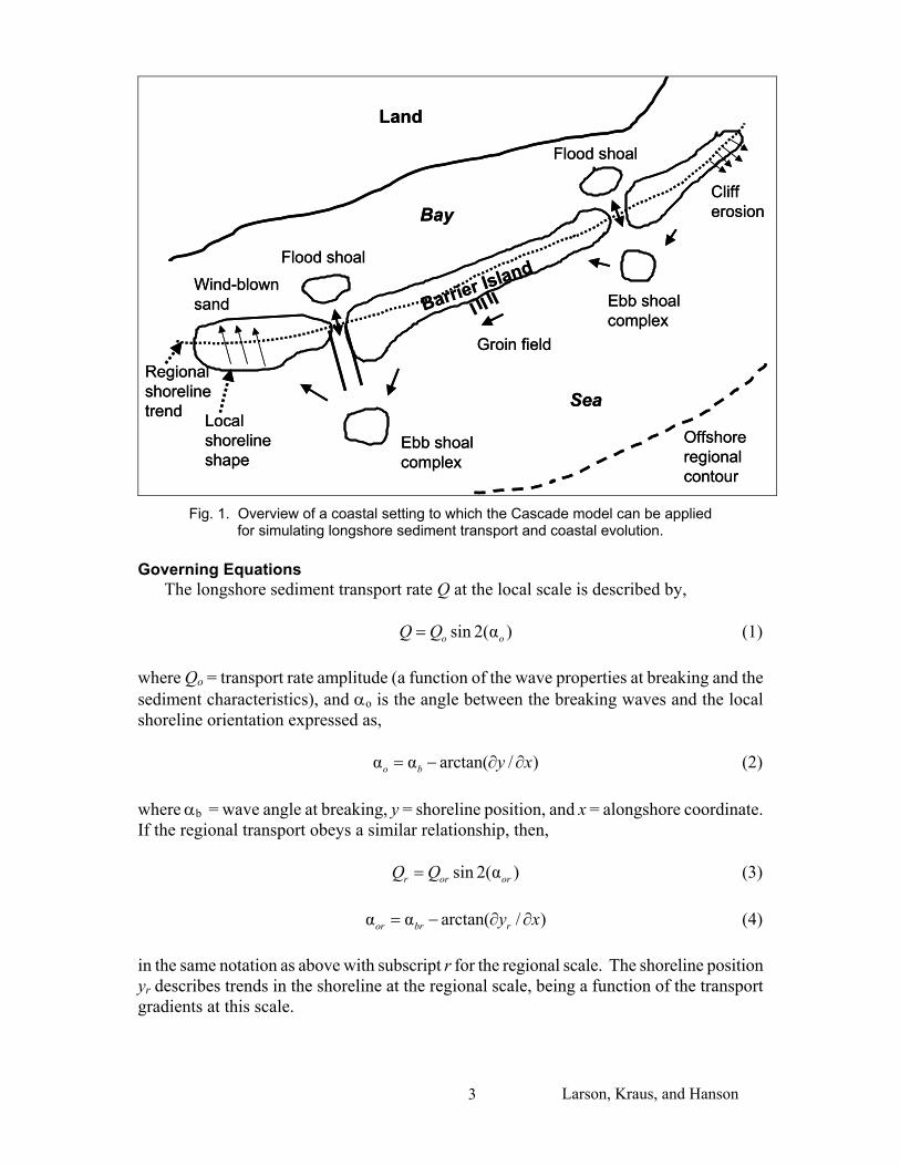
To address these issues, a new class of numerical model of longshore transport and coastal change, called Cascade, was developed to represent regional processes extending hundreds of kilometers and covering several inlets. Time intervals of interest span decades to centuries. At regional time and space scales, the model includes such phenomena as inlet creation, ebb- and flood-tidal shoal development, bypassing bars between beaches and inlets, channel dredging, regional trends in the shape of the coast, relative change in sea level, wind-blown sand, storms, periodic beach nourishment, and shore-protection structures such as groins and seawalls. The name Cascade derives from recognition that processes at different spatial and temporal scales act simultaneously in what can be viewed as cascading of scales from regional to local. For example, offshore contours of a coastal region might have a curved trend, upon which local projects are emplaced (and interact) that may individually appear to have straight trends in shoreline position. The embedding of local processes requires cascading of information from wide-area to local, from long-term to immediate, and from project to project site. In the following, the main components of Cascade are described, including algorithms for computing breaking wave properties, longshore sediment transport, sediment bypassing of jetties, and inlet sediment storage and transfer. Validation of Cascade encompassed general model testing and evaluation for a number of hypothetical cases (not discussed here), as well as a detailed simulation for the south shore of Long Island, New York. For the field validation, comparisons between model simulations and measurements were made for the net annual longshore transport rate and shoreline response after opening of two inlets (Shinnecock Inlet and Moriches Inlet). MODEL THEORY Cascade simulates longshore sediment transport and coastal evolution at the regional and local scale. Fig. 1 provides an overview of a typical coastal setting to which Cascade may be applied. The figure shows three barrier islands separated by inlets with and without jetties, where the sediment is transferred around an inlet through the inlet-shoal complex. A number of sources (sinks) are shown including cliff erosion and wind-blown sand. The shoreline of the barrier island chain displays a curved trend at the regional scale with local variations in between the inlets. Initial model development focused on developing fast, reliable, and robust algorithms for calculating waves and sediment transport. Also, an important part was formulation of realistic boundary conditions, which in some cases constitute complex submodels (e.g., jetty bypassing, inlet sediment transfer). Below, a short description is given of the following model components: (1) governing equations and boundary conditions, (2) breaking wave properties, (3) longshore sediment transport, (4) bypassing transport, and (5) inlet sediment storage and transfer. Some of these components required new theory to be developed, whereas other components were based on previous work. The summary here mainly covers new developments needed for Cascade.

Larson, Kraus, and Hanson 2

Land

Flood shoal

Flood shoal

Ebb shoal complex

Ebb shoal complex

Groin fieldRegional shorelinetrend

Clifferosion

Wind-blownsand

Offshore regionalcontour

Local shorelineshape

Sea

Bay

Barrier Island

Land

Flood shoal

Flood shoal

Ebb shoal complex

Ebb shoal complex

Groin fieldRegional shorelinetrend

Clifferosion

Wind-blownsand

Offshore regionalcontour

Local shorelineshape

Sea

Bay

Barrier Island

Fig. 1. Overview of a coastal setting to which the Cascade model can be applied

for simulating longshore sediment transport and coastal evolution. Governing Equations The longshore sediment transport rate Q at the local scale is described by, sin 2(α )oQ Q o= (1) where Qo = transport rate amplitude (a function of the wave properties at breaking and the sediment characteristics), and αo is the angle between the breaking waves and the local shoreline orientation expressed as, α α arctan( / )o b y x= − ∂ ∂ (2) where αb = wave angle at breaking, y = shoreline position, and x = alongshore coordinate. If the regional transport obeys a similar relationship, then, sin 2(α )r or orQ Q= (3) α α arctan( / )or br ry x= − ∂ ∂ (4) in the same notation as above with subscript r for the regional scale. The shoreline position yr describes trends in the shoreline at the regional scale, being a function of the transport gradients at this scale.

Larson, Kraus, and Hanson 3

In Cascade, it is assumed that the local shoreline evolves with respect to the regional shoreline, yielding the following transport equation: ( )( )sin 2 arctan /o br bQ Q y x= α +α − ∂ ∂ (5) If yr is in equilibrium (Qr=0), Eq. 4 implies that αbr=arctan(dyr/dx). Thus, after yr has been determined, y can be obtained directly by solving Eq. 5 in combination with the sand volume conservation equation,

( , )Q yD q xx t

t∂ ∂+ =

∂ ∂ (6)

where D = depth of transport, t = time, and q = a source (sink) term varying in time and space. The regional trend yr may be determined trough spatial filtering using a window size appropriate for the features that should be resolved. In Cascade, sediment may be added or taken away from the coastal area through sources or sinks, respectively, creating a shoreline response. Common sediment sources are: cliff erosion, dune erosion, beach nourishment, wind-blown sand, river-transported sediment, and onshore transport of material from deeper water. Common sediment sinks are: wind-blown sand, dredging, barrier-island wash-over, and offshore transport of material to deeper water. Thus, certain processes may act both as a source and a sink for the shoreline depending on the particular conditions. Four different types of boundary conditions have been formulated for Cascade: (1) no transport (Q=0), (2) no shoreline change (∂Q/∂x=0), (3) bypassing, and (4) bypassing and inlet sediment storage and transfer (for the two latter boundary conditions, Q is derived in submodels, discussed below). Breaking Wave Properties The transport rate Q must be calculated at a large number of points in space and for many time steps. Thus, the wave properties at the break point are computed a large number of times, and it is of great value to have an efficient algorithm to do this. Assuming input wave conditions in deep water, the wave properties at breaking are obtained by simultaneously solving the energy flux conservation equation and Snell’s law, both equations taken from deep water to the break point. The two equations are written, 2 2cos coso go o b gb bH C H Cθ = θ (7)

sin sino

o bC Cbθ θ

= (8)

where H = wave height, Cg = group speed, C = phase speed, θ = wave angle (with respect to the local shoreline orientation), and o and b denote deep water and the break point, respectively. The two equations are coupled and are solved through an iterative procedure. Introducing expressions for the various wave quantities valid for deep and shallow water, and substituting the unknown angle from Snell’s law into the energy flux conservation

Larson, Kraus, and Hanson 4

equation gives the following equation to solve with the water depth at breaking as the unknown,

5/ 2 2

2

coscos arcsin 2 sin2 2

b bo

o o b

h hL L

o o

o

HL

θπ θ = γ π

(9)

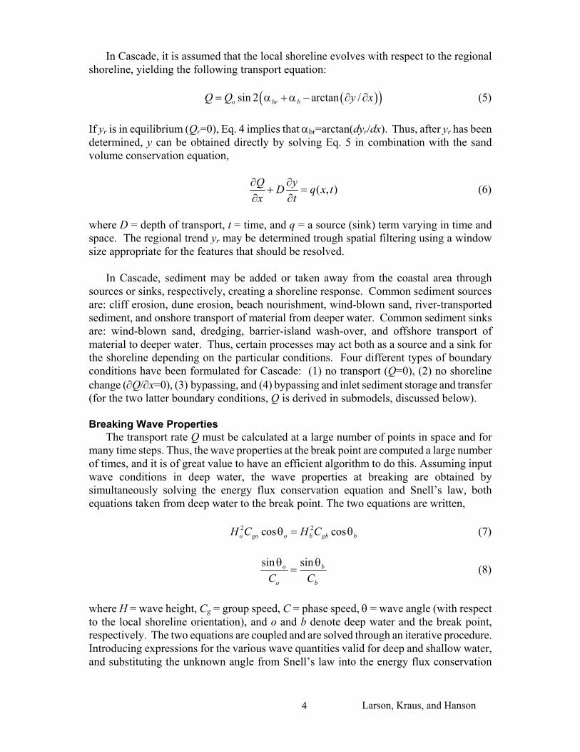
where hb = water depth at the break point, Lo = deepwater wavelength, and γb = wave height to water depth at incipient breaking (taken to be 0.78). This equation shows that hb/Lo (or, equivalently hb/Ho) is a function only of Ho/Lo and θo. A look-up table is employed to quickly obtain hb from known input wave properties. Once hb is obtained, the other quantities at the break point may be calculated directly. Fig. 2 illustrates the variation of hb/Ho with Ho/Lo and θo (solid lines).

0.00 0.01 0.10Deepwater Wave Steepness (Ho/Lo)

0.5

1.0

1.5

2.0

2.5

3.0

Non-

Dim

ensi

onal

Dep

th a

t Bre

akin

g (h

b/H o

)

10 deg20 deg

30 deg

40 deg

50 deg

60 deg

Deepwater Wave Angle

Fig. 2. Normalized depth at breaking as a function of wave steepness and angle in deep water

(exact and approximate solutions). If the wave angle at breaking is small, cos θb ≅ 1.0, and hb can be calculated explicitly from:

2 /52

2

cos2 2

b o o

o o b

h HL L

θ= γ π

(10)

Fig. 2 also includes solutions for this approximate expression (broken lines), indicating that the error introduced by this expression is marginal for a wide range of values on Ho/Lo and θo (calculations showed that the error is maximum 10% for all angles and steepnesses). The wave angle at the break point is calculated from Snell’s law:

Larson, Kraus, and Hanson 5

arcsin 2 sin bb

o

hL

θ = π θ

o (11)

Longshore Sediment Transport A newly derived formula (Larson and Bayram 2002) for the total longshore sediment transport rate was implemented in Cascade, in which it is possible to include currents generated by tide and wind. In the derivation of this formula, it was assumed that suspended sediment mobilized by breaking waves is the dominant mode of transport. A certain ratio of the incident wave energy flux provides the work for maintaining a steady-state concentration in the surf zone. The product between the concentration and the longshore current (from waves, wind, and tide) yields the transport rate Q as,

( )(1 )s

Qa gw

FVε=

ρ −ρ − (12)

where F = wave energy flux directed toward shore, V = surf-zone average longshore current velocity, ε = empirical coefficient, ρs (ρ)= sediment (water) density, a the porosity, and w = sediment fall speed. Values on ε must be established through calibration against data, but an alternative method is to compare the new formula with the CERC formula. Larson and Bayram (2002) made such a comparison, employing the mean longshore current in the surf zone based on the alongshore momentum equation with linearized friction and F from linear wave theory. An equilibrium beach profile was assumed, using the relationship between the shape parameter A and w from Kriebel et al. (1991). For small angles at breaking, the transport coefficient is given by ε=0.77cf K, where K = transport rate coefficient in the CERC formula, and cf = bottom friction coefficient. Bypassing of Jetties To determine the bypassing at jetties (or groins), a model is needed to calculate the cross-shore distribution of the longshore transport rate updrift the jetty. Such a model was implemented in Cascade based on a sediment transport formula originally developed by Larson and Hanson (1996). This formula was derived under similar assumptions as the total longshore sediment transport formula previously discussed. However, because the local transport is needed, the concentration profile becomes a function of the local wave energy dissipation P. The transport rate per unit length across shore ql is given by,

( )(1 )

cl

s

qa gw

VPε=

ρ −ρ − (13)

where V = local longshore current velocity, and εc - transport coefficient. The simplest approach to determine how much of the sediment that may bypass a groin or jetty is to assume that all sediment transported seaward of the groin tip is bypassed, whereas the transport shoreward of the tip is blocked. To compute V and P, the random wave transformation model by Larson (1995) was employed, although a more simplified description of the energy dissipation due to breaking was used. Integrating ql across the profile and assuming that the tip of the groin is located

Larson, Kraus, and Hanson 6

at x=xg, the ratio p of the total sediment transport that bypasses the groin is,

12 2

0

1 1

gx

d dp dx dxdx dxh h

−∞ ∞ ξ ξ =

∫ ∫ (14)

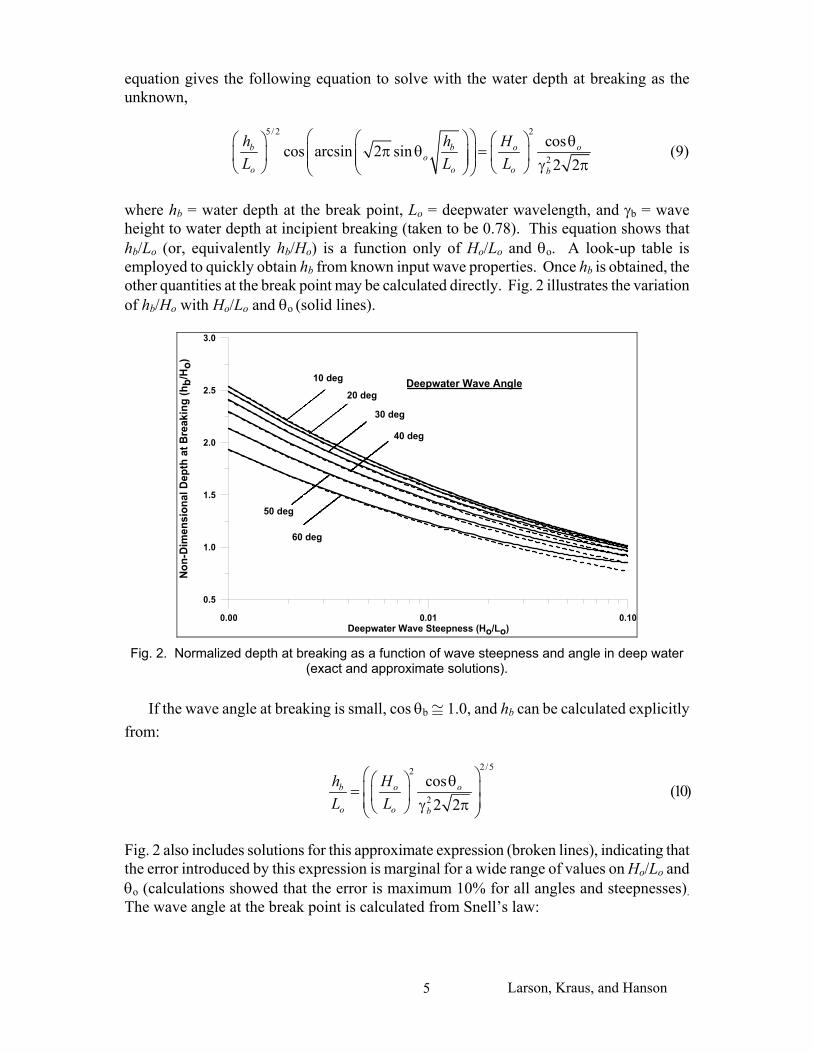
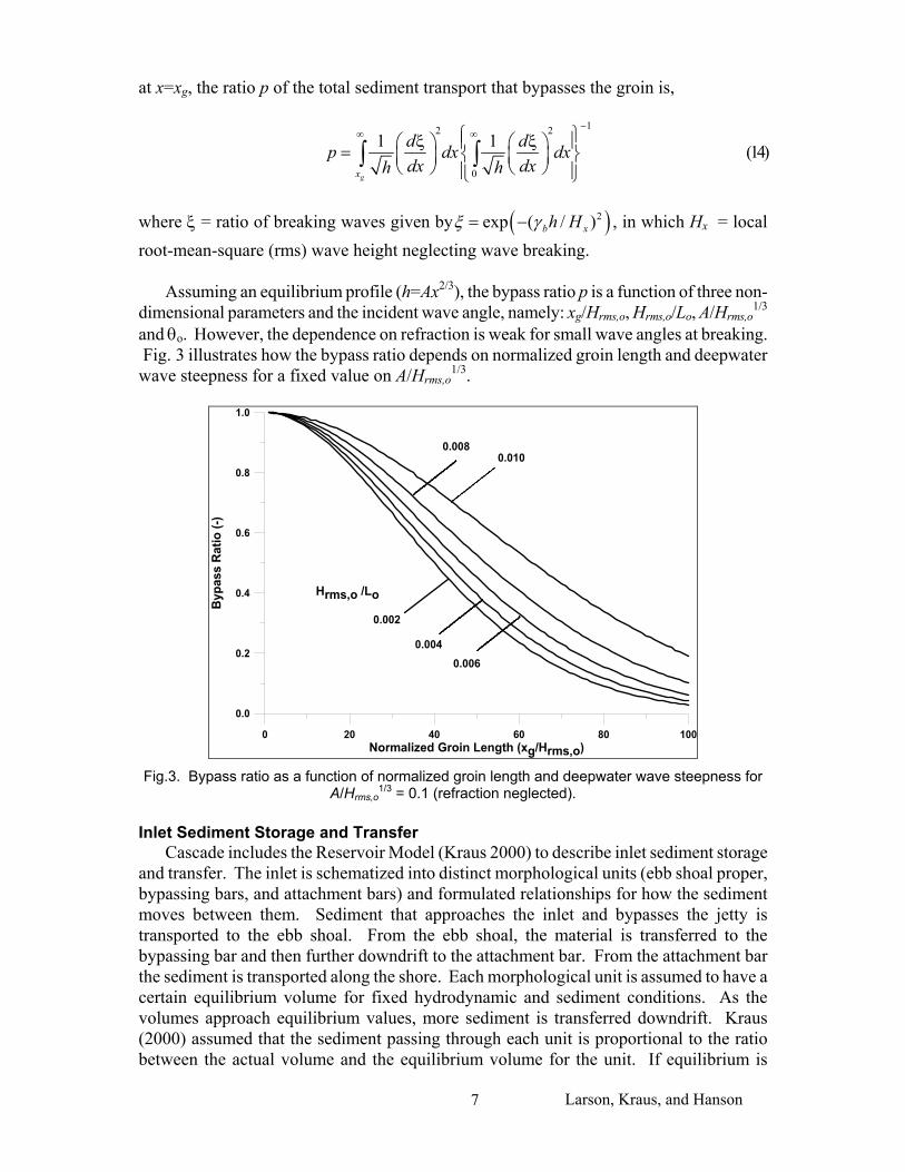
where ξ = ratio of breaking waves given by ( )2exp ( / )b xh Hξ γ= − , in which Hx = local root-mean-square (rms) wave height neglecting wave breaking. Assuming an equilibrium profile (h=Ax2/3), the bypass ratio p is a function of three non-dimensional parameters and the incident wave angle, namely: xg/Hrms,o, Hrms,o/Lo, A/Hrms,o

1/3 and θo. However, the dependence on refraction is weak for small wave angles at breaking. Fig. 3 illustrates how the bypass ratio depends on normalized groin length and deepwater wave steepness for a fixed value on A/Hrms,o

1/3.

0 20 40 60 80Normalized Groin Length (xg/Hrms,o)

100

0.0

0.2

0.4

0.6

0.8

1.0

Bypa

ss R

atio

(-)

0.002

0.0040.006

0.0080.010

Hrms,o /Lo

Fig.3. Bypass ratio as a function of normalized groin length and deepwater wave steepness for

A/Hrms,o1/3 = 0.1 (refraction neglected).

Inlet Sediment Storage and Transfer Cascade includes the Reservoir Model (Kraus 2000) to describe inlet sediment storage and transfer. The inlet is schematized into distinct morphological units (ebb shoal proper, bypassing bars, and attachment bars) and formulated relationships for how the sediment moves between them. Sediment that approaches the inlet and bypasses the jetty is transported to the ebb shoal. From the ebb shoal, the material is transferred to the bypassing bar and then further downdrift to the attachment bar. From the attachment bar the sediment is transported along the shore. Each morphological unit is assumed to have a certain equilibrium volume for fixed hydrodynamic and sediment conditions. As the volumes approach equilibrium values, more sediment is transferred downdrift. Kraus (2000) assumed that the sediment passing through each unit is proportional to the ratio between the actual volume and the equilibrium volume for the unit. If equilibrium is

Larson, Kraus, and Hanson 7

attained, all sediment entering the particular morphologic unit is transferred downstream. Thus, for each morphologic unit (ebb shoal, bypassing bar, attachment bar), two equations govern storage and transfer of sediment,

out ineq

VQ QV

= (15)

in outdV Q Qdt

= − (16)

where Qin (Qout )= transport (from) the morphologic unit, V = sediment volume of the unit, and Veq =equilibrium value. Walton and Adams (1976) derived empirical equations for the equilibrium shoal volume based on field data from a large number of United States inlets approximately corresponding to the sum of the ebb shoal and bypassing bar volumes. To employ these equations for computing Veq of the different units, some assumptions must be made concerning the size relationship among them. Here, the assumption is made that the equilibrium volume ratio between the bypassing bar and the ebb shoal, as well as between the attachment bar and the ebb shoal, is constant. Presently, these ratios are set to 0.25 and 0.1, respectively. In the general case, transport can be directed both to the left and the right, and there will be bypassing and attachment bars on both sides of the inlet. If the cross-sectional area of an inlet changes, it is necessary to allow for a time-varying Veq. During closure of an inlet, the Veq that the tidal flow can maintain may fall below the actual volume in the ebb shoal complex, implying that sediment is released to adjacent beaches. Mathematically, Eqs.15 and 16 can describe this situation, but from a physical point the release might be too rapid and cause unrealistic local growth of the shoreline. To remedy this situation, Eq. 15 was changed into a nonlinear relationship according to Qout=Qin(V/Veq)n, where n is a power. By specifying a value of n<1 for situations where sediment is released to the beach, the release will be slower than for the linear model. In simulations for Long Island, n was set to 1.0 for periods when the ebb shoal complex was growing, whereas n=0.1-0.2 when the shoal experienced reduction in volume. MODELING EVOLUTION OF THE LONG ISLAND SOUTH SHORE

The south shore of Long Island, New York, was selected as a suitable location for validating the capability of Cascade to simulate sediment transport and coastal evolution on regional scale. Several studies (e.g., Kana 1995; Rosati et al. 1999) provide substantial information for model validation. The stretch includes many coastal features and processes characterizing evolution on the regional scale. The study area extended from Fire Island Inlet to Montauk Point (named FIMP in the following) because most available information originated from this coastal stretch. The area includes two inlets (besides Fire Island Inlet at the western boundary), namely Shinnecock Inlet and Moriches Inlet. The cross-sectional areas of the inlets have varied substantially with time, altering the size of the ebb shoal complexes and sediment removed from the nearshore transport system, providing an opportunity to model a complex morphologic system.

Two types of simulations were performed with Cascade for the FIMP area: (1) determining the overall annual net longshore transport pattern along the coast (based on

Larson, Kraus, and Hanson 8

shoreline positions and waves from 1983 to 1995); and (2) simulating coastal evolution in connection with the opening of Moriches Inlet and Shinnecock Inlet (simulation period 1931-1983). Objectives of these simulations were to validate that the model could (1) predict longshore transport rates along a stretch of coastline where trends in the wave climate and shoreline shape are present at the regional scale, and (2) predict coastal evolution in terms of shoreline response and changes in the ebb-shoal complex where regional processes and controls exert a significant influence on local processes. General Model Setup The south shore of Long Island is approximately oriented 67.5 deg TN. A coordinate system was defined that had a similar orientation. In defining the new coordinate system, baseline points employed by Rosati et al. (1999) were referenced. The lateral boundary condition of “no shoreline change” was specified based on shoreline measurements covering 1830 to 1995. Suitable locations for such a boundary condition were identified approximately 10 km west of Montauk Point and either adjacent to or 15 km east of Fire Island Inlet, depending on the simulation period. In simulation of inlet openings, the boundary was placed about 15 km east of Fire Island Inlet to avoid describing spit movement taking place there. The time step was set at 24 hr and length step at 500 m. The length of the modeled shoreline in combination with shadowing from surrounding landmasses made it necessary account for variation in wave climate alongshore. Hindcast waves from WIS Stations 75, 78, and 81 were input (20-year time series of height, period, and angle from 1976 to 1995), linearly interpolated between stations. Depth of active sediment transport was set to 8 m, and the representative median grain size 0.3 mm. The studied shoreline shows large-scale (i.e., regional) features that persist with time. Without taking these features into account through yr, diffusion would eliminate them. In Cascade, yr enters as a source term in the governing transport equation for the local shoreline evolution y. The shape of yr was determined from spatial filtering of the shoreline measured 1870 when no inlets existed and using a window length of 7 km. For the long-term simulation 1931-1983, the equilibrium volumes of the ebb shoals and bypassing bars were specified as a function of time based on the recorded inlet cross-sectional areas. In the shorter simulation 1983-1996, the equilibrium volumes were held constant because the inlets did not change substantially during this time period. Jetty lengths on each side of the inlets and the time of construction were specified according to available data. Two sources of sediment were included in the present Cascade simulations for the FIMP area, input from cliff erosion west of Montauk Point and from beach fills placed west of Shinnecock Inlet. A total fill volume of about 800,000 m3 was placed west of Shinnecock Inlet between 1949 and 1983, and another 1,150,000 m3 was put in this area between 1983 and 1995 (Morang 1999). Smaller beach fills have been placed at other locations, but were neglected. In the simulations, the beach fill volumes were converted to sediment sources with constant strength in time and space. Rosati et al. (1999) estimated the cliff erosion at Montauk Point to yield about 33,000 m3 per year, which input to the model and introduced as a distributed source with constant strength in time. The Westhampton groin field was not resolved in the simulations.

Larson, Kraus, and Hanson 9

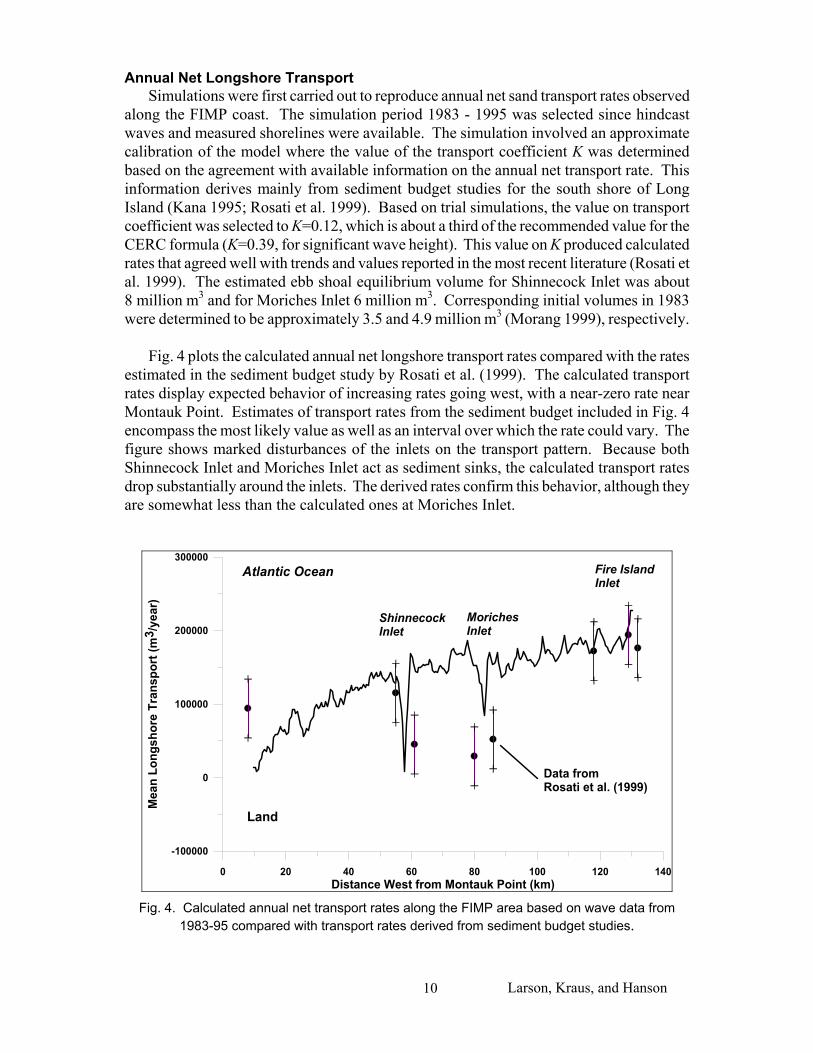
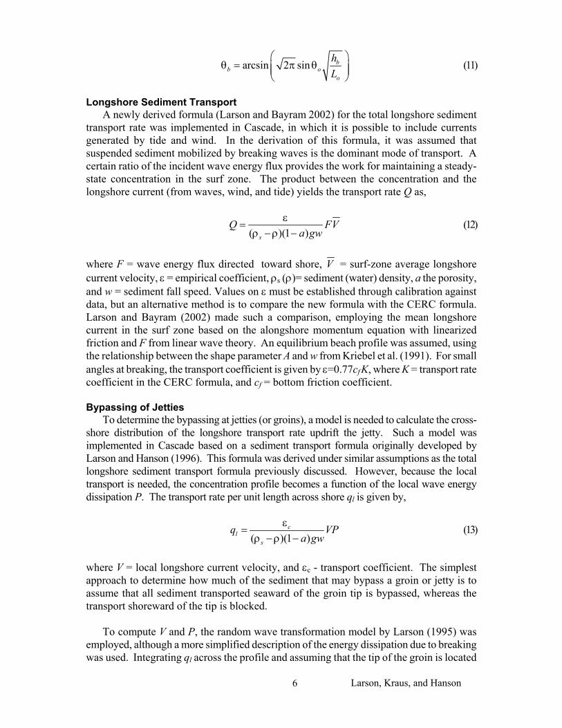
Annual Net Longshore Transport Simulations were first carried out to reproduce annual net sand transport rates observed along the FIMP coast. The simulation period 1983 - 1995 was selected since hindcast waves and measured shorelines were available. The simulation involved an approximate calibration of the model where the value of the transport coefficient K was determined based on the agreement with available information on the annual net transport rate. This information derives mainly from sediment budget studies for the south shore of Long Island (Kana 1995; Rosati et al. 1999). Based on trial simulations, the value on transport coefficient was selected to K=0.12, which is about a third of the recommended value for the CERC formula (K=0.39, for significant wave height). This value on K produced calculated rates that agreed well with trends and values reported in the most recent literature (Rosati et al. 1999). The estimated ebb shoal equilibrium volume for Shinnecock Inlet was about 8 million m3 and for Moriches Inlet 6 million m3. Corresponding initial volumes in 1983 were determined to be approximately 3.5 and 4.9 million m3 (Morang 1999), respectively. Fig. 4 plots the calculated annual net longshore transport rates compared with the rates estimated in the sediment budget study by Rosati et al. (1999). The calculated transport rates display expected behavior of increasing rates going west, with a near-zero rate near Montauk Point. Estimates of transport rates from the sediment budget included in Fig. 4 encompass the most likely value as well as an interval over which the rate could vary. The figure shows marked disturbances of the inlets on the transport pattern. Because both Shinnecock Inlet and Moriches Inlet act as sediment sinks, the calculated transport rates drop substantially around the inlets. The derived rates confirm this behavior, although they are somewhat less than the calculated ones at Moriches Inlet.

0 20 40 60 80 100 120 140Distance West from Montauk Point (km)

-100000

0

100000

200000

300000

Mea

n Lo

ngsh

ore

Tran

spor

t (m

3 /ye

ar)

ShinnecockInlet

MorichesInlet

Fire IslandInlet

Land

Atlantic Ocean

Data fromRosati et al. (1999)

Fig. 4. Calculated annual net transport rates along the FIMP area based on wave data from

1983-95 compared with transport rates derived from sediment budget studies.

Larson, Kraus, and Hanson 10

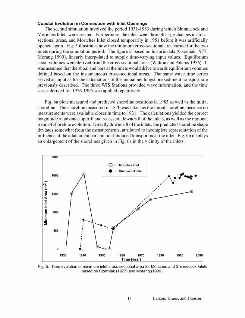
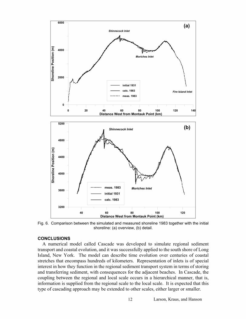
Coastal Evolution in Connection with Inlet Openings The second simulation involved the period 1931-1983 during which Shinnecock and Moriches Inlets were created. Furthermore, the inlets went through large changes in cross-sectional areas, and Moriches Inlet closed temporarily in 1951 before it was artificially opened again. Fig. 5 illustrates how the minimum cross-sectional area varied for the two inlets during the simulation period. The figure is based on historic data (Czerniak 1977; Morang 1999), linearly interpolated to supply time-varying input values. Equilibrium shoal volumes were derived from the cross-sectional areas (Walton and Adams 1976). It was assumed that the shoal and bars at the inlets would drive towards equilibrium volumes defined based on the instantaneous cross-sectional areas. The same wave time series served as input as for the calculations of the annual net longshore sediment transport rate previously described. The three WIS Stations provided wave information, and the time series derived for 1976-1995 was applied repetitively. Fig. 6a plots measured and predicted shoreline positions in 1983 as well as the initial shoreline. The shoreline measured in 1870 was taken as the initial shoreline, because no measurements were available closer in time to 1931. The calculations yielded the correct magnitude of advance updrift and recession downdrift of the inlets, as well as the regional trend of shoreline evolution. Directly downdrift of the inlets, the predicted shoreline shape deviates somewhat from the measurements, attributed to incomplete representation of the influence of the attachment bar and tidal-induced transport near the inlet. Fig. 6b displays an enlargement of the shorelines given in Fig. 6a in the vicinity of the inlets.

1930 1940 1950 1960 1970 1980 1990 2000Time (year)

0

400

800

1200

1600

2000

Min

imum

Inle

t Are

a (m

2 )

Moriches Inlet

Shinnecock Inlet

Fig. 5. Time evolution of minimum inlet cross-sectional area for Moriches and Shinnecock Inlets

based on Czerniak (1977) and Morang (1999).

Larson, Kraus, and Hanson 11

0 20 40 60 80 100 120Distance West from Montauk Point (km)

140

0

2000

4000

6000

Shor

elin

e Po

sitio

n (m

)

initial 1931

calc. 1983

meas. 1983

Shinnecock Inlet

Moriches Inlet

Fire Island Inlet

(a)

40 60 80 100 120Distance West from Montauk Point (km)

3200

3600

4000

4400

4800

5200

Shor

elin

e Po

sitio

n (m

)

meas. 1983

initial 1931

calc. 1983

Shinnecock Inlet

Moriches Inlet

(b)

Fig. 6. Comparison between the simulated and measured shoreline 1983 together with the initial

shoreline: (a) overview, (b) detail. CONCLUSIONS A numerical model called Cascade was developed to simulate regional sediment transport and coastal evolution, and it was successfully applied to the south shore of Long Island, New York. The model can describe time evolution over centuries of coastal stretches that encompass hundreds of kilometers. Representation of inlets is of special interest in how they function in the regional sediment transport system in terms of storing and transferring sediment, with consequences for the adjacent beaches. In Cascade, the coupling between the regional and local scale occurs in a hierarchical manner, that is, information is supplied from the regional scale to the local scale. It is expected that this type of cascading approach may be extended to other scales, either larger or smaller.

Larson, Kraus, and Hanson 12

Larson, Kraus, and Hanson 13

Application of Cascade to the south shore of Long Island, New York demonstrated its capability to simulate regional sediment transport and coastal evolution for complex conditions. The simulations included two inlets that opened and evolvied through significant changes in cross-sectional area, changing the equilibrium volumes of the ebb shoal complex. Eroded and accreted volumes updrift and downdrift the inlets, respectively, were well predicted, whereas the calculated and measured shoreline shape differed somewhat downdrift of the inlets. This discrepancy is attributed to the algorithm for releasing sediment from the attachment bar to the adjacent beach. Work is underway to enhance the model as well as to include other features at the regional scale, such as spit evolution, sediment storage and transfer in the flood shoal and channels of an inlet, and barrier-island migration due to overwash. ACKNOWLEDGEMENTS This paper was prepared under the Regional Sediment Management Program and the Coastal Inlets Research Program, U.S. Army Corps of Engineers (USACE). We appreciate reviews by Dr. Jack Davis and Julie Dean Rosati. Permission was granted by Headquarters, USACE, to publish this information. REFERENCES Czerniak, M.T. 1977. Inlet interaction and stability theory verification. Proc. Coastal

Sediments ’77, ASCE, 754-773. Kana, T. W. 1995. A mesoscale sediment budget for Long Island, New York Marine

Geology, 126, 87-110. Kraus, N.C. 2000. Reservoir model of ebb-tidal shoal evolution and sand bypassing. J.

Waterway, Port, Coastal, and Ocean Engineering, 126(6), 305-313. Kriebel, D.L., Kraus, N.C., and Larson, M. 1991. Engineering methods for predicting

beach profile response. Proc. Coastal Sediments '91, ASCE, 557-571. Larson, M. 1995. Model for decay of random waves in the surf zone. J. Waterway, Port,

Coastal and Ocean Engineering, 121(1), 1-12. Larson, M., and Bayram, A. 2002. Calculating cross-shore distribution of longshore

sediment transport. In: Port Engineering. Ed. Per Bruun, Butterworth (in press). Larson, M., and Hanson, H. 1996. Schematized numerical model of three-dimensional

beach change. Proc. 10th Congress of the Asia and Pacific Division, IAHR, Langkawi, Malaysia, 325-332.

Larson, M., Rosati, J.D., and Kraus, N.C. 2002. Overview of regional coastal processes and controls. Coastal and Hydraulics Engineering Technical Note CHETN XIV-4, U.S. Army Engineer Research and Development Center, Vicksburg, MS.

http://chl.wes.army.mil/library/publications/chetn/pdf/chetn-xiv4.pdf Morang, A. 1999. Shinnecock Inlet, New York, Site investigation, Report 1: Morphology

and historical behavior. Tech. Rep. CHL-98-32, U.S. Army Corps of Engineers, Waterways Experiment Station, Vicksburg, MS.

Rosati, J.D., Gravens, M.B., and Smith W.G. 1999. Regional sediment budget for Fire Island to Montauk Point, New York, USA. Proc. Coastal Sediments ´99, ASCE, 802-817.

Walton, T.L., and Adams, W.D. 1976. Capacity of inlet outer bars to store sand. Proc. 15th Coastal Eng. Conf., ASCE, 1919-1937.