Simulation and Management of Distributed Generating Units ...
166
Simulation and Management of Distributed Generating Units using Intelligent Techniques Vom Fachbereich Ingenieurwissenschaften der Universität Duisburg-Essen zur Erlangung des akademischen Grades eines Doktoringenieurs (Dr. -Ing.) genehmigte Dissertation von AHMED MOHAMED REFAAT AZMY aus Menoufya, Ägypten Referent: Prof. Dr.-Ing. habil. István Erlich Korreferent: Prof. Dr.-Ing. Peter Schegner Tag der mündlichen Prüfung: 14.01.2005
-
Upload
khangminh22 -
Category
Documents
-
view
2 -
download
0
Transcript of Simulation and Management of Distributed Generating Units ...
Simulation and Management of Distributed
Generating Units using Intelligent Techniques
Vom Fachbereich Ingenieurwissenschaften der
Universität Duisburg-Essen
zur Erlangung des akademischen Grades eines
Doktoringenieurs (Dr. -Ing.)
genehmigte Dissertation
von
AHMED MOHAMED REFAAT AZMY aus
Menoufya, Ägypten
Referent: Prof. Dr.-Ing. habil. István Erlich
Korreferent: Prof. Dr.-Ing. Peter Schegner
Tag der mündlichen Prüfung: 14.01.2005


Acknowledgment All praises and thanks are to Allah, the Lord of the world, the most Beneficent,
the most Merciful for helping me to accomplish this work. I am beholden to a number of people and organisations, who supported me to
carry out this work. First and foremost, my heartily profound thanks, gratitude and appreciation to my advisor Univ. Prof. Dr. Eng. habil. István Erlich for his encouragement, help and kind support. His invaluable technical and editorial ad-vice, suggestions, discussions and guidance were a real support to complete this dissertation.
I would like also to express my thanks to my co-advisor Prof. Dr.-Ing. Peter
Schegner for his critical reading and discussion and also the useful suggestions to my dissertation.
Furthermore, I would like to express my deepest gratitude and thanks to all staff
members of “Fachgebiet Elektrische Anlagen und Netze” for contributing to such an inspiring and pleasant atmosphere.
Very special thank to my family, especially my parents and my wife, for their
patience, understanding and encouragement during the different phases of my work. They spared no effort until this work comes to existence.
Last but not least, I wish to acknowledge the financial support of the Missions
Department-Egypt and the Faculty of Engineering, Tanta University for giving me the opportunity to pursue my doctoral degree in Germany.
Ahmed Mohamed Refaat Azmy
Duisburg, January 2005

To my parents, my brothers, my sister, my wife
and my children Rawan, Maryam and Karim
Abstract Distributed generation is attracting more attention as a viable alternative to
large centralized generation plants, driven by the rapidly evolving liberalization and deregulation environments. This interest is also motivated by the need for eliminating the unnecessary transmission and distribution costs, reducing the greenhouse gas emissions, deferring capital costs and improving the availability and reliability of electrical networks. Therefore, distributed generation is ex-pected to play an increasingly important role in meeting future power generation requirements and to provide consumers with flexible and cost effective solutions for many of their energy needs. However, the integration of these sources into the electrical networks can cause some challenges regarding their expected impacts on the security and the dynamic behaviour of the entire network. It is essential to study these issues and to analyze the performance of the expected future systems to ensure satisfactory operation and to maximize the benefits of utilizing the dis-tributed resources.
The thesis focuses on some topics related to the dynamic simulation and opera-
tion of distributed generating units, specifically fuel cells and micro-turbines. The objective of this dissertation is to put emphasis on the following aspects:
Dynamic modelling of fuel cells: Analyzing electrical power systems requires suitable dynamic models for all components forming the system. Since fuel cell units represent new promising sources, the research ascribes special con-sideration to developing models that describe their dynamic behaviour. It is envisaged to develop a simple and flexible model for stability studies and con-troller-design purposes in addition to an exhaustive nonparametric model for detailed analysis of the fuel cells.
Simulation of a large number of DG units incorporated into a multi-machine network: With large numbers of distributed sources, it is expected that decentralized generation impacts the dynamic behaviour of the high volt-age network. Therefore, it is intended to investigate the case, where several fuel cells and micro-turbines are integrated into the distribution system of a multi-machine network. This can help in studying the operation of the entire network and highlighting the mutual impact of the high-voltage and low-voltage networks on each other.
Dynamic modelling and simulation of hybrid fuel cell/micro-turbine units: The hybrid configuration of fuel cells and micro-turbines exhibits many ad-vantages enabling this technology to represent a considerable percentage of the next advanced power generation systems. The dynamic performance of such units, however, is still not fully understood. Hence, it is desirable for un-derstanding their behaviour to highlight the dynamic interdependencies be-tween the fuel cell and the micro-turbine, the overall system transient per-formance, and the dynamic control requirements.
Dynamic equivalents of distribution power networks: The need for fast and simplified analysis of interconnected power networks obligates developing robust dynamic equivalents for certain electrical power subsystems. Non-parametric dynamic equivalents will avoid the identification of complicated mathematical models, which would adequately reflect the performance of the replaced network under various operating conditions. For distribution systems, the equivalent model has to take into consideration the characteristics of dis-tributed generating units which are mostly connected to the network through inverters and in some cases their operating principles are not based on the electromechanical energy conversion mechanism.
Impact of distributed generation on the stability of power systems: The exis-tence of distributed sources with large numbers can impact the stability of the power system considerably. Angle-stability, frequency stability as well as voltage stability can be affected when the power from these units increases. It is essential to study this impact to ensure secure operation of the power sys-tem. Therefore, it is envisaged to study the performance of a hypothetical network and to demonstrate different stability classes at different penetration levels of the distributed generating units.
Online management of fuel cells and micro-turbines for residential applica-tions: The optimal management of the power in distributed generation for residential applications can significantly reduce the operating cost and con-tribute towards improving their economic feasibility. The management proc-ess, however, has to be accomplished in the online mode and to account for all decision variables that affect the setting values. Therefore, it is aimed to de-velop an online intelligent strategy to manage the power generated in fuel cells and micro-turbines when used to supply residential loads in order to minimize the daily operating cost and achieve an overall reduction in the elec-tricity price.
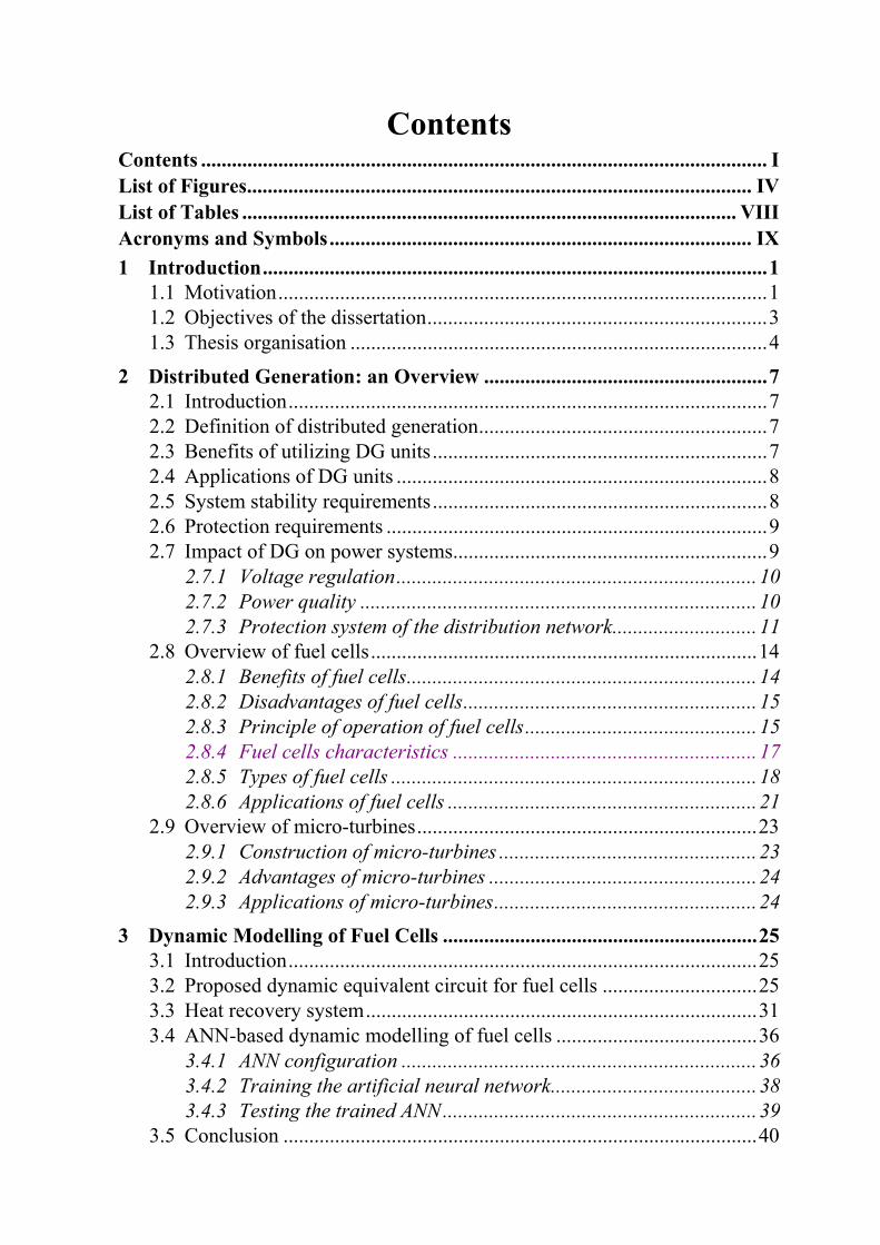
Contents Contents .............................................................................................................. I List of Figures.................................................................................................. IV List of Tables ................................................................................................ VIII Acronyms and Symbols.................................................................................. IX 1 Introduction..................................................................................................1
1.1 Motivation...............................................................................................1 1.2 Objectives of the dissertation..................................................................3 1.3 Thesis organisation .................................................................................4
2 Distributed Generation: an Overview .......................................................7 2.1 Introduction.............................................................................................7 2.2 Definition of distributed generation........................................................7 2.3 Benefits of utilizing DG units.................................................................7 2.4 Applications of DG units ........................................................................8 2.5 System stability requirements.................................................................8 2.6 Protection requirements ..........................................................................9 2.7 Impact of DG on power systems.............................................................9
2.7.1 Voltage regulation...................................................................... 10 2.7.2 Power quality ............................................................................. 10 2.7.3 Protection system of the distribution network............................ 11
2.8 Overview of fuel cells...........................................................................14 2.8.1 Benefits of fuel cells.................................................................... 14 2.8.2 Disadvantages of fuel cells......................................................... 15 2.8.3 Principle of operation of fuel cells............................................. 15 2.8.4 Fuel cells characteristics ........................................................... 17 2.8.5 Types of fuel cells ....................................................................... 18 2.8.6 Applications of fuel cells ............................................................ 21
2.9 Overview of micro-turbines..................................................................23 2.9.1 Construction of micro-turbines .................................................. 23 2.9.2 Advantages of micro-turbines .................................................... 24 2.9.3 Applications of micro-turbines................................................... 24
3 Dynamic Modelling of Fuel Cells .............................................................25 3.1 Introduction...........................................................................................25 3.2 Proposed dynamic equivalent circuit for fuel cells ..............................25 3.3 Heat recovery system............................................................................31 3.4 ANN-based dynamic modelling of fuel cells .......................................36
3.4.1 ANN configuration ..................................................................... 36 3.4.2 Training the artificial neural network........................................ 38 3.4.3 Testing the trained ANN............................................................. 39
3.5 Conclusion ............................................................................................40
Contents II
4 Simulation of a Large Number of DG Units Incorporated into a Multi-Machine Network............................................................................41
4.1 Introduction..................................................................................................41 4.2 Modelling the investigated network .....................................................42
4.2.1 Network description ................................................................... 42 4.2.2 Modelling of micro-turbines....................................................... 45 4.2.3 Modelling of fuel cells ................................................................ 47
4.3 Implementation in the PSD simulation package...................................47 4.4 Simulation results and discussion.........................................................50 4.5 Hybrid fuel-cell/micro-turbine unit ......................................................55
4.5.1 Unit structure ............................................................................. 56 4.5.2 Dynamic modelling .................................................................... 58 4.5.3 Network modifications................................................................ 60 4.5.4 Simulation results and discussion .............................................. 60
4.6 Conclusion ............................................................................................64
5 Artificial Neural Network-Based Dynamic Equivalents for Distri-bution Systems Containing Active Sources .............................................65 5.1 Introduction...........................................................................................65 5.2 Survey over existing approaches ..........................................................66
5.2.1 Linear-based approaches........................................................... 66 5.2.2 Nonlinear-based approaches ..................................................... 67
5.3 Proposed technique ...............................................................................68 5.4 Application with the PST16 network ...................................................70 5.5 Recurrent ANNs for dynamic equivalents............................................73
5.5.1 Data preparation........................................................................ 73 5.5.2 ANN structure............................................................................. 73 5.5.3 Training process......................................................................... 74
5.6 Implementation of the ANN-based equivalent .....................................74 5.7 Simulation results and discussion.........................................................75 5.8 Conclusion ............................................................................................80
6 Impact of DG on the Stability of Electrical Power Systems ..................81 6.1 Introduction...........................................................................................81 6.2 Power system description .....................................................................82 6.3 Impact on the power losses...................................................................84 6.4 Impact on the voltage profiles ..............................................................85 6.5 Angle stability analysis .........................................................................86
6.5.1 Oscillatory stability .................................................................... 86 6.5.2 Transient stability....................................................................... 88
6.6 Frequency stability analysis..................................................................90 6.7 Voltage stability analysis ......................................................................91 6.8 Conclusion ............................................................................................94
Contents III
7 Online Management of DG Units for Residential Applications............95 7.1 Introduction...........................................................................................95 7.2 Structure of the residential system........................................................96 7.3 PEM fuel cell economic model.............................................................97
7.3.1 Objective function ...................................................................... 97 7.3.2 Constraints ............................................................................... 100
7.4 Multi-population real-coded genetic algorithm..................................101 7.4.1 Constraints representation....................................................... 102 7.4.2 Evolution process ..................................................................... 102 7.4.3 GA parameters ......................................................................... 105 7.4.4 Results of the optimization process .......................................... 105
7.5 Management of three identical units simultaneously .........................109 7.6 Management of a micro-turbine unit ..................................................112 7.7 Generalizing the optimization for online employment.......................116
7.7.1 ANN-based generalization ....................................................... 116 7.7.2 Decision tree-based generalization.......................................... 122 7.7.3 Decision trees versus ANN....................................................... 126
7.8 Conclusion ..........................................................................................128
8 Conclusion and Future Directions .........................................................129 8.1 Conclusion ..........................................................................................129
8.1.1 Dynamic modelling of fuel cells ............................................... 129 8.1.2 Simulation of a large number of DG units incorporated into a
multi-machine network............................................................. 129 8.1.3 Dynamic simulation of hybrid fuel cell/micro-turbine units.... 130 8.1.4 Dynamic equivalents of distribution power networks.............. 130 8.1.5 Impact of distributed generation on power systems stability... 131 8.1.6 Online management of fuel cells and micro-turbines .............. 131
8.2 Future directions .................................................................................132
References.......................................................................................................133 Appendices......................................................................................................139
Appendix A................................................................................................139 Appendix B................................................................................................140 Appendix C................................................................................................141 Appendix D................................................................................................142 Appendix E ................................................................................................143 Appendix F ................................................................................................144 Appendix G................................................................................................145
List of Figures Fig 1-1 Operation principles of fuel cells.............................................................2 Fig 2-1 Principle of false tripping due to DG ....................................................12 Fig 2-2 Reduction of the observed fault current as a result of utilizing DG
units........................................................................................................13 Fig 2-3 Fuel cell: principle of operation.............................................................16 Fig 2-4 Electrical characteristics of the fuel cell................................................17 Fig 2-5 Construction of the micro-turbine unit ..................................................23 Fig 3-1 Block diagram of the fuel cell ...............................................................26 Fig 3-2 V-I characteristic and loss resistance.....................................................27 Fig 3-3 Three-phase PWM inverter ...................................................................27 Fig 3-4 Dynamic equivalent circuit of the fuel cell ...........................................28 Fig 3-5 Response of the FC to a 20% step decrease in the load resistance .......29 Fig 3-6 Response of the FC to 20% step decrease in the input fuel rate ...........30 Fig 3-7 Response to 20% step decrease in the load resistance and 20% step
increase in the input fuel rate.................................................................30 Fig 3-8 Response to 20% step increase in the load resistance and 30% step
decrease in the input fuel rate ................................................................31 Fig 3-9 A simple heat recovery system..............................................................31 Fig 3-10 Controllers associated with the heat recovery system...........................34 Fig 3-11 Response of the FC to a 15% step increase in the load impedance ......35 Fig 3-12 Response of the FC to a 10% step decrease in the load impedance......35 Fig 3-13 The structure of the Artificial Neural Network .....................................37 Fig 3-14 Evaluating the performance of the ANN-based model in the training
phase: case (1)........................................................................................39 Fig 3-15 Evaluating the performance of the ANN-based model in the training
phase: case (2)........................................................................................39 Fig 3-16 Testing the response of the ANN-based model under new distur-
bances: test (1) .......................................................................................39 Fig 3-17 Testing the response of the ANN-based model under new distur-
bances: test (2) .......................................................................................40 Fig 4-1 The one line diagram of the PST16 network.........................................43 Fig 4-2 Modelling the medium and the low-voltage sections showing the
integration of the DG units near the end user terminals........................44 Fig 4-3 Block diagram model of the micro-turbine generating unit ..................46 Fig 4-4 Implementation of the fuel cell model in the PSD package ..................48 Fig 4-5 Implementation of the micro-turbine model in the PSD package.........49
List of figures and tables V
Fig 4-6 Response of a selected fuel cell to a load switching in the low-voltage area ............................................................................................50
Fig 4-7 Response of a selected micro-turbine to a load switching in the low-voltage area ............................................................................................51
Fig 4-8 Response of a selected fuel cell to a load switching in the high-voltage area ............................................................................................52
Fig 4-9 Response of a selected micro-turbine to a load switching in the high-voltage area ...................................................................................52
Fig 4-10 Response of a selected fuel cell to a short circuit in the 380kV area....53 Fig 4-11 Response of a selected micro-turbine to a short circuit in the 380kV
area.........................................................................................................53 Fig 4-12 Active power transferred to the 110kV network ...................................54 Fig 4-13 Change in the total active power transfer with and without DG units
as a result of a 3-phase short circuit in the 380kV network ..................55 Fig 4-14 Voltage variation at a low voltage bus with and without DG units as
a result of a three-phase short circuit in the 380kV network.................55 Fig 4-15 The augmented unit (Topping mode) ....................................................57 Fig 4-16 The augmented unit (Bottoming mode) ................................................58 Fig 4-17 Dynamic interdependency of the fuel cell and the micro-turbine.........59 Fig 4-18 Introducing the effect of FC output power on MT mechanical power..59 Fig 4-19 CFCMT response to a 500+j100kVA load switching in the low-
voltage area ............................................................................................61 Fig 4-20 CFCMT response to a 100+j20MVA load switching in the high-
voltage area ............................................................................................61 Fig 4-21 Response of a hybrid unit to a 80ms short circuit in the high-voltage
area.........................................................................................................62 Fig 4-22 Response of two individual FC and MT units operating in parallel to
a 80ms short circuit in the high-voltage area.........................................63 Fig 4-23 Change in the total power transferred to the 110kV area with three
different cases as a result of a three-phase short circuit in the 380kV network ..................................................................................................63
Fig 4-24 Voltage variation at a low-voltage bus with and without DG units as a result of a three-phase short circuit in the 380kV network.................64
Fig 5-1 Representing the replaced subsystem using reduced linear model .......66 Fig 5-2 Representing coherent generators by a single equivalent one...............67 Fig 5-3 Principles of the proposed dynamic equivalent approach .....................69 Fig 5-4 Comparison between the performance of the original full-system
and the two-lumped load-modelling approximations............................72
List of figures and tables VI
Fig 5-5 Structure of the ANN.............................................................................74 Fig 5-6 Implementation and interaction of the ANN-based dynamic equiva-
lent with the retained network ...............................................................75 Fig 5-7 Comparing the equivalent power of active sources at boundary
buses under a disturbance, which is used in the training process .........76 Fig 5-8 Comparing the equivalent power of active sources at boundary
buses under a disturbance, which is not used in the training process ...76 Fig 5-9 Comparing the performance of the original and the equivalent sys-
tems starting from a new power-flow initial condition .........................77 Fig 5-10 Comparing the full-model and the equivalent system after reducing
the power of the DG sources to about 50% of the initial value ............79 Fig 5-11 Comparison between the performance at three different integration
time steps ...............................................................................................79 Fig 5-12 Comparison with a new integration time step and new regulators for
generators...............................................................................................80 Fig 6-1 The one line diagram of the electrical network showing the integra-
tion of FCs and MTs near the end user terminals..................................83 Fig 6-2 Total power loss with different power contributions from DG units....85 Fig 6-3 Voltage levels at 5 feeder nodes with different contributions from
DG units.................................................................................................86 Fig 6-4 Eigenvalues with different power contributions from DG units ...........87 Fig 6-5 Critical eigenvalues with different power from DG units .....................87 Fig 6-6 Change of the power angle due to a fault in the high-voltage net-
work: case 1, no DG unit is switched off ..............................................89 Fig 6-7 Change of the power angle due to a fault in the high-voltage net-
work: case 2, some DG units are switched off ......................................89 Fig 6-8 Frequency response as a result of a 5MW load switching in the
high-voltage network .............................................................................91 Fig 6-9 Frequency response as a result of a 10MW load switching in the
high-voltage network .............................................................................91 Fig 6-10 Voltage deviation of a synchronous generator and a selected load as
a result of a three-phase fault in the high-voltage network ...................92 Fig 6-11 Voltage deviation of a synchronous generator and a selected load as
a result of switching a load of 10Mvar in the high-voltage network ....93 Fig 6-12 Voltage deviation at two load terminals as a result of switching a
load of 1Mvar in the low-voltage network ............................................93 Fig 7-1 Structure of the residential system supplied by a fuel cell ....................97 Fig 7-2 Typical efficiency curves of PEM fuel cell ...........................................98
List of figures and tables VII
Fig 7-3 Relation between the thermal and the electrical power in the FC.......100 Fig 7-4 Flowchart of the GA evolution process...............................................103 Fig 7-5 Roulette wheel selection......................................................................104 Fig 7-6 Unit optimal output power without selling electricity.........................106 Fig 7-7 Unit optimal output power when selling electricity for 0.07$/kWh ...106 Fig 7-8 Effect of varying the sold electricity tariff ..........................................107 Fig 7-9 Effect of varying the purchase electricity tariff...................................107 Fig 7-10 Effect of varying the natural gas tariff for supplying the fuel cell ......108 Fig 7-11 Effect of varying the natural gas tariff to supply the residential load .109 Fig 7-12 Structure of the residential system supplied by three FCs in parallel .109 Fig 7-13 Comparing the performance of one and three fuel cells: case (1).......111 Fig 7-14 Comparing the performance of one and three fuel cells: case (2).......111 Fig 7-15 Comparing the performance of one and three fuel cells: case (3).......112 Fig 7-16 Electrical and thermal efficiency curves of the MT ............................112 Fig 7-17 The electrical efficiency and the thermal power of the MT................113 Fig 7-18 A comparison between using a MT and a FC: case (1).......................114 Fig 7-19 A comparison between using a MT and a FC: case (2).......................114 Fig 7-20 A comparison between using a MT and a FC: case (3).......................115 Fig 7-21 Neural Network structure ....................................................................117 Fig 7-22 Comparing the ANN output with the optimal target: case (1) ............118 Fig 7-23 Comparing the ANN output with the optimal target: case (2) ............119 Fig 7-24 Comparing the ANN output with the optimal target: case (3) ............119 Fig 7-25 Comparing the ANN output with the optimal test target: case (1)......120 Fig 7-26 Comparing the ANN output with the optimal test target: case (2)......120 Fig 7-27 Comparing the ANN output with the optimal test target: case (3)......121 Fig 7-28 Daily operating cost using optimal settings and applying ANN.........121 Fig 7-29 Percentage increase in the operating costs as a result of using the
ANN settings .......................................................................................122 Fig 7-30 Comparing the DT outputs with the GA-based optimal target ...........123 Fig 7-31 Average percentage increase in the daily cost for the different prun-
ing levels considering the full tree as a reference measure .................124 Fig 7-32 Comparing the DT output with the optimal target: case (1)................125 Fig 7-33 Comparing the DT output with the optimal target: case (2)................125 Fig 7-34 Comparing the DT output with the optimal target: case (3)................126 Fig 7-35 Average daily operating cost with the GA-based settings, ANN-
based settings and DT-based settings at different pruning levels .......127

List of figures and tables VIII
List of Tables Table 2-1 Summary of chemical reactions in different types of fuel cells ..........16 Table 2-2 Properties of the main types of fuel cells ............................................21 Table 4-1 Information about the different areas in the PST16 network ..............42 Table 5-1 Summary of components in the retained and replaced subsystems ....71 Table 5-2 Voltages and powers at boundary buses for the base and the new
power-flow cases.................................................................................77 Table 5-3 The new loading conditions of the active units in the replaced
network................................................................................................78 Table 6-1 The number of components in the investigated network ....................82 Table 6-2 Critical modes with different power contributions from DG units .....87 Table 7-1 Parameters used in the GA-based optimization process ...................105 Table 7-2 A list of load curves used in the study...............................................105 Table 7-3 Different tariffs and the corresponding operating cost when op-
timizing the operation of one and three fuel cell units to supply a residential load ..................................................................................110
Table 7-4 Load curves, operating tariffs and the corresponding operating costs when optimizing the operation of a FC and a MT to supply a residential load ...............................................................................113
Table 7-5 Average daily cost and average difference with respect to opti-mal case .............................................................................................115
Table 7-6 Average cost and the average difference of the quasi-optimal set-tings with respect to the GA-based optimal values...........................127
Acronyms and Symbols Acronyms
AFC Alkaline Fuel Cells ANN Artificial Neural Network BPFFNN Back Propagation Feed Forward Neural Network CFCMT Combined Fuel Cell/Micro-Turbine CHP Combined Heat and Power DG Distributed Generation DT Decision Tree FC Fuel Cell GA Genetic Algorithms IGBT Insulated Gate Bipolar Transistor MCFC Molten Carbonate Fuel Cell MT Micro-Turbines PAFC Phosphoric Acid Fuel Cell PEMFC Proton Exchange Membrane Fuel Cell PM Permanent Magnet PMSG Permanent Magnet Synchronous Generator PSD Power System Dynamics PST16 Power System Transient test network PV Photovoltaic PWM Pulse Width Modulation SOFC Solid Oxide Fuel Cell
Symbols
Latin Symbols
tA Tank surface area of the heat recovery system cm2 a1,2 Cross section area of heat-exchanger outer and inner tubes
respect. cm2
Cel-p Tariff of purchased electricity $/kWh Cel-s Tariff of sold electricity $/kWh Cn1, 2nC Natural gas tariffs for DG units and residential loads respect. $/kWh
SPC Average specific heat of the stack of the fuel cell cal/gm.KWPC Average specific heat of the water in the tank cal/gm.K1PC Average specific heat of the cooling fluid of the FC stack cal/gm.K2PC Average specific heat of the second fluid of the heat exchanger cal/gm.K
d Internal diameter of the inner tube of the heat exchanger cm DCPE Daily cost of purchased electricity to supply residential load $
Acronyms and Symbols X
DCPF Daily cost of purchased gas for residential loads $ DFC Daily fuel cost for the DG units $ DOC Daily total operating cost of the DG units $ DISE Daily income for sold electricity $ F Faraday’s constant= 96485.35 oC mol-1
maxf Maximum fitness value of individuals - fref Reference frequency of the micro-turbine unit p.u. H Inertia constant of the PMSG s I Fuel cell stack current A
a,iI , 0iaI , Current of active sources at boundary bus i and its initial value A
j No. of boundary buses between replaced and retained systems - Kg Gain of speed governor of the micro-turbine unit - Kgen Gain of the generator of the micro-turbine unit -
MOK & The operating and maintenance cost per kWh $/kWh L Heat-exchanger tube length cm Lel,J, Lth,JElectrical and thermal load demands respectively at interval J kW M Modulation index (ratio) of the PWM inverter -
LM•
Water mass flow rate from the storage tank to the load gm/s
MRT The minimum running period of the fuel cell h MST The minimum stop period of the fuel cell h
tM Water mass in the tank gm
1M•
, 2M•
Mass flow rates of the two fluids in the heat exchanger gm/s
n Number of cells in series of the fuel cell structure - indN Number of the individuals within the population of the GA -
Nmax The maximum daily number of starts and stops of DG units - nstart-stop The number of starts and stops of DG units per day - O&M Daily operating and maintenance cost of the fuel cell $ Pa Power required for auxiliary devices with the fuel cell system kW
acP , dcP AC and DC power respectively of the FC ANN-based model p.u. Pele Input-electrical power to the PMSG of the micro-turbine unit p.u. Pfc A signal representing the power contained in the FC exhaust p.u.
iP , 0iP The active power at bus i and its initial value kW
PJ Net electrical power produced in the fuel cell at interval J kW PJ,t-1 The power generated in the fuel cell at interval “t-1” kW Pm Input mechanical power to the PMSG of the MT unit p.u. Pmax The maximum limit of the generated power in the fuel cell kW Pmin The minimum limit of the generated power in the fuel cell kW Pref Reference thermal power of the micro-turbine unit p.u. Pth Input thermal power of the micro-turbine unit p.u.
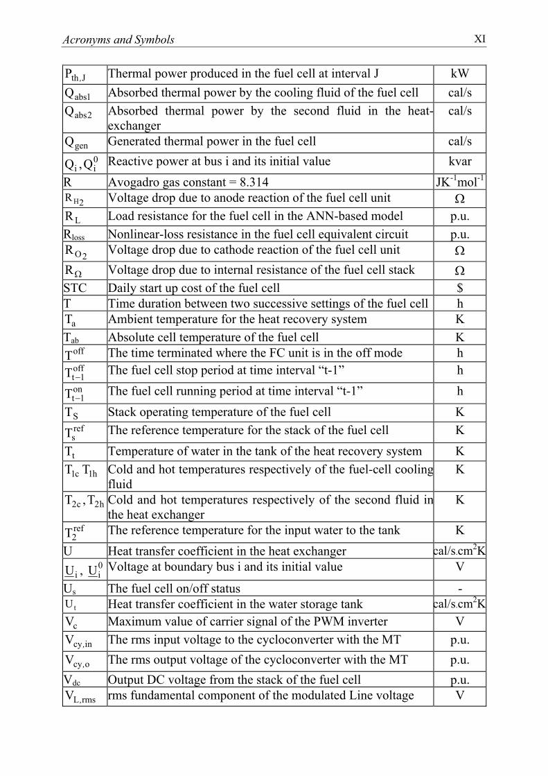
Acronyms and Symbols XI
JthP , Thermal power produced in the fuel cell at interval J kW
1absQ Absorbed thermal power by the cooling fluid of the fuel cell cal/s
2absQ Absorbed thermal power by the second fluid in the heat-exchanger
cal/s
genQ Generated thermal power in the fuel cell cal/s
iQ , 0iQ Reactive power at bus i and its initial value kvar
R Avogadro gas constant = 8.314 JK-1mol-1
2HR Voltage drop due to anode reaction of the fuel cell unit Ω LR Load resistance for the fuel cell in the ANN-based model p.u.
Rloss Nonlinear-loss resistance in the fuel cell equivalent circuit p.u. 2OR Voltage drop due to cathode reaction of the fuel cell unit Ω
ΩR Voltage drop due to internal resistance of the fuel cell stack Ω STC Daily start up cost of the fuel cell $ T Time duration between two successive settings of the fuel cell h
aT Ambient temperature for the heat recovery system K Tab Absolute cell temperature of the fuel cell K
offT The time terminated where the FC unit is in the off mode h off
1tT − The fuel cell stop period at time interval “t-1” h on
1tT − The fuel cell running period at time interval “t-1” h
ST Stack operating temperature of the fuel cell K refsT The reference temperature for the stack of the fuel cell K
tT Temperature of water in the tank of the heat recovery system K
c1T h1T Cold and hot temperatures respectively of the fuel-cell coolingfluid
K
c2T , h2T Cold and hot temperatures respectively of the second fluid inthe heat exchanger
K
ref2T The reference temperature for the input water to the tank K
U Heat transfer coefficient in the heat exchanger cal/s.cm2K
iU , 0iU Voltage at boundary bus i and its initial value V
Us The fuel cell on/off status - tU Heat transfer coefficient in the water storage tank cal/s.cm2K
cV Maximum value of carrier signal of the PWM inverter V
incyV , The rms input voltage to the cycloconverter with the MT p.u.
ocyV , The rms output voltage of the cycloconverter with the MT p.u. Vdc Output DC voltage from the stack of the fuel cell p.u.
rmsLV , rms fundamental component of the modulated Line voltage V

Acronyms and Symbols XII
mV Maximum value of modulating signal of the PWM inverter V rmsphV , rms fundamental component of the modulated phase voltage p.u.
VR The output signal from the reformer to the stack of the FC p.u. Vref Reference voltage of the micro-turbine unit p.u.
SV Stack volume of the fuel cell cm3 V0 the open circuit reversible potential of the FC p.u.
s0V The value of V0 at standard conditions p.u.
fW The turbine input signal of the micro-turbine unit p.u.
minW The offset representing the fuel demand at no-load for the MT p.u. Y (k) Output from the ANN-based model of the FC at interval “k” p.u.
LZ Load impedance to the fuel cell for the ANN-based model p.u. Greek Symbols
α Firing angle of the cycloconverter with the MT unit rad. αh Hot start up cost of the fuel cell $ αh+β Cold start up cost of the fuel cell $
sα A scaling factor in the crossover process - ∆H Total enthalpy of the reaction in the fuel cell stack J/mole
na,iI∆ Normalized current-deviation of active components at bound-
ary bus i -
∆PD The lower limit of the ramp rate of the fuel cell kW/s ∆PU The upper limit of the ramp rate of the fuel cell kW/s ∆S Irreversible entropy change of the reaction in the fuel cell J/mole.K
niU∆ Normalized voltage-deviation at boundary bus i -
PV∆ Change in reversible potential due to the change in pressure mV
TV∆ Change in reversible potential due to the change of temperature mV ηJ Fuel cell efficiency at interval J - ω Angular speed of the PMSG of the MT unit p.u. ωref Reference angular speed of the PMSG p.u.
Sρ Stack mass density of the fuel cell gm/cm3
1ρ , 2ρ The mass density of the two fluids in the heat exchanger gm/cm3
τ The fuel cell cooling time constant h τcd Lag-time constant of compressor discharge of the MT unit s τf Lag-time constant of fuel system of the MT unit s τg Lag-time constant of the speed governor of the MT unit s τgen Lag-time constant of generator of the MT unit s
Rτ , Sτ Time constants of reformer and stack in the FC system respect. s τvp Lag-time constant of valve positioner of the MT unit s
Chapter 1
Introduction
1
1.1 Motivation The ever increasing demand for electrical power has created many challenges
for the energy industry, which can affect the quality of the generated power in short and long terms [1]. The problem will imminently take a new form when bottlenecks occur in the transmission and distribution infrastructure. At the same time, the wide utilization of conventional fossil fuel-based sources will dramati-cally impact the quality and sustainability of life on earth. The realization of the problems associated with the conventional sources is defining a new set of power supply requirements that can better be served through Distributed Generation (DG). Therefore, DG is gaining a lot of attention as it provides solutions for both the short and long term problems [2-5]. They are becoming more feasible as a result of falling price of small-scale power plants and intelligent development of data communications and control technologies. Small DG units are expected to spread rapidly within power systems and have the potential to account for 20-30% of the distribution-system demand by 2020 [6, 7]. Among the promising en-ergy sources, Fuel Cells (FCs) [8-11] and Micro-Turbines (MTs) [12-15] are candidate to support the existing centralized power systems.
MTs can produce low-cost low-emission electricity but at low efficiency which
is limited by the combustion process. The other advantages of MTs include the compact and simple design, small size, low maintenance requirements, durability, load-following capabilities, the ability to operate on a variety of fuels and the possibility of Combined Heat and Power (CHP) applications [16]. However, the dependency of the efficiency on the inlet fuel parameters and the noisy operation represent the main disadvantages of MTs.
FCs offer the potential for lower emissions and higher efficiencies but are
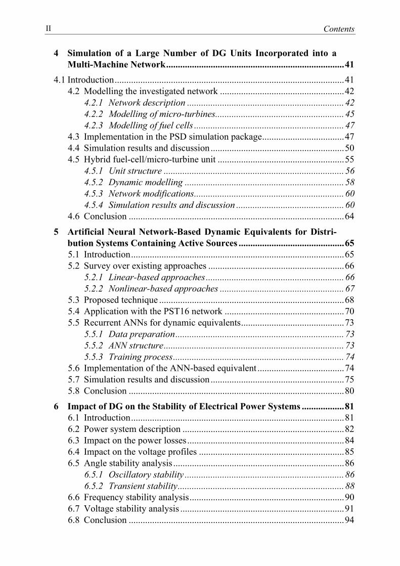
likely to be too expensive for many applications. The first FC unit was discov-ered and developed in 1839 by Sir William Grove [17]. However, it was not prac-tically used until the 1960's when it was utilized to supply electric power for spacecraft [17]. Nowadays, FCs are being used in many applications because of
1. Introduction 2
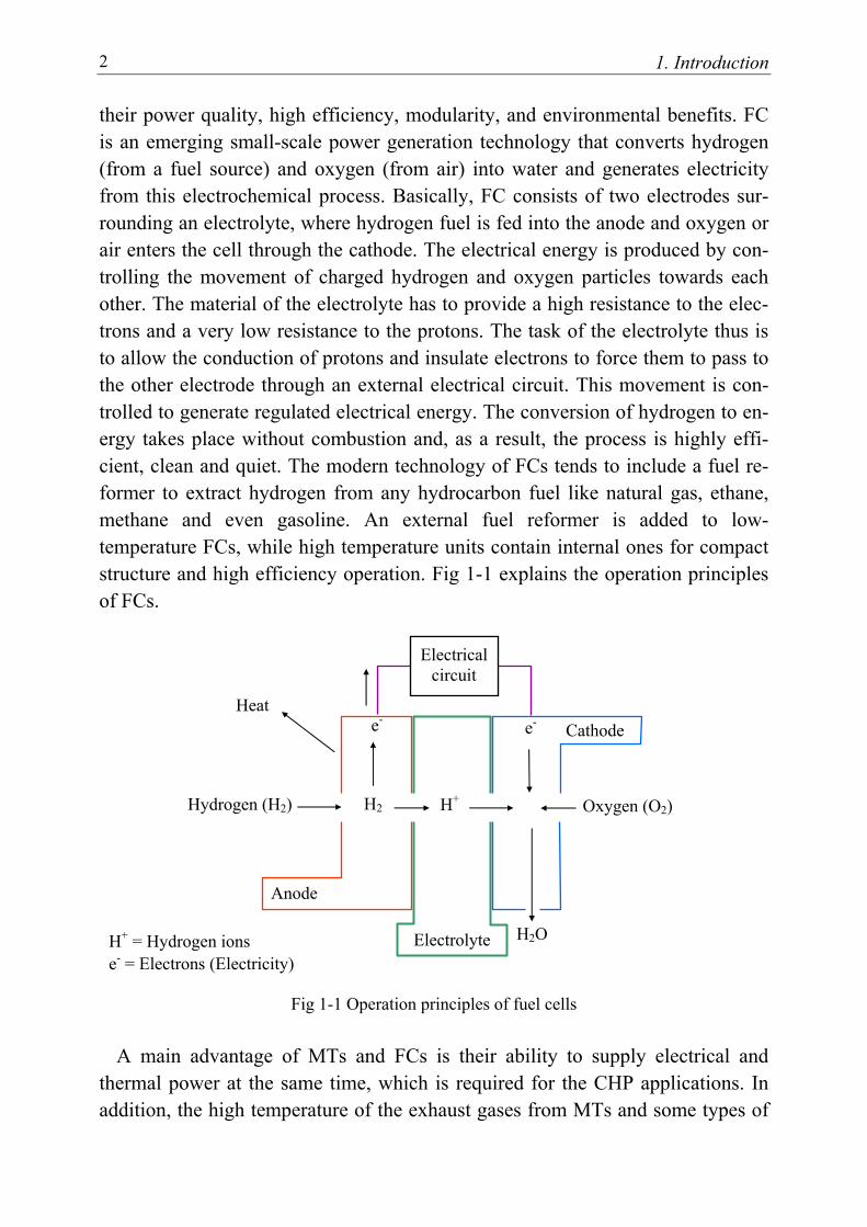
their power quality, high efficiency, modularity, and environmental benefits. FC is an emerging small-scale power generation technology that converts hydrogen (from a fuel source) and oxygen (from air) into water and generates electricity from this electrochemical process. Basically, FC consists of two electrodes sur-rounding an electrolyte, where hydrogen fuel is fed into the anode and oxygen or air enters the cell through the cathode. The electrical energy is produced by con-trolling the movement of charged hydrogen and oxygen particles towards each other. The material of the electrolyte has to provide a high resistance to the elec-trons and a very low resistance to the protons. The task of the electrolyte thus is to allow the conduction of protons and insulate electrons to force them to pass to the other electrode through an external electrical circuit. This movement is con-trolled to generate regulated electrical energy. The conversion of hydrogen to en-ergy takes place without combustion and, as a result, the process is highly effi-cient, clean and quiet. The modern technology of FCs tends to include a fuel re-former to extract hydrogen from any hydrocarbon fuel like natural gas, ethane, methane and even gasoline. An external fuel reformer is added to low-temperature FCs, while high temperature units contain internal ones for compact structure and high efficiency operation. Fig 1-1 explains the operation principles of FCs.
Fig 1-1 Operation principles of fuel cells A main advantage of MTs and FCs is their ability to supply electrical and
thermal power at the same time, which is required for the CHP applications. In addition, the high temperature of the exhaust gases from MTs and some types of
H+ = Hydrogen ions e- = Electrons (Electricity)
Anode
Hydrogen (H2) H2
e-
Electrolyte
H+
e-
H2O
Oxygen (O2)
Heat Cathode
Electrical circuit
1. Introduction 3
FCs enables the combination of the two units to generate more electricity by util-izing the heat energy [18-19]. This configuration is expected to reduce the fuel consumption and to decrease the cost per unit energy.
In spite of the benefits of utilizing DG units within power systems, such as the
increase of the system efficiency and the improvements in the power quality and reliability [20], many technical and operational challenges have to be resolved before DG becomes commonplace. The lack of suitable control strategies for electrical networks with high penetration levels of DG units represents a problem for the futuristic systems. Also, the dynamic interaction between high-voltage parts of the network from one side and DG units from the other side is an essen-tial subject that needs extensive research. To simulate the behaviour of modern electrical networks, suitable static and dynamic models for DG units and the re-lated interface devices are required. In addition, many topics of critical interest regarding the employment of DG have to be investigated. Some of these topics are the overall system stability, the power quality and the interaction between the local regulators with those of the centralized energy plants.
This thesis attempts to highlight some issues related to the use of DG units
from different points of view. Intelligent techniques, i.e. Artificial Neural Net-works (ANNs), Genetic Algorithms (GAs) and Decision Trees (DTs), are em-ployed in different stages of the research due to their capabilities of dealing with many unconventional problems.
1.2 Objectives of the dissertation According to the present-day and the expected-future situations regarding DG
within power systems, it is extremely important to investigate the following is-sues, which are the main topics within the scope of this thesis:
• The development of suitable dynamic models for the FC unit for different
simulation and investigation purposes. This includes: simplified dynamic model for stability study and control-design purposes more detailed dynamic model for thorough analysis of the unit
• The performance investigation of high-voltage multi-machine networks comprising large numbers of selected DG units. The objective is to address the following topics: the impact of DG on the dynamic behaviour of the high-voltage network and vice-versa
1. Introduction 4
the variation on the dynamic behaviour of the low-voltage-network as a result of the influence of integrating DG units on the characteristics of the end-user nodes
• The hybrid configuration based on augmented FC and MT units and the operation of such units within interconnected power systems.
• The development of generic dynamic equivalents for distribution networks containing active DG sources to simplify the analysis of the network.
• The assessment of the potential impacts that DG might have on the stability of electrical power networks.
• The economic operation of DG units when used to supply residential loads by optimizing their daily operating cost and generalizing the optimization process using ANNs or DTs to overcome the disadvantages of the classical optimization techniques.
1.3 Thesis organisation The work in this dissertation is organized as follows: In CHAPTER 1, an introduction about the thesis is presented. As a background, CHAPTER 2 gives an overview of the DG units and their
potential impacts on power systems. Also an overview of FC and MT technolo-gies is presented in this chapter.
The main focus in CHAPTER 3 is on the dynamic modelling of FCs as a
promising DG unit. A simplified nonlinear dynamic model for stability analysis and control-design purposes is proposed. For detailed analysis, a new approach to get an accurate model from input/output data using a recurrent ANN is presented.
An investigation about the dynamic performance of the expected-futuristic
networks that comprise large numbers of DG units is introduced in CHAPTER 4. The mutual dynamic impacts between DG units in the distribution system and high-voltage parts of the network are studied. In addition, this chapter investi-gates the dynamic modelling and simulation of hybrid units consisting of high-temperature FCs and MTs.
Since the analysis of networks including such large number of DG units is a
time consuming process, CHAPTER 5 presents a new dynamic equivalent ap-
1. Introduction 5
proach to replace certain distribution networks by nonparametric equivalents. The idea is to simplify the analysis of the network by replacing these parts of the net-work by recurrent ANN-based dynamic equivalents.
The objective of CHAPTER 6 is to investigate the impact of integrating se-
lected DG units with different penetration levels on the stability of bulk electrical power systems. In particular, the performance of a hypothetical power system with significant penetration of DG units is described to assess different classes of stability.
CHAPTER 7 deals with the economic issues of DG units when used for resi-
dential applications. A new intelligent technique to optimize the daily operation of selected DG units is introduced. The development of the optimization results in a generalized frame using ANNs and DTs is also presented. The online capa-bility of this technique to minimize the daily operating cost by managing the elec-trical and thermal power in these units is discussed.
Finally, deduced conclusions from the thesis and future directions are summa-
rized in CHAPTER 8.

1. Introduction 6
Chapter 2
Distributed Generation: an Overview
2
2.1 Introduction DG can provide many benefits to the power-distribution network [20]. To
maximize these benefits, reliable DG units have to be connected at proper loca-tions and with proper sizes [21]. However, such units will not generally be utility owned, which means that the adequate utilization of DG units is not guaranteed [5]. Moreover, some DG units, such as solar and wind, are variable energy sources and depend in their operation on weather conditions. Therefore, it is not ensured whether DG will satisfy and meet all operation criteria in the power sys-tem. Some issues arise when these units are connected to power systems includ-ing the power quality, proper system operation and network protection [5].
This chapter gives a brief overview of DG units in general and discusses their
potential impact on the distribution networks. In addition, a summary of some aspects related to FC and MT units as new promising DG sources is given. The objective is to clarify some critical points about these technologies, whose simu-lation and economic aspects are extensively studied through the dissertation.
2.2 Definition of distributed generation DG is defined as the integrated or stand-alone utilization of small, modular
electric generation near the end-user terminals [7]. Another generic definition assigns the DG phrase for any generation utilized near consumers regardless of the size or the type of the unit [2, 20]. According to the latter definition, DG may include any generation integrated into distribution system, commercial and resi-dential back-up generation, stand-alone onsite generators and generators installed by the utility for voltage support or other reliability purposes.
2.3 Benefits of utilizing DG units In many applications, DG technology can provide valuable benefits for both the
consumers and the electric-distribution systems [20, 22 and 23]. The small size and the modularity of DG units encourage their utilization in a broad range of
2. Distributed Generation: an overview 8
applications. The downstream location of DG units in distribution systems re-duces energy losses and allows utilities to postpone upgrades to transmission and distribution facilities. The benefits of utilizing DG can be summarized as follows:
• improving availability and reliability of utility system • voltage support and improved power quality • reduction of the transmitted power and, as a result, the transmission and dis-
tribution expenditures are postponed or avoided • power-loss reduction • possibility of cogeneration applications • emission reduction
2.4 Applications of DG units DG can be used for different applications due to their small size, modularity
and location in power systems. The main applications of DG units include the following fields [7]:
• generating the base-load power, as in the case of variable-energy DG sources • providing additional reserve power at peak-load intervals • providing emergency or back-up power to increase the stability and reliability
of important loads • supplying remote loads separated from the main-grid system • supporting the voltage and reliability by providing power services to the grid • cooling and heating purposes It is also possible to use DG to cover the load demand most of the time. In this
case, DG has to be connected to a local grid for back-up power. Another possibil-ity is to use energy storage devices to ensure the continuity of supplying the load.
2.5 System stability requirements Stability studies on large-scale power systems are concerned with the electro-
mechanical stability of large generators. These studies are performed to evaluate the stability of the system under different disturbances. To some extent, the DG stability studies are similar to traditional ones. However, the size and interface of such units with power systems results in some differences. The small size of DG units compared to the entire power system implies that an individual unit has no significant influence on the stability of the bulk system [24]. However, the stabil-
2. Distributed Generation: an overview 9
ity of the DG unit itself has to be investigated to evaluate the ability of these units to remain operating in parallel with the network during and after different distur-bances. Effective damping of the oscillatory behaviour is essential for DG unit regarding their stability. In all cases, accurate models of the entire network in-cluding DG units are required to perform stability analysis [4].
2.6 Protection requirements As mentioned earlier, DG units are not generally owned by the utility and
hence, their protection is the responsibility of the owner or operator. The distribu-tion utility itself will not take any responsibility for protecting DG units or their infrastructure under any operating conditions. In the following, some require-ments of the DG protection system are introduced [3, 5, 25 and 26]:
• it has to be ensured that faults on the utility system will not damage the DG
equipments • DG units have to be completely isolated from faulted areas in the distribution
system considering selectivity principals of the network protection system • DG units have not to energize any de-energized circuits owned by the utility • DG should be disconnected from the network in the case of an abnormality in
voltage or frequency • the synchronization of DG units with the utility is the responsibility of the
operator The protection system of any DG source has to involve the following devices:
• undervoltage and overvoltage protection • short circuit current protection • power directional protection • frequency protection for over and under frequencies • synchronizing relay
2.7 Impact of DG on power systems The utilization of large numbers of DG units within distribution systems im-
pacts the steady state and the dynamics of power networks. Some issues of criti-cal importance are: voltage regulation, power quality and protection coordination in the distribution network. In the following, the potential impact of DG units on the power utility will be discussed regarding these three main points.
2. Distributed Generation: an overview 10
2.7.1 Voltage regulation
Generally, DG units provide voltage support due to their proximity to the end user [7, 20]. The voltages in distribution systems, which commonly have radial structure, are regulated using tap changing transformers at substations and/or switched capacitors on feeder. In addition, supplementary line regulators can also be used on feeders [4]. Since the voltage regulation practice depends on radial power flow from substation to loads, the utilization of DG units, which provide electrical power in different directions, may cause confusions to this practice. Feeding power from DG units can cause negative impacts on the voltage regula-tion in case a DG unit is placed just downstream to a load tap-changer trans-former [5]. In this case, the regulators will not correctly measure feeder demands. Rather, they will see lower values since DG units reduce the observed load due to the onsite power generation. This will lead to setting the voltages at lower values than that required to maintain adequate levels at the tail ends of the feeders [5]. However, most favourable locations of DG units near the end user terminals can provide the required voltage support at the feeder nodes.
2.7.2 Power quality
High power quality requires adequate voltage and frequency levels at customer side. This may require voltage and reactive power support to achieve an accept-able level of voltage regulation. In the stand-alone mode, DG units have to in-volve effective controllers to maintain both voltage and frequency within stan-dard levels. In addition to the level itself, the voltage contents of flickers and harmonics have to be kept as low as possible. The impact of DG units on these two important indices is discussed in the following.
2.7.2.1 Voltage flickers
Voltage flicker is the rapid and repetitive change of voltage that causes visible fluctuations in the light output. Therefore, it is necessary to limit voltage fluctua-tions to restrict the light flickers. Generally, flicker can be caused by load fluctua-tions as well as source fluctuations [27]. DG units have the potential to cause un-wanted fluctuations and cause noticeable voltage flicker in the local power grid. Step changes in the outputs of the DG units with frequent fluctuations and the interaction between DG and the voltage controlling devices in the feeder can re-sult in noticeable lighting flicker [4]. The standalone operation of DG units gives more potential for voltage flickers due to load disturbances, which cause sudden current changes to the DG inverter. If the output impedance of the inverter is high

2. Distributed Generation: an overview 11
enough, the changes in the current will cause significant changes in the voltage drop, and thus, the AC output voltage will fluctuate. Conversely, weak ties in grid integration mode give a chance for fluctuations to take place but with lower de-grees than in the standalone mode [5].
At the time where the analysis of voltage flicker itself is a straightforward task,
the dynamic behaviour of the machines and their interactions with other sources and regulators can complicate the analysis considerably [4]. The DG fluctuations may not be strong enough to create visible flickers. However, these fluctuations may cause hunting for regulators, which can create visible flickers. To dynami-cally model DG for its potential flicker impact, a detailed knowledge is required about the characteristics of DG units including prime mover response, generator controls and machine impedance characteristics [4, 5].
2.7.2.2 Harmonic distortion
The DG technology depends usually on inverter interface and, as a result, con-necting DG units to power systems will contribute towards harmonics. Since har-monic distortion is an additive effect, the utilization of several DG units can strengthen the total harmonic distortion in some locations in the utility even if the harmonic contribution from one DG unit is negligible [5]. The type and severity of these harmonics depend on the power converter technology, the interface con-figuration, and the mode of operation [2]. Fortunately, most new inverters are based on the Insulated Gate Bipolar Transistor (IGBT), which uses Pulse Width Modulation (PWM) to generate quasi-sine wave [4]. Recent advances in semi-conductor technology enable the use of higher frequencies for the carrier wave, which results in quite pure waveforms [2]. In all cases, the total harmonic distor-tion must be controlled within standard level as measured at the load terminals.
2.7.3 Protection system of the distribution network
Distribution networks have traditionally been designed for unidirectional power flow from upper voltage levels down to customers located along radial feeders [26]. This has enabled a relatively straightforward protection strategy depending on well-known aspects and experiences. Large scale implementation of DG will convert simple systems into complicated networks, which demands essential modifications in protection systems [3]. Traditional protection schemes may be-come ineffective and the proper coordination between protection devices of the network and the DG units is extremely important for secure operation of the net-work [26]. Generally, synchronous generators are capable of feeding large sus-
2. Distributed Generation: an overview 12
tained fault currents while currents from inverter-based sources can be limited to lower values [26]. The impact of DG units on the protective system is influenced by the following factors [5, 26]:
• type and size of the DG source • voltage level at the connection point • location of the DG unit on the network • distribution system configuration
In addition to the contribution of DG units on the levels of fault currents, the direction of the currents from these units can adversely impact the operation of protective devices [3]. Some of the typical feeder protection problems, which may be caused by DG, are given in the following [3, 5, 25 and 26]:
Change of short-circuit current levels
Short circuit studies are performed to define the fault currents at different loca-tions in power systems to determine the interrupting ratings of protective devices, which are necessary for coordinated operation of these devices. Generally, the contribution of a small DG unit can not affect the level of the short-circuit cur-rent. However, a number of small DG units or a single large unit can cause a sig-nificant change in short circuit currents observed by the protective devices [5]. When several DG units are utilized, each protective device may observe different fault current. This can cause miscoordination and, hence, affects the reliability and safety of the distribution system [3].
False tripping of feeders
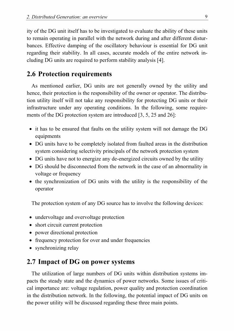
False tripping is typically caused by synchronous generators, which can feed sustained short-circuit currents [26]. Without proper coordination between pro-tection devices, there is a possibility of unnecessarily disconnection of DG units and/or feeders when faults occur on adjacent feeders fed from the same substa-tion [26]. The basic principle of false tripping is shown in Fig 2-1 [26].
Fig 2-1 Principle of false tripping due to DG
DG
Feeder 1 Feeder 2
DG

2. Distributed Generation: an overview 13
If the total current fed by the DG units as a result of the fault in feeder 1 is high enough, the relay on feeder 2 will trip and the whole feeder will be disconnected. False tripping of healthy feeders can likely be solved by using directional over-current relays [26]. Using conventional relays with proper relay settings is also possible conditioned by the adequate coordination between the protection devices of the DG units and the distribution system [3].
Preventing the operation of feeder protection
When a large DG unit or several small ones are connected in the distribution network, the fault current observed by the feeder protection relay may be lower than the actual fault current as seen in Fig 2-2 [26]. This may prevent the opera-tion of the feeder protection relay in the desirable time.
Fig 2-2 Reduction of the observed fault current as a result of utilizing DG units
Reducing the current setting of the feeder protection relay can solve this prob-lem [26]. However, these reduced settings may conflict with the problem of un-necessary disconnection of a healthy feeder [26]. Defining the proper settings to avoid these two problems is essential for reliable operation of the network.
Unwanted islanding
In some cases after a sudden loss of grid connection, parts of the network con-taining DG units may keep operating as an island [3, 5]. This kind of operation is undesirable since the reconnection of the islanded part to the network becomes complicated [26]. In addition, the power quality in the islanded part is not guaran-teed and there is a possibility for abnormal voltage levels or frequency fluctua-tions [26]. Therefore, anti-islanding protection is necessary in most cases to maintain security and reliability in distribution systems [26].
Generally, the use of DG units in distribution systems will impact the protec-tion system and new coordination strategies have to be applied to avoid the ex-pected problems [5]. Despite the importance of this subject, it is out of the main focus of the research in this thesis.
DG
I1 If
I2

2. Distributed Generation: an overview 14
2.8 Overview of fuel cells FC systems were previously found to be suitable for on-site cogeneration and
transportation applications. Nowadays, projects demonstrate FCs for portable power, transportation, utility power, and on-site power generation for residential applications [17]. In the following, an overview of FCs will be introduced since their modelling, simulation and economic aspects are extensively studied through the dissertation.
2.8.1 Benefits of fuel cells
FC power plants have demonstrated better reliability and durability than other sources. As they rely on chemical instead of combustion process, FCs can run continuously for long time without breakdown due to the absence of combustion and moving parts. The main advantages of utilizing FCs include [17, 28-30]:
Operation at high efficiencies: FCs operate at higher efficiencies than com-
bustion-based sources since they eliminate the intermediate steps of combus-tors and mechanical devices used in turbines and pistons. A typical electrical efficiency of FCs lies in the range of 40% to 60%, while the utilization of both electrical and thermal power increases the overall efficiency to 70% for small units and 75% for large units [30]. Unlike conventional systems, FCs operate at high efficiencies also at partial load and in many cases the part-of-load efficiency is higher than the full load value. In addition, small units pro-vide similar high efficiencies like large units due to their modularity [29].
Reduction of Air Pollution: emissions from FCs running on pure hydrogen
are just water vapour, which could dramatically reduce greenhouse gas emis-sion. FCs that use reformers to convert hydrocarbon fuels such as natural gas to hydrogen emit small amounts of air pollutants but still much smaller than emissions from the cleanest fuel combustion systems.
Fuel flexibility: FC system is capable of generating electricity using hydrogen
extracted from a variety of sources like natural gas, ethanol, methanol, coal, and even gasoline. Also, it is possible to utilize hydrogen from renewable sources such as biomass and from wind and solar energy through electrolysis.
Possibility of cogeneration: in addition to the electrical energy produced in
FCs, a considerable amount of useful exhaust heat is also generated as a result
2. Distributed Generation: an overview 15
of the electrochemical process. In some cases, the thermal energy produced is higher than the electrical energy. Thus, FCs are well suited for CHP opera-tion, which contributes in increasing the unit efficiency.
Modularity and simplicity of installation: like photovoltaic, FC stack is
manufactured by augmenting individual cells in parallel (to reach the required current and capacity) and in series (to obtain the suitable voltage). This ad-vantage enables the operator to form modules with different capacities and voltages to be suitable for different purposes starting from portable units to utility applications.
Silent operation: FCs are quiet sources (a 40kW FC power plant has a sound
level of 68dB at a point 10 feet from the cabinet) [29]. This gives the chance to place the FC plant in the load centre near the end user, which eliminates the need for long transmission.
Suitable for the integration with renewable energy sources: FC power plants
can be integrated more efficiently with renewable energy sources [31-32]. They can smooth out the oscillations occurring when using PV arrays or wind turbine and, hence, the power from these sources can be maximized without any modification in the control system. In this case, it will be possible to have significant levels of renewable power penetration. Also, the load requirements will be met more efficiently as the system reliability will be increased.
2.8.2 Disadvantages of fuel cells
The main drawback of FCs is their extremely high cost [29]. Their production cost has to be significantly reduced to become commercially comparable with the conventional power plants. Also, more efforts and researches are required to demonstrate endurance and reliability of high-temperature units [29].
2.8.3 Principle of operation of fuel cells
FCs consist of two electrodes with an electrolyte between them. The principle of operation of FCs is based on the reaction of hydrogen gas (H2), which is sup-plied at the anode, and oxygen gas (O2), which is supplied at the cathode, to form water, heat and electricity [17].
2H2 + O2 ⇒ 2H2O (2-1)
2. Distributed Generation: an overview 16
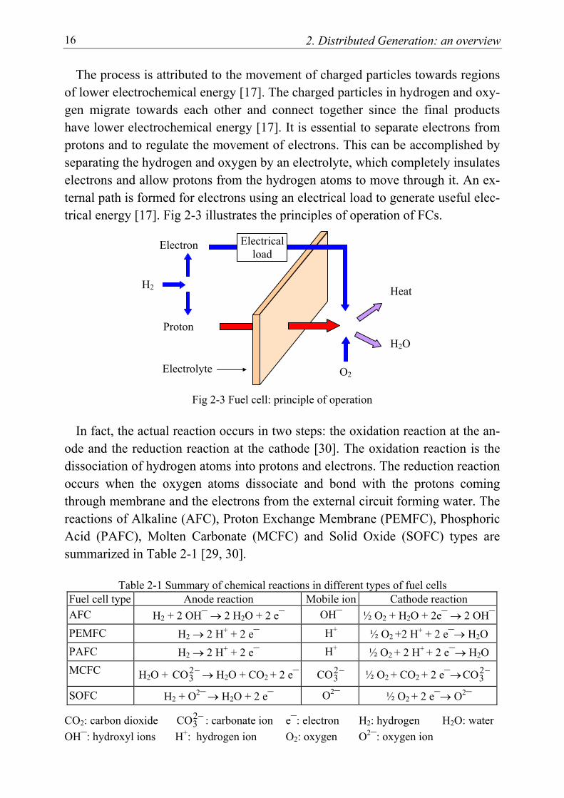
The process is attributed to the movement of charged particles towards regions of lower electrochemical energy [17]. The charged particles in hydrogen and oxy-gen migrate towards each other and connect together since the final products have lower electrochemical energy [17]. It is essential to separate electrons from protons and to regulate the movement of electrons. This can be accomplished by separating the hydrogen and oxygen by an electrolyte, which completely insulates electrons and allow protons from the hydrogen atoms to move through it. An ex-ternal path is formed for electrons using an electrical load to generate useful elec-trical energy [17]. Fig 2-3 illustrates the principles of operation of FCs.
Fig 2-3 Fuel cell: principle of operation
In fact, the actual reaction occurs in two steps: the oxidation reaction at the an-ode and the reduction reaction at the cathode [30]. The oxidation reaction is the dissociation of hydrogen atoms into protons and electrons. The reduction reaction occurs when the oxygen atoms dissociate and bond with the protons coming through membrane and the electrons from the external circuit forming water. The reactions of Alkaline (AFC), Proton Exchange Membrane (PEMFC), Phosphoric Acid (PAFC), Molten Carbonate (MCFC) and Solid Oxide (SOFC) types are summarized in Table 2-1 [29, 30].
Table 2-1 Summary of chemical reactions in different types of fuel cells
Fuel cell type Anode reaction Mobile ion Cathode reaction AFC H2 + 2 OH¯ → 2 H2O + 2 e¯ OH¯ ½ O2 + H2O + 2e¯ → 2 OH¯PEMFC H2 → 2 H+ + 2 e¯ H+ ½ O2 +2 H+ + 2 e¯→ H2O PAFC H2 → 2 H+ + 2 e¯ H+ ½ O2 + 2 H+ + 2 e¯→ H2O MCFC H2O + −2
3CO → H2O + CO2 + 2 e¯ −23CO ½ O2 + CO2 + 2 e¯→ −2
3CO
SOFC H2 + O2¯ → H2O + 2 e¯ O2¯ ½ O2 + 2 e¯→ O2¯
CO2: carbon dioxide −23CO : carbonate ion e¯: electron H2: hydrogen H2O: water
OH¯: hydroxyl ions H+: hydrogen ion O2: oxygen O2¯: oxygen ion
H2
Proton
Electron
O2
Heat H2O
Electrolyte
Electrical load

2. Distributed Generation: an overview 17
2.8.4 Fuel cells characteristics
Depending on the Nernst’s equation and Ohm’s law, the stack output voltage at no load conditions can be calculated as follows [33, 34]:
O2H
212O2Habab
0 XXX
F2RT
F2STHV
/
ln+∆−∆
= (2-2)
where: V0 : the open circuit reversible potential ∆H : the total reaction enthalpy ∆S : the irreversible entropy change F : the Faraday’s constant= 96485.35 oC mol-1 R : the Avogadro gas constant = 8.314 JK-1 mol-1 Tab : the absolute cell temperature Xi : the mole fractions of species The cell resistance and the overpotentials at the anode and the cathode cause a
voltage drop, where the terminal voltage (V) can be calculated by:
( ) n )RR(RI -VV 2O2HΩ0 ⋅−−⋅= (2-3)
where: I, n : the stack current and number of cells in series respectively
2O2H R RR ,,Ω : the voltage drop due to the internal resistance, anode reaction
and cathode reaction respectively The typical voltage-current characteristic of FCs is shown in Fig 2-4. The ef-fect of resistive voltage drop as well as the cathode and anode overpotentials are illustrated separately [35].
Fig 2-4 Electrical characteristics of the fuel cell
Current density (J)
V0 - I.(RΩ+ 2OR + 2HR )
Cell voltage (V)
V0 - I.RΩ
V0 - I.(RΩ + 2OR )
Region 1 Region 2 Region 3
2. Distributed Generation: an overview 18
At small currents (region 1), the sharp drop in the voltage is caused by the acti-vation energy associated with the chemical reaction [35]. At relatively higher cur-rents, (region 2), the voltage drop is dominated by the losses in the electrode structure and the electrolyte, which is almost constant [35]. At very high currents (region 3), the voltage drop is defined by the rate of reaction diffusion [35]. Due to the limitation caused by the diffusion process, the current reaches a maximum value called the limiting current. Therefore FCs can not supply currents that ex-ceed their limiting currents. A FC is said to have good characteristics if it has a flatter curve and a higher limiting current [35].
2.8.5 Types of fuel cells
The operating characteristics, constituent materials and fabrication techniques of FCs are significantly different. FCs are usually classified based on the electro-lytic material into five main types: AFC, PEMFC, PAFC, MCFC and SOFC. In spite of the different materials and operating temperatures of each type, FCs have the same basic principles of operation. Due to the differences in materials and operating characteristics, each type is suited for specific applications. In the fol-lowing a brief overview of the characteristics, advantages and disadvantages of the main types of FCs is introduced.
2.8.5.1 Alkaline Fuel Cell (AFC)
AFC was one of the first modern FCs to be developed, beginning in 1960 when it is used by NASA on space missions [17]. A liquid solution of potassium hy-droxide is used in AFC as an electrolyte. Generally, the slowness of FCs is de-fined by the cathode reaction because it takes more time to react than the anode reaction. AFC is characterized by a faster cathode reaction than other types of FCs, which enhances its overall performance and speeds up its electrical re-sponse. The lower operating temperature (80-100°C) gives a fast-start advantage for this type of FCs, which can achieve efficiencies up to 60% [29].
However, AFCs are intolerant of carbon dioxide and, hence, it cannot use nor-
mal outside air directly as a source of oxygen [17]. A system that removes the carbon dioxide from intake air streams has to be employed. Also, the life time of this type of FCs is relatively short due to the use of a corrosive electrolyte, which gradually wears out the other parts. Since the use of expensive catalysts such as platinum results in a high manufacture cost, the use of other less expensive cata-lysts, such as low cost carbon and metal oxide based electrodes, is also being in-vestigated [17].
2. Distributed Generation: an overview 19
2.8.5.2 Proton Exchange Membrane Fuel Cells (PEMFC)
PEMFCs have gained a lot of attention in the last few years as one of the most promising FC types [28, 36]. It uses a solid organic polymer poly-perflourosulfonic acid as an electrolyte [30]. The solid electrolyte in PEMFCs has a very high resistance to gas crossover, and its membrane, which is made of a Teflon-like material, represents an excellent conductor of protons and an insula-tor of electrons [30]. The other benefits of utilizing a solid electrolyte include the lower corrosion and the absence of the liquid management.
The efficiency of PEMFCs at rated current reaches 50% when operated on hy-
drogen and pressurized air. A major advantage of PEMFCs is their high power density, which is higher than any other FC except for AFC [30]. Like AFC, the low operating temperature (80-100°C) results in a quick start-up and, hence, PEMFCs are favourable in many fields like residential applications and vehicles. Another advantage of PEMFCs is their long operating life as proven in laboratory experiments. The high efficiency and power density and the fast start-up make PEMFCs an attractive alternative to conventional automobile engines [28].
The low operating temperature, however, results in slow chemical kinetics,
where precious metal catalyst, typically platinum, is needed to facilitate the reac-tions [36]. In spite of the attempts that succeeded to reduce the required amount of platinum, further reduction of platinum is needed in order to bring the cost of PEMFCs in competition with combustion engines. Another disadvantage of PEMFCs is their sensitivity to carbon monoxide [17].
2.8.5.3 Phosphoric Acid Fuel Cell (PAFC)
PAFC has been under development for more than 20 years and was the first commercial FC [30]. This caused a significant reduction in the cost and remark-able increase in the efficiency. It utilizes a liquid phosphoric acid as an electro-lyte with an operating temperature of 200°C. This temperature is high enough to facilitate the recovery of heat for water and space heating. It prevents also the water, which is produced as a sub-product, from dissolving in the liquid electro-lyte [30]. Higher operating temperatures are not possible since the phosphoric acid begins to decompose at 210 °C [17]. PAFC generates electricity at more than 40% efficiency, which can be significantly increased with the use of the produced steam in cogeneration [37]. It can efficiently process impure fuels and therefore, PAFC systems are relatively cheaper than other types due to the reduction in the reformer cost [17].

2. Distributed Generation: an overview 20
The expensive catalysts of the PAFCs, typically platinum, increase the overall price of the stack [17]. Also, the high operating temperature necessitates a warm-up period, which increases the start up time. Due to their low power densities, the large size represents another disadvantage for PAFCs. PAFCs are sometimes used in vehicle applications because of their tolerance to fuel impurities. How-ever, this is restricted by their large size, which represents a barrier for employing PAFCs in this field of applications.
2.8.5.4 Molten Carbonate Fuel Cell (MCFC)
Many of the disadvantages related to low-temperature FCs can be alleviated by increasing the operating temperature. MCFC is a promising high-temperature FC (operates at 650 °C), which uses molten alkali carbonate mixture as an electrolyte (usually consists of lithium carbonate and potassium carbonate) [30]. At these high temperatures, precious metal catalysts are not required for the FC reactions, rather, the cell reactions occur with nickel catalysts [30]. In addition, the heat available from the stack is high enough for cogeneration applications [29]. The rejected cell heat can also be used to drive a gas turbine and/or produce a high-pressure steam for use in a steam turbine. Furthermore, internal reforming can be utilized, which reduces the size and the cost of the unit. Another advantage of the MCFC is the possibility of operating efficiently with CO, hydrogen, natural gas, propane marine diesel and simulated coal gasification products [30].
However, MCFC needs a source of CO2 at the cathode (usually recycled from
anode exhaust) to form the carbonate ions [30]. The high operating temperature results in some material problems, particularly mechanical stability that reduces the unit life. Therefore, the use of stainless steel as the cell hardware material is required [30]. To achieve economically viable operation of MCFC, it is designed for median-size and large stationary power applications. However, the target markets for MCFC technology include small DG systems for utilities as well as building cogeneration systems at sizes of 0.1 to 2.0MW [30].
2.8.5.5 Solid Oxide Fuel Cells (SOFC)
The SOFC has the longest continuous development period, starting in the late 1950s [9, 10, 38]. It usually uses a solid ceramic material (yttria-stabilised zirco-nia) instead of a liquid electrolyte, allowing the operating temperature to reach 1000 oC, which is the highest temperature of all FC systems [29, 30]. The solid ceramic material represents an excellent insulator for negatively charged ions at high temperatures. Like MCFC, SOFC can use carbon dioxide as well as hydro-

2. Distributed Generation: an overview 21
gen as its direct fuel but without any requirements for CO2 at the cathode. The high temperature helps to increase the unit efficiency and gives the SOFC the ability to use a wide variety of less expensive catalysts than the low temperature FCs. The configuration of SOFC is also simpler due to possibility of internal re-forming [29]. The high operating temperature gives also the facility for develop-ing cogeneration systems or using hybrid configurations, where SOFC is aug-mented with gas turbines and/or steam units [38]. Furthermore, the solid electro-lyte eliminates the corrosion and management problems, which regularly happen with liquid electrolytes.
On the other hand, the high operating temperature has some disadvantages
since it speeds up the breakdown of the cell components, which shortens the life of many parts of the unit [30]. SOFCs are being considered mainly for medium and large-scale power generation. However, efforts succeeded to develop SOFC for small applications. Since the electrolyte is solid, the cell can be formed in a variety of configurations such as tubular and planar types.
Table 2-2 summarizes the different properties of the five mentioned types of
FCs including the operating temperature, utilized gas and oxidant, system effi-ciency and electrolyte materials [17, 29, 30, 36].
Table 2-2 Properties of the main types of fuel cells
Type Operating temperature
Cell gas Oxidant Efficiency Electrolyte
AFC 80∼100 oC Pure H2 Pure O2 50∼60 % Potassium hydroxide PEMFC 80∼100 oC H2 O2, air 35∼50 % Solid organic polymer PAFC 160∼200 oC CH4 or H2 O2, air 40 % Liquid phosphoric acid MCFC 650 oC CH4, H2 or coal gas O2, air 45∼65 % Molten carbonate SOFC 800∼1000 oC CH4, H2 or coal gas O2, air 50∼70 % Solid ceramic material
2.8.6 Applications of fuel cells
In spite of the similarity in the operating principles, the variety of materials, op-erating temperatures, power densities and utilized gases expands the applications of FCs to cover most of known fields. Some of these applications are given in the following [30, 36].
2.8.6.1 Portable Power
Portable power refers to systems that generate power of few watts up to few hundred watts. In portable power applications, FCs would be merged to the elec-tronic device with a small container of fuel or compressed hydrogen inserted into
2. Distributed Generation: an overview 22
an inlet port [36]. A very small blower can be used to supply air, which can also be supplied by natural convection. A new fuel container can replace the old one when the fuel is completely depleted [30]. Unlike batteries, recharging would not be necessary and also new fuel container would be lighter and less expensive. Examples include power for portable electronic devices such as laptops and power for soldiers deployed in the field.
2.8.6.2 Transportation
FCs are expected to thrive in the field of vehicle application as they represent a clean-energy technology [28]. Many attempts are directed to advance the FC technology to produce a power source at a cost and volume that are competitive with the existing internal combustion engine. PEMFC has attained a special at-tention due to its fast acceleration rate and high power densities, which reduces the required accommodation place. Most of the technical objectives are directed to decrease the production cost and to solve the fuel supply problems [36].
2.8.6.3 Stationary Power generation
FCs are promising sources for stationary applications including distributed power generation for utilities, backup power generation industry and cogenera-tion applications [17, 28]. As DG units, FCs are advantageous due to their high efficiency, modularity, and low environmental impacts. Also, they can be benefi-cial and attractive sources in remote areas to solve many problems in the con-gested distributed systems. In these cases, it would be more economical to add a new decentralized source near the load than upgrading the utility grid. For large-scale stationary applications, FCs will operate continuously and, hence, the long time required to reach the operating temperature from a cold start, which charac-terizes high-temperature FCs will not represent an important drawback. Thus, MCFC and SOFC systems can be considered, where the energy content in the exhaust gas can also be utilized to drive a downstream turbine producing more useful electrical energy. For small-scale stationary applications, FCs can be used near the end users to provide power, and in most cases heat, to residential homes and small businesses. During the summer, FCs serving a residence can provide electricity while supplying thermal energy for heating water. In the winter they can meet electrical demand and supply thermal energy for space and water heat-ing. In this case, the produced thermal energy can offset some of the electricity-production cost reducing the overall energy costs [29, 36].
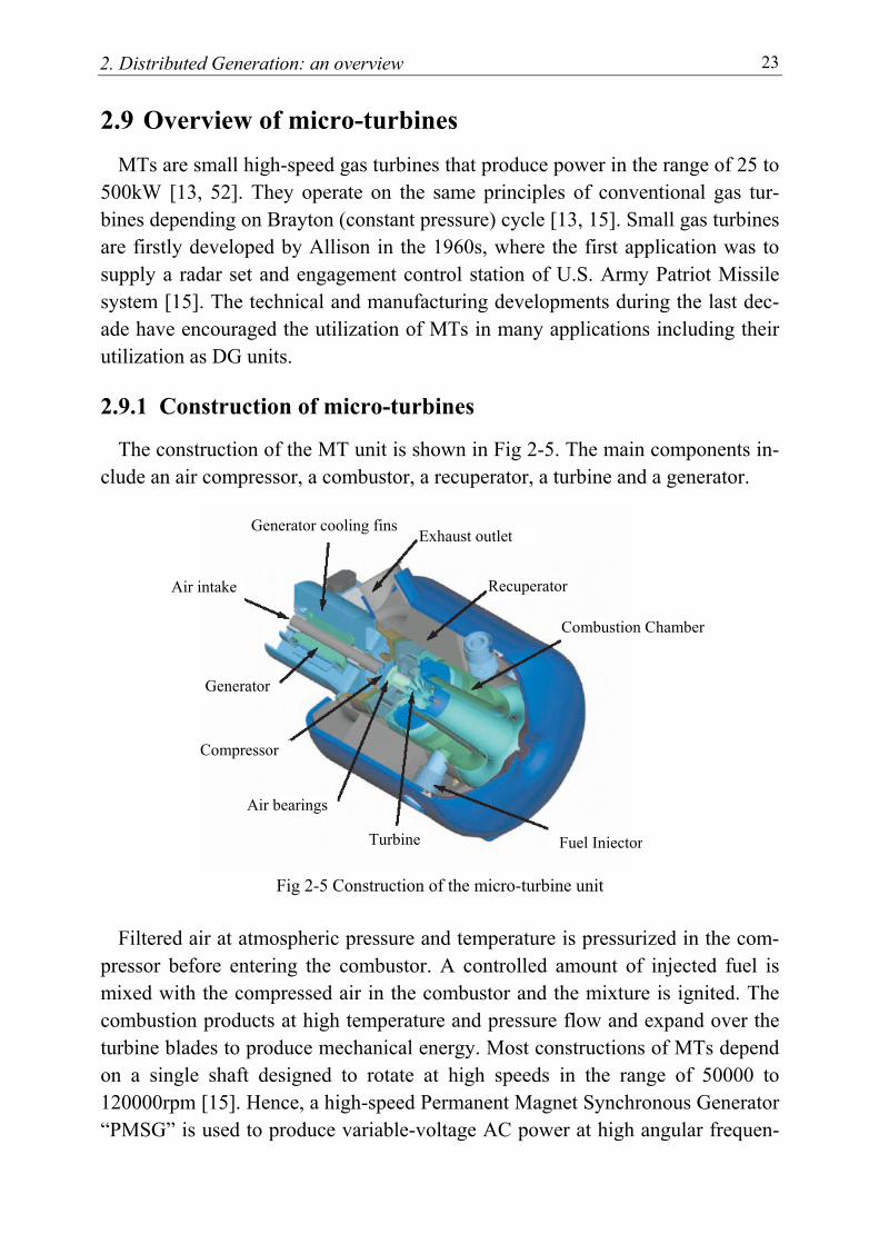
2. Distributed Generation: an overview 23
2.9 Overview of micro-turbines MTs are small high-speed gas turbines that produce power in the range of 25 to
500kW [13, 52]. They operate on the same principles of conventional gas tur-bines depending on Brayton (constant pressure) cycle [13, 15]. Small gas turbines are firstly developed by Allison in the 1960s, where the first application was to supply a radar set and engagement control station of U.S. Army Patriot Missile system [15]. The technical and manufacturing developments during the last dec-ade have encouraged the utilization of MTs in many applications including their utilization as DG units.
2.9.1 Construction of micro-turbines
The construction of the MT unit is shown in Fig 2-5. The main components in-clude an air compressor, a combustor, a recuperator, a turbine and a generator.
Fig 2-5 Construction of the micro-turbine unit Filtered air at atmospheric pressure and temperature is pressurized in the com-
pressor before entering the combustor. A controlled amount of injected fuel is mixed with the compressed air in the combustor and the mixture is ignited. The combustion products at high temperature and pressure flow and expand over the turbine blades to produce mechanical energy. Most constructions of MTs depend on a single shaft designed to rotate at high speeds in the range of 50000 to 120000rpm [15]. Hence, a high-speed Permanent Magnet Synchronous Generator “PMSG” is used to produce variable-voltage AC power at high angular frequen-
Recuperator
Combustion Chamber
Exhaust outlet Generator cooling fins
Air intake
Generator
Compressor
Air bearings
Turbine Fuel Injector
2. Distributed Generation: an overview 24
cies up to 10000rad/s. A part of the extracted horsepower in the turbine is used for driving the air compressor. The recuperator is used to improve the overall ef-ficiency of the system by transferring the waste heat from the exhaust gas to the combustion air stream. The high frequency of the generated power can be re-duced using cycloconverters or rectifier-inverter systems.
2.9.2 Advantages of micro-turbines
The newly developed MTs have the following advantages [15]: • low installation and infrastructure requirements, about 700 $/kW • low maintenance costs, about 0.005$/kWh • smaller and lighter than other engines with the same capacity • reliable and durable due to the simplicity of the structure • fuel flexibility since they can run on a variety of fuels including natural gas,
diesel, ethanol, propane and gasoline • high efficiency, with fuel energy-to-electricity conversion reaching 25%-30% • possibility of cogeneration by using the waste heat recovery, which could
achieve overall energy efficiency levels reaching 75% • environmental superiority of MTs operating on natural gas
2.9.3 Applications of micro-turbines
The availability of small, low cost, high efficient MTs is well suited for the fol-lowing applications [15]:
• firm power for isolated communities, small commercial buildings and light industry
• peak shaving for utility-system in order to decrease the required incremental cost to serve additional loads
• standby and emergency power for more reliable operation of the utility and with important loads
• uninterruptible power supply (UPS) since they provide low initial cost, low maintenance requirements and high reliability
Chapter 3
Dynamic Modelling of Fuel Cells
3
3.1 Introduction Besides the studies that concentrate on the use of FCs in small-size applica-
tions, the recent technology advancs have extended their energy products to in-clude large-scale electricity generation [39]. The development of FCs has been extensively discussed in the technical literature [35-41]. However, most studies concern with the static performance depending on the Nernest and Butler-Volmer equations [31, 40]. Recently, there have been some studies about the dynamic performance of the FCs with respect to thermo-dynamical behaviour [10, 29]. The investigation of any generating unit, however, requires dynamical models, which can describe the physical system. The modelling process depending on a detailed theoretical analysis is very complicated and a time consuming task espe-cially when the parameters are not easy to be defined. This is the case when con-sidering FCs where the electrical, chemical and thermo-dynamical processes in-teract strongly with each other in a nonlinear form.
In this chapter, a simplified third-order mathematical model is proposed to rep-
resent the dynamical behaviour of the FC including temperature and pressure variations. Furthermore, a heat recovery system is simulated for CHP applica-tions. For more detailed analysis, a recurrent ANN-based model, which can be obtained directly from measured input/output data, is developed to capture the dynamics of the FC. The objective is to avoid the complicated mathematical analysis and to develop flexible models with proper orders for FCs.
3.2 Proposed dynamic equivalent circuit for fuel cells The FC generating unit consists of three main parts: the reformer, the stack and
the power conditioner. The task of the reformer is to process the raw fuel to get a hydrogen-rich gas. The reformed fuel and the oxidant are directed with an elec-trochemical process through the stack (power section) to combine. As a result of this combination, DC power is generated and heat and water are produced. A power conditioner is required for DC/AC power conversion, where the AC power can then be used for either utility or stand-alone applications. These processes are
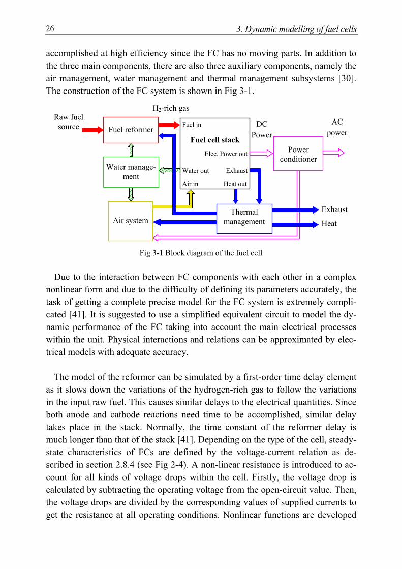
3. Dynamic modelling of fuel cells 26
accomplished at high efficiency since the FC has no moving parts. In addition to the three main components, there are also three auxiliary components, namely the air management, water management and thermal management subsystems [30]. The construction of the FC system is shown in Fig 3-1.
Fig 3-1 Block diagram of the fuel cell Due to the interaction between FC components with each other in a complex
nonlinear form and due to the difficulty of defining its parameters accurately, the task of getting a complete precise model for the FC system is extremely compli-cated [41]. It is suggested to use a simplified equivalent circuit to model the dy-namic performance of the FC taking into account the main electrical processes within the unit. Physical interactions and relations can be approximated by elec-trical models with adequate accuracy.
The model of the reformer can be simulated by a first-order time delay element
as it slows down the variations of the hydrogen-rich gas to follow the variations in the input raw fuel. This causes similar delays to the electrical quantities. Since both anode and cathode reactions need time to be accomplished, similar delay takes place in the stack. Normally, the time constant of the reformer delay is much longer than that of the stack [41]. Depending on the type of the cell, steady-state characteristics of FCs are defined by the voltage-current relation as de-scribed in section 2.8.4 (see Fig 2-4). A non-linear resistance is introduced to ac-count for all kinds of voltage drops within the cell. Firstly, the voltage drop is calculated by subtracting the operating voltage from the open-circuit value. Then, the voltage drops are divided by the corresponding values of supplied currents to get the resistance at all operating conditions. Nonlinear functions are developed
AC powerFuel reformer
Fuel in
Fuel cell stack
Elec. Power out
Water out Exhaust
Air in Heat out
Raw fuel source
Air system
Power conditioner
H2-rich gas
DC Power
Thermal management
Exhaust
Heat
Water manage-ment
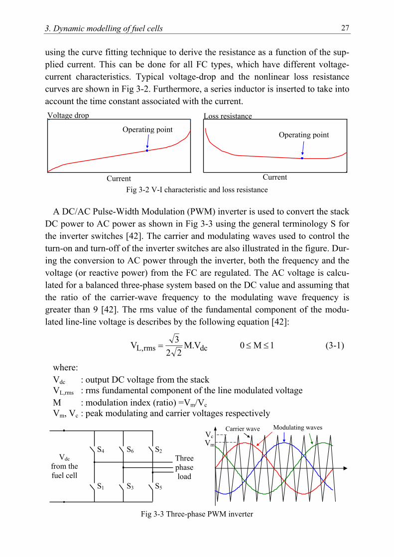
3. Dynamic modelling of fuel cells 27
using the curve fitting technique to derive the resistance as a function of the sup-plied current. This can be done for all FC types, which have different voltage-current characteristics. Typical voltage-drop and the nonlinear loss resistance curves are shown in Fig 3-2. Furthermore, a series inductor is inserted to take into account the time constant associated with the current.
Fig 3-2 V-I characteristic and loss resistance
A DC/AC Pulse-Width Modulation (PWM) inverter is used to convert the stack DC power to AC power as shown in Fig 3-3 using the general terminology S for the inverter switches [42]. The carrier and modulating waves used to control the turn-on and turn-off of the inverter switches are also illustrated in the figure. Dur-ing the conversion to AC power through the inverter, both the frequency and the voltage (or reactive power) from the FC are regulated. The AC voltage is calcu-lated for a balanced three-phase system based on the DC value and assuming that the ratio of the carrier-wave frequency to the modulating wave frequency is greater than 9 [42]. The rms value of the fundamental component of the modu-lated line-line voltage is describes by the following equation [42]:
dcrms,L V.M22
3V = 1M0 ≤≤ (3-1)
where: Vdc : output DC voltage from the stack VL,rms : rms fundamental component of the line modulated voltage M : modulation index (ratio) =Vm/Vc Vm, Vc : peak modulating and carrier voltages respectively
Fig 3-3 Three-phase PWM inverter
Current
Voltage drop
Operating point
Loss resistance
Current
Operating point
Vdc from the fuel cell
S4 S6 S2 S1 S3 S5
Three phase load
Vm
VcModulating waves Carrier wave
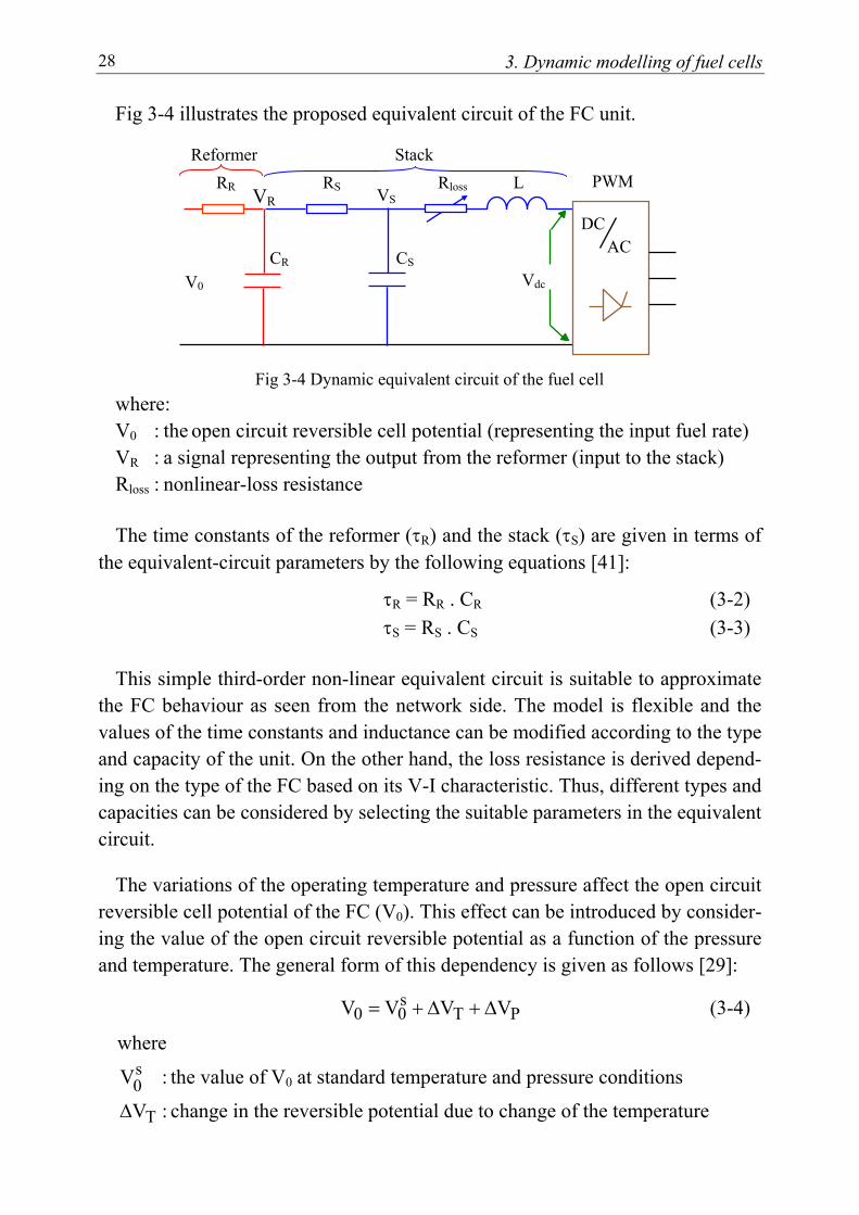
3. Dynamic modelling of fuel cells 28
Fig 3-4 illustrates the proposed equivalent circuit of the FC unit.
Fig 3-4 Dynamic equivalent circuit of the fuel cell where: V0 : the open circuit reversible cell potential (representing the input fuel rate) VR : a signal representing the output from the reformer (input to the stack) Rloss : nonlinear-loss resistance The time constants of the reformer (τR) and the stack (τS) are given in terms of
the equivalent-circuit parameters by the following equations [41]:
τR = RR . CR (3-2)
τS = RS . CS (3-3)
This simple third-order non-linear equivalent circuit is suitable to approximate the FC behaviour as seen from the network side. The model is flexible and the values of the time constants and inductance can be modified according to the type and capacity of the unit. On the other hand, the loss resistance is derived depend-ing on the type of the FC based on its V-I characteristic. Thus, different types and capacities can be considered by selecting the suitable parameters in the equivalent circuit.
The variations of the operating temperature and pressure affect the open circuit reversible cell potential of the FC (V0). This effect can be introduced by consider-ing the value of the open circuit reversible potential as a function of the pressure and temperature. The general form of this dependency is given as follows [29]:
PTs00 VVVV ∆+∆+= (3-4)
where s0V : the value of V0 at standard temperature and pressure conditions
TV∆ : change in the reversible potential due to change of the temperature
CR CS
PWM
DC AC
Reformer Stack RR RS Rloss L
Vdc V0
VR VS
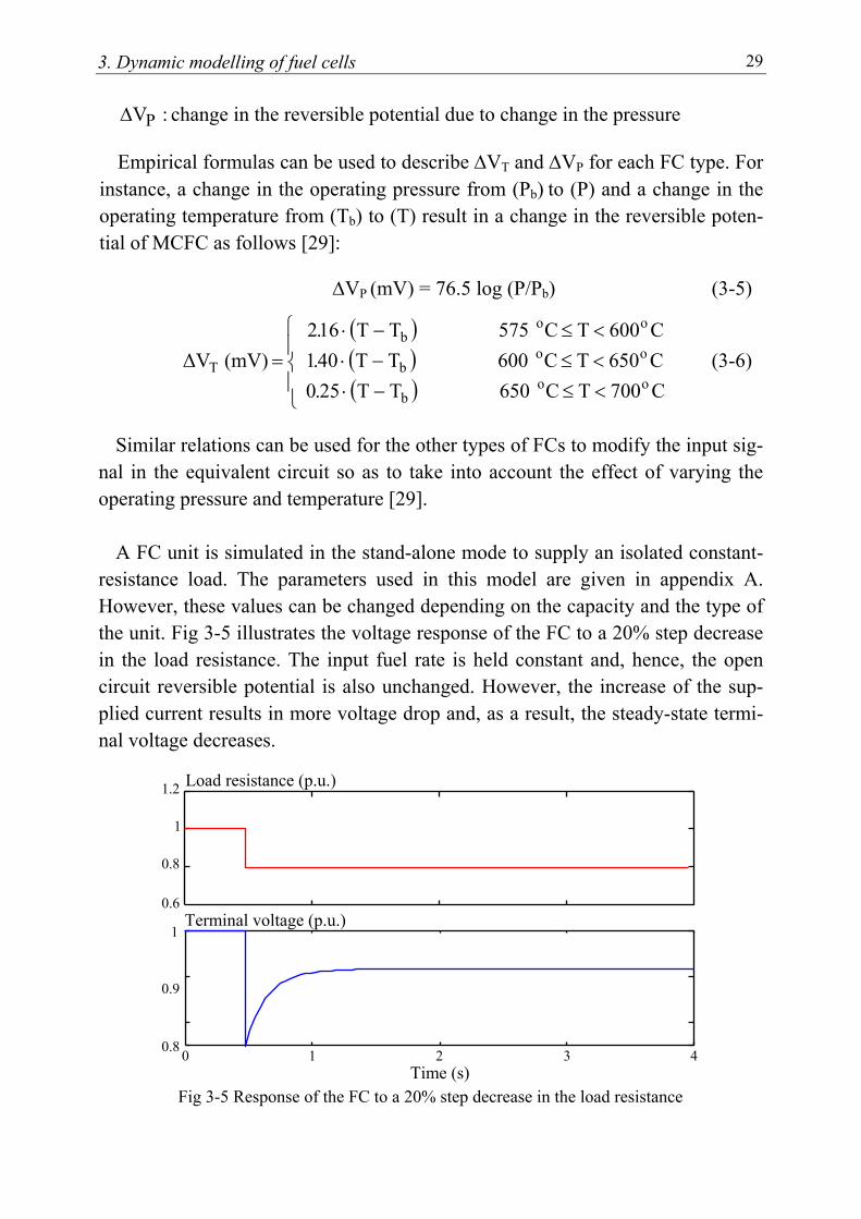
3. Dynamic modelling of fuel cells 29
PV∆ : change in the reversible potential due to change in the pressure
Empirical formulas can be used to describe ∆VT and ∆VP for each FC type. For instance, a change in the operating pressure from (Pb) to (P) and a change in the operating temperature from (Tb) to (T) result in a change in the reversible poten-tial of MCFC as follows [29]:
∆VP (mV) = 76.5 log (P/Pb) (3-5)
( )( )( )
<≤−⋅<≤−⋅<≤−⋅
=C700TC 650 TT25.0C650TC 600 TT40.1C600TC 575 TT16.2
(mV) ∆Voo
b
oob
oob
T (3-6)
Similar relations can be used for the other types of FCs to modify the input sig-nal in the equivalent circuit so as to take into account the effect of varying the operating pressure and temperature [29].
A FC unit is simulated in the stand-alone mode to supply an isolated constant-
resistance load. The parameters used in this model are given in appendix A. However, these values can be changed depending on the capacity and the type of the unit. Fig 3-5 illustrates the voltage response of the FC to a 20% step decrease in the load resistance. The input fuel rate is held constant and, hence, the open circuit reversible potential is also unchanged. However, the increase of the sup-plied current results in more voltage drop and, as a result, the steady-state termi-nal voltage decreases.
Fig 3-5 Response of the FC to a 20% step decrease in the load resistance
0.6
0.8
1
1.2
0 1 2 3 4 Time (s)
Load resistance (p.u.)
Terminal voltage (p.u.)
0.8
0.9
1
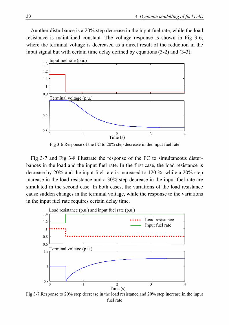
3. Dynamic modelling of fuel cells 30
Another disturbance is a 20% step decrease in the input fuel rate, while the load resistance is maintained constant. The voltage response is shown in Fig 3-6, where the terminal voltage is decreased as a direct result of the reduction in the input signal but with certain time delay defined by equations (3-2) and (3-3).
Fig 3-6 Response of the FC to 20% step decrease in the input fuel rate Fig 3-7 and Fig 3-8 illustrate the response of the FC to simultaneous distur-
bances in the load and the input fuel rate. In the first case, the load resistance is decrease by 20% and the input fuel rate is increased to 120 %, while a 20% step increase in the load resistance and a 30% step decrease in the input fuel rate are simulated in the second case. In both cases, the variations of the load resistance cause sudden changes in the terminal voltage, while the response to the variations in the input fuel rate requires certain delay time.
Fig 3-7 Response to 20% step decrease in the load resistance and 20% step increase in the input fuel rate
0 1 2 3 4 0.8
0.9
1 Terminal voltage (p.u.)
Input fuel rate (p.u.)
Time (s)
0.9
1
1.1
1.2
1.3
Time (s)
Terminal voltage (p.u.)
0 1 2 3 4 0.8
1
1.2
Load resistance (p.u.) and input fuel rate (p.u.)
0.6
0.8
1
1.2
1.4 Load resistance Input fuel rate
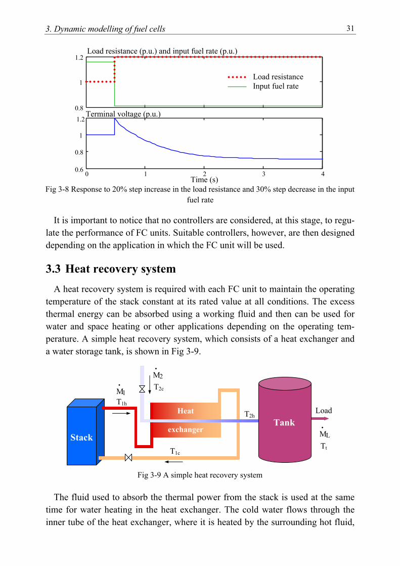
3. Dynamic modelling of fuel cells 31
Fig 3-8 Response to 20% step increase in the load resistance and 30% step decrease in the input fuel rate
It is important to notice that no controllers are considered, at this stage, to regu-late the performance of FC units. Suitable controllers, however, are then designed depending on the application in which the FC unit will be used.
3.3 Heat recovery system A heat recovery system is required with each FC unit to maintain the operating
temperature of the stack constant at its rated value at all conditions. The excess thermal energy can be absorbed using a working fluid and then can be used for water and space heating or other applications depending on the operating tem-perature. A simple heat recovery system, which consists of a heat exchanger and a water storage tank, is shown in Fig 3-9.
Fig 3-9 A simple heat recovery system
The fluid used to absorb the thermal power from the stack is used at the same time for water heating in the heat exchanger. The cold water flows through the inner tube of the heat exchanger, where it is heated by the surrounding hot fluid,
0.8
1
1.2
0 1 2 3 4 0.6
0.8
1
Load resistance Input fuel rate
Terminal voltage (p.u.)
Load resistance (p.u.) and input fuel rate (p.u.)
Time (s)
1.2
T1h
T1c
T2c
2M•
T2h Load
Tt
Tank Stack
Heat
exchanger
1M•
LM•
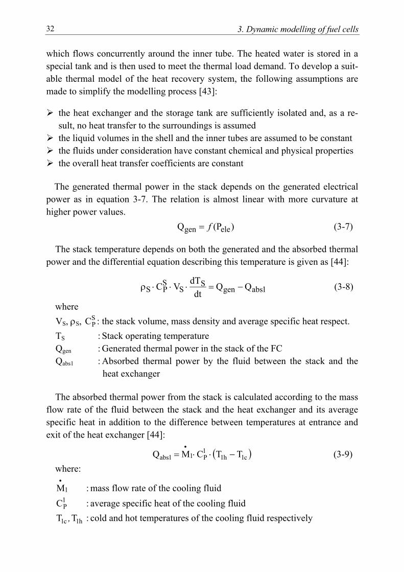
3. Dynamic modelling of fuel cells 32
which flows concurrently around the inner tube. The heated water is stored in a special tank and is then used to meet the thermal load demand. To develop a suit-able thermal model of the heat recovery system, the following assumptions are made to simplify the modelling process [43]:
the heat exchanger and the storage tank are sufficiently isolated and, as a re-sult, no heat transfer to the surroundings is assumed
the liquid volumes in the shell and the inner tubes are assumed to be constant the fluids under consideration have constant chemical and physical properties the overall heat transfer coefficients are constant The generated thermal power in the stack depends on the generated electrical
power as in equation 3-7. The relation is almost linear with more curvature at higher power values.
)(PQ elegen f= (3-7)
The stack temperature depends on both the generated and the absorbed thermal power and the differential equation describing this temperature is given as [44]:
1absgenS
SSPS QQ
dtdTVC −=⋅⋅⋅ρ (3-8)
where VS, ρS, S
PC : the stack volume, mass density and average specific heat respect. TS : Stack operating temperature Qgen : Generated thermal power in the stack of the FC Qabs1 : Absorbed thermal power by the fluid between the stack and the
heat exchanger The absorbed thermal power from the stack is calculated according to the mass
flow rate of the fluid between the stack and the heat exchanger and its average specific heat in addition to the difference between temperatures at entrance and exit of the heat exchanger [44]:
( )c1h11P11abs TTCMQ −⋅⋅=
•
(3-9) where:
1M•
: mass flow rate of the cooling fluid 1PC : average specific heat of the cooling fluid
h1c1 T T , : cold and hot temperatures of the cooling fluid respectively
3. Dynamic modelling of fuel cells 33
Considering energy balance relations in the heat exchanger, the following equations can be used to describe the temperatures of the two fluids at the exit of the heat exchanger [43, 45]:
( ) ( )
−
⋅π⋅⋅+−⋅
⋅ρ⋅=
•
c1h21P
c1h1111
c1 TTC
dULTTMaL
1dt
dT (3-10)
( ) ( )
−
⋅π⋅⋅+−⋅
⋅ρ⋅=
•
h2c12P
h2c2222
h2 TTC
dULTTMaL
1dt
dT (3-11)
where T2c, T2h : cold and hot temperatures respect. of the water in the heat exchanger L : length of the heat exchanger tube ρ1, ρ2 : the mass densities of the two fluids in the heat exchanger a1, a2 : cross section areas of the outer and inner tubes of the heat exchanger
respectively
2M•
: mass flow rate of the water in the heat exchanger 2PC : average specific heat of the water in the heat exchanger
U : heat transfer coefficient in the heat exchanger d : internal diameter of the inner tube The absorbed thermal power from the fluid in the shell tube to be transferred to
the water in the inner tube is given by [43, 44]:
( )c2h22P22abs TTCMQ −⋅⋅=
•
(3-12)
To calculate the mass of the stored water in the tank, the difference between the mass flow rates of the input and the output water into and out of the tank can be used as follows [44]:
L2t MMdt
dM ••
−= (3-13)
Finally the temperature of the stored water depends on the energy balance of the tank. Assuming that the absorbed thermal power by the water in the inner tube of the heat exchanger will completely be transferred to the water in the tank, the following differential equation can be used to calculate the temperature of the stored water in the tank [44]:
( )attttW
Pt2abs TTAUdt
dTCMQ −⋅⋅+⋅⋅= (3-14)
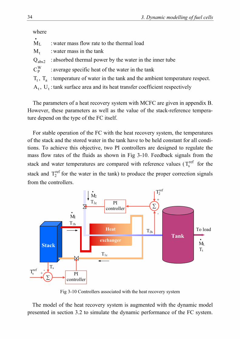
3. Dynamic modelling of fuel cells 34
T1h
1M•
T1c
T2c
T2h
Stack
Heat
exchanger
+
-
Ts
ref2T
refsT
To load
Tt
Tank
∑
- +
∑
PI controller
PI controller
2M•
LM•
where
LM•
: water mass flow rate to the thermal load
tM : water mass in the tank
2absQ : absorbed thermal power by the water in the inner tube WPC : average specific heat of the water in the tank
tT , aT : temperature of water in the tank and the ambient temperature respect.
tA , tU : tank surface area and its heat transfer coefficient respectively The parameters of a heat recovery system with MCFC are given in appendix B.
However, these parameters as well as the value of the stack-reference tempera-ture depend on the type of the FC itself.
For stable operation of the FC with the heat recovery system, the temperatures
of the stack and the stored water in the tank have to be held constant for all condi-tions. To achieve this objective, two PI controllers are designed to regulate the mass flow rates of the fluids as shown in Fig 3-10. Feedback signals from the stack and water temperatures are compared with reference values ( ref
sT for the
stack and ref2T for the water in the tank) to produce the proper correction signals
from the controllers.
Fig 3-10 Controllers associated with the heat recovery system
The model of the heat recovery system is augmented with the dynamic model presented in section 3.2 to simulate the dynamic performance of the FC system.
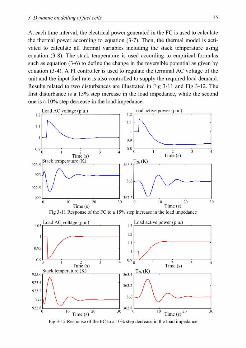
3. Dynamic modelling of fuel cells 35
At each time interval, the electrical power generated in the FC is used to calculate the thermal power according to equation (3-7). Then, the thermal model is acti-vated to calculate all thermal variables including the stack temperature using equation (3-8). The stack temperature is used according to empirical formulas such as equation (3-6) to define the change in the reversible potential as given by equation (3-4). A PI controller is used to regulate the terminal AC voltage of the unit and the input fuel rate is also controlled to supply the required load demand. Results related to two disturbances are illustrated in Fig 3-11 and Fig 3-12. The first disturbance is a 15% step increase in the load impedance, while the second one is a 10% step decrease in the load impedance.
Fig 3-11 Response of the FC to a 15% step increase in the load impedance
Fig 3-12 Response of the FC to a 10% step decrease in the load impedance
0 10 20 30 922
Stack temperature (K)
Time (s) 0 10 20 30
922.5
923
923.5
362.5
363
363.5 T2h (K)
Time (s)
Time (s)
Load AC voltage (p.u.)
0 1 2 3 40.9
1
1.1
1.2
0.8
0.9
1
1.1
1.2 Load active power (p.u.)
Time (s) 0 1 2 3 4
Stack temperature (K) T2h (K)Time (s) Time (s)
Time (s) Time (s) 0 10 20 30922.8
923
923.2
923.4
923.6
0 10 20 30362.8
363
363.2
363.4
Load active power (p.u.) Load AC voltage (p.u.)
0 1 2 3 40.9
1
1.1
1.2
1.3
0 1 2 3 40.9
0.95
1
1.05
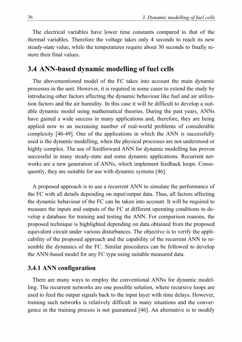
3. Dynamic modelling of fuel cells 36
The electrical variables have lower time constants compared to that of the thermal variables. Therefore the voltage takes only 4 seconds to reach its new steady-state value, while the temperatures require about 30 seconds to finally re-store their final values.
3.4 ANN-based dynamic modelling of fuel cells The abovementioned model of the FC takes into account the main dynamic
processes in the unit. However, it is required in some cases to extend the study by introducing other factors affecting the dynamic behaviour like fuel and air utiliza-tion factors and the air humidity. In this case it will be difficult to develop a suit-able dynamic model using mathematical theories. During the past years, ANNs have gained a wide success in many applications and, therefore, they are being applied now to an increasing number of real-world problems of considerable complexity [46-49]. One of the applications in which the ANN is successfully used is the dynamic modelling, when the physical processes are not understood or highly complex. The use of feedforward ANN for dynamic modelling has proven successful in many steady-state and some dynamic applications. Recurrent net-works are a new generation of ANNs, which implement feedback loops. Conse-quently, they are suitable for use with dynamic systems [46].
A proposed approach is to use a recurrent ANN to simulate the performance of
the FC with all details depending on input/output data. Thus, all factors affecting the dynamic behaviour of the FC can be taken into account. It will be required to measure the inputs and outputs of the FC at different operating conditions to de-velop a database for training and testing the ANN. For comparison reasons, the proposed technique is highlighted depending on data obtained from the proposed equivalent circuit under various disturbances. The objective is to verify the appli-cability of the proposed approach and the capability of the recurrent ANN to re-semble the dynamics of the FC. Similar procedures can be followed to develop the ANN-based model for any FC type using suitable measured data.
3.4.1 ANN configuration
There are many ways to employ the conventional ANNs for dynamic model-ling. The recurrent networks are one possible solution, where recursive loops are used to feed the output signals back to the input layer with time delays. However, training such networks is relatively difficult in many situations and the conver-gence in the training process is not guaranteed [46]. An alternative is to modify
3. Dynamic modelling of fuel cells 37
the processing in the neurons and the connections between them to introduce the dynamic action. This structure, however, still requires more investigations to be suitably applicable [46]. The most straightforward way is to use time histories to incorporate dynamics. Past inputs and/or outputs are used to predict the present outputs, where the training process is accomplished offline. A drawback of this method is the accumulation of error when the developed model is used in the online mode. The error at each step affects the following steps and also the over-all performance of the model. This problem does not arise in the training phase since predefined values are used at the input layer without real recurrent loops. To avoid this accumulation of error, high accuracy is an essential requirement in the training phase to ensure adequate performance in the online mode. The latter technique is employed to develop the ANN-based model for FCs taking into ac-count the necessity of reducing the training error to the minimum available level.
A Back Propagation Feed Forward Neural Network (BPFFNN) is developed
with one hidden layer comprising eight neurons. A third order dynamic model is assumed to give enough accuracy with respect to the actual data and, therefore, three past values of the output voltage are used at the input layer. Tanh-sigmoid transfer functions are chosen for all neurons in the hidden layer, while a linear transfer function is selected for the neuron in the output layer. The structure of the ANN is illustrated in Fig 3-13 with the DC voltage is chosen as an output.
Fig 3-13 The structure of the Artificial Neural Network The DC voltage depends on the input fuel rate and the equivalent resistance of
the load as seen from the FC side. The equivalent resistance of the load imped-ance can be deduced by equalling the active power in both the DC and the AC sides of the PWM inverter assuming a lossless inverter.
L
2
L
rmsph
dc
2dc
acdc RZ
V 3
RV PP ⋅=→= ,. (3-16)
Substituting from equation (3-1) yields:
Rdc
V0
Vdc (K-1)
Vdc (K-2)
Vdc (K-3)
Vdc (K) ...
3. Dynamic modelling of fuel cells 38
2L
2L
dc MRZ
672R .= (3-17)
where Pdc, Pac : DC power and AC active power respectively Vph,rms : rms fundamental component of the modulated phase voltage RL, ZL : load resistance and impedance respectively Rdc : the equivalent resistance of the load impedance as seen in the FC side At each time interval, the load impedance and the equivalent DC resistance can
be calculated to prepare the ANN inputs to get the new DC output voltage.
3.4.2 Training the artificial neural network
To get a suitable database, step changes in the input fuel rate and the load resis-tance are simulated and the corresponding voltage curves are observed. Some of these results are used in the training process, while the remainder are left for test-ing the trained ANN. The MATLAB toolbox is used for training the ANN, where the mean square error, which represents the average squared error between the network output and the target, is in the order of 10-7. Depending on the results obtained from the training process, a third order non-linear mathematical model is developed to describe the dynamics of the FC in the following form:
))3(k-) , V2(k-) , V1(k-,V, V( R (k) V dcdcdc0dcdc f= (3-15)
The function (f) given in equation (3-15) is derived from the construction and parameters of the ANN. The order of this model is defined depending on the number of recurrent loops and can be changed to get a suitable accuracy with re-spect to the measured data. The required decision variables can be introduced as inputs to the ANN to take into account their impact. The model is initially sub-jected to some disturbances that are used in the training process. Fig 3-14 and Fig 3-15 show comparisons between the target response and the response of the ANN-based model for two disturbances. The first disturbance “case (1)” is a 30% step decrease in the equivalent load resistance and a 20% step increase in the in-put fuel rate, while the second one “case (2)” is a 20% step decrease in the equivalent load resistance and 40% step decrease in the input fuel rate.
The comparisons indicate that the ANN succeeded to capture the nonlinear per-
formance of the original system and to behave in the same manner, which reflects the success of the training process.
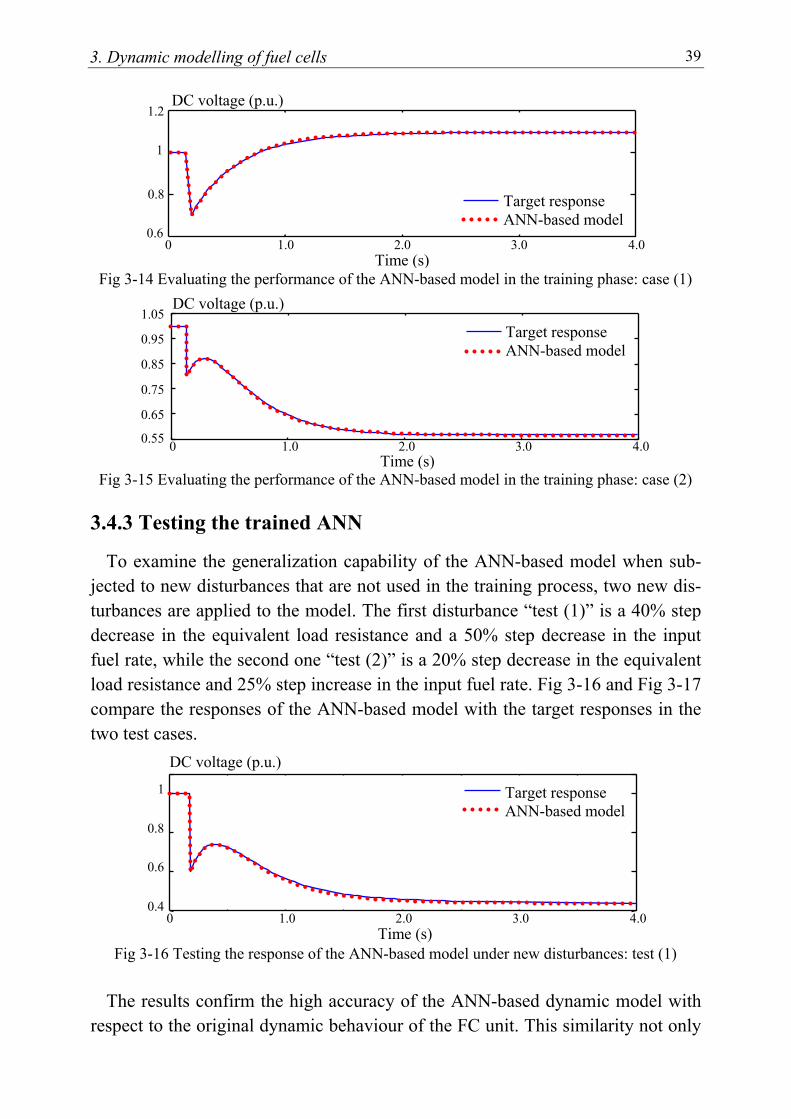
3. Dynamic modelling of fuel cells 39
Fig 3-14 Evaluating the performance of the ANN-based model in the training phase: case (1)
Fig 3-15 Evaluating the performance of the ANN-based model in the training phase: case (2)
3.4.3 Testing the trained ANN
To examine the generalization capability of the ANN-based model when sub-jected to new disturbances that are not used in the training process, two new dis-turbances are applied to the model. The first disturbance “test (1)” is a 40% step decrease in the equivalent load resistance and a 50% step decrease in the input fuel rate, while the second one “test (2)” is a 20% step decrease in the equivalent load resistance and 25% step increase in the input fuel rate. Fig 3-16 and Fig 3-17 compare the responses of the ANN-based model with the target responses in the two test cases.
Fig 3-16 Testing the response of the ANN-based model under new disturbances: test (1)
The results confirm the high accuracy of the ANN-based dynamic model with
respect to the original dynamic behaviour of the FC unit. This similarity not only
Time (s)
DC voltage (p.u.)
0 1.0 2.0 3.0 4.0
0.8
1
1.2
0.6
Target response ANN-based model
0.4
0.6
0.8
1
0 1.0 2.0 3.0 4.0 Time (s)
DC voltage (p.u.)
Target response ANN-based model
0.55
0.65
0.75
0.85
0.95
1.05 Target response ANN-based model
0 1.0 2.0 3.0 4.0 Time (s)
DC voltage (p.u.)

3. Dynamic modelling of fuel cells 40
reflects the success of the ANN to capture the non-linear dynamics of the actual system, but also ensures the possibility of using the proposed technique to de-velop models to simulate other types of FCs with high accuracy. Thus, the per-formance of the FC units can be investigated in detail taking into consideration the effect of all important variables that affect this performance.
Fig 3-17 Testing the response of the ANN-based model under new disturbances: test (2)
3.5 Conclusion To analyze the dynamic performance of FCs, proper dynamic models are re-
quired for different investigation purposes. Therefore, a third-order equivalent circuit, which reflects the physical processes within FCs, is proposed to simulate the dynamics of FCs for stability studies and control-system design purposes. The effect of varying the operating temperature and pressure is considered using em-pirical formulas. A simple model is also developed to simulate the heat recovery system with suitable controllers to maintain constant temperatures for the stack and the stored water in the tank.
The use of a recurrent ANN to develop a detailed model directly from meas-
ured input/output data to avoid the use of complex mathematical analyses is also discussed. The structure of the ANN can be modified to consider the required de-cisions, as inputs to the ANN, and to change the order of the model to achieve acceptable agreement with the actual data. The comparisons between the re-sponses of the ANN-based model and the target responses prove the capability of the ANN to capture the nonlinearity associated with the FC dynamics. Depending on these results, the ANN is candidate to be used to give suitable models for dif-ferent types of FC generating units directly from the input/output measurements.
0.8
1
1.2 DC voltage (p.u.)
0 1.0 2.0 3.0 4.0 Time (s)
Target response ANN-based model
Chapter 4
Simulation of a Large Number of DG Units Incorporated into a Multi-Machine Network
4
4.1 Introduction The centralized power plants, which are the main sources for electric grid sys-
tems, can not continue in meeting the increasing demand of electricity at a high degree of quality. DG units can solve many difficulties associated with the con-ventional power systems and provide an important support to the main central-ized power plants [12]. New trends aim to increase the penetration levels of the DG units in distribution systems. The expected large power from DG units neces-sitates the investigation of two main topics. The first one is related to the issues concerning with the dynamic interaction between DG units and the overlaying high-voltage networks. This includes the impact of the dynamics from such units on the performance of the high-voltage networks and vice versa. This issue will take new dimensions in the near future, when the contributions of DG units fur-ther increase due to the technological progress according to the political and so-cial expectations. The second topic is the modelling of this large number of DG units within the power system. It is not acceptable to model the distribution net-works with many active sources using lumped load representation. Also, model-ling the distribution systems in detail will be an overcomplicated task [50].
This chapter concerns with the first topic, while the second topic is discussed in
the next chapter. The investigation presented in this chapter is accomplished in two stages. In the first stage, a study for the case where many individual FCs and MTs are connected to different nodes in the distribution system of a multi-machine network is presented. MT and FC units are chosen since they are candi-date to be used in large scales especially when technical solutions for hybrid units consisting of FCs and MTs are well developed [18]. It is assumed that up to 30% of the total demand in the low-voltage area is covered by the DG units. The per-formance of the network is deeply investigated and the dynamic interaction be-tween low-voltage and high-voltage areas is studied. In the second stage, dy-namic models and the corresponding simulation results of hybrid FC/MT units are presented. The dynamic interdependencies between the FC and the MT units,
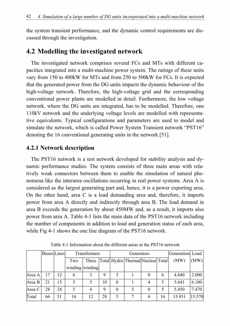
4. Simulation of a large number of DG units incorporated into a multi-machine network 42
the system transient performance, and the dynamic control requirements are dis-cussed through the investigation.
4.2 Modelling the investigated network The investigated network comprises several FCs and MTs with different ca-
pacities integrated into a multi-machine power system. The ratings of these units vary from 150 to 400kW for MTs and from 250 to 500kW for FCs. It is expected that the generated power from the DG units impacts the dynamic behaviour of the high-voltage network. Therefore, the high-voltage grid and the corresponding conventional power plants are modelled in detail. Furthermore, the low voltage network, where the DG units are integrated, has to be modelled. Therefore, one 110kV network and the underlying voltage levels are modelled with representa-tive equivalents. Typical configurations and parameters are used to model and simulate the network, which is called Power System Transient network “PST16” denoting the 16 conventional generating units in the network [51].
4.2.1 Network description
The PST16 network is a test network developed for stability analysis and dy-namic performance studies. The system consists of three main areas with rela-tively weak connectors between them to enable the simulation of natural phe-nomena like the interarea oscillations occurring in real power systems. Area A is considered as the largest generating part and, hence, it is a power exporting area. On the other hand, area C is a load demanding area and, therefore, it imports power from area A directly and indirectly through area B. The load demand in area B exceeds the generation by about 450MW and, as a result, it imports also power from area A. Table 4-1 lists the main data of the PST16 network including the number of components in addition to load and generation status of each area, while Fig 4-1 shows the one line diagram of the PST16 network.
Table 4-1 Information about the different areas in the PST16 network
Transformers Generators Buses Lines Two
winding Three
windingTotal Hydro Thermal Nuclear Total
Generation (MW)
Load(MW)
Area A 17 12 6 3 9 5 1 0 6 4.840 2.000Area B 21 15 5 5 10 0 1 4 5 5.641 6.100Area C 28 24 5 4 9 0 5 0 5 5.450 7.470Total 66 51 16 12 28 5 7 4 16 15.931 15.570
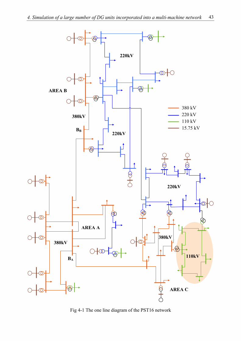
4. Simulation of a large number of DG units incorporated into a multi-machine network 43
Fig 4-1 The one line diagram of the PST16 network
AREA C
AREA B
AREA A
380 kV 220 kV 110 kV 15.75 kV
BA
BB 220kV
380kV
220kV
380kV
220kV
110kV
380kV
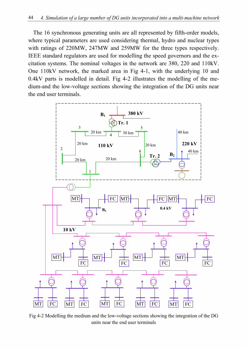
4. Simulation of a large number of DG units incorporated into a multi-machine network 44
The 16 synchronous generating units are all represented by fifth-order models, where typical parameters are used considering thermal, hydro and nuclear types with ratings of 220MW, 247MW and 259MW for the three types respectively. IEEE standard regulators are used for modelling the speed governors and the ex-citation systems. The nominal voltages in the network are 380, 220 and 110kV. One 110kV network, the marked area in Fig 4-1, with the underlying 10 and 0.4kV parts is modelled in detail. Fig 4-2 illustrates the modelling of the me-dium-and the low-voltage sections showing the integration of the DG units near the end user terminals.
Fig 4-2 Modelling the medium and the low-voltage sections showing the integration of the DG units near the end user terminals
20 km
20 km 20 km
30 km
20 km
20 km
380 kV
110 kV 40 km
Tr. 1
Tr. 2
10 kV
B2
FC MT FC MT FC MT FC MT FC MT
MT FC
MT FC
MTFC
MT FC
BL 0.4 kV
FC MT FC MTFC MT
1
2
3
4
5
6
220 kV
40 km
B1
4. Simulation of a large number of DG units incorporated into a multi-machine network 45
As shown in the figure, two standard steps of transformation are used to reach the 0.4kV level starting from the 110kV system. The first step is from 110kV to 10kV and the second one is from 10kV to 0.4kV. A MT and a FC are located near each of the 56 load nodes in the low-voltage area. The configuration of the distribution system is illustrated starting from one 110kV bus, i.e. bus 1. The other five busses, i.e. bus 2 through bus 6, have similar configurations, where the DG units are connected to the load centres with 100-300m cables.
With the abovementioned configuration, consumers in the low-voltage area are
supplied through two sources: the centralized power plants through the 10/0.4kV transformers and the DG units. The power transfer to the 110kV area from the other high-voltage parts is carried out via “Tr. 1” and “Tr. 2” as shown in Fig 4-2. Utilizing DG units with this configuration reduces the power required in the low-voltage area and increases the reliability at the consumer terminals
4.2.2 Modelling of micro-turbines
As mentioned earlier, MT system comprises three main components: the com-pressor, the combustor and the turbine in addition to the electrical generator. The dynamic modelling of the MTs is based on the dynamics of these components. Fig 4-3 shows the block diagram of the MT dynamic model used in this investi-gation [13, 52].
The PMSG is represented in this study by a simple first order model as shown
in Fig 4-3, while the following function is used to simulate the performance of the turbine [13, 52]:
ω)(1 50)WW( 31 minf −+−= ..f (4-1)
where minW : the offset representing the fuel demand at no-load condition
fW : the turbine input signal ω : the angular speed To reduce the frequency of the generated power to standard values, a cyclo-
converter is used to interface the PMSG with the utility. The cycloconverter is used not only to reduce and control the unit frequency but can also be used to regulate the unit voltage. For this purpose two PI controllers are implemented with each cycloconverter.

4. Simulation of a large number of DG units incorporated into a multi-machine network 46
The main symbols in the figure are as follows: H : inertia constant Kg, Kgen : gains of the speed governor and the generator respectively τg, τvp, τf, τcd, τgen : lag-time constants of the speed governor, the valve positioner, the
fuel system, the compressor discharge and the generator respec-tively
ω : angular speed of the PMSG Pele, Pm, Pth : input-electrical, mechanical, and thermal power respectively Vref, fref, ωref, Pref : reference voltage, frequency, angular speed, and thermal power
respect.
Fig 4-3 Block diagram model of the micro-turbine generating unit
The first controller is used to maintain the frequency of the unit constant by regulating the operating time of both the positive and the negative converters [53]. The second PI controller regulates the output voltage through the firing an-gle (α) in the basis of the three-phase controlled rectifiers [53]. The rms output voltage in the utility side of the cycloconverter is calculated as follows [53]:
( )
+α−π
π=
22αsin1VV incyocy ,, (4-2)
where Vcy,in, Vcy,o : the rms input and output voltages of the cycloconverter respect. α : firing angle
Max
Min
Kg
1+τg s
1
2H.s
1
1+τcd s
1
1+τf s
1
1+τVP sf
Cycloconverter
PI PI
PI
Speed governor
- +ωref
∑
∑
ω
Pref + - Pth
+ +
Offset Wmin
∑
Fuel system
+ +Wf
Pele
Pm ∑
ω
++
Generator
Constant flux
- + Vref ∑
VoltageFrequency
fref
-
ω
∑
Limiter Turbine
+ +
1-Wmin
+ +
Compressordischarge Valve
positioner
+
Kgen
1+τgens f1
f2
Current
P
Q

4. Simulation of a large number of DG units incorporated into a multi-machine network 47
The utilization of the turbine exhaust gas in CHP applications is also consid-ered in this study. A PI controller is used to modify the reference speed to enable the thermal power to meet the thermal load demand. It is common to consider the thermal demand as a constant value during the simulation of the electrical behav-iour of power systems since the electrical time constants are very small compared to the thermal ones. Therefore, the setting value of the thermal power is main-tained constant during the simulation.
The part of the model over the dotted line in Fig 4-3 describes the dynamics of
the three main parts of the MT. The blocks under the dotted line represent the machine inertia, the generator model, and the cycloconverter with its controllers. The parameters used in the MT model are listed in appendix C [13, 52].
4.2.3 Modelling of fuel cells
The proposed equivalent circuit of FCs introduced in chapter 3 (section 3.2) is used to simulate the dynamics of the FC units. Typical V-I-characteristics are used to develop the loss-resistances as functions of the supplied currents for dif-ferent types of FCs [10, 54, 55]. This includes the PEMFC with 250 and 350kW ratings, the AFC with 400kW rating and the SOFC with 450 and 500kW ratings. The parameters of these models are given in appendix D.
Similar to the MT, the heat produced in the stack of the FC is high enough to
be used for CHP applications. It is assumed that meeting thermal load demand has priority in the FC control. For simplicity, the thermal power is assumed to be in proportional with the generated electrical power. A PI controller, which regu-lates the input fuel rate, is used to control the thermal power. The thermal output power from the FC is calculated as a function of the output electrical power and compared with the thermal load demand. The error signal is used to activate the PI controller, which regulates the input fuel rate in order to readjust the thermal output power from the unit.
4.3 Implementation in the PSD simulation package The simulation program PSD is a package for modelling and simulating power
systems including online transient simulation and steady state analysis [56]. It is based on the principles of electromechanical-transient computations in electrical networks. The package has a strong library providing accurate dynamic models for most known elements in power systems. Synchronous machine, two and three

4. Simulation of a large number of DG units incorporated into a multi-machine network 48
winding transformers and transmission lines are some examples of these compo-nents. For instance, the user can chose a suitable model for the synchronous ma-chine among the second-, fifth- and sixth-order models and define the parameters himself. It is also possible to build special units like FC, MT and FACTS devices in a so-called “regulator files” depending on their block diagram models. These models are integrated into the described network through connecting nodes, which helps the operator to build his own models for the regularly variant com-ponents like the voltage and speed-governor regulators. The interaction between the built units and the network is accomplished through selected variables, which are exchangeable during the simulation process. The PST16 network is built us-ing the standard models found in the library of the PSD. On the other hand, the models of FCs and MTs are built in regulator files depending on their block dia-gram models using special code in the PSD. Fig 4-4 and Fig 4-5 show respec-tively the implementation of the FC and the MT models in the PSD package.
Fig 4-4 Implementation of the fuel cell model in the PSD package
DIV1
/
KP1
L_UM1 L_P1 L_Q1
+ +
K
KENL1
SUM5
MUL2
INVERTER
1 1+τf s
L_P1
L_Q1
P-K
PK3 REF CELL
MUL3 MUL7 1 1+τvp s
FUEL SUM3
Max Min
LIM
+ +
KENL
∑ MUL1
SUM2
DIFF
PI1
PI
+ +
Ls 1+Ts K-P
+ -
+ +
+ + SUM4
MUL3
Vter
SOLL
+ -
∑
PROP
fth-fc
SOLL2
+ -
+ -
PI2 Pth-ref-fc Max Min
LIM2
SUM1 SUM6
S_I
∑
∑
∑
S_I
Pel
/ ACOS
DIV2 ACOS
∑ PI
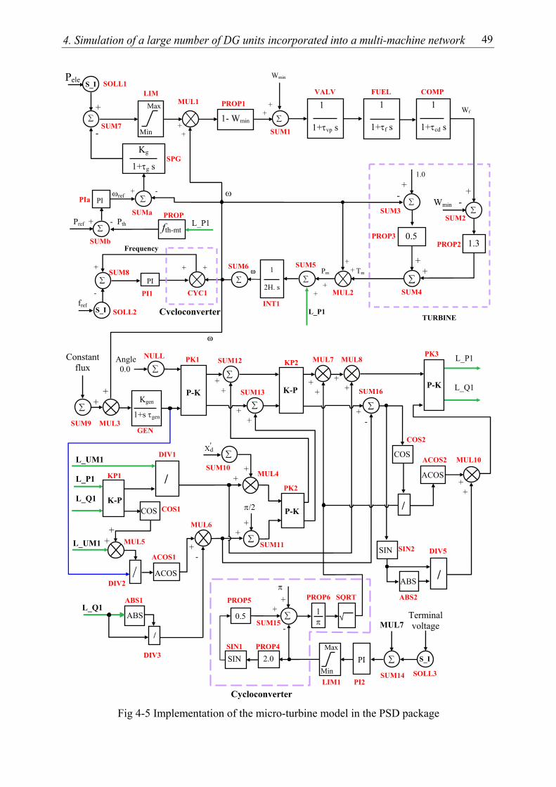
4. Simulation of a large number of DG units incorporated into a multi-machine network 49
Fig 4-5 Implementation of the micro-turbine model in the PSD package
L_P1
L_Q1
2.0
∑ 1 π
π ++ -
SIN1 PROP4
PROP6 SQRT
MUL7 MUL8
Cycloconverter LIM1 PI2
+ +
∑
+ +
P-K
∑ ∑
PROP5
PK1 KP2 PK3
SUM12
SUM13 SUM16 + +
√
KP1
L_UM1 L_P1 L_Q1
∑
π/2
++
++ MUL4
PK2
SUM11
P-K Kgen
1+s τgen
+ +
GEN
∑
SUM10
SUM9
Constant flux
∑
NULL
∑
∑
SUM14
MUL7
X'd
+ -
/
ACOS
DIV1
/
COS
+ +
COS2
ABS2
DIV5
ACOS2 MUL10
MUL3
Angle 0.0
0.5
SIN
SIN SIN2
ABS /
+ -
MUL6
DIV2
+ +
/
COS
ACOS
ACOS1
ABS
/
ABS1
DIV3
COS1
MUL5
L_Q1
+ +
L_UM1
Max
Min
PI
Terminal voltage
S_I
SOLL3
K-P
K-P
P-K
1- Wmin
Tm
LIM
+ +
VALV FUEL COMP
1
2H. s
Wmin
∑
1.3
+ -Wmin
∑
0.5
+ -
∑
1.0
PI
L_P1
Pm
TURBINE
CYC1
SUM1
SUM2
PROP3
SUM3
MUL2 INT1
∑ + +
+ ++ +
+ + Wf
Frequency
+ +
∑
1 1+τvp s
1
1+τf s
∑
SUM5
SOLL2 fref
S_I
∑
SUM6+ -
ω
SUM8
Max Min
ωref
SOLL1 Pele
SPG
∑ + -
S_I
∑ + -
SUMa
SUM7
Kg
1+τg s
SUM4
PROP2
1
1+τcd s
ω
PI1
PI
∑ Pref + - Pth
SUMb
PIa
SUM15
Cycloconverter
L_P1 PROP
fth-mt
ω
MUL1 PROP1
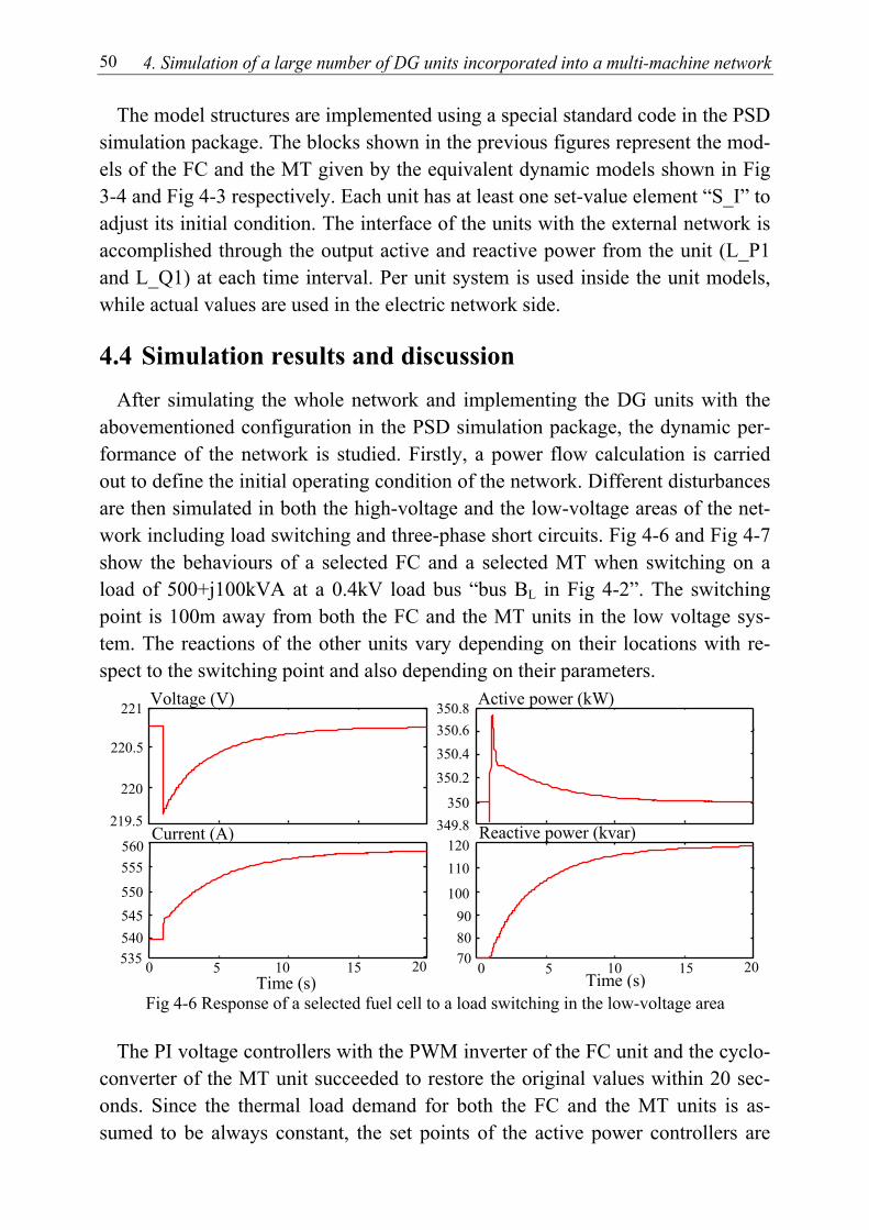
4. Simulation of a large number of DG units incorporated into a multi-machine network 50
The model structures are implemented using a special standard code in the PSD simulation package. The blocks shown in the previous figures represent the mod-els of the FC and the MT given by the equivalent dynamic models shown in Fig 3-4 and Fig 4-3 respectively. Each unit has at least one set-value element “S_I” to adjust its initial condition. The interface of the units with the external network is accomplished through the output active and reactive power from the unit (L_P1 and L_Q1) at each time interval. Per unit system is used inside the unit models, while actual values are used in the electric network side.
4.4 Simulation results and discussion After simulating the whole network and implementing the DG units with the
abovementioned configuration in the PSD simulation package, the dynamic per-formance of the network is studied. Firstly, a power flow calculation is carried out to define the initial operating condition of the network. Different disturbances are then simulated in both the high-voltage and the low-voltage areas of the net-work including load switching and three-phase short circuits. Fig 4-6 and Fig 4-7 show the behaviours of a selected FC and a selected MT when switching on a load of 500+j100kVA at a 0.4kV load bus “bus BL in Fig 4-2”. The switching point is 100m away from both the FC and the MT units in the low voltage sys-tem. The reactions of the other units vary depending on their locations with re-spect to the switching point and also depending on their parameters.
Fig 4-6 Response of a selected fuel cell to a load switching in the low-voltage area The PI voltage controllers with the PWM inverter of the FC unit and the cyclo-
converter of the MT unit succeeded to restore the original values within 20 sec-onds. Since the thermal load demand for both the FC and the MT units is as-sumed to be always constant, the set points of the active power controllers are
Voltage (V)
219.5
220
220.5
221
349.8350
350.2
350.4350.6350.8
Time (s) 70 8090
100
110 120
Active power (kW)
Reactive power (kvar)
0 2010 15 5
Current (A)
540
545
550
555 560
Time (s) 0 2010 15 5
535
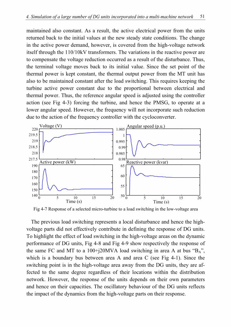
4. Simulation of a large number of DG units incorporated into a multi-machine network 51
maintained also constant. As a result, the active electrical power from the units returned back to the initial values at the new steady state conditions. The change in the active power demand, however, is covered from the high-voltage network itself through the 110/10kV transformers. The variations in the reactive power are to compensate the voltage reduction occurred as a result of the disturbance. Thus, the terminal voltage moves back to its initial value. Since the set point of the thermal power is kept constant, the thermal output power from the MT unit has also to be maintained constant after the load switching. This requires keeping the turbine active power constant due to the proportional between electrical and thermal power. Thus, the reference angular speed is adjusted using the controller action (see Fig 4-3) forcing the turbine, and hence the PMSG, to operate at a lower angular speed. However, the frequency will not incorporate such reduction due to the action of the frequency controller with the cycloconverter.
Fig 4-7 Response of a selected micro-turbine to a load switching in the low-voltage area
The previous load switching represents a local disturbance and hence the high-voltage parts did not effectively contribute in defining the response of DG units. To highlight the effect of load switching in the high-voltage areas on the dynamic performance of DG units, Fig 4-8 and Fig 4-9 show respectively the response of the same FC and MT to a 100+j20MVA load switching in area A at bus “BA”, which is a boundary bus between area A and area C (see Fig 4-1). Since the switching point is in the high-voltage area away from the DG units, they are af-fected to the same degree regardless of their locations within the distribution network. However, the response of the units depends on their own parameters and hence on their capacities. The oscillatory behaviour of the DG units reflects the impact of the dynamics from the high-voltage parts on their response.
Active power (kW)
Time (s) 140 150 160 170 180 190
0 5 10 15 20
Reactive power (kvar)
Time (s) 50
55
60
65
0 5 10 15 20
217.5 218
218.5 219
219.5 220
Voltage (V)
0.980.985
0.990.995
11.005
Angular speed (p.u.)
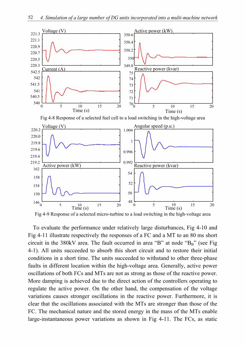
4. Simulation of a large number of DG units incorporated into a multi-machine network 52
Fig 4-8 Response of a selected fuel cell to a load switching in the high-voltage area
Fig 4-9 Response of a selected micro-turbine to a load switching in the high-voltage area
To evaluate the performance under relatively large disturbances, Fig 4-10 and
Fig 4-11 illustrate respectively the responses of a FC and a MT to an 80 ms short circuit in the 380kV area. The fault occurred in area “B” at node “BB” (see Fig 4-1). All units succeeded to absorb this short circuit and to restore their initial conditions in a short time. The units succeeded to withstand to other three-phase faults in different location within the high-voltage area. Generally, active power oscillations of both FCs and MTs are not as strong as those of the reactive power. More damping is achieved due to the direct action of the controllers operating to regulate the active power. On the other hand, the compensation of the voltage variations causes stronger oscillations in the reactive power. Furthermore, it is clear that the oscillations associated with the MTs are stronger than those of the FC. The mechanical nature and the stored energy in the mass of the MTs enable large-instantaneous power variations as shown in Fig 4-11. The FCs, as static
Voltage (V) Active power (kW)
220.3 220.5 220.7 220.9 221.1 221.3
349.8
350
350.2
350.4
350.6
Reactive power (kvar)
540.5
541.5
542.5
707172737475
0 5 10 15 20Time (s)
540
541
542
0 5 10 15 20Time (s)
Current (A)
Voltage (V)
Active power (kW) 219.2 219.4
219.6 219.8 220.0 220.2
Time (s) 146
150
154
158
162
0 5 10 15 20Time (s)
Angular speed (p.u.)
Reactive power (kvar) 0.992
0.996
1
1.004
48
50
52
54
0 5 15 2010
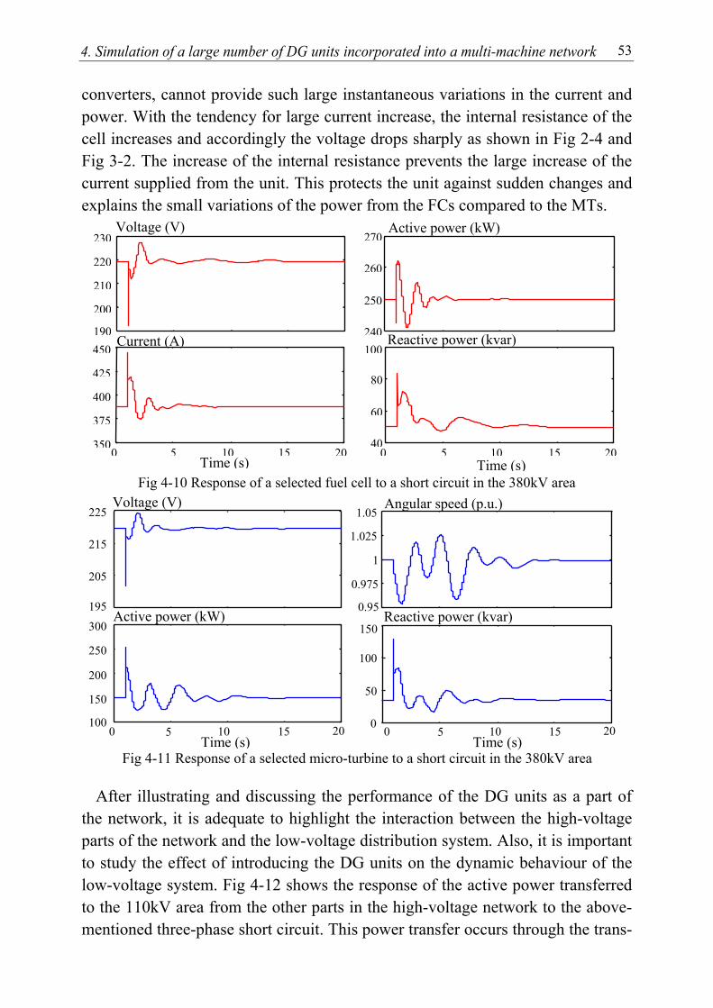
4. Simulation of a large number of DG units incorporated into a multi-machine network 53
converters, cannot provide such large instantaneous variations in the current and power. With the tendency for large current increase, the internal resistance of the cell increases and accordingly the voltage drops sharply as shown in Fig 2-4 and Fig 3-2. The increase of the internal resistance prevents the large increase of the current supplied from the unit. This protects the unit against sudden changes and explains the small variations of the power from the FCs compared to the MTs.
Fig 4-10 Response of a selected fuel cell to a short circuit in the 380kV area
Fig 4-11 Response of a selected micro-turbine to a short circuit in the 380kV area After illustrating and discussing the performance of the DG units as a part of
the network, it is adequate to highlight the interaction between the high-voltage parts of the network and the low-voltage distribution system. Also, it is important to study the effect of introducing the DG units on the dynamic behaviour of the low-voltage system. Fig 4-12 shows the response of the active power transferred to the 110kV area from the other parts in the high-voltage network to the above-mentioned three-phase short circuit. This power transfer occurs through the trans-
Time (s) Time (s)
Voltage (V)
Active power (kW) 195
205
215
225
0.95
0.975
1
1.025
1.05
150
200
250
300
0
50
100
150
100
Angular speed (p.u.)
Reactive power (kvar)
0 2010 15 5 0 2010 15 5
190
200
210
220
230
240
250
260
270Voltage (V)
Current (A)
0 5 10 15 2040
60
80
100
Time (s) 0 5 10 15 20
350
375
400
425
450
Time (s)
Active power (kW)
Reactive power (kvar)
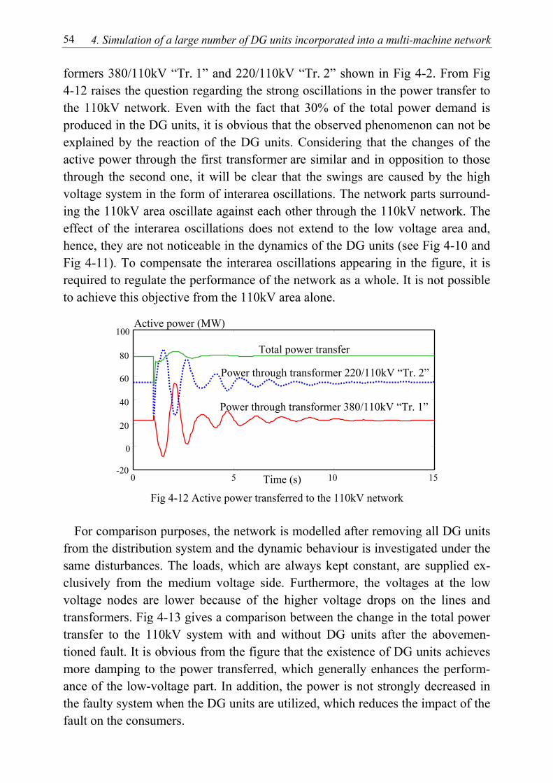
4. Simulation of a large number of DG units incorporated into a multi-machine network 54
formers 380/110kV “Tr. 1” and 220/110kV “Tr. 2” shown in Fig 4-2. From Fig 4-12 raises the question regarding the strong oscillations in the power transfer to the 110kV network. Even with the fact that 30% of the total power demand is produced in the DG units, it is obvious that the observed phenomenon can not be explained by the reaction of the DG units. Considering that the changes of the active power through the first transformer are similar and in opposition to those through the second one, it will be clear that the swings are caused by the high voltage system in the form of interarea oscillations. The network parts surround-ing the 110kV area oscillate against each other through the 110kV network. The effect of the interarea oscillations does not extend to the low voltage area and, hence, they are not noticeable in the dynamics of the DG units (see Fig 4-10 and Fig 4-11). To compensate the interarea oscillations appearing in the figure, it is required to regulate the performance of the network as a whole. It is not possible to achieve this objective from the 110kV area alone.
Fig 4-12 Active power transferred to the 110kV network For comparison purposes, the network is modelled after removing all DG units
from the distribution system and the dynamic behaviour is investigated under the same disturbances. The loads, which are always kept constant, are supplied ex-clusively from the medium voltage side. Furthermore, the voltages at the low voltage nodes are lower because of the higher voltage drops on the lines and transformers. Fig 4-13 gives a comparison between the change in the total power transfer to the 110kV system with and without DG units after the abovemen-tioned fault. It is obvious from the figure that the existence of DG units achieves more damping to the power transferred, which generally enhances the perform-ance of the low-voltage part. In addition, the power is not strongly decreased in the faulty system when the DG units are utilized, which reduces the impact of the fault on the consumers.
Time (s)
Power through transformer 380/110kV “Tr. 1”
Total power transfer
Active power (MW)
Power through transformer 220/110kV “Tr. 2”
0 5 10 15 -20
0
20
40
60
80
100
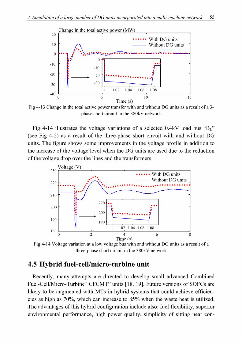
4. Simulation of a large number of DG units incorporated into a multi-machine network 55
Fig 4-13 Change in the total active power transfer with and without DG units as a result of a 3-phase short circuit in the 380kV network
Fig 4-14 illustrates the voltage variations of a selected 0.4kV load bus “BL”
(see Fig 4-2) as a result of the three-phase short circuit with and without DG units. The figure shows some improvements in the voltage profile in addition to the increase of the voltage level when the DG units are used due to the reduction of the voltage drop over the lines and the transformers.
Fig 4-14 Voltage variation at a low voltage bus with and without DG units as a result of a three-phase short circuit in the 380kV network
4.5 Hybrid fuel-cell/micro-turbine unit Recently, many attempts are directed to develop small advanced Combined
Fuel-Cell/Micro-Turbine “CFCMT” units [18, 19]. Future versions of SOFCs are likely to be augmented with MTs in hybrid systems that could achieve efficien-cies as high as 70%, which can increase to 85% when the waste heat is utilized. The advantages of this hybrid configuration include also: fuel flexibility, superior environmental performance, high power quality, simplicity of sitting near con-
Voltage (V) With DG units Without DG units
0 2 4 6 8180
190
210
220
230
1 1.02 1.04 1.06 1.08180
200
220
Time (s)
200
Change in the total active power (MW)
Time (s)
1 1.02 1.04 1.06 1.08
-30
-20
-10
0
0 5 10 15 -40
-30
-20
-10
0
10
20 With DG units Without DG units

4. Simulation of a large number of DG units incorporated into a multi-machine network 56
sumers, possibility of independent operation of the FC and MT units and lower capital cost compared to that of the FC alone [18, 19]. One project is now under development in California depending on SOFC technology to manufacture a 190kW unit with emission that is 50 times less than natural gas turbines [57]. The unit has an overall efficiency of 70% and it is planned to develop a 20 MW unit by the year 2015 with an overall efficiency exceeding 80%. Another project in Italy aims at developing and demonstrating a 100kW system combining a MCFC with a MT unit [58].
The construction of the CFCMT unit and some related technical aspects are
discussed in few literatures [18, 19, 57, 58]. The dynamic behaviour of the aug-mented unit and the integration of such units into large networks are other ap-proaches, which need to be investigated. The dynamic interdependencies between the FC and the MT, the dynamic performance of the entire system, and the dy-namic control requirements are some points, which are still ambiguous. The main objective of following sections is to emphasis on a new framework that deals with the dynamic performance of the CFCMT unit with multi-machine networks.
4.5.1 Unit structure
The CFCMT unit consists of a high-temperature FC with an internal reformer, an air compressor, a high-speed low-capacity gas turbine, and a PMSG. The ex-haust air from the FC, which still contains energy, can be used to drive a down-stream turbine replacing the classical combustor. Another approach is to utilize the residual energy in the power cycle more efficiently by using the hot exhaust from the turbine as an air supply to the FC. The former configuration is known as the “topping mode” while the latter is called the “bottoming mode” regarding the location of the FC with respect to the turbine. SOFCs can operate effectively in the “topping” mode due to their high temperature which reaches 1000°C, while MCFCs, which operates at 650°C, are more suitable for the “bottoming” mode [19]. In both configurations, electric power is generated by the FC (DC power) and the MT generator (AC power) using the same fuel/air flow.
4.5.1.1 Topping mode
In the topping mode, the FC replaces the classical combustor of the MT [57]. During normal operation, the compressor is used to pressurize air before entering a heat exchanger. The pressurized air is then preheated in the heat exchanger be-fore entering the FC. An internal reformer is used to produce hydrogen rich re-formed gas, which is also pressurized using a fuel pump and is then introduced to
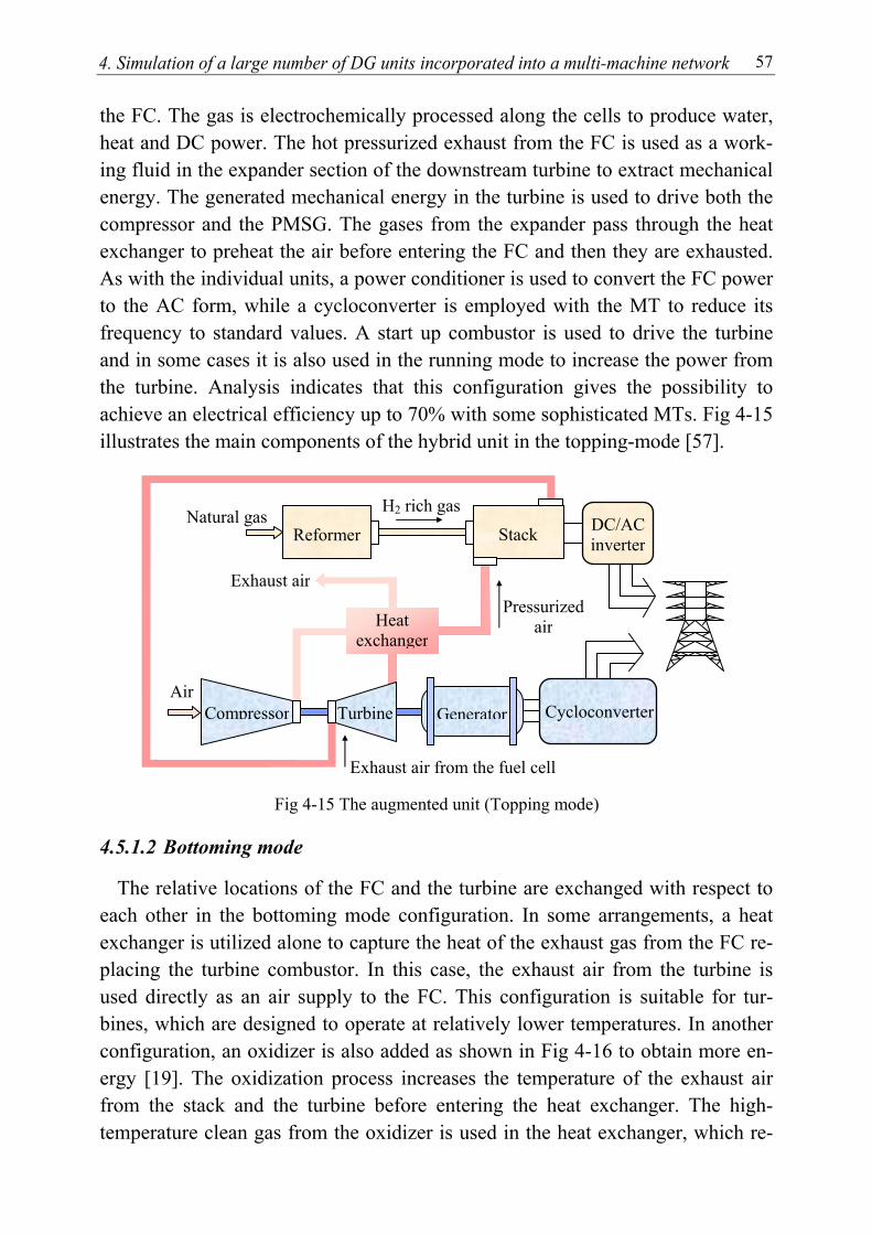
4. Simulation of a large number of DG units incorporated into a multi-machine network 57
the FC. The gas is electrochemically processed along the cells to produce water, heat and DC power. The hot pressurized exhaust from the FC is used as a work-ing fluid in the expander section of the downstream turbine to extract mechanical energy. The generated mechanical energy in the turbine is used to drive both the compressor and the PMSG. The gases from the expander pass through the heat exchanger to preheat the air before entering the FC and then they are exhausted. As with the individual units, a power conditioner is used to convert the FC power to the AC form, while a cycloconverter is employed with the MT to reduce its frequency to standard values. A start up combustor is used to drive the turbine and in some cases it is also used in the running mode to increase the power from the turbine. Analysis indicates that this configuration gives the possibility to achieve an electrical efficiency up to 70% with some sophisticated MTs. Fig 4-15 illustrates the main components of the hybrid unit in the topping-mode [57].
Fig 4-15 The augmented unit (Topping mode)
4.5.1.2 Bottoming mode
The relative locations of the FC and the turbine are exchanged with respect to each other in the bottoming mode configuration. In some arrangements, a heat exchanger is utilized alone to capture the heat of the exhaust gas from the FC re-placing the turbine combustor. In this case, the exhaust air from the turbine is used directly as an air supply to the FC. This configuration is suitable for tur-bines, which are designed to operate at relatively lower temperatures. In another configuration, an oxidizer is also added as shown in Fig 4-16 to obtain more en-ergy [19]. The oxidization process increases the temperature of the exhaust air from the stack and the turbine before entering the heat exchanger. The high-temperature clean gas from the oxidizer is used in the heat exchanger, which re-
Exhaust air from the fuel cell
H2 rich gas
Pressurized air
Exhaust air
Compressor Air
Generator
Stack
Cycloconverter
DC/AC inverter
Turbine
Heat exchanger
Natural gasReformer
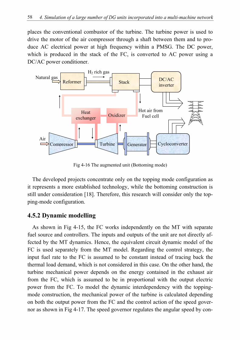
4. Simulation of a large number of DG units incorporated into a multi-machine network 58
places the conventional combustor of the turbine. The turbine power is used to drive the motor of the air compressor through a shaft between them and to pro-duce AC electrical power at high frequency within a PMSG. The DC power, which is produced in the stack of the FC, is converted to AC power using a DC/AC power conditioner.
Fig 4-16 The augmented unit (Bottoming mode) The developed projects concentrate only on the topping mode configuration as
it represents a more established technology, while the bottoming construction is still under consideration [18]. Therefore, this research will consider only the top-ping-mode configuration.
4.5.2 Dynamic modelling
As shown in Fig 4-15, the FC works independently on the MT with separate fuel source and controllers. The inputs and outputs of the unit are not directly af-fected by the MT dynamics. Hence, the equivalent circuit dynamic model of the FC is used separately from the MT model. Regarding the control strategy, the input fuel rate to the FC is assumed to be constant instead of tracing back the thermal load demand, which is not considered in this case. On the other hand, the turbine mechanical power depends on the energy contained in the exhaust air from the FC, which is assumed to be in proportional with the output electric power from the FC. To model the dynamic interdependency with the topping-mode construction, the mechanical power of the turbine is calculated depending on both the output power from the FC and the control action of the speed gover-nor as shown in Fig 4-17. The speed governor regulates the angular speed by con-
Hot air fromFuel cell
Natural gas H2 rich gas
Reformer
GeneratorAir
DC/AC inverter
Heat exchanger
Cycloconverter Compressor Turbine
Oxidizer
Stack
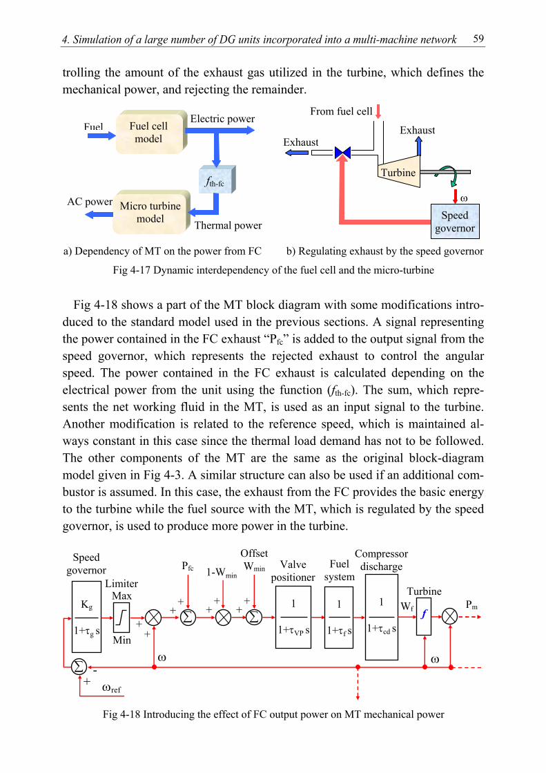
4. Simulation of a large number of DG units incorporated into a multi-machine network 59
trolling the amount of the exhaust gas utilized in the turbine, which defines the mechanical power, and rejecting the remainder.
a) Dependency of MT on the power from FC b) Regulating exhaust by the speed governor
Fig 4-17 Dynamic interdependency of the fuel cell and the micro-turbine
Fig 4-18 shows a part of the MT block diagram with some modifications intro-
duced to the standard model used in the previous sections. A signal representing the power contained in the FC exhaust “Pfc” is added to the output signal from the speed governor, which represents the rejected exhaust to control the angular speed. The power contained in the FC exhaust is calculated depending on the electrical power from the unit using the function (fth-fc). The sum, which repre-sents the net working fluid in the MT, is used as an input signal to the turbine. Another modification is related to the reference speed, which is maintained al-ways constant in this case since the thermal load demand has not to be followed. The other components of the MT are the same as the original block-diagram model given in Fig 4-3. A similar structure can also be used if an additional com-bustor is assumed. In this case, the exhaust from the FC provides the basic energy to the turbine while the fuel source with the MT, which is regulated by the speed governor, is used to produce more power in the turbine.
Fig 4-18 Introducing the effect of FC output power on MT mechanical power
Max
Min
Kg
1+τg s
1
1+τcd s
1
1+τf s
1
1+τVP sf
Speed governor
- + ωref
∑ ω
+ +
Offset Wmin
∑
Fuel system
Wf Pm
ω
Limiter Turbine
++
1-Wmin
+ +
Compressor discharge Valve
positionerPfc
∑ + +
Fuel
AC power
Fuel cell model
Micro turbine model
fth-fc
Electric power
Thermal power
From fuel cell
Speed governor
ω
Turbine
ExhaustExhaust

4. Simulation of a large number of DG units incorporated into a multi-machine network 60
4.5.3 Network modifications Some modifications are introduced to the distribution system to study the per-
formance of the hybrid units. Instead of 112 DG units, the low-voltage area com-prises 56 CFCMT units, where the FCs are augmented with the MTs to form the hybrid units. This is accomplished by connecting a SOFC and a MT unit to the same bus and introducing a signal from the FC output power to the MT model as explained earlier. Technical developments show that the FC can produce from 55% up to 90% of the unit electricity, while the turbine produces the reminder [19]. The 56 hybrid units are modelled with different capacities from 400kW to 900kW. Based on the capacities of the individual units, the percentage power from the FCs varies in the range of 55.6 up to 77% of the total power in the hy-brid-units. As the previous case, the power from the CFCMT units reaches up to 30% of the total demand in the 110kV area. The parameters used in the modelling vary depending on their capacities as given with the individual units.
4.5.4 Simulation results and discussion
The control strategy is to regulate the terminal voltages using PI controllers in-corporated with both the cycloconverter and the PWM inverter. An attempt to regulate the turbine speed through the fuel source of the FC failed to achieve a satisfactory operation. The fuel source regulates the electrical and thermal power in the FC and, consequently, the mechanical power of the turbine. However, at the time where the turbine performance is improved the reaction of the FC seems to be poor and vice versa. It is found that regulating the performance of the FC and the turbine at the same time using the fuel source of the FC is very difficult. It will be adequate to use separate controllers with each part to give better results.
Different disturbances are applied to test the performance of the network in-
cluding the new CFCMT units. For comparison reasons, the response of the sys-tem to the same disturbances simulated in the network with individual units is introduced. Fig 4-19 illustrates the response of a selected hybrid unit to a 500+j100kVA load switching at a 0.4kV load bus “bus BL in Fig 4-2”. More than 7kW additional active power from the CFCMT unit is supplied, while different contributions from the other units are achieved depending on their locations rela-tive to the switching point. Despite the fact that the input fuel rate to the FC is constant, more exhaust from the FC is utilized in the turbine to compensate for the angular-speed reduction as a result of increasing the load demand. On the other hand, the increase of the output power from the FC is caused only due to the change of the operating point and, as a result, the internal power loss.
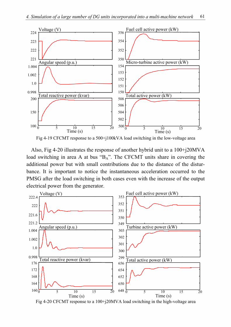
4. Simulation of a large number of DG units incorporated into a multi-machine network 61
Fig 4-19 CFCMT response to a 500+j100kVA load switching in the low-voltage area
Also, Fig 4-20 illustrates the response of another hybrid unit to a 100+j20MVA load switching in area A at bus “BA”. The CFCMT units share in covering the additional power but with small contributions due to the distance of the distur-bance. It is important to notice the instantaneous acceleration occurred to the PMSG after the load switching in both cases even with the increase of the output electrical power from the generator.
Fig 4-20 CFCMT response to a 100+j20MVA load switching in the high-voltage area
221
222
223
224
0.998
1.002
1.004
1.0
150151
152
153
154
Voltage (V)
350
352
354
356Fuel cell active power (kW)
Angular speed (p.u.) Micro-turbine active power (kW)
Total reactive power (kvar) Total active power (kW)
100
150
200
0 5 10 15 20Time (s)
502
504
506508
0 5 10 15 20500Time (s)
221.2
221.6
222
222.4
349350
351
352
353Voltage (V) Fuel cell active power (kW)
648
650
652
654
656
Turbine active power (kW) Angular speed (p.u.)
Total active power (kW) Total reactive power (kvar)
Time (s) 0 5 15 2010 160
164
168
172
176
Time (s) 0 5 15 10 20
299
300
301
302
303
0.998
1.002
1.004
1.0

4. Simulation of a large number of DG units incorporated into a multi-machine network 62
Any increase in the electrical output power of a conventional MT causes a de-celeration to the generator as shown in Fig 4-7 and Fig 4-9. In the hybrid configu-ration, on the other hand, the angular speed will be defined according to both the turbine input mechanical power and the output electrical power. The fast increase of the electrical power in the FC causes an increase to the mechanical power of the turbine. Since the instantaneous value of the mechanical power exceeds that of the electrical output power, the PMSG is accelerated.
The response of a CFCMT to a 80ms three-phase short circuit in area “B” at
node “BB” (see Fig 4-1) is shown in Fig 4-21. Similar to the previous cases, the PMSG is accelerated unlike the performance of the separate MT unit shown in Fig 4-11. The Turbine receives more mechanical power, due to the rise in the electrical power in the FC, while the generator output power is decreased.
Fig 4-21 Response of a hybrid unit to a 80ms short circuit in the high-voltage area
To highlight the difference between the performance of the hybrid unit and in-dividual units operating in parallel, the FCs and the MTs are modelled and con-nected without any constructional connections between them. The response of the parallel units to the same 80ms short circuit is shown in Fig 4-22. From Fig 4-21 and Fig 4-22, the similarity of the voltage, which is defined by the network rather than the DG units, is obvious. As a result, the reactive power varies also in the same manner despite its relatively stronger oscillations with the hybrid units. On the other hand, the turbine active power and the angular speed react differently. This means that the main effect of the hybrid structure is on the active power and
Voltage (V)
200 210 220 230
340
350
360
370
380Fuel cell active power (kW)
Angular speed (p.u.)
0.99 1
1.01 1.02 1.03 Turbine active power (kW)
120
130
140
150
160
Total active power (kW) Total reactive power (kvar)
100 150 200 250 300
50 Time (s)
0 5 10 15 20 460480500520540560
Time (s) 0 5 10 15 20
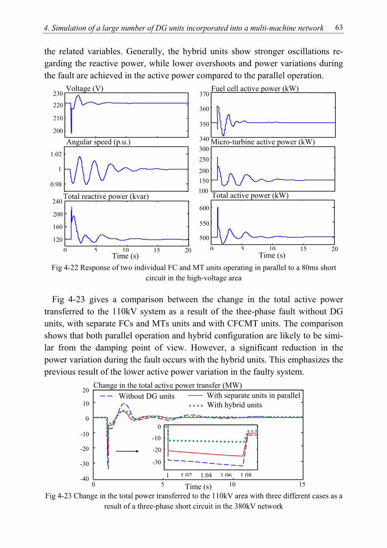
4. Simulation of a large number of DG units incorporated into a multi-machine network 63
the related variables. Generally, the hybrid units show stronger oscillations re-garding the reactive power, while lower overshoots and power variations during the fault are achieved in the active power compared to the parallel operation.
Fig 4-22 Response of two individual FC and MT units operating in parallel to a 80ms short
circuit in the high-voltage area
Fig 4-23 gives a comparison between the change in the total active power transferred to the 110kV system as a result of the thee-phase fault without DG units, with separate FCs and MTs units and with CFCMT units. The comparison shows that both parallel operation and hybrid configuration are likely to be simi-lar from the damping point of view. However, a significant reduction in the power variation during the fault occurs with the hybrid units. This emphasizes the previous result of the lower active power variation in the faulty system.
Fig 4-23 Change in the total power transferred to the 110kV area with three different cases as a
result of a three-phase short circuit in the 380kV network
200
210
220
230
0.98
1
1.02
Voltage (V)
Angular speed (p.u.) 340
350
360
370Fuel cell active power (kW)
Micro-turbine active power (kW)
150
200
250
300
100
500
550
600
Total active power (kW)
0 5 10 15 20Time (s)
240 Total reactive power (kvar)
120
160
200
0 5 10 15 20Time (s)
Time (s) 0 5 10 15 -40
-30
-20
-10
0
10
20 With separate units in parallel Without DG units
Change in the total active power transfer (MW)
With hybrid units
1 1.02 1.04 1.06 1.08
-30
-20
-10
0
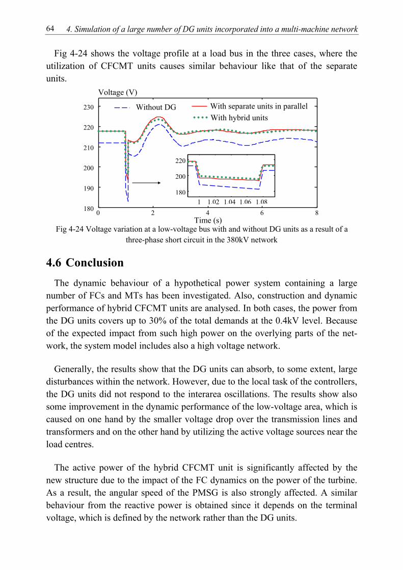
4. Simulation of a large number of DG units incorporated into a multi-machine network 64
Fig 4-24 shows the voltage profile at a load bus in the three cases, where the utilization of CFCMT units causes similar behaviour like that of the separate units.
Fig 4-24 Voltage variation at a low-voltage bus with and without DG units as a result of a
three-phase short circuit in the 380kV network
4.6 Conclusion The dynamic behaviour of a hypothetical power system containing a large
number of FCs and MTs has been investigated. Also, construction and dynamic performance of hybrid CFCMT units are analysed. In both cases, the power from the DG units covers up to 30% of the total demands at the 0.4kV level. Because of the expected impact from such high power on the overlying parts of the net-work, the system model includes also a high voltage network.
Generally, the results show that the DG units can absorb, to some extent, large
disturbances within the network. However, due to the local task of the controllers, the DG units did not respond to the interarea oscillations. The results show also some improvement in the dynamic performance of the low-voltage area, which is caused on one hand by the smaller voltage drop over the transmission lines and transformers and on the other hand by utilizing the active voltage sources near the load centres.
The active power of the hybrid CFCMT unit is significantly affected by the
new structure due to the impact of the FC dynamics on the power of the turbine. As a result, the angular speed of the PMSG is also strongly affected. A similar behaviour from the reactive power is obtained since it depends on the terminal voltage, which is defined by the network rather than the DG units.
0 2 4 6 8 180
190
200
210
220
230
1 1.02 1.04 1.06 1.08180
200
220
Voltage (V)
Time (s)
With separate units in parallel Without DG With hybrid units

Chapter 5
Artificial Neural Network-Based Dy-namic Equivalents for Distribution Systems Containing Active Sources
5
5.1 Introduction Accurate modelling of electric power systems is essential for stability studies
from both planning and operation points of view. The computational difficulty associated with large interconnected power systems increases dramatically with the rapid increase of the size of networks [59]. It is not practical, and also in most cases not necessary, to fully model the large interconnected networks. It will be also formidable computational task to simulate power systems in detail when a large number of active DG sources are considered within distribution systems [59]. On the other hand, approximating the dynamics of the distribution networks using passive lumped loads will lack the sufficient accuracy to simulate the dy-namics of DG units. The need for fast simplified analysis of power systems obli-gate the reduction of certain subsystems that are outside the investigation focus. However, any realistic dynamic model has to give reasonable approximations to the dynamics of active sources and their impacts on the high-voltage networks. Replacing distribution systems that comprise hundreds or thousands of active components with suitable dynamic equivalents will achieve large simplification for the analysis of power systems [60].
In this chapter, a generic nonlinear dynamic equivalent model based on recur-
rent ANNs is presented and used to replace the 110kV area and the underlying distribution systems in the PST16 network. The development of such dynamic equivalent does not obligate specifying a particular model configuration in ad-vance. Rather, the equivalent model is specified based on the structure and the parameters describing the ANN (activation functions, biases and weights). The main advantage of this equivalent is the need for measurements only at boundary buses between reduced and retained subsystems. Hence, the parameters, topology and complexity of the replaced subsystem will not affect the procedures. Fur-thermore, the accuracy of the developed model is not significantly affected by changing the operating point, i.e. it is not restricted to certain initial power-flow
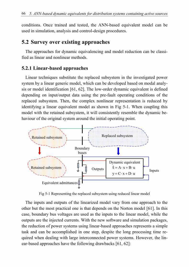
5. ANN-based dynamic equivalents for distribution systems containing active sources 66
conditions. Once trained and tested, the ANN-based equivalent model can be used in simulation, analysis and control-design procedures.
5.2 Survey over existing approaches The approaches for dynamic equivalencing and model reduction can be classi-
fied as linear and nonlinear methods.
5.2.1 Linear-based approaches
Linear techniques substitute the replaced subsystem in the investigated power system by a linear generic model, which can be developed based on modal analy-sis or model identification [61, 62]. The low-order dynamic equivalent is defined depending on input/output data using the pre-fault operating conditions of the replaced subsystem. Then, the complex nonlinear representation is reduced by identifying a linear equivalent model as shown in Fig 5-1. When coupling this model with the retained subsystem, it will consistently resemble the dynamic be-haviour of the original system around the initial operating point.
Fig 5-1 Representing the replaced subsystem using reduced linear model
The inputs and outputs of the linearized model vary from one approach to the other but the most practical one is that depends on the Norton model [61]. In this case, boundary bus voltages are used as the inputs to the linear model, while the outputs are the injected currents. With the new software and simulation packages, the reduction of power systems using linear-based approaches represents a simple task and can be accomplished in one step, despite the long processing time re-quired when dealing with large interconnected power systems. However, the lin-ear-based approaches have the following drawbacks [61, 62]:
Dynamic equivalent
Outputs Inputs
Equivalent admittances
Boundary buses
Replaced subsystem
uDxCyuBxAx
⋅+⋅=⋅+⋅=.
Retained subsystem
Retained subsystem
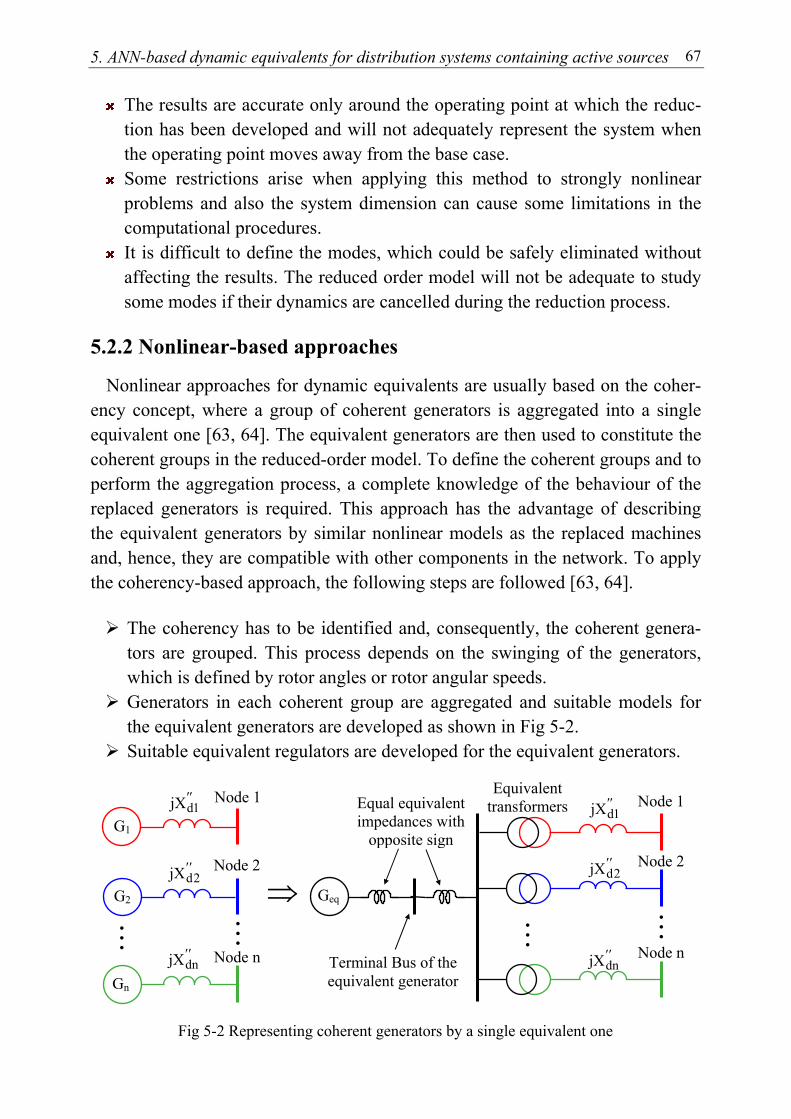
5. ANN-based dynamic equivalents for distribution systems containing active sources 67
The results are accurate only around the operating point at which the reduc-tion has been developed and will not adequately represent the system when the operating point moves away from the base case.
Some restrictions arise when applying this method to strongly nonlinear problems and also the system dimension can cause some limitations in the computational procedures.
It is difficult to define the modes, which could be safely eliminated without affecting the results. The reduced order model will not be adequate to study some modes if their dynamics are cancelled during the reduction process.
5.2.2 Nonlinear-based approaches
Nonlinear approaches for dynamic equivalents are usually based on the coher-ency concept, where a group of coherent generators is aggregated into a single equivalent one [63, 64]. The equivalent generators are then used to constitute the coherent groups in the reduced-order model. To define the coherent groups and to perform the aggregation process, a complete knowledge of the behaviour of the replaced generators is required. This approach has the advantage of describing the equivalent generators by similar nonlinear models as the replaced machines and, hence, they are compatible with other components in the network. To apply the coherency-based approach, the following steps are followed [63, 64].
The coherency has to be identified and, consequently, the coherent genera-tors are grouped. This process depends on the swinging of the generators, which is defined by rotor angles or rotor angular speeds.
Generators in each coherent group are aggregated and suitable models for the equivalent generators are developed as shown in Fig 5-2.
Suitable equivalent regulators are developed for the equivalent generators.
Fig 5-2 Representing coherent generators by a single equivalent one
G1
GeqG2 ⇒
Node 1
Node 2
Node 1
Node 2
Equivalent transformers Equal equivalent
impedances with opposite sign
Gn
Node n Node nTerminal Bus of the equivalent generator
...
''1djX
''2djX
''dnjX
. . . ...
...
''1djX
''2djX
''dnjX
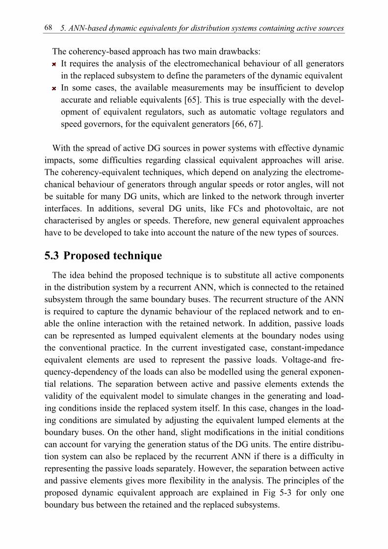
5. ANN-based dynamic equivalents for distribution systems containing active sources 68
The coherency-based approach has two main drawbacks: It requires the analysis of the electromechanical behaviour of all generators
in the replaced subsystem to define the parameters of the dynamic equivalent In some cases, the available measurements may be insufficient to develop
accurate and reliable equivalents [65]. This is true especially with the devel-opment of equivalent regulators, such as automatic voltage regulators and speed governors, for the equivalent generators [66, 67].
With the spread of active DG sources in power systems with effective dynamic
impacts, some difficulties regarding classical equivalent approaches will arise. The coherency-equivalent techniques, which depend on analyzing the electrome-chanical behaviour of generators through angular speeds or rotor angles, will not be suitable for many DG units, which are linked to the network through inverter interfaces. In additions, several DG units, like FCs and photovoltaic, are not characterised by angles or speeds. Therefore, new general equivalent approaches have to be developed to take into account the nature of the new types of sources.
5.3 Proposed technique The idea behind the proposed technique is to substitute all active components
in the distribution system by a recurrent ANN, which is connected to the retained subsystem through the same boundary buses. The recurrent structure of the ANN is required to capture the dynamic behaviour of the replaced network and to en-able the online interaction with the retained network. In addition, passive loads can be represented as lumped equivalent elements at the boundary nodes using the conventional practice. In the current investigated case, constant-impedance equivalent elements are used to represent the passive loads. Voltage-and fre-quency-dependency of the loads can also be modelled using the general exponen-tial relations. The separation between active and passive elements extends the validity of the equivalent model to simulate changes in the generating and load-ing conditions inside the replaced system itself. In this case, changes in the load-ing conditions are simulated by adjusting the equivalent lumped elements at the boundary buses. On the other hand, slight modifications in the initial conditions can account for varying the generation status of the DG units. The entire distribu-tion system can also be replaced by the recurrent ANN if there is a difficulty in representing the passive loads separately. However, the separation between active and passive elements gives more flexibility in the analysis. The principles of the proposed dynamic equivalent approach are explained in Fig 5-3 for only one boundary bus between the retained and the replaced subsystems.
5. ANN-based dynamic equivalents for distribution systems containing active sources 69
Fig 5-3 Principles of the proposed dynamic equivalent approach In addition to the ANN itself, the model requires two supplementary functions:
a mapping function to prepare the ANN inputs and demapping function to proc-ess the outputs from the ANN to calculate complex power. These two functions represent the interface between the ANN and the retained network. The equiva-lent model interacts with the retained system through the boundary buses. It is perturbed by the voltages at these buses and reacts by supplying the correspond-ing complex power at each time interval. The ANN itself acts as a Norton model, where the normalized deviations of voltages are used as main inputs and the nor-malized deviations of currents represent the outputs. In addition to the input volt-ages, past values of currents and voltages are also introduced at the input layer to achieve the recurrent structure. Thus, the ANN is able to capture the dynamic na-ture of the original system and to maintain the continuous-time operation of the entire network.
The current rather than power is used as output from the ANN as it represents
independent variable, whereas power depends on the voltage, which is an input to the ANN. Therefore the use of current gives better convergence in the training process compared to the complex power due to the complete decoupling between outputs and inputs of the ANN. The use of normalized deviations as inputs and outputs in the ANN allows the use of the equivalent model under new initial power-flow condition. The ANN in this case represents a normalized model
Pp, Qp
P, Q ANN Pa, Qa
U
f2
Passive elementsActive elements
P, Q
f1
. . .
. . .
nU∆naI∆
Replaced network
Retained networkReplaced network
U
Retained network
nz−
2z−1z−
mz−
1z−
2z−
U
5. ANN-based dynamic equivalents for distribution systems containing active sources 70
scaled on initial conditions at the boundary buses. Augmenting this feature with the independent representation of active and passive elements results in a univer-sal model, which is capable of simulating the original system under different op-erating conditions.
At each time interval, the dynamic equivalent recognizes the operating status of
the retained network through the instantaneous values of boundary-bus voltages (U). The normalized voltage-deviations ( nU∆ ) are then computed through the mapping function (f1). The ANN is used to define the corresponding normalized deviations of currents for the active components ( n
aI∆ ). The complex power (P, Q) is calculated using the demapping function (f2) and supplied to the retained network. The normalized deviations of currents and voltages are computed based on their initial conditions as follows:
0a,i
0a,ia,in
a,iI
III∆
−= i=1,2…j (5-1)
0i
0iin
i UUUU∆ −
= i=1,2…j (5-2)
where: na,iI∆ : normalized current-deviation of active components at boundary bus i
a,iI , 0iaI , : current of active sources at boundary bus i and its initial value
niU∆ : normalized voltage-deviation at boundary bus i
iU , 0iU : voltage at boundary bus i and its initial value
j : number of boundary buses
Real and imaginary parts of niU∆ are used as separate inputs to the ANN,
while real and imaginary components of na,iI∆ are obtained separately at the out-
put layer. The actual values of complex currents are calculated inside the function (f2) and used to calculate the active and reactive power at each boundary bus.
5.4 Application with the PST16 network In the PST16 network, the 110kV system with the underlying 10 and 0.4kV
parts is assumed as the replaced subsystem. This system, which contains 56 FCs and 56 MTs with different capacities, is to be replaced by the recurrent ANN and

5. ANN-based dynamic equivalents for distribution systems containing active sources 71
the equivalent lumped loads. The retained subsystem is the rest of the high-voltage network including area “A”, area “B” and the 220 and 380kV parts of area “C”. The interface between the retained high-voltage system and the re-placed system is through two buses, i.e. B1 and B2 in area C (see Fig 4-2). If the focus of the study is not directed to the distribution system itself, replacing this network with all active sources by a suitable dynamic equivalent will achieve a great simplification in the simulation. Table 5-1 summarizes the number of elec-tric components in both the retained high-voltage network and the replaced dis-tribution system.
Table 5-1 Summary of components in the retained and replaced subsystems
Retained subsystem Replaced subsystem Buses 60 238 Branches 45 178 Transformers 26 64 Generators 16 0 Micro-turbines (MTs) 0 56 Fuel cells (FCs) 0 56
The large number of components in the distribution system complicates the dy-
namic simulation considerably. In real interconnected systems, where the number of elements in distribution systems reaches up to thousands of units, the detailed simulation of all elements will be unfeasible. Conventionally, lumped-load repre-sentation with suitable voltage-and frequency-dependant elements is used to rep-resent distribution networks. With large power from active DG units, their impact on the high-voltage networks has to be considered. Neglecting this dynamic con-tribution will cause an unacceptable error in the analysis.
To assess this error in more detail, the performance of the entire network is in-
vestigated in three cases. In the first case, the distribution system is modelled in detail with all DG units. In the second case, the conventional lumped representa-tion is considered, where the equivalent load at each boundary bus depends on the voltage at this bus with general exponential relation. In the third case, the power of the equivalent loads is related to the voltages at all boundary buses with general exponential relations as follows:
⋅=
,i2p
02
2,i1p
01
10ii U
UUUPP i=1,2 (5-3)
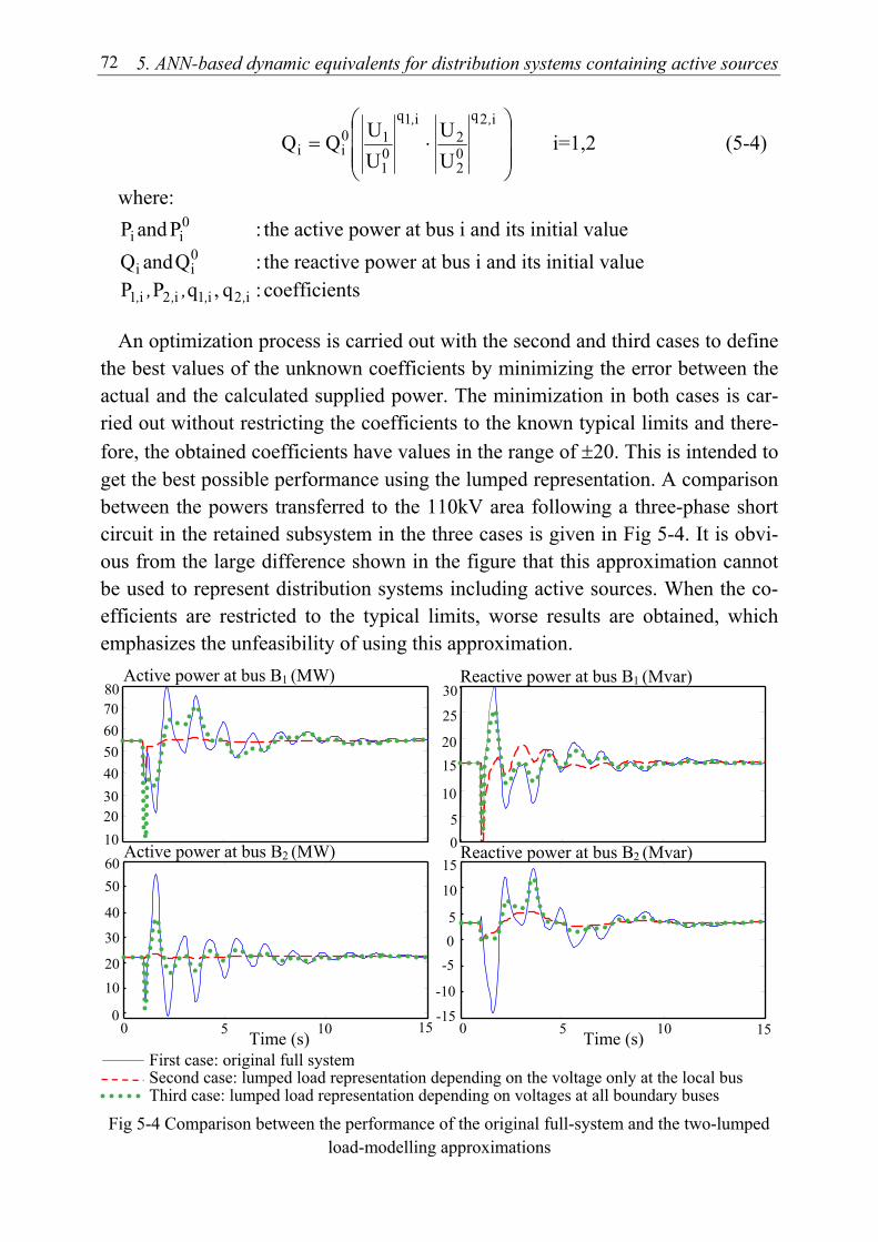
5. ANN-based dynamic equivalents for distribution systems containing active sources 72
⋅=
i2q
02
2i1q
01
10ii U
UUUQQ
,,
i=1,2 (5-4)
where:
iP and 0iP : the active power at bus i and its initial value
iQ and 0iQ : the reactive power at bus i and its initial value
i2i1i2i1 q ,qPP ,,,, ,, : coefficients An optimization process is carried out with the second and third cases to define
the best values of the unknown coefficients by minimizing the error between the actual and the calculated supplied power. The minimization in both cases is car-ried out without restricting the coefficients to the known typical limits and there-fore, the obtained coefficients have values in the range of ±20. This is intended to get the best possible performance using the lumped representation. A comparison between the powers transferred to the 110kV area following a three-phase short circuit in the retained subsystem in the three cases is given in Fig 5-4. It is obvi-ous from the large difference shown in the figure that this approximation cannot be used to represent distribution systems including active sources. When the co-efficients are restricted to the typical limits, worse results are obtained, which emphasizes the unfeasibility of using this approximation.
Fig 5-4 Comparison between the performance of the original full-system and the two-lumped load-modelling approximations
10 20 30 40 50 60 70 80
Active power at bus B1 (MW)
-15
-10
-505
10
15
0 5 10 15Time (s)
Reactive power at bus B2 (Mvar)
0
10 20
30
40
50 60
Active power at bus B2 (MW) 05
10
15 20
25
30 Reactive power at bus B1 (Mvar)
0 5 10 15 Time (s)
First case: original full system Second case: lumped load representation depending on the voltage only at the local bus Third case: lumped load representation depending on voltages at all boundary buses
5. ANN-based dynamic equivalents for distribution systems containing active sources 73
5.5 Recurrent ANNs for dynamic equivalents ANNs have high capability to deal with complicated nonlinear problems in a
general frame, which enables them to be successfully applied to new situations that are not used in the training phase [65]. Therefore, good-trained recurrent ANNs can replace complex distribution systems and are expected to properly in-teract with the retained network at a wide range of operating conditions. With the use of ANNs for dynamic modelling purposes, no information about the system structure is required and the use of complex mathematical analysis is avoided. This represents a significant advantage especially when there is a limited under-standing of the relations between system variables.
5.5.1 Data preparation
Several three-phase short circuits are simulated at different locations in the re-tained network. The simulation of each fault is carried out for 10s, which is enough to restore the steady state conditions after the fault clearance. A 10ms in-tegration time step is used in the simulation, which results in 1000 pattern with each fault. Complex voltages and injected currents at the boundary-buses are stored during the fault simulation and subsequently used to prepare suitable pat-terns for training the ANN.
5.5.2 ANN structure
Since the ANN is required to capture the dynamics of the replaced network, which is distinct by currents, recursive loops are used to feedback normalized current deviations to the input layer with time delays. In addition, the ANN inter-acts with the retained network and recognizes its dynamic behaviour through the voltages. Therefore, past values of normalized voltage deviations are also used at the input layer. With two boundary buses, the ANN has 4 main inputs represent-ing the real and imaginary components of normalized voltage-deviations. Fur-thermore, normalized deviations of these voltages at four previous time intervals are received at the input neurons. On the other hand, four outputs representing the real and imaginary components of normalized deviations of currents are obtained from the ANN. Four recursive loops with delay actions from each output are fed back to the input layer of the ANN. This results in a total number of 20 inputs in addition to 16 recurrent loops.
The ANN contains two hidden layers with 10 and 5 neurons respectively. All
hidden layers comprise neurons with nonlinear-sigmoid activation functions,

5. ANN-based dynamic equivalents for distribution systems containing active sources 74
while neurons in the output layer have linear functions. The structure of the ANN is shown in Fig 5-5.
Fig 5-5 Structure of the ANN
5.5.3 Training process
Patterns corresponding to eight different three-phase short circuits are used in the training process. Time-histories of voltage variables are involved in the input features to the network, while real recurrent loops from output current variables are considered. A special program is developed to train the ANN with actual re-current loops. With 1000 pattern belonging to each waveform, 8000 patterns are used in the training process, which is accomplished offline without actual interac-tion with the retained network. However, the test and validation of the developed dynamic model are based on real-online interactions. The results from the train-ing process (i.e. biases and weights) are saved to be used in the implementation procedures.
5.6 Implementation of the ANN-based equivalent Since the equivalent model is intended for online applications, it has to be im-
plemented in such a way that it interacts with the retained subsystem at each time step to give similar behaviour like that of the original network. As mentioned in section 4.3, unconventional energy sources are simulated in the PSD package in a so-called “regulator files”. In these files, a complete description of the dynamic behaviour of the element can be stored and integrated into the network through one or more buses. The processing within the regulator files is accomplished us-ing pre-constructed blocks to describe the dynamic behaviour of the element. The
z-m
...
z-1
z-2
U (t)
U (t-1)
U (t-n)
Output current vector
I (t)
Input voltage vector
.........
...
...
. . .
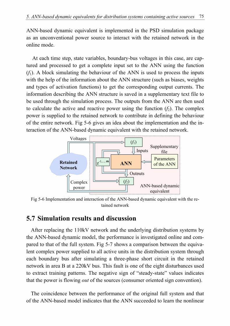
5. ANN-based dynamic equivalents for distribution systems containing active sources 75
ANN-based dynamic equivalent is implemented in the PSD simulation package as an unconventional power source to interact with the retained network in the online mode.
At each time step, state variables, boundary-bus voltages in this case, are cap-
tured and processed to get a complete input set to the ANN using the function (f1). A block simulating the behaviour of the ANN is used to process the inputs with the help of the information about the ANN structure (such as biases, weights and types of activation functions) to get the corresponding output currents. The information describing the ANN structure is saved in a supplementary text file to be used through the simulation process. The outputs from the ANN are then used to calculate the active and reactive power using the function (f2). The complex power is supplied to the retained network to contribute in defining the behaviour of the entire network. Fig 5-6 gives an idea about the implementation and the in-teraction of the ANN-based dynamic equivalent with the retained network.
Fig 5-6 Implementation and interaction of the ANN-based dynamic equivalent with the re-
tained network
5.7 Simulation results and discussion After replacing the 110kV network and the underlying distribution systems by
the ANN-based dynamic model, the performance is investigated online and com-pared to that of the full system. Fig 5-7 shows a comparison between the equiva-lent complex power supplied to all active units in the distribution system through each boundary bus after simulating a three-phase short circuit in the retained network in area B at a 220kV bus. This fault is one of the eight disturbances used to extract training patterns. The negative sign of “steady-state” values indicates that the power is flowing out of the sources (consumer oriented sign convention).
The coincidence between the performance of the original full system and that
of the ANN-based model indicates that the ANN succeeded to learn the nonlinear
Inputs
(f1)
ANN
Outputs
Voltages
(f2) ANN-based dynamic
equivalent
Retained Network
z-1,..., m
Complex power
Parameters of the ANN
Supplementary file
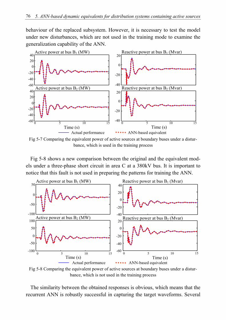
5. ANN-based dynamic equivalents for distribution systems containing active sources 76
behaviour of the replaced subsystem. However, it is necessary to test the model under new disturbances, which are not used in the training mode to examine the generalization capability of the ANN.
Fig 5-7 Comparing the equivalent power of active sources at boundary buses under a distur-bance, which is used in the training process
Fig 5-8 shows a new comparison between the original and the equivalent mod-
els under a three-phase short circuit in area C at a 380kV bus. It is important to notice that this fault is not used in preparing the patterns for training the ANN.
Fig 5-8 Comparing the equivalent power of active sources at boundary buses under a distur-bance, which is not used in the training process
The similarity between the obtained responses is obvious, which means that the
recurrent ANN is robustly successful in capturing the target waveforms. Several
Active power at bus B1 (MW)
-60 -40 -20
0 20 40
Reactive power at bus B1 (Mvar)
-40
-20
0
20
-60 -40 -20
0 20 40 Active power at bus B2 (MW)
Time (s) 0 5 10 15
-40
-20
0
20Reactive power at bus B2 (Mvar)
Time (s) 0 5 10 15
Actual performance ANN-based equivalent
Active power at bus B1 (MW)
-100
-50
0
50
Reactive power at bus B2 (Mvar)
Time (s) 15
-60
-20
0
20
0 5 10
-40
Active power at bus B2 (MW)
Time (s) -100
-50 0
50 100
0 5 10 15
Reactive power at bus B1 (Mvar) 40
-40
-20
0
20
Actual performance ANN-based equivalent

5. ANN-based dynamic equivalents for distribution systems containing active sources 77
comparisons are carried out under other new disturbances, where the performance is always similar to that of the original full model. This ensures that the ANN-based model effectively reproduces the behaviour of the replaced subsystem in a general form. Therefore, different studies of the entire network including the pro-posed equivalent model are possible with high accuracy.
To demonstrate the capability of the proposed equivalent model to cover new
operating conditions, the behaviour of the same model is studied under new power-flow conditions by varying the loading status in the retained network. The generated power and load demand in the replaced subsystem are maintained con-stant. Thus, the total power transferred to the low-voltage network is not changed. However, the voltages and the partition of the power at the boundary buses are changed as shown in Table 5-2. The total power transferred is slightly increased to account for the increase in the power loss due to the voltage reduction.
Table 5-2 Voltages and powers at boundary buses for the base and the new power-flow cases
U1 (kV) U2 (kV) S1 (MVA) S2 (MVA) Base case 381.150 222.530 54.823+j15.307 22.332+j3.262 New case 378.340 221.420 61.428+j13.431 15.844+j5.945
A new three-phase short circuit is simulated in area C at a 220kV bus under the
new power-flow conditions with both the full network and that comprising the ANN-based equivalent model. Fig 5-9 compares between the powers supplied by active units through the two boundary buses using the full-model and the ANN-based model.
Fig 5-9 Comparing the performance of the original and the equivalent systems starting from a new power-flow initial condition
Active power at bus B1 (MW)
-40
-20 0
20
-60
Reactive power at bus B1 (Mvar) 5
-20
-10-5
0
-15
Active power at bus B2 (MW)
Time (s) 0 5 10 15
-40
-20
0
20 Reactive power at bus B2 (Mvar)
-20
0
Time (s)
-10
-30 0 5 10 15
Actual performance ANN-based equivalent
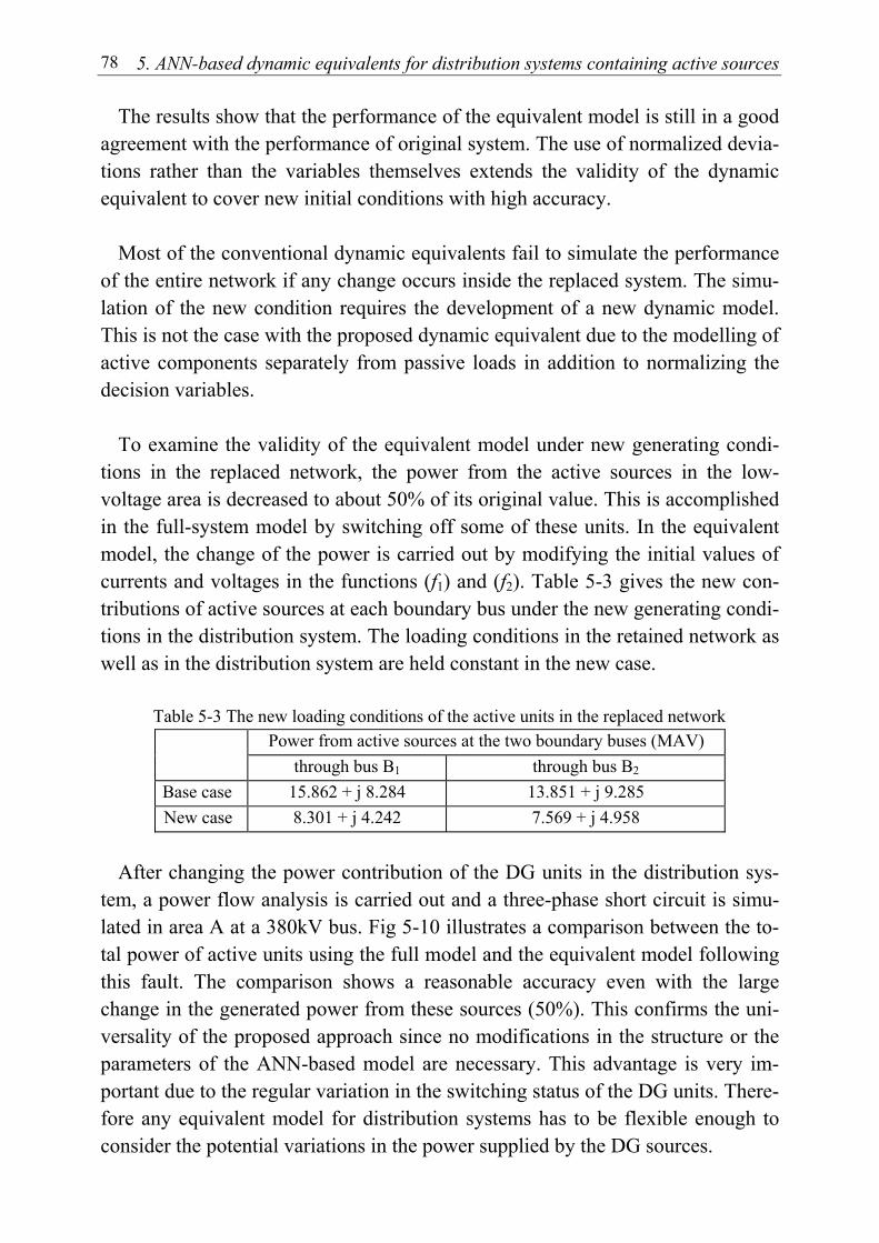
5. ANN-based dynamic equivalents for distribution systems containing active sources 78
The results show that the performance of the equivalent model is still in a good agreement with the performance of original system. The use of normalized devia-tions rather than the variables themselves extends the validity of the dynamic equivalent to cover new initial conditions with high accuracy.
Most of the conventional dynamic equivalents fail to simulate the performance
of the entire network if any change occurs inside the replaced system. The simu-lation of the new condition requires the development of a new dynamic model. This is not the case with the proposed dynamic equivalent due to the modelling of active components separately from passive loads in addition to normalizing the decision variables.
To examine the validity of the equivalent model under new generating condi-
tions in the replaced network, the power from the active sources in the low-voltage area is decreased to about 50% of its original value. This is accomplished in the full-system model by switching off some of these units. In the equivalent model, the change of the power is carried out by modifying the initial values of currents and voltages in the functions (f1) and (f2). Table 5-3 gives the new con-tributions of active sources at each boundary bus under the new generating condi-tions in the distribution system. The loading conditions in the retained network as well as in the distribution system are held constant in the new case.
Table 5-3 The new loading conditions of the active units in the replaced network
Power from active sources at the two boundary buses (MAV) through bus B1 through bus B2
Base case 15.862 + j 8.284 13.851 + j 9.285 New case 8.301 + j 4.242 7.569 + j 4.958
After changing the power contribution of the DG units in the distribution sys-
tem, a power flow analysis is carried out and a three-phase short circuit is simu-lated in area A at a 380kV bus. Fig 5-10 illustrates a comparison between the to-tal power of active units using the full model and the equivalent model following this fault. The comparison shows a reasonable accuracy even with the large change in the generated power from these sources (50%). This confirms the uni-versality of the proposed approach since no modifications in the structure or the parameters of the ANN-based model are necessary. This advantage is very im-portant due to the regular variation in the switching status of the DG units. There-fore any equivalent model for distribution systems has to be flexible enough to consider the potential variations in the power supplied by the DG sources.
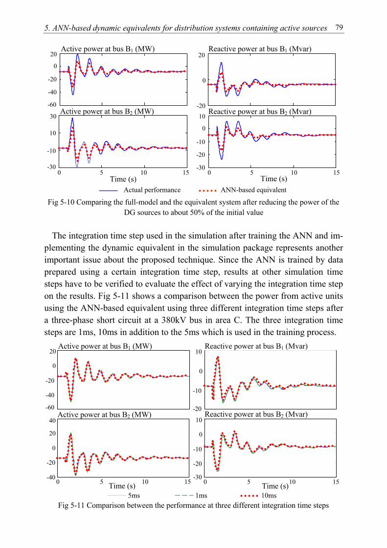
5. ANN-based dynamic equivalents for distribution systems containing active sources 79
Fig 5-10 Comparing the full-model and the equivalent system after reducing the power of the DG sources to about 50% of the initial value
The integration time step used in the simulation after training the ANN and im-
plementing the dynamic equivalent in the simulation package represents another important issue about the proposed technique. Since the ANN is trained by data prepared using a certain integration time step, results at other simulation time steps have to be verified to evaluate the effect of varying the integration time step on the results. Fig 5-11 shows a comparison between the power from active units using the ANN-based equivalent using three different integration time steps after a three-phase short circuit at a 380kV bus in area C. The three integration time steps are 1ms, 10ms in addition to the 5ms which is used in the training process.
Fig 5-11 Comparison between the performance at three different integration time steps
Actual performance ANN-based equivalent
Active power at bus B1 (MW) Reactive power at bus B1 (Mvar)
Active power at bus B2 (MW)
Time (s) 0 5 10 15
Reactive power at bus B2 (Mvar) -60
-40
-20
0
20
-20
0
20
-30
-10
10
30
Time (s) 0 5 10 15
-30
-20
-10
0
10
5ms 1ms 10ms
Active power at bus B1 (MW) Reactive power at bus B1 (Mvar)
Time (s) Time (s)
Active power at bus B2 (MW) Reactive power at bus B2 (Mvar) -60
-40
-20
0
20
0 5 10 15-40
-20
0
20
40
-20
-10
0
10
0 5 10 15-30
-20
-10
0
10
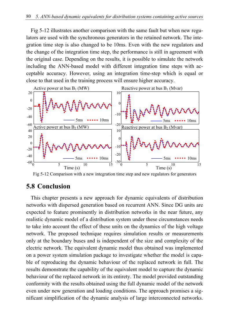
5. ANN-based dynamic equivalents for distribution systems containing active sources 80
Fig 5-12 illustrates another comparison with the same fault but when new regu-lators are used with the synchronous generators in the retained network. The inte-gration time step is also changed to be 10ms. Even with the new regulators and the change of the integration time step, the performance is still in agreement with the original case. Depending on the results, it is possible to simulate the network including the ANN-based model with different integration time steps with ac-ceptable accuracy. However, using an integration time-step which is equal or close to that used in the training process will ensure higher accuracy.
Fig 5-12 Comparison with a new integration time step and new regulators for generators
5.8 Conclusion This chapter presents a new approach for dynamic equivalents of distribution
networks with dispersed generation based on recurrent ANN. Since DG units are expected to feature prominently in distribution networks in the near future, any realistic dynamic model of a distribution system under these circumstances needs to take into account the effect of these units on the dynamics of the high voltage network. The proposed technique requires simulation results or measurements only at the boundary buses and is independent of the size and complexity of the electric network. The equivalent dynamic model thus obtained was implemented on a power system simulation package to investigate whether the model is capa-ble of reproducing the dynamic behaviour of the replaced network in full. The results demonstrate the capability of the equivalent model to capture the dynamic behaviour of the replaced network in its entirety. The model provided outstanding conformity with the results obtained using the full dynamic model of the network even under new generation and loading conditions. The approach promises a sig-nificant simplification of the dynamic analysis of large interconnected networks.
5ms 10ms
Active power at bus B1 (MW) Reactive power at bus B1 (Mvar)
Time (s) Time (s)
Active power at bus B2 (MW) Reactive power at bus B2 (Mvar)
0 5 10 15 0 5 10 15-60
-60
-40
-20
0
20
-20
-10
0
10
-40
-20 0
20 40
-30
-20
-10
0
10
5ms 10ms 5ms 10ms
5ms 10ms
Chapter 6
Impact of Distributed Generation on the Stability of Electrical Power Systems
6
6.1 Introduction The special characteristics of DG units and their low inertia can cause many
technical and operating challenges regarding the stability of power systems [24, 68]. Generally, few numbers of quite small-size DG units, compared to the large centralized power stations, will not influence the operation of the power network and, hence, their impact can be neglected. However, when networks begin to comprise large numbers of DG units with higher capacities, the overall dynamics and the stability of power systems are significantly impacted [24]. Therefore, power system analysis becomes more emerging problem especially with the wide range of technologies associated with the DG units and the configuration unique-ness of each distribution network [6].
Among numerous investigation issues related to power systems containing DG
units, stability analysis becomes more critical, and adequate damping of the oscil-latory behaviour is of major interest [6, 24, 68]. The conventional approach, which depends on representing DG units together with passive loads in an aggregated form or omitting their effect when analyzing power system stability, is about to be changed [68, 69]. Modern power systems are mostly operating close to their stability limits for economical reasons. This situation demands accurate model-ling of power systems taking into consideration the different penetration levels of DG units to adequately evaluate their impacts on the stability of power systems.
This chapter aims at analysing the potential impacts that DG might have on the
stability of electrical power networks. In particular, the performance of a power system with different penetrations of DG units is described to assess different types of stability of the bulk networks. For this purpose, a hypothetical network is simulated with two main centralized power plants and several DG units con-nected onto the electric distribution system. The investigation is carried out at constant load demands but with different contributions from FCs and MTs. Cer-tain numbers of DG units are switched on to supply the required power in the range from 0.0% up to 28.3% of the total load demand in the distribution net-
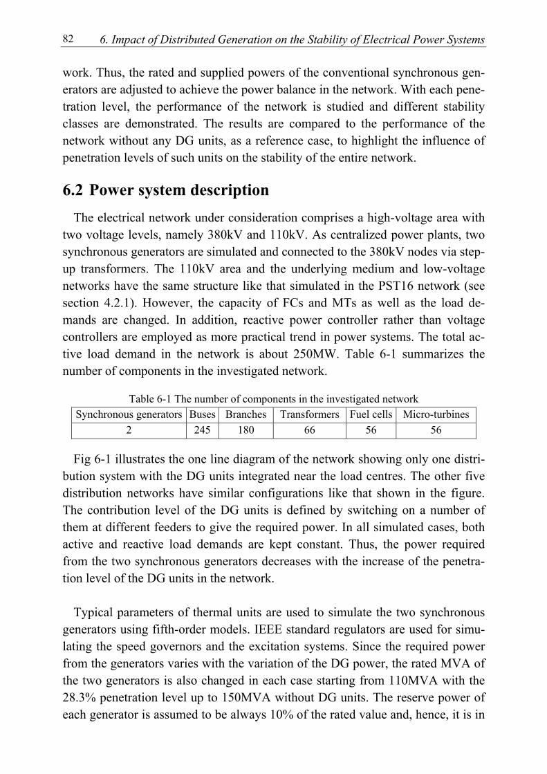
6. Impact of Distributed Generation on the Stability of Electrical Power Systems 82
work. Thus, the rated and supplied powers of the conventional synchronous gen-erators are adjusted to achieve the power balance in the network. With each pene-tration level, the performance of the network is studied and different stability classes are demonstrated. The results are compared to the performance of the network without any DG units, as a reference case, to highlight the influence of penetration levels of such units on the stability of the entire network.
6.2 Power system description The electrical network under consideration comprises a high-voltage area with
two voltage levels, namely 380kV and 110kV. As centralized power plants, two synchronous generators are simulated and connected to the 380kV nodes via step-up transformers. The 110kV area and the underlying medium and low-voltage networks have the same structure like that simulated in the PST16 network (see section 4.2.1). However, the capacity of FCs and MTs as well as the load de-mands are changed. In addition, reactive power controller rather than voltage controllers are employed as more practical trend in power systems. The total ac-tive load demand in the network is about 250MW. Table 6-1 summarizes the number of components in the investigated network.
Table 6-1 The number of components in the investigated network
Synchronous generators Buses Branches Transformers Fuel cells Micro-turbines 2 245 180 66 56 56
Fig 6-1 illustrates the one line diagram of the network showing only one distri-bution system with the DG units integrated near the load centres. The other five distribution networks have similar configurations like that shown in the figure. The contribution level of the DG units is defined by switching on a number of them at different feeders to give the required power. In all simulated cases, both active and reactive load demands are kept constant. Thus, the power required from the two synchronous generators decreases with the increase of the penetra-tion level of the DG units in the network.
Typical parameters of thermal units are used to simulate the two synchronous
generators using fifth-order models. IEEE standard regulators are used for simu-lating the speed governors and the excitation systems. Since the required power from the generators varies with the variation of the DG power, the rated MVA of the two generators is also changed in each case starting from 110MVA with the 28.3% penetration level up to 150MVA without DG units. The reserve power of each generator is assumed to be always 10% of the rated value and, hence, it is in
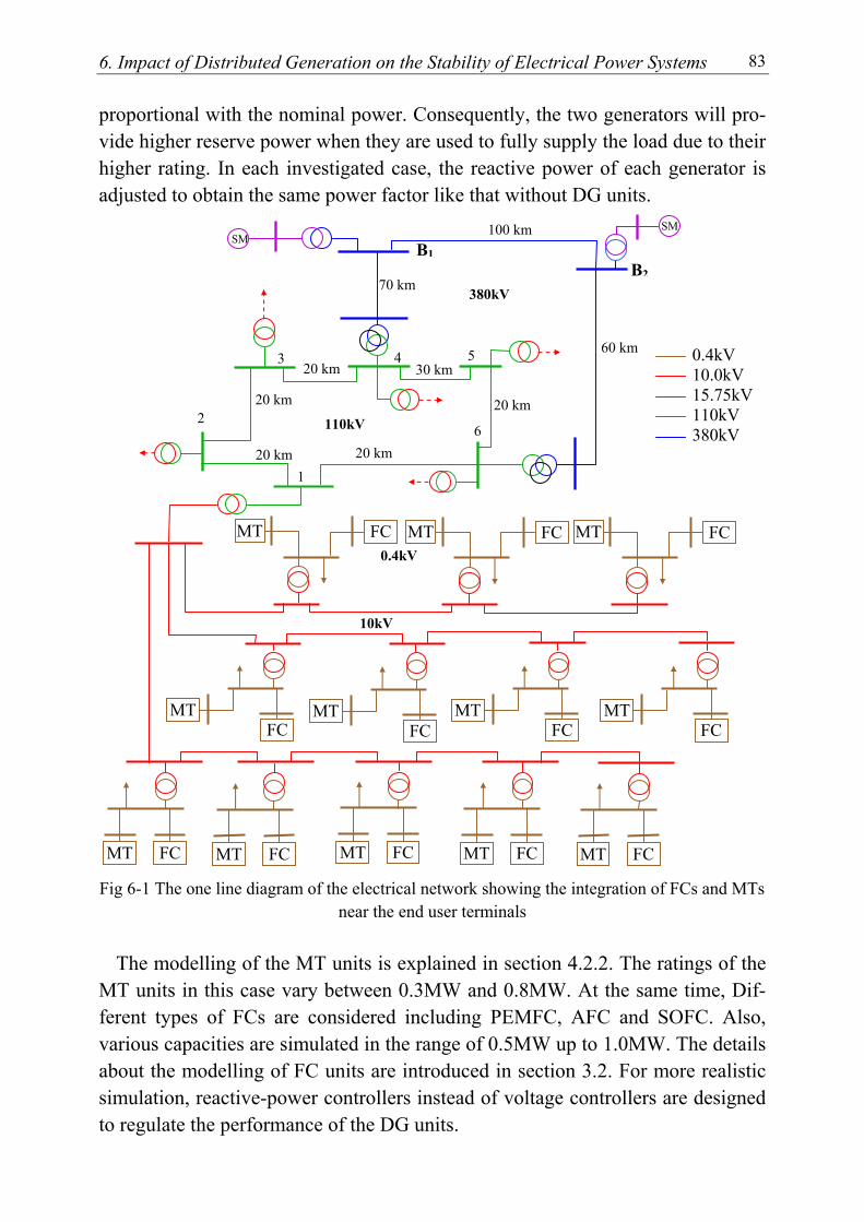
6. Impact of Distributed Generation on the Stability of Electrical Power Systems 83
proportional with the nominal power. Consequently, the two generators will pro-vide higher reserve power when they are used to fully supply the load due to their higher rating. In each investigated case, the reactive power of each generator is adjusted to obtain the same power factor like that without DG units.
Fig 6-1 The one line diagram of the electrical network showing the integration of FCs and MTs near the end user terminals
The modelling of the MT units is explained in section 4.2.2. The ratings of the
MT units in this case vary between 0.3MW and 0.8MW. At the same time, Dif-ferent types of FCs are considered including PEMFC, AFC and SOFC. Also, various capacities are simulated in the range of 0.5MW up to 1.0MW. The details about the modelling of FC units are introduced in section 3.2. For more realistic simulation, reactive-power controllers instead of voltage controllers are designed to regulate the performance of the DG units.
20 km
20 km 20 km
30 km
20 km
20 km
MT FC
FC MT FC MT FC MT FC MT FC MT
MT FC
MTFC
MT FC
FC MTFC MTFC MT
1
2
3 4 5
6
SM SM
60 km
70 km
100 kmB1
B2
0.4kV 10.0kV 15.75kV110kV 380kV
380kV
110kV
0.4kV
10kV
6. Impact of Distributed Generation on the Stability of Electrical Power Systems 84
Since most of the DG units are not utility owned, the power supplied from these units will be defined according to economic consideration. Therefore, it is assumed in the simulation that the power from the DG units will not be adjusted to follow up the load demand. Rather, the owner of the DG unit will supply a specific value of the power to achieve the maximum profit regardless of load changes. For secure operation, the DG units are assumed to be disconnected from the network if the voltages at their terminals decrease lower than 80% of their rated values. This is important to protect the power electronic converter with these units. A delay time of 100ms (five cycles) is assumed for measurements and disconnection of any DG unit after reaching the critical limit. The disconnec-tion of some of the DG units during the simulation represents an additional dis-turbance to the network. Once any unit is switched off, it is not connected again since the simulation time is smaller than the time required for accomplishing the conventional procedures of the reconnection.
Before investigating the impact of DG units on the stability of the power sys-
tem, it is appropriate to study their impacts on the power losses and the voltage profiles of the distribution network.
6.3 Impact on the power losses Generally, the onsite power generation near the load centres causes reduction in
the network power losses as a result of the reduction occurring in the transmitted and distributed power. Even if the power loss is increased in some parts in the distribution feeders, the overall losses within distribution systems, and hence in the entire network, will be reduced. In the investigated network, the power gener-ated by any DG unit is lower than the local load demand and, as a result, the power losses will always be lower compared to the disconnection of all DG units. In spite of the relation between the power-loss reduction in the entire network and that in the distribution network, it is more realistic to observe the former for a comprehensive perspective. For different power levels from the DG units, power flow analyses are carried out and the total power losses in the entire network are computed. Fig 6-2 illustrates the percentage of the total power losses in the net-work versus the power contribution of the DG units. The power of the DG units is increased in steps from 0% up to 28.3%. As shown in the figure, the total power losses in the network decrease with the increase of the power generated in the DG units. However, the magnitude of this reduction depends not only on the power contribution of the DG units but also on their location within the distribu-tion network.
6. Impact of Distributed Generation on the Stability of Electrical Power Systems 85
Fig 6-2 Total power loss with different power contributions from DG units
6.4 Impact on the voltage profiles Keeping the voltage within typical limits along all feeders in the distribution
network is necessary to avoid improper operation of power system and customer equipments. Common practice in regulating the voltages depends on tap-changing transformers to control the source voltages at substations [2]. In addi-tion, switched capacitors, synchronous condensers, or static var compensators can also be used on feeders for controlling the reactive power [21]. Providing a por-tion of energy onsite using DG units can effectively improve and support feeder voltages if these units are properly integrated with the existing network. With the latest-type static converters, the utilization of the DG units could achieve the re-quired voltage support in the distribution network. This can be accomplished by regulating the reactive power through the power factor of converters based on voltage levels on local nodes [2]. On the other hand, tap-changing transformers will not be suitable for the effective regulation of the voltages at all feeder nodes as they assume decreasing voltages along radial feeders [2, 21]. Furthermore, the voltage regulators will not correctly measure feeder demands, rather, the ob-served loads will be lower than actual values due to the onsite generated power.
To highlight the effect of DG on the voltage profiles, the voltages at different
locations are observed considering different DG powers. Fig 6-3 shows the volt-ages at five nodes of one feeder with different contributions from DG units. The insertion of DG reduces the difference between maximum and minimum voltages of loads supplied from the same feeder. Without DG units, the voltage decreases with the distance of the bus from the power source. Adding DG units causes variations in the voltage levels depending on the location of the added units. With large contributions from DG units, the voltage can be maintained almost constant at different load nodes as in the last two cases with 25% and 28.3% contributions.
0 5 10 15 20 25 30 0
1
2
3
4 Percentage total power loss (%)
Percentage power contribution from DG units (%)
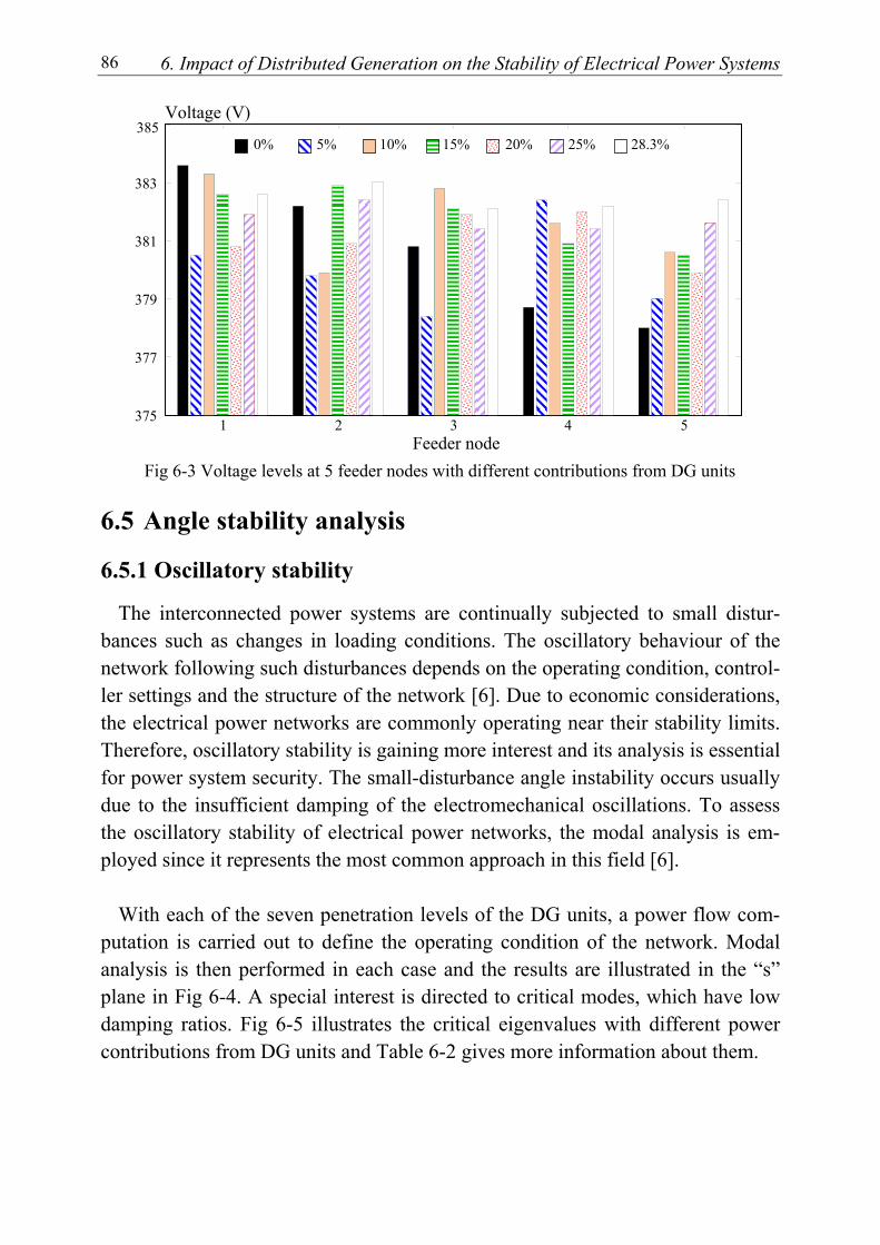
6. Impact of Distributed Generation on the Stability of Electrical Power Systems 86
Fig 6-3 Voltage levels at 5 feeder nodes with different contributions from DG units
6.5 Angle stability analysis
6.5.1 Oscillatory stability
The interconnected power systems are continually subjected to small distur-bances such as changes in loading conditions. The oscillatory behaviour of the network following such disturbances depends on the operating condition, control-ler settings and the structure of the network [6]. Due to economic considerations, the electrical power networks are commonly operating near their stability limits. Therefore, oscillatory stability is gaining more interest and its analysis is essential for power system security. The small-disturbance angle instability occurs usually due to the insufficient damping of the electromechanical oscillations. To assess the oscillatory stability of electrical power networks, the modal analysis is em-ployed since it represents the most common approach in this field [6].
With each of the seven penetration levels of the DG units, a power flow com-
putation is carried out to define the operating condition of the network. Modal analysis is then performed in each case and the results are illustrated in the “s” plane in Fig 6-4. A special interest is directed to critical modes, which have low damping ratios. Fig 6-5 illustrates the critical eigenvalues with different power contributions from DG units and Table 6-2 gives more information about them.
1 2 3 4 5 375
377
379
381
383
385 0% 5% 10% 15% 20% 25% 28.3%
Voltage (V)
Feeder node
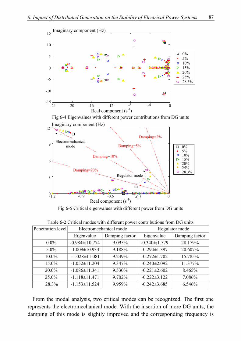
6. Impact of Distributed Generation on the Stability of Electrical Power Systems 87
Fig 6-4 Eigenvalues with different power contributions from DG units
Fig 6-5 Critical eigenvalues with different power from DG units
Table 6-2 Critical modes with different power contributions from DG units Electromechanical mode Regulator mode Penetration level
Eigenvalue Damping factor Eigenvalue Damping factor 0.0% -0.984±j10.774 9.095% -0.340±j1.579 28.179% 5.0% -1.009±10.933 9.188% -0.294±1.397 20.607% 10.0% -1.028±11.081 9.239% -0.272±1.702 15.785% 15.0% -1.052±11.204 9.347% -0.240±2.092 11.377% 20.0% -1.086±11.341 9.530% -0.221±2.602 8.465% 25.0% -1.118±11.471 9.702% -0.222±3.122 7.086% 28.3% -1.153±11.524 9.959% -0.242±3.685 6.546%
From the modal analysis, two critical modes can be recognized. The first one
represents the electromechanical mode. With the insertion of more DG units, the damping of this mode is slightly improved and the corresponding frequency is
-24 -20 -16 -12 0 -15
-10
-5
0
5
10
15
Real component (s-1)
0% 5% 10% 15% 20% 25% 28.3%
-8 -4
Imaginary component (Hz)
-1.2 -0.9 -0.6 -0.3 00
3
6
9
12
0% 5% 10% 15% 20% 25% 28.3%
Real component (s-1)
Imaginary component (Hz)
Damping=2%
Damping=5%
Damping=10%
Regulator mode
Electromechanical mode
Damping=20%
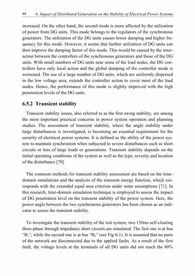
6. Impact of Distributed Generation on the Stability of Electrical Power Systems 88
increased. On the other hand, the second mode is more affected by the utilization of power from DG units. This mode belongs to the regulators of the synchronous generators. The utilization of the DG units causes lower damping and higher fre-quency for this mode. However, it seems that further utilization of DG units can then improve the damping factor of this mode. This would be caused by the inter-action between the controllers of the synchronous generators and those of the DG units. With small numbers of DG units near some of the load nodes, the DG con-trollers have only local action and the global damping of the controller mode is worsened. The use of a large number of DG units, which are uniformly dispersed in the low voltage area, extends the controller action to cover most of the load nodes. Hence, the performance of this mode is slightly improved with the high penetration levels of the DG units.
6.5.2 Transient stability
Transient stability issues, also referred to as the first swing stability, are among the most important practical concerns in power system operation and planning studies. The assessment of transient stability, where the angle stability under large disturbances is investigated, is becoming an essential requirement for the security of electrical power systems. It is defined as the ability of the power sys-tem to maintain synchronism when subjected to severe disturbances such as short circuits or loss of large loads or generations. Transient stability depends on the initial operating conditions of the system as well as the type, severity and location of the disturbance [70].
The common methods for transient stability assessment are based on the time-
domain simulations and the analysis of the transient energy function, which cor-responds with the extended equal area criterion under some assumptions [71]. In this research, time-domain simulation technique is employed to assess the impact of DG penetration level on the transient stability of the power system. Here, the power angle between the two synchronous generators has been chosen as an indi-cator to assess the transient stability.
To investigate the transient stability of the test system, two 150ms self-clearing
three-phase through impedance short circuits are simulated. The first one is at bus “B1”, while the second one is at bus “B2” (see Fig 6-1). It is assumed that no parts of the network are disconnected due to the applied faults. As a result of the first fault, the voltage levels at the terminals of all DG units did not reach the 80%
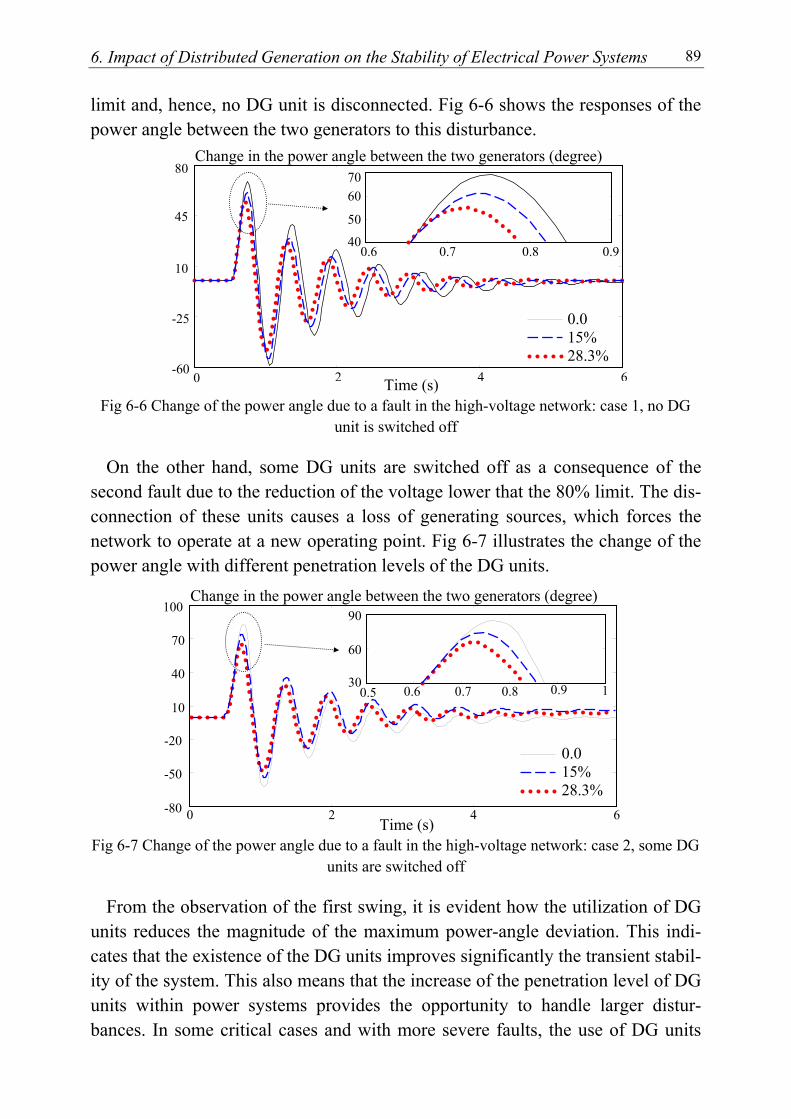
6. Impact of Distributed Generation on the Stability of Electrical Power Systems 89
limit and, hence, no DG unit is disconnected. Fig 6-6 shows the responses of the power angle between the two generators to this disturbance.
Fig 6-6 Change of the power angle due to a fault in the high-voltage network: case 1, no DG unit is switched off
On the other hand, some DG units are switched off as a consequence of the second fault due to the reduction of the voltage lower that the 80% limit. The dis-connection of these units causes a loss of generating sources, which forces the network to operate at a new operating point. Fig 6-7 illustrates the change of the power angle with different penetration levels of the DG units.
Fig 6-7 Change of the power angle due to a fault in the high-voltage network: case 2, some DG units are switched off
From the observation of the first swing, it is evident how the utilization of DG units reduces the magnitude of the maximum power-angle deviation. This indi-cates that the existence of the DG units improves significantly the transient stabil-ity of the system. This also means that the increase of the penetration level of DG units within power systems provides the opportunity to handle larger distur-bances. In some critical cases and with more severe faults, the use of DG units
Time (s)
Change in the power angle between the two generators (degree)
0.0 15% 28.3%
0 2 4 6-60
-25
10
45
80
0.6 0.7 0.8 0.9 40
50
6070
-80
-50
-20
10
40
70
100
0.5 1 30
60
90
0.9 0.6 0.7 0.8
Time (s)
Change in the power angle between the two generators (degree)
0.0 15% 28.3%
2 4 6 0
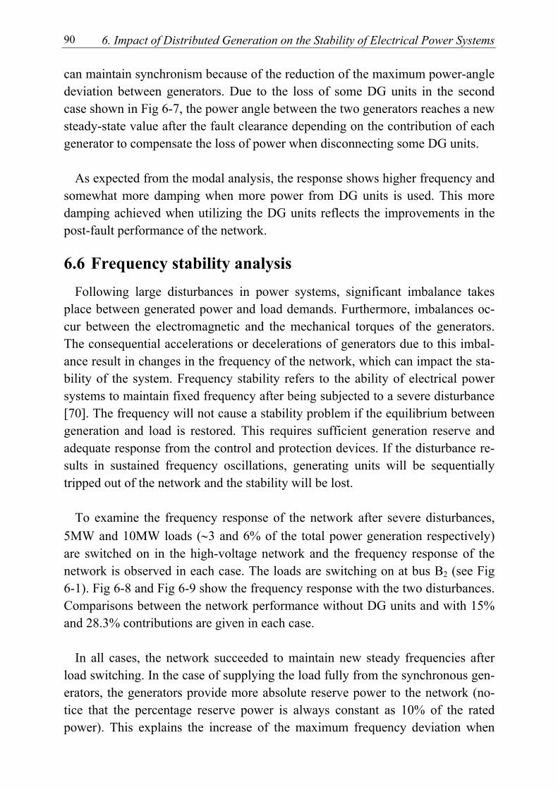
6. Impact of Distributed Generation on the Stability of Electrical Power Systems 90
can maintain synchronism because of the reduction of the maximum power-angle deviation between generators. Due to the loss of some DG units in the second case shown in Fig 6-7, the power angle between the two generators reaches a new steady-state value after the fault clearance depending on the contribution of each generator to compensate the loss of power when disconnecting some DG units.
As expected from the modal analysis, the response shows higher frequency and
somewhat more damping when more power from DG units is used. This more damping achieved when utilizing the DG units reflects the improvements in the post-fault performance of the network.
6.6 Frequency stability analysis Following large disturbances in power systems, significant imbalance takes
place between generated power and load demands. Furthermore, imbalances oc-cur between the electromagnetic and the mechanical torques of the generators. The consequential accelerations or decelerations of generators due to this imbal-ance result in changes in the frequency of the network, which can impact the sta-bility of the system. Frequency stability refers to the ability of electrical power systems to maintain fixed frequency after being subjected to a severe disturbance [70]. The frequency will not cause a stability problem if the equilibrium between generation and load is restored. This requires sufficient generation reserve and adequate response from the control and protection devices. If the disturbance re-sults in sustained frequency oscillations, generating units will be sequentially tripped out of the network and the stability will be lost.
To examine the frequency response of the network after severe disturbances,
5MW and 10MW loads (∼3 and 6% of the total power generation respectively) are switched on in the high-voltage network and the frequency response of the network is observed in each case. The loads are switching on at bus B2 (see Fig 6-1). Fig 6-8 and Fig 6-9 show the frequency response with the two disturbances. Comparisons between the network performance without DG units and with 15% and 28.3% contributions are given in each case.
In all cases, the network succeeded to maintain new steady frequencies after
load switching. In the case of supplying the load fully from the synchronous gen-erators, the generators provide more absolute reserve power to the network (no-tice that the percentage reserve power is always constant as 10% of the rated power). This explains the increase of the maximum frequency deviation when
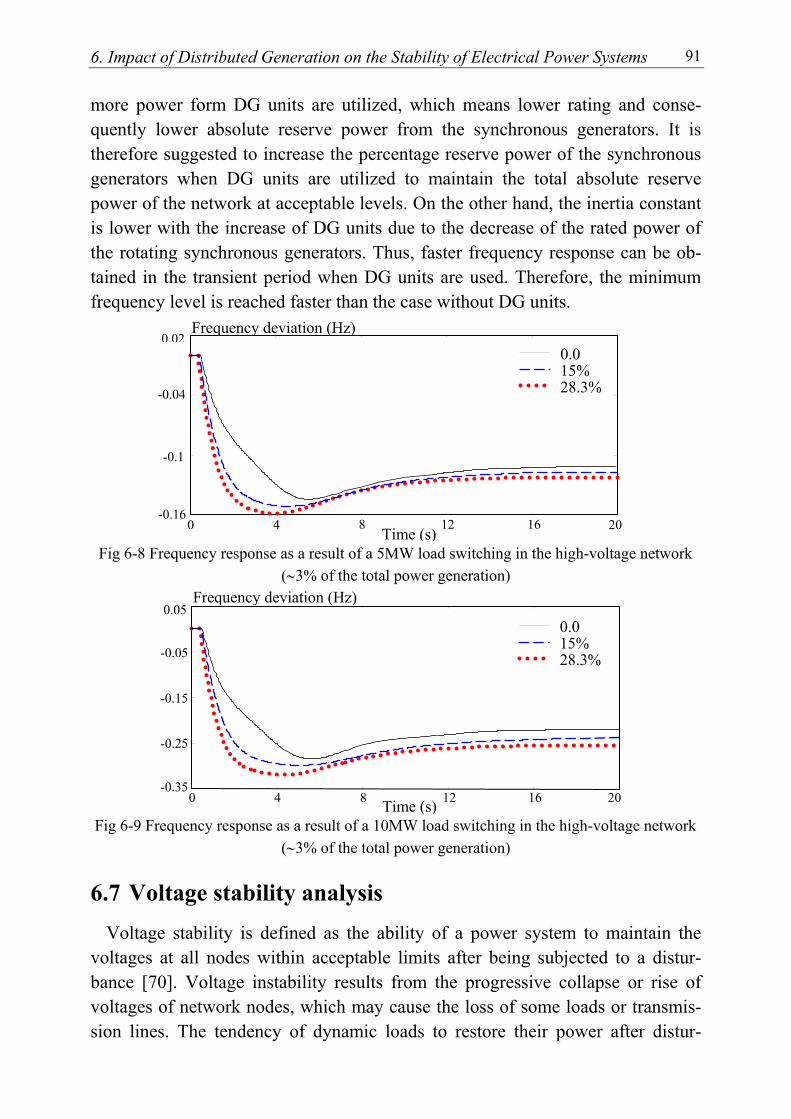
6. Impact of Distributed Generation on the Stability of Electrical Power Systems 91
more power form DG units are utilized, which means lower rating and conse-quently lower absolute reserve power from the synchronous generators. It is therefore suggested to increase the percentage reserve power of the synchronous generators when DG units are utilized to maintain the total absolute reserve power of the network at acceptable levels. On the other hand, the inertia constant is lower with the increase of DG units due to the decrease of the rated power of the rotating synchronous generators. Thus, faster frequency response can be ob-tained in the transient period when DG units are used. Therefore, the minimum frequency level is reached faster than the case without DG units.
Fig 6-8 Frequency response as a result of a 5MW load switching in the high-voltage network (∼3% of the total power generation)
Fig 6-9 Frequency response as a result of a 10MW load switching in the high-voltage network (∼3% of the total power generation)
6.7 Voltage stability analysis Voltage stability is defined as the ability of a power system to maintain the
voltages at all nodes within acceptable limits after being subjected to a distur-bance [70]. Voltage instability results from the progressive collapse or rise of voltages of network nodes, which may cause the loss of some loads or transmis-sion lines. The tendency of dynamic loads to restore their power after distur-
-0.35
-0.25
-0.15
-0.05
0.05
0 4 8 12 16 20 Time (s)
Frequency deviation (Hz)
0.0 15% 28.3%
-0.16
-0.04
-0.1
0.02
0 4 8 12 16 20 Time (s)
Frequency deviation (Hz)
0.0 15% 28.3%
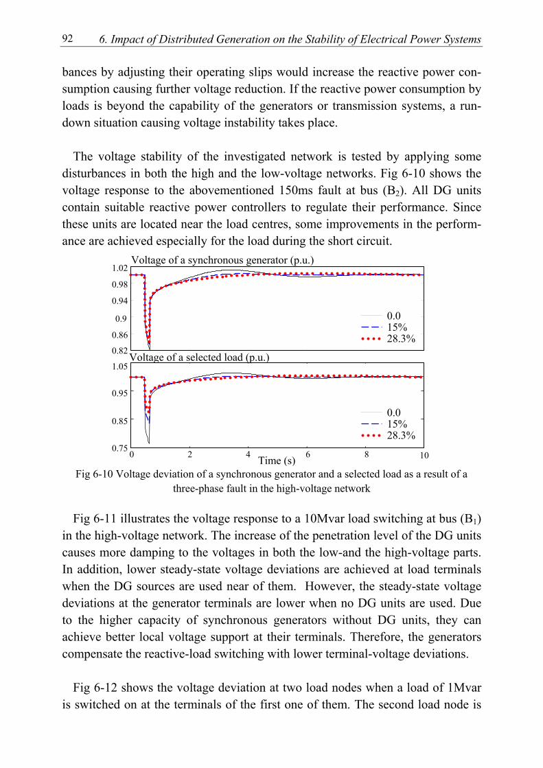
6. Impact of Distributed Generation on the Stability of Electrical Power Systems 92
bances by adjusting their operating slips would increase the reactive power con-sumption causing further voltage reduction. If the reactive power consumption by loads is beyond the capability of the generators or transmission systems, a run-down situation causing voltage instability takes place.
The voltage stability of the investigated network is tested by applying some
disturbances in both the high and the low-voltage networks. Fig 6-10 shows the voltage response to the abovementioned 150ms fault at bus (B2). All DG units contain suitable reactive power controllers to regulate their performance. Since these units are located near the load centres, some improvements in the perform-ance are achieved especially for the load during the short circuit.
Fig 6-10 Voltage deviation of a synchronous generator and a selected load as a result of a
three-phase fault in the high-voltage network Fig 6-11 illustrates the voltage response to a 10Mvar load switching at bus (B1)
in the high-voltage network. The increase of the penetration level of the DG units causes more damping to the voltages in both the low-and the high-voltage parts. In addition, lower steady-state voltage deviations are achieved at load terminals when the DG sources are used near of them. However, the steady-state voltage deviations at the generator terminals are lower when no DG units are used. Due to the higher capacity of synchronous generators without DG units, they can achieve better local voltage support at their terminals. Therefore, the generators compensate the reactive-load switching with lower terminal-voltage deviations.
Fig 6-12 shows the voltage deviation at two load nodes when a load of 1Mvar
is switched on at the terminals of the first one of them. The second load node is
0.82
0.86
0.9
0.94
0.98
1.02
0.75
0.85
0.95
1.05
0 2 4 6 8Time (s)
Voltage of a synchronous generator (p.u.)
Voltage of a selected load (p.u.)
10
0.0 15% 28.3%
0.0 15% 28.3%
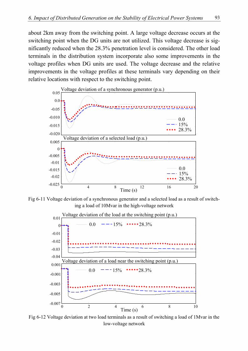
6. Impact of Distributed Generation on the Stability of Electrical Power Systems 93
about 2km away from the switching point. A large voltage decrease occurs at the switching point when the DG units are not utilized. This voltage decrease is sig-nificantly reduced when the 28.3% penetration level is considered. The other load terminals in the distribution system incorporate also some improvements in the voltage profiles when DG units are used. The voltage decrease and the relative improvements in the voltage profiles at these terminals vary depending on their relative locations with respect to the switching point.
Fig 6-11 Voltage deviation of a synchronous generator and a selected load as a result of switch-ing a load of 10Mvar in the high-voltage network
Fig 6-12 Voltage deviation at two load terminals as a result of switching a load of 1Mvar in the low-voltage network
-0.025
-0.02 -0.015
-0.01 -0.005
0.005
-0.020
-0.015
-0.010
-0.05
0.0
0.05
0
Time (s) 0 4 8 12 16 20
Voltage deviation of a synchronous generator (p.u.)
Voltage deviation of a selected load (p.u.)
0.0 15% 28.3%
0.0 15% 28.3%
-0.04
-0.03
-0.02
-0.01
0
0.01
0 2 4 6 8 10 -0.007
-0.005
-0.003
-0.001
0.001
Voltage deviation of the load at the switching point (p.u.)
Voltage deviation of a load near the switching point (p.u.)
0.0 15% 28.3%
Time (s)
0.0 15% 28.3%
6. Impact of Distributed Generation on the Stability of Electrical Power Systems 94
Generally, the analysis of the voltage performance shows that DG can support and improve the voltage profiles at load terminals. This can extend the stability margin of dynamic loads, i.e. induction motors, which can loss their stability with large voltage dips.
6.8 Conclusion This chapter addresses the impact of DG with different penetration levels on
the stability of power systems. A hypothetical network with two conventional power plants and many DG units is simulated. Based on the results and discus-sion, it can be concluded that DG can improve the stability of power systems if suitable types and appropriate locations are selected. Regarding the oscillatory stability, the utilization of DG improves the damping of the electromechanical modes and slightly increases their frequency. This fact is confirmed through the time-domain simulation of some disturbances. The transient stability analysis shows that the maximum power-angle deviations between the generators are de-creased with the increase of the penetration level of the DG units. However, the disconnection of some DG units when the voltage decreases lower than 80% of the nominal value represents an additional disturbance to the network. With more power from the DG units, the absolute reserve power from synchronous genera-tors and the network inertia constant are smaller due to the lower rated power of the rotating synchronous generators. As a result, the frequency response shows faster behaviour with higher maximum-frequency deviations when more DG units are employed. The voltage profiles at load terminals are also improved due to the use of active DG sources near end-user terminals. The controllers designed to regulate the performance of the DG units participate also in improving the voltage stability of the network. To maximize the benefits behind utilizing DG units, the stability of the individual DG units themselves has to be improved to ensure their continuous and reliable operation to provide effective support to the stability of the entire network.
Chapter 7
Online Management of DG Units for Residential Applications
7
7.1 Introduction One of the important applications of DG units, where FCs and MTs are particu-
larly suitable, is the utilization of small-modular commercial or residential units for onsite service. In this case, the capacity of the DG unit can be chosen to cover most of the load demand most of the time, where the surplus/shortage is exported to/imported from the main grid system. Thus, the reduction of energy price is be-coming increasingly important in order to bring DG units to competition with the main-grid system [30]. To decrease the generation cost, both the capital and the operating costs should be reduced. Therefore, the operation of the DG units has to be properly managed to reduce the operating cost to the minimum level. This re-duction in the operating cost can significantly contribute in decreasing the total energy price and, as a result, improving the economic feasibility of these units. Among the different types of FCs, the PEMFCs have approved good features es-pecially for low-capacity applications [72]. PEMFCs are candidates to be used in many fields because of their quick start-up characteristics and high power densi-ties, which reduced the required accommodation place.
The management of DG units requires an accurate economic model to describe
the operating cost of the unit taking into account both electrical and thermal rela-tions. Such a model is discontinuous and nonlinear in nature and, hence, necessi-tates the utilization of a robust optimization tool. The GA has proven high capa-bilities for handling such optimization problems because of its flexibility and ro-bustness [73]. Obviously, the optimized settings will be valid only for certain op-erating conditions and have to be recomputed after each variation. However, the optimization process, which can be carried out only in the offline mode, is a complicated and a time-consuming task and, therefore, requires high computa-tional capabilities. It is important to standardize a simple management method, which is probably adapted by the manufacturer and has to be online and locally updated by the operator. Therefore, a generalization framework has to be applied to extend the optimization results in a generic form. The ANN can be used for
7. Online Management of Fuel Cells for Residential Applications 96
this task due to its capabilities of learning and generalizing large scales of nonlin-earities by extracting system features using training data [48, 49]. Also, the Deci-sion Tree “DT” methodology can be employed as a nonparametric learning tech-nique, which is capable of deducing solutions for new unobserved cases [74, 75].
This chapter demonstrates a new-two-stage intelligent technique to manage the
operation of DG units for residential utilization. In the first stage, a GA is used to define the optimal settings of DG units depending on detailed economic models. This process is applied for three alternative scenarios: utilizing a single PEMFC, using three identical PEMFCs in parallel and utilizing a MT. For online applica-tions and to avoid the repetitive time-consuming optimization process, the proce-dure is generalized in the second stage using ANNs and DTs as two alternatives. The objective is to develop an intelligent management tool, which can be used in the online mode and depends only on the structure and parameters obtained from the second stage. The generalization process is applied only with the single PEMFC as it shows the most economic operation among the three alternatives.
7.2 Structure of the residential system The electrical and thermal load demands are supplied mainly by the DG. How-
ever, the shortage in electricity can be covered from the main grid system and the surplus of electricity can be sold back to the grid at different tariffs. The tariffs of sold and purchased electricity vary from one market to the other and from one season to the other. Two energy meters can separately measure the purchased and the sold electricity from/to the grid system. The thermal energy produced in the DG unit(s) is utilized for water and space heating of the domestic building. The load is provided also by a natural-gas supply to compensate for expectable defi-ciencies in thermal production in the DG unit(s). Most natural gas suppliers offer several tariffs depending on the field of application (e.g. residential, commercial, industrial, electric generation... etc). The consumptions of natural gas by the DG unit and the thermal load are measured independently to calculate the cost of each part depending on its own tariff.
Fig 7-1 shows the structure of the residential system supplied by a single FC.
For simplicity, the auxiliary devices (e.g. dump-electric-and-thermal loads, pumps, fans... etc) are not illustrated in the figure. No electrical or thermal stor-age devices are assumed in the study as they may increase the capital cost of the system. At the same time, the maintenance and technical considerations of these devices may cause many difficulties to the operator.
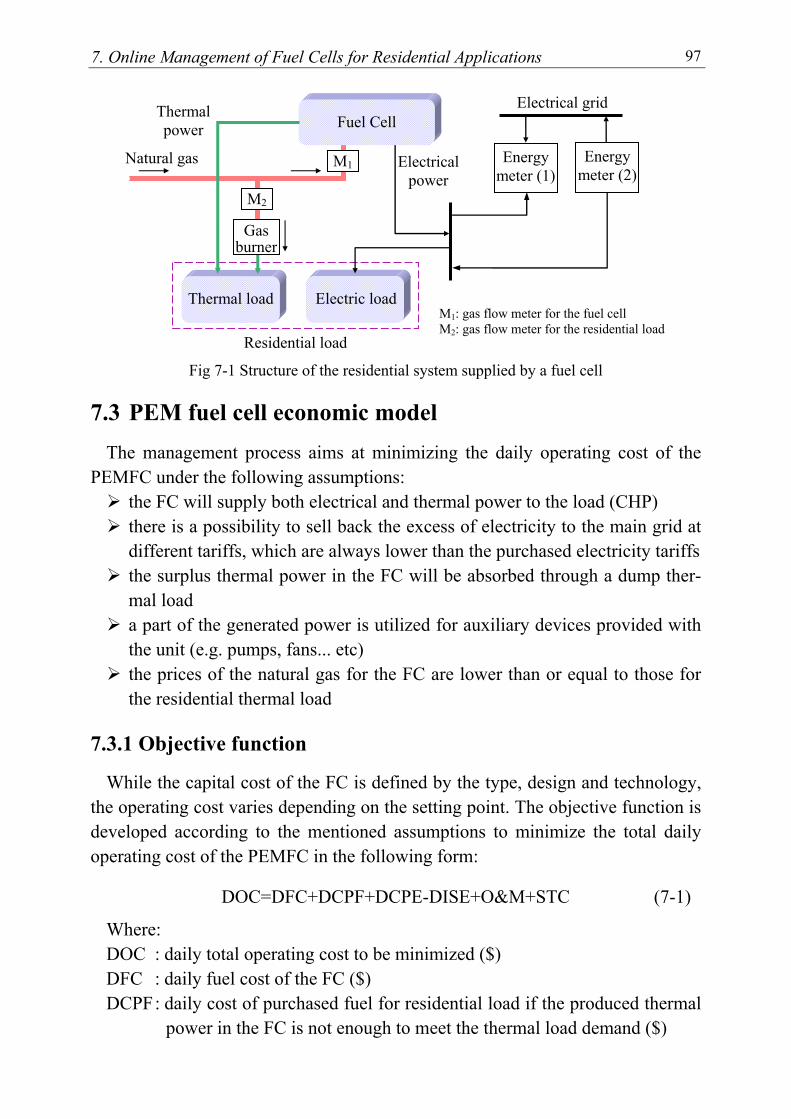
7. Online Management of Fuel Cells for Residential Applications 97
Fig 7-1 Structure of the residential system supplied by a fuel cell
7.3 PEM fuel cell economic model The management process aims at minimizing the daily operating cost of the
PEMFC under the following assumptions: the FC will supply both electrical and thermal power to the load (CHP) there is a possibility to sell back the excess of electricity to the main grid at different tariffs, which are always lower than the purchased electricity tariffs
the surplus thermal power in the FC will be absorbed through a dump ther-mal load
a part of the generated power is utilized for auxiliary devices provided with the unit (e.g. pumps, fans... etc)
the prices of the natural gas for the FC are lower than or equal to those for the residential thermal load
7.3.1 Objective function
While the capital cost of the FC is defined by the type, design and technology, the operating cost varies depending on the setting point. The objective function is developed according to the mentioned assumptions to minimize the total daily operating cost of the PEMFC in the following form:
DOC=DFC+DCPF+DCPE-DISE+O&M+STC (7-1)
Where: DOC : daily total operating cost to be minimized ($) DFC : daily fuel cost of the FC ($) DCPF : daily cost of purchased fuel for residential load if the produced thermal
power in the FC is not enough to meet the thermal load demand ($)
M1
M2
Fuel Cell
Electric load
Electrical grid
Natural gas
Residential load
Thermal power
Thermal load M1: gas flow meter for the fuel cell M2: gas flow meter for the residential load
Electrical power
Energy meter (1)
Energy meter (2)
Gas burner
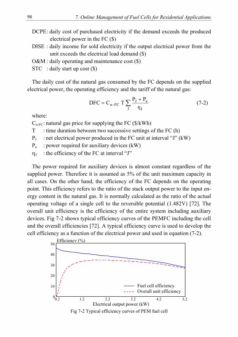
7. Online Management of Fuel Cells for Residential Applications 98
DCPE : daily cost of purchased electricity if the demand exceeds the produced electrical power in the FC ($)
DISE : daily income for sold electricity if the output electrical power from the unit exceeds the electrical load demand ($)
O&M : daily operating and maintenance cost ($) STC : daily start up cost ($) The daily cost of the natural gas consumed by the FC depends on the supplied
electrical power, the operating efficiency and the tariff of the natural gas:
∑+
=J J
aJFC-n η
PP T CDFC (7-2)
where: Cn-FC : natural gas price for supplying the FC ($/kWh) T : time duration between two successive settings of the FC (h) PJ : net electrical power produced in the FC unit at interval “J” (kW) Pa : power required for auxiliary devices (kW) ηJ : the efficiency of the FC at interval “J” The power required for auxiliary devices is almost constant regardless of the
supplied power. Therefore it is assumed as 5% of the unit maximum capacity in all cases. On the other hand, the efficiency of the FC depends on the operating point. This efficiency refers to the ratio of the stack output power to the input en-ergy content in the natural gas. It is normally calculated as the ratio of the actual operating voltage of a single cell to the reversible potential (1.482V) [72]. The overall unit efficiency is the efficiency of the entire system including auxiliary devices. Fig 7-2 shows typical efficiency curves of the PEMFC including the cell and the overall efficiencies [72]. A typical efficiency curve is used to develop the cell efficiency as a function of the electrical power and used in equation (7-2).
Fig 7-2 Typical efficiency curves of PEM fuel cell
0 10
20
30
40
50
Fuel cell efficiency Overall unit efficiency
0.2 1.2 2.2 3.2 4.2 5.2 Electrical output power (kW)
Efficiency (%)
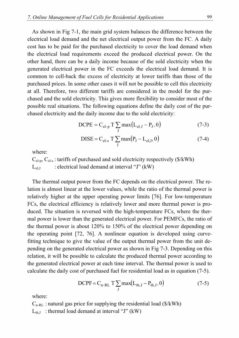
7. Online Management of Fuel Cells for Residential Applications 99
As shown in Fig 7-1, the main grid system balances the difference between the electrical load demand and the net electrical output power from the FC. A daily cost has to be paid for the purchased electricity to cover the load demand when the electrical load requirements exceed the produced electrical power. On the other hand, there can be a daily income because of the sold electricity when the generated electrical power in the FC exceeds the electrical load demand. It is common to cell-back the excess of electricity at lower tariffs than those of the purchased prices. In some other cases it will not be possible to cell this electricity at all. Therefore, two different tariffs are considered in the model for the pur-chased and the sold electricity. This gives more flexibility to consider most of the possible real situations. The following equations define the daily cost of the pur-chased electricity and the daily income due to the sold electricity:
( )∑ −=J
JJel p-el 0 PLmax TCDCPE ,, (7-3)
( )∑ −=J
el,JJs-el 0 ,LPmax T CDISE (7-4)
where: Cel-p, Cel-s : tariffs of purchased and sold electricity respectively ($/kWh) Lel,J : electrical load demand at interval “J” (kW) The thermal output power from the FC depends on the electrical power. The re-
lation is almost linear at the lower values, while the ratio of the thermal power is relatively higher at the upper operating power limits [76]. For low-temperature FCs, the electrical efficiency is relatively lower and more thermal power is pro-duced. The situation is reversed with the high-temperature FCs, where the ther-mal power is lower than the generated electrical power. For PEMFCs, the ratio of the thermal power is about 120% to 150% of the electrical power depending on the operating point [72, 76]. A nonlinear equation is developed using curve-fitting technique to give the value of the output thermal power from the unit de-pending on the generated electrical power as shown in Fig 7-3. Depending on this relation, it will be possible to calculate the produced thermal power according to the generated electrical power at each time interval. The thermal power is used to calculate the daily cost of purchased fuel for residential load as in equation (7-5).
( )∑ −=J
JthJthRL-n 0 PLmax T CDCPF ,,, (7-5)
where: Cn-RL : natural gas price for supplying the residential load ($/kWh) Lth,J : thermal load demand at interval “J” (kW)
7. Online Management of Fuel Cells for Residential Applications 100
Pth,J : thermal power produced in the FC at interval “J” (kW)
Fig 7-3 Relation between the thermal and the electrical power in the FC The operating and maintenance cost (O&M) is assumed to be in proportional
with the produced energy, where the proportional constant is ( MOK & ).
∑=J
JMO P T KO&M & (7-6)
The start-up cost depends on the temperature of the unit and consequently on the time terminated where the unit was in the off mode before starting it up once again [77].
−⋅β+α= τ
− offT
h e1STC (7-7)
where: αh : hot start up cost αh+β : cold start up cost Toff : the time terminated where the unit was in the off mode (h) τ : the FC cooling time constant (h) The fuel and electricity tariffs (i.e. Cn-FC, Cn-RL, Cel-p and Cel-s) in the presented
model represent the four decision variables, which affect the optimal settings of the FC.
7.3.2 Constraints
The operation of the FC to supply the residential load is restricted by many limitations. Mathematically, the minimization of the objective function (7-1) is limited by the following operational and technical constraints:
0.0 0.5 1 1.5 2 2.5 3 3.5 4
Thermal power (kW)
Electrical power (kW) 0 1 2 3 4 5 6 7
7. Online Management of Fuel Cells for Residential Applications 101
Upper and lower capacity constraints: Pmin ≤ PJ ≤ Pmax (7-8)
Constraints of upper ramp rate: U1J,t-J,t ∆P-PP ≤ (7-9)
Constraints of lower ramp rate: DJ,t1J,t- ∆P-PP ≤ (7-10)
where: Pmin, Pmax : the minimum and maximum limits of the generated power respect. ∆PU, ∆PD : the upper and lower limits of the ramp rate respectively PJ,t-1 : the power generated at interval “t-1”
Once the FC unit is switched on, it has to operate continuously at least for a certain minimum time before switching it off again. On the other hand, a certain stop time has to be terminated before starting the unit. The violation of such con-straints can cause shortness in the life time of the unit. These constraints are for-mulated as continuous running/stop time constraint as follows:
( ) ( ) 0UUMRTT ts1tson
1t ≥−⋅− −− ,, (7-11)
( ) ( ) 0UUMSTT 1tstsoff
1t ≥−⋅− −− ,, (7-12)
where: on
1tT − , off1tT − : the FC running and stop periods at time interval “t-1” respect. (h)
MRT, MST : the minimum running and stop periods of the FC respectively (h) Us : the unit on/off status: Us=1 for running mode and 0 for stop mode Finally, the number of starts and stops per day (nstart-stop) should not exceed a
certain maximum number (Nmax).
nstart-stop ≤ Nmax (7-13)
The parameters used in the FC economic model are given in appendix E.
7.4 Multi-population real-coded genetic algorithm The model of the FC presented in the previous section requires a special opti-
mization tool to handle the discontinuity and nonlinearity of such highly-constrained model. Most of the deterministic optimization methods are not suit-able to simulate and solve the presented optimization problem due to many simu-lation difficulties. The GA is a probabilistic intelligent search algorithm, which searches a population of points in parallel [48, 78]. Basically, GA differs from other traditional optimization methods in three significant points. It searches a

7. Online Management of Fuel Cells for Residential Applications 102
population of points in parallel, it uses probabilistic rules rather than determinis-tic ones, and it can process an encoding set of parameters. The real coding is used in this research since it provides better performance and faster conversion com-pared to other coding methods [73]. With other coding, it is required to alternate to the real coding in the phase of calculating the total daily cost, which results in additional processing time.
7.4.1 Constraints representation
To employ GA with a tightly-constrained problem, such as the economic model of the FC, it is possible to generate only feasible solutions by avoiding individu-als which violate the given constraints. Since the infeasible solutions mostly cover the search space at the initial generation, the complete avoidance of the in-feasible solutions gives a high possibility for missing the area of global minimum [73]. Another approach is to move the infeasible individuals to the nearest feasi-ble area. For the highly-constrained problem, this would be too complex and a very time consuming process. The penalty function approach is another alterna-tive that converts the constrained problem to an unconstrained one by augmenting additional cost terms with the main objective function. The additional terms as-sign nonlinear costs for solutions that violate the constraints depending on their relative locations with respect to the feasibility boundaries [73].
The adequate choice of the penalty functions and their parameters is an essen-
tial requirement to achieve rapid rejection of the infeasible solutions. It is neces-sary for this approach to differentiate in performance between the infeasible indi-viduals themselves, which will help in the evolution process. To ensure fast rejec-tion of the solutions that violate the constraints, a higher cost value has to be as-signed to any infeasible solution than the feasible members. In this research, ex-ponential penalty factors are used for ramp rate violation, while quadratic ones are applied when violating the constraints of minimum running/stop periods and maximum number of starts and stops per day.
7.4.2 Evolution process
The GA searches for the global optimum value of the objective function through a search space, which is called population. The population is constituted from a number of possible solutions known as individuals. Each individual, which is also called chromosome, represents a definite scenario of the output electrical power from the FC through one day. It is assumed that the setting of the FC is updated each 15 minutes and, thus, 96 unknown variables are associated
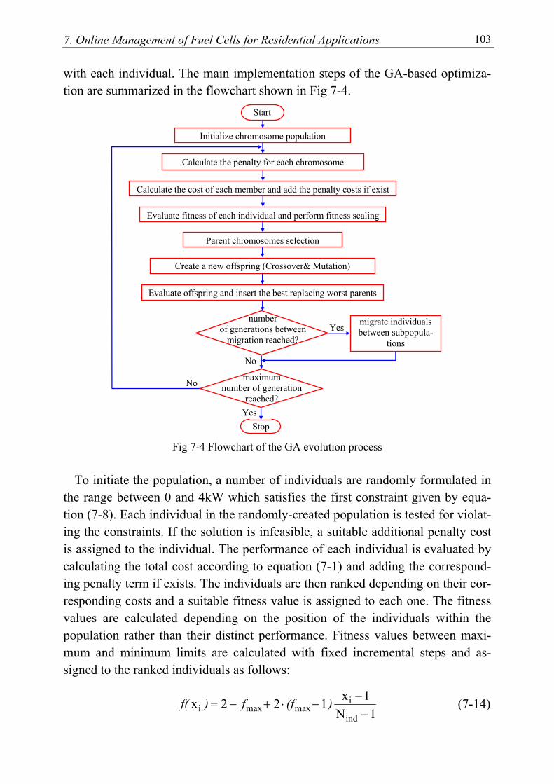
7. Online Management of Fuel Cells for Residential Applications 103
with each individual. The main implementation steps of the GA-based optimiza-tion are summarized in the flowchart shown in Fig 7-4.
Fig 7-4 Flowchart of the GA evolution process To initiate the population, a number of individuals are randomly formulated in
the range between 0 and 4kW which satisfies the first constraint given by equa-tion (7-8). Each individual in the randomly-created population is tested for violat-ing the constraints. If the solution is infeasible, a suitable additional penalty cost is assigned to the individual. The performance of each individual is evaluated by calculating the total cost according to equation (7-1) and adding the correspond-ing penalty term if exists. The individuals are then ranked depending on their cor-responding costs and a suitable fitness value is assigned to each one. The fitness values are calculated depending on the position of the individuals within the population rather than their distinct performance. Fitness values between maxi-mum and minimum limits are calculated with fixed incremental steps and as-signed to the ranked individuals as follows:
1N
1x 122xind
imaxmaxi −
−−⋅+−= )(ff)f( (7-14)
Initialize chromosome population
Calculate the cost of each member and add the penalty costs if exist
Evaluate fitness of each individual and perform fitness scaling
Parent chromosomes selection
Create a new offspring (Crossover& Mutation)
Stop
Evaluate offspring and insert the best replacing worst parents
number of generations between
migration reached?
No
No
Yes
Yes
migrate individuals between subpopula-
tions
Calculate the penalty for each chromosome
Start
maximum number of generation
reached?

7. Online Management of Fuel Cells for Residential Applications 104
where: f(xi) : the fitness value of the individual with a position (xi) in the population
fmax : maximum fitness value (typically has a value between 1.1 and 2.0) Nind : number of the individuals within the population The fitness scaling represents a basic step to select parents to create new off-
springs. Strings with higher fitness are selected using the roulette wheel tech-nique and used in the recombination process [48]. With “N” required selections, “N” equally spaced pointers can be used instead of a single selection pointer, which is conventionally employed in the classical roulette wheel method. This idea is shown in Fig 7-5 with 9 individuals and 8 pointers.
Fig 7-5 Roulette wheel selection
The new generation is produced by means of two main processes: crossover
and mutation. Crossover is a genetic process by which information can be ex-changed between the members of the population, possibly creating more highly fit members. For the real-valued encoding, the max-min arithmetical crossover operator is used as follows [73]:
( ) 2s1s1 P1PG ⋅α−+⋅α= (7-15)
( ) 2s1s2 PP1G ⋅α+⋅α−= (7-16)
where: G1, G2 : the new generation “strings” of individuals P1, P2 : the parents selected using the roulette wheel technique αs : a scaling factor Mutation is the second process in the recombination, which is used to escape
from possible local minima. The mutation in the real-coded representations is ac-complished by disturbing the gene values with low probability [73].
1
12
13
456
7
8
9Pointers Individuals
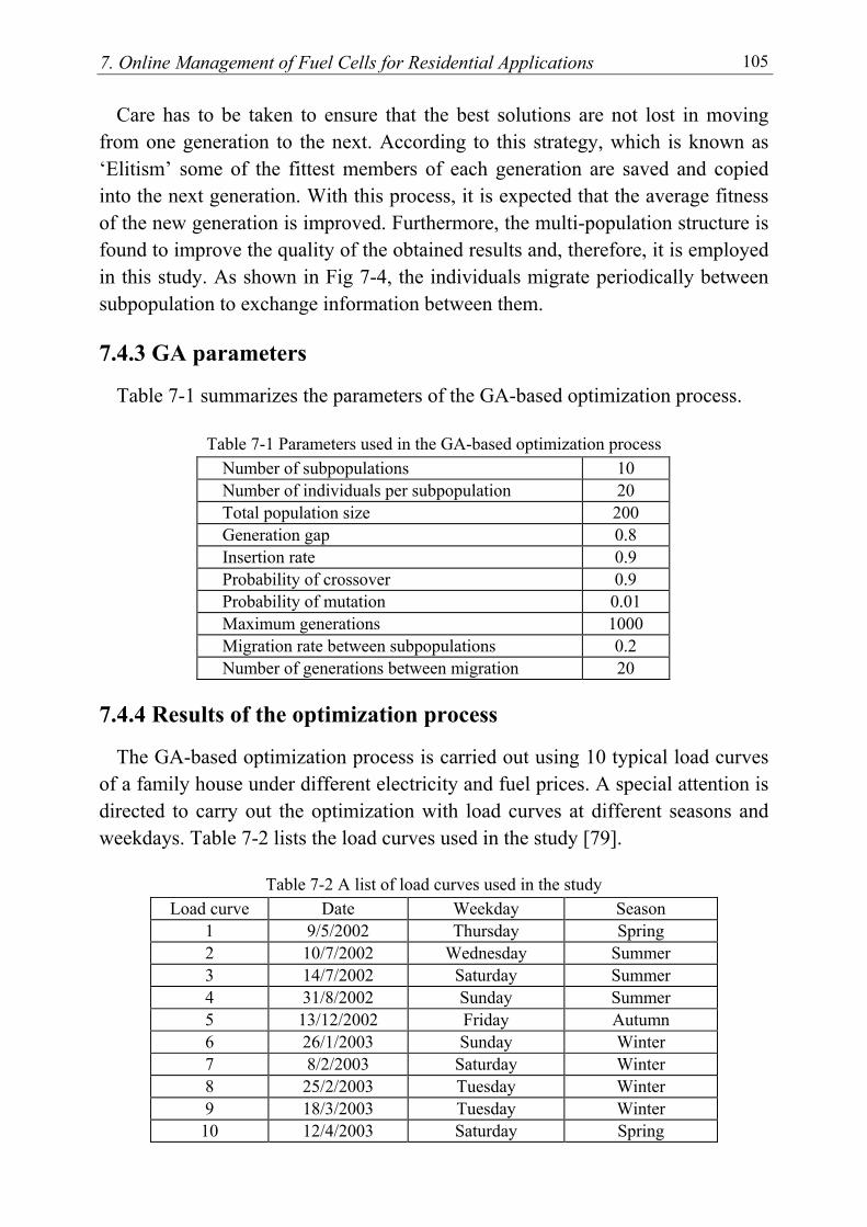
7. Online Management of Fuel Cells for Residential Applications 105
Care has to be taken to ensure that the best solutions are not lost in moving from one generation to the next. According to this strategy, which is known as ‘Elitism’ some of the fittest members of each generation are saved and copied into the next generation. With this process, it is expected that the average fitness of the new generation is improved. Furthermore, the multi-population structure is found to improve the quality of the obtained results and, therefore, it is employed in this study. As shown in Fig 7-4, the individuals migrate periodically between subpopulation to exchange information between them.
7.4.3 GA parameters
Table 7-1 summarizes the parameters of the GA-based optimization process.
Table 7-1 Parameters used in the GA-based optimization process Number of subpopulations 10 Number of individuals per subpopulation 20 Total population size 200 Generation gap 0.8 Insertion rate 0.9 Probability of crossover 0.9 Probability of mutation 0.01 Maximum generations 1000 Migration rate between subpopulations 0.2 Number of generations between migration 20
7.4.4 Results of the optimization process
The GA-based optimization process is carried out using 10 typical load curves of a family house under different electricity and fuel prices. A special attention is directed to carry out the optimization with load curves at different seasons and weekdays. Table 7-2 lists the load curves used in the study [79].
Table 7-2 A list of load curves used in the study
Load curve Date Weekday Season 1 9/5/2002 Thursday Spring 2 10/7/2002 Wednesday Summer 3 14/7/2002 Saturday Summer 4 31/8/2002 Sunday Summer 5 13/12/2002 Friday Autumn 6 26/1/2003 Sunday Winter 7 8/2/2003 Saturday Winter 8 25/2/2003 Tuesday Winter 9 18/3/2003 Tuesday Winter 10 12/4/2003 Saturday Spring
7. Online Management of Fuel Cells for Residential Applications 106
Fig 7-6 and Fig 7-7 show two examples for the optimal settings of the FC with the load curve number (8). In the first case, no electricity is sold back to the main grid. In this case, the output power covers the electrical demand and a part of the thermal demand. In the second case, the excess of electricity is sold back for 0.07$/kWh. This gives the possibility to produce more electrical power and to cover the thermal load demand. In both cases, the other three tariffs are kept con-stant as shown in the following table:
Cn-FC Cn-RL Cel-p 0.03$/kWh 0.05$/kWh 0.12$/kWh
Fig 7-6 Unit optimal output power without selling electricity
Fig 7-7 Unit optimal output power when selling electricity for 0.07$/kWh
To evaluate the effect of varying the four tariffs on the optimal settings, some comparisons are given in Fig 7-8 through Fig 7-11 for load curve (1). One tariff is changed each time, while the others are held constant. Fig 7-8 shows the effect of varying the sold-electricity tariff with the other tariffs kept constant as follows:
0 4 8 12 16 20 240
Time (h) Time (h)
Electrical power (kW)
1
2
3
4
5 10Load demand Optimal setting
0
Thermal power (kW)
2
4
6
8
0 4 8 12 16 20 24
Load demand Optimal setting
0
1
2
3
4
5
6 Electrical power (kW) Thermal power (kW)
0 4 8 12 16 20 24Time (h) Time (h)
10
0
2
4
6
8
0 4 8 12 16 20 24
Load demand Optimal setting
Load demand Optimal setting

7. Online Management of Fuel Cells for Residential Applications 107
Cn-FC Cn-RL Cel-p 0.03$/kWh 0.05$/kWh 0.12$/kWh
With lower values of the sold-electricity tariff, the FC follows up the electrical
load demand, while thermal load demand impacts the optimal settings more than the electrical demand with intermediate values (i.e. 0.07$/kWh). At higher values of the sold electricity tariff, the optimal scenario is to produce electrical power that exceeds the 2.35kW level over the whole day.
Fig 7-8 Effect of varying the sold electricity tariff Fig 7-9 depicts the effect of varying the purchased-electricity tariff for the same
load curve, while the other tariffs are given as follows:
Cn-FC Cn-RL Cel-s 0.05$kWh 0.09$/kWh 0.1$/kWh
Fig 7-9 Effect of varying the purchase electricity tariff
Load demand 0.0$/kWh 0.07$/kWh 0.1$/kWh
0
1
2
3
4 Electrical power (kW) Thermal power (kW)
0 4 8 12 16 20 24Time (h) Time (h)
0
2
4
6
8
0 4 8 12 16 20 24
Load demand 0.12$/kWh 0.16$/kWh
0
1
2
3
4 Electrical power (kW) Thermal power (kW)
0 4 8 12 16 20 24Time (h) Time (h)
0
2
4
6
8
0 4 8 12 16 20 24
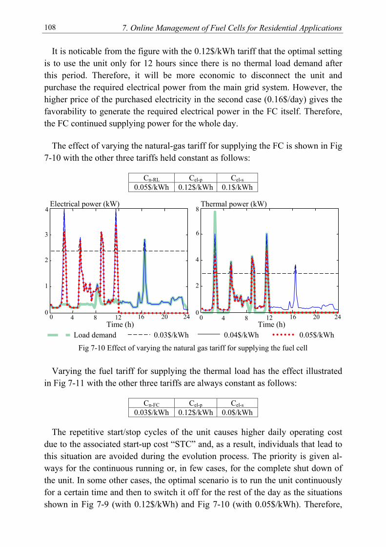
7. Online Management of Fuel Cells for Residential Applications 108
It is noticable from the figure with the 0.12$/kWh tariff that the optimal setting is to use the unit only for 12 hours since there is no thermal load demand after this period. Therefore, it will be more economic to disconnect the unit and purchase the required electrical power from the main grid system. However, the higher price of the purchased electricity in the second case (0.16$/day) gives the favorability to generate the required electrical power in the FC itself. Therefore, the FC continued supplying power for the whole day.
The effect of varying the natural-gas tariff for supplying the FC is shown in Fig
7-10 with the other three tariffs held constant as follows:
Cn-RL Cel-p Cel-s 0.05$/kWh 0.12$/kWh 0.1$/kWh
Fig 7-10 Effect of varying the natural gas tariff for supplying the fuel cell
Varying the fuel tariff for supplying the thermal load has the effect illustrated in Fig 7-11 with the other three tariffs are always constant as follows:
Cn-FC Cel-p Cel-s
0.03$/kWh 0.12$/kWh 0.0$/kWh The repetitive start/stop cycles of the unit causes higher daily operating cost
due to the associated start-up cost “STC” and, as a result, individuals that lead to this situation are avoided during the evolution process. The priority is given al-ways for the continuous running or, in few cases, for the complete shut down of the unit. In some other cases, the optimal scenario is to run the unit continuously for a certain time and then to switch it off for the rest of the day as the situations shown in Fig 7-9 (with 0.12$/kWh) and Fig 7-10 (with 0.05$/kWh). Therefore,
Load demand 0.03$/kWh 0.04$/kWh 0.05$/kWh
0
1
2
3
Thermal power (kW)
0 4 8 12 16 20 24Time (h) Time (h)
0
2
4
6
0 4 8 12 16 20 24
4 8Electrical power (kW)
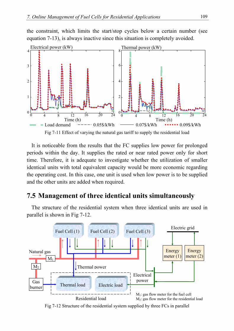
7. Online Management of Fuel Cells for Residential Applications 109
the constraint, which limits the start/stop cycles below a certain number (see equation 7-13), is always inactive since this situation is completely avoided.
Fig 7-11 Effect of varying the natural gas tariff to supply the residential load It is noticeable from the results that the FC supplies low power for prolonged
periods within the day. It supplies the rated or near rated power only for short time. Therefore, it is adequate to investigate whether the utilization of smaller identical units with total equivalent capacity would be more economic regarding the operating cost. In this case, one unit is used when low power is to be supplied and the other units are added when required.
7.5 Management of three identical units simultaneously The structure of the residential system when three identical units are used in
parallel is shown in Fig 7-12.
Fig 7-12 Structure of the residential system supplied by three FCs in parallel
Load demand 0.05$/kWh 0.07$/kWh 0.09$/kWh
0
1
2
3
Electrical power (kW) Thermal power (kW)
0 4 8 12 16 20 24Time (h) Time (h)
0
2
4
6
0 4 8 12 16 20 24
4 8
M2
Electric load
Electric grid
Natural gas
Residential load
Thermal power
Thermal load
M1: gas flow meter for the fuel cell M2: gas flow meter for the residential load
Electrical power
Energy meter (2)M1
Fuel Cell (2)Fuel Cell (1) Fuel Cell (3)
Energy meter (1)
Gas burner
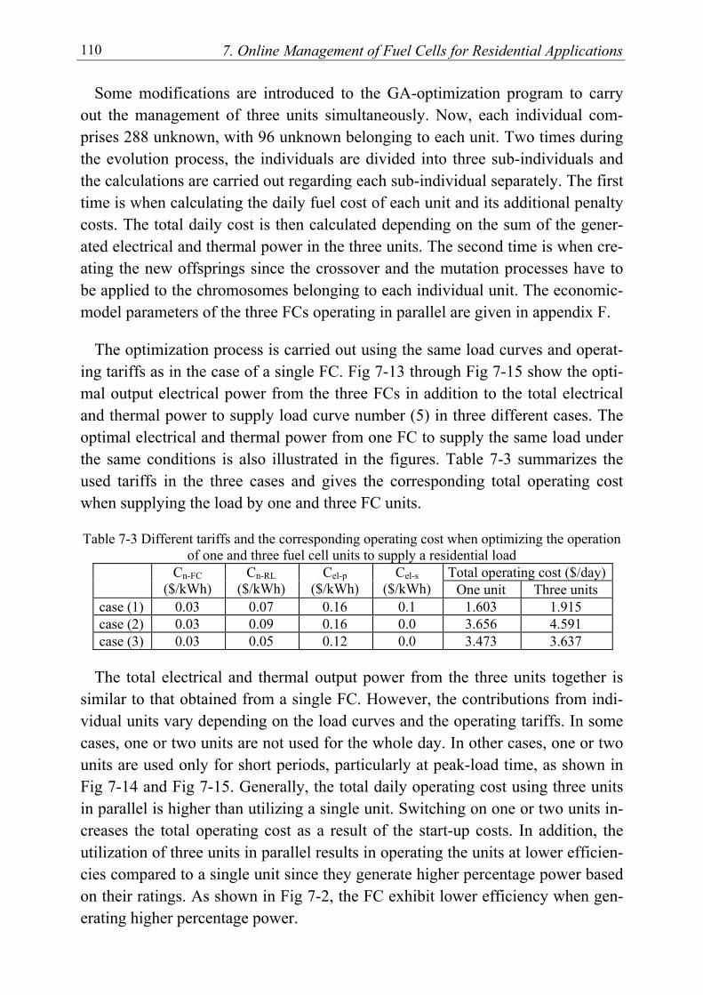
7. Online Management of Fuel Cells for Residential Applications 110
Some modifications are introduced to the GA-optimization program to carry out the management of three units simultaneously. Now, each individual com-prises 288 unknown, with 96 unknown belonging to each unit. Two times during the evolution process, the individuals are divided into three sub-individuals and the calculations are carried out regarding each sub-individual separately. The first time is when calculating the daily fuel cost of each unit and its additional penalty costs. The total daily cost is then calculated depending on the sum of the gener-ated electrical and thermal power in the three units. The second time is when cre-ating the new offsprings since the crossover and the mutation processes have to be applied to the chromosomes belonging to each individual unit. The economic-model parameters of the three FCs operating in parallel are given in appendix F.
The optimization process is carried out using the same load curves and operat-ing tariffs as in the case of a single FC. Fig 7-13 through Fig 7-15 show the opti-mal output electrical power from the three FCs in addition to the total electrical and thermal power to supply load curve number (5) in three different cases. The optimal electrical and thermal power from one FC to supply the same load under the same conditions is also illustrated in the figures. Table 7-3 summarizes the used tariffs in the three cases and gives the corresponding total operating cost when supplying the load by one and three FC units.
Table 7-3 Different tariffs and the corresponding operating cost when optimizing the operation
of one and three fuel cell units to supply a residential load Total operating cost ($/day) Cn-FC
($/kWh) Cn-RL
($/kWh) Cel-p
($/kWh) Cel-s
($/kWh) One unit Three units case (1) 0.03 0.07 0.16 0.1 1.603 1.915 case (2) 0.03 0.09 0.16 0.0 3.656 4.591 case (3) 0.03 0.05 0.12 0.0 3.473 3.637
The total electrical and thermal output power from the three units together is
similar to that obtained from a single FC. However, the contributions from indi-vidual units vary depending on the load curves and the operating tariffs. In some cases, one or two units are not used for the whole day. In other cases, one or two units are used only for short periods, particularly at peak-load time, as shown in Fig 7-14 and Fig 7-15. Generally, the total daily operating cost using three units in parallel is higher than utilizing a single unit. Switching on one or two units in-creases the total operating cost as a result of the start-up costs. In addition, the utilization of three units in parallel results in operating the units at lower efficien-cies compared to a single unit since they generate higher percentage power based on their ratings. As shown in Fig 7-2, the FC exhibit lower efficiency when gen-erating higher percentage power.
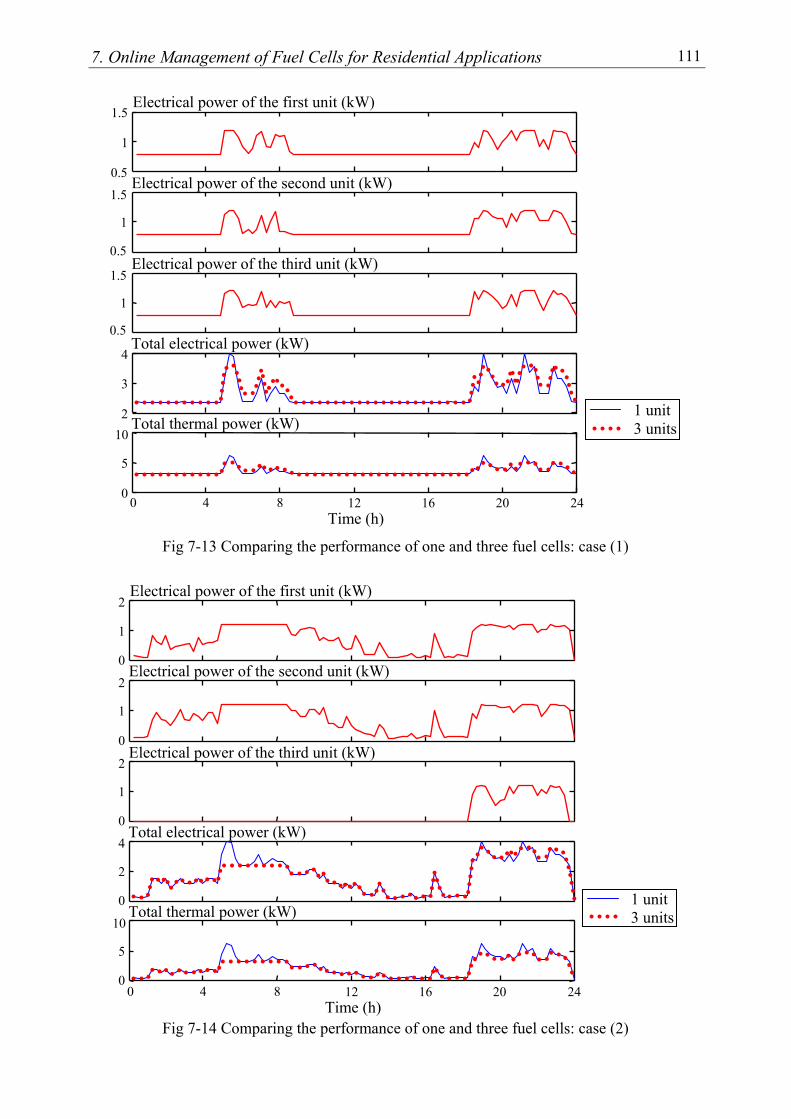
7. Online Management of Fuel Cells for Residential Applications 111
Fig 7-13 Comparing the performance of one and three fuel cells: case (1)
Fig 7-14 Comparing the performance of one and three fuel cells: case (2)
Time (h)
Electrical power of the first unit (kW)
Total thermal power (kW)
0.5
1
1.5
2
3
4
0 4 8 12 16 20 24 0
5
10
Electrical power of the second unit (kW)
Electrical power of the third unit (kW)
Total electrical power (kW)
0.5
1
1.5
0.5
1
1.5
1 unit 3 units
0
1
2
0
1
2
0
1
2
0
2
4
0
5
10
Time (h)
Electrical power of the first unit (kW)
Total thermal power (kW)
0 4 8 12 16 20 24
Electrical power of the second unit (kW)
Electrical power of the third unit (kW)
Total electrical power (kW)
1 unit 3 units
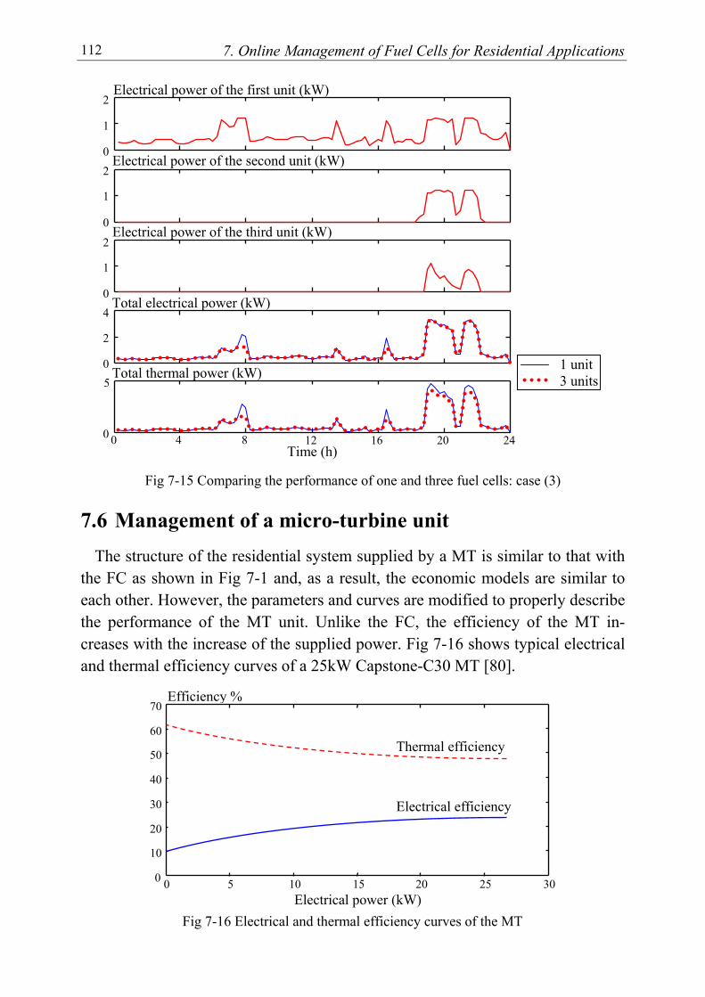
7. Online Management of Fuel Cells for Residential Applications 112
Fig 7-15 Comparing the performance of one and three fuel cells: case (3)
7.6 Management of a micro-turbine unit The structure of the residential system supplied by a MT is similar to that with
the FC as shown in Fig 7-1 and, as a result, the economic models are similar to each other. However, the parameters and curves are modified to properly describe the performance of the MT unit. Unlike the FC, the efficiency of the MT in-creases with the increase of the supplied power. Fig 7-16 shows typical electrical and thermal efficiency curves of a 25kW Capstone-C30 MT [80].
Fig 7-16 Electrical and thermal efficiency curves of the MT
0
1
2
0
1
2
0
1
2
0
2
4
0
5
Time (h)
Electrical power of the first unit (kW)
Total thermal power (kW)
0 4 8 12 16 20 24
Electrical power of the second unit (kW)
Electrical power of the third unit (kW)
Total electrical power (kW)
1 unit 3 units
Efficiency %
0
10
20
30
40
50
60
70
0 5 10 15 20 25 30 Electrical power (kW)
Thermal efficiency Electrical efficiency
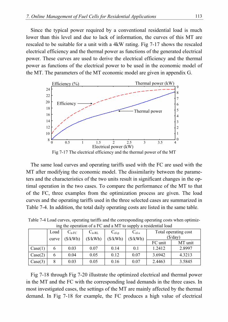
7. Online Management of Fuel Cells for Residential Applications 113
Since the typical power required by a conventional residential load is much lower than this level and due to lack of information, the curves of this MT are rescaled to be suitable for a unit with a 4kW rating. Fig 7-17 shows the rescaled electrical efficiency and the thermal power as functions of the generated electrical power. These curves are used to derive the electrical efficiency and the thermal power as functions of the electrical power to be used in the economic model of the MT. The parameters of the MT economic model are given in appendix G.
Fig 7-17 The electrical efficiency and the thermal power of the MT
The same load curves and operating tariffs used with the FC are used with the MT after modifying the economic model. The dissimilarity between the parame-ters and the characteristics of the two units result in significant changes in the op-timal operation in the two cases. To compare the performance of the MT to that of the FC, three examples from the optimization process are given. The load curves and the operating tariffs used in the three selected cases are summarized in Table 7-4. In addition, the total daily operating costs are listed in the same table.
Table 7-4 Load curves, operating tariffs and the corresponding operating costs when optimiz-
ing the operation of a FC and a MT to supply a residential load Total operating cost
($/day) Load
curve Cn-FC
($/kWh) Cn-RL
($/kWh) Cel-p
($/kWh) Cel-s
($/kWh) FC unit MT unit
Case(1) 6 0.03 0.07 0.14 0.1 1.2412 2.8997 Case(2) 6 0.04 0.05 0.12 0.07 3.6942 4.3213 Case(3) 8 0.03 0.05 0.16 0.07 2.4463 3.5845 Fig 7-18 through Fig 7-20 illustrate the optimized electrical and thermal power
in the MT and the FC with the corresponding load demands in the three cases. In most investigated cases, the settings of the MT are mainly affected by the thermal demand. In Fig 7-18 for example, the FC produces a high value of electrical
0 1 2 3 4 5 6 7 8 9
Thermal power (kW)
0 0.5 1 1.5 2 2.5 3 3.5 4 8 10 12 14
16 18 20
22 24
Efficiency (%)
Electrical power (kW)
Efficiency
Thermal power
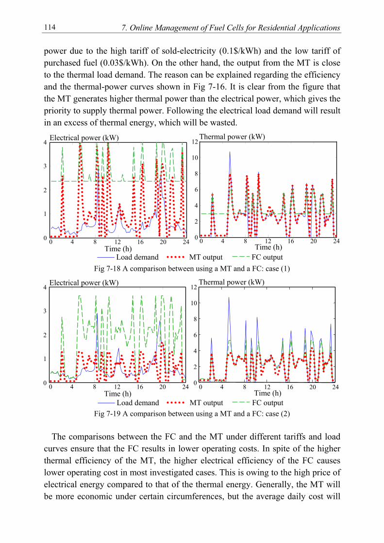
7. Online Management of Fuel Cells for Residential Applications 114
power due to the high tariff of sold-electricity (0.1$/kWh) and the low tariff of purchased fuel (0.03$/kWh). On the other hand, the output from the MT is close to the thermal load demand. The reason can be explained regarding the efficiency and the thermal-power curves shown in Fig 7-16. It is clear from the figure that the MT generates higher thermal power than the electrical power, which gives the priority to supply thermal power. Following the electrical load demand will result in an excess of thermal energy, which will be wasted.
Fig 7-18 A comparison between using a MT and a FC: case (1)
Fig 7-19 A comparison between using a MT and a FC: case (2)
The comparisons between the FC and the MT under different tariffs and load
curves ensure that the FC results in lower operating costs. In spite of the higher thermal efficiency of the MT, the higher electrical efficiency of the FC causes lower operating cost in most investigated cases. This is owing to the high price of electrical energy compared to that of the thermal energy. Generally, the MT will be more economic under certain circumferences, but the average daily cost will
Load demand MT output FC output
0 4 8 12 16 20 240
1
2
3
4 Electrical power (kW)
0
2
4
6
8
10
12 Thermal power (kW)
Time (h) 0 4 8 12 16 20 24
Time (h)
Load demand MT output FC output
0 4 8 12 16 20 240
1
2
3
4 Electrical power (kW)
0
2
4
6
8
10
12 Thermal power (kW)
Time (h) 0 4 8 12 16 20 24
Time (h)

7. Online Management of Fuel Cells for Residential Applications 115
be always lower with the FC. For special loads, which have high thermal and low electrical demands, MT units may be favourable in terms of operating costs.
Fig 7-20 A comparison between using a MT and a FC: case (3) To evaluate the potential reduction in the total daily operating cost when the
optimization process is applied, the results of optimizing a single FC, as the most economic choice among the three alternatives, are compared with three conven-tional settings. The first one is to operate the unit always at its rated power. The second and third cases are to follow up the electrical or thermal load demands respectively. Table 7-5 gives the average cost as well as the average difference of the three conventional settings with respect to the GA-based optimal case for one load curve under 81 different operating conditions.
Table 7-5 Average daily cost and average difference with respect to optimal case
Average difference with respect to optimal case Average cost($/day) Average difference
($/day) Average percentage
difference Optimal settings (from GA) Settings=rating Settings=electrical demand Settings=thermal demand
3.722 8.582 4.855 4.637
0.0 4.860 1.133 0.915
0.0 130.575 % 30.441 % 24.584 %
The high operating cost of the first conventional case indicates that this sce-
nario is not relevant. The high electrical power results in surplus thermal power, which is wasted since no thermal storage is assumed. The unit in the second and third scenarios will cover either the electrical or the thermal load demands and, therefore, the cost is relatively decreased. Following the optimal scenario can achieve a reduction of 0.915$/day (334$/year) compared to the best conventional settings. This represents a significant reduction not only in the operating cost of the FC but also in the total energy price. However, evaluating the optimization
Load demand MT output FC output
0 4 8 12 16 20 240
1
2
3
4 Electrical power (kW)
0
2
4
6
8
10
12 Thermal power (kW)
Time (h) 0 4 8 12 16 20 24
Time (h)
7. Online Management of Fuel Cells for Residential Applications 116
process depending on the best conventional settings alone is not fair and mislead-ing. The type and natural of load demands affect the results considerably. For other loads, following the thermal demand can be more expensive than other con-ventional choices. Therefore, various conventional settings have to be considered when evaluating the reduction achieved using the optimization process.
7.7 Generalizing the optimization for online employment Regardless the significant reduction in the daily operating cost, it is obvious
that the optimal output varies within the same day depending on the operating tariffs and the electrical and thermal demands. Therefore, it is obligatory to repeat the management process everyday and also with each variation in the operating tariffs. This restricts the online application of the optimization process, especially in liberal markets with the frequently variations of the operating tariffs. The ob-jective behind extending the management process through a generalization stage is to overcome the time-consuming problem characterizing the GA-based optimi-zation and to enable the online application of the approach. The generalization is carried out only for the single FC as the most economic alternative as discussed in the previous section. Two techniques are employed to accomplish the generali-zation process: ANNs and DTs.
7.7.1 ANN-based generalization
An ANN is used to generalize the results obtained in the first stage due to its high capability of generalizing such nonlinear complicated problems [48, 49]. After training and testing the ANN, it will be prepared for the onsite application to define the settings of the FC in the online mode. A simple hardware can be de-veloped based on the structure and parameters of the ANN to define the optimal or quasi-optimal settings of the unit.
7.7.1.1 Neural network structure
Beside the input and output layers, the ANN comprises also three hidden lay-ers, which gives the best results among the other structures experimented in this research. The number of neurons in the first, second, and third hidden layers are 40, 30, and 20 neurons respectively. Tanh-sigmoid transfer functions are used as activation functions for all neurons in the hidden layers, while a log-sigmoid transfer function is used for the output neuron. The nodes in the input layer re-ceive 54 inputs, while a single output is obtained at the output layer. The inputs to the network include two different natural gas tariffs for supplying the FC and the
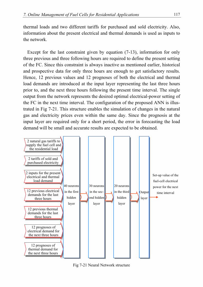
7. Online Management of Fuel Cells for Residential Applications 117
thermal loads and two different tariffs for purchased and sold electricity. Also, information about the present electrical and thermal demands is used as inputs to the network.
Except for the last constraint given by equation (7-13), information for only
three previous and three following hours are required to define the present setting of the FC. Since this constraint is always inactive as mentioned earlier, historical and prospective data for only three hours are enough to get satisfactory results. Hence, 12 previous values and 12 prognoses of both the electrical and thermal load demands are introduced at the input layer representing the last three hours prior to, and the next three hours following the present time interval. The single output from the network represents the desired optimal electrical-power setting of the FC in the next time interval. The configuration of the proposed ANN is illus-trated in Fig 7-21. This structure enables the simulation of changes in the natural gas and electricity prices even within the same day. Since the prognosis at the input layer are required only for a short period, the error in forecasting the load demand will be small and accurate results are expected to be obtained.
Fig 7-21 Neural Network structure
Set-up value of the
fuel-cell electrical
power for the next
time interval
2 inputs for the present electrical and thermal
load demand
12 previous electrical demands for the last
three hours
12 previous thermal demands for the last
three hours
12 prognoses of thermal demand for the next three hours
12 prognoses of electrical demand for the next three hours
2 natural gas tariffs to supply the fuel cell and
the residential load
2 tariffs of sold and purchased electricity
40 neurons
in the first
hidden
layer
30 neurons
in the sec-
ond hidden
layer
20 neurons
in the third
hidden
layer
Output
layer

7. Online Management of Fuel Cells for Residential Applications 118
7.7.1.2 Training process
The results obtained from the optimization process are managed and suitable patterns are extracted. Results corresponding to eight load curves are used in the training process, while results regarding another load curve are kept for testing the trained network. For each one of the four operating tariffs, between three and four different values are used with each load curve, resulting in more than 56000 patterns. The online back propagation approach is followed in the training proc-ess, where the weights are updated after the representation of each pattern. The training is carried out for more than 1000 epochs to ensure high accuracy in the training process.
To evaluate the effectiveness of the training process, Fig 7-22 through Fig 7-24
illustrate three comparisons between the optimal targets as obtained from the GA-based optimization and the output from the ANN. The three cases correspond to different load curves and operating tariffs as listed in the following table.
Total operating cost ($/day) Load
curve Cn-FC
($/kWh) Cn-RL
($/kWh) Cel-p
($/kWh)Cel-s
($/kWh) GA-based settings ANN settings Case 1 2 0.05 0.07 0.12 0.1 2.413 2.481 Case 2 3 0.04 0.09 0.14 0.04 2.233 2.303 Case 3 4 0.03 0.05 0.16 0.0 2.041 2.088
Fig 7-22 Comparing the ANN output with the optimal target: case (1) The agreement between the ANN-based settings and the GA-based optimal tar-
get reflects the high accuracy of the training process, ensuring the high capability of the ANN to extract the features of the optimal performance.
GA-based optimal settings Output from ANN
0 4 8 12 16 20 240
1
2
3
4 Electrical power (kW)
0
2
4
6
8
10 Thermal power (kW)
Time (h) 0 4 8 12 16 20 24
Time (h)

7. Online Management of Fuel Cells for Residential Applications 119
Fig 7-23 Comparing the ANN output with the optimal target: case (2)
Fig 7-24 Comparing the ANN output with the optimal target: case (3)
7.7.1.3 Testing the trained neural network
In the testing phase, the trained ANN is activated by new testing data to verify the generalization capability of the network. Load curve number (8), which is not used in the training process, is used to test the trained network at different fuel and electricity tariffs. This includes 81 different investigated cases with a total number of 7776 patterns. Fig 7-25 through Fig 7-27 illustrate three selected com-parisons between the optimal target and the ANN-based settings as obtained from the test results. The different tariffs and the corresponding daily operating cost in each case are given in the following table.
00
1
2
3
4
GA-based optimal settings Output from ANN Time (h)
4 8 12 16 20 24
Electrical power (kW)
0
6Thermal power (kW)
0 4 8 12 16 20 24Time (h)
2
4
GA-based optimal settings Output from ANN
0 4 8 12 16 20 240
1
2
3
4 Electrical power (kW)
0
6Thermal power (kW)
Time (h) 0 4 8 12 16 20 24
Time (h)
2
4
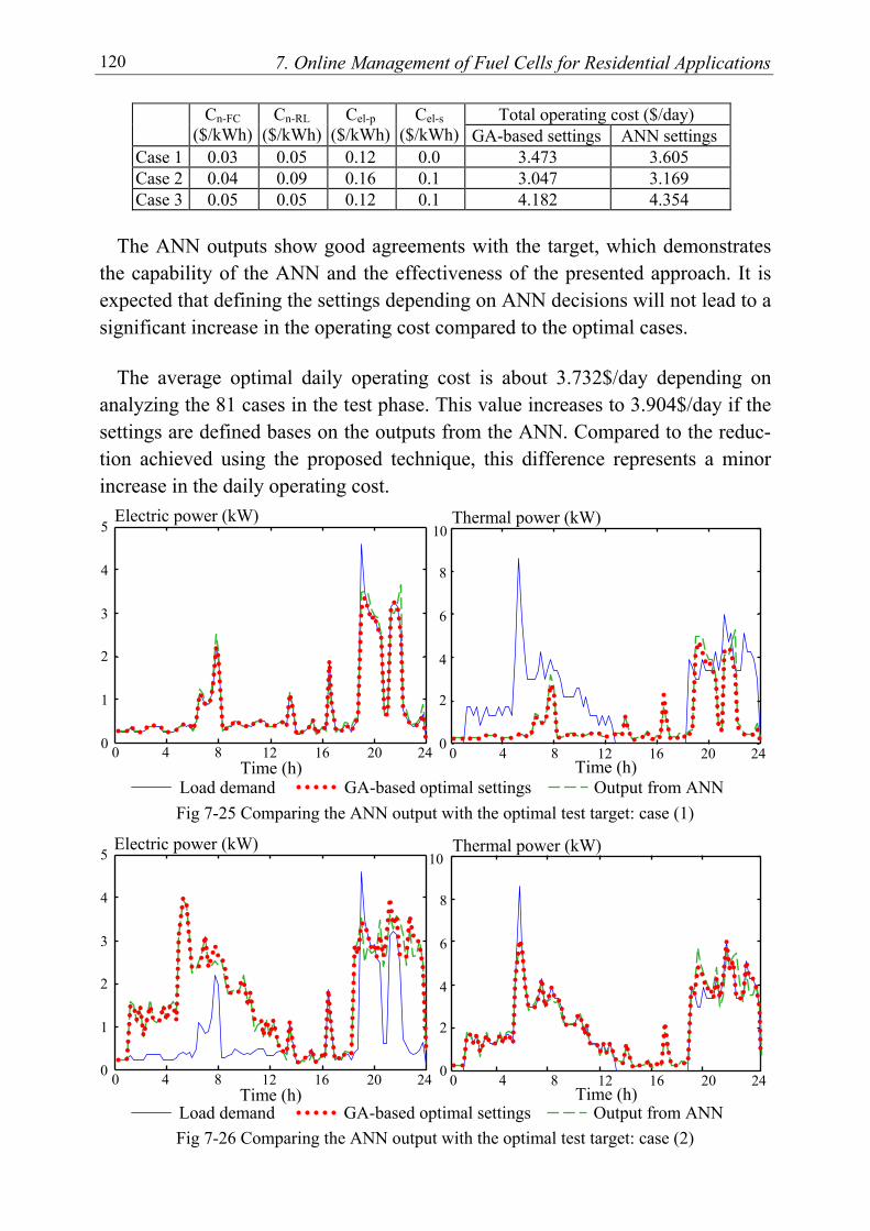
7. Online Management of Fuel Cells for Residential Applications 120
Total operating cost ($/day) Cn-FC ($/kWh)
Cn-RL ($/kWh)
Cel-p ($/kWh)
Cel-s ($/kWh) GA-based settings ANN settings
Case 1 0.03 0.05 0.12 0.0 3.473 3.605 Case 2 0.04 0.09 0.16 0.1 3.047 3.169 Case 3 0.05 0.05 0.12 0.1 4.182 4.354
The ANN outputs show good agreements with the target, which demonstrates
the capability of the ANN and the effectiveness of the presented approach. It is expected that defining the settings depending on ANN decisions will not lead to a significant increase in the operating cost compared to the optimal cases.
The average optimal daily operating cost is about 3.732$/day depending on
analyzing the 81 cases in the test phase. This value increases to 3.904$/day if the settings are defined bases on the outputs from the ANN. Compared to the reduc-tion achieved using the proposed technique, this difference represents a minor increase in the daily operating cost.
Fig 7-25 Comparing the ANN output with the optimal test target: case (1)
Fig 7-26 Comparing the ANN output with the optimal test target: case (2)
Load demand GA-based optimal settings Output from ANN
0
1
2
3
4
5 10Electric power (kW)
0 4 8 12 16 20 24Time (h)
0
2
4
6
8
Thermal power (kW)
0 4 8 12 16 20 24Time (h)
Load demand GA-based optimal settings Output from ANN
0
1
2
3
4
5 10Electric power (kW)
0 4 8 12 16 20 24Time (h)
0
2
4
6
8
Thermal power (kW)
0 4 8 12 16 20 24Time (h)
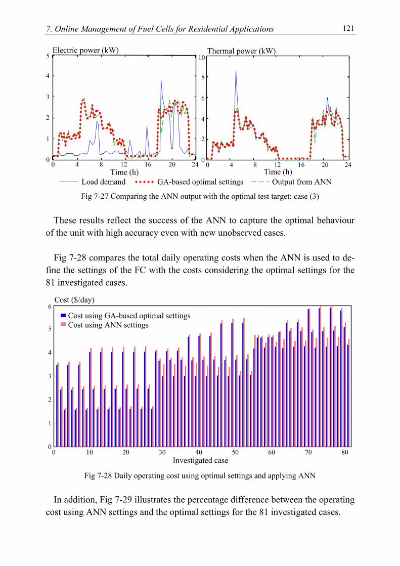
7. Online Management of Fuel Cells for Residential Applications 121
Fig 7-27 Comparing the ANN output with the optimal test target: case (3) These results reflect the success of the ANN to capture the optimal behaviour
of the unit with high accuracy even with new unobserved cases. Fig 7-28 compares the total daily operating costs when the ANN is used to de-
fine the settings of the FC with the costs considering the optimal settings for the 81 investigated cases.
Fig 7-28 Daily operating cost using optimal settings and applying ANN In addition, Fig 7-29 illustrates the percentage difference between the operating
cost using ANN settings and the optimal settings for the 81 investigated cases.
0 10 20 30 40 50 60 70 80 0
1
2
3
4
5
6 Cost ($/day)
Investigated case
Cost using GA-based optimal settingsCost using ANN settings
Load demand GA-based optimal settings Output from ANN
0
1
2
3
4
5 10Electric power (kW)
0 4 8 12 16 20 24Time (h)
0
2
4
6
8
Thermal power (kW)
0 4 8 12 16 20 24Time (h)
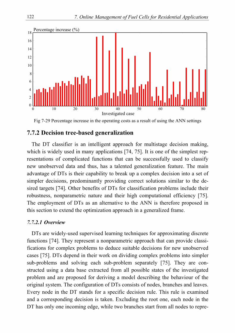
7. Online Management of Fuel Cells for Residential Applications 122
Fig 7-29 Percentage increase in the operating costs as a result of using the ANN settings
7.7.2 Decision tree-based generalization
The DT classifier is an intelligent approach for multistage decision making, which is widely used in many applications [74, 75]. It is one of the simplest rep-resentations of complicated functions that can be successfully used to classify new unobserved data and thus, has a talented generalization feature. The main advantage of DTs is their capability to break up a complex decision into a set of simpler decisions, predominantly providing correct solutions similar to the de-sired targets [74]. Other benefits of DTs for classification problems include their robustness, nonparametric nature and their high computational efficiency [75]. The employment of DTs as an alternative to the ANN is therefore proposed in this section to extend the optimization approach in a generalized frame.
7.7.2.1 Overview
DTs are widely-used supervised learning techniques for approximating discrete functions [74]. They represent a nonparametric approach that can provide classi-fications for complex problems to deduce suitable decisions for new unobserved cases [75]. DTs depend in their work on dividing complex problems into simpler sub-problems and solving each sub-problem separately [75]. They are con-structed using a data base extracted from all possible states of the investigated problem and are proposed for deriving a model describing the behaviour of the original system. The configuration of DTs consists of nodes, branches and leaves. Every node in the DT stands for a specific decision rule. This rule is examined and a corresponding decision is taken. Excluding the root one, each node in the DT has only one incoming edge, while two branches start from all nodes to repre-
0 10 20 30 40 50 60 70 80Investigated case
8
10
12
14
16
18 Percentage increase (%)
0
2
4
6
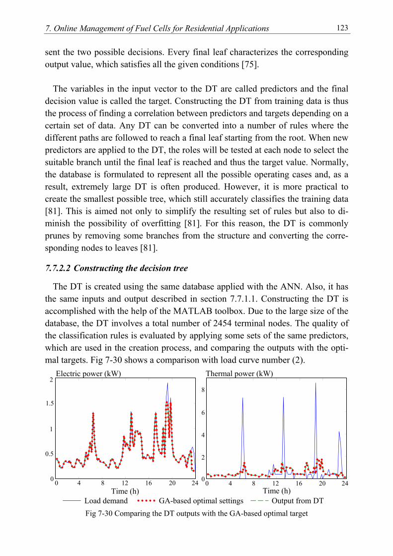
7. Online Management of Fuel Cells for Residential Applications 123
sent the two possible decisions. Every final leaf characterizes the corresponding output value, which satisfies all the given conditions [75].
The variables in the input vector to the DT are called predictors and the final
decision value is called the target. Constructing the DT from training data is thus the process of finding a correlation between predictors and targets depending on a certain set of data. Any DT can be converted into a number of rules where the different paths are followed to reach a final leaf starting from the root. When new predictors are applied to the DT, the roles will be tested at each node to select the suitable branch until the final leaf is reached and thus the target value. Normally, the database is formulated to represent all the possible operating cases and, as a result, extremely large DT is often produced. However, it is more practical to create the smallest possible tree, which still accurately classifies the training data [81]. This is aimed not only to simplify the resulting set of rules but also to di-minish the possibility of overfitting [81]. For this reason, the DT is commonly prunes by removing some branches from the structure and converting the corre-sponding nodes to leaves [81].
7.7.2.2 Constructing the decision tree
The DT is created using the same database applied with the ANN. Also, it has the same inputs and output described in section 7.7.1.1. Constructing the DT is accomplished with the help of the MATLAB toolbox. Due to the large size of the database, the DT involves a total number of 2454 terminal nodes. The quality of the classification rules is evaluated by applying some sets of the same predictors, which are used in the creation process, and comparing the outputs with the opti-mal targets. Fig 7-30 shows a comparison with load curve number (2).
Fig 7-30 Comparing the DT outputs with the GA-based optimal target
0
1
2 Electric power (kW)
Time (h) 0
2
4
6
8
Thermal power (kW)
0 4 8 12 16 20 24 0 4 8 12 16 20 24Time (h)
0.5
1.5
Load demand GA-based optimal settings Output from DT
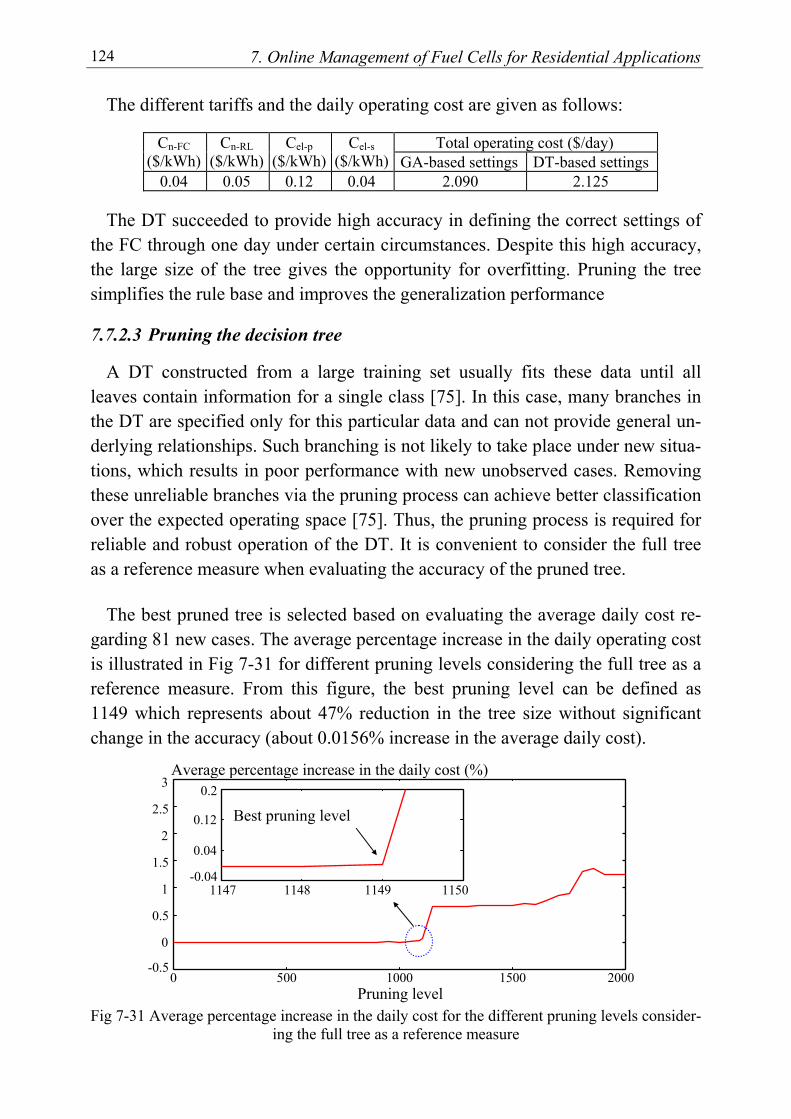
7. Online Management of Fuel Cells for Residential Applications 124
The different tariffs and the daily operating cost are given as follows:
Total operating cost ($/day) Cn-FC ($/kWh)
Cn-RL ($/kWh)
Cel-p ($/kWh)
Cel-s ($/kWh) GA-based settings DT-based settings
0.04 0.05 0.12 0.04 2.090 2.125
The DT succeeded to provide high accuracy in defining the correct settings of the FC through one day under certain circumstances. Despite this high accuracy, the large size of the tree gives the opportunity for overfitting. Pruning the tree simplifies the rule base and improves the generalization performance
7.7.2.3 Pruning the decision tree
A DT constructed from a large training set usually fits these data until all leaves contain information for a single class [75]. In this case, many branches in the DT are specified only for this particular data and can not provide general un-derlying relationships. Such branching is not likely to take place under new situa-tions, which results in poor performance with new unobserved cases. Removing these unreliable branches via the pruning process can achieve better classification over the expected operating space [75]. Thus, the pruning process is required for reliable and robust operation of the DT. It is convenient to consider the full tree as a reference measure when evaluating the accuracy of the pruned tree.
The best pruned tree is selected based on evaluating the average daily cost re-
garding 81 new cases. The average percentage increase in the daily operating cost is illustrated in Fig 7-31 for different pruning levels considering the full tree as a reference measure. From this figure, the best pruning level can be defined as 1149 which represents about 47% reduction in the tree size without significant change in the accuracy (about 0.0156% increase in the average daily cost).
Fig 7-31 Average percentage increase in the daily cost for the different pruning levels consider-
ing the full tree as a reference measure
Pruning level
Average percentage increase in the daily cost (%)
-0.5
0
0.5
1
1.5
2
2.5
3
0 500 1000 1500 2000
0.2
-0.04
0.04
0.12
1148 1149 1150
Best pruning level
1147
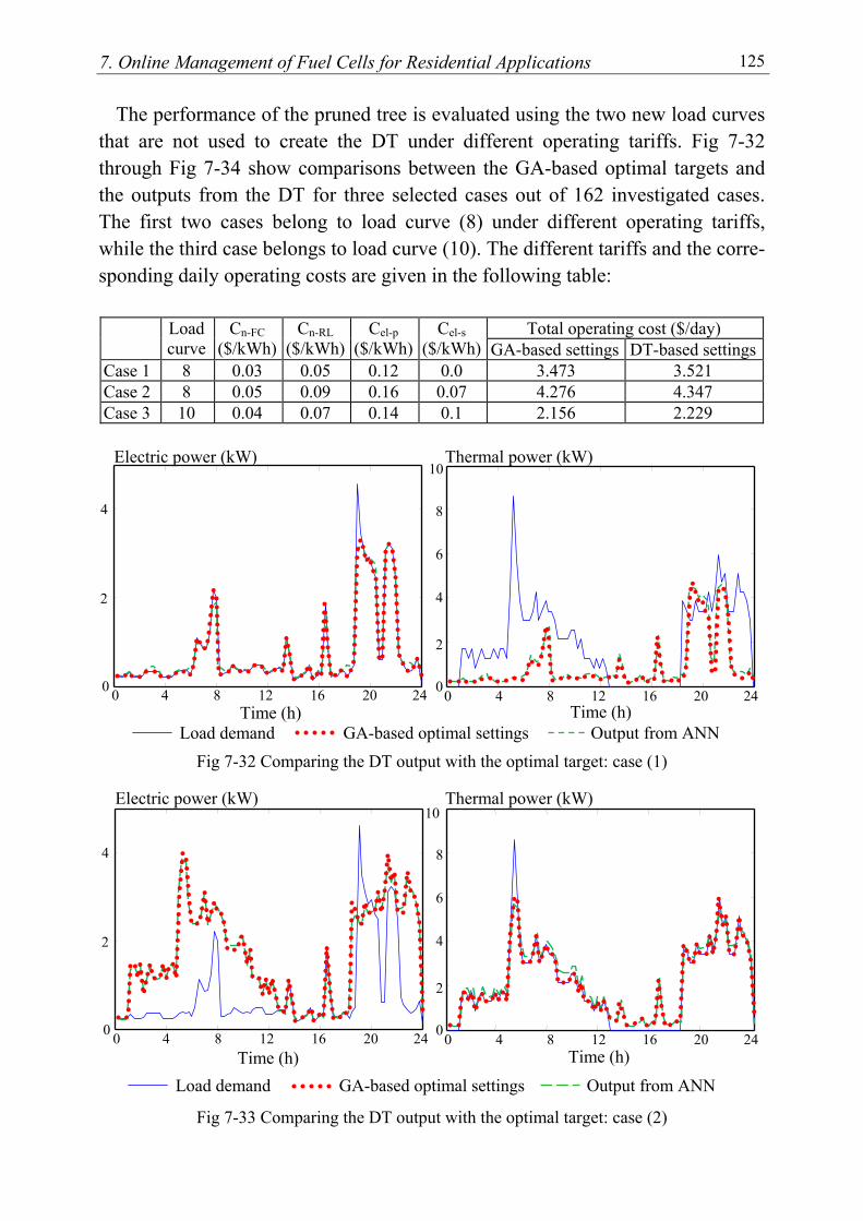
7. Online Management of Fuel Cells for Residential Applications 125
The performance of the pruned tree is evaluated using the two new load curves that are not used to create the DT under different operating tariffs. Fig 7-32 through Fig 7-34 show comparisons between the GA-based optimal targets and the outputs from the DT for three selected cases out of 162 investigated cases. The first two cases belong to load curve (8) under different operating tariffs, while the third case belongs to load curve (10). The different tariffs and the corre-sponding daily operating costs are given in the following table:
Total operating cost ($/day) Load
curve Cn-FC
($/kWh) Cn-RL
($/kWh) Cel-p
($/kWh)Cel-s
($/kWh) GA-based settings DT-based settingsCase 1 8 0.03 0.05 0.12 0.0 3.473 3.521 Case 2 8 0.05 0.09 0.16 0.07 4.276 4.347 Case 3 10 0.04 0.07 0.14 0.1 2.156 2.229
Fig 7-32 Comparing the DT output with the optimal target: case (1)
Fig 7-33 Comparing the DT output with the optimal target: case (2)
0
2
4
Electric power (kW)
0
2
4
6
8
Thermal power (kW)
0 4 8 12 16 20 24 0 4 8 12 16 20 24Time (h) Time (h)
Load demand GA-based optimal settings Output from ANN
10
0
2
4
Electric power (kW)
Time (h)
0
2
4
6
8
Thermal power (kW)
0 4 8 12 16 20 24 0 4 8 12 16 20 24Time (h)
Load demand GA-based optimal settings Output from ANN
10
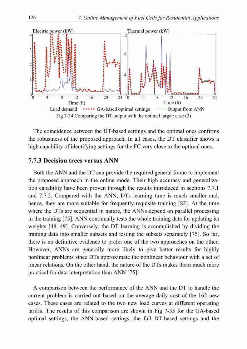
7. Online Management of Fuel Cells for Residential Applications 126
Fig 7-34 Comparing the DT output with the optimal target: case (3)
The coincidence between the DT-based settings and the optimal ones confirms
the robustness of the proposed approach. In all cases, the DT classifier shows a high capability of identifying settings for the FC very close to the optimal ones.
7.7.3 Decision trees versus ANN
Both the ANN and the DT can provide the required general frame to implement the proposed approach in the online mode. Their high accuracy and generaliza-tion capability have been proven through the results introduced in sections 7.7.1 and 7.7.2. Compared with the ANN, DTs learning time is much smaller and, hence, they are more suitable for frequently-requisite training [82]. At the time where the DTs are sequential in nature, the ANNs depend on parallel processing in the training [75]. ANN continually tests the whole training data for updating its weights [48, 49]. Conversely, the DT learning is accomplished by dividing the training data into smaller subsets and testing the subsets separately [75]. So far, there is no definitive evidence to prefer one of the two approaches on the other. However, ANNs are generally more likely to give better results for highly nonlinear problems since DTs approximate the nonlinear behaviour with a set of linear relations. On the other hand, the nature of the DTs makes them much more practical for data interpretation than ANN [75].
A comparison between the performance of the ANN and the DT to handle the
current problem is carried out based on the average daily cost of the 162 new cases. These cases are related to the two new load curves at different operating tariffs. The results of this comparison are shown in Fig 7-35 for the GA-based optimal settings, the ANN-based settings, the full DT-based settings and the
0
1
2
3
4
4
8
12Electric power (kW)
0
Thermal power (kW)
0 4 8 12 16 20 24 0 4 8 12 16 20 24Time (h) Time (h)
Load demand GA-based optimal settings Output from ANN
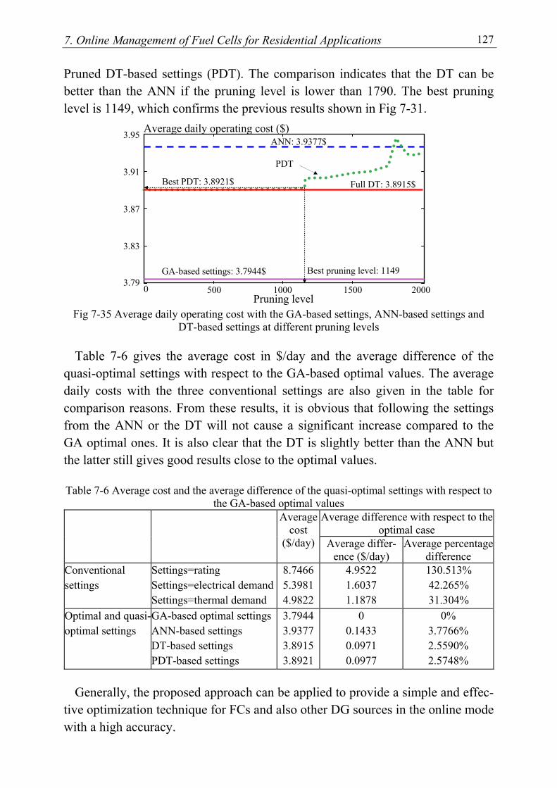
7. Online Management of Fuel Cells for Residential Applications 127
Pruned DT-based settings (PDT). The comparison indicates that the DT can be better than the ANN if the pruning level is lower than 1790. The best pruning level is 1149, which confirms the previous results shown in Fig 7-31.
Fig 7-35 Average daily operating cost with the GA-based settings, ANN-based settings and
DT-based settings at different pruning levels Table 7-6 gives the average cost in $/day and the average difference of the
quasi-optimal settings with respect to the GA-based optimal values. The average daily costs with the three conventional settings are also given in the table for comparison reasons. From these results, it is obvious that following the settings from the ANN or the DT will not cause a significant increase compared to the GA optimal ones. It is also clear that the DT is slightly better than the ANN but the latter still gives good results close to the optimal values.
Table 7-6 Average cost and the average difference of the quasi-optimal settings with respect to the GA-based optimal values
Average difference with respect to the optimal case
Average cost
($/day) Average differ-ence ($/day)
Average percentage difference
Conventional settings
Settings=rating Settings=electrical demandSettings=thermal demand
8.7466 5.3981 4.9822
4.9522 1.6037 1.1878
130.513% 42.265% 31.304%
Optimal and quasi-optimal settings
GA-based optimal settings ANN-based settings DT-based settings PDT-based settings
3.7944 3.9377 3.8915 3.8921
0 0.1433 0.0971 0.0977
0% 3.7766% 2.5590% 2.5748%
Generally, the proposed approach can be applied to provide a simple and effec-
tive optimization technique for FCs and also other DG sources in the online mode with a high accuracy.
0 500 1000 1500 2000 Pruning level
Average daily operating cost ($)ANN: 3.9377$
Full DT: 3.8915$
GA-based settings: 3.7944$
PDT
Best pruning level: 1149
Best PDT: 3.8921$
3.79
3.83
3.87
3.91
3.95
7. Online Management of Fuel Cells for Residential Applications 128
7.8 Conclusion This chapter presents a new approach for optimizing the performance of
PEMFCs and MTs for residential applications. A real-coded multi-population GA is used offline to carry out the optimization process under different operating tar-iffs and load curves. The performances of a single FC, three FCs operating in par-allel and a single MT, as three alternatives, are optimized based on detailed eco-nomic models. The GA has proven good capability to handle the operation man-agement problem of the selected DG units when supplying a residential load. Analyzing the obtained results demonstrates a significant reduction in the daily operating costs using the management process, which contributes in improving the economic feasibility of the DG units. Supplying the residential load using a single FC shows lower daily operating cost compared to the other two alterna-tives. The high electrical efficiency of the FC results in lower operating cost com-pared to the use of a MT. Also, the nature of the FC efficiency curve, which de-creases with the increase of the supplied power, shifts the optimum allocation in favour of using a single unit rather than using smaller identical units in parallel.
It is also proposed to formulate the management process in a general frame us-
ing ANNs and DTs as two alternatives to avoid the need for repetitive optimiza-tion after changes in operating conditions take place. Both the ANN and the DT are trained and tested using a database extracted from the GA-based optimization for different load curves and operating tariffs. The inputs, which represent the load demand and the operating tariffs, can be updated online to simulate the variations in the operating conditions. The generalization stage is applied only with the single FC as the most-economic alternative. The effectiveness of the suggested approach is confirmed through the agreement between the optimized settings and the outputs from the ANN and the DT. The results show that the DT can be better than the ANN for this application if a suitable pruning level is se-lected. However, the ANN will give better results if the DT is pruned beyond this level. The online adjustment of the settings in a fast and simple manner demon-strates the viability of this approach for optimum deployment of different DG units for residential applications.
Chapter 8
Conclusion and Future Directions
8
8.1 Conclusion The defined scope of the thesis is on some topics related to the utilization of
DG units within electrical power networks. The growing importance of such units and their expected impact on the dynamics of power networks encourage the in-vestigation of these subjects to overcome the potential challenges of increasing their penetration levels. In particular, the following issues are addressed in this dissertation to highlight a vital area related to future power systems.
8.1.1 Dynamic modelling of fuel cells
A third order equivalent circuit is proposed to simulate the dynamics of differ-ent types of FCs for stability analysis and control design purposes. The model can be extended to involve the effect of varying the cell temperature and pressure us-ing empirical formulas. The use of an ANN to develop a detailed model directly from measured input/output data is also discussed. The structure of the ANN can be modified to include as many variables as required and to change the order of the model to ensure high performance accuracy. In view of the fact that no ex-perimental data was available, the ANN is trained using patterns extracted from the proposed equivalent circuit. This can be accepted since the main objective is not to develop a specific dynamic model but to introduce the approach itself. The comparisons between the output from the ANN and the target behaviour confirm the capability of the ANN to capture the dynamic performance of the FC and en-courage the use of this technique to obtain suitable models for different types of FCs directly from the input/output measurements.
8.1.2 Simulation of a large number of DG units incorporated into a multi-machine network
A hypothetical multi-machine network is simulated and a total number of 112 FCs and MTs are connected in the low-voltage area of the network. This required the development of suitable dynamic models for MTs and different types of FCs with various capacities. The total power from the DG units covers up to 30% of the total load demand in the 0.4kV system. The performance of the entire net-

8. Conclusion and future directions 130
work is investigated under different disturbances in both the low and high-voltage parts. At the time where the DG units succeeded to absorb large disturbances within the network, they did not respond to interarea oscillations as a result of the local task of their controllers. The dynamic performance of the low-voltage area is somewhat improved due to the existence of active sources near the load centres and the decrease of the voltage drop over transformers and transmission lines.
8.1.3 Dynamic simulation of hybrid fuel cell/micro-turbine units
The construction and the dynamic performance of hybrid FC/MT units are studied and the two integration approaches of the augmented configuration are discussed. A suitable dynamic model is developed and used to investigate the performance of such units in a multi-machine network. The performance of the hybrid units is compared to the performance of separate units operating in paral-lel under the same conditions. The idea is to identify the effect of augmenting the two units on their dynamic performance. The active power of the hybrid unit is significantly affected by the new structure due to the impact of the FC dynamics on the turbine power. As a result, the angular speed of the PMSG is also strongly affected. A similar behaviour of the reactive power is obtained from the hybrid units compared to separate sources due to its dependency on the terminal voltage, which is defined by the network rather than the individual units.
8.1.4 Dynamic equivalents of distribution power networks
A new approach is developed and applied to identify generic dynamic equiva-lents for distribution systems containing large numbers of active DG units based on recurrent ANNs. The model, which has a nonparametric nature, requires simu-lation results or measurements only at the boundary buses. The proposed tech-nique is not based on electromechanical analyses and, therefore, it will not con-flict with the characteristics of DG units, which are mostly connected to the net-work through inverters and in some cases are not distinct by angles or speeds. In addition, the proposed approach would be favourable when there is limited un-derstanding of the relations between system variables. It is also advantageous re-garding the complicated mathematical models required to precisely reflect the performance of the replaced network under various operating conditions.
A training program for the ANN with actual recurrent loops is developed and
used to obtain the parameters of the dynamic model. The equivalent dynamic model thus obtained was implemented on a power system simulation package to verify its capability of reproducing the dynamic behaviour of the replaced net-

8. Conclusion and future directions 131
work in full. The results demonstrate the capability of the equivalent model to capture the dynamic behaviour of the replaced networks in its entirety. The model provided outstanding conformity with the results obtained using the full dynamic model of the network even under new generation and loading conditions. The approach promises a significant simplification of the dynamic analysis of large interconnected networks without significant loss of accuracy.
8.1.5 Impact of distributed generation on power systems stability
The impact of DG units with different penetration levels on the stability of power systems is addressed. The results showed the possibility of improving the power system stability when DG units are utilized. Regarding the oscillatory sta-bility, the damping of the electromechanical mode is somewhat improved and the corresponding frequency is slightly increased. The maximum power-angle devia-tions between the generators are also decreased with the increase of the penetra-tion level of the DG units, which reflects the enhancement in the transient stabil-ity of the overall power system. In addition, the network requires smaller time to reach the minimum frequency level when more DG units are employed. Further-more, the voltage profiles at load terminals are improved due to the use of active DG sources near end-user terminals. The controllers designed to regulate the per-formance of the DG units participate also in improving the voltage stability of the network.
8.1.6 Online management of fuel cells and micro-turbines
A novel intelligent approach for optimizing the performance of DG units for residential applications is presented. The investigation involves the management of a single FC, three FCs operating in parallel and a single MT as three alterna-tives. In the first stage of the proposed approach, a real-coded multi-population GA is used offline to carry out the optimization process for different operating conditions and load curves. This stage showed a significant reduction in the daily operating costs with large influence from the fuel and electricity tariffs on the optimal settings of the DG units. The comparisons demonstrated that the single FC is the favourite alternative regarding the operating cost due to the level and nature of its electrical efficiency.
Repetitive optimization processes are obligatory with the variation of the oper-
ating circumstances, which requires long time and complex computations in addi-tion to advanced experience from the operator. Therefore, ANNs and DTs are used in the second stage as two alternatives to facilitate the online employment of
8. Conclusion and future directions 132
the optimization procedures. The second stage is employed only with the single FC as the most economic choice regarding the operating costs. Both the ANN and the DT are trained and tested using the same knowledgebase with all decision variables included in the input vector. To simulate the variations in the operating conditions, it will be enough to update these inputs online without any modifica-tions in the structure of the developed model. The results confirmed the high ac-curacy of the proposed approach to define online settings for DG units that are very close to the optimal ones in a fast and simple manner. This encourages the utilization of this methodology for optimum deployment of different DG units for residential applications. A comparison between the ANN and DT showed that the DT can outperform the ANN for this application under certain conditions. How-ever, the latter gives also a high accuracy with respect to the optimal values.
8.2 Future directions It is not sought to provide solutions to specific problems related to DG in
power systems. Rather, the research represents a beginning attempt in addressing areas of concern and opportunities for utilizing DG units in the future networks. Moving forward, some possible future directions can be identified as follows:
• using ANNs to develop specific dynamic models for FCs regarding the comprehensive performance using real input/output measurements
• designing centralized robust controllers to achieve more damping in inter-connected power systems including large numbers of DG units over a wide range of operating points
• developing more accurate mathematical models for the CFCMT units in-cluding topping and bottoming modes with more sophisticated controllers
• applying the proposed ANN-based equivalent approach for identifying suit-able equivalents for some subsystems in high-voltage networks including the conventional generators with their regulators
• investigating the impact of using distinct types of DG units with different characteristics on the stability of large interconnected power systems
• online operation management of DG units supplying residential loads con-sidering storage devices with identifying the optimal storage capacity
• applying stochastic optimization methods to consider uncertainties in the online operation management of DG units supplying residential loads

References
[1] T. E. Hoff, H. J. Wenger and B. K. Farmer, “Distributed generation: an alternative to elec-
tric utility investments in system capacity” Energy policy, Vol. 24, No. 2, pp. 137-147, 1996
[2] T. Ackermann and V. Knyazkin, “Interaction between distributed generation and the distri-bution network: operation aspect” IEEE/PES Transmission and Distribution Conf. and Ex-hibition 2002: Asia Pacific, Vol. 2, 6-10 Oct. 2002, pp. 1357-1362, Yokohama, Japan
[3] M. T. Doyle, “Reviewing the impacts of distributed generation on distribution system pro-tection” Power Engineering Society Summer Meeting, 2002 IEEE, Chicago, USA, Vol. 1, 21-25 July 2002, pp. 103-105
[4] P. P. Barker and B. K. Johnson, “Power system modeling requirements for rotating ma-chine interfaced distributed resources” Power Engineering Society Summer Meeting, 2002 IEEE, Chicago, USA, Vol. 1, 21-25 July 2002, pp. 161-166
[5] P. P. Barker and R. W de Mello, “Determining the impact of distributed generation on power systems: Part I. Radial distribution systems” Power Engineering Society Summer Meeting, Seattle, Washington, USA, 2000 IEEE, Vol. 3, 16-20 July 2000, pp. 1645-1656
[6] F. V. Edwards, G. J. W. Dudgeon, J. R. McDonald and W. E. Leithead, “Dynamics of dis-tribution networks with distributed generation” Power Engineering Society Summer Meet-ing, Seattle, Washington, USA, 2000 IEEE, Vol. 2, 16-20 July 2000, pp. 1032-1037
[7] In-Su Bae, Jin-O Kim, Jae-Chul Kim and C. Singh, “Optimal operating strategy for distrib-uted generation considering hourly reliability worth” Power Systems, IEEE Transactions on, Vol. 19, No. 1, February 2004
[8] A. G. Amendola and M. C. Rocha, “Fuel cell plant-a proposed analysis for economical feasibility of implantation” Electricity Distribution, 16th Int. Conference and Exhibition on, Amsterdam, the Netherlands, 18-21 June 2001, Part 1, (IEE Conf. Publ. No. 482), Vol. 4
[9] C. Haynes and W.J. Wepfer, “‘Design for power’ of a commercial grade tubular solid oxide fuel cell” Energy Conversion & management, Vol. 41, Issue 11, July 2000, pp. 1123-1139
[10] D. J. Hall and R. G. Colclaser, “Transient modelling and simulation of a tubular solid ox-ide fuel cell” Energy Conversion, IEEE transactions on, Vol. 14, No. 3, September 1999
[11] D. Singh, D. M. Lu and N. Djilali, “A two-dimensional analysis of mass transport in pro-ton exchange membrane fuel cell” International Journal of Engineering science, Vol. 37, Issue 4, March 1999, pp. 431-452
[12] Bagnasco, B. Delfino, G.B. Denegri and S. Massucco, “Management and dynamic per-formances of combined cycle power plants during parallel and islanding operation” Energy Conversion, IEEE Transactions on, Vol. 13, No. 2, June 1998

References 134
[13] Borghetti, G. Migliavacca, C. A. Nucci and S. Spelta, “Black-startup simulation of a re-powered thermoelectric unit” IFAC Symposium on power plants & Power Systems Con-trol, 26-29 April, 2000, Brussels, Belgium, pp. 119-126
[14] Amer Al-Hinai and Ali Feliachi, “Dynamic model of a microturbine used as a distributed generator” System Theory 2002, Proceedings of the 34th Southeastern Symposium on, Huntsville, Alabama, 18-19 March 2002, pp. 209-213
[15] W. G. Scott, “Micro-Turbine Generators for Distribution Systems,” IEEE Applications Magazine, Vol. 4, Issue 4, pp. 57-62, May/June, 1998.
[16] K. Tomsovic and T. Hiyama, “Intelligent control methods for systems with dispersed gen-eration” Power Engineering Society Winter Meeting, 2001 IEEE, Columbus, Ohio, USA, Vol. 2, 28 Jan.-1 Feb., 2001, pp. 913-917
[17] J. A. Smith, M. H. Nehrir, V. Gerez and S. R. Shaw, “A broad look at the workings, types, and applications of fuel cells” Power Engineering Society Summer Meeting, 2002 IEEE, Chicago, USA, Vol. 1, 21-25 July 2002, pp. 70-75
[18] Shinji Kimijima and Nobuhuíde Kasagi, “Performance evaluation of gas turbine-fuel cell hybrid micro generation system” Proceedings of ASME TURBO EXPO 2002, June 3-6, 2002, Amsterdam, the Netherlands
[19] F. Jurado and J. Saenz, “Adaptive control of a fuel cell-microturbine hybrid power plant” Power Engineering Society Summer Meeting, 2002 IEEE, Chicago USA, Vol. 1, pp. 76-81
[20] Peter A. Daly and Jay Morrison, “Understanding the potential benefits of distributed gen-eration on power delivery systems” Rural Electric Power Conference, 29 April-1 May 2001, pp. A2-1–A2-13, Little Rock, Arkansas, USA
[21] A. Agustoni, M. Brenna, R. Faranda, E. Tironi, C. Pincella and G. Simioli, “Constraints for the interconnection of distributed generation in radial distribution systems” Harmonics and Quality of Power, 10th International Conference on, Vol. 1, 6-9 Oct. 2002, pp. 310-315, Rio de Janeiro, Brazil
[22] M. Begovic, A. Pregelj, A. Rohatgi and D. Novosel, “Impact of renewable distributed gen-eration on power systems” System Sciences, 2001, Proceedings of the 34th Annual Hawaii International Conference on, Jan. 3-6, 2001, pp. 654- 663, Maui, Hawaii
[23] Bruno Delfino, “Modelling of the integration of distributed generation into the electrical system” Power Engineering Society Summer Meeting, 2002 IEEE, Chicago USA, Vol. 1, 21-25 July 2002, pp. 170-175
[24] J. G. Slootweg and W. L. Kling, “Impacts of distributed generation on power system tran-sient stability” Power Engineering Society Summer Meeting, 2002 IEEE, Chicago USA, Vol. 2, 21-25 July 2002, pp. 862-867
[25] A. Girgis and S. Brahma, “Effect of distributed generation on protective device coordina-tion in distribution system” Power Engineering, 2001, LESCOPE '01, Large Engineering Systems Conference on, 11-13 July 2001, pp. 115-119, Halifax, Nova Scotia, Canada
References 135
[26] Kauhaniemi, K., Kumpulainen, L.: Impact of distributed generation on the protection of distribution networks. Developments in Power System Protection, IEE International Con-ference, 5-8 April 2004, Amsterdam, pp. 315-318
[27] Stan Blazwicz and David Kleinschmidt, “Distributed Generation: System Interfaces” White paper prepared by Arthur D. Little, Cambridge, MA. 1999, http://www.encorp.com/dwnld/pdf/whitepaper/wp_ADL_2.pdf
[28] S. J. C. Cleghorn, X. Ren, T. E. Springer, M. S. Wilson, C. Zawodzinski, T. A. Zawodzin-ski and S. Gottesfeld, “PEM fuel cells for transportation and stationary power generation applications” Int. Journal of Hydrogen Energy, Vol. 22, No. 12, 1997, pp. 1137-1144
[29] W. Morgantown, “Fuel Cell Handbook” 6th Edition, EG&G Technical Services, Virginia, November 2002, http://www.rwth-aachen.de/lbz/FCHandbook6.pdf
[30] M. W. Ellis, M. R. Von Spakovsky and D. J. Nelson, “Fuel cell systems: efficient, flexible energy conversion for the 21st century” Proceedings of the IEEE , Vol. 89, Issue: 12, Dec. 2001, pp. 1808-1818
[31] Kyoungsoo Ro and Saifur Rahman, “Two-loop Controller for Maximizing Performance of a Grid-Connected Photovoltaic-Fuel Cell Hybrid Power Plant” Energy Conversion, IEEE transactions on, Vol. 13, No. 3, September 1998
[32] P.A. Lehman, C.E. Chamberlin, J.I. Zoellick and R. Engel, “A photovoltaic/fuel cell power system for a remote telecommunications station” Photovoltaic Specialists Conference, 2000, Conference Record of the 28th IEEE, 15-22 Sept. 2000, pp. 1552-1555, Alaska, USA
[33] Valery Knyazkin, Lennart Söder and Claudio Canizares, “Control challenges of fuel cell-driven distributed generation” the 2003 IEEE Bologna Power Tech Conference, June 23rd-26th, Bologna, Italy
[34] K. Sedghisigarchi and A. Feliachi, “Control of grid-connected fuel cell power plant for transient stability enhancement” Power Engineering Society Winter Meeting, 2002 IEEE, New York, USA, 27-31 Jan. 2002, Vol. 1, pp. 383-388
[35] Saifur Rahman and Kwa-sur Tam, “A feasibility study of photovoltaic-fuel cell hybrid system” Energy Conversion, IEEE Transactions on, Vol. 3, No. 1, March 1988
[36] F. Ordubadi, “PEM fuel cells and future opportunities” Power Engineering Society Sum-mer Meeting, 2001. IEEE, Vancouver, Canada, Vol. 1, 15-19 July 2001, pp. 710-716
[37] R.Anahara, S.Yokokawa and M.Sakurai, “Present status and future prospects for fuel cell power systems” Proceedings of the IEEE, Vol. 81, Issue: 3, March 1993, pp. 399-408
[38] J. T. Brown, “Solid oxide fuel cell technology” Energy Conversion, IEEE Transactions on, Vol. 3, No. 2, June 1988
[39] Michael D. Lukas, Kwang Y. Lee and Hossein Ghezel-Ayagh, “Development of a stack simulation model for control study on direct reforming molten carbonate fuel cell power plant” Energy Conversion, IEEE Transactions on, Vol. 14, No. 4, December 1999
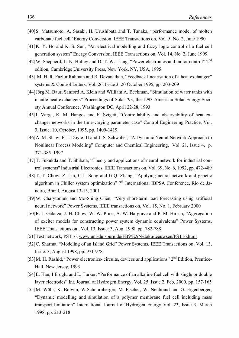
References 136
[40] S. Matsumoto, A. Sasaki, H. Urushibata and T. Tanaka, “performance model of molten carbonate fuel cell” Energy Conversion, IEEE Transactions on, Vol. 5, No. 2, June 1990
[41] K. Y. Ho and K. S. Sun, “An electrical modelling and fuzzy logic control of a fuel cell generation system” Energy Conversion, IEEE Transactions on, Vol. 14, No. 2, June 1999
[42] W. Shepherd, L. N. Hulley and D. T. W. Liang, “Power electronics and motor control” 2nd edition, Cambridge University Press, New York, NY, USA, 1995
[43] M. H. R. Fazlur Rahman and R. Devanathan, “Feedback linearisation of a heat exchanger” systems & Control Letters, Vol. 26, Issue 3, 20 October 1995, pp. 203-209
[44] Jörg M. Baur, Sanford A. Klein and William A. Beckman, “Simulation of water tanks with mantle heat exchangers” Proceedings of Solar ’93, the 1993 American Solar Energy Soci-ety Annual Conference, Washington DC, April 22-28, 1993
[45] I. Varga, K. M. Hangos and F. Szigeti, “Controllability and observability of heat ex-changer networks in the time-varying parameter case” Control Engineering Practice, Vol. 3, Issue. 10, October, 1995, pp. 1409-1419
[46] A. M. Shaw, F. J. Doyle III and J. S. Schwaber, “A Dynamic Neural Network Approach to Nonlinear Process Modeling” Computer and Chemical Engineering, Vol. 21, Issue 4, p. 371-385, 1997
[47] T. Fukukda and T. Shibata, “Theory and applications of neural network for industrial con-trol systems" Industrial Electronics, IEEE Transactions on, Vol. 39, No. 6, 1992, pp. 472-489
[48] T. T. Chow, Z. Lin, C.L. Song and G.Q. Zhang, “Applying neural network and genetic algorithm in Chiller system optimization” 7th International IBPSA Conference, Rio de Ja-neiro, Brazil, August 13-15, 2001
[49] W. Charytoniuk and Mo-Shing Chen, “Very short-term load forecasting using artificial neural network” Power Systems, IEEE transactions on, Vol. 15, No. 1, February 2000
[50] R. J. Galarza, J. H. Chow, W. W. Price, A. W. Hargrave and P. M. Hirsch, “Aggregation of exciter models for constructing power system dynamic equivalents” Power Systems, IEEE Transactions on , Vol. 13, Issue: 3, Aug. 1998, pp. 782-788
[51] Test network, PST16, www.uni-duisburg.de/FB9/EAN/doku/teeuwsen/PST16.html [52] C. Sharma, “Modeling of an Island Grid” Power Systems, IEEE Transactions on, Vol. 13,
Issue. 3, August 1998, pp. 971-978 [53] M. H. Rashid, “Power electronics- circuits, devices and applications” 2nd Edition, Prentice-
Hall, New Jersey, 1993 [54] E. Han, I Eroglu and L. Türker, “Performance of an alkaline fuel cell with single or double
layer electrodes” Int. Journal of Hydrogen Energy, Vol. 25, Issue 2, Feb. 2000, pp. 157-165 [55] M. Wöhr, K. Bolwin, W.Schnurnberger, M. Fischer, W. Neubrand and G. Eigenberger,
“Dynamic modelling and simulation of a polymer membrane fuel cell including mass transport limitation” International Journal of Hydrogen Energy Vol. 23, Issue 3, March 1998, pp. 213-218
References 137
[56] István Erlich, "Analysis and simulation of dynamic behaviour of power system", Postdoc-toral lecture qualification, Dept. of elect. engineering , Dresden University, Germany, 1995
[57] Scott Samuelsen, “Fuel cell/gas turbine hybrid systems” © 2004 ASME Int. Gas Turbine Institute, http://www.asme.org/igti/resources/articles/turbo-fuel-cell_report_feb04.pdf
[58] O. Lamquet, R. Massa, F. Parodi, W. Prandoni and S. Spelta, “Dynamic model of an hy-brid plant based on MCFC fuel cells and microturbine for process analysis and control” the 2003 IEEE Bologna Power Tech Conf., June 23th-26th, Bologna, Italy
[59] L. Wang, M. Klein, S. Yirga and P. Kundur, “Dynamic reduction of large power systems for stability studies” Power Systems, IEEE Transactions on, Vol. 12, Issue: 2, May 1997, pp. 889-895
[60] P. Ju and X. Y. Zhou, “Dynamic equivalents of distribution systems for voltage stability studies” Generation, Transmission and Distribution, IEE Proceedings, Vol. 148, Issue: 1, Jan. 2001, pp. 49-53
[61] Sven Demmig, Habil Hans Pundt and István Erlich, “Identification of external system equivalents for power system stability studies using the software package MATLAB” 12th power systems computation conference, Dresden, Germany, August 19-23, 1996
[62] K. Nojiri, S. Suzaki, K. Takenaka and M. Goto, “Modal reduced dynamic equivalent model for analog type power system simulator” Power Systems, IEEE Transactions on, Vol. 12, Issue: 4, Nov. 1997, pp. 1518-1523
[63] S. K. Joo, C. C. Liu and J. W. Choe, “Enhancement of coherency identification techniques for power system dynamic equivalents” Power Engineering Society Summer Meeting 2001, IEEE, Vancouver, Canada, Vol. 3 ,15-19 July 2001, pp. 1811-1816
[64] Mang-Hui Wang and Hong-Chan Chang, “Novel clustering method for coherency identifi-cation using an artificial neural network” Power Systems, IEEE Transactions on, Vol. 9, Is-sue: 4, Nov. 1994, pp. 2056-2062
[65] Aleksander M. Stankovic, Andrija T. Saric and Mirjana Milosevic, “Identification of non-parametric dynamic power system equivalents with artificial neural network” Power Sys-tems, IEEE Transactions on, Vol. 18, Issue: 4, Nov. 2003, pp. 1478-1486
[66] M. Miah, “Simple dynamic equivalent for fast online transient stability assessment” Gen-eration, Transmission and Distribution, IEE Proceedings, Vol. 145, Issue: 1, January 1998, pp. 49-55
[67] S. K. Joo, C. C. Liu, L. Jones and J. W. Choe, “Coherency techniques for dynamic equiva-lents incorporating rotor and voltage dynamics” Bulk Power Systems Dynamics and Con-trol–V, Security and Reliability in a Changing Environment, Aug. 2001, Hiroshima, Japan
[68] M. K. Donnelly, J. E. Dagle, D. J. Trudnowski and G. J. Rogers, “Impacts of the distrib-uted utility on transmission system stability” Power Systems, IEEE Transactions on, Vol. 11, Issue: 2, May 1996, pp. 741-746
References 138
[69] N. W. Miller, R. A. Walling and A. S. Achilles, “Impact of distributed resources on system dynamic performance” Transmission and Distribution Conference and Exposition, 2001 IEEE/PES, Vol. 2, 28 Oct.-2 Nov, 2001, pp. 951- 952, Atlanta, USA
[70] P. Kundur, J. Paserba, V. Ajjarapu, G. Andersson, A. Bose, C. Canizares, N. Hatziargy-riou, D. Hill, A. Stankovic, C. Taylor, T. Van Cutsem and V. Vittal, “Definition and classi-fication of power system stability” IEEE/CIGRE joint task force on stability terms and de-finitions, Power Systems, IEEE Transactions on, Vol. 19, Issue 3, pp. 1387-1401, Aug. 2004
[71] Y. H. Song, L. Z. Yao, Y. X. Ni and P. L. Mao, “Integrated direct methods for transient stability analysis” Electric Machines and Power Systems, 1 February 1999, Vol. 27, issue 2, pp. 139-155
[72] Barbir and T. Gomez, “Efficiency and Economics of Proton Exchange Membrane (PEM) Fuel Cell” Int. Journal of Hydrogen Energy, Vol. 21, Issue 10, pp 891-901, October 1996
[73] Ioannis G. Damousis, Anastasios G. Bakirtzis, and Petros S. Dokopoulos, “Network-Constrained Economic Dispatch Using Real-Coded Genetic Algorithm” Power Systems, IEEE Transactions on, Vol. 18, No. 1, February 2003
[74] K. Mei and S. M. Rovnyak, “Response-based decision trees to trigger one-shot stabilizing control” Power Systems, IEEE Transactions on, Vol. 19, Issue: 1, Feb. 2004, pp. 531-537
[75] S. R. Safavian and D. Landgrebe, “A survey of decision tree classifier methodology” Sys-tems, Man and Cybernetics, IEEE Transactions on, Vol. 21, issue 3 , May-June 1991, pp. 660-674
[76] Ian Beausoleil-Morrison, Dave Cuthbert, Gord Deuchars and Gordon McAlary, “The simulation of fuel cell cogeneration systems within residential buildings” The bi-annual conference of International Building Performance Simulation Association IBPSA-Canada, September 11th-13th, 2002, Montréal, Canada
[77] S. O. Orero and M. R. Irving, “Large scale unit commitment using a hybrid genetic algo-rithm” International Journal of Electrical Power & Energy systems, Vol. 19, No. 1, pp. 45-55, 1997, (UK)
[78] C. R. Houck, J.A. Joines and M. G. Kay, “A genetic algorithm for function optimization: A Matlab implementation” NCSU-IE technical report 95-09. North Carolina State Univer-sity, 1995, http://www.fmmcenter.ncsu.edu/fac_staff/joines/papers
[79] Solarsiedlung Gelsenkirchen Bramkampstrasse, http://www.50solarsiedlungen.de [80] R. J. Yinger, “Behaviour of capstone and Honeywell microturbine generators during load
changes” Lawrence Berkeley National Laboratory (LBNL-49095) for CERTS, July 2001, http://certs.lbl.gov/pdf/LBNL_49095.pdf
[81] Almuallim Hussein, “An efficient algorithm for optimal pruning of decision trees” Artificial Intelligence, Vol. 83, Issue: 2, June, 1996, pp. 347-362
[82] L. Atlas, R. Cole, Y. Muthusamy, A. Lippman, J. Connor, D. Park, M. El-sharkawi and R. J. Marks, “A performance comparison of trained multilayer perceptrons and trained classi-fication trees” Proceedings of the IEEE, Vol. 78, Issue. 10, pp. 1614-1619, October 1990
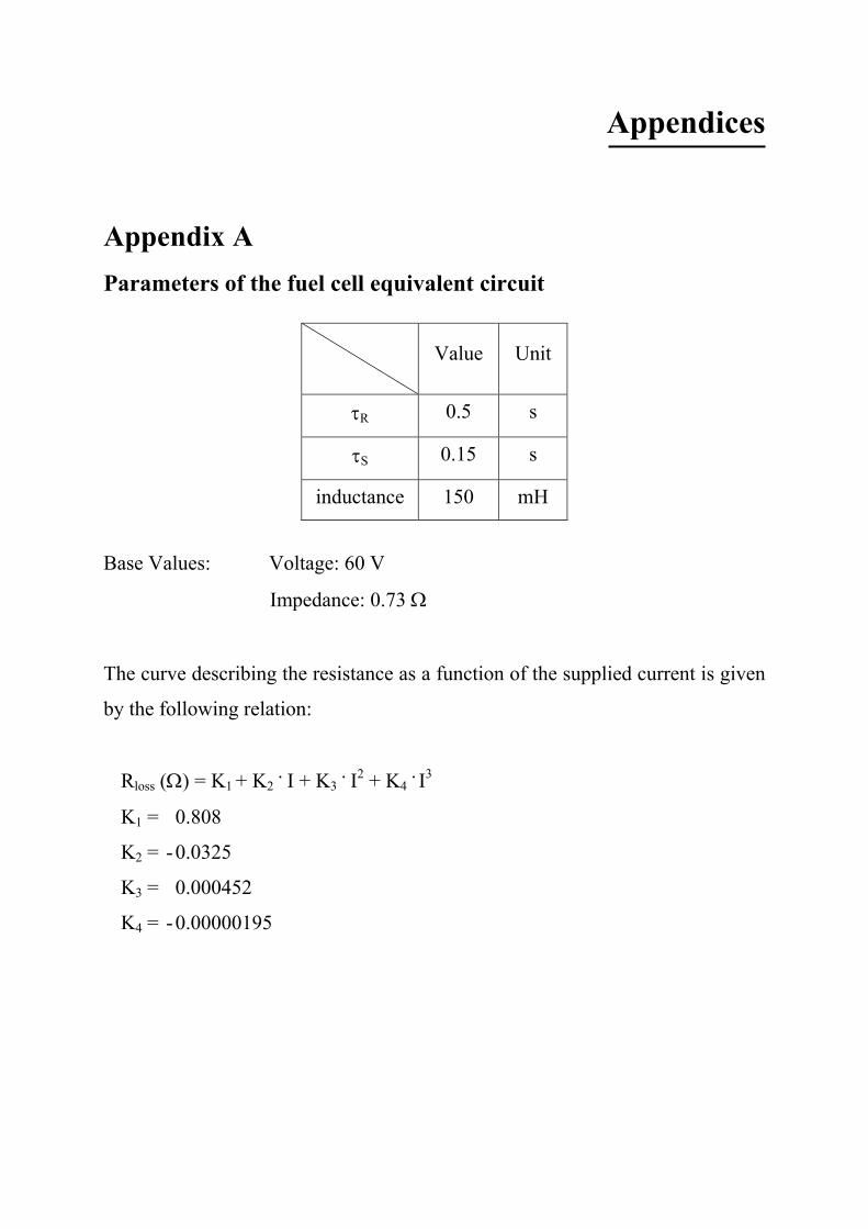
Appendices
Appendix A Parameters of the fuel cell equivalent circuit
Value Unit
τR 0.5 s
τS 0.15 s
inductance 150 mH
Base Values: Voltage: 60 V
Impedance: 0.73 Ω
The curve describing the resistance as a function of the supplied current is given
by the following relation:
Rloss (Ω) = K1 + K2 . I + K3 . I2 + K4 . I3
K1 = 0.808
K2 = - 0.0325
K3 = 0.000452
K4 = - 0.00000195
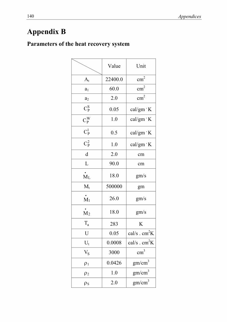
Appendices 140
Appendix B Parameters of the heat recovery system
Value Unit
At 22400.0 cm2
a1 60.0 cm2
a2 2.0 cm2 SPC 0.05 cal/gm . K WPC 1.0 cal/gm . K
1PC 0.5 cal/gm . K 2PC 1.0 cal/gm . K
d 2.0 cm
L 90.0 cm
LM•
18.0 gm/s
Mt 500000 gm
1M•
26.0 gm/s
2M•
18.0 gm/s
aT 283 K
U 0.05 cal/s . cm2K
Ut 0.0008 cal/s . cm2K
SV 3000 cm3
ρ1 0.0426 gm/cm3
ρ2 1.0 gm/cm3
ρS 2.0 gm/cm3
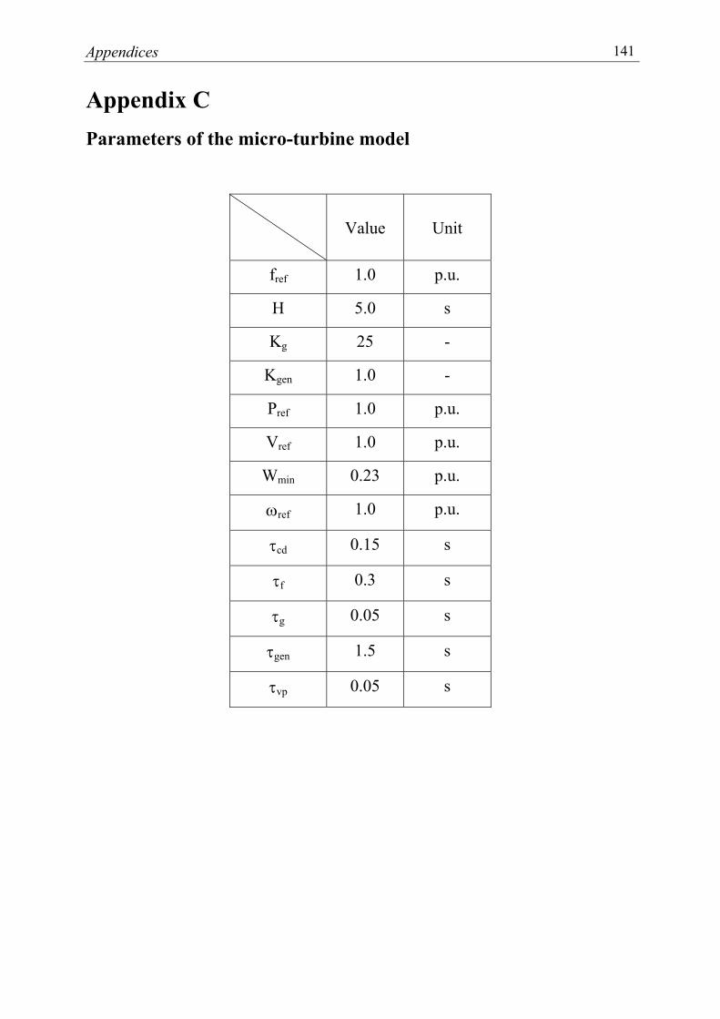
Appendices 141
Appendix C Parameters of the micro-turbine model
Value Unit
fref 1.0 p.u.
H 5.0 s
Kg 25 -
Kgen 1.0 -
Pref 1.0 p.u.
Vref 1.0 p.u.
Wmin 0.23 p.u.
ωref 1.0 p.u.
τcd 0.15 s
τf 0.3 s
τg 0.05 s
τgen 1.5 s
τvp 0.05 s

Appendices 142
Appendix D Parameters of the fuel cell units integrated into PST16 network
τR (s) τS (s)
Inductance (mH)
PEMFC (250kW) 0.8 0.08 110
PEMFC (350kW) 1.0 0.12 120
AFC (400kW) 1.3 0.15 130
SOFC (450kW) 1.5 0.18 140
SOFC (500kW) 1.7 0.20 150
The loss resistance as a function of the supplied current is given as:
Supplied current (p.u.) Loss resistance (p.u.)
0.25 0.5 0.75 1.0 1.25 1.5 1.75 2.0
PEMFC (250kW) 0.759 0.41 0.35 0.34 0.34 0.345 0.36 0.393
PEMFC (350kW) 0.759 0.41 0.35 0.34 0.34 0.345 0.36 0.393
AFC (400kW) 0.821 0.482 0.367 0.333 0.333 0.334 0.337 0.413
SOFC (450kW) 0.516 0.417 0.380 0.379 0.379 0.382 0.400 0.425
SOFC (500kW) 0.516 0.417 0.380 0.379 0.379 0.382 0.400 0.425
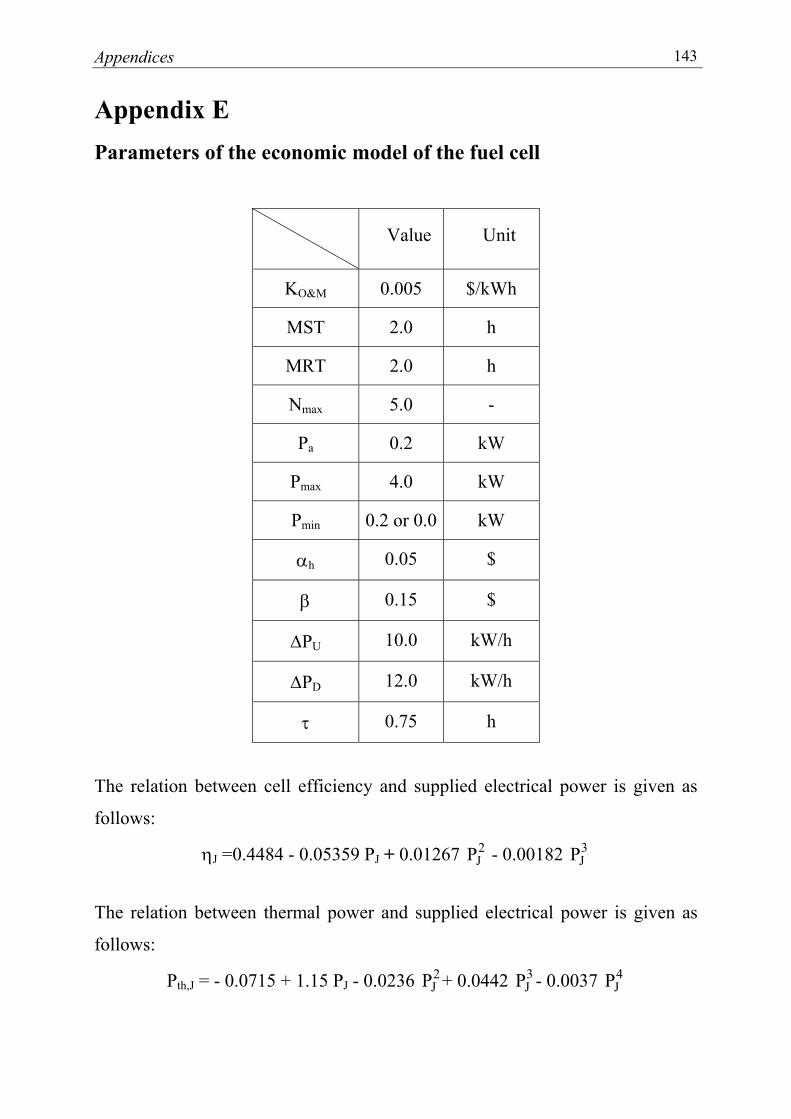
Appendices 143
Appendix E Parameters of the economic model of the fuel cell
Value Unit
KO&M 0.005 $/kWh
MST 2.0 h
MRT 2.0 h
Nmax 5.0 -
Pa 0.2 kW
Pmax 4.0 kW
Pmin 0.2 or 0.0 kW
αh 0.05 $
β 0.15 $
∆PU 10.0 kW/h
∆PD 12.0 kW/h
τ 0.75 h
The relation between cell efficiency and supplied electrical power is given as
follows:
ηJ =0.4484 - 0.05359 PJ + 0.01267 2JP - 0.00182 3
JP
The relation between thermal power and supplied electrical power is given as
follows:
Pth,J = - 0.0715 + 1.15 PJ - 0.0236 2JP + 0.0442 3
JP - 0.0037 4JP

Appendices 144
Appendix F Parameters of the economic model of 3 FCs operating in parallel The parameters of the identical fuel cell units are:
Value Unit
MOK & 0.005 $/kWh
MDT 2.0 h MUT 2.0 h
Nmax 5.0 -
Pa 0.08 kW
Pmax 1.3 kW
Pmin 0.1 or 0.0 kW
αh 0.02 $
β 0.06 $
∆PU 3.2 kW/h
∆PD 4.0 kW/h
τ 0.5 h
The relation between cell efficiency and supplied electrical power is given as
follows:
ηJ = 0.4484 - 0.16076 . PJ + 0.11399 . 2JP - 0.049072 . 3
JP
The relation between thermal power and supplied electrical power is given as
follows:
Pth,J = - 0.020723 + 1.0 . PJ - 0.061653 . 2JP + 0.34064 . 3
JP - 0.08752 . 4JP
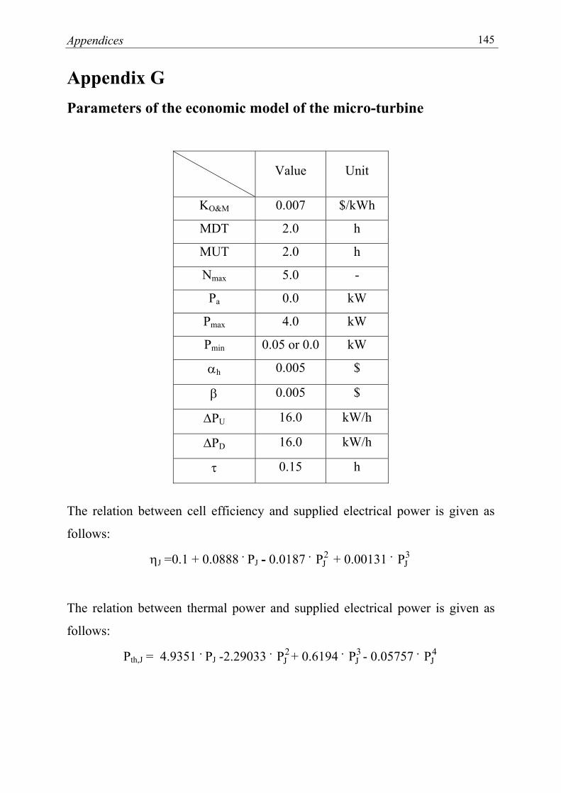
Appendices 145
Appendix G Parameters of the economic model of the micro-turbine
Value Unit
KO&M 0.007 $/kWh
MDT 2.0 h
MUT 2.0 h
Nmax 5.0 -
Pa 0.0 kW
Pmax 4.0 kW
Pmin 0.05 or 0.0 kW
αh 0.005 $
β 0.005 $
∆PU 16.0 kW/h
∆PD 16.0 kW/h
τ 0.15 h
The relation between cell efficiency and supplied electrical power is given as
follows:
ηJ =0.1 + 0.0888 . PJ - 0.0187 . 2JP + 0.00131 . 3
JP
The relation between thermal power and supplied electrical power is given as
follows:
Pth,J = 4.9351 . PJ -2.29033 . 2JP + 0.6194 . 3
JP - 0.05757 . 4JP

Appendices 146

Curriculum Vitae
Personal data
Name: Ahmed Mohamed Refaat Azmy
Gender: Male
Date, place of birth: August 17, 1968, Quesna, Menoufiya, Egypt
Nationality: Egyptian
Marital status: Married
School education 1974 ~ 1980 Attended the primary school, Quesna City, Menoufya, Egypt
1980 ~ 1983 Attended the Middle school, Quesna City, Menoufya, Egypt
1983 ~ 1986 Attended the High School, Quesna City, Menoufya, Egypt
Study
1986 ~ 1991 Undergraduate student, Department of Electrical Engineer-
ing, Faculty of Engineering, Menoufya University, Egypt
1993 ~ 1996 Graduate student, Department of Electrical Engineering,
Faculty of Engineering, Menoufya University, Egypt
Work experience 1992 ~ 1996 Instructor, Department of Power Engineering and Electrical
Machines, Faculty of Engineering, Tanta University, Egypt
1996 ~ 2001 Assistant lecture, Department of Power Engineering and
Electrical Machines, Faculty of Engineering, Tanta Univer-
sity, Egypt
2001 ~ Present Research assistant, Department of Electrical Engineering,
University Duisburg-Essen, Germany
Curriculum Vitae 148
Published Papers Journal Paper
1- Ahmed M. Azmy, I. Erlich and P. Sowa, “Artificial neural network-based dynamic equiva-lents for distribution systems containing active sources” Generation Transmission and Dis-tribution, IEE Proceedings, Vol. 151, Issue: 6, pp. 681–688, ISSN: 1350-2360, Nov. 2004
2- Ahmed M. Azmy and I. Erlich, “Online optimal management of PEM fuel cells using neural networks” accepted for publication in the Power Delivery, IEEE Transactions on
Conference Proceedings
1- Ahmed M. Azmy and I. Erlich, “Dynamic simulation of fuel cells and micro-turbines inte-grated with a multi-machine network” Power Tech Conference Proceedings, 2003 IEEE Bo-logna, Italy, Vol. 2, June 23-26, 2003, pp. 550-555
2- Ahmed M. Azmy and I. Erlich, “Dynamic simulation of hybrid fuel cell/micro-turbine units integrated into large power systems” The Ninth International Middle-East Power Systems Conference (MEPCON), Egypt, December, 16-18, 2003
3- Ahmed M. Azmy, B. P. Wachholz and I. Erlich, “Management of PEM fuel cells for resi-dential applications using genetic algorithms” The Ninth International Middle-East Power Systems Conference (MEPCON), Egypt, December, 16-18, 2003
4- Ahmed M. Azmy and I. Erlich “Intelligent operation management of fuel cells and micro-turbines using genetic algorithms and neural networks” International Conference on new and renewable energy technologies for sustainable development, 28 June-1 July 2004, Évora, Portugal
5- Ahmed M. Azmy, I. Erlich and P. Sowa, “Dynamic equivalents for calculation of power system restoration” the 8th international scientific conference in current electrical energy problems (APE’04), 7-9 June, Wisla, Poland, pp. 104-108
6- Ahmed M. Azmy and I. Erlich, “Identification of dynamic equivalents for distribution power networks using recurrent ANNs” IEEE 2004 Power Systems Conference and Exposi-tion, October 10-13, 2004, New York City
7- Ahmed M. Azmy and I. Erlich, “Impact of Distributed Generation on the Stability of Elec-trical Power Systems” accepted for publication in the 2005 IEEE PES General Meeting, San
Francisco, California, 12-16 June 2005
Papers under publications
1- Ahmed M. Azmy and I. Erlich, “Decision Trees-Based Online Management of PEM Fuel Cells for Residential Applications”