Simulating the Blade-Water Interactions of the Sprint Canoe ...

Simulating the Blade-Water Interactions of the

Sprint Canoe Stroke

SIMULATING THE BLADE-WATER INTERACTIONS OF THE

SPRINT CANOE STROKE

BY

DANA MORGOCH, B.Eng.

a thesis

submitted to the department of mechanical engineering

and the school of graduate studies

of mcmaster university

in partial fulfilment of the requirements

for the degree of

Master of Applied Science

c© Copyright by Dana Morgoch, April 2016

All Rights Reserved

Master of Applied Science (2016) McMaster University

(Mechanical Engineering) Hamilton, Ontario, Canada

TITLE: Simulating the Blade-Water Interactions of the Sprint

Canoe Stroke

AUTHOR: Dana Morgoch

B.Eng., (Mechanical Engineering)

McMaster University, Hamilton, Canada

SUPERVISOR: Dr. Stephen Tullis

NUMBER OF PAGES: xxi, 107

ii

To taking the scenic route and the adventures along the way.

Abstract

As a sprint canoe athlete takes a stroke, the flow around their blade governs the

transfer of power from the athlete to the water. Gaining a better understanding of

this flow can lead to improved equipment design and athlete technique to increase the

efficiency of their stroke. A method of modelling the complex motion of the sprint

canoe stroke was developed that was able to simulate the transient 2-phase blade-

water interactions during the stroke using computational fluid dynamics (CFD). The

blade input motion was determined by extrapolating the changing blade position

from video analysis of a national team athlete. To simulate the blade motion a rigid

inner mesh translated and rotated according to the extrapolated blade path while

an outer mesh deformed according to the translation of the inner mesh; allowing for

independent motion of the blade throughout the xy-plane. Instabilities associated

with the blade piercing a free surface were dealt with by using a piecewise solution.

The developed model provided a first look into the complex hydrodynamics of the

sprint canoe stroke. Examination of the resultant flow patterns showed the develop-

ment and shedding of tip and side vortices and the resultant pressure on the blade.

Late in the catch, there was an unrealistic drop in the net force on the blade which

was attributed to the over-rotation of the blade causing the top two-thirds of the

blade to accelerate the near surface water forward. The inclusion of an approximated

iv

shaft flexibility showed the ability to improve the net force to more realistic values.

v

Acknowledgements

I would like to thank Dr. Stephen Tullis not only for his help and guidance along the

way but for the best piece of advice I got in university, to email and talk to your

professors. I never thought an email could lead to so much.

To all my fellow students and lab-mates through the years, thank you for never

treating a discussion as a distraction.

I would like to acknowledge and thank Own the Podium for their financial support,

SHARCNET for their computational resources and the Canadian National Sprint

Canoe Team for their support.

Thank you to my family, especially my parents, Bob and Shari, for their love,

support, encouragement and for teaching me always to ask why even when I know

the answer would never be short.

And to my fiance, Melissa, thank you for the unconditional support and encour-

agement both academically as well as with all my adventures along the way.

vi

Notation and Abbreviations

Roman symbols

a: Distance from top of paddle to bottom hand applied force [m]

A: Area [m2]

Amix: Interfacial area per unit volume [m-1]

b: Distance from bottom hand applied force to center of pressure on blade [m]

CDkω: Cross-diffusion limiter term

CD: Dimensionless drag coefficient

CDinterfacial: Interfacial drag coefficient

CL: Dimensionless lift coefficient

cµ: Experimentally determined constant

Dinterfacial: Interfacial drag [N]

dmix: Mixture length scale [mm]

E: Young’s modulus [Pa]

Fαβ: Surface tension force [N m-2]

F1: Blending function 1

F2: Blending function 2

Fapplied: Applied bending profile [N]

vii

FBottomHand: Bottom hand force [N]

FD: Drag force [N]

FL: Lift force [N]

FN : Normal Force [N]

FNet: Net force [N]

FP : Propulsive force [N]

FTopHand: Top hand force [N]

FV : Vertical force [N]

g: Acceleration due to gravity [m s-2]

I: Moment of inertia [kg m2]

k: Turbulent kinetic energy [J kg-1]

L: Length of the paddle [m]

Lm: Actual distance between paddle shaft markers [m]

Lmxy : Projected distance between paddle shaft markers [m]

Lxy: Projected length of the paddle [m]

M : Moment [N m]

Mwater: Momentum transfer from water to air [kg m s-1]

Mair: Momentum transfer from air to water [kg m s-1]

nαβ: Interface normal vector

P : Mean pressure [Pa]

p: Instantaneous pressure [Pa]

p′: Fluctuating pressure [Pa]

Pk: Production limiter term

r: Radial location from the center of inner subdomain [m]

viii

S: Strain rate [s-1]

Scfg: Centrifugal force source term [N m-3]

SCor: Coriolis force source term [N m-3]

SEuler: Euler force source term [N m-3]

t: Time [s]

U: Velocity of inner subdomain [m s-1]

Ui: Mean velocity component in the x-direction [m s-1]

ui: Instantaneous velocity component in the x-direction [m s-1]

u′i: Fluctuating velocity component in the x-direction [m s-1]

v: Velocity [m s-1]

Vrel: Relative velocity of the blade with respect to stationary water [m s-1]

xi: Cartesian x-coordinate

y: Wall distance [m]

Greek symbols and maths

α: Angle of attack [◦]

αnom: Nominal angle of attack [◦]

αnom,flex: Nominal angle of attack of case 2 flexible shaft [◦]

αnom,stiff : Nominal angle of attack of case 1 stiff shaft [◦]

β: Angle of paddle when viewed from the front [◦]

Γdisp: Mesh stiffness

δ: Deflection [m]

δdistance: Deflection distance due to shaft flexibility [m]

δmesh : Mesh node displacement [m]

ix

ε: Turbulence dissipation rate [m2 s-3]

θ: Horizontal angle [◦]

θdeflect: Angular deflection due to shaft flexibility [◦]

καβ: Surface curvature [m-1]

µ: Dynamic viscosity [Pa s]

µt: Turbulent viscosity [Pa s]

ν: Kinematic viscosity [m2 s-1]

ρ: Density [kg m-3]

σ: Surface tension coefficient [N m-1]

φ: Volume fraction

Φ: General form of a constant

ω: Turbulence frequency [s-1]

ωBlade: Angular velocity of the blade [◦ s-1]

Abbreviations

AoA: Angle of Attack

CEL: CFX expression language

CFD: Computational fluid dynamics

COP: Center of pressure

DOF: Degrees of Freedom

EOM: Equations of motion

GGI: General grid interface

RANS: Reynolds average Navier-Stokes

RMS: Root mean square

x

SST: Shear stress transport

VOF: Volume of fluids

Terminology

C1/C2/C4: Boat categories for Canadian canoe events

Canadian Canoe: Official name for sprint canoe events

Clean Catch: When the blade enters the water in a way such that the nominal angle

of attack at the water surface remains 0◦

Equivalent Bend Load: A fictional normal force applied at the center of the blade

that would be required to bend the paddle shaft the same as the actual combined

net force and torque acting on the blade

Horizontal Angle: Angle from the water surface to the back face of the blade when

viewed from the side

International Canoe Federation (ICF): Governing body for sprint canoe racing

Reverse Pressure: When pressure on the back side of the blade is higher than

pressure on the front side of the blade producing a negative component to the net

force

Zone of Reverse Pressure: Area on the blade where reverse pressure occurs

xi

Contents

Abstract iv

Acknowledgements vi

Notation and Abbreviations vii

1 Introduction and Background 1

1.1 Sport Background . . . . . . . . . . . . . . . . . . . . . . . . . . . . . 1

1.2 The Canoe Paddle . . . . . . . . . . . . . . . . . . . . . . . . . . . . 2

1.3 The Canoe Stroke . . . . . . . . . . . . . . . . . . . . . . . . . . . . . 4

2 Literature Review 8

2.1 Blade Hydrodynamics . . . . . . . . . . . . . . . . . . . . . . . . . . 8

2.1.1 Moment on Blade . . . . . . . . . . . . . . . . . . . . . . . . . 10

2.1.2 Transient Blade Flow Characteristics . . . . . . . . . . . . . . 11

2.2 Experimental Studies . . . . . . . . . . . . . . . . . . . . . . . . . . . 11

2.2.1 Indirect Off-Water Experimental Methods . . . . . . . . . . . 12

2.2.2 Direct On-Water Experimental Methods . . . . . . . . . . . . 13

2.3 Numerical Models . . . . . . . . . . . . . . . . . . . . . . . . . . . . . 14

xii

2.4 Objectives and Motivation . . . . . . . . . . . . . . . . . . . . . . . . 17

3 Methodology 19

3.1 Video Analysis and Blade Path . . . . . . . . . . . . . . . . . . . . . 19

3.1.1 Effects of Shaft Flexibility on the Blade Path . . . . . . . . . 22

3.2 Geometry and Mesh Motion . . . . . . . . . . . . . . . . . . . . . . . 30

3.3 Fluid Modelling (Numerics) . . . . . . . . . . . . . . . . . . . . . . . 32

3.3.1 Navier-Stokes Equations . . . . . . . . . . . . . . . . . . . . . 32

3.3.2 Rotating Domain Numerics . . . . . . . . . . . . . . . . . . . 34

3.3.3 Turbulence Models . . . . . . . . . . . . . . . . . . . . . . . . 35

3.3.4 Multiphase Flow . . . . . . . . . . . . . . . . . . . . . . . . . 39

3.4 Boundary and Initial Conditions . . . . . . . . . . . . . . . . . . . . . 43

3.5 Mesh . . . . . . . . . . . . . . . . . . . . . . . . . . . . . . . . . . . . 43

3.6 Free Surface Initialization . . . . . . . . . . . . . . . . . . . . . . . . 46

3.7 Model Stability During Blade Entry . . . . . . . . . . . . . . . . . . . 47

3.8 Flow Solver . . . . . . . . . . . . . . . . . . . . . . . . . . . . . . . . 49

4 Results and Discussion 52

4.1 Video Analysis and Orientation Definition . . . . . . . . . . . . . . . 52

4.2 Case 1: Stiff Shaft . . . . . . . . . . . . . . . . . . . . . . . . . . . . 55

4.2.1 Canoe Blade Motion . . . . . . . . . . . . . . . . . . . . . . . 56

4.2.2 Flow Characteristics . . . . . . . . . . . . . . . . . . . . . . . 61

4.2.3 Forces on the Blade . . . . . . . . . . . . . . . . . . . . . . . . 70

4.3 Case 2: Flexible Shaft . . . . . . . . . . . . . . . . . . . . . . . . . . 76

4.3.1 Applied Bending Profile . . . . . . . . . . . . . . . . . . . . . 76

xiii

4.3.2 Flexible Shaft Blade Path . . . . . . . . . . . . . . . . . . . . 78

4.3.3 Changes in Flow Patterns and Force . . . . . . . . . . . . . . 81

4.3.4 Summary . . . . . . . . . . . . . . . . . . . . . . . . . . . . . 91

5 Conclusions and Future Work 93

5.1 Conclusions . . . . . . . . . . . . . . . . . . . . . . . . . . . . . . . . 93

5.2 Future Work . . . . . . . . . . . . . . . . . . . . . . . . . . . . . . . . 96

A Blade Motion Validation 98

xiv

List of Tables

2.1 Experimental studies on different blade-based water sports. . . . . . . 14

2.2 Numerical studies on different blade-based water sports. . . . . . . . 18

3.1 Major geometry dimensions of the domain, 2D blade, and 3D blade . 31

3.2 Constants used for the SST turbulence model . . . . . . . . . . . . . 38

3.3 Initial blade depths above (positive) and below (negative) the surface

corresponding to the starting times of the simulation. . . . . . . . . . 48

4.1 Information on the athlete, equipment and environmental conditions

during testing. . . . . . . . . . . . . . . . . . . . . . . . . . . . . . . . 53

4.2 Information on the modelled stroke. . . . . . . . . . . . . . . . . . . . 55

4.3 Pull-phases of the modelled stroke. . . . . . . . . . . . . . . . . . . . 60

A.1 Details about the geometry and mesh used for blade motion method

validation. . . . . . . . . . . . . . . . . . . . . . . . . . . . . . . . . . 99

xv

List of Figures

1.1 A view of the front (top) and back (bottom) faces of blades from dif-

ferent manufacturers ranging from 1974 to today. From the oldest

design to the newest, the blade types shown are (from left to right) the

Campere (note, the original wooden shaft has been replaced with a car-

bon fibre shaft), Gere Neptune, Braca-Sport Medium, Turbo Strength

Standard Wing Face, Braca-Sport Extra Wide, Turbo Strength Sprint

Racing Wing Face, and Plastex Canoe Bionic. . . . . . . . . . . . . . 3

1.2 Pictures of an athlete during the different technical phases of the stroke. 7

2.1 A demonstration of the net force, FNet, which is made up of the com-

bined lift, FL, and drag, FD, forces can be broken into its x and y

components determining the propulsive, FP , and vertical, FV , forces,

respectively. . . . . . . . . . . . . . . . . . . . . . . . . . . . . . . . 10

3.1 Plot of x and y position and angular rotation of blade over time from

video analysis. Sixth order polynomials were fit to the points. . . . . 23

3.2 Plot of the position of the blade from video analysis with the position

of the blade from the equations of motion (EOM). The solid dark grey

lines represent the blade every 0.05 seconds. . . . . . . . . . . . . . . 24

xvi

3.3 Plot of the relative velocity and nominal angle of attack over time of

the video analysis data (points) and equations of motion (dashed lines). 25

3.4 Bending diagram of the paddle. The red line is the stiff shaft location

of the blade while the green line is the flexible shaft location of the blade. 26

3.5 Blade bend distance and angle as a function of applied blade normal

force. These linear relationships are used to create bend terms in the

equations of motion. . . . . . . . . . . . . . . . . . . . . . . . . . . . 29

3.6 View of semi-spherical 3D geometry showing the outer stationary bound-

ary, inner moving subdomain and blade position. The free surface be-

tween the water (bottom) and air (top) is shown in blue about halfway

through the domain. . . . . . . . . . . . . . . . . . . . . . . . . . . . 33

3.7 The unstructured tetrahedral mesh with hexahedral boundary layer

cells around the blade. The stationary outer boundary is shown in

grey, the deforming outer subdomain is shown in red, the translating

and rotating inner subdomain is shown in green and the blade mesh is

shown in black. . . . . . . . . . . . . . . . . . . . . . . . . . . . . . . 45

3.8 Contour plot of spurious current water velocity after steady state ini-

tialization. Max velocity occurs at free surface (shown as black line)

but reduces as it extends deeper into the water . . . . . . . . . . . . . 47

3.9 The resultant force on a 2D blade starting at different points in time

corresponding to the blade being fully out of the water, with the tip

buried, half buried, 3/4 buried and fully buried. These relate to the

simulation start times and initial blade depths described in table 3.3. 50

xvii

4.1 Blade path from 6 different strokes. The black points represent the top

of the blade while the grey points represent the bottom of the blade.

Lines are added to help clarify different strokes. The solid lines with

circular symbols represent the chosen blade path used for the model,

and the dotted lines represent strokes measured but not modelled. . . 54

4.2 Coordinate system and definition of terms used to describe locations

on the blade and the directions of motion of the blade and flow. . . . 56

4.3 The case 1 stiff shaft path of the canoe blade through the water. Blue

lines denote the blade position every 0.05 seconds. The red lines denote

the blade position at the start of the stroke, the start of the catch,

transition, draw, drive pull-phases and at the end of the modelled

stroke, respectively. . . . . . . . . . . . . . . . . . . . . . . . . . . . . 58

4.4 Relative velocity, nominal angle of attack (AoA) and rate of angular

rotation of the blade throughout the five pull-phases of the stroke. The

blade first contacts the water at the start of the entry pull-phase at

0.017 s. The relative velocity and nominal angle of attack are shown

for three locations on the blade: top, bottom and middle. . . . . . . . 60

xviii

4.5 Flow and pressure images of the blade towards the end of the entry

pull-phase at (0.0375 s). a) is the velocity vectors on the centreline

plane, b) is the velocity vectors relative to the motion of the blade

on the centreline plane, c) is the non-hydrostatic pressure contours of

the back (left) and front (right) of the blade, d) is the centreline non-

hydrostatic pressure of the back (blue) and front (red) of the blade

and e) shows streamlines of the flow moving around the blade tip and

blade edge. The direction of boat motion is in the positive x-direction

(left to right in a)and b) and slightly down right c). The position of

the water surface is shown by the blue surface in a), b) and e) and by

the blue lines in c). . . . . . . . . . . . . . . . . . . . . . . . . . . . . 63

4.6 Flow and pressure images of the blade as described in figure 4.5 at the

end of the catch pull-phase (0.088 s). . . . . . . . . . . . . . . . . . . 65


end of the transition pull-phase (0.17 s). . . . . . . . . . . . . . . . . 67


end of the draw pull-phase (0.24 s). . . . . . . . . . . . . . . . . . . . 69


end of the drive pull-phase (0.3 s). . . . . . . . . . . . . . . . . . . . . 71

4.10 The case 1 stiff shaft resultant net force, along with its propulsive and

vertical components, torque and equivalent bend load acting on the

blade throughout the stroke. . . . . . . . . . . . . . . . . . . . . . . 75

4.11 The applied bending load and case 1 stiff shaft net force. . . . . . . . 77

xix

4.12 The applied deflection distance (δdistance) and angular deflection (θdeflect)

throughout the modelled stroke. . . . . . . . . . . . . . . . . . . . . . 78

4.13 The blade path for the flexible shaft case. The red lines denote the

blade path between different phases while the blue lines show the blade

every 0.025 s. The black dashed line indicates the path of the middle

of the blade for the stiff shaft case. . . . . . . . . . . . . . . . . . . . 80

4.14 Example of how the rate of change of deflection during the entry and

catch pull-phases induces an additional velocity component, Vdeflect,

which alters Vrel and decreases αnom for the flexible shaft case. Stiff

shaft motions are shown in black while flexible shaft motions are shown

in blue. . . . . . . . . . . . . . . . . . . . . . . . . . . . . . . . . . . . 81

4.15 Comparison of Vrel for the flexible shaft (solid lines) and stiff shaft

(dashed lines) cases. . . . . . . . . . . . . . . . . . . . . . . . . . . . 82

4.16 Comparison of αnom for the flexible shaft (solid lines) and stiff shaft

(dashed lines) cases. . . . . . . . . . . . . . . . . . . . . . . . . . . . 82

4.17 Comparison of the water velocity on the centreline plane of the blade

towards the end of the entry at t = 0.0375 s between the case 1: stiff

shaft and case 2: flexible shaft . . . . . . . . . . . . . . . . . . . . . . 84

4.18 The resultant forces acting on blade throughout both cases. Dashed

lines represent case 1 stiff shaft results while solid lines represent case

2 flexible shaft results. . . . . . . . . . . . . . . . . . . . . . . . . . . 86

4.19 A comparison of the non-hydrostatic pressures along the blade centre-

line between case 1: stiff shaft (left) and case 2: flexible shaft (right). 88

xx

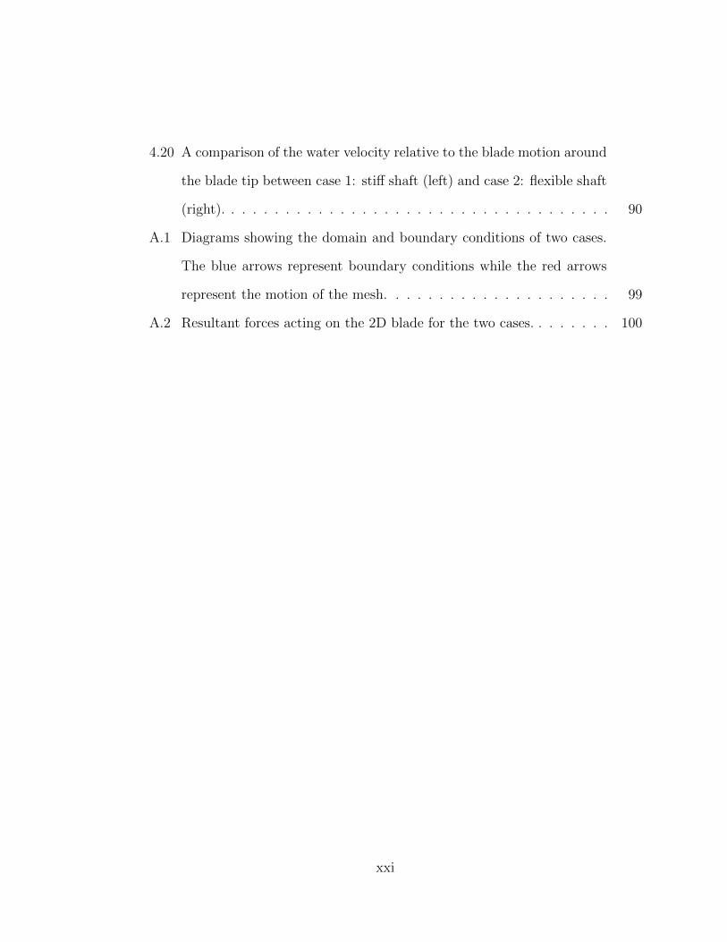
4.20 A comparison of the water velocity relative to the blade motion around

the blade tip between case 1: stiff shaft (left) and case 2: flexible shaft

(right). . . . . . . . . . . . . . . . . . . . . . . . . . . . . . . . . . . . 90

A.1 Diagrams showing the domain and boundary conditions of two cases.

The blue arrows represent boundary conditions while the red arrows

represent the motion of the mesh. . . . . . . . . . . . . . . . . . . . . 99

A.2 Resultant forces acting on the 2D blade for the two cases. . . . . . . . 100

xxi

Chapter 1

Introduction and Background

In the sport of sprint canoe, a force is exerted by an athlete onto a paddle. As the

paddle works to move through the water, the water’s resistance to motion works to

accelerate the athlete and boat forward. The details of the hydrodynamics of the

flow around the blade controls how the athlete’s power is transferred into boat speed.

Different factors can affect the blade hydrodynamics such as blade design and athlete

paddling technique.

1.1 Sport Background

In sprint canoe (also known as Canadian canoe) athletes race down a straight course

over distances of 200 m, 500 m or 1000 m. While the International Canoe Federation

(ICF) also sanctions 5000 m races which include turns, they are not raced at the

Olympics. Athletes are positioned on one knee with the other leg extending forward.

An athlete may paddle on the left or right side of the boat but not both. There are

three different type of boat categories in international competition: C1, C2 and C4

1

M.A.Sc. Thesis - Dana Morgoch McMaster - Mechanical Engineering

representing the Canadian canoe for 1, 2 and 4 athletes, respectively. While there

are strict rules that govern the design of a Canadian canoe (such as weight, length

and hull shape), there are practically no regulations that govern the paddle and blade

design other than the “Canadian canoe shall be propelled solely by means of single-

bladed paddles” and “the paddles may not be fixed on the boats in any way” (ICF,

2015).

1.2 The Canoe Paddle

The canoe paddle has three main components, the T-grip, the shaft and the blade.

The athlete grips the paddle across the T-grip (with their top hand) and along the

paddle shaft at about the midpoint of the paddle (with their bottom hand). Tradi-

tionally, paddles were made out of wood. In the mid-1980’s manufacturers started

to use composite materials; first using composite materials for the paddle shaft then

eventually the blade and T-grip.

In general, since the inception of the sport in the Olympics, blades have been

shaped as a relatively flat plate with shoulders at the top of the blade that tapper

in towards the shaft. The trend has been for blades slowly to become shorter and

wider, which can be seen by the different blade designs ranging from the 1970’s to

2010’s in figure 1.1. The development of composite blades in the 1980’s allowed

manufacturers to produce stronger and lighter paddles as well as more complicated

blade shapes. Despite this ability to create more complex blade shapes, the design of

the blade has remained relatively stagnant with only a few manufacturers producing

major variations such as the Turbo Strength Wing Face which has a more concave

back face, and the Plastex Canoe Bionic which is non-symmetric and individualized

2


for left and right sided paddlers. The most common blade used at the 2012 Olympics

was the Braca-Sport Extra-Wide, which still uses the mostly traditional flat plate with

tapered shoulders approach; however, is shorter and wider than previous paddles.

Figure 1.1: A view of the front (top) and back (bottom) faces of blades from dif-ferent manufacturers ranging from 1974 to today. From the oldest design to thenewest, the blade types shown are (from left to right) the Campere (note, the originalwooden shaft has been replaced with a carbon fibre shaft), Gere Neptune, Braca-Sport Medium, Turbo Strength Standard Wing Face, Braca-Sport Extra Wide, TurboStrength Sprint Racing Wing Face, and Plastex Canoe Bionic.

3


1.3 The Canoe Stroke

The canoe stroke is one complete cycle of power output and recovery. The motion of

the athlete is such that they use their body more than arms to pull themselves (and

the boat) forward. This motion is described through 5 technical phases.

• Setup: The positioning of the athlete and paddle right before the blade enters

the water (figure 1.2a). The athlete sets up forward above the water surface

by rotating their paddle side hip and lower body forward while extending the

paddle forward with a straight bottom arm and firm top arm. During the setup,

the shape of the athlete and paddle is an “A” when viewed from the side. Both

hands are over the water such that the paddle appears vertical when viewed

from the front.

• Catch: The act of burying the blade into the water (figure 1.2b). The catch is

the start of the application of power during the stroke. The athlete works to

maintain rotation in order to continue reaching forward while the blade enters

the water. They work to spear the blade forward into the water creating a clean

catch where air is not dragged into the water with the blade. As the blade is

buried, the athlete applies more pressure on the paddle by transferring their

body weight over the water and supporting themself with the paddle.

• Draw: The drawing (or pulling) forward motion of the athlete (figure 1.2c). At

the start of the draw phase, the blade is buried with maximum reach. Through

this phase, the athlete pulls themself forward by sitting up with their body while

de-rotating their hips and trunk. At the same time, they continue to support

their body weight and keep the blade buried by keeping downward pressure

4


on the paddle with their hands. The draw technical phase is also sometimes

referred to as the pull phase.

• Exit: The start of reloading the paddle side forward as the blade exits from

the water (figure 1.2d). As the paddle approaches the athlete’s paddle side hip,

the athlete begins reloading forward; first with their hip and then their paddle

side while maintaining back pressure on the paddle. At the same time, the

athlete begins rotating the paddle outwards (so the back face turns away from

the athlete) while starting to lifting it up and forward out of the water. The

rotation of the blade works to steer the boat. By the end of the exit, when the

blade is no longer in the water, the momentum of the athlete’s body should be

moving forward relative to the boat.

• Recovery: The reload of the body and paddle forwards to the setup position

(figure 1.2e). The goal of recovery is for the athlete to re-position themself for

the next stroke while minimizing the work done in the air, and relaxing the

body, arms and hands to get a short period of recovery while the blade is not

in the water.

It should be noted that in some literature, the pull phase refers to any time when the

blade is in the water producing a propulsive force. Since rudders or other steering

apparatuses are not allow (ICF, 2015), during a typical stroke, athletes use their

paddle to steer during the exit phase. Athletes can also alter earlier phases of the

stroke to help steer when needed, however, this is not ideal. While most follow the

concept of the five technical phases of the canoe stroke, different athletes and regions

have slight variations on technique.

5


Due to the difficulty in testing new equipment and changes in the athlete’s tech-

nique in a sport where environmental factors (such as the wind) often affect results

more than the changes that are being measured, athletes and coaches typically rely on

anecdotal evidence based on the perception of performance improvement. A study on

the hydrodynamics of the canoe stroke can provide insight on what is happening be-

low the water surface that drives the athlete forward which, in turn, can help lead to

better equipment design and more efficient technique; improving athlete performance.

6


(a) An athlete in the setup position. (b) Midway through the catch phase.

(c) Midway through the draw phase. (d) Midway through the exit phase.

(e) During the exit phase.

Figure 1.2: Pictures of an athlete during the different technical phases of the stroke.

7

Chapter 2

Literature Review

There has been very limited research specifically on sprint canoe blade hydrodynam-

ics. Fortunately, other blade-based water sports, such as sprint kayak and rowing,

have received slightly more attention and many parallels can be drawn. In this chap-

ter, literature on the blade-water interactions in different blade-based water sports

is discussed. First, previous work studying the relationships between blade motion

and the resultant forces are discussed. Next, experimental and numerical studies on

different blade-based water sports are discussed. Based on this literature review, a

summary of the objective of this thesis as well as an outline of its structure is given

at the end of this chapter.

2.1 Blade Hydrodynamics

The basis for understanding blade hydrodynamics lies first with understanding the

blade motion in the water. For the sport of sprint kayak, Jackson et al. (1992),

Jackson (1995) first looked at why the winged kayak blade that was introduced in

8


the mid-1980’s was more efficient than the traditional flat blade. It was noticed that

during the stroke, particularly at the exit, the blade swept away from the boat. This

lateral movement introduced flow normal to the boat velocity, which went around the

unsymmetrical wing shaped blade similar to flow over an air plane wing, producing

a lift force acting in the direction of the boat’s velocity.

In rowing, Wellicome (1967) examined rowing blade hydrodynamics and observed

that at the catch and finish, when the blade chord is more aligned with the hull’s

direction of motion, interactions between the blade and water produce an air-filled

cavity and an interacting vortex system. Wellicome proposed that these interactions

favourably align the resultant forces away from the chord normal to increase propul-

sion. Nolte (1993) attributed the more favourably aligned forces at the catch and

finish to the blade acting as a hydrofoil producing both drag and lift forces when ex-

amining why the hatchet blade increased efficiency over the traditional macon blade.

The net force on the blade can be determined by treating the blade as a hydrofoil

and calculating the drag and lift forces according to

FD =1

2CDρv

2A (2.1)

FL =1

2CLρv

2A (2.2)

where CD and CL are dimensionless drag and lift coefficients. A number of studies

have been completed to determine these drag and lift coefficients for different blade

designs (Sumner et al., 2003; Caplan and Gardner, 2007b; Ritchie and Selamat, 2010;

Sliasas, 2009; Sliasas and Tullis, 2009, 2011; Yusof et al., 2014). The net force can

then be broken up into propulsive and, for canoe, vertical components as shown in

9


figure 2.1. This approach usually, however, treats the blade as if it sees a distinct

uniform steady flow across the entire blade surface at each instant in time. Such a

quasi-steady approach then does not include the fully transient nature of the flow

over the rotating and translating blades.

Figure 2.1: A demonstration of the net force, FNet, which is made up of the combinedlift, FL, and drag, FD, forces can be broken into its x and y components determiningthe propulsive, FP , and vertical, FV , forces, respectively.

2.1.1 Moment on Blade

Besides the force on the blade itself, the moment, or centre of action of the force,

must be described. When Ritchie and Selamat (2010) examined the pressure profiles

on different blade designs, they noted that lowering the center of pressure may act

to increase the perceived moment on the blade. The effect of the moment acting on

10


the blade, however, has not been studied. It is likely to be a significant contribution

to the total load on the paddle due to the high rate of rotation of the blade. Since it

acts opposite to the direction of rotation, if the moment is significant, it could reduce

the overall efficiency of the stroke.

2.1.2 Transient Blade Flow Characteristics

Similarities between the dynamic nature of the rowing blade motion to that of an

oscillating air foil were demonstrated by Sliasas (2009). The dynamic behaviour of

the rowing blade was shown to develop a vortex at the leading edge of the blade which

translated along the blade surface before eventually shedding. This altered the drag

and lift coefficients compared to that of a blade in similar steady state conditions.

The altered drag and lift coefficients were due to a time-lag response to the pressure

on the blade altering the perceived angle of attack, which corresponded to a similar

time-lag response seen by McCroskey (1982) on oscillating air foils. Similar transient

effects are also likely to be present on the canoe blade, which follows a similar motion

to the rowing blade. Therefore, a fully transient model must be used to study the

true flow characteristics of the canoe stroke.

2.2 Experimental Studies

Experimental studies have focused on trying to measure, indirectly or directly, the

force acting on the paddle and blade. Indirect methods use off-water experiments

that help gain a better understanding of the hydrodynamics which can be used for

11


numerical models to calculate the force on the paddle. Direct methods aim at mea-

suring the force during on-water application. Direct methods primarily focus around

characterizing aspects of the stroke to provide quick feedback to the athlete and

coach. The feedback is aimed to guide technical or training changes and ignores the

hydrodynamics of the blade. A summary of relevant experimental studies is provided

in table 2.1.

2.2.1 Indirect Off-Water Experimental Methods

Indirect methods have been used to study the drag coefficients on different types of

blades. Sumner et al. (2003) examined how using different kayak blade shapes affect

the drag and lift coefficients. They placed different styles of kayak blades in a wind

tunnel and applied a free stream air velocity to match the Reynolds number seen by

a blade during a stroke. By adjusting the angle of the blade (changing both pitch

and yaw) and measuring the force acting on the blade, they were able to determine

the drag and lift coefficients of different blades for a range of angles of attack. They

determined that blade shape has little effect on the drag coefficient but using a winged

paddle increases the lift coefficient when rotated in steady state conditions. Caplan

and Gardner (2007b,c) used a similar method to measure the drag and lift coefficients

for a rowing blade through a range of angles of attack. They placed a blade in a water

flume which gave them the advantage of seeing the free surface effects. These drag

and lift coefficients are used as a basis for calculating propulsive forces in a number of

numerical models which will be discussed in section 2.3; however, as will be discussed,

these experimentally determined coefficients are determined in steady state and do

not account for important transient flow effects that affect them.

12


2.2.2 Direct On-Water Experimental Methods

Stothart et al. (1986) were the first to create a direct system to measure the force on

a canoe and kayak paddle. Stothart et al. (1986) showed that strain gauges attached

to a paddle shaft can be used to measure the shaft bend that occurs throughout a

stroke. The strain gauges were calibrated by supporting the shaft at specified points

and applying a known force at another. By measuring the amount the shaft bends

with different applied loads, the strain gauge signal can be converted into an applied

force. Other studies have used this method to create force profiles of the stroke

(see table 2.1). These profiles are used to examine specific factors about the studied

athletes. For example, in kayak, their left side can be measured against their right side

to see if they are producing similar forces or to compare force profiles from different

athletes in team boats (Baker, 1998; Coker, 2010).

One issue with bench calibrated shaft strain gauge systems is that it is not always

clear what the measurements represent during on-water testing. This difficulty in

understanding what the results represent is best seen by the widespread values of

forces noted by different strain gauge experiments on kayak paddles. They use similar

methods to measure force, yet the force values range from under 250 N to over 400 N.

This is likely due to not fully understanding what is being measured, such as where

the applied load is acting on the blade and the different mechanisms which contribute

to the bending of the shaft.

In rowing, Peach Innovations (2014) developed the PowerLine Rowing Instrumen-

tation and Telemetry system. With this system, the oarlock, which attaches the

rowing oar to the rowing shell, measures the fore-aft force on the swivelling oarlock

pin to provide real-time information to the coach and athlete. While this system has

13


been shown to be both accurate and useful as a training and coaching tool (Coker

et al., 2009), it still does not give the all important blade forces themselves. Of course,

such a system also requires the direct oarlock connection between the oar and the

hull and, therefore, cannot be applied to canoe and kayak.

Study Sport Area Measurement TypeStothart et al. (1986) Canoe, Kayak Paddle Strain GaugeBarnes and Adams (1998) Kayak Paddle Ergometer ReadingBaker (1998) Kayak Paddle Strain Gauge

Kleshnev (1999) RowingOar, Blade,Hull

Various Sensors

Sumner et al. (2003) Kayak Blade Force PlateSprigings et al. (2006) Kayak Blade Force TransducerCaplan and Gardner (2007b) Rowing Blade Strain GaugeHo et al. (2009) Dragon boat Blade Strain GaugeCoker et al. (2009) Rowing Oar, Hull Various SensorsCoker (2010) Rowing Oar, Hull Various SensorsHelmer et al. (2011) Kayak Blade Force SensorFleming et al. (2012) Kayak Blade, Athlete Strain GaugeYun (2013) Kayak Blade Strain Gauge

Table 2.1: Experimental studies on different blade-based water sports.

2.3 Numerical Models

A summary of relevant numerical studies on blade-based water sports is presented in

table 2.2. The majority of numerical models work to calculate the resultant propulsive

force by simplifying the forces acting on the blade throughout the stroke. The simplest

model used a force balance between the propulsive blade force and the boat drag force

by treating the blade as a fixed point of rotation where no energy was lost due to the

hydrodynamics of the blade (Millward, 1987). This model represents the ideal case

where 100% of the energy input by the athlete is transferred into forward thrust.

14


Other models have used similar methods of calculating the boat velocity by ap-

plying a force balance but accounted for hydrodynamic losses by treating the blade as

a moving hydrofoil. Pope (1973) hypothesized that the propulsive force on a rowing

blade is the component of the drag force which acts in the direction of motion of the

boat. This method does not account for lift forces which act on the blade. Similarly,

Sprigings et al. (2006) and Caplan (2008) assumed the kayak blade and outrigger

canoe blade, respectively, moves parallel to the boat velocity. This assumption orien-

tates the drag and lift forces so that only drag force contributes to the total propulsive

force.

Caplan and Gardner (2007a) and Morgoch and Tullis (2011) examined how both

drag and lift contribute to the total propulsion using a true representation of the blade

path. In rowing, Caplan and Gardner (2007a) determined instantaneous angles of

attack and relative velocities of the blade throughout the stroke using the boat velocity

and angular position of the rowing oar. In sprint canoe, Morgoch and Tullis (2011)

determined instantaneous angles of attack and relative velocities of the blade by

measuring the position of the paddle shaft above the water surface and calculating the

changing position of the blade below the water surface. By applying experimentally

determined drag and lift coefficients, they were able to see that the lift on the blade has

a significant contribution to the total propulsion. Use of this quasi-steady approach,

where the total force acting on the blade is the sum of instantaneous steady-state

forces acting on the blade at different positions, however, is unable to capture the

transient hydrodynamic effects.

Leroyer et al. (2008) showed that computational fluid dynamics (CFD) can be

a useful tool for studying the highly transient flow around a rowing blade. They

15


created an experimental apparatus which replicated the motion of a rowing blade

by rotating a rowing blade through water that was attached to a movable carriage.

Using force transducers, they determined the instantaneous force acting on the blade

and extrapolated the propulsive and orthogonal forces as well as the moment acting

about the moving center of rotation on the carriage. They then used CFD to simulate

the experimental blade motions and found strong agreement with the experimental

results; however, they did note grid independence was not met. While this did not

demonstrate the hydrodynamics of the rowing blade in an on-water application (nor

was it their goal too), it did demonstrate that CFD could be used to model the rowing

blade.

Sliasas (2009); Sliasas and Tullis (2009, 2010a,b) used CFD to simulate the rowing

blade hydrodynamics. The model first replicated the steady state experiments by

Caplan and Gardner (2007b,c) of a quarter scale rowing blade held at different angles

and showed that the CFD model’s steady state drag and lift coefficients matched the

experimental results well. To simulate the transient blade motions, the bulk flow was

accelerated according to a measured boat acceleration, and a rotating domain (which

housed the modelled rowing blade) rotated according to the changing oar angle. The

transient results showed that modelling the stroke using a quasi-steady approach, as

done by Caplan and Gardner (2007a), Caplan (2008) and, for canoe, Morgoch and

Tullis (2011), does not capture the true hydrodynamics of the stroke. Therefore, to

predict the resultant forces acting on the blade, transient effects must be included.

Sliasas and Tullis also included the water surface, although the blade remained buried

throughout the considered stroke as they did not need to move the blade through the

surface.

16


Sliasas and Tullis (2011) examined how bending of the oar shaft affected the force

acting on the blade. Oar shaft bending modifies the blade position and orientation

in the water when compared to the given oar angle history (as given at the oarlock

pivot point). It was found that when including the shaft bend, the propulsive force

followed a similar profile as when using a perfectly rigid oar shaft; however, the force

profile was delayed by about 0.15 s in the case which included shaft bend.

2.4 Objectives and Motivation

Based on this literature review, the objective of this thesis is to develop a model using

CFD that can investigate the unsteady flow of water around a sprint canoe blade

during a stroke in order to gain an understanding of the different flow characteristics

that drive the pressure acting on the blade and the resultant forces. Consideration

of the water surface (i.e. 2 phase flow) is required in this analysis. Chapter 3 of this

thesis provides an outline of the methodology used to model the studied stroke. This

includes the methods used to determine the motion of the blade, how that motion is

applied to the CFD model as well as the methods used to model the complex 3D, 2

phase transient flow. A brief review of literature relevant to the methods of modelling

used is presented along with those methods. In chapter 4, the results of two cases are

presented and discussed. The first case assumed a rigid paddle shaft when the blade

motion was determined. The second case altered the input blade motion by including

an approximation of the deflection of the blade due to shaft flexibility. The results of

case 2 are compared to case 1 to examine the effects of slight changes in input blade

path. Chapter 5 discusses conclusions from the work completed for this thesis and

recommendations for future work.

17


Study Sport Area Methodology 2-PhaseDegreesofFreedom

ActualBladePath

Transient

Wellicome (1967) Rowing BladeAnalysis of flow aroundrowing blade

Yes N/A Yes N/A

Pope (1973) RowingBlade,Hull

Propulsion is the forwardcomponent of dragforce on the blade

Yes 3 Yes Quasi

Millward (1987) RowingBlade,Hull

Assume blade rotatesabout fixed point

N/A 0 No N/A

Jackson et al. (1992) KayakBlade,Hull

Energy analysis ofwater vortex generation

Yes N/A Yes No

Nolte (1993) Rowing BladeAnalysis of flowaround rowing blade

N/A N/A Yes N/A

Jackson (1995) KayakBlade,Hull

Energy analysis ofwater vortex generation

Yes N/A Yes No

Cabrera et al. (2006) RowingBlade,Hull

Momentum balance ofboat, athletes and blade

No N/A N/A N/A

Caplan and Gardner (2007a) Rowing BladeMathematical equationsof boat drag vs.propulsion

Yes 3 Yes Quasi

Caplan and Gardner (2007c) Rowing BladeMathematical equationsof boat drag vs.propulsion

Yes 3 Yes Quasi

Leroyer et al. (2008) Rowing BladeTransient CFDsimulation

Yes 3 Yes Yes

Caplan (2008) OutriggerBlade,Hull

Mathematical equationof boat drag vs.propulsion

No 2 No Quasi

Michael et al. (2009) KayakBlade,Hull

Review of blade and hullhydrodynamics andoverview of equipmentadvancements

N/A N/A N/A N/A

Sliasas (2009) Rowing BladeTransient CFDsimulation

Yes 3 Yes Yes

Sliasas and Tullis (2009) Rowing BladeTransient CFDsimulation

Yes 3 Yes Yes

Ritchie and Selamat (2010)

Canoe,Chundan,DB,Macon

BladeCFD model to get CDin steady state ofdifferent blades

No N/A No No

Sliasas and Tullis (2010a) Rowing BladeTransient CFDsimulation

Yes 3 Yes Yes

Sliasas and Tullis (2010b) Rowing BladeTransient CFDsimulation

Yes 3 Yes Yes

Morgoch and Tullis (2011) Canoe Blade

Numerical Analysis ofblade motion and forceswith quasi-steadyapproach

Yes 3 Yes Quasi

Sliasas and Tullis (2011) Rowing BladeTransient CFDsimulation

Yes 3 Yes Yes

Banks et al. (2013) KayakBlade,Hull

CFD model of kayakblade rotating aboutpoint fixed to boat

Yes 3 No Yes

Yusof et al. (2014) Rowing BladeSteady state CFD ofblade at 45 degreeangle attack

No 1 No No

Table 2.2: Numerical studies on different blade-based water sports.18

Chapter 3

Methodology

The following chapter presents the methodology used to create the CFD model of

the sprint canoe blade motion. The process used to determine the input blade path

through video analysis and how the blade motion is applied to the model is discussed.

This includes a description of how shaft flexibility can affect the blade motion analysis

and be approximated. Next, details of the model are discussed including the numer-

ics involved with modelling transient two-phase flow along with the related literature,

the boundary and initial conditions and the mesh along with the related indepen-

dence testing. Lastly, methods used to increase model stability associated with the

blade piercing the water surface, as well as the stability of the free surface itself, are

discussed.

3.1 Video Analysis and Blade Path

The first step in creating a transient model was to define the blade motion which

was particularly difficult as canoe paddles are not fixed to the boat, so the blade

19


can move freely with 6 degrees of freedom. During the catch and draw phases of

the stroke, the athlete works to keep the paddle oriented within the x (horizontal)

and y (vertical) plane, therefore, the blade motion can be simplified to 3 degrees of

freedom, x and y translation and rotation about z-axis. Towards the exit phase of

the stroke, as the blade force becomes steering focused, the blade path has off plane

motions. Because the exit path may frequently change depending on the changing

steering requirements, the model ended with the start of the exit phase at 0.3 s.

Video analysis was used to determine the blade path within the xy-plane using a

method similar to Morgoch and Tullis (2011). Video analysis was completed using

video of an athlete paddling at race pace past a camera. The camera was mounted

on a tripod on shore 15 m to 20 m perpendicular to the athlete’s path and about 1.5

m above the water surface. The video camera captured video at a resolution of 1440

x 1080, frame rate of 29.97 Hz and shutter speed ranging from 1/500 s to 1/2000 s.

Two markers were placed on the athlete’s paddle shaft and their distances from the

bottom of the paddle measured. The software Tracker 4.80 (Open Source Physics)

was used to measure and digitize the changing positions of the markers during the

stroke. The length of the boat (5.2 m) was used as a distance reference and the

water surface as the x-axis location. The tracking of each marker was repeated a

minimum of 3 times and averaged to increase the accuracy of the tracking position.

The maximum repeatability error was 6 mm of any individual point.

While out of plane rotation is assumed to have minimal effects on the hydrody-

namics of the stroke, it must be included to determine the position of the blade within

the xy-plane. To do this, the projected distance between shaft markers as seen by

the video, Lmxy , was compared to the actual distance, Lm, to determine the out of

20


plane angle of rotation, β according to,

β = arctanLmxy sin θ

L2m − L2

mxycos2 θ − L2

mxysin2 θ

(3.1)

This angle was then used to determine a projected paddle length, Lxy according to,

Lxy =

√cos2 θ

cos2 θ + sin2 θ + sin2 θcos2 β

(3.2)

The projected paddle length was used to determine the x and y position of the blade

in each video frame using cosine and sine relationships respectively.

Equations of motion (EOM) of the blade were developed by plotting the x and y

positions of the blade along with the orientation of the blade in each video frame as a

function of time and fitting 6th order polynomials (equations (3.3) to (3.5)) over the

first 0.33 s as shown in figure 3.1.

x(t) = −4541.4t6 + 4106.3t5 − 1331.9t4 + 224.92t3 − 34.663t2 + 4.8795t

R2 = 0.9994

(3.3)

y(t) = −3769.0t6 + 3633.1t5 − 1427.9t4 + 297.97t3 − 19.404t2 − 4.6533t

R2 = 0.99996

(3.4)

θ(t) = 364230t6 − 349260t5 + 119960t4 − 18076t3 + 1274.6t2 + 187.41t

R2 = 0.99996

(3.5)

21


The 6th order polynomials have a strong fit to the measured blade location (R2

>0.9994). The resultant path of the top and bottom of the blade traced by equa-

tions (3.3) to (3.5) along with the measured position of the blade from the video

analysis are presented in figure 3.2. The path traced by the equations of motion

compared very well to the video analysis data for the modelled portion of the stroke.

This strong fit during the modelled portion of the stroke is reflected when comparing

the simulated blade velocity and nominal angle of attack determined by the equations

of motion to the video analysis as seen in figure 3.3. The simulated blade velocities

match the video analysis very well until 0.3 s when the relative velocities drops rather

than continue to rise. Since the model ended at 0.3 s, this was not a concern.

3.1.1 Effects of Shaft Flexibility on the Blade Path

As the paddle is loaded with the input forces of the athlete and reaction forces on the

blade, it bends. This bend can affect both the blade position and angle compared to

the perceived position from the video analysis. The exact amount the paddle bent was

not known, however, it was estimated. To estimate how much the paddle bent during

a stroke some assumptions were made about how the force acts on the paddle. As the

blade moves through the water, a pressure force is applied to the full surface of the

blade which results in a distributed load. Due to the length of the shaft compared

to the blade, the majority of the bend in the paddle was assumed to occur in the

shaft, above the blade. The force on the blade, therefore, was treated as a point load

at the center of pressure. It was unknown how the center of pressure moves during

a stroke so it was assumed the force acts slightly below the center of the blade due

to its cambered shoulders (Ritchie and Selamat, 2010). Using these assumptions, the

22


Figure 3.1: Plot of x and y position and angular rotation of blade over time fromvideo analysis. Sixth order polynomials were fit to the points.

23


Figure 3.2: Plot of the position of the blade from video analysis with the position ofthe blade from the equations of motion (EOM). The solid dark grey lines representthe blade every 0.05 seconds.

24


Figure 3.3: Plot of the relative velocity and nominal angle of attack over time of thevideo analysis data (points) and equations of motion (dashed lines).

25


bend on the paddle was calculated by treating the paddle as a 3 point loaded beam

with the 3 points being the top and bottom hand positions, and 20 cm up from the

bottom of the blade. Figure 3.4 shows the bending diagram of the paddle.

Figure 3.4: Bending diagram of the paddle. The red line is the stiff shaft location ofthe blade while the green line is the flexible shaft location of the blade.

The Euler-Bernoulli beam theory states that,

M(x) = −EI d2δ

dx2(3.6)

26


where x is the distance along the beam, M(x) is the moment at point x, E and I

are the Youngs modulus and moment of inertia respectively, and δ is the deflection

at point x. Integrating equation (3.6), assuming the paddle is a 3 point loaded beam,

determines the deflection of the paddle shaft at distance x away from the top handle

according to,

if 0 ≤ x ≤ a

δ1 =−FBottomHandbx

6EIL[L2 − b2 − x2] (3.7)

and if a < x ≤ b

δ2 =−FBottomHandbx

6EIL[L2 − b2 − x2]− FBottomHand(x− a)3

6EI(3.8)

where L is the length of the paddle and a and b are the distances to load FBottomHand

from the top of the paddle and the center of pressure on the blade, respectively. For

the case of a canoe paddle, load FBottomHand is the pulling force at the bottom hand

position and was calculated using the blade normal force, FN , according to,

FBottomHand =L

aFN (3.9)

The value of EI was determined by comparing the stiffness rating of the shaft to the

Braca method of rating the shaft stiffness. Braca canoe paddle shaft stiffness is rated

according to the midpoint deflection distance during a 3 point load test; the shaft is

placed on two supports 1 m apart, and a 10 kg load is hung in the middle (BRACA-

SPORT, 2015). Applying equations (3.7) and (3.8) to a shaft with a stiffness rating

of 1.6 mm, EI = 1277 Nm2

The estimated angular deflection, θDeflect, and deflection distance, δDistance of the

27


blade was calculated by comparing the deflection of different points along the paddle

shaft to the perceived position of the paddle (as shown in figure 3.4) according to,

θDeflect = θBlade + θMark (3.10)

and

δDistance = δBottomHand − δMidBlade + (xMidBlade − xBottomHand) sin θMark (3.11)

where

θMark = arctan

(δTopMark − δBottomMark

xTopMark − xBottomMark

)(3.12)

and

θBlade = arctan

(δTopBlade − δBottomBlade

xTopBlade − xBottomBlade

)(3.13)

Since the deflection of the blade was small relative to the paddle length, the blade

bend angle and deflection is essentially linear where,

θDeflect(◦) ' 0.019FN (3.14)

δDistance(m) ' 0.00017FN (3.15)

as seen in figure 3.5. Using this relationship, bending terms were added to the blade

equations of motion using an applied bending profile, Fapplied (which will be described

in more detail in section 4.3.1), that smoothly increased to a max of 160 N over the

first 0.08 s then held about constant. While Fapplied is based on initial 3D results, it

is not coupled to the resultant force during the simulation.

28


Figure 3.5: Blade bend distance and angle as a function of applied blade normal force.These linear relationships are used to create bend terms in the equations of motion.

29


3.2 Geometry and Mesh Motion

The motions of the blade were simulated by dividing the computational domain into

two subdomains, an inner moving subdomain and an outer stationary subdomain.

Cylindrical domains were used for 2D simulations, and semi-spherical domains were

used for 3D simulations. A view of the 3D-domain is presented in figure 3.6 show-

ing the inner and outer semi-spherical subdomains, the position of the canoe blade

and the free surface. The inner subdomain had a rigid mesh, relative to the blade,

which translated and rotated according to the motion of the blade as defined by the

equations of motion (equations (3.3) to (3.5)). The inner subdomain was big enough

to capture the flow effects due to the blade motion. The outer subdomain was used

to create a volume that the inner subdomain could move within. The outer subdo-

main’s mesh deformed according to the x and y translation of the inner subdomain.

The outer subdomain was large enough that the mesh deformation due to the inner

subdomain’s motion did not induce flow on the inner subdomain that may affect

the flow around the blade. At the interface between the two subdomains, the inner

interface translated along the outer interface according to the rotation of the inner

subdomain. The interface was defined using a general grid interface (GGI) connec-

tion (CFX-Solver, 2011b). The GGI connection maintained conservation of the mass

and momentum equations across the interface while allowing the mesh on either side

of the interface to be slightly misaligned due to the circular interface being made

out of tetrahedral elements. This maintenance of the conservation equations across

the interface allowed the interface to translate according to the motion of the blade

without inducing flow throughout the domain. The dimensions of the 2D and 3D

geometries are presented in table 3.1.

30


DomainInner Domain Diameter 12.5 mOuter Domain Diameter 20 m2D Domain width 1 cm

2D Blade GeometryPlanar Shape RectangularBlade Height 50 cmBlade Width 1 cmBlade Thickness 0.5 cmTip Chamfer 5 cm

3D Blade GeometryPlanar Shape Braca canoe extra wideBlade Height 50 cmBlade Width 24 cmBlade Thickness 0.5 cmTip Chamfer 1.5875 cmSide Chamfer 0.9525 cm

Table 3.1: Major geometry dimensions of the domain, 2D blade, and 3D blade

The position of the blade within the inner subdomain was such that the center

of the blade coincided with the center of the inner subdomain. The position of the

inner subdomain was offset from the center of the outer subdomain according to the

starting position of the blade. The height of the inner subdomain, compared to the

center of the outer subdomain, was the height above the water surface of the middle

of the blade at the start of the simulation. The geometry of the blade is shown

in table 3.1. The motion of the inner subdomain was specified by defining a mesh

motion through the use of CFX expression language (CEL) functions. These functions

combined the equations of motion (equations (3.3) to (3.5)) together to define a

location of each mesh element as a function of time. The mesh that defined the outer

boundary of the outer subdomain was fixed in location; however, the remainder of the

31


outer subdomain’s mesh was free to deform according to the translation of the inner

subdomain. The deformation was governed by the displacement diffusion model,

∇ · (Γdisp∇δmesh) = 0 (3.16)

where Γdisp is the mesh stiffness which is inversely proportional to the element vol-

ume size and δmesh is the displacement of a node relative to its previous location.

The implementation of the moving mesh was validated against the commonly used

method of applying motion by specifying an inlet velocity to accelerate the fluid past

a stationary (or rotating) object (see appendix A).

3.3 Fluid Modelling (Numerics)

3.3.1 Navier-Stokes Equations

Simulation of the canoe blade was completed by solving modified versions of the

governing equations of fluid motion. The governing equations were solved through a

finite element approach, where the geometry was divided into a region of finite volumes

and the governing equations solved for each fluid volume element. For isothermal,

incompressible, Newtonian flow, the governing equations are the conservation of mass

and conservation of momentum,

∂ui∂xi

= 0 (3.17)

ρ∂

∂t(uj) + ρ

∂

∂xi(uiuj) = − ∂p

∂xj+

∂

∂xi

[µ

(∂uj∂xi

+∂ui∂xj

)]− ρgj (3.18)

32


Figure 3.6: View of semi-spherical 3D geometry showing the outer stationary bound-ary, inner moving subdomain and blade position. The free surface between the water(bottom) and air (top) is shown in blue about halfway through the domain.

33


Collectively, equations (3.17) and (3.18) are known as the Navier-Stokes equations.

They must, however, be modified to include effects such as turbulence and multiphase

flow.

3.3.2 Rotating Domain Numerics

The unsteady angular velocity of the inner subdomain imposes three forces on the

bulk flow through the subdomain. These forces were accounted for by imposing source

terms on the momentum equation (equation (3.18)) such that,

ρ∂

∂t(uj) + ρ

∂

∂xi(uiuj) = − ∂p

∂xj+

∂

∂xi

[µ

(∂uj∂xi

+∂ui∂xj

)]− ρgj

+ SCor + Scfg + SEuler (3.19)

where the source terms, SCor, Scfg and SEuler account for the Coriolis, centrifugal and

Euler acceleration forces, respectively. These source terms were defined according to,

SCor = −2ρωBlade ×U (3.20)

Scfg = −ρωBlade × (ωBlade × r) (3.21)

SEuler = −ρ∂ωBlade∂t

× r (3.22)

where ωBlade and U are the rate of rotation and velocity of the inner subdomain,

respectively, as defined by the motion of the blade and r is the radial location from

the center of the inner subdomain.

34


3.3.3 Turbulence Models

The structure of turbulent flow is chaotic in nature but can be characterized by treat-

ing the instantaneous velocity, ui, and pressure, p, at a specific point as a combination

of a time averaged value (Ui and P ) and a fluctuating value (u′i and p′),

ui = Ui + u′i (3.23)

p = P + p′ (3.24)

Substituting equations (3.23) and (3.24) into the Navier-Stokes equations (equa-

tions (3.17) and (3.18)), the time averaged conservation of mass equation becomes,

∂Ui∂xi

= 0 (3.25)

and time averaged conservation of momentum equation becomes,

ρ∂

∂t(Uj) + ρ

∂

∂xi(UiUj) = − ∂P

∂xj+

∂

∂xi

[µ

(∂Uj∂xi

+∂Ui∂xj− ρu′ju′i

)]− ρgj (3.26)

Equations (3.25) and (3.26) are known as the Reynolds averaged Navier-Stokes (RANS)

equations. The extra terms ρu′ju′i are known as the Reynolds stresses. In order to

directly solve the RANS equations, an additional six equations would be needed due

to the six extra Reynolds stress terms creating a closure problem. Turbulence models

act to get around this by approximating the Reynolds stresses.

Boussinesq hypothesized that turbulence mixing acts to diffuse momentum. This

meant that the Reynolds stresses could be modelled as an increase to the effective

35


viscosity such that,

−ρu′ju′i = µt

(∂Uj∂xi

+∂Ui∂xj

)+

2

3kδij (3.27)

where µt is a turbulence viscosity. This turbulence viscosity is not a property of the

fluid itself; most turbulence models work to approximate it though the characteristics

of the turbulent flow (Zaıdi et al., 2010).

The k-ε model (Jones and Launder, 1972) uses the relationship between the tur-

bulent kinetic energy, k, and the turbulence dissipation, ε, to predict the turbulent

viscosity.

µt = ρcµk2

ε(3.28)

The term cµ is an experimentally determined constant (Cousteix, 1989). The k-ε

model is known to handle free stream flow very well, however, within the turbulent

boundary layer, it fails to capture the turbulent viscosity. When studying flow sep-

aration, such as is the case with a canoe blade moving through the water, this can

cause a delay in the predicted flow separation point.

The k-ω model (Wilcox, 1988) predicts the turbulent viscosity through the rela-

tionship between the turbulent kinetic energy and the turbulence frequency, ω, as

µt = α∗ρk

ω(3.29)

where α∗ is a correction coefficient for low Reynolds numbers (Zaıdi et al., 2010). The

k-ω resolves the turbulent boundary layer and turbulence characteristics very well

but in regions of free-shear, it is very sensitive to the turbulence frequencies. This

sensitivity makes it difficult for capturing flow separation due to external adverse

pressure gradients.

36


The shear stress transport (SST) model (Menter, 1994) works to combine the k-ε

and k-ω models. In the free shear regions, the SST model follows the k-ε method, and

in the near wall regions, it transitions to the k-ω method using a blending function.

The SST model uses two transport equations,

ρ∂

∂tk + ρ

∂

∂tUik = Pk − β∗ρωk +

∂

∂xi

[(µ+ σk3µt

∂k

∂xi

)](3.30)

ρ∂

∂tω + ρ

∂

∂tUiω = α

ω

kPk − βρω2 +

∂

∂xi

[(µ+ σω3µt

∂ω

∂xi

)]+ 2(1− F1)ρσω2

1

ω

∂k

∂xi

∂ω

∂xi(3.31)

The blending function, F1, smoothly transitions from 0 to 1 as the distance to the

wall, y, decreases, transitioning from the k-ε to the k-ω method,

F1 = tanh

{

min

[max

( √k

β∗ωy,500v

y2ω

),

4ρσω2k

CDkωy2

]}4 (3.32)

where CDkω is a limiter for the cross-diffusion term,

CDkω = max

(2ρσω2

1

ω

∂k

∂xi

∂ω

∂xi, 10−10

)(3.33)

The production limiter Pk is used to prevent the build-up of turbulence in regions of

stagnation,

Pk = µtS2 (3.34)

where S is the absolute value of the strain rate,

S =√

2SijSij (3.35)

37


The turbulence viscosity is defined as,

µt =ρα1k

max(α1ω, SF2)(3.36)

The second blending function, F2 switches from 0 to 1 as the distance to the wall

decreases, similar to F1,

F2 = tanh

[

max

(2√k

β∗ωy,500v

y2ω

)]2 (3.37)

The constants (in general form written as, Φ) are determined by blending the con-

stants of the k-ε (denoted by the subscript 1) and k-ω (denoted by the subscript

2),

Φ3 = F1Φ1 + (1− F1)Φ2 (3.38)

The constants that were used are shown in table 3.2

α 0.31

β∗ 0.09α1 5/9β1 3/40σk1 0.5σomega1 0.5α2 0.44β2 0.0828σk2 1σomega2 0.856

Table 3.2: Constants used for the SST turbulence model

Given the changing nominal blade velocity and the blade dimensions, it is expected

that the Reynolds number for the flow around the blade be in the range of 2×105 to

38


1×106; therefore, it is expected that the flow transitions to turbulent along the blade’s

surface. The SST model’s ability to accurately predict flow separation in adverse

pressure gradients (Huang et al., 1997), makes it the most appropriate turbulence

model for the presented case. Further, Sliasas (2009) found that for similar flow

around a rowing blade, the gross features of the flow were not strongly dependent on

the turbulence model.

3.3.4 Multiphase Flow

Volume of Fluids

Modelling multiphase (2-phase) flow is accomplished using the Eulerian volume of

fluids (VOF) approach (Hirt and Nichols, 1981). The VOF approach creates a dis-

tinction between the air and water phases by defining a fluid volume fraction, ϕ, for

each finite mesh volume (cell). Most cells contain only air or water (ϕair = 1 or

ϕwater = 1). Cells at the interface of the two phases have a volume fraction between

0 and 1. A free surface is constructed along adjacent cells with partial volume frac-

tions. The VOF model provides an accurate method for modelling surface break up

and reconnection (Gueyffier et al., 1999).

The main properties that represent different fluids in isothermal multiphase flow

are density and dynamic viscosity. The change in these properties is represented by

modifying the Navier-Stokes equations. Assuming conservation of volume, which was

valid here, in each cell

ϕwater + ϕair ≡ 1 (3.39)

39


Since there was no mass transfer between the air and water, the mass of each individ-

ual phase is conserved; therefore, the conservation of mass equation (equation (3.17))

can be written individually for each phase,

ρwater∂

∂t(ϕwater) + ρwater

∂

∂xi(ϕwaterui) = 0 (3.40)

ρair∂

∂t(ϕair) + ρair

∂

∂xi(ϕairui) = 0 (3.41)

For non-homogeneous flow, the flow field is defined separately for each phase. There-

fore, the conservation of momentum equations are defined individually for each phase

as well. Equation (3.18) can be rewritten for 2-phase flow as,

ρwater∂

∂t(ϕwateruwaterj) + ρwater

∂

∂xi(ϕwateruwateriuwaterj)

= −ϕwater∂pwater∂xj

+∂

∂xi

[ϕwaterµwater

(∂uwaterj∂xi

+∂uwateri∂xj

)]− ϕwaterρwatergj +Mwater (3.42)

ρair∂

∂t(ϕairuairj) + ρair

∂

∂xi(ϕairuairiuairj)

= −ϕair∂pair∂xj

+∂

∂xi

[ϕairµair

(∂uairj∂xi

+∂uairi∂xj

)]− ϕairρairgj +Mair (3.43)

where the terms Mwater and Mair represent the transfer of momentum to the water

phase from the air phase and to the air phase from the water phase, respectively.

40


Since momentum is conserved,

Mwater = −Mair (3.44)

For free surface flow, where the water and air are modelled as continuous fluids, the

momentum transfer is due to the interfacial drag force which is driven by the difference

in velocity between the phases (CFX-Solver, 2011a; Godderidge et al., 2009; Strubelj

et al., 2009). The total interfacial drag per unit volume, Dinterfacial, is,

Dinterfacial = CDinterficialρmixAmix|Uwater −Uair|(Uwater −Uair) (3.45)

where ρmix is the mixture density as given by,

ρmix = ϕwaterρwater + ϕairρair (3.46)

and Amix is the interfacial area per unit volume as given by,

Amix =ϕwaterϕairdmix

(3.47)

The mixture length scale, dmix, was 1 mm which was based on an approximated

entrained droplet size (Frank, 2005). The interfacial drag coefficient, CDinterficial, was

0.44, similar to the drag on a sphere which is commonly used for free surface flow

(Frank, 2005; Godderidge et al., 2009).

41


Surface Tension Model

While the effects of surface tension were minimal, it was modelled using a continuum

surface model (Brackbill et al., 1992). In this model, surface tension is treated as a

continuous volume force concentrated at the interface. Primary (water, denoted by

α) and secondary (air, denoted by β) phases were defined and the surface tension

force modelled according to,

Fαβ = fαβδαβ (3.48)

where

fαβ = −σαβκαβnαβ +∇sσ (3.49)

and

δαβ = |∇rαβ| (3.50)

where nαβ is the interface normal vector pointing from the water phase to the air

phase, σ is the surface tension coefficient and was constant and ∇s is the gradient

operator on the interface. Since the surface tension coefficient was constant, the

second term in equation (3.49) was equal to zero; and therefore, the surface tension

force acted normal to the surface. The surface curvature, καβ is defined by,

καβ = ∇ · nαβ (3.51)

The term δαβ keeps the effects of the surface tension force local to the interface by

reducing to 0 away from the interface.

This method of solving free surface multiphase flow using the ANSYS CFX solver

code has been shown to predict the drag and lift coefficients in similar conditions.

42


Sliasas and Tullis (2009) used a similar method to predict the drag and lift coefficients

of a rowing blade held in steady state with good agreement to the experimental values

of Caplan and Gardner (2007c) in matching conditions.

3.4 Boundary and Initial Conditions

The blade surface was defined as a no-slip surface with a velocity set by the mesh

motion. The outer domain surface was defined as an opening with a relative pressure

equal to the hydrostatic pressure. About the blade centreline, a symmetry bound-

ary condition was applied. This symmetry boundary condition was advantageous

as it halved the overall size of the 3D domain, significantly reducing computational

costs; however, it assumed the blade wake was axisymmetric. Johari and Stein (2002)

demonstrated that on impulsively started disks, the wake remains axisymmetric until

the disk travels 6 times the diameter. Since the blade tip, which travels the fur-

thest, moves less than six times the width of the blade, the blade wake will remain

axisymmetric about the symmetry boundary throughout the full simulation.

The volume fraction of each cell was initially defined according to a step func-

tion creating a sharp transition between water and air at the free surface location.

The initial conditions were the result of a steady state simulation as described in

section 3.6.

3.5 Mesh

An unstructured tetrahedral mesh with hexahedral boundary layer cells was generated

using ANSYS CFX-Mesh (figure 3.7). A 10 cell inflated boundary layer was applied

43


to the blade surface with a total thickness of 3 mm. A maximum element edge length

of 5 mm and 2 mm was used for the blade faces and sides, respectively. A maximum

element length of 10 cm was used for the inner subdomain mesh (as described in

section 3.2) with a growth rate of 1.075 expanding from the fine blade mesh. This

growth rate kept the mesh in the vicinity of the blade fine while allowing the mesh

to become course away from the blade. The mesh at the interface between the two

subdomains initially aligned prior to any mesh motion. In the outer subdomain, the

mesh grew with a growth rate of 1.2 from a maximum element length of 10 cm (at

the interface) to 25 cm.

Mesh independence was conducted using a 2D single phase model. Using a 2D

single phase model reduced the computational costs associated with the full 3D models

and eliminated effects of air-water interactions as they were not the primary focus of

study. The mesh was refined by decreasing the maximum element length on the blade

surface, within inner subdomain and within the outer subdomain independently from

each other by a factor of 2; yielding a range of total elements of 77000 for the mesh used

in the presented simulations, to 272000 for the most refined case. The resultant force

on the blade between these cases differed by less than 2% with a few outliers reaching

as high as 3%. The mesh on the blade surface and within the inner subdomain was

also similar to the mesh sizing that was found to be grid independent by Sliasas (2009)

while simulating the flow around a rowing blade of similar dimensions (50.4 cm by

25 cm) and under similar flow conditions (Sliasas used a maximum edge length of 0.5

cm on the blade surface and 10 cm throughout the domain).

44


Figure 3.7: The unstructured tetrahedral mesh with hexahedral boundary layer cellsaround the blade. The stationary outer boundary is shown in grey, the deformingouter subdomain is shown in red, the translating and rotating inner subdomain isshown in green and the blade mesh is shown in black.

45


3.6 Free Surface Initialization

Prior to running the transient simulation, if the model is not properly initialized, an

issue can form where a point of extreme pressure (over 102 to 1012 times larger than

hydraulic pressure) during the first timestep. This point of extreme pressure causes

a shock wave to expand out moving the fluid throughout the domain and breaking

apart the free surface. The exact cause of this is not known; however, it is likely

due to a conservation of volume issue which attempts to compress the incompressible

water in a single cell. To properly initialize the model, a steady state simulation was

run. During the steady state initialization period, difficulty solving the free surface

is known to cause spurious waves to form on the surface (CFX-Solver, 2011a). The

propagation of these waves causes small currents near the surface that increase in

magnitude with the initialization period length. While this issue of wave propagation

could affect the transient results as well, since the number of iterations per timestep

was minimal, it was not a concern. Decreasing the steady state timescale reduces

the magnitude of the spurious currents, however, decreasing this timescale increases

the number of steady state iterations needed to initialize the model. To accurately

simulate the free surface, a balance between initialization length and the timescale

needed to be maintained, where the point of extreme pressure does not form and the

magnitude of the spurious currents are significantly smaller than the speed of the

blade through the water.

It was found that using a steady state timescale of 1.85×10−4 and an initialization

length of 100 steady state iterations did not produce any points of extreme pressure

while maintaining minimal spurious currents. After 100 iterations, the peak superfi-

cial water velocity, which occurs at the free surface, was less than 0.05 m/s and the

46


average water velocity in the volume which the blade moves through was less than

0.01 m/s, as can be seen in figure 3.8. Therefore, the velocity of the spurious currents

was significantly lower (less than 1%) than the velocity of the blade moving through

the water at the catch and will not have a significant impact on the end results.

Figure 3.8: Contour plot of spurious current water velocity after steady state initial-ization. Max velocity occurs at free surface (shown as black line) but reduces as itextends deeper into the water

3.7 Model Stability During Blade Entry

As the blade enters the water, flow can separate from the blade tip forming an air

pocket in front of the blade. The formation of this air pocket, along with its size, is

very sensitive to the blade motion. In some cases, this air pocket can fold in on itself

and be pinched off at the point where the water reattaches to the blade. In real life,

athletes can feel if an air pocket folds in on itself as it results in a slapping feeling as

the water reattaches to the blade and a ”kerplunking” noise. Higher level athletes are

tuned to the blade entry and make small adjustments to the paddle motion to prevent

the formation of this air pocket. When modelling the blade entry, if an air pocket

47


forms, the point of reattachment is initially not resolved well by the finite grid and

can result in high impact pressures at single grid cells and non-convergence. Limiting

the flow separation off the blade tip can help decrease the size of the air pocket, so

the pocket does not get pinched off higher on the blade surface, better representing

real world conditions as well as increasing the stability of the model. This decrease

in flow separation can be accomplished by starting later in time, at a point along the

blade path where a portion of the blade is initially buried in the water. However, by

starting at a later point in time, the flow effects during the initial blade entry are no

longer captured. In order to start later in time, and reduce the tip flow separation,

the missed flow effects must have a minimal impact later in the stroke.

Testing was completed to determine how sensitive the pressure around the blade

and the resultant force on the blade are to the starting depth of the blade. Testing

was carried out using a 2D model because, in 2D, flow separation was found to be

less sensitive to the blade path, allowing the blade to start out of the water and

remain stable throughout the full simulation. Simulations started at different initial

positions in time corresponding to the blade being at different starting depth as

labelled in table 3.3.

Simulation Name Start Time (s) Initial Blade Tip Depth (cm)

Out of Water 0 9.91Tip Buried 0.023125 -3.3Half Buried 0.0555 -21.63/4 Buried 0.08325 -35.3Fully Buried 0.12025 -49.8

Table 3.3: Initial blade depths above (positive) and below (negative) the surfacecorresponding to the starting times of the simulation.

The resultant propulsive and vertical forces are plotted in figure 3.9. At the start

48


of each simulation, there is a spike in force associated with impulsively starting the

blade motion. As the blade starts with a larger portion in the water, the magnitude of

this force spike increases due to the increase resistance to sudden motion of the water

relative to the air. In each case, the impulsive effects are limited to within the first six

timesteps. After the initial impulse effects, the propulsive and vertical forces acting

on the blade match very well between the each simulation apart from the fully buried

case. Therefore, starting the model with the blade partially buried can increase the

model stability and better match real world condition without sacrificing accuracy so

long as the model starts prior to the blade being three-quarters buried.

3.8 Flow Solver

The conservation equations were solved using the ANSYS CFX commercial CFD

code (CFX-Solver, 2011a). Initial steady state models were run for 100 iterations

to initialize the free surface as described in section 3.6. The conservation equations

were solved using a high resolution advection scheme which used a blending function

that switched from a first order to a second order scheme in areas of lower variable

gradients. Turbulence quantities were solved using a first order advection scheme.

A steady state timescale of 1.85×10−4 s was applied. A timescale for the volume

fraction equation class of 1.85×10−5 s was applied.

Transient simulations were run using the same conservation equation and turbu-

lence quantity advection schemes. The transient terms of the conservation equations

were solved using a second order backward Euler scheme. Turbulent transient terms

were solved using a first order backward Euler scheme. Transient volume fraction

terms were solved using a bound second order backward Euler scheme. The ANSYS

49


Figure 3.9: The resultant force on a 2D blade starting at different points in timecorresponding to the blade being fully out of the water, with the tip buried, halfburied, 3/4 buried and fully buried. These relate to the simulation start times andinitial blade depths described in table 3.3.

50


CFX Solver (ANSYS, 2011) was used to solve the governing mass and momentum

equations iteratively at each timestep until the root mean square (RMS) of the resid-

uals fell below 10−4.

The transient simulation was completed in two stages. This was due to impulsive

effects of the instantaneously moving blade in the incompressible water at the start of

the simulation. It was found that impulse effect created a large pressure spike on the

blade which lasted 4-6 timesteps, regardless of the timestep size. The first stage ran for

ten timesteps at 1/10th the timestep size as the second stage. This two-stage process

allowed for impulsive effects (similar to the impulsive effects seen in section 3.7) to

work themselves out without advancing too far in time. The second stage ran for the

remaining length of the simulation (until 0.3 s or instability occurred as explained

in section 3.7). One phase, 2D timestep independence showed that a timestep of

1.85×10−3 was sufficient for resolving the transient flow throughout the bulk of the

stroke. However, a timestep of 4.625×10−4 increased stability as the blade pierced

the water surface; therefore, 4.625×10−4 was used as the second transient simulation

stage timestep.

51

Chapter 4

Results and Discussion

The following chapter presents and discusses the results of 2 cases. Case 1 assumes the

paddle shaft is perfectly stiff when determining the blade path from the video analysis.

Case 2 approximates the flexibility of the paddle shaft to determine an altered input

blade path to case 1. Both cases follow the numerical methods presented in the

methodology chapter and differ only by the input blade motion. While the mesh

used for all simulations follow the same method of generation outlined in section 3.5,

their meshes differ slightly due to their unstructured nature. The resultant blade-

water interactions, including the pressure and forces acting on the blade, are first

presented in detail for case 1. Case 2 is then compared against the case 1 results.

4.1 Video Analysis and Orientation Definition

Video of a national team level canoeist with multiple world championship medals,

including for the C1 200 m event, was used for analysis. Information on the athlete,

equipment and conditions is presented in table 4.1. Wind speed was not measured

52


during the testing but was minimal. Testing was done at the end of a canal, where

there was no water current. A total of 6 strokes were examined in detail using the

video analysis procedure outlined in section 3.1. The resultant blade paths from each

stroke are presented in figure 4.1. There is some minor variation between each stroke

with all following the same general motion. One stroke was selected to be modelled

(shown by the solid lines in figure 4.1). This stroke was selected because it was

the smoothest blade path and had minimal blade slip at the surface representing a

clean catch, aiding model stability associated with the blade entry (as explained in

section 3.7). Information about the specific stroke modelled is shown in table 4.2.

While each blade path slightly differed from each other, the stroke chosen to be

modelled represents a sample race pace stroke from an internationally ranked athlete.

The average velocity of the boat throughout the stroke was within 1.6% of the world

record average boat speed for the C1 200 m event.

Athlete

Athlete Height 1.75 mRace Type Men C1 200 m

Equipment

Canoe Model Nelo C1 Vanquish III 2Paddle Length 1.69 mPaddle Type Braca Canoe Extra WidePaddle Width 24 cm

Conditions

Wind Speed Very Slight Head WindWater Current Negligible

Table 4.1: Information on the athlete, equipment and environmental conditions dur-ing testing.

When analysing the blade-water interactions, a coordinate system and directional

53


Figure 4.1: Blade path from 6 different strokes. The black points represent the topof the blade while the grey points represent the bottom of the blade. Lines are addedto help clarify different strokes. The solid lines with circular symbols represent thechosen blade path used for the model, and the dotted lines represent strokes measuredbut not modelled.

54


Stroke Rate 76 Strokes/minBoat Velocity 5.16 m/sStroke Distance 4.08 mApproximate 200 m race time 38.75 s

Table 4.2: Information on the modelled stroke.

terms are defined with respect to the direction of motion of the boat as shown in

figure 4.2. The x-axis is horizontal, parallel to the direction of motion of the boat

going through the centreline of the canoe blade. The y-axis and z-axis act up and

outward to the right of the athlete, respectively. Positive and negative y-axis values

represent the height above or depth below the water surface, respectively. Different

directional terms are also used to describe the motion of the blade and the surrounding

water. Motion in the direction of the boat’s velocity (positive x) is referred to as

forward while backwards (or aft) represents opposite the boat’s velocity (negative x).

The front and back faces of the blade represent the surfaces of the blade that face

forwards and backwards, respectively. The blade tip and chamfer refer to the bottom

edge of the blade chamfer which creates the pointed tip. The blade’s edge refers to

the edge that runs along the side of the paddle starting at the tip and finishing at

the top of the blade. Generally, figures presented are shown as if the direction of the

motion of the boat was from left to right.

4.2 Case 1: Stiff Shaft

For case 1, the blade shaft was assumed to be perfectly stiff when extrapolating the

blade positions from the video used to determine the input blade path. Cabrera

et al. (2006) showed that including the flexibility of oar shafts has minimal effect on

55


Figure 4.2: Coordinate system and definition of terms used to describe locations onthe blade and the directions of motion of the blade and flow.

predicting the athlete input forces and resultant blade forces when using a momentum

balance approach to model rowing forces and kinematics. It has been common practice

to assume stiff shafts when modelling the canoe, kayak and rowing stroke (Caplan and

Gardner, 2007a; Caplan, 2008; Leroyer et al., 2008; Sliasas and Tullis, 2009; Sliasas,

2009; Sliasas and Tullis, 2010a,b; Morgoch and Tullis, 2011; Banks et al., 2013). While

the resultant forces on the blade are sensitive to changes in the blade path associated

with the inclusion of shaft flexibility, which will be discussed in case 2, modelling the

blade motion assuming a stiff paddle shaft provides a base case that can be used for

comparison.

4.2.1 Canoe Blade Motion

The modelled blade path is shown in figure 4.3. The blade enters the water at an

initial paddle angle of approximately 56◦ with a diving motion, extending forward as

56


it is driven down into the water. As the blade continues into the water, the rotation

of the blade, due to the de-rotation and forward velocity of the athlete, causes the

blade tip to start to slip backwards (aft) as it drops deeper while the top of the

blade continues into the water with a forward motion. After the blade is fully buried

and rotates past 90◦ the blade midpoint starts to slip backwards slightly (∼3 cm)

as the athlete focuses on pulling the paddle essentially straight backwards. Due to

the continued rotation of the paddle, however, the blade tip sweeps significantly back

while the top of the blade continues to slip forward. As the blade approaches the

end of the stroke, it is lifted up as the athlete begins focusing on driving their body

forward to set-up for the next stroke. Near the end of the stroke, after the modelled

portion ends, the blade appears to be dragged forward and out of the water; however,

at this point (as mentioned in section 3.1) there are out of plane motions not captured

by the video analysis.

The stroke is traditionally divided into 5 phases as defined in section 1.2: setup,

catch, draw, exit and recovery. Examining the characteristics of the blade motion

(such as the direction of motion, the relative velocity and nominal angle of attack

of the blade) 5 distinct regimes of motion (or pull-phases) can be seen within the

traditional catch and draw phases of the stroke (figure 4.4). The nominal angle of

attack (αnom) is defined using the blade orientation and relative motion in hypothet-

ically quiescent water. The top, bottom and middle relative velocities and nominal

angles of attack of the blade are shown separately to demonstrate the varying flow

profile seen on the blade due its high rate of rotation compared to its translation.

The different pull-phases are outlined in table 4.3 and described with their technical

motions (Buday, 2015) as follows:

57


Figure 4.3: The case 1 stiff shaft path of the canoe blade through the water. Blue linesdenote the blade position every 0.05 seconds. The red lines denote the blade positionat the start of the stroke, the start of the catch, transition, draw, drive pull-phasesand at the end of the modelled stroke, respectively.

58


1. Entry: The initial surface piercing of the blade into the water. The athlete

increases the rotation of their upper and lower body and focuses on a clean

entry to avoid creating large air pockets while beginning to apply power into

the water.

2. Catch: The blade continues into the water while continuing to extend forward

with positive slip. The athlete tries to maintain the rotation of their upper

body which helps maintain a constant rate of rotation as the blade continues

into the water.

3. Transition: The blade stops extending forward as it drops down becoming com-

pletely buried transitioning between the traditional catch and draw technical

phases. The athlete transitions into a pulling motion by fully engaging their

lower body leading to a de-rotation of their upper body and an increase in the

rate of rotation of the blade.

4. Draw: The middle of the blade begins slipping backward with minimal depth

changes. The athlete pulls the paddle essentially straight backward and reaches

a maximum point of de-rotation of their lower body before slowing down the

de-rotation of their upper body.

5. Drive: The blade stops slipping backwards and starts to lift up with the athlete’s

upper body. The athlete begins driving their lower body forward to start to

reload for the next stroke.

A detailed examination of the flow during each pull-phase can provide insight into

how the different characteristics of blade motion drive the flow around the blade and

the resultant pressure on the blade.

59


Pull-Phase Time (s) % BuriedNominal Angleof Attack

RelativeVelocity

Blade Slip Depth ChangeRate of AngularRotation

Entry 0.017 - 0.04 0 - 30 Slight Increase Decrease Positive Lowering IncreaseCatch 0.04 - 0.09 30 - 80 Constant Decrease Positive Lowering ConstantTransition 0.09 - 0.17 80 - 100 Slight Increase Decrease Minimal Lowering Increase

Draw 0.17 - 0.25 100 Large IncreaseDecreasethen Increase

Negative MinimalIncreasethen Decrease

Drive 0.25 - 0.3 100 Slight Increase Increase Minimal Rising Decrease

Table 4.3: Pull-phases of the modelled stroke.

Figure 4.4: Relative velocity, nominal angle of attack (AoA) and rate of angularrotation of the blade throughout the five pull-phases of the stroke. The blade firstcontacts the water at the start of the entry pull-phase at 0.017 s. The relative velocityand nominal angle of attack are shown for three locations on the blade: top, bottomand middle.

60


4.2.2 Flow Characteristics

As the blade moves through the water, the flow around it produces a pressure field on

the blade which provides the resultant forces that act to propel the boat and athlete

forward. In this section, the details of the CFD calculated flow patterns around the

blade are explained throughout each pull-phase.

Entry Pull-Phase

During the entry pull-phase, the blade first pierces the water with an extremely

shallow nominal angle of attack (αnom) and high relative velocity (Vrel) where αnom

and Vrel are relative to the stationary water. As the blade tip is buried, αnom increases

slightly, and Vrel decreases. The shallow αnom keeps the flow around the blade tip

attached to the blade (figure 4.5b). On the front face of the blade, this creates areas

of low pressure (suction) near the blade tip and above the tip chamfer where the

flow must make a rapid change of direction (figure 4.5c). On the back face of the

blade, the pressure increases due to the impingement of the water on the blade face,

with the highest pressure occurring at the blade tip where αnom is highest. The

pressure magnitudes on both faces increase as the blade enters the water, reaching a

maximum pressure difference, which occurs at the blade tip, at the end of the entry;

acting to increase the net force on the blade (figure 4.5d). This pressure difference

reduces up the blade to zero at the surface. Since the largest pressure difference

occurs near the blade tip, the resultant net force induces a significant torque acting

on the blade which increases as the pressure magnitudes increase. This pressure

difference causes a circulation of water around the blade tip from the back face to

the front face (figures 4.5a and 4.5e). Similarly, vortices start to form along the

61


edges of the blade (figure 4.5e). The low-pressure cores at the vortex centres reduce

the pressure magnitudes along the blade’s edges and extend to the surface creating

surface depressions.

During this pull-phase of the stroke, the low pressure aft of the blade and high

pressure in front of the blade cause the water surface to bulge up and depress down

aft and in front of the blade, respectively, while accelerating the near surface water

backwards (figures 4.5a and 4.5e).

(a) Velocity Vector (b) Relative Velocity Vector

(c) Pressure Profile (d) Centreline Pressure

62


(e) Circulation of flow around tip and side vortex

Figure 4.5: Flow and pressure images of the blade towards the end of the entrypull-phase at (0.0375 s). a) is the velocity vectors on the centreline plane, b) is thevelocity vectors relative to the motion of the blade on the centreline plane, c) is thenon-hydrostatic pressure contours of the back (left) and front (right) of the blade, d)is the centreline non-hydrostatic pressure of the back (blue) and front (red) of theblade and e) shows streamlines of the flow moving around the blade tip and bladeedge. The direction of boat motion is in the positive x-direction (left to right in a)andb) and slightly down right c). The position of the water surface is shown by the bluesurface in a), b) and e) and by the blue lines in c).

Catch Pull-Phase

During the catch pull-phase, as the blade continues to be submerged with a diving

forward motion, αnom remains fairly constant while Vrel decreases. As in the entry

pull-phase, the minimum and maximum pressures on the blade faces occur near the

blade tip (on the front and back faces, respectively) although the pressure magnitudes

now reduce due to the reduced Vrel. Flow separation from the front face starts to

63


occur off of blade tip and just above the chamfer, causing the formation of a tip vortex

(figures 4.6b and 4.6e).

As the blade continues into the water, the forward rotation of the top of the blade

causes αnom at the surface to decrease past 0◦ and become negative (or positive with

respect to the front face). This negative αnom, coupled with the previously induced

aft-ward flow of the water near the surface, causes a zone of reverse pressure (defined

as an area of the blade with positive pressure on the front face and negative pressure

on the back face producing a negative component to the net force) on the top of the

blade (the portion of the blade which enters the water after the entry pull-phase).

This zone of reverse pressure is seen in figure 4.6d above a depth of -32 cm. The

growing zone of reverse pressure, along with the reducing tip pressure acts to reduce

the total net force on the blade. The now suction pressure aft of the blade near the

surface also causes a new trough to form behind the blade.

64





Figure 4.6: Flow and pressure images of the blade as described in figure 4.5 at theend of the catch pull-phase (0.088 s).

65


Transition Pull-Phase

During the transition pull-phase, as the blade is fully buried in the water, Vrel con-

tinues to decrease, and αnom near the bottom of the blade begins to increase. The

tip vortex begins growing in size and strength (as seen by the relative velocity vec-

tors and tip vortex streamlines in figures 4.7b and 4.7e, respectively) growing faster

towards the blade centreline. The growth of the tip vortex shifts the location of the

peak suction (associated with the core of the tip vortex) up the blade front face.

Once the blade is fully buried, the horizontal speed of the water around the top

of the blade (which has been accelerating forward) begins to match the forward but

decelerating horizontal speed of the blade. This match of the horizontal speeds of the

blade and water leads to a decrease in the magnitude and area of the zone of reverse

pressure such that by the end of the transition, the total reverse pressure is negligible

(figure 4.7d). The combination of the growing area of tip suction with the reducing

reverse pressure works to increase the net force on the blade.

The edge vortex continues to grow in size and strength near the bottom of the

blade. Near the tapered shoulders, where αnom is negative, this edge vortex detaches

from the blade and a secondary vortex of reverse direction forms and grows where the

main vortex shed away from the blade. Once the top of the blade is fully submerged,

the free surface disconnects from the blade and begins levelling out; however, since

the paddle shaft is not modelled with the blade, the details of the disconnection may

not completely match the real world.

66





Figure 4.7: Flow and pressure images of the blade as described in figure 4.5 at theend of the transition pull-phase (0.17 s).

67


Draw Pull-Phase

During the draw pull-phase, as the blade is pulled aft essentially horizontally, αnom

rises rapidly, and Vrel decreases reaching a minimum when αnom reaches 90◦. As

αnom rises past 90◦, Vrel starts increasing again, and the flow on the blade face begins

to reverse direction moving down the blade face rather than up. The downward

flow remains attached to the front blade face aiding the shedding of the tip vortex

(figure 4.8b).

As the tip vortex sheds from the blade, the velocity profile around the front face

becomes more uniform. This uniform velocity profile creates a relatively constant

pressure on the front face with the exception of a spike in suction as the flow turns

around the tip chamfer. On the back face, the high pressure near the blade tip seen in

previous phases reduces, resulting in an essentially constant pressure across the back

face (figure 4.8c). While the more constant pressure profiles increase the pressure

difference across the top portion of the blade, the loss of both the low-pressure tip

vortex and the high-pressure on the back of the blade results in a drop in the net

force on the blade. However, since the pressure profile is more uniform on the blade

surface, the resultant torque about the centre of the blade reduces. The primary edge

vortex now detaches from the bottom half of the blade, and the secondary reversed

vortex begins detaching from the top of the blade.

68





Figure 4.8: Flow and pressure images of the blade as described in figure 4.5 at theend of the draw pull-phase (0.24 s).

69


Drive Pull-Phase

During the drive pull-phase, as the blade begins lifting up towards the surface, αnom

increases from 160◦ to 172◦ (i.e. 20◦ to 8◦ with respect to the top back face), and

Vrel increases. The pressure profiles on the blade follow a similar pattern as the draw

phase (relatively constant on the front and back faces with a small spike in suction

around the tip chamfer) but the pressure difference across the blade increases slightly

(figure 4.9d). This increase in pressure difference acts to increase both the net force

on the blade as well as the torque about the center of the blade.

As αnom of the top of the blade approaches -170◦ (i.e. 10◦ with respect to the top

front face), a small separative vortex forms at the top of the aft face of the blade.

The effects of this are seen in figure 4.9d by the zone of reverse pressure in the top

2–3 cm of the blade. However, since the blade is narrowest in this area, the total

effect on the net force is very small.

4.2.3 Forces on the Blade

The total propulsive and vertical forces acting on the blade are the combined x and

y components of the pressure and viscous shear forces acting on the blade. While

shear forces are included in the force calculation, they are very small compared to

the pressure forces acting on the essentially flat blade, as demonstrated by the net

force on the blade acting about normal (within 1◦) to the blade surface throughout

the stroke. The torque on the blade is calculated about the center of the blade (25

cm from the blade tip).

70





Figure 4.9: Flow and pressure images of the blade as described in figure 4.5 at theend of the drive pull-phase (0.3 s).

71


Equivalent Bend Load

Experimental studies that use strain gauges to measure the applied loads on the

paddle measure the strain locally on the paddle shaft. Torque on the blade depends

on both the applied loads on the paddle as well as the points of applications of those

loads. Previous strain gauge experiments work under the assumption that only the

net force on the blade contributes to the strain on the paddle shaft and do not measure

the locations of the applied loads or torque on the blade. This exclusion of the torque

acting on the blade can lead to an overestimation of the net force acting on the blade.

The equivalent bend load is the fictional equivalent normal force acting on the centre

of the blade required to strain the paddle shaft the same as the actual combined net

force and torque on the blade. The equivalent bend load is what a strain gauge placed

between the athletes hands would read if calibrated to a normal force acting at the

center of the blade, and can also be used as a measure of the total applied load on

the blade.

Force Discussion

The resultant forces (the net force and its propulsive and vertical components), torque

and equivalent bend load are presented in figure 4.10. During the catch pull-phase,

there is an unrealistic drop in the net force on the blade due to an overestimation

of the build-up of reverse pressure on the blade. This dip in force while the blade

is entering the water was not seen in studies by Baker (1998) and Ho et al. (2009)

that measured the local strain on kayak and dragon boat paddle shafts, respectively,

to determine the applied force on the paddle throughout the stroke. Ho et al. (2009)

noted that the applied force on the paddle increases rapidly as the blade is being

72


buried reaching a peak force, after which the force reduces, approaching zero at the

exit. Baker (1998) saw profiles in kayak similar to Ho et al. (2009) however also noticed

that some athletes produce dual peak force curves where the force dips slightly after

the initial peak before rising again to produce a second peak during the draw phase

of the stroke. While the dip seen by Baker (1998) is similar to the dip in net force

during the draw pull-phase, neither studies saw a drop in force while the blade is being

buried similar to that produced in the presented model. Further, it seems unrealistic

that the athlete produces a negative net force on the blade during the initial phases

of the stroke.

A similar, but smaller, drop in normal force (the force approached zero but did

not go negative) was seen by Morgoch and Tullis (2011) when using a quasi-steady

analytical model to calculate the force on the blade. As both models use the same

method of video analysis to determine the input blade motion (section 3.1), the drop

in force at the catch is quite possibly associated with the input blade motion.

As will be discussed in section 4.3, a source of blade path error is thought to be

due to excluding the flexibility of the blade shaft when extrapolating the position of

the blade below the water surface. Sliasas and Tullis (2011) showed that the flexibility

of a rowing oar, where the blade can deflect by up to 16.4 cm causing a change in

blade angle of 4 degrees, has a large effect on the resultant force on the blade when

modelling the transient flow around the blade. This force dependency on the oar

flexibility was contrary to Cabrera et al. (2006) who found that including the shaft

flexibility did not improve the fit of their rowing momentum balance model results.

While the magnitude of the forces acting on blade throughout the stroke may be

erroneous, it is believed that observations can still be made on what drives the net

73


force and torque on the blade as well as their contributions to the total load on the

paddle. The net force on the blade is the sum of the pressure profiles in 3 regions.

The front near-tip suction pressure is driven by the flow separation over the blade tip

and the development and shedding of the tip vortex as a result of the changing α at

the blade tip. The back near-tip high-pressure region is due to the impingement of

flow near the blade tip. The pressure on the remaining portion of the blade is driven

by the bulk acceleration of the water around the blade. The surface deformation

during the entry, catch and transition is due to the near surface pressure accelerating

the water surface up and down. Here, with a clean catch, the surface deformation

has little effect on the bulk flow around the blade and the pressure effects, since the

vented air pockets around the blade are small and localized. The edge vortex reduces

the pressure magnitude at the edge of the blade, however, unlike the tip vortex; it

does not develop onto the blade face, so its effects are small and localized.

74


Figure 4.10: The case 1 stiff shaft resultant net force, along with its propulsive andvertical components, torque and equivalent bend load acting on the blade throughoutthe stroke.

75


4.3 Case 2: Flexible Shaft

A second case was modelled which altered the case 1 blade path by including the

flexibility of the paddle shaft. As the exact amount of bend in the paddle shaft could

not be accurately measured from the video analysis, it was approximated using the

manufacturer supplied shaft stiffness and a simplified paddle loading. These were

used to determine the deflection distance, δDistance, and angular deflection, θDeflect,

of the blade in order to create a new input blade path for the CFD model. As the

deflection of the blade was approximated, the aim was not to get exact results but to

compare to the stiff shaft case, seeing the effect of the change in blade position, path

and angle.

4.3.1 Applied Bending Profile

The applied bending profile is a rough estimation of the applied net force on the blade

that contributes to bending the paddle shaft throughout the stroke. The relationship,

Fapplied =

0, if t ≤ 0.015s

160 tanh((t− 0.015s)50), if t > 0.015s

(4.1)

was used to create an applied bending profile and is plotted with the case 1 stiff shaft

resultant net force for comparison in figure 4.11. Fapplied increases smoothly through-

out the entry and catch pull-phases starting at 0.015 s, about when the blade first

contacts the water, to a maximum value of 160 N. This maximum force is similar

to the maximum net force in case 1. Fapplied remains constant throughout the tran-

sition, draw, and drive pull-phases. While this does not follow the dips in force seen

76


in the case 1 results, it is closer to the force profile shapes seen in the strain gauge

experiments from Baker (1998) and Ho et al. (2009). Since the presented simulation

ends prior to the exit phase, the drop in Fapplied associated with the exit is not mod-

elled. As Fapplied is approximated rather than uses the modelled resultant forces, the

paddle shaft bend calculations are not iterative in nature, ensuring that the shaft

flexibility equations are not an additional source of model instability. Substituting

equation (4.1) into equations (3.7) to (3.13) provides the approximate blade deflec-

tion distance and the angular deflection throughout the stroke which are shown in

figure 4.12.

Figure 4.11: The applied bending load and case 1 stiff shaft net force.

77


Figure 4.12: The applied deflection distance (δdistance) and angular deflection (θdeflect)throughout the modelled stroke.

4.3.2 Flexible Shaft Blade Path

As the blade is loaded and the deflection distance and angular deflection increase, the

motion of the blade in the water is altered (figure 4.13). While Fapplied is increasing,

the deflection of the blade increases the forward slip while slowing down the rate of

angular rotation of the blade compared to the paddle shaft of the stiff shaft case

during the entry and beginning of the catch pull-phases. The increase in forward slip

into the water and reduced rate of rotation maintains a nominal angle of attack of

the blade at the water surface closer to 0◦, aiding in the concept of a clean catch. The

78


angular deflection leads to the blade maintaining a slightly lower horizontal angle, θ,

(by about 3◦) throughout the remainder of the stroke.

The rate of change of deflection distance due to the increase in Fapplied during the

entry and catch pull-phases causes an additional velocity component, Vdeflect, normal

to the paddle angle as shown in figure 4.14. This additional velocity component causes

the sudden increase in Vrel and decrease in αnom seen during the entry in figures 4.15

and 4.16, respectively. The negative αnom,flex at the begin of the entry is an indication

that Fapplied likely increases too rapidly initially; however, since the initial entry is

not modelled due to surface instability, over-estimating the initial Fapplied has little

effect on the model results. During the catch pull-phase, the rate of change of the

deflection distance, and therefore, Vdeflect, decreases enough that the associated drop

in αnom is less than the increase in αnom due to the deflection angle itself resulting in

a higher αnom,flex than αnom,stiff .

When Fapplied reaches its maximum of 160 N during the catch phase, the deflection

distance and angular deflection become constant at 2.7 cm and 3.0◦, respectively, as

seen in figure 4.12. Beyond this point, the path of the blade follows a similar motion

to the stiff shaft case but slightly further forward (ranging from 2.1 cm to 2.7 cm)

creating an apparent time lag. The lower horizontal angle of the blade causes αnom,flex

to remain steadily higher than αnom,stiff throughout the catch, transition and most

of the drive pull-phases. During the draw and start of the drive, when αnom is rapidly

increasing from 30◦ to 150◦, the apparent time lag in the blade motion causes αnom,flex

to increase slightly later than αnom,stiff (figure 4.16).

79


Figure 4.13: The blade path for the flexible shaft case. The red lines denote the bladepath between different phases while the blue lines show the blade every 0.025 s. Theblack dashed line indicates the path of the middle of the blade for the stiff shaft case.

80


Vdeflect

Vrel,f lex

Vrel,stiff

Original Blade Position

Stiff Paddle Flexible PaddleBlade Position Blade Position

αnom,flexαnom,stiff

Figure 4.14: Example of how the rate of change of deflection during the entry andcatch pull-phases induces an additional velocity component, Vdeflect, which alters Vreland decreases αnom for the flexible shaft case. Stiff shaft motions are shown in blackwhile flexible shaft motions are shown in blue.

4.3.3 Changes in Flow Patterns and Force

Figures showing a comparison of the resultant forces on the blade (figure 4.18), the

blade centreline pressure distribution (figure 4.19) and water relative velocity around

the blade tip (figure 4.20) between both cases are presented at the end of this section.

The flexible shaft force profile has a similar shape as the stiff shaft case with a few

significant differences.

• The initial peak loads reach much higher magnitudes (about 1.7 times the stiff

shaft case) and occur slightly later into the catch phase.

• The drop in force during the catch phase is still unrealistic when compared to

the strain gauge experiments of Baker (1998); Ho et al. (2009); however, the

now positive minimum forces show that including the flexibility of the paddle

81


Figure 4.15: Comparison of Vrel for the flexible shaft (solid lines) and stiff shaft(dashed lines) cases.

Figure 4.16: Comparison of αnom for the flexible shaft (solid lines) and stiff shaft(dashed lines) cases.

82


shaft can positively affect the result.

• The dip in force during the draw and drive phases is larger than the stiff shaft

case; however, the torque acting on the blade is about equal.

The flow characteristics that drive the change in pressure acting on the blade—and

therefore, the resultant force on the blade—are driven by the same defining flow

characteristics as the stiff shaft case. The differences are mainly in the timing of the

development of these flow characteristics (such as how quickly the tip vortex develops

and sheds) and their magnitudes. Therefore, by examining the general development of

flow around the blade and the resultant changes in pressure, observations about how

the different forces relate to each other can be made. While other flow characteristics

such as edge vortices development and flow separation around the top of the blade

also see minor changes in timing and magnitude, they are not compared in detail due

to their limited effect on the overall blade pressure.

During the entry (t = 0.0174 s to t = 0.0375 s) as the shaft is actively bending

(and the blade is actively deflecting), the lower initial αnom,flex reduces the pressure

on and around the blade (figures 4.19a and 4.19b) leading to the lower initial aft-ward

flow of water in front of and behind the blade near the surface compared to the stiff

shaft case as seen in figure 4.17. The actively deflecting blade also reduces the αnom

at the surface creating a cleaner catch which disturbs the water surface significantly

less; producing almost no surface depression or bulge up in front of or behind the

blade and drawing very little air into the water with the blade as seen in figure 4.17.

Early in the catch pull-phase (t = 0.0375 s to t = 0.0467 s) the flow over the blade

tip is similar between both cases producing a similar near-tip pressure distribution;

albeit with a slightly higher pressure magnitude on the back face of the blade for the

83


(a) Case 1: stiff shaft (b) Case 2: flexible shaft

Figure 4.17: Comparison of the water velocity on the centreline plane of the bladetowards the end of the entry at t = 0.0375 s between the case 1: stiff shaft and case2: flexible shaft

flexible shaft case associated with the now higher αnom,F lex (figures 4.19c and 4.19d).

Similar to the stiff shaft case, as the top of the blade enters the water, it begins to

accelerate the aft-ward moving water near the surface forwards; however, since the

entry produced lower initial aft water velocities, the onset of reverse pressure occurs

later in the catch. This delay in reverse pressure allows the net force on the blade

to continue to grow with the tip pressure magnitude resulting in the higher and later

peak force on the blade seen at t = 0.0467 s in figure 4.18. As in the stiff shaft case,

the development of reverse pressure on the blade causes the unrealistic drop in force

on the blade. While approximating the shaft flexibility results in higher, and positive,

blade forces—due to the higher αnom,flex increasing the pressure on the back face of

the blade (figures 4.19e and 4.19f), and initiating flow separation over the blade tip

earlier (figures 4.20e and 4.20f)—the large drop in force demonstrates that the build

up of reverse pressure during the catch pull-phase is still over-exaggerated.

84


From the beginning of the transition pull-phase (t = 0.09 s), the tip vortex grows

up the blade front face increasing the tip suction force. While the tip vortex grows

in this manner in both cases, the higher αnom,flex causes it to start to occur at the

beginning of the transition rather than part way through. This earlier growth results

in a larger tip vortex, and thus, tip suction area at the end of the transition at t =

0.17 s (figures 4.19g, 4.19h, 4.20g and 4.20h). On the back face of the blade, the high

pressure from the catch drops such that at the end of the transition, the back-tip

pressure is about equal between cases. Away from the blade tip, the magnitude of

the reverse pressure begins dying out; however, it dies out slower in the flexible shaft

case resulting in a higher negative component to the net force.

During the draw pull-phase (t = 0.17 s to t = 0.25 s), the quicker rise in αnom,stiff

than αnom,flex causes the tip vortex to shed from the blade in a similar manner in both

cases. The result of this is similar tip suction pressures between both cases by the end

of the draw (figures 4.20i and 4.20j). Above the tip, the zone of reverse pressure begins

to produce a positive pressure difference; however, the positive pressure develops

slower than the stiff shaft case (figures 4.19i and 4.19j). Since by the end of the draw

the majority of the net force on the blade is due to the pressure difference on the

bulk of the blade rather than near the tip, the resultant net force on the blade for

the flexible shaft case is half that of the stiff shaft case (t = 0.25 s on figure 4.18).

During the drive pull-phase (t = 0.25 s to t = 0.3 s), the positive pressure across

the bulk of the blade begins to grow faster in the flexible shaft case. By the end

of the drive, the pressure profile across the full blade is very similar between cases

(figures 4.19k and 4.19l). The similar pressure profiles result in a similar net force on

the blade at the end of the modelled stroke.

85


Figure 4.18: The resultant forces acting on blade throughout both cases. Dashedlines represent case 1 stiff shaft results while solid lines represent case 2 flexible shaftresults.

86


(a) Stiff Case at t = 0.037 s (b) Bend Case at t = 0.037 s

(c) Stiff Case at t = 0.047 s (d) Bend Case at t = 0.047 s

(e) Stiff Case at t = 0.088 s (f) Bend Case at t = 0.088 s

87


(g) Stiff Case at t = 0.17 s (h) Bend Case at t = 0.17 s

(i) Stiff Case at t = 0.24 s (j) Bend Case at t = 0.24 s

(k) Stiff Case at t = 0.30 s (l) Bend Case at t = 0.30 s

Figure 4.19: A comparison of the non-hydrostatic pressures along the blade centrelinebetween case 1: stiff shaft (left) and case 2: flexible shaft (right).

88


(a) Stiff Case at t = 0.037 s (b) Bend Case at t = 0.037 s

(c) Stiff Case at t = 0.047 s (d) Bend Case at t = 0.047 s

(e) Stiff Case at t = 0.088 s (f) Bend Case at t = 0.088 s

89


(g) Stiff Case at t = 0.17 s (h) Bend Case at t = 0.17 s

(i) Stiff Case at t = 0.24 s (j) Bend Case at t = 0.24 s

(k) Stiff Case at t = 0.30 s (l) Bend Case at t = 0.30 s

Figure 4.20: A comparison of the water velocity relative to the blade motion aroundthe blade tip between case 1: stiff shaft (left) and case 2: flexible shaft (right).

90


4.3.4 Summary

With the exception of the initial entry, where slight changes in angle can significantly

affect surface deformation and air entrainment, altering the blade path by approxi-

mating the shaft flexibility has little effect on the types of flow characteristics that

develop during a stroke. However, the magnitude and timing of characteristic flow

development are sensitive to small changes in blade path and angle, causing large

changes in the resultant blade forces as shown in figure 4.18. The comparison of the

flow characteristics and blade forces in section 4.3.3 indicate that the resultant forces

on the blade are driven mainly by the balance between the high back tip pressure,

the front tip suction pressure, and the bulk blade pressure away from the tip. The

high back tip pressure is due to the impingement of flow around the blade near the

tip. The front tip suction pressure is driven by the development and shedding of a

tip vortex. The bulk blade pressure (which initially produces a negative net force

component before becoming positive during the draw pull-phase) is driven by the

initial aft-ward then forward acceleration of water in front of and behind the blade.

The contributions to the equivalent bend load of the propulsive and vertical com-

ponents of the net force on the blade are similar between both cases (figure 4.18).

Since the blade remains mostly upright throughout the stroke (rotating between about

59◦ and 124◦) the majority of the net force acts propulsively. This is important as

the propulsive force is the only force which directly acts to accelerate the boat for-

ward. The flexible shafts’ reduction of horizontal blade angle acts to increase slightly

the vertical component of the net force favourably compared to the stiff shaft case,

delaying the onset of the negative vertical force that results when the blade rotates

beyond 90◦. While this negative force is inevitable, due to the rotation of the blade,

91


it is non-ideal as it acts to increase the effective weight of the athlete increasing the

total drag of the boat.

Torque accounts for a significant portion of the applied load on the paddle. If

the torque is not accounted for when using the strain on the paddle to measuring

the applied load on the blade, it can lead to more than a 20% over-estimation of the

maximum net force on the blade as shown by the equivalent bend load. Since the

torque on the blade acts against the athlete, it increases the needed applied load by

the athlete to generate the same net force on the blade, decreasing the efficiency of the

stroke. The source of this torque is due to the development of the tip vortex causing

the majority of the applied load on the blade (or the blade resistance to motion)

to act near the blade tip. This is why the torque increases proportionally with the

net force on the blade during the entry, catch and transition pull-phases (when the

net force on the blade is dependent mainly on the tip pressure) and is about equal

between cases during the draw and drive pull-phases (after the vortex has shed, and

the tip pressure on the blade is about equal between cases).

The inclusion of the flexible shaft does not resolve the unrealistic drop in force

during the catch; however, the sensitivity of the timing and magnitude of the reverse

pressure which drives the drop in force demonstrates that this is likely an error in

the input motion. Even though this unrealistic drop in force demonstrates that the

build up of reverse pressure in the model is over-exaggerated, it is likely that in a real

world setting some reverse pressure may exist due to the net forward motion of the

blade. If this is the case, it represents a significant loss of energy and efficiency as it

produced a negative propulsive force.

92

Chapter 5

Conclusions and Future Work

5.1 Conclusions

In this thesis, a method of modelling the blade-water interactions during a sprint ca-

noe stroke using computational fluid dynamics was developed. In order to model the

complex motions of the canoe blade, a method of moving the blade within the model

had to be developed. The motion of the blade was determined through video analysis

where marker points along the paddle shaft were tracked and used to extrapolate the

position of the blade. This motion was then applied to the model by defining two

subdomains. An inner subdomain, which had a rigid mesh that was fixed to the po-

sition of the blade, translated and rotated according to the blade’s motion. An outer

subdomain deformed according to the translation of the inner subdomain. While this

method of blade motion could be adapted to study the full 3D-motion of the blade,

it was limited here to the catch and draw technical phases of the stroke where the

blade is assumed only to move within the vertical plane. This limitation was due to

the method of video analysis used not being able to measure the off-plane motions

93


typically associated with exit phase accurately. This model does, however, signif-

icantly improve on previous numerical models on similar blade-based water sports

which assumed that the blade moved with only one or two degrees of freedom or

ignored transient effects. Blade entry into the water was also incorporated into the

model using a piecewise approach to limit surface instabilities.

Using the developed CFD model, a robust analysis of the blade-water interaction

throughout the stroke was completed. During the early portion of the stroke, the

majority of the blade’s resistance to the motion was due to the build-up of pressure

near the blade tip. On the front face, flow separated off the blade tip causing the

formation of a low-pressure tip vortex. On the back face, flow impingement on the

leading edge caused the peak pressure to occur near the blade tip. Since the majority

of the net force acted near the blade tip, a significant torque (moment) on the blade

was induced that worked against the motion of the athlete and boat. The difference in

tip pressure also accelerated the water in front of and behind the blade tip backwards

(aft) near the surface. Once the blade was over 30% buried, the high rate of rotation

of the blade caused the remainder of the blade to have a lower aft velocity than

already aft moving the near surface water. This lower aft velocity of the blade caused

a build-up of reverse pressure on the blade—where the pressure on the blade front

face is higher than the pressure on the blade back face—which decelerated the near

surface water. This reverse pressure grew in magnitude until the blade was about

80% buried then reduced to a negligible amount as the blade became fully buried,

and the blade and water horizontal velocities started to match. Once the blade was

fully buried, the tip dominated pressure began decreasing as the nominal angle of

attack at the blade tip began rapidly increasing and the tip vortex started to shed

94


from the blade. By the time the blade reached its maximum depth, the pressure

profile on the blade was relatively constant, with a slight peak in suction pressure

near the blade tip. Throughout the stroke, edge vortices also formed and shed from

the blade although their effects on the pressure profile on the blade were small. When

examining the force profile throughout the stroke, however, the build-up of reverse

pressure while the blade was being buried caused an unrealistic drop in the force

on the blade. It was suspected that this was due to inaccuracies in the blade path,

particularly not accounting for the flexibility of the paddle shaft when determining

the blade position.

A second case was modelled where the shaft flexibility was approximated using

the manufacturer supplied shaft stiffness and an approximated applied load. As the

flexibility of the paddle was only approximated, the goal of modelling the second case

was to examine the effects of the flow around the blade and the resultant forces due

to a small change in blade path rather than try to get exact results. The inclusion of

shaft flexibility reduced the rate of rotation of the blade during the early entry of the

blade into the water which had the effect of delaying the onset of reverse pressure on

the blade. This delay in reverse pressure formation had large effects on the resultant

forces on the blade demonstrated by the max net force reaching 1.6 times higher in the

flexible shaft case. While the build-up of reverse pressure still occurred in the flexible

shaft case, the force stayed positive showing improvements compared to the stiff shaft

case. The flow characteristics that drove the change in pressure on the blade were

similar; however, the timing of the development of those flow characteristics varied

due to the differences in angle of attack of the blade throughout the stroke.

95


The analysis of the blade-water interactions presented provides a base under-

standing of how the motion of the blade and reaction of the water as the blade moves

through it, affects the pressure on the blade, and ultimately, drives the athlete for-

ward. This information can be of great interest to athletes, coaches, manufacturers

and researchers. Understanding the blade motion and how changes in motion ef-

fects the resultant force is of interest to athletes and coaches when analysing athlete

technique and making recommendations. Understanding the flow characteristics that

drive the pressure on the blade could also help manufacturers design new blades that

can favourably control the development of those characteristics. Understanding the

importance of the force distribution on the blade and the resultant torque is impor-

tant for future researchers. While this research does not provide concrete evidence

as to how to improve the performance of athletes, it provides a first look into the

complex hydrodynamics that takes place for future work to expand on, taking a more

detailed analysis of specific aspects discussed here.

5.2 Future Work

The research presented demonstrates how CFD can be used to model the canoe stroke

as well as takes a first look into the hydrodynamics of the canoe stroke. A more

accurate method of determining the blade path is needed to study the blade-water

interactions further. An instrumented paddle with a 9 degree of freedom inertial

measurement unit could be used to measure full 3D blade path. Ideally, this setup

would directly measure the blade location rather than extrapolate its position based

on the paddle shaft; eliminating errors associated with the paddle shaft flexibility.

96


Measuring blade forces directly is another approach to understanding the blade-

water interaction and would help in further validating the model. Current shaft-based

single strain measurements (as discussed earlier) do not give the complete picture

of force point of application and resultant torque, and are not coupled with blade

orientation to give force components. A series of strain gauge bridges placed at

different points on the paddle could be used to measure the net force and bending

moment on the blade. Alternatively, compact load cells could be used to get force

and torque data.

Flow visualization using a camera that is either stationary with respect to the

water or fixed to the paddle could be used to study the flow around the blade and

the motion of the free surface. Alternatively, other forms of flow measurement such

as particle image velocimetry could be used to measure the flow of water around the

blade. However, the 3D nature of the flow around the blade and issues involving

imaging through a free surface would make these techniques difficult to use.

With a more accurate method of determining the 3D blade path and a more

thoroughly validated model, simulating a variety of blade paths from the same and

different athletes would be the next logical step. The simulation of various blade

paths would allow for a detailed comparison of how changes technique due to different

body types or paddling styles affect the blade hydrodynamics and stroke efficiency.

Similarly, examining different blade shapes could work to optimize blade design or

size for individual athletes. However, as the blade path is not fixed in any way,

any change in blade shape would modify the resultant path. Therefore, for every new

blade shape, new blade paths would need to be measured during on-water application.

97

Appendix A

Blade Motion Validation

Validation of the method of blade motion use was completed by comparing the resul-

tant blade forces between two simulations which used different methods of applying

the blade motion. The baseline simulation modelled the translation of the blade by

applying an inlet velocity that accelerated the fluid within the domain according to

the blade’s velocity as described in figure A.1a. This method of accelerating the bulk

flow within the domain has been adopted as common practice when modelling 1D

flow. The second simulation used the method of applying a moving mesh as described

in section 3.2 and shown in figure A.1b. Both cases used the same 2D geometry and

mesh described in table A.1. Within both simulations, the blade was modelled as if

it was accelerated along the x-axis at 2 m/s2 for one second while rotating about its

center at 180 ◦/s. The strong agreements in the resultant x and y forces between both

simulations (seen in figure A.2) demonstrate that using a moving mesh to simulate

the motion of the blade can be an accurate method of modelling the sprint canoe

blade motion.

98


(a) Applied Inlet Velocity (b) Applied Mesh Motion

Figure A.1: Diagrams showing the domain and boundary conditions of two cases.The blue arrows represent boundary conditions while the red arrows represent themotion of the mesh.

Geometry

2DOuter Subdomain Diameter 30 mInner Subdomain Diameter 10 mBlade Shape Flat Plate (50 cm x 0.5 cm)

Mesh

Blade Face 5 mmBlade Top & Bottom 3 mmInner Subdomain 0.15 mOuter Subdomain 0.5 m

Table A.1: Details about the geometry and mesh used for blade motion methodvalidation.

99


Figure A.2: Resultant forces acting on the 2D blade for the two cases.

100

Bibliography

ANSYS, C. (2011). Release 14.0-user manual. Canonsburg, PA, USA.

Baker, J. (1998). Evaluation of biomechanic performance related factors with on-water

tests. In International Seminar on Kayak-Canoe Coaching and Science (edited by

Vrijens, J.), pages 50–66.

Banks, J., Phillips, A. B., Turnock, S. R., Hudson, D. A., and Taunton, D. J. (2013).

Kayak blade-hull interactions: A body-force approach for self-propelled simula-

tions. Proceedings of the Institution of Mechanical Engineers, Part P: Journal of

Sports Engineering and Technology, page 1754337113493847.

Barnes, C. and Adams, P. (1998). Reliability and criterion validity of a 120 s maximal

sprint on a kayak ergometer. J Sports Sci, 16(1), 25–26.

BRACA-SPORT (2015). Braca-sport paddles. [Online; accessed 23-July-2015].

Brackbill, J., Kothe, D. B., and Zemach, C. (1992). A continuum method for modeling

surface tension. Journal of computational physics, 100(2), 335–354.

Buday, T. (2015). personal communication.

101


Cabrera, D., Ruina, A., and Kleshnev, V. (2006). A simple 1+ dimensional model

of rowing mimics observed forces and motions. Human movement science, 25(2),

192–220.

Caplan, N. (2008). A simulation of outrigger canoe paddling performance (p19). In

The Engineering of Sport 7, pages 97–105. Springer.

Caplan, N. and Gardner, T. (2007a). A mathematical model of the oar blade–water

interaction in rowing. Journal of sports sciences, 25(9), 1025–1034.

Caplan, N. and Gardner, T. N. (2007b). A fluid dynamic investigation of the big blade

and macon oar blade designs in rowing propulsion. Journal of sports sciences, 25(6),

643–650.

Caplan, N. and Gardner, T. N. (2007c). Optimization of oar blade design for improved

performance in rowing. Journal of sports sciences, 25(13), 1471–1478.

CFX-Solver, A. (2011a). Ansys cfx-solver modeling guide. Release l4.

CFX-Solver, A. (2011b). Ansys cfx-solver theory guide. Release l4.

Coker, J. (2010). Using a boat instrumentation system to measure and improve elite

on-water sculling performance. Ph.D. thesis, Auckland University of Technology.

Coker, J., Hume, P., and Nolte, V. (2009). Validity of the powerline boat instrumen-

tation system. In ISBS-Conference Proceedings Archive, volume 1.

Cousteix, J. (1989). Aerodynamique. Cepadues-editions.

102


Fleming, N., Donne, B., Fletcher, D., and Mahony, N. (2012). A biomechanical

assessment of ergometer task specificity in elite flatwater kayakers. Journal of

sports science & medicine, 11(1), 16.

Frank, T. (2005). Numerical simulation of slug flow regime for an air-water two-phase

flow in horizontal pipes. In Proceedings of the 11th International Topical Meeting

on Nuclear Reactor Thermal-Hydraulics (NURETH-11), Avignon, France, October,

pages 2–6.

Godderidge, B., Turnock, S., Tan, M., and Earl, C. (2009). An investigation of

multiphase cfd modelling of a lateral sloshing tank. Computers & Fluids, 38(2),

183–193.

Gueyffier, D., Li, J., Nadim, A., Scardovelli, R., and Zaleski, S. (1999). Volume-of-

fluid interface tracking with smoothed surface stress methods for three-dimensional

flows. Journal of Computational Physics, 152(2), 423–456.

Helmer, R., Farouil, A., Baker, J., and Blanchonette, I. (2011). Instrumentation of

a kayak paddle to investigate blade/water interactions. Procedia Engineering, 13,

501–506.

Hirt, C. W. and Nichols, B. D. (1981). Volume of fluid (vof) method for the dynamics

of free boundaries. Journal of computational physics, 39(1), 201–225.

Ho, S. R., Smith, R., and O’Meara, D. (2009). Biomechanical analysis of dragon boat

paddling: A comparison of elite and sub-elite paddlers. Journal of sports sciences,

27(1), 37–47.

103


Huang, P., Bardina, J., and Coakley, T. (1997). Turbulence modeling validation,

testing, and development. NASA Technical Memorandum, 110446.

ICF (2015). Icf canoe sprint competition rules.

Jackson, P. (1995). Performance prediction for olympic kayaks. Journal of sports

Sciences, 13(3), 239–245.

Jackson, P., Locke, N., and Brown, P. (1992). The hydrodynamics of paddle propul-

sion. In Proceedings of the 11th Australasian fluid mechanics conference, pages

1197–1200. University of Tasmania Hobart.

Johari, H. and Stein, K. (2002). Near wake of an impulsively started disk. Physics of

Fluids (1994-present), 14(10), 3459–3474.

Jones, W. and Launder, B. (1972). The prediction of laminarization with a two-

equation model of turbulence. International journal of heat and mass transfer,

15(2), 301–314.

Kleshnev, V. (1999). Propulsive efficiency of rowing. In Proceedings of the XVII

International Symposium on Biomechanics in Sports, pages 224–228.

Leroyer, A., Barre, S., Kobus, J.-M., and Visonneau, M. (2008). Experimental and

numerical investigations of the flow around an oar blade. Journal of marine science

and technology, 13(1), 1–15.

McCroskey, W. (1982). Unsteady airfoils. Annual review of fluid mechanics, 14(1),

285–311.

104


Menter, F. R. (1994). Two-equation eddy-viscosity turbulence models for engineering

applications. AIAA journal, 32(8), 1598–1605.

Michael, J. S., Smith, R., and Rooney, K. B. (2009). Determinants of kayak paddling

performance. Sports Biomechanics, 8(2), 167–179.

Millward, A. (1987). A study of the forces exerted by an oarsman and the effect on

boat speed. Journal of sports sciences, 5(2), 93–103.

Morgoch, D. and Tullis, S. (2011). Force analysis of a sprint canoe blade. Proceedings

of the Institution of Mechanical Engineers, Part P: Journal of Sports Engineering

and Technology, 225(4), 253–258.

Nolte, V. (1993). Do you need hatchets to chop your water. American Rowing, 2,

23–26.

Peach Innovations (2014). Powerline rowing instrumentation and telemetry. [Online;

accessed 25-September-2015].

Pope, D. (1973). On the dynamics of men and boats and oars. Mechanics and sport,

pages 113–130.

Ritchie, A. C. and Selamat, M. F. B. (2010). Comparison of blade designs in paddle

sports. Sports Technology, 3(2), 141–149.

Sliasas, A. (2009). Simulating the unsteady hydrodynamics of a rowing oar blade

during a stroke. Master’s thesis, Mcmaster University.

Sliasas, A. and Tullis, S. (2009). Numerical modelling of rowing blade hydrodynamics.

Sports Engineering, 12(1), 31–40.

105


Sliasas, A. and Tullis, S. (2010a). The dynamic flow behaviour of an oar blade

in motion using a hydrodynamics-based shell-velocity-coupled model of a rowing

stroke. Proceedings of the Institution of Mechanical Engineers, Part P: Journal of

Sports Engineering and Technology, 224(1), 9–24.

Sliasas, A. and Tullis, S. (2010b). A hydrodynamics-based model of a rowing stroke

simulating effects of drag and lift on oar blade efficiency for various cant angles.

Procedia Engineering, 2(2), 2857–2862.

Sliasas, A. and Tullis, S. (2011). Modelling the effect of oar shaft bending during

the rowing stroke. Proceedings of the Institution of Mechanical Engineers, Part P:

Journal of Sports Engineering and Technology, 225(4), 265–270.

Sprigings, E., McNair, P., Mawston, G., Sumner, D., and Boocock, M. (2006). A

method for personalising the blade size for competitors in flatwater kayaking. Sports

Engineering, 9(3), 147–153.

Stothart, J., Reardon, F., and Thoden, J. (1986). A system for the evaluation of on-

water stroke force development during canoe and kayak events. In IV International

symposium on biomechanics in sports, Halifax, Canada.

Strubelj, L., Tiselj, I., and Mavko, B. (2009). Simulations of free surface flows with

implementation of surface tension and interface sharpening in the two-fluid model.

International Journal of Heat and Fluid Flow, 30(4), 741–750.

Sumner, D., Sprigings, E., Bugg, J., and Heseltine, J. (2003). Fluid forces on kayak

paddle blades of different design. Sports Engineering, 6(1), 11–19.

106


Wellicome, J. (1967). Some hydrodynamic aspects of rowing. In Rowing: a scientific

approach, A symposium.

Wilcox, D. C. (1988). Reassessment of the scale-determining equation for advanced

turbulence models. AIAA journal, 26(11), 1299–1310.

Yun, L. L. (2013). Biomechanics study in sprint kayaking using simulator and on-

water measurement instrumentation: an overview-kiv.

Yusof, A. A. M., Syahrom, A., Harun, M., and Omar, A. (2014). Fluid structure

interaction of rowing blade for hydrodynamic propulsion to enhance rowing perfor-

mance. MoHE 2014.

Zaıdi, H., Fohanno, S., Taıar, R., and Polidori, G. (2010). Turbulence model choice for

the calculation of drag forces when using the cfd method. Journal of biomechanics,

43(3), 405–411.

107

Simulating the Blade-Water Interactions of the Sprint Canoe ...

Documents

Transcript of Simulating the Blade-Water Interactions of the Sprint Canoe ...