Simulating Organogenesis: Algorithms for the Image-based Determination of Displacement Fields

39

Simulating Organogenesis: Algorithms for the Image-basedDetermination of Displacement Fields

CLEMENS ARTHUR SCHWANINGER, ETH ZurichDENIS MENSHYKAU, ETH ZurichDAGMAR IBER, ETH Zurich

Recent advances in imaging technology now provide us with 3D images of developing organs. These can beused to extract 3D geometries for simulations of organ development. To solve models on growing domains,the displacement fields between consecutive image frames need to be determined. Here we develop andevaluate different landmark-free algorithms for the determination of such displacement fields from imagedata. In particular, we examine minimal distance, normal distance, diffusion-based and uniform mappingalgorithms and test these algorithms with both synthetic and real data in 2D and 3D. We conclude thatin most cases the normal distance algorithm is the method of choice and wherever it fails, diffusion-basedmapping provides a good alternative.

ACM Reference Format:C. Arthur Schwaninger, Denis Menshykau, Dagmar Iber, 2014. Simulating Organogenesis: Algorithms forthe Image-based Determination of Displacement Fields ACM Trans. Embedd. Comput. Syst. 9, 4, Article 39(January 2014), 21 pages.DOI:http://dx.doi.org/10.1145/0000000.0000000

1. INTRODUCTIONDuring the development of multicellular organisms, patterns emerge that result inthe appearance of body axes, organs, appendages and other functional structures.While many of the responsible genes have been identified, it is still unclear how thepatterning processes are controlled in time and space and the regulatory processesare typically too complex to be addressed by verbal reasoning alone. Mathematicalmodels have a long history in developmental biology [Turing 1952; Wolpert 1969], buthave long been difficult to test experimentally. Recent technical advances now yieldan increasing amount of quantitative data [Oates et al. 2009; Wartlick et al. 2009;Wartlick et al. 2011], and now permit the generation of more detailed, data-based andtestable models [Iber and Zeller 2012; Morelli et al. 2012].

We and others have developed mathematical models for a range of developmentalprocesses as recently reviewed in [Iber and Menshykau 2013; Iber and Germann 2014],including the control of branching morphogenesis [Menshykau et al. 2012; Celliereet al. 2012; Menshykau and Iber 2013], limb development [Probst et al. 2011; Baduguet al. 2012] and bone development [Tanaka and Iber 2013]. The models are based on

This work is supported by SystemsX grants of the Swiss National Fund (SNF).Author’s addresses: C.A. Schwaninger, D. Menshykau and D. Iber, D-BSSE, ETH Zurich, Mattenstrasse 26,4058 Basel, Switzerland; Swiss Institute of Bioinformatics (SIB), Switzerland.Permission to make digital or hard copies of part or all of this work for personal or classroom use is grantedwithout fee provided that copies are not made or distributed for profit or commercial advantage and thatcopies show this notice on the first page or initial screen of a display along with the full citation. Copyrightsfor components of this work owned by others than ACM must be honored. Abstracting with credit is per-mitted. To copy otherwise, to republish, to post on servers, to redistribute to lists, or to use any componentof this work in other works requires prior specific permission and/or a fee. Permissions may be requestedfrom Publications Dept., ACM, Inc., 2 Penn Plaza, Suite 701, New York, NY 10121-0701 USA, fax +1 (212)869-0481, or [email protected]© 2014 ACM 1539-9087/2014/01-ART39 $15.00DOI:http://dx.doi.org/10.1145/0000000.0000000

ACM Transactions on Embedded Computing Systems, Vol. 9, No. 4, Article 39, Publication date: January 2014.

arX

iv:s

ubm

it/10

9136

8 [

q-bi

o.Q

M]

16

Oct

201

4

39:2 C. A. Schwaninger et al.

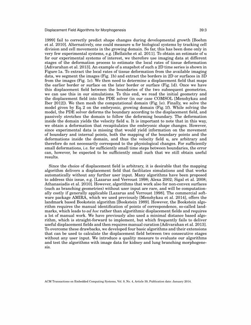
Fig. 1: The Image-Based Modelling Approach. a) an image of mouse embryonickidney explant, b) segmented image, c) extracted border in the shape of the embry-onic kidney explant, d) displacement field, e) computational mesh and f) solution of acomputational model on a growing domain. Adapted from [Adivarahan et al. 2013].

partial differential equations (PDEs) of the form

ci = Di∆ci +R(c1, . . . , cn) (1)

where ci denotes the time derivative of ci, ci denotes the concentration of the dif-ferent species i, Di represents the diffusion coefficient of species i, ∆ the Laplaceoperator, and R(c1, . . . , cn) the biochemical reactions between the n different speciesi ∈ [1, n]. Parameter values for the models are set so that embryonic gene expressionand signalling patterns from wild type and mutant mice can be reproduced on theidealised 2D and 3D domains. To further increase the accuracy and thus the predictivepower of the models, it is important to solve them on realistic embryonic geometries.Recent advances in imaging technology, algorithms and computer power now permitthe development of such increasingly realistic simulations of biological processes. Inparticular, it is now possible to obtain 2D and 3D shapes of developing organs and tosolve the models on those embryonic geometries [Gleghorn et al. 2012; Clement et al.2012; Menshykau et al. 2014; Iber et al. 2015].

During embryonic development, growth and patterning are tightly linked [Iber et al.2015]. It is therefore insufficient to solve the reaction-diffusion equations on a staticdomain. When solving Eq. 1 on a growing domain, we need to include advection anddilution terms [Iber et al. 2015] and obtain

ci +∇(u · ci) = Di∆ci +R(c1, . . . , cn). (2)

Here, u represents the velocity field of the moving domain. To develop a mechanisticmodel of growth control that yields u, we would need to understand how growth iscontrolled at the molecular level during development. This is not yet the case, andrecent measurements demonstrate that simple growth models [Dillon and Othmer


Displacement Field Algorithms for Morphogenesis 39:3

1999] fail to correctly predict shape changes during developmental growth [Boehmet al. 2010]. Alternatively, one could measure u for biological systems by tracking celldivision and cell movements in the growing domain. So far, this has been done only invery few experimental systems, e.g. [Bellaıche et al. 2011]. To obtain an estimate of ufor our experimental systems of interest, we therefore use imaging data at differentstages of the deformation process to estimate the local rates of tissue deformation[Adivarahan et al. 2013]. An example of a snapshot of such a 2D time series is shown inFigure 1a. To extract the local rates of tissue deformation from the available imagingdata, we segment the images (Fig. 1b) and extract the borders in 2D or surfaces in 3Dfrom the images (Fig. 1c). We then need to determine a displacement field that mapsthe earlier border or surface on the later border or surface (Fig. 1d). Once we havethis displacement field between the boundaries of the two subsequent geometries,we can use this in our simulations. To this end, we read the initial geometry andthe displacement field into the PDE solver (in our case COMSOL [Menshykau andIber 2012]). We then mesh the computational domain (Fig. 1e). Finally, we solve themodel given by Eq. 2 on the embryonic, growing domain (Fig. 1f). While solving themodel, the PDE solver deforms the boundary according to the displacement field, andpassively stretches the domain to follow the deforming boundary. The deformationinside the domain yields the velocity field u. It is important to note that in this way,we obtain a deformation that recapitulates the embryonic shape changes. However,since experimental data is missing that would yield information on the movementof boundary and internal points, both the mapping of the boundary points and thedeformations inside the domain, and thus the velocity field u, are arbitrary andtherefore do not necessarily correspond to the physiological changes. For sufficientlysmall deformations, i.e. for sufficiently small time steps between boundaries, the errorcan, however, be expected to be sufficiently small such that we still obtain usefulresults.

Since the choice of displacement field is arbitrary, it is desirable that the mappingalgorithm delivers a displacement field that facilitates simulations and that worksautomatically without any further user input. Many algorithms have been proposedto address this issue, e.g. [Lazarus and Verroust 1998; Alexa 2002; Sigal et al. 2008;Athanasiadis et al. 2010]. However, algorithms that work also for non-convex surfaces(such as branching geometries) without user input are rare, and will be computation-ally costly if generally applicable [Lazarus and Verroust 1998]. The commercial soft-ware package AMIRA, which we used previously [Menshykau et al. 2014], offers thelandmark based Bookstein algorithm [Bookstein 1989]. However, the Bookstein algo-rithm requires the manual identification of points of correspondence, so-called land-marks, which leads to ad hoc rather than algorithmic displacement fields and requiresa lot of manual work. We have previously also used a minimal distance based algo-rithm, which is straight-forward to implement, but which frequently fails to deliveruseful displacement fields and then requires manual curation [Adivarahan et al. 2013].To overcome these drawbacks, we developed four basic algorithms and their extensionsthat can be used to calculate the displacement field between two consecutive stageswithout any user input. We introduce a quality measure to evaluate our algorithmsand test the algorithms with image data for kidney and lung branching morphogene-sis.



(a) Displacement field of entire domain (b) Local displacement field

Fig. 2: Displacement Field. Curve C1 represents the shape of an embryonic structureat a time step t; curve C2 represents the same structure at a later time point t+∆t. Forour simulations of growing organs it is essential to find a high quality displacementfield that maps points from C1 to C2. (a) An example of the displacement field forthe entire growing embryonic kidney explant. (b) The displacement field at some localposition of the domain shown in panel (a).

2. ALGORITHMS FOR COMPUTING THE DISPLACEMENT FIELDS2.1. Basic AlgorithmsWe denote the curve at time t by C1 and the curve at time t + ∆t by C2 as shownin Figure 2. Prior to the calculation of the displacement field we interpolated the setof discrete points on C1 and C2 such that both curves contain the same number ofpoints that were equally spaced on each curve. Here we used the MATLAB functioninterparc [D’Errico 2012b] and we used spline interpolation for smooth curves andlinear interpolation in case of corner points. The interpolated points were then mappedusing one of the following basic algorithms. In Section 2.2 we will show how thesealgorithms can be extended.

(1) Minimal Distance Mapping: Every point on the curve C1 is mapped to the pointon the curve C2 to which it has the minimal distance. The point on C2 can bedetermined using the MATLAB function distance2curve [D’Errico 2012a].

(2) Normal Mapping: The normal vector is determined at every point on C1 and ismapped to the closest point on C2 where the normal and C2 intersect.

(3) Diffusion Mapping: This mapping is obtained by solving the steady state diffusionequation (Laplace equation)

∆c = 0, (3)

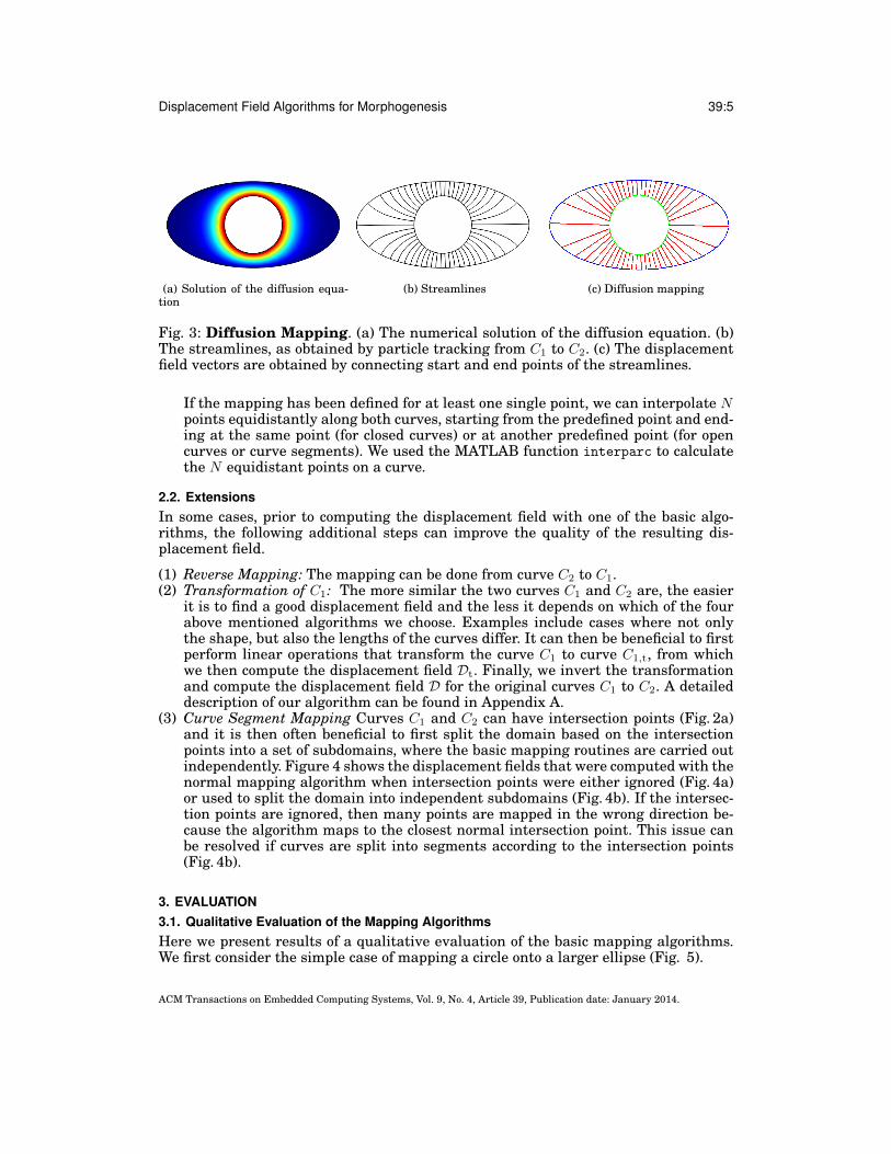
which follows from Eq. 1 in steady state (c = 0) and in the absence of reactions(R = 0). Eq. 3 is solved in the area between the two curves in 2D, or between twosurfaces in 3D using COMSOL Multiphysics (Fig. 3a). As initial conditions we useDirichlet boundary conditions and we set the value c to be 1 on C1 and 0 on C2 orvice versa. The start and end points on C1 and C2 are determined by computing thestreamlines using particle tracking (Fig. 3b); the start and end points define themapping vector (Fig. 3c).

(4) Uniform Mapping: For this algorithm we need at least one point on C1 and onepoint on C2, for which we know that they should be mapped onto each other. Thesetwo points can either be selected manually or algorithmically. To determine suchpoints algorithmically, one could use curve intersection points in case of intersect-ing curves, or in case of open, non-intersecting curves, beginning and end points.



(a) Solution of the diffusion equa-tion

(b) Streamlines (c) Diffusion mapping

Fig. 3: Diffusion Mapping. (a) The numerical solution of the diffusion equation. (b)The streamlines, as obtained by particle tracking from C1 to C2. (c) The displacementfield vectors are obtained by connecting start and end points of the streamlines.

If the mapping has been defined for at least one single point, we can interpolate Npoints equidistantly along both curves, starting from the predefined point and end-ing at the same point (for closed curves) or at another predefined point (for opencurves or curve segments). We used the MATLAB function interparc to calculatethe N equidistant points on a curve.

2.2. ExtensionsIn some cases, prior to computing the displacement field with one of the basic algo-rithms, the following additional steps can improve the quality of the resulting dis-placement field.

(1) Reverse Mapping: The mapping can be done from curve C2 to C1.(2) Transformation of C1: The more similar the two curves C1 and C2 are, the easier

it is to find a good displacement field and the less it depends on which of the fourabove mentioned algorithms we choose. Examples include cases where not onlythe shape, but also the lengths of the curves differ. It can then be beneficial to firstperform linear operations that transform the curve C1 to curve C1,t, from whichwe then compute the displacement field Dt. Finally, we invert the transformationand compute the displacement field D for the original curves C1 to C2. A detaileddescription of our algorithm can be found in Appendix A.

(3) Curve Segment Mapping Curves C1 and C2 can have intersection points (Fig. 2a)and it is then often beneficial to first split the domain based on the intersectionpoints into a set of subdomains, where the basic mapping routines are carried outindependently. Figure 4 shows the displacement fields that were computed with thenormal mapping algorithm when intersection points were either ignored (Fig. 4a)or used to split the domain into independent subdomains (Fig. 4b). If the intersec-tion points are ignored, then many points are mapped in the wrong direction be-cause the algorithm maps to the closest normal intersection point. This issue canbe resolved if curves are split into segments according to the intersection points(Fig. 4b).

3. EVALUATION3.1. Qualitative Evaluation of the Mapping AlgorithmsHere we present results of a qualitative evaluation of the basic mapping algorithms.We first consider the simple case of mapping a circle onto a larger ellipse (Fig. 5).



(a) Global mapping (b) Segment mapping

Fig. 4: Mapping of Curves with Intersections. (a) The displacement field was com-puted globally using normal mapping. Note that many points map to the wrong seg-ment on C2. (b) The curves were split into subdomains based on the intersection pointsand only segments were mapped onto each other using normal mapping. The mappingsare now correct.

— Minimal Distance: Mappings based on the minimal distance between two points areeasy to implement but prone to errors since the algorithm only gives good resultsif the domain grows uniformly. Problems occur as soon as big changes in curvatureare observed, which are typical for branching morphogenesis and morphogenesisin general. Figure 6a shows that the minimal distance algorithm fails to map astraight line to the line with a protrusion; no point on C1 is mapped onto the curvesegment between points A and B. Minimal distance mapping strongly dependson the direction of mapping. In many cases reverse minimal distance mappingprovides better results (Fig. 6b), because the complexity of the domain structuretypically increases rather than decreases during development. Our circle-ellipseexample illustrates the limitations of minimal distance mapping (Fig. 5a). Theproblem can be resolved by reversing the algorithm (Fig. 5b). A slight improvementis observed if we do a transformation beforehand (Fig. 5c).

— Normal Mapping: The normal mapping algorithm provides an excellent mappingfor the simple test case of a circle and a cylinder (Fig. 5d). Unlike the minimaldistance algorithm, the normal mapping algorithm is not very much affected by thecurvature of C2. It is, however, sensitive to the curvature of C1. If the curvature inlocally concave regions of C1 is comparably higher than the distance between thecurves, then crossings of the displacement field vectors can be observed (Fig. 7a).Therefore, the quality of a displacement field computed by normal mapping stronglydepends on whether C1 encloses a concave domain and whether C2 is far away fromthese concave regions. This problem is illustrated in Fig. 7a where the two curveslook very much alike but are far away from each other and the enclosed domain of C1

is not convex. This case results in a crossing of the displacement field vectors, whichis not desirable. As shown in Fig. 7b this problem is locally solved by doing a reversemapping. In case of our simple circle-ellipse example we observe that a normalmapping works very well because a circle is a concave domain (Fig. 5d). On the othera hand, a reverse normal mapping in this configuration (Fig. 5e) leads to crossingsof the displacement field vectors and large parts of the ellipse are not mapped onto



(a) Minimal distance mapping (b) Reverse minimal distance map-ping

(c) Transformed minimal distancemapping

(d) Normal mapping (e) Reverse normal mapping (f) Transfomed normal mapping

(g) Diffusion mapping (h) Reverse diffusion mapping (i) Transformed diffusion mapping

Fig. 5: Comparison of Mapping Algorithms with a Simple Test Case. Displace-ment fields (red) for the simple mapping problem between C1, a circle (green) and C2,an ellipse (blue), as generated by mapping algorithms based on minimal distance, nor-mal vectors, or diffusion, as well as their reverse and transformed versions.

the circle because the normal vectors from these regions fail to reach the circle. Thisproblem can be addressed by a re-scaling of the domains prior to normal mapping(Fig. 5f), such that similar results are obtained as with the original normal mapping.

— Diffusion Mapping: Many real world mapping problems can be resolved by onlymapping curve segments onto each other, because they often only have one curva-ture direction, such that we can find a good mappings based on normal or mini-mal distance mapping, in combination with the appropriate prior transformations.However, if the curvature changes its sign within the subdomain, i.e. if the curvechanges between being locally convex or concave (Fig. 8), minimal distance, nor-mal mapping and the reverse mappings all yield bad results in some section of thecurve. In Figure 8a, normal mapping gives good results in region B where the curvewe are mapping from is locally concave and returns crossings in region A where thecurve is locally convex. Minimal distance mapping fails in the opposite situations



(a) Minimal distance (b) Reverse minimal distance

Fig. 6: Minimal Distance Mapping. Every point on the curve C1 is mapped to thepoint on the curve C2 to which it has the minimal distance. If curve C2 shows bigchanges in curvature, it is often advisable to use reverse minimal distance mapping.(a) Minimal distance mapping cannot map points onto points in the segment betweenpoints A and B. (b) Reverse minimal distance mapping can resolve the issue shown inpanel a.

(a) Normal mapping (b) Reverse normal mapping

Fig. 7: Normal mapping. (a) If C1 encloses a non–convex domain and both curvesare not very close to each other in these concave regions of C1, then the displacementfield vectors generated by normal mapping cross each other. (b) The problem can beresolved by using reverse normal mapping.

(Fig. 8b) and the reverse mapping will help in neither case due to the symmetry ofthe problem. Good mapping results can, however, be obtained with diffusion map-ping, because the streamlines reach any region of C2 and will never cross each other.The downside of the diffusion method is that small regions on the generally shortercurve C1 are mapped onto fairly large regions on C2 as can be seen in Figure 5g.In this case, the reverse mapping can help (Fig. 5h) as well as a first scaling of C1

(Fig. 5i).Diffusion mapping is very safe but does not give overall as good results as normaland minimal distance mapping. Furthermore, it is computationally much moreexpensive than any of the other mapping algorithms and it is therefore wise to onlyapply it when normal or minimal distance fail, due to their limitations on curvesthat have changing curvature sign and lie far apart from each other.

— Uniform Mapping: Uniform mapping is the method of choice for open curveswith relatively small deformation (Fig. 9a). For closed curves or curve segmentsbetween two intersection points this method is advisable only if the curves arerelatively short or the changes in curvature are small because the direction of thedisplacement field is always biased towards the direction of the biggest change in



(a) Normal mapping fails (b) Minimal distance fails

Fig. 8: Normal and Minimal Distance Mapping Fail. When we try to map curvesof changing curvature sign that lie far apart from each other, we run into problemswith both minimal distance and normal mapping. We have a symmetric problem thatcannot be solved by reversing the algorithm. In (a) we do a normal mapping that leadsto crossings in region A that will just lead to crossings in region B when we reverse thealgorithm, and in (b) minimal distance gives us bad results in region B since we areignoring some parts of the curve onto which we are mapping to. This can also not besolved by using reverse minimal distance because the same problem would show up incurve region A.

growth, as can be seen in Figure 9b.

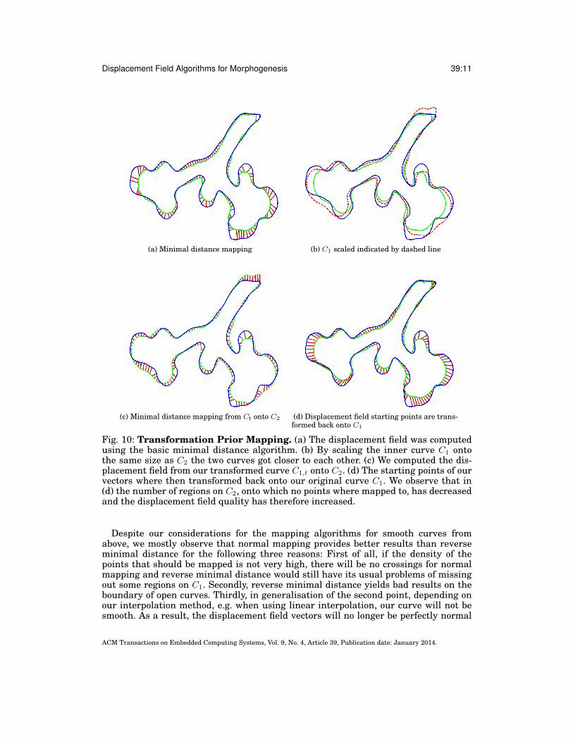
— Transformed Mapping: We have applied our basic algorithms to the circle-ellipseexample (Fig. 5) and saw that scaling the circle beforehand could lead to an improve-ment of the displacement field quality. Now we apply the transformation algorithmto our mouse kidney data and compare it qualitatively with the non-transformedalgorithm (Fig. 10a). In Figure 10a we see that minimal distance fails in many curveregions. The transformation algorithm first scales and aligns the curve C1 whichresults in the dashed curve C1,t (Fig. 10b). Then C1,t is mapped onto C2 (Fig. 10c).The starting points of the displacement field vectors that lie on C1,t, are back trans-formed onto C1 such that we get the final displacement field vectors (Fig. 10d). We

(a) (b)

Fig. 9: Uniform Mapping (a) The displacement fields of open curves are determinedby interpolating both curves with equidistant points and by mapping the points con-secutively onto each other. (b) When the growth of the domain is not uniform, we get adisplacement field that is biased towards the direction of maximal growth.



observe that the newly obtained displacement field has a much higher quality thanwithout prior transformation since C1,t and C2 are on average closer to each otherthan C1 to C2. The downside of this method is that the displacement field vectorsare very often distorted, i.e. the angles between the vectors and the C1 normal vec-tors are large. When do we want to first scale the curve C1? The more uniformlythe growing domain develops, the better it is to scale C1 prior to doing the mapping.Usually there are many curve segments Cin ⊆ C2 that lie inside the domain boundedby C1. By scaling, we usually improve the mapping from C1 to Cout = C2\Cin andworsen the mapping results from C1 to Cin. So it is not advisable to do scaling if Cin

is large and does not always lie close to C1. This is often the case if we map C1 ontoa much later developed domain C2 since the complexity of the curves are increasingand do not only grow uniformly.

In summary, we showed that the different algorithms are suited for different map-ping problems. The normal and minimal distance mapping algorithms often producethe nicest displacement fields, but they fail for curves with strong changes in the cur-vature. The diffusion mapping algorithm rarely fails, but overall gives sub-optimalresults.

3.2. Mapping in the Limiting Case of an Infinite Number of PointsIn this section we will discuss the mapping algorithms for smooth curves and the con-sequences in a discrete space. In case of smooth curves, the displacement field algo-rithm D: C1 → C2, is applied onto all the infinite number of points along the curveC1 that are mapped onto C2. We call the mapping well-defined on a subset C1 ⊆ C1 if∀p1 ∈ C1,∃p2 = D(p1) ∈ C2. Both uniform and diffusion mapping have the propertiesthat C1 = C1 and the mapping is bijective. These are desirable properties since a de-forming domain will neither have boundary points that vanish nor will points contractto a single point. Furthermore, both algorithms have the property that they do notallow crossings of the theoretical displacement field. When we talk about the crossingof the displacement field, we mean that each point on C1 is mapped onto C2 such thatthe order in which the points occur along the curve is conserved.

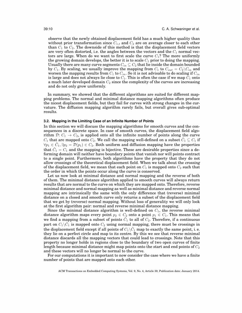
Let us now look at minimal distance and normal mapping and the reverse of bothof them. The minimal distance algorithm applied to smooth curves will always returnresults that are normal to the curve on which they are mapped onto. Therefore, reverseminimal distance and normal mapping as well as minimal distance and reverse normalmapping are intrinsically the same with the only difference that (reverse) minimaldistance on a closed and smooth curve only returns a subset of the displacement fieldthat we get by (reverse) normal mapping. Without loss of generality we will only lookat the first algorithm pair: normal and reverse minimal distance mapping.

Since the minimal distance algorithm is well-defined on C1, the reverse minimaldistance algorithm maps every point p2 ∈ C2 onto a point p1 ∈ C1. This means thatwe find a mapping from a subset of points C1 to all of C2. Therefore, if a continuouspart on C1\C1 is mapped onto C2 using normal mapping, there must be crossings inthe displacement field except if all points of C1\C1 map to exactly the same point, i. e.they lie on a perfect circle and map to its centre. By this we see that reverse minimaldistance discards all the mapping vectors that could lead to crossings. Note that thisproperty no longer holds in regions close to the boundary of two open curves of finitelength because minimal distance might map points onto the start and end points of C2

and these vectors will no longer be normal to the curve.For our computations it is important to now consider the case where we have a finite

number of points that are mapped onto each other.



(a) Minimal distance mapping (b) C1 scaled indicated by dashed line

(c) Minimal distance mapping from Ct onto C2 (d) Displacement field starting points are trans-formed back onto C1

Fig. 10: Transformation Prior Mapping. (a) The displacement field was computedusing the basic minimal distance algorithm. (b) By scaling the inner curve C1 ontothe same size as C2 the two curves got closer to each other. (c) We computed the dis-placement field from our transformed curve C1,t onto C2. (d) The starting points of ourvectors where then transformed back onto our original curve C1. We observe that in(d) the number of regions on C2, onto which no points where mapped to, has decreasedand the displacement field quality has therefore increased.

Despite our considerations for the mapping algorithms for smooth curves fromabove, we mostly observe that normal mapping provides better results than reverseminimal distance for the following three reasons: First of all, if the density of thepoints that should be mapped is not very high, there will be no crossings for normalmapping and reverse minimal distance would still have its usual problems of missingout some regions on C1. Secondly, reverse minimal distance yields bad results on theboundary of open curves. Thirdly, in generalisation of the second point, depending onour interpolation method, e.g. when using linear interpolation, our curve will not besmooth. As a result, the displacement field vectors will no longer be perfectly normal



on C1 and reverse minimal distance will preferably map onto local extrema that aregiven by the points where C1 is not smooth. Therefore, if we map closed curves ontoeach other, it is advisable to first compute the density of the points and do reverse min-imal distance mapping if the density exceeds some given density threshold; otherwisewe use normal mapping.

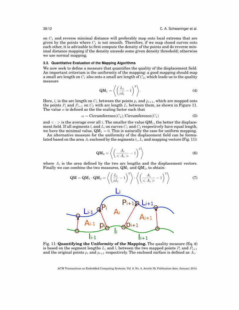
3.3. Quantitative Evaluation of the Mapping AlgorithmsWe now seek to define a measure that quantifies the quality of the displacement field.An important criterium is the uniformity of the mapping: a good mapping should mapa small arc length on C1 also onto a small arc length of C2, which leads us to the qualitymeasure

QM1 =

⟨(Li

αli− 1

)2⟩. (4)

Here, li is the arc length on C1 between the points pi and pi+1, which are mapped ontothe points Pi and Pi+1 on C2 with arc length Li between them, as shown in Figure 11.The value α is defined as the the scaling factor such that

α = Circumference(C2)/Circumference(C1) (5)

and < · > is the average over all i. The smaller the value QM1, the better the displace-ment field. If all segments li and Li on curves C1 and C2 respectively have equal length,we have the minimal value, QM1 = 0. This is naturally the case for uniform mapping.

An alternative measure for the uniformity of the displacement field can be formu-lated based on the areaAi enclosed by the segments li, Li and mapping vectors (Fig. 11):

QM2 =

⟨(Ai

< Ai >− 1

)2⟩

(6)

where Ai is the area defined by the two arc lengths and the displacement vectors.Finally we can combine the two measures, QM1 and QM2, to obtain:

QM = QM1 ·QM2 =

⟨(Li

αli− 1

)2⟩·

⟨(Ai

< Ai >− 1

)2⟩

(7)

Fig. 11: Quantifying the Uniformity of the Mapping. The quality measure (Eq. 4)is based on the segment lengths Li and li between the two mapped points Pi and Pi+1

and the original points pi and pi+1 respectively. The enclosed surface is defined as Ai.



Table I: Quality measures calculated for the test case of a circle mapped onto an ellipse(Fig. 5). The lowest values for the quality measures are marked in bold.

Mapping QM1 QM2 QMminimal distance mapping 13.4 22.4 301reverse minimal distance 0.128 0.134 0.017

transformed minimal distance 1.69 2.71 4.58normal mapping 0.103 0.398 0.041reverse normal 56.1 2.45 137

transformed normal 0.084 0.397 0.033diffusion mapping 0.494 1.17 0.577reverse diffusion 1.589 0.088 0.140

transformed diffusion 0.224 0.559 0.125

Table I shows the calculated values of QM1, QM2 and QM for the simple test case ofthe circle being mapped onto the ellipse (Fig. 5). The three measures yield the sameranking within the basic algorithms for minimal distance and normal mappings.However, in case of diffusion mapping, QM1 favours the transformed mapping whileQM2 favours the reverse mapping. The combined measure QM yields the sameranking as QM1. Visual inspection confirms that all highlighted mappings deliverexcellent results (Fig. 5), with QM1 and QM delivering the most appropriate ranking.

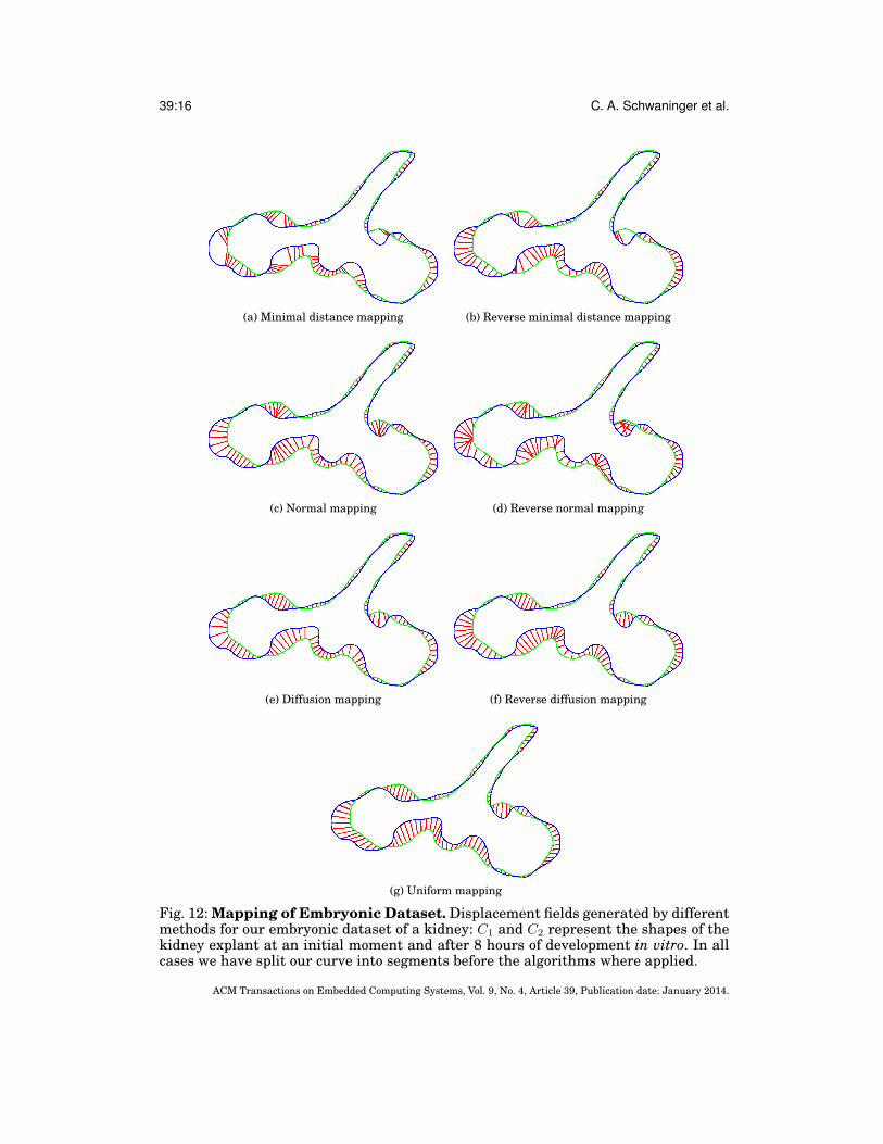
We repeated the analysis with the dataset for ex vivo kidney branching morphogen-sis [Adivarahan et al. 2013]. We used five datasets and mapped the starting embry-onic shape to embryonic datasets that had been acquired after 1h, 2h, 4h, 8h (TableII). As expected, the difference between shapes after 1h of development is so smallthat the quality measures yield more or less the same results; all our mapping algo-rithms return good and very similar results. The longer the time difference betweenthe two datasets, the worse the mapping, i.e. the value of our quality measures in-creases as we map curves that are increasingly distant (Table II). Minimal distance(Fig. 12a) and reverse minimal distance (Fig. 12b) yield rather poor results for big timesteps and strong changes in curvature. The same holds for normal and reverse nor-mal mapping where we observe crossings (Fig. 12c and Fig. 12d); as expected there aremore crossings for the reverse normal mapping since it maps from a curve with higherchanges in curvature to a curve with lower changes in curvature. The poor results ofthe normal mapping algorithm are in line with our previous observation that normalmapping gives bad results for very big time steps. The algorithm, however, still yieldsgood results for smaller deformations, i.e. until ∆ ≤ 4h (Table II).

Uniform mapping naturally gives the best results for QM1 as it lets QM1 converge tozero by its definition. However, visual inspection reveals that uniform mapping resultsin slightly distorted displacement fields (Fig. 12g) compared to the reverse diffusionmapping (Fig. 12f). We note that the solution differs substantially from the one ob-tained with a normal mapping, i.e. the angle between displacement field vectors andthe normal vectors are rather large. This is also reflected in QM2, which identifies thereverse diffusion mapping as the best mapping.

Finally, if we look at QM in Table II, we observe that uniform mapping will againgive the best results, since it is almost zero for QM1. However given the distortionsthat we get for the uniform mapping, uniform mapping is not necessarily the method



of choice. Based on the QM value, normal mappings yield the second best result forall cases. The QM ranking does not penalize for crossings. In case of crossings, reversediffusion would be the method of choice. These considerations are taken into accountfor our final algorithm for the image-based determination of displacement fields.

Table II: Quality measure calculated for the test case of the embryonic kidney branch-ing morphogenesis. The lowest values for the quality measures are marked in bold; theuniform mapping was not considered as it gives the lowest value for QM1 and QM bydefinition.

Mapping QM1(∆=1h) QM1(∆=2h) QM1(∆=4h) QM1(∆=8h)minimal distance 0.027 0.056 0.294 2.03

reverse minimal distance 0.033 0.046 0.144 71.6normal 0.010 0.031 0.089 0.281

reverse normal 0.154 0.108 172 148.9diffusion 0.019 0.041 0.193 2.03

reverse diffusion 0.077 0.039 0.131 0.559uniform mapping 0.002 0.011 0.010 0.028

QM2(∆=1h) QM2(∆=2h) QM2(∆=4h) QM2(∆=8h)minimal distance 0.650 0.809 1.89 5.75

reverse minimal distance 0.587 0.593 1.009 1.748normal 0.591 0.657 1.04 1.08

reverse normal 0.564 0.531 0.830 1.08diffusion 0.612 0.833 2.080 6.00

reverse diffusion 0.506 0.510 0.795 0.811uniform mapping 0.599 0.612 0.951 0.999

QM(∆=1h) QM(∆=2h) QM(∆=4h) QM(∆=8h)minimal distance 1.76E-2 4.53E-2 0.556 11.66

reverse minimal distance 1.94E-2 2.73E-2 0.145 125normal 0.591E-2 2.04E-2 9.25E-2 0.304

reverse normal 8.69E-2 5.73E-2 143 161diffusion 1.16E-2 3.42E-2 0.401 12.2

reverse diffusion 3.90E-2 1.99E-2 0.104 0.454uniform mapping 0.120E-2 0.673E-2 0.951E-2 0.280

4. DISPLACEMENT FIELDS FOR 3D OBJECTSIn a final step, we extended the basic algorithms to 3D to enable also 3D simulationson growing domains. The only basic algorithm that cannot be used in 3D is uniformmapping. Since computations in 3D can get very expensive, we have used the OPCODEcollision detection library [Terdiman 2002] for our normal mapping algorithm. Thislibrary efficiently computes ray-mash intersection points by creating a collision treefor the possibly ray intersecting mesh. To determine the computational efficiency ofthe algorithm, we determined the computational time that is needed to compute anincreasing number of displacement field vectors using our normal mapping algorithmfor a mesh size of 3’527 and 4’064 mesh-faces of the 3D surface (Fig. 13). As can be seen,the computational time increases linearly with the number of computed displacementfield vectors.



Figure 14 shows the mapping of a sphere onto an ellipsoid. We observe the samelimitations for minimal distance mapping in 3D (Fig. 14a) that we have seen alreadyin 2D (Fig. 5a). Much as in 2D, the sphere is not mapped to all regions of the ellipsoid.Once again normal mapping (Fig. 14b) and diffusion mapping (Fig. 14c) perform well.

Figure 15 shows the displacement field computed for the embryonic mouse lung ep-ithelium at two developmental stages [Blanc et al. 2012]. Similarly as for the exampleof a sphere and an ellipsoid, normal mapping and diffusional mapping provide highquality displacement fields, as judged by eye.

5. CONCLUSIONBased on the evaluation of the mapping algorithms we propose a workflow (Algo-rithm 1 for the 2D case) for the determination of high quality displacement fields fromimages of subsequent developmental stages. From our overall observations and analy-sis we learn that it is generally desirable to apply normal mapping as a first attempt.When curves (in 2D) or surfaces (in 3D) intersect, it is advisable to divide the probleminto sub-problems according to intersections and then apply the mapping algorithmsseparately on each segment. If we get a low quality displacement field (e .g. crossingsoccur), then the normal mapping must be rejected and reverse diffusion mapping canbe used. Reverse diffusion mapping is less error–prone when the two curves are faraway. In the case of open curves, we can transform the starting and end points of bothcurves onto each other by translating, rotating and scaling one of the curves, thenapply (scaled) normal or reverse diffusion mapping, depending on the crossings as forclosed curve segments and finally transform back the curve and the displacement field.

ALGORITHM 1: Algorithm to determine 2D Displacement FieldsInput: Two closed curves C1 and C2

Output: Displacement fieldif C1 and C2 intersect then

split into subproblems;else

consider C1 and C2 as one subproblemendforeach subproblem do

do normal mapping;if crossings then

do reverse diffusion mapping;end

endreturn displacement field;

In this manuscript, we described and evaluated different algorithms that can beused to compute displacement fields that are required for the simulation of signallingmodels on growing domains. We have presented four basic algorithms, discussed theirproperties and presented an algorithm that takes their advantages and disadvantagesinto account. We must note that our final algorithm does not guarantee a perfect dis-placement field, nor that the best basic method is used. However, the algorithm workswell for many cases and minimises manual curation and modifications of the displace-ment field, as intended.

Acknowledgements. We thank Edoardo Mazza, Gerald Kress and Simon Tanaka fordiscussions.



(a) Minimal distance mapping (b) Reverse minimal distance mapping

(c) Normal mapping (d) Reverse normal mapping

(e) Diffusion mapping (f) Reverse diffusion mapping

(g) Uniform mapping

Fig. 12: Mapping of Embryonic Dataset. Displacement fields generated by differentmethods for our embryonic dataset of a kidney: C1 and C2 represent the shapes of thekidney explant at an initial moment and after 8 hours of development in vitro. In allcases we have split our curve into segments before the algorithms where applied.



Fig. 13: Benchmark for 3D Normal Mapping. Using a mesh size of 3’527 and 4’064mesh-faces, the computational time increases linearly with the number of computeddisplacement field vectors.

(a) Minimal distance mapping (b) Normal mapping

(c) Diffusion mapping

Fig. 14: 3D Minimal Distance and Normal Mapping. The displacement field froma sphere onto an ellipsoid is computed using (a) minimal distance, (b) normal mappingand (c) diffusion mapping. We observe in (a) that some regions on the ellipsoid cannotbe mapped onto and that we get better results in (b) and (c).



Fig. 15: Normal Mapping applied to 3D Lung Data. The displacement field com-puted by using the normal mapping algorithm.



REFERENCESSrivathsan Adivarahan, Denis Menshykau, Odysse Michos, and Dagmar Iber. 2013. Dynamic Image-Based

Modelling of Kidney Branching Morphogenesis. In Computational Methods in Systems Biology. SpringerBerlin Heidelberg, Berlin, Heidelberg, 106–119.

Marc Alexa. 2002. Recent Advances in Mesh Morphing. Computer graphics forum 21, 2 (2002), 173–197.Theodoris Athanasiadis, Ioannis Fudos, Christophoros Nikou, and Vasiliki Stamati. 2010. Feature-based

3D morphing based on geometrically constrained sphere mapping optimization. Proceedings of the 2010ACM Symposium on Applied Computing - SAC ’10 (2010), 1258.

Amarendra Badugu, Conradin Kraemer, Philipp Germann, Denis Menshykau, and Dagmar Iber. 2012. Digitpatterning during limb development as a result of the BMP-receptor interaction. Scientific reports 2(2012), 991.

Y. Bellaıche, F. Bosveld, F. Graner, K. Mikula, M. Remesıkova, and M. Smısek. 2011. New robust algorithmfor tracking cells in videos of Drosophila morphogenesis based on finding an ideal path in segmentedspatio-temporal cellular structures. Conf Proc IEEE Eng Med Biol Soc (2011), 6609–12.

Pierre Blanc, Karen Coste, Pierre Pouchin, Jean-Marc Azaıs, Loıc Blanchon, Denis Gallot, and VincentSapin. 2012. A role for mesenchyme dynamics in mouse lung branching morphogenesis. PLoS ONE 7, 7(2012), e41643.

Bernd Boehm, Henrik Westerberg, Gaja Lesnicar-Pucko, Sahdia Raja, Michael Rautschka, James Cotterell,Jim Swoger, and James Sharpe. 2010. The role of spatially controlled cell proliferation in limb budmorphogenesis. PLoS Biol 8, 7 (0 2010), e1000420. DOI:http://dx.doi.org/10.1371/journal.pbio.1000420

FL Bookstein. 1989. Principal warps: Thin-plate splines and the decomposition of deformations. IEEETPAMI 2 (1989), 567–585.

Geraldine Celliere, Denis Menshykau, and Dagmar Iber. 2012. Simulations demonstrate a simple networkto be sufficient to control branch point selection, smooth muscle and vasculature formation during lungbranching morphogenesis. Biology Open 1, 8 (Aug. 2012), 775–788.

Raphael Clement, Pierre Blanc, Benjamin Mauroy, Vincent Sapin, and Stephane Douady. 2012. Shape self-regulation in early lung morphogenesis. PLoS ONE 7, 5 (2012), e36925.

John D’Errico. 2012a. distance2curve function. MATLAB Central – File Exchange. (2012). http://www.mathworks.in/matlabcentral/fileexchange/34869-distance2curve

John D’Errico. 2012b. Interparc function. MATLAB Central – File Exchange. (2012). http://www.mathworks.in/matlabcentral/fileexchange/34874-interparc

R. Dillon and H. G. Othmer. 1999. A mathematical model for outgrowth and spatial patterning of the verte-brate limb bud. J Theor Biol 197, 3 (4 1999), 295–330. DOI:http://dx.doi.org/10.1006/jtbi.1998.0876

Jason P Gleghorn, Jiyong Kwak, Amira L Pavlovich, and Celeste M Nelson. 2012. Inhibitory morphogensand monopodial branching of the embryonic chicken lung. Developmental dynamics 241 (March 2012),852–862.

Dagmar Iber and Philipp Germann. 2014. How do digits emerge? - mathematical models of limb develop-ment. Birth Defects Res C Embryo Today 102, 1 (3 2014), 1–12. DOI:http://dx.doi.org/10.1002/bdrc.21057

Dagmar Iber and Denis Menshykau. 2013. The control of branching morphogenesis. Open Biol 3, 9 (0 2013),130088. DOI:http://dx.doi.org/10.1098/rsob.130088

Dagmar Iber, Simon Tanaka, Patrick Fried, Philipp Germann, and Denis Menshykau. 2015. Simulating tis-sue morphogenesis and signaling. Methods in molecular biology (Clifton, N.J.) 1189, Chapter 21 (2015),323–338.

Dagmar Iber and Rolf Zeller. 2012. Making sense-data-based simulations of vertebrate limb development.Curr Opin Genet Dev 22, 6 (Dec. 2012), 570–577.

F. Lazarus and A. Verroust. 1998. Three-dimensional metamorphosis: a survey. Visual Computer 14 (1998),373–389.

Denis Menshykau, Pierre Blanc, Erkan Unal, Vincent Sapin, and Dagmar Iber. 2014. An Interplay of Ge-ometry and Signaling enables Robust Lung Branching Morphogenesis. Development in press (2014).

Denis Menshykau and Dagmar Iber. 2012. Simulating Organogenesis with Comsol: Interacting and Deform-ing Domains . Proceedings of COMSOL Conference 2012 (Sept. 2012).

Denis Menshykau and Dagmar Iber. 2013. Kidney branching morphogenesis under the control of a ligand-receptor-based Turing mechanism. Physical biology 10, 4 (June 2013), 046003.

Denis Menshykau, Conradin Kraemer, and Dagmar Iber. 2012. Branch Mode Selection during Early LungDevelopment. Plos Computational Biology 8, 2 (Feb. 2012), e1002377.

Luis G Morelli, Koichiro Uriu, Saul Ares, and Andrew C Oates. 2012. Computational approaches to devel-opmental patterning. Science 336, 6078 (April 2012), 187–91.


http://dx.doi.org/10.1371/journal.pbio.1000420

http://www.mathworks.in/matlabcentral/fileexchange/34869-distance2curve

http://www.mathworks.in/matlabcentral/fileexchange/34869-distance2curve

http://www.mathworks.in/matlabcentral/fileexchange/34874-interparc

http://www.mathworks.in/matlabcentral/fileexchange/34874-interparc

http://dx.doi.org/10.1006/jtbi.1998.0876

http://dx.doi.org/10.1002/bdrc.21057

http://dx.doi.org/10.1098/rsob.130088


Andrew C Oates, Nicole Gorfinkiel, Marcos Gonzalez-Gaitan, and Carl-Philipp Heisenberg. 2009. Quantita-tive approaches in developmental biology. Nat Rev Genet 10, 8 (Aug. 2009), 517–530.

Simone Probst, Conradin Kraemer, Philippe Demougin, Rushikesh Sheth, Gail R Martin, Hidetaka Shira-tori, Hiroshi Hamada, Dagmar Iber, Rolf Zeller, and Aimee Zuniga. 2011. SHH propagates distal limbbud development by enhancing CYP26B1-mediated retinoic acid clearance via AER-FGF signalling.Development (Cambridge, England) 138, 10 (May 2011), 1913–1923.

Ian Sigal, Michael R Hardisty, and Cari M Whyne. 2008. Mesh-morphing algorithms for specimen-specificfinite element modeling. Journal of biomechanics 41, 7 (2008), 1381–9.

Simon Tanaka and Dagmar Iber. 2013. Inter-dependent tissue growth and Turing patterning in a model forlong bone development. Physical biology 10, 5 (Oct. 2013), 056009.

Pierre Terdiman. 2002. OPCODE collision detection library. (2002). http://www.codercorner.com/Opcode.htmAlan M. Turing. 1952. The chemical basis of morphogenesis. Phil. Trans. Roy. Soc. Lond B237 (1952), 37–72.Ortrud Wartlick, Anna Kicheva, and Marcos Gonzalez-Gaitan. 2009. Morphogen gradient formation. Cold

Spring Harbor perspectives in biology 1, 3 (Sept. 2009), a001255.O Wartlick, P Mumcu, A Kicheva, T Bittig, C Seum, F Julicher, and M Gonzalez-Gaitan. 2011. Dynamics of

Dpp signaling and proliferation control. Science 331, 6021 (March 2011), 1154–1159.L Wolpert. 1969. Positional information and the spatial pattern of cellular differentiation. Journal of theo-

retical biology 25, 1 (Oct. 1969), 1–47.


http://www.codercorner.com/Opcode.htm


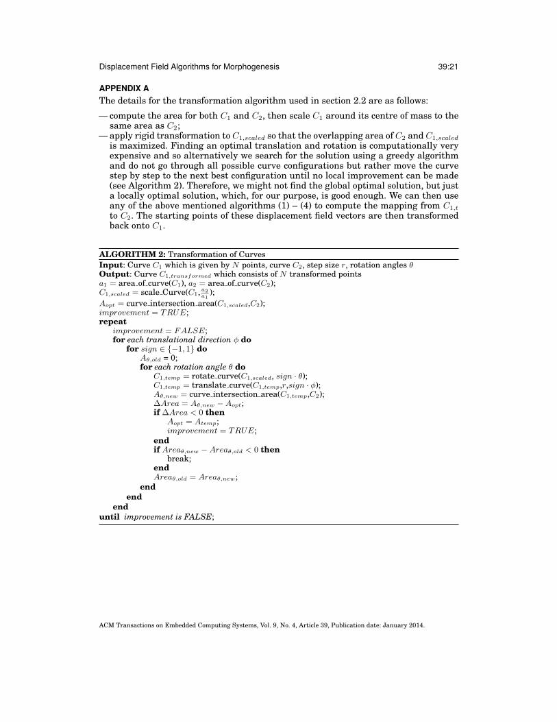
APPENDIX AThe details for the transformation algorithm used in section 2.2 are as follows:

— compute the area for both C1 and C2, then scale C1 around its centre of mass to thesame area as C2;

— apply rigid transformation to C1,scaled so that the overlapping area of C2 and C1,scaled

is maximized. Finding an optimal translation and rotation is computationally veryexpensive and so alternatively we search for the solution using a greedy algorithmand do not go through all possible curve configurations but rather move the curvestep by step to the next best configuration until no local improvement can be made(see Algorithm 2). Therefore, we might not find the global optimal solution, but justa locally optimal solution, which, for our purpose, is good enough. We can then useany of the above mentioned algorithms (1) – (4) to compute the mapping from C1,t

to C2. The starting points of these displacement field vectors are then transformedback onto C1.

ALGORITHM 2: Transformation of CurvesInput: Curve C1 which is given by N points, curve C2, step size r, rotation angles θOutput: Curve C1,transformed which consists of N transformed pointsa1 = area of curve(C1), a2 = area of curve(C2);C1,scaled = scale Curve(C1,a2

a1);

Aopt = curve intersection area(C1,scaled,C2);improvement = TRUE;repeat

improvement = FALSE;for each translational direction φ do

for sign ∈ {−1, 1} doAθ,old = 0;for each rotation angle θ do

C1,temp = rotate curve(C1,scaled, sign · θ);C1,temp = translate curve(C1,temp,r,sign · φ);Aθ,new = curve intersection area(C1,temp,C2);∆Area = Aθ,new −Aopt;if ∆Area < 0 then

Aopt = Atemp;improvement = TRUE;

endif Areaθ,new −Areaθ,old < 0 then

break;endAreaθ,old = Areaθ,new;

endend

enduntil improvement is FALSE;


Simulating Organogenesis: Algorithms for the Image-based Determination of Displacement Fields

Documents

Transcript of Simulating Organogenesis: Algorithms for the Image-based Determination of Displacement Fields