Simulating Materials Properties fromFirst Principles (PHU.014UF)

SS 2020 – VASP exercises

Assoz.-Prof. Peter PuschnigInstitut fur Physik, Fachbereich Theoretische Physik

Karl-Franzens-Universitat Graz

Universitatsplatz 5, A-8010 Graz

peter.puschnig@uni-graz.at

http://physik.uni-graz.at/~pep

Graz, March 30, 2020

ii

Contents

1 Introduction 1

1.1 Density Functional Theory in a Nutshell . . . . . . . . . . . . . . . . . . . . . . . . . 1

1.2 The Vienna Ab initio Simulation Package (VASP) . . . . . . . . . . . . . . . . . . . . 2

2 Basic Exercises 3

2.1 Basic Linux Shell Commands . . . . . . . . . . . . . . . . . . . . . . . . . . . . . . . 3

2.2 Exercise 1 – Hello fcc-Al . . . . . . . . . . . . . . . . . . . . . . . . . . . . . . . . . . 3

2.2.1 The POSCAR file . . . . . . . . . . . . . . . . . . . . . . . . . . . . . . . . . . 4

2.2.2 The INCAR file . . . . . . . . . . . . . . . . . . . . . . . . . . . . . . . . . . . 4

2.2.3 The KPOINTS file . . . . . . . . . . . . . . . . . . . . . . . . . . . . . . . . . 5

2.2.4 The POTCAR file . . . . . . . . . . . . . . . . . . . . . . . . . . . . . . . . . 5

2.2.5 Starting the calculation . . . . . . . . . . . . . . . . . . . . . . . . . . . . . . . 6

2.2.6 Most important output files . . . . . . . . . . . . . . . . . . . . . . . . . . . . 6

2.2.7 Plotting the density of states . . . . . . . . . . . . . . . . . . . . . . . . . . . 7

2.2.8 Things to try . . . . . . . . . . . . . . . . . . . . . . . . . . . . . . . . . . . . 8

2.3 Exercise 2 – Equation of state and convergence tests . . . . . . . . . . . . . . . . . . . 8

2.3.1 Equation of state . . . . . . . . . . . . . . . . . . . . . . . . . . . . . . . . . . 9

2.3.2 Convergence tests . . . . . . . . . . . . . . . . . . . . . . . . . . . . . . . . . . 11

2.3.3 More things to try . . . . . . . . . . . . . . . . . . . . . . . . . . . . . . . . . 12

2.4 Exercise 3 – Band structure of silicon . . . . . . . . . . . . . . . . . . . . . . . . . . . 13

2.4.1 Self-consistent calculation . . . . . . . . . . . . . . . . . . . . . . . . . . . . . 13

2.4.2 Non-Self-consistent band structure calculation . . . . . . . . . . . . . . . . . . 14

2.4.3 Plotting the results . . . . . . . . . . . . . . . . . . . . . . . . . . . . . . . . . 15

3 Projects 17

3.1 Project 1 – Magnetic phases of iron . . . . . . . . . . . . . . . . . . . . . . . . . . . . 17

3.1.1 Description . . . . . . . . . . . . . . . . . . . . . . . . . . . . . . . . . . . . . 17

3.1.2 Tasks . . . . . . . . . . . . . . . . . . . . . . . . . . . . . . . . . . . . . . . . . 18

iii

3.2 Project 2 – Band structure of diamond, graphite and graphene . . . . . . . . . . . . . 19

3.2.1 Description . . . . . . . . . . . . . . . . . . . . . . . . . . . . . . . . . . . . . 19

3.2.2 Tasks . . . . . . . . . . . . . . . . . . . . . . . . . . . . . . . . . . . . . . . . . 20

3.3 Project 3 – Adsorption of CO molecule on a surface . . . . . . . . . . . . . . . . . . . 21

3.3.1 Description . . . . . . . . . . . . . . . . . . . . . . . . . . . . . . . . . . . . . 21

3.3.2 Tasks . . . . . . . . . . . . . . . . . . . . . . . . . . . . . . . . . . . . . . . . . 22

Bibliography 25

iv

Chapter 1

Introduction

1.1 Density Functional Theory in a Nutshell

Applied scientific research depends on the existence of accurate theoretical models. In particular,

highly reliable ab-initio methods are in-dispensable for designing novel materials as well as for a de-

tailed understanding of their properties. The development of such theories describing the electronic

structure of atoms, molecules, and solids has been one of the success stories of physics in the 20th cen-

tury. Among these, density functional theory (DFT) [1–4] has proven to yield ground state properties

for a vast number of systems in a very precise manner.1

DFT [1, 2, 4, 5] provides a rigorous framework to reduce the interacting many-electron problem to an

effective system of non-interacting electrons which is the topic of the related lecture ”Fundamentals

of Electronic Structure Theory”. There it will be shown that the quantum-mechanical, i.e. ab-initio,

treatment of materials properties becomes tractable by solving the so-called Kohn-Sham equations.

These equations are essentially single-particle Schrodinger equations with an effective potential.[−1

2∆ + vs(r)

]ϕnk(r) = εnkϕnk(r). (1.1)

Here vs(r) is an effective potential, the Kohn-Sham potential,

vs(r) = v(r) + vH(r) + vxc(r), (1.2)

comprised of the external potential v(r) due to the atomic nuclei, the Hartree potential vH(r) and

the so-called exchange-correlation potential vxc(r). The eigenvalues εnk of Eq. 1.1 are the Kohn-Sham

1The Nobel Prize in Chemistry 1998 was awarded to Walter Kohn for his development of the density-functionaltheory.

1

energies, and the eigenfunctions ϕnk(r) the Kohn-Sham orbitals. The density n(r) is constructed from

the single particle orbitals ϕnk(r), as

n(r) =BZ∑k

∑n

fnk |ϕnk(r)|2 , (1.3)

where fnk are occupation numbers. It is important to note that Eqs. 1.1 and 1.3 have to be solved

self-consistently, i.e. iteratively, since the Hartree as well as the exchange-correlation potential depend

on the density. Finally, the total energy E of the system is obtained as a functional of the density

from the converged electron density as E[n(r)].

Recommended Literature. (i) Lecture Notes ”Fundamentals of Electronic Structure Theory”, P.

Puschnig (pdf) (ii) A Primer in Density Functional Theory. [6]; (iii) Density Functional Theory: A

Practical Introduction, Sholl and Steckel [7].

1.2 The Vienna Ab initio Simulation Package (VASP)

VASP is one of the most-widely used quantum chemistry computer programs applicable for periodic

systems and will be used in these exercises. The following short description of VASP has been taken

from the VASP-webpage VASP-webpage, more information can also be found on the VASP-wiki.

The Vienna Ab initio Simulation Package (VASP) is a computer program for atomic scale materials

modelling, e.g. electronic structure calculations and quantum-mechanical molecular dynamics, from

first principles.

VASP computes an approximate solution to the many-body Schrodinger equation, either within den-

sity functional theory (DFT), solving the Kohn-Sham equations, or within the Hartree-Fock (HF) ap-

proximation, solving the Roothaan equations. Hybrid functionals that mix the Hartree-Fock approach

with density functional theory are implemented as well. Furthermore, Green’s functions methods (GW

quasiparticles, and ACFDT-RPA) and many-body perturbation theory (2nd-order Moller-Plesset) are

available in VASP.

In VASP, central quantities, like the one-electron orbitals, the electronic charge density, and the

local potential are expressed in plane wave basis sets. The interactions between the electrons and

ions are described using norm-conserving or ultrasoft pseudopotentials, or the projector-augmented-

wave method. To determine the electronic groundstate, VASP makes use of efficient iterative matrix

diagonalisation techniques, like the residual minimisation method with direct inversion of the iterative

subspace (RMM-DIIS) or blocked Davidson algorithms. These are coupled to highly efficient Broyden

and Pulay density mixing schemes to speed up the self-consistency cycle.

2

Chapter 2

Basic Exercises

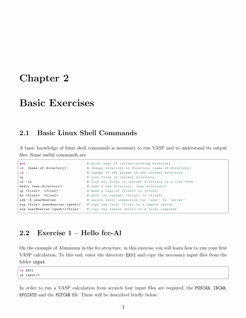
2.1 Basic Linux Shell Commands

A basic knowledge of linux shell commands is necessary to run VASP and to understand its output

files. Some useful commands are� �pwd # print name of current/working directory

cd <name -of -directory > # change directory to directory <name -of-directory >

cd .. # change to the parent of the current directory

ls # list files in current directory

ls -la # list all files in current directory in a list -form

mkdir <new -directory > # make a new directory <new -directory >

cp <file1 > <file2 > # make a copy of <file1 > to <file2 >

mv <file1 > <file2 > # move (or rename) <file1 > to <file2 >

ssh -X user@server # secure shell connection for ’user ’ to ’server ’

scp <file > user@server:<path >/. # copy the local <file > to a remote server

scp user@server:<path >/<file > . # copy the remote <file > to a local computer� �

2.2 Exercise 1 – Hello fcc-Al

On the example of Aluminum in the fcc-structure, in this exercise you will learn how to run your first

VASP calculation. To this end, enter the directory EX01 and copy the necessary input files from the

folder input� �cd EX01

cp input/* .� �In order to run a VASP calculation from scratch four input files are required, the POSCAR, INCAR,

KPOINTS and the POTCAR file. These will be described briefly below:

3

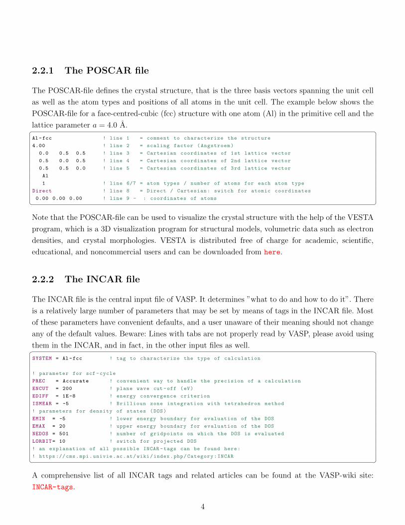
2.2.1 The POSCAR file

The POSCAR-file defines the crystal structure, that is the three basis vectors spanning the unit cell

as well as the atom types and positions of all atoms in the unit cell. The example below shows the

POSCAR-file for a face-centred-cubic (fcc) structure with one atom (Al) in the primitive cell and the

lattice parameter a = 4.0 A.� �Al-fcc ! line 1 = comment to characterize the structure

4.00 ! line 2 = scaling factor (Angstroem)

0.0 0.5 0.5 ! line 3 = Cartesian coordinates of 1st lattice vector

0.5 0.0 0.5 ! line 4 = Cartesian coordinates of 2nd lattice vector

0.5 0.5 0.0 ! line 5 = Cartesian coordinates of 3rd lattice vector

Al

1 ! line 6/7 = atom types / number of atoms for each atom type

Direct ! line 8 = Direct / Cartesian: switch for atomic coordinates

0.00 0.00 0.00 ! line 9 - : coordinates of atoms� �Note that the POSCAR-file can be used to visualize the crystal structure with the help of the VESTA

program, which is a 3D visualization program for structural models, volumetric data such as electron

densities, and crystal morphologies. VESTA is distributed free of charge for academic, scientific,

educational, and noncommercial users and can be downloaded from here.

2.2.2 The INCAR file

The INCAR file is the central input file of VASP. It determines ”what to do and how to do it”. There

is a relatively large number of parameters that may be set by means of tags in the INCAR file. Most

of these parameters have convenient defaults, and a user unaware of their meaning should not change

any of the default values. Beware: Lines with tabs are not properly read by VASP, please avoid using

them in the INCAR, and in fact, in the other input files as well.� �SYSTEM = Al-fcc ! tag to characterize the type of calculation

! parameter for scf -cycle

PREC = Accurate ! convenient way to handle the precision of a calculation

ENCUT = 200 ! plane wave cut -off (eV)

EDIFF = 1E-8 ! energy convergence criterion

ISMEAR = -5 ! Brillioun zone integration with tetrahedron method

! parameters for density of states (DOS)

EMIN = -5 ! lower energy boundary for evaluation of the DOS

EMAX = 20 ! upper energy boundary for evaluation of the DOS

NEDOS = 501 ! number of gridpoints on which the DOS is evaluated

LORBIT= 10 ! switch for projected DOS

! an explanation of all possible INCAR -tags can be found here:

! https ://cms.mpi.univie.ac.at/wiki/index.php/Category:INCAR� �A comprehensive list of all INCAR tags and related articles can be found at the VASP-wiki site:

INCAR-tags.

4

2.2.3 The KPOINTS file

The file KPOINTS defines the k-point grid for Brillouin zone (BZ) integrations or for band structure

calculations. An example for a KPOINTS-file to be used during a self-consistency calculations is listed

below.� �automatic mesh ! this turns on the automatic generation of k-points

0 ! number of k-points = 0 -> automatic generation scheme

Monkhurst ! so -called Monkhorst -Pack k-grids [Phys. Rev. B 13, 5188 -5192 (1976)]

15 15 15 ! subdivisions N_1 , N_2 and N_3 along reciprocal lattice vectors

0 0 0 ! optional shift of the mesh (s_1 , s_2 , s_3)� �2.2.4 The POTCAR file

The POTCAR file contains the pseudopotential for each atomic species used in the calculation. Unlike,

the previous three input files, the user is not supposed to edit the POTCAR-file, rather this file is

provided with the VASP-code for each element in the periodic table. The first few lines of a POTCAR-

file for Aluminium using the so-called projector augmented wave (PAW) method and to be used for

GGA-calculations (generalized gradient approximation for exchange-correlation) is listed below.� �1 PAW_PBE Al 04 Jan2001

2 3.00000000000000000

3 parameters from PSCTR are:

4 VRHFIN =Al: s2p1

5 LEXCH = PE

6 EATOM = 53.5387 eV, 3.9350 Ry

7

8 TITEL = PAW_PBE Al 04 Jan2001

9 LULTRA = F use ultrasoft PP ?

10 IUNSCR = 1 unscreen: 0-lin 1-nonlin 2-no

11 RPACOR = 1.500 partial core radius

12 POMASS = 26.982; ZVAL = 3.000 mass and valenz

13 RCORE = 1.900 outmost cutoff radius

14 RWIGS = 2.650; RWIGS = 1.402 wigner -seitz radius (au A)

15 ENMAX = 240.300; ENMIN = 180.225 eV

16 ICORE = 2 local potential

17 LCOR = T correct aug charges

18 LPAW = T paw PP

19 EAUG = 291.052

20 DEXC = -.041� �A few important pieces of information to be learned from the POTCAR-file: The first line indicates the

type of pseudopotential (here: PAW = projector augmented wave), the exchange-correlation potential

(here: PBE = Perdew-Burke-Ernzerhof GGA), and the atom type. Line 12 shows how many electrons

are treated as valence electrons (here ZVAL = 3). Line 15 specifies the recommended range of the

plane-wave cut-off to be used. In case, the INCAR-file does not contain ENCUT, these values together

with the PREC-tag decide about the plane wave cut-off to be used.

5

2.2.5 Starting the calculation

In order to run a VASP calculation, the VASP executable needs to be started. On the computer

system used in this exercises, this is invoked by submitting the following job script to the queuing

system� �1 #!/bin/bash

2 #

3 #SBATCH --job -name=EX01

4 #SBATCH --ntasks =2

5 #SBATCH --ntasks -per -core=1

6 #SBATCH -o outfile # send stdout to outfile

7 #SBATCH -e errfile # send stderr to errfile

8

9 mpirun /home/shared/VASP/vasp .5.4.1/ bin/vasp_std� �In the third line, a name for the job can be given (here: EX01), in line 4, the number of computer

cores to be used in parallel can be specified (here: 2), and line 9 contains the actual call of the

vasp executable (vasp_std), which is executed in parallel using message passing interface (MPI)

parallelization protocol. The job submission is completed by the following command� �sbatch run.EX01� �Other useful commands of the job-managing system slurm are:� �sbatch <name -of -job -file > ! submit job

scancel <job -number > ! delete job with the job number <job -number >

squeue ! display status of running jobs

sinfo ! display information about the available compute nodes� �2.2.6 Most important output files

Once the calculation is running, a number of output files appear in the working directory. Here, only

the most important ones are explained briefly.

The so-called OSZICAR file contains information about convergence speed during a self-consistent

calculation. Always keep a copy of the OSZICAR file, it might give important information. In our

example, it looks as follows:� �1 N E dE d eps ncg rms rms(c)

2 DAV: 1 -0.325642244910E+01 -0.32564E+01 -0.62741E+02 1540 0.146E+02

3 DAV: 2 -0.374211031115E+01 -0.48569E+00 -0.47829E+00 1700 0.150E+01

4 DAV: 3 -0.374371789381E+01 -0.16076E-02 -0.16551E-02 1435 0.814E-01

5 DAV: 4 -0.374371883240E+01 -0.93858E-06 -0.94185E-06 1635 0.204E-02

6 DAV: 5 -0.374371883373E+01 -0.13361E-08 -0.12914E-08 1490 0.590E-04 0.961E-01

7 DAV: 6 -0.373018285171E+01 0.13536E-01 -0.13857E-03 1410 0.223E-01 0.598E-01

8 DAV: 7 -0.372017583614E+01 0.10007E-01 -0.46700E-03 1430 0.403E-01 0.258E-02

9 DAV: 8 -0.372018608662E+01 -0.10250E-04 -0.12387E-05 1450 0.336E-02 0.697E-03

6

10 DAV: 9 -0.372018998477E+01 -0.38982E-05 -0.46089E-07 1460 0.412E-03 0.764E-04

11 DAV: 10 -0.372018958907E+01 0.39570E-06 -0.27681E-09 1470 0.391E-04 0.210E-04

12 DAV: 11 -0.372018959123E+01 -0.21537E-08 -0.24462E-10 775 0.125E-04

13 1 F= -.37201896E+01 E0= -.37201896E+01 d E =0.000000E+00� �Here N is the number of electronic steps, E the current free energy, dE the change in the free energy

from the last to the current step and d eps the change in the bandstructure energy. After convergence

has been reached (line 13), the converged total energy is given.

Extensive information about various details of the information can be found in the OUTCAR-file of

which only the first few lines are shown here� �1 vasp .5.3.3 18 Dez12 (build Dec 22 2012 23:36:35) complex

2

3 executed on LinuxIFCmkl date 2018.04.04 13:39:19

4 serial version

5

6

7 --------------------------------------------------------------------------------------------------------

8

9

10 INCAR:

11 POTCAR: PAW_PBE Al 04 Jan2001

12 POTCAR: PAW_PBE Al 04 Jan2001� �Browse the OUTCAR file (using e.g. gedit) to get an overview of the information it contains. For

instance, look for the converged value of the Fermi energy. Hint: it is convenient to use the linux

command grep (print lines matching a pattern) to grab certain information from text files, try:� �grep Fermi OUTCAR� �2.2.7 Plotting the density of states

The density of states (DOS) is written to the DOSCAR file. Have a look at this text file and try to

interpret it content. In order to plot, the DOS the following python script ex01.py can be used� �1 import vasp as vasp # import class with functions to read in VASP input / output

2 import numpy as np

3 import matplotlib.pyplot as plt

4

5 # EXERCISE 01: plot density of states #

6 d = vasp.DOS(’../ EX01/DOSCAR ’) # the DOS is read from file to the object d

7 d.plot_dos () # use the function plot_dos to plot the DOS

8 plt.show()� �Enter the directory Python and execute the python script by� �python ex01.py� �

7

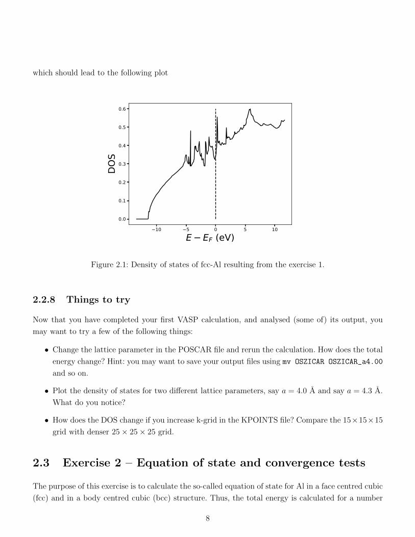
which should lead to the following plot

10 5 0 5 10E EF (eV)

0.0

0.1

0.2

0.3

0.4

0.5

0.6DO

S

Figure 2.1: Density of states of fcc-Al resulting from the exercise 1.

2.2.8 Things to try

Now that you have completed your first VASP calculation, and analysed (some of) its output, you

may want to try a few of the following things:

• Change the lattice parameter in the POSCAR file and rerun the calculation. How does the total

energy change? Hint: you may want to save your output files using mv OSZICAR OSZICAR_a4.00

and so on.

• Plot the density of states for two different lattice parameters, say a = 4.0 A and say a = 4.3 A.

What do you notice?

• How does the DOS change if you increase k-grid in the KPOINTS file? Compare the 15×15×15

grid with denser 25× 25× 25 grid.

2.3 Exercise 2 – Equation of state and convergence tests

The purpose of this exercise is to calculate the so-called equation of state for Al in a face centred cubic

(fcc) and in a body centred cubic (bcc) structure. Thus, the total energy is calculated for a number

8

of unit cell volumes, respectively, lattice parameters. To this end, we will make use of a linux bash

script and we will investigate the convergence of our results with repect to the plane wave cut-off and

the k-grid for BZ integrations.

2.3.1 Equation of state

In principle you could obtain the data points, total energy versus lattice parameter, by stepwise

changing the lattice parameter manually in the POSCAR file and subsequently running VASP. A

more convenient way to achieve this, is by using a linux shell script. Enter the directory cd EX02/fcc

and have a look at the job script run.fcc listed below:� �1 #!/bin/bash

2 #

3 #SBATCH --job -name=EX02fcc

4 #SBATCH --ntasks =2

5 #SBATCH --ntasks -per -core=1

6 #SBATCH -o outfile # send stdout to outfile

7 #SBATCH -e errfile # send stderr to errfile

8

9 for a in 3.80 3.85 3.90 3.95 4.00 4.05 4.10 4.15 4.20 4.25 4.30 4.35 4.40

10 do

11 cat >POSCAR <<EOF

12 Al-fcc

13 $a

14 0.0 0.5 0.5

15 0.5 0.0 0.5

16 0.5 0.5 0.0

17 Al

18 1

19 Direct

20 0.0 0.0 0.0

21 EOF

22 mkdir a_$a

23 mpirun /home/shared/VASP/vasp .5.4.1/ bin/vasp_std

24 /bin/rm WAVECAR EIG*

25 /bin/mv CHGCAR OUTCAR OSZICAR POSCAR DOSCAR a_$a

26 done� �This bash script performs a loop (lines 9–26) over all lattice parameters listed in line 9. Using the

linux command cat, it first writes the lines 12–20 to a file named POSCAR. Note that in line 13 $a

causes writing the value of the variable. Then (line 22), a subdirectory is created, named e.g. a_3.80,

VASP is executed (line 23), some output files are deleted (line 24) and the CHGCAR, OUTCAR

OSZICAR, POSCAR and DOSCAR files are moved into the respective subdirectory (line 25), before

a new POSCAR file with the next lattice parameter is written.

Submit the job using the already familiar� �sbatch run.fcc� �

9

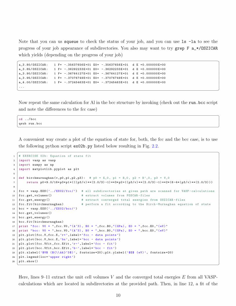
Note that you can us squeue to check the status of your job, and you can use ls -la to see the

progress of your job appearance of subdirectories. You also may want to try grep F a_*/OSZICAR

which yields (depending on the progress of your job)� �a_3 .80/ OSZICAR: 1 F= -.35637656E+01 E0= -.35637656E+01 d E =0.000000E+00

a_3 .85/ OSZICAR: 1 F= -.36292233E+01 E0= -.36292233E+01 d E =0.000000E+00

a_3 .90/ OSZICAR: 1 F= -.36764127E+01 E0= -.36764127E+01 d E =0.000000E+00

a_3 .95/ OSZICAR: 1 F= -.37076749E+01 E0= -.37076749E+01 d E =0.000000E+00

a_4 .00/ OSZICAR: 1 F= -.37245463E+01 E0= -.37245463E+01 d E =0.000000E+00

...� �Now repeat the same calculation for Al in the bcc structure by invoking (check out the run.bcc script

and note the differences to the fcc case)� �cd ../ bcc

qsub run.bcc� �A convenient way create a plot of the equation of state for, both, the fcc and the bcc case, is to use

the following python script ex02b.py listed below resulting in Fig. 2.2.� �1 # EXERCISE 02b: Equation of state fit

2 import vasp as vasp

3 import numpy as np

4 import matplotlib.pyplot as plt

5

6 def birchmurnaghan(v,p0 ,p1,p2,p3): # p0 = E_0 , p1 = B_0 , p2 = B’_0, p3 = V_0

7 return p0 +9.0/16* p3*p1*(((p3/v)**(2.0/3) -1)**3*p2+((p3/v)**(2.0/3) -1)**2*(6 -4*(p3/v)**(2.0/3)))

8

9 fcc = vasp.EOS(’../ EX02/fcc/’) # all subdirectories at given path are scanned for VASP -calculations

10 fcc.get_volumes () # extract volumes from POSCAR -files

11 fcc.get_energy () # extract converged total energies from OSZICAR -files

12 fcc.fit(birchmurnaghan) # perform a fit according to the Birch -Murnaghan equation of state

13 bcc = vasp.EOS(’../ EX02/bcc/’)

14 bcc.get_volumes ()

15 bcc.get_energy ()

16 bcc.fit(birchmurnaghan)

17 print "fcc: V0 = ",fcc.V0,"(A^3), B0 = ",fcc.B0 ,"(GPa), E0 = ",fcc.E0,"(eV)"

18 print "bcc: V0 = ",bcc.V0,"(A^3), B0 = ",bcc.B0 ,"(GPa), E0 = ",bcc.E0,"(eV)"

19 plt.plot(fcc.V,fcc.E,’r+’,label=’fcc - data points ’)

20 plt.plot(bcc.V,bcc.E,’bx’,label=’bcc - data points ’)

21 plt.plot(fcc.Vfit ,fcc.Efit ,’r-’,label=’fcc - fit’)

22 plt.plot(bcc.Vfit ,bcc.Efit ,’b-’,label=’bcc - fit’)

23 plt.xlabel(’$V$ (${\\AA}^3$)’, fontsize =20);plt.ylabel(’$E$ (eV)’, fontsize =20)

24 plt.legend(loc=’upper right’)

25 plt.show()� �Here, lines 9–11 extract the unit cell volumes V and the converged total energies E from all VASP-

calculations which are located in subdirectories at the provided path. Then, in line 12, a fit of the

10

5 10 15 20 25 30

V (3

)

4.0

3.5

3.0

2.5

2.0

1.5

E (

eV

)

fcc - data pointsbcc - data pointsfcc - fitbcc - fit

Figure 2.2: Total energy versus volume for Al for fcc and bcc structures (symbols) and fits accordingto the Birch-Murnaghan equation of state (lines).

data points using the so-called Birch-Murnaghan equation of state is performed [8]

E(V ) = E0 +9

16V0B0

((V0V

) 23

− 1

)3

B′0 +

((V0V

) 23

− 1

)2(6− 4

(V0V

) 23

) . (2.1)

Here, the four fit parameters E0, V0, B0 and B′0 are the energy at the minimum, the equilibrium volume,

the bulk modulus at the equilibrium and the pressure-derivative of the bulk modulus, respectively.

These numbers are printed in lines 17 and 18 for the fcc and bcc case, respectively, before lines 19-24

create the plot reproduced in Fig. 2.2 which shows the data points as well as the fits according to

Equation 2.1.

2.3.2 Convergence tests

One appealing fact about density functional calculations is that it allows the ab-initio, or parameter-

free, computation of materials properties meaning that the obtained results follow directly from apply-

ing the fundamental laws of physics, that is by solving the many-electron problem which is mapped to

Kohn-Sham equations. In practice, there are, however, a number of computational parameters which

govern the precision of the computed results. Two examples for such parameters are the number of

basis functions used to expand the Kohn-Sham orbitals and the number of k-points used in the sum-

11

mation over the Brillouin zone. It is the duty of any DFT practitioner to make sure that the obtained

results are converged with respect to these computational parameters.

In our example of fcc Al, this means that we investigate how the desired quantities, e.g. the equilibrium

volume V0 and the bulk modulus B0 depend on these convergence parameters.

• Compute the equation of state for fcc-Al and the resulting equilibrium volume V0 and bulk

modulus B0 using four different k-grids: 5× 5× 5, 11× 11× 11, 21× 21× 21, and 31× 31× 31.

(fix the plane wave cut-off to 200 eV). Which k-grid do you consider to yield converged results?

• Now fix the k-grid and investigate how the plane wave cut-off (ENCUT) influences the equation

of state and the resulting equilibrium volume V0 and bulk modulus B0. Try values of 150 eV,

200 eV, 300 eV and 400 eV. Do you observe convergence of your results? What do you notice

regarding the computational time?

2.3.3 More things to try

• Compute the equation of state for fcc-Al using the local density approximation (LDA) for the

exchange-correlation potential. Compare your results to the previous GGA-results and to the

experimental value (aexp = 4.019 A, see also Ref. [9]). Hint: for an LDA calculation you must

replace the POTCAR file (see directories LDA-PAW)

• Compute the equation of state for another element. Check out the available POTCAR files in the

directories LDA-PAW or PBE-PAW for LDA or GGA exchange-correlation potentials, respectively.

• Set up a calculation for Al in the hexagonal-close-packed (hcp) structure, compute its equation

of state and compare it with the results obtained above for the fcc and bcc structures. Hint: a

POSCAR file for an hcp structure is given below.

� �Al-hcp

3.80

0.50 -0.8660254037844386468 0.000000000 ! a_1 =(1/2, -sqrt (3)/2, 0)

0.50 0.8660254037844386468 0.000000000 ! a_2 =(1/2, sqrt (3)/2, 0)

0.00 0.0000000000000000000 1.632993162 ! a_3 =( 0, 0, c/a = sqrt (8/3))

Al

2 ! there are two atoms in the hcp -cell

Direct

0.3333333333333 0.66666666666666666666 0.250000000000000

0.6666666666666 0.33333333333333333333 0.750000000000000� �12

2.4 Exercise 3 – Band structure of silicon

Density functional theory is a theory for the electronic ground state of a system of N interacting

electrons which is characterized by its electron density n(r) and the ground state total energy E[n(r)]

of this N -electron system. However, the electronic band structure is, by its very definition, not a ground

state property since it requires electrons to be added or removed from the system. Thus, although

there is no rigorous connection of the Kohn-Sham energies εnk obtained by solving the Kohn-Sham

equations 1.1, it is common practice to interpret these Kohn-Sham energies as band structure of the

system (see my lecture-notes for more details). Note that the converged Kohn-Sham eigenvalues of

a VASP calculation are written to the file EIGENVAL.

In this exercise, we will calculate the band structure of Silicon in the diamond structure which consists

of two steps. First, the electron density (and the corresponding Kohn-Sham potential) has to be

determined self-consistently in the usual manner. In the second step, a non-self-consistent calculation

has to be performed, that is the charge density and the potential are fixed, for a number of k-points

along high-symmetry directions in the Brillouin zone.

2.4.1 Self-consistent calculation

The corresponding POSCAR, INCAR and KPOINTS files are listed below and can also be found in the

directory EX03/input.� �bulk -Si in diamond structure

5.43 ! lattice parameter

0.0 0.5 0.5 ! fcc -lattice vectors

0.5 0.0 0.5

0.5 0.5 0.0

Si

2 ! the diamond structure has 2 inequivalent atoms in the unit cell

Direct

-0.125 -0.125 -0.125 ! bond -center is an inversion center and is set at origin of the cell

0.125 0.125 0.125� �� �SYSTEM = Si-diamond structure

PREC = Accurate

ENCUT = 240

EDIFF =1E-8

ISMEAR =-5� �� �automatic mesh

0

Monkhurst

12 12 12

0 0 0� �13

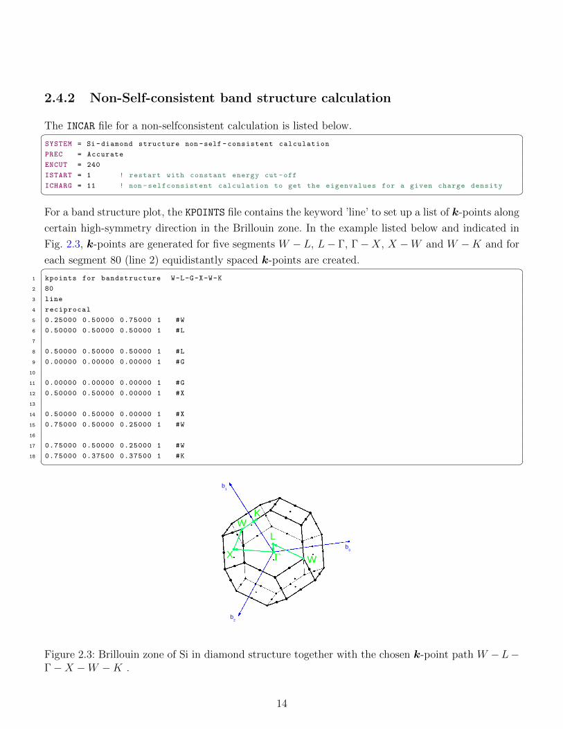
2.4.2 Non-Self-consistent band structure calculation

The INCAR file for a non-selfconsistent calculation is listed below.� �SYSTEM = Si-diamond structure non -self -consistent calculation

PREC = Accurate

ENCUT = 240

ISTART = 1 ! restart with constant energy cut -off

ICHARG = 11 ! non -selfconsistent calculation to get the eigenvalues for a given charge density� �For a band structure plot, the KPOINTS file contains the keyword ’line’ to set up a list of k-points along

certain high-symmetry direction in the Brillouin zone. In the example listed below and indicated in

Fig. 2.3, k-points are generated for five segments W − L, L− Γ, Γ−X, X −W and W −K and for

each segment 80 (line 2) equidistantly spaced k-points are created.� �1 kpoints for bandstructure W-L-G-X-W-K

2 80

3 line

4 reciprocal

5 0.25000 0.50000 0.75000 1 #W

6 0.50000 0.50000 0.50000 1 #L

7

8 0.50000 0.50000 0.50000 1 #L

9 0.00000 0.00000 0.00000 1 #G

10

11 0.00000 0.00000 0.00000 1 #G

12 0.50000 0.50000 0.00000 1 #X

13

14 0.50000 0.50000 0.00000 1 #X

15 0.75000 0.50000 0.25000 1 #W

16

17 0.75000 0.50000 0.25000 1 #W

18 0.75000 0.37500 0.37500 1 #K� �

W

L

X

WK

b1

b2

b3

Figure 2.3: Brillouin zone of Si in diamond structure together with the chosen k-point path W −L−Γ−X −W −K .

14

2.4.3 Plotting the results

After completing the non-scf calculation, the EIGENVAL file contain the Kohn-Sham eigenvalues εnk

for each k (in our example 5 × 80 = 400 points). For each k the lowest NBANDS (in this example

eigenvalues NBANDS=8) have been computed. A convenient way to visualize the band structure is to

use the following Python script which produces the Fig. 2.4.� �1 import vasp as vasp

2 import numpy as np

3 import matplotlib.pyplot as plt

4 # EXERCISE 03: Band structure plot

5 cell = vasp.POSCAR(’../ EX03/POSCAR ’) # read unit cell vectors

6 cell.reciprocal () # setup reciprocal lattice vectors

7 bs = vasp.BS(’../ EX03/KPOINTS ’,’../ EX03/EIGENVAL ’,Ef =5.9733)

8 Eg = min(bs.eig [: ,4])-max(bs.eig[:,3]);print "E_gap = ",Eg

9 bs.set_kpath(cell.b1 ,cell.b2,cell.b3)

10 bs.plot_bs(ymin =-13.0,ymax =5.0, Klabel =[’W’,’L’,’$\Gamma$ ’,’X’,’W’,’K’])� �

W L Γ X W K

10

5

0

5

E−EF

(eV

)

Figure 2.4: The electronic band structure of Si along the high-symmetry directions indicated in Fig. 2.3.

• How many occupied bands are there? Why?

• Why do certain directions (e.g. X −W ) appear to have less bands than other directions (e.g.

W − L)?

• How large is the computed Kohn-Sham band gap? How does this value compare to the experi-

mental value of Eg = 1.17 eV (compare Ref. [10])?

15

16

Chapter 3

Projects

3.1 Project 1 – Magnetic phases of iron

3.1.1 Description

The goal of this project is to calculate the equation of state for Fe with different magnetic configura-

tions. By default, VASP performs a non spin-polarized calculation (ISPIN=1) in which the resulting

charge density is identical for spin-up and spin-down electrons, thus n↑(r) = n↓(r). On the other

hand, VASP can also conduct so-called spin-polarized calculations in which the magnetic moments are

collinear, that is, the magnetic moments of adjacent atoms are aligned either parallel (ferro-magnetic

ordering) or anti-parallel. (anti-ferro-magnetic ordering). Thus, the electron densities for spin-up and

spin-down electrons is allowed to be different n↑(r) 6= n↓(r) and is determined self-consistently.

Below you find examples of POSCAR and INCAR files for bcc-Fe imposing a ferromagentic (FM) ordering� �Fe-bcc -FM

2.80

-0.5000000000 0.5000000000000000000 0.50000000000000

0.5000000000 -0.5000000000000000000 0.50000000000000

0.5000000000 0.5000000000000000000 -0.50000000000000

Fe

1

Direct

0.000000000000 0.000000000000000 0.000000000000� �� �SYSTEM = Fe-bcc -FM

PREC = Accurate

ENCUT = 300

EDIFF=1E-7

ISMEAR = -5

ISPIN = 2 ! spin polarized calculation (ferro -magnetic)

MAGMOM = 1 ! starting value for magnetic moment� �17

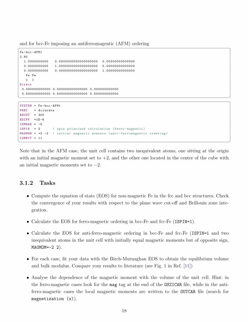
and for bcc-Fe imposing an antiferromagentic (AFM) ordering� �Fe-bcc -AFM1

2.80

1.0000000000 0.0000000000000000000 0.00000000000000

0.0000000000 1.0000000000000000000 0.00000000000000

0.0000000000 0.0000000000000000000 1.00000000000000

Fe Fe

1 1

Direct

0.000000000000 0.000000000000000 0.000000000000

0.500000000000 0.500000000000000 0.500000000000� �� �SYSTEM = Fe-bcc -AFM1

PREC = Accurate

ENCUT = 300

EDIFF =1E-6

ISMEAR = -5

ISPIN = 2 ! spin polarized calculation (ferro -magnetic)

MAGMOM = +2 -2 ! initial magnetic moments (anti -ferromagnetic ordering)

LORBIT = 11� �Note that in the AFM case, the unit cell contains two inequivalent atoms, one sitting at the origin

with an initial magnetic moment set to +2, and the other one located in the center of the cube with

an initial magnetic moments set to −2.

3.1.2 Tasks

• Compute the equation of state (EOS) for non-magnetic Fe in the fcc and bcc structures. Check

the convergence of your results with respect to the plane wave cut-off and Brillouin zone inte-

gration.

• Calculate the EOS for ferro-magnetic ordering in bcc-Fe and fcc-Fe (ISPIN=1).

• Calculate the EOS for anti-ferro-magnetic ordering in bcc-Fe and fcc-Fe (ISPIN=1 and two

inequivalent atoms in the unit cell with initially equal magnetic moments but of opposite sign,

MAGMOM=-2 2).

• For each case, fit your data with the Birch-Murnaghan EOS to obtain the equilibrium volume

and bulk modulus. Compare your results to literature (see Fig. 1 in Ref. [11])

• Analyse the dependence of the magnetic moment with the volume of the unit cell. Hint: in

the ferro-magnetic cases look for the mag tag at the end of the OSZICAR file, while in the anti-

ferro-magnetic cases the local magnetic moments are written to the OUTCAR file (search for

magnetization (x)).

18

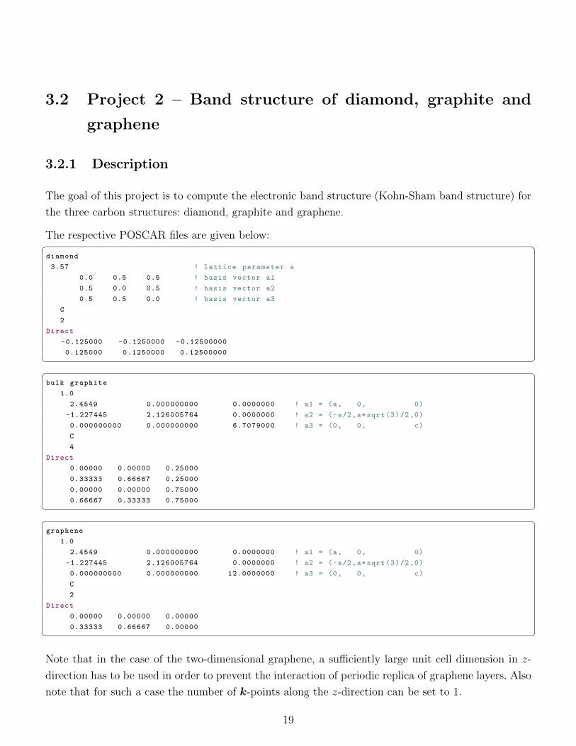
3.2 Project 2 – Band structure of diamond, graphite and

graphene

3.2.1 Description

The goal of this project is to compute the electronic band structure (Kohn-Sham band structure) for

the three carbon structures: diamond, graphite and graphene.

The respective POSCAR files are given below:� �diamond

3.57 ! lattice parameter a

0.0 0.5 0.5 ! basis vector a1

0.5 0.0 0.5 ! basis vector a2

0.5 0.5 0.0 ! basis vector a3

C

2

Direct

-0.125000 -0.1250000 -0.12500000

0.125000 0.1250000 0.12500000� �� �bulk graphite

1.0

2.4549 0.000000000 0.0000000 ! a1 = (a, 0, 0)

-1.227445 2.126005764 0.0000000 ! a2 = (-a/2,a*sqrt (3)/2,0)

0.000000000 0.000000000 6.7079000 ! a3 = (0, 0, c)

C

4

Direct

0.00000 0.00000 0.25000

0.33333 0.66667 0.25000

0.00000 0.00000 0.75000

0.66667 0.33333 0.75000� �� �graphene

1.0

2.4549 0.000000000 0.0000000 ! a1 = (a, 0, 0)

-1.227445 2.126005764 0.0000000 ! a2 = (-a/2,a*sqrt (3)/2,0)

0.000000000 0.000000000 12.0000000 ! a3 = (0, 0, c)

C

2

Direct

0.00000 0.00000 0.00000

0.33333 0.66667 0.00000� �Note that in the case of the two-dimensional graphene, a sufficiently large unit cell dimension in z-

direction has to be used in order to prevent the interaction of periodic replica of graphene layers. Also

note that for such a case the number of k-points along the z-direction can be set to 1.

19

3.2.2 Tasks

• Compute the equation of state for diamond using the PBE-GGA-functional. What is the equi-

librium lattice parameter and the bulk modulus?

• Optimize the in-plane lattice parameter a for graphene. What value do you get? Compare the

resulting C–C bond lengths in diamond and graphene.

• Using the optimized in-plane lattice parameter a for graphene, determine the optimal lattice

parameter c for graphite. Note: the interaction of adjacent graphene layers in graphite is of

van-der-Waals type which is ill-described with a GGA-functional. A simple way to correct for

the missing van-der-Waals interactions is the empirical correction scheme according to Grimme

which is turned on by the switch IVDW=1 in the INCAR file.

• Compute and plot the density of states for diamond, graphite and graphene. Note: For the

bulk structures, diamond and graphene, the tetrahedron method (ISMEAR=-5) can be used for

BZ-integrations, while for graphene a smearing technique has to be used (e.g. ISMEAR=-1 with

SIGMA=0.1). Why?

• Compute and plot the band structures of diamond, graphite and graphene along high-symmetry

directions in the BZ. Hint: For diamond you can use the k-points defined in Sec. 2.4.2 for Silicon,

for the hexagonal graphite and graphene cells you can use the points listed below.

• Check the convergence of all your results with respect to the plane wave cut-off and the k-grid

density for BZ integrations.� �k-points along high symmetry lines for hexagonal str.

50

line

rec

0.000 0.000 0.500 ! A

0.000 0.000 0.000 ! Gamma

0.000 0.000 0.000 ! Gamma

0.500 0.000 0.000 ! M

0.500 0.000 0.000 ! M

0.333333 0.333333 0.000 ! K

0.333333 0.333333 0.000 ! K

0.000 0.000 0.000 ! Gamma� �20

3.3 Project 3 – Adsorption of CO molecule on a surface

3.3.1 Description

The goal of this project is to calculate the (110)-surface Palladium by using the so-called repeated-slab

approach. In a second step, the adsorption of a CO-molecule on this surface will be studied.

Owing to its plane-wave basis set, all calculations in VASP must obey periodic boundary conditions

for all three spatial directions. The commonly used method to simulate two-dimensional structures,

such as surfaces, is to use the so-called repeated slab approach. Here, a slab of a given thickness is

cut out of the crystal and separated by a vacuum slab from its periodic replica. The POSCAR file for

a repeated slab model for the (110)-termination of an fcc-Palladium crystal with a thickness of five

atomic layers is given below:� �Pd(110) surface - 5 layer slab

1.0

2.786000718 0.00 0.0 ! a1 = (a/sqrt (2), 0, 0)

0.000000000 3.94 0.0 ! a2 = (0 a, 0)

0.000000000 0.00 20.0 ! a3 = (0 0, c)

Pd

5

Selective dynamics

Direct

0.00 0.00 -0.13930 F F T

0.50 0.50 -0.06965 F F T

0.00 0.00 0.00000 F F F

0.50 0.50 0.06965 F F T

0.00 0.00 0.13930 F F T� �In contrast to the previous exercises and the other two projects, this structure containing five Pd atoms

per unit cell is characterized by internal (or ionic) degrees of freedom. This means that z-coordinates

of the atoms are not determined by the symmetry of the crystal. As explained in more detail in my

lecture ”Fundamentals of Electronic Structure Theory”, the converged electron density n(r) also

gives rise to the force F k acting on the k-th atomic nucleus in the unit cell. The application of the

Hellmann-Feynman theorem leads to the following expression

F k = − ∂E

∂Rk

=

⟨ψ

∣∣∣∣∣− ∂H

∂Rk

∣∣∣∣∣ψ⟩

=

∫d3r n(r)

Zk(r −Rk)

|r −Rk|3+∑l 6=k

ZkZl(Rk −Rl)

|Rk −Rl|3. (3.1)

Thus, according to the electro-static force theorem, once the spatial distribution of the electrons n(r)

has been determined by solving Kohn-Sham equations, all the forces in the system can be calculated

using classical electrostatics. These atomic forces can be used to find the equilibrium arrangement of

the atoms within a unit cell.

In order to turn on the ionic relaxation, the following INCAR file can be used

21

� �SYSTEM = Pd(110) slab (5 layers)

PREC = ACCURATE

EDIFF = 1.E-08

EDIFFG = -0.02 ! break condition for the ionic relaxation loop: all forces < 0.02 eV/Angstroem

NSW = 100 ! sets the maximum number of ionic steps

IBRION = 2 ! ionic relaxation using conjugate gradient algorithm

POTIM = 0.10 ! scaling factor for atomic forces

ISIF = 0 ! no stress tensor is calculated

LORBIT = 11

EMIN = -10.

EMAX = 5.

NEDOS = 1501

ISMEAR = 1 ! occupation according to Methfessel -Paxton scheme of order 1

SIGMA = 0.2 ! specifies the width of the smearing in eV� �Note that the keywords Selective dynamics and the true (T) and false (F) tags given for each ionic

coordinate in the POSCAR file indicate whether a given ionic coordinate is allowed to relax (T) or kept

fixed (F).

Because of the vacuum slab in z-direction, only one k-point suffices in this direction as can be seen

from the KPOINTS file provided below:� �automatic mesh

0

Monkhurst

12 9 1

0 0 0� �3.3.2 Tasks

• Perform an ionic relaxation for the 5-layer Pd(110) slab. How many ionic steps are needed until

all atomic forces are below 0.02 eV/A? Plot the total energy as well as the atomic forces on

the two topmost Pd-atoms as a function of the relaxation step. Hint: the total energy can be

found conveniently in the OSZICAR file, the atomic forces are written to the OUTCAR file (try the

following: grep -A 8 TOTAL-FORCE OUTCAR)

• Analyse the relaxed structure in terms of the interlayer spacing and compare it to the interlayer

spacing in bulk Pd which is d = a/(2√

2), where a is the lattice parameter of Pd.

• Compute the adsorption geometry of a CO-molecule on the Pd(110) slab. Use the initial POSCAR

and INCAR file given below.

• Also try other starting geometries, e.g., the CO-molecule pointing with the oxygen atom towards

the surface, and also try other adsorption sites characterized by the x and y coordinates of the

22

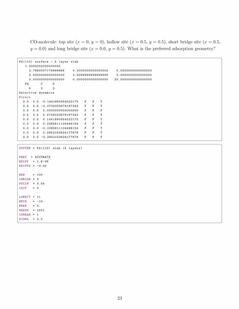
CO-molecule: top site (x = 0, y = 0), hollow site (x = 0.5, y = 0.5), short bridge site (x = 0.5,

y = 0.0) and long bridge site (x = 0.0, y = 0.5). What is the preferred adsorption geometry?

� �Pd(110) surface - 5 layer slab

1.0000000000000000

2.7860007179999999 0.0000000000000000 0.0000000000000000

0.0000000000000000 3.9399999999999999 0.0000000000000000

0.0000000000000000 0.0000000000000000 20.0000000000000000

Pd C O

5 2 2

Selective dynamics

Direct

0.0 0.0 -0.1441660454022175 F F T

0.5 0.5 -0.0706333678187342 F F T

0.0 0.0 0.0000000000000000 F F F

0.5 0.5 0.0706333678187342 F F T

0.0 0.0 0.1441660454022175 F F T

0.0 0.0 0.2385811124496154 F F T

0.0 0.0 -0.2385811124496154 F F T

0.0 0.0 0.2952153824177678 F F T

0.0 0.0 -0.2952153824177678 F F T� �� �SYSTEM = Pd(110) slab (5 layers)

PREC = ACCURATE

EDIFF = 1.E-06

EDIFFG = -0.02

NSW = 100

IBRION = 2

POTIM = 0.04

ISIF = 0

LORBIT = 11

EMIN = -10.

EMAX = 5.

NEDOS = 1501

ISMEAR = 1

SIGMA = 0.2� �

23

24

Bibliography

[1] P. Hohenberg and W. Kohn. Inhomogeneous electron gas. Phys. Rev., 136:B864, 1964.

[2] W. Kohn and L. J. Sham. Self-consistent equations including exchange and correlation effects.

Phys. Rev., 140(4A):A1133–A1138, Nov 1965.

[3] W. Kohn. An essay on condensed matter physics in the twentieth century. Rev. Mod. Phys., 71,

1999.

[4] W. Kohn. Nobel lecture: Electronic structure of matter-wave functions and density functionals.

Rev. Mod. Phys., 71:1253, 1999.

[5] R. O. Jones and O. Gunnarsson. The density functional formalism, its application and prospects.

Rev. Mod. Phys., 61:689, 1989.

[6] C. Fiolhais, F. Nogueira, and M. A. L. Marques, editors. A Primer in Density Functional Theory.

Springer, Berlin, 2003.

[7] D. S. Sholl and J. A. Steckel. Density Functional Theory: A Practical Introduction. Wiley, 2009.

[8] Francis Birch. Finite elastic strain of cubic crystals. Phys. Rev., 71(11):809–824, Jun 1947.

[9] Philipp Haas, Fabien Tran, and Peter Blaha. Calculation of the lattice constant of solids with

semilocal functionals. Phys. Rev. B, 79(8):085104, 2009.

[10] Fabien Tran and Peter Blaha. Accurate band gaps of semiconductors and insulators with a

semilocal exchange-correlation potential. Phys. Rev. Lett., 102(22):226401, 2009.

[11] D. E. Jiang and Emily A. Carter. Carbon dissolution and diffusion in ferrite and austenite from

first principles. Phys. Rev. B, 67(21):214103–214113, Jun 2003.

25