SIMULACIÓN DE UNA TURBINA DE VAPOR DE UNA CENTRAL ...
116
ESCUELA TÉCNICA SUPERIOR DE INGENIERÍA (ICAI) INGENIERO INDUSTRIAL SIMULACIÓN DE UNA TURBINA DE VAPOR DE UNA CENTRAL NUCLEAR CON EL CÓDIGO TRACE Autor: Adoración Garrido-Lestache Romero Director: Prof. Dr. Rafael Macián Juan Madrid Mayo 2015
-
Upload
khangminh22 -
Category
Documents
-
view
0 -
download
0
Transcript of SIMULACIÓN DE UNA TURBINA DE VAPOR DE UNA CENTRAL ...

ESCUELA TÉCNICA SUPERIOR DE INGENIERÍA (ICAI)
INGENIERO INDUSTRIAL
SIMULACIÓN DE UNA TURBINA DE VAPOR DE UNA CENTRAL NUCLEAR CON EL
CÓDIGO TRACE
Autor: Adoración Garrido-Lestache Romero Director: Prof. Dr. Rafael Macián Juan
Madrid Mayo 2015


:-Y*o',::',I'=iCor*rirnS
AUToRrzAcróru paRr te DrGrrAL¡zAc¡óru, oepósro y DrvutGAc¡órr¡ ¡lu AccEso
AB t ERTo ( REsrRrruG tn,ol DE Docu M ENrRcróru
7e. Decldración de la autorío y acreditación de la misma.
El autor o. Ñrr-tJviou GAe-r-§r, - L-:e'sr¡.ea<¡ , como N rrr.ts\ de
la UNIVERSIDAD PONTIFICIA COMILLAS (COMILLAS), DECLARA
que es el titular de los derechos de propiedad intelectual, objeto de la presente cesión,
en
obra
relación la
1,
que ésta es una obra original, y que ostenta la condición de autor en el sentido que
otorga la Ley de Propiedad lntelectual como titular único o cotitular de la obra.
En caso de ser cotitular, el autor (fírmante) declara asimismo que cuenta con el
consentimiento de los restantes titulares para hacer la presente cesión. En caso de
previa cesión a terceros de derechos de explotación de la obra, el autor declara que
tiene la oportuna autor¡zación de dichos titulares de derechos a los fines de esta
cesión o bien que retiene la facultad de ceder estos derechos en la forma prevista en la
presente cesión y así lo acredita.
2e. Objeto y fínes de la cesión.
Con el fin de dar la máxima difusión a la obra citada a través del Repositorio
institucional de la Universidad y hacer posible su utilización de forma libre y grotuita (
con las limitociones que más odelonte se detollanl por todos los usuarios del
1 Especificar si es una tesis doctoral, proyecto fin de carrera, proyecto fin de Máster o cualquier otrotrabajo que deba ser objeto de evaluación académica
con

I::r'a::'IiComÍrnS
repositorio y del portal e-ciencia, el autor CEDE a la Universidad pontificia Comillas deforma gratuita y no exclusiva, por el máximo plazo legal y con ámbito universal, los
derechos de digitalización, de archivo, de reproducción, de distribución, de
comunicación pública, incluido el derecho de puesta a disposición electrónica, tal ycomo se describen en [a Ley de Propiedad Intelectual. El derecho de transformación se
cede a los únicos efectos de lo dispuesto en la letra (a) del apartado siguiente.
3e. Condiciones de la cesión.
Sin perjuicio de la titularidad de la obra, que sigue correspondiendo a su autor, la
cesión de derechos contemplada en esta licencia, el repositorio institucional podrá:
(a) Transformarla para adaptarla a cualquier tecnología susceptible de incorporarla a
interneU realizar adaptaciones para hacer posible la utilización de la obra en formatoselectrónicos, así como incorporar metadatos para realizar el registro de la obra eincorporar "marcas de agua" o cualquier otro sistema de seguridad o de protección.
(b) Reproducirla en un soporte digital para su incorporación a una base de datos
electrónica, incluyendo el derecho de reproducir y almacenar la obra en servidores, a
los efectos de garantizar su seguridad, conservación y preservar el formato. .
(c) Comunicarla y ponerla a disposición del público a través de un archivo abiertoinstitucional, accesible de modo libre y gratuito a través de internet.2
(d) Distribuir copias electrónicas de la obra a los usuarios en un soporte digital. 3
2 En el supuesto de que el autor opte por el acceso restringido, este apartado quedaría redactado en lossiguientes términos:
(c) Comunicarla y ponerla a disposición del público a través de un archivo institucional, accesible demodo restringido, en los términos previstos en el Reglamento del Repositorio lnstitucíonal
3 En el supuesto de que el autor opte por el acceso restringido, este apartado quedaría eliminado.

XE'xiall's',iCor*,rÍmS
4e. Derechos del outor.
El autor, en tanto que titular de una obra que cede con carácter no exclusivo a laUniversidad por medio de su registro en el Repositorio lnstitucional tiene derecho a:
a) A que la Universidad identifique claramente su nombre como el autor o propietario
de los derechos del documento.
b) Comunicar y dar publicidad a
través de cualquier medio.
c) Solicitar la retirada de la obra
ponerse en contacto
(curiarte@rec. upcomillas.es).
la obra en la versión que ceda y en otras posteriores a
d) Autorizar expresamente a COMILLAS para, en su caso, realizar los trámitesnecesaríos para la obtención del ISBN.
d) Recibir notificación fehaciente de cualquier reclamación que puedan formular
terceras personas en relación con la obra y, en particular, de reclamaciones relativas a
los derechos de propiedad intelectual sobre ella.
del repositorio por causa justificada. A tal fin deberá
con el vicerrector/a de investigación
5e. Deberes del autor.
El autor se compromete a:
a) Garantizar que el compromiso que adquiere
infringe ningún derecho de terceros, ya sean de
cualquier otro.
mediante el presente escrito no
propiedad industrial, intelectual o
b) Garantizar que el contenido de las obras no atenta contra los derechos al honor, a la
intimidad y a la imagen de terceros.

,)-:''.^:¡:::r,=iCorrrnrnS
c) Asumir toda reclamación o responsabilidad, incluyendo las indemnizaciones pordaños, que pudieran ejercítarse contra la Universidad por terceros que vieraninfringidos sus derechos e intereses a causa de la cesión.
d) Asumir la responsabilidad en el caso de que las instituciones fueran condenadas porinfracción de derechos derivada de las obras objeto de la cesión.
6e. Fines y funcionomiento del Repositorío lnstitucional.
La obra se pondrá a disposición de los usuarios para que hagan de ella un uso justo yrespetuoso con los derechos del autor, según lo permitido por la legislación aplicable,y con fines de estudio, investigación, o cualquier otro fin lícito. Con dicha finalidad, la
Universidad asume los siguientes deberes y se reserva las siguientes facultades:
a) Deberes del repositorio lnstitucional:
- La Universidad informará a los usuarios del archivo sobre los usos permitidos, y nogarantiza ni asume responsabilidad alguna por otras formas en que |os usuarios hagan
un uso posterior de las obras no conforme con la legislación vigente. El uso posterior,más allá de la copia privada, requerirá que se cite la fuente y se reconozcala autoría,que no se obtenga beneficio comercial, y que no se realicen obras derivadas.
- La Universidad no revisará el contenido de las obras, que en todo caso permanecerá
bajo la responsabilidad exclusiva del autor y no estará obligada a ejercitar acciones
legales en nombre del autor en el supuesto de infraccíones a derechos de propiedadintelectual derivados del depósito y archivo de las obras. El autor renuncia a cualquierreclamación frente a la Universidad por las formas no ajustadas a la legislación vigenteen que los usuarios hagan uso de las obras.
- La Universidad adoptará las medidas necesarias para la preservación de la obra en
un futuro.

tr--I
l
lI
i
I
I ':Eyo'::',I'lCoriírmS
----l
b) Derechos que se reserva el Repositorio institucional respecto de las obras en él
- retirar la obra, previa notificación al autor, en supuestos suficientemente justificados,
o en caso de reclamaciones de terceros.
Madrid, ^
. Z6...ue .......Aarlr+-....... de .¿0.460


r -- I
Proyecto realizado por el alumno/a:
Garrido-Lestaóhe Romero
Fdo.
Autorizada la entrega del proyecto cuya información no es de carácterconfidencial
EL DIRECTOR DEL PROYECTO
Rafae! Macián Juan
recna:-/f .t e.§.t €drt{
Vo Bo del Coordinador de Proyectos
Fdo.:


ESCUELA TÉCNICA SUPERIOR DE INGENIERÍA (ICAI)
INGENIERO INDUSTRIAL
SIMULACIÓN DE UNA TURBINA DE VAPOR DE UNA CENTRAL NUCLEAR CON EL
CÓDIGO TRACE
Autor: Adoración Garrido-Lestache Romero Director: Prof. Dr. Rafael Macián Juan
Madrid Mayo 2015


Resumen en español
SIMULACIÓN DE UNA TURBINA DE VAPOR DE UNA CENTRAL NUCLEAR CON EL CÓDIGO TRACE
Autor: Adoración Garrido-Lestache Romero
Director: Prof. Dr. Rafael Macián Juan
Entidad Colaboradora: TUM – Technische Universität München
RESUMEN DEL PROYECTO
Introducción:
Una Central Nuclear está compuesta por un primer circuito, en el que se encuentra el reactor nuclear, y por un segundo circuito, el cual es similar al de una central térmica convencional.
Desde el punto de vista de la seguridad nuclear, el primer circuito de una central es el de mayor importancia para los análisis, y por lo tanto, los modelos desarrollados de este circuito son muy sofisticados. Por otro lado, como el análisis de seguridad en el segundo circuito carece de tanta importancia, los modelos de las turbinas desarrollados para simular su comportamiento bajo condiciones normales y adversas son muy simples.
El objetivo de este proyecto es desarrollar un modelo de la turbina de vapor de una central nuclear que proporciones resultados de funcionamiento realistas bajo condiciones normales y bajo el efecto de transitorios. El código TRACE, que fue desarrollado por el gobierno de los Estados Unidos para modelar el funcionamiento de centrales nucleares, es la herramienta utilizada para el desempeño de este proyecto.
Un esquema del circuito a simular fue proporcionado al principio del trabajo y ha sido usado como base para el desarrollo del modelo. El modelo final del circuito está compuesto por: una turbina de alta y otra de baja presión, un separador, un calentador, una válvula de seguridad, y condensadores.
!
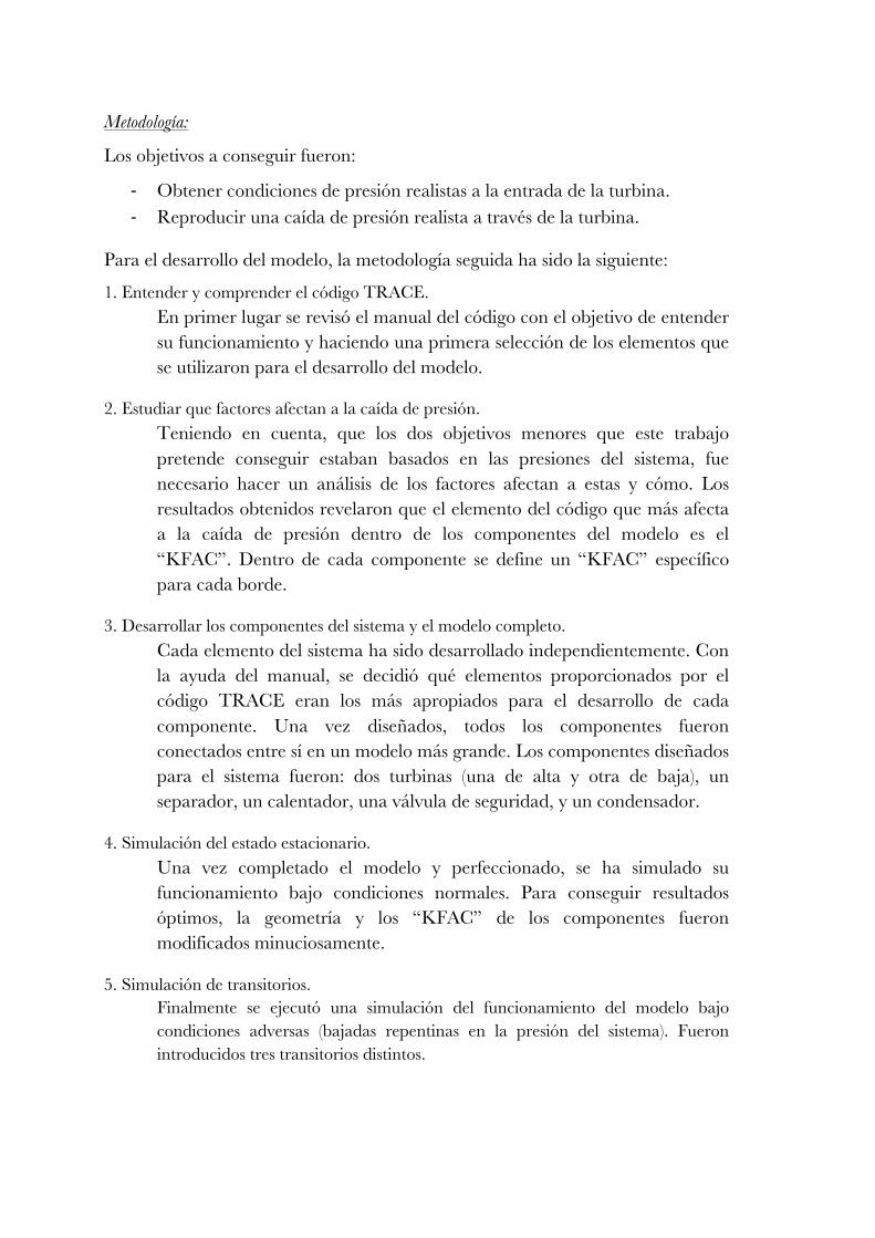
Metodología:
Los objetivos a conseguir fueron:
! Obtener condiciones de presión realistas a la entrada de la turbina. ! Reproducir una caída de presión realista a través de la turbina.
Para el desarrollo del modelo, la metodología seguida ha sido la siguiente:
1. Entender y comprender el código TRACE. En primer lugar se revisó el manual del código con el objetivo de entender su funcionamiento y haciendo una primera selección de los elementos que se utilizaron para el desarrollo del modelo.
2. Estudiar que factores afectan a la caída de presión. Teniendo en cuenta, que los dos objetivos menores que este trabajo pretende conseguir estaban basados en las presiones del sistema, fue necesario hacer un análisis de los factores afectan a estas y cómo. Los resultados obtenidos revelaron que el elemento del código que más afecta a la caída de presión dentro de los componentes del modelo es el “KFAC”. Dentro de cada componente se define un “KFAC” específico para cada borde.
3. Desarrollar los componentes del sistema y el modelo completo. Cada elemento del sistema ha sido desarrollado independientemente. Con la ayuda del manual, se decidió qué elementos proporcionados por el código TRACE eran los más apropiados para el desarrollo de cada componente. Una vez diseñados, todos los componentes fueron conectados entre sí en un modelo más grande. Los componentes diseñados para el sistema fueron: dos turbinas (una de alta y otra de baja), un separador, un calentador, una válvula de seguridad, y un condensador.
4. Simulación del estado estacionario. Una vez completado el modelo y perfeccionado, se ha simulado su funcionamiento bajo condiciones normales. Para conseguir resultados óptimos, la geometría y los “KFAC” de los componentes fueron modificados minuciosamente.
5. Simulación de transitorios. Finalmente se ejecutó una simulación del funcionamiento del modelo bajo condiciones adversas (bajadas repentinas en la presión del sistema). Fueron introducidos tres transitorios distintos.

6. Recopilación de los datos de las simulaciones. Una vez terminadas las simulaciones se recopilaron y analizaron todos los resultados.
Resultados:
Los modelos simplificados de las turbinas de alta y baja presión fueron desarrollados para probar la efectividad del modelo de las turbinas en TRACE utilizando las condiciones de contorno de diseño. Después de simular ambos modelos, los resultados fueron recopilados y comparados con los datos reales medidos en la planta. El análisis de los resultados se ha focalizado en la caída de presión a lo largo de la turbina, ya que el elemento FILL impone las condiciones a la entrada de la turbina. La comparación entre los resultados de la simulación y los datos reales de medida en la planta fue muy positiva. Después de analizar los resultados de los modelos simplificado, se implementó el modelo completo. Los resultados obtenidos de la simulación del estado estacionario en el modelo completo no fueron tan buenos como los obtenidos de la simulación de los modelos simplificados. La diferencia que existe entre los resultados de ambos modelos es debido al efecto causado por los demás componentes del sistema (separador y calentador). Después de obtener buenos resultados de las simulaciones de los modelos en estado estacionario, se simularon tres transitorios distintos. Los resultados obtenidos de la simulación de los transitorios han sido muy positivos. El patrón descrito por el transitorio introducido en el sistema ha sido seguido por todos los componentes. Teniendo en cuenta los objetivos del proyecto (obtener condiciones de presión realistas en las turbinas) y que la comparación entre los datos reales y los resultados de las simulaciones es muy positiva, se ha considerado que el modelo desarrollado es válido para el estado estacionario y para la simulación de transitorios.

!
Resumen en inglés
SIMULATION OF A NPP STEAM TURBINE WITH THE BEST-ESTIMATE CODE TRACE
Autor: Adoración Garrido-Lestache Romero
Director: Prof. Dr. Rafael Macián Juan
Entidad Colaboradora: TUM – Technische Universität München
PROYECT SUMMARY
Introduction:
A NPP is composed of a primary side, which contains the nuclear reactor, and a secondary side, which is similar to a conventional thermal power station.
From a safety analysis point of view, the primary side of a NPP is the most important; hence, detailed models of the primary side exist in order to run simulations under different conditions. In contrast, since the safety analysis of a NPP secondary side is less important, the turbine simulation models are very simple.
The objective of this Master’s Thesis is to develop a NPP secondary side model that provides realistic results under normal and transient operation conditions. The best-estimate reactor system code used to achieve this objective is TRACE, which was developed by the U.S. Nuclear Regulatory Commission for analysing steady-state behaviour, transients, Loss of Coolant Accidents (LOCA’s), and other accidents in light water reactors (PWR’s and BWR’s).
At the beginning of this work, a basic diagram of the system to simulate was provided, which has been used as the basis for the model development. The final model includes the following main components: high-pressure turbine, separator, over-heater, low-pressure turbine, and condensers.

Methodology:
The goals to be achieved here were:
! Reach realistic conditions at the turbine inlet. ! Reproduce a realistic pressure drop through the turbine.
In order to develop the model, the methodology that has been followed was:
1. Comprehension and understanding of the best-estimate code TRACE.
The code manual was reviewed in order to understand the basic concepts necessary to work with the code. A first selection of the main components that would be used in the model was made.
2. Make an analysis of the main factors that affect the pressure drop inside the turbine components.
Taking into account that the main objective of this work is to reach a realistic pressure drop inside the turbine components, an analysis of the most significant factors that affect the pressure drop was necessary. The results obtained from the simulation showed that the element that mostly affects the pressure drop inside the components is the KFAC array. Inside every model component the KFAC array must be input.
3. Development of the system components and of the complete model. Each element of the system has been developed separately. All the elements used for the development of the model were provided by the code TRACE. After designing each element, all of them were implemented inside a bigger model. The components designed for the system were: Low-Pressure and High-Pressure Turbine, a separator, an over-heater, a security stop valve, and a condenser.
4. Steady-State Simulation. Once the model was completed and improved, a steady-state simulation was run. In order to reach optimal results, the geometry and the KFAC array of al the components were manually tuned.
5. Transient Simulation. Finally a transient simulation was run (adverse conditions: smooth pressure drop). Three different transients were run.

!
6. Compilation of simulation results. After running the simulations all the results were collected and analysed.
Results:
The simplified HP- and LP-Turbine models were developed in order to test the capabilities of the turbine TRACE model using boundary conditions from the turbine design data. After simulating both models, the results were collected and compared to the real turbine data. The data analysis focussed on the pressure drop inside the turbine, since the FILL component imposed the turbine inlet conditions. The simulation results and the real data show good agreement.
After analysing the simplified model data, the complete model was implemented.
The results are not as good as those of the simplified models. The slightly difference between the simulation and the real data is caused by the fact that the code has to compensate for the losses from the other components such as separator and over-heater.
After optimal results for the steady-state simulation were achieved, three different transient models were simulated. The results obtained from the transient simulations are very remarkable.
The objectives to achieve were reaching realistic conditions at both turbine inlets and reproducing a realistic pressure drop inside the turbine. A comparison between the simulation and the real data at both turbines reveals that both the inlet pressure and the pressure drop in the turbines are near to reality. This was valid for both the steady state and transient simulations.

!


Master’s Thesis
Adoración Garrido-Lestache Romero
Simulation of a NPP steam turbine
with the best-estimate system code
TRACE
Betreuer TUM: Prof. Dr. Rafael Macián-Juan
Betreuer: Dipl.-Ing. Dan-Ovidiu Melinte
Ausgegeben: 01.11.14
Abgegeben: 30.04.15


!

III
Acknowledgements
This work is part of the Research Project No. 1501441 - “Plant specific dynamic
modelling of LWR turbo generator sets by adjustment of general models with
measurement data” which has been financed by the German Federal Ministry for
Economic Affairs and Energy (BMWi).
It would not have been possible to write this Thesis without the help and support of
many people around me.
First of all, I would like to express my deepest gratitude to Dipl. Ing. Dan-Ovidiu
Melinte for the guidance provided during the course of my work, his good advice, and
all the time he has dedicated to assist me. Without his help this work would have not
been possible. I would also like to thank Prof. Dr. Macián-Juan for his many valuable
suggestions and his continuous support, and also for bringing me the opportunity to
write my Master’s Thesis in the Department of Nuclear Engineering. I would also like to
thank all the members of the department, for making my time here very pleasant.
I would like to take the chance to thank my family, for all their support, and for always
encouraging me, but especially, for being the sustenance of my life.
Finally, I thank all my friends with whom I have shared my wonderful experience in
Munich, especially to my Ludwigs-Mitbewohners and my “ICAIs”. But, above all, I
would like to thank my “PC-Raum-Team” for making these six months unforgettable.

!
IV

V
Declaration
I hereby declare that I have made this thesis independently and without the help of
others. Ideas and quotes that I have taken over directly or indirectly from other sources
are marked as such. This thesis has not been submitted to any inspection authority in
the same or similar form and has not been published.
I hereby agree that this thesis can be made available to the public by Lehrstuhl für
Nukleartechnik.
Munich, April the 30th, 2015
Adoración Garrido-Lestache Romero.

!
VI

VII
Table of contents
Acknowledgements ............................................................................................... III
Declaration ............................................................................................................ V
Table of contents ................................................................................................ VII
List of figures ....................................................................................................... XI
List of tables ........................................................................................................ XV
List of acronyms .............................................................................................. XVII
Abstract ............................................................................................................ XIX
1. Introduction ....................................................................................................... 1
2. Theoretical Background ..................................................................................... 3
2.1 Nuclear Power Plant .................................................................................... 3
2.1.1 Pressurized Water Reactor .................................................................... 4
2.2 TRACE ........................................................................................................ 8
2.2.1 List of Components: .............................................................................. 8
2.2.2 FRIC and K-FACTOR ...................................................................... 11
2.3 System description ...................................................................................... 12
2.3.1 System nominal data ........................................................................... 13
3. TRACE Model Components ........................................................................... 17
3.1 Valve .......................................................................................................... 17
3.2 HP-Turbine ................................................................................................ 19
3.3 Separator .................................................................................................... 24
3.4 Over-Heater ............................................................................................... 24
3.5 LP-Turbine ................................................................................................. 25

!
VIII
3.6 Condenser .................................................................................................. 29
3.7 Mass Flow Distribution .............................................................................. 30
3.8 Complete Model ........................................................................................ 31
4.Steady-State: Simulation & Results .................................................................. 33
4.1 FILL ........................................................................................................... 33
4.2 Results ........................................................................................................ 33
4.2.1 Simplified HP-Turbine model ............................................................ 34
4.2.2 Simplified LP-Turbine model ............................................................. 36
4.2.3 Complete Model ................................................................................. 39
4.3 K-Factors ................................................................................................... 47
5. Transient: Simulation & Results ...................................................................... 49
5.1 Modifications ............................................................................................. 49
5.1.1 FILL .................................................................................................... 49
5.1.2 NFRC1 NAMELIST variable ............................................................ 49
5.2 Transient 1: Definition and results ............................................................ 49
FILL Table ................................................................................................... 50
HP-Turbine .................................................................................................. 50
LP-Turbine .................................................................................................. 52
5.3 Transient 2: Definition and results ............................................................ 54
FILL Table ................................................................................................... 54
HP-Turbine .................................................................................................. 55
LP-Turbine .................................................................................................. 57
5.4 Transient 3: Definition and results ............................................................ 59
FILL Table ................................................................................................... 59
HP-Turbine .................................................................................................. 60
LP-Turbine .................................................................................................. 62
6. Conclusions ...................................................................................................... 65
7. Possible future improvements .......................................................................... 67
Optimization of the KFAC arrays ................................................................... 67
HEATR component implementation .............................................................. 67

IX
Complete the model closing the loop ............................................................... 68
Bibliography ......................................................................................................... 71

!
X

XI
List of figures
Figure 2.1: Basic scheme of a NPP (PWR) ....................................................................... 3"
Figure 2.2: Chain Reaction ............................................................................................... 4"
Figure 2.3: Steam generator and turbine of a PWR. ........................................................ 5"
Figure 2.4: Rankine Cycle ................................................................................................ 6"
Figure 2.5: BREAK component ....................................................................................... 8"
Figure 2.6: FILL component ............................................................................................ 9"
Figure 2.7: PIPE component ............................................................................................ 9"
Figure 2.8: TURB component nodalization ................................................................... 10"
Figure 2.9: VALVE component noding diagram ........................................................... 11"
Figure 2.10: System scheme ............................................................................................ 13"
Figure 3.1: VALVE-TRIP component ........................................................................... 17"
Figure 3.2: TRIP Setpoint Values .................................................................................. 19"
Figure 3.3: HP-Turbine Model ....................................................................................... 20"
Figure 3.4: Single HP-Turbine ....................................................................................... 20"
Figure 3.5: Separator ...................................................................................................... 24"
Figure 3.6: LP-Turbine model ........................................................................................ 25"
Figure 3.7: Condenser ..................................................................................................... 29"
Figure 3.8: Complete Model ........................................................................................... 31"
Figure 4.1: Modelled HP-Turbine .................................................................................. 34"
Figure 4.2: Graph-Simulated vs. Real HP-Turbine Pressure ......................................... 35"

!
XII
Figure 4.3: Graph-Simulated vs. Real HP-Turbine Pressure Drop per stage ................ 36"
Figure 4.4: LP-Turbine simplified model ........................................................................ 36"
Figure 4.5: Graph-Simulated vs. Real LP-Turbine Pressure .......................................... 38"
Figure 4.6: Graph-Simulated vs. Real LP-Turbine Pressure Drop per stage ................. 38"
Figure 4.7: Graph-Simulated vs. Real HP-Turbine Pressure ......................................... 39"
Figure 4.8: Graph-Simulated vs. Real HP-Turbine Outlet Pressure .............................. 40"
Figure 4.9: Graph-Simulated vs. real HP-Turbine pressure drop .................................. 40"
Figure 4.10: Graph-Simulated HP-Turbine Mass Flow ................................................. 41"
Figure 4.11: Graph-Simulated Separator Mass Flow ..................................................... 42"
Figure 4.12: Graph-Simulated Separator Pressure Drop ................................................ 42"
Figure 4.13: Graph-Simulated Over-Heater Gas Temperature at cell 2 ........................ 43"
Figure 4.14: Graph-Simulated vs. Real LP-Turbine Pressure ........................................ 44"
Figure 4.15: Graph-Simulated vs. Real LP-Turbine Pressure Drop per Stage .............. 44"
Figure 4.16: Graph-Simulated LP-Turbine Mass Flow .................................................. 45"
Figure 4.17: Graph-Simulated Condenser Mass Flow .................................................... 45"
Figure 4.18: TRIP Setpoint Values ................................................................................. 46"
Figure 4.19: Stop Valve Operation (normalized values) ................................................. 46"
Figure 4.20: TURB component KFAC analysis ............................................................. 47"
Figure 5.1: HP-Turbine inlet mass flow .......................................................................... 50"
Figure 5.2: Real vs. Simulated HP-Turbine Inlet pressure ............................................. 51"
Figure 5.3: Real vs. Simulated HP-Turbine pressure ..................................................... 51"
Figure 5.4: HP-Turbine Extraction mass flow ................................................................ 52"
Figure 5.5: HP-Turbine Extraction pressure .................................................................. 52"
Figure 5.6: LP-Turbine inlet mass flow ........................................................................... 52"
Figure 5.7: Real vs. Simulated LP-Turbine inlet pressure .............................................. 53"
Figure 5.8: Real vs. Simulated LP-Turbine pressure ...................................................... 53"

XIII
Figure 5.9: Real vs. Simulated LP-Turbine outlet pressure ........................................... 54"
Figure 5.10: HP-Turbine inlet mass flow ........................................................................ 55"
Figure 5.11: Real vs. Simulated HP-Turbine inlet pressure ........................................... 56"
Figure 5.12: Real vs. Simulated HP-Turbine pressure ................................................... 56"
Figure 5.13: HP-Turbine Extraction mass flow .............................................................. 57"
Figure 5.14: HP-Turbine Extraction pressure ................................................................ 57"
Figure 5.15: LP-Turbine inlet mass flow ........................................................................ 57"
Figure 5.16: Real vs. Simulated LP-Turbine inlet pressure ............................................ 58"
Figure 5.17: Real vs. Simulated LP-Turbine pressure .................................................... 58"
Figure 5.18: Real vs. Simulated LP-Turbine pressure .................................................... 59"
Figure 5.19: Real vs. Simulated HP-Turbine inlet pressure ........................................... 60"
Figure 5.20: Real vs. Simulated HP-Turbine inlet pressure ........................................... 60"
Figure 5.21: Real vs. Simulated HP-Turbine pressure ................................................... 61"
Figure 5.22: HP-Turbine Extraction mass flow .............................................................. 61"
Figure 5.23: HP-Turbine Extraction pressure ................................................................ 61"
Figure 5.24: LP-Turbine inlet mass flow ........................................................................ 62"
Figure 5.25: Real vs. Simulated LP-Turbine inlet pressure ............................................ 63"
Figure 5.26: Real vs. Simulated LP-Turbine pressure .................................................... 63"
Figure 5.27: Real vs. Simulated LP-Turbine outlet pressure ......................................... 64"


XV
List of tables
Table 2.1: HP-Turbine nominal data ............................................................................. 13"
Table 2.2: Separator nominal data ................................................................................. 13"
Table 2.3: Extraction nominal data ................................................................................ 14"
Table 2.4: Over-Heater nominal data ............................................................................ 14"
Table 2.5: LP-Turbine nominal data ............................................................................. 14"
Table 2.6: Condenser nominal data ............................................................................... 14"
Table 3.1: VALVE initial conditions .............................................................................. 18"
Table 3.2: VALVE description ....................................................................................... 18"
Table 3.3: HP-Turbine geometry data ........................................................................... 20"
Table 3.4: TURB components 13-15 geometry ............................................................. 22"
Table 3.5: TURB components 13-15 geometry 2 .......................................................... 22"
Table 3.6: TURB component 13-17 initial conditions ................................................... 23"
Table 3.7: TURB component 15-19 initial conditions ................................................... 23"
Table 3.8: BREAK 14-16-18-20 initial conditions ......................................................... 23"
Table 3.9: HTSTR boundary conditions ....................................................................... 25"
Table 3.10: LP-Turbine geometry data .......................................................................... 26"
Table 3.11: TURB component 35-39 geometry ............................................................ 26"
Table 3.12: TURB component 35-39 geometry 2 ......................................................... 27"
Table 3.13: TURB component 35 initial conditions ...................................................... 27"
Table 3.14: TURB component 36 initial conditions ...................................................... 27"
Table 3.15: TURB component 37 initial conditions ...................................................... 28"
Table 3.16: TURB component 38 initial conditions ...................................................... 28"

!
XVI
Table 3.17: TURB component 39 initial conditions ...................................................... 28"
Table 3.18: BREAK components 30-34 initial conditions ............................................. 28"
Table 3.19: HTSTR boundary conditions ...................................................................... 29"
Table 4.1: Steady-State FILL description ....................................................................... 33"
Table 4.2: HP-Turbine simplified model boundary conditions ...................................... 34"
Table 4.3: HP-Turbine simplified model results ............................................................. 35"
Table 4.4: LP-Turbine simplified model boundary conditions ....................................... 36"
Table 4.5: LP-Turbine simplified model results .............................................................. 37"
Table 4.5: Over-Heater outlet conditions ....................................................................... 43"
Table 4.6: KFAC array ................................................................................................... 47"
Table 4.7: KFAC analysis results .................................................................................... 48"
Table 5.1: Transient 1 FILL description ......................................................................... 50"
Table 5.2: Transient 2 FILL description ......................................................................... 54"
Table 5.3: Transient 3 FILL description ......................................................................... 59"

XVII
List of acronyms
A
Aflow_inlet
Aflow_outlet
An
Arotor
Atotal
Binlet
Boutlet
BWR
Dinlet
Doutlet
Drotor
eV
HP
HWR
h
LOCA
LP
Mf
Mfn
MPa
NFF
NPP
P
PWR
Pn
Area
Inlet Flow Area
Outlet Flow Area
Area value used for normalization
Rotor Area
Total Area
Blade Inlet Height
Blade Outlet Height
Boiled Water Reactor
Inlet Mean Diameter
Outlet Mean Diameter
Rotor Diameter
Electron volt
High Pressure
Heavy Water Reactor
Enthalpy
Loss of Coolant Accident
Low Pressure
Mass Flow
Mass flow value used for normalization
Mega Pascal
Friction Factor Correlation Option
Nuclear Power Plant
Pressure
Pressurized Water Reactor
Pressure value used for normalization

!
XVIII
QA
T
Tn
U
WT
WP
WN
Added Thermal Energy
Temperature
Temperature value used for normalization
Uranium
Turbine Work
Pump Work
Net Work

XIX
Abstract
The main objective of this Master’s Thesis was to simulate the operation of a NPP steam turbine under normal, as well as transient, conditions. To achieve this objective, a simulation model of a NPP secondary loop was developed, using the TRACE system code as a working tool.
The motivation for carrying out this Master’s Thesis was that, since from a safety analysis point of view the turbine system has a lower priority, the models normally used for the simulation of a NPP steam-turbine operation were simplified models, which did not provide optimal results under transient conditions.
The goals to be achieved here were:
! Reach realistic conditions at the turbine inlet. ! Reproduce a realistic pressure drop through the turbine.
The model was developed and thoroughly improved until the steady-state simulation results were optimal. Also, three different transient models were set up and simulated, which provided good results.
This document includes the necessary theoretical background to understand the developed model, as well as a detailed description of the components modelling. The thesis also includes an analysis of the results obtained from the simulations.

1. Introduction 1
1. Introduction
A NPP is composed of a primary side, which contains the nuclear reactor, and a secondary side, which is similar to a conventional thermal power station (see figure 2.1) [1].
From a safety analysis point of view, the primary side of a NPP is the most important; hence, detailed models of the primary side exist in order to run simulations under different conditions. In contrast, since the safety analysis of a NPP secondary side is less important, the turbine simulation models are very simple.
The objective of this Master’s Thesis is to develop a NPP secondary side model that provides realistic results under normal and transient operation conditions. The best-estimate reactor system code used to achieve this objective is TRACE, which was developed by the U.S. Nuclear Regulatory Commission for analysing steady-state behaviour, transients, Loss of Coolant Accidents (LOCA’s), and other accidents in light water reactors (PWR’s and BWR’s).
At the beginning of this work, a basic diagram of the system to simulate was provided, which has been used as the basis for the model development. The final model includes the following main components: high-pressure turbine, separator, over-heater, low-pressure turbine, and condensers. The work done has followed these steps:
1. Analysis of the geometry and k-factors effect on the pressure drop. 2. Development of the HP- and LP-Turbine simplified model. 3. Insertion of the HP- and LP-Turbine in the complete model. 4. Development of the separator, over-heater, and emergency stop valve. 5. Improvement of the model. 6. Insertion of the condenser. 7. Steady-state simulation. 8. Model set up and transient simulation. 9. Extraction of the results, comparison and conclusions.
This document includes a theoretical section, which contains a brief description of a typical NPP operation, and the main characteristics of the TRACE system code. The thesis also includes a detailed description of the model components setup, as well as an analysis of the results obtained from the simulations.


2. Theoretical Background
3
2. Theoretical Background
This chapter includes an overview of the main characteristics of a Pressurized Water Reactor, an introduction to the best-estimate system code used for the simulations, and a brief explanation of the simulated system, which corresponds to the secondary side of a PWR.
2.1 Nuclear Power Plant A nuclear power plant operates as a conventional thermal power station, yet using a nuclear reactor as heat source. A NPP is divided in two major areas: “nuclear area” and “turbine area” [1].
Figure 2.1: Basic scheme of a NPP (PWR)
Inside the “nuclear area”, NPP primary side, a nuclear reactor produces thermal energy from nuclear fissions: “A nuclear reactor is simply a sufficiently large mass of fissile material for a given shape in which such a fissile reaction can be sustained”. [2].
In a nuclear fission two particles collide, a neutron (projectile) and a heavy nuclei (target). The fissile nuclei split into two lighter nuclei and several neutrons, releasing approximately 200 MeV. The neutrons trigger a chain reaction, which is controlled

Simulation of a NPP Steam Turbine with the best-estimate system code TRACE 4
inside the nuclear reactor’s core. The energy released by the fissions is used to heat water; hence, to produce thermal energy.
Figure 2.2: Chain Reaction
NPPs with Light Water Reactors (LWR) use uranium dioxide (UO2) as fuel. Natural uranium is composed of two different isotopes: U238 (99.3%), and U235 (0.72%). Since the fissile nuclei are U235, the enrichment of U235, 2.5-5%, is necessary in order to maintain a chain reaction.
In the “turbine area”, NPP secondary side, the thermal energy is transformed in to electricity by steam turbines and generators.
Depending on the type of reactor, a NPP requires a specific configuration to transport the heat energy from the primary to the secondary side [3].
2.1.1 Pressurized Water Reactor A PWR is a LWR that requires a NPP configuration with two different coolant circuits (see Figure 2.1). Both circuits connect the primary to the secondary side without mass exchange; hence, the radioactive material remains always inside the primary coolant loop. The main characteristic of a PWR is that the pressure inside the primary coolant circuit is maintained high, approximately 15 MPa, to avoid saturated boiling in the core [3].
Primary Side of a PWR A containment surrounds the primary side of a PWR as a security measure since all the radioactive material is there. The elements that compound the primary side are: the pressure vessel, which contains the nuclear core, the pressurizer, which regulates the pressure of the system, and the steam generator, which operates as a connection between the primary and the secondary coolant circuits [3].

2. Theoretical Background
5
Secondary Side of a PWR In the secondary side takes place the transformation of thermal energy into mechanical energy through the expansion of the steam inside the turbines. Then, the mechanical energy is transformed into electricity by the generator.
The main elements of the secondary side of a NPP and their operating principles are:
! Steam generator Steam generators are vertical elements that integrate a bundle of U-tubes, through which the heated water from the reactor flows, and an upper section prepared with the proper equipment to produce high quality steam (99.75%). The preheated feed water coming from the secondary coolant loop enters the top of the steam generator, flows downward, is distributed across the bundle of U-tubes, and then flows upward and lefts the steam generator as high quality steam [4].
! Steam Turbine The purpose of a steam turbine is to convert the internal energy of a high-temperature steam into mechanical work. Steam turbines are designed to receive a pressurized fluid and remove its momentum. [5] The fluid enters the turbine and expands through a nozzle. Part of the enthalpy of the fluid is converted into kinetic energy, producing an increase on the fluid velocity. The high-velocity fluid flows across the turbine blades, which lead the fluid to the rotor. The momentum of the fluid changes producing forces on the blades. These forces make the turbine-shaft turn generating mechanical work [6].
Figure 2.3: Steam generator and turbine of a PWR.
The steam generator is the connection between the primary and the secondary loop. Several U-tubes are inside the steam generator, in which the heated water of the primary coolant circuit flows. The heat is transferred through the tube walls to the

Simulation of a NPP Steam Turbine with the best-estimate system code TRACE 6
condensate of the secondary loop, which is evaporated, and then transferred to the high-pressure turbine. Inside the turbine the steam expands, decreasing its pressure and increasing its velocity. After flowing through the turbine, the quality of the steam decreases. In order to improve the water properties before entering into the low-pressure turbine, a separator and an over-heater are included. After leaving the LP-turbine, the steam is condensed and pumped back to the steam generator.
Rankine Cycle The Rankine Cycle is a thermodynamic cycle, which takes place in the secondary loop of a PWR.
The Rankine Cycle involves a phase change of the working fluid. The explanation includes four steps that correspond to Figure 2.4:
! 1-2. Superheated or saturated vapour expands adiabatically (turbine). ! 2-3. The vapour-liquid mixture condenses to saturated liquid (condenser). ! 3-4. The liquid is pumped to higher pressure (pump). ! 4-1. The fluid is heated at constant pressure until the liquid boils and becomes
saturated vapour (over-heater) [6].
Figure 2.4: Rankine Cycle
The turbine and the pump works, WT and WP respectively, are:
!! = ! ℎ! − ℎ! Equation 2.1
!! = !(ℎ! − ℎ!) Equation 2.2

2. Theoretical Background
7
The net work, WN, is:
!! =!! −!! Equation 2.3
Inserting Eq. 2.1 and Eq. 2.2 in Eq. 2.3:
!! = !( ℎ! − ℎ! − ℎ! − ℎ! ) Equation 2.4
The addition of thermal energy, QA, is:
!! = ! ℎ! − ℎ! Equation 2.5
The efficiency of the cycle, η, is defined as:
! =!!!!
= ℎ! − ℎ! − ℎ! − ℎ!ℎ! − ℎ!
Equation 2.6
Neglecting the pump work:
ℎ! ≈ ℎ!
! =!!!!
= ℎ! − ℎ!ℎ! − ℎ!
Equation 2.7

Simulation of a NPP Steam Turbine with the best-estimate system code TRACE 8
2.2 TRACE Considering the objective of this thesis, which is simulating transients in NPP secondary loops, this present thesis uses TRACE.
TRACE is a best-estimate reactor system code developed by the U.S. Nuclear Regulatory Commission for analysing steady-state behaviour, transients, Loss of Coolant Accidents (LOCA’s), and other accidents in light water reactors (PWR’s and BWR’s). TRACE uses finite-volume numerical methods to solve the two-phase flow and heat transfer equations.
TRACE takes a component-based approach to model a reactor system. Each TRACE-component can be divided in different cells over which the fluid, conduction and kinetics equations are averaged. The hydraulic components defined in TRACE are: pipes (PIPE), plenums (PLENUM), pressurizers (PRIZR), BWR fuel channels (CHAN), pumps (PUMP), jet pumps (JETP), separators (SEPD), tees (TEE), turbines (TURB), feed-water heaters (HEATR), valves (VALVE), and vessels (VESSEL). To model fuel elements or heated walls, heat structures (HTSTR) are included in TRACE. To simulate steady state and transients, FILL and BREAK components are used to apply the desired coolant-flow and boundary conditions.
The simulation time is a function of the total number of cells, the maximum step size, and the rate of change of the evaluated neutronic and thermal-hydraulic phenomena.
TRACE is only applicable within its assessment range. TRACE has been qualified to analyse the Economic Simplified Boiling Water Reactor (ESBWR) design and conventional PWR and BWR break Loss of Coolant Accidents (LOCAs) [7].
2.2.1 List of Components: This list describes all the components used to accomplish the simulation.
! BREAK The BREAK component is the most often used TRACE component to specify boundary conditions. The BREAK component imposes a pressure boundary condition one cell away from its adjacent component (see figure 2.5). The BREAK component does not necessary represent a physical entity in the simulated model; it represents the known hydrodynamic conditions of an actual physical location of the modelled system.
Figure 2.5: BREAK component
2. Theoretical Background
9
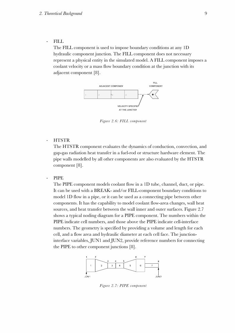
! FILL The FILL component is used to impose boundary conditions at any 1D hydraulic component junction. The FILL component does not necessary represent a physical entity in the simulated model. A FILL component imposes a coolant velocity or a mass flow boundary condition at the junction with its adjacent component [8].
Figure 2.6: FILL component
! HTSTR The HTSTR component evaluates the dynamics of conduction, convection, and gap-gas radiation heat transfer in a fuel-rod or structure hardware element. The pipe walls modelled by all other components are also evaluated by the HTSTR component [8].
! PIPE The PIPE component models coolant flow in a 1D tube, channel, duct, or pipe. It can be used with a BREAK- and/or FILL-component boundary conditions to model 1D flow in a pipe, or it can be used as a connecting pipe between other components. It has the capability to model coolant flow-area changes, wall heat sources, and heat transfer between the wall inner and outer surfaces. Figure 2.7 shows a typical noding diagram for a PIPE component. The numbers within the PIPE indicate cell numbers, and those above the PIPE indicate cell-interface numbers. The geometry is specified by providing a volume and length for each cell, and a flow area and hydraulic diameter at each cell face. The junction- interface variables, JUN1 and JUN2, provide reference numbers for connecting the PIPE to other component junctions [8].
Figure 2.7: PIPE component

Simulation of a NPP Steam Turbine with the best-estimate system code TRACE 10
! SEPD The SEPD component is usually employed to model the steam separators and moisture dryers [8].
! TURB The TURB component is a special TEE component case (the TEE component consists of two pipe components connected by a single junction), which includes additional models to simulate the operation of a steam turbine. The TURB component simulates energy removal from the flow due to the conversion of fluid energy to mechanical energy, the efficiency of the turbine, and the pressure losses. In addition, the TURB component includes the capability to simulate liquid drains or steam taps, and the dynamics of multi- stages and turbine rotor assembly[8]. The TURB component must be simulated with 2 cells in the primary arm of the TEE component (i.e., NCELL1 = 2) and with one cell in the side arm (i.e., NCELL2 = 1). The side arm connects to cell 2 of the primary arm (i.e., JCELL = 2) (see Figure 2.8). The flow through the turbine is not treated in detail based on first principals, but is simulated by adjusting the momentum and energy flow at cell edge 2 consistent with a lumped momentum and energy balance for the turbine component[8].
Figure 2.8: TURB component nodalization
! VALVE
The VALVE component is used to model various types of valves associated with light-water reactors. The valve action is modelled by a component action that adjusts the flow area and hydraulic diameter at a cell interface of a 1D hydraulic component as shown in Figure 2.9 [8].

2. Theoretical Background
11
Figure 2.9: VALVE component noding diagram
2.2.2 FRIC and K-FACTOR K-Factors are form-loss coefficients, and all the TRACE components included in the model require setting K-Factors as input.
To model pressure losses in 1D components TRACE system code includes the friction-factor correlation option flag (NFF). Several options are available.
! NFF = 1 applies a homogeneous-flow friction factor for wall and structure drag. ! NFF = –1 is the same but adds an internal form-loss computation for abrupt
changes in flow area between mesh cells. ! NFF = –100 applies the form-loss computation only.
It is recommended that NFF = 1 or –1 be applied at mesh- cell interfaces everywhere except at an interface where flow choking is anticipated. NFF = 0 is recommended for this case. The reason for setting NFF = 0 at the flow-choking interface is to avoid becoming friction limited as the onset of flow choking is approached. It is recommended that the user account for gradual flow-area change, flow turning, and orifice form losses by specifying FRIC or KFAC additive form-loss coefficients as well [8].
TRACE models all flow area changes as smooth area changes and evaluates only the Bernoulli- equation reversible pressure loss or gain associated with such an area change. Therefore, additive loss coefficients must be input for all irreversible form losses in the modelled system. For example, additive loss coefficients must be input to model the irreversible form loss at a cell- edge interface for a change in cell-average fluid flow area, a change in flow direction, or a flow orifice. It may be necessary to add additional loss coefficients to obtain the correct pressure drops across the component [8].
Inside the NAMELIST included in the model some variables can be defined. IKFAC is the option that defines whether additive loss coefficients (FRIC) or K-factors need to be input in the component data:
! IKAC=0: additive loss coefficients will be input. ! IKFAC=1: K-factors will be input.

Simulation of a NPP Steam Turbine with the best-estimate system code TRACE 12
When this option is selected (IKFAC=1), K-factors (dimensioned NCELLS+1) replace the FRIC array input cards in all components, and vice versa.
For TURB components a FRIC of 1021 at a cell edge results in essentially no liquid flow across that cell edge, while a FRIC of -1021 at a cell edge results in essentially no vapour flow across that cell edge. A FRIC of 1021 results in TRACE using a wall drag friction coefficient of 1021 for the liquid phase and a wall drag friction coefficient of 0.0 for the vapour phase and zero interfacial shear at that cell edge. A FRIC of -1021 results in TRACE using a Wall drag friction coefficient of 0.0 for the liquid phase and a wall drag coefficient of 1021 for the vapour phase [9].
To input K factors that depend on flow direction, TRACE system code includes the NFRC1 option. This option can be used to require input of forward and reverse loss coefficients for all 1D components. When NFRC1=2, the dimension of the FRIC array is doubled to 2 x (NCELLS + 1). The input data must be defined to provide two consecutive arrays of loss coefficients, each dimensioned NCELLS + 1. Each array is in LOAD format and must be terminated with an “E.” The first array provides loss coefficients that are used with positive velocities, and the second array provides loss coefficients that are used with negative velocities [9].
2.3 System description In the secondary side of a NPP the thermal energy extracted from the nuclear reactor is transformed into mechanical energy.
The secondary system to simulate is composed of a steam generator, one double-flux HP-turbine and three double-flux LP-turbines. A separator, an extraction, and an over-heater are placed between the HP-Turbines and the LP-Turbines. Three condensers are located after the LP-Turbines, and a set of over-heaters and pumps close the circuit.
The steam leaves the steam generator and enters the HP-Turbine. Inside the turbine the vapour quality decreases. After leaving the turbine, the fluid flows through the separator, which extracts most of the liquid, the extraction, which reduces the mass flow, and the over-heater, which provides the fluid the necessary temperature to become over-heated vapour. Then, the high-quality vapour is distributed to the LP-Turbines. Finally, the steam is condensed, heated, and pumped back to the steam generator.
Since this system corresponds to a real NPP, all the data are confidential. Consequently, the data included in this document, both nominal data and results, have been normalized. Normalization consists of dividing each type of parameter (pressure, mass flow…) by a set value: Pn for pressure, Tn for temperature, An for the flow area, and Mfn for mass flow.
! Pn is the pressure at the inlet of the system valve. ! Tn is the saturated temperature at Pn.
2. Theoretical Background
13
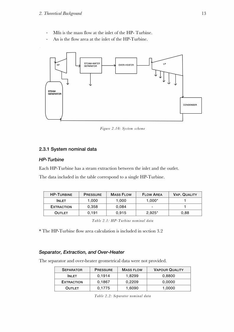
! Mfn is the mass flow at the inlet of the HP- Turbine. ! An is the flow area at the inlet of the HP-Turbine.
Figure 2.10: System scheme
2.3.1 System nominal data
HP-Turbine
Each HP-Turbine has a steam extraction between the inlet and the outlet.
The data included in the table correspond to a single HP-Turbine.
HP-TURBINE PRESSURE MASS FLOW FLOW AREA VAP. QUALITY INLET 1,000 1,000 1,000* 1
EXTRACTION 0,358 0,084 - 1 OUTLET 0,191 0,915 2,925* 0,88
Table 2.1: HP-Turbine nominal data
* The HP-Turbine flow area calculation is included in section 3.2
Separator, Extraction, and Over-Heater The separator and over-heater geometrical data were not provided.
SEPARATOR PRESSURE MASS FLOW VAPOUR QUALITY INLET 0,1914 1,8299 0,8800
EXTRACTION 0,1867 0,2209 0,0000 OUTLET 0,1775 1,6090 1,0000
Table 2.2: Separator nominal data

Simulation of a NPP Steam Turbine with the best-estimate system code TRACE 14
EXTRACTION PRESSURE MASS FLOW VAPOUR QUALITY INLET 0,0177 1,6090 1,0000
EXTRACTION 0,0177 0,1420 1,0000 OUTLET 0,0177 1,4670 1,0000
Table 2.3: Extract ion nominal data
OVER-HEATER PRESSURE VAPOUR QUALITY INLET 0,0177 1,0000
OUTLET 0,1806 1,0000
Table 2.4: Over-Heater nominal data
LP-Turbine Each single LP-Turbine has five steam extractions. In the data provided, two of the extractions are considered as one.
The data included in the table correspond to a single LP-Turbine.
LP-TURBINE PRESSURE MASS FLOW FLOW AREA VAP. QUALITY INLET 0,1806 0,2445 1,0289* 1
EXTRACTION 1 0,0606 0,0097 - 1 EXTRACTION 2 0,0276 0,0144 - 0,98 EXTRACTION 3 0,0100 0,0154 - 0,74 EXTRACTION 4 0,0023 0,0133 - 0,38
OUTLET 0,0009 0,1918 24,758* 0,89
Table 2.5: LP-Turbine nominal data
* The LP-Turbine flow area calculation is included in section 3.5
Condenser The geometrical data of the condenser were not provided.
CONDENSER PRESSURE VAPOUR QUALITY INLET 0,00093 0,8900
OUTLET 0,00093 0,0000
Table 2.6: Condenser nominal data

2. Theoretical Background
15


3. TRACE Model Components
17
3. TRACE Model Components
This chapter includes a detailed description of the components designing. All the data included have been normalized.
3.1 Valve
The model includes a stop valve, which is set to close when the pressure on its cell 1 reaches a 108% of the set value. To simulate the valve, a TRIP, a Signal Variable, and a VALVE component were necessary.
Figure 3.1: VALVE-TRIP component
VALVE component
TRACE system code includes different types of valves. The model uses VALVE component [3]: constant flow area until trip IVTR is set ON, then flow-area fraction vs. independent-variable-form table is evaluated [9].
The valve geometry is defined as a normal pipe. The flow area and the junction flow area are the same as the inlet flow area of the HP-Turbine, which is defined in section 3.2. The length and the volume were estimated in order to be compatible with the adjacent components.

Simulation of a NPP Steam Turbine with the best-estimate system code TRACE 18
The VALVE component characteristic inputs are:
Pressure 1 Temperature 1
Vapour quality 1
Table 3.1: VALVE init ial condit ions
! Valve Interface The valve interface is the cell interface number where the VALVE flow area is adjusted. In this model the valve interface is at edge 2.
! Flow Area Adjustment type: [0] Flow area fraction per second. ! Opening conditions
Maximum valve rate 0,5 [1/s] Off adjustment rate 0,5 [1/s] Minimum position 0 [-] Maximum position 1 [-]
Initial flow area fraction 1 [-] Valve stem position 1 [-]
Table 3.2: VALVE description
! Adjustment tables
First Adjustment Table Second Valve Table
No unit Area Fraction 0 1
Time [s] No unit 0 1 5 0
The first adjustment table corresponds to the initial conditions, and the second valve table is activated as the TRIP is set ON.
Signal Variable
A signal variable is a specialized control block, which takes its input from some parameter at any location in the computational mesh, and sends that value to its own output [8].
In this model the signal variable type is [21] Pressure, its behaviour mode is “Exact Value”, and the signal source is the first cell pressure of the VALVE component.

3. TRACE Model Components
19
TRIP component
A trip is an ON/OFF switch that can be used to decide when to evaluate a component hardware action.
The trip-signal definition and setpoint values are associated with the input specification of a trip. In this model the trip-signal type is a Signal Variable and the input source is the pressure signal defined above. Setpoint data are values that define the exact state of the trip (ONforward, ONreverse, or OFF), based upon where the actual trip-signal lies, as compared to the setpoint point(s) [8]. For the modelled TRIP, the setpoint values are P1=1,08Pn and P2=1,1Pn (see figure 3.2). The TRIP initial set status is [1] ON forward.
Figure 3.2: TRIP Setpoint Values
3.2 HP-Turbine The real system includes double-flux turbines. Since the TRACE system code does not model double-flux turbines, each turbine has been simulated as two different elements.
The simulation of a single HP-turbine needs two TURB components, one to simulate the pressure drop between the inlet and the extraction, and another one to simulate the pressure drop between the extraction and the outlet. Since the model needs two turbines to simulate a double-flux turbine, the total number of TURB components that includes the model is four.
Simulation of a NPP Steam Turbine with the best-estimate system code TRACE 20
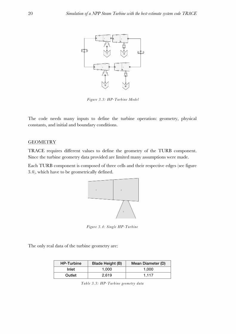
Figure 3.3: HP-Turbine Model
The code needs many inputs to define the turbine operation: geometry, physical constants, and initial and boundary conditions.
GEOMETRY
TRACE requires different values to define the geometry of the TURB component. Since the turbine geometry data provided are limited many assumptions were made.
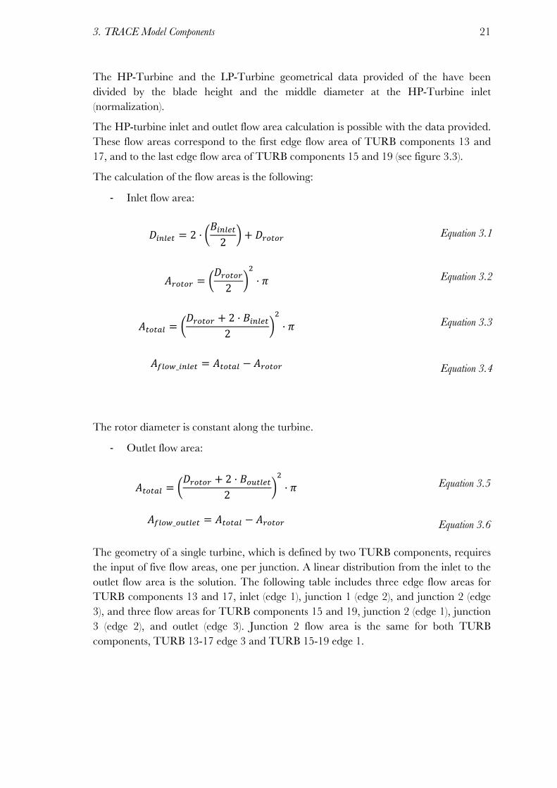
Each TURB component is composed of three cells and their respective edges (see figure 3.4), which have to be geometrically defined.
Figure 3.4: Single HP-Turbine
The only real data of the turbine geometry are:
HP-Turbine Blade Height (B) Mean Diameter (D) Inlet 1,000 1,000
Outlet 2,619 1,117
Table 3.3: HP-Turbine geometry data
3. TRACE Model Components
21
The HP-Turbine and the LP-Turbine geometrical data provided of the have been divided by the blade height and the middle diameter at the HP-Turbine inlet (normalization).
The HP-turbine inlet and outlet flow area calculation is possible with the data provided. These flow areas correspond to the first edge flow area of TURB components 13 and 17, and to the last edge flow area of TURB components 15 and 19 (see figure 3.3).
The calculation of the flow areas is the following:
! Inlet flow area:
!!"#$% = 2 · !!"#$%2 + !!"#"! Equation 3.1
!!"#"! =!!"#"!2
!· ! Equation 3.2
!!"!#$ =!!"#"! + 2 · !!"#$%
2!· ! Equation 3.3
!!"#$_!"#$% = !!"!#$ − !!"#"! Equation 3.4
The rotor diameter is constant along the turbine.
! Outlet flow area:
!!"!#$ =!!"#"! + 2 · !!"#$%#
2!· ! Equation 3.5
!!"#$_!"#$%# = !!"!#$ − !!"#"! Equation 3.6
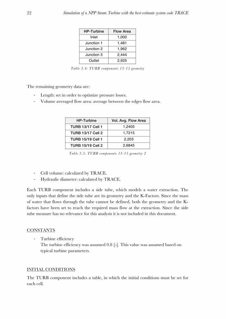
The geometry of a single turbine, which is defined by two TURB components, requires the input of five flow areas, one per junction. A linear distribution from the inlet to the outlet flow area is the solution. The following table includes three edge flow areas for TURB components 13 and 17, inlet (edge 1), junction 1 (edge 2), and junction 2 (edge 3), and three flow areas for TURB components 15 and 19, junction 2 (edge 1), junction 3 (edge 2), and outlet (edge 3). Junction 2 flow area is the same for both TURB components, TURB 13-17 edge 3 and TURB 15-19 edge 1.
Simulation of a NPP Steam Turbine with the best-estimate system code TRACE 22
HP-Turbine Flow Area Inlet 1,000
Junction 1 1,481 Junction 2 1,962 Junction 3 2,444
Outlet 2,925
Table 3.4: TURB components 13-15 geometry
The remaining geometry data are:
! Length: set in order to optimize pressure losses. ! Volume averaged flow area: average between the edges flow area.
HP-Turbine Vol. Avg. Flow Area TURB 13/17 Cell 1 1,2405 TURB 13/17 Cell 2 1,7215 TURB 15/19 Cell 1 2,203 TURB 15/19 Cell 2 2,6845
Table 3.5: TURB components 13-15 geometry 2
! Cell volume: calculated by TRACE. ! Hydraulic diameter: calculated by TRACE.
Each TURB component includes a side tube, which models a water extraction. The only inputs that define the side tube are its geometry and the K-Factors. Since the mass of water that flows through the tube cannot be defined, both the geometry and the K-factors have been set to reach the required mass flow at the extraction. Since the side tube measure has no relevance for this analysis it is not included in this document.
CONSTANTS
! Turbine efficiency The turbine efficiency was assumed 0.8 [-]. This value was assumed based on typical turbine parameters.
INITIAL CONDITIONS
The TURB component includes a table, in which the initial conditions must be set for each cell.

3. TRACE Model Components
23
TURB component 13-17
Cell Number Pressure Liquid Temperature
Vapour Temperature
Gas Volume Fraction
1 1 1 1 0,9953 2 0,358 0,8905 0,8905 0,907 3 0,358 0,8905 0,8905 0,907
Table 3.6: TURB component 13-17 init ial condit ions
TURB component 15-19
Cell Number Pressure Liquid
Temperature Vapour
Temperature Gas Volume
Fraction 1 0,358 0,8905 0,8905 0,907 2 0,191 0,8353 0,8353 0,8424 3 0,191 0,8353 0,8353 0,8424
Table 3.7: TURB component 15-19 init ial condit ions
BOUNDARY CONDITIONS
The BREAK components located at the outlet of the side tubes set the boundary conditions. To define a BREAK component the inputs are:
! Volume The BREAK component volume is the same as the volume of its adjacent cell.
! Length The BREAK length is defined to provide the same flow area as the one of the adjacent cell edge.
!"#$%!"#$%! =!"#$%!"#$%&
!"#.!"##!"#$!!"#! Equation 3.7
The BREAK component adjacent cell corresponds to the TURB component side tube.
! Initial Gas Volume Fraction The initial gas volume fraction is 0 for the four BREAK components.
! Pressure and temperature
BREAK 14-18 BREAK 16-20 Pressure 0,359 0,191
Temperature 0,8905 0,8353
Table 3.8: BREAK 14-16-18-20 init ial condit ions

Simulation of a NPP Steam Turbine with the best-estimate system code TRACE 24
3.3 Separator The system separator has been simulated with a SEPD component. A SEPD component is composed of a main tube and a side tube. The separator has been designed with two cells on the main tube and one on the side tube, and its orientation is vertical. Inside the second cell, the fluid is separated in steam and liquid. The steam flows out of the separator, and the liquid water flows downwards through the side-tube.
The flow area of the separator main tube is the same as the HP-Turbine inlet flow area, and the side-tube flow area was estimated in order to extract the desired liquid mass flow. The initial conditions are the same as the HP-Turbine’s outlet conditions. The BREAK component, which is located after the side tube, is set to 0.187 [P/Pn] and 0.833 [T/Tn].
The separator type used in the model is: [0] Ideal Separator.
Figure 3.5: Separator
3.4 Over-Heater To simulate an over-heater the model uses a PIPE in combination with a HTSTR.
PIPE
The pipe is composed of two cells, which have the same flow area as the HP-turbine inlet. The initial conditions are the same as at the LP-Turbine inlet. The PIPE component includes the option of editing a HTSTR within it.
HTSTR
The HTSTR component, which is edited inside the PIPE component, is cylindrical, and its axial plane is in X direction.
To define a HTSTR the code includes a table, in which the heat structure boundary condition data and axial nodalization are set.

3. TRACE Model Components
25
Inner Surface Boundary Conditions
Axial Cell
Outer Surface Boundary Conditions
[2] Pipe: 25 Cell: 1 1 [1] HTC:- SFT:- [2] Pipe: 25 Cell: 2 2 [5] Surf Temperature
Table 3.9: HTSTR boundary condit ions
Boundary conditions:
! [1] Constant HTC SFT: constant heat transfer coefficient, and constant sink temperature.
! [2] Hydro component: heat structure is coupled to the hydro component. ! [5] Constant Surface Temp: constant fixed surface temperature.
The inner surface boundary conditions are type [2]; therefore, the heat structure inner surface is coupled to PIPE 25, which is the PIPE that models the over-heater.
The outer surface boundary condition of HTSTR axial cell 1 is type [1] in order to heat the steam and evaporate the liquid. At axial cell 2 the outer boundary condition is type [5] since the system requires a specific temperature at the LP-Turbine inlet.
3.5 LP-Turbine The real system includes three double-flux LP-turbines. Each turbine has been simulated as two different elements; therefore, the LP-Turbine model includes six turbines. Each single LP-Turbine has five extractions, but just four of them are simulated since there are no data from one extraction. For the simulation of an extraction the code requires a TURB component. Figure 3.6 shows the complete model of the LP-Turbine.
Figure 3.6: LP-Turbine model
Simulation of a NPP Steam Turbine with the best-estimate system code TRACE 26
The code needs many inputs to define the turbine operation: geometry, physical constants, and initial and boundary conditions.
GEOMETRY
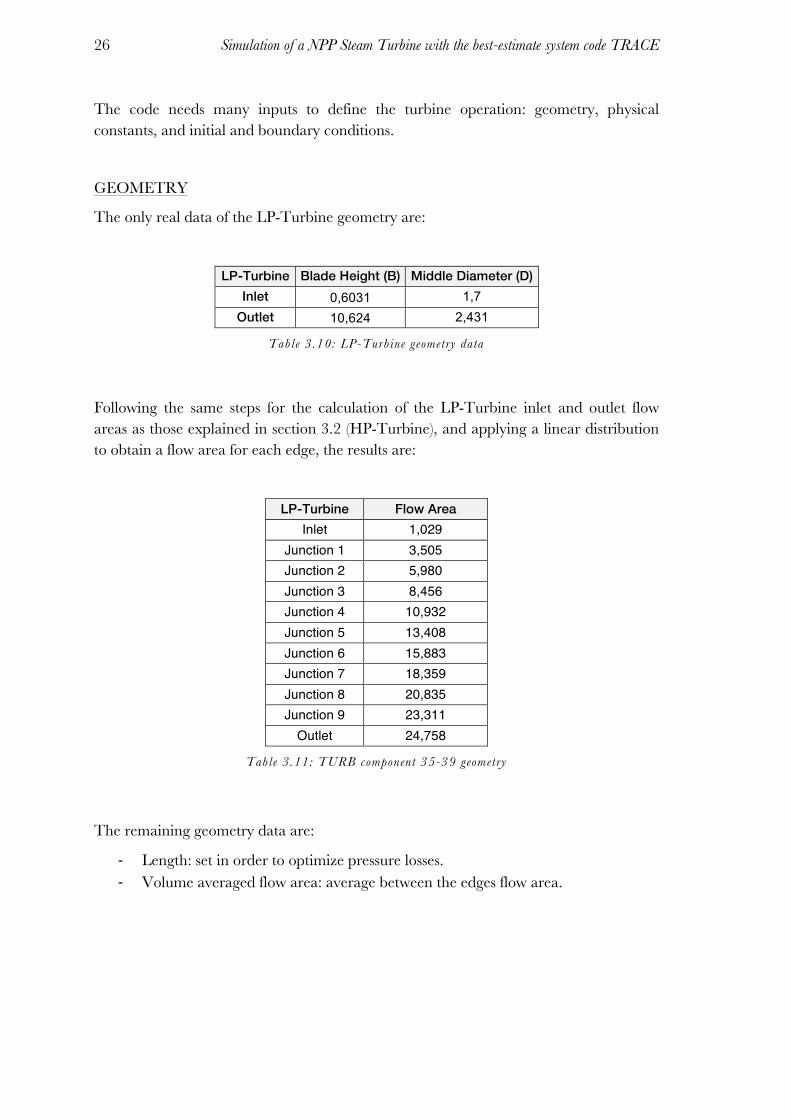
The only real data of the LP-Turbine geometry are:
LP-Turbine Blade Height (B) Middle Diameter (D) Inlet 0,6031 1,7
Outlet 10,624 2,431
Table 3.10: LP-Turbine geometry data
Following the same steps for the calculation of the LP-Turbine inlet and outlet flow areas as those explained in section 3.2 (HP-Turbine), and applying a linear distribution to obtain a flow area for each edge, the results are:
LP-Turbine Flow Area Inlet 1,029
Junction 1 3,505 Junction 2 5,980 Junction 3 8,456 Junction 4 10,932 Junction 5 13,408 Junction 6 15,883 Junction 7 18,359 Junction 8 20,835 Junction 9 23,311
Outlet 24,758
Table 3.11: TURB component 35-39 geometry
The remaining geometry data are:
! Length: set in order to optimize pressure losses. ! Volume averaged flow area: average between the edges flow area.

3. TRACE Model Components
27
LP-Turbine Avg. Vol. Flow Area TURB 35 Cell 1 2,2667 TURB 35 Cell 2 4,7422 TURB 36 Cell 1 7,2180 TURB 36 Cell 2 9,6940 TURB 37 Cell 1 12,1698 TURB 37 Cell 2 14,6455 TURB 38 Cell 1 17,1213 TURB 38 Cell 2 19,5970 TURB 39 Cell 1 22,0728 TURB 39 Cell 2 24,0341
Table 3.12: TURB component 35-39 geometry 2
! Cell volume: calculated by TRACE. ! Hydraulic diameter: calculated by TRACE.
Each TURB component includes a side tube, which models a water extraction. The only inputs that define the side tube are geometry and K-Factors. Since the mass of water that flows through the tube cannot be defined, both geometry and K-factors have been set to reach the required mass flow at the extraction. Since the side tube measure has no relevance for this analysis it is not included in this document.
TURB component 35
Cell Number Pressure Liquid Temperature
Vapour Temperature
Gas Volume Fraction
1 0,1806 0,83 0,83 1
2 0,0607 0,751 0,751 1
3 0,0607 0,751 0,751 1
Table 3.13: TURB component 35 init ial condit ions
TURB component 36
Cell Number Pressure Liquid Temperature
Vapour Temperature
Gas Volume Fraction
1 0,0607 0,751 0,751 1
2 0,276 0,704 0,704 0,98
3 0,276 0,704 0,704 0,98
Table 3.14: TURB component 36 init ial condit ions

Simulation of a NPP Steam Turbine with the best-estimate system code TRACE 28
TURB component 37
Cell Number Pressure Liquid Temperature
Vapour Temperature
Gas Volume Fraction
1 0,276 0,704 0,704 0,98
2 0,276* 0,704* 0,704* 0,74
3 0,01 0,652 0,652 0,74
Table 3.15: TURB component 37 init ial condit ions
TURB component 38
Cell Number Pressure Liquid Temperature
Vapour Temperature
Gas Volume Fraction
1 0,03* 0,709* 0,709* 0,74
2 0,03* 0,709* 0,709* 0,38
3 2,32E-03 0,709 0,709 0,38
Table 3.16: TURB component 38 init ial condit ions
TURB component 39
Cell Number Pressure Liquid
Temperature Vapour
Temperature Gas Volume
Fraction 1 0,03* 0,709* 0,709* 0,38
2 0,03* 0,709* 0,709* 0,89
3 9,26E-04 0,559 0,559 0,89
Table 3.17: TURB component 39 init ial condit ions
For initialization purposes all the data marked with a “*” are higher than the real initial conditions.
BOUNDARY CONDITIONS
Pressure and temperature:
BREAK 30 BREAK 31 BREAK 32 BREAK 33 BREAK 34 Pressure 0,0607 0,276 0,01 2,32E-03 9,26E-04
Temperature 0,751 0,704 0,652 0,591 0,559
Table 3.18: BREAK components 30-34 init ial condit ions
The remaining BREAK component design features are explained on section 3.2.

3. TRACE Model Components
29
3.6 Condenser The real system includes three condensers, one per double-flux LP-Turbine. Each condenser was defined as a long PIPE component in combination with a HTSTR.
Figure 3.7: Condenser
PIPE
The PIPE component dimensions were designed in order to condense the whole mass flow. The PIPE was defined with two cells, the first one much shorter than the second one (see figure 3.7). The PIPE initial conditions are the same as at the LP-Turbine outlet (see table 3.17, cell 3).
HTSTR
The HTSTR is defined within the PIPE component. The HTSTR geometry is cylindrical, and its axial plane is in X direction.
To define a HTSTR the code includes a table, in which the heat structure boundary conditions and axial nodalization are set.
Inner Surface Boundary Conditions
Axial Cell Outer Surface Boundary Conditions
[2] Pipe: 310 Cell: 1 1 [5] Surf Temperature [2] Pipe: 310 Cell: 2 2 [0] Flux
Table 3.19: HTSTR boundary condit ions
Boundary conditions:
! [0] Constant Heat Flux ! [2] Hydro component: heat structure is coupled to the hydro component. ! [5] Constant Surface Temp: constant fixed surface temperature.
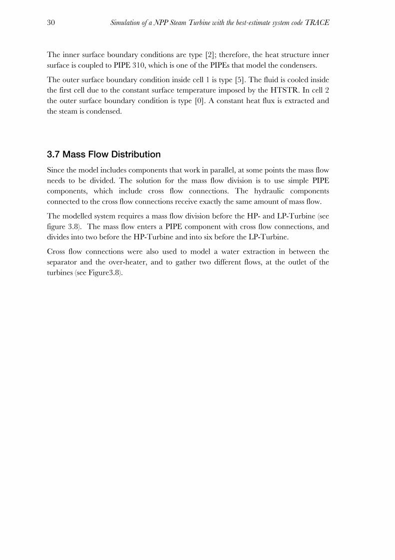
Simulation of a NPP Steam Turbine with the best-estimate system code TRACE 30
The inner surface boundary conditions are type [2]; therefore, the heat structure inner surface is coupled to PIPE 310, which is one of the PIPEs that model the condensers.
The outer surface boundary condition inside cell 1 is type [5]. The fluid is cooled inside the first cell due to the constant surface temperature imposed by the HTSTR. In cell 2 the outer surface boundary condition is type [0]. A constant heat flux is extracted and the steam is condensed.
3.7 Mass Flow Distribution Since the model includes components that work in parallel, at some points the mass flow needs to be divided. The solution for the mass flow division is to use simple PIPE components, which include cross flow connections. The hydraulic components connected to the cross flow connections receive exactly the same amount of mass flow.
The modelled system requires a mass flow division before the HP- and LP-Turbine (see figure 3.8). The mass flow enters a PIPE component with cross flow connections, and divides into two before the HP-Turbine and into six before the LP-Turbine.
Cross flow connections were also used to model a water extraction in between the separator and the over-heater, and to gather two different flows, at the outlet of the turbines (see Figure3.8).
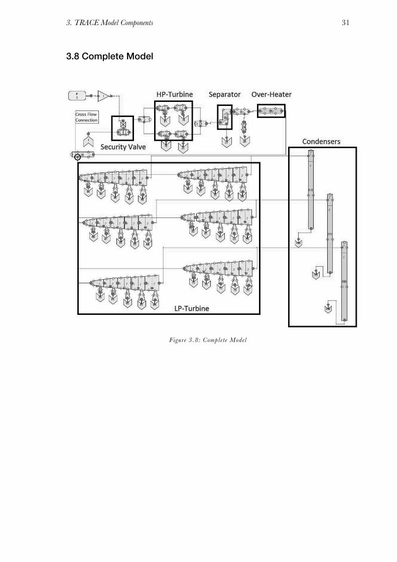
3. TRACE Model Components
31
3.8 Complete Model
Figure 3.8: Complete Model

Simulation of a NPP Steam Turbine with the best-estimate system code TRACE 32

4. Steady-State: Simulation & Results
33
4.Steady-State: Simulation & Results
To run a steady-state simulation the option [0] Steady-State must be set. The model used for the steady-state simulation is the one defined in chapter 3.
This chapter includes the FILL component set up, the steady-state simulation results, and an argumentation for the K-factors used in the model.
4.1 FILL The FILL component included in the model simulates the conditions before the fluid enters the valve and the HP-Turbine. These conditions are not the same as at the steam generator outlet since there are form losses and a steam extraction located between the HP-turbine and the steam generator.
TRACE includes different configurations of the FILL component. For the steady-state simulation this model uses FILL [2] (constant mass flow).
The main input data used to set the FILL component are:
FILL type [2] Pressure 1
Temperature 1 Mass Flow 2
Vapour quality 1
Table 4.1: Steady-State FILL description
4.2 Results After running the TRACE model the relevant data provided by the program were analysed. This section includes a comparison between the extracted data from the real NPP and the data provided by the simulation. All the data included in this section have been normalized.
Since the model includes many components, which affect the boundary conditions at the inlet and outlet of the turbines, both the HP- and LP-Turbines have been developed in two separate models. In this way it is possible to set proper boundary conditions, and obtain simulation results, which are very close to the expected ones. The simplified model results will be compared with the data obtained from the complete model

Simulation of a NPP Steam Turbine with the best-estimate system code TRACE 34
simulation, in order to explain how the components included in the complete system affect the HP- and LP-turbines operation.
4.2.1 Simplified HP-Turbine model The HP-Turbine simplified model (see figure 4.1) includes two TURB components, three BREAK components, and one FILL component.
Figure 4.1: Modelled HP-Turbine
Both TURB components have the same initial conditions and geometry as the components included in the complete model (see section 3.2).
The FILL and the BREAK components set the boundary conditions at the HP-Turbine inlet, extraction, and outlet.
Pressure Saturation Temperature
Mass Flow
Vapour Quality
FILL 60 1 1 1 1 BREAK 14 0,358 0,891 - 0 BREAK 15 0,191 0,827 - 0 BREAK 60 0,191 0,827 - 0
Table 4.2: HP-Turbine simplif ied model boundary condit ions
The TRACE system code does not include the option of defining a fixed inlet mass flow in the BREAK component.
The simulation of the HP-Turbine simplified model reaches steady state after 10.022 simulated seconds, and the CPU time is 0.359 [s].
The HP-Turbine real data provided are pressure measurements at some specific points of the turbine: inlet, outlet, and fluid extraction.

4. Steady-State: Simulation & Results
35
Inlet Pressure Extraction
Pressure Outlet Pressure
REAL 0,9620 0,3867 0,1846 SIMULATED 0,9725 0,3721 0,1935 ERROR [%] 1,092 -3,775 4,844
Table 4.3: HP-Turbine simplif ied model results
Table 4.3 shows the error calculated from the comparison between the simulation results and the real pressure data. At the inlet of the HP-Turbine, the calculated error is very small. At the extraction and at the outlet the error is bigger.
Figure 4.2 and 4.3 correspond to graphs, which show a comparison between the real data (blue) and the simulation results (red).
Figure 4.2 shows the pressure inside the HP-Turbine stages per unit time. Each line represents the pressure inside the TURB component cells:
! Sim. Inlet Pressure: TURB component 13, cell 1. ! Sim. Extraction Pressure: TURB component 13, cell 2. ! Sim. Outlet Pressure: TURB component 15, cell 2.
The graphical comparison between the real and the simulated data reveals that the simulated pressure inside the turbine is realistic.
Figure 4.3 shows the HP-Turbine pressure drop per stage, which follows the same pattern as the real pressure drop.
Figure 4.2: Graph-Simulated vs. Real HP-Turbine Pressure Drop
0
0,2
0,4
0,6
0,8
1
1,2
1 2 3 4 5 6 7 8 9
P/Pn
Time [s]
Real vs. Simulated HP-Turbine Pressure Drop!
Sim. Inlet Pressure
Real Inlet Pressure
Sim. Extr. Pressure
Real Extr. Pressure
Sim. Oulet Pressure
Real Outlet Pressure

Simulation of a NPP Steam Turbine with the best-estimate system code TRACE 36
Figure 4.3: Graph-Simulated vs. Real HP-Turbine Pressure Drop per s tage
4.2.2 Simplified LP-Turbine model The LP-Turbine simplified model (see figure 4.4) includes five TURB components, six BREAK components, and one FILL component.
Figure 4.4: LP-Turbine simplif ied model
All the TURB components have the same initial conditions and geometry as the components included in the complete model (see section 3.6).
The FILL and the BREAK components set the boundary conditions at the HP-Turbine inlet, extractions, and outlet (see table 4.4).
Pressure Saturation Temperature Mass Flow Vapour
Quality FILL 10 0,181 0,831 0,238 1
BREAK 30 0,061 0,751 - 0 BREAK 31 0,0276 0,704 - 0 BREAK 32 0,01 0,652 - 0 BREAK 33 2,31E-03 0,591 - 0 BREAK 34 9,26E-04 0,559 - 0
BREAK 140 9,26E-04 0,559 - 0
Table 4.4: LP-Turbine simplif ied model boundary condit ions
0
0,2
0,4
0,6
0,8
1
1,2
1 2 3
P/Pn
HP-Turbine Pressure drop per stage!
Real Pressure
Sim. Pressure

4. Steady-State: Simulation & Results
37
The simulation of the HP-Turbine simplified model reaches steady state after 61.84 simulated seconds, and the CPU time is 0.514 [s].
Inlet Pressure Extraction 1 Pressure
Extraction 2 Pressure
Outlet Pressure
REAL 0,17835 0,06271 0,02721 0,00129 SIMULATED 0,16559 0,06122 0,02770 0,00123 ERROR [%] -7,15415 -2,36664 1,77813 -4,52251
Table 4.5: LP-Turbine simplif ied model results
Table 4.5 shows the error calculated from the comparison between the simulation results and the real pressure data. At the inlet of the LP-Turbine, the calculated error is significant, but at the extractions and at the outlet the error is smaller.
Figure 4.5 and 4.6 correspond to graphs, which show a comparison between the real data (blue) and the simulation results (red).
Figure 4.5 shows the pressure inside the LP-Turbine stages per unit time. Each line represents the pressure drop inside a TURB component cell:
! Sim. Inlet Pressure: TURB component 35, cell 1. ! Sim. Extraction 1 Pressure: TURB component 35, cell 2. ! Sim. Extraction 2 Pressure: TURB component 36, cell 2. ! Sim. Outlet Pressure: TURB component 39, cell 2.
The remaining extractions are not taken into consideration since no real data of them were provided.
Except for the simulated inlet pressure, which is slightly lower than the real one (see table 4.5), the simulated pressure at the extractions and the outlet is very similar to the real one.

Simulation of a NPP Steam Turbine with the best-estimate system code TRACE 38
Figure 4.5: Graph-Simulated vs. Real LP-Turbine Pressure Drop
Figure 4.6 shows the LP-Turbine pressure drop per stage. This graph includes the simulated pressure at all the stages, and the real pressure at four stages since no real data were provided of extractions 3 and 4. As the graph shows, the simulated pressure drop follows the same pattern as the real one.
Figure 4.6: Graph-Simulated vs. Real LP-Turbine Pressure Drop per s tage
0
0,02
0,04
0,06
0,08
0,1
0,12
0,14
0,16
0,18
0,2
1 6 11 16 21 26 31 36 41 46
P/Pn
Time [s]
Real vs. Simulated LP-Turbine Pressure Drop !
Sim. Inlet Pressure
Real Inlet Pressure
Sim. Ext1 Pressure
Real Ext1 Pressure
Sim. Ext2 Pressure
Real Ext2 Pressure
Sim. Outlet Pressure
Real Outlet Pressure
0
0,05
0,1
0,15
0,2
1 2 3 4 5 6
P/Pn
LP-Turbine Pressure drop per stage!
Real Pressure
Sim. Pressure

4. Steady-State: Simulation & Results
39
4.2.3 Complete Model This section includes a more detailed analysis of all the components included in the complete model (see figure 3.8). The main data of each component were extracted from the simulation results
HP-TURBINE
In the complete model, the HP-Turbine corresponds to two turbines (see Figure 3.3). Since the TURB components are placed in parallel (13-17 and 15-19 respectively) just one single turbine results (TURB components 13 and 15) are taken into consideration for the data analysis.
Figure 4.7 shows the real (blue) and simulated (red) pressure inside the HP-Turbine stages per unit time. Each line represents the pressure inside the TURB component cells:
! Sim. Inlet Pressure: TURB component 13, cell 1. ! Sim. Extraction Pressure: TURB component 13, cell 2. ! Sim. Outlet Pressure: TURB component 15, cell 2.
The difference between the simulated and the real outlet pressure is big (see figure 4.8) due to the effect that the separator and the over-heater cause on the system.
Figure 4.7: Graph-Simulated vs. Real HP-Turbine Pressure
0
0,2
0,4
0,6
0,8
1
1,2
1 26 51 76 101 126 151 176
P/Pn
Time [s]
Real vs. Simulated HP-Turbine Pressure !
Sim. Inlet Pressure
Real Inlet Pressure
Sim. Extr. Pressure
Real Extr. Pressure
Sim. Outlet Pressure
Real Outlet Pressure

Simulation of a NPP Steam Turbine with the best-estimate system code TRACE 40
Figure 4.8: Graph-Simulated vs. Real HP-Turbine Outle t Pressure
Figure 4.9 shows the HP-Turbine pressure drop per stage. This graph illustrates that there is hardly any pressure drop between the second and the third stage of the simulated model, while between the real stages the pressure drop is significant.
Figure 4.9: Graph-Simulated vs. real HP-Turbine pressure drop
Figure 4.10 shows the progress of the mass flow through the HP-Turbine per unit time. The water extracted in the simulation is lower than the nominal one: 0,0447 [Mf/Mfn] vs. 0,0866 [Mf/Mfn]. The water is only extracted in TURB component 13 because the TURB component 15 side-tube was blocked by the input of a special FRIC array (see section 2.2.2 FRIC and K-Factors). In TURB components 15 and 19 a FRIC value of 1021 and -1021 was set at edges 4 and 5 respectively.
00,10,20,30,40,50,60,70,80,9
1
1 26 51 76 101 126 151 176
P/Pn
Time [s]
HP-Turbine Outlet Pressure!
Real Pressure
Simulated Pressure
0
0,2
0,4
0,6
0,8
1
1,2
1 2 3
P/Pn
Real vs. Simulated HP-Turbine Pressure drop per stage!
Real
Simulated

4. Steady-State: Simulation & Results
41
Figure 4.10: Graph-Simulated HP-Turbine Mass Flow
SEPARATOR, OVER-HEATER
The purpose of the separator is to extract the liquid water from the mass flow. Figure 4.11 shows the difference between the inlet mass flow (dark colours) and the outlet mass flow (light colours).
! Inlet total mass flow: total mass flow at SEPD edge 2. ! Inlet vapour mass flow: vapour mass flow at SEPD edge 2. ! Inlet liquid mass flow: liquid mass flow at SEPD edge 2. ! Outlet total mass flow: total mass flow at SEPD edge 3. ! Outlet vapour mass flow: vapour mass flow at SEPD edge 3. ! Outlet liquid mass flow: liquid mass flow at SEPD edge 3.
The extracted liquid water is the difference between the two green lines, which also corresponds to the difference between the blue lines. As the graph shows the liquid mass flow at the separator outlet is near to zero.
0"
0,2"
0,4"
0,6"
0,8"
1"
1,2"
1" 51" 101" 151" 201" 251"
Mf/Mfn!
Time [s]
HP-Turbine Mass Flow!
Inlet"Mass"Flow"
Extrac9on"Mass"Flow"
Outlet"Mass"Flow"

Simulation of a NPP Steam Turbine with the best-estimate system code TRACE 42
Figure 4.11: Graph-Simulated Separator Mass Flow
Figure 4.12 shows the pressure drop inside the separator per unit time, which is bigger than the expected one.
! Inlet pressure: pressure at SEPD cell 2. ! Outlet pressure: pressure at SEPD cell3.
A considerable pressure drop takes place inside the separator since the TRACE system code requires the definition of a KFAC in between cells 2 and 3 to run.
Figure 4.12: Graph-Simulated Separator Pressure Drop
0
0,5
1
1,5
2
2,5
1" 51" 101" 151" 201" 251"
Mf/M
fn
Time![s]!
Separator Mass Flow !
Inlet Mass Flow
Inlet Vapour Flow
Inlet Liquid Flow
Outlet Mass Flow
Outlet Vapour Flow
Outlet Liquid Flow
0,2
0,25
0,3
0,35
1 51 101 151 201 251
P/Pn
Time [s]
Separator Pressure Drop!
Inlet Pressure
Outlet Pressure

4. Steady-State: Simulation & Results
43
The purpose of the over-heater is to make the fluid reach a certain temperature and vapour quality before it enters the LP-Turbine. Figure 4.13 shows the gas temperature inside PIPE 25 (over-heater), cell 2. Table 4.6 shows the difference between the nominal data and the simulation results, which is very small.
Figure 4.13: Graph-Simulated Over-Heater Gas Temperature at ce l l 2
Nominal Simulated Temperature 0,9673 0,973625933
Vapour Quality 1 1
Table 4.6: Over-Heater outle t condit ions
LP-TURBINE
In the complete model, the LP-Turbine corresponds to six turbines (see Figure 3.6). Since the TURB components of each turbine are placed in parallel, just the results of one turbine (TURB components 35-39) are taken into consideration.
Figure 4.14 shows the real (blue) and simulated (red) pressure inside the LP-Turbine stages per unit time. Each line represents the pressure drop inside a TURB component cell:
! Sim. Inlet Pressure: TURB component 35, cell 1. ! Sim. Extraction 1 Pressure: TURB component 35, cell 2. ! Sim. Extraction 2 Pressure: TURB component 36, cell 2. ! Sim. Outlet Pressure: TURB component 39, cell 2.
The comparison between the real and the simulated pressures reveals that due to the error accumulated in the first part of the complete system (HP-Turbine, separator, and over-heater) the pressure inside the simulated LP-Turbine is higher than the real one. In
0,75
0,8
0,85
0,9
0,95
1
1 21 41 61 81
T/Tn
Time [s]
Over-Heater Gas Temperature!

Simulation of a NPP Steam Turbine with the best-estimate system code TRACE 44
spite of reaching a higher pressure, figure 4.15 shows that the pressure drop in the simulated turbine follows the same pattern as the real one.
Figure 4.14: Graph-Simulated vs. Real LP-Turbine Pressure
Figure 4.15: Graph-Simulated vs. Real LP-Turbine Pressure Drop per Stage
Figure 4.16 shows the progress of the mass flow through the LP-Turbine per unit time:
! Inlet Mass Flow: total mass flow at TURB 35, edge 1. ! Sum of Extractions: sum of the TURB 35, 36, 37 and 38 extractions.
0
0,05
0,1
0,15
0,2
1 26 51 76 101 126 151 176
P/Pn
Time [s]
LP-Turbine Pressure Drop!
Real Inlet Pressure
Sim. Inlet Pressure
Real Extr.1 Pressure
Sim. Extr.1 Pressure
Real Extr.2 Pressure
Sim. Extr.2 Pressure
Real Outlet Pressure
Sim. Outlet Pressure
0
0,05
0,1
0,15
0,2
0,25
1 2 3 4 5 6
P/Pn
LP-Turbine Pressure Drop per Stage !
Real Pressure
Sim. Pressure

4. Steady-State: Simulation & Results
45
! Outlet Mass Flow: total mass flow at TURB 39, edge 3.
The water is extracted in TURB components 35, 36, 37 and 38 because the TURB component 39 side-tube was blocked by the input of an especial FRIC array (see section 2.2.2 FRIC and K-Factors). In TURB component 39 a FRIC value of 1021 and -1021 was set at edges 4 and 5 respectively.
Figure 4.16: Graph-Simulated LP-Turbine Mass Flow
CONDENSER
TRACE system code does not include a specific component to simulate condensers; therefore, a simple PIPE component in combination with a HTSTR was used to simulate a condenser. The aim of this element is to condense the whole vapour mass flow. Figure 4.17 shows how the vapour mass flow is reduced to zero.
Figure 4.17: Graph-Simulated Condenser Mass Flow
0
0,1
0,2
0,3
1 26 51 76 101 126
Mf/M
fn
Time [s]
LP-Turbine Mass Flow !
Inlet Mass Flow
Outlet Mass Flow
Sum of Extractions
0!
0,1!
0,2!
0,3!
0,4!
1! 3! 5! 7! 9! 11! 13! 15! 17! 19! 21! 23! 25! 27! 29! 31!
Mf/M
fn!
Time [s]!
Condenser Mass Flow !
Total Mass Flow!
Liquid Mass Flow!
Vapor Mass Flow!

Simulation of a NPP Steam Turbine with the best-estimate system code TRACE 46
VALVE
In order to simulate the operation of the stop valve a specific model was necessary, in which the pressure at valve cell 2 increases up to 107,5%, TRIP set value (see section 3.1). At this value (red marker in figure 4.19) the TRIP component changes its status from [1]ONfoward to [0]OFF since the pressure value at valve cell 2 is in between Setpoints 2 and 4. As the pressure is still increasing, the TRIP component changes its status from [0]OFF to [-1]ONreverse. When the TRIP starts changing its status, the valve starts closing (see figure 4.19). After the valve starts closing, the pressure at valve cell 2 decreases and the TRIP component changes its status from [-1]ONreverse to [0]OFF. As the valve flow area is decreasing, the pressure at valve cell 1 increases rapidly, which makes the simulation crash.
Figure 4.18: TRIP Setpoint Values
Figure 4.19: Stop Valve Operation (normalized values)
-1
-0,5
0
0,5
1
1,5
2
2,5
3
1 2 3 4 5 6
Time [s]
Stop Valve Operation!
Valve Cell 1 Pressure
Valve Cell 2 Pressure
TRIP
Valve Area
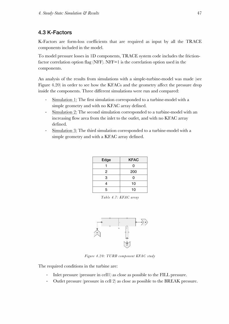
4. Steady-State: Simulation & Results
47
4.3 K-Factors K-Factors are form-loss coefficients that are required as input by all the TRACE components included in the model.
To model pressure losses in 1D components, TRACE system code includes the friction-factor correlation option flag (NFF). NFF=1 is the correlation option used in the components.
An analysis of the results from simulations with a simple-turbine-model was made (see Figure 4.20) in order to see how the KFACs and the geometry affect the pressure drop inside the components. Three different simulations were run and compared:
! Simulation 1: The first simulation corresponded to a turbine-model with a simple geometry and with no KFAC array defined.
! Simulation 2: The second simulation corresponded to a turbine-model with an increasing flow area from the inlet to the outlet, and with no KFAC array defined.
! Simulation 3: The third simulation corresponded to a turbine-model with a simple geometry and with a KFAC array defined.
Edge KFAC 1 0 2 200 3 0 4 10 5 10
Table 4.7: KFAC array
Figure 4.20: TURB component KFAC study
The required conditions in the turbine are:
! Inlet pressure (pressure in cell1) as close as possible to the FILL pressure. ! Outlet pressure (pressure in cell 2) as close as possible to the BREAK pressure.

Simulation of a NPP Steam Turbine with the best-estimate system code TRACE 48
Results:
FILL Pressure Inlet Pressure Outlet Pressure BREAK pressure Simulation 1 1 0,3889 0,3777 0,3776 Simulation 2 1 0,3922 0,38 0,3776 Simulation 3 1 0,895 0,3852 0,3776
Table 4.8: KFAC analysis results
Table 4.8 shows the results of the three simulations, from which is concluded that the KFAC array strongly affects the pressure drop inside the TURB component.
Taking into consideration the conclusion obtained from the analysis, an analytic method was sought to calculate the TURB component KFAC array for the simplified models. Due to the lack of geometrical data many assumptions for the calculation of the KFACs were made. Since the simulation results of the simplified models (see figures 4.1 and 4.4) after inserting the KFACs were not the expected ones, the KFAC array calculated was rejected. Finally, all the KFACs were manually tuned until the pressure drop inside the turbines was as close as possible to the real data.
As the explanation above clarifies (section “4.2 Results”), both the HP- and LP-Turbines were developed separately and then inserted in the same model. The results obtained from the simulation of the complete model were not the expected ones. In order to reach the desired pressure drop inside the HP- and LP-Turbines, the KFAC arrays of the TURBs and of the other components were manually tuned again.
To block the TURB component side-tubes a specific FRIC array is necessary. To insert a FRIC array, the IKFAC NAMELIST option needs to be set to 0. After that, all the KFACs inserted in the model components are automatically transformed into FRIC coefficients. The specific FRIC array that blocks the TURB component extraction only works during a simulation when IKFAC is set to 1.
After revising the results from the simulations and comparing them to the real data, the conclusion is that the KFACs inserted in the model are optimal since the results are very close to the expected ones.

5. Transient: Simulation & Results 49
5. Transient: Simulation & Results
To run a transient simulation the option [1] Transient must be set. The model used to run transients is the one explained in chapter three. Three different transients were run; hence, three different model setups were necessary.
This chapter includes the model modifications and the transient results, which correspond to the HP- and LP-Turbine pressure.
5.1 Modifications 5.1.1 FILL The transient was defined in the FILL component. The FILL type used in the transient simulation was: [5] mass flow vs. independent-variable from the table.
The transient was defined by inserting a specific mass flow distribution in the FILL table. The inserted mass flow corresponds to the real transient mass flow, and the independent variable was the time.
5.1.2 NFRC1 NAMELIST variable In the three simulated transients the pressure drops up to very low values. In order to avoid water flowing from the BREAK components into the system, the NFRC1 NAMELIST variable was set to 2 (see Chapter 2- FRIC and KFAC). When NFRC1 is set to 2, the dimension of the FRIC array is doubled to 2 x (NCELLS + 1), the first array provides loss coefficients that are used with positive velocities, and the second array provides loss coefficients that are used with negative velocities.
In order to block the water flowing from BREAK components (negative velocities) to the system, the second FRIC array of the all the TURB side-tubes (edges 4 and 5) was set to 1021 and -1021. For the SEPD and the remaining PIPEs, the second FRIC array was set to 1020 and -1020 on the edges connected to the BREAKs.
5.2 Transient 1: Definition and results Transient 1 simulates a smooth pressure drop in the system. The system power decreases from 100% to 60% (approximately) in 800 seconds. To produce the required pressure drop, the FILL component table imposes a smooth mass flow change, which follows the same pattern as the transient.

Simulation of a NPP Steam Turbine with the best-estimate system code TRACE 50
FILL Table To run the first transient, the table input in the FILL component is Table 5.1. The first part of the transient simulation lasts 2200 seconds, in which the mass flow is constant, since it is the time necessary to reach the steady state conditions. After that time, the mass flow decreases linearly from 2 to 1.194.
Time [s] Mass Flow 0 2
2200 2 3001 1,194 3200 1,178
Table 5.1: Transient 1 FILL descript ion
HP-Turbine Figure 5.1 shows the HP-Turbine inlet mass flow, which corresponds exactly to half of the FILL mass flow.
A comparison between figures 5.1 and 5.2 reveals that both the pressure and the mass flow follow the transient pattern, which proves that there is a close relationship between pressure and mass flow. It is important to note that, as the data are normalized, both graphs start at 1 and end at 0.6.
Figure 5.1: HP-Turbine inle t mass f low
Figure 5.2 shows the pressure at the first stage of the HP-Turbine. The pressure obtained at the inlet of the HP-Turbine is very close to the real one. Taking into consideration that the only input that describes the transient is the FILL table, this result is considered realistic.
0
0,2
0,4
0,6
0,8
1
1,2
1 251 501 751 1001
M/M
n
Time [s]
HP-Turbine Inlet Mass Flow !

5. Transient: Simulation & Results 51
Figure 5.2: Real vs. Simulated HP-Turbine Inlet pressure
Figure 5.3 shows the pressure at the extraction and outlet. As it was expected from the observation of the Steady-State simulation results, the pressure at the outlet of the simulated HP-Turbine is higher than the real one. Despite of the higher pressure, the graph shows that both, the pressure at the extraction and at the outlet, follow the same pattern as the real pressure.
Figure 5.3: Real vs. Simulated HP-Turbine pressure
Figure 5.4 shows the mass flow at the HP-Turbine extraction, which decreases at the same rate as the HP-Turbine inlet mass flow does. The extracted mass flow becomes 0 when the extraction pressure (see figure 5.5) reaches the same value as the one defined in the break that is connected to the turbine, 0.359 [P/Pn] (see table 3.8). Since the pressure at the turbine extraction is still decreasing, the mass flow inside the BREAK component tends to flow towards the turbine. The reverse flow FRIC array inserted (see
0"
0,2"
0,4"
0,6"
0,8"
1"
1,2"
1" 151" 301" 451" 601" 751" 901" 1051"
P/Pn
!
Time![s]!
HP Inlet Pressure!
Real"Pressure"
Sim."Pressure"
0
0,1
0,2
0,3
0,4
0,5
1 251 501 751 1001
P/Pn
Time [s]
Real vs. Simulated HP-Turbine Pressure!
Real Extraction Pressure
Sim. Extraction Pressure
Real Outlet Pressure
Sim. Oulet Pressure

Simulation of a NPP Steam Turbine with the best-estimate system code TRACE 52
section 5.1.2) blocks the flow from the break to the turbine. Due to the blocking, the extracted mass flow remains constant (0) until the end of the simulation.
Figure 5.4: HP-Turbine Extract ion mass f low
Figure 5.5: HP-Turbine Extract ion pressure
LP-Turbine Figure 5.6 shows the mass flow at the LP-Turbine inlet, which follows the transient pattern distinctly. Compared to the HP-Turbine inlet mass flow (see figure 5.1), the LP-Turbine inlet mass flow is slightly more fluctuating due to the disturbances produced by the other components.
A comparison between figures 5.6 and 5.7 reveals that both the pressure and the mass flow follow the transient pattern, which proves that a close relationship between pressure and mass flow exists. The results of the LP-Turbine simulation are remarkable since they reveal that the transient pattern is followed through the whole system, which ratifies the validity of the design model.
Figure 5.6: LP-Turbine inle t mass f low
0
0,01
0,02
0,03
0,04
0,05
1 251 501 751 1001
M/M
n
Time [s]
Extraction Mass Flow !
0,359
0
0,1
0,2
0,3
0,4
0,5
1 251 501 751 1001
P/Pn
Time [s]
Extraction Pressure!
0
0,05
0,1
0,15
0,2
0,25
0,3
1 251 501 751 1001
M/M
n
Time [s]
LP-Turbine Inlet Mass Flow!

5. Transient: Simulation & Results 53
Figure 5.7 shows the pressure at the inlet of the LP-Turbine. The simulated pressure is higher than the real pressure, as it is in the steady state simulation. The simulated pressure follows the same pattern as the real one, which was the main objective.
Figure 5.7: Real vs. Simulated LP-Turbine inle t pressure
Figure 5.8 shows that the difference between the real and the simulated pressure remains constant at the extractions, but again the transient pattern is followed by the pressure.
Figure 5.8: Real vs. Simulated LP-Turbine pressure
As figure 5.9 shows, the real pressure does not follow the transient pattern as clear as the other pressure measurements do, which, in addition to the effect caused by the
0
0,05
0,1
0,15
0,2
0,25
1 251 501 751 1001
P/Pn
Time [s]
Real vs. Simulated LP-Turbine Inlet Pressure!
Real Inlet Pressure
Sim. Inlet Pressure
00,010,020,030,040,050,060,070,080,09
1 251 501 751 1001
P/Pn
Time [s]
Real vs. Simulated LP-Turbine Pressure!
Real Extr.1 Pressure
Sim. Extr.1 Pressure
Real Extr. 2 Pressure
Sim. Extr. 2 Pressure

Simulation of a NPP Steam Turbine with the best-estimate system code TRACE 54
condenser pressure, affect the LP-Turbine outlet pressure, which differs slightly from reality.
Figure 5.9: Real vs. Simulated LP-Turbine outle t pressure
5.3 Transient 2: Definition and results Transient 2 simulates a smooth pressure increase in the system. The system power increases from 60% to 100% (approximately) in 860 seconds. To produce the required pressure drop, the FILL component table imposes a smooth mass flow change, which follows the same pattern as the transient.
FILL Table To run the second transient, the table input in the FILL component is Table 5.2. The first part of the transient simulation lasts 2210 seconds, in which the mass flow is constant, since is the time necessary to reach the steady state conditions. After that time, the mass flow increases linearly from 1.184 to 2.01.
Time [s] Mass Flow 0 1,184
2210 1,184 3070 2,010 3200 2,010
Table 5.2: Transient 2 FILL descript ion
0
0,0005
0,001
0,0015
0,002
1 251 501 751 1001
P/Pn
Time [s]
Real vs. Simulated LP-Turbine Outlet Pressure!
Real Outlet Pressure
Sim. Outlet Pressure

5. Transient: Simulation & Results 55
HP-Turbine Figure 5.10 shows the HP-Turbine inlet mass flow, which corresponds exactly to half of the FILL mass flow.
A comparison between figure 5.10 and figure 5.11 reveals that both the pressure and the mass flow follow the transient pattern, which proves that there is a close relationship between pressure and mass flow. It is important to note that, as the data are normalized, both graphs start at 0.6 and end at 1.
Figure 5.10: HP-Turbine inle t mass f low
Figure 5.11 shows the real (blue) and simulated (red) HP-Turbine inlet pressure. The comparison between both pressures reveals that the turbine inlet conditions are realistic. These results are remarkable since the transient starts at a lower pressure value and increases until the nominal one in a realistic way. It also should be noted that the only input to describe the transient pattern is the mass flow distribution described in the FILL table.
Figure 5.12 shows the simulated HP-Turbine outlet pressure, which is higher than the real one due to the effect caused by the other system components.
0
0,2
0,4
0,6
0,8
1
1,2
1 251 501 751 1001
M/M
n
Time [s]
HP-Turbine Inlet Mass Flow !
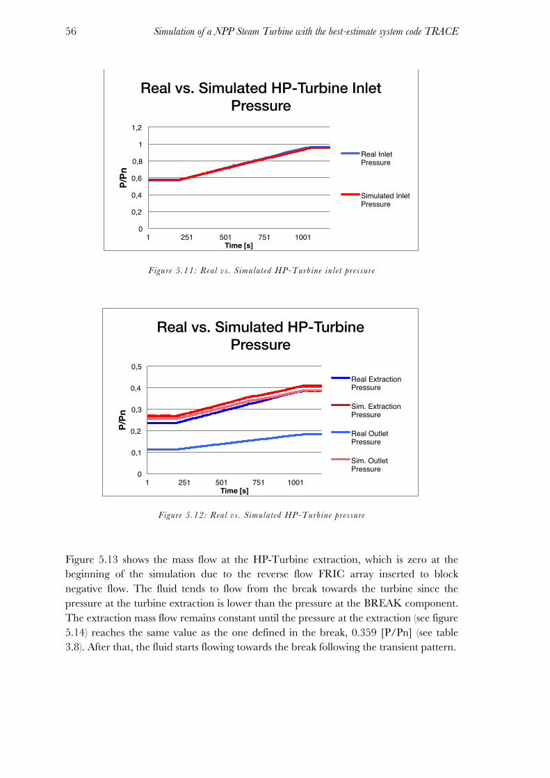
Simulation of a NPP Steam Turbine with the best-estimate system code TRACE 56
Figure 5.11: Real vs. Simulated HP-Turbine inle t pressure
Figure 5.12: Real vs. Simulated HP-Turbine pressure
Figure 5.13 shows the mass flow at the HP-Turbine extraction, which is zero at the beginning of the simulation due to the reverse flow FRIC array inserted to block negative flow. The fluid tends to flow from the break towards the turbine since the pressure at the turbine extraction is lower than the pressure at the BREAK component. The extraction mass flow remains constant until the pressure at the extraction (see figure 5.14) reaches the same value as the one defined in the break, 0.359 [P/Pn] (see table 3.8). After that, the fluid starts flowing towards the break following the transient pattern.
0
0,2
0,4
0,6
0,8
1
1,2
1 251 501 751 1001
P/Pn
Time [s]
Real vs. Simulated HP-Turbine Inlet Pressure!
Real Inlet Pressure
Simulated Inlet Pressure
0
0,1
0,2
0,3
0,4
0,5
1 251 501 751 1001
P/Pn
Time [s]
Real vs. Simulated HP-Turbine Pressure!
Real Extraction Pressure
Sim. Extraction Pressure
Real Outlet Pressure
Sim. Outlet Pressure

5. Transient: Simulation & Results 57
Figure 5.13: HP-Turbine Extract ion mass f low
Figure 5.14: HP-Turbine Extract ion pressure
LP-Turbine Figure 5.15 shows the mass flow at the LP-Turbine inlet, which follows the transient pattern distinctly. Compared to the HP-Turbine inlet mass flow (see figure 5.10), the LP-Turbine inlet mass flow is slightly more fluctuating due to the disturbances produced by the other components.
A comparison between figures 5.15 and 5.16 reveals that both the pressure and the mass flow follow the transient pattern, which proves that a close relationship between pressure and mass flow exists. The results of the LP-Turbine simulation are remarkable since they reveal that the transient pattern is followed through the whole system.
Figure 5.15: LP-Turbine inle t mass f low
Figure 5.16 shows a comparison between the real and the simulated LP-Turbine inlet pressure. The simulated pressure follows the transient pattern as the real one, which was the main objective of the simulation. Due to the error accumulated in the first part of the complete system, the simulated pressure is higher than the expected one.
00,010,020,030,040,05
1 251 501 751 1001
M/M
n
Time [s]
Extraction Mass Flow!
0,359
00,10,20,30,40,5
1 251 501 751 1001
P/Pn
Time [s]
Extraction Pressure!
00,05
0,10,150,2
0,250,3
1 251 501 751 1001
M/M
n
Time [s]
LP-Turbine Inlet Mass Flow!

Simulation of a NPP Steam Turbine with the best-estimate system code TRACE 58
Figure 5.16: Real vs. Simulated LP-Turbine inle t pressure
Figure 5.17 shows a comparison between how the simulated pressure and the real pressure evolve inside the LP-Turbine, and figure 5.18 illustrates that the LP-Turbine outlet pressure does not follow the transient pattern as clearly as the inlet pressure.
Figure 5.17: Real vs. Simulated LP-Turbine pressure
0
0,05
0,1
0,15
0,2
0,25
1 251 501 751 1001
P/Pn
Time [s]
Real vs. Simulated LP-Turbine Inlet Pressure!
Real Inlet Pressure
Sim. Inlet Pressure
0
0,02
0,04
0,06
0,08
0,1
1 251 501 751 1001
P/Pn
Time [s]
Real vs. Simulated LP-Turbine Pressure!
Real Extr. 1 Pressure
Sim. Extr. 1 Pressure
Real Extr. 2 Pressure
Sim. Extr. 2 Pressure
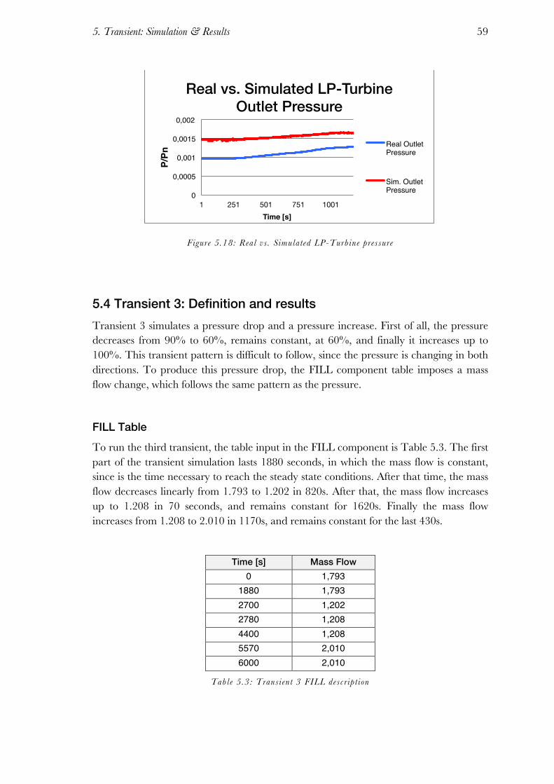
5. Transient: Simulation & Results 59
Figure 5.18: Real vs. Simulated LP-Turbine pressure
5.4 Transient 3: Definition and results Transient 3 simulates a pressure drop and a pressure increase. First of all, the pressure decreases from 90% to 60%, remains constant, at 60%, and finally it increases up to 100%. This transient pattern is difficult to follow, since the pressure is changing in both directions. To produce this pressure drop, the FILL component table imposes a mass flow change, which follows the same pattern as the pressure.
FILL Table To run the third transient, the table input in the FILL component is Table 5.3. The first part of the transient simulation lasts 1880 seconds, in which the mass flow is constant, since is the time necessary to reach the steady state conditions. After that time, the mass flow decreases linearly from 1.793 to 1.202 in 820s. After that, the mass flow increases up to 1.208 in 70 seconds, and remains constant for 1620s. Finally the mass flow increases from 1.208 to 2.010 in 1170s, and remains constant for the last 430s.
Time [s] Mass Flow 0 1,793
1880 1,793 2700 1,202 2780 1,208 4400 1,208 5570 2,010 6000 2,010
Table 5.3: Transient 3 FILL descript ion
0
0,0005
0,001
0,0015
0,002
1 251 501 751 1001
P/Pn
Time [s]
Real vs. Simulated LP-Turbine Outlet Pressure!
Real Outlet Pressure
Sim. Outlet Pressure

Simulation of a NPP Steam Turbine with the best-estimate system code TRACE 60
HP-Turbine Figure 5.19 shows the HP-Turbine inlet mass flow, which corresponds exactly to half of the FILL mass flow.
Once again, the comparison between the simulated inlet mass flow and inlet pressure (see figures 5.19 and 5.20) reveals the close relation that exists between them. As the graphs show, both the inlet pressure and the inlet mass flow follow clearly the transient pattern.
Figure 5.19: Real vs. Simulated HP-Turbine inle t pressure
Figure 5.20 shows a comparison between the simulated (red) and the real (blue) HP-Turbine inlet pressure. As the graph illustrates, the simulated pressure is exactly the same as the real one, even though the transient pattern is complex. Considering the complexity of the pattern, and the real and simulated pressure analogy, this result confirms the validity of the designed system.
Figure 5.20: Real vs. Simulated HP-Turbine inle t pressure
0
0,2
0,4
0,6
0,8
1
1,2
1 1001 2001 3001 4001
M/M
n
Time [s]
Sim. HP-Turbine Inlet Mass Flow !
0
0,2
0,4
0,6
0,8
1
1 1001 2001 3001 4001 5001
P/Pn
Time [s]
Real vs. Simulated HP-Turbine Inlet Pressure !
Sim. Inlet Pressure
Real Inlet Pressure

5. Transient: Simulation & Results 61
Figure 5.21 shows the pressure at the HP-Turbine extraction and outlet. As it was explained with the results of transients 1 and 2, the outlet pressure is higher than the desired one due to the effect caused by the other components.
Figure 5.21: Real vs. Simulated HP-Turbine pressure
Figures 5.22 and 5.23 show the progress of the mass flow and the pressure at the HP-Turbine extraction over the transient simulation. A comparison between both graphs demonstrates that when the pressure at the extraction is higher than the break pressure, 0.359 [P/Pn], the extracted mass flow is positive. On the other hand, when the pressure at the extraction is lower than the break pressure, the extracted mass flow is zero. The results obtained from the comparison between figures 5.22 and 5.23, verify the proper function of the reverse flow FRIC array inserted in the model (see section 5.1.2).
Figure 5.22: HP-Turbine Extract ion mass f low
Figure 5.23: HP-Turbine Extract ion pressure
0
0,2
0,4
0,6
1 1001 2001 3001 4001 5001
P/Pn
Time [s]
Real vs. Simulated HP-Turbine Pressure!
Sim. Extr. Pressure
Real Extr. Pressure
Sim. Outlet Pressure
Real Outlet Pressure
0
0,01
0,02
0,03
0,04
0,05
1 1001 2001 3001 4001
M/M
n
Time [s]
Extraction Mass Flow!
0,359 0,359
0
0,1
0,2
0,3
0,4
0,5
1 1001 2001 3001 4001 5001
P/Pn
Time [s]
Extraction Pressure!

Simulation of a NPP Steam Turbine with the best-estimate system code TRACE 62
LP-Turbine Figure 5.24 shows the mass flow at the LP-Turbine inlet, which follows the transient pattern clearly. The LP-Turbine inlet mass flow fluctuates more than the HP-Turbine inlet mass flow (see figure 5.19) due to the disturbances produced by the vapour flow through the system components.
A comparison between figures 5.23 and 5.24 shows that, both the pressure and the mass flow follow the transient pattern. The results of the LP-Turbine simulation are remarkable since they reveal that the transient pattern is followed through the whole system.
Figure 5.24: LP-Turbine inle t mass f low
Figure 5.25 shows a comparison between the real (blue) and the simulated (red) LP-Turbine inlet pressure. As the graph illustrates both the real and the simulated pressure follow the transient pattern, which also verifies, as the results of the HP-Turbine do, the validity of the designed system.
0
0,05
0,1
0,15
0,2
0,25
0,3
1 1001 2001 3001 4001
M/M
n
Time [s]
Inlet LP-Turbine Mass FLow!
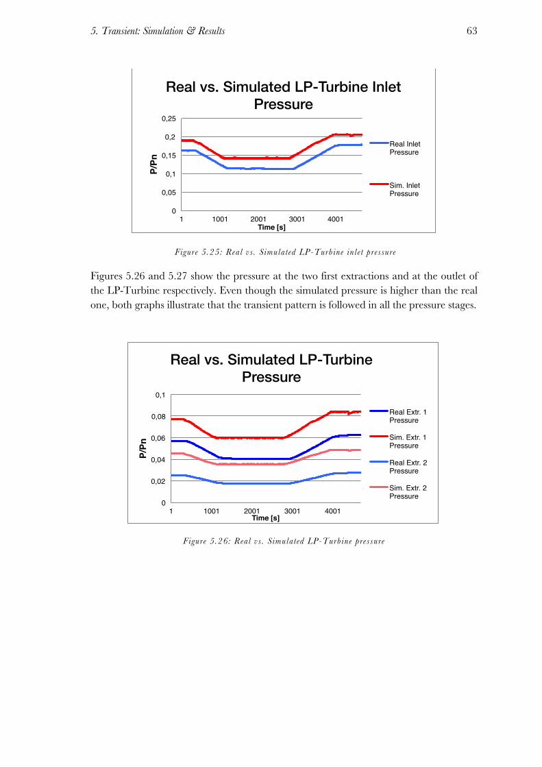
5. Transient: Simulation & Results 63
Figure 5.25: Real vs. Simulated LP-Turbine inle t pressure
Figures 5.26 and 5.27 show the pressure at the two first extractions and at the outlet of the LP-Turbine respectively. Even though the simulated pressure is higher than the real one, both graphs illustrate that the transient pattern is followed in all the pressure stages.
Figure 5.26: Real vs. Simulated LP-Turbine pressure
0
0,05
0,1
0,15
0,2
0,25
1 1001 2001 3001 4001
P/Pn
Time [s]
Real vs. Simulated LP-Turbine Inlet Pressure!
Real Inlet Pressure
Sim. Inlet Pressure
0
0,02
0,04
0,06
0,08
0,1
1 1001 2001 3001 4001
P/Pn
Time [s]
Real vs. Simulated LP-Turbine Pressure!
Real Extr. 1 Pressure
Sim. Extr. 1 Pressure
Real Extr. 2 Pressure
Sim. Extr. 2 Pressure

Simulation of a NPP Steam Turbine with the best-estimate system code TRACE 64
Figure 5.27: Real vs. Simulated LP-Turbine outle t pressure
0
0,0005
0,001
0,0015
0,002
1 1001 2001 3001 4001
P/Pn
Time [s]
Real vs. Simulated LP-Turbine Outlet Pressure!
Real Outlet Pressure
Sim. Outlet Pressure

6. Conclusions
65
6. Conclusions
The main objective of this Master’s Thesis was to simulate the operation of a NPP steam turbine in order to obtain realistic results. Using the TRACE system code as a working tool, part of a NPP secondary loop model was developed. The two main characteristics to be achieved by the designed model were:
! Reach realistic conditions at the turbine inlet. ! Reproduce a realistic pressure drop throughout the model.
The developed model has been used to run steady-state and transient simulations, from which relatively good results were obtained. The criterion used to determine whether the results are acceptable or not is their comparison to real data.
As it is explained in this document, after developing and improving the model, the steady-state model was run. The analysis of the steady-state results was divided in three different sections:
! Simplified HP-Turbine ! Simplified LP-Turbine ! Complete model
The simplified HP- and LP-Turbine models were developed in order to test the capabilities of the turbine TRACE model using boundary conditions from the turbine design data. After simulating both models, the results were collected and compared to the real turbine data. The data analysis focussed on the pressure drop inside the turbine, since the FILL component imposed the turbine inlet conditions. The simulation results and the real data show good agreement.
After analysing the simplified model data, the complete model was implemented.
Again, the results obtained from the simulation were compared to the turbine real data. As the graphs included in section 4.2.3 illustrates, the results are not as good as those of the simplified models. The slightly difference between the simulation and the real data is caused by the fact that the code has to compensate for the losses from the other components such as separator and over-heater. For instance, graph 4.11 illustrates that inside the separator a significant pressure drop takes place due to the extraction of liquid water, which affects the HP-Turbine outlet pressure.
Figures 4.7 and 4.13 illustrate a comparison between the simulation and real pressure data at the inlet of the HP- and the LP-Turbine respectively. Also, figures 4.9 and 4.13 show a comparison between the simulated and the real pressure drop inside both

Simulation of a NPP Steam Turbine with the best-estimate system code TRACE 66
turbines. Considering the similarity between the simulation and the real data, the complete model data analysis ratifies the validity of the designed system.
Section 4.2.3 also includes the results of the separator, the over-heater, and the condenser, since part of the work covered by this Master’s Thesis was the improvement of the complete model operation in order to reach optimal conditions at the HP- and LP-Turbines inlet.
As previously mentioned, after the optimal results for the steady-state simulation were achieved, three different transient models were simulated. The results obtained from the transient simulations are very remarkable.
The objectives to achieve were reaching realistic conditions at both turbine inlets and reproducing a realistic pressure drop inside the turbine. A comparison between the simulation and the real data at both turbines reveals that both the inlet pressure and the pressure drop in the turbines are near to reality. This was valid for both the steady state and transient simulations.

7. Possible future improvements 67
7. Possible future improvements
The model developed here can be further improved regarding the following aspects:
! Optimization of KFAC array ! Implementation of the HEATR component ! Complete the model by closing the loop
Optimization of the KFAC arrays The biggest problem encountered during the model design was the definition of the KFAC array of each component. The first attempt to define the KFAC array was an analytical calculation. Due to the lack of real data and as a result of all the approaches tried, the calculated KFAC array did not provide the expected results. Based on the previous calculations, the k-factors of each component were manually tuned until the obtained results were considered close enough to the real data.
But through more modifications of the KFAC array aspects such as pressure drop or turbine water extractions can be further optimized.
HEATR component implementation The HEATR component provides you with the capability of modelling typical feed-water heaters found in nuclear steam supply systems. A HEATR can be used to model the Shell (condensing) side of a closed-type feed-water heater, and is meant to be coupled to a PIPE and HTSTR to include modelling of the feed-water flow and heat transfer within the heaters. A HEATR (or a series thereof) component can also be employed to model the main steam condensers, again in combination with a PIPE and HTSTR, which in this case would model the circulating cooling water [8].
During the development of the complete model, the HEATR component was chosen for the designing of the over-heater and the condensers. Due to the limited timeframe of the project the decision was to design simplified models for both components in order to reach the desired conditions at the inlet and outlet of the LP-Turbine.
With enough time and the proper data, a realistic model of an over-heater or a condenser can be developed using a HEATR component coupled to a PIPE and a HTSTR.

Simulation of a NPP Steam Turbine with the best-estimate system code TRACE 68
Complete the model by closing the loop As it is clarified in Chapter 2: Theoretical Background, the steam turbine is a component of the NPP secondary loop. In order to simulate the proper operation of the steam turbine the circuit should be completed.
The connection between the condenser and the HP-Turbine is composed of many heat exchangers, which collect the steam from the turbine extractions to heat the condensate, and the Steam-generator, in which the heated condensate is transformed into steam.
The development of such a complex model could be another way of further development of the model.

69


71
Bibliography
[1] Nuclear Engineering HandBook, Section I, Chapter 2 PWR, R. Schreiber.
[2] Macián, (2014), TU Munich, Course: Fundamentals of Nuclear Engineering, Lecture 1.
[3] Macián, (2013), TU Munich, Course: Introduction to Nuclear Energy, Lecture 8.
[4] Mechanical Engineers’ Handbook: Energy and Power, Volume 4, Third Edition.
Edited by Myer Kutz. Copyright © 2006 by John Wiley & Sons, Inc.
[5] Mecánica de Fluidos, Sexta edición, Frank M. White.
[6] Macián, (2013), TU Munich, Course: Fundamentals of Thermal-hydraulics in Nuclear Systems, Lecture 4.
[7] TRACE V5.0 Theory Manual: Field Equations, Solution Methods, and Physical Models. Division of Safety Analysis Office of Nuclear Regulatory Research.
[8] TRACE V5.0 USER’S MANUAL, Volume 2: Modelling guidelines. Division of Safety Analysis Office of Nuclear Regulatory Research.
[9] TRACE V5.0 USER’S MANUAL, Volume 1: Input Specification. Division of Safety Analysis Office of Nuclear Regulatory Research.


Adoración Garrido-Lestache
Romero
SIM
ULA
CIÓ
N D
E U
NA
TU
RB
INA
DE
VAPO
R D
E U
NA
CEN
TRA
L N
UC
LEA
R C
ON
EL
CÓ
DIG
O T
RA
CE