(WZB) Berlin Social Science Center Research Area Markets and Choice Research Unit Market Behavior

Put your Research Area and Unit

Jana Friedrichsen Signals Sell: Designing a Product Line when Consumers Have Social Image Concerns

Discussion Paper

SP II 2016–202 March 2016

Wissenschaftszentrum Berlin für Sozialforschung gGmbH Reichpietschufer 50 10785 Berlin Germany www.wzb.eu

Jana Friedrichsen Signals Sell: Designing a Product Line when Consumers Have Social Image Concerns

Affiliation of the author:

Jana Friedrichsen DIW Berlin and Humboldt-Universität zu Berlin

Copyright remains with the author.

Discussion papers of the WZB serve to disseminate the research results of work in progress prior to publication to encourage the exchange of ideas and academic debate. Inclusion of a paper in the discussion paper series does not constitute publication and should not limit publication in any other venue. The discussion papers published by the WZB represent the views of the respective author(s) and not of the institute as a whole.

Wissenschaftszentrum Berlin für Sozialforschung gGmbH Reichpietschufer 50 10785 Berlin Germany www.wzb.eu

Abstract

Signals Sell: Designing a Product Line when Consumers Have Social Image Concerns

by Jana Friedrichsen*

One important function of consumption is for consumers to show off their taste, virtue or wealth. While empirical observations suggest that producers take this into account, existing research has concentrated on analyzing the demand side. This paper investigates how a monopolist optimally designs its product line when consumers differ both in their taste for quality and their desire for a positive social image. The monopolist distorts qualities and prices to allocate images to consumers. It generically pools consumers with different tastes because high-taste consumers lend a positive image to the product of their choice and thereby increase the product’s value to others. Often, average quality is lower than in a market without image concerns and there is underprovision as compared to the welfare-maximizing allocation. Although average quality is higher in a competitive market, welfare typically is not.

Keywords: image motivation, conspicuous consumption, two-dimensional screening, mechanism design

JEL classification: D21, D82, L15

* jana.friedrichsen@hu-berlin.de. A predecessor of this paper was circulated under the title “Image

concerns and the provision of quality.” For helpful suggestions and comments on earlier versions I thank Pierre Boyer, Yves Breitmoser, Dirk Engelmann, Renaud Foucart, Boris Ginzburgh, Hans-Peter Grüner, Bruno Jullien, Heiko Karle, Botond Kőszegi, Sergei Kovbasyuk, Dorothea Kübler, Yassine Lefouili, Christian Michel, Andras Niedermayer, Volker Nocke, Martin Peitz, Patrick Rey, David Sauer, Nicolas Schutz, Anastasia Shchepatova, André Stenzel, Jean Tirole, Péter Vida, Georg Weizsäcker, Philipp Zahn, and three anonymous reviewers as well as participants at various conferences and seminars. Part of the research leading to this paper was undertaken while I was visiting Toulouse School of Economics and I am grateful for the hospitality experienced there. All errors are mine.

1. Introduction

Consumption is about satisfaction of needs. Partly these needs are addressed by the physicalnature of products: the mobile allows us to make calls and text, a wine tastes good, a carprovides mobility and comfort, and so forth. But we also consume because we want to showoff.1 Only a few decades ago, consumers mostly showed off their wealth, trying to “keep upwith the Joneses” by amassing as much new stuff as the neighbors. But when many goods areaffordable to almost everyone around them, and wealth may have become a less desirable char-acteristic, consumers increasingly seek to advertise virtue or taste instead of pure wealth (Frickand Hauser, 2008; The Economist, 2010). Although producers certainly cater to this desire—several examples follow below—hardly any research has analyzed this response.2 Moreover, thepossibility that consumers buy to advertise another characteristic but wealth is typically ignoredin the literature. This paper contributes to filling this gap by analyzing how a strategic firmadjusts the variety, qualities, and prices of its product line when individuals differ both in theirvaluations of quality and their desire for social image.3

To analyze the supply side response to image concerns, I set up a simple model of marketswhere consumers may derive utility from a product’s quality as well as from the image associatedwith it. Types are binary in both dimensions but in contrast to existing research I do notimpose any restrictions on the correlation. The image of a product emerges endogenouslyfrom the individual consumers’ consumption decisions as a product’s image is the conditionalexpectation of a consumer’s taste for quality after purchases have been observed.4

Technology companies, wine makers, health clubs or hotel groups, fashion designers, and pro-ducers of luxury products segment their markets by offering products that appeal to differentgroups of people and their signaling desires. For instance, the fashion designer Armani differ-entiates its product line into three tiers, distinct in style and price, that are tailored to differentsets of consumers (Amaldoss and Jain, 2010; Kotler and Keller, 2011, p. 320). Even though thisdifferentiation may partially be motivated by differential tastes for quality in the first place, thethree tiers are associated with different sets of customers and thereby public images. These im-ages are themselves valued by customers and add to a product’s physical value thereby justifyinghigh price premia in the upper tiers. Mobile phones can also function as status goods (Abeeleet al., 2014). Apple’s iPhone, in particular, is in high demand partly for social positioningreasons (Arruda-Filho and Lennon, 2011), and the design of Apple’s product line hints towardimage concerns being addressed. Section 2.1 provides more detailed empirical applications anddiscusses where standard screening models that concentrate on the effects of heterogeneous

1Empirically, it is well-documented that consumers pay for demonstrating their wealth, taste, or preferences.See for instance Chao and Schor 1998; Charles et al. 2009; Heffetz 2011; Sexton and Sexton 2014. A possiblemechanism to microfound such behavior is that being perceived as “good” increases an agent’s matchingopportunities and future payoffs (Pesendorfer, 1995; Rege, 2008).

2A large number of theoretical studies investigate how consumer behavior is affected by the desire to demonstratewealth but do not allow for strategic responses on the supply side (Veblen, 1915; Ireland, 1994; Bagwell andBernheim, 1996; Glazer and Konrad, 1996; Corneo and Jeanne, 1997). The only study that investigatesstrategic product design in this context, Rayo (2013), does not apply to the empirically relevant case thatthe desire to signal is heterogeneous across consumers and negatively correlated with the characteristic to besignaled. Section 8 provides a detailed discussion.

3The notion of quality is a general one here. For instance, quality can also refer to the extent to whichproduction is environmentally friendly. Instead of image motivation or image concern (for similar use see forinstance Ariely et al., 2009), others have used the terms signaling motivation, status concern, or conspicuousconsumption. Sometimes the meaning is restricted to the signaling of wealth. Cabral (2005) suggests using“reputation” for situations “when agents believe a particular agent to be something.” As this is uncommon inthe relevant literature it is not used here.

4Consumption is conspicuous in that it provides evidence of the personal characteristic “taste for quality”.Conspicuous consumption according to Veblen (1915, p. 47) is the “specialized consumption of goods as anevidence of pecuniary strength”. Here, the “taste for quality” can be driven by wealth or expertise and therebysignaling this trait can have similar benefits as signaling “pecuniary strength.”

1

tastes for quality are insufficient to entirely explain the observed market segmentation and pricedifferences.

After discussing the empirical evidence, Sections 3 and 4 analyze image concerns in monopo-listic markets. Monopoly captures an essential aspect of status goods, namely their inimitability,and could reflect a firm with market power when it comes to wine, luxuries, or technology. Al-ternatively, in the case of food items, we can think of a supermarket chain that is deciding whichproduct qualities to slot within a certain category and which prices to charge. The analysis re-veals that monopolists react to the heterogeneity of image concerns by designing a product linethat always induces a partial pooling of consumers. The monopolist distorts product qualitiesand prices differently than what would be predicted by differences in quality valuations aloneto induce this pooling. If the value of image is at an intermediate level, the monopolist offers aproduct of intermediate quality in addition to the low and high quality product he would offerin the absence of image concerns. The additional product offers prestige and symbolic benefitsas well as intermediate quality and allows the monopolist to profitably screen consumers withrespect to their willingness to pay a premium for image. Purely image-concerned consumerspool with purely quality-concerned consumers and buy this product, which can be interpretedas a “masstige” product (Truong et al., 2009; Heine, 2012). Therefore, in this scenario, latertermed image building, fewer consumers decide in favor of the lowest quality than if imageconcerns were absent. The highest-quality product’s price reflects its premium image and isattractive only to consumers who value both quality and image. Therefore, fewer consumerschoose high quality than in the absence of image concerns. Depending on the distribution ofconsumer types, average quality in the market may then decrease if the value of image increases.If image is very valuable, the monopolist offers only a low and an exclusive high quality product.Prices are set such that the high quality product is only bought by consumers who value imagein addition to quality, whereas all others prefer the low quality product. Thus, average qualityin the market decreases for sure as compared to a model without image concerns when imageconcerns become very strong.

In Section 5, I study a perfectly competitive setting. This allows me to disentangle the effectsof strategic consumer behavior from those due to strategic supply. I show that firms operatingin perfect competition cannot exploit image concerns to make positive profits. Still if the valueof image is sufficiently high, image concerns remain relevant in a market where producers areprice-takers, but the predicted distortions are different than in monopoly. As prices are drivendown to marginal cost, consumers cannot use prices to signal their interest in quality—as amonopolist’s product line would encourage them to do. Instead, consumers who value bothimage and quality buy inefficiently high quality, which serves as a functional excuse to separatefrom lower valuation consumers. Such a high quality product is too expensive for purely image-concerned consumers even if it is sold at marginal cost. Purely image-concerned consumers poolwith purely quality-concerned consumers on a lower quality product that has the same qualitylevel as the “high-quality” product by the monopolist. In contrast to this upward distortion incompetitive qualities, monopoly induces separation by a downward distortion in quality. A keyresult is that quality is on average higher in competition than in monopoly. Welfare, however,is often higher in monopoly than in competition. The reason is that consumers buy excessivequality in the competitive market to acquire a good image. Producing these quality levels, andtherefore this way of signaling, is inefficient. A monopolist allows for less wasteful signalingby restricting the product line. The policy implications therefore differ with respect to marketstructure. Although monopoly achieves product differentiation by a low-quality product, theintroduction of a minimum quality standard is shown to weakly decrease welfare and consumersurplus. In a competitive market, the allocation is inefficient due to an upward distorted high-quality product: a luxury tax strictly increases welfare but does not in general yield a Paretoimprovement.

2

The rest of the paper is structured as follows. In Section 2, I first discuss empirical exampleswhere firm behavior is consistent with predictions of my model for heterogeneous image concerns.I also present empirical support of a negative correlation between intrinsic quality concerns andimage motivation, which is the arguably most interesting case of my model. Then, I introducethe monopolistic model and discuss two benchmark cases in Section 3, and analyze the fullmodel in Section 4. Section 5 then studies heterogeneous image concerns in a competitivemarket. Section 6 addresses welfare implications and possible policy interventions, and Section7 presents generalizations and extensions. In Section 8, I discuss how my work relates to theliterature before I conclude in Section 9. Proofs which are not included in the main text arecontained in Appendix A. Appendix B provides supplementary material.

2. Empirical relevance of heterogeneous image concerns

2.1. Supply side caters to (heterogeneous) image concerns

Example 1: Apple and the iPhone The iPhone signals something about its owner and apparently,Apple’s customers are willing to pay a substantial premium for this signal. The first generationof iPhones was marketed clearly as an exclusive product, of interest only to people who neededthe phone’s technological features and were willing to pay a premium for being among those firstadopters (Arruda-Filho et al., 2010). While Apple has always targeted a market segment thatis willing to buy into the brand prestige, the company has recently moved toward segmentingits market further. Until the iPhone 5, Apple introduced new iPhone models one at a time.The iPhone 5C and iPhone 5S, however, were introduced simultaneously. While the iPhone 5Clacks some features of the iPhone 5S (reduced quality), the signaling part is more prominent inform of the colorful casing. Offering these two version simultaneously allowed Apple to price-discriminate between those consumers who wanted to have the most high-end product and thosewho wanted to be seen with a new iPhone but were less interested in new features. Interestingly,Apple made sure that the different versions could be distinguished from each other through theirdesign. The move to simultaneous versions occurred at a time when Apple’s brand value andstock prices stagnated and even decreased. Apple’s behavior could indicate a decreasing valueof image, to which a masstige strategy was the answer in line with my model.5

Example 2: Bordeaux Wines The finest wine producers in France, particularly in the Bordeauxregion, commonly offer a so-called“second label wine” in addition to their first label. The secondwine is produced from grapes grown on the same estate, but it may be based on special plotsor vines that are younger or do not perform as well. Depending on the quality of the vintage,a house may allocate a larger part or even all of the harvest to its second wine so as not tocompromise the reputation of its Grand vin. While the quality difference may be small, theprice differential is typically large. According to an empirical study by Ashenfelter (2008),there are two motivations for buying mature Bordeaux: interest in the wine itself and interestin the status symbol. In line with my theoretical analysis for the heterogeneous purchasingmotives documented in Ashenfelter (2008), wine producers have adopted a two-tier productline. The Grand vin of superior quality receives an enormous image premium that is paid buythose who want a status symbol but also value the underlying quality. The lower quality second

5See http://www.statista.com/statistics/326052/apple-brand-value/ and http://finance.yahoo.com

for the numbers. In line with the brand value increasing again as indicated by increasing stock prices during2014, Apple appears to go back to an exclusive market strategy with the newest generation. While mostfeatures are the same, the iPhone 6 Plus is larger and has much better power and battery than the iPhone6. Thus, the iPhone 6 Plus is a rather different product than the iPhone 6 which is of typical size. Incontrast, the functional differences between iPhone 5C and 5S are much smaller and appear to be moreartificial. The simultaneous introduction of iPhone 6 and iPhone 6 Plus could be an attempt of classicalprice-discrimination along the dimension of features. For features and introduction dates of the iPhone seehttp://en.wikipedia.org/wiki/IPhone.

3

label wine appeals to those who are unwilling to pay a reputation premium for the Grand vinand choose the second label for its good quality-to-price ratio. But the second label wine alsoappeals to those who care mostly about the associated image, possibly because they are ignorantof the quality; they buy for the good image-to-price ratio. The image of a great wine maker’ssecond label is considerably better than the image associated with an unknown producer’s wine.Moreover, the (expected) quality of this wine is higher than that of the unknown wine.

Example 3: Hotel chains Hotels offer opportunities to meet people, and for some it is impor-tant what type of person they are perceived as in such encounters: Business hotel customers payhigh rates in upper end hotels also to impress business contacts, and hotels appeal to images thatare consistent with the signaling desires of their guests to increase customer satisfaction (Back,2005). A hotel chain caters to image concerns by offering different hotel categories, sometimesunder the same brand name. For instance, Accor has luxury hotels named Sofitel, Novotel andMercure in the upscale range, Ibis Red and Ibis Styles in the Midscale, and Ibis Budget in theEconomy range.6 Across hotel categories, not only service quality but also the clientele andthe associated image differ, and hotels appear to be charging for it. Similar strategies can beobserved for health clubs, which again are places where people do not only train but also meet.

Example 4: Socially Responsible Products It has become increasingly important to consumersthat goods are ethically acceptable and sustainably produced. The market for organic productsgrew on average by more than 14% per year between 1999 and 2007 (Sahota, 2009), and Fair-trade sales experienced two-digit annual growth rates during recent years in many Europeanmarkets (http://www.fairtrade.net/annual-reports.html). At the same time these goodsare becoming status symbols (Kapferer, 2010; Frick and Hauser, 2008, p. 28). Empirical stud-ies find that higher prices for green products can be partly explained by image concerns (e.gCasadesus-Masanell et al., 2009; Griskevicius et al., 2010; Sexton and Sexton, 2014). While thereis much acceptance of the mainstreaming of responsible consumption, critical voices lament adilution of the underlying principles as products are tailored to a broader audience (for instanceClark, 2011 and Stevens, 2011). According to my model, this observation is consistent with adiscounter optimizing its product listings in response to rising image concerns:7 To profit fromimage concerns and attract consumers who do not so much care about sustainable productionper se, the discounter will offer an inferior version of a sustainable product, probably an own-brand product, in addition to the fully sustainable product, which can consequently be sold ata premium. In line with this, the independent German testing organization Stiftung Warentesthas recently found that organge juice of the discounter Lidl’s Fairglobe (Lidl’s own-brand car-rying the Fairtrade logo) does not satisfy basic requirements with respect to labor conditionsand environment (Stiftung Warentest, 2014). Still, Lidl’s Fairglobe products sell very well andhave contributed to the increase in market size for Fairtrade products.

Also, the soft drinks “ChariTea” and “LemonAid” clearly appeal to non-consumption valuesthrough their names and the bottles are easily recognized even from a distance through theirunusual design.8 At a local German supermarket, a consumer will pay about 1.30 Euro for a330ml bottle of ChariTea or LemonAid while a same-sized soft drink that fulfills comparablesocial and environmental standards sells at less than a Euro per 330ml bottle. This price differ-

6This is only one example. Among others, also Best Western Hotels, Choice Hotels, Hilton Worldwide, andHyatt Hotels Corporation offer hotels in different categories targeting different sets of consumers. These arebrand extensions in the form of vertical line extensions (Keller, 2015). Product and brand images have beenshown to be crucial for such extensions (e.g. Kirmani et al., 1999). The marketing literature offers manyempirical studies but little theoretical background for the estimated effects.

7In accordance with my model, producers engage in Corporate Social Responsibility (CSR) strategically (Kitz-mueller and Shimshack, 2012): they green their production or tighten social standards to better tailor theproducts to individuals’ demand for responsible products for profit-maximizing reasons. Producers and trad-ing companies might of course themselves have intrinsic concerns for ethical production. This is not includedin my model.

8These two drinks are advertised with “Drinking helps!”. See http://www.lemon-aid.de/ and Figure B1 inAppendix B.

4

ence cannot be justified by the 5 Cents donation per bottle to charitable projects alone.9 Barsand Cafes where consumption is more visible and signaling desires more relevant (Griskeviciuset al., 2007) are frequent outlets for these drinks, making image concerns the most plausibleexplanation for the price premium. Quality-based models would not predict higher popularityof responsible products in public spaces.

Recently, several long-standing firms in Fairtrade and organic production have introducedtheir own standards which lie above the one implemented in mainstream retailing.10 This iscompatible with my results and can thus be interpreted as a reaction to increased competitionfrom discounters and supermarkets.11 An increase in the valuations for Fairtrade and organicproducts would similarly predict an increase in top quality. However, if consumers value onlyquality, it is puzzling that the low-quality alternative is unchanged or even worsens: The jointoccurrence of both events can be explained by quality concerns only if there are heterogeneouschanges in preferences. In contrast, their joint occurrence exactly matches my predictions ifconsumers also have image concerns and the signaling value of sustainable consumption increasesin response to increased public attention to environmental and social issues.

Example 5: Luxury Products Luxury products are typically bought because of the associatedprestige as well as their intrinsic quality. Expressive purchase motives like status concernsincrease their importance relative to intrinsic ones such as quality the more visibly a productis consumed (Hudders, 2012). Producers of luxury or premium products regularly face thechallenge of increasing their market share through lower-priced lines while not jeopardizing theprestige of the company’s products (Chen, 2013). One example to address this challenge isthat producers segment the market for luxury handbags by offering “loud” and “quiet” bags.The loud ones carry a visible brand logo and tailor to consumers who want to signal affluencethrough their brand choice but lack connoisseurship. The quiet bags, in contrast, do not carrya visible brand logo such that they can be used for signaling only by those who know and valuethe subtle design and quality of the bag itself. According to Han et al. (2010), Gucci and LuisVuitton sell quieter handbags and shoes at a price premium, and similarly, it is the lower-pricedcars by Mercedes that carry a larger emblems. This is consistent with a market segmentationstrategy where the premium consumers who are able to judge the product’s quality and desireto signal their superiority are separated from those who either lack the knowledge for quality orare not willing to pay an image premium (note that even the larger emblem cars and the loudbags are usually of high quality).12 A purely quality-based segmentation, in contrast, cannotexplain the loud-quiet distinction. Alternatively, loud bags might be cheaper to compensateconsumers for being ad-carriers for the respective brand. Given that many consumers want tobe recognized as wearing the brand, this is unlikely to be the sole explanation for the observedpatterns either.

Example 6: Cars Automobile manufacturers usually offer product lines, and social status hascome to be associated more with particular vehicles than with the manufacturer itself. Luxurycars such as Lexus, Mercedes S-class, or Tesla offer not only increased comfort and safety totheir owners as compared to less expensive variants from the same manufacturers, but they alsoconfer status benefits. The associated status depends on price, style, and engineering of the

9Information regarding the donation cannot be found on the bottles or the shelves and not on the product’swebsite either but only in an interview with the founders (Baurmann, 2013).

10See for instance http://fair-plus.de/, and Purvis (2008) on Fairtrade. For organic products, a number ofvoluntary agreements exist which enforce more stringent standards than e.g the certified organic standard ofthe European Union (see http://www.ifoam.org/sub/faq.html).

11Such coexistence of monopoly and competitive predictions may be observed if purchasing modes vary: someconsumers choose first which quality they want to buy and select the outlet accordingly. This competitiveelement leads to excessive quality. Others first pick an outlet and then a quality within this outlet’s portfolio.This monopoly element leads to the availability of lower quality products.

12Han et al. (2010) employ a consumer categorization that differs from the one used in this paper. In particular,they assume a distinction in connoissership which together with wealth and income determines the marginalutility from quality. Moreover, they assume that what the different consumers want to signal is not identical.

5

car but also on public opinion (Berger, 2001, p. 160). Moreover, Mercedes Benz introduced theBlueTEC and BlueEFFICIENCY label that additionally allow consumers to signal their concernfor the environment in several categories of cars.13 Mercedes thereby addresses signaling desiresin several dimensions: wealth through size of the car and environmental preferences throughthe label (see Section 7.2).

2.2. Intrinsic motivation and image concerns correlate negatively

The predictions derived for the monopoly market are most interesting in the case where theintrinsic interest in quality and image concerns are uncorrelated or negatively correlated.14 I amnot aware of any study documenting a positive correlation even though it is not unreasonableto expect those with a high taste for quality care more about their reputation than others.On the other hand, those who highly value quality, know that they do and may have less of abenefit from demonstrating this to others. Those who value quality less may benefit more frombeing held for better-reputed quality lovers. Indeed, there is substantial evidence that intrinsicinterest and image concerns are negatively correlated.

The cleanest evidence to my knowledge is a laboratory experiment by Friedrichsen and En-gelmann (2013), in which we test whether intrinsically motivated individuals exhibit strongeror less pronounced image concerns when it comes to buying Fairtrade chocolate. We show thatthere is a negative relationship: those who do not value Fairtrade chocolate intrinsically, exhibitstronger image concerns.

A number of other studies provide indirect evidence of a negative correlation. For instance,Truong and McColl (2011) argue that the correlation between intrinsic purchasing motives andsignaling is negative in the context of luxury consumption, and Vermeir and Verbeke (2006)present similar findings in the context of socially responsible consumption. Results by Riedl andSmeets (2015) indicate a negative correlation between intrinsic motivation and image concernsamong financial investors. The authors combine experimental data on intrinsic social prefer-ences of investors with administrative data about these investors’ portfolios from a mutual fundand with survey data on the investors’ motivations. Social preferences are found to predict in-vestment in socially responsible mutual funds only if these are not associated with tax benefits.Moreover, the results suggest that “selfish” investors invest in socially responsible mutual fundswithout tax benefits for signaling reasons. No evidence for signaling motivations is found forthose who are classified as pro-social. Field experimental evidence from Germany (Boyer et al.,2014; Dwenger et al., 2016) as well a an empirical analysis of Italian tax records (Filippin et al.,2013) indicate that those who are intrinsically motivated to pay taxes are less subject to imageconcerns.

3. Monopolistic quality provision and image concerns: Model andbenchmarks

3.1. The model

Consider a monopolist who sells products of potentially different quality to heterogeneous con-sumers from a population of unit mass. Quality is chosen by the monopolist on a continuousscale and perfectly observable. A product is a combination of quality and price and is in equilib-rium associated with an image that reflects which consumer types buy the respective product.

13See http://www.mercedes-benz.com/fleet-CO2.14How much value is attributed to the image of being quality-concerned can depend on the social institutions in

a society, modeled as matching patterns (Mailath and Postlewaite, 2006). Theoretically, agents may thereforediffer in image concerns because they engage in types of interactions where the other’s type is more payoff-relevant or less so.

6

Consumers’ utility depends positively on quality s ∈ R≥0 and image (or reputation) R ∈[0, 1], and negatively on price p ∈ R≥0 of a product. Consumers can differ in both, theirtaste for quality σ and their image concern ρ. The two-dimensional type (σ, ρ) is drawn from{σL, σH} × {0, 1} with Prob(σ = σH) = β, Prob(ρ = 1|σ = σH) = αs, and Prob(ρ = 1|σ =σL) = αn. To simplify the exposition, I work with σL = 0 and σH = 1 in the main part ofthe paper. Section 7.1 discusses how this affects results. The resulting four different types ofconsumers are indexed by σρ; their frequencies are stated in Table 1. For a consumer of typeσρ, utility takes the form:

(1) Uσρ(s, p,R) = σs+ ρλR− p

The parameter λ > 0 describes the value of image relative to the marginal utility fromquality.15 The image R of consumer (σ, ρ) is the expectation of his quality preference parameterσ conditional on his purchasing decision. It reflects an outside spectator’s (or the consumermass’) inference of a consumer’s interest in quality. A formal definition of image follows withthe equilibrium definition in Section 3.3.

Table 1: Consumer types and their frequencies.

image concernno yesρ = 0 ρ = 1

∑quality concern

no: σ = 0 (1− β)(1− αn) (1− β)αn (1− β)yes: σ = 1 β(1− αs) βαs β

The monopolist offers a product line M ⊂ R2≥0 to maximize expected profit. Perfect price

discrimination is impossible because consumers are privately informed about their types. Themonopolist has prior beliefs about the distribution of of consumer types that are identical withthe actual distribution. He chooses a product line such that consumers self-select (second-degreeprice discrimination). The monopolist cannot choose image directly, but takes into accountwhich image will be associated with each of its products in equilibrium. Unit costs are assumedto be linear in quantity sold and convex increasing in quality, specifically c(s) = 1

2s2.16

Each consumer can choose a preferred product from the line of quality-price offers or decidenot to buy any of them. The latter case corresponds to obtaining the outside good of zeroquality at a price of zero. Reservation utility is then equal to the utility derived from the imageof non-buyers (=outside good buyers). The analysis remains essentially unchanged if buyingan outside good with zero quality gives the same utility, say a, for all consumers. Voluntaryparticipation is taken care off by requiring the outside option (0, 0) to be part of the productline M.17 If the monopolist allocates (0, 0) to a consumer type this means this type choosesthe outside option.

3.2. The structure

The distribution of σ and ρ and the value of λ are common knowledge and so is the setup of themarket interaction. Consumers have private information about their types. Quality is correctly

15Alternatively I could allow for (σ, ρ) drawn from {0, σ}×{0, ρ} for arbitrary σ, ρ > 0. This is equivalent to myformulation with λ = ρ

σ. Since λ gives the relative weight on image concerns I can also rewrite the analysis

with a weight γ ∈ [0, 1] on image and a weight 1− γ on quality such that I obtain the above formulation withλ = γ

1−γ .16Specifying a functional form allows to obtain closed form solutions. The results are qualitatively the same with

constant unit costs c(s) = c (see Appendix B.9).17In the following, taking (0, 0) will also be referred to as non-participation since this is its meaning. Strictly

speaking all types participate by construction.

7

perceived by consumers; cheating on quality is prevented e.g. through third-party verificationor because it is obvious from inspection.

The timing is as follows:

(i) The monopolist offers a product line M. Qualities and prices are observed by all con-sumers.

(ii) Types are drawn and each consumers privately learns his type σρ.

(iii) All consumers simultaneously choose a product (s, p)σρ ∈ M which maximizes utility fortheir type.

(iv) Images associated with each product and payoffs realize.

In this model, the utility of a consumer does not only depend on his action but also on beliefsabout his type. Thus, the game analyzed here falls into what is called perception games byGradwohl and Smorodinsky (2014) and it is similar to psychological games (Geanakoplos et al.,1989) in which a player’s utility depends on all players’ actions and on the player’s beliefs aboutothers’ strategy profiles. Formally, one can represent images as a consumer’s perception of thebeliefs that an implicit third player forms about his type after consumption decision have beenexecuted. This inactive player may exists in reality or only in the consumer’s imagination.

3.3. Equilibrium

In the presence of image concerns the product line offered by the monopolist induces a gameamong consumers. Image-concerned consumers’ payoffs depend on image and thereby on equi-librium play. Consumers form beliefs about which products other consumer types buy andtake this into account when deciding on their purchases. Consumers who value image have anincentive to buy a product which they believe is bought by consumers with an intrinsic interestin quality since this signals caring about quality and is rewarded with a higher image. Whetheror not a consumer cares about image does not influence his image directly but influences thechoice of a product and can thereby indirectly impact on the image. Image depends on thepartition of consumers on different products and thereby only indirectly on absolute productquality.

For every product line M ∈ P(R2≥0) the choice correspondence bM : {0, 1}2 → M states

which product (s, p) ∈M is chosen by consumer type σρ. For every product line M the belieffunction µM : M → [0, 1] assigns probabilities to a consumer having σ = 1 given that shebuys a specific product (s, p) or does not participate. Beliefs are assumed to be identical for allconsumers. Since there is a belief function for each product line, the same product occurringin different product lines can be associated with different beliefs. In equilibrium the posteriorbelief and thereby images must be consistent with Bayes’ rule, that is they must reflect theactual distribution of types. Given that a choice occurs with positive probability the posteriorbelief µM must fulfill

(2) µM(s, p) =

∑ρ=0,1 Prob(1, ρ)Prob(bM(1ρ) = (s, p))∑

σ=0,1

∑ρ=0,1 Prob(σ, ρ)Prob(bM(σρ) = (s, p))

Definition 1. Given any product line M, a pure-strategy equilibrium in the consumption stageis a set of functions bM : {0, 1}2 →M and µM :M→ [0, 1] such that

(i) bM(σρ) ∈ argmax(s,p)∈Mσs+ ρλR(s, p)− p for σ, ρ ∈ {0, 1} (Utility maximization).

(ii) R(s, p,M) = E[σ|bM(σρ) = (s, p)] = µM(s, p) and µM is defined in (2) if (s, p) is chosenwith positive probability and µM ∈ [0, 1] otherwise (Bayesian Inference).

8

Mixed-strategy equilibrium is defined accordingly.

An equilibrium of the complete game is given by a product line M, a correspondence bMand a belief function µM such that among the feasible product lines, M gives the highestprofit to the producer given that for each feasible product line consumer behavior is consistentwith equilibrium as defined in Definition 1.18 This equilibrium definition corresponds to aPerfect Bayesian Equilibrium in an extended game, where consumers are punished whenevertheir perceived image does not coincide with the Bayesian posterior. To simplify notation, inthe following the argument M in the image is dropped unless this creates ambiguities.

I assume throughout that in case of multiple equilibria in the consumption stage, the preferredequilibrium of the monopolist is played. Furthermore, let the following tie-breaking rule holdfor consumers who value quality but not image to facilitate the analysis.19

Assumption 1. Consumers with σ = 1, ρ = 0 always buy (s, p) if indifferent with not partici-pating, i.e. if U10(s, p) = s− p = 0 = U10(0, 0).

The monopolist solves the following Problem (3).

maxM

∑σ,ρ∈{0,1}

∑(s,p)∈M

Prob(σ, ρ)Prob(bM(σρ) = (s, p))(p− c(s))(3)

s.t.

(ICσρ−σ′ρ′) σsσρ + ρλR(sσρ, pσρ)− pσρ ≥ σsσ′ρ′ + ρλR(sσ′ρ′ , pσ′ρ′)− pσ′ρ′for σ, ρ, σ′, ρ′ ∈ {0, 1} and (σ, ρ) 6= (σ′, ρ′)

(PCσρ) σsσρ + ρλR(sσρ, pσρ)− pσρ ≥ ρλR(0, 0)

for σ, ρ ∈ {0, 1}(BI) R(sσρ, pσρ) = E[σ|bM = (sσρ, pσρ)] for all (sσρ, pσρ) ∈M, σ, ρ ∈ {0, 1}

which are bought with positive probability in equilibrium

Lemma 1. (Existence) For each product offer of the monopolist there exists a (not necessarilypure-strategy) equilibrium in the consumption stage.

For some product lines, a pure-strategy equilibrium in the consumption stage does not exist.

Example 1. Suppose the monopolist offers M = {(0, 0), (1, 1)} and λ ∈ (1, β+αn(1−β)β ). Type

01 does better buying (1, 1) than not buying when none of his type buys. However, when all ofhis type buy (1, 1) he does better not buying. In any equilibrium in the consumption stage, type01 randomizes between the two products.

With a continuum of consumers, this randomization can be interpreted as shares of con-sumers of the same type choosing different actions with certainty. At the population level thiscorresponds to a mixed strategy. While mixed strategies are required to prove existence ofequilibrium in every subgame, the product lines for which only mixed-strategy equilibria existare not profitable to the monopolist (see Appendix B.8). The following derivations thereforeconcentrate on the monopolist offering a product line which induces a pure-strategy equilibriumin the consumption stage.

18With slight abuse of notation I do not distinguish between the sets of offered and accepted products but denoteboth byM. Since the two sets can only differ in options not taken in equilibrium one could assume an ε costfor putting a product on the market to ensure that the monopolist offers only products which are accepted inequilibrium.

19Allowing the monopolist to select an equilibrium amounts to the monopolist maximizing also over µM inProblem 3. Each consumer in the continuum is atomless so that individual deviations are not profitable.However, sometimes profitable collective deviations exist and lead to multiple equilibria. Qualitatively similarresults hold up when one instead assumes that, in every subgame, consumers coordinate on the equilibriumwhich maximizes consumer surplus (see Appendix B.7). In Appendix B, I also relax Assumption 1 and showthat it does not qualitatively affect the results.

9

3.4. Benchmark cases: nobody or everyone values image

This section shows that homogeneous image concerns do not influence the production of quality.If either no consumer cares about image, or all consumers care about image, the monopolistfaces only two consumer types: A fraction β of consumers value quality (σ = 1), the others donot.20

Lemma 2. (No image concern) If αs = αn = 0, the unique equilibrium is separating.Consumers obtain (s, p) = (1, 1) if they value quality and (0, 0) otherwise.

Lemma 3. (Homogeneous image concern) If αs = αn = 1, the unique equilibrium isseparating. Consumers buy (1, 1 + λ) if they value quality and (0, 0) otherwise. The imagesassociated with the products in equilibrium are R(0, 0) = 0 and R(1, 1 + λ) = 1.

Without image concerns, consumer surplus equals zero. The monopolist receives the entiresurplus β(s1− c(s1)) = β

2 . A formal proof of this standard result (e.g. Bolton and Dewatripont,2004, p. 52ff) is omitted here. Homogeneous image concerns increase the utility of buyinga product which is bought by good types and thereby increase the price a monopolist cancharge for it without changing the allocation of quality. The prize increase corresponds exactlyto the image gain and aggregate consumer surplus is zero. The image concern increases themonopolist’s profits by βλ. If p > s, the monopolist charges an image-premium, which isjustified through the consumers’ willingness to pay for the image associated with the product.21

4. Monopoly with heterogeneous image concerns

This section covers the general case of Problem 3, where consumers may differ in their marginalutility from quality σ ∈ {0, 1} as well as their marginal utility from image ρ ∈ {0, 1}. To abstractfrom less interesting non-generic cases, I assume that each of the four feasible consumer typesis indeed present in the market.

Assumption 2. All consumer types occur with positive probability, β, αs, αn ∈ (0, 1).

4.1. The consumption stage

The four consumer types can theoretically split into groups in 15 different ways. But only fourtypes of pure-strategy partitions in the consumption stage are consistent with profit maximiza-tion. Since in equilibrium, the monopolist maximizes its profits, it is without loss of generalitythat other partitions in the consumption stage are not characterized here. I begin the analysiswith reducing the set of equilibrium candidates to those where partial pooling occurs.

Lemma 4. A fully separating equilibrium does not exist.

Proof. In a fully separating equilibrium, consumer types must be correctly identified with re-spect to their interest in quality since their purchases disclose their types. This prevents purelyimage-concerned consumers from buying positive quality since this alone is worthless to them.Thereby they pool with consumers interested in neither image nor quality on the outside option(0, 0).

Moreover, pure image goods which would be bought by all image-concerned consumers irre-spective of their quality concern are not viable.

20With full information and the ability to price-discriminate between consumers efficient qualities without andwith image concerns are s∗0, s

∗1 such that c′(s0) = 0 and c′(s1) = 1. This implies s∗0 = 0 and s∗1 = 1.

21Lemmas 2 and 3 are easily generalized to allow for 0 < σL < σH or a continuous distribution of quality valu-ations. The optimal product line features the same qualities in the situation without and with homogeneousimage concerns, and image concerns lead to price increases corresponding to the image gain provided by aspecific product.

10

Lemma 5. A pure image good equilibrium in which image-concerned consumers choose (s, p) 6=(0, 0) and those unconcerned with image the outside good does not exist.

A pure image good would allow the monopolist to fully charge consumers for the value oftheir image gain without incurring any costs of producing quality which purely image-concernedconsumers would not pay for.22 However, exactly these consumers lower the image associatedwith the pure image good whereas the outside option is associated with a positive image toosince purely quality-concerned consumers choose it. So the gain in image when choosing theimage good is relatively low. In fact, the monopolist makes strictly higher profits by poolingthe purely image-concerned with the purely quality-concerned consumers and those who valueneither quality nor image (cf. exclusive good as will be described in Proposition 1). Thisdeteriorates the image on the outside good and improves the image on the good sold.

Proposition 1 rules out all remaining but four specific product lines. In the proof, I firstexclude all but four partitions of consumers as inconsistent with profit maximization. Second,I derive the prices and qualities which maximize the monopolist’s profit subject to the corre-sponding incentive compatibility and participation constraints given each of the four partitionsand optimal consumer behavior.

Proposition 1. In equilibrium, only a standard good, a mass market, an image building productline, or an exclusive good as specified in Table 2 may be offered by the monopolist.

Table 2: Equilibrium candidates from Proposition 1, products stated as (quality,price), purchas-ing group in curly brackets. Consumer types choosing (0, 0) are omitted.

σρ λ ≤ 1 1 < λ ≤ λ1 λ1 < λ ≤ λ2 λ2 < λ ≤ 2 λ > 2

standard {10,11} (1,1) (λ, λ) n.a.

mass {01,10,11} (λ ββ+αn(1−β) , λ

ββ+αn(1−β)) (1,1)

image {01,10} (λ (1−αs)β(1−αs)β+αn(1−β) , λ

(1−αs)β(1−αs)β+αn(1−β)) (1,1)

building {11} (1, 1 + λ αn(1−β)(1−αs)β+αn(1−β)) (1, 1 + λ αn(1−β)

(1−αs)β+αn(1−β))

exclusive {11} (1, 1 + λ 1−β1−αsβ )

λ1 = αn(1−β)+ββ , λ2 = αn(1−β)+(1−αs)β

(1−αs)β

The standard good is identical to the separating product offer without image concerns (seeLemma 2); all quality-concerned consumers buy a product (s, p) 6= (0, 0) whether or not theyare also interested in image. In a mass market consumers who value neither quality nor imageare excluded while all consumers who value at least one of the two characteristics buy thesame product. The image building product line offers two distinct products, a lower quality,lower price version for consumers who value neither image nor quality and a premium versionfor image-concerned consumers with a taste for quality. The premium product offers higherquality and higher image at a higher price. If the value of image is large, the two products caneven have the same quality and differ only in image and price. Prices are chosen strategicallyand induce consumers who value only image not to imitate those who value both quality andimage. If the monopolist sells an exclusive good, this product—independently of the value ofimage—features the quality level that would be first-best without image concerns. A premiumprice reflecting the image gain is sufficient to deter purely image-concerned consumers frombuying this product because the cost of quality exceeds their willingness-to-pay. At the same

22Note that the monopolist cannot profit from offering any positive quality for either of the two products. Eitherproduct is supposed to be bought by a consumer whose willingness to pay for quality is zero so that it cannotcharge any positive price for quality.

11

Standard good:

ignore image

s = 1p = 1R = 1

don’t buyR = 0

σ = 0

σ = 1

ρ = 0 ρ = 1

Mass market:

pool all

s = 1

R < 1p = 1

don’t buyR = 0

σ = 0

σ = 1

ρ = 0 ρ = 1

Image building:

product differentiation

sh = 1ph > 1R = 1

don’t buyR=0

sl ≤ 1pl = slR < 1

sl ≤ 1

R < 1pl = slσ = 0

σ = 1

ρ = 0 ρ = 1

Exclusive good:

reduce market

s = 1

R = 1p > 1

don’t buyR > 0

σ = 0

σ = 1

ρ = 0 ρ = 1

Figure 1: Possible market partitions in equilibrium (Proposition 1).

time, however, the price premium is so high that it renders the exclusive product unattractive topurely quality-concerned consumers who therefore choose the outside good too. The purchasingbehavior of consumers is illustrated in Figure 1.

4.2. Profit maximization

Having understood how consumers behave for a given product line, I identify for each value ofimage, which product line the monopolist offers to maximize its profits.

Proposition 2. There exist 0 < λm ≤ ˜λm such that the profit-maximizing product offer of a

monopolistic producer is given by

(i) standard good if λ ≤ λm.

(ii) image building if λm ≤ λ ≤ ˜λm.

(iii) exclusive good if λ ≥ ˜λm.

If αs >13 and β < 3αs−1

αs+α2s

and αn <β(1+αs(β+αsβ−3))2

4αs(1−β)2 , then λm =˜λm. Thus, only standard good

and exclusive good can be optimal.

In the proof, the characterization of products from Proposition 1 is used to compute profit as afunction of λ for each product line. The optimal product offer for each distribution of preferencesand each value of image is derived by comparing profits across product lines. The profit-maximizing product line, optimal consumer behavior, and consistent beliefs together constitutethe equilibrium of the complete game.

The mass market is always dominated by an image building product line. The latter allows tocharge consumers a premium if they value image and quality without compromising too muchon profits on the other consumers. The threshold values for λ depend on the parameters butholding fixed a parameter set, the equilibrium is a standard good for low λ, an exclusive goodfor high λ and possibly image building for intermediate values of λ.

Corollary 1. The interval of λ where image building is optimal is empty only if image concernsand intrinsic motivation are positively correlated, αn < αs.

Figure 2 illustrates the findings of Proposition 2. The underlying intuition is as follows. Imageconcerns only matter if they are intense enough. For λ close to zero, profits with the exclusivegood and profits from image building are lower than profits from standard good so that offeringa standard good must be optimal. Since not all consumers value image, the monopolist cannotcharge an image-premium and the offer is identical to the one observed in the absence of imageconcerns (cf. Section 3.4).

12

λ

0

standard good

λm

image building

1˜λm

exclusive good

2

Figure 2: Equilibrium in monopoly.

averagequality

λ

0

standard good

λm

image building

1˜λm

exclusive good

β

λβ(1− αs) + βαs

β + (1− β)αn

βαs

Figure 3: Average quality in a monopoly market. In the absence of image concerns, averagequality equals β.

When image concerns become more important, λ increases, profits from image building andexclusive good increase in λ while standard good profits remain constant or even decrease.Thus, the monopolist profits from modifying the product line. For intermediate values of imageconcerns, two products are sold and all consumers who value quality or image buy. One productis of high-quality and sells with an image-premium; the other is priced at the monopoly pricefor quality23, can be of lower quality, and has lower image. The introduction of the low qualityinto the market allows the monopolist to “build image” and sell to more consumers as well asincrease prices for those who value both image and quality. When image concerns become evenmore important, the monopolist has an incentive to market a high-quality product exclusivelyto consumers who value both image and quality, so that the share of consumers buying highquality decreases as compared to the benchmark cases.

Suppose we are interested in the quality of a randomly chosen product in the market. Eachconsumer who does not buy from the monopolist is assumed to consume the outside option,which is a product of zero quality. Average quality in the market is the sum of the fractionsof consumers multiplied with the quality of the product that they buy in equilibrium. Animplication of Proposition 2 is that average quality is not in general increasing in the value ofimage as illustrated in Figure 3. The reason is that changes in the value of image may inducethe monopolist to offer a different product line which affects the average quality level due to areduction in product quality (moving from standard good to image building) or due to a reducedshare of the market being served by the monopolist (moving from image building to exclusivegood).

Corollary 2. There exist parameters such that an increase in the value of image λ decreasesthe average quality in the monopoly market.

More comparative statics results are contained in Appendix B.1. Testable predictions thatfollow from the formal results are discussed below.

4.3. Testable predictions

First, we can compare a market without image concerns to one with image concerns but with thesame fraction of intrinsically motivated consumers and the same market structure. Alternatively,

23This equals the marginal cost of increasing quality, s, and has to be distinguished from the unit cost 12s2. For

s < 2 the monopoly price is greater than the unit cost such that the monopolist makes positive profits fromselling.

13

we can investigate changes in the strength of image concerns, given that the distribution ofpreferences remains constant. This yields predictions 1 and 2. Second, we can analyze oneparticular market over time. If we can observe not only changes in qualities and prices but areable to get an idea of changes in the preference distribution, we obtain predictions 3 and 4.

Prediction 1. As compared to a market without or with smaller image concerns, the modelpredicts a larger ratio between the variance in prices and the variance in qualities in the marketthat is subject to image concerns.24

In both markets, the set of available qualities is predicted to be the same. But in the imagemarket, at least the highest quality product is sold at a premium price but the lowest qualityproduct is not. So the variance in prices goes up. If consumers have homogeneous imageconcerns or image concerns and taste for quality are perfectly positively correlated, Prediction1 still applies.

In the wine market for example, the model would predict that for producers who are better-known and thereby have a higher signaling value λ, the spread in prices for a given set ofqualities is larger than it is for a less well-known producers offering the same qualities.

Prediction 2. Suppose image concerns are already reflected in the market. Then, an increasein the value of image, λ, either leads to an increase in prices and a weak increase in qualitiesfor an unchanged number of products in the line, or the product line becomes shorter and onlyprices increase.

In the special case where taste for quality and image concerns are perfectly positively cor-related, the prediction is simply that an increase in the value of image leads to price changeswhereas the set of available qualities is unaffected.

Prediction 3. Increases in the fraction of image-concerned consumers, whether they are con-cerned with quality (αs) or not (αn),

(i) trigger the monopolist to reduce quality and increase prices,

(ii) lead to an increase in profits,

(iii) but make individual consumers worse off.

Prediction 4. As the share of quality-concerned consumers (β) increases, the monopolist raisesboth quality and prices.

If image concerns and taste for quality are perfectly positively correlated, an increase inthe share of image-concerned consumers leaves the set of available qualities unaffected. In amodel without image concerns, qualities and prices would not react to changes in the fraction ofquality-concerned consumers. Only the market share of high quality products would be affected.

5. Competition

As a product becomes more familiar, more producers can credibly supply any desired qualitylevel and a monopolistic market becomes less likely. This section illustrates that heterogeneousimage concerns promote product differentiation which is not driven by heterogeneous qualityvaluations but by heterogeneous image concerns even in the absence of market power on thesupply side. A crucial difference in a competitive market is, however, that for image concernslarge enough all consumers who value image or quality buy a product with positive quality,whereas a monopoly would offer an exclusive good which is only bought by consumers who de-rive utility from both image and quality. Moreover, the mechanisms of separation are different.

24Comparative statics with respect to the value of image can be directly read-off from Table 2.

14

Taking the quality level which would be sold in the absence of image concerns as a benchmark,product differentiation occurs through an additional product with higher quality in the com-petitive market (upward distortion). In contrast, the monopolist induces separation through anadditional product with lower quality (downward distortion).

5.1. A model of perfect competition

The consumer side is set up exactly as in Section 3. For the supply side, suppose that allqualities are available at different prices equal to or above the marginal cost of provision, p(s) ≥c(s) = 1

2s2. This captures a situation of competition without actually modeling the interaction

among producers and is more general than assuming zero profits as is often done to modelperfect competition.25 The game reduces to all consumers simultaneously choosing a product(s, p) ∈M to maximize utility. The set from which they choose is now given as

M =

{(s, p) ∈ R2|s ≥ 0 and p ≥ 1

2s2

}.

An equilibrium is given by consumer choices satisfying Definition 1. Images are formed asan outside spectator would form them and are consistent with consumers’ actual choices inequilibrium. This spectator is a virtual second player who moves after consumers and who paysconsumers in the form of image, so that the game resembles a signaling game. The equilibriumis generally not unique. I therefore rely on a refinement in the spirit of the Intuitive Criterionby Cho and Kreps (1987).26

5.2. Competitive equilibrium

Note first that consumers who value neither image nor quality never buy any product (s, p) 6=(0, 0). Furthermore, a consumer who values quality alone will not be influenced by image andwill always buy the product which offers the best deal in terms of quality and price. His utilityis independent of beliefs and maximized at (s, p) = (1, 1

2) ∈M. Thus, the driving forces behindthe equilibrium outcome are the decisions of the two consumer types who care about image.Since unconcerned consumers always choose the outside good, the image of not buying is equalto zero unless any quality-concerned consumer also chooses this option.

Single-product equilibria In general, several competitive equilibria coexist. Consider firstequilibria such that unconcerned consumers do not buy, and all other consumer types pool onthe product (1, 1

2).

Lemma 6. There exists a partially pooling equilibrium where all consumers who value qualitybuy (1, 1

2) and purely image-concerned consumers randomize between buying (1, 12) with proba-

bility q and not buying at all with probability 1− q where

(4) q =

0 if λ < 1

2

(2λ− 1) βαs(2−β)αn

if 12 ≤ λ ≤

12

(1−αs)β+qαn(1−β)(1−αs)β

1 otherwise.

25The product design problem is assumed away on purpose in order to better understand how strategic productdesign contributes to the results in the monopoly case. The assumption precludes multi-product firms whichcould otherwise cross-subsidize products.

26Formally, the model does not have a receiver of signals and therefore is not a proper signaling game. Thisrefinement is formulated in terms of best responses (Cho and Kreps, 1987). Here, formally no party acts uponthe product choice but the images can be interpreted as a consumer’s perception of an inactive third player’sbelief about his type. Then, the original logic of the refinement applies. See also Gradwohl and Smorodinsky(2014) for using the Intuitive Criterion in Perception Games.

15

The image associated with buying (1, 12) is R(1, 1

2) = βq(1−β)αn+β .

In a competitive market, (1, 12) is always available to purely quality-concerned consumers.

Thus, a competitive equilibrium analogous to the exclusive good does not exist. For values ofimage up to 1

2 , the efficient quality level s = 1 is sold at a price equal to marginal cost to allconsumers who care about quality and only to those. Those who do not value quality choosethe outside option. This is the competitive version of the standard good; image does notmanifest itself in changes in quality, price or purchasing behavior. For values of image λ > 1

2 ,purchasing the product (1, 1

2) becomes attractive to purely image-concerned consumers since itis associated with image R(1, 1

2) = 1. Thus, the only single-product equilibrium for λ > 12 is

one of (partial) mainstreaming where consumers who value image or quality all buy (1, 12).

As purely image-concerned consumers buy (1, 12) with positive probability, the associated image

decreases though. When image becomes valuable enough, consumers who only value image buy(1, 1

2) with probability 1 since even the resulting image (which is strictly lower than one) isworth more than the price of 1

2 . For intermediate values of image, however, only a fractionq ∈ (0, 1) of purely image-concerned consumers buys (1, 1

2).27 In contrast to the monopolisticmass market where quality would typically be distorted downward, the quality level within anycompetitive mainstreaming equilibrium equals the level that would be first best without imageconcerns. Moreover, the product is priced at marginal cost, whereas the monopoly charges thestrictly higher monopoly price for quality.

Two-product equilibria It is easy to see that partially separating equilibria must induce aconsumer partition where purely quality-concerned and purely image-concerned consumers poolon the product (1, 1

2), consumers who value both quality and image separate from the othersby buying another product (s′, p′), and those who value neither quality nor image choose theoutside option. Suppose to the contrary that consumers who value only quality buy (1, 1

2)whereas purely image-concerned consumers and those who value image and quality pool on adifferent product (s, p) 6= (1, 1

2). Then, the image of (s, p) is smaller than 1 due to the purchasesof purely image-concerned consumers. Thus, consumers who value image and quality would bebetter off by also purchasing (1, 1

2) with associated image of 1.Among the partially separating two-product equilibria, we can distinguish two classes: those

where products are priced at marginal costs and those where prices exceed marginal costs.

Lemma 7. For λ > 12 , we find ε > 0 such that the two products (1, 1

2) and (1 + ε, (1+ε)2

2 ) forma separating equilibrium with

R

(1 + ε,

(1 + ε)2

2

)= 1, R

(1,

1

2

)=

β(1− αs)β(1− αs) + q(1− β)αn

, R(0, 0) = 0

where purely image-concerned consumers buy with probability q and

(5) q =

{(2λ− 1) βαs

(1−β)αnif 1

2 < λ ≤ 12

(1−αs)β+qαn(1−β)(1−αs)β

1 if λ > 12

(1−αs)β+qαn(1−β)(1−αs)β

Consumers who value both quality and image buy (1 + ε, (1+ε)2

2 ), a product which providesa functional excuse while being priced at marginal cost. These consumers use excessivequality as a way to pay a higher price to signal that they value quality. Purely image-concernedconsumers refrain from imitating them because the price of the high quality product exceedsthe value of the associated image. Instead, they buy (1, 1

2). This same product is also boughtby consumers who only value quality so that the associated image is positive.

27This type of randomization is consistent with Assumption 1 but never chosen by the monopolist.

16

Lemma 8. For λ > 12 , we find s ≥ 1 and η > 0 such that the two products (1, 1

2) and (s, 12s

2 +η)form a separating equilibrium with

R

(s,

1

2s2 + η

)= 1, R

(1,

1

2

)=

β(1− αs)β(1− αs) + q(1− β)αn

, R(0, 0) = 0

where purely image-concerned consumers buy with probability q and

(6) q =

{(2λ− 1) βαs

(1−β)αnif 1

2 < λ ≤ 12

(1−αs)β+qαn(1−β)(1−αs)β

1 if λ > 12

(1−αs)β+qαn(1−β)(1−αs)β

In this type of equilibrium, consumers who value image and quality pay a price premiumabove marginal costs to separate from purely image-concerned consumers. It turns out thatthis way of separating requires beliefs that are not consistent with a standard refinement.

5.3. Equilibrium refinement

There are generically multiple two-product equilibria. Furthermore, the single-product equi-librium from Lemma 6 also coexists with the two-product ones. I employ a refinement in thespirit of the Intuitive Criterion (IC) by Cho and Kreps (1987) to obtain a unique equilibriumprediction.28 It turns out that the refinement rules out image-premia, i.e. equilibria in whichconsumers who value both quality and image buy overpriced products to obtain an image byspending more money than necessary. Instead they buy excessive quality at marginal cost. Fur-thermore, it rules out single-product equilibria where purely image-concerned consumers buypositive quality. Figure 4 illustrates the result.

Proposition 3. The equilibrium satisfying the Intuitive Criterion is unique. All products aresold at marginal cost and the equilibrium is

(i) the standard good with (s, p) = (1, 12) if λ ≤ 1

2 .

(ii) functional excuse with (sL, pL) = (1, 12) and (sH , pH) = (1 + ε, 1

2(1 + ε)2) for ε =√1 + 2λ q(1−β)αn

β(1−αs)+q(1−β)αn− 1 if 1

2 < λ.

In functional excuse, the participation probability of purely image-concerned types is q = (2λ−1) ((1−αs)β))

(αn(1−β)) for 12 ≤ λ <

12

(1−αs)β+αn(1−β)(1−αs)β) , and q = 1 otherwise.

The first claim is trivial. For λ < 12 purely image-concerned consumers prefer (0, 0) over

buying the product (1, 12) even when the latter is associated with the best image R(1, 1

2) = 1.Since the choice of purely quality-concerned consumers is independent of beliefs, the imageassociated with product (1, 1

2) is R(1, 12) = 1. Thus, consumers who value image and quality

also choose (1, 12). To prove the second claim, I first rule out all two-product equilibria but

the one that separates at least cost to the consumers. Then, I show that the single-productequilibrium is inconsistent with the Intuitive Criterion for λ > 1

2 : Suppose we are in the single-product equilibrium. There always exists ε > 0 such that a consumer who values both quality

and image profits from deviating to product (1 + ε, (1+ε)2

2 ) if he beliefs this to be associatedwith R = 1, while purely image-concerned consumers cannot profit from deviating to product

(1+ε, (1+ε)2

2 ) for any belief. Then, the associated image must be R(1+ε, (1+ε)2

2 ) = 1. Otherwisewe would assign positive probability to a type who would never gain from choosing this product.But then a consumer who values quality and image would always want to deviate.

28As argued in Footnote 26 my model can be interpreted as a signaling game by introducing a third inactiveplayer. Then, the intuitive criterion applies in the conventional way.

17

λ

0

standard

12

functional excuse

Figure 4: Competitive equilibrium satisfying the Intuitive Criterion.

averagequality

λ

0

standard good

12

functional excuse

ββ + (1− β)αn

β + (1− β)αs + αsβ

(√1 +

2αn(1−β)λαn(1−β)+(1−αsβ

− 1

)

Figure 5: Average quality in a competitive market. In the absence of image concerns, averagequality equals β.

If the intensity of image concerns is small, the equilibrium resembles the monopolistic stan-dard good case: a product with quality s = 1 is bought by all consumers who value qual-ity. Those who do not value quality pick the outside option, which can be thought of as aconventional good without any quality component. If the value of image increases, purelyimage-concerned consumers are attracted by the same product and thus separation becomesworthwhile for the consumer who values image and quality. Product differentiation within thequality segment occurs even though the market is perfectly competitive. Consumers who valueboth quality and image are willing to buy excessive quality: they use a functional excuse toseparate from other consumers and obtain higher image. Product differentiation then featuresan upward distortion in quality: The lower quality product has quality s = 1 and is boughtby consumers who value either image or quality. The high quality product with s > 1 is notattractive for the purely image-concerned consumers due to its high price even at marginal costpricing.29

Proposition 3 characterizes the competitive equilibrium as a function of the value of image λ.From this, one can compute average quality in the market. Figure 5 illustrates that the averagequality level, which depends on the qualities sold to consumers as well as on the fractions ofconsumers who buy a given quality, is increasing in the value of image λ.

In contrast to the monopoly case, the prevalence of different equilibria is unaffected by changesin the preference distribution since the threshold between standard good and functional excuseis independent of the preference distribution. Moreover, changes in the frequencies of consumertypes affect products and purchases only if consumers behave according to functional excuseand purely image-concerned consumers purchase (1, 1

2) with probability one. As long as purelyimage-concerned consumers randomize over choosing (0, 0) and buying (1, 1

2), the productsin functional excuse are independent of the preference distribution. Trivially, products andpurchases do not depend on the preference distribution in standard good either.

29This result relies on the additivity of utility from image and quality. The convex cost of quality productionexceeds the value of quality for every quality level above one and only consumers who in addition realizeimage utility are willing to pay the price.

18

5.4. Testable predictions

Prediction 5. In a competitive market, (i) average quality is (weakly) higher than in monopoly,and (ii) average quality increases in the value of image λ.

In contrast, in a model where image concerns are not taken into account, are assumed to behomogeneous across individuals, or perfectly positively correlated with tastes for quality, wewould not predict average quality to be higher in a competitive setting than in monopoly.

Prediction 6. In a competitive market, average quality increases in αs and αn and is non-monotone in β.

In a model without image concerns, only an increase in β is predicted to trigger an increasein average quality due to an enlarged market share for the high-quality product.30

6. Welfare analysis

Since image cannot be allocated independently of quality (it depends on equilibrium behavior),even a welfare maximizer would be bound to trade off efficiency in allocating image versusefficiency in allocating quality. Moreover, the partition of consumers determines how muchimage in total is allocated in the market. Since prices are an instrument to enforce a partition,they are not welfare neutral in market-based allocations.

6.1. Welfare-maximizing allocations

The analysis of profit-maximizing behavior focused on consumer partitions that can be sus-tained by incentive-compatible product lines. As the welfare-maximizing partition may not beincentive-compatible, more partitions have to be considered. In total, the four types of con-sumers can be grouped in 15 different ways. For the welfare analysis, I have analyzed all ofthese partitions. First, I identify the quality levels that maximize welfare for a given partition.Second, I compare welfare across partitions. The welfare measure is the aggregate consumerutility31 generated by the quality allocations minus the cost of producing the respective qualitylevels.

Proposition 4. Welfare is maximized by providing quality as if image concerns were absent ifλ ≤ 1

2 . If λ > 12 , welfare is maximized by providing zero quality to consumers who value neither

quality nor image, swL = (1−αs)β(1−αs)β+αn(1−β) to consumers who value either quality or image, and

swH = 1 to consumers who value both quality and image.

Corollary 3. Quality swL is independent of the value of image, λ. The monopolist underprovidesquality to purely image-concerned consumers and to purely quality-concerned consumers, smL <swL , for λ < 1, and overprovides it, smL > swL , for λ > 1.

Corollary 4. The competitive market implements the welfare optimum for λ ≤ 12 . For λ > 1

2 ,the competitive market, overprovides quality to all consumers but those who value neither imagenor quality, i.e. swL < scL and swH < scH .

30Prediction 5 can be directly read off from Figures 3 and 5. The formal result behind Prediction 6 is proved inAppendix B.1.

31Note that in this special case with σL = ρL = 0, utility of unconcerned consumers equals zero. The resultsgeneralizes easily to σL > 0.

19

6.2. When does monopoly yield higher welfare than competition?

Even though the monopolist does not in general implement the welfare maximizing allocation,competition does in general not do better. The reason is that the monopolist can stabilizeseparation through its pricing while consumers use excessive quality to separate in competition.The former often yields higher welfare. For instance, monopoly yields higher welfare thancompetition if half of the population values quality, half is concerned with their image, the imageconcern is independent of the taste for quality, and image and quality are weighed equally inthe utility function.

Proposition 5. There generically exist parameters such that monopoly yields higher welfarethan competition.

Proof. The proof is by example.

Example 2. Suppose λ = 1, β = 0.5, αn = 0.5, and αs = 0.5. Then λm = .5 < λ < 6 =˜λm.

Welfare in monopoly, which yields image building, is 0.5625 whereas welfare in competition,which yields functional excuse, is 0.478553.

Welfare in monopoly is continuous in λ for λ /∈ {λm, ˜λm} and in competition for λ 6= 12 . Thus,

we find parameter constellations close to the example such that welfare with monopoly is stillhigher than welfare with competition.

The result from Proposition 5 that the competitive market outcome may lead to lower welfarethan monopoly does not depend on the refinement used in the competitive setting, and it doesnot depend on the equilibrium selection in monopoly either (see Appendix B.6 and B.7).

When competition leads to higher welfare than monopoly, it also leads to higher consumersurplus than monopoly. But even if competition reduces welfare, consumers may still profit.Whether consumers are better off in competition or monopoly depends on the consumer typeand the product line offered by the monopolist.

Corollary 5. Consumers who value quality always benefit from competition but there existparameters such that consumers who value only image are better off in monopoly.

Corollary 6. If the monopolist offers an image building product line, all consumer types wouldbe (weakly) better off in a competitive market.

6.3. A minimum quality standard decreases and a luxury tax increases welfare

The model allows for the analysis of some common policy measures. The introduction of aminimum quality standard (MQS), which is intended to ensure that all consumers get a highquality product, can hurt consumers. With a binding minimum quality standard, the monopolisthas to adjust the low quality upwards and the price for high quality downwards to achieveproduct differentiation; this benefits consumers. However, since the adjustments make productdifferentiation less profitable, the monopolist will resort to an exclusive good or standard goodregime for a larger set of parameters. Due to this change in equilibrium, quality regulation cantrigger decreases in consumer surplus and in welfare.

Proposition 6. There exist parameters such that the introduction of a binding minimum qualitystandard in a monopolistic market decreases consumer surplus and welfare.

A minimum quality standard as analyzed for the monopoly case does not bite in competitionbecause qualities are already upward distorted. However, if product differentiation prevailsunder competition, a tax on higher qualities can improve welfare. By increasing consumerprices above marginal costs, it allows consumers to achieve a high image at lower qualitieswhich can be produced more efficiently.

20

Proposition 7. In competition, we can design a luxury tax on excessive quality such that welfarestrictly increases.

This finding mirrors the results in e.g. Ireland (1994) and Hopkins and Kornienko (2004) thattaxation improves welfare in the presence of image or status concerns but in a very differentmodel. In Ireland (1994), the tax corrects a problem of overconsumption by increasing the priceof the good so that all consumption levels are shifted downwards without affecting the sortingof consumers. Here, the tax only affects the high quality product thereby shifting the separat-ing equilibrium from one in which quality differences ensure separation to one where (mostly)price differences ensure separation. Hopkins and Kornienko (2004) analyze a consumption taxin the form of a Pigouvian tax that corrects the status externality. However, the optimal tax intheir model depends on a consumer’s income whereas in my model, a tax on certain qualities issufficient to improve welfare. It is important to note, that in my model the tax does not nec-essarily constitute a Pareto improvement without further redistributive measures. Consumerswho value quality and image might be worse off with a luxury tax than without it because thetax might exceed the private gain from regulation. The private gain is given by the reductionin price(=marginal cost) corrected for the reduction in quality.32

Whereas in a standard model without image concerns, all consumers would profit from themarket becoming more competitive, my model predicts that consumers are differently affected.Moreover, the mentioned policy measures affect market participants differently. To investigatethis in detail, one would need data about consumer satisfaction and purchasing motivations fora period where a market with image concerns becomes more competitive. Consumer surveysmay be a reasonable source.

7. Extensions and robustness

7.1. Generalizing types

The main analysis concentrates on the simplified case with σL = ρL = 0 for two reasons. One istractability but the more important one is that this simplification prevents quality distortions inthe benchmark model without image concerns because the low quality valuation type is alwaysexcluded. If I modify the model such that σL > 0, the decision whether or not to exclude anyconsumer type becomes more delicate. Still, the results from before go through qualitatively:For low image concern, the product line looks the same as if image concerns were absent: twoquality levels are offered. For intermediate image concerns, three different quality levels areoffered, and consumers who have a low quality valuation and care about image pool with thosewho have a high valuation and do not value image on the product of intermediate quality. Forhigh image concerns, two quality levels are sold, one exclusively to those who value image andquality, the other one to all other consumers.

These qualitative results are modified in that any type of product line as derived in themain analysis exists in two versions: one where consumers with the lowest willingness to payare excluded, so that the product of lowest quality is (0, 0), and one where they are served aproduct of positive quality, where the product of lowest quality is (sL, pL) 6= (0, 0). Whetherthe product intended for the lowest type is equal to the outside option or not depends on thedistribution of preferences, σL and σH but it does not depend on the strength of image concerns,λ, and exclusion does not need to occur.33

32The social gain is positive. A reduction in quality moves the quality level closer to first best and therebynarrows the gap between the consumers quality valuation and marginal cost. The quality valuation minusmarginal cost of quality is negative since image concerns induce the consumer to choose a quality that isgreater than what is first best without image concerns.

33Supplementary material regarding this generalization is available upon request. For the review process, therespective files have been included in the submission as supplementary material.

21

7.2. Heterogeneity in wealth

If consumers do not differ in intrinsic quality preferences but in wealth and desire to signalwealth rather than quality preferences, the model can be directly interpreted that way. Inthis reinterpretation, a higher willingness to pay for quality is a signal of wealth not qualitypreferences. While the model has been framed as one in which consumers have different tastesfor quality which they want to signal, there is a dual interpretation in which consumers areheterogeneous in wealth and want to signal their wealth to other consumers. Heterogeneoustastes for quality in the indirect utility functions of the presented model can be derived fromdirect utility functions with identical reservation prices but income heterogeneity (see e.g. Peitz,1995). In this setting, consumers with higher income (or higher wealth) value quality more.Put differently, the taste parameter σ in the indirect utility representation is a measure of themarginal intrinsic utility from quality relative to the marginal value of money.

If consumers were interested in signaling the compound of taste and income, the model itselfwould not have to change. However, the screening problem in which consumers also differ intheir signaling motivation becomes potentially much more complicated because the compoundof the two motivations can take on more than two different values. But this modification is likelyto again yield partial pooling in equilibrium. The underlying intuition is the same as before:consumers with relatively high intrinsic motivation and wealth but with low image concernprovide positive externalities to consumers with high image concern but relatively low intrinsicmotivation and wealth such that surplus can be increased by pooling these types.

The problem becomes more complicated if instead the inferences regarding taste for qualityand wealth enter utility with opposite signs. Benabou and Tirole (2006) analyze a relatedproblem in which agents choose their degree of prosocial behavior in the presence of imageconcerns and monetary incentives. In contrast to their setting, my paper focuses on a strategicsupplier who interferes with the signal space. Providing a formal extension that incorporates thesignal jamming intuition from Benabou and Tirole (2006) is beyond the scope of this paper.34

Let me nonetheless provide some intuition on how inferences in my model would be affected byadditional wealth heterogeneity. If intrinsic taste for quality and income are perfectly positivelycorrelated, the dimensionality of the model remains the same but the spread in valuationsincreases. If the correlation is positive but imperfect, the image of having a high taste for qualityassociated with the purchase of a high quality product is diluted by the wealth confound butthe basic intuitions of the model will still apply because purchasing higher quality remains asignal of having a high taste for quality. However, if the correlation between wealth and intrinsictaste for quality is negative, the inference about intrinsic preferences from purchases becomesincreasingly blurred by wealth differences. In the extreme case of a perfect negative correlation,those with low intrinsic interest but high wealth may have the highest willingness to pay forquality and therefore, ceteris paribus, buy the highest quality product. If consumers care aboutbeing perceived as intrinsically interested in quality, such a situation would resemble one inwhich purchasing a high quality product is stigmatized (cf. Section 7.4). Those who care abouttheir image are deterred from buying the high quality because the associated image is worsethan the one of buying lower quality or not buying at all because the less wealthy who valuequality cannot afford high quality. In such a situation, the monopolist will try and pool thewealthy with the quality-concerned consumers by lowering the price accordingly.

A simple way to capture the intuition from additional wealth heterogeneity, without explicitlymodeling it, is to interpret λ as the product of the informativeness of the purchasing decisionwith respect to taste and the value of the social image as such. If the distribution of wealth andtastes are not aligned, a purchase is not very informative about tastes and thus, the realizedutility from image is low, and vice versa.

34Benabou and Tirole (2006) provide a solution for their model under the assumption that valuations are normallydistributed and image concerns are independent from intrinsic motivation. The problem becomes significantlymore complicated by introducing a strategic producer and by letting go of independence.

22

I find a different approach much more relevant though: If a consumer population is hetero-geneous with respect to the three dimensions quality preferences, wealth, and image concern,the producer could differentiate its products in two quality dimensions, one that appeals to theintrinsic quality valuation and one that targets wealth alone. We observe this for instance in thecar market, where different categories of cars target wealth but within each category cars differin how environmentally friendly they are. Thus, the manufacturer also screens with respect tosustainability preferences. The formal analysis of optimally screening along multiple dimensions(other than image concerns) is again beyond the scope of this paper. See for instance Ketelaarand Szalay (2014) for recent progress in this direction.

7.3. Stigmatization of consumers with low quality concern

The analysis assumes that consumers derive positive utility from being considered as those whohave a high taste for quality. An alternative possibility is that consumers experience negativeutility from being considered as having a low taste for quality. The latter view is one of socialpressure to which individuals want to conform. A modified model that includes the socialpressure interpretation gives exactly the same predictions (see Appendix B.4). The welfareanalysis, however, depends on the frame. Whereas higher visibility of behavior, reflected in ahigher λ, increases consumer utility and welfare in the positive social image frame, consumerutility and welfare decrease in λ in the social pressure frame. If the mechanism at work is indeedsocial pressure, consumers may profit from policies that hinder inferences about individuals’purchasing motivations, for instance restrictions in the variety of products being sold.

7.4. High interest in quality is stigmatized

Suppose the model is as laid out in the monopolistic case in Section 4 but now image decreasesutility, λ < 0. Being recognized as a consumer who values quality gives a negative image and thisimage is more negative the better identified consumers preferences are from their consumptionchoice. Examples are goods where quality has a strong negative externality and its consumptionis therefore seen as morally unacceptable. Imagine a preference for big, polluting cars. Beingaware of the fact that showing this preference gives a negative image is likely to influencepurchasing behavior and thus should also be reflected in the marketing strategy of the producer.Another way to interpret a negative value of image would be a social norm against showing off.Consumers might still value good quality but at the same time dislike being identified as thosewho are rich enough to afford it. For instance, showing a taste for expensive jewelry can lead toreduced status in a neighborhood where equality is valued above all. The Scandinavian JanteLaw describes a pattern of group behavior consistent with this interpretation.

Proposition 8. Suppose image exhibits a negative effect on utility.

(i) For λ < −12αs only types who care about quality but not about image buy quality s = 1 at

monopoly price p = 1.

(ii) For λ ≥ −12αs both types who care about quality buy quality s = 1 at price p = 1 + λ < 1

below the conventional monopoly price.

If quality is associated with stigma, the monopolist either reduces the price of quality oraccepts to sell to fewer consumers than in the absence of image concerns. For small negativeimage concerns, the stigma of being interested in quality implies a lower price. Consumerswho are indifferent with respect to image concerns profit from the existence of image-concernedconsumers through a lower price for both of them. For stronger negative image concerns, thosewho care about image choose the outside option. In this case, the product sold is identical tothe one offered in the absence of image concerns.

23

7.5. Differing views on what gives a good image

An alternative view would not interpret image as a means of vertical dimension but instead takean identity perspective, where consumers are located on different value positions and try to finda product which matches their identity (Akerlof and Kranton, 2000). In a version of my modelin which consumers derive utility from signaling their preference for quality instead of followinga common norm of what is “good” behavior, the set of profitable product lines changes ascompared to the preceding analysis. Pooling on a positive quality level does not occur anymore.Instead, the monopolist offers two products at opposite quality levels and charges an imagepremium on both of them.

7.6. Quality as a public good

Extending the application to ethical consumption, we can interpret the purchase of quality asa private contribution to a public good as in Besley and Ghatak (2007). The monopolisticproducer bundles the private consumption good with a contribution to the public good byengaging in responsible production methods. These are interpreted as quality here. Someconsumers experience warm glow utility from purchasing the good with the bundled contribution(for warm glow see Andreoni, 1990). Some experience utility from being seen as contributors(image utility). No-one, however, takes into account that his individual purchase has an impacton the aggregate level of provision of the public good.

In general, efficient provision will not be reached with monopoly. Provision in the competitivemarket is typically higher than in monopoly but not in general at the efficient level either. Thereason for this result is of course that—in contrast to the socially efficient level of provision—themarket-based provision of quality is independent of the social value of quality. This finding isalso evident in Figures 3 and 5: If the social value per unit of quality is γ, the socially efficientprovision level is β + γ which is constant in λ but in general different from the market-basedlevels of provision. Still, under some conditions image concerns can help to move aggregateconsumption of quality closer to the optimum so that the pessimistic perspective of Frank(2005) on positional goods might have to be reconsidered.35

For products which have a public good character like Fairtrade or organic production, non-governmental organizations may try to “raise awareness” to foster their cause. However, “raisingawareness” may, depending on its meaning, have unintended consequences. First, raising aware-ness can mean that public recognition increases and therefore the value of image, λ, increases.Second, raising awareness can mean that the number of intrinsically motivated consumers, β,increases. Finally, it can mean that the fraction of consumers who value image - αs, αn, whetheror not they value quality - increases. At first sight, one might guess that all effects go in thesame direction since they all increase the population-wide willingness-to-pay for quality. As hasbeen shown in Corollary 2, however, this intuition is wrong; increases in image concerns candecrease the provision of quality.

8. Discussion of existing and new insights

8.1. Conspicuous consumption and status seeking in economic theory

The idea that individuals engage in consumption conspicuously goes back at least to Veblen(1915). While Becker’s (1974) analysis of the influence of social interactions can be applied tounderstand status concerns in consumer behavior, Frank (1985) provides a more explicit formal

35Frank (2005) discusses how “positional externalities cause large and preventable welfare losses” by inducingpeople to spend too much. In my paper, images lead to positional externalities and quality is a positionalgood in the sense of Frank (2005). If image motivated spending helps to provide a public good, it is not purewaste of resources anymore and welfare effects become more complex.

24

analysis of how status seeking behavior affects the consumption of observable and unobservablegoods. Since then, several studies have presented theoretical analyses of the distorting forcesof status seeking behavior on patterns of consumption (Ireland, 1994; Bagwell and Bernheim,1996; Corneo and Jeanne, 1997).36 In line with these approaches, I model images as signalsabout a consumer’s type. There is, however, also a strand in the literature that models theconspicuousness of a good as a consumption externality that depends only on the number ofconsumers (e.g. Buehler and Halbheer, 2012). Within this class of papers, some authors distin-guish snobs who prefer to consume in a small group and followers who gain utility when moreothers consume the same product (Leibenstein, 1950; Amaldoss and Jain, 2011; Tereyagogluand Veeraraghavan, 2012). Corneo and Jeanne (1997) show that the signaling approach is moregeneral as a follower and a snob effect (Leibenstein, 1950) emerge endogenously.

Despite the length and breadth of this literature, only few studies analyze production andpricing decisions of strategic firms facing a population of conspicuous consumers. To the bestof my knowledge, only in the model by Rayo (2013) the producer decides about a productline to profit from image concerns. Rayo (2013) extends a Mussa-Rosen type model of qualityprovision to allow for heterogeneous image concerns. In contrast to my model, he assumesthat marginal utility from quality and image are proportional to each other which simplifiesthe monopolist’s problem to a one-dimensional screening problem. The distortions in qualityprovision are identical to those well-known from the literature and image concerns influencesolely the pricing schedule. Pooling occurs if and only if the monopolist’s marginal revenuefunction is somewhere decreasing in consumer type.37 My model illustrates a different reasonfor pooling, namely that marginal utilities in both dimensions are not aligned.38

Vikander (2011) allows for strategic producer behavior in a different way: keeping the productline fixed, he analyzes how a firm optimally chooses its advertising strategy to maximize profitfrom a population that differs in wealth and cares about status. Mazali and Rodrigues-Neto(2013) analyze how many different brands a monopolist wants to provide if consumers differ inability that they want to signal to potential match partners. In their paper, brands are purestatus goods and the focus is on the effect of fixed development costs. In addition, several papersfocus on rationing strategies that foster status through artificial scarcity when consumers careabout reference group effects (Amaldoss and Jain, 2008, 2010).39 These models do not allowthe producer to offer multiple quality-differentiated products. Moreover, Amaldoss and Jain(2008, 2010) distinguish consumers who are leaders and can purchase first from those who arefollowers, observe behavior, and desire to emulate leaders. Thus, the characteristics that identifya leader have to be observable.40 Here, I am interested in second-degree price discriminationwhen consumers desire to signal an unobservable trait like taste, wealth, or prosociality so thatthis paper is complementary to those analyses.

The monopolist in my paper is designing a product line to influence how consumers sort intogroups by purchasing different products. The products are associated with different imagesthat are derived from the types of consumers who purchase them. Relatedly, Board (2009)investigates how a firm designs groups by setting a menu of access prices when agents careabout peer effects and can self-select into their preferred group. One way to specify the peereffect is as the conditional expectation of an agent’s type in a given group. An agent’s utility

36Status seeking behavior has also been analysed as a motivation for charitable giving, a special variant ofconsumption (Glazer and Konrad, 1996; Harbaugh, 1998a,b).

37This corresponds to a violation of the often made assumption that the hazard rate of the type distribution isincreasing. Bolton and Dewatripont (2004) discuss this phenomenon as “bunching and ironing” (p. 88ff).

38Note the similarity to a bundling problem. If the correlation between the individual valuations for the twocommodities or dimensions are not too strongly positive, bundling is the optimal strategy for the monopolist(e.g. Bolton and Dewatripont, 2004, p. 210).

39Tereyagoglu and Veeraraghavan (2012) show that a firm may create scarcity by using an expensive source tocommit to a low production volume.

40In a similar spirit, Kircher and Postlewaite (2008) analyze how consumer emulation leads firms to treat better-informed consumers better than others.

25

from the peer effect and his marginal contribution to the peer effect are assumed to be perfectlycorrelated. The paper offers interesting results on the way the peer technology and cost of groupformation affect the optimal group structure and how it differs from the market outcome. In thispaper, I am instead interested in quality decisions in the presence of a particular type of peereffect. Moreover, I am particularly interested in the consequences of an imperfect correlationbetween an agent’s valuation of the peer effect, here the image concern, and his contribution tothis peer effect as given by his taste for quality.

In contrast to classic conspicuous consumption models in which consumers signal their wealthby adjusting their purchased quantity freely (Ireland, 1994; Bagwell and Bernheim, 1996; Corneoand Jeanne, 1997), I assume unit demand. Thus, the effect of image concerns shows up ininefficient quality levels whereas status concerned consumers buy inefficient quantities in theclassic setup. If image is not related to wealth but to other traits, however, signaling viaquantity is unreasonable. Moreover, I assume that consumers also differ in their image concernand not only in their taste for quality as is the case in the classic models.

The utility function in my model is similar to the one used in Bernheim (1994) where intrinsicutility and image also enter utility additively. Apart from that, the models differ substantially.Bernheim (1994) assumes a continuous distribution over intrinsic preferences and imposes ahomogeneous interest in status. In contrast, I work with only two different values for intrinsicpreferences but with heterogeneous interests in image. Moreover, the focus of the analysisin Bernheim (1994) is how concerns for social esteem influence consumers’ actions in a setupwhere the action space of consumers is unrestricted. The main point of my analysis is howthe supply side reacts to consumers’ status concerns and how it manipulates the signalingpossibilities in the market. It thereby sheds light on a hitherto underresearched aspect ofconspicuous consumption. Following Bernheim (1994) more closely, it would be an interestingfurther question to analyze institutional design in the presence of status concerns and conformity.In this line, for instance Daughety and Reinganum (2010) analyze when contributions to a publicgood should be observable or unobservable if agents are subject to social pressure.

8.2. Relation to (two-dimensional) screening models

My model also contributes to the literature on two-dimensional screening as it adds a seconddegree of preference heterogeneity to a conspicuous consumption model. Types are binary inboth dimensions as in Armstrong and Rochet (1999). But in contrast to their paper, image asthe additional product characteristic cannot be chosen freely in my model but product imagesmust be consistent with consumers’ purchasing choices so that already the first-best solutionsof the models differ. By designing the product line, the monopolist influences which imagesare available in the market. As a consequence, pooling occurs generically and for reasonsdifferent from the bunching condition in existing (multi-dimensional) screening models (Rochetand Chone, 1998). Due to the heterogeneity in image concerns, allocating image is not a zero-sum game anymore. Pooling is a tool to create value in the form of image to consumer typeswho value image but who by themselves do not contribute to a positive image. Several consumertypes may bunch on the outside option, that is exclusion might involve pooling, but poolingalso occurs on products with positive qualities. While exclusion is of additional interest inmulti-dimensional models, the main analysis in my paper uses a setup, where exclusion occursby design. As the lower valuations have been set to zero, the lowest type will never find itoptimal to buy a product with a positive price and therefore will never be sold a product withpositive quality. In the generalized model with σH > σL > 0, exclusion occurs endogenously(see Section 7.1).

A main result of the paper is that the monopolist reacts to image concern by offering aproduct of inferior quality in addition to its regular product line. This finding is reminiscent ofthe argument by Deneckere and McAfee (1996) that producers may segment a market by offeringa damaged version in addition to the regular product. In Deneckere and McAfee (1996), the

26

damaged product is more costly to produce than the high quality product so that the predictionthat producers actually damage parts of their production is striking. In my model, the decreasein quality comes with a cost reduction to the producers and is thus less surprising. But incontrast to Deneckere and McAfee (1996) (which is itself closely related to the typical downwarddistortions found in screening models as for instance Mussa and Rosen, 1978), the intuitionbehind lowering the quality is different here. The product with lower quality compromises onquality to save production costs: The quality is chosen such that its value does not exceedthat of the image because the price of the lower quality product cannot exceed the value ofthe associated image. On the other hand, pooling purely image-concerned with purely quality-concerned consumers “damages” the image associated with the lower quality product so as tokeep it unattractive for those who care about image and quality.

9. Conclusion

In this paper, I analyze quality provision and prices under the assumption that individuals differin their valuation of quality as well as in their interest in social image. Assuming that consumerscan derive utility from the quality of a product and the social image attached to it, I derivethe optimal product line offered by a monopolist for any combination of the relative frequenciesof four types of consumers and compare it to a perfectly competitive market with respect towelfare and quality provision.

When image concerns are sufficiently strong, the profit-maximizing product line is distorted totake consumers’ signaling desire into account. Even though not justified by heterogeneous tastesfor quality, different quality levels can be sold in equilibrium to accommodate heterogeneousimage concerns. By introducing a low quality product, the monopolist creates value in the formof the associated image and thereby manages to sell to more consumers at higher prices. In acompetitive market, consumers’ image concerns also induce differentiated product purchases.In contrast to the monopoly case, consumers use excessive quality as a functional excuse toseparate from others and improve their image. The competitive outcome of separation viaexcessive quality is less efficient than separation in monopoly via strategic product line design.Therefore, welfare is higher in monopoly than in competition for generic sets of parameters.

Contrary to what one might expect, image concerns do not always increase the provisionof quality. Instead, the monopolist caters to image concerns by increasing prices for thoseconsumers who are willing to pay a premium for the image in addition to the price for quality.To charge as high an image premium as possible on the highest quality product, the producermay either offer a low quality alternative and thus depress average quality or reduce the marketto an exclusive high-price product. Thus, if quality is considered a public good, as seemsreasonable when we talk about quality as representing working standards, environmentallyfriendly production methods, or other components of CSR, image concerns can be detrimental.If advertising these causes or campaigns which are intended to raise awareness do not increaseconsumers’ intrinsic interest but raise only their image concerns, such publicity campaigns caninduce a reduction in the aggregate provision of the public good. Under competition, however,quality provision never decreases when image concerns increase. Even though competition leadsto higher average consumption of quality, welfare may be lower than in monopoly if the cost ofproviding quality and the utility provided in form of image are taken into account.

The predictions for the monopoly case in my model depend on tastes for quality and im-age concerns are correlated. However, little research has investigated heterogeneity in imageconcerns. In related work (Friedrichsen and Engelmann, 2013), we find evidence for a nega-tive relationship between intrinsic motivation and image concerns in Fairtrade consumption.Results in other studies, discussed above, also point toward negative correlations between thetwo motivations in the context of luxury consumption, organic purchases, financial investing,

27

and tax evasion. This underlines the empirical relevance of the most interesting image buildingequilibrium. It corresponds to a masstige strategy as discussed in the marketing literature.

References

Abeele, M. V., M. L. Antheunis, and A. P. Schouten (2014). Me, Myself and My Mobile: ASegmentation of Youths Based on Their Attitudes towards the Mobile Phone as a StatusInstrument. Telematics and Informatics 31 (2), 194 – 208.

Akerlof, G. A. and R. E. Kranton (2000). Economics and Identity. Quarterly Journal ofEconomics 115, 715–753.

Amaldoss, W. and S. Jain (2008). Research Note-Trading Up: A Strategic Analysis of ReferenceGroup Effects. Marketing Science 27 (5), 932–942.

Amaldoss, W. and S. Jain (2010). Reference Groups and Product Line Decisions: an Experimen-tal Investigation of Limited Editions and Product Proliferation. Management Science 56 (4),621–644.

Amaldoss, W. and S. Jain (2011). Conspicuous Consumption and Sophisticated Thinking.Management Science 51 (10), 1449–1466.

Andreoni, J. (1990). Impure Altruism and Donations to Public Goods: A Theory of Warm-GlowGiving. The Economic Journal 100 (401), 464–477.

Ariely, D., A. Bracha, and S. Meier (2009). Doing Good or Doing Well? American EconomicReview 99 (1), 544–555.

Armstrong, M. and J.-C. Rochet (1999). Multi-Dimensional Screening: A User’s Guide. Euro-pean Economic Review 43 (4-6), 959 – 979.

Arruda-Filho, E. J., J. A. Cabusas, and N. Dholakia (2010). Social Behavior and Brand Devotionamong iPhone Innovators. International Journal of Information Management 30 (6), 475–480.

Arruda-Filho, E. J. and M. M. Lennon (2011). How iPhone Innovators Changed Their Con-sumption in iDay2: Hedonic Post or Brand Devotion. International Journal of InformationManagement 31 (6), 524–532.

Ashenfelter, O. (2008). Predicting the Quality and Prices of Bordeaux Wine. The EconomicJournal 118 (529), F174–F184.

Back, K.-J. (2005). The Effects of Image Congruence on Customers’ Brand Loyalty in the UpperMiddle-Class Hotel Industry. Journal of Hospitality & Tourism Research 29 (4), 448–467.

Bagwell, L. S. and B. D. Bernheim (1996). Veblen Effects in a Theory of Conspicuous Con-sumption. American Economic Review 86 (3), 349–373.

Baurmann, J. G. (2013). Die Brause-Boys. Drei Hamburger verkaufen gutes Gewissen inFlaschen und profitieren vom wachsenden Limonadenmarkt. Die Zeit, No. 49/2013, December8, 2013.

Becker, G. S. (1974). A Theory of Social Interactions. Journal of Political Economy 82 (6),1063–1093.

Benabou, R. and J. Tirole (2006). Incentives and Prosocial Behavior. American EconomicReview 96 (5), 1652–1678.

28

Berger, M. L. (2001). The Automobile in American History and Culture: a Reference Guide.Greenwood.

Bernheim, B. D. (1994). A Theory of Conformity. Journal of Political Economy 102 (5), 841–877.

Besley, T. and M. Ghatak (2007, September). Retailing Public Goods: The Economics ofCorporate Social Responsibility. Journal of Public Economics 91 (9), 1645–1663.

Board, S. (2009). Monopolistic Group Design with Peer Effects. Theoretical Economics 4 (1),89–125.

Bolton, P. and M. Dewatripont (2004). Contract Theory. Cambridge, Massachussetts: MITPress.

Boyer, P., N. Dwenger, and J. Rincke (2014). Do Taxes Crowd Out Intrinsic Motivation? Field-Experimental Evidence from Germany. Working Paper of the MPI for Tax Law and PublicFinance No. 2014-23, Munich.

Buehler, S. and D. Halbheer (2012). Persuading Consumers With Social Attitudes. Journal ofEconomic Behavior & Organization 84 (1), 439–450.

Cabral, L. M. B. (2005). The Economics of Trust and Reputation: A Primer. Mimeo, NewYork University.

Casadesus-Masanell, R., M. Crooke, F. Reinhardt, and V. Vasishth (2009). Households’ Will-ingness to Pay for“Green” Goods: Evidence from Patagonia’s Introduction of Organic CottonSportswear. Journal of Economics & Management Strategy 18 (1), 203–233.

Chao, A. and J. B. Schor (1998). Empirical Tests of Status Consumption: Evidence fromWomen’s Cosmetics. Journal of Economic Psychology 1998 (19), 107–131.

Charles, K. K., E. Hurst, and N. Roussanov (2009). Conspicuous Consumption and Race.Quarterly Journal of Economics 124 (2), 425–467.

Chen, B. X. (2013). Luxury Brands Face Hazards When Testing Lower Costs. The New YorkTimes, September 9, 2013.

Cho, I.-K. and D. M. Kreps (1987). Signaling Games and Stable Equilibria. Quarterly Journalof Economics 102 (2), 179–221.

Clark, S. (2011). An American Rebel Roils Ethical Commerce. Bloomberg Businessweek,November 13, 2011, Section “Retail”, pages 15–16.

Corneo, G. and O. Jeanne (1997). Conspicuous Consumption, Snobbism and Conformism.Journal of Public Economics 66 (1), 55 – 71.

Daughety, A. F. and J. F. Reinganum (2010). Public Goods, Social Pressure, and the Choicebetween Privacy and Publicity. American Economic Journal: Microeconomics 2 (2), 191–221.

Deneckere, R. J. and R. P. McAfee (1996). Damaged Goods. Journal of Economics & Manage-ment Strategy 5 (2), 149–174.

Dwenger, N., H. Kleven, I. Rasul, and J. Rincke (2016). Extrinsic and Intrinsic Motivationsfor Tax Compliance: Evidence from a Field Experiment in Germany. American EconomicJournal: Economic Policy (forthcoming).

29

Filippin, A., C. V. Fiorio, and E. Viviano (2013). The Effect of Tax Enforcement on Tax Morale.European Journal of Political Economy 32, 320–331.

Frank, R. H. (1985). The Demand for Unobservable and Other Nonpositional Goods. AmericanEconomic Review 75 (1), 101–116.

Frank, R. H. (2005). Positional Externalities Cause Large and Preventable Welfare Losses.American Economic Review, Papers and Proceedings 95 (2), 137–141.

Frick, K. and M. Hauser (2008). Statusfaction. How We Shall Maintain Our Status Tomorrow.GDI Study No. 28, Gottlieb Duttweiler Institut, Ruschlikon/Zurich.

Friedrichsen, J. and D. Engelmann (2013). Who Cares for Social Image? Interactions betweenIntrinsic Motivation and Social Image Concerns. CESifo Working Paper 4514.

Geanakoplos, J., D. Pearce, and E. Stacchetti (1989). Psychological Games and SequentialRationality. Games and Economic Behavior 1, 60–79.

Glazer, A. and K. A. Konrad (1996). A Signaling Explanation for Charity. American EconomicReview 86 (4), 1019–1028.

Gradwohl, R. and R. Smorodinsky (2014). Subjective Perception Games and Privacy.http://arxiv.org/abs/1409.1487.

Griskevicius, V., J. M. Tybur, J. M. Sundie, R. B. Cialdini, G. F. Miller, and D. T. Kenrick(2007). Blatant Benevolence and Conspicuous Consumption: When Romantic Motives ElicitStrategic Costly Signals. Journal of Personality and Social Psychology 93 (1), 85.

Griskevicius, V., J. M. Tybur, and B. Van den Bergh (2010). Going Green to Be Seen: Sta-tus, Reputation, and Conspicuous Conservation. Journal of Personality and Social Psychol-ogy 98 (3), 392–404.

Han, Y. J., J. C. Nunes, and X. Dreze (2010). Signaling Status with Luxury Goods: the Roleof Brand Prominence. Journal of Marketing 74 (4), 15–30.

Harbaugh, W. T. (1998a). The Prestige Motive for Making Charitable Transfers. AmericanEconomic Review 88 (2), 277–282.

Harbaugh, W. T. (1998b). What Do Donations Buy? A Model of Philanthropy Based on Prestigeand Warm Glow. Journal of Public Economics 67 (2), 269–284.

Heffetz, O. (2011). A Test of Conspicuous Consumption: Visibility and Income Elasticities.Review of Economics and Statistics 93 (4), 1101–1117.

Heine, K. (2012). The Concept of Luxury Brands. Technical University of Berlin. ISSN: 2193-1208.

Hopkins, E. and T. Kornienko (2004). Running to Keep in the Same Place: Consumer Choiceas a Game of Status. American Economic Review 94 (4), 1085–1107.

Hudders, L. (2012). Why the Devil Wears Prada: Consumers’ Purchase Motives for Luxuries.Journal of Brand Management 19 (7), 609–622.

Ireland, N. J. (1994). On Limiting the Market for Status Signals. Journal of Public Eco-nomics 53 (1), 91–110.

Kapferer, J.-N. (2010). All That Glitters is not Green: The Challenge of Sustainable Luxury.European Business Review 2010 (November-December), 40–45.

30

Keller, K. L. (2015). Designing and Implementing Brand Architecture Strategies. Journal ofBrand Management . Advance access: http://dx.doi.org/10.1057/bm.2014.38.

Ketelaar, F. and D. Szalay (2014). Pricing a Package of Services. CEPR Discussion Paper No.DP10313, Center for Economic Policy Research, London.

Kircher, P. and A. Postlewaite (2008). Strategic Firms and Endogenous Consumer Emulation.Quarterly Journal of Economics 123 (2), 621.

Kirmani, A., S. Sood, and S. Bridges (1999). The Ownership Effect in Consumer Responses toBrand Line Stretches. The Journal of Marketing 63 (1), 88–101.

Kitzmueller, M. and J. Shimshack (2012). Economic Perspectives on Corporate Social Respon-sibility. Journal of Economic Literature 50 (1), 51–84.

Kotler, P. and K. L. Keller (2011). Marketing Management, 14th edition. Prentice Hall.

Leibenstein, H. (1950). Bandwagon, Snob, and Veblen Effects in the Theory of Consumers’Demand. Quarterly Journal of Economics 64 (2), 183–207.

Mailath, G. J. and A. Postlewaite (2006). Social Assets. International Economic Review 47 (4),1057–1091.

Mazali, R. and J. A. Rodrigues-Neto (2013). Dress to Impress: Brands as Status Symbols.Games and Economic Behavior 82, 103–131.

Mussa, M. and S. Rosen (1978). Monopoly and Product Quality. Journal of Economic The-ory 18 (2), 301–317.

Peitz, M. (1995). Utility Maximization in Models of Discrete Choice. Economics Letters 49 (1),91–94.

Pesendorfer, W. (1995). Design Innovation and Fashion Cycles. American Economic Re-view 85 (4), 771–92.

Purvis, A. (2008). Fairer than Fairtrade. The Guardian, Word of Mouth Blog,June 23, 2008. http://www.guardian.co.uk/lifeandstyle/wordofmouth/2008/jun/23/

fairerthanfairtrade (accessed: October 1, 2012).

Rayo, L. (2013). Monopolistic Signal Provision. The B.E. Journal of Theoretical Eco-nomics 13 (1).

Rege, M. (2008). Why Do People Care about Social Status? Journal of Economic Behavior &Organization 66 (2), 233–242.

Riedl, A. and P. Smeets (2015). Why Do Investors Hold Socially Responsible Mutual Funds?Mimeo, Maastricht University.

Rochet, J.-C. and P. Chone (1998). Ironing, Sweeping, and Multidimensional Screening. Econo-metrica 66 (4), 783–826.

Sahota, A. (2009). The Global Market for Organic Food & Drink. In H. Willer and L. Kilcher(Eds.), The World of Organic Agriculture. Statistics and Emerging Trends 2009, pp. 59–64.Bonn, Frick, Geneva: FIBL-IFOAM Report.

Sexton, S. E. and A. L. Sexton (2014). Conspicuous Conservation: The Prius Halo and Will-ingness to Pay for Environmental Bona Fides. Journal of Environmental Economics andManagement 67 (3), 303–317.

31

Stevens, J. (2011). US Branch of Fair Trade Goes It Alone in Move ’To Relax Standards’.The Independent, November 25, 2011. http://www.independent.co.uk/news/world/americas/us-branch-of-fair-trade-goes-it-alone-in-move-to-relax-standards-6267706.html (ac-cessed: October 1, 2012).

Stiftung Warentest (2014). Bittere Ernte: Produktionsbedingungen von Orangensaft. TechnicalReport test 04/2014, p. 30, Stiftung Warentest, Berlin.

Tereyagoglu, N. and S. Veeraraghavan (2012). Selling to Conspicuous Consumers: Pricing,Production, and Sourcing Decisions. Management Science 58 (12), 2168–2189.

The Economist (2010). The Status Seekers. Consumers Are Finding New Ways to Flaunt TheirStatus. The Economist, Schumpeter’s Blog, December 2, 2010. http://www.economist.com/node/17627313 (accessed: February 12, 2011).

Truong, Y. and R. McColl (2011). Intrinsic Motivations, Self-Esteem, and Luxury Goods Con-sumption. Journal of Retailing and Consumer Services 18 (6), 555–561.

Truong, Y., R. McColl, and P. J. Kitchen (2009). New Luxury Brand Positioning and theEmergence of Masstige Brands. Journal of Brand Management 16 (5), 375–382.

Veblen, T. (1915). The Theory of the Leisure Class: An Economic Study of Institutions. Macmil-lan.

Vermeir, I. and W. Verbeke (2006). Sustainable Food Consumption: Exploring the Con-sumer ‘Attitude – Behavioral Intention’ Gap. Journal of Agricultural and EnvironmentalEthics 19 (2), 169–194.

Vikander, N. (2011). Targeted Advertising and Social Status. Tinbergen Institute DiscussionPapers 11-016/1, Tinbergen Institute.

Appendix

A. Proofs

In the proofs, I refer to unconcerned consumers as type 00, to purely image-concerned consumersas type 01, to purely quality-concerned consumers as type 10, and to consumers who value bothquality and image as type 11. In the one-dimensional benchmarks, type 0 refers to consumerswith σ = 0 and type 1 to consumers with σ = 1. Non-participation corresponds to the product(0, 0), the image of which might be positive. I index images, qualities, and prices within aproduct line by L and H to indicate that these values belong to, respectively, the ‘low’ and‘high’ product, where the ranking is based on the image. To simplify notation define λ1 :=αn(1−β)+β

β and λ2 := αn(1−β)+(1−αs)β(1−αs)β .

Proof of Lemma 1

Proof. Suppose the monopolist offers M ⊂ R2≥0. Denote by (s, p)∗ the product in M which

maximizes s− p. Assume without loss of generality that the maximizer is unique.41 Then type10 buys this product. Note that unconcerned consumers who do value neither quality nor image,

41If there were two maximizers (s, p) 6= (s′, p′), in the consumption stage two equilibria exist where consumersbehave as if (s, p) or (s′, p′) was the unique maximizer of s − p and ignore the other one. Possibly theconsumption stage has mixed strategy equilibria in addition. Note, however, that the monopolist is alwaysbetter off including only one of the two products in the product line, namely the one that yields a higherprofit margin p− 1

2s2.

32

σ = ρ = 0 decide not to buy from the monopolist for any positive price. Thus, non-participation(0, 0) always occurs in equilibrium and its image is restricted by Bayes’ rule.

Let beliefs be such that R(s, p) = 0 for all (s, p) ∈M with (s, p) 6= (s, p)∗ and R((s, p)∗) > 0.Then, (s, p)∗ = bM(10) = bM(11). Furthermore, (0, 0) = bM(00).

Finally,

bM(01) =

(0, 0) if λ < R((s, p)∗)−1p

∈ {(0, 0), (s, p)∗} if λ = R((s, p)∗)−1p

(s, p)∗ if λ > R((s, p)∗)−1p

I distinguish two cases:Case 1: Suppose (s, p)∗ 6= (0, 0). Then, for λ < β

β+αn(1−β) and for λ > 1, a pure strategy

equilibrium in the consumer game exists. For λ < ββ+αn(1−β) , types 10 and 11 buy (s, p)∗ and

type 00 and 01 do not buy. For λ > 1, types 10, 11, and 01 buy (s, p)∗ and type 00 does not buy.For β

β+αn(1−β) ≤ λ ≤ 1, a mixed strategy equilibrium exists, where types 10, 11 and fraction q

of type 01 buy. Type 00 and fraction (1− q) of type 01 do not buy. The mixing probability is

given by q = (λ−p)βpαn(1−β) .

Case 2: Suppose (s, p)∗ = (0, 0). Then, the consumption stage has a pure strategy equilib-rium in which no consumer buys but all choose (0, 0).

Proof of Lemma 3

Proof. Suppose the monopolist offers a separating contract and that given this contract thepreferred equilibrium of the monopolist is played. Due to separation R1 = 1 and R0 = 0.In analogy to the case without image concerns, by profit maximization type 0’s participationconstraint and type 1’s incentive compatibility constraint bind: p0 = 0 · s0 + λR0 = 0 andp1 = 1 · s1 − (1− 0)s0 + λ(R1 −R0) = s1 − s0 + λ.

The maximization problem becomes

maxs0,s1

β(s1 − s0 + λ− 1

2s2

1) + (1− β)(−1

2s2

0).

Taking derivatives and observing that quality cannot be negative gives

β(1− s1) = 0⇒ s∗1 = 1 and − β − (1− β)s0 < 0⇒ s∗0 = 0.

Prices are p∗1 = 1 + λ and p∗0 = 0. It is easily seen that the participation constraint of type1 and the incentive compatibility constraint of type 0 are fulfilled at these values. The profitcorresponding to the separating product line is ΠS = β

2 +βλ > 0. Profit decreases with imperfectseparation since then consumers of type 1 do not buy, the image of non-participation becomespositive, and therefore those who do buy pay less.

Suppose there is full pooling, i.e. the same product (s, p) 6= (0, 0) is bought by all consumers.The participation constraint of type 0 is the strictest and thus binds: p = 0 ·s+λ(β1+(1−β)0−R0) = λ(β − R0). Since the outside good is chosen only out of equilibrium, the consumptionstage has a continuum of equilibria with associated images R0 = E[σ|(0, 0)] ∈ [0, β]. Obviously,the monopolist’s profit from pooling is largest for R0 = 0. In this case profit maximization givess∗ = 0 and p∗ = βλ. The corresponding profit is ΠP = βλ < ΠS . The equilibrium offer isseparating. If non-participation is associated with higher image out of equilibrium, profits willbe even lower and thus pooling is not optimal.42

42Note that after the separating contract has been offered, there is another equilibrium in the consumer game.High type consumers could collectively deviate to buying the lower quality thereby realizing higher utilitysince then R(0, 0) = β. Since the monopolist would in this case make zero profits, offering this product linecannot be optimal for the monopolist so that I do not have to consider it further. The same argument applies

33

Proof of Lemma 5

Proof. Suppose to the contrary that the monopolist offers (sP , pP ) to types 01 and 11, a differentproduct (s10, p10)) and types 10 and 00 choose (0, 0).

Then, R(0, 0) = β(1−αs)(1−β)(1−αn)+β(1−αs) , whereas the product (sP , pP )—chosen by consumers

of types 11 and 01—has R(sP , pP ) = βαs(1−β)αn+βαs

. The maximum price sP is determined by

type 01’s participation constraint, λR(sP , pP ) − pP ≥ R(0, 0). If this is fulfilled, type 11’sparticipation constraint is automatically fulfilled. Thus, pP = λ(R(sP , pP ) − R(0, 0)) and theoptimal prize is independent of quality. Since quality is costly, the monopolist sets sP = 0and profit from pooling types 01 and 11 is at most Π∗ = (βαs + (1 − β)αn)λ( βαs

(1−β)αn+βαs−

β(1−αs)(1−β)(1−αn)+β(1−αs)). Selling instead only to type 11 allows to sell (s, p) = (1, 1 +λ(1− β(1−αs)

1−αsβ )

and obtain profits ΠE = βαs(1 +λ(1− β(1−αs)1−αsβ )− 1

2). Profit from only selling to type 11 strictlydominates profits from the offer that pools type 01 and 11:

ΠE −Π∗ >αsβ

2− αsβλ

β(1− αs)1− αsβ

+ (βαs + (1− β)αn)λβ(1− αs)1− αsβ

=αsβ

2+ (1− β)αnλ

β(1− αs)1− αsβ

> 0

Proof of Proposition 1

Proof. I first prove that the monopolist will offer at most two products different from the non-participation option. Remember that for expositional reasons the latter, (0, 0) is always partof the product line M. Second, I exclude all but four partitions of consumers on products asinconsistent with profit maximization in Lemma A2. Third, I derive the prices and qualitieswhich maximize the monopolist’s profit subject to the corresponding incentive compatibilityand participation constraints given each of the four partitions in Lemmas A3 to A6. For ease ofexposition I introduce the names for the equilibrium candidates already in Lemma A2. Later,these names refer only to the equilibrium candidates which remain in Proposition 1.

Lemma A1. The monopolist offers at most 2 products and non-participation (0, 0).

Proof. Suppose the monopolist offers (0, 0), (sL, pL), (sH , pH), where (sL, pL) 6= (sH , pH) andboth are different from non-participation. Suppose further there is a pure-strategy equilibriumin the consumer game, where type 00 takes (0, 0), type 10 and 01 take (sL, pL), and type 11takes (sH , pH) and profit is maximal in the set of 2 product lines with voluntary participation.I show (by contradiction) that the monopolist cannot increase profits by offering a third (non-zero) product (s′, p′) /∈ {(sL, pL), (sH , pH)}. By Corollary 4 a product line with 3 products andnon-participation involves randomization of at least one consumer type and (partial) pooling.Type 00 always takes (0, 0).

(i) Suppose a single type σρ ∈ {01, 10, 11} randomizes over (s′, p′) and his original choice.Type 01 alone would not buy (s′, p′) because it has zero image. Type 10 or 11 only randomizesif s′ − p′ = si − pi for i = L,H, respectively. But if (s′, p′) gives higher per unit profit, theoriginal offer was not optimal.

(ii) Suppose types 11 and 10 buy (s′, p′). Then, R(s′, p′) = R(sH , pH) = 1. For type 10 itmust hold that pL−p′ = sL−s′, for type 11 pH−p′ = sH−s′. These imply pH = pL+(sH−sL).The participation constraint of type 10, pL ≤ sL, yields pH ≤ sH and p′ ≤ s′. At the profitmaximum both bind and quality is s′ = sH . But then p′ = pH .

to equilibria where only a fraction of consumers coordinates. I discuss contracts which are robust againstconsumer coordination in Appendix B.7.

34

(iii) Suppose (s′, p′) is bought by types 11 and 01. Then p′ ≤ R(s′, p′) and profit wouldincrease if type 10 bought (s′, p′) too to increase the feasible price R(s′, p′) (see Lemma A2).This does not maximize profits either as shown in Lemma A8.

(iv) Suppose types 10 and 01 buy (s′, p′) and thus R(s′, p′) ∈ (0, 1). Assume that R(s′, p′) >R(sL, pL). Then, incentive compatibility and profit maximization yield sL = min{λ(R(sL, pL)−R0), 1} ≤ 1 and pL = sL as well as s′ = min{λ(R(s′, p′)−R(sL, pL)), 1} ≤ 1 and p′ = s′. Sincecosts are convex in s, profit from types 10 and 01 is concave in s and is highest if only oneproduct is offered to types 01 and 10.

(v) Suppose (s′, p′) is bought by types 11, 10 and 01. According to Lemma A8 the originalproduct line (0, 0), (sL, pL), (sH , pH) must yield higher profit.

The same arguments apply for several additional products. As it is not profitable to introduceone additional product into the two-product line, introducing several is not profitable either.

Lemma A2. If the monopolist maximizes profits, the equilibrium features one of the followingfour consumer partitions (s, sL, sH > 0 and p, pL, pH > 0): Standard good - types 10 and 11buy (s, p), others (0, 0). Mass market - types 01, 10, and 11 buy (s, p), others (0, 0). Imagebuilding - types 01 and 10 buy (sL, pL), type 11 buys (sH , pH), others (0, 0). Exclusive good- type 11 buys (s, p), others (0, 0).

Proof. Theoretically, there are 15 ways to split consumers into groups (see Proof of Proposition4) but most are inconsistent with profit maximization. First, Lemma 2 states an equilibriumcandidate which offers strictly positive profit under heterogeneous image concerns. Thus, anyother equilibrium candidate must offer strictly positive profit. Second, type 00 chooses (0, 0) inany equilibrium since she values neither quality nor image. Further, it is always profitable tosell s > 0 to type 11. Thus, no equilibrium candidate can pool these two types. Third, type 01does not buy if his image is zero but he only buys if he is pooled with type 10 or type 11. Thisalso implies that a partition that isolates type 01 cannot be profit-maximizing. Fourth, types10 and 11 cannot be profitably split from each other and separated from a pool of types 01 and00 because they prefer the same quality-price combination which for both is associated with theideal image. Moreover, Lemma 4 rules out full separation, and by Lemma 5 a pure image gooddoes not exist in equilibrium.

Finally, types 01 and 11 cannot be pooled without type 10. Suppose to the contrary thatthe monopolist offers (sP , pP ) to types 01 and 11, a different product (s10, p10)) 6= (0, 0) totype 10 and type 00 chooses (0, 0). Then, consumers obtain images R(0, 0) = 0, R(sP , pP ) =

βαs(1−β)αn+βαs

, and R(s10, p10) = 1. Incentive compatibility for purely quality-concerned con-

sumers requires sP − pP = s01 − p01 ≤ s10 − p10 which implies by R(sP , pP ) < 1 thatsP + λRP − pP = s11 + λR11 − p11 < s10 + λ − p10 = s10 + λR10 − p10. This violates in-centive compatibility for consumers of type 11. Therefore type 01 and type 11 choose the sameproduct only if type 10 chooses the same product.

To further restrict the set of equilibrium candidates, the following four lemmas characterizethe offers which—for a given partition—give the highest profit.

Lemma A3. In standard good, the monopolist maximizes profits by offering

(s, p) =

{(1, 1) if λ ≤ 1

(λ, λ) if λ > 1

for λ ≤ 2. If λ > 2 a standard good cannot be profitably sustained.

Proof. Denote the product offered by the monopolist by (s, p) with s, p > 0 and the imagecorresponding to it by R. Types 01 and 00 are not willing to pay for quality, do not buy, andobtain an image of zero R(0, 0) = 0. Type 10 buys (s, p) if s−p ≥ 0. Type 11 receive additional

35

image utility and buys too. As profit increases in p, s = p. To prevent type 01 from buying(s, p), it has to fulfill λR(0, 0) ≥ λR − p = λR − s. The monopolist chooses s to maximizeβ(s− 1

2s2) such that s ≥ λR = λ. If the separation is sustained R = 1 and thus, s = max{1, λ}.

If image concern is more than twice as large as marginal utility from quality, λ > 2, a standardgood is not feasible anymore. Hindering type 01 from buying would require a quality so highthat profit is negative.

Lemma A4. In mass market, the monopolist maximizes profits by offering

(s, p) =

{(λR, λR) if λ ≤ R−1

(1, 1) if λ > R−1.

Proof. Type 00 does not buy and receives image R(0, 0) = 0. The remaining group has imageR = β

β+αn(1−β) . Incentive compatibility for types 01 and 10 requires p ≤ min{λR, s}. If thesehold, incentive compatibility for type 11 follows. Since profit is increasing in price and a higherp does not violate any other constraint, p = min{λR, s}.

I show in two steps that profit maximization requires s ≤ min{λR, 1}. Since profit is increas-ing in s for s ≤ 1 this implies s = min{λR, 1}.

Step 1: Show that s ≤ λR. Suppose to the contrary s > λR. Consider an alternativeproduct (s′, p′) = (λR, λR) which offers lower quality at the same price. Incentive compatibilityis still fulfilled and profit increases by ∆Π = (β+αn(1− β))(−1

2(λR)2 + 12s

2). Since s > λR byassumption, ∆Π > 0 contradicting optimality.

Step 2: Show that s ≤ 1. From step 1 we know s ≤ λR and therefore p = s. I distinguishtwo cases depending on the size of λ. Suppose first λ ≤ R−1. In this case λR ≤ 1 and part 1applies. Suppose now λ > R−1. Then, λR > 1. The monopolist chooses s to maximize (β +αn(1− β))(s− 1

2s2) such that s ≤ λR. Since λR > 1, the optimal high quality is unconstrained

and thus s = 1.

Lemma A5. In image building, the monopolist maximizes profits by offering

(sL, pL) =

{(λRL, λRL) if λ ≤ R−1

L

(1, 1) if λ > R−1L

and (sH , pH) =

(1, 1 + λ

αn(1− β)

(1− αs)β + αn(1− β)

)Proof. Type 00 does not buy and R(0, 0) = 0. The group of types 10 and 01 receives image

RL = β(1−αs)(1−αs)β+αn(1−β) and type 11 gets image RH = 1. Incentive compatibility for type 11

requires sH + λRH − pH ≥ sL + λRL − pL which is equivalent to

pH ≤ pL + λαn(1− β)

(1− αs)β + αn(1− β)+ sH − sL(7)

Participation of 10 and 01 requires pL ≤ min{λRL, sL}. Incentive compatibility needs sL−pL ≥sH −pH and λRL−pL ≥ λRH −pH . Profit increases in pH and all other constraints are relaxedif the price for high quality goes up. Thus, (7) binds and pH = pL+λ αn(1−β)

(1−αs)β+αn(1−β) +sH−sL.

Then, price is chosen as high as possible at pL = min{λRL, sL}. I show in two steps that profitmaximization requires sL ≤ min{λRL, 1}. Since profit is increasing in s for s ≤ 1 this impliessL = min{λRL, 1}.

Step 1: Show that sL ≤ λRL. Suppose instead sL > λRL. Consider an alternative product(s′, p′) = (λRL, λRL) of lower quality but the same price. Adjust the price of the high qualityproduct by the same amount if necessary to ensure incentive compatibility. Profit increases byat least ∆Π = (β(1− αs) + (1− β)αn)(−1

2(λRL)2 + 12(sL)2). Since sL > λRL, ∆Π > 0. Thus,

the original product offer was not optimal.

36

Step 2: Show that sL ≤ 1. By step 1 sL ≤ λRL and therefore pL = sL. I distinguishtwo cases depending on λ and show that sL = 1 < λRL is optimal if λ > R−1

L and sL = λRLotherwise. Suppose first that λ ≤ R−1

L . Then, λRL ≤ 1 and by step 1 the claim is true. Suppose

now λ > R−1L . Then, λRL > 1. Thus, I have pL = sL and pH = λ αn(1−β)

(1−αs)β+αn(1−β) + sH .Using these values, the monopolist chooses sL, sH to maximize

(β(1− αs) + (1− β)αn)(sL −1

2s2L) + βαs(λ

αn(1− β)

(1− αs)β + αn(1− β)+ sH −

1

2s2H).

This yields sL = sH = 1 and pL = 1 < 1 + λ αn(1−β)(1−αs)β+αn(1−β) = pH .

Lemma A6. In exclusive market, the monopolist maximizes profits by offering

(s, p) = (1, 1 + λ1− β

1− αsβ).

Proof. If we require 00, 01, and 10 to make the same choice, it must be that none of them buyssince 00 will never buy. The group’s image is positive, R(0, 0) = (1−αs)β

1−αsβ < 1. Type 11 has image

RH = 1. Incentive compatibility for 11 requires pH ≤ sH + λ(RH −RL) = sH + λ 1−β1−αsβ . For 10

not to prefer 11’s product requires sH ≤ pH and for 01 incentive compatibility requires pH ≥λ(RH−RL). Both are relaxed if pH increases and profit goes up. Thus, pH = sH +λ(RH−RL).

The profit maximization problem of the monopolist becomes maxsH

Π = βαs(sH+λ 1−β1−αsβ−

12s

2H).

The profit maximizing choice is s∗1 = 1 and p1 = 1 + λ 1−β1−αsβ .

Lemmas A2, A3, A4, A5, and A6 together constitute the proof of Proposition 1.

Proof of Proposition 2

Proof. I first characterize the profit functions, then exclude mass market from consideration,and finally compare profits across the remaining equilibrium candidates.

Lemma A7. Profits from standard good, image building, and exclusive good are continuous inλ. (i) Profit in standard good (ΠS) is constant for λ < 1 and decreasing and concave for λ ≥ 1.

(ii) Profit in image building (ΠI) is increasing and concave for λ < αn(1−β)+(1−αs)β(1−αs)β and linearly

increasing for λ > αn(1−β)+(1−αs)β(1−αs)β . (iii) Profit in exclusive good (ΠE) is linearly increasing.

Proof. Lemmas A3, A5, and A6 yield the following profit functions:

ΠS =

{β2 if λ ≤ 1

β(λ− λ2

2

)otherwise

(8)

ΠI =

β(αn(1−β)(αs+2λ)+(1−αs)β(αs(1−λ)2+(2−λ)λ))

2αn+2(1−αn−αs)β if λ ≤ λ2

12(β + αn(1− β)) + αnαs(1−β)βλ

(1−αs)β+αn(1−β) otherwise(9)

ΠE = αsβ

(1

2+

(1− (1− αs)β − αsβ)λ

1− αsβ

)(10)

From these I derive

37

∂ΠS

∂λ =

{0 if λ ≤ 1

β(1− λ) < 0 if λ ≥ 1∂2ΠS

∂λ2 =

{0 if λ ≤ 1

−β < 0 if λ ≥ 1

∂ΠI

∂λ =

{β(αn(1−β)+(1−αs)2β(1−λ))

αn+(1−αn−αs)β > 0 if λ ≤ λ2

αnαs(1−β)βαn+(1−αn−αs)β > 0 if λ ≥ λ2

∂2ΠI

∂λ2 =

{(1−αs)2β2

−αn−(1−αn−αs)β < 0 if λ ≤ λ2

0 if λ ≥ λ2

∂ΠE

∂λ = αs(1−β)β1−αsβ > 0 ∂2ΠE

∂λ2 = 0

Lemma A8. Offering a mass market product, i.e. a product which attracts all but the ignorantconsumers, is never optimal for the monopolist.

Proof. From Lemma A4, profit in mass market is

(11) ΠM =

{12βλ

(2− βλ

β+αn(1−β)

)if λ ≤ λ1

12(αn(1− β) + β) otherwise

Suppose λ ≤ λ1. Rearranging profits ΠI −ΠM as given in equations 9 and 11, yields

ΠI −ΠM > 0⇔ λ2 αsβ2(αn(2−αs)(1−β)+β(1−αs))2(αn(1−β)+β)((1−αs)β+αn(1−β))︸ ︷︷ ︸

A

+λ (1−αs)αsβ2

(1−αs)β+αn(1−β)︸ ︷︷ ︸B

+αsβ2 > 0

Since A>0 and B<0, ΠI −ΠM does not have a real root but ΠI > ΠM for all λ ≥ 0.Suppose λ1 < λ ≤ λ2.

ΠI −ΠM > 0

⇔ −λ2 ((1−αs)β)2

2((1−αs)β+αn(1−β))+λ ((1−αs)β)2+(1−αs)βαn(1−β)+αn(1−β)αsβ(1−αs)β+αn(1−β) − (1−αs)β+αn(1−β)

2 > 0

The LHS is a downward-opening parabolic function in λ whose roots enclose the interval (λ1, λ2].Thus, for λ1 < λ ≤ λ2, it takes only positive values and ΠI > ΠM .

Suppose λ > λ2. In this case, ΠI −ΠM = αnαs(1−β)βλ(1−αs)β+αn(1−β) > 0.

Derivation of λm:For λ ≥ 1, ΠS is decreasing in λ, ΠM is increasing in λ, and at λ = 1 ΠM > ΠS (equations

8 and 11). By Lemma A8 ΠM is never maximal and therefore λm < 1. Suppose now λ < 1.Rearranging terms gives

ΠS ≥ ΠI ⇔ λ2 − λ2(αn(1− β) + (1− αs)2β)

(1− αs)2β+αn + (1− αs − αn)β

(1− αs)β≥ 0

Tis expression has two roots λ(1),(2) = 1 + αn(1−β)(1−αs)2β

±√αn(1−β)(αn(1−β)+(1−αs)2(1+αs)β)

(1−αs)2βand it is

easy to see that λ(1) < 1 < λ(2) so that we have have

(12) ΠS ≥ ΠI if λ ≤ λ(1) = 1 + αn(1−β)(1−αs)2β

−√αn(1−β)(αn(1−β)+(1−αs)2(1+αs)β)

(1−αs)2β=: λSI

Using the respective profit functions from equations 8 and 10 I obtain

(13) ΠS ≥ ΠE if λ ≤ (1− αs)(1− αsβ)

2αs(1− β)=: λSE

38

Standard good is optimal if and only if it gives higher profit than image building and exclusivegood, λm := min{λSE , λSI}. Using the definitions in (12) and (13) I compute

(14) λSE ≤ λSI ⇔ αs >13 and β < 3αs−1

αs+α2s

and αn ≤ β(1+αs(β+αsβ−3))2

4αs(1−β)2

and thus have

λm :=

(1−αs)(1−αsβ)

2αs(1−β) if 14 holds

1 + αn(1−β)(1−αs)2β

−√αn(1−β)(αn(1−β)+(1−αs)2(1+αs)β)

(1−αs)2βotherwise

Derivation of ˜λm:

Suppose λ ≤ λ2.

(15) ΠI ≥ ΠE ⇔ λ2 − λ2β(1− αs) + (1− β)αn − βαs(1− βαs)

β(1− αs)(1− βαs)≤ 0

The expression has two real roots λ(1) = 0 and λ(2) = 2β(1−αs)+(1−β)αn−βαs(1−βαs)β(1−αs)(1−βαs) and it is

ΠI > ΠE if λ ∈ [0,min{λ(2), λ2}]. Define for later use

(16) λIE,low := λ(2) = 2β(1− αs) + (1− β)αn − βαs(1− βαs)

β(1− αs)(1− βαs)

Suppose now λ ≥ λ2. Rearranging terms yields

(17) ΠI ≥ ΠE ⇔ λ ≤ 1

2

(β(1− αs) + (1− β)αn)2(1− βαs)(1− αs)β2αs(1− β)(1− αn)

=: λIE,high

ΠI is concave in λ for λ ≤ λ2, linear thereafter and ΠE is linear in λ for all values of λ(Lemma A7). Furthermore, we see that ΠE |λ=0 < ΠI |λ=0. Thus, ΠI crosses ΠE only once andfrom above. Therefore, the region of λ where image building is optimal, is an interval. WithλIE,low and λIE,high as defined in equations 16 and 17 we have

λIE,high ≥ λ2 ⇒ λIE,low ≥ λ2, and λIE,low ≤ λ2 ⇒ λIE,high ≤ λ2(18)

and λSE ≤ λSI ⇒ λIE,low ≤ λSI

Using (14) and (18), I define

˜λm =

λSE if (14) holds

λIE,low if λIE,low ≤ λ2 and ¬(14) holds

λIE,high if λIE,high ≥ λ2 and ¬(14) hold

(19)

Proof of Corollary 1:

Proof. Suppose αs >13 and β < 3αs−1

αs+α2s

and αn <β(1+αs(β+αsβ−3))2

4αs(1−β)2 so that by Proposition 2

image building is never optimal. The proof is by contradiction.

Since β(1+αs(β+αsβ−3))2

4αs(1−β)2 is increasing in β, we have αn <(1+αs)(3αs−1)3

16αs. Suppose αn ≥ αs.

The above implies (1+αs)(3αs−1)3

16αs≥ αs ⇔ 27α4

s − 34α2s + 8αs − 1 ≥ 0. However, if αs >

13 then

27α4s − 34α2

s + 8αs − 1 = 27α2s(α

2s − 1)− 7αs(αs − 1)− 1 < 0 .

39

Proof of Lemma 6

Proof. There cannot be a partially pooling equilibrium at another product since purely quality-concerned consumers will always defect to buying (1, 1

2).

Moreover, for λ < 12αn(1−β)+(1−αs)β

(1−αs)β , purely image-concerned consumers must be indifferent

between (1, 12) and (0, 0). In equilibrium only a fraction q of the purely image-concerned con-

sumers buy (1, 12). The associated image is then R(1, 1

2 , q) = βq(1−β)αn+β . The indifference

condition for purely image-concerned consumers pins down its participation probability q andthereby the associated image uniquely:

λβ

q(1− β)αn + β=

1

2⇔ q = (2λ− 1)

βαs(2− β)αn

(20)

Images associated with all other products must be such that no consumer type wants toswitch. This is ensured for instance by beliefs µ(s′, p′) = 0 for all (s′, p′) 6= (1, 1

2).

Proof of Lemma 7

Proof. Suppose two products (1, 12) and (1 + ε, (1+ε)2

2 ) constitute a partially separating equilib-

rium: type 11 buys (1 + ε, (1+ε)2

2 ), type 10 buys (1, 12), type 00 chooses (0, 0). Type 01 buys

(1, 12) with probability q and chooses (0, 0) with probability 1− q, where q is given in equation

5. Images are R(0, 0) = 0, R(1, 12) = β(1−αs)

β(1−αs)+q(1−β)αn, and R(1 + ε, (1+ε)2

2 ) = 1. Suppose

out-of-equilibrium beliefs are µ(s, p) = 0 for all other products.Clearly, type 10 prefers (1, 1

2) over any other product independent of beliefs.

Type 01 indeed prefers (1, 12) over (1 + ε, (1+ε)2

2 ) in the proposed equilibrium if

(21) U01(1,1

2, R(1,

1

2)) > U01(1 + ε,

(1 + ε)2

2, R(1 + ε,

(1 + ε)2

2))

⇔ λβ(1− αs)

β(1− αs) + q(1− β)αn− 1

2> λ− (1 + ε)2

2

⇔ ε > ε :=

√1 + 2λ

q(1− β)αnβ(1− αs) + q(1− β)αn

− 1

For λ < 12

(1−αs)β+qαn(1−β)(1−αs)β , participation of type 01 is partial since the image of the low quality

product under full participation is too low to compensate for the price of 12 . The participation

probability q of type 01 is given in Equation 5 in the main text.

Consumer type 11 prefers (1 + ε, (1+ε)2

2 ) over (1, 12) if

(22) U11(1,1

2, R(1,

1

2)) < U11(1 + ε,

(1 + ε)2

2, R(1 + ε,

(1 + ε)2

2))

⇔ 1 + λβ(1− αs)

β(1− αs) + q(1− β)αn− 1

2< 1 + ε+ λ− (1 + ε)2

2

⇔ ε < ε :=

√2λ

q(1− β)αnβ(1− αs) + q(1− β)αn

It follows from (21) and (22) that there is a continuum of separating equilibria (1 + ε, (1+ε)2

2 )such that ε ∈ [ε, ε].

40

The following beliefs sustain (1 + ε, (1+ε)2

2 ) as an equilibrium:

µ(s, p) =

1 if (s, p) = (1 + ε, (1+ε)2

2 )β(1−αs)

β(1−αs)+q(1−β)αnif (s, p) = (1, 1

2)

0 else.

Proof of Lemma 8

Proof. Suppose two products (1, 12) and (1, 1

2 + η) constitute a partially separating equilibrium:type 11 buys (s, 1

2s2 + η), type 10 buys (1, 1

2), type 00 chooses (0, 0). Type 01 buys (1, 12) with

probability q and chooses (0, 0) with probability 1 − q, where q is given in equation 6. Images

are R(0, 0) = 0, R(1, 12) = β(1−αs)

β(1−αs)+q(1−β)αn, and R(s, 1

2s2 + η) = 1. Suppose out-of-equilibrium

beliefs are µ(s, p) = 0 for all other products.Clearly, type 10 prefers (1, 1

2) over any other product independent of beliefs.Type 01 indeed prefers (1, 1

2) over (s, 12s

2 + η) in the proposed equilibrium if

(23) U01(1,1

2, R(1,

1

2)) ≥ U01(s,

1

2s2 + η,R(s,

1

2s2 + η))

⇔ λβ(1− αs)

β(1− αs) + q(1− β)αn− 1

2≥ λ− 1

2s2 − η

⇔ η ≥ η := λq(1− β)αn

β(1− αs) + q(1− β)αn+

1

2(1− s2)

For λ < 12

(1−αs)β+qαn(1−β)(1−αs)β , participation of type 01 is partial since the image of the low quality

product under full participation is too low to compensate for the price of 12 . The participation

probability q of type 01 is given in Equation 6.Consumer type 11 prefers (s, 1

2s2 + η) over (1, 1

2) if

(24) U11(1,1

2, R(1,

1

2)) ≤ U11(s,

1

2s2 + η,R(s,

1

2s2 + η)

⇔ 1 + λβ(1− αs)

β(1− αs) + q(1− β)αn− 1

2≤ s+ λ− 1

2s2 − η

⇔ η ≤ η := λq(1− β)αn

β(1− αs) + q(1− β)αn+ (s− 1) +

1

2(1− s2)

It follows from (23) and (24) that there is a continuum separating equilibria (for s = 1, a uniqueequilibrium) with two products: (1, 1

2) is bought by type 10 and type 01, (s, 12s

2 +η) with s > 1and η ∈ (η, η) is bought by type 11, and type 00 chooses the outside good (0, 0). The followingbeliefs sustain this as an equilibrium:

µ(s, p) =

1 if (s, p) = (s, 1

2s2 + η) with s > 1, η ∈ (η, η)

β(1−αs)β(1−αs)+q(1−β)αn

if (s, p) = (1, 12)

0 else.

With these beliefs, any other product—associated with zero image—is less attractive to con-sumer type 11 and 01 than (1, 1

2).

Proof of Proposition 3

41

Proof. For the second part, suppose λ > 12 . I first show that among the separating equilibria a

unique one is consistent with the Intuitive Criterion (IC). In this separating equilibrium ε = ε.Then, I show that no pooling equilibrium is consistent with IC.

(i) The proof is by contradiction. Assume there is a separating equilibrium as derived inLemma 7 with ε > ε. Sustaining this equilibrium would require the belief on (1 + ε, 1+ε

2 ) to

be sufficiently low. A necessary condition for “sufficiently low” is µ(1 + ε, 1+ε2 ) < 1. However,

type 00 would do worse by buying (1 + ε, 1+ε2 ) instead of choosing (0, 0) for any belief. Type

01 cannot profit from deviating to (1 + ε, 1+ε2 ) for any belief R(1 + ε, 1+ε

2 ) ∈ [0, 1] by definitionof ε (see the proof of Lemma 7, in particular Equation 22). Also type 10 is better off buying(1, 1

2) than anything else, independent of beliefs. Only type 11 can strictly profit from deviating

from (1 + ε, 1+ε2 ) to (1 + ε, 1+ε

2 ). Thus, the only belief consistent with the Intuitive Criterion is

µ(1 + ε, 1+ε2 ) = 1 for which type 11 is better off buying (1 + ε, 1+ε

2 ) than (1 + ε, 1+ε2 ).

The same argument goes through for all potentially separating equilibria, where s = 1 + ε

and p > 1+ε2 . The only separating equilibrium, which remains is (1, 1

2) and (1 + ε, (1+ε)2

2 ) withparticipation behavior and beliefs as defined in Lemma 7.

(ii) Consider a pooling equilibrium where type 01 buys (1, 12) with probability q as defined

in Equation 4 and with probability 1− q type 01 choose (0, 0) so that R(1, 12) = β

q(1−β)αn+β . Ishow in the following that there always exists ε > 0 such that type 11 profits from deviating to

product (1 + ε, (1+ε)2

2 ) if he beliefs this to be associated with R = 1, while type 01 cannot profit

from deviating for any belief. But then, according to the Intuitive Criterion, R(1+ε, (1+ε)2

2 ) = 1

since for R(1 + ε, (1+ε)2

2 ) < 1 we would assign positive probability to a type who would nevergain from choosing this product.

Choose ε > 0 such that ε2 < λ(1 − q(1−β)αn

β(1−αs)+q(1−β)αn) < ε + ε

2 . Then, for the product (1 +

ε, (1+ε)2

2 ) the following holds:

(a) For the most favorable belief R(1 + ε, (1+ε)2

2 ) = 1, type 11 gains from separating:

(25) U11(1, 12 , R(1, 1

2)) < U11(1 + ε, (1+ε)2

2 , R = 1)⇔ ε2 < λ(1− q(1−β)αn

β(1−αs)+q(1−β)αn)

(b) Type 01 cannot gain from deviating to (1 + ε, (1+ε)2

2 ) even for the most favorable belief

R(1 + ε, (1+ε)2

2 ) = 1:

(26) U01(1 + ε, (1+ε)2

2 , µ = 1) < U01(1, 12 , R(1, 1

2))⇔ λ(1− q(1−β)αnβ(1−αs)+q(1−β)αn

) < ε+ ε2

Proof of Proposition 4

Proof. If incentive compatibility and profit maximization do not have to be considered, thepopulation of four types of consumers can be partitioned in 15 different ways:

One group: 1. {00, 01, 10, 11} (full pooling): Maximizing the welfare function with respect toqualities yields s = β. Welfare is

(27) W1 = αn(1− β)(λβ − 1

2β2)

+ αsβ(λβ − 1

2β2 + β

)+(1− αs)β

(β − 1

2β2)− 1

2(1− αn)(1− β)β2.

42

Two groups: 2. {00, 01}, {10, 11} (standard good): Maximizing the welfare function withrespect to qualities yields sL = 0, sH = 1. Welfare is

(28) W2 = αsβ(λ+ 1

2

)+ (1− αs)β 1

2 .

3. {00, 10}, {01, 11} (image good): Maximizing the welfare function with respect to qualities

yields sL = (1−αs)β1−αn(1−β)−αsβ and sH = αsβ

αn(1−β)+αsβ. Welfare is

(29) W3 = αsβ(− α2

sβ2

2(αn(1−β)+αsβ)2 + αsβλαn(1−β)+αsβ

+ αsβαn(1−β)+αsβ

)+αn(1− β)

(αsβλ

αn(1−β)+αsβ− α2

sβ2

2(αn(1−β)+αsβ)2

)− (1− αn)(1− β) (1−αs)2β2

2(αn(1−β)+αsβ−1)2

+(1− αs)β(

(1−αs)β1−αn(1−β)−αsβ −

(1−αs)2β2

2(1−αn(1−β)−αsβ)2

).

4. {00, 01, 10}, {11} (exclusive good): Maximizing the welfare function with respect to qual-

ities yields sL = (1−αs)β1−αsβ , sH = 1. Welfare is

(30) W4 = αsβ(λ+ 1

2

)+ αn(1− β)

((1−αs)βλ

1−β+(1−αs)β −(1−αs)2β2

2(1−αsβ)2

)−(1− αn)(1− β) (1−αs)2β2

2(1−αsβ)2 + (1− αs)β(

(1−αs)β1−αsβ −

(1−αs)2β2

2(1−αsβ)2

).

5. {00}, {01, 10, 11} (mass market): Maximizing the welfare function with respect to qualitiesyields sL = 0, sH = β

αn(1−β)+β . Welfare is

(31) W5 = αsβ(− β2

2αn(1−β)+β)2 + βλαn(1−β)+β + β

(1−αn)β+β

)+(1− αs)β

(β2

2αn(1−β)+β)2 − βαn(1−β)+β

)+ αn(1− β)

(βλ

αn(1−β)+β −β2

2αn(1−β)+β)2

).

6. {10}, {00, 01, 11} (other 1): Maximizing the welfare function with respect to qualitiesyields sL = αsβ

1−β(1−αs) and sH = 1. Welfare is

(32) W6 = αn(1− β)(

αsβλ1−β(1−αs) −

α2sβ

2

2(1−β(1−αs))2

)− (1−αn)α2

s(1−β)β2

2(1−β(1−αs))2

+αsβ(− α2

sβ2

2(1−β(1−αs))2 + αsβλ1−β(1−αs) + αsβ

1−β(1−αs)

)+ 1

2(1− αs)β.

7. {01}, {00, 10, 11} (other 2): Maximizing the welfare function with respect to qualitiesyields sL = 0 and sH = β

1−αn(1−β) . Welfare is

(33) W7 = αsβ(

βλ(1−αn)(1−β)+β + β

1−αn(1−β) −β2

2(1−αn(1−β))2

)+(1− αs)β

(β

1−αn(1−β) −β2

2(1−αn(1−β))2

)− (1−αn)(1−β)β2

2(1−αn(1−β))2 .

8. {00, 11}, {01, 10} (other 3): Maximizing the welfare function with respect to qualities

yields sL = (1−αs)βαn(1−β)+(1−αs)β and sH = αsβ

1−αn(1−β)−β(1−αs) . Welfare is

(34) W8 = αn(1− β)(

(1−αs)βλαn(1−β)+(1−αs)β −

(αs−1)2β2

2(αnβ−αn+αsβ−β)2

)+(1− αs)β

((αs−1)β

αnβ−αn+αsβ−β −(αs−1)2β2

2(αnβ−αn+αsβ−β)2

)− (1−αn)α2

s(1−β)β2

2(1−αn(1−β)−β(1−αs))2

+αsβ(

αsβλ(1−αn)(1−β)+αsβ

+ αsβ1−αn(1−β)−β(1−αs) −

α2sβ

2

2(1−αn(1−β)−β(1−αs))2

).

43

Three groups: 9. {00}, {01, 10}, {11} (image building): Maximizing the welfare function with

respect to qualities yields sL = 0,sM = (1−αs)βαn(1−β)+(1−αs)β , and sH = 1. Welfare is

(35) W9 = αn(1− β)(

(1−αs)βλαn(1−β)+(1−αs)β −

(1−αs)2β2

2(αn(1−β)+(1−αs)β)2

)+(1− αs)β

((1−αs)β

αn(1−β)+β(1−αs) −(1−αs)2β2

2(αn(1−β)+(1−αs)β)2

)+ αsβ

(λ+ 1

2

).

10. {10}, {00, 01}, {11} (other 5): Maximizing the welfare function with respect to qualitiesyields sL = 0, sM = sH = 1. Welfare is

(36) W10 = αsβ

(λ+

1

2

)+

1

2(1− αs)β.

11. {01}, {10, 11}, {00} (other 6): Maximizing the welfare function with respect to qualitiesyields sL = sM = 0, sH = 1. Welfare is

(37) W11 = αsβ(λ+ 1

2

)+ 1

2(1− αs)β.

12. {10}, {00, 11}, {01} (other 7): Maximizing the welfare function with respect to qualitiesyields sL = 0, sM = αsβ

1−αn(1−β)−β(1−αs) , sH = 1. Welfare is

(38) W12 = αsβ(− α2

sβ2

2(αnβ−αn+αsβ−β+1)2 + αsβλ(1−αn)(1−β)+αsβ

+ αsβαnβ−αn+αsβ−β+1

)− (1−αn)α2

s(1−β)β2

2(αnβ−αn+αsβ−β+1)2 + 12(1− αs)β.

13. {11}, {10, 00}, {01} (other 8): Maximizing the welfare function with respect to qualities

yields sL = 0, sM = (1−αs)β1−αn(1−β)−αsβ , sH = 1. Welfare is

(39) W13 = − (1−αn)(1−αs)2(1−β)β2

2(1−αn(1−β)−αsβ)2 + αsβ(λ+ 1

2

)+(1− αs)β

((1−αs)β

1−αn(1−β)−αsβ −(1−αs)2β2

2(1−αn(1−β)−αsβ)2

).

14. {10}, {01, 11}, {00} (other 9): Maximizing the welfare function with respect to qualitiesyields sL = 0, sM = αsβ

αn(1−β)+αsβ, sH = 1. Welfare is

(40) W14 = αsβ(

αsβλαn(1−β)+αsβ

+ αsβαn(1−β)+αsβ

− α2sβ

2

2(αn(1−β)+αsβ)2

)+αn(1− β)

(αsβλ

αn(1−β)+αsβ− α2

sβ2

2(αn(1−β)+αsβ)2

)+ 1

2(1− αs)β.

Four groups: 15. {00}, {01}, {10}, {11} (full separation): In this setting, optimal qualities areobviously s00 = 0, s01 = 0, s10 = 1, s11 = 1. Welfare is

(41) W15 = β(αsλ+ 1

2

).

Rearranging terms reveals that W2 > W3, W2 > W15, W2 > W6, W2 > W7, W2 > W10,W2 > W11, W2 > W12, W2 > W13, W2 > W14, W9 > W8, W9 > W5 > W1, and W9 > W4, sothat the only two candidates for welfare maximization are partitions 2 and 9.

W2 > W9 ⇔αn(αs − 1)(β − 1)β(1− 2λ)

2β(αn + αs − 1)− 2αn⇔ λ >

1

2(42)

44

Proof of Corollary 3

Proof. According to the welfare maximizing allocation, consumers who value either quality orimage are provided with swL = (1−αs)β

αn(1−β)+(1−αs)β but the profit-maximizing allocation is smL =(1−αs)βλ

αn(1−β)+(1−αs)β . It is swL > smL ⇔ λ < 1.

Proof of Corollary 4

Proof. The first part is obvious from Proposition 3 and 4. Suppose that λ > 12 . In the compet-

itive allocation, consumers who value either quality or image purchase a product with scL = 1.

The welfare-maximizing allocation is swL = (1−αs)βαn(1−β)+(1−αs)β < 1. Consumers who care about

both image and quality purchase a product with scH > 1 = swH .

Proof of Corollary 5

Proof. Purely image-concerned consumers either buy quality s at price p = s or choose (0, 0) inmonopoly. Both yield zero surplus, whereas they receive surplus 1

2 in competition from buying(1, 1

2) for all λ.For consumers who value image and quality, surplus in monopoly is

(43) CSmon11 =

λ if λ < λm

λ (1−αs)β(1−αs)β+αn(1−β) if λm < λ <

˜λm

λ (1−αs)β(1−αs)β+1−β if λ >

˜λm

In competition, surplus to consumers who value image and quality is

(44) CScomp11 =

{λ+ 1

2 if λ ≤ 12

λ+ (s− s2

2 ) with s =√

1 + 2λ (1−β)αn(1−β)αn+β(1−αs) if λ > 1

2

Thus, for type 11 consumers monopoly surplus is highest in image building and competitivesurplus is lowest in functional excuse with full participation of types 01. Therefore, I onlyevaluate this most extreme case.

(45) CSmon11 − CScomp

11 =1

2−

√1 + 2λ

αn(1− β)λ

(1− αs)β + αn(1− β)≤ 0 for all λ > 0

Even in this case, competition yields higher surplus to types 11. So they are always better offwith competition.

Consumers who value only image can be worse off under competition as demonstrated by

the following example. Apart from jump points at λ ∈ {λm, ˜λm, αn(1−β)+(1−αs)β(1−αs)β }, the surplus

to consumers who value only image, is continuous in λ and is continuous in other parameters.Thus, the example is generic.

Example 3. Suppose αs = 0.625, αn = 0.25, β = 0.625, and λ = 1.5. Then, surplus topurely image-concerned consumers is 0.576923 in monopoly, which yields an exclusive good.The surplus purely image-concerned consumers is only 0.571429 in competition, where functionalexcuse obtains.

45

Proof of Corollary 6

Proof. Consumers who value neither image nor quality obtain a surplus of 0 in either case.Consumers who value quality profit from competition as proven in Corollary 5.

For consumers who value only image obtain, surplus in monopoly is

CSmon01 =

0 if λ < λm

0 if λm < λ <˜λm and λ ≤ λ1

λ ((1−αs)β)αn(1−β)+(1−αs)β − 1 if λm < λ <

˜λm and λ > λ1

λ ((1−αs)β)1−αsβ if λ >

˜λm

In competition, surplus to this consumer type is

CScomp01 =

{0 if λ ≤ 1

2

λ ((1−αs)β)αn(1−β)+(1−αs)β −

12 if λ > 1

2

If image building would give positive surplus to consumers who value only image, competitionleads to the functional excuse equilibrium:

λ((1− αs)β)

αn(1− β) + (1− αs)β> 1(46)

⇔ λ >αn(1− β) + (1− αs)β

(1− αs)β>

1

2(47)

For λ ≤ λ1, image building yields zero surplus to consumers who value only image so thatfunctional excuse does clearly better. Also for λ > λ1, surplus to purely image-concernedconsumers from image building is always lower than that from functional excuse: CSmon

01 −CScomp

01 = −12 .

Proof of Proposition 6

Proof. Suppose the monopolist has to obey a MQS of s = 1. Products in the standard goodand the exclusive good are unaffected by the MQS. For the mass market (see Lemma A4) themonopolist then chooses s = max{1,min{1, λR}} = 1. Prices are adjusted such that incentivecompatibility is fulfilled. The optimal product offer is

(s, p) =

{(1, λR) if λ ≤ R−1

(1, 1) if λ > R−1

For the image building product line (see Lemma A5) the monopolist cannot decrease qualitybelow 1 and chooses sL = max{1,min{1, λRL}} = 1. Incentive compatibility requires thatthe price for the high quality product is adjusted upwards. For λ < R−1, the price for thelow quality product lies below its quality since otherwise the purely image-concerned consumerwould not buy. This yields the optimal product line as

(sL, pL) =

{(1, λRL) if λ ≤ R−1

L

(1, 1) if λ > R−1L

(sH , pH) =

{(1, λ) if λ ≤ R−1

L

(1, 1 + λ(1−RL)) if λ > R−1L

From this I compute profits for each consumer partition. For any set of parameters, theequilibrium with regulation is given by the offer which maximizes profits. Then, I computeconsumer surplus for each equilibrium, and also welfare as the sum of consumers surplus and

46

profit. I compare consumer surplus and welfare with regulation with results from Section 6.The proof is completed by Examples 4 and 5:

Example 4. Suppose αn = 34 , αs = 1

48 , β = 1364 , λ = 3. With and without regulation, the

monopolist offers an image building product line. The introduction of the MQS s = 1 decreasesprofits from 0.38484 to 0.20898 but increases consumer surplus from 0.00317 to 0.05414. Theformer effect is stronger: Welfare is 0.38801 without regulation and only 0.26312 with the MQS.

Example 5. Suppose αn = 34096 , αs = 1

224 , β = 14096 , λ = 2. The monopolist offers an image

building product line without regulation and an exclusive good in the presence of the MQS s = 1.Consumer surplus decreases from 5.43230× 10−7 without regulation to 3.56475× 10−7 with theMQS. Profit also decreases. Welfare decreases from 0.00037 without regulation to 3.08073×10−6

with regulation.

Proof of Proposition 7

Proof. Any single-product equilibrium features s = 1 and is unaffected. Suppose we are in atwo-product equilibrium. By Proposition 3 the product chosen by type 11 in this equilibrium

is characterized by s =√

1 + 2αn(1−β)λαn(1−β)+(1−αs)β > 1. MC(s) = 1

2 + αn(1−β)λαn(1−β)+(1−αs)β is just high

enough to ensure that type 01 prefers to buy (1, 12).

Choose 0 < ε <√

1 + 2αn(1−β)λαn(1−β)+(1−αs)β − 1. For each product (s, p) set the tax to

(48) t(s, p) =

0 if s ≤ 1

λ αn(1−β)αn(1−β)+(1−αs)β if s > 1 and s 6= 1 + ε

λ αn(1−β)αn(1−β)+(1−αs)β − ε

2 if s = 1 + ε

Then, type 11 is best off choosing (1+ε,MC(1+ε)) and paying the associated tax. Assuming

separation holds, his utility is then U11(1 + ε,MC(1 + ε), t) = 12 + λ (1−αs)β

αn(1−β)+(1−αs)β + 12ε

2.

This is greater than utility would be from choosing (1, 12) which equals 1

2 + λ (1−αs)βαn(1−β)+(1−αs)β .

Moreover, for any other quality level s > 1, s− 12s

2 < 12 and type 11 derives strictly lower utility

U11(s,MC(s), t) = 12 + λ (1−αs)β

αn(1−β)+(1−αs)β + s − 12s

2 − 12 from choosing it than from choosing

(1, 12). Type 01 does not want to mimic type 11 since U01(1, 1

2) = λ (1−αs)βαn(1−β)+(1−αs)β −

12 >

λ (1−αs)βαn(1−β)+(1−αs)β −

12 + 1

2ε2 − ε = U01(1 + ε,MC(1 + ε), t). Thus, separation indeed holds.

Since separation is unchanged, the allocation of image remains the same and welfare increasesby the increased efficiency in production because the quality which type 11 chooses now 1 + εis smaller than s by construction.

The tax income does not directly affect welfare but is a transit item since it is subtractedfrom surplus of type 11 consumers. Thus, it can be seen that there always exists a welfareimproving tax scheme. However, not necessarily everyone is better off. The tax does not affectchoices by types 00, 01, and 10 and thereby does not affect their surplus either. Type 11 isaffected, though. If the functional excuse s is relatively small, s < 3, type 11 is hurt by theluxury tax even though welfare increases. The reason is that the tax can be larger than theper unit increase in net surplus. Since taxes cancel out in welfare this implies an increase inaggregate welfare but consumers of type 11 are still worse off so that the tax does not constitutea Pareto improvement.

In the absence of the tax, type 11 would choose s =√

1 + 2αn(1−β)λαn(1−β)+(1−αs)β > 1 at a price

p = MC(s) = 12 + αn(1−β)λ

αn(1−β)+(1−αs)β which yields utility U11(s,MC(s)) = s + λ − 12 s

2. Utility

47

with taxation is higher if the following holds:

1

2+ λ

(1− αs)βαn(1− β) + (1− αs)β

+1

2ε2 > s+ λ− 1

2s2

From the definition of s we know that λ − 12 s

2 = λ (1−αs)βαn(1−β)+(1−αs)β −

12 so that the former is

equivalent to ε2 > 2(s− 1) which is only true if ε >√

2(s− 1) > 0. This requirement on ε canbe fulfilled whenever√

2(s− 1) < s− 1⇒ 2s− 2 < s2 − 2s+ 1⇔ s2 − 4s+ 3 > 0

Given s > 1 by definition, this inequality is fulfilled for all s > 3. Thus, a welfare-improvingtax that also constitutes a Pareto improvement exists, whenever s > 3.

To ensure that consumer surplus remains unchanged but choices are unaffected or increases,a more complicated tax scheme has to be put in place which redistributes the tax income to allconsumers in a lumpsum way. It is not clear that such a scheme always exists.

Proof of Proposition 8

Proof. It is clear that purely image-concerned consumers cannot be attracted to buy at anypositive price. Only quality-concerned consumers with σ = 1 buy at all and therefore anyproduct (s, p) 6= (0, 0) will obtain R(s, p) = 1. This implies that no differentiation in termsof image is possible. The monopolist therefore has to decide only whether to offer a productwhich is accepted by both—consumers who only value quality and consumers who additionallyvalue image—or whether to separate the two. Suppose first that only purely quality-concernedconsumers are served. Then the participation constraint of consumers who only value qualitymust bind: p10 = s10. The maximal profit in this case is at s10 = 1 with Π = (1−αs)β)

2 . Supposeinstead that also image aware consumers buy. Then, the binding participation constraint is theone of consumers who value both quality and image: p11 = s11 − λ. The profit maximizingquality level is s11 = 1 and profits are Π = (1

2 − λ)(β). The proof is completed by comparingthe two expressions.

48

B. Supplementary material

Figure B1: Design of bottles for LemonAid and ChariTea.

B.1. Formal comparative statics results

Increases in the fraction of image-concerned consumers, whether they occur among those con-cerned with quality (αs) or among those who do not value quality (αn), trigger the monopolistto reduce quality and increase prices. Whereas this increases profits, it makes individual con-sumers worse off. As the share of quality-concerned consumers (β) increases, the monopolistraises both quality (as long as it still below s = 1) and prices.

Corollary B1. Suppose the monopolist offers (sL, pL) and (sH , pH) as an image building prod-uct line with pH > pL.

(i) If λ < αn(1−β)+ββ , sL, pL, pH , and pH−pL increase in β. Otherwise, only pH and pH−pL

increase in β.

(ii) If λ < αn(1−β)+(1−αs)β(1−αs)β , sL and pL decrease, and sH − sL, pH , and pH − pL increase in αs

and αn. Otherwise, only pH and pH − pL increase αs and αn.

Suppose (s, p) is an exclusive good offer. Then, p increases in β and αs, and is independent ofαn. Quality s is independent of preferences.

Proof. This follows directly from taking the respective derivatives of qualities and prices asdefined in Table 2 in the main body of the paper.

Aside from affecting products offered within a given type of equilibrium, changes in the pref-erence distribution also affect the prevalence of different types of equilibrium. More generally,the standard good is offered more often if the share of consumers who experience utility fromquality directly (β) increases. However, if instead the fraction of consumers who buy a productonly for its image (αn) increases, the standard good becomes less attractive to the monopolist.Simultaneously, distortions in quality provision in form of either image building or the exclusivegood become more prevalent the greater the share of consumers with image concerns. FigureB2 shows a typical example for how the equilibrium thresholds in monopoly depend on the frac-tion of intrinsically motivated consumers and demonstrates the relevance of the image buildingproduct line.

B.1

Exclusive good

Image building

Standard good

0.2 0.4 0.6 0.8 1.0Β0.0

0.2

0.4

0.6

0.8

1.0

Λ

Λ + 1

Image building

Standard good

Exclusive good

0.2 0.4 0.6 0.8 1.0Β0.0

0.2

0.4

0.6

0.8

1.0

Λ

Λ + 1

Figure B2: Equilibrium thresholds in monopoly for αs = αn = 0.5 (left panel) and αs = αn = 0.9(right panel). The value of image is rescaled as λ

λ+1 ∈ [0, 1] which is the weight on

image in the utility function.

Proposition B1. Monopoly offers (i) standard good more often if β increases, (ii) standardgood less often if αs or αn increases, (iii) image building more often if αn increases, and (iv)exclusive good less often if αn increases.

Proof. Suppose image building does not occur. Then, λm =˜λm = λSE = (1−αs)(1−αsβ)

2αs(1−β) asdefined in Equation 13 in the main body of the paper. The derivatives are

∂λm∂β

=(1− αs)2

2αs(1− β)2> 0,

∂λm∂αs

= − 1− α2sβ

2α2s(1− β)

< 0,∂λm∂αn

= 0

Suppose image building does occur, λm <˜λm For λm and

˜λm as defined in equations 15 and 19

in the main body of the paper, we find

∂λm∂β

=αn(

2αn(1−β)+(1−αs)2(1+αs)β−2√αn(1−β)(αn(1−β)+(1−αs)2(1+αs)β)

)2(1−αs)2β2

√αn(1−β)(αn(1−β)+(1−αs)2(1+αs)β)

> 0

∂λm∂αs

= −αn(1−β)

(4αn(1−β)+(1−αs)2(3+αs)β−4

√αn(1−β)(αn(1−β)+(1−αs)2(1+αs)β)

)2(1−αs)3β

√αn(1−β)(αn(1−β)+(1−αs)2(1+αs)β)

< 0

∂λm∂αn

= −(1−β)

(2αn(1−β)+(1−αs)2(1+αs)β−2

√αn(1−β)(αn(1−β)+(1−αs)2(1+αs)β)

)2(1−αs)2β

√αn(1−β)(αn(1−β)+(1−αs)2(1+αs)β)

< 0

Independent of whether˜λm = λIE,low or

˜λm = λIE,high,

˜λm increases in αn.

∂˜λm∂αn

=

2(

1β−αsβ −

11−αsβ

)if

˜λm = λIE,low

(1−αsβ)(2−αn(1−β)−(1+αs)β)(αn+(1−αn−αs)β)2(1−αn)2(1−αs)αs(1−β)β2 if

˜λm = λIE,high

and therefore

∂˜λm∂αn

> 0

The signs of the derivatives of˜λm with respect to αs and β are ambiguous. I consider the

different formula for˜λm one after the other.

B.2

Case 1:˜λ = λIE,low

∂λIE,low

∂β> 0 if

αsβ2 − α2

sβ2

1− 2αsβ + αsβ2> αn

∂λIE,low

∂αs> 0 if αn >

β − α2sβ

2

1 + β − 2αsβ

Case 2:˜λ = λIE,high

∂λIE,high

∂β=

(αn+(1−αn−αs)β)((1−αs)2β2+αn(1−β)(2−β−αsβ))2(1−αn)(1−αs)αs(1−β)2β3

∂λIE,high

∂αs= − (αn+(1−αn−αs)β)((1−αs)β(1−α2

sβ)+αn(1−β)(1−αs(2−αsβ)))2(1−αn)(1−αs)2α2

s(1−β)β2

∂λIE,high

∂β> 0

if (αn <1−2αs+α2

s1+αs

and 3αn+αnαs2(−1+αn+2αs+αnαs−α2

s)+ 1

2

√8αn+α2

n−16αnαs−2α2nαs+8αnα2

s+α2nα

2s

(−1+αn+2αs+αnαs−α2s)

2 < β)

or (αn = 1−2αs+α2s

1+αsand 2

3+αs< β)

or (1−2αs+α2s

1+αs< αn and 3αn+αnαs

2(−1+αn+2αs+αnαs−α2s)− 1

2

√8αn+α2

n−16αnαs−2α2nαs+8αnα2

s+α2nα

2s

(−1+αn+2αs+αnαs−α2s)

2 < β)

∂λIE,high

∂αs> 0

if 12 < αs and β < 1−2αs

−2αs+α2s

and β−αsβ−α2sβ

2+α3sβ

2

−1+2αs+β−2αsβ−α2sβ+α2

sβ2 < αn

Corollary B2. Suppose competition yields a functional excuse equilibrium, where consumerswho value image and quality buy (s, p). Then, s decreases in β and increases in αs and αn.Average quality increases in αs and αn and is non-monotone in β.

Proof. From Proposition 3 in the main body of the paper, we know that in functional excuse

(s, p) =

(√1 +

2αn(1− β)λ

αn(1− β) + (1− αs)β,1

2+

αn(1− β)λ

αn(1− β) + (1− αs)β

)

if purely image concerned consumers buy (1, 12) with probability one. From this I derive

∂s

∂β=−2αn(1−αn−αs)(1−β)λ

(αn(1−β)+(1−αs)β)2 − 2αnλαn(1−β)+(1−αs)β

2√

1 + 2αn(1−β)λαn(1−β)+(1−αs)β

< 0

∂s

∂αs=

αn(1− β)βλ

(αn(1− β) + (1− αs)β)2√

1 + 2αn(1−β)λαn(1−β)+(1−αs)β

> 0

∂s

∂αn=− 2αn(1−β)2λ

(αn(1−β)+(1−αs)β)2 + 2(1−β)λαn(1−β)+(1−αs)β

2√

1 + 2αn(1−β)λαn(1−β)+(1−αs)β

> 0

B.3

With the separating products (1, 12) and (s, p) as defined above, average quality in functional

excuse is computed as

Saverage = αn(1− β) + (1− αs)β + αsβ

√1 +

2αn(1− β)λ

αn(1− β) + (1− αs)β

From this I obtain

∂Saverage

∂β= 1− αn − αs + αn(−1+αs)αsβλ

(αn+β−(αn+αs)β)2√

1+2αn(−1+β)λ

−αn+(−1+αn+αs)β

+αs

√1 + 2αn(−1+β)λ

−αn+(−1+αn+αs)β≶ 0

∂Saverage

∂αs= αnαs(1−β)β2λ

(αn(1−β)+(1−αs)β)2√

1+2αn(1−β)λ

αn(1−β)+(1−αs)β

+β(√

1 + 2αn(1−β)λαn(1−β)+(1−αs)β − 1) > 0

∂Saverage

∂αn= 1− β +

αsβ

(− 2αn(1−β)2λ

(αn(1−β)+(1−αs)β)2+

2(1−β)λαn(1−β)+(1−αs)β

)2√

1+2αn(1−β)λ

αn(1−β)+(1−αs)β

> 0

B.2. Generalizing types

The main analysis concentrates on the simplified case with σL = ρL = 0 for two reasons. One istractability but the more important one is that this simplification prevents quality distortions inthe benchmark model without image concerns because the low quality valuation type is alwaysexcluded. If I modify the model such that σL > 0, the decision whether or not to exclude anyconsumer type becomes more delicate. Still, the results from before go through qualitatively:For low image concern, the product line looks the same as if image concerns were absent: twoquality levels are offered. For intermediate image concerns, three different quality levels areoffered, and consumers who have a low quality valuation and care about image pool with thosewho have a high valuation and do not value image on the product of intermediate quality. Forhigh image concerns, two quality levels are sold, one exclusively to those who value image andquality, the other one to all other consumers.

These qualitative results are modified in that any type of product line as derived in themain analysis exists in two versions: one where consumers with the lowest willingness to payare excluded, so that the product of lowest quality is (0, 0), and one where they are served aproduct of positive quality, where the product of lowest quality is (sL, pL) 6= (0, 0). Whetherthe product intended for the lowest type is equal to the outside option or not depends on thedistribution of preferences, σL and σH but it does not depend on the strength of image concerns,λ, and exclusion does not need to occur.43

B.3. Heterogeneity in wealth

If consumers do not differ in intrinsic quality preferences but in wealth and desire to signalwealth rather than quality preferences, the model can be directly interpreted that way. Inthis reinterpretation, a higher willingness to pay for quality is a signal of wealth not qualitypreferences. While the model has been framed as one in which consumers have different tastesfor quality which they want to signal, there is a dual interpretation in which consumers areheterogeneous in wealth and want to signal their wealth to other consumers. Heterogeneous

43Supplementary material regarding this generalization is available on the author’s homepage or upon request.

B.4

tastes for quality in the indirect utility functions of the presented model can be derived fromdirect utility functions with identical reservation prices but income heterogeneity (see e.g. Peitz,1995). In this setting, consumers with higher income (or higher wealth) value quality more.Put differently, the taste parameter σ in the indirect utility representation is a measure of themarginal intrinsic utility from quality relative to the marginal value of money.

If consumers were interested in signaling the compound of taste and income, the model itselfwould not have to change. However, the screening problem in which consumers also differ intheir signaling motivation becomes potentially much more complicated because the compoundof the two motivations can take on more than two different values. But this modification is likelyto again yield partial pooling in equilibrium. The underlying intuition is the same as before:consumers with relatively high intrinsic motivation and wealth but with low image concernprovide positive externalities to consumers with high image concern but relatively low intrinsicmotivation and wealth such that surplus can be increased by pooling these types.

The problem becomes more complicated if instead the inferences regarding taste for qualityand wealth enter utility with opposite signs. Benabou and Tirole (2006) analyze a relatedproblem in which agents choose their degree of prosocial behavior in the presence of imageconcerns and monetary incentives. In contrast to their setting, my paper focuses on a strategicsupplier who interferes with the signal space. Providing a formal extension that incorporates thesignal jamming intuition from Benabou and Tirole (2006) is beyond the scope of this paper.44

Let me nonetheless provide some intuition on how inferences in my model would be affected byadditional wealth heterogeneity. If intrinsic taste for quality and income are perfectly positivelycorrelated, the dimensionality of the model remains the same but the spread in valuationsincreases. If the correlation is positive but imperfect, the image of having a high taste for qualityassociated with the purchase of a high quality product is diluted by the wealth confound butthe basic intuitions of the model will still apply because purchasing higher quality remains asignal of having a high taste for quality. However, if the correlation between wealth and intrinsictaste for quality is negative, the inference about intrinsic preferences from purchases becomesincreasingly blurred by wealth differences. In the extreme case of a perfect negative correlation,those with low intrinsic interest but high wealth may have the highest willingness to pay forquality and therefore, ceteris paribus, buy the highest quality product. If consumers care aboutbeing perceived as intrinsically interested in quality, such a situation would resemble one inwhich purchasing a high quality product is stigmatized (cf. Section 7.4). Those who care abouttheir image are deterred from buying the high quality because the associated image is worsethan the one of buying lower quality or not buying at all because the less wealthy who valuequality cannot afford high quality. In such a situation, the monopolist will try and pool thewealthy with the quality-concerned consumers by lowering the price accordingly.

A simple way to capture the intuition from additional wealth heterogeneity, without explicitlymodeling it, is to interpret λ as the product of the informativeness of the purchasing decisionwith respect to taste and the value of the social image as such. If the distribution of wealth andtastes are not aligned, a purchase is not very informative about tastes and thus, the realizedutility from image is low, and vice versa.

I find a different approach much more relevant though: If a consumer population is hetero-geneous with respect to the three dimensions quality preferences, wealth, and image concern,the producer could differentiate its products in two quality dimensions, one that appeals to theintrinsic quality valuation and one that targets wealth alone. We observe this for instance in thecar market, where different categories of cars target wealth but within each category cars differin how environmentally friendly they are. Thus, the manufacturer also screens with respect tosustainability preferences. The formal analysis of optimally screening along multiple dimensions

44Benabou and Tirole (2006) provide a solution for their model under the assumption that valuations are normallydistributed and image concerns are independent from intrinsic motivation. The problem becomes significantlymore complicated by introducing a strategic producer and by letting go of independence.

B.5

(other than image concerns) is again beyond the scope of this paper. See for instance Ketelaarand Szalay (2014) for recent progress in this direction.

B.4. Equivalence between social image and social pressure formulation

Let consumers differ in their interest σ in quality (intrinsic motivation). Suppose consumersexperience negative utility from being seen as consumers who have a low taste for quality,that is they experience social pressure not to consumer low quality. Denote the inferencethat enters utility by Q. Let consumers also differ in their susceptibility to social pressureρ. The two-dimensional type (σ, ρ) is drawn from {σL, σH} × {0, 1} with Prob(σ = σH) = β,Prob(ρ = 1|σ = σH) = αs, and Prob(ρ = 1|σ = σL) = αn.

For a consumer of type σρ, utility takes the form:

(B1) Vσρ(s, p,Q) = σs− ρλQ− p

The term Q realized by a consumer (σ, ρ) is the probability that she has a low taste forquality conditional on his purchasing decision. Let the model be set up exactly as above on themonopolist’s side, and use the notation from above.

For any product lineM, the term Q is derived from the posterior belief νM that a consumerhas low taste for quality. This conditional probability is given by

(B2) νM(s, p) =

∑ρ=0,1 Prob(0, ρ)Prob(bM(0ρ) = (s, p))∑

σ=0,1

∑ρ=0,1 Prob(σ, ρ)Prob(bM(σρ) = (s, p))

and we obtain for any product line and for each product within a line:

Q(s, p,M) = E[σ = 0|bM(σρ) = (s, p)] = νM(s, p)

The belief νM satisfies (B2) if (s, p) is chosen with positive probability and νM ∈ [0, 1]otherwise (Bayesian Inference).

Proposition B2. The solution to the monopolist’s problem are equivalent for the utility func-tions as stated in equation (1) in the main body of the paper and equation (B1).

Proof. I show that the participation and incentive compatibility constraints of the two problemscoincide.

First note that

Q(s, p,M) = 1−R(s, p,M)(B3)

⇒ Vσρ(s, p,Q) = Uσρ,R(s, p)− λρ(B4)

Note further that this relationship holds also true for the images R and Q associated withthe outside option (0, 0).

Consider the participation constraint of consumer type σρ:

Vσρ(s, p,Q(s, p)) ≥ −λρQ(0, 0)

⇔ σs− ρλQ(s, p)− p ≥ −λρQ⇔ σs− ρλ(1−R(s, p))− p ≥ −λρ(1−R(0, 0))

⇔ Uσρ(s, p,R(s, p)) ≥ λρR(0, 0)

Consider the incentive compatibility constraint between products (s, p) and (s′, p′) of con-sumer type σρ:

B.6

Vσρ(s, p,Q(s, p)) ≥ Vσρ(s′, p′, Q(s′, p′))

⇔ σs− ρλQ(s, p)− p ≥ σs′ − ρλQ(s′, p′)− p′

⇔ σs− ρλ(1−R(s, p))− p ≥ σs′ − ρλ(1−R(s′, p′))− p′

⇔ Uσρ(s, p,R(s, p)) ≥ Uσρ(s′, p′, R(s′, p′))

B.5. Selecting the welfare-maximizing competitive equilibrium

Comparing the competitive market outcome to the welfare-maximizing allocation, we observethat the competitive allocation implements the optimal partition of consumers but not in themost efficient way. But the welfare comparison between monopoly and competition does notdepend on the Intuitive Criterion selecting a particularly bad equilibrium. Even when I use theequilibrium which gives the highest welfare in the competitive market, there still exist parameterconstellations such that monopoly yields higher welfare.

Lemma B9. The competitive equilibrium which yields the highest welfare is

(i) standard good for λ ≤ 12

(ii) image building with sl = sh = 1 for λ > 12 .

(a) for 12 < λ < 1

2β(1−αs)+(1−β)αn

β(1−αs) , purely image-concerned consumers participate with

probability q = (2λ−1) β(1−β)αn

and prices are pl = 12 , ph = 1

2 +λ(1− β(1−αs)β(1−αs)+q(1−β)αn

).

(b) for λ ≥ 12β(1−αs)+(1−β)αn

β(1−αs) , purely image-concerned consumers participate with proba-

bility one and prices are pl = 12 , ph = 1

2 + λ(1− β(1−αs)β(1−αs)+(1−β)αn

).

Proof. I have shown that for λ < 12 , the equilibrium in the competitive setup is unique. Thus,

the respective equilibrium, the standard good, where consumers with σ = 1 buy quality s = 1at price p = 1

2 and consumers with σ = 0 choose the outside option (0, 0) is also the welfaremaximizing equilibrium in the competitive market for λ < 1

2 .For λ > 1

2 , the standard good cannot be sustained as in equilibrium anymore. A continuumof partially separating equilibria (purely image-concerned and purely quality interested buyersbuy the same product and those who value both characteristics separate by buying anotherproduct) and pooling equilibria (consumers who value at least one of the tow characteristicsquality and image buy the same product, no other product is sold) coexist (see Lemmas 6,7, and 8 in the main body of the paper). Since for a given partition of consumers, pricesdo not affect welfare, I can exclude the pooling equilibria (with full and partial participationof purely image-concerned consumers) from consideration according to Proposition 4 in themain body of the paper. Among the partially separating equilibria, the welfare maximizingequilibrium allocates quality sL = 1 to consumers who care about either quality or image andquality sH = 1 to consumers who value image and quality because s = 1 maximizes efficiencyin production. Separation is ensured through setting prices pL < pH and beliefs appropriately.

For simplicity, I assume in the following, that beliefs on all products (s, p) not bought inequilibrium are zero, µ(s, p) = 0. In any partially separating equilibrium with participation

probability q for purely image-concerned consumers, beliefs are µ(sL, pL) = β(1−αs)β(1−αs)+q(1−β)αn

and µ(sH , pH) = 1. It follows from Lemma 8 in the main body of the paper that pL = 12 and

pH = 12 + λ β(1−αs)

β(1−αs)+q(1−β)αn.

The participation probability of consumers who only care for quality is determined by thevalue of image. For λ ≤ 1

2 , no purely image-concerned consumer wants to participate, for λ >

B.7

12β(1−αs)+(1−β)αn

β(1−αs) , all purely image-concerned consumers prefer to participate. For intermediatevalues of λ, the indifference condition of these consumer types pins down the participationprobability as q = (2λ− 1) β

(1−β)αn.

The following examples show that Proposition 5 from the main body of the paper extends toa setting where I select the competitive equilibrium which yields the highest attainable welfarein competition.

Example B6. Suppose λ = 1.71875, β = 0.484375, αs = 0.853859, and αn = 13 . Then,

λm =˜λm = 0.0973251 < λ. Thus, monopoly offers the exclusive good which yields welfare

WE = 0.953308. Welfare from the best competitive equilibrium for these parameters is onlyW sep−all = 0.953278.

Example B7. Suppose λ = 0.75, β = 0.5, αs = 0.0208333, and αn = 0.5. Then, λm =

0.5 < λ <˜λm = 212.276. Thus, monopoly implements image building which yields welfare

WE = 0.289058. In competition, the best welfare equilibrium for these parameters is a par-tially separating equilibrium. Purely image-concerned consumers participate with probabilityq = 0.755319 and welfare is only W sep−part = 0.257813.

B.6. Consumers play against monopolist’s plan

If the monopolist offers an image building product line or an exclusive good as derived above,the consumer game has two equilibria. One where the consumers behave as intended by themonopolist and one where consumers coordinate against him. The second case leads to theproduct not being optimal anymore for the monopolist so that one equilibrium condition isviolated. If consumers are anticipated to deviate, an alternative product offer can be derivedthat induces a unique equilibrium in the ensuing consumer game.

Lemma B10. Suppose consumers can coordinate and choose a product different from the onethe monopolist intended they buy. In the adjusted image building product line, the monopolistmaximizes profits by offering

(sL, pL) =

{(λRL, λRL) if λ ≤ R−1

L

(1, 1) if λ > R−1L

and (sH , pH) =

(1, 1 + λ

αn(1− β)

β + αn(1− β)

)Proof. If the monopolist offers two products as derived for the image building product line in themain part, the ensuing subgame among consumers has two equilibria. One, where consumerssort onto the two products as intended by the monopolist, and a second one, where consumertypes 01, 10, and 11 all buy the lower quality product and nobody buys the high qualityproduct. In this equilibrium, types 01 and 11 are better off than in the separating equilibrium,while profits to the monopolist are lower. The adapted product line leaves an appropriatelyhigher rent to type 11 to deter this deviation. The non-deviation constraint is

pH = sH − sL + pL + λ(R(sH)|sep −R(sL)|pool)

With optimal quality choices, the optimal low quality price and plugging in for images thisbecomes

pH = 1 + λαn(1− β)

β + αn(1− β).

B.8

Lemma B11. Suppose consumers can coordinate and choose a product different from the onethe monopolist intended they buy. In the adjusted exclusive market, the monopolist maxi-mizes profits by offering

(s, p) = (1, 1 + λ(1− β)).

Proof. If the monopolist offers an exclusive good, the consumption stage again has two equilib-ria. Instead of actually buying the exclusive good, types 11 could collectively deviate from themonopolist’s plan and not buy at all. This would increase the image associated with not buyingsuch that types 11 and 01 are better off than if the exclusive good was bought by type 11. Themonopolist would have preferred to offer a product which is immune to such deviations. Thisrequires that the following constraint holds:

pH = sH + λ(R(sH)|sep −R(sL)|pool) = 1 + λ(1− β)

If consumers play their preferred equilibrium in both cases where there is multiplicity, themonopolist adjusts its behavior and in equilibrium never offers the ambiguous products but thedeviation-proof versions.

Proposition B3. Suppose consumers can coordinate and choose a product different from the

one the monopolist intended they buy. There exist 0 < λadjm ≤ ˜λadjm such that the profit-

maximizing product offer of a monopolistic producer is given by

(i) standard good if λ ≤ λadjm .

(ii) adjusted image building if λadjm ≤ λ ≤ ˜λadjm .

(iii) adjusted exclusive good if λ ≥ ˜λadjm .

Proof. From Lemmas B2 and B3, I compute the following profit functions.

ΠI,adj =

12β(αs + 2λ− 2αsβλ

αn+β−αnβ + (−1+αs)2βλ2

−αn+(−1+αn+αs)β

)if λ ≤ λ2

12(αn(1− β) + (1− αs)β) + αsβ

(12 + αn(1−β)λ

αn(1−β)+(1−αs)β+αsβ

)if λ > λ2

ΠE,adj = αsβ

(1

2+ (1− (1− αs)β − αsβ)λ

)Note that profits in standard good and mass market are unchanged as the respective productsare unchanged. These are stated in Equations 8 and 11 in the main body of the paper.

Results for the overall equilibrium are qualitatively the same as derived above. I proceed asfollows.

First, one can show that image building gives always at least the same profit as mass market,ΠI ≥ ΠM , and therefore mass market does not have to be considered further.

Second, the standard good maximizes profits for low λ:

ΠS > ΠI,adj ⇔ λ < λadjSI

where

λadjSI := (αn(1−β)+β(1−αs)2

(1−αs)2(β+αn(1−β)(B5)

−√αn(1−β)(αn(1−β)+(1−αs)β)(α2

n(1−β)2+αn(2−(3−αs)α2s)(1−β)β+(1−αs)2(1+2αs)β2)

(1−αs)2(αn(1−β)+β)β

B.9

and

ΠS > ΠE,adj ⇔ λ <1− αs

2αs(1− β)=: λadj

SE(B6)

Define the threshold λadj as the minimum of the two

(B7) λadj := min{λadjSE , λ

adjSI }

A sufficient condition for image building determining the threshold is that image concerns aremore prevalent for those not intrinsically interested in quality, αn > αs.

Next, I derive the value of image for which exclusive good gives higher profit than imagebuilding. Since image building is determined piecewise, two cases have to be considered

ΠE,adj > ΠI,adj if

{λ > λadj

IE,low if λ < λ2

λ > λadjIE,high if λ > λ2

where

(B8) λadjIE,low := 2(αn(1−β)+(1−αs)β)(αn(1−αs(1−β))(1−β)−(1−αs(2−β))β)

(1−αs)2(αn(1−β)+β)β

and

(B9) λadjIE,high :=

(αn(1− β) + β)(αn(1− β) + (1− αs)β)

2(1− αn)αs(1− β)β2

One can show that

λadjIE,low < λ2 ⇒ λadj

IE,high < λ2 and λadjIE,high > λ2 ⇒ λadj

IE,low > λ2

by noting that the profit functions for image building is continuous and weakly concave whereasthe profit function for exclusive good is linearly increasing. Thus, if image building maximizesprofit for some λ, it maximizes profit for an interval of values for λ. If image building is notoptimal for any value of λ, the threshold to exclusive good is given by λadj

SE . Using the definitionsfrom Equations B6, B7, B8, and B9, I obtain

˜λadj :=

λadjSE if λadj = λadj

SE

λadjIE,low if λ < λ2 and λadj = λadj

SI

λadjIE,high if λ > λ2 and λadj = λadj

SI

(B10)

Qualitatively, the equilibrium is exactly what I have shown by focusing on the equilibriumpreferred by the monopolist.

While consumers intend to do better by coordinating against the monopolist, the adjustmentof the product line may be detrimental to consumer surplus. The following numerical exampleillustrates the case.

Example B8. Suppose the parameters take the following values: β = 0.00170898, αn =0.00012207, αs = 0.314941, and λ = 1.28931. Then, the thresholds derived above are λadj =

λadjSI = 0.67984 < 1.08887 = λadjSE,˜λadj = λadjIE,high = 1.28879 > 1.10409 = λ2. Thus, if consumers

coordinated against the monopolist would offer an exclusive good. Corresponding consumer sur-plus is CSE,adj = 1.369983−6. If instead, consumers follows the prescriptions by the monopolist,

the thresholds are λ = λSI = 0.67984 < 1.08887 = λSE,˜λ = λIE,high = 1.32751 > 1.10409 = λ2.

B.10

If unconstrained by consumers’s coordination, the monopolist would still offer an image buildingproduct line. Consumer surplus would be CSI = 0.000629.

Using the computations on the welfare-maximizing competitive equilibrium (see Lemma B1),it turns out that there still exist parameter constellations such that monopoly gives higherwelfare than competition.

Example B9. Suppose the following values: αs = 0.0625, αn = 0.109375, β = 0.0546875, λ =

1. Then, λadj = λadjSI = 0.522462 < 7.93388 = λadjSE,˜λadj = λadjIE,high = 77.6802, and λ2 = 3.01667.

Monopoly implements an image building product line which yields welfare W I,adj = 0.047899.The welfare-maximizing equilibrium in competition is a partially separating equilibrium withpartial participation and yields only welfare W sep-part = 0.030762.

Example B10. Suppose the following parameter values αs = 0.852661, αn = 0.335938, β =

0.486328, λ = 1.70703. Then, λadj =˜λadj = λadjSE = 0.1682 < 0.201117 = λadjSI . Monopoly

implements and exclusive good and yields welfare WE,adj = 0.951257. Competition in thewelfare-maximizing equilibrium yields a partially separating equilibrium with full participationof purely image concerned consumers (λ > 1.70411 = 1

2R−1L ) and thereby only lower welfare of

W sep-all = 0.951172.

B.7. The role of Assumption 1

In the main text, I have derived the optimal product offer under the assumption that consumersdo not randomize but if indifferent between buying a product and not participating alwayspurchase the product (Assumption 1 in the main body of the paper). In this subsection I firstshow that the equilibrium under Assumption 1 is indeed in pure strategies. Second, I derive theoptimal product offer without this tie-breaking assumption and illustrate that the result fromthe main text remain qualitatively unchanged.

B.7.1. The equilibrium under Assumption 1 is in pure strategies

Proposition B4. Under Assumption 1, the profit maximizing product line induces an equilib-rium in pure strategies in the consumption stage.

Proof of Proposition B5:

Proof. By Lemma A1, the monopolist offers at most two products and the non-participationoption. Using this result, I first proof that randomization in single-product lines is not profitable(Lemma B4). Then, I show that in two-product lines, randomization between products is notprofitable either (Lemma B5). Finally, I show, that randomization by type 01 or 11 in two-product lines is also not profitable (Lemmas B6 and B7). Randomization by type 10 has beenexcluded through Assumption 1.

Lemma B12. Suppose the monopolist maximizes profits by offering one product (s, p) 6= (0, 0).Then, the offer induces a pure-strategy equilibrium in the consumer game.

Proof. Suppose the monopolist offers (s, p) 6= (0, 0). Since otherwise profit is zero, at least someconsumers of type 10 or type 11 buy (s, p) and p > 1

2s2.

(i) Suppose consumer type 11 buys (s, p) with probability q and (0, 0) with probability 1− q.For given price and quality, profit increases in q since p− 1

2s2 > 0. Further, the image associated

with (s, p) (with (0, 0)) increases (decreases) in q. Thus, the price which can be maximallycharged increases in q. Therefore, the monopolist maximizes profit for q = 1. The sameargument holds for type 10.

B.11

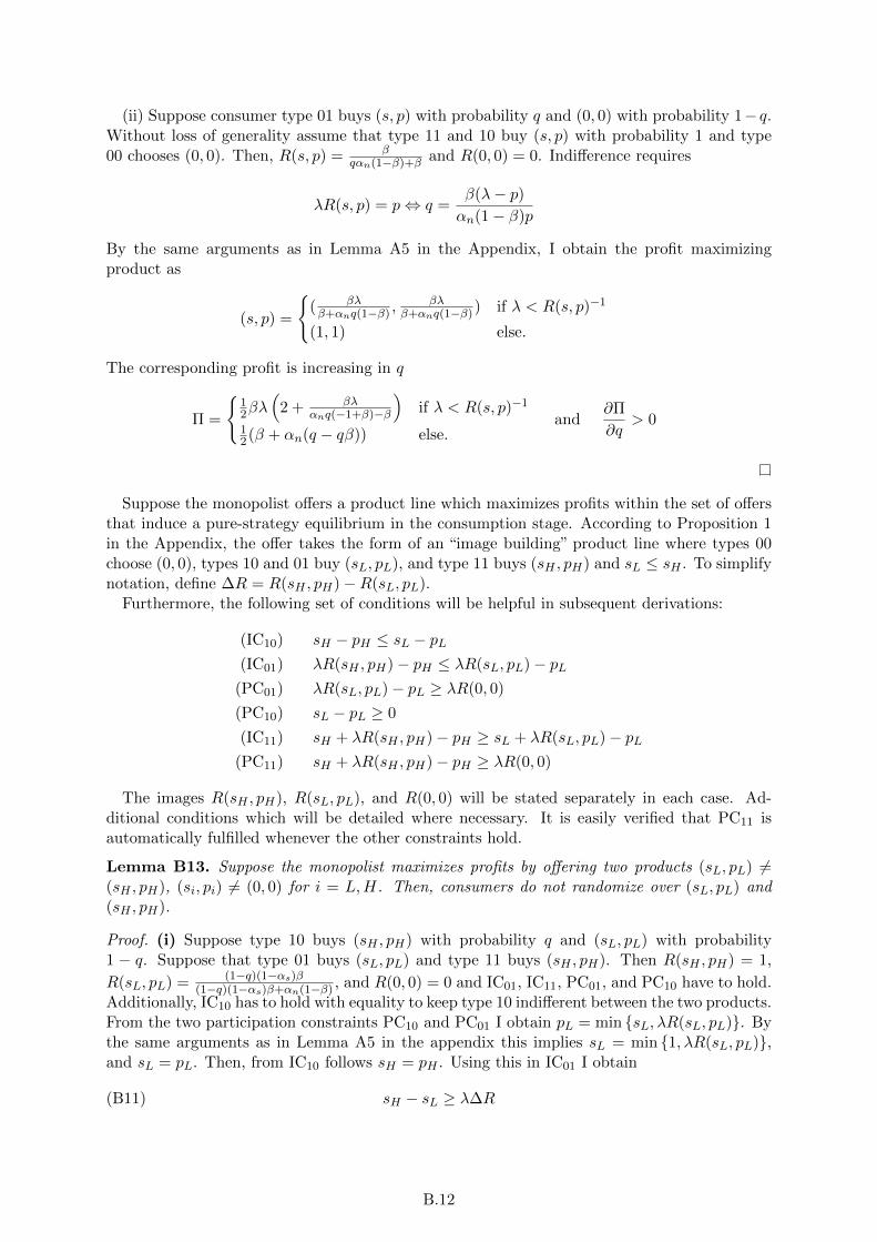
(ii) Suppose consumer type 01 buys (s, p) with probability q and (0, 0) with probability 1− q.Without loss of generality assume that type 11 and 10 buy (s, p) with probability 1 and type00 chooses (0, 0). Then, R(s, p) = β

qαn(1−β)+β and R(0, 0) = 0. Indifference requires

λR(s, p) = p⇔ q =β(λ− p)αn(1− β)p

By the same arguments as in Lemma A5 in the Appendix, I obtain the profit maximizingproduct as

(s, p) =

{( βλβ+αnq(1−β) ,

βλβ+αnq(1−β)) if λ < R(s, p)−1

(1, 1) else.

The corresponding profit is increasing in q

Π =

{12βλ

(2 + βλ

αnq(−1+β)−β

)if λ < R(s, p)−1

12(β + αn(q − qβ)) else.

and∂Π

∂q> 0

Suppose the monopolist offers a product line which maximizes profits within the set of offersthat induce a pure-strategy equilibrium in the consumption stage. According to Proposition 1in the Appendix, the offer takes the form of an “image building” product line where types 00choose (0, 0), types 10 and 01 buy (sL, pL), and type 11 buys (sH , pH) and sL ≤ sH . To simplifynotation, define ∆R = R(sH , pH)−R(sL, pL).

Furthermore, the following set of conditions will be helpful in subsequent derivations:

(IC10) sH − pH ≤ sL − pL(IC01) λR(sH , pH)− pH ≤ λR(sL, pL)− pL

(PC01) λR(sL, pL)− pL ≥ λR(0, 0)

(PC10) sL − pL ≥ 0

(IC11) sH + λR(sH , pH)− pH ≥ sL + λR(sL, pL)− pL(PC11) sH + λR(sH , pH)− pH ≥ λR(0, 0)

The images R(sH , pH), R(sL, pL), and R(0, 0) will be stated separately in each case. Ad-ditional conditions which will be detailed where necessary. It is easily verified that PC11 isautomatically fulfilled whenever the other constraints hold.

Lemma B13. Suppose the monopolist maximizes profits by offering two products (sL, pL) 6=(sH , pH), (si, pi) 6= (0, 0) for i = L,H. Then, consumers do not randomize over (sL, pL) and(sH , pH).

Proof. (i) Suppose type 10 buys (sH , pH) with probability q and (sL, pL) with probability1 − q. Suppose that type 01 buys (sL, pL) and type 11 buys (sH , pH). Then R(sH , pH) = 1,

R(sL, pL) = (1−q)(1−αs)β(1−q)(1−αs)β+αn(1−β) , and R(0, 0) = 0 and IC01, IC11, PC01, and PC10 have to hold.

Additionally, IC10 has to hold with equality to keep type 10 indifferent between the two products.From the two participation constraints PC10 and PC01 I obtain pL = min {sL, λR(sL, pL)}. Bythe same arguments as in Lemma A5 in the appendix this implies sL = min {1, λR(sL, pL)},and sL = pL. Then, from IC10 follows sH = pH . Using this in IC01 I obtain

(B11) sH − sL ≥ λ∆R

B.12

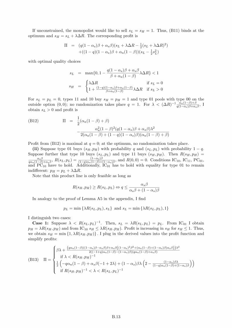
If unconstrained, the monopolist would like to sell sL = sH = 1. Thus, (B11) binds at theoptimum and sH = sL + λ∆R. The corresponding profit is

Π = (q(1− αs)β + αsβ)(sL + λ∆R− 12(sL + λ∆R)2)

+((1− q)(1− αs)β + αn(1− β))(sL − 12s

2L)

with optimal quality choices

sL = max{0, 1− q(1− αs)β + αsβ

β + αn(1− β)λ∆R} < 1

sH =

{λ∆R if sL = 0

1 + (1−q)(1−αs)β+αn(1−β)β+αn(1−β) λ∆R if sL > 0

For sL = pL = 0, types 11 and 10 buy sH = pH = 1 and type 01 pools with type 00 on theoutside option (0, 0); no randomization takes place q = 1. For λ < (∆R)−1 αn(1−β)+β

q(1−αs)β+αsβ, I

obtain sL > 0 and profit is

Π =1

2(αn(1− β) + β)(B12)

− α2n(1− β)2(q(1− αs)β + αsβ)λ2

2(αn(1− β) + (1− q)(1− αs)β)(αn(1− β) + β)

Profit from (B12) is maximal at q = 0; at the optimum, no randomization takes place.(ii) Suppose type 01 buys (sH , pH) with probability q and (sL, pL) with probability 1 − q.

Suppose further that type 10 buys (sL, pL) and type 11 buys (sH , pH). Then R(sH , pH) =αsβ

qαn(1−β)+αsβ, R(sL, pL) = (1−αs)β

(1−q)αn(1−β)+(1−αs)β , and R(0, 0) = 0. Conditions IC10, IC11, PC01,and PC10 have to hold. Additionally, IC01 has to hold with equality for type 01 to remainindifferent: pH = pL + λ∆R.

Note that this product line is only feasible as long as

R(sH , pH) ≥ R(sL, pL)⇔ q ≤ αsβ

αsβ + (1− αs)β

In analogy to the proof of Lemma A5 in the appendix, I find

pL = min {λR(sL, pL), sL} and sL = min {λR(sL, pL), 1}

I distinguish two cases:Case 1: Suppose λ < R(sL, pL)−1. Then, sL = λR(sL, pL) = pL. From IC01 I obtain

pH = λR(sH , pH) and from IC10 sH ≤ λR(sH , pH). Profit is increasing in sH for sH ≤ 1. Thus,we obtain sH = min {1, λR(sH , pH)} . I plug in the derived values into the profit function andsimplify profits:

(B13) Π =

βλ+

(qαn(1−β)((1−αs)β−αsβ)β+αsβ((1−αs)2β2+(αn(1−β)+(1−αs)β)αsβ))λ2

2((−1+q)αn(1−β)−(1−αs)β)(qαn(1−β)+αsβ)

if λ < R(sH , pH)−1

12

(−qαn(1− β) + αsβ(−1 + 2λ) + (1− αs)βλ

(2− (1−αs)βλ

(1−q)αn(1−β)+(1−αs)β

))if R(sH , pH)−1 < λ < R(sL, pL)−1

B.13

I maximize profit according to (B13) with respect to the probability q that type 01 buys (sH , pH)and obtain

q∗ =

αs if λ < R(sH , pH)−1

12

(1 +

(1−αs)β(αn(1−β)+(1−αs)β+(1−αs)βλ2)αn(1−β)(αn(1−β)+(1−αs)β) −

√((αn(1−β)+(1−αs)2β)2+(1−αs)2β2λ2)2

α2n(1−β)2(αn(1−β)+(1−αs)β)2

)if R(sH , pH)−1 < λ < R(sL, pL)−1

Profit at q∗ is

Π =

12βλ

(2− βλ

αn(1−β)+β

)if λ < R(sH , pH)−1

αsβ(−1

2 + λ)

+ 12(1− αs)βλ

(2− (1−αs)βλ

αn(1−β)+(1−αs)β

)if R(sH , pH)−1 < λ < R(sL, pL)−1

and never exceeds profit from a deterministic image building product line as derived in Lem-mas A5 and A7 and stated in equation 8 in the appendix.

Case 2: Suppose λ ≥ R(sL, pL)−1. SinceR(sL, pL) < R(sH , pH) this implies λ > R(sH , pH)−1.Due to the quadratic cost function profit is decreasing in qualities si for si > 1, i = L,H. There-fore, the monopolist sets sL = sH = 1. This yields pL = 1 and pH = 1 + λ∆R. Profit is then

Π =1

2(αn(1− β) + β) +

αn(1− β)(−αsβ + qβ)λ

(−1 + q)αn(1− β)− (1− αs)β

This profit is maximal at q = 0 and the monopolist does not profit from randomization.(iii) It is easy to see that profits do not increase either if type 11 randomizes between the

high and the low quality product. Suppose type 11 is indifferent between (sL, pL) and (sH , pH).If a fraction 1− q of type 11 buys (sL, pL) this increases the associated image. However, if themonopolist increases pL in response to the image increase, types 10 stop buying (sL, pL) unlesshe also increases sL. But an increase in sL makes the low quality product more attractive totype 11, thereby breaking the indifference of type 11.45 Therefore, pL and sL remain unchanged.Having type 11 buy the low quality decreases profits since pH − 1

2s2H > pL − 1

2s2L due to the

image-premium charged from type 11.

Lemma B14. Suppose the monopolist maximizes profits by offering two products (sL, pL) 6=(sH , pH), (si, pi) 6= (0, 0) for i = L,H. Then, consumer type 01 does not randomize over (sL, pL)and (0, 0).

Proof. Let q denote the probability that type 01 buys (sL, pL) and with (1− q) he takes (0, 0).

Suppose only type 11 buys (sH , pH). Then R(sL, pL) = (1−αs)β(1−αs)β+qαn(1−β) and R(sH , pH) = 1.

For type 01 to mix between (sL, pL) and (0, 0), PC01 has to bind. Together with PC10 thisgives sL ≥ λR(sL, pL) = pL. Since quality is costly to produce the monopolist sets sL =λR(sL, pL).

Using this in IC11 yields

(B14) pH ≤ pL + sH − sL + λ∆R = sH + λ∆R.

Under profit maximization constraint B14 binds. The monopolist maximizes profits by settingsH = 1 and

(sL, pL) = (λR(sL, pL), λR(sL, pL)) and (sH , pH) = (1, 1 + λ∆R).

45The monopolist can increase sH to sustain indifference but this does quite obviously not increase profits either.

B.14

The corresponding profit increases in q:

Π = αsβ2 + qαn(1−β)αsβλ

(1−αs)β+qαn(1−β)

+(qαn(1− β) + (1− αs)β)(

(1−αs)βλ(1−αs)β+qαn(1−β) −

(1−αs)2β2λ2

2(qαn(1−β)+(1−αs)β)2

)∂Π

∂q=

αn(1− αs)(1− β)β2(2αs + (1− αs)λ)λ

2(αnq(1− β) + (1− αs)β)2> 0.

Lemma B15. Suppose the monopolist maximizes profits by offering two products (sL, pL) 6=(sH , pH), (si, pi) 6= (0, 0) for i = L,H. Then, consumer type 11 does not randomize over anyproduct and (0, 0).

Proof. Let q denote the probability of type 11 buying (sH , pH) and by (1− q) the probability ofher choosing (0, 0). Denote by γi10, γ

i01 the fractions of the population which are of type 10 and

01, respectively, and buy product i for i ∈ {L,H}. The required indifference in PC11 implies

pH = λ(R(sH , pH)−R(0, 0)) + sH

= λ(1− (1− q)αsβ(1− q)αsβ + (1− β)αn(1− γL01 − γH01) + (1− αs)β(1− γL10 − γH10)

) + sH

The price pH increases in q and so do per-unit profits from sales of (sH , pH). Furthermore,profits from selling (sL, pL) also increase in q since analogous to Lemma A5 in the appendix:

pL = sL

= min{1, λ((1−αs)βγL10

(1−αs)βγL10+(1−β)αnγL01− (1−q)αsβ

(1−q)αsβ+(1−β)αn(1−γL01−γH01)+(1−αs)β(1−γL10−γH10))}

and thus pL and sL increase in q. Finally, at the margin type 11 buying (sH , pH) contributespH − 1

2s2H > 0 to profits so that the monopolist looses from type 11 not buying directly.

Thus, I have shown that randomization of types 01 or 11 is not profitable. By Assumption 1type 10 does not randomize. This completes the proof.

B.7.2. Without Assumption 1 qualitatively similar results obtain but inducing consumersto randomize may be profitable

To investigate the problem without Assumption 1, I fist prove the generalization of Lemma B4.

Lemma B16. Suppose the monopolist maximizes profits by offering one product (s, p) 6= (0, 0).Then type 10 does not randomize between (s, p) and (0, 0).

Proof. Let q denote the probability of type 10 buying the high quality product and 1 − q theprobability that type 10 chooses (0, 0). Suppose q ∈ (0, 1). Type 10 finds it profitable torandomize in this way if and only if s = p. The profit maximizing quality choice is then s = 1and profits from sales of (s, p) are (q(1 − αs)β + αsβ)(sH − 1

2s2H) = 1

2(q(1 − αs)β + αsβ) andincreasing in q. Thus, q ∈ {0, 1} and type 10 does not randomize.

The next lemma characterizes a possibly profitable 2-product line where type 10 randomizesbetween the lower quality product and not participating. I call this image building withrandomization because of its similarity to the image building product line.

Lemma B17. There exists a stochastic mechanism where two products with positive quality areoffered and type 10 randomizes over buying the lower quality product and not participating anda set of parameters such that this mechanism maximizes monopoly profits.

B.15

Proof. Suppose a product line with two positive quality products (sL, pL), (sH , pH) is offeredand that type 10 randomizes over buying the lower of the two qualities, sL, and not buyingat all. Denote by q the probability that type 10 buys the lower quality product; 1 − q is theprobability that type 10 does not buy.

When type 10 does not always participate, the image of non-participation increases whereasthe image associated with the lower quality product decreases. The proposed structure is onlyfeasible as long as the image associated with the lower quality product is greater than the imageassociated with not buying since only the difference between the two, multiplied by the valueof image λ is the price which can be charged for this product.

The image of the lower quality product is higher than the one for non-participation as longas

R(sL, pL) ≥ R(0, 0)⇔ q ≥ αn

Thus, for αn = 1 the only admissible product line of this type has q = 1 and randomizationof type 10 does not have to be considered.

Analogous to the derivation of the pure strategy image building product line, I derive thatthe products with randomization take the following form:

sH = 1 and sL =

λ(

(1−αs)qβαn(1−β)+(1−αs)qβ −

(1−αs)(1−q)β1−αn(1−β)−αsβ−(1−αs)qβ

)if λ < (RL −R(0))−1

1 else

pH = 1 + λαn(1− β)

q(1− αs)β + αn(1− β)and pL = sL

Suppose this product line is feasible, i.e. q ≥ αn. Profit from image building with randomiza-tion is then

(B15)

ΠIrand =

αsβ2 + αnαs(1−β)βλ

αn(1−β)+(1−αs)qβ

+(αn(1− β) + (1− αs)qβ){(

(1−αs)qβαn(1−β)+(1−αs)qβ −

(1−αs)(1−q)β1−αn(1−β)−αsβ−(1−αs)qβ

)λ

−12

((1−αs)qβ

αn(1−β)+(1−αs)qβ −(1−αs)(1−q)β

1−αn(1−β)−αsβ−(1−αs)qβ

)2λ2}

if λ < (RL −R(0))−1

12(αn(1− β) + αsβ + (1− αs)qβ) + αnαs(1−β)βλ

αn(1−β)+(1−αs)qβelse

I conclude the proof by an example in which image building with randomization gives higherprofit than any pure strategy mechanism.

Example B11. Profitable randomization: Suppose we have α10 = 132 , α01 = 379

4096 , α11 =116 , λ = 21

4 , q = 34 . Plugging in reveals that the relevant constraints onλ and q are satisfied. I

have shown before that for λ large enough, as is the case here, neither the standard good northe mass market have to be considered (see Lemma A8 in the appendix and Proposition 2 in thepaper).

Profits corresponding to the example are ΠIrand = 13659773891200 = 0.351043,ΠIdet = 468531

1384448 =0.338424,ΠE = 223

640 = 0.348438 with ΠIrand being the largest.

B.16

Corollary B3. Inducing partial participation of type 10 allows to sell two different quality levelsfor higher values of image than under full participation.

Proof. In general, the threshold above which both qualities are equal to one is (RL −R(0))−1.Since partial participation decreases RL and increases R(0), the threshold increases (as long asthe participation probability is admissible, see above).

It is instructive that we find an example in the case where sL = 1 = pL < λRL in thedeterministic image building. In this case, the value of image is so large that the purely imageconcerned consumer 01 earns a rent when buying the lower quality product. Having type 10only partially participate reduces the image associated with the lower quality product. Thislowers not only the rent to type 01 but also the rent which has to be left to type 11. By inducingtype 10 to only partially participate, the monopolist can increase the price charged on the higherquality product without having to adjust price and quality of the lower quality product. Thus,when participation changes at the margin, profit on those still buying goes up.

Suppose such a mixed-strategy image building product line is optimal. The structure of thisproduct line is the same as in the pure strategy image building apart from the fact that sometype 10 consumers do not buy anything and image as well as quality of the lower quality productdeteriorate. While average quality changes, this type of equilibrium does not give fundamentallydifferent insights than what we learn from the pure strategy equilibria. Qualitatively, theonly profitable randomization induces an image building product line but does not change theintuition of the results.

The following proposition characterizes the equilibrium without Assumption 1. The result isillustrated in Figure B3

Proposition B5. Suppose αn, αs, β and q ∈ (αn, 1) are such that profit from image buildingwith randomization is strictly higher than profit from any other product line for some λ > 0.

If such q exists, there are λ(q) < λm <ˆλ(q) such that image building with randomization gives

highest profits for all λ ∈ [λ(q),ˆλ(q)].

Proof. Profit from image building with randomization is given in B15 where

(RL −R(0))−1 =(1− αn(1− β)− αs(1− q)β − qβ)(αn(1− β) + (1− αs)qβ)

(1− αs)(1− αn)(1− β)β

is the inverse of the image premium from buying low quality instead of not buying at all.It is easily verified that the profit function from image building with mixing is continuous,

increasing, and concave in λ for λ ≤ (RL−R(0))−1 and linearly increasing for λ > (RL−R(0))−1.I have shown in Lemma A7 that profit from image building in pure strategies is continuous,

increasing, and concave in λ for λ ≤ λ2 and linearly increasing for λ > λ2.Both product lines give the same profit for λ = 0, ΠI |λ=0 = Πmix|λ=0. Furthermore, if

λm > λ2 the slope from profit with mixing is always greater than the slope from profit withimage building:

∂ΠI

∂λ|λ=λm

<∂Πmix

∂λ|λ=λm

Moreover, the slope from profit with mixing is lower than the slope from profit with exclusivegood when evaluated at λ = (RL −R(0))−1.

This can be seen relatively easily by assuming that λ ≥ (RL − R(0))−1 such that also threeprofit functions are linear. Profit from exclusive good and deterministic image building are linearfor any λ > λ2 and λ2 < (RL−R(0))−1. Since, profit from mixing is linear for λ > (RL−R(0))−1,concave for smaller λ, and continuous in λ, the slope for any smaller λ is only greater such thatthe first inequality still holds.

B.17

0

standard good

λm

image building

1 λ˜λm

ˆλ

exclusive good

2

image buildingwith randomization

of type 10

Figure B3: Equilibrium in monopoly without Assumption 1.

The case where λm < λ2 is more complicated since then only profit from exclusive good islinear. However, we know that profit from mixing and profit from image building are concaveand that at λ = 0, both give the same profit. Furthermore, one can show that for λ < λ2 thefollowing holds:

∂2Πmix

∂λ2≥ ∂2ΠI

∂λ2

Since ∂2Πmix

∂λ2 < 0 and ∂2ΠI

∂λ2 < 0 this means that the slope of profit from image building isdecreasing faster than the slope from profit with mixing. From this we know that if for someλ > 0 profit from mixing is higher than profit from image building and ∂ΠI

∂λ |λ <∂Πmix

∂λ |λ, thenmixing will give higher profit than image building for all λ′ > λ subject to the assumption thatλ′ < λ2.

Since for λ = 0 profits are equal, this implies that profit from mixing and profit from de-terministic image building cross at most once for λ < λ2 with profit from image building withrandomization coming from below (and additionally the two product lines give the same profitfor λ = 0).

Combining the two insights for λ < λ2 and λ > λ2, I have shown that if mixing is best for

some λ > 0, then there exist q ∈ (αn, 1) and λ(q) <ˆλ(q) such that mixing with an induced

participation probability q for type 10 maximizes profit for λ ∈ [λ(q),ˆλ(q)].

In the first part, I have shown that the slope of mixing for λ > λm is lower than the slopeof exclusive good profits. Thus, if profits haven’t intersected before, they will not do so later.

Thus, I have also shown that λ(q) <˜λm <

ˆλ(q).

B.8. Constant unit cost

Suppose the unit cost is constant in quality, c(s) = c > 0 and utility from obtaining quality sis equal to s. Suppose further that quality cannot exceed 1, e.g. because quality is the fractionof high quality inputs into the final good. I assume that producing quality is cheap enoughrelative to the value of image and the type distribution for it being profitable to sell to engagein product differentiation and where marginal utility from quality exceeds its marginal cost, i.e.c < max{1, λ β(1−αs)

β(1−αs)+(1−β)αn}.

As in the setup with quadratic costs of quality, there are four possible sortings in the coordi-nation game among consumers. Optimal products which sustain these equilibria are presentedin Table B1.

I derive the optimal products as follows:

Standard good (sg): If λ < 1, type 01 does not want to buy at the monopoly price p = 1even for maximal image R = 1. If λ > 1, however, separation requires: λR(ssg, psg) < psg andssg ≥ psg. Since profit is increasing in psg and thus in ssg, set ssg = 1 and psg = ssg. Separationis then sustainable if and only if λR(ssg, psg) < 1⇔ λ < 1.

B.18

product line group products: (quality,price)

Image value λ ≤ 1 1 < λ ≤ λ1 λ1 < λ ≤ λ2 λ2 < λ

standard 00,01 (0,0) -good 10,11 (1,1) -

mass 00 (0,0) (0,0)

market 01,10,11 (1, λ ββ+(1−β)αn

) (1,1)

image 00 (0,0) (0,0)

building 01,10 (λβ(1−αs)

β(1−αs)+(1−β)αn, λ

β(1−αs)β(1−αs)+(1−β)αn

) (1,1)

11 (1,1 + λ(1−β)αn

β(1−αs)+(1−β)αn) (1,1 + λ

(1−β)αnβ(1−αs)+(1−β)αn

)

exclusive 00,01,10 (0,0)

good 11 (1,1 + λ 1−β1−βαs

)

Table B1: Characterization of possible product lines with constant unit cost

Mass market (mm): Denote the product for the mass market by (smm, pmm). Types 10 and01 buy if p ≤ min {s, λR(smm, pmm)}. It is R(smm, pmm) = α11+α10

α01+β . Then, since there is no

separation, smm = 1. Note that for λ > λ1, λ ββ+(1−β)αn

> 1 and thus price is not bound byvaluation of type 01 for image anymore, and therefore p = 1.

Image building: Denote by (sH , pH) and (sI , pI) the high and the lower quality product inthis product line. Images are given through the sorting. To gain the most from separation,high quality must be set at its maximum, sH = 1, and price is set at the highest valuewhich is still incentive compatible, pH = pL + (sH − sL) + λ(R(sH , pH) − R(sI − pI)) =

1 + λ (1−β)αnβ(1−αs)+(1−β)αn

. For the lower quality product, the monopolist sets price such as tokeep the type with lower willingness to pay just indifferent between buying and not buying,sL = min{sL, λ β(1−αs)

β(1−αs)+(1−β)αn}. Thus, he will set quality such as not to exceed the value of

the associated image, sL = min{1, λ β(1−αs)β(1−αs)+(1−β)αn

}. To summarize:

sL = pL =

{λ β(1−αs)β(1−αs)+(1−β)αn

if λ < λ2

1 else.

To maximize profits, the monopolist does not want to increase the quality of the lower qualityproduct even though marginal cost are constant. The reason is that providing sL > λRLtightens the upper bound on the high quality product’s price more than necessary and therebyreduces profits.

Exclusive good (eg): To sustain a sorting where only type 11 buys, the price has to be highenough, peg ≥ max {λ, seg}. Furthermore for type 11 to buy, peg ≤ seg + λ 1−β

1−βαs . To maximize

profits, the monopolist sets seg = 1, and peg = 1 + λ 1−β1−βαs .

Given these four product lines, I compute profits as summarized in Table B2 and identifywhich of those gives the highest profit for given type distribution and value of image.

Note first, that mass market never maximizes profits and I can restrict attention to theremaining three types of offers.

ΠM −ΠE =

αsβ(αn+β−(αn+αs+λ(1−αs))β)

−αn−(1−αn−αs)β < 0 if λ < λ1

−α2n(1−β)2+αn(λ−2(1−αs))(1−β)β−(1−αs)2(1−λ)β2

−αn−(1−αn−αs)β < 0 if λ1 < λ < λ2

αnαsλ(1−β)β−αn−(1−αn−αs)β < 0 if λ > λ2

B.19

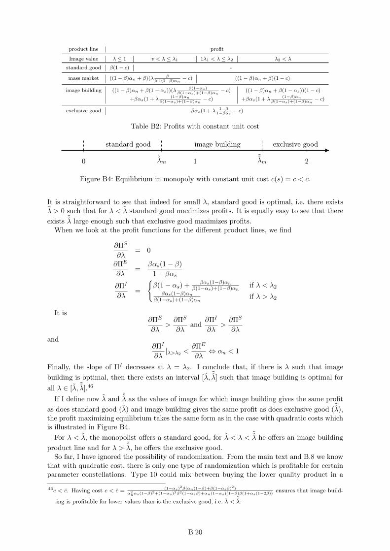
product line profit

Image value λ ≤ 1 v < λ ≤ λ1 1λ1 < λ ≤ λ2 λ2 < λ

standard good β(1− c) -

mass market ((1− β)αn + β)(λ ββ+(1−β)αn

− c) ((1− β)αn + β)(1− c)

image building ((1− β)αn + β(1− αs))(λ β(1−αs)β(1−αs)+(1−β)αn

− c) ((1− β)αn + β(1− αs))(1− c)+βαs(1 + λ

(1−β)αnβ(1−αs)+(1−β)αn

− c) +βαs(1 + λ(1−β)αn

β(1−αs)+(1−β)αn− c)

exclusive good βαs(1 + λ 1−β1−βαs

− c)

Table B2: Profits with constant unit cost

0

standard good

λm

image building

1˜λm

exclusive good

2

Figure B4: Equilibrium in monopoly with constant unit cost c(s) = c < c.

It is straightforward to see that indeed for small λ, standard good is optimal, i.e. there existsλ > 0 such that for λ < λ standard good maximizes profits. It is equally easy to see that there

exists˜λ large enough such that exclusive good maximizes profits.

When we look at the profit functions for the different product lines, we find

∂ΠS

∂λ= 0

∂ΠE

∂λ=

βαs(1− β)

1− βαs∂ΠI

∂λ=

{β(1− αs) + βαs(1−β)αn

β(1−αs)+(1−β)αnif λ < λ2

βαs(1−β)αnβ(1−αs)+(1−β)αn

if λ > λ2

It is∂ΠE

∂λ>∂ΠS

∂λand

∂ΠI

∂λ>∂ΠS

∂λ

and∂ΠI

∂λ|λ>λ2 <

∂ΠE

∂λ⇔ αn < 1

Finally, the slope of ΠI decreases at λ = λ2. I conclude that, if there is λ such that image

building is optimal, then there exists an interval [λ,˜λ] such that image building is optimal for

all λ ∈ [λ,˜λ].46

If I define now λ and˜λ as the values of image for which image building gives the same profit

as does standard good (λ) and image building gives the same profit as does exclusive good (˜λ),

the profit maximizing equilibrium takes the same form as in the case with quadratic costs whichis illustrated in Figure B4.

For λ < λ, the monopolist offers a standard good, for λ < λ <˜λ he offers an image building

product line and for λ >˜λ, he offers the exclusive good.

So far, I have ignored the possibility of randomization. From the main text and B.8 we knowthat with quadratic cost, there is only one type of randomization which is profitable for certainparameter constellations. Type 10 could mix between buying the lower quality product in a

46c < c. Having cost c < c = (1−αs)2β(αn(1−β)+β(1−αsβ)2)

α2nαs(1−β)3+(1−αs)3β2(1−αsβ)+αn(1−αs)(1−β)β(1+αs(1−2β))

ensures that image build-

ing is profitable for lower values than is the exclusive good, i.e. λ <˜λ.

B.20

two-product line and not buying at all. In analogy to the analysis with quadratic unit costs,one can derive precise conditions for the optimality of randomization. However, this would gobeyond the scope of this robustness check. Proposition B7 shows that there are parameters suchthat randomization by type 10 is not profitable with constant marginal cost of quality. Notethat the proposition derives sufficient conditions and their not being fulfilled does not implythat randomization is optimal.

Proposition B6. Suppose marginal cost of quality is constant. For each set of parameters,αs, αn, β, λ, such that βαs < αn(1 − β) + β(1 − αs), there exists c > 0 such that for c ≤ ca two-product mechanism where type 10 randomizes between buying the lower quality from themonopolist and not buying at all gives lower profit than a deterministic mechanism where type10 buys the low quality product with certainty.

Proof. Suppose an image building product line is offered and denote the high quality product by(sH , pH), the low quality product by (sL, pL). Suppose a fraction q of type 10 consumers buys(sL, pL) and the remaining fraction of (1 − q) of type 10 consumers does not buy but obtains(0, 0). I compare the gain in profit from selling this product line with partial participation overthe one where all type 10 consumers participate.

∆Π = ΠrandI −Πdet

I

= αsβλ( (1−β)αn(1−β)αn+β(1−αs) −

(1−β)αn(1−β)αn+qβ(1−αs))

− (1− q)β(1− αs)(λ (1−β)αn(1−β)αn+β(1−αs) − c)

− ((1− β)αn + β(1− αs))λ( β(1−αs)(1−β)αn+β(1−αs) −

qβ(1−αs)(1−β)αn+qβ(1−αs))

= (1− q)(c− λ (1−β)αn((1−β)αn+β(1−αs)−βαs)((1−β)αn+β(1−αs))((1−β)αn+qβ(1−αs)))

Then,

∆Π < 0

⇔ c < λ(1− β)αn((1− β)αn + β(1− αs)− βαs)

((1− β)αn + β(1− αs))((1− β)αn + qβ(1− αs))=: c(B16)

For c ≤ c, profit with randomization is lower than with deterministic participation. Further-more, the term is decreasing in q, such that no randomization is profitable starting from q = 1.The intuition behind this finding is that for costs low enough, the cost saving from selling tofewer consumers does outweigh the loss from selling to them. We also learn from this specialcase with constant cost, that if randomization is profitable with quadratic cost, this is relatedto the fact that underproducing quality for the low quality product (i.e. sL < 1) is not efficientand thereby dropping some of this consumers in exchange for higher prices from those servedat efficient levels, may pay off.

The threshold c from (B16) is positive as long as the fraction of image and quality concernedconsumers is small enough, i.e. βαs < αn(1− β) + β(1− αs)⇒ c > 0

B.21

All discussion papers are downloadable: http://www.wzb.eu/en/publications/discussion-papers/markets-and-choice

Discussion Papers of the Research Area Markets and Choice 2016

Research Unit: Market Behavior

David Danz, Steffen Huck, Philippe Jehiel SP II 2016-201 Public statistics and private experience: Varying feedback information in a take-or-pass game

Jana Friedrichsen Signals sell: Designing a product line when consumers have social image concerns

SPII 2016-202

Research Unit: Economics of Change

Armin Falk, Nora Szech SP II 2016-301 Pleasures of skill and moral conduct

Thomas Deckers, Armin Falk, Fabian Kosse, Nora Szech SP II 2016-302 Homo moralis: Personal characteristics, institutions, and moral decision-making

Research Professorship: Market Design: Theory and Pragmatics

Kevin McLaughlin, Daniel Friedman SP II 2016-501 Online ad auctions: An experiment